CMS-HIG-17-020

CMS-HIG-17-020 ; CERN-EP-2018-026
Search for additional neutral MSSM Higgs bosons in the $\tau\tau$ final state in proton-proton collisions at $\sqrt{s} = $ 13 TeV
CMS Collaboration
17 March 2018
JHEP 09 (2018) 007
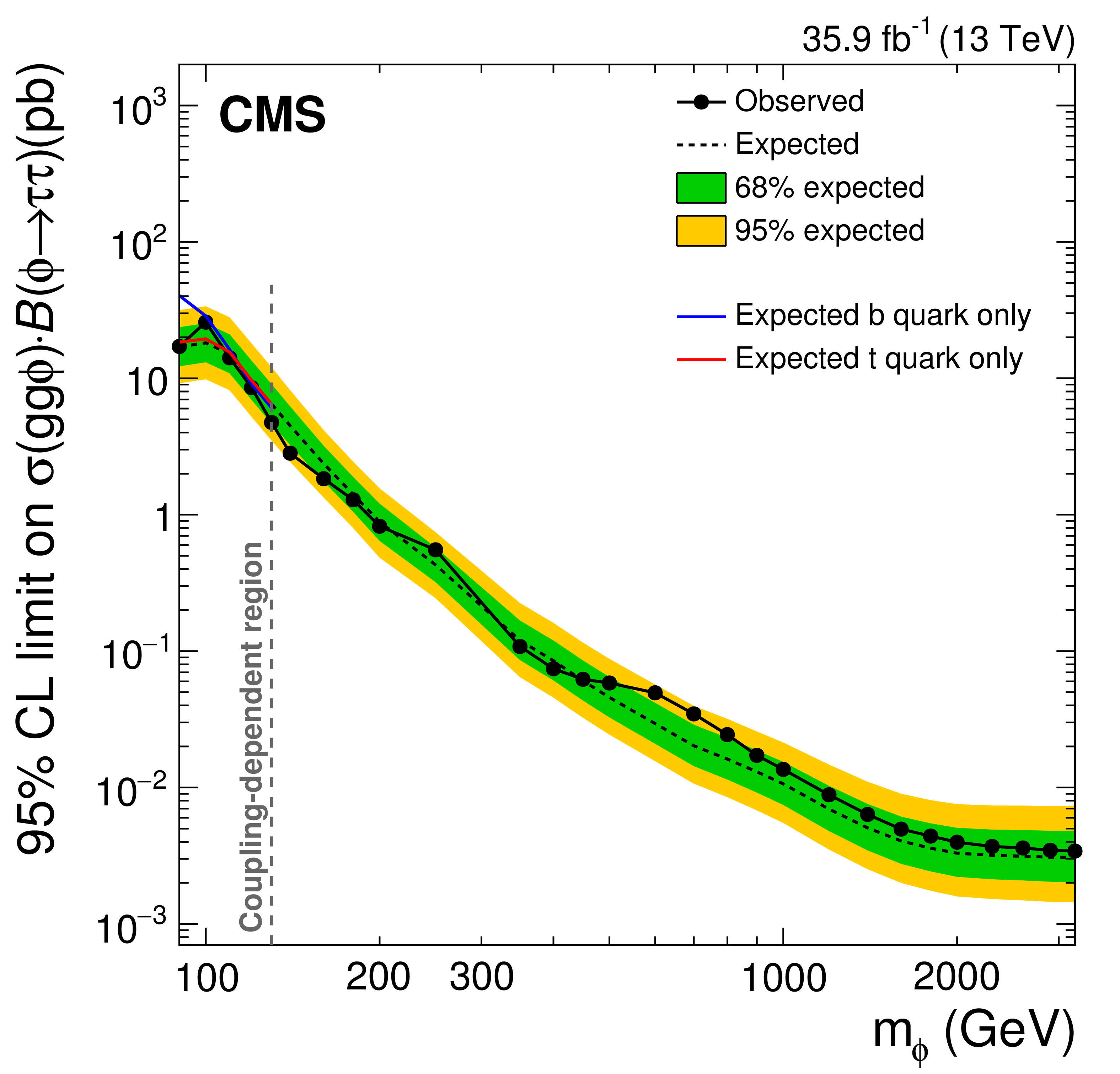
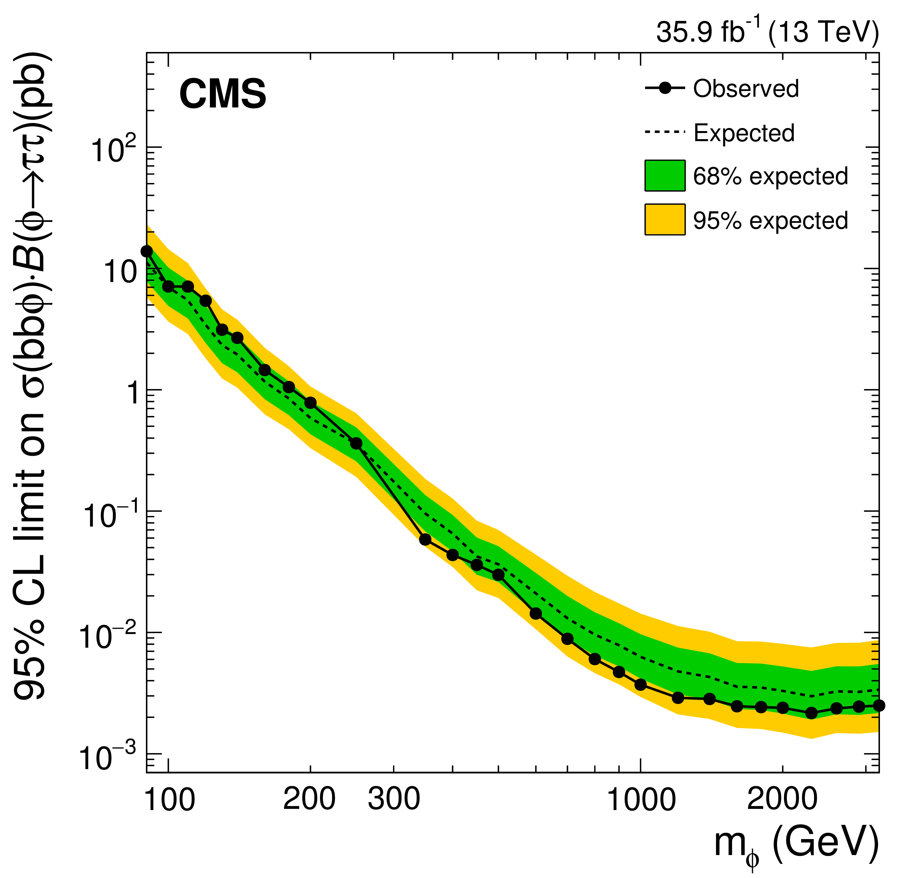
Abstract: A search is presented for additional neutral Higgs bosons in the $\tau\tau$ final state in proton-proton collisions at the LHC. The search is performed in the context of the minimal supersymmetric extension of the standard model (MSSM), using the data collected with the CMS detector in 2016 at a center-of-mass energy of 13 TeV, corresponding to an integrated luminosity of 35.9 fb$^{-1}$. To enhance the sensitivity to neutral MSSM Higgs bosons, the search includes production of the Higgs boson in association with b quarks. No significant deviation above the expected background is observed. Model-independent limits at 95% confidence level (CL) are set on the product of the branching fraction for the decay into $\tau$ leptons and the cross section for the production via gluon fusion or in association with b quarks. These limits range from 18 pb at 90 GeV to 3.5 fb at 3.2 TeV for gluon fusion and from 15 pb (at 90 GeV) to 2.5 fb (at 3.2 TeV) for production in association with b quarks. In the ${m_{\text{h}}^{\text{mod+}}}$ scenario these limits translate into a 95% CL exclusion of $\tan\beta > $ 6 for neutral Higgs boson masses below 250 GeV, where $\tan\beta$ is the ratio of the vacuum expectation values of the neutral components of the two Higgs doublets. The 95% CL exclusion contour reaches 1.6 TeV for $\tan\beta= $ 60.
Links: e-print arXiv:1803.06553 [hep-ex] (PDF) ; CDS record ; inSPIRE record ; HepData record ; CADI line (restricted) ;

Figures & Tables	Summary	Additional Figures & Tables & Material	References	CMS Publications

Figures
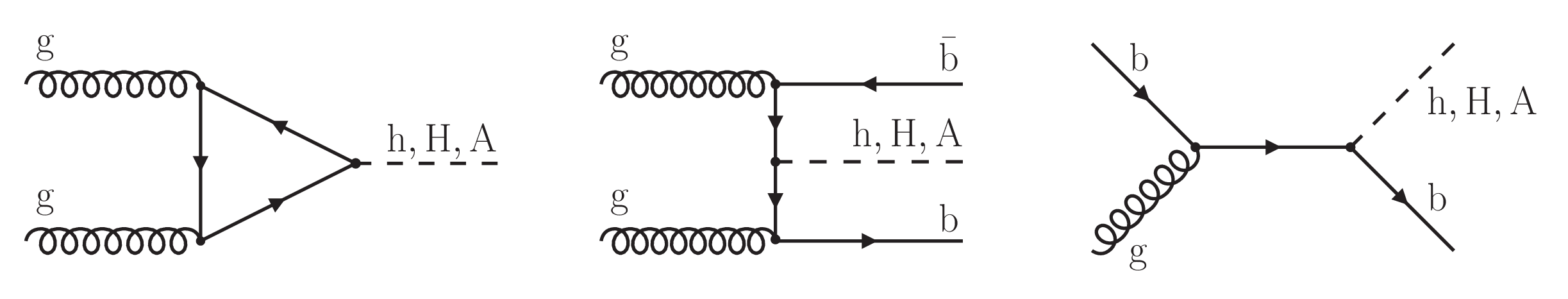
png pdf	Figure 1: Diagrams for the production of neutral Higgs bosons (left) via gluon fusion and (middle and right) in association with b quarks. In supersymmetric extensions of the SM, the super-partners also contribute to the fermion loop, shown in the left panel. In the middle panel a pair of b quarks is produced from two gluons (the LO process in the four-flavor scheme). In the right panel the Higgs boson is radiated from a b quark in the proton (the LO process in the five-flavor scheme).
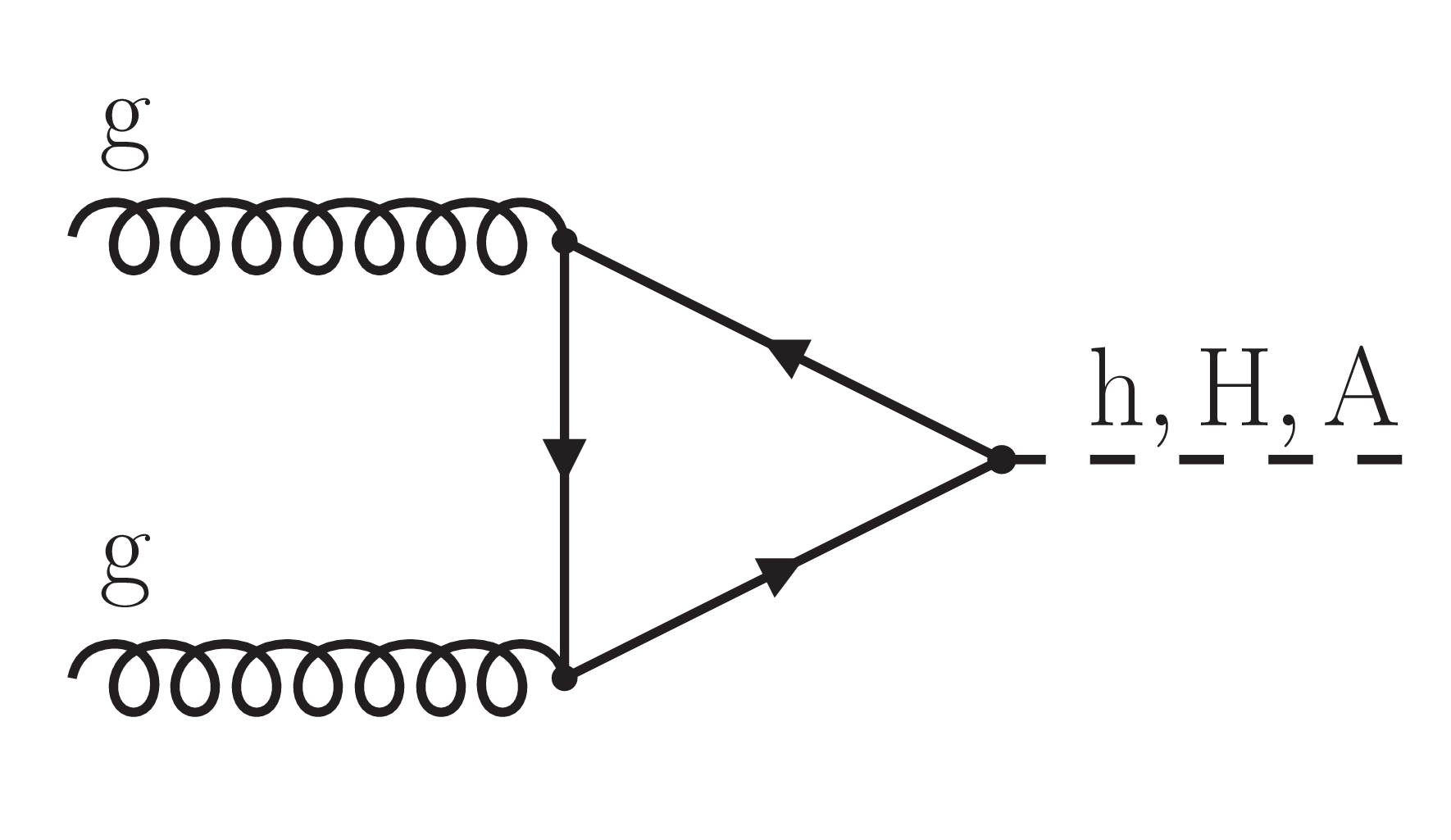
png pdf	Figure 1-a: Diagram for the production of neutral Higgs bosons via gluon fusion. In supersymmetric extensions of the SM, the super-partners also contribute to the fermion loop.
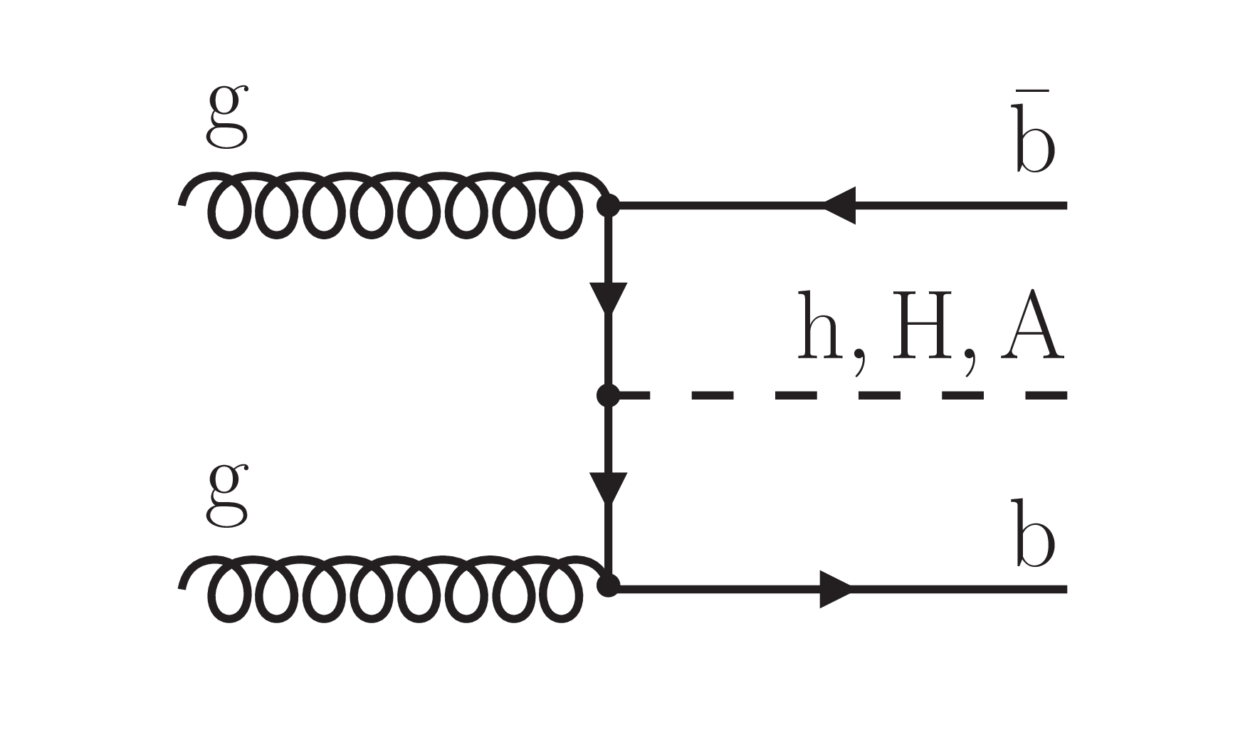
png pdf	Figure 1-b: Diagram for the production of neutral Higgs bosons in association with b quarks. A pair of b quarks is produced from two gluons (the LO process in the four-flavor scheme).
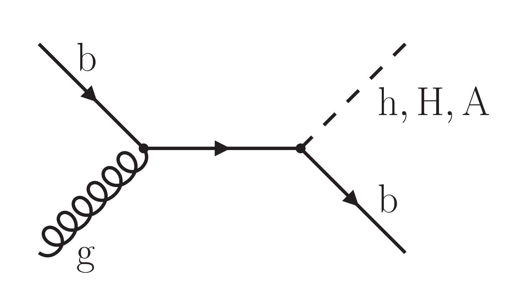
png pdf	Figure 1-c: Diagram for the production of neutral Higgs bosons in association with b quarks. The Higgs boson is radiated from a b quark in the proton (the LO process in the five-flavor scheme).
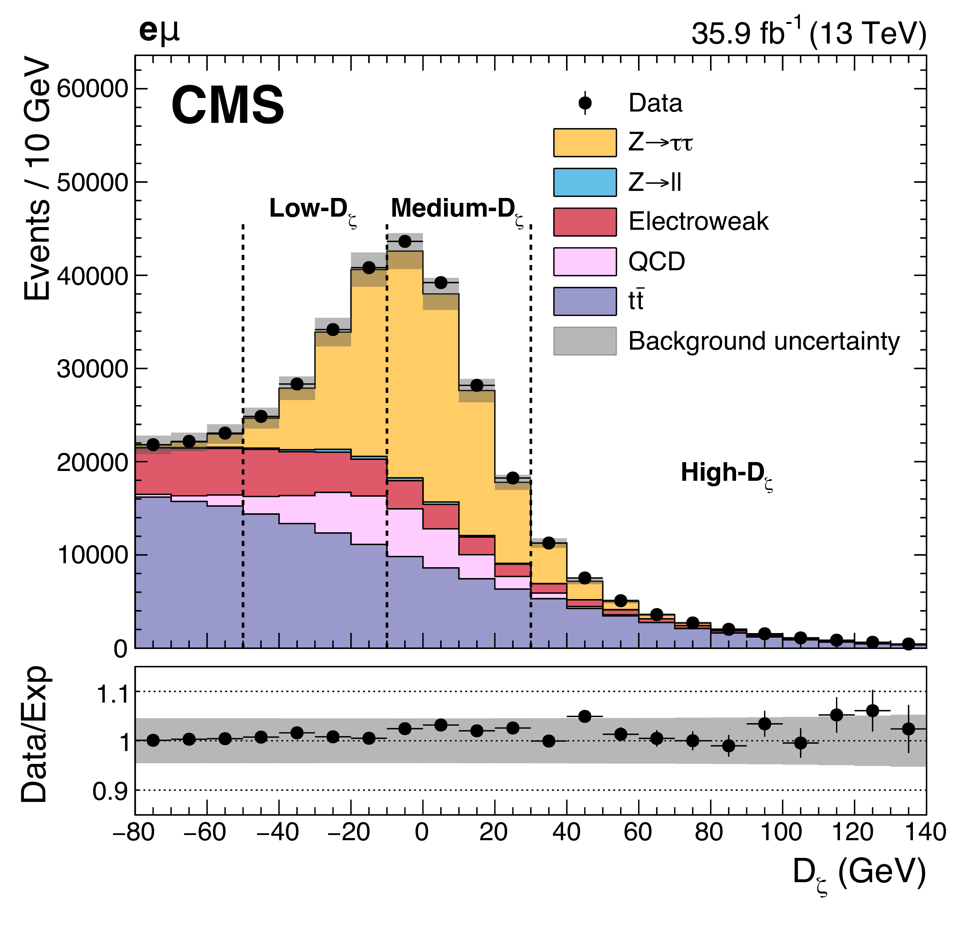
png pdf	Figure 2: Observed and expected distributions of (left) $ {D_{\zeta}} $ in the $ {\mathrm {e}} {{\mu}}$ final state and (right) $ {m_{\text {T}}^{\mu}} $ in the $ {{\mu}} {\tau}_{\text {h}} $ final state. The dashed vertical lines indicate the definition of the subcategories in each final state. The label "$\text {jet}\to {\tau}_{\text {h}} $'' indicates events with jets misidentified as hadronic $ {\tau}$ lepton decays, e.g. $ {{\mathrm {W}}}{+}\text {jets} $ events, which are estimated from data as described in Section 5.2. A detailed description of the composition of the expected background is given in Section 6. The distributions are shown before any event categorization and prior to the fit used for the signal extraction. For these figures no uncertainties that affect the shape of the distributions have been included in the uncertainty model.
png pdf	Figure 2-a: Observed and expected distribution of $ {D_{\zeta}} $ in the $ {\mathrm {e}} {{\mu}}$ final state. The dashed vertical lines indicate the definition of the subcategories in each final state. The label "$\text {jet}\to {\tau}_{\text {h}} $'' indicates events with jets misidentified as hadronic $ {\tau}$ lepton decays, e.g. $ {{\mathrm {W}}}{+}\text {jets} $ events, which are estimated from data as described in Section 5.2. A detailed description of the composition of the expected background is given in Section 6. The distributions are shown before any event categorization and prior to the fit used for the signal extraction. For this figure no uncertainties that affect the shape of the distributions have been included in the uncertainty model.
png pdf	Figure 2-b: Observed and expected distribution of $ {m_{\text {T}}^{\mu}} $ in the $ {{\mu}} {\tau}_{\text {h}} $ final state. The dashed vertical lines indicate the definition of the subcategories in each final state. The label "$\text {jet}\to {\tau}_{\text {h}} $'' indicates events with jets misidentified as hadronic $ {\tau}$ lepton decays, e.g. $ {{\mathrm {W}}}{+}\text {jets} $ events, which are estimated from data as described in Section 5.2. A detailed description of the composition of the expected background is given in Section 6. The distributions are shown before any event categorization and prior to the fit used for the signal extraction. For this figure no uncertainties that affect the shape of the distributions have been included in the uncertainty model.
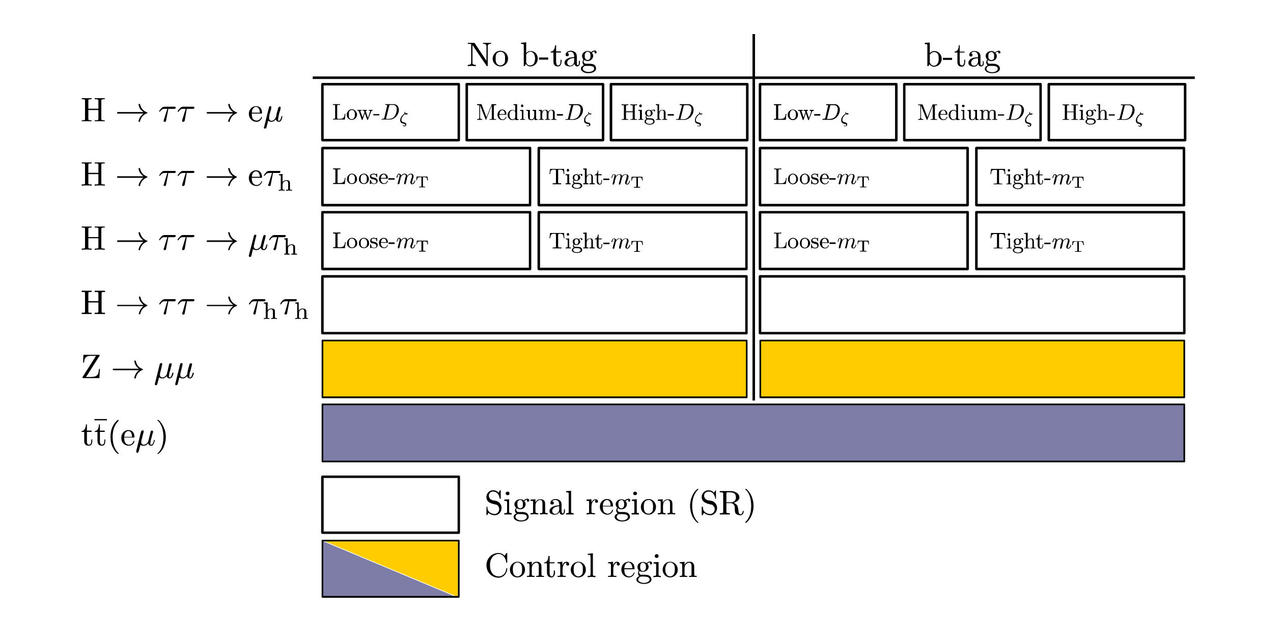
png pdf	Figure 3: Overview of all event subcategories that enter the statistical analysis. Sixteen signal categories are complemented by three background control regions in the main analysis as described in Section 5.
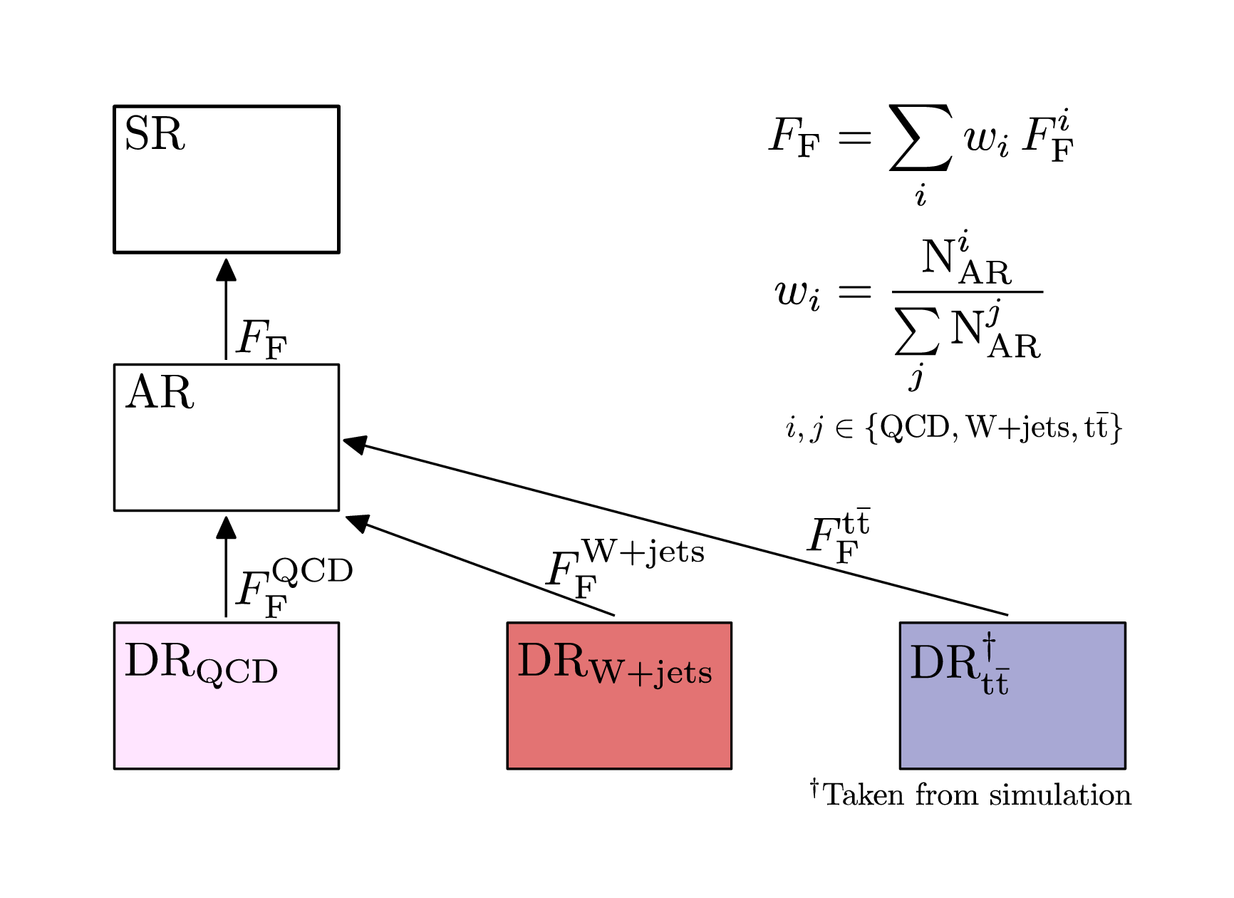
png pdf	Figure 4: Schematic view of the determination and application of the $ {F_{\text {F}}} ^{i}$ and $ {F_{\text {F}}} $ for the estimation of the background from QCD multijet, $ {{\mathrm {W}}}{+}\text {jets} $, and $ {{\mathrm {t}\overline {\mathrm {t}}}} $ events due to the misidentification of jets as hadronic $\tau $ lepton decays. Note that DR$_{{{\mathrm {t}\overline {\mathrm {t}}}}}$ is taken from simulation.
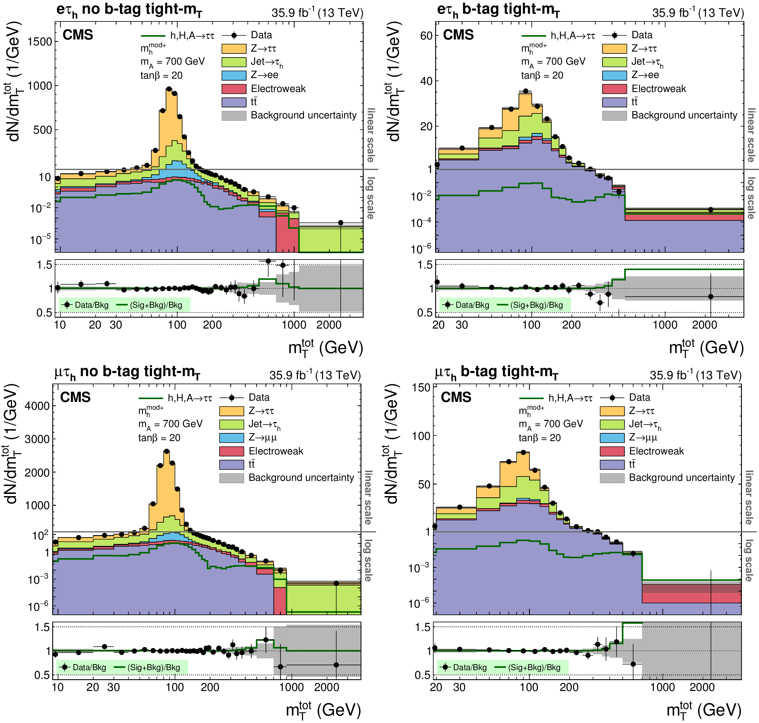
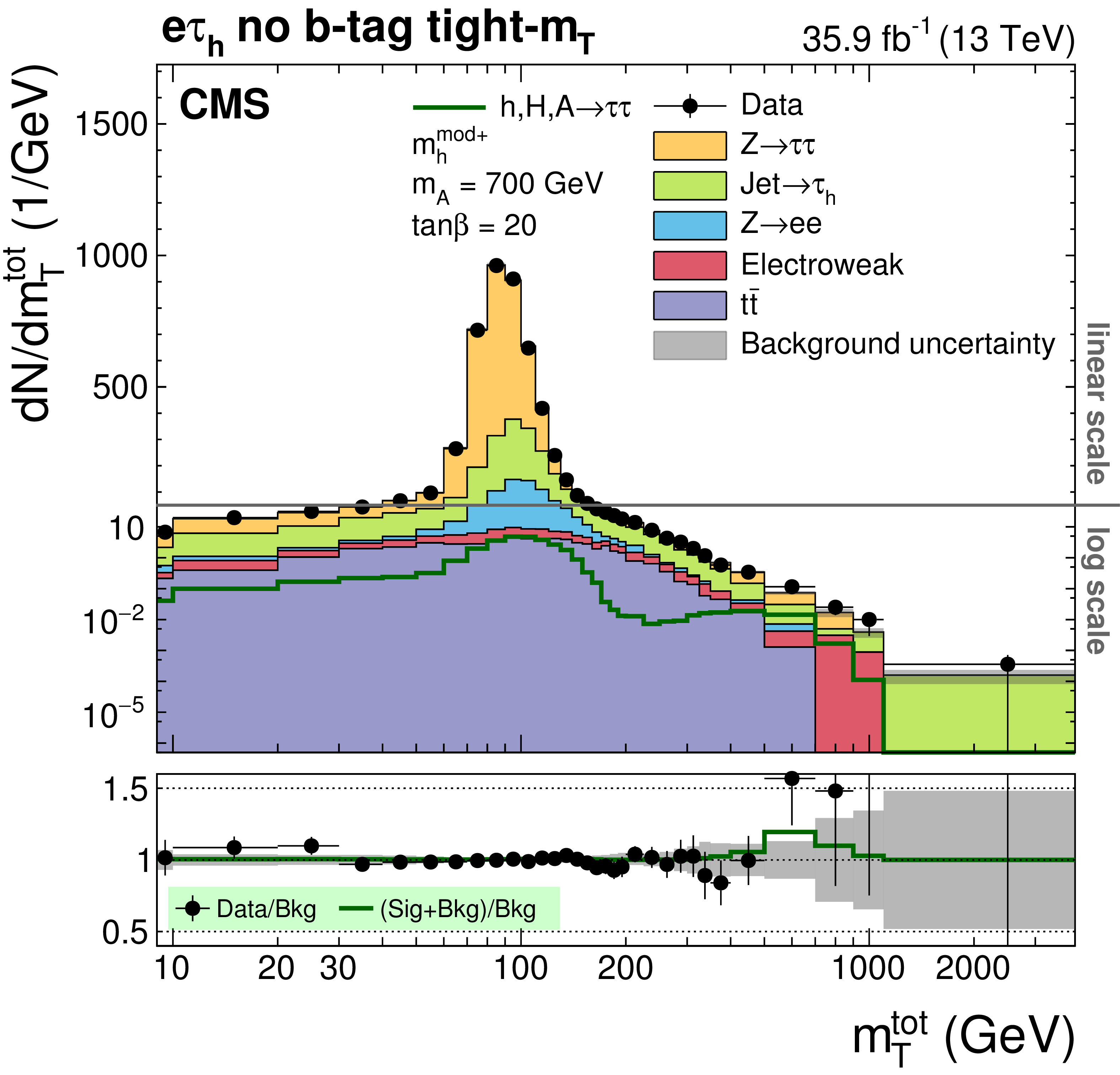
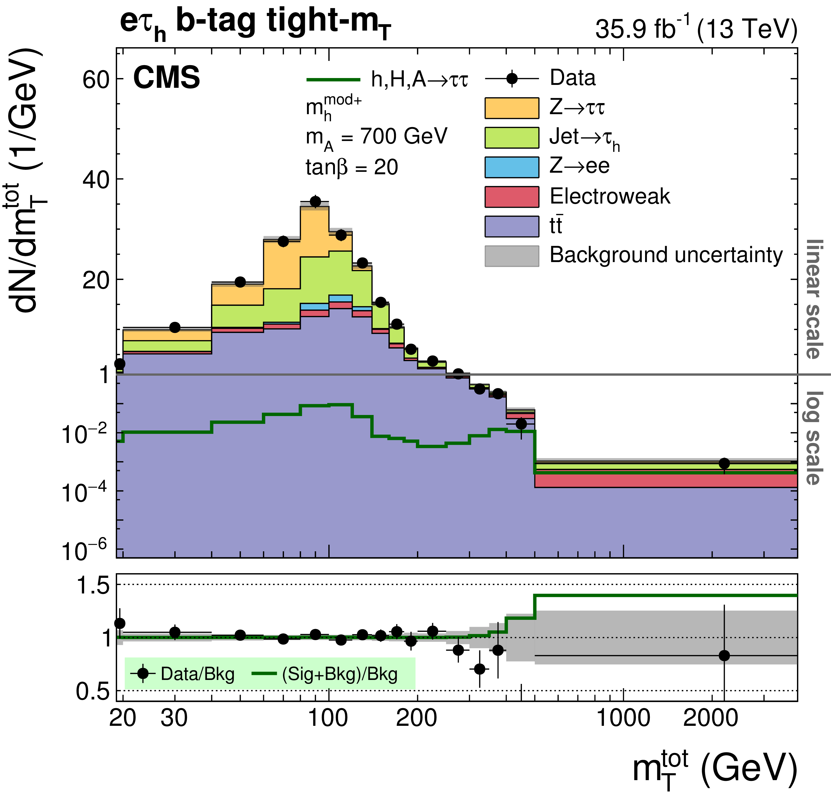
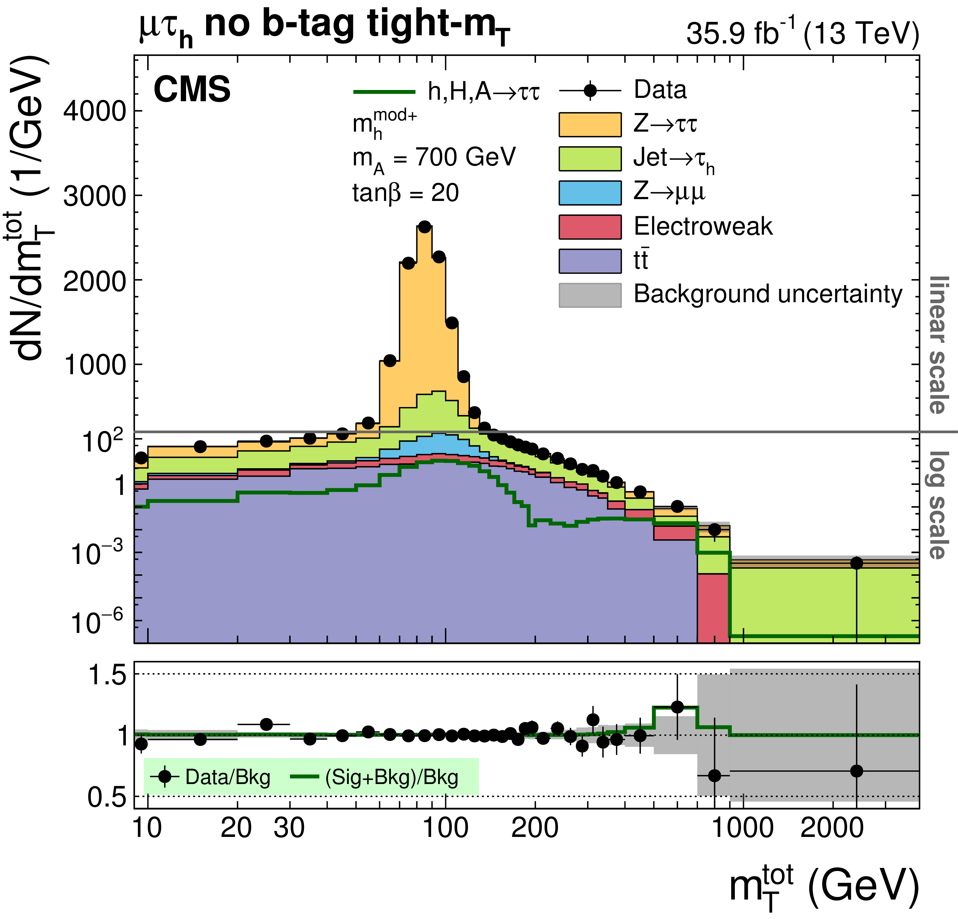
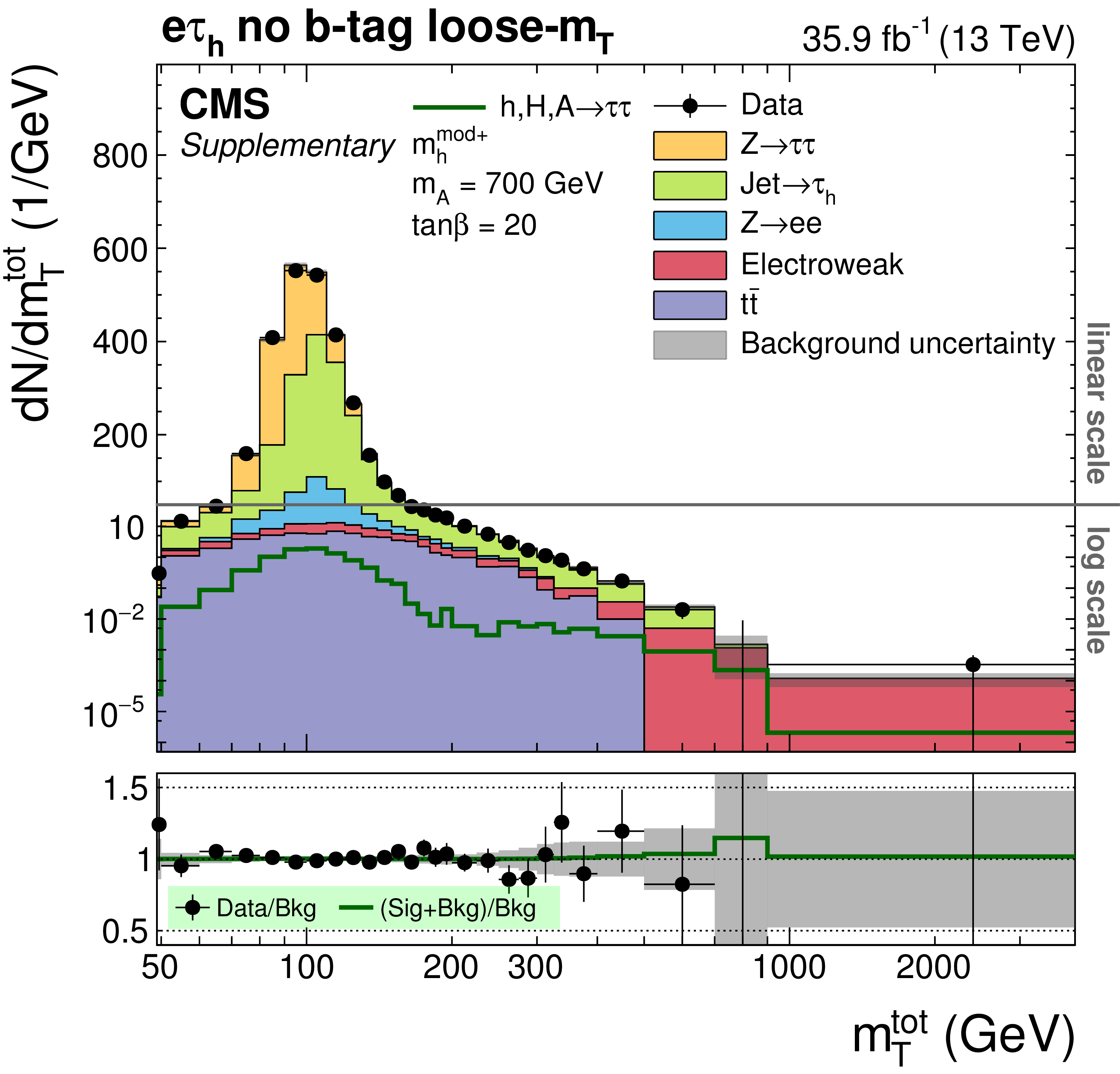
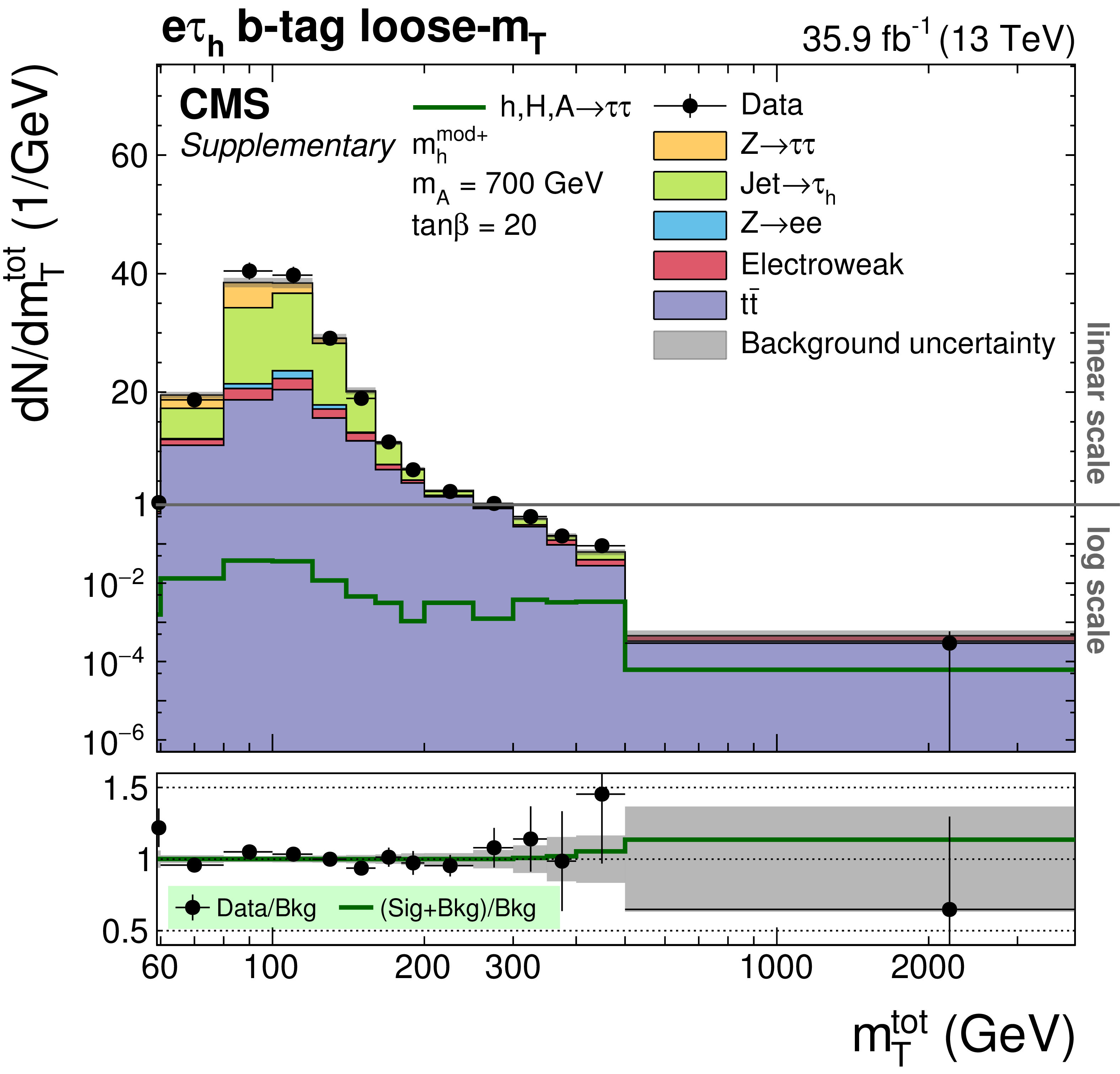
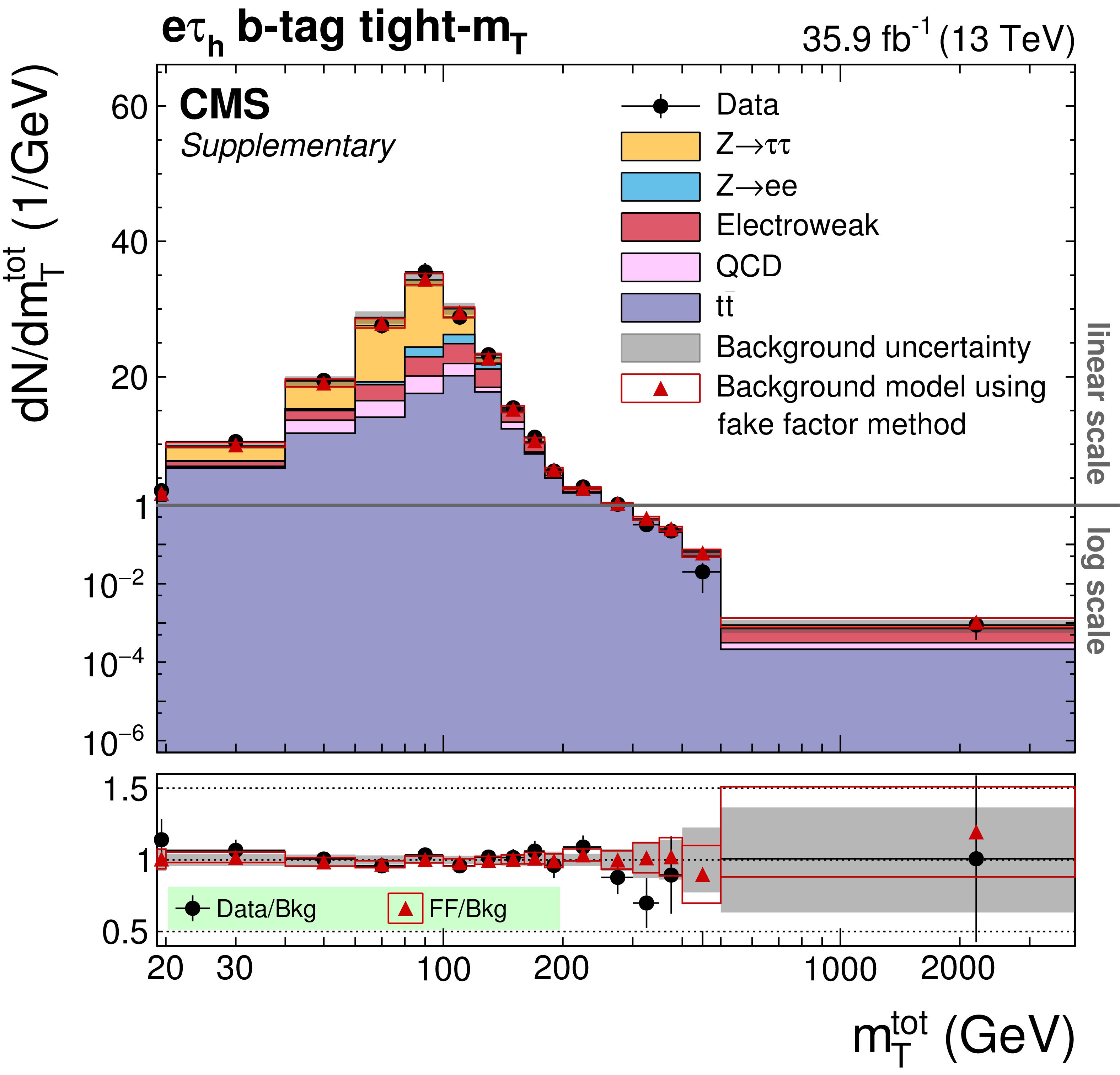
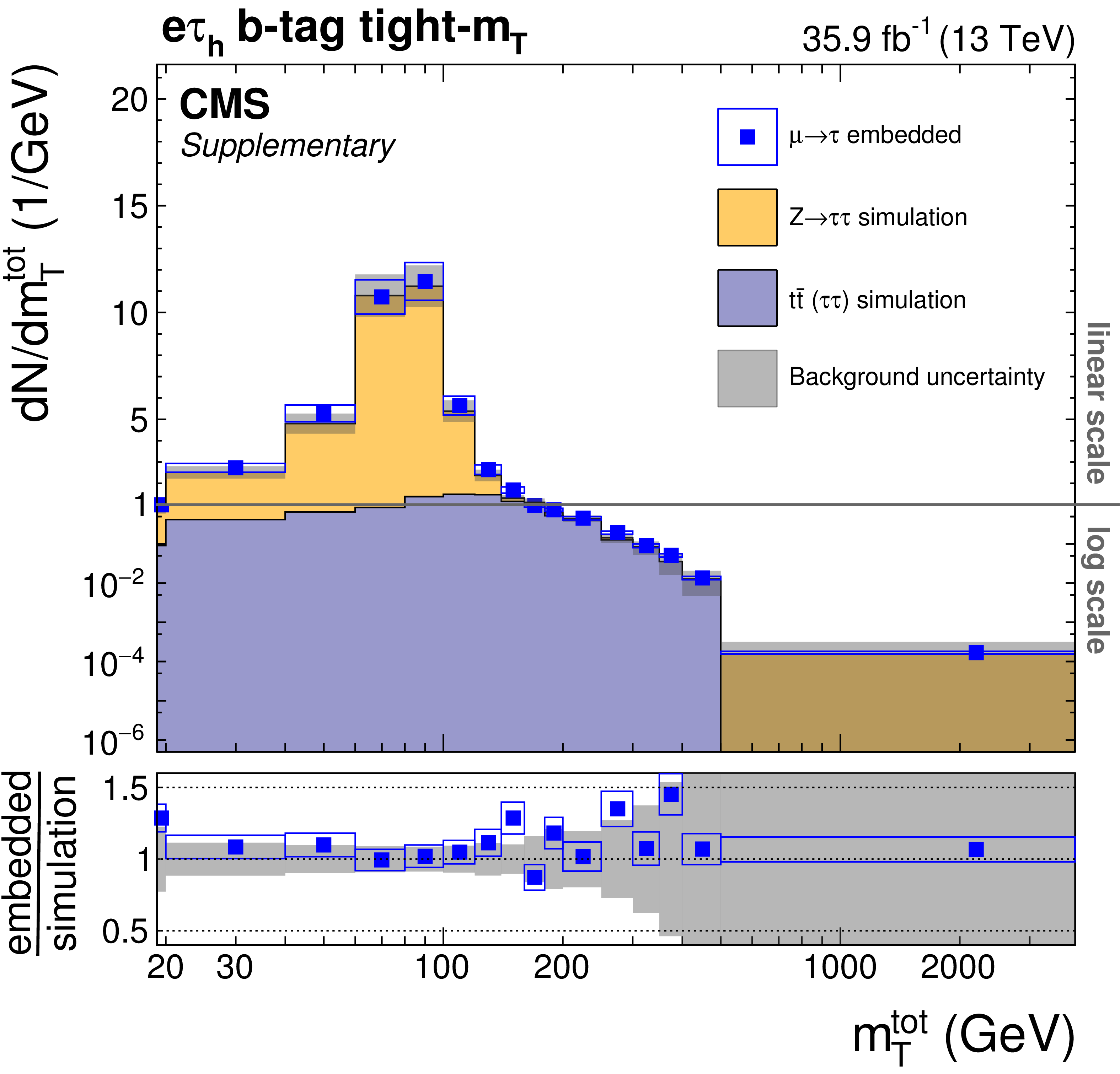
png pdf	Figure 5: Distribution of $ {m_{\text {T}}^{\text {tot}}} $ in the global no b-tag (left) and b-tag (right) categories in the $ {\mathrm {e}} {\tau}_{\text {h}} $ (upper row) and $ {{\mu}} {\tau}_{\text {h}} $ (lower row) final states. In all cases the most sensitive tight-$ {m_{\text {T}}}$ event subcategory is shown. The gray horizontal line in the upper panel of each subfigure indicates the change from logarithmic to linear scale on the vertical axis.
png pdf	Figure 5-a: Distribution of $ {m_{\text {T}}^{\text {tot}}} $ in the global no b-tag category in the $ {\mathrm {e}} {\tau}_{\text {h}} $ final state. The most sensitive tight-$ {m_{\text {T}}}$ event subcategory is shown. The gray horizontal line in the upper panel indicates the change from logarithmic to linear scale on the vertical axis.
png pdf	Figure 5-b: Distribution of $ {m_{\text {T}}^{\text {tot}}} $ in the global b-tag category in the $ {\mathrm {e}} {\tau}_{\text {h}} $ final state. The most sensitive tight-$ {m_{\text {T}}}$ event subcategory is shown. The gray horizontal line in the upper panel indicates the change from logarithmic to linear scale on the vertical axis.
png pdf	Figure 5-c: Distribution of $ {m_{\text {T}}^{\text {tot}}} $ in the global no b-tag category in the $ {{\mu}} {\tau}_{\text {h}} $ final state. The most sensitive tight-$ {m_{\text {T}}}$ event subcategory is shown. The gray horizontal line in the upper panel indicates the change from logarithmic to linear scale on the vertical axis.
png pdf	Figure 5-d: Distribution of $ {m_{\text {T}}^{\text {tot}}} $ in the global b-tag category in the $ {{\mu}} {\tau}_{\text {h}} $ final state. The most sensitive tight-$ {m_{\text {T}}}$ event subcategory is shown. The gray horizontal line in the upper panel indicates the change from logarithmic to linear scale on the vertical axis.
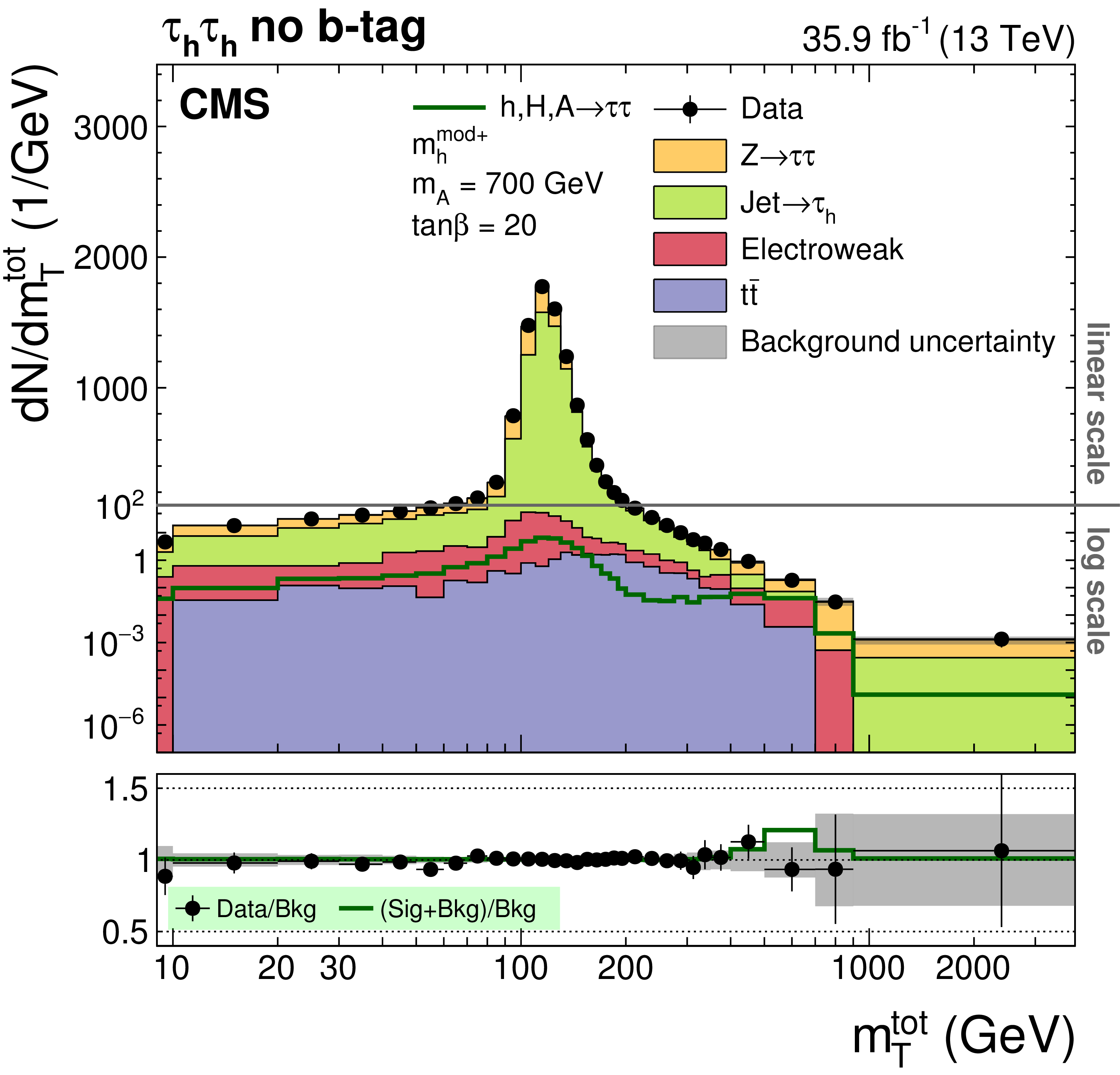
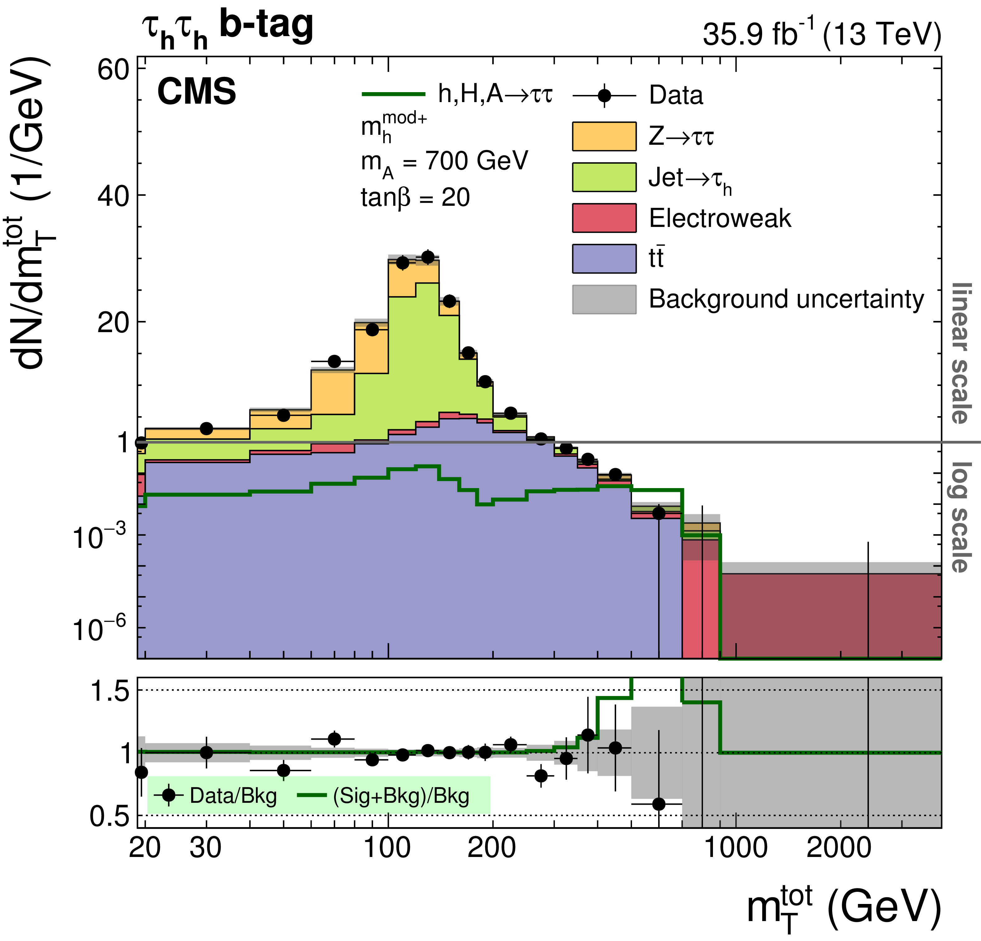
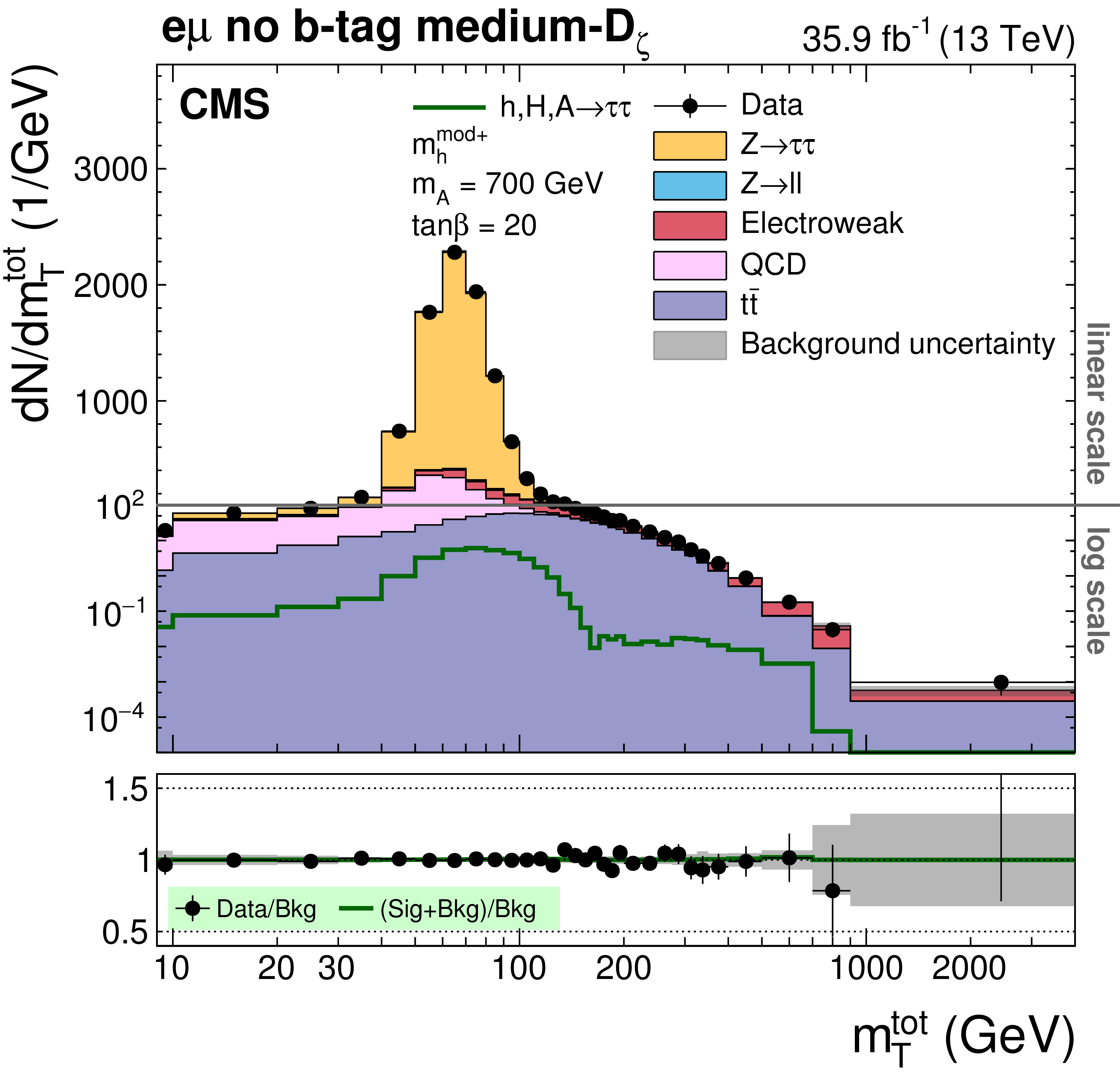
png pdf	Figure 6: Distribution of $ {m_{\text {T}}^{\text {tot}}} $ in the global no b-tag (left) and b-tag (right) categories in the $ {\tau}_{\text {h}} {\tau}_{\text {h}} $ (upper row) and $ {\mathrm {e}} {{\mu}}$ (lower row) final states. For the $ {\mathrm {e}} {{\mu}}$ final state the most sensitive medium-$ {D_{\zeta}} $ event subcategory is shown. The gray horizontal line in the upper panel of each subfigure indicates the change from logarithmic to linear scale on the vertical axis.
png pdf	Figure 6-a: Distribution of $ {m_{\text {T}}^{\text {tot}}} $ in the global no b-tag category in the $ {\tau}_{\text {h}} {\tau}_{\text {h}} $ final state. The gray horizontal line in the upper panel indicates the change from logarithmic to linear scale on the vertical axis.
png pdf	Figure 6-b: Distribution of $ {m_{\text {T}}^{\text {tot}}} $ in the global b-tag category in the $ {\tau}_{\text {h}} {\tau}_{\text {h}} $ final state. The gray horizontal line in the upper panel indicates the change from logarithmic to linear scale on the vertical axis.
png pdf	Figure 6-c: Distribution of $ {m_{\text {T}}^{\text {tot}}} $ in the global no b-tag category in the $ {\mathrm {e}} {{\mu}}$ final state. The most sensitive medium-$ {D_{\zeta}} $ event subcategory is shown. The gray horizontal line in the upper panel indicates the change from logarithmic to linear scale on the vertical axis.
png pdf	Figure 6-d: Distribution of $ {m_{\text {T}}^{\text {tot}}} $ in the global b-tag category in the $ {\mathrm {e}} {{\mu}}$ final state. The most sensitive medium-$ {D_{\zeta}} $ event subcategory is shown. The gray horizontal line in the upper panel indicates the change from logarithmic to linear scale on the vertical axis.
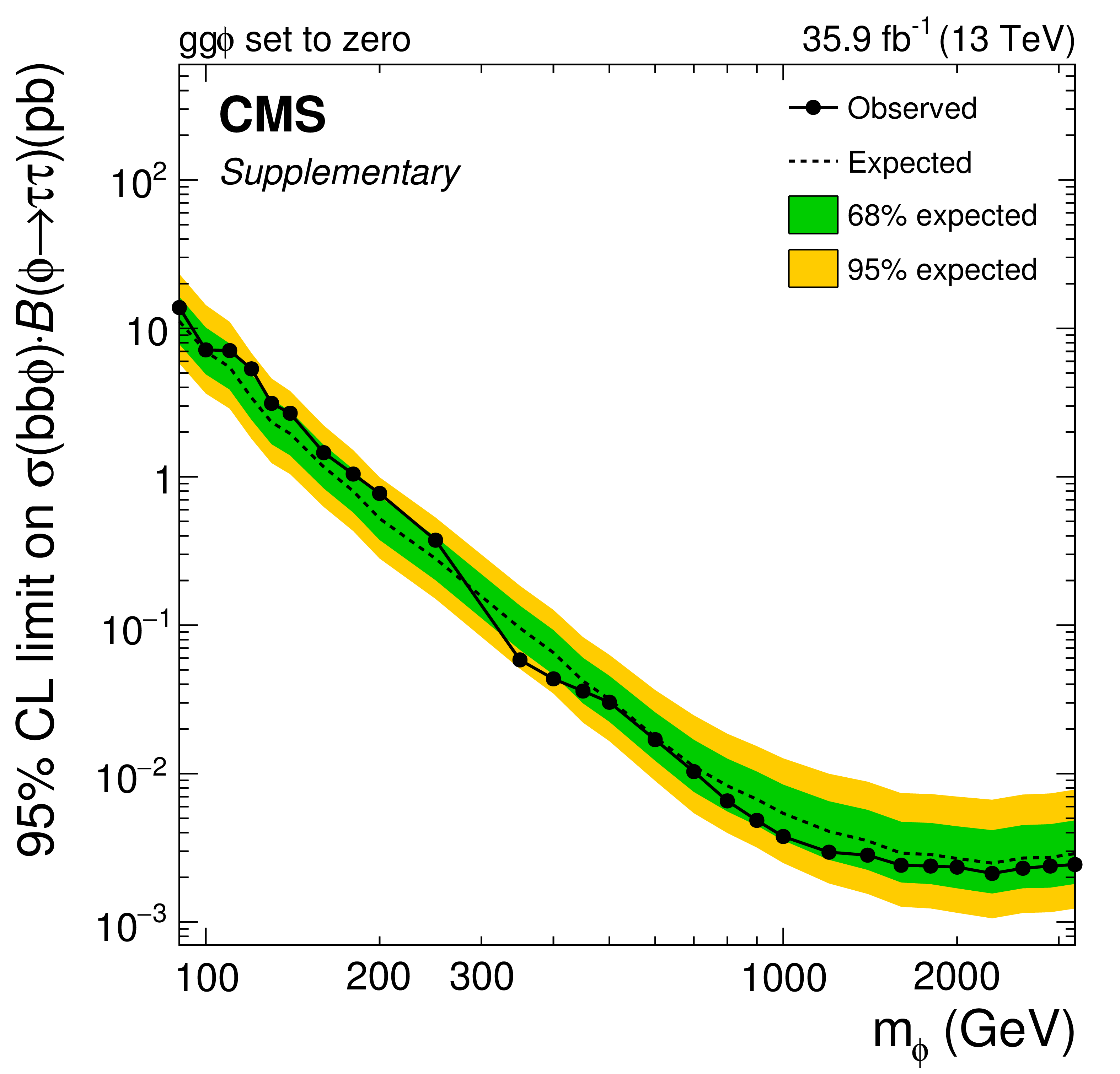
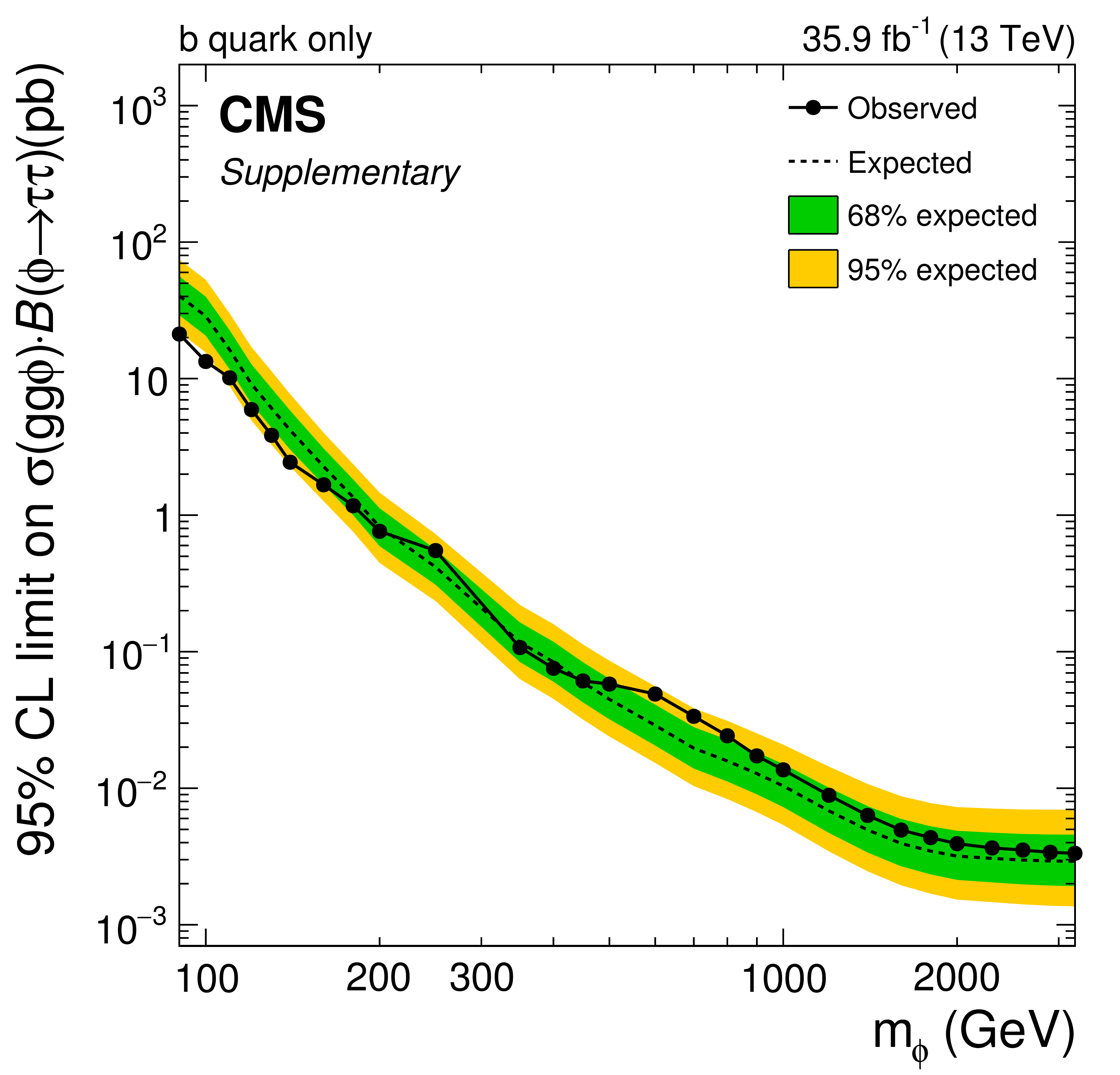
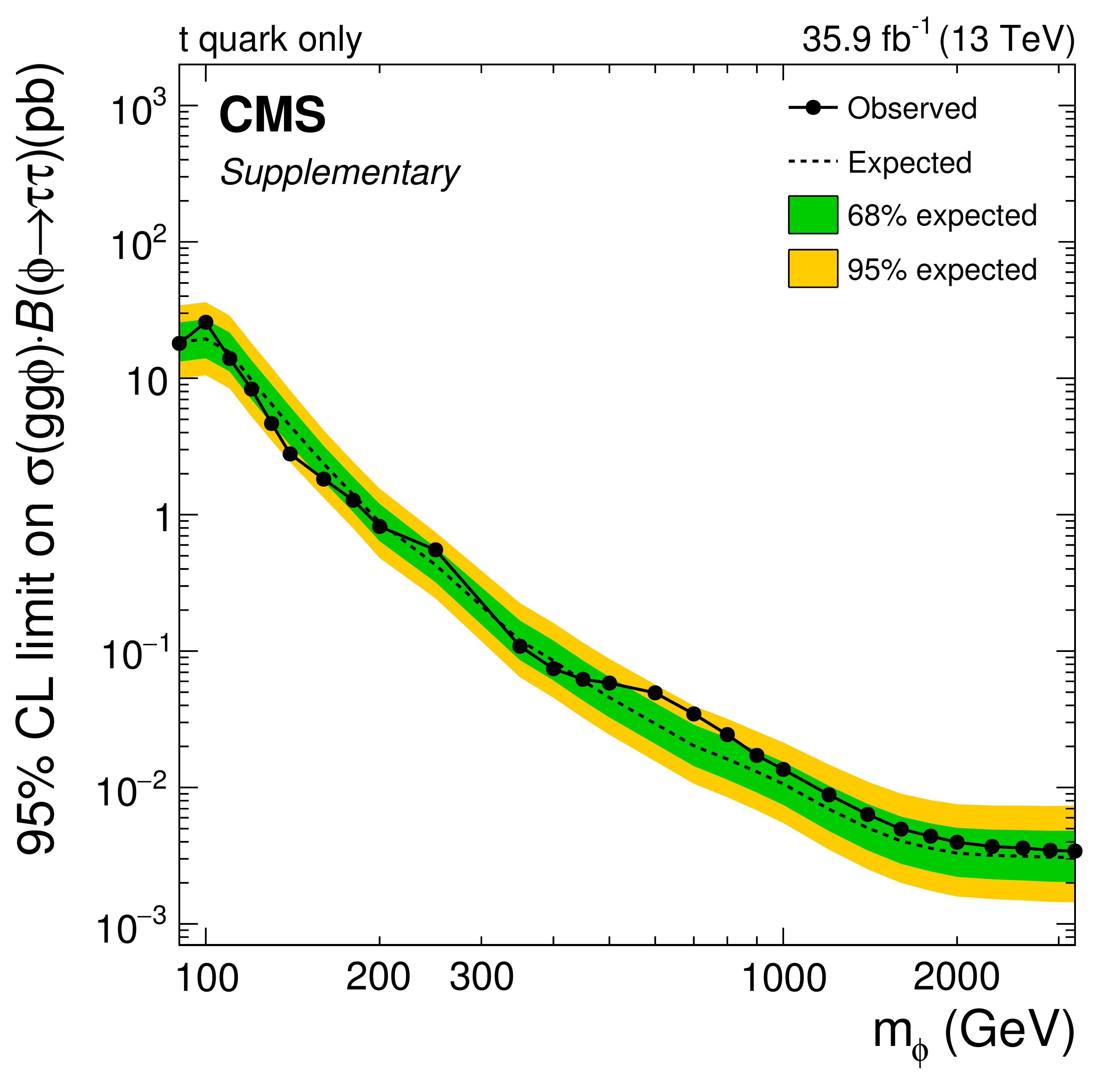
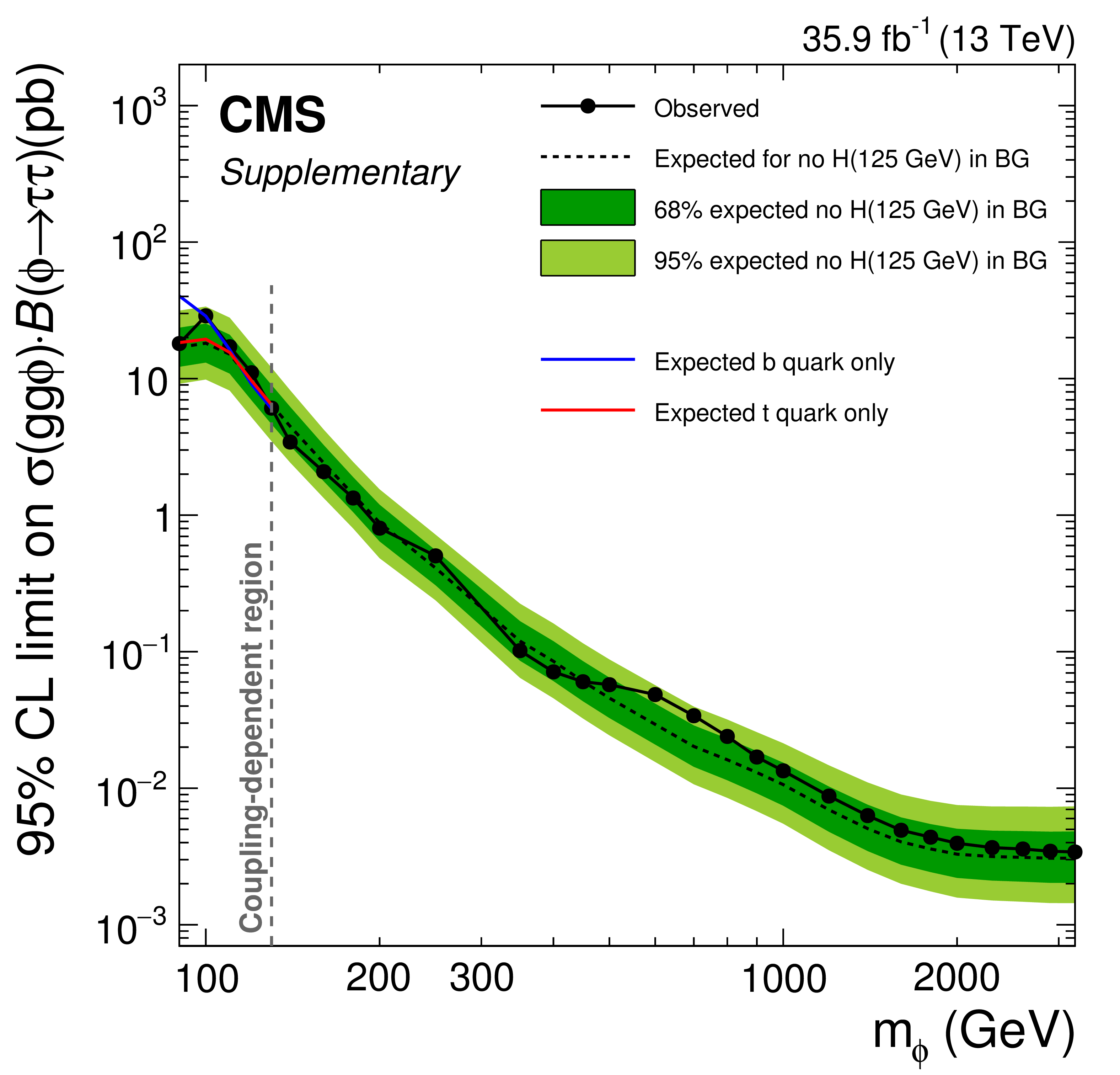
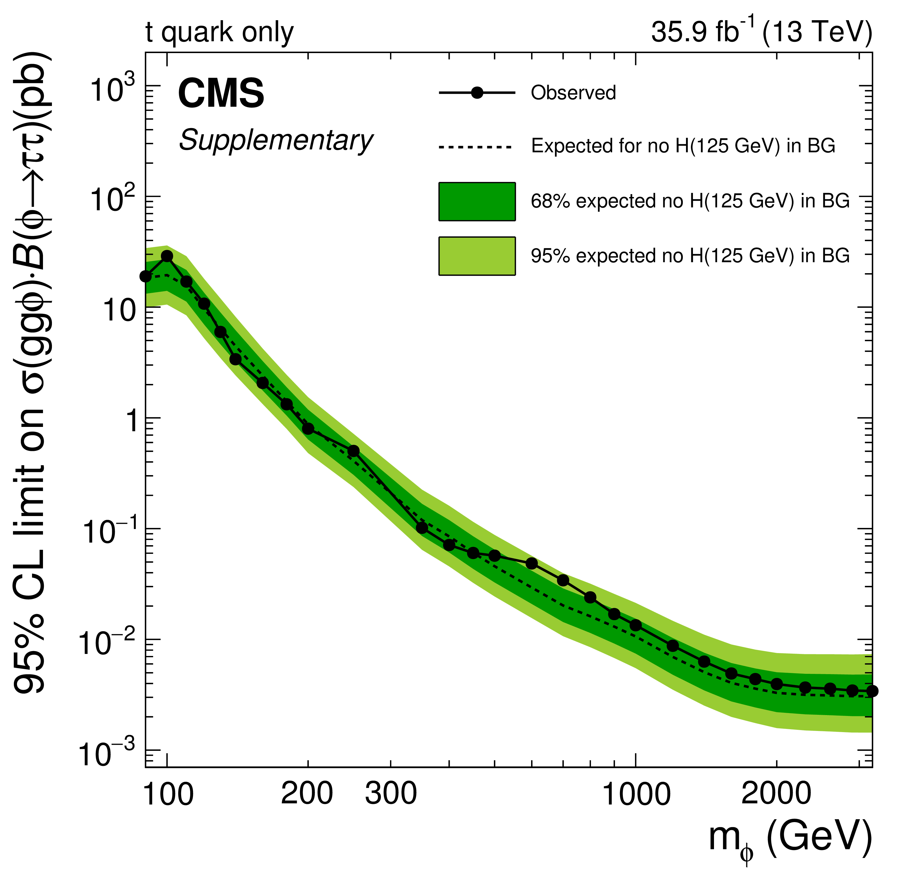
png pdf	Figure 7: Expected and observed 95% CL upper limits for the production of a single narrow resonance, $\phi $, with a mass between 90 GeV and 3.2 TeV in the $\tau \tau $ final state (left) for the production via gluon fusion (gg$\phi $) and (right) in association with b quarks (bb$\phi $). The expected median of the exclusion limit is shown by the dashed line. The dark green and bright yellow bands indicate the 68 and 95% confidence intervals for the variation of the expected exclusion limit. The black dots correspond to the observed limits. In the left panel the expected exclusion limits for the cases where (blue continuous line) only the b quark and (red continuous line) only the t quark are taken into account in the fermion loop are also shown. Left of the dashed vertical line the two different assumptions lead to visible differences in the expected exclusion limit.
png pdf	Figure 7-a: Expected and observed 95% CL upper limits for the production of a single narrow resonance, $\phi $, with a mass between 90 GeV and 3.2 TeV in association with b quarks (bb$\phi $). The expected median of the exclusion limit is shown by the dashed line. The dark green and bright yellow bands indicate the 68 and 95% confidence intervals for the variation of the expected exclusion limit. The black dots correspond to the observed limits. The expected exclusion limits for the cases where (blue continuous line) only the b quark and (red continuous line) only the t quark are taken into account in the fermion loop are also shown. Left of the dashed vertical line the two different assumptions lead to visible differences in the expected exclusion limit.
png pdf	Figure 7-b: Expected and observed 95% CL upper limits for the production of a single narrow resonance, $\phi $, with a mass between 90 GeV and 3.2 TeV in association with b quarks (bb$\phi $). The expected median of the exclusion limit is shown by the dashed line. The dark green and bright yellow bands indicate the 68 and 95% confidence intervals for the variation of the expected exclusion limit. The black dots correspond to the observed limits.
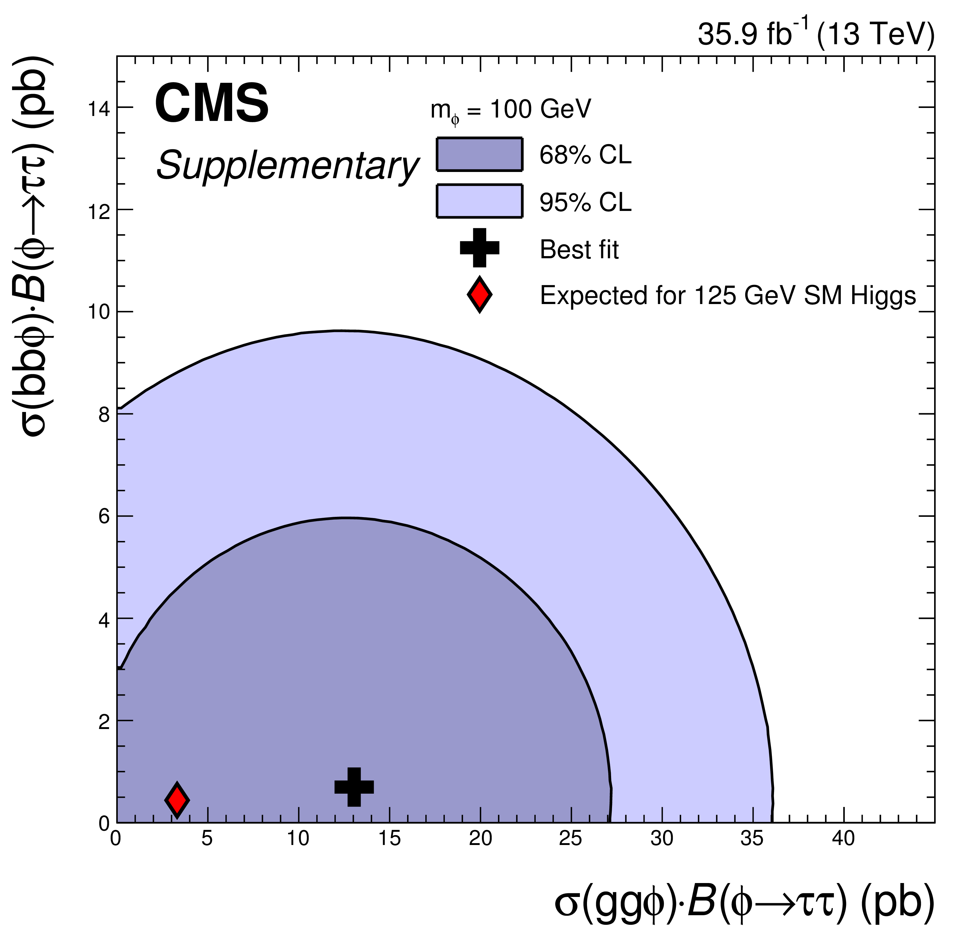
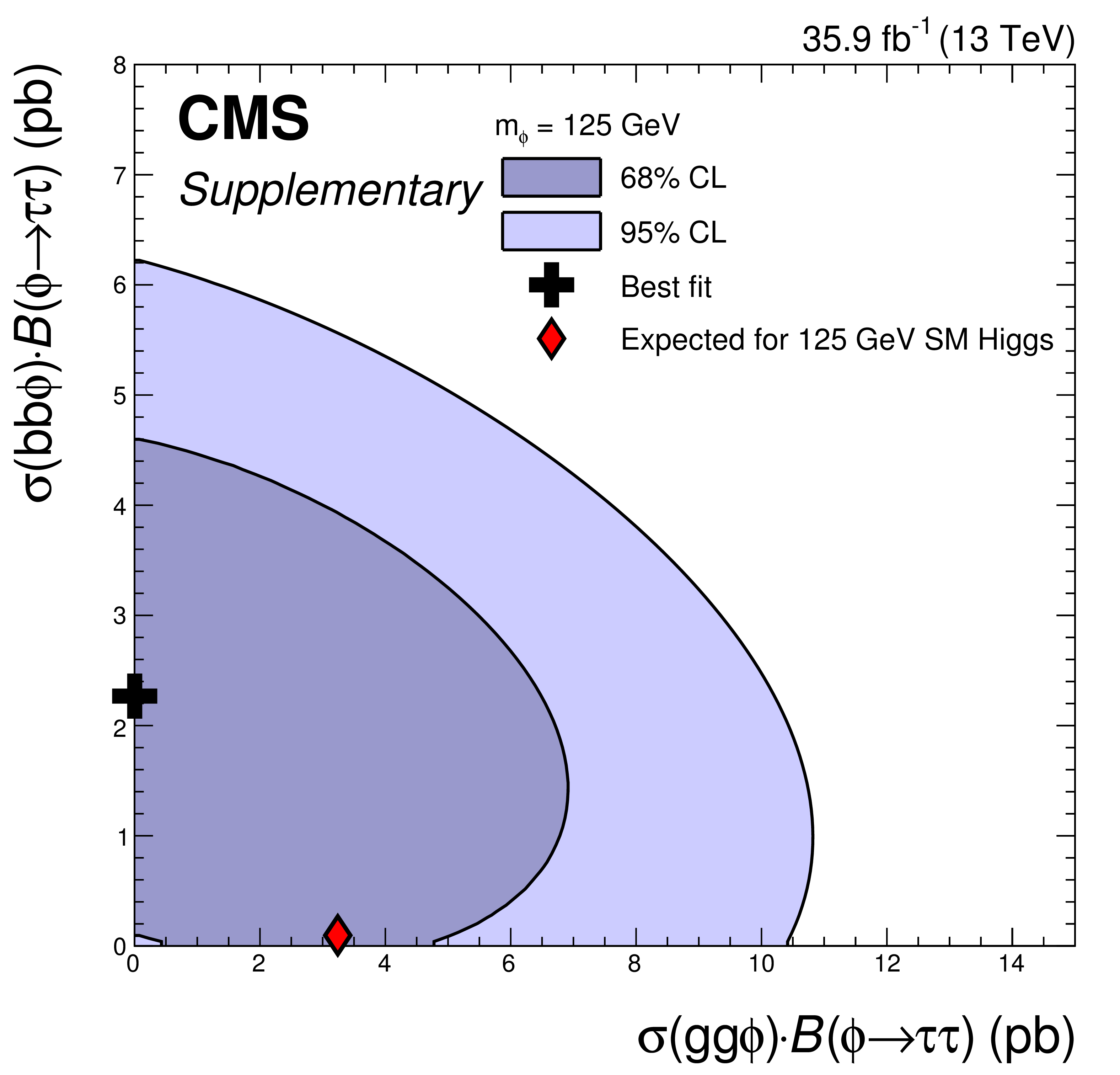
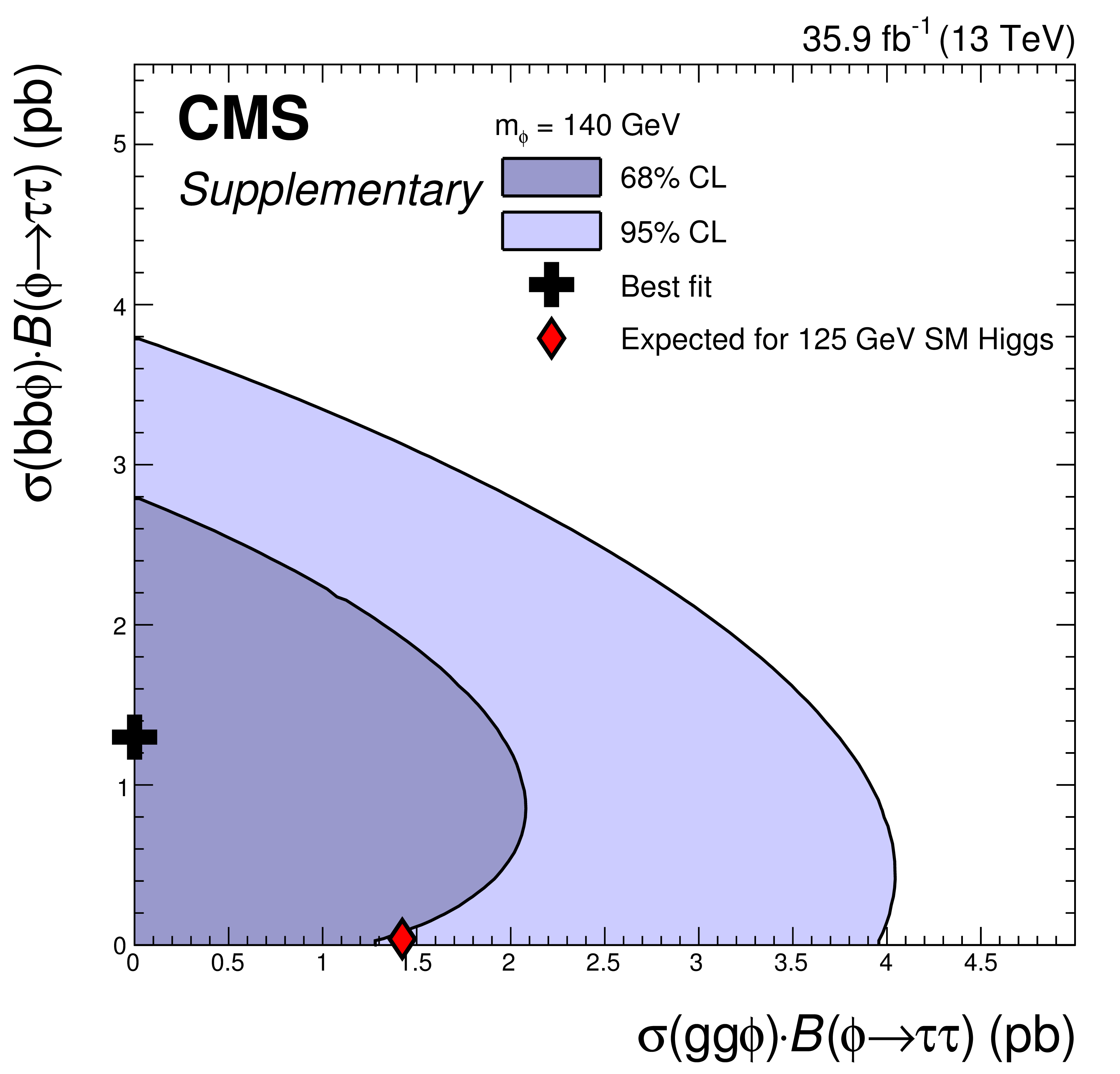
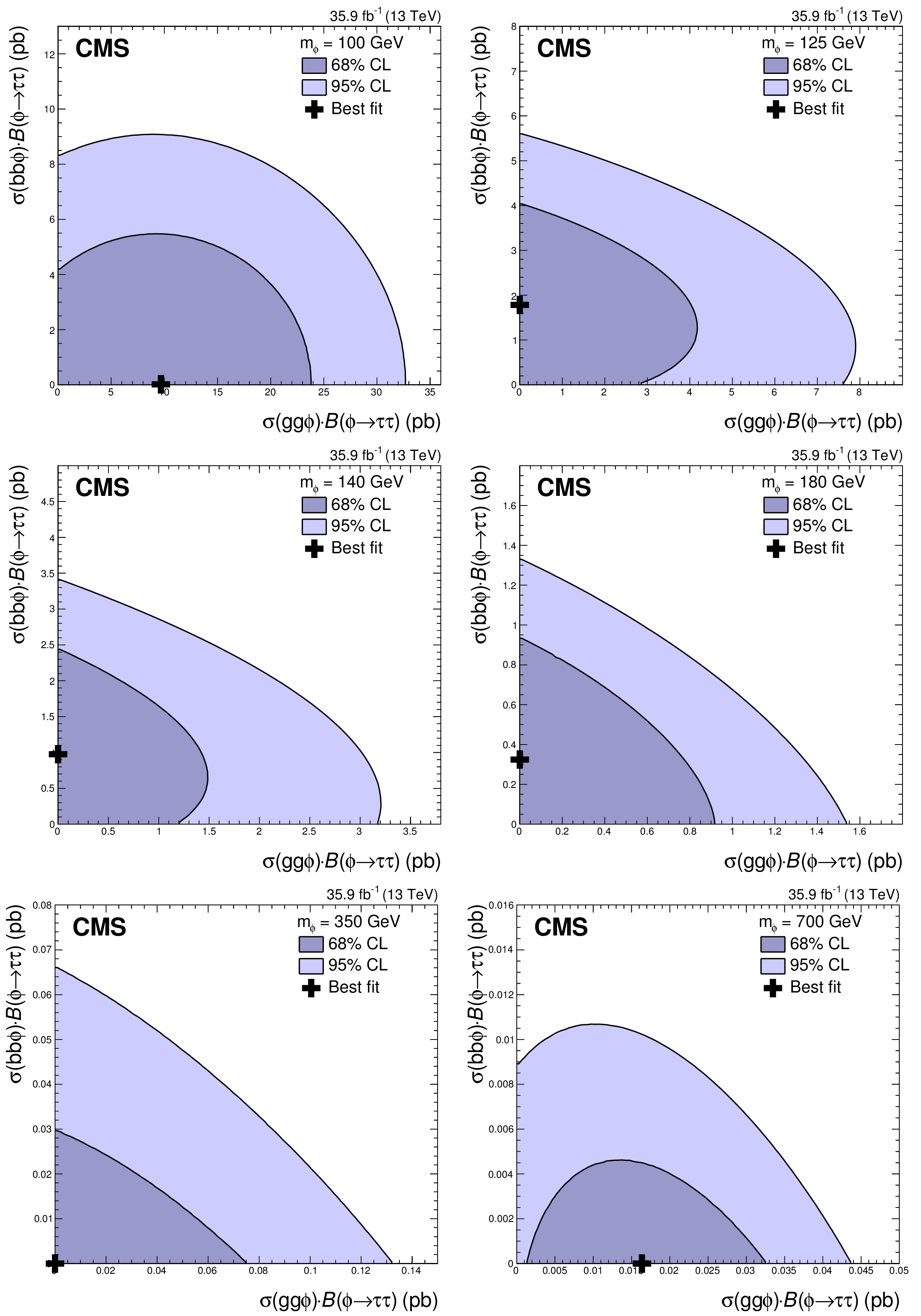
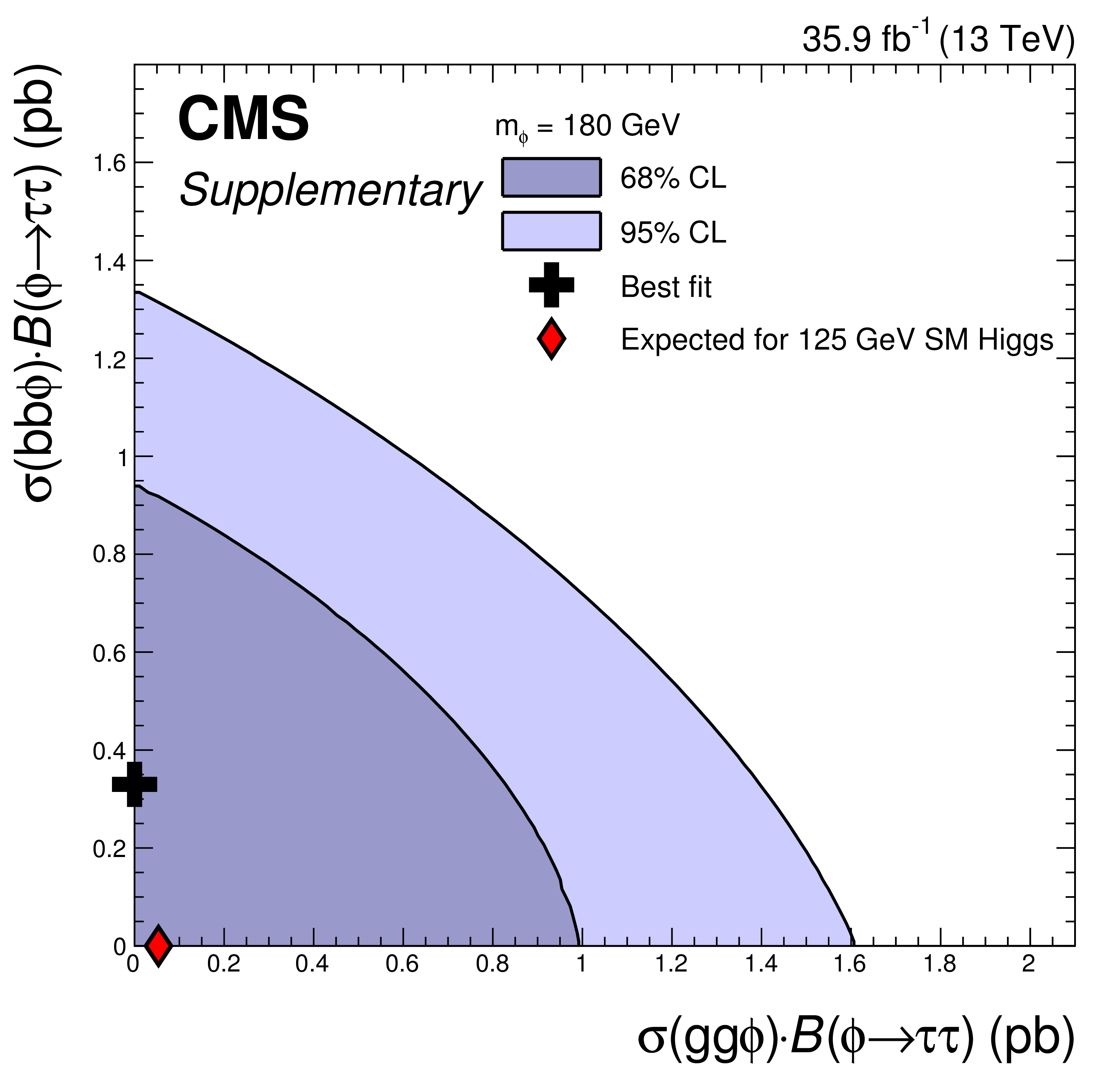
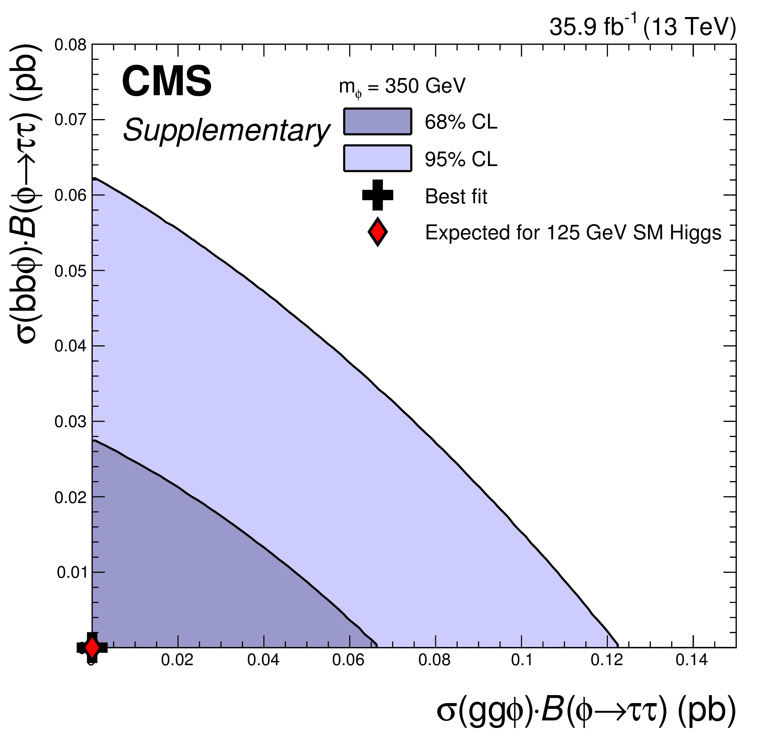
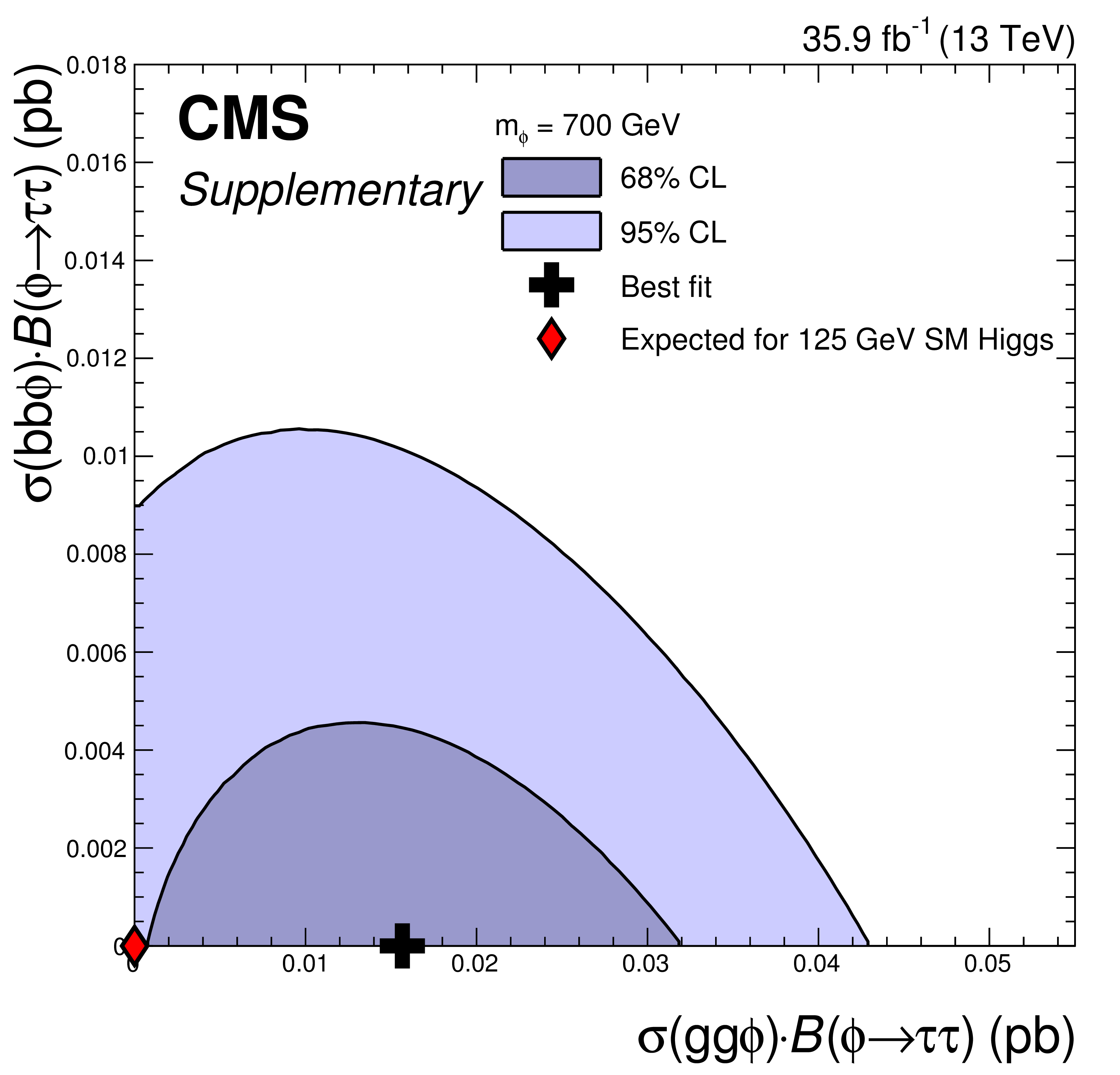
png pdf	Figure 8: Scan of the likelihood function for the search in the $\tau \tau $ final state for a single narrow resonance, $\phi $, produced via gluon fusion ($ {\mathrm {g}} {\mathrm {g}} \phi $) or in association with b quarks ($ {\mathrm {b}} {\mathrm {b}} \phi $). A representative subset of the mass points tested at (upper left) 100 GeV, (upper right) 125 GeV, (middle left) 140 GeV, (middle right) 180 GeV, (lower left) 350 GeV, and (lower right) 700 GeV is shown. Note that in the fits the signal strengths are not allowed to become negative.
png pdf	Figure 8-a: Scan of the likelihood function for the search in the $\tau \tau $ final state for a single narrow resonance, $\phi $, produced via gluon fusion ($ {\mathrm {g}} {\mathrm {g}} \phi $) or in association with b quarks ($ {\mathrm {b}} {\mathrm {b}} \phi $). The result is shown at mass point 100 GeV. Note that in the fit the signal strengths are not allowed to become negative.
png pdf	Figure 8-b: Scan of the likelihood function for the search in the $\tau \tau $ final state for a single narrow resonance, $\phi $, produced via gluon fusion ($ {\mathrm {g}} {\mathrm {g}} \phi $) or in association with b quarks ($ {\mathrm {b}} {\mathrm {b}} \phi $). The result is shown at mass point 125 GeV. Note that in the fit the signal strengths are not allowed to become negative.
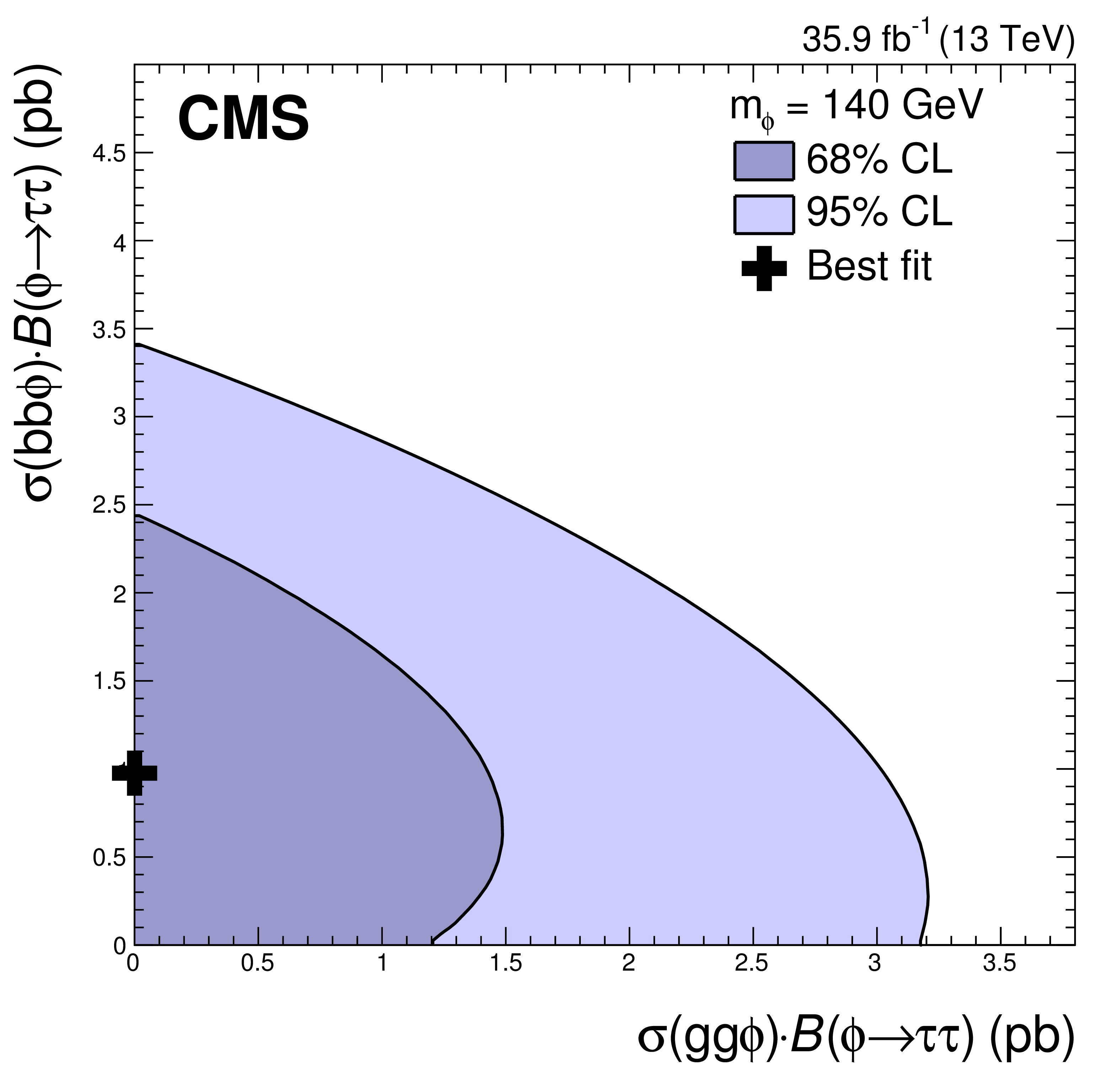
png pdf	Figure 8-c: Scan of the likelihood function for the search in the $\tau \tau $ final state for a single narrow resonance, $\phi $, produced via gluon fusion ($ {\mathrm {g}} {\mathrm {g}} \phi $) or in association with b quarks ($ {\mathrm {b}} {\mathrm {b}} \phi $). The result is shown at mass point 140 GeV. Note that in the fit the signal strengths are not allowed to become negative.
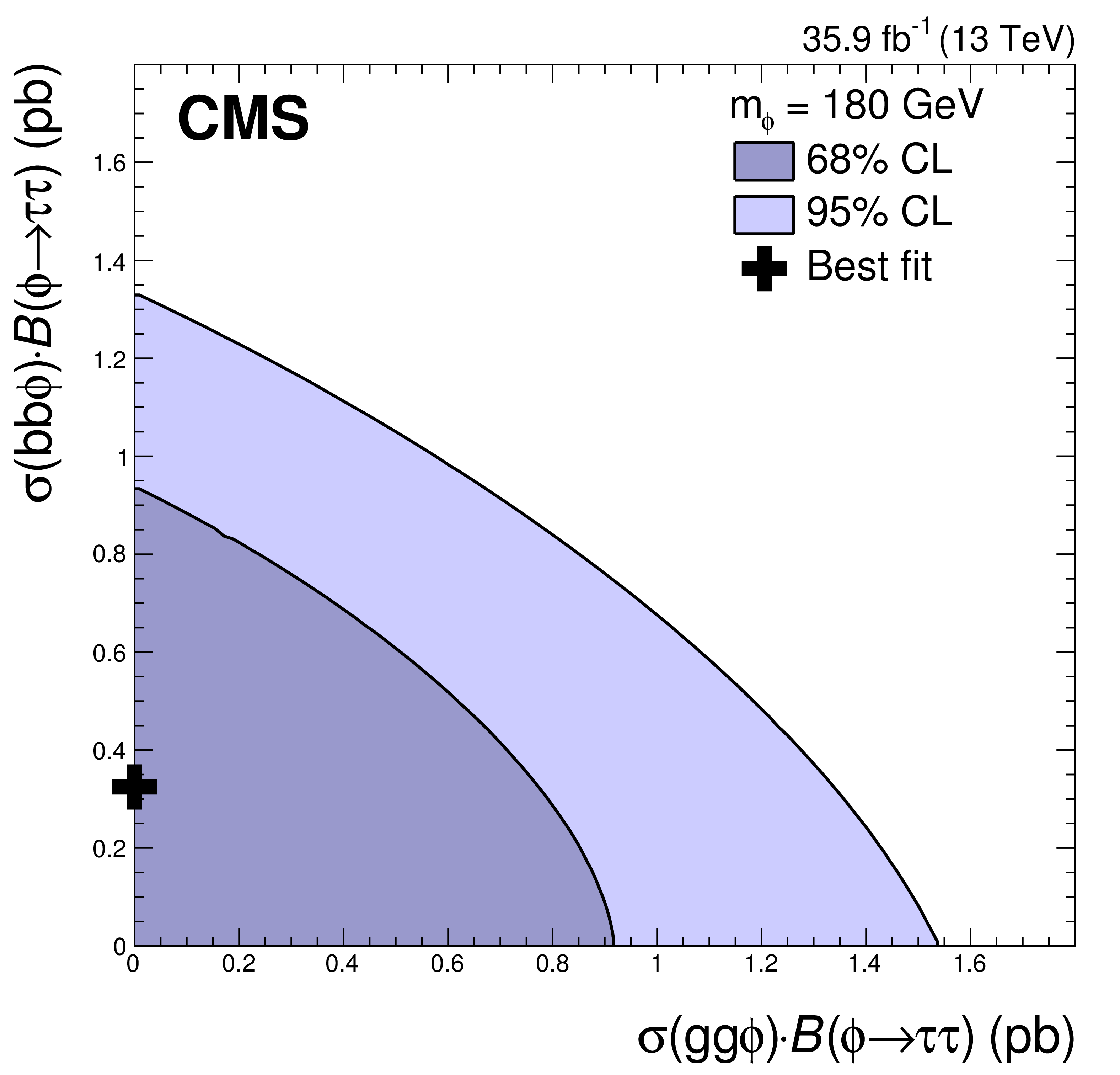
png pdf	Figure 8-d: Scan of the likelihood function for the search in the $\tau \tau $ final state for a single narrow resonance, $\phi $, produced via gluon fusion ($ {\mathrm {g}} {\mathrm {g}} \phi $) or in association with b quarks ($ {\mathrm {b}} {\mathrm {b}} \phi $). The result is shown at mass point 180 GeV. Note that in the fit the signal strengths are not allowed to become negative.
png pdf	Figure 8-e: Scan of the likelihood function for the search in the $\tau \tau $ final state for a single narrow resonance, $\phi $, produced via gluon fusion ($ {\mathrm {g}} {\mathrm {g}} \phi $) or in association with b quarks ($ {\mathrm {b}} {\mathrm {b}} \phi $). The result is shown at mass point 350 GeV. Note that in the fit the signal strengths are not allowed to become negative.
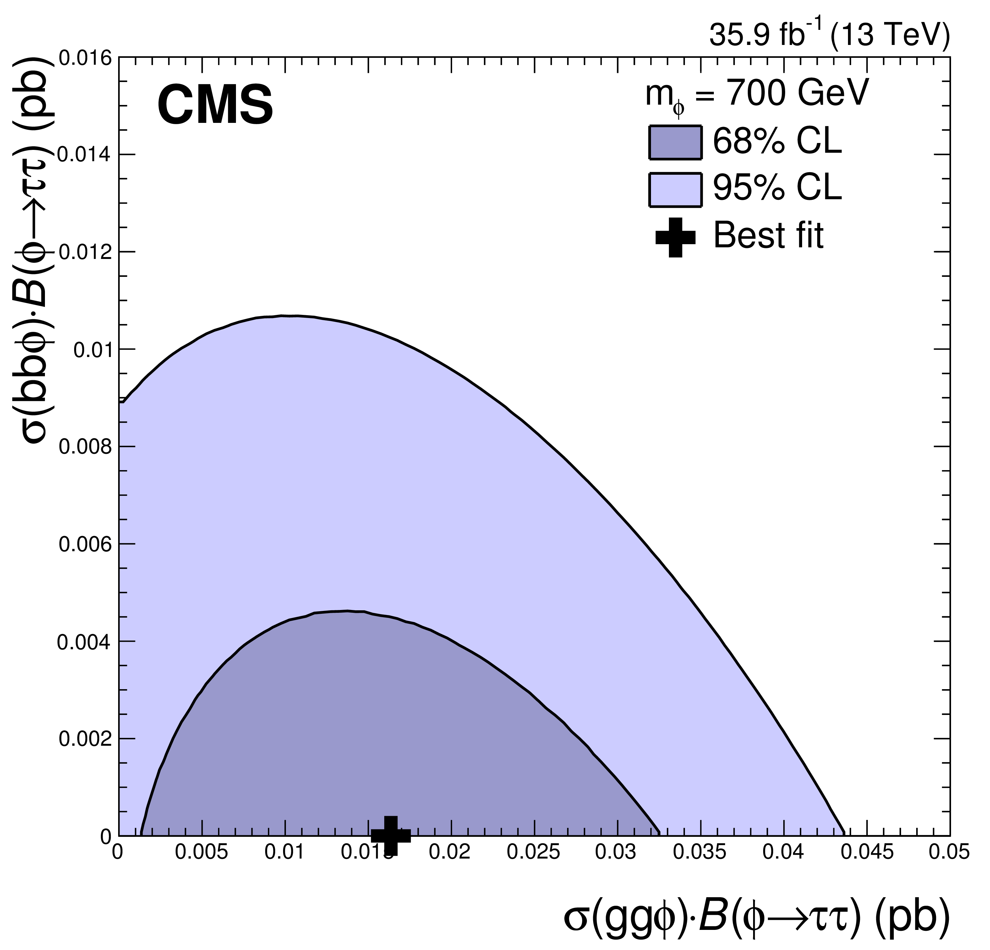
png pdf	Figure 8-f: Scan of the likelihood function for the search in the $\tau \tau $ final state for a single narrow resonance, $\phi $, produced via gluon fusion ($ {\mathrm {g}} {\mathrm {g}} \phi $) or in association with b quarks ($ {\mathrm {b}} {\mathrm {b}} \phi $). The result is shown at mass point 700 GeV. Note that in the fit the signal strengths are not allowed to become negative.
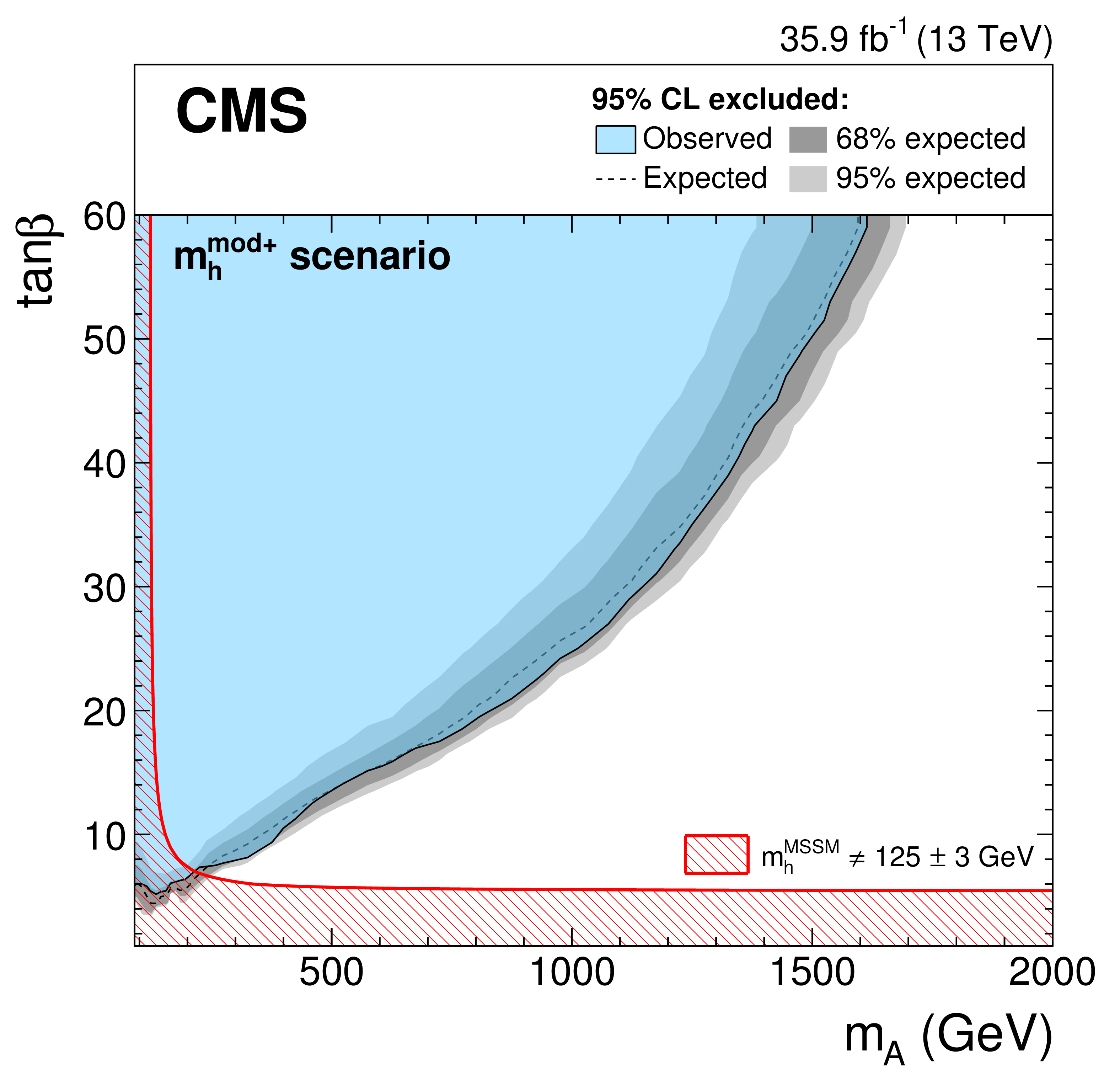
png pdf	Figure 9: Expected and observed 95% CL exclusion contour (left) in the MSSM $ {m_{\text {h}}^{\text {mod+}}}$ and (right) in the hMSSM scenarios. The expected median is shown as a dashed black line. The dark and bright gray bands indicate the 68 and 95% confidence intervals for the variation of the expected exclusion. The observed exclusion contour is indicated by the colored blue area. For the $ {m_{\text {h}}^{\text {mod+}}}$ scenario, those parts of the parameter space, where $m_{{\mathrm {h}}}$ deviates by more then ${\pm}$3 GeV from the mass of the observed Higgs boson at 125 GeV are indicated by a red hatched area.
png pdf	Figure 9-a: Expected and observed 95% CL exclusion contour in the MSSM $ {m_{\text {h}}^{\text {mod+}}}$ scenario. The expected median is shown as a dashed black line. The dark and bright gray bands indicate the 68 and 95% confidence intervals for the variation of the expected exclusion. The observed exclusion contour is indicated by the colored blue area. Those parts of the parameter space, where $m_{{\mathrm {h}}}$ deviates by more then ${\pm}$3 GeV from the mass of the observed Higgs boson at 125 GeV are indicated by a red hatched area.
png pdf	Figure 9-b: Expected and observed 95% CL exclusion contour in the hMSSM scenario. The expected median is shown as a dashed black line. The dark and bright gray bands indicate the 68 and 95% confidence intervals for the variation of the expected exclusion. The observed exclusion contour is indicated by the colored blue area.

Tables
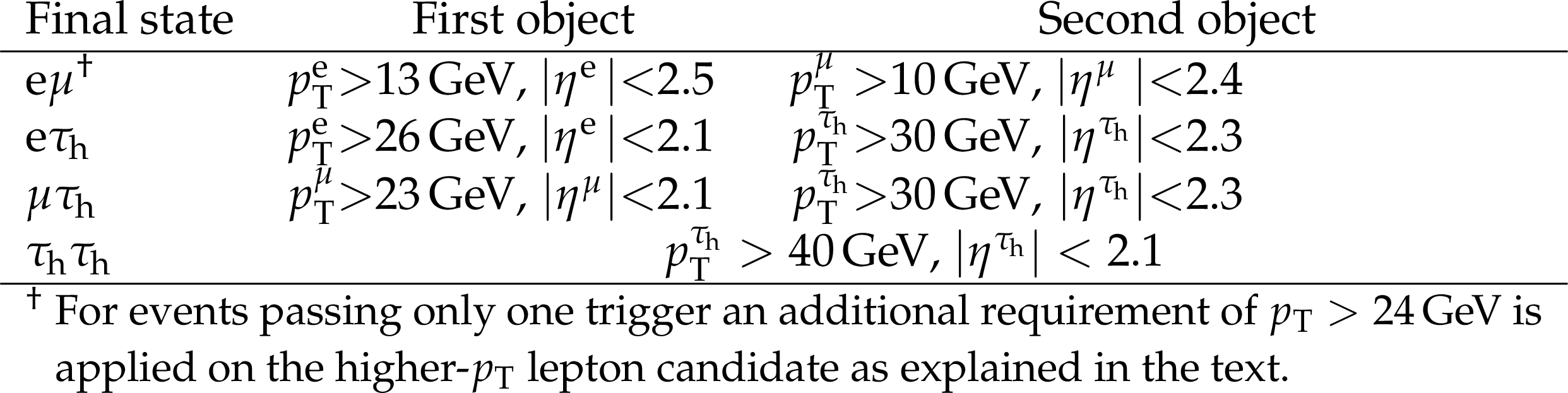
png pdf	Table 1: Kinematic selection of the $\tau $ lepton decay products in the $ {\mathrm {e}} {{\mu}}$, $ {\mathrm {e}} {\tau}_{\text {h}} $, $ {{\mu}} {\tau}_{\text {h}} $, and $ {\tau}_{\text {h}} {\tau}_{\text {h}} $ final states. The expression "First (Second) object'' refers to the final state label used in the first column.
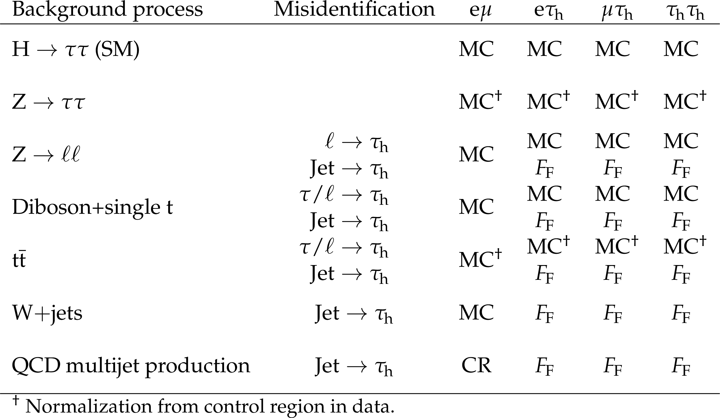
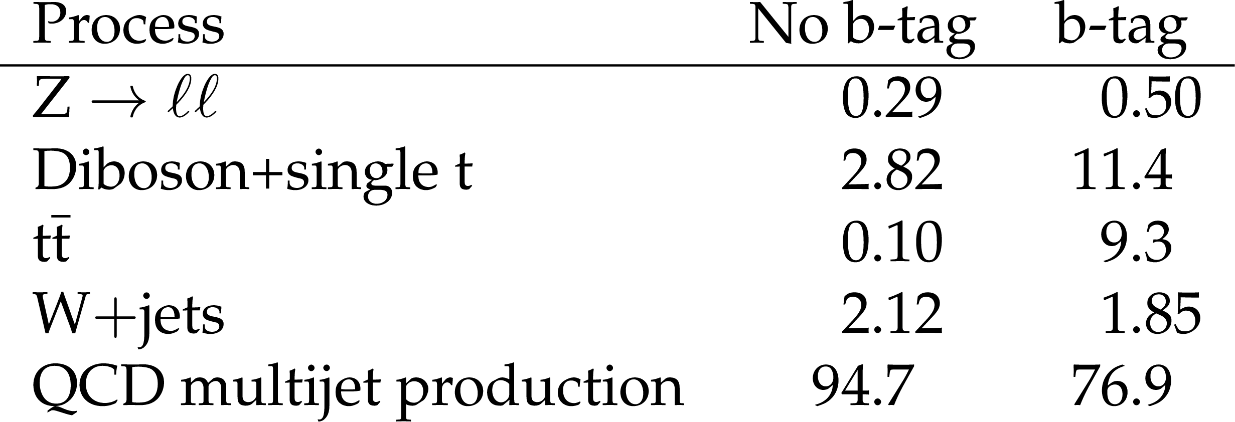
png pdf	Table 2: Background processes contributing to the event selection, as given in Section wwwww. The first row corresponds to the SM Higgs boson in the $\tau \tau $ final state, which is also taken into account in the statistical analysis. The further splitting of the processes in the second column refers only to final states that contain a $ {\tau}_{\text {h}} $ candidate. The label "MC'' implies that the process is taken from simulation; the label "$ {F_{\text {F}}} $'' implies that the process is determined from data using the fake factor method, as described in Section 5.2. The label "CR'' implies that both the shape and normalization of QCD multijet events are estimated from control regions in data. The symbol $\ell $ corresponds to an electron or muon.
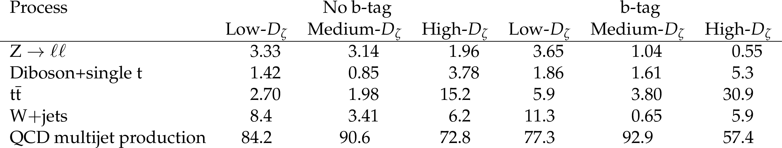
png pdf	Table 3: Observed number of selected events ($ {N_{\text {data}}}$) and the relative contribution of the expected backgrounds in all event categories in the $ {\mathrm {e}} {{\mu}}$, $ {\mathrm {e}} {\tau}_{\text {h}} $, $ {{\mu}} {\tau}_{\text {h}} $, and $ {\tau}_{\text {h}} {\tau}_{\text {h}} $ final states. The relative contribution of the expected backgrounds is given in %, including the contribution of an SM Higgs boson with a mass of 125 GeV, and prior to the fit used for the signal extraction. In all but the $ {\mathrm {e}} {{\mu}}$ final state, processes in which a jet is misidentified as a hadronic $\tau $ lepton decay are subsumed into a common $\text {jet}\to {\tau}_{\text {h}} $ background class which is estimated from data.
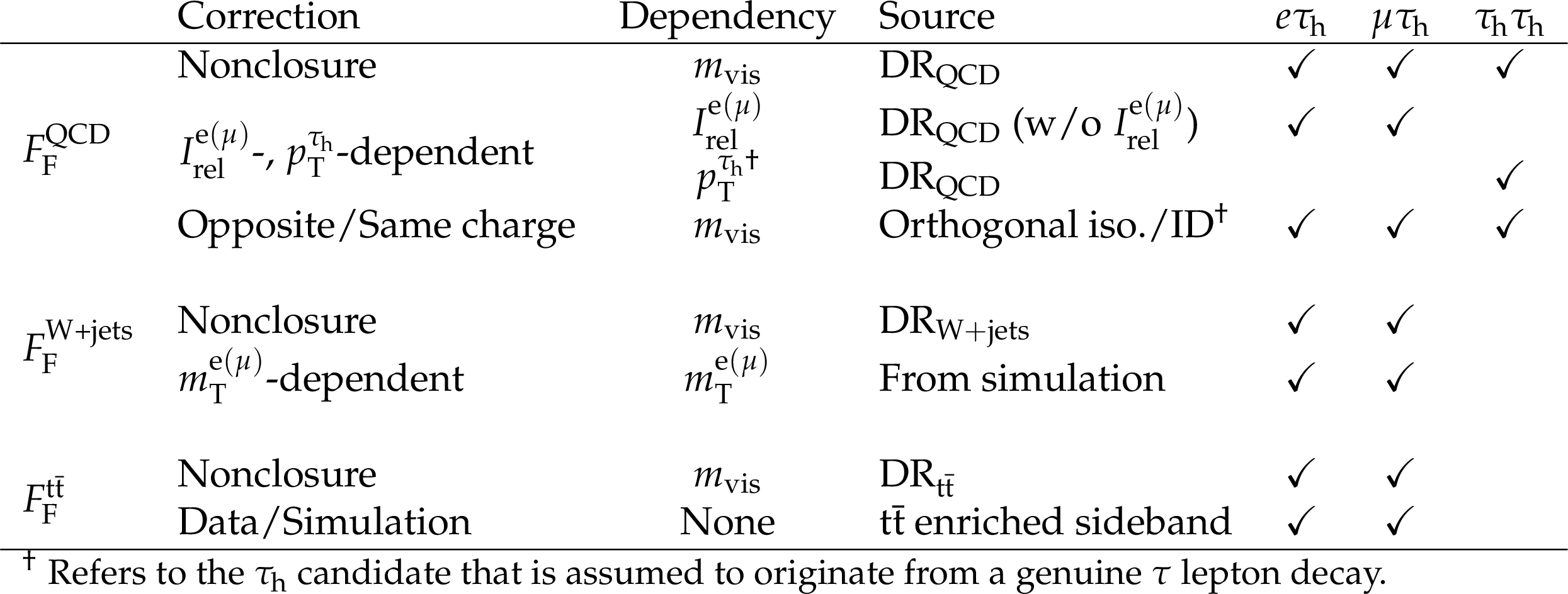
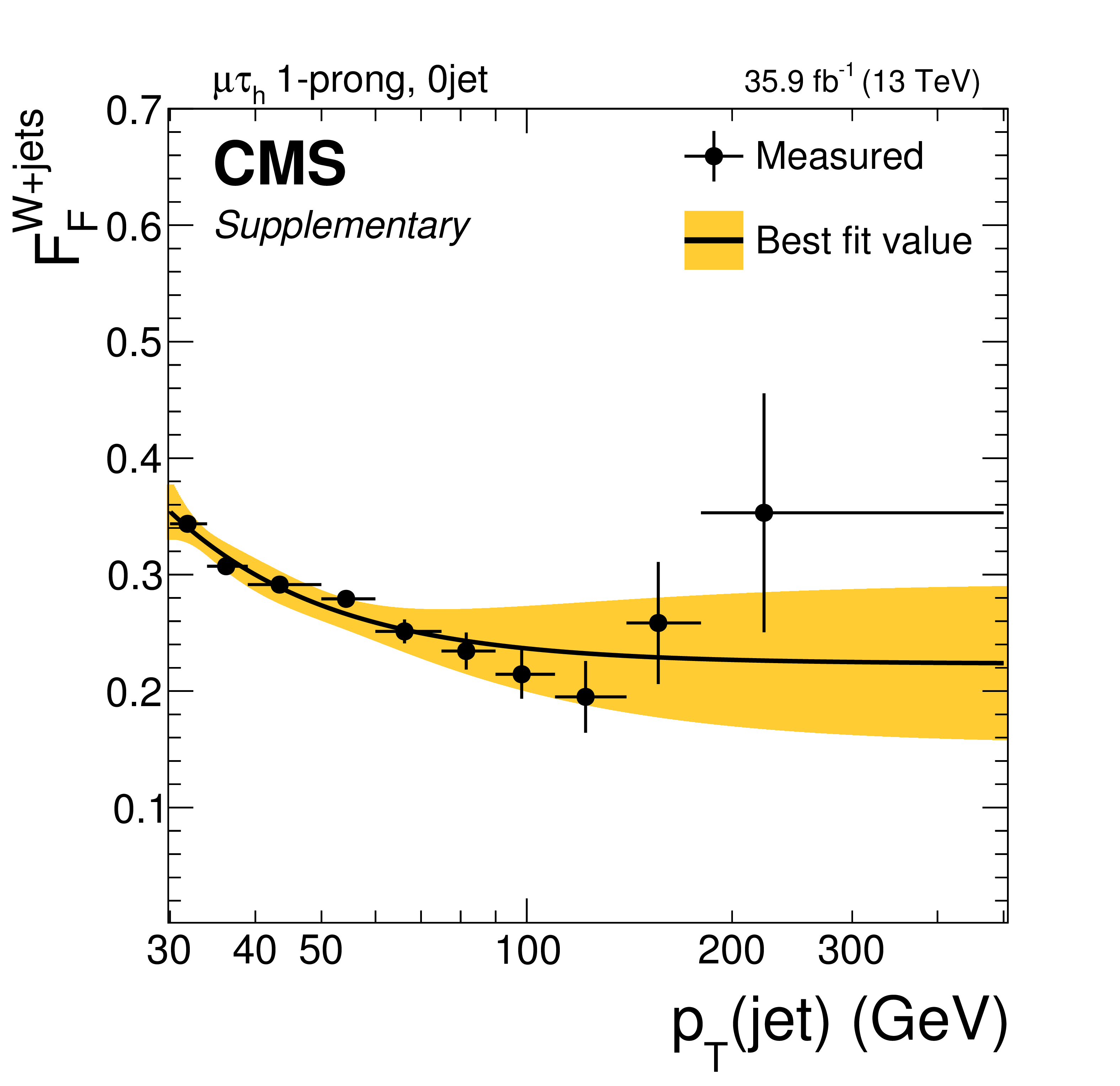
png pdf	Table 4: Corrections applied to the $ {F_{\text {F}}} ^{\text {QCD}}$, $ {F_{\text {F}}} ^{{{\mathrm {W}}}{+}\text {jets}}$, and $ {F_{\text {F}}} ^{{{\mathrm {t}\overline {\mathrm {t}}}}}$ as described in the text. In the fourth column the source is indicated from which the correction is derived. The dependency $ {p_{\mathrm {T}}} ^{{\tau}_{\text {h}}}$ in the third line refers to the $ {p_{\mathrm {T}}} $ of the $ {\tau}_{\text {h}} $ candidate that is assumed to originate from a genuine $\tau $ lepton decay.

Summary

A search for additional heavy neutral Higgs bosons in the decay into two $\tau$ leptons in the context of the minimal supersymmetric standard model (MSSM) has been presented. This search has been performed in the most sensitive $\mathrm{e}\mu$, $\mathrm{e}\tau_{\mathrm{h}}$, $\mu\tau_{\mathrm{h}}$, and $\tau_{\mathrm{h}}\tau_{\mathrm{h}}$ final states of the $\tau\tau$ pair, where $\tau_{\mathrm{h}}$ indicates a hadronic $\tau$ lepton decay. No signal has been found. Model-independent limits at 95% confidence level have been set for the production of a single narrow resonance decaying into a pair of $\tau$ leptons. These range from 18 pb at 90 GeV to 3.5 fb at 3.2 TeV for production via gluon fusion and from 15 pb (at 90 GeV) to 2.5 fb (at 3.2 TeV) for production in association with b quarks. Finally 95% confidence level exclusion contours have been provided for two representative benchmark scenarios, namely the ${m_{\text{h}}^{\text{mod+}}}$ and the hMSSM scenarios. In these two scenarios the presence of a neutral heavy MSSM Higgs boson up to $m_{A < 250 GeV}$ is excluded for $\tan\beta$ values above 6. The exclusion contour reaches 1.6 TeV for $\tan\beta= $ 60.

Additional Figures
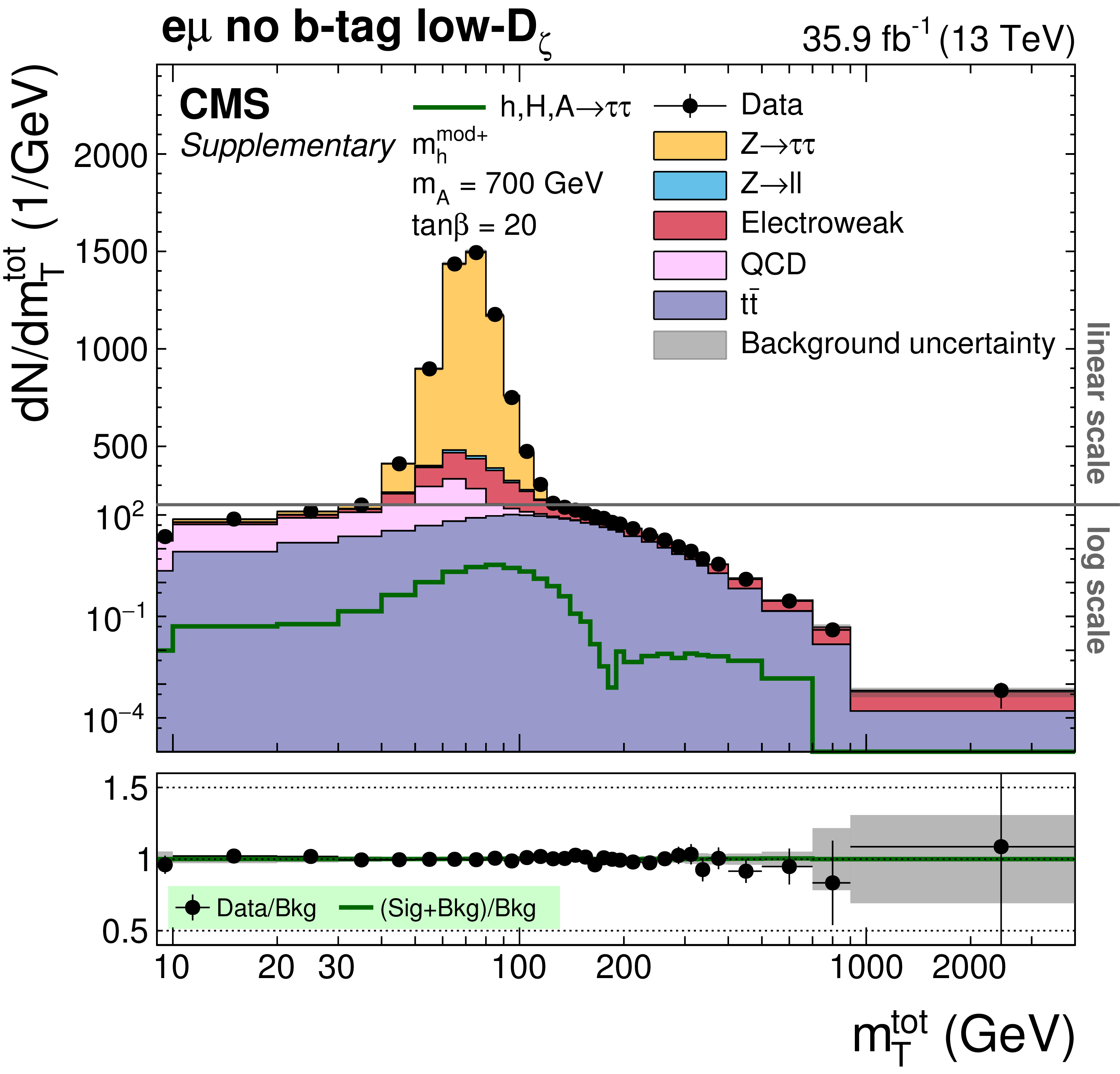
png pdf	Additional Figure 1: Distribution of $m_{\text {T}}^{\text {tot}}$ in the no b-tag low-$D_{\zeta}$ event category in the $ {\mathrm {e}} {{\mu}}$ final state.
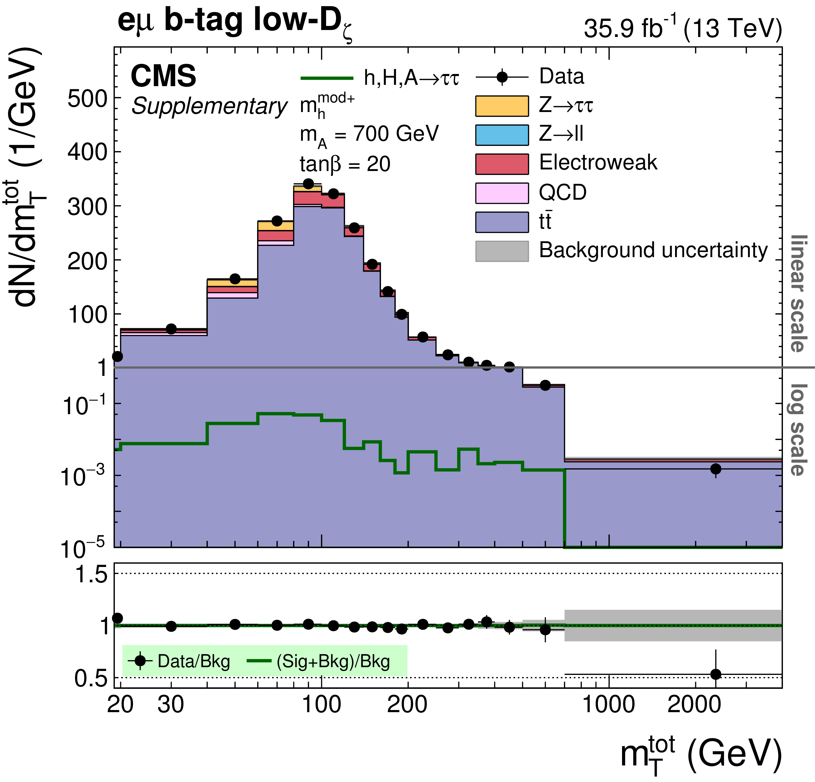
png pdf	Additional Figure 2: Distribution of $m_{\text {T}}^{\text {tot}}$ in the b-tag low-$D_{\zeta}$ event category in the $ {\mathrm {e}} {{\mu}}$ final state.
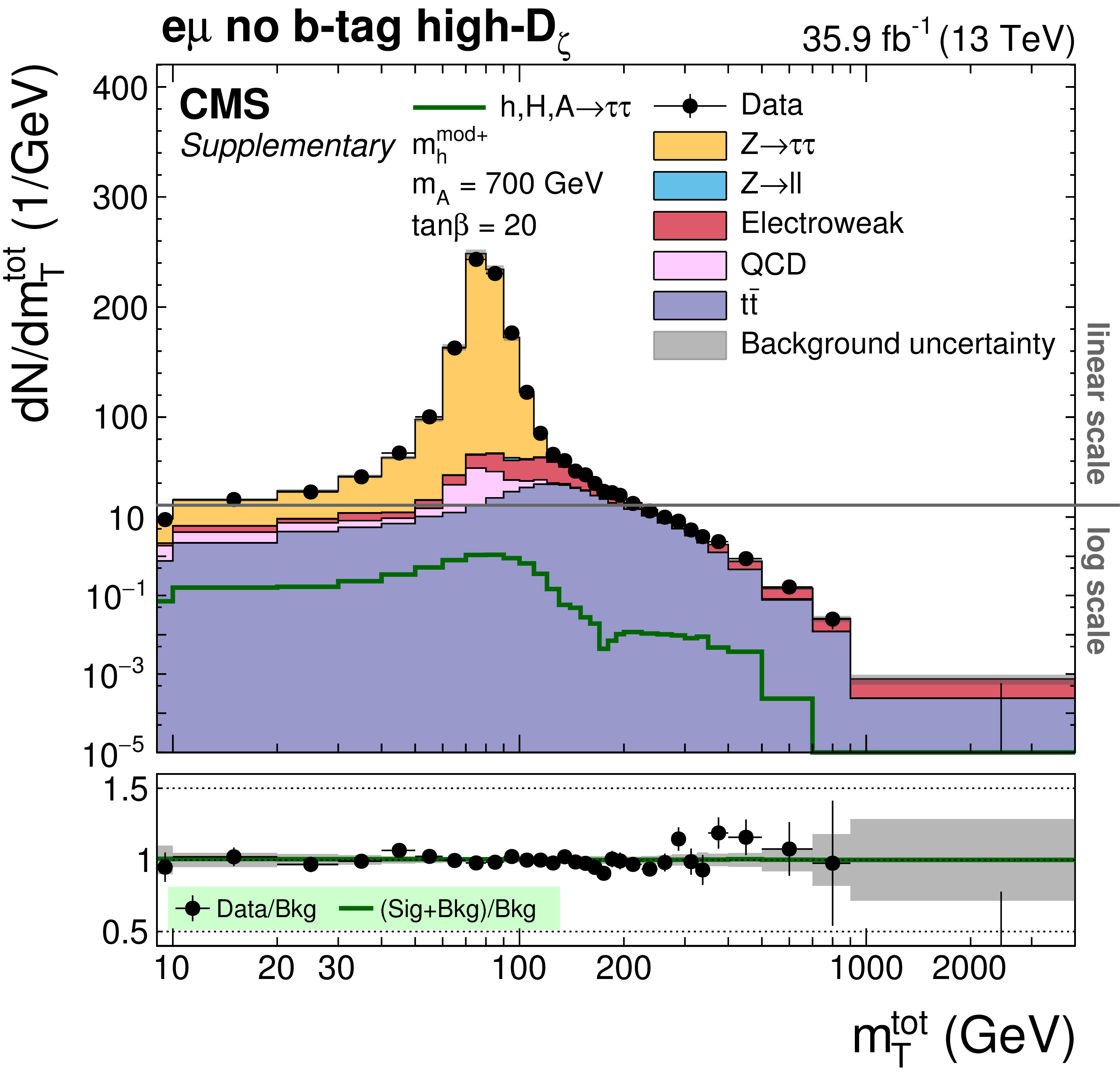
png pdf	Additional Figure 3: Distribution of $m_{\text {T}}^{\text {tot}}$ in the no b-tag high-$D_{\zeta}$ event category in the $ {\mathrm {e}} {{\mu}}$ final state.
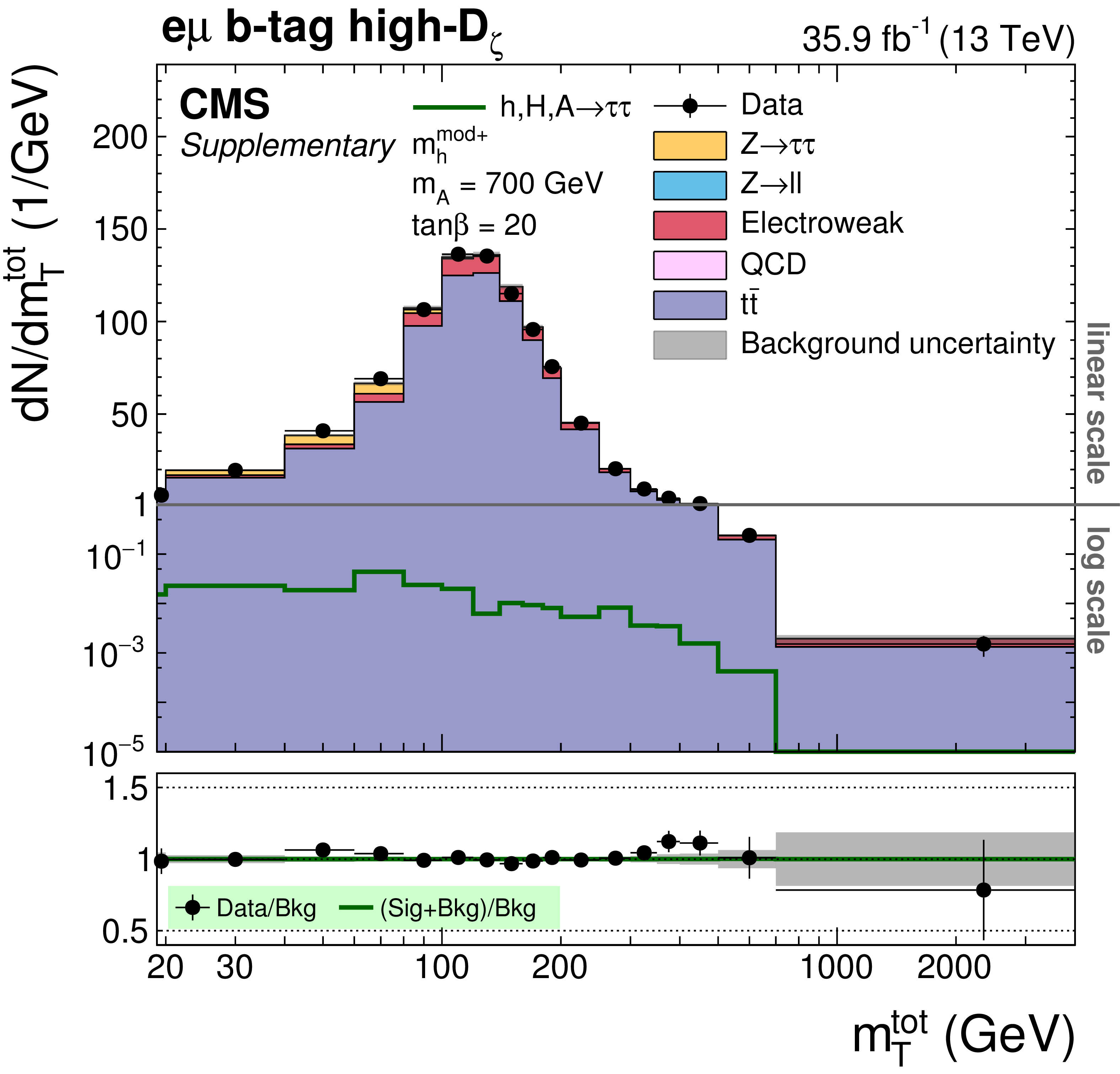
png pdf	Additional Figure 4: Distribution of $m_{\text {T}}^{\text {tot}}$ in the b-tag high-$D_{\zeta}$ event category in the $ {\mathrm {e}} {{\mu}}$ final state.
png pdf	Additional Figure 5: Distribution of $m_{\text {T}}^{\text {tot}}$ in the no b-tag loose-$m_{\text {T}}$ event category in the $ {\mathrm {e}} {\tau}_{\text {h}} $ final state.
png pdf	Additional Figure 6: Distribution of $m_{\text {T}}^{\text {tot}}$ in the b-tag loose-$m_{\text {T}}$ event category in the $ {\mathrm {e}} {\tau}_{\text {h}} $ final state.
png pdf	Additional Figure 7: Distribution of $m_{\text {T}}^{\text {tot}}$ in the no b-tag loose-$m_{\text {T}}$ event category in the $ {{\mu}} {\tau}_{\text {h}} $ final state.
png pdf	Additional Figure 8: Distribution of $m_{\text {T}}^{\text {tot}}$ in the b-tag loose-$m_{\text {T}}$ event category in the $ {{\mu}} {\tau}_{\text {h}} $ final state.
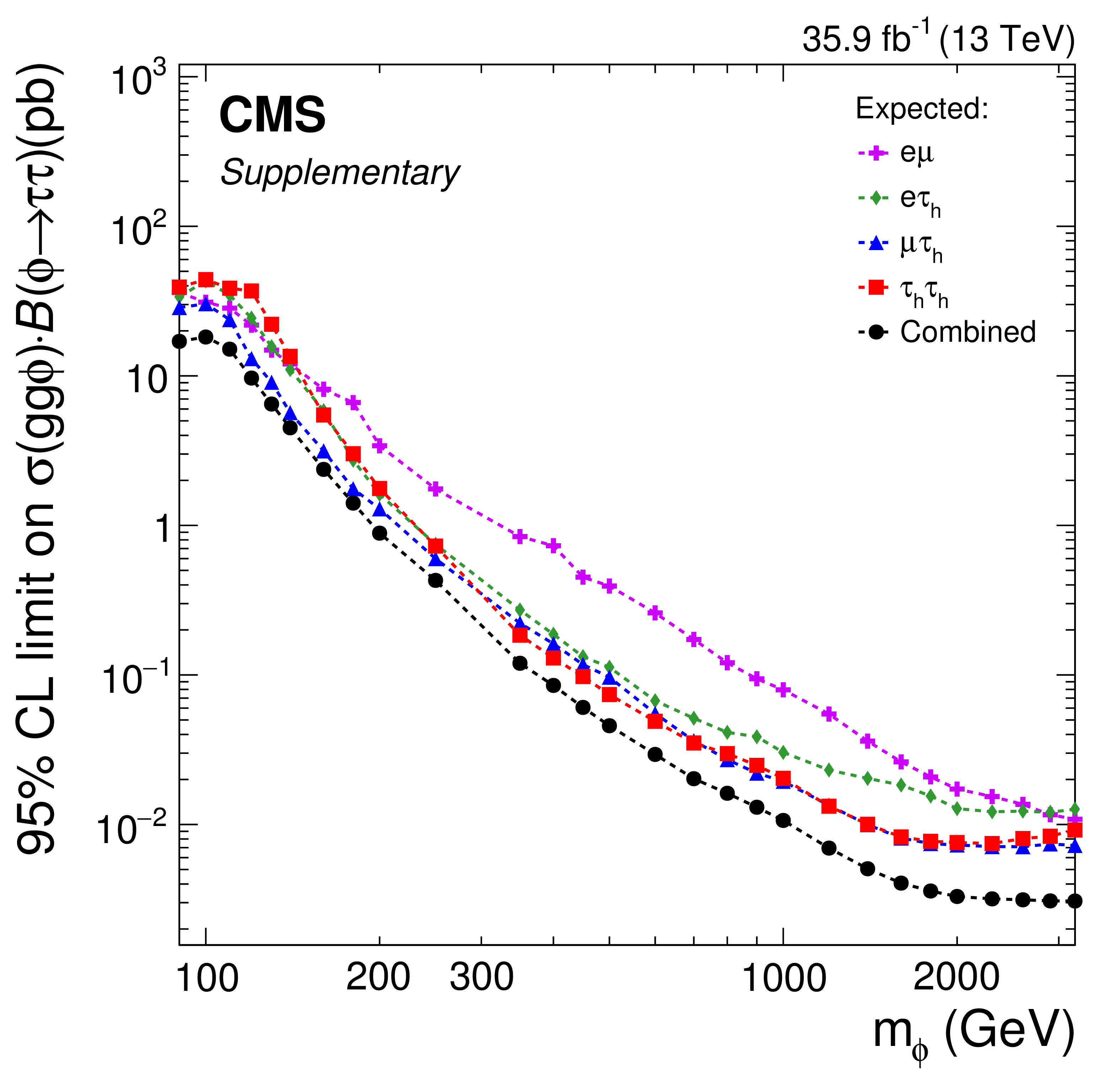
png pdf	Additional Figure 9: Expected 95% CL upper limits for the production of a single narrow resonance $\phi $ with a mass between 90 GeV and 3.2 TeV via gluon-fusion (gg$\phi $) in the $\tau \tau $ final sate. The individual contributions to the combined analysis have been split by the decay modes of the final state $\tau $ leptons. For these limits the SM Higgs boson has been added to the non-Higgs SM background.
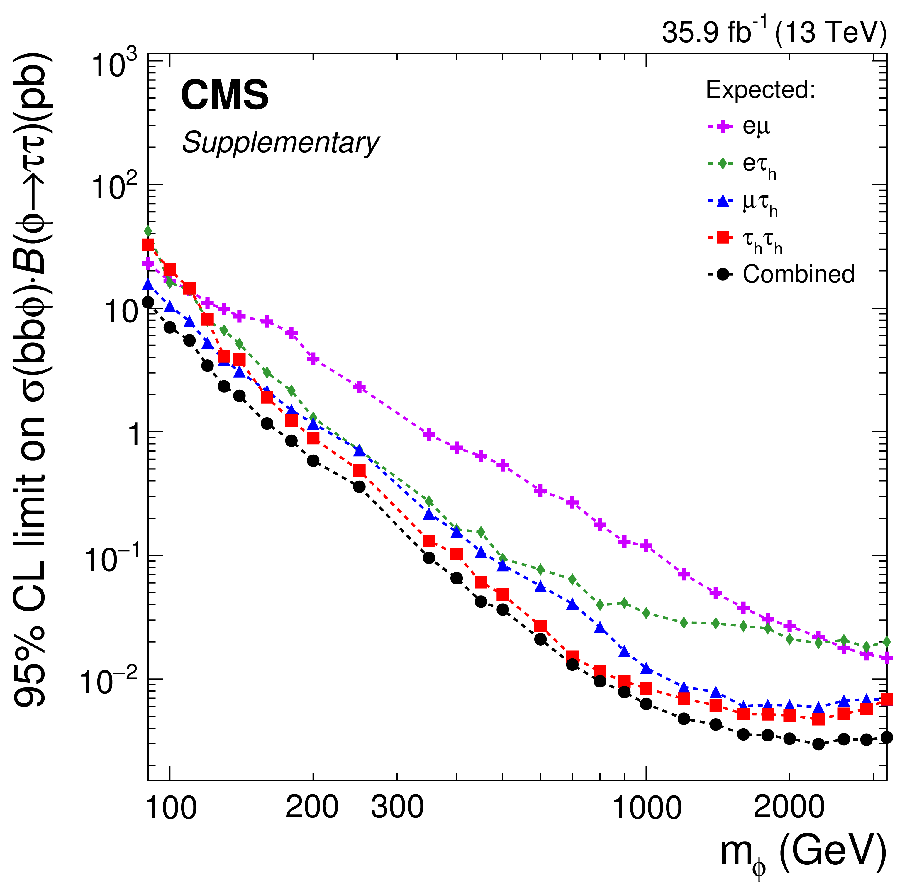
png pdf	Additional Figure 10: Expected 95% CL upper limits for the production of a single narrow resonance $\phi $ with a mass between 90 GeV and 3.2 TeV in association with b quarks (bb$\phi $) in the $\tau \tau $ final state. The individual contributions to the combined analysis have been split by the decay modes of the final state $\tau $ leptons. For these limits the SM Higgs boson has been added to the non-Higgs SM background.
png pdf	Additional Figure 11: Expected and observed 95% CL upper limits for the production of a single narrow resonance $\phi $ with a mass between 90 GeV and 3.2 TeV via gluon-fusion (gg$\phi $) in the $\tau \tau $ final state. For these limits the cross section for the production in association with b quarks (bb$\phi $) has been set to zero; the SM Higgs boson has been added to the non-Higgs SM background.
png pdf	Additional Figure 12: Expected and observed 95% CL upper limits for the production of a single narrow resonance $\phi $ with a mass between 90 GeV and 3.2 TeV in association with b quarks (bb$\phi $) in the $\tau \tau $ final state. For these limits the cross section for the production via gluon-fusion has been set to zero; the SM Higgs boson has been added to the non-Higgs SM background.
png pdf	Additional Figure 13: Expected and observed 95% CL upper limits for the production of a single narrow resonance $\phi $ with a mass between 90 GeV and 3.2 TeV via gluon-fusion (gg$\phi $) in the $\tau \tau $ final state. For these limits only b quarks have been considered in the fermion loop; the SM Higgs boson has been added to the non-Higgs SM background.
png pdf	Additional Figure 14: Expected and observed 95% CL upper limits for the production of a single narrow resonance $\phi $ with a mass between 90 GeV and 3.2 TeV via gluon-fusion (gg$\phi $) in the $\tau \tau $ final state. For these limits only t quarks have been considered in the fermion loop; the SM Higgs boson has been added to the non-Higgs SM background.
png pdf	Additional Figure 15: Expected and observed 95% CL upper limits for the production of a single narrow resonance $\phi $ with a mass between 90 GeV and 3.2 TeV via gluon-fusion (gg$\phi $) in the $\tau \tau $ final state. For these limits the SM Higgs boson has not been included in the background model. The expected exclusion limits for the cases where (blue continuous line) only the b quark and (red continuous line) only the t quark are taken into account in the fermion loop are also shown.
png pdf	Additional Figure 16: Expected and observed 95% CL upper limits for the production of a single narrow resonance $\phi $ with a mass between 90 GeV and 3.2 TeV in association with b quarks (bb$\phi $) in the $\tau \tau $ final state. For these limits the SM Higgs boson has not been included in the background model.
png pdf	Additional Figure 17: Expected and observed 95% CL upper limits for the production of a single narrow resonance $\phi $ with a mass between 90 GeV and 3.2 TeV via gluon-fusion (gg$\phi $) in the $\tau \tau $ final state. For these limits only b quarks have been considered in the fermion loop; the SM Higgs boson has not been included in the background model.
png pdf	Additional Figure 18: Expected and observed 95% CL upper limits for the production of a single narrow resonance $\phi $ with a mass between 90 GeV and 3.2 TeV via gluon-fusion (gg$\phi $) in the $\tau \tau $ final state. For these limits only t quarks have been considered in the fermion loop; the SM Higgs boson has not been included in the background model.
png pdf	Additional Figure 19: Scan of the likelihood function used for the search for a single narrow resonance $\phi $, with a mass of 100 GeV, produced via gluon-fusion or in association with b quarks, in the $\tau \tau $ final state. For this scan the SM Higgs boson has not been included in the background model. Instead the expected signal for a SM Higgs boson at 125 GeV is indicated by a red diamond.
png pdf	Additional Figure 20: Scan of the likelihood function used for the search for a single narrow resonance $\phi $, with a mass of 125 GeV, produced via gluon-fusion or in association with b quarks, in the $\tau \tau $ final state. For this scan the SM Higgs boson has not been included in the background model. Instead the expected signal for a SM Higgs boson at 125 GeV is indicated by a red diamond.
png pdf	Additional Figure 21: Scan of the likelihood function used for the search for a single narrow resonance $\phi $, with a mass of 140 GeV, produced via gluon-fusion or in association with b quarks, in the $\tau \tau $ final state. For this scan the SM Higgs boson has not been included in the background model. Instead the expected signal for a SM Higgs boson at 125 GeV is indicated by a red diamond.
png pdf	Additional Figure 22: Scan of the likelihood function used for the search for a single narrow resonance $\phi $, with a mass of 180 GeV, produced via gluon-fusion or in association with b quarks, in the $\tau \tau $ final state. For this scan the SM Higgs boson has not been included in the background model. Instead the expected signal for a SM Higgs boson at 125 GeV is indicated by a red diamond.
png pdf	Additional Figure 23: Scan of the likelihood function used for the search for a single narrow resonance $\phi $, with a mass of 350 GeV, produced via gluon-fusion or in association with b quarks, in the $\tau \tau $ final state. For this scan the SM Higgs boson has not been included in the background model. Instead the expected signal for a SM Higgs boson at 125 GeV is indicated by a red diamond.
png pdf	Additional Figure 24: Scan of the likelihood function used for the search for a single narrow resonance $\phi $, with a mass of 700 GeV, produced via gluon-fusion or in association with b quarks, in the $\tau \tau $ final state. For this scan the SM Higgs boson has not been included in the background model. Instead the expected signal for a SM Higgs boson at 125 GeV is indicated by a red diamond.
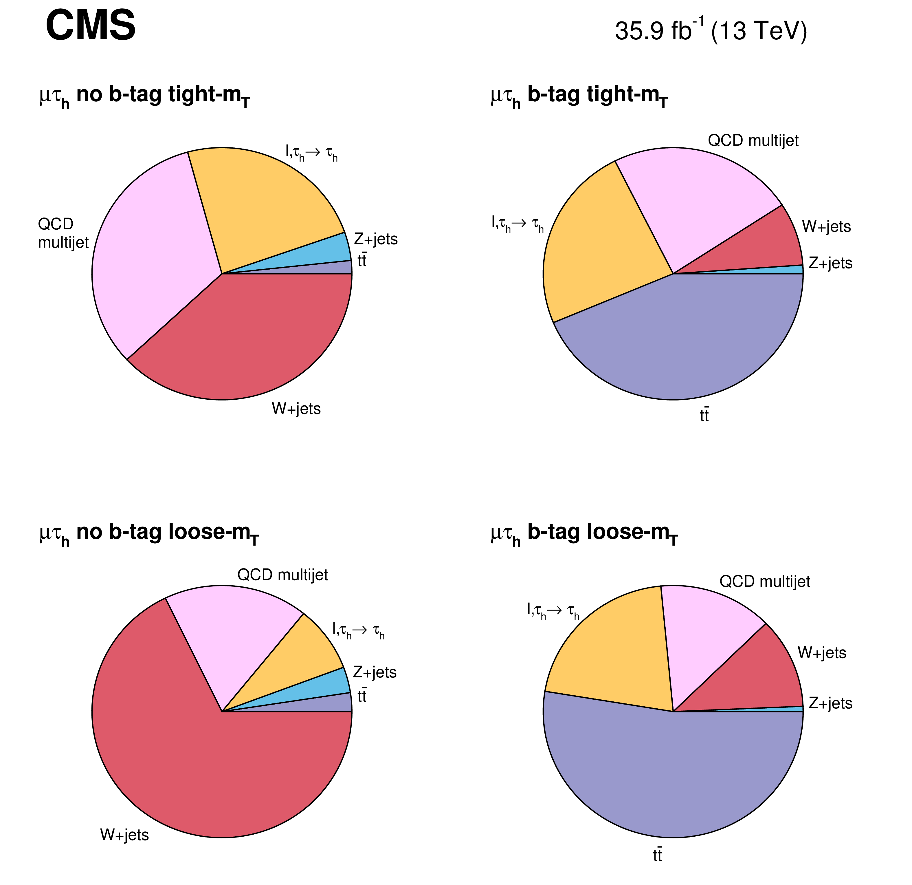
png pdf	Additional Figure 25: Composition of the data in the application region (AR) used for the fake factor method, split by processes and as expected from the simulation, in the $ {{\mu}} {\tau}_{\text {h}} $ final state.
png pdf	Additional Figure 26: Misidentification factor, $ {F_{\text {F}}}^{{{\mathrm {t}\overline {\mathrm {t}}}}}$, as obtained from simulation as a function of the transverse momentum of the misidentified jet in the 1-prong $N_{\text {jet}}\geq$ 0 category, in the $ {{\mu}} {\tau}_{\text {h}} $ final state.
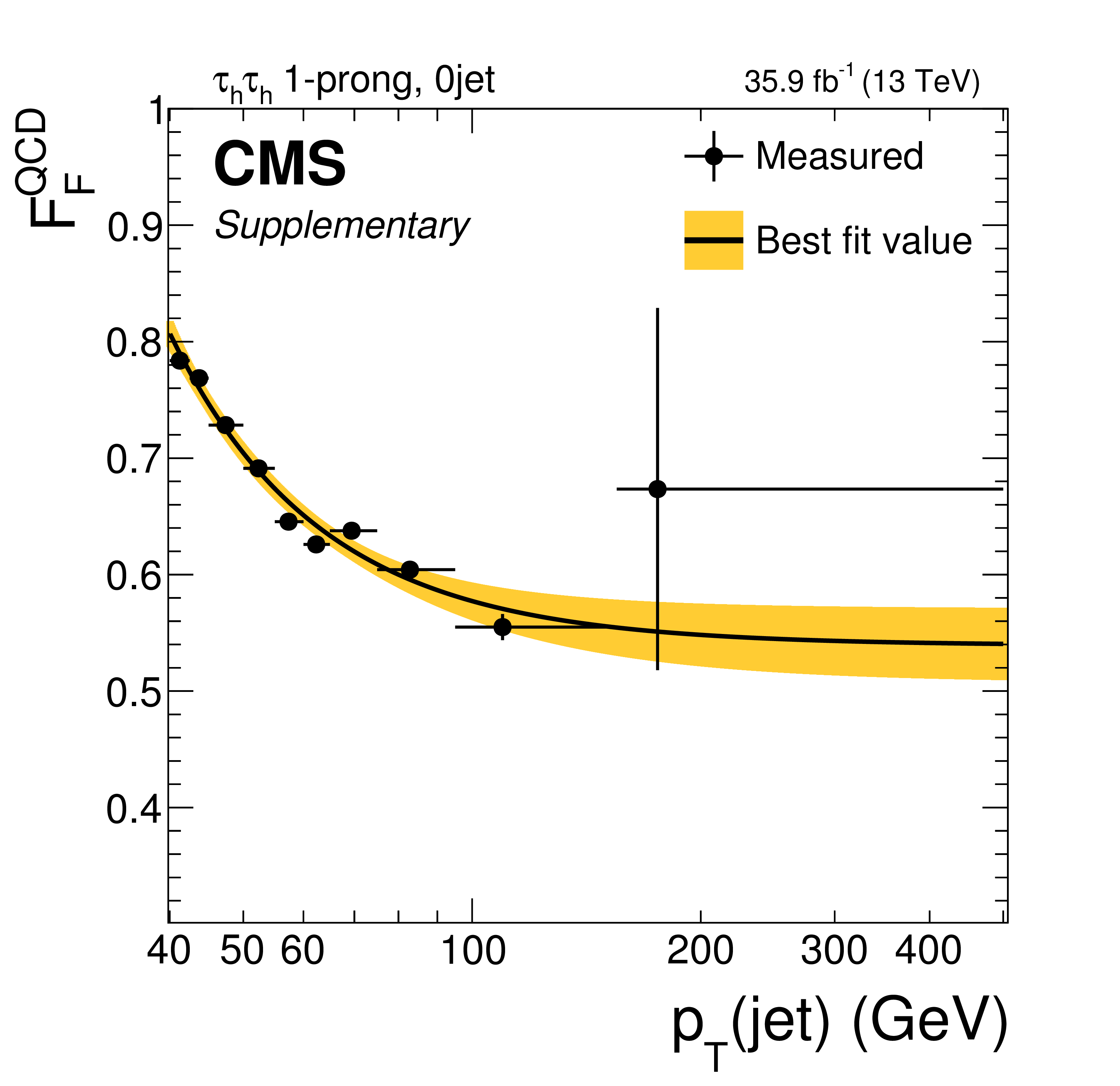
png pdf	Additional Figure 27: Misidentification factor, $ {F_{\text {F}}}^{\text {QCD}}$, as obtained from the determination region DR$_{\text {QCD}}$ as a function of the transverse momentum of the misidentified jet in the 1-prong $N_{\text {jet}}= $ 0 category, in the $ {{\mu}} {\tau}_{\text {h}} $ final state.
png pdf	Additional Figure 28: Misidentification factor, $ {F_{\text {F}}}^{{{\mathrm {W}}}{+}\text {jets}}$, as obtained from DR$_{{{\mathrm {W}}}{+}\text {jets}}$ as a function of the transverse momentum of the misidentified jet in the 1-prong $N_{\text {jet}}= $ 0 category, in the $ {{\mu}} {\tau}_{\text {h}} $ final state.
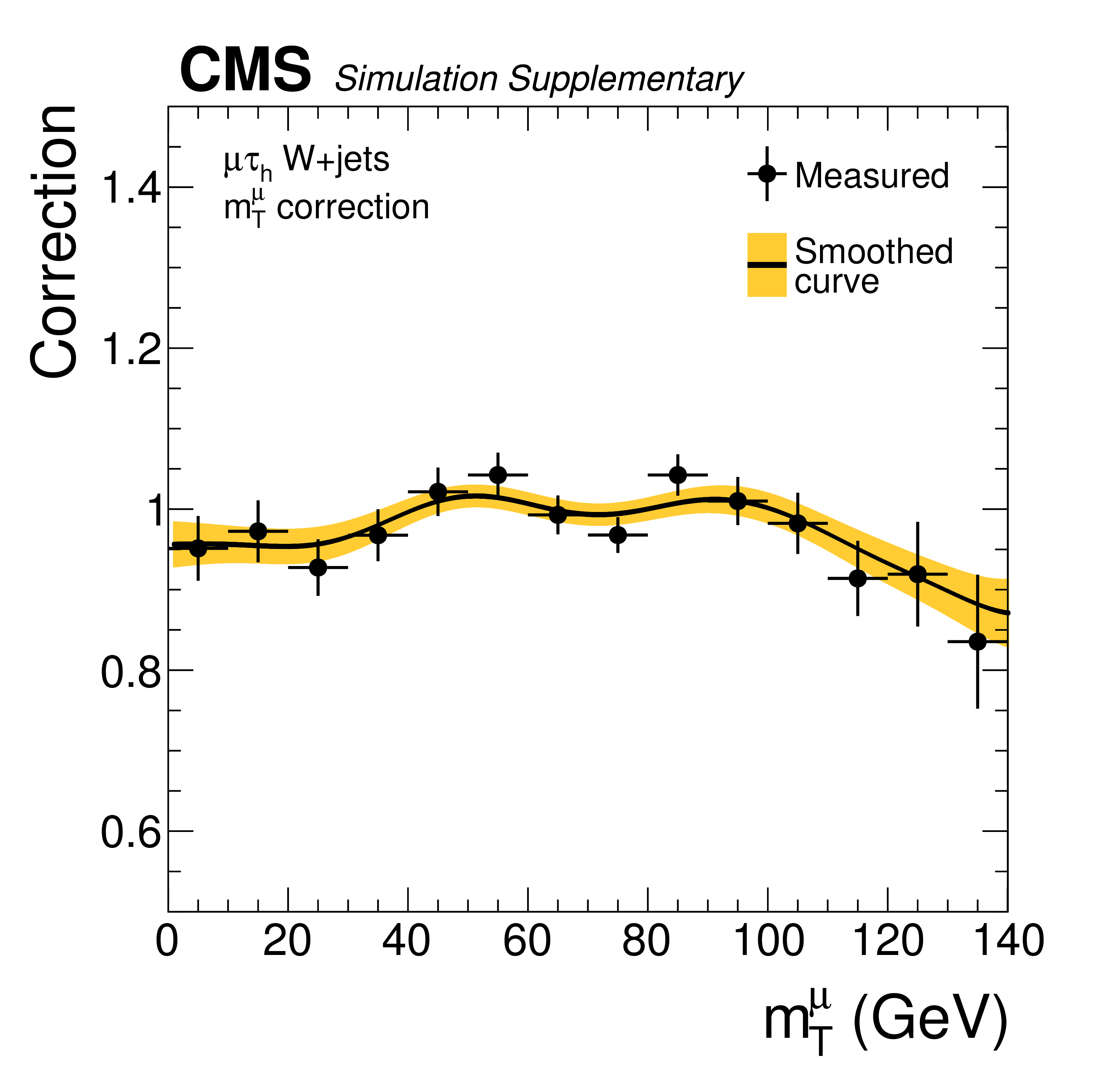
png pdf	Additional Figure 29: Correction to $ {F_{\text {F}}}^{{{\mathrm {W}}}{+}\text {jets}}$ to account for differences between the event kinematics in the application region (AR) and signal region (SR) relative to the determination region DR$_{{{\mathrm {W}}}{+}\text {jets}}$, in the $ {{\mu}} {\tau}_{\text {h}} $ final state. The correction has been obtained as a function of $m_{\text {T}}^{\mu}$ from the simulation.
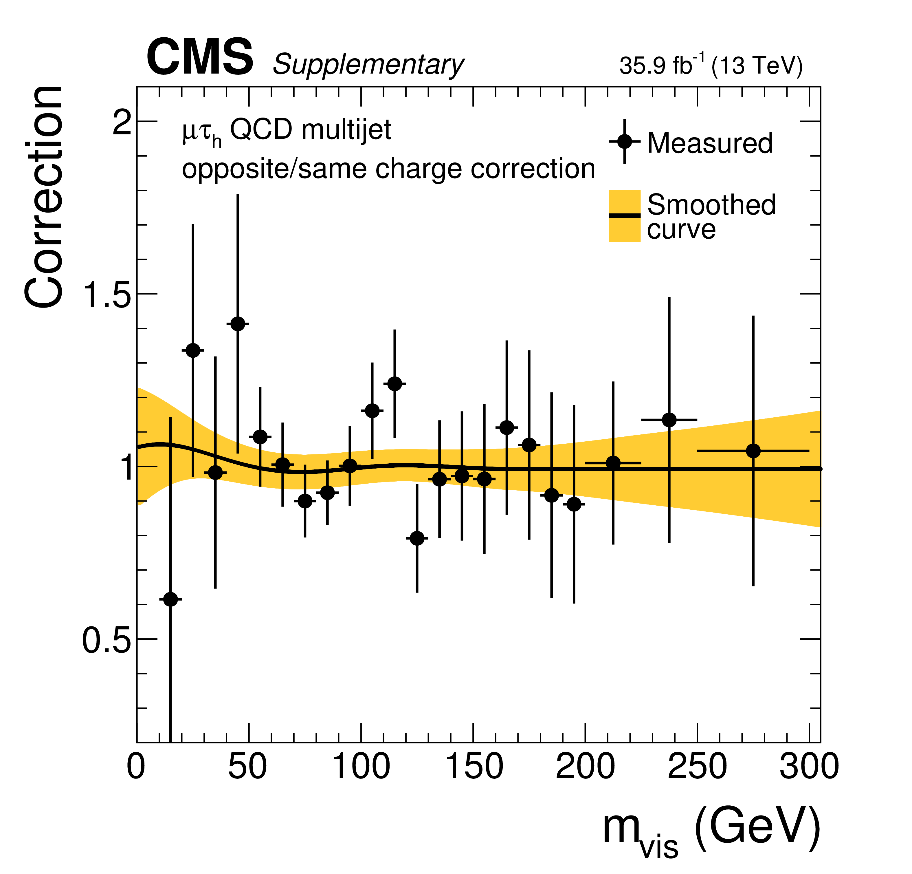
png pdf	Additional Figure 30: Correction to $ {F_{\text {F}}}^{\text {QCD}}$ to account for differences in the event selection due to the opposite charge requirement on the selected $\tau \tau $ pair in the SR with respect to the same charge requirement in DR$_{\text {QCD}}$, in the $ {{\mu}} {\tau}_{\text {h}} $ final state. This correction has been obtained as a function of the mass of the visible decay products of the $\tau \tau $ system, $m_{\text {vis}}$, from a sideband region in data, where the isolation requirement on the muon has been chosen to be orthogonal to the SR.
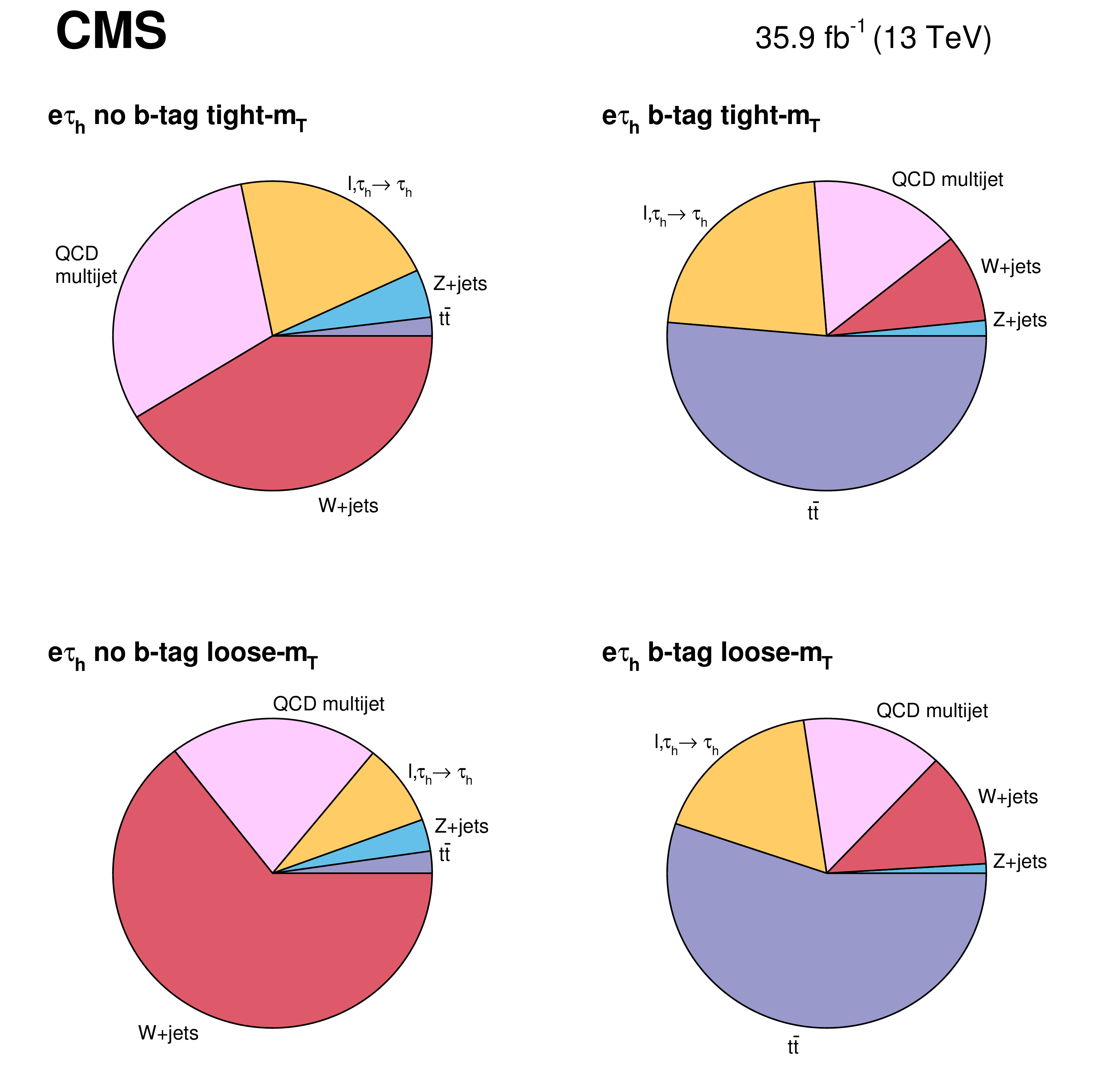
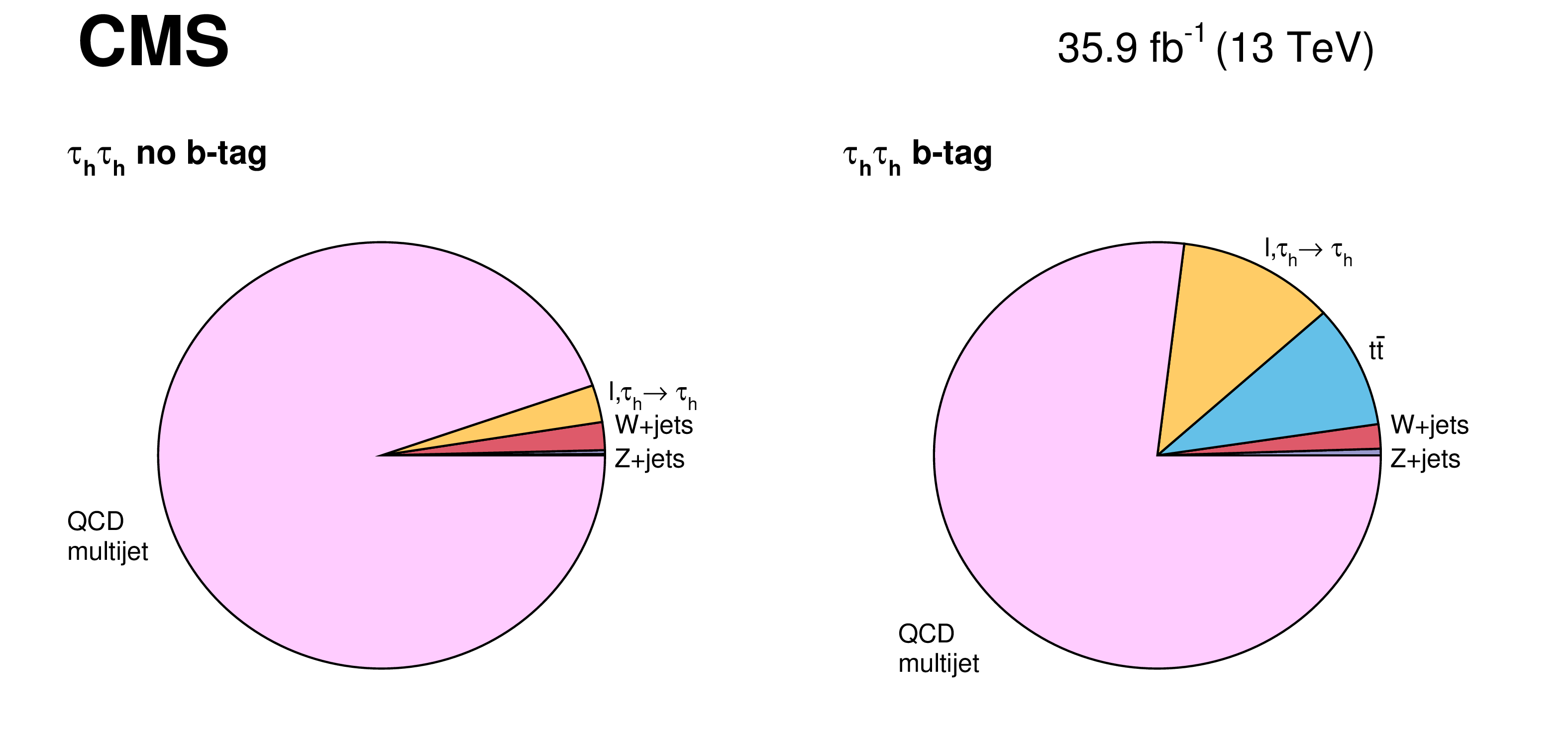
png pdf	Additional Figure 31: Composition of the data in the AR used for the fake factor method, split by processes and as expected from the simulation, in the $ {\mathrm {e}} {\tau}_{\text {h}} $ final state.
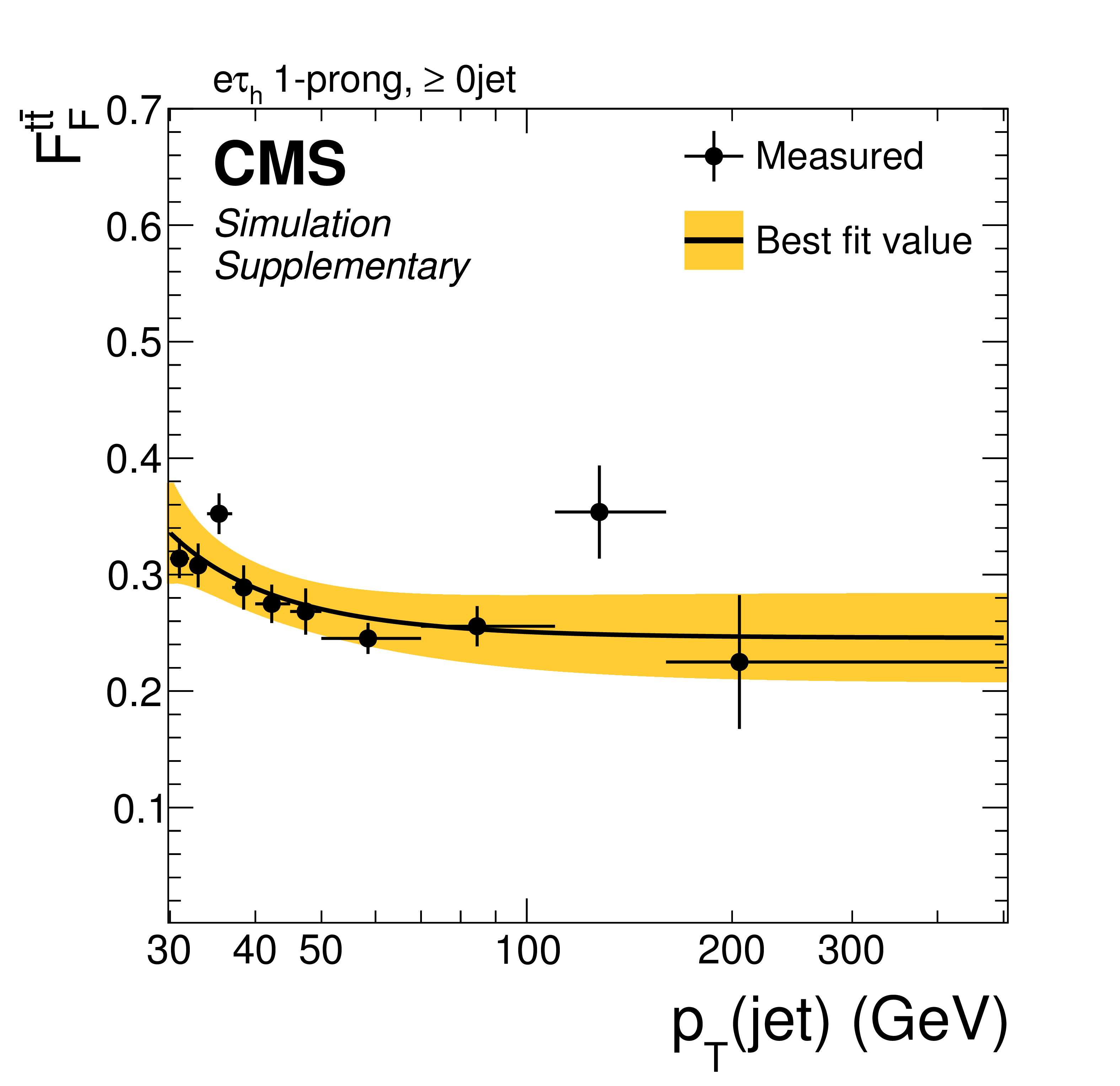
png pdf	Additional Figure 32: Misidentification factor, $ {F_{\text {F}}}^{{{\mathrm {t}\overline {\mathrm {t}}}}}$, as obtained from simulation as a function of the transverse momentum of the misidentified jet in the 1-prong $N_{\text {jet}}\geq$ 0 category, in the $ {\mathrm {e}} {\tau}_{\text {h}} $ final state.
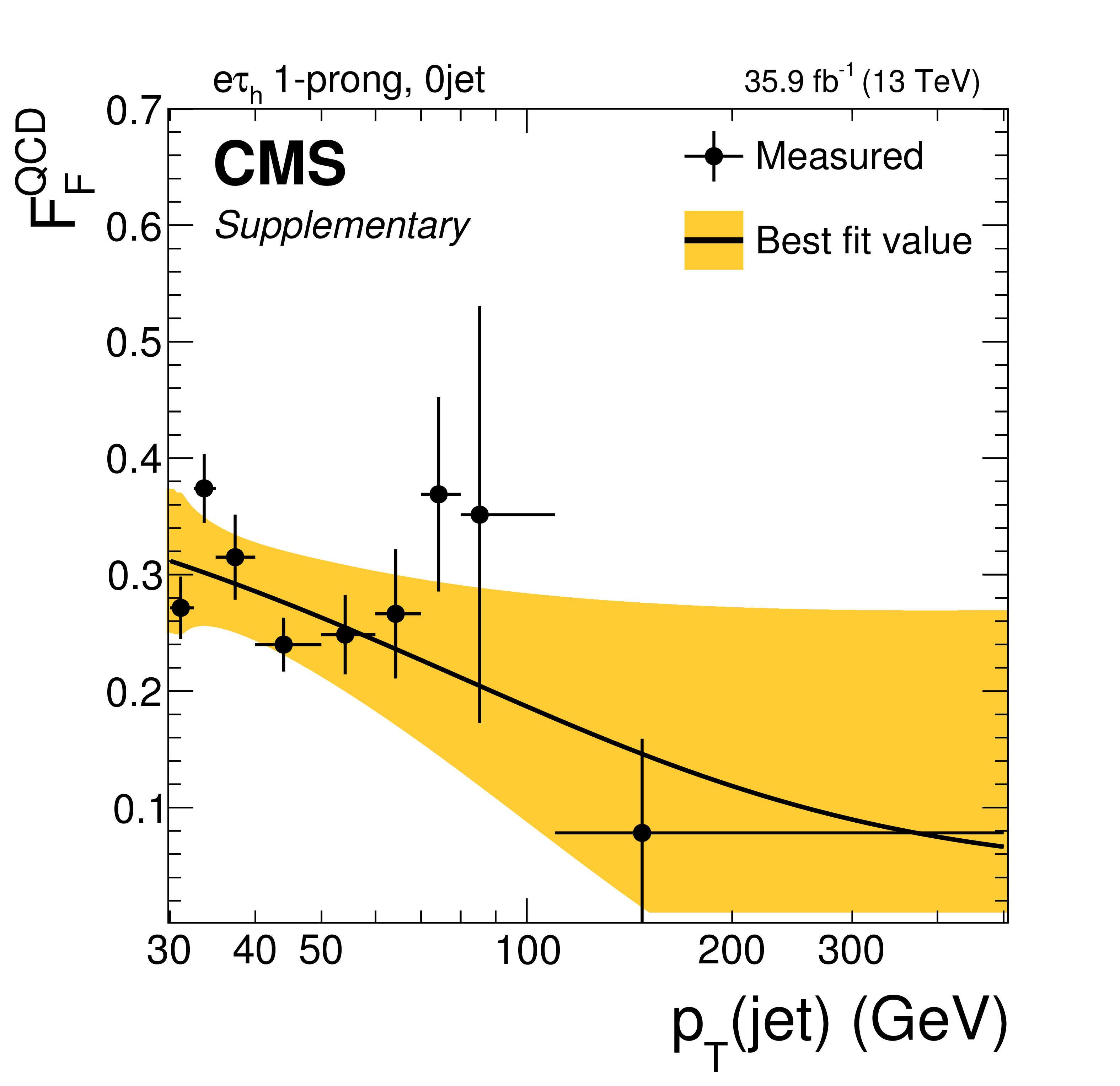
png pdf	Additional Figure 33: Misidentification factor, $ {F_{\text {F}}}^{\text {QCD}}$, as obtained from DR$_{\text {QCD}}$ as a function of the transverse momentum of the misidentified jet in the 1-prong $N_{\text {jet}}= $ 0 category, in the $ {\mathrm {e}} {\tau}_{\text {h}} $ final state.
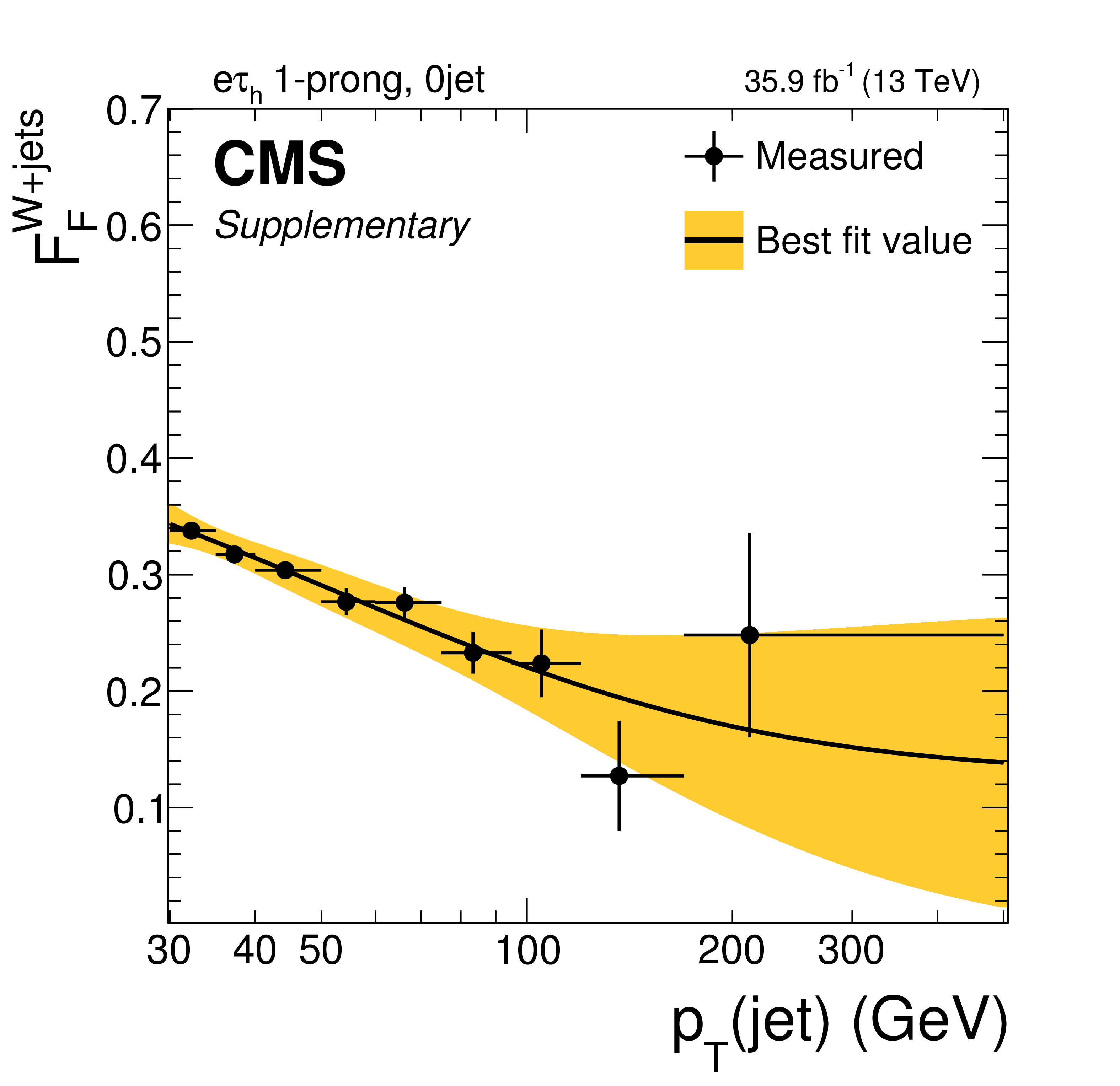
png pdf	Additional Figure 34: Misidentification factor, $ {F_{\text {F}}}^{{{\mathrm {W}}}{+}\text {jets}}$, as obtained from DR$_{{{\mathrm {W}}}{+}\text {jets}}$ as a function of the transverse momentum of the misidentified jet in the 1-prong $N_{\text {jet}}= $ 0 category, in the $ {\mathrm {e}} {\tau}_{\text {h}} $ final state.
png pdf	Additional Figure 35: Composition of the data in the AR used for the fake factor method, split by processes and as expected from the simulation, in the $ {\tau}_{\text {h}} {\tau}_{\text {h}} $ final state.
png pdf	Additional Figure 36: Misidentification factor, $ {F_{\text {F}}}^{\text {QCD}}$, as obtained from DR$_{\text {QCD}}$ as a function of the transverse momentum of the misidentified jet in the 1-prong $N_{\text {jet}}= $ 0 category in the $ {\tau}_{\text {h}} {\tau}_{\text {h}} $ final state.
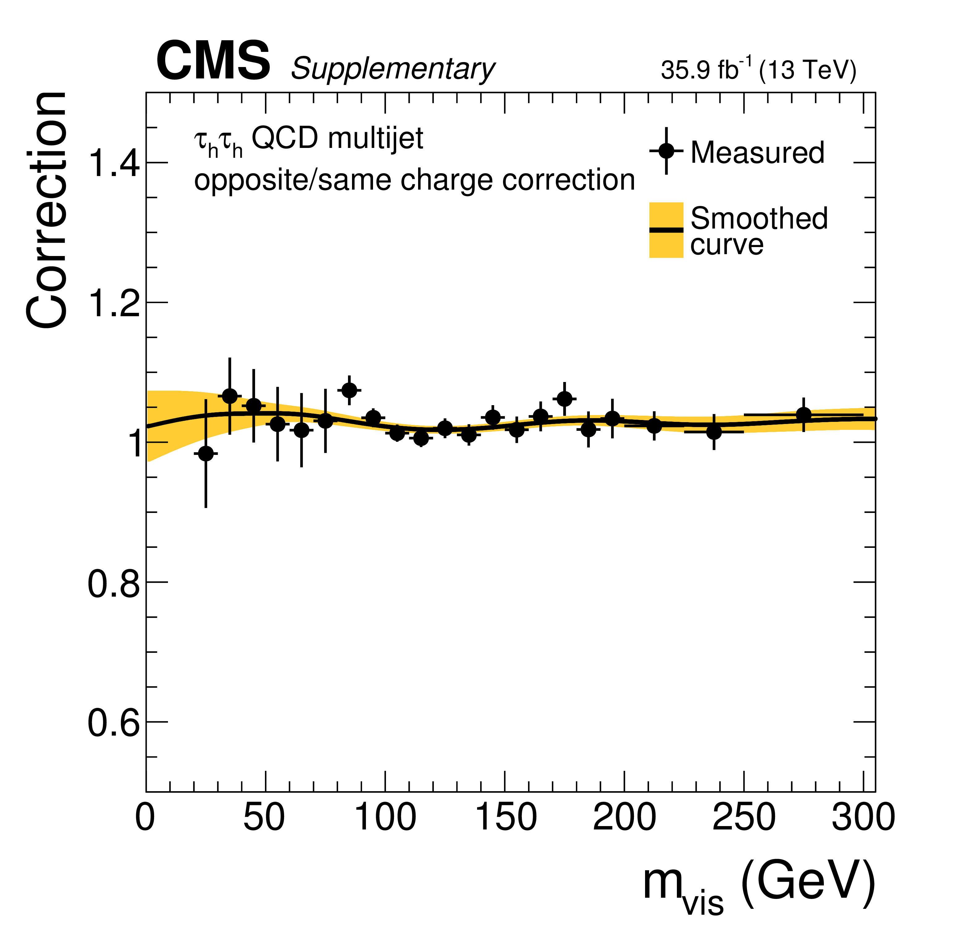
png pdf	Additional Figure 37: Correction to $ {F_{\text {F}}}^{\text {QCD}}$ to account for differences in the event selection due to the opposite charge requirement on the selected $\tau \tau $ pair in the SR with respect to the same charge requirement in DR$_{\text {QCD}}$, in the $ {\tau}_{\text {h}} {\tau}_{\text {h}} $ final state. This correction has been obtained as a function of the mass of the visible decay products of the $\tau \tau $ system, $m_{\text {vis}}$, from a sideband region in data, where the isolation requirement on the other $\tau _{h}$ candidate has been chosen to be orthogonal to the SR.
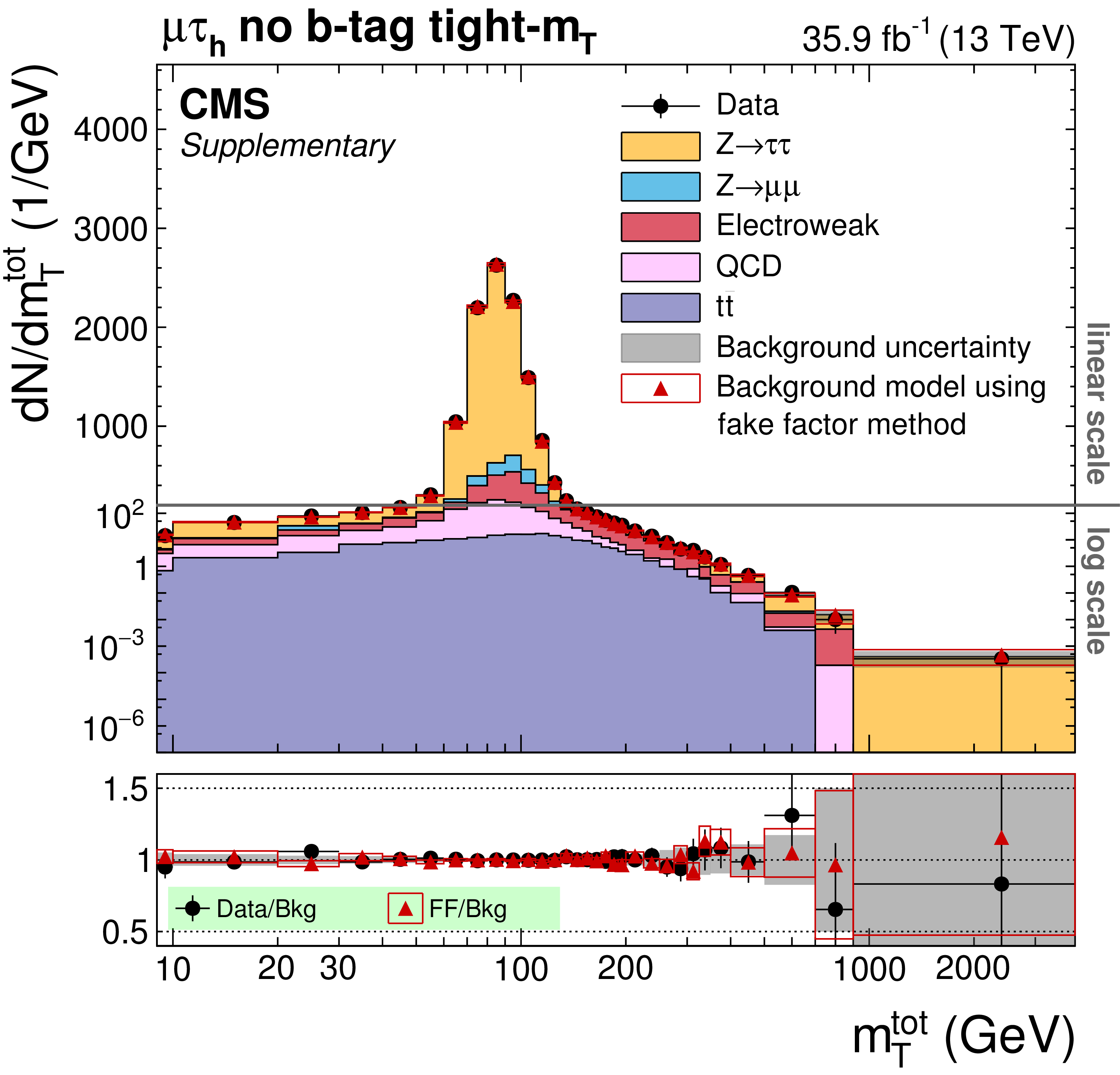
png pdf	Additional Figure 38: Distribution of $m_{\text {T}}^{\text {tot}}$ in the no b-tag tight-$m_{\text {T}}$ event category in the $ {{\mu}} {\tau}_{\text {h}} $ final state, using the simulation based cross check as described in the text. The triangles correspond to the background estimate from the fake factor method. The boxes enclosing the triangles correspond to the combined background uncertainty when using the fake factor method.
png pdf	Additional Figure 39: Distribution of $m_{\text {T}}^{\text {tot}}$ in the b-tag tight-$m_{\text {T}}$ event category in the $ {{\mu}} {\tau}_{\text {h}} $ final state, using the simulation based cross check as described in the text. The triangles correspond to the background estimate obtained from the fake factor method. The boxes enclosing the triangles correspond to the combined background uncertainty when using the fake factor method.
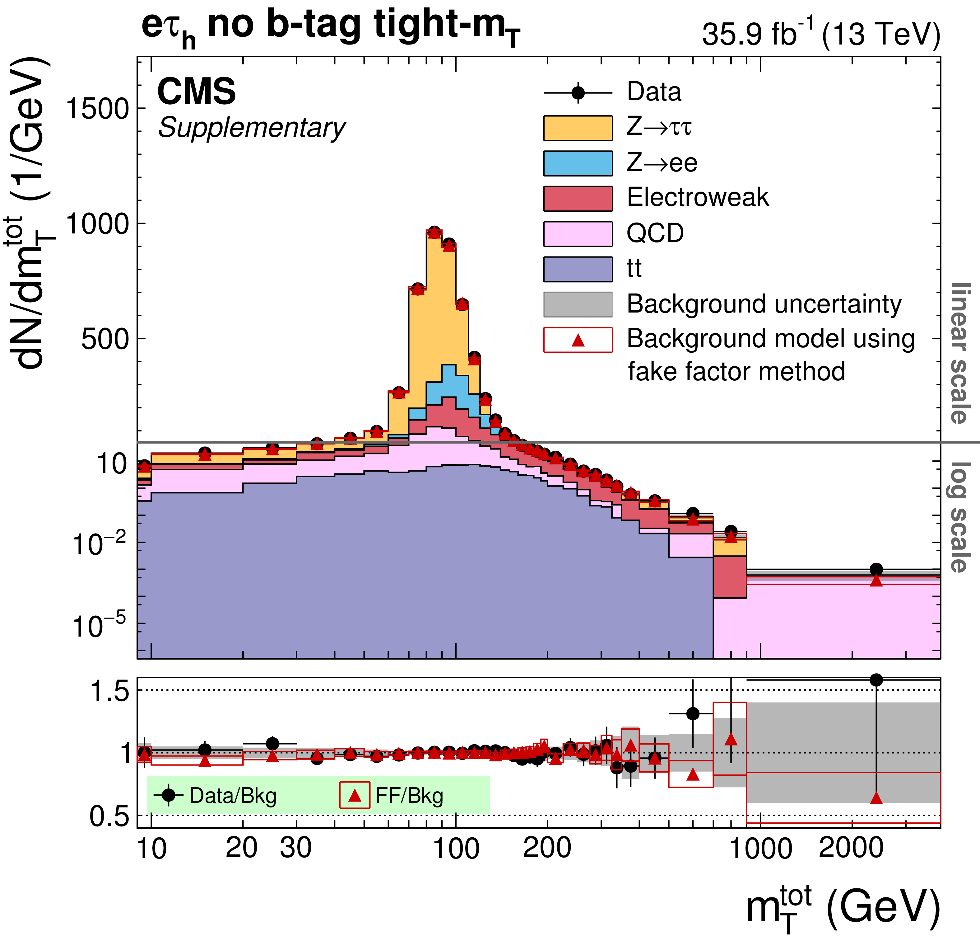
png pdf	Additional Figure 40: Distribution of $m_{\text {T}}^{\text {tot}}$ in the no b-tag tight-$m_{\text {T}}$ event category in the $ {\mathrm {e}} {\tau}_{\text {h}} $ final state, using the simulation based cross check as described in the text. The triangles correspond to the background estimate obtained from the fake factor method. The boxes enclosing the triangles correspond to the combined background uncertainty when using the fake factor method.
png pdf	Additional Figure 41: Distribution of $m_{\text {T}}^{\text {tot}}$ in the b-tag tight-$m_{\text {T}}$ event category in the $ {\mathrm {e}} {\tau}_{\text {h}} $ final state, using the simulation based cross check as described in the text. The triangles correspond to the background estimate obtained from the fake factor method. The boxes enclosing the triangles correspond to the combined background uncertainty when using the fake factor method.
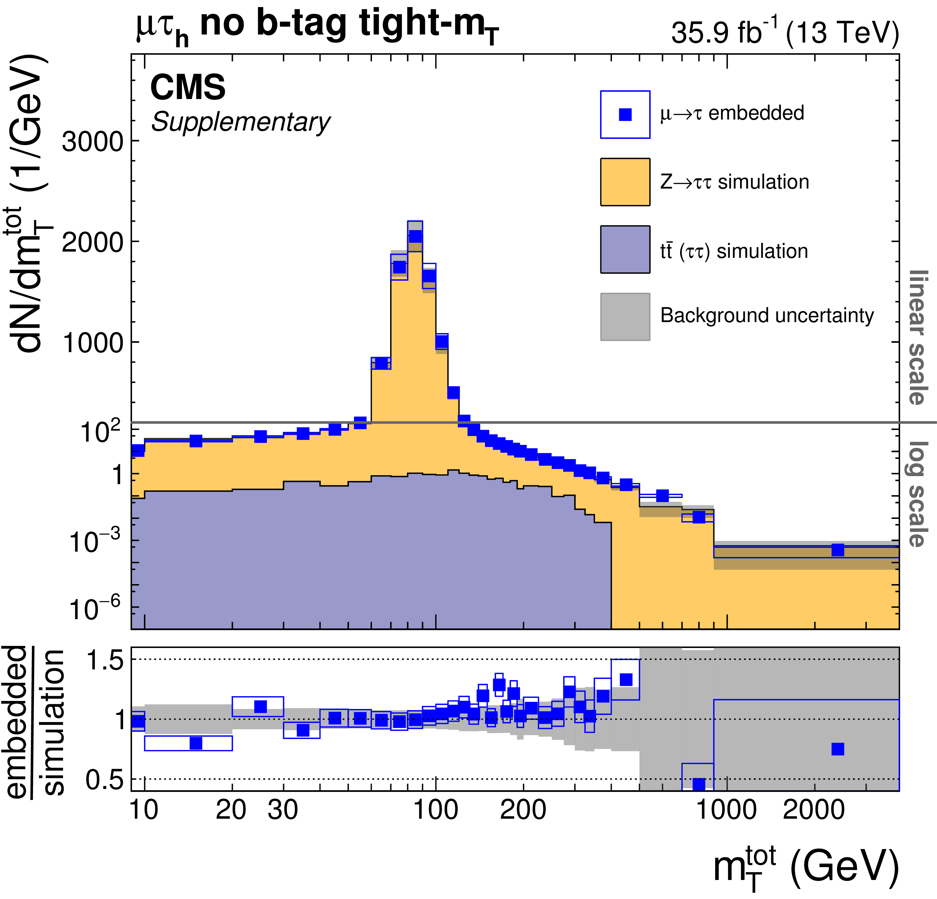
png pdf	Additional Figure 42: Distribution of $m_{\text {T}}^{\text {tot}}$ in the no b-tag tight-$m_{\text {T}}$ event category in the $ {{\mu}} {\tau}_{\text {h}} $ final state. Shown is a comparison of the estimate from data using the $\mu \to \tau $ embedding technique with the estimate of the relevant processes from simulation as used for the main analysis, before performing the fit for the statistical inference of the signal.
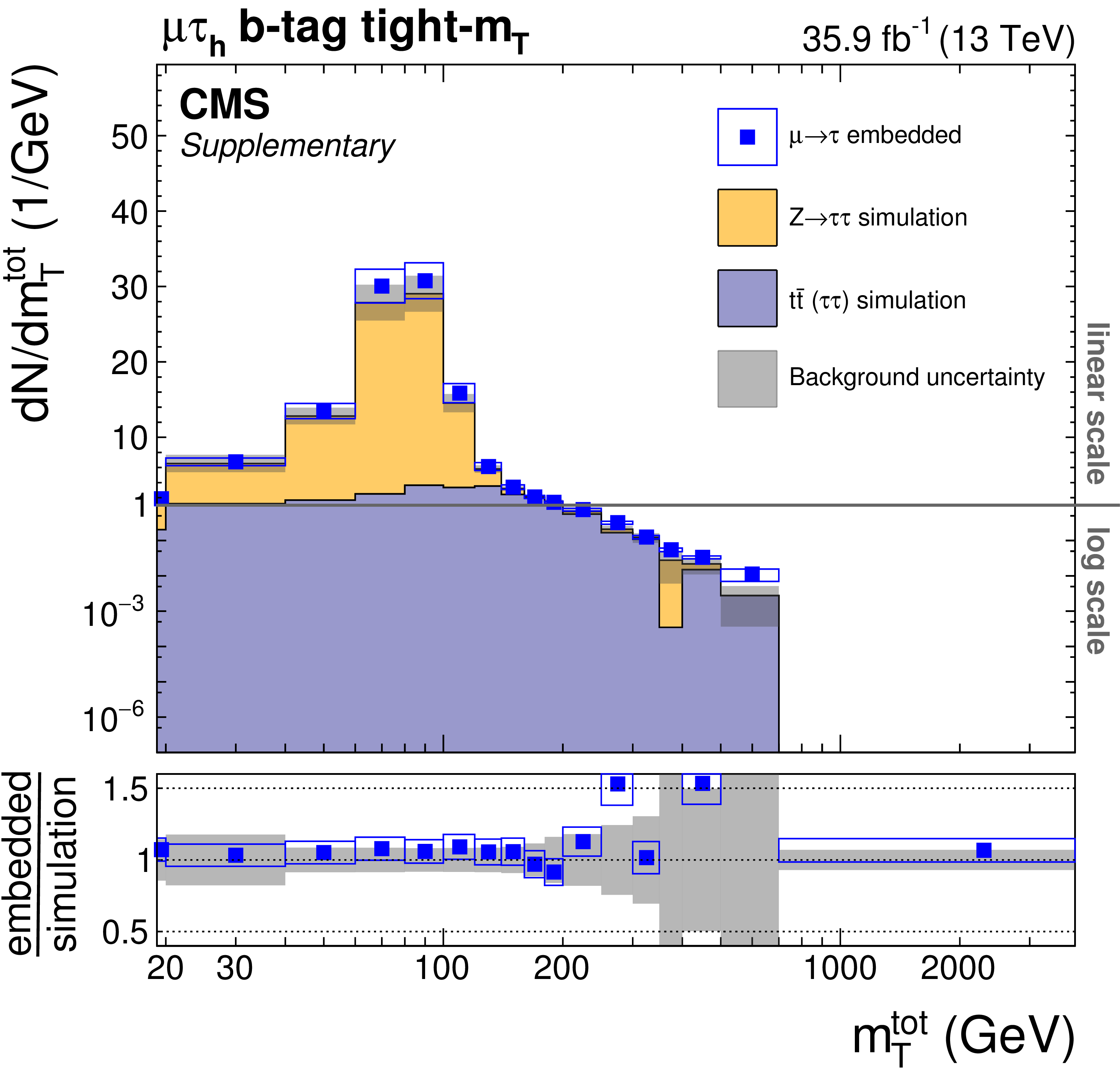
png pdf	Additional Figure 43: Distribution of $m_{\text {T}}^{\text {tot}}$ in the b-tag tight-$m_{\text {T}}$ event category in the $ {{\mu}} {\tau}_{\text {h}} $ final state. Shown is a comparison of the estimate from data using the $\mu \to \tau $ embedding technique with the estimate of the relevant processes from simulation as used for the main analysis, before performing the fit for the statistical inference of the signal.
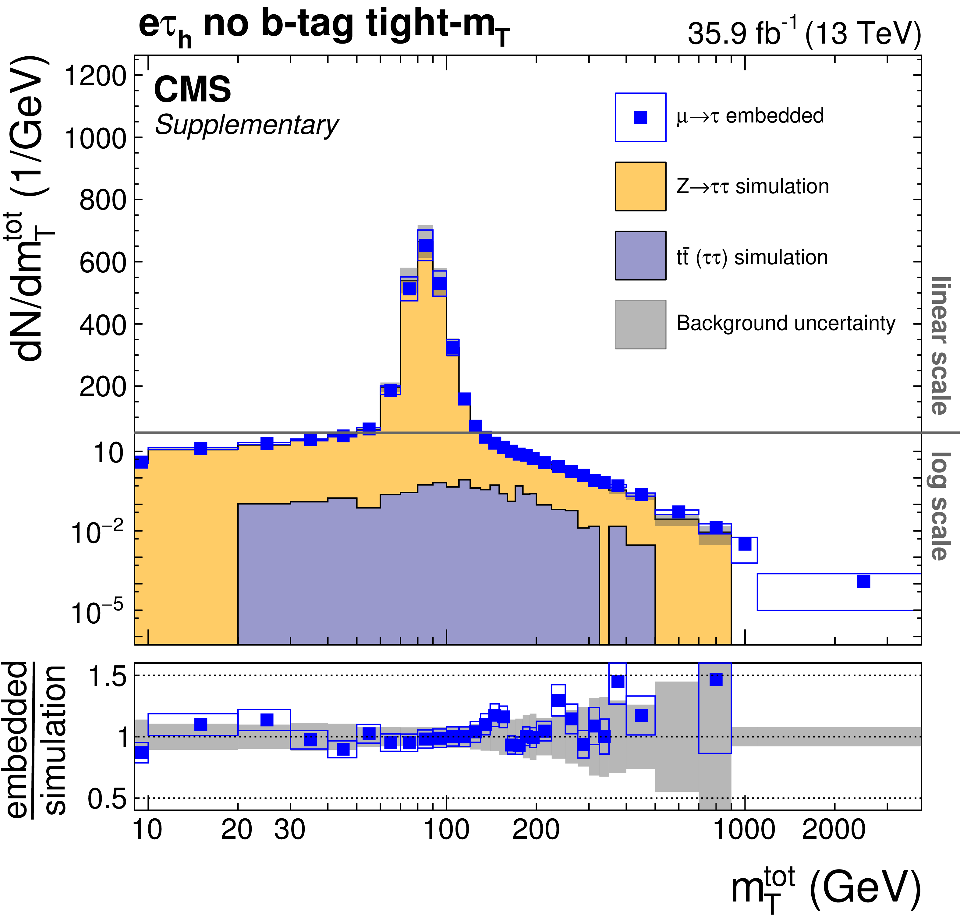
png pdf	Additional Figure 44: Distribution of $m_{\text {T}}^{\text {tot}}$ in the no b-tag tight-$m_{\text {T}}$ event category in the $ {\mathrm {e}} {\tau}_{\text {h}} $ final state. Shown is a comparison of the estimate from data using the $\mu \to \tau $ embedding technique with the estimate of the relevant processes from simulation as used for the main analysis, before performing the fit for the statistical inference of the signal.
png pdf	Additional Figure 45: Distribution of $m_{\text {T}}^{\text {tot}}$ in the b-tag tight-$m_{\text {T}}$ event category in the $ {\mathrm {e}} {\tau}_{\text {h}} $ final state. Shown is a comparison of the estimate from data using the $\mu \to \tau $ embedding technique with the estimate of the relevant processes from simulation as used for the main analysis, before performing the fit for the statistical inference of the signal.
png pdf	Additional Figure 46: Distribution of $m_{\text {T}}^{\text {tot}}$ in the no b-tag tight-$m_{\text {T}}$ event category in the $ {\tau}_{\text {h}} {\tau}_{\text {h}} $ final state. Shown is a comparison of the estimate from data using the $\mu \to \tau $ embedding technique with the estimate of the relevant processes from simulation as used for the main analysis, before performing the fit for the statistical inference of the signal.
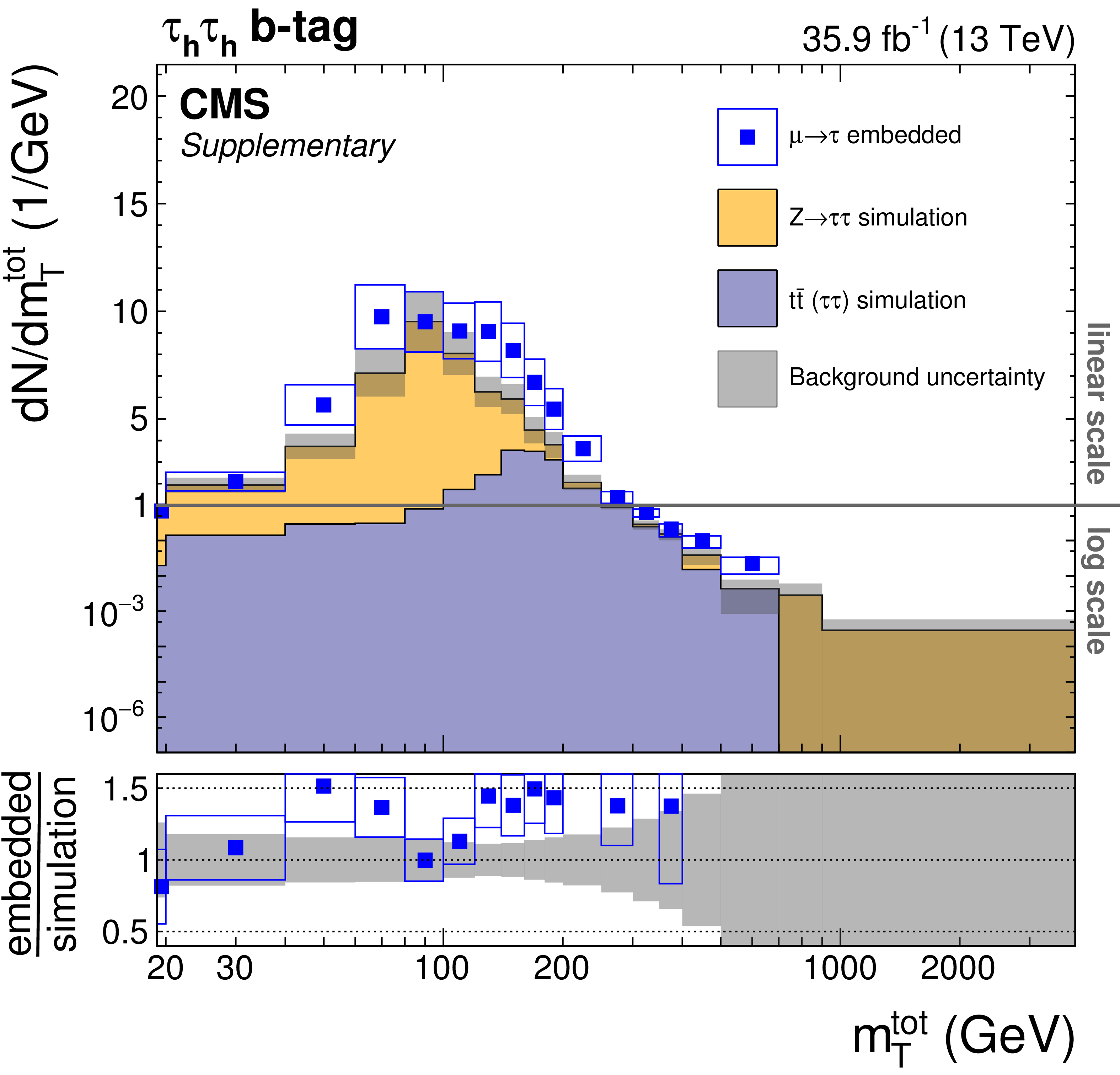
png pdf	Additional Figure 47: Distribution of $m_{\text {T}}^{\text {tot}}$ in the b-tag tight-$m_{\text {T}}$ event category in the $ {\tau}_{\text {h}} {\tau}_{\text {h}} $ final state. Shown is a comparison of the estimate from data using the $\mu \to \tau $ embedding technique with the estimate of the relevant processes from simulation as used for the main analysis, before performing the fit for the statistical inference of the signal.
png pdf	Additional Figure 48: Expected and observed 95% CL exclusion contour in the MSSM $ {M_{\text {h}}^{125}}$ scenario, as proposed in arxiv:1808.07542. The expected median is shown as a dashed black line. The dark and bright gray bands indicate the 68 and 95% confidence intervals for the variation of the expected exclusion. The observed exclusion contour is indicated by the colored blue area. For the $ {M_{\text {h}}^{125}}$ scenario, those parts of the parameter space, where $m_{{\mathrm {h}}}$ deviates by more than ${\pm}$3 GeV from the mass of the observed Higgs boson at 125 GeV are indicated by a red hatched area.
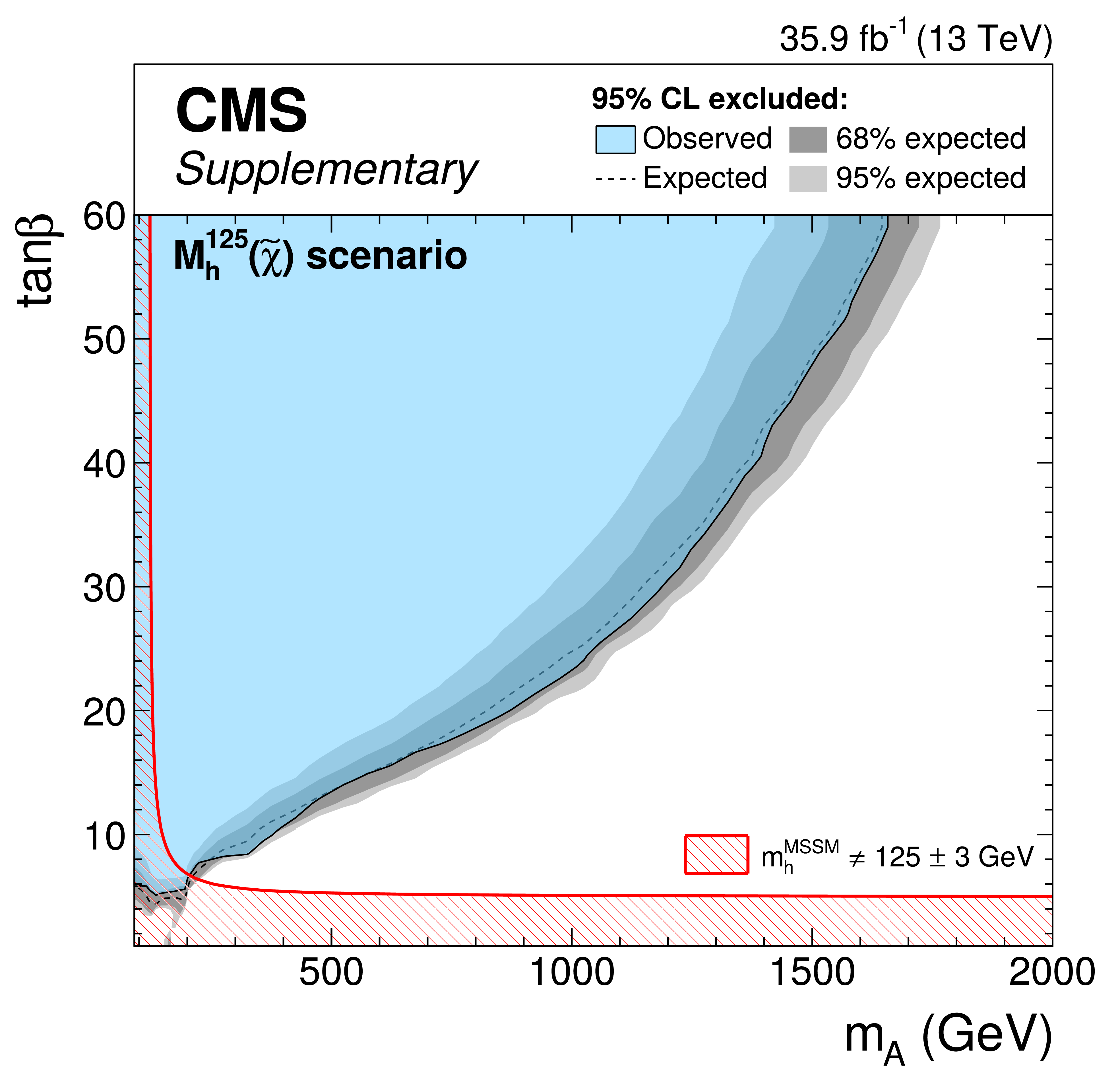
png pdf	Additional Figure 49: Expected and observed 95% CL exclusion contour in the MSSM $ {M_{\text {h}}^{125}(\tilde\chi)}$ scenario, as proposed in arxiv:1808.07542. The expected median is shown as a dashed black line. The dark and bright gray bands indicate the 68 and 95% confidence intervals for the variation of the expected exclusion. The observed exclusion contour is indicated by the colored blue area. For the $ {M_{\text {h}}^{125}(\tilde\chi)}$ scenario, those parts of the parameter space, where $m_{{\mathrm {h}}}$ deviates by more than ${\pm}$ 3 GeV from the mass of the observed Higgs boson at 125 GeV are indicated by a red hatched area.
png pdf	Additional Figure 50: Expected and observed 95% CL exclusion contour in the MSSM $ {M_{\text {h}}^{125}(\tilde\tau)}$ scenario, as proposed in arxiv:1808.07542. The expected median is shown as a dashed black line. The dark and bright gray bands indicate the 68 and 95% confidence intervals for the variation of the expected exclusion. The observed exclusion contour is indicated by the colored blue area. For the $ {M_{\text {h}}^{125}(\tilde\tau)}$ scenario, those parts of the parameter space, where $m_{{\mathrm {h}}}$ deviates by more than ${\pm}$ 3 GeV from the mass of the observed Higgs boson at 125 GeV are indicated by a red hatched area.

Additional Tables
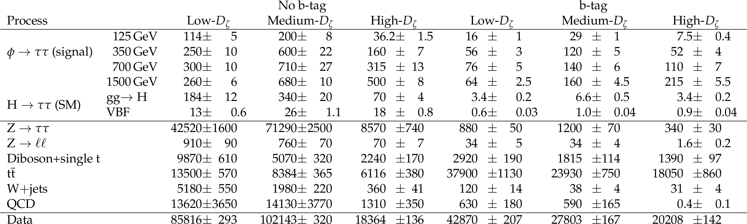
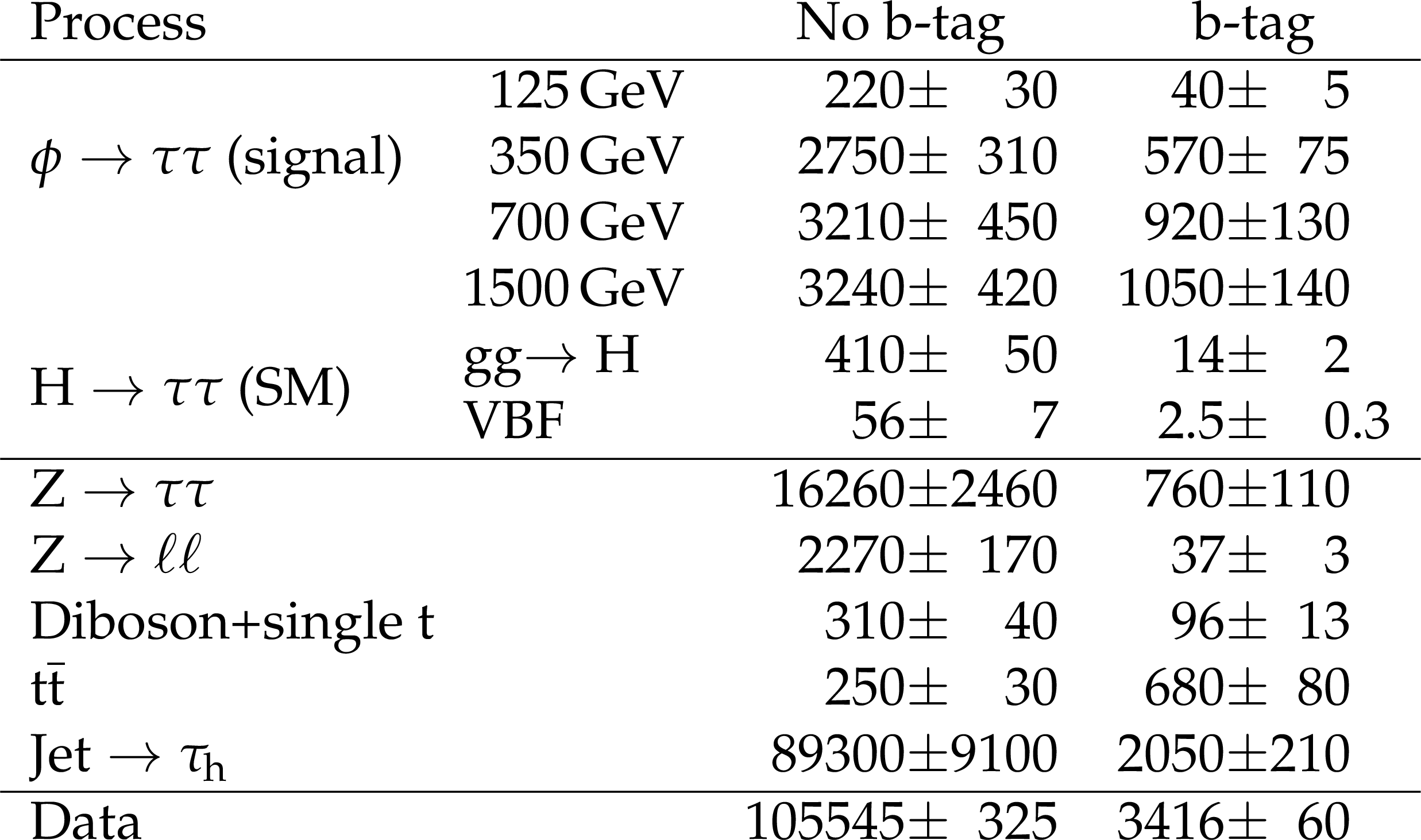
png pdf	Additional Table 1: Expected and observed number of selected events in each event category in the $ {\mathrm {e}} {{\mu}}$ final state. The expected number of events and corresponding uncertainties are shown prior to the fit used for the signal extraction, taking into account the correlations across channels and final states. Some uncertainties, as described in the text, alter the shape of the $m_{\text {T}}^{\text {tot}}$ distribution; the components of these that influence the overall normalization are taken into account. For the SM Higgs boson, the expectations from only gluon fusion and VBF are shown. The yield for the signal is given for a single narrow resonance $\phi $ with a cross section of 1 pb for each of the production via gluon fusion and in association with b quarks. For gluon fusion the contributions due to the b and t quarks are chosen as expected for the SM Higgs boson at the given mass. The yields are given for four different mass values.
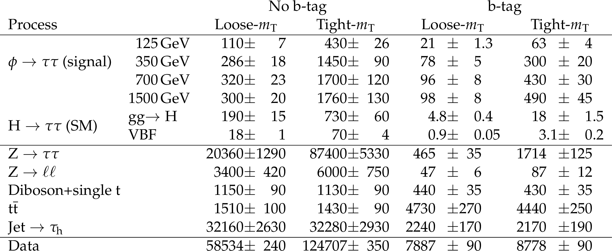
png pdf	Additional Table 2: Expected and observed number of selected events in each event category in the $ {\mathrm {e}} {\tau}_{\text {h}} $ final state. The expected number of events and corresponding uncertainties are shown prior to the fit used for the signal extraction, taking into account the correlations across channels and final states. Some uncertainties, as described in the text, alter the shape of the $m_{\text {T}}^{\text {tot}}$ distribution; the components of these that influence the overall normalization are taken into account. For the SM Higgs boson, the expectations from only gluon fusion and VBF are shown. The yield for the signal is given for a single narrow resonance $\phi $ with a cross section of 1 pb for each of the production via gluon fusion and in association with b quarks. For gluon fusion the contributions due to the b and t quarks are chosen as expected for the SM Higgs boson at the given mass. The yields are given for four different mass values.
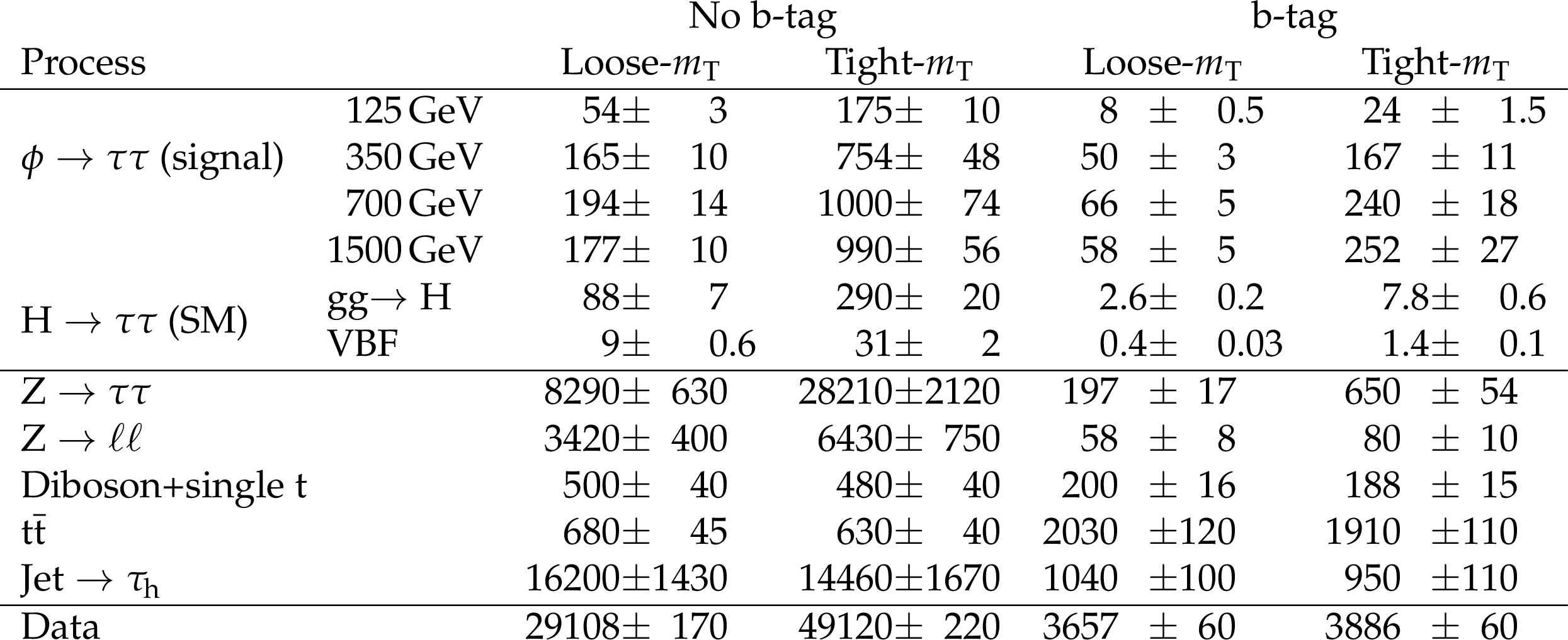
png pdf	Additional Table 3: Expected and observed number of selected events in each event category in the $ {{\mu}} {\tau}_{\text {h}} $ final state. The expected number of events and corresponding uncertainties are shown prior to the fit used for the signal extraction, taking into account the correlations across channels and final states. Some uncertainties, as described in the text, alter the shape of the $m_{\text {T}}^{\text {tot}}$ distribution; the components of these that influence the overall normalization are taken into account. For the SM Higgs boson, the expectations from only gluon fusion and VBF are shown. The yield for the signal is given for a single narrow resonance $\phi $ with a cross section of 1 pb for each of the production via gluon fusion and in association with b quarks. For gluon fusion the contributions due to the b and t quarks are chosen as expected for the SM Higgs boson at the given mass. The yields are given for four different mass values.
png pdf	Additional Table 4: Expected and observed number of selected events in each event category in the $ {\tau}_{\text {h}} {\tau}_{\text {h}} $ final state. The expected number of events and corresponding uncertainties are shown prior to the fit used for the signal extraction, taking into account the correlations across channels and final states. Some uncertainties, as described in the text, alter the shape of the $m_{\text {T}}^{\text {tot}}$ distribution; the components of these that influence the overall normalization are taken into account. For the SM Higgs boson, the expectations from only gluon fusion and VBF are shown. The yield for the signal is given for a single narrow resonance $\phi $ with a cross section of 1 pb for each of the production via gluon fusion and in association with b quarks. For gluon fusion the contributions due to the b and t quarks are chosen as expected for the SM Higgs boson at the given mass. The yields are given for four different mass values.
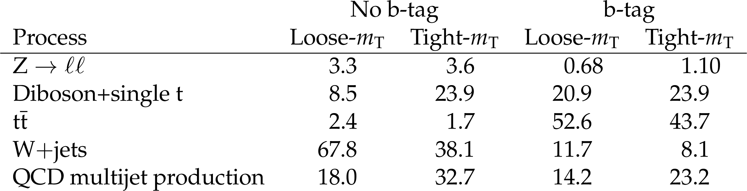
png pdf	Additional Table 5: Expected composition, from simulation, of the AR in the fake factor method in the event categories used for the analysis, split by process, in the $ {{\mu}} {\tau}_{\text {h}} $ final state. The relative contribution is given in %.
png pdf	Additional Table 6: Expected composition, from simulation, of the AR in the fake factor method in the event categories used for the analysis, split by process, in the $ {\mathrm {e}} {\tau}_{\text {h}} $ final state. The relative contribution is given in %.
png pdf	Additional Table 7: Expected composition, from simulation, of the AR in the fake factor method in the event categories used for the analysis, split by process, in the $ {\tau}_{\text {h}} {\tau}_{\text {h}} $ final state. The relative contribution is given in %.
png pdf	Additional Table 8: Expected composition of the AR for the estimate of QCD multijet events in the event categories used for the analysis, split by process, in the $ {\mathrm {e}} {{\mu}}$ final. All processes but QCD multijet production are estimated from the simulation. The relative contribution is given in %.

Database for the 2 dimensional likelihood scans

References
1	ATLAS Collaboration	Observation of a new particle in the search for the standard model Higgs boson with the ATLAS detector at the LHC	PLB 716 (2012) 1	1207.7214
2	CMS Collaboration	Observation of a new boson at a mass of 125 GeV with the CMS experiment at the LHC	PLB 716 (2012) 30	CMS-HIG-12-028 1207.7235
3	CMS Collaboration	Observation of a new boson with mass near 125 GeV in $ {\mathrm{p}}{\mathrm{p}} $ collisions at $ \sqrt{s} = $ 7 and 8 TeV	JHEP 06 (2013) 081	CMS-HIG-12-036 1303.4571
4	P. W. Higgs	Broken symmetries, massless particles and gauge fields	PL12 (1964) 132
5	P. W. Higgs	Broken symmetries and the masses of gauge bosons	PRL 13 (1964) 508
6	G. S. Guralnik, C. R. Hagen, and T. W. B. Kibble	Global conservation laws and massless particles	PRL 13 (1964) 585
7	P. W. Higgs	Spontaneous symmetry breakdown without massless bosons	PR145 (1966) 1156
8	T. W. B. Kibble	Symmetry breaking in non-abelian gauge theories	PR155 (1967) 1554
9	F. Englert and R. Brout	Broken symmetry and the mass of gauge vector mesons	PRL 13 (1964) 321
10	ATLAS and CMS Collaboration	Combined measurement of the Higgs boson mass in $ {\mathrm{p}}{\mathrm{p}} $ collisions at $ \sqrt{s}= $ 7 and 8 TeV with the ATLAS and CMS experiments	PRL 114 (2015) 191803	1503.07589
11	ATLAS and CMS Collaboration	Measurements of the Higgs boson production and decay rates and constraints on its couplings from a combined ATLAS and CMS analysis of the LHC $ {\mathrm{p}}{\mathrm{p}} $ collision data at $ \sqrt{s}= $ 7 and 8 TeV	JHEP 08 (2016) 045	1606.02266
12	Y. A. Gol'fand and E. P. Likhtman	Extension of the algebra of Poincar$ \'e $ group generators and violation of P invariance	JEPTL 13 (1971)323
13	J. Wess and B. Zumino	Supergauge transformations in four-dimensions	NPB 70 (1974) 39
14	P. Fayet	Supergauge invariant extension of the Higgs mechanism and a model for the electron and its neutrino	NPB 90 (1975) 104
15	P. Fayet	Spontaneously broken supersymmetric theories of weak, electromagnetic and strong interactions	PLB 69 (1977) 489
16	M. Carena et al.	MSSM Higgs boson searches at the LHC: Benchmark scenarios after the discovery of a Higgs-like particle	EPJC 73 (2013) 2552	1302.7033
17	ATLAS Collaboration	Search for additional heavy neutral Higgs and gauge bosons in the ditau final state produced in $ 36 fb$^{-1} of $ {\mathrm{p}}{\mathrm{p}} $ collisions at $ \sqrt{s} = $ 13 TeV with the ATLAS detector	JHEP 01 (2017) 052	1709.07242
18	CMS Collaboration	Search for neutral MSSM Higgs bosons decaying to a pair of tau leptons in pp collisions	JHEP 10 (2014) 160	CMS-HIG-13-021 1408.3316
19	DELPHI, OPAL, ALEPH, L3 and LEP Working Group for Higgs Boson Searches Collaboration	Search for neutral MSSM Higgs bosons at LEP	EPJC 47 (2006) 547	hep-ex/0602042
20	CDF Collaboration	Search for Higgs bosons predicted in Two-Higgs-Doublet models via decays to tau lepton pairs in $ 1.96 $ TeV $ {\mathrm{p}}\bar{{\mathrm{p}}} $ collisions	PRL 103 (2009) 201801	0906.1014
21	D0 Collaboration	Search for neutral Higgs bosons in the multi-b-jet topology in $ 5.2 fb$^{-1} of $ {\mathrm{p}}\bar{{\mathrm{p}}} $ collisions at $ \sqrt{s} = $ 1.96 TeV	PLB 698 (2011) 97	1011.1931
22	D0 Collaboration	Search for Higgs bosons decaying to $ \tau^{+}\tau^{-} $ pairs in $ {\mathrm{p}}\bar{{\mathrm{p}}} $ collisions at $ \sqrt{s} = $ 1.96 TeV	PLB 707 (2012) 323	1106.4555
23	CDF Collaboration	Search for Higgs bosons produced in association with b-quarks	PRD 85 (2012) 032005	1106.4782
24	CMS Collaboration	Search for a Higgs boson decaying into a b-quark pair and produced in association with b quarks in proton-proton collisions at 7 TeV	PLB 722 (2013) 207	CMS-HIG-12-033 1302.2892
25	CMS Collaboration	Search for neutral MSSM Higgs bosons decaying into a pair of bottom quarks	JHEP 11 (2015) 071	CMS-HIG-14-017 1506.08329
26	ATLAS Collaboration	Search for the neutral Higgs bosons of the minimal supersymmetric standard model in $ {\mathrm{p}}{\mathrm{p}} $ collisions at $ \sqrt{s} = $ 7 TeV with the ATLAS detector	JHEP 02 (2013) 095	1211.6956
27	CMS Collaboration	Search for neutral MSSM Higgs bosons decaying to $ \mu^{+} \mu^{-} $ in pp collisions at $ \sqrt{s} = $ 7 and 8 TeV	PLB 752 (2016) 221	CMS-HIG-13-024 1508.01437
28	ATLAS Collaboration	Search for neutral Higgs bosons of the minimal supersymmetric standard model in pp collisions at $ \sqrt{s} = $ 8 TeV with the ATLAS detector	JHEP 11 (2014) 056	1409.6064
29	ATLAS Collaboration	Search for minimal supersymmetric standard model Higgs bosons $ \mathrm{H}/\text{A} $ and for a $ \mathrm{Z}^{\prime} $ boson in the $ \tau \tau $ final state produced in $ {\mathrm{p}}{\mathrm{p}} $ collisions at $ \sqrt{s} = $ 13 TeV with the ATLAS detector	EPJC 76 (2016) 585	1608.00890
30	CMS Collaboration	Search for neutral minimal supersymmetric standard model Higgs bosons decaying to tau pairs in $ {\mathrm{p}}{\mathrm{p}} $ collisions at $ \sqrt{s} = $ 7 TeV	PRL 106 (2011) 231801	CMS-HIG-10-002 1104.1619
31	CMS Collaboration	Search for neutral Higgs bosons decaying to tau pairs in $ {\mathrm{p}}{\mathrm{p}} $ collisions at $ \sqrt{s} = $ 7 TeV	PLB 713 (2012) 68	CMS-HIG-11-029 1202.4083
32	CMS Collaboration	Description and performance of track and primary-vertex reconstruction with the CMS tracker	JINST 9 (2014) P10009	CMS-TRK-11-001 1405.6569
33	CMS Collaboration	Performance of electron reconstruction and selection with the CMS detector in proton-proton collisions at $ \sqrt{s} = $ 8 TeV	JINST 10 (2015) P06005	CMS-EGM-13-001 1502.02701
34	CMS Collaboration	Performance of CMS muon reconstruction in $ {\mathrm{p}}{\mathrm{p}} $ collision events at $ \sqrt{s} = $ 7 TeV	JINST 7 (2012) P10002	CMS-MUO-10-004 1206.4071
35	CMS Collaboration	Performance of photon reconstruction and identification with the CMS detector in proton-proton collisions at $ \sqrt{s} = $ 8 TeV	JINST 10 (2015) P08010	CMS-EGM-14-001 1502.02702
36	CMS Collaboration	The CMS trigger system	JINST 12 (2017) P01020	CMS-TRG-12-001 1609.02366
37	CMS Collaboration	The CMS experiment at the CERN LHC	JINST 3 (2008) S08004	CMS-00-001
38	CMS Collaboration	Particle-flow reconstruction and global event description with the CMS detector	JINST 12 (2017) P10003	CMS-PRF-14-001 1706.04965
39	K. Rose	Deterministic annealing for clustering, compression, classification, regression, and related optimization problems	Proceedings of the IEEE 86 (1998) 2210
40	M. Cacciari, G. P. Salam, and G. Soyez	The anti-$ {k_{\mathrm{T}}} $ jet clustering algorithm	JHEP 04 (2008) 063	0802.1189
41	M. Cacciari, G. P. Salam, and G. Soyez	FastJet user manual	EPJC 72 (2012) 1896	1111.6097
42	CMS Collaboration	Identification of heavy-flavour jets with the CMS detector in pp collisions at 13 TeV	Submitted to \it JINST	CMS-BTV-16-002 1712.07158
43	CMS Collaboration	Reconstruction and identification of $ \tau lepton $ decays to hadrons and $ \mathrm{g}n_\tau $ at CMS	JINST 11 (2016) P01019	CMS-TAU-14-001 1510.07488
44	CMS Collaboration	Performance of reconstruction and identification of $ \tau $ leptons in their decays to hadrons and $ \nu_{\tau} $ in LHC Run-2	CMS-PAS-TAU-16-002	CMS-PAS-TAU-16-002
45	CDF Collaboration	Search for neutral Higgs bosons of the minimal supersymmetric standard model decaying to $ \tau $ pairs in $ {\mathrm{p}}\bar{{\mathrm{p}}} $ collisions at $ \sqrt{s} = $ 1.96 TeV	PRL 96 (2006) 011802	hep-ex/0508051
46	J. Alwall et al.	MadGraph 5: going beyond	JHEP 06 (2011) 128	1106.0522
47	J. Alwall et al.	The automated computation of tree-level and next-to-leading order differential cross sections, and their matching to parton shower simulations	JHEP 07 (2014) 079	1405.0301
48	P. Nason	A new method for combining NLO QCD with shower Monte Carlo algorithms	JHEP 11 (2004) 040	hep-ph/0409146
49	S. Frixione, P. Nason, and C. Oleari	Matching NLO QCD computations with parton shower simulations: the POWHEG method	JHEP 11 (2007) 070	0709.2092
50	S. Alioli, P. Nason, C. Oleari, and E. Re	NLO Higgs boson production via gluon fusion matched with shower in POWHEG	JHEP 04 (2009) 002	0812.0578
51	S. Alioli, P. Nason, C. Oleari, and E. Re	A general framework for implementing NLO calculations in shower Monte Carlo programs: the POWHEG BOX	JHEP 06 (2010) 043	1002.2581
52	S. Alioli et al.	Jet pair production in POWHEG	JHEP 04 (2011) 081	1012.3380
53	E. Bagnaschi, G. Degrassi, P. Slavich, and A. Vicini	Higgs production via gluon fusion in the POWHEG approach in the SM and in the MSSM	JHEP 02 (2012) 088	1111.2854
54	K. Melnikov and F. Petriello	Electroweak gauge boson production at hadron colliders through $ \mathcal{O}(\alpha_{s}^{2}) $	PRD 74 (2006) 114017	hep-ph/0609070
55	M. Czakon and A. Mitov	Top++: A program for the calculation of the top-pair cross-section at hadron colliders	CPC 185 (2014) 2930	1112.5675
56	N. Kidonakis	Top quark production	in Proceedings, Helmholtz International Summer School on Physics of Heavy Quarks and Hadrons (HQ 2013), p. 139 JINR, Dubna, Russia, July	1311.0283
57	J. M. Campbell, R. K. Ellis, and C. Williams	Vector boson pair production at the LHC	JHEP 07 (2011) 018	1105.0020
58	T. Sjostrand et al.	An introduction to PYTHIA 8.2	CPC 191 (2015) 159	1410.3012
59	E. Bagnaschi et al.	Resummation ambiguities in the Higgs transverse-momentum spectrum in the standard model and beyond	JHEP 01 (2016) 090	1510.08850
60	E. Bagnaschi and A. Vicini	The Higgs transverse momentum distribution in gluon fusion as a multiscale problem	JHEP 01 (2016) 056	1505.00735
61	R. V. Harlander, H. Mantler, and M. Wiesemann	Transverse momentum resummation for Higgs production via gluon fusion in the MSSM	JHEP 11 (2014) 116	1409.0531
62	NNPDF Collaboration	Parton distributions for the LHC run II	JHEP 04 (2015) 040	1410.8849
63	CMS Collaboration	Event generator tunes obtained from underlying event and multiparton scattering measurements	EPJC 76 (2016) 155	CMS-GEN-14-001 1512.00815
64	GEANT4 Collaboration	GEANT4---a simulation toolkit	NIMA 506 (2003) 250
65	CMS Collaboration	Measurement of the $ \mathrm{Z}\gamma^{*}\to\tau\tau $ cross section in $ {\mathrm{p}}{\mathrm{p}} $ collisions at $ \sqrt{s} = $ 13 TeV and validation of $ \tau $ lepton analysis techniques	Submitted to \it EPJC	CMS-HIG-15-007 1801.03535
66	CMS Collaboration	Measurements of inclusive $ \mathrm{W} $ and $ \mathrm{Z} $ cross sections in $ {\mathrm{p}}{\mathrm{p}} $ collisions at $ \sqrt{s} = $ 7 TeV	JHEP 01 (2011) 080	CMS-EWK-10-002 1012.2466
67	CMS Collaboration	Measurement of the differential cross section for top quark pair production in $ {\mathrm{p}}{\mathrm{p}} $ collisions at $ \sqrt{s} = $ 8 TeV	EPJC 75 (2015) 542	CMS-TOP-12-028 1505.04480
68	CMS Collaboration	Evidence for the 125 GeV Higgs boson decaying to a pair of $ \tau $ leptons	JHEP 05 (2014) 104	CMS-HIG-13-004 1401.5041
69	ATLAS Collaboration	Modelling $ \mathrm{Z}\rightarrow\tau\tau $ processes in ATLAS with $ \tau $-embedded $ \mathrm{Z}\rightarrow\mu\mu $ data	JINST 10 (2015) P09018	1506.05623
70	A. L. Read	Linear interpolation of histograms	NIMA 425 (1999) 357
71	CMS Collaboration	CMS luminosity measurements for the 2016 data taking period	CMS-PAS-LUM-17-001	CMS-PAS-LUM-17-001
72	CMS Collaboration	Cross section measurement of t-channel single top quark production in $ {\mathrm{p}}{\mathrm{p}} $ collisions at $ \sqrt{s} = $ 13 TeV	PLB 772 (2017) 752	CMS-TOP-16-003 1610.00678
73	CMS Collaboration	Measurement of the $ \mathrm{W}\mathrm{Z} $ production cross section in $ {\mathrm{p}}{\mathrm{p}} $ collisions at $ \sqrt{s} = $ 13 TeV	PLB 766 (2017) 268	CMS-SMP-16-002 1607.06943
74	D. de Florian et al.	Handbook of LHC Higgs cross sections: 4. deciphering the nature of the Higgs sector	CERN-2017-002-M	1610.07922
75	A. D. Martin, W. J. Stirling, R. S. Thorne, and G. Watt	Parton distributions for the LHC	EPJC 63 (2009) 189	0901.0002
76	A. D. Martin, W. J. Stirling, R. S. Thorne, and G. Watt	Uncertainties on $ \alpha_{s} $ in global PDF analyses and implications for predicted hadronic cross sections	EPJC 64 (2009) 653	0905.3531
77	T. Junk	Confidence level computation for combining searches with small statistics	NIMA 434 (1999) 435	hep-ex/9902006
78	A. L. Read	Presentation of search results: The CL$ _{\text{s}} $ technique	JPG 28 (2002) 2693
79	ATLAS and CMS Collaborations	Procedure for the LHC Higgs boson search combination in summer 2011	ATL-PHYS-PUB 2011-11, CMS NOTE 2011/005, CERN
80	CMS Collaboration	Combined results of searches for the standard model Higgs boson in $ {\mathrm{p}}{\mathrm{p}} $ collisions at $ \sqrt{s} = $ 7 TeV	PLB 710 (2012) 26	CMS-HIG-11-032 1202.1488
81	G. Cowan, K. Cranmer, E. Gross, and O. Vitells	Asymptotic formulae for likelihood-based tests of new physics	EPJC 71 (2011) 1554	1007.1727
82	L. Maiani, A. D. Polosa, and V. Riquer	Bounds to the Higgs sector masses in minimal supersymmetry from LHC data	PLB 724 (2013) 274	1305.2172
83	A. Djouadi et al.	The post-Higgs MSSM scenario: Habemus MSSM?	EPJC 73 (2013) 2650	1307.5205
84	A. Djouadi et al.	Fully covering the MSSM Higgs sector at the LHC	JHEP 06 (2015) 168	1502.05653
85	G. Degrassi et al.	Towards high-precision predictions for the MSSM Higgs sector	EPJC 28 (2003) 133	hep-ph/0212020
86	B. C. Allanach et al.	Precise determination of the neutral Higgs boson masses in the MSSM	JHEP 09 (2004) 044	hep-ph/0406166
87	S. Heinemeyer et al.	Handbook of LHC Higgs cross sections: 3. Higgs properties	CERN-2013-004	1307.1347
88	R. V. Harlander, S. Liebler, and H. Mantler	SusHi: A program for the calculation of Higgs production in gluon fusion and bottom-quark annihilation in the standard model and the MSSM	CPC 184 (2013) 1605	1212.3249
89	M. Spira, A. Djouadi, D. Graudenz, and P. M. Zerwas	Higgs boson production at the LHC	NPB 453 (1995) 17	hep-ph/9504378
90	R. V. Harlander and M. Steinhauser	Supersymmetric Higgs production in gluon fusion at next-to-leading order	JHEP 09 (2004) 066	hep-ph/0409010
91	R. Harlander and P. Kant	Higgs production and decay: analytic results at next-to-leading order QCD	JHEP 12 (2005) 015	hep-ph/0509189
92	G. Degrassi and P. Slavich	NLO QCD bottom corrections to Higgs boson production in the MSSM	JHEP 11 (2010) 044	1007.3465
93	G. Degrassi, S. Di Vita, and P. Slavich	NLO QCD corrections to pseudoscalar Higgs production in the MSSM	JHEP 08 (2011) 128	1107.0914
94	G. Degrassi, S. Di Vita, and P. Slavich	On the NLO QCD corrections to the production of the heaviest neutral Higgs scalar in the MSSM	EPJC 72 (2012) 2032	1204.1016
95	R. V. Harlander and W. B. Kilgore	Next-to-next-to-leading order Higgs production at hadron colliders	PRL 88 (2002) 201801	hep-ph/0201206
96	C. Anastasiou and K. Melnikov	Higgs boson production at hadron colliders in NNLO QCD	NPB 646 (2002) 220	hep-ph/0207004
97	V. Ravindran, J. Smith, and W. L. van Neerven	NNLO corrections to the total cross-section for Higgs boson production in hadron-hadron collisions	NPB 665 (2003) 325	hep-ph/0302135
98	R. V. Harlander and W. B. Kilgore	Production of a pseudo-scalar Higgs boson at hadron colliders at next-to-next-to leading order	JHEP 10 (2002) 017	hep-ph/0208096
99	C. Anastasiou and K. Melnikov	Pseudoscalar Higgs boson production at hadron colliders in next-to-next-to-leading order QCD	PRD 67 (2003) 037501	hep-ph/0208115
100	U. Aglietti, R. Bonciani, G. Degrassi, and A. Vicini	Two-loop light fermion contribution to Higgs production and decays	PLB 595 (2004) 432	hep-ph/0404071
101	R. Bonciani, G. Degrassi, and A. Vicini	On the generalized harmonic polylogarithms of one complex variable	CPC 182 (2011) 1253	1007.1891
102	S. Dittmaier, M. Kramer, and M. Spira	Higgs radiation off bottom quarks at the Fermilab Tevatron and the CERN LHC	PRD 70 (2004) 074010	hep-ph/0309204
103	S. Dawson, C. B. Jackson, L. Reina, and D. Wackeroth	Exclusive Higgs boson production with bottom quarks at hadron colliders	PRD 69 (2004) 074027	hep-ph/0311067
104	R. V. Harlander and W. B. Kilgore	Higgs boson production in bottom quark fusion at next-to-next-to-leading order	PRD 68 (2003) 013001	hep-ph/0304035
105	R. Harlander, M. Kramer, and M. Schumacher	Bottom-quark associated Higgs-boson production: Reconciling the four- and five-flavour scheme approach	CERN-PH-TH-2011-134, FR-PHENO-2011-009, TTK-11-17, WUB-11-04	1112.3478
106	S. Heinemeyer, W. Hollik, and G. Weiglein	FeynHiggs: A program for the calculation of the masses of the neutral CP-even Higgs bosons in the MSSM	CPC 124 (2000) 76	hep-ph/9812320
107	S. Heinemeyer, W. Hollik, and G. Weiglein	The masses of the neutral CP-even Higgs bosons in the MSSM: Accurate analysis at the two-loop level	EPJC 9 (1999) 343	hep-ph/9812472
108	M. Frank et al.	The Higgs boson masses and mixings of the complex MSSM in the Feynman-diagrammatic approach	JHEP 02 (2007) 047	hep-ph/0611326
109	T. Hahn et al.	High-precision predictions for the light CP-even Higgs boson mass of the minimal supersymmetric standard model	PRL 112 (2014) 141801	1312.4937
110	A. Djouadi, J. Kalinowski, and M. Spira	HDECAY: A program for Higgs boson decays in the standard model and its supersymmetric extension	CPC 108 (1998) 56	hep-ph/9704448