

Compact Muon Solenoid
LHC, CERN
| CMS-HIG-18-005 ; CERN-EP-2018-343 | ||
| Search for a heavy pseudoscalar boson decaying to a Z and a Higgs boson at $\sqrt{s} = $ 13 TeV | ||
| CMS Collaboration | ||
| 3 March 2019 | ||
| Eur. Phys. J. C 79 (2019) 564 | ||
| Abstract: A search is presented for a heavy pseudoscalar boson A decaying to a Z boson and the standard model Higgs boson. In the final state considered, the Higgs boson decays to a bottom quark and antiquark, and the Z boson decays either into a pair of electrons, muons, or neutrinos. The analysis is performed using a data sample corresponding to an integrated luminosity of 35.9 fb$^{-1}$ collected in 2016 by the CMS experiment at the LHC from proton-proton collisions at a center-of-mass energy of 13 TeV. The data are found to be consistent with the background expectations. Exclusion limits are set in the context of two-Higgs-doublet models in the A boson mass range between 225 and 1000 GeV. | ||
| Links: e-print arXiv:1903.00941 [hep-ex] (PDF) ; CDS record ; inSPIRE record ; CADI line (restricted) ; | ||
| Figures | |

png pdf |
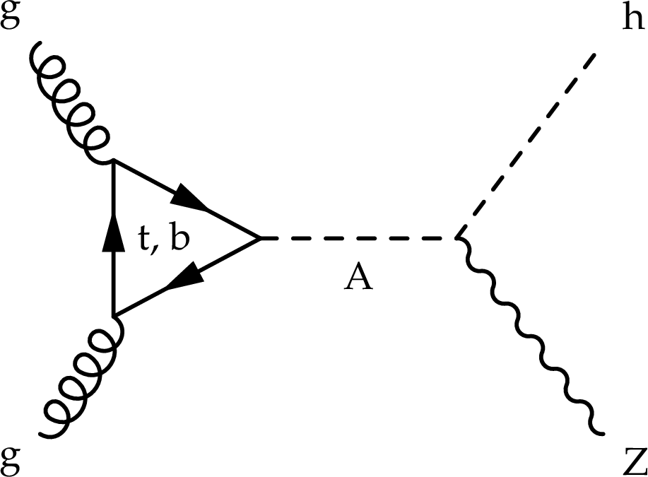
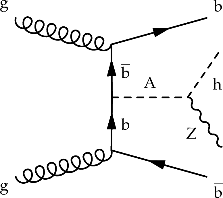
Figure 1:
Representative Feynman diagrams of the production in the 2HDM of a pseudoscalar A boson via gluon-gluon fusion (left) and in association with b quarks (right). |
png pdf |
Figure 1-a:
Representative Feynman diagram of the production in the 2HDM of a pseudoscalar A boson via gluon-gluon fusion. |
png pdf |
Figure 1-b:
Representative Feynman diagram of the production in the 2HDM of a pseudoscalar A boson in association with b quarks. |

png pdf |
Figure 2:
Product of the signal acceptance and selection efficiency $\varepsilon $ for an A boson produced via gluon-gluon fusion (left) and in association with b quarks (right) as a function of ${m_{{\mathrm {A}}}}$. The number of events passing the signal region selections is denoted as $N^\mathrm {SR}$, and $N^\mathrm {gen}$ is the number of events generated before applying any selection. |

png pdf |
Figure 2-a:
Product of the signal acceptance and selection efficiency $\varepsilon $ for an A boson produced via gluon-gluon fusion as a function of ${m_{{\mathrm {A}}}}$. The number of events passing the signal region selections is denoted as $N^\mathrm {SR}$, and $N^\mathrm {gen}$ is the number of events generated before applying any selection. |

png pdf |
Figure 2-b:
Product of the signal acceptance and selection efficiency $\varepsilon $ for an A boson produced in association with b quarks as a function of ${m_{{\mathrm {A}}}}$. The number of events passing the signal region selections is denoted as $N^\mathrm {SR}$, and $N^\mathrm {gen}$ is the number of events generated before applying any selection. |

png pdf |
Figure 3:
Pre- (dashed gray lines) and post-fit (stacked histograms) numbers of events in the different control regions used in the fit. The label in each bin summarizes the selection on the number and flavor of the leptons, the number of b-tagged jets, and if the two leptons are within (on Z) or outside the Z mass window (off Z). |

png pdf |
Figure 4:
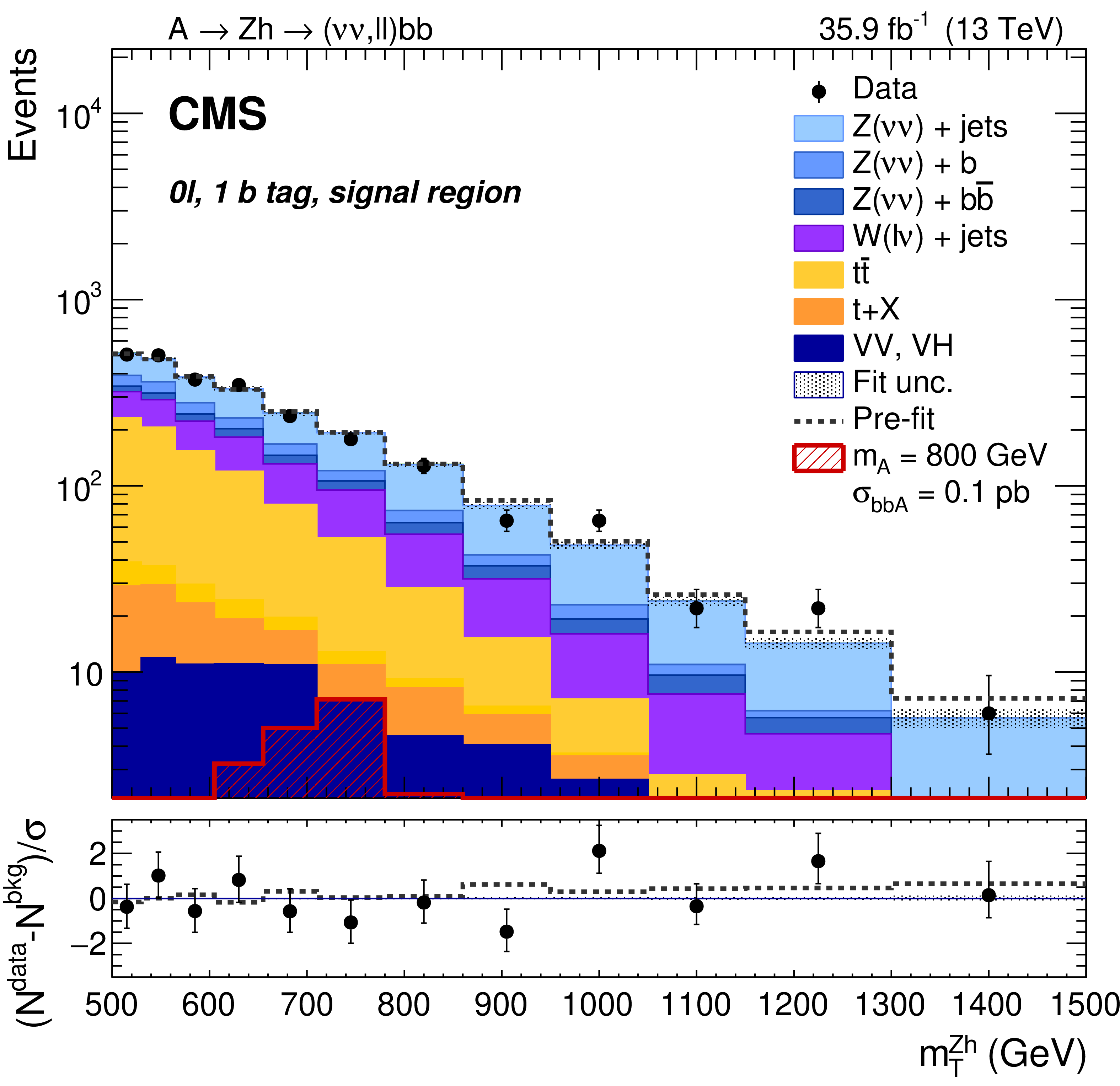
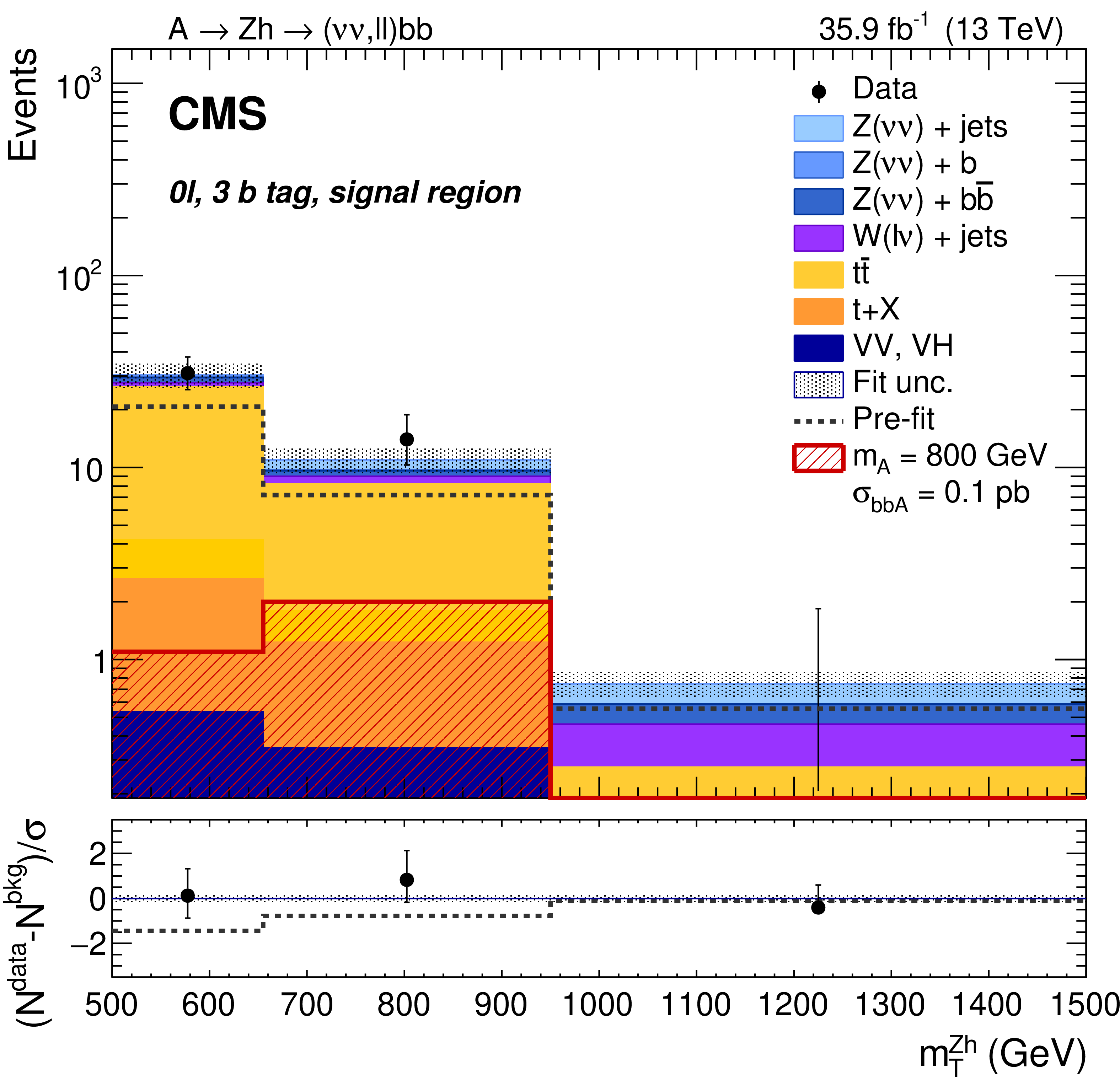
Distributions of the ${{m_{\mathrm {T}}} ^{{\mathrm {Z}} {\mathrm {h}}}}$ variable in the 0$\ell $ categories (left) and ${m_{{\mathrm {Z}} {\mathrm {h}}}}$ in the 2$\ell $ categories (right), in the 1 b tag (upper), 2 b tag (center), and 3 b tag (lower) SRs. In the 2$\ell $ categories, the contribution of the 2$ {\mathrm {e}}$ and 2$\mu $ channels have been summed. The gray dotted line represents the sum of the background before the fit; the shaded area represents the post-fit uncertainty. The hatched red histograms represent signals produced in association with b quarks and corresponding to $\sigma _{{\mathrm {A}}} {\mathcal {B}}({\mathrm {A}} \to {\mathrm {Z}} {\mathrm {h}}) {\mathcal {B}}({\mathrm {h}} \to {{\mathrm {b}} {\overline {\mathrm {b}}}})= $ 0.1 pb. The bottom panels depict the pulls in each bin, $(N^\text {data}-N^\text {bkg})/\sigma $, where $\sigma $ is the statistical uncertainty in data. |
png pdf |
Figure 4-a:
Distribution of the ${{m_{\mathrm {T}}} ^{{\mathrm {Z}} {\mathrm {h}}}}$ variable in the 0$\ell $, 1 b tag signal region. The gray dotted line represents the sum of the background before the fit; the shaded area represents the post-fit uncertainty. The hatched red histograms represent signals produced in association with b quarks and corresponding to $\sigma _{{\mathrm {A}}} {\mathcal {B}}({\mathrm {A}} \to {\mathrm {Z}} {\mathrm {h}}) {\mathcal {B}}({\mathrm {h}} \to {{\mathrm {b}} {\overline {\mathrm {b}}}})= $ 0.1 pb. The bottom panel depicts the pulls in each bin, $(N^\text {data}-N^\text {bkg})/\sigma $, where $\sigma $ is the statistical uncertainty in data. |

png pdf |
Figure 4-b:
Distribution of the ${m_{{\mathrm {Z}} {\mathrm {h}}}}$ variable in the 2$\ell $, 1 b tag signal region. The contribution of the 2$ {\mathrm {e}}$ and 2$\mu $ channels have been summed. The gray dotted line represents the sum of the background before the fit; the shaded area represents the post-fit uncertainty. The hatched red histograms represent signals produced in association with b quarks and corresponding to $\sigma _{{\mathrm {A}}} {\mathcal {B}}({\mathrm {A}} \to {\mathrm {Z}} {\mathrm {h}}) {\mathcal {B}}({\mathrm {h}} \to {{\mathrm {b}} {\overline {\mathrm {b}}}})= $ 0.1 pb. The bottom panel depicts the pulls in each bin, $(N^\text {data}-N^\text {bkg})/\sigma $, where $\sigma $ is the statistical uncertainty in data. |

png pdf |
Figure 4-c:
Distribution of the ${{m_{\mathrm {T}}} ^{{\mathrm {Z}} {\mathrm {h}}}}$ variable in the 0$\ell $, 2 b tags signal region.The gray dotted line represents the sum of the background before the fit; the shaded area represents the post-fit uncertainty. The hatched red histograms represent signals produced in association with b quarks and corresponding to $\sigma _{{\mathrm {A}}} {\mathcal {B}}({\mathrm {A}} \to {\mathrm {Z}} {\mathrm {h}}) {\mathcal {B}}({\mathrm {h}} \to {{\mathrm {b}} {\overline {\mathrm {b}}}})= $ 0.1 pb. The bottom panel depicts the pulls in each bin, $(N^\text {data}-N^\text {bkg})/\sigma $, where $\sigma $ is the statistical uncertainty in data. |

png pdf |
Figure 4-d:
Distribution of the ${m_{{\mathrm {Z}} {\mathrm {h}}}}$ variable in the 2$\ell $, 2 b tags signal region. The contribution of the 2$ {\mathrm {e}}$ and 2$\mu $ channels have been summed. The gray dotted line represents the sum of the background before the fit; the shaded area represents the post-fit uncertainty. The hatched red histograms represent signals produced in association with b quarks and corresponding to $\sigma _{{\mathrm {A}}} {\mathcal {B}}({\mathrm {A}} \to {\mathrm {Z}} {\mathrm {h}}) {\mathcal {B}}({\mathrm {h}} \to {{\mathrm {b}} {\overline {\mathrm {b}}}})= $ 0.1 pb. The bottom panel depicts the pulls in each bin, $(N^\text {data}-N^\text {bkg})/\sigma $, where $\sigma $ is the statistical uncertainty in data. |
png pdf |
Figure 4-e:
Distribution of the ${{m_{\mathrm {T}}} ^{{\mathrm {Z}} {\mathrm {h}}}}$ variable in the 0$\ell $, 3 b tags signal region. The gray dotted line represents the sum of the background before the fit; the shaded area represents the post-fit uncertainty. The hatched red histograms represent signals produced in association with b quarks and corresponding to $\sigma _{{\mathrm {A}}} {\mathcal {B}}({\mathrm {A}} \to {\mathrm {Z}} {\mathrm {h}}) {\mathcal {B}}({\mathrm {h}} \to {{\mathrm {b}} {\overline {\mathrm {b}}}})= $ 0.1 pb. The bottom panel depicts the pulls in each bin, $(N^\text {data}-N^\text {bkg})/\sigma $, where $\sigma $ is the statistical uncertainty in data. |

png pdf |
Figure 4-f:
Distribution of the ${m_{{\mathrm {Z}} {\mathrm {h}}}}$ variable in the 2$\ell $, 3 b tags signal region. The contribution of the 2$ {\mathrm {e}}$ and 2$\mu $ channels have been summed. The gray dotted line represents the sum of the background before the fit; the shaded area represents the post-fit uncertainty. The hatched red histograms represent signals produced in association with b quarks and corresponding to $\sigma _{{\mathrm {A}}} {\mathcal {B}}({\mathrm {A}} \to {\mathrm {Z}} {\mathrm {h}}) {\mathcal {B}}({\mathrm {h}} \to {{\mathrm {b}} {\overline {\mathrm {b}}}})= $ 0.1 pb. The bottom panel depicts the pulls in each bin, $(N^\text {data}-N^\text {bkg})/\sigma $, where $\sigma $ is the statistical uncertainty in data. |

png pdf |
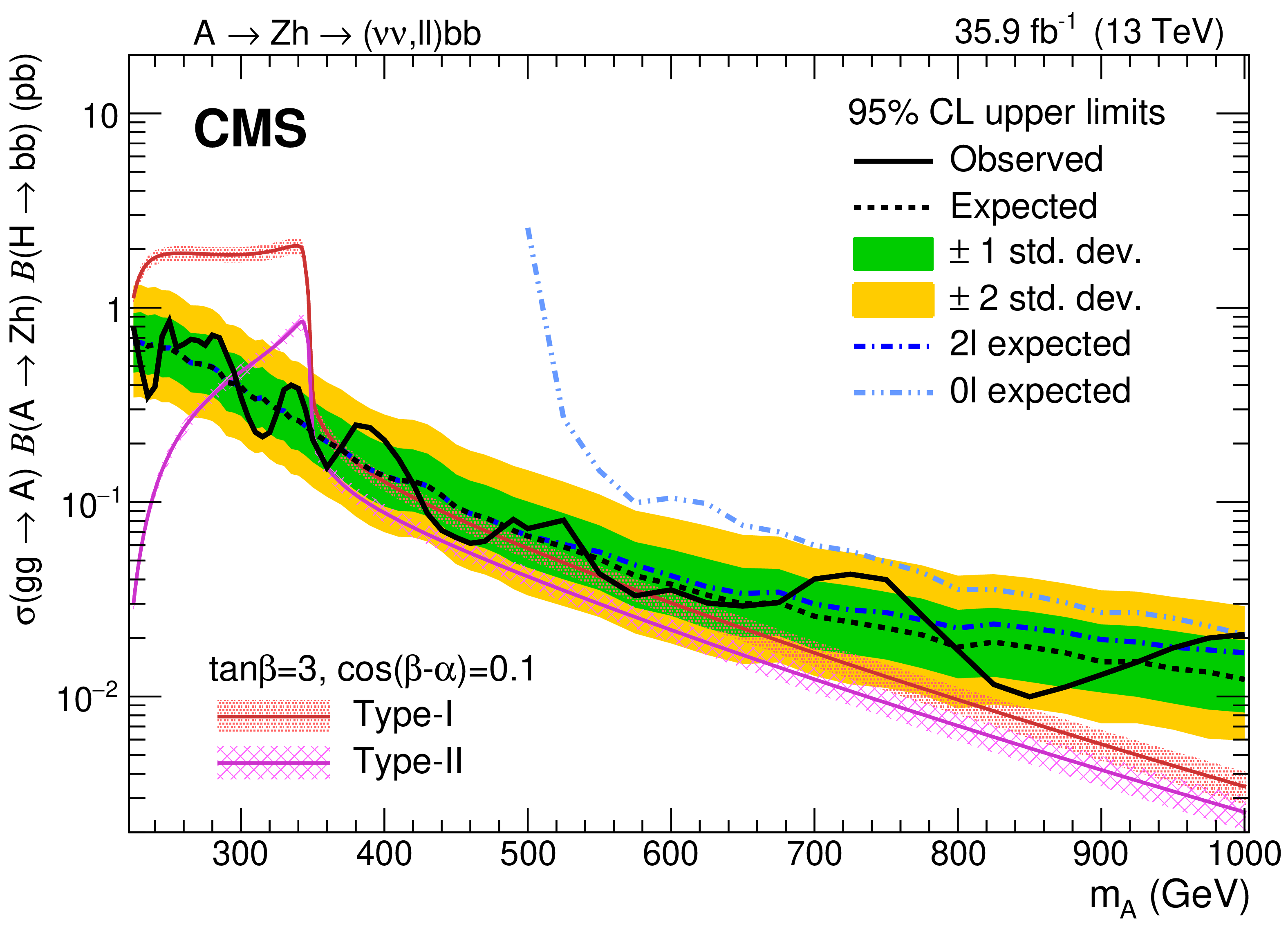
Figure 5:
Observed (solid black) and expected (dotted black) 95% CL upper limits on $\sigma _ {\mathrm {A}} \, {\mathcal {B}}({\mathrm {A}} \to {\mathrm {Z}} {\mathrm {h}}) \, {\mathcal {B}}({\mathrm {h}} \to {{\mathrm {b}} {\overline {\mathrm {b}}}})$ for an A boson produced via gluon-gluon fusion (left) and in association with b quarks (right) as a function of ${m_{{\mathrm {A}}}}$. The blue dashed lines represent the expected limits of the 0$\ell $ and 2$\ell $ categories separately. The red and magenta solid curves and their shaded areas correspond to the product of the cross sections and the branching fractions and the relative uncertainties predicted by the 2HDM Type-I and Type-II for the arbitrary parameters $\tan\beta =$ 3 and $ \cos(\beta -\alpha) =$ 0.1. |
png pdf |
Figure 5-a:
Observed (solid black) and expected (dotted black) 95% CL upper limits on $\sigma _ {\mathrm {A}} \, {\mathcal {B}}({\mathrm {A}} \to {\mathrm {Z}} {\mathrm {h}}) \, {\mathcal {B}}({\mathrm {h}} \to {{\mathrm {b}} {\overline {\mathrm {b}}}})$ for an A boson produced via gluon-gluon fusion as a function of ${m_{{\mathrm {A}}}}$. The blue dashed lines represent the expected limits of the 0$\ell $ and 2$\ell $ categories separately. The red and magenta solid curves and their shaded areas correspond to the product of the cross sections and the branching fractions and the relative uncertainties predicted by the 2HDM Type-I and Type-II for the arbitrary parameters $\tan\beta =$ 3 and $ \cos(\beta -\alpha) =$ 0.1. |

png pdf |
Figure 5-b:
Observed (solid black) and expected (dotted black) 95% CL upper limits on $\sigma _ {\mathrm {A}} \, {\mathcal {B}}({\mathrm {A}} \to {\mathrm {Z}} {\mathrm {h}}) \, {\mathcal {B}}({\mathrm {h}} \to {{\mathrm {b}} {\overline {\mathrm {b}}}})$ for an A boson produced in association with b quarks as a function of ${m_{{\mathrm {A}}}}$. The blue dashed lines represent the expected limits of the 0$\ell $ and 2$\ell $ categories separately. The red and magenta solid curves and their shaded areas correspond to the product of the cross sections and the branching fractions and the relative uncertainties predicted by the 2HDM Type-I and Type-II for the arbitrary parameters $\tan\beta =$ 3 and $ \cos(\beta -\alpha) =$ 0.1. |
png pdf |
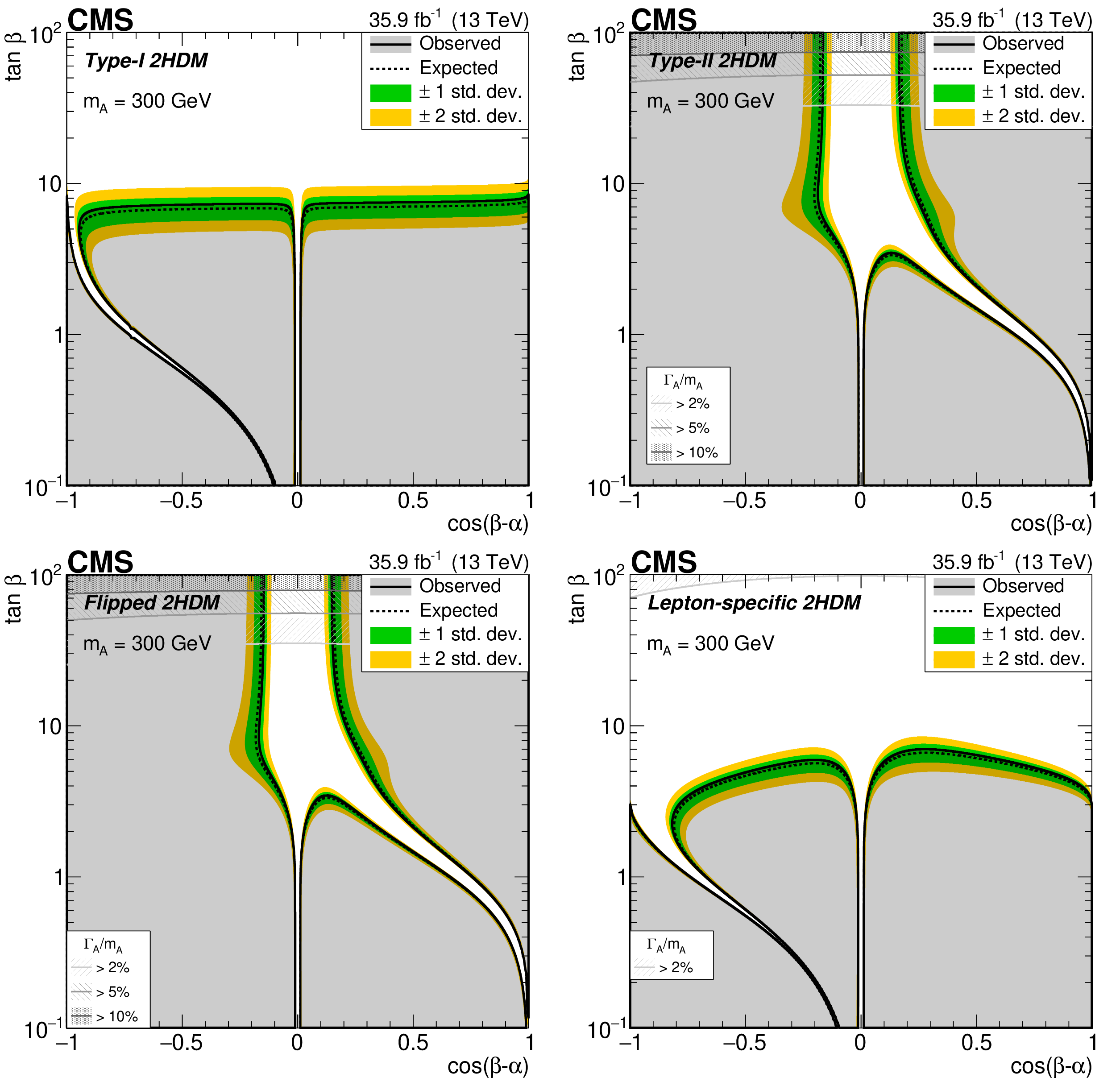
Figure 6:
Observed and expected (with $\pm$1, $\pm$2 standard deviation bands) exclusion limits for Type-I (upper left), Type-II (upper right), flipped (lower left), lepton-specific (lower right) models, as a function of $\cos(\beta -\alpha)$ and ${\tan\beta}$. Contours are derived from the projection on the 2HDM parameter space for the ${m_{{\mathrm {A}}}} = $ 300 GeV signal hypothesis. The excluded region is represented by the shaded gray area. The regions of the parameter space where the natural width of the A boson $\Gamma _ {\mathrm {A}} $ is comparable to the experimental resolution and thus the narrow width approximation is not valid are represented by the hatched gray areas. |

png pdf |
Figure 6-a:
Observed and expected (with $\pm$1, $\pm$2 standard deviation bands) exclusion limits for Type-I models, as a function of $\cos(\beta -\alpha)$ and ${\tan\beta}$. Contours are derived from the projection on the 2HDM parameter space for the ${m_{{\mathrm {A}}}} = $ 300 GeV signal hypothesis. The excluded region is represented by the shaded gray area. The regions of the parameter space where the natural width of the A boson $\Gamma _ {\mathrm {A}} $ is comparable to the experimental resolution and thus the narrow width approximation is not valid are represented by the hatched gray areas. |

png pdf |
Figure 6-b:
Observed and expected (with $\pm$1, $\pm$2 standard deviation bands) exclusion limits for Type-II models, as a function of $\cos(\beta -\alpha)$ and ${\tan\beta}$. Contours are derived from the projection on the 2HDM parameter space for the ${m_{{\mathrm {A}}}} = $ 300 GeV signal hypothesis. The excluded region is represented by the shaded gray area. The regions of the parameter space where the natural width of the A boson $\Gamma _ {\mathrm {A}} $ is comparable to the experimental resolution and thus the narrow width approximation is not valid are represented by the hatched gray areas. |
png pdf |
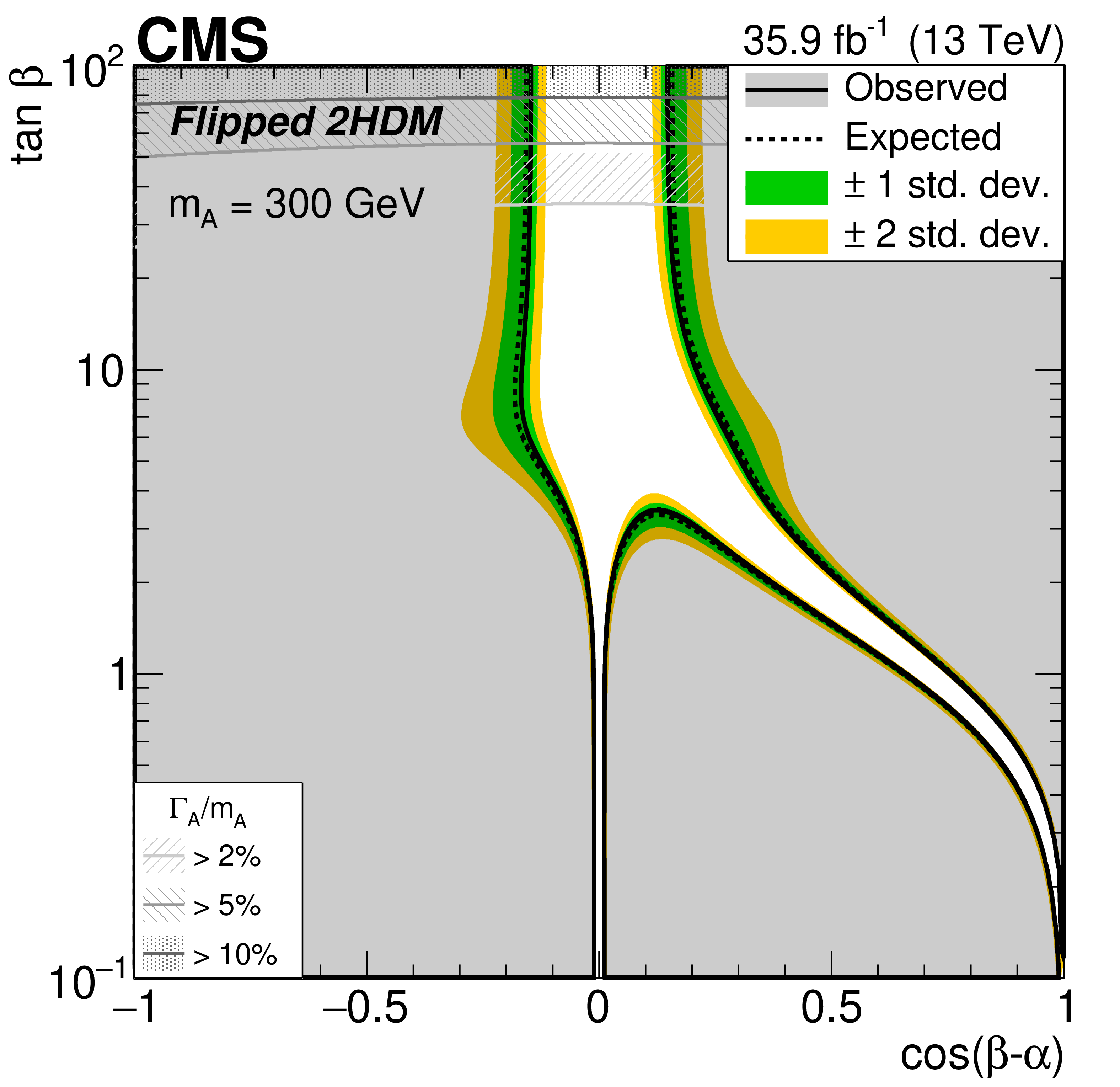
Figure 6-c:
Observed and expected (with $\pm$1, $\pm$2 standard deviation bands) exclusion limits for flipped models, as a function of $\cos(\beta -\alpha)$ and ${\tan\beta}$. Contours are derived from the projection on the 2HDM parameter space for the ${m_{{\mathrm {A}}}} = $ 300 GeV signal hypothesis. The excluded region is represented by the shaded gray area. The regions of the parameter space where the natural width of the A boson $\Gamma _ {\mathrm {A}} $ is comparable to the experimental resolution and thus the narrow width approximation is not valid are represented by the hatched gray areas. |

png pdf |
Figure 6-d:
Observed and expected (with $\pm$1, $\pm$2 standard deviation bands) exclusion limits for lepton-specific models, as a function of $\cos(\beta -\alpha)$ and ${\tan\beta}$. Contours are derived from the projection on the 2HDM parameter space for the ${m_{{\mathrm {A}}}} = $ 300 GeV signal hypothesis. The excluded region is represented by the shaded gray area. The regions of the parameter space where the natural width of the A boson $\Gamma _ {\mathrm {A}} $ is comparable to the experimental resolution and thus the narrow width approximation is not valid are represented by the hatched gray areas. |

png pdf |
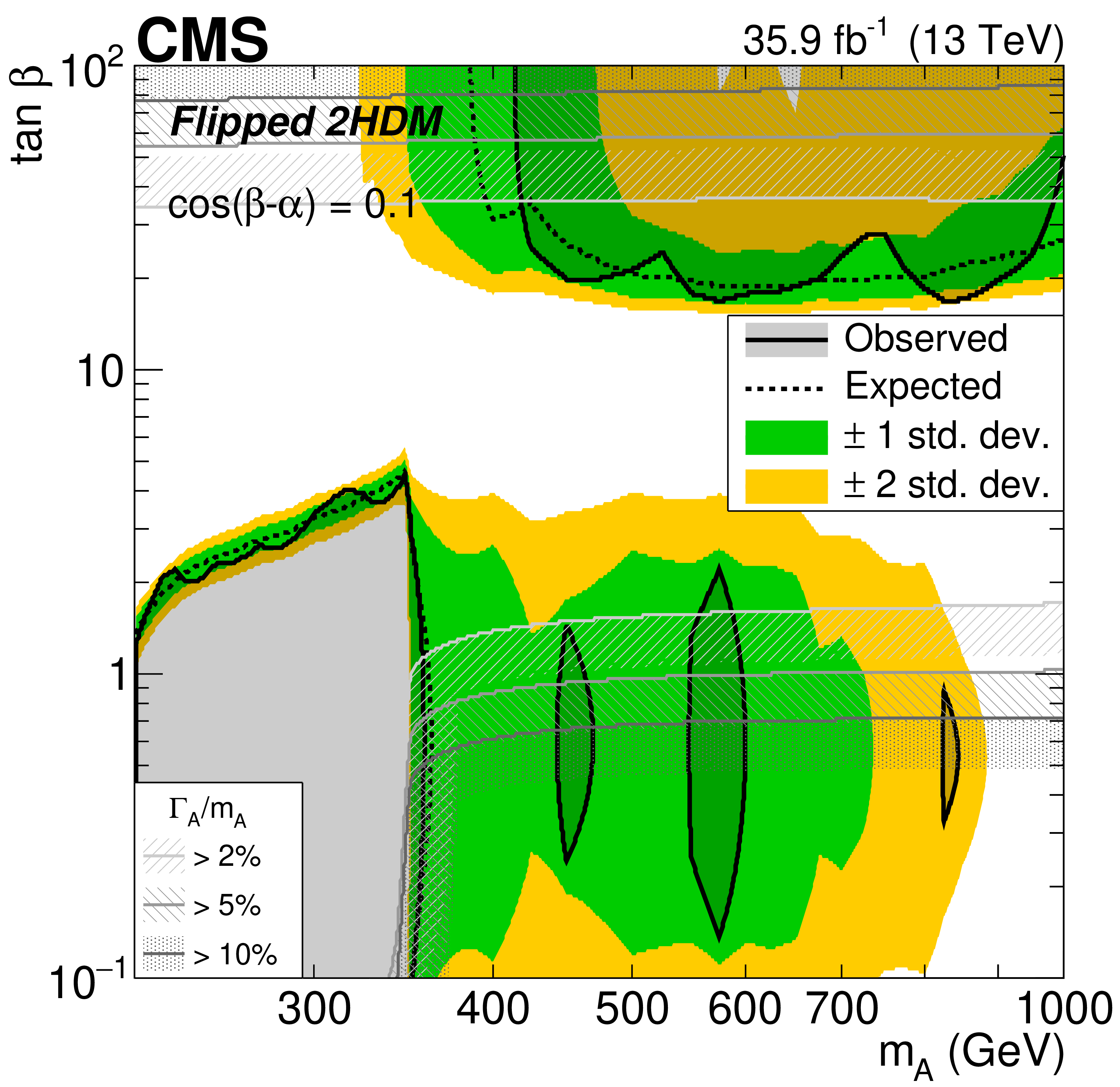
Figure 7:
Observed and expected (with $\pm$1, $\pm$2 standard deviation bands) exclusion limits for Type-I (upper left), Type-II (upper right), flipped (lower left), lepton-specific (lower right) models, as a function of ${m_{{\mathrm {A}}}}$ and ${\tan\beta}$, fixing $ \cos(\beta -\alpha) = $ 0.1. The excluded region is represented by the shaded gray area. The regions of the parameter space where the natural width of the A boson $\Gamma _ {\mathrm {A}} $ is comparable to the experimental resolution and thus the narrow width approximation is not valid are represented by the hatched gray areas. |
png pdf |
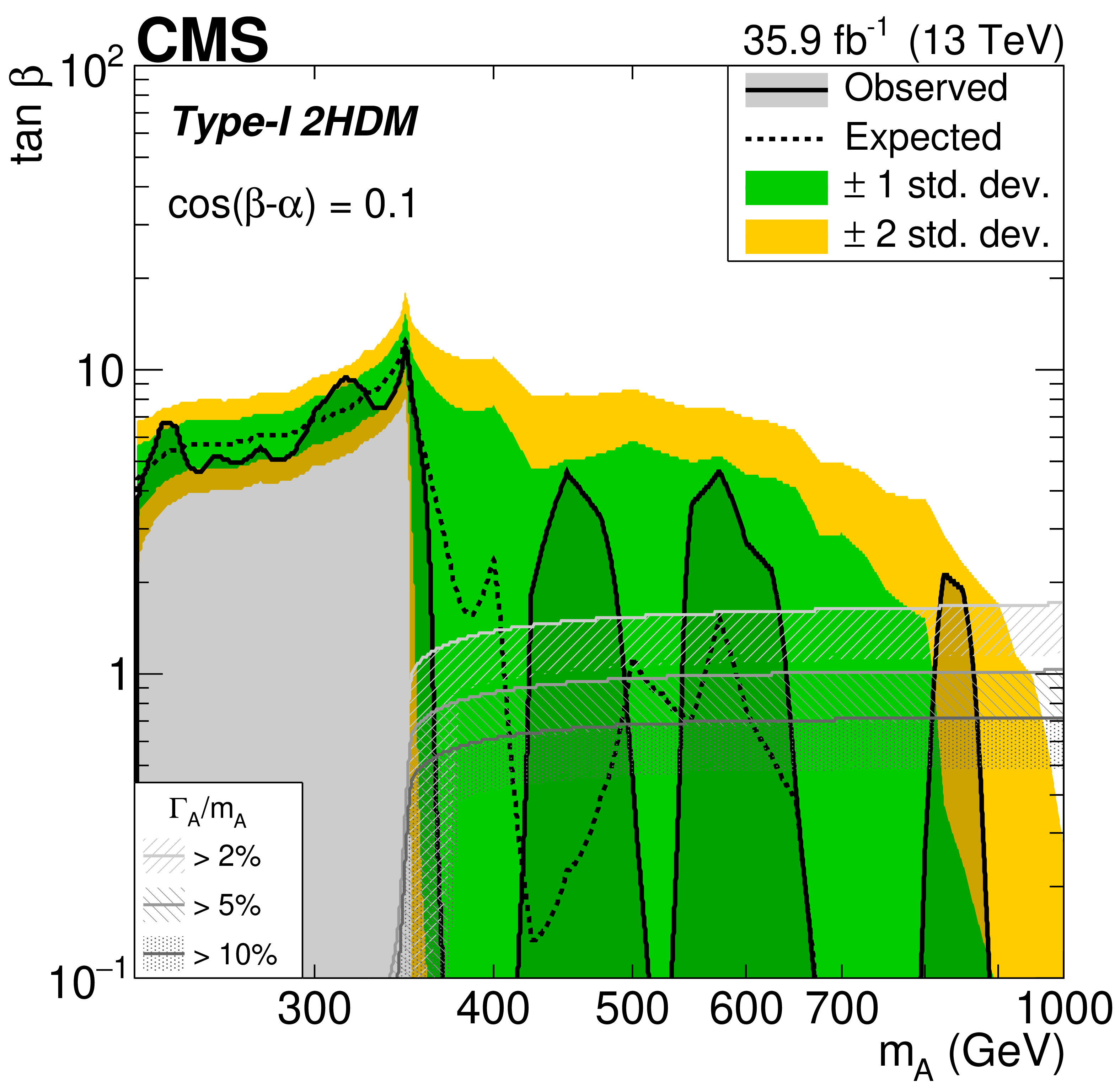
Figure 7-a:
Observed and expected (with $\pm$1, $\pm$2 standard deviation bands) exclusion limits for Type-I models, as a function of ${m_{{\mathrm {A}}}}$ and ${\tan\beta}$, fixing $ \cos(\beta -\alpha) = $ 0.1. The excluded region is represented by the shaded gray area. The regions of the parameter space where the natural width of the A boson $\Gamma _ {\mathrm {A}} $ is comparable to the experimental resolution and thus the narrow width approximation is not valid are represented by the hatched gray areas. |

png pdf |
Figure 7-b:
Observed and expected (with $\pm$1, $\pm$2 standard deviation bands) exclusion limits for Type-II models, as a function of ${m_{{\mathrm {A}}}}$ and ${\tan\beta}$, fixing $ \cos(\beta -\alpha) = $ 0.1. The excluded region is represented by the shaded gray area. The regions of the parameter space where the natural width of the A boson $\Gamma _ {\mathrm {A}} $ is comparable to the experimental resolution and thus the narrow width approximation is not valid are represented by the hatched gray areas. |
png pdf |
Figure 7-c:
Observed and expected (with $\pm$1, $\pm$2 standard deviation bands) exclusion limits for flipped models, as a function of ${m_{{\mathrm {A}}}}$ and ${\tan\beta}$, fixing $ \cos(\beta -\alpha) = $ 0.1. The excluded region is represented by the shaded gray area. The regions of the parameter space where the natural width of the A boson $\Gamma _ {\mathrm {A}} $ is comparable to the experimental resolution and thus the narrow width approximation is not valid are represented by the hatched gray areas. |

png pdf |
Figure 7-d:
Observed and expected (with $\pm$1, $\pm$2 standard deviation bands) exclusion limits for lepton-specific models, as a function of ${m_{{\mathrm {A}}}}$ and ${\tan\beta}$, fixing $ \cos(\beta -\alpha) = $ 0.1. The excluded region is represented by the shaded gray area. The regions of the parameter space where the natural width of the A boson $\Gamma _ {\mathrm {A}} $ is comparable to the experimental resolution and thus the narrow width approximation is not valid are represented by the hatched gray areas. |
| Tables | |

png pdf |
Table 1:
Definition of the signal and control regions. In 2$\ell $ regions, the leptons are required to have opposite electric charge. The entries marked with $\dagger $ indicate that the ${{p_{\mathrm {T}}} ^\text {miss}}$ is calculated subtracting the four momentum of the lepton. |
png pdf |
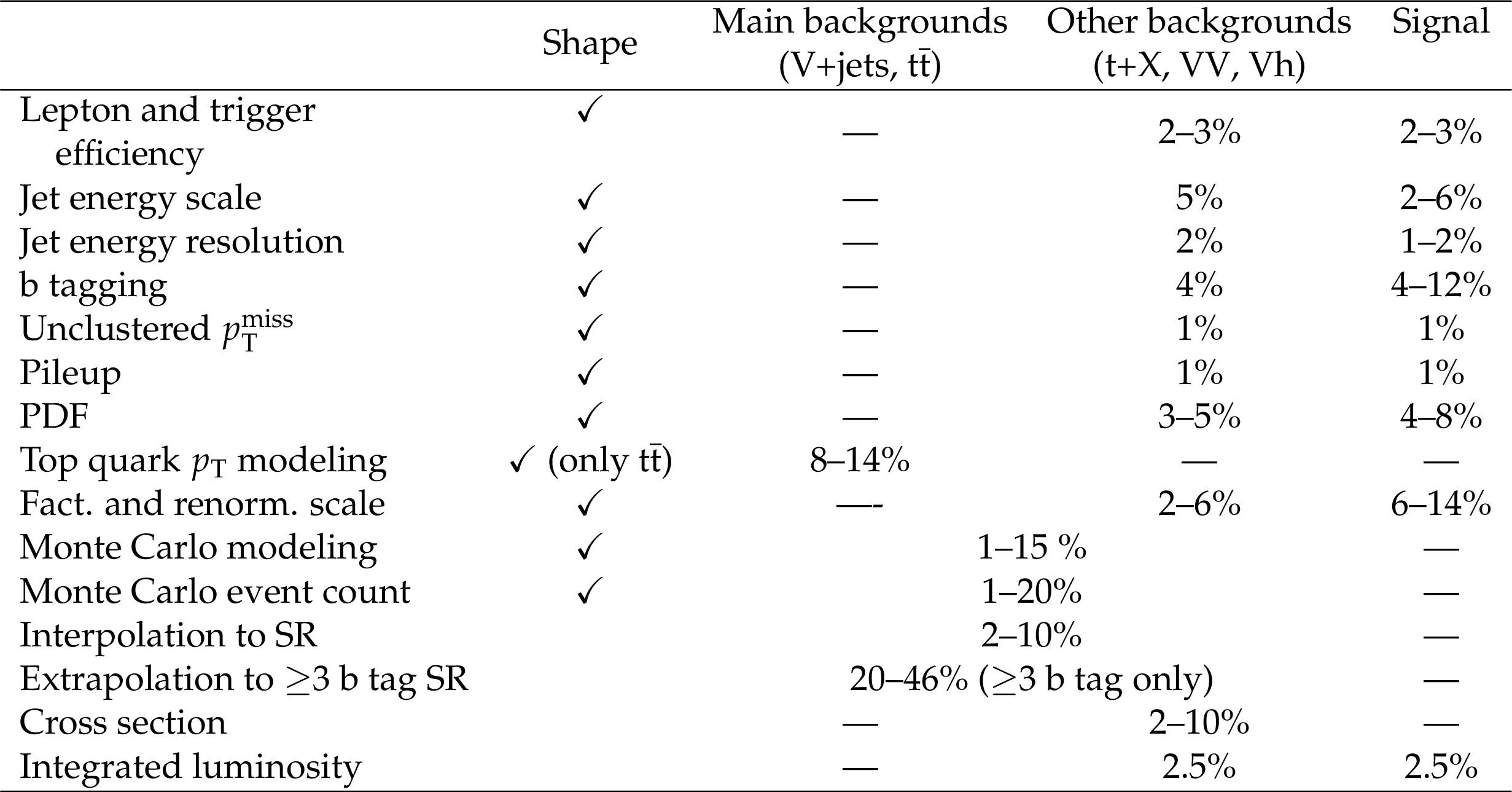
Table 2:
Summary of statistical and systematic uncertainties for backgrounds and signal. The uncertainties marked with a check mark are also propagated to the ${m_{{\mathrm {Z}} {\mathrm {h}}}}$ and ${{m_{\mathrm {T}}} ^{{\mathrm {Z}} {\mathrm {h}}}}$ distributions. |

png pdf |
Table 3:
Scale factors for the main backgrounds, as derived by the combined fit in the background-only hypothesis, with respect to the event yield from simulated samples. |

png pdf |
Table 4:
Expected and observed event yields after the fit in the signal regions. The dielectron and dimuon categories are summed together. The "-'' symbol represents backgrounds with no simulated events passing the selections. The signal yields refer to pre-fit values corresponding to a cross section multiplied by $ {\mathcal {B}}({\mathrm {A}} \to {\mathrm {Z}} {\mathrm {h}}) \, {\mathcal {B}}({\mathrm {h}} \to {{\mathrm {b}} {\overline {\mathrm {b}}}})$ of 0.1 pb (gluon-gluon fusion for $ {m_{{\mathrm {A}}}} = $ 300 GeV, and in association with b quarks for $ {m_{{\mathrm {A}}}} = $ 1000 GeV). |
| Summary |
| A search is presented in the context of an extended Higgs boson sector for a heavy pseudoscalar boson A that decays into a Z boson and a standard model (SM) h boson, with the Z boson decaying into electrons, muons, or neutrinos, and the h boson into $\mathrm{b\bar{b}}$. The SM backgrounds are suppressed by using the characteristics of the considered signal, namely the production and decay angles of the A, Z, and h bosons, and by improving the A mass resolution through a kinematic constraint on the reconstructed invariant mass of the h boson candidate. No excess of data over the background prediction is observed. Upper limits are set at 95% confidence level on the product of the A boson cross sections and the branching fractions $\sigma_{\mathrm{A}} \,{\mathcal{B}}({\mathrm{A}} \to\mathrm{Z}\mathrm{h}) \,{\mathcal{B}}(\mathrm{h}\to\mathrm{b\bar{b}})$, which exclude 1 to 0.01 pb in the 225-1000 GeV mass range. Interpretations are given in the context of Type-I, Type-II, flipped, and lepton-specific two-Higgs-doublet model formulations, thereby reducing the allowed parameter space for extensions of the SM. |
| References | ||||
| 1 | ATLAS Collaboration | Observation of a new particle in the search for the Standard Model Higgs boson with the ATLAS detector at the LHC | PLB 716 (2012) 1 | 1207.7214 |
| 2 | CMS Collaboration | Observation of a new boson at a mass of 125 GeV with the CMS experiment at the LHC | PLB 716 (2012) 30 | CMS-HIG-12-028 1207.7235 |
| 3 | CMS Collaboration | Observation of a new boson with mass near 125 GeV in pp collisions at $ \sqrt{s} = $ 7 and 8 TeV | JHEP 06 (2013) 081 | CMS-HIG-12-036 1303.4571 |
| 4 | ATLAS Collaboration | Measurement of the Higgs boson mass from the $ H\rightarrow{}\gamma{}\gamma{} $ and $ H\rightarrow{}Z{Z}^{*}\rightarrow{}4\ell{} $ channels in pp collisions at center-of-mass energies of 7 and 8~TeV with the ATLAS detector | PRD 90 (2014) 052004 | 1406.3827 |
| 5 | CMS Collaboration | Precise determination of the mass of the Higgs boson and tests of compatibility of its couplings with the standard model predictions using proton collisions at 7 and 8 TeV | EPJC 75 (2015) 212 | CMS-HIG-14-009 1412.8662 |
| 6 | CMS Collaboration | Evidence for the direct decay of the 125 GeV Higgs boson to fermions | NP 10 (2014) 557 | CMS-HIG-13-033 1401.6527 |
| 7 | ATLAS and CMS Collaborations | Combined measurement of the Higgs boson mass in pp collisions at $ \sqrt{s}= $ 7 and 8 TeV with the ATLAS and CMS experiments | PRL 114 (2015) 191803 | 1503.07589 |
| 8 | G. C. Branco et al. | Theory and phenomenology of two-Higgs-doublet models | PR 516 (2012) 1 | 1106.0034 |
| 9 | S. P. Martin | A Supersymmetry primer | Adv. Ser. Direct. HEP 21 (2010) 1 | hep-ph/9709356 |
| 10 | J. E. Kim | Light pseudoscalars, particle physics and cosmology | PR 150 (1987) 1 | |
| 11 | L. Fromme, S. J. Huber, and M. Seniuch | Baryogenesis in the two-Higgs doublet model | JHEP 11 (2006) 038 | hep-ph/0605242 |
| 12 | CMS Collaboration | Combined measurements of Higgs boson couplings in proton-proton collisions at $ \sqrt{s}= $ 13 TeV | Submitted to \it EPJC | CMS-HIG-17-031 1809.10733 |
| 13 | CMS Collaboration | Search for a pseudoscalar boson decaying into a Z boson and the 125 GeV Higgs boson in $ \ell^+\ell^- b\overline{b} $ final states | PLB 748 (2015) 221 | CMS-HIG-14-011 1504.04710 |
| 14 | CMS Collaboration | Search for heavy resonances decaying into a vector boson and a Higgs boson in final states with charged leptons, neutrinos and b quarks at $ \sqrt{s}= $ 13 TeV | JHEP 11 (2018) 172 | CMS-B2G-17-004 1807.02826 |
| 15 | ATLAS Collaboration | Search for heavy resonances decaying into a $ W $ or $ Z $ boson and a Higgs boson in final states with leptons and $ b $-jets in 36 fb$ ^{-1} $ of $ \sqrt s = $ 13 TeV pp collisions with the ATLAS detector | JHEP 03 (2018) 174 | 1712.06518 |
| 16 | CMS Collaboration | The CMS experiment at the CERN LHC | JINST 3 (2008) S08004 | CMS-00-001 |
| 17 | CMS Collaboration | Description and performance of track and primary-vertex reconstruction with the CMS tracker | JINST 9 (2014) P10009 | CMS-TRK-11-001 1405.6569 |
| 18 | CMS Collaboration | Performance of CMS muon reconstruction in pp collision events at $ \sqrt{s}= $ 7 TeV | JINST 7 (2012) P10002 | CMS-MUO-10-004 1206.4071 |
| 19 | CMS Collaboration | The CMS trigger system | JINST 12 (2017) P01020 | CMS-TRG-12-001 1609.02366 |
| 20 | CMS Collaboration | Particle-flow reconstruction and global event description with the cms detector | JINST 12 (2017) P10003 | CMS-PRF-14-001 1706.04965 |
| 21 | CMS Collaboration | Pileup removal algorithms | CMS-PAS-JME-14-001 | CMS-PAS-JME-14-001 |
| 22 | CMS Collaboration | Performance of electron reconstruction and selection with the CMS detector in proton-proton collisions at $ \sqrt{s} = $ 8 TeV | JINST 10 (2015) P06005 | CMS-EGM-13-001 1502.02701 |
| 23 | CMS Collaboration | Reconstruction and identification of $ \tau $ lepton decays to hadrons and $ \nu_\tau $ at CMS | JINST 11 (2016) P01019 | CMS-TAU-14-001 1510.07488 |
| 24 | M. Cacciari, G. P. Salam, and G. Soyez | The anti-$ k_\text{t} $ jet clustering algorithm | JHEP 04 (2008) 063 | 0802.1189 |
| 25 | M. Cacciari, G. P. Salam, and G. Soyez | FastJet user manual | EPJC 72 (2012) 1896 | 1111.6097 |
| 26 | M. Cacciari, G. P. Salam, and G. Soyez | The catchment area of jets | JHEP 04 (2008) 005 | 0802.1188 |
| 27 | CMS Collaboration | Jet energy scale and resolution in the CMS experiment in pp collisions at 8 TeV | JINST 12 (2017) P02014 | CMS-JME-13-004 1607.03663 |
| 28 | CMS Collaboration | Identification of heavy-flavour jets with the CMS detector in pp collisions at 13 TeV | JINST 13 (2018) P05011 | CMS-BTV-16-002 1712.07158 |
| 29 | J. Alwall et al. | The automated computation of tree-level and next-to-leading order differential cross sections, and their matching to parton shower simulations | JHEP 07 (2014) 079 | 1405.0301 |
| 30 | P. Artoisenet, R. Frederix, O. Mattelaer, and R. Rietkerk | Automatic spin-entangled decays of heavy resonances in Monte Carlo simulations | JHEP 03 (2013) 015 | 1212.3460 |
| 31 | D. Eriksson, J. Rathsman, and O. St\aal | 2HDMC --- two-Higgs-doublet model calculator physics and manual | CPC 181 (2010) 189 | 0902.0851 |
| 32 | R. V. Harlander, S. Liebler, and H. Mantler | SusHi: A program for the calculation of Higgs production in gluon fusion and bottom-quark annihilation in the Standard Model and the MSSM | CPC 184 (2013) 1605 | 1212.3249 |
| 33 | Particle Data Group Collaboration | Review of particle physics | PRD 98 (2018) 030001 | |
| 34 | J. Alwall et al. | Comparative study of various algorithms for the merging of parton showers and matrix elements in hadronic collisions | EPJC 53 (2008) 473 | 0706.2569 |
| 35 | Y. Li and F. Petriello | Combining QCD and electroweak corrections to dilepton production in FEWZ | PRD 86 (2012) 094034 | 1208.5967 |
| 36 | S. Kallweit et al. | NLO QCD+EW predictions for V+jets including off-shell vector-boson decays and multijet merging | JHEP 04 (2016) 021 | 1511.08692 |
| 37 | P. Nason | A new method for combining NLO QCD with shower Monte Carlo algorithms | JHEP 11 (2004) 040 | hep-ph/0409146 |
| 38 | S. Frixione, P. Nason, and C. Oleari | Matching NLO QCD computations with parton shower simulations: the POWHEG method | JHEP 11 (2007) 070 | 0709.2092 |
| 39 | S. Alioli, P. Nason, C. Oleari, and E. Re | A general framework for implementing NLO calculations in shower Monte Carlo programs: the POWHEG BOX | JHEP 06 (2010) 043 | 1002.2581 |
| 40 | M. Czakon and A. Mitov | Top++: A program for the calculation of the top-pair cross-section at hadron colliders | CPC 185 (2014) 2930 | 1112.5675 |
| 41 | CMS Collaboration | Measurement of differential cross sections for top quark pair production using the lepton+jets final state in proton-proton collisions at 13 TeV | PRD 95 (2017) 092001 | CMS-TOP-16-008 1610.04191 |
| 42 | R. Frederix and S. Frixione | Merging meets matching in MC@NLO | JHEP 12 (2012) 061 | 1209.6215 |
| 43 | NNPDF Collaboration | Parton distributions for the LHC Run II | JHEP 04 (2015) 040 | 1410.8849 |
| 44 | T. Sjostrand, S. Mrenna, and P. Skands | A brief introduction to PYTHIA 8.1 | CPC 178 (2008) 852 | 0710.3820 |
| 45 | T. Sjostrand, S. Mrenna, and P. Skands | PYTHIA 6.4 physics and manual | JHEP 05 (2006) 026 | hep-ph/0603175 |
| 46 | CMS Collaboration | Event generator tunes obtained from underlying event and multiparton scattering measurements | EPJC 76 (2016) 155 | CMS-GEN-14-001 1512.00815 |
| 47 | CMS Collaboration | Investigations of the impact of the parton shower tuning in Pythia 8 in the modelling of $ \mathrm{t\overline{t}} $ at $ \sqrt{s}= $ 8 and 13 TeV | CMS-PAS-TOP-16-021 | CMS-PAS-TOP-16-021 |
| 48 | GEANT4 Collaboration | GEANT4---a simulation toolkit | NIMA 506 (2003) 250 | |
| 49 | J. Butterworth et al. | PDF4LHC recommendations for LHC Run II | JPG 43 (2016) 23001 | 1510.03865 |
| 50 | A. Kalogeropoulos and J. Alwall | The SysCalc code: A tool to derive theoretical systematic uncertainties | 1801.08401 | |
| 51 | S. Catani, D. de Florian, M. Grazzini, and P. Nason | Soft gluon resummation for Higgs boson production at hadron colliders | JHEP 07 (2003) 028 | hep-ph/0306211 |
| 52 | CMS Collaboration | CMS luminosity measurement for the 2016 data taking period | CDS | |
| 53 | R. Barlow and C. Beeston | Fitting using finite Monte Carlo samples | CPC 77 (1993) 219 | |
| 54 | T. Junk | Confidence level computation for combining searches with small statistics | NIMA 434 (1999) 435 | hep-ex/9902006 |
| 55 | A. L. Read | Presentation of search results: the $ CL_s $ technique | JPG 28 (2002) 2693 | |
| 56 | ATLAS and CMS Collaborations | Procedure for the LHC Higgs boson search combination in Summer 2011 | CMS-NOTE-2011-005 | |
| 57 | G. Cowan, K. Cranmer, E. Gross, and O. Vitells | Asymptotic formulae for likelihood-based tests of new physics | EPJC 71 (2011) 1554 | 1007.1727 |
|
|
Compact Muon Solenoid LHC, CERN |
|

|

|

|

|

|