Compact Muon Solenoid
LHC, CERN

Visit us: CMS Public Website, CMS Physics ; Contact us: CMS Publications Committee

CMS-SMP-20-006 ; CERN-EP-2020-168

Measurements of production cross sections of polarized same-sign W boson pairs in association with two jets in proton-proton collisions at $\sqrt{s} = $ 13 TeV

CMS Collaboration

20 September 2020

Phys. Lett. B 812 (2020) 136018

Abstract: The first measurements of production cross sections of polarized same-sign ${\mathrm{W}^\pm\mathrm{W}^\pm} $ boson pairs in proton-proton collisions are reported. The measurements are based on a data sample collected with the CMS detector at the LHC at a center-of-mass energy of 13 TeV, corresponding to an integrated luminosity of 137 fb$^{-1}$. Events are selected by requiring exactly two same-sign leptons, electrons or muons, moderate missing transverse momentum, and two jets with a large rapidity separation and a large dijet mass to enhance the contribution of same-sign $ {\mathrm{W}^\pm\mathrm{W}^\pm} $ scattering events. An observed (expected) 95% confidence level upper limit of 1.17 (0.88) fb is set on the production cross section for longitudinally polarized same-sign ${\mathrm{W}^\pm\mathrm{W}^\pm} $ boson pairs. The electroweak production of same-sign ${\mathrm{W}^\pm\mathrm{W}^\pm} $ boson pairs with at least one of the W bosons longitudinally polarized is measured with an observed (expected) significance of 2.3 (3.1) standard deviations.

Links: e-print arXiv:2009.09429 [hep-ex] (PDF) ; CDS record ; inSPIRE record ; HepData record ; CADI line (restricted) ;

Figures
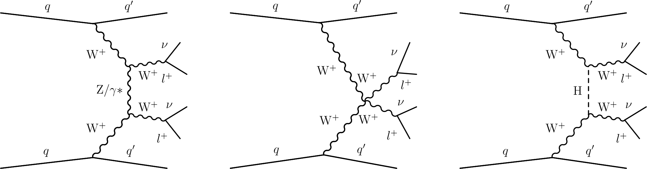
png pdf	Figure 1: Illustrative Feynman diagrams of VBS processes, where W bosons are radiated from incoming quarks (q), contributing to the EW-induced production of events containing two forward jets and $ {\mathrm{W} ^\pm \mathrm{W} ^\pm} $ boson pairs decaying to leptons. Diagrams with the triple gauge coupling vertex (left), the quartic gauge coupling vertex (center), and the $t$-channel Higgs boson exchange (right) are shown.
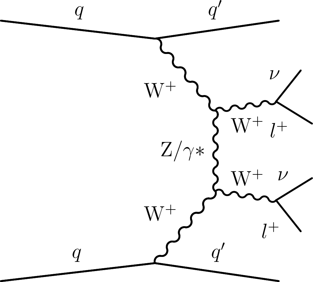
png pdf	Figure 1-a: Illustrative Feynman diagram of VBS process, where W bosons are radiated from incoming quarks (q), contributing to the EW-induced production of events containing two forward jets and $ {\mathrm{W} ^\pm \mathrm{W} ^\pm} $ boson pairs decaying to leptons, with triple gauge coupling vertex.
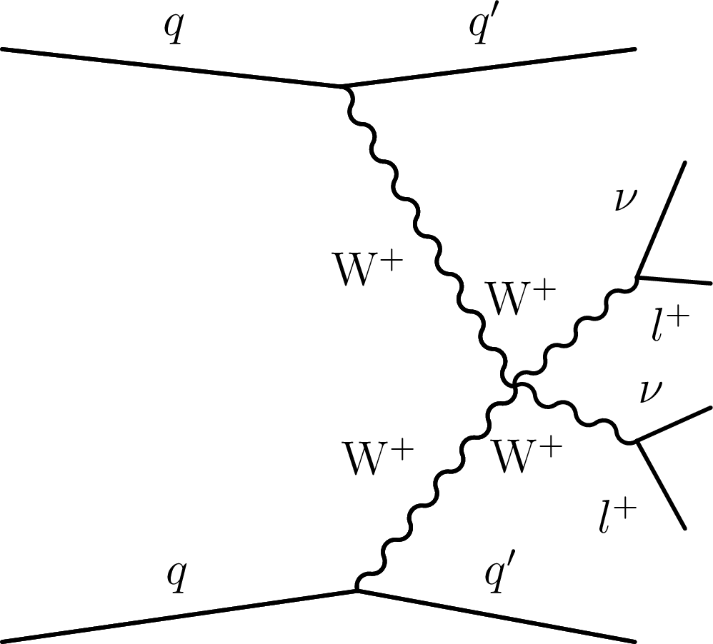
png pdf	Figure 1-b: Illustrative Feynman diagram of VBS process, where W bosons are radiated from incoming quarks (q), contributing to the EW-induced production of events containing two forward jets and $ {\mathrm{W} ^\pm \mathrm{W} ^\pm} $ boson pairs decaying to leptons, with quartic gauge coupling vertex.
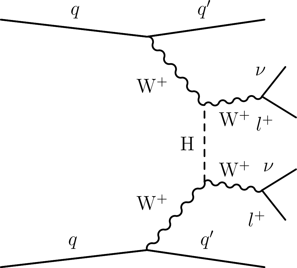
png pdf	Figure 1-c: Illustrative Feynman diagram of VBS process, where W bosons are radiated from incoming quarks (q), contributing to the EW-induced production of events containing two forward jets and $ {\mathrm{W} ^\pm \mathrm{W} ^\pm} $ boson pairs decaying to leptons, with $t$-channel Higgs boson exchange.
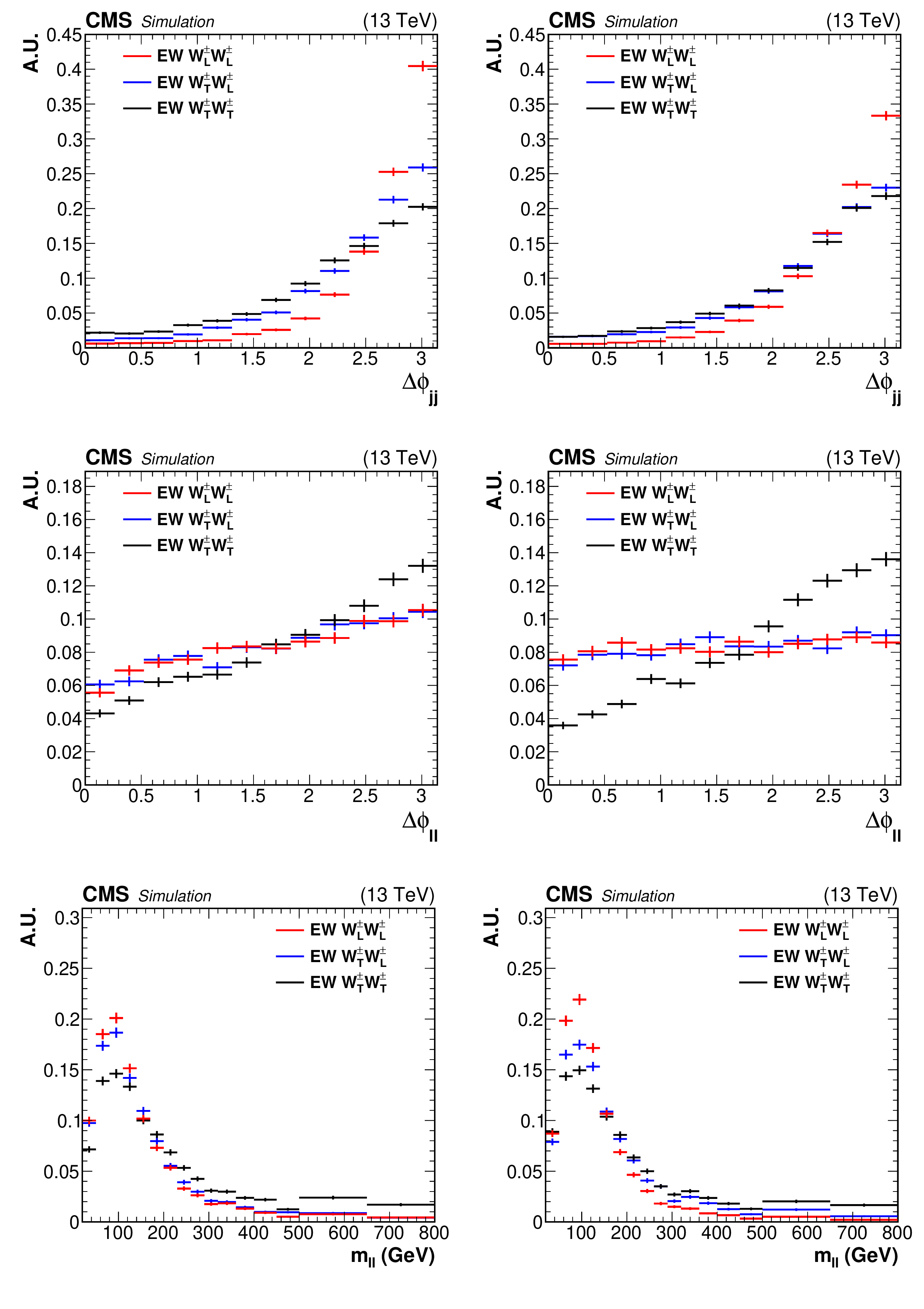
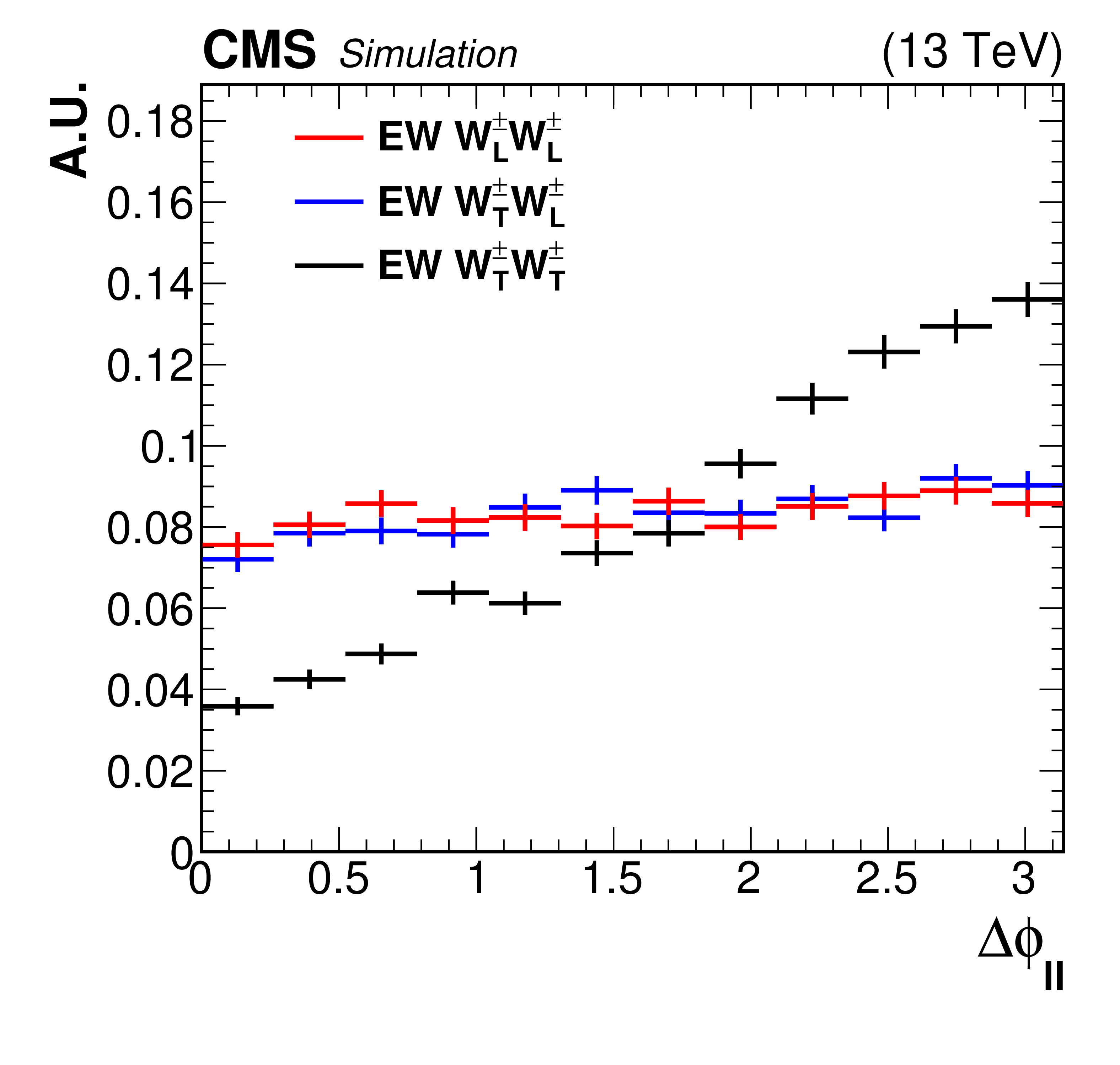
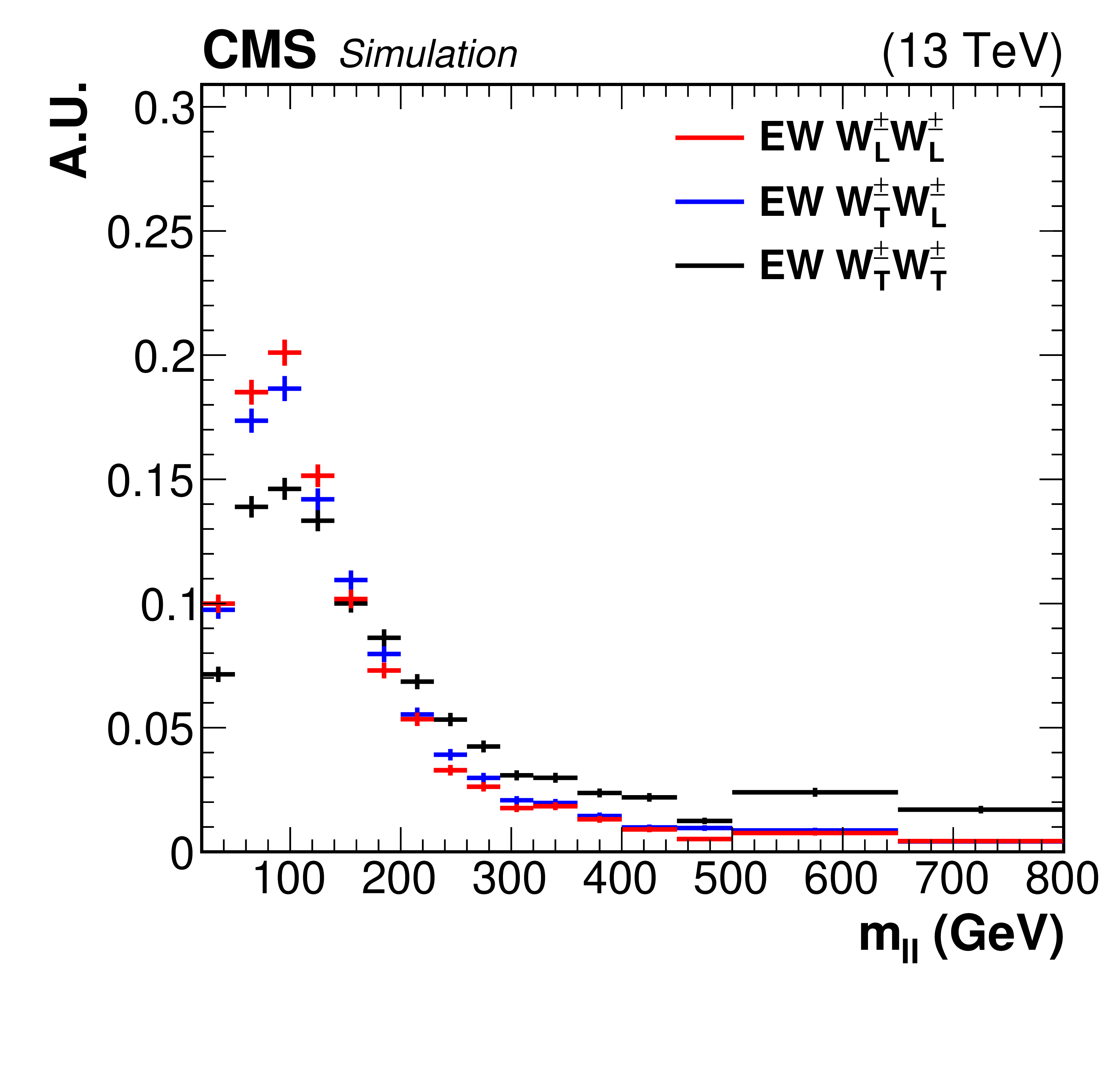
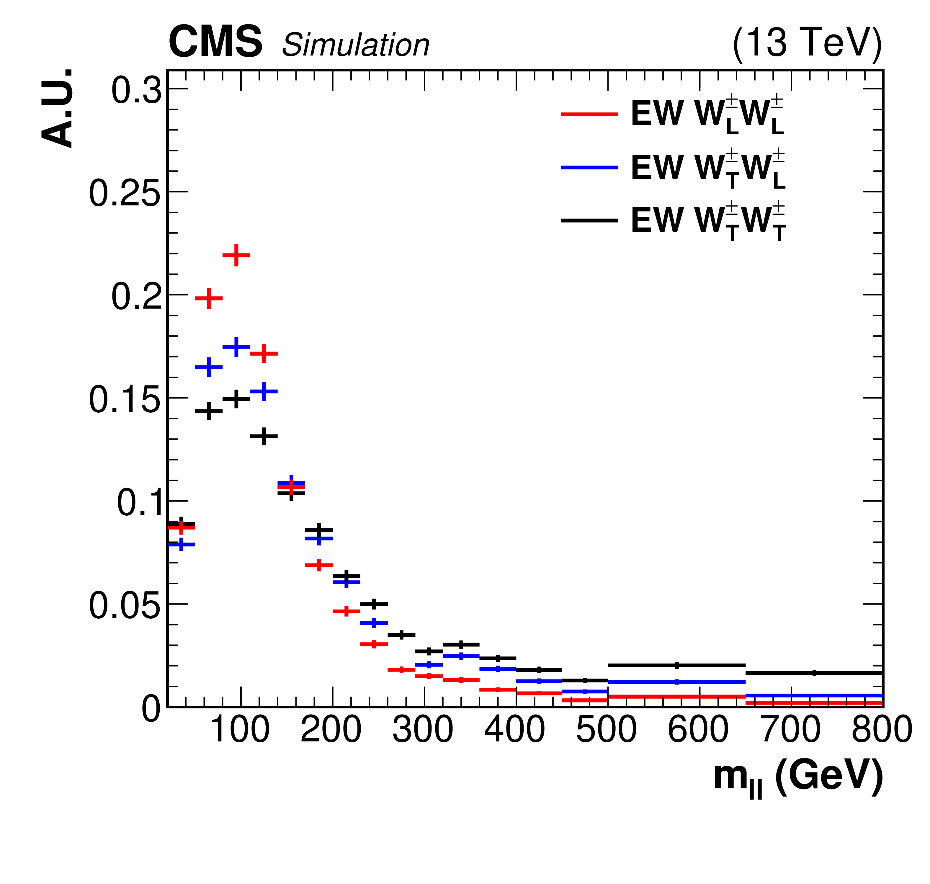
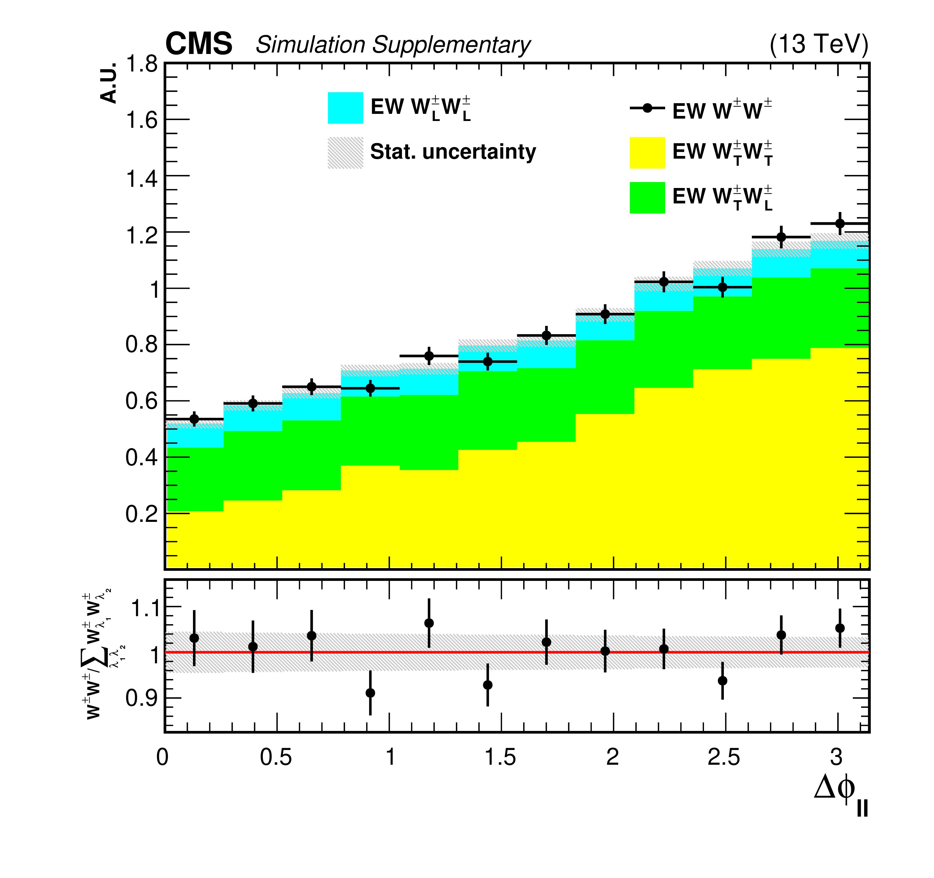
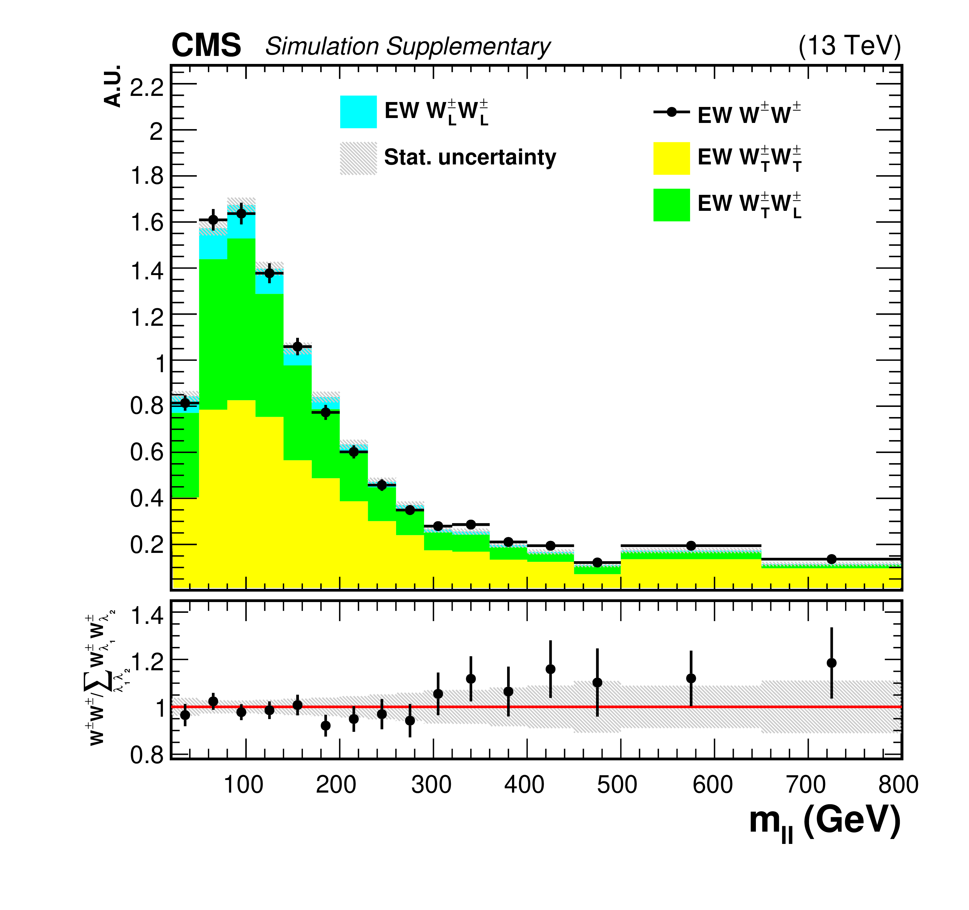
png pdf	Figure 2: Generator level distributions of $ {\Delta \phi _{{\mathrm {j}} {\mathrm {j}}}} $ (upper), $\Delta \phi _{\ell \ell}$ (center), and $ {m_{\ell \ell}} $ (lower) in the fiducial region for the $ {\mathrm{W} ^\pm _{\mathrm {L}}\mathrm{W} ^\pm _{\mathrm {L}}} $, $ {\mathrm{W} ^\pm _{\mathrm {L}}\mathrm{W} ^\pm _{\mathrm {T}}} $, and $ {\mathrm{W} ^\pm _{\mathrm {T}}\mathrm{W} ^\pm _{\mathrm {T}}} $ processes with the helicity eigenstates defined in the parton-parton (left) and $ {\mathrm{W} ^\pm \mathrm{W} ^\pm} $ (right) center-of-mass reference frames. The error bars represent the uncertainties associated with the limited numbers of simulated events.
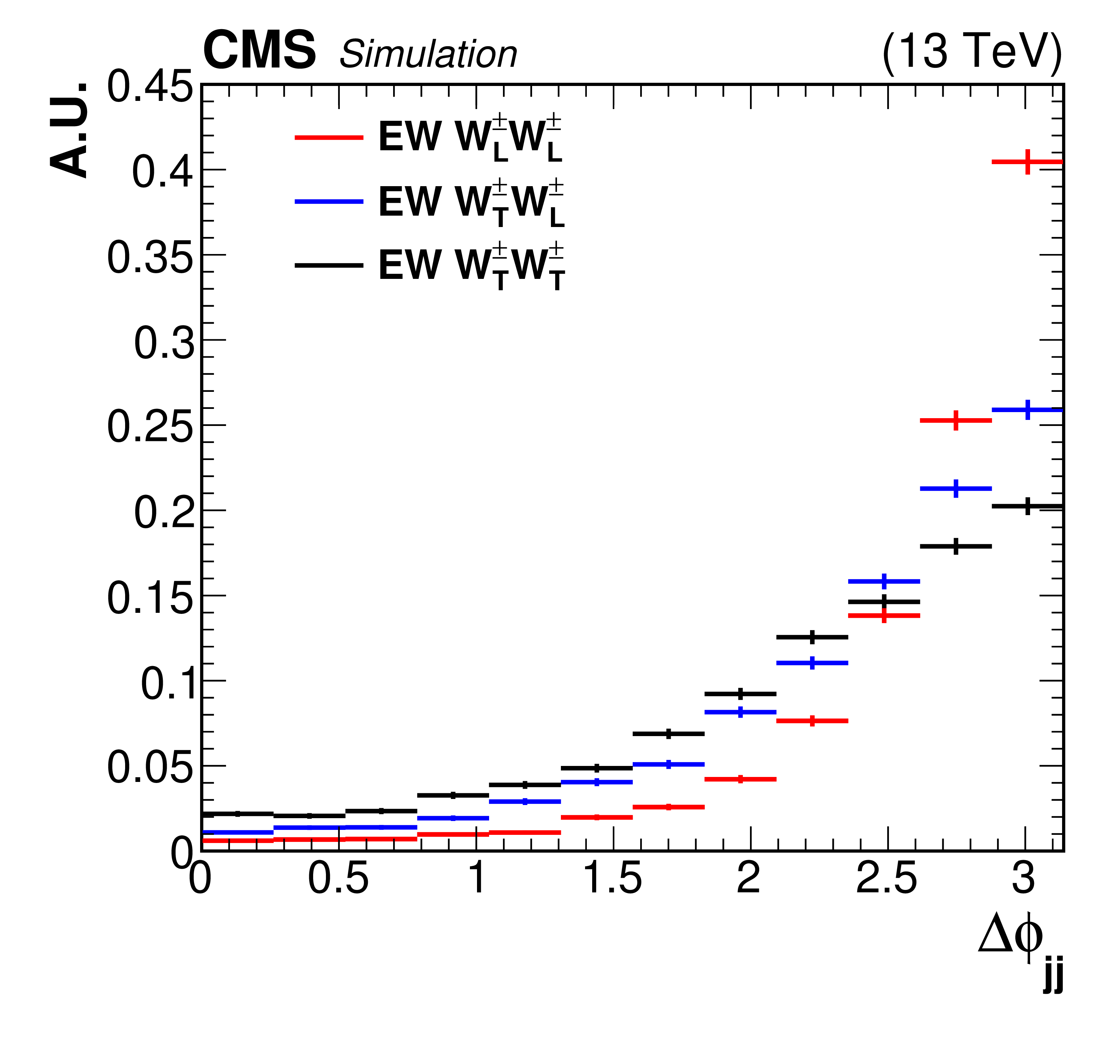
png pdf	Figure 2-a: Generator level distributions of $ {\Delta \phi _{{\mathrm {j}} {\mathrm {j}}}} $ in the fiducial region for the $ {\mathrm{W} ^\pm _{\mathrm {L}}\mathrm{W} ^\pm _{\mathrm {L}}} $, $ {\mathrm{W} ^\pm _{\mathrm {L}}\mathrm{W} ^\pm _{\mathrm {T}}} $, and $ {\mathrm{W} ^\pm _{\mathrm {T}}\mathrm{W} ^\pm _{\mathrm {T}}} $ processes with the helicity eigenstates defined in the parton-parton center-of-mass reference frame. The error bars represent the uncertainties associated with the limited numbers of simulated events.
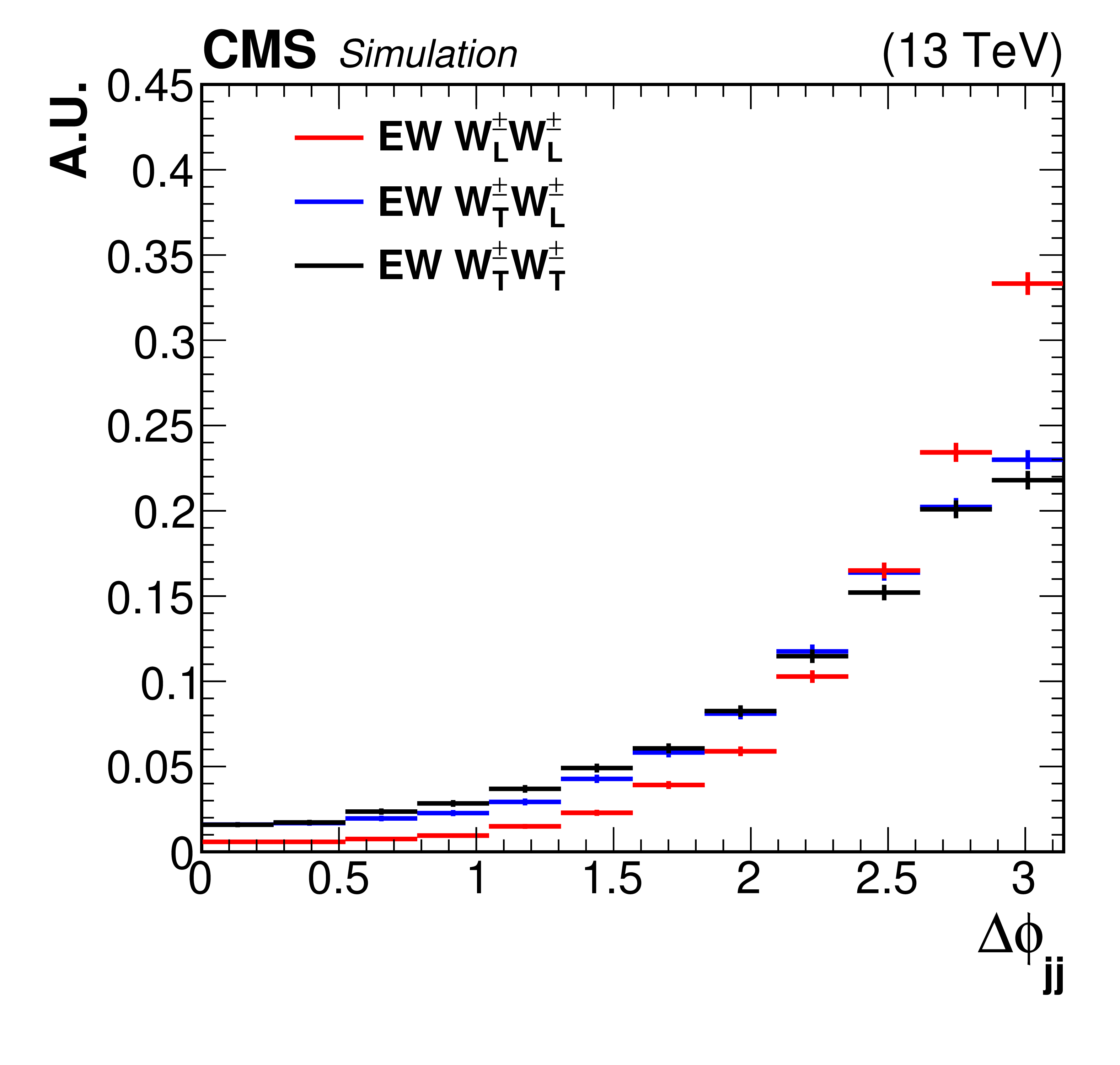
png pdf	Figure 2-b: Generator level distributions of $ {\Delta \phi _{{\mathrm {j}} {\mathrm {j}}}} $ in the fiducial region for the $ {\mathrm{W} ^\pm _{\mathrm {L}}\mathrm{W} ^\pm _{\mathrm {L}}} $, $ {\mathrm{W} ^\pm _{\mathrm {L}}\mathrm{W} ^\pm _{\mathrm {T}}} $, and $ {\mathrm{W} ^\pm _{\mathrm {T}}\mathrm{W} ^\pm _{\mathrm {T}}} $ processes with the helicity eigenstates defined in the $ {\mathrm{W} ^\pm \mathrm{W} ^\pm} $ center-of-mass reference frame. The error bars represent the uncertainties associated with the limited numbers of simulated events.
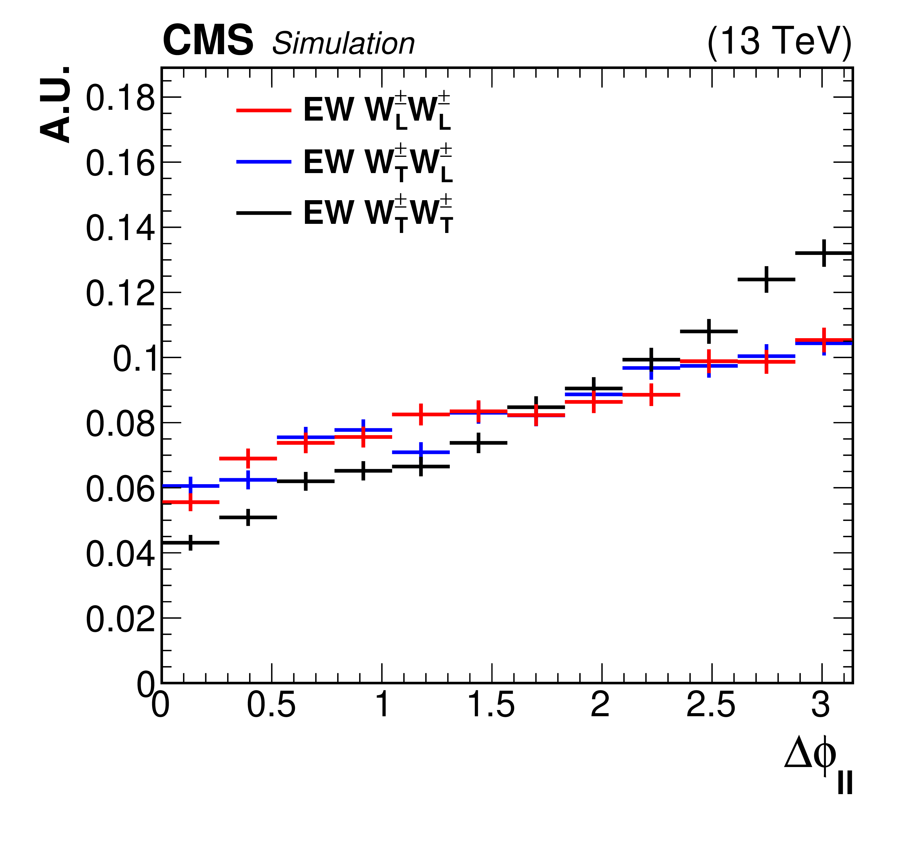
png pdf	Figure 2-c: Generator level distributions of $\Delta \phi _{\ell \ell}$ in the fiducial region for the $ {\mathrm{W} ^\pm _{\mathrm {L}}\mathrm{W} ^\pm _{\mathrm {L}}} $, $ {\mathrm{W} ^\pm _{\mathrm {L}}\mathrm{W} ^\pm _{\mathrm {T}}} $, and $ {\mathrm{W} ^\pm _{\mathrm {T}}\mathrm{W} ^\pm _{\mathrm {T}}} $ processes with the helicity eigenstates defined in the parton-parton center-of-mass reference frame. The error bars represent the uncertainties associated with the limited numbers of simulated events.
png pdf	Figure 2-d: Generator level distributions of $\Delta \phi _{\ell \ell}$ in the fiducial region for the $ {\mathrm{W} ^\pm _{\mathrm {L}}\mathrm{W} ^\pm _{\mathrm {L}}} $, $ {\mathrm{W} ^\pm _{\mathrm {L}}\mathrm{W} ^\pm _{\mathrm {T}}} $, and $ {\mathrm{W} ^\pm _{\mathrm {T}}\mathrm{W} ^\pm _{\mathrm {T}}} $ processes with the helicity eigenstates defined in the $ {\mathrm{W} ^\pm \mathrm{W} ^\pm} $ center-of-mass reference frame. The error bars represent the uncertainties associated with the limited numbers of simulated events.
png pdf	Figure 2-e: Generator level distributions of $ {m_{\ell \ell}} $ in the fiducial region for the $ {\mathrm{W} ^\pm _{\mathrm {L}}\mathrm{W} ^\pm _{\mathrm {L}}} $, $ {\mathrm{W} ^\pm _{\mathrm {L}}\mathrm{W} ^\pm _{\mathrm {T}}} $, and $ {\mathrm{W} ^\pm _{\mathrm {T}}\mathrm{W} ^\pm _{\mathrm {T}}} $ processes with the helicity eigenstates defined in the parton-parton center-of-mass reference frame. The error bars represent the uncertainties associated with the limited numbers of simulated events.
png pdf	Figure 2-f: Generator level distributions of $ {m_{\ell \ell}} $ in the fiducial region for the $ {\mathrm{W} ^\pm _{\mathrm {L}}\mathrm{W} ^\pm _{\mathrm {L}}} $, $ {\mathrm{W} ^\pm _{\mathrm {L}}\mathrm{W} ^\pm _{\mathrm {T}}} $, and $ {\mathrm{W} ^\pm _{\mathrm {T}}\mathrm{W} ^\pm _{\mathrm {T}}} $ processes with the helicity eigenstates defined in the $ {\mathrm{W} ^\pm \mathrm{W} ^\pm} $ center-of-mass reference frame. The error bars represent the uncertainties associated with the limited numbers of simulated events.
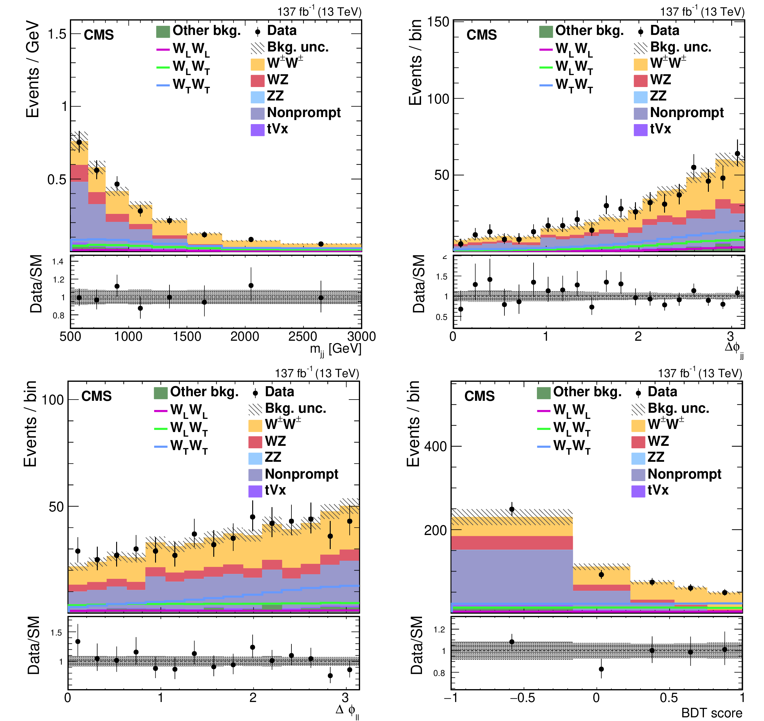
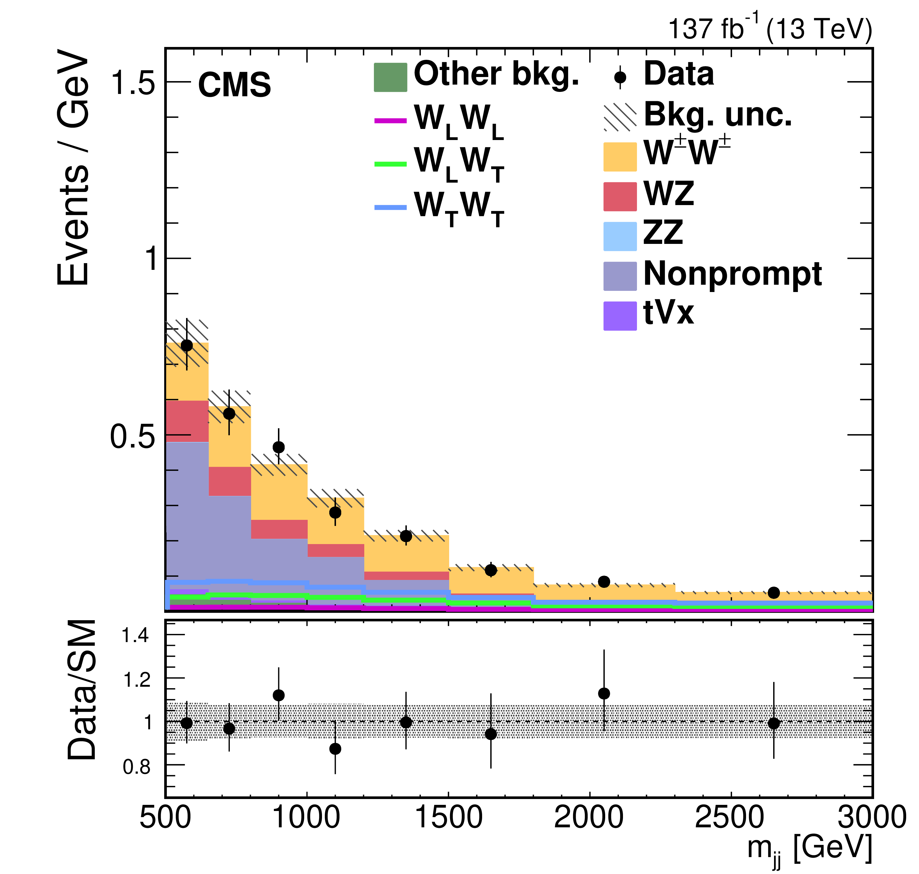
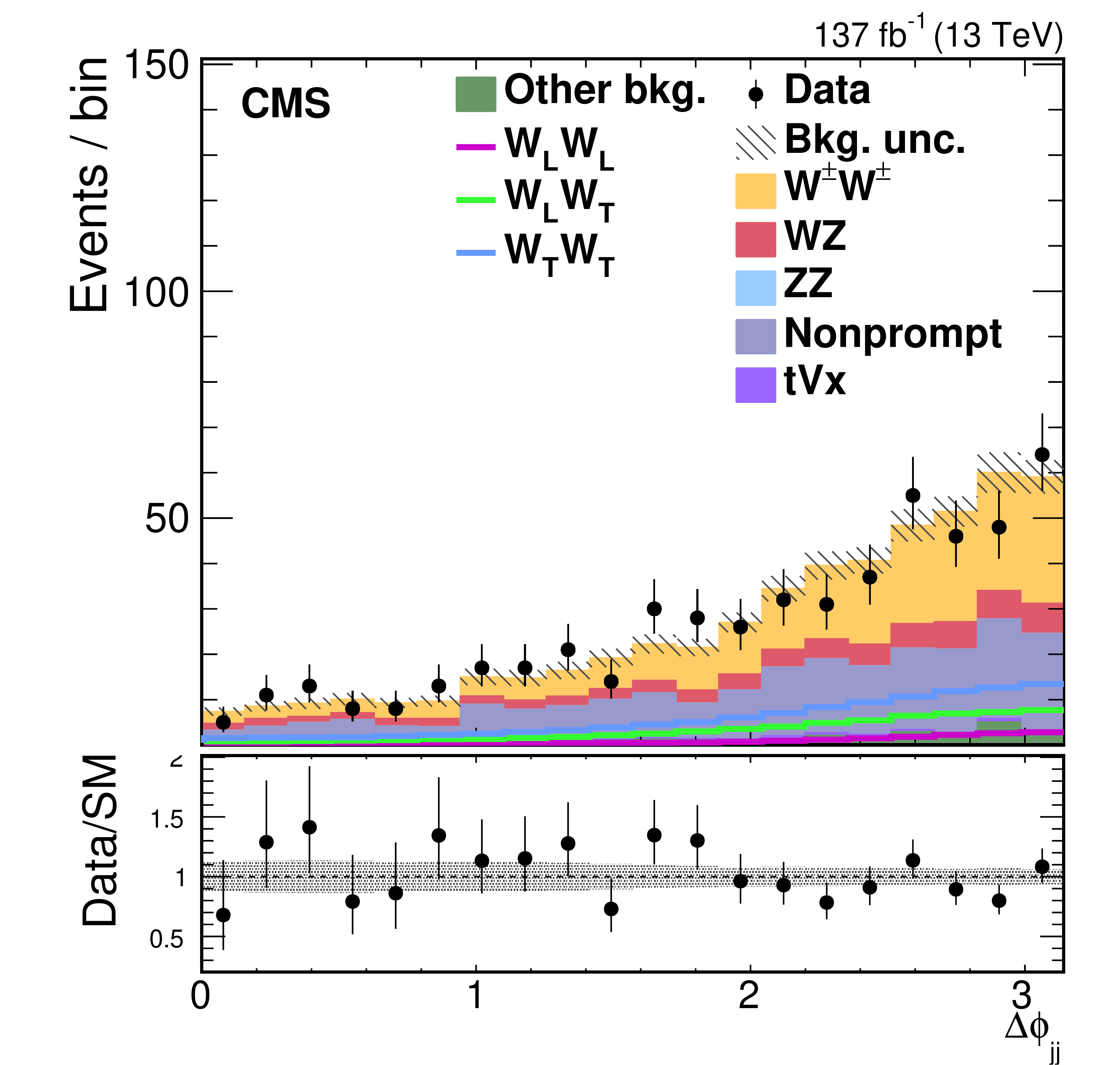
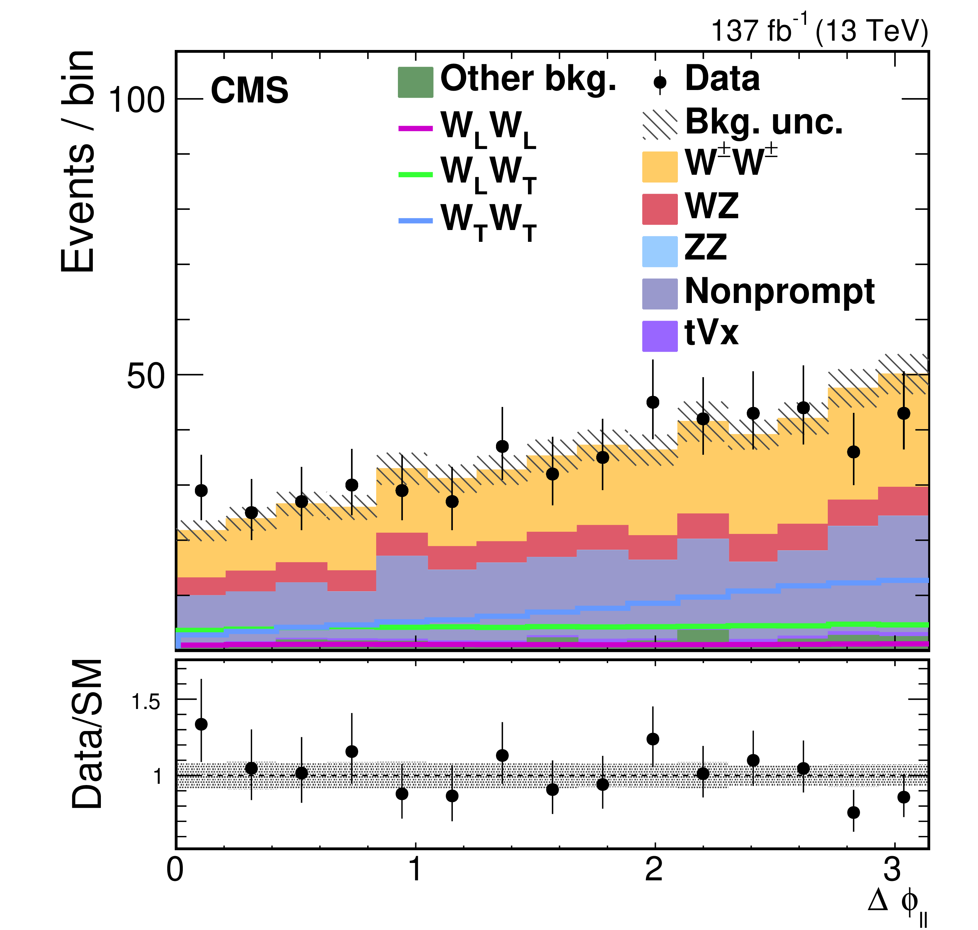
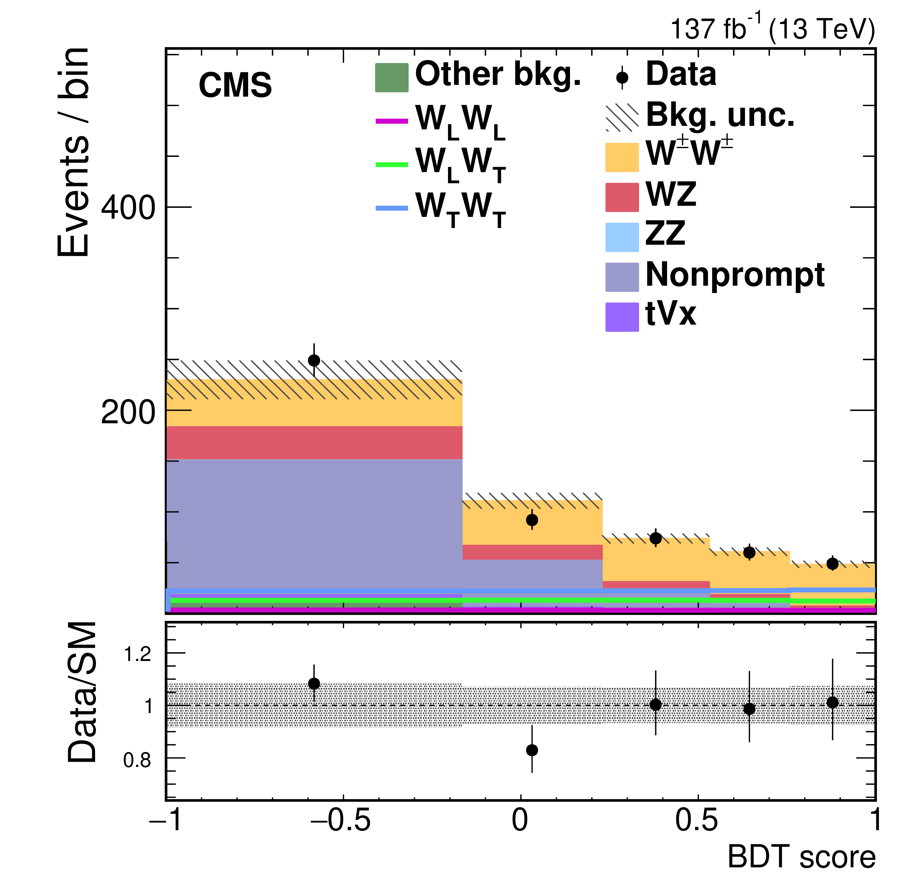
png pdf	Figure 3: Distributions of the $ {m_{{\mathrm {j}} {\mathrm {j}}}} $ (upper left), $ {\Delta \phi _{{\mathrm {j}} {\mathrm {j}}}} $ (upper right), $\Delta \phi _{\ell \ell}$ (lower left), and of the output score of the inclusive BDT (lower right) in the $ {\mathrm{W} ^\pm \mathrm{W} ^\pm} $ SR. The predicted yields are shown with their best fit normalizations from the simultaneous fit. The histograms for the $ {\mathrm{W} ^\pm \mathrm{W} ^\pm} $ process include the contributions from the $ {\mathrm{W} ^\pm _{\mathrm {L}}\mathrm{W} ^\pm _{\mathrm {L}}} $, $ {\mathrm{W} ^\pm _{\mathrm {L}}\mathrm{W} ^\pm _{\mathrm {T}}} $, and $ {\mathrm{W} ^\pm _{\mathrm {T}}\mathrm{W} ^\pm _{\mathrm {T}}} $ processes (shown as solid lines), QCD $ {\mathrm{W} ^\pm \mathrm{W} ^\pm} $, and interference. The histograms for other backgrounds include the contributions from double parton scattering, VVV, and from oppositely charged dilepton final states from ${\mathrm{t} \mathrm{\bar{t}}} $, $\mathrm{t} \mathrm{W} $, $\mathrm{W} ^{+}\mathrm{W} ^{-}$, and Drell-Yan processes. The overflow is included in the last bin. The bottom panel in each figure shows the ratio of the number of events observed in data to that of the total SM prediction. The gray bands represent the uncertainties in the predicted yields. The vertical bars represent the statistical uncertainties in the data.
png pdf	Figure 3-a: Distribution of $ {m_{{\mathrm {j}} {\mathrm {j}}}} $ in the $ {\mathrm{W} ^\pm \mathrm{W} ^\pm} $ SR. The predicted yields are shown with their best fit normalizations from the simultaneous fit. The histograms for the $ {\mathrm{W} ^\pm \mathrm{W} ^\pm} $ process include the contributions from the $ {\mathrm{W} ^\pm _{\mathrm {L}}\mathrm{W} ^\pm _{\mathrm {L}}} $, $ {\mathrm{W} ^\pm _{\mathrm {L}}\mathrm{W} ^\pm _{\mathrm {T}}} $, and $ {\mathrm{W} ^\pm _{\mathrm {T}}\mathrm{W} ^\pm _{\mathrm {T}}} $ processes (shown as solid lines), QCD $ {\mathrm{W} ^\pm \mathrm{W} ^\pm} $, and interference. The histograms for other backgrounds include the contributions from double parton scattering, VVV, and from oppositely charged dilepton final states from ${\mathrm{t} \mathrm{\bar{t}}} $, $\mathrm{t} \mathrm{W} $, $\mathrm{W} ^{+}\mathrm{W} ^{-}$, and Drell-Yan processes. The overflow is included in the last bin. The bottom panel shows the ratio of the number of events observed in data to that of the total SM prediction. The gray bands represent the uncertainties in the predicted yields. The vertical bars represent the statistical uncertainties in the data.
png pdf	Figure 3-b: Distribution of $ {\Delta \phi _{{\mathrm {j}} {\mathrm {j}}}} $ in the $ {\mathrm{W} ^\pm \mathrm{W} ^\pm} $ SR. The predicted yields are shown with their best fit normalizations from the simultaneous fit. The histograms for the $ {\mathrm{W} ^\pm \mathrm{W} ^\pm} $ process include the contributions from the $ {\mathrm{W} ^\pm _{\mathrm {L}}\mathrm{W} ^\pm _{\mathrm {L}}} $, $ {\mathrm{W} ^\pm _{\mathrm {L}}\mathrm{W} ^\pm _{\mathrm {T}}} $, and $ {\mathrm{W} ^\pm _{\mathrm {T}}\mathrm{W} ^\pm _{\mathrm {T}}} $ processes (shown as solid lines), QCD $ {\mathrm{W} ^\pm \mathrm{W} ^\pm} $, and interference. The histograms for other backgrounds include the contributions from double parton scattering, VVV, and from oppositely charged dilepton final states from ${\mathrm{t} \mathrm{\bar{t}}} $, $\mathrm{t} \mathrm{W} $, $\mathrm{W} ^{+}\mathrm{W} ^{-}$, and Drell-Yan processes. The overflow is included in the last bin. The bottom panel shows the ratio of the number of events observed in data to that of the total SM prediction. The gray bands represent the uncertainties in the predicted yields. The vertical bars represent the statistical uncertainties in the data.
png pdf	Figure 3-c: Distribution of $\Delta \phi _{\ell \ell}$ in the $ {\mathrm{W} ^\pm \mathrm{W} ^\pm} $ SR. The predicted yields are shown with their best fit normalizations from the simultaneous fit. The histograms for the $ {\mathrm{W} ^\pm \mathrm{W} ^\pm} $ process include the contributions from the $ {\mathrm{W} ^\pm _{\mathrm {L}}\mathrm{W} ^\pm _{\mathrm {L}}} $, $ {\mathrm{W} ^\pm _{\mathrm {L}}\mathrm{W} ^\pm _{\mathrm {T}}} $, and $ {\mathrm{W} ^\pm _{\mathrm {T}}\mathrm{W} ^\pm _{\mathrm {T}}} $ processes (shown as solid lines), QCD $ {\mathrm{W} ^\pm \mathrm{W} ^\pm} $, and interference. The histograms for other backgrounds include the contributions from double parton scattering, VVV, and from oppositely charged dilepton final states from ${\mathrm{t} \mathrm{\bar{t}}} $, $\mathrm{t} \mathrm{W} $, $\mathrm{W} ^{+}\mathrm{W} ^{-}$, and Drell-Yan processes. The overflow is included in the last bin. The bottom panel shows the ratio of the number of events observed in data to that of the total SM prediction. The gray bands represent the uncertainties in the predicted yields. The vertical bars represent the statistical uncertainties in the data.
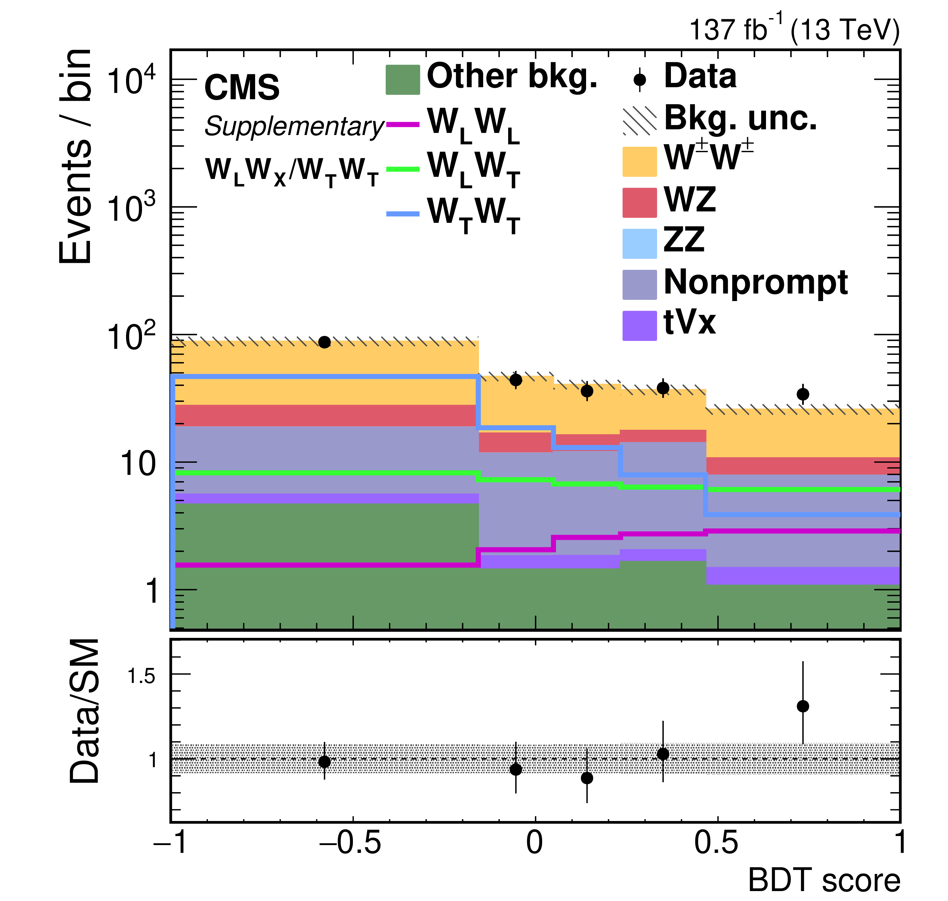
png pdf	Figure 3-d: Distribution of the output score of the inclusive BDT in the $ {\mathrm{W} ^\pm \mathrm{W} ^\pm} $ SR. The predicted yields are shown with their best fit normalizations from the simultaneous fit. The histograms for the $ {\mathrm{W} ^\pm \mathrm{W} ^\pm} $ process include the contributions from the $ {\mathrm{W} ^\pm _{\mathrm {L}}\mathrm{W} ^\pm _{\mathrm {L}}} $, $ {\mathrm{W} ^\pm _{\mathrm {L}}\mathrm{W} ^\pm _{\mathrm {T}}} $, and $ {\mathrm{W} ^\pm _{\mathrm {T}}\mathrm{W} ^\pm _{\mathrm {T}}} $ processes (shown as solid lines), QCD $ {\mathrm{W} ^\pm \mathrm{W} ^\pm} $, and interference. The histograms for other backgrounds include the contributions from double parton scattering, VVV, and from oppositely charged dilepton final states from ${\mathrm{t} \mathrm{\bar{t}}} $, $\mathrm{t} \mathrm{W} $, $\mathrm{W} ^{+}\mathrm{W} ^{-}$, and Drell-Yan processes. The overflow is included in the last bin. The bottom panel shows the ratio of the number of events observed in data to that of the total SM prediction. The gray bands represent the uncertainties in the predicted yields. The vertical bars represent the statistical uncertainties in the data.
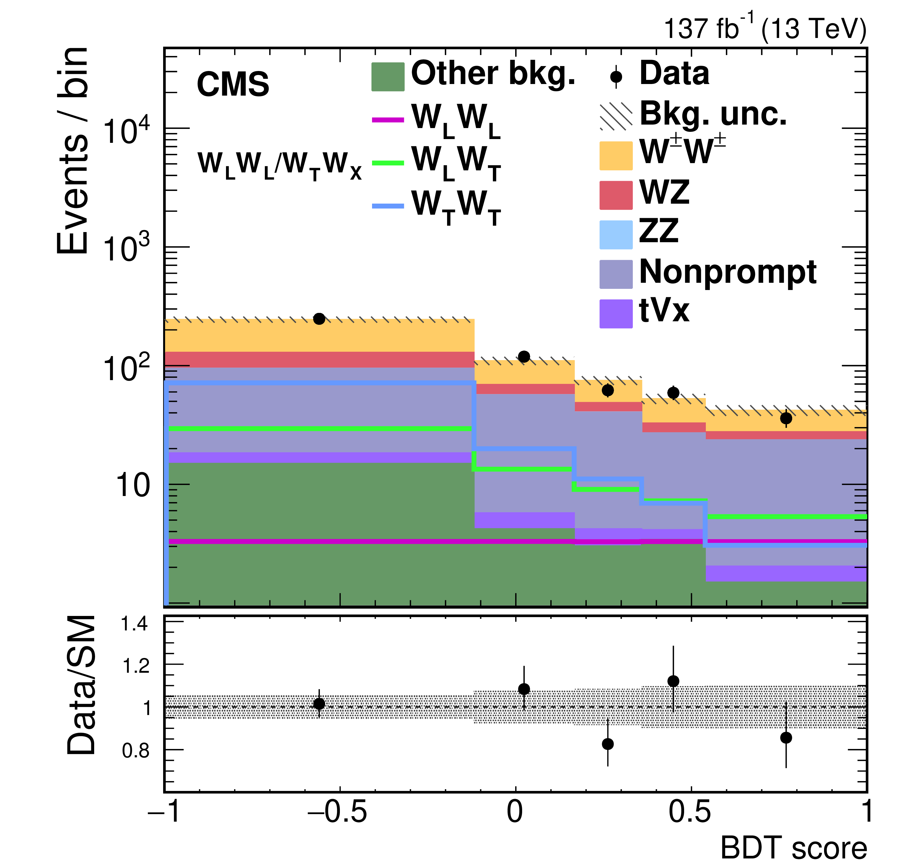
png pdf	Figure 4: Distributions of the output score of the signal BDT used for the $ {\mathrm{W} ^\pm _{\mathrm {L}}\mathrm{W} ^\pm _{\mathrm {L}}} $ and $ {\mathrm{W} ^\pm _{X}\mathrm{W} ^\pm _{\mathrm {T}}} $ cross section measurements (left) and of the output score of the signal BDT used for the $ {\mathrm{W} ^\pm _{\mathrm {L}}\mathrm{W} ^\pm _{X}} $ and $ {\mathrm{W} ^\pm _{\mathrm {T}}\mathrm{W} ^\pm _{\mathrm {T}}} $ cross section measurements (right). The predicted yields are shown with their best fit normalizations from the simultaneous fit. The histograms for the $ {\mathrm{W} ^\pm \mathrm{W} ^\pm} $ process include the contributions from the $ {\mathrm{W} ^\pm _{\mathrm {L}}\mathrm{W} ^\pm _{\mathrm {L}}} $, $ {\mathrm{W} ^\pm _{\mathrm {L}}\mathrm{W} ^\pm _{\mathrm {T}}} $, and $ {\mathrm{W} ^\pm _{\mathrm {T}}\mathrm{W} ^\pm _{\mathrm {T}}} $ processes (shown as solid lines), QCD $ {\mathrm{W} ^\pm \mathrm{W} ^\pm} $, and interference. The histograms for other backgrounds include the contributions from double parton scattering, VVV, and from oppositely charged dilepton final states from ${\mathrm{t} \mathrm{\bar{t}}} $, $\mathrm{t} \mathrm{W} $, $\mathrm{W} ^{+}\mathrm{W} ^{-}$, and Drell-Yan processes. The bottom panel in each figure shows the ratio of the number of events observed in data to that of the total SM prediction. The gray bands represent the uncertainties in the predicted yields. The vertical bars represent the statistical uncertainties in the data.
png pdf	Figure 4-a: Distribution of the output score of the signal BDT used for the $ {\mathrm{W} ^\pm _{\mathrm {L}}\mathrm{W} ^\pm _{\mathrm {L}}} $ and $ {\mathrm{W} ^\pm _{X}\mathrm{W} ^\pm _{\mathrm {T}}} $ cross section measurements. The predicted yields are shown with their best fit normalizations from the simultaneous fit. The histograms for the $ {\mathrm{W} ^\pm \mathrm{W} ^\pm} $ process include the contributions from the $ {\mathrm{W} ^\pm _{\mathrm {L}}\mathrm{W} ^\pm _{\mathrm {L}}} $, $ {\mathrm{W} ^\pm _{\mathrm {L}}\mathrm{W} ^\pm _{\mathrm {T}}} $, and $ {\mathrm{W} ^\pm _{\mathrm {T}}\mathrm{W} ^\pm _{\mathrm {T}}} $ processes (shown as solid lines), QCD $ {\mathrm{W} ^\pm \mathrm{W} ^\pm} $, and interference. The histograms for other backgrounds include the contributions from double parton scattering, VVV, and from oppositely charged dilepton final states from ${\mathrm{t} \mathrm{\bar{t}}} $, $\mathrm{t} \mathrm{W} $, $\mathrm{W} ^{+}\mathrm{W} ^{-}$, and Drell-Yan processes. The bottom panel in each figure shows the ratio of the number of events observed in data to that of the total SM prediction. The gray bands represent the uncertainties in the predicted yields. The vertical bars represent the statistical uncertainties in the data.
png pdf	Figure 4-b: Distribution of the output score of the signal BDT used for the $ {\mathrm{W} ^\pm _{\mathrm {L}}\mathrm{W} ^\pm _{X}} $ and $ {\mathrm{W} ^\pm _{\mathrm {T}}\mathrm{W} ^\pm _{\mathrm {T}}} $ cross section measurements. The predicted yields are shown with their best fit normalizations from the simultaneous fit. The histograms for the $ {\mathrm{W} ^\pm \mathrm{W} ^\pm} $ process include the contributions from the $ {\mathrm{W} ^\pm _{\mathrm {L}}\mathrm{W} ^\pm _{\mathrm {L}}} $, $ {\mathrm{W} ^\pm _{\mathrm {L}}\mathrm{W} ^\pm _{\mathrm {T}}} $, and $ {\mathrm{W} ^\pm _{\mathrm {T}}\mathrm{W} ^\pm _{\mathrm {T}}} $ processes (shown as solid lines), QCD $ {\mathrm{W} ^\pm \mathrm{W} ^\pm} $, and interference. The histograms for other backgrounds include the contributions from double parton scattering, VVV, and from oppositely charged dilepton final states from ${\mathrm{t} \mathrm{\bar{t}}} $, $\mathrm{t} \mathrm{W} $, $\mathrm{W} ^{+}\mathrm{W} ^{-}$, and Drell-Yan processes. The bottom panel in each figure shows the ratio of the number of events observed in data to that of the total SM prediction. The gray bands represent the uncertainties in the predicted yields. The vertical bars represent the statistical uncertainties in the data.
png pdf	Figure 5: Profile likelihood scan as a function of the $ {\mathrm{W} ^\pm _{\mathrm {L}}\mathrm{W} ^\pm _{\mathrm {L}}} $ cross section. The red (blue) line represents the expected values in the background-only hypothesis, i.e., assuming no contribution from the $ {\mathrm{W} ^\pm _{\mathrm {L}}\mathrm{W} ^\pm _{\mathrm {L}}} $ process, considering all systematic uncertainties (only statistical ones). The green line shows the expected values for the signal-plus-background hypothesis. The observed values are represented by the black line.

Tables
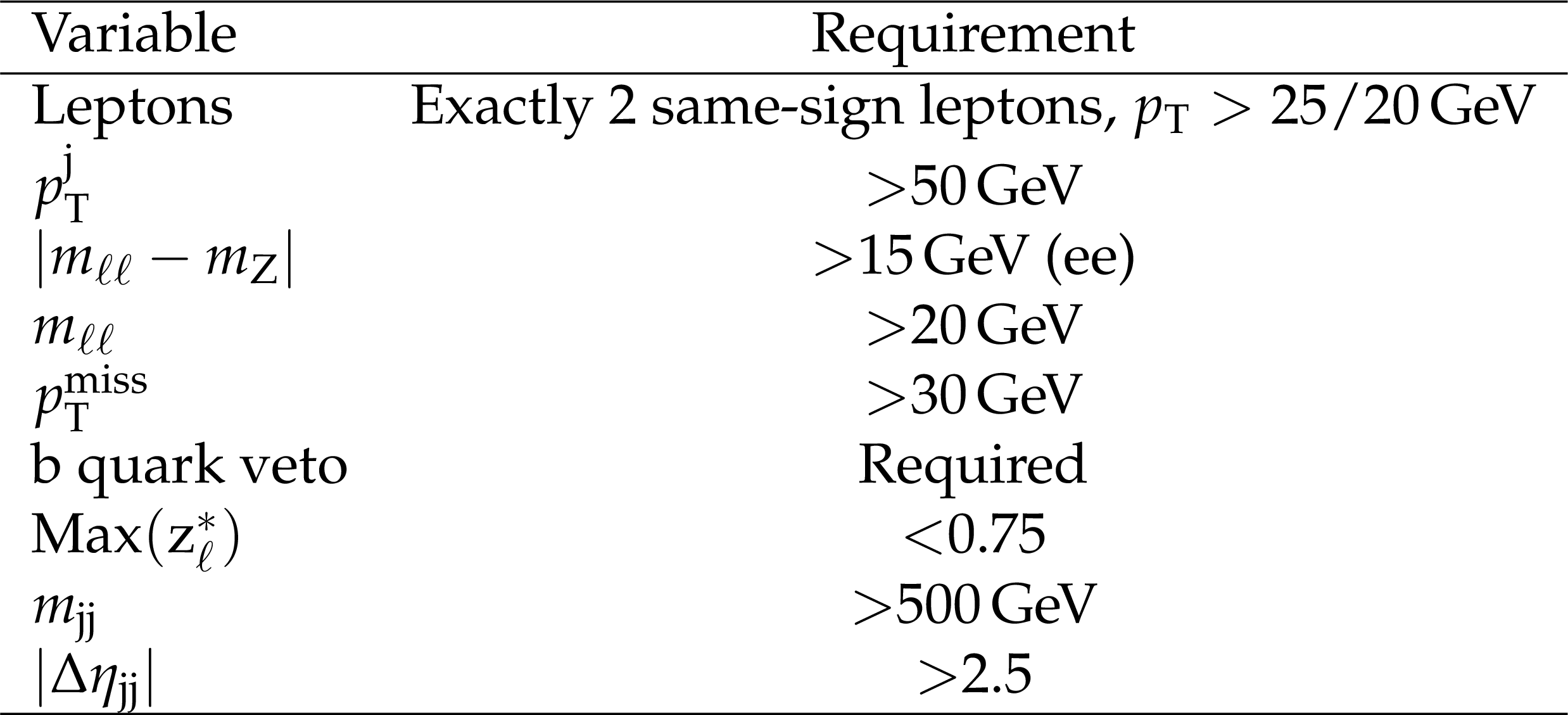
png pdf	Table 1: Summary of the requirements defining the $ {\mathrm{W} ^\pm \mathrm{W} ^\pm} $ SR. The $ {| {m_{\ell \ell}} - m_{\mathrm{Z}} |}$ requirement is applied to the dielectron final state only.
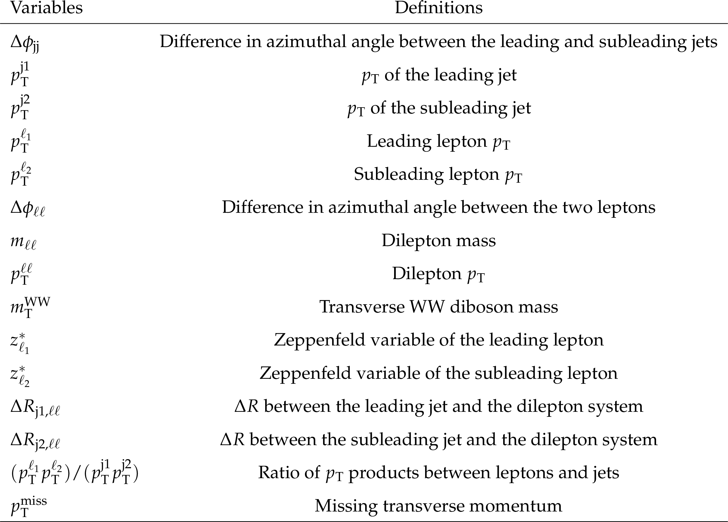
png pdf	Table 2: List and description of all the input variables for the signal BDT trainings.
png pdf	Table 3: List and description of the input variables for the inclusive BDT training.
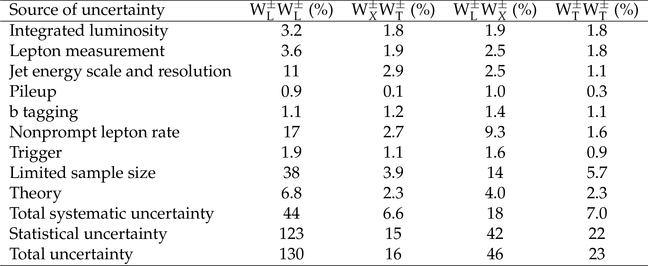
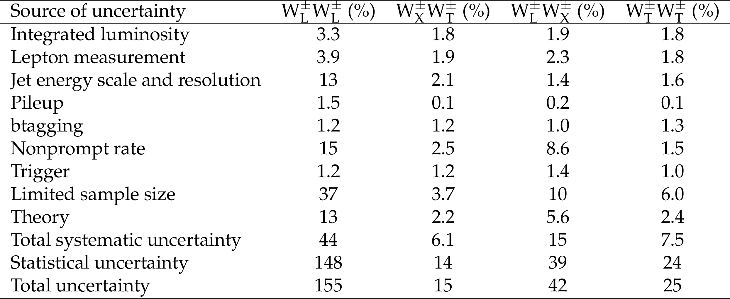
png pdf	Table 4: Systematic uncertainties of the $ {\mathrm{W} ^\pm _{\mathrm {L}}\mathrm{W} ^\pm _{\mathrm {L}}} $ and $ {\mathrm{W} ^\pm _{X}\mathrm{W} ^\pm _{\mathrm {T}}} $, and $ {\mathrm{W} ^\pm _{\mathrm {L}}\mathrm{W} ^\pm _{X}} $ and $ {\mathrm{W} ^\pm _{\mathrm {T}}\mathrm{W} ^\pm _{\mathrm {T}}} $ cross section measurements in units of percent.
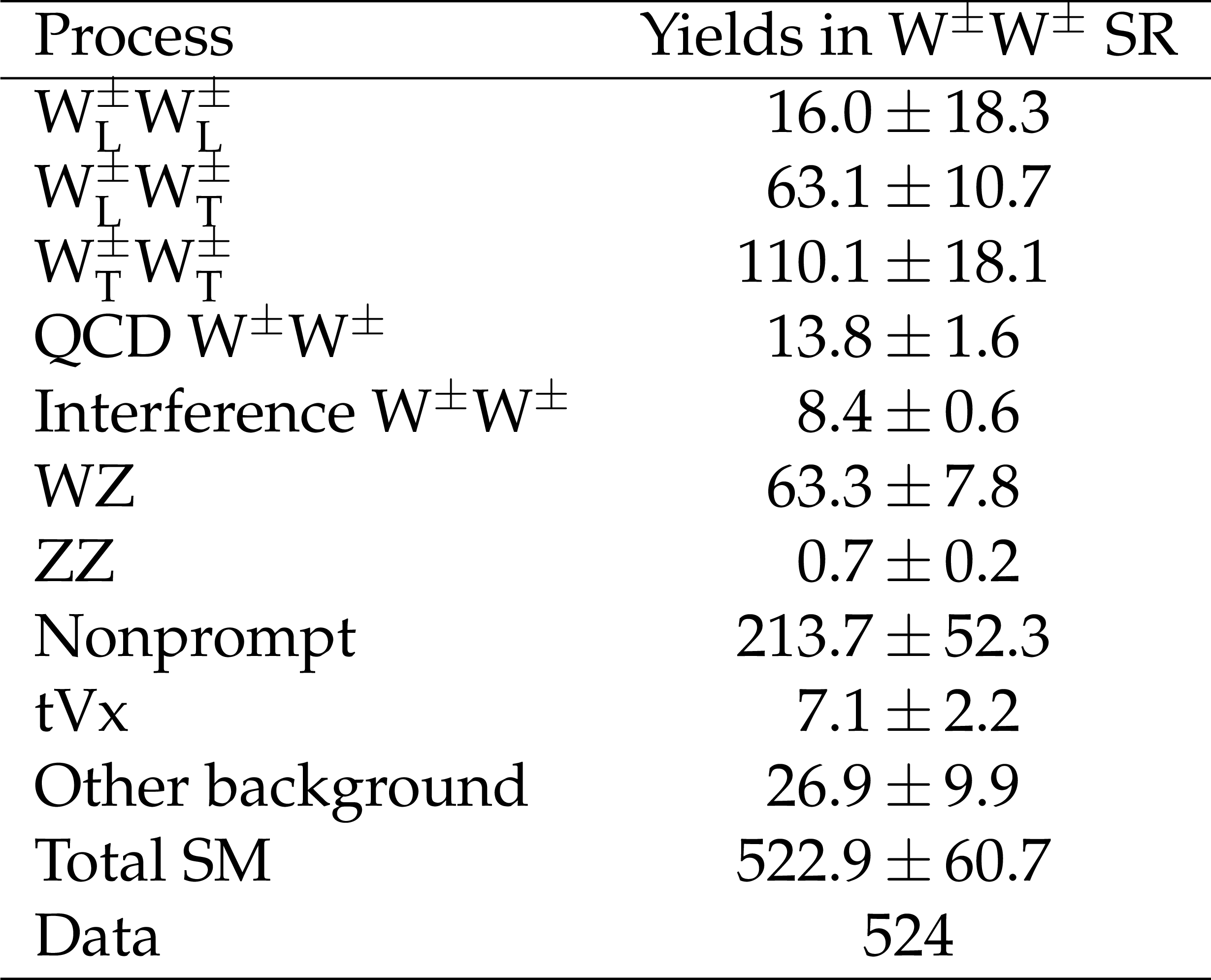
png pdf	Table 5: Expected yields from various SM processes and observed data events in $ {\mathrm{W} ^\pm \mathrm{W} ^\pm} $ SR. The combination of the statistical and systematic uncertainties is shown. The expected yields are shown with their best fit normalizations from the simultaneous fit for the $ {\mathrm{W} ^\pm _{\mathrm {L}}\mathrm{W} ^\pm _{\mathrm {L}}} $ and $ {\mathrm{W} ^\pm _{X}\mathrm{W} ^\pm _{\mathrm {T}}} $ cross sections. The $ {\mathrm{W} ^\pm _{\mathrm {L}}\mathrm{W} ^\pm _{\mathrm {T}}} $ and $ {\mathrm{W} ^\pm _{\mathrm {T}}\mathrm{W} ^\pm _{\mathrm {T}}} $ yields are obtained from the $ {\mathrm{W} ^\pm _{X}\mathrm{W} ^\pm _{\mathrm {T}}} $ yield assuming the SM prediction for the ratio of the yields. The $ {\mathrm{t} \mathrm{V} \mathrm {x}} $ background yield includes the contributions from ${\mathrm{t} \mathrm{\bar{t}}} \mathrm{V} $ and $ {\mathrm{t} \mathrm{Z} \mathrm{q}} $ processes.
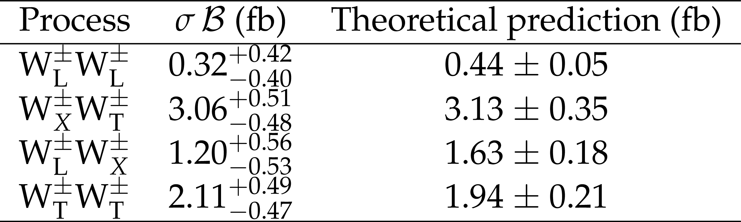
png pdf	Table 6: Measured fiducial cross sections for the $ {\mathrm{W} ^\pm _{\mathrm {L}}\mathrm{W} ^\pm _{\mathrm {L}}} $ and $ {\mathrm{W} ^\pm _{X}\mathrm{W} ^\pm _{\mathrm {T}}} $ processes, and for the $ {\mathrm{W} ^\pm _{\mathrm {L}}\mathrm{W} ^\pm _{X}} $ and $ {\mathrm{W} ^\pm _{\mathrm {T}}\mathrm{W} ^\pm _{\mathrm {T}}} $ processes for the helicity eigenstates defined in the $ {\mathrm{W} ^\pm \mathrm{W} ^\pm} $ center-of-mass frame. The combination of the statistical and systematic uncertainties is shown. The theoretical predictions including the $\mathcal {O}({\alpha _\mathrm {S}} \alpha ^6)$ and $\mathcal {O}(\alpha ^7)$ corrections to the MadGraph 5\_aMC@NLO LO cross sections, as described in the text, are also shown. The theoretical uncertainties include statistical, PDF, and LO scale uncertainties; $\mathcal {B}$ is the branching fraction for $\mathrm{W} \mathrm{W} \to \ell \nu \ell '\nu $ [55].
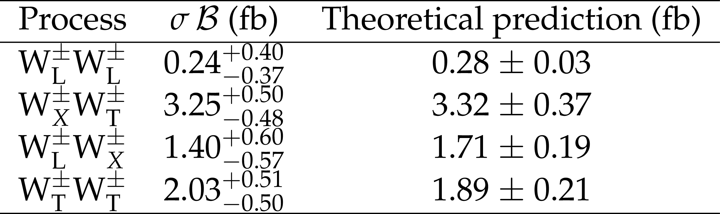
png pdf	Table 7: Measured fiducial cross sections for the $ {\mathrm{W} ^\pm _{\mathrm {L}}\mathrm{W} ^\pm _{\mathrm {L}}} $ and $ {\mathrm{W} ^\pm _{X}\mathrm{W} ^\pm _{\mathrm {T}}} $ processes, and for the $ {\mathrm{W} ^\pm _{\mathrm {L}}\mathrm{W} ^\pm _{X}} $ and $ {\mathrm{W} ^\pm _{\mathrm {T}}\mathrm{W} ^\pm _{\mathrm {T}}} $ processes for the helicity eigenstates defined in the parton-parton center-of-mass frame. The combination of the statistical and systematic uncertainties is shown. The theoretical predictions including the $\mathcal {O}({\alpha _\mathrm {S}} \alpha ^6)$ and $\mathcal {O}(\alpha ^7)$ corrections to the MadGraph 5\_aMC@NLO LO cross sections, as described in the text, are also shown. The theoretical uncertainties include statistical, PDF, and LO scale uncertainties; $\mathcal {B}$ is the branching fraction for $\mathrm{W} \mathrm{W} \to \ell \nu \ell '\nu $ [55].

Summary

The first measurements of production cross sections for polarized same-sign ${\mathrm{W}^\pm\mathrm{W}^\pm} $ boson pairs are reported. The measurements are based on a sample of proton-proton collisions at a center-of-mass energy of 13 TeV collected by the CMS detector at the LHC, corresponding to an integrated luminosity of 137 fb$^{-1}$ . Events are selected by requiring exactly two same-sign leptons (electrons or muons), moderate missing transverse momentum, and two jets with a large rapidity separation and a high dijet mass. Boosted decision trees are used to separate between the polarized scattering processes by exploiting the kinematic differences. An observed (expected) 95% confidence level upper limit on the production cross section for longitudinally polarized same-sign ${\mathrm{W}^\pm\mathrm{W}^\pm} $ boson pairs of 1.17 (0.88) fb is reported with the helicity eigenstates defined in the ${\mathrm{W}^\pm\mathrm{W}^\pm} $ center-of-mass reference frame. The electroweak production of the ${\mathrm{W}^\pm\mathrm{W}^\pm} $ boson pairs where at least one of the W bosons is longitudinally polarized is measured with an observed (expected) significance of 2.3 (3.1) standard deviations. Results are also reported with the polarizations defined in the parton-parton center-of-mass reference frame. The measured cross section values agree with the standard model predictions.

Additional Figures
png pdf	Additional Figure 1: Distributions of the output score of the signal BDT used for the $ {{\mathrm {W}}^\pm _{\mathrm {L}} {\mathrm {W}}^\pm _{\mathrm {L}}} $ and $ {{\mathrm {W}}^\pm _{\mathrm {X}} {\mathrm {W}}^\pm _{\mathrm {T}}} $ cross section measurements (left) and of the output score of the signal BDT used for the $ {{\mathrm {W}}^\pm _{\mathrm {L}} {\mathrm {W}}^\pm _{\mathrm {X}}} $ and $ {{\mathrm {W}}^\pm _{\mathrm {T}} {\mathrm {W}}^\pm _{\mathrm {T}}} $ cross section measurements (right), after requiring the output score of the inclusive BDT greater than 0. The predicted yields are shown with their best fit normalizations from the simultaneous fit. The histograms for $ {{\mathrm {W}}^\pm {\mathrm {W}}^\pm} $ process include the contributions from the $ {{\mathrm {W}}^\pm _{\mathrm {L}} {\mathrm {W}}^\pm _{\mathrm {L}}} $, $ {{\mathrm {W}}^\pm _{\mathrm {L}} {\mathrm {W}}^\pm _{\mathrm {T}}} $, and $ {{\mathrm {W}}^\pm _{\mathrm {T}} {\mathrm {W}}^\pm _{\mathrm {T}}} $ processes (shown as solid lines), QCD $ {{\mathrm {W}}^\pm {\mathrm {W}}^\pm} $, and interference. The histograms for $\mathrm{tVx}$ backgrounds include the contributions from $ {{\mathrm {t}\overline {\mathrm {t}}}} \mathrm{V}$ and $ {\mathrm {t} {\mathrm {Z}} {\mathrm {q}}} $ processes. The histograms for other backgrounds include the contributions from double parton scattering and VVV processes. The bottom panel in each figure shows the ratio of the number of events observed in data to that of the total SM prediction. The gray bands represent the uncertainties in the predicted yields.
png pdf	Additional Figure 1-a: Distribution of the output score of the signal BDT used for the $ {{\mathrm {W}}^\pm _{\mathrm {L}} {\mathrm {W}}^\pm _{\mathrm {L}}} $ and $ {{\mathrm {W}}^\pm _{\mathrm {X}} {\mathrm {W}}^\pm _{\mathrm {T}}} $ cross section measurements, after requiring the output score of the inclusive BDT greater than 0. The predicted yields are shown with their best fit normalizations from the simultaneous fit. The histograms for $ {{\mathrm {W}}^\pm {\mathrm {W}}^\pm} $ process include the contributions from the $ {{\mathrm {W}}^\pm _{\mathrm {L}} {\mathrm {W}}^\pm _{\mathrm {L}}} $, $ {{\mathrm {W}}^\pm _{\mathrm {L}} {\mathrm {W}}^\pm _{\mathrm {T}}} $, and $ {{\mathrm {W}}^\pm _{\mathrm {T}} {\mathrm {W}}^\pm _{\mathrm {T}}} $ processes (shown as solid lines), QCD $ {{\mathrm {W}}^\pm {\mathrm {W}}^\pm} $, and interference. The histograms for $\mathrm{tVx}$ backgrounds include the contributions from $ {{\mathrm {t}\overline {\mathrm {t}}}} \mathrm{V}$ and $ {\mathrm {t} {\mathrm {Z}} {\mathrm {q}}} $ processes. The histograms for other backgrounds include the contributions from double parton scattering and VVV processes. The bottom panel shows the ratio of the number of events observed in data to that of the total SM prediction. The gray bands represent the uncertainties in the predicted yields.
png pdf	Additional Figure 1-b: Distribution of the output score of the signal BDT used for the $ {{\mathrm {W}}^\pm _{\mathrm {L}} {\mathrm {W}}^\pm _{\mathrm {X}}} $ and $ {{\mathrm {W}}^\pm _{\mathrm {T}} {\mathrm {W}}^\pm _{\mathrm {T}}} $ cross section measurements, after requiring the output score of the inclusive BDT greater than 0. The predicted yields are shown with their best fit normalizations from the simultaneous fit. The histograms for $ {{\mathrm {W}}^\pm {\mathrm {W}}^\pm} $ process include the contributions from the $ {{\mathrm {W}}^\pm _{\mathrm {L}} {\mathrm {W}}^\pm _{\mathrm {L}}} $, $ {{\mathrm {W}}^\pm _{\mathrm {L}} {\mathrm {W}}^\pm _{\mathrm {T}}} $, and $ {{\mathrm {W}}^\pm _{\mathrm {T}} {\mathrm {W}}^\pm _{\mathrm {T}}} $ processes (shown as solid lines), QCD $ {{\mathrm {W}}^\pm {\mathrm {W}}^\pm} $, and interference. The histograms for $\mathrm{tVx}$ backgrounds include the contributions from $ {{\mathrm {t}\overline {\mathrm {t}}}} \mathrm{V}$ and $ {\mathrm {t} {\mathrm {Z}} {\mathrm {q}}} $ processes. The histograms for other backgrounds include the contributions from double parton scattering and VVV processes. The bottom panel shows the ratio of the number of events observed in data to that of the total SM prediction. The gray bands represent the uncertainties in the predicted yields.
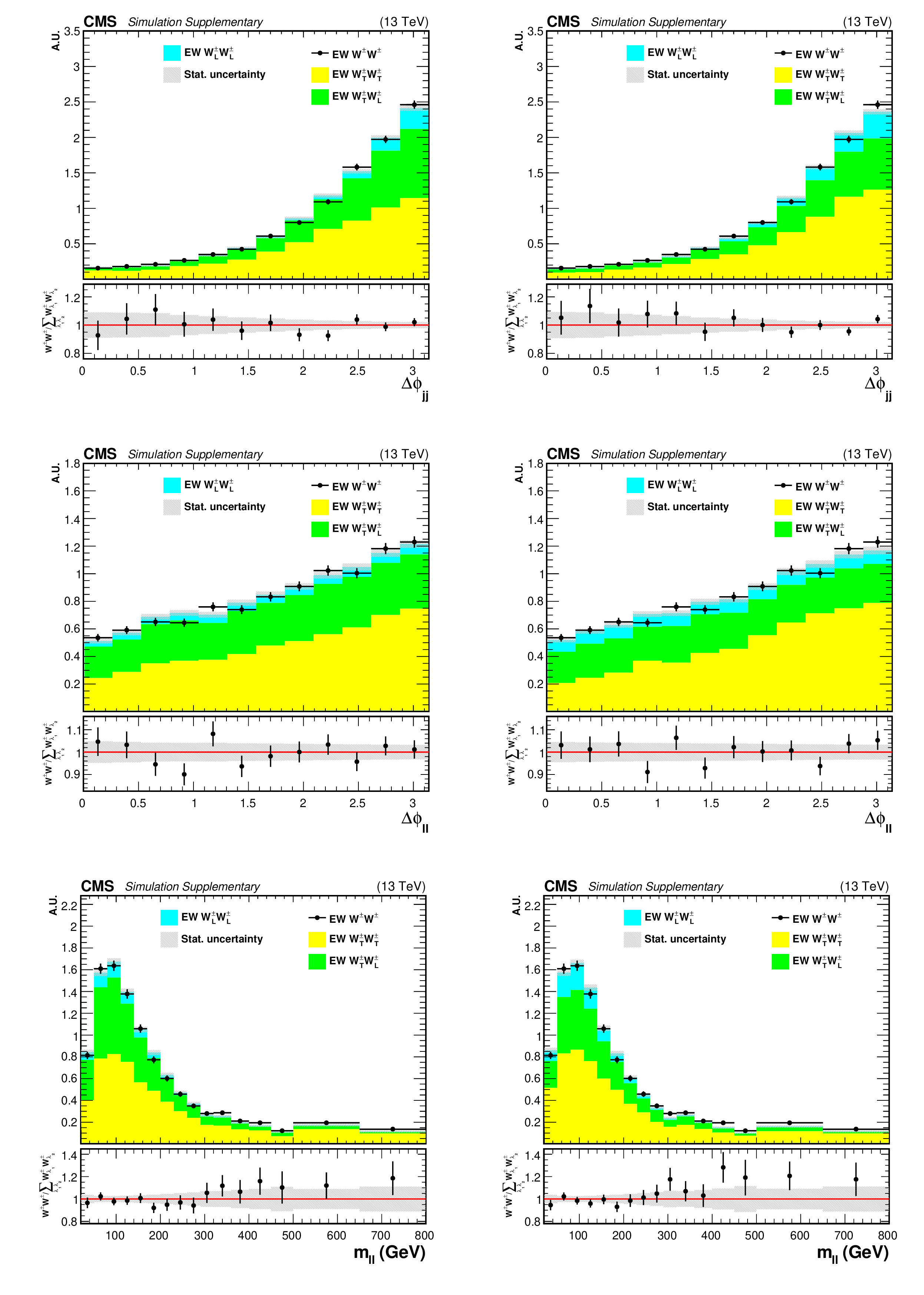
png pdf	Additional Figure 2: Generator level distributions of $ {\Delta \phi _{{\mathrm {j}} {\mathrm {j}}}} $ (upper), $\Delta \phi _{\ell \ell}$ (center), and $ {m_{\ell \ell}} $ (lower) in the fiducial region for the $ {{\mathrm {W}}^\pm _{\mathrm {L}} {\mathrm {W}}^\pm _{\mathrm {L}}} $, $ {{\mathrm {W}}^\pm _{\mathrm {L}} {\mathrm {W}}^\pm _{\mathrm {T}}} $, and $ {{\mathrm {W}}^\pm _{\mathrm {T}} {\mathrm {W}}^\pm _{\mathrm {T}}} $ processes with the helicity eigenstates defined in the parton-parton (left) and $ {{\mathrm {W}}^\pm {\mathrm {W}}^\pm} $ (right) center-of-mass reference frames. The distributions are also shown for the unpolarized EW $ {{\mathrm {W}}^\pm {\mathrm {W}}^\pm} $ process. The bottom panel in each figure shows the ratio of the contribution of the unpolarized $ {{\mathrm {W}}^\pm {\mathrm {W}}^\pm} $ process to that of the sum of the $ {{\mathrm {W}}^\pm _{\mathrm {L}} {\mathrm {W}}^\pm _{\mathrm {L}}} $, $ {{\mathrm {W}}^\pm _{\mathrm {L}} {\mathrm {W}}^\pm _{\mathrm {T}}} $, and $ {{\mathrm {W}}^\pm _{\mathrm {T}} {\mathrm {W}}^\pm _{\mathrm {T}}} $ processes. The gray bands represent the statistical uncertainties associated with the limited number of simulated events.
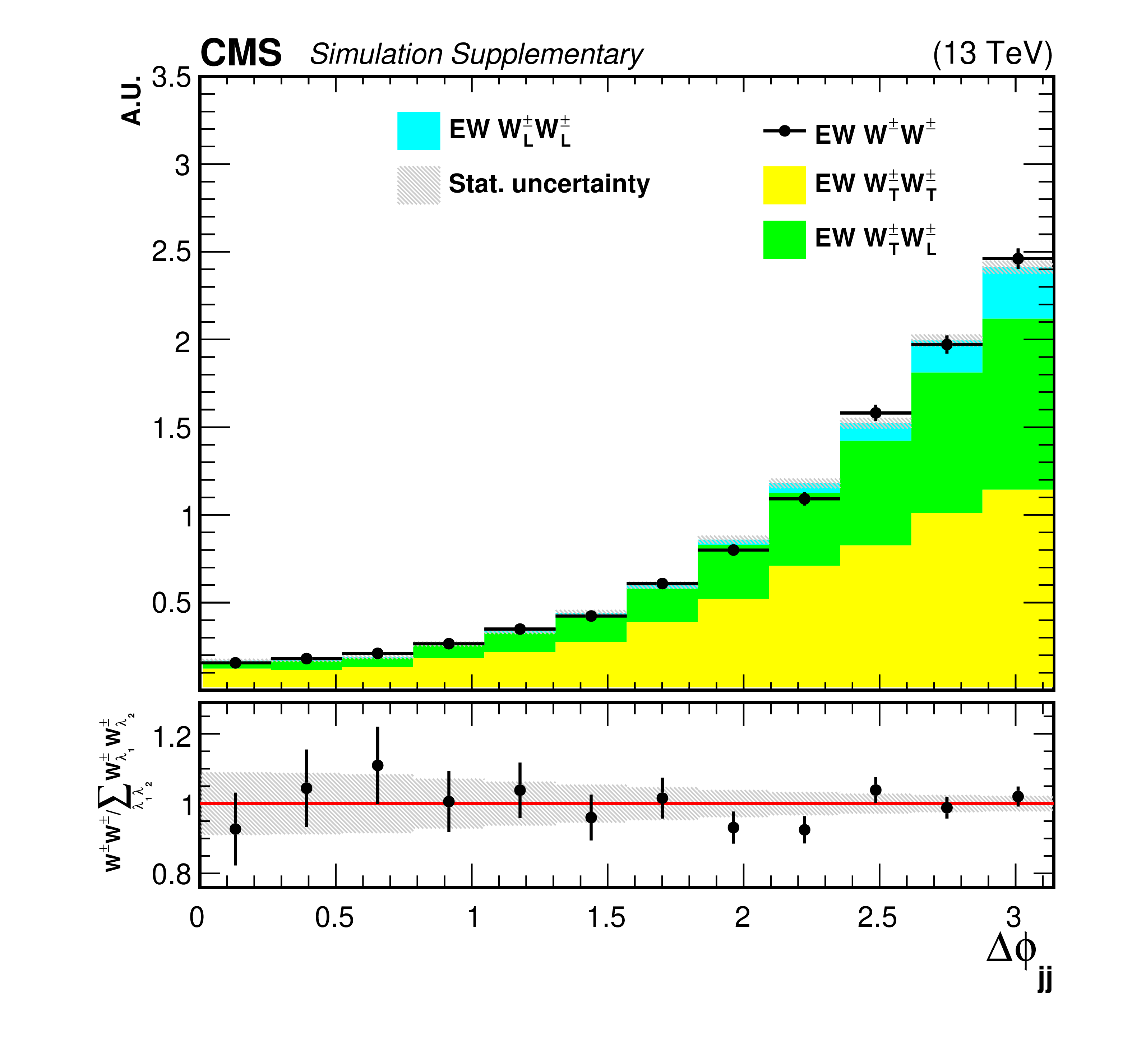
png pdf	Additional Figure 2-a: Generator level distributions of $ {\Delta \phi _{{\mathrm {j}} {\mathrm {j}}}} $ in the fiducial region for the $ {{\mathrm {W}}^\pm _{\mathrm {L}} {\mathrm {W}}^\pm _{\mathrm {L}}} $, $ {{\mathrm {W}}^\pm _{\mathrm {L}} {\mathrm {W}}^\pm _{\mathrm {T}}} $, and $ {{\mathrm {W}}^\pm _{\mathrm {T}} {\mathrm {W}}^\pm _{\mathrm {T}}} $ processes with the helicity eigenstates defined in the parton-parton center-of-mass reference frame. The distributions are also shown for the unpolarized EW $ {{\mathrm {W}}^\pm {\mathrm {W}}^\pm} $ process. The bottom panel shows the ratio of the contribution of the unpolarized $ {{\mathrm {W}}^\pm {\mathrm {W}}^\pm} $ process to that of the sum of the $ {{\mathrm {W}}^\pm _{\mathrm {L}} {\mathrm {W}}^\pm _{\mathrm {L}}} $, $ {{\mathrm {W}}^\pm _{\mathrm {L}} {\mathrm {W}}^\pm _{\mathrm {T}}} $, and $ {{\mathrm {W}}^\pm _{\mathrm {T}} {\mathrm {W}}^\pm _{\mathrm {T}}} $ processes. The gray bands represent the statistical uncertainties associated with the limited number of simulated events.
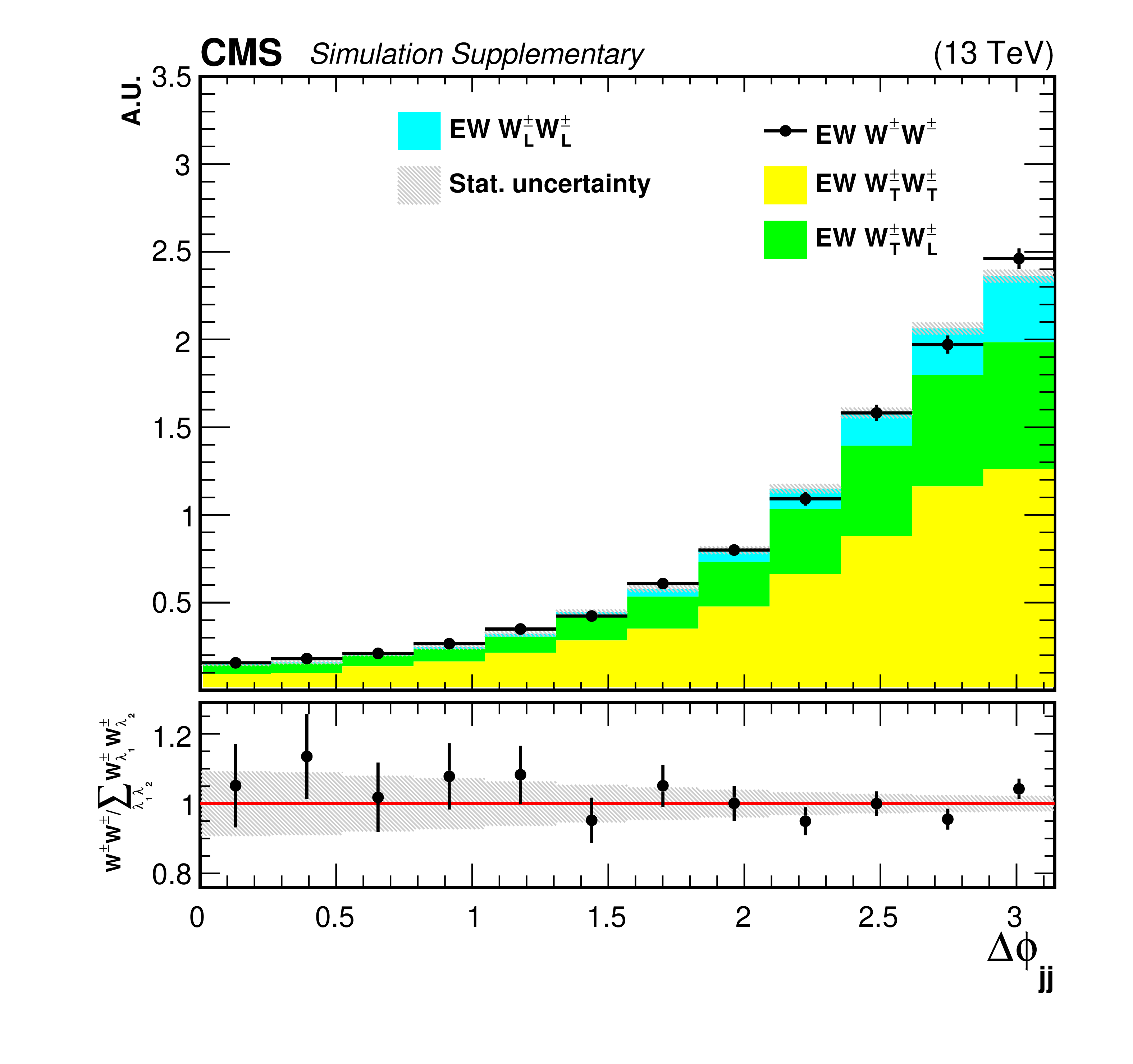
png pdf	Additional Figure 2-b: Generator level distributions of $ {\Delta \phi _{{\mathrm {j}} {\mathrm {j}}}} $ in the fiducial region for the $ {{\mathrm {W}}^\pm _{\mathrm {L}} {\mathrm {W}}^\pm _{\mathrm {L}}} $, $ {{\mathrm {W}}^\pm _{\mathrm {L}} {\mathrm {W}}^\pm _{\mathrm {T}}} $, and $ {{\mathrm {W}}^\pm _{\mathrm {T}} {\mathrm {W}}^\pm _{\mathrm {T}}} $ processes with the helicity eigenstates defined in the $ {{\mathrm {W}}^\pm {\mathrm {W}}^\pm} $ center-of-mass reference frame. The distributions are also shown for the unpolarized EW $ {{\mathrm {W}}^\pm {\mathrm {W}}^\pm} $ process. The bottom panel shows the ratio of the contribution of the unpolarized $ {{\mathrm {W}}^\pm {\mathrm {W}}^\pm} $ process to that of the sum of the $ {{\mathrm {W}}^\pm _{\mathrm {L}} {\mathrm {W}}^\pm _{\mathrm {L}}} $, $ {{\mathrm {W}}^\pm _{\mathrm {L}} {\mathrm {W}}^\pm _{\mathrm {T}}} $, and $ {{\mathrm {W}}^\pm _{\mathrm {T}} {\mathrm {W}}^\pm _{\mathrm {T}}} $ processes. The gray bands represent the statistical uncertainties associated with the limited number of simulated events.
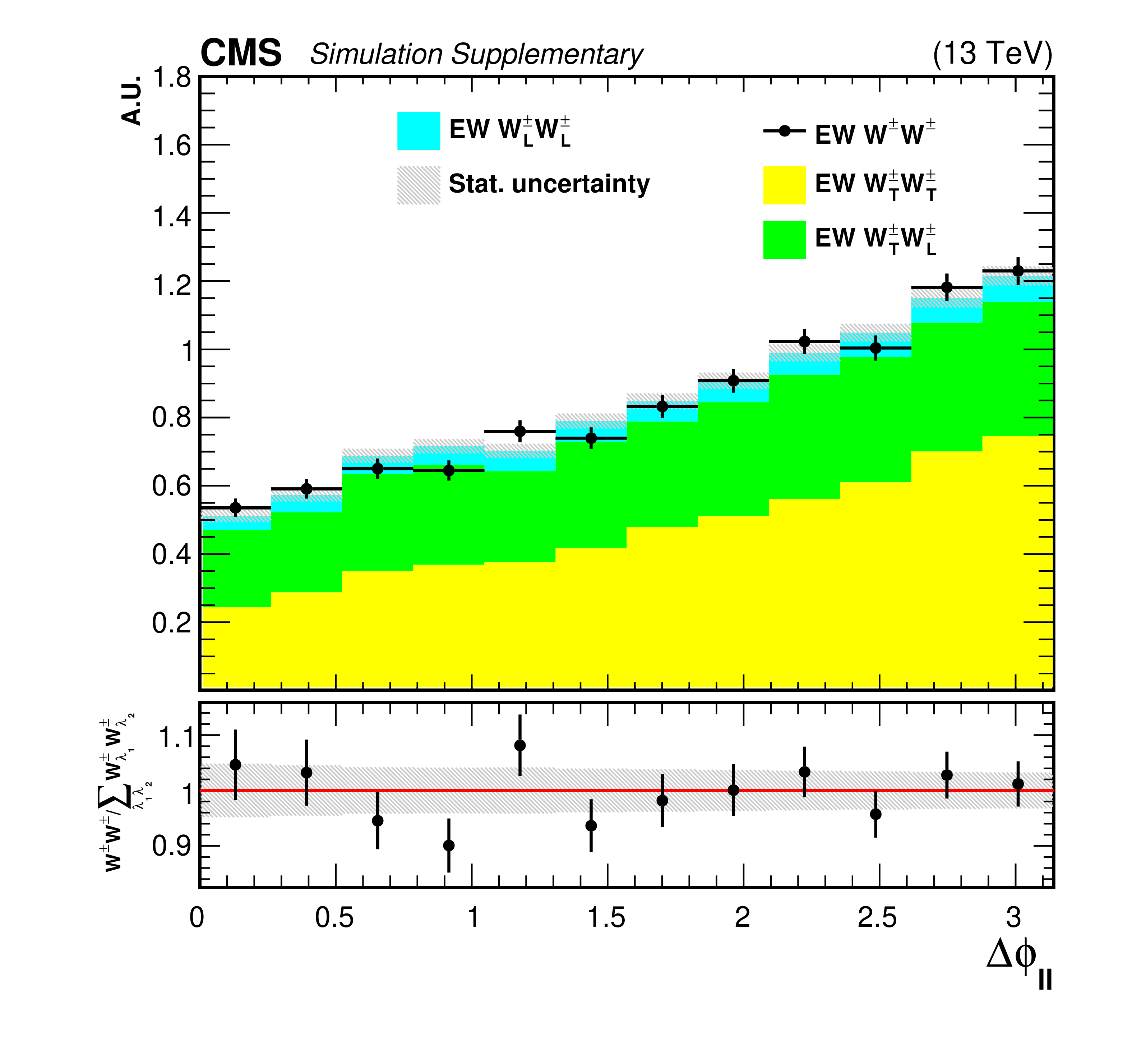
png pdf	Additional Figure 2-c: Generator level distributions of $\Delta \phi _{\ell \ell}$ in the fiducial region for the $ {{\mathrm {W}}^\pm _{\mathrm {L}} {\mathrm {W}}^\pm _{\mathrm {L}}} $, $ {{\mathrm {W}}^\pm _{\mathrm {L}} {\mathrm {W}}^\pm _{\mathrm {T}}} $, and $ {{\mathrm {W}}^\pm _{\mathrm {T}} {\mathrm {W}}^\pm _{\mathrm {T}}} $ processes with the helicity eigenstates defined in the parton-parton center-of-mass reference frame. The distributions are also shown for the unpolarized EW $ {{\mathrm {W}}^\pm {\mathrm {W}}^\pm} $ process. The bottom panel shows the ratio of the contribution of the unpolarized $ {{\mathrm {W}}^\pm {\mathrm {W}}^\pm} $ process to that of the sum of the $ {{\mathrm {W}}^\pm _{\mathrm {L}} {\mathrm {W}}^\pm _{\mathrm {L}}} $, $ {{\mathrm {W}}^\pm _{\mathrm {L}} {\mathrm {W}}^\pm _{\mathrm {T}}} $, and $ {{\mathrm {W}}^\pm _{\mathrm {T}} {\mathrm {W}}^\pm _{\mathrm {T}}} $ processes. The gray bands represent the statistical uncertainties associated with the limited number of simulated events.
png pdf	Additional Figure 2-d: Generator level distributions of $\Delta \phi _{\ell \ell}$ in the fiducial region for the $ {{\mathrm {W}}^\pm _{\mathrm {L}} {\mathrm {W}}^\pm _{\mathrm {L}}} $, $ {{\mathrm {W}}^\pm _{\mathrm {L}} {\mathrm {W}}^\pm _{\mathrm {T}}} $, and $ {{\mathrm {W}}^\pm _{\mathrm {T}} {\mathrm {W}}^\pm _{\mathrm {T}}} $ processes with the helicity eigenstates defined in the $ {{\mathrm {W}}^\pm {\mathrm {W}}^\pm} $ center-of-mass reference frame. The distributions are also shown for the unpolarized EW $ {{\mathrm {W}}^\pm {\mathrm {W}}^\pm} $ process. The bottom panel shows the ratio of the contribution of the unpolarized $ {{\mathrm {W}}^\pm {\mathrm {W}}^\pm} $ process to that of the sum of the $ {{\mathrm {W}}^\pm _{\mathrm {L}} {\mathrm {W}}^\pm _{\mathrm {L}}} $, $ {{\mathrm {W}}^\pm _{\mathrm {L}} {\mathrm {W}}^\pm _{\mathrm {T}}} $, and $ {{\mathrm {W}}^\pm _{\mathrm {T}} {\mathrm {W}}^\pm _{\mathrm {T}}} $ processes. The gray bands represent the statistical uncertainties associated with the limited number of simulated events.
png pdf	Additional Figure 2-e: Generator level distributions of $ {m_{\ell \ell}} $ in the fiducial region for the $ {{\mathrm {W}}^\pm _{\mathrm {L}} {\mathrm {W}}^\pm _{\mathrm {L}}} $, $ {{\mathrm {W}}^\pm _{\mathrm {L}} {\mathrm {W}}^\pm _{\mathrm {T}}} $, and $ {{\mathrm {W}}^\pm _{\mathrm {T}} {\mathrm {W}}^\pm _{\mathrm {T}}} $ processes with the helicity eigenstates defined in the parton-parton center-of-mass reference frame. The distributions are also shown for the unpolarized EW $ {{\mathrm {W}}^\pm {\mathrm {W}}^\pm} $ process. The bottom panel shows the ratio of the contribution of the unpolarized $ {{\mathrm {W}}^\pm {\mathrm {W}}^\pm} $ process to that of the sum of the $ {{\mathrm {W}}^\pm _{\mathrm {L}} {\mathrm {W}}^\pm _{\mathrm {L}}} $, $ {{\mathrm {W}}^\pm _{\mathrm {L}} {\mathrm {W}}^\pm _{\mathrm {T}}} $, and $ {{\mathrm {W}}^\pm _{\mathrm {T}} {\mathrm {W}}^\pm _{\mathrm {T}}} $ processes. The gray bands represent the statistical uncertainties associated with the limited number of simulated events.
png pdf	Additional Figure 2-f: Generator level distributions of $ {m_{\ell \ell}} $ in the fiducial region for the $ {{\mathrm {W}}^\pm _{\mathrm {L}} {\mathrm {W}}^\pm _{\mathrm {L}}} $, $ {{\mathrm {W}}^\pm _{\mathrm {L}} {\mathrm {W}}^\pm _{\mathrm {T}}} $, and $ {{\mathrm {W}}^\pm _{\mathrm {T}} {\mathrm {W}}^\pm _{\mathrm {T}}} $ processes with the helicity eigenstates defined in the $ {{\mathrm {W}}^\pm {\mathrm {W}}^\pm} $ center-of-mass reference frame. The distributions are also shown for the unpolarized EW $ {{\mathrm {W}}^\pm {\mathrm {W}}^\pm} $ process. The bottom panel shows the ratio of the contribution of the unpolarized $ {{\mathrm {W}}^\pm {\mathrm {W}}^\pm} $ process to that of the sum of the $ {{\mathrm {W}}^\pm _{\mathrm {L}} {\mathrm {W}}^\pm _{\mathrm {L}}} $, $ {{\mathrm {W}}^\pm _{\mathrm {L}} {\mathrm {W}}^\pm _{\mathrm {T}}} $, and $ {{\mathrm {W}}^\pm _{\mathrm {T}} {\mathrm {W}}^\pm _{\mathrm {T}}} $ processes. The gray bands represent the statistical uncertainties associated with the limited number of simulated events.
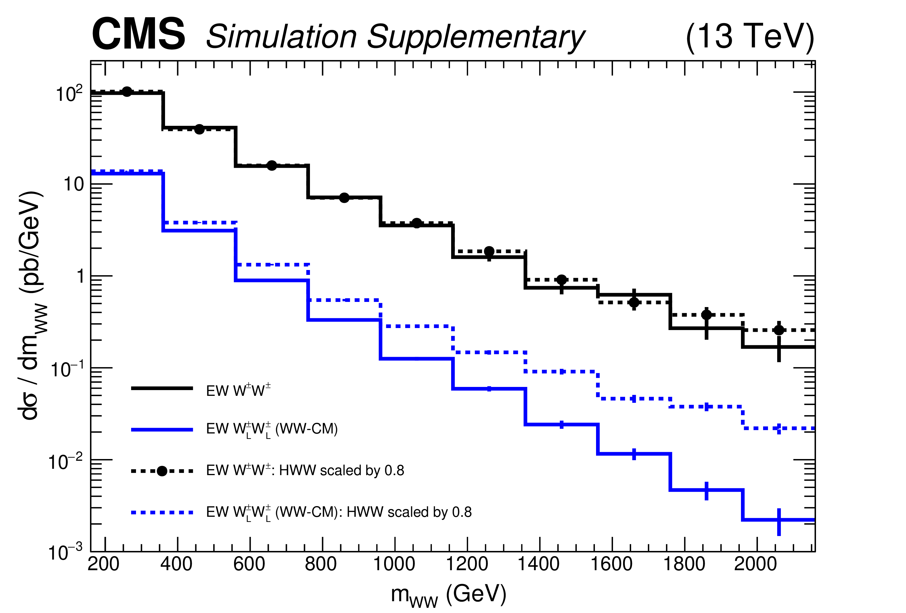
png pdf	Additional Figure 3: Generator level distribution of diboson mass for the SM $ {{\mathrm {W}}^\pm {\mathrm {W}}^\pm} $ (black) and $ {{\mathrm {W}}^\pm _{\mathrm {L}} {\mathrm {W}}^\pm _{\mathrm {L}}} $ (blue) processes with the helicity eigenstates defined in the $ {{\mathrm {W}}^\pm {\mathrm {W}}^\pm} $ center-of-mass reference frame. The distributions are shown requiring jets with $ {p_{\mathrm {T}}} > $ 30 GeV and $ {| \eta |} < $ 5.0, with a dijet mass $ {m_{{\mathrm {j}} {\mathrm {j}}}} > $ 400 GeV and a pseudorapidity separation $ {{| \Delta \eta _{{\mathrm {j}} {\mathrm {j}}} |}} > $ 2.4. The dashed lines show the distributions of the $ {{\mathrm {W}}^\pm {\mathrm {W}}^\pm} $ and $ {{\mathrm {W}}^\pm _{\mathrm {L}} {\mathrm {W}}^\pm _{\mathrm {L}}} $ processes with the value of the Higgs boson coupling to W bosons scaled by a factor of 0.8.

Additional Tables

png pdf

Additional Table 1: Relative systematic uncertainties in the $ {{\mathrm {W}}^\pm _{\mathrm {L}} {\mathrm {W}}^\pm _{\mathrm {L}}} $ and $ {{\mathrm {W}}^\pm _{\mathrm {X}} {\mathrm {W}}^\pm _{\mathrm {T}}} $, and in the $ {{\mathrm {W}}^\pm _{\mathrm {L}} {\mathrm {W}}^\pm _{\mathrm {X}}} $ and $ {{\mathrm {W}}^\pm _{\mathrm {T}} {\mathrm {W}}^\pm _{\mathrm {T}}} $ cross section measurements in units of percent, using the helicity eigenstates in the initial state parton-parton center-of-mass reference frame.

References
1	B. W. Lee, C. Quigg, and H. B. Thacker	The strength of weak interactions at very high-energies and the Higgs boson mass	PRL 38 (1977) 883
2	B. W. Lee, C. Quigg, and H. B. Thacker	Weak interactions at very high-energies: the role of the Higgs boson mass	PRD 16 (1977) 1519
3	ATLAS Collaboration	Observation of a new particle in the search for the standard model Higgs boson with the ATLAS detector at the LHC	PLB 716 (2012) 1	1207.7214
4	CMS Collaboration	Observation of a new boson at a mass of 125 GeV with the CMS experiment at the LHC	PLB 716 (2012) 30	CMS-HIG-12-028 1207.7235
5	CMS Collaboration	Observation of a new boson with mass near 125 GeV in pp collisions at $ \sqrt{s} = $ 7 and 8 TeV	JHEP 06 (2013) 081	CMS-HIG-12-036 1303.4571
6	D. Espriu and B. Yencho	Longitudinal WW scattering in light of the Higgs boson discovery	PRD 87 (2013) 055017	1212.4158
7	J. Chang, K. Cheung, C.-T. Lu, and T.-C. Yuan	WW scattering in the era of post-Higgs-boson discovery	PRD 87 (2013) 093005	1303.6335
8	ATLAS, CMS Collaboration	Measurements of the Higgs boson production and decay rates and constraints on its couplings from a combined ATLAS and CMS analysis of the LHC pp collision data at $ \sqrt{s}= $ 7 and 8 TeV	JHEP 08 (2016) 045	1606.02266
9	CMS Collaboration	Measurements of properties of the Higgs boson decaying to a W boson pair in pp collisions at $ \sqrt{s}= $ 13 TeV	PLB 791 (2019) 96	CMS-HIG-16-042 1806.05246
10	S. Brass et al.	Transversal modes and Higgs bosons in electroweak vector-boson scattering at the LHC	EPJC 78 (2018) 931	1807.02512
11	ATLAS Collaboration	Evidence for electroweak production of $ W^{\pm}W^{\pm} $jj in pp collisions at $ \sqrt{s}= $ 8 TeV with the ATLAS detector	PRL 113 (2014) 141803	1405.6241
12	CMS Collaboration	Study of vector boson scattering and search for new physics in events with two same-sign leptons and two jets	PRL 114 (2015) 051801	CMS-SMP-13-015 1410.6315
13	CMS Collaboration	Observation of electroweak production of same-sign W boson pairs in the two jet and two same-sign lepton final state in proton-proton collisions at $ \sqrt{s} = $ 13 TeV	PRL 120 (2018) 081801	CMS-SMP-17-004 1709.05822
14	ATLAS Collaboration	Observation of electroweak production of a same-sign $ W $ boson pair in association with two jets in pp collisions at $ \sqrt{s}= $ 13 TeV with the ATLAS detector	PRL 123 (2019) 161801	1906.03203
15	CMS Collaboration	Measurements of production cross sections of WZ and same-sign WW boson pairs in association with two jets in proton-proton collisions at $ \sqrt{s} = $ 13 TeV	PLB 809 (2020) 135710	CMS-SMP-19-012 2005.01173
16	CMS Collaboration	CMS luminosity measurement for the 2016 data-taking period	CMS-PAS-LUM-15-001	CMS-PAS-LUM-15-001
17	CMS Collaboration	CMS luminosity measurement for the 2017 data-taking period at $ \sqrt{s} = $ 13 TeV	CMS-PAS-LUM-17-004	CMS-PAS-LUM-17-004
18	CMS Collaboration	CMS luminosity measurement for the 2018 data-taking period at $ \sqrt{s} = $ 13 TeV	CMS-PAS-LUM-18-002	CMS-PAS-LUM-18-002
19	CMS Collaboration	The CMS experiment at the CERN LHC	JINST 3 (2008) S08004	CMS-00-001
20	CMS Collaboration	The CMS trigger system	JINST 12 (2017) P01020	CMS-TRG-12-001 1609.02366
21	\GEANTfour Collaboration	GEANT4 --- a simulation toolkit	NIMA 506 (2003) 250
22	R. Frederix and S. Frixione	Merging meets matching in MC@NLO	JHEP 12 (2012) 061	1209.6215
23	J. Alwall et al.	The automated computation of tree-level and next-to-leading order differential cross sections, and their matching to parton shower simulations	JHEP 07 (2014) 079	1405.0301
24	D. Buarque Franzosi, O. Mattelaer, R. Ruiz, and S. Shil	Automated predictions from polarized matrix elements	JHEP 04 (2020) 082	1912.01725
25	NNPDF Collaboration	Parton distributions from high-precision collider data	EPJC 77 (2017) 663	1706.00428
26	A. Ballestrero et al.	PHANTOM: a Monte Carlo event generator for six parton final states at high energy colliders	CPC 180 (2009) 401	0801.3359
27	A. Ballestrero, D. Buarque Franzosi, L. Oggero, and E. Maina	Vector boson scattering at the LHC: counting experiments for unitarized models in a full six fermion approach	JHEP 03 (2012) 031	1112.1171
28	A. Ballestrero, E. Maina, and G. Pelliccioli	$ \mathrm{W} $ boson polarization in vector boson scattering at the LHC	JHEP 03 (2018) 170	1710.09339
29	B. Biedermann, A. Denner, and M. Pellen	Large electroweak corrections to vector boson scattering at the Large Hadron Collider	PRL 118 (2017) 261801	1611.02951
30	B. Biedermann, A. Denner, and M. Pellen	Complete NLO corrections to W$ ^{+} $W$ ^{+} $ scattering and its irreducible background at the LHC	JHEP 10 (2017) 124	1708.00268
31	A. Denner and S. Pozzorini	One loop leading logarithms in electroweak radiative corrections. 1. Results	EPJC 18 (2001) 461	hep-ph/0010201
32	J. Alwall et al.	Comparative study of various algorithms for the merging of parton showers and matrix elements in hadronic collisions	EPJC 53 (2008) 473	0706.2569
33	S. Frixione and B. R. Webber	Matching NLO QCD computations and parton shower simulations	JHEP 06 (2002) 029	hep-ph/0204244
34	P. Nason	A new method for combining NLO QCD with shower Monte Carlo algorithms	JHEP 11 (2004) 040	hep-ph/0409146
35	S. Frixione, P. Nason, and C. Oleari	Matching NLO QCD computations with parton shower simulations: the POWHEG method	JHEP 11 (2007) 070	0709.2092
36	S. Alioli, P. Nason, C. Oleari, and E. Re	NLO vector-boson production matched with shower in POWHEG	JHEP 07 (2008) 060	0805.4802
37	S. Alioli, P. Nason, C. Oleari, and E. Re	A general framework for implementing NLO calculations in shower Monte Carlo programs: the POWHEG BOX	JHEP 06 (2010) 043	1002.2581
38	CMS Collaboration	Measurement of the associated production of a single top quark and a Z boson in pp collisions at $ \sqrt{s} = $ 13 TeV	PLB 779 (2018) 358	CMS-TOP-16-020 1712.02825
39	T. Sjostrand et al.	An introduction to PYTHIA 8.2	CPC 191 (2015) 159	1410.3012
40	NNPDF Collaboration	Parton distributions for the LHC Run II	JHEP 04 (2015) 040	1410.8849
41	P. Skands, S. Carrazza, and J. Rojo	Tuning PYTHIA 8.1: the Monash 2013 tune	EPJC 74 (2014) 3024	1404.5630
42	CMS Collaboration	Event generator tunes obtained from underlying event and multiparton scattering measurements	EPJC 76 (2016) 155	CMS-GEN-14-001 1512.00815
43	CMS Collaboration	Extraction and validation of a new set of CMS PYTHIA8 tunes from underlying-event measurements	EPJC 80 (2020) 4	CMS-GEN-17-001 1903.12179
44	CMS Collaboration	Particle-flow reconstruction and global event description with the CMS detector	JINST 12 (2017) P10003	CMS-PRF-14-001 1706.04965
45	M. Cacciari, G. P. Salam, and G. Soyez	The anti-$ {k_{\mathrm{T}}} $ jet clustering algorithm	JHEP 04 (2008) 063	0802.1189
46	M. Cacciari, G. P. Salam, and G. Soyez	FastJet user manual	EPJC 72 (2012) 1896	1111.6097
47	CMS Collaboration	Jet energy scale and resolution in the CMS experiment in pp collisions at 8 TeV	JINST 12 (2017) P02014	CMS-JME-13-004 1607.03663
48	CMS Collaboration	Pileup mitigation at CMS in 13 TeV data	JINST 15 (2020) P09018	CMS-JME-18-001 2003.00503
49	CMS Collaboration	Performance of missing transverse momentum reconstruction in proton-proton collisions at $ \sqrt{s} = $ 13 TeV using the CMS detector	JINST 14 (2019) P07004	CMS-JME-17-001 1903.06078
50	CMS Collaboration	Performance of electron reconstruction and selection with the CMS detector in proton-proton collisions at $ \sqrt{s} = $ 8 TeV	JINST 10 (2015) P06005	CMS-EGM-13-001 1502.02701
51	CMS Collaboration	Electron and photon performance in cms with the full 2017 data sample and additional 2016 highlights for the calor 2018 conference	CDS
52	CMS Collaboration	Performance of the CMS muon detector and muon reconstruction with proton-proton collisions at $ \sqrt{s} = $ 13 TeV	JINST 13 (2018) P06015	CMS-MUO-16-001 1804.04528
53	CMS Collaboration	Performance of CMS muon reconstruction in cosmic-ray events	JINST 5 (2010) T03022	CMS-CFT-09-014 0911.4994
54	CMS Collaboration	Performance of the reconstruction and identification of high-momentum muons in proton-proton collisions at $ \sqrt{s} = $ 13 TeV	JINST 15 (2020) P02027	CMS-MUO-17-001 1912.03516
55	Particle Data Group, P. A. Zyla et al.	Review of particle physics	Progress of Theoretical and Experimental Physics 2020 (2020) 083C01
56	D. L. Rainwater, R. Szalapski, and D. Zeppenfeld	Probing color singlet exchange in $ \mathrm{Z} $ + 2-jet events at the CERN LHC	PRD 54 (1996) 6680	hep-ph/9605444
57	CMS Collaboration	Identification of heavy-flavour jets with the CMS detector in pp collisions at 13 TeV	JINST 13 (2018) P05011	CMS-BTV-16-002 1712.07158
58	K. Doroba et al.	The $ \mathrm{W}_\mathrm{L}\mathrm{W}_\mathrm{L} $ scattering at the LHC: improving the selection criteria	PRD 86 (2012) 036011	1201.2768
59	H. Voss, A. Hocker, J. Stelzer, and F. Tegenfeldt	TMVA, the toolkit for multivariate data analysis with ROOT	in XIth International Workshop on Advanced Computing and Analysis Techniques in Physics Research (ACAT), p. 40 2007 [PoS(ACAT)040]	physics/0703039
60	F. Chollet et al.	Keras	link
61	M. Abadi et al.	Tensorflow: large-scale machine learning on heterogeneous distributed systems	2016 Software available from tensorflow.org. \url http://tensorflow.org/
62	ATLAS Collaboration	Measurement of the inelastic proton-proton cross section at $ \sqrt{s} = $ 13 TeV with the ATLAS detector at the LHC	PRL 117 (2016) 182002	1606.02625
63	CMS Collaboration	Measurement of the inelastic proton-proton cross section at $ \sqrt{s}= $ 13 TeV	JHEP 07 (2018) 161	CMS-FSQ-15-005 1802.02613
64	J. Butterworth et al.	PDF4LHC recommendations for LHC Run II	JPG 43 (2016) 023001	1510.03865
65	T. Junk	Confidence level computation for combining searches with small statistics	NIMA 434 (1999) 435	hep-ex/9902006
66	A. L. Read	Presentation of search results: the $ CL_s $ technique	JPG 28 (2002) 2693
67	G. Cowan, K. Cranmer, E. Gross, and O. Vitells	Asymptotic formulae for likelihood-based tests of new physics	EPJC 71 (2011) 1554	1007.1727
68	A. Ballestrero, E. Maina, and G. Pelliccioli	Different polarization definitions in same-sign $ WW $ scattering at the LHC	Submitted to PLB	2007.07133

Compact Muon Solenoid LHC, CERN

© Copyright CERN 2018 for the benefit of the CMS Collaboration