

Compact Muon Solenoid
LHC, CERN
| CMS-SMP-20-016 ; CERN-EP-2021-095 | ||
| Measurement of the electroweak production of Z$\gamma$ and two jets in proton-proton collisions at $\sqrt{s} = $ 13 TeV and constraints on anomalous quartic gauge couplings | ||
| CMS Collaboration | ||
| 21 June 2021 | ||
| Phys. Rev. D 104 (2021) 072001 | ||
| Abstract: The first observation of the electroweak (EW) production of a Z boson, a photon, and two forward jets (Z$ \gamma $jj) in proton-proton collisions at a center-of-mass energy of 13 TeV is presented. A data set corresponding to an integrated luminosity of 137 fb$^{-1}$, collected by the CMS experiment at the LHC in 2016-2018 is used. The measured fiducial cross section for EW Z$ \gamma $jj is $\sigma_{\mathrm{EW}}=$ 5.21 $\pm$ 0.52 (stat) $\pm$ 0.56 (syst) fb $ = $ 5.21 $\pm$ 0.76 fb. Single-differential cross sections in photon, leading lepton, and leading jet transverse momenta, and double-differential cross sections in $m_{\mathrm{jj}}$ and $|{\Delta\eta_{\mathrm{jj}}}|$ are also measured. Exclusion limits on anomalous quartic gauge couplings are derived at 95% confidence level in terms of the effective field theory operators M$_{0}$ to M$_{5}$, M$_{7}$, T$_{0}$ to T$_{2}$, and T$_{5}$ to T$_{9}$. | ||
| Links: e-print arXiv:2106.11082 [hep-ex] (PDF) ; CDS record ; inSPIRE record ; HepData record ; CADI line (restricted) ; | ||
| Figures | |

png pdf |
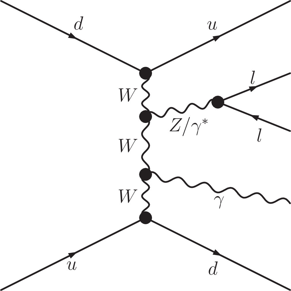
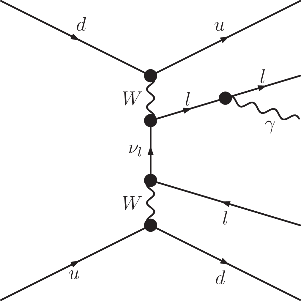
Figure 1:
Representative Feynman diagrams for Z$ \gamma $jj production. With the exception of the upper right one, the diagrams involve only EW vertices: VBS via W boson (upper left), VBS with QGC (upper center), vector boson fusion with TGCs (lower left), bremsstrahlung (lower center), multiperipheral (lower right), whereas the diagram (upper right) represents a QCD-induced contribution. |
png pdf |
Figure 1-a:
Representative Feynman diagram for Z$ \gamma $jj production. The diagram involves VBS via W bosons. |
png pdf |
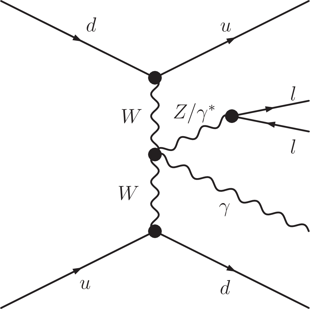
Figure 1-b:
Representative Feynman diagram for Z$ \gamma $jj production. The diagram involves VBS with a QGC. |
png pdf |
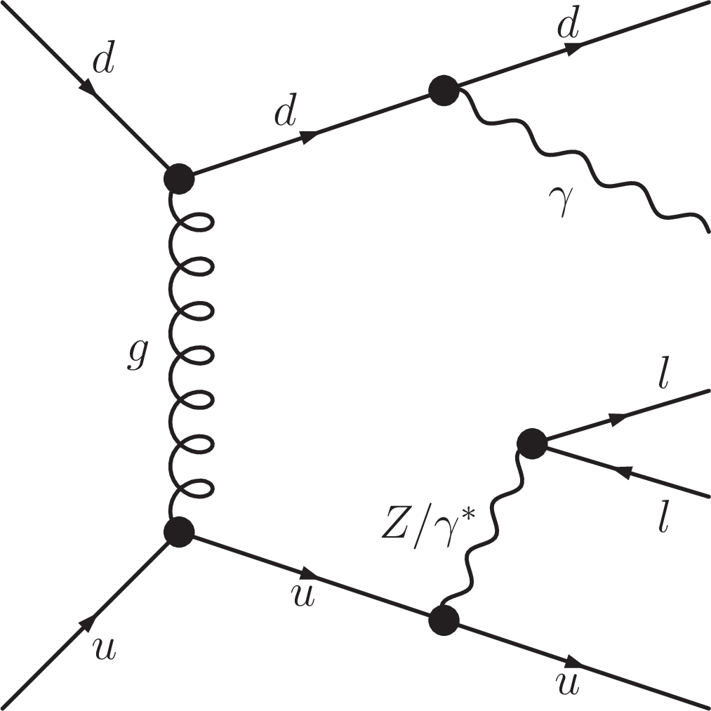
Figure 1-c:
Representative Feynman diagram for Z$ \gamma $jj production. The diagram represents a QCD-induced contribution. |

png pdf |
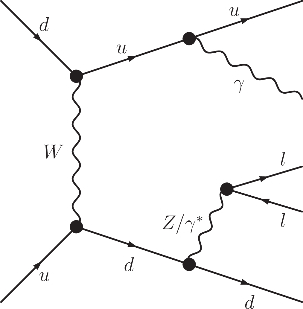
Figure 1-d:
Representative Feynman diagram for Z$ \gamma $jj production. The diagram involves vector boson fusion with a TGC. |
png pdf |
Figure 1-e:
Representative Feynman diagram for Z$ \gamma $jj production. The diagram involves bremsstrahlung vertices. |
png pdf |
Figure 1-f:
Representative Feynman diagram for Z$ \gamma $jj production. The diagram involves multiperipheral vertices. |
png pdf |
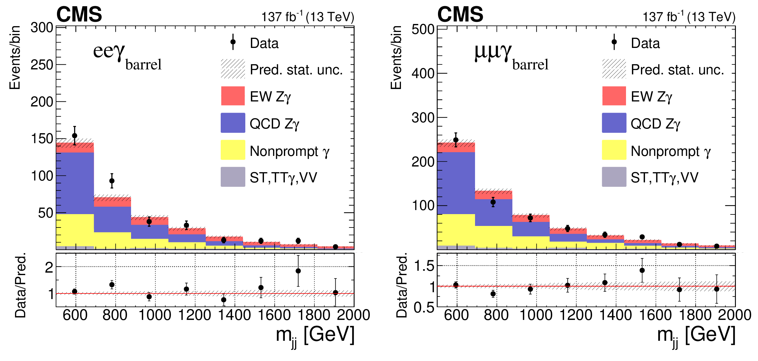
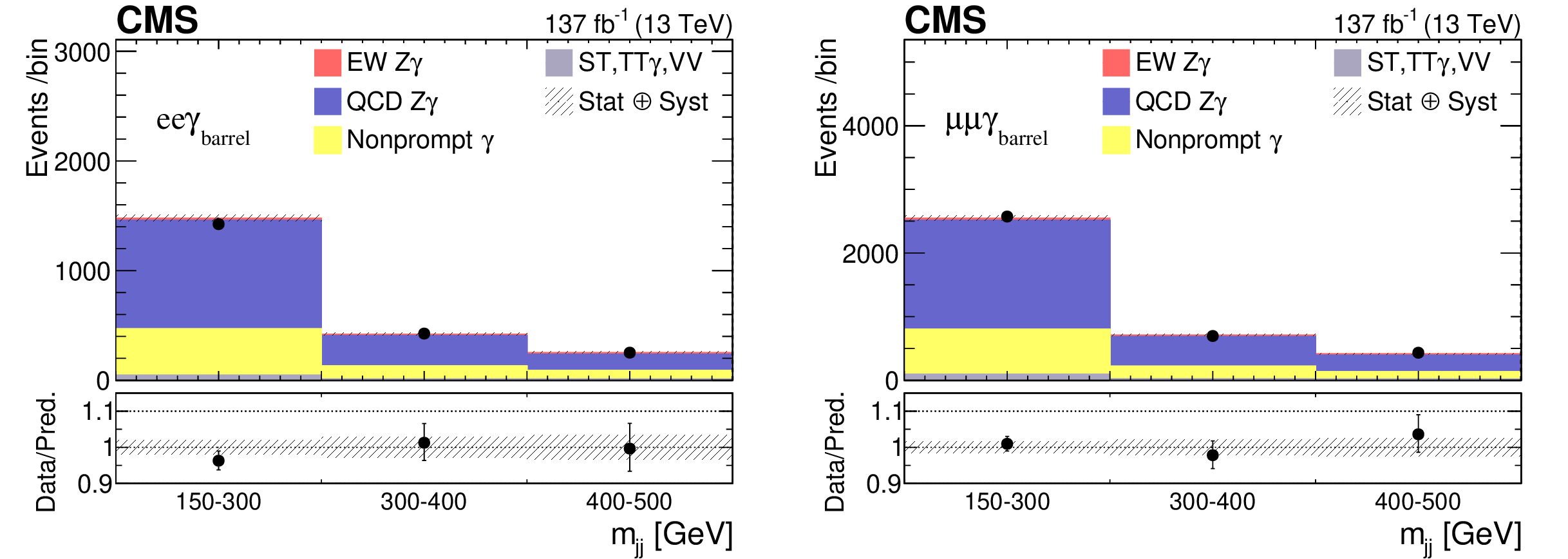
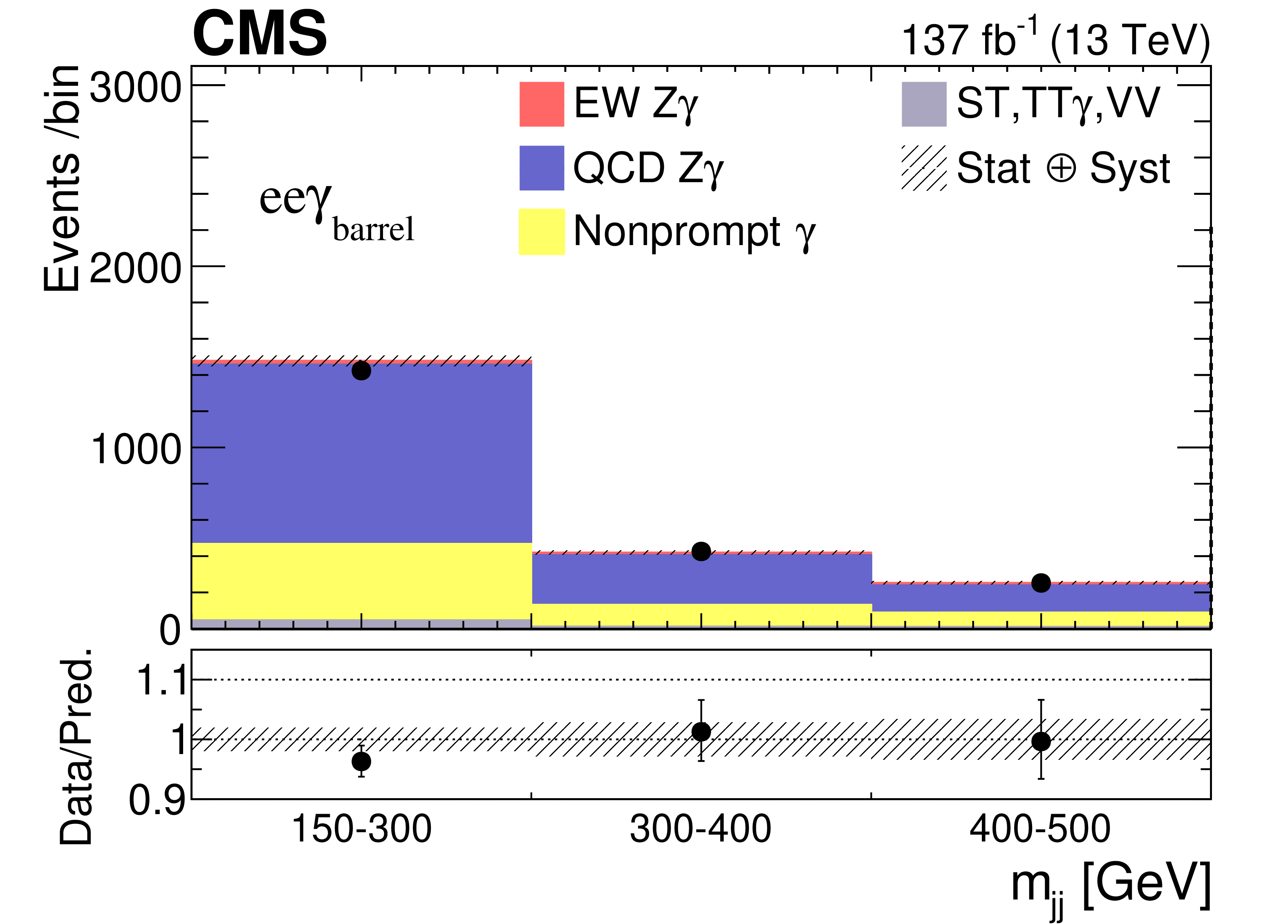
Figure 2:
The pre-fit $m_{\mathrm {jj}}$ distributions for the dilepton+$\gamma _{\text {barrel}}$ events are shown for the dielectron (left) and the dimuon (right) categories with data collected from 2016 to 2018. The data are compared to the sum of the signal and the background contributions. The black points with error bars represent the data and their statistical uncertainties, whereas the hatched bands represent the statistical uncertainty in the combined signal and background expectations. The last bin includes overflow events. The lower panel shows the ratio of the data to the expectation. |
png pdf |
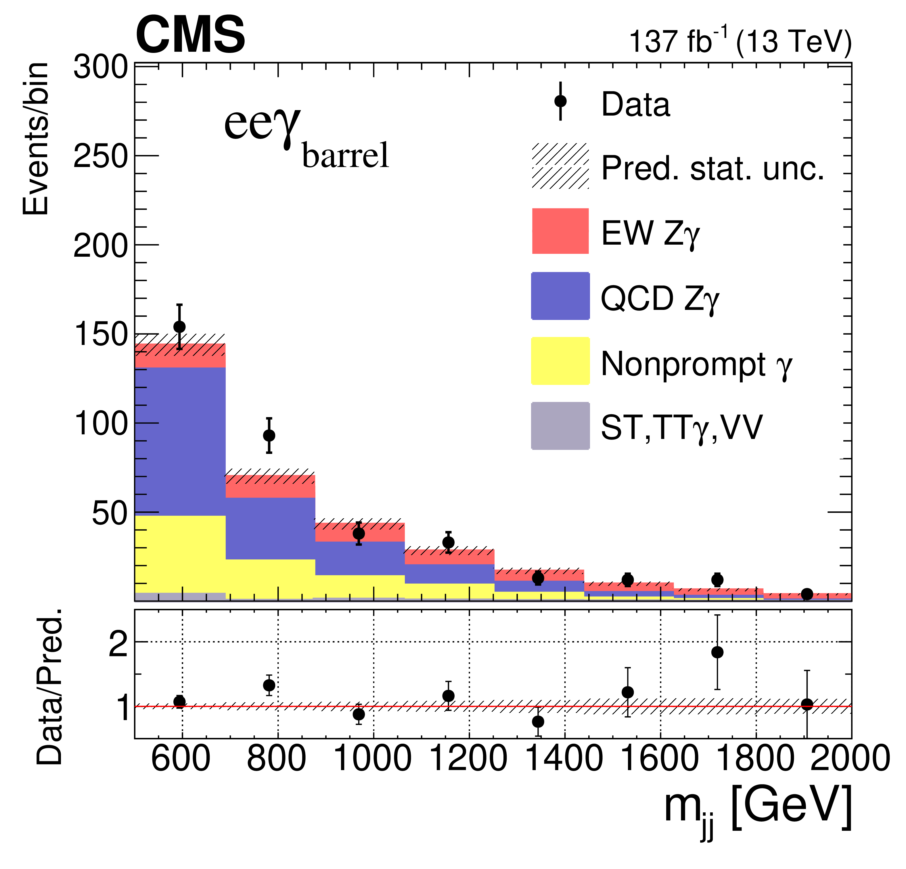
Figure 2-a:
The pre-fit $m_{\mathrm {jj}}$ distributions for the dilepton+$\gamma _{\text {barrel}}$ events are shown for the dielectron category with data collected from 2016 to 2018. The data are compared to the sum of the signal and the background contributions. The black points with error bars represent the data and their statistical uncertainties, whereas the hatched bands represent the statistical uncertainty in the combined signal and background expectations. The last bin includes overflow events. The lower panel shows the ratio of the data to the expectation. |
png pdf |
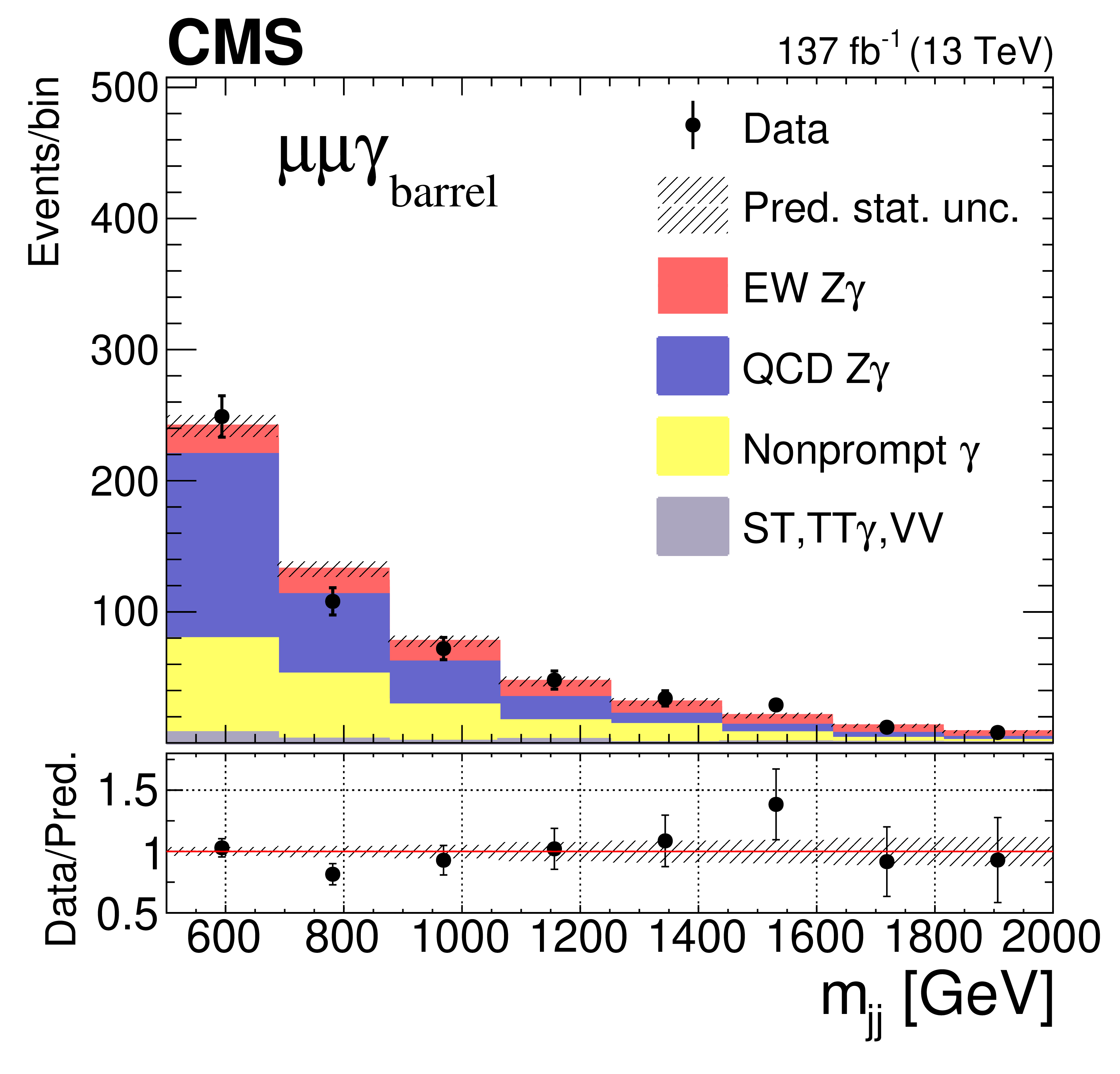
Figure 2-b:
The pre-fit $m_{\mathrm {jj}}$ distributions for the dilepton+$\gamma _{\text {barrel}}$ events are shown for the dimuon category with data collected from 2016 to 2018. The data are compared to the sum of the signal and the background contributions. The black points with error bars represent the data and their statistical uncertainties, whereas the hatched bands represent the statistical uncertainty in the combined signal and background expectations. The last bin includes overflow events. The lower panel shows the ratio of the data to the expectation. |
png pdf |
Figure 3:
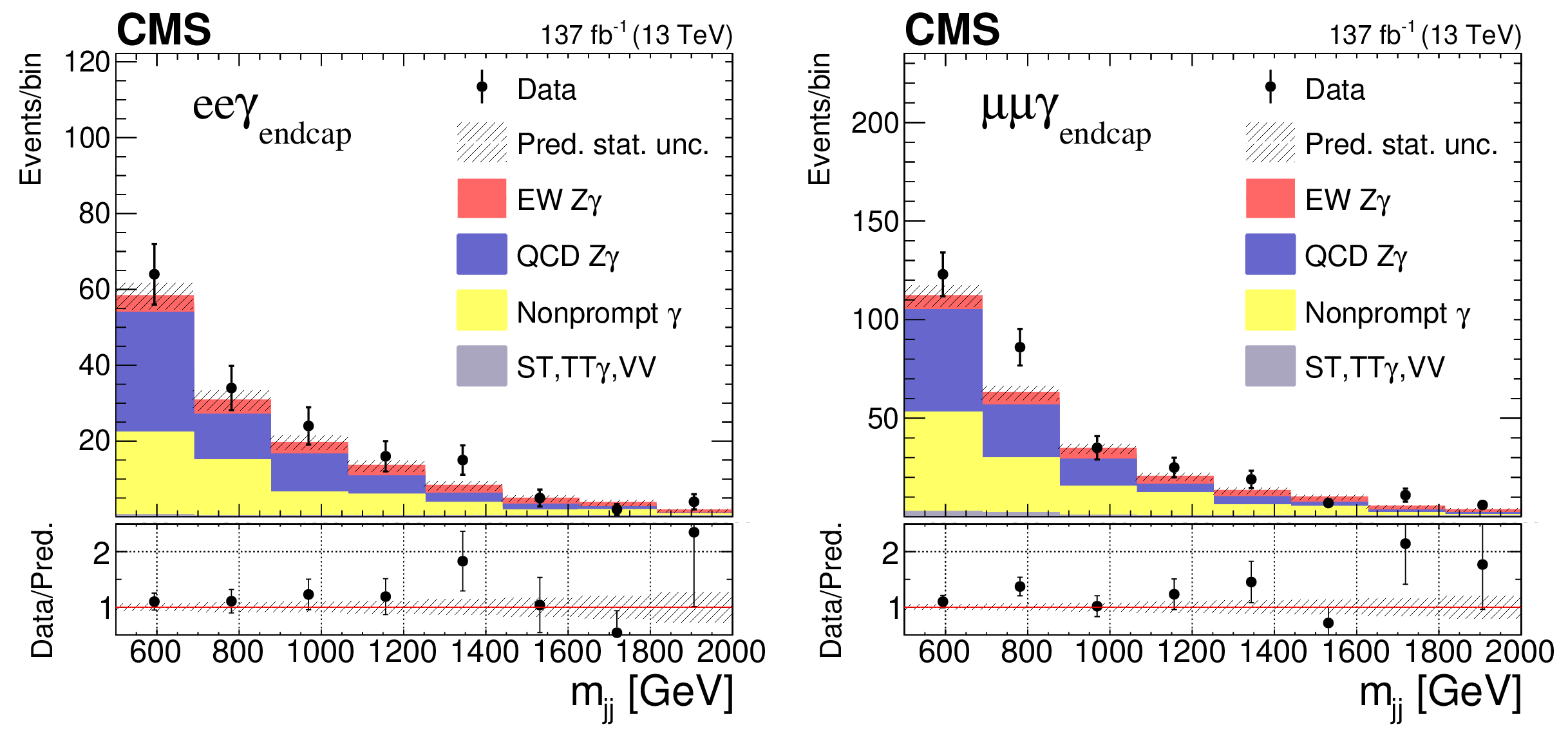
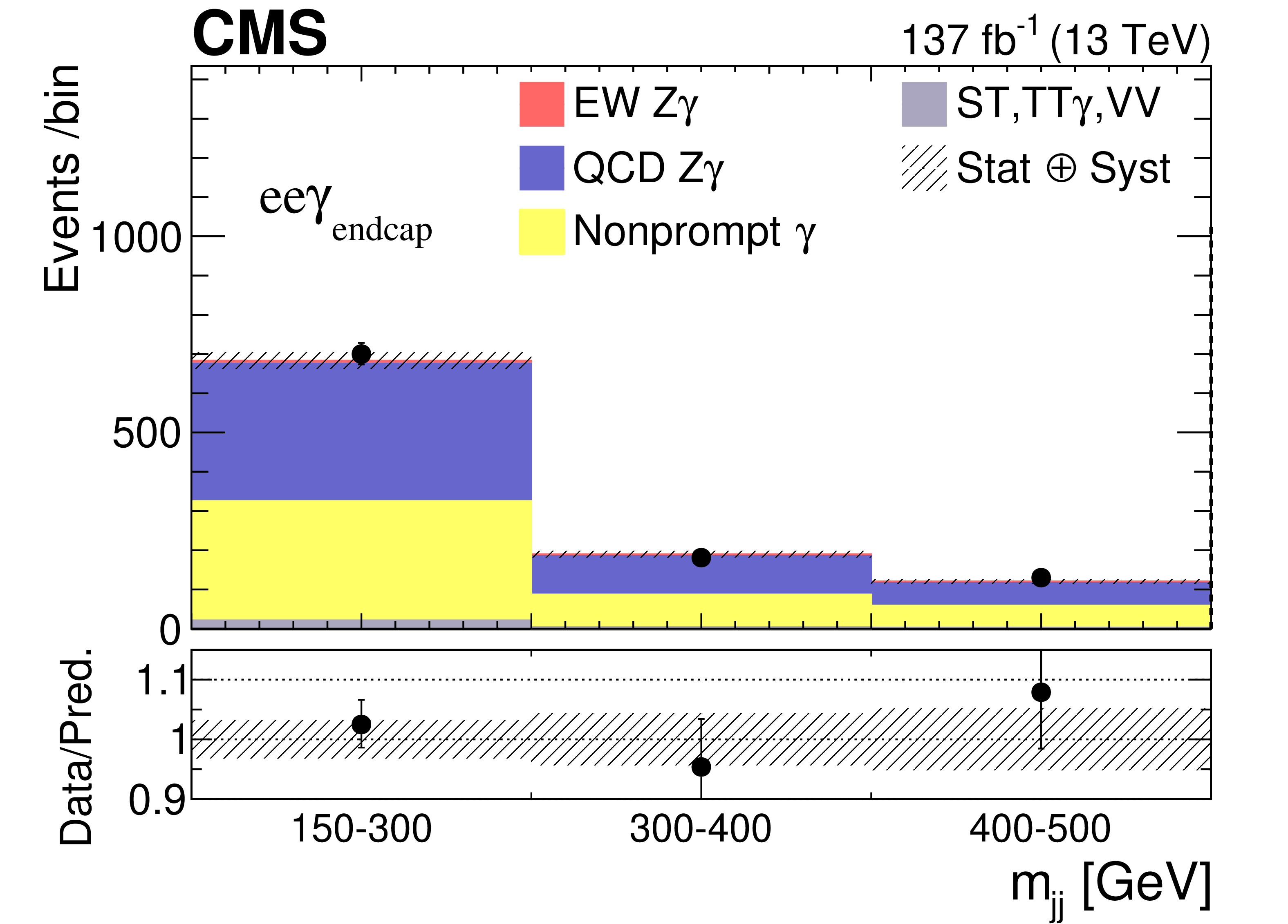
The pre-fit $m_{\mathrm {jj}}$ distributions for the dilepton+$\gamma _{\text {endcap}}$ events are shown for the dielectron (left) and the dimuon (right) categories with data collected from 2016 to 2018. The data are compared to the sum of the signal and the background contributions. The black points with error bars represent the data and their statistical uncertainties, whereas the hatched bands represent the statistical uncertainty in the combined signal and background expectations. The last bin includes overflow events. The lower panel shows the ratio of the data to the expectation. |
png pdf |
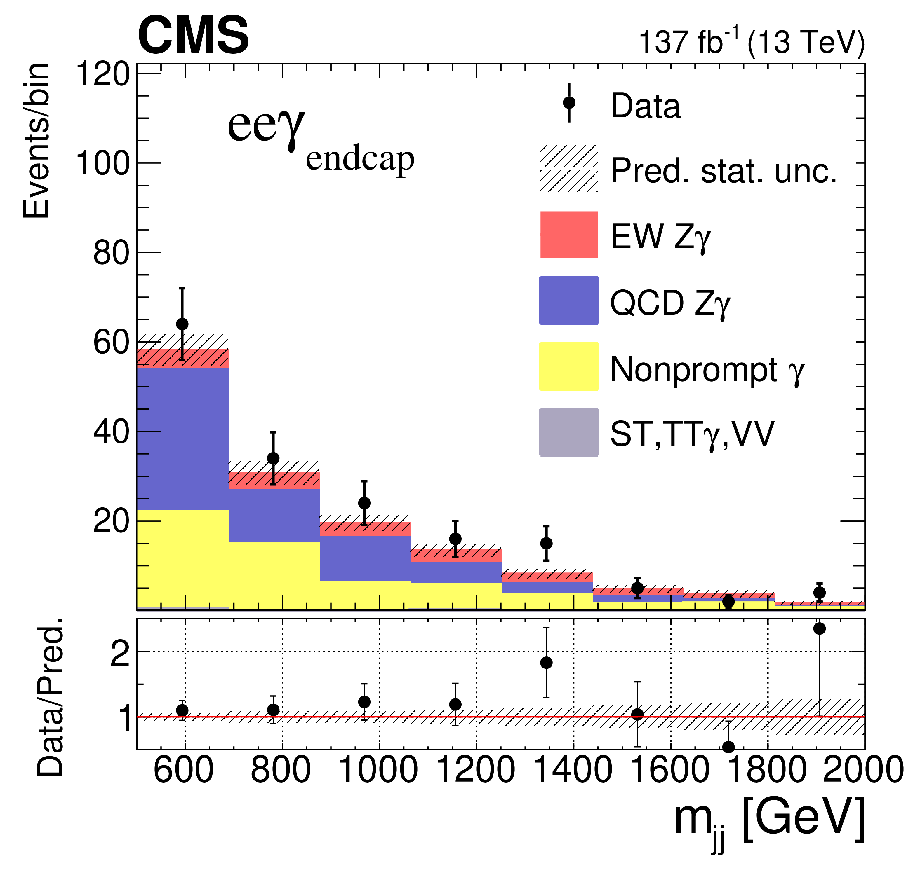
Figure 3-a:
The pre-fit $m_{\mathrm {jj}}$ distributions for the dilepton+$\gamma _{\text {endcap}}$ events are shown for the dielectron category with data collected from 2016 to 2018. The data are compared to the sum of the signal and the background contributions. The black points with error bars represent the data and their statistical uncertainties, whereas the hatched bands represent the statistical uncertainty in the combined signal and background expectations. The last bin includes overflow events. The lower panel shows the ratio of the data to the expectation. |

png pdf |
Figure 3-b:
The pre-fit $m_{\mathrm {jj}}$ distributions for the dilepton+$\gamma _{\text {endcap}}$ events are shown for the dimuon category with data collected from 2016 to 2018. The data are compared to the sum of the signal and the background contributions. The black points with error bars represent the data and their statistical uncertainties, whereas the hatched bands represent the statistical uncertainty in the combined signal and background expectations. The last bin includes overflow events. The lower panel shows the ratio of the data to the expectation. |
png pdf |
Figure 4:
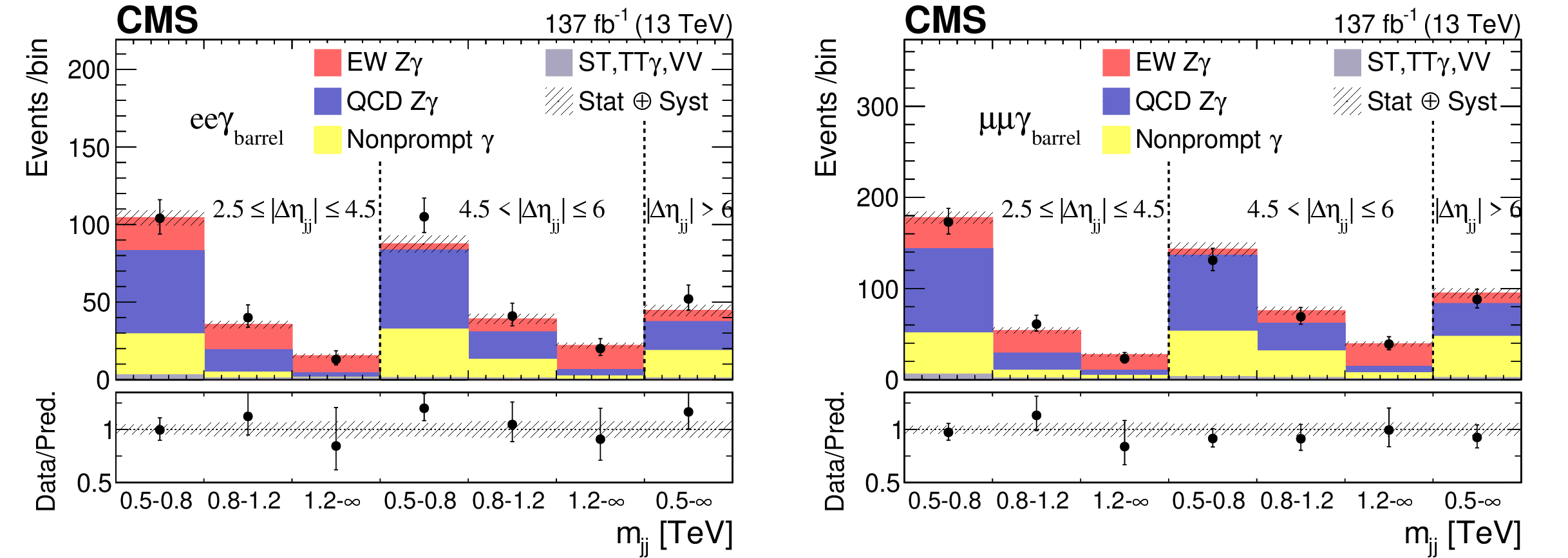
The post-fit 2D distributions of the dielectron (left) and dimuon (right) for the $\gamma _{\text {barrel}}$ categories, as functions of $m_\mathrm {jj}$ in bins of $ {| \Delta \eta _{\mathrm {jj}} |}$. The horizontal axis is split into bins of $ {| \Delta \eta _{\mathrm {jj}} |}$ of [2.5, 4.5], [4.5, 6.0], and $ > $6.0. The data are compared to the signal and background in the predictions. The black points with error bars represent the data and their statistical uncertainties, whereas the hatched bands represent the total uncertainties of the predictions. |

png pdf |
Figure 4-a:
The post-fit 2D distributions of the dielectron for the $\gamma _{\text {barrel}}$ categories, as functions of $m_\mathrm {jj}$ in bins of $ {| \Delta \eta _{\mathrm {jj}} |}$. The horizontal axis is split into bins of $ {| \Delta \eta _{\mathrm {jj}} |}$ of [2.5, 4.5], [4.5, 6.0], and $ > $6.0. The data are compared to the signal and background in the predictions. The black points with error bars represent the data and their statistical uncertainties, whereas the hatched bands represent the total uncertainties of the predictions. |
png pdf |
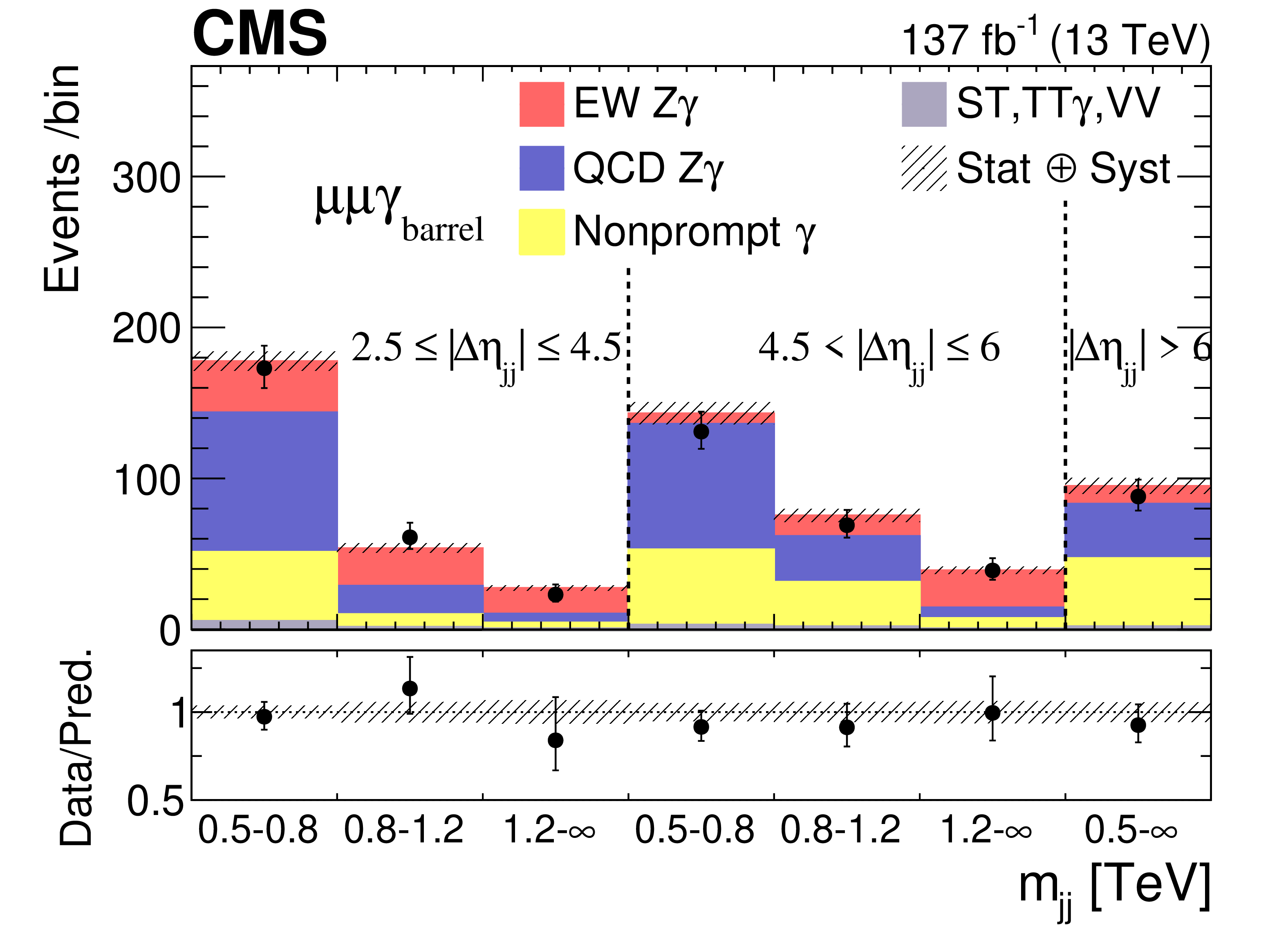
Figure 4-b:
The post-fit 2D distributions of the dimuon for the $\gamma _{\text {barrel}}$ categories, as functions of $m_\mathrm {jj}$ in bins of $ {| \Delta \eta _{\mathrm {jj}} |}$. The horizontal axis is split into bins of $ {| \Delta \eta _{\mathrm {jj}} |}$ of [2.5, 4.5], [4.5, 6.0], and $ > $6.0. The data are compared to the signal and background in the predictions. The black points with error bars represent the data and their statistical uncertainties, whereas the hatched bands represent the total uncertainties of the predictions. |

png pdf |
Figure 5:
The post-fit 2D distributions of the dielectron (left) and dimuon (right) for the $\gamma _{\text {endcap}}$ categories, as functions of $m_\mathrm {jj}$ in bins of $ {| \Delta \eta _{\mathrm {jj}} |}$. The horizontal axis is split into bins of $ {| \Delta \eta _{\mathrm {jj}} |}$ of [2.5, 4.5], [4.5, 6.0], and $ > $6.0. The data are compared to the signal and background in the predictions. The black points with error bars represent the data and their statistical uncertainties, whereas the hatched bands represent the total uncertainties of the predictions. |

png pdf |
Figure 5-a:
The post-fit 2D distributions of the dielectron for the $\gamma _{\text {endcap}}$ categories, as functions of $m_\mathrm {jj}$ in bins of $ {| \Delta \eta _{\mathrm {jj}} |}$. The horizontal axis is split into bins of $ {| \Delta \eta _{\mathrm {jj}} |}$ of [2.5, 4.5], [4.5, 6.0], and $ > $6.0. The data are compared to the signal and background in the predictions. The black points with error bars represent the data and their statistical uncertainties, whereas the hatched bands represent the total uncertainties of the predictions. |

png pdf |
Figure 5-b:
The post-fit 2D distributions of the dimuon for the $\gamma _{\text {endcap}}$ categories, as functions of $m_\mathrm {jj}$ in bins of $ {| \Delta \eta _{\mathrm {jj}} |}$. The horizontal axis is split into bins of $ {| \Delta \eta _{\mathrm {jj}} |}$ of [2.5, 4.5], [4.5, 6.0], and $ > $6.0. The data are compared to the signal and background in the predictions. The black points with error bars represent the data and their statistical uncertainties, whereas the hatched bands represent the total uncertainties of the predictions. |
png pdf |
Figure 6:
The post-fit distributions in the control region for the dielectron (left) and dimuon (right) for the $\gamma _{\text {barrel}}$ categories as a function of $m_\mathrm {jj}$. The horizontal axis is split into bins of $m_{\mathrm {jj}}$ of [150, 300], [300, 400], and [400,500]. The black points with error bars represent the data and their statistical uncertainties, whereas the hatched bands represent the total uncertainties of the predictions. |
png pdf |
Figure 6-a:
The post-fit distributions in the control region for the dielectron for the $\gamma _{\text {barrel}}$ categories as a function of $m_\mathrm {jj}$. The horizontal axis is split into bins of $m_{\mathrm {jj}}$ of [150, 300], [300, 400], and [400,500]. The black points with error bars represent the data and their statistical uncertainties, whereas the hatched bands represent the total uncertainties of the predictions. |

png pdf |
Figure 6-b:
The post-fit distributions in the control region for the dimuon for the $\gamma _{\text {barrel}}$ categories as a function of $m_\mathrm {jj}$. The horizontal axis is split into bins of $m_{\mathrm {jj}}$ of [150, 300], [300, 400], and [400,500]. The black points with error bars represent the data and their statistical uncertainties, whereas the hatched bands represent the total uncertainties of the predictions. |

png pdf |
Figure 7:
The post-fit distributions in the control region for the dielectron (left) and dimuon (right) for the $\gamma _{\text {endcap}}$ categories as a function of $m_\mathrm {jj}$. The horizontal axis is split into bins of $m_{\mathrm {jj}}$ of [150, 300], [300, 400], and [400,500]. The black points with error bars represent the data and their statistical uncertainties, whereas the hatched bands represent the total uncertainties of the predictions. |
png pdf |
Figure 7-a:
The post-fit distributions in the control region for the dielectron for the $\gamma _{\text {endcap}}$ categories as a function of $m_\mathrm {jj}$. The horizontal axis is split into bins of $m_{\mathrm {jj}}$ of [150, 300], [300, 400], and [400,500]. The black points with error bars represent the data and their statistical uncertainties, whereas the hatched bands represent the total uncertainties of the predictions. |

png pdf |
Figure 7-b:
The post-fit distributions in the control region for the dimuon for the $\gamma _{\text {endcap}}$ categories as a function of $m_\mathrm {jj}$. The horizontal axis is split into bins of $m_{\mathrm {jj}}$ of [150, 300], [300, 400], and [400,500]. The black points with error bars represent the data and their statistical uncertainties, whereas the hatched bands represent the total uncertainties of the predictions. |
png pdf |
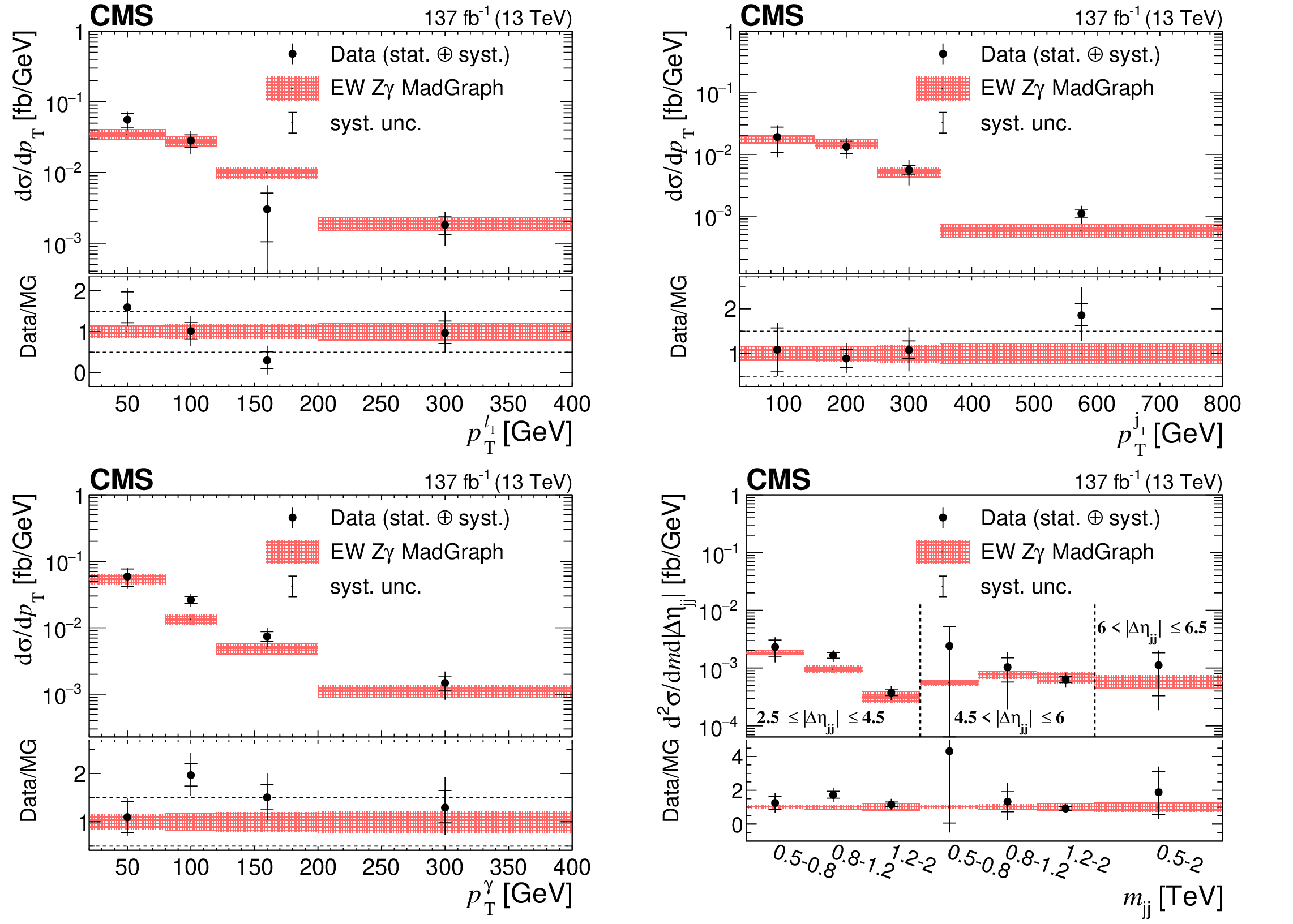
Figure 8:
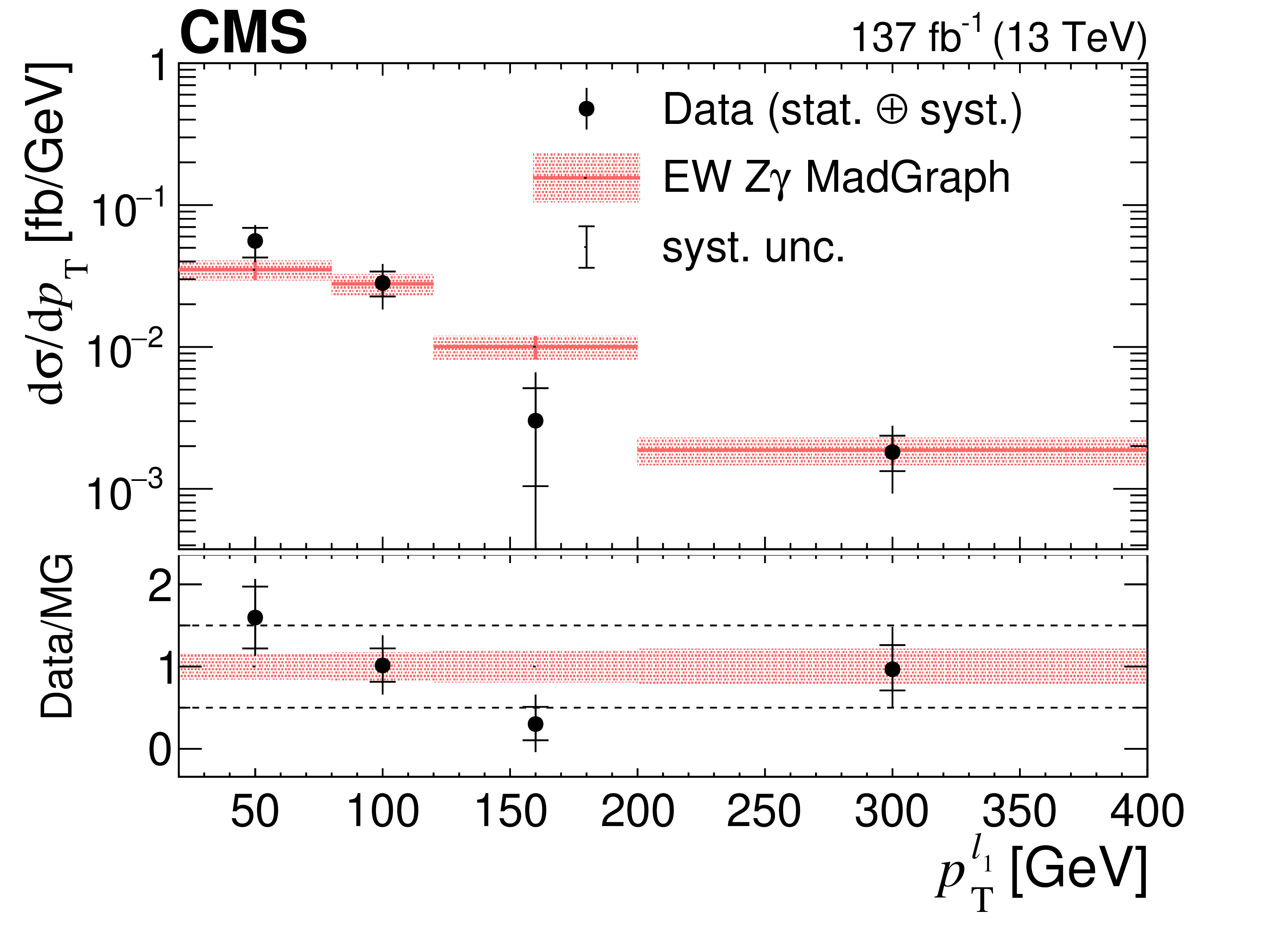
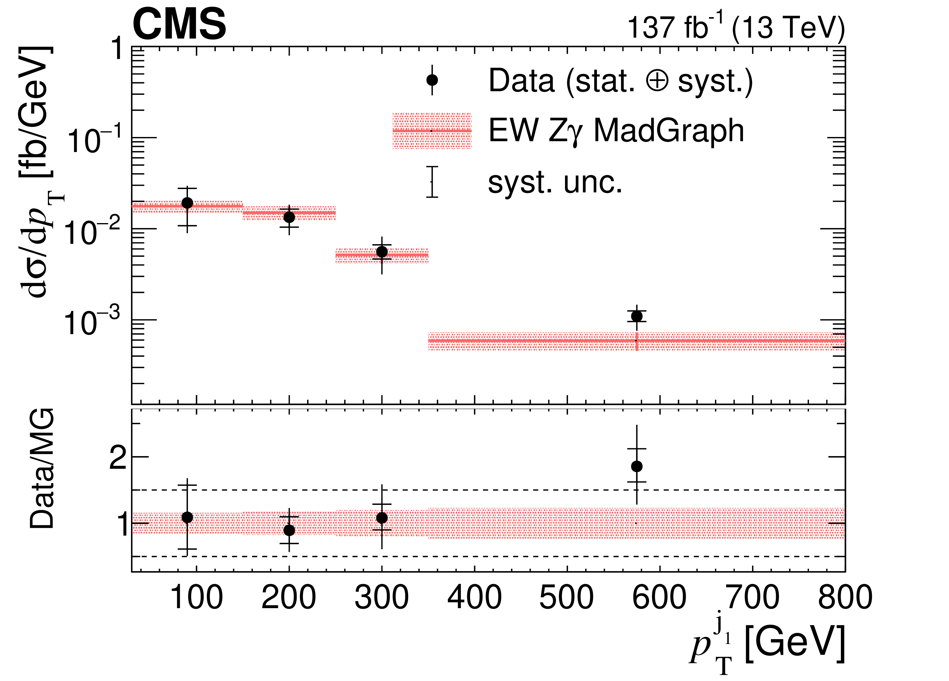
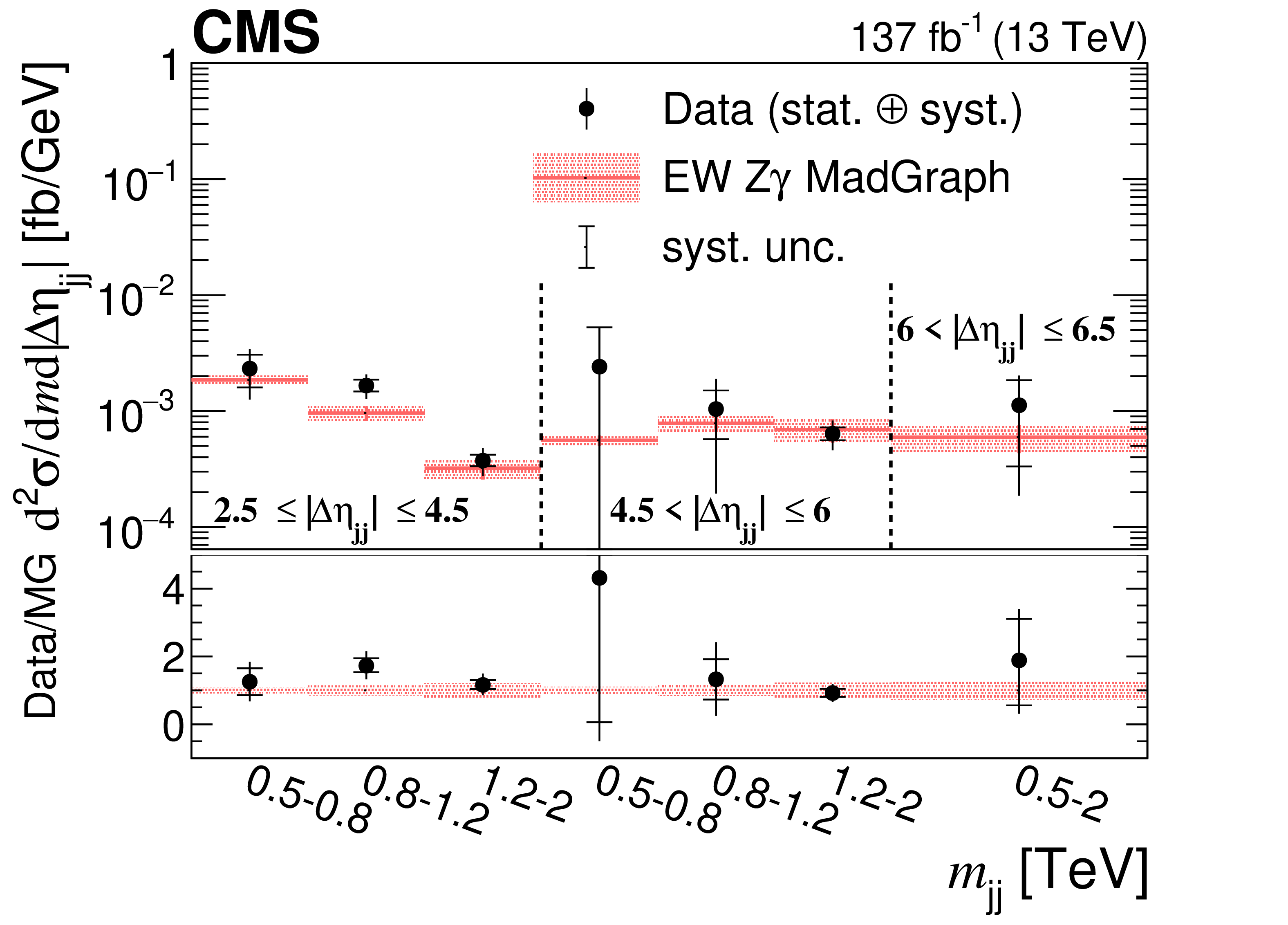
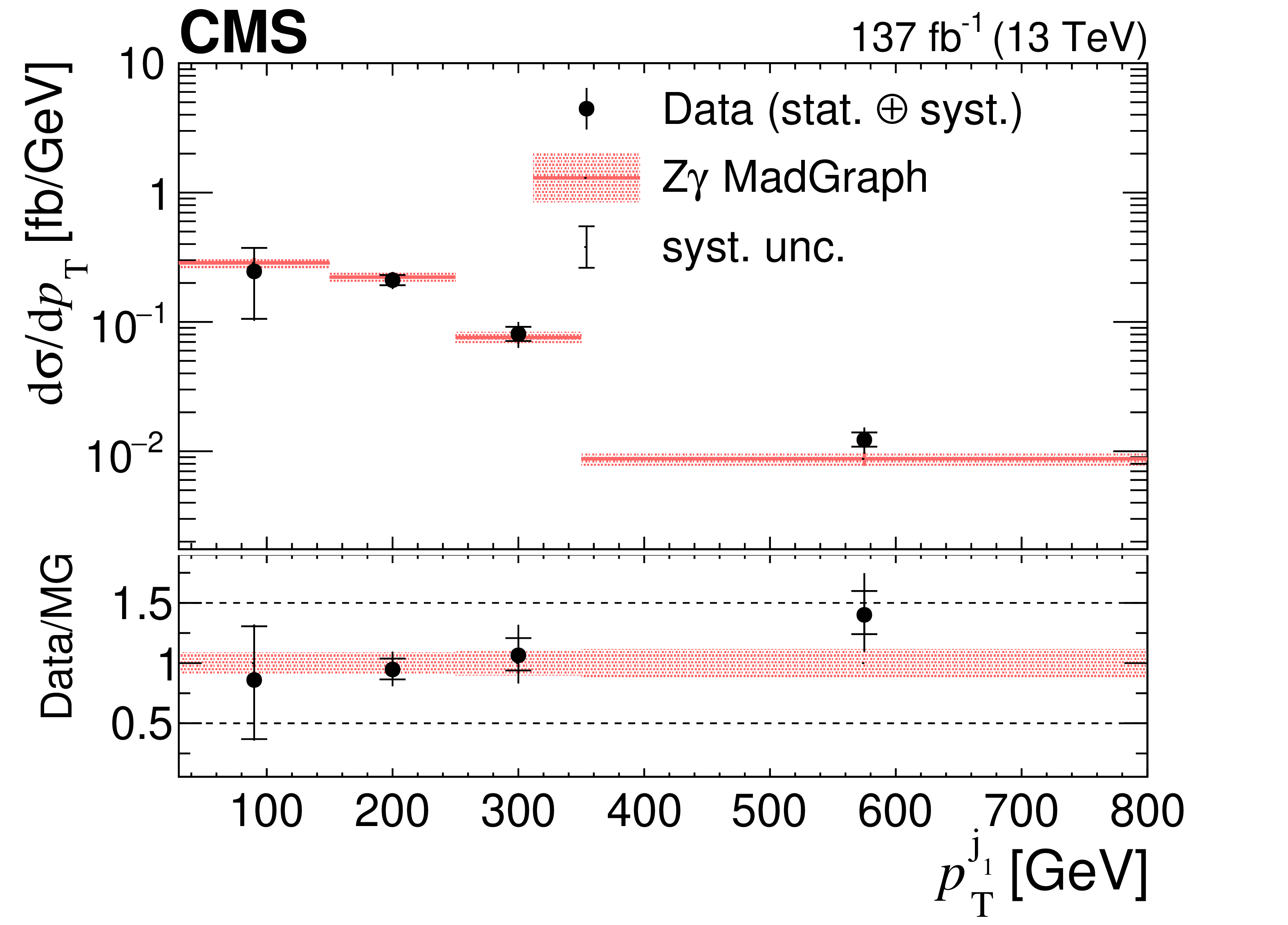
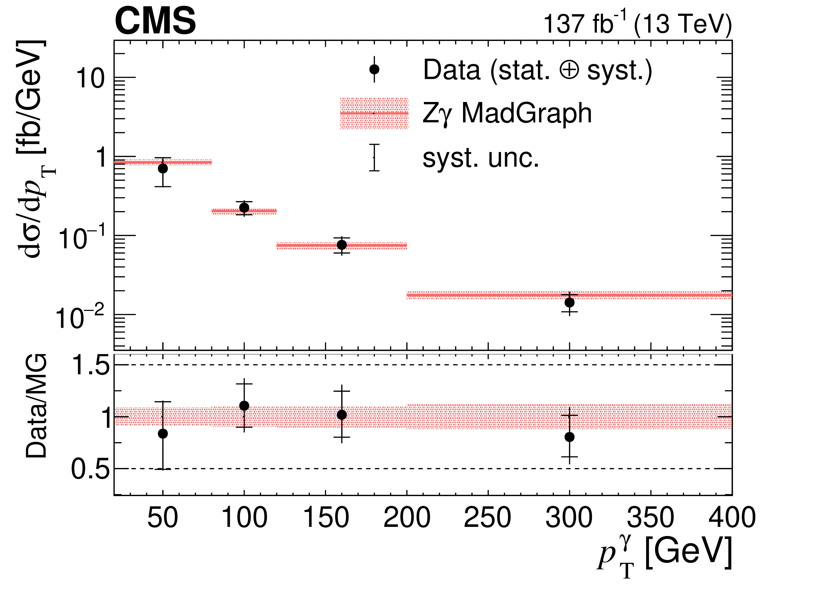
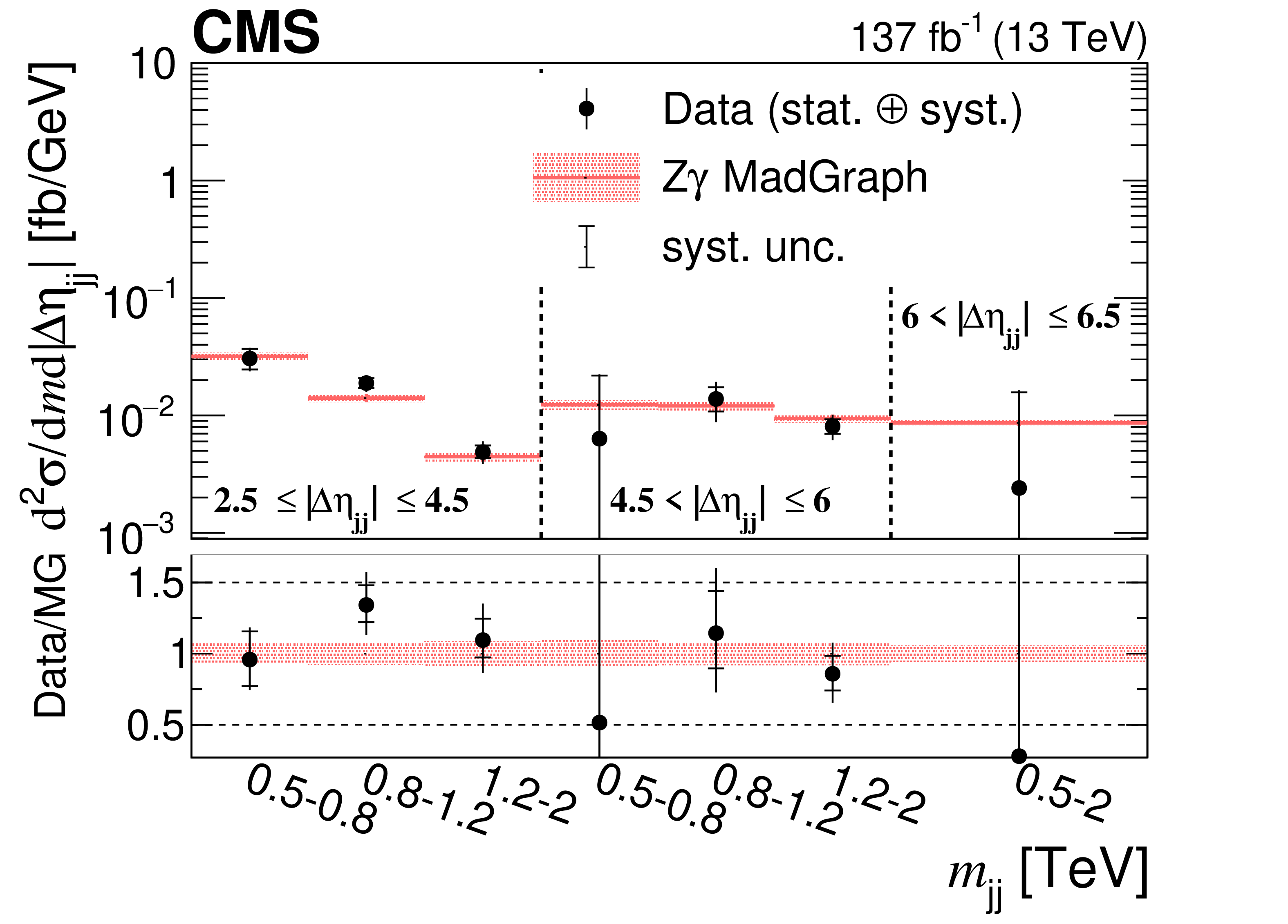
Unfolded differential cross section as a function of the leading lepton ${p_{\mathrm {T}}}$, leading jet ${p_{\mathrm {T}}}$, leading photon ${p_{\mathrm {T}}}$, and $m_{\mathrm {jj}}$-$ {| \Delta \eta _{\mathrm {jj}} |}$ for EW Z$ \gamma $jj. The black points with error bars represent the data and their statistical uncertainties, whereas the red bands represent the total theoretical uncertainties from the MG5 simulation. The last bin includes overflow events. |
png pdf |
Figure 8-a:
Unfolded differential cross section as a function of the leading lepton ${p_{\mathrm {T}}}$ for EW Z$ \gamma $jj. The black points with error bars represent the data and their statistical uncertainties, whereas the red bands represent the total theoretical uncertainties from the MG5 simulation. The last bin includes overflow events. |
png pdf |
Figure 8-b:
Unfolded differential cross section as a function of leading jet ${p_{\mathrm {T}}}$ for EW Z$ \gamma $jj. The black points with error bars represent the data and their statistical uncertainties, whereas the red bands represent the total theoretical uncertainties from the MG5 simulation. The last bin includes overflow events. |

png pdf |
Figure 8-c:
Unfolded differential cross section as a function of leading photon ${p_{\mathrm {T}}}$ for EW Z$ \gamma $jj. The black points with error bars represent the data and their statistical uncertainties, whereas the red bands represent the total theoretical uncertainties from the MG5 simulation. The last bin includes overflow events. |
png pdf |
Figure 8-d:
Unfolded differential cross section as a function of $m_{\mathrm {jj}}$-$ {| \Delta \eta _{\mathrm {jj}} |}$ for EW Z$ \gamma $jj. The black points with error bars represent the data and their statistical uncertainties, whereas the red bands represent the total theoretical uncertainties from the MG5 simulation. The last bin includes overflow events. |

png pdf |
Figure 9:
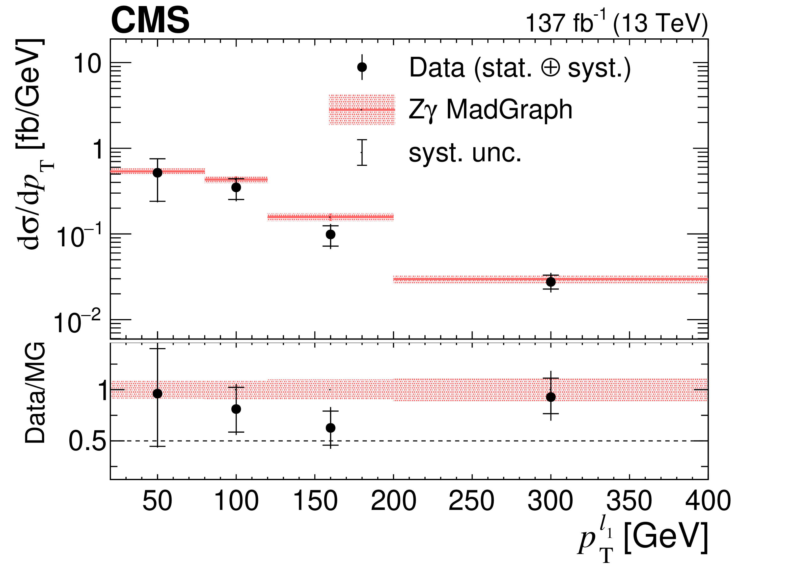
Unfolded differential cross section as a function of the leading lepton ${p_{\mathrm {T}}}$, leading photon ${p_{\mathrm {T}}}$, leading jet ${p_{\mathrm {T}}}$, and $m_{\mathrm {jj}}$-$ {| \Delta \eta _{\mathrm {jj}} |}$ for EW+QCD Z$ \gamma $jj. The black points with error bars represent the data and their statistical uncertainties, whereas the red bands represent the total theoretical uncertainties from the MG5 simulation. The last bin includes overflow events. |
png pdf |
Figure 9-a:
Unfolded differential cross section as a function of the leading lepton ${p_{\mathrm {T}}}$ for EW+QCD Z$ \gamma $jj. The black points with error bars represent the data and their statistical uncertainties, whereas the red bands represent the total theoretical uncertainties from the MG5 simulation. The last bin includes overflow events. |
png pdf |
Figure 9-b:
Unfolded differential cross section as a function of the leading photon ${p_{\mathrm {T}}}$ for EW+QCD Z$ \gamma $jj. The black points with error bars represent the data and their statistical uncertainties, whereas the red bands represent the total theoretical uncertainties from the MG5 simulation. The last bin includes overflow events. |
png pdf |
Figure 9-c:
Unfolded differential cross section as a function of the leading jet ${p_{\mathrm {T}}}$ for EW+QCD Z$ \gamma $jj. The black points with error bars represent the data and their statistical uncertainties, whereas the red bands represent the total theoretical uncertainties from the MG5 simulation. The last bin includes overflow events. |
png pdf |
Figure 9-d:
Unfolded differential cross section as a function of the $m_{\mathrm {jj}}$-$ {| \Delta \eta _{\mathrm {jj}} |}$ for EW+QCD Z$ \gamma $jj. The black points with error bars represent the data and their statistical uncertainties, whereas the red bands represent the total theoretical uncertainties from the MG5 simulation. The last bin includes overflow events. |
png pdf |
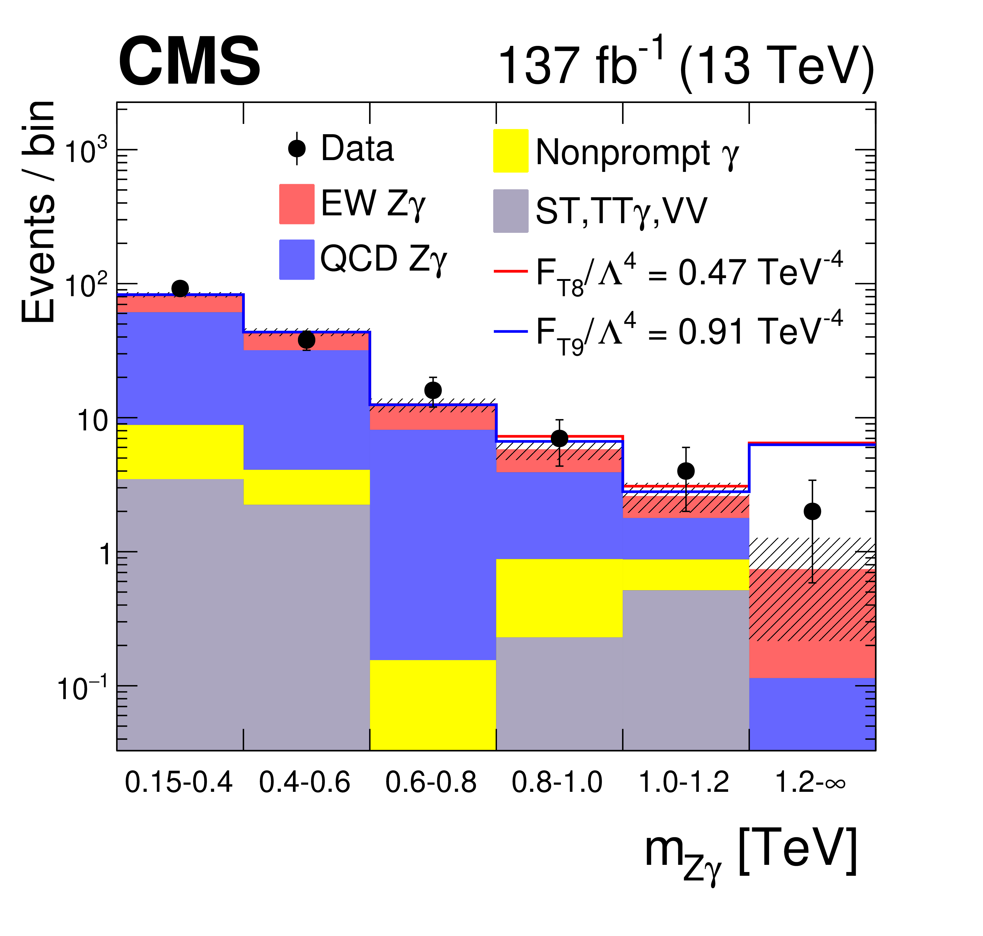
Figure 10:
The $m_{\mathrm{Z} \gamma}$ distribution for events satisfying the aQGC region selection, which is used to set constraints on the anomalous coupling parameters. The bins of $m_{\mathrm{Z} \gamma}$ are [150, 400, 600, 800, 1000, 1200, 2000] GeV, where the last bin includes overflow events. The red line represents a nonzero $F_{\mathrm {T8}}$ value and the blue line represents a nonzero $F_{\mathrm {T9}}$ value, which would significantly enhance the yields at high $m_{\mathrm{Z} \gamma}$. The black points with error bars represent the data and their statistical uncertainties, whereas the hatched bands represent the statistical uncertainties in the SM predictions. |
| Tables | |

png pdf |
Table 1:
Summary of the five sets of event selection criteria used to define events in the fiducial cross section measurement region, control region, EW signal extraction region, and the region used to search for aQGC contributions. |
png pdf |
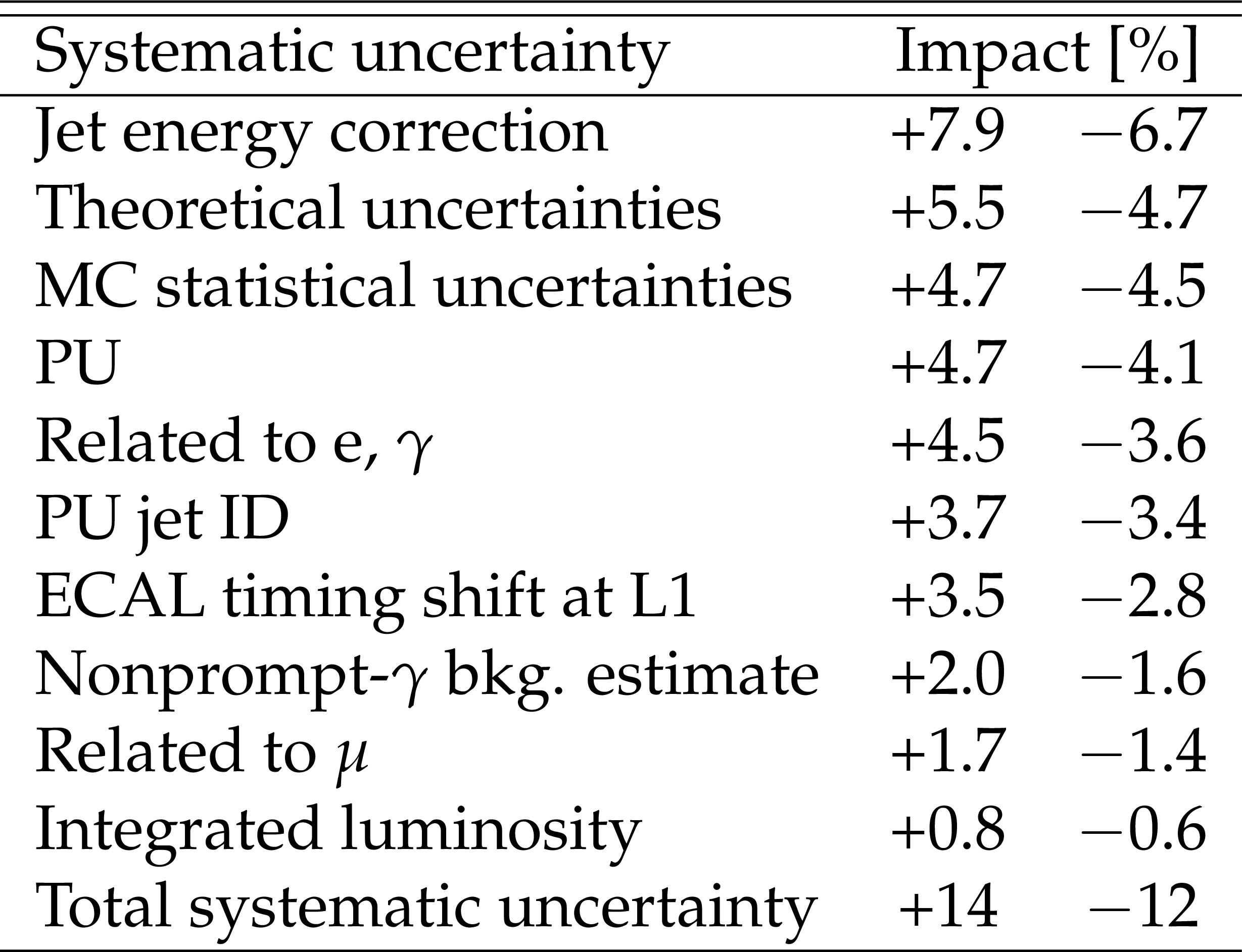
Table 2:
The impact of the systematic uncertainties on the EW signal strength measurement. |
png pdf |
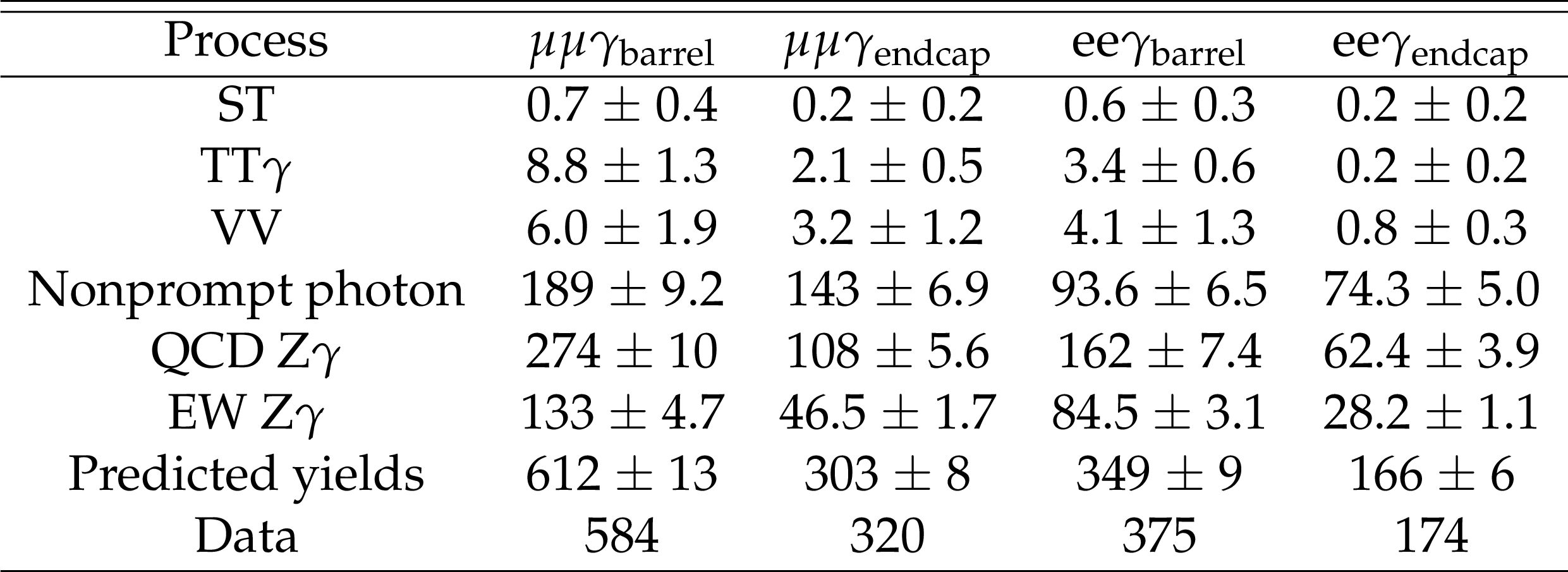
Table 3:
Post-fit yields of predicted signal and background with total uncertainties, and observed event counts after the selection in the EW signal region. The $\gamma _{\text {barrel}}$ and $\gamma _{\text {endcap}}$ columns represent events with photons in the ECAL barrel and endcaps, respectively. |

png pdf |
Table 4:
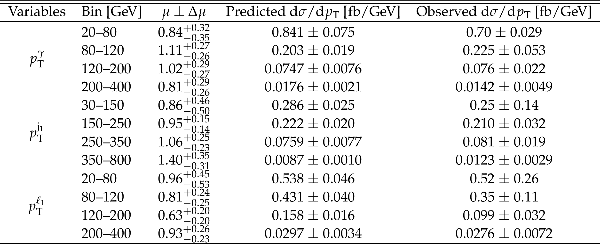
The signal strengths and differential cross sections from SM expectation and fit calculated as part of the unfolding of $ {p_{\mathrm {T}}} ^{\gamma}$, $ {p_{\mathrm {T}}} ^{\mathrm {j}_1}$, and $ {p_{\mathrm {T}}} ^{\ell _1}$ observables for EW Z$ \gamma $jj. The last bin includes overflow events. |
png pdf |
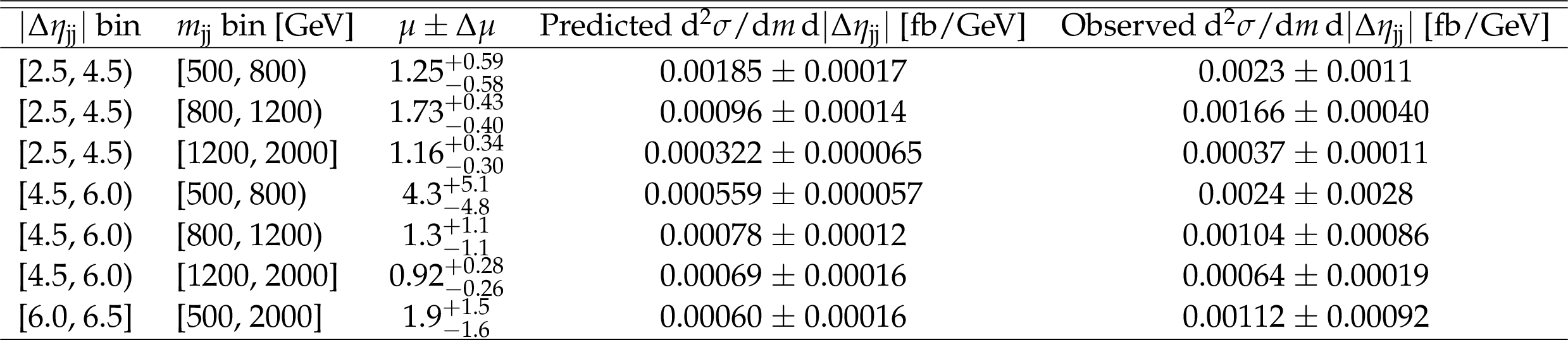
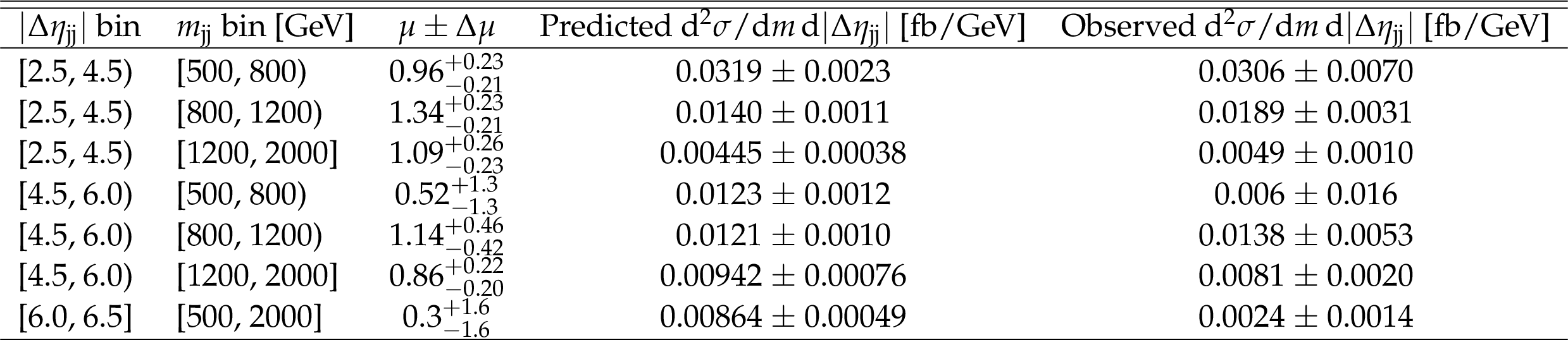
Table 5:
The signal strengths and differential cross sections from SM expectation and fit calculated as part of the unfolding of 2D $m_{\mathrm {jj}}$-$ {| \Delta \eta _{\mathrm {jj}} |}$ observables for EW Z$ \gamma $jj. The last bin includes overflow events. |
png pdf |
Table 6:
The signal strengths and differential cross sections from SM expectation and fit calculated as part of the unfolding of $ {p_{\mathrm {T}}} ^{\gamma}$, $ {p_{\mathrm {T}}} ^{\mathrm {j}_1}$, and $ {p_{\mathrm {T}}} ^{\ell _1}$ observables for EW+QCD Z$ \gamma $jj. The last bin includes overflow events. |
png pdf |
Table 7:
The signal strengths and differential cross sections from SM expectation and fit calculated as part of the unfolding of 2D $m_{\mathrm {jj}}$-$ {| \Delta \eta _{\mathrm {jj}} |}$ observables for EW+QCD Z$ \gamma $jj. The last bin includes overflow events. |

png pdf |
Table 8:
The expected and observed limits on the aQGC parameters at 95% confidence level. The last column presents the scattering energy values for which the amplitude would violate unitarity for the observed value of the aQGC parameter. All coupling parameter limits are set in $ TeV ^{-4}$, whereas the unitarity bounds are in TeV. |
| Summary |
| This paper presents the first observation of the electroweak (EW) production of a Z boson, a photon, and two jets (Z$ \gamma $jj) in $\sqrt{s} = $ 13 TeV proton-proton collisions recorded with the CMS detector in 2016-2018 corresponding to an integrated luminosity of 137 fb$^{-1}$. Events were selected by requiring two opposite-sign leptons with the same flavor from the decay of a Z boson, one identified photon, and two jets that have a large separation in pseudorapidity and a large dijet mass. The measured cross section in the fiducial volume defined in Table 1 for EW Z$ \gamma $jj production is 5.21 $\pm$ 0.52 (stat) $\pm$ 0.56 (syst) fb $ = $ 5.21 $\pm$ 0.76 fb, and the fiducial cross section of EW and QCD-induced production is 14.7 $\pm$ 0.80 (stat) $\pm$ 1.26 (syst) fb $ = $ 14.7 $\pm$ 1.53 fb. Both the observed and expected signal significances are well in excess of 5 standard deviations. Differential cross sections for EW and EW+QCD are measured for several observables and compared to standard model predictions computed at leading order. Within the uncertainties, the measurements agree with the predictions. Constraints are set on the effective field theory dimension-8 operators M$_{0}$ to M$_{5}$, M$_{7}$, T$_{0}$ to T$_{2}$, and T$_{5}$ to T$_{9}$, giving rise to anomalous quartic gauge couplings. These constraints are either competitive with or more stringent than those previously obtained. |
| References | ||||
| 1 | ATLAS Collaboration | Observation of a new particle in the search for the standard model Higgs boson with the ATLAS detector at the LHC | PLB 716 (2012) 1 | 1207.7214 |
| 2 | CMS Collaboration | Observation of a new boson at a mass of 125 GeV with the CMS experiment at the LHC | PLB 716 (2012) 30 | CMS-HIG-12-028 1207.7235 |
| 3 | CMS Collaboration | Observation of a new boson with mass near 125 GeV in pp collisions at $ \sqrt{s} = $ 7 and 8 TeV | JHEP 06 (2013) 081 | CMS-HIG-12-036 1303.4571 |
| 4 | ATLAS, CMS Collaboration | Measurements of the Higgs boson production and decay rates and constraints on its couplings from a combined ATLAS and CMS analysis of the LHC pp collision data at $ \sqrt{s}= $ 7 and 8 TeV | JHEP 08 (2016) 045 | 1606.02266 |
| 5 | CMS Collaboration | Combined measurements of Higgs boson couplings in proton-proton collisions at $ \sqrt{s} = $ 13 TeV | EPJC 79 (2019) 421 | CMS-HIG-17-031 1809.10733 |
| 6 | O. J. P. \'Eboli, M. C. Gonzalez-Garcia, and J. K. Mizukoshi | $ {\mathrm{p}}{\mathrm{p}} \rightarrow $ jje$ ^\pm \mu^\pm \nu\nu $ and jje$ ^\pm\mu^\mp\nu\nu $ at $ \mathcal{O} $($ \alpha^6_{\rm em} $) and $ \mathcal{O} $($ \alpha_{\rm em}^4 \alpha_{\rm s}^2 $) for the study of the quartic electroweak gauge boson vertex at CERN LHC | PRD 74 (2006) 073005 | hep-ph/0606118 |
| 7 | CMS Collaboration | Search for anomalous triple gauge couplings in WW and WZ production in lepton + jet events in proton-proton collisions at $ \sqrt{s} = $ 13 TeV | JHEP 12 (2019) 062 | CMS-SMP-18-008 1907.08354 |
| 8 | ATLAS Collaboration | Evidence for electroweak production of two jets in association with a $ \mathrm{Z} \gamma $ pair in pp collisions at $ \sqrt{s} = $ 13 TeV with the ATLAS detector | PLB 803 (2020) 135341 | 1910.09503 |
| 9 | CMS Collaboration | Measurement of the cross section for electroweak production of a Z boson, a photon and two jets in proton-proton collisions at $ \sqrt{s} = $ 13 TeV and constraints on anomalous quartic couplings | JHEP 06 (2020) 076 | CMS-SMP-18-007 2002.09902 |
| 10 | CMS Collaboration | The CMS experiment at the CERN LHC | JINST 3 (2008) S08004 | CMS-00-001 |
| 11 | CMS Collaboration | The CMS trigger system | JINST 12 (2017) P01020 | CMS-TRG-12-001 1609.02366 |
| 12 | J. Alwall et al. | The automated computation of tree-level and next-to-leading order differential cross sections, and their matching to parton shower simulations | JHEP 07 (2014) 079 | 1405.0301 |
| 13 | T. Melia, P. Nason, R. Rontsch, and G. Zanderighi | $ \text{W}^{+}\text{W}^{-} $, $ \mathrm{W}\mathrm{Z} $ and $ \mathrm{Z}\mathrm{Z} $ production in the POWHEG BOX | JHEP 11 (2011) 078 | 1107.5051 |
| 14 | P. Nason | A new method for combining NLO QCD with shower Monte Carlo algorithms | JHEP 11 (2004) 040 | hep-ph/0409146 |
| 15 | S. Frixione, P. Nason, and C. Oleari | Matching NLO QCD computations with parton shower simulations: the POWHEG method | JHEP 11 (2007) 070 | 0709.2092 |
| 16 | S. Alioli, P. Nason, C. Oleari, and E. Re | A general framework for implementing NLO calculations in shower Monte Carlo programs: the POWHEG BOX | JHEP 06 (2010) 043 | 1002.2581 |
| 17 | T. Sjostrand et al. | An introduction to PYTHIA 8.2 | CPC 191 (2015) 159 | 1410.3012 |
| 18 | R. Frederix and S. Frixione | Merging meets matching in MC@NLO | JHEP 12 (2012) 061 | 1209.6215 |
| 19 | O. Mattelaer | On the maximal use of Monte Carlo samples: re-weighting events at NLO accuracy | EPJC 76 (2016) 674 | 1607.00763 |
| 20 | NNPDF Collaboration | Parton distributions for the LHC run II | JHEP 04 (2015) 040 | 1410.8849 |
| 21 | NNPDF Collaboration | Parton distributions from high-precision collider data | EPJC 77 (2017) 663 | 1706.00428 |
| 22 | P. Skands, S. Carrazza, and J. Rojo | Tuning PYTHIA 8.1: the Monash 2013 tune | EPJC 74 (2014) 3024 | 1404.5630 |
| 23 | CMS Collaboration | Event generator tunes obtained from underlying event and multiparton scattering measurements | EPJC 76 (2016) 155 | CMS-GEN-14-001 1512.00815 |
| 24 | GEANT4 Collaboration | GEANT4-a simulation toolkit | NIMA 506 (2003) 250 | |
| 25 | GEANT4 Collaboration | GEANT4 developments and applications | IEEE Trans. Nucl. Sci. 53 (2006) 270 | |
| 26 | CMS Collaboration | Particle-flow reconstruction and global event description with the CMS detector | JINST 12 (2017) P10003 | CMS-PRF-14-001 1706.04965 |
| 27 | M. Cacciari, G. P. Salam, and G. Soyez | The anti-$ {k_{\mathrm{T}}} $ jet clustering algorithm | JHEP 04 (2008) 063 | 0802.1189 |
| 28 | M. Cacciari, G. P. Salam, and G. Soyez | FastJet user manual | EPJC 72 (2012) 1896 | 1111.6097 |
| 29 | CMS Collaboration | Electron and photon reconstruction and identification with the CMS experiment at the CERN LHC | JINST 16 (2021) P05014 | CMS-EGM-17-001 2012.06888 |
| 30 | CMS Collaboration | Performance of electron reconstruction and selection with the CMS detector in proton-proton collisions at $ \sqrt{s} = $ 8 TeV | JINST 10 (2015) P06005 | CMS-EGM-13-001 1502.02701 |
| 31 | CMS Collaboration | Performance of the CMS muon detector and muon reconstruction with proton-proton collisions at $ \sqrt{s}= $ 13 TeV | JINST 13 (2018) P06015 | CMS-MUO-16-001 1804.04528 |
| 32 | M. Cacciari and G. P. Salam | Pileup subtraction using jet areas | PLB 659 (2008) 119 | 0707.1378 |
| 33 | CMS Collaboration | Measurement of the inclusive $ \mathrm{W} $ and $ \mathrm{Z} $ production cross sections in pp collisions at $ \sqrt{s} = $ 7 TeV with the CMS experiment | JHEP 10 (2011) 132 | CMS-EWK-10-005 1107.4789 |
| 34 | CMS Collaboration | Energy calibration and resolution of the CMS electromagnetic calorimeter in pp collision at $ \sqrt{s}= $ 7 TeV | JINST 8 (2013) P09009 | CMS-EGM-11-001 1306.2016 |
| 35 | CMS Collaboration | Performance of photon reconstruction and identification with the CMS detector in proton-proton collisions at $ \sqrt{s} = $ 8 TeV | JINST 10 (2015) P08010 | CMS-EGM-14-001 1502.02702 |
| 36 | CMS Collaboration | Jet energy scale and resolution in the CMS experiment in pp collisions at 8 TeV | JINST 12 (2017) P02014 | CMS-JME-13-004 1607.03663 |
| 37 | CMS Collaboration | Pileup mitigation at CMS in 13 TeV data | JINST 15 (2020) P09018 | CMS-JME-18-001 2003.00503 |
| 38 | D. Rainwater, R. Szalapski, and D. Zeppenfeld | Probing color singlet exchange in Z+2-jet events at the CERN LHC | PRD 54 (1996) 6680 | hep-ph/9605444 |
| 39 | N. Kidonakis | Two-loop soft anomalous dimensions for single top quark associated production with a $ W^{-} $ or $ H^{-} $ | PRD 82 (2010) 054018 | 1005.4451 |
| 40 | J. Butterworth et al. | PDF4LHC recommendations for LHC Run II | JPG 43 (2016) 023001 | 1510.03865 |
| 41 | CMS Collaboration | Measurement of the inelastic proton-proton cross section at $ \sqrt{s}= $ 13 TeV | JHEP 07 (2018) 161 | CMS-FSQ-15-005 1802.02613 |
| 42 | CMS Collaboration | Precision luminosity measurement in proton-proton collisions at $ \sqrt{s} = $ 13 TeV in 2015 and 2016 at CMS | Submitted to EPJC | CMS-LUM-17-003 2104.01927 |
| 43 | CMS Collaboration | CMS luminosity measurement for the 2017 data-taking period at $ \sqrt{s} = $ 13 TeV | CMS-PAS-LUM-17-004 | CMS-PAS-LUM-17-004 |
| 44 | CMS Collaboration | CMS luminosity measurement for the 2018 data-taking period at $ \sqrt{s} = $ 13 TeV | CMS-PAS-LUM-18-002 | CMS-PAS-LUM-18-002 |
| 45 | L. Demortier | P values and nuisance parameters | in Statistical issues for LHC physics. Proceedings, Workshop, PHYSTAT-LHC, Geneva, 2008 | |
| 46 | G. Cowan, K. Cranmer, E. Gross, and O. Vitells | Asymptotic formulae for likelihood-based tests of new physics | EPJC 71 (2011) 1554 | 1007.1727 |
| 47 | P. C. Hansen | Computational aspects: Regularization methods | in Discrete inverse problems: insight and algorithms SIAM | |
| 48 | S. S. Wilks | The large-sample distribution of the likelihood ratio for testing composite hypotheses | Ann. Math. Statist 9 (1938) 60 | |
| 49 | CMS Collaboration | Precise determination of the mass of the Higgs boson and tests of compatibility of its couplings with the standard model predictions using proton collisions at 7 and 8 TeV | EPJC 75 (2015) 212 | CMS-HIG-14-009 1412.8662 |
| 50 | E. d. S. Almeida, O. J. P. Éboli, and M. C. Gonzalez-Garcia | Unitarity constraints on anomalous quartic couplings | PRD 101 (2020) 113003 | 2004.05174 |
|
|
Compact Muon Solenoid LHC, CERN |
|

|

|

|

|

|