

Compact Muon Solenoid
LHC, CERN
| CMS-SMP-21-014 ; TOTEM-2022-002 ; CERN-EP-2022-177 | ||
| Search for high-mass exclusive $ \gamma\gamma \to \mathrm{W}\mathrm{W} $ and $ \gamma\gamma \to \mathrm{Z}\mathrm{Z} $ production in proton-proton collisions at $ \sqrt{s}= $ 13 TeV | ||
| CMS and TOTEM Collaborations | ||
| 29 November 2022 | ||
| JHEP 07 (2023) 229 | ||
| Abstract: A search is performed for exclusive high-mass $ \gamma\gamma \to \mathrm{W}\mathrm{W} $ and $ \gamma\gamma \to \mathrm{Z}\mathrm{Z} $ production in proton-proton collisions using intact forward protons reconstructed in near-beam detectors, with both weak bosons decaying into boosted and merged jets. The analysis is based on a sample of proton-proton collisions collected by the CMS and TOTEM experiments at $ \sqrt{s}= $ 13 TeV, corresponding to an integrated luminosity of 100 fb$ ^{-1} $. No excess above the standard model background prediction is observed, and upper limits are set on the $ \mathrm{p}\mathrm{p}\to\mathrm{p}\mathrm{W}\mathrm{W}\mathrm{p} $ and $ \mathrm{p}\mathrm{p}\to\mathrm{p}\mathrm{Z}\mathrm{Z}\mathrm{p} $ cross sections in a fiducial region defined by the diboson invariant mass $ m(\mathrm{V}\mathrm{V}) > $ 1 TeV (with $ \mathrm{V} =\mathrm{W},\mathrm{Z} $) and proton fractional momentum loss 0.04 $ < \xi < $ 0.20. The results are interpreted as new limits on dimension-6 and dimension-8 anomalous quartic gauge couplings. | ||
| Links: e-print arXiv:2211.16320 [hep-ex] (PDF) ; CDS record ; inSPIRE record ; HepData record ; CADI line (restricted) ; | ||
| Figures | |
png pdf |
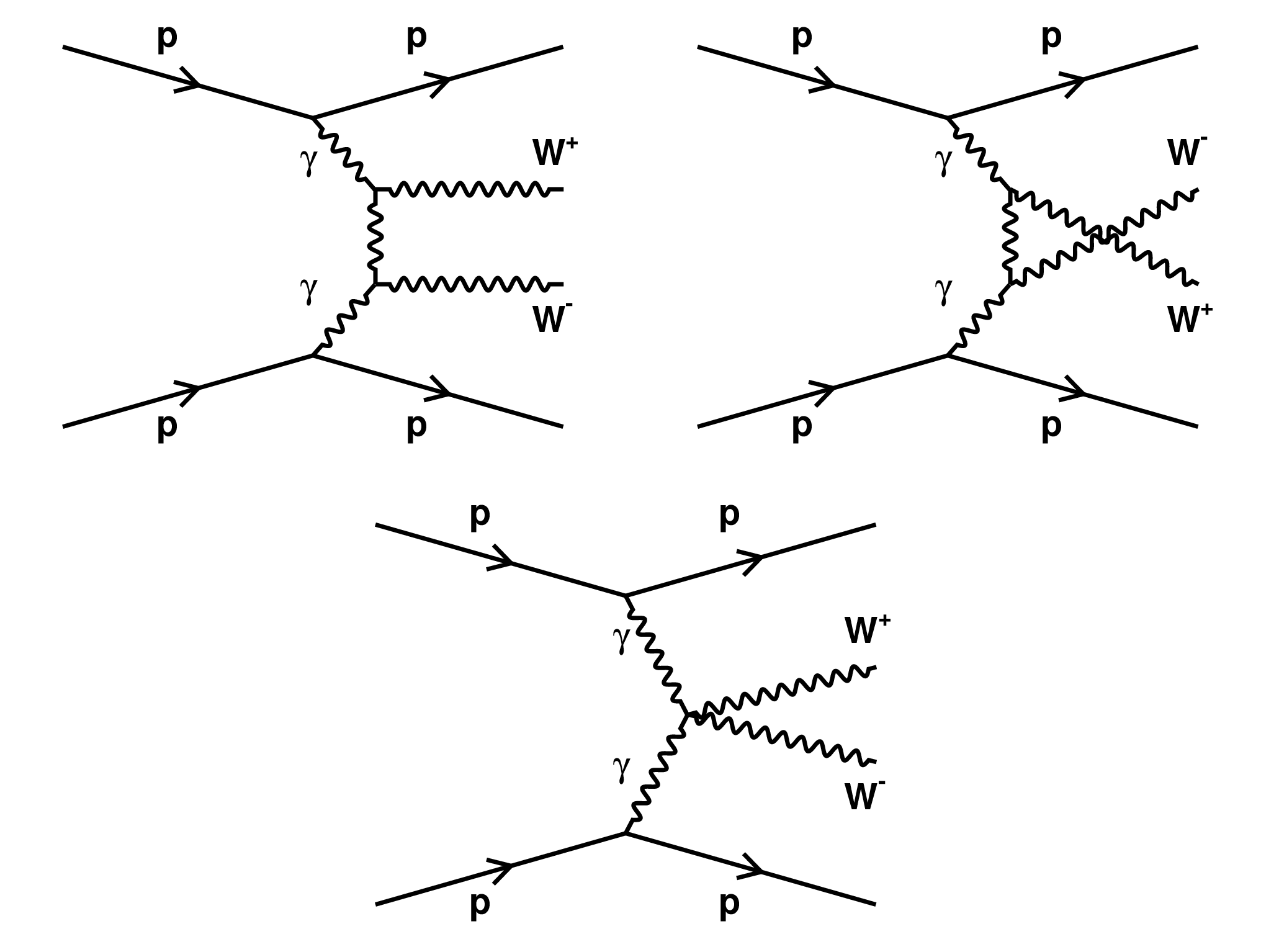
Figure 1:
Schematic diagrams of exclusive $ \gamma\gamma \to \mathrm{W}\mathrm{W} $ production with intact protons according to the standard model (SM). |
png pdf |
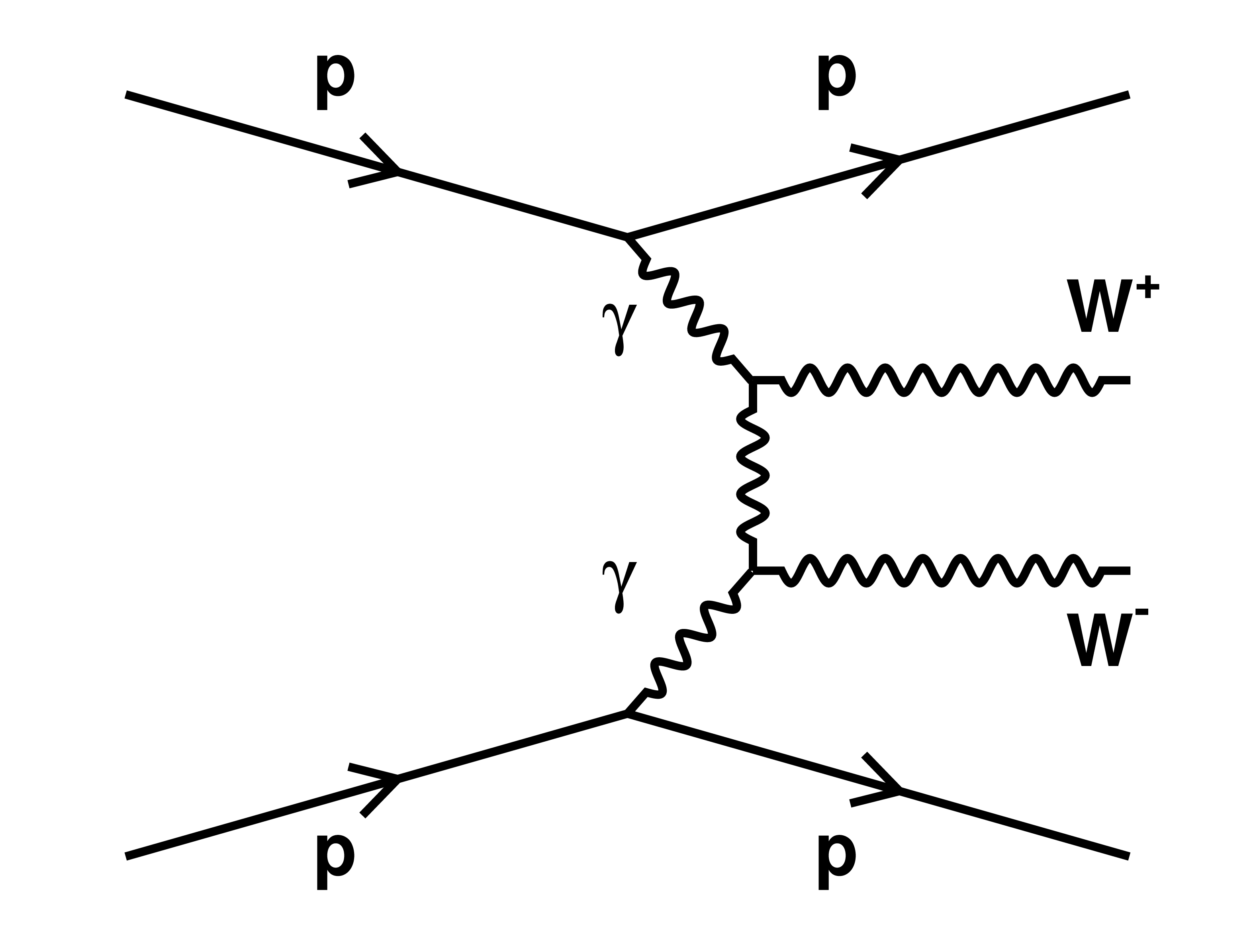
Figure 1-a:
Schematic diagrams of exclusive $ \gamma\gamma \to \mathrm{W}\mathrm{W} $ production with intact protons according to the standard model (SM). |
png pdf |
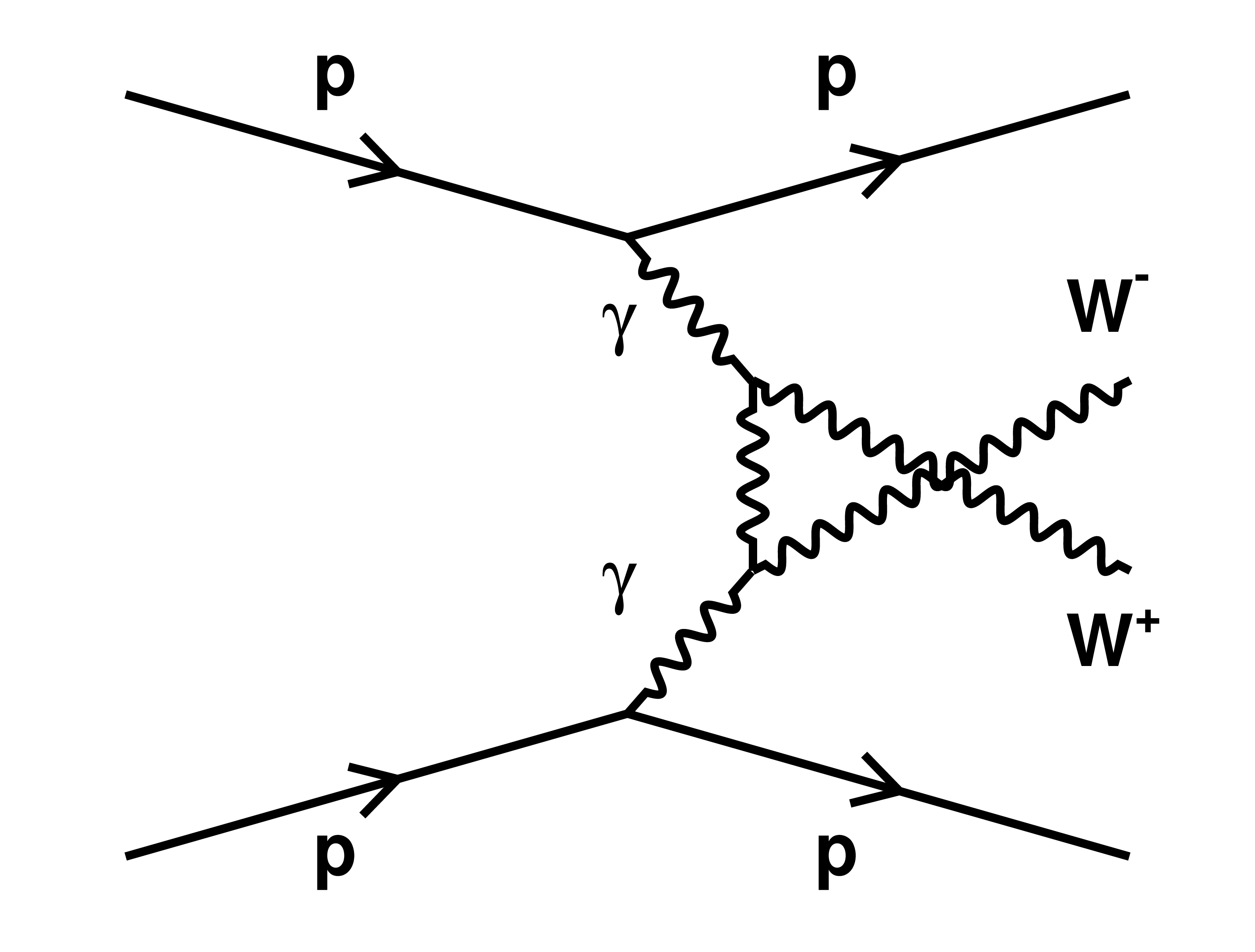
Figure 1-b:
Schematic diagrams of exclusive $ \gamma\gamma \to \mathrm{W}\mathrm{W} $ production with intact protons according to the standard model (SM). |
png pdf |
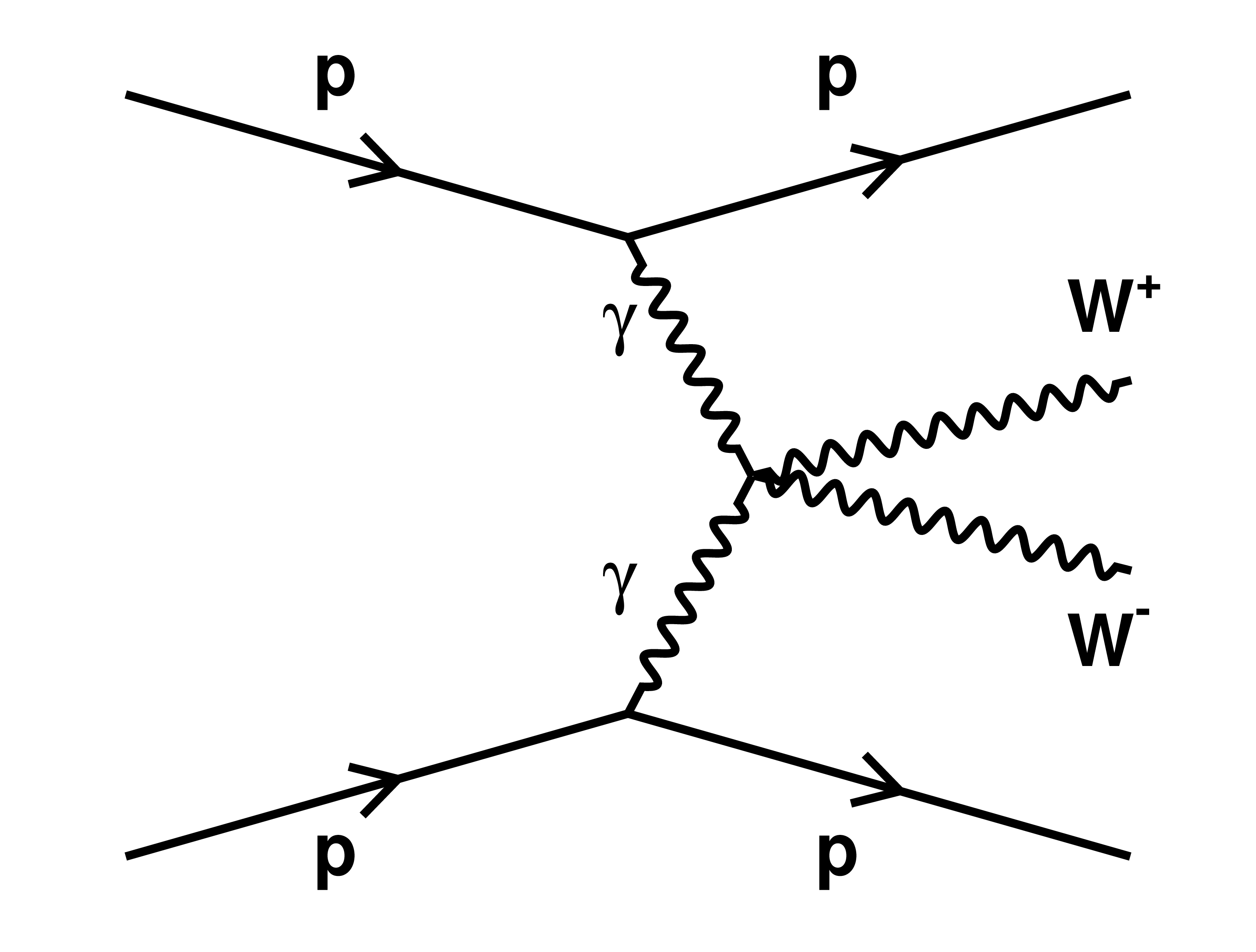
Figure 1-c:
Schematic diagrams of exclusive $ \gamma\gamma \to \mathrm{W}\mathrm{W} $ production with intact protons according to the standard model (SM). |
png pdf |
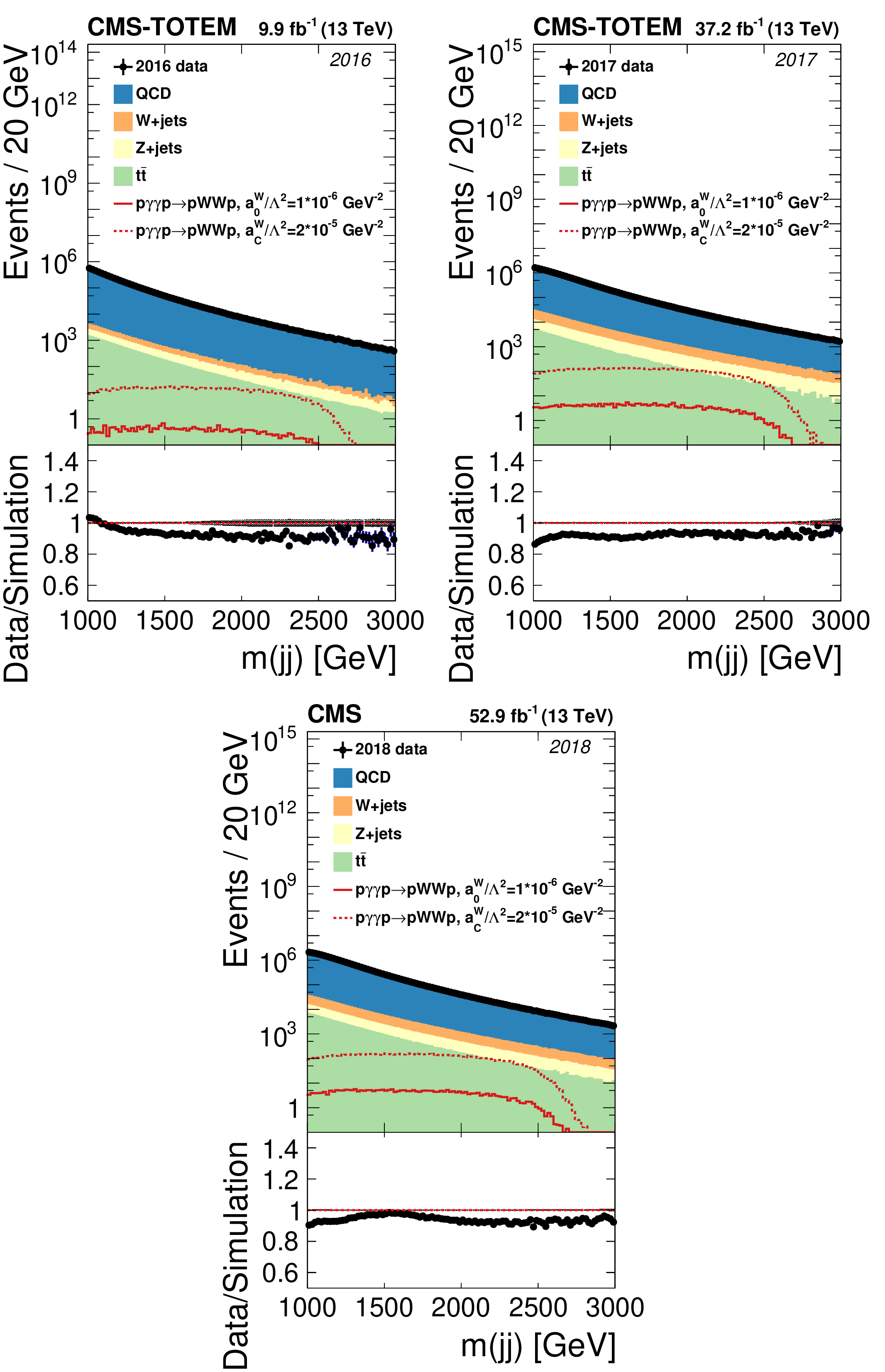
Figure 2:
Dijet invariant mass spectra in data and simulation, for the years 2016 (upper left), 2017 (upper right), and 2018 (lower). The distributions of number of events show data compared with the stacked background predictions from simulation, with the corresponding ratios of data to the sum of simulated backgrounds, shown below them. The plots are shown at the preselection level, with no requirements on the protons, jet substructure, or dijet balance. Examples of simulated signals are shown for protons generated in the range of 0.01 $ \le \xi \le $ 0.20. Only statistical uncertainties (dashed grey bands) are shown. |
png pdf |
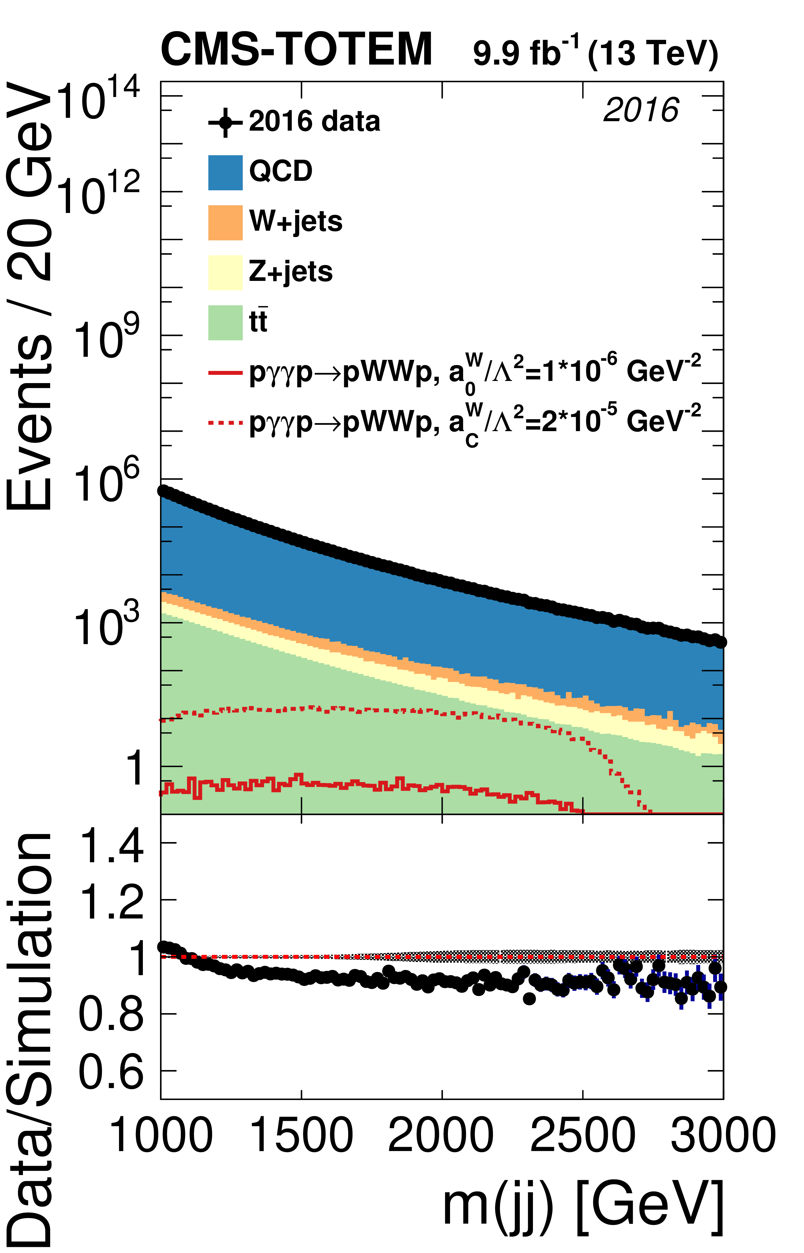
Figure 2-a:
Dijet invariant mass spectra in data and simulation, for the years 2016 (upper left), 2017 (upper right), and 2018 (lower). The distributions of number of events show data compared with the stacked background predictions from simulation, with the corresponding ratios of data to the sum of simulated backgrounds, shown below them. The plots are shown at the preselection level, with no requirements on the protons, jet substructure, or dijet balance. Examples of simulated signals are shown for protons generated in the range of 0.01 $ \le \xi \le $ 0.20. Only statistical uncertainties (dashed grey bands) are shown. |
png pdf |
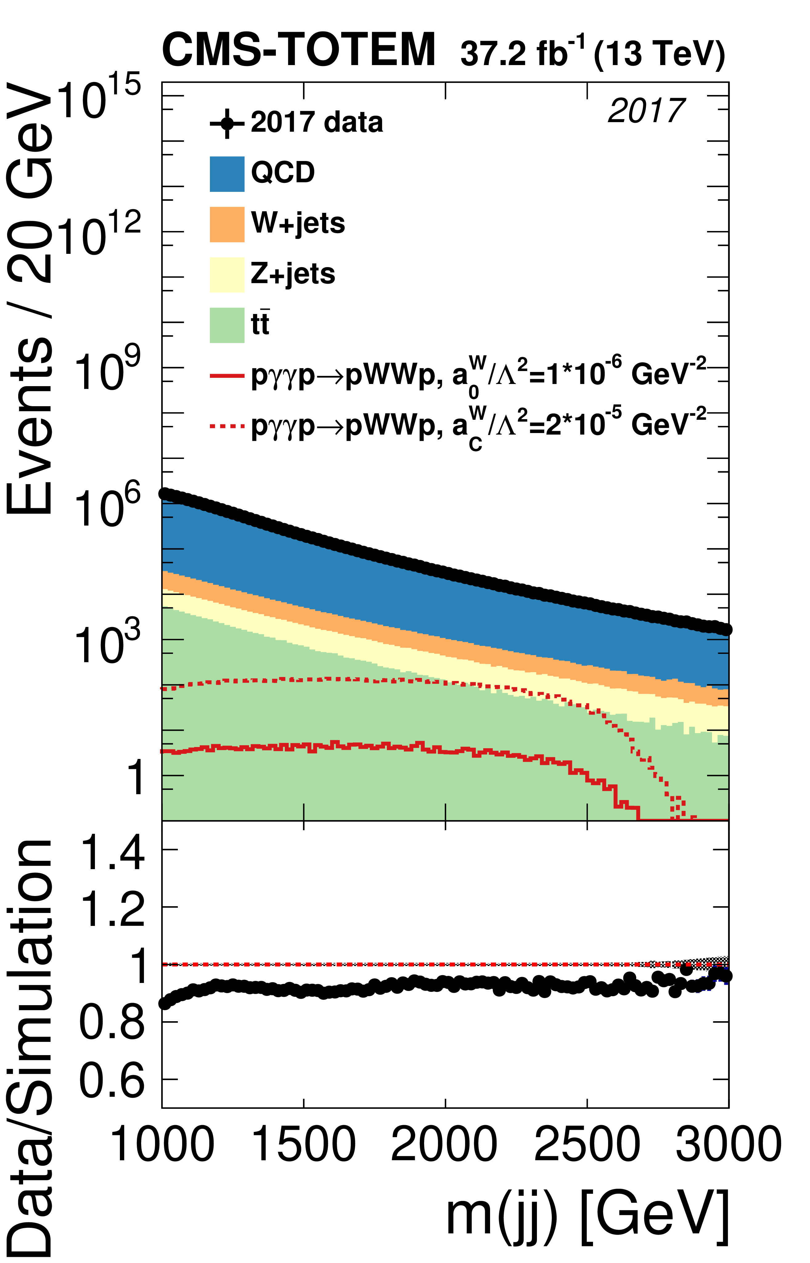
Figure 2-b:
Dijet invariant mass spectra in data and simulation, for the years 2016 (upper left), 2017 (upper right), and 2018 (lower). The distributions of number of events show data compared with the stacked background predictions from simulation, with the corresponding ratios of data to the sum of simulated backgrounds, shown below them. The plots are shown at the preselection level, with no requirements on the protons, jet substructure, or dijet balance. Examples of simulated signals are shown for protons generated in the range of 0.01 $ \le \xi \le $ 0.20. Only statistical uncertainties (dashed grey bands) are shown. |
png pdf |
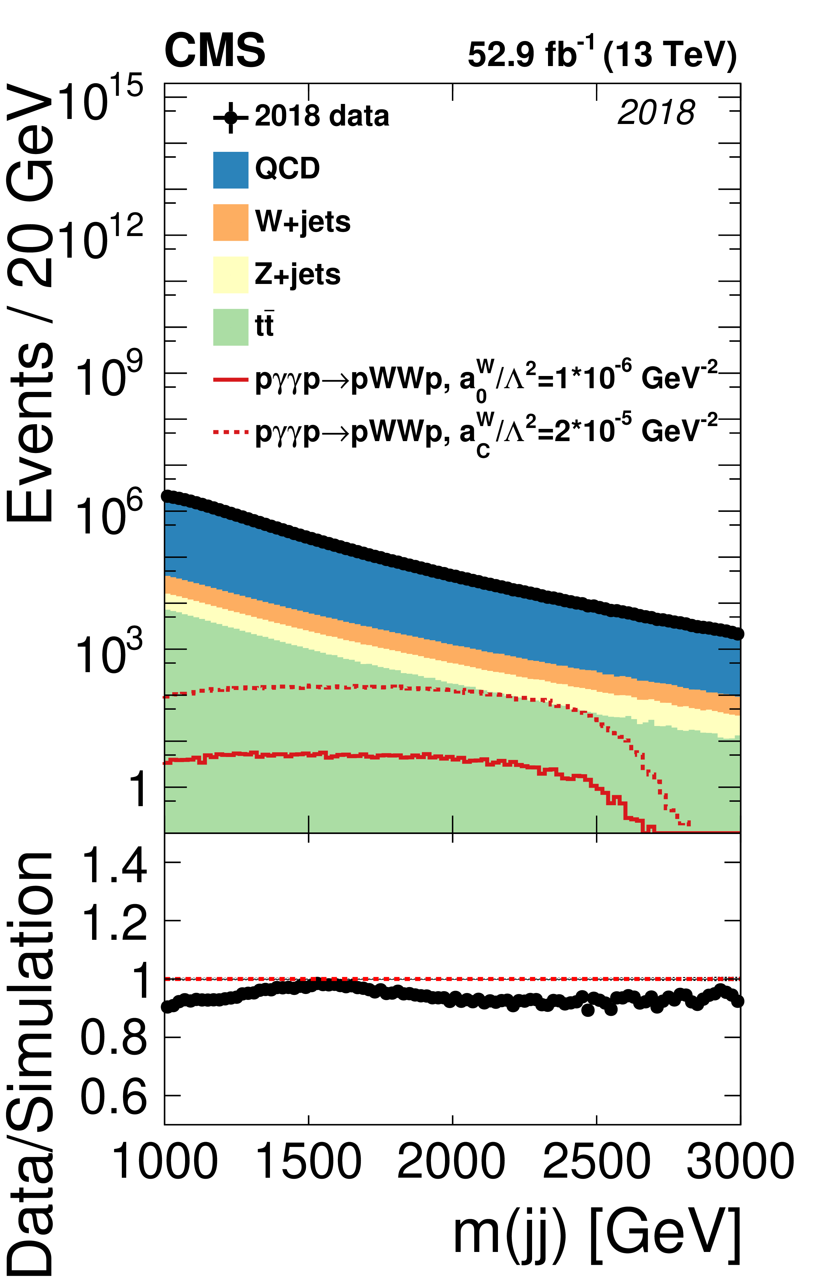
Figure 2-c:
Dijet invariant mass spectra in data and simulation, for the years 2016 (upper left), 2017 (upper right), and 2018 (lower). The distributions of number of events show data compared with the stacked background predictions from simulation, with the corresponding ratios of data to the sum of simulated backgrounds, shown below them. The plots are shown at the preselection level, with no requirements on the protons, jet substructure, or dijet balance. Examples of simulated signals are shown for protons generated in the range of 0.01 $ \le \xi \le $ 0.20. Only statistical uncertainties (dashed grey bands) are shown. |
png pdf |
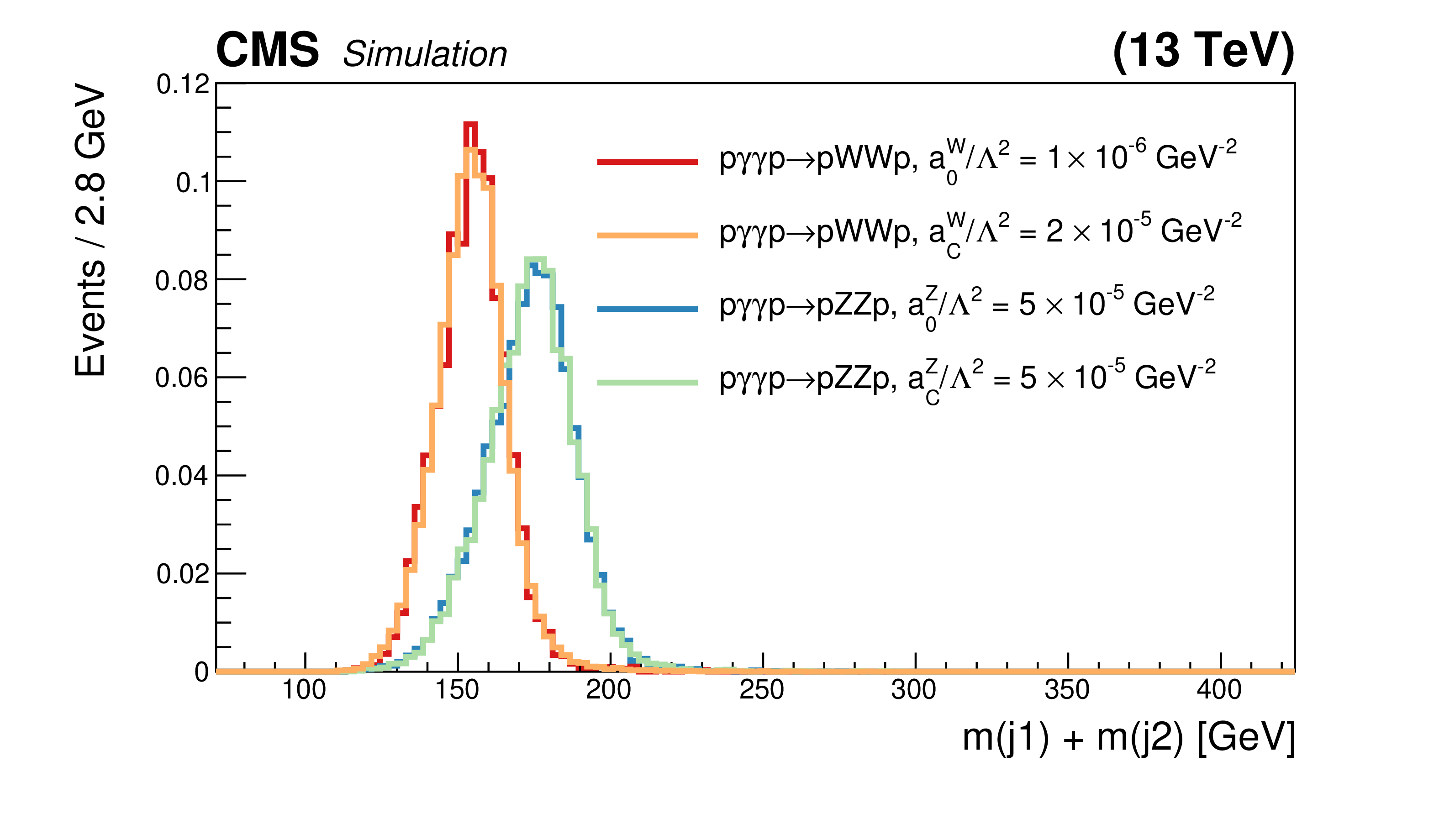
Figure 3:
Event distribution as a function of the discriminant described in the text for simulated WW and ZZ signal events. |
png pdf |
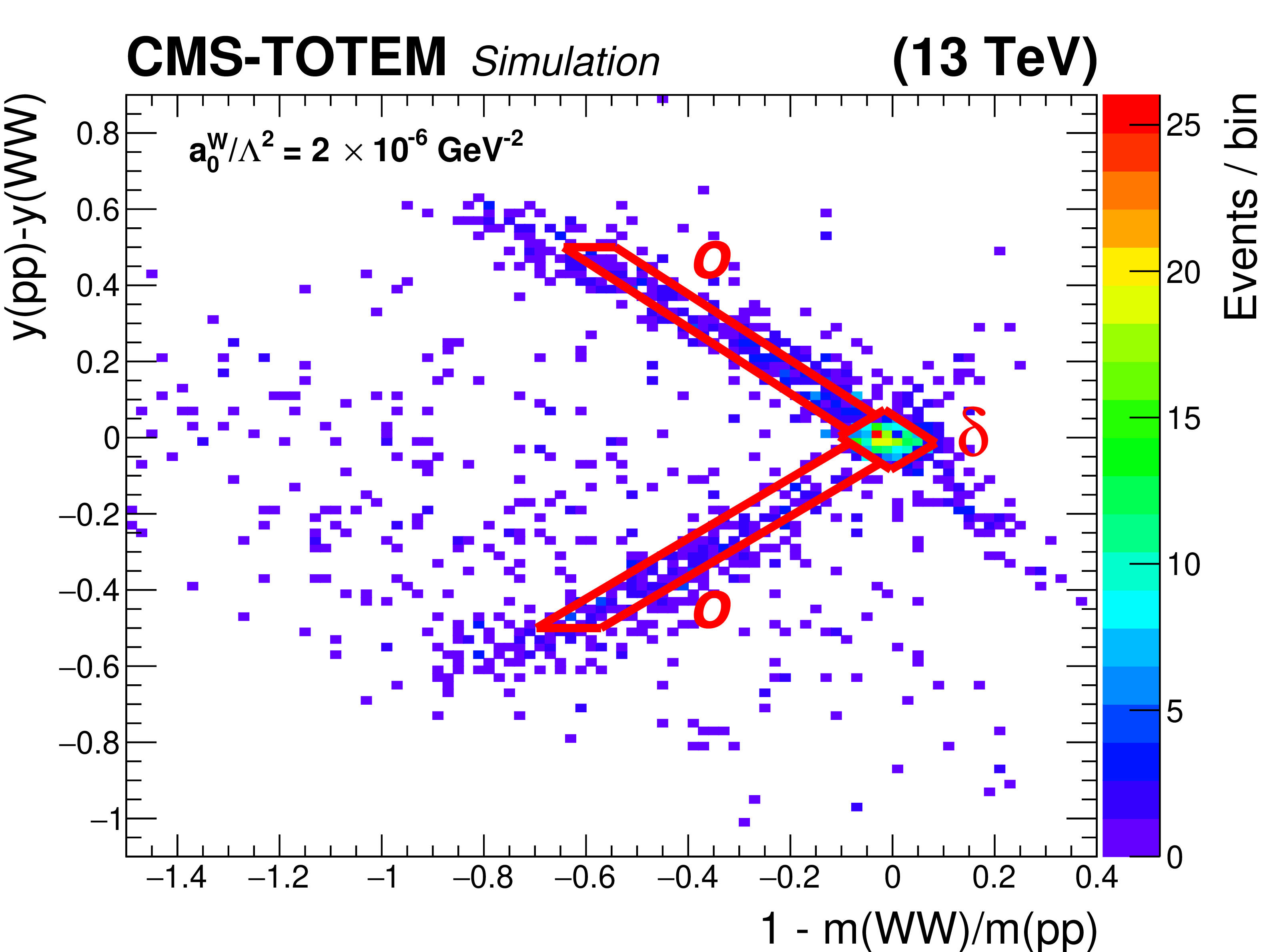
Figure 4:
Matching between the jets and the protons, in invariant mass and rapidity, for simulated WW exclusive signal events. The red diamond-shaped area near the origin (signal region $ \delta $) corresponds to the case where both protons are correctly matched to the jets. The areas within the red diagonal bands (signal region $ o $) correspond to the case where one proton is correctly matched, and the second proton originates from a pileup interaction. |
png pdf |
Figure 5:
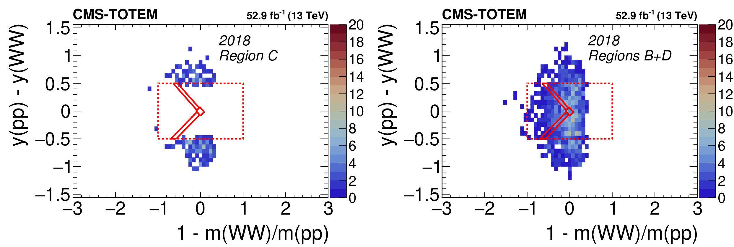
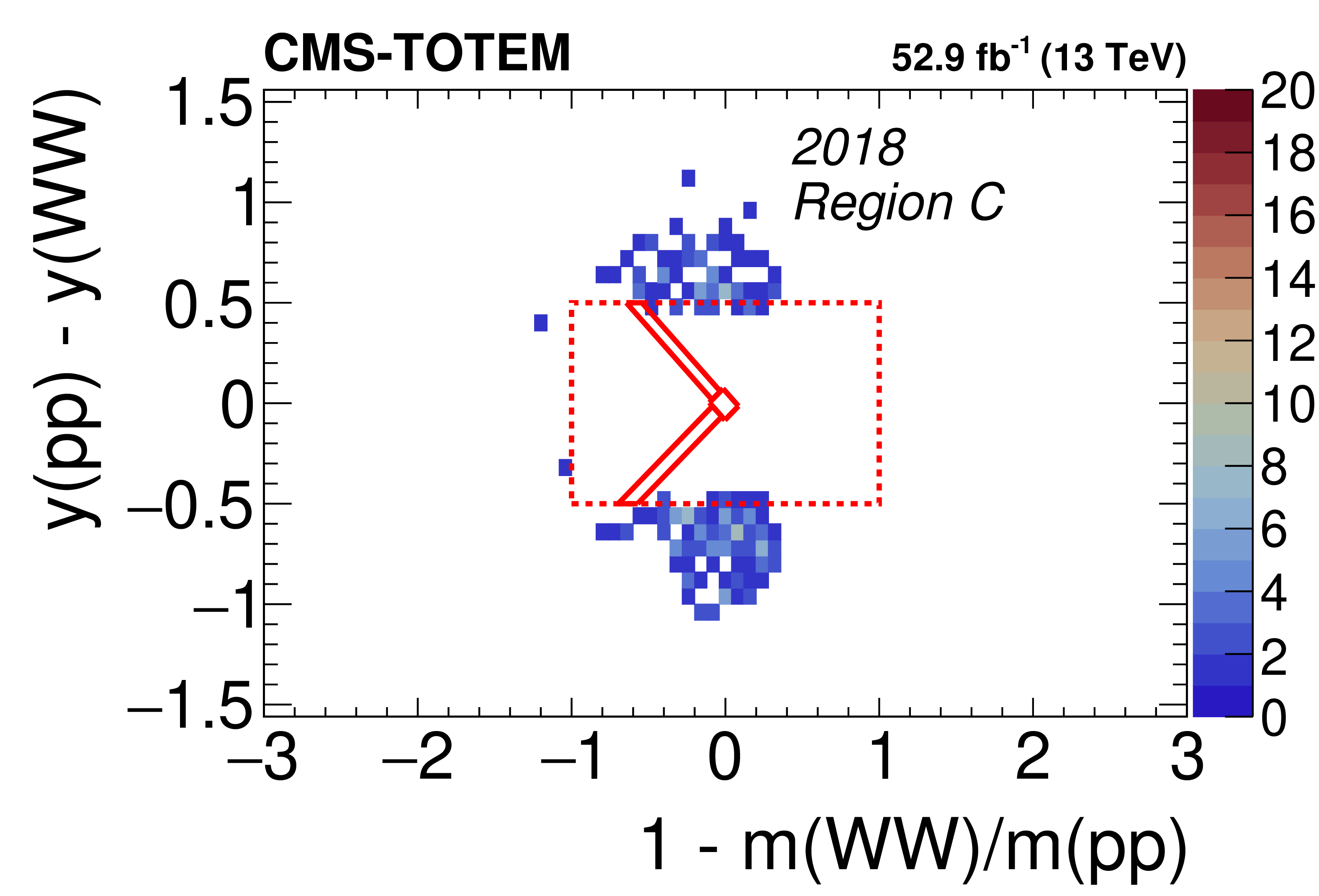
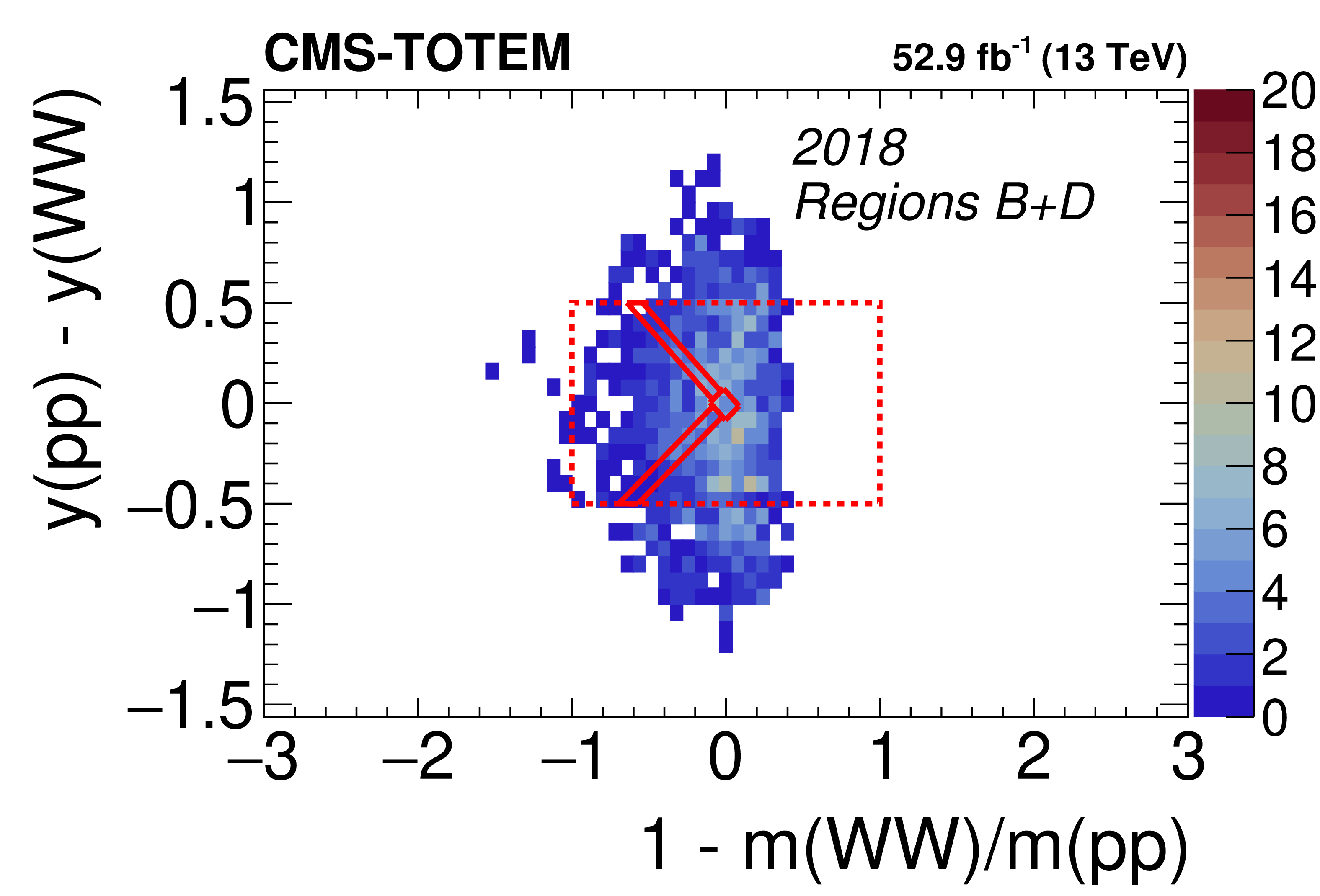
Distribution of the 2018 data in the $ y(\mathrm{p}\mathrm{p}) - y(\mathrm{VV}) $ vs 1 $ - m(\mathrm{VV})/m(\mathrm{p}\mathrm{p}) $ plane in the WW mass region. On the left, the sample with all selections applied is shown, except that the region inside the dashed lines remains blinded. On the right, the region with the acoplanarity requirement inverted is shown. The solid lines indicate the same signal regions as shown in Fig. 4. In the right plot the area inside the solid lines corresponds to ``region B'', while the area outside the dashed lines corresponds to ``region D''. The color scale on the $ z $ axis indicates the number of events in each bin. |
png pdf |
Figure 5-a:
Distribution of the 2018 data in the $ y(\mathrm{p}\mathrm{p}) - y(\mathrm{VV}) $ vs 1 $ - m(\mathrm{VV})/m(\mathrm{p}\mathrm{p}) $ plane in the WW mass region. On the left, the sample with all selections applied is shown, except that the region inside the dashed lines remains blinded. On the right, the region with the acoplanarity requirement inverted is shown. The solid lines indicate the same signal regions as shown in Fig. 4. In the right plot the area inside the solid lines corresponds to ``region B'', while the area outside the dashed lines corresponds to ``region D''. The color scale on the $ z $ axis indicates the number of events in each bin. |
png pdf |
Figure 5-b:
Distribution of the 2018 data in the $ y(\mathrm{p}\mathrm{p}) - y(\mathrm{VV}) $ vs 1 $ - m(\mathrm{VV})/m(\mathrm{p}\mathrm{p}) $ plane in the WW mass region. On the left, the sample with all selections applied is shown, except that the region inside the dashed lines remains blinded. On the right, the region with the acoplanarity requirement inverted is shown. The solid lines indicate the same signal regions as shown in Fig. 4. In the right plot the area inside the solid lines corresponds to ``region B'', while the area outside the dashed lines corresponds to ``region D''. The color scale on the $ z $ axis indicates the number of events in each bin. |
png pdf |
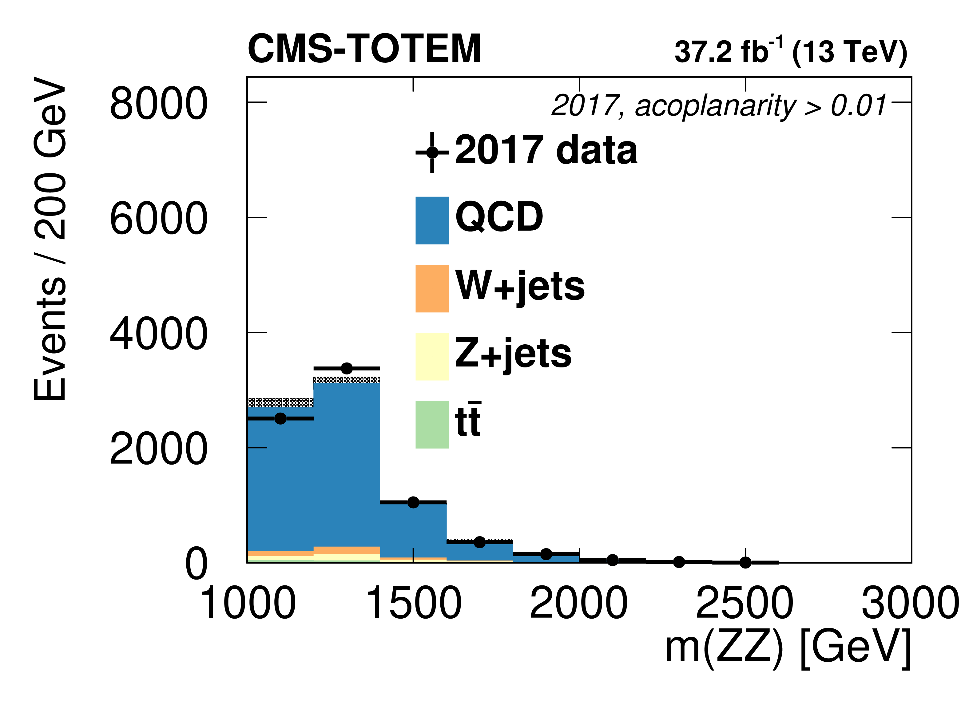
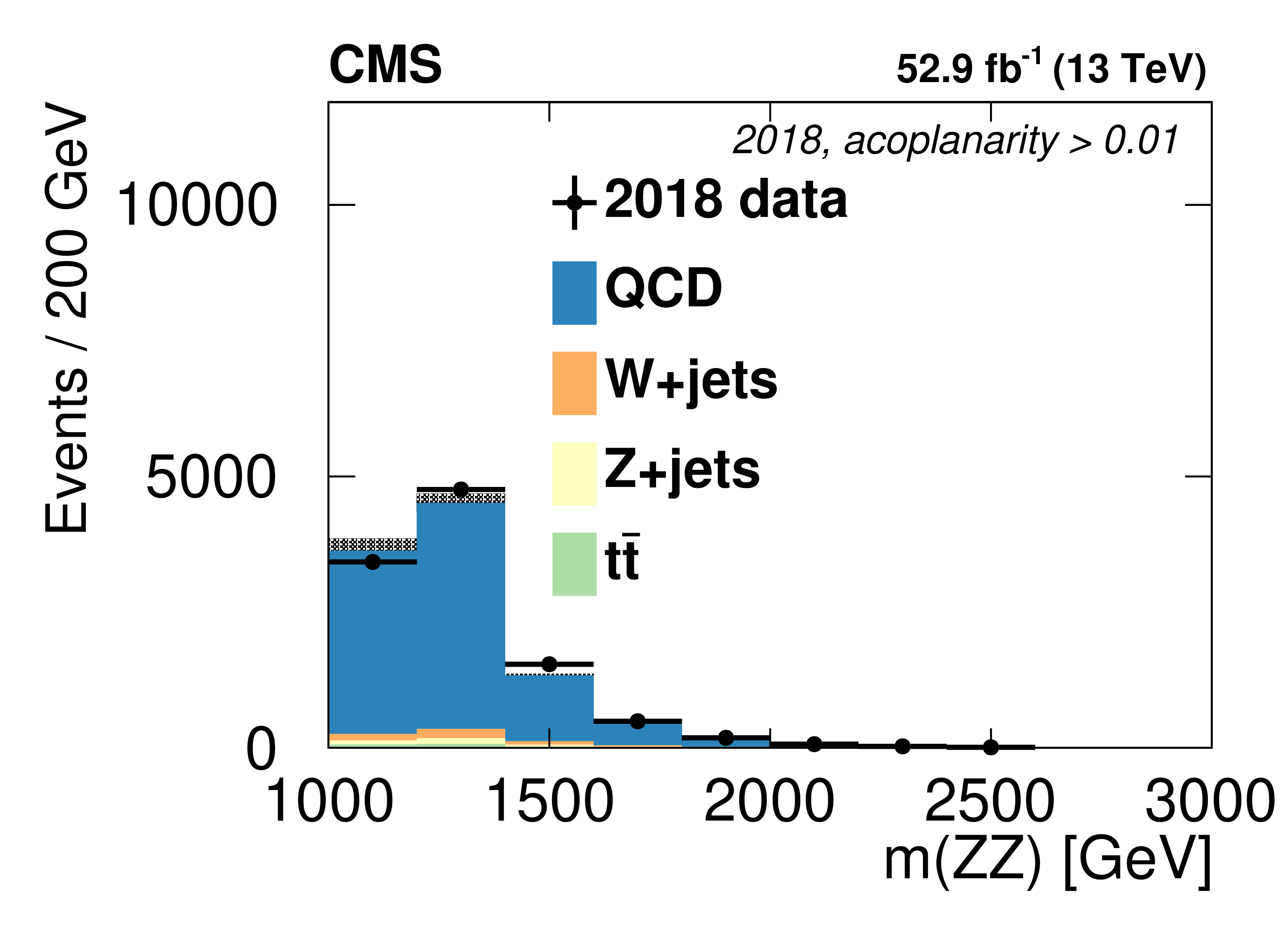
Figure 6:
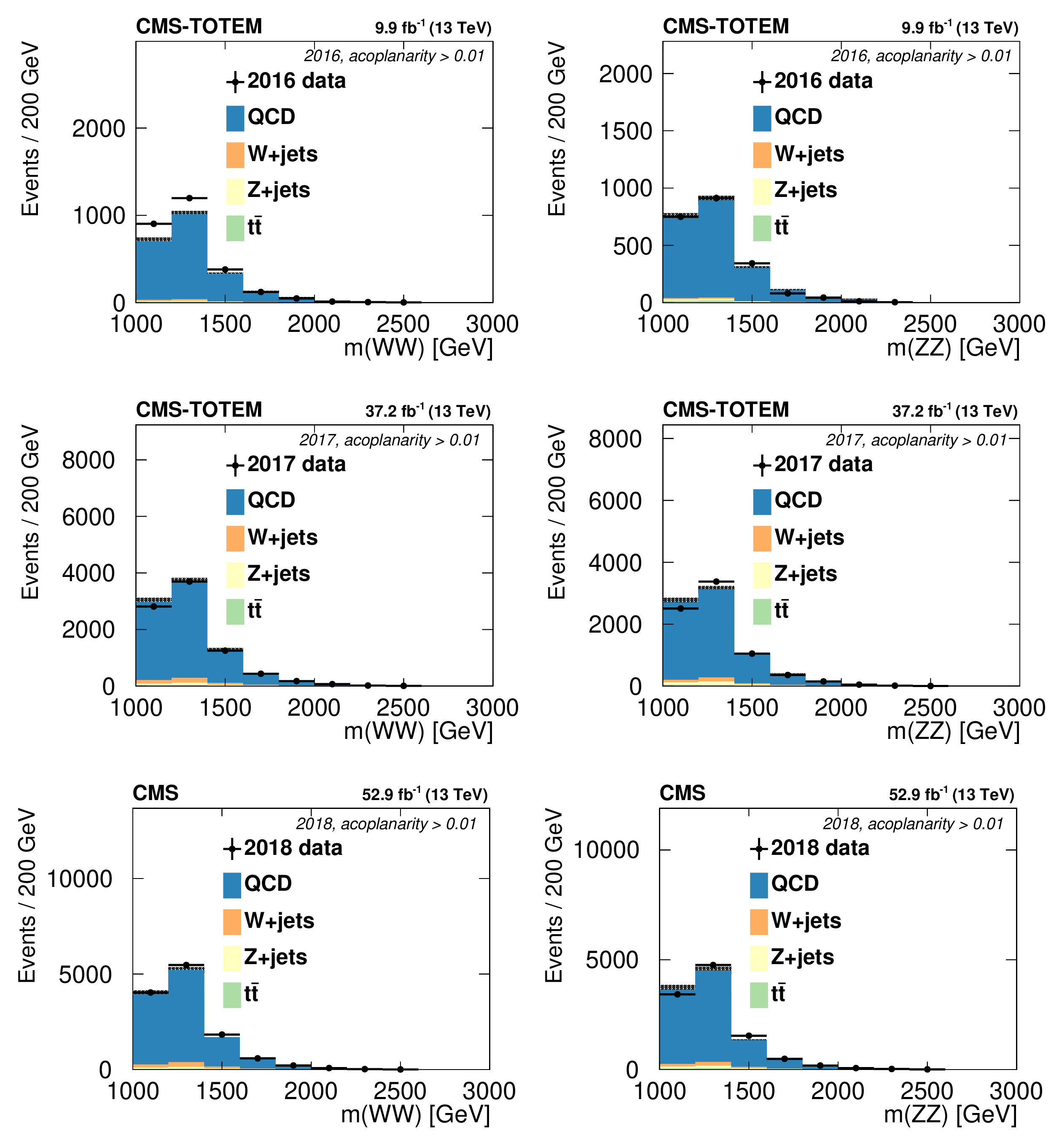
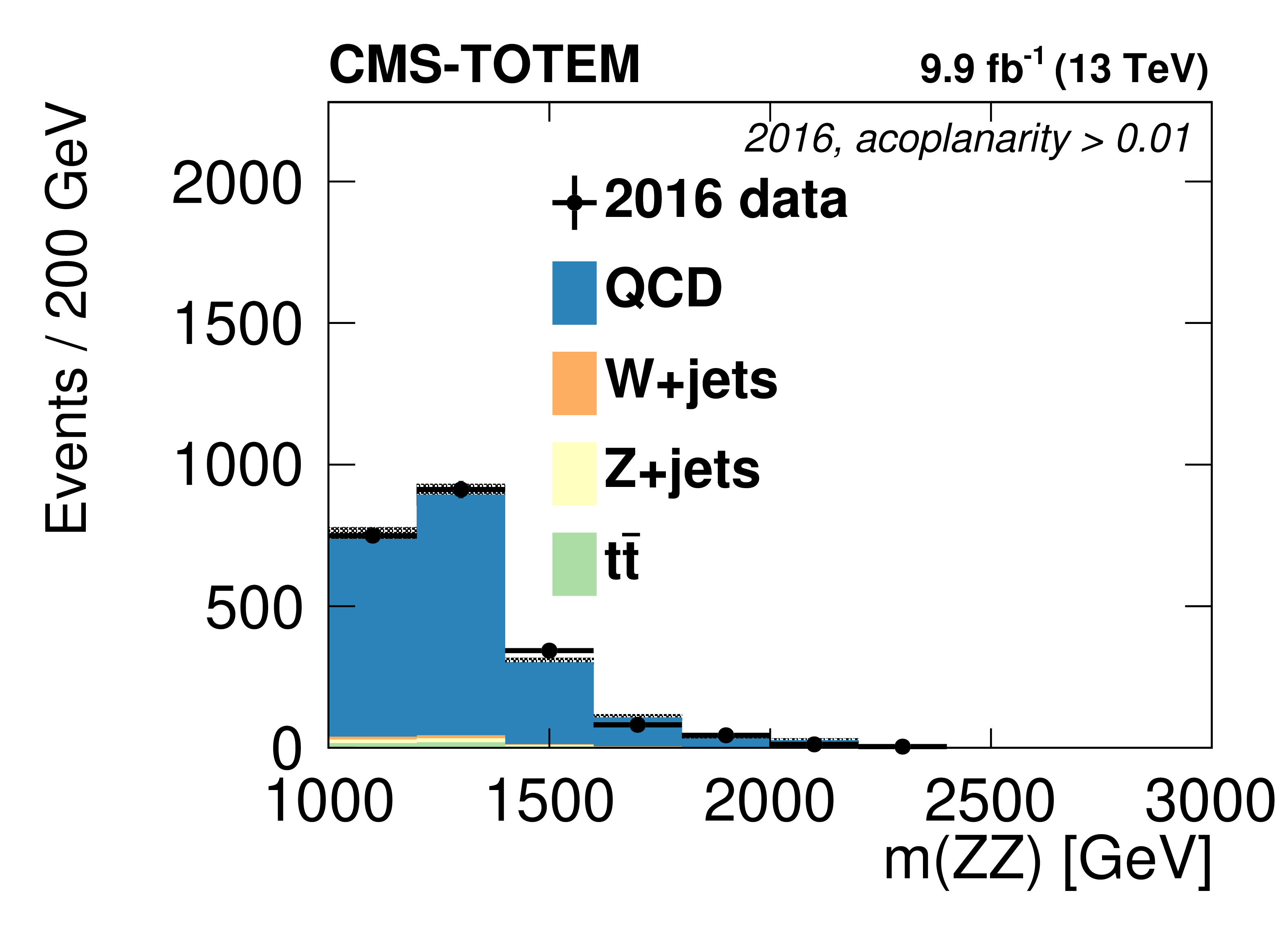
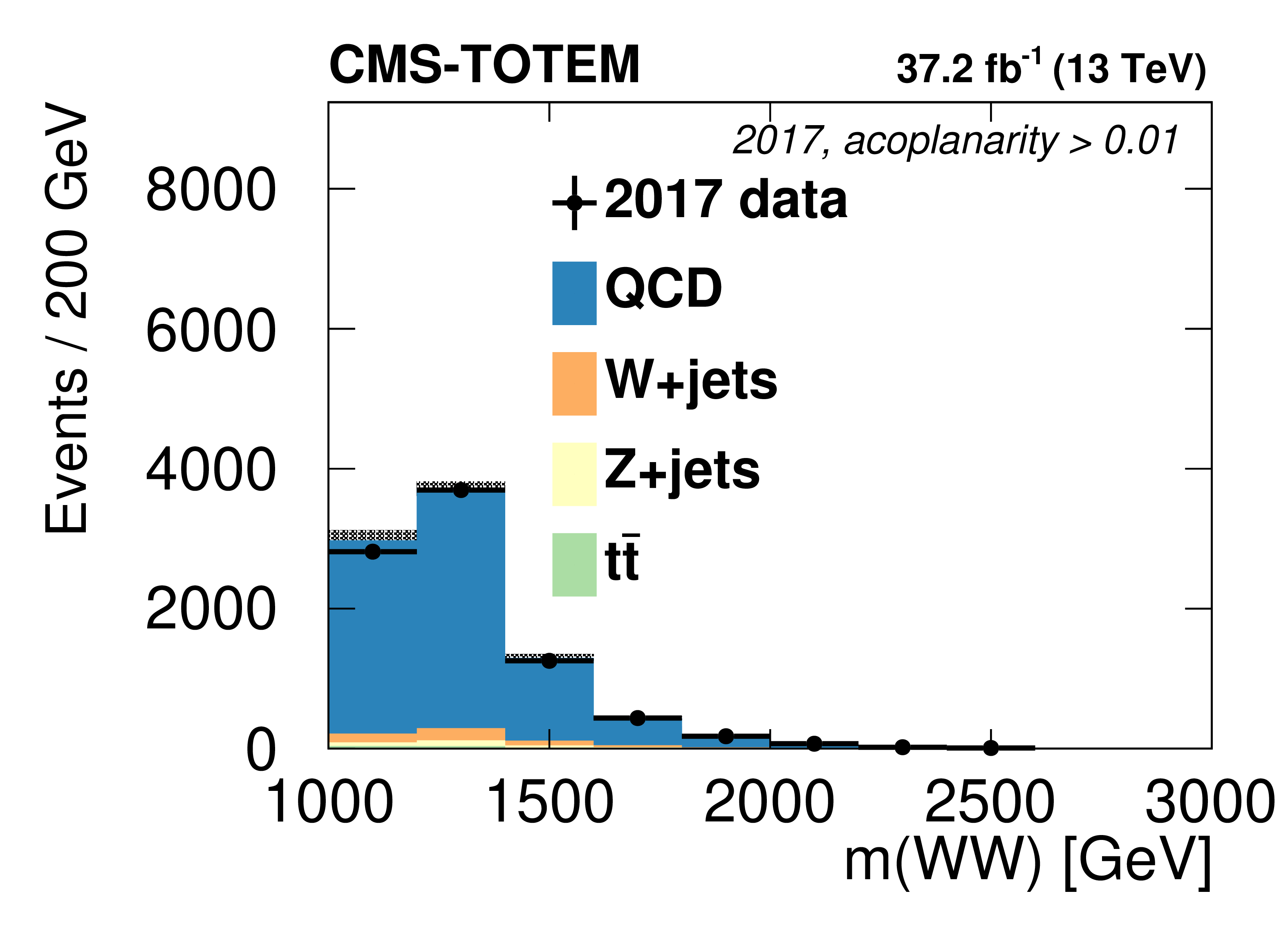
Diboson invariant mass distributions in data and simulation in the anti-acoplanarity region ($ a > $ 0.01), with no requirement on the proton matching. The plots from top to bottom are for the 2016, 2017, and 2018 data, respectively, with the WW region in the left column and the ZZ region in the right column. Only statistical uncertainties (dashed grey bands) are shown. |

png pdf |
Figure 6-a:
Diboson invariant mass distributions in data and simulation in the anti-acoplanarity region ($ a > $ 0.01), with no requirement on the proton matching. The plots from top to bottom are for the 2016, 2017, and 2018 data, respectively, with the WW region in the left column and the ZZ region in the right column. Only statistical uncertainties (dashed grey bands) are shown. |
png pdf |
Figure 6-b:
Diboson invariant mass distributions in data and simulation in the anti-acoplanarity region ($ a > $ 0.01), with no requirement on the proton matching. The plots from top to bottom are for the 2016, 2017, and 2018 data, respectively, with the WW region in the left column and the ZZ region in the right column. Only statistical uncertainties (dashed grey bands) are shown. |
png pdf |
Figure 6-c:
Diboson invariant mass distributions in data and simulation in the anti-acoplanarity region ($ a > $ 0.01), with no requirement on the proton matching. The plots from top to bottom are for the 2016, 2017, and 2018 data, respectively, with the WW region in the left column and the ZZ region in the right column. Only statistical uncertainties (dashed grey bands) are shown. |
png pdf |
Figure 6-d:
Diboson invariant mass distributions in data and simulation in the anti-acoplanarity region ($ a > $ 0.01), with no requirement on the proton matching. The plots from top to bottom are for the 2016, 2017, and 2018 data, respectively, with the WW region in the left column and the ZZ region in the right column. Only statistical uncertainties (dashed grey bands) are shown. |

png pdf |
Figure 6-e:
Diboson invariant mass distributions in data and simulation in the anti-acoplanarity region ($ a > $ 0.01), with no requirement on the proton matching. The plots from top to bottom are for the 2016, 2017, and 2018 data, respectively, with the WW region in the left column and the ZZ region in the right column. Only statistical uncertainties (dashed grey bands) are shown. |
png pdf |
Figure 6-f:
Diboson invariant mass distributions in data and simulation in the anti-acoplanarity region ($ a > $ 0.01), with no requirement on the proton matching. The plots from top to bottom are for the 2016, 2017, and 2018 data, respectively, with the WW region in the left column and the ZZ region in the right column. Only statistical uncertainties (dashed grey bands) are shown. |
png pdf |
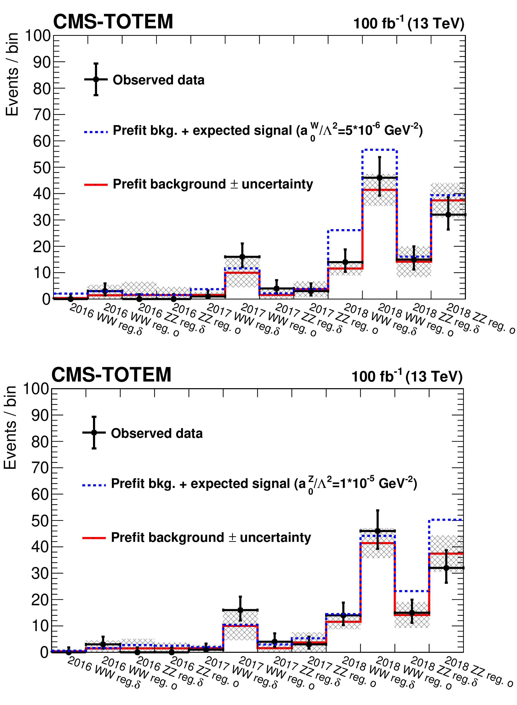
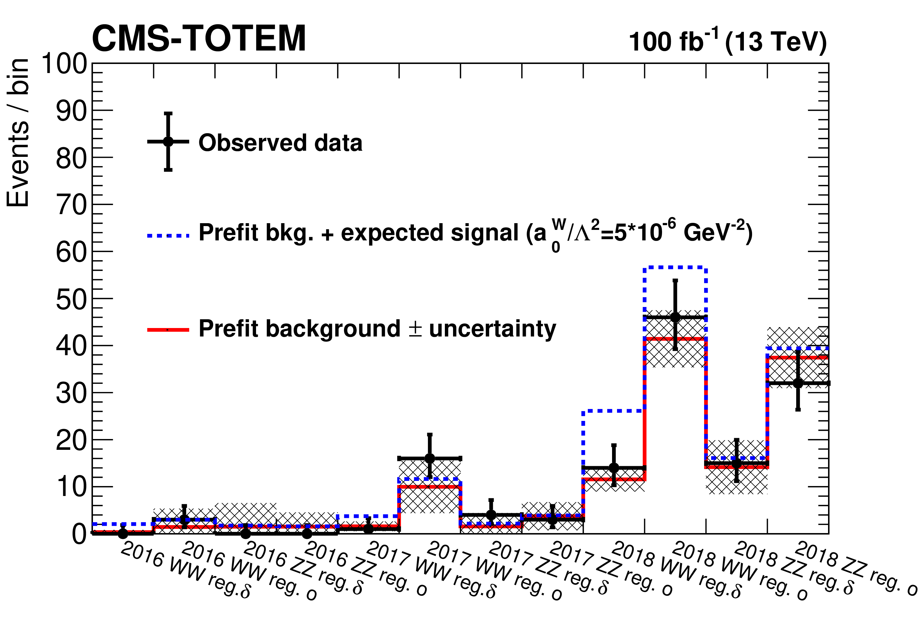
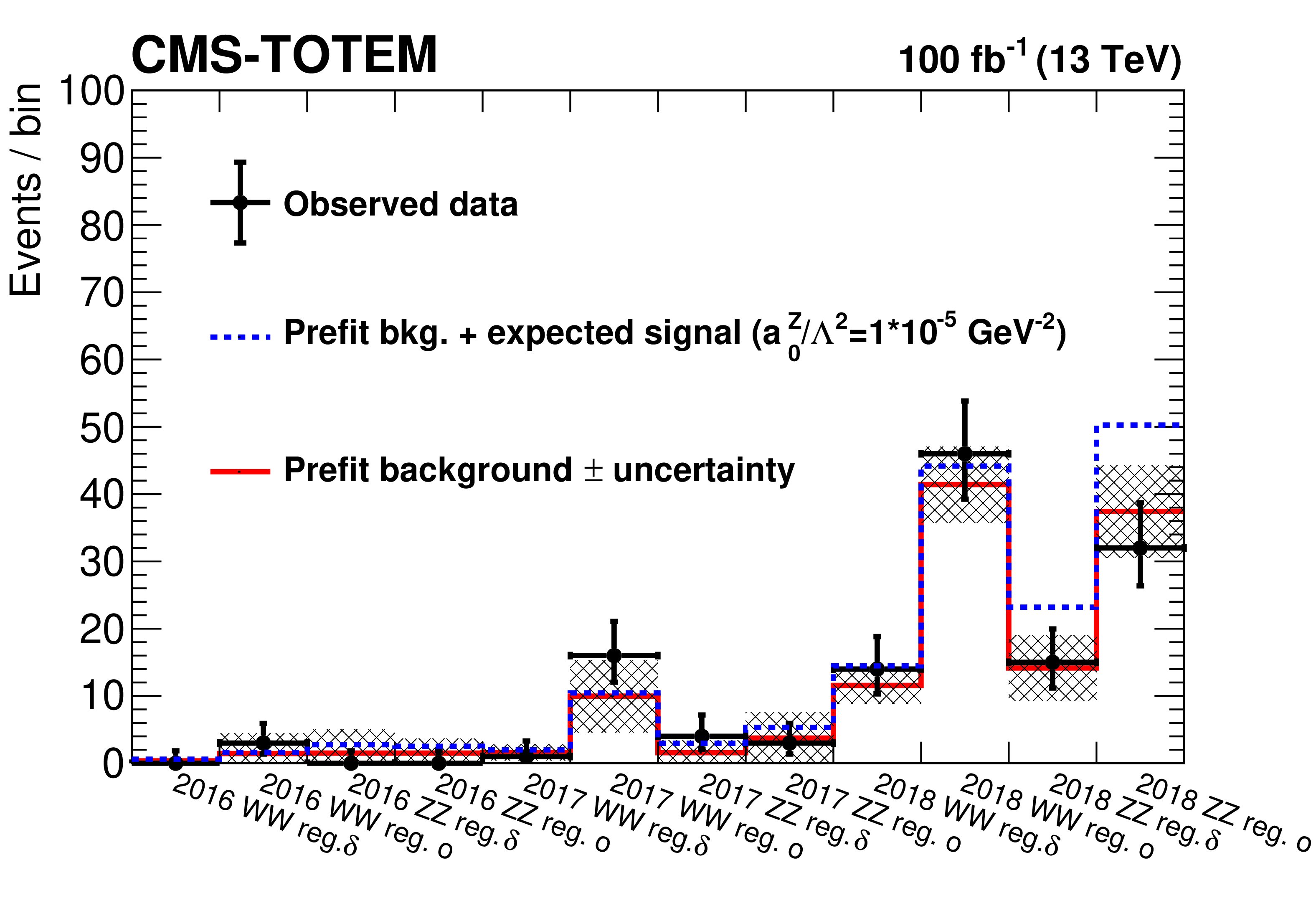
Figure 7:
Observed data and expected number of background events in each signal region. Hypothetical AQGC signals are also shown. The histogram with solid lines indicates the number expected for only background, with uncertainties shown by the shaded band. The dashed-line histogram shows the number for background plus assumed signals with $ a^{\mathrm{W}}_{0}/\Lambda^2=$ 5 $\times$ 10$^{-6}$ GeV$^{-2}$(upper) or $ a^{\mathrm{Z}}_{0}/\Lambda^2=$ 1 $\times$ 10$^{-5}$ GeV$^{-2}$(lower). The histograms and uncertainties are shown prior to the binned maximum-likelihood fit described in the text. The shaded band indicates the uncertainty in the background estimate, while the vertical bars on the points represent the statistical uncertainty in the observed data. |
png pdf |
Figure 7-a:
Observed data and expected number of background events in each signal region. Hypothetical AQGC signals are also shown. The histogram with solid lines indicates the number expected for only background, with uncertainties shown by the shaded band. The dashed-line histogram shows the number for background plus assumed signals with $ a^{\mathrm{W}}_{0}/\Lambda^2=$ 5 $\times$ 10$^{-6}$ GeV$^{-2}$(upper) or $ a^{\mathrm{Z}}_{0}/\Lambda^2=$ 1 $\times$ 10$^{-5}$ GeV$^{-2}$(lower). The histograms and uncertainties are shown prior to the binned maximum-likelihood fit described in the text. The shaded band indicates the uncertainty in the background estimate, while the vertical bars on the points represent the statistical uncertainty in the observed data. |
png pdf |
Figure 7-b:
Observed data and expected number of background events in each signal region. Hypothetical AQGC signals are also shown. The histogram with solid lines indicates the number expected for only background, with uncertainties shown by the shaded band. The dashed-line histogram shows the number for background plus assumed signals with $ a^{\mathrm{W}}_{0}/\Lambda^2=$ 5 $\times$ 10$^{-6}$ GeV$^{-2}$(upper) or $ a^{\mathrm{Z}}_{0}/\Lambda^2=$ 1 $\times$ 10$^{-5}$ GeV$^{-2}$(lower). The histograms and uncertainties are shown prior to the binned maximum-likelihood fit described in the text. The shaded band indicates the uncertainty in the background estimate, while the vertical bars on the points represent the statistical uncertainty in the observed data. |
png pdf |
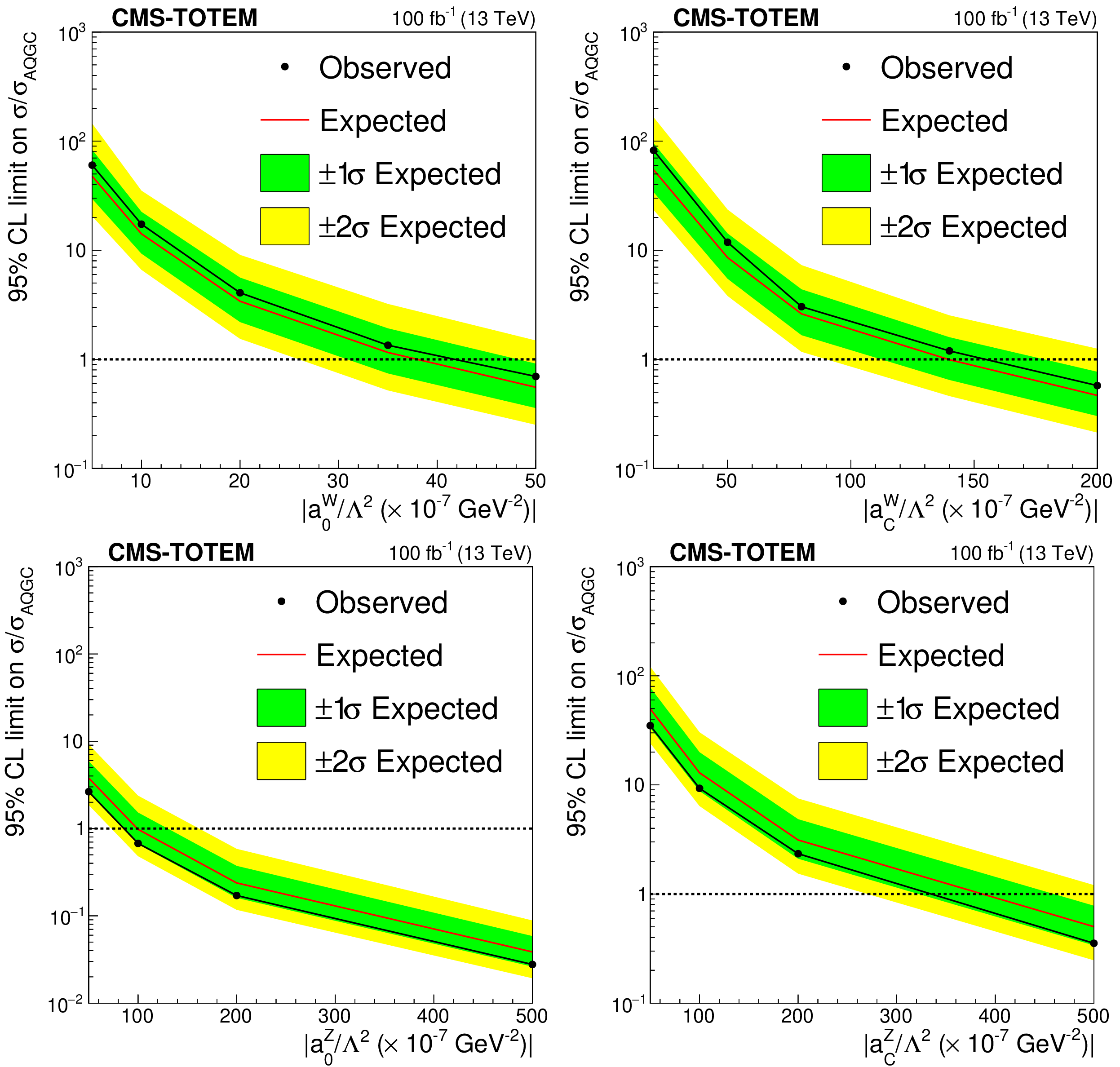
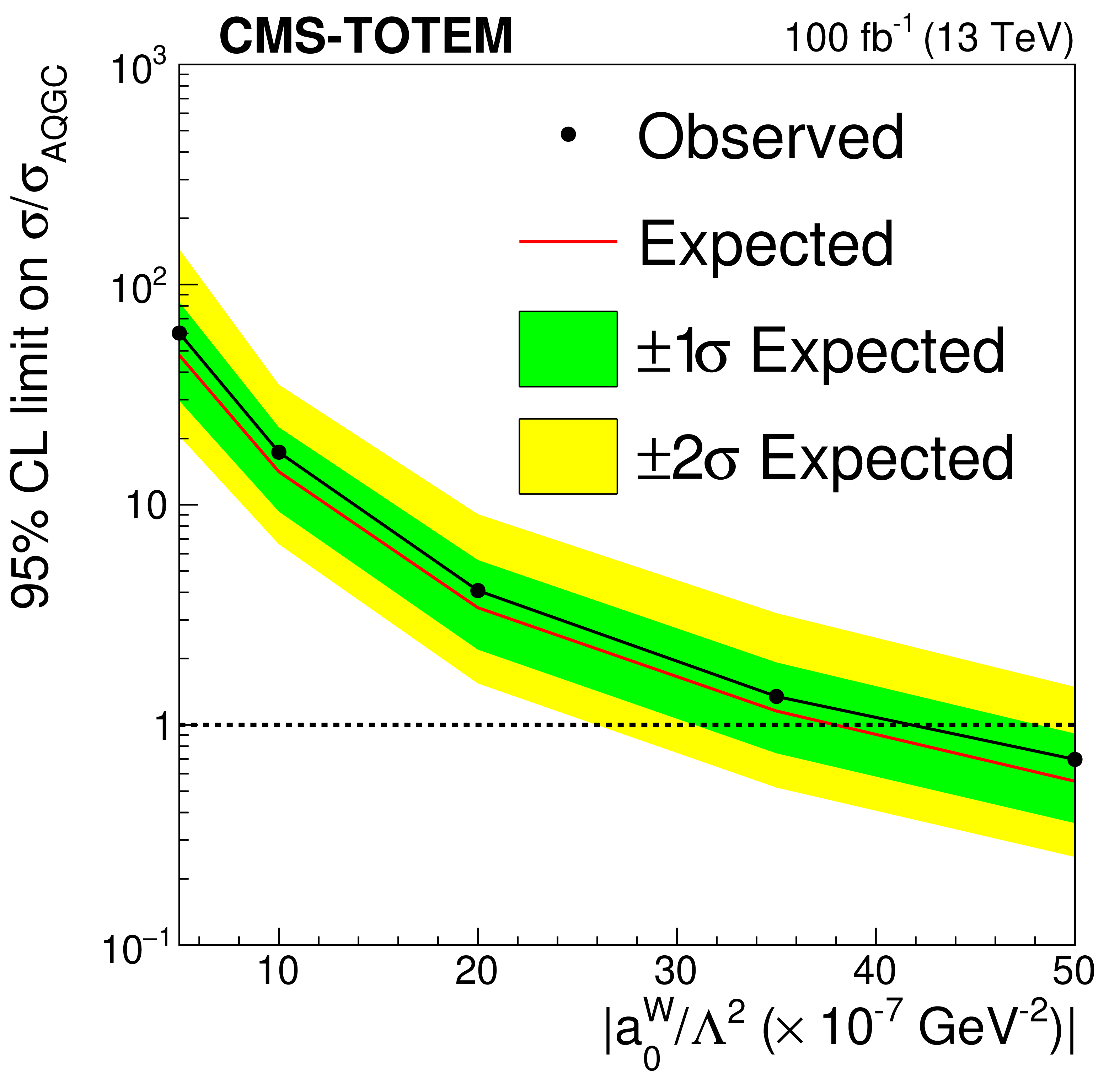
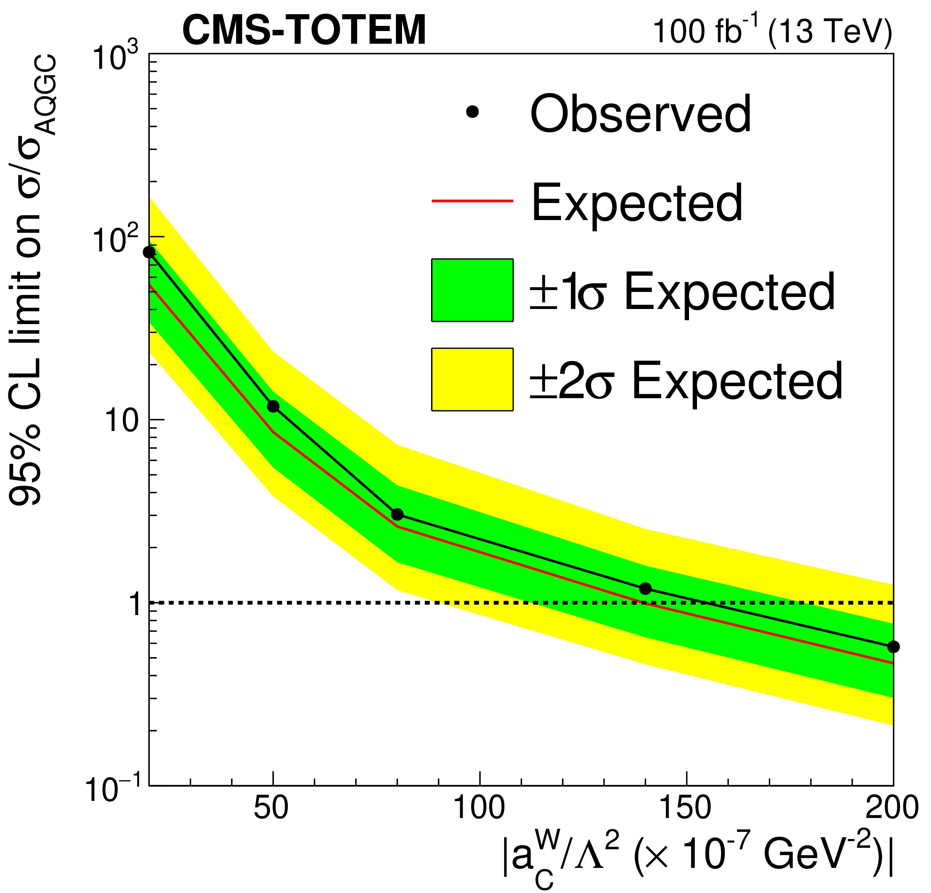
Figure 8:
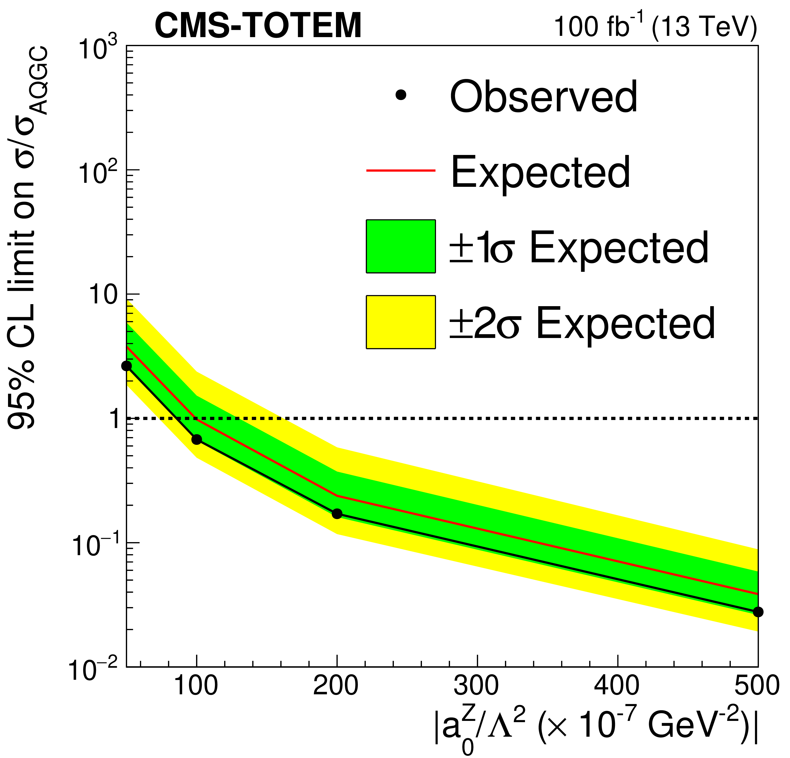
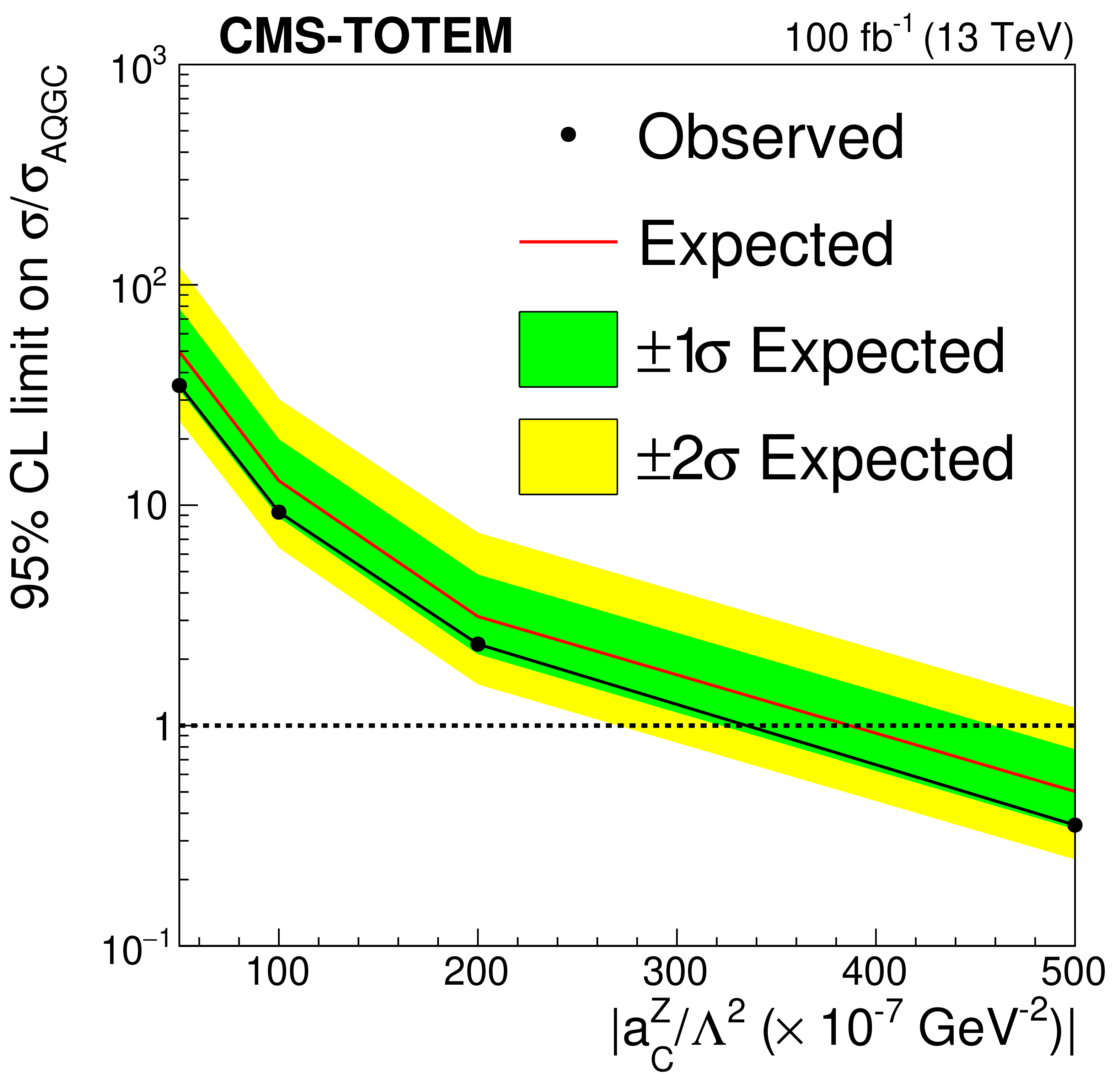
Expected and observed upper limits on the AQGC operators $ a^{\mathrm{W}}_{0}/\Lambda^{2} $ (upper left), $ a^{\mathrm{W}}_{C}/\Lambda^{2} $ (upper right), $ a^{\mathrm{Z}}_{0}/\Lambda^{2} $ (lower left), $ a^{\mathrm{Z}}_{C}/\Lambda^{2} $ (lower right), with no unitarization. The $ y $ axis shows the limit on the ratio of the observed cross section to the cross section predicted for each anomalous coupling value ($ \sigma_\mathrm{AQGC} $). |
png pdf |
Figure 8-a:
Expected and observed upper limits on the AQGC operators $ a^{\mathrm{W}}_{0}/\Lambda^{2} $ (upper left), $ a^{\mathrm{W}}_{C}/\Lambda^{2} $ (upper right), $ a^{\mathrm{Z}}_{0}/\Lambda^{2} $ (lower left), $ a^{\mathrm{Z}}_{C}/\Lambda^{2} $ (lower right), with no unitarization. The $ y $ axis shows the limit on the ratio of the observed cross section to the cross section predicted for each anomalous coupling value ($ \sigma_\mathrm{AQGC} $). |
png pdf |
Figure 8-b:
Expected and observed upper limits on the AQGC operators $ a^{\mathrm{W}}_{0}/\Lambda^{2} $ (upper left), $ a^{\mathrm{W}}_{C}/\Lambda^{2} $ (upper right), $ a^{\mathrm{Z}}_{0}/\Lambda^{2} $ (lower left), $ a^{\mathrm{Z}}_{C}/\Lambda^{2} $ (lower right), with no unitarization. The $ y $ axis shows the limit on the ratio of the observed cross section to the cross section predicted for each anomalous coupling value ($ \sigma_\mathrm{AQGC} $). |
png pdf |
Figure 8-c:
Expected and observed upper limits on the AQGC operators $ a^{\mathrm{W}}_{0}/\Lambda^{2} $ (upper left), $ a^{\mathrm{W}}_{C}/\Lambda^{2} $ (upper right), $ a^{\mathrm{Z}}_{0}/\Lambda^{2} $ (lower left), $ a^{\mathrm{Z}}_{C}/\Lambda^{2} $ (lower right), with no unitarization. The $ y $ axis shows the limit on the ratio of the observed cross section to the cross section predicted for each anomalous coupling value ($ \sigma_\mathrm{AQGC} $). |
png pdf |
Figure 8-d:
Expected and observed upper limits on the AQGC operators $ a^{\mathrm{W}}_{0}/\Lambda^{2} $ (upper left), $ a^{\mathrm{W}}_{C}/\Lambda^{2} $ (upper right), $ a^{\mathrm{Z}}_{0}/\Lambda^{2} $ (lower left), $ a^{\mathrm{Z}}_{C}/\Lambda^{2} $ (lower right), with no unitarization. The $ y $ axis shows the limit on the ratio of the observed cross section to the cross section predicted for each anomalous coupling value ($ \sigma_\mathrm{AQGC} $). |
png pdf |
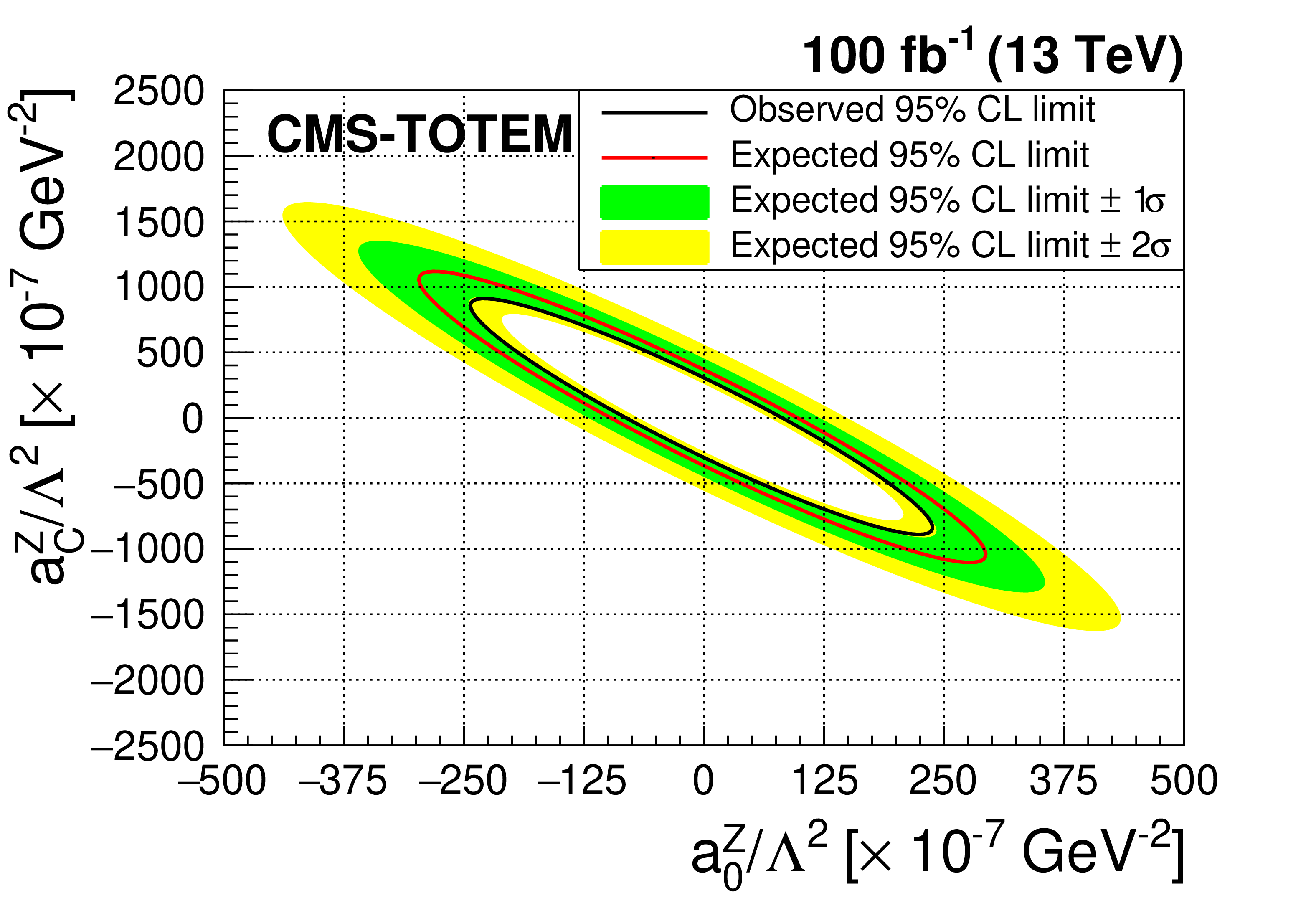
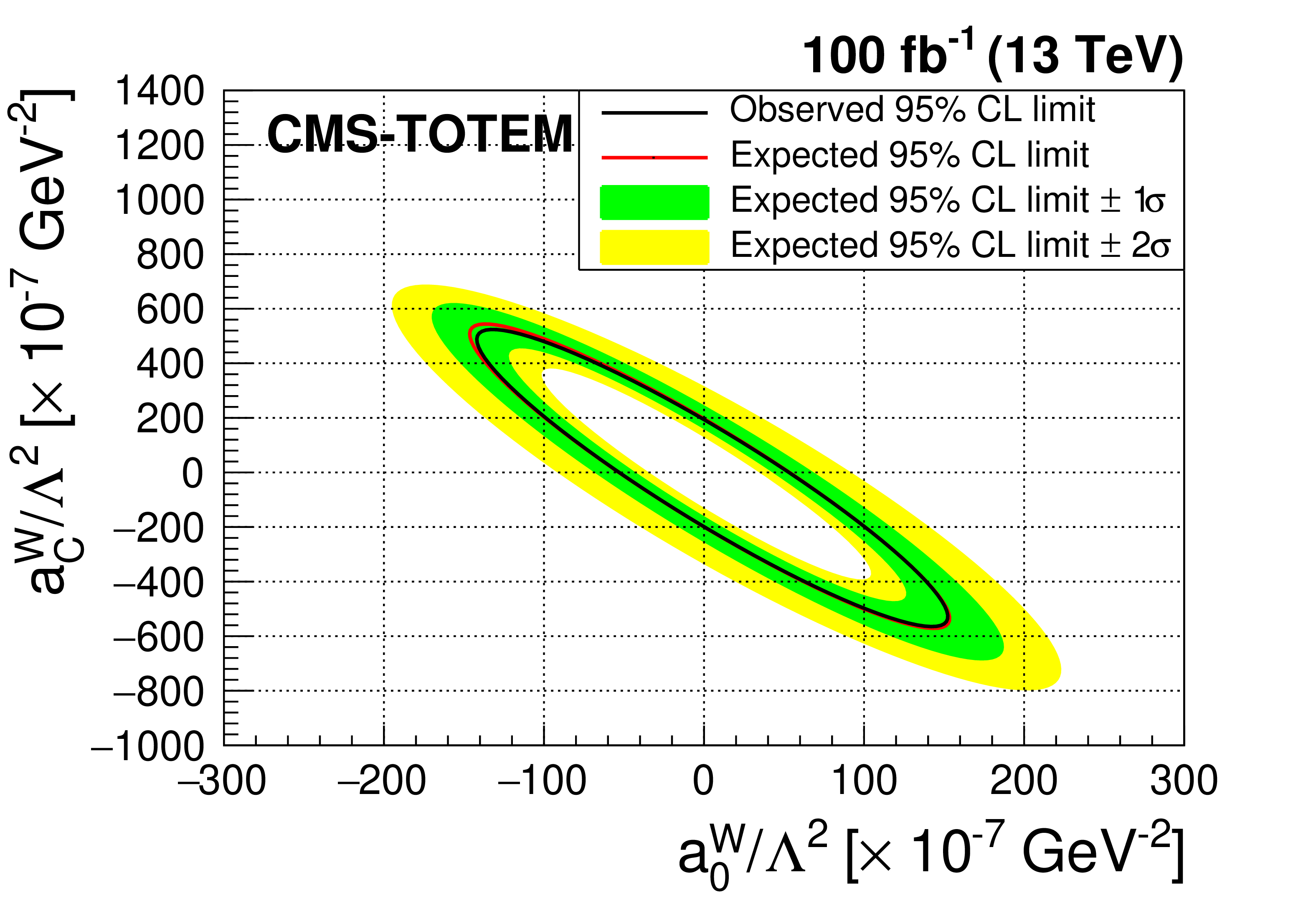
Figure 9:
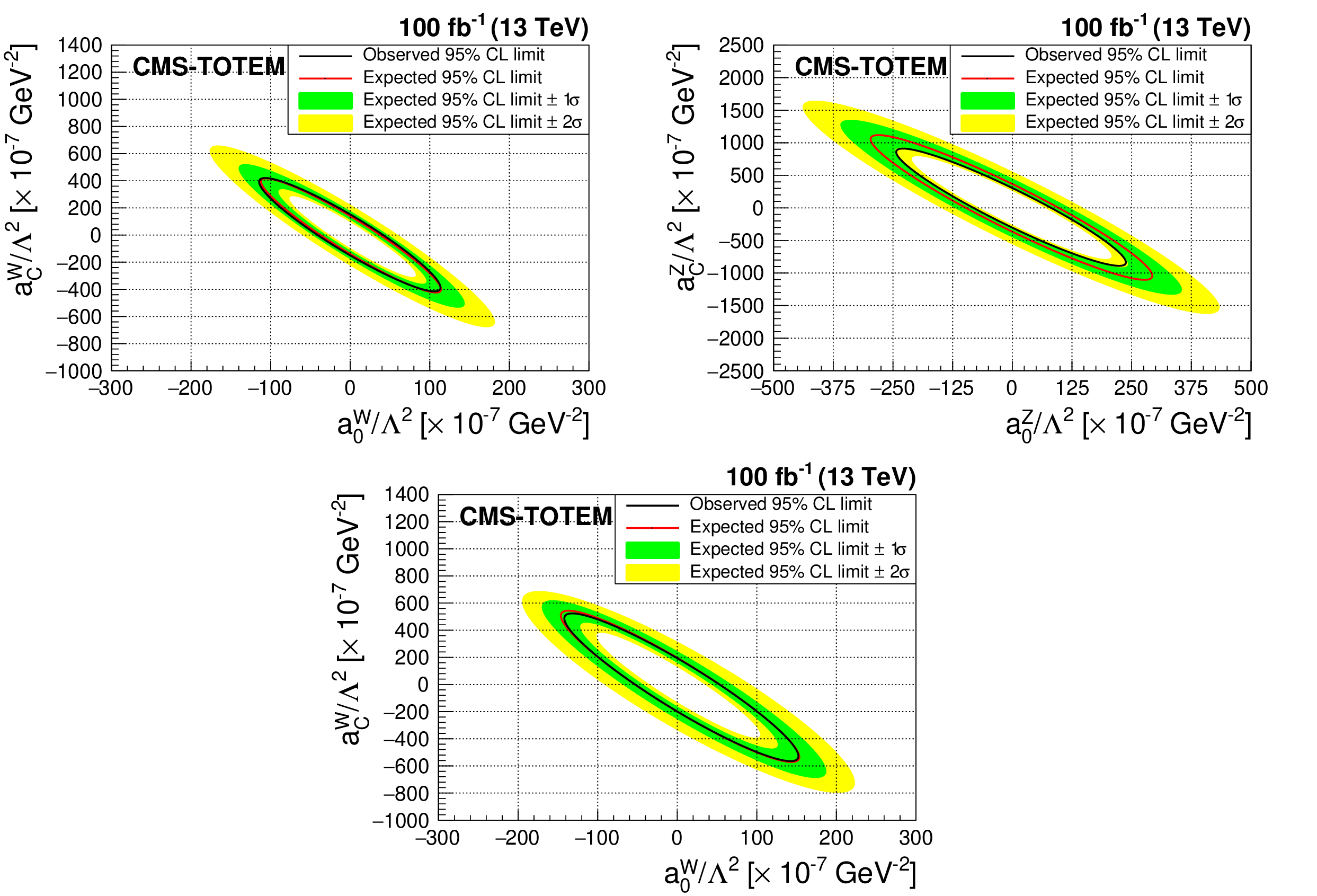
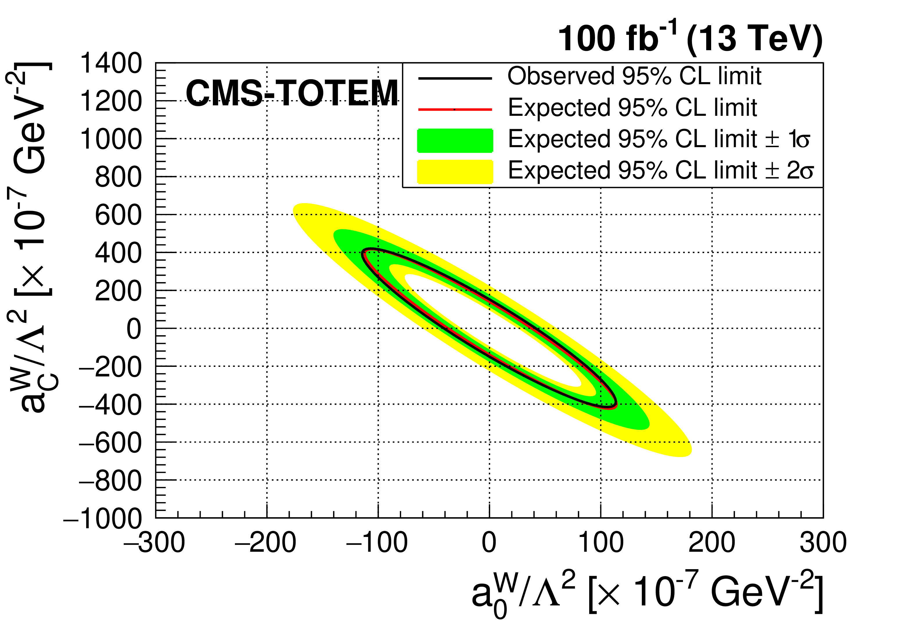
Expected and observed limits in the two-dimensional plane of $ a^{\mathrm{W}}_{0}/\Lambda^{2} $ vs $ a^{\mathrm{W}}_{C}/\Lambda^{2} $ (upper left), $ a^{\mathrm{Z}}_{0}/\Lambda^{2} $ vs. $ a^{\mathrm{Z}}_{C}/\Lambda^{2} $ (upper right), and $ a^{\mathrm{W}}_{0}/\Lambda^{2} $ vs. $ a^{\mathrm{W}}_{C}/\Lambda^{2} $ with unitarization imposed by clipping the signal model at 1.4 TeV (lower). |
png pdf |
Figure 9-a:
Expected and observed limits in the two-dimensional plane of $ a^{\mathrm{W}}_{0}/\Lambda^{2} $ vs $ a^{\mathrm{W}}_{C}/\Lambda^{2} $ (upper left), $ a^{\mathrm{Z}}_{0}/\Lambda^{2} $ vs. $ a^{\mathrm{Z}}_{C}/\Lambda^{2} $ (upper right), and $ a^{\mathrm{W}}_{0}/\Lambda^{2} $ vs. $ a^{\mathrm{W}}_{C}/\Lambda^{2} $ with unitarization imposed by clipping the signal model at 1.4 TeV (lower). |
png pdf |
Figure 9-b:
Expected and observed limits in the two-dimensional plane of $ a^{\mathrm{W}}_{0}/\Lambda^{2} $ vs $ a^{\mathrm{W}}_{C}/\Lambda^{2} $ (upper left), $ a^{\mathrm{Z}}_{0}/\Lambda^{2} $ vs. $ a^{\mathrm{Z}}_{C}/\Lambda^{2} $ (upper right), and $ a^{\mathrm{W}}_{0}/\Lambda^{2} $ vs. $ a^{\mathrm{W}}_{C}/\Lambda^{2} $ with unitarization imposed by clipping the signal model at 1.4 TeV (lower). |
png pdf |
Figure 9-c:
Expected and observed limits in the two-dimensional plane of $ a^{\mathrm{W}}_{0}/\Lambda^{2} $ vs $ a^{\mathrm{W}}_{C}/\Lambda^{2} $ (upper left), $ a^{\mathrm{Z}}_{0}/\Lambda^{2} $ vs. $ a^{\mathrm{Z}}_{C}/\Lambda^{2} $ (upper right), and $ a^{\mathrm{W}}_{0}/\Lambda^{2} $ vs. $ a^{\mathrm{W}}_{C}/\Lambda^{2} $ with unitarization imposed by clipping the signal model at 1.4 TeV (lower). |
| Tables | |
png pdf |
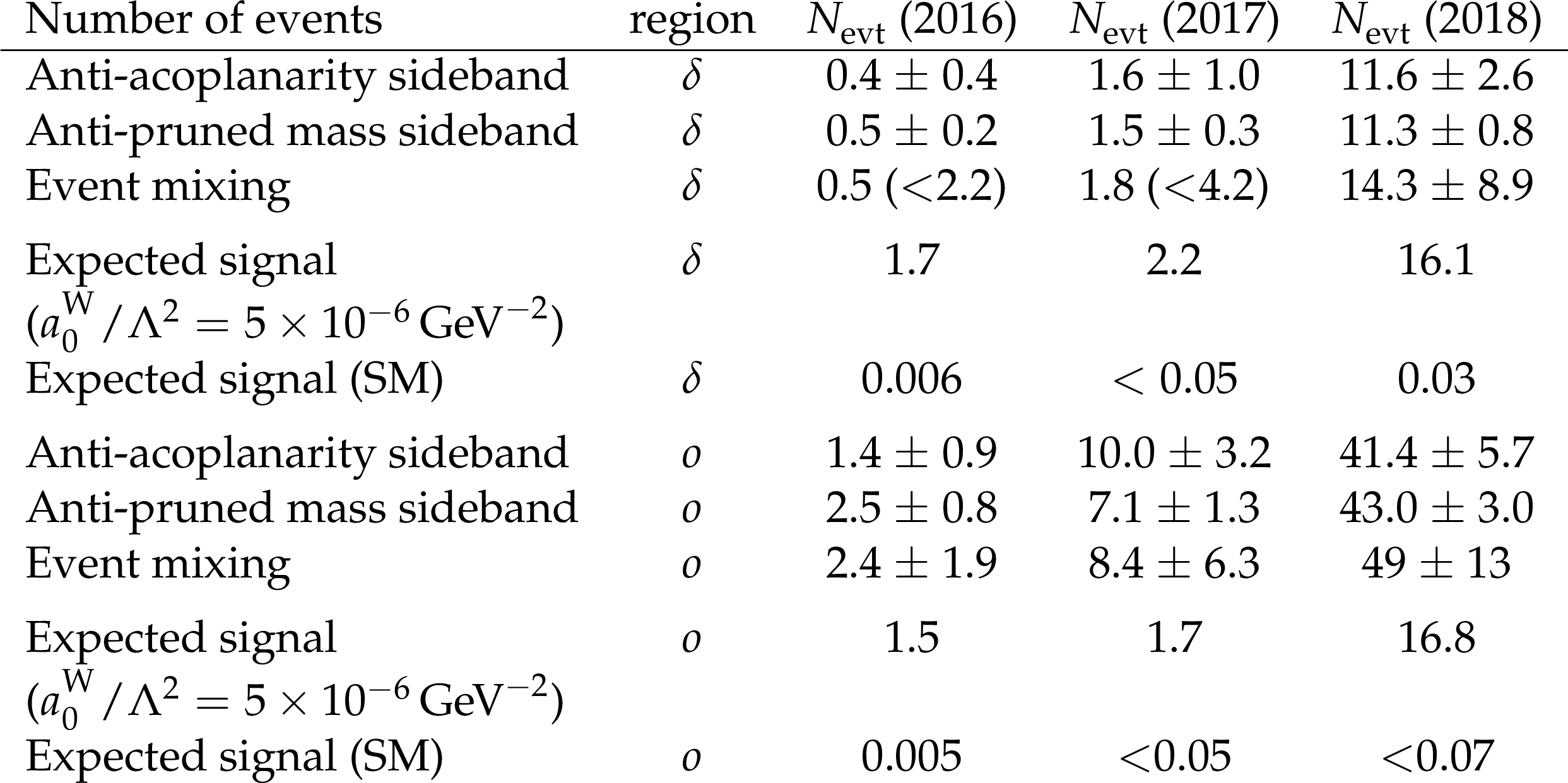
Table 1:
Number of background events ($ N_\text{evt} $ with statistical uncertainties) expected for all methods in the different WW analysis regions with reconstruction of both signal protons (region $ \delta $) or only one signal proton (region $ o $). The mean value of the expected number of signal events for one anomalous coupling point ($ a^{\mathrm{W}}_{0}/\Lambda^2=$ 5\times $ 10$^{-6}$ GeV$^{-2}$) and for the SM are also shown for comparison. In cases where zero simulated SM events pass the final selection, the value is displayed as a 95% confidence level upper limit. |
png pdf |
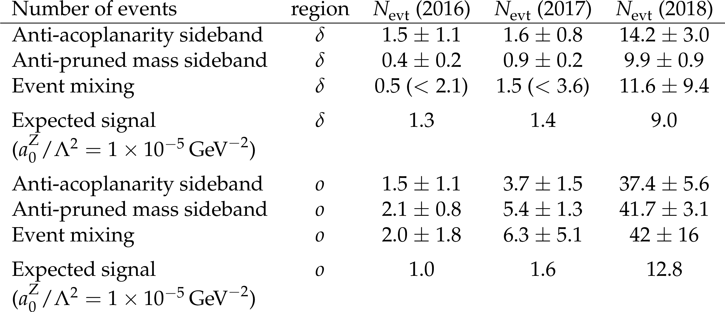
Table 2:
Number of background events ($ N_\text{evt} $ with statistical uncertainties) expected for all methods in the different ZZ analysis regions with reconstruction of both signal protons (region $ \delta $) or only one signal proton (region $ o $). The mean value of the expected number of the expected signal for one anomalous coupling point ($ a^{\mathrm{Z}}_{0}/\Lambda^2=$ 1 $\times$ 10$^{-5}$ GeV$^{-2}$) is also shown for comparison. |
png pdf |
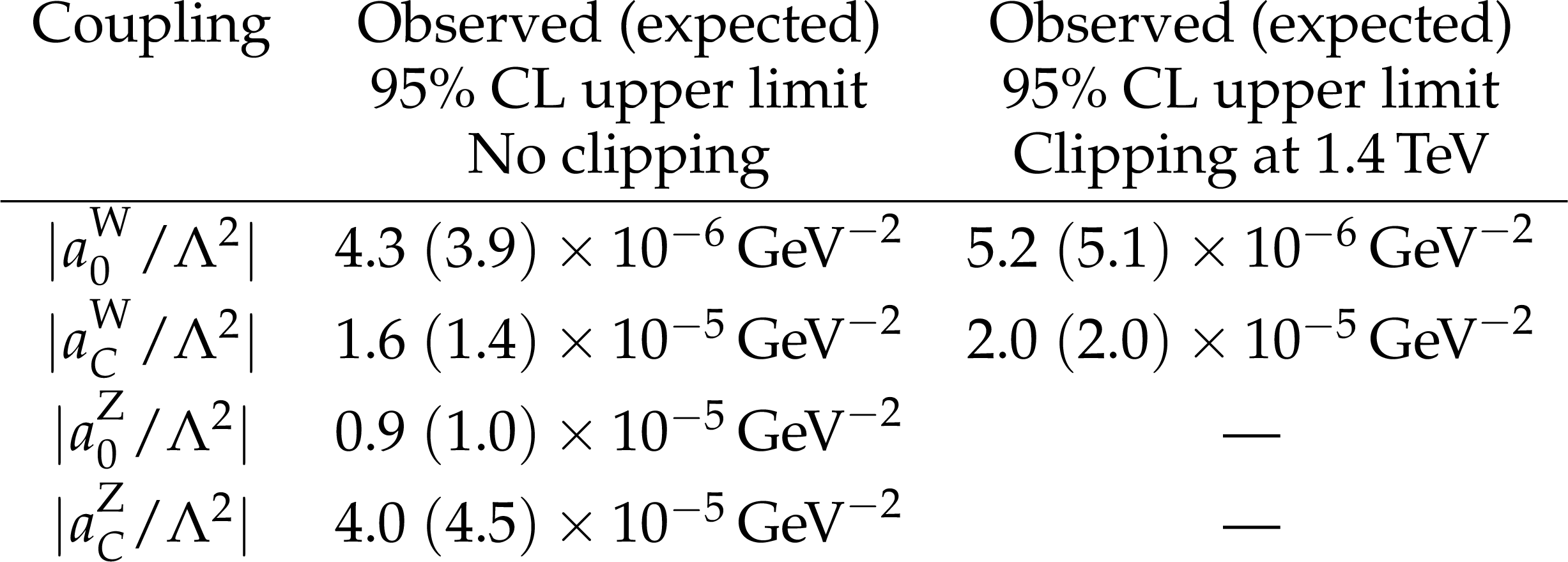
Table 3:
Limits on LEP-like dimension-6 anomalous quartic gauge coupling parameters [19], with and without unitarization via a clipping [27] procedure. |

png pdf |
Table 4:
Conversion of limits on $ a^{\mathrm{W}}_0 $ to dimension-8 $ f_{M,i} $ operators, using the assumption of vanishing $ \mathrm{W}\mathrm{W}\mathrm{Z}\gamma $ couplings to eliminate some parameters. When quoting limits on one of the operators, the other is fixed to zero. The results for $ |f_{M,0}/\Lambda^{4}| $ and $ |f_{M,4}/\Lambda^{4}| $ are shown with and without clipping of the signal model at 1.4 TeV, when the other parameter is fixed to the SM value of zero. |
png pdf |
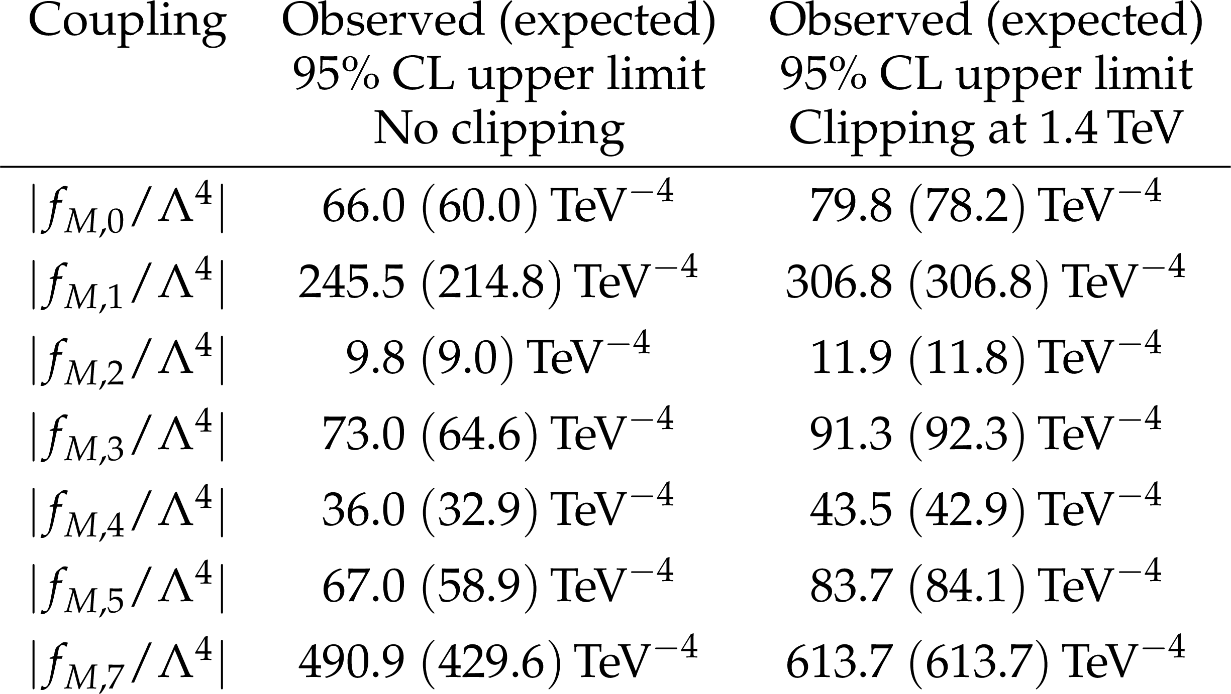
Table 5:
Conversion of limits on $ a^{\mathrm{W}}_0 $ and $ a^{\mathrm{W}}_C $ to dimension-8 $ f_{M,i} $ operators, using the assumption that all $ f_{M,i} $ except one are equal to zero. The results are shown with and without clipping of the signal model at 1.4 TeV. |
| Summary |
| A first search for exclusive high-mass $ \gamma\gamma \to \mathrm{W}\mathrm{W} $ and $ \gamma\gamma \to \mathrm{Z}\mathrm{Z} $ production with reconstructed forward protons has been performed, in final states with hadronically decaying W or Z bosons, using 100 fb$ ^{-1} $ of data collected in 13 TeV proton-proton collisions. No significant excess is found over the standard model background prediction. The resulting limits are interpreted in terms of nonlinear dimension-6 and linear dimension-8 anomalous quartic gauge couplings (AQGC). The unitarized dimension-6 $ \gamma\gamma \mathrm{W}\mathrm{W} $ AQGC limits are approximately 15--20 times more stringent than those obtained from the $ \gamma\gamma \to \mathrm{W}\mathrm{W} $ process without proton detection using the LHC Run 1 data [22,20]. The derived dimension-8 limits are close to those obtained from same-sign WW and WZ scattering at 13 TeV after unitarization, for the case when the $ \mathrm{W}\mathrm{W}\mathrm{Z}\gamma $ coupling is suppressed. The limits on $ \gamma\gamma \mathrm{Z}\mathrm{Z} $ anomalous couplings are the first obtained from the exclusive $ \gamma\gamma \to \mathrm{Z}\mathrm{Z} $ channel. New limits are placed on the cross section in a fiducial region of 0.04 $ < \xi < $ 0.20 and diboson invariant mass $ m(\mathrm{V}\mathrm{V}) > $ 1 TeV of $ \gamma\gamma \to \mathrm{W}\mathrm{W} $ and $ \gamma\gamma \to \mathrm{Z}\mathrm{Z} $ production with intact forward protons. Tabulated results are provided in HEPData [64]. |
| References | ||||
| 1 | CMS and TOTEM Collaborations | CMS-TOTEM Precision Proton Spectrometer | Technical Report CERN-LHCC-2014-021, TOTEM-TDR-003, CMS-TDR-13, 2014 | |
| 2 | CMS and TOTEM Collaboration | Observation of proton-tagged, central (semi)exclusive production of high-mass lepton pairs in pp collisions at 13 TeV with the CMS-TOTEM precision proton spectrometer | JHEP 07 (2018) 153 | 1803.04496 |
| 3 | E. Chapon, C. Royon, and O. Kepka | Anomalous quartic $ \mathrm{W}\mathrm{W}\gamma\gamma $, $ \mathrm{Z}\mathrm{Z}\gamma\gamma $, and trilinear $ \mathrm{W}\mathrm{W}\gamma $ couplings in two-photon processes at high luminosity at the LHC | PRD 81 (2010) 074003 | 0912.5161 |
| 4 | C. Baldenegro, G. Biagi, G. Legras, and C. Royon | Central exclusive production of W boson pairs in pp collisions at the LHC in hadronic and semi-leptonic final states | JHEP 12 (2020) 165 | 2009.08331 |
| 5 | M. Boonekamp et al. | FPMC: a generator for forward physics | 1102.2531 | |
| 6 | H.-S. Shao and D. d'Enterria | gamma-UPC: automated generation of exclusive photon-photon processes in ultraperipheral proton and nuclear collisions with varying form factors | JHEP 09 (2022) 248 | 2207.03012 |
| 7 | T. Pierzchala and K. Piotrzkowski | Sensitivity to anomalous quartic gauge couplings in photon-photon interactions at the LHC | Nucl. Phys. Proc. Suppl. 17 (2008) 9 | 0807.1121 |
| 8 | M. Maniatis, A. von Manteuffel, and O. Nachtmann | Anomalous couplings in $ \gamma\gamma\to\mathrm{W^+}\mathrm{W^-} $ at LHC and ILC | Nucl. Phys. Proc. Suppl. 17 (2008) 9 | |
| 9 | R. L. Delgado, A. Dobado, M. J. Herrero, and J. J. Sanz-Cillero | One-loop $ \gamma\gamma\to\mathrm{W^+}_{L}\mathrm{W^-}_{L} $ and $ \gamma\gamma\to\mathrm{Z}_{L}\mathrm{Z}_{L} $ from the electroweak chiral lagrangian with a light Higgs-like scalar | JHEP 07 (2014) 149 | 1404.2866 |
| 10 | S. Fichet and G. von Gersdorff | Anomalous gauge couplings from composite Higgs and warped extra dimensions | JHEP 03 (2014) 102 | 1311.6815 |
| 11 | R. S. Gupta | Probing quartic neutral gauge boson couplings using diffractive photon fusion at the LHC | PRD 85 (2012) 014006 | 1111.3354 |
| 12 | R. L. Delgado et al. | Collider production of electroweak resonances from $ \gamma\gamma $ states | JHEP 11 (2018) 010 | 1710.07548 |
| 13 | R. L. Delgado, A. Dobado, and F. J. Llanes-Estrada | Coupling WW, ZZ unitarized amplitudes to $ \gamma\gamma $ in the TeV region | EPJC 77 (2017) 205 | 1609.06206 |
| 14 | G. B é langer et al. | Bosonic quartic couplings at LEP2 | EPJC 13 (2000) 283 | hep-ph/9908254 |
| 15 | G. B é langer and F. Boudjema | $ \gamma\gamma\to\mathrm{W^+}\mathrm{W^-} $ and $ \gamma\gamma\to\mathrm{Z}\mathrm{Z} $ as tests of novel quartic couplings | PLB 288 (1992) 210 | |
| 16 | O. J. P. Éboli, M. C. Gonzalez-Garcia, and J. K. Mizukoshi | $ \mathrm{p}\mathrm{p} \to \mathrm{jj} \mathrm{e}^{\pm}\mu^\pm\nu\nu $ and $ \mathrm{jj}\mathrm{e}^{\pm}\mu^\mp\nu\nu $ at $ \mathcal{O}(\alpha_{\mathrm{em}}^{6}) $ and $ \mathcal{O}(\alpha_{\mathrm{em}}^{4}\alpha_{s}^{2}) $ for the study of the quartic electroweak gauge boson vertex at CERN LHC | PRD 74 (2006) 073005 | |
| 17 | O. J. P. Éboli, M. C. Gonzalez-Garcia, and S. M. Lietti | Bosonic quartic couplings at CERN LHC | PRD 69 (2004) 095005 | hep-ph/0310141 |
| 18 | O. J. P. Éboli and M. C. Gonzalez-Garcia | Classifying the bosonic quartic couplings | PRD 93 (2016) 093013 | 1604.03555 |
| 19 | OPAL Collaboration | Constraints on anomalous quartic gauge boson couplings from $ \nu\bar{\nu}\gamma\gamma $ and $ \mathrm{q}\bar{\mathrm{q}}\gamma\gamma $ events at CERN LEP2 | PRD 70 (2004) 032005 | hep-ex/0402021 |
| 20 | ATLAS Collaboration | Measurement of exclusive $ \gamma\gamma\to \mathrm{W^+}\mathrm{W^-} $ production and search for exclusive Higgs boson production in pp collisions at $ \sqrt{s} = $ 8 TeV using the ATLAS detector | PRD 94 (2016) 032011 | 1607.03745 |
| 21 | CMS Collaboration | Study of exclusive two-photon production of $ \mathrm{W^+}\mathrm{W^-} $ in pp collisions at $ \sqrt{s} = $ 7 TeV and constraints on anomalous quartic gauge couplings | JHEP 07 (2013) 116 | CMS-FSQ-12-010 1305.5596 |
| 22 | CMS Collaboration | Evidence for exclusive $ \gamma\gamma \to \mathrm{W^+} \mathrm{W^-} $ production and constraints on anomalous quartic gauge couplings in pp collisions at $ \sqrt{s}= $ 7 and 8 TeV | JHEP 08 (2016) 119 | CMS-FSQ-13-008 1604.04464 |
| 23 | CMS Collaboration | Observation of electroweak production of same-sign W boson pairs in the two jet and two same-sign lepton final state in proton-proton collisions at $ \sqrt{s}= $ 13 TeV | PRL 120 (2018) 081801 | CMS-SMP-17-004 1709.05822 |
| 24 | CMS Collaboration | Evidence for electroweak production of four charged leptons and two jets in proton-proton collisions at $ \sqrt{s}= $ 13 TeV | PLB 812 (2020) 135992 | CMS-SMP-20-001 2008.07013 |
| 25 | D0 Collaboration | Search for anomalous quartic $ \mathrm{W}\mathrm{W}\gamma\gamma $ couplings in dielectron and missing energy final states in $ \mathrm{p}\bar{\mathrm{p}} $ collisions at $ \sqrt{s} = $ 1.96 TeV | PRD 88 (2013) 012005 | 1305.1258 |
| 26 | ATLAS Collaboration | Observation of photon-induced $ \mathrm{W^+}\mathrm{W^-} $ production in pp collisions at $ \sqrt{s}= $ 13 TeV using the ATLAS detector | PLB 816 (2021) 136190 | 2010.04019 |
| 27 | CMS Collaboration | Measurements of production cross sections of WZ and same-sign WW boson pairs in association with two jets in proton-proton collisions at $ \sqrt{s}= $ 13 TeV | PLB 809 (2020) 135710 | CMS-SMP-19-012 2005.01173 |
| 28 | CMS Collaboration | Measurement of the electroweak production of $ \mathrm{Z}\gamma $ and two jets in proton-proton collisions at $ \sqrt{s}= $ 13 TeV and constraints on anomalous quartic gauge couplings | PRD 104 (2021) 072001 | CMS-SMP-20-016 2106.11082 |
| 29 | CMS Collaboration | Observation of electroweak production of $ \mathrm{W}\gamma $ with two jets in proton-proton collisions at $ \sqrt {s} = $ 13 TeV | PLB 811 (2020) 135988 | CMS-SMP-19-008 2008.10521 |
| 30 | CMS Collaboration | Measurement of vector boson scattering and constraints on anomalous quartic couplings from events with four leptons and two jets in proton-proton collisions at $ \sqrt{s}= $ 13 TeV | PLB 774 (2017) 682 | CMS-SMP-17-006 1708.02812 |
| 31 | CMS Collaboration | Measurements of the $ \mathrm{p}\mathrm{p}\to\mathrm{W}^{\pm}\gamma\gamma $ and $ \mathrm{p}\mathrm{p}\to\mathrm{Z}\gamma\gamma $ cross sections at $ \sqrt{s}= $ 13 TeV and limits on anomalous quartic gauge couplings | JHEP 10 (2021) 174 | CMS-SMP-19-013 2105.12780 |
| 32 | CMS and TOTEM Collaboration | First search for exclusive diphoton production at high mass with tagged protons in proton-proton collisions at $ \sqrt{s} = $ 13 TeV | PRL 129 (2022) 011801 | 2110.05916 |
| 33 | CMS Collaboration | The CMS experiment at the CERN LHC | JINST 3 (2008) S08004 | |
| 34 | CMS Collaboration | Performance of the CMS Level-1 trigger in proton-proton collisions at $ \sqrt{s} = $ 13 TeV | JINST 15 (2020) P10017 | CMS-TRG-17-001 2006.10165 |
| 35 | CMS Collaboration | The CMS trigger system | JINST 12 (2017) P01020 | CMS-TRG-12-001 1609.02366 |
| 36 | CMS Collaboration | Precision luminosity measurement in proton-proton collisions at $ \sqrt{s} = $ 13 TeV in 2015 and 2016 at CMS | EPJC 81 (2021) 800 | CMS-LUM-17-003 2104.01927 |
| 37 | CMS Collaboration | CMS luminosity measurement for the 2017 data-taking period at $ \sqrt{s} = $ 13 TeV | CMS Physics Analysis Summary , CERN, Geneva, 2018 CMS-PAS-LUM-17-004 |
CMS-PAS-LUM-17-004 |
| 38 | CMS Collaboration | CMS luminosity measurement for the 2018 data-taking period at $ \sqrt{s} = $ 13 TeV | CMS Physics Analysis Summary , CERN, Geneva, 2019 CMS-PAS-LUM-18-002 |
CMS-PAS-LUM-18-002 |
| 39 | T. Sjöstrand et al. | An introduction to PYTHIA 8.2 | Comput. Phys. Commun. 191 (2015) 159 | 1410.3012 |
| 40 | CMS Collaboration | Event generator tunes obtained from underlying event and multiparton scattering measurements | EPJC 76 (2016) 155 | CMS-GEN-14-001 1512.00815 |
| 41 | CMS Collaboration | Extraction and validation of a new set of CMS PYTHIA8 tunes from underlying-event measurements | EPJC 80 (2019) 4 | CMS-GEN-17-001 1903.12179 |
| 42 | J. Alwall et al. | The automated computation of tree-level and next-to-leading order differential cross sections, and their matching to parton shower simulations | JHEP 07 (2014) 079 | 1405.0301 |
| 43 | S. Alioli et al. | Jet pair production in POWHEG | JHEP 04 (2011) 081 | 1012.3380 |
| 44 | S. Frixione, P. Nason, and C. Oleari | Matching NLO QCD computations with parton shower simulations: the POWHEG method | JHEP 11 (2007) 070 | 0709.2092 |
| 45 | P. Nason | A new method for combining NLO QCD with shower Monte Carlo algorithms | JHEP 11 (2004) 040 | hep-ph/0409146 |
| 46 | GEANT4 Collaboration | GEANT 4---a simulation toolkit | NIM A 506 (2003) 250 | |
| 47 | CMS and TOTEM Collaborations | Proton reconstruction with the Precision Proton Spectrometer in Run 2 | Submitted to JINST, 2022 | 2210.05854 |
| 48 | D. Krohn, J. Thaler, and L.-T. Wang | Jet trimming | JHEP 02 (2010) 084 | 0912.1342 |
| 49 | CMS Collaboration | A multi-dimensional search for new heavy resonances decaying to boosted WW, WZ, or ZZ boson pairs in the dijet final state at 13 TeV | EPJC 80 (2020) 237 | 1906.05977 |
| 50 | CMS Collaboration | Technical proposal for the Phase-II upgrade of the Compact Muon Solenoid | CMS Technical Proposal CERN-LHCC-2015-010, CMS-TDR-15-02, 2015 CDS |
|
| 51 | CMS Collaboration | Particle-flow reconstruction and global event description with the CMS detector | JINST 12 (2017) P10003 | CMS-PRF-14-001 1706.04965 |
| 52 | M. Cacciari, G. P. Salam, and G. Soyez | The anti-$ k_{\mathrm{T}} $ jet clustering algorithm | JHEP 04 (2008) 063 | 0802.1189 |
| 53 | M. Cacciari, G. P. Salam, and G. Soyez | FastJet user manual | EPJC 72 (2012) 1896 | 1111.6097 |
| 54 | CMS Collaboration | Jet energy scale and resolution in the CMS experiment in pp collisions at 8 TeV | JINST 12 (2017) P02014 | CMS-JME-13-004 1607.03663 |
| 55 | J. Thaler and K. Van Tilburg | Identifying boosted objects with $ N $-subjettiness | JHEP 03 (2011) 015 | 1011.2268 |
| 56 | S. D. Ellis, C. K. Vermilion, and J. R. Walsh | Recombination algorithms and jet substructure: pruning as a tool for heavy particle searches | PRD 81 (2010) 094023 | 0912.0033 |
| 57 | CMS Collaboration | Identification techniques for highly boosted W bosons that decay into hadrons | JHEP 12 (2014) 017 | CMS-JME-13-006 1410.4227 |
| 58 | J. Dolen et al. | Thinking outside the ROCs: designing decorrelated taggers (DDT) for jet substructure | JHEP 05 (2016) 156 | 1603.00027 |
| 59 | F. Nemes | LHC optics determination with proton tracks measured in the CT-PPS detectors in 2016, before TS2 | Technical Report CERN-TOTEM-NOTE-2017-002, 2017 | |
| 60 | J. Kašpar | Alignment of CT-PPS detectors in 2016, before TS2 | Technical Report CERN-TOTEM-NOTE-2017-001, 2017 | |
| 61 | L. Harland-Lang, V. Khoze, and M. G. Ryskin | Elastic photon-initiated production at the LHC: the role of hadron-hadron interactions | SciPost Physics 1 (2021) 1 | 2104.13392 |
| 62 | J. S. Conway | Incorporating nuisance parameters in likelihoods for multisource spectra | in, 2011 PHYSTAT 201 (2011) 115 |
1103.0354 |
| 63 | J. Kalinowski et al. | Same-sign WW scattering at the LHC: can we discover BSM effects before discovering new states? | EPJC 78 (2018) 403 | 1802.02366 |
| 64 | CMS Collaboration | Search for $ \mathrm{W}\mathrm{W}\gamma $ and $ \mathrm{W}\mathrm{Z}\gamma $ production and constraints on anomalous quartic gauge couplings in pp collisions at $ \sqrt{s} = $ 8 TeV | PRD 90 (2014) 032008 | CMS-SMP-13-009 1404.4619 |
| 65 | CMS Collaboration | HEPData record for this analysis, 2022 | link | |
|
|
Compact Muon Solenoid LHC, CERN |
|

|

|

|

|

|