

Compact Muon Solenoid
LHC, CERN
| CMS-SMP-22-007 ; CERN-EP-2023-282 | ||
| Measurement of the primary Lund jet plane density in proton-proton collisions at $ \sqrt{s} = $ 13 TeV | ||
| CMS Collaboration | ||
| 27 December 2023 | ||
| Accepted for publication in J. High Energy Phys. | ||
| Abstract: A measurement is presented of the primary Lund jet plane (LJP) density in inclusive jet production in proton-proton collisions. The analysis uses 138 fb$ ^{-1} $ of data collected by the CMS experiment at $ \sqrt{s} = $ 13 TeV. The LJP, a representation of the phase space of emissions inside jets, is constructed using iterative jet declustering. The transverse momentum $ k_{\mathrm{T}} $ and the splitting angle $ \Delta R $ of an emission relative to its emitter are measured at each step of the jet declustering process. The average density of emissions as function of $ \ln(k_{\mathrm{T}}/$GeV$)$ and $ \ln(R/\Delta R) $ is measured for jets with distance parameters $ R = $ 0.4 or 0.8, transverse momentum $ p_{\mathrm{T}} > $ 700 GeV, and rapidity $ |y| < $ 1.7. The jet substructure is measured using the charged-particle tracks of the jet. The measured distributions, unfolded to the level of stable particles, are compared with theoretical predictions from simulations and with perturbative quantum chromodynamics calculations. Due to the ability of the LJP to factorize physical effects, these measurements can be used to improve different aspects of the physics modeling in event generators. | ||
| Links: e-print arXiv:2312.16343 [hep-ex] (PDF) ; CDS record ; inSPIRE record ; HepData record ; Physics Briefing ; CADI line (restricted) ; | ||
| Figures | |
png pdf |
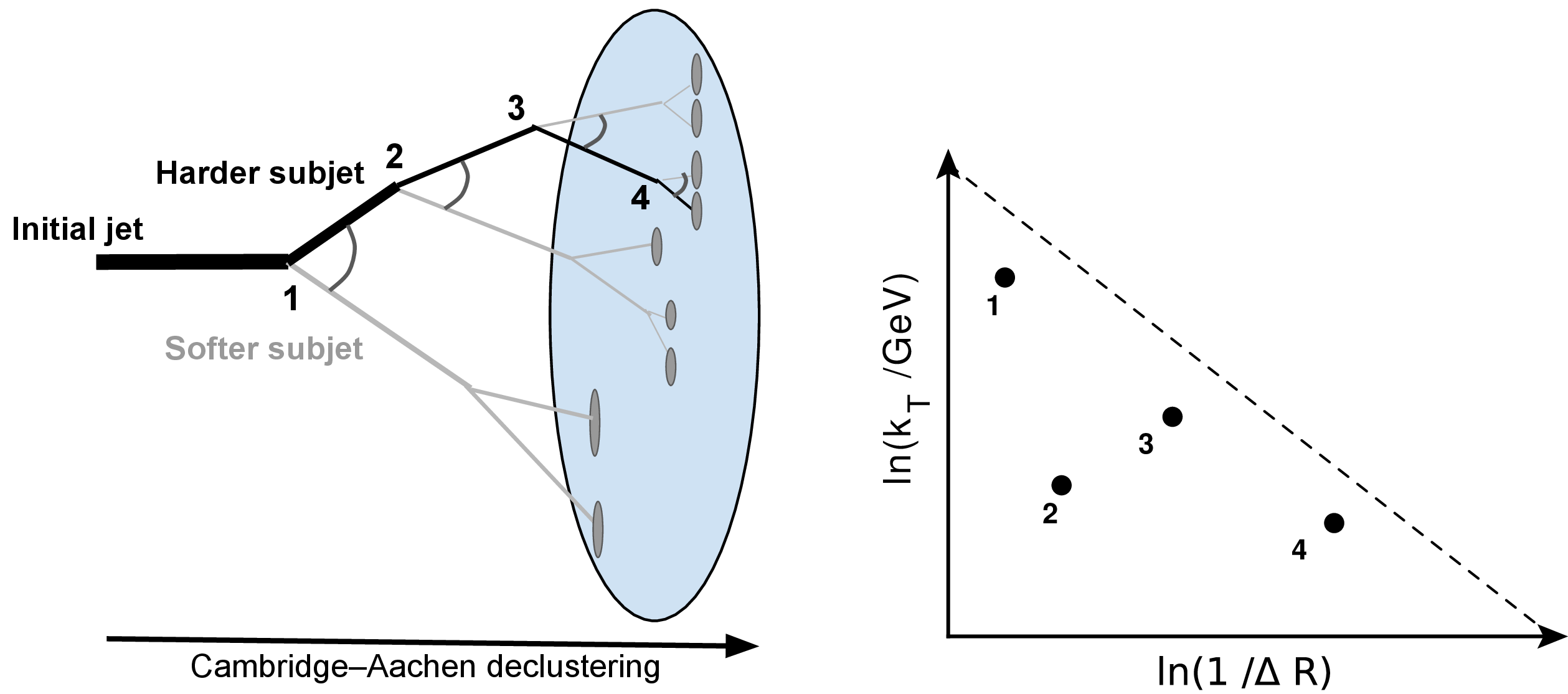
Figure 1:
Left: schematic diagram of the Cambridge-Aachen primary declustering tree of a jet. The black lines represent the branch that follows the harder subjet at each step of the declustering tree. The softer subjet at each node is used as a proxy for an emission in the primary LJP. Right: schematic diagram of the primary emissions of a jet in the LJP, which is filled from left to right corresponding to emissions ordered from large to small angles. The numbers represent the order of appearance in the declustering tree. The dashed diagonal line represents the kinematical limit. |
png pdf |
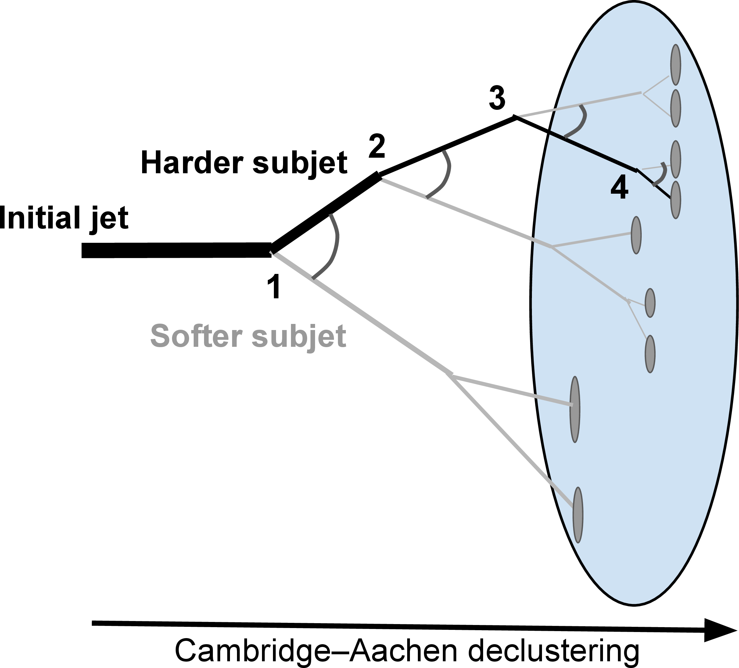
Figure 1-a:
Left: schematic diagram of the Cambridge-Aachen primary declustering tree of a jet. The black lines represent the branch that follows the harder subjet at each step of the declustering tree. The softer subjet at each node is used as a proxy for an emission in the primary LJP. Right: schematic diagram of the primary emissions of a jet in the LJP, which is filled from left to right corresponding to emissions ordered from large to small angles. The numbers represent the order of appearance in the declustering tree. The dashed diagonal line represents the kinematical limit. |
png pdf |
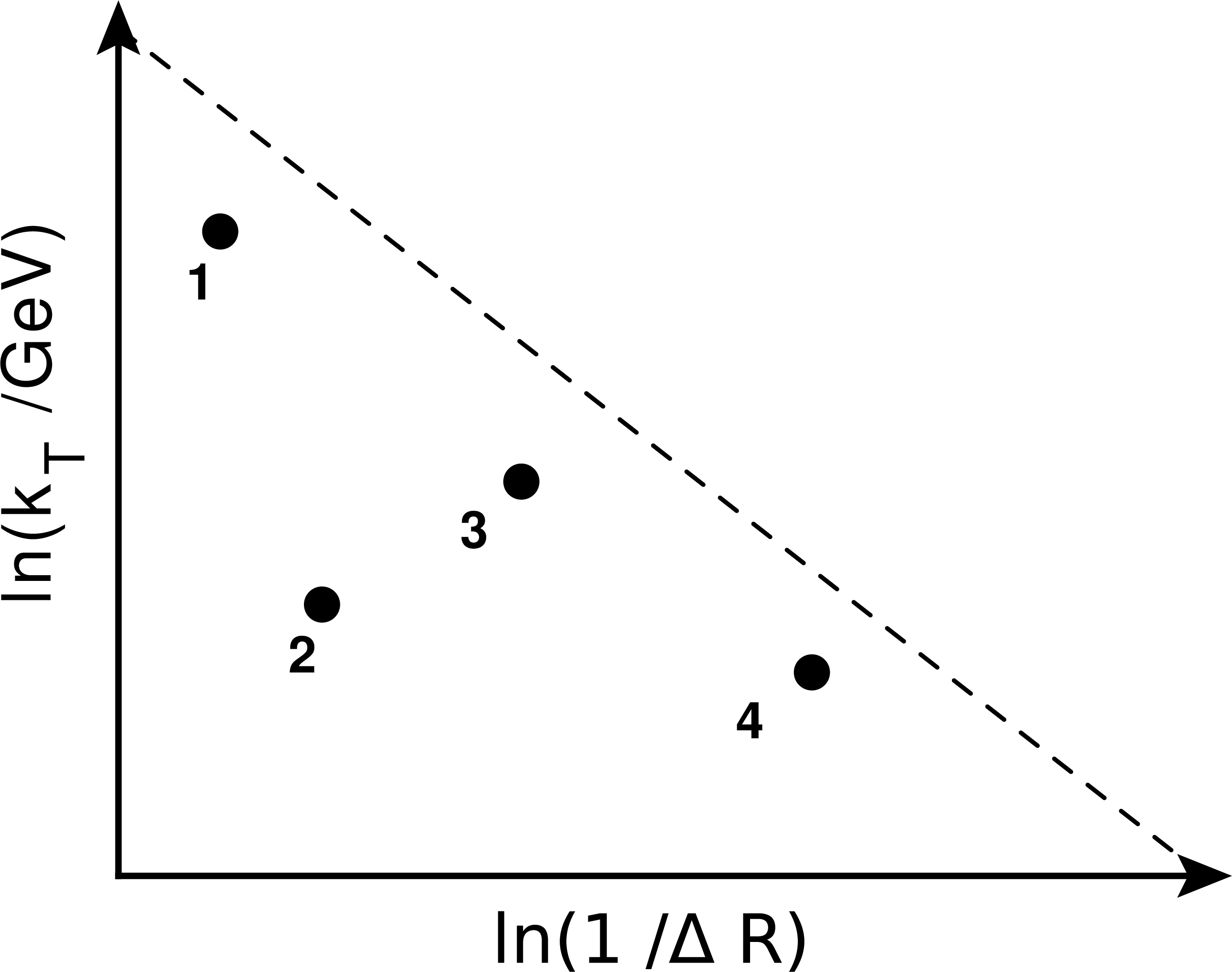
Figure 1-b:
Left: schematic diagram of the Cambridge-Aachen primary declustering tree of a jet. The black lines represent the branch that follows the harder subjet at each step of the declustering tree. The softer subjet at each node is used as a proxy for an emission in the primary LJP. Right: schematic diagram of the primary emissions of a jet in the LJP, which is filled from left to right corresponding to emissions ordered from large to small angles. The numbers represent the order of appearance in the declustering tree. The dashed diagonal line represents the kinematical limit. |

png pdf |
Figure 2:
Schematic diagram of the mechanisms affecting different regions of the primary LJP in a given proton-proton collision. Initial-state radiation (ISR), the underlying event (UE) activity, and multiple-parton interactions (MPI) affect wide-angle radiation at $ \Delta R \sim R $, close to the boundary of the jet. In an experimental context, pileup contributes to the same region as the UE. Hadronization affects the low $ \ln(k_{\mathrm{T}}/$GeV$)$ region (below $ k_{\mathrm{T}} \sim $ 1 GeV) at all angles. Soft and hard collinear parton splittings affect the rest of the LJP. The diagonal line represents the kinematical limit of the primary LJP, which corresponds to $ p_{\mathrm{T}}^{j_1} = p_{\mathrm{T}}^{j_2} $. |
png pdf |
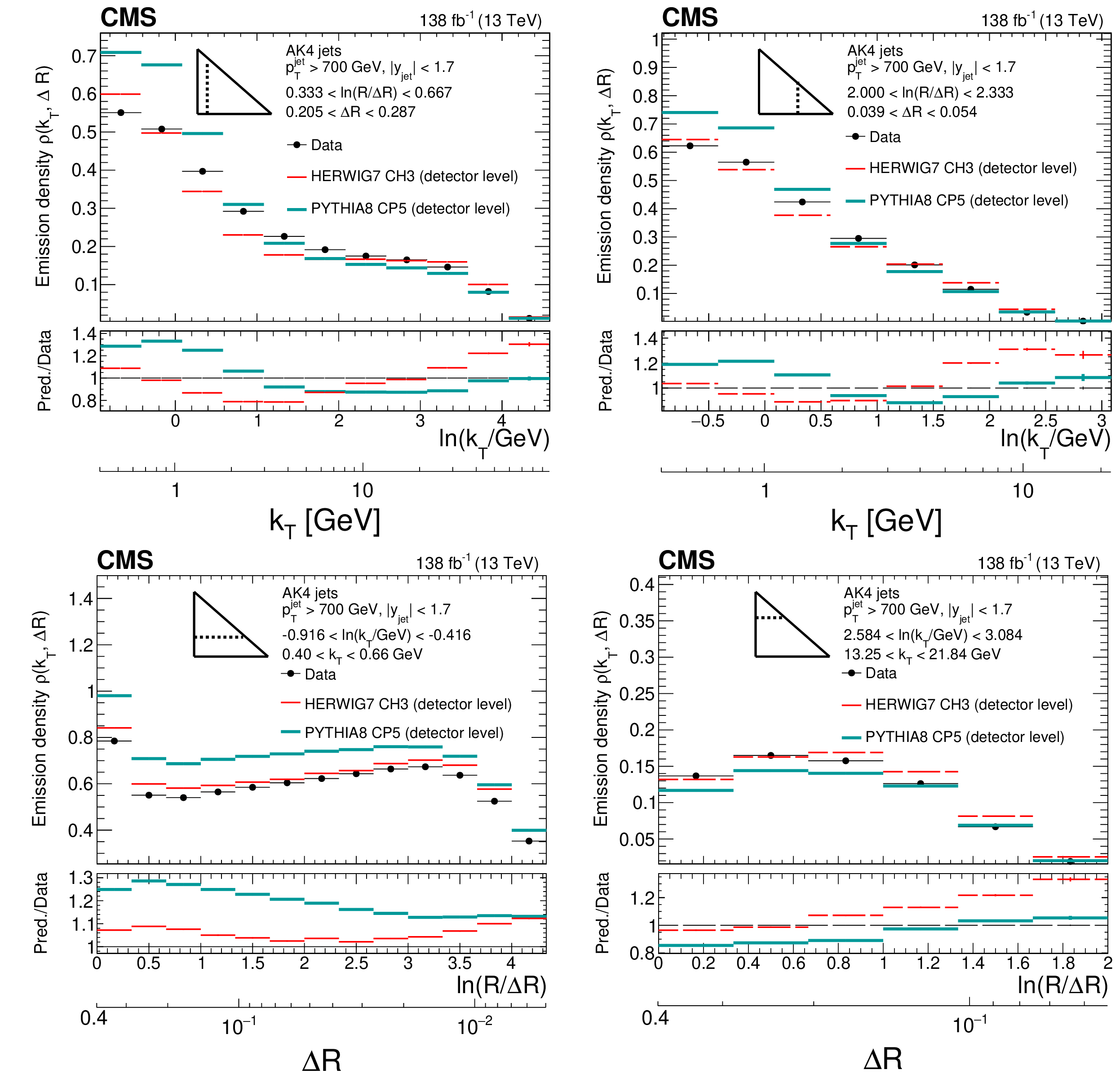
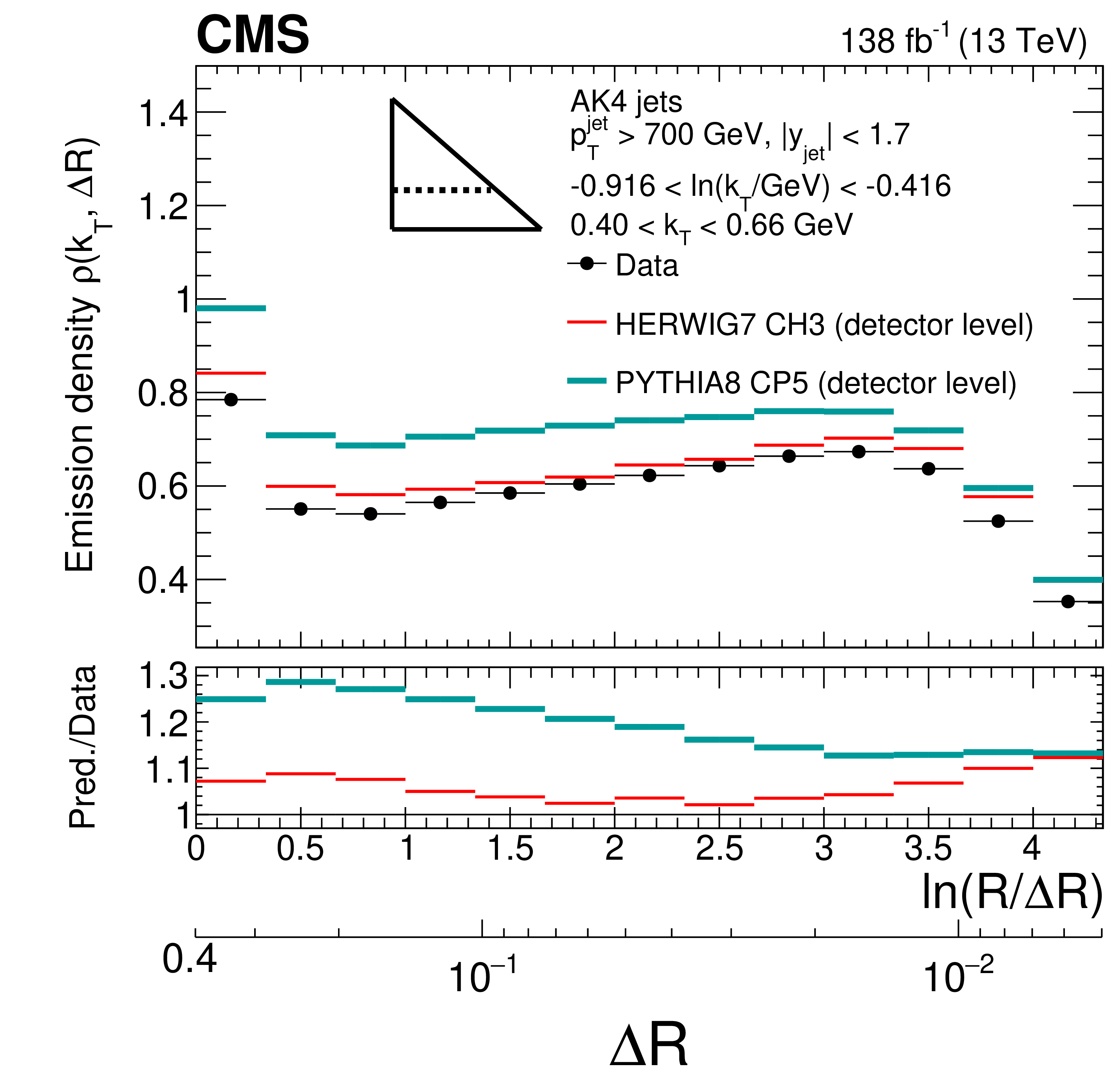
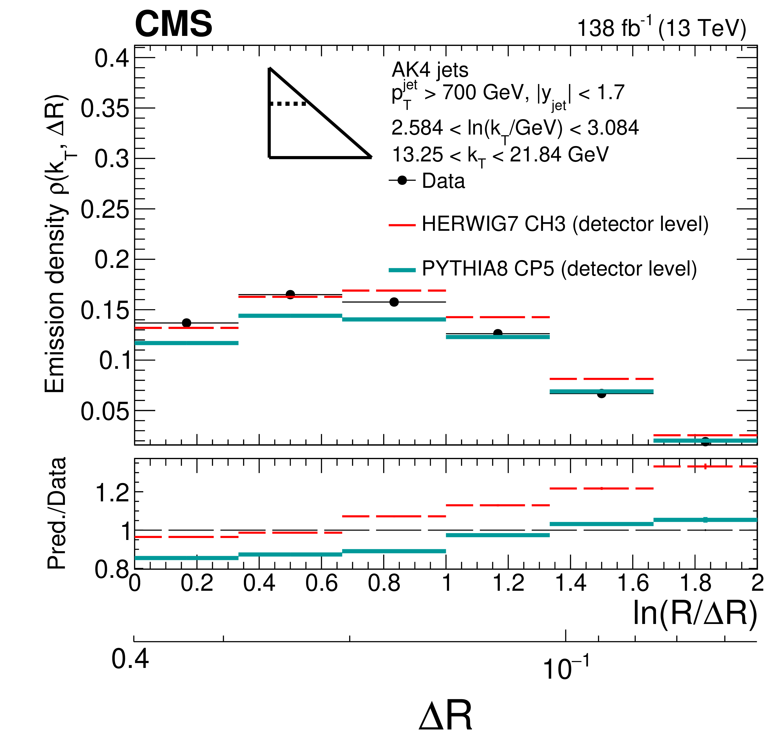
Figure 3:
Detector-level distributions of measured and MC-simulated events generated with PYTHIA8 CP5 and HERWIG 7 CH3 for four different slices of the LJP, as indicated by the triangular diagrams in the plots. The lower panels in the plots show the ratio of the predictions with respect to the data. Only statistical uncertainties are included here. The comparison shows that neither HERWIG 7 CH3 nor PYTHIA8 CP5 are able to describe the data well in various regions of the LJP. The vertical bars represent the statistical uncertainties, which are smaller than the markers for most of the bins. |

png pdf |
Figure 3-a:
Detector-level distributions of measured and MC-simulated events generated with PYTHIA8 CP5 and HERWIG 7 CH3 for four different slices of the LJP, as indicated by the triangular diagrams in the plots. The lower panels in the plots show the ratio of the predictions with respect to the data. Only statistical uncertainties are included here. The comparison shows that neither HERWIG 7 CH3 nor PYTHIA8 CP5 are able to describe the data well in various regions of the LJP. The vertical bars represent the statistical uncertainties, which are smaller than the markers for most of the bins. |

png pdf |
Figure 3-b:
Detector-level distributions of measured and MC-simulated events generated with PYTHIA8 CP5 and HERWIG 7 CH3 for four different slices of the LJP, as indicated by the triangular diagrams in the plots. The lower panels in the plots show the ratio of the predictions with respect to the data. Only statistical uncertainties are included here. The comparison shows that neither HERWIG 7 CH3 nor PYTHIA8 CP5 are able to describe the data well in various regions of the LJP. The vertical bars represent the statistical uncertainties, which are smaller than the markers for most of the bins. |
png pdf |
Figure 3-c:
Detector-level distributions of measured and MC-simulated events generated with PYTHIA8 CP5 and HERWIG 7 CH3 for four different slices of the LJP, as indicated by the triangular diagrams in the plots. The lower panels in the plots show the ratio of the predictions with respect to the data. Only statistical uncertainties are included here. The comparison shows that neither HERWIG 7 CH3 nor PYTHIA8 CP5 are able to describe the data well in various regions of the LJP. The vertical bars represent the statistical uncertainties, which are smaller than the markers for most of the bins. |
png pdf |
Figure 3-d:
Detector-level distributions of measured and MC-simulated events generated with PYTHIA8 CP5 and HERWIG 7 CH3 for four different slices of the LJP, as indicated by the triangular diagrams in the plots. The lower panels in the plots show the ratio of the predictions with respect to the data. Only statistical uncertainties are included here. The comparison shows that neither HERWIG 7 CH3 nor PYTHIA8 CP5 are able to describe the data well in various regions of the LJP. The vertical bars represent the statistical uncertainties, which are smaller than the markers for most of the bins. |
png pdf |
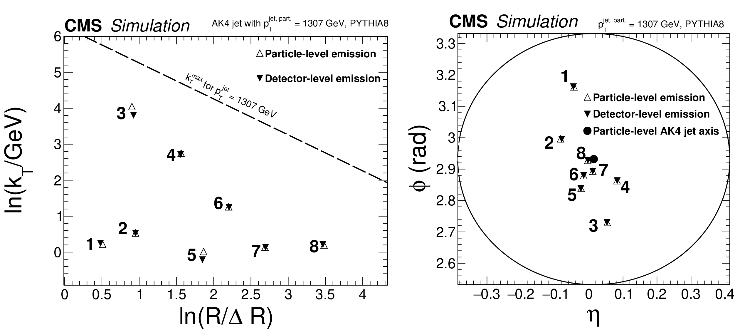
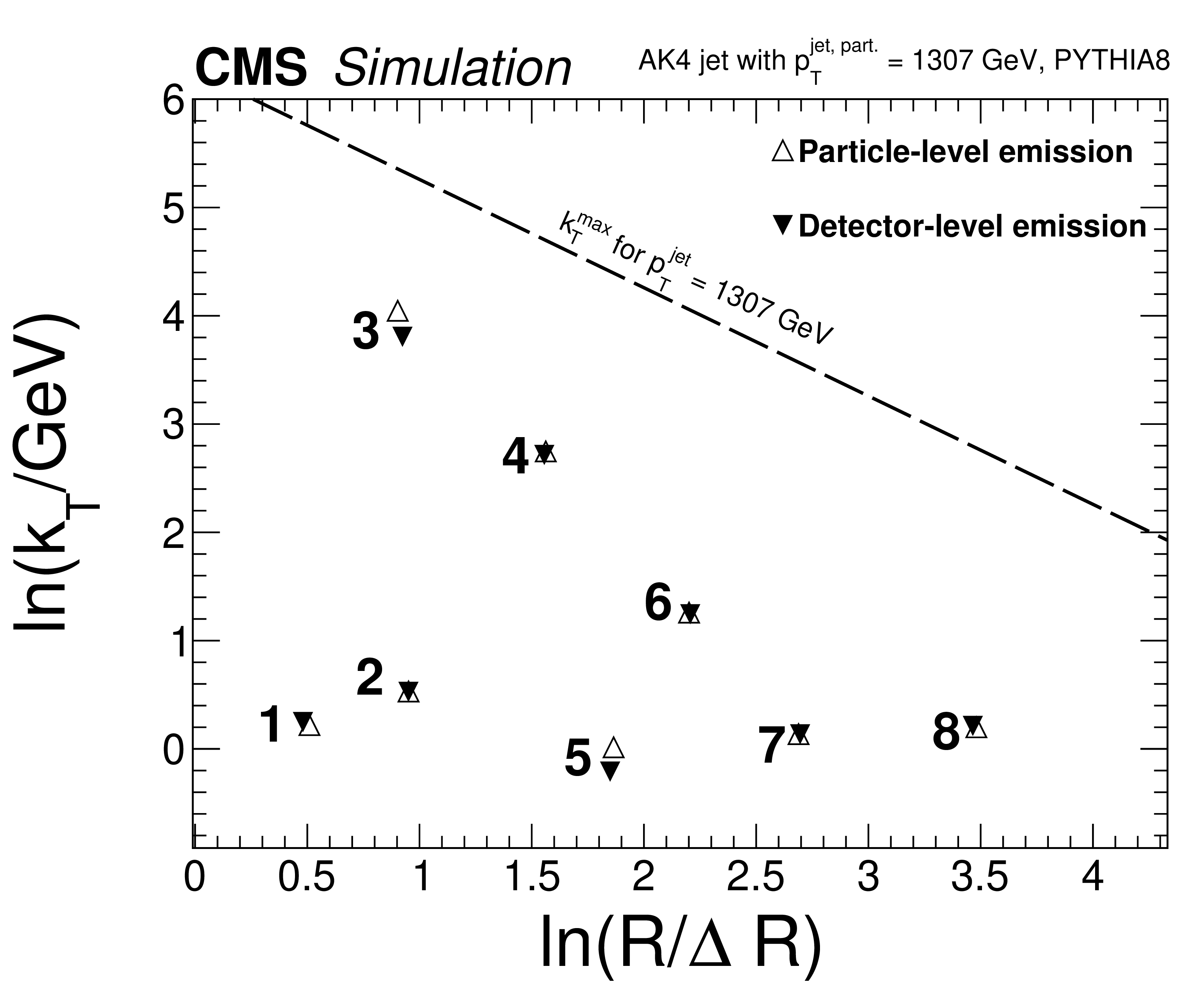
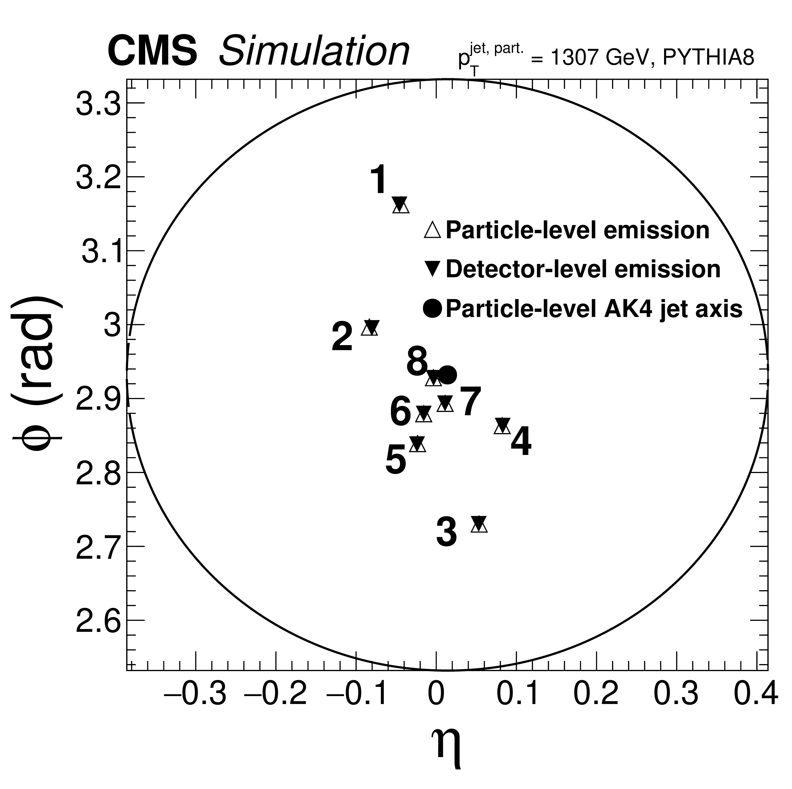
Figure 4:
Event displays of a simulated AK4 jet at detector level (solid triangles) and particle level (open triangles). The right-hand side plot represents the $ \eta $ and $ \phi $ coordinates of the emissions in the CMS coordinate system to illustrate the geometrical matching used for the corrections in the measurement. The center of the particle-level anti-$ k_{\mathrm{T}} $ jet is represented by the solid circular marker. The circular line with radius $ R = $ 0.4 serves as a proxy for the anti-$ k_{\mathrm{T}} $ distance parameter used to cluster the AK4 jet. The Lund plane on the left plot is associated with the same jet, and is filled with the primary emissions from the CA declustering from left to right (from large to small angles). The numbers in both plots represent the order of the emission of the primary CA tree declustering sequence. |
png pdf |
Figure 4-a:
Event displays of a simulated AK4 jet at detector level (solid triangles) and particle level (open triangles). The right-hand side plot represents the $ \eta $ and $ \phi $ coordinates of the emissions in the CMS coordinate system to illustrate the geometrical matching used for the corrections in the measurement. The center of the particle-level anti-$ k_{\mathrm{T}} $ jet is represented by the solid circular marker. The circular line with radius $ R = $ 0.4 serves as a proxy for the anti-$ k_{\mathrm{T}} $ distance parameter used to cluster the AK4 jet. The Lund plane on the left plot is associated with the same jet, and is filled with the primary emissions from the CA declustering from left to right (from large to small angles). The numbers in both plots represent the order of the emission of the primary CA tree declustering sequence. |
png pdf |
Figure 4-b:
Event displays of a simulated AK4 jet at detector level (solid triangles) and particle level (open triangles). The right-hand side plot represents the $ \eta $ and $ \phi $ coordinates of the emissions in the CMS coordinate system to illustrate the geometrical matching used for the corrections in the measurement. The center of the particle-level anti-$ k_{\mathrm{T}} $ jet is represented by the solid circular marker. The circular line with radius $ R = $ 0.4 serves as a proxy for the anti-$ k_{\mathrm{T}} $ distance parameter used to cluster the AK4 jet. The Lund plane on the left plot is associated with the same jet, and is filled with the primary emissions from the CA declustering from left to right (from large to small angles). The numbers in both plots represent the order of the emission of the primary CA tree declustering sequence. |
png pdf |
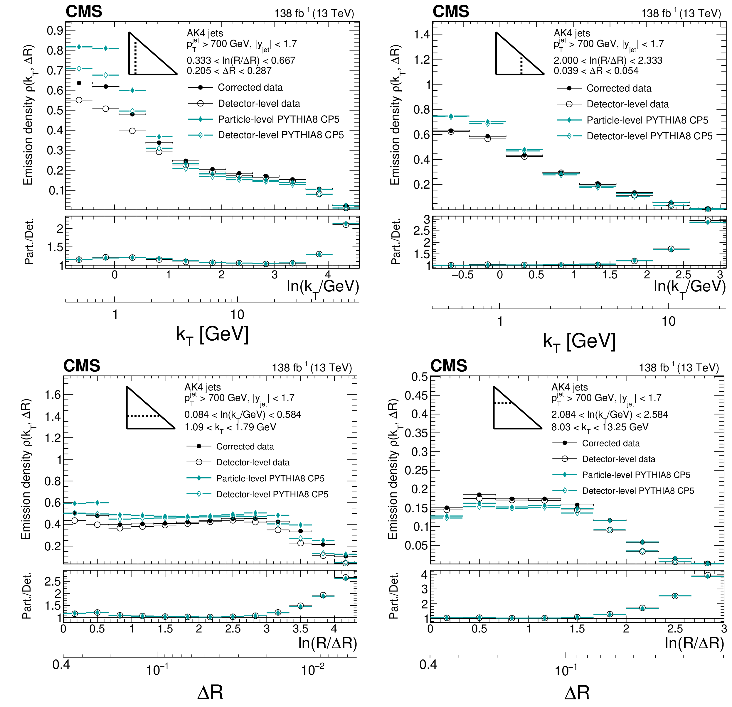
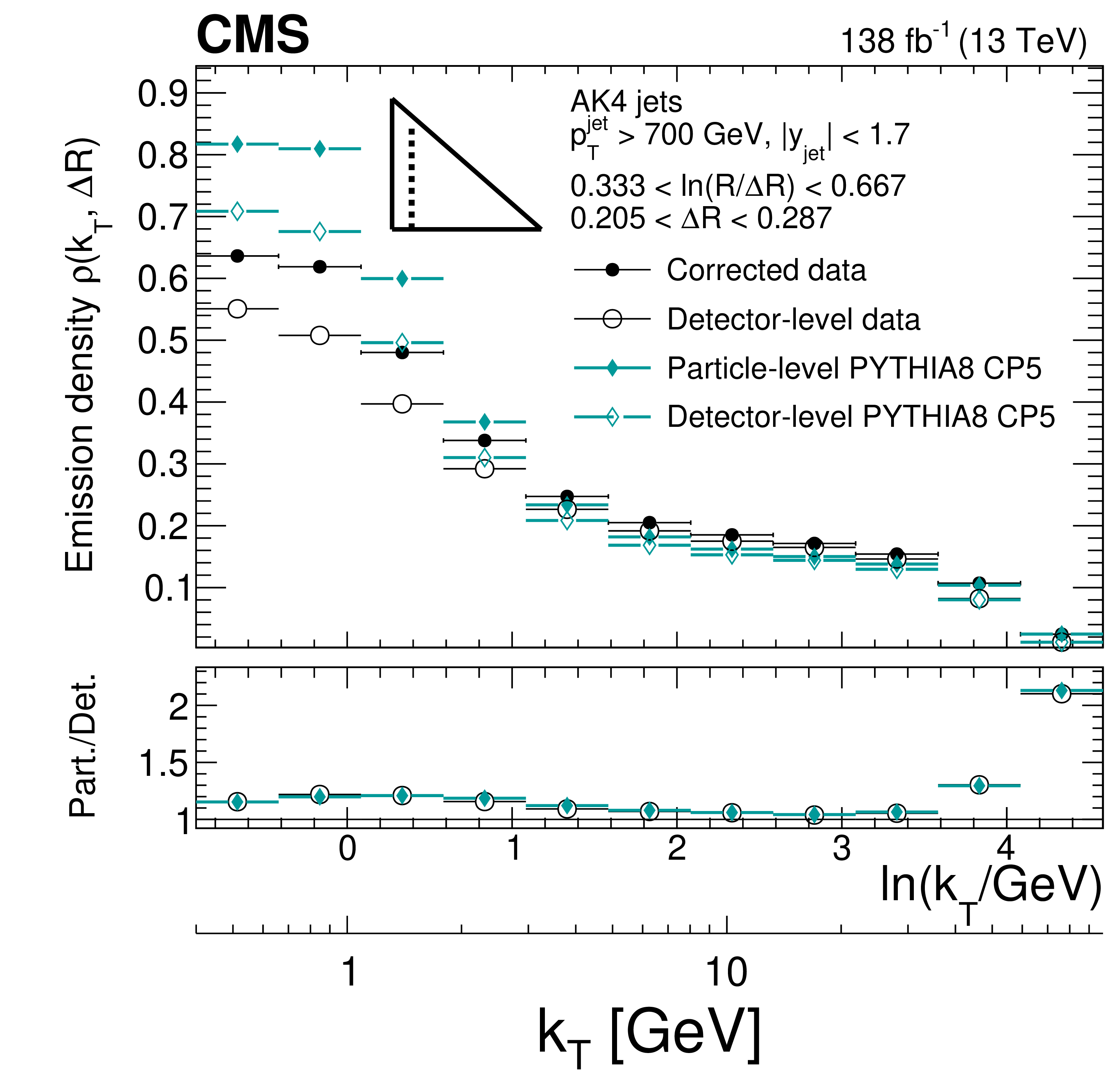
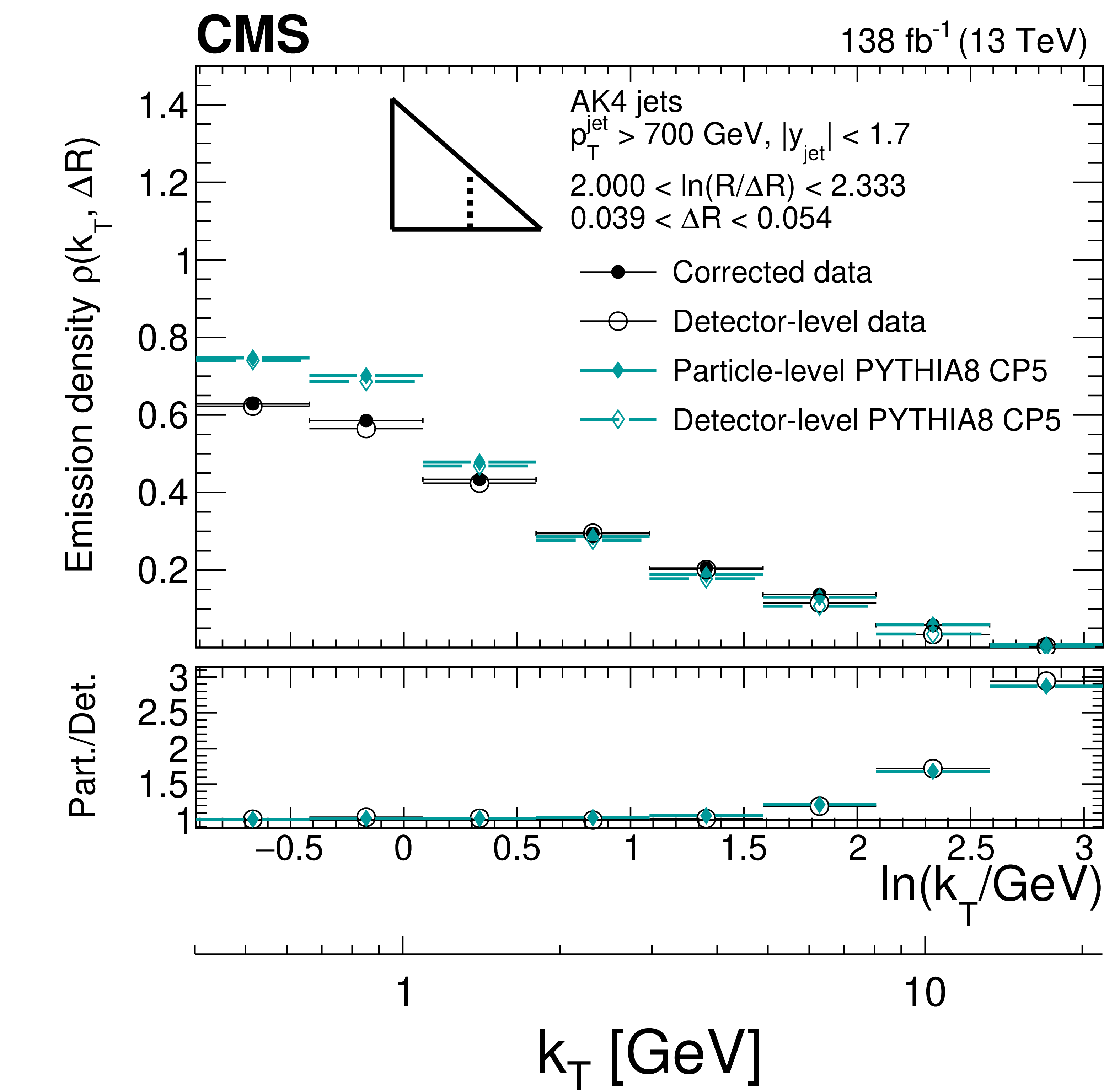
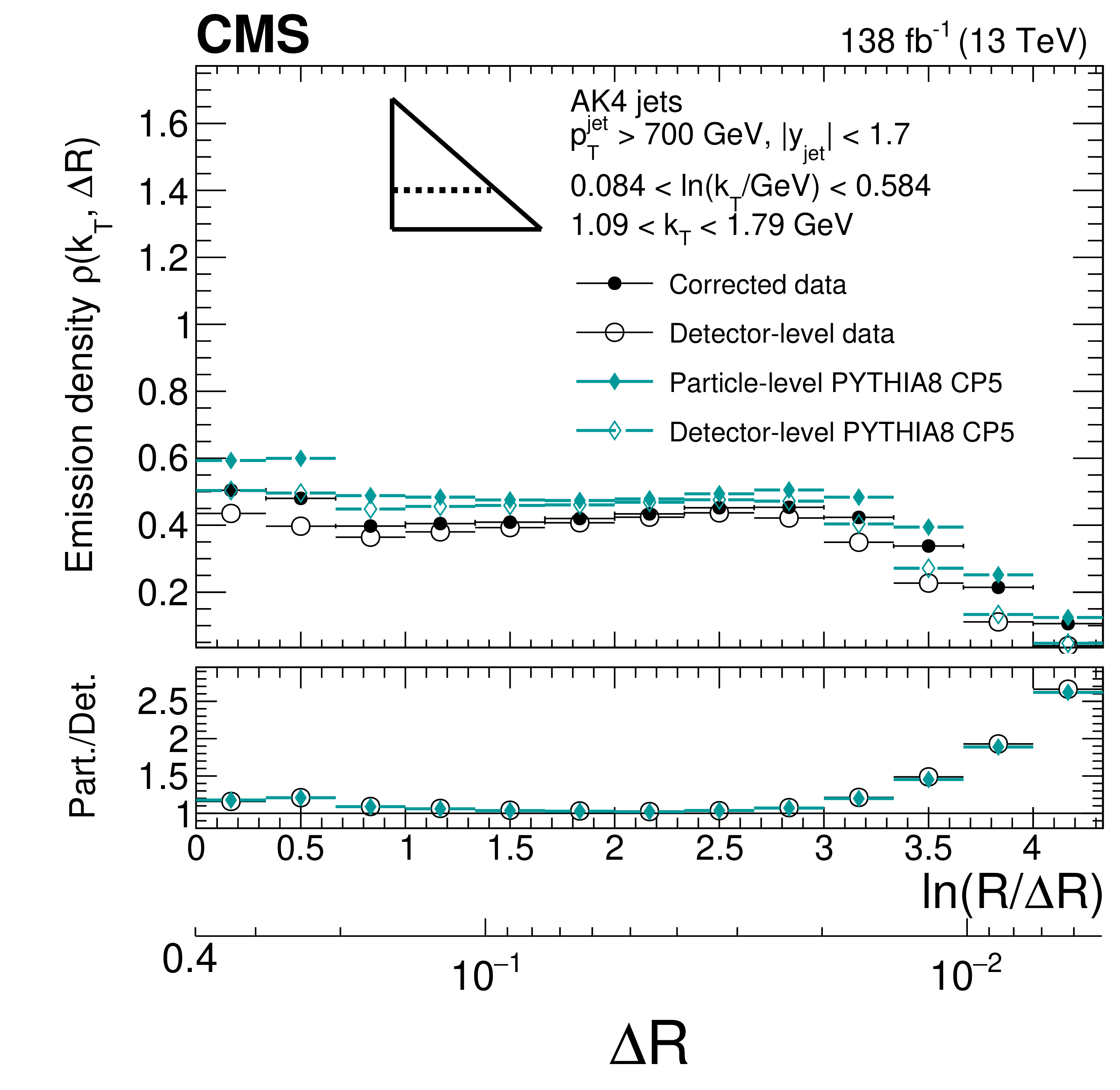
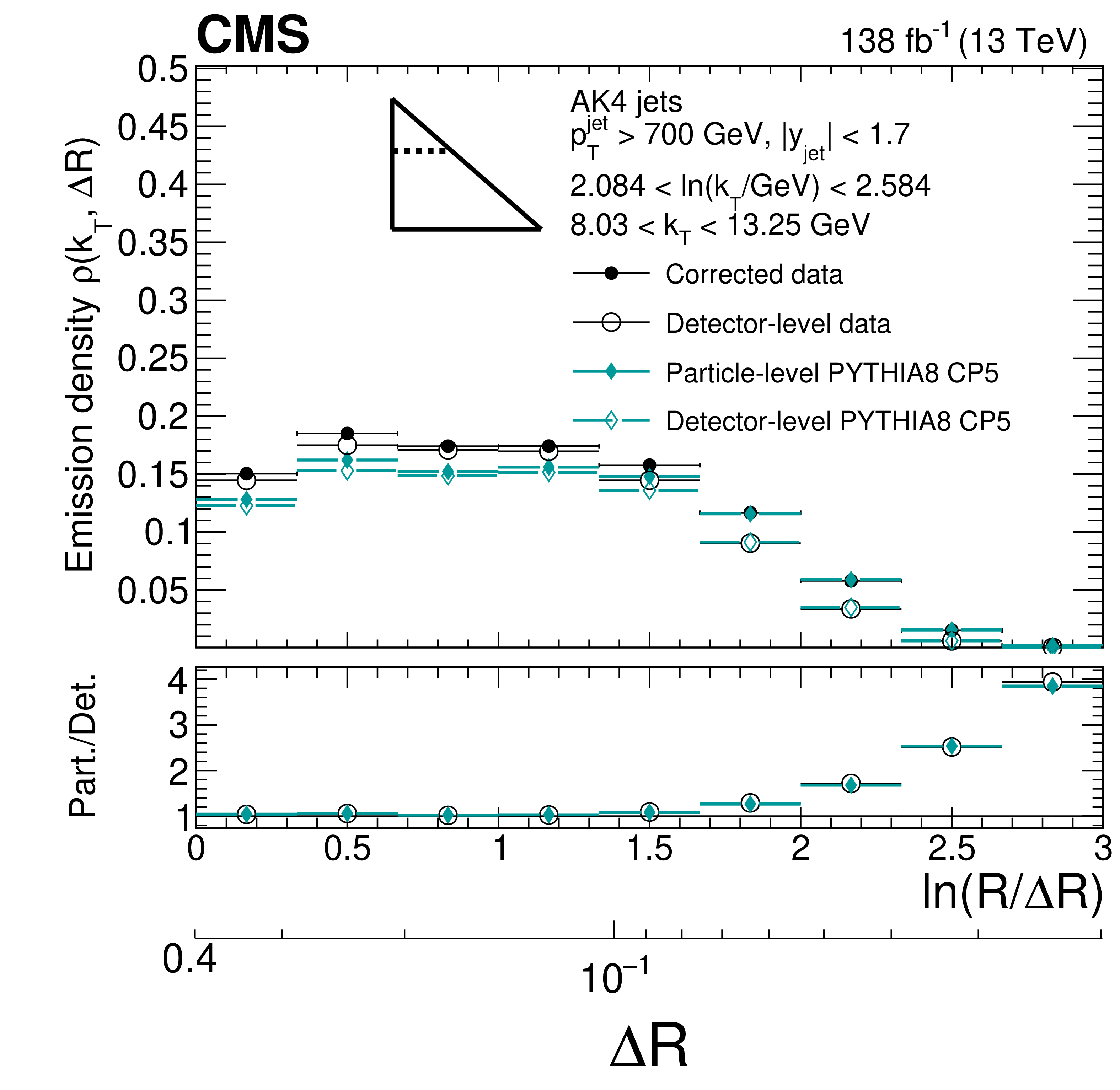
Figure 5:
Detector-level (open symbols) and particle-level (closed symbols) distributions for the data and MC simulated events of PYTHIA8 CP5. Only statistical uncertainties are included in these plots, which are smaller than the markers for most of the bins. The lower panels in the plot show the ratio of the particle-level to the respective detector-level distributions, which is used as a metric for the effective modifications of the LJP density because of the detector effects. The size of the corrections can be inferred from the ratio of the particle-level to the detector-level distributions, which are larger closer to the kinematical edge of the LJP. |
png pdf |
Figure 5-a:
Detector-level (open symbols) and particle-level (closed symbols) distributions for the data and MC simulated events of PYTHIA8 CP5. Only statistical uncertainties are included in these plots, which are smaller than the markers for most of the bins. The lower panels in the plot show the ratio of the particle-level to the respective detector-level distributions, which is used as a metric for the effective modifications of the LJP density because of the detector effects. The size of the corrections can be inferred from the ratio of the particle-level to the detector-level distributions, which are larger closer to the kinematical edge of the LJP. |
png pdf |
Figure 5-b:
Detector-level (open symbols) and particle-level (closed symbols) distributions for the data and MC simulated events of PYTHIA8 CP5. Only statistical uncertainties are included in these plots, which are smaller than the markers for most of the bins. The lower panels in the plot show the ratio of the particle-level to the respective detector-level distributions, which is used as a metric for the effective modifications of the LJP density because of the detector effects. The size of the corrections can be inferred from the ratio of the particle-level to the detector-level distributions, which are larger closer to the kinematical edge of the LJP. |
png pdf |
Figure 5-c:
Detector-level (open symbols) and particle-level (closed symbols) distributions for the data and MC simulated events of PYTHIA8 CP5. Only statistical uncertainties are included in these plots, which are smaller than the markers for most of the bins. The lower panels in the plot show the ratio of the particle-level to the respective detector-level distributions, which is used as a metric for the effective modifications of the LJP density because of the detector effects. The size of the corrections can be inferred from the ratio of the particle-level to the detector-level distributions, which are larger closer to the kinematical edge of the LJP. |
png pdf |
Figure 5-d:
Detector-level (open symbols) and particle-level (closed symbols) distributions for the data and MC simulated events of PYTHIA8 CP5. Only statistical uncertainties are included in these plots, which are smaller than the markers for most of the bins. The lower panels in the plot show the ratio of the particle-level to the respective detector-level distributions, which is used as a metric for the effective modifications of the LJP density because of the detector effects. The size of the corrections can be inferred from the ratio of the particle-level to the detector-level distributions, which are larger closer to the kinematical edge of the LJP. |

png pdf |
Figure 6:
Different components of the systematic uncertainties for AK4 jets for two different vertical slices of the LJP density. The upper plot is for large angles 0.205 $ < \Delta R < $ 0.287, and the lower plot is for small angles 0.039 $ < \Delta R < $ 0.054. The total experimental uncertainty is represented by the filled area. The statistical uncertainties in the data are represented by the hashed band. |
png pdf |
Figure 6-a:
Different components of the systematic uncertainties for AK4 jets for two different vertical slices of the LJP density. The upper plot is for large angles 0.205 $ < \Delta R < $ 0.287, and the lower plot is for small angles 0.039 $ < \Delta R < $ 0.054. The total experimental uncertainty is represented by the filled area. The statistical uncertainties in the data are represented by the hashed band. |

png pdf |
Figure 6-b:
Different components of the systematic uncertainties for AK4 jets for two different vertical slices of the LJP density. The upper plot is for large angles 0.205 $ < \Delta R < $ 0.287, and the lower plot is for small angles 0.039 $ < \Delta R < $ 0.054. The total experimental uncertainty is represented by the filled area. The statistical uncertainties in the data are represented by the hashed band. |

png pdf |
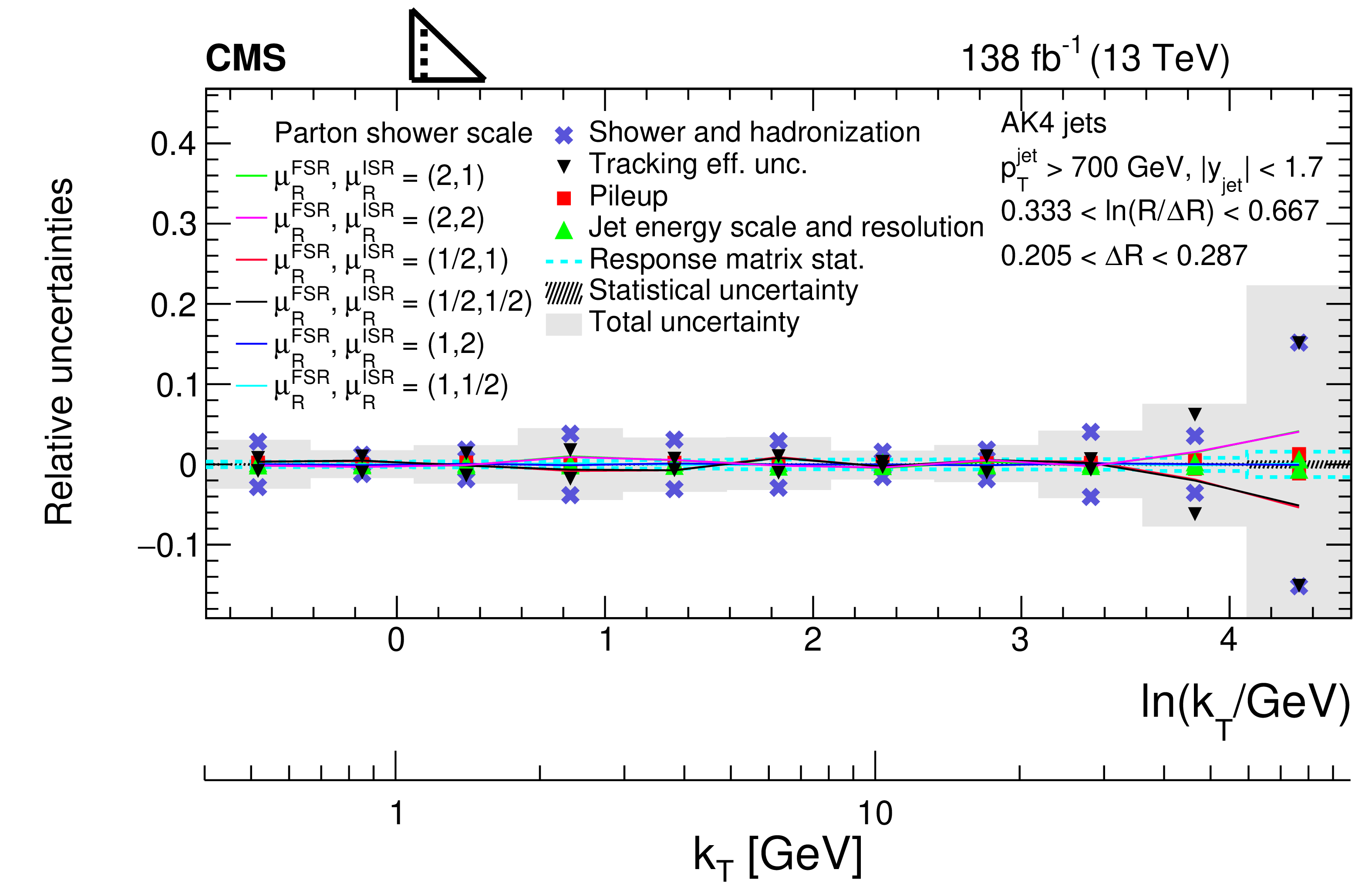
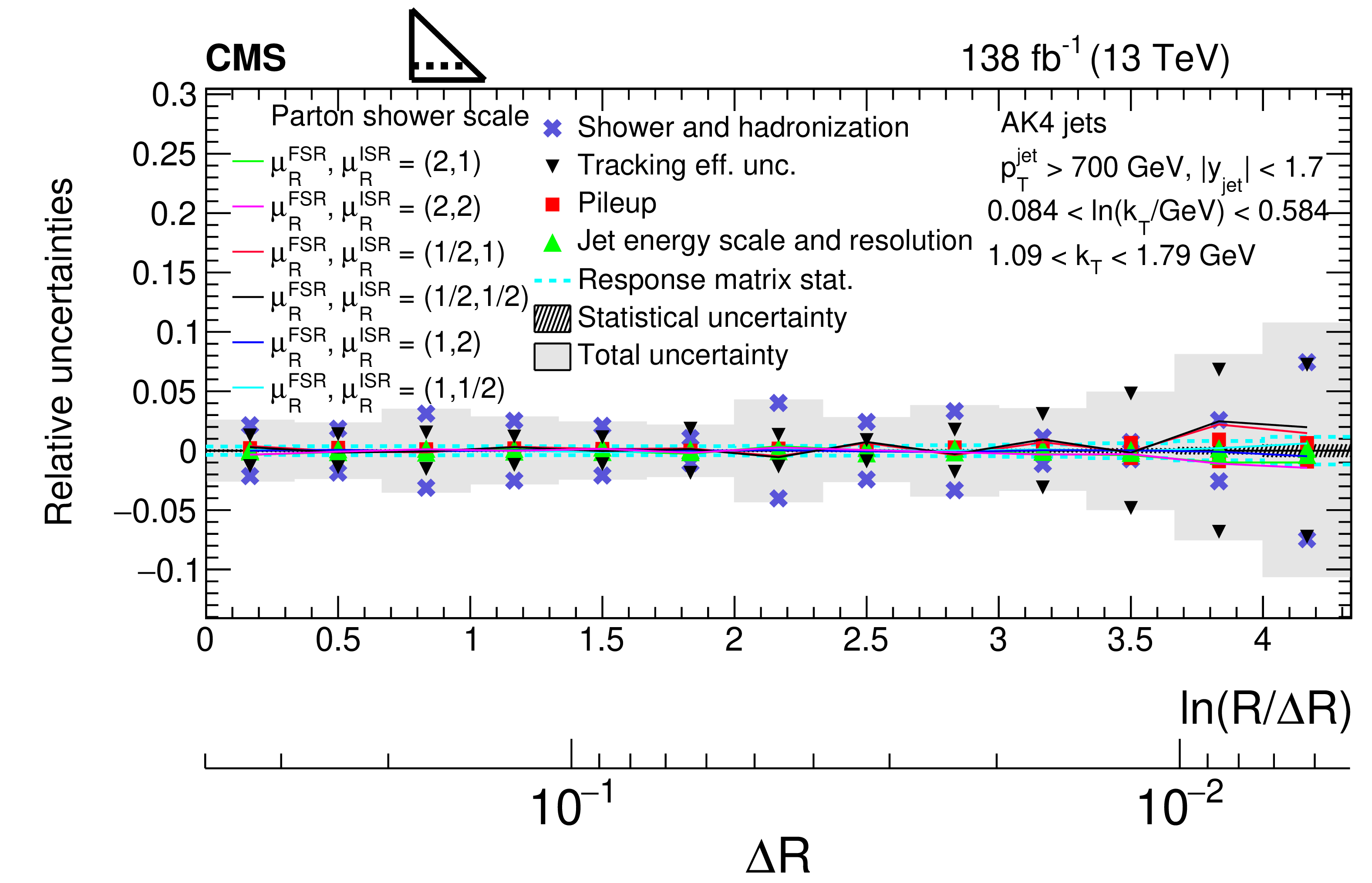
Figure 7:
Different components of the systematic uncertainties for AK4 jets for different horizontal slices of the LJP density. The upper plot is for low $ k_{\mathrm{T}} $ of 1.09 $ < k_{\mathrm{T}} < $ 1.79 GeV, and the lower plot is for higher $ k_{\mathrm{T}} $ of 8.03 $ < k_{\mathrm{T}} < $ 13.25 GeV. The total experimental uncertainty is represented by the filled area. The statistical uncertainties in the data are represented by the hashed band. |
png pdf |
Figure 7-a:
Different components of the systematic uncertainties for AK4 jets for different horizontal slices of the LJP density. The upper plot is for low $ k_{\mathrm{T}} $ of 1.09 $ < k_{\mathrm{T}} < $ 1.79 GeV, and the lower plot is for higher $ k_{\mathrm{T}} $ of 8.03 $ < k_{\mathrm{T}} < $ 13.25 GeV. The total experimental uncertainty is represented by the filled area. The statistical uncertainties in the data are represented by the hashed band. |

png pdf |
Figure 7-b:
Different components of the systematic uncertainties for AK4 jets for different horizontal slices of the LJP density. The upper plot is for low $ k_{\mathrm{T}} $ of 1.09 $ < k_{\mathrm{T}} < $ 1.79 GeV, and the lower plot is for higher $ k_{\mathrm{T}} $ of 8.03 $ < k_{\mathrm{T}} < $ 13.25 GeV. The total experimental uncertainty is represented by the filled area. The statistical uncertainties in the data are represented by the hashed band. |
png pdf |
Figure 8:
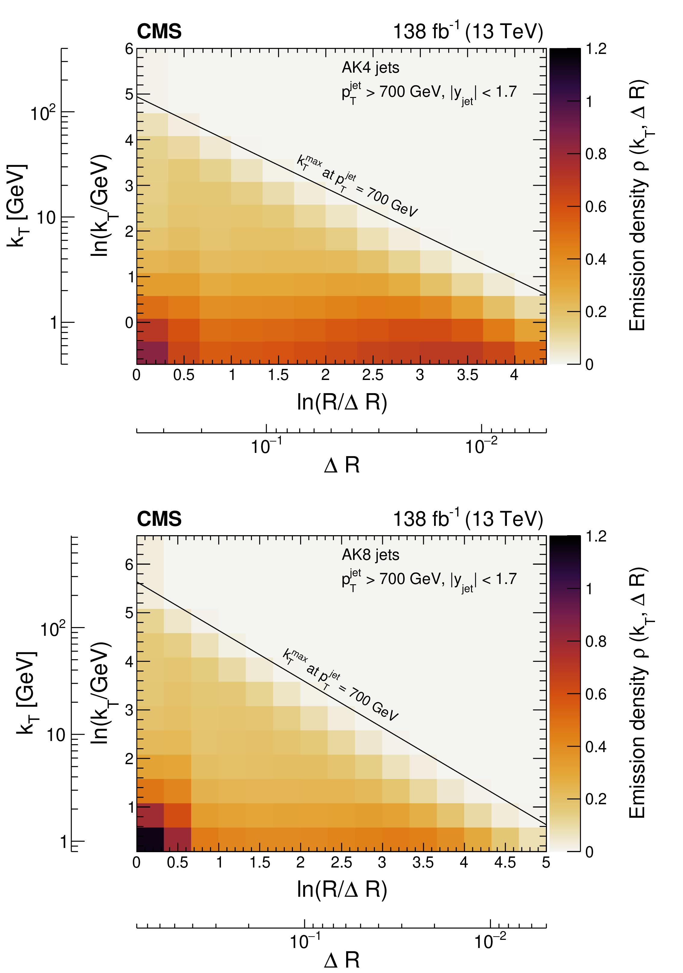
Two-dimensional distributions of the primary LJP densities corrected to particle level for AK4 jets (upper plot) and AK8 jets (lower plot). The diagonal line in both plots represents the kinematical limit of the emissions for a jet with $ p_{\mathrm{T}}^\text{jet} = $ 700 GeV. |
png pdf |
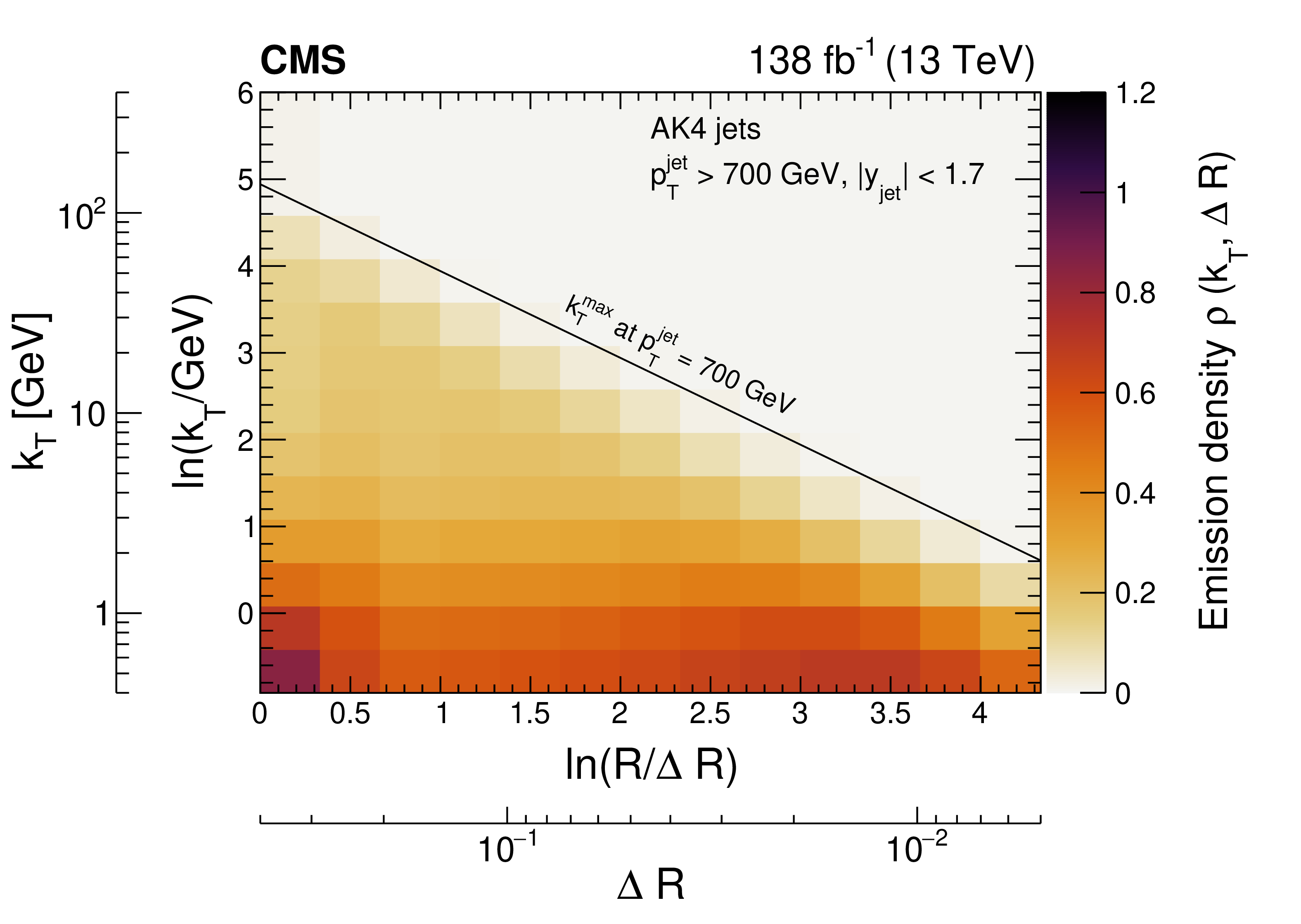
Figure 8-a:
Two-dimensional distributions of the primary LJP densities corrected to particle level for AK4 jets (upper plot) and AK8 jets (lower plot). The diagonal line in both plots represents the kinematical limit of the emissions for a jet with $ p_{\mathrm{T}}^\text{jet} = $ 700 GeV. |
png pdf |
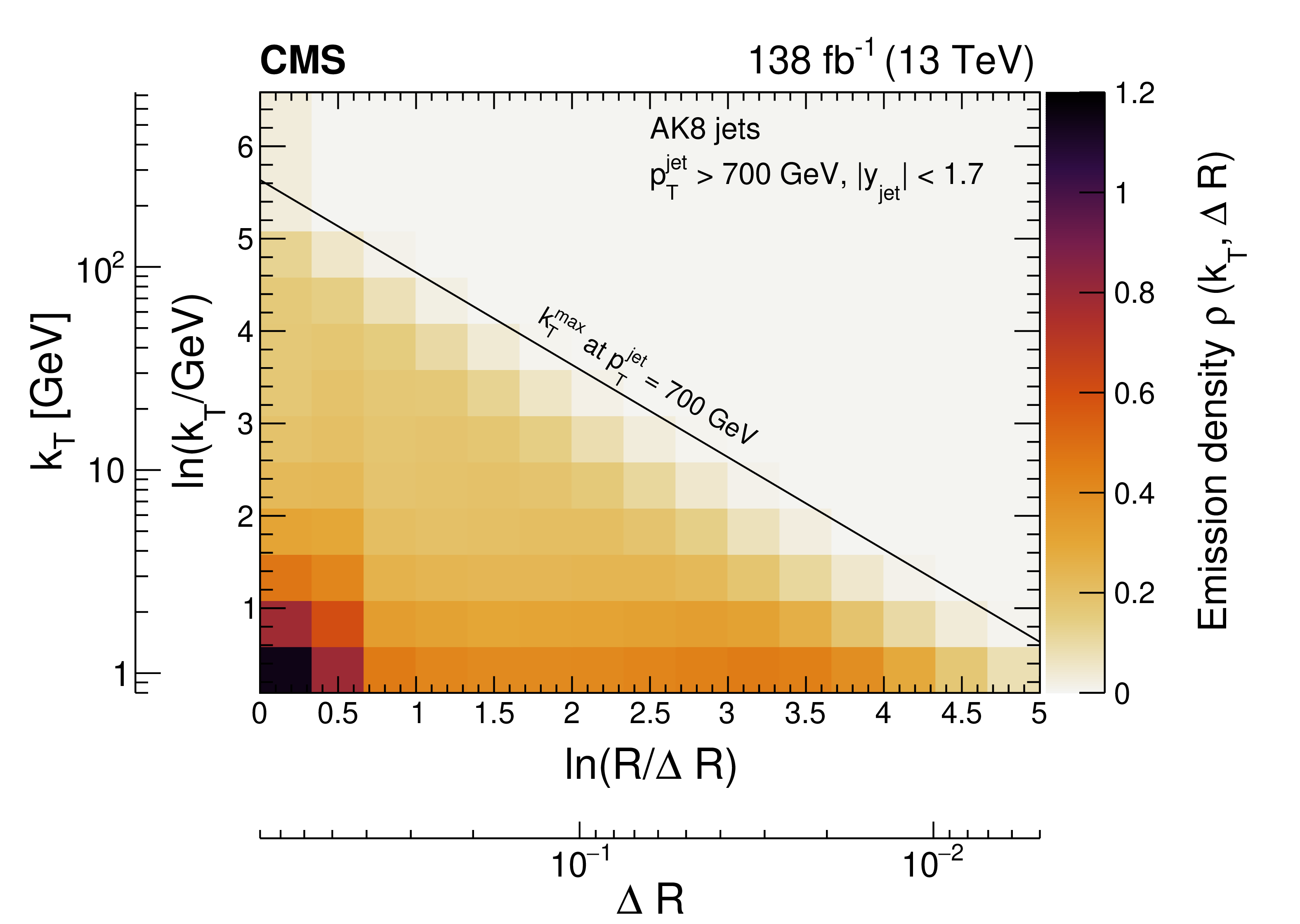
Figure 8-b:
Two-dimensional distributions of the primary LJP densities corrected to particle level for AK4 jets (upper plot) and AK8 jets (lower plot). The diagonal line in both plots represents the kinematical limit of the emissions for a jet with $ p_{\mathrm{T}}^\text{jet} = $ 700 GeV. |

png pdf |
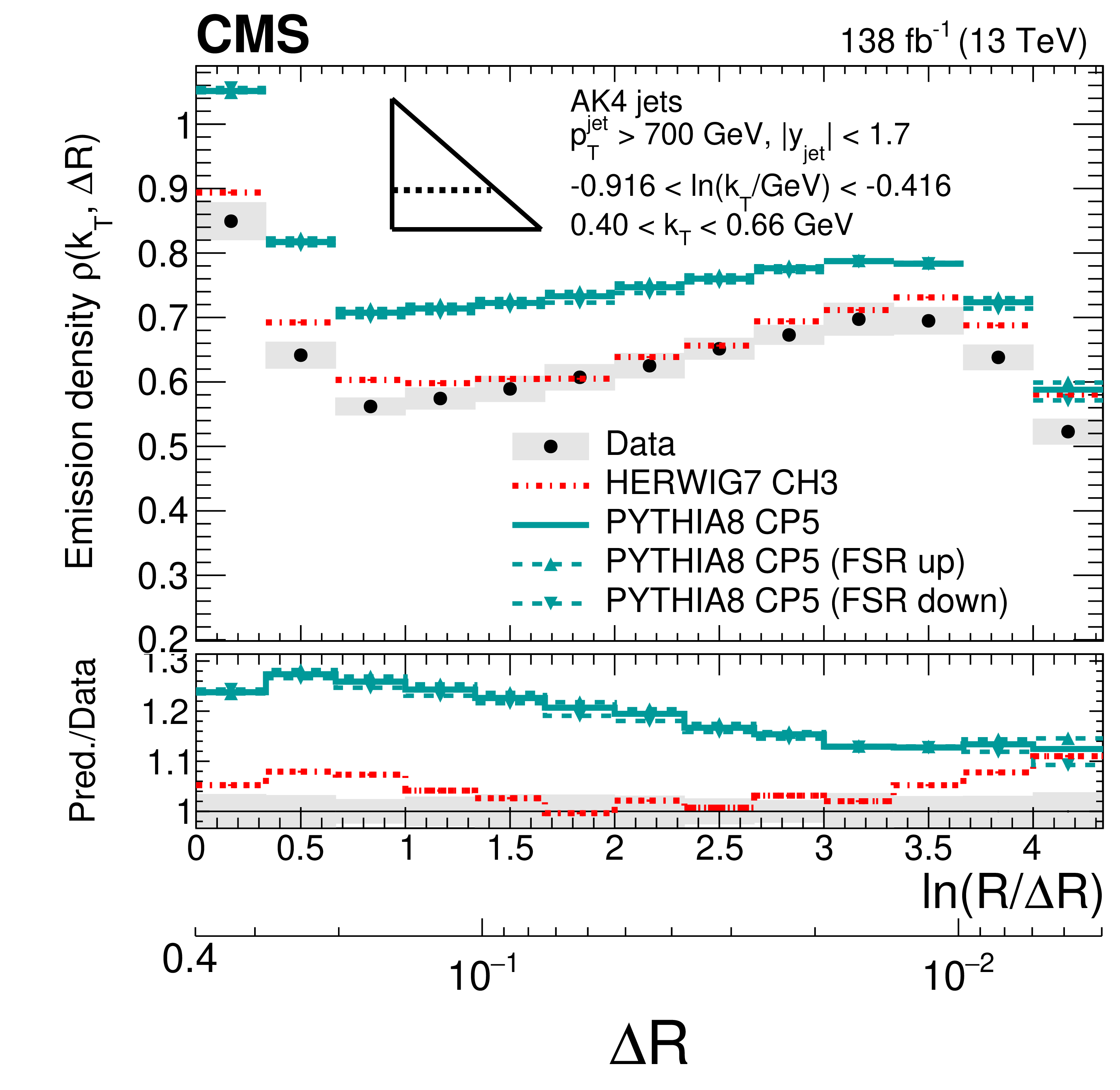
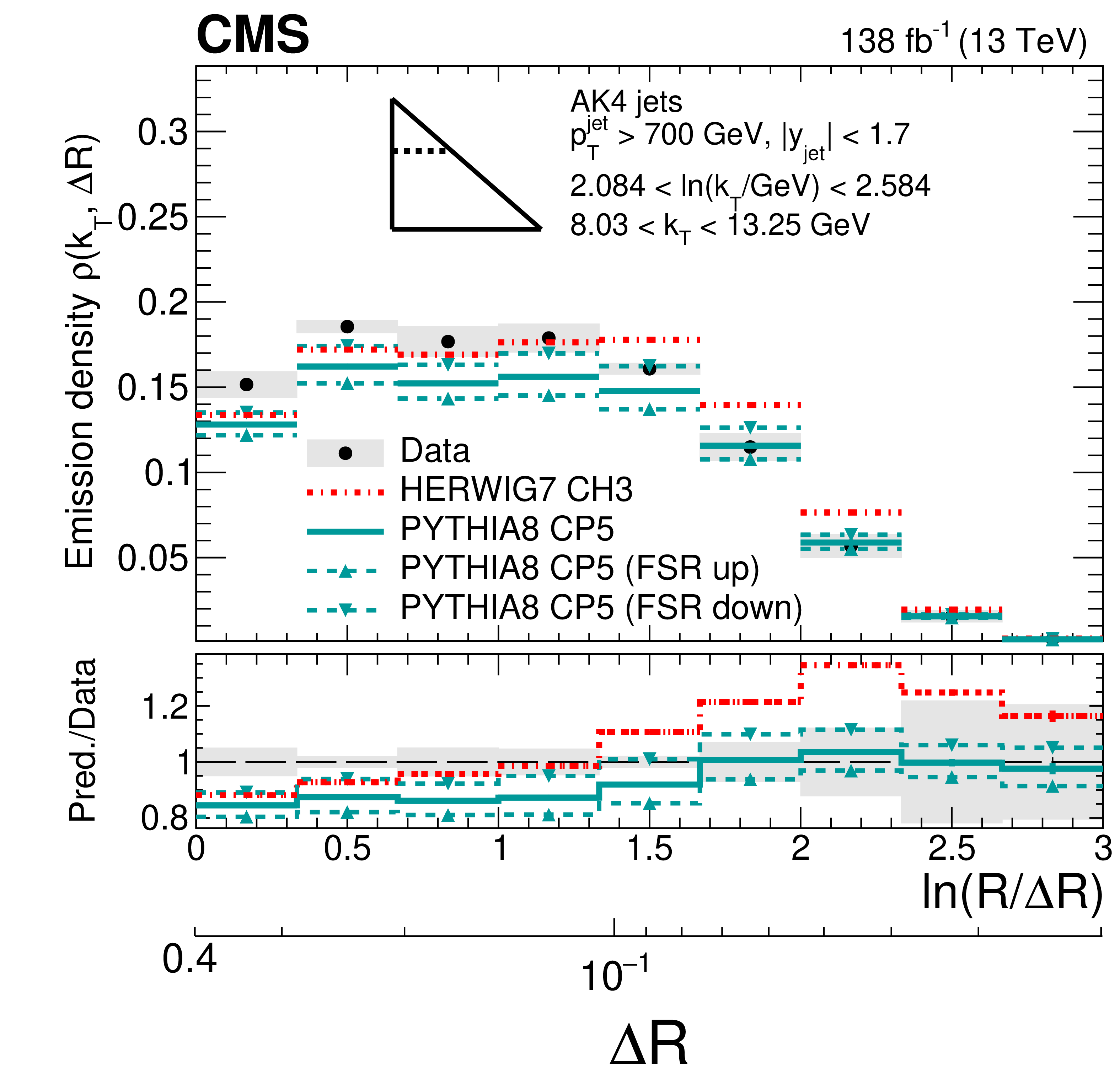
Figure 9:
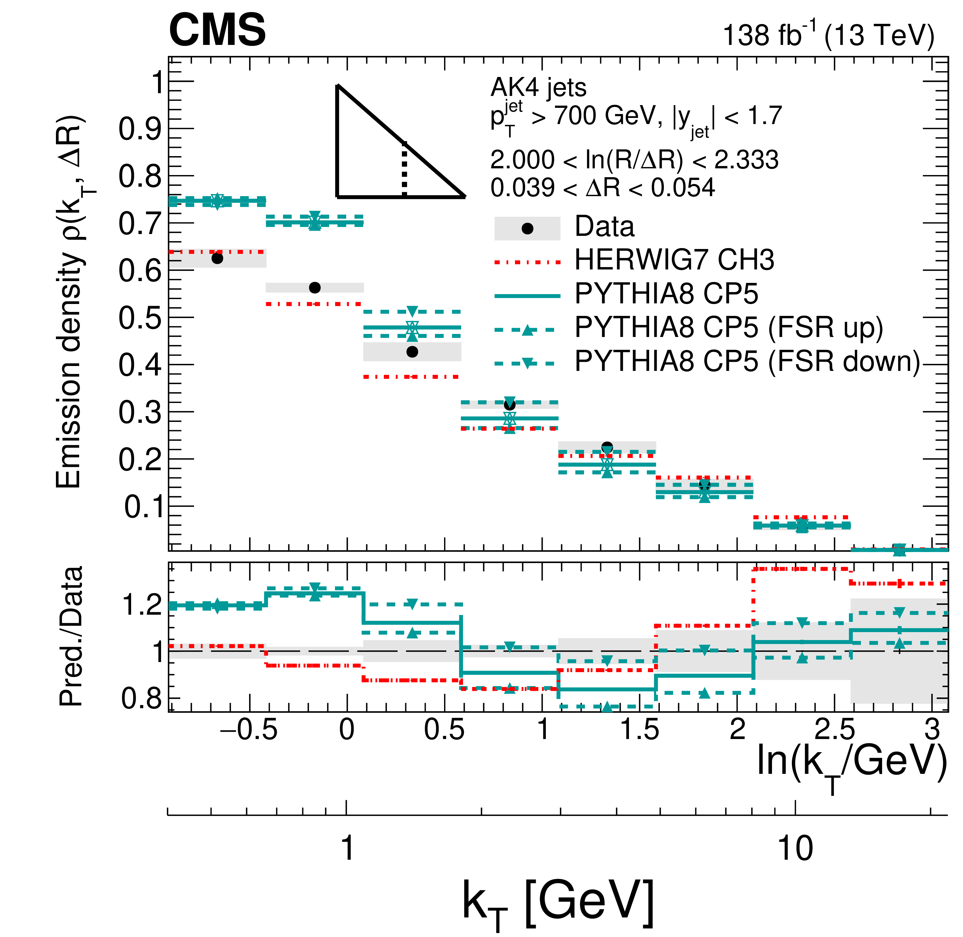
Four slices of the primary LJP density of AK4 jets compared with predictions by PYTHIA8 CP5 and HERWIG 7 CH3. Variations of the ISR and FSR scales for PYTHIA8 CP5 predictions are shown as well. The band represents the total experimental uncertainty. The upper two plots correspond to vertical slices for fixed $ \ln(R/\Delta R) $ (large angles on upper-left, small angles on upper-right). The lower two plots correspond to two different horizontal slices for fixed $ \ln(k_{\mathrm{T}}/$GeV$)$: the lower-left plot contains low-$ k_{\mathrm{T}} $ splittings, whereas the lower-right plot contains high-$ k_{\mathrm{T}} $ splittings, which populate mostly wide-angle radiation. |

png pdf |
Figure 9-a:
Four slices of the primary LJP density of AK4 jets compared with predictions by PYTHIA8 CP5 and HERWIG 7 CH3. Variations of the ISR and FSR scales for PYTHIA8 CP5 predictions are shown as well. The band represents the total experimental uncertainty. The upper two plots correspond to vertical slices for fixed $ \ln(R/\Delta R) $ (large angles on upper-left, small angles on upper-right). The lower two plots correspond to two different horizontal slices for fixed $ \ln(k_{\mathrm{T}}/$GeV$)$: the lower-left plot contains low-$ k_{\mathrm{T}} $ splittings, whereas the lower-right plot contains high-$ k_{\mathrm{T}} $ splittings, which populate mostly wide-angle radiation. |
png pdf |
Figure 9-b:
Four slices of the primary LJP density of AK4 jets compared with predictions by PYTHIA8 CP5 and HERWIG 7 CH3. Variations of the ISR and FSR scales for PYTHIA8 CP5 predictions are shown as well. The band represents the total experimental uncertainty. The upper two plots correspond to vertical slices for fixed $ \ln(R/\Delta R) $ (large angles on upper-left, small angles on upper-right). The lower two plots correspond to two different horizontal slices for fixed $ \ln(k_{\mathrm{T}}/$GeV$)$: the lower-left plot contains low-$ k_{\mathrm{T}} $ splittings, whereas the lower-right plot contains high-$ k_{\mathrm{T}} $ splittings, which populate mostly wide-angle radiation. |
png pdf |
Figure 9-c:
Four slices of the primary LJP density of AK4 jets compared with predictions by PYTHIA8 CP5 and HERWIG 7 CH3. Variations of the ISR and FSR scales for PYTHIA8 CP5 predictions are shown as well. The band represents the total experimental uncertainty. The upper two plots correspond to vertical slices for fixed $ \ln(R/\Delta R) $ (large angles on upper-left, small angles on upper-right). The lower two plots correspond to two different horizontal slices for fixed $ \ln(k_{\mathrm{T}}/$GeV$)$: the lower-left plot contains low-$ k_{\mathrm{T}} $ splittings, whereas the lower-right plot contains high-$ k_{\mathrm{T}} $ splittings, which populate mostly wide-angle radiation. |
png pdf |
Figure 9-d:
Four slices of the primary LJP density of AK4 jets compared with predictions by PYTHIA8 CP5 and HERWIG 7 CH3. Variations of the ISR and FSR scales for PYTHIA8 CP5 predictions are shown as well. The band represents the total experimental uncertainty. The upper two plots correspond to vertical slices for fixed $ \ln(R/\Delta R) $ (large angles on upper-left, small angles on upper-right). The lower two plots correspond to two different horizontal slices for fixed $ \ln(k_{\mathrm{T}}/$GeV$)$: the lower-left plot contains low-$ k_{\mathrm{T}} $ splittings, whereas the lower-right plot contains high-$ k_{\mathrm{T}} $ splittings, which populate mostly wide-angle radiation. |

png pdf |
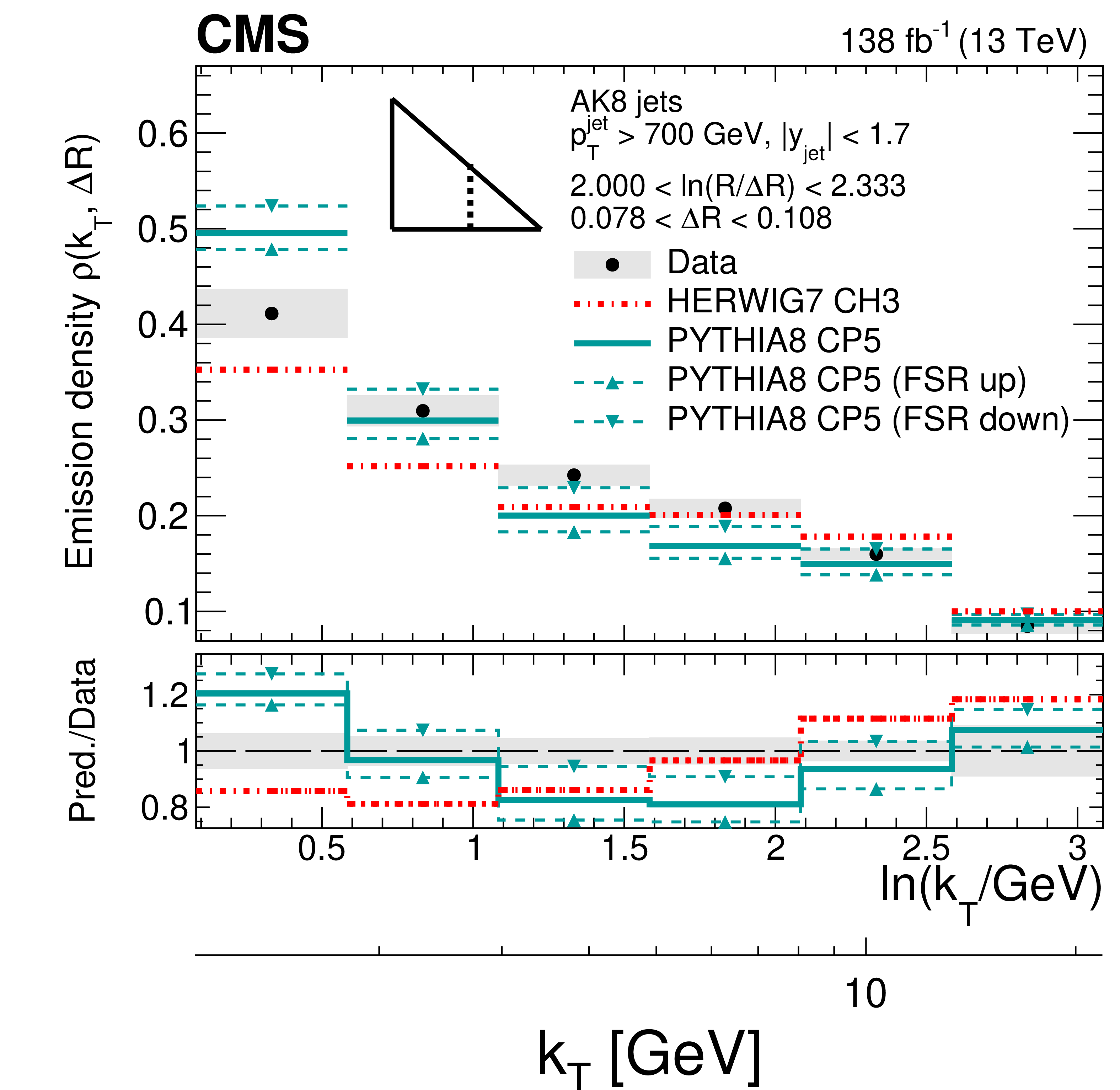
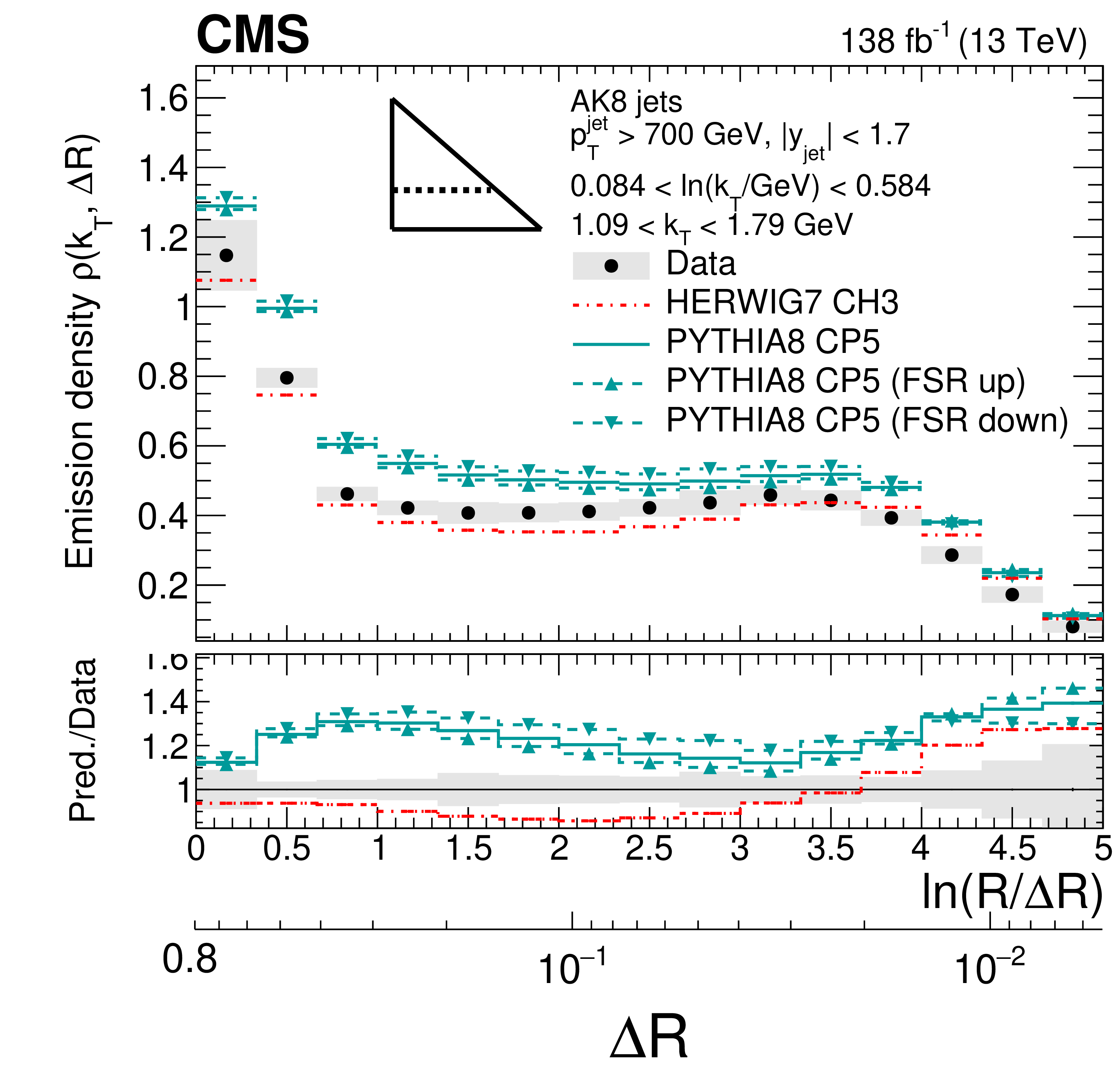
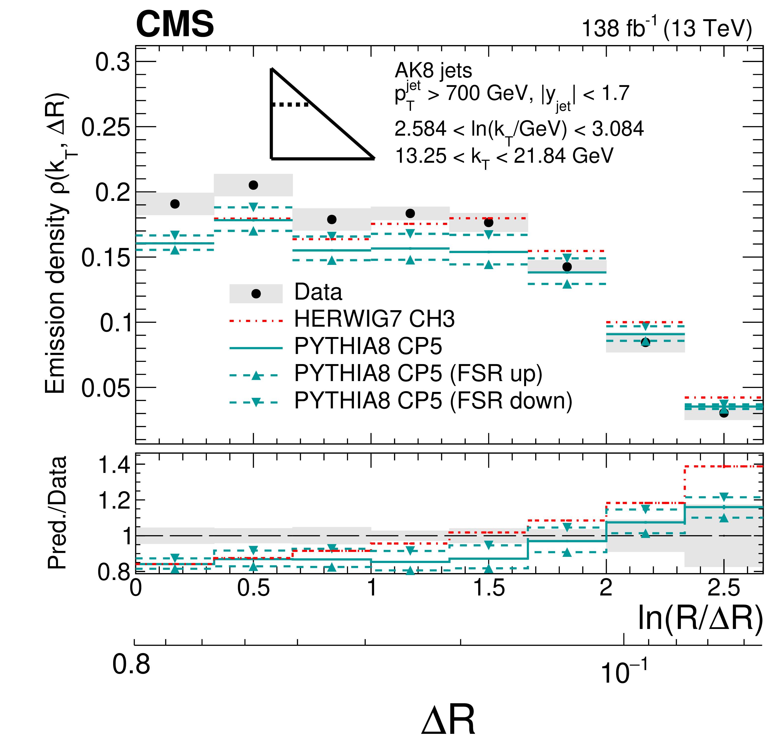
Figure 10:
Four slices of the primary LJP density of AK8 jets compared with predictions by PYTHIA8 CP5 and HERWIG 7 CH3. Variations of the ISR and FSR scales for PYTHIA8 CP5 predictions are shown as well. The band represents the total experimental uncertainty. The upper two plots correspond to vertical slices for fixed $ \ln(R/\Delta R) $ (large angles on upper-left, small angles on upper-right). The lower two plots correspond to two different horizontal slices for fixed $ \ln(k_{\mathrm{T}}/$GeV$)$: the lower-left plot corresponds to low-$ k_{\mathrm{T}} $ splittings and spans the full range in $ \ln(R/\Delta R) $, whereas the lower-right plot corresponds to high-$ k_{\mathrm{T}} $ splittings, which populate mostly wide-angle radiation. |

png pdf |
Figure 10-a:
Four slices of the primary LJP density of AK8 jets compared with predictions by PYTHIA8 CP5 and HERWIG 7 CH3. Variations of the ISR and FSR scales for PYTHIA8 CP5 predictions are shown as well. The band represents the total experimental uncertainty. The upper two plots correspond to vertical slices for fixed $ \ln(R/\Delta R) $ (large angles on upper-left, small angles on upper-right). The lower two plots correspond to two different horizontal slices for fixed $ \ln(k_{\mathrm{T}}/$GeV$)$: the lower-left plot corresponds to low-$ k_{\mathrm{T}} $ splittings and spans the full range in $ \ln(R/\Delta R) $, whereas the lower-right plot corresponds to high-$ k_{\mathrm{T}} $ splittings, which populate mostly wide-angle radiation. |
png pdf |
Figure 10-b:
Four slices of the primary LJP density of AK8 jets compared with predictions by PYTHIA8 CP5 and HERWIG 7 CH3. Variations of the ISR and FSR scales for PYTHIA8 CP5 predictions are shown as well. The band represents the total experimental uncertainty. The upper two plots correspond to vertical slices for fixed $ \ln(R/\Delta R) $ (large angles on upper-left, small angles on upper-right). The lower two plots correspond to two different horizontal slices for fixed $ \ln(k_{\mathrm{T}}/$GeV$)$: the lower-left plot corresponds to low-$ k_{\mathrm{T}} $ splittings and spans the full range in $ \ln(R/\Delta R) $, whereas the lower-right plot corresponds to high-$ k_{\mathrm{T}} $ splittings, which populate mostly wide-angle radiation. |
png pdf |
Figure 10-c:
Four slices of the primary LJP density of AK8 jets compared with predictions by PYTHIA8 CP5 and HERWIG 7 CH3. Variations of the ISR and FSR scales for PYTHIA8 CP5 predictions are shown as well. The band represents the total experimental uncertainty. The upper two plots correspond to vertical slices for fixed $ \ln(R/\Delta R) $ (large angles on upper-left, small angles on upper-right). The lower two plots correspond to two different horizontal slices for fixed $ \ln(k_{\mathrm{T}}/$GeV$)$: the lower-left plot corresponds to low-$ k_{\mathrm{T}} $ splittings and spans the full range in $ \ln(R/\Delta R) $, whereas the lower-right plot corresponds to high-$ k_{\mathrm{T}} $ splittings, which populate mostly wide-angle radiation. |
png pdf |
Figure 10-d:
Four slices of the primary LJP density of AK8 jets compared with predictions by PYTHIA8 CP5 and HERWIG 7 CH3. Variations of the ISR and FSR scales for PYTHIA8 CP5 predictions are shown as well. The band represents the total experimental uncertainty. The upper two plots correspond to vertical slices for fixed $ \ln(R/\Delta R) $ (large angles on upper-left, small angles on upper-right). The lower two plots correspond to two different horizontal slices for fixed $ \ln(k_{\mathrm{T}}/$GeV$)$: the lower-left plot corresponds to low-$ k_{\mathrm{T}} $ splittings and spans the full range in $ \ln(R/\Delta R) $, whereas the lower-right plot corresponds to high-$ k_{\mathrm{T}} $ splittings, which populate mostly wide-angle radiation. |
png pdf |
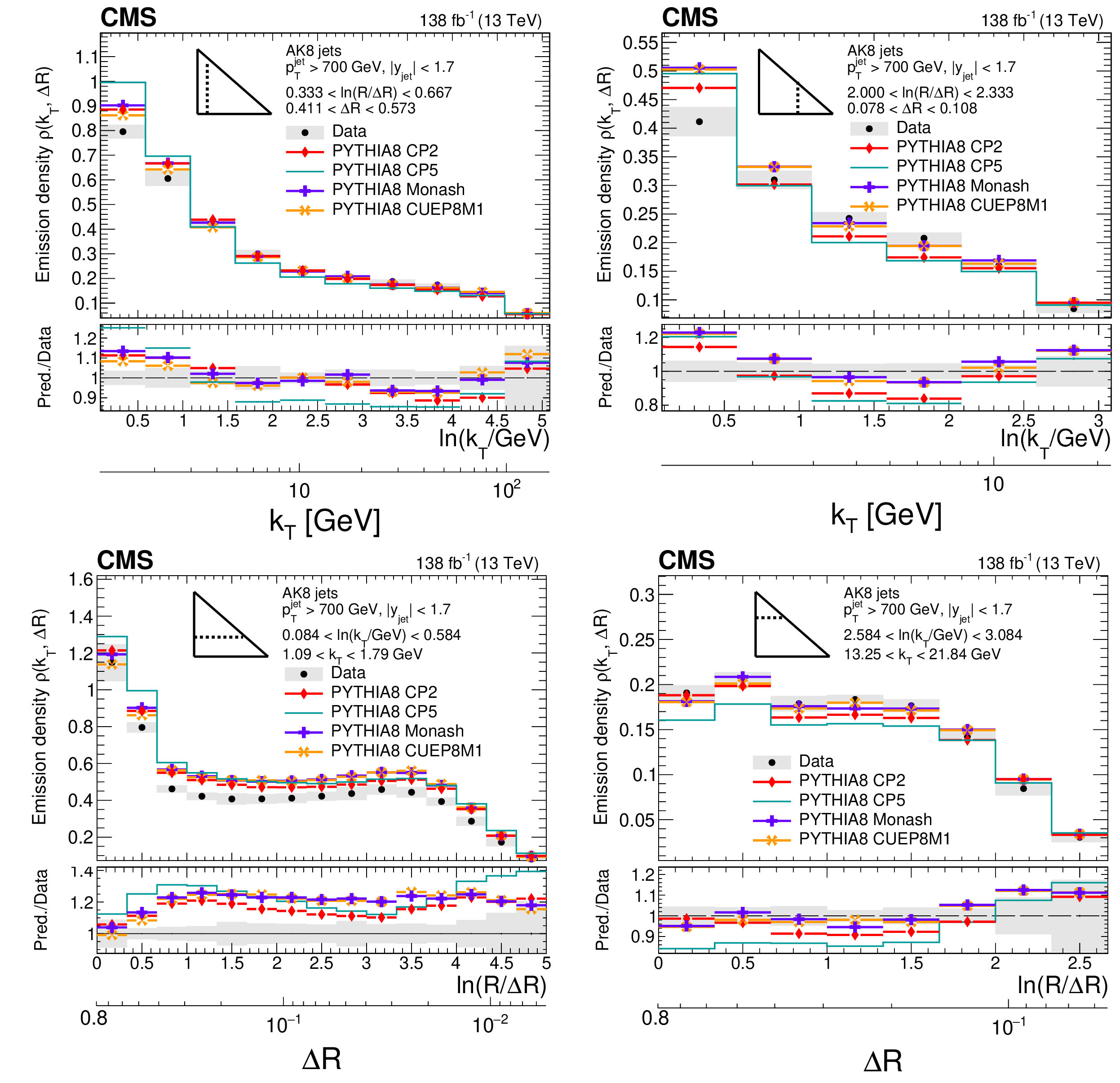
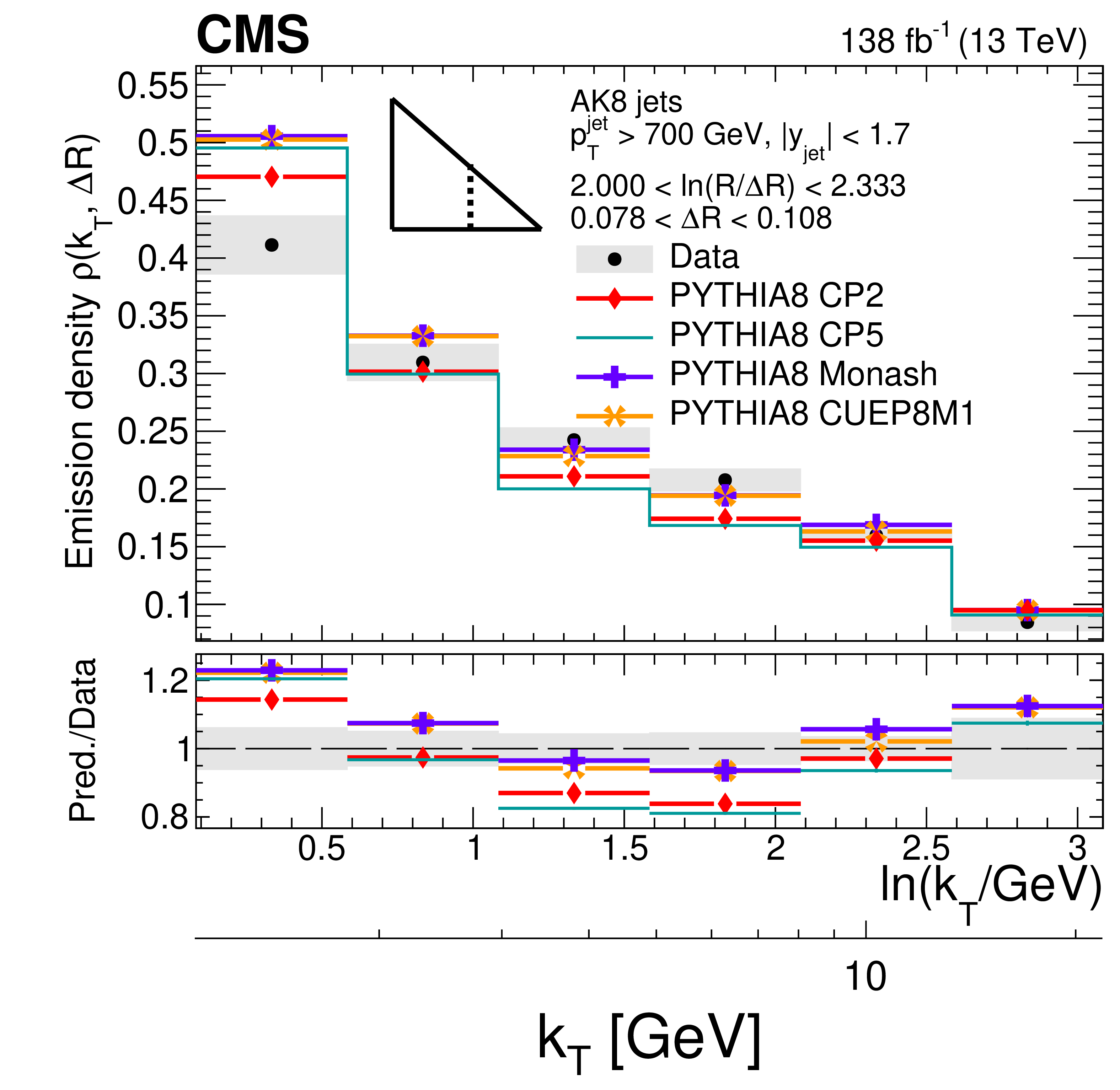
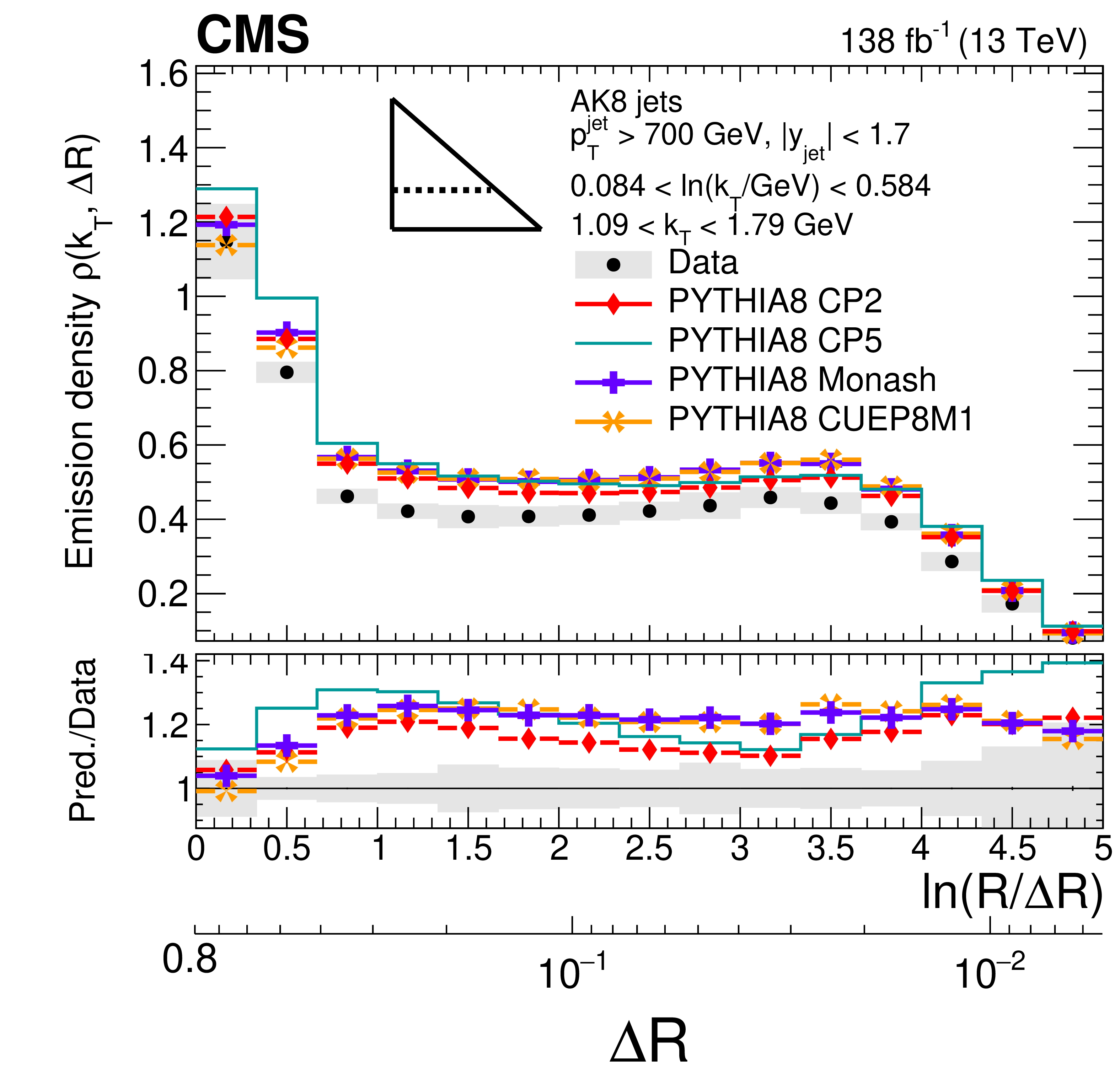
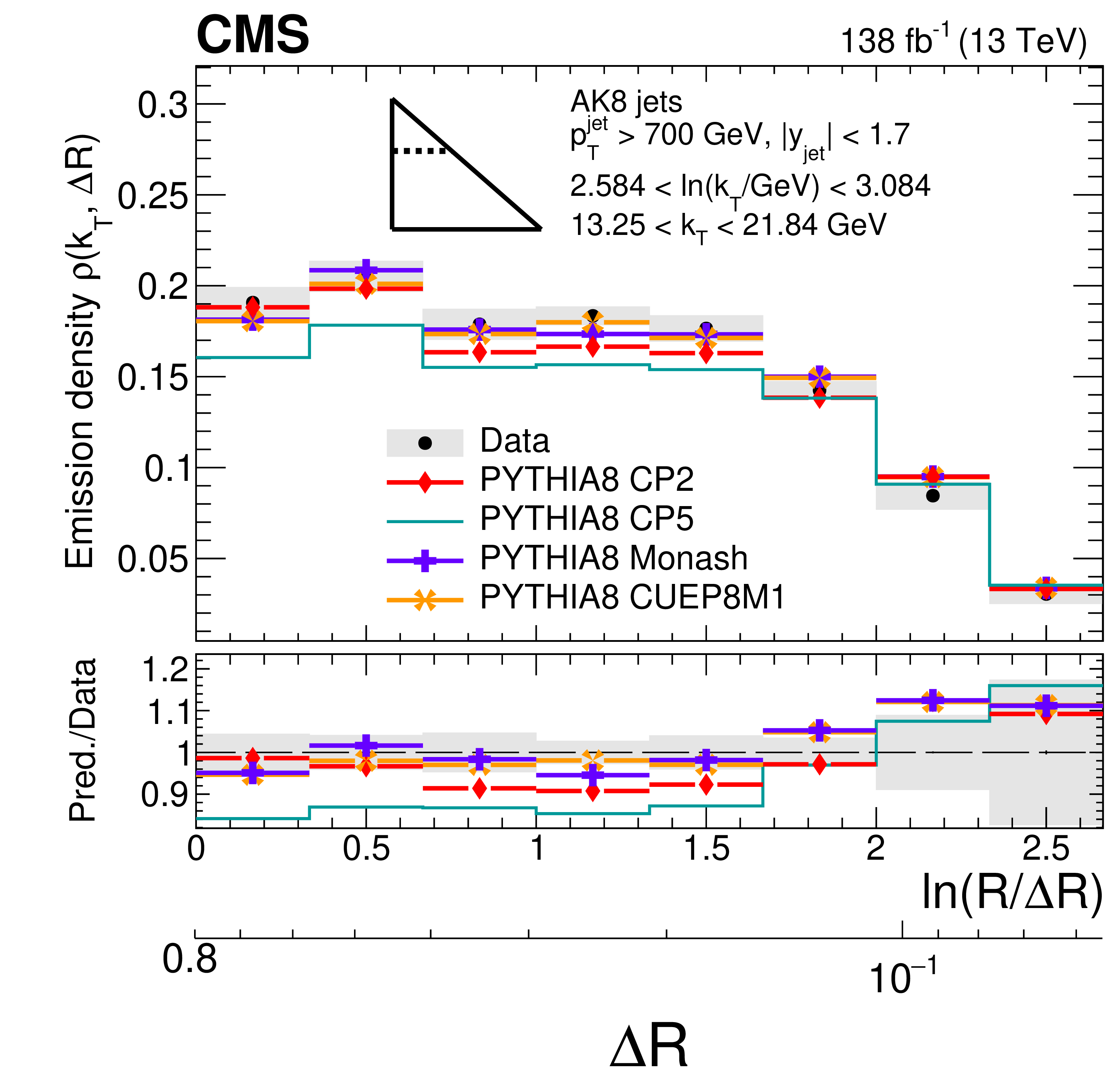
Figure 11:
Four different slices of the primary LJP density of AK8 jets compared with predictions generated with PYTHIA8 using tunes CP2, CP5, Monash, and CUEP8M1. The most important difference between the tunes is the value of $ \alpha_\mathrm{S}^\mathrm{FSR}(m_\mathrm{Z}) $, as described in the text. The band represents the total experimental uncertainty. The upper two plots correspond to vertical slices of the LJP for fixed $ \ln(R/\Delta R) $ (large angles on upper-left, small angles on upper-right). The lower two plots correspond to two different horizontal slices for fixed $ \ln(k_{\mathrm{T}}/$GeV$)$: the lower-left plot corresponds to low-$ k_{\mathrm{T}} $ splittings and spans the full range in $ \ln(R/\Delta R) $, whereas the lower-right plot corresponds to high-$ k_{\mathrm{T}} $ splittings, which populate mostly wide-angle radiation. Statistical uncertainties in data and MC-simulated events are represented by vertical bars, which are smaller than the markers in most of the bins. |

png pdf |
Figure 11-a:
Four different slices of the primary LJP density of AK8 jets compared with predictions generated with PYTHIA8 using tunes CP2, CP5, Monash, and CUEP8M1. The most important difference between the tunes is the value of $ \alpha_\mathrm{S}^\mathrm{FSR}(m_\mathrm{Z}) $, as described in the text. The band represents the total experimental uncertainty. The upper two plots correspond to vertical slices of the LJP for fixed $ \ln(R/\Delta R) $ (large angles on upper-left, small angles on upper-right). The lower two plots correspond to two different horizontal slices for fixed $ \ln(k_{\mathrm{T}}/$GeV$)$: the lower-left plot corresponds to low-$ k_{\mathrm{T}} $ splittings and spans the full range in $ \ln(R/\Delta R) $, whereas the lower-right plot corresponds to high-$ k_{\mathrm{T}} $ splittings, which populate mostly wide-angle radiation. Statistical uncertainties in data and MC-simulated events are represented by vertical bars, which are smaller than the markers in most of the bins. |
png pdf |
Figure 11-b:
Four different slices of the primary LJP density of AK8 jets compared with predictions generated with PYTHIA8 using tunes CP2, CP5, Monash, and CUEP8M1. The most important difference between the tunes is the value of $ \alpha_\mathrm{S}^\mathrm{FSR}(m_\mathrm{Z}) $, as described in the text. The band represents the total experimental uncertainty. The upper two plots correspond to vertical slices of the LJP for fixed $ \ln(R/\Delta R) $ (large angles on upper-left, small angles on upper-right). The lower two plots correspond to two different horizontal slices for fixed $ \ln(k_{\mathrm{T}}/$GeV$)$: the lower-left plot corresponds to low-$ k_{\mathrm{T}} $ splittings and spans the full range in $ \ln(R/\Delta R) $, whereas the lower-right plot corresponds to high-$ k_{\mathrm{T}} $ splittings, which populate mostly wide-angle radiation. Statistical uncertainties in data and MC-simulated events are represented by vertical bars, which are smaller than the markers in most of the bins. |
png pdf |
Figure 11-c:
Four different slices of the primary LJP density of AK8 jets compared with predictions generated with PYTHIA8 using tunes CP2, CP5, Monash, and CUEP8M1. The most important difference between the tunes is the value of $ \alpha_\mathrm{S}^\mathrm{FSR}(m_\mathrm{Z}) $, as described in the text. The band represents the total experimental uncertainty. The upper two plots correspond to vertical slices of the LJP for fixed $ \ln(R/\Delta R) $ (large angles on upper-left, small angles on upper-right). The lower two plots correspond to two different horizontal slices for fixed $ \ln(k_{\mathrm{T}}/$GeV$)$: the lower-left plot corresponds to low-$ k_{\mathrm{T}} $ splittings and spans the full range in $ \ln(R/\Delta R) $, whereas the lower-right plot corresponds to high-$ k_{\mathrm{T}} $ splittings, which populate mostly wide-angle radiation. Statistical uncertainties in data and MC-simulated events are represented by vertical bars, which are smaller than the markers in most of the bins. |
png pdf |
Figure 11-d:
Four different slices of the primary LJP density of AK8 jets compared with predictions generated with PYTHIA8 using tunes CP2, CP5, Monash, and CUEP8M1. The most important difference between the tunes is the value of $ \alpha_\mathrm{S}^\mathrm{FSR}(m_\mathrm{Z}) $, as described in the text. The band represents the total experimental uncertainty. The upper two plots correspond to vertical slices of the LJP for fixed $ \ln(R/\Delta R) $ (large angles on upper-left, small angles on upper-right). The lower two plots correspond to two different horizontal slices for fixed $ \ln(k_{\mathrm{T}}/$GeV$)$: the lower-left plot corresponds to low-$ k_{\mathrm{T}} $ splittings and spans the full range in $ \ln(R/\Delta R) $, whereas the lower-right plot corresponds to high-$ k_{\mathrm{T}} $ splittings, which populate mostly wide-angle radiation. Statistical uncertainties in data and MC-simulated events are represented by vertical bars, which are smaller than the markers in most of the bins. |
png pdf |
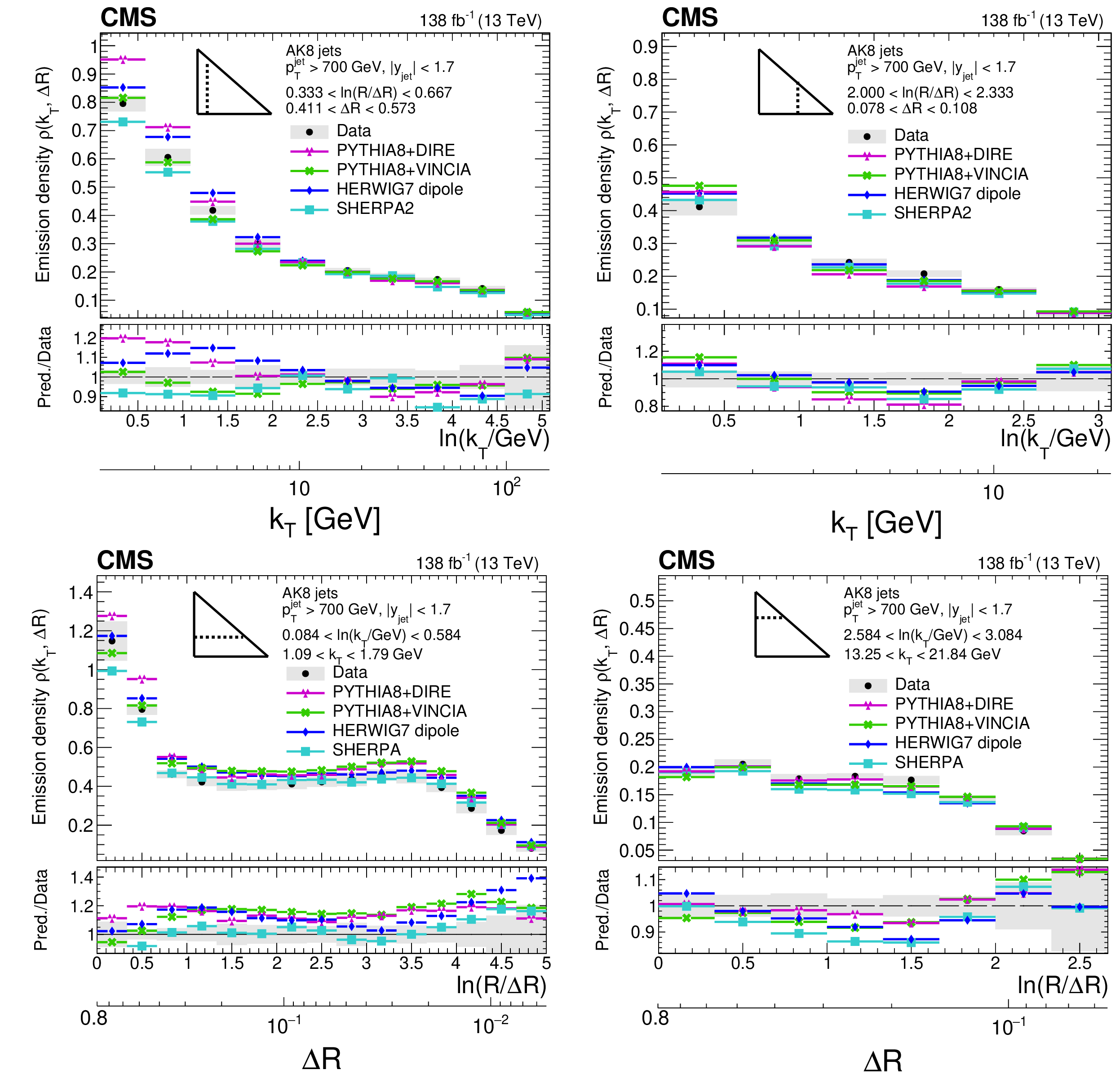
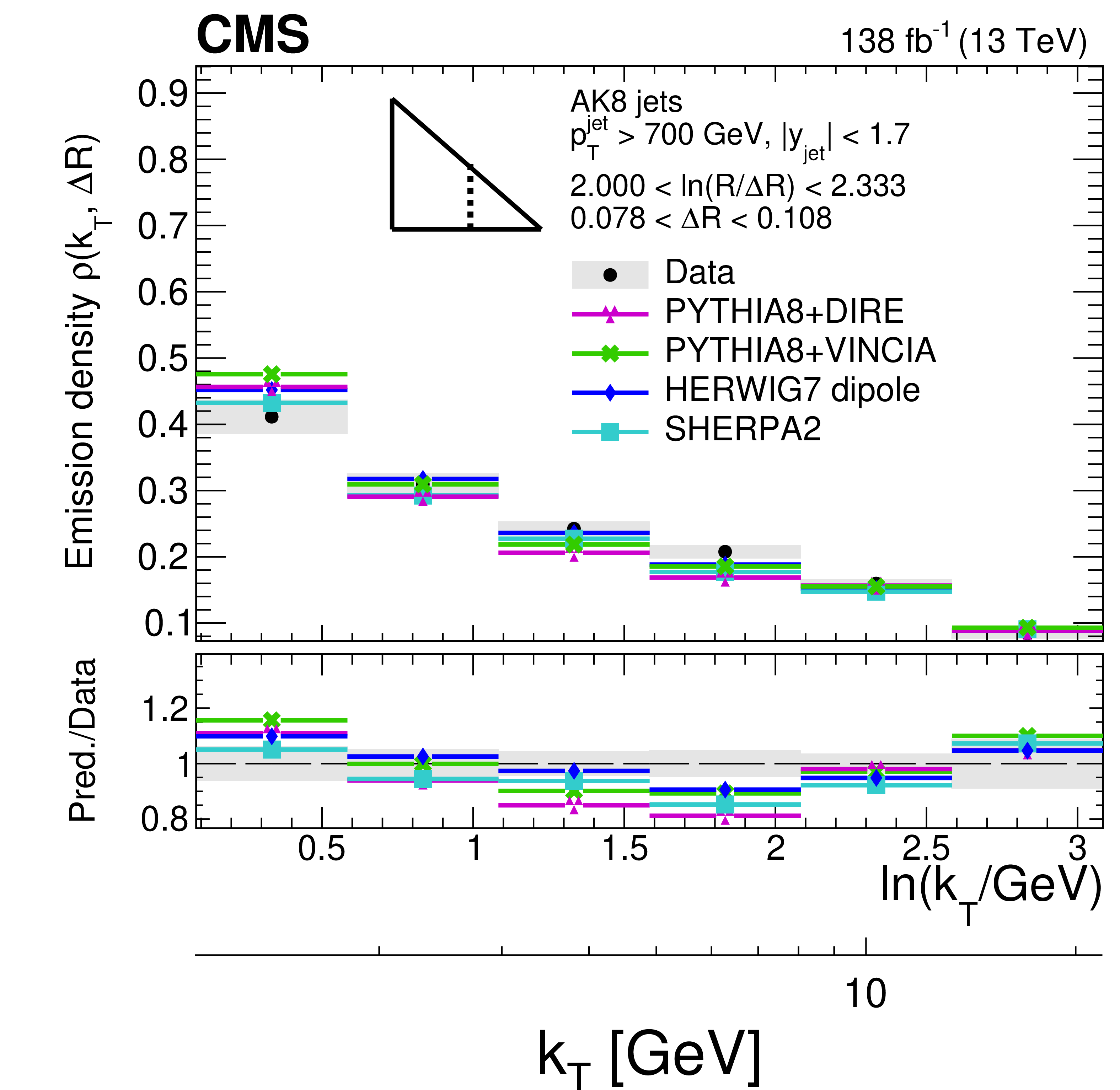
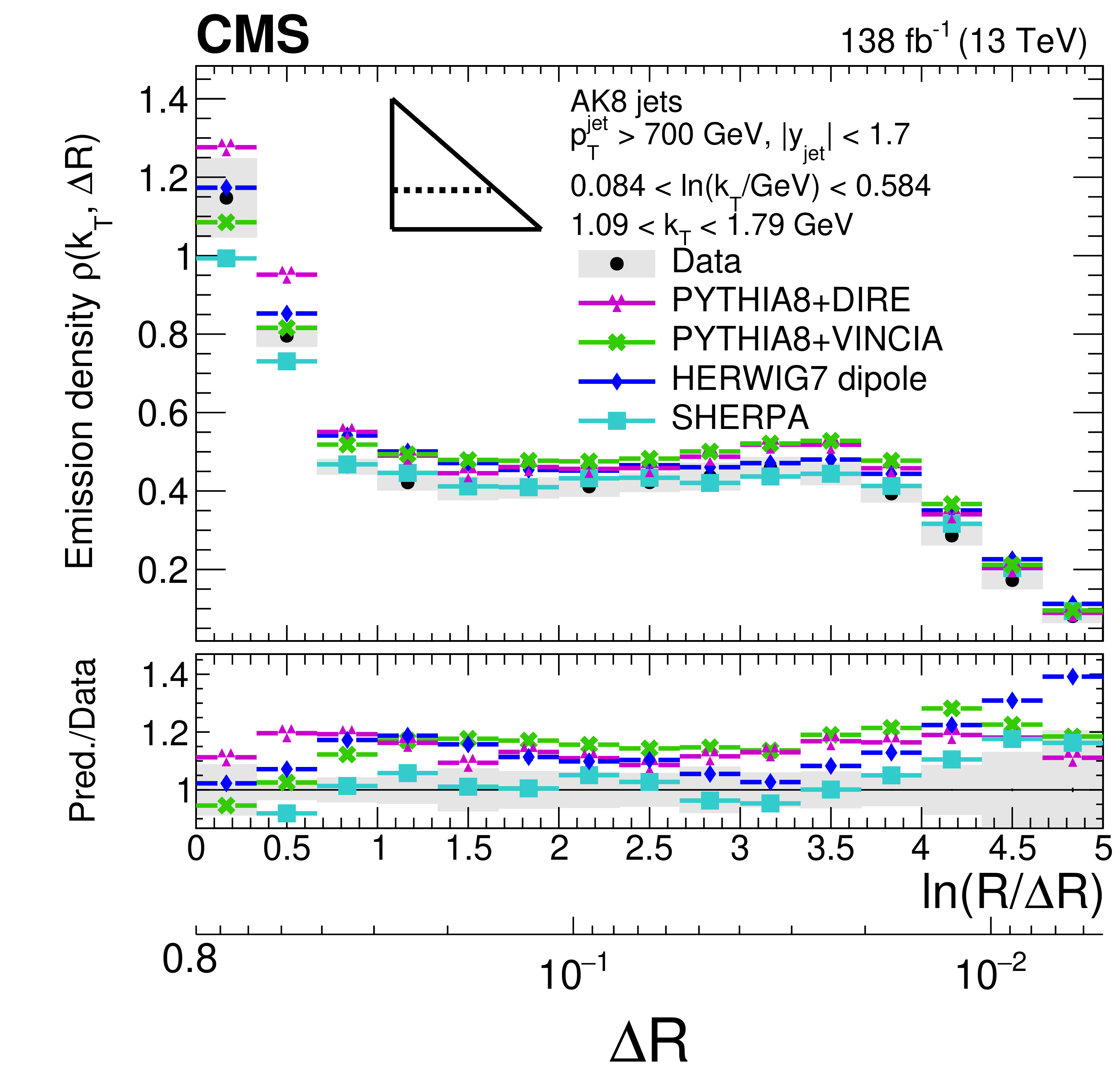
Figure 12:
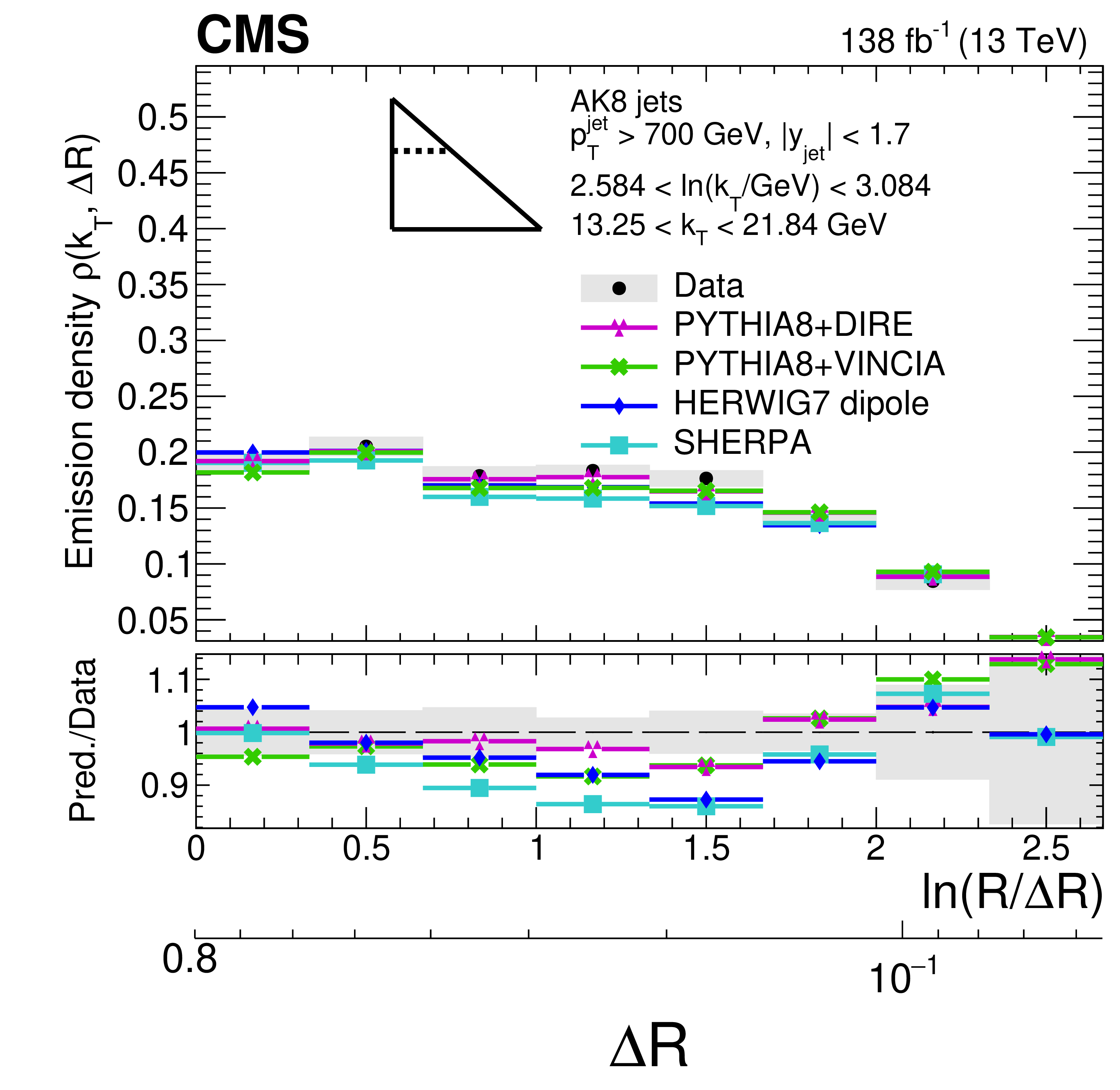
Four different slices of the primary LJP density of AK8 jets compared with predictions by PYTHIA8+ VINCIA, PYTHIA8+ DIRE, HERWIG 7 with dipole shower, and SHERPA 2. The band represents the total experimental uncertainty. The upper two plots correspond to vertical slices of the LJP for fixed $ \ln(R/\Delta R) $ (large angles on upper-left, small angles on upper-right). The lower two plots correspond to two different horizontal slices for fixed $ \ln(k_{\mathrm{T}}/$GeV$)$: the lower-left plot corresponds to low-$ k_{\mathrm{T}} $ splittings and spans the full range in $ \ln(R/\Delta R) $, whereas the lower-right plot corresponds to high-$ k_{\mathrm{T}} $ splittings, which populate mostly wide-angle radiation. Statistical uncertainties in data and MC-simulated events are represented by vertical bars, which are smaller than the markers in most of the bins. |

png pdf |
Figure 12-a:
Four different slices of the primary LJP density of AK8 jets compared with predictions by PYTHIA8+ VINCIA, PYTHIA8+ DIRE, HERWIG 7 with dipole shower, and SHERPA 2. The band represents the total experimental uncertainty. The upper two plots correspond to vertical slices of the LJP for fixed $ \ln(R/\Delta R) $ (large angles on upper-left, small angles on upper-right). The lower two plots correspond to two different horizontal slices for fixed $ \ln(k_{\mathrm{T}}/$GeV$)$: the lower-left plot corresponds to low-$ k_{\mathrm{T}} $ splittings and spans the full range in $ \ln(R/\Delta R) $, whereas the lower-right plot corresponds to high-$ k_{\mathrm{T}} $ splittings, which populate mostly wide-angle radiation. Statistical uncertainties in data and MC-simulated events are represented by vertical bars, which are smaller than the markers in most of the bins. |
png pdf |
Figure 12-b:
Four different slices of the primary LJP density of AK8 jets compared with predictions by PYTHIA8+ VINCIA, PYTHIA8+ DIRE, HERWIG 7 with dipole shower, and SHERPA 2. The band represents the total experimental uncertainty. The upper two plots correspond to vertical slices of the LJP for fixed $ \ln(R/\Delta R) $ (large angles on upper-left, small angles on upper-right). The lower two plots correspond to two different horizontal slices for fixed $ \ln(k_{\mathrm{T}}/$GeV$)$: the lower-left plot corresponds to low-$ k_{\mathrm{T}} $ splittings and spans the full range in $ \ln(R/\Delta R) $, whereas the lower-right plot corresponds to high-$ k_{\mathrm{T}} $ splittings, which populate mostly wide-angle radiation. Statistical uncertainties in data and MC-simulated events are represented by vertical bars, which are smaller than the markers in most of the bins. |
png pdf |
Figure 12-c:
Four different slices of the primary LJP density of AK8 jets compared with predictions by PYTHIA8+ VINCIA, PYTHIA8+ DIRE, HERWIG 7 with dipole shower, and SHERPA 2. The band represents the total experimental uncertainty. The upper two plots correspond to vertical slices of the LJP for fixed $ \ln(R/\Delta R) $ (large angles on upper-left, small angles on upper-right). The lower two plots correspond to two different horizontal slices for fixed $ \ln(k_{\mathrm{T}}/$GeV$)$: the lower-left plot corresponds to low-$ k_{\mathrm{T}} $ splittings and spans the full range in $ \ln(R/\Delta R) $, whereas the lower-right plot corresponds to high-$ k_{\mathrm{T}} $ splittings, which populate mostly wide-angle radiation. Statistical uncertainties in data and MC-simulated events are represented by vertical bars, which are smaller than the markers in most of the bins. |
png pdf |
Figure 12-d:
Four different slices of the primary LJP density of AK8 jets compared with predictions by PYTHIA8+ VINCIA, PYTHIA8+ DIRE, HERWIG 7 with dipole shower, and SHERPA 2. The band represents the total experimental uncertainty. The upper two plots correspond to vertical slices of the LJP for fixed $ \ln(R/\Delta R) $ (large angles on upper-left, small angles on upper-right). The lower two plots correspond to two different horizontal slices for fixed $ \ln(k_{\mathrm{T}}/$GeV$)$: the lower-left plot corresponds to low-$ k_{\mathrm{T}} $ splittings and spans the full range in $ \ln(R/\Delta R) $, whereas the lower-right plot corresponds to high-$ k_{\mathrm{T}} $ splittings, which populate mostly wide-angle radiation. Statistical uncertainties in data and MC-simulated events are represented by vertical bars, which are smaller than the markers in most of the bins. |
png pdf |
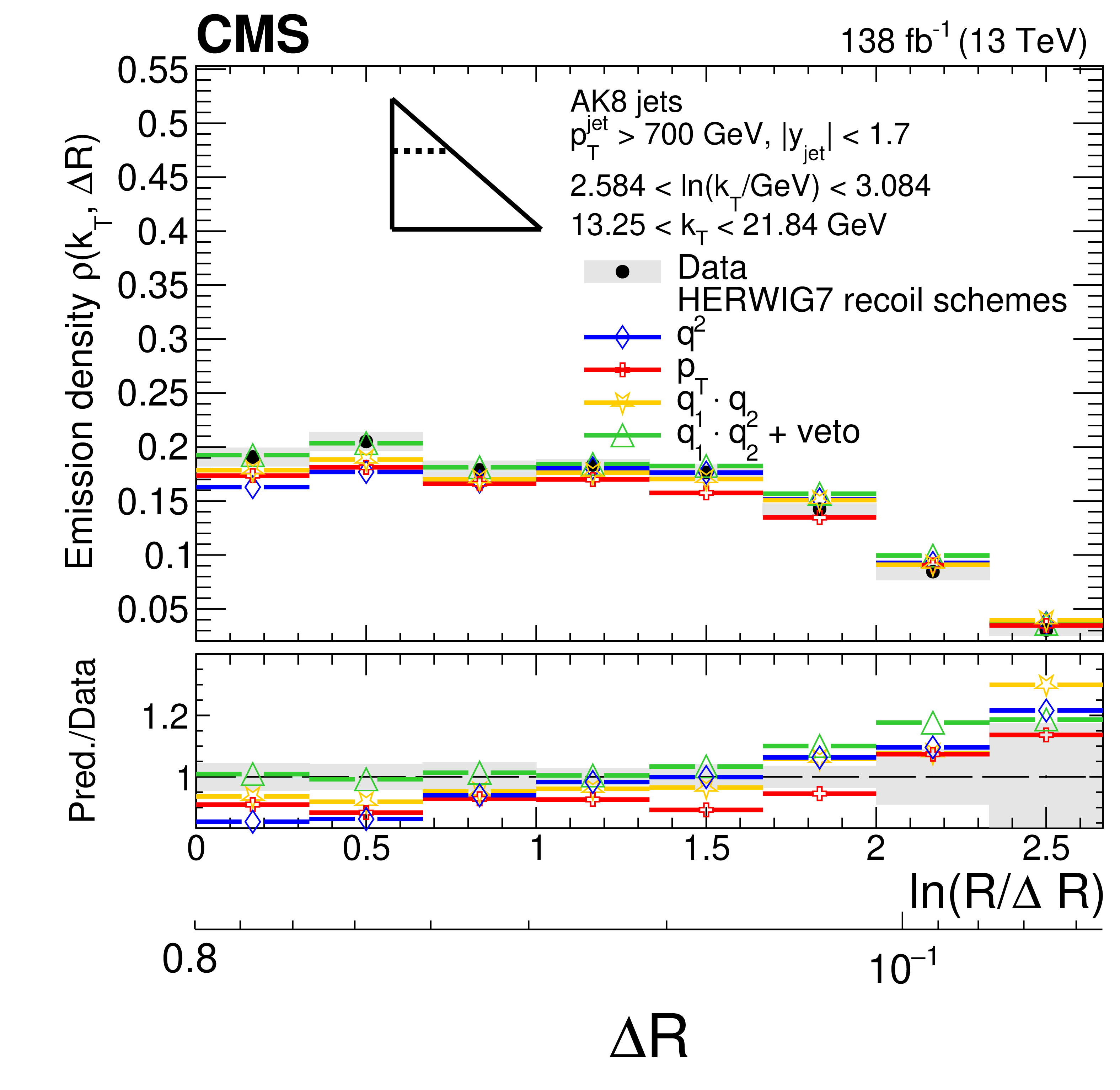
Figure 13:
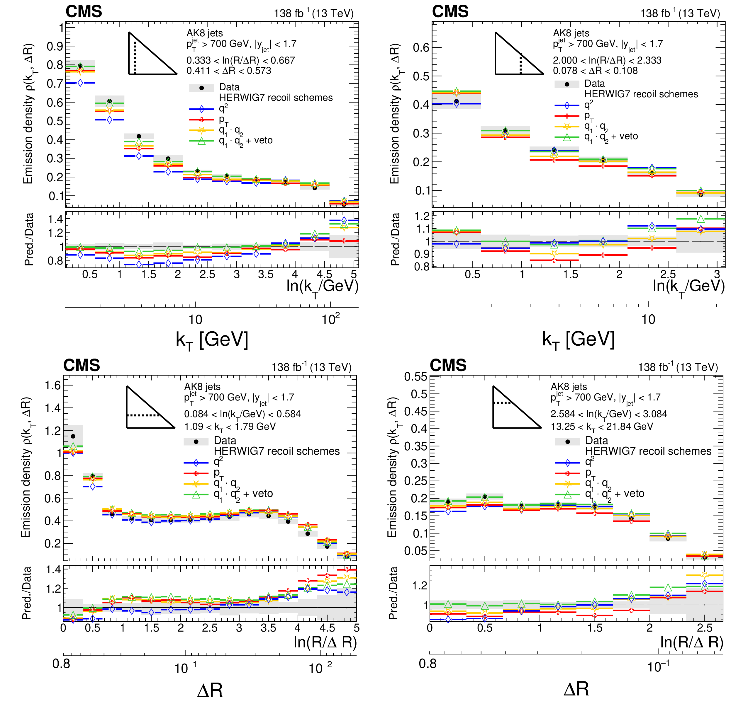
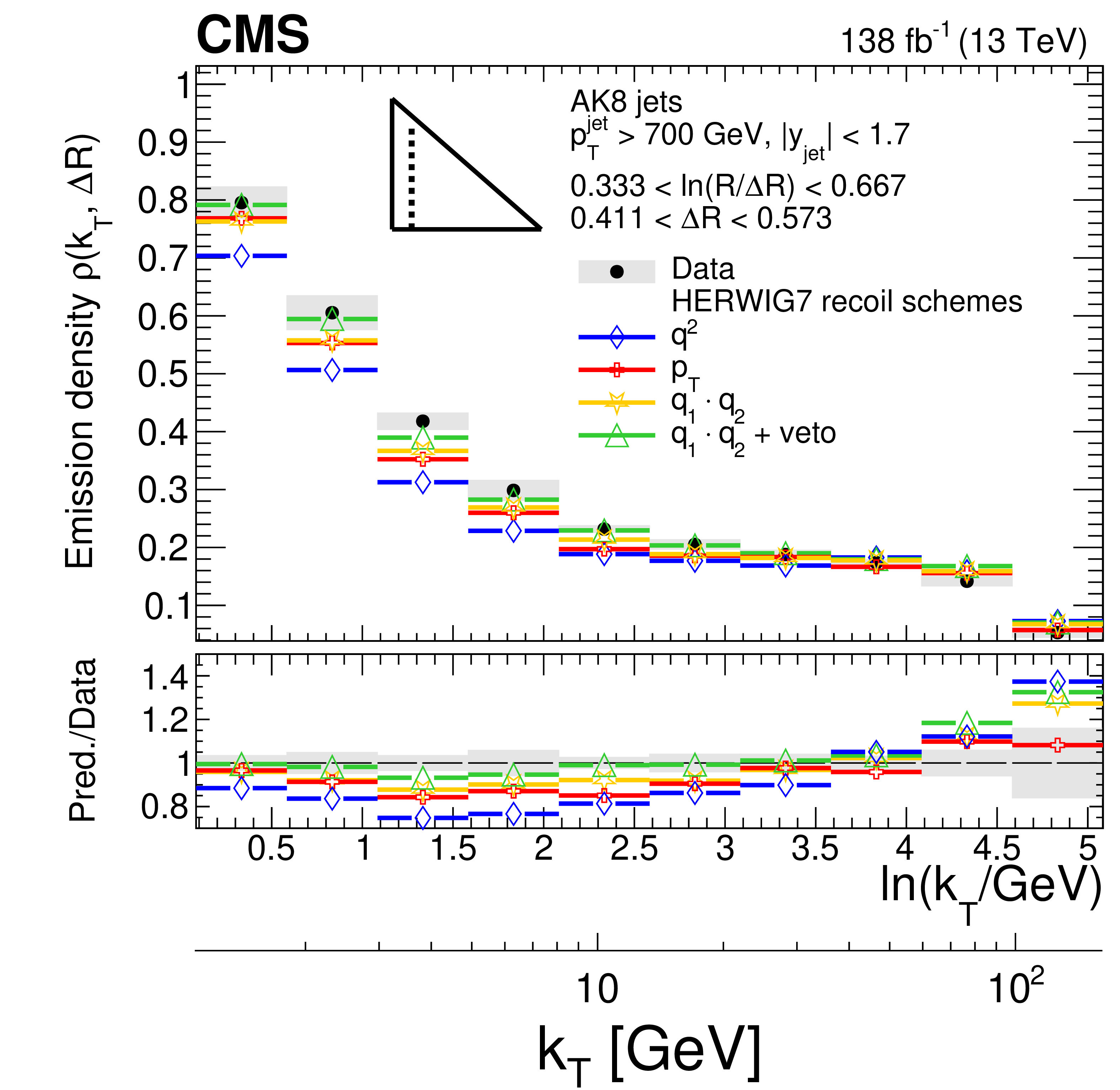
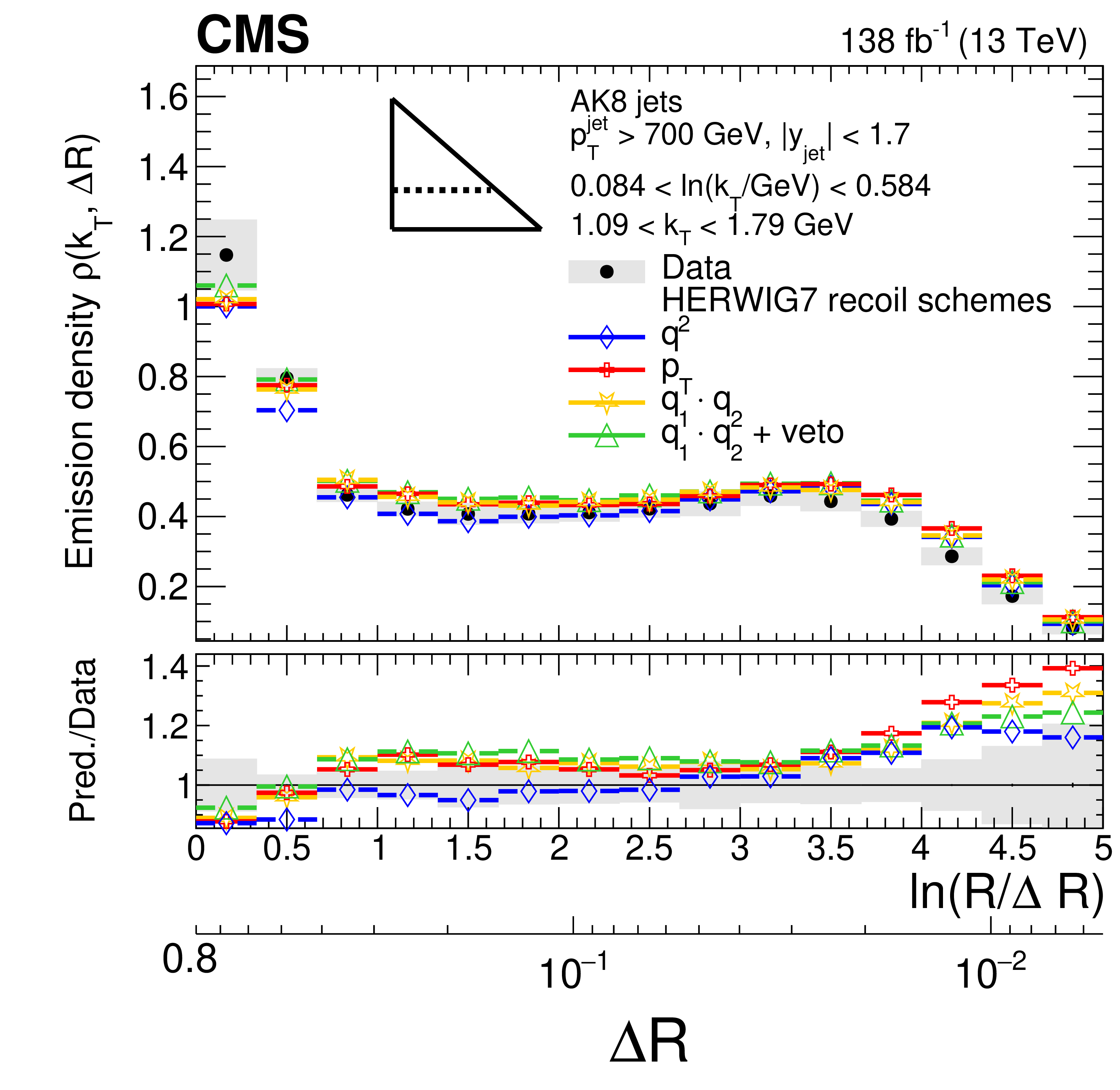
Four different slices of the primary LJP density of AK8 jets compared with predictions based on different choices of the recoil scheme of the angular-ordered shower of HERWIG 7. Each recoil scheme achieves a different degree of logarithmic accuracy, up to NLL for certain observables, as described in the text. The band represents the total experimental uncertainty. The upper two plots correspond to vertical slices of the LJP for fixed $ \ln(R/\Delta R) $ (large angles on upper-left, small angles on upper-right). The lower two plots correspond to two different horizontal slices for fixed $ k_{\mathrm{T}} $ interval: the lower-left plot corresponds to low-$ k_{\mathrm{T}} $ splittings and spans the full range in $ \ln(R/\Delta R) $, whereas the lower-right plot corresponds to high-$ k_{\mathrm{T}} $ splittings, which populate mostly wide-angle radiation. Statistical uncertainties in data and MC-simulated events are represented by vertical bars, which are smaller than the markers in most of the bins. |
png pdf |
Figure 13-a:
Four different slices of the primary LJP density of AK8 jets compared with predictions based on different choices of the recoil scheme of the angular-ordered shower of HERWIG 7. Each recoil scheme achieves a different degree of logarithmic accuracy, up to NLL for certain observables, as described in the text. The band represents the total experimental uncertainty. The upper two plots correspond to vertical slices of the LJP for fixed $ \ln(R/\Delta R) $ (large angles on upper-left, small angles on upper-right). The lower two plots correspond to two different horizontal slices for fixed $ k_{\mathrm{T}} $ interval: the lower-left plot corresponds to low-$ k_{\mathrm{T}} $ splittings and spans the full range in $ \ln(R/\Delta R) $, whereas the lower-right plot corresponds to high-$ k_{\mathrm{T}} $ splittings, which populate mostly wide-angle radiation. Statistical uncertainties in data and MC-simulated events are represented by vertical bars, which are smaller than the markers in most of the bins. |

png pdf |
Figure 13-b:
Four different slices of the primary LJP density of AK8 jets compared with predictions based on different choices of the recoil scheme of the angular-ordered shower of HERWIG 7. Each recoil scheme achieves a different degree of logarithmic accuracy, up to NLL for certain observables, as described in the text. The band represents the total experimental uncertainty. The upper two plots correspond to vertical slices of the LJP for fixed $ \ln(R/\Delta R) $ (large angles on upper-left, small angles on upper-right). The lower two plots correspond to two different horizontal slices for fixed $ k_{\mathrm{T}} $ interval: the lower-left plot corresponds to low-$ k_{\mathrm{T}} $ splittings and spans the full range in $ \ln(R/\Delta R) $, whereas the lower-right plot corresponds to high-$ k_{\mathrm{T}} $ splittings, which populate mostly wide-angle radiation. Statistical uncertainties in data and MC-simulated events are represented by vertical bars, which are smaller than the markers in most of the bins. |
png pdf |
Figure 13-c:
Four different slices of the primary LJP density of AK8 jets compared with predictions based on different choices of the recoil scheme of the angular-ordered shower of HERWIG 7. Each recoil scheme achieves a different degree of logarithmic accuracy, up to NLL for certain observables, as described in the text. The band represents the total experimental uncertainty. The upper two plots correspond to vertical slices of the LJP for fixed $ \ln(R/\Delta R) $ (large angles on upper-left, small angles on upper-right). The lower two plots correspond to two different horizontal slices for fixed $ k_{\mathrm{T}} $ interval: the lower-left plot corresponds to low-$ k_{\mathrm{T}} $ splittings and spans the full range in $ \ln(R/\Delta R) $, whereas the lower-right plot corresponds to high-$ k_{\mathrm{T}} $ splittings, which populate mostly wide-angle radiation. Statistical uncertainties in data and MC-simulated events are represented by vertical bars, which are smaller than the markers in most of the bins. |
png pdf |
Figure 13-d:
Four different slices of the primary LJP density of AK8 jets compared with predictions based on different choices of the recoil scheme of the angular-ordered shower of HERWIG 7. Each recoil scheme achieves a different degree of logarithmic accuracy, up to NLL for certain observables, as described in the text. The band represents the total experimental uncertainty. The upper two plots correspond to vertical slices of the LJP for fixed $ \ln(R/\Delta R) $ (large angles on upper-left, small angles on upper-right). The lower two plots correspond to two different horizontal slices for fixed $ k_{\mathrm{T}} $ interval: the lower-left plot corresponds to low-$ k_{\mathrm{T}} $ splittings and spans the full range in $ \ln(R/\Delta R) $, whereas the lower-right plot corresponds to high-$ k_{\mathrm{T}} $ splittings, which populate mostly wide-angle radiation. Statistical uncertainties in data and MC-simulated events are represented by vertical bars, which are smaller than the markers in most of the bins. |
png pdf |
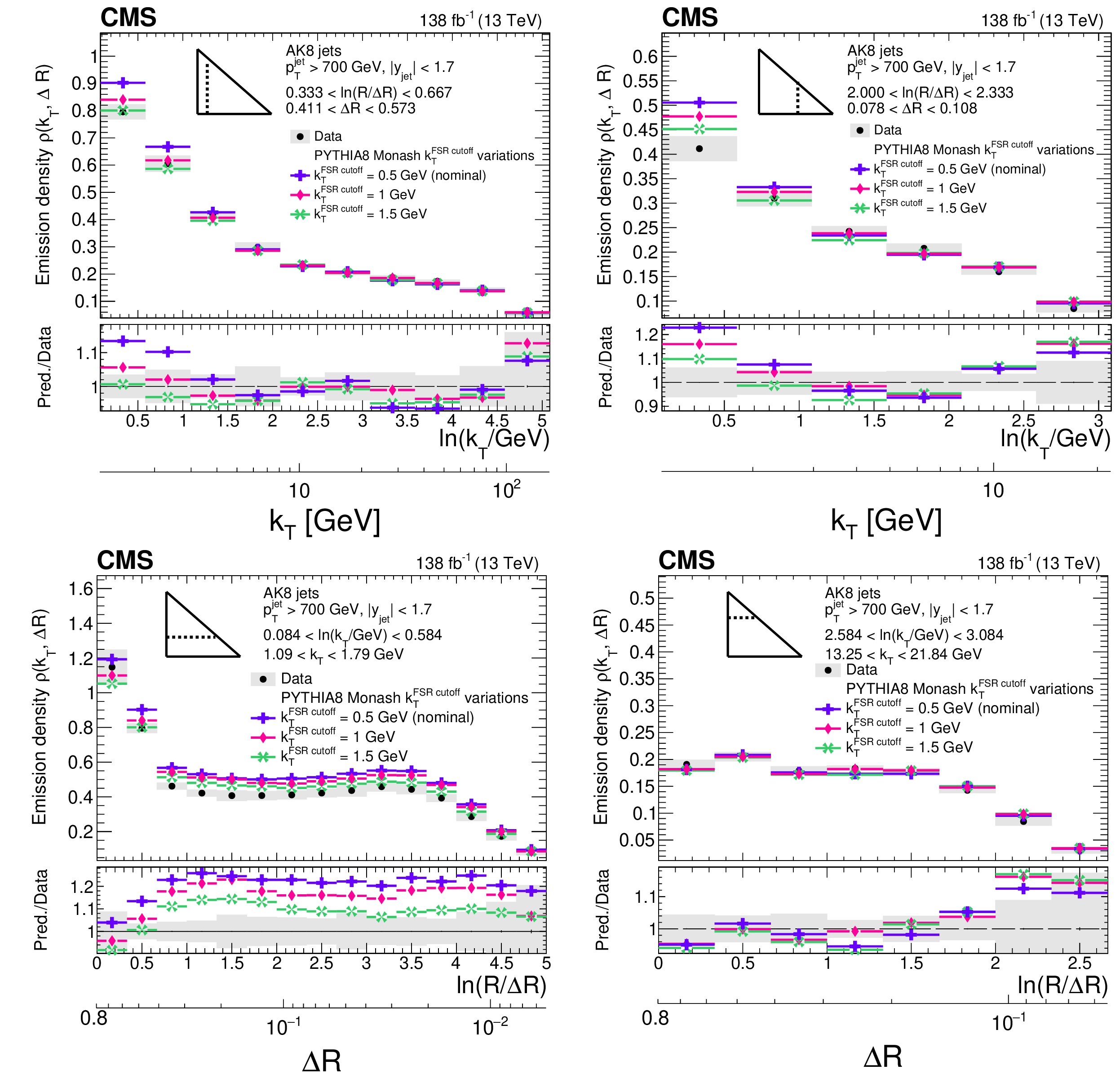
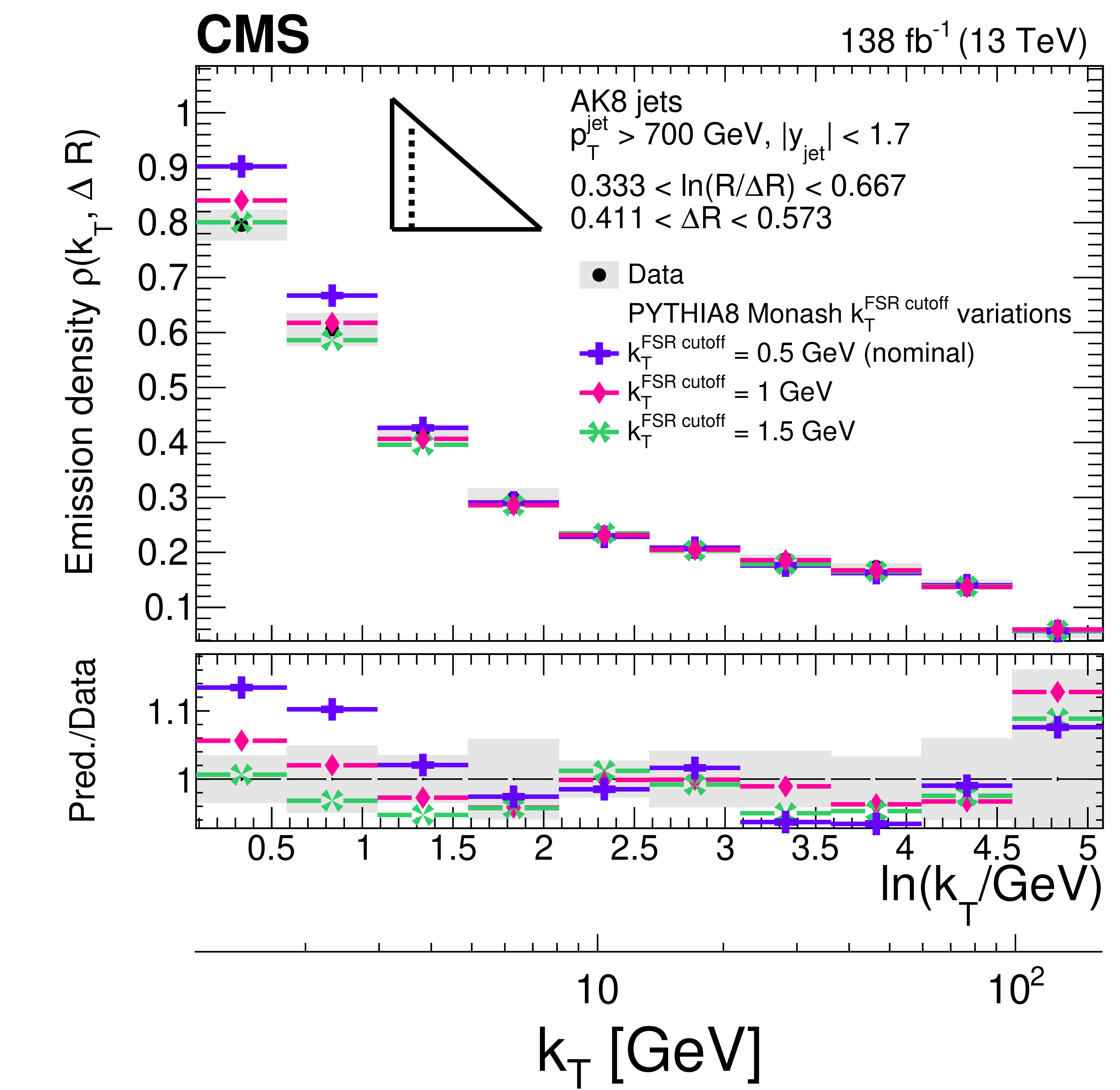
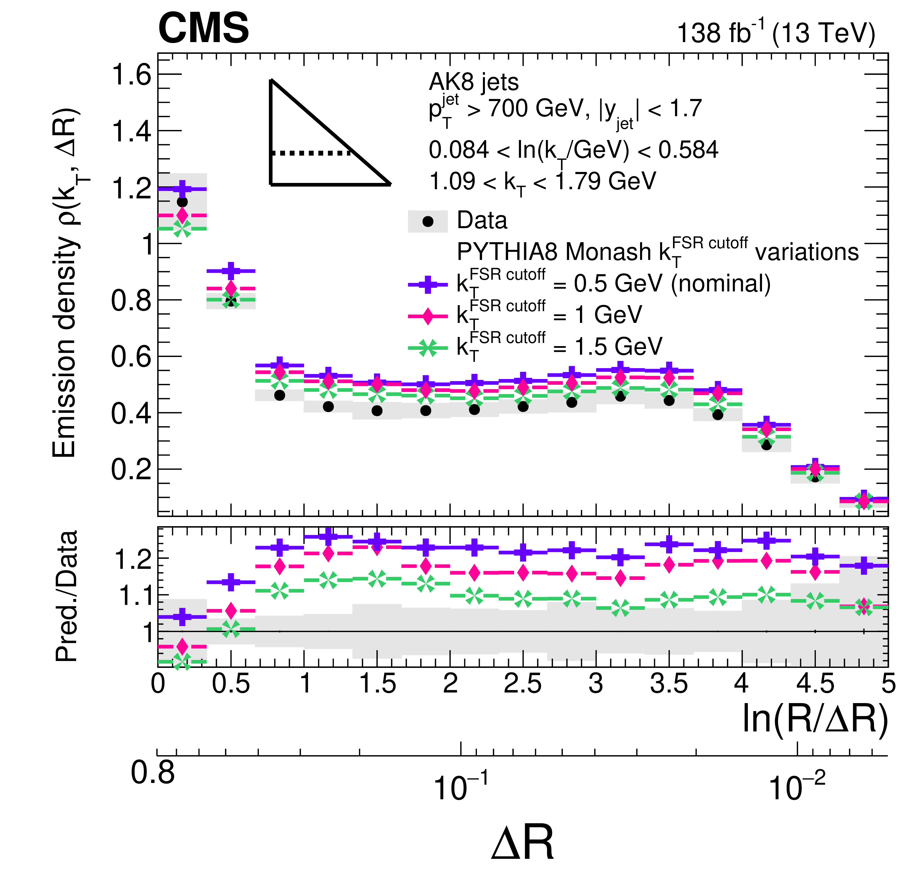
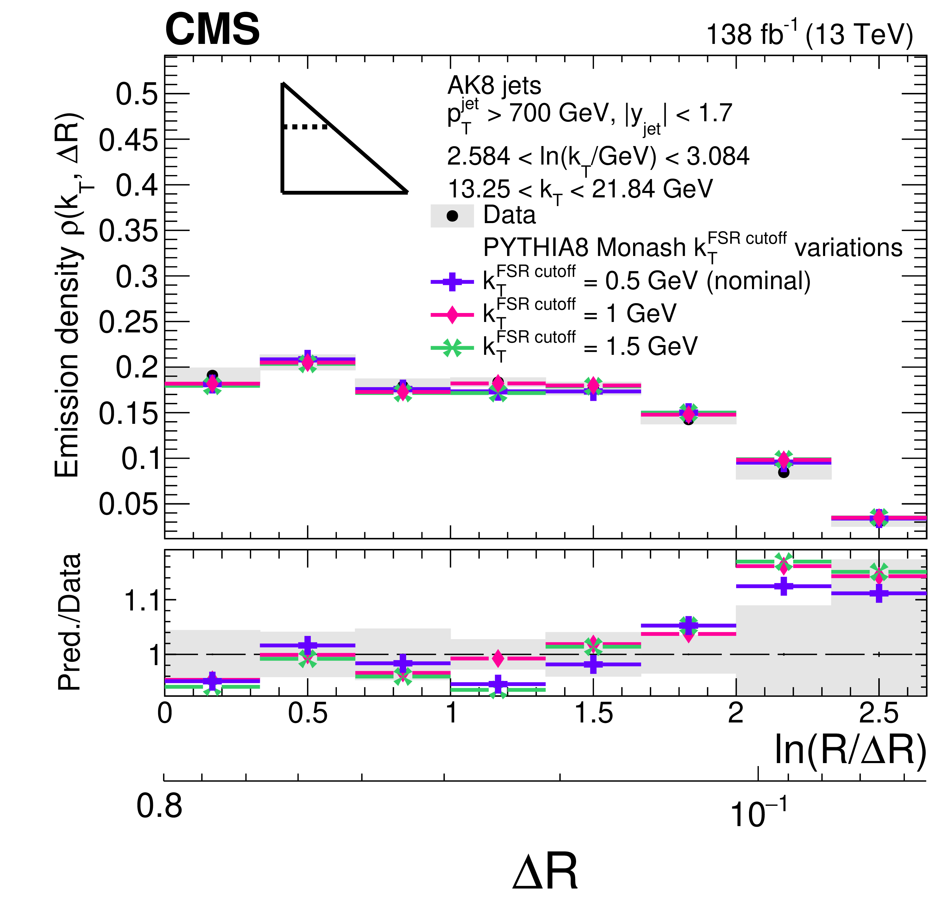
Figure 14:
Four different slices of the primary LJP density of AK8 jets compared with predictions based on different values of the transverse momentum cutoff used for FSR ($ k_{\mathrm{T}}^\text{FSR\,cutoff} $) in PYTHIA8 with the Monash tune. The larger $ k_{\mathrm{T}}^\text{FSR\,cutoff} $ value yields a better agreement with the data at low $ k_{\mathrm{T}} $. The lower two plots correspond to two different horizontal slices for fixed $ k_{\mathrm{T}} $ interval: the lower-left plot corresponds to low-$ k_{\mathrm{T}} $ splittings and spans the full range in $ \ln(R/\Delta R) $, whereas the lower-right plot corresponds to high-$ k_{\mathrm{T}} $ splittings, which populate mostly wide-angle radiation. Statistical uncertainties in data and MC-simulated events are represented by vertical bars, which are smaller than the markers in most of the bins. |
png pdf |
Figure 14-a:
Four different slices of the primary LJP density of AK8 jets compared with predictions based on different values of the transverse momentum cutoff used for FSR ($ k_{\mathrm{T}}^\text{FSR\,cutoff} $) in PYTHIA8 with the Monash tune. The larger $ k_{\mathrm{T}}^\text{FSR\,cutoff} $ value yields a better agreement with the data at low $ k_{\mathrm{T}} $. The lower two plots correspond to two different horizontal slices for fixed $ k_{\mathrm{T}} $ interval: the lower-left plot corresponds to low-$ k_{\mathrm{T}} $ splittings and spans the full range in $ \ln(R/\Delta R) $, whereas the lower-right plot corresponds to high-$ k_{\mathrm{T}} $ splittings, which populate mostly wide-angle radiation. Statistical uncertainties in data and MC-simulated events are represented by vertical bars, which are smaller than the markers in most of the bins. |

png pdf |
Figure 14-b:
Four different slices of the primary LJP density of AK8 jets compared with predictions based on different values of the transverse momentum cutoff used for FSR ($ k_{\mathrm{T}}^\text{FSR\,cutoff} $) in PYTHIA8 with the Monash tune. The larger $ k_{\mathrm{T}}^\text{FSR\,cutoff} $ value yields a better agreement with the data at low $ k_{\mathrm{T}} $. The lower two plots correspond to two different horizontal slices for fixed $ k_{\mathrm{T}} $ interval: the lower-left plot corresponds to low-$ k_{\mathrm{T}} $ splittings and spans the full range in $ \ln(R/\Delta R) $, whereas the lower-right plot corresponds to high-$ k_{\mathrm{T}} $ splittings, which populate mostly wide-angle radiation. Statistical uncertainties in data and MC-simulated events are represented by vertical bars, which are smaller than the markers in most of the bins. |
png pdf |
Figure 14-c:
Four different slices of the primary LJP density of AK8 jets compared with predictions based on different values of the transverse momentum cutoff used for FSR ($ k_{\mathrm{T}}^\text{FSR\,cutoff} $) in PYTHIA8 with the Monash tune. The larger $ k_{\mathrm{T}}^\text{FSR\,cutoff} $ value yields a better agreement with the data at low $ k_{\mathrm{T}} $. The lower two plots correspond to two different horizontal slices for fixed $ k_{\mathrm{T}} $ interval: the lower-left plot corresponds to low-$ k_{\mathrm{T}} $ splittings and spans the full range in $ \ln(R/\Delta R) $, whereas the lower-right plot corresponds to high-$ k_{\mathrm{T}} $ splittings, which populate mostly wide-angle radiation. Statistical uncertainties in data and MC-simulated events are represented by vertical bars, which are smaller than the markers in most of the bins. |
png pdf |
Figure 14-d:
Four different slices of the primary LJP density of AK8 jets compared with predictions based on different values of the transverse momentum cutoff used for FSR ($ k_{\mathrm{T}}^\text{FSR\,cutoff} $) in PYTHIA8 with the Monash tune. The larger $ k_{\mathrm{T}}^\text{FSR\,cutoff} $ value yields a better agreement with the data at low $ k_{\mathrm{T}} $. The lower two plots correspond to two different horizontal slices for fixed $ k_{\mathrm{T}} $ interval: the lower-left plot corresponds to low-$ k_{\mathrm{T}} $ splittings and spans the full range in $ \ln(R/\Delta R) $, whereas the lower-right plot corresponds to high-$ k_{\mathrm{T}} $ splittings, which populate mostly wide-angle radiation. Statistical uncertainties in data and MC-simulated events are represented by vertical bars, which are smaller than the markers in most of the bins. |

png pdf |
Figure 15:
Measured LJP distribution for AK8 jets, compared with the leading-order perturbative-QCD asymptotic prediction in the soft and collinear limit. The grey boxes represent the total experimental uncertainty from the measured data. For the prediction, an effective color factor of $ C_{\mathrm{R}}^{\text{eff}} = 0.59 C_{\mathrm{F}}+0.41 C_{\mathrm{A}} \approx $ 2 is assumed, as described in the text. The strong coupling $ \alpha_\mathrm{S} $ evolves with $ k_{\mathrm{T}} $ using the one-loop $ \beta $ function with $ \alpha_\mathrm{S} (m_\mathrm{Z}) = $ 0.118. The theoretical uncertainty band is calculated with variations of the renormalization scale up and down by factors of 2. The discontinuity is due to the change of the number of active flavors when $ k_{\mathrm{T}} $ reaches the mass of the bottom quark, which is assumed to be 4.2 GeV. |
png pdf |
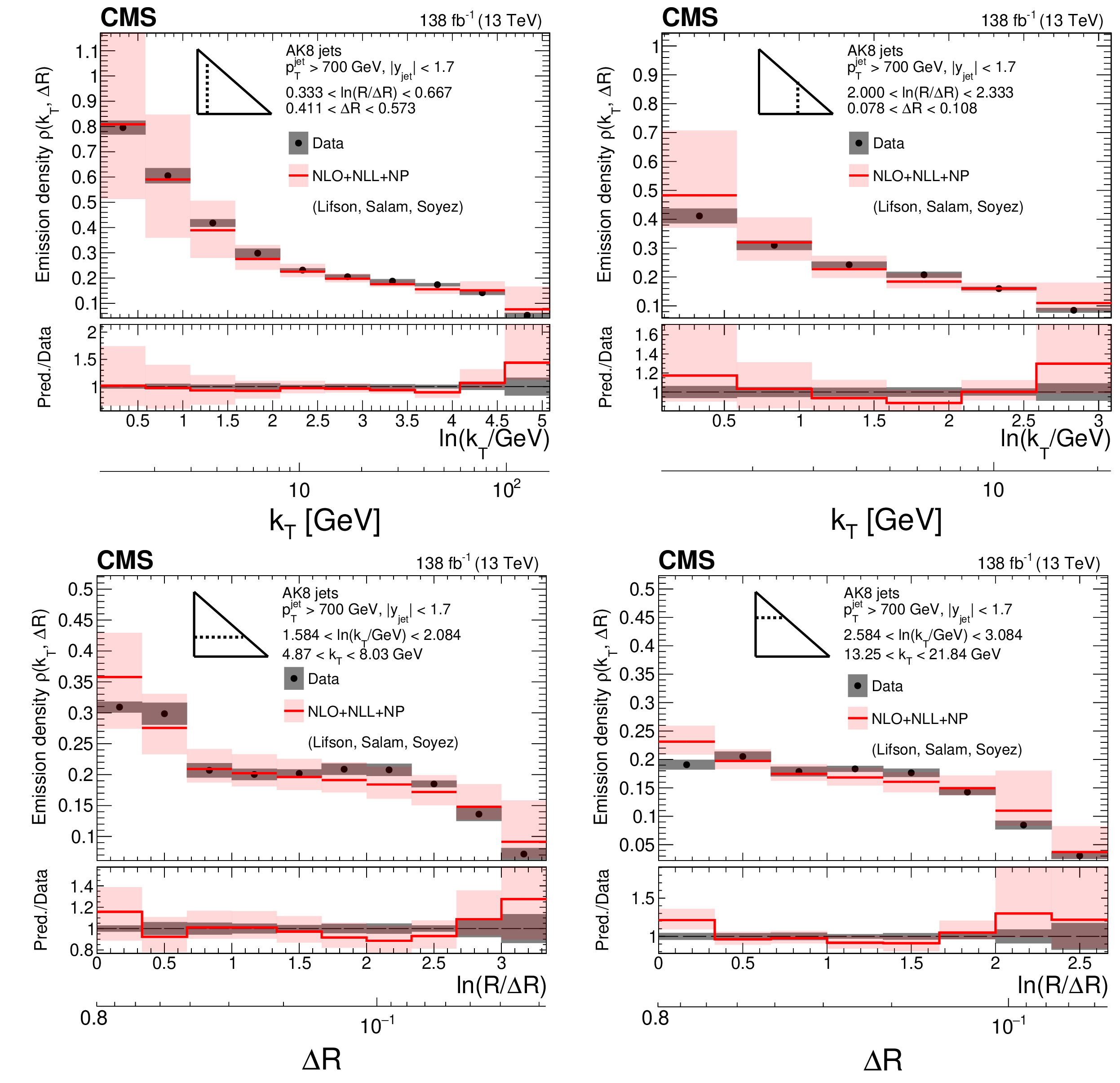
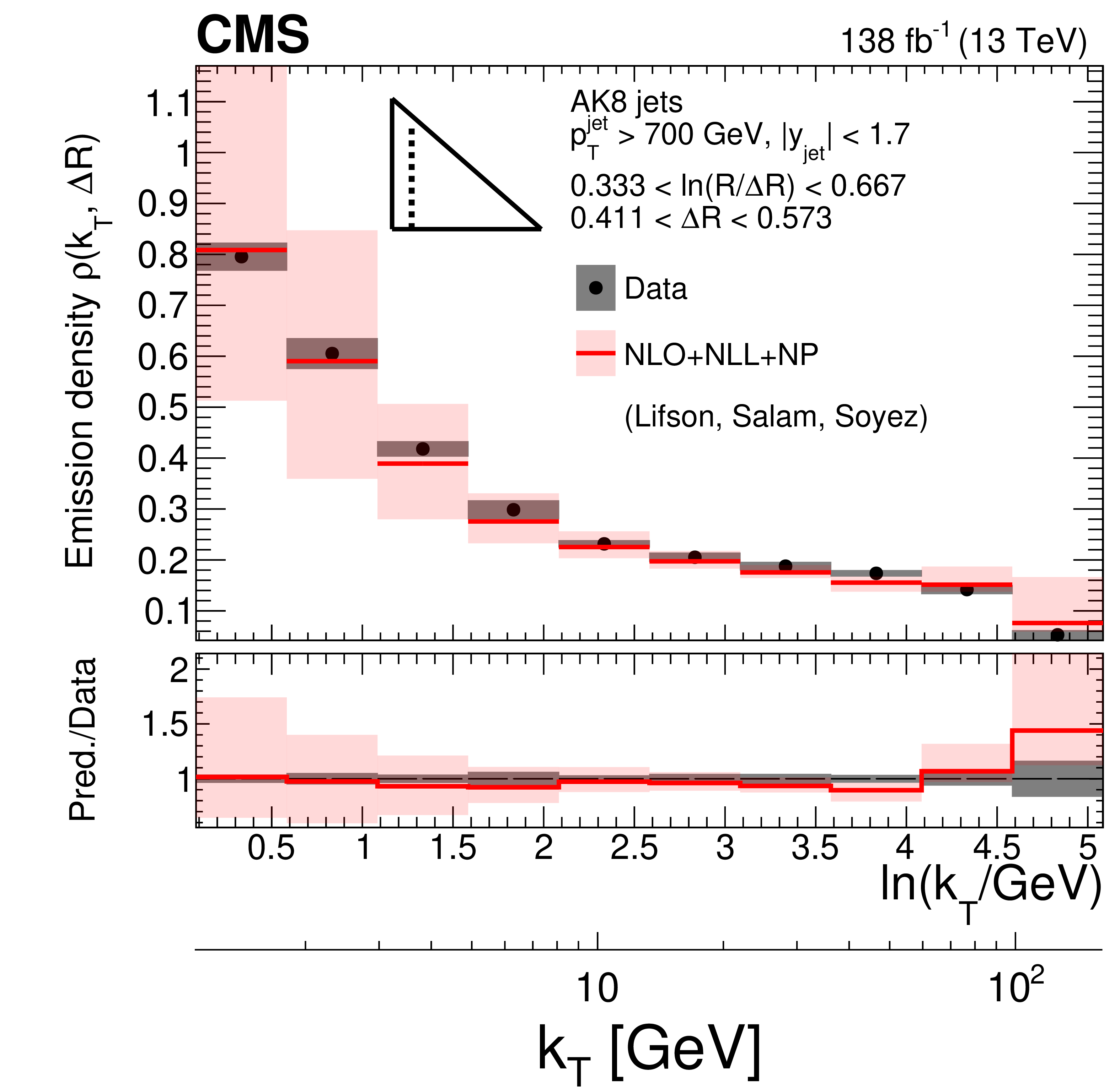
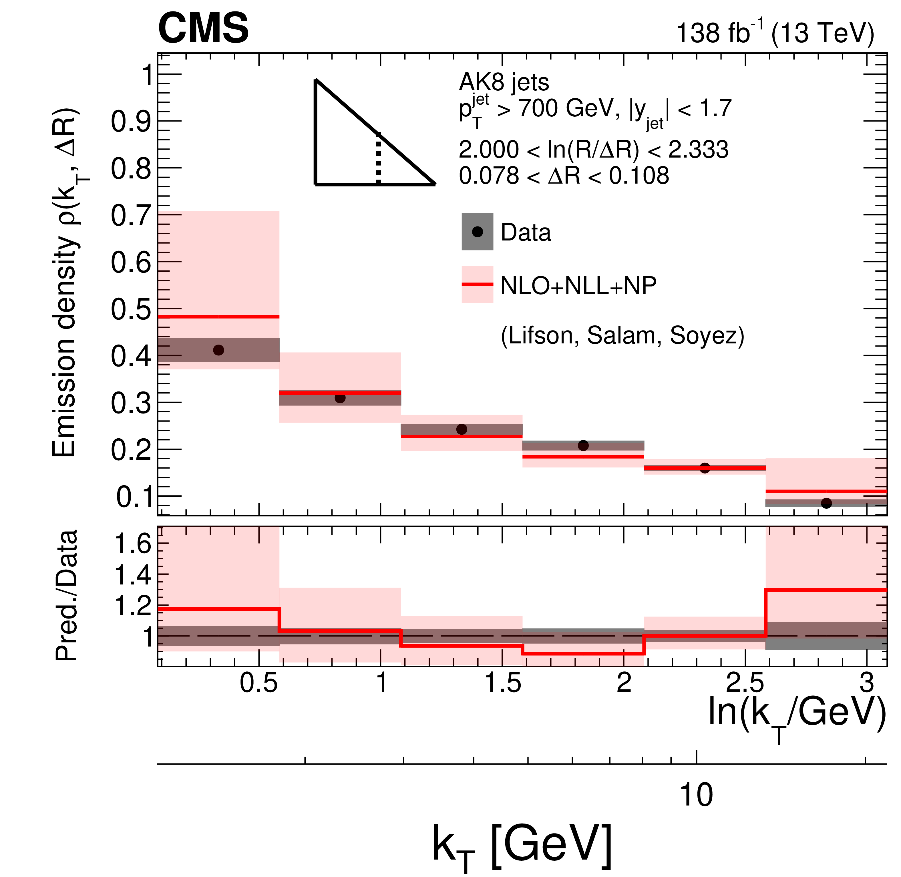
Figure 16:
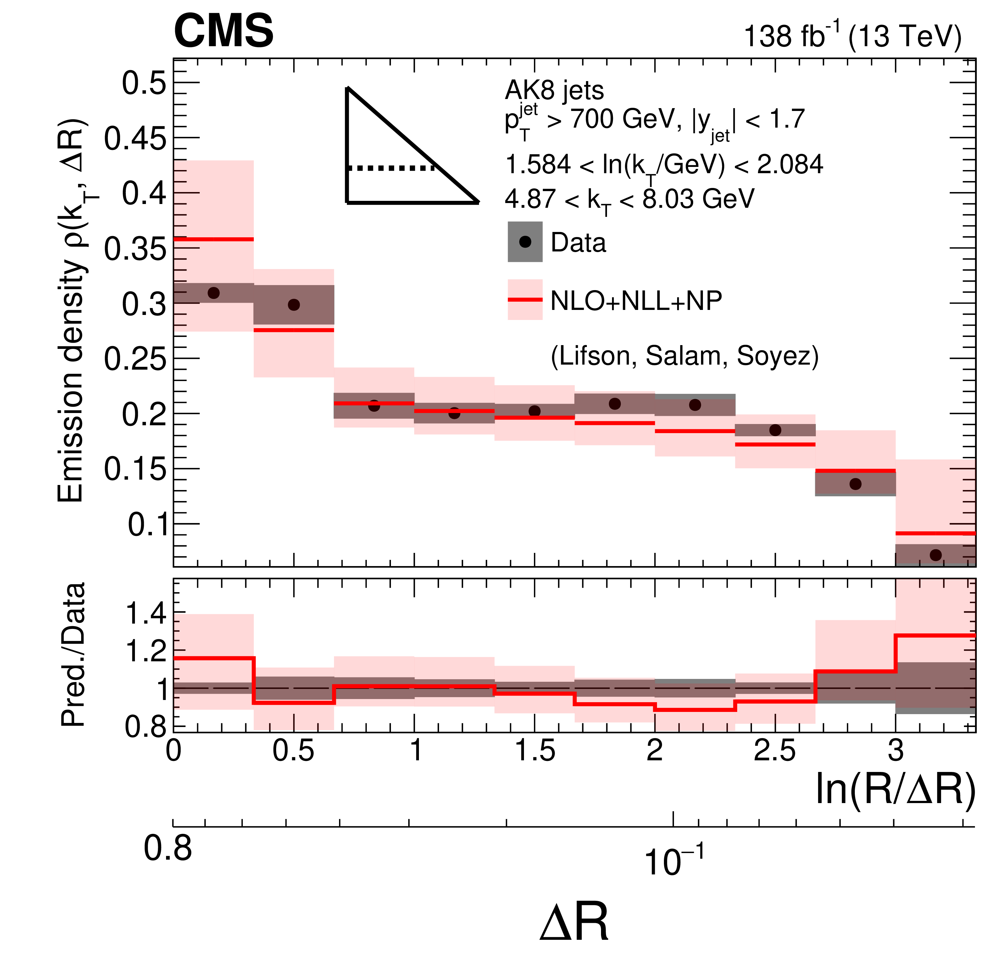
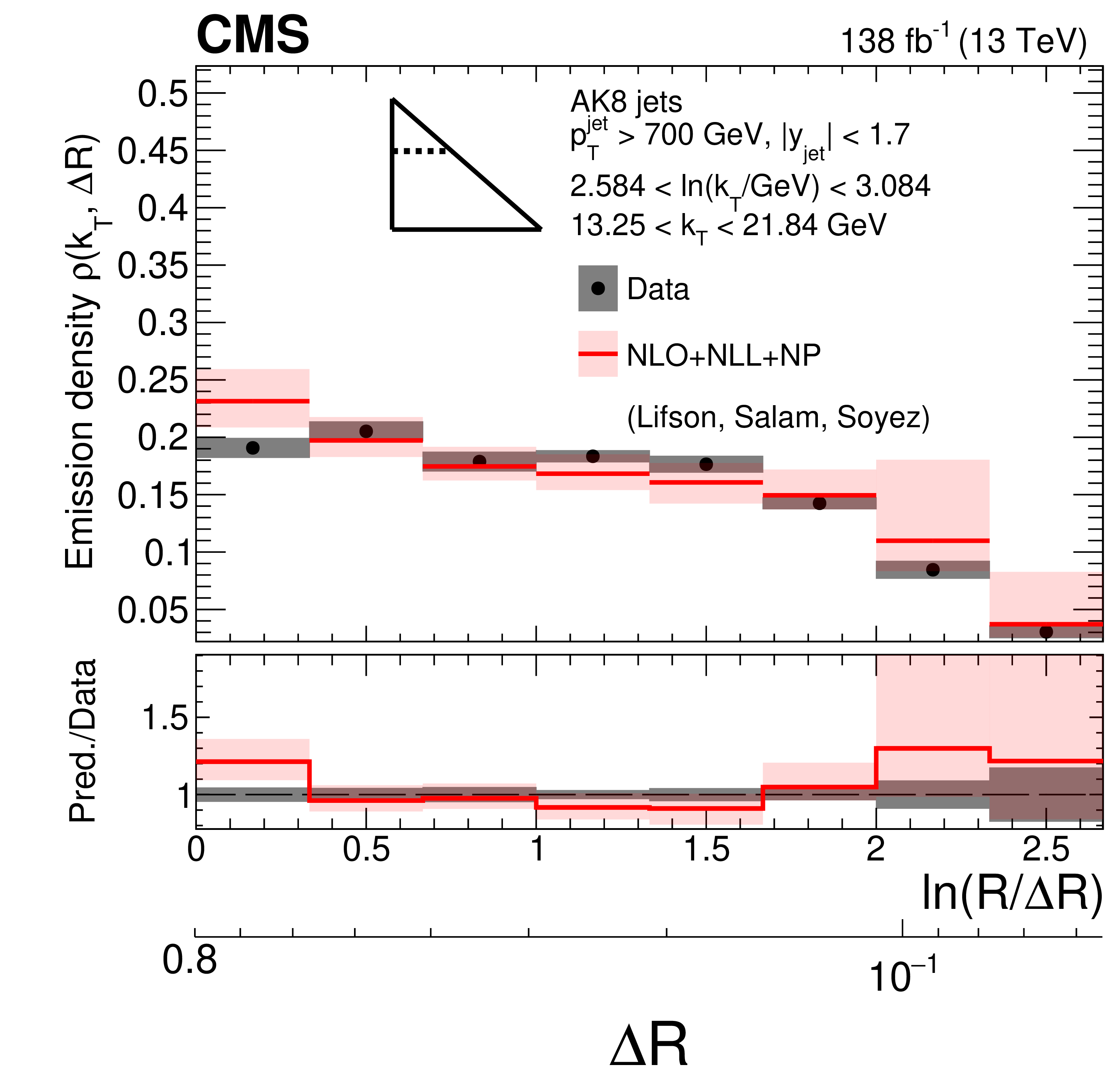
Four different slices of the primary LJP density of AK8 jets compared with perturbation theory calculations by A. Lifson, G. P. Salam, G. Soyez [10]. The calculations include all-orders resummation at next-to-leading logarithmic (NLL) accuracy matched to a next-to-leading order (NLO) fixed-order calculation, and supplemented with nonperturbative (NP) corrections, as described in the text. The band around the theory prediction represents the uncertainty from variations of the renormalization scale uncertainty in the perturbative calculation as well as uncertainties in the NP corrections. The gray band represents the total experimental uncertainty. The upper two plots correspond to vertical slices of the LJP for fixed $ \ln(R/\Delta R) $ (large angles on upper-left, small angles on upper-right). The lower two plots correspond to two different horizontal slices for fixed $ k_{\mathrm{T}} $ interval: the lower-left plot corresponds to low-$ k_{\mathrm{T}} $ splittings and spans the full range in $ \ln(R/\Delta R) $, whereas the lower-right plot corresponds to high-$ k_{\mathrm{T}} $ splittings, which populate mostly wide-angle radiation. |
png pdf |
Figure 16-a:
Four different slices of the primary LJP density of AK8 jets compared with perturbation theory calculations by A. Lifson, G. P. Salam, G. Soyez [10]. The calculations include all-orders resummation at next-to-leading logarithmic (NLL) accuracy matched to a next-to-leading order (NLO) fixed-order calculation, and supplemented with nonperturbative (NP) corrections, as described in the text. The band around the theory prediction represents the uncertainty from variations of the renormalization scale uncertainty in the perturbative calculation as well as uncertainties in the NP corrections. The gray band represents the total experimental uncertainty. The upper two plots correspond to vertical slices of the LJP for fixed $ \ln(R/\Delta R) $ (large angles on upper-left, small angles on upper-right). The lower two plots correspond to two different horizontal slices for fixed $ k_{\mathrm{T}} $ interval: the lower-left plot corresponds to low-$ k_{\mathrm{T}} $ splittings and spans the full range in $ \ln(R/\Delta R) $, whereas the lower-right plot corresponds to high-$ k_{\mathrm{T}} $ splittings, which populate mostly wide-angle radiation. |
png pdf |
Figure 16-b:
Four different slices of the primary LJP density of AK8 jets compared with perturbation theory calculations by A. Lifson, G. P. Salam, G. Soyez [10]. The calculations include all-orders resummation at next-to-leading logarithmic (NLL) accuracy matched to a next-to-leading order (NLO) fixed-order calculation, and supplemented with nonperturbative (NP) corrections, as described in the text. The band around the theory prediction represents the uncertainty from variations of the renormalization scale uncertainty in the perturbative calculation as well as uncertainties in the NP corrections. The gray band represents the total experimental uncertainty. The upper two plots correspond to vertical slices of the LJP for fixed $ \ln(R/\Delta R) $ (large angles on upper-left, small angles on upper-right). The lower two plots correspond to two different horizontal slices for fixed $ k_{\mathrm{T}} $ interval: the lower-left plot corresponds to low-$ k_{\mathrm{T}} $ splittings and spans the full range in $ \ln(R/\Delta R) $, whereas the lower-right plot corresponds to high-$ k_{\mathrm{T}} $ splittings, which populate mostly wide-angle radiation. |
png pdf |
Figure 16-c:
Four different slices of the primary LJP density of AK8 jets compared with perturbation theory calculations by A. Lifson, G. P. Salam, G. Soyez [10]. The calculations include all-orders resummation at next-to-leading logarithmic (NLL) accuracy matched to a next-to-leading order (NLO) fixed-order calculation, and supplemented with nonperturbative (NP) corrections, as described in the text. The band around the theory prediction represents the uncertainty from variations of the renormalization scale uncertainty in the perturbative calculation as well as uncertainties in the NP corrections. The gray band represents the total experimental uncertainty. The upper two plots correspond to vertical slices of the LJP for fixed $ \ln(R/\Delta R) $ (large angles on upper-left, small angles on upper-right). The lower two plots correspond to two different horizontal slices for fixed $ k_{\mathrm{T}} $ interval: the lower-left plot corresponds to low-$ k_{\mathrm{T}} $ splittings and spans the full range in $ \ln(R/\Delta R) $, whereas the lower-right plot corresponds to high-$ k_{\mathrm{T}} $ splittings, which populate mostly wide-angle radiation. |
png pdf |
Figure 16-d:
Four different slices of the primary LJP density of AK8 jets compared with perturbation theory calculations by A. Lifson, G. P. Salam, G. Soyez [10]. The calculations include all-orders resummation at next-to-leading logarithmic (NLL) accuracy matched to a next-to-leading order (NLO) fixed-order calculation, and supplemented with nonperturbative (NP) corrections, as described in the text. The band around the theory prediction represents the uncertainty from variations of the renormalization scale uncertainty in the perturbative calculation as well as uncertainties in the NP corrections. The gray band represents the total experimental uncertainty. The upper two plots correspond to vertical slices of the LJP for fixed $ \ln(R/\Delta R) $ (large angles on upper-left, small angles on upper-right). The lower two plots correspond to two different horizontal slices for fixed $ k_{\mathrm{T}} $ interval: the lower-left plot corresponds to low-$ k_{\mathrm{T}} $ splittings and spans the full range in $ \ln(R/\Delta R) $, whereas the lower-right plot corresponds to high-$ k_{\mathrm{T}} $ splittings, which populate mostly wide-angle radiation. |
| Summary |
| We have presented a measurement of the primary Lund jet plane (LJP) density in inclusive jet production in proton-proton collisions at $ \sqrt{s} = $ 13 TeV using data, corresponding to an integrated luminosity of 138 fb$ ^{-1} $, collected in Run 2 (2016-2018) with the CMS experiment. The LJP is a two-dimensional representation of the phase space of emissions inside a jet constructed using iterative Cambridge-Aachen declustering. The logarithm of the relative transverse momentum $ k_{\mathrm{T}} $ of the emission and the logarithm of the opening angle of the branching $ \Delta R $ are used for the vertical and horizontal axes of the LJP. We analyzed the substructure of jets initially clustered with the anti-$ k_{\mathrm{T}} $ algorithm with transverse momentum $ p_{\mathrm{T}} > $ 700 GeV and rapidity $ |y| < $ 1.7 clustered with distance parameters $ R = $ 0.4 or 0.8. The smaller $ R = $ 0.4 is the standard $ R $ for Run 2 analyses. The larger $ R = $ 0.8, used for the first time in a measurement of the primary LJP density, enables the exploration of a broader kinematical region of the LJP that is inaccessible with the $ R = $ 0.4 parameter value, particularly for wide-angle, hard radiation. Clustering effects associated with the initial anti-$ k_{\mathrm{T}} $ clustering have a less strong effect in the collinear region with the larger $ R $ value; hence the angular region where the emission density plateaus is wider for $ R = $ 0.8 jets. The corrected distributions have an experimental uncertainty in a range of 2-7% in the region away from the kinematical LJP edge and about 15-25% close to the LJP edge. We compared the corrected primary LJP density with various particle-level predictions from Monte Carlo (MC) simulated events. The predictions use different implementations of parton showers as well as different models for the underlying-event (UE) activity, beam-beam remnants, hadronization, and color reconnection effects. The aforementioned mechanisms can be effectively factorized in the primary LJP density, which allows for strong constraints in terms of the substructure of jets. At leading-logarithmic (LL) accuracy, the primary LJP density is proportional to the strong coupling $ \alpha_\mathrm{S}(k_{\mathrm{T}}) $, so it can be used to tune the value of $ \alpha_\mathrm{S} $ evaluated at the Z boson mass used for final-state radiation (FSR) in MC event generators, $ \alpha_\mathrm{S}^\mathrm{FSR}(m_\mathrm{Z}) $. Predictions generated with the CP5 tune of the PYTHIA8 generator underestimate the measured density of emissions in the perturbative region ($ k_{\mathrm{T}} > $ 5 GeV) by about 15% because of the small value of $ \alpha_\mathrm{S}^\mathrm{FSR}(m_\mathrm{Z}) $ used for this tune. Other PYTHIA8 tunes or parton shower options tested in the measurement are in better agreement with the data. The predictions generated with the angular-ordered shower of the HERWIG 7.2.0 generator are in better agreement with the data than those generated with its alternative dipole shower. The data were also compared with different recoil schemes of the angular-ordered shower of HERWIG 7, which allow the parton shower to reach up to next-to-LL (NLL) accuracy for certain global observables. The HERWIG 7 predictions with the dot-product preserving recoil scheme, together with a veto on high-virtuality partons, have the best global agreement with the data among the generators tested in the measurement. The low-$ k_{\mathrm{T}} $ region is dominated by hadronization effects in a wide range of $ \Delta R $ values, with additional contributions from the UE at large $ \Delta R \approx R $. The predictions based on cluster fragmentation models, such as those generated with HERWIG 7 or SHERPA 2 generators, are in better agreement with the data at low $ k_{\mathrm{T}} $ for a wide range of $ \Delta R $ values than those of PYTHIA8. The PYTHIA8 predictions, where hadronization is described with the Lund string fragmentation model, overestimate the LJP density by about 15-20% for $ k_{\mathrm{T}} $ at the GeV scale for a wide range of $ \Delta R $ values. One possibility to improve the description of the low $ k_{\mathrm{T}} $ region is to include the FSR cutoff $ k_{\mathrm{T}} $ as a free parameter in future event generator tuning; a larger FSR cutoff $ k_{\mathrm{T}} $ value decreases the density of emissions at low $ k_{\mathrm{T}} $ in the LJP without affecting the high-$ k_{\mathrm{T}} $ region that is dominated by the parton shower. Finally, the data are also compared with a perturbative QCD calculation with a resummation at NLL accuracy, which is matched to a fixed-order next-to-leading order calculation [10]. To compare with the measured LJP at hadron level, nonperturbative corrections are supplemented to the calculation. The predictions are in agreement with the data within the theoretical and experimental uncertainties. For collinear emissions, the data can be qualitatively described with the running of $ \alpha_\mathrm{S} $ with $ k_{\mathrm{T}} $. These measurements highlight the different aspects of the physics modeling of event generators that should be improved, ranging from the modeling of hadronization and up to the logarithmic accuracy of parton showering algorithms. |
| References | ||||
| 1 | A. J. Larkoski, I. Moult, and B. Nachman | Jet substructure at the Large Hadron Collider: a review of recent advances in theory and machine learning | Phys. Rept. 841 (2020) 1 | 1709.04464 |
| 2 | R. Kogler and others | Jet substructure at the Large Hadron Collider: experimental review | Rev. Mod. Phys. 91 (2019) 045003 | 1803.06991 |
| 3 | S. Marzani, G. Soyez, and M. Spannowsky | Looking inside jets: an introduction to jet substructure and boosted-object phenomenology | Lect. Notes Phys. 958 (2019) 1 | 1901.10342 |
| 4 | R. Kogler | Advances in jet substructure at the LHC: algorithms, measurements, and searches for new physical phenomena | Volume 284, Springer ISBN 978-3-030-72857-1, 978-3-030-72858-8, 2021 |
|
| 5 | B. Andersson, G. Gustafson, L. Lönnblad, and U. Pettersson | Coherence effects in deep inelastic scattering | Z. Phys. C 43 (1989) 625 | |
| 6 | H. A. Andrews et al. | Novel tools and observables for jet physics in heavy-ion collisions | JPG 47 (2020) 065102 | 1808.03689 |
| 7 | F. A. Dreyer, G. P. Salam, and G. Soyez | The Lund jet plane | JHEP 12 (2018) 064 | 1807.04758 |
| 8 | Y. L. Dokshitzer, G. D. Leder, S. Moretti, and B. R. Webber | Better jet clustering algorithms | JHEP 08 (1997) 001 | hep-ph/9707323 |
| 9 | M. Wobisch and T. Wengler | Hadronization corrections to jet cross sections in deep inelastic scattering | in Workshop on Monte Carlo generators for HERA physics, 1998 link |
hep-ph/9907280 |
| 10 | A. Lifson, G. P. Salam, and G. Soyez | Calculating the primary Lund jet plane density | JHEP 10 (2020) 170 | 2007.06578 |
| 11 | M. Dasgupta et al. | Logarithmic accuracy of parton showers: a fixed-order study | JHEP 09 (2018) 033 | 1805.09327 |
| 12 | M. Dasgupta et al. | Parton showers beyond leading logarithmic accuracy | PRL 125 (2020) 052002 | 2002.11114 |
| 13 | K. Hamilton et al. | Color and logarithmic accuracy in final-state parton showers | JHEP 03 (2021) 041 | 2011.10054 |
| 14 | J. R. Forshaw, J. Holguin, and S. Pl ä tzer | Building a consistent parton shower | JHEP 09 (2020) 014 | 2003.06400 |
| 15 | Z. Nagy and D. E. Soper | Summations by parton showers of large logarithms in electron-positron annihilation | 2011.04777 | |
| 16 | F. Herren et al. | A new approach to color-coherent parton evolution | JHEP 10 (2023) 091 | 2208.06057 |
| 17 | M. van Beekveld et al. | PanScales parton showers for hadron collisions: formulation and fixed-order studies | JHEP 11 (2022) 019 | 2205.02237 |
| 18 | M. van Beekveld et al. | PanScales showers for hadron collisions: all-order validation | JHEP 11 (2022) 020 | 2207.09467 |
| 19 | ALICE Collaboration | Direct observation of the dead-cone effect in quantum chromodynamics | Nature 605 (2022) 440 | 2106.05713 |
| 20 | F. A. Dreyer and H. Qu | Jet tagging in the Lund plane with graph networks | JHEP 03 (2021) 052 | 2012.08526 |
| 21 | L. Cavallini et al. | Tagging the Higgs boson decay to bottom quarks with color-sensitive observables and the Lund jet plane | EPJC 82 (2022) 493 | 2112.09650 |
| 22 | M. Dasgupta, A. Fregoso, S. Marzani, and G. P. Salam | Towards an understanding of jet substructure | JHEP 09 (2013) 029 | 1307.0007 |
| 23 | A. J. Larkoski, S. Marzani, G. Soyez, and J. Thaler | Soft drop | JHEP 05 (2014) 146 | 1402.2657 |
| 24 | CMS Collaboration | Measurement of the splitting function in pp and PbPb collisions at $ \sqrt{\smash[b]{s_{_{\mathrm{NN}}}}} = $ 5.02 TeV | PRL 120 (2018) 142302 | CMS-HIN-16-006 1708.09429 |
| 25 | CMS Collaboration | Measurements of the differential jet cross section as a function of the jet mass in dijet events from proton-proton collisions at $ \sqrt{s}= $ 13 TeV | JHEP 11 (2018) 113 | CMS-SMP-16-010 1807.05974 |
| 26 | CMS Collaboration | Measurement of jet substructure observables in $ \mathrm{t} \overline{\mathrm{t}} $ events from proton-proton collisions at $ \sqrt{s}= $ 13 TeV | PRD 98 (2018) 092014 | CMS-TOP-17-013 1808.07340 |
| 27 | ALICE Collaboration | First measurement of jet mass in PbPb and pPb collisions at the LHC | PLB 776 (2018) 249 | 1702.00804 |
| 28 | ATLAS Collaboration | Measurement of jet substructure observables in top quark, W boson and light jet production in proton-proton collisions at $ \sqrt{s}= $ 13 TeV with the ATLAS detector | JHEP 08 (2019) 033 | 1903.02942 |
| 29 | ATLAS Collaboration | Measurement of soft-drop jet observables in pp collisions with the ATLAS detector at $ \sqrt{s}= $ 13 TeV | PRD 101 (2020) 052007 | 1912.09837 |
| 30 | ALICE Collaboration | Exploration of jet substructure using iterative declustering in pp and PbPb collisions at LHC energies | PLB 802 (2020) 135227 | 1905.02512 |
| 31 | ALICE Collaboration | Measurement of the groomed jet radius and momentum splitting fraction in pp and PbPb collisions at $ \sqrt{\smash[b]{s_{_{\mathrm{NN}}}}}= $ 5.02 TeV | PRL 128 (2022) 102001 | 2107.12984 |
| 32 | ALICE Collaboration | Measurements of the groomed and ungroomed jet angularities in pp collisions at $ \sqrt{s}= $ 5.02 TeV | JHEP 05 (2022) 061 | 2107.11303 |
| 33 | CMS Collaboration | Study of quark and gluon jet substructure in Z+jet and dijet events from pp collisions | JHEP 01 (2022) 188 | CMS-SMP-20-010 2109.03340 |
| 34 | ATLAS Collaboration | Measurement of substructure-dependent jet suppression in PbPb collisions at 5.02 TeV with the ATLAS detector | Phys. Rev. C 107 (2023) 054909 | 2211.11470 |
| 35 | CMS Collaboration | Measurement of the differential $ \mathrm{t} \overline{\mathrm{t}} $ production cross section as a function of the jet mass and extraction of the top quark mass in hadronic decays of boosted top quarks | EPJC 83 (2023) 560 | CMS-TOP-21-012 2211.01456 |
| 36 | ATLAS Collaboration | Measurement of suppression of large-radius jets and its dependence on substructure in PbPb collisions at $ \sqrt{\smash[b]{s_{_{\mathrm{NN}}}}} = $ 5.02 TeV with the ATLAS detector | PRL 131 (2023) 172301 | 2301.05606 |
| 37 | ATLAS Collaboration | Measurement of the Lund jet plane using charged particles in 13 TeV proton-proton collisions with the ATLAS detector | PRL 124 (2020) 222002 | 2004.03540 |
| 38 | M. Cacciari, G. P. Salam, and G. Soyez | The anti-$ k_{\mathrm{T}} $ jet clustering algorithm | JHEP 04 (2008) 063 | 0802.1189 |
| 39 | M. Cacciari, G. P. Salam, and G. Soyez | FastJet user manual | EPJC 72 (2012) 1896 | 1111.6097 |
| 40 | CMS Collaboration | HEPData record for this analysis | link | |
| 41 | CMS Collaboration | The CMS experiment at the CERN LHC | JINST 3 (2008) S08004 | |
| 42 | CMS Collaboration | Description and performance of track and primary-vertex reconstruction with the CMS tracker | JINST 9 (2014) P10009 | CMS-TRK-11-001 1405.6569 |
| 43 | CMS Tracker Group | The CMS Phase-1 pixel detector upgrade | JINST 16 (2021) P02027 | 2012.14304 |
| 44 | CMS Collaboration | Track impact parameter resolution for the full pseudorapidity coverage in the 2017 dataset with the CMS Phase-1 pixel detector | CMS Detector Performance Note CMS-DP-2020-049, 2020 CDS |
|
| 45 | CMS Collaboration | Technical proposal for the Phase-2 upgrade of the Compact Muon Solenoid | CMS Technical Proposal CERN-LHCC-2015-010, CMS-TDR-15-02, 2015 CDS |
|
| 46 | CMS Collaboration | Particle-flow reconstruction and global event description with the CMS detector | JINST 12 (2017) P10003 | CMS-PRF-14-001 1706.04965 |
| 47 | CMS Collaboration | Jet energy scale and resolution in the CMS experiment in pp collisions at 8 TeV | JINST 12 (2017) P02014 | CMS-JME-13-004 1607.03663 |
| 48 | CMS Collaboration | Pileup mitigation at CMS in 13 TeV data | JINST 15 (2020) P09018 | CMS-JME-18-001 2003.00503 |
| 49 | CMS Collaboration | Performance of the CMS Level-1 trigger in proton-proton collisions at $ \sqrt{s} = $ 13 TeV | JINST 15 (2020) P10017 | CMS-TRG-17-001 2006.10165 |
| 50 | CMS Collaboration | The CMS trigger system | JINST 12 (2017) P01020 | CMS-TRG-12-001 1609.02366 |
| 51 | CMS Collaboration | Precision luminosity measurement in proton-proton collisions at $ \sqrt{s}= $ 13 TeV in 2015 and 2016 at CMS | EPJC 81 (2021) 800 | CMS-LUM-17-003 2104.01927 |
| 52 | CMS Collaboration | CMS luminosity measurement for the 2017 data-taking period at $ \sqrt{s} = $ 13 TeV | CMS Physics Analysis Summary, 2018 link |
CMS-PAS-LUM-17-004 |
| 53 | CMS Collaboration | CMS luminosity measurement for the 2018 data-taking period at $ \sqrt{s} = $ 13 TeV | CMS Physics Analysis Summary, 2019 link |
CMS-PAS-LUM-18-002 |
| 54 | T. Sjöstrand et al. | An introduction to PYTHIA8.2 | Comput. Phys. Commun. 191 (2015) 159 | 1410.3012 |
| 55 | B. Andersson, G. Gustafson, G. Ingelman, and T. Sjöstrand | Parton fragmentation and string dynamics | Phys. Rept. 97 (1983) 31 | |
| 56 | T. Sjöstrand | The merging of jets | PLB 142 (1984) 420 | |
| 57 | CMS Collaboration | Extraction and validation of a new set of CMS PYTHIA8 tunes from underlying-event measurements | EPJC 80 (2020) 4 | CMS-GEN-17-001 1903.12179 |
| 58 | NNPDF Collaboration | Parton distributions for the LHC Run 2 | JHEP 04 (2015) 040 | 1410.8849 |
| 59 | CMS Collaboration | Development and validation of HERWIG 7 tunes from CMS underlying-event measurements | EPJC 81 (2021) 312 | CMS-GEN-19-001 2011.03422 |
| 60 | S. Gieseke, P. Stephens, and B. Webber | New formalism for QCD parton showers | JHEP 12 (2003) 045 | hep-ph/0310083 |
| 61 | B. R. Webber | A QCD model for jet fragmentation including soft gluon interference | NPB 238 (1984) 492 | |
| 62 | GEANT4 Collaboration | GEANT 4---a simulation toolkit | NIM A 506 (2003) 250 | |
| 63 | P. Skands, S. Carrazza, and J. Rojo | Tuning PYTHIA8.1: the Monash 2013 tune | EPJC 74 (2014) 3024 | 1404.5630 |
| 64 | CMS Collaboration | Event generator tunes obtained from underlying event and multiparton scattering measurements | EPJC 76 (2016) 155 | CMS-GEN-14-001 1512.00815 |
| 65 | S. Höche and S. Prestel | The midpoint between dipole and parton showers | EPJC 75 (2015) 461 | 1506.05057 |
| 66 | W. T. Giele, D. A. Kosower, and P. Z. Skands | A simple shower and matching algorithm | PRD 78 (2008) 014026 | 0707.3652 |
| 67 | A. Gehrmann-De Ridder, T. Gehrmann, and E. W. N. Glover | Antenna subtraction at NNLO | JHEP 09 (2005) 056 | hep-ph/0505111 |
| 68 | H. Brooks, C. T. Preuss, and P. Skands | Sector showers for hadron collisions | JHEP 07 (2020) 032 | 2003.00702 |
| 69 | J. Bellm et al. | HERWIG 7.0/ HERWIG++ 3.0 release note | EPJC 76 (2016) 196 | 1512.01178 |
| 70 | J. Bellm et al. | HERWIG 7.2 release note | EPJC 80 (2020) 452 | 1912.06509 |
| 71 | S. Catani and M. H. Seymour | A general algorithm for calculating jet cross sections in NLO QCD | NPB 485 (1997) 291 | hep-ph/9605323 |
| 72 | E. Bothmann et al. | Event generation with SHERPA 2.2 | SciPost Phys. 7 (2019) 034 | 1905.09127 |
| 73 | F. Krauss, R. Kuhn, and G. Soff | \textscamegic++ 1.0: a matrix element generator in C++ | JHEP 02 (2002) 044 | hep-ph/0109036 |
| 74 | T. Gleisberg and S. Höche | Comix, a new matrix element generator | JHEP 12 (2008) 039 | 0808.3674 |
| 75 | S. Schumann and F. Krauss | A parton shower algorithm based on Catani--Seymour dipole factorization | JHEP 03 (2008) 038 | 0709.1027 |
| 76 | J.-C. Winter, F. Krauss, and G. Soff | A modified cluster hadronization model | EPJC 36 (2004) 381 | hep-ph/0311085 |
| 77 | G. Bewick, S. Ferrario Ravasio, P. Richardson, and M. H. Seymour | Logarithmic accuracy of angular-ordered parton showers | JHEP 04 (2020) 019 | 1904.11866 |
| 78 | A. Banfi, G. P. Salam, and G. Zanderighi | Principles of general final-state resummation and automated implementation | JHEP 03 (2005) 073 | hep-ph/0407286 |
| 79 | T. Sjöstrand and M. van Zijl | A multiple-interaction model for the event structure in hadron collisions | PRD 36 (1987) 2019 | |
| 80 | J. M. Butterworth, J. R. Forshaw, and M. H. Seymour | Multiparton interactions in photoproduction at HERA | Z. Phys. C 72 (1996) 637 | hep-ph/9601371 |
| 81 | I. Borozan and M. H. Seymour | An eikonal model for multiparticle production in hadron-hadron interactions | JHEP 09 (2002) 015 | hep-ph/0207283 |
| 82 | M. Bahr, S. Gieseke, and M. H. Seymour | Simulation of multiple partonic interactions in HERWIG++ | JHEP 07 (2008) 076 | 0803.3633 |
| 83 | S. Gieseke, C. Rohr, and A. Si \'o dmok | Color reconnections in HERWIG++ | EPJC 72 (2012) 2225 | 1206.0041 |
| 84 | CMS Collaboration | DeepCore: convolutional neural network for high-$ p_{\mathrm{T}} $ jet tracking | CMS Detector Performance Note CMS-DP-2019-007, 2019 CDS |
|
| 85 | G. D'Agostini | A multidimensional unfolding method based on Bayes' theorem | NIM A 362 (1995) 487 | |
| 86 | T. Adye | Unfolding algorithms and tests using RooUnfold | in PHYSTAT 2011 workshop on statistical issues related to discovery claims in search experiments and unfolding, 2011 PHYSTAT 201 (2011) 313 |
1105.1160 |
| 87 | M. Cacciari et al. | The $ \mathrm{t} \overline{\mathrm{t}} $ cross section at 1.8 TeV and 1.96 TeV: a study of the systematics due to parton densities and scale dependence | JHEP 04 (2004) 068 | hep-ph/0303085 |
| 88 | S. Catani, D. de Florian, M. Grazzini, and P. Nason | Soft-gluon resummation for Higgs boson production at hadron colliders | JHEP 07 (2003) 028 | hep-ph/0306211 |
| 89 | ATLAS Collaboration | Measurement of jet substructure in boosted $ \mathrm{t} \overline{\mathrm{t}} $ events with the ATLAS detector using 140 fb$ ^{-1} $ of 13 TeV pp collisions | Submitted to Phys. Rev. D, 2023 | 2312.03797 |
| 90 | CMS Collaboration | Jet algorithms performance in 13 TeV data | CMS Physics Analysis Summary, 2017 CMS-PAS-JME-16-003 |
CMS-PAS-JME-16-003 |
| 91 | Particle Data Group Collaboration | Review of particle physics | Prog. Theor. Exp. Phys. 2022 (2022) 083C01 | |
|
|
Compact Muon Solenoid LHC, CERN |
|

|

|

|

|

|