

Compact Muon Solenoid
LHC, CERN
| CMS-SUS-21-003 ; CERN-EP-2022-254 | ||
| Search for top squarks in the four-body decay mode with single lepton final states in proton-proton collisions at $ \sqrt{s}= $ 13 TeV | ||
| CMS Collaboration | ||
| 19 January 2023 | ||
| JHEP 06 (2023) 060 | ||
| Abstract: A search for the pair production of the lightest supersymmetric partner of the top quark, the top squark ($ \tilde{\mathrm{t}}_{1} $), is presented. The search targets the four-body decay of the $ \tilde{\mathrm{t}}_{1} $, which is preferred when the mass difference between the top squark and the lightest supersymmetric particle is smaller than the mass of the W boson. This decay mode consists of a bottom quark, two other fermions, and the lightest neutralino ($ \tilde{\chi}_{1}^{0} $), which is assumed to be the lightest supersymmetric particle. The data correspond to an integrated luminosity of 138 fb$ ^{-1} $ of proton-proton collisions at a center-of-mass energy of 13 TeV collected by the CMS experiment at the CERN LHC. Events are selected using the presence of a high-momentum jet, an electron or muon with low transverse momentum, and a significant missing transverse momentum. The signal is selected based on a multivariate approach that is optimized for the difference between $ m(\tilde{\mathrm{t}}_{1}) $ and $ m(\tilde{\chi}_{1}^{0}) $. The contribution from leading background processes is estimated from data. No significant excess is observed above the expectation from standard model processes. The results of this search exclude top squarks at 95% confidence level for masses up to 480 and 700 GeV for $ m(\tilde{\mathrm{t}}_{1}) - m(\tilde{\chi}_{1}^{0}) = $ 10 and 80 GeV, respectively. | ||
| Links: e-print arXiv:2301.08096 [hep-ex] (PDF) ; CDS record ; inSPIRE record ; Physics Briefing ; CADI line (restricted) ; | ||
| Figures | |

png pdf |
Figure 1:
Diagram of top squark pair production $ \tilde{\mathrm{t}}_{1} {\overline{\tilde{\mathrm{t}}}}_{1} $ in pp collisions, with a four-body decay of each top squark. |
png pdf |
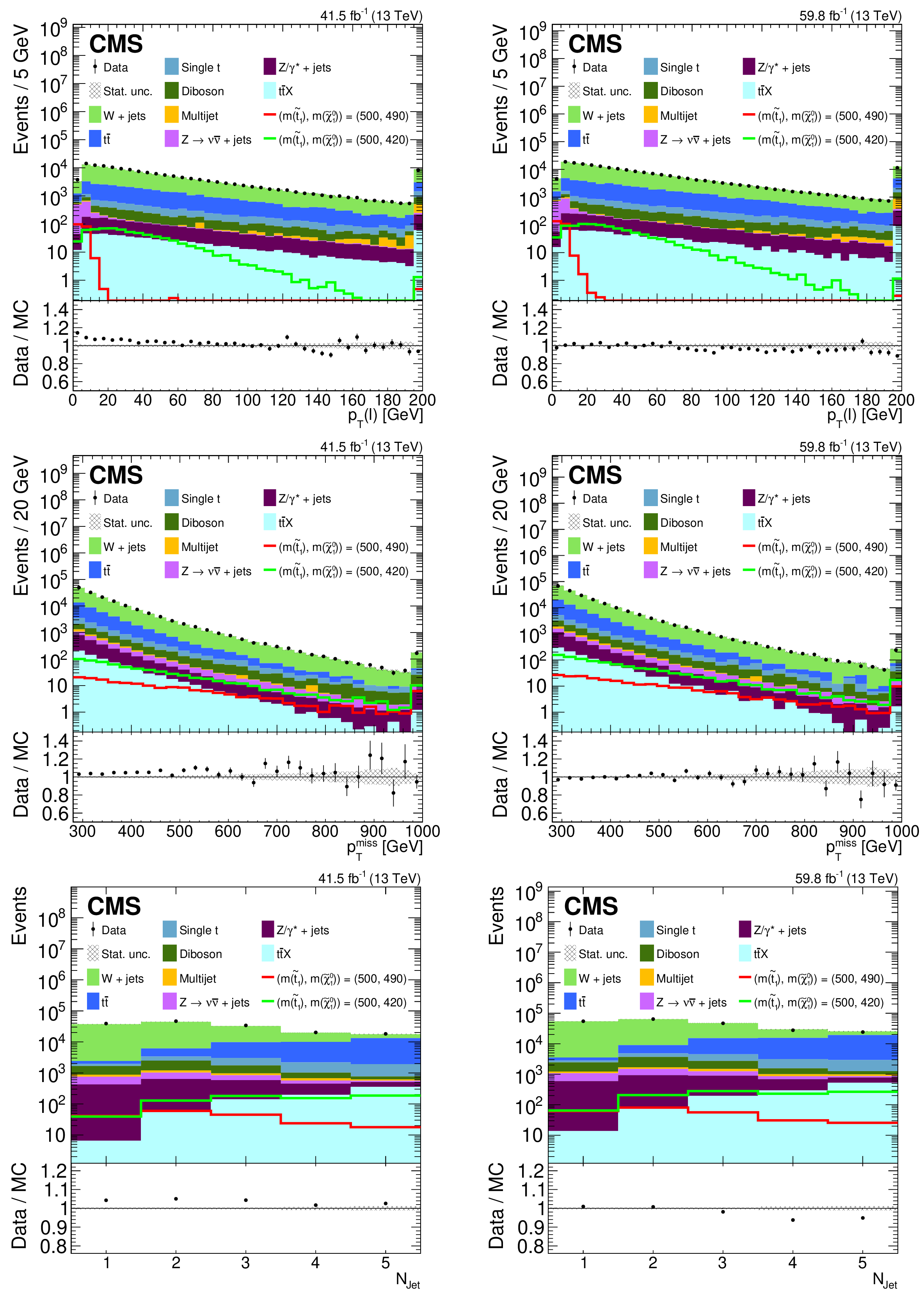
Figure 2:
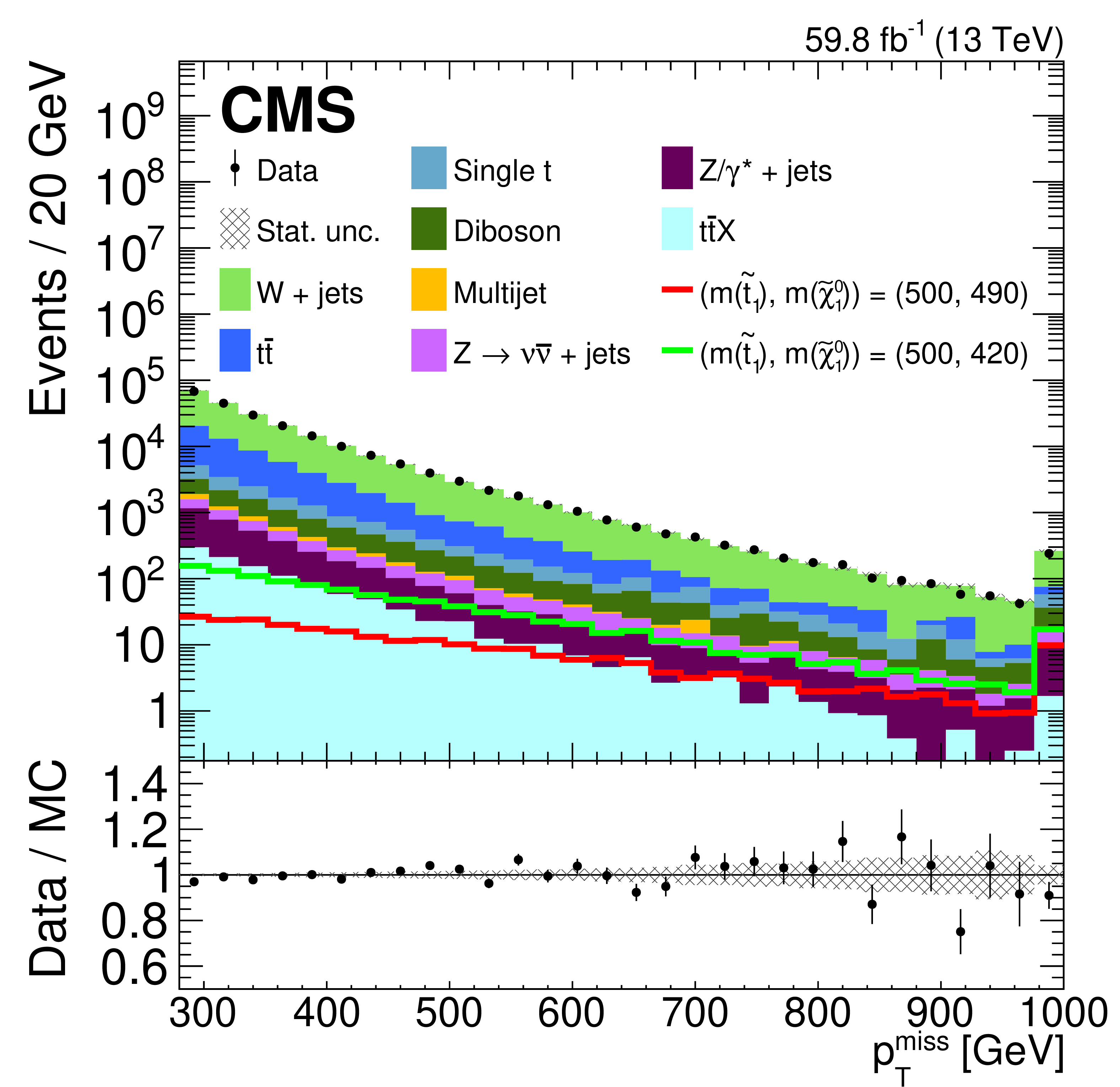
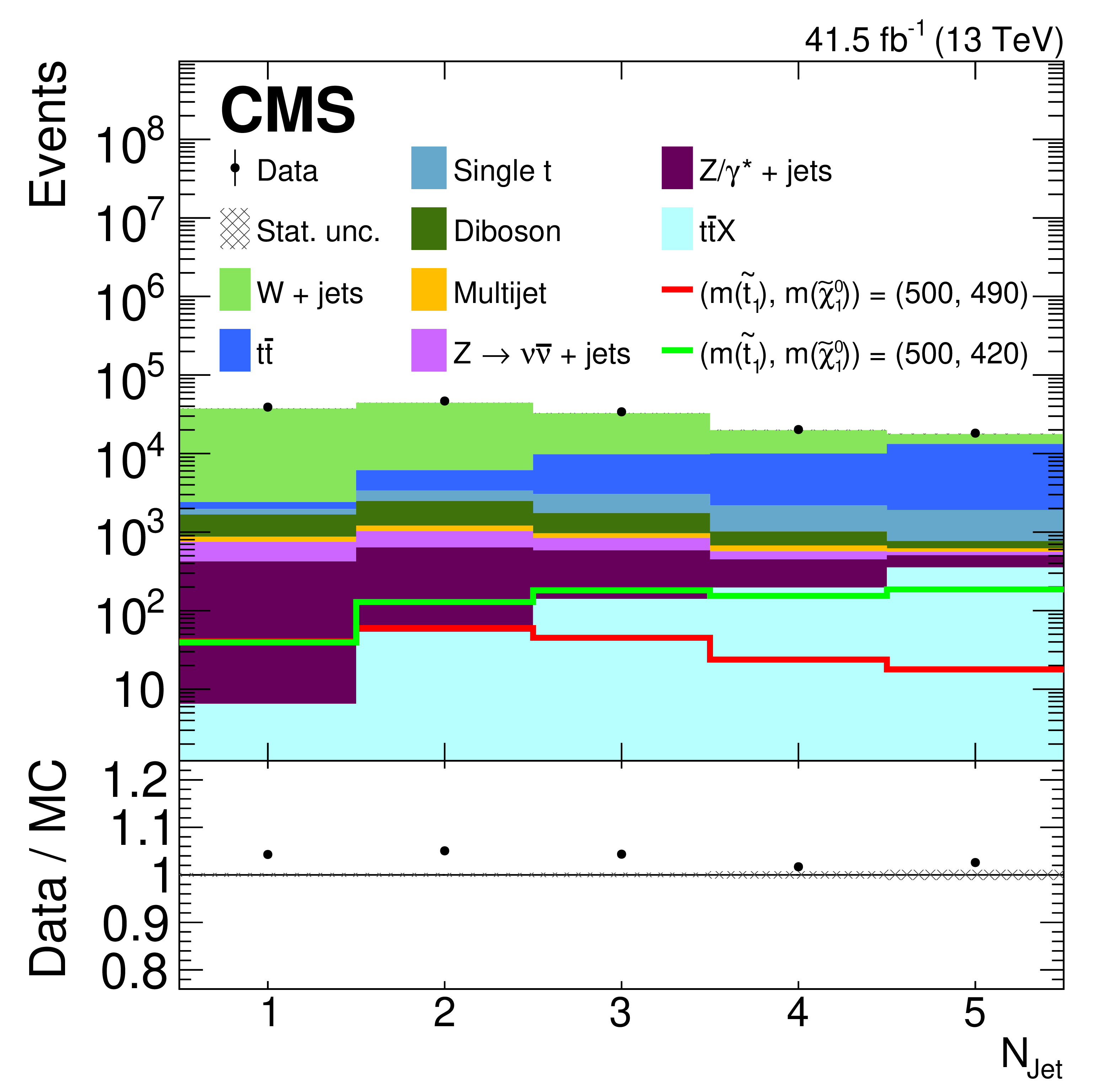
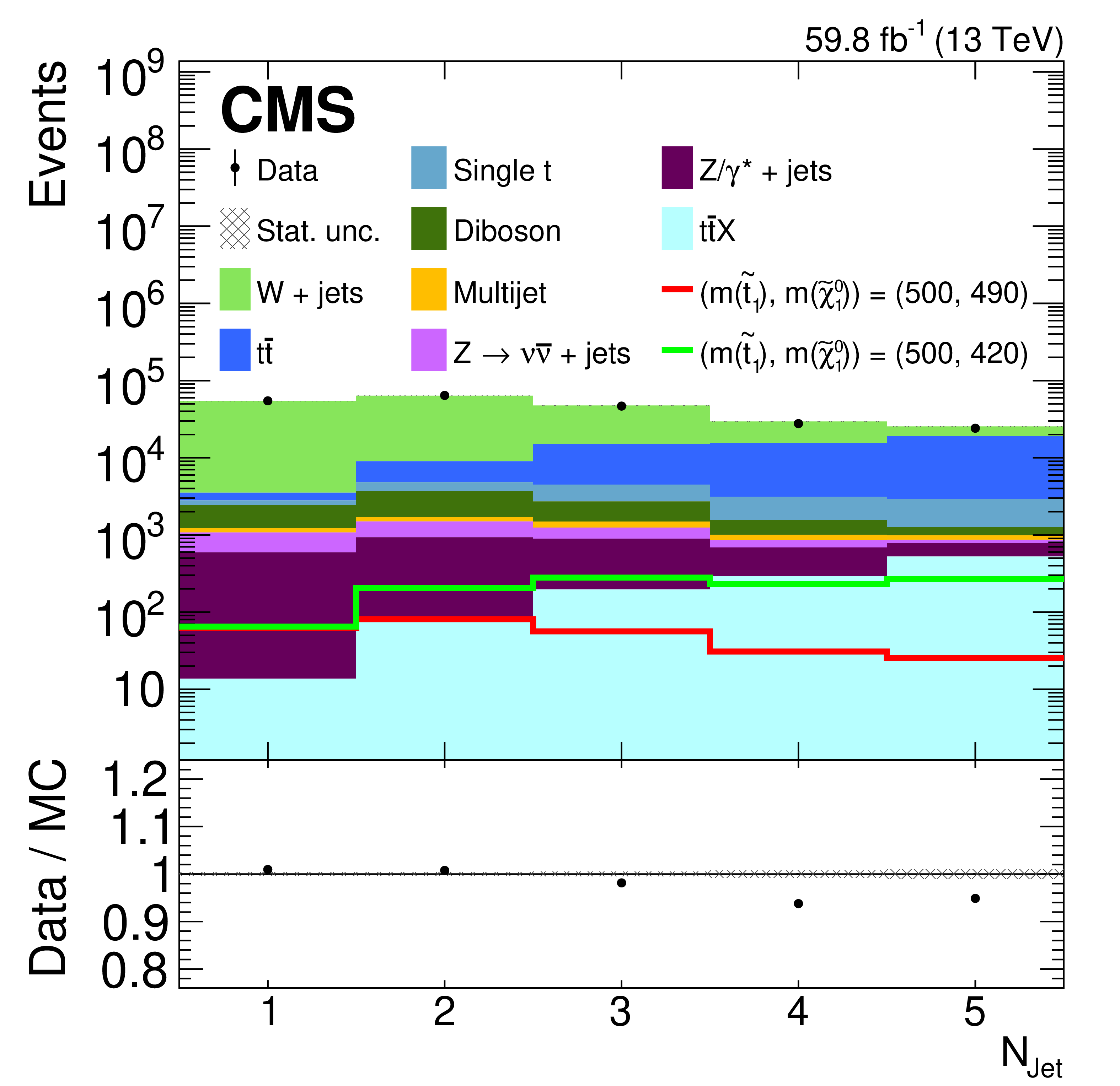
Distributions of $ p_{\mathrm{T}}(\ell) $ (upper), $ p_{\mathrm{T}}^\text{miss} $ (middle), and $ N_{\text{jet}} $ (lower), after the preselection from 2017 (left) and 2018 (right) data (points) and simulation (colored histograms). The simulated distribution of two signal points are represented by colored lines, while not being stacked on the background distributions: $ ({m}(\tilde{\mathrm{t}}_{1}), {m}(\tilde{\chi}_{1}^{0})) = $ (500, 490) and (500, 420) GeV. The last bin in each plot includes the overflow events. The lower panels show the ratio of data to the sum of the simulated SM backgrounds. The shaded bands indicate only the statistical uncertainty in the simulation predictions. |
png pdf |
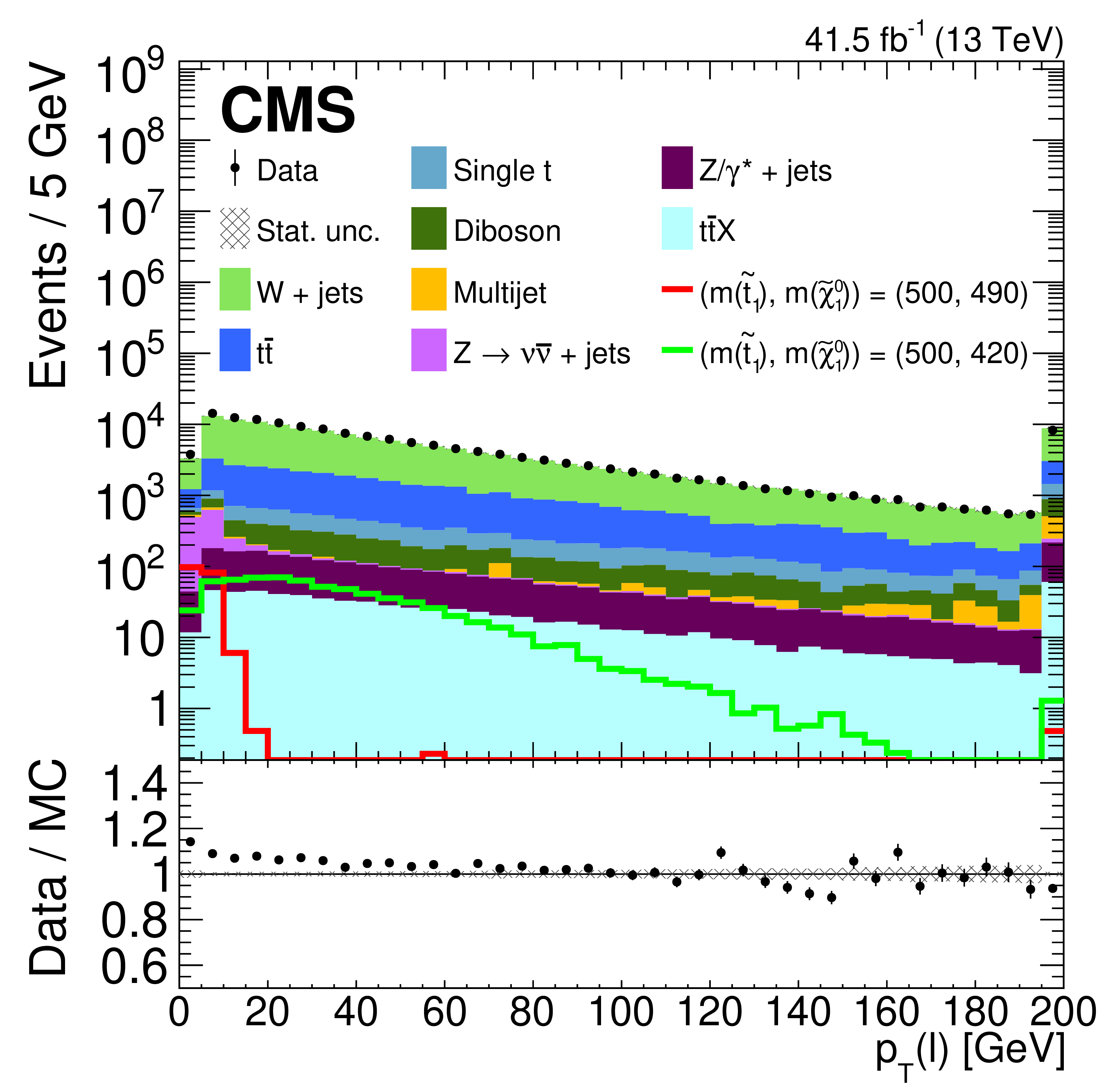
Figure 2-a:
Distributions of $ p_{\mathrm{T}}(\ell) $ (upper), $ p_{\mathrm{T}}^\text{miss} $ (middle), and $ N_{\text{jet}} $ (lower), after the preselection from 2017 (left) and 2018 (right) data (points) and simulation (colored histograms). The simulated distribution of two signal points are represented by colored lines, while not being stacked on the background distributions: $ ({m}(\tilde{\mathrm{t}}_{1}), {m}(\tilde{\chi}_{1}^{0})) = $ (500, 490) and (500, 420) GeV. The last bin in each plot includes the overflow events. The lower panels show the ratio of data to the sum of the simulated SM backgrounds. The shaded bands indicate only the statistical uncertainty in the simulation predictions. |
png pdf |
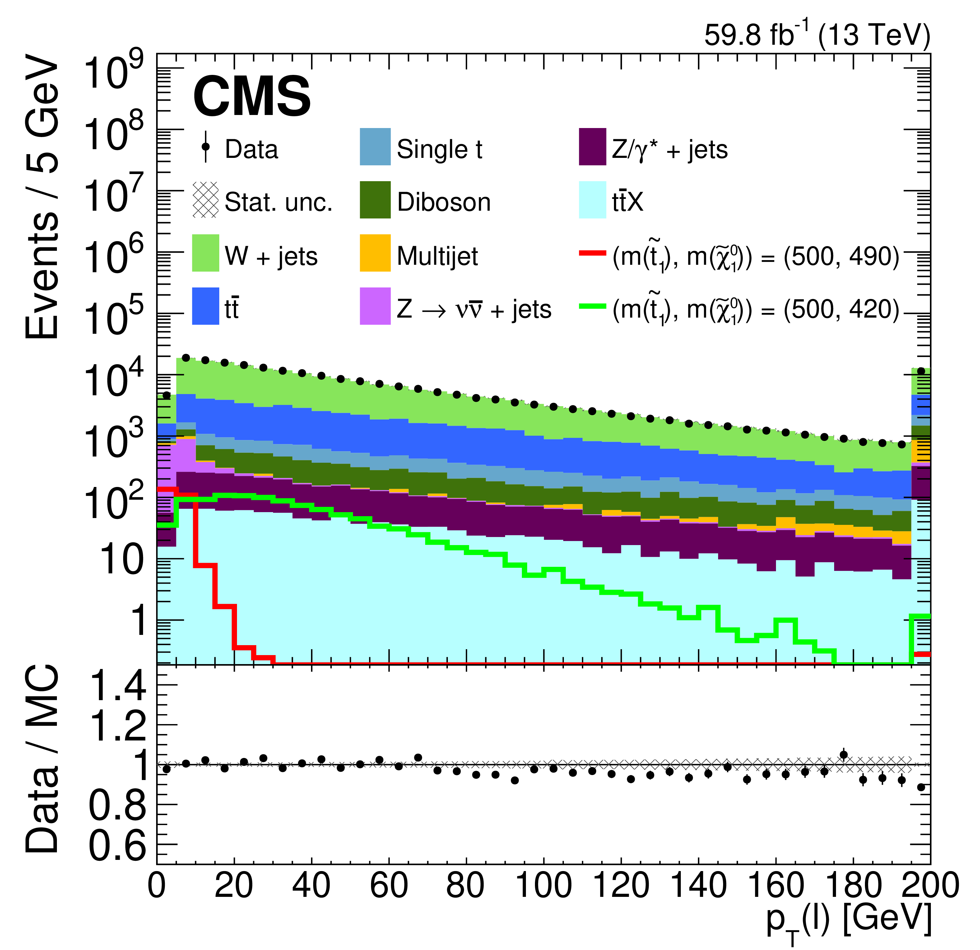
Figure 2-b:
Distributions of $ p_{\mathrm{T}}(\ell) $ (upper), $ p_{\mathrm{T}}^\text{miss} $ (middle), and $ N_{\text{jet}} $ (lower), after the preselection from 2017 (left) and 2018 (right) data (points) and simulation (colored histograms). The simulated distribution of two signal points are represented by colored lines, while not being stacked on the background distributions: $ ({m}(\tilde{\mathrm{t}}_{1}), {m}(\tilde{\chi}_{1}^{0})) = $ (500, 490) and (500, 420) GeV. The last bin in each plot includes the overflow events. The lower panels show the ratio of data to the sum of the simulated SM backgrounds. The shaded bands indicate only the statistical uncertainty in the simulation predictions. |
png pdf |
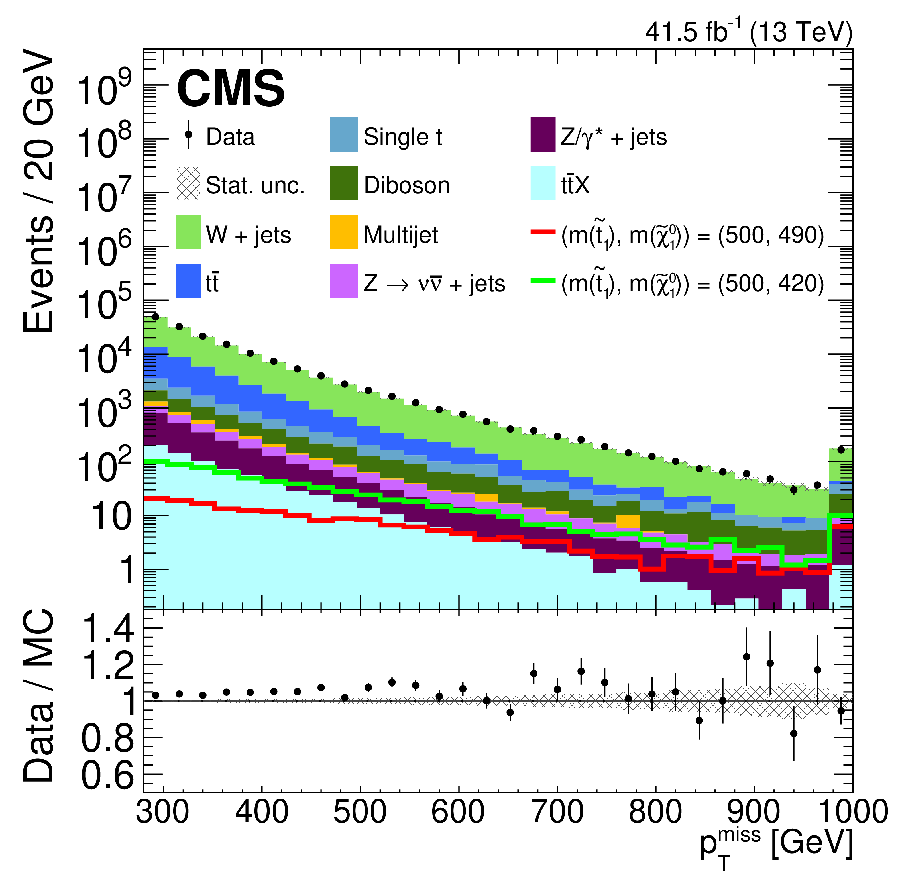
Figure 2-c:
Distributions of $ p_{\mathrm{T}}(\ell) $ (upper), $ p_{\mathrm{T}}^\text{miss} $ (middle), and $ N_{\text{jet}} $ (lower), after the preselection from 2017 (left) and 2018 (right) data (points) and simulation (colored histograms). The simulated distribution of two signal points are represented by colored lines, while not being stacked on the background distributions: $ ({m}(\tilde{\mathrm{t}}_{1}), {m}(\tilde{\chi}_{1}^{0})) = $ (500, 490) and (500, 420) GeV. The last bin in each plot includes the overflow events. The lower panels show the ratio of data to the sum of the simulated SM backgrounds. The shaded bands indicate only the statistical uncertainty in the simulation predictions. |
png pdf |
Figure 2-d:
Distributions of $ p_{\mathrm{T}}(\ell) $ (upper), $ p_{\mathrm{T}}^\text{miss} $ (middle), and $ N_{\text{jet}} $ (lower), after the preselection from 2017 (left) and 2018 (right) data (points) and simulation (colored histograms). The simulated distribution of two signal points are represented by colored lines, while not being stacked on the background distributions: $ ({m}(\tilde{\mathrm{t}}_{1}), {m}(\tilde{\chi}_{1}^{0})) = $ (500, 490) and (500, 420) GeV. The last bin in each plot includes the overflow events. The lower panels show the ratio of data to the sum of the simulated SM backgrounds. The shaded bands indicate only the statistical uncertainty in the simulation predictions. |
png pdf |
Figure 2-e:
Distributions of $ p_{\mathrm{T}}(\ell) $ (upper), $ p_{\mathrm{T}}^\text{miss} $ (middle), and $ N_{\text{jet}} $ (lower), after the preselection from 2017 (left) and 2018 (right) data (points) and simulation (colored histograms). The simulated distribution of two signal points are represented by colored lines, while not being stacked on the background distributions: $ ({m}(\tilde{\mathrm{t}}_{1}), {m}(\tilde{\chi}_{1}^{0})) = $ (500, 490) and (500, 420) GeV. The last bin in each plot includes the overflow events. The lower panels show the ratio of data to the sum of the simulated SM backgrounds. The shaded bands indicate only the statistical uncertainty in the simulation predictions. |
png pdf |
Figure 2-f:
Distributions of $ p_{\mathrm{T}}(\ell) $ (upper), $ p_{\mathrm{T}}^\text{miss} $ (middle), and $ N_{\text{jet}} $ (lower), after the preselection from 2017 (left) and 2018 (right) data (points) and simulation (colored histograms). The simulated distribution of two signal points are represented by colored lines, while not being stacked on the background distributions: $ ({m}(\tilde{\mathrm{t}}_{1}), {m}(\tilde{\chi}_{1}^{0})) = $ (500, 490) and (500, 420) GeV. The last bin in each plot includes the overflow events. The lower panels show the ratio of data to the sum of the simulated SM backgrounds. The shaded bands indicate only the statistical uncertainty in the simulation predictions. |
png pdf |
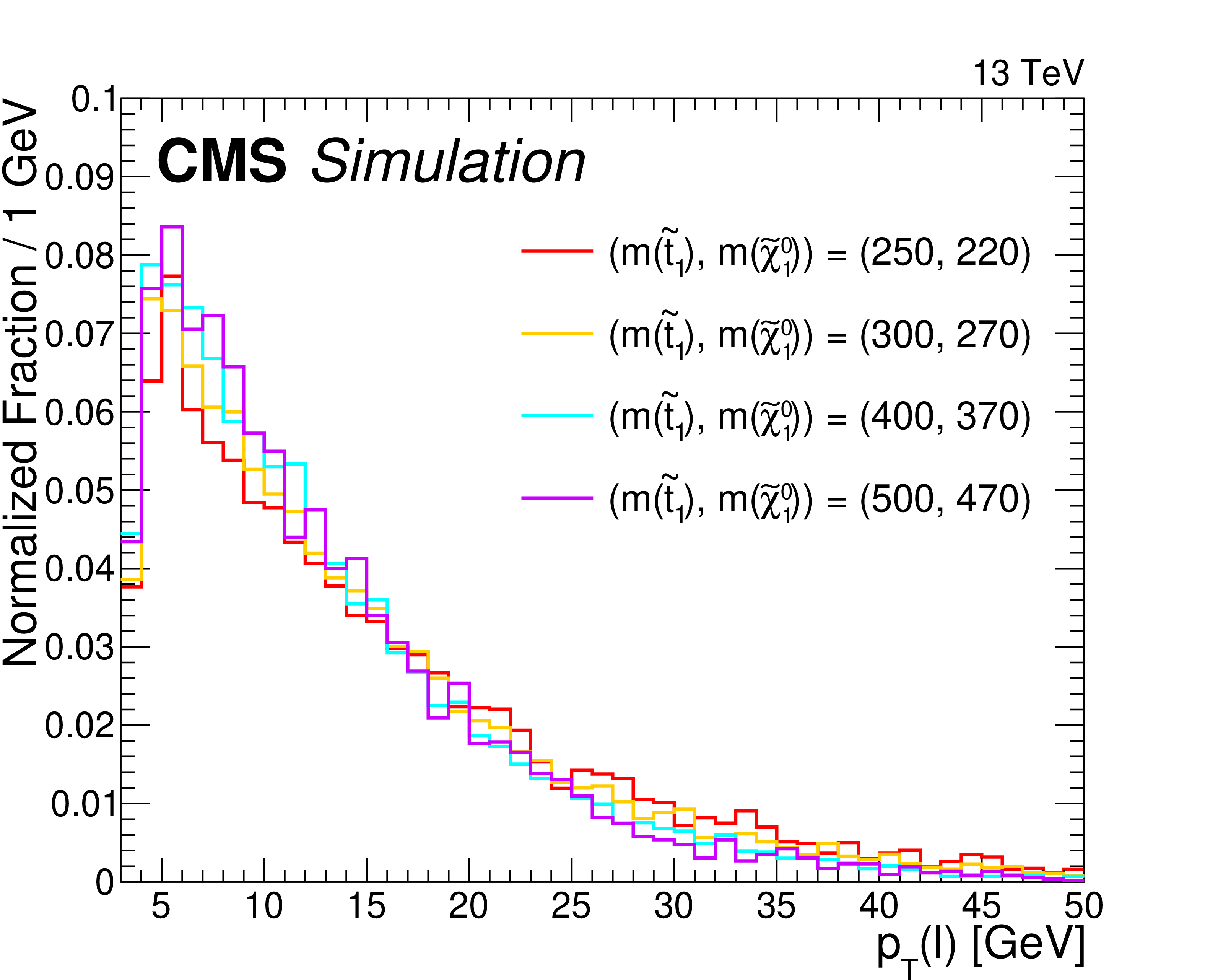
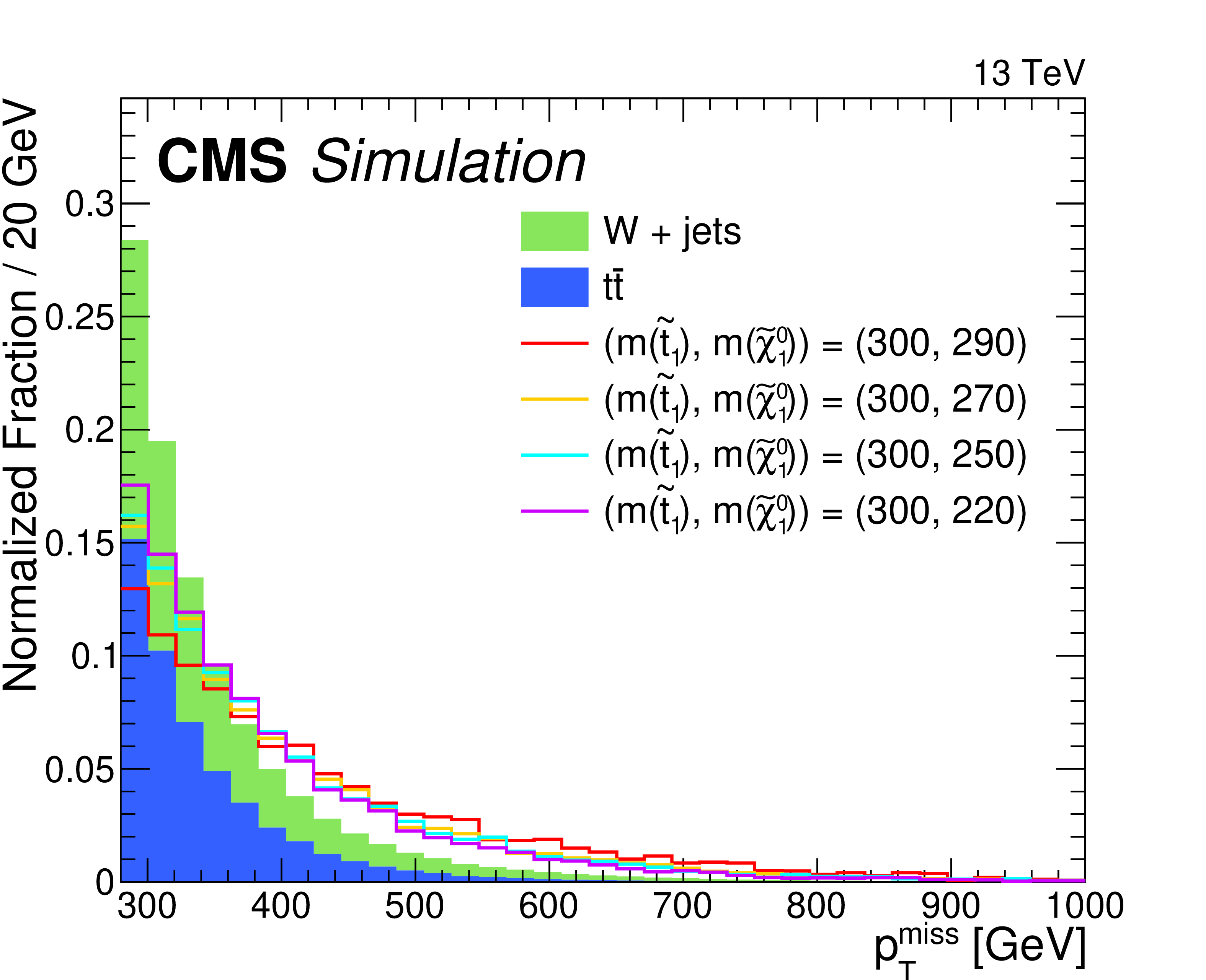
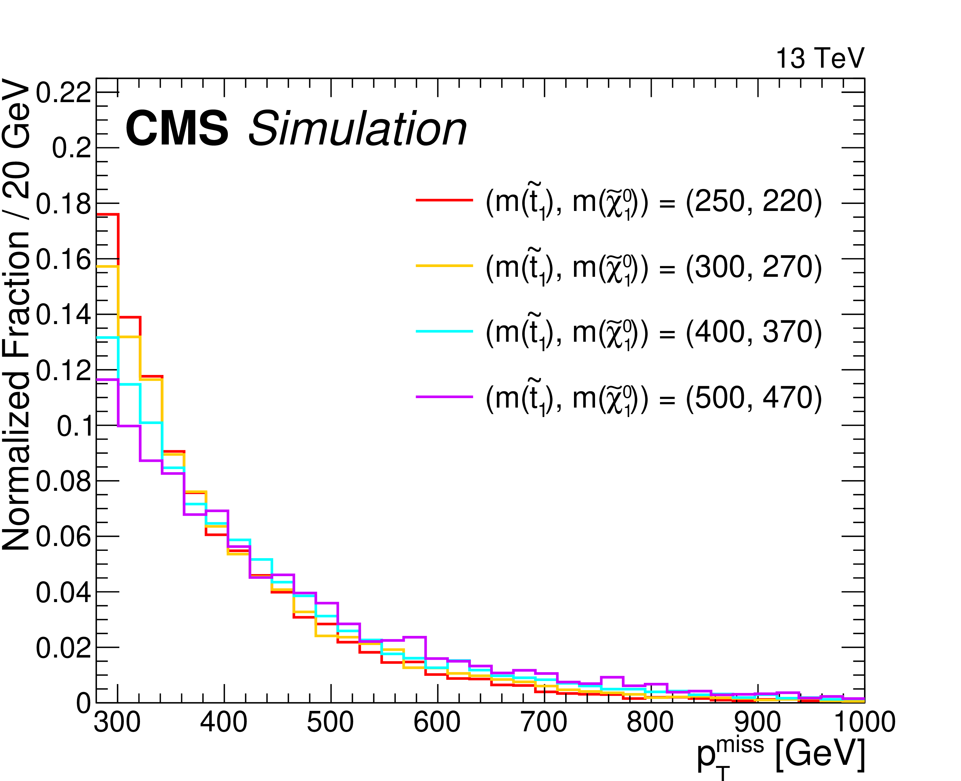
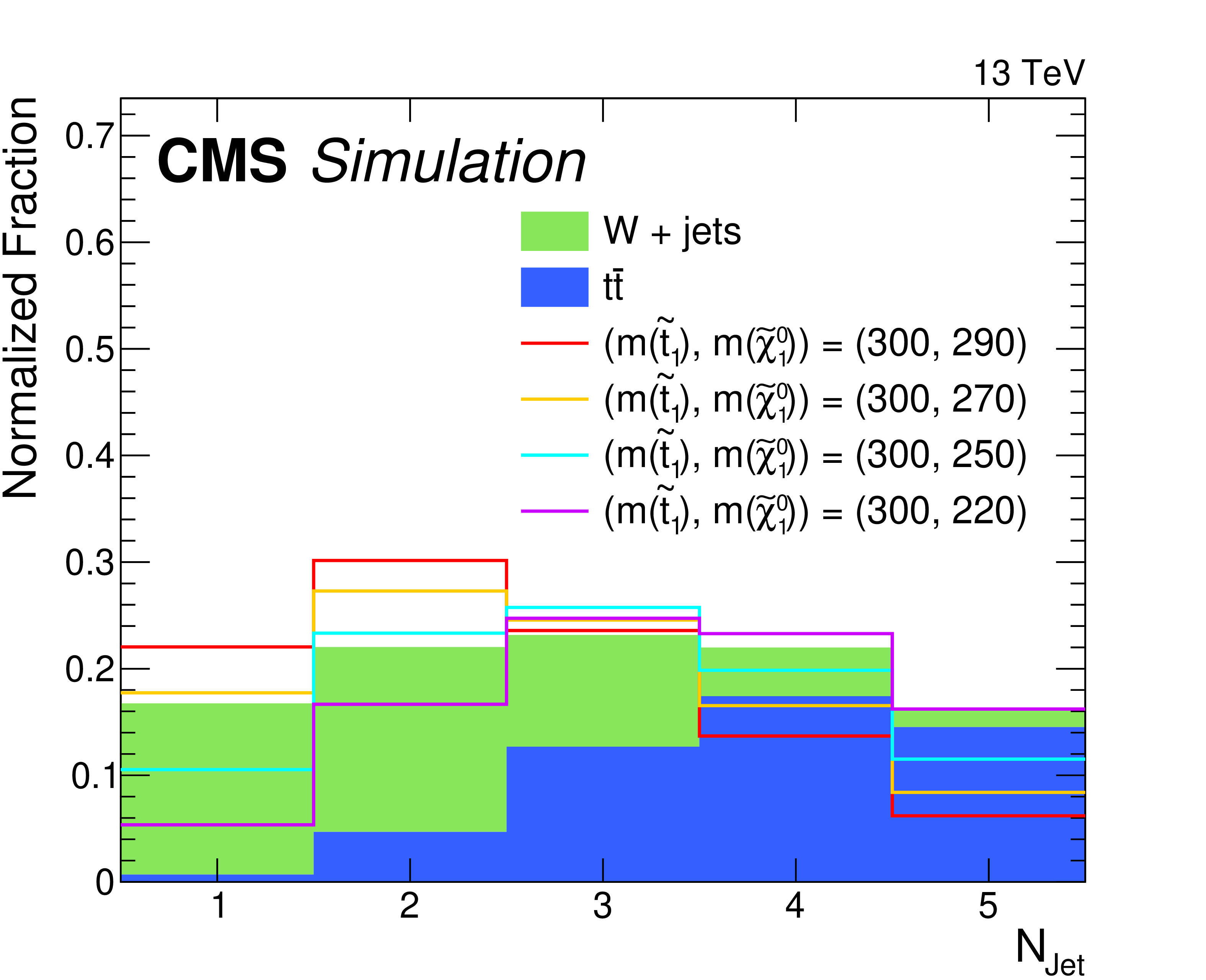
Figure 3:
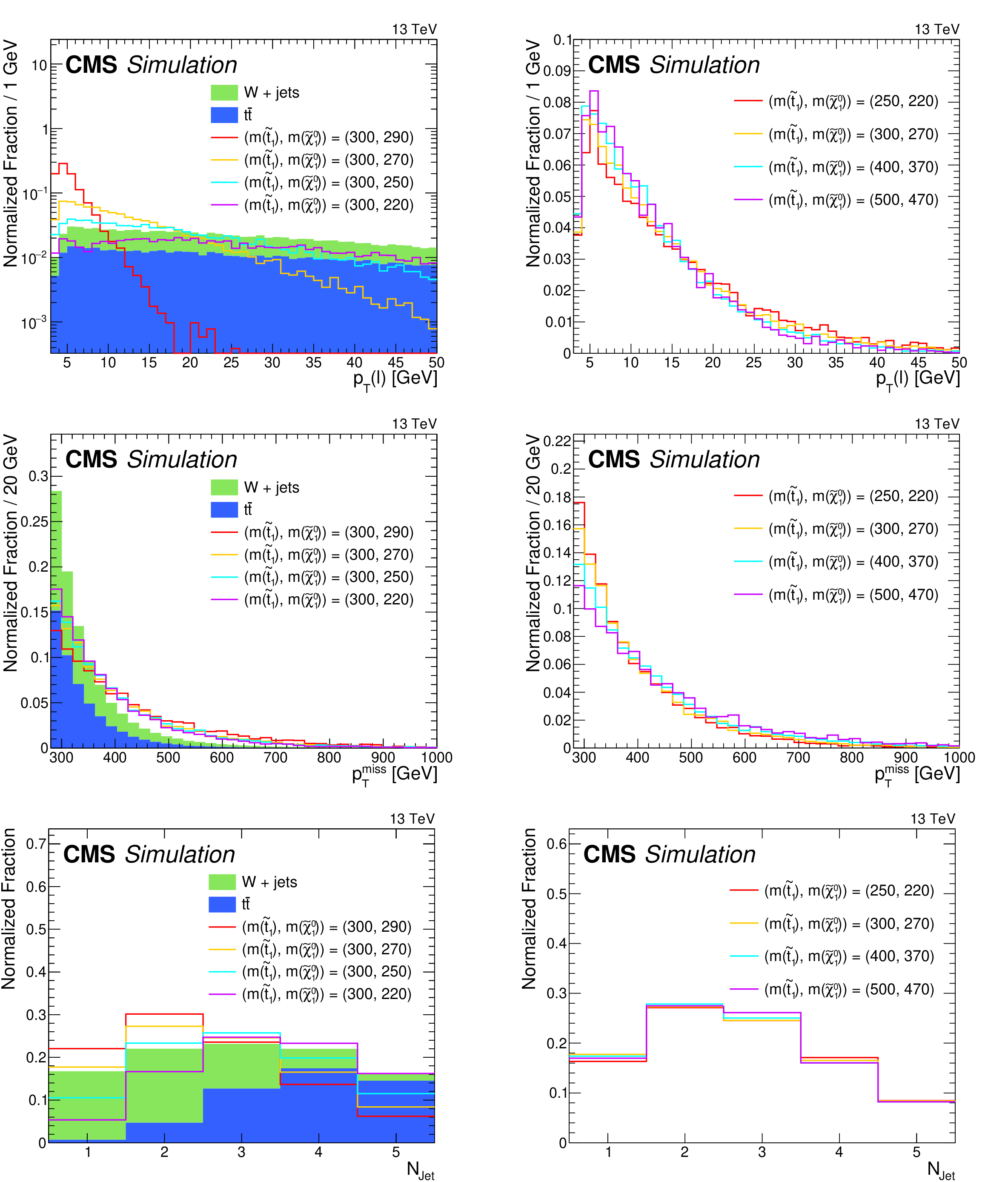
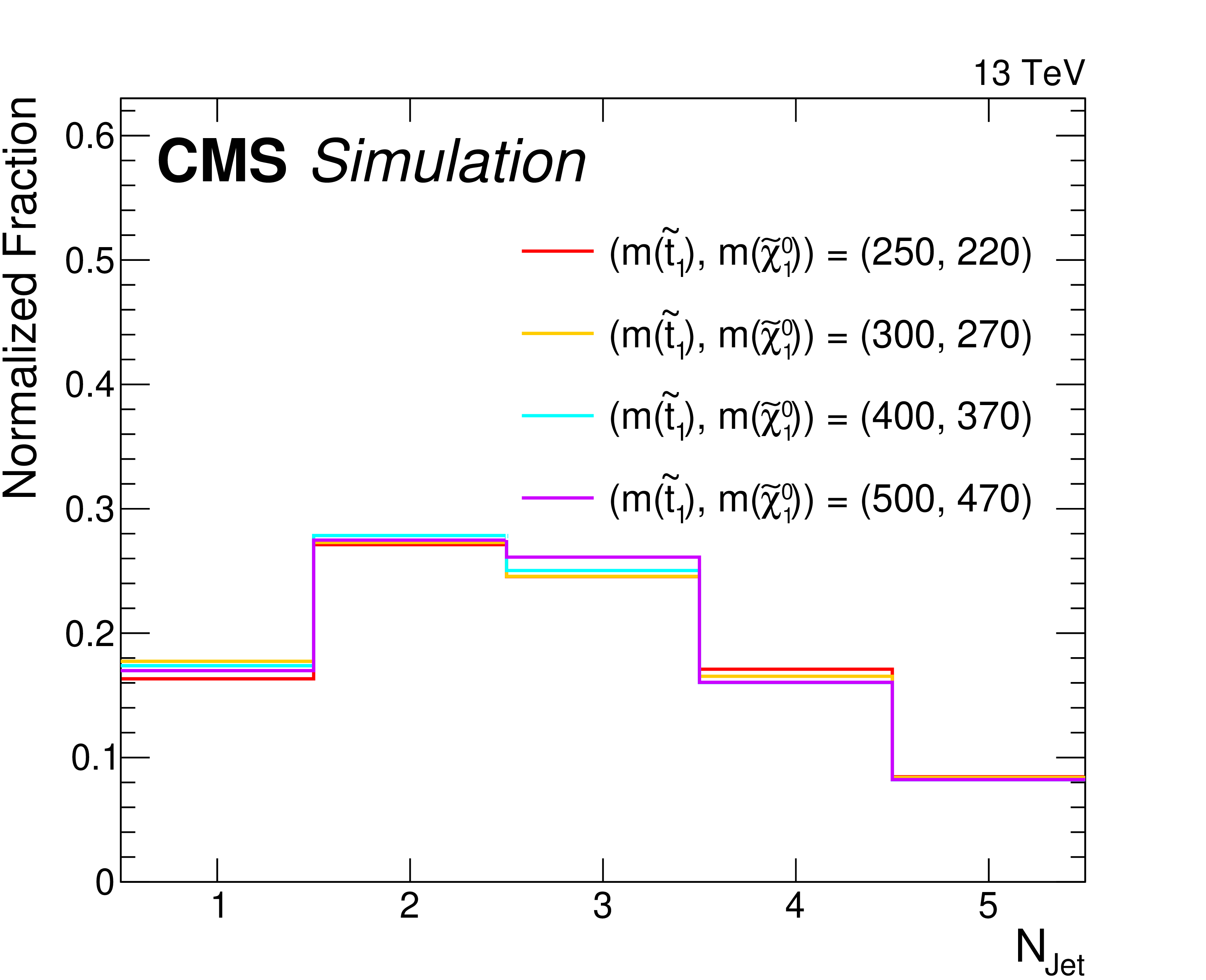
Simulated distributions of $ p_{\mathrm{T}}(\ell) $ (upper), $ p_{\mathrm{T}}^\text{miss} $ (middle), and $ N_{\text{jet}} $ (lower) after the preselection. The W+jets and $ \mathrm{t} \overline{\mathrm{t}} $ background distributions are shown as colored histograms, and the signal distributions by the solid lines. The total background distribution and the signal distributions are all normalized to unit area. On the left, the signal distributions are given for a top squark mass of 300 GeV and $ \Delta {m}= $ 10, 30, 50, and 80 GeV. On the right, the signal distributions are shown for four different $ ({m}(\tilde{\mathrm{t}}_{1}), {m}(\tilde{\chi}_{1}^{0})) $ values, all corresponding to the same $ \Delta {m}= $ 30 GeV. |

png pdf |
Figure 3-a:
Simulated distributions of $ p_{\mathrm{T}}(\ell) $ (upper), $ p_{\mathrm{T}}^\text{miss} $ (middle), and $ N_{\text{jet}} $ (lower) after the preselection. The W+jets and $ \mathrm{t} \overline{\mathrm{t}} $ background distributions are shown as colored histograms, and the signal distributions by the solid lines. The total background distribution and the signal distributions are all normalized to unit area. On the left, the signal distributions are given for a top squark mass of 300 GeV and $ \Delta {m}= $ 10, 30, 50, and 80 GeV. On the right, the signal distributions are shown for four different $ ({m}(\tilde{\mathrm{t}}_{1}), {m}(\tilde{\chi}_{1}^{0})) $ values, all corresponding to the same $ \Delta {m}= $ 30 GeV. |
png pdf |
Figure 3-b:
Simulated distributions of $ p_{\mathrm{T}}(\ell) $ (upper), $ p_{\mathrm{T}}^\text{miss} $ (middle), and $ N_{\text{jet}} $ (lower) after the preselection. The W+jets and $ \mathrm{t} \overline{\mathrm{t}} $ background distributions are shown as colored histograms, and the signal distributions by the solid lines. The total background distribution and the signal distributions are all normalized to unit area. On the left, the signal distributions are given for a top squark mass of 300 GeV and $ \Delta {m}= $ 10, 30, 50, and 80 GeV. On the right, the signal distributions are shown for four different $ ({m}(\tilde{\mathrm{t}}_{1}), {m}(\tilde{\chi}_{1}^{0})) $ values, all corresponding to the same $ \Delta {m}= $ 30 GeV. |
png pdf |
Figure 3-c:
Simulated distributions of $ p_{\mathrm{T}}(\ell) $ (upper), $ p_{\mathrm{T}}^\text{miss} $ (middle), and $ N_{\text{jet}} $ (lower) after the preselection. The W+jets and $ \mathrm{t} \overline{\mathrm{t}} $ background distributions are shown as colored histograms, and the signal distributions by the solid lines. The total background distribution and the signal distributions are all normalized to unit area. On the left, the signal distributions are given for a top squark mass of 300 GeV and $ \Delta {m}= $ 10, 30, 50, and 80 GeV. On the right, the signal distributions are shown for four different $ ({m}(\tilde{\mathrm{t}}_{1}), {m}(\tilde{\chi}_{1}^{0})) $ values, all corresponding to the same $ \Delta {m}= $ 30 GeV. |
png pdf |
Figure 3-d:
Simulated distributions of $ p_{\mathrm{T}}(\ell) $ (upper), $ p_{\mathrm{T}}^\text{miss} $ (middle), and $ N_{\text{jet}} $ (lower) after the preselection. The W+jets and $ \mathrm{t} \overline{\mathrm{t}} $ background distributions are shown as colored histograms, and the signal distributions by the solid lines. The total background distribution and the signal distributions are all normalized to unit area. On the left, the signal distributions are given for a top squark mass of 300 GeV and $ \Delta {m}= $ 10, 30, 50, and 80 GeV. On the right, the signal distributions are shown for four different $ ({m}(\tilde{\mathrm{t}}_{1}), {m}(\tilde{\chi}_{1}^{0})) $ values, all corresponding to the same $ \Delta {m}= $ 30 GeV. |
png pdf |
Figure 3-e:
Simulated distributions of $ p_{\mathrm{T}}(\ell) $ (upper), $ p_{\mathrm{T}}^\text{miss} $ (middle), and $ N_{\text{jet}} $ (lower) after the preselection. The W+jets and $ \mathrm{t} \overline{\mathrm{t}} $ background distributions are shown as colored histograms, and the signal distributions by the solid lines. The total background distribution and the signal distributions are all normalized to unit area. On the left, the signal distributions are given for a top squark mass of 300 GeV and $ \Delta {m}= $ 10, 30, 50, and 80 GeV. On the right, the signal distributions are shown for four different $ ({m}(\tilde{\mathrm{t}}_{1}), {m}(\tilde{\chi}_{1}^{0})) $ values, all corresponding to the same $ \Delta {m}= $ 30 GeV. |
png pdf |
Figure 3-f:
Simulated distributions of $ p_{\mathrm{T}}(\ell) $ (upper), $ p_{\mathrm{T}}^\text{miss} $ (middle), and $ N_{\text{jet}} $ (lower) after the preselection. The W+jets and $ \mathrm{t} \overline{\mathrm{t}} $ background distributions are shown as colored histograms, and the signal distributions by the solid lines. The total background distribution and the signal distributions are all normalized to unit area. On the left, the signal distributions are given for a top squark mass of 300 GeV and $ \Delta {m}= $ 10, 30, 50, and 80 GeV. On the right, the signal distributions are shown for four different $ ({m}(\tilde{\mathrm{t}}_{1}), {m}(\tilde{\chi}_{1}^{0})) $ values, all corresponding to the same $ \Delta {m}= $ 30 GeV. |

png pdf |
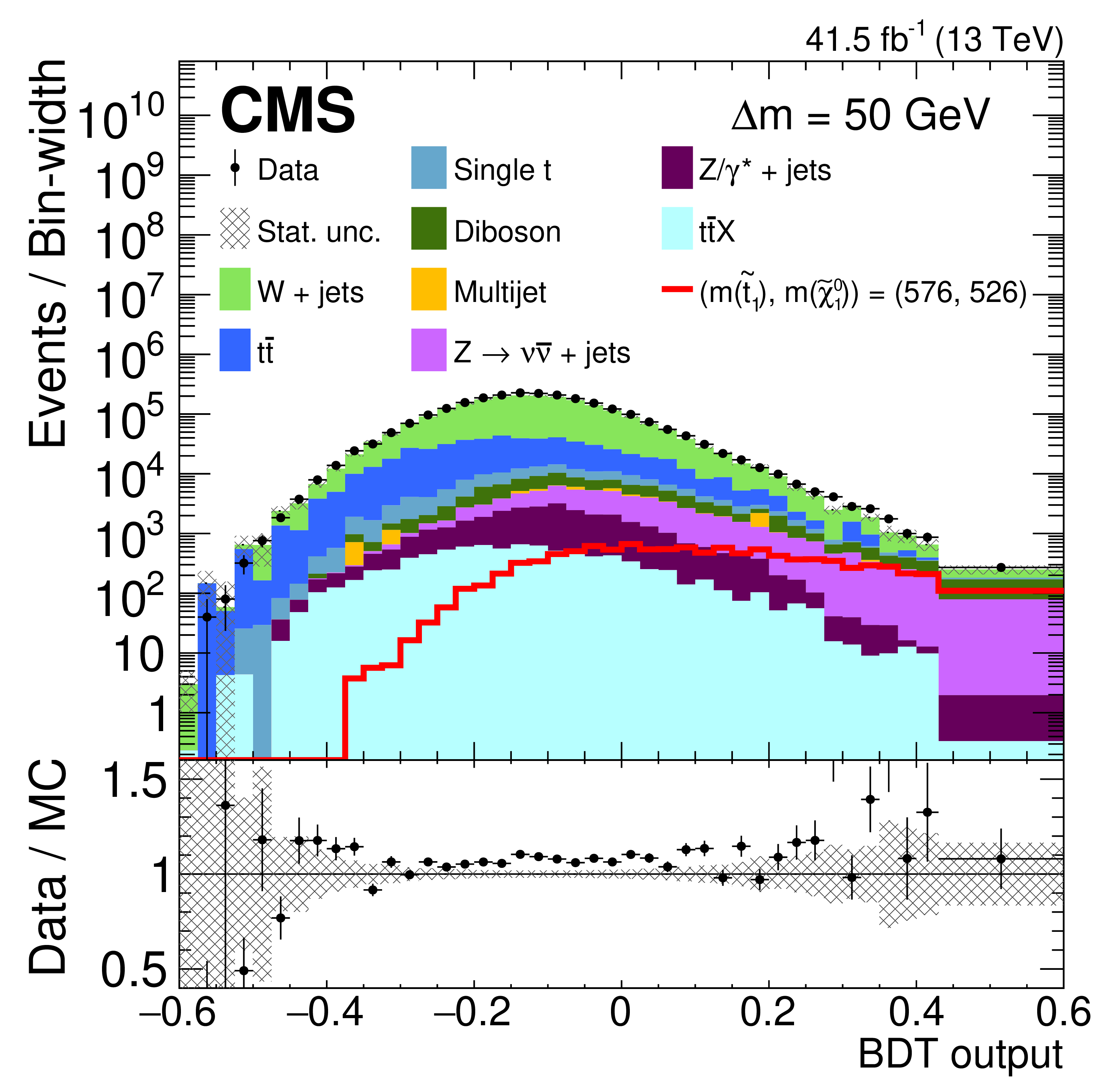
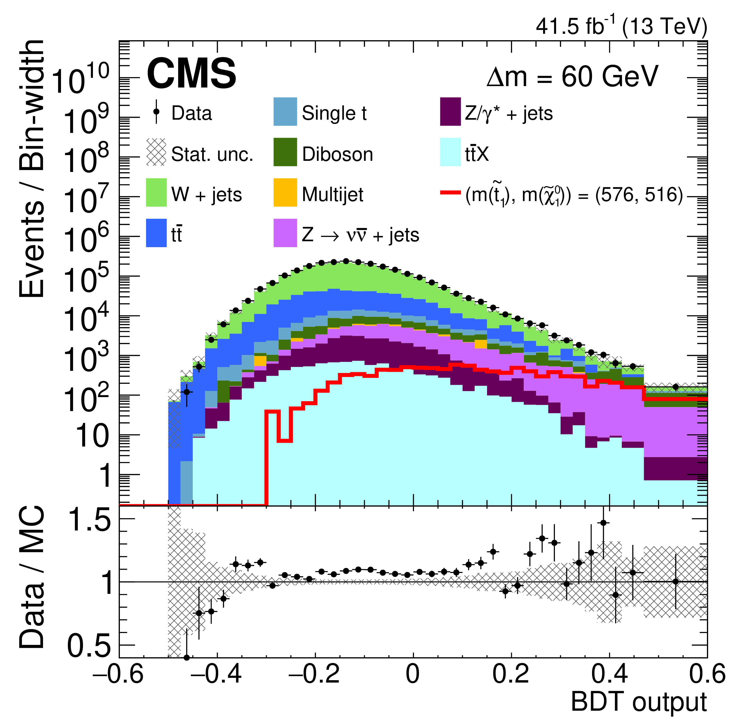
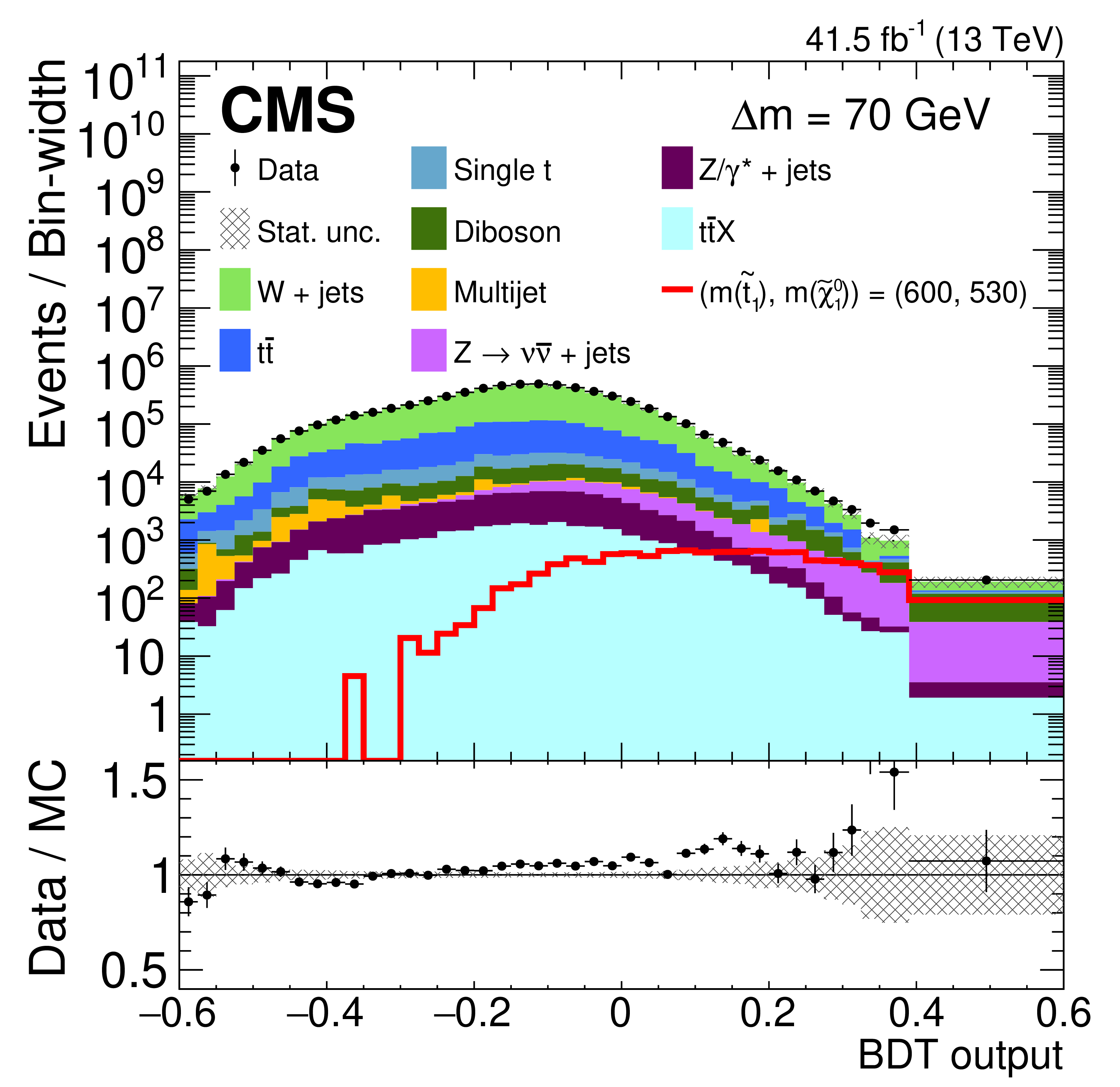
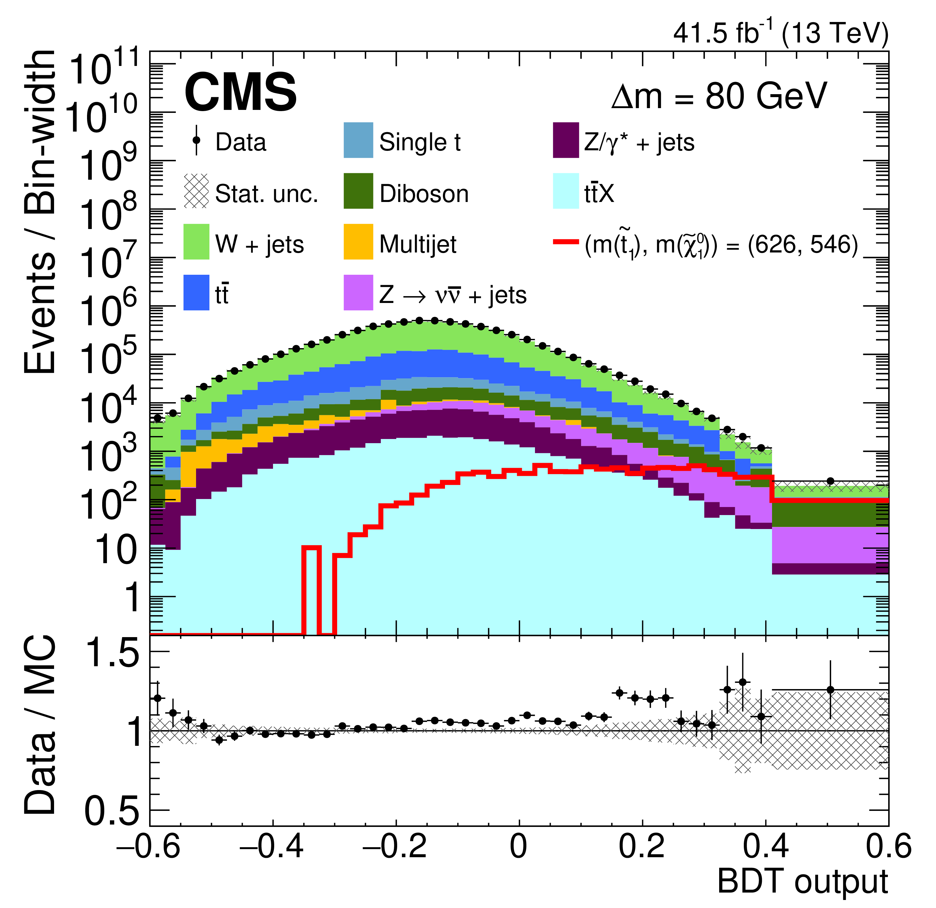
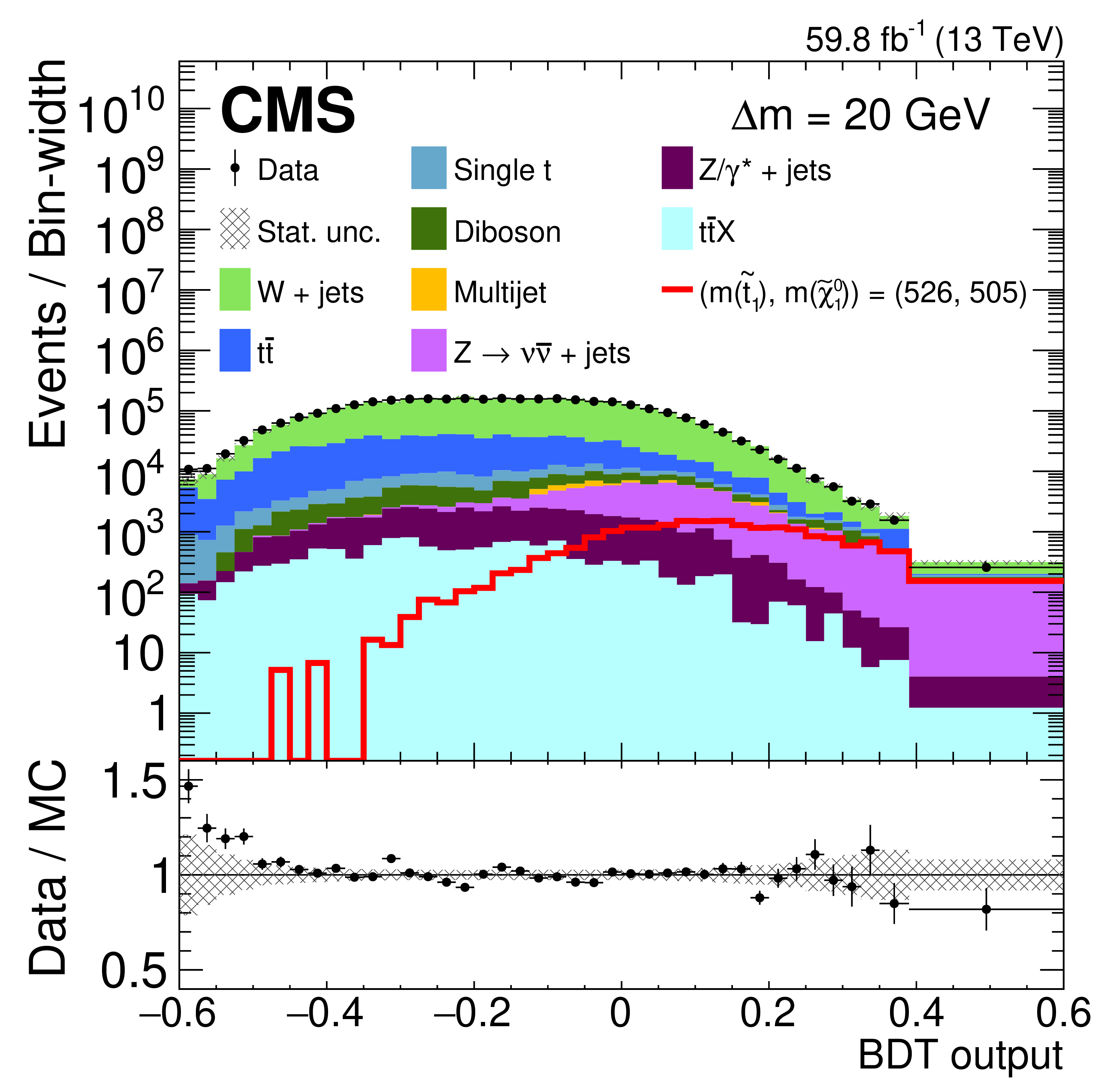
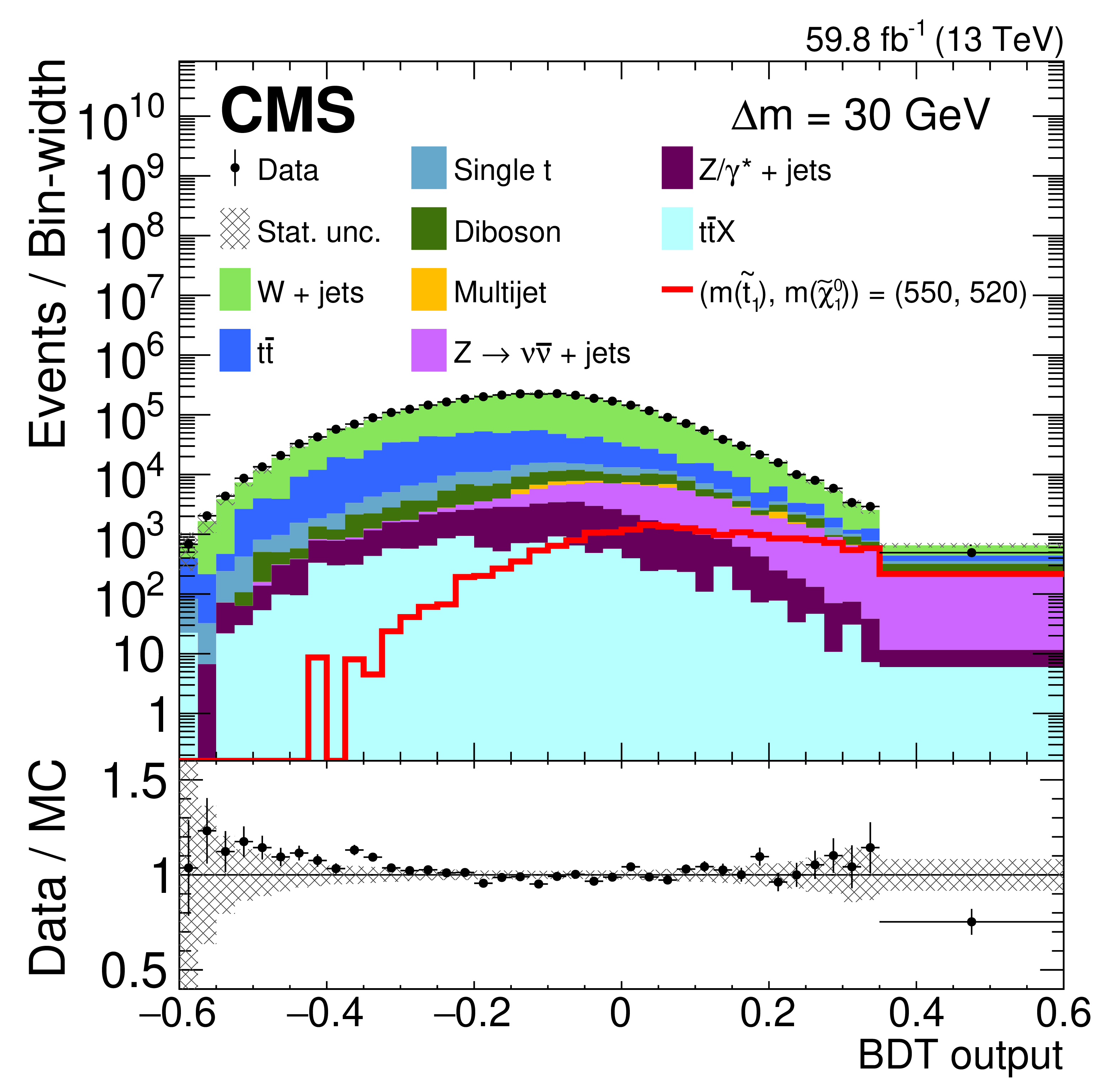
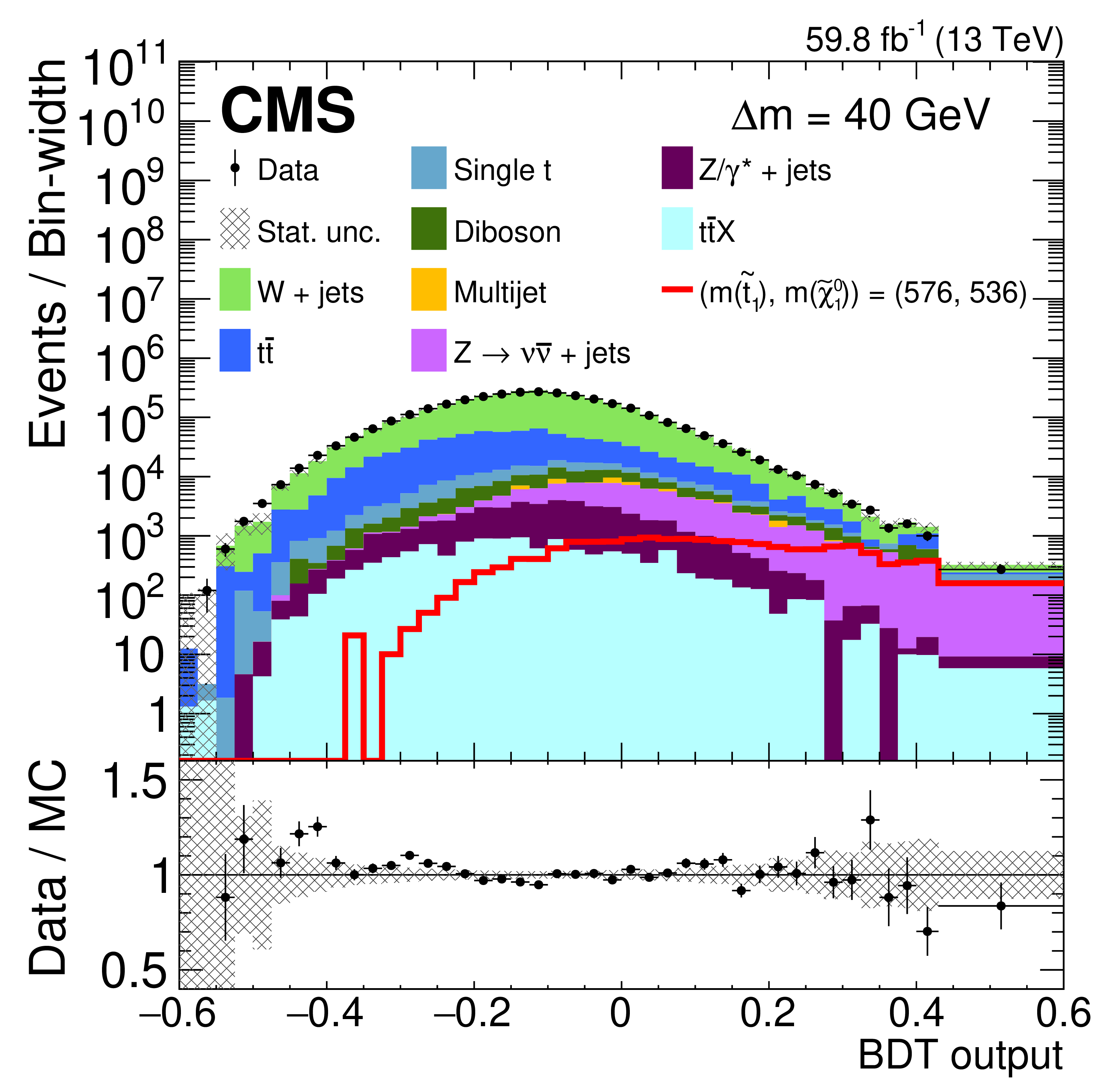
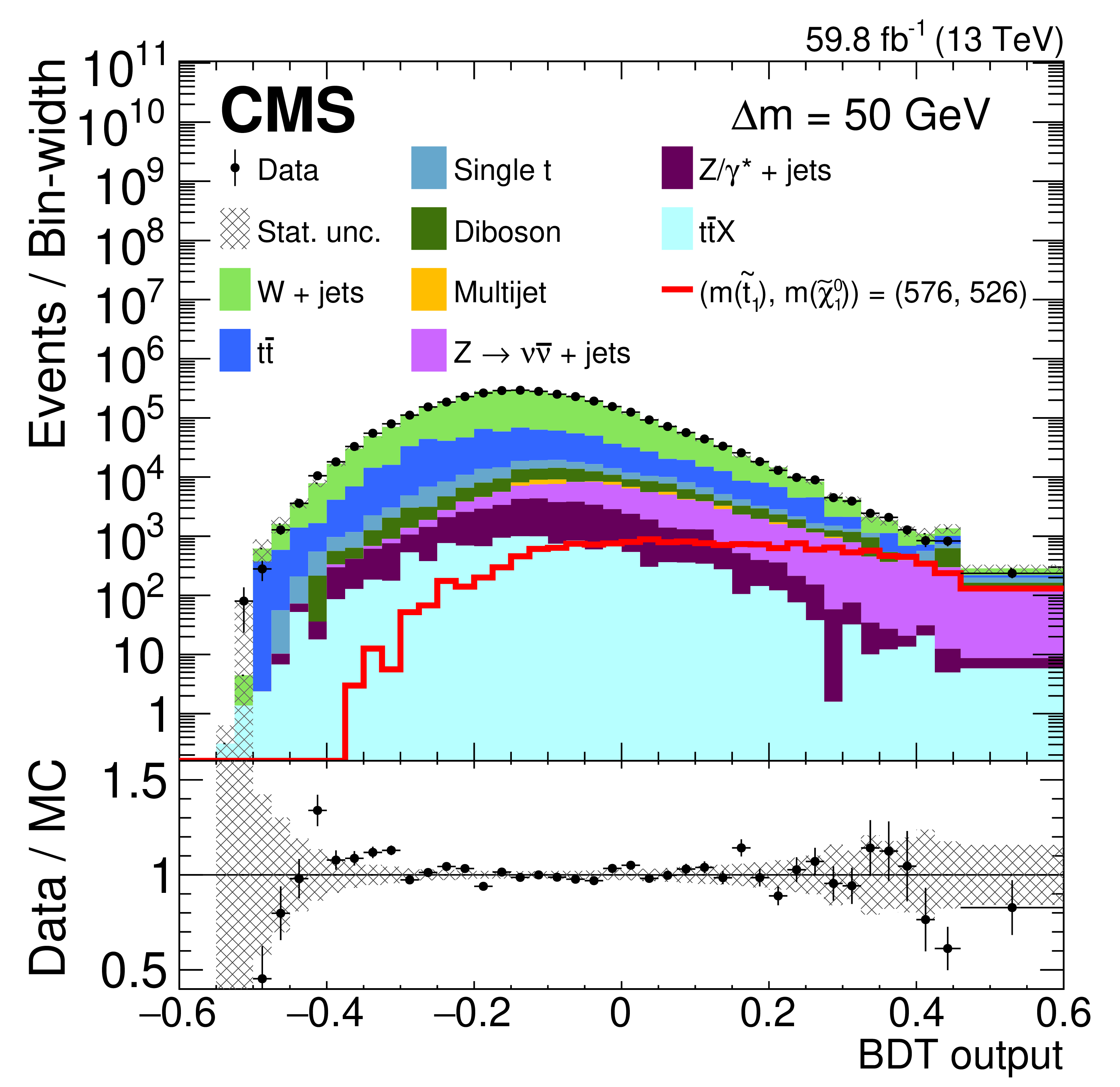
Figure 4:
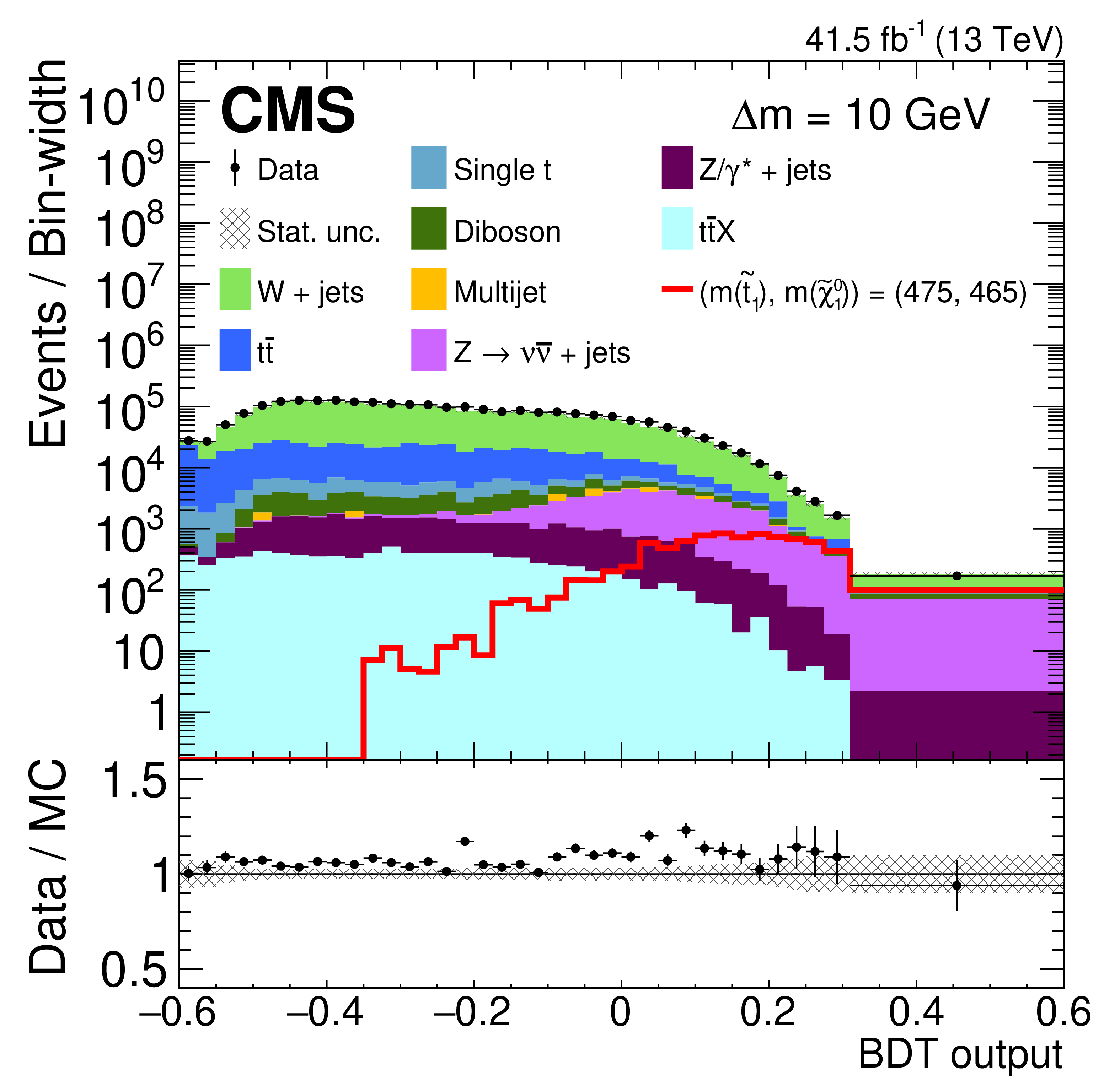
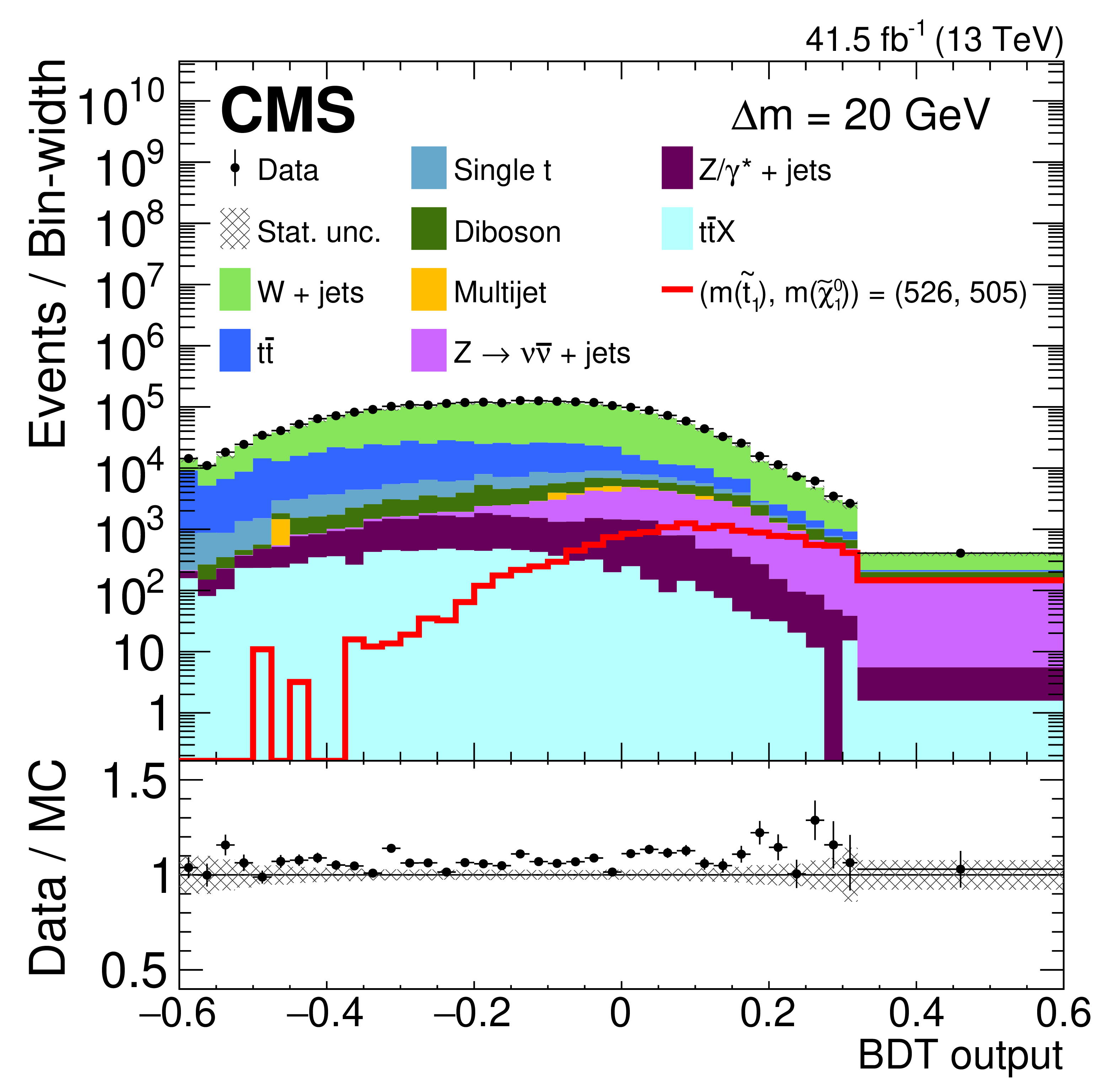
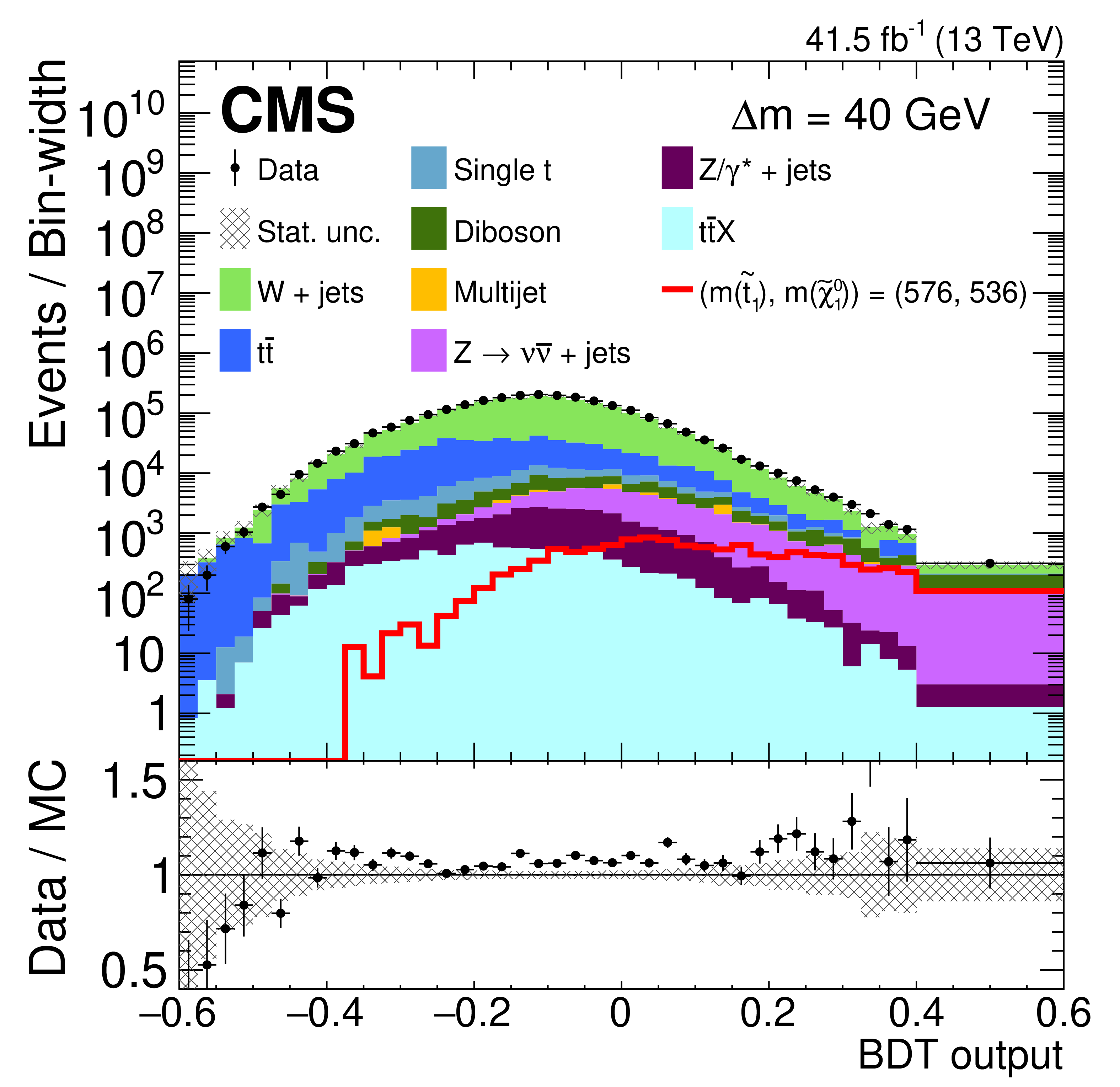
BDT output distributions from data (points) and simulation (colored histograms) after the preselection in 10 GeV steps of $ \Delta {m} $ from 10 (upper left) to 80 (lower right) GeV for the 2017 data. The last bin corresponds to the SR. For each $ \Delta {m} $ value, the predicted signal distribution is shown by the solid red line for a representative $ ({m}(\tilde{\mathrm{t}}_{1}), {m}(\tilde{\chi}_{1}^{0})) $ point, unstacked from the histograms. The lower panels show the ratio of the data to the sum of the background predictions, with the vertical bars and shaded area giving only the statistical uncertainty in the data and the simulated background, respectively. |
png pdf |
Figure 4-a:
BDT output distributions from data (points) and simulation (colored histograms) after the preselection in 10 GeV steps of $ \Delta {m} $ from 10 (upper left) to 80 (lower right) GeV for the 2017 data. The last bin corresponds to the SR. For each $ \Delta {m} $ value, the predicted signal distribution is shown by the solid red line for a representative $ ({m}(\tilde{\mathrm{t}}_{1}), {m}(\tilde{\chi}_{1}^{0})) $ point, unstacked from the histograms. The lower panels show the ratio of the data to the sum of the background predictions, with the vertical bars and shaded area giving only the statistical uncertainty in the data and the simulated background, respectively. |
png pdf |
Figure 4-b:
BDT output distributions from data (points) and simulation (colored histograms) after the preselection in 10 GeV steps of $ \Delta {m} $ from 10 (upper left) to 80 (lower right) GeV for the 2017 data. The last bin corresponds to the SR. For each $ \Delta {m} $ value, the predicted signal distribution is shown by the solid red line for a representative $ ({m}(\tilde{\mathrm{t}}_{1}), {m}(\tilde{\chi}_{1}^{0})) $ point, unstacked from the histograms. The lower panels show the ratio of the data to the sum of the background predictions, with the vertical bars and shaded area giving only the statistical uncertainty in the data and the simulated background, respectively. |

png pdf |
Figure 4-c:
BDT output distributions from data (points) and simulation (colored histograms) after the preselection in 10 GeV steps of $ \Delta {m} $ from 10 (upper left) to 80 (lower right) GeV for the 2017 data. The last bin corresponds to the SR. For each $ \Delta {m} $ value, the predicted signal distribution is shown by the solid red line for a representative $ ({m}(\tilde{\mathrm{t}}_{1}), {m}(\tilde{\chi}_{1}^{0})) $ point, unstacked from the histograms. The lower panels show the ratio of the data to the sum of the background predictions, with the vertical bars and shaded area giving only the statistical uncertainty in the data and the simulated background, respectively. |
png pdf |
Figure 4-d:
BDT output distributions from data (points) and simulation (colored histograms) after the preselection in 10 GeV steps of $ \Delta {m} $ from 10 (upper left) to 80 (lower right) GeV for the 2017 data. The last bin corresponds to the SR. For each $ \Delta {m} $ value, the predicted signal distribution is shown by the solid red line for a representative $ ({m}(\tilde{\mathrm{t}}_{1}), {m}(\tilde{\chi}_{1}^{0})) $ point, unstacked from the histograms. The lower panels show the ratio of the data to the sum of the background predictions, with the vertical bars and shaded area giving only the statistical uncertainty in the data and the simulated background, respectively. |
png pdf |
Figure 4-e:
BDT output distributions from data (points) and simulation (colored histograms) after the preselection in 10 GeV steps of $ \Delta {m} $ from 10 (upper left) to 80 (lower right) GeV for the 2017 data. The last bin corresponds to the SR. For each $ \Delta {m} $ value, the predicted signal distribution is shown by the solid red line for a representative $ ({m}(\tilde{\mathrm{t}}_{1}), {m}(\tilde{\chi}_{1}^{0})) $ point, unstacked from the histograms. The lower panels show the ratio of the data to the sum of the background predictions, with the vertical bars and shaded area giving only the statistical uncertainty in the data and the simulated background, respectively. |
png pdf |
Figure 4-f:
BDT output distributions from data (points) and simulation (colored histograms) after the preselection in 10 GeV steps of $ \Delta {m} $ from 10 (upper left) to 80 (lower right) GeV for the 2017 data. The last bin corresponds to the SR. For each $ \Delta {m} $ value, the predicted signal distribution is shown by the solid red line for a representative $ ({m}(\tilde{\mathrm{t}}_{1}), {m}(\tilde{\chi}_{1}^{0})) $ point, unstacked from the histograms. The lower panels show the ratio of the data to the sum of the background predictions, with the vertical bars and shaded area giving only the statistical uncertainty in the data and the simulated background, respectively. |
png pdf |
Figure 4-g:
BDT output distributions from data (points) and simulation (colored histograms) after the preselection in 10 GeV steps of $ \Delta {m} $ from 10 (upper left) to 80 (lower right) GeV for the 2017 data. The last bin corresponds to the SR. For each $ \Delta {m} $ value, the predicted signal distribution is shown by the solid red line for a representative $ ({m}(\tilde{\mathrm{t}}_{1}), {m}(\tilde{\chi}_{1}^{0})) $ point, unstacked from the histograms. The lower panels show the ratio of the data to the sum of the background predictions, with the vertical bars and shaded area giving only the statistical uncertainty in the data and the simulated background, respectively. |
png pdf |
Figure 4-h:
BDT output distributions from data (points) and simulation (colored histograms) after the preselection in 10 GeV steps of $ \Delta {m} $ from 10 (upper left) to 80 (lower right) GeV for the 2017 data. The last bin corresponds to the SR. For each $ \Delta {m} $ value, the predicted signal distribution is shown by the solid red line for a representative $ ({m}(\tilde{\mathrm{t}}_{1}), {m}(\tilde{\chi}_{1}^{0})) $ point, unstacked from the histograms. The lower panels show the ratio of the data to the sum of the background predictions, with the vertical bars and shaded area giving only the statistical uncertainty in the data and the simulated background, respectively. |

png pdf |
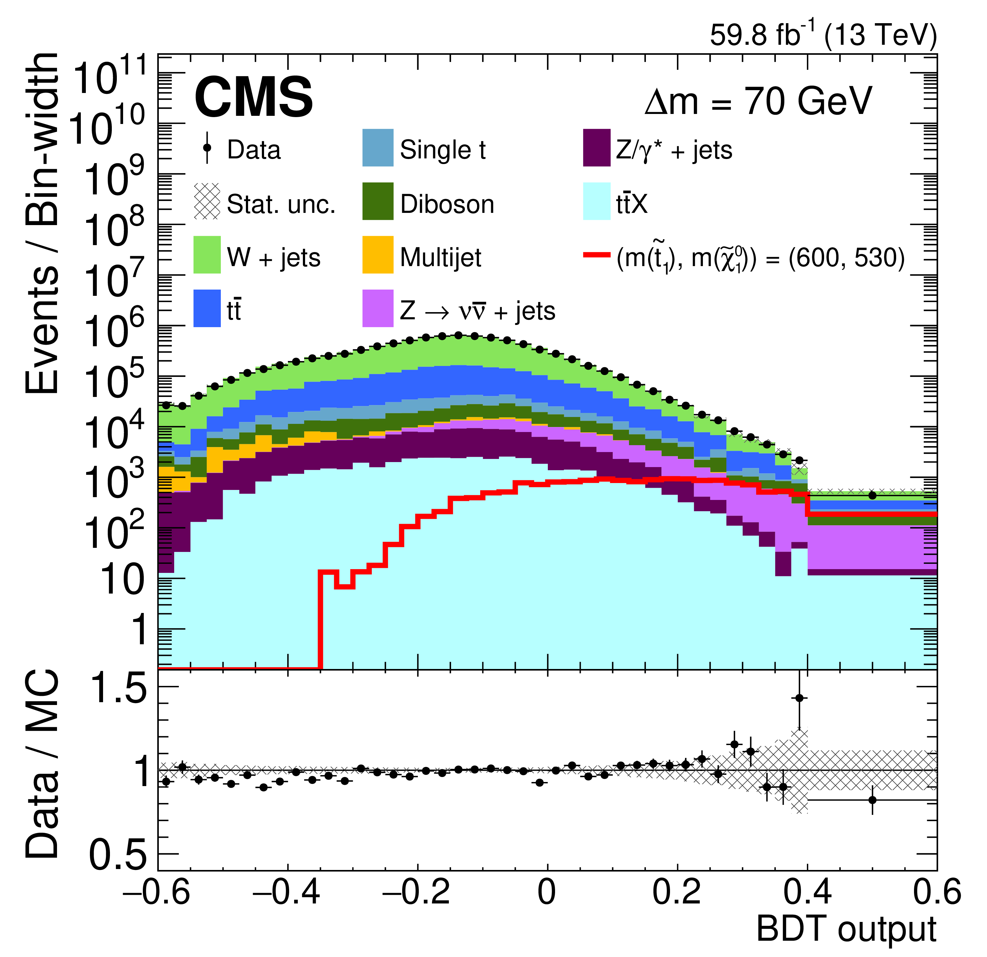
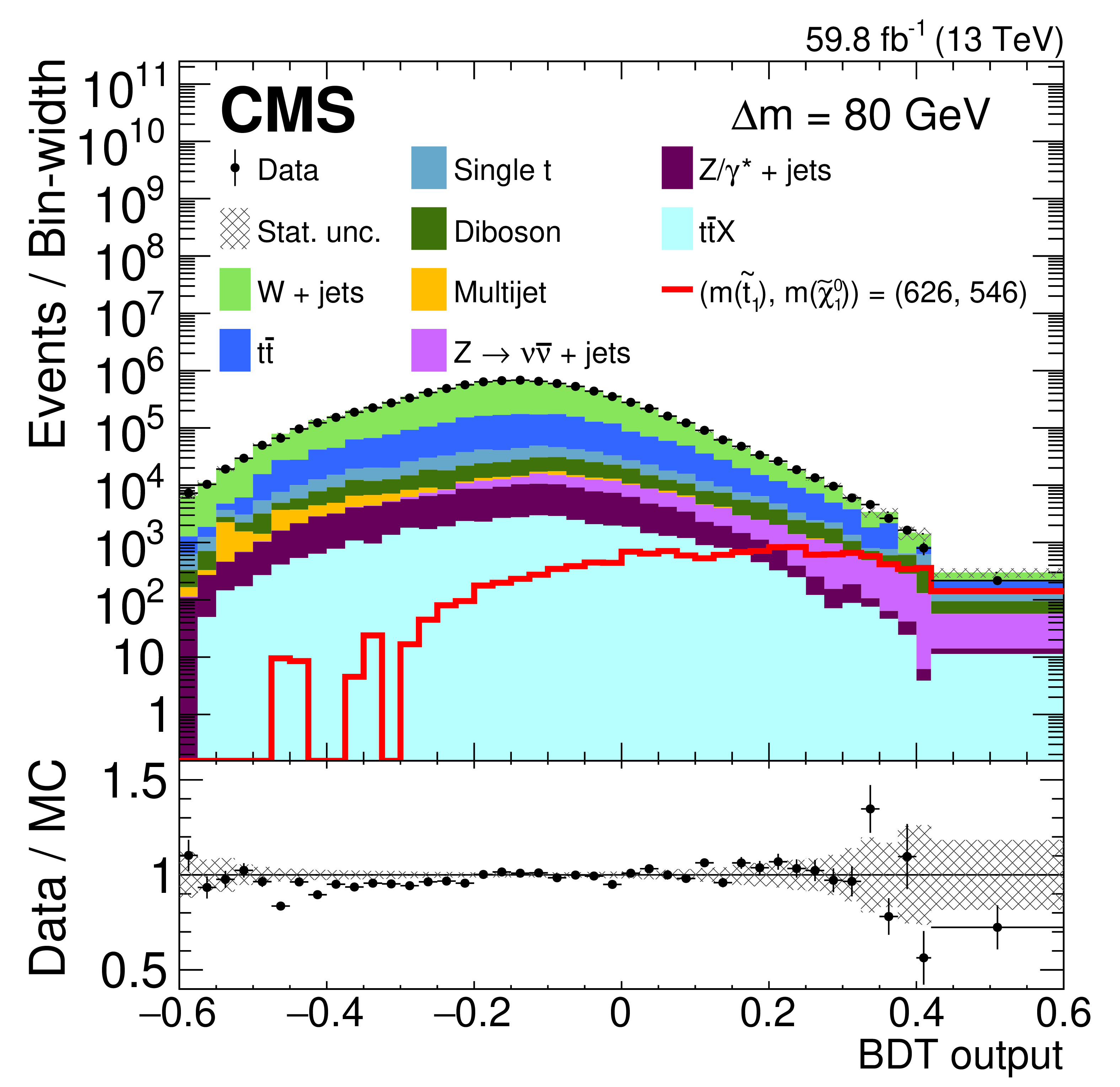
Figure 5:
BDT output distributions from data (points) and simulation (colored histograms) after the preselection in 10 GeV steps of $ \Delta {m} $ from 10 (upper left) to 80 (lower right) GeV for the 2018 data. The last bin corresponds to the SR. For each $ \Delta {m} $ value, the predicted signal distribution is shown by the solid red line for a representative $ ({m}(\tilde{\mathrm{t}}_{1}), {m}(\tilde{\chi}_{1}^{0})) $ point, unstacked from the histograms. The lower panels show the ratio of the data to the sum of the background predictions, with the vertical bars and shaded area giving only the statistical uncertainty in the data and the simulated background, respectively. |

png pdf |
Figure 5-a:
BDT output distributions from data (points) and simulation (colored histograms) after the preselection in 10 GeV steps of $ \Delta {m} $ from 10 (upper left) to 80 (lower right) GeV for the 2018 data. The last bin corresponds to the SR. For each $ \Delta {m} $ value, the predicted signal distribution is shown by the solid red line for a representative $ ({m}(\tilde{\mathrm{t}}_{1}), {m}(\tilde{\chi}_{1}^{0})) $ point, unstacked from the histograms. The lower panels show the ratio of the data to the sum of the background predictions, with the vertical bars and shaded area giving only the statistical uncertainty in the data and the simulated background, respectively. |
png pdf |
Figure 5-b:
BDT output distributions from data (points) and simulation (colored histograms) after the preselection in 10 GeV steps of $ \Delta {m} $ from 10 (upper left) to 80 (lower right) GeV for the 2018 data. The last bin corresponds to the SR. For each $ \Delta {m} $ value, the predicted signal distribution is shown by the solid red line for a representative $ ({m}(\tilde{\mathrm{t}}_{1}), {m}(\tilde{\chi}_{1}^{0})) $ point, unstacked from the histograms. The lower panels show the ratio of the data to the sum of the background predictions, with the vertical bars and shaded area giving only the statistical uncertainty in the data and the simulated background, respectively. |
png pdf |
Figure 5-c:
BDT output distributions from data (points) and simulation (colored histograms) after the preselection in 10 GeV steps of $ \Delta {m} $ from 10 (upper left) to 80 (lower right) GeV for the 2018 data. The last bin corresponds to the SR. For each $ \Delta {m} $ value, the predicted signal distribution is shown by the solid red line for a representative $ ({m}(\tilde{\mathrm{t}}_{1}), {m}(\tilde{\chi}_{1}^{0})) $ point, unstacked from the histograms. The lower panels show the ratio of the data to the sum of the background predictions, with the vertical bars and shaded area giving only the statistical uncertainty in the data and the simulated background, respectively. |
png pdf |
Figure 5-d:
BDT output distributions from data (points) and simulation (colored histograms) after the preselection in 10 GeV steps of $ \Delta {m} $ from 10 (upper left) to 80 (lower right) GeV for the 2018 data. The last bin corresponds to the SR. For each $ \Delta {m} $ value, the predicted signal distribution is shown by the solid red line for a representative $ ({m}(\tilde{\mathrm{t}}_{1}), {m}(\tilde{\chi}_{1}^{0})) $ point, unstacked from the histograms. The lower panels show the ratio of the data to the sum of the background predictions, with the vertical bars and shaded area giving only the statistical uncertainty in the data and the simulated background, respectively. |
png pdf |
Figure 5-e:
BDT output distributions from data (points) and simulation (colored histograms) after the preselection in 10 GeV steps of $ \Delta {m} $ from 10 (upper left) to 80 (lower right) GeV for the 2018 data. The last bin corresponds to the SR. For each $ \Delta {m} $ value, the predicted signal distribution is shown by the solid red line for a representative $ ({m}(\tilde{\mathrm{t}}_{1}), {m}(\tilde{\chi}_{1}^{0})) $ point, unstacked from the histograms. The lower panels show the ratio of the data to the sum of the background predictions, with the vertical bars and shaded area giving only the statistical uncertainty in the data and the simulated background, respectively. |
png pdf |
Figure 5-f:
BDT output distributions from data (points) and simulation (colored histograms) after the preselection in 10 GeV steps of $ \Delta {m} $ from 10 (upper left) to 80 (lower right) GeV for the 2018 data. The last bin corresponds to the SR. For each $ \Delta {m} $ value, the predicted signal distribution is shown by the solid red line for a representative $ ({m}(\tilde{\mathrm{t}}_{1}), {m}(\tilde{\chi}_{1}^{0})) $ point, unstacked from the histograms. The lower panels show the ratio of the data to the sum of the background predictions, with the vertical bars and shaded area giving only the statistical uncertainty in the data and the simulated background, respectively. |
png pdf |
Figure 5-g:
BDT output distributions from data (points) and simulation (colored histograms) after the preselection in 10 GeV steps of $ \Delta {m} $ from 10 (upper left) to 80 (lower right) GeV for the 2018 data. The last bin corresponds to the SR. For each $ \Delta {m} $ value, the predicted signal distribution is shown by the solid red line for a representative $ ({m}(\tilde{\mathrm{t}}_{1}), {m}(\tilde{\chi}_{1}^{0})) $ point, unstacked from the histograms. The lower panels show the ratio of the data to the sum of the background predictions, with the vertical bars and shaded area giving only the statistical uncertainty in the data and the simulated background, respectively. |
png pdf |
Figure 5-h:
BDT output distributions from data (points) and simulation (colored histograms) after the preselection in 10 GeV steps of $ \Delta {m} $ from 10 (upper left) to 80 (lower right) GeV for the 2018 data. The last bin corresponds to the SR. For each $ \Delta {m} $ value, the predicted signal distribution is shown by the solid red line for a representative $ ({m}(\tilde{\mathrm{t}}_{1}), {m}(\tilde{\chi}_{1}^{0})) $ point, unstacked from the histograms. The lower panels show the ratio of the data to the sum of the background predictions, with the vertical bars and shaded area giving only the statistical uncertainty in the data and the simulated background, respectively. |
png pdf |
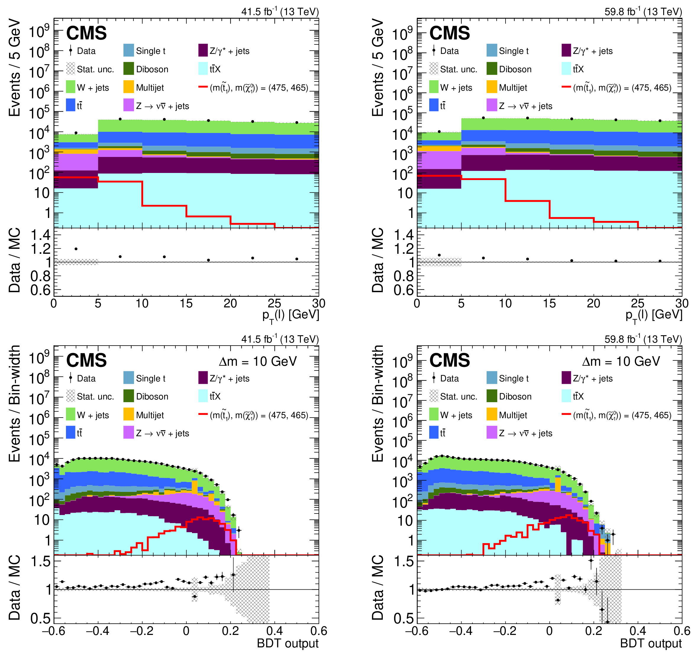
Figure 6:
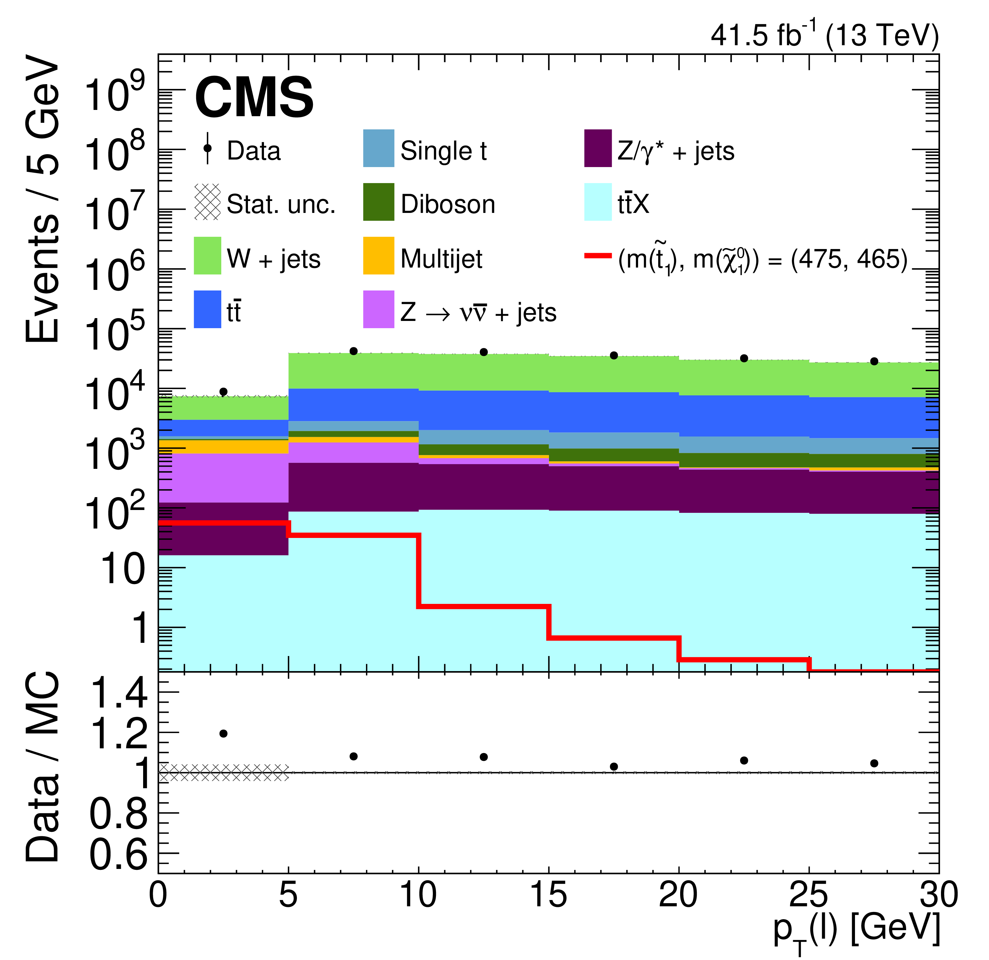
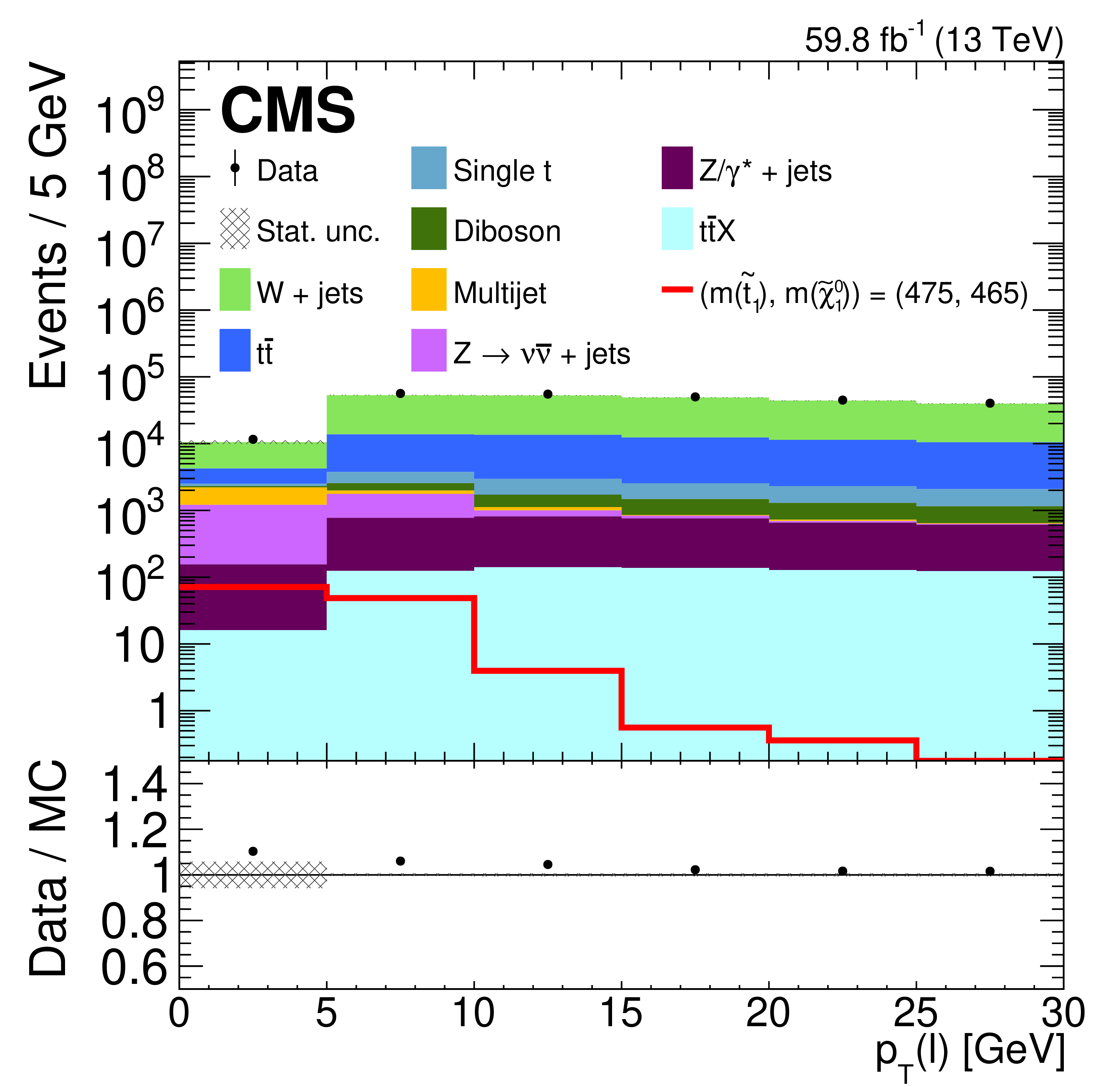
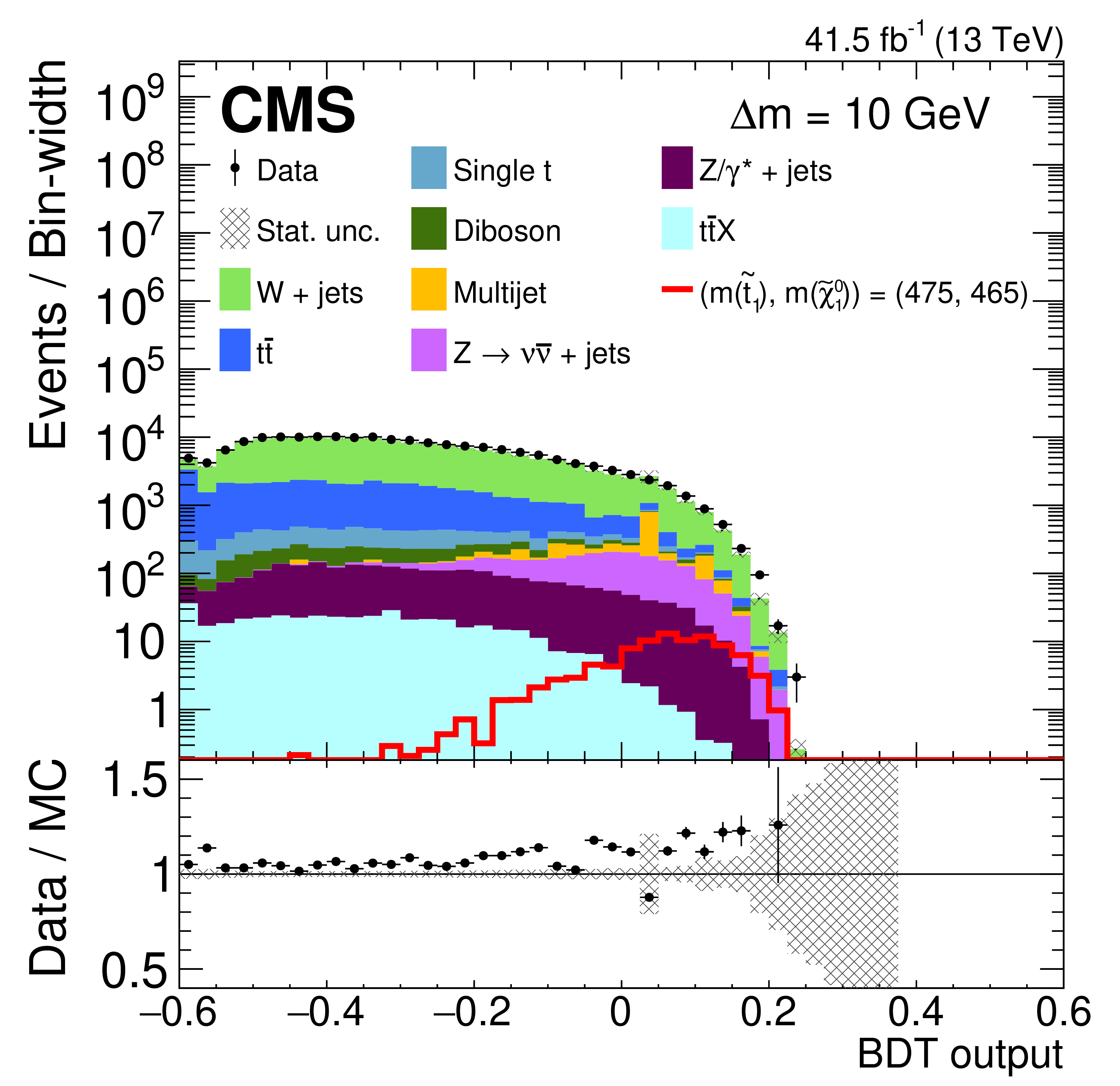
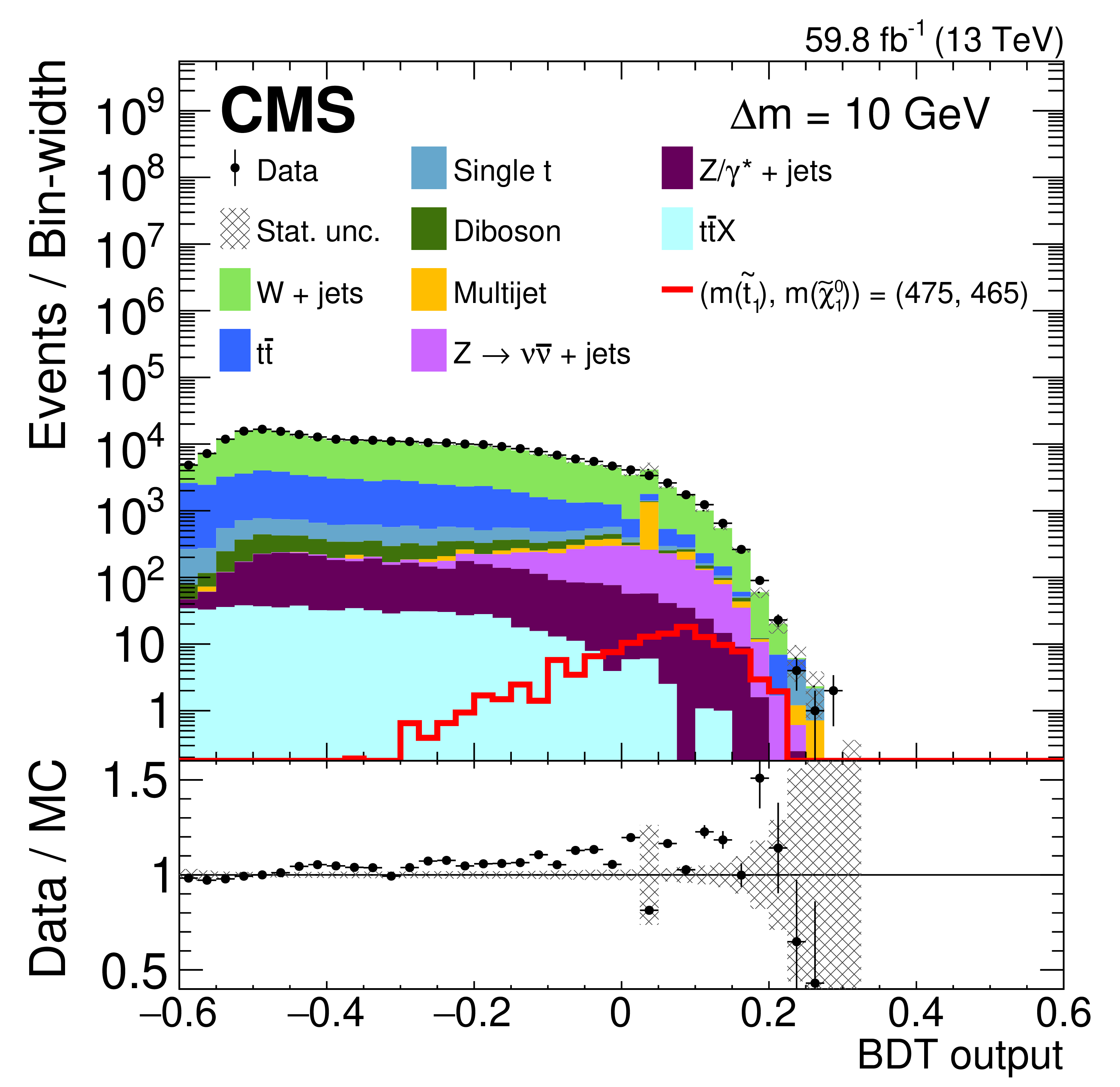
Distributions of $ p_{\mathrm{T}}(\ell) $ (upper) and BDT output for $ \Delta {m}= $ 10 GeV (lower) in the VR where 200 $ < p_{\mathrm{T}}^\text{miss} < $ 280 GeV, from 2017 (left) and 2018 (right) data (points) and simulation (colored histograms). The predicted signal distribution is shown by the solid red line for $ ({m}(\tilde{\mathrm{t}}_{1}), {m}(\tilde{\chi}_{1}^{0})) = $ (475, 465), unstacked from the histograms. The lower panels show the ratio of data to the sum of the simulated SM backgrounds. The shaded bands indicate only the statistical uncertainty in the simulation predictions. |
png pdf |
Figure 6-a:
Distributions of $ p_{\mathrm{T}}(\ell) $ (upper) and BDT output for $ \Delta {m}= $ 10 GeV (lower) in the VR where 200 $ < p_{\mathrm{T}}^\text{miss} < $ 280 GeV, from 2017 (left) and 2018 (right) data (points) and simulation (colored histograms). The predicted signal distribution is shown by the solid red line for $ ({m}(\tilde{\mathrm{t}}_{1}), {m}(\tilde{\chi}_{1}^{0})) = $ (475, 465), unstacked from the histograms. The lower panels show the ratio of data to the sum of the simulated SM backgrounds. The shaded bands indicate only the statistical uncertainty in the simulation predictions. |
png pdf |
Figure 6-b:
Distributions of $ p_{\mathrm{T}}(\ell) $ (upper) and BDT output for $ \Delta {m}= $ 10 GeV (lower) in the VR where 200 $ < p_{\mathrm{T}}^\text{miss} < $ 280 GeV, from 2017 (left) and 2018 (right) data (points) and simulation (colored histograms). The predicted signal distribution is shown by the solid red line for $ ({m}(\tilde{\mathrm{t}}_{1}), {m}(\tilde{\chi}_{1}^{0})) = $ (475, 465), unstacked from the histograms. The lower panels show the ratio of data to the sum of the simulated SM backgrounds. The shaded bands indicate only the statistical uncertainty in the simulation predictions. |
png pdf |
Figure 6-c:
Distributions of $ p_{\mathrm{T}}(\ell) $ (upper) and BDT output for $ \Delta {m}= $ 10 GeV (lower) in the VR where 200 $ < p_{\mathrm{T}}^\text{miss} < $ 280 GeV, from 2017 (left) and 2018 (right) data (points) and simulation (colored histograms). The predicted signal distribution is shown by the solid red line for $ ({m}(\tilde{\mathrm{t}}_{1}), {m}(\tilde{\chi}_{1}^{0})) = $ (475, 465), unstacked from the histograms. The lower panels show the ratio of data to the sum of the simulated SM backgrounds. The shaded bands indicate only the statistical uncertainty in the simulation predictions. |
png pdf |
Figure 6-d:
Distributions of $ p_{\mathrm{T}}(\ell) $ (upper) and BDT output for $ \Delta {m}= $ 10 GeV (lower) in the VR where 200 $ < p_{\mathrm{T}}^\text{miss} < $ 280 GeV, from 2017 (left) and 2018 (right) data (points) and simulation (colored histograms). The predicted signal distribution is shown by the solid red line for $ ({m}(\tilde{\mathrm{t}}_{1}), {m}(\tilde{\chi}_{1}^{0})) = $ (475, 465), unstacked from the histograms. The lower panels show the ratio of data to the sum of the simulated SM backgrounds. The shaded bands indicate only the statistical uncertainty in the simulation predictions. |
png pdf |
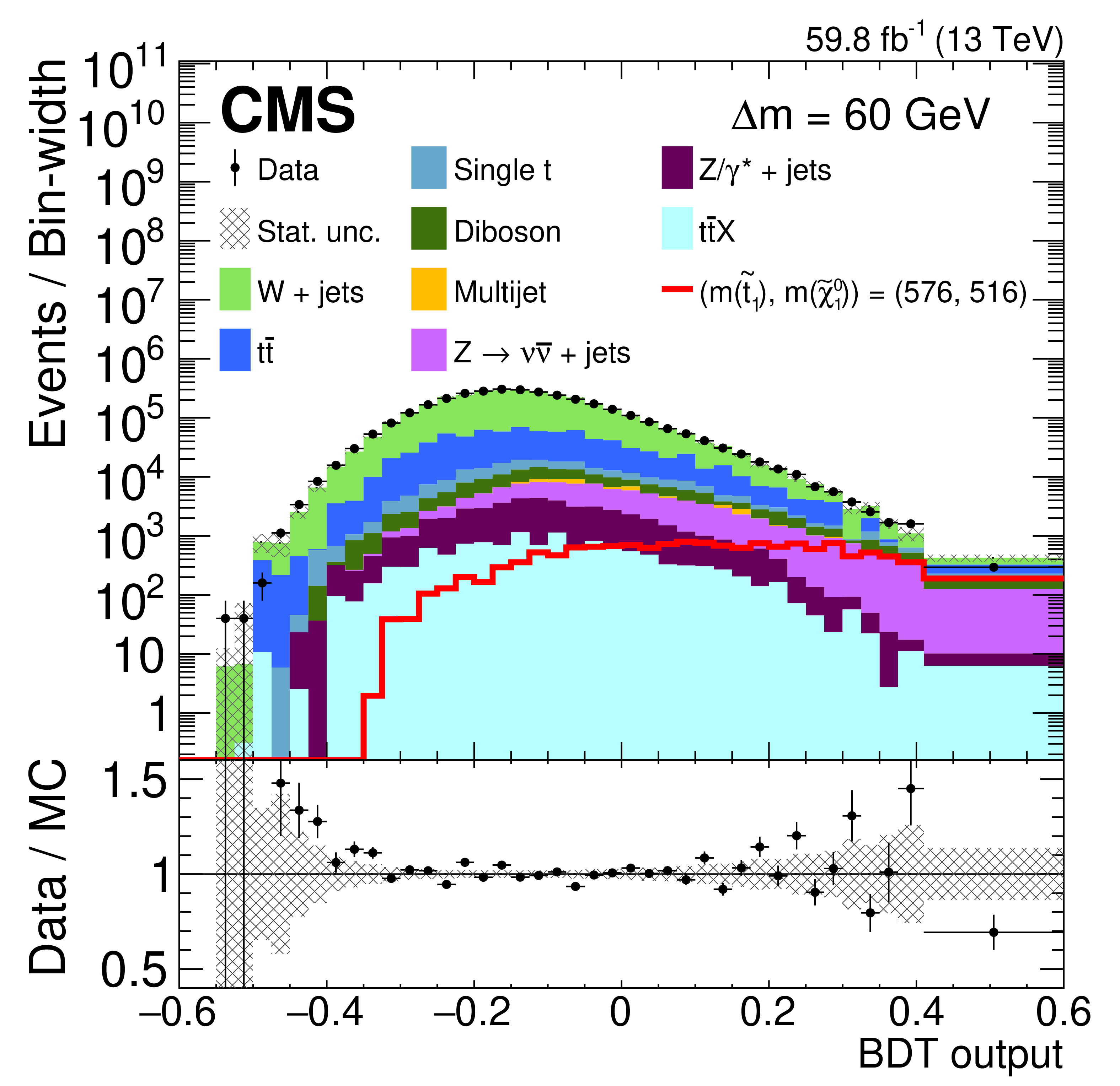
Figure 7:
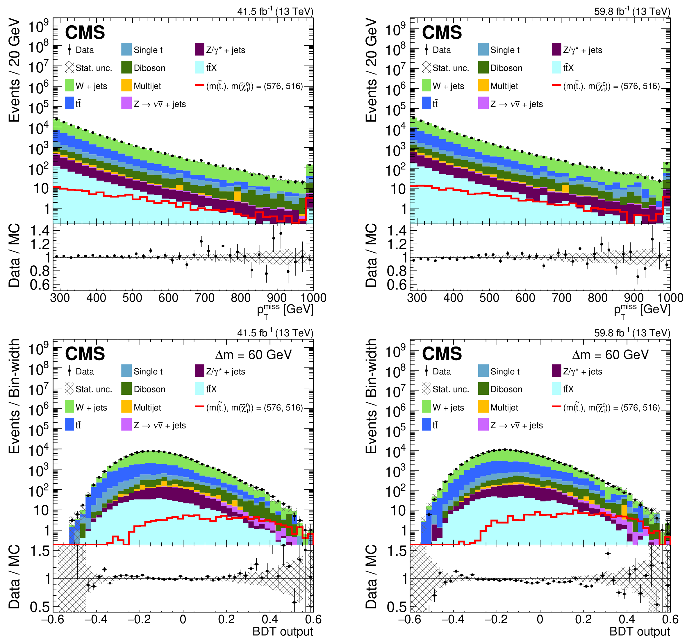
Distributions of $ p_{\mathrm{T}}^\text{miss} $ (upper) and BDT output for $ \Delta {m}= $ 60 GeV (lower) in the VR where $ p_{\mathrm{T}}(\ell) > $ 30 GeV, from 2017 (left) and 2018 (right) data (points) and simulation (colored histograms). The predicted signal distribution is shown by the solid red line for $ ({m}(\tilde{\mathrm{t}}_{1}), {m}(\tilde{\chi}_{1}^{0})) = $ (576, 516), unstacked from the histograms. The lower panels show the ratio of data to the sum of the simulated SM backgrounds. The shaded bands indicate only the statistical uncertainty in the simulation predictions. |
png pdf |
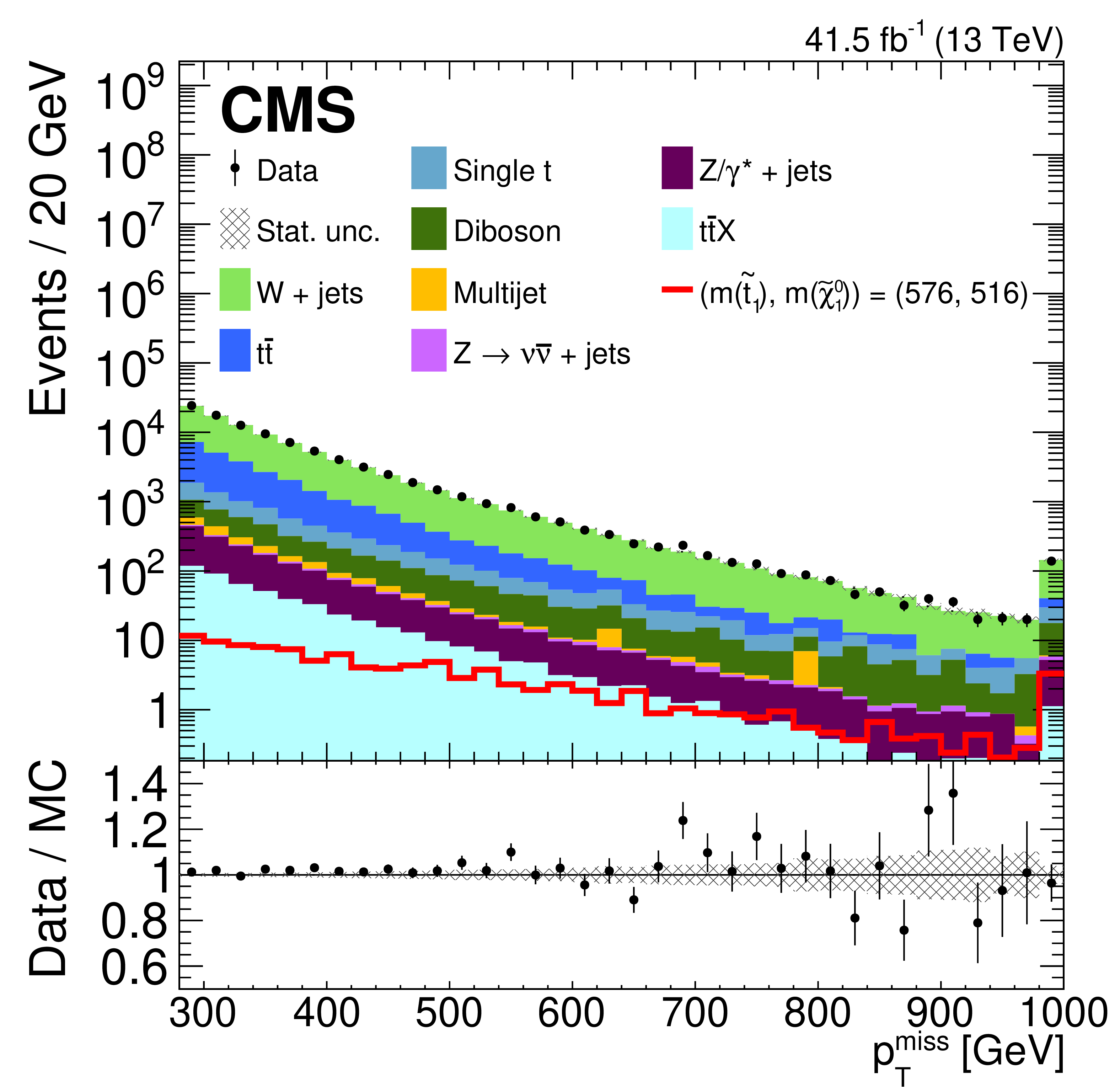
Figure 7-a:
Distributions of $ p_{\mathrm{T}}^\text{miss} $ (upper) and BDT output for $ \Delta {m}= $ 60 GeV (lower) in the VR where $ p_{\mathrm{T}}(\ell) > $ 30 GeV, from 2017 (left) and 2018 (right) data (points) and simulation (colored histograms). The predicted signal distribution is shown by the solid red line for $ ({m}(\tilde{\mathrm{t}}_{1}), {m}(\tilde{\chi}_{1}^{0})) = $ (576, 516), unstacked from the histograms. The lower panels show the ratio of data to the sum of the simulated SM backgrounds. The shaded bands indicate only the statistical uncertainty in the simulation predictions. |
png pdf |
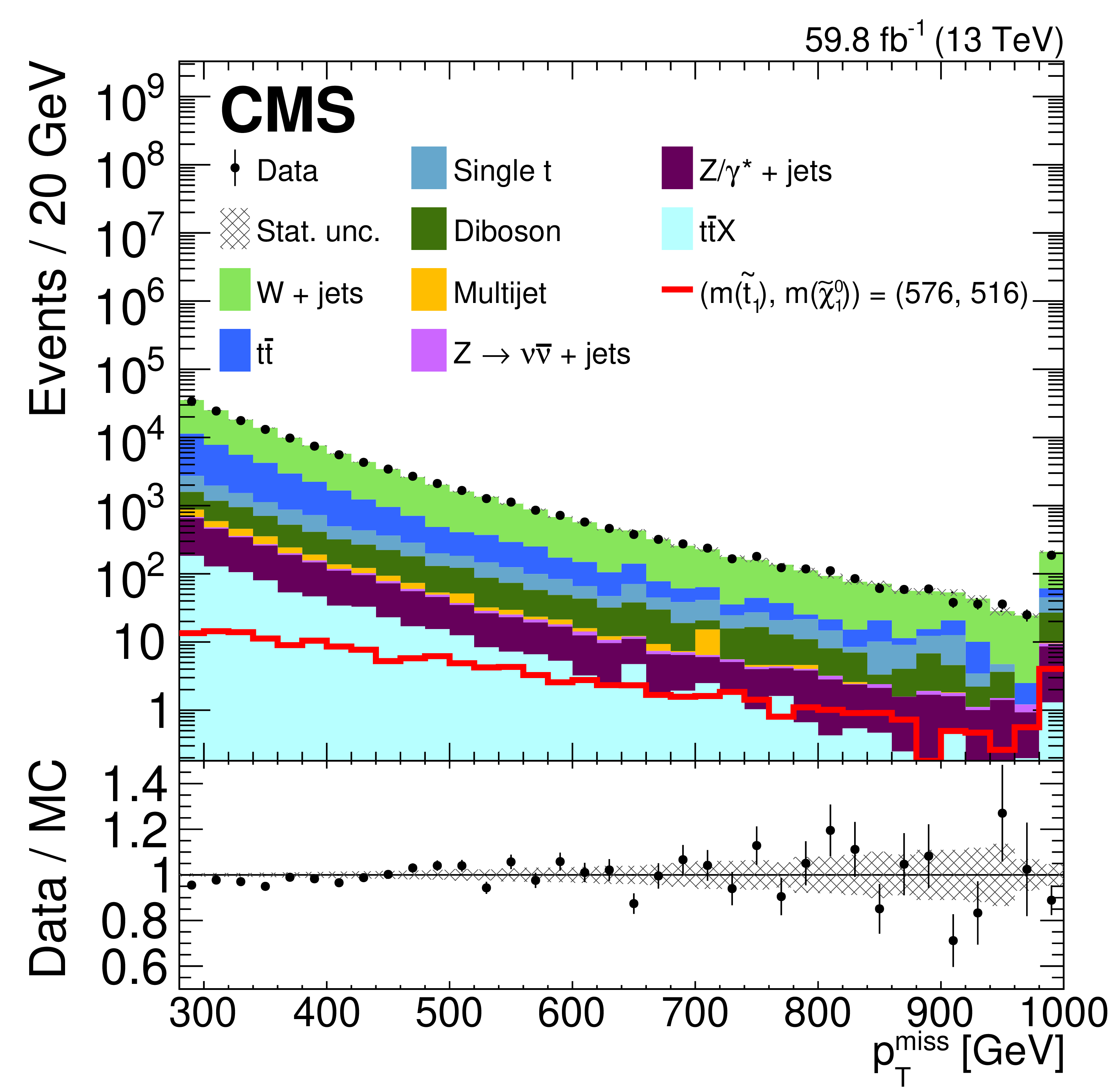
Figure 7-b:
Distributions of $ p_{\mathrm{T}}^\text{miss} $ (upper) and BDT output for $ \Delta {m}= $ 60 GeV (lower) in the VR where $ p_{\mathrm{T}}(\ell) > $ 30 GeV, from 2017 (left) and 2018 (right) data (points) and simulation (colored histograms). The predicted signal distribution is shown by the solid red line for $ ({m}(\tilde{\mathrm{t}}_{1}), {m}(\tilde{\chi}_{1}^{0})) = $ (576, 516), unstacked from the histograms. The lower panels show the ratio of data to the sum of the simulated SM backgrounds. The shaded bands indicate only the statistical uncertainty in the simulation predictions. |
png pdf |
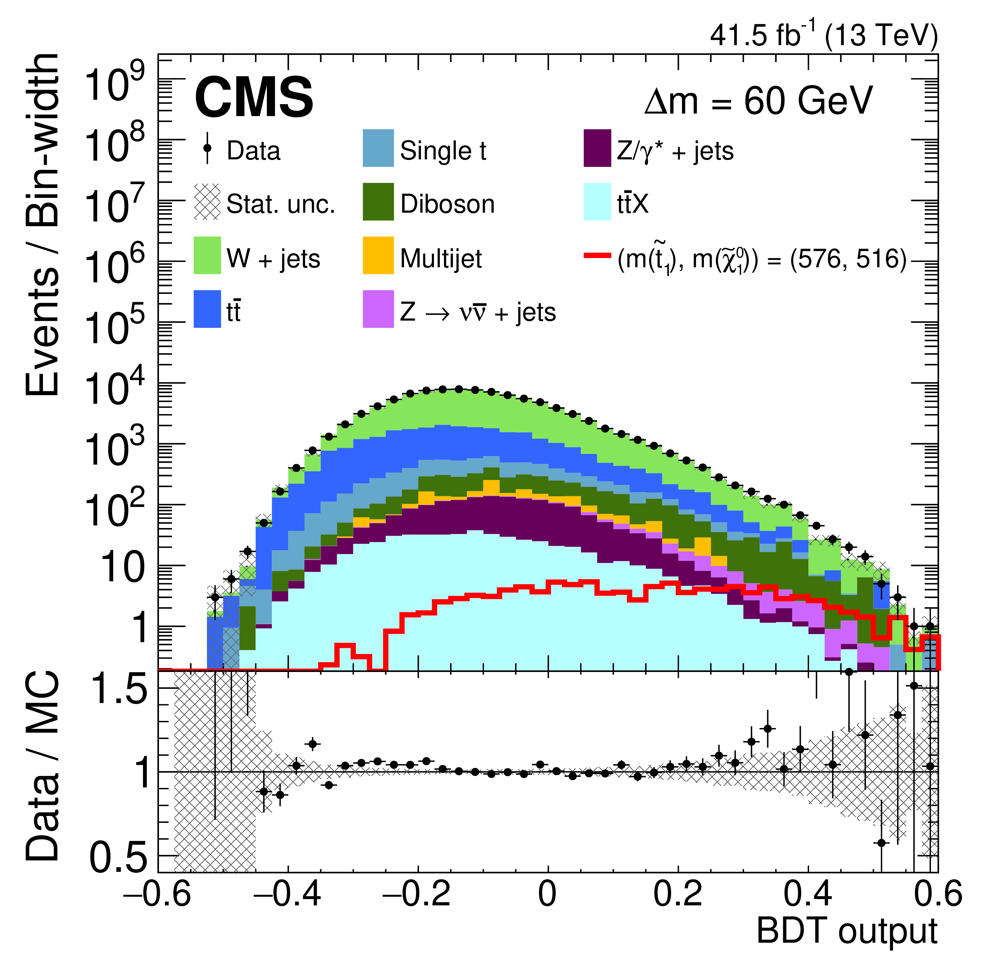
Figure 7-c:
Distributions of $ p_{\mathrm{T}}^\text{miss} $ (upper) and BDT output for $ \Delta {m}= $ 60 GeV (lower) in the VR where $ p_{\mathrm{T}}(\ell) > $ 30 GeV, from 2017 (left) and 2018 (right) data (points) and simulation (colored histograms). The predicted signal distribution is shown by the solid red line for $ ({m}(\tilde{\mathrm{t}}_{1}), {m}(\tilde{\chi}_{1}^{0})) = $ (576, 516), unstacked from the histograms. The lower panels show the ratio of data to the sum of the simulated SM backgrounds. The shaded bands indicate only the statistical uncertainty in the simulation predictions. |

png pdf |
Figure 7-d:
Distributions of $ p_{\mathrm{T}}^\text{miss} $ (upper) and BDT output for $ \Delta {m}= $ 60 GeV (lower) in the VR where $ p_{\mathrm{T}}(\ell) > $ 30 GeV, from 2017 (left) and 2018 (right) data (points) and simulation (colored histograms). The predicted signal distribution is shown by the solid red line for $ ({m}(\tilde{\mathrm{t}}_{1}), {m}(\tilde{\chi}_{1}^{0})) = $ (576, 516), unstacked from the histograms. The lower panels show the ratio of data to the sum of the simulated SM backgrounds. The shaded bands indicate only the statistical uncertainty in the simulation predictions. |

png pdf |
Figure 8:
The observed yields in data (points) and the predicted background components (colored histograms) in the eight SRs for the 2017 data. The vertical bars on the points give the statistical uncertainty in the data. The hatched area shows the total uncertainty in the sum of the backgrounds. The expected yields for two signal points with $ ({m}(\tilde{\mathrm{t}}_{1}), {m}(\tilde{\chi}_{1}^{0})) = $ (500, 490) and (600, 520) GeV are also given by the lines, unstacked from the histograms. The lower panel shows the ratio of the number of observed events to the predicted total background. The vertical bars on the points give the statistical uncertainty in the ratio and the hatched area the total uncertainty. |

png pdf |
Figure 9:
The observed yields in data (points) and the predicted background components (colored histograms) in the eight SRs for the 2018 data. The vertical bars on the points give the statistical uncertainty in the data. The hatched area shows the total uncertainty in the sum of the backgrounds. The expected yields for two signal points with $ ({m}(\tilde{\mathrm{t}}_{1}), {m}(\tilde{\chi}_{1}^{0})) = $ (500, 490) and (600, 520) GeV are also given by the lines, unstacked from the histograms. The lower panel shows the ratio of the number of observed events to the predicted total background. The vertical bars on the points give the statistical uncertainty in the ratio and the hatched area the total uncertainty. |
png pdf |
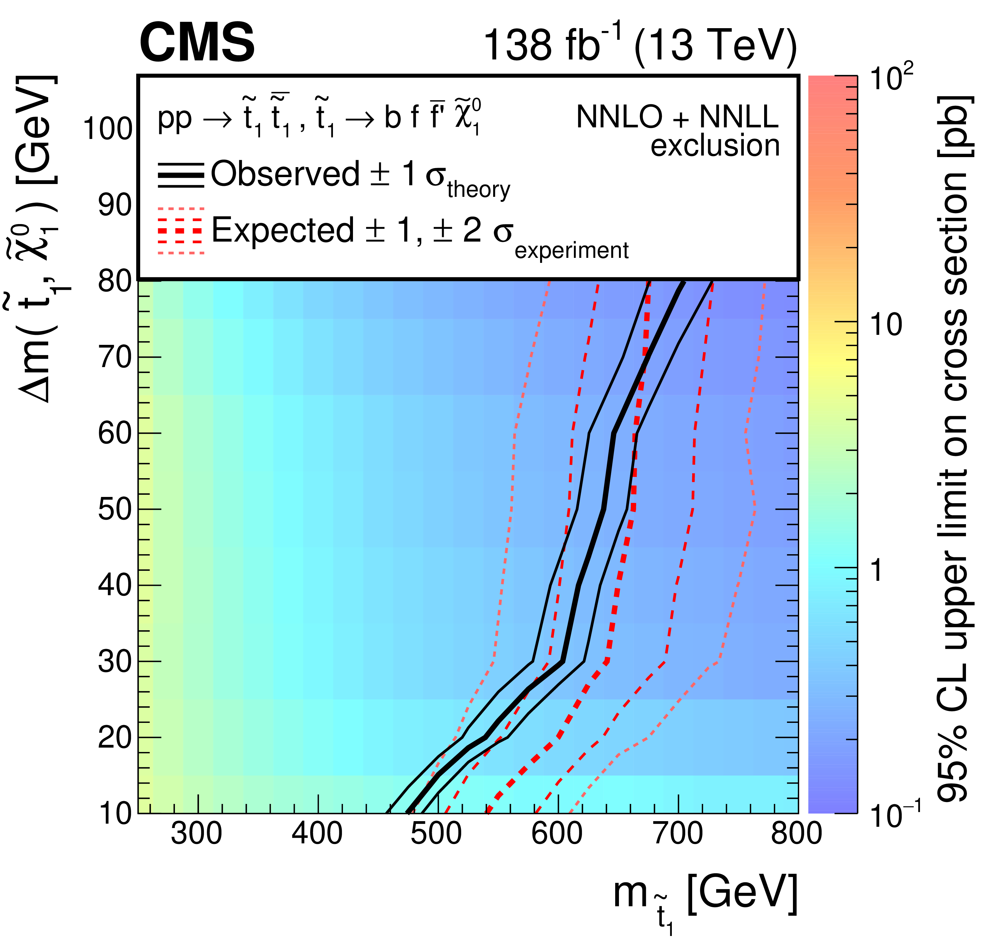
Figure 10:
The 95% CL upper limits in the (m($ \tilde{\mathrm{t}}_{1} $), $ \Delta {m} $) plane on the cross section for the production and four-body decay of the top squark using the combined 2016, 2017, and 2018 data. The color shading represents the observed upper limit for a given point in the plane, using the color scale to the right of the figure. The solid black and dashed red lines show the observed and expected 95% CL lower limits, respectively, on m($ \tilde{\mathrm{t}}_{1} $) as a function of $ \Delta {m} $. The thick lines give the central values of the limits. The corresponding thin lines represent the $ \pm $ 1 standard deviation ($ \sigma_{\text{theory}} $) variations in the limits due to the theoretical uncertainties in the case of the observed limits, and $ \pm $ 1 and 2 standard deviation ($ \sigma_{\text{experiment}} $) variations due to the experimental uncertainties in the case of the expected limits. |
| Tables | |
png pdf |
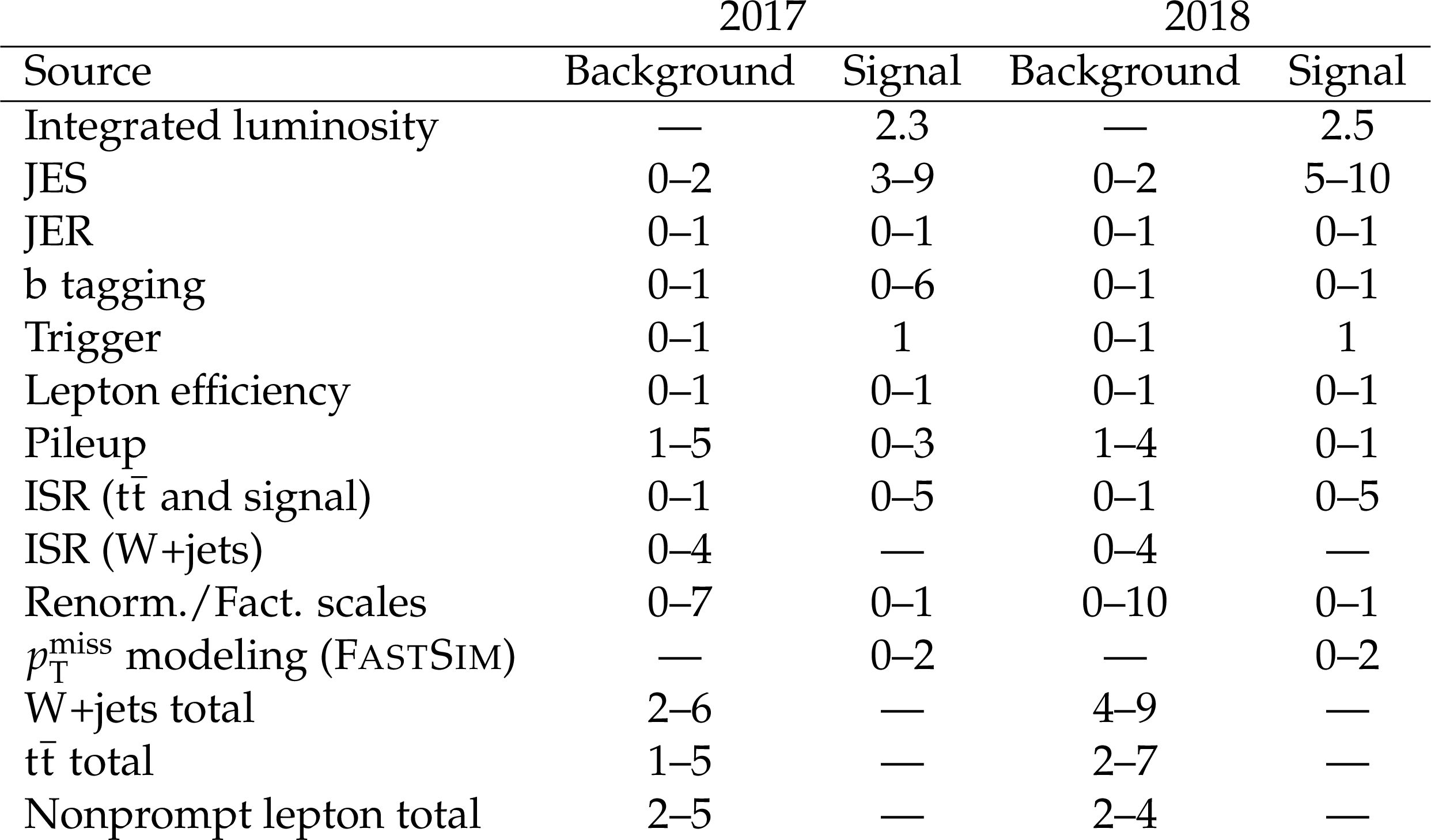
Table 1:
The relative systematic uncertainties in percent from the different sources in the signal and the total relative uncertainty in the W+jets, $ \mathrm{t} \overline{\mathrm{t}} $, and nonprompt background predictions, shown separately for the 2017 and 2018 data analysis. The ranges given are across the eight SRs. The ``$ \text{---} $'' symbol means that a given source of uncertainty is not applicable. |
png pdf |
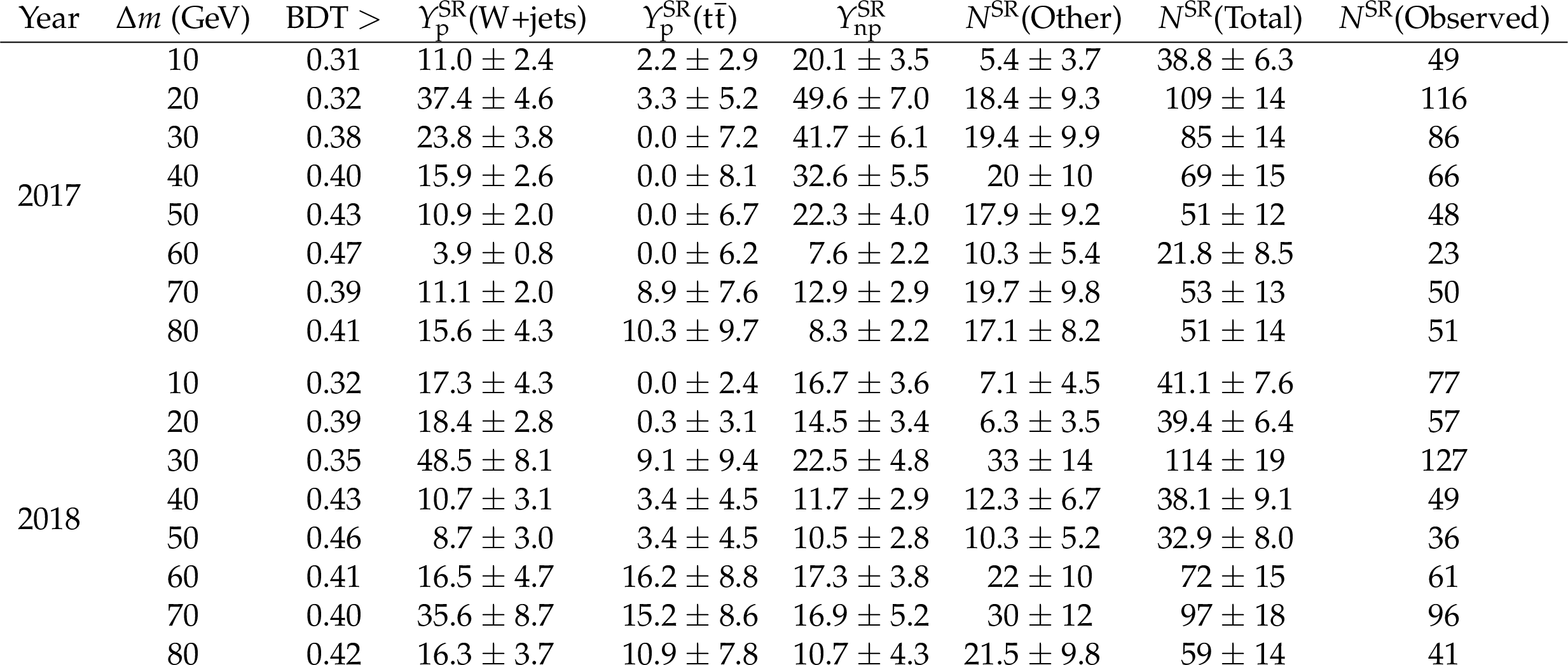
Table 2:
The predicted number of W+jets, $ \mathrm{t} \overline{\mathrm{t}} $, nonprompt, and other ($ N^\mathrm{SR} $(Other)) background events and their sum ($ N^\mathrm{SR} $(Total)), in the eight SRs for the 2017 and 2018 data analysis. The first 3 predicted yields are derived from data, while the yields of the other background processes come from simulation. The uncertainties shown are the quadratic sum of the statistical and systematic uncertainties given in Table 1 for all the background processes. The corresponding $ \Delta {m} $ and BDT output threshold values for each SR are displayed in the first and second columns, respectively, and the observed number of events in data is shown in the last column. |
| Summary |
| The results of a search for the direct pair production of top squarks in single-lepton final states are presented within a compressed scenario where $ R $ parity is conserved and the mass difference $ \Delta {m} = m(\tilde{\mathrm{t}}_{1}) - m(\tilde{\chi}_{1}^{0}) $ between the lightest top squark ($ \tilde{\mathrm{t}}_{1} $) and the lightest supersymmetric particle, taken to be the lightest neutralino $ \tilde{\chi}_{1}^{0} $, does not exceed the W boson mass. The considered decay mode of the top squark is the prompt four-body decay to $ \mathrm{b} \mathrm{f} \overline{\mathrm{f}}^{\,\prime} \tilde{\chi}_{1}^{0} $, where the fermions in the final state $ \mathrm{f} $ and $ \overline{\mathrm{f}}^{\,\prime} $ represent a charged lepton and its neutrino for the decay products of one $ \tilde{\mathrm{t}}_{1} $, and two quarks for the other top squark. The search is based on data collected from proton-proton collisions at $ \sqrt{s}= $ 13 TeV, recorded with the CMS detector during the years 2016, 2017, and 2018, corresponding to an integrated luminosity of 138 fb$ ^{-1} $. Events are selected containing a single lepton (electron or muon), at least one high-momentum jet, and significant missing transverse momentum. The analysis is based on a multivariate tool specifically trained for different $ \Delta {m} $ regions, thus adapting the signal selection to the evolution of the kinematical variables as a function of $ ({m}(\tilde{\mathrm{t}}_{1}), {m}(\tilde{\chi}_{1}^{0})) $. The dominant background processes are W+jets, $ \mathrm{t} \overline{\mathrm{t}} $, and events with nonprompt leptons, which are estimated using control regions in the data. The observed number of events is consistent with the predicted standard model backgrounds in all signal regions. Upper limits are set at the 95% confidence level on the $ \tilde{\mathrm{t}}_{1} {\overline{\tilde{\mathrm{t}}}}_{1} $ production cross section as a function of the $ \tilde{\mathrm{t}}_{1} $ and $ \tilde{\chi}_{1}^{0} $ masses, within the context of a simplified model. Assuming a 100% branching fraction in the four-body decay mode, the search excludes top squark masses up to 480 and 700 GeV at $ \Delta {m} = $ 10 and 80 GeV, respectively. The results summarized in this paper are among the best limits to date on the top squark pair production cross section, where the top squark decays via the four-body mode, and currently correspond to the most stringent limits for $ \Delta {m} < $ 30 GeV. |
| References | ||||
| 1 | S. P. Martin | A supersymmetry primer | Adv. Ser. Direct. High Energy Phys. 18 (1998) 1 | hep-ph/9709356 |
| 2 | J. Wess and B. Zumino | Supergauge transformations in four dimensions | NPB 70 (1974) 39 | |
| 3 | H. P. Nilles | Supersymmetry, supergravity and particle physics | Phys. Rept. 110 (1984) 1 | |
| 4 | H. E. Haber and G. L. Kane | The search for supersymmetry: Probing physics beyond the standard model | Phys. Reports 117 (1985) 75 | |
| 5 | R. Barbieri, S. Ferrara, and C. A. Savoy | Gauge models with spontaneously broken local supersymmetry | PLB 119 (1982) 343 | |
| 6 | S. Dawson, E. Eichten, and C. Quigg | Search for supersymmetric particles in hadron-hadron collisions | PRD 31 (1985) 1581 | |
| 7 | ATLAS Collaboration | Observation of a new particle in the search for the standard model Higgs boson with the ATLAS detector at the LHC | PLB 716 (2012) 1 | 1207.7214 |
| 8 | CMS Collaboration | Observation of a new boson at a mass of 125 GeV with the CMS experiment at the LHC | PLB 716 (2012) 30 | CMS-HIG-12-028 1207.7235 |
| 9 | CMS Collaboration | Observation of a new boson with mass near 125 GeV in pp collisions at $ \sqrt{s} = $ 7 and 8 TeV | JHEP 06 (2013) 081 | CMS-HIG-12-036 1303.4571 |
| 10 | G. R. Farrar and P. Fayet | Phenomenology of the production, decay, and detection of new hadronic states associated with supersymmetry | PLB 76 (1978) 575 | |
| 11 | C. Balázs, M. Carena, and C. E. M. Wagner | Dark matter, light stops and electroweak baryogenesis | PRD 70 (2004) 015007 | hep-ph/0403224 |
| 12 | T. Cohen et al. | SUSY simplified models at 14, 33, and 100 TeV proton colliders | JHEP 04 (2014) 117 | 1311.6480 |
| 13 | N. Arkani-Hamed et al. | MARMOSET: the path from LHC data to the new standard model via on-shell effective theories | hep-ph/0703088 | |
| 14 | J. Alwall, P. C. Schuster, and N. Toro | Simplified models for a first characterization of new physics at the LHC | PRD 79 (2009) 075020 | 0810.3921 |
| 15 | J. Alwall, M.-P. Le, M. Lisanti, and J. G. Wacker | Model-independent jets plus missing energy searches | PRD 79 (2009) 015005 | 0809.3264 |
| 16 | D. Alves et al. | Simplified models for LHC new physics searches | JPG 39 (2012) 105005 | 1105.2838 |
| 17 | CMS Collaboration | Interpretation of searches for supersymmetry with simplified models | PRD 88 (2013) 052017 | CMS-SUS-11-016 1301.2175 |
| 18 | CMS Collaboration | Search for top squarks decaying via four-body or chargino-mediated modes in single-lepton final states in proton-proton collisions at $ \sqrt{s} = $ 13 TeV | JHEP 09 (2018) 065 | CMS-SUS-17-005 1805.05784 |
| 19 | CMS Collaboration | Precision luminosity measurement in proton-proton collisions at $ \sqrt{s} = $ 13 TeV in 2015 and 2016 at CMS | EPJC 81 (2021) 800 | CMS-LUM-17-003 2104.01927 |
| 20 | ATLAS Collaboration | Search for new phenomena with top quark pairs in final states with one lepton, jets, and missing transverse momentum in pp collisions at $ \sqrt{s} = $ 13 TeV with the ATLAS detector | JHEP 04 (2021) 174 | 2012.03799 |
| 21 | CMS Collaboration | HEPData record for this analysis | link | |
| 22 | CMS Collaboration | The CMS experiment at the CERN LHC | JINST 3 (2008) S08004 | |
| 23 | CMS Collaboration | Performance of the CMS Level-1 trigger in proton-proton collisions at $ \sqrt{s}= $ 13 TeV | JINST 15 (2020) P10017 | CMS-TRG-17-001 2006.10165 |
| 24 | CMS Collaboration | The CMS trigger system | JINST 12 (2017) P01020 | CMS-TRG-12-001 1609.02366 |
| 25 | CMS Collaboration | Electron and photon reconstruction and identification with the CMS experiment at the CERN LHC | JINST 16 (2021) P05014 | CMS-EGM-17-001 2012.06888 |
| 26 | CMS Collaboration | Performance of the CMS muon detector and muon reconstruction with proton-proton collisions at $ \sqrt{s}= $ 13 TeV | JINST 13 (2018) P06015 | CMS-MUO-16-001 1804.04528 |
| 27 | CMS Collaboration | Description and performance of track and primary-vertex reconstruction with the CMS tracker | JINST 9 (2014) P10009 | CMS-TRK-11-001 1405.6569 |
| 28 | J. Alwall et al. | The automated computation of tree-level and next-to-leading order differential cross sections, and their matching to parton shower simulations | JHEP 07 (2014) 079 | 1405.0301 |
| 29 | P. Nason | A new method for combining NLO QCD with shower Monte Carlo algorithms | JHEP 11 (2004) 040 | hep-ph/0409146 |
| 30 | S. Frixione, P. Nason, and C. Oleari | Matching NLO QCD computations with parton shower simulations: the POWHEG method | JHEP 11 (2007) 070 | 0709.2092 |
| 31 | S. Alioli, P. Nason, C. Oleari, and E. Re | A general framework for implementing NLO calculations in shower Monte Carlo programs: the POWHEG BOX | JHEP 06 (2010) 043 | 1002.2581 |
| 32 | S. Alioli, P. Nason, C. Oleari, and E. Re | NLO single-top production matched with shower in POWHEG: $ s $- and $ t $-channel contributions | JHEP 09 (2009) 111 | 0907.4076 |
| 33 | E. Re | Single-top Wt-channel production matched with parton showers using the POWHEG method | EPJC 71 (2011) 1547 | 1009.2450 |
| 34 | T. Melia, P. Nason, R. Röntsch, and G. Zanderighi | $ W^+W^- $, $ WZ $ and $ ZZ $ production in the POWHEG BOX | JHEP 11 (2011) 078 | 1107.5051 |
| 35 | P. Nason and G. Zanderighi | $ W^+W^- $, $ WZ $ and $ ZZ $ production in the POWHEG-BOX-V2 | EPJC 74 (2014) 2702 | 1311.1365 |
| 36 | H. B. Hartanto, B. Jäger, L. Reina, and D. Wackeroth | Higgs boson production in association with top quarks in the POWHEG BOX | PRD 91 (2015) 094003 | 1501.04498 |
| 37 | NNPDF Collaboration | Parton distributions from high-precision collider data | EPJC 77 (2017) 663 | 1706.00428 |
| 38 | R. Frederix and S. Frixione | Merging meets matching in MC@NLO | JHEP 12 (2012) 061 | 1209.6215 |
| 39 | T. Sjöstrand et al. | An introduction to PYTHIA8.2 | Comput. Phys. Commun. 191 (2015) 159 | 1410.3012 |
| 40 | CMS Collaboration | Extraction and validation of a new set of CMS PYTHIA8 tunes from underlying-event measurements | EPJC 80 (2020) 4 | CMS-GEN-17-001 1903.12179 |
| 41 | GEANT4 Collaboration | GEANT 4 --- a simulation toolkit | NIM A 506 (2003) 250 | |
| 42 | W. Beenakker, R. Höpker, and M. Spira | PROSPINO: A program for the production of supersymmetric particles in next-to-leading order QCD | hep-ph/9611232 | |
| 43 | C. Borschensky et al. | Squark and gluino production cross sections in pp collisions at $ \sqrt{s} = $ 13, 14, 33 and 100 TeV | EPJC 74 (2014) 3174 | 1407.5066 |
| 44 | W. Beenakker, R. Höpker, M. Spira, and P. M. Zerwas | Squark and gluino production at hadron colliders | NPB 492 (1997) 51 | hep-ph/9610490 |
| 45 | A. Kulesza and L. Motyka | Threshold resummation for squark-antisquark and gluino-pair production at the LHC | PRL 102 (2009) 111802 | |
| 46 | A. Kulesza and L. Motyka | Soft gluon resummation for the production of gluino-gluino and squark-antisquark pairs at the LHC | PRD 80 (2009) 095004 | |
| 47 | W. Beenakker et al. | Soft-gluon resummation for squark and gluino hadroproduction | JHEP 12 (2009) 41 | |
| 48 | W. Beenakker et al. | Squark and gluino production | Int. J. Mod. Phys. A 26 (2011) 2637 | |
| 49 | W. Beenakker et al. | NNLL-fast: predictions for coloured supersymmetric particle production at the LHC with threshold and Coulomb resummation | JHEP 12 (2016) 133 | 1607.07741 |
| 50 | W. Beenakker et al. | NNLL resummation for stop pair-production at the LHC | JHEP 05 (2016) 153 | 1601.02954 |
| 51 | S. Abdullin et al. | The fast simulation of the CMS detector at LHC | J. Phys. Conf. Ser. 331 (2011) 032049 | |
| 52 | A. Giammanco | The fast simulation of the CMS experiment | J. Phys. Conf. Ser. 513 (2014) 022012 | |
| 53 | CMS Collaboration | Particle-flow reconstruction and global event description with the CMS detector | JINST 12 (2017) P10003 | CMS-PRF-14-001 1706.04965 |
| 54 | CMS | Technical proposal for the Phase-II upgrade of the Compact Muon Solenoid | CMS Technical Proposal CERN-LHCC-2015-010, CMS-TDR-15-02, 2020 | |
| 55 | M. Cacciari, G. P. Salam, and G. Soyez | The anti-$ k_{\mathrm{T}} $ jet clustering algorithm | JHEP 04 (2008) 063 | 0802.1189 |
| 56 | M. Cacciari, G. P. Salam, and G. Soyez | FastJet user manual | EPJC 72 (2012) 1896 | 1111.6097 |
| 57 | CMS Collaboration | Jet energy scale and resolution in the CMS experiment in pp collisions at 8 TeV | JINST 12 (2017) P02014 | CMS-JME-13-004 1607.03663 |
| 58 | CMS Collaboration | Identification of heavy-flavour jets with the CMS detector in pp collisions at 13 TeV | JINST 13 (2018) P05011 | CMS-BTV-16-002 1712.07158 |
| 59 | CMS Collaboration | Performance of the DeepJet b tagging algorithm using 41.9 fb$ ^{-1} $ of data from proton-proton collisions at 13 TeV with Phase 1 CMS detector | CMS Detector Performance Summary CMS-DP-2018-058, 2018 CDS |
|
| 60 | CMS Collaboration | Performance of missing transverse momentum reconstruction in proton-proton collisions at $ \sqrt{s}= $ 13 TeV using the CMS detector | JINST 14 (2019) P07004 | CMS-JME-17-001 1903.06078 |
| 61 | CMS Collaboration | Search for supersymmetry in pp collisions at $ \sqrt{s}= $ 13 TeV in the single-lepton final state using the sum of masses of large-radius jets | JHEP 08 (2016) 122 | CMS-SUS-15-007 1605.04608 |
| 62 | K. Rehermann and B. Tweedie | Efficient identification of boosted semileptonic top quarks at the LHC | JHEP 03 (2011) 059 | 1007.2221 |
| 63 | L. Rokach and O. Maimon | Data mining with decision trees: theory and applications | World Scientific Pub. Co. Inc., ISBN~978-981-277-171-1, 2008 | |
| 64 | A. Hocker et al. | TMVA - toolkit for multivariate data analysis | PoS ACAT 04 (2007) 0 | physics/0703039 |
| 65 | G. Cowan, K. Cranmer, E. Gross, and O. Vitells | Asymptotic formulae for likelihood-based tests of new physics | EPJC 71 (2011) 1554 | 1007.1727 |
| 66 | CMS Collaboration | Search for new physics in same-sign dilepton events in proton-proton collisions at $ \sqrt{s} = $ 13 TeV | EPJC 76 (2016) 439 | CMS-SUS-15-008 1605.03171 |
| 67 | CMS Collaboration | CMS luminosity measurement for the 2017 data-taking period at $ \sqrt{s} = $ 13 TeV | CMS Physics Analysis Summary, 2018 CMS-PAS-LUM-17-004 |
CMS-PAS-LUM-17-004 |
| 68 | CMS Collaboration | CMS luminosity measurement for the 2018 data-taking period at $ \sqrt{s} = $ 13 TeV | CMS Physics Analysis Summary, 2019 CMS-PAS-LUM-18-002 |
CMS-PAS-LUM-18-002 |
| 69 | CMS Collaboration | Measurement of the inelastic proton-proton cross section at $ \sqrt{s}= $ 13 TeV | JHEP 07 (2018) 161 | CMS-FSQ-15-005 1802.02613 |
| 70 | A. Kalogeropoulos and J. Alwall | The SysCalc code: A tool to derive theoretical systematic uncertainties | \hrefhttp://www.arXiv.org/abs/hep-ph/1801.08401\textttarXiv:hep-ph/1801.08401, 2018 | |
| 71 | T. Junk | Confidence level computation for combining searches with small statistics | NIM A 434 (1999) 435 | hep-ex/9902006 |
| 72 | A. L. Read | Presentation of search results: the CL$ _{\text{s}} $ technique | JPG 28 (2002) 2693 | |
| 73 | ATLAS and CMS Collaborations, LHC Higgs Combination Group | Procedure for the LHC Higgs boson search combination in summer 2011 | Technical Report ATL-PHYS-PUB/-11, /005, CERN, 2011 CMS NOTE 201 (2011) 1 |
|
|
|
Compact Muon Solenoid LHC, CERN |
|

|

|

|

|

|