

Compact Muon Solenoid
LHC, CERN
| CMS-TOP-17-019 ; CERN-EP-2019-098 | ||
| Search for the production of four top quarks in the single-lepton and opposite-sign dilepton final states in proton-proton collisions at $\sqrt{s}= $ 13 TeV | ||
| CMS Collaboration | ||
| 7 June 2019 | ||
| JHEP 11 (2019) 082 | ||
| Abstract: A search for the standard model production of four top quarks (${\mathrm{p}}{\mathrm{p}}\to \mathrm{ t \bar{t} }\mathrm{ t \bar{t} }$) is reported using single-lepton plus jets and opposite-sign dilepton plus jets signatures. Proton-proton collisions are recorded with the CMS detector at the LHC at a center-of-mass energy of 13 TeV in a sample corresponding to an integrated luminosity of 35.8 fb$^{-1}$. A multivariate analysis exploiting global event and jet properties is used to discriminate $\mathrm{ t \bar{t} }\mathrm{ t \bar{t} }$ from $\mathrm{t\bar{t}}$ production. No significant deviation is observed from the predicted background. An upper limit is set on the cross section for $\mathrm{ t \bar{t} }\mathrm{ t \bar{t} }$ production in the standard model of 48 fb at 95% confidence level. When combined with a previous measurement by the CMS experiment from an analysis of other final states, the observed signal significance is 1.4 standard deviations, and the combined cross section measurement is 13$^{+11}_{-\,9}$ fb. The result is also interpreted in the framework of effective field theory. | ||
| Links: e-print arXiv:1906.02805 [hep-ex] (PDF) ; CDS record ; inSPIRE record ; CADI line (restricted) ; | ||
| Figures | |
png pdf |
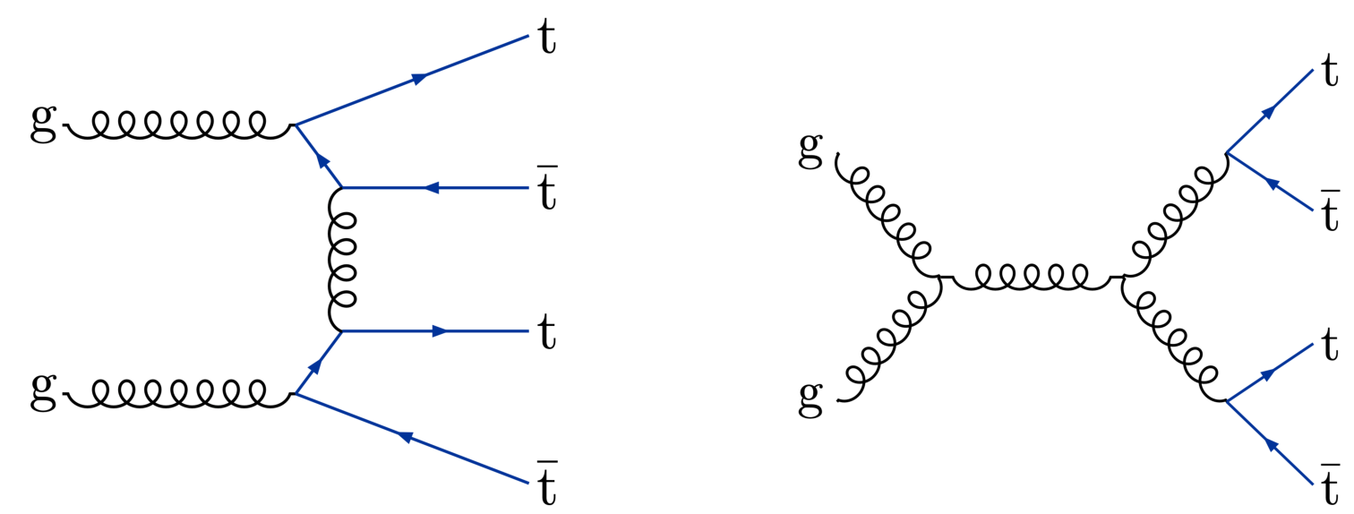
Figure 1:
Representative Feynman diagrams for ${\mathrm{p}} {\mathrm{p}} \to {\mathrm{t} \mathrm{\bar{t}} \mathrm{t} \mathrm{\bar{t}}} $ production at lowest order in the SM. |
png pdf |
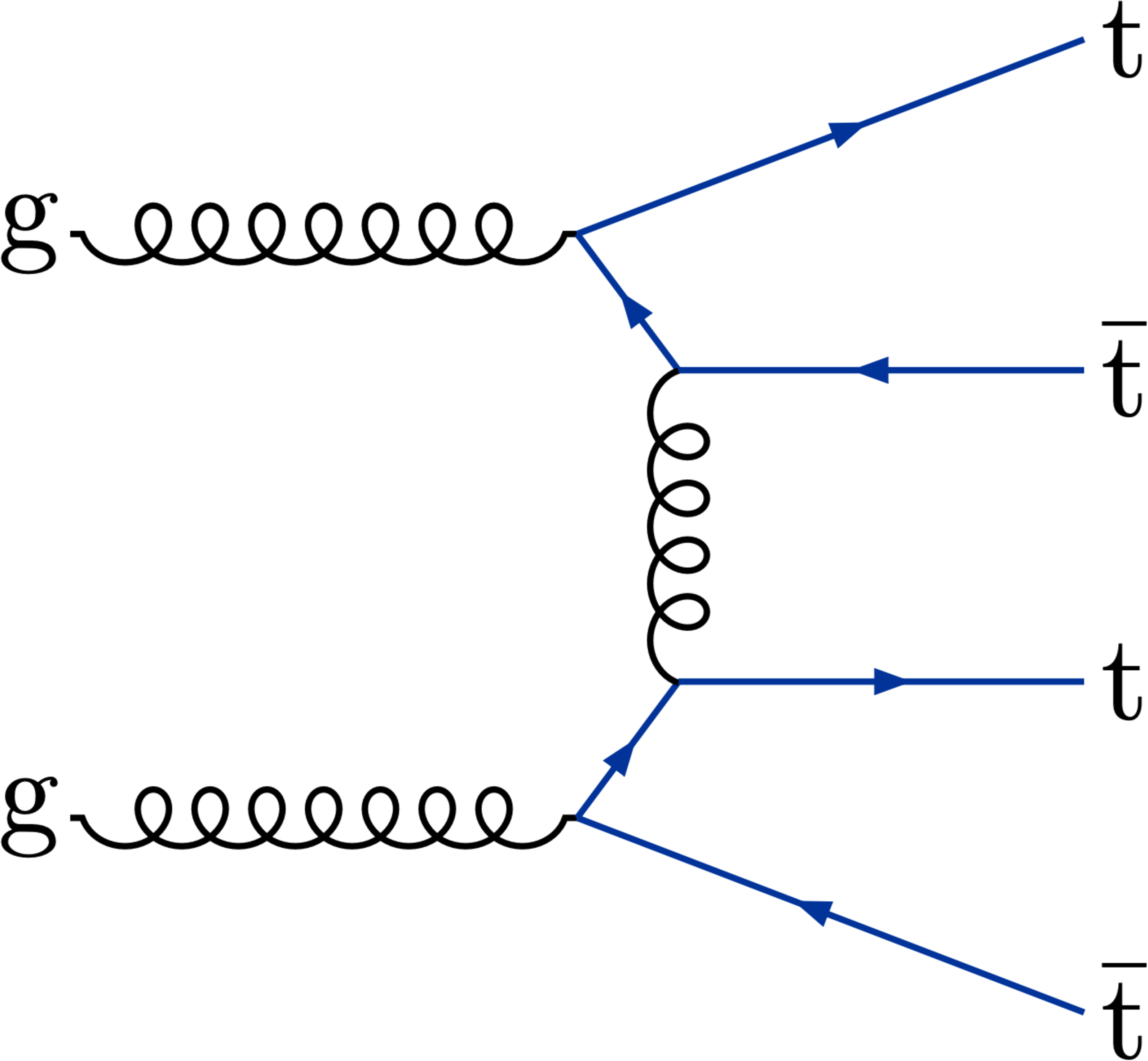
Figure 1-a:
Representative Feynman diagram for ${\mathrm{p}} {\mathrm{p}} \to {\mathrm{t} \mathrm{\bar{t}} \mathrm{t} \mathrm{\bar{t}}} $ production at lowest order in the SM. |
png pdf |
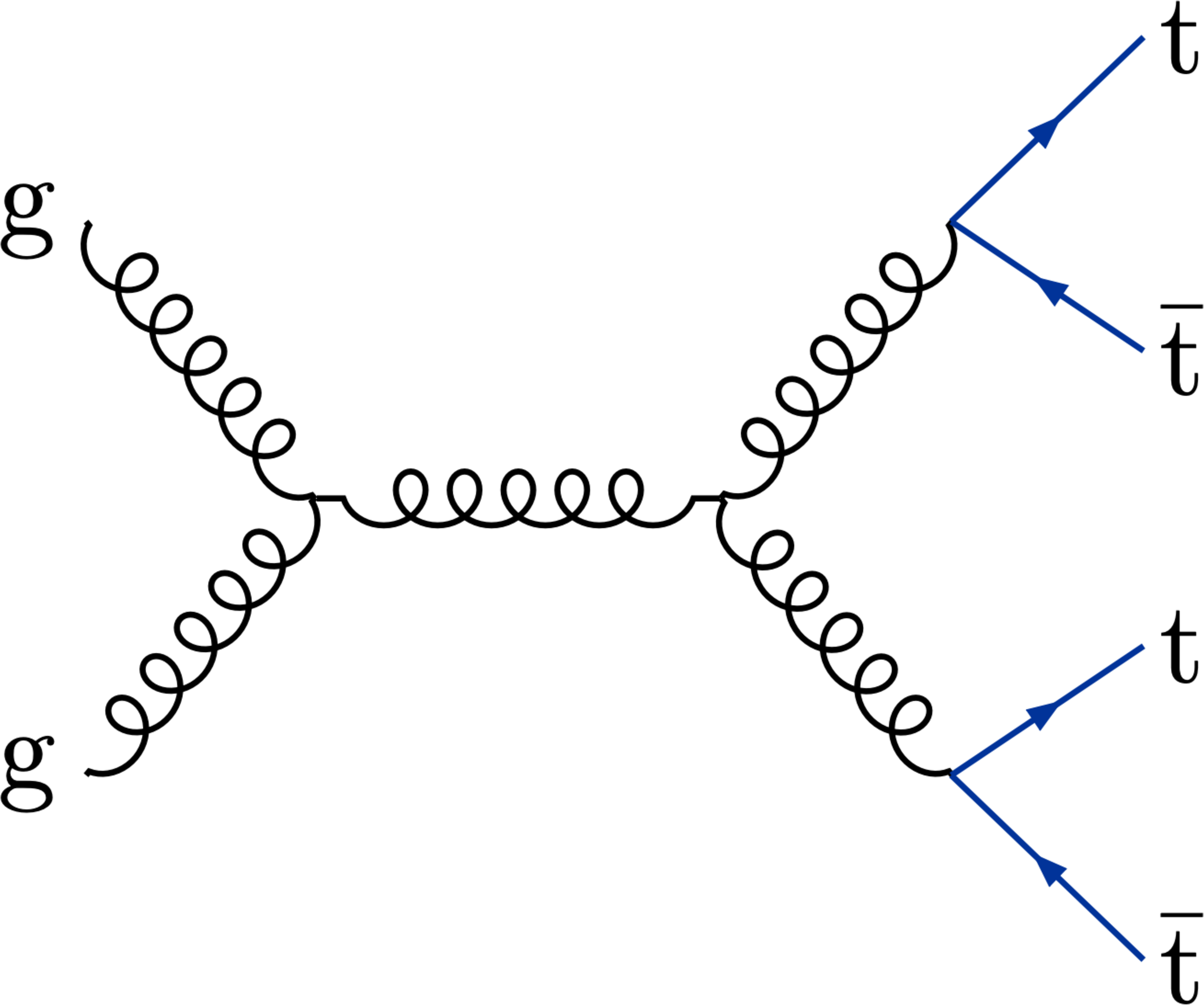
Figure 1-b:
Representative Feynman diagram for ${\mathrm{p}} {\mathrm{p}} \to {\mathrm{t} \mathrm{\bar{t}} \mathrm{t} \mathrm{\bar{t}}} $ production at lowest order in the SM. |
png pdf |
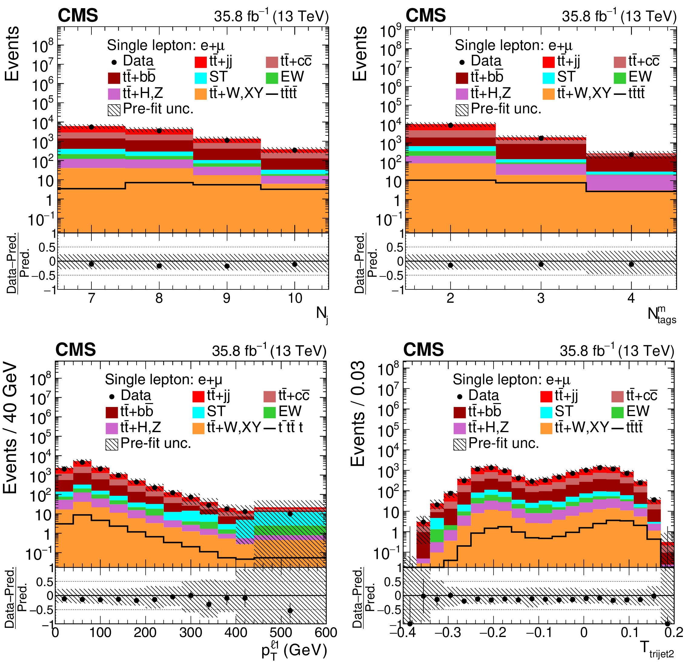
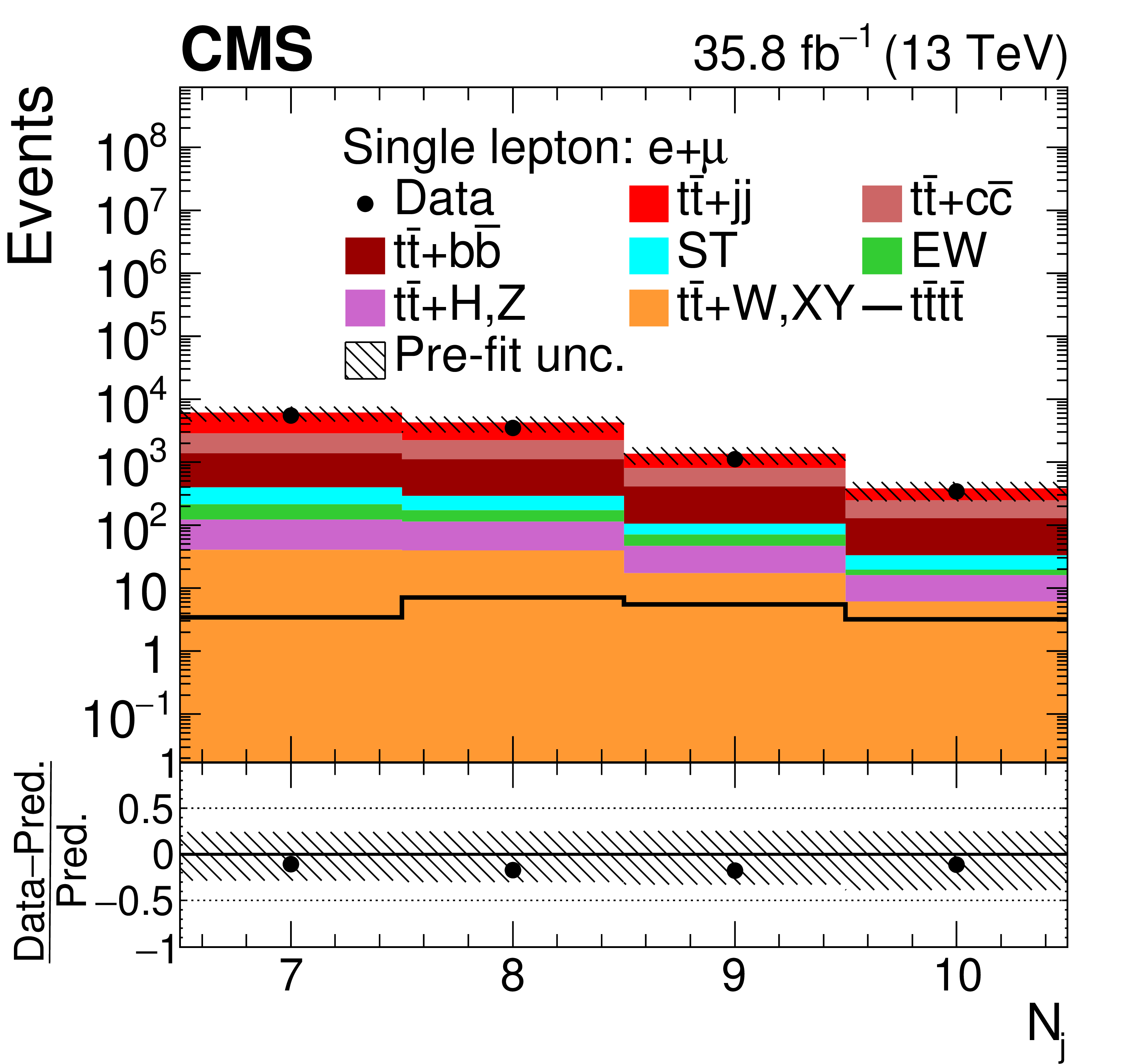
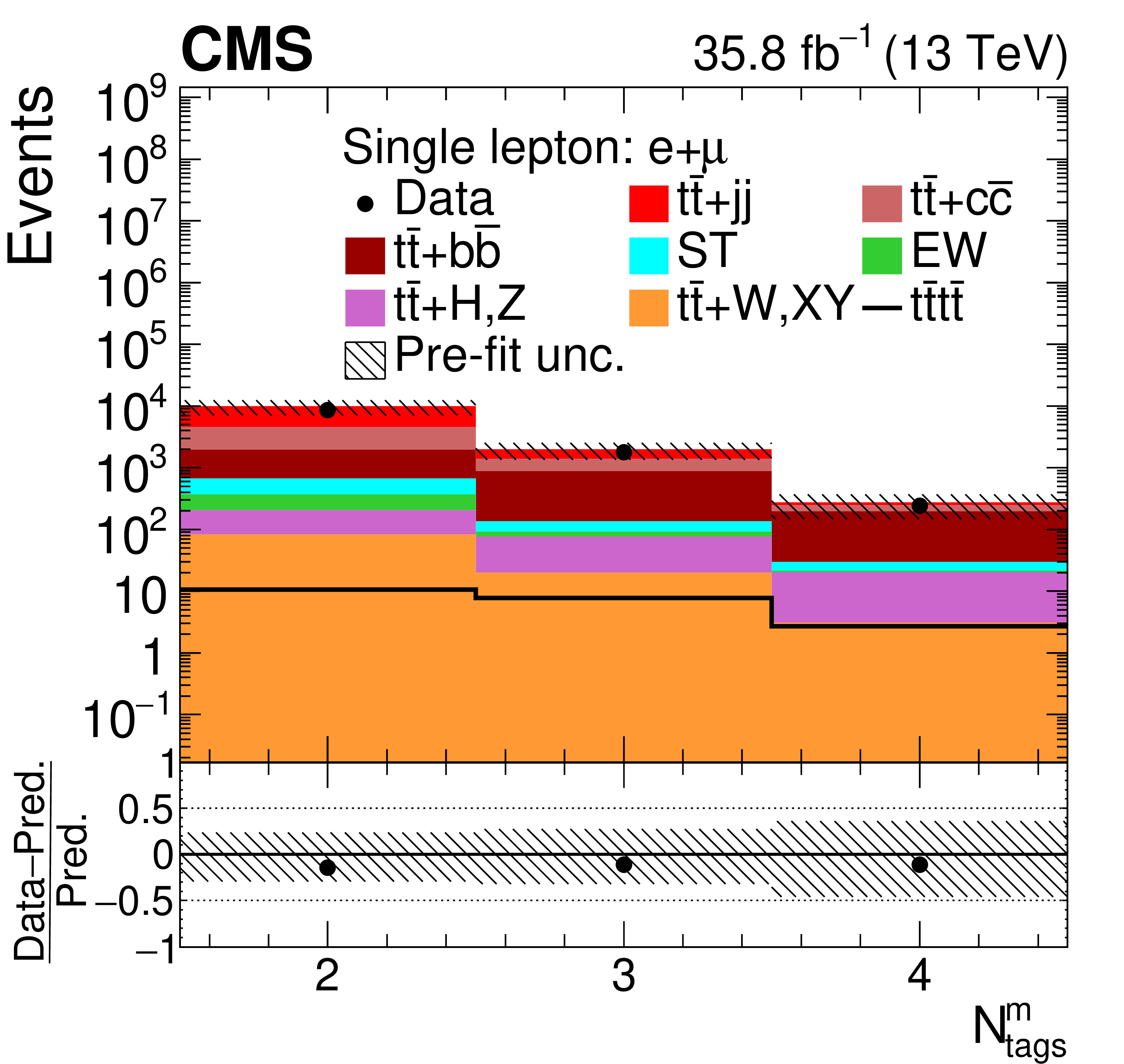
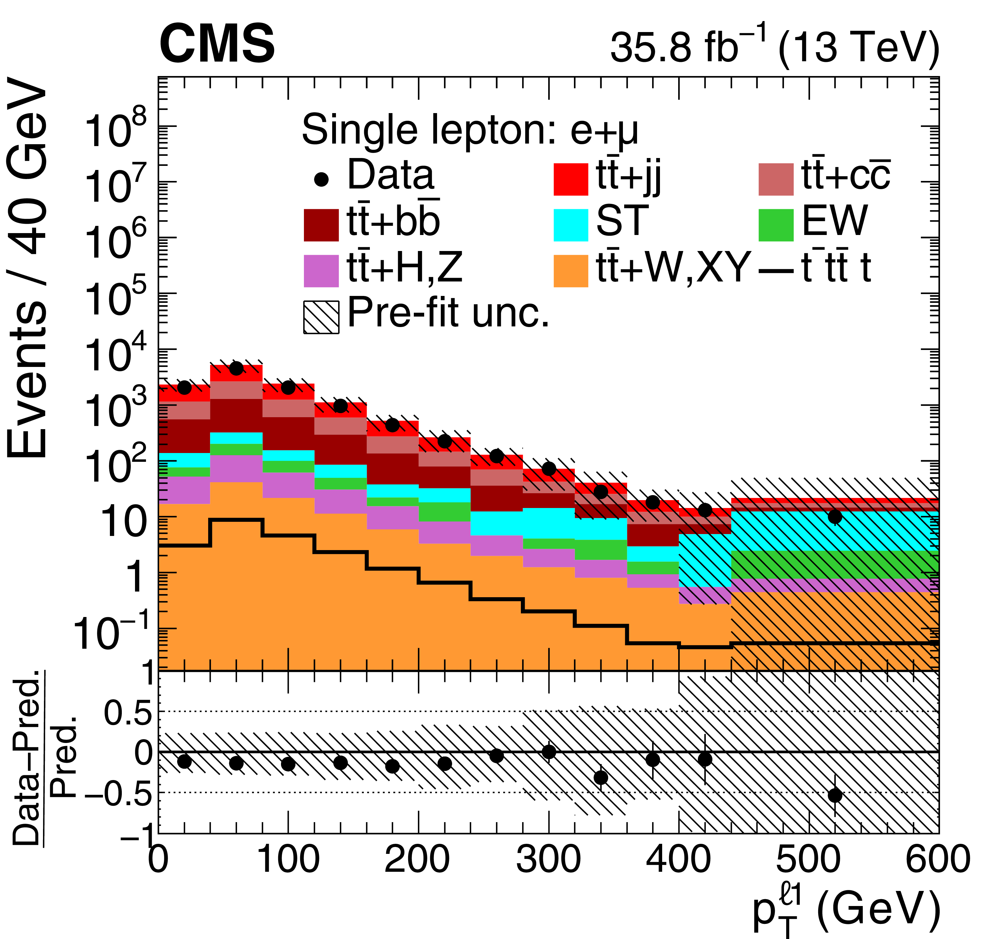
Figure 2:
Distributions of ${N_{\mathrm {j}}}$, ${N_{\text {tags}}^{\text {m}}}$, ${{p_{\mathrm {T}}} ^{\ell 1}}$ and ${T_{\text {trijet2}}}$ in the combined single-lepton channels. In the upper panels, the data are shown as dots with error bars representing statistical uncertainties, MC simulations are shown as a histogram. In the lower panels a relative difference of the data with respect to the MC prediction is also shown. In each panel, the shaded band represents the total systematic and statistical uncertainties in the ${\mathrm{t} {}\mathrm{\bar{t}}}$ simulation added in quadrature. See Section 4.2 for the definitions of the variables. |
png pdf |
Figure 2-a:
Distribution of ${N_{\mathrm {j}}}$ in the combined single-lepton channels. In the upper panel, the data are shown as dots with error bars representing statistical uncertainties, MC simulations are shown as a histogram. In the lower panel a relative difference of the data with respect to the MC prediction is also shown. In each panel, the shaded band represents the total systematic and statistical uncertainties in the ${\mathrm{t} {}\mathrm{\bar{t}}}$ simulation added in quadrature. |
png pdf |
Figure 2-b:
Distribution of ${N_{\text {tags}}^{\text {m}}}$ in the combined single-lepton channels. In the upper panel, the data are shown as dots with error bars representing statistical uncertainties, MC simulations are shown as a histogram. In the lower panel a relative difference of the data with respect to the MC prediction is also shown. In each panel, the shaded band represents the total systematic and statistical uncertainties in the ${\mathrm{t} {}\mathrm{\bar{t}}}$ simulation added in quadrature. |
png pdf |
Figure 2-c:
Distribution of ${{p_{\mathrm {T}}} ^{\ell 1}}$ in the combined single-lepton channels. In the upper panel, the data are shown as dots with error bars representing statistical uncertainties, MC simulations are shown as a histogram. In the lower panel a relative difference of the data with respect to the MC prediction is also shown. In each panel, the shaded band represents the total systematic and statistical uncertainties in the ${\mathrm{t} {}\mathrm{\bar{t}}}$ simulation added in quadrature. |

png pdf |
Figure 2-d:
Distribution of ${T_{\text {trijet2}}}$ in the combined single-lepton channels. In the upper panel, the data are shown as dots with error bars representing statistical uncertainties, MC simulations are shown as a histogram. In the lower panel a relative difference of the data with respect to the MC prediction is also shown. In each panel, the shaded band represents the total systematic and statistical uncertainties in the ${\mathrm{t} {}\mathrm{\bar{t}}}$ simulation added in quadrature. |
png pdf |
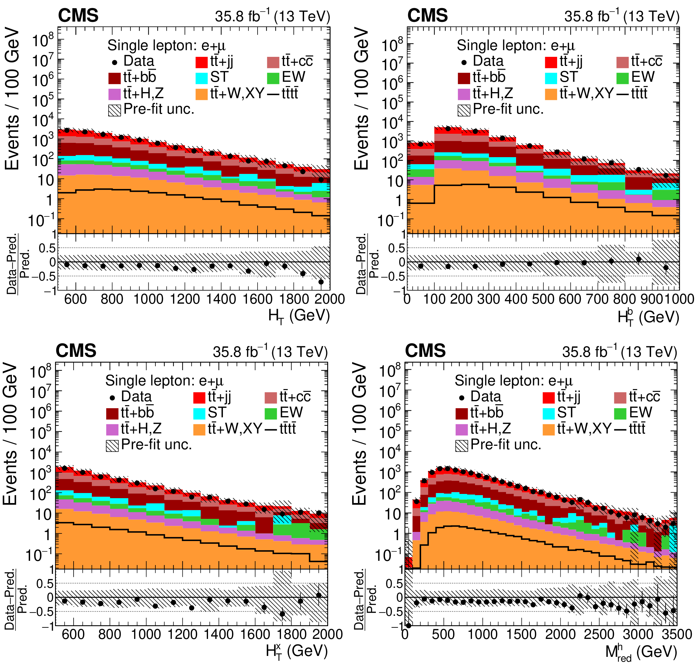
Figure 3:
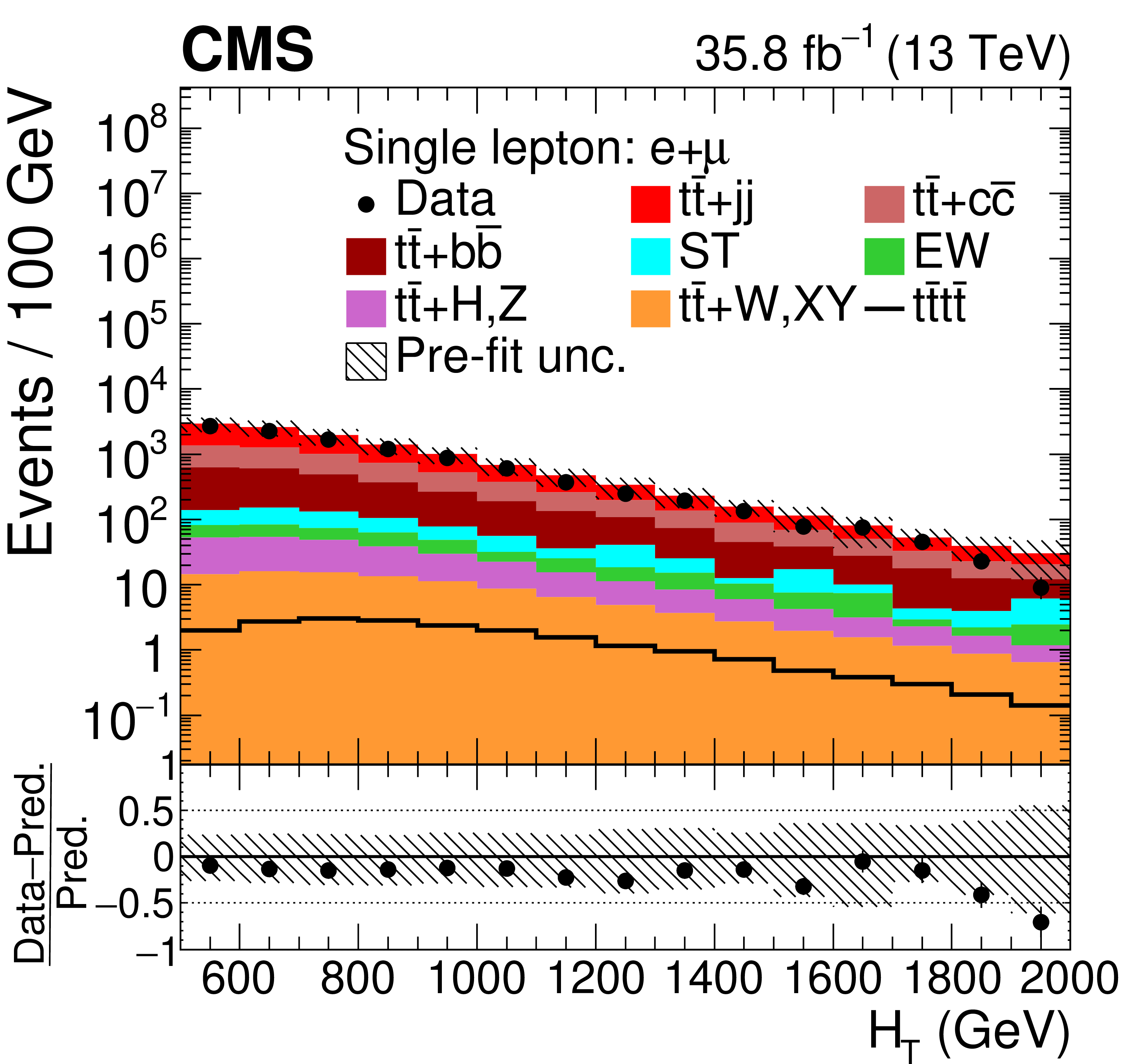
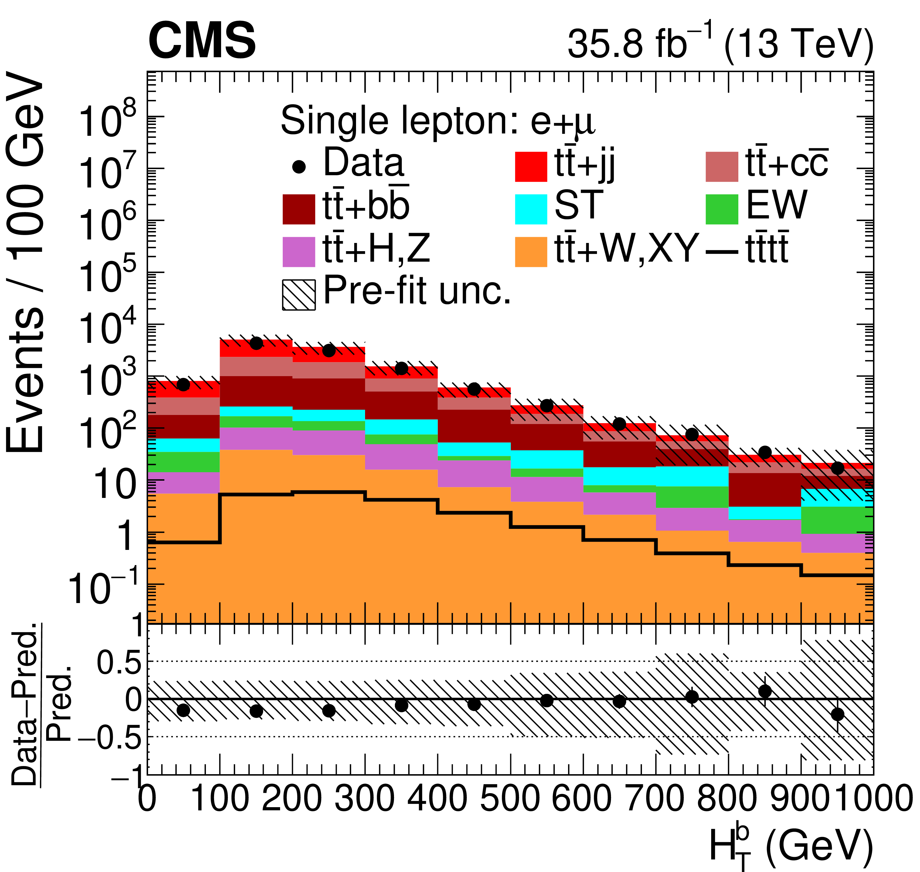
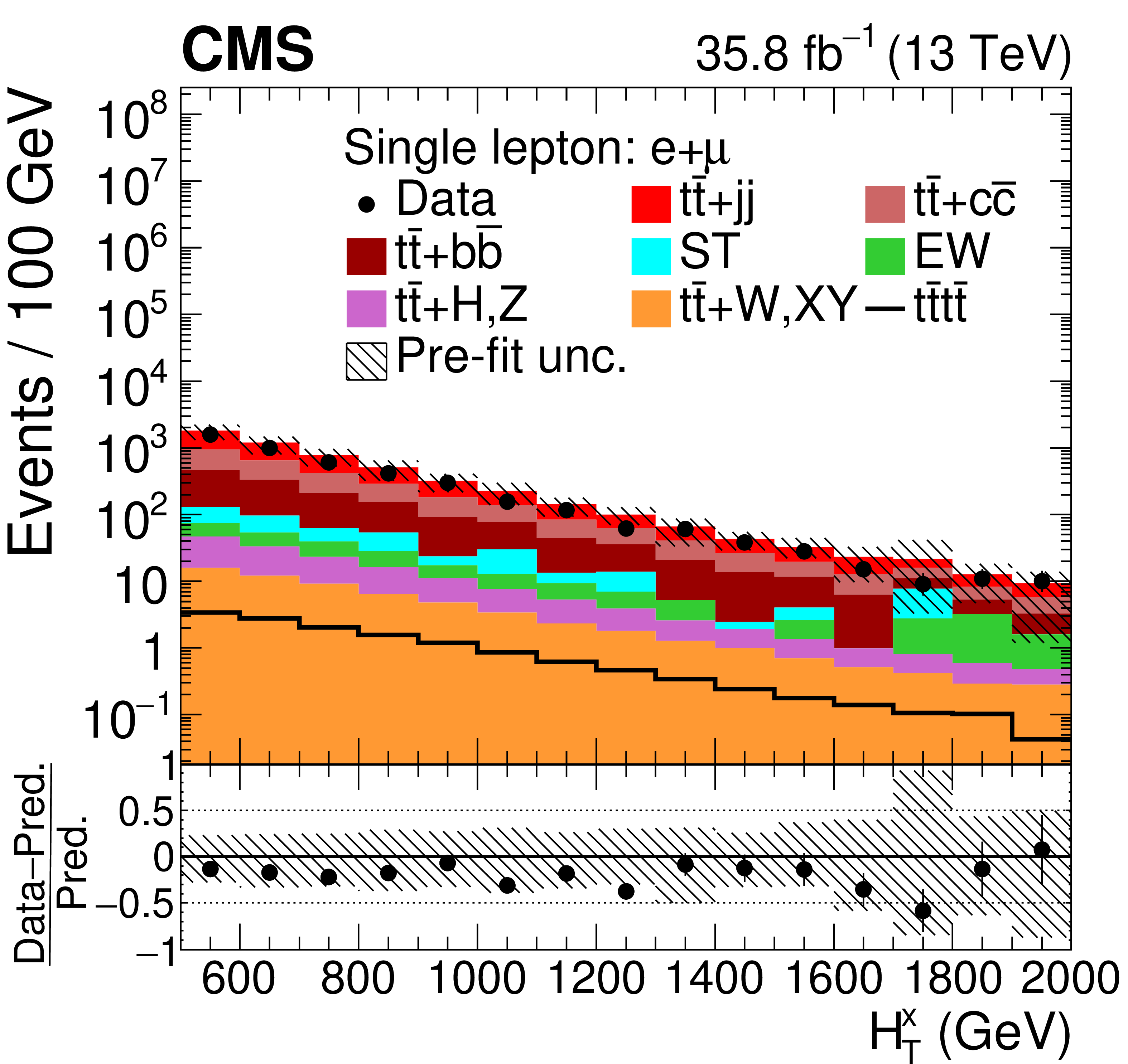
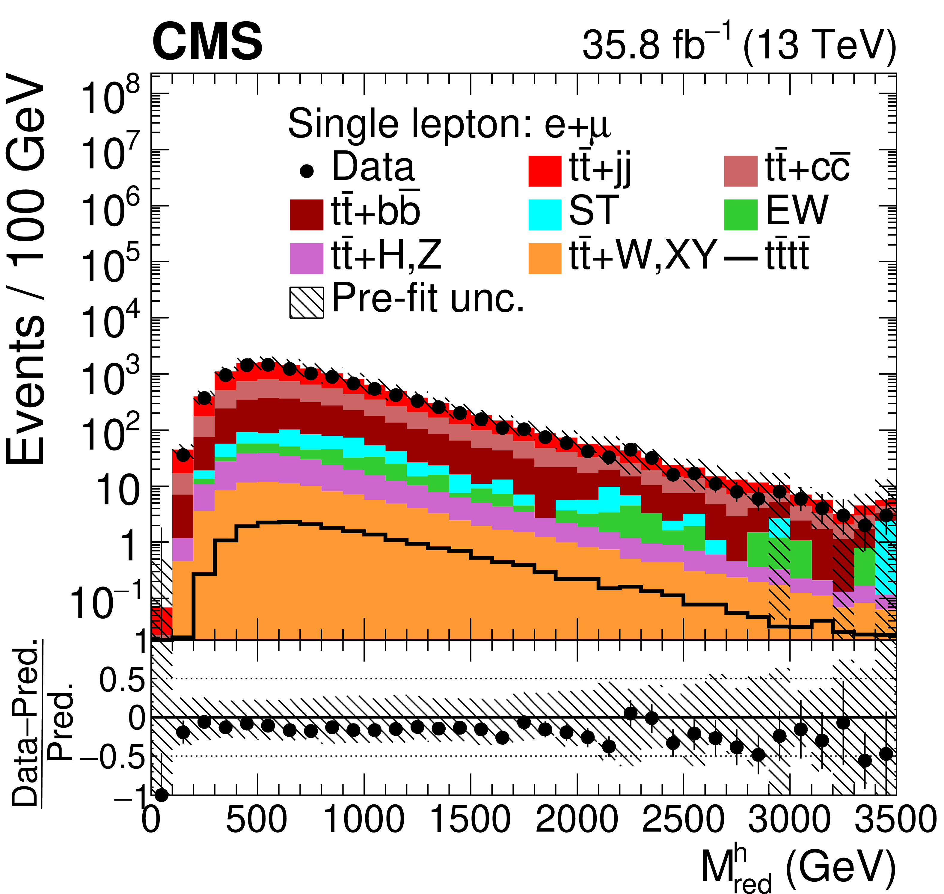
Distributions of ${H_{\mathrm {T}}}$, ${{H_{\mathrm {T}}} ^{{\mathrm{b}}}}$, ${H_{\mathrm {T}}^{\mathrm {x}}}$ and ${M_{\text {red}}^{\text {h}}}$ in the combined single-lepton channel. In the upper panels, the data are shown as dots with error bars representing statistical uncertainties, MC simulations are shown as a histogram. In the lower panels the relative difference of the data with respect to the MC prediction is also shown. In each panel, the shaded band represents the total systematic and statistical uncertainty in the ${\mathrm{t} {}\mathrm{\bar{t}}}$ simulation added in quadrature. See Section 4.2 for the definitions of the variables. |
png pdf |
Figure 3-a:
Distribution of ${H_{\mathrm {T}}}$ in the combined single-lepton channel. In the upper panel, the data are shown as dots with error bars representing statistical uncertainties, MC simulations are shown as a histogram. In the lower panel the relative difference of the data with respect to the MC prediction is also shown. In each panel, the shaded band represents the total systematic and statistical uncertainty in the ${\mathrm{t} {}\mathrm{\bar{t}}}$ simulation added in quadrature. |
png pdf |
Figure 3-b:
Distribution of ${{H_{\mathrm {T}}} ^{{\mathrm{b}}}}$ in the combined single-lepton channel. In the upper panel, the data are shown as dots with error bars representing statistical uncertainties, MC simulations are shown as a histogram. In the lower panel the relative difference of the data with respect to the MC prediction is also shown. In each panel, the shaded band represents the total systematic and statistical uncertainty in the ${\mathrm{t} {}\mathrm{\bar{t}}}$ simulation added in quadrature. |
png pdf |
Figure 3-c:
Distribution of ${H_{\mathrm {T}}^{\mathrm {x}}}$ in the combined single-lepton channel. In the upper panel, the data are shown as dots with error bars representing statistical uncertainties, MC simulations are shown as a histogram. In the lower panel the relative difference of the data with respect to the MC prediction is also shown. In each panel, the shaded band represents the total systematic and statistical uncertainty in the ${\mathrm{t} {}\mathrm{\bar{t}}}$ simulation added in quadrature. |
png pdf |
Figure 3-d:
Distribution of ${M_{\text {red}}^{\text {h}}}$ in the combined single-lepton channel. In the upper panel, the data are shown as dots with error bars representing statistical uncertainties, MC simulations are shown as a histogram. In the lower panel the relative difference of the data with respect to the MC prediction is also shown. In each panel, the shaded band represents the total systematic and statistical uncertainty in the ${\mathrm{t} {}\mathrm{\bar{t}}}$ simulation added in quadrature. |
png pdf |
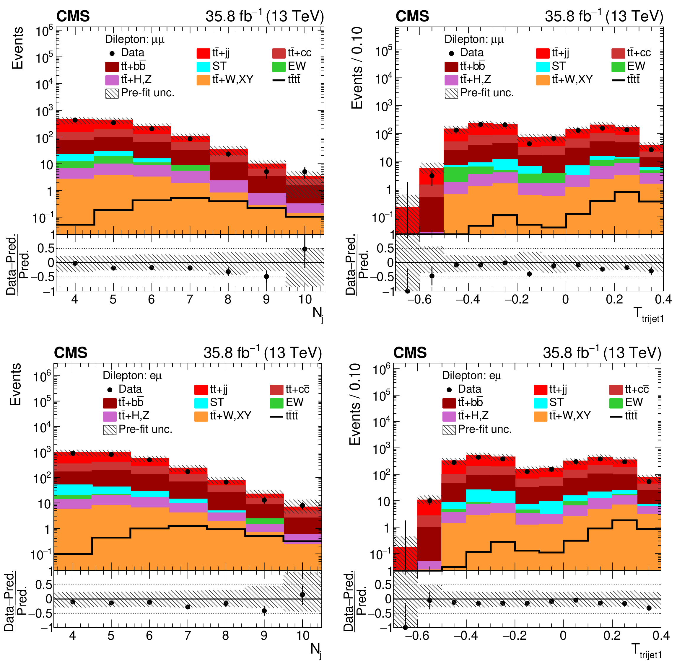
Figure 4:
Distributions of ${N_{\mathrm {j}}}$ and ${T_{\text {trijet1}}}$ in the $\mu^{+} {}\mu^{-} $ (upper row) and $\mu^{\pm} \mathrm{e^{\mp}} $ (lower row) channels. In the upper panels of each figure, the data are shown as dots with error bars representing statistical uncertainties, MC simulations are shown as a histogram. In the lower panels the relative difference of the data with respect to MC prediction is also shown. In each panel, the shaded band represents the total uncertainty in the dominant ${\mathrm{t} {}\mathrm{\bar{t}}}$ background estimate. See Section 4.2 for the definitions of the variables. |
png pdf |
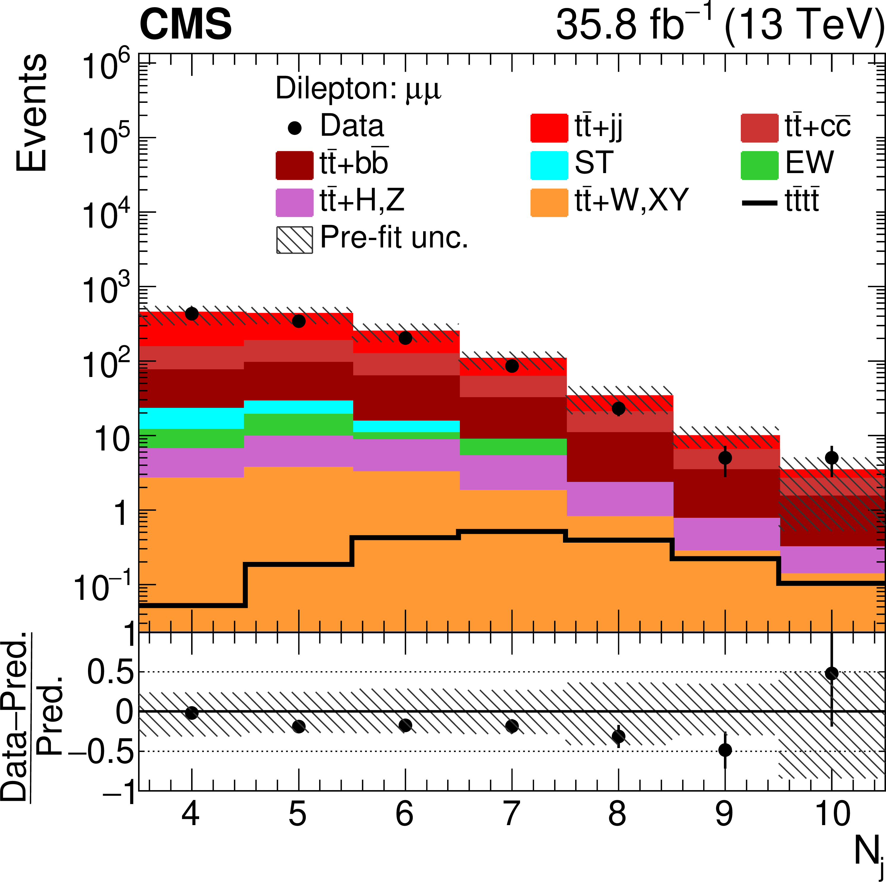
Figure 4-a:
Distributions of ${N_{\mathrm {j}}}$ in the $\mu^{+} {}\mu^{-} $ channel. In the upper panel, the data are shown as dots with error bars representing statistical uncertainties, MC simulations are shown as a histogram. In the lower panel the relative difference of the data with respect to MC prediction is also shown. In each panel, the shaded band represents the total uncertainty in the dominant ${\mathrm{t} {}\mathrm{\bar{t}}}$ background estimate. |
png pdf |
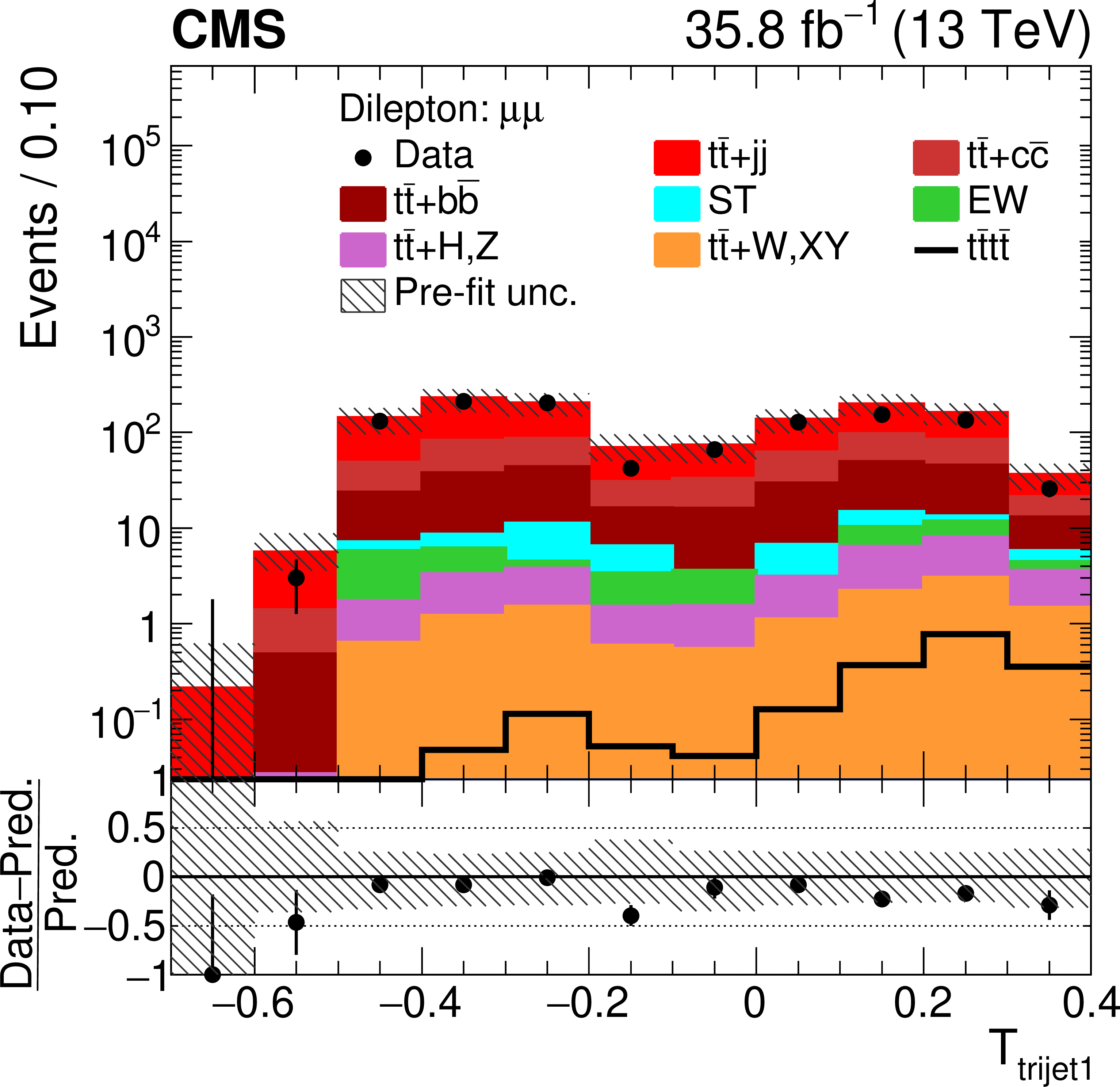
Figure 4-b:
Distributions of ${T_{\text {trijet1}}}$ in the $\mu^{+} {}\mu^{-} $ channel. In the upper panel, the data are shown as dots with error bars representing statistical uncertainties, MC simulations are shown as a histogram. In the lower panel the relative difference of the data with respect to MC prediction is also shown. In each panel, the shaded band represents the total uncertainty in the dominant ${\mathrm{t} {}\mathrm{\bar{t}}}$ background estimate. |
png pdf |
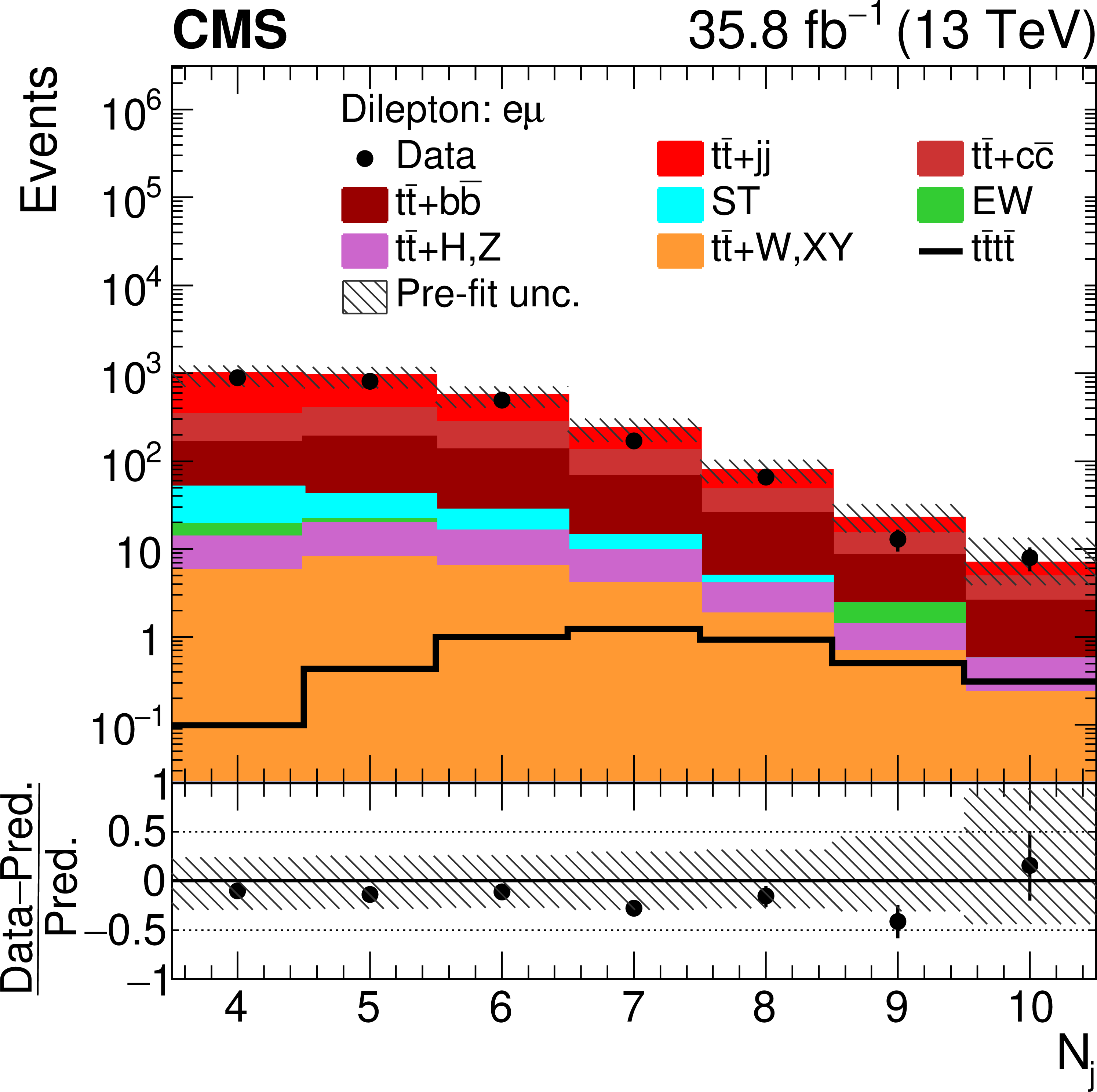
Figure 4-c:
Distributions of ${N_{\mathrm {j}}}$ in the $\mu^{\pm} \mathrm{e^{\mp}} $ channel. In the upper panel, the data are shown as dots with error bars representing statistical uncertainties, MC simulations are shown as a histogram. In the lower panel the relative difference of the data with respect to MC prediction is also shown. In each panel, the shaded band represents the total uncertainty in the dominant ${\mathrm{t} {}\mathrm{\bar{t}}}$ background estimate. |

png pdf |
Figure 4-d:
Distributions of ${T_{\text {trijet1}}}$ in the $\mu^{\pm} \mathrm{e^{\mp}} $ channel. In the upper panel, the data are shown as dots with error bars representing statistical uncertainties, MC simulations are shown as a histogram. In the lower panel the relative difference of the data with respect to MC prediction is also shown. In each panel, the shaded band represents the total uncertainty in the dominant ${\mathrm{t} {}\mathrm{\bar{t}}}$ background estimate. |

png pdf |
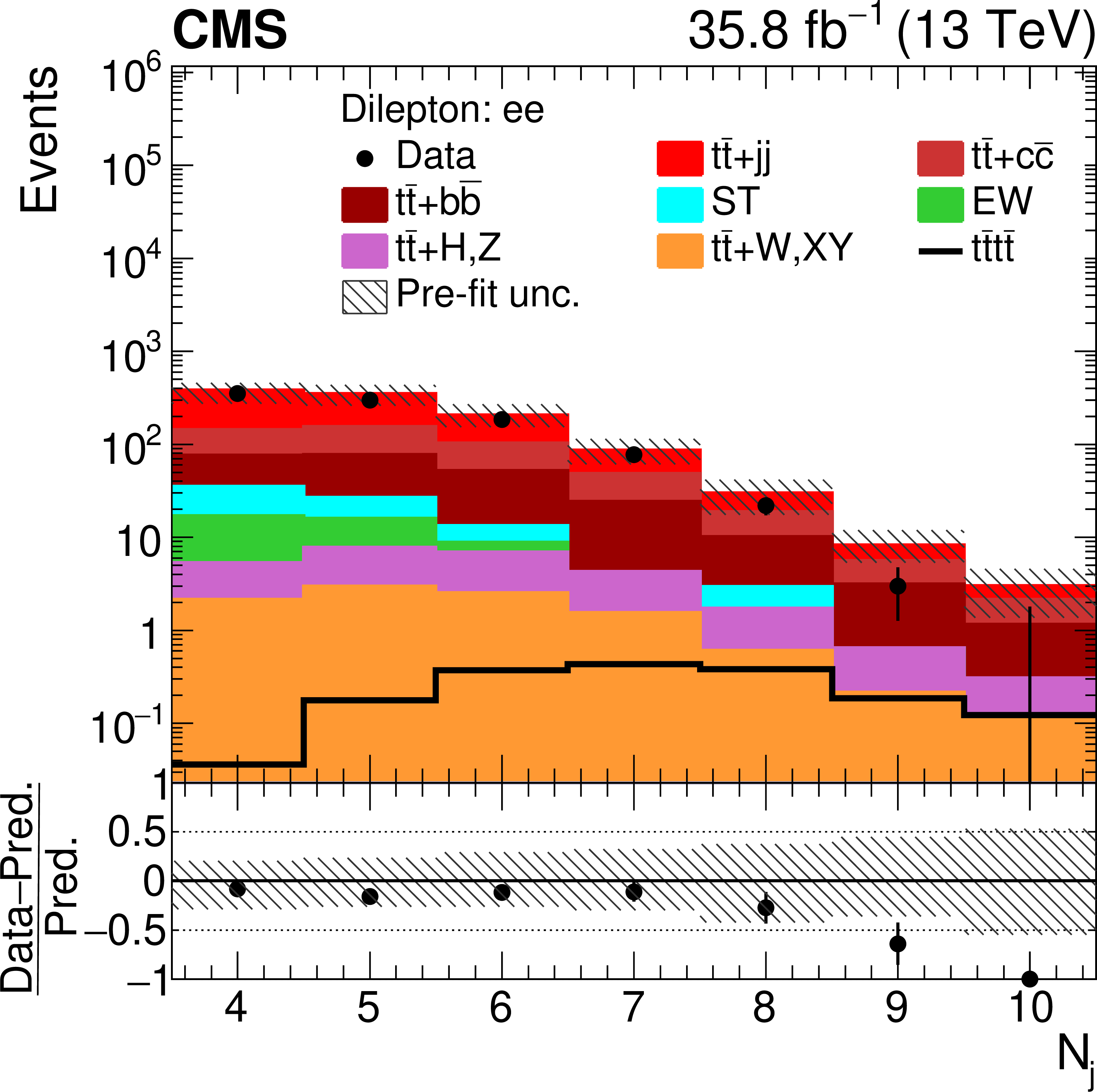
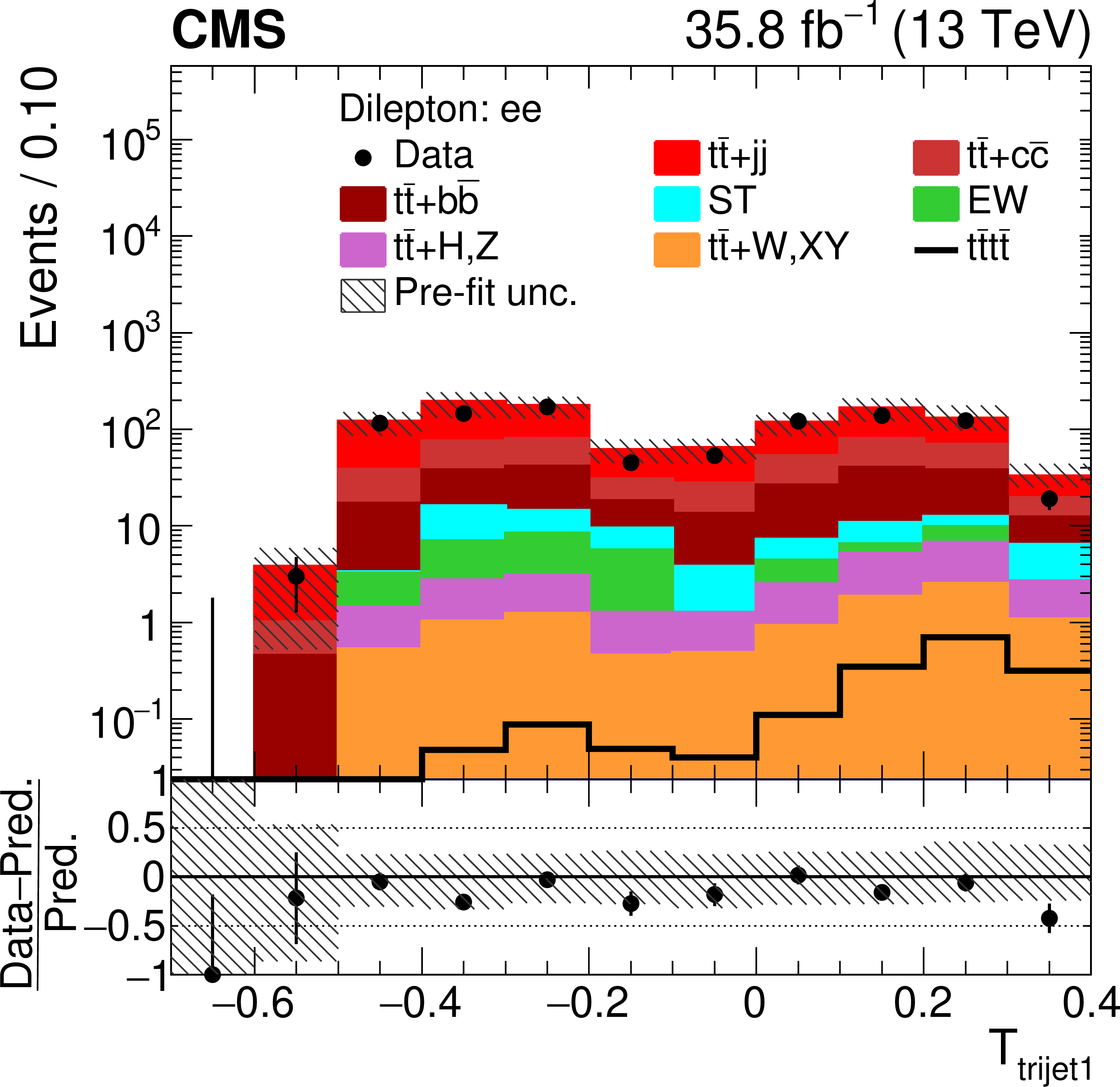
Figure 5:
Distributions of ${N_{\mathrm {j}}}$ and ${T_{\text {trijet1}}}$ in the $\mathrm{e^{+}} {}\mathrm{e^{-}} $ channel. In the upper panels of each figure, the data are shown as dots with error bars representing statistical uncertainties, MC simulations are shown as a histogram. In the lower panels the relative difference of the data with respect to MC prediction is also shown. In each panel, the shaded band represents the total uncertainty in the dominant ${\mathrm{t} {}\mathrm{\bar{t}}}$ background estimate. See Section 4.2 for the definitions of the variables. |
png pdf |
Figure 5-a:
Distribution of ${N_{\mathrm {j}}}$ in the $\mathrm{e^{+}} {}\mathrm{e^{-}} $ channel. In the upper panel, the data are shown as dots with error bars representing statistical uncertainties, MC simulations are shown as a histogram. In the lower panel the relative difference of the data with respect to MC prediction is also shown. In each panel, the shaded band represents the total uncertainty in the dominant ${\mathrm{t} {}\mathrm{\bar{t}}}$ background estimate. |
png pdf |
Figure 5-b:
Distribution of ${T_{\text {trijet1}}}$ in the $\mathrm{e^{+}} {}\mathrm{e^{-}} $ channel. In the upper panel, the data are shown as dots with error bars representing statistical uncertainties, MC simulations are shown as a histogram. In the lower panel the relative difference of the data with respect to MC prediction is also shown. In each panel, the shaded band represents the total uncertainty in the dominant ${\mathrm{t} {}\mathrm{\bar{t}}}$ background estimate. |
png pdf |
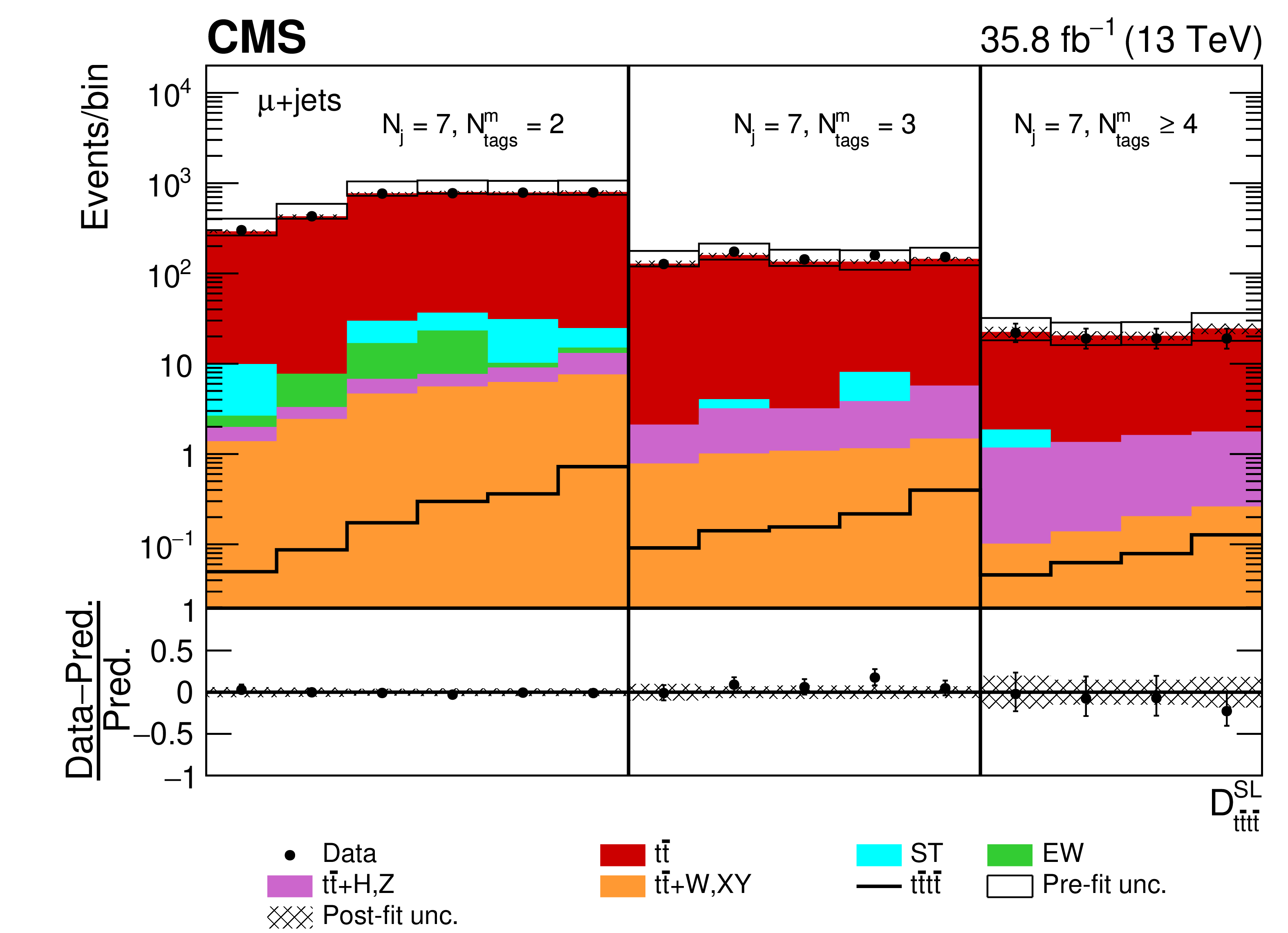
Figure 6:
Post-fit ${D_{{\mathrm{t} \mathrm{\bar{t}} \mathrm{t} \mathrm{\bar{t}}}}^{\text {SL}}}$ distribution in the single-muon channel for events satisfying baseline single-lepton selection and $ {N_{\mathrm {j}}} =$ 7, $ {N_{\text {tags}}^{\text {m}}} =$ 2, 3, $\geq $4. Non-uniform binning of the BDT discriminant was chosen to achieve approximately uniform distribution of the ${\mathrm{t} {}\mathrm{\bar{t}}}$ background. Dots represent data. Vertical error bars show the statistical uncertainties in data. The post-fit background predictions are shown as shaded histograms. Open boxes demonstrate the size of the pre-fit uncertainty in the total background and are centered around the pre-fit expectation value of the prediction. The hatched area shows the size of the post-fit uncertainty in the background prediction. The signal histogram template is shown as a solid line. The lower panel shows the relative difference of the observed number of events over the post-fit background prediction. |
png pdf |
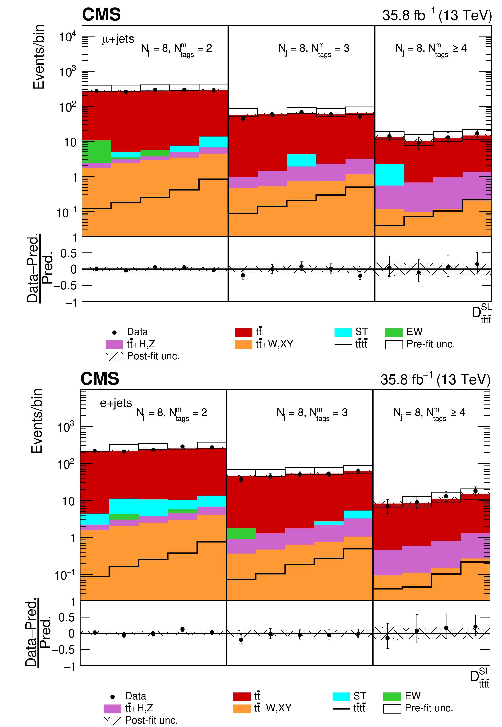
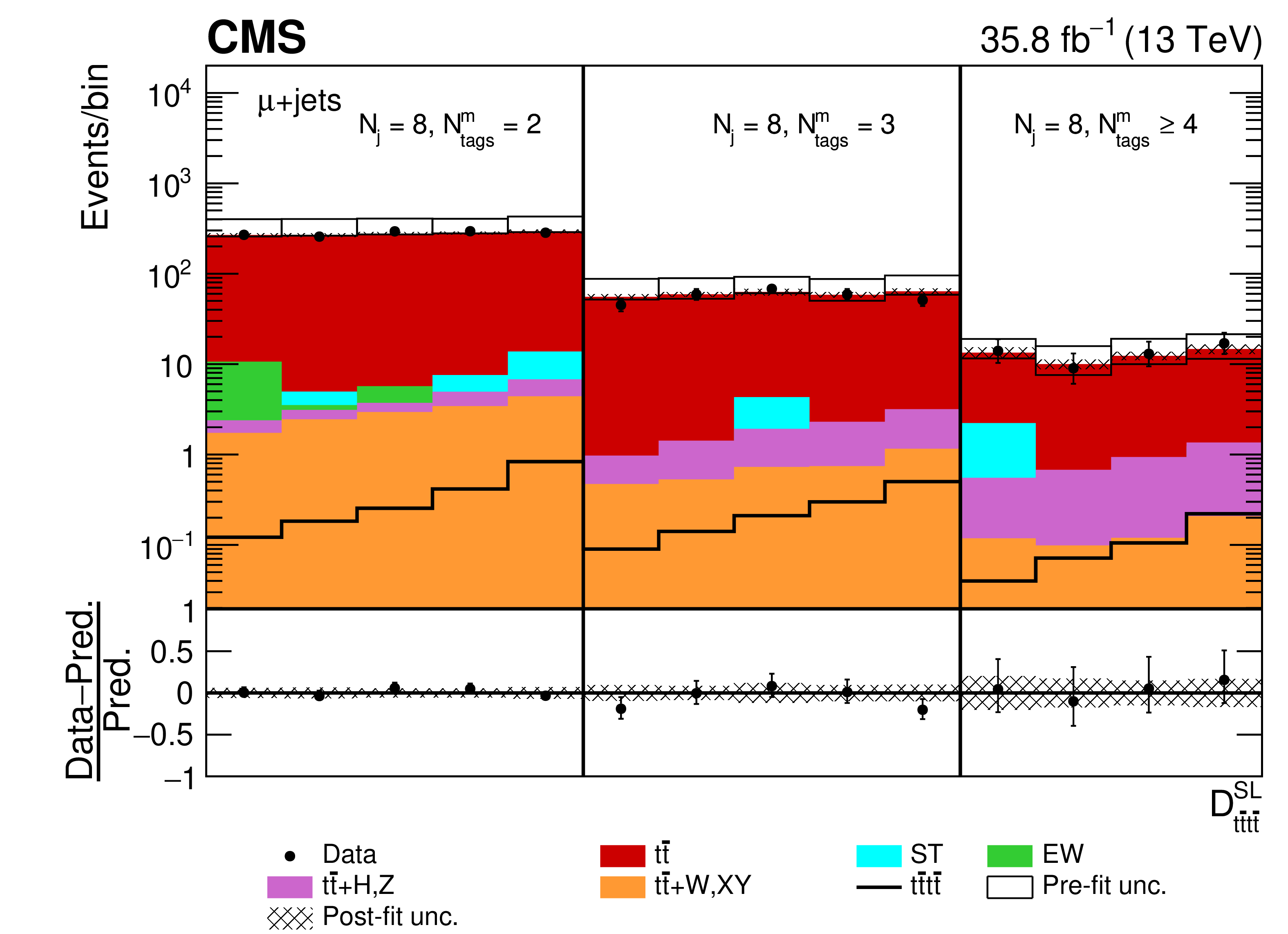
Figure 7:
Post-fit ${D_{{\mathrm{t} \mathrm{\bar{t}} \mathrm{t} \mathrm{\bar{t}}}}^{\text {SL}}}$ distribution in the (upper row) single-muon and (lower row) single-electron channels for events satisfying baseline single-lepton selection and $ {N_{\mathrm {j}}} =$ 8, $ {N_{\text {tags}}^{\text {m}}} =$ 2, 3, $\geq $4. Non-uniform binning of the BDT discriminant was chosen to achieve approximately uniform distribution of the ${\mathrm{t} {}\mathrm{\bar{t}}}$ background. Dots represent data. Vertical error bars show the statistical uncertainties in data. The post-fit background predictions are shown as shaded histograms. Open boxes demonstrate the size of the pre-fit uncertainty in the total background and are centered around the pre-fit expectation value of the prediction. The hatched area shows the size of the post-fit uncertainty in the background prediction. The signal histogram template is shown as a solid line. The lower panel shows the relative difference of the observed number of events over the post-fit background prediction. |
png pdf |
Figure 7-a:
Post-fit ${D_{{\mathrm{t} \mathrm{\bar{t}} \mathrm{t} \mathrm{\bar{t}}}}^{\text {SL}}}$ distribution in the single-muon channel for events satisfying baseline single-lepton selection and $ {N_{\mathrm {j}}} =$ 8, $ {N_{\text {tags}}^{\text {m}}} =$ 2, 3, $\geq $4. Non-uniform binning of the BDT discriminant was chosen to achieve approximately uniform distribution of the ${\mathrm{t} {}\mathrm{\bar{t}}}$ background. Dots represent data. Vertical error bars show the statistical uncertainties in data. The post-fit background predictions are shown as shaded histograms. Open boxes demonstrate the size of the pre-fit uncertainty in the total background and are centered around the pre-fit expectation value of the prediction. The hatched area shows the size of the post-fit uncertainty in the background prediction. The signal histogram template is shown as a solid line. The lower panel shows the relative difference of the observed number of events over the post-fit background prediction. |

png pdf |
Figure 7-b:
Post-fit ${D_{{\mathrm{t} \mathrm{\bar{t}} \mathrm{t} \mathrm{\bar{t}}}}^{\text {SL}}}$ distribution in the single-electron channel for events satisfying baseline single-lepton selection and $ {N_{\mathrm {j}}} =$ 8, $ {N_{\text {tags}}^{\text {m}}} =$ 2, 3, $\geq $4. Non-uniform binning of the BDT discriminant was chosen to achieve approximately uniform distribution of the ${\mathrm{t} {}\mathrm{\bar{t}}}$ background. Dots represent data. Vertical error bars show the statistical uncertainties in data. The post-fit background predictions are shown as shaded histograms. Open boxes demonstrate the size of the pre-fit uncertainty in the total background and are centered around the pre-fit expectation value of the prediction. The hatched area shows the size of the post-fit uncertainty in the background prediction. The signal histogram template is shown as a solid line. The lower panel shows the relative difference of the observed number of events over the post-fit background prediction. |

png pdf |
Figure 8:
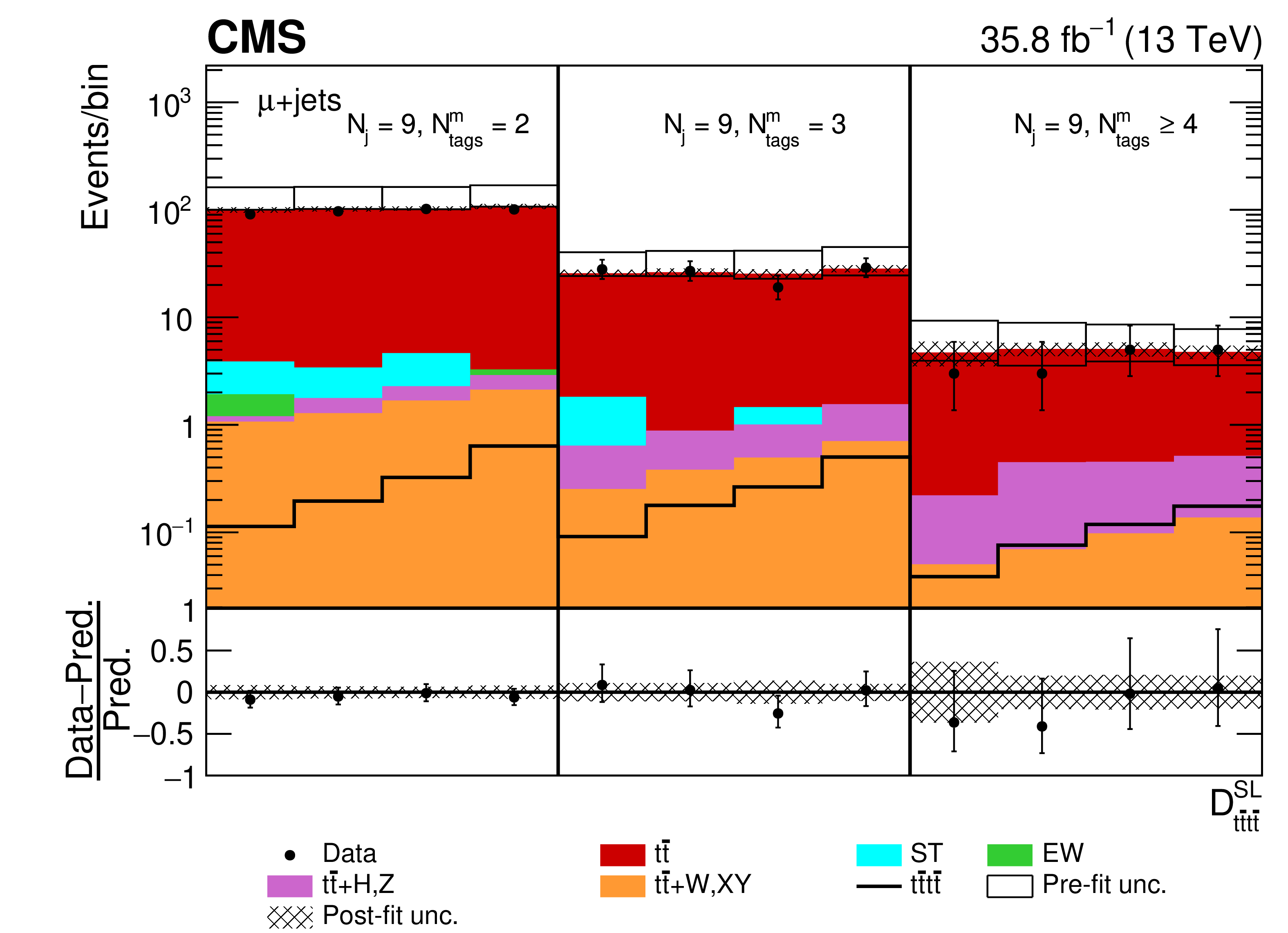
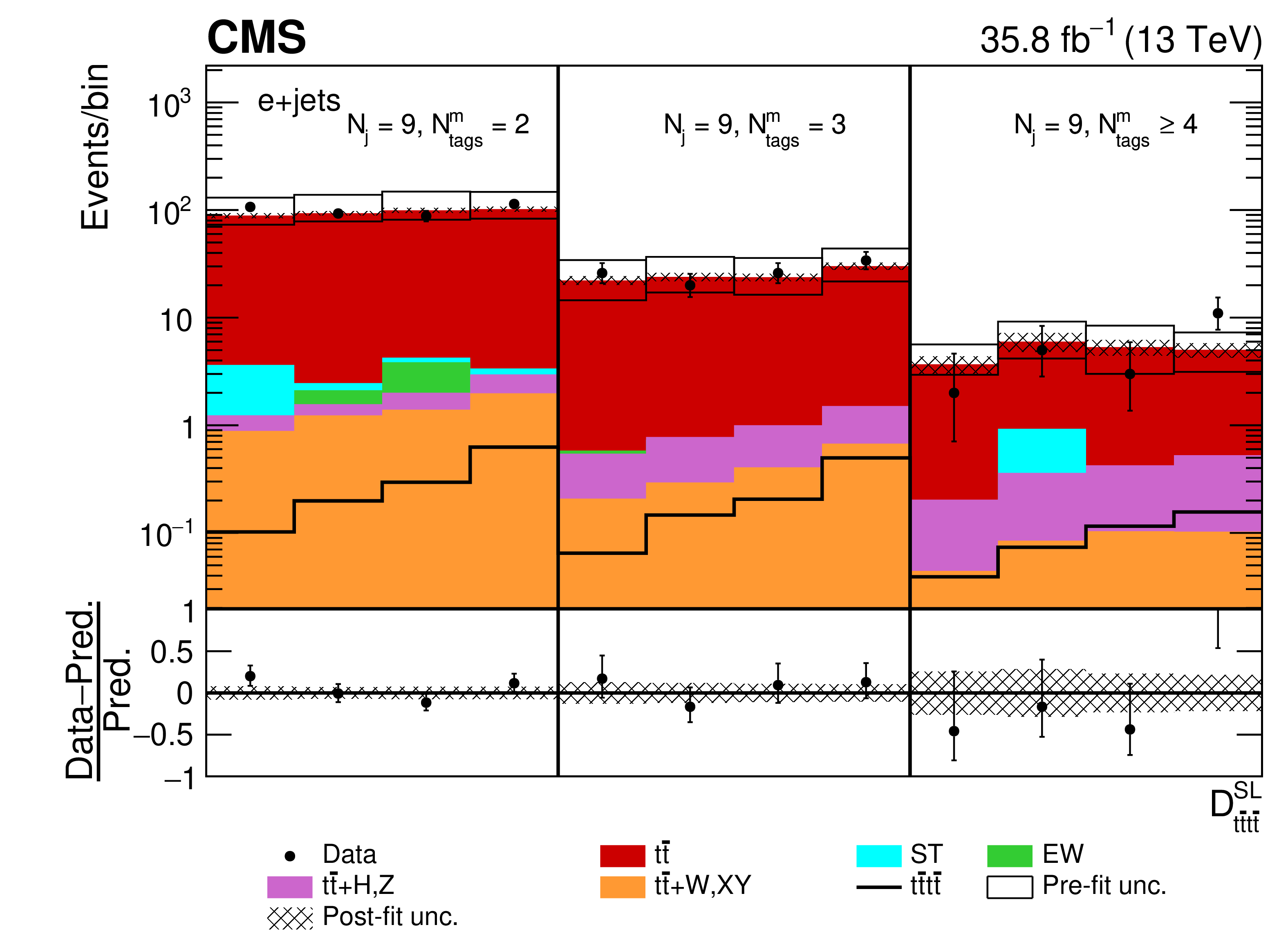
Post-fit ${D_{{\mathrm{t} \mathrm{\bar{t}} \mathrm{t} \mathrm{\bar{t}}}}^{\text {SL}}}$ distribution in the (upper row) single-muon and (lower row) single-electron channels for events satisfying baseline single-lepton selection and $ {N_{\mathrm {j}}} =$ 9, $ {N_{\text {tags}}^{\text {m}}} =$ 2, 3, $\geq $4. Non-uniform binning of the BDT discriminant was chosen to achieve approximately uniform distribution of the ${\mathrm{t} {}\mathrm{\bar{t}}}$ background. Dots represent data. Vertical error bars show the statistical uncertainties in data. The post-fit background predictions are shown as shaded histograms. Open boxes demonstrate the size of the pre-fit uncertainty in the total background and are centered around the pre-fit expectation value of the prediction. The hatched area shows the size of the post-fit uncertainty in the background prediction. The signal histogram template is shown as a solid line. The lower panel shows the relative difference of the observed number of events over the post-fit background prediction. |
png pdf |
Figure 8-a:
Post-fit ${D_{{\mathrm{t} \mathrm{\bar{t}} \mathrm{t} \mathrm{\bar{t}}}}^{\text {SL}}}$ distribution in the single-muon channel for events satisfying baseline single-lepton selection and $ {N_{\mathrm {j}}} =$ 9, $ {N_{\text {tags}}^{\text {m}}} =$ 2, 3, $\geq $4. Non-uniform binning of the BDT discriminant was chosen to achieve approximately uniform distribution of the ${\mathrm{t} {}\mathrm{\bar{t}}}$ background. Dots represent data. Vertical error bars show the statistical uncertainties in data. The post-fit background predictions are shown as shaded histograms. Open boxes demonstrate the size of the pre-fit uncertainty in the total background and are centered around the pre-fit expectation value of the prediction. The hatched area shows the size of the post-fit uncertainty in the background prediction. The signal histogram template is shown as a solid line. The lower panel shows the relative difference of the observed number of events over the post-fit background prediction. |
png pdf |
Figure 8-b:
Post-fit ${D_{{\mathrm{t} \mathrm{\bar{t}} \mathrm{t} \mathrm{\bar{t}}}}^{\text {SL}}}$ distribution in the single-electron channel for events satisfying baseline single-lepton selection and $ {N_{\mathrm {j}}} =$ 9, $ {N_{\text {tags}}^{\text {m}}} =$ 2, 3, $\geq $4. Non-uniform binning of the BDT discriminant was chosen to achieve approximately uniform distribution of the ${\mathrm{t} {}\mathrm{\bar{t}}}$ background. Dots represent data. Vertical error bars show the statistical uncertainties in data. The post-fit background predictions are shown as shaded histograms. Open boxes demonstrate the size of the pre-fit uncertainty in the total background and are centered around the pre-fit expectation value of the prediction. The hatched area shows the size of the post-fit uncertainty in the background prediction. The signal histogram template is shown as a solid line. The lower panel shows the relative difference of the observed number of events over the post-fit background prediction. |
png pdf |
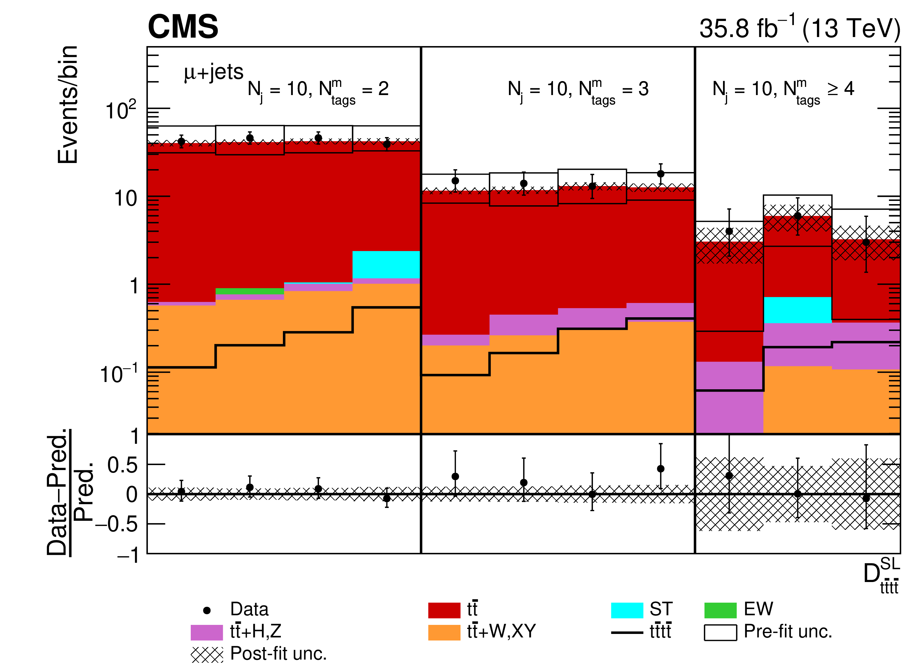
Figure 9:
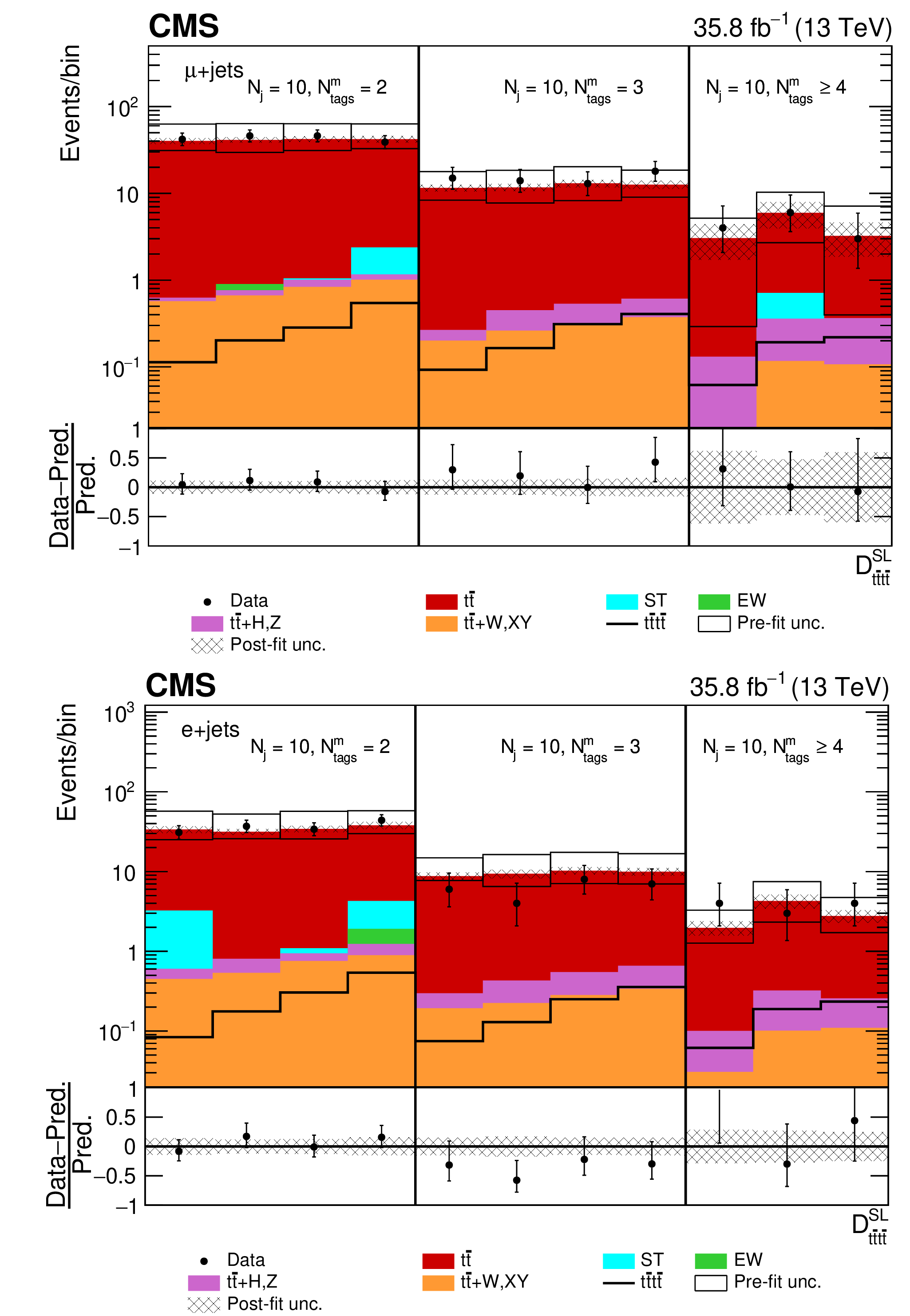
Post-fit ${D_{{\mathrm{t} \mathrm{\bar{t}} \mathrm{t} \mathrm{\bar{t}}}}^{\text {SL}}}$ distribution in the (upper row) single-muon and (lower row) single-electron channels for events satisfying baseline single-lepton selection and $ {N_{\mathrm {j}}} \geq$ 10, $ {N_{\text {tags}}^{\text {m}}} =$ 2, 3, $\geq $4. Non-uniform binning of the BDT discriminant was chosen to achieve approximately uniform distribution of the ${\mathrm{t} {}\mathrm{\bar{t}}}$ background. Dots represent data. Vertical error bars show the statistical uncertainties in data. The post-fit background predictions are shown as shaded histograms. Open boxes demonstrate the size of the pre-fit uncertainty in the total background and are centered around the pre-fit expectation value of the prediction. The hatched area shows the size of the post-fit uncertainty in the background prediction. The signal histogram template is shown as a solid line. The lower panel shows the relative difference of the observed number of events over the post-fit background prediction. |
png pdf |
Figure 9-a:
Post-fit ${D_{{\mathrm{t} \mathrm{\bar{t}} \mathrm{t} \mathrm{\bar{t}}}}^{\text {SL}}}$ distribution in the single-muon channel for events satisfying baseline single-lepton selection and $ {N_{\mathrm {j}}} \geq$ 10, $ {N_{\text {tags}}^{\text {m}}} =$ 2, 3, $\geq $4. Non-uniform binning of the BDT discriminant was chosen to achieve approximately uniform distribution of the ${\mathrm{t} {}\mathrm{\bar{t}}}$ background. Dots represent data. Vertical error bars show the statistical uncertainties in data. The post-fit background predictions are shown as shaded histograms. Open boxes demonstrate the size of the pre-fit uncertainty in the total background and are centered around the pre-fit expectation value of the prediction. The hatched area shows the size of the post-fit uncertainty in the background prediction. The signal histogram template is shown as a solid line. The lower panel shows the relative difference of the observed number of events over the post-fit background prediction. |
png pdf |
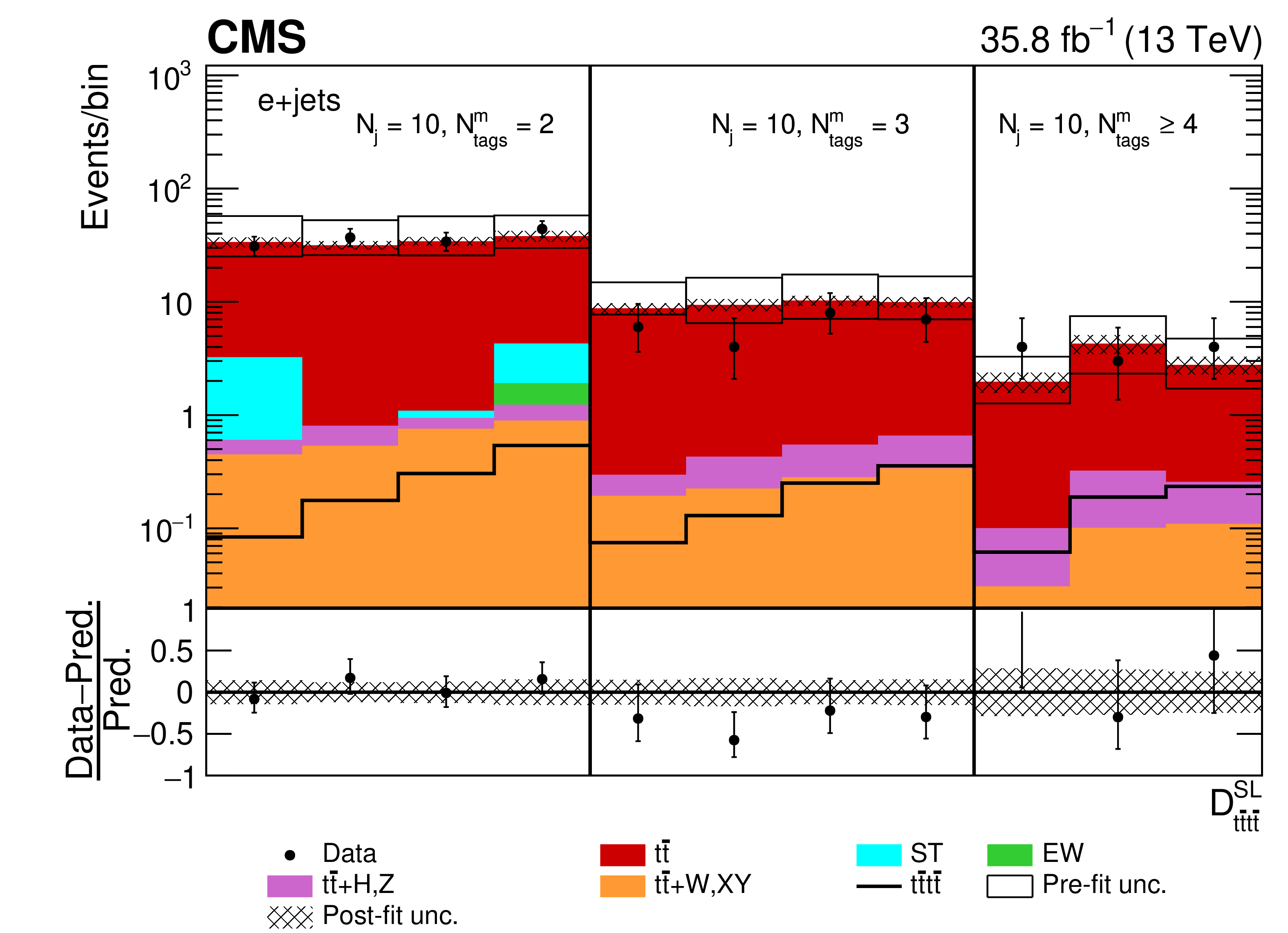
Figure 9-b:
Post-fit ${D_{{\mathrm{t} \mathrm{\bar{t}} \mathrm{t} \mathrm{\bar{t}}}}^{\text {SL}}}$ distribution in the single-electron channel for events satisfying baseline single-lepton selection and $ {N_{\mathrm {j}}} \geq$ 10, $ {N_{\text {tags}}^{\text {m}}} =$ 2, 3, $\geq $4. Non-uniform binning of the BDT discriminant was chosen to achieve approximately uniform distribution of the ${\mathrm{t} {}\mathrm{\bar{t}}}$ background. Dots represent data. Vertical error bars show the statistical uncertainties in data. The post-fit background predictions are shown as shaded histograms. Open boxes demonstrate the size of the pre-fit uncertainty in the total background and are centered around the pre-fit expectation value of the prediction. The hatched area shows the size of the post-fit uncertainty in the background prediction. The signal histogram template is shown as a solid line. The lower panel shows the relative difference of the observed number of events over the post-fit background prediction. |
png pdf |
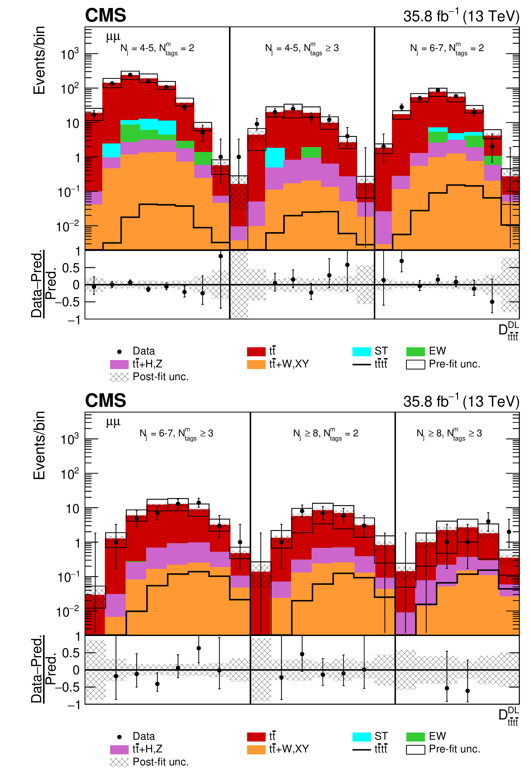
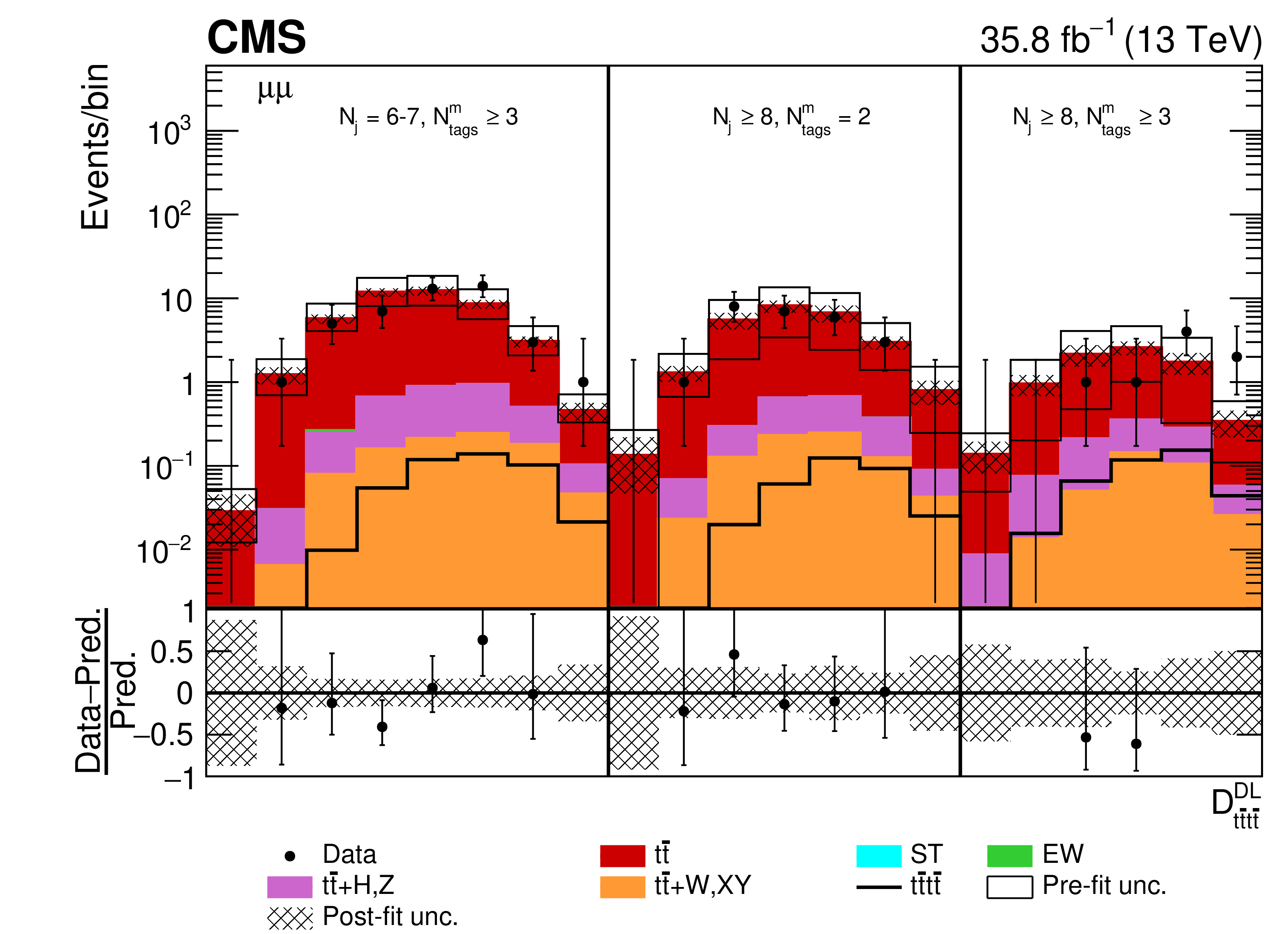
Figure 10:
Post-fit $ {D_{{\mathrm{t} \mathrm{\bar{t}} \mathrm{t} \mathrm{\bar{t}}}}^{\text {DL}}}$ distributions in the $\mu^{+} {}\mu^{-} $ channel for events satisfying baseline opposite-sign dilepton selection and (upper row) $ {N_{\mathrm {j}}} =$ 4-5, $ {N_{\text {tags}}^{\text {m}}} =$ 2, $\geq $3, $ {N_{\mathrm {j}}} =$ 6-7, $ {N_{\text {tags}}^{\text {m}}} =$ 2 and (lower row) $ {N_{\mathrm {j}}} =$ 6-7, $ {N_{\text {tags}}^{\text {m}}} \geq$ 3, $ {N_{\mathrm {j}}} \geq$ 8, $ {N_{\text {tags}}^{\text {m}}} =$ 2, $\geq $3. Dots represent data. Vertical error bars show the statistical uncertainties in data. The post-fit background predictions are shown as shaded histograms. Open boxes demonstrate the size of the pre-fit uncertainty in the total background and are centered around the pre-fit expectation value of the prediction. The hatched area shows the size of the post-fit uncertainty in the background prediction. The signal histogram template is shown as a solid line. The lower panel shows the relative difference of the observed number of events over the post-fit background prediction. |
png pdf |
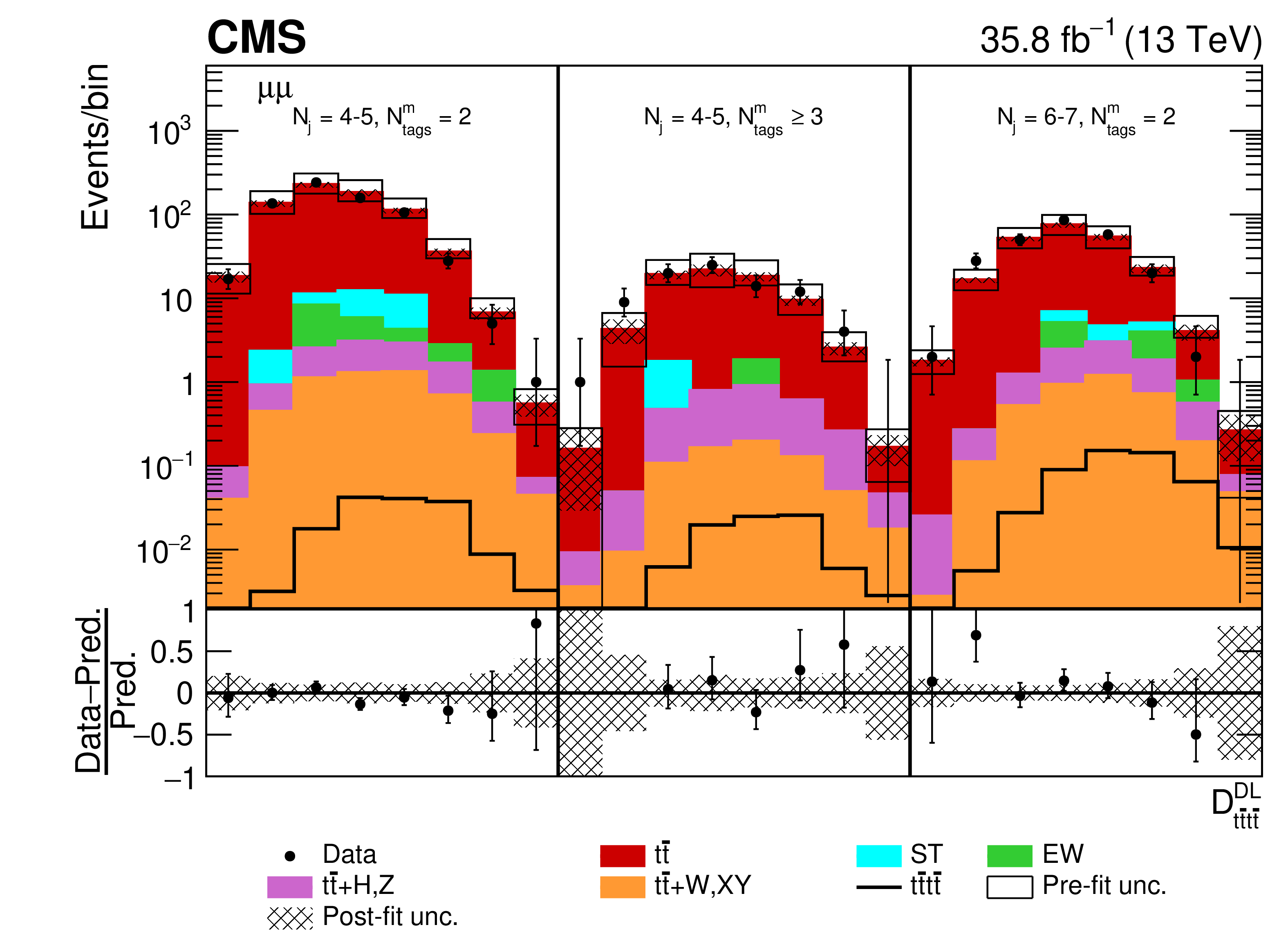
Figure 10-a:
Post-fit $ {D_{{\mathrm{t} \mathrm{\bar{t}} \mathrm{t} \mathrm{\bar{t}}}}^{\text {DL}}}$ distribution in the $\mu^{+} {}\mu^{-} $ channel for events satisfying baseline opposite-sign dilepton selection and $ {N_{\mathrm {j}}} =$ 4-5, $ {N_{\text {tags}}^{\text {m}}} =$ 2, $\geq $3, $ {N_{\mathrm {j}}} =$ 6-7, $ {N_{\text {tags}}^{\text {m}}} =$ 2. Dots represent data. Vertical error bars show the statistical uncertainties in data. The post-fit background predictions are shown as shaded histograms. Open boxes demonstrate the size of the pre-fit uncertainty in the total background and are centered around the pre-fit expectation value of the prediction. The hatched area shows the size of the post-fit uncertainty in the background prediction. The signal histogram template is shown as a solid line. The lower panel shows the relative difference of the observed number of events over the post-fit background prediction. |
png pdf |
Figure 10-b:
Post-fit $ {D_{{\mathrm{t} \mathrm{\bar{t}} \mathrm{t} \mathrm{\bar{t}}}}^{\text {DL}}}$ distribution in the $\mu^{+} {}\mu^{-} $ channel for events satisfying baseline opposite-sign dilepton selection and $ {N_{\mathrm {j}}} =$ 6-7, $ {N_{\text {tags}}^{\text {m}}} \geq$ 3, $ {N_{\mathrm {j}}} \geq$ 8, $ {N_{\text {tags}}^{\text {m}}} =$ 2, $\geq $3. Dots represent data. Vertical error bars show the statistical uncertainties in data. The post-fit background predictions are shown as shaded histograms. Open boxes demonstrate the size of the pre-fit uncertainty in the total background and are centered around the pre-fit expectation value of the prediction. The hatched area shows the size of the post-fit uncertainty in the background prediction. The signal histogram template is shown as a solid line. The lower panel shows the relative difference of the observed number of events over the post-fit background prediction. |

png pdf |
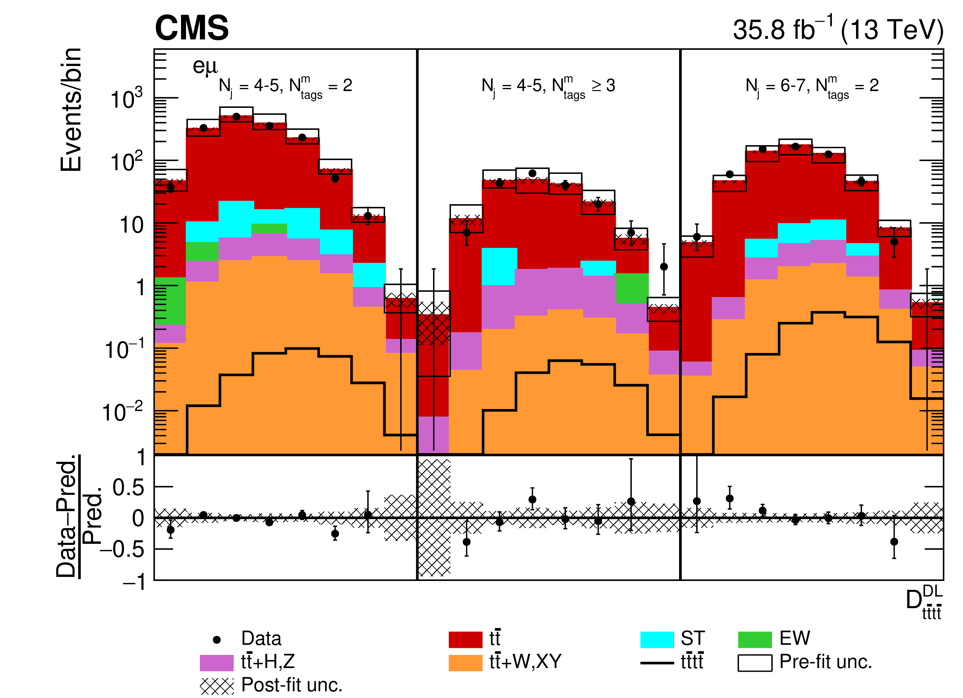
Figure 11:
Post-fit $ {D_{{\mathrm{t} \mathrm{\bar{t}} \mathrm{t} \mathrm{\bar{t}}}}^{\text {DL}}}$ distributions in the $\mu^{\pm} \mathrm{e^{\mp}} $ channel for events satisfying baseline opposite-sign dilepton selection and (upper row) $ {N_{\mathrm {j}}} =$ 4-5, $ {N_{\text {tags}}^{\text {m}}} =$ 2, $\geq $3, $ {N_{\mathrm {j}}} =$ 6-7, $ {N_{\text {tags}}^{\text {m}}} =$ 2 and (lower row) $ {N_{\mathrm {j}}} =$ 6-7, $ {N_{\text {tags}}^{\text {m}}} \geq$ 3, $ {N_{\mathrm {j}}} \geq$ 8, $ {N_{\text {tags}}^{\text {m}}} =$ 2, $\geq $3. Dots represent data. Vertical error bars show the statistical uncertainties in data. The post-fit background predictions are shown as shaded histograms. Open boxes demonstrate the size of the pre-fit uncertainty in the total background and are centered around the pre-fit expectation value of the prediction. The hatched area shows the size of the post-fit uncertainty in the background prediction. The signal histogram template is shown as a solid line. The lower panel shows the relative difference of the observed number of events over the post-fit background prediction. |
png pdf |
Figure 11-a:
Post-fit $ {D_{{\mathrm{t} \mathrm{\bar{t}} \mathrm{t} \mathrm{\bar{t}}}}^{\text {DL}}}$ distribution in the $\mu^{\pm} \mathrm{e^{\mp}} $ channel for events satisfying baseline opposite-sign dilepton selection and $ {N_{\mathrm {j}}} =$ 4-5, $ {N_{\text {tags}}^{\text {m}}} =$ 2, $\geq $3, $ {N_{\mathrm {j}}} =$ 6-7, $ {N_{\text {tags}}^{\text {m}}} =$ 2. Dots represent data. Vertical error bars show the statistical uncertainties in data. The post-fit background predictions are shown as shaded histograms. Open boxes demonstrate the size of the pre-fit uncertainty in the total background and are centered around the pre-fit expectation value of the prediction. The hatched area shows the size of the post-fit uncertainty in the background prediction. The signal histogram template is shown as a solid line. The lower panel shows the relative difference of the observed number of events over the post-fit background prediction. |
png pdf |
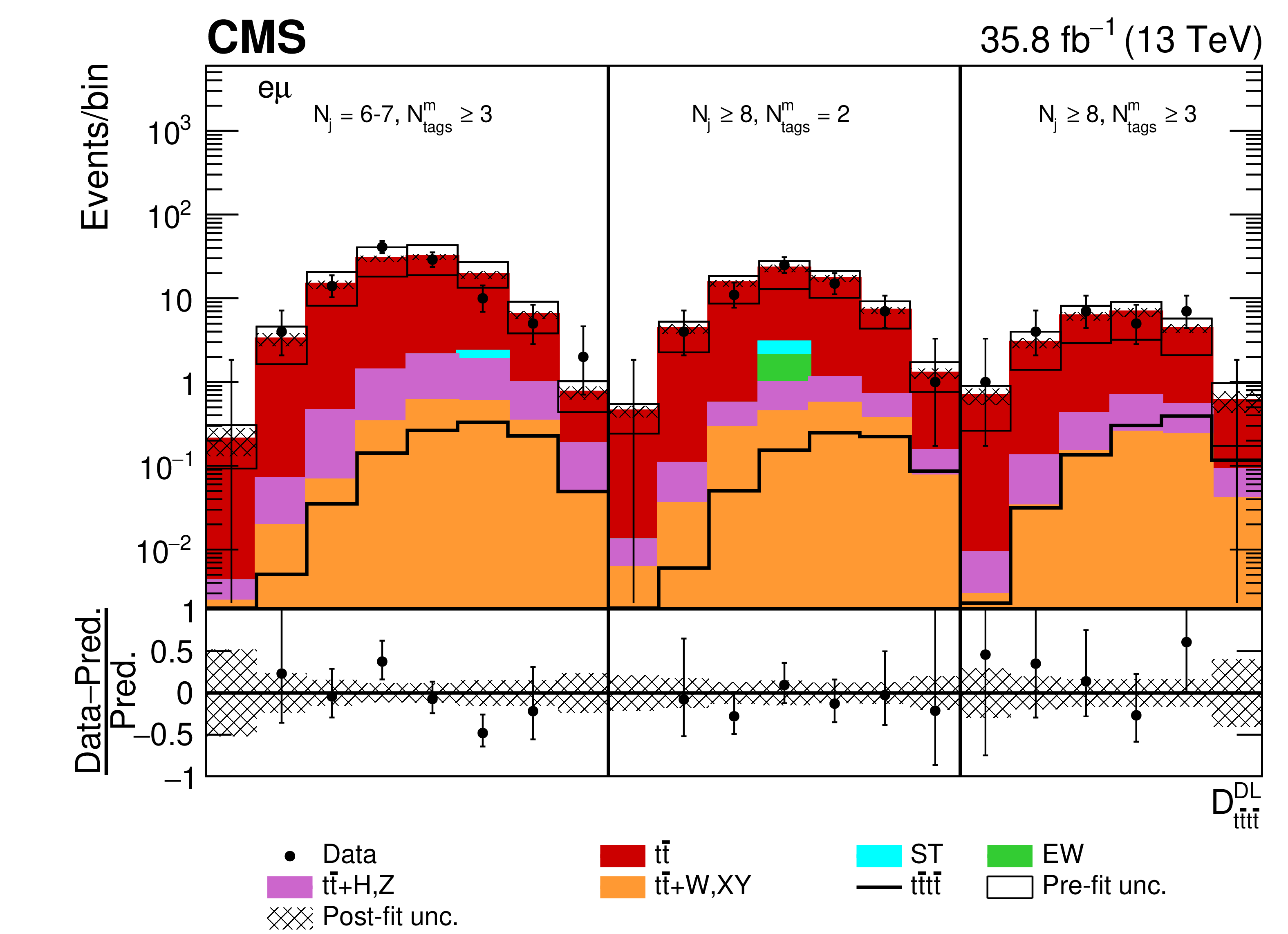
Figure 11-b:
Post-fit $ {D_{{\mathrm{t} \mathrm{\bar{t}} \mathrm{t} \mathrm{\bar{t}}}}^{\text {DL}}}$ distribution in the $\mu^{\pm} \mathrm{e^{\mp}} $ channel for events satisfying baseline opposite-sign dilepton selection and $ {N_{\mathrm {j}}} =$ 6-7, $ {N_{\text {tags}}^{\text {m}}} \geq$ 3, $ {N_{\mathrm {j}}} \geq$ 8, $ {N_{\text {tags}}^{\text {m}}} =$ 2, $\geq $3. Dots represent data. Vertical error bars show the statistical uncertainties in data. The post-fit background predictions are shown as shaded histograms. Open boxes demonstrate the size of the pre-fit uncertainty in the total background and are centered around the pre-fit expectation value of the prediction. The hatched area shows the size of the post-fit uncertainty in the background prediction. The signal histogram template is shown as a solid line. The lower panel shows the relative difference of the observed number of events over the post-fit background prediction. |
png pdf |
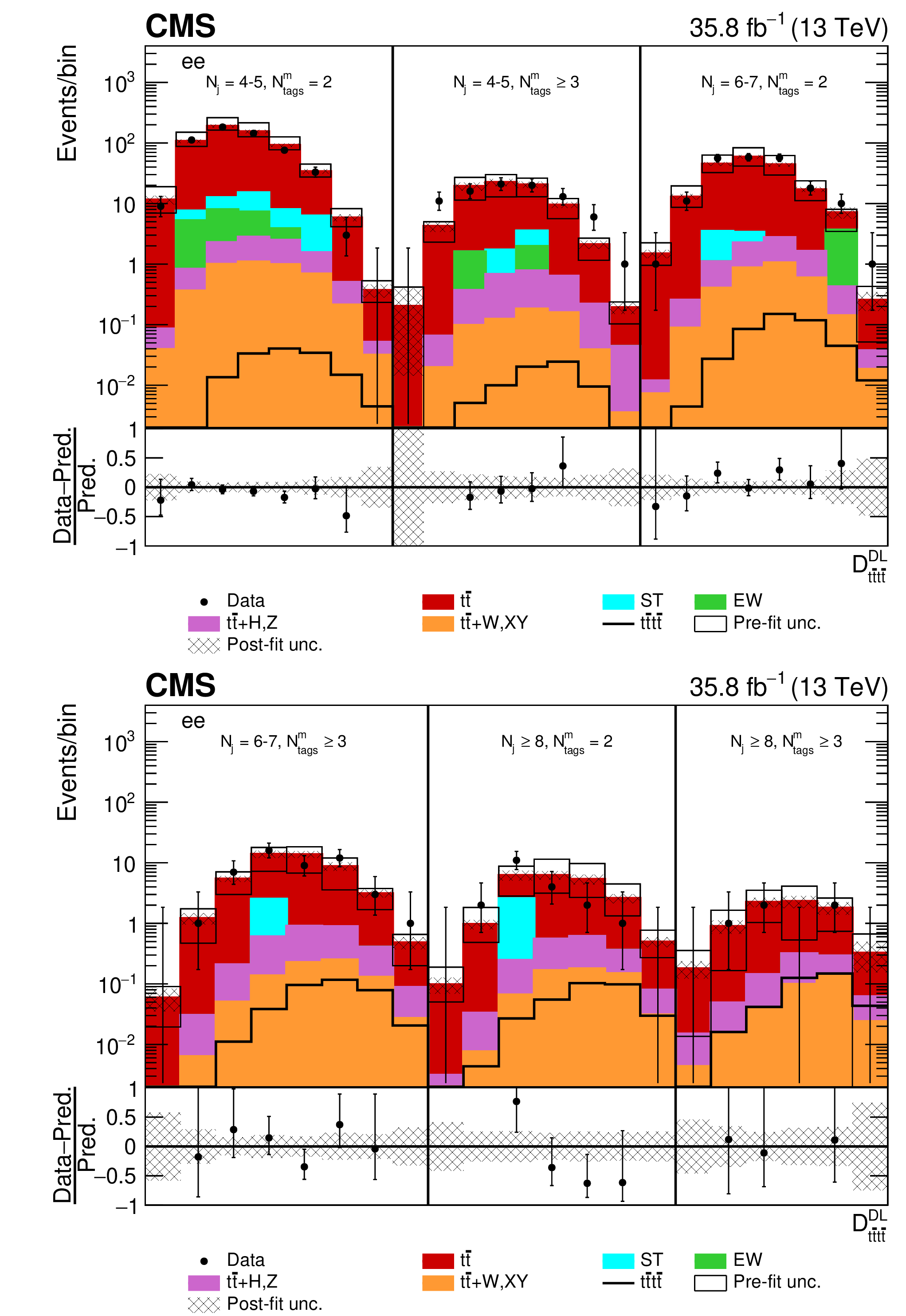
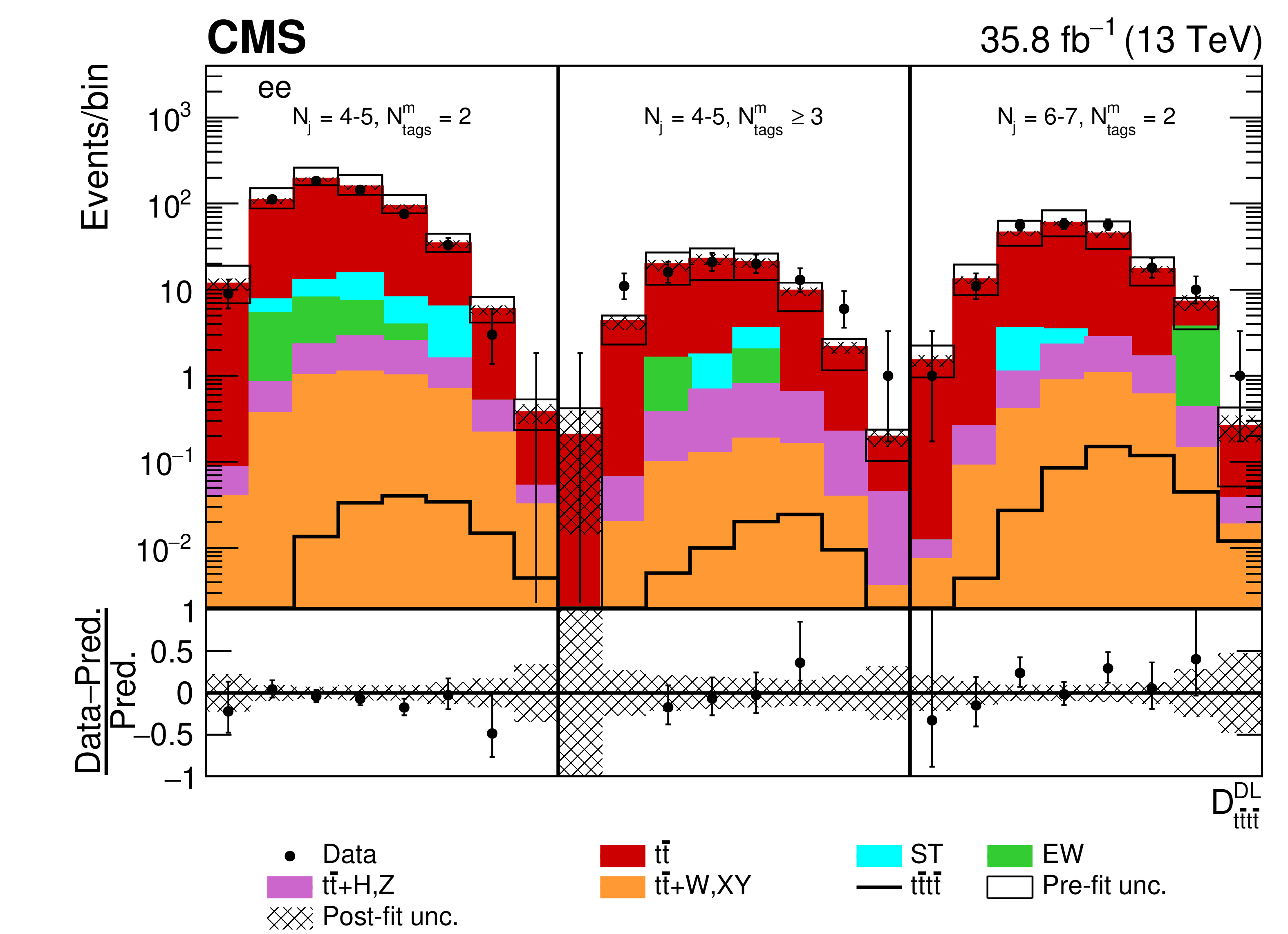
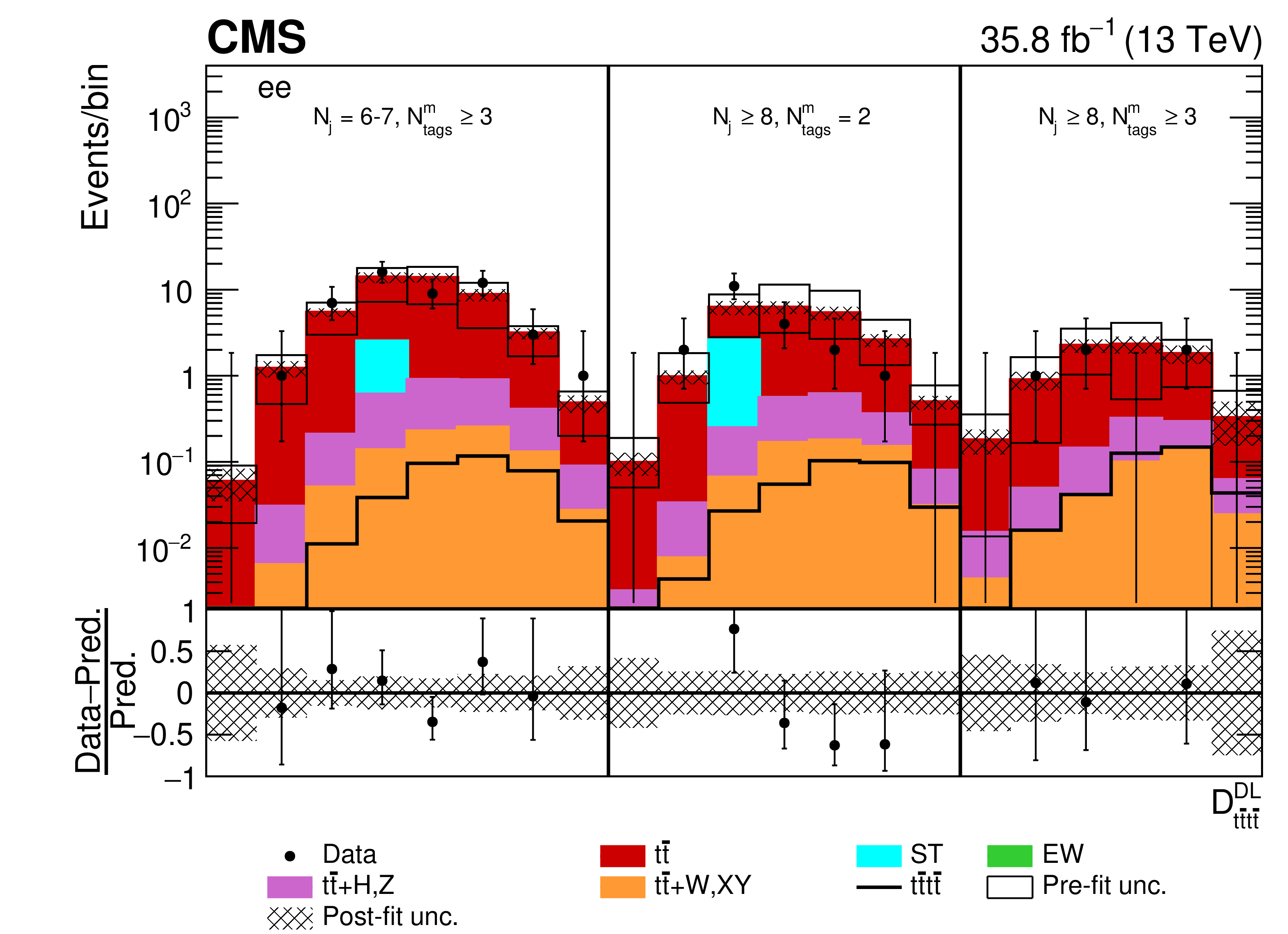
Figure 12:
Post-fit $ {D_{{\mathrm{t} \mathrm{\bar{t}} \mathrm{t} \mathrm{\bar{t}}}}^{\text {DL}}}$ distributions in the $\mathrm{e^{+}} {}\mathrm{e^{-}} $ channel for events satisfying baseline opposite-sign dilepton selection and (upper row) $ {N_{\mathrm {j}}} =$ 4-5, $ {N_{\text {tags}}^{\text {m}}} =$ 2, $\geq $3, $ {N_{\mathrm {j}}} =$ 6-7, $ {N_{\text {tags}}^{\text {m}}} =$ 2 and (lower row) $ {N_{\mathrm {j}}} =$ 6-7, $ {N_{\text {tags}}^{\text {m}}} \geq$ 3, $ {N_{\mathrm {j}}} \geq$ 8, $ {N_{\text {tags}}^{\text {m}}} =$ 2, $\geq $3. Dots represent data. Vertical error bars show the statistical uncertainties in data. The post-fit background predictions are shown as shaded histograms. Open boxes demonstrate the size of the pre-fit uncertainty in the total background and are centered around the pre-fit expectation value of the prediction. The hatched area shows the size of the post-fit uncertainty in the background prediction. The signal histogram template is shown as a solid line. The lower panel shows the relative difference of the observed number of events over the post-fit background prediction. |
png pdf |
Figure 12-a:
Post-fit $ {D_{{\mathrm{t} \mathrm{\bar{t}} \mathrm{t} \mathrm{\bar{t}}}}^{\text {DL}}}$ distribution in the $\mathrm{e^{+}} {}\mathrm{e^{-}} $ channel for events satisfying baseline opposite-sign dilepton selection and $ {N_{\mathrm {j}}} =$ 4-5, $ {N_{\text {tags}}^{\text {m}}} =$ 2, $\geq $3, $ {N_{\mathrm {j}}} =$ 6-7, $ {N_{\text {tags}}^{\text {m}}} =$ 2. Dots represent data. Vertical error bars show the statistical uncertainties in data. The post-fit background predictions are shown as shaded histograms. Open boxes demonstrate the size of the pre-fit uncertainty in the total background and are centered around the pre-fit expectation value of the prediction. The hatched area shows the size of the post-fit uncertainty in the background prediction. The signal histogram template is shown as a solid line. The lower panel shows the relative difference of the observed number of events over the post-fit background prediction. |
png pdf |
Figure 12-b:
Post-fit $ {D_{{\mathrm{t} \mathrm{\bar{t}} \mathrm{t} \mathrm{\bar{t}}}}^{\text {DL}}}$ distribution in the $\mathrm{e^{+}} {}\mathrm{e^{-}} $ channel for events satisfying baseline opposite-sign dilepton selection and $ {N_{\mathrm {j}}} =$ 6-7, $ {N_{\text {tags}}^{\text {m}}} \geq$ 3, $ {N_{\mathrm {j}}} \geq$ 8, $ {N_{\text {tags}}^{\text {m}}} =$ 2, $\geq $3. Dots represent data. Vertical error bars show the statistical uncertainties in data. The post-fit background predictions are shown as shaded histograms. Open boxes demonstrate the size of the pre-fit uncertainty in the total background and are centered around the pre-fit expectation value of the prediction. The hatched area shows the size of the post-fit uncertainty in the background prediction. The signal histogram template is shown as a solid line. The lower panel shows the relative difference of the observed number of events over the post-fit background prediction. |
| Tables | |
png pdf |
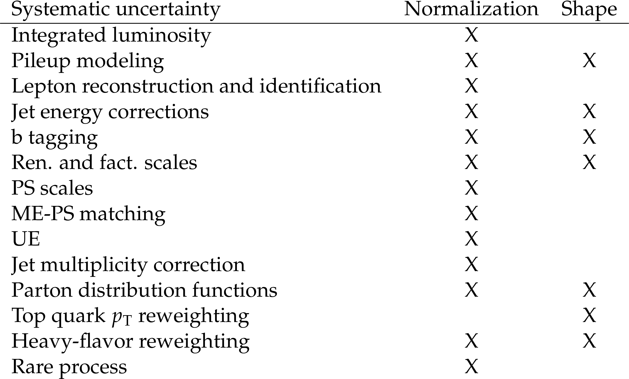
Table 1:
Uncertainties that affect the normalization of the data sets and shapes of the ${D_{{\mathrm{t} \mathrm{\bar{t}} \mathrm{t} \mathrm{\bar{t}}}}^{\text {SL}}}$ and $ {D_{{\mathrm{t} \mathrm{\bar{t}} \mathrm{t} \mathrm{\bar{t}}}}^{\text {DL}}}$ discriminants. Their contribution to different effects are marked by X. |
png pdf |
Table 2:
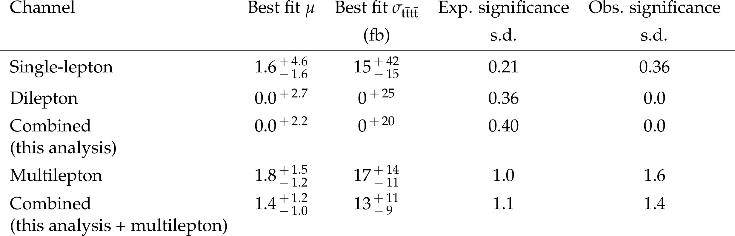
Maximum-likelihood signal strength and cross section estimates, as well as the expected and observed significance of SM $ {\mathrm{t} \mathrm{\bar{t}} \mathrm{t} \mathrm{\bar{t}}}$ production. The results for the two analyses from this paper are shown separately and combined. The results from a previous CMS multilepton measurement are also given [15]. The values quoted for the uncertainties on the signal strengths and cross sections are the one standard deviation (s.d.) values and include all statistical and systematic uncertainties. The expected significance is calculated assuming that the data are distributed according to the prediction of the SM with nominal $ {\mathrm{t} \mathrm{\bar{t}} \mathrm{t} \mathrm{\bar{t}}}$ production cross section value $\sigma _{{\mathrm{t} \mathrm{\bar{t}} \mathrm{t} \mathrm{\bar{t}}}}^\text {SM}$, which corresponds to the assumed signal strength modifier value $\mu =$ 1. |
png pdf |
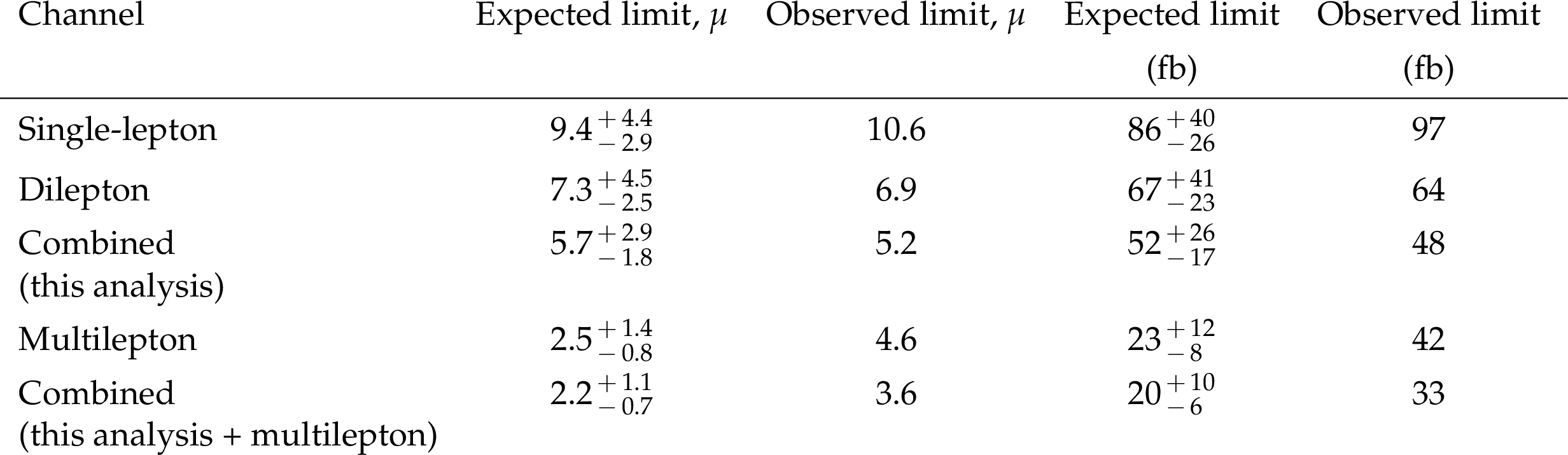
Table 3:
Expected and observed 95% CL upper limits on SM $ {\mathrm{t} \mathrm{\bar{t}} \mathrm{t} \mathrm{\bar{t}}}$ production as a multiple of ${\sigma _{{\mathrm{t} \mathrm{\bar{t}} \mathrm{t} \mathrm{\bar{t}}}}^{\text {SM}}}$ and in fb. The results for the two analyses from this paper are shown separately and combined. The results from a previous CMS multilepton search are also given [15]. The values quoted for the uncertainties in the expected limits indicate the regions containing 68% of the distribution of limits expected under the background-only hypothesis. The expected upper limits are calculated assuming that the data are distributed according to the prediction of the background-only model corresponding to the scenario with signal strength modifier value $\mu =$ 0. |
png pdf |
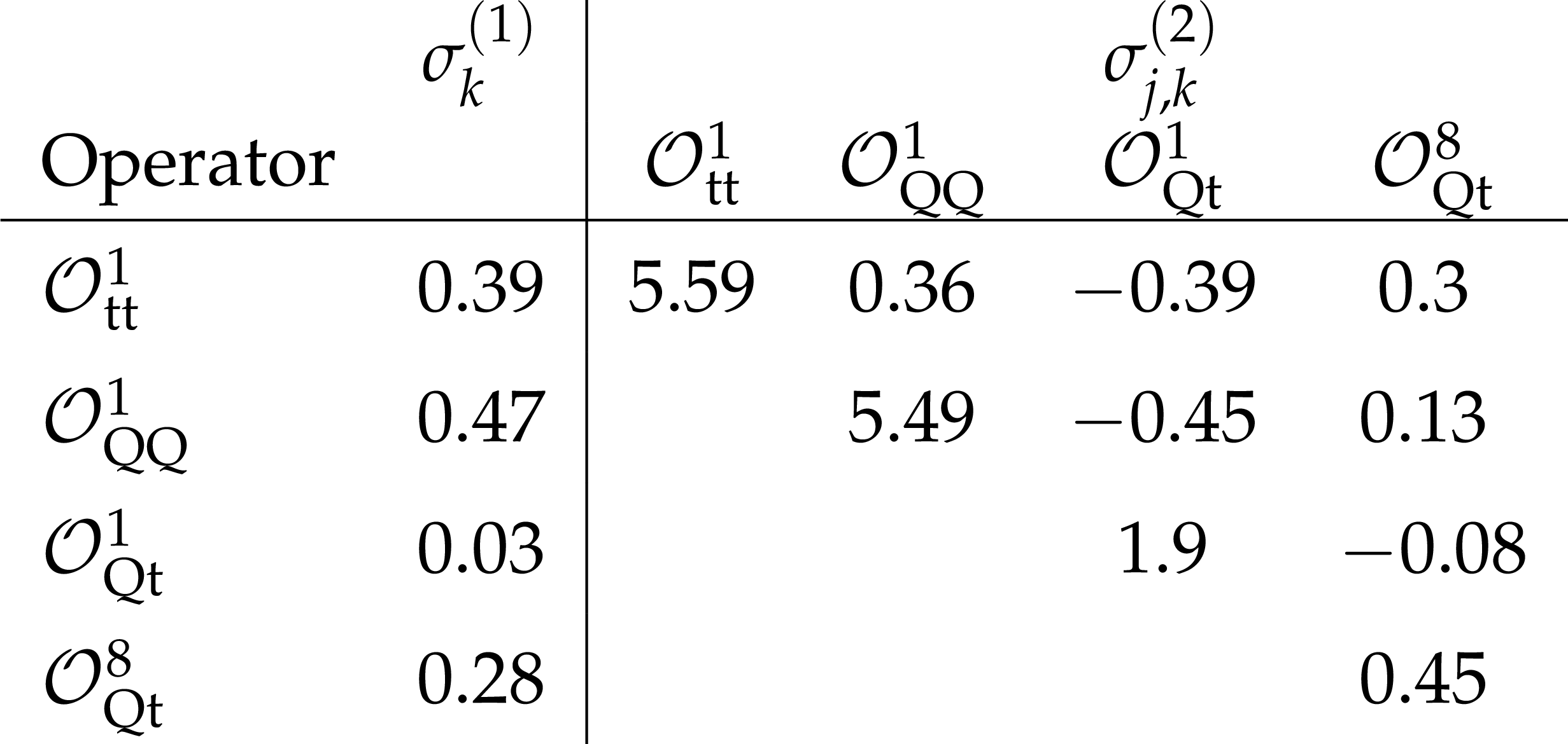
Table 4:
Linear (left) and quadratic (right) parameterization coefficients, $\sigma _{k}^{\left (1\right)}$ and $\sigma _{{j},{k}}^{\left (2\right)}$, of Eq. 3. The coefficients $\sigma _{k}^{\left (1\right)}$ are in units (fb TeV$^{2}$), while the coefficients $\sigma _{{j},{k}}^{\left (2\right)}$ are in units (fb TeV$^{4}$). |
png pdf |
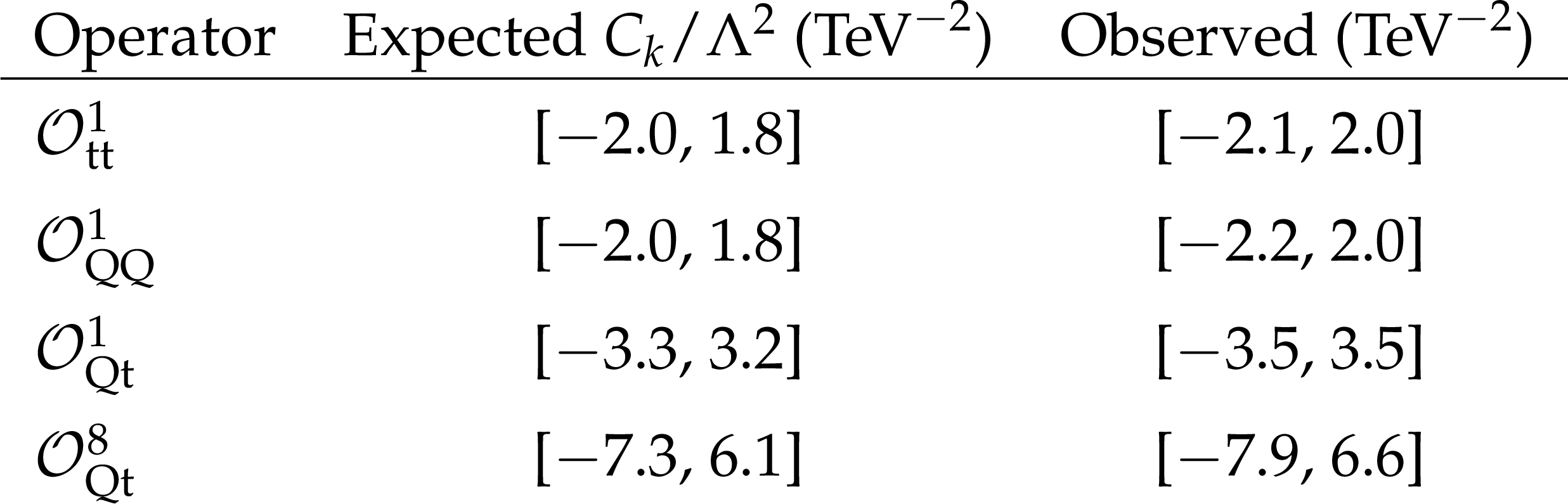
Table 5:
Expected and observed 95% CL intervals for selected coupling parameters. The intervals are extracted from upper limit on the $ {\mathrm{t} \mathrm{\bar{t}} \mathrm{t} \mathrm{\bar{t}}}$ production cross section in the EFT model, where only one selected operator has a nonvanishing contribution. |
png pdf |
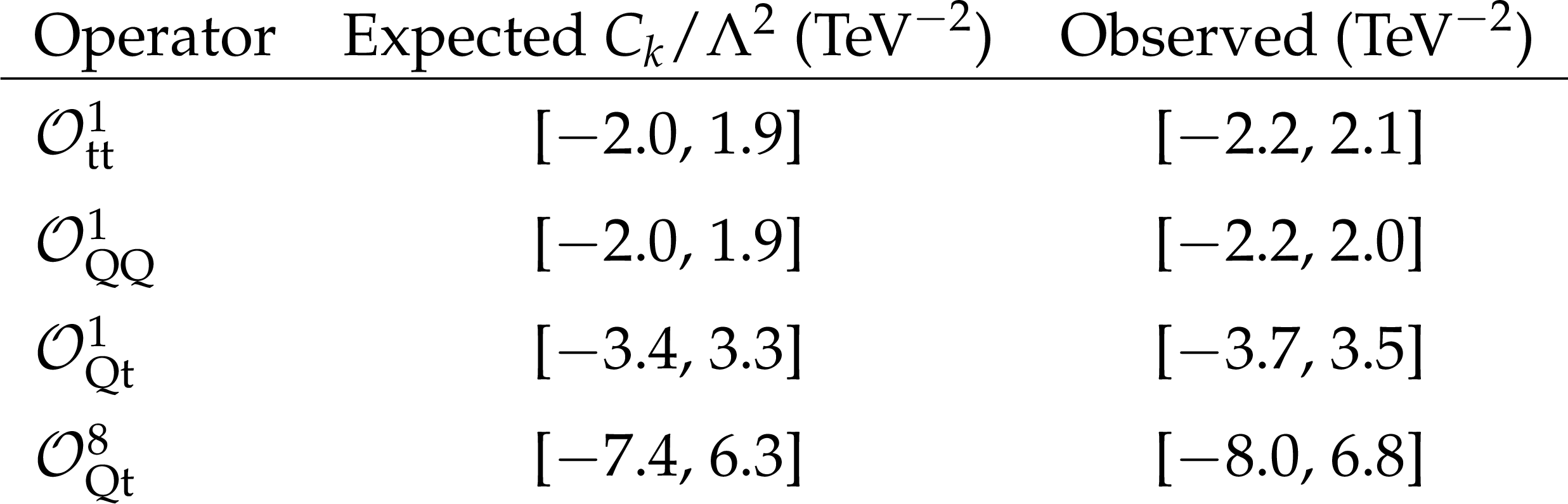
Table 6:
Expected and observed 95% CL intervals for selected coupling parameters when contribution of other operators is marginalized. |
| Summary |
| A search for standard model ${\mathrm{ t \bar{t} }\mathrm{ t \bar{t} }}$ production has been performed in final states with one or two oppositely signed muons or electrons plus jets. The observed yields attributed to ${\mathrm{ t \bar{t} }\mathrm{ t \bar{t} }}$ production are consistent with the background predictions. An upper limit at 95% confidence level of 48 fb is set on the cross section for ${\mathrm{ t \bar{t} }\mathrm{ t \bar{t} }}$ production. Combining this result with a previous same-sign dilepton and multilepton search [15] the resulting cross section is 13$^{+11}_{-9}$ fb with an observed significance of 1.4 standard deviations. The combined result constitutes one of the most stringent constraints from CMS on the production of four top quarks and can be used for phenomenological reinterpretation of a wide range of new physics models. The experimental results are interpreted in the effective field theory framework and yield limits on dimension-6 four-fermion operators coupling to third generation quarks. |
| References | ||||
| 1 | H. P. Nilles | Supersymmetry, supergravity and particle physics | Phys. Rep. 110 (1984) 1 | |
| 2 | S. P. Martin | A supersymmetry primer | in Perspectives on Supersymmetry II, G. L. Kane, ed., p. 1 World Scientific, 2010 Adv. Ser. Direct. High Energy Phys., vol. 21 | |
| 3 | G. Cacciapaglia et al. | Composite scalars at the LHC: the Higgs, the sextet and the octet | JHEP 11 (2015) 201 | 1507.02283 |
| 4 | K. Kumar, T. M. P. Tait, and R. Vega-Morales | Manifestations of top compositeness at colliders | JHEP 05 (2009) 022 | 0901.3808 |
| 5 | G. Cacciapaglia, A. Deandrea, and J. Llodra-Perez | A dark matter candidate from Lorentz invariance in 6D | JHEP 03 (2010) 083 | 0907.4993 |
| 6 | O. Ducu, L. Heurtier, and J. Maurer | LHC signatures of a $ \mathrm{Z}' $ mediator between dark matter and the SU(3) sector | JHEP 03 (2016) 006 | 1509.05615 |
| 7 | C. Degrande et al. | Non-resonant new physics in top pair production at hadron colliders | JHEP 03 (2011) 125 | 1010.6304 |
| 8 | G. Bevilacqua and M. Worek | Constraining BSM physics at the LHC: four top final states with NLO accuracy in perturbative QCD | JHEP 07 (2012) 111 | 1206.3064 |
| 9 | J. Alwall et al. | The automated computation of tree-level and next-to-leading order differential cross sections, and their matching to parton shower simulations | JHEP 07 (2014) 079 | 1405.0301 |
| 10 | R. Frederix, D. Pagani, and M. Zaro | Large NLO corrections in $ t\bar{t}W^{\pm} $ and $ t\bar{t}t\bar{t} $ hadroproduction from supposedly subleading EW contributions | JHEP 02 (2018) 031 | 1711.02116 |
| 11 | CMS Collaboration | Search for standard model production of four top quarks in the lepton+jets channel in pp collisions at $ \sqrt{s} = $ 8 TeV | JHEP 11 (2014) 154 | CMS-TOP-13-012 1409.7339 |
| 12 | ATLAS Collaboration | Search for supersymmetry at $ \sqrt{s} = $ 8 TeV in final states with jets and two same-sign leptons or three leptons with the ATLAS detector | JHEP 06 (2014) 035 | 1404.2500 |
| 13 | CMS Collaboration | Search for standard model production of four top quarks in proton-proton collisions at $ \sqrt{s} = $ 13 TeV | PLB 772 (2017) 336 | CMS-TOP-16-016 1702.06164 |
| 14 | ATLAS Collaboration | Search for four-top-quark production in the single-lepton and opposite-sign dilepton final states in pp collisions at $ \sqrt{s} = $ 13 TeV with the ATLAS detector | PRD 99 (2019) 052009 | 1811.02305 |
| 15 | CMS Collaboration | Search for standard model production of four top quarks with same-sign and multilepton final states in proton-proton collisions at $ \sqrt{s} = $ 13 TeV | EPJC 78 (2017) 140 | CMS-TOP-17-009 1710.10614 |
| 16 | CMS Collaboration | Search for physics beyond the standard model in events with two leptons of same sign, missing transverse momentum, and jets in proton-proton collisions at $ \sqrt{s} = $ 13 TeV | EPJC 77 (2017) 578 | CMS-SUS-16-035 1704.07323 |
| 17 | ATLAS Collaboration | Search for pair production of up-type vector-like quarks and for four-top-quark events in final states with multiple $ b $-jets with the ATLAS detector | JHEP 07 (2018) 089 | 1803.09678 |
| 18 | CMS Collaboration | The CMS experiment at the CERN LHC | JINST 3 (2008) S08004 | CMS-00-001 |
| 19 | M. L. Mangano, M. Moretti, F. Piccinini, and M. Treccani | Matching matrix elements and shower evolution for top-quark production in hadronic collisions | JHEP 01 (2007) 013 | hep-ph/0611129 |
| 20 | S. Frixione, G. Ridolfi, and P. Nason | A positive-weight next-to-leading-order Monte Carlo for heavy flavour hadroproduction | JHEP 09 (2007) 126 | 0707.3088 |
| 21 | P. Nason | A new method for combining NLO QCD with shower Monte Carlo algorithms | JHEP 11 (2004) 040 | hep-ph/0409146 |
| 22 | S. Frixione, P. Nason, and C. Oleari | Matching NLO QCD computations with parton shower simulations: the POWHEG method | JHEP 11 (2007) 070 | 0709.2092 |
| 23 | S. Alioli, P. Nason, C. Oleari, and E. Re | A general framework for implementing NLO calculations in shower Monte Carlo programs: the POWHEG BOX | JHEP 06 (2010) 043 | 1002.2581 |
| 24 | S. Alioli, S.-O. Moch, and P. Uwer | Hadronic top-quark pair-production with one jet and parton showering | JHEP 01 (2012) 137 | 1110.5251 |
| 25 | M. Czakon and A. Mitov | Top++: A program for the calculation of the top-pair cross-section at hadron colliders | CPC 185 (2014) 2930 | 1112.5675 |
| 26 | M. Beneke, P. Falgari, S. Klein, and C. Schwinn | Hadronic top-quark pair production with NNLL threshold resummation | NPB 855 (2012) 695 | 1109.1536 |
| 27 | M. Cacciari et al. | Top-pair production at hadron colliders with next-to-next-to-leading logarithmic soft-gluon resummation | PLB 710 (2012) 612 | 1111.5869 |
| 28 | P. Barnreuther, M. Czakon, and A. Mitov | Percent level precision physics at the Tevatron: first genuine NNLO QCD corrections to $ q \bar{q} \to t \bar{t} + X $ | PRL 109 (2012) 132001 | 1204.5201 |
| 29 | M. Czakon and A. Mitov | NNLO corrections to top-pair production at hadron colliders: the all-fermionic scattering channels | JHEP 12 (2012) 054 | 1207.0236 |
| 30 | M. Czakon and A. Mitov | NNLO corrections to top pair production at hadron colliders: the quark-gluon reaction | JHEP 01 (2013) 080 | 1210.6832 |
| 31 | M. Czakon, P. Fiedler, and A. Mitov | Total top-quark pair-production cross section at hadron colliders through $ {\cal{O}}(\alpha_S^4) $ | PRL 110 (2013) 252004 | 1303.6254 |
| 32 | CMS Collaboration | Investigations of the impact of the parton shower tuning in Pythia 8 in the modelling of $ \mathrm{t}\bar{\mathrm{t}} $ at $ \sqrt{s} = $ 8 and 13 TeV | CMS-PAS-TOP-16-021 | CMS-PAS-TOP-16-021 |
| 33 | CMS Collaboration | Event generator tunes obtained from underlying event and multiparton scattering measurements | EPJC 76 (2016) 155 | CMS-GEN-14-001 1512.00815 |
| 34 | P. Skands, S. Carrazza, and J. Rojo | Tuning PYTHIA 8.1: the Monash 2013 tune | EPJC 74 (2014) 3024 | 1404.5630 |
| 35 | CMS Collaboration | Measurements of $ \mathrm{t\overline{t}} $ differential cross sections in proton-proton collisions at $ \sqrt{s} = $ 13 TeV using events containing two leptons | JHEP 02 (2019) 149 | CMS-TOP-17-014 1811.06625 |
| 36 | CMS Collaboration | Measurement of differential cross sections for the production of top quark pairs and of additional jets in lepton+jets events from pp collisions at $ \sqrt{s} = $ 13 TeV | PRD 97 (2018) 112003 | CMS-TOP-17-002 1803.08856 |
| 37 | M. Czakon, D. Heymes, and A. Mitov | High-precision differential predictions for top-quark pairs at the LHC | PRL 116 (2016) 082003 | 1511.00549 |
| 38 | N. Kidonakis | NNLL threshold resummation for top-pair and single-top production | Phys. Part. Nucl. 45 (2014) 714 | 1210.7813 |
| 39 | E. Re | Single-top Wt-channel production matched with parton showers using the POWHEG method | EPJC 71 (2011) 1547 | 1009.2450 |
| 40 | M. Aliev et al. | HATHOR: Hadronic top and heavy quarks cross section calculator | CPC 182 (2011) 1034 | 1007.1327 |
| 41 | P. Kant et al. | HatHor for single top-quark production: updated predictions and uncertainty estimates for single top-quark production in hadronic collisions | CPC 191 (2015) 74 | 1406.4403 |
| 42 | J. Alwall et al. | Comparative study of various algorithms for the merging of parton showers and matrix elements in hadronic collisions | EPJC 53 (2008) 473 | 0706.2569 |
| 43 | D. de Florian et al. | Handbook of LHC Higgs cross sections: 4. Deciphering the nature of the Higgs sector | CERN-2017-002-M | 1610.07922 |
| 44 | NNPDF Collaboration | Parton distributions for the LHC Run II | JHEP 04 (2015) 040 | 1410.8849 |
| 45 | T. Sjostrand et al. | An introduction to PYTHIA 8.2 | CPC 191 (2015) 159 | 1410.3012 |
| 46 | GEANT4 Collaboration | GEANT4 --- a simulation toolkit | NIMA 506 (2003) 250 | |
| 47 | CMS Collaboration | The CMS trigger system | JINST 12 (2017) P01020 | CMS-TRG-12-001 1609.02366 |
| 48 | CMS Collaboration | Particle-flow reconstruction and global event description with the CMS detector | JINST 12 (2017) P10003 | CMS-PRF-14-001 1706.04965 |
| 49 | CMS Collaboration | Performance of the CMS muon detector and muon reconstruction with proton-proton collisions at $ \sqrt{s} = $ 13 TeV | JINST 13 (2018) P06015 | CMS-MUO-16-001 1804.04528 |
| 50 | CMS Collaboration | Performance of electron reconstruction and selection with the CMS detector in proton-proton collisions at $ \sqrt{s} = $ 8 TeV | JINST 10 (2015) P06005 | CMS-EGM-13-001 1502.02701 |
| 51 | M. Cacciari, G. P. Salam, and G. Soyez | The anti-$ {k_{\mathrm{T}}} $ jet clustering algorithm | JHEP 04 (2008) 063 | 0802.1189 |
| 52 | M. Cacciari, G. P. Salam, and G. Soyez | FastJet user manual | EPJC 72 (2012) 1896 | 1111.6097 |
| 53 | M. Cacciari, G. P. Salam, and G. Soyez | The catchment area of jets | JHEP 04 (2008) 005 | 0802.1188 |
| 54 | CMS Collaboration | Pileup removal algorithms | CMS-PAS-JME-14-001 | CMS-PAS-JME-14-001 |
| 55 | CMS Collaboration | Jet energy scale and resolution in the CMS experiment in pp collisions at 8 TeV | JINST 12 (2017) P02014 | CMS-JME-13-004 1607.03663 |
| 56 | CMS Collaboration | Performance of missing transverse momentum in pp collisions at $ \sqrt{s} = $ 13 TeV using the CMS detector | CMS-PAS-JME-17-001 | CMS-PAS-JME-17-001 |
| 57 | CMS Collaboration | Identification of heavy-flavour jets with the CMS detector in pp collisions at 13 TeV | JINST 13 (2018) P05011 | CMS-BTV-16-002 1712.07158 |
| 58 | L. Breiman, J. Friedman, R. A. Olshen, and C. J. Stone | Classification and regression trees | Chapman and Hall/CRC | |
| 59 | J. H. Friedman | Recent advances in predictive (machine) Learning | J. Classif. 23 (2006) 175 | |
| 60 | Y. Freund and R. E. Schapire | A decision-theoretic generalization of on-line learning and an application to boosting | J. Comput. Syst. Sci. 55 (1997) 119 | |
| 61 | H. Voss, A. Hocker, J. Stelzer, and F. Tegenfeldt | TMVA, the toolkit for multivariate data analysis with ROOT | in XIth International Workshop on Advanced Computing and Analysis Techniques in Physics Research (ACAT) 2007 | physics/0703039 |
| 62 | J. D. Bjorken and S. J. Brodsky | Statistical model for electron-positron annihilation into hadrons | PRD 1 (1970) 1416 | |
| 63 | CMS Collaboration | CMS luminosity measurements for the 2016 data taking period | CMS-PAS-LUM-17-001 | CMS-PAS-LUM-17-001 |
| 64 | CMS Collaboration | Measurement of the inelastic proton-proton cross section at $ \sqrt{s} = $ 13 TeV | JHEP 07 (2018) 161 | CMS-FSQ-15-005 1802.02613 |
| 65 | CMS Collaboration | Identification of b quark jets at the CMS experiment in the LHC Run 2 | CMS-PAS-BTV-15-001 | CMS-PAS-BTV-15-001 |
| 66 | CMS Collaboration | Investigations of the impact of the parton shower tuning in Pythia 8 in the modelling of $ \mathrm{t\overline{t}} $ at $ \sqrt{s} = $ 8 and 13 TeV | CMS-PAS-TOP-16-021 | CMS-PAS-TOP-16-021 |
| 67 | J. Butterworth et al. | PDF4LHC recommendations for LHC Run II | JPG 43 (2016) 023001 | 1510.03865 |
| 68 | L. A. Harland-Lang, A. D. Martin, P. Motylinski, and R. S. Thorne | Parton distributions in the LHC era: MMHT 2014 PDFs | EPJC 75 (2015) 204 | 1412.3989 |
| 69 | S. Dulat et al. | New parton distribution functions from a global analysis of quantum chromodynamics | PRD 93 (2016) 033006 | 1506.07443 |
| 70 | CMS Collaboration | Measurements of $ \mathrm{t\overline{t}} $ cross sections in association with b jets and inclusive jets and their ratio using dilepton final states in pp collisions at $ \sqrt{s} = $ 13 TeV | PLB 776 (2018) 355 | CMS-TOP-16-010 1705.10141 |
| 71 | T. Junk | Confidence level computation for combining searches with small statistics | NIMA 434 (1999) 435 | hep-ex/9902006 |
| 72 | A. L. Read | Presentation of search results: the $ CL_{s} $ technique | JPG 28 (2002) 2693 | |
| 73 | L. Moneta et al. | The RooStats project | in 13th international workshop on advanced computing and analysis techniques in physics research (ACAT2010), p. 057 2010 PoS(ACAT2010)057 | 1009.1003 |
| 74 | G. Cowan, K. Cranmer, E. Gross, and O. Vitells | Asymptotic formulae for likelihood-based tests of new physics | EPJC. 71 (2011) 1554 | 1007.1727 |
| 75 | ATLAS and CMS Collaborations and the LHC Higgs combination group | Procedure for the LHC Higgs boson search combination in summer 2011 | CMS-NOTE-2011-005 | |
| 76 | W. Buchmuller and D. Wyler | Effective Lagrangian analysis of new interactions and flavor conservation | NPB 268 (1986) 621 | |
| 77 | B. Grzadkowski, M. Iskrzy\'nski, M. Misiak, and J. Rosiek | Dimension-six terms in the standard model Lagrangian | JHEP 10 (2010) 085 | 1008.4884 |
| 78 | N. P. Hartland et al. | A Monte Carlo global analysis of the standard model effective field theory: the top quark sector | 1901.05965 | |
| 79 | S. Weinberg | Baryon and lepton nonconserving processes | PRL 43 (1979) 1566 | |
| 80 | J. Aguilar-Saavedra et al. | Interpreting top-quark LHC measurements in the standard-model effective field theory | 1802.07237 | |
| 81 | A. Alloul et al. | FeynRules 2.0 --- a complete toolbox for tree-level phenomenology | CPC 185 (2014) 2250 | 1310.1921 |
|
|
Compact Muon Solenoid LHC, CERN |
|

|

|

|

|

|