

Compact Muon Solenoid
LHC, CERN
| CMS-TOP-18-009 ; CERN-EP-2019-124 | ||
| Measurement of top quark pair production in association with a Z boson in proton-proton collisions at $\sqrt{s} = $ 13 TeV | ||
| CMS Collaboration | ||
| 25 July 2019 | ||
| JHEP 03 (2020) 056 | ||
| Abstract: A measurement of the inclusive cross section of top quark pair production in association with a Z boson using proton-proton collisions at a center-of-mass energy of 13 TeV at the LHC is performed. The data sample corresponds to an integrated luminosity of 77.5 fb$^{-1}$, collected by the CMS experiment during 2016 and 2017. The measurement is performed using final states containing three or four charged leptons (electrons or muons), and the Z boson is detected through its decay to an oppositely charged lepton pair. The production cross section is measured to be $\sigma({\mathrm{t\bar{t}}\mathrm{Z}} )=$ 0.95 $\pm$ 0.05 (stat) $\pm$ 0.06 (syst) pb. For the first time, differential cross sections are measured as functions of the transverse momentum of the Z boson and the angular distribution of the negatively charged lepton from the Z boson decay. The most stringent direct limits to date on the anomalous couplings of the top quark to the Z boson are presented, including constraints on the Wilson coefficients in the framework of the standard model effective field theory. | ||
| Links: e-print arXiv:1907.11270 [hep-ex] (PDF) ; CDS record ; inSPIRE record ; HepData record ; CADI line (restricted) ; | ||
| Figures & Tables | Summary | Additional Figures | References | CMS Publications |
|---|
| Figures | |
png pdf |
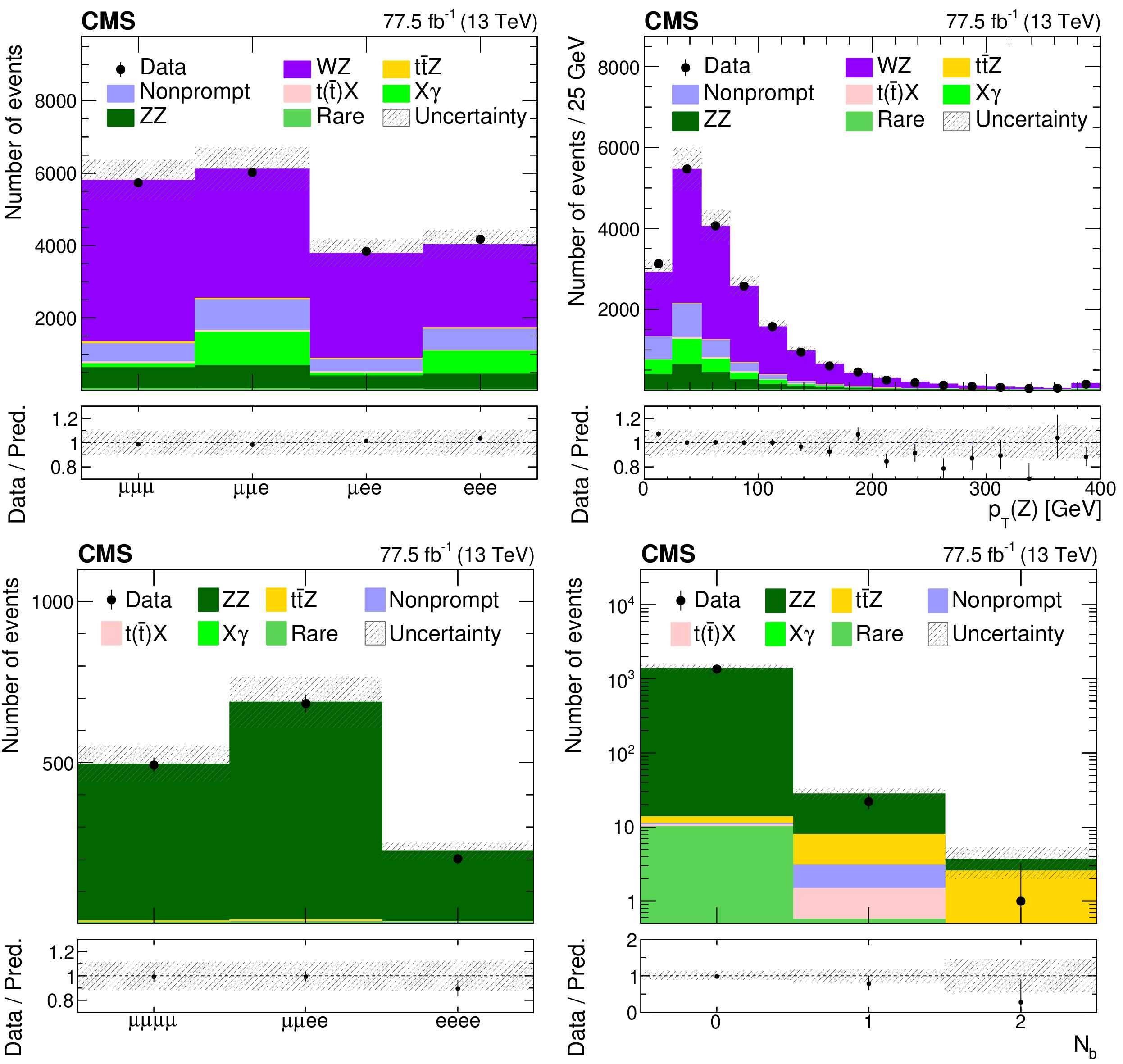
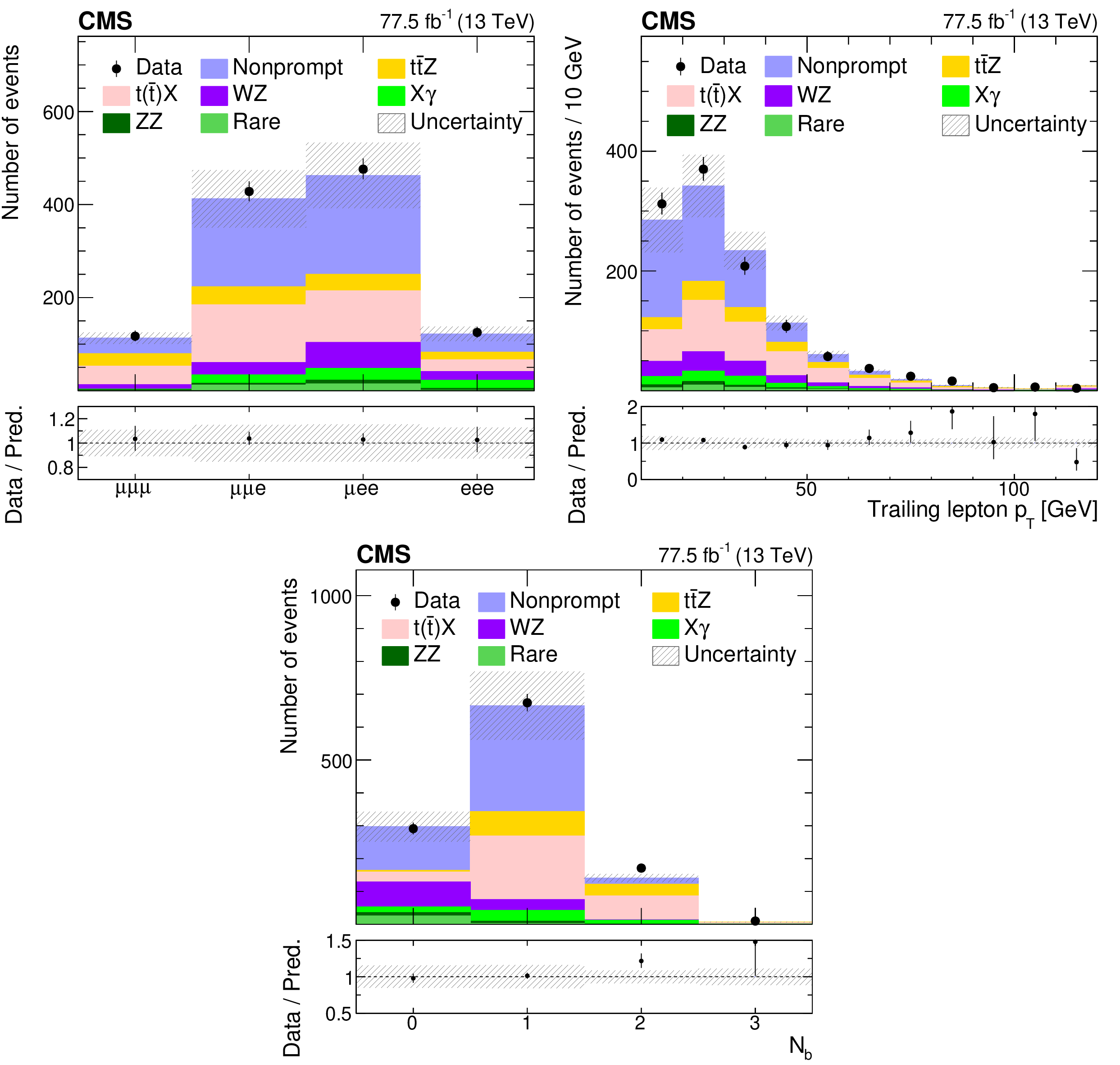
Figure 1:
The observed (points) and predicted (shaded histograms) event yields versus lepton flavor (upper left), and the reconstructed transverse momentum of the Z boson candidates (upper right) in the WZ-enriched data control event category, and versus lepton flavor (lower left) and ${N_{\mathrm{b}}}$ (lower right) in the ZZ-enriched event category. The vertical lines on the points show the statistical uncertainties in the data, and the band the total uncertainty in the predictions. The lower panels show the ratio of the event yields in data to the predictions. |
png pdf |
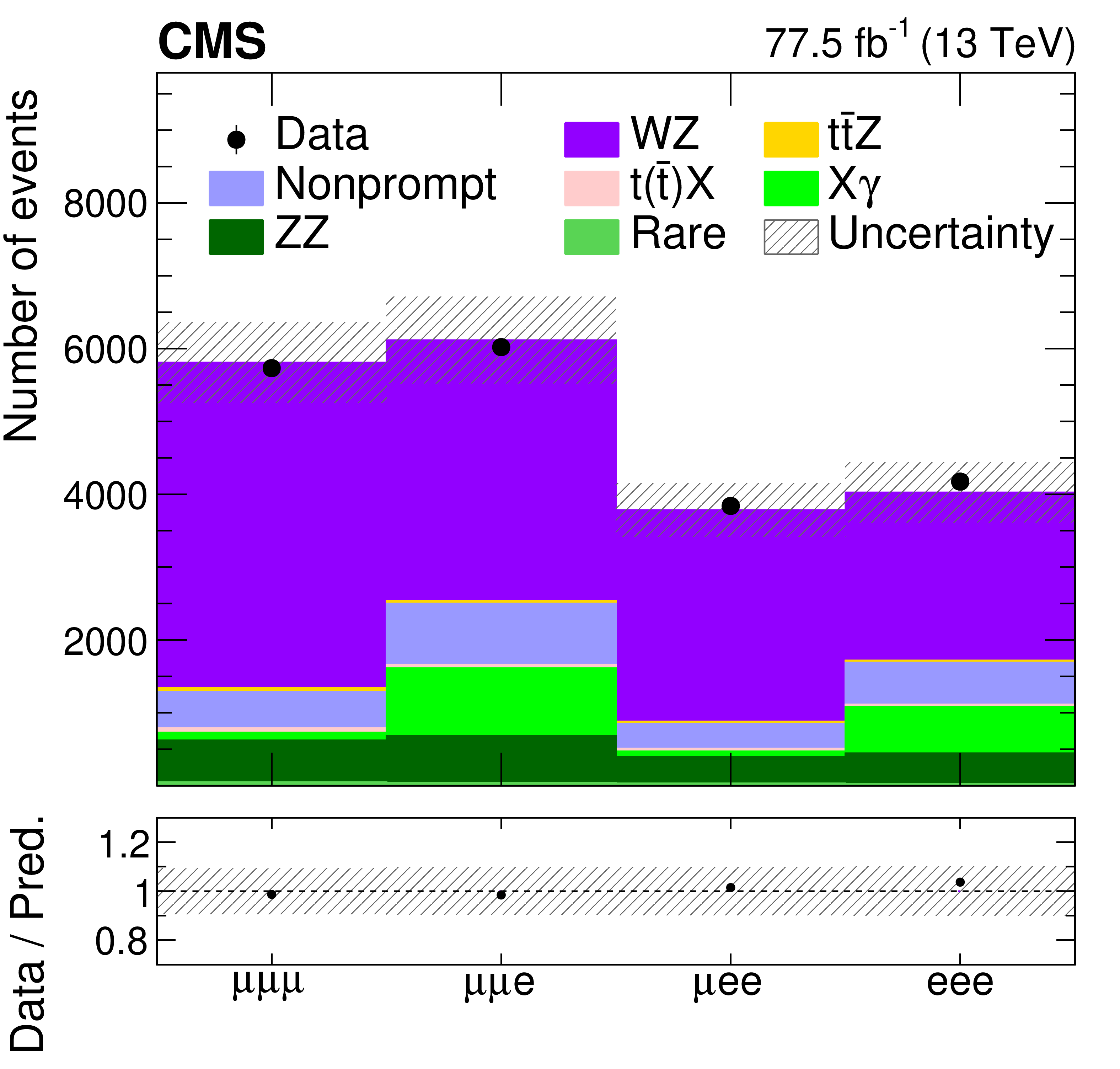
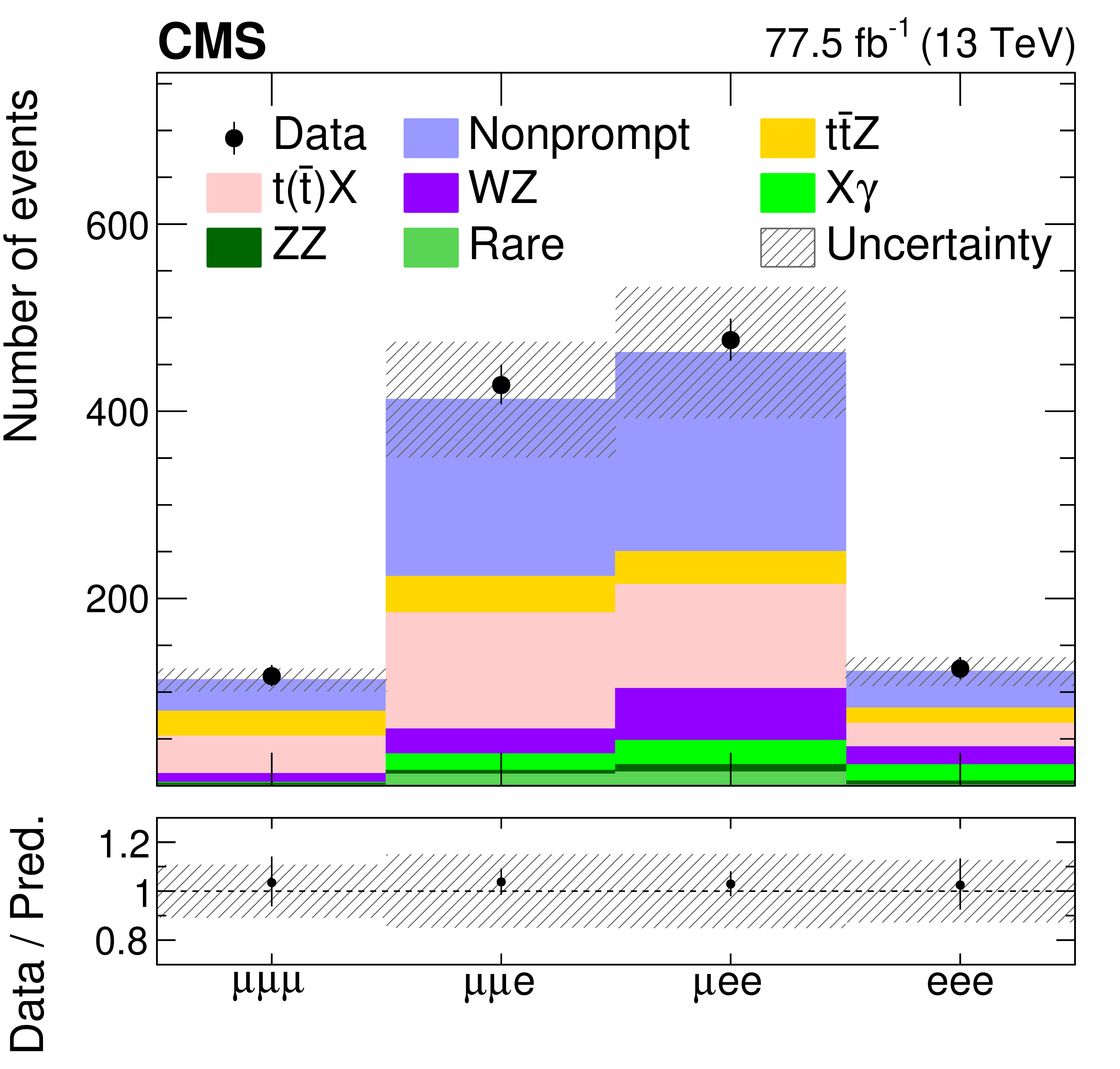
Figure 1-a:
The observed (points) and predicted (shaded histograms) event yields versus lepton flavor in the WZ-enriched data control event category. The vertical lines on the points show the statistical uncertainties in the data, and the band the total uncertainty in the predictions. The lower panel shows the ratio of the event yields in data to the predictions. |
png pdf |
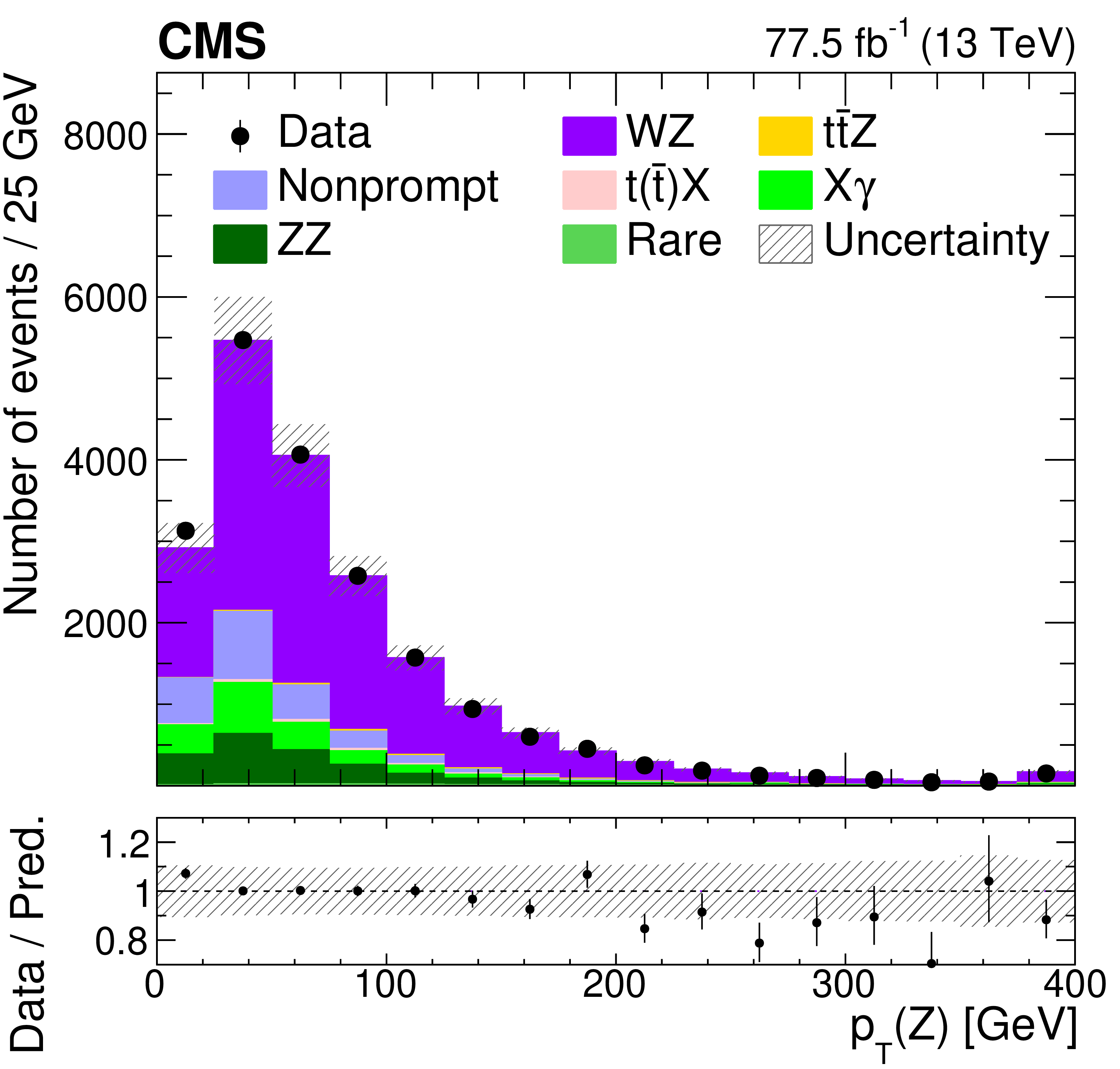
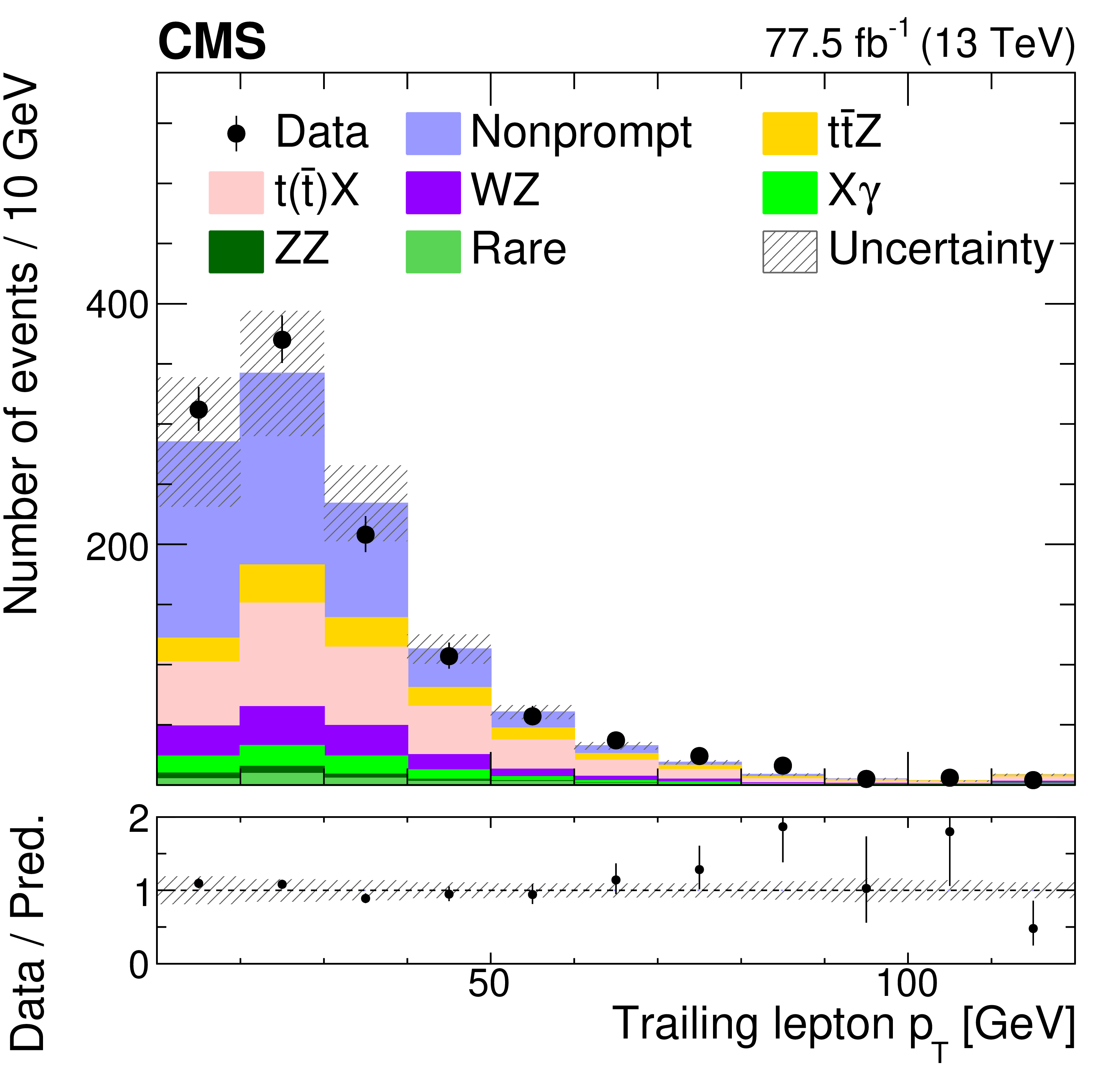
Figure 1-b:
The observed (points) and predicted (shaded histograms) event yields versus the reconstructed transverse momentum of the Z boson candidates in the WZ-enriched data control event category. The vertical lines on the points show the statistical uncertainties in the data, and the band the total uncertainty in the predictions. The lower panel shows the ratio of the event yields in data to the predictions. |
png pdf |
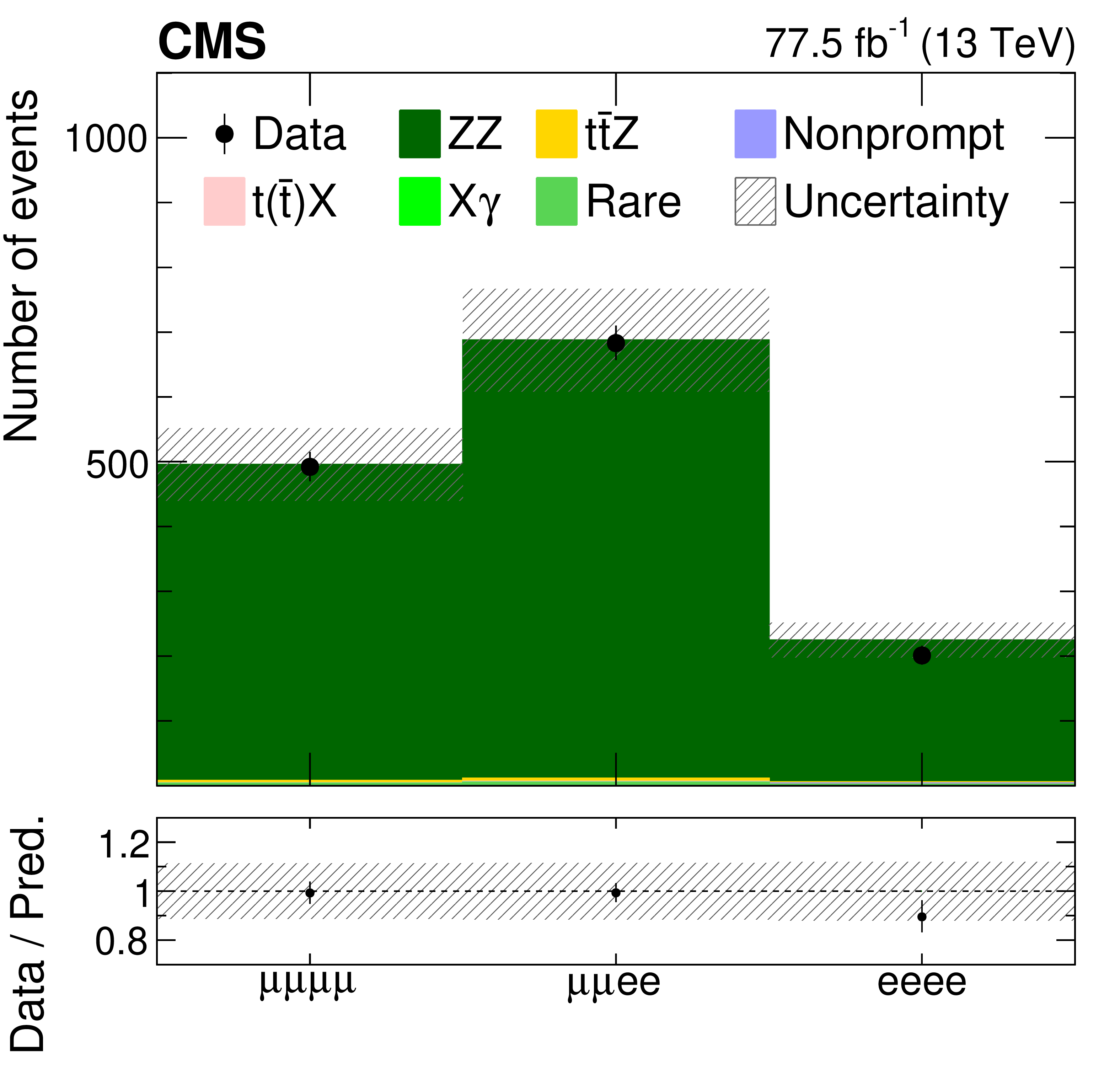
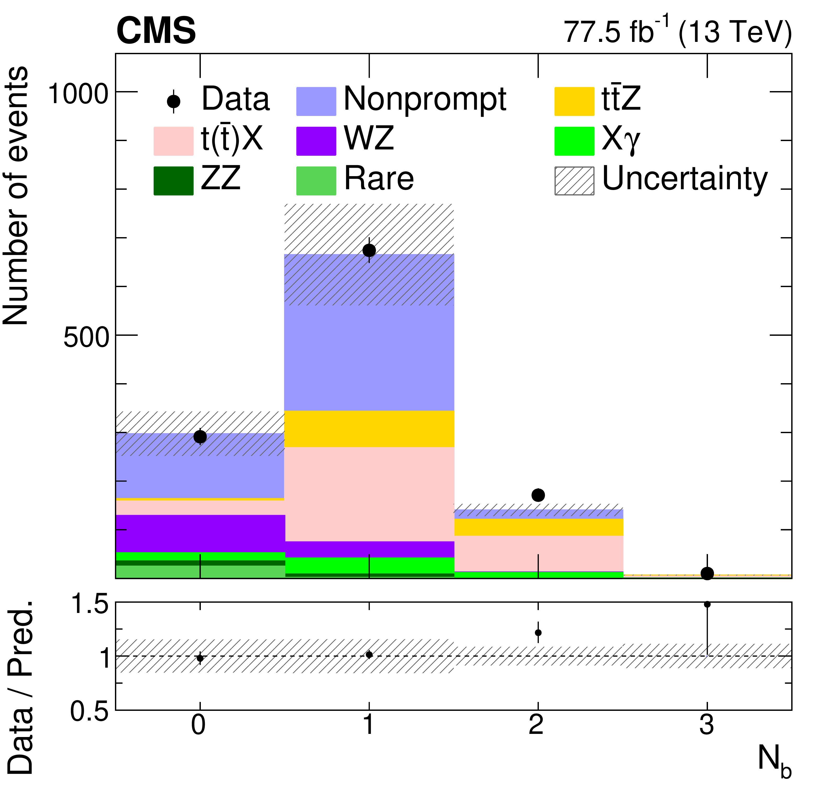
Figure 1-c:
The observed (points) and predicted (shaded histograms) event yields versus lepton flavor in the ZZ-enriched event category. The vertical lines on the points show the statistical uncertainties in the data, and the band the total uncertainty in the predictions. The lower panel shows the ratio of the event yields in data to the predictions. |

png pdf |
Figure 1-d:
The observed (points) and predicted (shaded histograms) event yields versus ${N_{\mathrm{b}}}$ in the ZZ-enriched event category. The vertical lines on the points show the statistical uncertainties in the data, and the band the total uncertainty in the predictions. The lower panel shows the ratio of the event yields in data to the predictions. |
png pdf |
Figure 2:
The observed (points) and predicted (shaded histograms) event yields in regions enriched with nonprompt lepton backgrounds in $ {\mathrm{t} \mathrm{\bar{t}}} $-like processes as a function of the lepton flavors (upper left), the ${p_{\mathrm {T}}}$ of the lowest-${p_{\mathrm {T}}}$ (trailing) lepton (upper right), and ${N_{\mathrm{b}}}$ (bottom). The vertical lines on the points show the statistical uncertainties in the data, and the band the total uncertainty in the predictions. The lower panels show the ratio of the event yields in data to the background predictions. |
png pdf |
Figure 2-a:
The observed (points) and predicted (shaded histograms) event yields in regions enriched with nonprompt lepton backgrounds in $ {\mathrm{t} \mathrm{\bar{t}}} $-like processes as a function of the lepton flavors. The vertical lines on the points show the statistical uncertainties in the data, and the band the total uncertainty in the predictions. The lower panel shows the ratio of the event yields in data to the background predictions. |
png pdf |
Figure 2-b:
The observed (points) and predicted (shaded histograms) event yields in regions enriched with nonprompt lepton backgrounds in $ {\mathrm{t} \mathrm{\bar{t}}} $-like processes as a function of the ${p_{\mathrm {T}}}$ of the lowest-${p_{\mathrm {T}}}$ (trailing) lepton. The vertical lines on the points show the statistical uncertainties in the data, and the band the total uncertainty in the predictions. The lower panel shows the ratio of the event yields in data to the background predictions. |
png pdf |
Figure 2-c:
The observed (points) and predicted (shaded histograms) event yields in regions enriched with nonprompt lepton backgrounds in $ {\mathrm{t} \mathrm{\bar{t}}} $-like processes as a function of ${N_{\mathrm{b}}}$. The vertical lines on the points show the statistical uncertainties in the data, and the band the total uncertainty in the predictions. The lower panel shows the ratio of the event yields in data to the background predictions. |

png pdf |
Figure 3:
Observed event yields in data for different values of ${N_\text {j}}$ and ${N_{\mathrm{b}}}$ for events with 3 and 4 leptons, compared with the signal and background yields, as obtained from the fit. The lower panel displays the ratio of the data to the predictions of the signal and background from simulation. The inner and outer bands show the statistical and total uncertainties, respectively. |
png pdf |
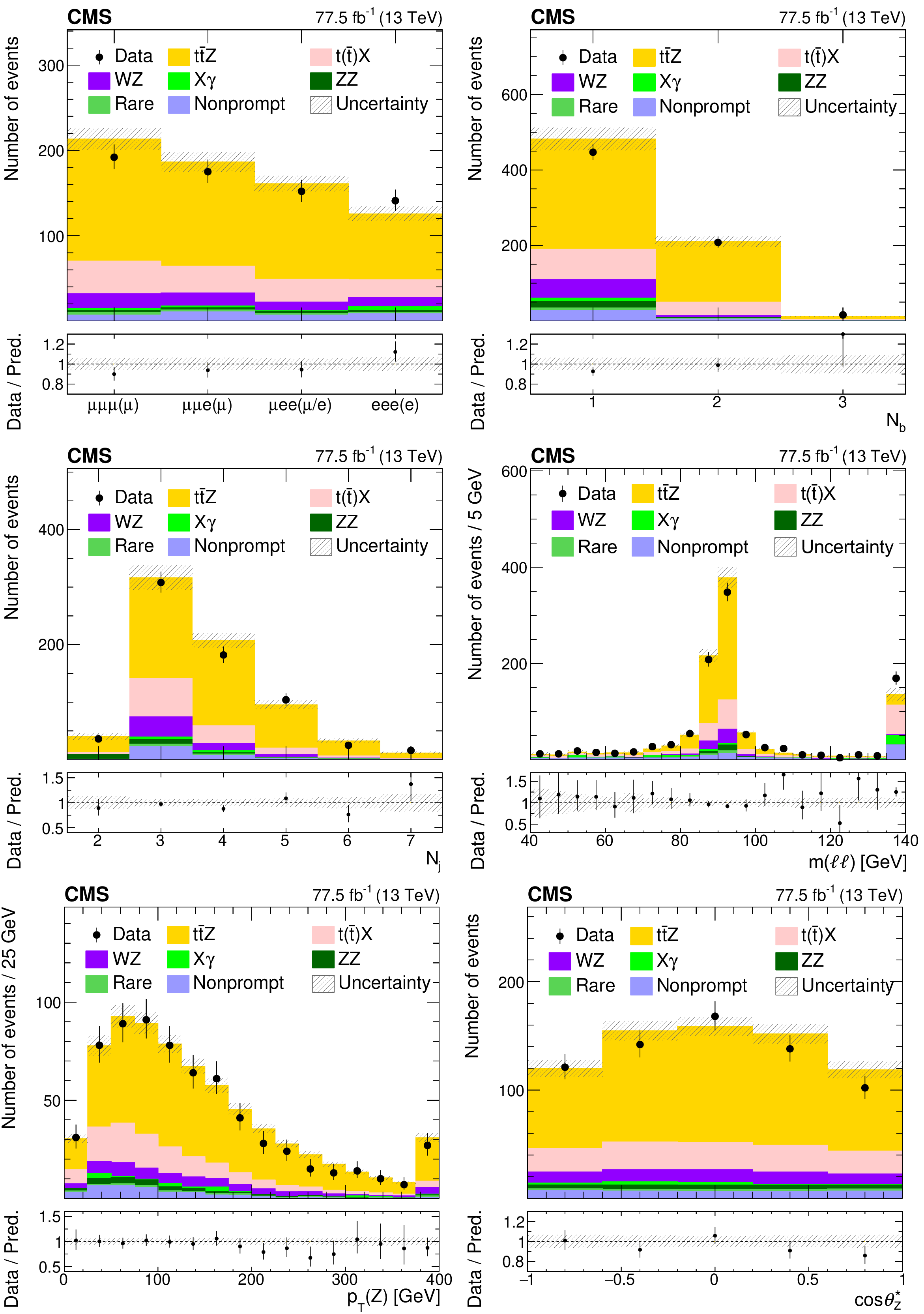
Figure 4:
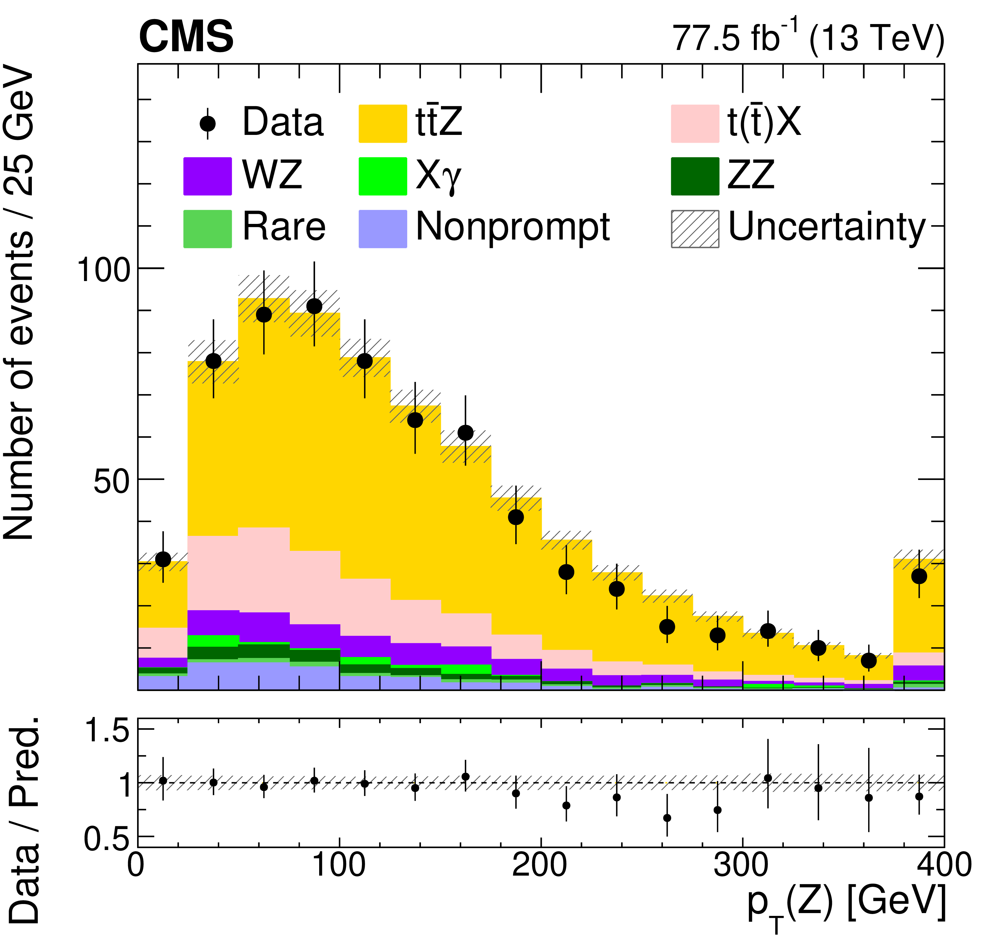
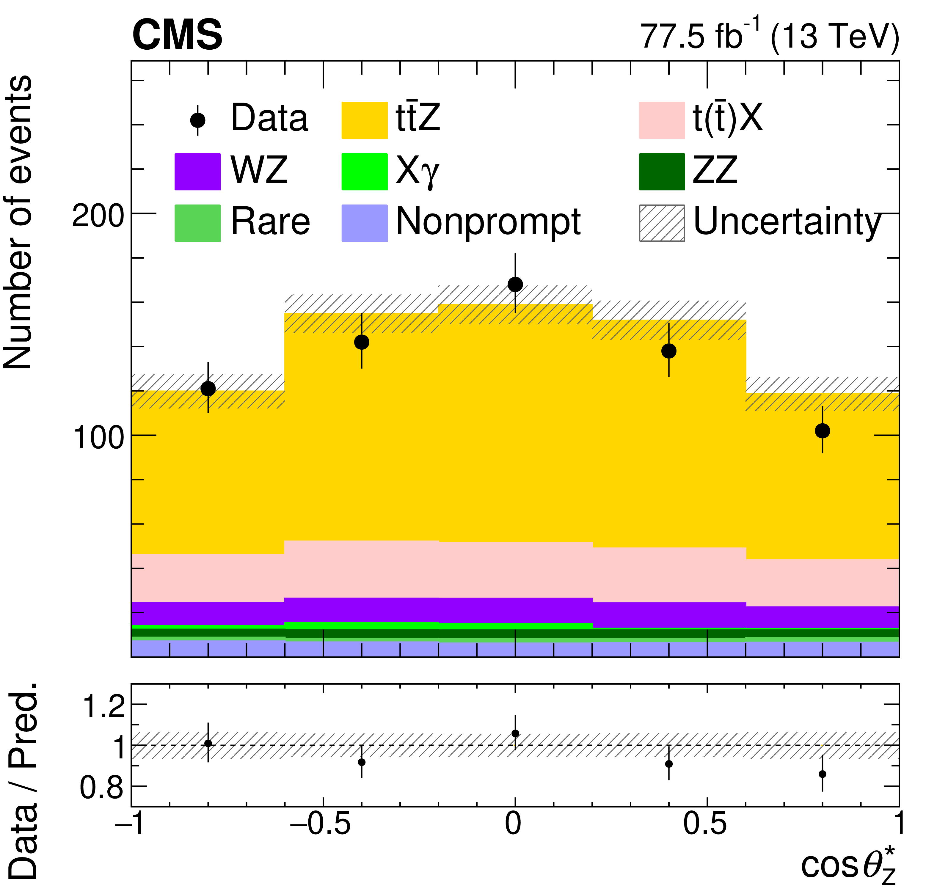
Kinematic distributions from a ${{\mathrm{t} \mathrm{\bar{t}}} \mathrm{Z}}$ signal-enriched subset of events for data (points), compared to the contributions of the signal and background yields from the fit (shaded histograms). The distributions include the lepton flavor (upper left), number of b-tagged jets (upper right), jet multiplicity (middle left), dilepton invariant mass ${m(\ell \ell)}$ (middle right), ${{p_{\mathrm {T}}} (\mathrm{Z})}$ (lower left), and $\cos\theta ^\ast _{\mathrm{Z}}$ (lower right). The lower panels in each plot give the ratio of the data to the sum of the signal and background from the fit. The band shows the total uncertainty in the signal and background yields, as obtained from the fit. |

png pdf |
Figure 4-a:
Distribution of the lepton flavor, from a ${{\mathrm{t} \mathrm{\bar{t}}} \mathrm{Z}}$ signal-enriched subset of events for data (points), compared to the contributions of the signal and background yields from the fit (shaded histograms). The lower panel gives the ratio of the data to the sum of the signal and background from the fit. The band shows the total uncertainty in the signal and background yields, as obtained from the fit. |
png pdf |
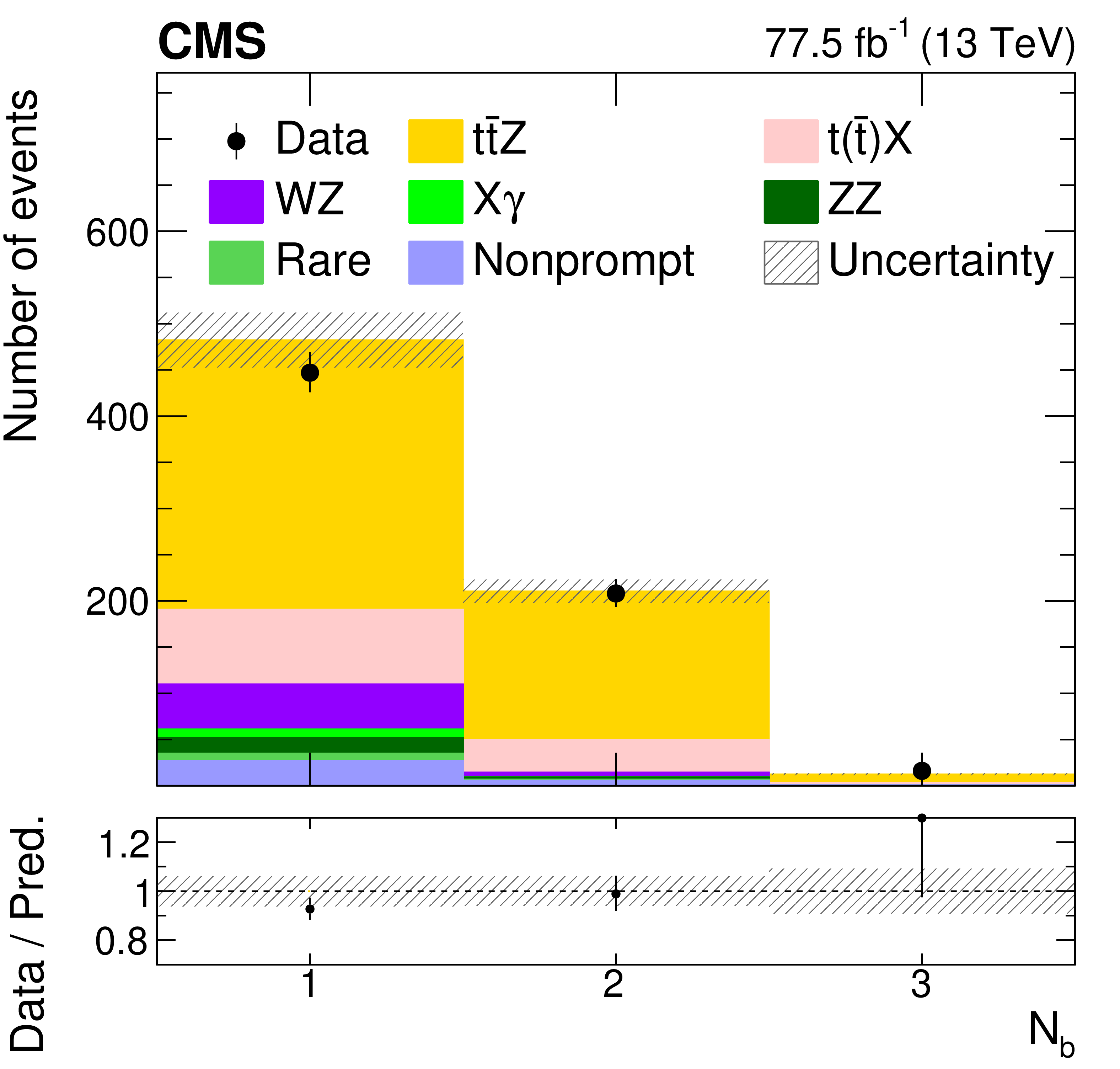
Figure 4-b:
Distribution of the number of b-tagged jets, from a ${{\mathrm{t} \mathrm{\bar{t}}} \mathrm{Z}}$ signal-enriched subset of events for data (points), compared to the contributions of the signal and background yields from the fit (shaded histograms). The lower panel gives the ratio of the data to the sum of the signal and background from the fit. The band shows the total uncertainty in the signal and background yields, as obtained from the fit. |
png pdf |
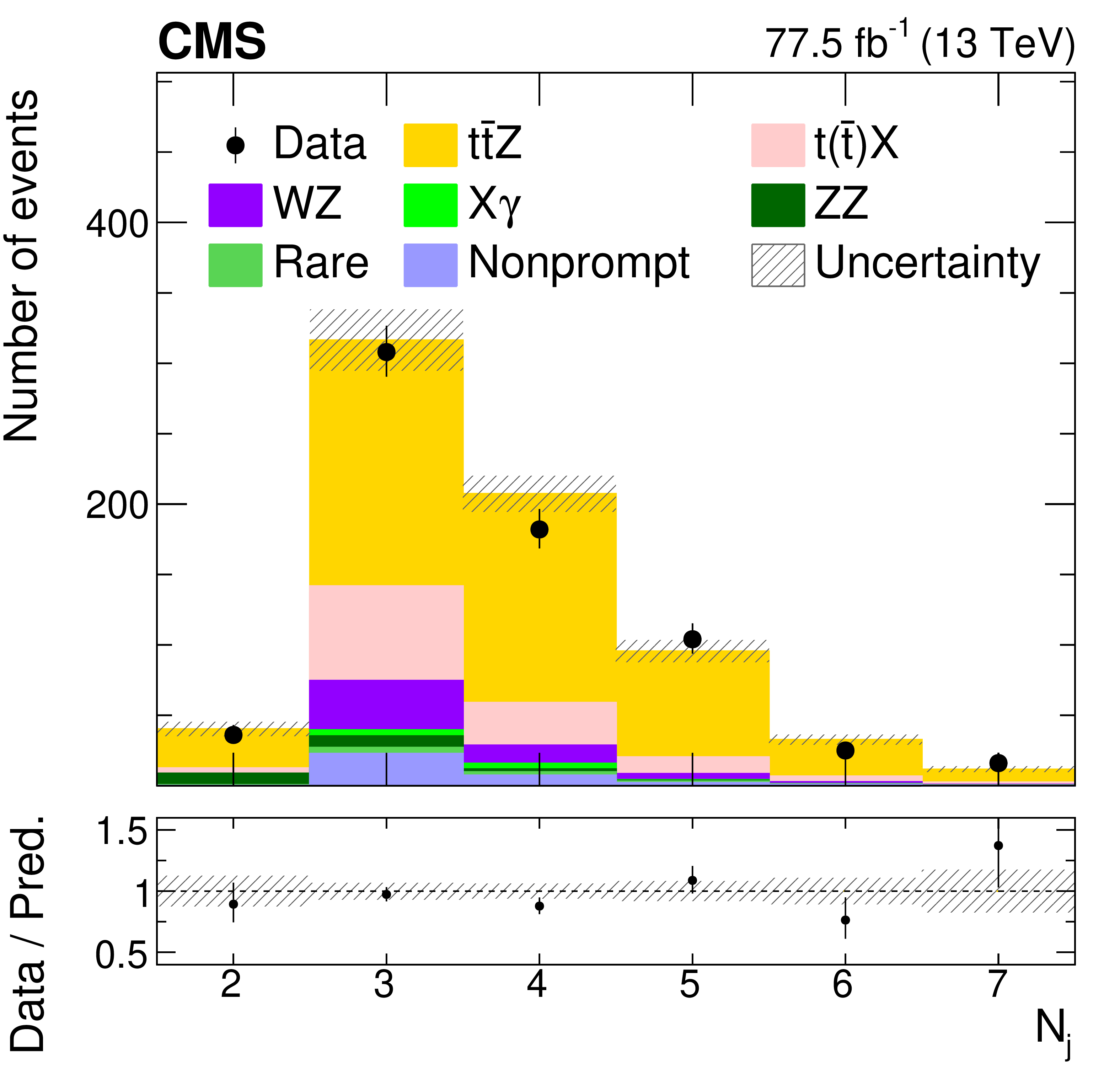
Figure 4-c:
Distribution of the jet multiplicity, from a ${{\mathrm{t} \mathrm{\bar{t}}} \mathrm{Z}}$ signal-enriched subset of events for data (points), compared to the contributions of the signal and background yields from the fit (shaded histograms). The lower panel gives the ratio of the data to the sum of the signal and background from the fit. The band shows the total uncertainty in the signal and background yields, as obtained from the fit. |
png pdf |
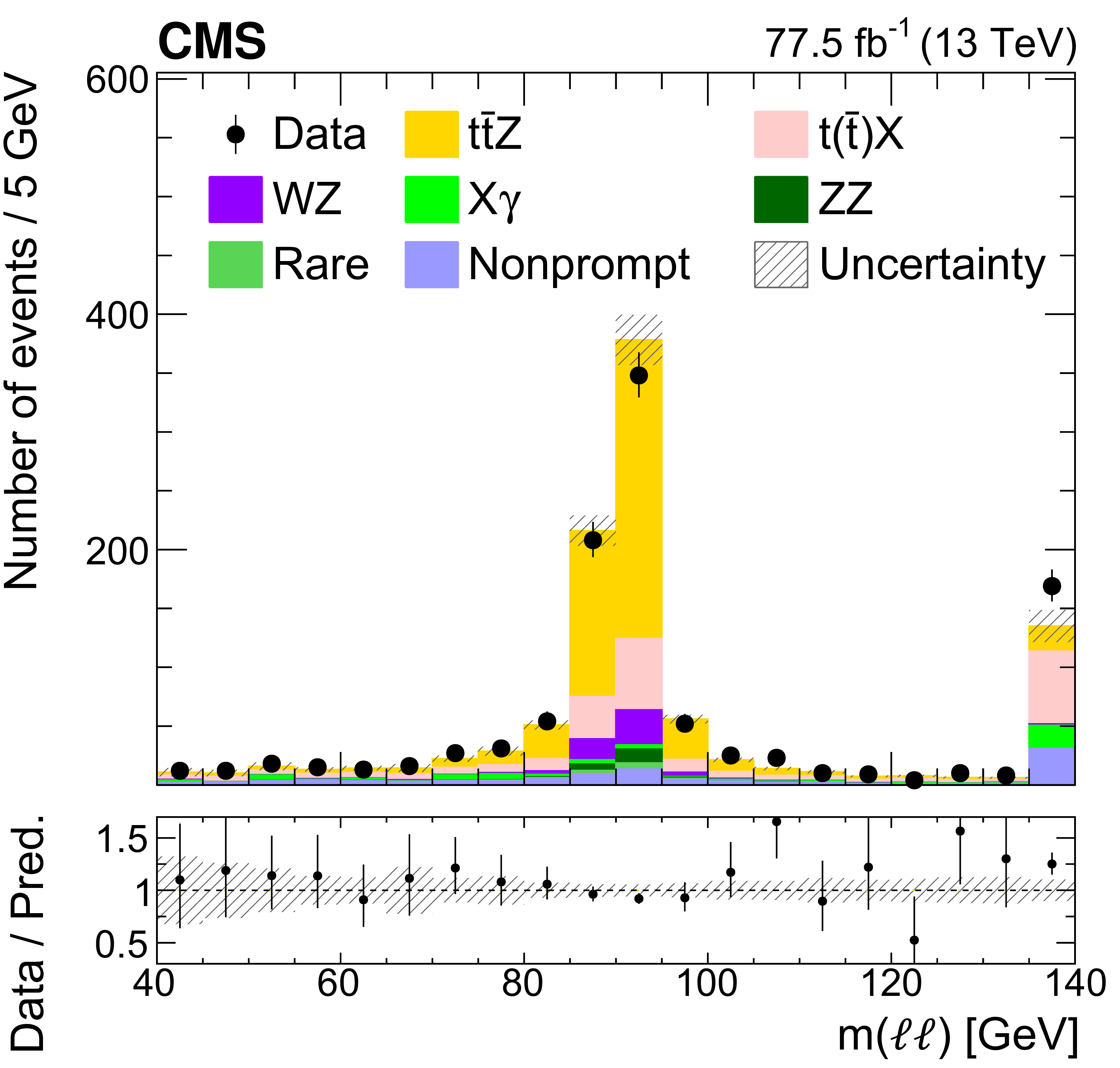
Figure 4-d:
Distribution of the dilepton invariant mass ${m(\ell \ell)}$, from a ${{\mathrm{t} \mathrm{\bar{t}}} \mathrm{Z}}$ signal-enriched subset of events for data (points), compared to the contributions of the signal and background yields from the fit (shaded histograms). The lower panel gives the ratio of the data to the sum of the signal and background from the fit. The band shows the total uncertainty in the signal and background yields, as obtained from the fit. |
png pdf |
Figure 4-e:
Distribution of ${{p_{\mathrm {T}}} (\mathrm{Z})}$, from a ${{\mathrm{t} \mathrm{\bar{t}}} \mathrm{Z}}$ signal-enriched subset of events for data (points), compared to the contributions of the signal and background yields from the fit (shaded histograms). The lower panel gives the ratio of the data to the sum of the signal and background from the fit. The band shows the total uncertainty in the signal and background yields, as obtained from the fit. |
png pdf |
Figure 4-f:
Distribution of $\cos\theta ^\ast _{\mathrm{Z}}$, from a ${{\mathrm{t} \mathrm{\bar{t}}} \mathrm{Z}}$ signal-enriched subset of events for data (points), compared to the contributions of the signal and background yields from the fit (shaded histograms). The lower panel gives the ratio of the data to the sum of the signal and background from the fit. The band shows the total uncertainty in the signal and background yields, as obtained from the fit. |
png pdf |
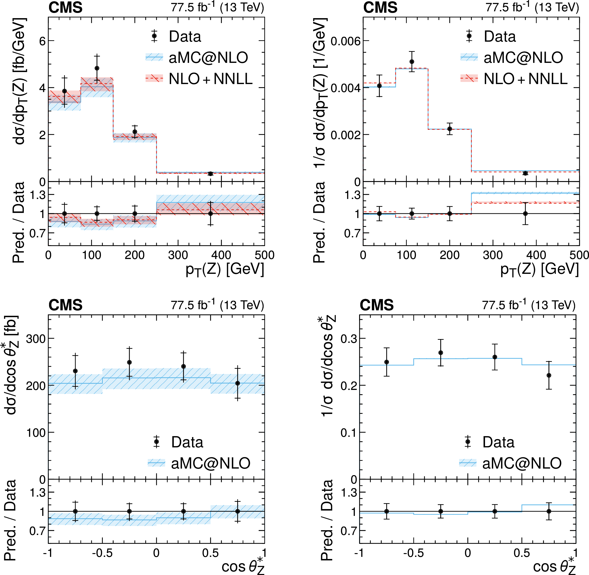
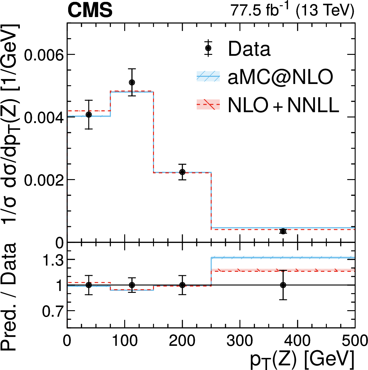
Figure 5:
Measured differential ${{\mathrm{t} \mathrm{\bar{t}}} \mathrm{Z}}$ production cross sections in the full phase space as a function of the transverse momentum ${{p_{\mathrm {T}}} (\mathrm{Z})}$ of the Z boson (upper row) and $\cos\theta ^\ast _{\mathrm{Z}}$, as defined in the text (lower row). Shown are the absolute (left) and normalized (right) cross sections. The data are represented by the points. The inner (outer) vertical lines indicate the statistical (total) uncertainties. The solid histogram shows the prediction from the MadGraph 5\_aMC@NLO MC simulation, and the dashed histogram shows the theory prediction at NLO+NNLL accuracy. The hatched bands indicate the theoretical uncertainties in the predictions, as defined in the text. The lower panels display the ratios of the predictions to the measurement. |
png pdf |
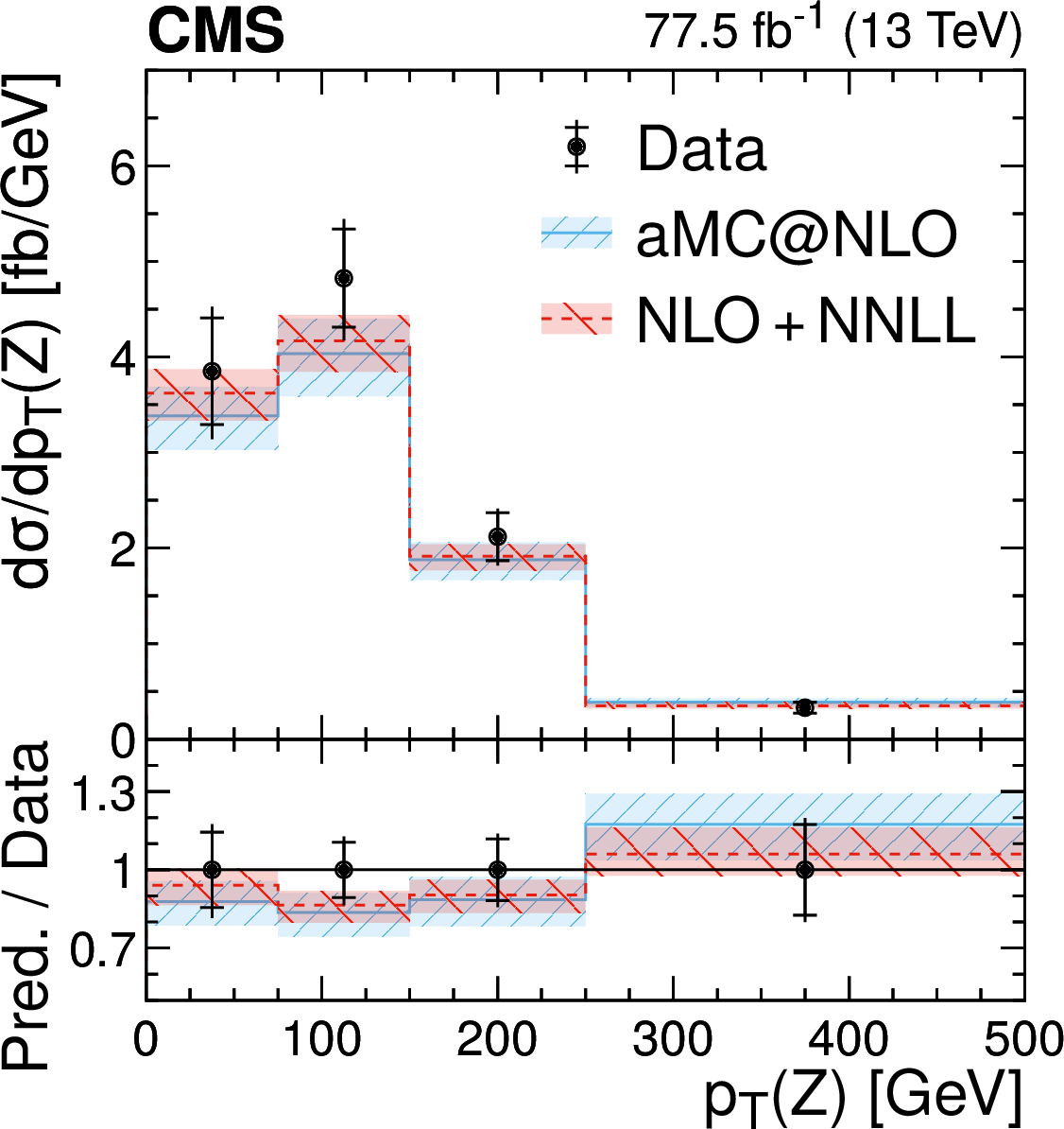
Figure 5-a:
Measured differential ${{\mathrm{t} \mathrm{\bar{t}}} \mathrm{Z}}$ production cross sections in the full phase space as a function of the transverse momentum ${{p_{\mathrm {T}}} (\mathrm{Z})}$ of the Z boson Shown are the absolute cross sections. The data are represented by the points. The inner (outer) vertical lines indicate the statistical (total) uncertainties. The solid histogram shows the prediction from the MadGraph 5_aMC@NLO MC simulation, and the dashed histogram shows the theory prediction at NLO+NNLL accuracy. The hatched bands indicate the theoretical uncertainties in the predictions, as defined in the text. The lower panel displays the ratios of the predictions to the measurement. |
png pdf |
Figure 5-b:
Measured differential ${{\mathrm{t} \mathrm{\bar{t}}} \mathrm{Z}}$ production cross sections in the full phase space as a function of the transverse momentum ${{p_{\mathrm {T}}} (\mathrm{Z})}$ of the Z boson. Shown are the normalized cross sections. The data are represented by the points. The inner (outer) vertical lines indicate the statistical (total) uncertainties. The solid histogram shows the prediction from the MadGraph 5_aMC@NLO MC simulation, and the dashed histogram shows the theory prediction at NLO+NNLL accuracy. The hatched bands indicate the theoretical uncertainties in the predictions, as defined in the text. The lower panel displays the ratios of the predictions to the measurement. |

png pdf |
Figure 5-c:
Measured differential ${{\mathrm{t} \mathrm{\bar{t}}} \mathrm{Z}}$ production cross sections in the full phase space as a function of the transverse momentum ${{p_{\mathrm {T}}} (\mathrm{Z})}$ of $\cos\theta ^\ast _{\mathrm{Z}}$. Shown are the absolute cross sections. The data are represented by the points. The inner (outer) vertical lines indicate the statistical (total) uncertainties. The solid histogram shows the prediction from the MadGraph 5_aMC@NLO MC simulation, and the dashed histogram shows the theory prediction at NLO+NNLL accuracy. The hatched bands indicate the theoretical uncertainties in the predictions, as defined in the text. The lower panel displays the ratios of the predictions to the measurement. |

png pdf |
Figure 5-d:
Measured differential ${{\mathrm{t} \mathrm{\bar{t}}} \mathrm{Z}}$ production cross sections in the full phase space as a function of the transverse momentum ${{p_{\mathrm {T}}} (\mathrm{Z})}$ of $\cos\theta ^\ast _{\mathrm{Z}}$. Shown are the normalized cross sections. The data are represented by the points. The inner (outer) vertical lines indicate the statistical (total) uncertainties. The solid histogram shows the prediction from the MadGraph 5_aMC@NLO MC simulation, and the dashed histogram shows the theory prediction at NLO+NNLL accuracy. The hatched bands indicate the theoretical uncertainties in the predictions, as defined in the text. The lower panel displays the ratios of the predictions to the measurement. |
png pdf |
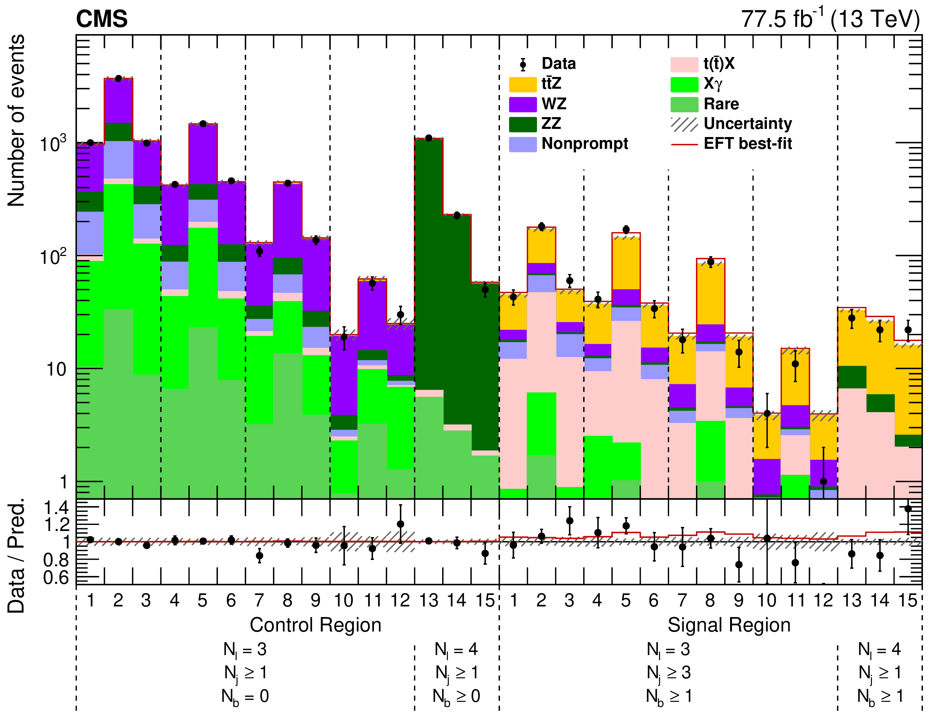
Figure 6:
The observed (points) and predicted (shaded histograms) post-fit yields for the combined 2016 and 2017 data sets in the control and signal regions. In the $ {N_{\ell}} =$ 3 control and signal regions (bins 1-12), each of the four ${{p_{\mathrm {T}}} (\mathrm{Z})}$ categories is further split into three $\cos\theta ^\ast _{\mathrm{Z}}$ bins. The horizontal bars on the points give the statistical uncertainties in the data. The lower panel displays the ratio of the data to the predictions and the hatched regions show the total uncertainty. The solid line shows the best-fit prediction from the SMEFT fit. |
png pdf |
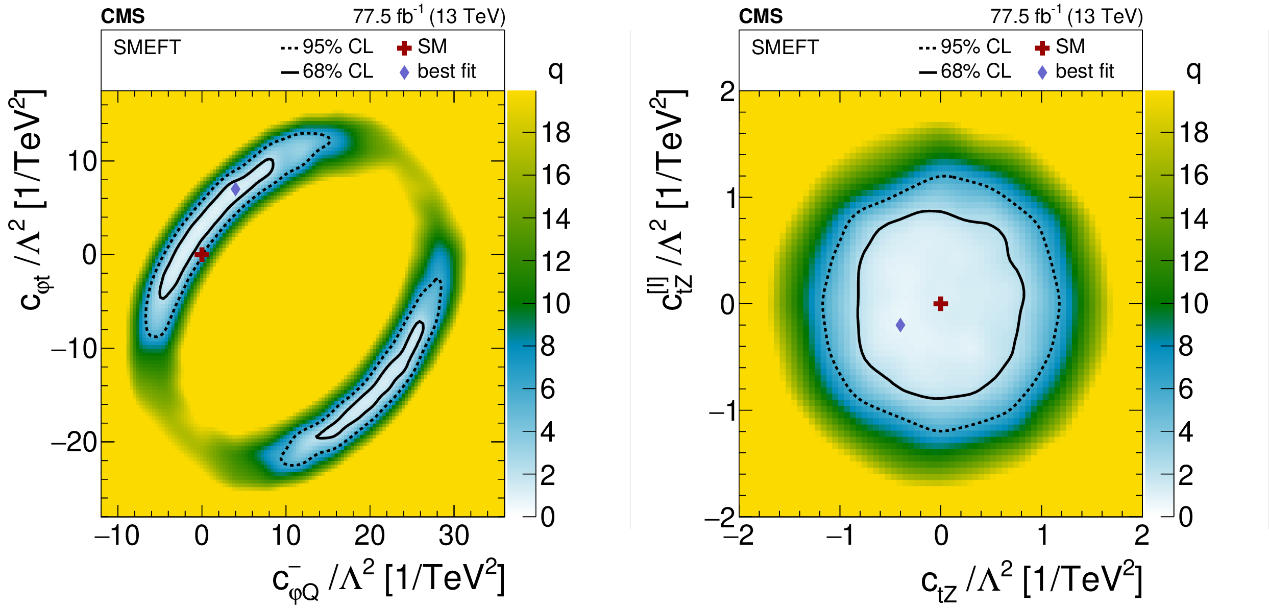
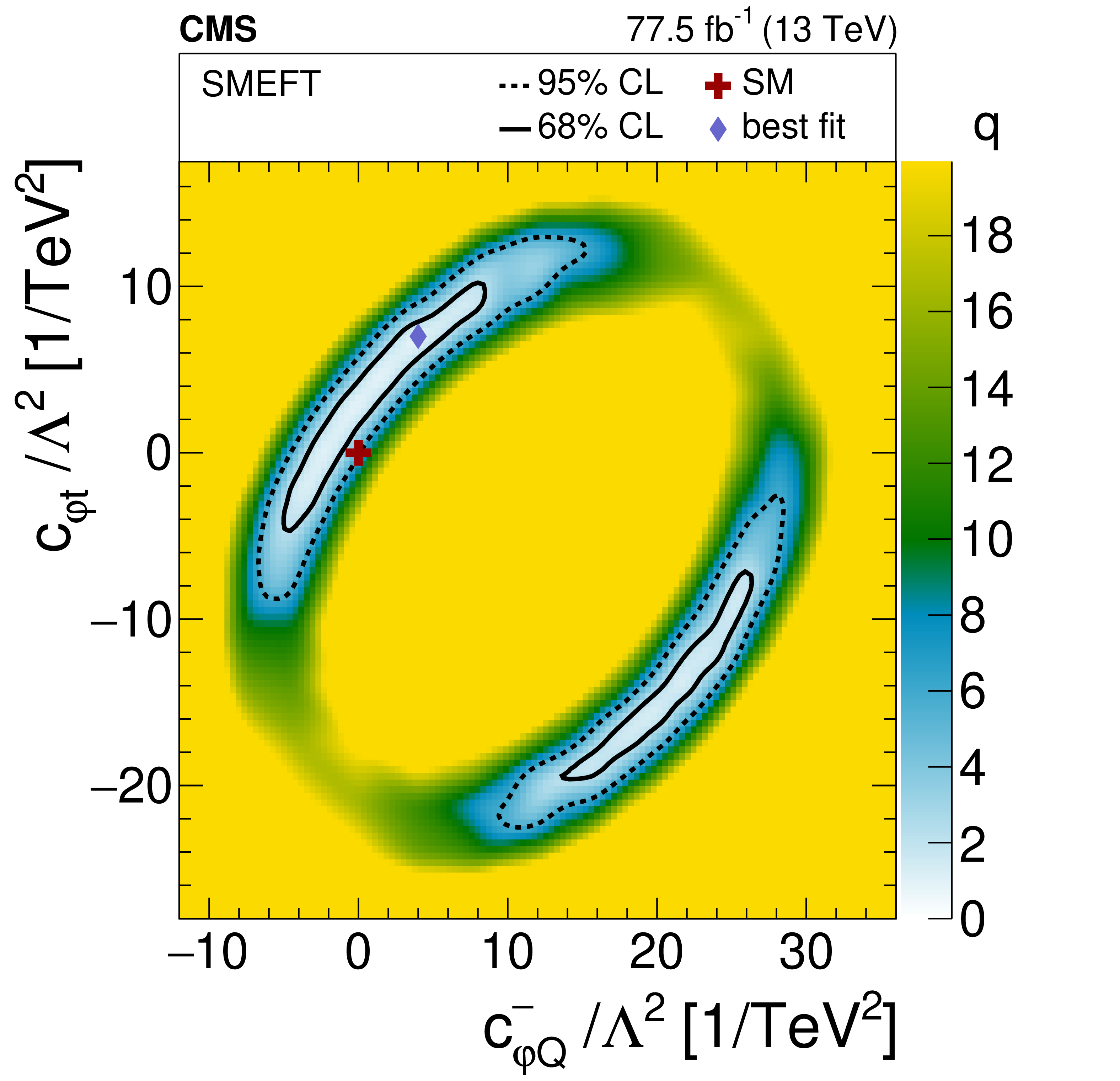
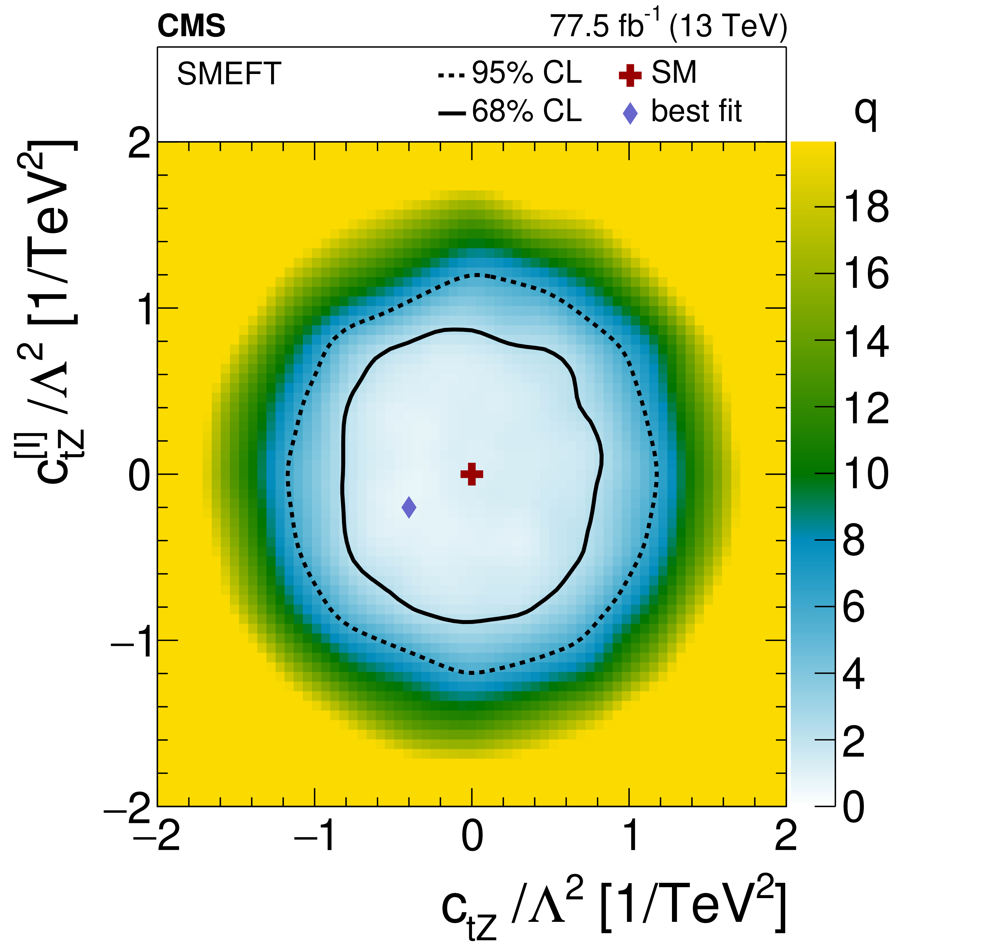
Figure 7:
Results of scans in two 2D planes for the SMEFT interpretation. The shading quantified by the gray scale on the right reflects the negative log-likelihood ratio $q$ with respect to the best-fit value, designated by the diamond. The solid and dashed lines indicate the 68 and 95% CL contours from the fit, respectively. The cross shows the SM prediction. |
png pdf |
Figure 7-a:
Result of a scan in a two 2D plane for the SMEFT interpretation. The shading quantified by the gray scale on the right reflects the negative log-likelihood ratio $q$ with respect to the best-fit value, designated by the diamond. The solid and dashed lines indicate the 68 and 95% CL contours from the fit, respectively. The cross shows the SM prediction. |
png pdf |
Figure 7-b:
Result of a scan in a two 2D plane for the SMEFT interpretation. The shading quantified by the gray scale on the right reflects the negative log-likelihood ratio $q$ with respect to the best-fit value, designated by the diamond. The solid and dashed lines indicate the 68 and 95% CL contours from the fit, respectively. The cross shows the SM prediction. |
png pdf |
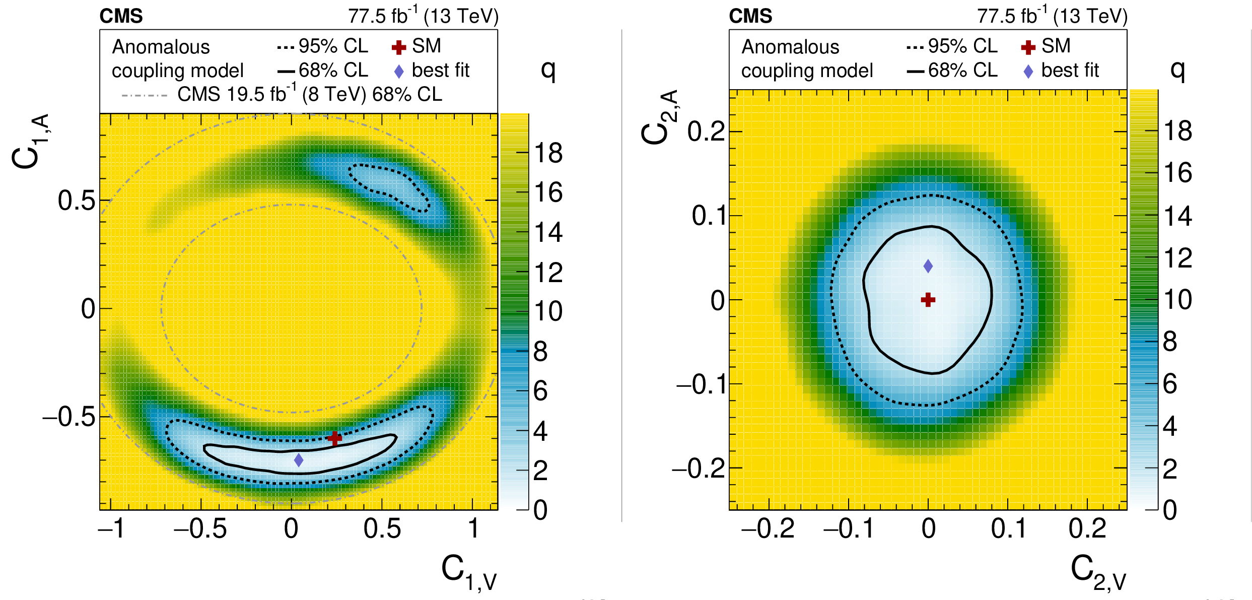
Figure 8:
Results of scans in the axial-vector and vector current coupling plane (left) and the electroweak dipole moment plane (right). The shading quantified by the gray scale on the right of each plot reflects the log-likelihood ratio $q$ with respect to the best-fit value, designated by the diamond. The solid and dashed lines indicate the 68 and 95% CL contours from the fit, respectively. The cross shows the SM prediction. The area between the dot-dashed ellipses in the axial-vector and vector current coupling plane corresponds to the observed 68% CL area from the previous CMS result [89]. |
png pdf |
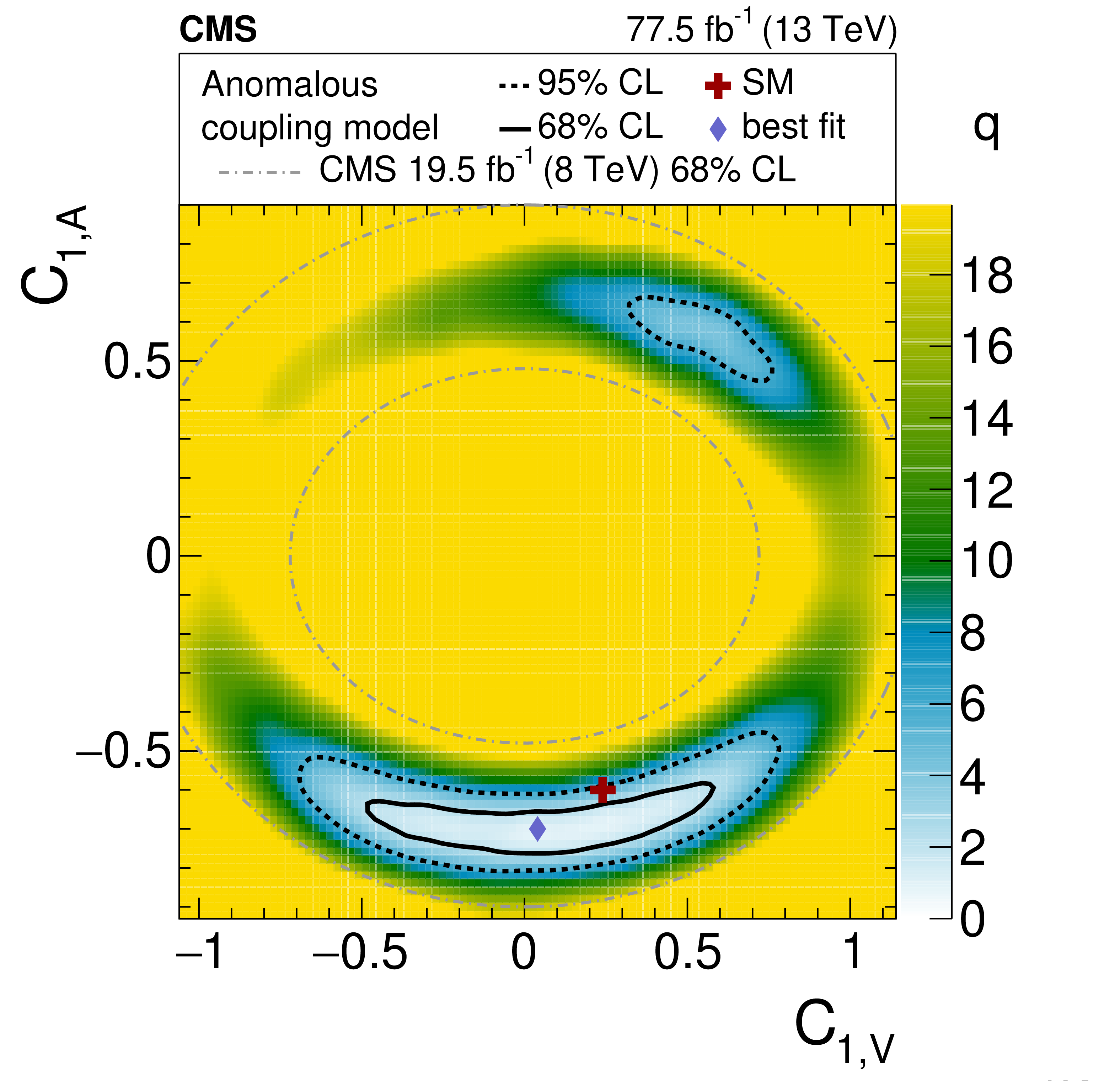
Figure 8-a:
Result of a scan in the axial-vector and vector current coupling plane. The shading quantified by the gray scale on the right of each plot reflects the log-likelihood ratio $q$ with respect to the best-fit value, designated by the diamond. The solid and dashed lines indicate the 68 and 95% CL contours from the fit, respectively. The cross shows the SM prediction. The area between the dot-dashed ellipses in the plane corresponds to the observed 68% CL area from the previous CMS result [89]. |
png pdf |
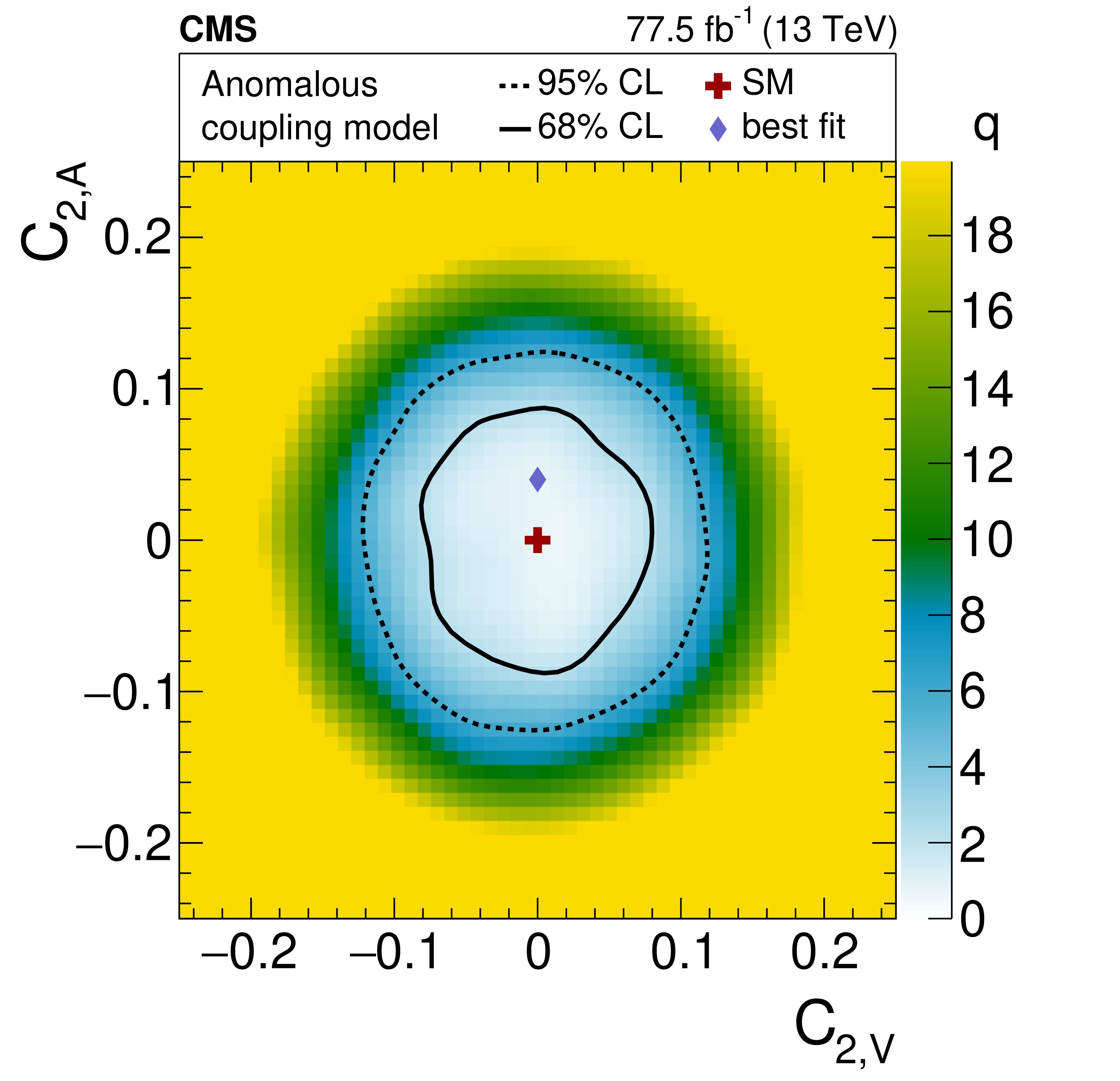
Figure 8-b:
Result of a scan in the electroweak dipole moment plane. The shading quantified by the gray scale on the right of each plot reflects the log-likelihood ratio $q$ with respect to the best-fit value, designated by the diamond. The solid and dashed lines indicate the 68 and 95% CL contours from the fit, respectively. The cross shows the SM prediction. |

png pdf |
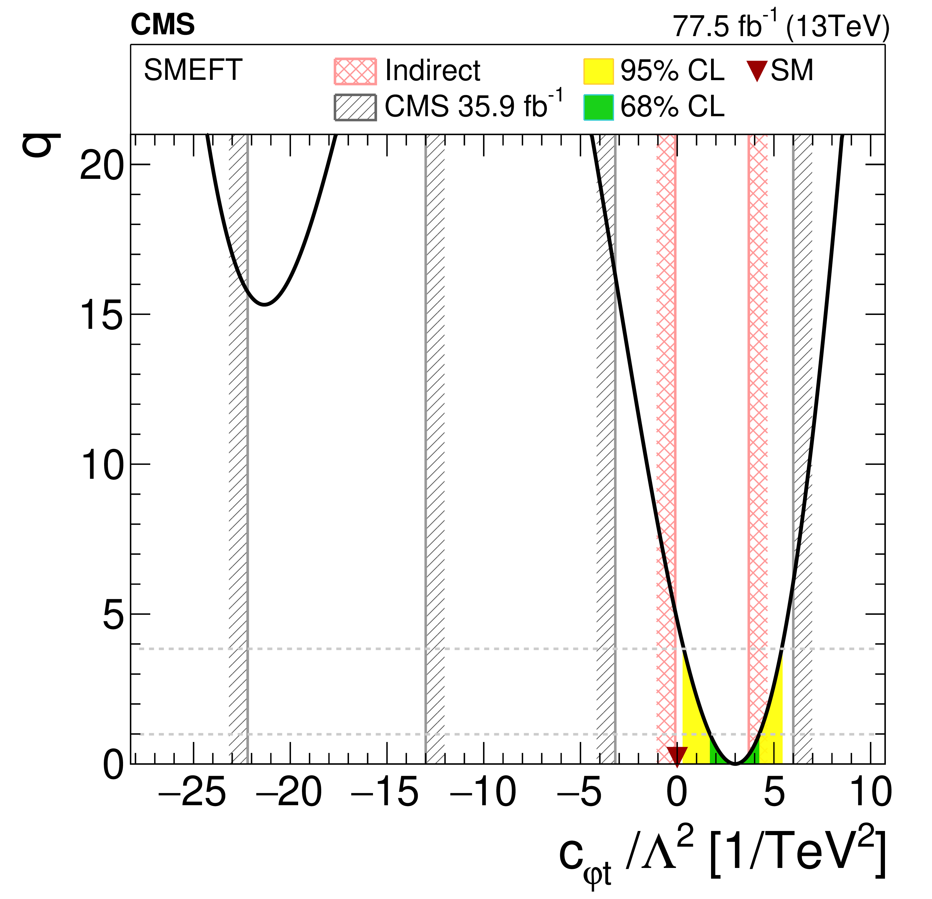
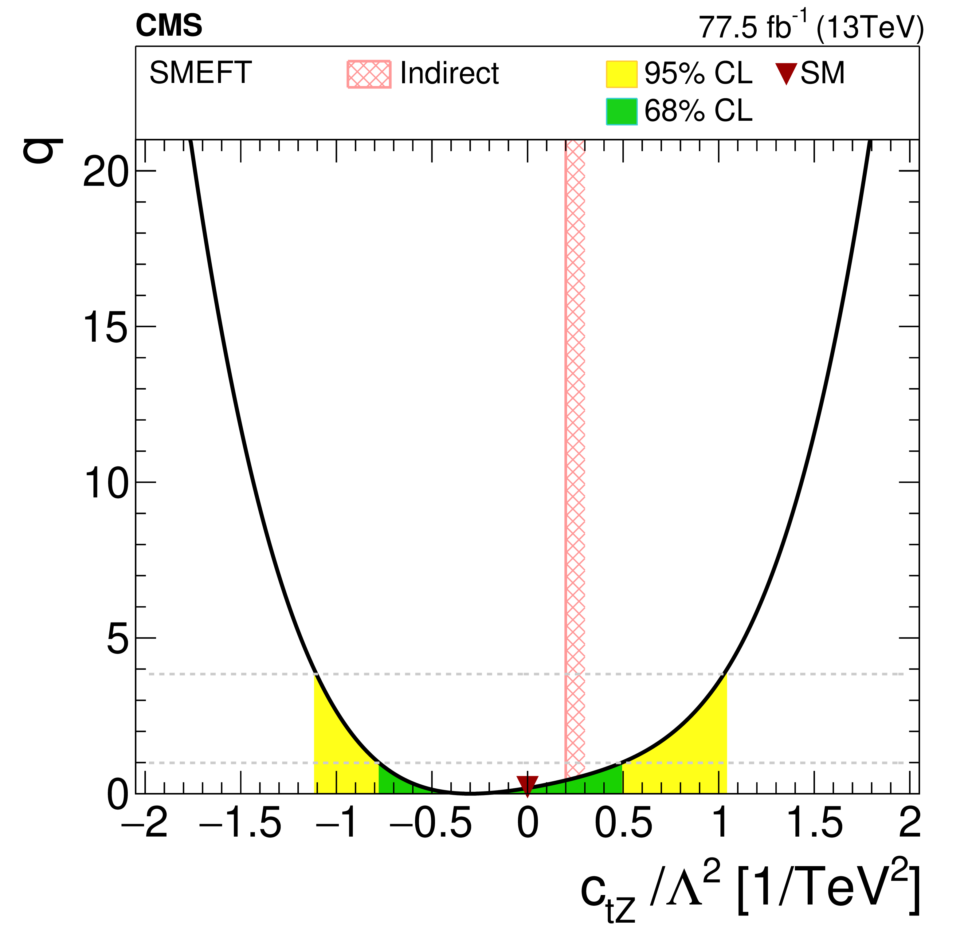
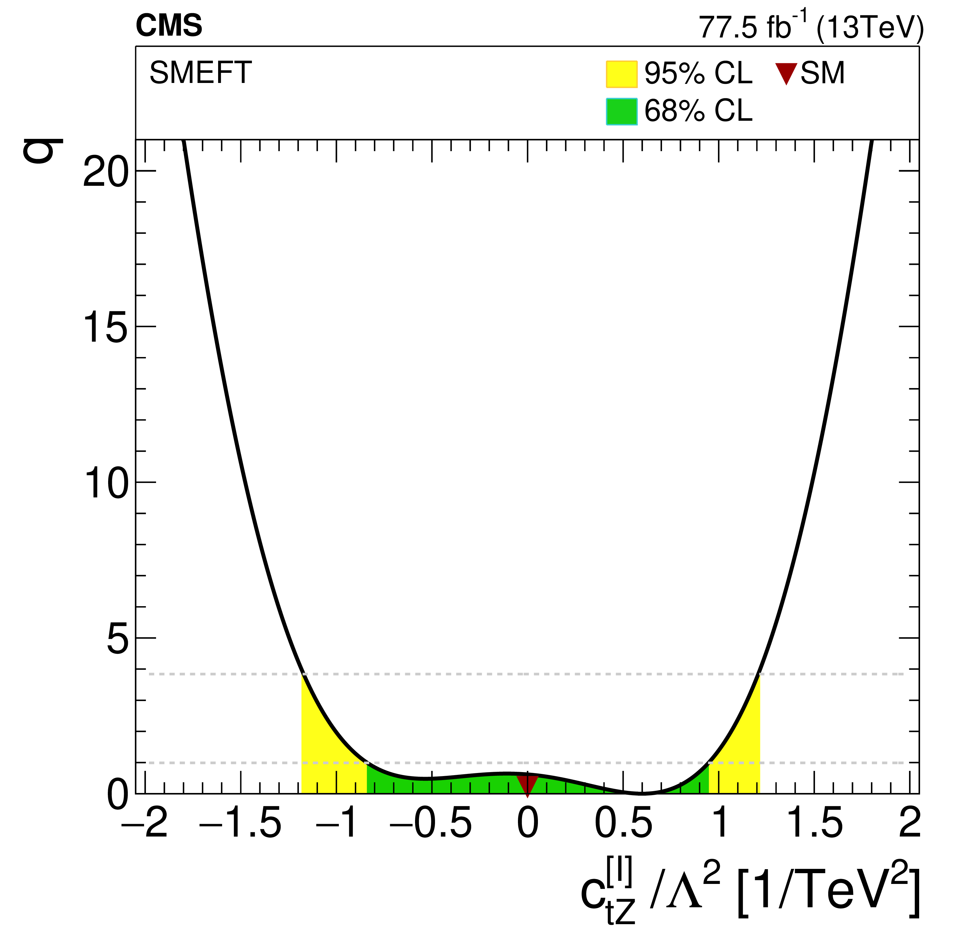
Figure 9:
1D scans of two Wilson coefficients, with the value of the other Wilson coefficients set to zero. The shaded areas correspond to the 68 and 95% CL intervals around the best fit value, respectively. The downward triangle indicates the SM value. Previously excluded regions at 95% CL [3] (if available) are indicated by the hatched band. Indirect constraints from Ref. [90] are shown as a cross-hatched band. |

png pdf |
Figure 9-a:
1D scan of two Wilson coefficients, with the value of the other Wilson coefficients set to zero. The shaded areas correspond to the 68 and 95% CL intervals around the best fit value, respectively. The downward triangle indicates the SM value. Indirect constraints from Ref. [90] are shown as a cross-hatched band. |
png pdf |
Figure 9-b:
1D scan of two Wilson coefficients, with the value of the other Wilson coefficients set to zero. The shaded areas correspond to the 68 and 95% CL intervals around the best fit value, respectively. The downward triangle indicates the SM value. Previously excluded regions at 95% CL [3] are indicated by the hatched band. Indirect constraints from Ref. [90] are shown as a cross-hatched band. |
png pdf |
Figure 9-c:
1D scan of two Wilson coefficients, with the value of the other Wilson coefficients set to zero. The shaded areas correspond to the 68 and 95% CL intervals around the best fit value, respectively. The downward triangle indicates the SM value. Indirect constraints from Ref. [90] are shown as a cross-hatched band. |
png pdf |
Figure 9-d:
1D scan of two Wilson coefficients, with the value of the other Wilson coefficients set to zero. The shaded areas correspond to the 68 and 95% CL intervals around the best fit value, respectively. The downward triangle indicates the SM value. Indirect constraints from Ref. [90] are shown as a cross-hatched band. |
png pdf |
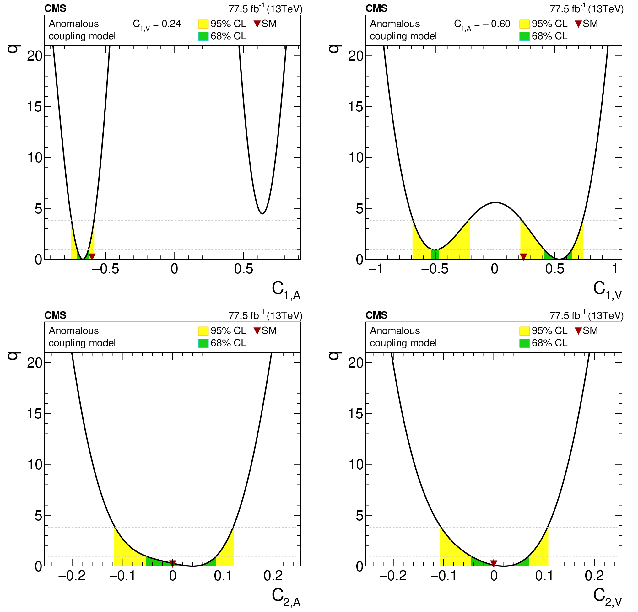
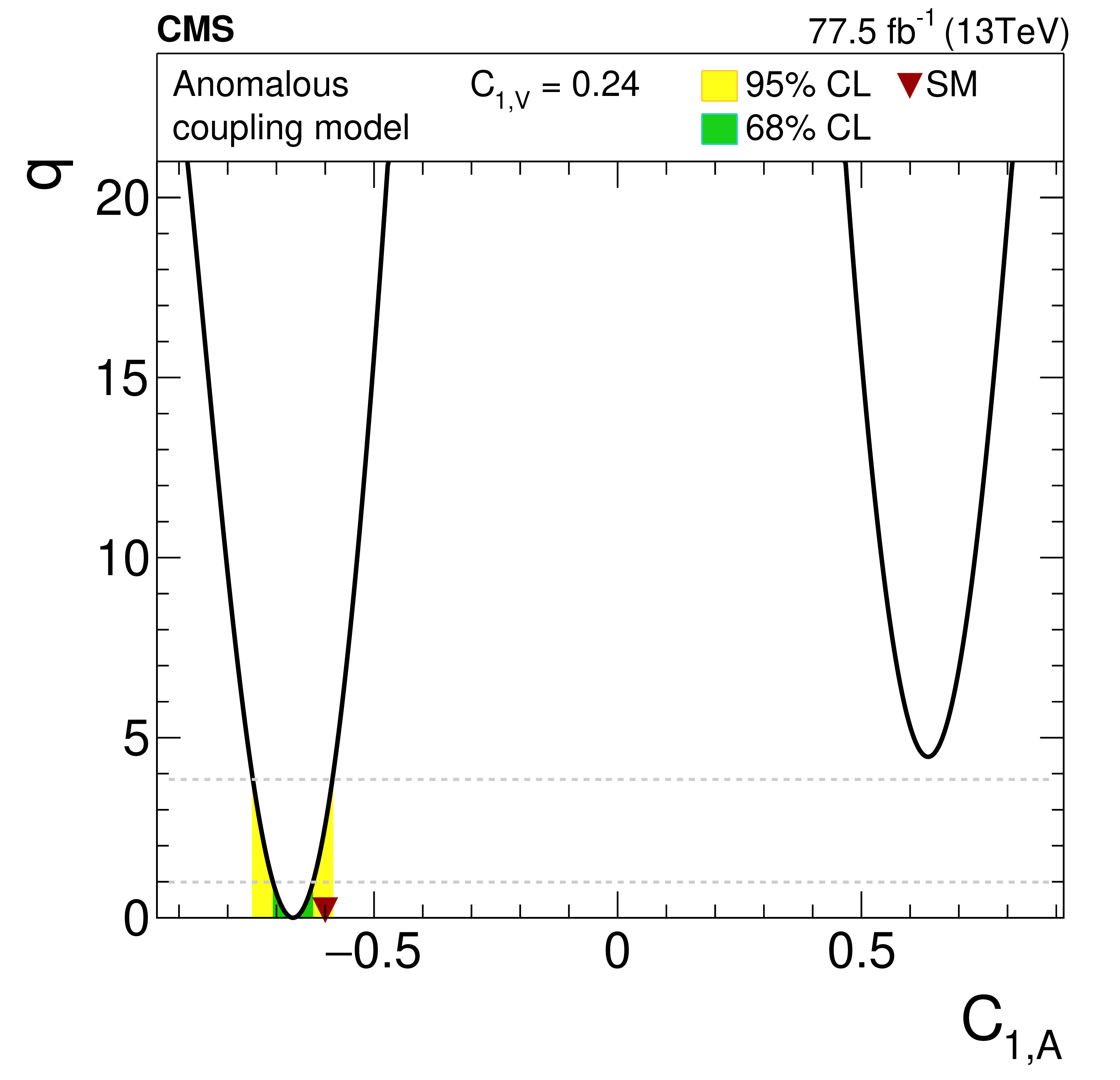
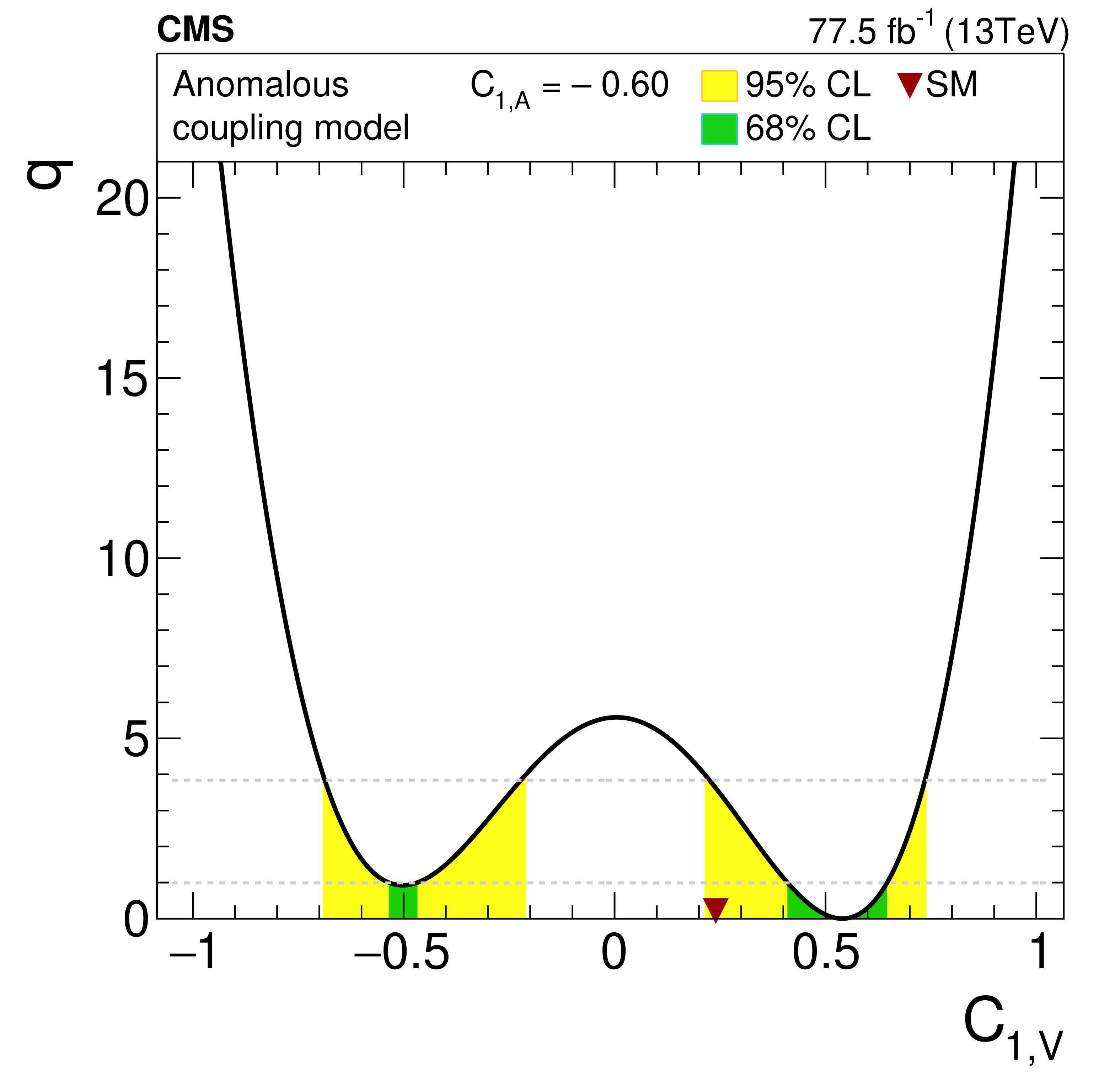
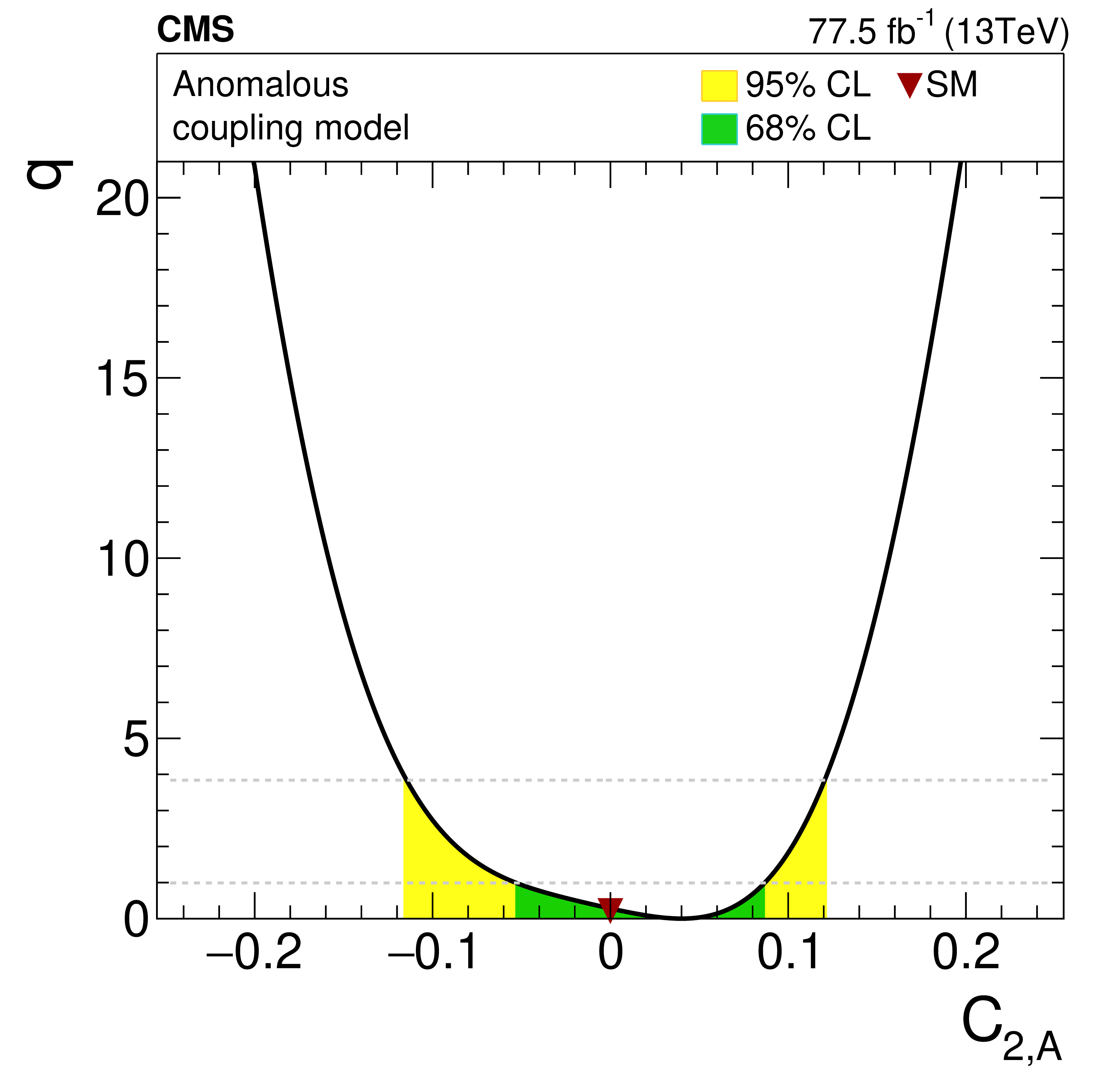
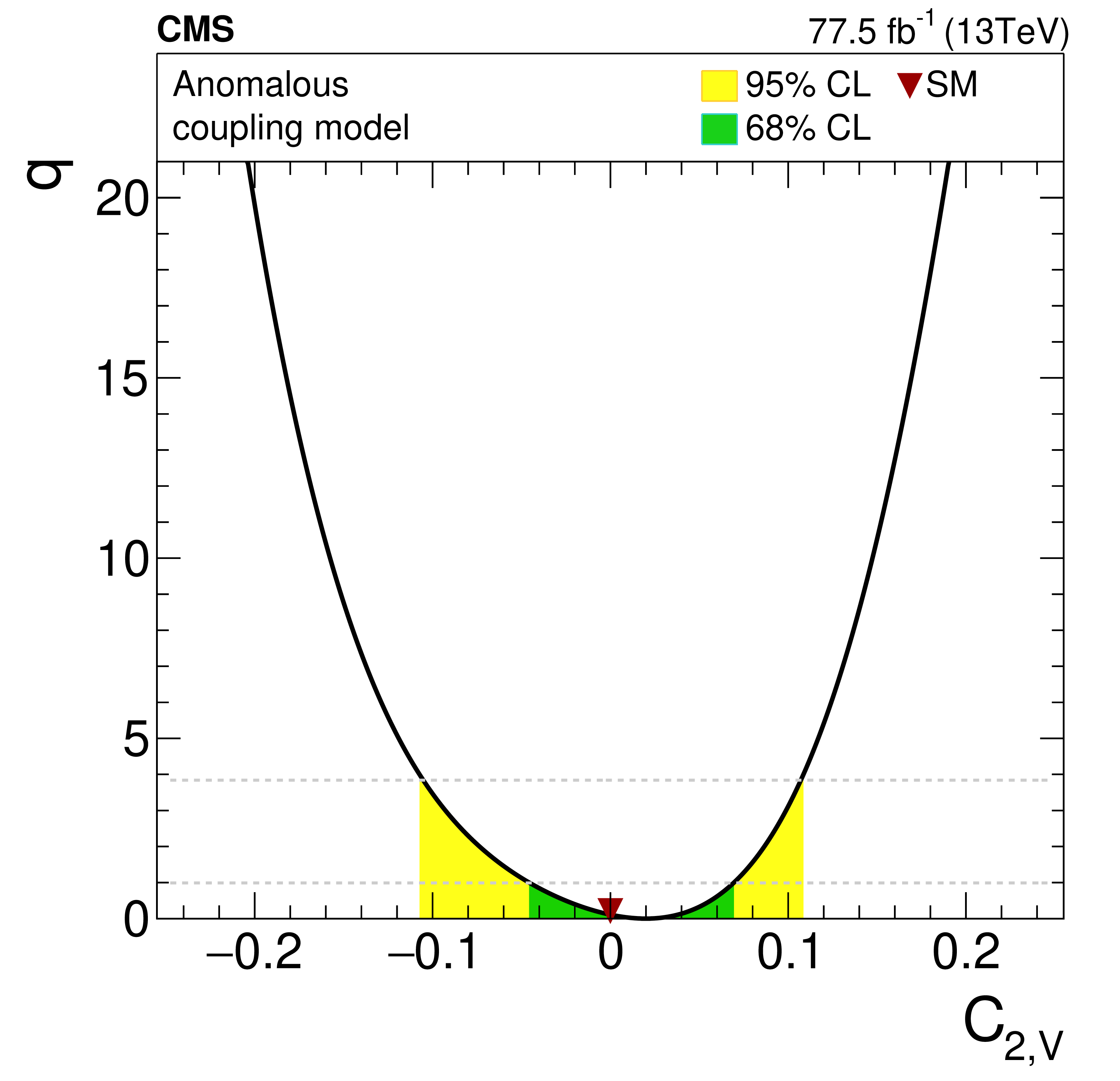
Figure 10:
Log-likelihood ratios for 1D scans of anomalous couplings. For the scan of $ {C_{1,\mathrm {A}}}$ (upper left), $ {C_{1,\mathrm {V}}}$ was set to the SM value of 0.24, and for the scan of $ {C_{1,\mathrm {V}}}$ (upper right), $ {C_{1,\mathrm {A}}}$ was set to the SM value of $-0.60$. For the scans of $ {C_{2,\mathrm {A}}}$ (lower left) and $ {C_{2,\mathrm {V}}}$ (lower right), which correspond to the top quark electric and magnetic dipole moments, respectively, both $ {C_{1,\mathrm {V}}}$ and $ {C_{1,\mathrm {A}}}$ are set to the SM values. The shaded areas correspond to the 68 and 95% CL intervals around the best-fit value, respectively. The downward triangle indicates the SM value. |
png pdf |
Figure 10-a:
Log-likelihood ratio for the 1D scan of the $ {C_{1,\mathrm {A}}}$ anomalous coupling. The value of $ {C_{1,\mathrm {V}}}$ was set to the SM value of 0.24. The shaded areas correspond to the 68 and 95% CL intervals around the best-fit value, respectively. The downward triangle indicates the SM value. |
png pdf |
Figure 10-b:
Log-likelihood ratio for the 1D scan of the $ {C_{1,\mathrm {V}}}$ anomalous coupling. The value of $ {C_{1,\mathrm {A}}}$ was set to the SM value of $-0.60$. The shaded areas correspond to the 68 and 95% CL intervals around the best-fit value, respectively. The downward triangle indicates the SM value. |
png pdf |
Figure 10-c:
Log-likelihood ratio for the 1D scan of the $ {C_{2,\mathrm {A}}}$ anomalous coupling, which correspond to the top quark electric dipole moment. The values of $ {C_{1,\mathrm {V}}}$ and $ {C_{1,\mathrm {A}}}$ were set to the SM values. The shaded areas correspond to the 68 and 95% CL intervals around the best-fit value, respectively. The downward triangle indicates the SM value. |
png pdf |
Figure 10-d:
Log-likelihood ratio for the 1D scan of the $ {C_{2,\mathrm {V}}}$ anomalous coupling, which correspond to the top quark magnetic dipole moment. The values of $ {C_{1,\mathrm {V}}}$ and $ {C_{1,\mathrm {A}}}$ were set to the SM values. The shaded areas correspond to the 68 and 95% CL intervals around the best-fit value, respectively. The downward triangle indicates the SM value. |
png pdf |
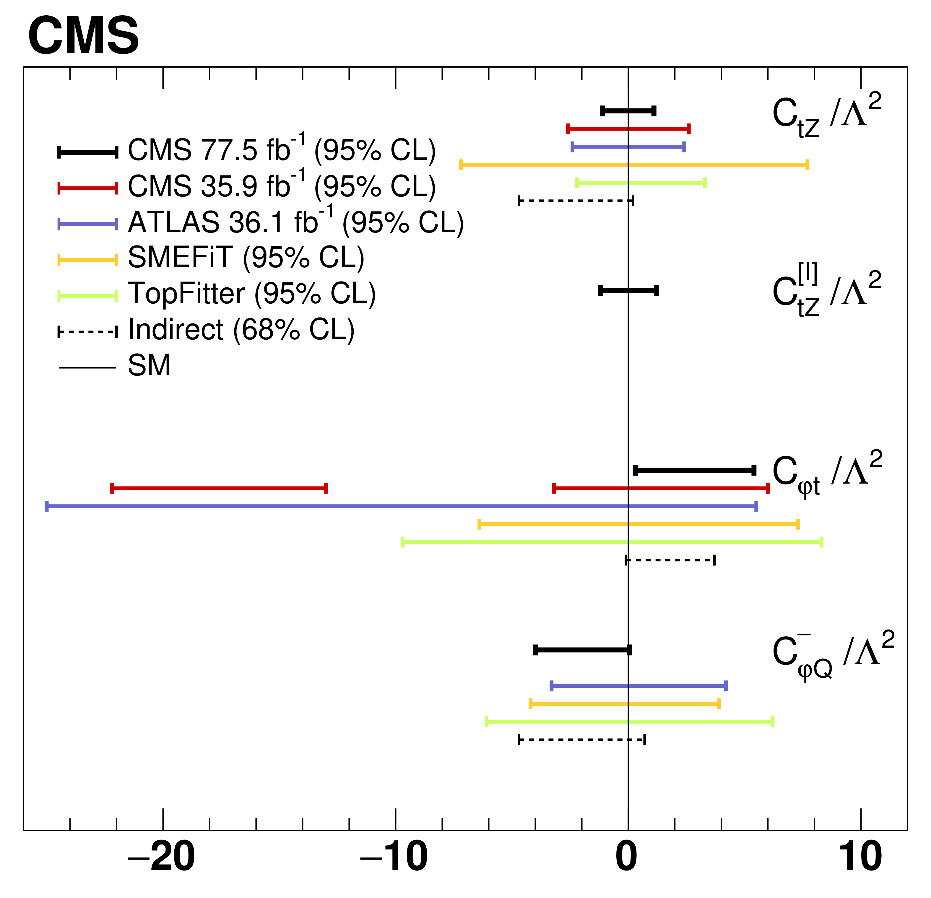
Figure 11:
The observed 95% CL intervals for the Wilson coefficients from this measurement, the previous CMS result based on the inclusive ${{\mathrm{t} \mathrm{\bar{t}}} \mathrm{Z}}$ cross section measurement [3], and the most recent ATLAS result [4]. The direct limits within the SMEFiT framework [87] and from the TopFitter Collaboration [88], and the 68% CL indirect limits from electroweak data are also shown [90]. The vertical line displays the SM prediction. |
| Tables | |
png pdf |
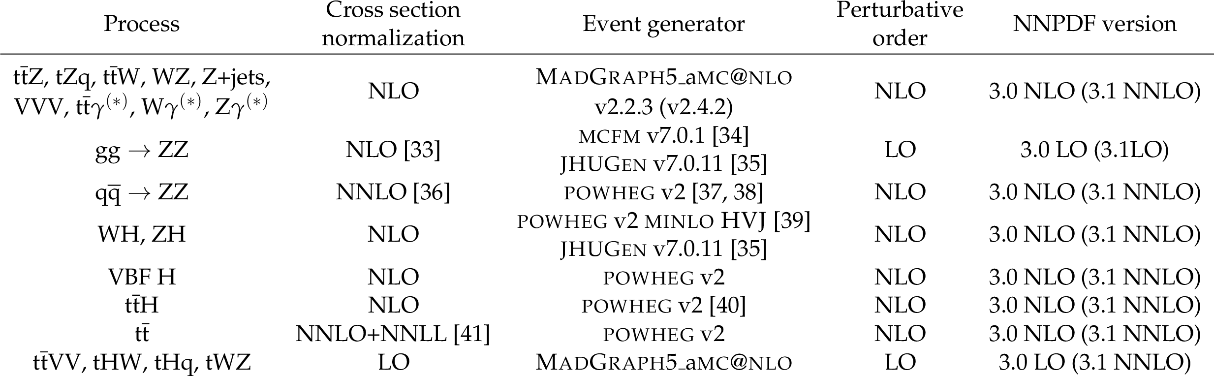
Table 1:
Event generators used to simulate events for the various processes. For each of the simulated processes shown, the order of the cross section normalization, the event generator used, the perturbative order of the generator calculation, and the NNPDF versions at NLO and at next-to-next-to-leading order (NNLO) used in simulating samples for the 2016 (2017) data sets. |
png pdf |
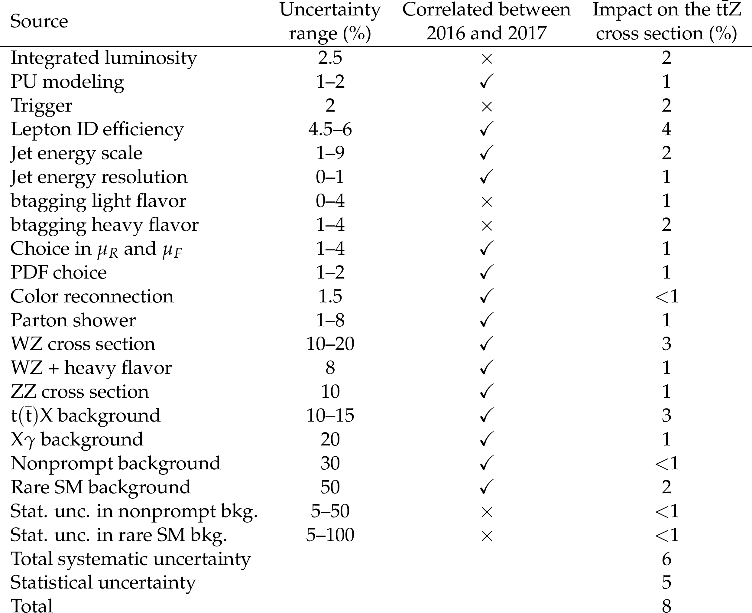
Table 2:
Summary of the sources, magnitudes, treatments, and effects of the systematic uncertainties in the final ${{\mathrm{t} \mathrm{\bar{t}}} \mathrm{Z}}$ cross section measurement. The first column indicates the source of the uncertainty, the second column shows the corresponding input uncertainty range for each background source and the signal. The third column indicates how correlations are treated between the uncertainties in the 2016 and 2017 data, where xx means fully correlated and ${\times}$ uncorrelated. The last column gives the corresponding systematic uncertainty in the ${{\mathrm{t} \mathrm{\bar{t}}} \mathrm{Z}}$ cross section from each source. The total systematic uncertainty, the statistical uncertainty and the total uncertainty in the ${{\mathrm{t} \mathrm{\bar{t}}} \mathrm{Z}}$ cross section are shown in the last three lines. |
png pdf |
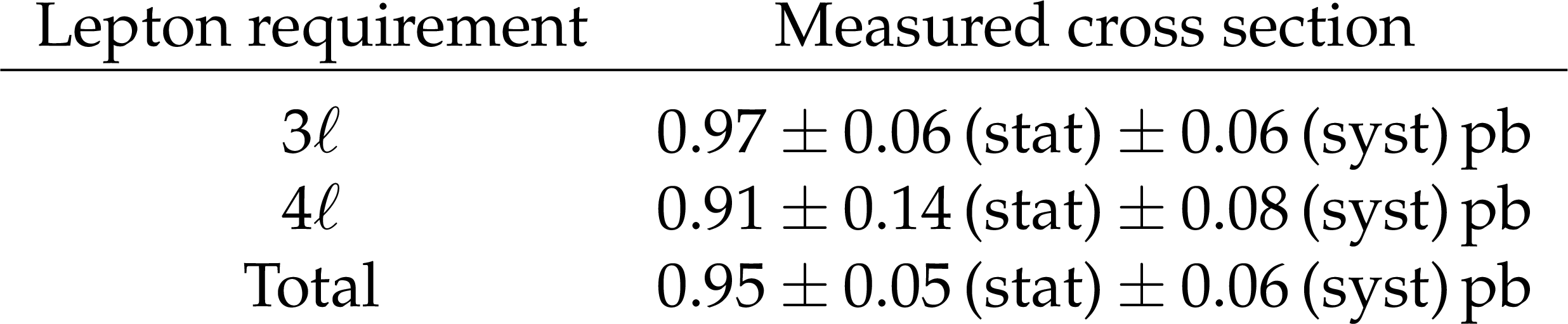
Table 3:
The measured ${{\mathrm{t} \mathrm{\bar{t}}} \mathrm{Z}}$ cross section for events with with 3 and 4 leptons and the combined measurement. |
png pdf |
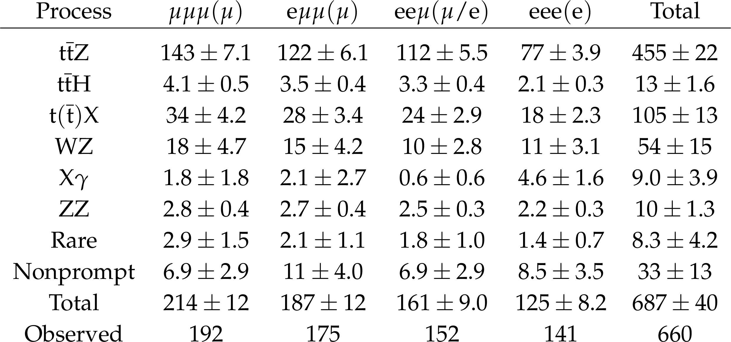
Table 4:
The observed number of events for three- and four-lepton events in a signal-enriched sample of events, and the predicted yields and total uncertainties from the fit for each process. |
png pdf |
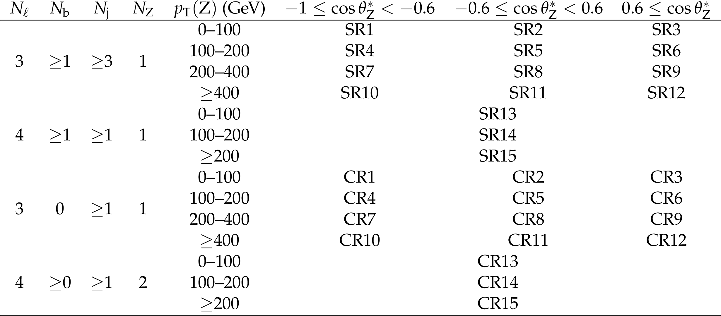
Table 5:
Definition of the signal regions (SRs) and control regions (CRs). For signal regions SR13, SR14, and SR15 and control regions CR13, CR14, and CR15, there is no requirement on $\cos\theta ^\ast _{\mathrm{Z}}$. |
png pdf |
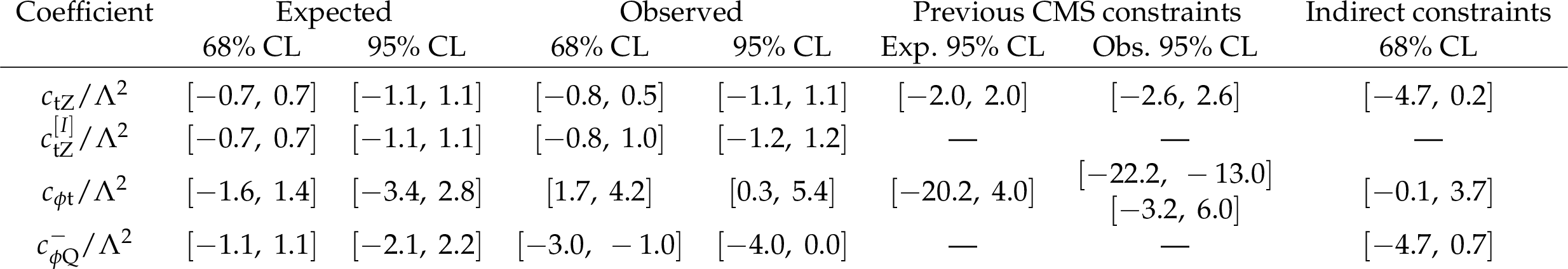
Table 6:
Expected and observed 68 and 95% CL intervals from this measurement for the listed Wilson coefficients. The expected and observed 95% CL intervals from a previous CMS measurement [3] and indirect 68% CL constraints from precision electroweak data [90] are shown for comparison. |
| Summary |
|
A measurement of top quark pair production in association with a Z boson using a data sample of proton-proton collisions at $\sqrt{s} = $ 13 TeV, corresponding to an integrated luminosity of 77.5 fb$^{-1}$, collected with the CMS detector at the LHC has been presented. The analysis was performed in the three- and four-lepton final states using analysis categories defined with jet and b jet multiplicities. Data samples enriched in background processes were used to validate predictions, as well as to constrain their uncertainties. The larger data set and reduced systematic uncertainties such as those associated with the lepton identification, helped to substantially improve the precision on the measured cross section with respect to previous measurements reported in Refs. [3,4]. The measured inclusive cross section $\sigma({\mathrm{t\bar{t}}\mathrm{Z}} )=$ 0.95 $\pm$ 0.05 (stat) $\pm$ 0.06 (syst) pb is in good agreement with the standard model prediction of 0.84 $\pm$ 0.10 pb [30,31,32]. This is the most precise measurement of the ${\mathrm{t\bar{t}}\mathrm{Z}}$ cross section to date, and the first measurement with a precision competing with current theoretical calculations. Absolute and normalized differential cross sections for the transverse momentum of the Z boson and for ${\cos\theta^\ast_{\mathrm{Z}}} $, the angle between the direction of the Z boson and the direction of the negatively charged lepton in the rest frame of the Z boson, are measured for the first time. The standard model predictions at next-to-leading order are found to be in good agreement with the measured differential cross sections. The measurement is also interpreted in terms of anomalous interactions of the t quark with the Z boson. Confidence intervals for the anomalous vector and the axial-vector current couplings and the dipole moment interactions are presented. Constraints on the Wilson coefficients in the standard model effective field theory are also presented. |
| Additional Figures | |

png pdf |
Additional Figure 1:
Covariance matrix of the measured absolute differential cross section as a function of $ {p_{\mathrm {T}}} (\mathrm{Z})$. |
png pdf |
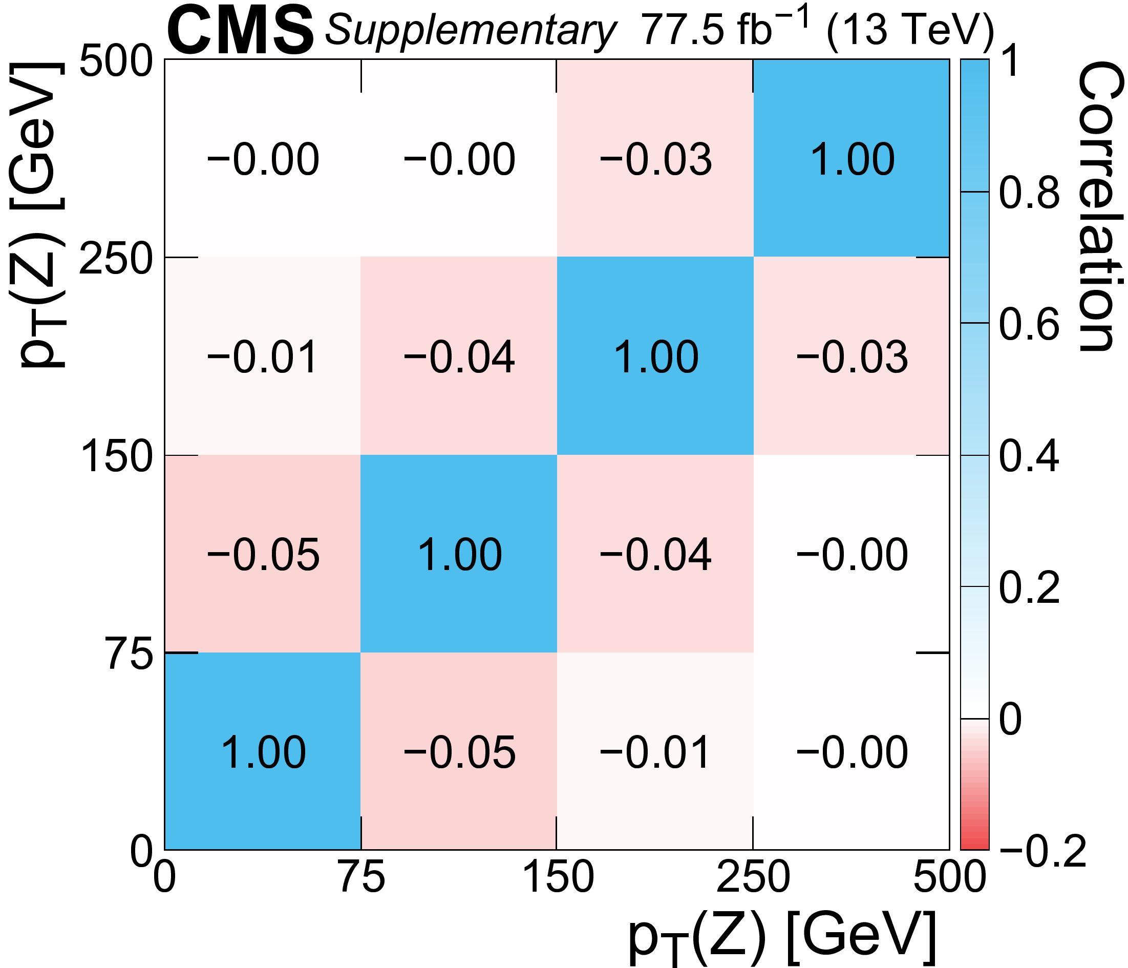
Additional Figure 2:
Correlation matrix of the measured absolute differential cross section as a function of $ {p_{\mathrm {T}}} (\mathrm{Z})$. |

png pdf |
Additional Figure 3:
Covariance matrix of the measured normalized differential cross section as a function of $ {p_{\mathrm {T}}} (\mathrm{Z})$. |

png pdf |
Additional Figure 4:
Correlation matrix of the measured normalized differential cross section as a function of $ {p_{\mathrm {T}}} (\mathrm{Z})$. |
png pdf |
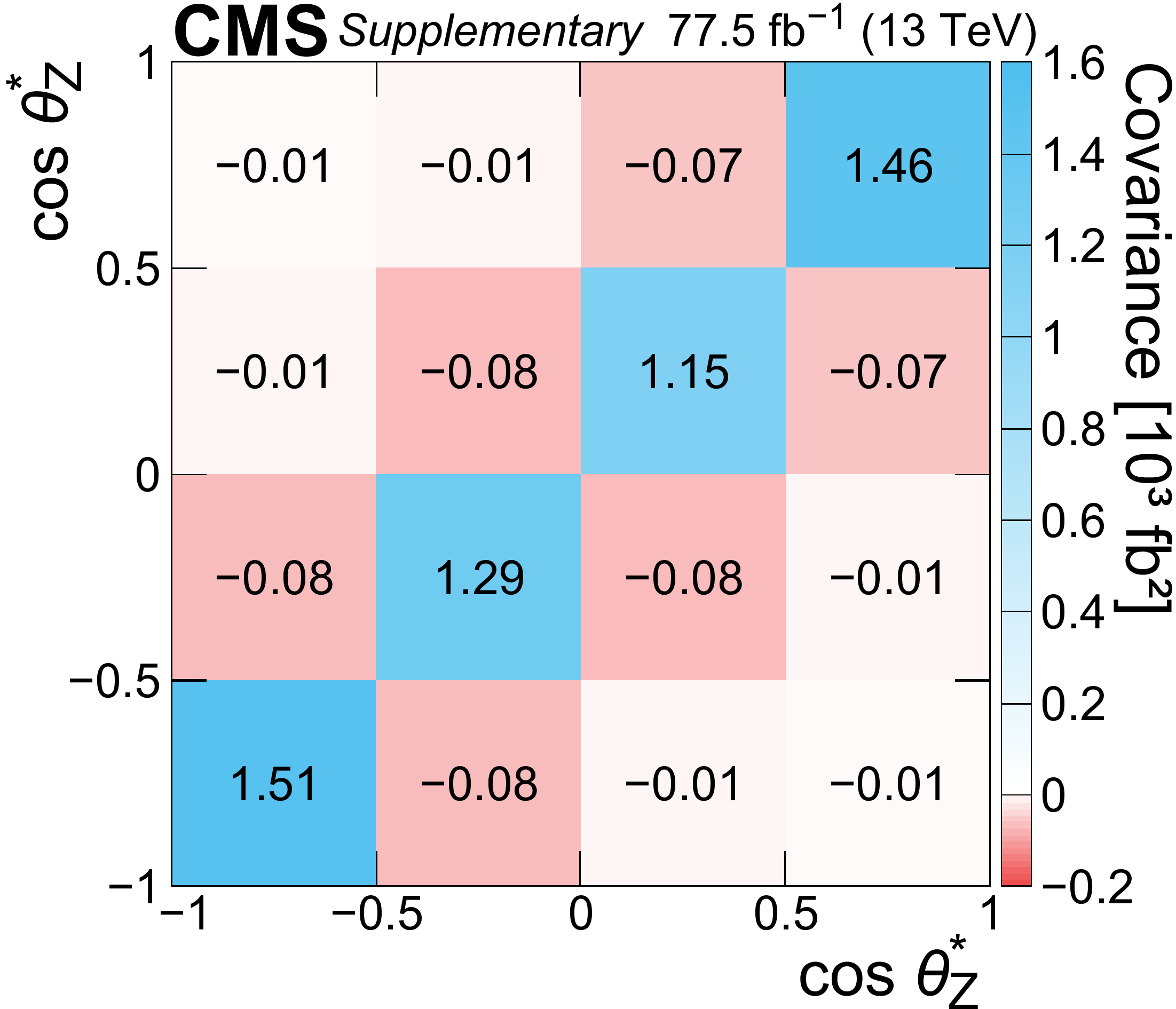
Additional Figure 5:
Covariance matrix of the measured absolute differential cross section as a function of $\cos\theta _{\mathrm{Z}}^{*} $. |
png pdf |
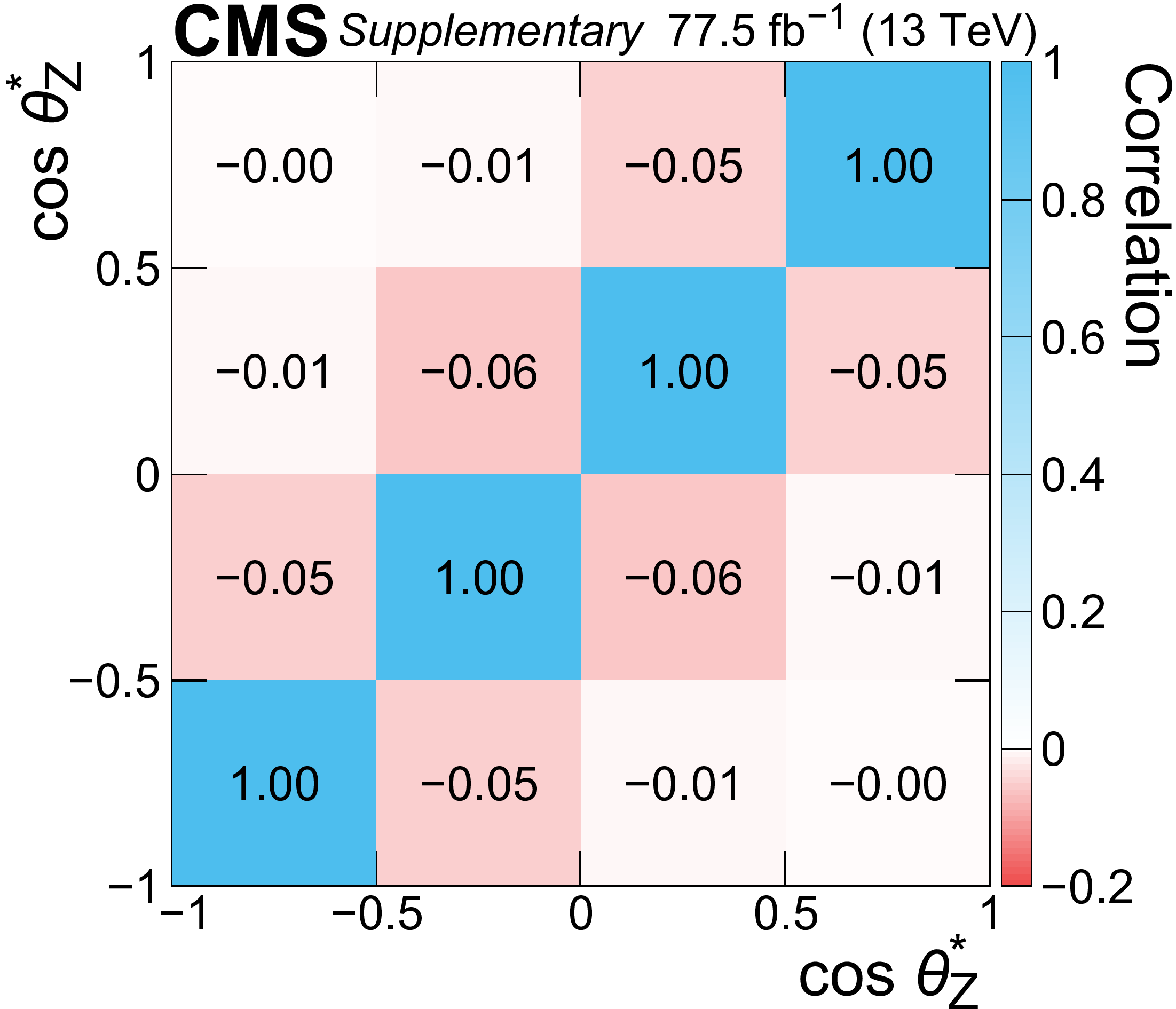
Additional Figure 6:
Correlation matrix of the measured absolute differential cross section as a function of $\cos\theta _{\mathrm{Z}}^{*} $. |
png pdf |
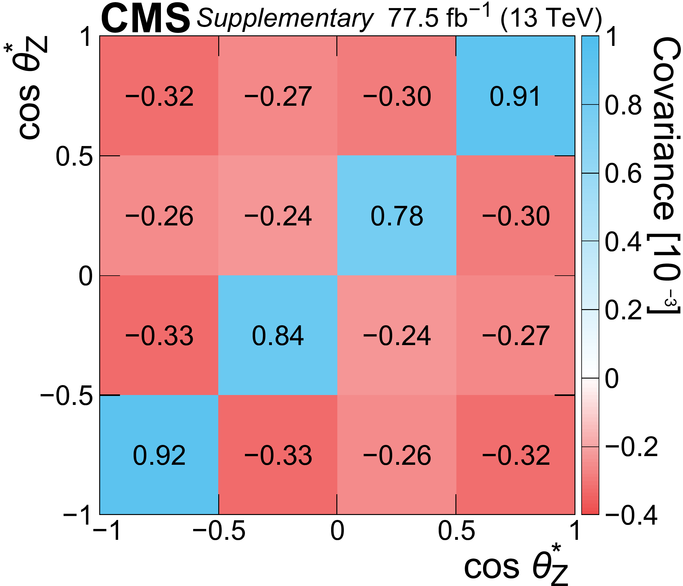
Additional Figure 7:
Covariance matrix of the measured normalized differential cross section as a function of $\cos\theta _{\mathrm{Z}}^{*} $. |
png pdf |
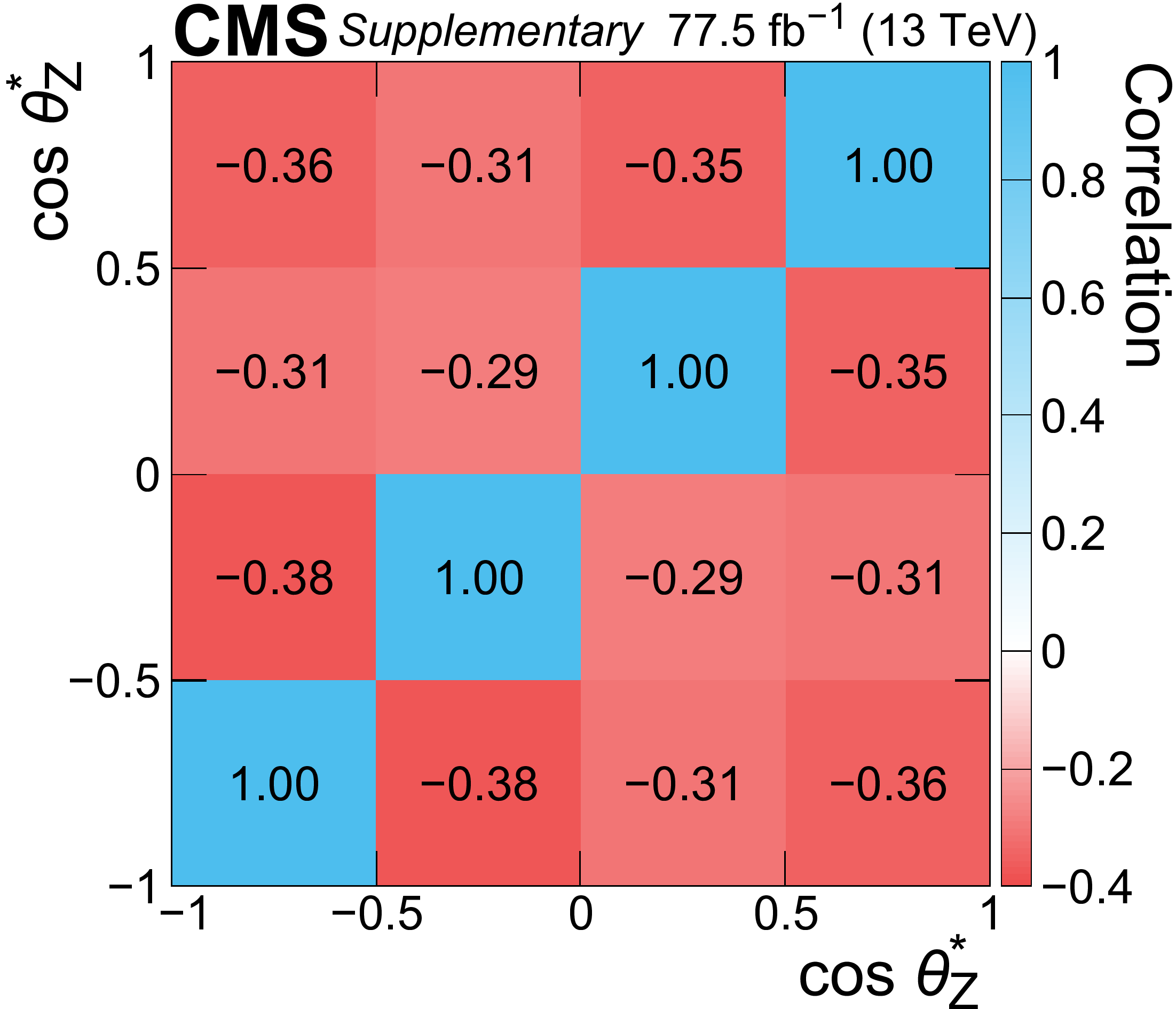
Additional Figure 8:
Correlation matrix of the measured normalized differential cross section as a function of $\cos\theta _{\mathrm{Z}}^{*} $. |
png pdf |
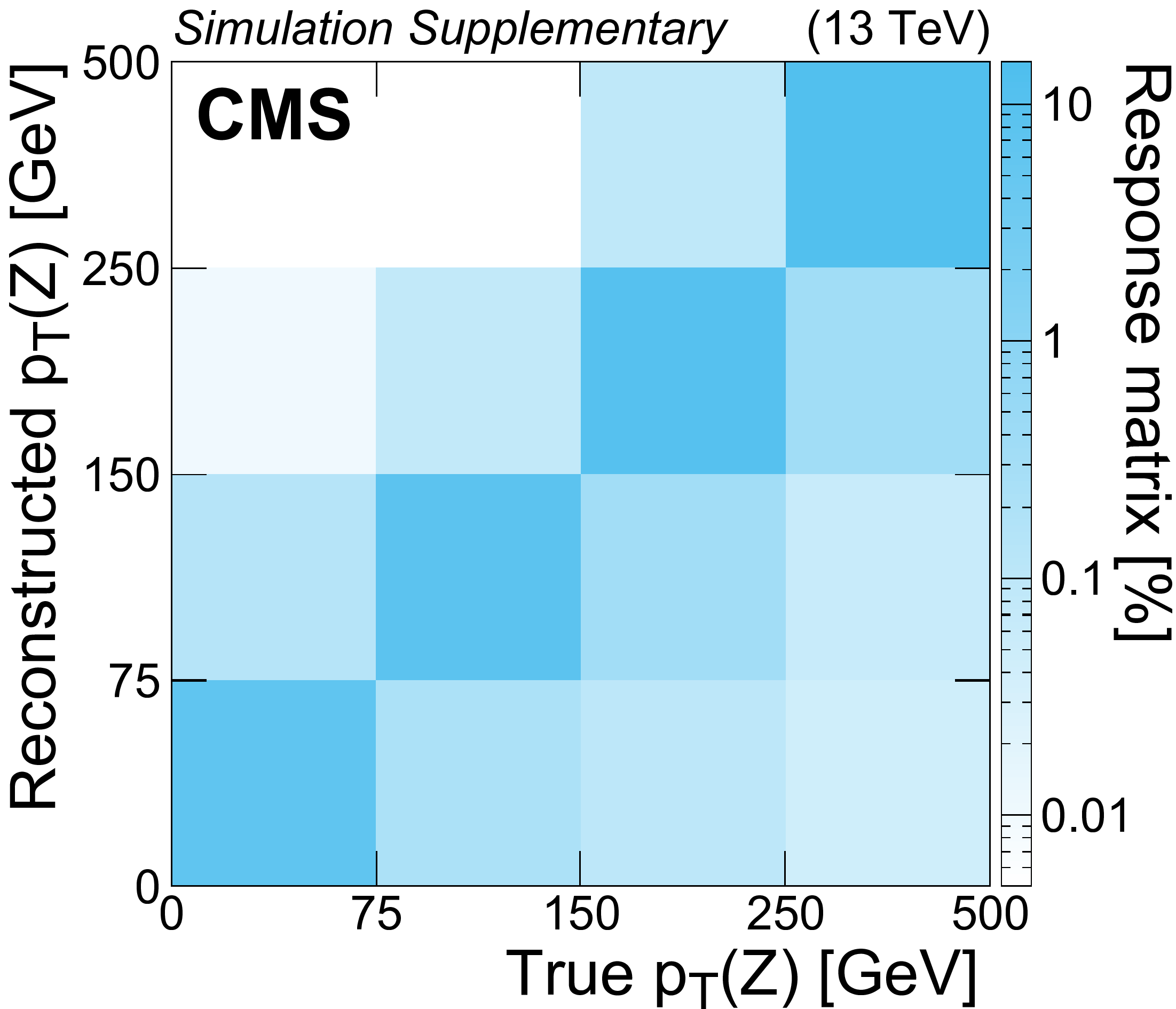
Additional Figure 9:
Response matrix describing the probability for a ${\mathrm{t} \mathrm{\bar{t}}} \mathrm{Z} $ event with a certain true value of the Z boson ${p_{\mathrm {T}}}$ to be selected with a certain reconstructed value of the Z boson ${p_{\mathrm {T}}}$. |

png pdf |
Additional Figure 10:
Response matrix describing the probability for a ${\mathrm{t} \mathrm{\bar{t}}} \mathrm{Z} $ event with a certain true value of $\cos\theta _{\mathrm{Z}}^{*} $ to be selected with a certain reconstructed value of $\cos\theta _{\mathrm{Z}}^{*} $. |
| References | ||||
| 1 | O. Bessidskaia Bylund et al. | Probing top quark neutral couplings in the standard model effective field theory at NLO in QCD | JHEP 05 (2016) 052 | 1601.08193 |
| 2 | C. Englert, R. Kogler, H. Schulz, and M. Spannowsky | Higgs coupling measurements at the LHC | EPJC 76 (2016) 393 | 1511.05170 |
| 3 | CMS Collaboration | Measurement of the cross section for top quark pair production in association with a W or Z boson in proton-proton collisions at $ \sqrt{s}= $ 13 TeV | JHEP 08 (2018) 011 | CMS-TOP-17-005 1711.02547 |
| 4 | ATLAS Collaboration | Measurement of the $ \mathrm{t\bar{t}Z} $ and $ \mathrm{t\bar{t}W} $ cross sections in proton-proton collisions at $ \sqrt{s}= $ 13 TeV with the ATLAS detector | PRD 99 (2019) 072009 | 1901.03584 |
| 5 | W. Hollik et al. | Top dipole form-factors and loop induced CP violation in supersymmetry | NPB 551 (1999) 3 | hep-ph/9812298 |
| 6 | K. Agashe, G. Perez, and A. Soni | Collider signals of top quark flavor violation from a warped extra dimension | PRD 75 (2007) 015002 | hep-ph/0606293 |
| 7 | A. L. Kagan, G. Perez, T. Volansky, and J. Zupan | General minimal flavor violation | PRD 80 (2009) 076002 | 0903.1794 |
| 8 | T. Ibrahim and P. Nath | Top quark electric dipole moment in a minimal supersymmetric standard model extension with vectorlike multiplets | PRD 82 (2010) 055001 | 1007.0432 |
| 9 | T. Ibrahim and P. Nath | Chromoelectric dipole moment of the top quark in models with vectorlike multiplets | PRD 84 (2011) 015003 | 1104.3851 |
| 10 | C. Grojean, O. Matsedonskyi, and G. Panico | Light top partners and precision physics | JHEP 10 (2013) 160 | 1306.4655 |
| 11 | J. A. Aguilar-Saavedra | A minimal set of top anomalous couplings | NPB 812 (2009) 181 | 0811.3842 |
| 12 | B. Grzadkowski, M. Iskrzynski, M. Misiak, and J. Rosiek | Dimension-six terms in the standard model Lagrangian | JHEP 10 (2010) 085 | 1008.4884 |
| 13 | J. A. Aguilar Saavedra et al. | Interpreting top-quark LHC measurements in the standard-model effective field theory | 1802.07237 | |
| 14 | CMS Collaboration | The CMS trigger system | JINST 12 (2017) P01020 | CMS-TRG-12-001 1609.02366 |
| 15 | CMS Collaboration | The CMS experiment at the CERN LHC | JINST 3 (2008) S08004 | CMS-00-001 |
| 16 | J. Alwall et al. | The automated computation of tree-level and next-to-leading order differential cross sections, and their matching to parton shower simulations | JHEP 07 (2014) 079 | 1405.0301 |
| 17 | S. Alioli, P. Nason, C. Oleari, and E. Re | A general framework for implementing NLO calculations in shower Monte Carlo programs: the POWHEG BOX | JHEP 06 (2010) 043 | 1002.2581 |
| 18 | NNPDF Collaboration | Parton distributions for the LHC Run II | JHEP 04 (2015) 040 | 1410.8849 |
| 19 | NNPDF Collaboration | Parton distributions from high-precision collider data | EPJC 77 (2017) 663 | 1706.00428 |
| 20 | T. Sjostrand, S. Mrenna, and P. Z. Skands | A brief introduction to PYTHIA 8.1 | CPC 178 (2008) 852 | 0710.3820 |
| 21 | T. Sjostrand et al. | An introduction to PYTHIA 8.2 | CPC 191 (2015) 159 | 1410.3012 |
| 22 | P. Skands, S. Carrazza, and J. Rojo | Tuning PYTHIA 8.1: the Monash 2013 tune | EPJC 74 (2014) 3024 | 1404.5630 |
| 23 | CMS Collaboration | Event generator tunes obtained from underlying event and multiparton scattering measurements | EPJC 76 (2016) 155 | CMS-GEN-14-001 1512.00815 |
| 24 | CMS Collaboration | Extraction and validation of a new set of CMS PYTHIA8 tunes from underlying-event measurements | Submitted to EPJC | CMS-GEN-17-001 1903.12179 |
| 25 | CMS Collaboration | Investigations of the impact of the parton shower tuning in PYTHIA 8 in the modelling of $ \mathrm{t\overline{t}} $ at $ \sqrt{s}= $ 8 and 13 TeV | CMS-PAS-TOP-16-021 | CMS-PAS-TOP-16-021 |
| 26 | J. Alwall et al. | Comparative study of various algorithms for the merging of parton showers and matrix elements in hadronic collisions | EPJC 53 (2008) 473 | 0706.2569 |
| 27 | R. Frederix and S. Frixione | Merging meets matching in MC@NLO | JHEP 12 (2012) 061 | 1209.6215 |
| 28 | Particle Data Group, M. Tanabashi et al. | Review of particle physics | PRD 98 (2018) 030001 | |
| 29 | J. Butterworth et al. | PDF4LHC recommendations for LHC Run II | JPG 43 (2016) 023001 | 1510.03865 |
| 30 | D. de Florian et al. | Handbook of LHC Higgs cross sections: 4. Deciphering the nature of the Higgs sector | CERN-2017-002-M | 1610.07922 |
| 31 | S. Frixione et al. | Electroweak and QCD corrections to top-pair hadroproduction in association with heavy bosons | JHEP 06 (2015) 184 | 1504.03446 |
| 32 | R. Frederix et al. | The automation of next-to-leading order electroweak calculations | JHEP 07 (2018) 185 | 1804.10017 |
| 33 | F. Caola, K. Melnikov, R. Rontsch, and L. Tancredi | QCD corrections to ZZ production in gluon fusion at the LHC | PRD 92 (2015) 094028 | 1509.06734 |
| 34 | J. M. Campbell and R. K. Ellis | MCFM for the Tevatron and the LHC | NPPS 205-206 (2010) 10 | 1007.3492 |
| 35 | S. Bolognesi et al. | Spin and parity of a single-produced resonance at the LHC | PRD 86 (2012) 095031 | 1208.4018 |
| 36 | F. Cascioli et al. | ZZ production at hadron colliders in NNLO QCD | PLB 735 (2014) 311 | 1405.2219 |
| 37 | T. Melia, P. Nason, R. Rontsch, and G. Zanderighi | $ \mathrm{W}^+\mathrm{W}^- $, $ \mathrm{W}\mathrm{Z} $ and $ \mathrm{Z}\mathrm{Z} $ production in the POWHEG BOX | JHEP 11 (2011) 078 | 1107.5051 |
| 38 | P. Nason and G. Zanderighi | $ \mathrm{W}^+\mathrm{W}^- $ , $ \mathrm{W}\mathrm{Z} $ and $ \mathrm{Z}\mathrm{Z} $ production in the POWHEG-BOX-V2 | EPJC 74 (2014) 2702 | 1311.1365 |
| 39 | G. Luisoni, P. Nason, C. Oleari, and F. Tramontano | $ \rm HW^{\pm} $/$\mathrm{HZ}$ + 0 and 1 jet at NLO with the POWHEG BOX interfaced to GoSam and their merging within MiNLO | JHEP 10 (2013) 083 | 1306.2542 |
| 40 | H. B. Hartanto, B. Jager, L. Reina, and D. Wackeroth | Higgs boson production in association with top quarks in the POWHEG BOX | PRD 91 (2015) 094003 | 1501.04498 |
| 41 | M. Czakon and A. Mitov | Top++: A program for the calculation of the top-pair cross section at hadron colliders | CPC 185 (2014) 2930 | 1112.5675 |
| 42 | GEANT4 Collaboration | GEANT4--a simulation toolkit | NIMA 506 (2003) 250 | |
| 43 | CMS Collaboration | Particle-flow reconstruction and global event description with the CMS detector | JINST 12 (2017) P10003 | CMS-PRF-14-001 1706.04965 |
| 44 | CMS Collaboration | Performance of electron reconstruction and selection with the CMS detector in proton-proton collisions at $ \sqrt{s} = $ 8 TeV | JINST 10 (2015) P06005 | CMS-EGM-13-001 1502.02701 |
| 45 | CMS Collaboration | Performance of CMS muon reconstruction in pp collision events at $ \sqrt{s} = $ 7 TeV | JINST 7 (2012) P10002 | CMS-MUO-10-004 1206.4071 |
| 46 | M. Cacciari, G. P. Salam, and G. Soyez | The anti-$ {k_{\mathrm{T}}} $ jet clustering algorithm | JHEP 04 (2008) 063 | 0802.1189 |
| 47 | M. Cacciari, G. P. Salam, and G. Soyez | FastJet user manual | EPJC 72 (2012) 1896 | 1111.6097 |
| 48 | CMS Collaboration | Pileup removal algorithms | CMS-PAS-JME-14-001 | CMS-PAS-JME-14-001 |
| 49 | CMS Collaboration | Determination of jet energy calibration and transverse momentum resolution in CMS | JINST 6 (2011) P11002 | CMS-JME-10-011 1107.4277 |
| 50 | CMS Collaboration | Jet energy scale and resolution in the CMS experiment in pp collisions at 8 TeV | JINST 12 (2017) P02014 | CMS-JME-13-004 1607.03663 |
| 51 | CMS Collaboration | Identification of heavy-flavour jets with the CMS detector in pp collisions at 13 TeV | JINST 13 (2018) P05011 | CMS-BTV-16-002 1712.07158 |
| 52 | CMS Collaboration | Observation of $ \mathrm{t\overline{t}} $H production | PRL 120 (2018) 231801 | CMS-HIG-17-035 1804.02610 |
| 53 | H. Voss, A. Hocker, J. Stelzer, and F. Tegenfeldt | TMVA, the toolkit for multivariate data analysis with ROOT | in XIth International Workshop on Advanced Computing and Analysis Techniques in Physics Research (ACAT), p. 40 2007 [PoS(ACAT)040] | physics/0703039 |
| 54 | CMS Collaboration | Search for supersymmetry in pp collisions at $ \sqrt{s}= $ 13 TeV in the single-lepton final state using the sum of masses of large-radius jets | JHEP 08 (2016) 122 | CMS-SUS-15-007 1605.04608 |
| 55 | J. Campbell, R. K. Ellis, and R. Rontsch | Single top production in association with a Z boson at the LHC | PRD 87 (2013) 114006 | 1302.3856 |
| 56 | CMS Collaboration | Observation of single top quark production in association with a Z boson in proton-proton collisions at $ \sqrt{s} = $ 13 TeV | PRL 122 (2019) 132003 | CMS-TOP-18-008 1812.05900 |
| 57 | CMS Collaboration | Measurement of differential cross sections for Z boson pair production in association with jets at $ \sqrt{s} = $ 8 and 13 TeV | PLB 789 (2019) 19 | CMS-SMP-17-005 1806.11073 |
| 58 | D. T. Nhung, L. D. Ninh, and M. M. Weber | NLO corrections to WWZ production at the LHC | JHEP 12 (2013) 096 | 1307.7403 |
| 59 | CMS Collaboration | Measurement of the Z$ \gamma $ production cross section in pp collisions at 8 TeV and search for anomalous triple gauge boson couplings | JHEP 04 (2015) 164 | CMS-SMP-13-014 1502.05664 |
| 60 | CMS Collaboration | Measurement of the cross section for electroweak production of Z$ \gamma $ in association with two jets and constraints on anomalous quartic gauge couplings in proton-proton collisions at $ \sqrt{s} = $ 8 TeV | PLB 770 (2017) 380 | CMS-SMP-14-018 1702.03025 |
| 61 | CMS Collaboration | CMS luminosity measurements for the 2016 data taking period | CMS-PAS-LUM-17-001 | CMS-PAS-LUM-17-001 |
| 62 | CMS Collaboration | CMS luminosity measurement for the 2017 data-taking period at $ \sqrt{s} = $ 13 TeV | CMS-PAS-LUM-17-004 | CMS-PAS-LUM-17-004 |
| 63 | CMS Collaboration | Measurement of the inelastic proton-proton cross section at $ \sqrt{s}= $ 13 TeV | JHEP 07 (2018) 161 | CMS-FSQ-15-005 1802.02613 |
| 64 | ATLAS Collaboration | Measurement of the inelastic proton-proton cross section at $ \sqrt{s} = $ 13 TeV with the ATLAS detector at the LHC | PRL 117 (2016) 182002 | 1606.02625 |
| 65 | CMS Collaboration | Identification of b-quark jets with the CMS experiment | JINST 8 (2013) P04013 | CMS-BTV-12-001 1211.4462 |
| 66 | R. D. Ball et al. | Parton distributions with LHC data | NPB 867 (2013) 244 | 1207.1303 |
| 67 | A. D. Martin, W. J. Stirling, R. S. Thorne, and G. Watt | Uncertainties on $ \alpha_S $ in global PDF analyses and implications for predicted hadronic cross sections | EPJC 64 (2009) 653 | 0905.3531 |
| 68 | J. Gao et al. | CT10 next-to-next-to-leading order global analysis of QCD | PRD 89 (2014) 033009 | 1302.6246 |
| 69 | S. Argyropoulos and T. Sjostrand | Effects of color reconnection on $ \mathrm{t\bar{t}} $ final states at the LHC | JHEP 11 (2014) 043 | 1407.6653 |
| 70 | J. R. Christiansen and P. Z. Skands | String formation beyond leading colour | JHEP 08 (2015) 003 | 1505.01681 |
| 71 | T. Junk | Confidence level computation for combining searches with small statistics | NIMA 434 (1999) 435 | hep-ex/9902006 |
| 72 | A. L. Read | Presentation of search results: The CL$ {}_s $ technique | JPG 28 (2002) 2693 | |
| 73 | ATLAS and CMS Collaborations | Procedure for the LHC Higgs boson search combination in summer 2011 | ATL-PHYS-PUB-2011-011, CMS NOTE-2011/005 | |
| 74 | G. Cowan, K. Cranmer, E. Gross, and O. Vitells | Asymptotic formulae for likelihood-based tests of new physics | EPJC 71 (2011) 1554 | 1007.1727 |
| 75 | A. Kulesza et al. | Associated production of a top quark pair with a heavy electroweak gauge boson at NLO+NNLL accuracy | EPJC 79 (2019) 249 | 1812.08622 |
| 76 | G. Cowan | Statistical data analysis | Clarendon Press, Oxford | |
| 77 | S. Schmitt | TUnfold, an algorithm for correcting migration effects in high energy physics | JINST 7 (2012) T10003 | 1205.6201 |
| 78 | A. Kulesza et al. | Associated top-pair production with a heavy boson production through NLO+NNLL accuracy at the LHC | in 54th Rencontres de Moriond on QCD and High Energy Interactions (Moriond QCD 2019), La Thuile, Italy, March 23-30, 2019 2019 | 1905.07815 |
| 79 | R. Rontsch and M. Schulze | Constraining couplings of top quarks to the Z boson in $ \mathrm{t\overline{t}} $+Z production at the LHC | JHEP 07 (2014) 091 | 1404.1005 |
| 80 | J. Bernabeu, D. Comelli, L. Lavoura, and J. P. Silva | Weak magnetic dipole moments in two-Higgs-doublet models | PRD 53 (1996) 5222 | hep-ph/9509416 |
| 81 | A. Czarnecki and B. Krause | On the dipole moments of fermions at two loops | Acta Phys. Polon. B 28 (1997) 829 | hep-ph/9611299 |
| 82 | M. Schulze and Y. Soreq | Pinning down electroweak dipole operators of the top quark | EPJC 76 (2016) 8 | 1603.08911 |
| 83 | C. Zhang and S. Willenbrock | Effective-field-theory approach to top-quark production and decay | PRD 83 (2011) 034006 | 1008.3869 |
| 84 | CMS Collaboration | Measurements of $ \mathrm{t\overline{t}} $ differential cross sections in proton-proton collisions at $ \sqrt{s}= $ 13 TeV using events containing two leptons | JHEP 02 (2019) 149 | CMS-TOP-17-014 1811.06625 |
| 85 | CMS Collaboration | Measurement of the W boson helicity fractions in the decays of top quark pairs to lepton+jets final states produced in pp collisions at $ \sqrt s= $ 8 TeV | PLB 762 (2016) 512 | CMS-TOP-13-008 1605.09047 |
| 86 | J. A. Aguilar-Saavedra and J. Bernabeu | W polarisation beyond helicity fractions in top quark decays | NPB 840 (2010) 349 | 1005.5382 |
| 87 | N. P. Hartland et al. | A Monte Carlo global analysis of the standard model effective field theory: the top quark sector | JHEP 04 (2019) 100 | 1901.05965 |
| 88 | A. Buckley et al. | Constraining top quark effective theory in the LHC Run II era | JHEP 04 (2016) 015 | 1512.03360 |
| 89 | CMS Collaboration | Observation of top quark pairs produced in association with a vector boson in pp collisions at $ \sqrt{s}= $ 8 TeV | JHEP 01 (2016) 096 | CMS-TOP-14-021 1510.01131 |
| 90 | C. Zhang, N. Greiner, and S. Willenbrock | Constraints on nonstandard top quark couplings | PRD 86 (2012) 014024 | 1201.6670 |
|
|
Compact Muon Solenoid LHC, CERN |
|

|

|

|

|

|