

Compact Muon Solenoid
LHC, CERN
| CMS-B2G-20-011 ; CERN-EP-2022-175 | ||
| Search for pair production of vector-like quarks in leptonic final states in proton-proton collisions at $ \sqrt{s} = $ 13 TeV | ||
| CMS Collaboration | ||
| 15 September 2022 | ||
| JHEP 07 (2023) 020 | ||
| Abstract: A search is presented for vector-like $ \mathrm{T} $ and $ \mathrm{B} $ quark-antiquark pairs produced in proton-proton collisions at a center-of-mass energy of 13 TeV. Data were collected by the CMS experiment at the CERN LHC in 2016-2018, with an integrated luminosity of 138 fb$ ^{-1} $. Events are separated into single-lepton, same-sign charge dilepton, and multilepton channels. In the analysis of the single-lepton channel a multilayer neural network and jet identification techniques are employed to select signal events, while the same-sign dilepton and multilepton channels rely on the high-energy signature of the signal to distinguish it from standard model backgrounds. The data are consistent with standard model background predictions, and the production of vector-like quark pairs is excluded at 95% confidence level for $ \mathrm{T} $ quark masses up to 1.54 TeV and $ \mathrm{B} $ quark masses up to 1.56 TeV, depending on the branching fractions assumed, with maximal sensitivity to decay modes that include multiple top quarks. The limits obtained in this search are the strongest limits to date for $ \mathrm{T} \overline{\mathrm{T}} $ production, excluding masses below 1.48 TeV for all decays to third generation quarks, and are the strongest limits to date for $ \mathrm{B} \overline{\mathrm{B}} $ production with $ \mathrm{B} $ quark decays to tW. | ||
| Links: e-print arXiv:2209.07327 [hep-ex] (PDF) ; CDS record ; inSPIRE record ; HepData record ; CADI line (restricted) ; | ||
| Figures & Tables | Summary | Additional Figures | References | CMS Publications |
|---|
| Figures | |
png pdf |
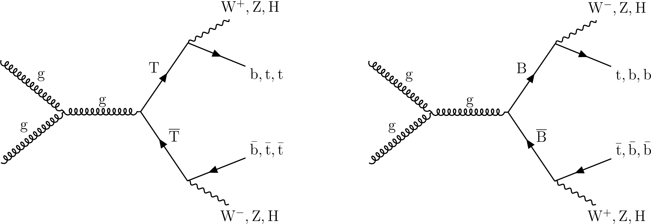
Figure 1:
Representative Feynman diagrams of the pair production of $ \mathrm{T} \overline{\mathrm{T}} $ (left) and $ \mathrm{B} \overline{\mathrm{B}} $ (right), with decays to third generation quarks and SM bosons. |
png pdf |
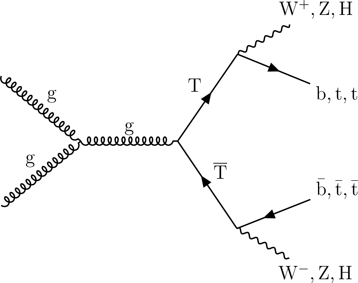
Figure 1-a:
Representative Feynman diagram of the pair production of $ \mathrm{T} \overline{\mathrm{T}} $, with decays to third generation quarks and SM bosons. |
png pdf |
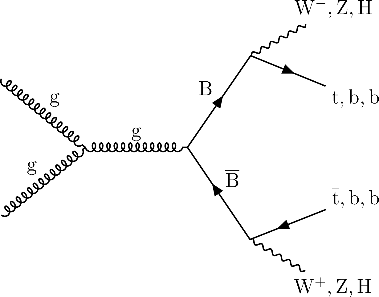
Figure 1-b:
Representative Feynman diagram of the pair production of $ \mathrm{B} \overline{\mathrm{B}} $, with decays to third generation quarks and SM bosons. |
png pdf |
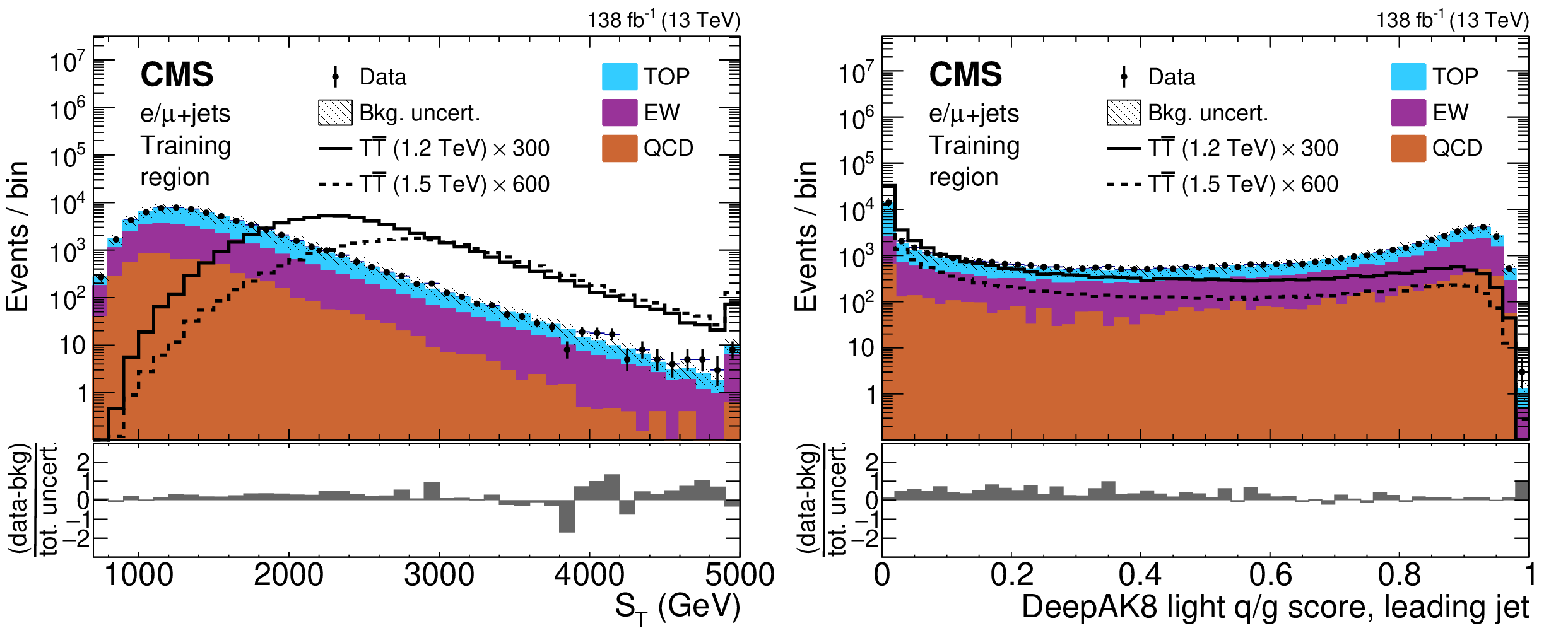
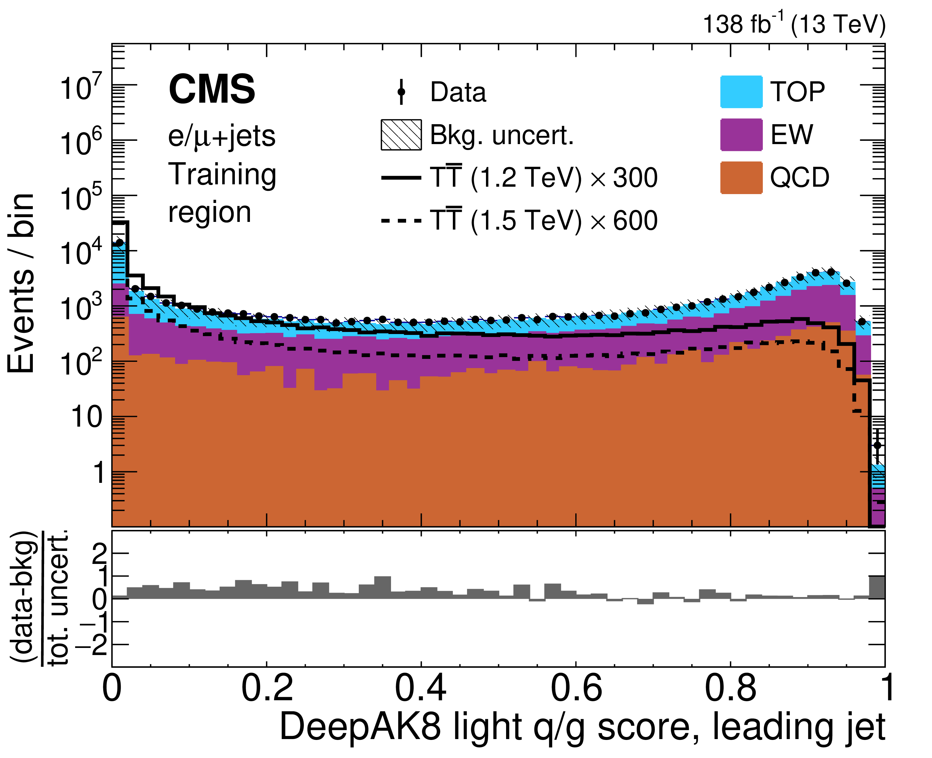
Figure 2:
Example single-lepton channel MLP input distributions of $ S_\mathrm{T} $ (left) and the leading jet's DEEPAK8 light quark or gluon score (right) in the training region for the $ \mathrm{T} \overline{\mathrm{T}} $ MLP. The observed data are shown using black markers, predicted $ \mathrm{T} \overline{\mathrm{T}} $ signal with mass of 1.2 (1.5) TeV in the singlet scenario using solid (dashed) lines, and backgrounds, using filled histograms. Statistical and systematic uncertainties in the background prediction before performing the fit to data are shown by the hatched region. The lower panels show the difference between the data and the background estimate as a multiple of the total uncertainty in both sources. The signal predictions have been scaled for visibility by the factors indicated in the figures. |

png pdf |
Figure 2-a:
Single-lepton channel MLP input distribution of $ S_\mathrm{T} $ in the training region for the $ \mathrm{T} \overline{\mathrm{T}} $ MLP. The observed data are shown using black markers, predicted $ \mathrm{T} \overline{\mathrm{T}} $ signal with mass of 1.2 (1.5) TeV in the singlet scenario using solid (dashed) lines, and backgrounds, using filled histograms. Statistical and systematic uncertainties in the background prediction before performing the fit to data are shown by the hatched region. The lower panel shows the difference between the data and the background estimate as a multiple of the total uncertainty in both sources. The signal predictions have been scaled for visibility by the factors indicated in the figures. |
png pdf |
Figure 2-b:
Single-lepton channel MLP input distribution of the leading jet's DEEPAK8 light quark or gluon score in the training region for the $ \mathrm{T} \overline{\mathrm{T}} $ MLP. The observed data are shown using black markers, predicted $ \mathrm{T} \overline{\mathrm{T}} $ signal with mass of 1.2 (1.5) TeV in the singlet scenario using solid (dashed) lines, and backgrounds, using filled histograms. Statistical and systematic uncertainties in the background prediction before performing the fit to data are shown by the hatched region. The lower panel shows the difference between the data and the background estimate as a multiple of the total uncertainty in both sources. The signal predictions have been scaled for visibility by the factors indicated in the figures. |
png pdf |
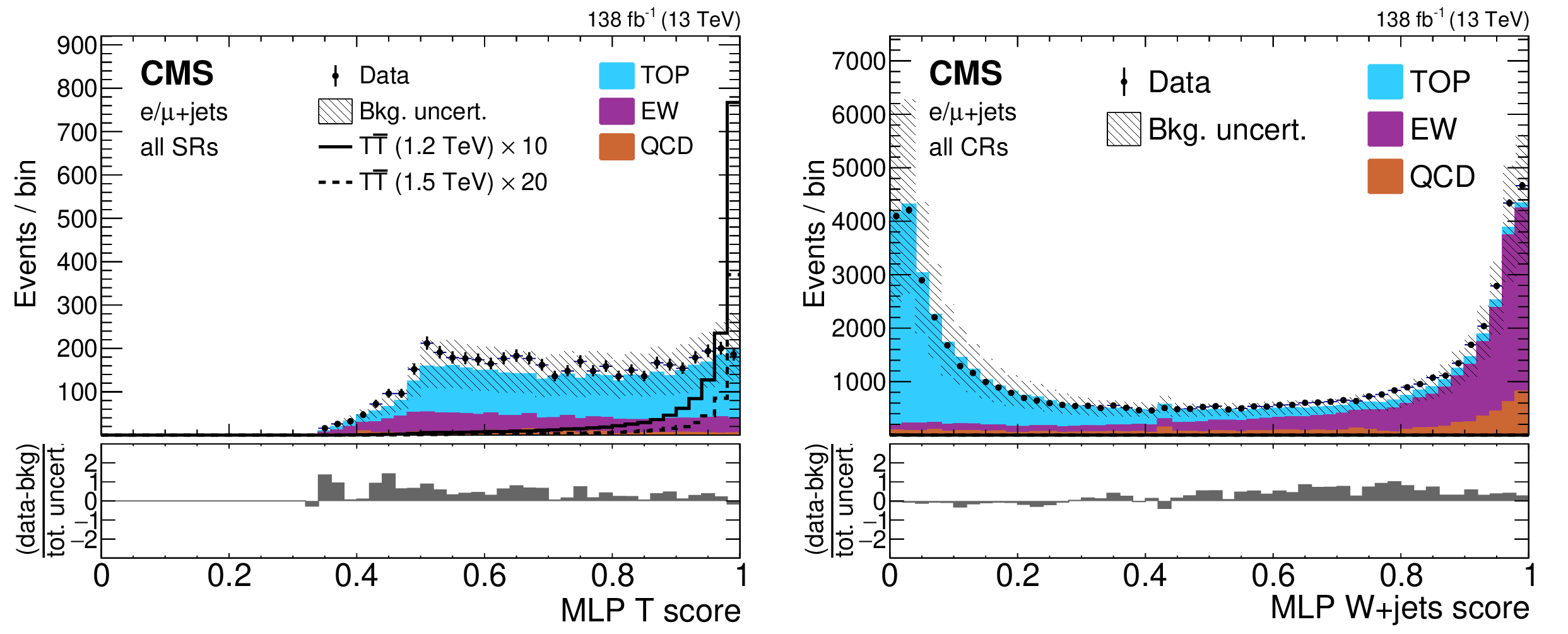
Figure 3:
Example single-lepton channel $ \mathrm{T} \overline{\mathrm{T}} $ MLP output distributions of the $ \mathrm{T} $ quark score in the inclusive SR (left) and the W +jets score in the CRs (right). The observed data are shown using black markers, predicted $ \mathrm{T} \overline{\mathrm{T}} $ signal with mass of 1.2 (1.5) TeV in the singlet scenario using solid (dashed) lines, and backgrounds, using filled histograms. Statistical and systematic uncertainties in the background estimate before performing the fit to data are shown by the hatched region. The lower panels show the difference between the data and the background estimate as a multiple of the total uncertainty in both sources. The signal predictions in the left distribution have been scaled for visibility by the factor indicated in the figure. |
png pdf |
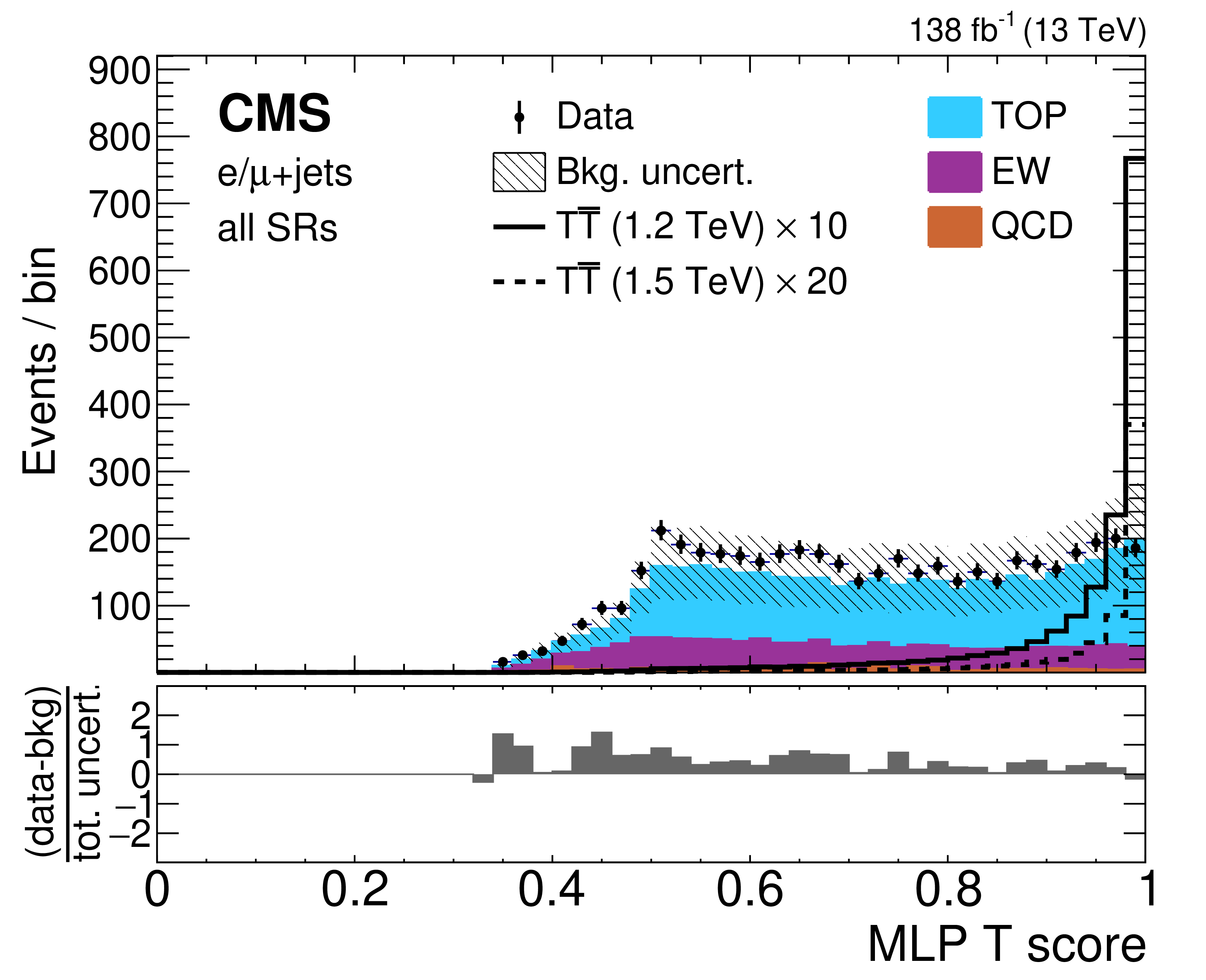
Figure 3-a:
Single-lepton channel $ \mathrm{T} \overline{\mathrm{T}} $ MLP output distribution of the $ \mathrm{T} $ quark score in the inclusive SR. The observed data are shown using black markers, predicted $ \mathrm{T} \overline{\mathrm{T}} $ signal with mass of 1.2 (1.5) TeV in the singlet scenario using solid (dashed) lines, and backgrounds, using filled histograms. Statistical and systematic uncertainties in the background estimate before performing the fit to data are shown by the hatched region. The lower panel shows the difference between the data and the background estimate as a multiple of the total uncertainty in both sources. The signal predictions in the left distribution have been scaled for visibility by the factor indicated in the figure. |
png pdf |
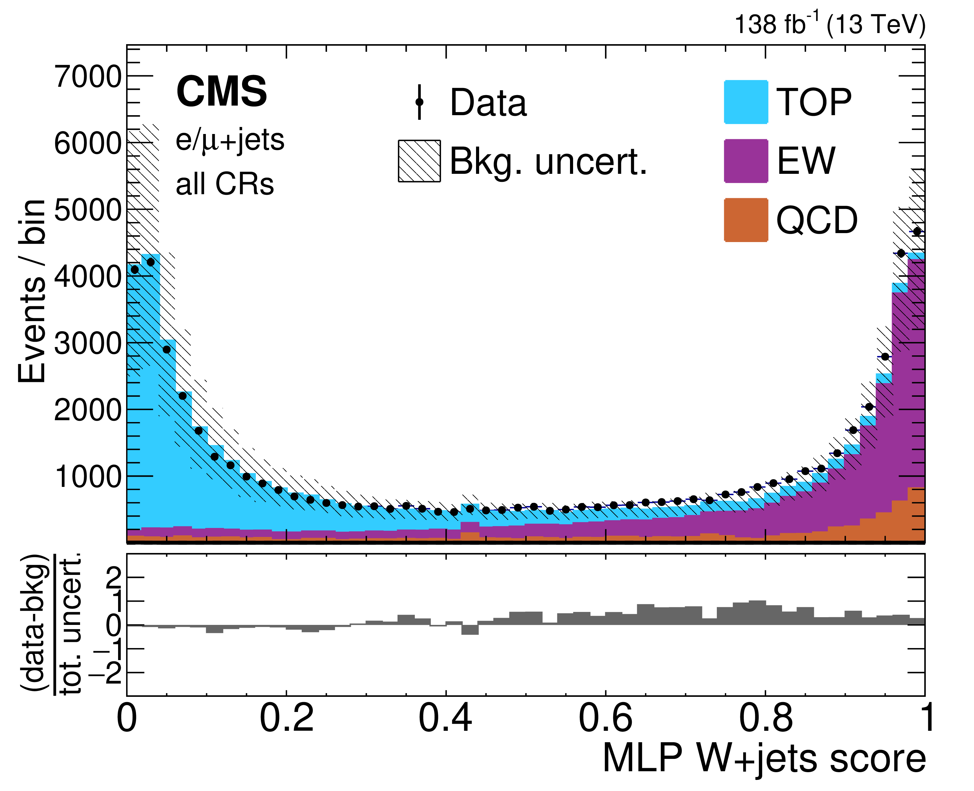
Figure 3-b:
Single-lepton channel $ \mathrm{T} \overline{\mathrm{T}} $ MLP output distribution of the W +jets score in the CRs. The observed data are shown using black markers, predicted $ \mathrm{T} \overline{\mathrm{T}} $ signal with mass of 1.2 (1.5) TeV in the singlet scenario using solid (dashed) lines, and backgrounds, using filled histograms. Statistical and systematic uncertainties in the background estimate before performing the fit to data are shown by the hatched region. The lower panel shows the difference between the data and the background estimate as a multiple of the total uncertainty in both sources. The signal predictions in the left distribution have been scaled for visibility by the factor indicated in the figure. |
png pdf |
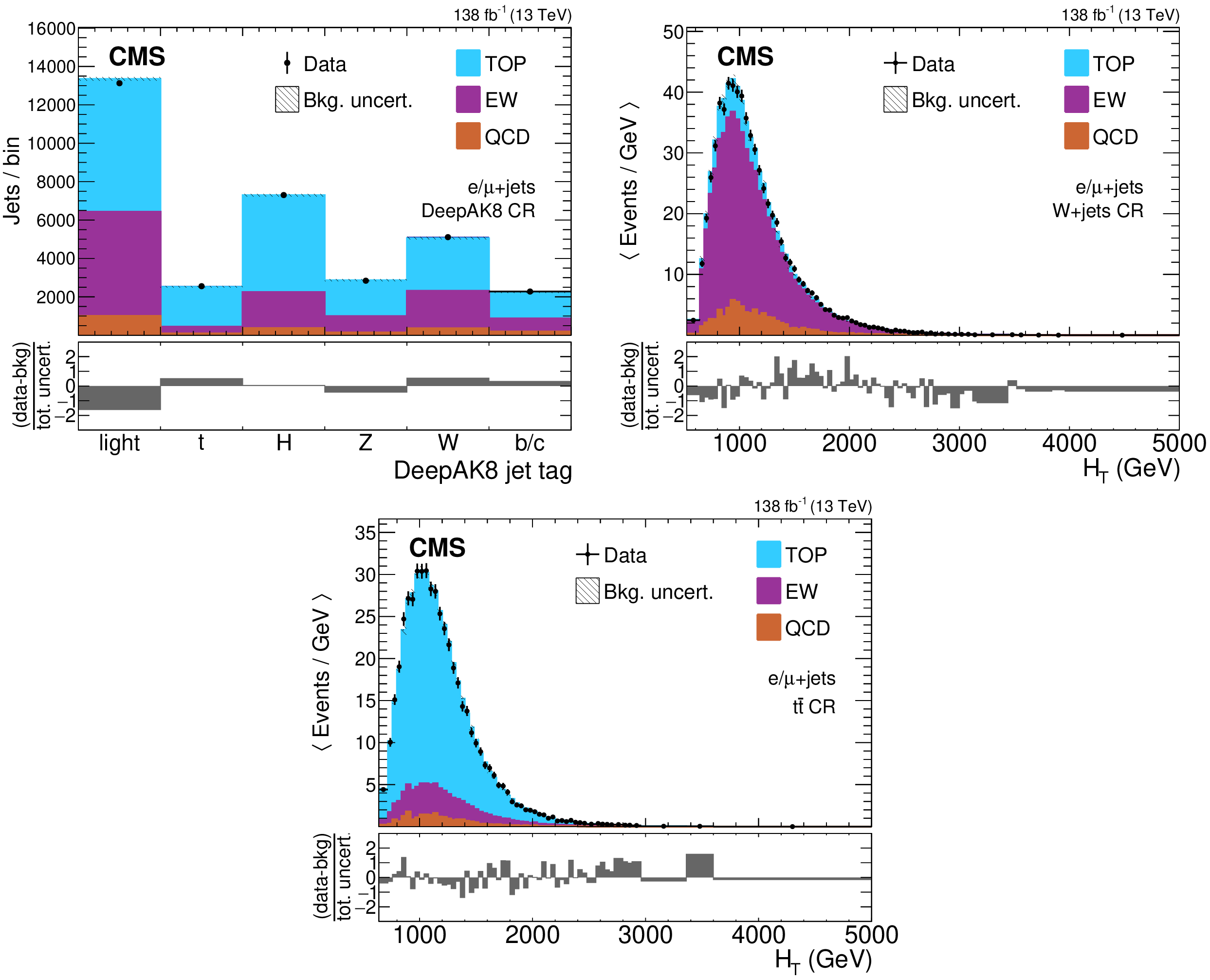
Figure 4:
Single-lepton channel template histograms of the DEEPAK8 jet tags in the DEEPAK8 CR (upper left), and $ H_{\mathrm{T}} $ in the W +jets (upper right) and $ \mathrm{t}\overline{\mathrm{t}} $ (lower) CRs for the $ \mathrm{T} \overline{\mathrm{T}} $ search. The observed data are shown using black markers and the post-fit background estimates, using filled histograms. Statistical and systematic uncertainties in the background estimate after performing the fit to data are shown by the hatched region. The lower panels show the difference between the data and the background estimate as a multiple of the total uncertainty in both sources. Electron and muon categories have been combined for illustration with their uncertainties added in quadrature. |
png pdf |
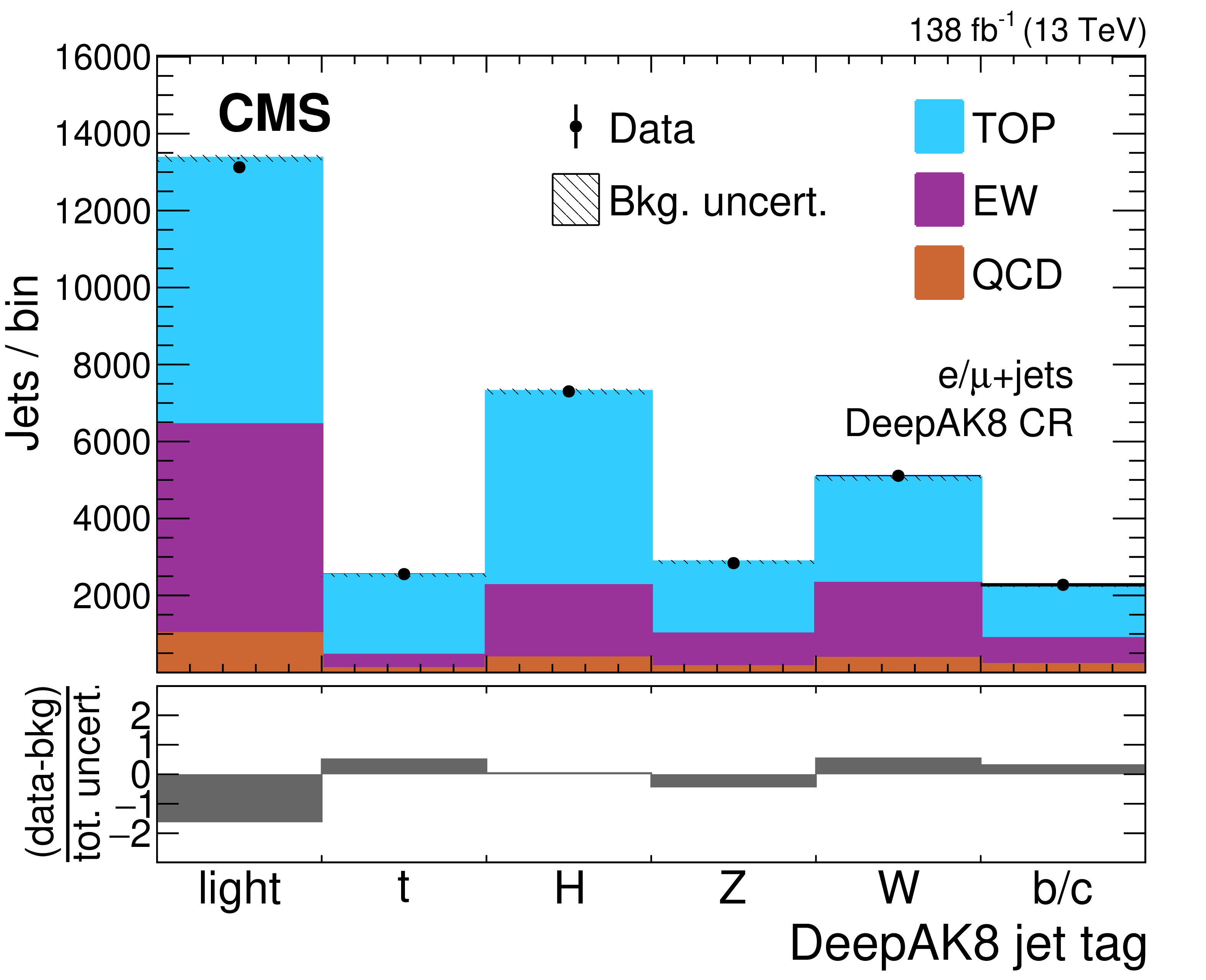
Figure 4-a:
Single-lepton channel template histogram of the DEEPAK8 jet tags in the DEEPAK8 CR for the $ \mathrm{T} \overline{\mathrm{T}} $ search. The observed data are shown using black markers and the post-fit background estimates, using filled histograms. Statistical and systematic uncertainties in the background estimate after performing the fit to data are shown by the hatched region. The lower panel shows the difference between the data and the background estimate as a multiple of the total uncertainty in both sources. Electron and muon categories have been combined for illustration with their uncertainties added in quadrature. |
png pdf |
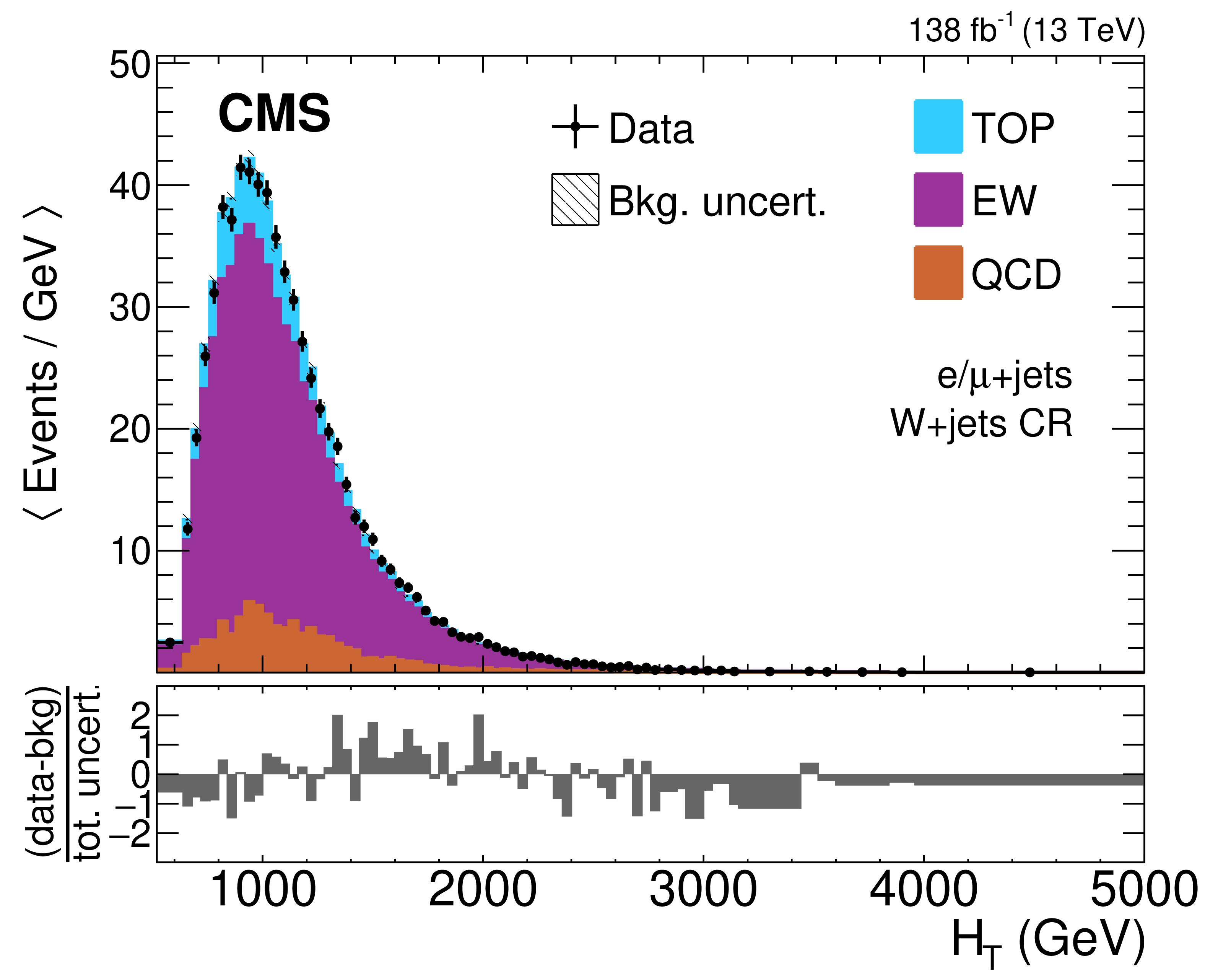
Figure 4-b:
Single-lepton channel template histogram of $ H_{\mathrm{T}} $ in the W +jets CR for the $ \mathrm{T} \overline{\mathrm{T}} $ search. The observed data are shown using black markers and the post-fit background estimates, using filled histograms. Statistical and systematic uncertainties in the background estimate after performing the fit to data are shown by the hatched region. The lower panel shows the difference between the data and the background estimate as a multiple of the total uncertainty in both sources. Electron and muon categories have been combined for illustration with their uncertainties added in quadrature. |
png pdf |
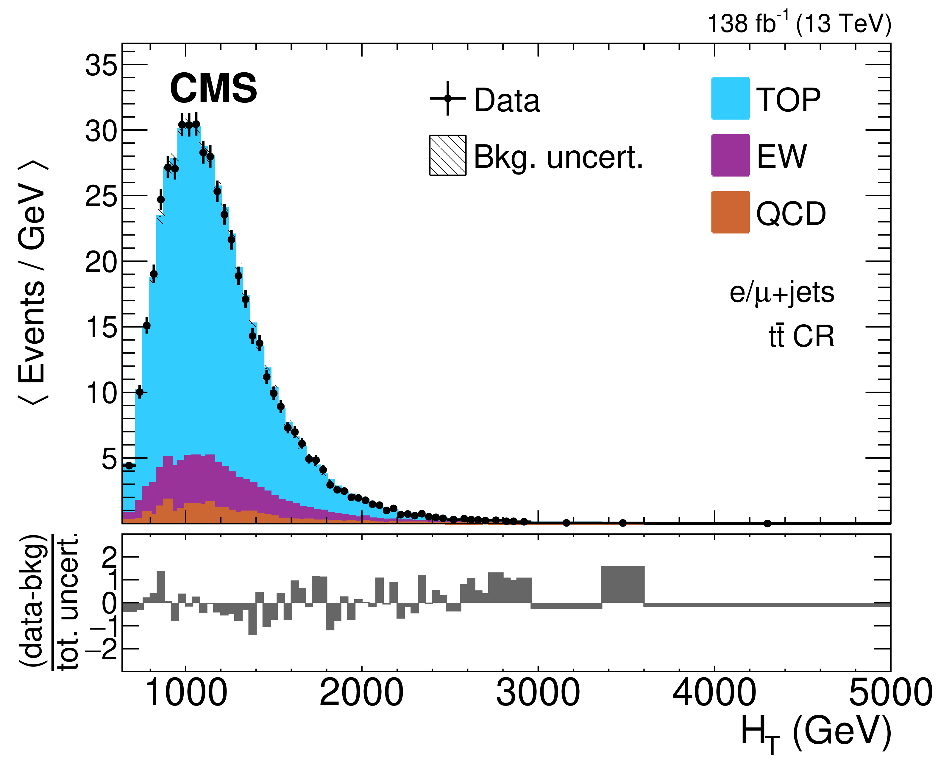
Figure 4-c:
Single-lepton channel template histogram of $ H_{\mathrm{T}} $ in the $ \mathrm{t}\overline{\mathrm{t}} $ CR for the $ \mathrm{T} \overline{\mathrm{T}} $ search. The observed data are shown using black markers and the post-fit background estimates, using filled histograms. Statistical and systematic uncertainties in the background estimate after performing the fit to data are shown by the hatched region. The lower panel shows the difference between the data and the background estimate as a multiple of the total uncertainty in both sources. Electron and muon categories have been combined for illustration with their uncertainties added in quadrature. |
png pdf |
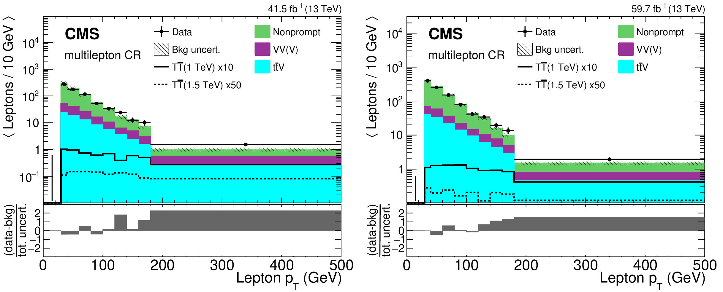
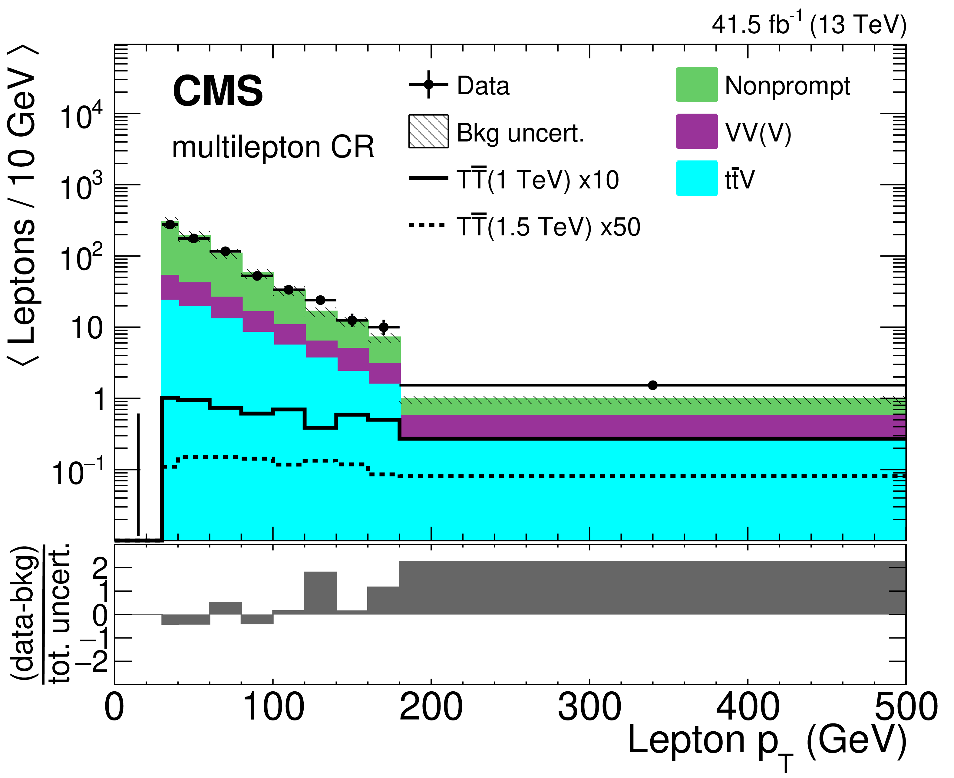
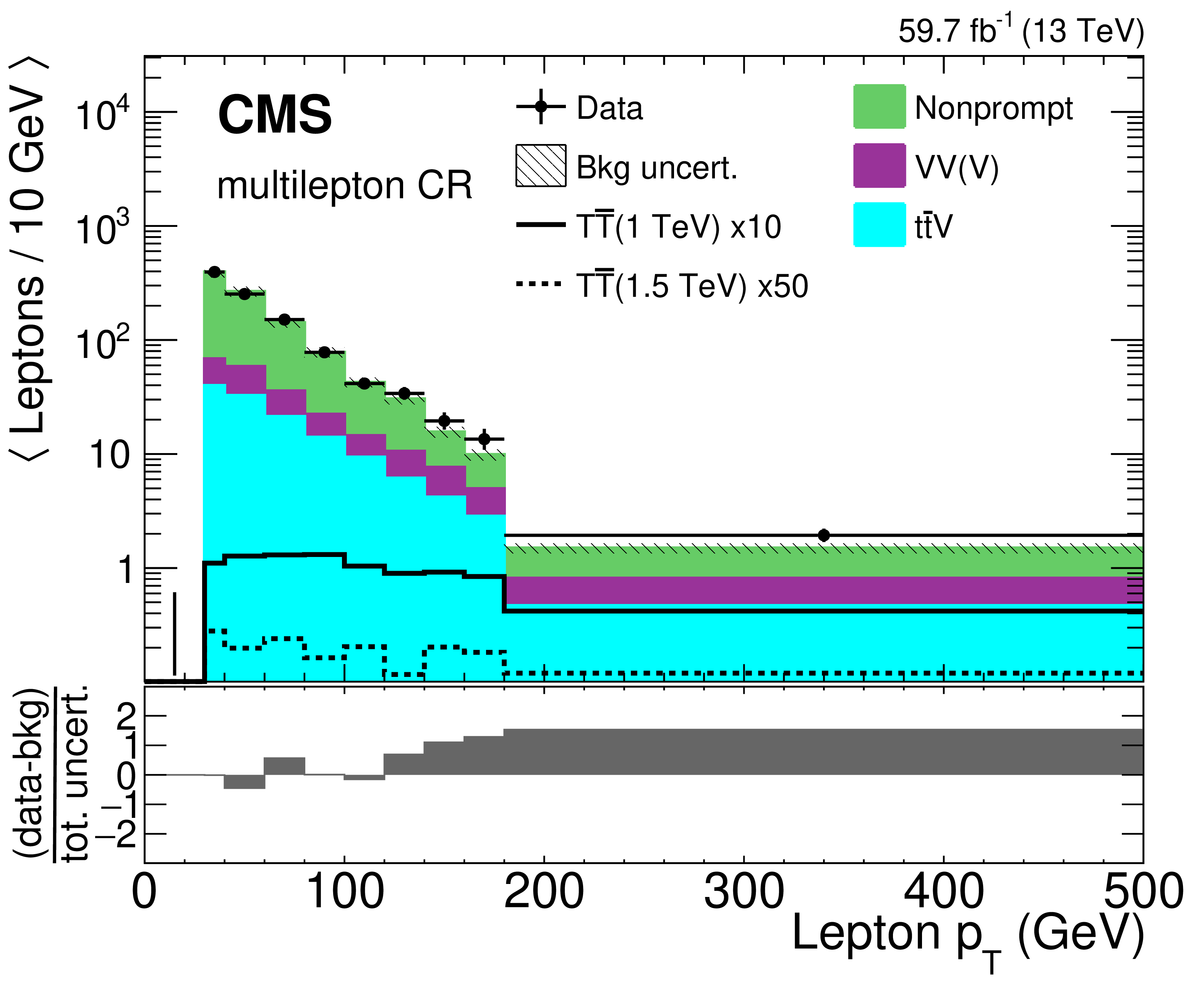
Figure 5:
Distribution of lepton $ p_{\mathrm{T}} $ in 2017 (left) and 2018 (right) in the multilepton channel nonprompt lepton CR for all flavor categories, evaluated with the best fit nonprompt rates. The $ p_{\mathrm{T}} $ values of the three leptons in each event are included in the histogram. The uncertainty shown is the quadratic sum of the statistical and systematic components. The lower panel shows the difference between the data and the background estimate as a multiple of the total uncertainty in both sources. The signal predictions have been scaled for visibility by the factors indicated in the figures. |
png pdf |
Figure 5-a:
Distribution of lepton $ p_{\mathrm{T}} $ in 2017 in the multilepton channel nonprompt lepton CR for all flavor categories, evaluated with the best fit nonprompt rates. The $ p_{\mathrm{T}} $ values of the three leptons in each event are included in the histogram. The uncertainty shown is the quadratic sum of the statistical and systematic components. The lower panel shows the difference between the data and the background estimate as a multiple of the total uncertainty in both sources. The signal predictions have been scaled for visibility by the factors indicated in the figures. |
png pdf |
Figure 5-b:
Distribution of lepton $ p_{\mathrm{T}} $ in 2018 in the multilepton channel nonprompt lepton CR for all flavor categories, evaluated with the best fit nonprompt rates. The $ p_{\mathrm{T}} $ values of the three leptons in each event are included in the histogram. The uncertainty shown is the quadratic sum of the statistical and systematic components. The lower panel shows the difference between the data and the background estimate as a multiple of the total uncertainty in both sources. The signal predictions have been scaled for visibility by the factors indicated in the figures. |
png pdf |
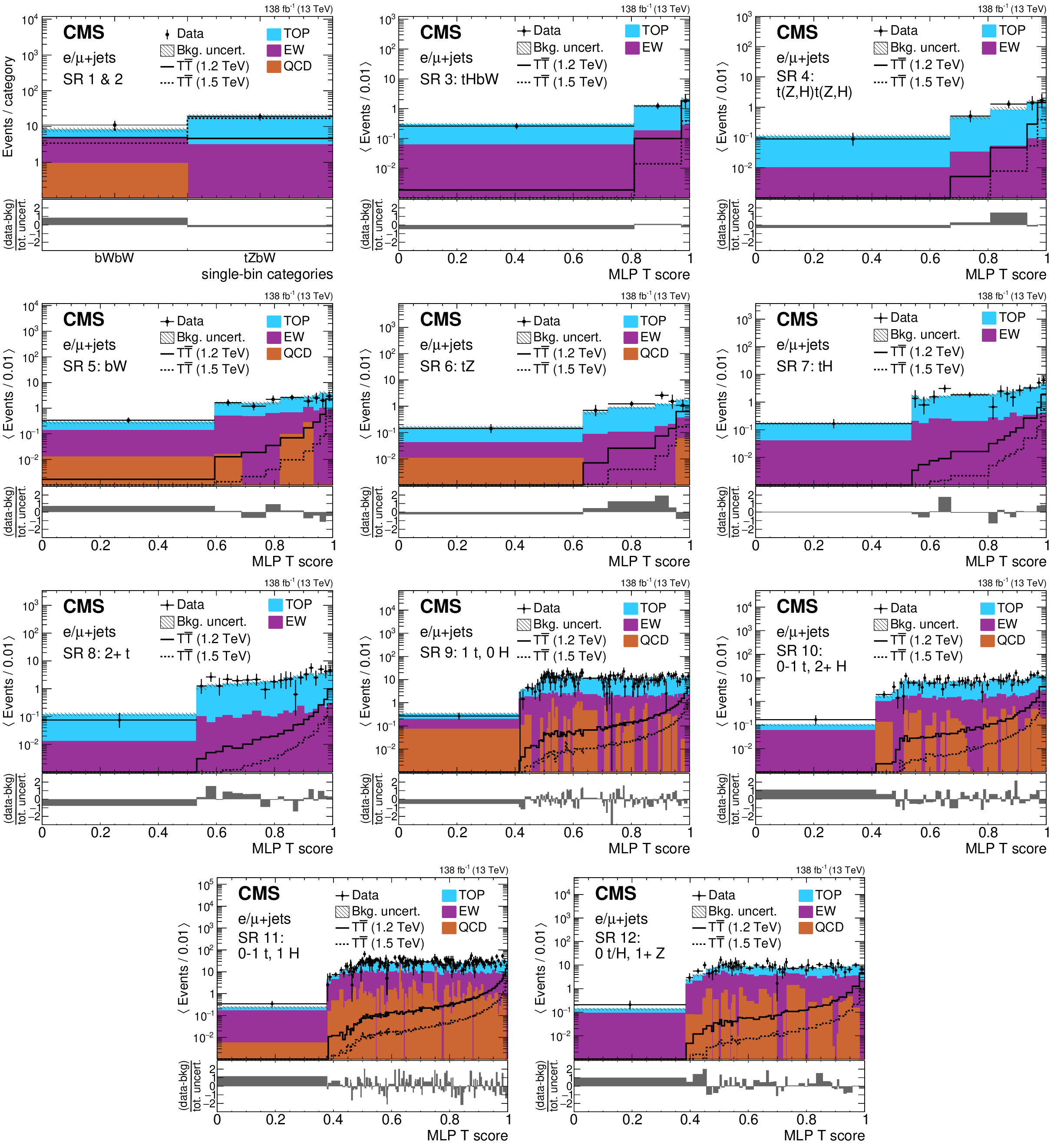
Figure 6:
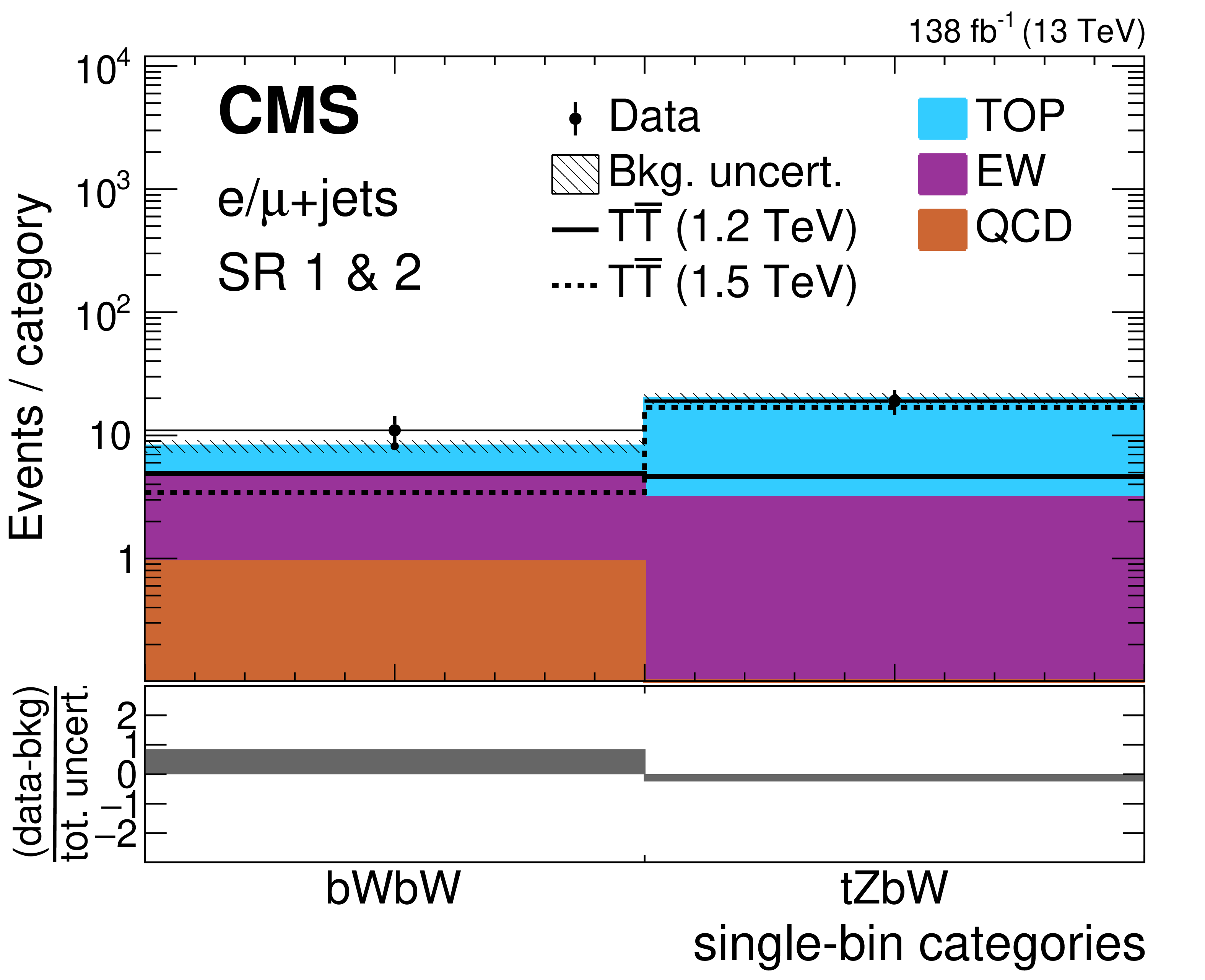
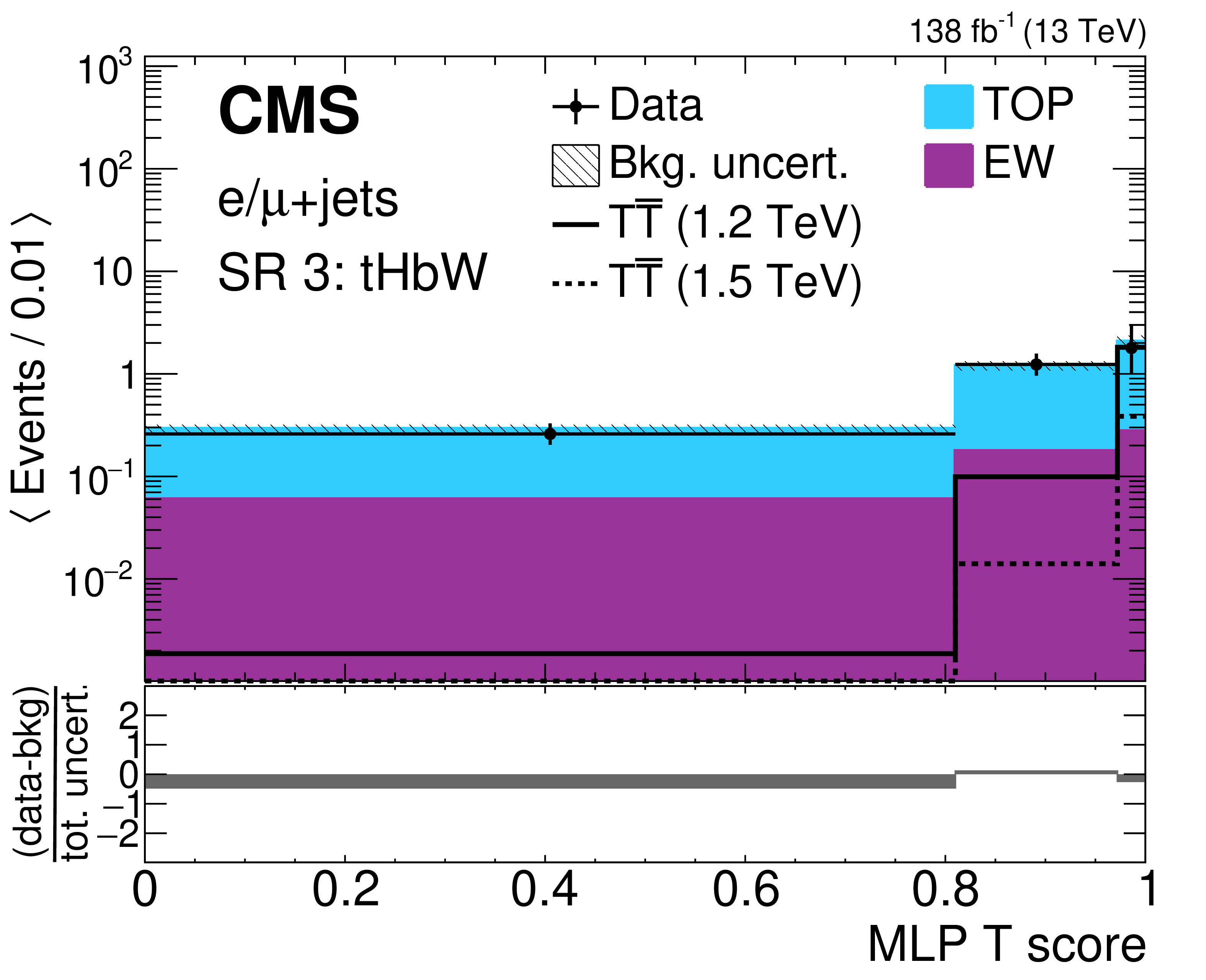
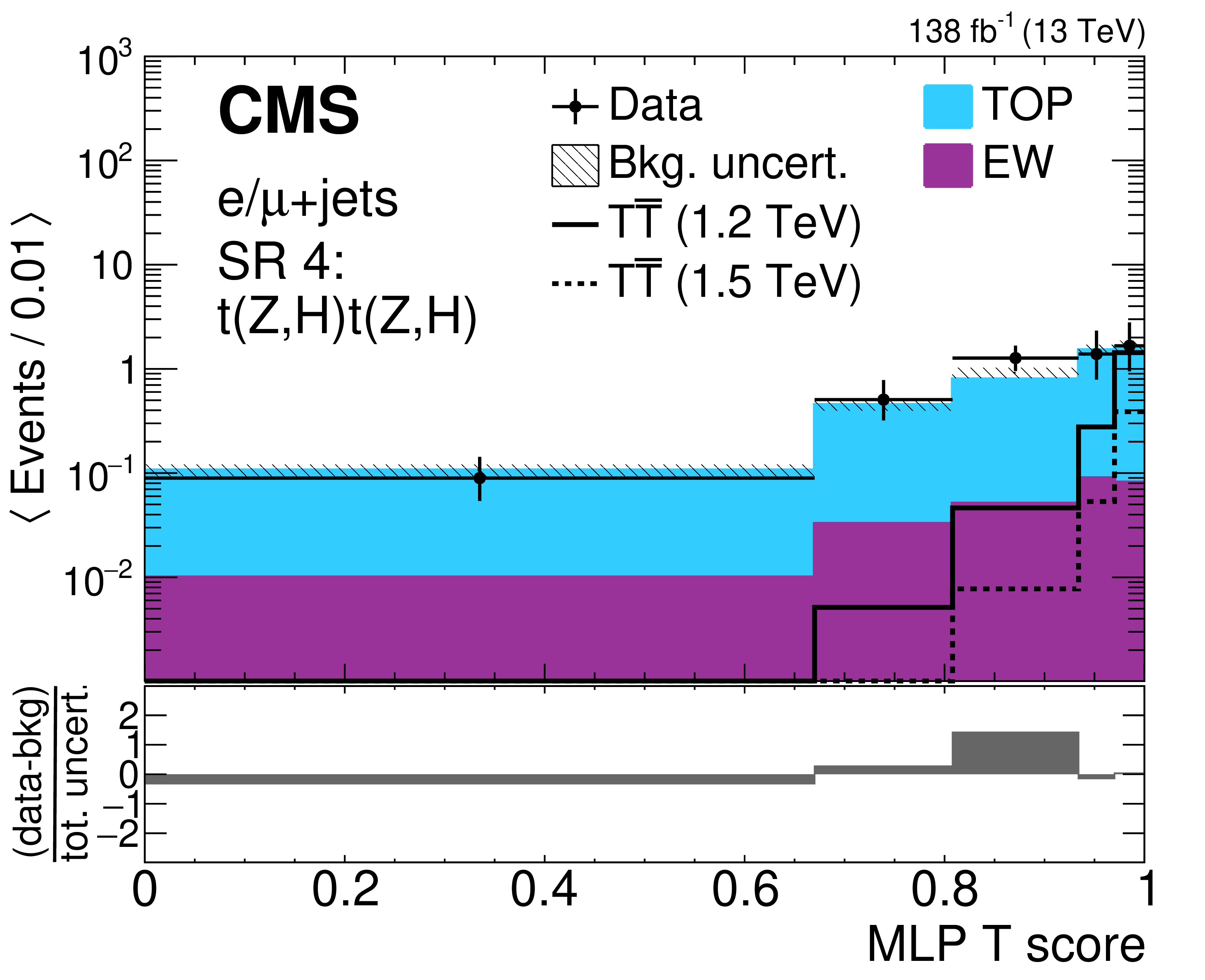
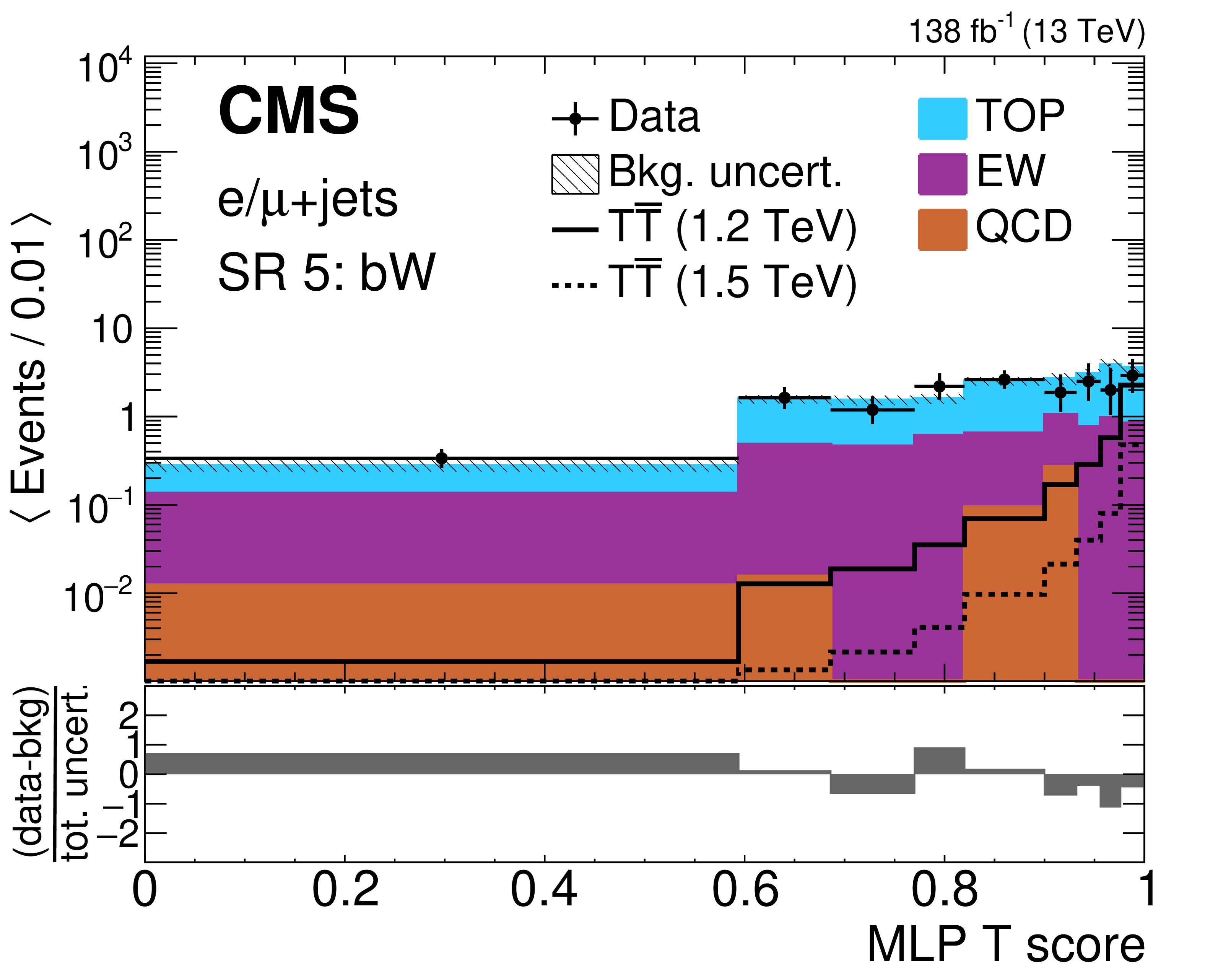
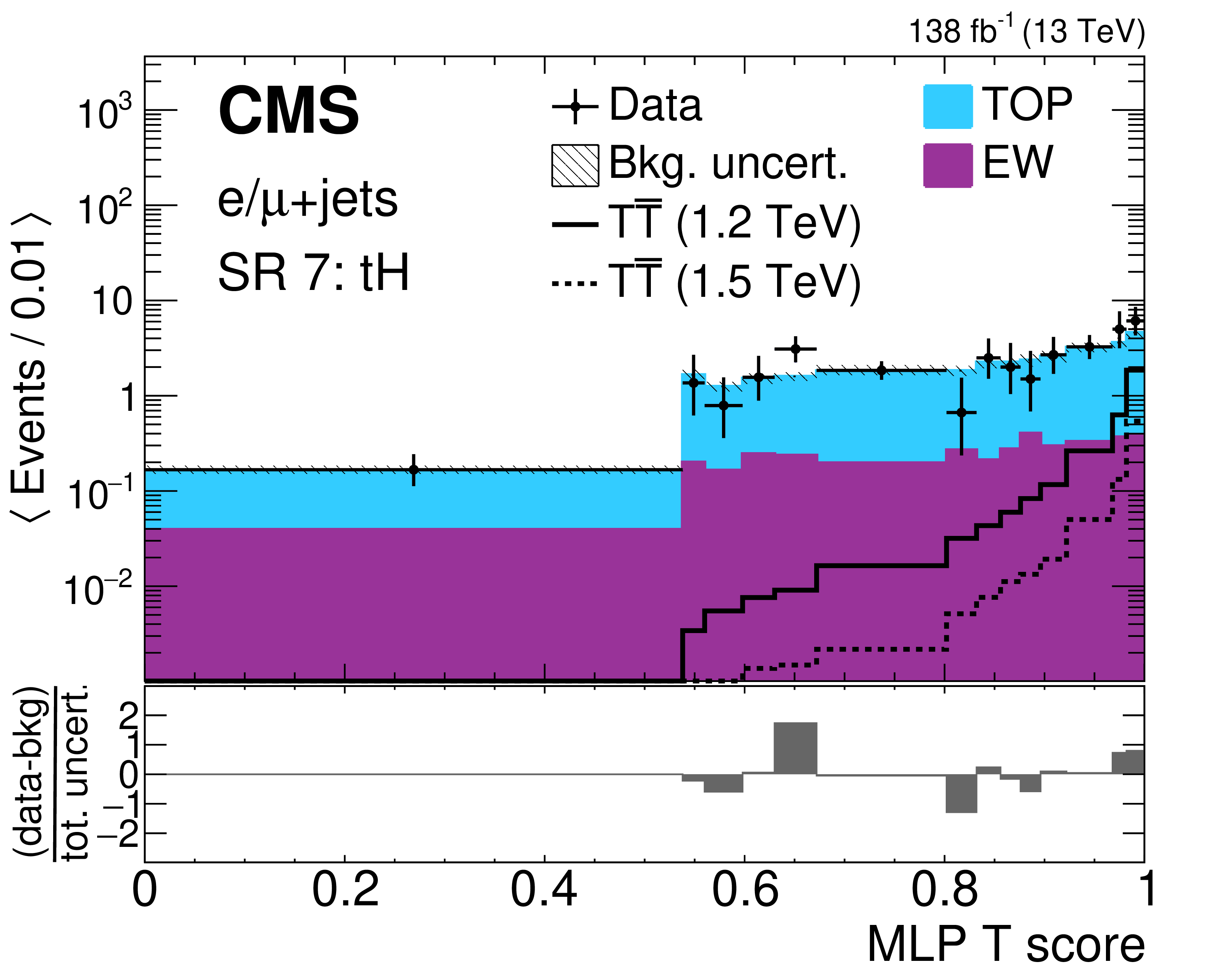
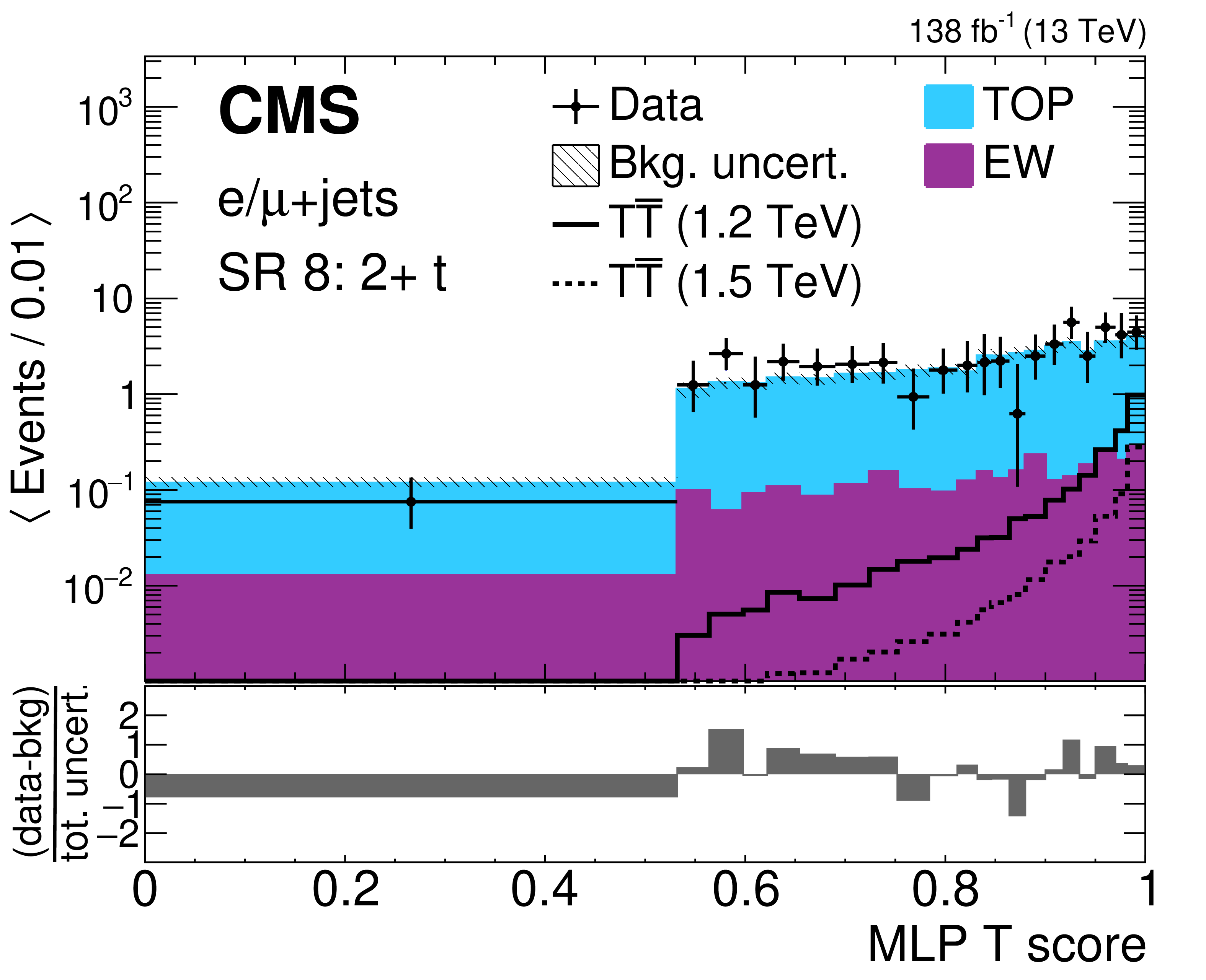
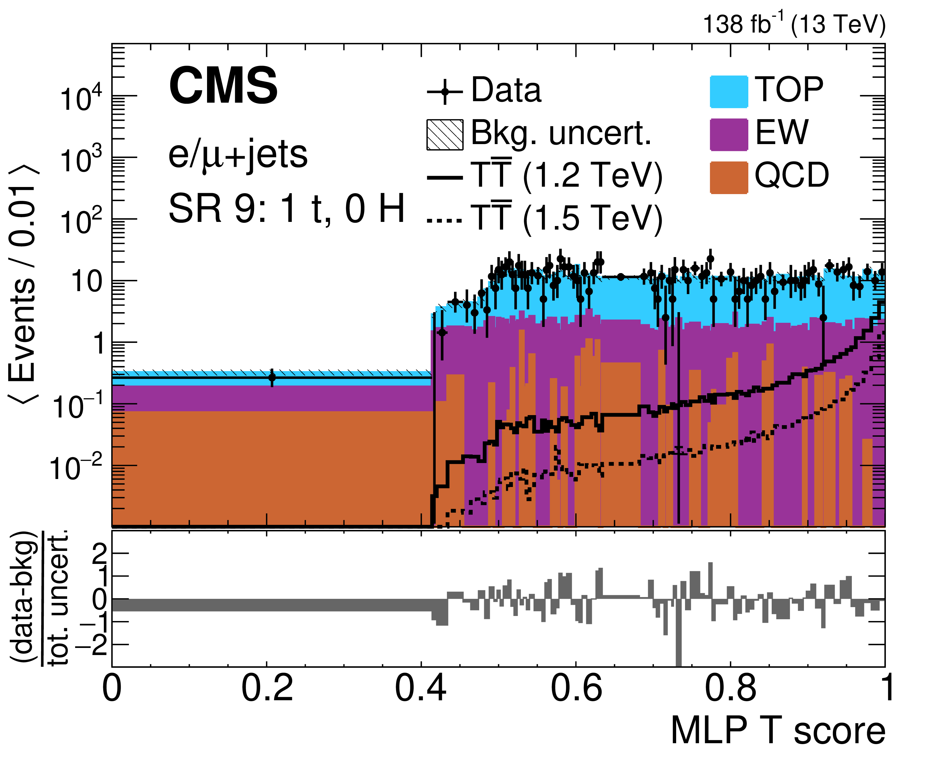
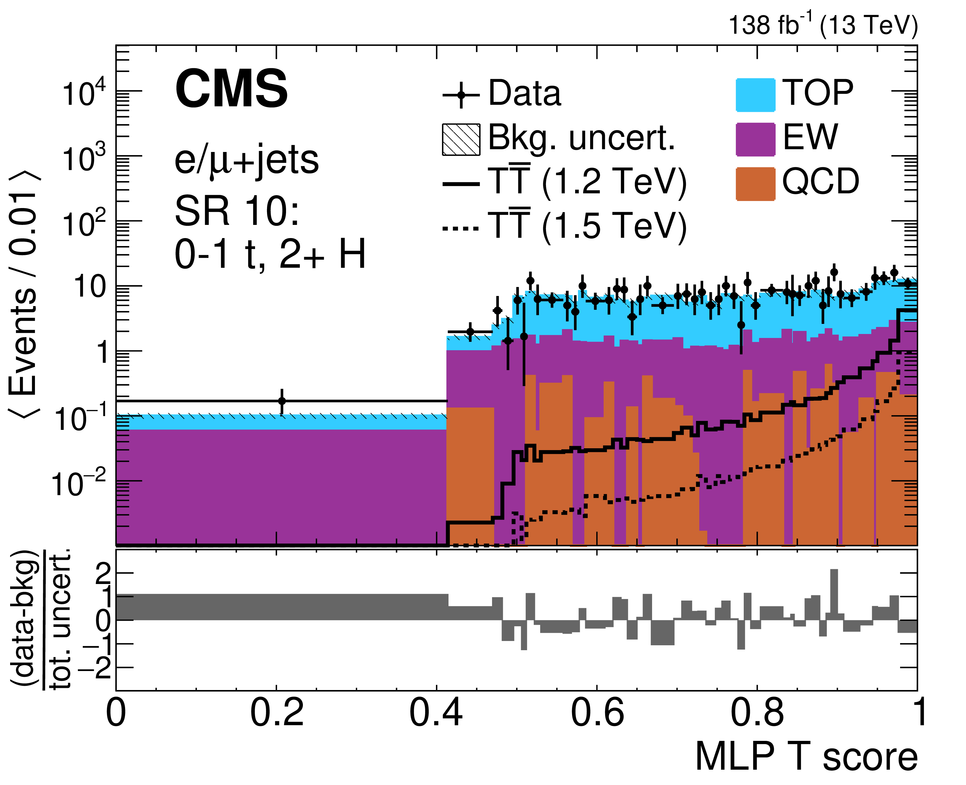
Template histograms of the VLQ score in single-lepton SRs 1 and 2 combined, and SRs 3-12 (left-to-right, upper-to-lower). The observed data are shown using black markers, the predicted $ \mathrm{T} \overline{\mathrm{T}} $ signal for a mass of 1.2 (1.5) TeV in the singlet scenario using solid (dashed) lines, and the post-fit background estimates, using filled histograms. Statistical and systematic uncertainties in the background estimate after performing the fit to data are shown by the hatched region. The lower panels show the difference between the data and the background estimate as a multiple of the total uncertainty in both sources. Electron and muon categories have been combined for illustration with their uncertainties added in quadrature. |
png pdf |
Figure 6-a:
Template histograms of the VLQ score in single-lepton SRs 1 and 2 combined. The observed data are shown using black markers, the predicted $ \mathrm{T} \overline{\mathrm{T}} $ signal for a mass of 1.2 (1.5) TeV in the singlet scenario using solid (dashed) lines, and the post-fit background estimates, using filled histograms. Statistical and systematic uncertainties in the background estimate after performing the fit to data are shown by the hatched region. The lower panels show the difference between the data and the background estimate as a multiple of the total uncertainty in both sources. Electron and muon categories have been combined for illustration with their uncertainties added in quadrature. |
png pdf |
Figure 6-b:
Template histograms of the VLQ score in single-lepton SR 3. The observed data are shown using black markers, the predicted $ \mathrm{T} \overline{\mathrm{T}} $ signal for a mass of 1.2 (1.5) TeV in the singlet scenario using solid (dashed) lines, and the post-fit background estimates, using filled histograms. Statistical and systematic uncertainties in the background estimate after performing the fit to data are shown by the hatched region. The lower panels show the difference between the data and the background estimate as a multiple of the total uncertainty in both sources. Electron and muon categories have been combined for illustration with their uncertainties added in quadrature. |
png pdf |
Figure 6-c:
Template histograms of the VLQ score in single-lepton SR 4. The observed data are shown using black markers, the predicted $ \mathrm{T} \overline{\mathrm{T}} $ signal for a mass of 1.2 (1.5) TeV in the singlet scenario using solid (dashed) lines, and the post-fit background estimates, using filled histograms. Statistical and systematic uncertainties in the background estimate after performing the fit to data are shown by the hatched region. The lower panels show the difference between the data and the background estimate as a multiple of the total uncertainty in both sources. Electron and muon categories have been combined for illustration with their uncertainties added in quadrature. |
png pdf |
Figure 6-d:
Template histograms of the VLQ score in single-lepton SR 5. The observed data are shown using black markers, the predicted $ \mathrm{T} \overline{\mathrm{T}} $ signal for a mass of 1.2 (1.5) TeV in the singlet scenario using solid (dashed) lines, and the post-fit background estimates, using filled histograms. Statistical and systematic uncertainties in the background estimate after performing the fit to data are shown by the hatched region. The lower panels show the difference between the data and the background estimate as a multiple of the total uncertainty in both sources. Electron and muon categories have been combined for illustration with their uncertainties added in quadrature. |

png pdf |
Figure 6-e:
Template histograms of the VLQ score in single-lepton SR 6. The observed data are shown using black markers, the predicted $ \mathrm{T} \overline{\mathrm{T}} $ signal for a mass of 1.2 (1.5) TeV in the singlet scenario using solid (dashed) lines, and the post-fit background estimates, using filled histograms. Statistical and systematic uncertainties in the background estimate after performing the fit to data are shown by the hatched region. The lower panels show the difference between the data and the background estimate as a multiple of the total uncertainty in both sources. Electron and muon categories have been combined for illustration with their uncertainties added in quadrature. |
png pdf |
Figure 6-f:
Template histograms of the VLQ score in single-lepton SR 7. The observed data are shown using black markers, the predicted $ \mathrm{T} \overline{\mathrm{T}} $ signal for a mass of 1.2 (1.5) TeV in the singlet scenario using solid (dashed) lines, and the post-fit background estimates, using filled histograms. Statistical and systematic uncertainties in the background estimate after performing the fit to data are shown by the hatched region. The lower panels show the difference between the data and the background estimate as a multiple of the total uncertainty in both sources. Electron and muon categories have been combined for illustration with their uncertainties added in quadrature. |
png pdf |
Figure 6-g:
Template histograms of the VLQ score in single-lepton SR 8. The observed data are shown using black markers, the predicted $ \mathrm{T} \overline{\mathrm{T}} $ signal for a mass of 1.2 (1.5) TeV in the singlet scenario using solid (dashed) lines, and the post-fit background estimates, using filled histograms. Statistical and systematic uncertainties in the background estimate after performing the fit to data are shown by the hatched region. The lower panels show the difference between the data and the background estimate as a multiple of the total uncertainty in both sources. Electron and muon categories have been combined for illustration with their uncertainties added in quadrature. |
png pdf |
Figure 6-h:
Template histograms of the VLQ score in single-lepton SR 9. The observed data are shown using black markers, the predicted $ \mathrm{T} \overline{\mathrm{T}} $ signal for a mass of 1.2 (1.5) TeV in the singlet scenario using solid (dashed) lines, and the post-fit background estimates, using filled histograms. Statistical and systematic uncertainties in the background estimate after performing the fit to data are shown by the hatched region. The lower panels show the difference between the data and the background estimate as a multiple of the total uncertainty in both sources. Electron and muon categories have been combined for illustration with their uncertainties added in quadrature. |
png pdf |
Figure 6-i:
Template histograms of the VLQ score in single-lepton SR 10. The observed data are shown using black markers, the predicted $ \mathrm{T} \overline{\mathrm{T}} $ signal for a mass of 1.2 (1.5) TeV in the singlet scenario using solid (dashed) lines, and the post-fit background estimates, using filled histograms. Statistical and systematic uncertainties in the background estimate after performing the fit to data are shown by the hatched region. The lower panels show the difference between the data and the background estimate as a multiple of the total uncertainty in both sources. Electron and muon categories have been combined for illustration with their uncertainties added in quadrature. |

png pdf |
Figure 6-j:
Template histograms of the VLQ score in single-lepton SR 11. The observed data are shown using black markers, the predicted $ \mathrm{T} \overline{\mathrm{T}} $ signal for a mass of 1.2 (1.5) TeV in the singlet scenario using solid (dashed) lines, and the post-fit background estimates, using filled histograms. Statistical and systematic uncertainties in the background estimate after performing the fit to data are shown by the hatched region. The lower panels show the difference between the data and the background estimate as a multiple of the total uncertainty in both sources. Electron and muon categories have been combined for illustration with their uncertainties added in quadrature. |

png pdf |
Figure 6-k:
Template histograms of the VLQ score in single-lepton SR 12. The observed data are shown using black markers, the predicted $ \mathrm{T} \overline{\mathrm{T}} $ signal for a mass of 1.2 (1.5) TeV in the singlet scenario using solid (dashed) lines, and the post-fit background estimates, using filled histograms. Statistical and systematic uncertainties in the background estimate after performing the fit to data are shown by the hatched region. The lower panels show the difference between the data and the background estimate as a multiple of the total uncertainty in both sources. Electron and muon categories have been combined for illustration with their uncertainties added in quadrature. |
png pdf |
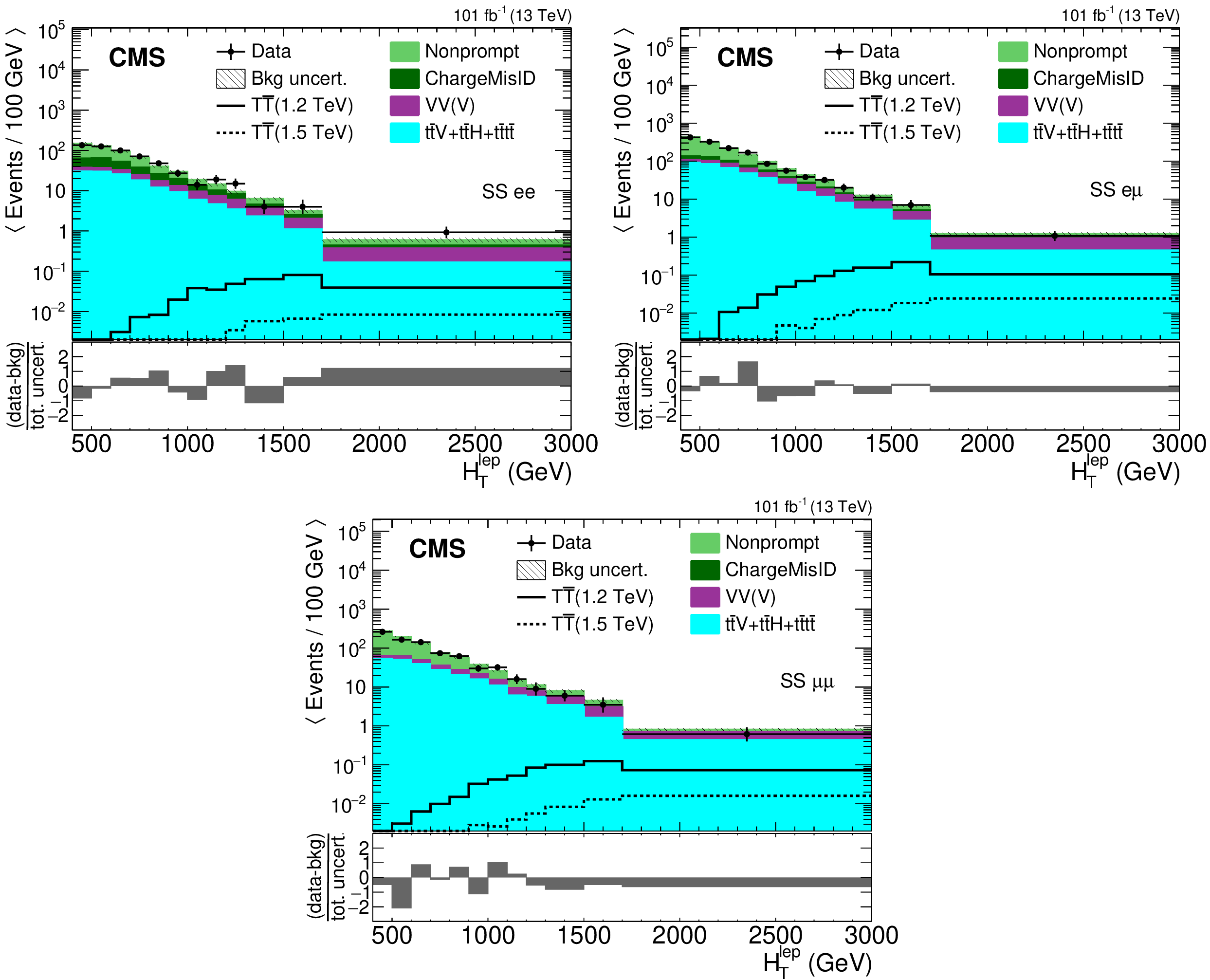
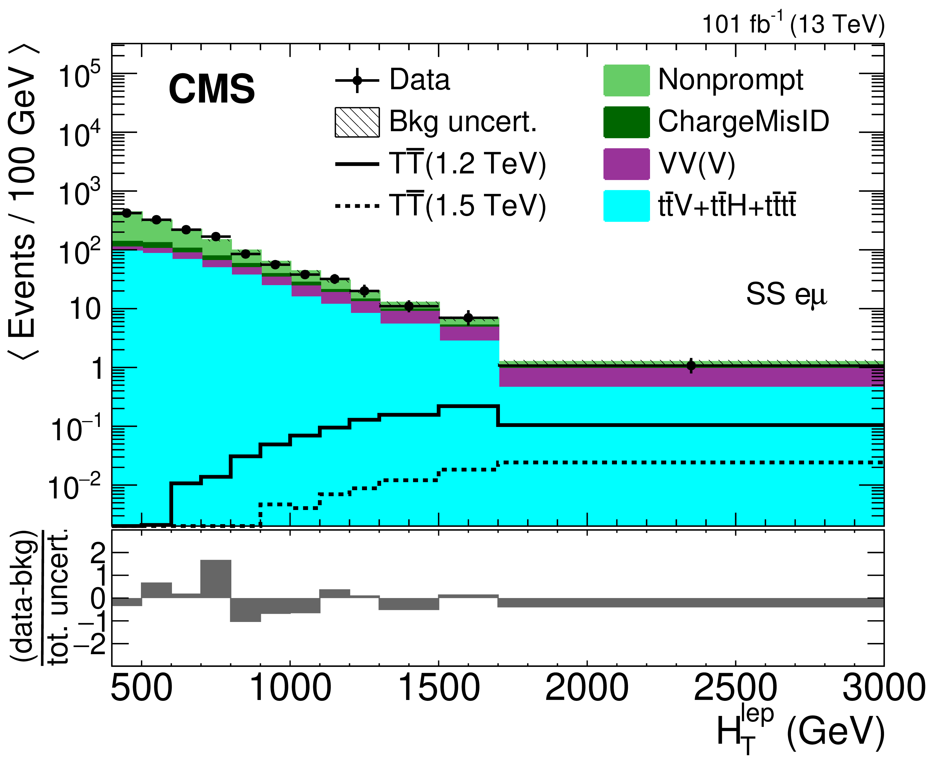
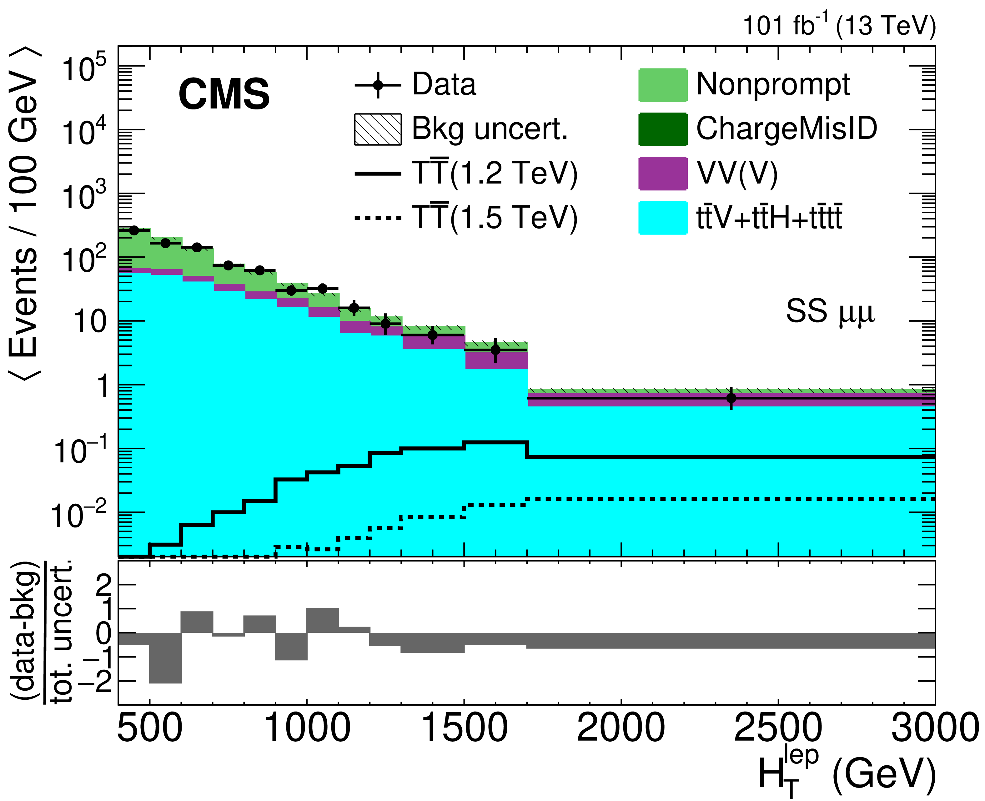
Figure 7:
Template histograms of $ H_{\mathrm{T}} ^{\mathrm{lep}} $ in the same-sign dilepton signal region for $ \mathrm{e} \mathrm{e} $ (upper left), $ \mathrm{e} \mu $ (upper right), and $ \mu \mu $ categories (lower). The observed data from 2017-2018 (combined for illustration) are shown using black markers, the predicted $ \mathrm{T} \overline{\mathrm{T}} $ signal for a mass of 1.2 (1.5) TeV in the singlet scenario using solid (dashed) lines, and the post-fit background estimates, using filled histograms. Statistical and systematic uncertainties in the background estimate after performing the fit to data are shown by the hatched region. The lower panels show the difference between the data and the background estimate as a multiple of the total uncertainty in both sources. |

png pdf |
Figure 7-a:
Template histogram of $ H_{\mathrm{T}} ^{\mathrm{lep}} $ in the same-sign dilepton signal region for $ \mathrm{e} \mathrm{e} $ category. The observed data from 2017-2018 (combined for illustration) are shown using black markers, the predicted $ \mathrm{T} \overline{\mathrm{T}} $ signal for a mass of 1.2 (1.5) TeV in the singlet scenario using solid (dashed) lines, and the post-fit background estimates, using filled histograms. Statistical and systematic uncertainties in the background estimate after performing the fit to data are shown by the hatched region. The lower panel shows the difference between the data and the background estimate as a multiple of the total uncertainty in both sources. |
png pdf |
Figure 7-b:
Template histogram of $ H_{\mathrm{T}} ^{\mathrm{lep}} $ in the same-sign dilepton signal region for $ \mathrm{e} \mu $ category. The observed data from 2017-2018 (combined for illustration) are shown using black markers, the predicted $ \mathrm{T} \overline{\mathrm{T}} $ signal for a mass of 1.2 (1.5) TeV in the singlet scenario using solid (dashed) lines, and the post-fit background estimates, using filled histograms. Statistical and systematic uncertainties in the background estimate after performing the fit to data are shown by the hatched region. The lower panel shows the difference between the data and the background estimate as a multiple of the total uncertainty in both sources. |
png pdf |
Figure 7-c:
Template histogram of $ H_{\mathrm{T}} ^{\mathrm{lep}} $ in the same-sign dilepton signal region for $ \mu \mu $ category. The observed data from 2017-2018 (combined for illustration) are shown using black markers, the predicted $ \mathrm{T} \overline{\mathrm{T}} $ signal for a mass of 1.2 (1.5) TeV in the singlet scenario using solid (dashed) lines, and the post-fit background estimates, using filled histograms. Statistical and systematic uncertainties in the background estimate after performing the fit to data are shown by the hatched region. The lower panel shows the difference between the data and the background estimate as a multiple of the total uncertainty in both sources. |
png pdf |
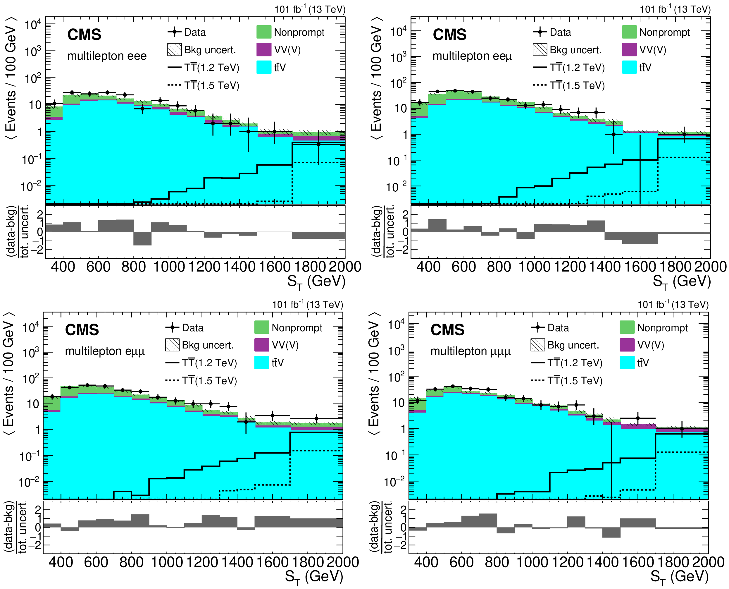
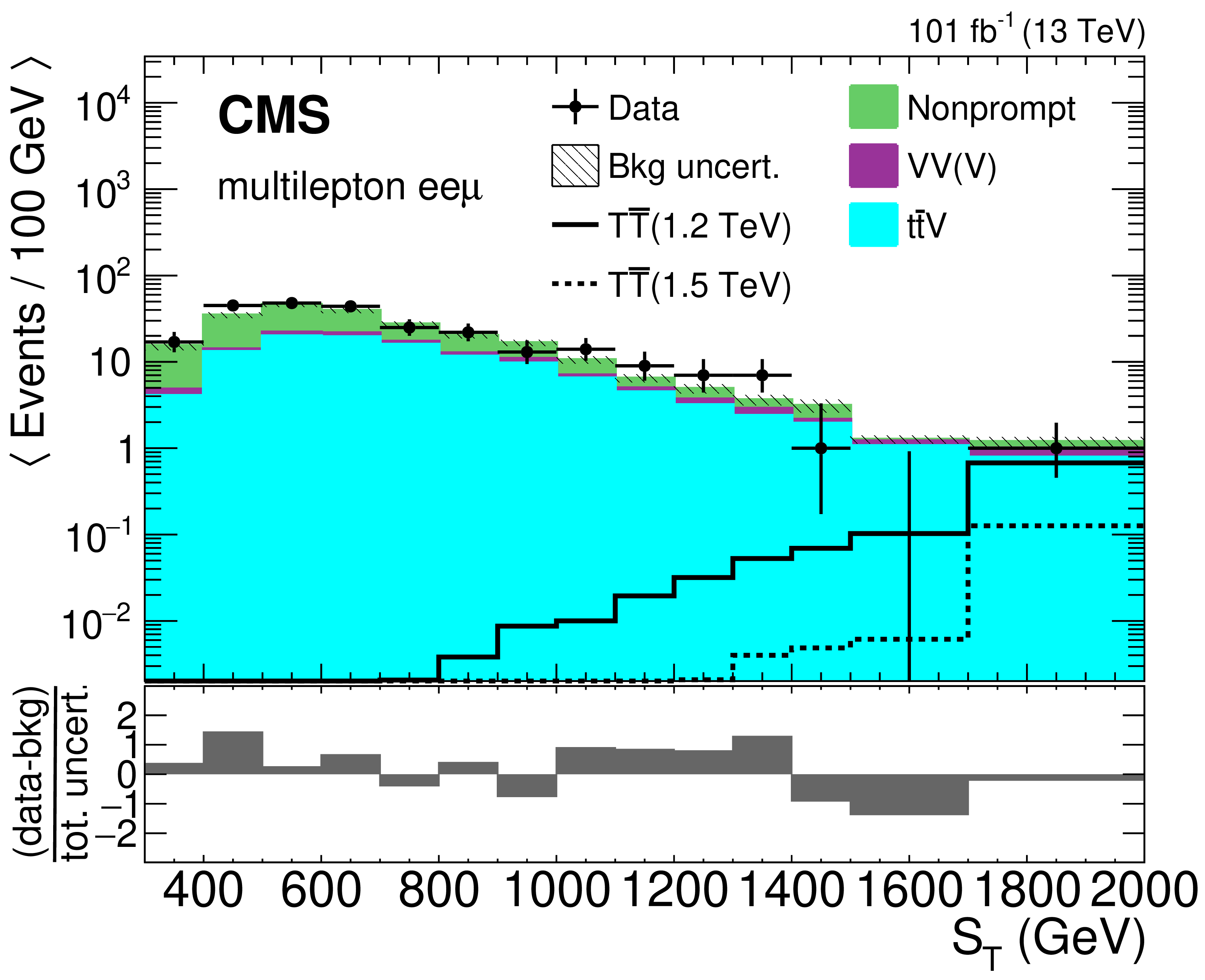
Figure 8:
Template histograms of $ S_\mathrm{T} $ in the multilepton signal region for $ \mathrm{e} \mathrm{e} \mathrm{e} $, $ \mathrm{e} \mathrm{e} \mu $, $ \mathrm{e} \mu \mu $, and $ \mu \mu \mu $ categories (left-to-right, upper-to-lower). The observed data from 2017-2018 (combined for illustration) are shown using black markers, the predicted $ \mathrm{T} \overline{\mathrm{T}} $ signal for a mass of 1.2 (1.5) TeV in the singlet scenario using solid (dashed) lines, and the post-fit background estimates, using filled histograms. Statistical and systematic uncertainties in the background estimate after performing the fit to data are shown by the hatched region. The lower panels show the difference between the data and the background estimate as a multiple of the total uncertainty in both sources. |

png pdf |
Figure 8-a:
Template histograms of $ S_\mathrm{T} $ in the multilepton signal region for $ \mathrm{e} \mathrm{e} \mathrm{e} $ category. The observed data from 2017-2018 (combined for illustration) are shown using black markers, the predicted $ \mathrm{T} \overline{\mathrm{T}} $ signal for a mass of 1.2 (1.5) TeV in the singlet scenario using solid (dashed) lines, and the post-fit background estimates, using filled histograms. Statistical and systematic uncertainties in the background estimate after performing the fit to data are shown by the hatched region. The lower panel shows the difference between the data and the background estimate as a multiple of the total uncertainty in both sources. |
png pdf |
Figure 8-b:
Template histograms of $ S_\mathrm{T} $ in the multilepton signal region for $ \mathrm{e} \mathrm{e} \mu $ category. The observed data from 2017-2018 (combined for illustration) are shown using black markers, the predicted $ \mathrm{T} \overline{\mathrm{T}} $ signal for a mass of 1.2 (1.5) TeV in the singlet scenario using solid (dashed) lines, and the post-fit background estimates, using filled histograms. Statistical and systematic uncertainties in the background estimate after performing the fit to data are shown by the hatched region. The lower panel shows the difference between the data and the background estimate as a multiple of the total uncertainty in both sources. |

png pdf |
Figure 8-c:
Template histograms of $ S_\mathrm{T} $ in the multilepton signal region for $ \mathrm{e} \mu \mu $ category. The observed data from 2017-2018 (combined for illustration) are shown using black markers, the predicted $ \mathrm{T} \overline{\mathrm{T}} $ signal for a mass of 1.2 (1.5) TeV in the singlet scenario using solid (dashed) lines, and the post-fit background estimates, using filled histograms. Statistical and systematic uncertainties in the background estimate after performing the fit to data are shown by the hatched region. The lower panel shows the difference between the data and the background estimate as a multiple of the total uncertainty in both sources. |

png pdf |
Figure 8-d:
Template histograms of $ S_\mathrm{T} $ in the multilepton signal region for $ \mu \mu \mu $ category. The observed data from 2017-2018 (combined for illustration) are shown using black markers, the predicted $ \mathrm{T} \overline{\mathrm{T}} $ signal for a mass of 1.2 (1.5) TeV in the singlet scenario using solid (dashed) lines, and the post-fit background estimates, using filled histograms. Statistical and systematic uncertainties in the background estimate after performing the fit to data are shown by the hatched region. The lower panel shows the difference between the data and the background estimate as a multiple of the total uncertainty in both sources. |
png pdf |
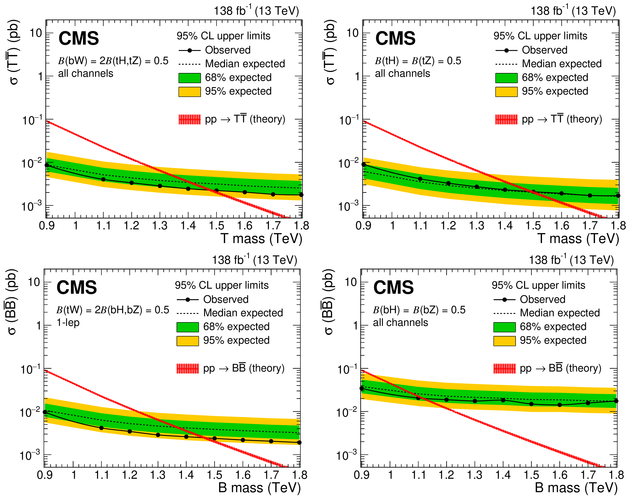
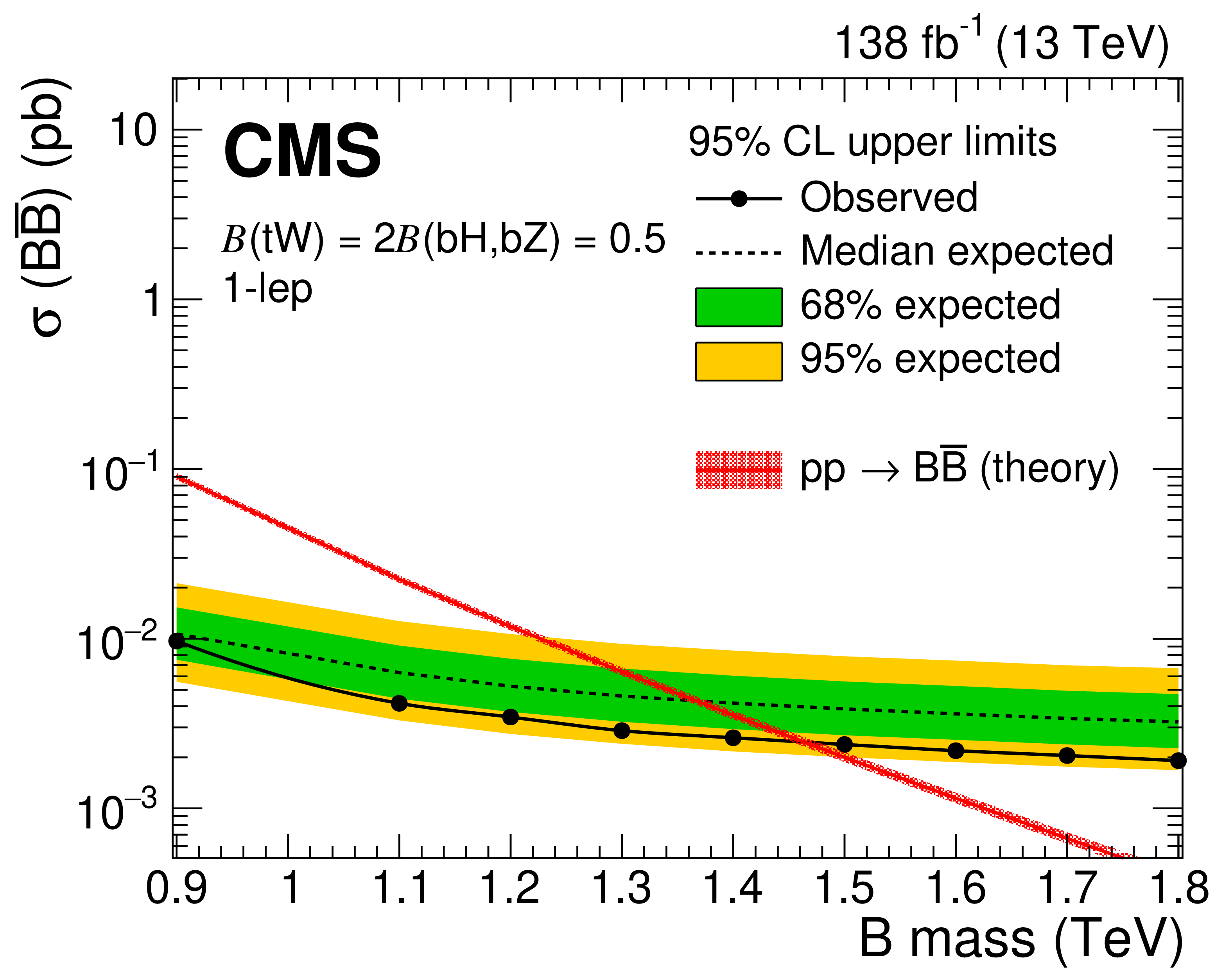
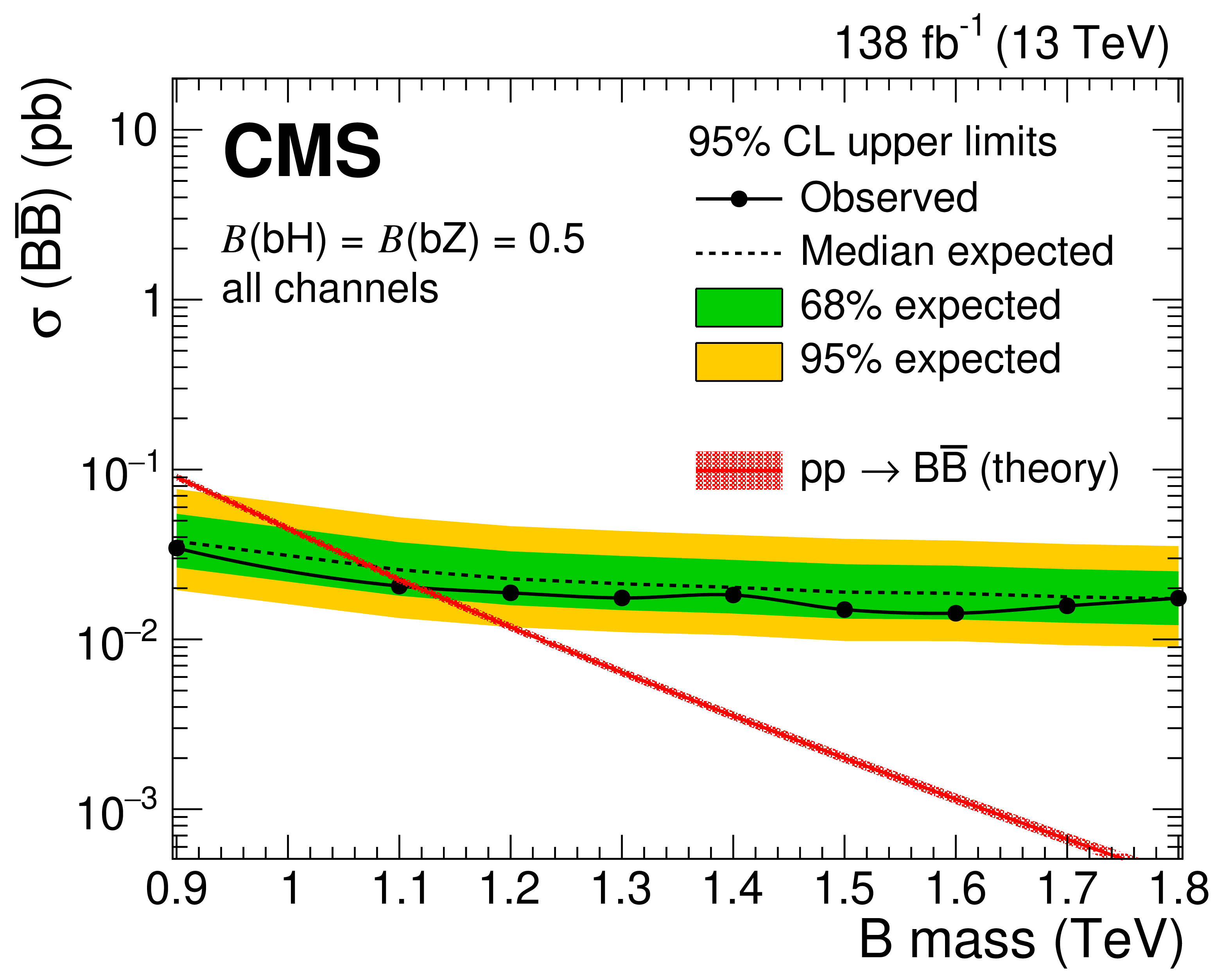
Figure 9:
Observed (solid lines) and expected (dashed lines) 95% CL upper limits on $ \mathrm{T} \overline{\mathrm{T}} $ (upper) and $ \mathrm{B} \overline{\mathrm{B}} $ (lower) production cross sections for the singlet (left) and doublet (right) hypotheses, from the combined fit to all channels. Predicted cross sections are shown by the red line surrounded by a band representing energy scale and PDF uncertainties in the calculation. |
png pdf |
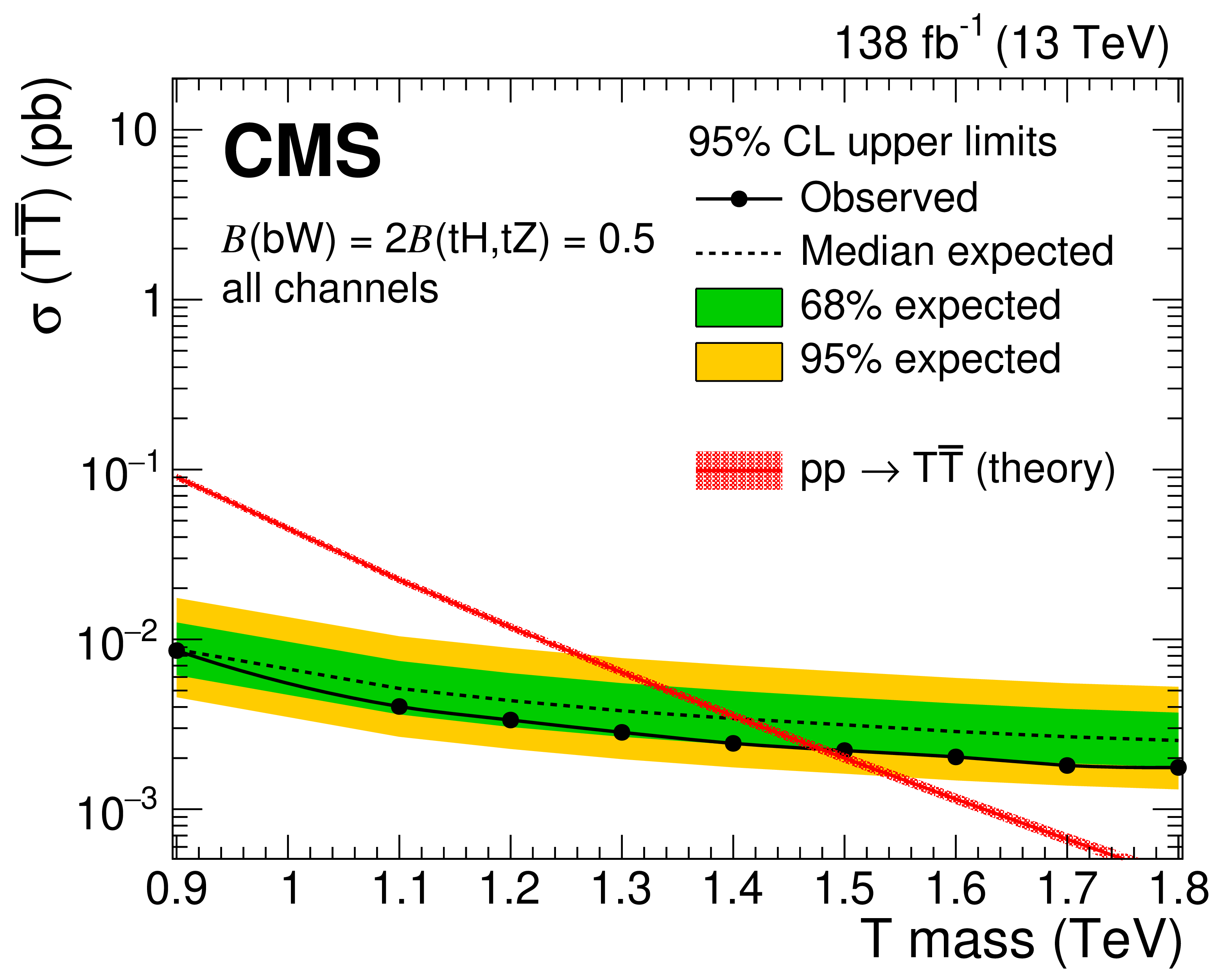
Figure 9-a:
Observed (solid lines) and expected (dashed lines) 95% CL upper limits on $ \mathrm{T} \overline{\mathrm{T}} $ production cross sections for the singlet hypothesis, from the combined fit to all channels. Predicted cross sections are shown by the red line surrounded by a band representing energy scale and PDF uncertainties in the calculation. |
png pdf |
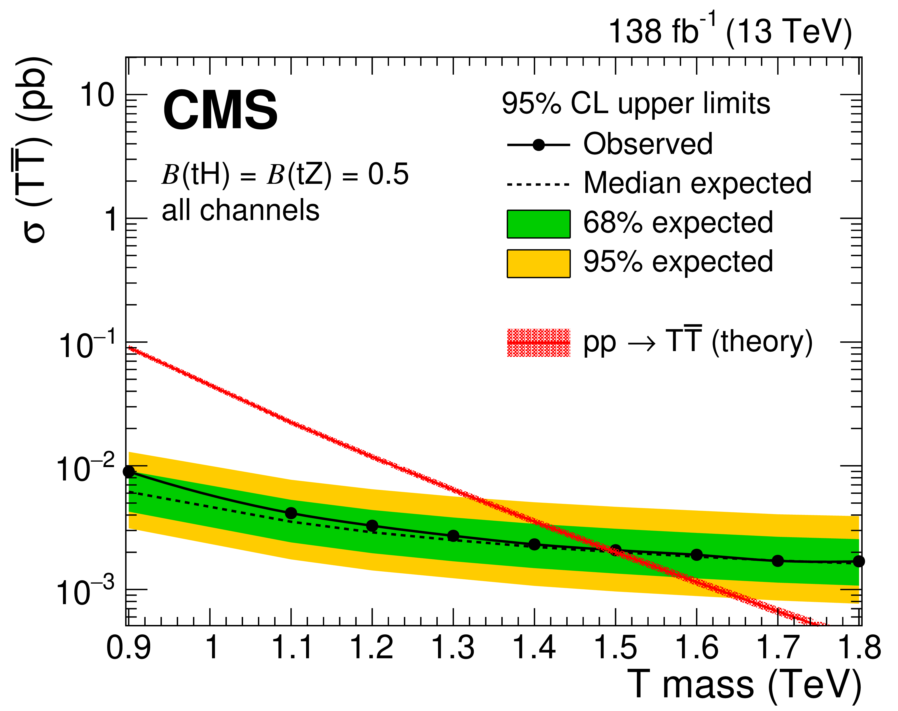
Figure 9-b:
Observed (solid lines) and expected (dashed lines) 95% CL upper limits on $ \mathrm{T} \overline{\mathrm{T}} $ production cross sections for the doublet hypothesis, from the combined fit to all channels. Predicted cross sections are shown by the red line surrounded by a band representing energy scale and PDF uncertainties in the calculation. |
png pdf |
Figure 9-c:
Observed (solid lines) and expected (dashed lines) 95% CL upper limits on $ \mathrm{B} \overline{\mathrm{B}} $ production cross sections for the singlet hypothesis, from the combined fit to all channels. Predicted cross sections are shown by the red line surrounded by a band representing energy scale and PDF uncertainties in the calculation. |
png pdf |
Figure 9-d:
Observed (solid lines) and expected (dashed lines) 95% CL upper limits on $ \mathrm{B} \overline{\mathrm{B}} $ production cross sections for the doublet hypothesis, from the combined fit to all channels. Predicted cross sections are shown by the red line surrounded by a band representing energy scale and PDF uncertainties in the calculation. |
png pdf |
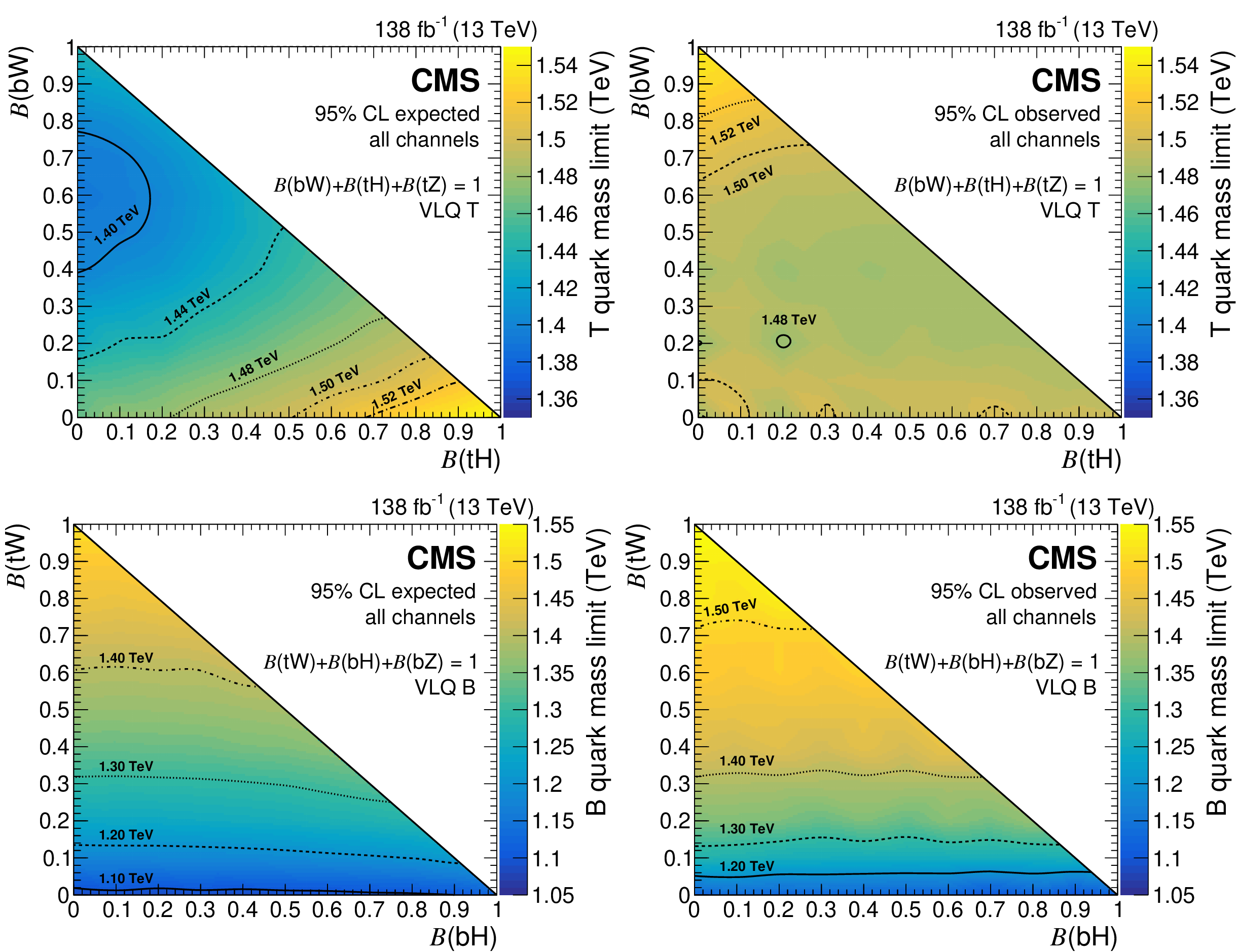
Figure 10:
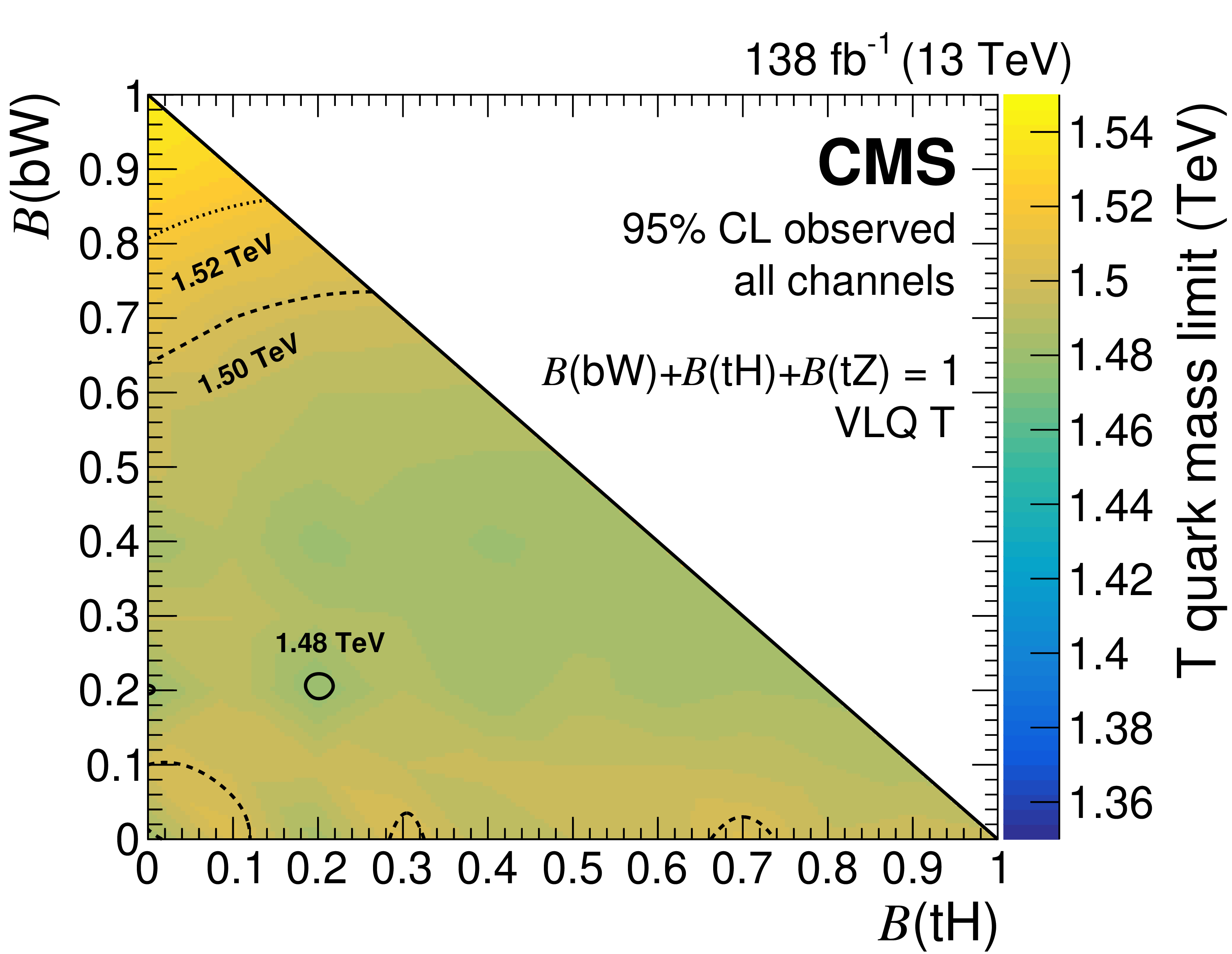
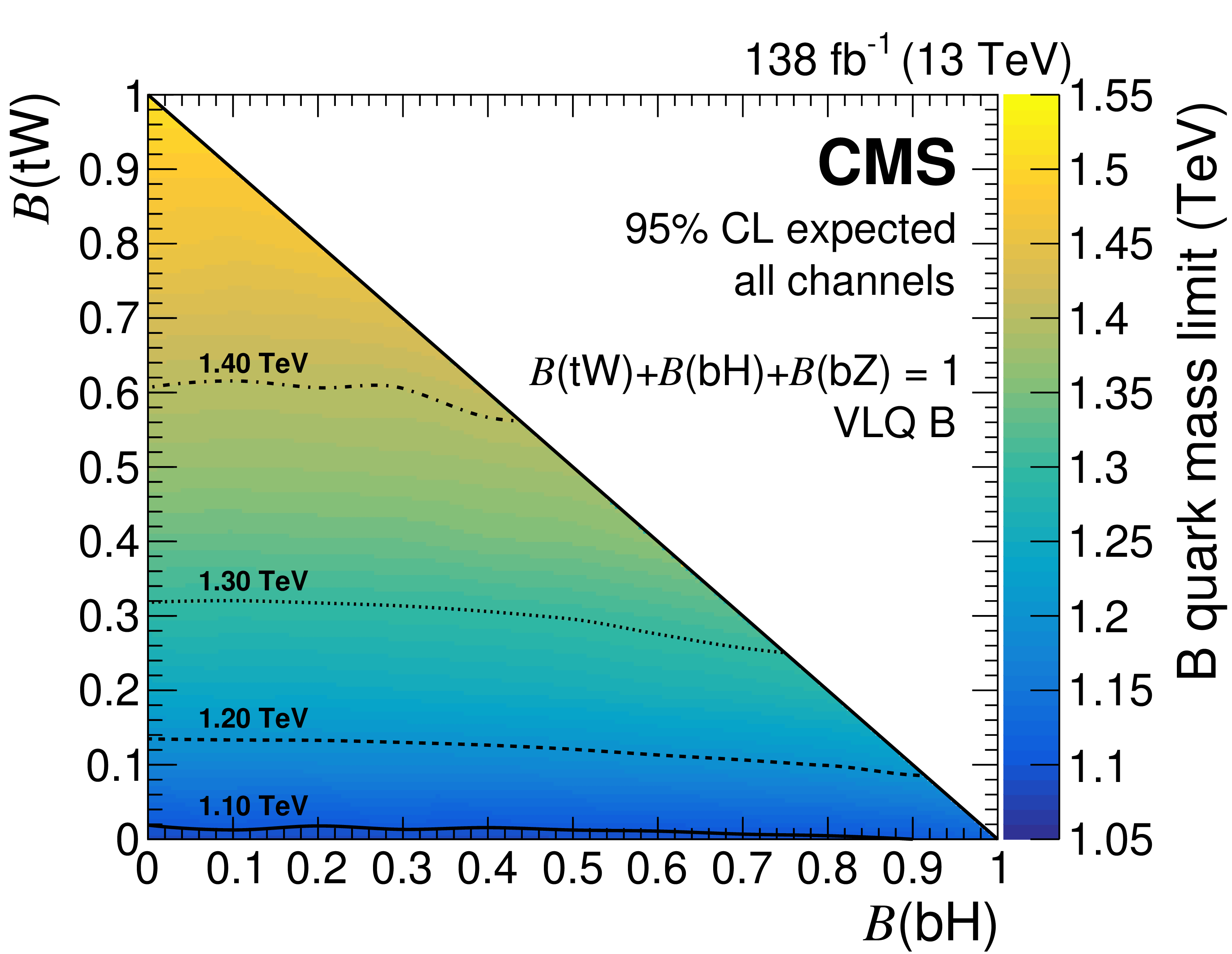
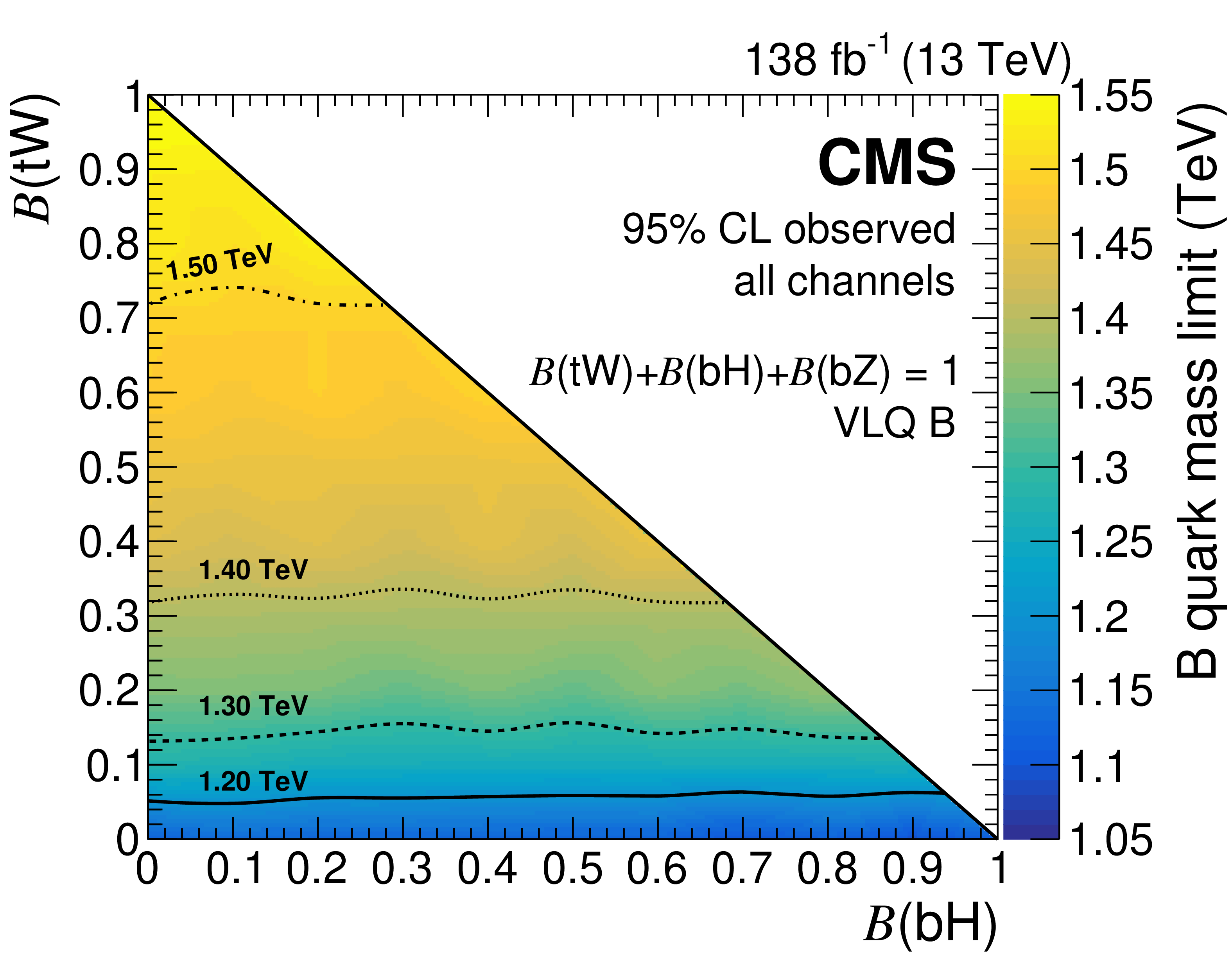
The 95% CL expected (left) and observed (right) lower mass limits on pair-produced $ \mathrm{T} $ (upper) and $ \mathrm{B} $ (lower) quark masses, from the combined fit to all channels, as functions of their branching ratios to H and W bosons. Mass contours are shown with lines of various styles. |
png pdf |
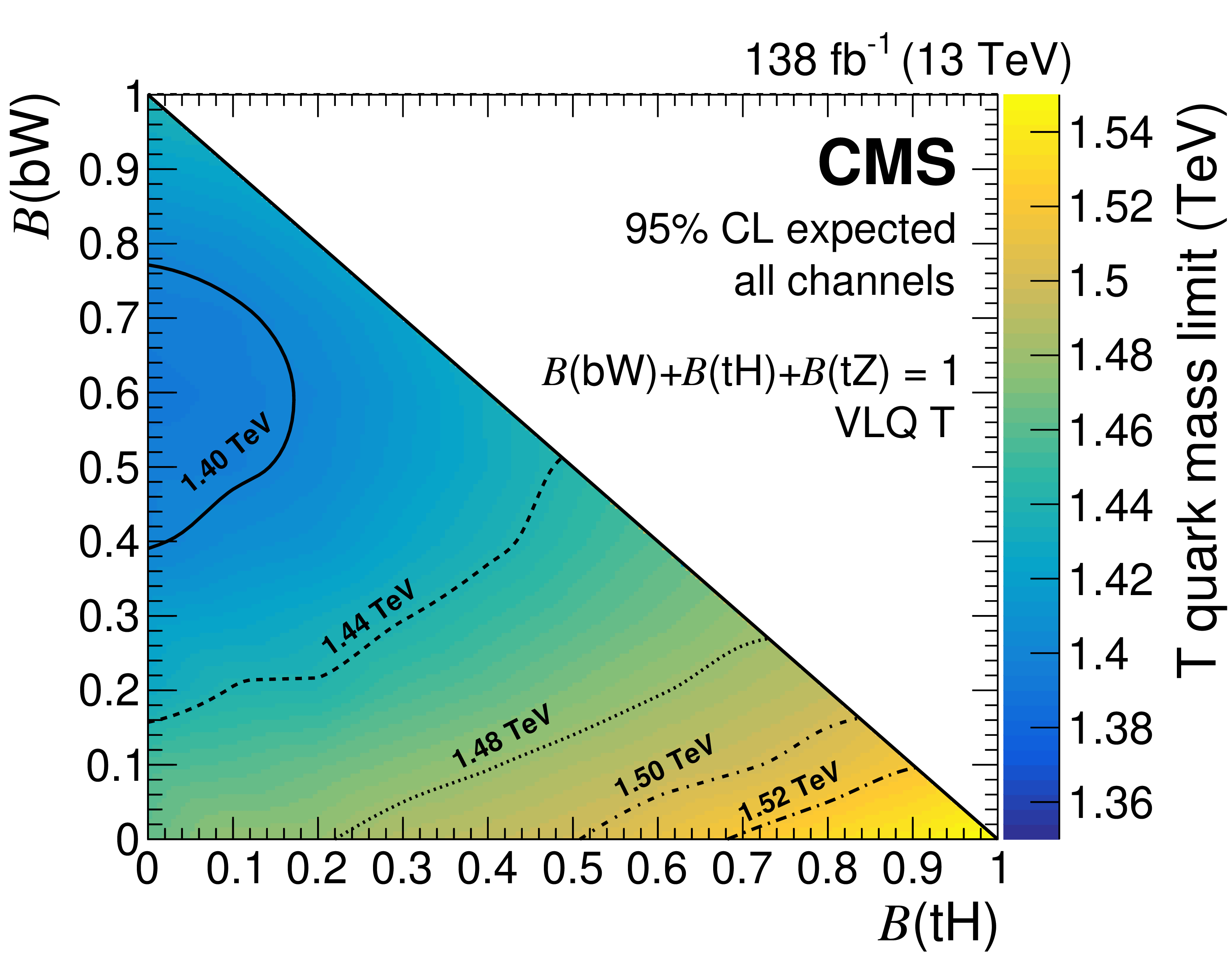
Figure 10-a:
The 95% CL expected lower mass limits on pair-produced $ \mathrm{T} $ quark masses, from the combined fit to all channels, as functions of their branching ratios to H and W bosons. Mass contours are shown with lines of various styles. |
png pdf |
Figure 10-b:
The 95% CL observed lower mass limits on pair-produced $ \mathrm{T} $ quark masses, from the combined fit to all channels, as functions of their branching ratios to H and W bosons. Mass contours are shown with lines of various styles. |
png pdf |
Figure 10-c:
The 95% CL expected lower mass limits on pair-produced $ \mathrm{B} $ quark masses, from the combined fit to all channels, as functions of their branching ratios to H and W bosons. Mass contours are shown with lines of various styles. |
png pdf |
Figure 10-d:
The 95% CL observed lower mass limits on pair-produced $ \mathrm{B} $ quark masses, from the combined fit to all channels, as functions of their branching ratios to H and W bosons. Mass contours are shown with lines of various styles. |
| Tables | |
png pdf |
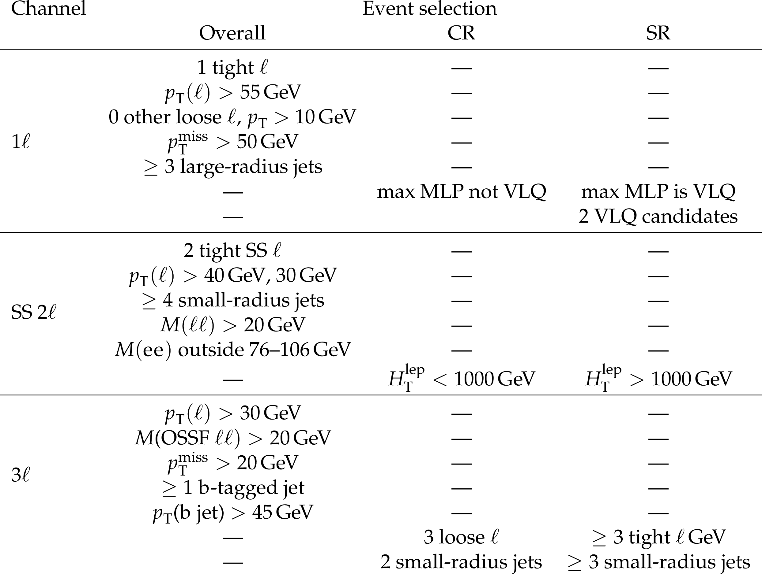
Table 1:
Summary of event selection criteria for the primary CRs and SRs in the three search channels. The label ``OSSF'' refers to opposite-sign charge, same-flavor lepton pairs, and the phrase ``max MLP'' refers to the largest score from the single-lepton MLP network. |
png pdf |
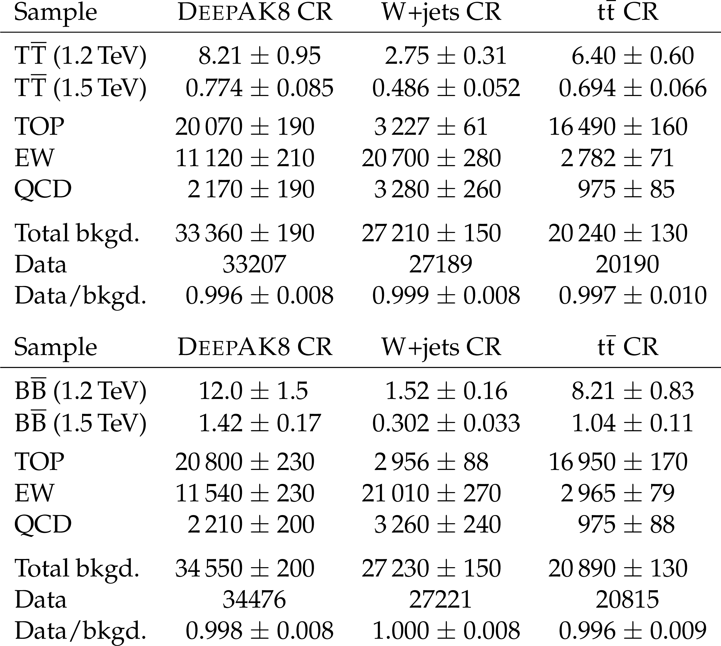
Table 2:
Numbers of predicted and observed CR events in 2016-2018 data (138 fb$ ^{-1} $) for the $ \mathrm{T} \overline{\mathrm{T}} $ (upper section) and $ \mathrm{B} \overline{\mathrm{B}} $ (lower section) signal hypotheses in the single-lepton channel, after a background-only fit to data described in Section 10. Predicted numbers of signal events before the fit to data are included for comparison, using the singlet branching fraction scenario. Uncertainties include statistical and systematic components, and lepton flavor categories are combined for illustration with their uncertainties added in quadrature. Values in the DEEPAK8 CR represent the number of large-radius jets rather than the number of events. |
png pdf |
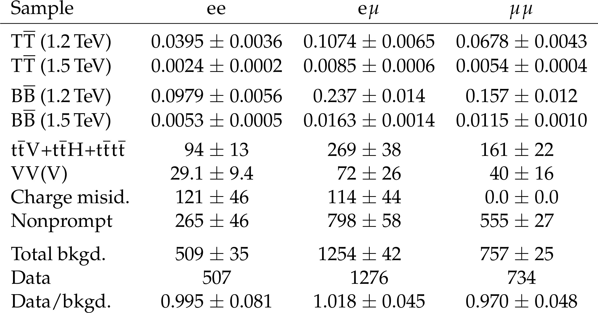
Table 3:
Numbers of predicted and observed CR events in 2017-2018 data (101 fb$ ^{-1} $) in the SS dilepton channel, after a background-only fit to data. Predicted numbers of signal events before the fit to data are included for comparison, using the singlet branching fraction scenario. Uncertainties include statistical and systematic components. Predictions for 2017 and 2018 are combined with their uncertainties added in quadrature. |
png pdf |
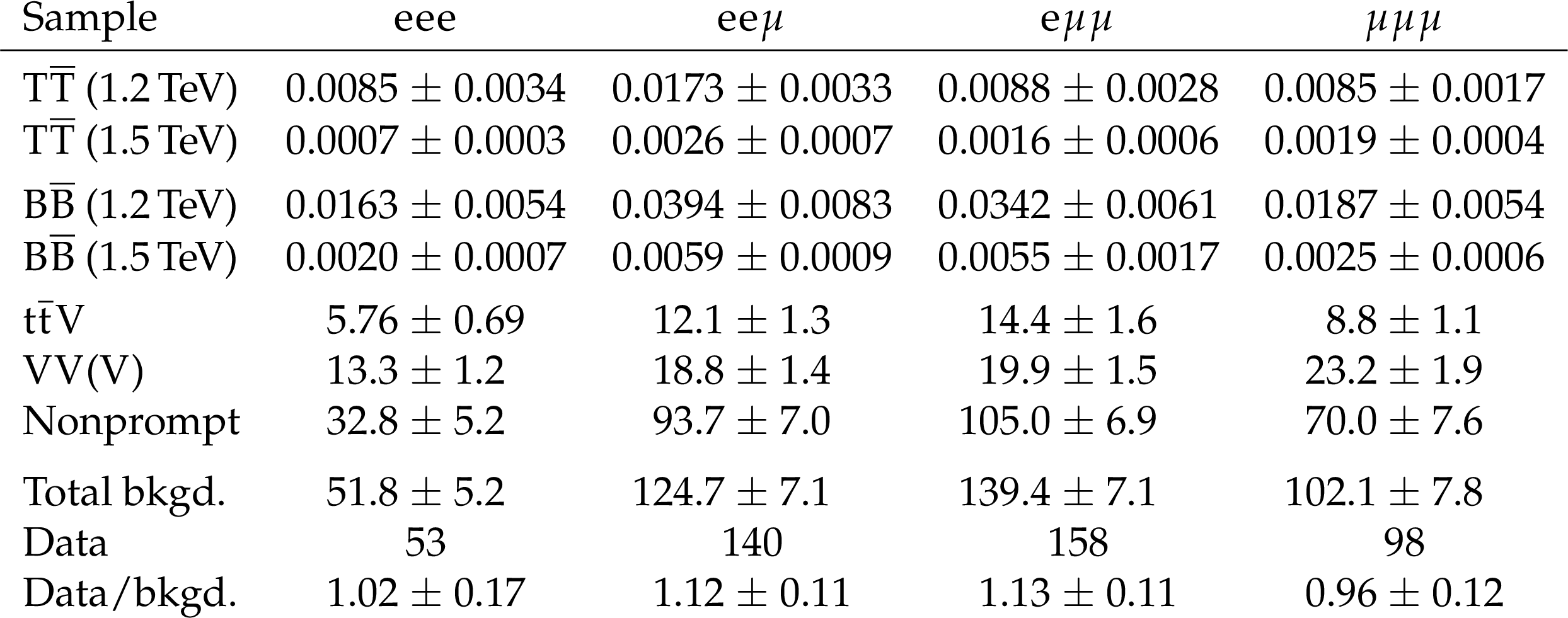
Table 4:
Numbers of predicted and observed CR events in 2017-2018 data (101 fb$ ^{-1} $) in the multilepton channel, after a background-only fit to data. Predicted numbers of signal events before the fit to data are included for comparison, using the singlet branching fraction scenario. Uncertainties include statistical and systematic components. Predictions for 2017 and 2018 are combined with their uncertainties added in quadrature. |
png pdf |
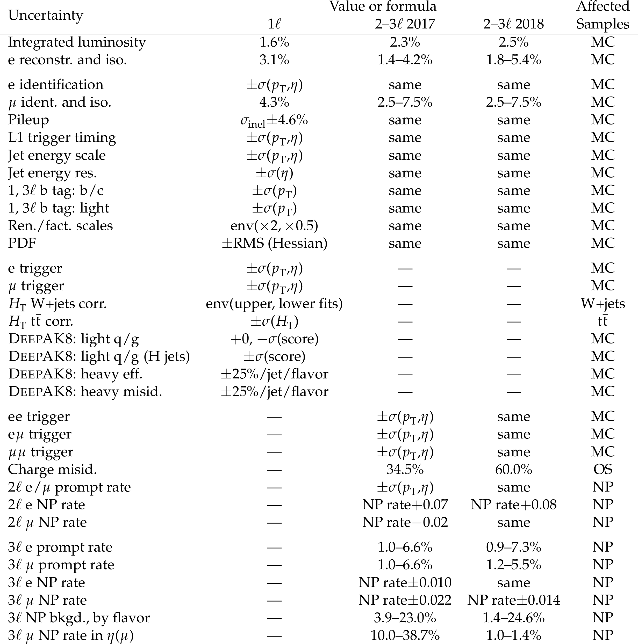
Table 5:
Summary of systematic uncertainties for the various analysis channels, grouped according to the channel. The second column shows uncertainties for the single-lepton channel, evaluated with 2016-2018 data combined. The third and fourth columns show uncertainties for the other channels, evaluated using 2017 or 2018 data. Uncertainties that are common across multiple channels appear in the first relevant column, followed by the label ``same'' in other columns. Ranges indicate values across different lepton flavor categories, and functional forms describe the quantities on which the uncertainty's numerical value depends. The final column shows which predictions are affected by each uncertainty: ``MC'' denotes all simulation (including signal), ``OS'' denotes charge misidentification background, and ``NP'' denotes nonprompt lepton background. |
png pdf |
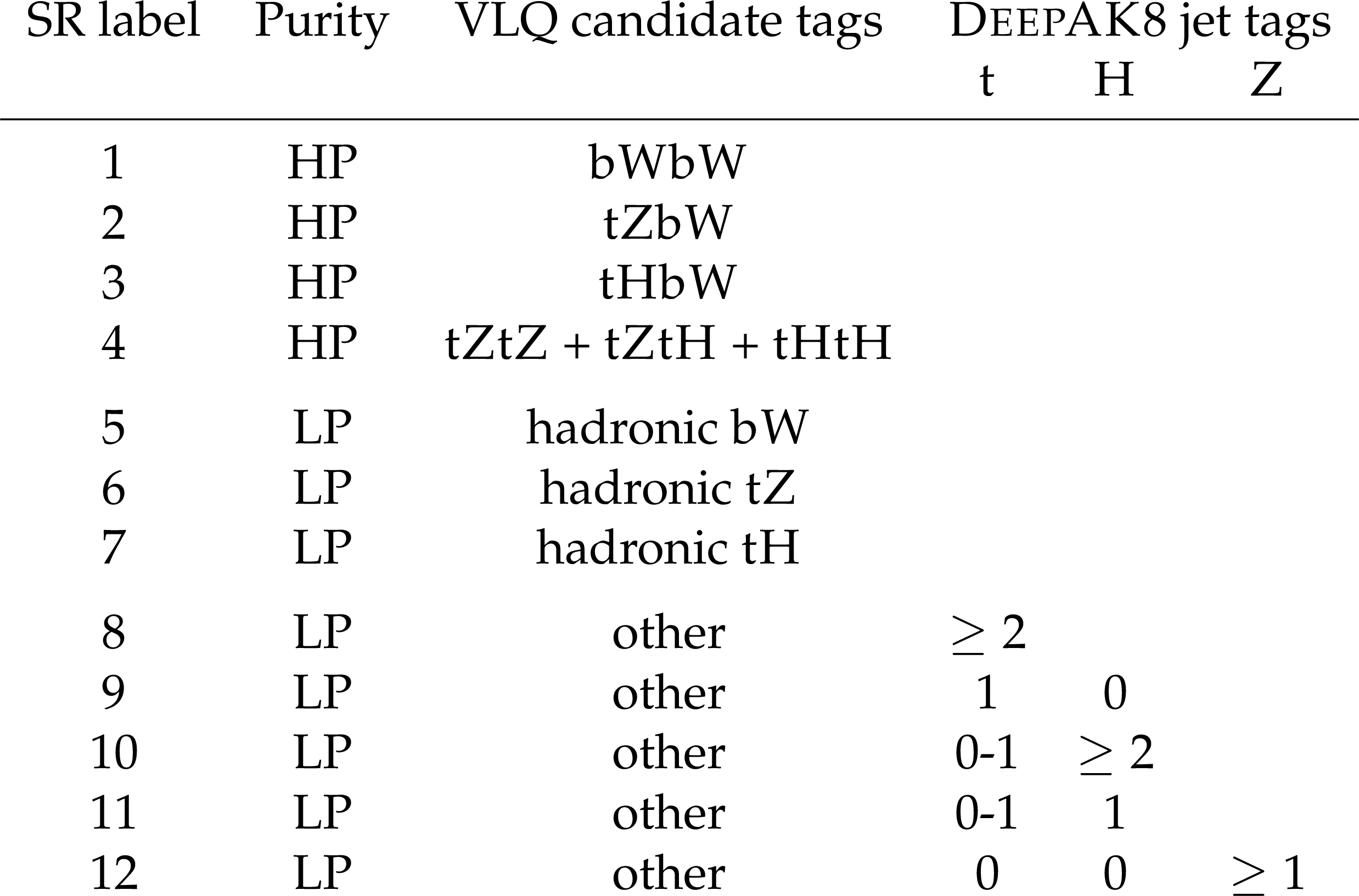
Table 6:
Category labels and definitions for the SRs of the single-lepton channel $ \mathrm{T} \overline{\mathrm{T}} $ analysis. Electron and muon events are analyzed separately in all categories. The VLQ candidate tag describes the pairings formed from the leptonic particle candidate and three large-radius jets. The hadronic VLQ candidate is reconstructed from two large-radius jets, and a VLQ candidate tag of ``other'' indicates that the hadronic VLQ candidate did not consist of $ \mathrm{b} \mathrm{W} $-, $ \mathrm{t} \mathrm{Z} $-, or $ \mathrm{t} \mathrm{H} $-tagged jets. In the $ \mathrm{B} \overline{\mathrm{B}} $ analysis, the VLQ candidate tags considered are tW, $ \mathrm{b} \mathrm{Z} $, and $ \mathrm{b} \mathrm{H} $. Categories 4, 6, and 7 are not included in the $ \mathrm{B} \overline{\mathrm{B}} $ analysis. |
png pdf |
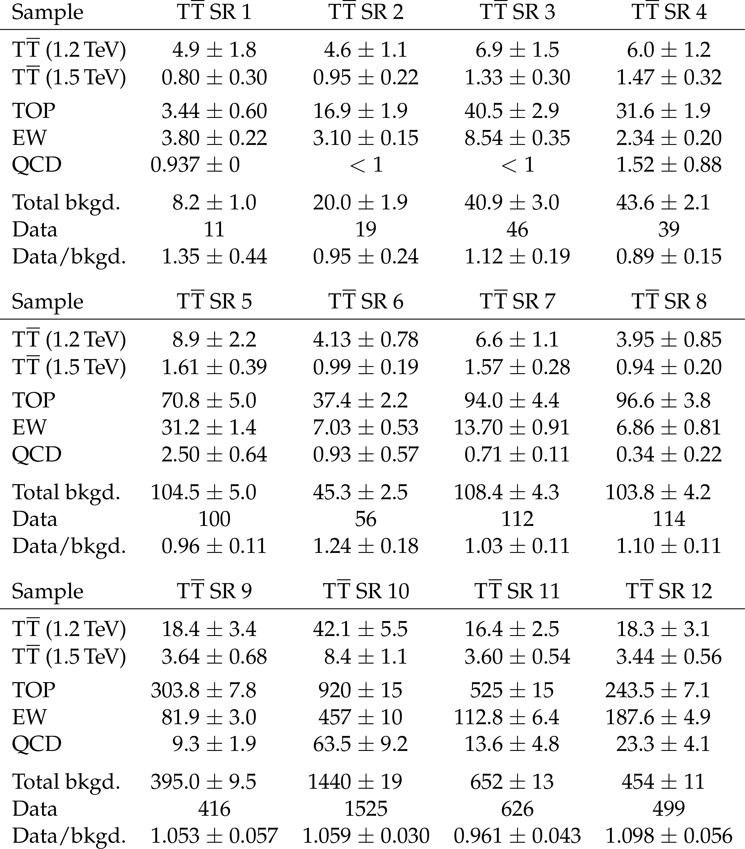
Table 7:
Numbers of predicted and observed events in 2016-2018 data (138 fb$ ^{-1} $) in the $ \mathrm{T} \overline{\mathrm{T}} $ SR categories considered in the single-lepton channel, after a background-only fit to data. Electron and muon categories have been combined for illustration. Predicted numbers of signal events before the fit to data are included for comparison, using the singlet branching fraction scenario. Uncertainties include statistical and systematic components, with the uncertainties in the electron and muon categories added in quadrature. |

png pdf |
Table 8:
Numbers of predicted and observed events in 2016-2018 data (138 fb$ ^{-1} $) in the $ \mathrm{B} \overline{\mathrm{B}} $ SR categories considered in the single-lepton channel, after a background-only fit to data. Electron and muon categories have been combined for illustration. Predicted numbers of signal events before the fit to data are included for comparison, using the singlet branching fraction scenario. Uncertainties include statistical and systematic components, with the uncertainties in the electron and muon categories added in quadrature. |
png pdf |
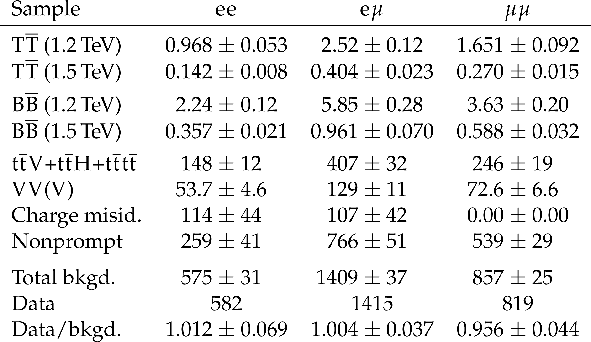
Table 9:
Numbers of predicted and observed SR events in 2017-2018 data (101 fb$ ^{-1} $) in the SS dilepton channel, after a background-only fit to data. Predicted numbers of signal events before the fit to data are included for comparison, using the singlet branching fraction scenario. Uncertainties include statistical and systematic components. Predictions for 2017 and 2018 are combined for illustration with their uncertainties added in quadrature. |
png pdf |
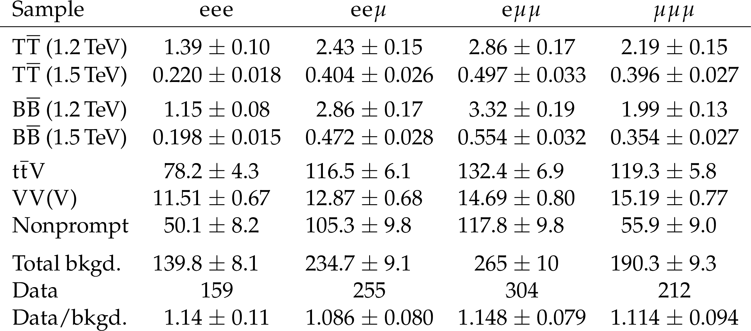
Table 10:
Numbers of predicted and observed SR events in 2017-2018 data (101 fb$ ^{-1} $) in the multilepton channel, after a background-only fit to data. Predicted numbers of signal events before the fit to data are included for comparison, using the singlet branching fraction scenario. Uncertainties include statistical and systematic components. Predictions for 2017 and 2018 are combined for illustration with their uncertainties added in quadrature. |
png pdf |
Table 11:
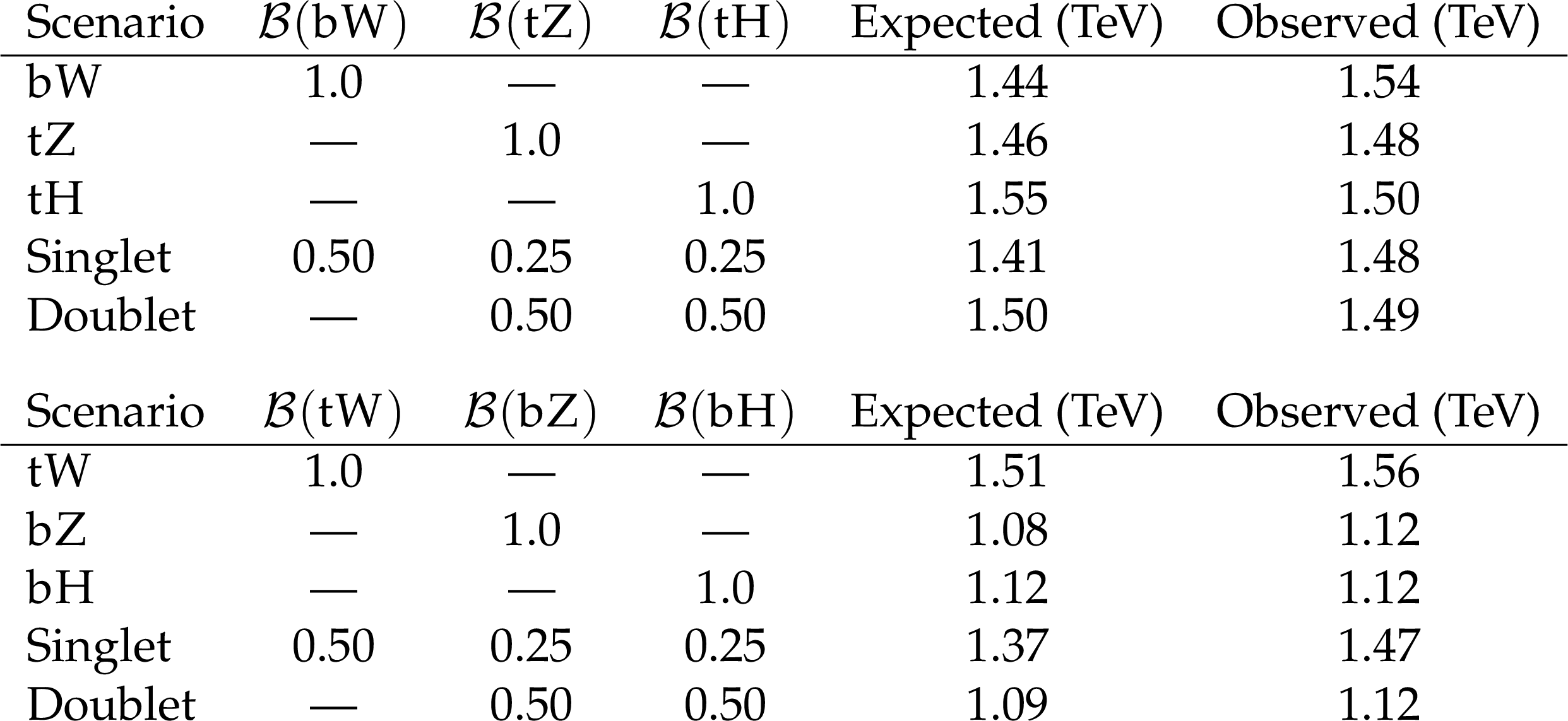
Expected and observed 95% CL lower limits on the $ \mathrm{T} $ (upper section) and $ \mathrm{B} $ (lower section) quark masses. |
| Summary |
| A search has been presented for vector-like $ \mathrm{T} $ and $ \mathrm{B} $ quark-antiquark pairs produced in proton-proton collisions at a center-of-mass energy of 13 TeV. Data collected by the CMS experiment at the LHC in 2016-2018 are analyzed in the single-lepton final state, and data from 2017-2018 are analyzed in the same-sign charge dilepton and multilepton final states. In the single-lepton channel, parent particles of large-radius jets are identified using the DEEPAK8 algorithm, and vector-like quark candidates are reconstructed. A multilayer perceptron network is trained to separate signal events from standard model backgrounds. In the same-sign charge dilepton and multilepton channels, low background rates and the large energy signature of the signal are exploited by studying jet and lepton momentum scalar sum distributions. Pair production is excluded at 95% confidence level for $ \mathrm{T} $ quarks with masses up to 1.54 TeV and for $ \mathrm{B} $ quarks with masses up to 1.56 TeV, depending on the branching fraction scenario, and $ \mathrm{T} $ quarks with masses below 1.48 TeV are excluded in any scenario. The limits obtained in this search are the strongest limits to date for $ \mathrm{T} \overline{\mathrm{T}} $ production with all $ \mathrm{T} $ quark decay modes, and are the strongest limits to date for $ \mathrm{B} \overline{\mathrm{B}} $ production with $ \mathrm{B} $ quark decays to tW. |
| Additional Figures | |

png pdf |
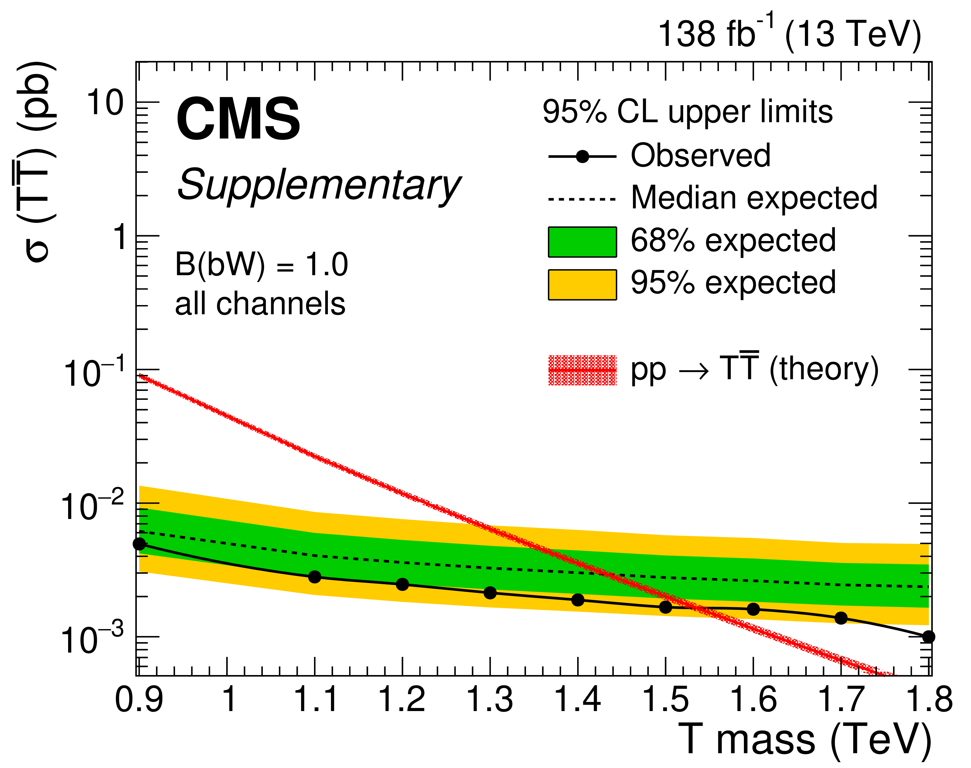
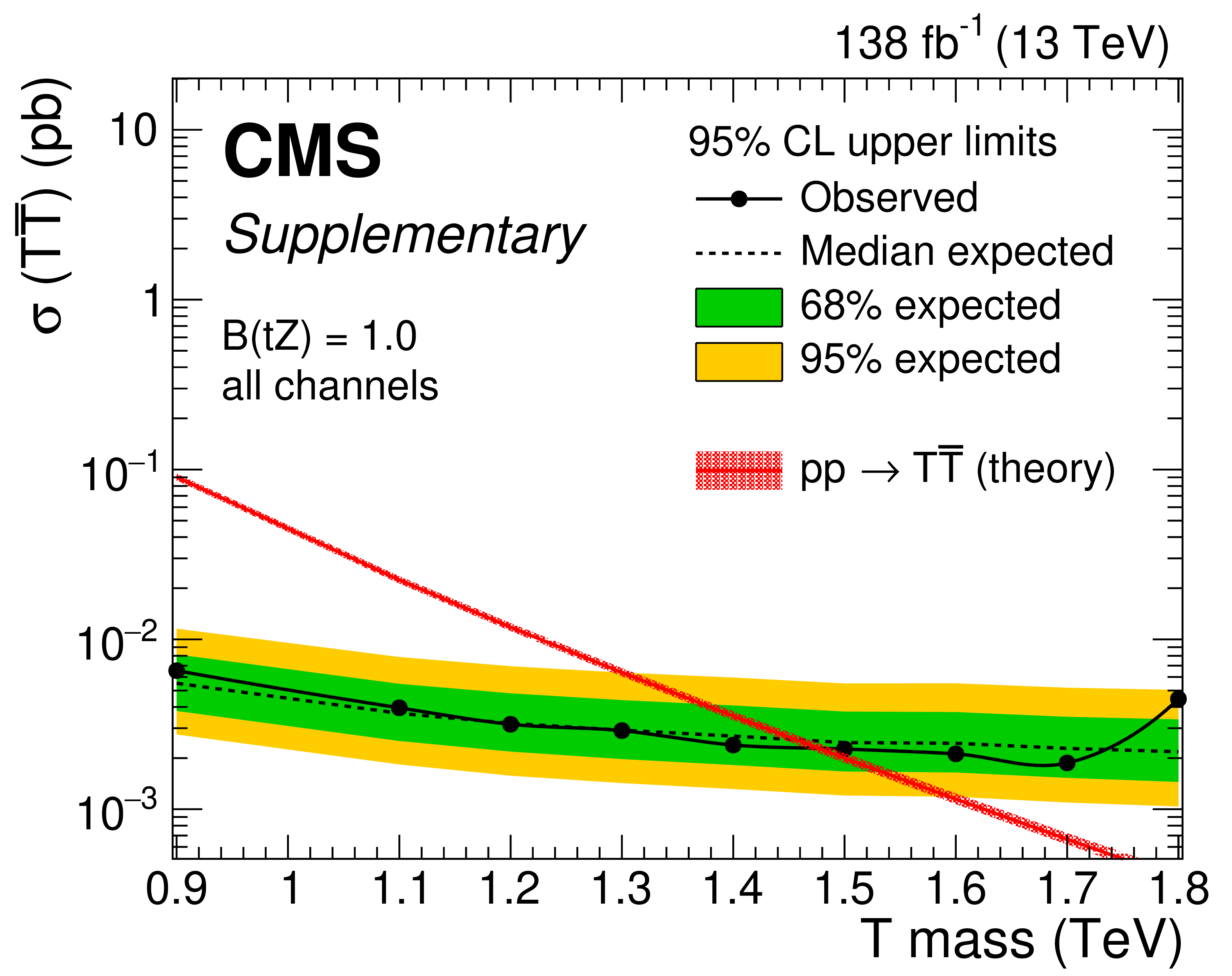
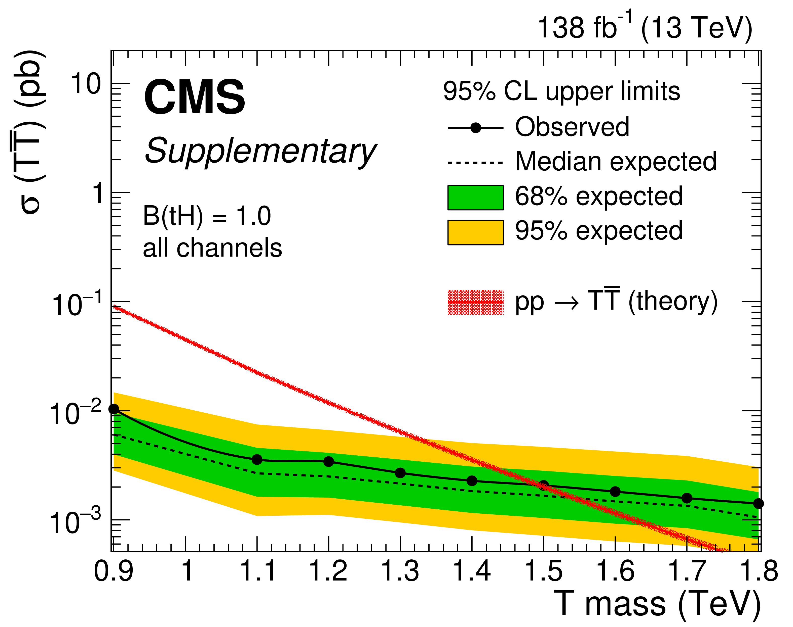
Additional Figure 1:
Observed (solid lines) and expected (dashed lines) 95% CL upper limits on the $ {\mathrm{T}} \overline{\mathrm{T}} $ production cross section for the hypotheses of 100% branching fraction to $ \mathrm{b}\mathrm{W} $ (upper left), $ \mathrm{t}\mathrm{Z} $ (upper right), or $ \mathrm{t}\mathrm{H} $ (lower), from the combined fit to all channels. Predicted cross sections are shown by the red line surrounded by a band representing energy scale and PDF uncertainties in the calculation. |
png pdf |
Additional Figure 1-a:
Observed (solid lines) and expected (dashed lines) 95% CL upper limits on the $ {\mathrm{T}} \overline{\mathrm{T}} $ production cross section for the hypotheses of 100% branching fraction to $ \mathrm{b}\mathrm{W} $ (upper left), $ \mathrm{t}\mathrm{Z} $ (upper right), or $ \mathrm{t}\mathrm{H} $ (lower), from the combined fit to all channels. Predicted cross sections are shown by the red line surrounded by a band representing energy scale and PDF uncertainties in the calculation. |
png pdf |
Additional Figure 1-b:
Observed (solid lines) and expected (dashed lines) 95% CL upper limits on the $ {\mathrm{T}} \overline{\mathrm{T}} $ production cross section for the hypotheses of 100% branching fraction to $ \mathrm{b}\mathrm{W} $ (upper left), $ \mathrm{t}\mathrm{Z} $ (upper right), or $ \mathrm{t}\mathrm{H} $ (lower), from the combined fit to all channels. Predicted cross sections are shown by the red line surrounded by a band representing energy scale and PDF uncertainties in the calculation. |
png pdf |
Additional Figure 1-c:
Observed (solid lines) and expected (dashed lines) 95% CL upper limits on the $ {\mathrm{T}} \overline{\mathrm{T}} $ production cross section for the hypotheses of 100% branching fraction to $ \mathrm{b}\mathrm{W} $ (upper left), $ \mathrm{t}\mathrm{Z} $ (upper right), or $ \mathrm{t}\mathrm{H} $ (lower), from the combined fit to all channels. Predicted cross sections are shown by the red line surrounded by a band representing energy scale and PDF uncertainties in the calculation. |

png pdf |
Additional Figure 2:
Observed (solid lines) and expected (dashed lines) 95% CL upper limits on the $ {\mathrm{B}} \overline{\mathrm{B}} $ production cross section for the hypothesis of 100% branching fraction to $ \mathrm{t}\mathrm{W} $, from the combined fit to all channels. Predicted cross sections are shown by the red line surrounded by a band representing energy scale and PDF uncertainties in the calculation. |
| References | ||||
| 1 | ATLAS Collaboration | Observation of a new particle in the search for the Standard Model Higgs boson with the ATLAS detector at the LHC | PLB 716 (2012) 1 | 1207.7214 |
| 2 | CMS Collaboration | Observation of a new boson at a mass of 125 GeV with the CMS experiment at the LHC | PLB 716 (2012) 30 | CMS-HIG-12-028 1207.7235 |
| 3 | CMS Collaboration | Observation of a new boson with mass near 125 GeV in pp collisions at $ \sqrt{s} = $ 7 and 8 TeV | JHEP 06 (2013) 081 | CMS-HIG-12-036 1303.4571 |
| 4 | Particle Data Group | Review of Particle Physics | Reviews 14: Neutrino Masses, Mixing, and Oscillations, and 27: Dark Matter, 2022 PTEP 2022 (2022) 083C01 |
|
| 5 | M. Perelstein, M. E. Peskin, and A. Pierce | Top quarks and electroweak symmetry breaking in little Higgs models | PRD 69 (2004) 075002 | hep-ph/0310039 |
| 6 | O. Matsedonskyi, G. Panico, and A. Wulzer | Light top partners for a light composite Higgs | JHEP 01 (2013) 164 | 1204.6333 |
| 7 | R. Contino, L. Da Rold, and A. Pomarol | Light custodians in natural composite Higgs models | PRD 75 (2007) 055014 | hep-ph/0612048 |
| 8 | R. Contino, T. Kramer, M. Son, and R. Sundrum | Warped/composite phenomenology simplified | JHEP 05 (2007) 074 | hep-ph/0612180 |
| 9 | J. A. Aguilar-Saavedra, R. Benbrik, S. Heinemeyer, and M. P é rez-Victoria | Handbook of vectorlike quarks: Mixing and single production | PRD 88 (2013) 094010 | 1306.0572 |
| 10 | A. De Simone, O. Matsedonskyi, R. Rattazzi, and A. Wulzer | A first top partner hunter's guide | JHEP 04 (2013) 004 | 1211.5663 |
| 11 | J. A. Aguilar-Saavedra | Mixing with vector-like quarks: Constraints and expectations | EPJ Web Conf. 60 (2013) 16012 | 1306.4432 |
| 12 | F. del Aguila, L. Ametller, G. L. Kane, and J. Vidal | Vector-like fermion and standard Higgs production at hadron colliders | NPB 334 (1990) 1 | |
| 13 | CMS Collaboration | Search for a vector-like quark with charge 2/3 in t+Z events from pp collisions at $ \sqrt{s}= $ 7 TeV | PRL 107 (2011) 271802 | CMS-EXO-11-005 1109.4985 |
| 14 | CMS Collaboration | Search for pair produced fourth-generation up-type quarks in $ pp $ collisions at $ \sqrt{s}= $ 7 TeV with a lepton in the final state | PLB 718 (2012) 307 | CMS-EXO-11-099 1209.0471 |
| 15 | ATLAS Collaboration | Search for pair production of a new quark that decays to a Z boson and a bottom quark with the ATLAS detector | PRL 109 (2012) 071801 | 1204.1265 |
| 16 | CMS Collaboration | Search for vector-like charge 2/3 $ \mathrm{T} $ quarks in proton-proton collisions at $ \sqrt{s} = $ 8 TeV | PRD 92 (2016) 012003 | 1509.04177 |
| 17 | CMS Collaboration | Inclusive search for a vector-like $ \mathrm{T} $ quark with charge $ \frac{2}{3} $ in pp collisions at $ \sqrt{s} = $ 8 TeV | PLB 729 (2014) 149 | 1311.7667 |
| 18 | ATLAS Collaboration | Search for pair production of a new heavy quark that decays into a W boson and a light quark in pp collisions at $ \sqrt{s} = $ 8 TeV with the ATLAS detector | PRD 92 (2015) 112007 | 1509.04261 |
| 19 | ATLAS Collaboration | Search for production of vector-like quark pairs and of four top quarks in the lepton-plus-jets final state in pp collisions at $ \sqrt{s}= $ 8 TeV with the ATLAS detector | JHEP 08 (2015) 105 | 1505.04306 |
| 20 | CMS Collaboration | Search for pair production of vector-like quarks in the $ \mathrm{b} \mathrm{W} \overline{\mathrm{b}} \mathrm{W} $ channel from proton-proton collisions at $ \sqrt{s} = $ 13 TeV | PLB 779 (2018) 82 | 1710.01539 |
| 21 | CMS Collaboration | Search for vector-like $ \mathrm{T} $ and $ \mathrm{B} $ quark pairs in final states with leptons at $ \sqrt{s} = $ 13 TeV | JHEP 08 (2018) 177 | 1805.04758 |
| 22 | CMS Collaboration | Search for vector-like quarks in events with two oppositely charged leptons and jets in proton-proton collisions at $ \sqrt{s} = $ 13 TeV | EPJC 79 (2019) 364 | 1812.09768 |
| 23 | CMS Collaboration | Search for pair production of vectorlike quarks in the fully hadronic final state | PRD 100 (2019) 072001 | 1906.11903 |
| 24 | CMS Collaboration | A search for bottom-type, vector-like quark pair production in a fully hadronic final state in proton-proton collisions at $ \sqrt{s} = $ 13 TeV | PRD 102 (2020) 112004 | 2008.09835 |
| 25 | ATLAS Collaboration | Combination of the searches for pair-produced vector-like partners of the third-generation quarks at $ \sqrt{s} = $ 13 TeV with the ATLAS detector | PRL 121 (2018) 211801 | 1808.02343 |
| 26 | CMS Collaboration | HEPData record for this analysis | link | |
| 27 | CMS Collaboration | The CMS Experiment at the CERN LHC | JINST 3 (2008) S08004 | |
| 28 | CMS Collaboration | Particle-flow reconstruction and global event description with the CMS detector | JINST 12 (2017) P10003 | CMS-PRF-14-001 1706.04965 |
| 29 | M. Cacciari, G. P. Salam, and G. Soyez | The anti-$ k_{\mathrm{T}} $ jet clustering algorithm | JHEP 04 (2008) 063 | 0802.1189 |
| 30 | M. Cacciari, G. P. Salam, and G. Soyez | FastJet user manual | EPJC 72 (2012) 1896 | 1111.6097 |
| 31 | D. Bertolini, P. Harris, M. Low, and N. Tran | Pileup per particle identification | JHEP 10 (2014) 059 | 1407.6013 |
| 32 | CMS Collaboration | Pileup mitigation at CMS in 13 TeV data | JINST 15 (2020) P09018 | CMS-JME-18-001 2003.00503 |
| 33 | CMS Collaboration | Jet energy scale and resolution in the CMS experiment in pp collisions at 8 TeV | JINST 12 (2017) P02014 | CMS-JME-13-004 1607.03663 |
| 34 | CMS Collaboration | Performance of missing transverse momentum reconstruction in proton-proton collisions at $ \sqrt{s} = $ 13 TeV using the CMS detector | JINST 14 (2019) P07004 | CMS-JME-17-001 1903.06078 |
| 35 | CMS Collaboration | Performance of the CMS Level-1 trigger in proton-proton collisions at $ \sqrt{s} = $ 13 TeV | JINST 15 (2020) P10017 | CMS-TRG-17-001 2006.10165 |
| 36 | CMS Collaboration | The CMS trigger system | JINST 12 (2017) P01020 | CMS-TRG-12-001 1609.02366 |
| 37 | NNPDF Collaboration | Parton distributions for the LHC Run II | JHEP 04 (2015) 040 | 1410.8849 |
| 38 | NNPDF Collaboration | Parton distributions from high-precision collider data | EPJC 77 (2017) 663 | 1706.00428 |
| 39 | J. Butterworth et al. | PDF4LHC recommendations for LHC Run II | JPG 43 (2016) 023001 | 1510.03865 |
| 40 | P. Nason | A new method for combining NLO QCD with shower Monte Carlo algorithms | JHEP 11 (2004) 040 | hep-ph/0409146 |
| 41 | S. Frixione, P. Nason, and C. Oleari | Matching NLO QCD computations with parton shower simulations: The POWHEG method | JHEP 11 (2007) 070 | 0709.2092 |
| 42 | S. Alioli, P. Nason, C. Oleari, and E. Re | A general framework for implementing NLO calculations in shower Monte Carlo programs: The POWHEG BOX | JHEP 06 (2010) 043 | 1002.2581 |
| 43 | S. Frixione, P. Nason, and G. Ridolfi | A positive-weight next-to-leading-order Monte Carlo for heavy flavour hadroproduction | JHEP 09 (2007) 126 | 0707.3088 |
| 44 | S. Alioli, P. Nason, C. Oleari, and E. Re | NLO single-top production matched with shower in POWHEG: $ s $- and $ t $-channel contributions | JHEP 09 (2009) 111 | 0907.4076 |
| 45 | E. Re | Single-top $ \mathrm{W} \mathrm{t} $-channel production matched with parton showers using the POWHEG method | EPJC 71 (2011) 1547 | 1009.2450 |
| 46 | T. Melia, P. Nason, R. Rontsch, and G. Zanderighi | $ \mathrm{W} ^+ \mathrm{W} ^- $, $ \mathrm{W} \mathrm{Z} $ and $ \mathrm{Z} \mathrm{Z} $ production in the POWHEG BOX | JHEP 11 (2011) 078 | 1107.5051 |
| 47 | P. Nason and G. Zanderighi | $ \mathrm{W} ^+ \mathrm{W} ^- $, $ \mathrm{W} \mathrm{Z} $ and $ \mathrm{Z} \mathrm{Z} $ production in the POWHEG-BOX-V2 | EPJC 74 (2014) 2702 | 1311.1365 |
| 48 | P. Artoisenet, R. Frederix, O. Mattelaer, and R. Rietkerk | Automatic spin-entangled decays of heavy resonances in Monte Carlo simulations | JHEP 03 (2013) 015 | 1212.3460 |
| 49 | J. Alwall et al. | The automated computation of tree-level and next-to-leading order differential cross sections, and their matching to parton shower simulations | JHEP 07 (2014) 079 | 1405.0301 |
| 50 | J. Alwall et al. | Comparative study of various algorithms for the merging of parton showers and matrix elements in hadronic collisions | EPJC 53 (2008) 473 | 0706.2569 |
| 51 | R. Frederix and S. Frixione | Merging meets matching in MC@NLO | JHEP 12 (2012) 061 | 1209.6215 |
| 52 | M. Czakon and A. Mitov | Top++: A program for the calculation of the top-pair cross-section at hadron colliders | Comput. Phys. Commun. 185 (2014) 2930 | 1112.5675 |
| 53 | T. Sj ö strand et al. | An introduction to PYTHIA 8.2 | Comput. Phys. Commun. 191 (2015) 159 | 1410.3012 |
| 54 | CMS Collaboration | Event generator tunes obtained from underlying event and multiparton scattering measurements | EPJC 76 (2016) 155 | CMS-GEN-14-001 1512.00815 |
| 55 | CMS Collaboration | Investigations of the impact of the parton shower tuning in PYTHIA8 in the modelling of $ { \mathrm{t} {} \overline{\mathrm{t}} } $ at $ \sqrt{s}= $ 8 and 13 TeV | CMS Physics Analysis Summary, 2016 CMS-PAS-TOP-16-021 |
CMS-PAS-TOP-16-021 |
| 56 | CMS Collaboration | Extraction and validation of a new set of CMS PYTHIA8 tunes from underlying-event measurements | EPJC 80 (2020) 4 | CMS-GEN-17-001 1903.12179 |
| 57 | GEANT4 Collaboration | GEANT4---a simulation toolkit | NIM A 506 (2003) 250 | |
| 58 | CMS Collaboration | Technical proposal for the Phase-II upgrade of the Compact Muon Solenoid | CMS Technical Proposal CERN-LHCC-2015-010, CMS-TDR-15-02, 2015 CDS |
|
| 59 | CMS Collaboration | Performance of electron reconstruction and selection with the CMS detector in proton-proton collisions at $ \sqrt{s} = $ 8 TeV | JINST 10 (2015) P06005 | CMS-EGM-13-001 1502.02701 |
| 60 | CMS Collaboration | Electron and photon reconstruction and identification with the CMS experiment at the CERN LHC | JINST 16 (2021) P05014 | CMS-EGM-17-001 2012.06888 |
| 61 | CMS Collaboration | Search for top quark partners with charge 5/3 in the same-sign dilepton and single-lepton final states in proton-proton collisions at $ \sqrt{s}= $ 13 TeV | JHEP 03 (2019) 082 | 1810.03188 |
| 62 | CMS Collaboration | Performance of the CMS muon detector and muon reconstruction with proton-proton collisions at $ \sqrt{s}= $ 13 TeV | JINST 13 (2018) P06015 | CMS-MUO-16-001 1804.04528 |
| 63 | M. Cacciari, G. P. Salam, and G. Soyez | The catchment area of jets | JHEP 04 (2008) 005 | 0802.1188 |
| 64 | CMS Collaboration | Jet algorithms performance in 13 TeV data | CMS Physics Analysis Summary, 2017 CMS-PAS-JME-16-003 |
CMS-PAS-JME-16-003 |
| 65 | E. Bols et al. | Jet flavour classification using DeepJet | JINST 15 (2020) P12012 | 2008.10519 |
| 66 | CMS Collaboration | Performance of the DeepJet b tagging algorithm using 41.9 fb$^{-1}$ of data from proton-proton collisions at 13 TeV with Phase 1 CMS detector | CMS Detector Performance Note CMS-DP-2018-058, 2018 CDS |
|
| 67 | CMS Collaboration | Identification of heavy, energetic, hadronically decaying particles using machine-learning techniques | JINST 15 (2020) P06005 | CMS-JME-18-002 2004.08262 |
| 68 | J. Thaler and K. Van Tilburg | Identifying boosted objects with $ N $-subjettiness | JHEP 03 (2011) 015 | 1011.2268 |
| 69 | M. Dasgupta, A. Fregoso, S. Marzani, and G. P. Salam | Towards an understanding of jet substructure | JHEP 09 (2013) 029 | 1307.0007 |
| 70 | J. M. Butterworth, A. R. Davison, M. Rubin, and G. P. Salam | Jet substructure as a new Higgs search channel at the LHC | PRL 100 (2008) 242001 | 0802.2470 |
| 71 | A. J. Larkoski, S. Marzani, G. Soyez, and J. Thaler | Soft drop | JHEP 05 (2014) 146 | 1402.2657 |
| 72 | L. B. Almeida | C1.2 Multilayer perceptrons | in Handbook of Neural Computation, E.~Fiesler and R.~Beale, eds. IOP Publishing and Oxford University Press, 1997 | |
| 73 | CMS Collaboration | Calibration of the mass-decorrelated ParticleNet tagger for boosted $ \mathrm{b} {} \overline{\mathrm{b}} $ and $ \mathrm{c} {} \overline{\mathrm{c}} $ jets using LHC Run 2 data | CMS Detector Performance Note CMS-DP-2022-005, 2022 CDS |
|
| 74 | F. Pedregosa et al. | Scikit-learn: Machine learning in Python | J. Mach. Learn. Res. 12 (2011) 2825 | 1201.0490 |
| 75 | D. P. Kingma and J. Ba | Adam: A method for stochastic optimization | in 3rd International Conference for Learning Representations, 2015 | 1412.6980 |
| 76 | CMS Collaboration | Performance of the reconstruction and identification of high-momentum muons in proton-proton collisions at $ \sqrt{s} = $ 13 TeV | JINST 15 (2020) P02027 | CMS-MUO-17-001 1912.03516 |
| 77 | J. Wong | Search for pair production of vector-like quarks in leptonic final states in proton-proton collisions at 13 TeV at the CMS detector in the LHC | PhD thesis, Brown University,. CERN-THESIS-2022-038, 2022 link |
|
| 78 | CMS Collaboration | Precision luminosity measurement in proton-proton collisions at $ \sqrt{s} = $ 13 TeV in 2015 and 2016 at CMS | EPJC 81 (2021) 800 | CMS-LUM-17-003 2104.01927 |
| 79 | CMS Collaboration | CMS luminosity measurement for the 2017 data-taking period at $ \sqrt{s} = $ 13 TeV | CMS Physics Analysis Summary, 2018 CMS-PAS-LUM-17-004 |
CMS-PAS-LUM-17-004 |
| 80 | CMS Collaboration | CMS luminosity measurement for the 2018 data-taking period at $ \sqrt{s} = $ 13 TeV | CMS Physics Analysis Summary, 2019 CMS-PAS-LUM-18-002 |
CMS-PAS-LUM-18-002 |
| 81 | CMS Collaboration | Measurement of the inelastic proton-proton cross section at $ \sqrt{s}= $ 13 TeV | JHEP 07 (2018) 161 | CMS-FSQ-15-005 1802.02613 |
| 82 | W. S. Cleveland | Robust locally weighted regression and smoothing scatterplots | J. Am. Stat. Assoc. 74 (1979) 829 | |
| 83 | W. S. Cleveland and S. J. Devlin | Locally weighted regression: An approach to regression analysis by local fitting | J. Am. Stat. Assoc. 83 (1988) 596 | |
| 84 | R. Barlow and C. Beeston | Fitting using finite Monte Carlo samples | Comput. Phys. Commun. 77 (1993) 219 | |
| 85 | J. S. Conway | Incorporating nuisance parameters in likelihoods for multisource spectra | in PHYSTAT, 2011 link |
1103.0354 |
| 86 | G. Cowan, K. Cranmer, E. Gross, and O. Vitells | Asymptotic formulae for likelihood-based tests of new physics | EPJC 71 (2011) 1554 | 1007.1727 |
| 87 | A. L. Read | Presentation of search results: The $ \text{CL}_\text{s} $ technique | JPG 28 (2002) 2693 | |
| 88 | T. Junk | Confidence level computation for combining searches with small statistics | NIM A 434 (1999) 435 | hep-ex/9902006 |
|
|
Compact Muon Solenoid LHC, CERN |
|

|

|

|

|

|