

Compact Muon Solenoid
LHC, CERN
| CMS-EXO-22-015 ; CERN-EP-2024-049 | ||
| Search for new physics with emerging jets in proton-proton collisions at $ \sqrt{s} = $ 13 TeV | ||
| CMS Collaboration | ||
| 3 March 2024 | ||
| Submitted to J. High Energy Phys. | ||
| Abstract: A search for ``emerging jets'' produced in proton-proton collisions at a center-of-mass energy of 13 TeV is performed using data collected by the CMS experiment corresponding to an integrated luminosity of 138 fb$ ^{-1} $. This search examines a hypothetical dark quantum chromodynamics (QCD) sector that couples to the standard model (SM) through a scalar mediator. The scalar mediator decays into an SM quark and a dark sector quark. As the dark sector quark showers and hadronizes, it produces long-lived dark mesons that subsequently decay into SM particles, resulting in a jet, known as an emerging jet, with multiple displaced vertices. This search looks for pair production of the scalar mediator at the LHC, which yields events with two SM jets and two emerging jets at leading order. The results are interpreted using two dark sector models with different flavor structures, and exclude mediator masses up to 1950 (1850) GeV for an unflavored (flavor-aligned) dark QCD model. The unflavored results surpass a previous search for emerging jets by setting the most stringent mediator mass exclusion limits to date, while the flavor-aligned results provide the first direct mediator mass exclusion limits to date. | ||
| Links: e-print arXiv:2403.01556 [hep-ex] (PDF) ; CDS record ; inSPIRE record ; CADI line (restricted) ; | ||
| Figures & Tables | Summary | Additional Figures & Tables | References | CMS Publications |
|---|
| Figures | |
png pdf |
Figure 1:
Feynman diagrams for pair production of dark mediator particles via gluon-gluon fusion (left) and quark-antiquark annihilation (right), with each mediator decaying to an SM quark and a dark quark. |
png pdf |
Figure 1-a:
Feynman diagrams for pair production of dark mediator particles via gluon-gluon fusion (left) and quark-antiquark annihilation (right), with each mediator decaying to an SM quark and a dark quark. |

png pdf |
Figure 1-b:
Feynman diagrams for pair production of dark mediator particles via gluon-gluon fusion (left) and quark-antiquark annihilation (right), with each mediator decaying to an SM quark and a dark quark. |
png pdf |
Figure 2:
Distributions of the jet variables $ \langle {d_{xy}} \rangle $ (left) and $ \alpha_\text{3D} $ with $ D_{N}^\text{max}= $ 4 (right) used for the model-agnostic EJ tagging that targets the unflavored dark sector models are shown for data (points), SM multijet simulation (gray line), and signal jets in simulation (colored lines). The sums of the entries are normalized to unity. |

png pdf |
Figure 2-a:
Distributions of the jet variables $ \langle {d_{xy}} \rangle $ (left) and $ \alpha_\text{3D} $ with $ D_{N}^\text{max}= $ 4 (right) used for the model-agnostic EJ tagging that targets the unflavored dark sector models are shown for data (points), SM multijet simulation (gray line), and signal jets in simulation (colored lines). The sums of the entries are normalized to unity. |
png pdf |
Figure 2-b:
Distributions of the jet variables $ \langle {d_{xy}} \rangle $ (left) and $ \alpha_\text{3D} $ with $ D_{N}^\text{max}= $ 4 (right) used for the model-agnostic EJ tagging that targets the unflavored dark sector models are shown for data (points), SM multijet simulation (gray line), and signal jets in simulation (colored lines). The sums of the entries are normalized to unity. |

png pdf |
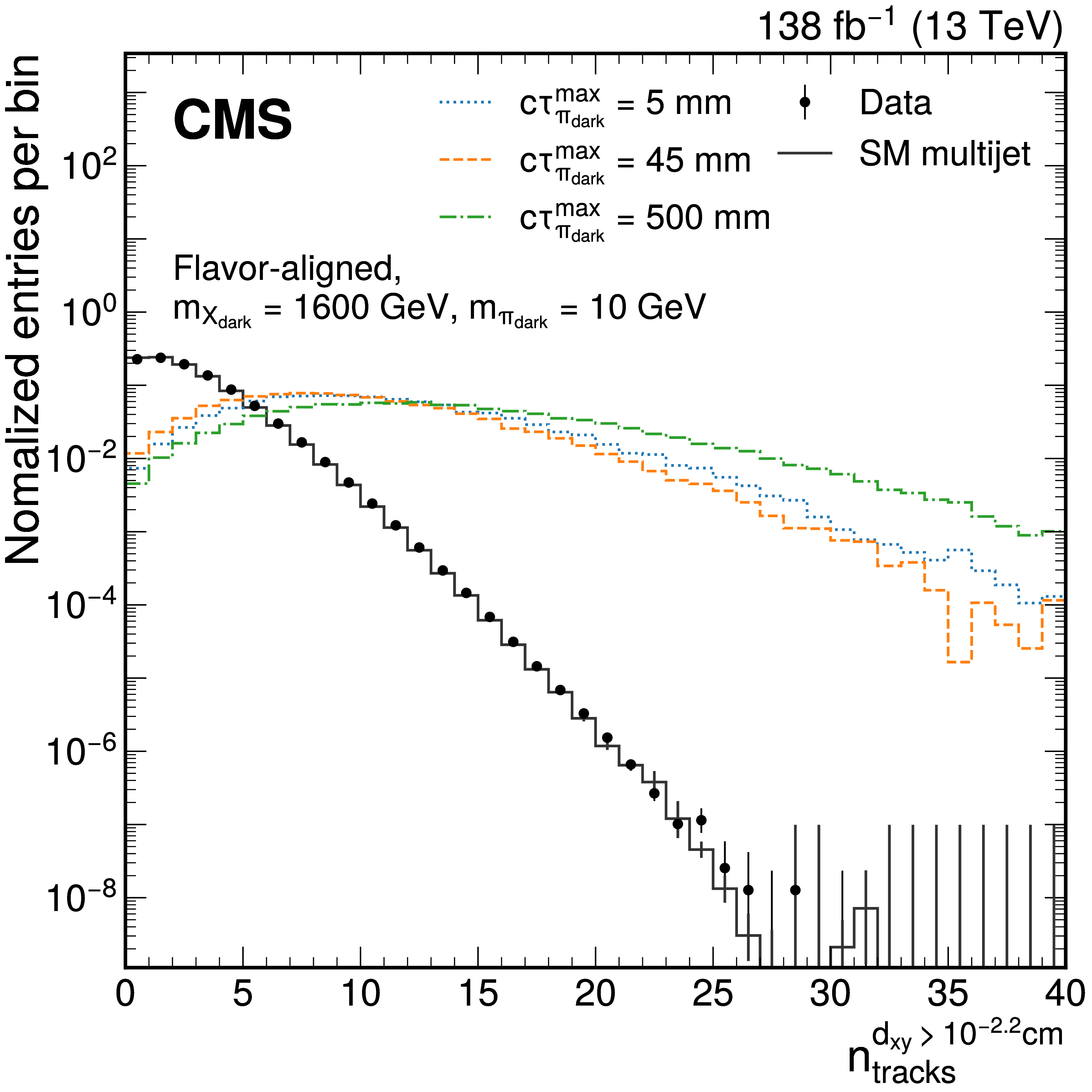
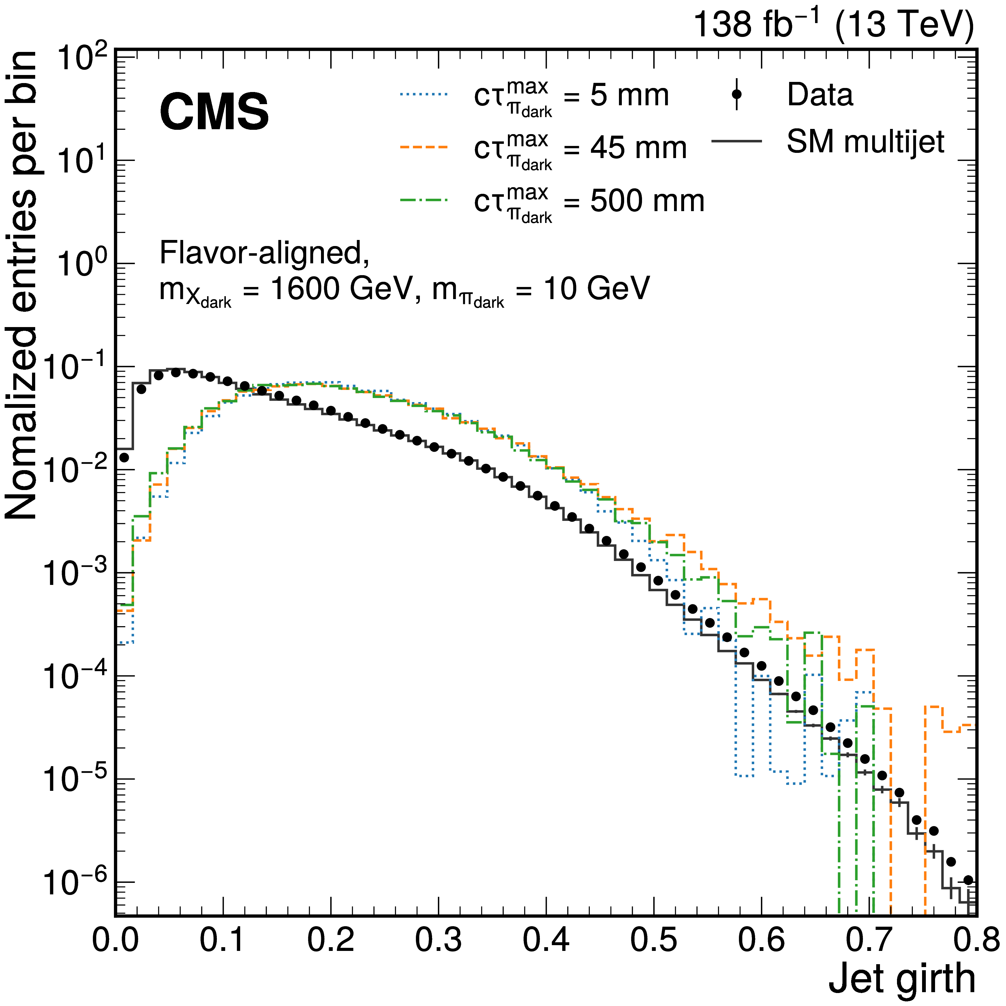
Figure 3:
Distributions of the jet variables used for the model-agnostic EJ tagging targeting flavor-aligned dark sector models for jets obtained in data (points), SM multijet simulation (gray line), and simulated signal jets (colored lines). The distribution of the number of tracks with $ d_{xy} > $ 10$^{-2.2}$ cm (jet girth) is shown on the left (right). The sums of the entries are normalized to unity. |
png pdf |
Figure 3-a:
Distributions of the jet variables used for the model-agnostic EJ tagging targeting flavor-aligned dark sector models for jets obtained in data (points), SM multijet simulation (gray line), and simulated signal jets (colored lines). The distribution of the number of tracks with $ d_{xy} > $ 10$^{-2.2}$ cm (jet girth) is shown on the left (right). The sums of the entries are normalized to unity. |
png pdf |
Figure 3-b:
Distributions of the jet variables used for the model-agnostic EJ tagging targeting flavor-aligned dark sector models for jets obtained in data (points), SM multijet simulation (gray line), and simulated signal jets (colored lines). The distribution of the number of tracks with $ d_{xy} > $ 10$^{-2.2}$ cm (jet girth) is shown on the left (right). The sums of the entries are normalized to unity. |

png pdf |
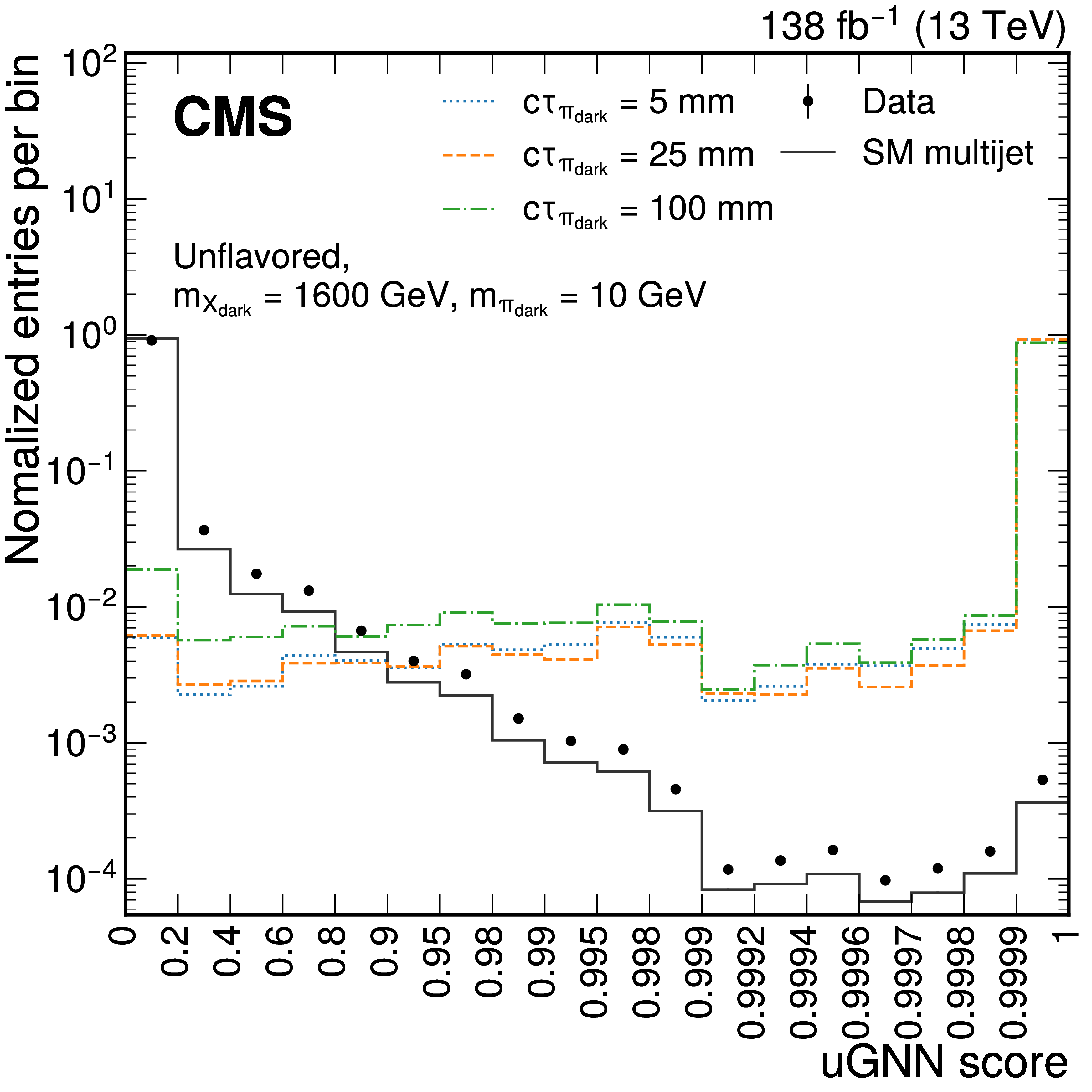
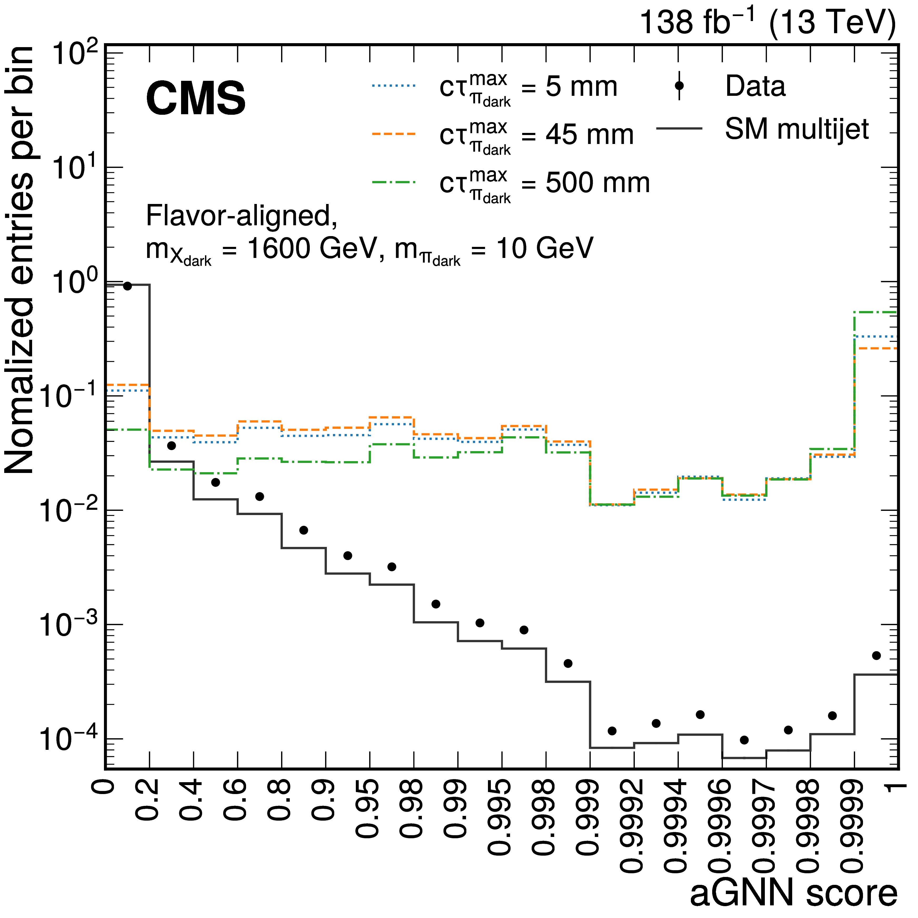
Figure 4:
Distributions of the output score of the uGNN (left) and aGNN (right) for the data (points with error bars), SM multijet simulation (dark gray line), and signal simulation (colored lines). The signal distributions in the left (right) plot are generated from the unflavored (flavor-aligned) model. Bins are chosen to correspond to the jet selection criteria defined in Table 5. The sums of the entries are normalized to unity. |
png pdf |
Figure 4-a:
Distributions of the output score of the uGNN (left) and aGNN (right) for the data (points with error bars), SM multijet simulation (dark gray line), and signal simulation (colored lines). The signal distributions in the left (right) plot are generated from the unflavored (flavor-aligned) model. Bins are chosen to correspond to the jet selection criteria defined in Table 5. The sums of the entries are normalized to unity. |
png pdf |
Figure 4-b:
Distributions of the output score of the uGNN (left) and aGNN (right) for the data (points with error bars), SM multijet simulation (dark gray line), and signal simulation (colored lines). The signal distributions in the left (right) plot are generated from the unflavored (flavor-aligned) model. Bins are chosen to correspond to the jet selection criteria defined in Table 5. The sums of the entries are normalized to unity. |
png pdf |
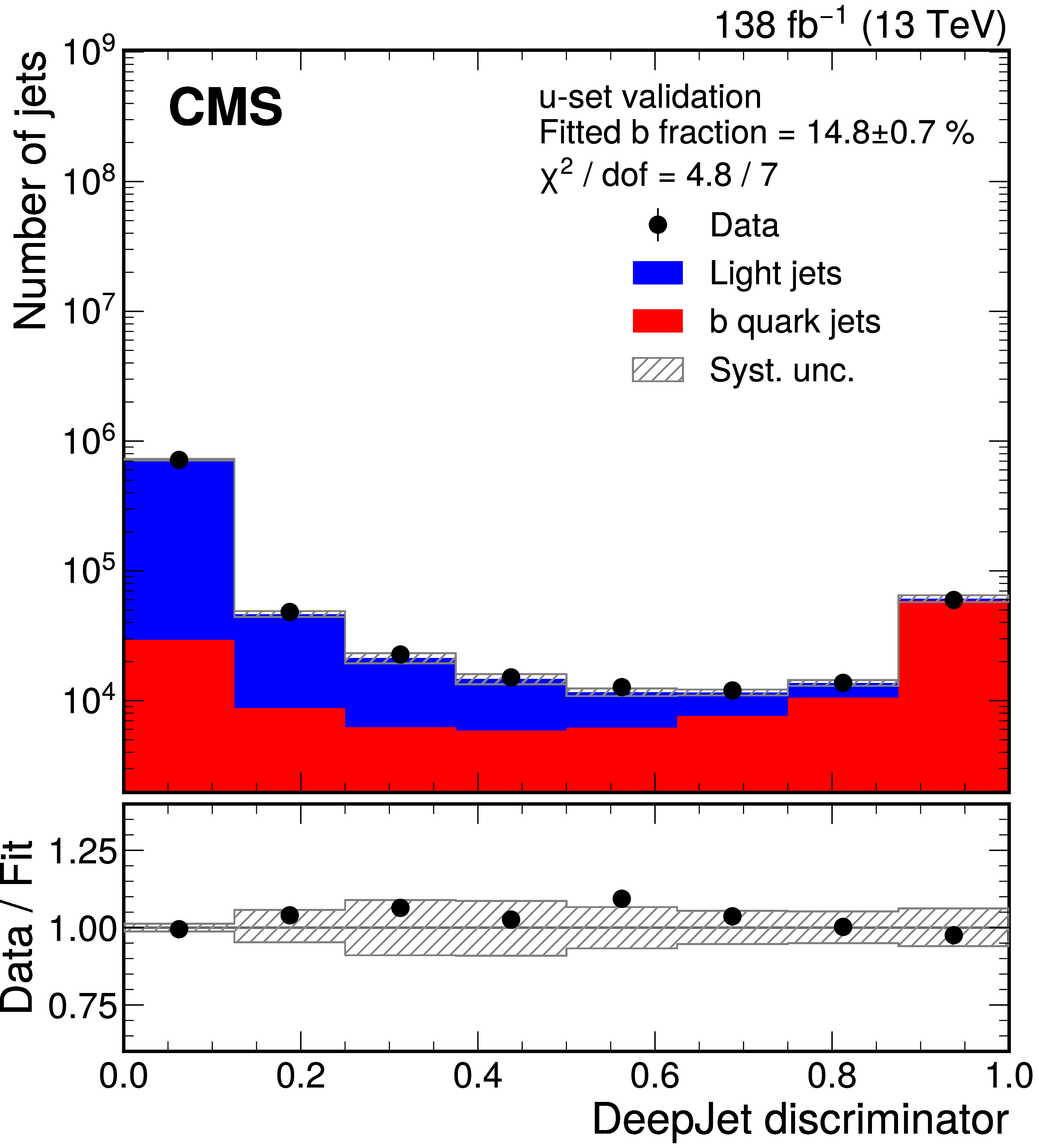
Figure 5:
Template fit of the DEEPJET discriminator used to determine the b jet fraction of the non-EJ tagged jets for data events that pass the ``u-set validation'' selection criteria, except with the requirement on the number of EJ-tagged jets changed from 2 to 1. The lower panel shows the ratio of the number of jets in the data compared to the sum of the fitted template distributions. |

png pdf |
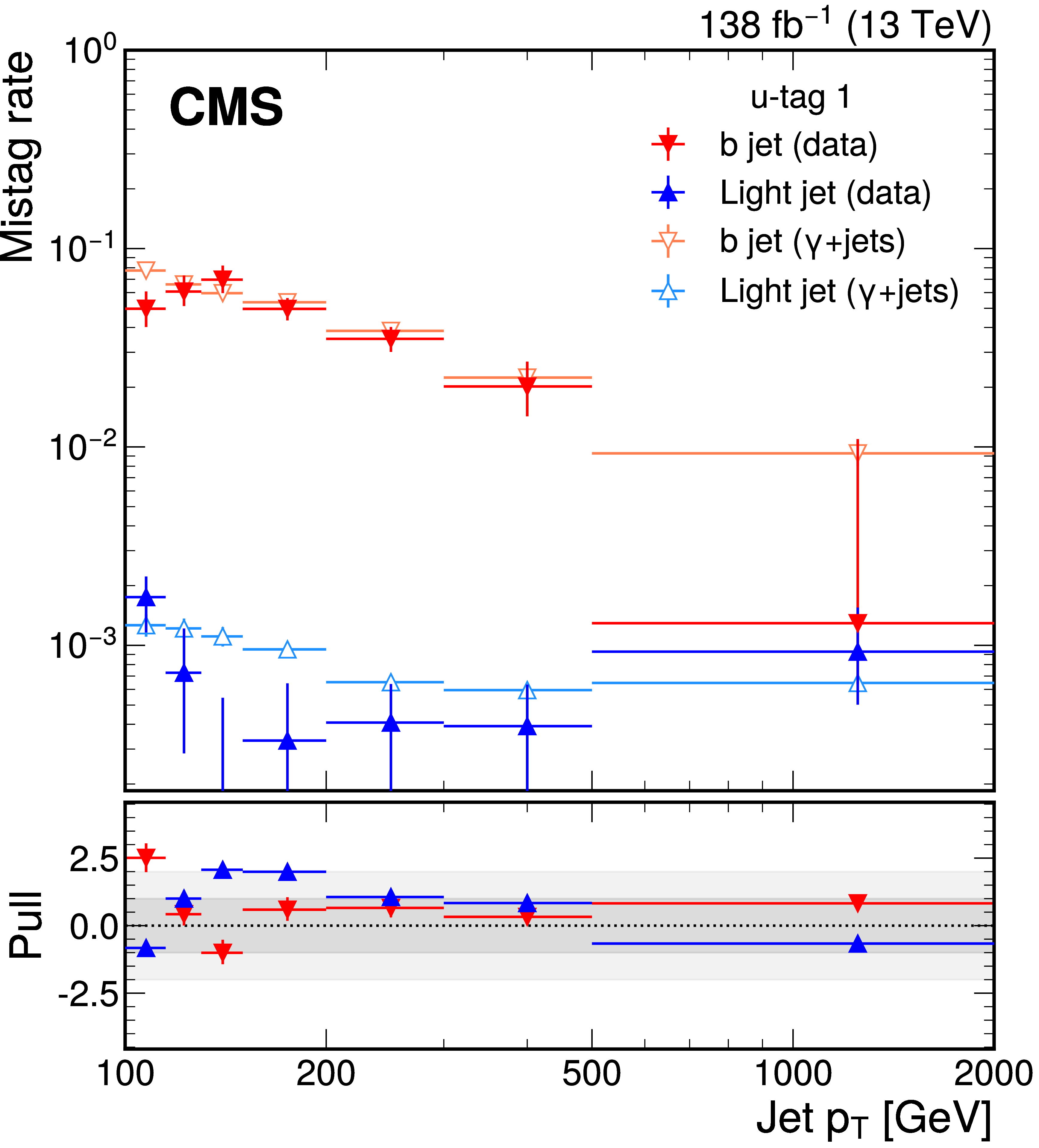
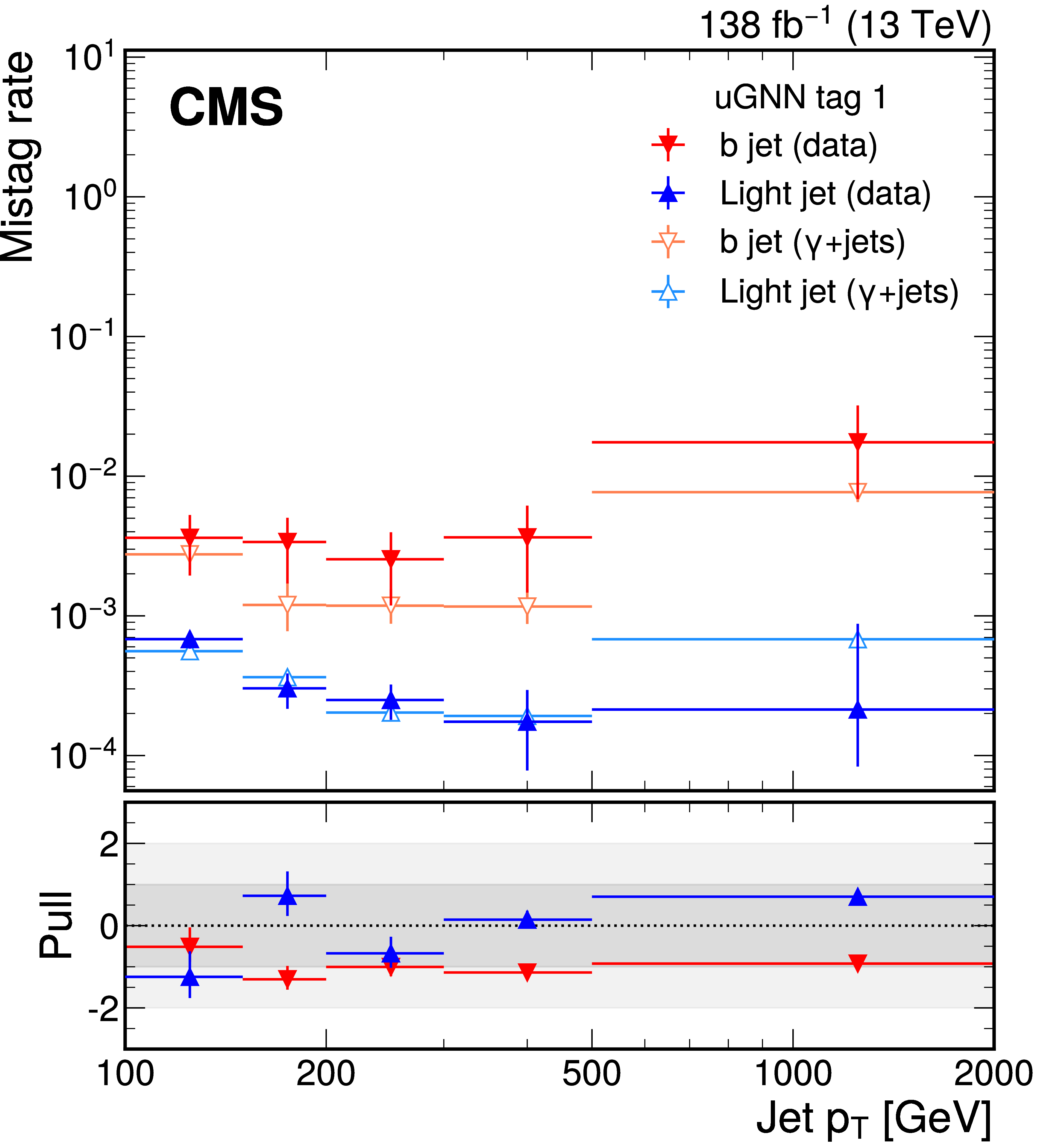
Figure 6:
The EJ tagger misidentification probability for b quark jets (red, orange) and light jets (light blue, dark blue) as a function of jet $ p_{\mathrm{T}} $ for the model-agnostic tagger ``u-tag 1'' (left) and the ML-based tagger ``uGNN tag 1'' (right), as defined in Tables 3 and 5, evaluated using data (red, dark blue) and generator-level flavor information from simulated samples (orange, light blue) in events containing a high-$ p_{\mathrm{T}} $ photon. The lower panel shows the pull, defined as the difference between the mistag rate calculated in simulation and mistag rate measured in data divided by the uncertainty measured in data. |
png pdf |
Figure 6-a:
The EJ tagger misidentification probability for b quark jets (red, orange) and light jets (light blue, dark blue) as a function of jet $ p_{\mathrm{T}} $ for the model-agnostic tagger ``u-tag 1'' (left) and the ML-based tagger ``uGNN tag 1'' (right), as defined in Tables 3 and 5, evaluated using data (red, dark blue) and generator-level flavor information from simulated samples (orange, light blue) in events containing a high-$ p_{\mathrm{T}} $ photon. The lower panel shows the pull, defined as the difference between the mistag rate calculated in simulation and mistag rate measured in data divided by the uncertainty measured in data. |
png pdf |
Figure 6-b:
The EJ tagger misidentification probability for b quark jets (red, orange) and light jets (light blue, dark blue) as a function of jet $ p_{\mathrm{T}} $ for the model-agnostic tagger ``u-tag 1'' (left) and the ML-based tagger ``uGNN tag 1'' (right), as defined in Tables 3 and 5, evaluated using data (red, dark blue) and generator-level flavor information from simulated samples (orange, light blue) in events containing a high-$ p_{\mathrm{T}} $ photon. The lower panel shows the pull, defined as the difference between the mistag rate calculated in simulation and mistag rate measured in data divided by the uncertainty measured in data. |
png pdf |
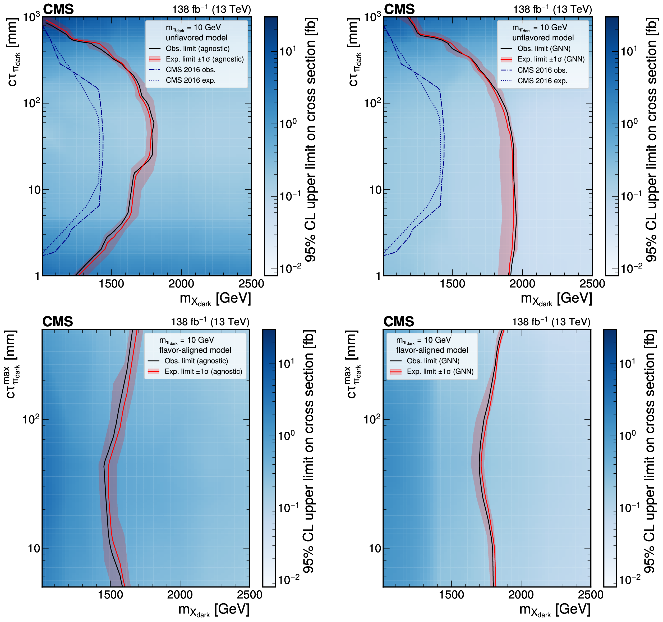
Figure 7:
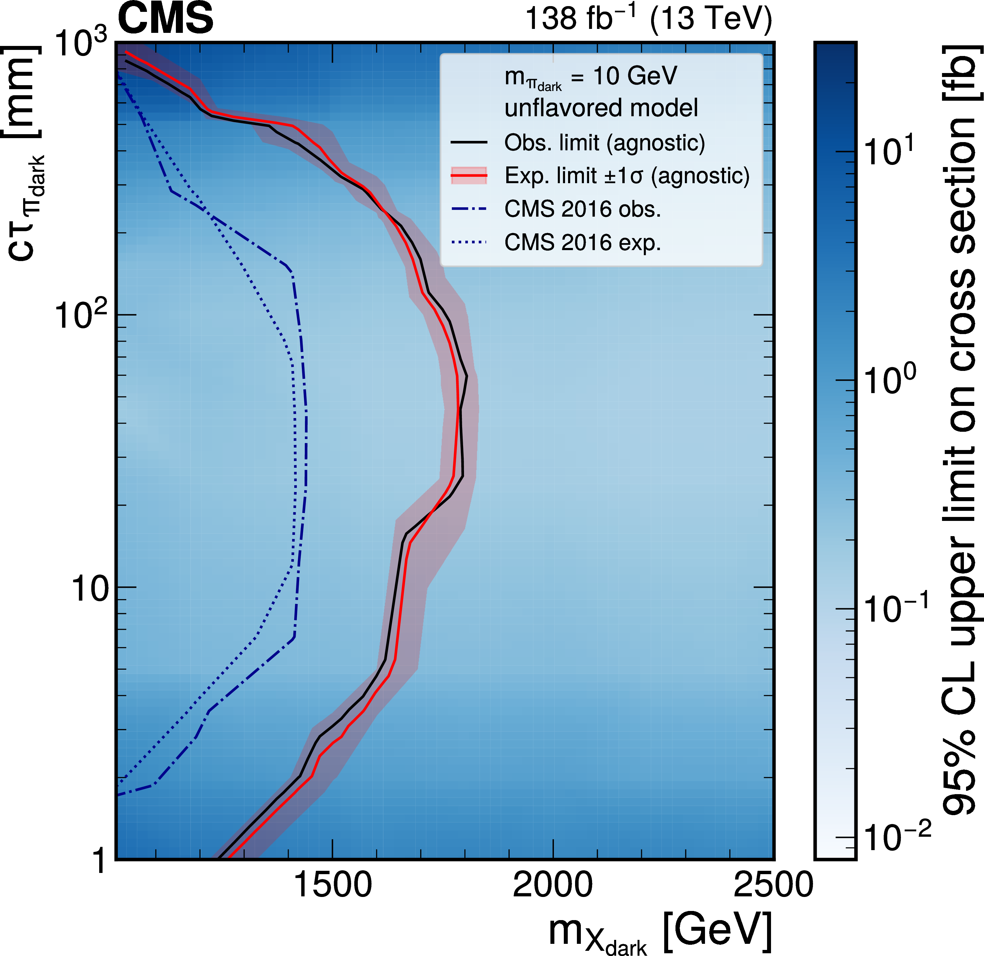
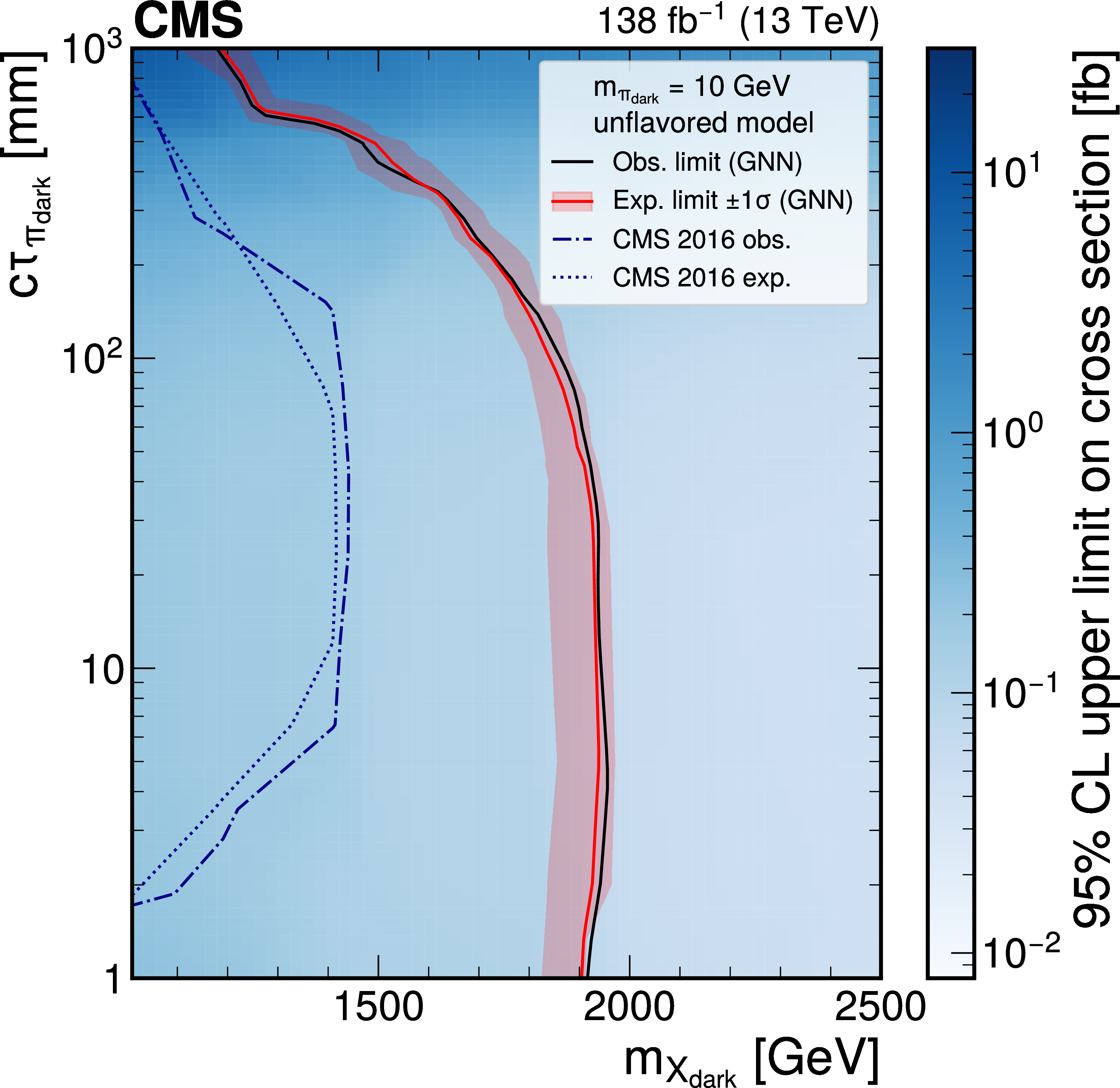
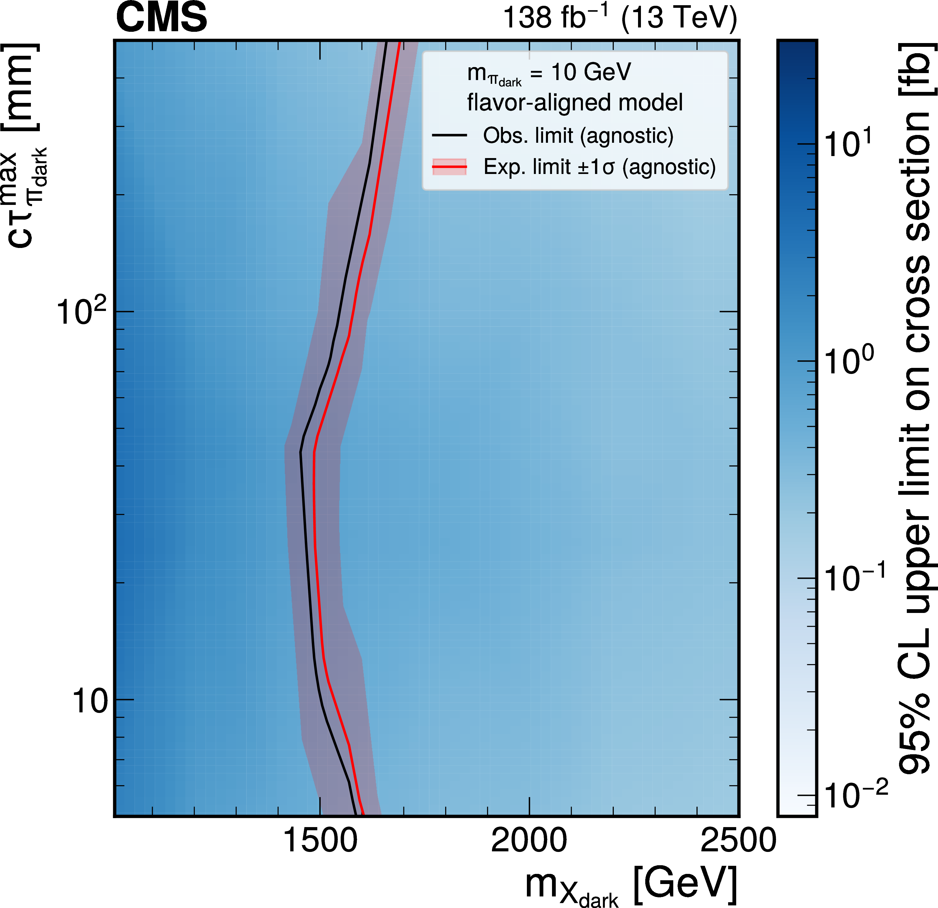
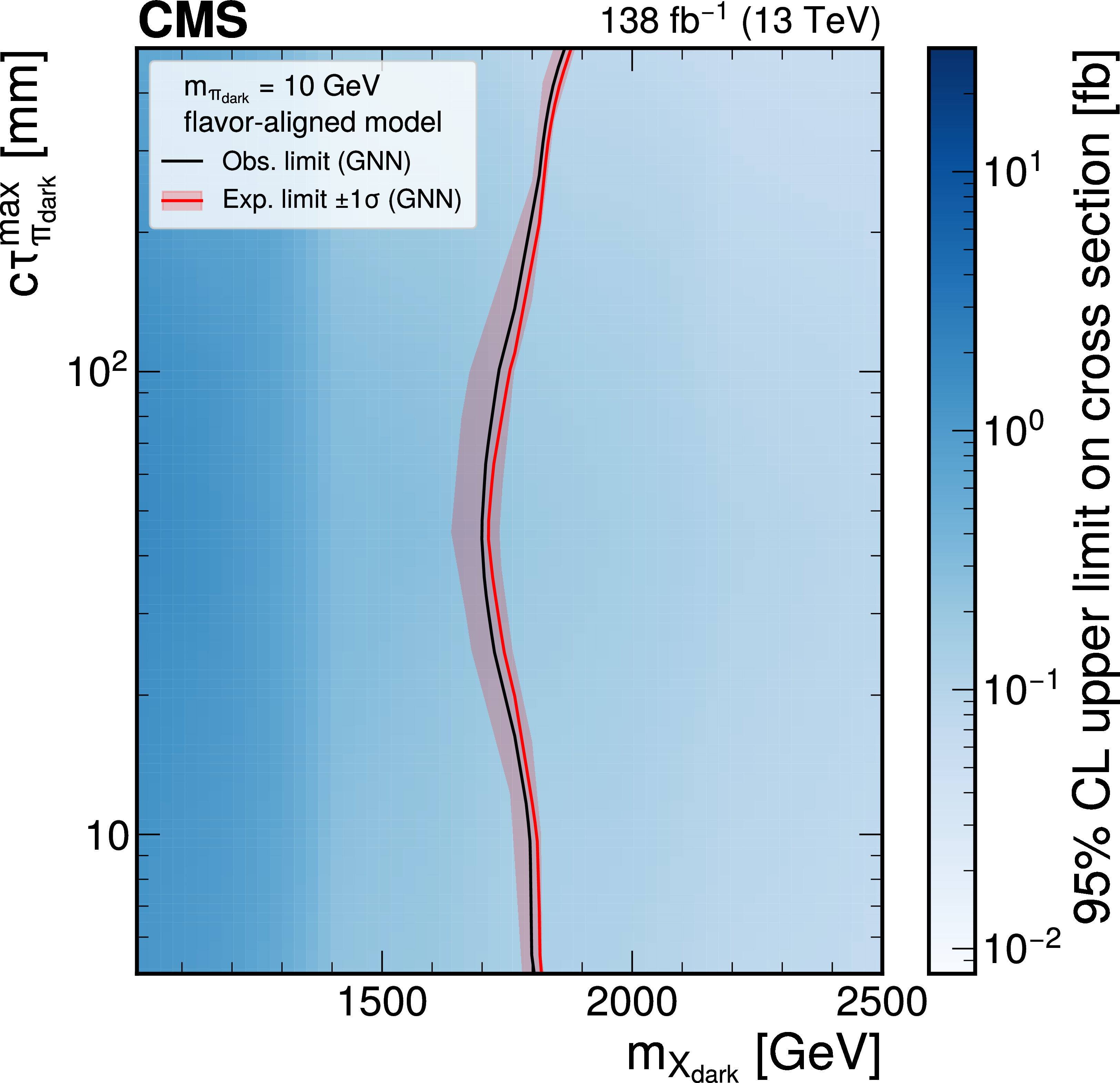
The 95% CL upper limits on the production cross section for various signal models in the unflavored scenario (upper plots) and the flavor-aligned scenario (lower plots) with $ m_{\pi_{\text{dark}}}= $ 10 GeV using the model-agnostic (GNN) EJ tagging method, on the left (right). The red curve is the expected exclusion limit, with the band representing its 68% CL variation. The black curve is the observed limit. The dark blue dotted curves in the upper plots are the expected and observed limits previously obtained by CMS [20]. |
png pdf |
Figure 7-a:
The 95% CL upper limits on the production cross section for various signal models in the unflavored scenario (upper plots) and the flavor-aligned scenario (lower plots) with $ m_{\pi_{\text{dark}}}= $ 10 GeV using the model-agnostic (GNN) EJ tagging method, on the left (right). The red curve is the expected exclusion limit, with the band representing its 68% CL variation. The black curve is the observed limit. The dark blue dotted curves in the upper plots are the expected and observed limits previously obtained by CMS [20]. |
png pdf |
Figure 7-b:
The 95% CL upper limits on the production cross section for various signal models in the unflavored scenario (upper plots) and the flavor-aligned scenario (lower plots) with $ m_{\pi_{\text{dark}}}= $ 10 GeV using the model-agnostic (GNN) EJ tagging method, on the left (right). The red curve is the expected exclusion limit, with the band representing its 68% CL variation. The black curve is the observed limit. The dark blue dotted curves in the upper plots are the expected and observed limits previously obtained by CMS [20]. |
png pdf |
Figure 7-c:
The 95% CL upper limits on the production cross section for various signal models in the unflavored scenario (upper plots) and the flavor-aligned scenario (lower plots) with $ m_{\pi_{\text{dark}}}= $ 10 GeV using the model-agnostic (GNN) EJ tagging method, on the left (right). The red curve is the expected exclusion limit, with the band representing its 68% CL variation. The black curve is the observed limit. The dark blue dotted curves in the upper plots are the expected and observed limits previously obtained by CMS [20]. |
png pdf |
Figure 7-d:
The 95% CL upper limits on the production cross section for various signal models in the unflavored scenario (upper plots) and the flavor-aligned scenario (lower plots) with $ m_{\pi_{\text{dark}}}= $ 10 GeV using the model-agnostic (GNN) EJ tagging method, on the left (right). The red curve is the expected exclusion limit, with the band representing its 68% CL variation. The black curve is the observed limit. The dark blue dotted curves in the upper plots are the expected and observed limits previously obtained by CMS [20]. |
png pdf |
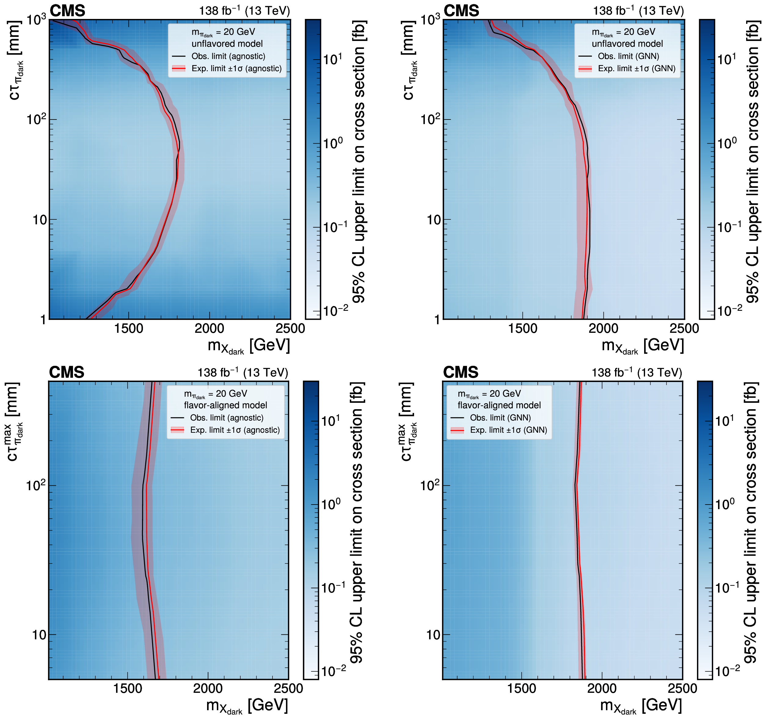
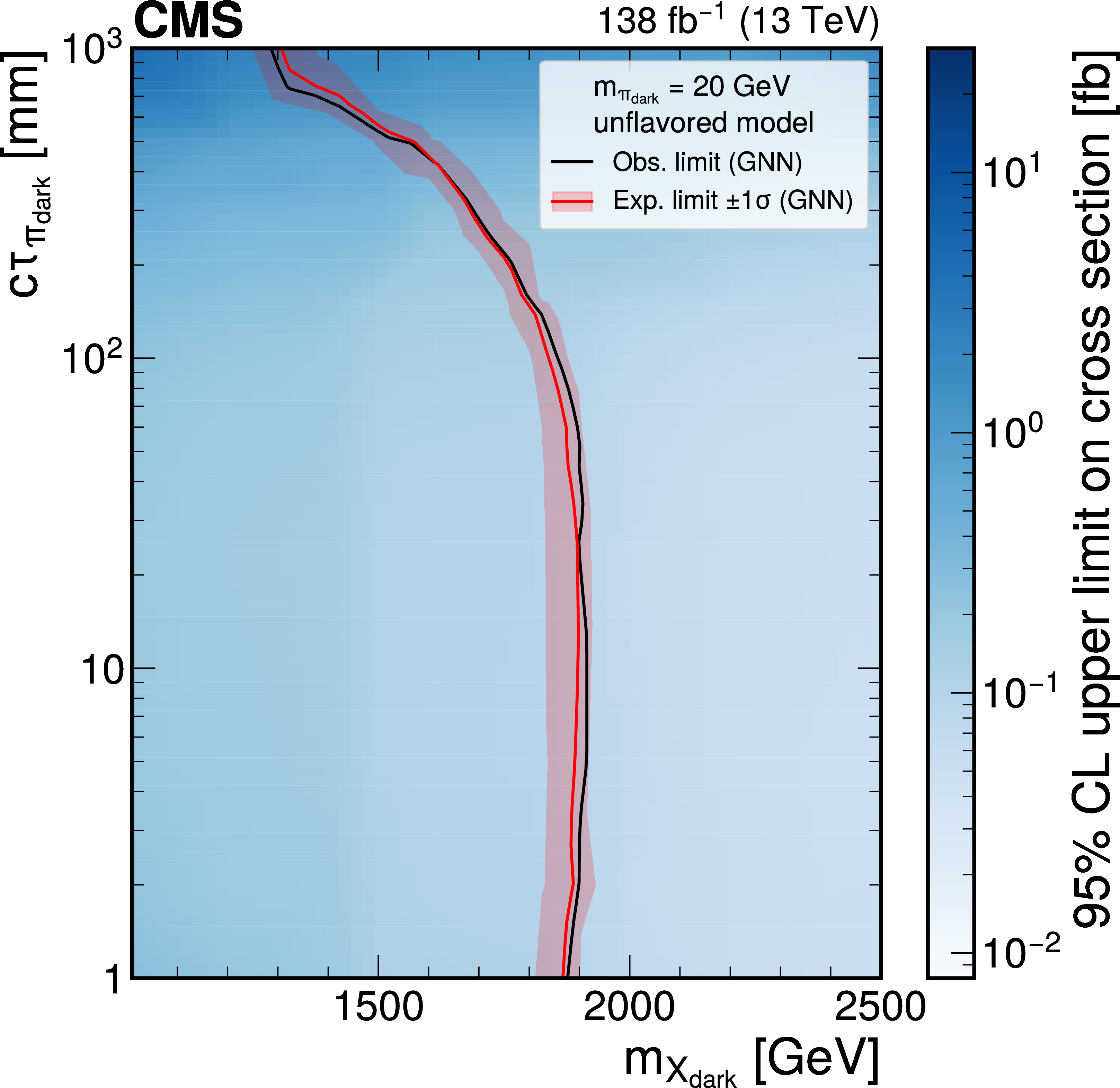
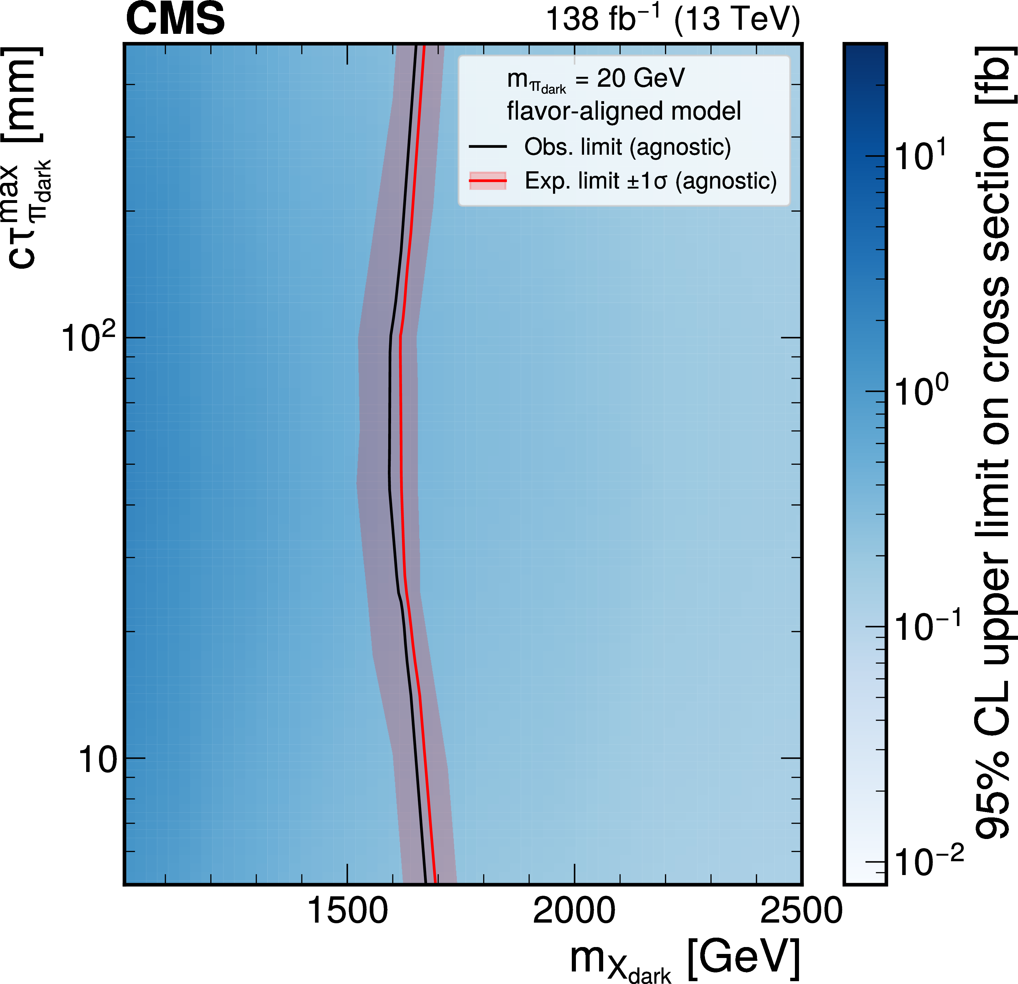
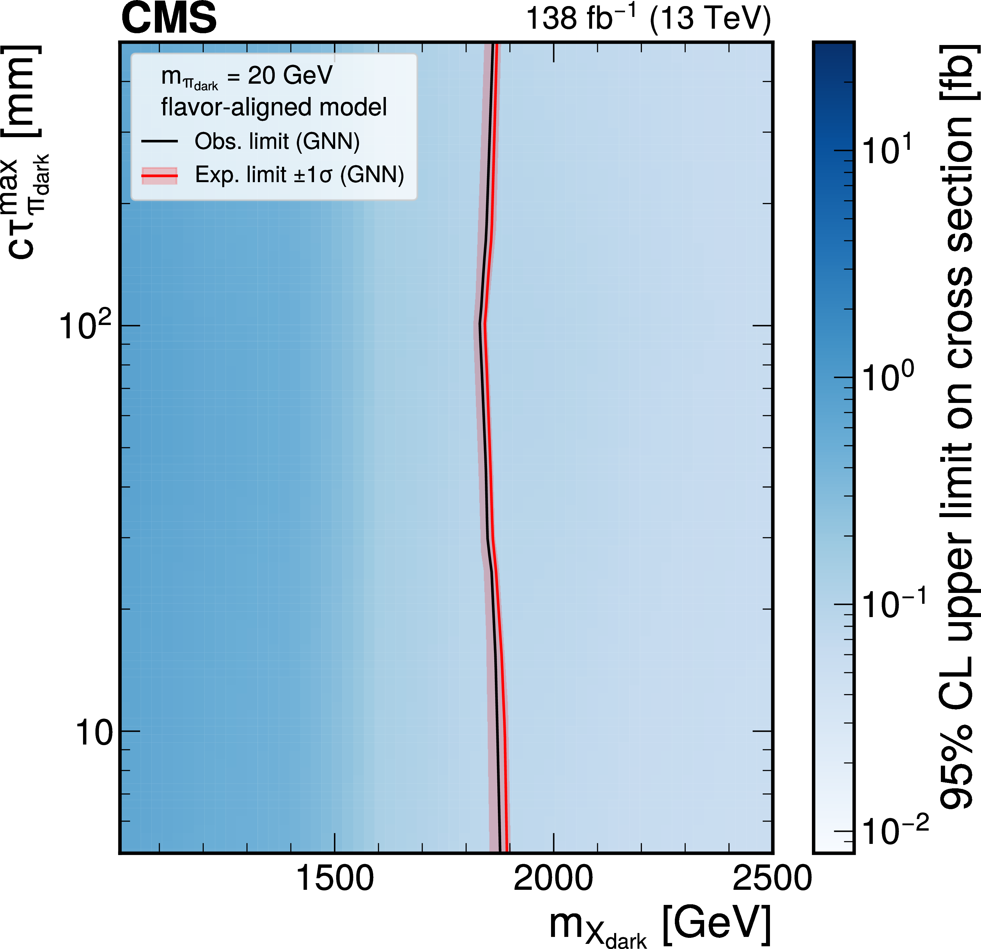
Figure 8:
The 95% CL upper limits on the production cross section for various signal models in the unflavored scenario (upper plots) and the flavor-aligned scenario (lower plots) with $ m_{\pi_{\text{dark}}}= $ 20 GeV using the model-agnostic (GNN) EJ tagging method, on the left (right). The red curve is the expected exclusion limit, with the band representing its 68% CL variation. The black curve is the observed limit. |

png pdf |
Figure 8-a:
The 95% CL upper limits on the production cross section for various signal models in the unflavored scenario (upper plots) and the flavor-aligned scenario (lower plots) with $ m_{\pi_{\text{dark}}}= $ 20 GeV using the model-agnostic (GNN) EJ tagging method, on the left (right). The red curve is the expected exclusion limit, with the band representing its 68% CL variation. The black curve is the observed limit. |
png pdf |
Figure 8-b:
The 95% CL upper limits on the production cross section for various signal models in the unflavored scenario (upper plots) and the flavor-aligned scenario (lower plots) with $ m_{\pi_{\text{dark}}}= $ 20 GeV using the model-agnostic (GNN) EJ tagging method, on the left (right). The red curve is the expected exclusion limit, with the band representing its 68% CL variation. The black curve is the observed limit. |
png pdf |
Figure 8-c:
The 95% CL upper limits on the production cross section for various signal models in the unflavored scenario (upper plots) and the flavor-aligned scenario (lower plots) with $ m_{\pi_{\text{dark}}}= $ 20 GeV using the model-agnostic (GNN) EJ tagging method, on the left (right). The red curve is the expected exclusion limit, with the band representing its 68% CL variation. The black curve is the observed limit. |
png pdf |
Figure 8-d:
The 95% CL upper limits on the production cross section for various signal models in the unflavored scenario (upper plots) and the flavor-aligned scenario (lower plots) with $ m_{\pi_{\text{dark}}}= $ 20 GeV using the model-agnostic (GNN) EJ tagging method, on the left (right). The red curve is the expected exclusion limit, with the band representing its 68% CL variation. The black curve is the observed limit. |
png pdf |
Figure 9:
The 95% CL upper limits on the production cross section for various signal models in the flavor-aligned scenario with $ m_{\pi_{\text{dark}}}= $ 6 GeV using the model-agnostic (GNN) EJ tagging method, on the left (right). The red curve is the expected exclusion limit, with the band representing its 68% CL variation. The black curve is the observed limit. |
png pdf |
Figure 9-a:
The 95% CL upper limits on the production cross section for various signal models in the flavor-aligned scenario with $ m_{\pi_{\text{dark}}}= $ 6 GeV using the model-agnostic (GNN) EJ tagging method, on the left (right). The red curve is the expected exclusion limit, with the band representing its 68% CL variation. The black curve is the observed limit. |
png pdf |
Figure 9-b:
The 95% CL upper limits on the production cross section for various signal models in the flavor-aligned scenario with $ m_{\pi_{\text{dark}}}= $ 6 GeV using the model-agnostic (GNN) EJ tagging method, on the left (right). The red curve is the expected exclusion limit, with the band representing its 68% CL variation. The black curve is the observed limit. |
| Tables | |
png pdf |
Table 1:
Model parameters for the unflavored model. |
png pdf |
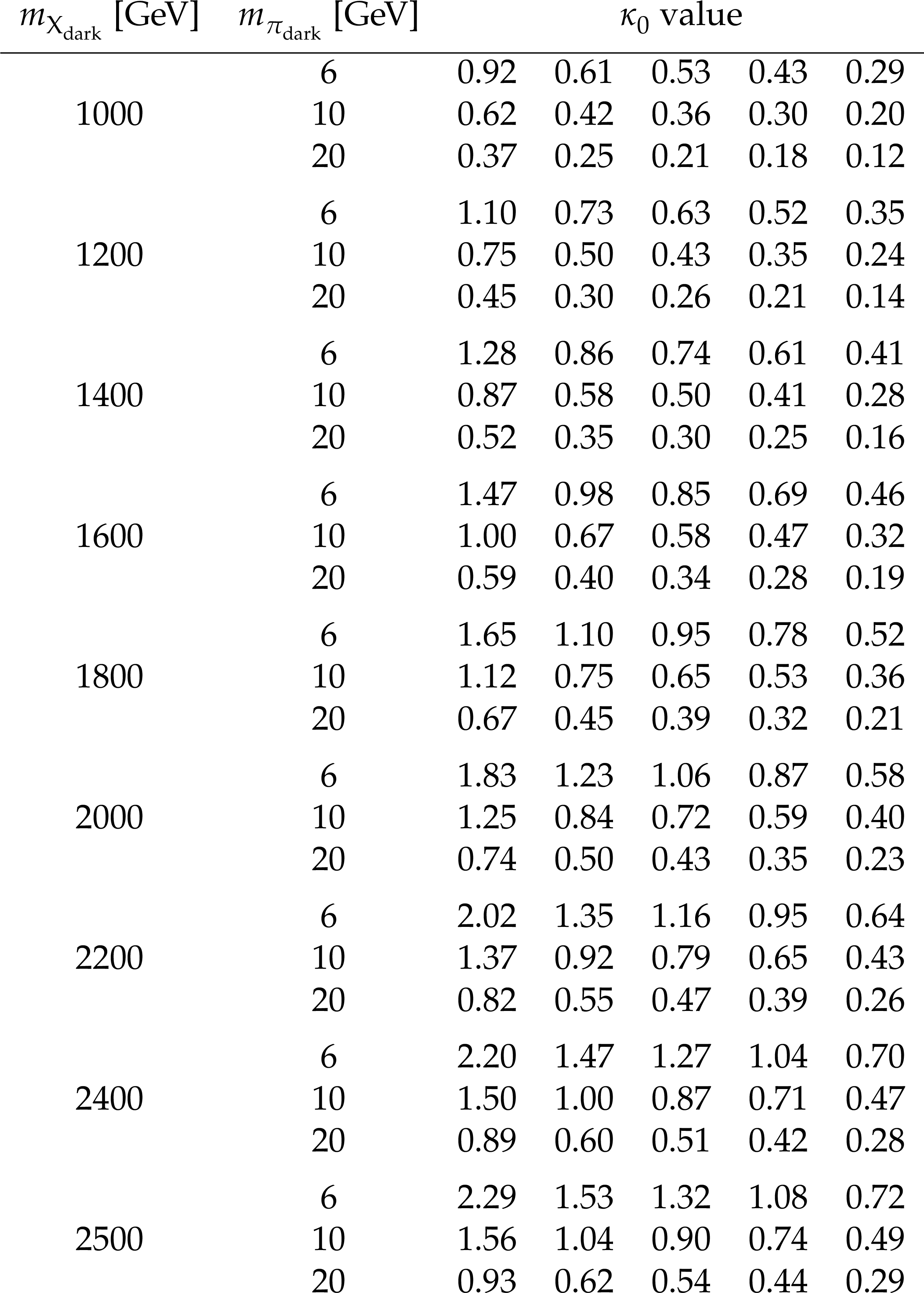
Table 2:
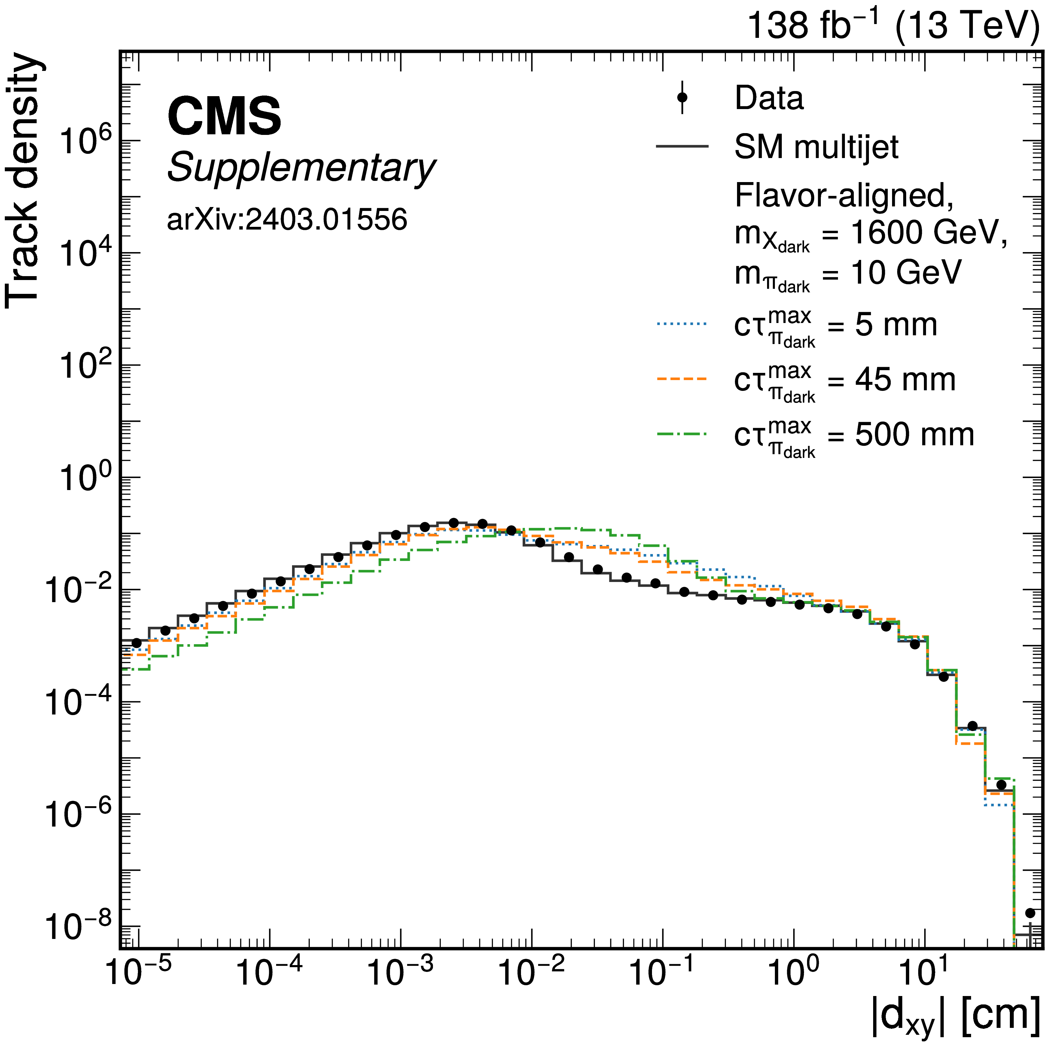
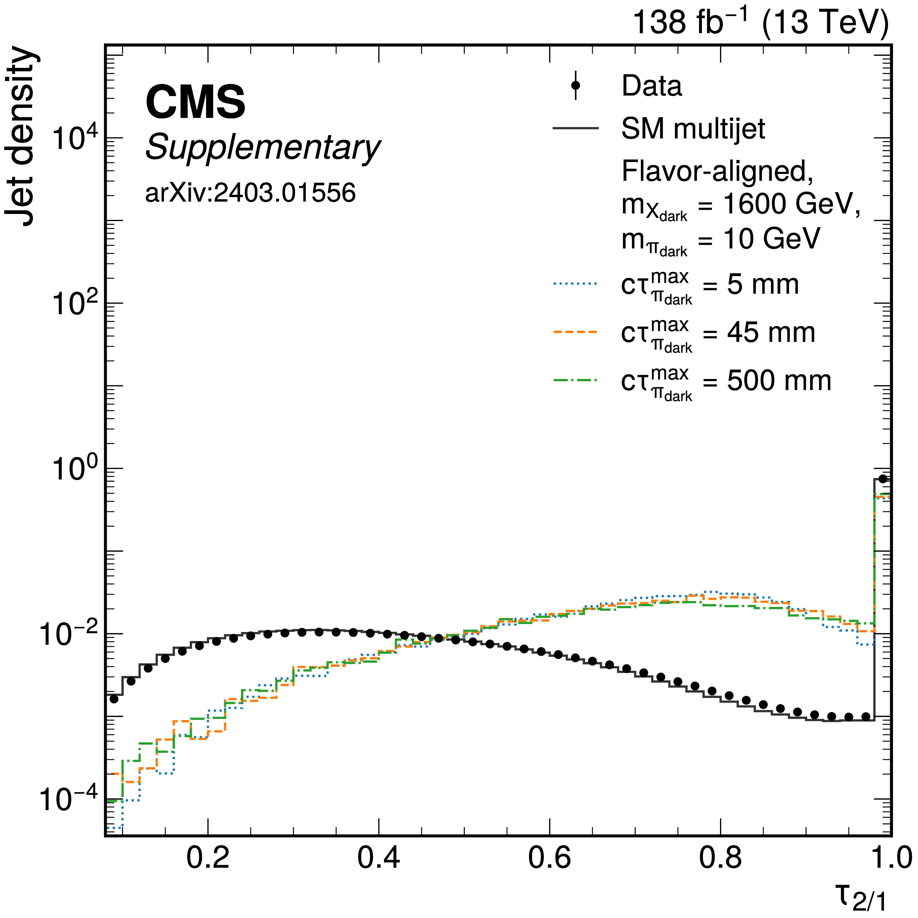
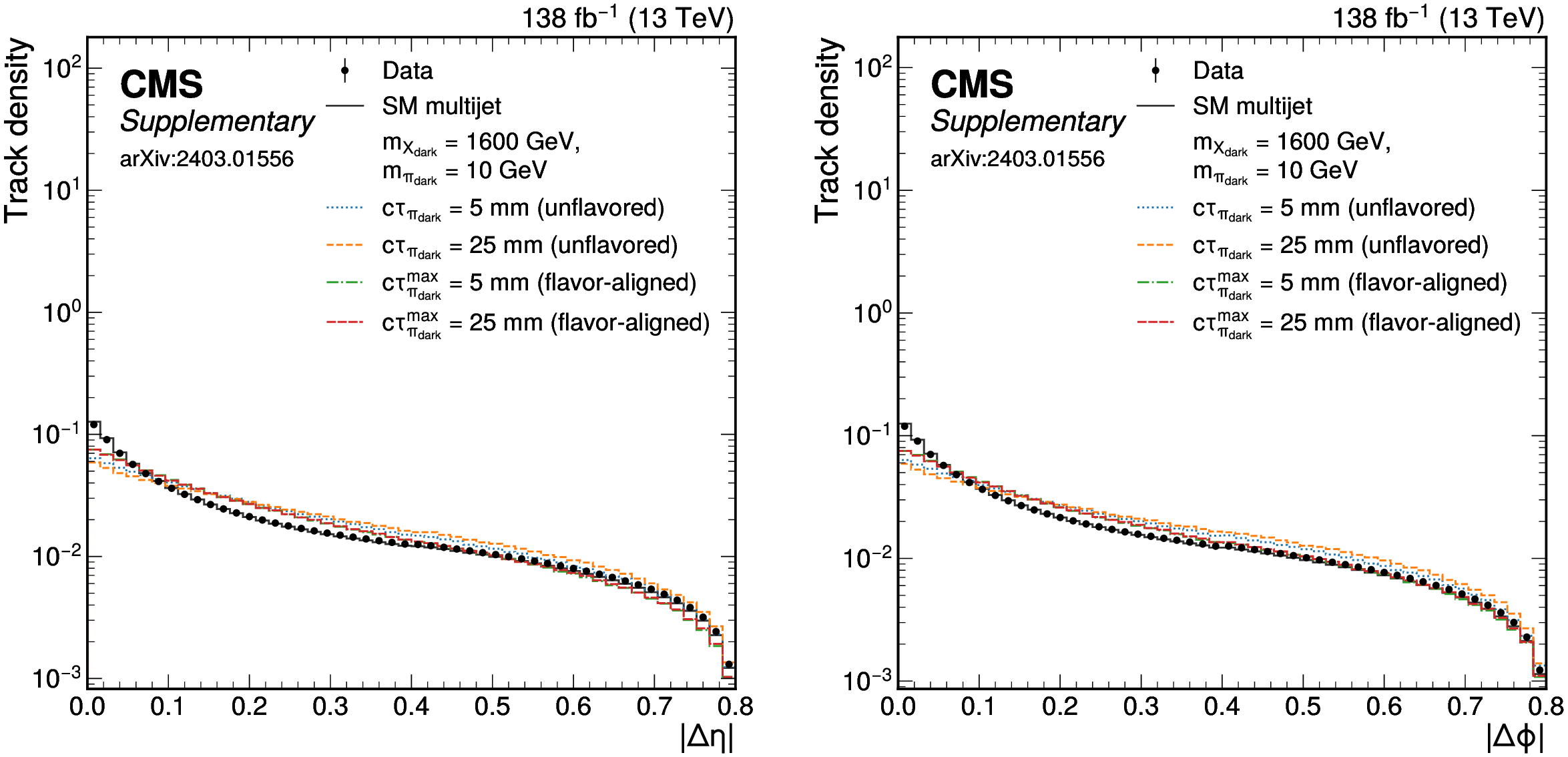
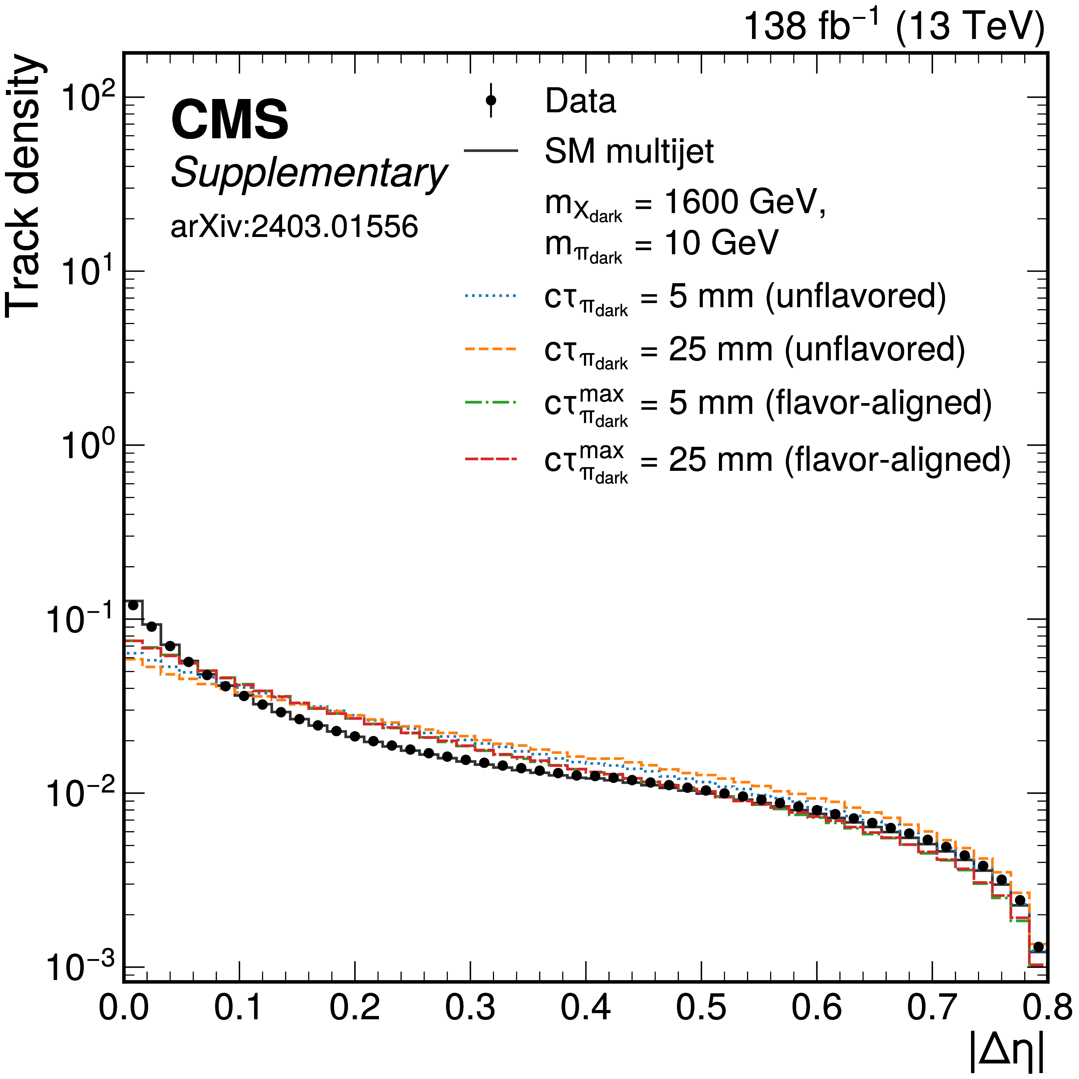
Parameters used for the flavor-aligned model. In order to probe a range of lifetimes, the values of $ \kappa_0 $ listed in columns 3--7 are tuned to give the desired $ c\tau_{\pi_{\text{dark}}}^{\text{max}} $ values of 5, 25, 45, 100, and 500 mm. In addition, samples were made with fixed $ \kappa_0= $ 1, with a resultant value of $ c\tau_{\pi_{\text{dark}}}^{\text{max}} $ that depends on the other model parameters. |
png pdf |
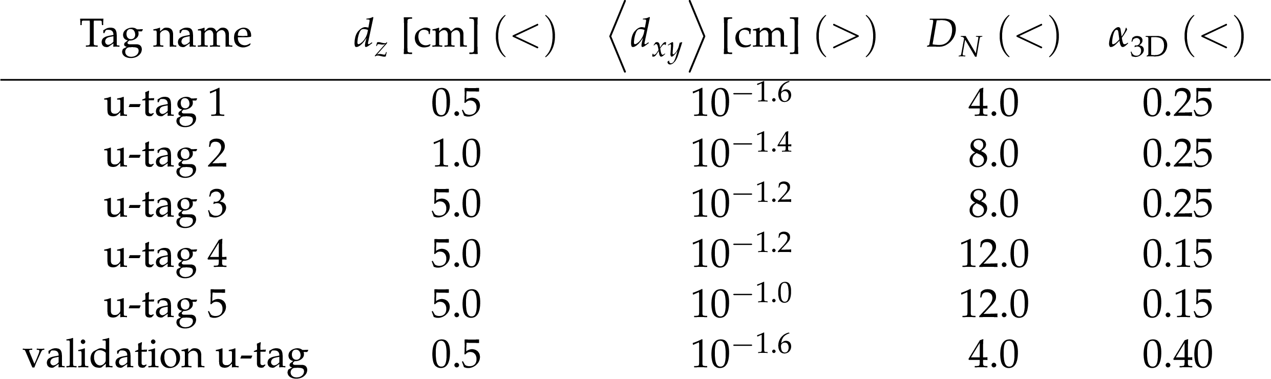
Table 3:
Emerging jet selection criteria for the model-agnostic analysis designed for the unflavored scenario. The validation regions are discussed in Section 5.4. The symbols in parentheses indicate a minimum ($> $) or maximum ($<$) requirement. |

png pdf |
Table 4:
Emerging jet selection criteria for the model-agnostic analysis designed for the flavor-aligned scenario. The validation tag is described in Section 5.4. The symbols in parentheses indicate a minimum ($> $) or maximum ($<$) requirement. |
png pdf |
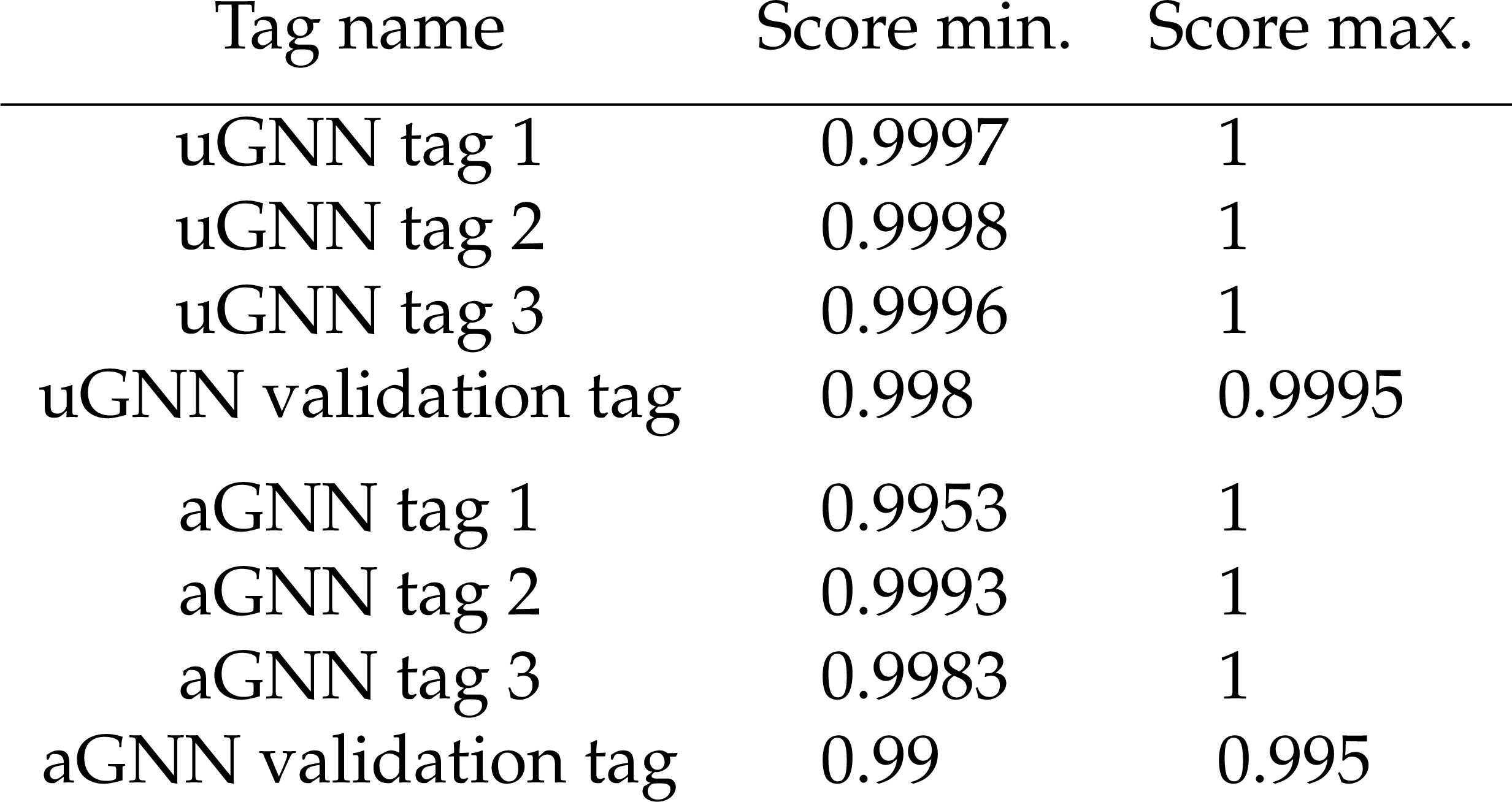
Table 5:
The GNN score range used to identify a jet as an EJ. The uGNN (aGNN) tag indicates that the tagger uses the output score of the GNN trained on the unflavored (flavor-aligned) simulated signal samples. The validation tags are described in Section 5.4. |
png pdf |
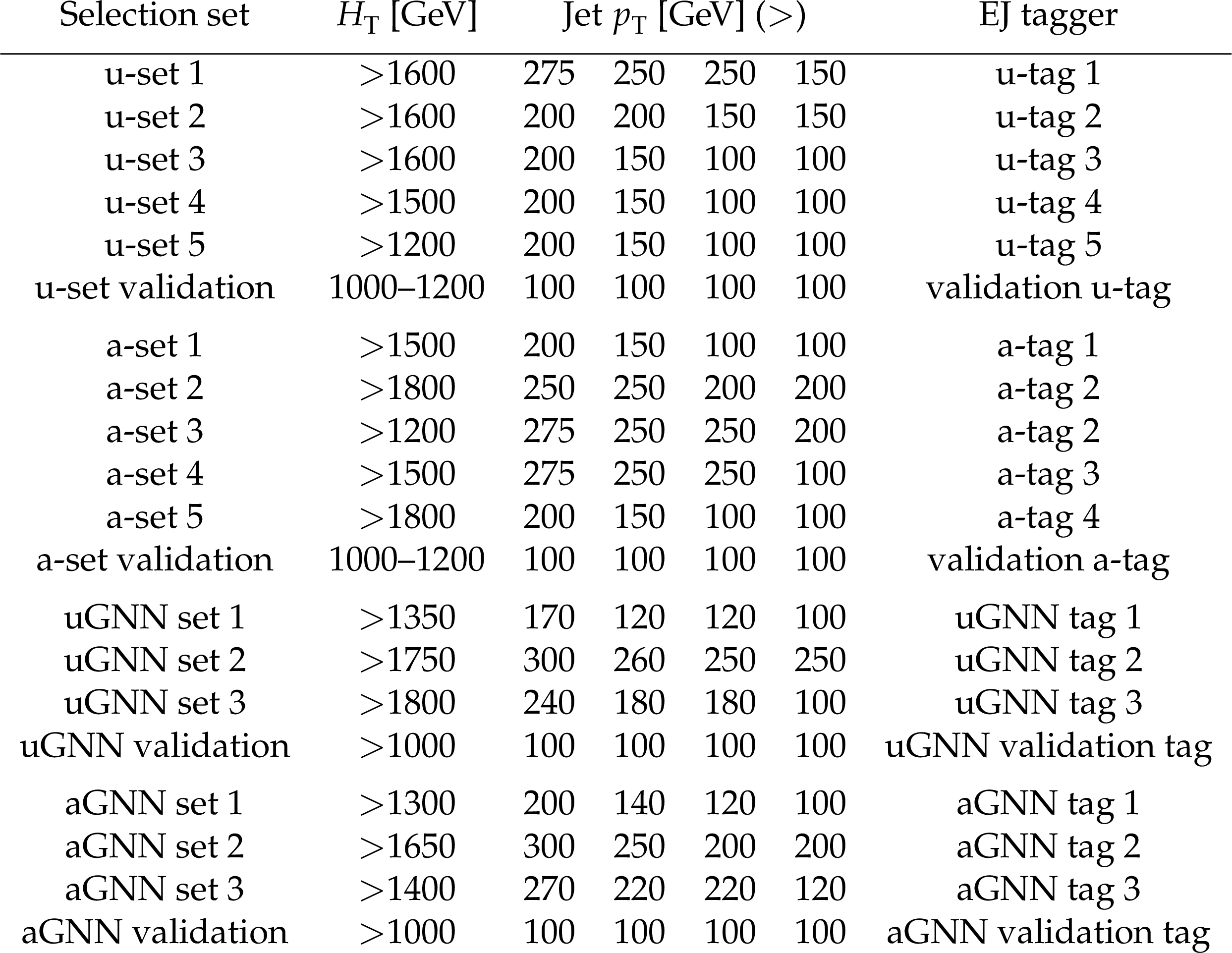
Table 6:
Event selection criteria used for the analysis. The validation selection criteria are described in Section 5.4. |
png pdf |
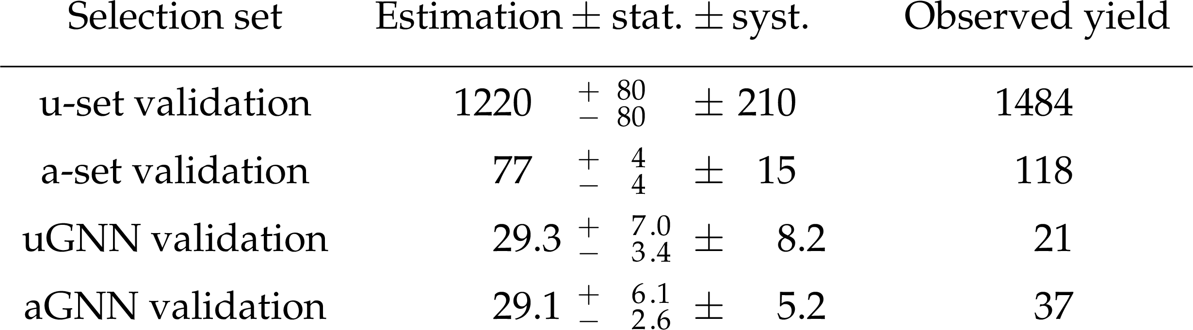
Table 7:
The observed yield of events in data satisfying the validation selection criteria with at least two jets passing the corresponding validation tag, and the estimation based on the misidentification rate calculated using validation events with exactly one jet passing the validation tagger scaled by the factor given in Eq. (4). The statistical and systematic uncertainties are reported for the estimated yields. |
png pdf |
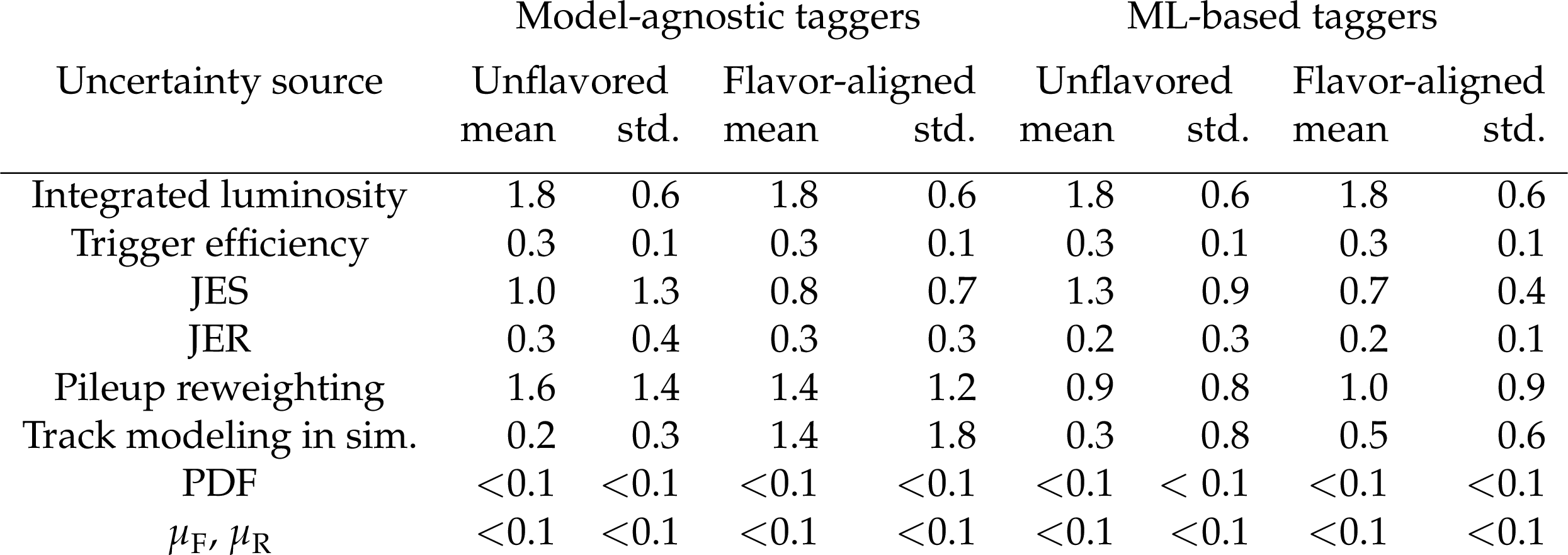
Table 8:
Mean and standard deviation (std.) of the relative uncertainty calculated on the unflavored and flavor-aligned samples, by source, in percent. |

png pdf |
Table 9:
The estimated number of events from the background prediction based on control samples in data and the observed event yields. Statistical and systematic uncertainties in the estimated background are provided. |
| Summary |
| A search for emerging jet signatures arising from a strongly interacting dark sector produced in proton-proton collisions has been presented, using data corresponding to an integrated luminosity of 138 fb$ ^{-1} $ at $ \sqrt{s}= $ 13 TeV. The signal model contains a family of dark quarks that couple to the standard model (SM) quarks via a scalar mediator $ \text{X}_{\text{dark}} $. Dark pions ($ \pi_{\text{dark}} $) with a significant lifetime ($ c\tau_{\pi_{\text{dark}}} $) are produced by the hadronization of the dark quarks; these then decay to SM particles at vertices displaced from the proton-proton interaction point. As the scalar mediator is assumed to be produced in pairs, and each decays to an SM quark and a dark quark, the signature of this process is two SM jets plus two jets of particles with constituents emerging from displaced vertices. Both unflavored and flavor-aligned couplings between the SM quarks and the dark quarks are examined in the search. Events are selected using either a traditional cut-based approach or a graph neural network to identify emerging jets, in combination with other event-level selection criteria. The overall selection requirements are optimized for each coupling scenario and for different combinations of the mediator particle mass, dark pion mass, and dark pion lifetime. No excess of events beyond the SM expectations is found, and the observed 95% confidence level exclusion limits agree with the expected limits. For the unflavored model, dark mediator masses $ m_{\text{X}_{\text{dark}}} < $ 1950 GeV are excluded for $ c\tau_{\pi_{\text{dark}}}\approx$ 100 mm and $ m_{\pi_{\text{dark}}}= $ 10 GeV, while the flavor-aligned model result excludes $ m_{\text{X}_{\text{dark}}} < $ 1850 GeV at $ c\tau_{\pi_{\text{dark}}}^{\text{max}}\approx$ 500 mm for $ m_{\pi_{\text{dark}}}= $ 10 GeV. This result surpasses the previous search for emerging jets in the unflavored scenario, increasing the experimental limit of the dark mediator particle by $ {\approx} $ 500 GeV to set the most stringent limits to date, and provides the first direct exclusion of the flavor-aligned scenario. |
| Additional Figures | |
png pdf |
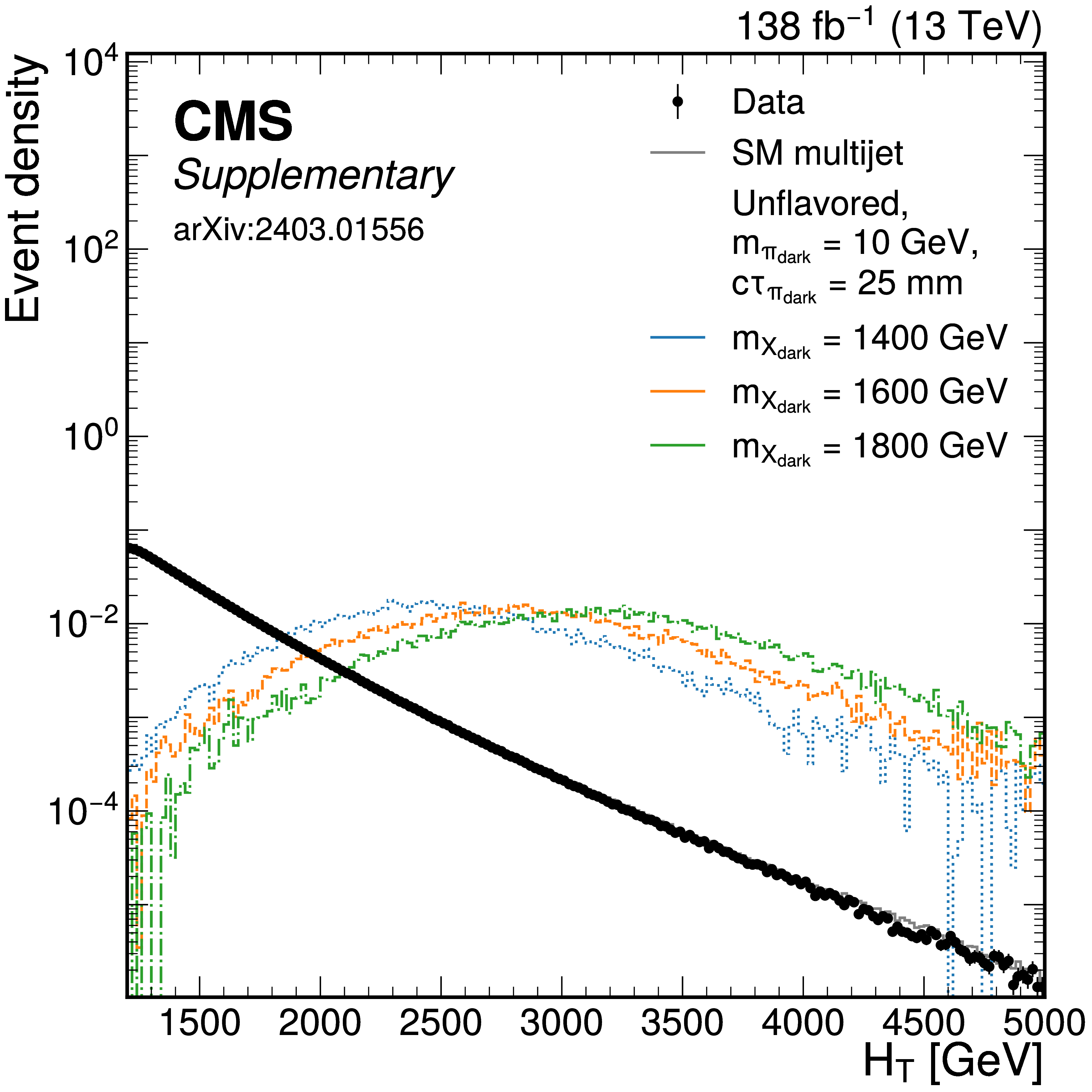
Additional Figure 1:
Example of $ H_{\mathrm{T}} $ distribution of events in CMS data (points), SM multijet events from simulation (gray line), and various signal samples with varying dark mediator masses (colored lines) for events that pass the trigger requirements and also have 4 jets with $ p_{\mathrm{T}} > $ 100 GeV. The distribution from various processes have their total event count normalized to 1. |
png pdf |
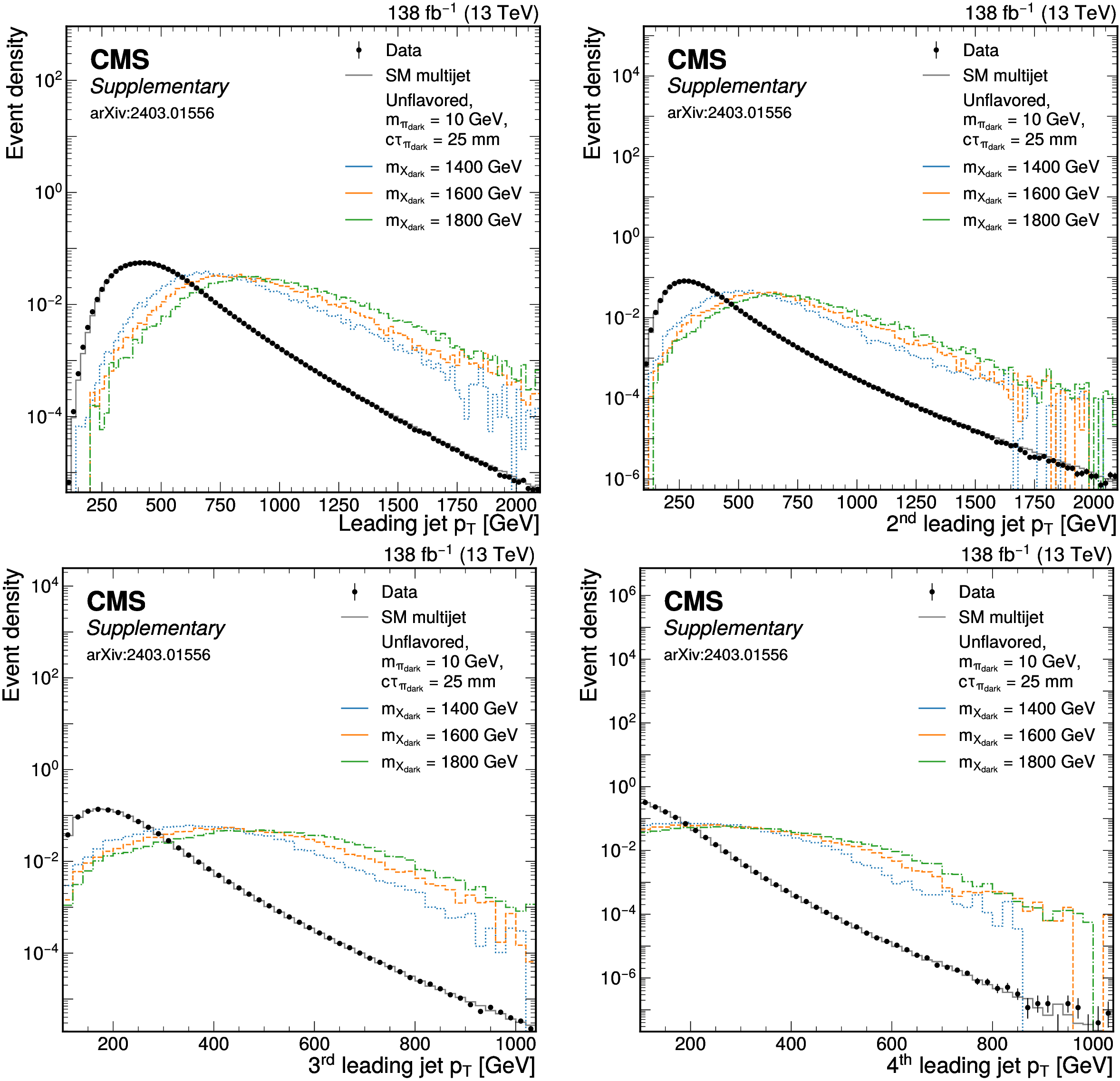
Additional Figure 2:
Example of jet $ p_{\mathrm{T}} $ distributions of events in CMS data (points), SM multijet events from simulation (gray line), and various signal samples with varying dark mediator masses (colored lines) for events that pass the trigger requirements and also have 4 jets with $ p_{\mathrm{T}} > $ 100 GeV. The leading jet $ p_{\mathrm{T}} $ distribution is shown in the top right plot, the second leading jet $ p_{\mathrm{T}} $ in the top left, the third leading jet $ p_{\mathrm{T}} $ in the bottom left, and the forth leading jet $ p_{\mathrm{T}} $ in the bottom right. The distribution from various processes have their total event count normalized to 1. |
png pdf |
Additional Figure 2-a:
Example of jet $ p_{\mathrm{T}} $ distributions of events in CMS data (points), SM multijet events from simulation (gray line), and various signal samples with varying dark mediator masses (colored lines) for events that pass the trigger requirements and also have 4 jets with $ p_{\mathrm{T}} > $ 100 GeV. The leading jet $ p_{\mathrm{T}} $ distribution is shown in the top right plot, the second leading jet $ p_{\mathrm{T}} $ in the top left, the third leading jet $ p_{\mathrm{T}} $ in the bottom left, and the forth leading jet $ p_{\mathrm{T}} $ in the bottom right. The distribution from various processes have their total event count normalized to 1. |
png pdf |
Additional Figure 2-b:
Example of jet $ p_{\mathrm{T}} $ distributions of events in CMS data (points), SM multijet events from simulation (gray line), and various signal samples with varying dark mediator masses (colored lines) for events that pass the trigger requirements and also have 4 jets with $ p_{\mathrm{T}} > $ 100 GeV. The leading jet $ p_{\mathrm{T}} $ distribution is shown in the top right plot, the second leading jet $ p_{\mathrm{T}} $ in the top left, the third leading jet $ p_{\mathrm{T}} $ in the bottom left, and the forth leading jet $ p_{\mathrm{T}} $ in the bottom right. The distribution from various processes have their total event count normalized to 1. |
png pdf |
Additional Figure 2-c:
Example of jet $ p_{\mathrm{T}} $ distributions of events in CMS data (points), SM multijet events from simulation (gray line), and various signal samples with varying dark mediator masses (colored lines) for events that pass the trigger requirements and also have 4 jets with $ p_{\mathrm{T}} > $ 100 GeV. The leading jet $ p_{\mathrm{T}} $ distribution is shown in the top right plot, the second leading jet $ p_{\mathrm{T}} $ in the top left, the third leading jet $ p_{\mathrm{T}} $ in the bottom left, and the forth leading jet $ p_{\mathrm{T}} $ in the bottom right. The distribution from various processes have their total event count normalized to 1. |
png pdf |
Additional Figure 2-d:
Example of jet $ p_{\mathrm{T}} $ distributions of events in CMS data (points), SM multijet events from simulation (gray line), and various signal samples with varying dark mediator masses (colored lines) for events that pass the trigger requirements and also have 4 jets with $ p_{\mathrm{T}} > $ 100 GeV. The leading jet $ p_{\mathrm{T}} $ distribution is shown in the top right plot, the second leading jet $ p_{\mathrm{T}} $ in the top left, the third leading jet $ p_{\mathrm{T}} $ in the bottom left, and the forth leading jet $ p_{\mathrm{T}} $ in the bottom right. The distribution from various processes have their total event count normalized to 1. |
png pdf |
Additional Figure 3:
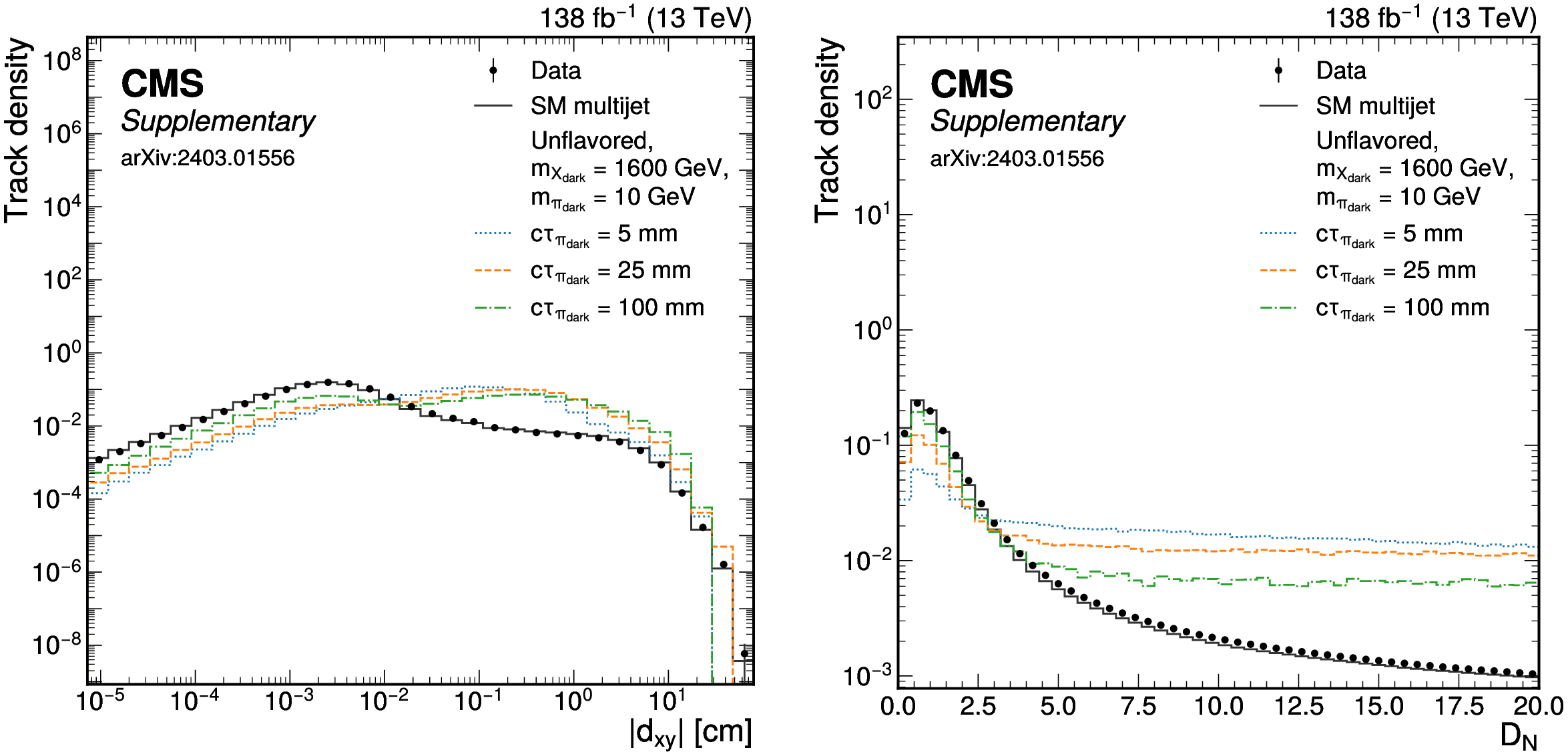
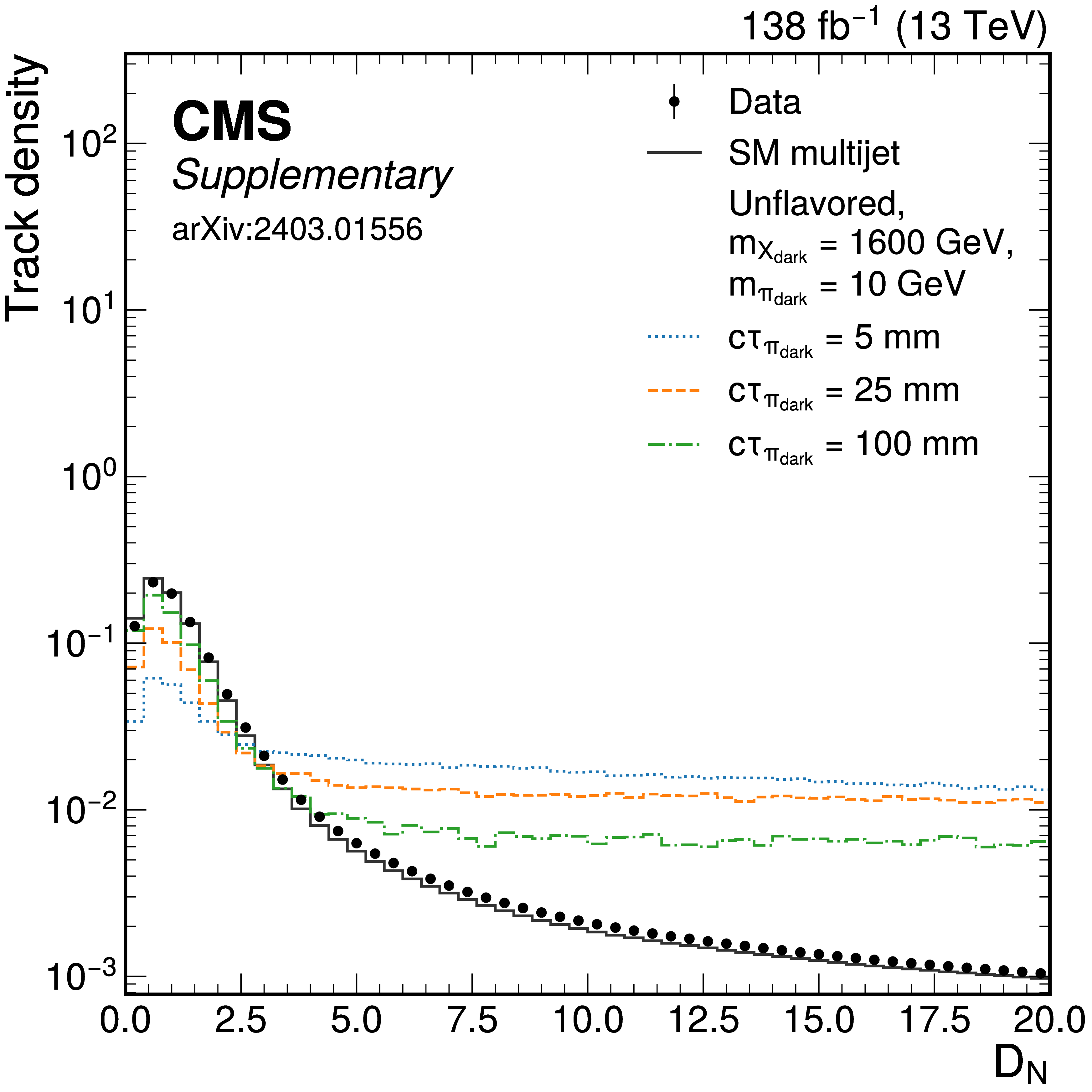
Example distributions of track-level variables that is used to calculate the tagging EJs produced in unflavored signal models for CMS data (points), SM multijet events from simulation (gray line), and various signal samples with varying dark pion lifetime (colored lines). The distribution of track $ d_{xy} $ ($ D_{N} $) is shown on the left (right). Distributions for various processes have their total track count normalized to 1. |
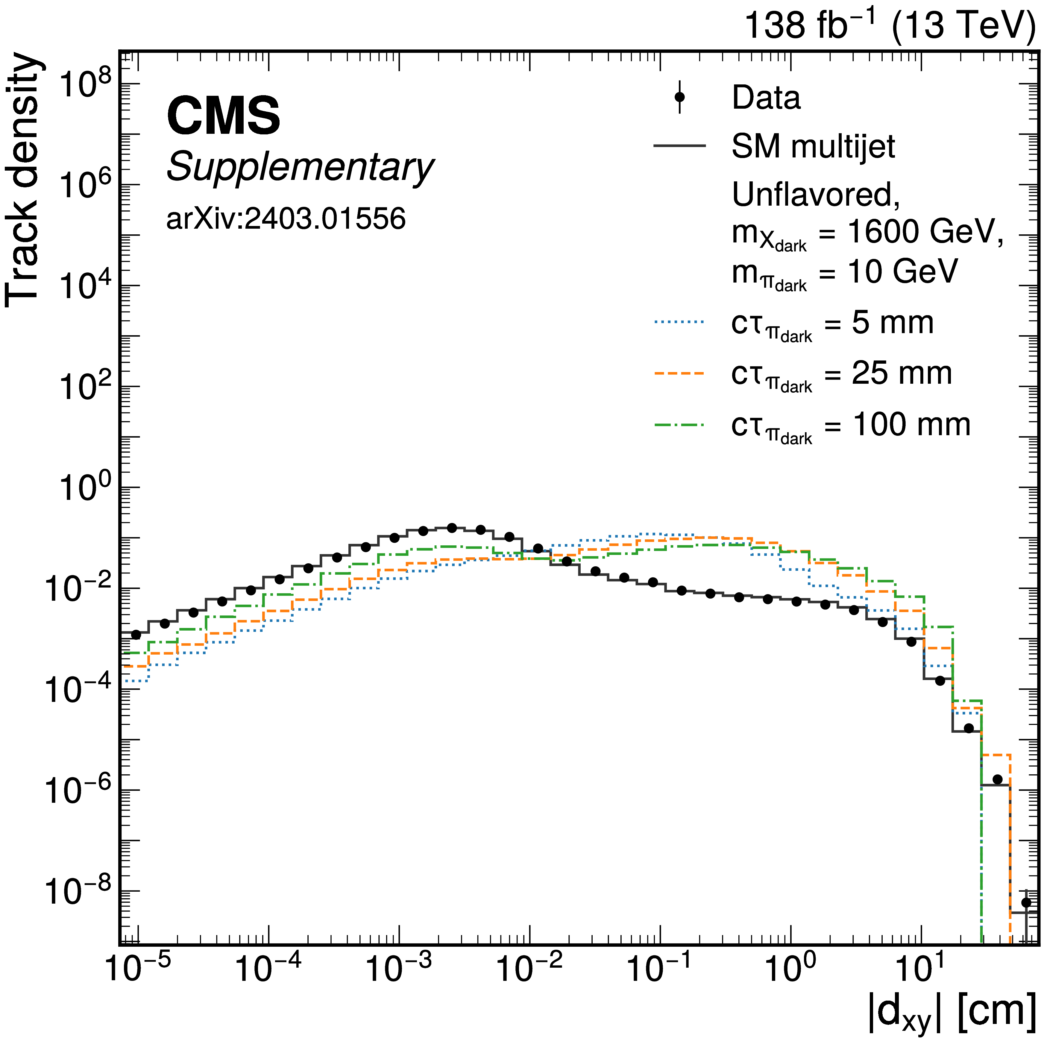
png pdf |
Additional Figure 3-a:
Example distributions of track-level variables that is used to calculate the tagging EJs produced in unflavored signal models for CMS data (points), SM multijet events from simulation (gray line), and various signal samples with varying dark pion lifetime (colored lines). The distribution of track $ d_{xy} $ ($ D_{N} $) is shown on the left (right). Distributions for various processes have their total track count normalized to 1. |
png pdf |
Additional Figure 3-b:
Example distributions of track-level variables that is used to calculate the tagging EJs produced in unflavored signal models for CMS data (points), SM multijet events from simulation (gray line), and various signal samples with varying dark pion lifetime (colored lines). The distribution of track $ d_{xy} $ ($ D_{N} $) is shown on the left (right). Distributions for various processes have their total track count normalized to 1. |
png pdf |
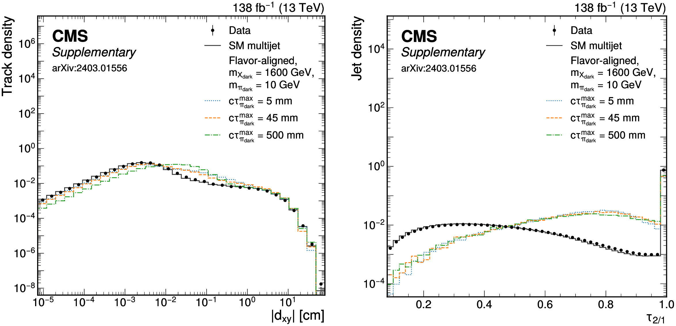
Additional Figure 4:
Example distributions of variables that is used to calculate the tagging EJs produced in flavor-aligned signal models for CMS data (points), SM multijet events from simulation (gray line), and various signal samples with varying dark pion lifetime (colored lines). The distribution of the $ d_{xy} $ of tracks ($\bar{\tau}_{2/1}$ of jets) is shown on the left (right). Distributions for various processes have their total count normalized to 1. |
png pdf |
Additional Figure 4-a:
Example distributions of variables that is used to calculate the tagging EJs produced in flavor-aligned signal models for CMS data (points), SM multijet events from simulation (gray line), and various signal samples with varying dark pion lifetime (colored lines). The distribution of the $ d_{xy} $ of tracks ($\bar{\tau}_{2/1}$ of jets) is shown on the left (right). Distributions for various processes have their total count normalized to 1. |
png pdf |
Additional Figure 4-b:
Example distributions of variables that is used to calculate the tagging EJs produced in flavor-aligned signal models for CMS data (points), SM multijet events from simulation (gray line), and various signal samples with varying dark pion lifetime (colored lines). The distribution of the $ d_{xy} $ of tracks ($\bar{\tau}_{2/1}$ of jets) is shown on the left (right). Distributions for various processes have their total count normalized to 1. |
png pdf |
Additional Figure 5:
Example distributions of track variables that is used to as coordinate inputs of the GNN used for EJ tagging for CMS data (points), SM multijet events from simulation (gray line), and various signal samples (colored lines). The distribution of $ |\Delta\eta| $ ($ |\Delta\phi| $) between the jet and associated tracks is shown on the left (right). Distributions for various processes have their total count normalized to 1. |
png pdf |
Additional Figure 5-a:
Example distributions of track variables that is used to as coordinate inputs of the GNN used for EJ tagging for CMS data (points), SM multijet events from simulation (gray line), and various signal samples (colored lines). The distribution of $ |\Delta\eta| $ ($ |\Delta\phi| $) between the jet and associated tracks is shown on the left (right). Distributions for various processes have their total count normalized to 1. |
png pdf |
Additional Figure 5-b:
Example distributions of track variables that is used to as coordinate inputs of the GNN used for EJ tagging for CMS data (points), SM multijet events from simulation (gray line), and various signal samples (colored lines). The distribution of $ |\Delta\eta| $ ($ |\Delta\phi| $) between the jet and associated tracks is shown on the left (right). Distributions for various processes have their total count normalized to 1. |
png pdf |
Additional Figure 6:
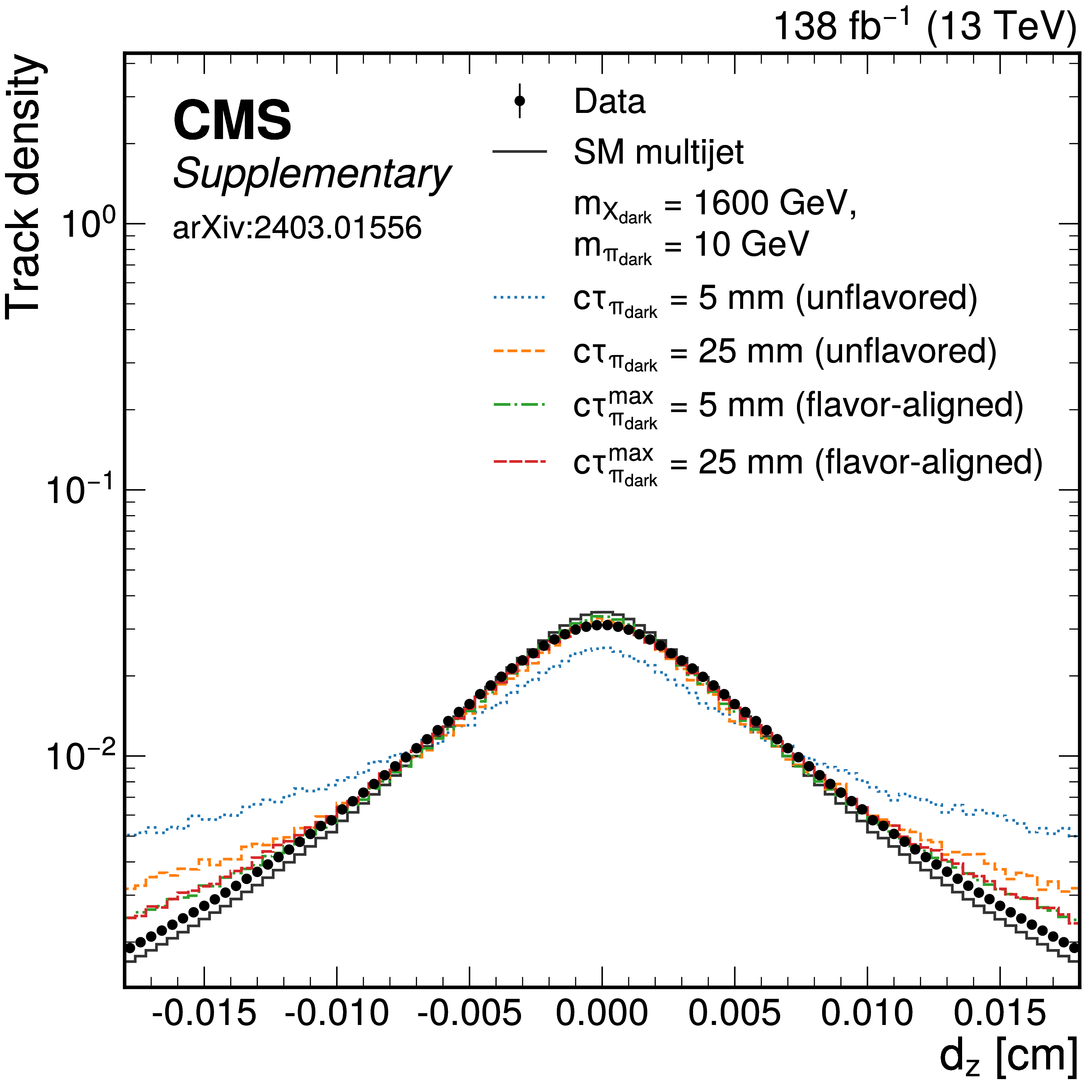
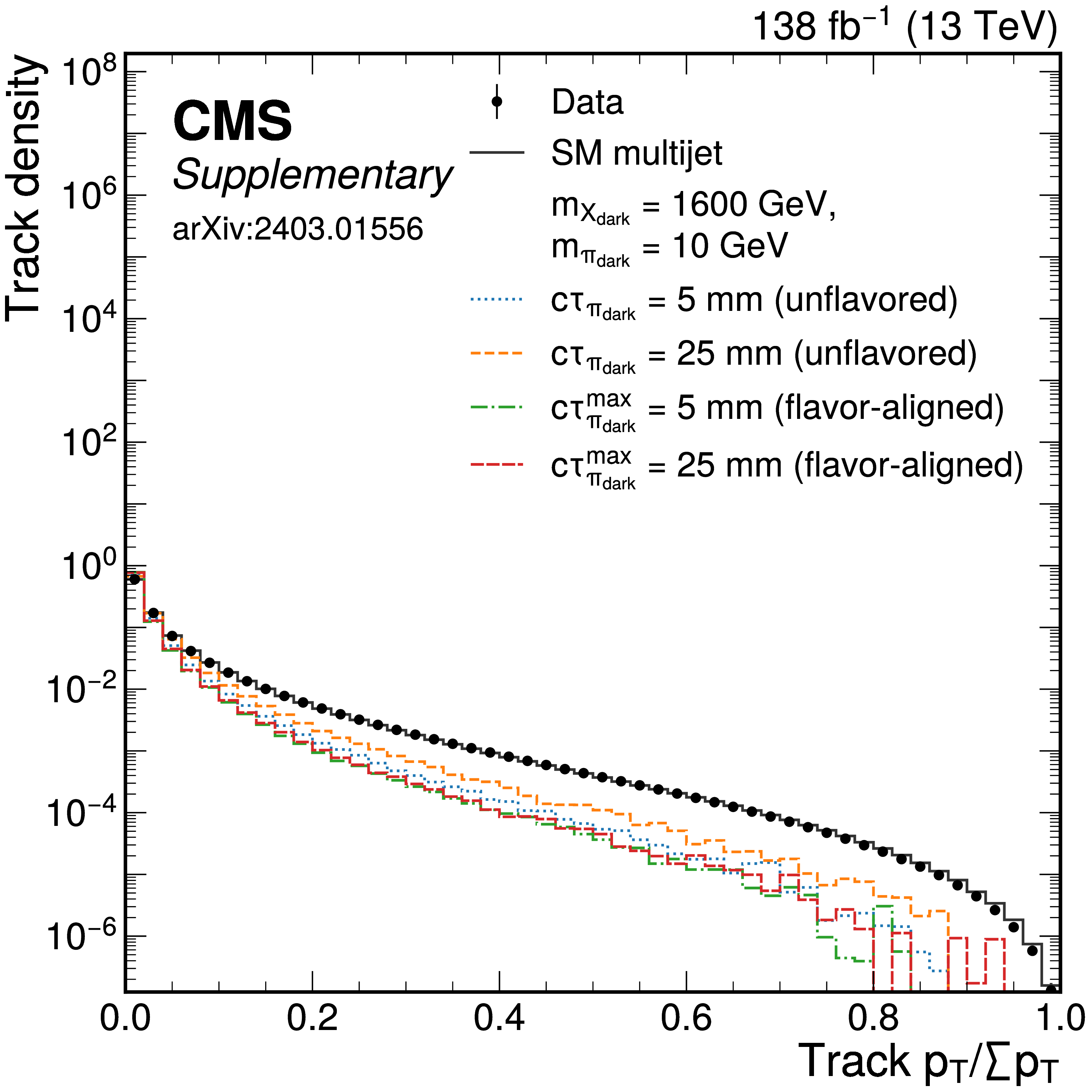
Example distributions of track variables that is used to as inputs of the GNN used for EJ tagging for CMS data (points), SM multijet events from simulation (gray line), and various signal samples (colored lines). The distribution of $ d_{xy} $ ($ d_{z} $) is shown on the top left (bottom left), while the distribution of the track $ p_{\mathrm{T}} $ ($ p_{\mathrm{T}}^\text{track}/\sum_{\text{track}}p_{\mathrm{T}}^{\text{track}} $) is shown on the top right (bottom right). Distributions for various processes have their total count normalized to 1. |
png pdf |
Additional Figure 6-a:
Example distributions of track variables that is used to as inputs of the GNN used for EJ tagging for CMS data (points), SM multijet events from simulation (gray line), and various signal samples (colored lines). The distribution of $ d_{xy} $ ($ d_{z} $) is shown on the top left (bottom left), while the distribution of the track $ p_{\mathrm{T}} $ ($ p_{\mathrm{T}}^\text{track}/\sum_{\text{track}}p_{\mathrm{T}}^{\text{track}} $) is shown on the top right (bottom right). Distributions for various processes have their total count normalized to 1. |
png pdf |
Additional Figure 6-b:
Example distributions of track variables that is used to as inputs of the GNN used for EJ tagging for CMS data (points), SM multijet events from simulation (gray line), and various signal samples (colored lines). The distribution of $ d_{xy} $ ($ d_{z} $) is shown on the top left (bottom left), while the distribution of the track $ p_{\mathrm{T}} $ ($ p_{\mathrm{T}}^\text{track}/\sum_{\text{track}}p_{\mathrm{T}}^{\text{track}} $) is shown on the top right (bottom right). Distributions for various processes have their total count normalized to 1. |
png pdf |
Additional Figure 6-c:
Example distributions of track variables that is used to as inputs of the GNN used for EJ tagging for CMS data (points), SM multijet events from simulation (gray line), and various signal samples (colored lines). The distribution of $ d_{xy} $ ($ d_{z} $) is shown on the top left (bottom left), while the distribution of the track $ p_{\mathrm{T}} $ ($ p_{\mathrm{T}}^\text{track}/\sum_{\text{track}}p_{\mathrm{T}}^{\text{track}} $) is shown on the top right (bottom right). Distributions for various processes have their total count normalized to 1. |
png pdf |
Additional Figure 6-d:
Example distributions of track variables that is used to as inputs of the GNN used for EJ tagging for CMS data (points), SM multijet events from simulation (gray line), and various signal samples (colored lines). The distribution of $ d_{xy} $ ($ d_{z} $) is shown on the top left (bottom left), while the distribution of the track $ p_{\mathrm{T}} $ ($ p_{\mathrm{T}}^\text{track}/\sum_{\text{track}}p_{\mathrm{T}}^{\text{track}} $) is shown on the top right (bottom right). Distributions for various processes have their total count normalized to 1. |
png pdf |
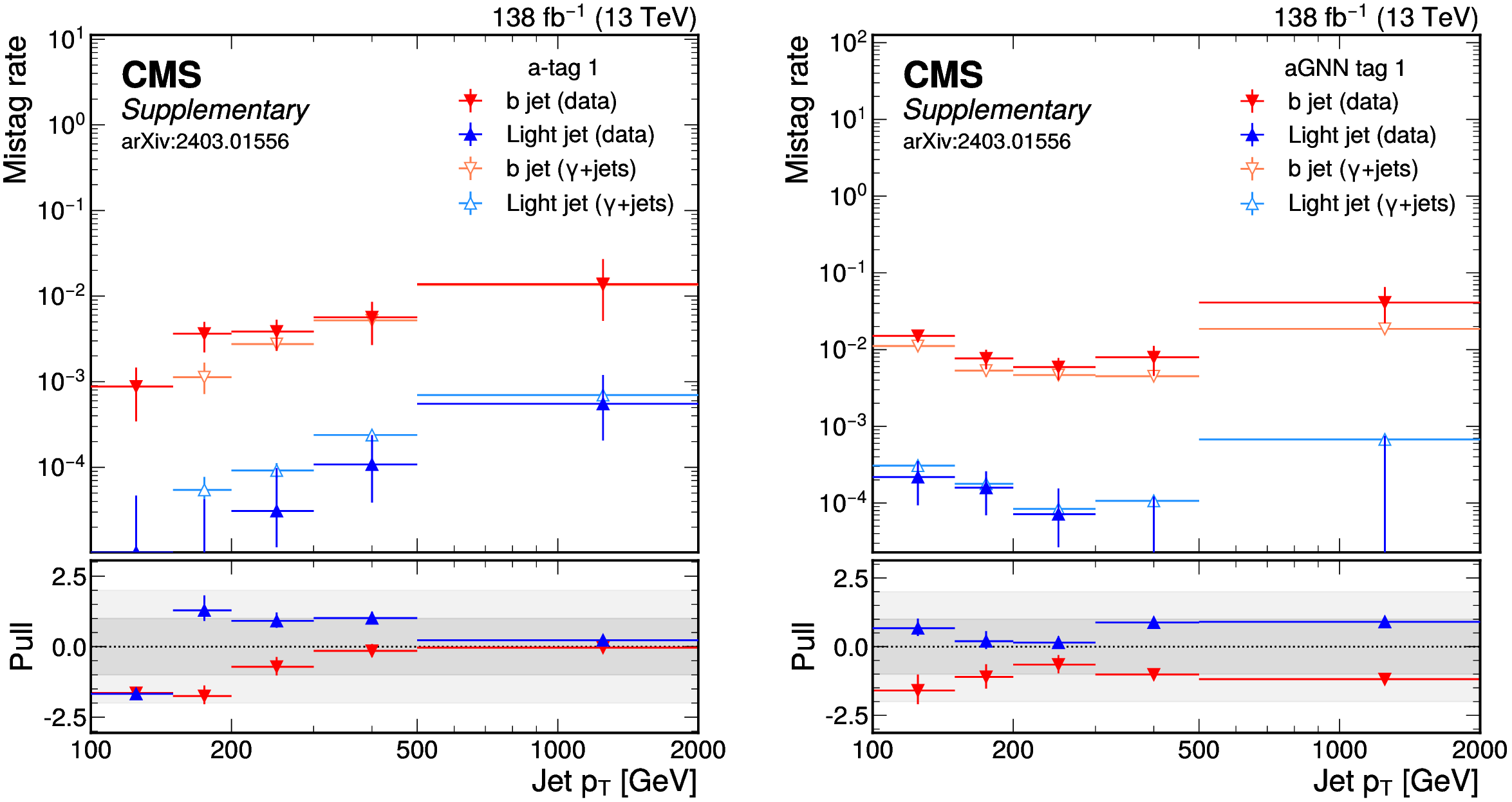
Additional Figure 7:
The mistag rate of the a-tag 1 (left) and aGNN tag 1 (right) EJ tagger evaluated in data and $ \gamma $+jets events from simulation as a function of jet $ p_{\mathrm{T}} $. |
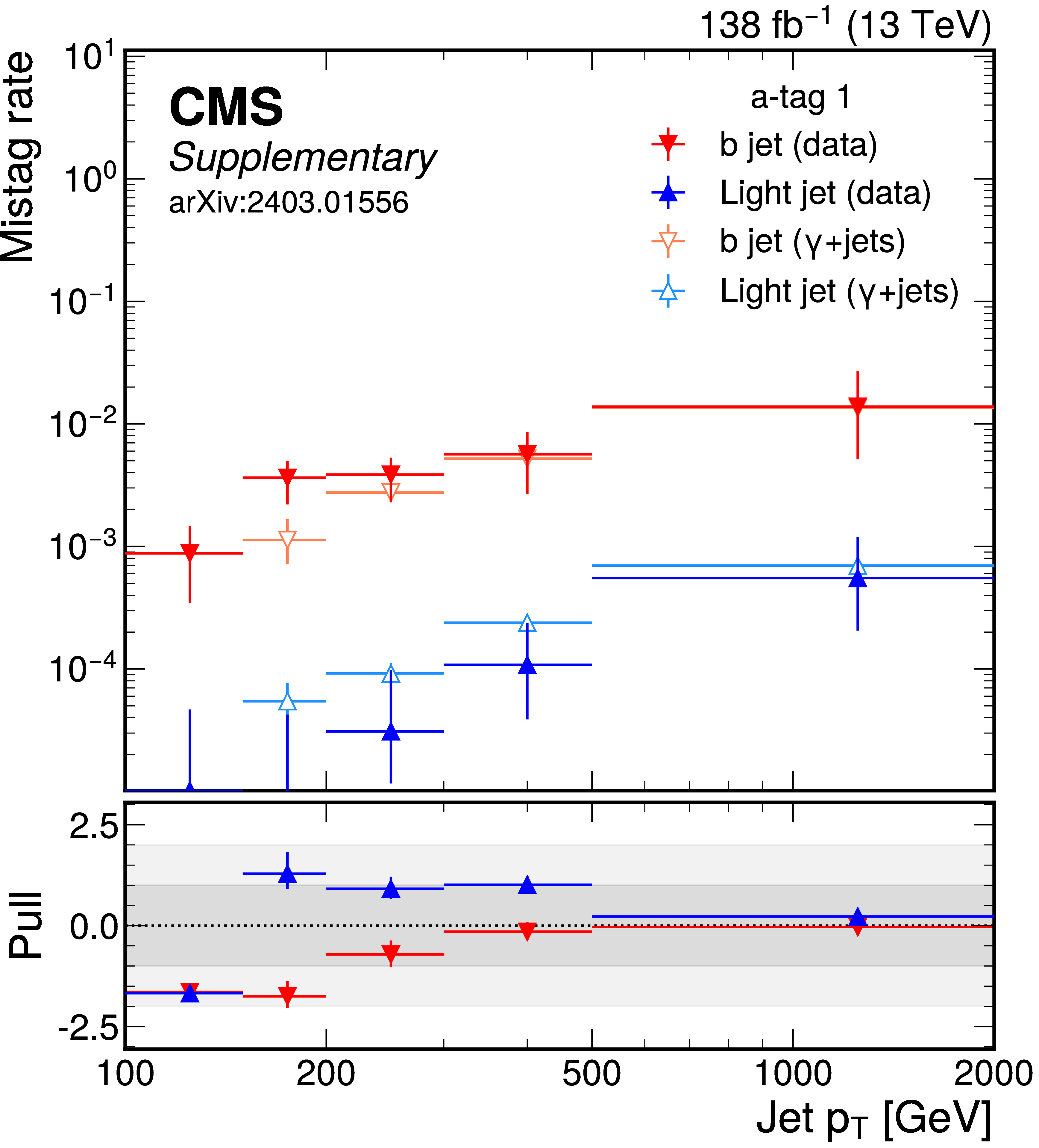
png pdf |
Additional Figure 7-a:
The mistag rate of the a-tag 1 (left) and aGNN tag 1 (right) EJ tagger evaluated in data and $ \gamma $+jets events from simulation as a function of jet $ p_{\mathrm{T}} $. |

png pdf |
Additional Figure 7-b:
The mistag rate of the a-tag 1 (left) and aGNN tag 1 (right) EJ tagger evaluated in data and $ \gamma $+jets events from simulation as a function of jet $ p_{\mathrm{T}} $. |

png pdf |
Additional Figure 8:
Signal acceptance of signal models in the unflavored scenario with $ m_{\pi_\text{dark}}= $ 10 GeV with EJ tagging performed using the model-agnostic method, using the CMS detector configuration of 2016 pre-APV configuration fixes (top left), 2016 post-APV configuration fixes (top right), 2017 (bottom left) and 2018 (bottom right). The number in each box represents which cutset is being applied to each EJ sample; changes in cutsets in consecutive EJ samples can cause dips in efficiency as each cutset is optimized to maximize signal acceptance and background rejection. |
png pdf |
Additional Figure 8-a:
Signal acceptance of signal models in the unflavored scenario with $ m_{\pi_\text{dark}}= $ 10 GeV with EJ tagging performed using the model-agnostic method, using the CMS detector configuration of 2016 pre-APV configuration fixes (top left), 2016 post-APV configuration fixes (top right), 2017 (bottom left) and 2018 (bottom right). The number in each box represents which cutset is being applied to each EJ sample; changes in cutsets in consecutive EJ samples can cause dips in efficiency as each cutset is optimized to maximize signal acceptance and background rejection. |
png pdf |
Additional Figure 8-b:
Signal acceptance of signal models in the unflavored scenario with $ m_{\pi_\text{dark}}= $ 10 GeV with EJ tagging performed using the model-agnostic method, using the CMS detector configuration of 2016 pre-APV configuration fixes (top left), 2016 post-APV configuration fixes (top right), 2017 (bottom left) and 2018 (bottom right). The number in each box represents which cutset is being applied to each EJ sample; changes in cutsets in consecutive EJ samples can cause dips in efficiency as each cutset is optimized to maximize signal acceptance and background rejection. |

png pdf |
Additional Figure 8-c:
Signal acceptance of signal models in the unflavored scenario with $ m_{\pi_\text{dark}}= $ 10 GeV with EJ tagging performed using the model-agnostic method, using the CMS detector configuration of 2016 pre-APV configuration fixes (top left), 2016 post-APV configuration fixes (top right), 2017 (bottom left) and 2018 (bottom right). The number in each box represents which cutset is being applied to each EJ sample; changes in cutsets in consecutive EJ samples can cause dips in efficiency as each cutset is optimized to maximize signal acceptance and background rejection. |

png pdf |
Additional Figure 8-d:
Signal acceptance of signal models in the unflavored scenario with $ m_{\pi_\text{dark}}= $ 10 GeV with EJ tagging performed using the model-agnostic method, using the CMS detector configuration of 2016 pre-APV configuration fixes (top left), 2016 post-APV configuration fixes (top right), 2017 (bottom left) and 2018 (bottom right). The number in each box represents which cutset is being applied to each EJ sample; changes in cutsets in consecutive EJ samples can cause dips in efficiency as each cutset is optimized to maximize signal acceptance and background rejection. |
png pdf |
Additional Figure 9:
Signal acceptance of signal models in the unflavored scenario with $ m_{\pi_\text{dark}}= $ 10 GeV with EJ tagging performed using the GNN method, for all CMS detector 2016--2018 eras combined. The number in each box represents which cutset is being applied to each EJ sample; changes in cutsets in consecutive EJ samples can cause dips in efficiency as each cutset is optimized to maximize signal acceptance and background rejection. |

png pdf |
Additional Figure 10:
Signal acceptance of signal models in the unflavored scenario with $ m_{\pi_\text{dark}}= $ 20 GeV with EJ tagging performed using the model-agnostic method, using the CMS detector configuration of 2016 pre-APV configuration fixes (top left), 2016 post-APV configuration fixes (top right), 2017 (bottom left) and 2018 (bottom right). The number in each box represents which cutset is being applied to each EJ sample; changes in cutsets in consecutive EJ samples can cause dips in efficiency as each cutset is optimized to maximize signal acceptance and background rejection. |

png pdf |
Additional Figure 10-a:
Signal acceptance of signal models in the unflavored scenario with $ m_{\pi_\text{dark}}= $ 20 GeV with EJ tagging performed using the model-agnostic method, using the CMS detector configuration of 2016 pre-APV configuration fixes (top left), 2016 post-APV configuration fixes (top right), 2017 (bottom left) and 2018 (bottom right). The number in each box represents which cutset is being applied to each EJ sample; changes in cutsets in consecutive EJ samples can cause dips in efficiency as each cutset is optimized to maximize signal acceptance and background rejection. |

png pdf |
Additional Figure 10-b:
Signal acceptance of signal models in the unflavored scenario with $ m_{\pi_\text{dark}}= $ 20 GeV with EJ tagging performed using the model-agnostic method, using the CMS detector configuration of 2016 pre-APV configuration fixes (top left), 2016 post-APV configuration fixes (top right), 2017 (bottom left) and 2018 (bottom right). The number in each box represents which cutset is being applied to each EJ sample; changes in cutsets in consecutive EJ samples can cause dips in efficiency as each cutset is optimized to maximize signal acceptance and background rejection. |

png pdf |
Additional Figure 10-c:
Signal acceptance of signal models in the unflavored scenario with $ m_{\pi_\text{dark}}= $ 20 GeV with EJ tagging performed using the model-agnostic method, using the CMS detector configuration of 2016 pre-APV configuration fixes (top left), 2016 post-APV configuration fixes (top right), 2017 (bottom left) and 2018 (bottom right). The number in each box represents which cutset is being applied to each EJ sample; changes in cutsets in consecutive EJ samples can cause dips in efficiency as each cutset is optimized to maximize signal acceptance and background rejection. |
png pdf |
Additional Figure 10-d:
Signal acceptance of signal models in the unflavored scenario with $ m_{\pi_\text{dark}}= $ 20 GeV with EJ tagging performed using the model-agnostic method, using the CMS detector configuration of 2016 pre-APV configuration fixes (top left), 2016 post-APV configuration fixes (top right), 2017 (bottom left) and 2018 (bottom right). The number in each box represents which cutset is being applied to each EJ sample; changes in cutsets in consecutive EJ samples can cause dips in efficiency as each cutset is optimized to maximize signal acceptance and background rejection. |

png pdf |
Additional Figure 11:
Signal acceptance of signal models in the unflavored scenario with $ m_{\pi_\text{dark}}= $ 20 GeV with EJ tagging performed using the GNN method, for all CMS detector 2016--2018 eras combined. The number in each box represents which cutset is being applied to each EJ sample; changes in cutsets in consecutive EJ samples can cause dips in efficiency as each cutset is optimized to maximize signal acceptance and background rejection. |
png pdf |
Additional Figure 12:
Signal acceptance of signal models in the flavor-aligned scenario with $ m_{\pi_\text{dark}}= $ 6 GeV with EJ tagging performed using the model-agnostic method, using the CMS detector configuration of 2016 pre-APV configuration fixes (top left), 2016 post-APV configuration fixes (top right), 2017 (bottom left) and 2018 (bottom right). The number in each box represents which cutset is being applied to each EJ sample; changes in cutsets in consecutive EJ samples can cause dips in efficiency as each cutset is optimized to maximize signal acceptance and background rejection. |
png pdf |
Additional Figure 12-a:
Signal acceptance of signal models in the flavor-aligned scenario with $ m_{\pi_\text{dark}}= $ 6 GeV with EJ tagging performed using the model-agnostic method, using the CMS detector configuration of 2016 pre-APV configuration fixes (top left), 2016 post-APV configuration fixes (top right), 2017 (bottom left) and 2018 (bottom right). The number in each box represents which cutset is being applied to each EJ sample; changes in cutsets in consecutive EJ samples can cause dips in efficiency as each cutset is optimized to maximize signal acceptance and background rejection. |
png pdf |
Additional Figure 12-b:
Signal acceptance of signal models in the flavor-aligned scenario with $ m_{\pi_\text{dark}}= $ 6 GeV with EJ tagging performed using the model-agnostic method, using the CMS detector configuration of 2016 pre-APV configuration fixes (top left), 2016 post-APV configuration fixes (top right), 2017 (bottom left) and 2018 (bottom right). The number in each box represents which cutset is being applied to each EJ sample; changes in cutsets in consecutive EJ samples can cause dips in efficiency as each cutset is optimized to maximize signal acceptance and background rejection. |
png pdf |
Additional Figure 12-c:
Signal acceptance of signal models in the flavor-aligned scenario with $ m_{\pi_\text{dark}}= $ 6 GeV with EJ tagging performed using the model-agnostic method, using the CMS detector configuration of 2016 pre-APV configuration fixes (top left), 2016 post-APV configuration fixes (top right), 2017 (bottom left) and 2018 (bottom right). The number in each box represents which cutset is being applied to each EJ sample; changes in cutsets in consecutive EJ samples can cause dips in efficiency as each cutset is optimized to maximize signal acceptance and background rejection. |
png pdf |
Additional Figure 12-d:
Signal acceptance of signal models in the flavor-aligned scenario with $ m_{\pi_\text{dark}}= $ 6 GeV with EJ tagging performed using the model-agnostic method, using the CMS detector configuration of 2016 pre-APV configuration fixes (top left), 2016 post-APV configuration fixes (top right), 2017 (bottom left) and 2018 (bottom right). The number in each box represents which cutset is being applied to each EJ sample; changes in cutsets in consecutive EJ samples can cause dips in efficiency as each cutset is optimized to maximize signal acceptance and background rejection. |
png pdf |
Additional Figure 13:
Signal acceptance of signal models in the flavor-aligned scenario with $ m_{\pi_\text{dark}}= $ 6 GeV with EJ tagging performed using the GNN method, for all CMS detector 2016--2018 eras combined. The number in each box represents which cutset is being applied to each EJ sample; changes in cutsets in consecutive EJ samples can cause dips in efficiency as each cutset is optimized to maximize signal acceptance and background rejection. |
png pdf |
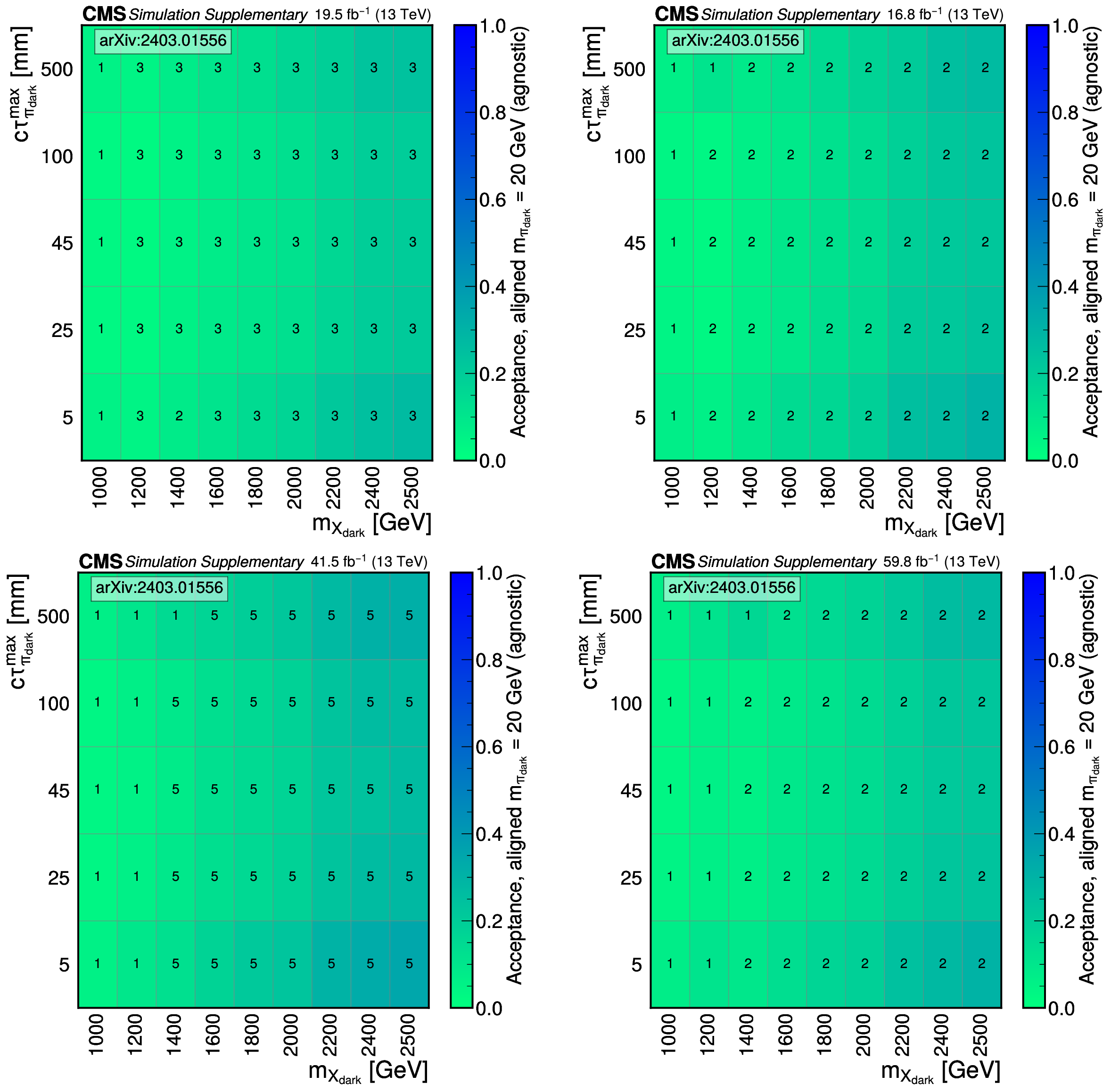
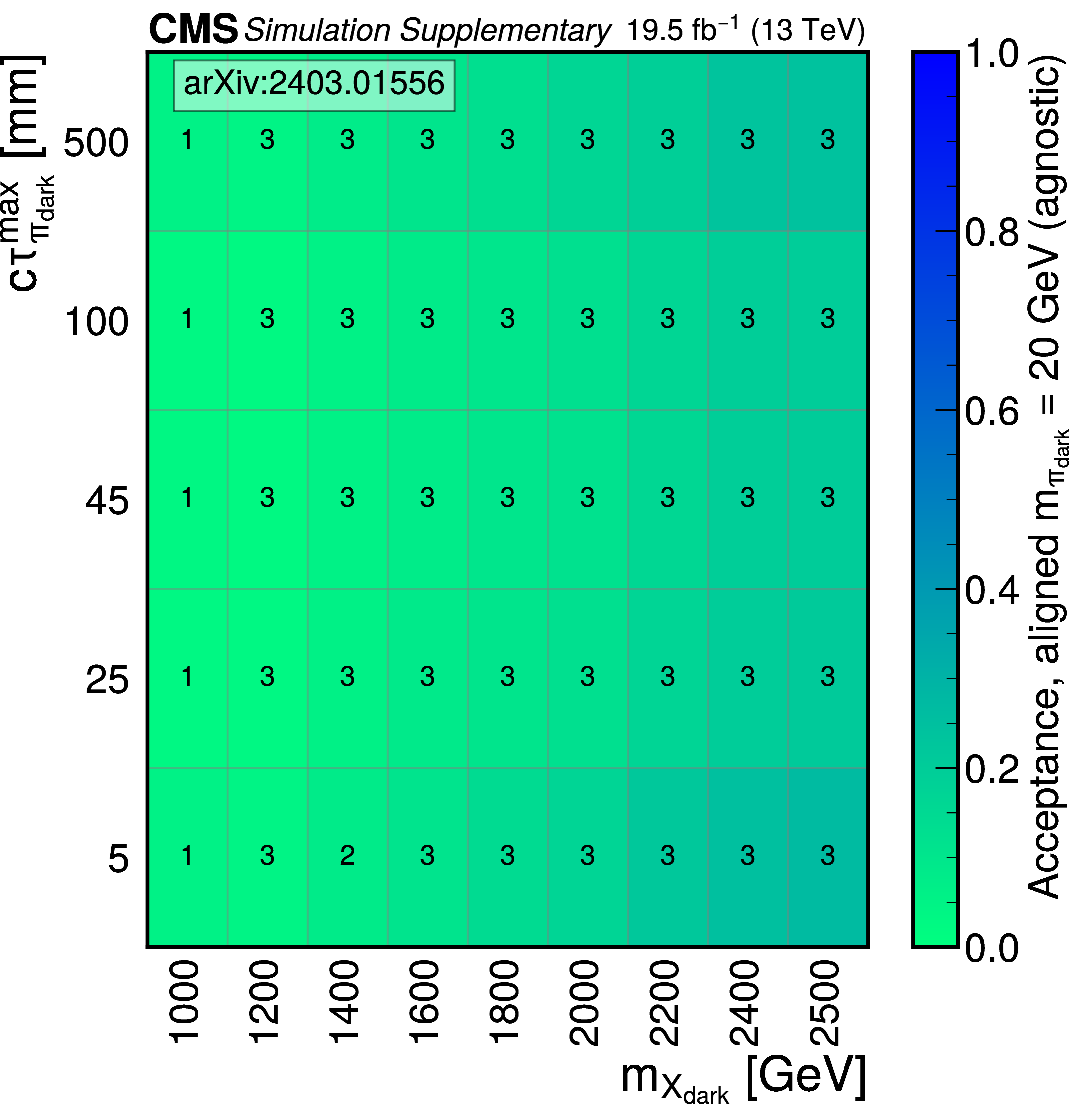
Additional Figure 14:
Signal acceptance of signal models in the flavor-aligned scenario with $ m_{\pi_\text{dark}}= $ 10 GeV with EJ tagging performed using the model-agnostic method, using the CMS detector configuration of 2016 pre-APV configuration fixes (top left), 2016 post-APV configuration fixes (top right), 2017 (bottom left) and 2018 (bottom right). The number in each box represents which cutset is being applied to each EJ sample; changes in cutsets in consecutive EJ samples can cause dips in efficiency as each cutset is optimized to maximize signal acceptance and background rejection. |
png pdf |
Additional Figure 14-a:
Signal acceptance of signal models in the flavor-aligned scenario with $ m_{\pi_\text{dark}}= $ 10 GeV with EJ tagging performed using the model-agnostic method, using the CMS detector configuration of 2016 pre-APV configuration fixes (top left), 2016 post-APV configuration fixes (top right), 2017 (bottom left) and 2018 (bottom right). The number in each box represents which cutset is being applied to each EJ sample; changes in cutsets in consecutive EJ samples can cause dips in efficiency as each cutset is optimized to maximize signal acceptance and background rejection. |
png pdf |
Additional Figure 14-b:
Signal acceptance of signal models in the flavor-aligned scenario with $ m_{\pi_\text{dark}}= $ 10 GeV with EJ tagging performed using the model-agnostic method, using the CMS detector configuration of 2016 pre-APV configuration fixes (top left), 2016 post-APV configuration fixes (top right), 2017 (bottom left) and 2018 (bottom right). The number in each box represents which cutset is being applied to each EJ sample; changes in cutsets in consecutive EJ samples can cause dips in efficiency as each cutset is optimized to maximize signal acceptance and background rejection. |
png pdf |
Additional Figure 14-c:
Signal acceptance of signal models in the flavor-aligned scenario with $ m_{\pi_\text{dark}}= $ 10 GeV with EJ tagging performed using the model-agnostic method, using the CMS detector configuration of 2016 pre-APV configuration fixes (top left), 2016 post-APV configuration fixes (top right), 2017 (bottom left) and 2018 (bottom right). The number in each box represents which cutset is being applied to each EJ sample; changes in cutsets in consecutive EJ samples can cause dips in efficiency as each cutset is optimized to maximize signal acceptance and background rejection. |
png pdf |
Additional Figure 14-d:
Signal acceptance of signal models in the flavor-aligned scenario with $ m_{\pi_\text{dark}}= $ 10 GeV with EJ tagging performed using the model-agnostic method, using the CMS detector configuration of 2016 pre-APV configuration fixes (top left), 2016 post-APV configuration fixes (top right), 2017 (bottom left) and 2018 (bottom right). The number in each box represents which cutset is being applied to each EJ sample; changes in cutsets in consecutive EJ samples can cause dips in efficiency as each cutset is optimized to maximize signal acceptance and background rejection. |
png pdf |
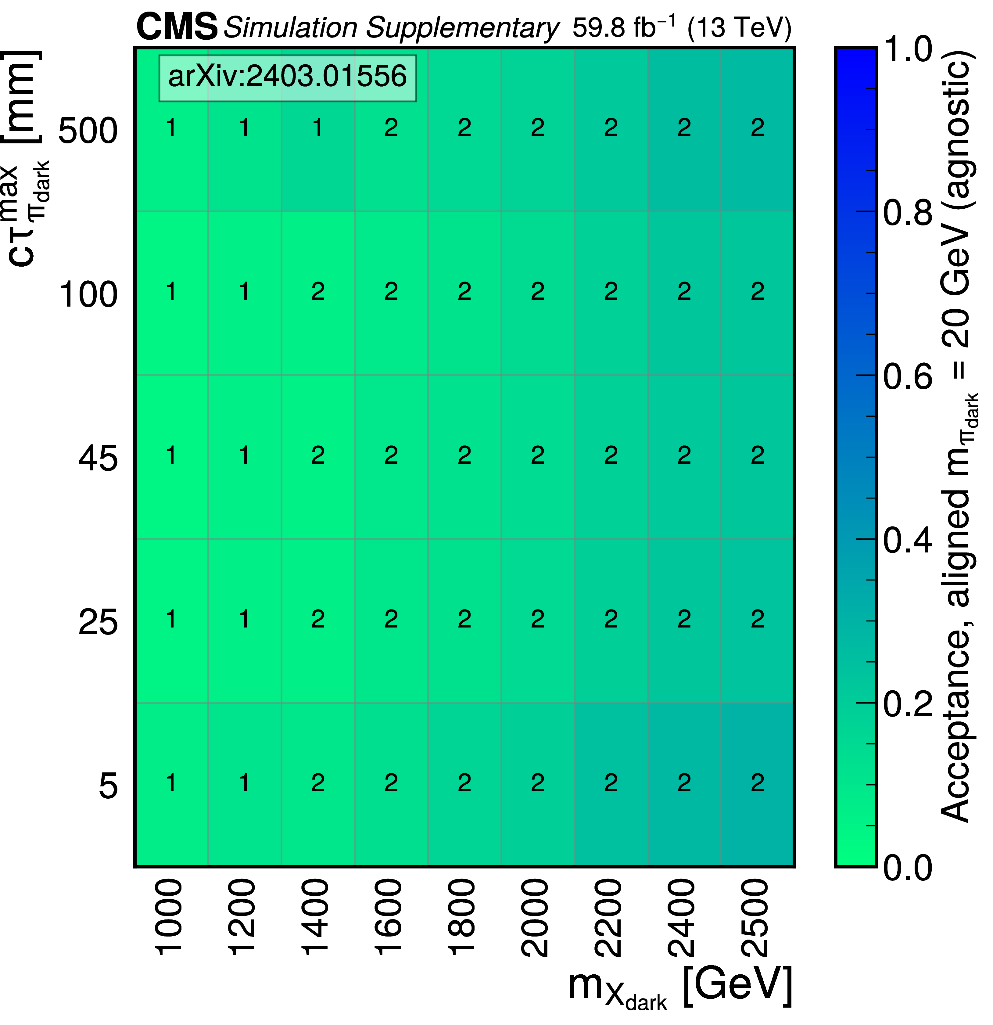
Additional Figure 15:
Signal acceptance of signal models in the flavor-aligned scenario with $ m_{\pi_\text{dark}}= $ 10 GeV with EJ tagging performed using the GNN method, for all CMS detector 2016--2018 eras combined. The number in each box represents which cutset is being applied to each EJ sample; changes in cutsets in consecutive EJ samples can cause dips in efficiency as each cutset is optimized to maximize signal acceptance and background rejection. |
png pdf |
Additional Figure 16:
Signal acceptance of signal models in the flavor-aligned scenario with $ m_{\pi_\text{dark}}= $ 20 GeV with EJ tagging performed using the model-agnostic method, using the CMS detector configuration of 2016 pre-APV configuration fixes (top left), 2016 post-APV configuration fixes (top right), 2017 (bottom left) and 2018 (bottom right). The number in each box represents which cutset is being applied to each EJ sample; changes in cutsets in consecutive EJ samples can cause dips in efficiency as each cutset is optimized to maximize signal acceptance and background rejection. |
png pdf |
Additional Figure 16-a:
Signal acceptance of signal models in the flavor-aligned scenario with $ m_{\pi_\text{dark}}= $ 20 GeV with EJ tagging performed using the model-agnostic method, using the CMS detector configuration of 2016 pre-APV configuration fixes (top left), 2016 post-APV configuration fixes (top right), 2017 (bottom left) and 2018 (bottom right). The number in each box represents which cutset is being applied to each EJ sample; changes in cutsets in consecutive EJ samples can cause dips in efficiency as each cutset is optimized to maximize signal acceptance and background rejection. |

png pdf |
Additional Figure 16-b:
Signal acceptance of signal models in the flavor-aligned scenario with $ m_{\pi_\text{dark}}= $ 20 GeV with EJ tagging performed using the model-agnostic method, using the CMS detector configuration of 2016 pre-APV configuration fixes (top left), 2016 post-APV configuration fixes (top right), 2017 (bottom left) and 2018 (bottom right). The number in each box represents which cutset is being applied to each EJ sample; changes in cutsets in consecutive EJ samples can cause dips in efficiency as each cutset is optimized to maximize signal acceptance and background rejection. |

png pdf |
Additional Figure 16-c:
Signal acceptance of signal models in the flavor-aligned scenario with $ m_{\pi_\text{dark}}= $ 20 GeV with EJ tagging performed using the model-agnostic method, using the CMS detector configuration of 2016 pre-APV configuration fixes (top left), 2016 post-APV configuration fixes (top right), 2017 (bottom left) and 2018 (bottom right). The number in each box represents which cutset is being applied to each EJ sample; changes in cutsets in consecutive EJ samples can cause dips in efficiency as each cutset is optimized to maximize signal acceptance and background rejection. |
png pdf |
Additional Figure 16-d:
Signal acceptance of signal models in the flavor-aligned scenario with $ m_{\pi_\text{dark}}= $ 20 GeV with EJ tagging performed using the model-agnostic method, using the CMS detector configuration of 2016 pre-APV configuration fixes (top left), 2016 post-APV configuration fixes (top right), 2017 (bottom left) and 2018 (bottom right). The number in each box represents which cutset is being applied to each EJ sample; changes in cutsets in consecutive EJ samples can cause dips in efficiency as each cutset is optimized to maximize signal acceptance and background rejection. |
png pdf |
Additional Figure 17:
Signal acceptance of signal models in the flavor-aligned scenario with $ m_{\pi_\text{dark}}= $ 20 GeV with EJ tagging performed using the GNN method, for all CMS detector 2016--2018 eras combined. The number in each box represents which cutset is being applied to each EJ sample; changes in cutsets in consecutive EJ samples can cause dips in efficiency as each cutset is optimized to maximize signal acceptance and background rejection. |
png pdf |
Additional Figure 18:
Template fit of the DEEPJET discriminator used to determine the b jet fraction of the non-EJ tagged jets in data events that pass the 1-EJ selection of the ``u-set 1'' (``a-set 1'') criteria on the left (right). |
png pdf |
Additional Figure 18-a:
Template fit of the DEEPJET discriminator used to determine the b jet fraction of the non-EJ tagged jets in data events that pass the 1-EJ selection of the ``u-set 1'' (``a-set 1'') criteria on the left (right). |
png pdf |
Additional Figure 18-b:
Template fit of the DEEPJET discriminator used to determine the b jet fraction of the non-EJ tagged jets in data events that pass the 1-EJ selection of the ``u-set 1'' (``a-set 1'') criteria on the left (right). |
png pdf |
Additional Figure 19:
Template fit of the DEEPJET discriminator used to determine the b jet fraction of the non-EJ tagged jets in data events that pass the 1-EJ selection of the ``uGNN set 1'' (``aGNN set 1'') criteria on the left (right). |
png pdf |
Additional Figure 19-a:
Template fit of the DEEPJET discriminator used to determine the b jet fraction of the non-EJ tagged jets in data events that pass the 1-EJ selection of the ``uGNN set 1'' (``aGNN set 1'') criteria on the left (right). |
png pdf |
Additional Figure 19-b:
Template fit of the DEEPJET discriminator used to determine the b jet fraction of the non-EJ tagged jets in data events that pass the 1-EJ selection of the ``uGNN set 1'' (``aGNN set 1'') criteria on the left (right). |
png pdf |
Additional Figure 20:
Comparison between the cut-based (model-agnostic) EJ tagging method with the unflavored (left) and flavor-aligned (right) GNN for 3 different EJ unflavored samples. The cut-based tagger performance is worse than the GNN in all 3 EJ samples. |
png pdf |
Additional Figure 20-a:
Comparison between the cut-based (model-agnostic) EJ tagging method with the unflavored (left) and flavor-aligned (right) GNN for 3 different EJ unflavored samples. The cut-based tagger performance is worse than the GNN in all 3 EJ samples. |

png pdf |
Additional Figure 20-b:
Comparison between the cut-based (model-agnostic) EJ tagging method with the unflavored (left) and flavor-aligned (right) GNN for 3 different EJ unflavored samples. The cut-based tagger performance is worse than the GNN in all 3 EJ samples. |
png pdf |
Additional Figure 21:
Performance of the GNN EJ tagger on different EJ unflavored samples. The GNN was trained on the $ m_{\pi_\text{dark}} = $ 10 and 20 GeV (green and red curves), but not 0.7 or 1 GeV (blue and orange curves), showing how the performance degrades when the tagger is applied to a sample outside what it is presented with at training. |
png pdf |
Additional Figure 22:
Fraction of jet-associated tracks of SM jets from simulation that pass the ``uGNN tag 1'' (aGNN tag 1) EJ tagging criteria shown on the top (bottom) as a function of $ \Delta R $ between the jet and track of interest and $ \text{sign}(d_{xy})\cdot\ln{(1+\lvert {d_{xy}}/{1\ \text{cm}}\rvert )} $, with $ d_{xy} $ being the transverse impact parameter of the track of interest. |

png pdf |
Additional Figure 22-a:
Fraction of jet-associated tracks of SM jets from simulation that pass the ``uGNN tag 1'' (aGNN tag 1) EJ tagging criteria shown on the top (bottom) as a function of $ \Delta R $ between the jet and track of interest and $ \text{sign}(d_{xy})\cdot\ln{(1+\lvert {d_{xy}}/{1\ \text{cm}}\rvert )} $, with $ d_{xy} $ being the transverse impact parameter of the track of interest. |
png pdf |
Additional Figure 22-b:
Fraction of jet-associated tracks of SM jets from simulation that pass the ``uGNN tag 1'' (aGNN tag 1) EJ tagging criteria shown on the top (bottom) as a function of $ \Delta R $ between the jet and track of interest and $ \text{sign}(d_{xy})\cdot\ln{(1+\lvert {d_{xy}}/{1\ \text{cm}}\rvert )} $, with $ d_{xy} $ being the transverse impact parameter of the track of interest. |
| Additional Tables | |
png pdf |
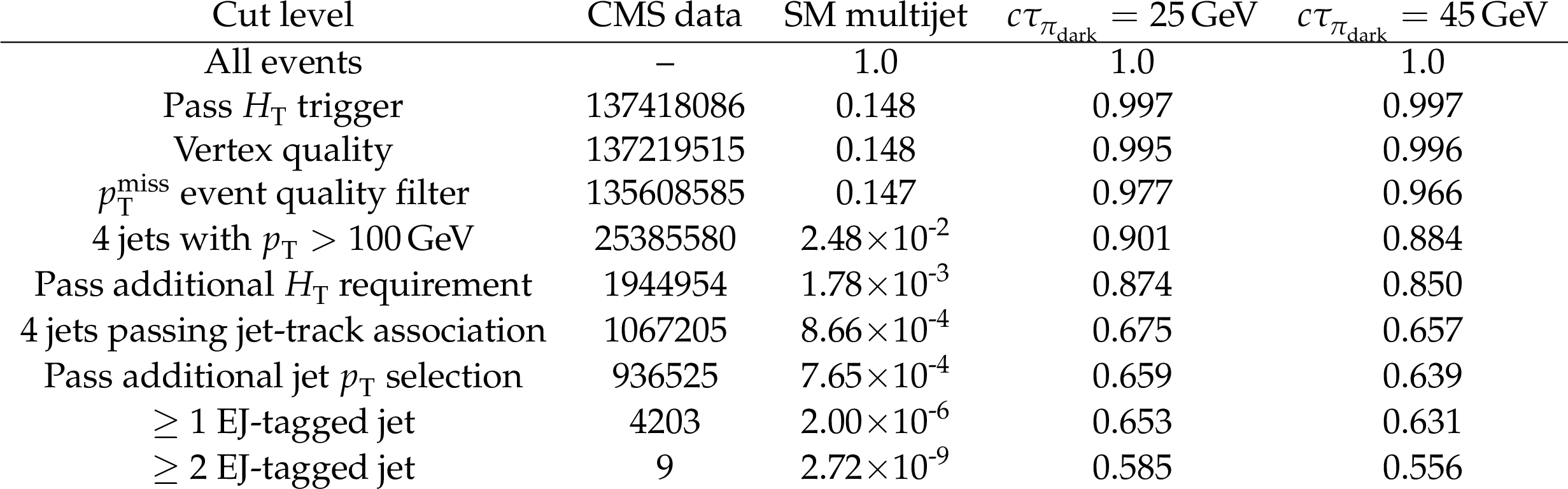
Additional Table 1:
Example cut flow used for selecting signals events using the u-set 4 selection criteria. Simulated background and signal yields are normalized to unity. The example signal events are generated with $ m_{\text{X}_\text{dark}}= $ 1600 GeV and $ m_{\pi_\text{dark}}= $ 10 GeV in the unflavored scenario. |
png pdf |
Additional Table 2:
Example cut flow used for selecting signals events using the uGNN set 3 selection criteria. Simulated background and signal yields are normalized to unity. The example signal events are generated with $ m_{\text{X}_\text{dark}}= $ 1600 GeV and $ m_{\pi_\text{dark}}= $ 10 GeV in the unflavored scenario. |

png pdf |
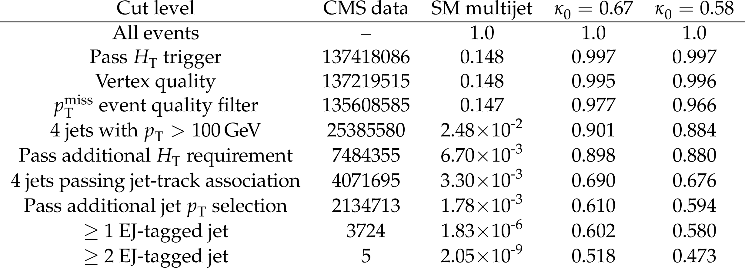
Additional Table 3:
Example cut flow used for selecting signals events using the a-set 3 selection criteria. Simulated background and signal yields are normalized to unity. The example signal events are generated with $ m_{\text{X}_\text{dark}}= $ 1600 GeV and $ m_{\pi_\text{dark}}= $ 10 GeV in the flavor-aligned scenario. |
png pdf |
Additional Table 4:
Example cut flow used for selecting signals events using the aGNN set 3 selection criteria. Simulated background and signal yields are normalized to unity. The example signal events are generated with $ m_{\text{X}_\text{dark}}= $ 1600 GeV and $ m_{\pi_\text{dark}}= $ 10 GeV in the flavor-aligned scenario. |
| References | ||||
| 1 | V. C. Rubin, N. Thonnard, and W. K. Ford, Jr. | Rotational properties of 21 SC galaxies with a large range of luminosities and radii, from NGC 4605 (R = 4 kpc) to UGC 2885 (R = 122 kpc) | Astrophys. J. 238 (1980) 471 | |
| 2 | M. Persic, P. Salucci, and F. Stel | The universal rotation curve of spiral galaxies: I. The dark matter connection | Mon. Not. Roy. Astron. Soc. 281 (1996) 27 | astro-ph/9506004 |
| 3 | D. Clowe et al. | A direct empirical proof of the existence of dark matter | Astrophys. J. 648 (2006) L109 | astro-ph/0608407 |
| 4 | DES Collaboration | Dark Energy Survey year 1 results: curved-sky weak lensing mass map | Mon. Not. Roy. Astron. Soc. 475 (2018) 3165 | 1708.01535 |
| 5 | Planck Collaboration | Planck 2018 results. VI. Cosmological parameters | Astron. Astrophys. 641 (2020) A6 | 1807.06209 |
| 6 | M. J. Strassler and K. M. Zurek | Echoes of a hidden valley at hadron colliders | PLB 651 (2007) 374 | hep-ph/0604261 |
| 7 | K. Petraki and R. R. Volkas | Review of asymmetric dark matter | Int. J. Mod. Phys. A 28 (2013) 1330028 | 1305.4939 |
| 8 | H. Beauchesne, E. Bertuzzo, and G. Grilli di Cortona | Dark matter in Hidden Valley models with stable and unstable light dark mesons | JHEP 04 (2019) 118 | 1809.10152 |
| 9 | Y. Bai and P. Schwaller | Scale of dark QCD | PRD 89 (2014) 063522 | 1306.4676 |
| 10 | T. Cohen, M. Lisanti, and H. K. Lou | Semi-visible jets: Dark matter undercover at the LHC | PRL 115 (2015) 171804 | 1503.00009 |
| 11 | P. Schwaller, D. Stolarski, and A. Weiler | Emerging jets | JHEP 05 (2015) 059 | 1502.05409 |
| 12 | P. Agrawal, M. Blanke, and K. Gemmler | Flavored dark matter beyond Minimal Flavor Violation | JHEP 10 (2014) 072 | 1405.6709 |
| 13 | S. Renner and P. Schwaller | A flavoured dark sector | JHEP 08 (2018) 052 | 1803.08080 |
| 14 | P. Fayet and S. Ferrara | Supersymmetry | Phys. Rept. 32 (1977) 249 | |
| 15 | C. Borschensky et al. | Squark and gluino production cross sections in pp collisions at $ \sqrt{s} = $ 13, 14, 33 and 100 TeV | EPJC 74 (2014) 3174 | 1407.5066 |
| 16 | W. Beenakker et al. | NNLL-fast: predictions for coloured supersymmetric particle production at the LHC with threshold and Coulomb resummation | JHEP 12 (2016) 133 | 1607.07741 |
| 17 | CMS Collaboration | Search for resonant production of strongly coupled dark matter in proton-proton collisions at 13 TeV | JHEP 06 (2022) 156 | CMS-EXO-19-020 2112.11125 |
| 18 | ATLAS Collaboration | Search for non-resonant production of semi-visible jets using Run 2 data in ATLAS | PLB 848 (2024) 138324 | 2305.18037 |
| 19 | ATLAS Collaboration | Search for resonant production of dark quarks in the dijet final state with the ATLAS detector | JHEP 02 (2024) 128 | 2311.03944 |
| 20 | CMS Collaboration | Search for new particles decaying to a jet and an emerging jet | JHEP 02 (2019) 179 | CMS-EXO-18-001 1810.10069 |
| 21 | CMS Collaboration | HEPData record for this analysis | link | |
| 22 | CMS Collaboration | Description and performance of track and primary-vertex reconstruction with the CMS tracker | JINST 9 (2014) P10009 | CMS-TRK-11-001 1405.6569 |
| 23 | Tracker Group of the CMS Collaboration | The CMS phase-1 pixel detector upgrade | JINST 16 (2021) P02027 | 2012.14304 |
| 24 | CMS Collaboration | Track impact parameter resolution for the full pseudo rapidity coverage in the 2017 dataset with the CMS phase-1 pixel detector | CMS Detector Performance Note CMS-DP-2020-049, 2020 CDS |
|
| 25 | CMS Collaboration | Performance of the CMS Level-1 trigger in proton-proton collisions at $ \sqrt{s} = $ 13 TeV | JINST 15 (2020) P10017 | CMS-TRG-17-001 2006.10165 |
| 26 | CMS Collaboration | The CMS trigger system | JINST 12 (2017) P01020 | CMS-TRG-12-001 1609.02366 |
| 27 | CMS Collaboration | The CMS experiment at the CERN LHC | JINST 3 (2008) S08004 | |
| 28 | L. Carloni and T. Sjöstrand | Visible effects of invisible hidden valley radiation | JHEP 09 (2010) 105 | 1006.2911 |
| 29 | L. Carloni, J. Rathsman, and T. Sjöstrand | Discerning secluded sector gauge structures | JHEP 04 (2011) 091 | 1102.3795 |
| 30 | T. Sjöstrand et al. | An introduction to PYTHIA 8.2 | Comput. Phys. Commun. 191 (2015) 159 | 1410.3012 |
| 31 | J. Alwall et al. | The automated computation of tree-level and next-to-leading order differential cross sections, and their matching to parton shower simulations | JHEP 07 (2014) 079 | 1405.0301 |
| 32 | J. Alwall et al. | Comparative study of various algorithms for the merging of parton showers and matrix elements in hadronic collisions | EPJC 53 (2008) 473 | 0706.2569 |
| 33 | CMS Collaboration | Extraction and validation of a new set of CMS PYTHIA8 tunes from underlying-event measurements | EPJC 80 (2020) 4 | CMS-GEN-17-001 1903.12179 |
| 34 | NNPDF Collaboration | Parton distributions from high-precision collider data | EPJC 77 (2017) 663 | 1706.00428 |
| 35 | GEANT4 Collaboration | GEANT4---a simulation toolkit | NIM A 506 (2003) 250 | |
| 36 | CMS Collaboration | Particle-flow reconstruction and global event description with the CMS detector | JINST 12 (2017) P10003 | CMS-PRF-14-001 1706.04965 |
| 37 | CMS Collaboration | Performance of reconstruction and identification of $ \tau $ leptons decaying to hadrons and $ \nu_\tau $ in pp collisions at $ \sqrt{s}= $ 13 TeV | JINST 13 (2018) P10005 | CMS-TAU-16-003 1809.02816 |
| 38 | CMS Collaboration | Jet energy scale and resolution in the CMS experiment in pp collisions at 8 TeV | JINST 12 (2017) P02014 | CMS-JME-13-004 1607.03663 |
| 39 | CMS Collaboration | Performance of missing transverse momentum reconstruction in proton-proton collisions at $ \sqrt{s} = $ 13 TeV using the CMS detector | JINST 14 (2019) P07004 | CMS-JME-17-001 1903.06078 |
| 40 | M. Cacciari, G. P. Salam, and G. Soyez | The anti-$ k_{\mathrm{T}} $ jet clustering algorithm | JHEP 04 (2008) 063 | 0802.1189 |
| 41 | M. Cacciari, G. P. Salam, and G. Soyez | FastJet user manual | EPJC 72 (2012) 1896 | 1111.6097 |
| 42 | E. Bols et al. | Jet flavour classification using DeepJet | JINST 15 (2020) P12012 | 2008.10519 |
| 43 | CMS Collaboration | Identification of heavy-flavour jets with the CMS detector in pp collisions at 13 TeV | JINST 13 (2018) P05011 | CMS-BTV-16-002 1712.07158 |
| 44 | CMS Collaboration | Performance summary of AK4 jet b tagging with data from proton-proton collisions at 13 TeV with the CMS detector | CMS Detector Performance Note CMS-DP-2023-005, 2023 CDS |
|
| 45 | K. Rose | Deterministic annealing for clustering, compression, classification, regression, and related optimization problems | IEEE Proc. 86 (1998) 2210 | |
| 46 | R. Fruhwirth, W. Waltenberger, and P. Vanlaer | Adaptive vertex fitting | JPG 34 (2007) N343 | |
| 47 | CMS Collaboration | Technical proposal for the Phase-II upgrade of the Compact Muon Solenoid | CMS Technical Proposal CERN-LHCC-2015-010, CMS-TDR-15-02, 2015 CDS |
|
| 48 | CMS Collaboration | Pileup mitigation at CMS in 13 TeV data | JINST 15 (2020) P09018 | CMS-JME-18-001 2003.00503 |
| 49 | CMS Collaboration | Jet algorithms performance in 13 TeV data | CMS Physics Analysis Summary, 2017 CMS-PAS-JME-16-003 |
CMS-PAS-JME-16-003 |
| 50 | J. Thaler and K. Van Tilburg | Identifying boosted objects with N-subjettiness | JHEP 03 (2011) 015 | 1011.2268 |
| 51 | H. Qu and L. Gouskos | Jet tagging via particle clouds | PRD 101 (2020) 056019 | 1902.08570 |
| 52 | CMS Collaboration | Precision luminosity measurement in proton-proton collisions at $ \sqrt{s} = $ 13 TeV in 2015 and 2016 at CMS | EPJC 81 (2021) 800 | CMS-LUM-17-003 2104.01927 |
| 53 | CMS Collaboration | CMS luminosity measurement for the 2017 data-taking period at $ \sqrt{s} = $ 13 TeV | CMS Physics Analysis Summary, 2018 CMS-PAS-LUM-17-004 |
CMS-PAS-LUM-17-004 |
| 54 | CMS Collaboration | CMS luminosity measurement for the 2018 data-taking period at $ \sqrt{s}= $ 13 TeV | CMS Physics Analysis Summary, 2019 CMS-PAS-LUM-18-002 |
CMS-PAS-LUM-18-002 |
| 55 | CMS Collaboration | Measurement of the inelastic proton-proton cross section at $ \sqrt{s}= $ 13 TeV | JHEP 07 (2018) 161 | CMS-FSQ-15-005 1802.02613 |
| 56 | NNPDF Collaboration | Parton distributions with QED corrections | NPB 877 (2013) 290 | 1308.0598 |
| 57 | CMS Collaboration | Muon tracking performance in the CMS Run-2 Legacy data using the tag-and-probe technique | CMS Detector Performance Note CMS-DP-2020-035, 2020 CDS |
|
| 58 | M. Cacciari et al. | The t anti-t cross-section at 1.8-TeV and 1.96-TeV: A study of the systematics due to parton densities and scale dependence | JHEP 04 (2004) 068 | hep-ph/0303085 |
| 59 | S. Catani, D. de Florian, M. Grazzini, and P. Nason | Soft gluon resummation for Higgs boson production at hadron colliders | JHEP 07 (2003) 028 | hep-ph/0306211 |
| 60 | T. Junk | Confidence level computation for combining searches with small statistics | NIM A 434 (1999) 435 | hep-ex/9902006 |
| 61 | A. L. Read | Presentation of search results: the $ \text{CL}_\text{s} $ technique | JPG 28 (2002) 2693 | |
| 62 | ATLAS and CMS Collaborations, and LHC Higgs Combination Group | Procedure for the LHC Higgs boson search combination in Summer 2011 | Technical Report CMS-NOTE-2011-005, ATL-PHYS-PUB-2011-11, 2011 | |
|
|
Compact Muon Solenoid LHC, CERN |
|

|

|

|

|

|