

Compact Muon Solenoid
LHC, CERN
| CMS-EXO-19-020 ; CERN-EP-2021-252 | ||
| Search for resonant production of strongly coupled dark matter in proton-proton collisions at 13 TeV | ||
| CMS Collaboration | ||
| 21 December 2021 | ||
| JHEP 06 (2022) 156 | ||
| Abstract: The first collider search for dark matter arising from a strongly coupled hidden sector is presented and uses a data sample corresponding to 138 fb$^{-1}$, collected with the CMS detector at the CERN LHC, at $\sqrt{s} = $ 13 TeV. The hidden sector is hypothesized to couple to the standard model (SM) via a heavy leptophobic Z' mediator produced as a resonance in proton-proton collisions. The mediator decay results in two "semivisible'' jets, containing both visible matter and invisible dark matter. The final state therefore includes moderate missing energy aligned with one of the jets, a signature ignored by most dark matter searches. No structure in the dijet transverse mass spectra compatible with the signal is observed. Assuming the Z' boson has a universal coupling of 0.25 to the SM quarks, an inclusive search, relevant to any model that exhibits this kinematic behavior, excludes mediator masses of 1.5-4.0 TeV at 95% confidence level, depending on the other signal model parameters. To enhance the sensitivity of the search for this particular class of hidden sector models, a boosted decision tree (BDT) is trained using jet substructure variables to distinguish between semivisible jets and SM jets from background processes. When the BDT is employed to identify each jet in the dijet system as semivisible, the mediator mass exclusion increases to 5.1 TeV, for wider ranges of the other signal model parameters. These limits exclude a wide range of strongly coupled hidden sector models for the first time. | ||
| Links: e-print arXiv:2112.11125 [hep-ex] (PDF) ; CDS record ; inSPIRE record ; HepData record ; CADI line (restricted) ; | ||
| Figures & Tables | Summary | Additional Figures & Tables | References | CMS Publications |
|---|
| Figures | |
png pdf |
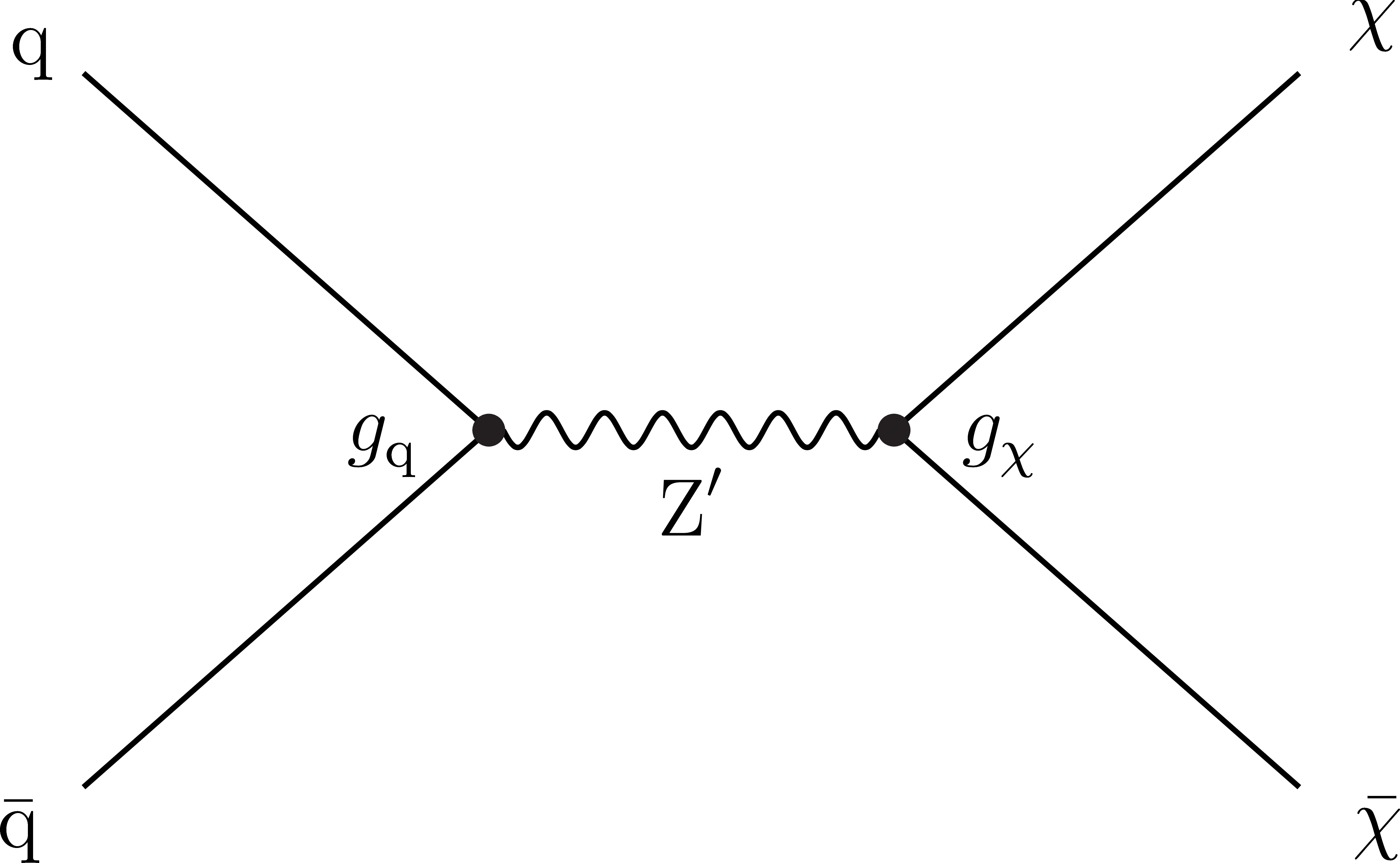
Figure 1:
Feynman diagram of leading-order resonant production of dark quarks through a Z' mediator. The relevant couplings to SM quarks and dark quarks, ${g_{\mathrm{q}}}$ and ${g_{{\chi}}}$, are indicated at the labeled vertices. |
png pdf root |
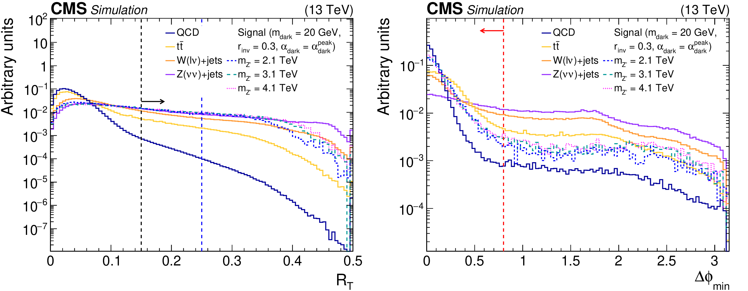
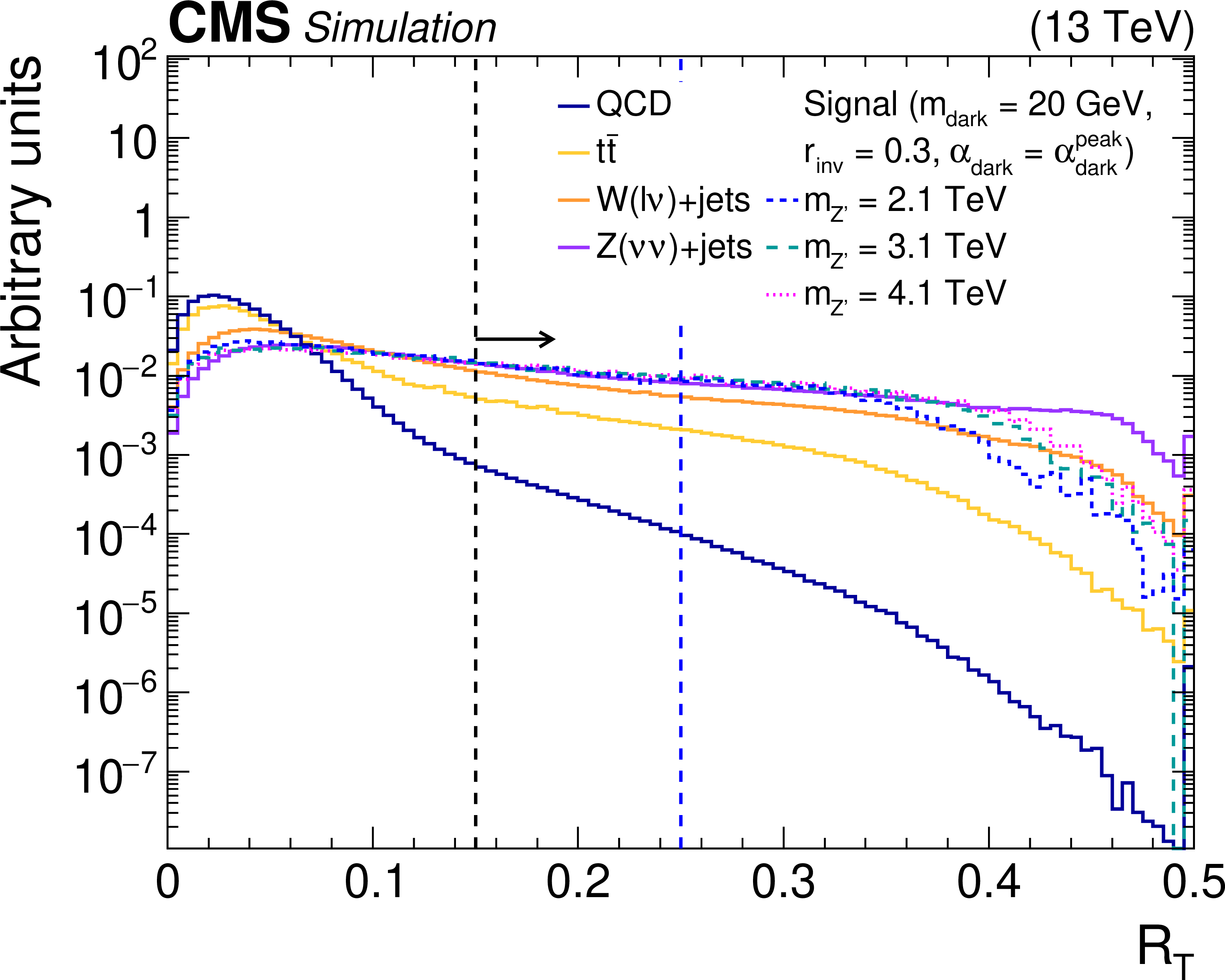
Figure 2:
The normalized distributions of the characteristic variables ${R_{\mathrm {T}}}$ and ${\Delta \phi _{\text {min}}}$ for the simulated SM backgrounds and several signal models. For each variable, the requirement on that variable is omitted, but all other preselection requirements are applied. The black (red) vertical dotted line indicates the preselection (final selection) requirement on the variable, if any. The blue vertical dotted line indicates the boundary between different signal regions. The last bin of each histogram includes the overflow events. |
png pdf root |
Figure 2-a:
The normalized distribution of ${R_{\mathrm {T}}}$ for the simulated SM backgrounds and several signal models. The requirement on that variable is omitted, but all other preselection requirements are applied. The black (red) vertical dotted line indicates the preselection (final selection) requirement on the variable, if any. The blue vertical dotted line indicates the boundary between different signal regions. The last bin includes the overflow events. |

png pdf root |
Figure 2-b:
The normalized distribution of ${\Delta \phi _{\text {min}}}$ for the simulated SM backgrounds and several signal models. The requirement on that variable is omitted, but all other preselection requirements are applied. The black (red) vertical dotted line indicates the preselection (final selection) requirement on the variable, if any. The blue vertical dotted line indicates the boundary between different signal regions. The last bin includes the overflow events. |
png pdf |
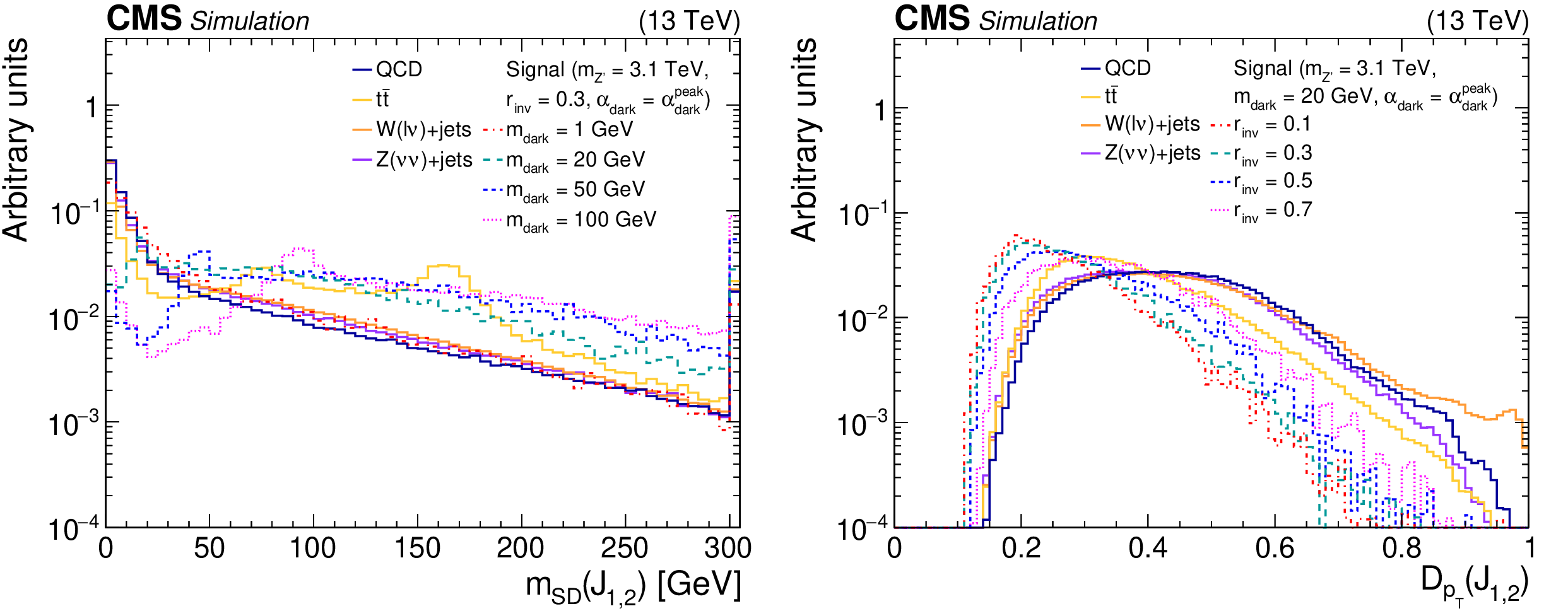
Figure 3:
The normalized distributions of the BDT input variables ${m_{\mathrm {SD}}}$ and ${D_{{p_{\mathrm {T}}}}}$ for the two highest ${p_{\mathrm {T}}}$ jets from the simulated SM backgrounds and several signal models. Each sample's jet ${p_{\mathrm {T}}}$ distribution is weighted to match a reference distribution (see text). The last bin of each histogram includes the overflow events. |

png pdf root |
Figure 3-a:
The normalized distribution of the BDT input variable ${m_{\mathrm {SD}}}$ for the two highest ${p_{\mathrm {T}}}$ jets from the simulated SM backgrounds and several signal models. Each sample's jet ${p_{\mathrm {T}}}$ distribution is weighted to match a reference distribution (see text). The last bin includes the overflow events. |
png pdf root |
Figure 3-b:
The normalized distribution of the BDT input variable ${D_{{p_{\mathrm {T}}}}}$ for the two highest ${p_{\mathrm {T}}}$ jets from the simulated SM backgrounds and several signal models. Each sample's jet ${p_{\mathrm {T}}}$ distribution is weighted to match a reference distribution (see text). The last bin includes the overflow events. |
png pdf |
Figure 4:
Left: The normalized BDT discriminator distribution for the two highest ${p_{\mathrm {T}}}$ jets from the simulated SM backgrounds and several signal models. The discriminator WP of 0.55 is indicated as a dashed line. Right: The BDT ROC curves for the two highest ${p_{\mathrm {T}}}$ jets, comparing the simulated SM backgrounds with one signal model. The area under the ROC curve is listed in parentheses for each pairing. The discriminator WP of 0.55 is indicated on each curve as a filled circle. |
png pdf root |
Figure 4-a:
The normalized BDT discriminator distribution for the two highest ${p_{\mathrm {T}}}$ jets from the simulated SM backgrounds and several signal models. The discriminator WP of 0.55 is indicated as a dashed line. |
png pdf root |
Figure 4-b:
The BDT ROC curves for the two highest ${p_{\mathrm {T}}}$ jets, comparing the simulated SM backgrounds with one signal model. The area under the ROC curve is listed in parentheses for each pairing. The discriminator WP of 0.55 is indicated on each curve as a filled circle. |

png pdf |
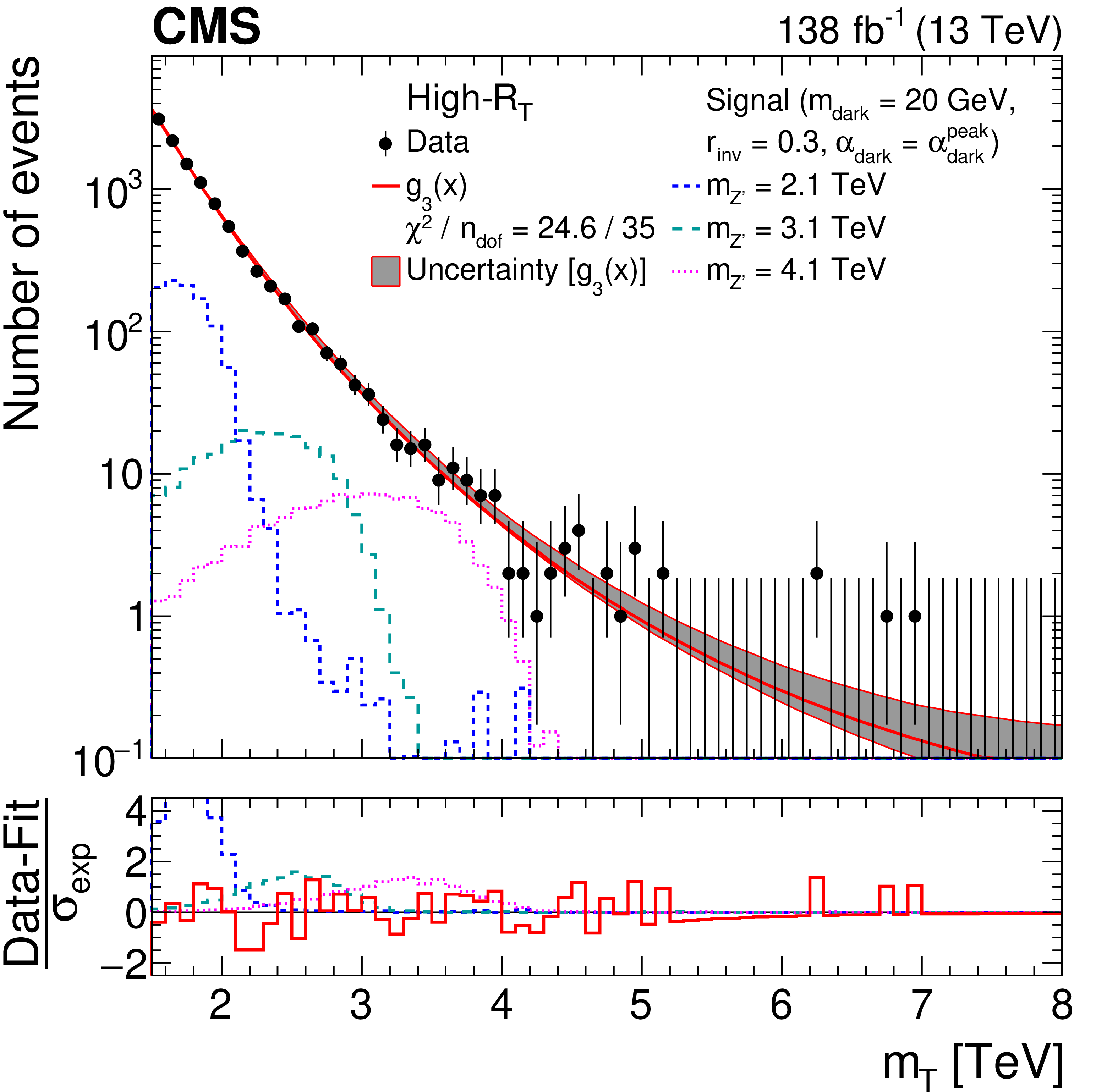
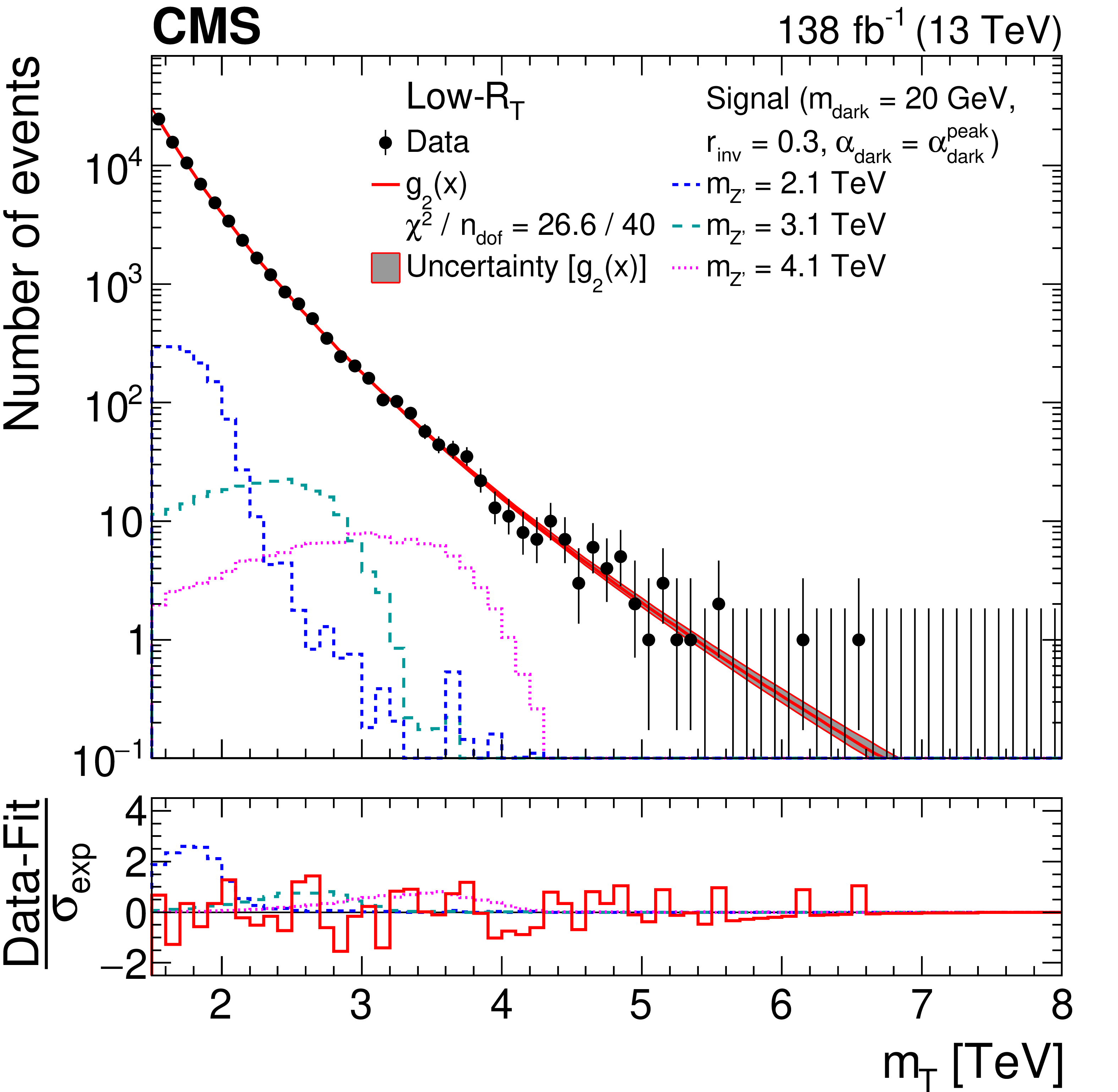
Figure 5:
The ${m_{\mathrm {T}}}$ distribution for the high-${R_{\mathrm {T}}}$ (left) and low-${R_{\mathrm {T}}}$ (right) signal regions, comparing the observed data to the background prediction from the analytic fit (${g_{3}(x) = \exp(p_1 x) x^{p_2 (1 + p_3 \ln(x))}}$, ${g_{2}(x) = \exp(p_1 x) x^{p_2}}$, ${x = {m_{\mathrm {T}}} /\,\sqrt {\smash [b]{s}}}$). The lower panel shows the difference between the observation and the prediction divided by the statistical uncertainty in the observation (${\sigma _{\text {exp}}}$). The distributions from several example signal models, with cross sections corresponding to the observed limits, are superimposed. |
png pdf root |
Figure 5-a:
The ${m_{\mathrm {T}}}$ distribution for the high-${R_{\mathrm {T}}}$ signal region, comparing the observed data to the background prediction from the analytic fit (${g_{3}(x) = \exp(p_1 x) x^{p_2 (1 + p_3 \ln(x))}}$, ${x = {m_{\mathrm {T}}} /\,\sqrt {\smash [b]{s}}}$). The lower panel shows the difference between the observation and the prediction divided by the statistical uncertainty in the observation (${\sigma _{\text {exp}}}$). The distributions from several example signal models, with cross sections corresponding to the observed limits, are superimposed. |
png pdf root |
Figure 5-b:
The ${m_{\mathrm {T}}}$ distribution for the low-${R_{\mathrm {T}}}$ signal region, comparing the observed data to the background prediction from the analytic fit (${g_{2}(x) = \exp(p_1 x) x^{p_2}}$, ${x = {m_{\mathrm {T}}} /\,\sqrt {\smash [b]{s}}}$). The lower panel shows the difference between the observation and the prediction divided by the statistical uncertainty in the observation (${\sigma _{\text {exp}}}$). The distributions from several example signal models, with cross sections corresponding to the observed limits, are superimposed. |
png pdf |
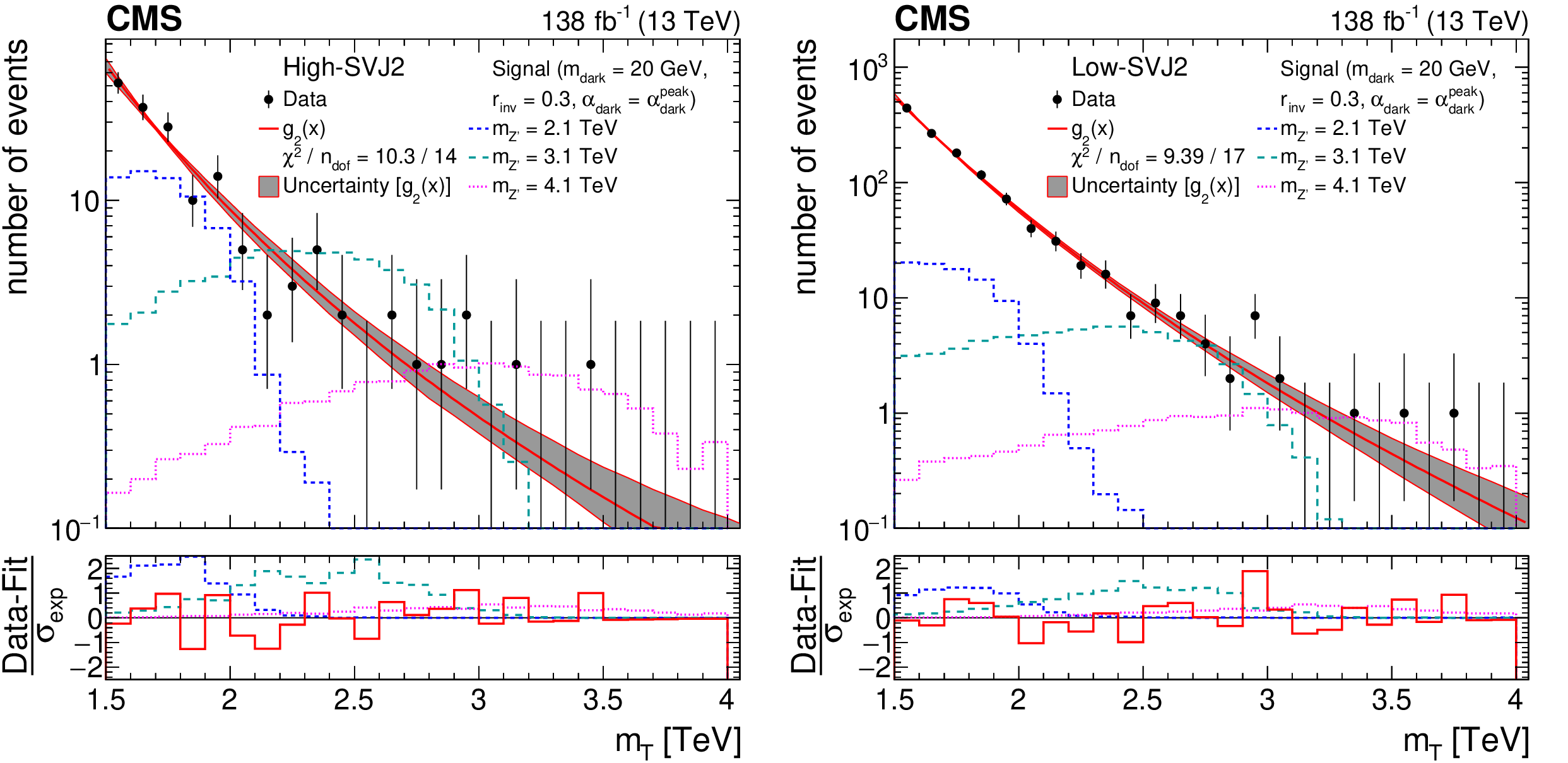
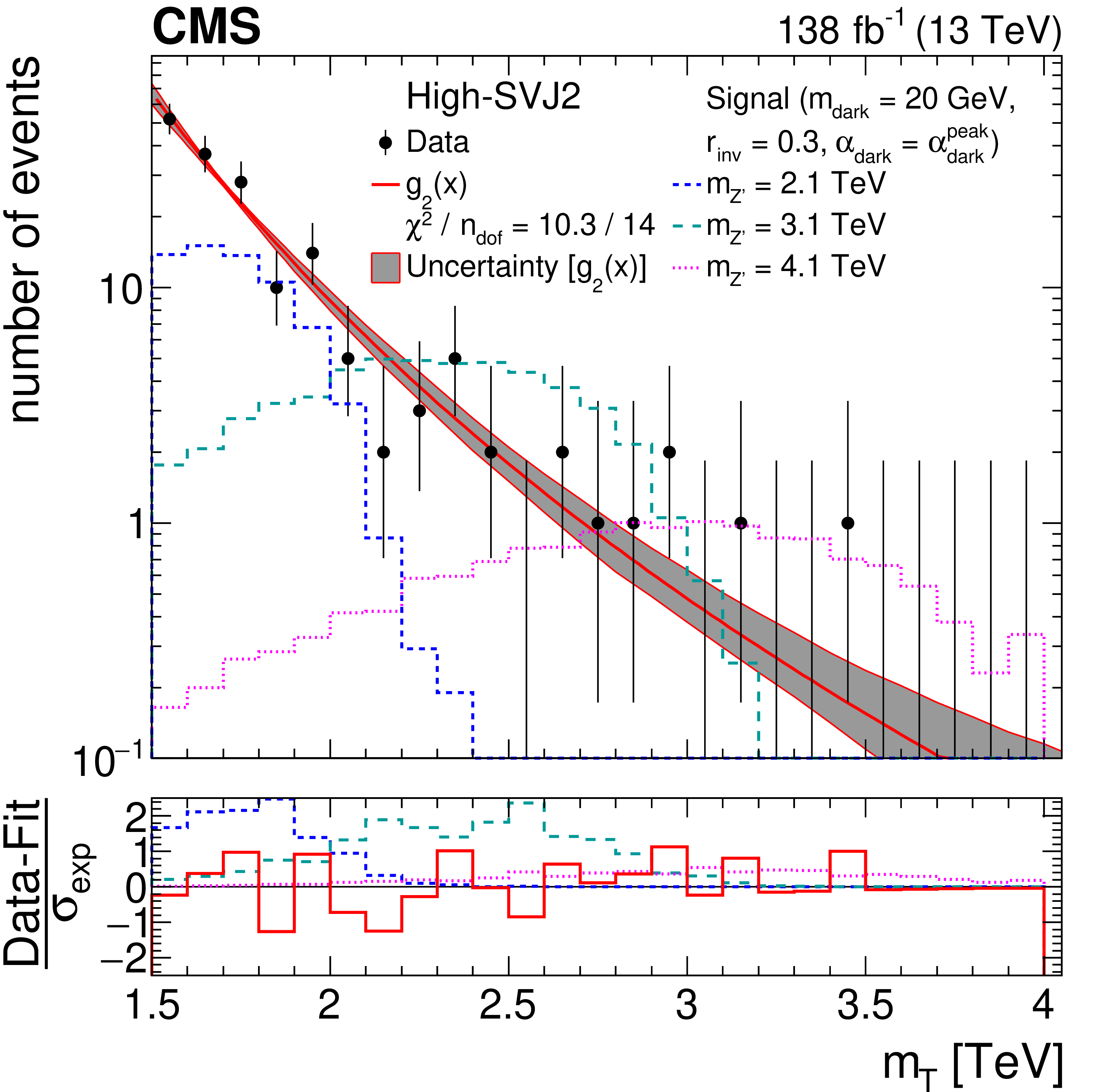
Figure 6:
The ${m_{\mathrm {T}}}$ distribution for the high-SVJ2 (left) and low-SVJ2 (right) signal regions, comparing the observed data to the background prediction from the analytic fit (${g_{2}(x) = \exp(p_1 x) x^{p_2}}$, ${x = {m_{\mathrm {T}}} /\,\sqrt {\smash [b]{s}}}$). The lower panel shows the difference between the observation and the prediction divided by the statistical uncertainty in the observation (${\sigma _{\text {exp}}}$). The distributions from several example signal models, with cross sections corresponding to the observed limits, are superimposed. |
png pdf root |
Figure 6-a:
The ${m_{\mathrm {T}}}$ distribution for the high-SVJ2 signal region, comparing the observed data to the background prediction from the analytic fit (${g_{2}(x) = \exp(p_1 x) x^{p_2}}$, ${x = {m_{\mathrm {T}}} /\,\sqrt {\smash [b]{s}}}$). The lower panel shows the difference between the observation and the prediction divided by the statistical uncertainty in the observation (${\sigma _{\text {exp}}}$). The distributions from several example signal models, with cross sections corresponding to the observed limits, are superimposed. |

png pdf root |
Figure 6-b:
The ${m_{\mathrm {T}}}$ distribution for the low-SVJ2 signal region, comparing the observed data to the background prediction from the analytic fit (${g_{2}(x) = \exp(p_1 x) x^{p_2}}$, ${x = {m_{\mathrm {T}}} /\,\sqrt {\smash [b]{s}}}$). The lower panel shows the difference between the observation and the prediction divided by the statistical uncertainty in the observation (${\sigma _{\text {exp}}}$). The distributions from several example signal models, with cross sections corresponding to the observed limits, are superimposed. |

png pdf |
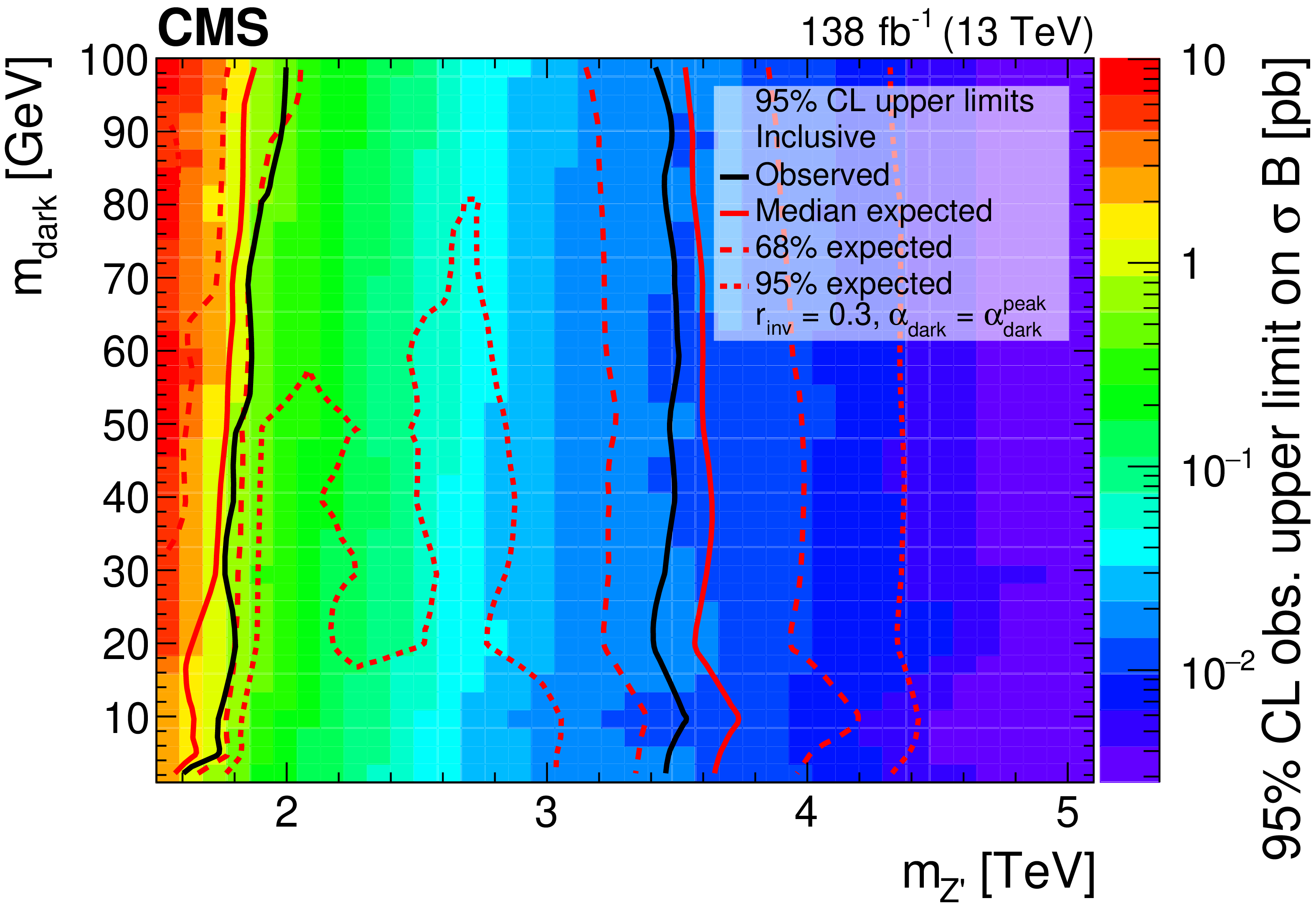
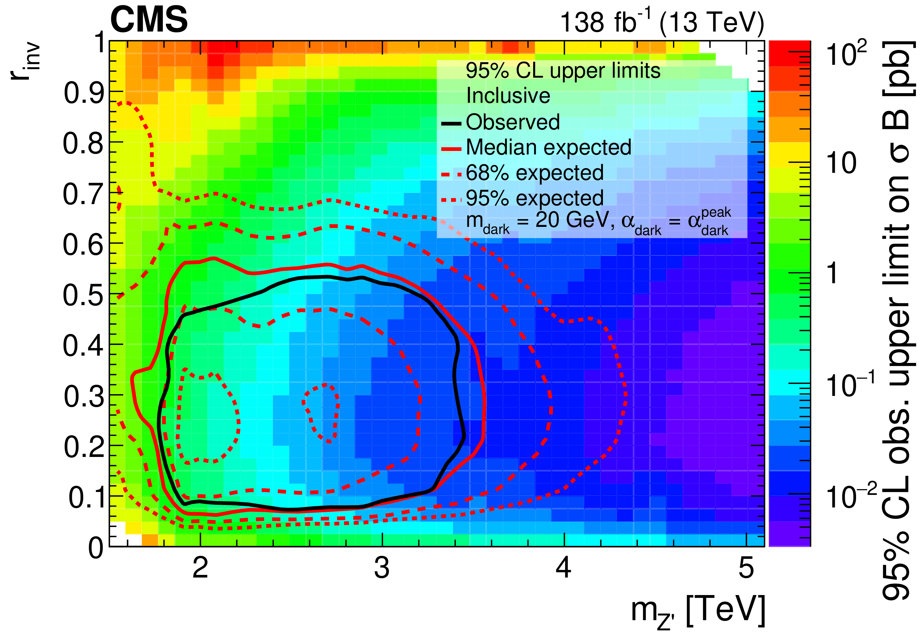
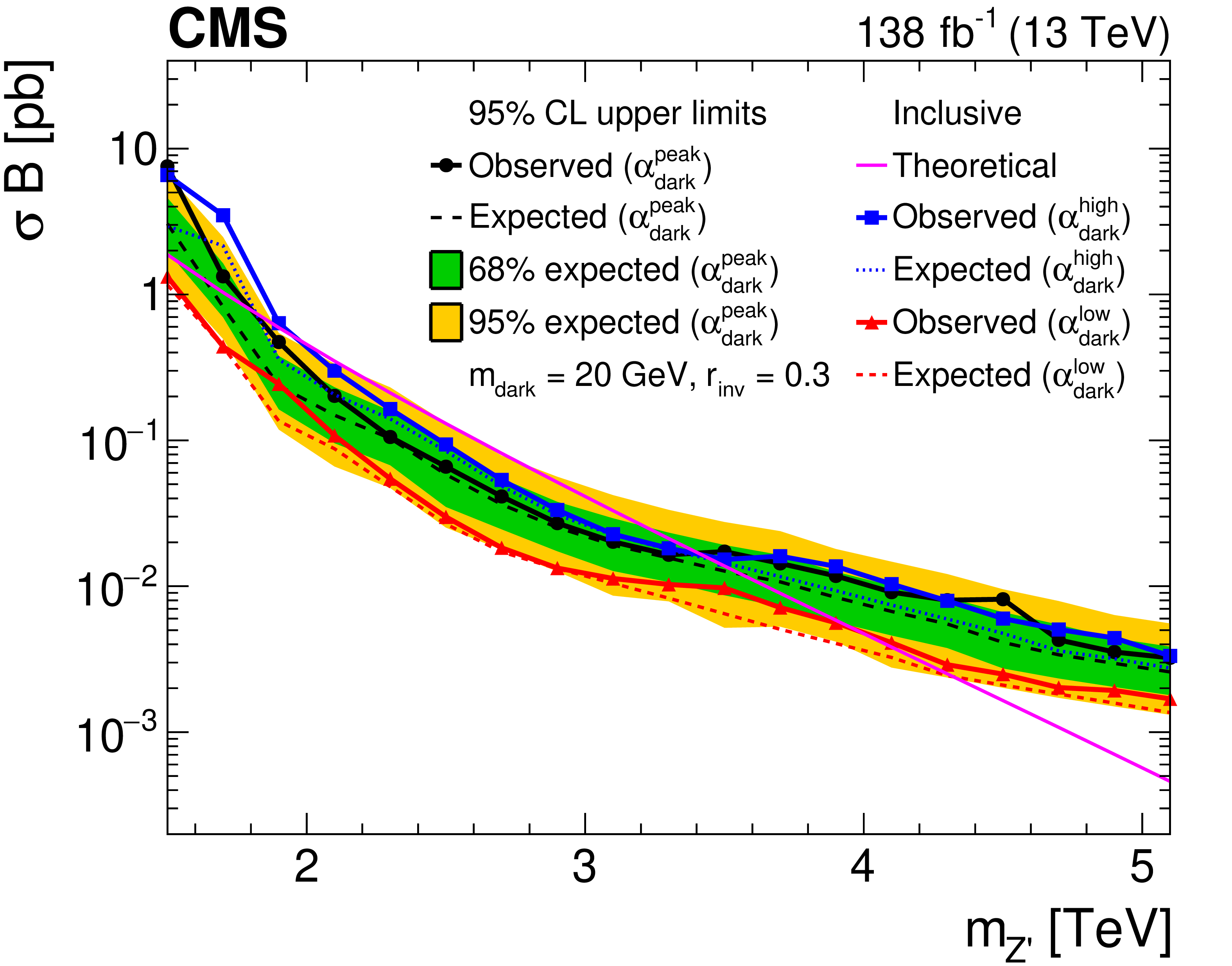
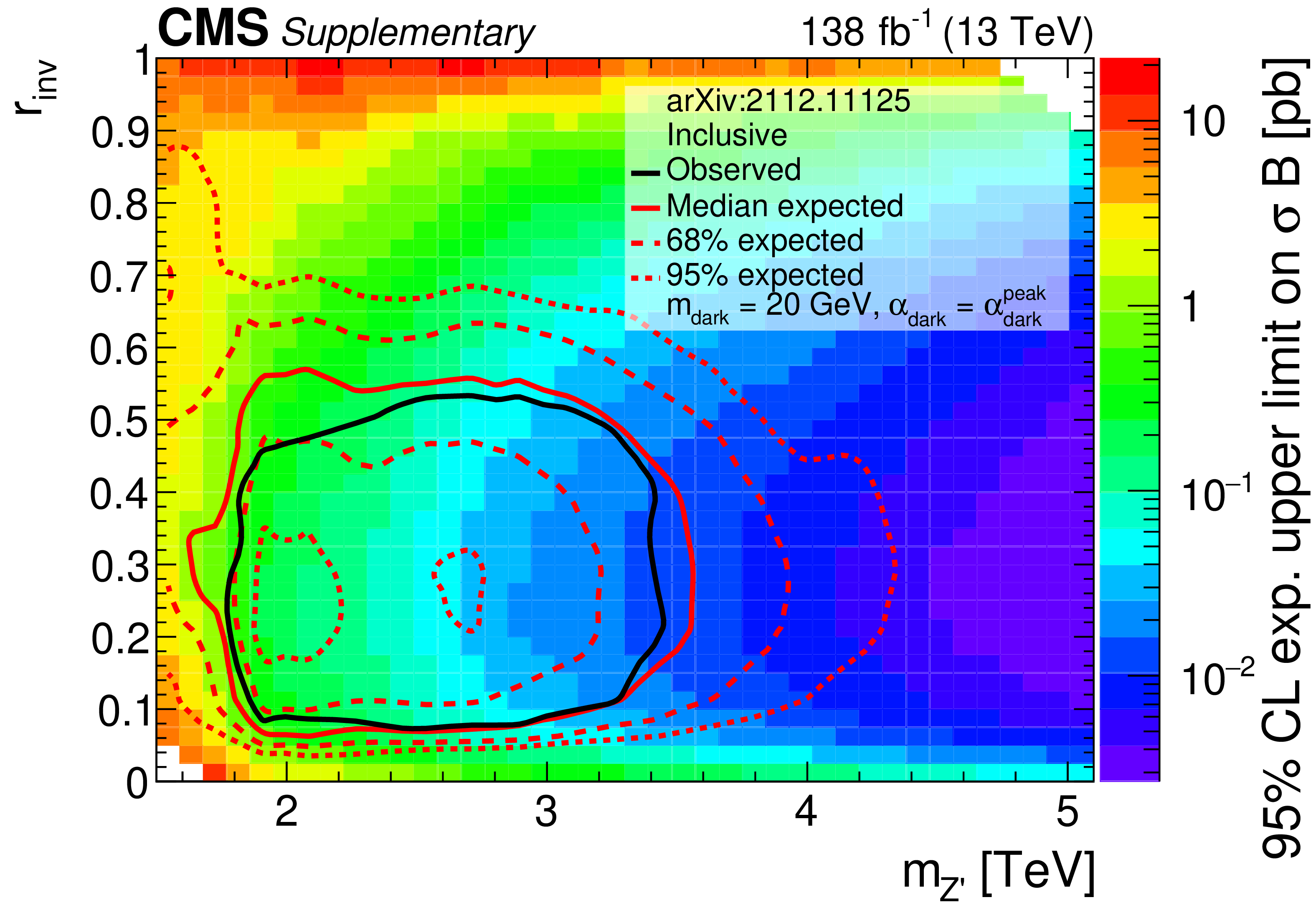
Figure 7:
The 95% CL upper limits on the product of the cross section and branching fraction from the inclusive search, for variations of pairs of the signal model parameters. In the upper plots, the filled region indicates the observed upper limit. The solid black curves indicate the observed exclusions for the nominal Z' cross section, while the solid red curves indicate the expected exclusions, and the dashed lines indicate the regions containing 68 and 95% of the distributions of expected exclusions. In the upper left plot, the regions between the respective pairs of lines or below the inner 95% dashed line are excluded. In the upper right plot, the regions inside the circles are excluded. The lower plot shows the ${\alpha _{\text {dark}}}$ variation as multiple curves in one dimension, because there are only three parameter values considered. The black, blue, and red solid lines show the observed upper limits for each variation, while the dashed lines show the expected limits. The inner (green) and outer (yellow) bands indicate the regions containing 68 and 95%, respectively, of the distributions of expected limits. The purple solid line labeled "Theoretical'' represents the nominal Z' cross section. |
png pdf root |
Figure 7-a:
The 95% CL upper limits on the product of the cross section and branching fraction from the inclusive search, for variations of pairs of the signal model parameters. The filled region indicates the observed upper limit. The solid black curves indicate the observed exclusions for the nominal Z' cross section, while the solid red curves indicate the expected exclusions, and the dashed lines indicate the regions containing 68 and 95% of the distributions of expected exclusions. The regions between the respective pairs of lines or below the inner 95% dashed line are excluded. |
png pdf root |
Figure 7-b:
The 95% CL upper limits on the product of the cross section and branching fraction from the inclusive search, for variations of pairs of the signal model parameters. The filled region indicates the observed upper limit. The solid black curves indicate the observed exclusions for the nominal Z' cross section, while the solid red curves indicate the expected exclusions, and the dashed lines indicate the regions containing 68 and 95% of the distributions of expected exclusions. The regions inside the circles are excluded. |
png pdf root |
Figure 7-c:
The 95% CL upper limits on the product of the cross section and branching fraction from the inclusive search. The plot shows the ${\alpha _{\text {dark}}}$ variation as multiple curves in one dimension, because there are only three parameter values considered. The black, blue, and red solid lines show the observed upper limits for each variation, while the dashed lines show the expected limits. The inner (green) and outer (yellow) bands indicate the regions containing 68 and 95%, respectively, of the distributions of expected limits. The purple solid line labeled "Theoretical'' represents the nominal Z' cross section. |

png pdf |
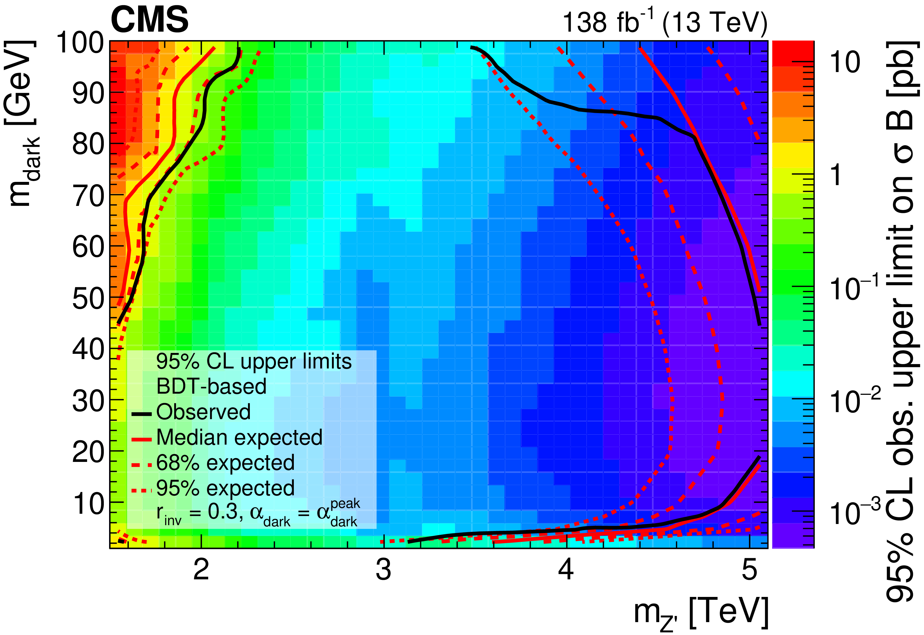
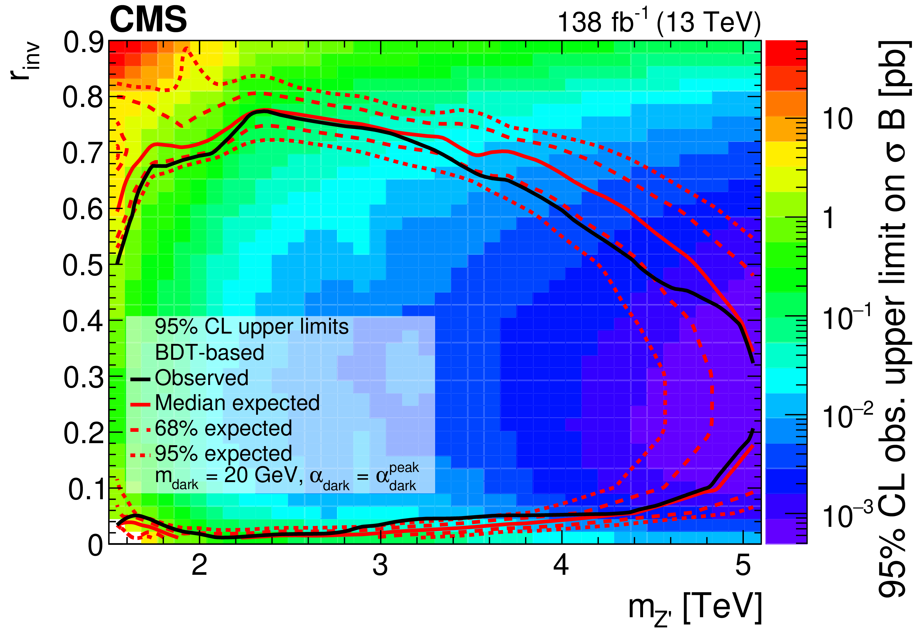
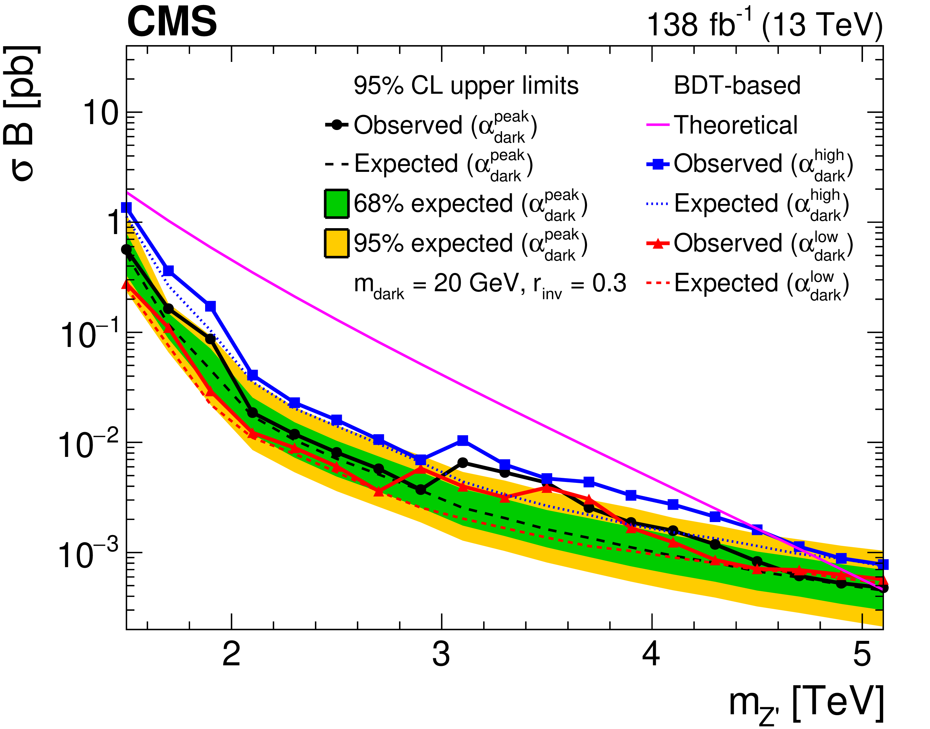
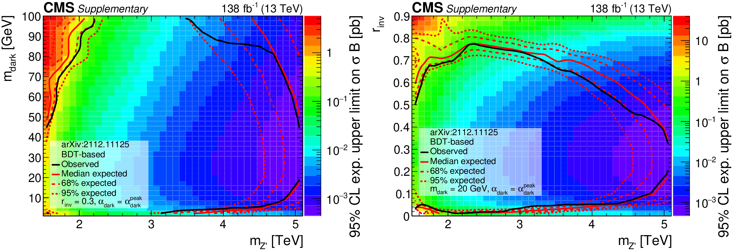
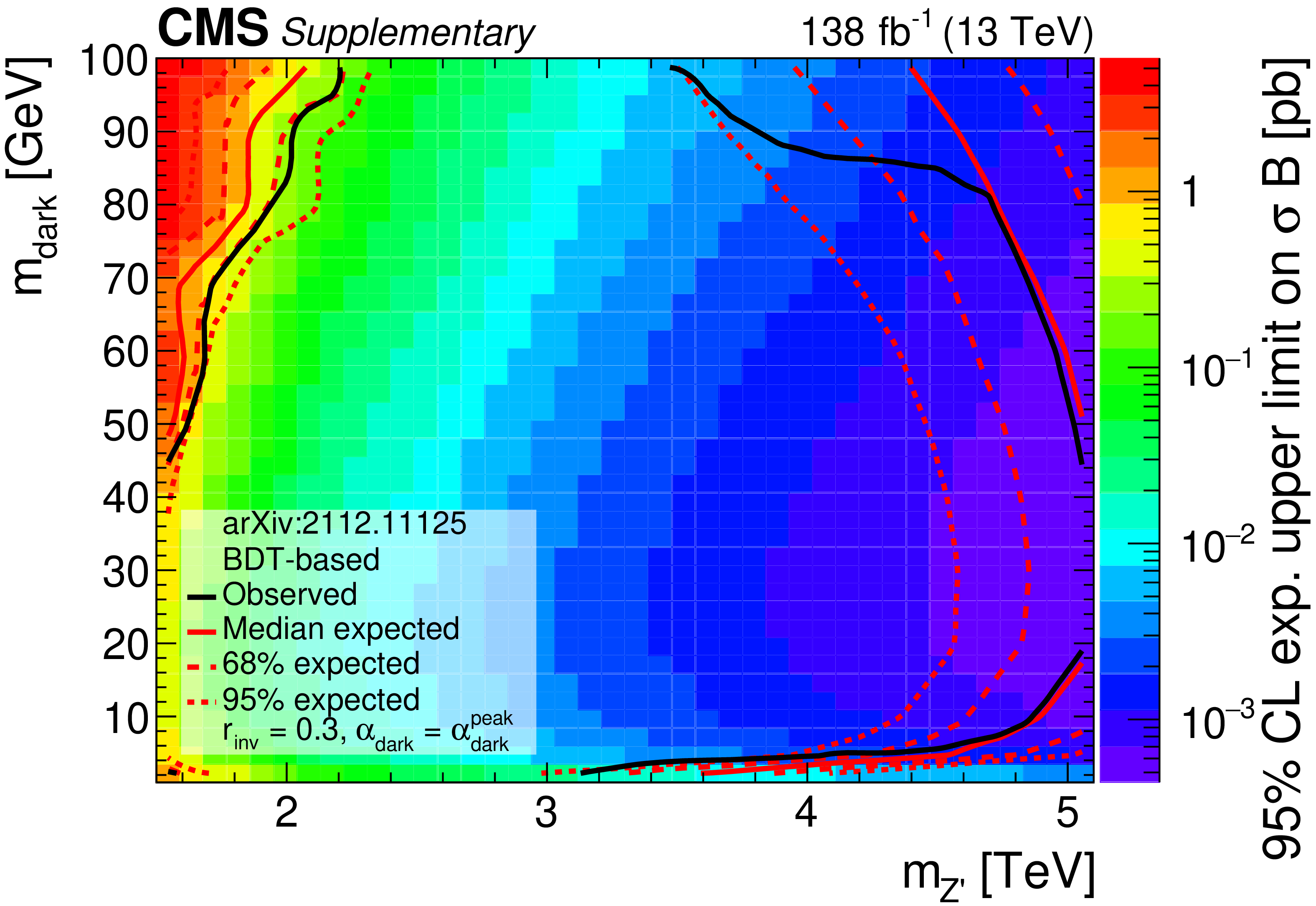
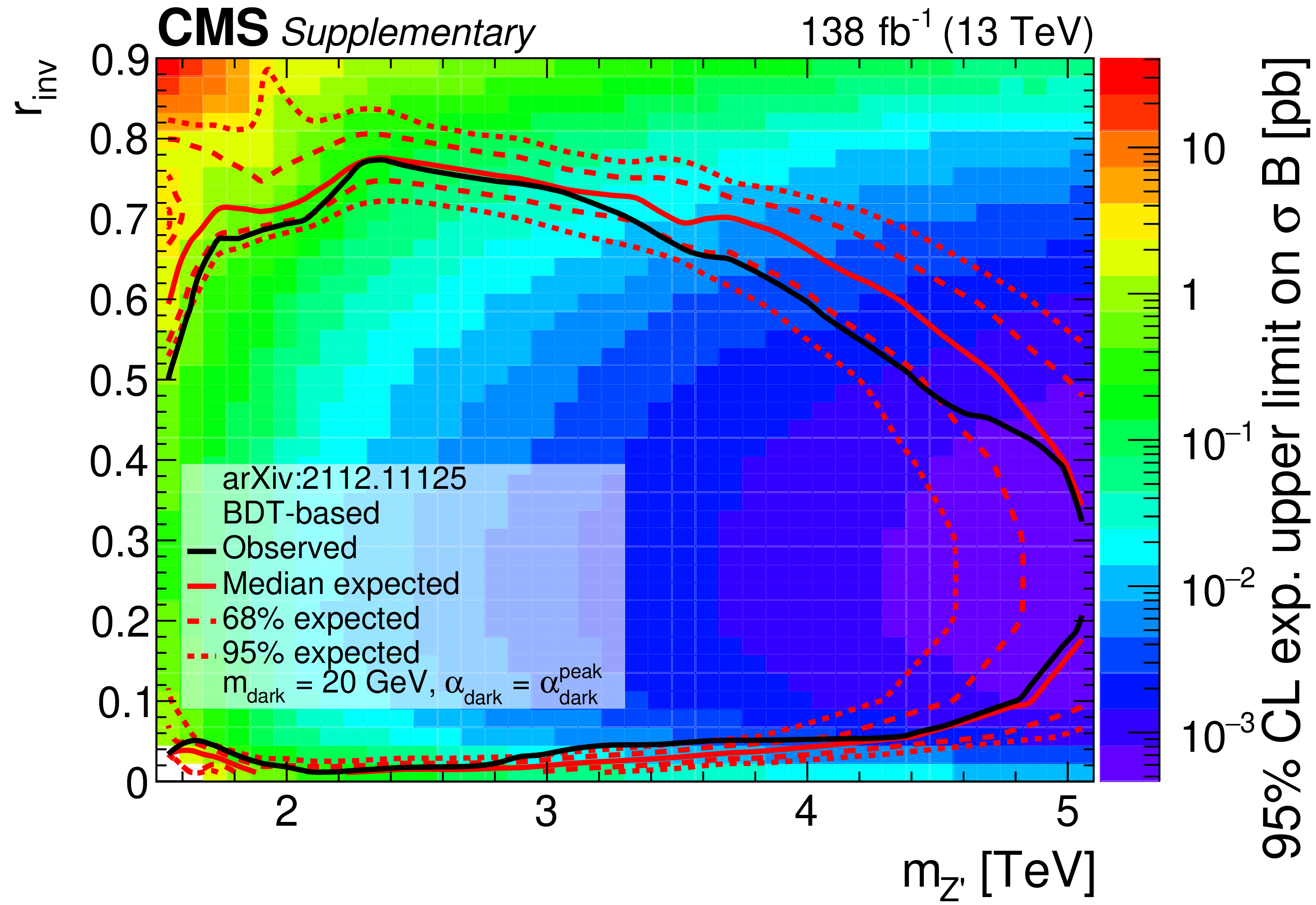
Figure 8:
The 95% CL upper limits on the product of the cross section and branching fraction from the BDT-based search, for variations of pairs of the signal model parameters. In the upper plots, the filled region indicates the observed upper limit. The solid black curves indicate the observed exclusions for the nominal Z' cross section, while the solid red curves indicate the expected exclusions, and the dashed lines indicate the regions containing 68 and 95% of the distributions of expected exclusions. The regions inside the circles are excluded. The lower plot shows the ${\alpha _{\text {dark}}}$ variation as multiple curves in one dimension, because there are only three parameter values considered. The black, blue, and red solid lines show the observed upper limits for each variation, while the dashed lines show the expected limits. The inner (green) and outer (yellow) bands indicate the regions containing 68 and 95%, respectively, of the distributions of expected limits. The purple solid line labeled "Theoretical'' represents the nominal Z' cross section. |
png pdf root |
Figure 8-a:
The 95% CL upper limits on the product of the cross section and branching fraction from the BDT-based search, for variations of pairs of the signal model parameters. The filled region indicates the observed upper limit. The solid black curves indicate the observed exclusions for the nominal Z' cross section, while the solid red curves indicate the expected exclusions, and the dashed lines indicate the regions containing 68 and 95% of the distributions of expected exclusions. The regions inside the circles are excluded. |
png pdf root |
Figure 8-b:
The 95% CL upper limits on the product of the cross section and branching fraction from the BDT-based search, for variations of pairs of the signal model parameters. The filled region indicates the observed upper limit. The solid black curves indicate the observed exclusions for the nominal Z' cross section, while the solid red curves indicate the expected exclusions, and the dashed lines indicate the regions containing 68 and 95% of the distributions of expected exclusions. The regions inside the circles are excluded. |
png pdf root |
Figure 8-c:
The 95% CL upper limits on the product of the cross section and branching fraction from the BDT-based search. The plot shows the ${\alpha _{\text {dark}}}$ variation as multiple curves in one dimension, because there are only three parameter values considered. The black, blue, and red solid lines show the observed upper limits for each variation, while the dashed lines show the expected limits. The inner (green) and outer (yellow) bands indicate the regions containing 68 and 95%, respectively, of the distributions of expected limits. The purple solid line labeled "Theoretical'' represents the nominal Z' cross section. |
| Tables | |
png pdf |
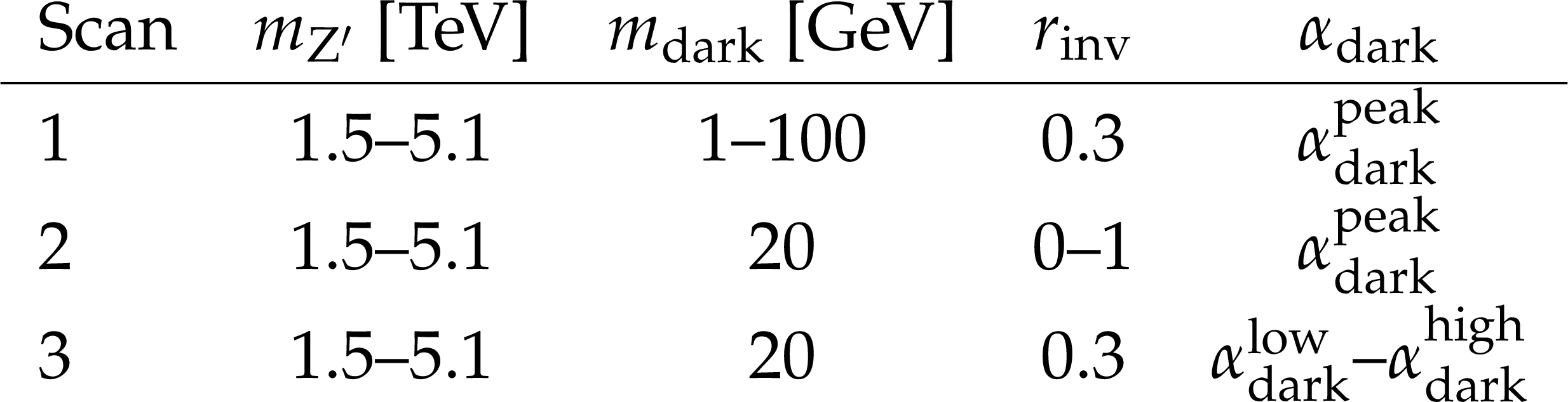
Table 1:
The three two-dimensional signal model parameter scans. For each scan, the ranges of the parameters that are varied in that scan are indicated by dashes. |
png pdf |
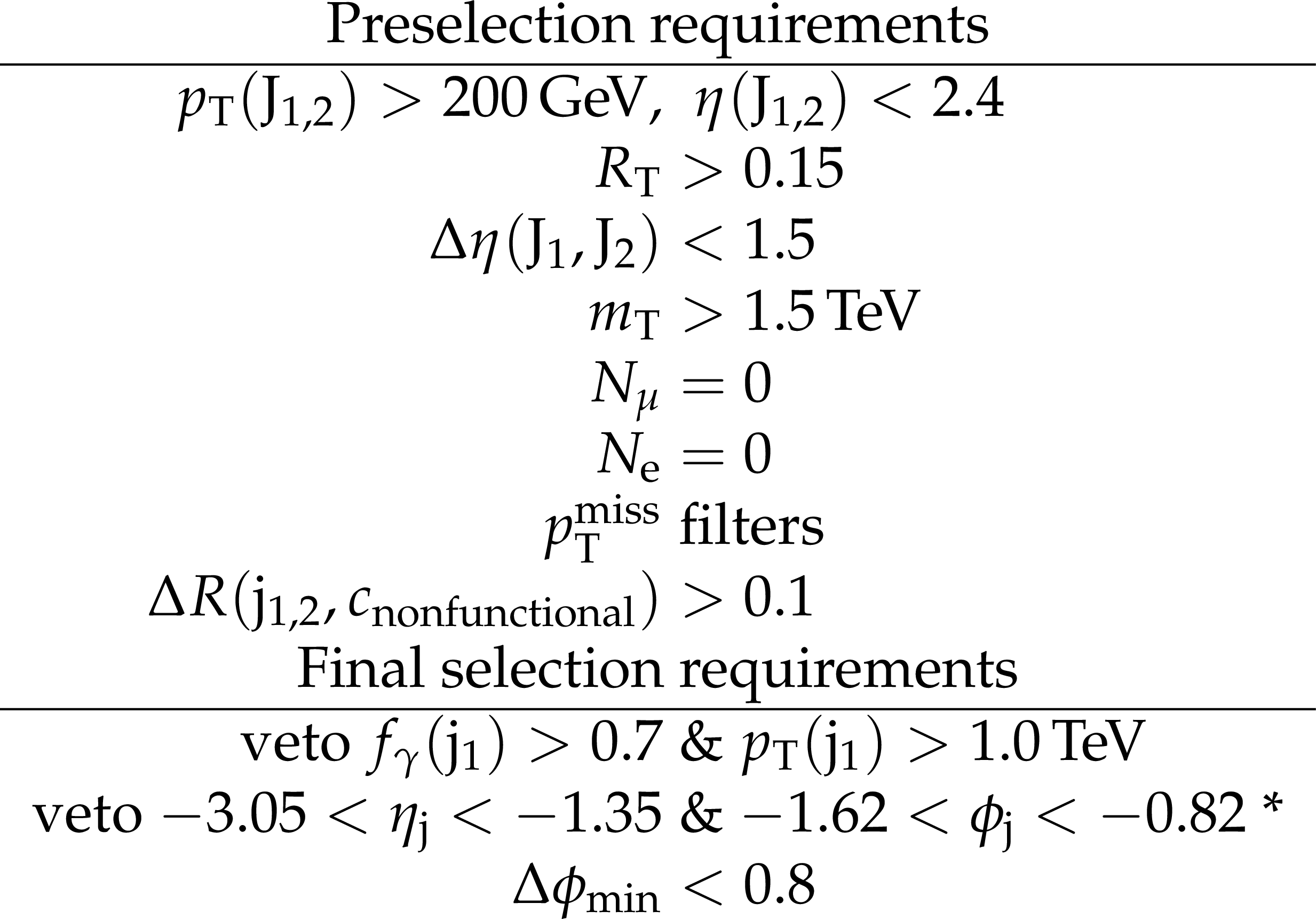
Table 2:
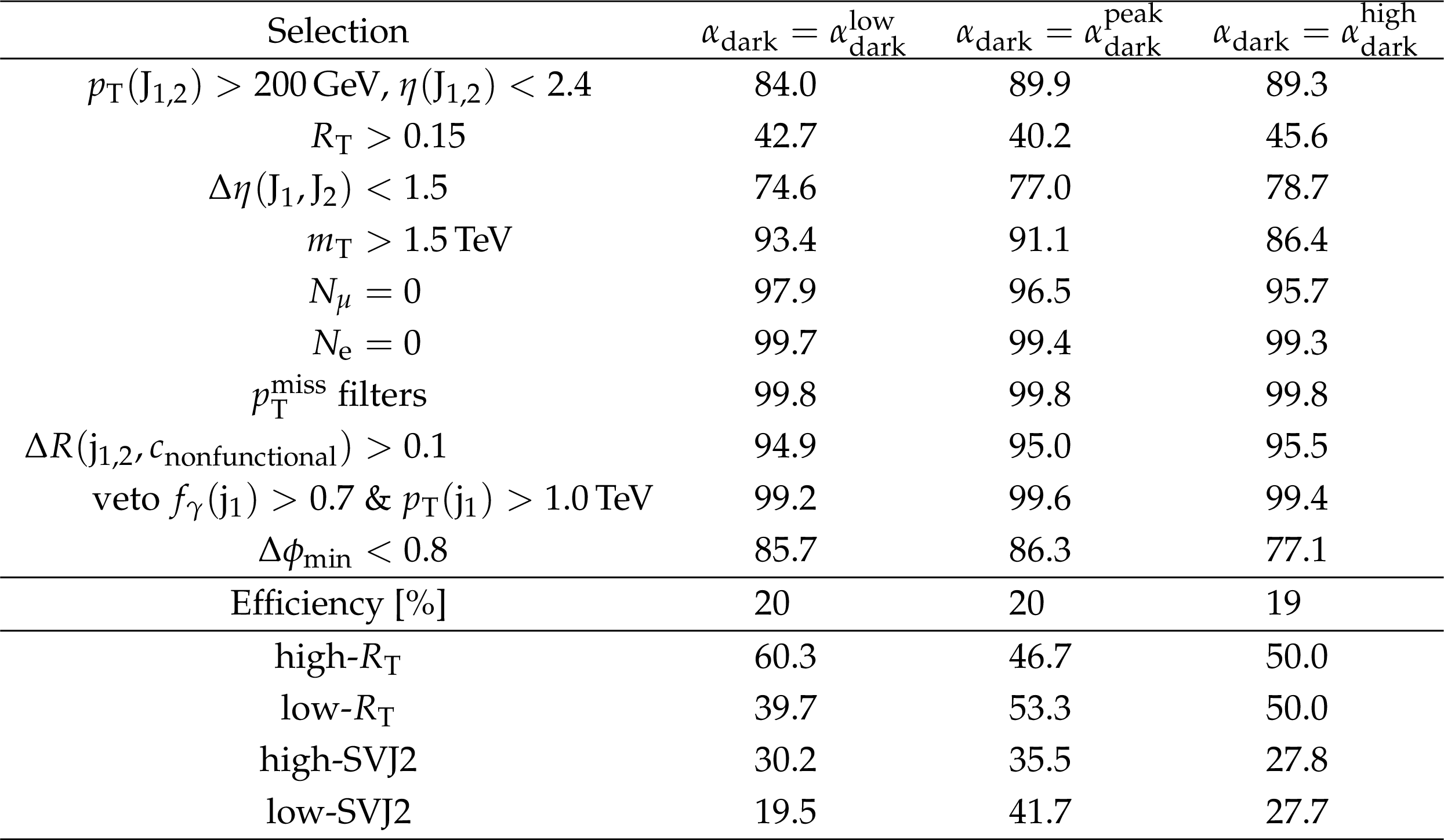
Summary of the preselection and final selection requirements. The symbol * indicates a selection applied only to the later portion of the 2018 data. |
png pdf |
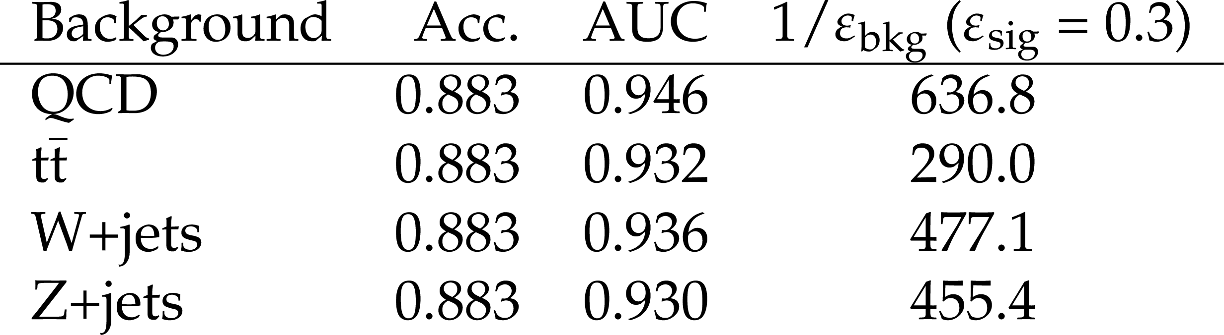
Table 3:
Metrics representing the performance of the BDT for the benchmark signal model ($ {m_{{{\mathrm{Z}}^{\prime}}}} = $ 3.1 TeV, $ {m_{\text {dark}}} = $ 20 GeV, $ {r_{\text {inv}}} = $ 0.3, $ {\alpha _{\text {dark}}} = \alpha {} _{\text {dark}} ^{\text {peak}} $), compared to each of the major SM background processes. |
png pdf |
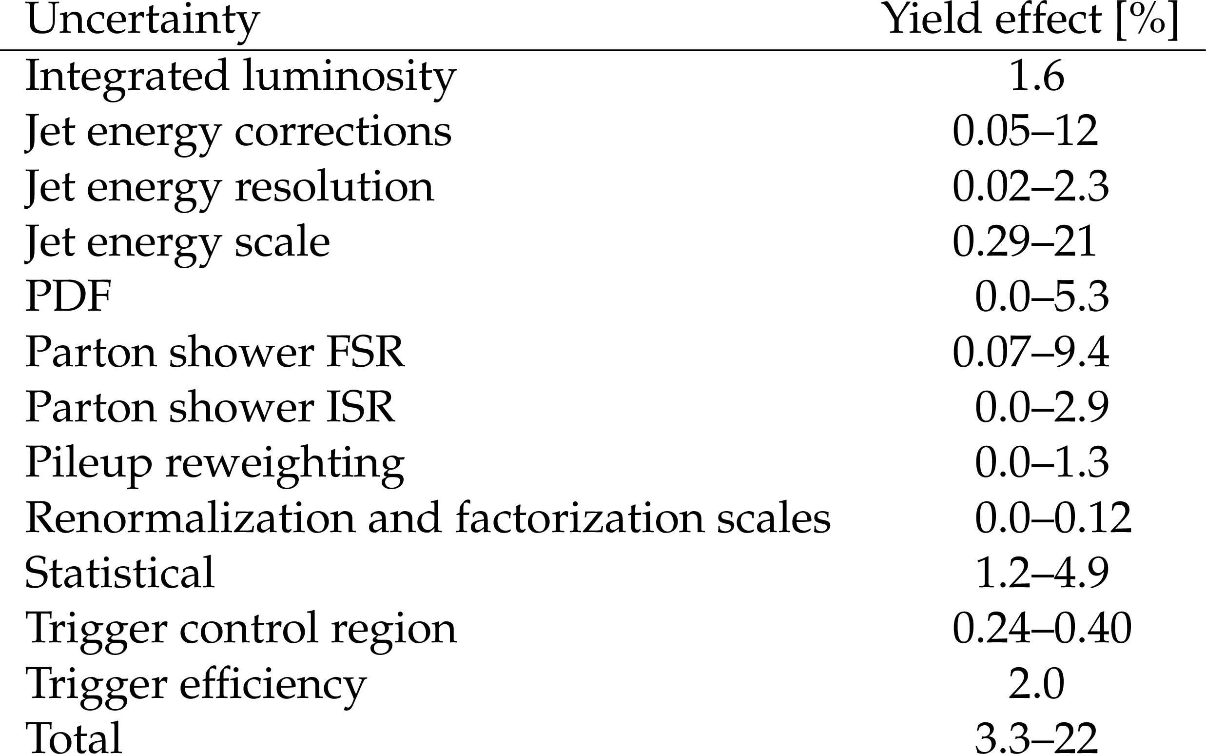
Table 4:
The range of effects on the signal yield for each systematic uncertainty and the total. Values less than 0.01% are rounded to 0.0%. |
| Summary |
|
We present the first collider search for resonant production of dark matter from a strongly coupled hidden sector. The search uses proton-proton collision data collected with the CMS detector in 2016-2018, corresponding to an integrated luminosity of 138 fb$^{-1}$ at a center-of-mass energy of 13 TeV. The signal model introduces a dark sector with multiple flavors of dark quarks that are charged under a dark confining force and form stable and unstable dark hadrons. The stable dark hadrons constitute dark matter candidates, while the unstable dark hadrons decay promptly to standard model (SM) quarks, forming collimated sprays of both invisible and visible particles known as "semivisible'' jets. The hidden sector communicates with the SM via a leptophobic Z' boson mediator. We consider variations in several parameters of the hidden sector signal model: the Z' mass, ${m_{Z'}} $; the dark hadron mass, ${m_{\text{dark}}} $; the fraction of stable, invisible dark hadrons, ${r_{\text{inv}}} $; and the running coupling of the dark force, ${\alpha_{\text{dark}}} $. We pursue a dual strategy to maximize both generality and sensitivity. The general version of the search, which uses only event-level kinematic variables, excludes models with 1.5 $ < {m_{Z'}} < $ 4.0 TeV and 0.07 $ < {r_{\text{inv}}} < $ 0.53 at 95% confidence level (CL), depending on the other signal model parameters. The more sensitive version of the search employs a boosted decision tree (BDT) to discriminate between signal and background jets. With the BDT-based search, the 95% CL exclusion limits extend to 1.5 $ < {m_{Z'}} < $ 5.1 TeV and 0.01 $ < {r_{\text{inv}}} < $ 0.77, for wider ranges of the other signal model parameters. Depending on the mediator mass, all variations considered for ${m_{\text{dark}}} $ and ${\alpha_{\text{dark}}} $ can be excluded. These improvements indicate the power of machine learning techniques to separate dark sector signals from large SM backgrounds. These results complement existing searches for dijet resonances and dark matter events with missing momentum and initial-state radiation. Existing strategies did not target strongly coupled hidden sector models, which produce events with jets aligned with moderate missing transverse momentum. Compared to standard dijet searches, the backgrounds are reduced and the resolution is improved by including missing momentum in the event selection and the resonance mass reconstruction, respectively. Events with jets aligned with missing momentum are explicitly rejected from other collider dark matter searches. In addition, the use of jet substructure provides a substantial increase in model-dependent sensitivity. As a result, a wide range of these models with intermediate ${r_{\text{inv}}} $ values are now excluded for the first time. |
| Additional Figures | |
png pdf root |
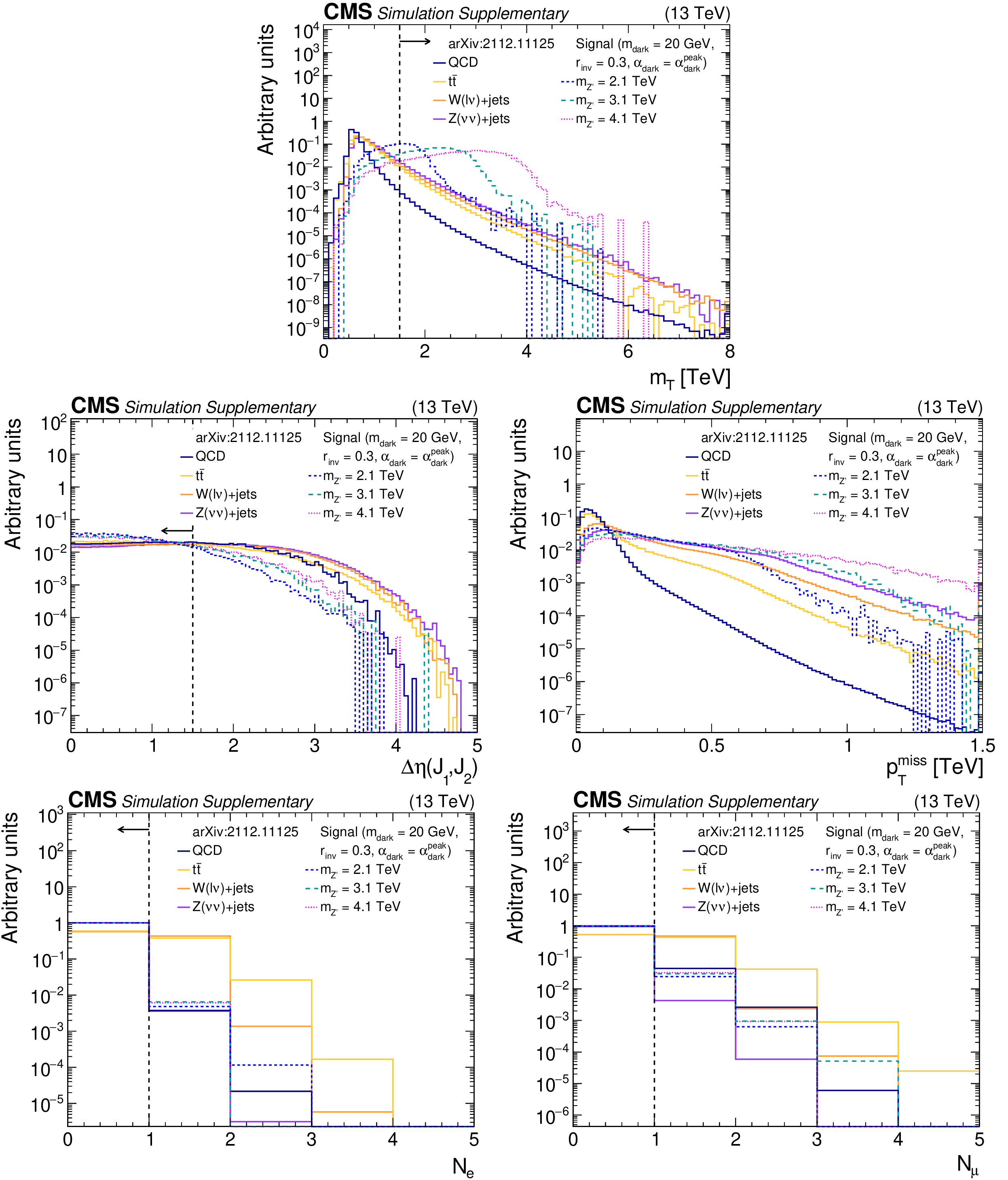
Additional Figure 1:
The normalized distributions of the variables ${m_{\mathrm {T}}}$, ${\Delta \eta ({\mathrm {J}} _{1}, {\mathrm {J}} _{2})}$, ${{p_{\mathrm {T}}} ^\text {miss}}$, ${N_{{\mathrm {e}}}}$, and ${N_{{{\mu}}}}$ for the simulated SM backgrounds and several signal models. For each variable, the requirement on that variable is omitted, but all other preselection requirements are applied. The ${R_{\mathrm {T}}}$ selection is omitted for the ${{p_{\mathrm {T}}} ^\text {miss}}$ distribution. The vertical dotted line indicates the preselection (final selection) requirement on the variable, if any. The last bin of each histogram includes the overflow events. |
png pdf root |
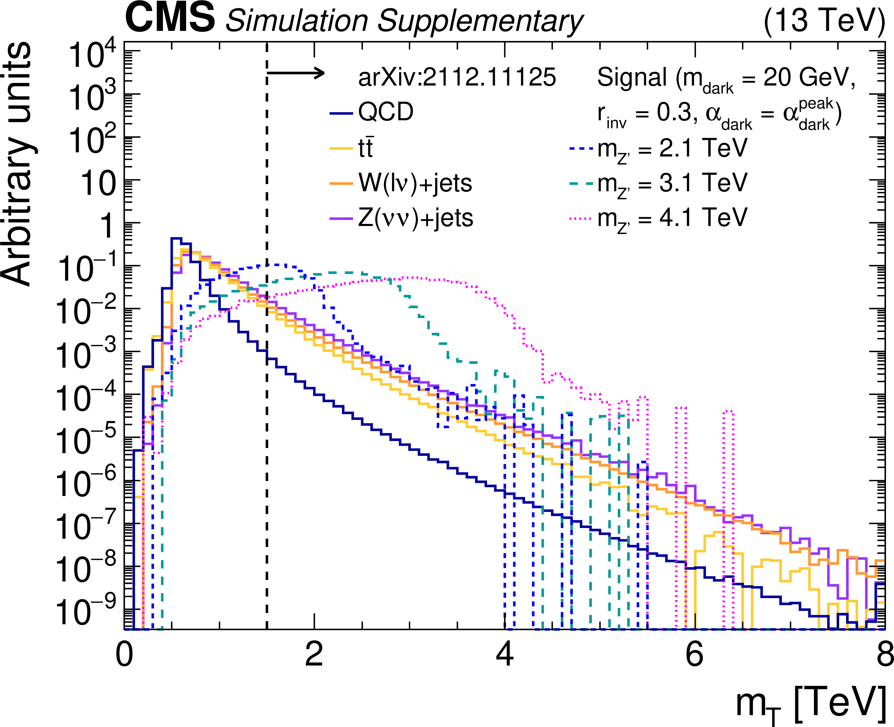
Additional Figure 1-a:
The normalized distribution of the variable ${m_{\mathrm {T}}}$ for the simulated SM backgrounds and several signal models. The requirement on that variable is omitted, but all other preselection requirements are applied. The vertical dotted line indicates the preselection (final selection) requirement on the variable. The last bin of each histogram includes the overflow events. |
png pdf root |
Additional Figure 1-b:
The normalized distribution of the variable ${\Delta \eta ({\mathrm {J}} _{1} {\mathrm {J}} _{2})}$ for the simulated SM backgrounds and several signal models. The requirement on that variable is omitted, but all other preselection requirements are applied. The vertical dotted line indicates the preselection (final selection) requirement on the variable. The last bin of each histogram includes the overflow events. |
png pdf root |
Additional Figure 1-c:
The normalized distribution of the variable ${{p_{\mathrm {T}}} ^\text {miss}}$ for the simulated SM backgrounds and several signal models. The requirement on that variable is omitted, but all other preselection requirements are applied. The ${R_{\mathrm {T}}}$ selection is omitted. The last bin of each histogram includes the overflow events. |
png pdf root |
Additional Figure 1-d:
The normalized distribution of the variable ${N_{{\mathrm {e}}}}$ for the simulated SM backgrounds and several signal models. The requirement on that variable is omitted, but all other preselection requirements are applied. The vertical dotted line indicates the preselection (final selection) requirement on the variable. The last bin of each histogram includes the overflow events. |
png pdf root |
Additional Figure 1-e:
The normalized distribution of the variable ${N_{{{\mu}}}}$ for the simulated SM backgrounds and several signal models. The requirement on that variable is omitted, but all other preselection requirements are applied. The vertical dotted line indicates the preselection (final selection) requirement on the variable. The last bin of each histogram includes the overflow events. |
png pdf root |
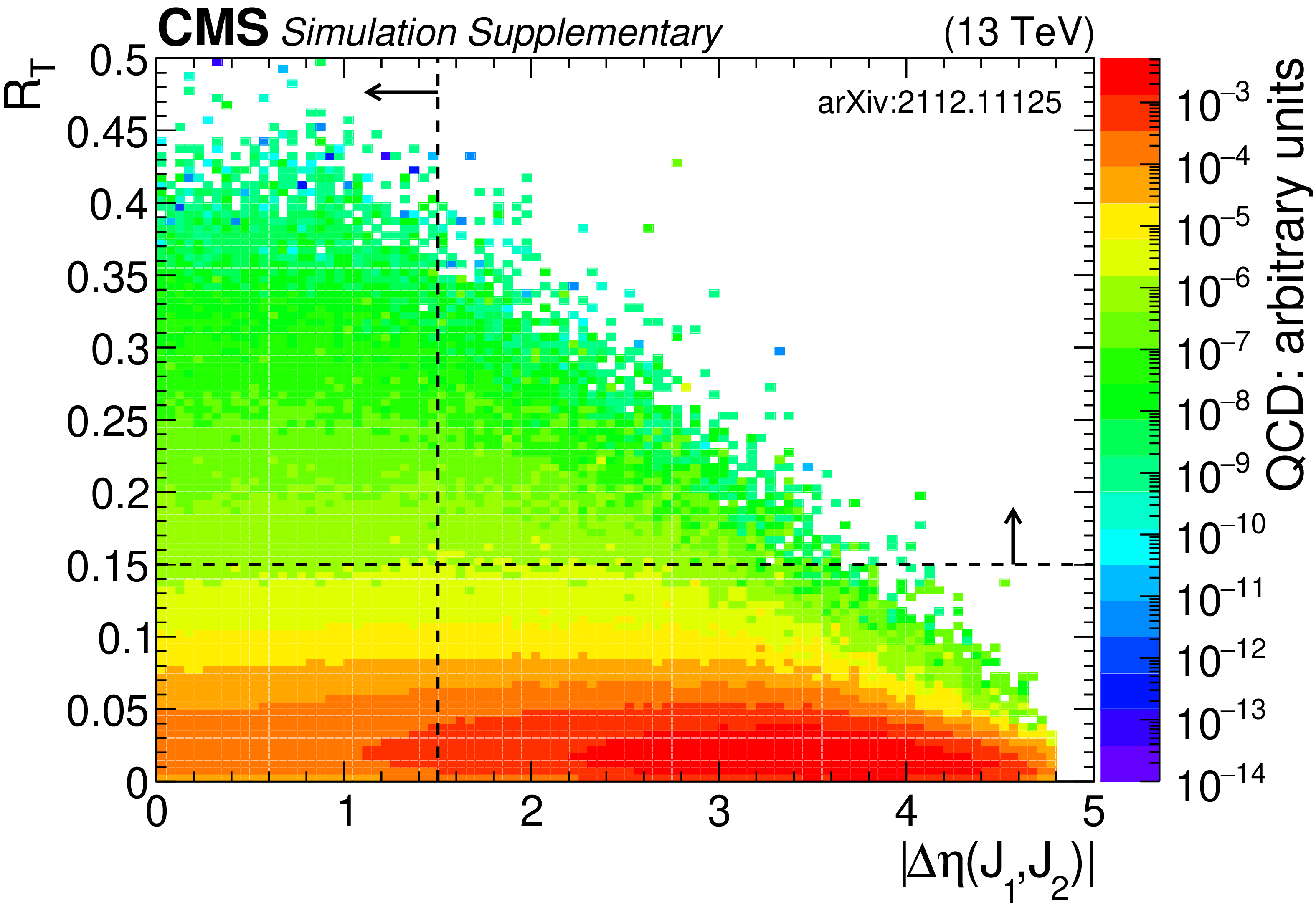
Additional Figure 2:
The normalized distribution of ${\Delta \eta ({\mathrm {J}} _{1}, {\mathrm {J}} _{2})}$ vs. ${R_{\mathrm {T}}}$ for the simulated QCD background. The preselection requirements on both variables are omitted, but all other preselection requirements are applied. The black dotted lines indicates the preselection requirements on the variables. |
png pdf root |
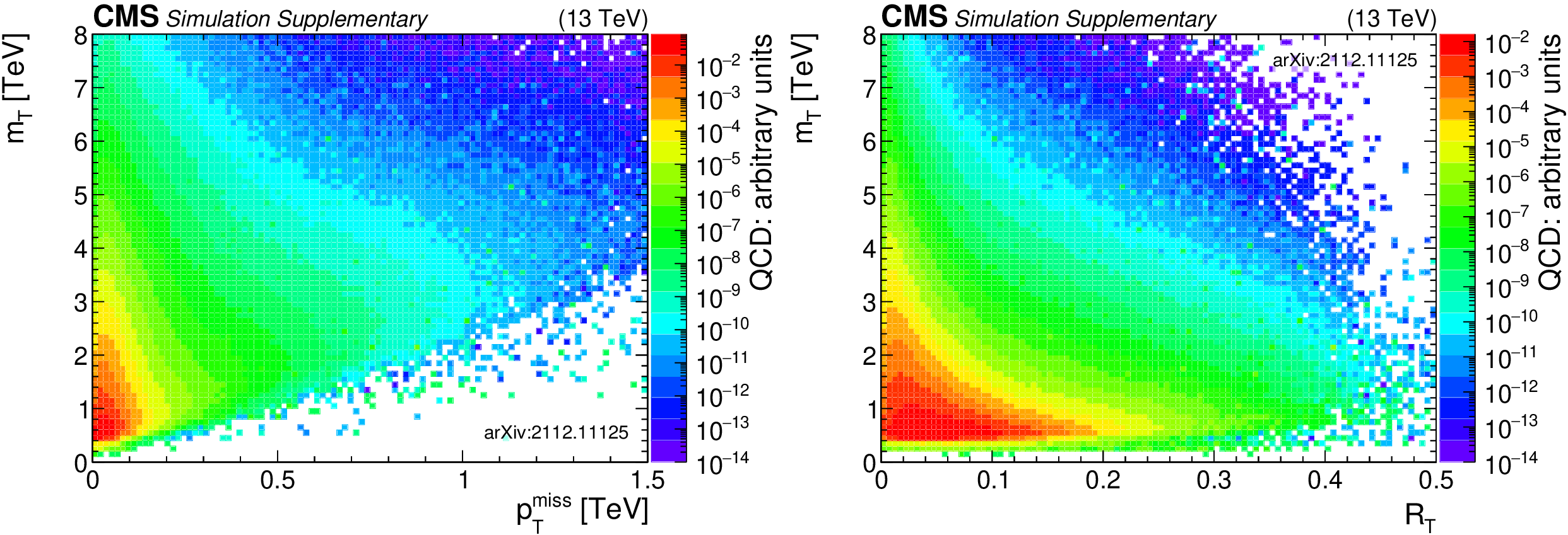
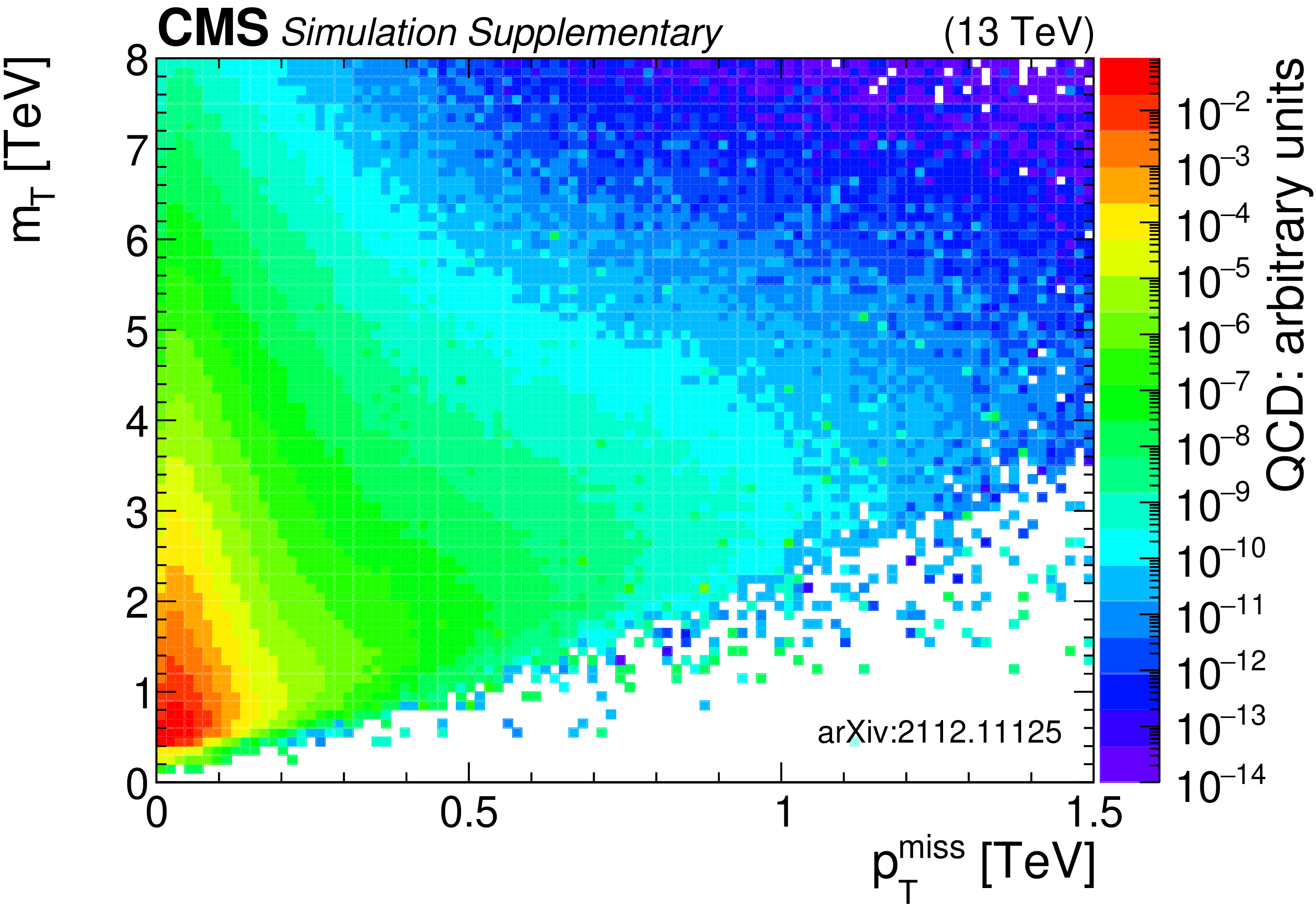
Additional Figure 3:
The normalized distributions of ${{p_{\mathrm {T}}} ^\text {miss}}$ vs. ${m_{\mathrm {T}}}$ and ${R_{\mathrm {T}}}$ vs. ${m_{\mathrm {T}}}$ for the simulated QCD background. All selection requirements are omitted, except for the requirement of two high-${p_{\mathrm {T}}}$ wide jets. |
png pdf root |
Additional Figure 3-a:
The normalized distributions of ${{p_{\mathrm {T}}} ^\text {miss}}$ vs. ${m_{\mathrm {T}}}$ for the simulated QCD background. All selection requirements are omitted, except for the requirement of two high-${p_{\mathrm {T}}}$ wide jets. |

png pdf root |
Additional Figure 3-b:
The normalized distributions of ${R_{\mathrm {T}}}$ vs. ${m_{\mathrm {T}}}$ for the simulated QCD background. All selection requirements are omitted, except for the requirement of two high-${p_{\mathrm {T}}}$ wide jets. |
png pdf root |
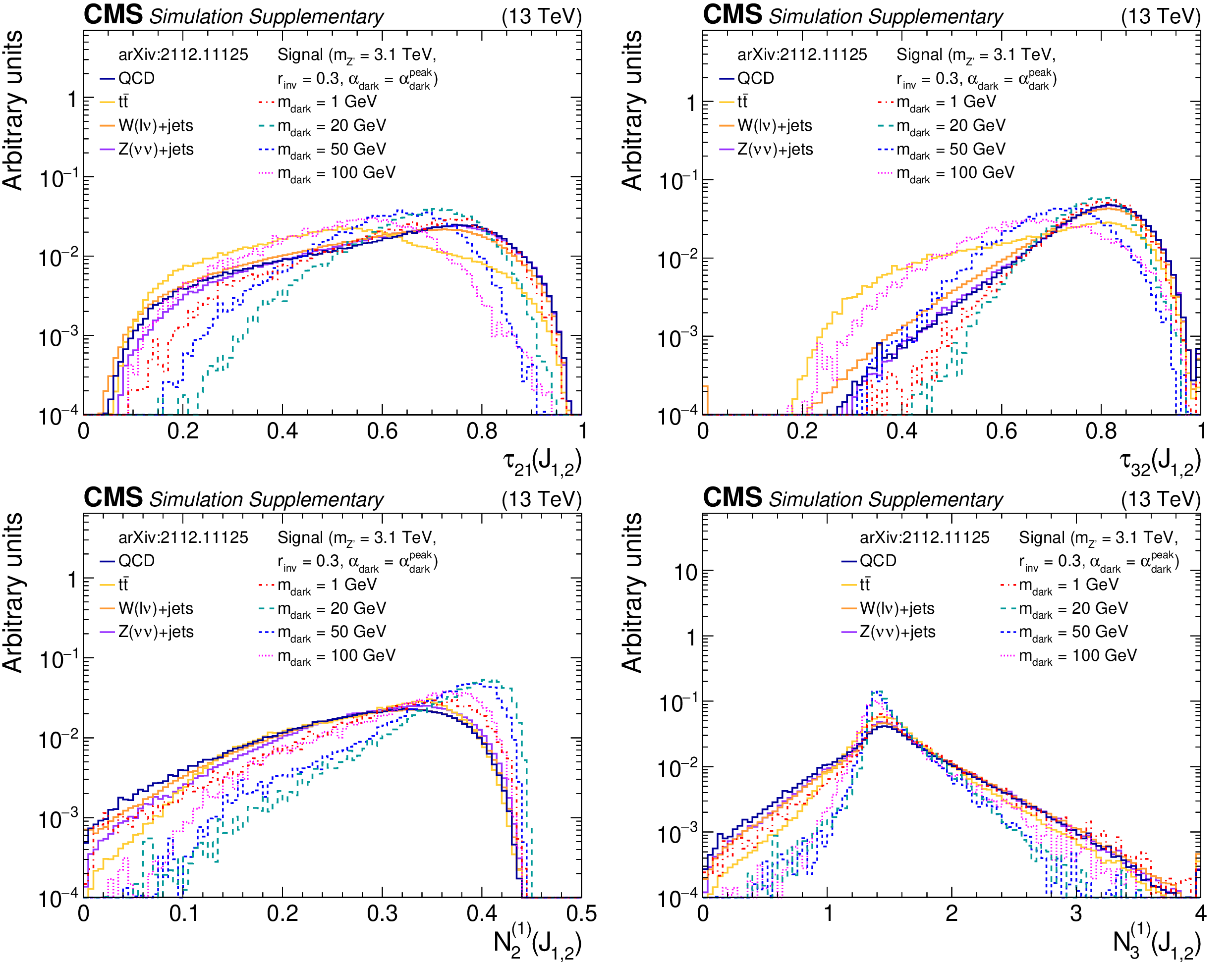
Additional Figure 4:
The normalized distributions of the BDT input variables ${\tau _{21}}$, ${\tau _{32}}$, ${N_{2}^{(1)}}$, and ${N_{3}^{(1)}}$ for the two highest ${p_{\mathrm {T}}}$ wide jets from the simulated SM backgrounds and several signal models with varying ${m_{\mathrm {dark}}}$ values. Each sample's jet ${p_{\mathrm {T}}}$ distribution is weighted to match a reference distribution (see text). The last bin of each histogram includes the overflow events. |

png pdf root |
Additional Figure 4-a:
The normalized distributions of the BDT input variable ${\tau _{21}}$ for the two highest ${p_{\mathrm {T}}}$ wide jets from the simulated SM backgrounds and several signal models with varying ${m_{\mathrm {dark}}}$ values. Each sample's jet ${p_{\mathrm {T}}}$ distribution is weighted to match a reference distribution (see text). The last bin of each histogram includes the overflow events. |
png pdf root |
Additional Figure 4-b:
The normalized distributions of the BDT input variable ${\tau _{32}}$ for the two highest ${p_{\mathrm {T}}}$ wide jets from the simulated SM backgrounds and several signal models with varying ${m_{\mathrm {dark}}}$ values. Each sample's jet ${p_{\mathrm {T}}}$ distribution is weighted to match a reference distribution (see text). The last bin of each histogram includes the overflow events. |

png pdf root |
Additional Figure 4-c:
The normalized distributions of the BDT input variable ${N_{2}^{(1)}}$ for the two highest ${p_{\mathrm {T}}}$ wide jets from the simulated SM backgrounds and several signal models with varying ${m_{\mathrm {dark}}}$ values. Each sample's jet ${p_{\mathrm {T}}}$ distribution is weighted to match a reference distribution (see text). The last bin of each histogram includes the overflow events. |
png pdf root |
Additional Figure 4-d:
The normalized distributions of the BDT input variable ${N_{3}^{(1)}}$ for the two highest ${p_{\mathrm {T}}}$ wide jets from the simulated SM backgrounds and several signal models with varying ${m_{\mathrm {dark}}}$ values. Each sample's jet ${p_{\mathrm {T}}}$ distribution is weighted to match a reference distribution (see text). The last bin of each histogram includes the overflow events. |
png pdf root |
Additional Figure 5:
The normalized distributions of the BDT input variables ${g_{\text {jet}}}$, ${\sigma _{\text {major}}}$, ${\sigma _{\text {minor}}}$, and $\Delta \phi (\vec{{\mathrm {J}}}, {\vec{p}_{\mathrm {T}}}^{\,\text {miss}})$ for the two highest ${p_{\mathrm {T}}}$ wide jets from the simulated SM backgrounds and several signal models with varying ${r_{\mathrm {inv}}}$ values. Each sample's jet ${p_{\mathrm {T}}}$ distribution is weighted to match a reference distribution (see text). The last bin of each histogram includes the overflow events. |
png pdf root |
Additional Figure 5-a:
The normalized distributions of the BDT input variable ${g_{\text {jet}}}$ for the two highest ${p_{\mathrm {T}}}$ wide jets from the simulated SM backgrounds and several signal models with varying ${r_{\mathrm {inv}}}$ values. Each sample's jet ${p_{\mathrm {T}}}$ distribution is weighted to match a reference distribution (see text). The last bin of each histogram includes the overflow events. |
png pdf root |
Additional Figure 5-b:
The normalized distributions of the BDT input variable ${\sigma _{\text {major}}}$ for the two highest ${p_{\mathrm {T}}}$ wide jets from the simulated SM backgrounds and several signal models with varying ${r_{\mathrm {inv}}}$ values. Each sample's jet ${p_{\mathrm {T}}}$ distribution is weighted to match a reference distribution (see text). The last bin of each histogram includes the overflow events. |

png pdf root |
Additional Figure 5-c:
The normalized distributions of the BDT input variable ${\sigma _{\text {minor}}}$ for the two highest ${p_{\mathrm {T}}}$ wide jets from the simulated SM backgrounds and several signal models with varying ${r_{\mathrm {inv}}}$ values. Each sample's jet ${p_{\mathrm {T}}}$ distribution is weighted to match a reference distribution (see text). The last bin of each histogram includes the overflow events. |
png pdf root |
Additional Figure 5-d:
The normalized distributions of the BDT input variable $\Delta \phi (\vec{{\mathrm {J}}}, {\vec{p}_{\mathrm {T}}}^{\,\text {miss}})$ for the two highest ${p_{\mathrm {T}}}$ wide jets from the simulated SM backgrounds and several signal models with varying ${r_{\mathrm {inv}}}$ values. Each sample's jet ${p_{\mathrm {T}}}$ distribution is weighted to match a reference distribution (see text). The last bin of each histogram includes the overflow events. |
png pdf root |
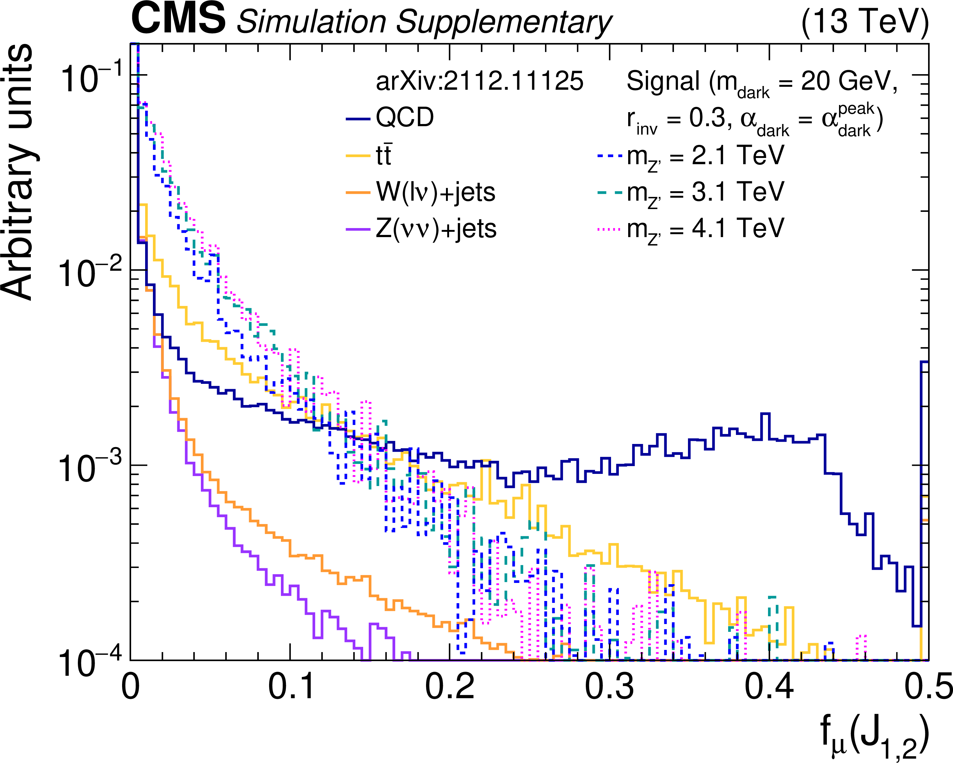
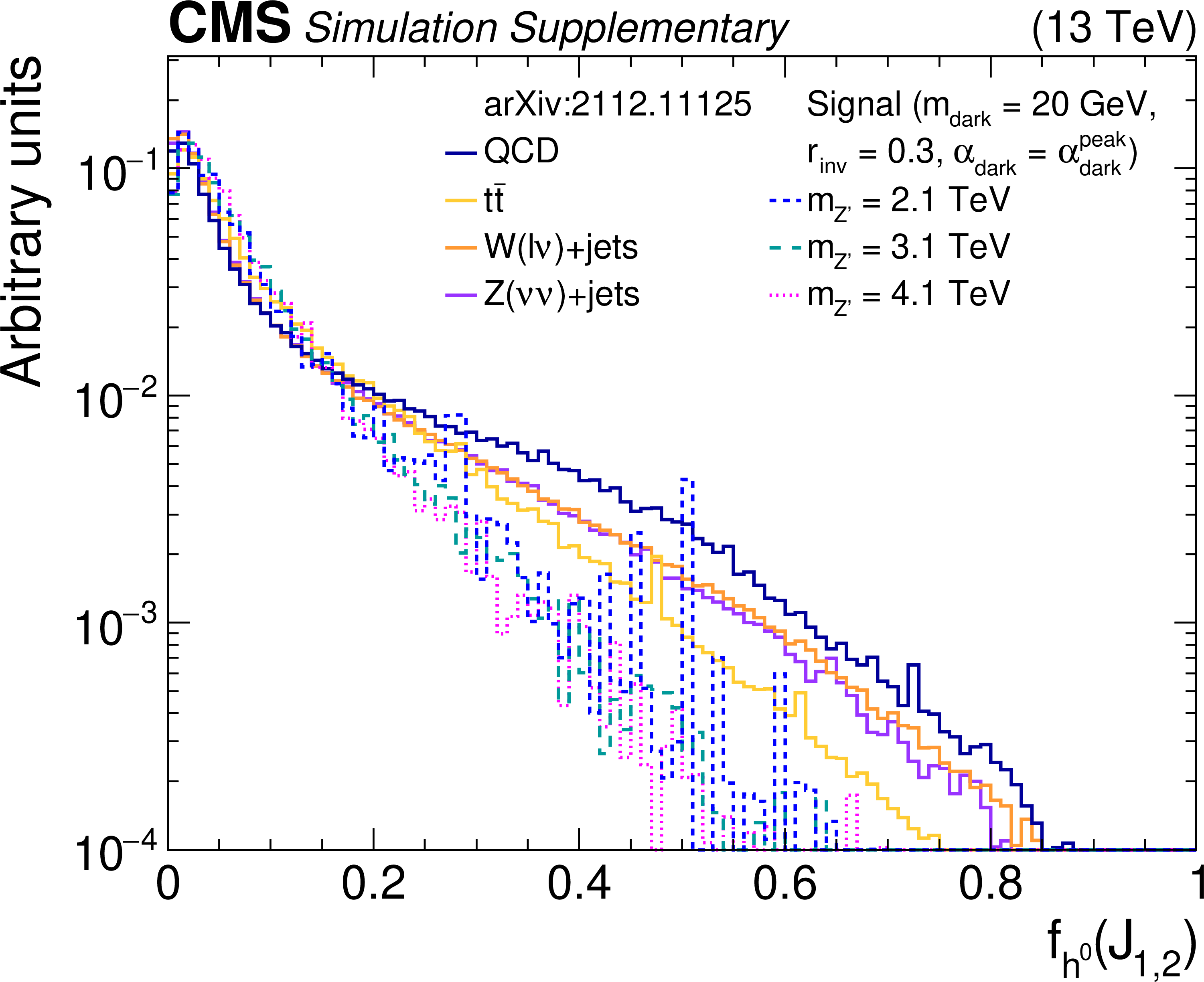
Additional Figure 6:
The normalized distributions of the BDT input variables $f_{{\mathrm {h}^{\pm}}}$, $f_{{\mathrm {e}}}$, $f_{{{\mu}}}$, $f_{{\mathrm {h}^{0}}}$, and $f_{\gamma}$ for the two highest ${p_{\mathrm {T}}}$ wide jets from the simulated SM backgrounds and several signal models with varying ${m_{{{{\mathrm {Z}}}^{\prime}}}}$ values. Each sample's jet ${p_{\mathrm {T}}}$ distribution is weighted to match a reference distribution (see text). The last bin of each histogram includes the overflow events. |
png pdf root |
Additional Figure 6-a:
The normalized distributions of the BDT input variables $f_{{\mathrm {h}^{\pm}}}$ or the two highest ${p_{\mathrm {T}}}$ wide jets from the simulated SM backgrounds and several signal models with varying ${m_{{{{\mathrm {Z}}}^{\prime}}}}$ values. Each sample's jet ${p_{\mathrm {T}}}$ distribution is weighted to match a reference distribution (see text). The last bin of each histogram includes the overflow events. |

png pdf root |
Additional Figure 6-b:
The normalized distributions of the BDT input variables $f_{{\mathrm {e}}}$ for the two highest ${p_{\mathrm {T}}}$ wide jets from the simulated SM backgrounds and several signal models with varying ${m_{{{{\mathrm {Z}}}^{\prime}}}}$ values. Each sample's jet ${p_{\mathrm {T}}}$ distribution is weighted to match a reference distribution (see text). The last bin of each histogram includes the overflow events. |
png pdf root |
Additional Figure 6-c:
The normalized distributions of the BDT input variables $f_{{{\mu}}}$ for the two highest ${p_{\mathrm {T}}}$ wide jets from the simulated SM backgrounds and several signal models with varying ${m_{{{{\mathrm {Z}}}^{\prime}}}}$ values. Each sample's jet ${p_{\mathrm {T}}}$ distribution is weighted to match a reference distribution (see text). The last bin of each histogram includes the overflow events. |
png pdf root |
Additional Figure 6-d:
The normalized distributions of the BDT input variables $f_{{\mathrm {h}^{0}}}$ for the two highest ${p_{\mathrm {T}}}$ wide jets from the simulated SM backgrounds and several signal models with varying ${m_{{{{\mathrm {Z}}}^{\prime}}}}$ values. Each sample's jet ${p_{\mathrm {T}}}$ distribution is weighted to match a reference distribution (see text). The last bin of each histogram includes the overflow events. |

png pdf root |
Additional Figure 6-e:
The normalized distributions of the BDT input variables $f_{\gamma}$ for the two highest ${p_{\mathrm {T}}}$ wide jets from the simulated SM backgrounds and several signal models with varying ${m_{{{{\mathrm {Z}}}^{\prime}}}}$ values. Each sample's jet ${p_{\mathrm {T}}}$ distribution is weighted to match a reference distribution (see text). The last bin of each histogram includes the overflow events. |
png pdf |
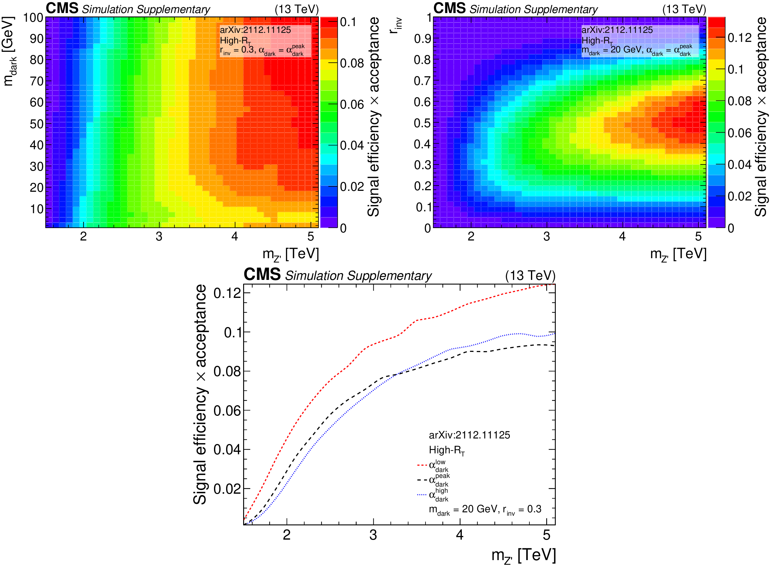
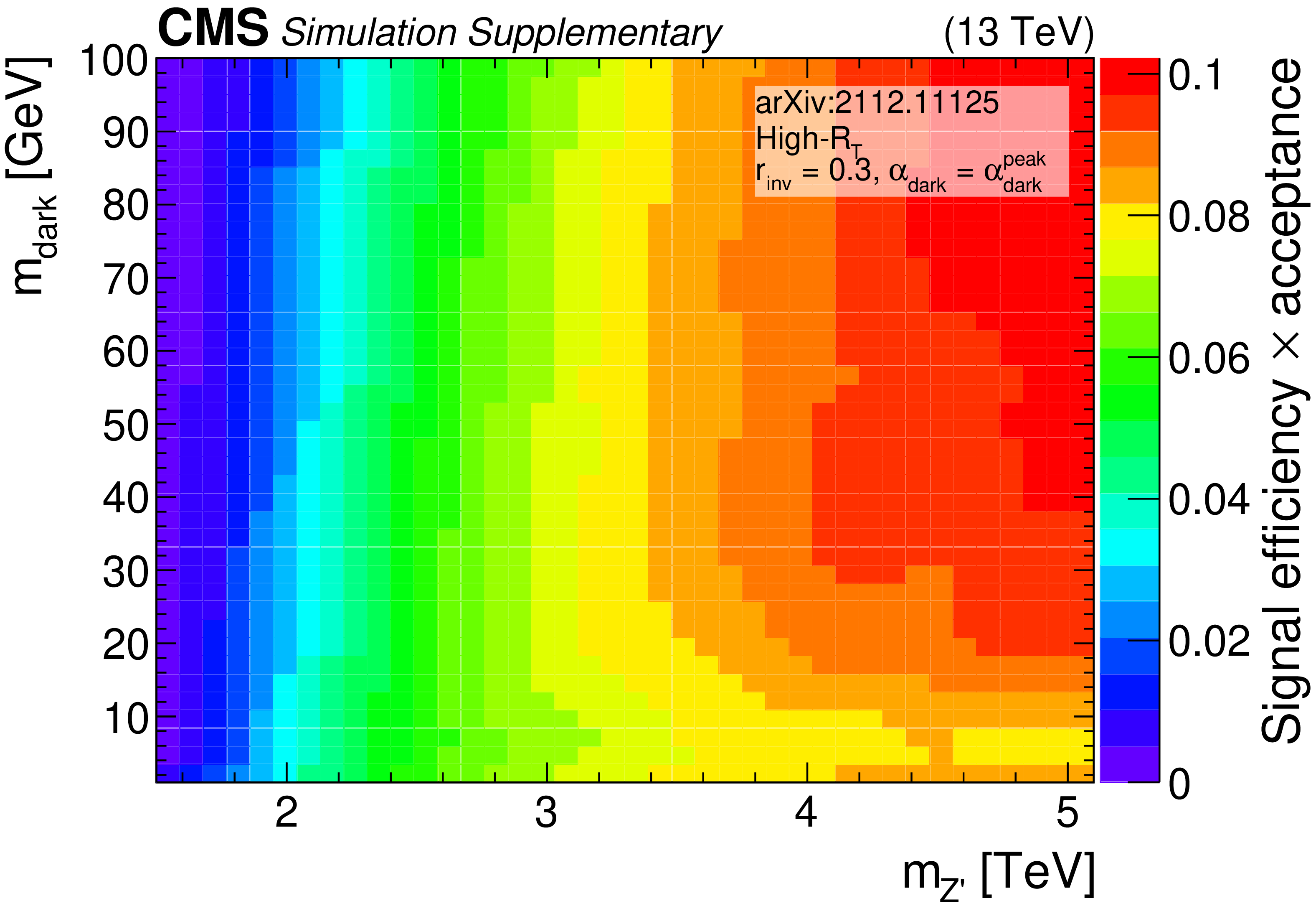
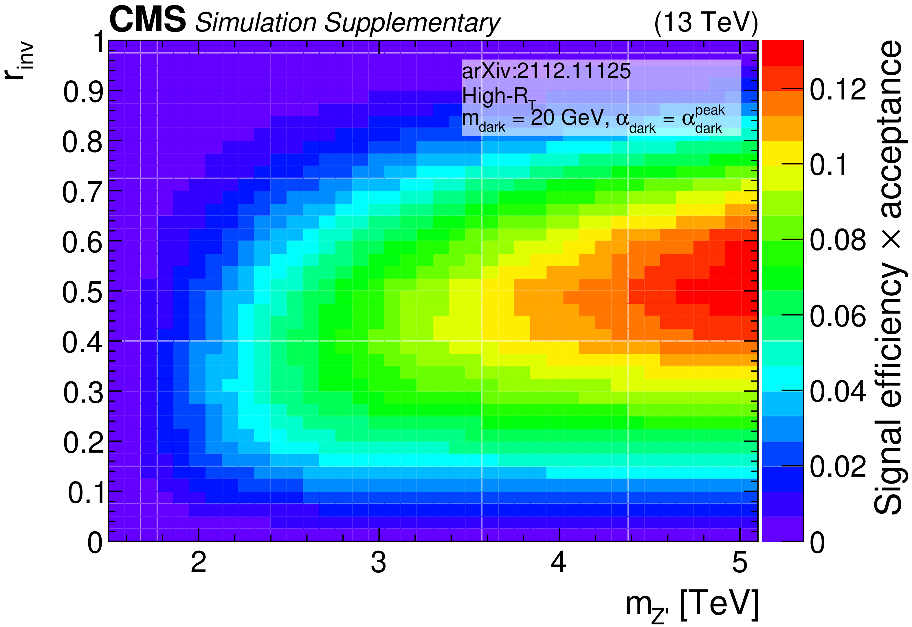
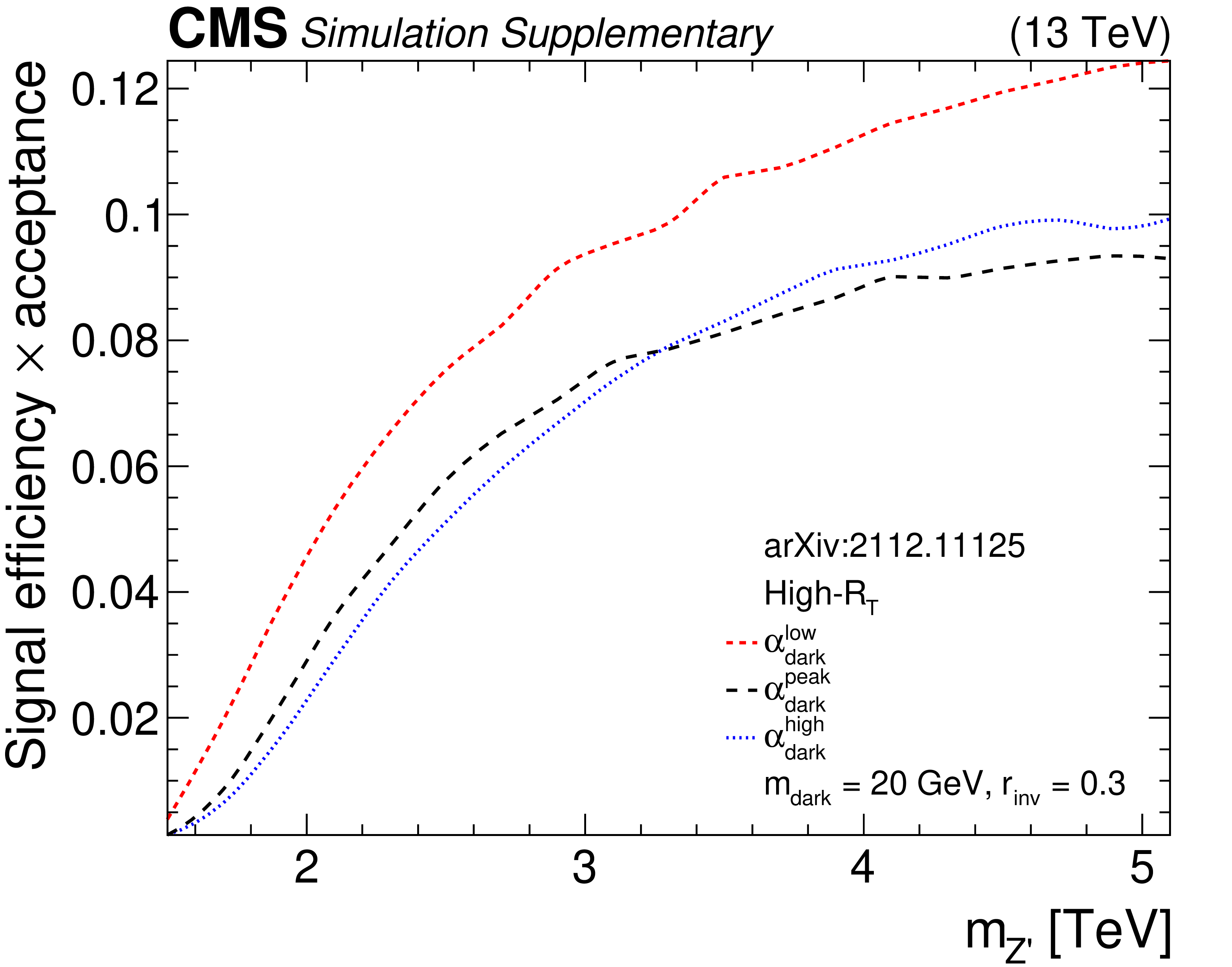
Additional Figure 7:
The product of signal acceptance and efficiency in the high-${R_{\mathrm {T}}}$ signal region, for variations of pairs of the signal model parameters. |
png pdf root |
Additional Figure 7-a:
The product of signal acceptance and efficiency in the high-${R_{\mathrm {T}}}$ signal region, for variations of pairs of the signal model parameters. |
png pdf root |
Additional Figure 7-b:
The product of signal acceptance and efficiency in the high-${R_{\mathrm {T}}}$ signal region, for variations of pairs of the signal model parameters. |
png pdf root |
Additional Figure 7-c:
The product of signal acceptance and efficiency in the high-${R_{\mathrm {T}}}$ signal region, for variations of pairs of the signal model parameters. |

png pdf |
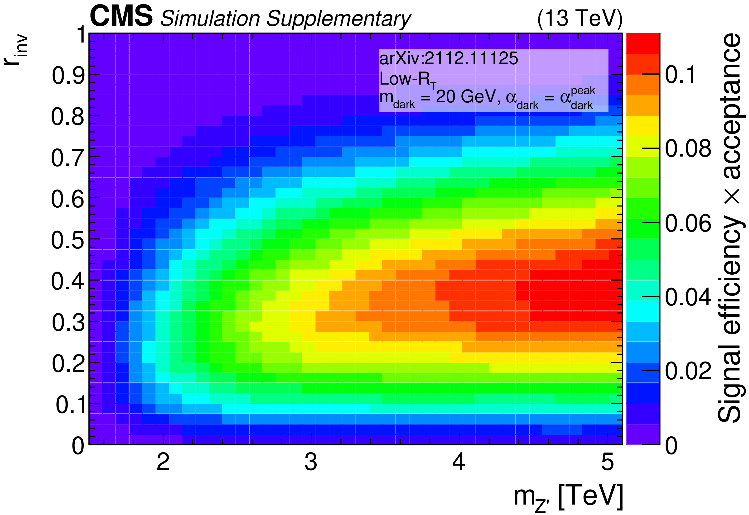
Additional Figure 8:
The product of signal acceptance and efficiency in the low-${R_{\mathrm {T}}}$ signal region, for variations of pairs of the signal model parameters. |

png pdf root |
Additional Figure 8-a:
The product of signal acceptance and efficiency in the low-${R_{\mathrm {T}}}$ signal region, for variations of pairs of the signal model parameters. |
png pdf root |
Additional Figure 8-b:
The product of signal acceptance and efficiency in the low-${R_{\mathrm {T}}}$ signal region, for variations of pairs of the signal model parameters. |

png pdf root |
Additional Figure 8-c:
The product of signal acceptance and efficiency in the low-${R_{\mathrm {T}}}$ signal region, for variations of pairs of the signal model parameters. |
png pdf |
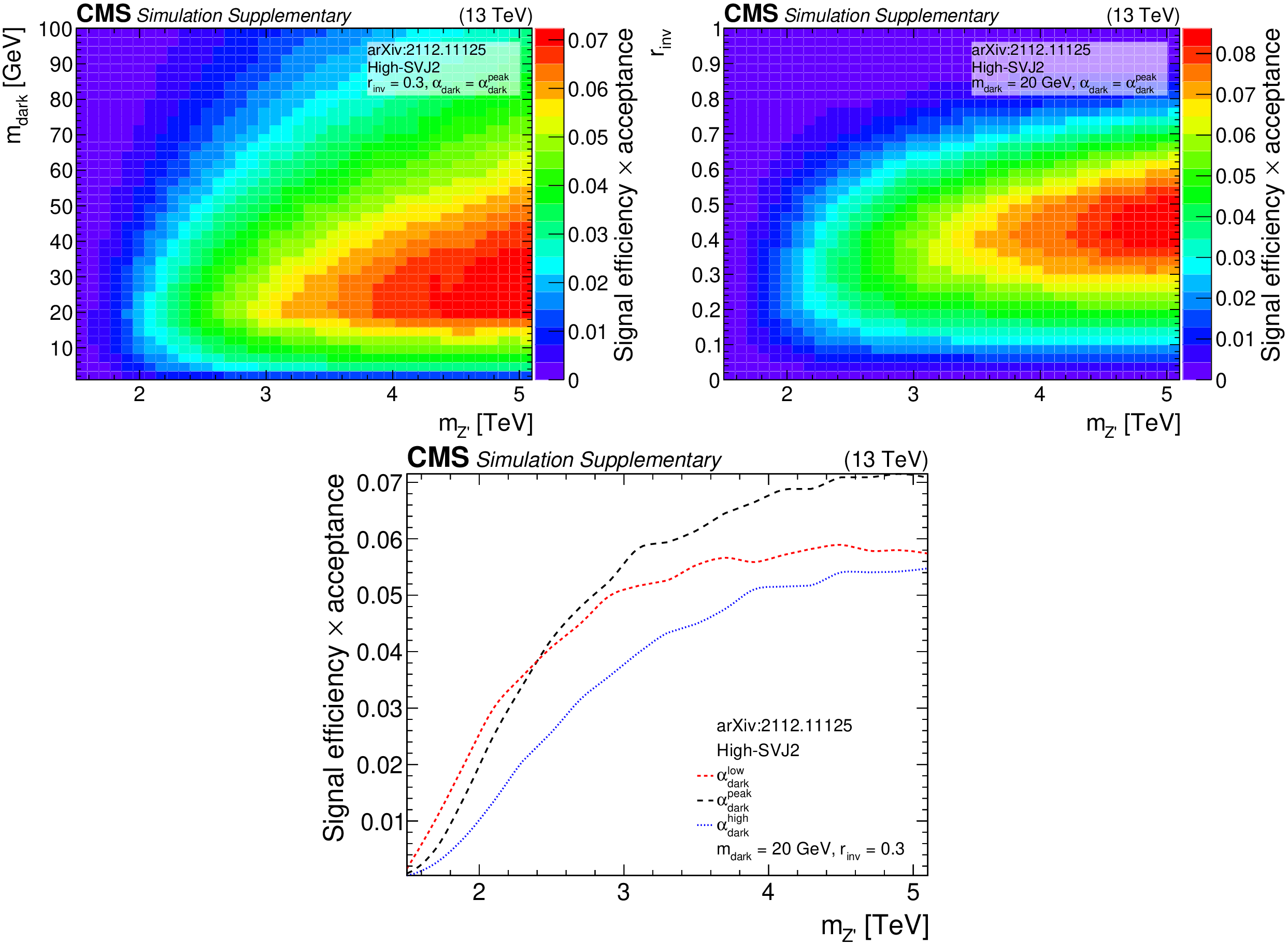
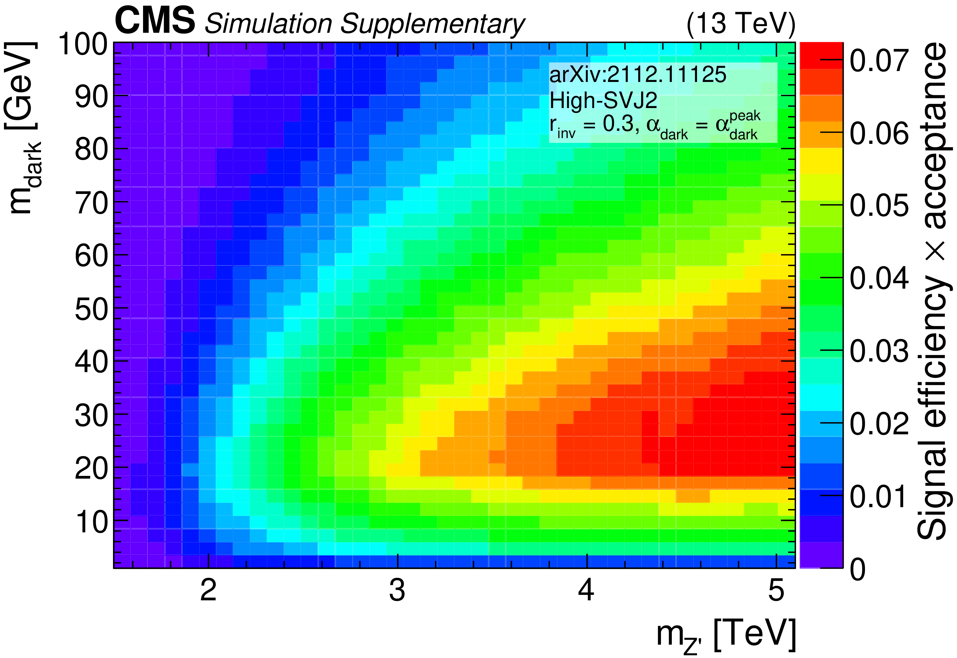
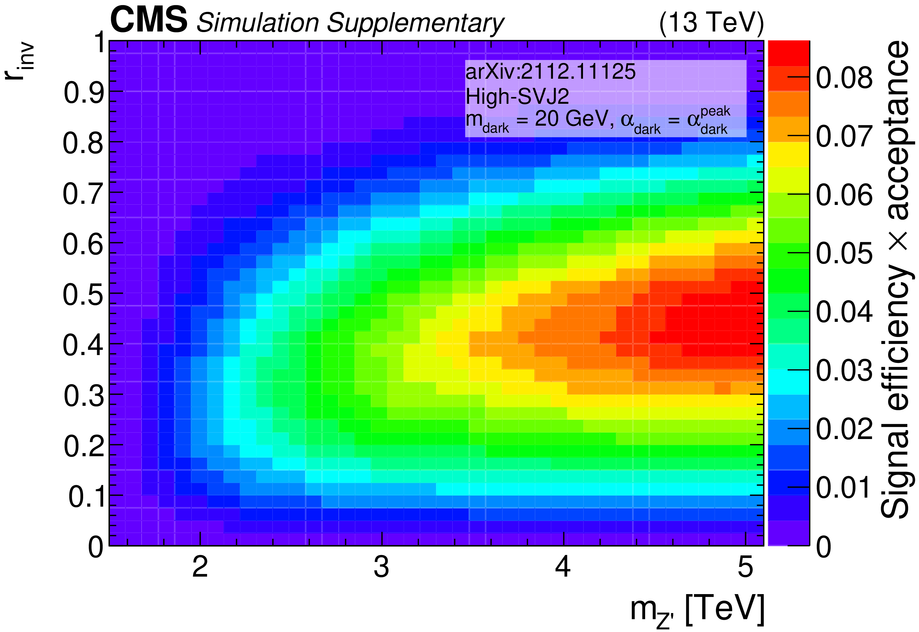
Additional Figure 9:
The product of signal acceptance and efficiency in the high-SVJ2 signal region, for variations of pairs of the signal model parameters. |
png pdf root |
Additional Figure 9-a:
The product of signal acceptance and efficiency in the high-SVJ2 signal region, for variations of pairs of the signal model parameters. |
png pdf root |
Additional Figure 9-b:
The product of signal acceptance and efficiency in the high-SVJ2 signal region, for variations of pairs of the signal model parameters. |

png pdf root |
Additional Figure 9-c:
The product of signal acceptance and efficiency in the high-SVJ2 signal region, for variations of pairs of the signal model parameters. |
png pdf |
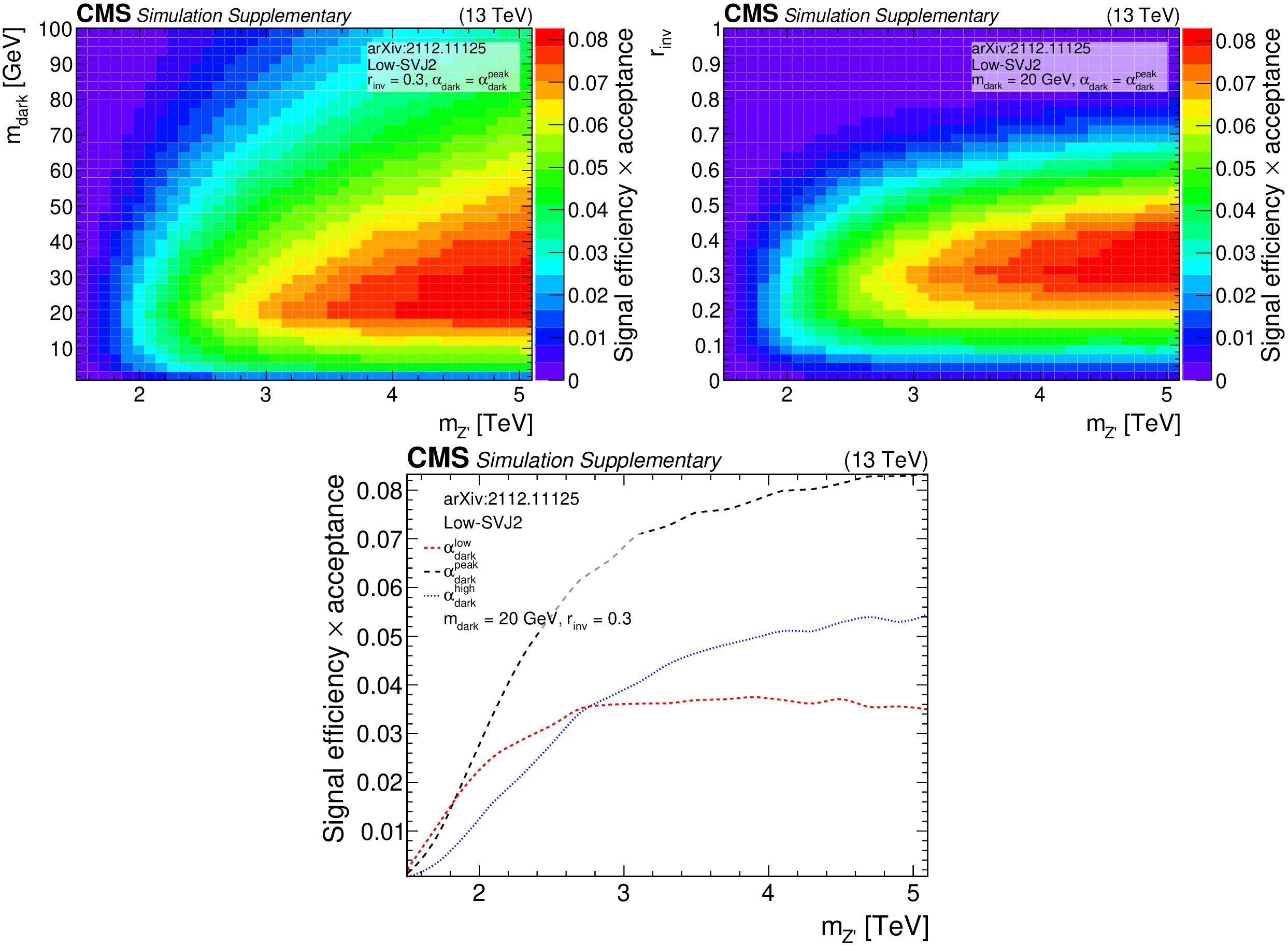
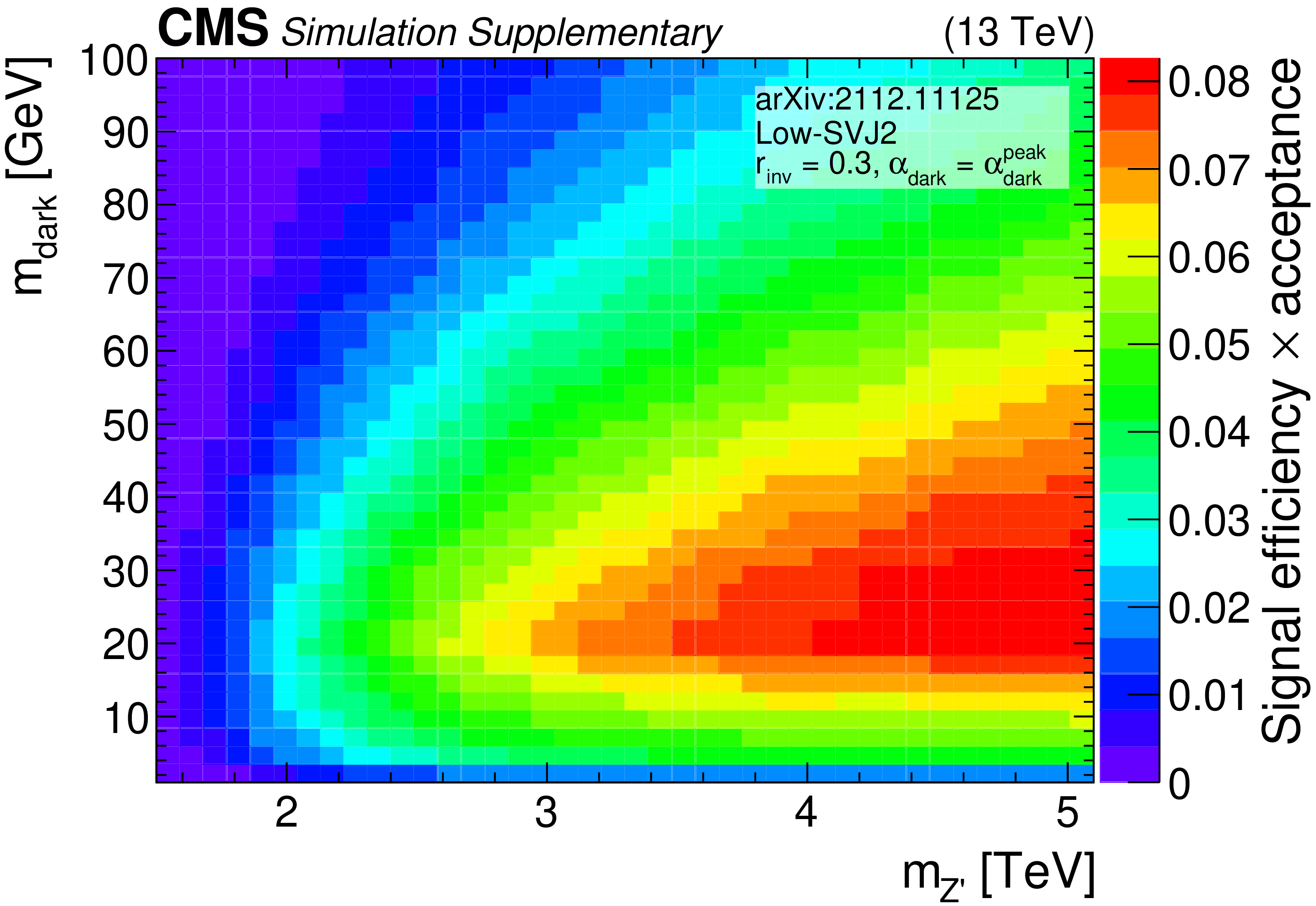
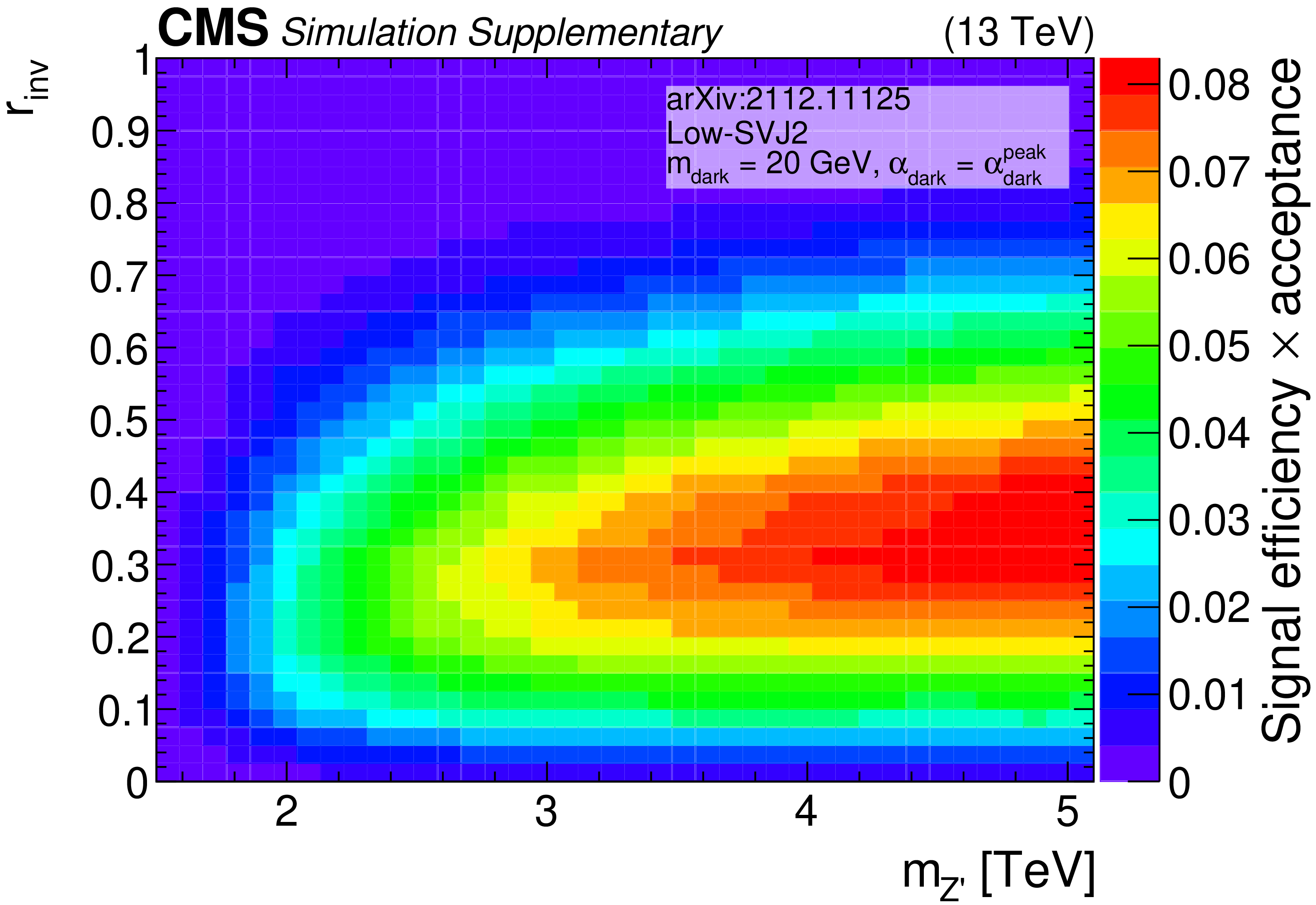
Additional Figure 10:
The product of signal acceptance and efficiency in the low-SVJ2 signal region, for variations of pairs of the signal model parameters. |
png pdf root |
Additional Figure 10-a:
The product of signal acceptance and efficiency in the low-SVJ2 signal region, for variations of pairs of the signal model parameters. |
png pdf root |
Additional Figure 10-b:
The product of signal acceptance and efficiency in the low-SVJ2 signal region, for variations of pairs of the signal model parameters. |
png pdf root |
Additional Figure 10-c:
The product of signal acceptance and efficiency in the low-SVJ2 signal region, for variations of pairs of the signal model parameters. |
png pdf root |
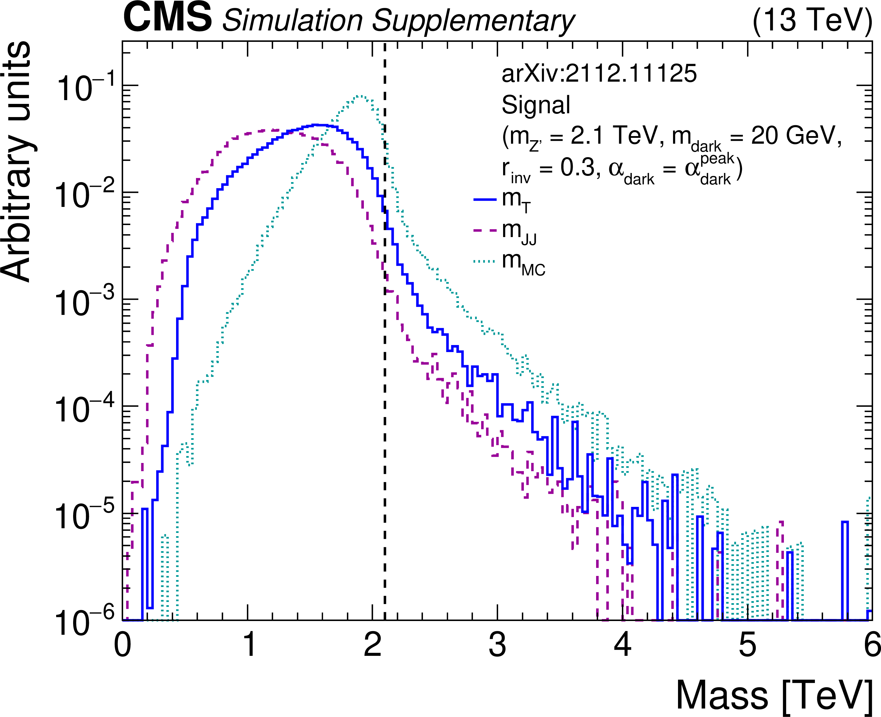
Additional Figure 11:
Comparison of the dijet mass ${m_{{\mathrm {J}} {\mathrm {J}}}}$, the transverse mass ${m_{\mathrm {T}}}$, and the Monte Carlo (MC) mass ${m_{\mathrm {MC}}}$ for a signal model with ${m_{{{{\mathrm {Z}}}^{\prime}}}} = $ 2.1 TeV (shown as a dotted black line). No selection is applied, except that there must be at least two jets. ${m_{\mathrm {MC}}}$ is computed by adding the generator-level four-vectors for invisible particles to the dijet system, to represent the achievable resolution if the invisible component were fully measured. The last bin of each histogram includes the overflow events. |
png pdf |
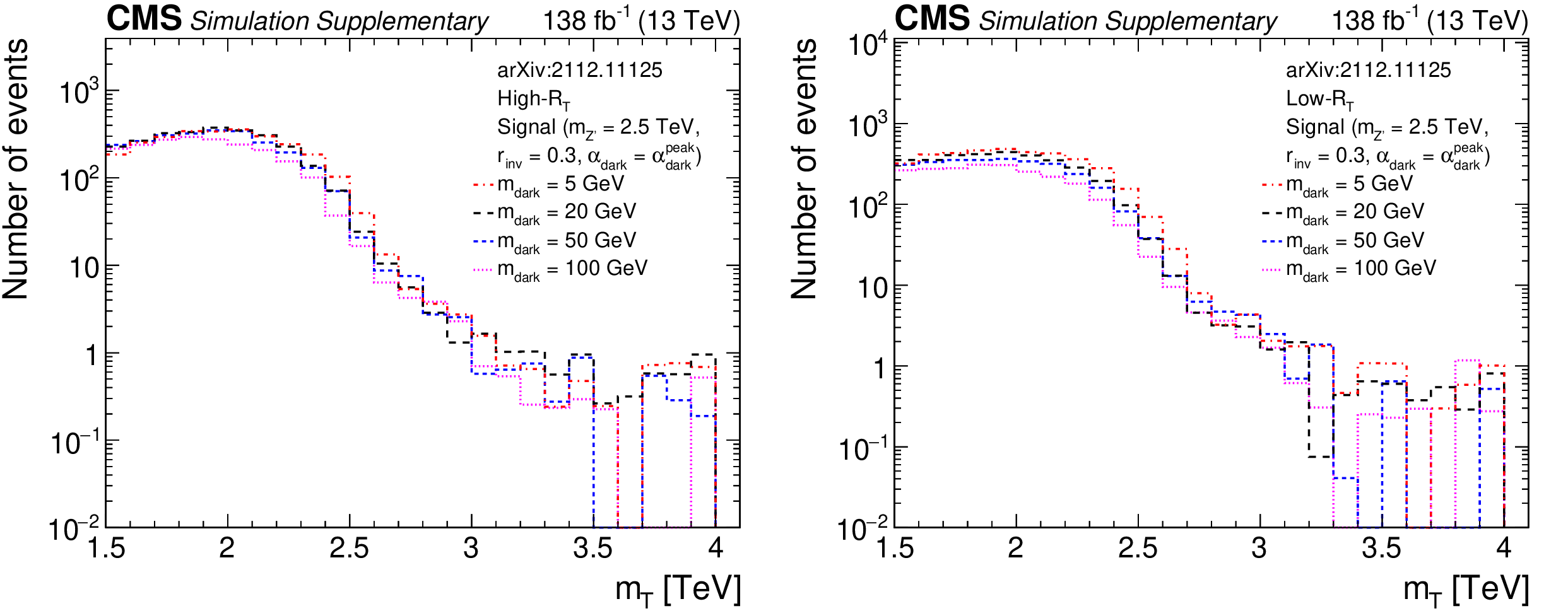
Additional Figure 12:
${m_{\mathrm {T}}}$ distributions for signal models with different ${m_{\mathrm {dark}}}$ values for the high-${R_{\mathrm {T}}}$ (left) and low-${R_{\mathrm {T}}}$ (right) inclusive signal regions. |
png pdf root |
Additional Figure 12-a:
${m_{\mathrm {T}}}$ distributions for signal models with different ${m_{\mathrm {dark}}}$ values for the high-${R_{\mathrm {T}}}$ inclusive signal region. |
png pdf root |
Additional Figure 12-b:
${m_{\mathrm {T}}}$ distributions for signal models with different ${m_{\mathrm {dark}}}$ values for the low-${R_{\mathrm {T}}}$ inclusive signal region. |
png pdf |
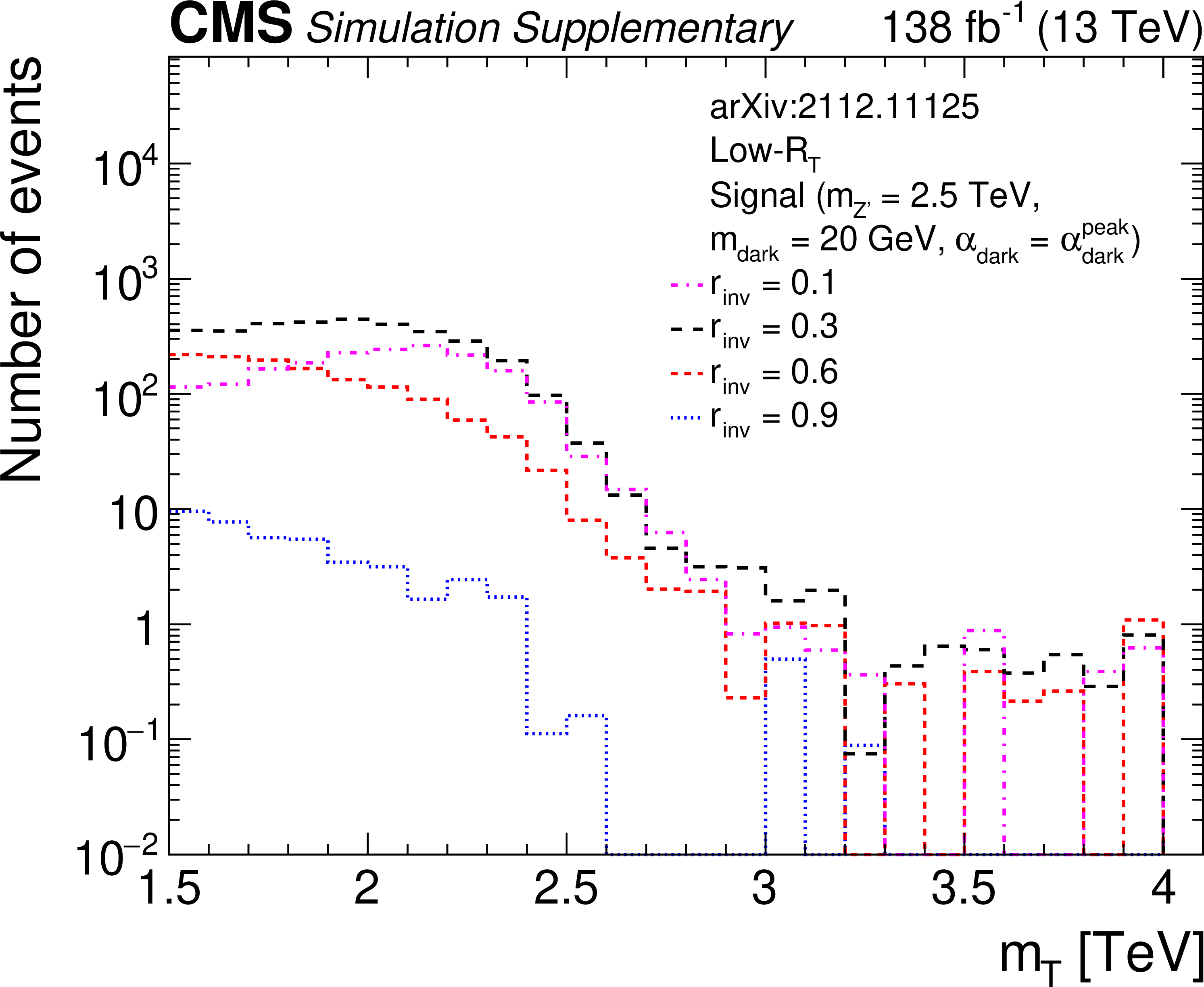
Additional Figure 13:
${m_{\mathrm {T}}}$ distributions for signal models with different ${r_{\mathrm {inv}}}$ values for the low-${R_{\mathrm {T}}}$ inclusive signal region. |
png pdf root |
Additional Figure 13-a:
${m_{\mathrm {T}}}$ distributions for signal models with different ${r_{\mathrm {inv}}}$ values for the high-${R_{\mathrm {T}}}$ inclusive signal region. |
png pdf root |
Additional Figure 13-b:
${m_{\mathrm {T}}}$ distributions for signal models with different ${r_{\mathrm {inv}}}$ values for the low-${R_{\mathrm {T}}}$ inclusive signal region. |
png pdf |
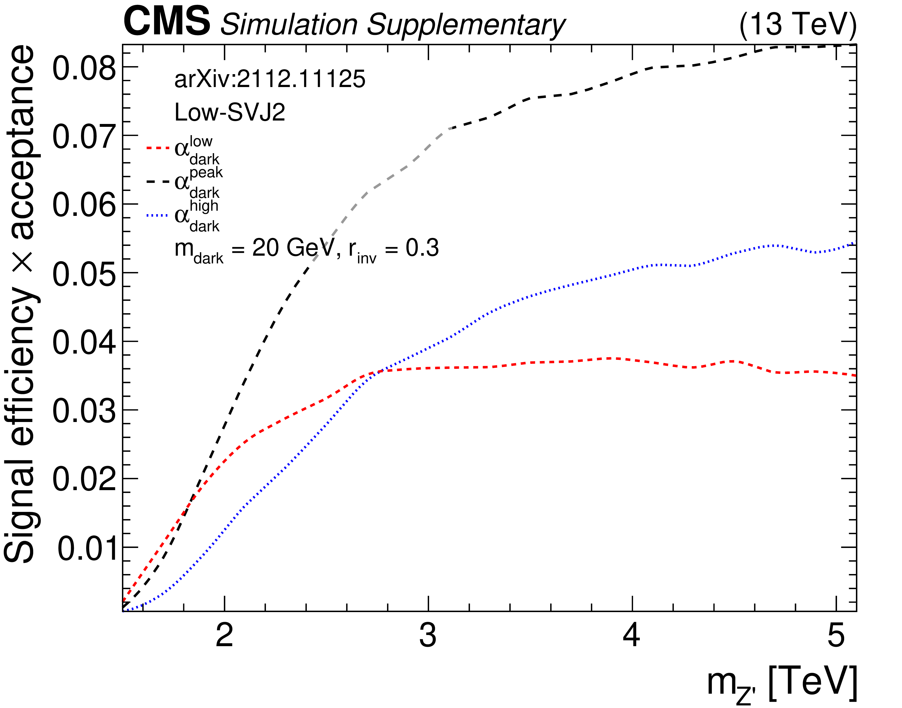
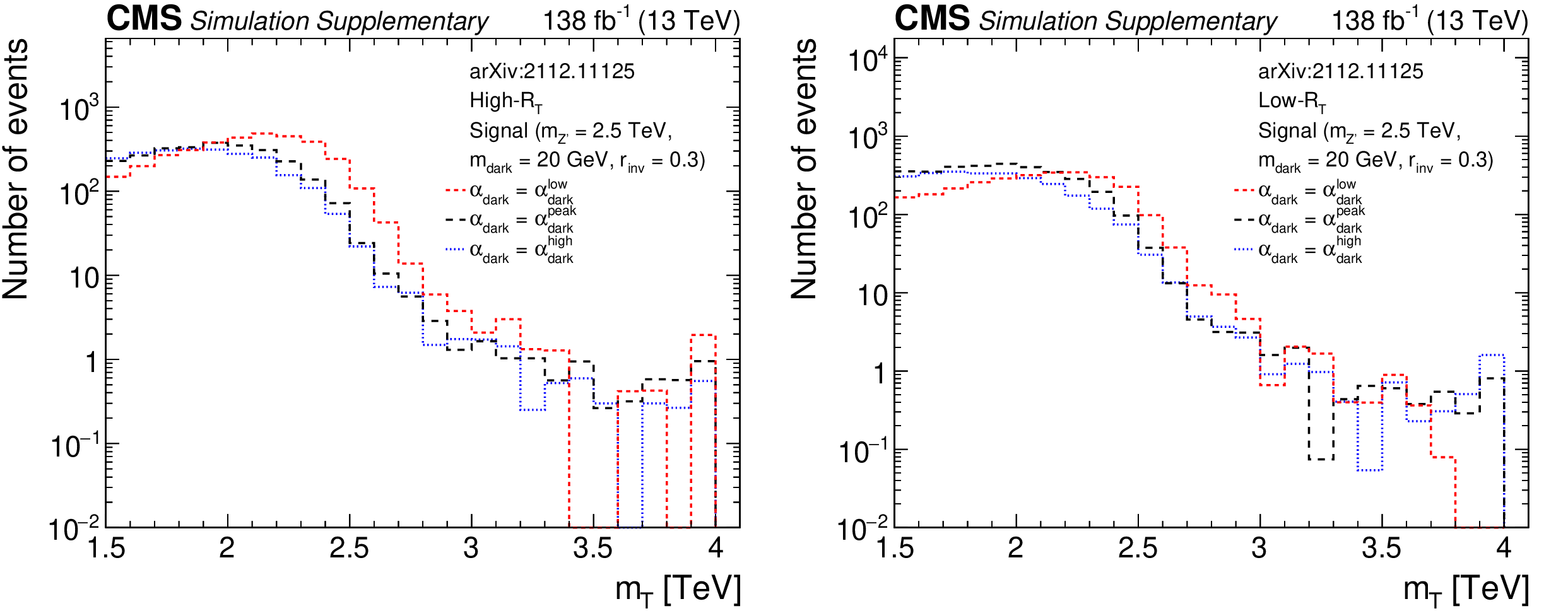
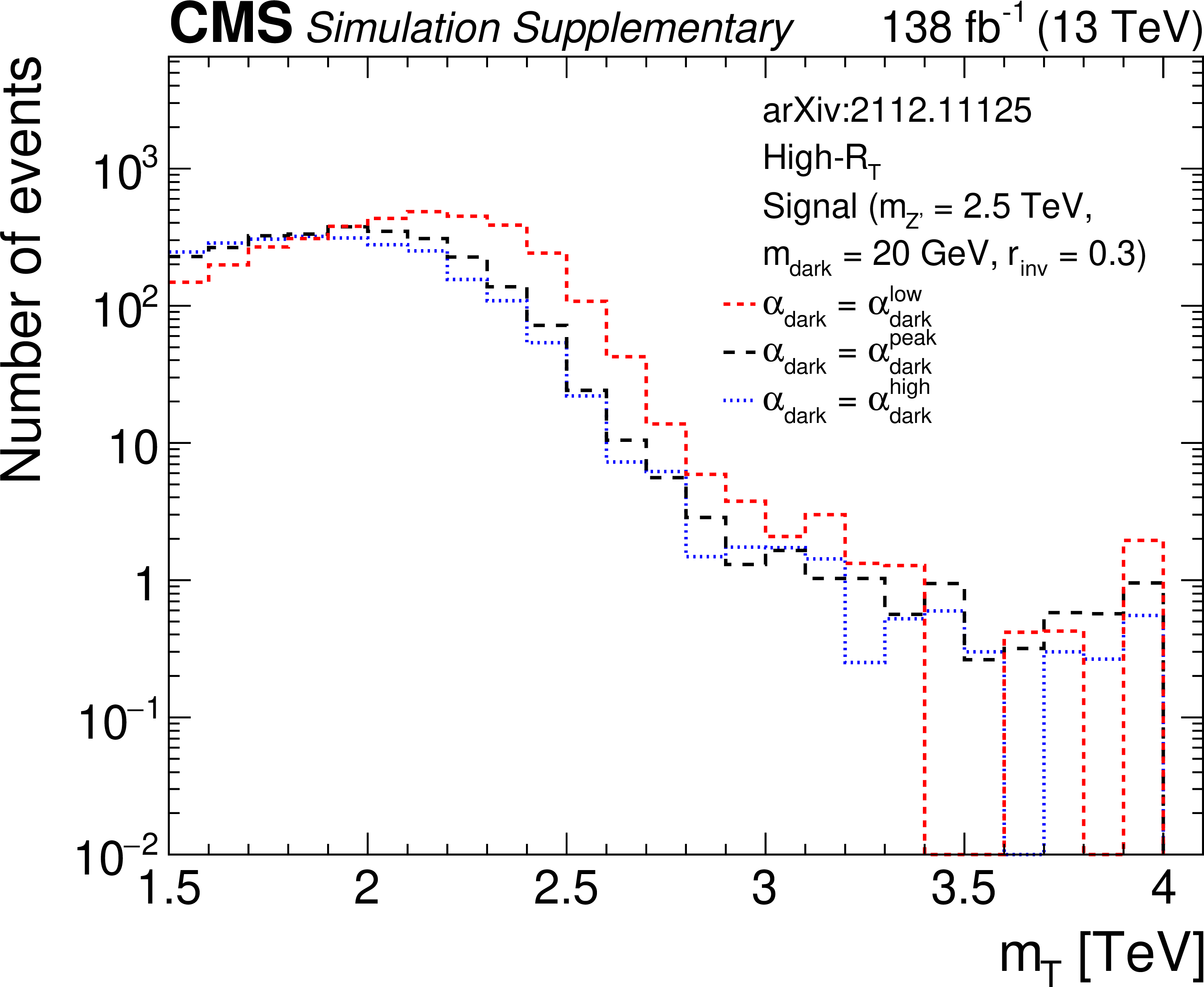
Additional Figure 14:
${m_{\mathrm {T}}}$ distributions for signal models with different ${\alpha _{\mathrm {dark}}}$ values for thelow-${R_{\mathrm {T}}}$ inclusive signal region. |
png pdf root |
Additional Figure 14-a:
${m_{\mathrm {T}}}$ distributions for signal models with different ${\alpha _{\mathrm {dark}}}$ values for the high-${R_{\mathrm {T}}}$ inclusive signal region. |

png pdf root |
Additional Figure 14-b:
${m_{\mathrm {T}}}$ distributions for signal models with different ${\alpha _{\mathrm {dark}}}$ values for thelow-${R_{\mathrm {T}}}$ inclusive signal region. |

png pdf |
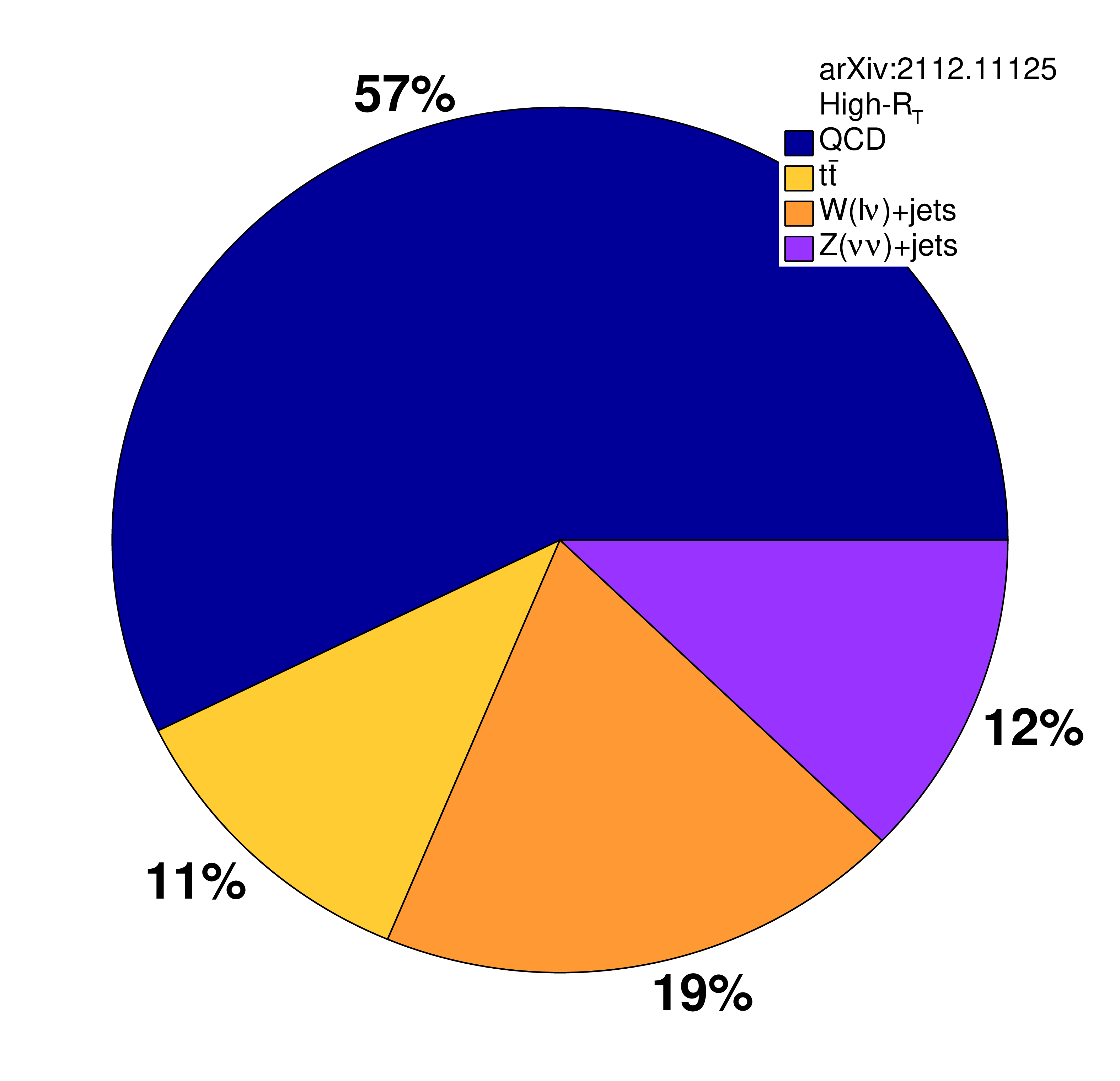
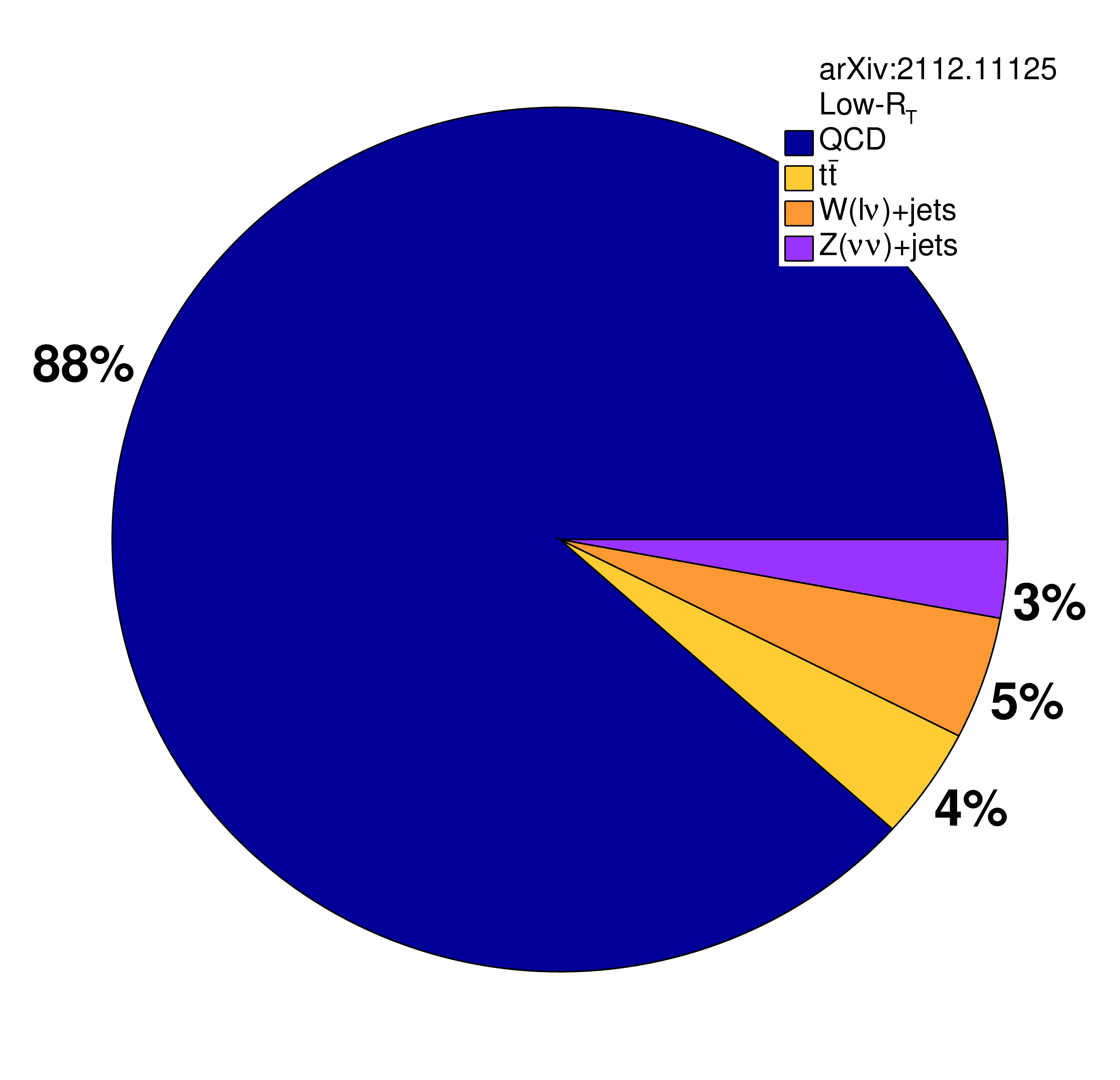
Additional Figure 15:
The proportions of each SM background process in the inclusive signal regions. |
png pdf root |
Additional Figure 15-a:
The proportions of each SM background process in the inclusive signal regions. |
png pdf root |
Additional Figure 15-b:
The proportions of each SM background process in the inclusive signal regions. |
png pdf |
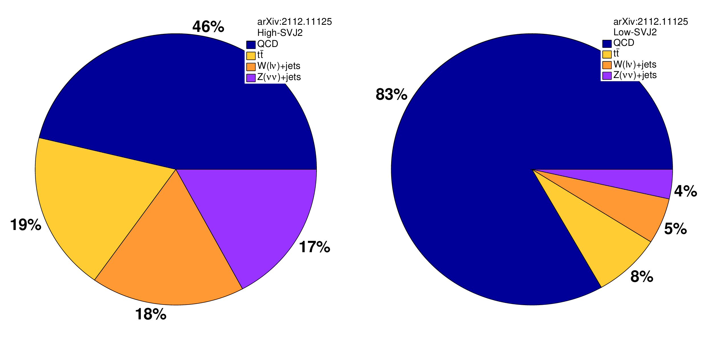
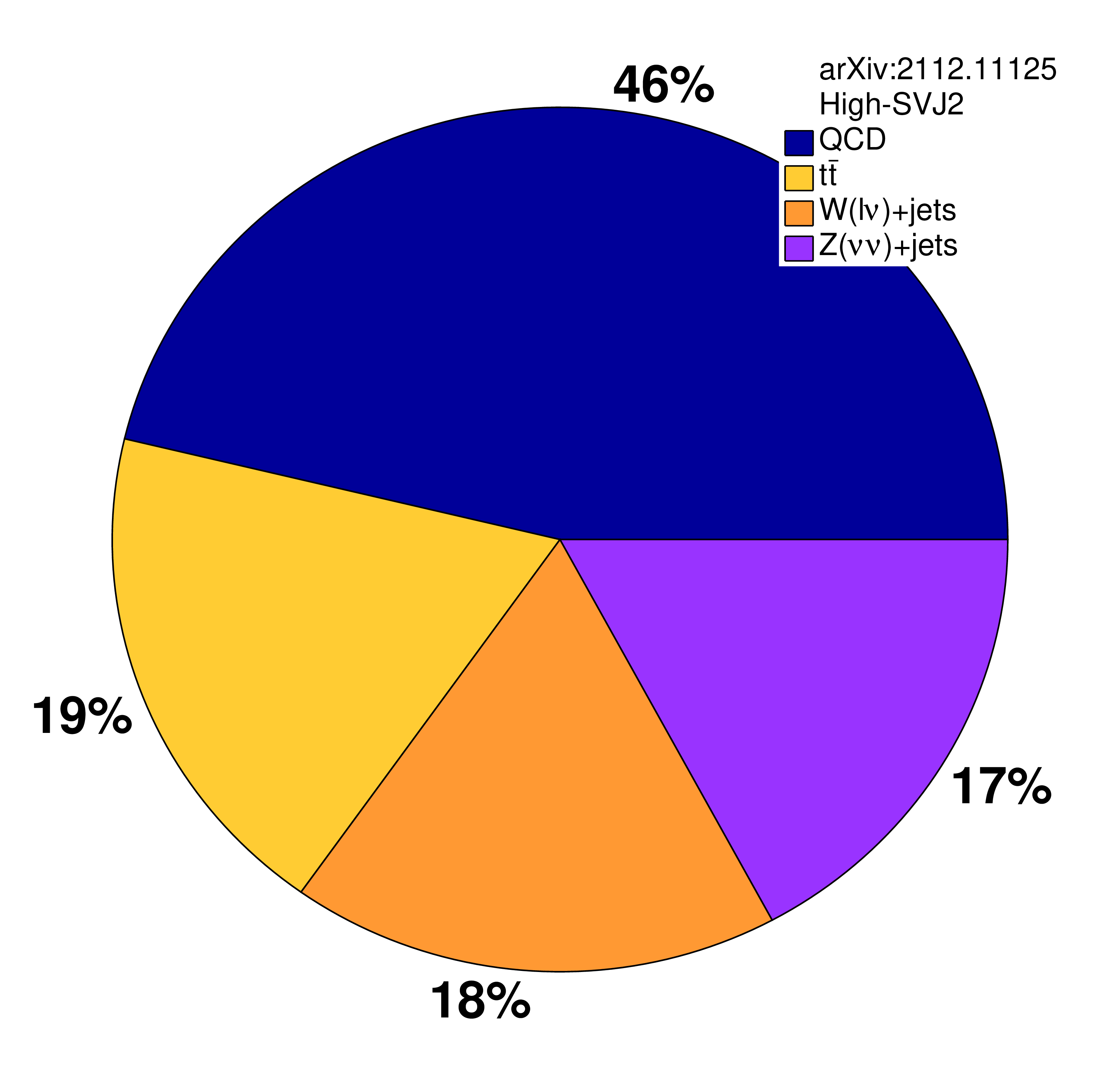
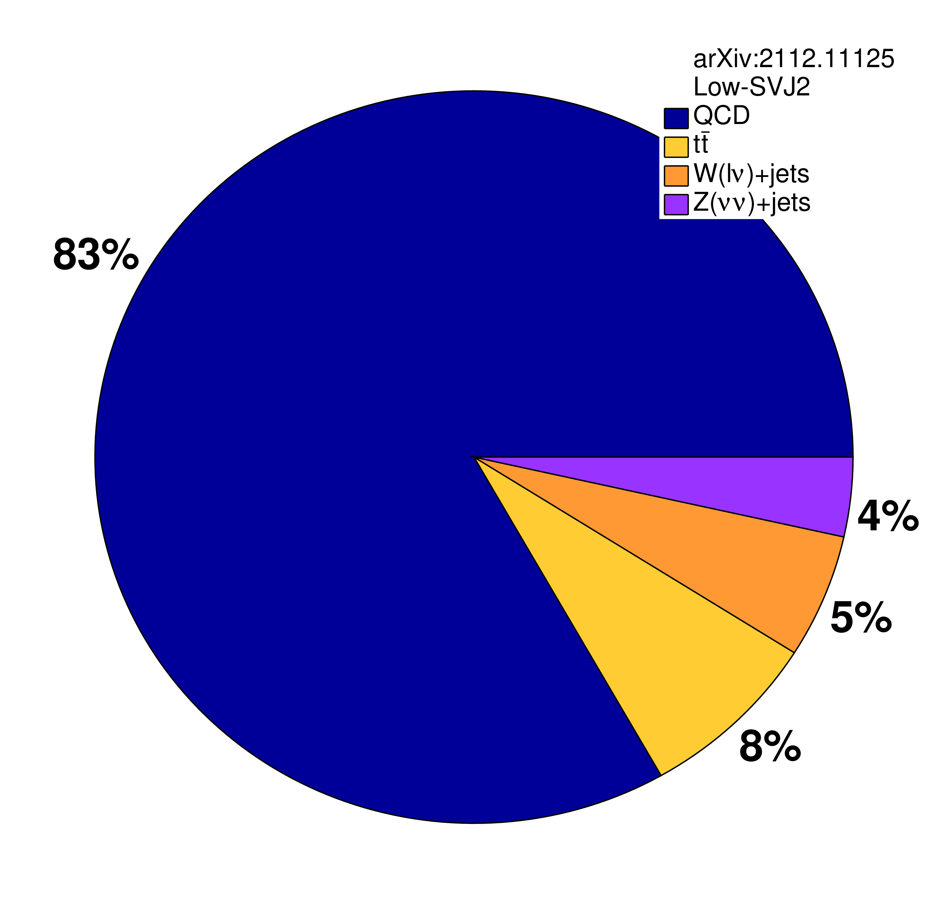
Additional Figure 16:
The proportions of each SM background process in the BDT-based signal regions. |
png pdf root |
Additional Figure 16-a:
The proportions of each SM background process in the BDT-based signal regions. |
png pdf root |
Additional Figure 16-b:
The proportions of each SM background process in the BDT-based signal regions. |

png pdf |
Additional Figure 17:
The 95% CL upper limits on the product of the cross section and branching fraction from the inclusive search for variations of pairs of the signal model parameters. The filled region indicates the expected upper limit. The solid black curves indicate the observed exclusions for the nominal ${{{\mathrm {Z}}}^{\prime}}$ cross section, while the solid red curves indicate the expected exclusions, and the dashed lines indicate the regions containing 68 and 95% of the distributions of expected exclusions. In the left plot, the regions between the respective pairs of lines or below the inner 95% dashed line are excluded. In the right plot, the regions inside the circles are excluded. |

png pdf root |
Additional Figure 17-a:
The 95% CL upper limits on the product of the cross section and branching fraction from the inclusive search for variations of a pair of the signal model parameters. The filled region indicates the expected upper limit. The solid black curves indicate the observed exclusions for the nominal ${{{\mathrm {Z}}}^{\prime}}$ cross section, while the solid red curves indicate the expected exclusions, and the dashed lines indicate the regions containing 68 and 95% of the distributions of expected exclusions. The regions between the respective pairs of lines or below the inner 95% dashed line are excluded. |
png pdf root |
Additional Figure 17-b:
The 95% CL upper limits on the product of the cross section and branching fraction from the inclusive search for variations of a pair of the signal model parameters. The filled region indicates the expected upper limit. The solid black curves indicate the observed exclusions for the nominal ${{{\mathrm {Z}}}^{\prime}}$ cross section, while the solid red curves indicate the expected exclusions, and the dashed lines indicate the regions containing 68 and 95% of the distributions of expected exclusions. The regions inside the circles are excluded. |
png pdf |
Additional Figure 18:
The 95% CL upper limits on the product of the cross section and branching fraction from the BDT-based search for variations of pairs of the signal model parameters. The filled region indicates the expected upper limit. The solid black curves indicate the observed exclusions for the nominal ${{{\mathrm {Z}}}^{\prime}}$ cross section, while the solid red curves indicate the expected exclusions, and the dashed lines indicate the regions containing 68 and 95% of the distributions of expected exclusions. The regions inside the circles are excluded. |
png pdf root |
Additional Figure 18-a:
The 95% CL upper limits on the product of the cross section and branching fraction from the BDT-based search for variations of a pair of the signal model parameters. The filled region indicates the expected upper limit. The solid black curves indicate the observed exclusions for the nominal ${{{\mathrm {Z}}}^{\prime}}$ cross section, while the solid red curves indicate the expected exclusions, and the dashed lines indicate the regions containing 68 and 95% of the distributions of expected exclusions. The regions inside the circles are excluded. |
png pdf root |
Additional Figure 18-b:
The 95% CL upper limits on the product of the cross section and branching fraction from the BDT-based search for variations of a pair of the signal model parameters. The filled region indicates the expected upper limit. The solid black curves indicate the observed exclusions for the nominal ${{{\mathrm {Z}}}^{\prime}}$ cross section, while the solid red curves indicate the expected exclusions, and the dashed lines indicate the regions containing 68 and 95% of the distributions of expected exclusions. The regions inside the circles are excluded. |
| Additional Tables | |
png pdf |
Additional Table 1:
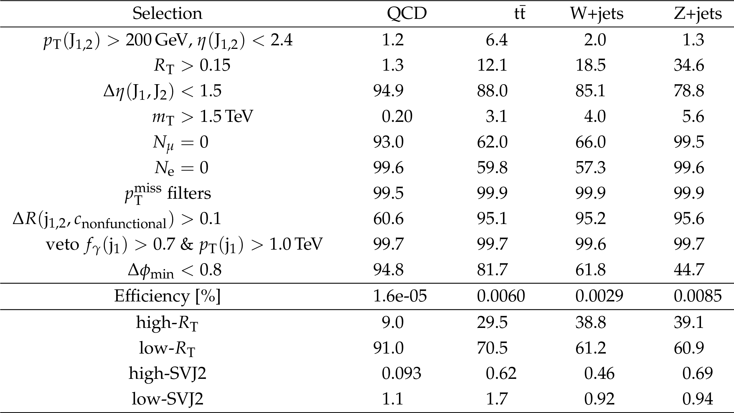
Relative efficiencies in% for each step of the event selection process for the major background processes. Statistical uncertainties, at most 1.8%, are omitted. The line "Efficiency [%]'' is the absolute efficiency after the final selection. The subsequent lines show the efficiency for each signal region, relative to the final selection. |
png pdf |
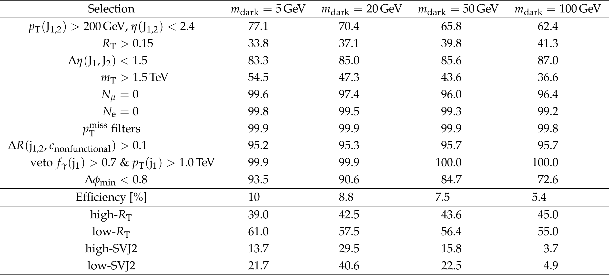
Additional Table 2:
Relative efficiencies in% for each step of the event selection process for signals with $ {m_{{{{\mathrm {Z}}}^{\prime}}}} = $ 2.1 TeV, varying ${m_{\mathrm {dark}}}$ values, $ {r_{\mathrm {inv}}} = $ 0.3, and $ {\alpha _{\mathrm {dark}}} = {{\alpha _{\mathrm {dark}}} ^{\text {peak}}} $. Statistical uncertainties, at most 0.5%, are omitted. The line "Efficiency [%]'' is the absolute efficiency after the final selection. The subsequent lines show the efficiency for each signal region, relative to the final selection. |
png pdf |
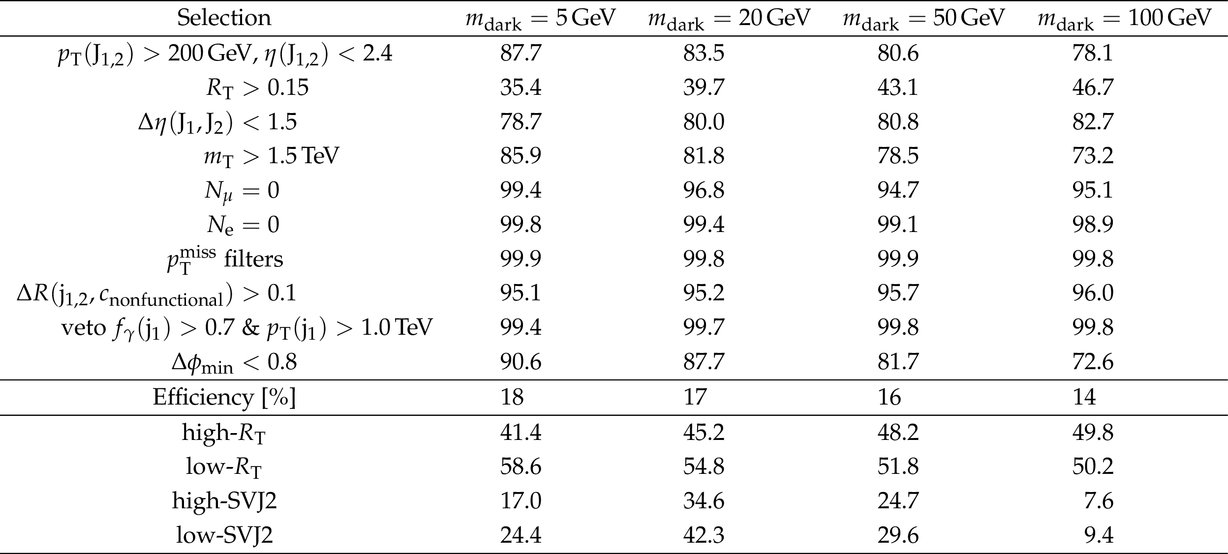
Additional Table 3:
Relative efficiencies in% for each step of the event selection process for signals with $ {m_{{{{\mathrm {Z}}}^{\prime}}}} = $ 3.1 TeV, varying ${m_{\mathrm {dark}}}$ values, $ {r_{\mathrm {inv}}} = $ 0.3, and $ {\alpha _{\mathrm {dark}}} = {{\alpha _{\mathrm {dark}}} ^{\text {peak}}} $. Statistical uncertainties, at most 0.4%, are omitted. The line "Efficiency [%]'' is the absolute efficiency after the final selection. The subsequent lines show the efficiency for each signal region, relative to the final selection. |
png pdf |
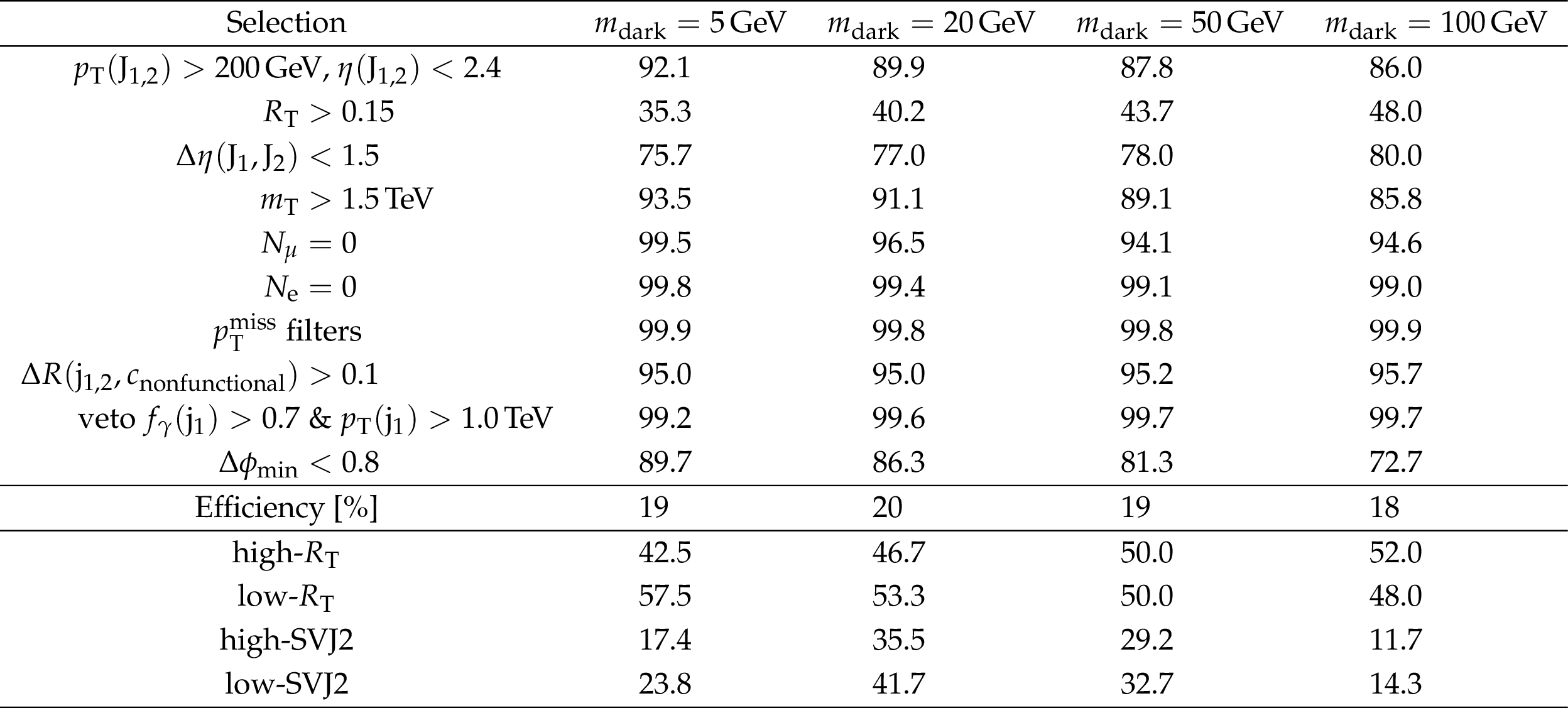
Additional Table 4:
Relative efficiencies in% for each step of the event selection process for signals with $ {m_{{{{\mathrm {Z}}}^{\prime}}}} = $ 4.1 TeV, varying ${m_{\mathrm {dark}}}$ values, $ {r_{\mathrm {inv}}} = $ 0.3, and $ {\alpha _{\mathrm {dark}}} = {{\alpha _{\mathrm {dark}}} ^{\text {peak}}} $. Statistical uncertainties, at most 0.4%, are omitted. The line "Efficiency [%]'' is the absolute efficiency after the final selection. The subsequent lines show the efficiency for each signal region, relative to the final selection. |
png pdf |
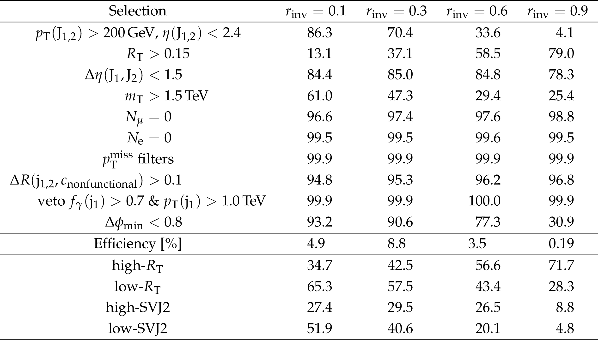
Additional Table 5:
Relative efficiencies in% for each step of the event selection process for signals with $ {m_{{{{\mathrm {Z}}}^{\prime}}}} = $ 2.1 TeV, $ {m_{\mathrm {dark}}} = $ 20 GeV, varying ${r_{\mathrm {inv}}}$ values, and $ {\alpha _{\mathrm {dark}}} = {{\alpha _{\mathrm {dark}}} ^{\text {peak}}} $. Statistical uncertainties, at most 2.6%, are omitted. The line "Efficiency [%]'' is the absolute efficiency after the final selection. The subsequent lines show the efficiency for each signal region, relative to the final selection. |

png pdf |
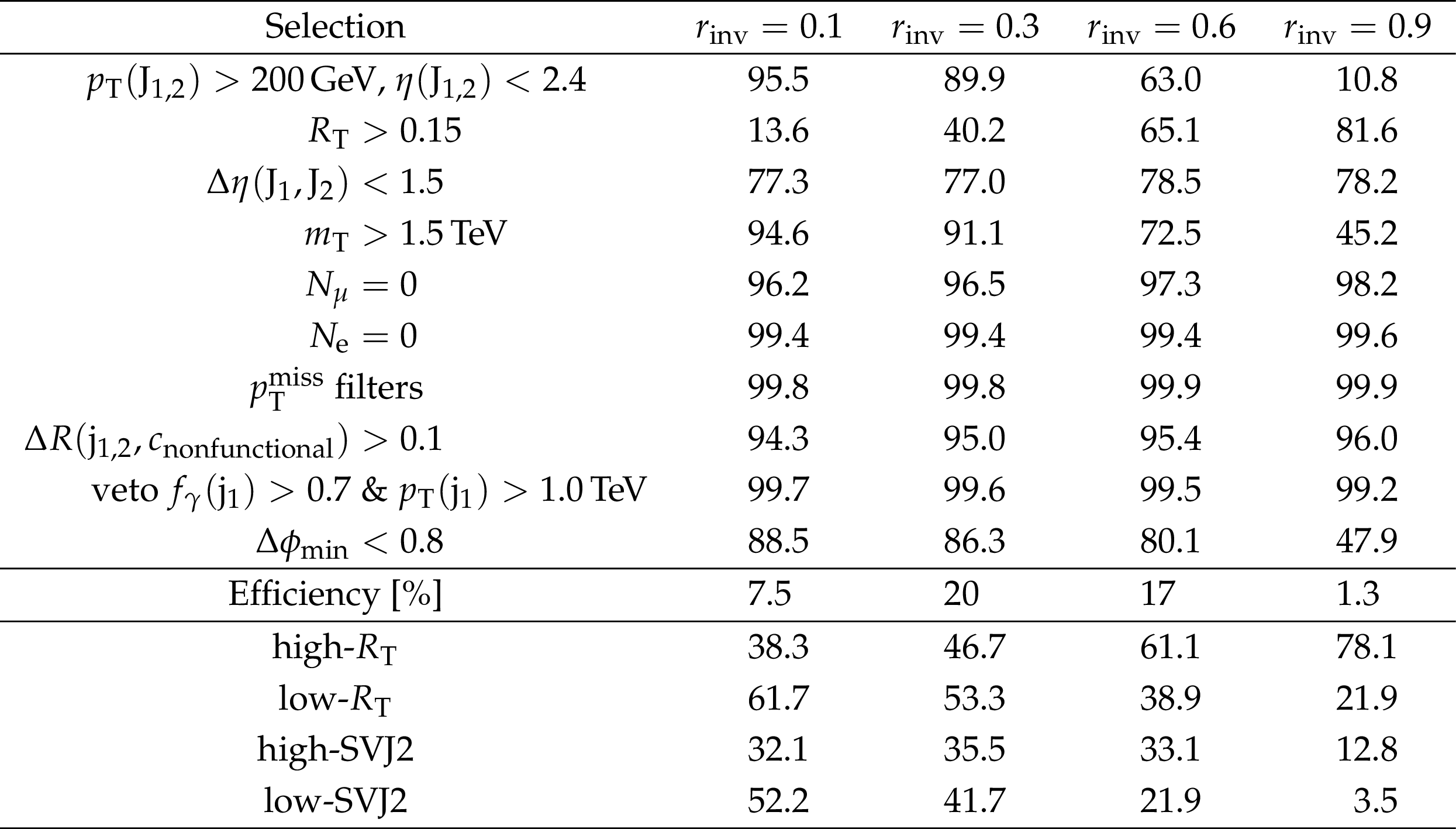
Additional Table 6:
Relative efficiencies in% for each step of the event selection process for signals with $ {m_{{{{\mathrm {Z}}}^{\prime}}}} = $ 3.1 TeV, $ {m_{\mathrm {dark}}} = $ 20 GeV, varying ${r_{\mathrm {inv}}}$ values, and $ {\alpha _{\mathrm {dark}}} = {{\alpha _{\mathrm {dark}}} ^{\text {peak}}} $. Statistical uncertainties, at most 1.2%, are omitted. The line "Efficiency [%]'' is the absolute efficiency after the final selection. The subsequent lines show the efficiency for each signal region, relative to the final selection. |
png pdf |
Additional Table 7:
Relative efficiencies in% for each step of the event selection process for signals with $ {m_{{{{\mathrm {Z}}}^{\prime}}}} = $ 4.1 TeV, $ {m_{\mathrm {dark}}} = $ 20 GeV, varying ${r_{\mathrm {inv}}}$ values, and $ {\alpha _{\mathrm {dark}}} = {{\alpha _{\mathrm {dark}}} ^{\text {peak}}} $. Statistical uncertainties, at most 0.9%, are omitted. The line "Efficiency [%]'' is the absolute efficiency after the final selection. The subsequent lines show the efficiency for each signal region, relative to the final selection. |
png pdf |
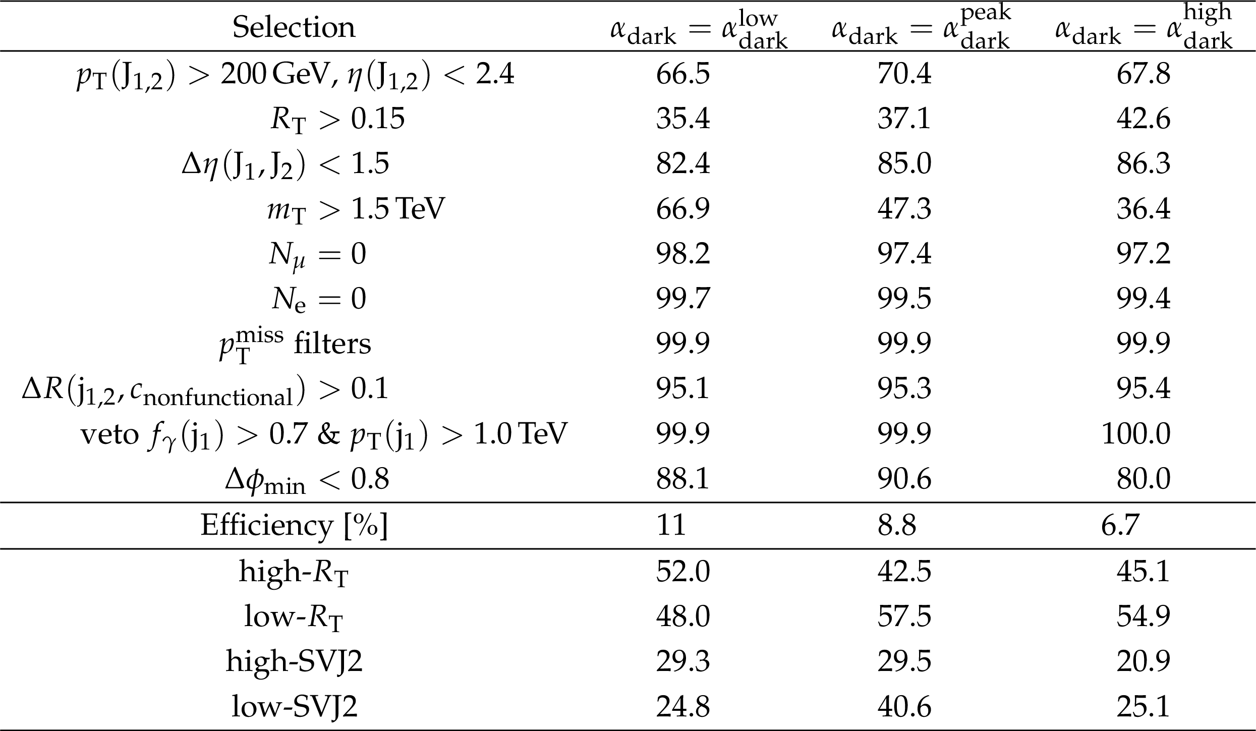
Additional Table 8:
Relative efficiencies in% for each step of the event selection process for signals with $ {m_{{{{\mathrm {Z}}}^{\prime}}}} = $ 2.1 TeV, $ {m_{\mathrm {dark}}} = $ 20 GeV, $ {r_{\mathrm {inv}}} = $ 0.3, and varying ${\alpha _{\mathrm {dark}}}$ values. Statistical uncertainties, at most 0.4%, are omitted. The line "Efficiency [%]'' is the absolute efficiency after the final selection. The subsequent lines show the efficiency for each signal region, relative to the final selection. |
png pdf |
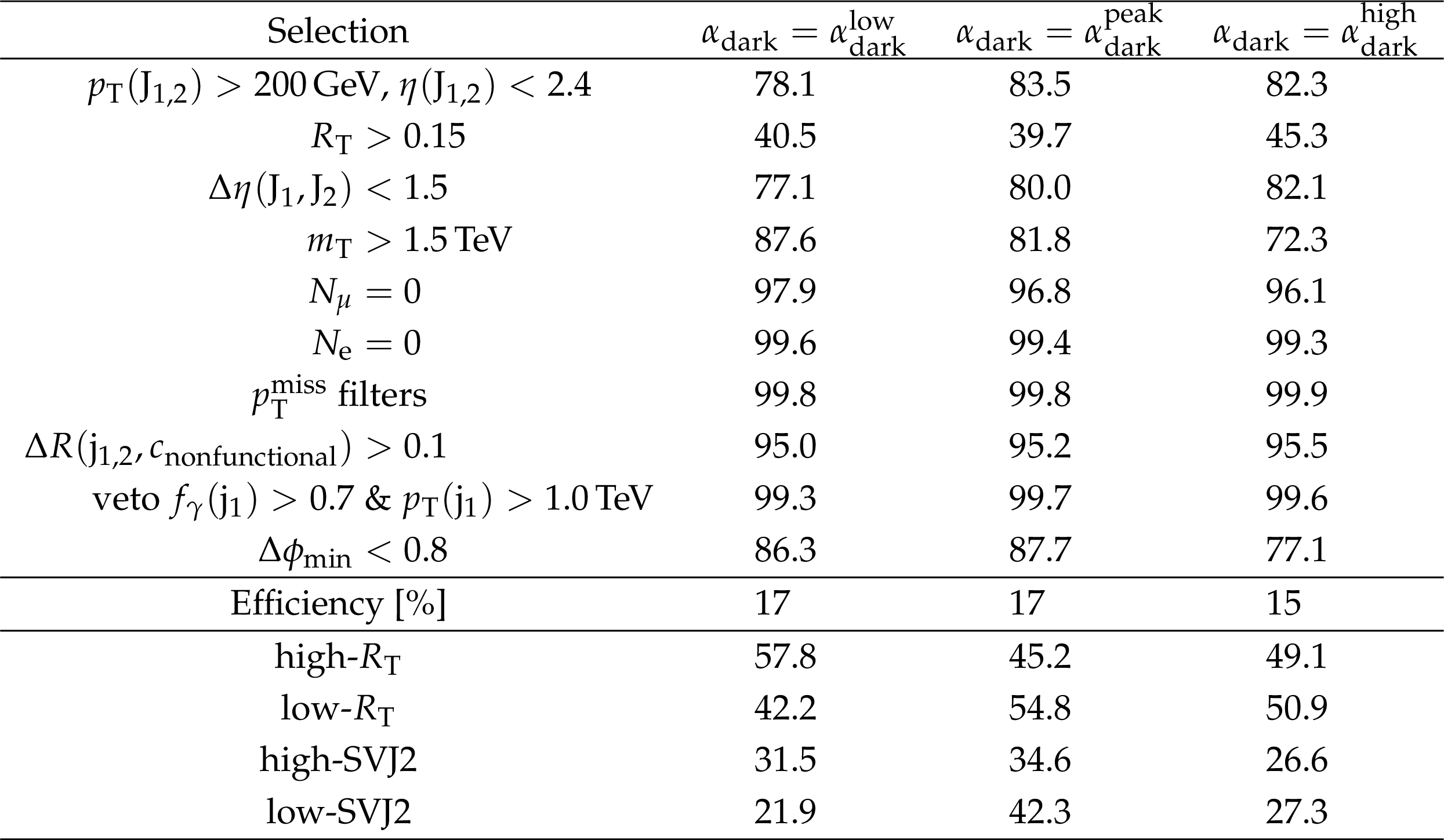
Additional Table 9:
Relative efficiencies in% for each step of the event selection process for signals with $ {m_{{{{\mathrm {Z}}}^{\prime}}}} = $ 3.1 TeV, $ {m_{\mathrm {dark}}} = $ 20 GeV, $ {r_{\mathrm {inv}}} = $ 0.3, and varying ${\alpha _{\mathrm {dark}}}$ values. Statistical uncertainties, at most 0.4%, are omitted. The line "Efficiency [%]'' is the absolute efficiency after the final selection. The subsequent lines show the efficiency for each signal region, relative to the final selection. |
png pdf |
Additional Table 10:
Relative efficiencies in% for each step of the event selection process for signals with $ {m_{{{{\mathrm {Z}}}^{\prime}}}} = $ 4.1 TeV, $ {m_{\mathrm {dark}}} = $ 20 GeV, $ {r_{\mathrm {inv}}} = $ 0.3, and varying ${\alpha _{\mathrm {dark}}}$ values. Statistical uncertainties, at most 0.4%, are omitted. The line "Efficiency [%]'' is the absolute efficiency after the final selection. The subsequent lines show the efficiency for each signal region, relative to the final selection. |
| References | ||||
| 1 | V. C. Rubin, N. Thonnard, and W. K. Ford, Jr. | Rotational properties of 21 SC galaxies with a large range of luminosities and radii, from NGC 4605 (R = 4 kpc) to UGC 2885 (R = 122 kpc) | Astrophys. J. 238 (1980) 471 | |
| 2 | M. Persic, P. Salucci, and F. Stel | The universal rotation curve of spiral galaxies: I. The dark matter connection | Mon. Not. Roy. Astron. Soc. 281 (1996) 27 | astro-ph/9506004 |
| 3 | D. Clowe et al. | A direct empirical proof of the existence of dark matter | Astrophys. J. 648 (2006) L109 | astro-ph/0608407 |
| 4 | DES Collaboration | Dark Energy Survey year 1 results: curved-sky weak lensing mass map | Mon. Not. Roy. Astron. Soc. 475 (2018) 3165 | 1708.01535 |
| 5 | Planck Collaboration | Planck 2018 results. VI. Cosmological parameters | Astron. Astrophys. 641 (2020) A6 | 1807.06209 |
| 6 | M. Battaglieri et al. | US cosmic visions: New ideas in dark matter 2017: Community report | link | 1707.04591 |
| 7 | G. Jungman, M. Kamionkowski, and K. Griest | Supersymmetric dark matter | PR 267 (1996) 195 | hep-ph/9506380 |
| 8 | CMS Collaboration | Search for new physics in final states with a single photon and missing transverse momentum in proton-proton collisions at $ \sqrt{s} = $ 13 TeV | JHEP 02 (2019) 074 | CMS-EXO-16-053 1810.00196 |
| 9 | CMS Collaboration | Search for dark matter produced in association with a leptonically decaying Z boson in proton-proton collisions at $ \sqrt{s} = $ 13 TeV | EPJC 81 (2021) 13 | CMS-EXO-19-003 2008.04735 |
| 10 | CMS Collaboration | Search for new particles in events with energetic jets and large missing transverse momentum in proton-proton collisions at $ \sqrt{s} = $ 13 TeV | JHEP 11 (2021) 153 | CMS-EXO-20-004 2107.13021 |
| 11 | CMS Collaboration | Search for dark matter produced in association with a Higgs boson decaying to a pair of bottom quarks in proton--proton collisions at $ \sqrt{s}= $ 13 TeV | EPJC 79 (2019) 280 | CMS-EXO-16-050 1811.06562 |
| 12 | CMS Collaboration | Search for dark matter produced in association with a single top quark or a top quark pair in proton-proton collisions at $ \sqrt{s}= $ 13 TeV | JHEP 03 (2019) 141 | CMS-EXO-18-010 1901.01553 |
| 13 | CMS Collaboration | Search for invisible decays of a Higgs boson produced through vector boson fusion in proton-proton collisions at $ \sqrt{s} = $ 13 TeV | PLB 793 (2019) 520 | CMS-HIG-17-023 1809.05937 |
| 14 | ATLAS Collaboration | Search for dark matter in events with a hadronically decaying vector boson and missing transverse momentum in pp collisions at $ \sqrt{s} = $ 13 TeV with the ATLAS detector | JHEP 10 (2018) 180 | 1807.11471 |
| 15 | ATLAS Collaboration | Search for invisible Higgs boson decays in vector boson fusion at $ \sqrt{s} = $ 13 TeV with the ATLAS detector | PLB 793 (2019) 499 | 1809.06682 |
| 16 | ATLAS Collaboration | Constraints on mediator-based dark matter and scalar dark energy models using $ \sqrt s = $ 13 TeV pp collision data collected by the ATLAS detector | JHEP 05 (2019) 142 | 1903.01400 |
| 17 | ATLAS Collaboration | Search for new phenomena in events with two opposite-charge leptons, jets and missing transverse momentum in pp collisions at $ \sqrt{s} = $ 13 TeV with the ATLAS detector | JHEP 04 (2021) 165 | 2102.01444 |
| 18 | ATLAS Collaboration | Search for new phenomena with top quark pairs in final states with one lepton, jets, and missing transverse momentum in pp collisions at $ \sqrt{s} = $ 13 TeV with the ATLAS detector | JHEP 04 (2021) 174 | 2012.03799 |
| 19 | ATLAS Collaboration | Search for new phenomena in events with an energetic jet and missing transverse momentum in pp collisions at $ \sqrt{s} = $ 13 TeV with the ATLAS detector | PRD 103 (2021) 112006 | 2102.10874 |
| 20 | M. J. Strassler and K. M. Zurek | Echoes of a hidden valley at hadron colliders | PLB 651 (2007) 374 | hep-ph/0604261 |
| 21 | LHCb Collaboration | Search for dark photons produced in 13 TeV pp $ collisions | PRL 120 (2018) 061801 | 1710.02867 |
| 22 | ATLAS Collaboration | Search for long-lived particles in final states with displaced dimuon vertices in pp collisions at $ \sqrt{s}= $ 13 TeV with the ATLAS detector | PRD 99 (2019) 012001 | 1808.03057 |
| 23 | CMS Collaboration | A search for pair production of new light bosons decaying into muons in proton-proton collisions at 13 TeV | PLB 796 (2019) 131 | CMS-HIG-18-003 1812.00380 |
| 24 | CMS Collaboration | Search for dark photons in decays of Higgs bosons produced in association with Z bosons in proton-proton collisions at $ \sqrt{s} = $ 13 TeV | JHEP 10 (2019) 139 | CMS-EXO-19-007 1908.02699 |
| 25 | ATLAS Collaboration | Search for light long-lived neutral particles produced in pp collisions at $ \sqrt{s} = $ 13 TeV and decaying into collimated leptons or light hadrons with the ATLAS detector | EPJC 80 (2020) 450 | 1909.01246 |
| 26 | LHCb Collaboration | Search for A' $ \to\mu^+\mu^- $ Decays | PRL 124 (2020) 041801 | 1910.06926 |
| 27 | CMS Collaboration | Search for a narrow resonance lighter than 200 GeV decaying to a pair of muons in proton-proton collisions at $ \sqrt{s} = $ 13 TeV | PRL 124 (2020) 131802 | CMS-EXO-19-018 1912.04776 |
| 28 | LHCb Collaboration | Searches for low-mass dimuon resonances | JHEP 10 (2020) 156 | 2007.03923 |
| 29 | CMS Collaboration | Search for dark photons in Higgs boson production via vector boson fusion in proton-proton collisions at $ \sqrt{s} = $ 13 TeV | JHEP 03 (2021) 011 | CMS-EXO-20-005 2009.14009 |
| 30 | J. Alimena et al. | Searching for long-lived particles beyond the standard model at the Large Hadron Collider | JPG 47 (2020) 090501 | 1903.04497 |
| 31 | K. Petraki and R. R. Volkas | Review of asymmetric dark matter | Int. J. Mod. Phys. A 28 (2013) 1330028 | 1305.4939 |
| 32 | Planck Collaboration | Planck 2015 results. XIII. cosmological parameters | Astron. Astrophys. 594 (2016) A13 | 1502.01589 |
| 33 | Y. Bai and P. Schwaller | Scale of dark QCD | PRD 89 (2014) 063522 | 1306.4676 |
| 34 | H. Beauchesne, E. Bertuzzo, and G. Grilli di Cortona | Dark matter in Hidden Valley models with stable and unstable light dark mesons | JHEP 04 (2019) 118 | 1809.10152 |
| 35 | T. Cohen, M. Lisanti, and H. K. Lou | Semi-visible jets: Dark matter undercover at the LHC | PRL 115 (2015) 171804 | 1503.00009 |
| 36 | T. Cohen, M. Lisanti, H. K. Lou, and S. Mishra-Sharma | LHC searches for dark sector showers | JHEP 11 (2017) 196 | 1707.05326 |
| 37 | CMS Collaboration | Search for high mass dijet resonances with a new background prediction method in proton-proton collisions at $ \sqrt{s} = $ 13 TeV | JHEP 05 (2020) 033 | CMS-EXO-19-012 1911.03947 |
| 38 | ATLAS Collaboration | Search for new resonances in mass distributions of jet pairs using 139 fb$ ^{-1} $ of pp collisions at $ \sqrt{s}= $ 13 TeV with the ATLAS detector | JHEP 03 (2020) 145 | 1910.08447 |
| 39 | P. Schwaller, D. Stolarski, and A. Weiler | Emerging jets | JHEP 05 (2015) 059 | 1502.05409 |
| 40 | CMS Collaboration | Search for new particles decaying to a jet and an emerging jet | JHEP 02 (2019) 179 | CMS-EXO-18-001 1810.10069 |
| 41 | CMS Collaboration | Precision luminosity measurement in proton-proton collisions at $ \sqrt{s} = $ 13 TeV in 2015 and 2016 at CMS | EPJC 81 (2021) 800 | CMS-LUM-17-003 2104.01927 |
| 42 | CMS Collaboration | HEPData record for this analysis | link | |
| 43 | CMS Collaboration | Performance of the CMS Level-1 trigger in proton-proton collisions at $ \sqrt{s} = $ 13 TeV | JINST 15 (2020) P10017 | CMS-TRG-17-001 2006.10165 |
| 44 | CMS Collaboration | The CMS trigger system | JINST 12 (2017) P01020 | CMS-TRG-12-001 1609.02366 |
| 45 | CMS Collaboration | The CMS experiment at the CERN LHC | JINST 3 (2008) S08004 | CMS-00-001 |
| 46 | T. Sjostrand et al. | An introduction to PYTHIA 8.2 | CPC 191 (2015) 159 | 1410.3012 |
| 47 | A. Albert et al. | Recommendations of the LHC dark matter working group: Comparing LHC searches for dark matter mediators in visible and invisible decay channels and calculations of the thermal relic density | Phys. Dark Univ. 26 (2019) 100377 | 1703.05703 |
| 48 | A. Boveia et al. | Recommendations on presenting LHC searches for missing transverse energy signals using simplified $ s $-channel models of dark matter | Phys. Dark Univ. 27 (2020) 100365 | 1603.04156 |
| 49 | R. K. Ellis, W. J. Stirling, and B. R. Webber | QCD and collider physics | Camb. Monogr. Part. Phys. NP Cosmol. 8 (1996) 1 | |
| 50 | GEANT4 Collaboration | GEANT4---a simulation toolkit | NIMA 506 (2003) 250 | |
| 51 | J. Alwall et al. | The automated computation of tree-level and next-to-leading order differential cross sections, and their matching to parton shower simulations | JHEP 07 (2014) 079 | 1405.0301 |
| 52 | J. Alwall et al. | Comparative study of various algorithms for the merging of parton showers and matrix elements in hadronic collisions | EPJC 53 (2008) 473 | 0706.2569 |
| 53 | M. Beneke, P. Falgari, S. Klein, and C. Schwinn | Hadronic top-quark pair production with NNLL threshold resummation | NPB 855 (2012) 695 | 1109.1536 |
| 54 | M. Cacciari et al. | Top-pair production at hadron colliders with next-to-next-to-leading logarithmic soft-gluon resummation | PLB 710 (2012) 612 | 1111.5869 |
| 55 | P. Barnreuther, M. Czakon, and A. Mitov | Percent level precision physics at the Tevatron: First genuine NNLO QCD corrections to $ \mathrm{q\bar{q}}\to\mathrm{t\bar{t}} $+X | PRL 109 (2012) 132001 | 1204.5201 |
| 56 | M. Czakon and A. Mitov | NNLO corrections to top-pair production at hadron colliders: the all-fermionic scattering channels | JHEP 12 (2012) 054 | 1207.0236 |
| 57 | M. Czakon and A. Mitov | NNLO corrections to top pair production at hadron colliders: the quark-gluon reaction | JHEP 01 (2013) 080 | 1210.6832 |
| 58 | M. Czakon, P. Fiedler, and A. Mitov | Total top-quark pair-production cross section at hadron colliders through $ O({\alpha_S}^4) $ | PRL 110 (2013) 252004 | 1303.6254 |
| 59 | Y. Li and F. Petriello | Combining QCD and electroweak corrections to dilepton production in FEWZ | PRD 86 (2012) 094034 | 1208.5967 |
| 60 | NNPDF Collaboration | Parton distributions for the LHC run II | JHEP 04 (2015) 040 | 1410.8849 |
| 61 | NNPDF Collaboration | Parton distributions with QED corrections | NPB 877 (2013) 290 | 1308.0598 |
| 62 | CMS Collaboration | Event generator tunes obtained from underlying event and multiparton scattering measurements | EPJC 76 (2016) 155 | CMS-GEN-14-001 1512.00815 |
| 63 | NNPDF Collaboration | Parton distributions from high-precision collider data | EPJC 77 (2017) 663 | 1706.00428 |
| 64 | CMS Collaboration | Extraction and validation of a new set of CMS PYTHIA8 tunes from underlying-event measurements | EPJC 80 (2020) 4 | CMS-GEN-17-001 1903.12179 |
| 65 | CMS Collaboration | Particle-flow reconstruction and global event description with the CMS detector | JINST 12 (2017) P10003 | CMS-PRF-14-001 1706.04965 |
| 66 | M. Cacciari, G. P. Salam, and G. Soyez | The anti-$ {k_{\mathrm{T}}} $ jet clustering algorithm | JHEP 04 (2008) 063 | 0802.1189 |
| 67 | M. Cacciari, G. P. Salam, and G. Soyez | FastJet user manual | EPJC 72 (2012) 1896 | 1111.6097 |
| 68 | CMS Collaboration | Performance of missing transverse momentum reconstruction in proton-proton collisions at $ \sqrt{s} = $ 13 TeV using the CMS detector | JINST 14 (2019) P07004 | CMS-JME-17-001 1903.06078 |
| 69 | CMS Collaboration | Electron and photon reconstruction and identification with the CMS experiment at the CERN LHC | JINST 16 (2021) P05014 | CMS-EGM-17-001 2012.06888 |
| 70 | CMS Collaboration | Performance of the CMS muon detector and muon reconstruction with proton-proton collisions at $ \sqrt{s} = $ 13 TeV | JINST 13 (2018) P06015 | CMS-MUO-16-001 1804.04528 |
| 71 | D. Bertolini, P. Harris, M. Low, and N. Tran | Pileup per particle identification | JHEP 10 (2014) 059 | 1407.6013 |
| 72 | CMS Collaboration | Pileup mitigation at CMS in 13 TeV data | JINST 15 (2020) P09018 | CMS-JME-18-001 2003.00503 |
| 73 | CMS Collaboration | Jet energy scale and resolution in the CMS experiment in pp collisions at 8 TeV | JINST 12 (2017) P02014 | CMS-JME-13-004 1607.03663 |
| 74 | CMS Collaboration | Jet algorithms performance in 13 TeV data | CMS-PAS-JME-16-003 | CMS-PAS-JME-16-003 |
| 75 | M. Cacciari and G. P. Salam | Pileup subtraction using jet areas | PLB 659 (2008) 119 | 0707.1378 |
| 76 | K. Rehermann and B. Tweedie | Efficient identification of boosted semileptonic top quarks at the LHC | JHEP 03 (2011) 059 | 1007.2221 |
| 77 | G. Cowan, K. Cranmer, E. Gross, and O. Vitells | Asymptotic formulae for likelihood-based tests of new physics | EPJC 71 (2011) 1554 | 1007.1727 |
| 78 | M. Park and M. Zhang | Tagging a jet from a dark sector with jet-substructures at colliders | PRD 100 (2019) 115009 | 1712.09279 |
| 79 | T. Cohen, J. Doss, and M. Freytsis | Jet substructure from dark sector showers | JHEP 09 (2020) 118 | 2004.00631 |
| 80 | E. Bernreuther et al. | Casting a graph net to catch dark showers | SciPost Phys. 10 (2021) 046 | 2006.08639 |
| 81 | J. Thaler and K. Van Tilburg | Identifying boosted objects with $ N $-subjettiness | JHEP 03 (2011) 015 | 1011.2268 |
| 82 | I. Moult, L. Necib, and J. Thaler | New angles on energy correlation functions | JHEP 12 (2016) 153 | 1609.07483 |
| 83 | A. J. Larkoski, S. Marzani, G. Soyez, and J. Thaler | Soft drop | JHEP 05 (2014) 146 | 1402.2657 |
| 84 | J. Gallicchio and M. D. Schwartz | Quark and gluon jet substructure | JHEP 04 (2013) 090 | 1211.7038 |
| 85 | CMS Collaboration | Performance of quark/gluon discrimination in 8 TeV pp data | CMS-PAS-JME-13-002 | CMS-PAS-JME-13-002 |
| 86 | F. Pedregosa et al. | Scikit-learn: Machine learning in Python | J. Mach. Learn. Res. 12 (2011) 2825 | 1201.0490 |
| 87 | T. Likhomanenko et al. | Reproducible Experiment Platform | J. Phys. Conf. Ser. 664 (2015) 052022 | 1510.00624 |
| 88 | R. G. Lomax and D. L. Hahs-Vaughn | Statistical concepts: a second course | Taylor and Francis, Hoboken, NJ | |
| 89 | UA2 Collaboration | A measurement of two jet decays of the W and Z bosons at the CERN $ \bar{p} p $ collider | Z. Phys. C 49 (1991) 17 | |
| 90 | UA2 Collaboration | A search for new intermediate vector mesons and excited quarks decaying to two jets at the CERN $ \bar{p} p $ collider | NPB 400 (1993) 3 | |
| 91 | CMS Collaboration | CMS luminosity measurement for the 2017 data-taking period at $ \sqrt{s} = $ 13 TeV | CMS-PAS-LUM-17-004 | CMS-PAS-LUM-17-004 |
| 92 | CMS Collaboration | CMS luminosity measurement for the 2018 data-taking period at $ \sqrt{s}= $ 13 TeV | CMS-PAS-LUM-18-002 | CMS-PAS-LUM-18-002 |
| 93 | CMS Collaboration | Measurement of the inelastic proton-proton cross section at $ \sqrt{s}= $ 13 TeV | JHEP 07 (2018) 161 | CMS-FSQ-15-005 1802.02613 |
| 94 | A. Kalogeropoulos and J. Alwall | The SysCalc code: A tool to derive theoretical systematic uncertainties | 2018 | 1801.08401 |
| 95 | S. Catani, D. de Florian, M. Grazzini, and P. Nason | Soft gluon resummation for Higgs boson production at hadron colliders | JHEP 07 (2003) 028 | hep-ph/0306211 |
| 96 | M. Cacciari et al. | The $ \mathrm{t\bar{t}} $ cross-section at 1.8 TeV and 1.96 TeV: a study of the systematics due to parton densities and scale dependence | JHEP 04 (2004) 068 | hep-ph/0303085 |
| 97 | S. Mrenna and P. Skands | Automated parton-shower variations in Pythia 8 | PRD 94 (2016) 074005 | 1605.08352 |
| 98 | T. Junk | Confidence level computation for combining searches with small statistics | NIMA 434 (1999) 435 | hep-ex/9902006 |
| 99 | A. L. Read | Presentation of search results: the CLs technique | JPG 28 (2002) 2693 | |
|
|
Compact Muon Solenoid LHC, CERN |
|

|

|

|

|

|