

Compact Muon Solenoid
LHC, CERN
| CMS-HIG-18-009 ; CERN-EP-2018-305 | ||
| Search for associated production of a Higgs boson and a single top quark in proton-proton collisions at $\sqrt{s} = $ 13 TeV | ||
| CMS Collaboration | ||
| 23 November 2018 | ||
| Phys. Rev. D 99 (2019) 092005 | ||
| Abstract: A search is presented for the production of a Higgs boson in association with a single top quark, based on data collected in 2016 by the CMS experiment at the LHC at a center-of-mass energy of 13 TeV, which corresponds to an integrated luminosity of 35.9 fb$^{-1}$ . The production cross section for this process is highly sensitive to the absolute values of the top quark Yukawa coupling, ${y_\mathrm{t}} $, the Higgs boson coupling to vector bosons, ${g_{\mathrm{H}\mathrm{VV}}} $, and, uniquely, to their relative sign. Analyses using multilepton signatures, targeting $\mathrm{H}\to\mathrm{W}\mathrm{W}$, $\mathrm{H}\to\tau\tau$, and $\mathrm{H}\to\mathrm{Z}\mathrm{Z}$ decay modes, and signatures with a single lepton and a $\mathrm{b\bar{b}}$ pair, targeting the $\mathrm{H}\to\mathrm{b\bar{b}}$ decay, are combined with a reinterpretation of a measurement in the $\mathrm{H}\to{\gamma\gamma} $ channel to constrain ${y_\mathrm{t}} $. For a standard model-like value of ${g_{\mathrm{H}\mathrm{VV}}} $, the data favor positive values of ${y_\mathrm{t}} $ and exclude values of ${y_\mathrm{t}} $ below about $-0.9\,{y_\mathrm{t}} ^\mathrm{SM}$. | ||
| Links: e-print arXiv:1811.09696 [hep-ex] (PDF) ; CDS record ; inSPIRE record ; HepData record ; CADI line (restricted) ; | ||
| Figures & Tables | Summary | Additional Figures | References | CMS Publications |
|---|
| Figures | |
png pdf |
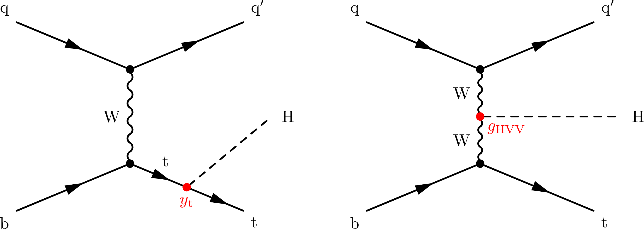
Figure 1:
Leading order Feynman diagrams for the associated production of a single top quark and a Higgs boson in the $t$ channel, where the Higgs boson couples either to the top quark (left) or the W boson (right). |
png pdf |
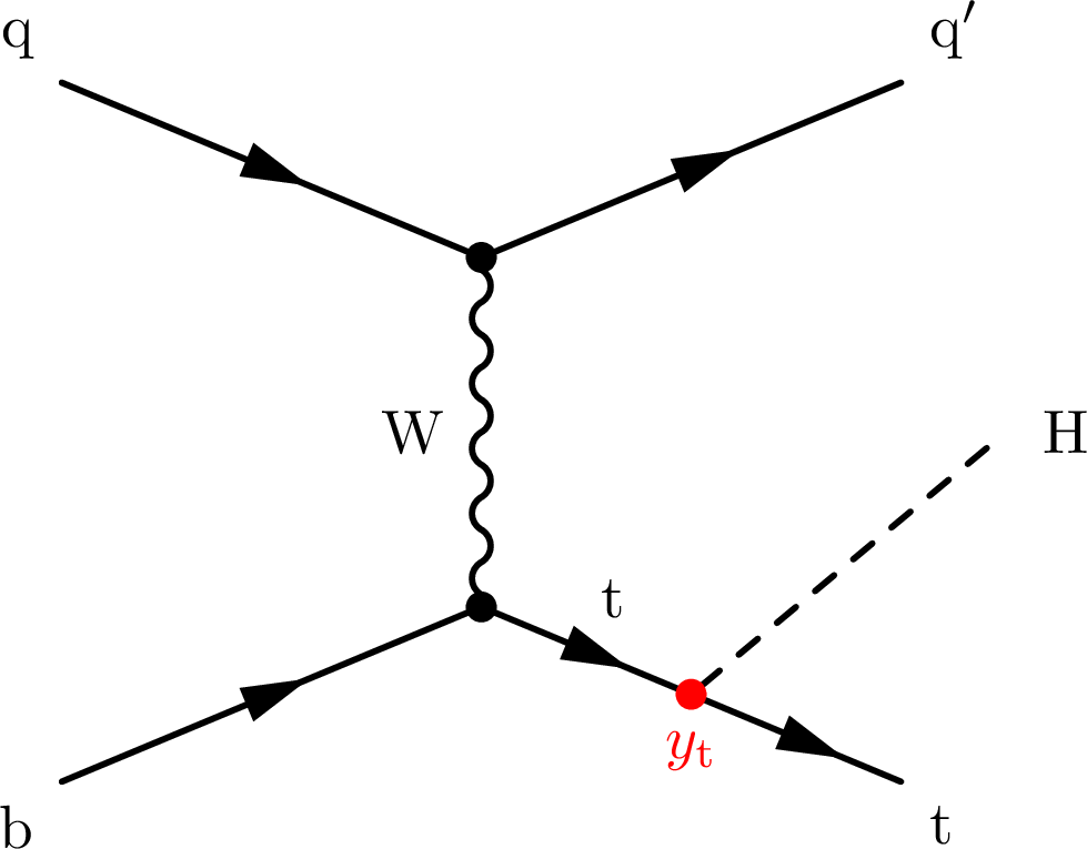
Figure 1-a:
Leading order Feynman diagras for the associated production of a single top quark and a Higgs boson in the $t$ channel, where the Higgs boson couples to the top quark. |

png pdf |
Figure 1-b:
Leading order Feynman diagras for the associated production of a single top quark and a Higgs boson in the $t$ channel, where the Higgs boson couples to the W boson. |
png pdf |
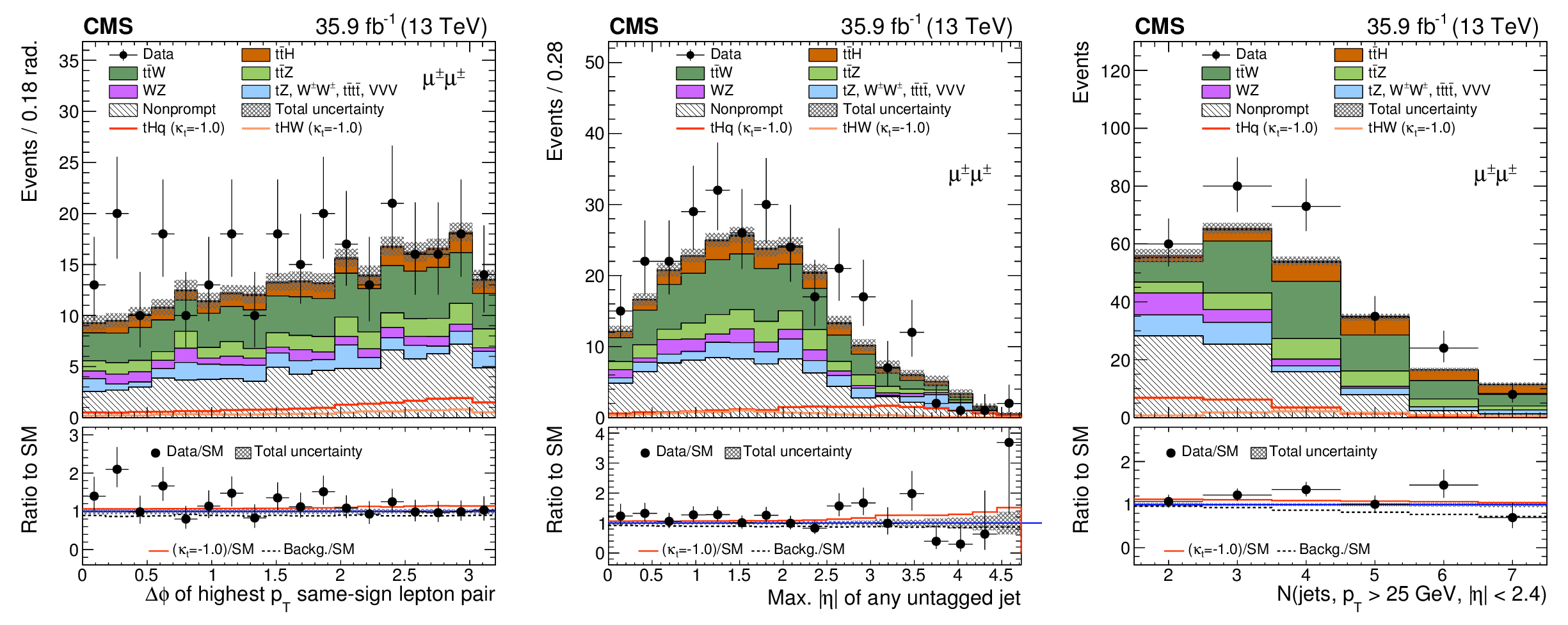
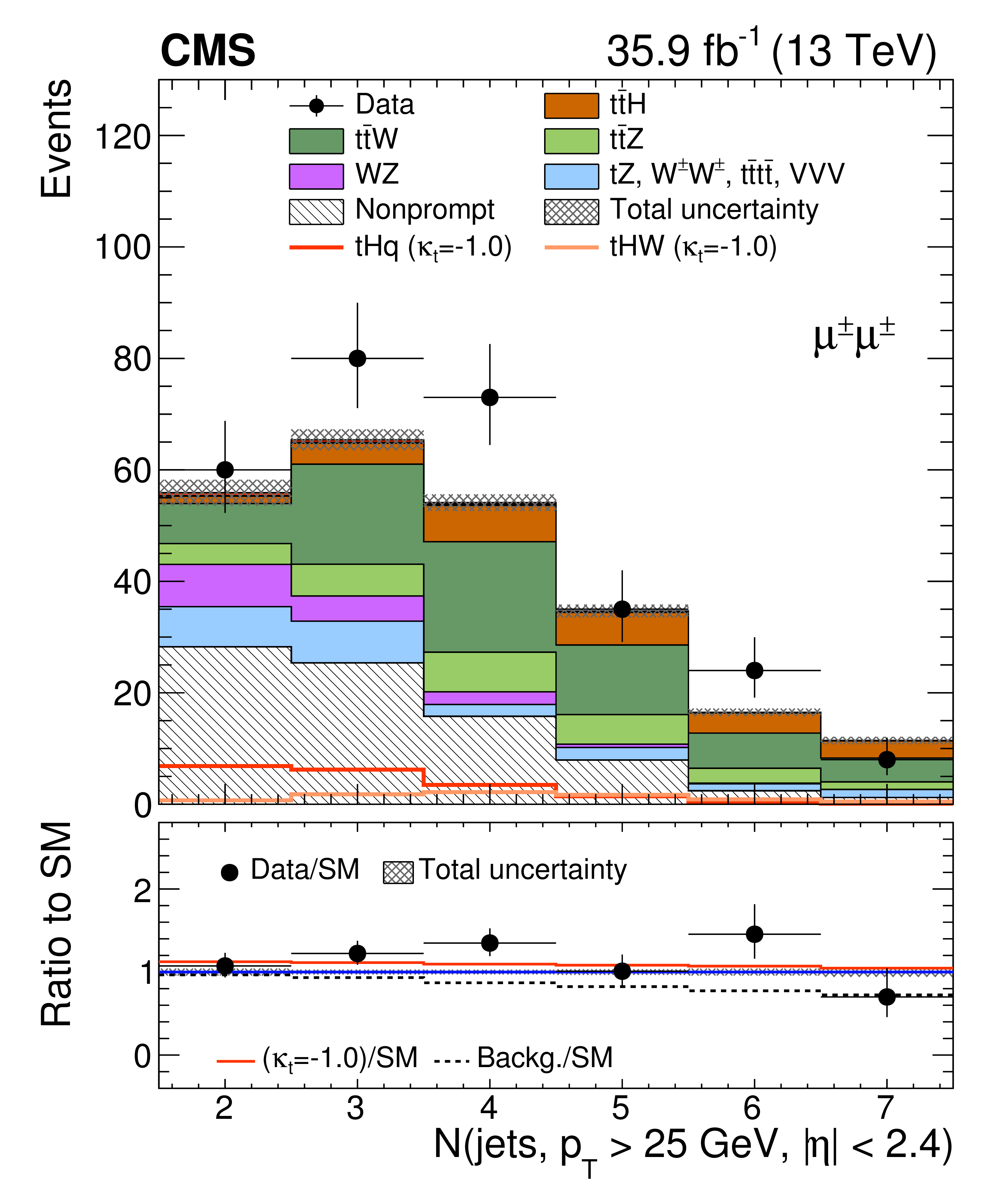
Figure 2:
Distributions of discriminating observables for the same-sign $ {{{\mu}}^\pm {{\mu}}^\pm} $ channel, normalized to 35.9 fb$^{-1}$, before fitting the signal discriminant to the data. The grey band represents the unconstrained (pre-fit) statistical and systematic uncertainties. In the panel below each distribution, the ratio of the observed and predicted event yields is shown. The shape of the two $ {{\mathrm {t}} {\mathrm {H}}} $ signals for $ {\kappa _ {\mathrm {t}}} =-1.0$ is shown, normalized to their respective cross sections for $ {\kappa _ {\mathrm {t}}} =-1.0$, ${\kappa _\text {V}} =1.0$. |

png pdf |
Figure 2-a:
Distribution of a discriminating observable for the same-sign $ {{{\mu}}^\pm {{\mu}}^\pm} $ channel, normalized to 35.9 fb$^{-1}$, before fitting the signal discriminant to the data. The grey band represents the unconstrained (pre-fit) statistical and systematic uncertainties. In the panel below the distribution, the ratio of the observed and predicted event yields is shown. The shape of the two $ {{\mathrm {t}} {\mathrm {H}}} $ signals for $ {\kappa _ {\mathrm {t}}} =-1.0$ is shown, normalized to their respective cross sections for $ {\kappa _ {\mathrm {t}}} =-1.0$, ${\kappa _\text {V}} =1.0$. |

png pdf |
Figure 2-b:
Distribution of a discriminating observable for the same-sign $ {{{\mu}}^\pm {{\mu}}^\pm} $ channel, normalized to 35.9 fb$^{-1}$, before fitting the signal discriminant to the data. The grey band represents the unconstrained (pre-fit) statistical and systematic uncertainties. In the panel below the distribution, the ratio of the observed and predicted event yields is shown. The shape of the two $ {{\mathrm {t}} {\mathrm {H}}} $ signals for $ {\kappa _ {\mathrm {t}}} =-1.0$ is shown, normalized to their respective cross sections for $ {\kappa _ {\mathrm {t}}} =-1.0$, ${\kappa _\text {V}} =1.0$. |
png pdf |
Figure 2-c:
Distribution of a discriminating observable for the same-sign $ {{{\mu}}^\pm {{\mu}}^\pm} $ channel, normalized to 35.9 fb$^{-1}$, before fitting the signal discriminant to the data. The grey band represents the unconstrained (pre-fit) statistical and systematic uncertainties. In the panel below the distribution, the ratio of the observed and predicted event yields is shown. The shape of the two $ {{\mathrm {t}} {\mathrm {H}}} $ signals for $ {\kappa _ {\mathrm {t}}} =-1.0$ is shown, normalized to their respective cross sections for $ {\kappa _ {\mathrm {t}}} =-1.0$, ${\kappa _\text {V}} =1.0$. |
png pdf |
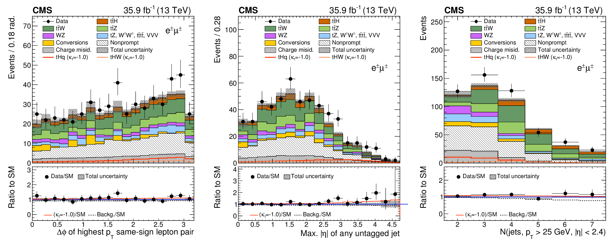
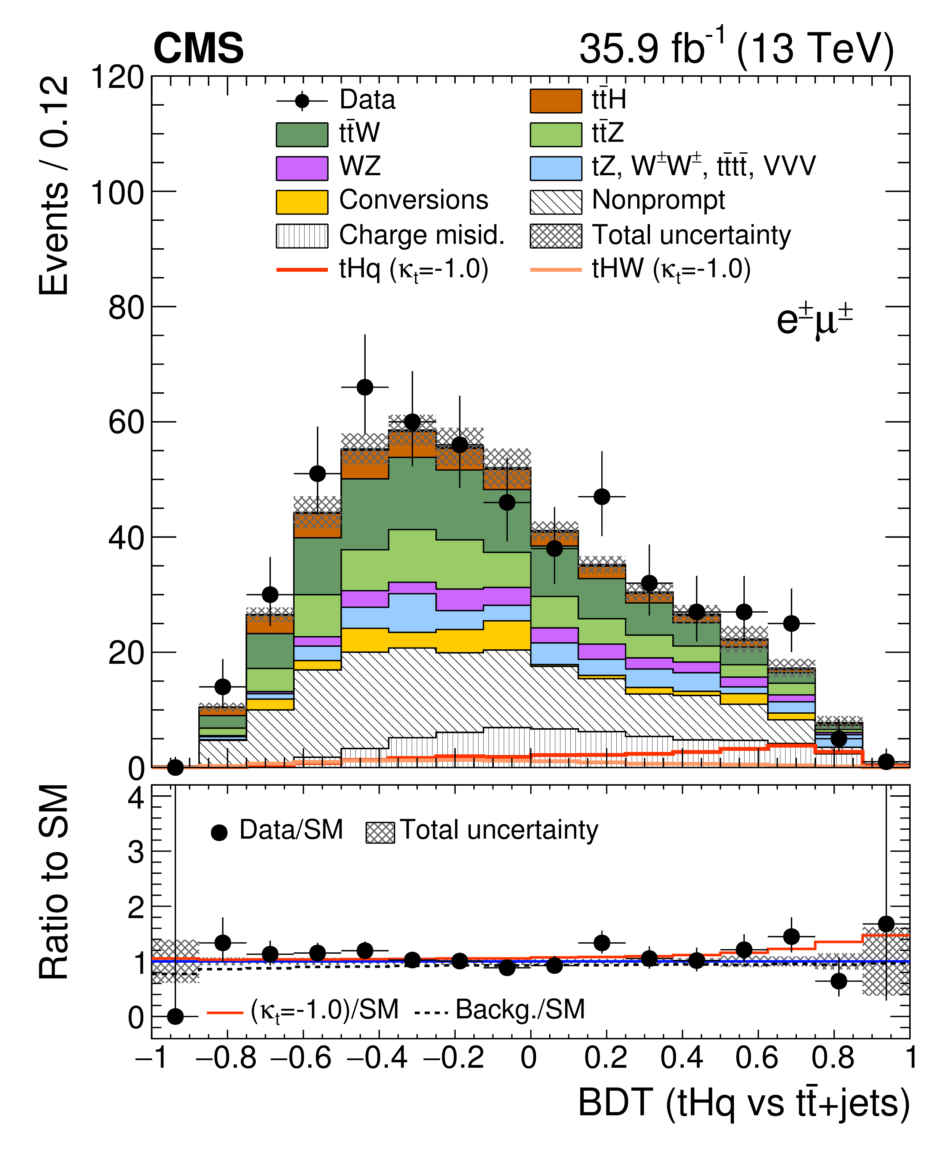
Figure 3:
Distributions of discriminating observables for the same-sign $ {{\mathrm {e}^\pm} {{\mu}}^\pm} $ channel, normalized to 35.9 fb$^{-1}$, before fitting the signal discriminant to the data. The grey band represents the unconstrained (pre-fit) statistical and systematic uncertainties. In the panel below each distribution, the ratio of the observed and predicted event yields is shown. The shape of the two $ {{\mathrm {t}} {\mathrm {H}}} $ signals for $ {\kappa _ {\mathrm {t}}} =-1.0$ is shown, normalized to their respective cross sections for $ {\kappa _ {\mathrm {t}}} =-1.0$, ${\kappa _\text {V}} =1.0$. |

png pdf |
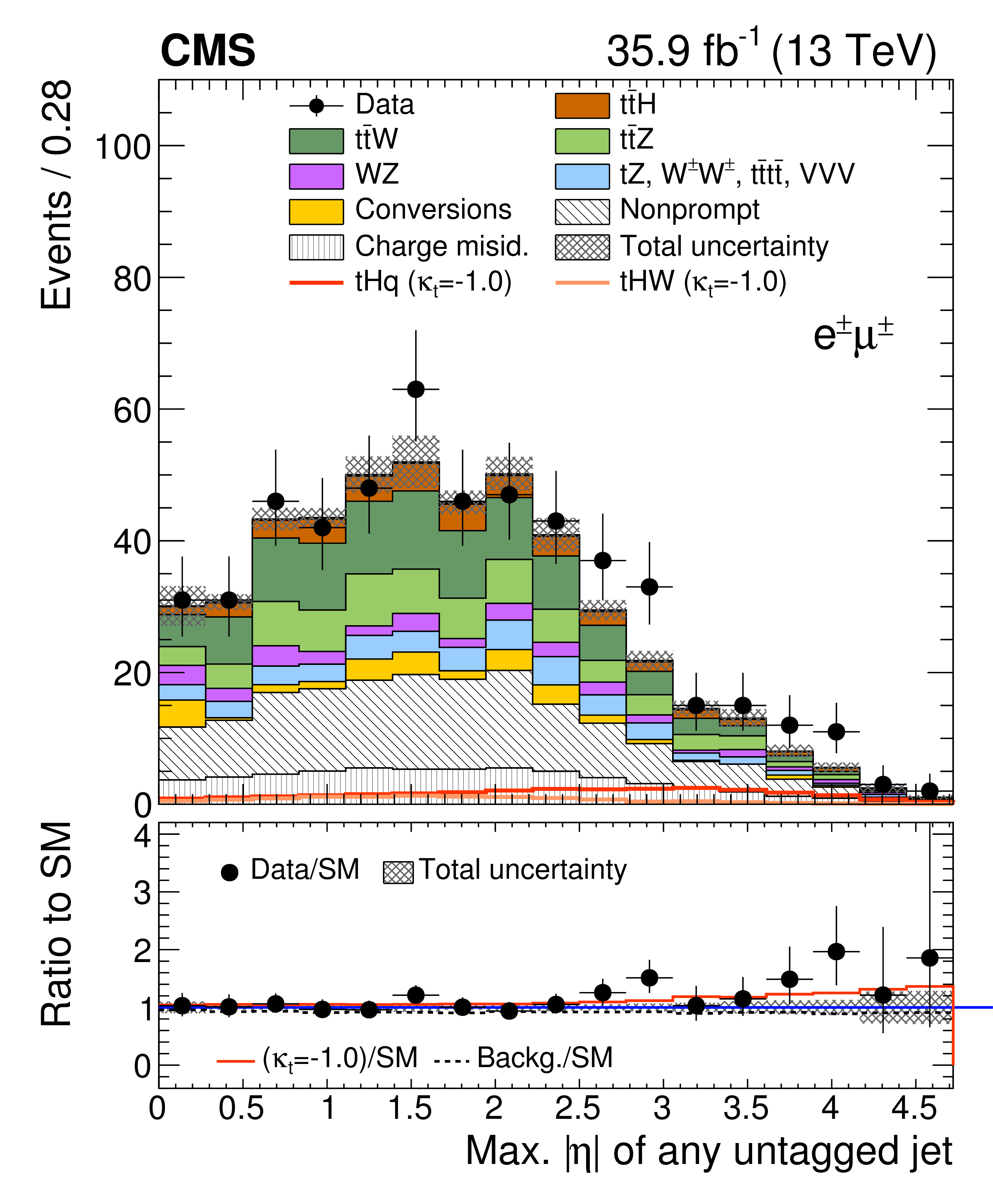
Figure 3-a:
Distribution of a discriminating observable for the same-sign $ {{\mathrm {e}^\pm} {{\mu}}^\pm} $ channel, normalized to 35.9 fb$^{-1}$, before fitting the signal discriminant to the data. The grey band represents the unconstrained (pre-fit) statistical and systematic uncertainties. In the panel below the distribution, the ratio of the observed and predicted event yields is shown. The shape of the two $ {{\mathrm {t}} {\mathrm {H}}} $ signals for $ {\kappa _ {\mathrm {t}}} =-1.0$ is shown, normalized to their respective cross sections for $ {\kappa _ {\mathrm {t}}} =-1.0$, ${\kappa _\text {V}} =1.0$. |
png pdf |
Figure 3-b:
Distribution of a discriminating observable for the same-sign $ {{\mathrm {e}^\pm} {{\mu}}^\pm} $ channel, normalized to 35.9 fb$^{-1}$, before fitting the signal discriminant to the data. The grey band represents the unconstrained (pre-fit) statistical and systematic uncertainties. In the panel below the distribution, the ratio of the observed and predicted event yields is shown. The shape of the two $ {{\mathrm {t}} {\mathrm {H}}} $ signals for $ {\kappa _ {\mathrm {t}}} =-1.0$ is shown, normalized to their respective cross sections for $ {\kappa _ {\mathrm {t}}} =-1.0$, ${\kappa _\text {V}} =1.0$. |
png pdf |
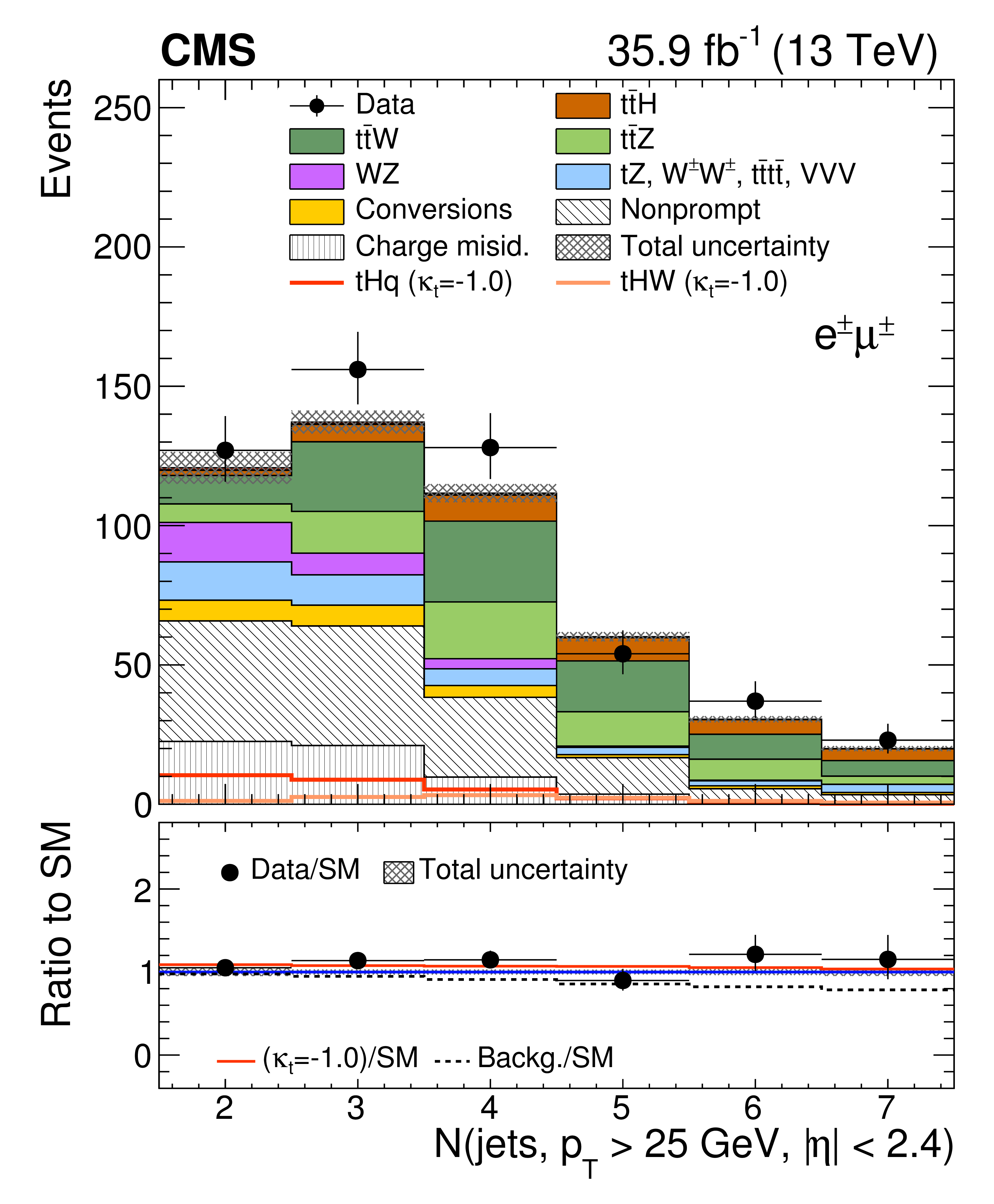
Figure 3-c:
Distribution of a discriminating observable for the same-sign $ {{\mathrm {e}^\pm} {{\mu}}^\pm} $ channel, normalized to 35.9 fb$^{-1}$, before fitting the signal discriminant to the data. The grey band represents the unconstrained (pre-fit) statistical and systematic uncertainties. In the panel below the distribution, the ratio of the observed and predicted event yields is shown. The shape of the two $ {{\mathrm {t}} {\mathrm {H}}} $ signals for $ {\kappa _ {\mathrm {t}}} =-1.0$ is shown, normalized to their respective cross sections for $ {\kappa _ {\mathrm {t}}} =-1.0$, ${\kappa _\text {V}} =1.0$. |

png pdf |
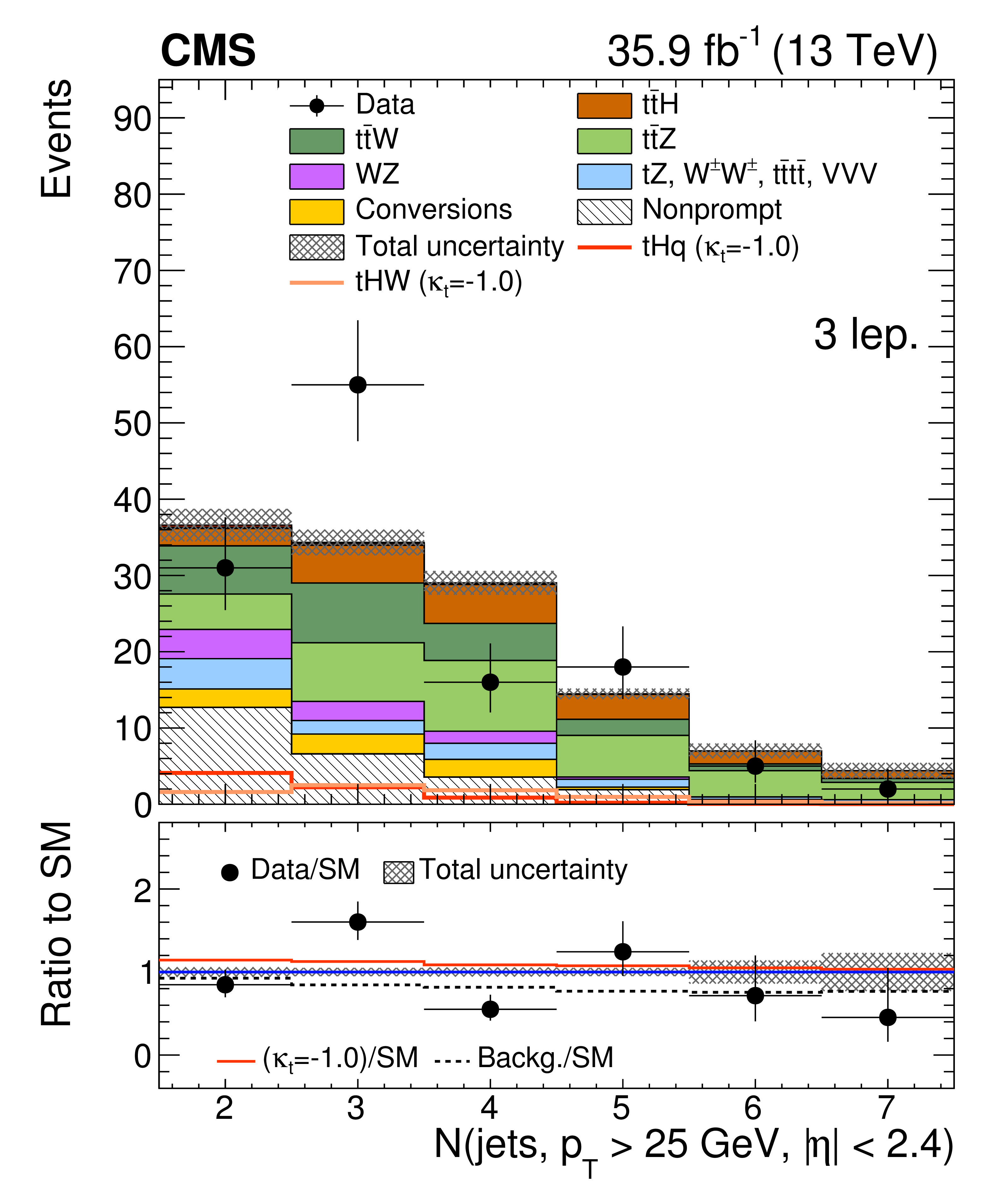
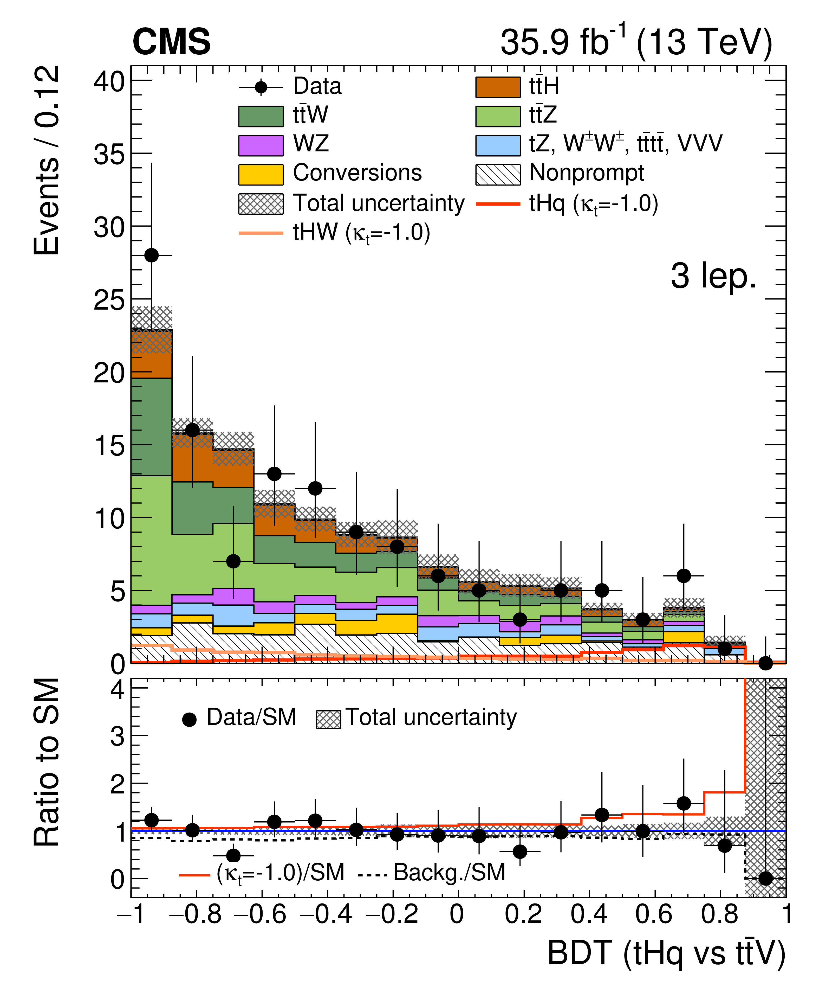
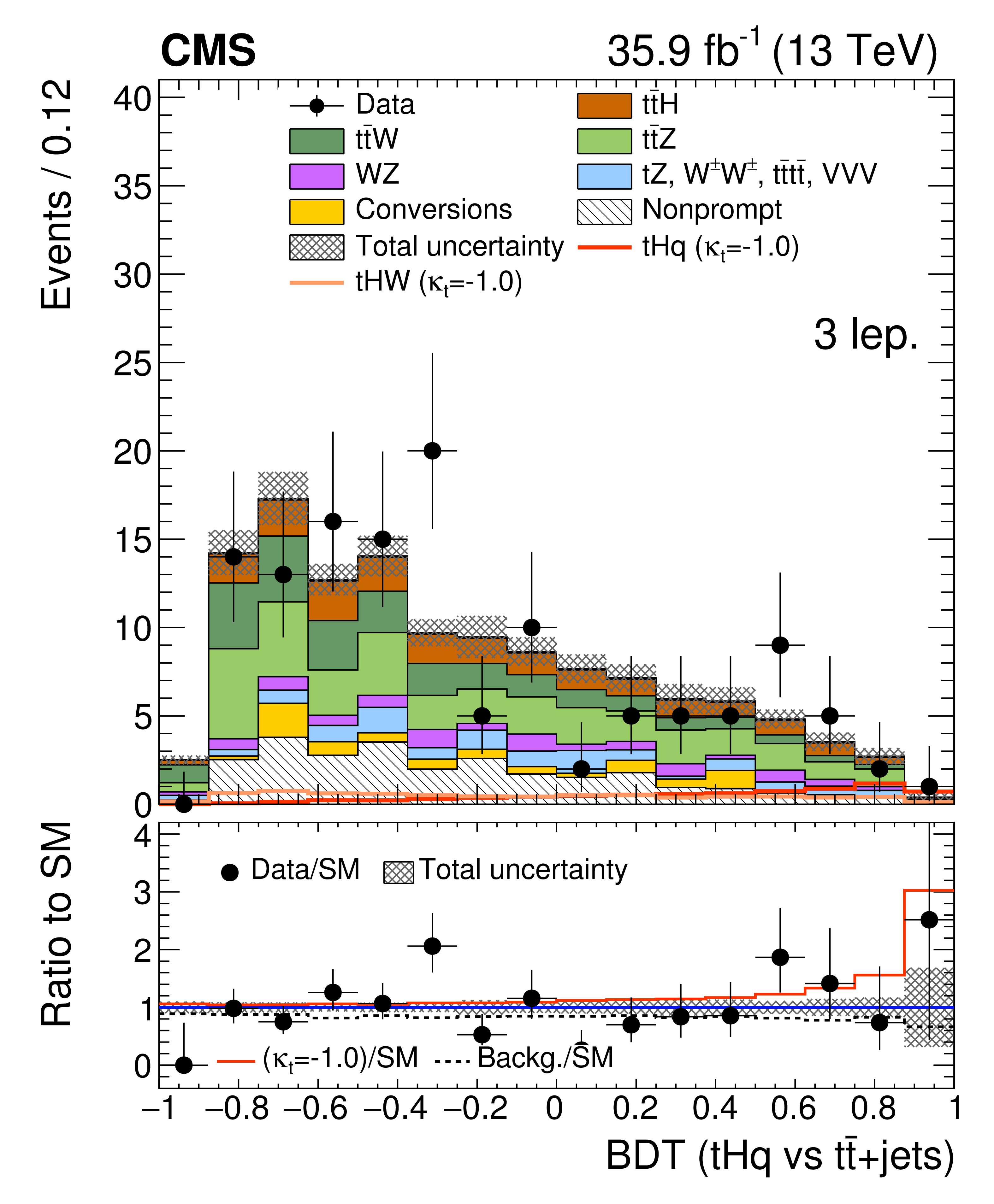
Figure 4:
Distributions of discriminating observables for the three lepton channel, normalized to 35.9 fb$^{-1}$, before fitting the signal discriminant to the data. The grey band represents the unconstrained (pre-fit) statistical and systematic uncertainties. In the panel below each distribution, the ratio of the observed and predicted event yields is shown. The shape of the two $ {{\mathrm {t}} {\mathrm {H}}} $ signals for $ {\kappa _ {\mathrm {t}}} =-1.0$ is shown, normalized to their respective cross sections for $ {\kappa _ {\mathrm {t}}} =-1.0$, ${\kappa _\text {V}} =1.0$. |

png pdf |
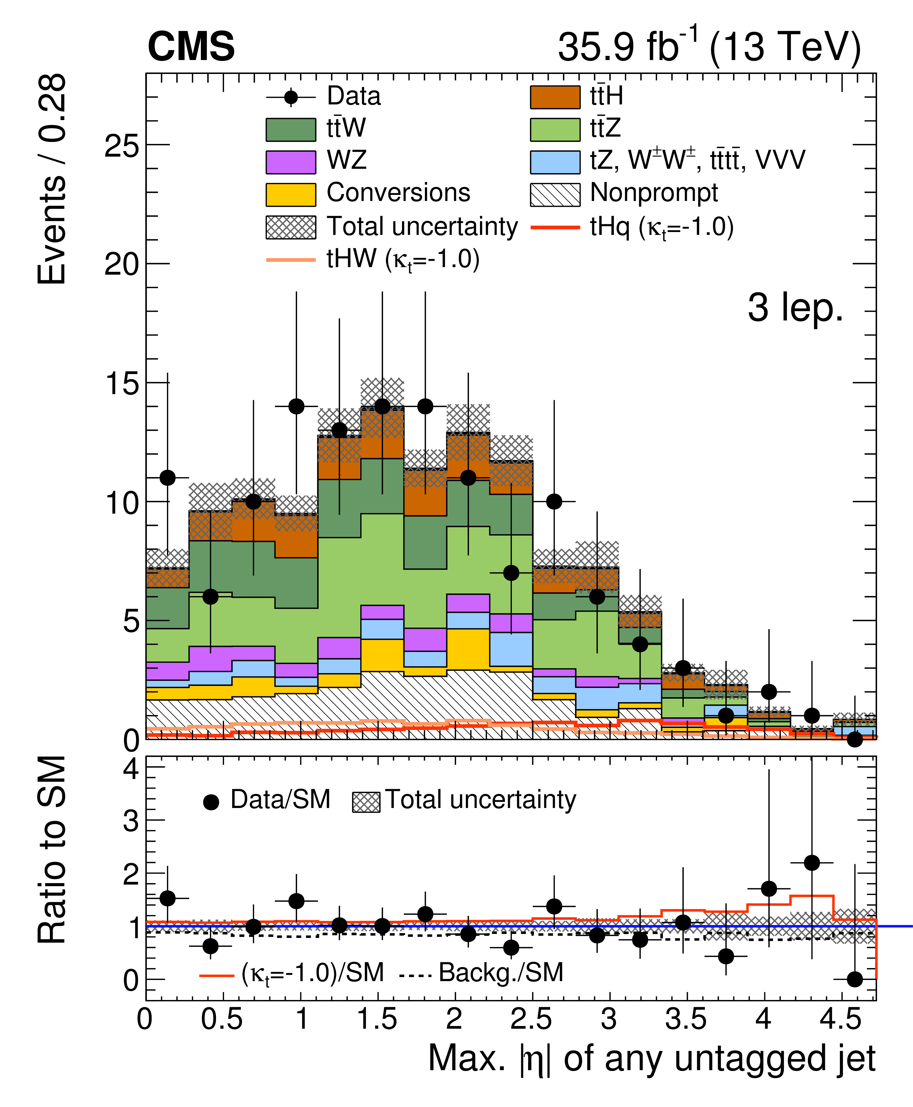
Figure 4-a:
Distribution of a discriminating observablea for the three lepton channel, normalized to 35.9 fb$^{-1}$, before fitting the signal discriminant to the data. The grey band represents the unconstrained (pre-fit) statistical and systematic uncertainties. In the panel below the distribution, the ratio of the observed and predicted event yields is shown. The shape of the two $ {{\mathrm {t}} {\mathrm {H}}} $ signals for $ {\kappa _ {\mathrm {t}}} =-1.0$ is shown, normalized to their respective cross sections for $ {\kappa _ {\mathrm {t}}} =-1.0$, ${\kappa _\text {V}} =1.0$. |
png pdf |
Figure 4-b:
Distribution of a discriminating observablea for the three lepton channel, normalized to 35.9 fb$^{-1}$, before fitting the signal discriminant to the data. The grey band represents the unconstrained (pre-fit) statistical and systematic uncertainties. In the panel below the distribution, the ratio of the observed and predicted event yields is shown. The shape of the two $ {{\mathrm {t}} {\mathrm {H}}} $ signals for $ {\kappa _ {\mathrm {t}}} =-1.0$ is shown, normalized to their respective cross sections for $ {\kappa _ {\mathrm {t}}} =-1.0$, ${\kappa _\text {V}} =1.0$. |
png pdf |
Figure 4-c:
Distribution of a discriminating observablea for the three lepton channel, normalized to 35.9 fb$^{-1}$, before fitting the signal discriminant to the data. The grey band represents the unconstrained (pre-fit) statistical and systematic uncertainties. In the panel below the distribution, the ratio of the observed and predicted event yields is shown. The shape of the two $ {{\mathrm {t}} {\mathrm {H}}} $ signals for $ {\kappa _ {\mathrm {t}}} =-1.0$ is shown, normalized to their respective cross sections for $ {\kappa _ {\mathrm {t}}} =-1.0$, ${\kappa _\text {V}} =1.0$. |
png pdf |
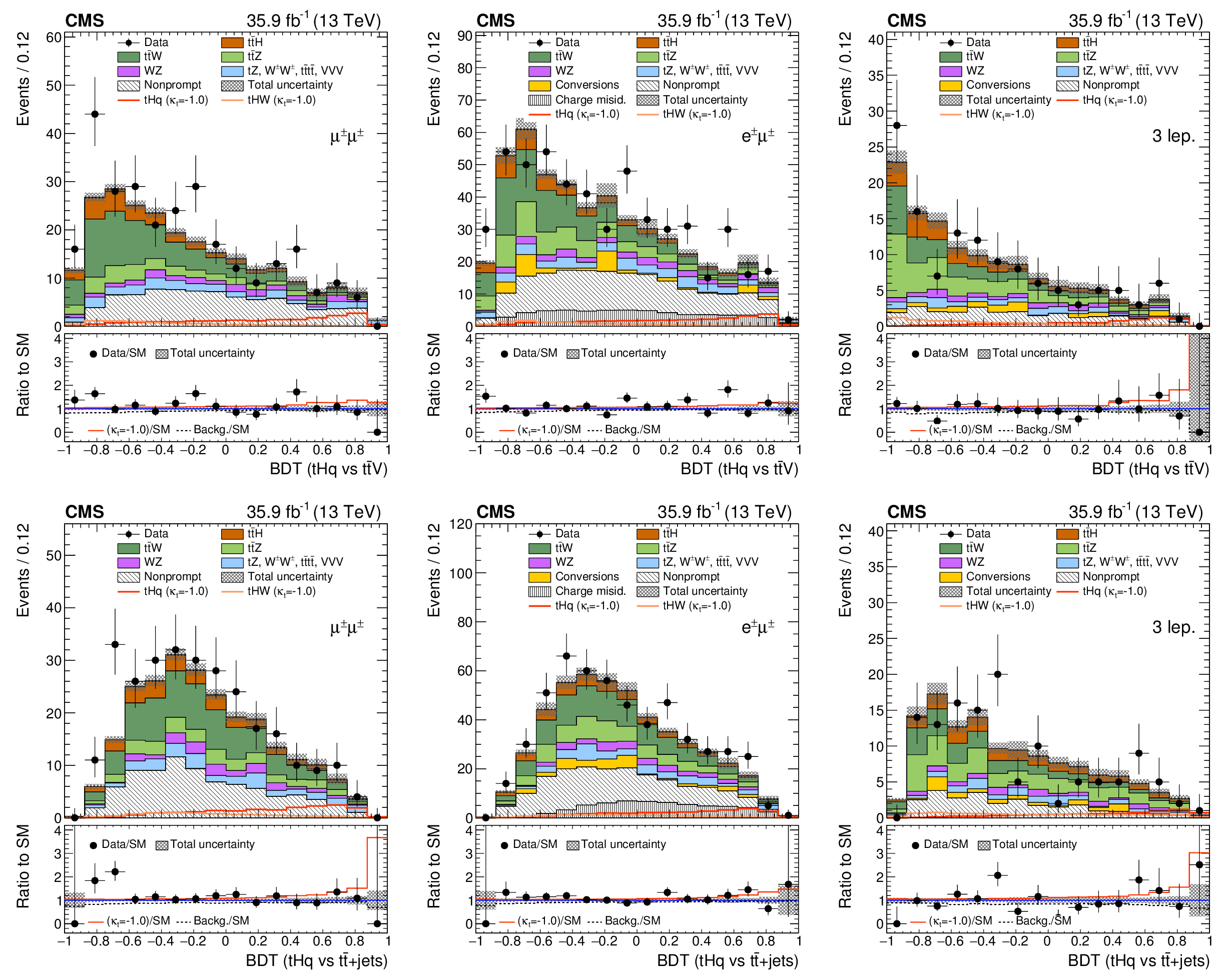
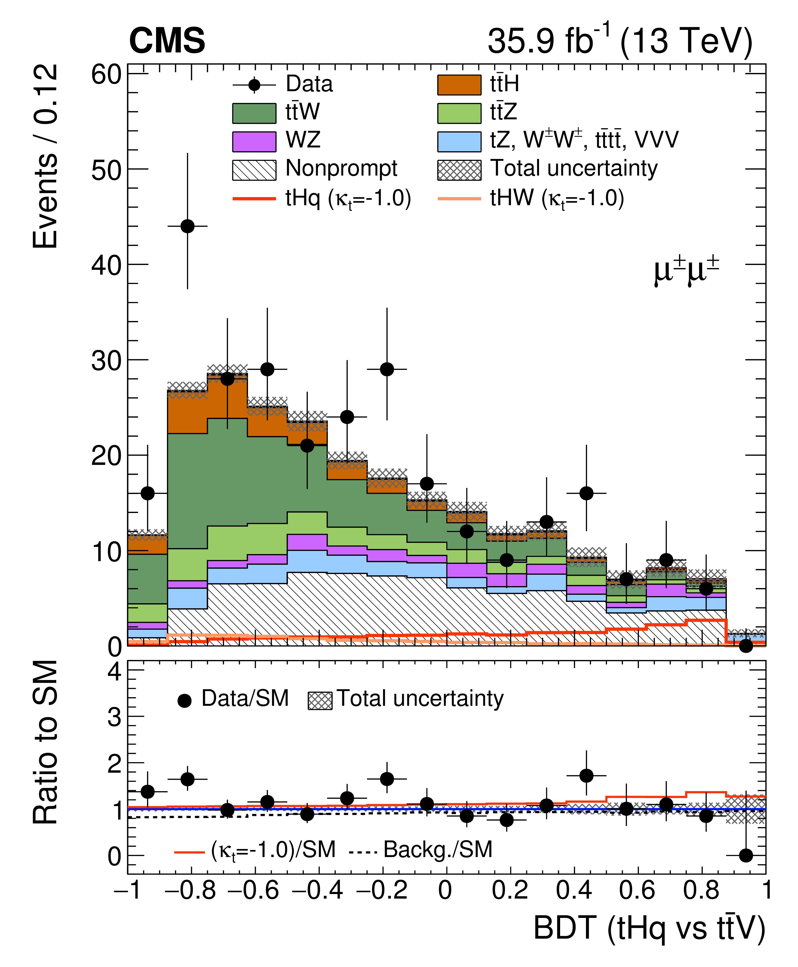
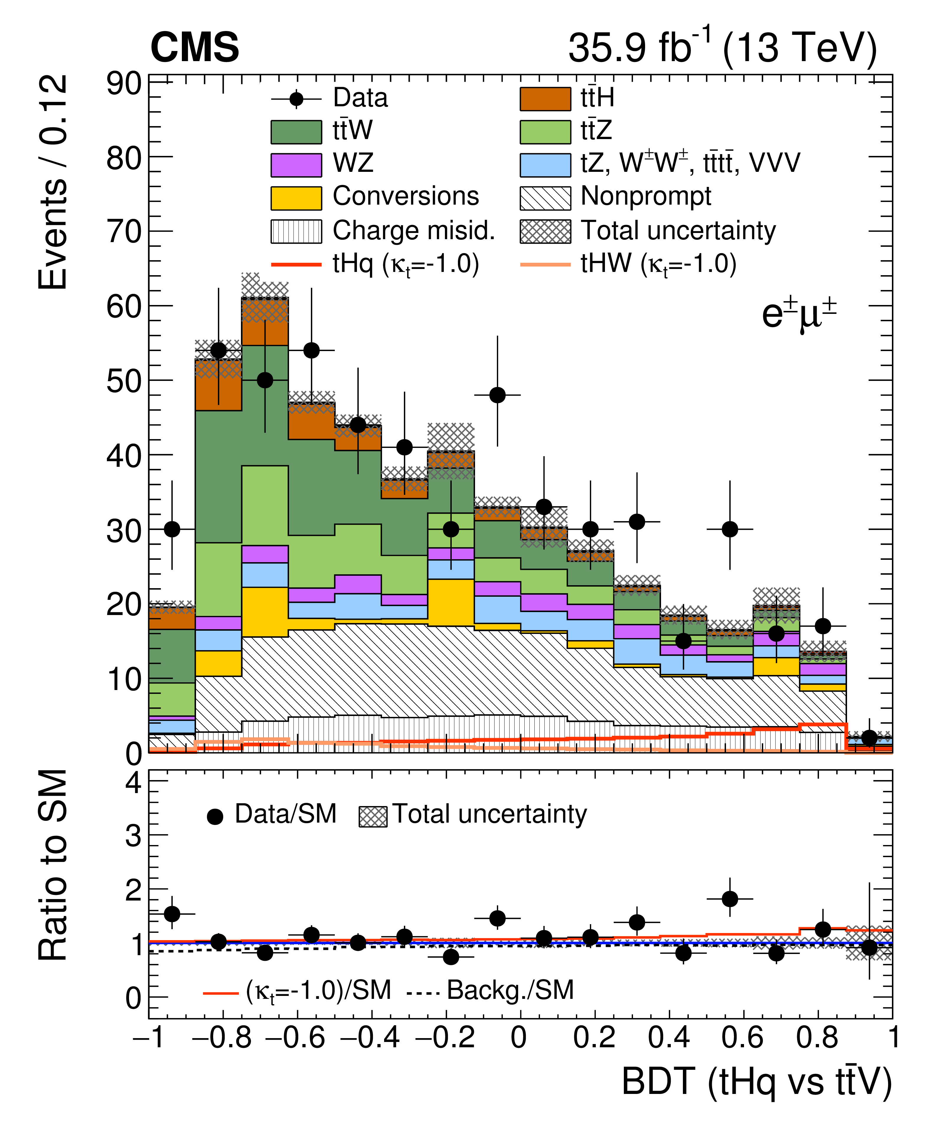
Figure 5:
Pre-fit classifier outputs, for the $ {{{\mu}}^\pm {{\mu}}^\pm} $ channel (left), $ {{\mathrm {e}^\pm} {{\mu}}^\pm} $ channel (center), and three-lepton channel (right), for training against ${{{\mathrm {t}\overline {\mathrm {t}}}} \mathrm {V}} $ (top row) and against ${{{\mathrm {t}\overline {\mathrm {t}}}} {+}\text {jets}} $ (bottom row). In the box below each distribution, the ratio of the observed and predicted event yields is shown. The shape of the two $ {{\mathrm {t}} {\mathrm {H}}} $ signals for $ {\kappa _ {\mathrm {t}}} =-1.0$ is shown, normalized to their respective cross sections for $ {\kappa _ {\mathrm {t}}} =-1.0$, ${\kappa _\text {V}} =1.0$. The grey band represents the unconstrained (pre-fit) statistical and systematic uncertainties. |
png pdf |
Figure 5-a:
Pre-fit classifier output, for the $ {{{\mu}}^\pm {{\mu}}^\pm} $ channel, for training against ${{{\mathrm {t}\overline {\mathrm {t}}}} \mathrm {V}} $. In the box below the distribution, the ratio of the observed and predicted event yields is shown. The shape of the two $ {{\mathrm {t}} {\mathrm {H}}} $ signals for $ {\kappa _ {\mathrm {t}}} =-1.0$ is shown, normalized to their respective cross sections for $ {\kappa _ {\mathrm {t}}} =-1.0$, ${\kappa _\text {V}} =1.0$. The grey band represents the unconstrained (pre-fit) statistical and systematic uncertainties. |
png pdf |
Figure 5-b:
Pre-fit classifier output, for the $ {{\mathrm {e}^\pm} {{\mu}}^\pm} $ channel, for training against ${{{\mathrm {t}\overline {\mathrm {t}}}} \mathrm {V}} $. In the box below the distribution, the ratio of the observed and predicted event yields is shown. The shape of the two $ {{\mathrm {t}} {\mathrm {H}}} $ signals for $ {\kappa _ {\mathrm {t}}} =-1.0$ is shown, normalized to their respective cross sections for $ {\kappa _ {\mathrm {t}}} =-1.0$, ${\kappa _\text {V}} =1.0$. The grey band represents the unconstrained (pre-fit) statistical and systematic uncertainties. |
png pdf |
Figure 5-c:
Pre-fit classifier output, for the three-lepton channel, for training against ${{{\mathrm {t}\overline {\mathrm {t}}}} \mathrm {V}} $. In the box below the distribution, the ratio of the observed and predicted event yields is shown. The shape of the two $ {{\mathrm {t}} {\mathrm {H}}} $ signals for $ {\kappa _ {\mathrm {t}}} =-1.0$ is shown, normalized to their respective cross sections for $ {\kappa _ {\mathrm {t}}} =-1.0$, ${\kappa _\text {V}} =1.0$. The grey band represents the unconstrained (pre-fit) statistical and systematic uncertainties. |

png pdf |
Figure 5-d:
Pre-fit classifier output, for the $ {{{\mu}}^\pm {{\mu}}^\pm} $ channel, for training against ${{{\mathrm {t}\overline {\mathrm {t}}}} {+}\text {jets}} $. In the box below the distribution, the ratio of the observed and predicted event yields is shown. The shape of the two $ {{\mathrm {t}} {\mathrm {H}}} $ signals for $ {\kappa _ {\mathrm {t}}} =-1.0$ is shown, normalized to their respective cross sections for $ {\kappa _ {\mathrm {t}}} =-1.0$, ${\kappa _\text {V}} =1.0$. The grey band represents the unconstrained (pre-fit) statistical and systematic uncertainties. |
png pdf |
Figure 5-e:
Pre-fit classifier output, for the $ {{\mathrm {e}^\pm} {{\mu}}^\pm} $ channel, for training against ${{{\mathrm {t}\overline {\mathrm {t}}}} {+}\text {jets}} $. In the box below the distribution, the ratio of the observed and predicted event yields is shown. The shape of the two $ {{\mathrm {t}} {\mathrm {H}}} $ signals for $ {\kappa _ {\mathrm {t}}} =-1.0$ is shown, normalized to their respective cross sections for $ {\kappa _ {\mathrm {t}}} =-1.0$, ${\kappa _\text {V}} =1.0$. The grey band represents the unconstrained (pre-fit) statistical and systematic uncertainties. |
png pdf |
Figure 5-f:
Pre-fit classifier output, for the three-lepton channel, for training against ${{{\mathrm {t}\overline {\mathrm {t}}}} {+}\text {jets}} $. In the box below the distribution, the ratio of the observed and predicted event yields is shown. The shape of the two $ {{\mathrm {t}} {\mathrm {H}}} $ signals for $ {\kappa _ {\mathrm {t}}} =-1.0$ is shown, normalized to their respective cross sections for $ {\kappa _ {\mathrm {t}}} =-1.0$, ${\kappa _\text {V}} =1.0$. The grey band represents the unconstrained (pre-fit) statistical and systematic uncertainties. |
png pdf |
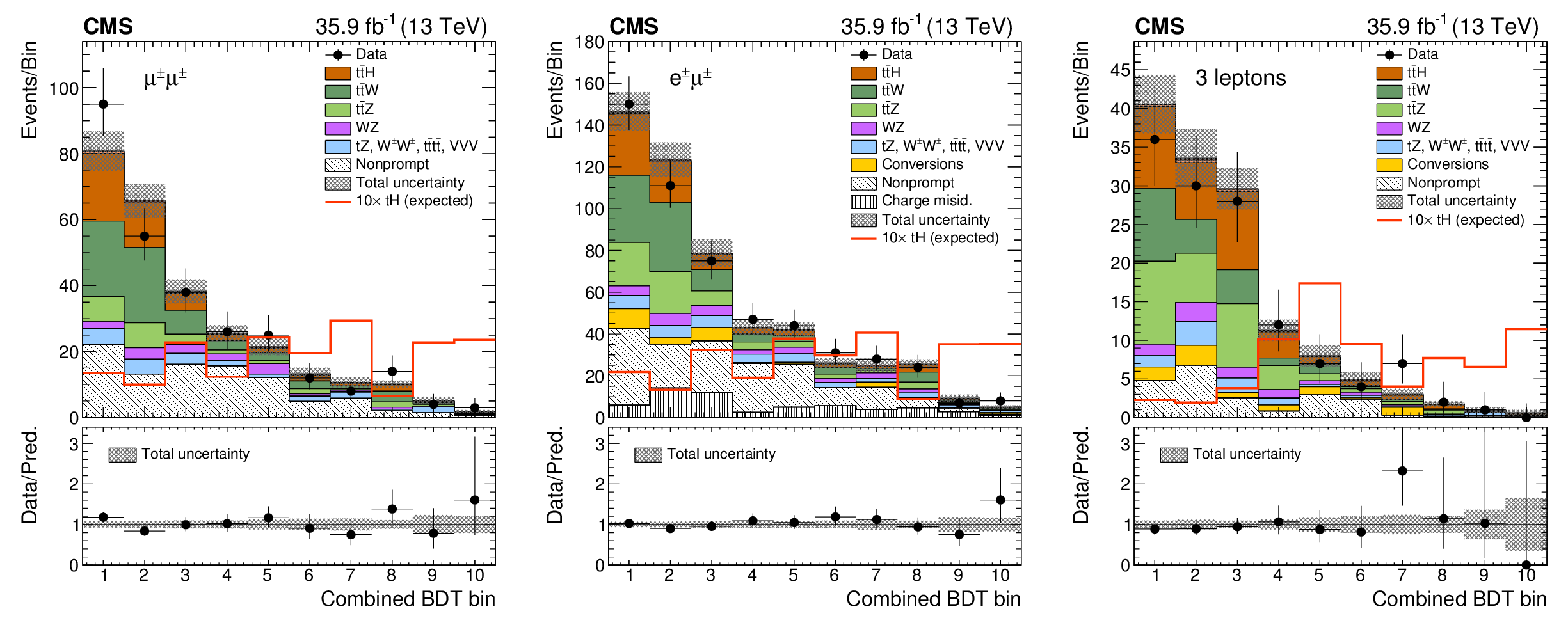
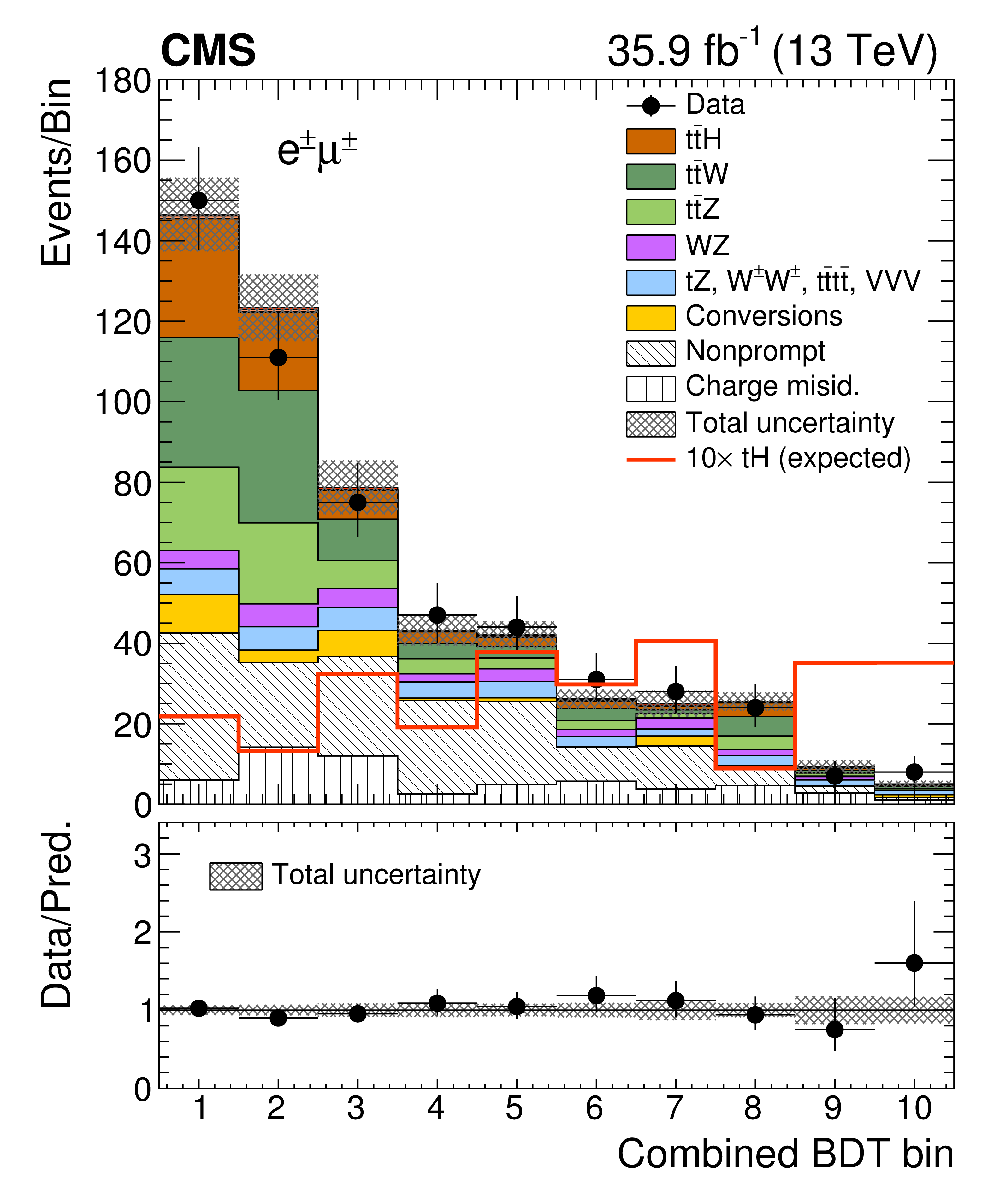
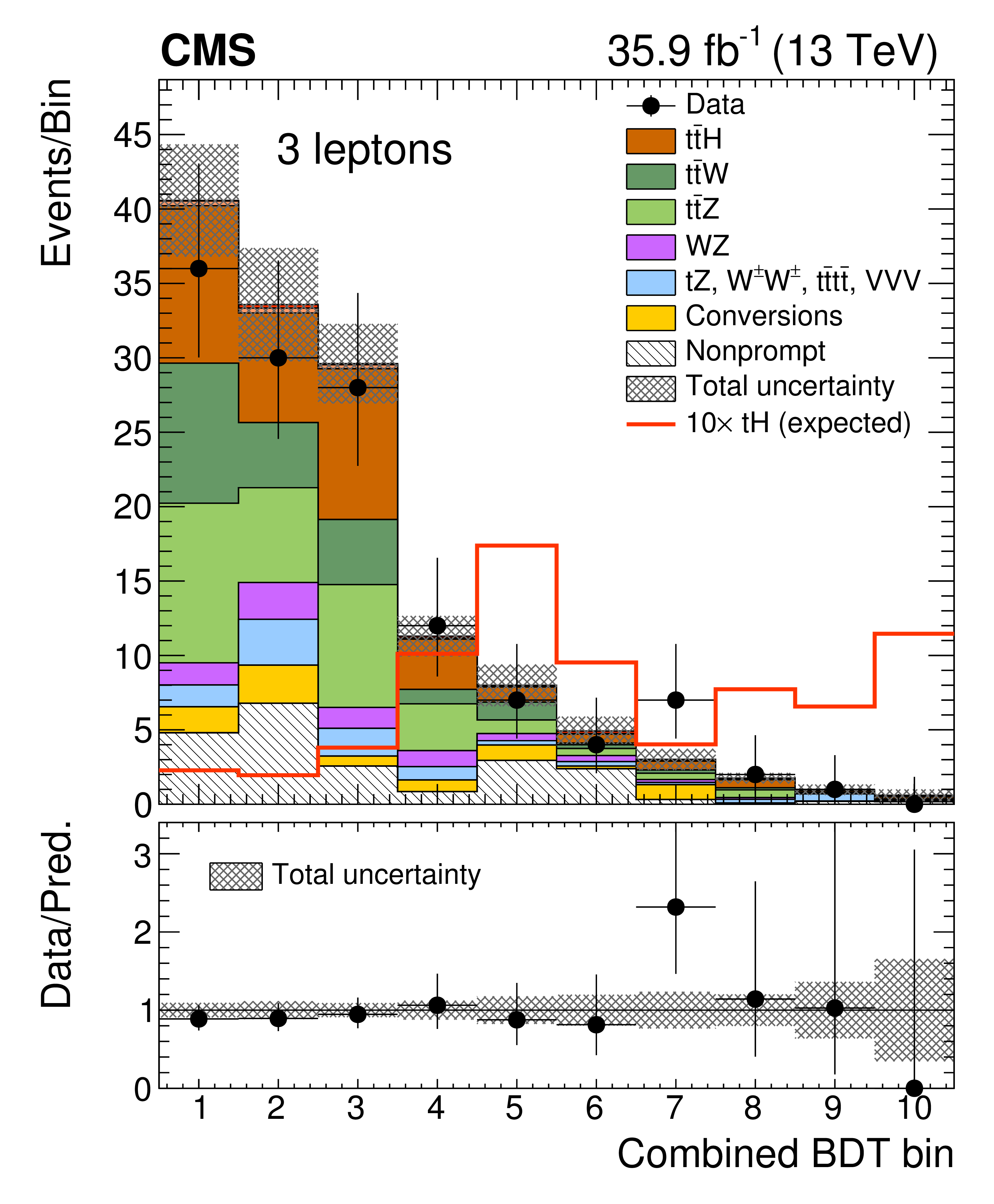
Figure 6:
Post-fit categorized classifier outputs as used in the maximum likelihood fit for the $ {{{\mu}}^\pm {{\mu}}^\pm} $ channel (left), $ {{\mathrm {e}^\pm} {{\mu}}^\pm} $ channel (center), and three-lepton channel (right), for 35.9 fb$^{-1}$. In the box below each distribution, the ratio of the observed and predicted event yields is shown. The shape of the $ {{\mathrm {t}} {\mathrm {H}}} $ signal is indicated with 10 times the SM. |

png pdf |
Figure 6-a:
Post-fit categorized classifier output as used in the maximum likelihood fit for the $ {{{\mu}}^\pm {{\mu}}^\pm} $ channel, for 35.9 fb$^{-1}$. In the box below the distribution, the ratio of the observed and predicted event yields is shown. The shape of the $ {{\mathrm {t}} {\mathrm {H}}} $ signal is indicated with 10 times the SM. |
png pdf |
Figure 6-b:
Post-fit categorized classifier output as used in the maximum likelihood fit for the $ {{\mathrm {e}^\pm} {{\mu}}^\pm} $ channel, for 35.9 fb$^{-1}$. In the box below the distribution, the ratio of the observed and predicted event yields is shown. The shape of the $ {{\mathrm {t}} {\mathrm {H}}} $ signal is indicated with 10 times the SM. |
png pdf |
Figure 6-c:
Post-fit categorized classifier output as used in the maximum likelihood fit for the three-lepton channel, for 35.9 fb$^{-1}$. In the box below the distribution, the ratio of the observed and predicted event yields is shown. The shape of the $ {{\mathrm {t}} {\mathrm {H}}} $ signal is indicated with 10 times the SM. |
png pdf |
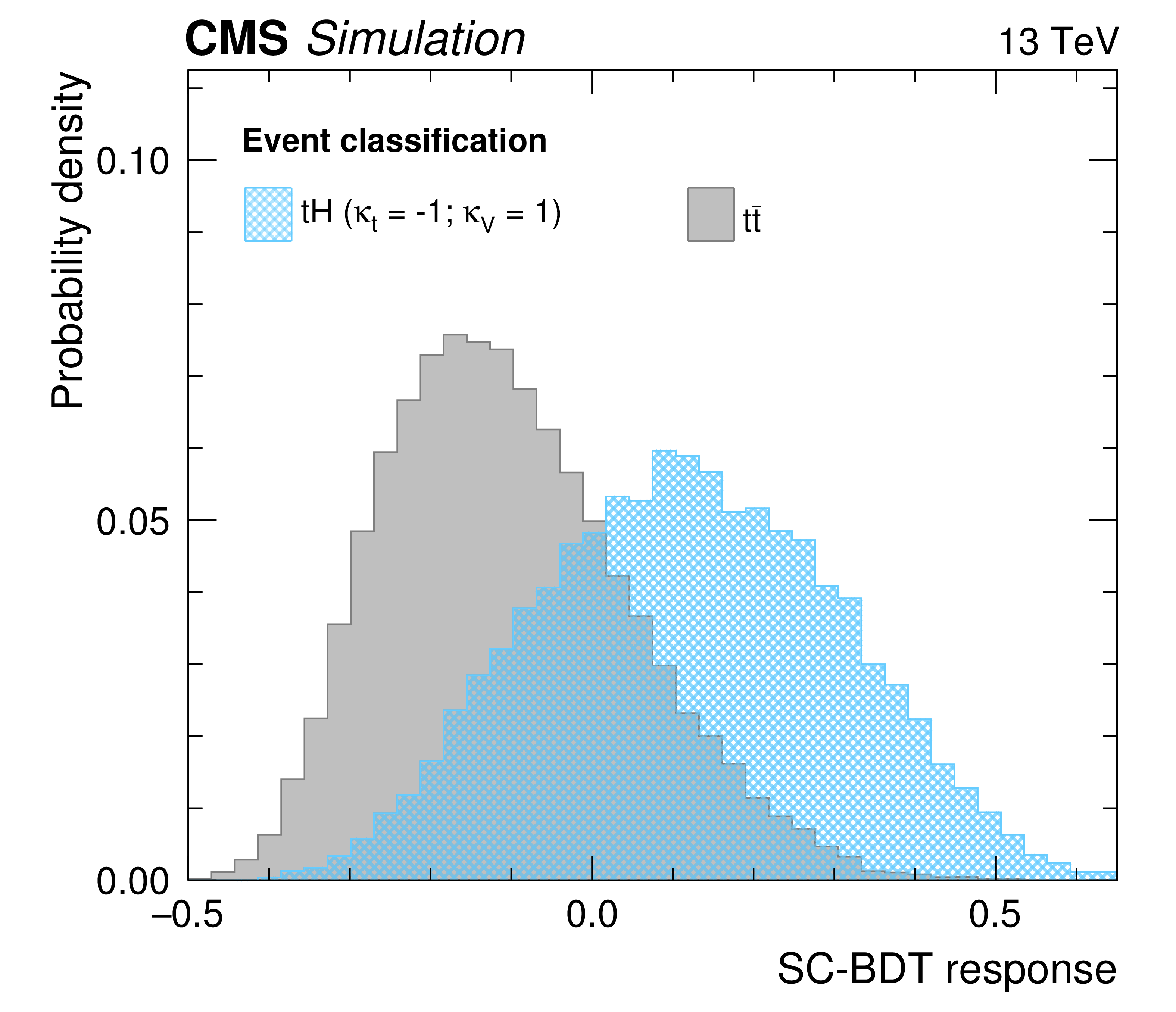
Figure 7:
Output values of the SC-BDT. |
png pdf |
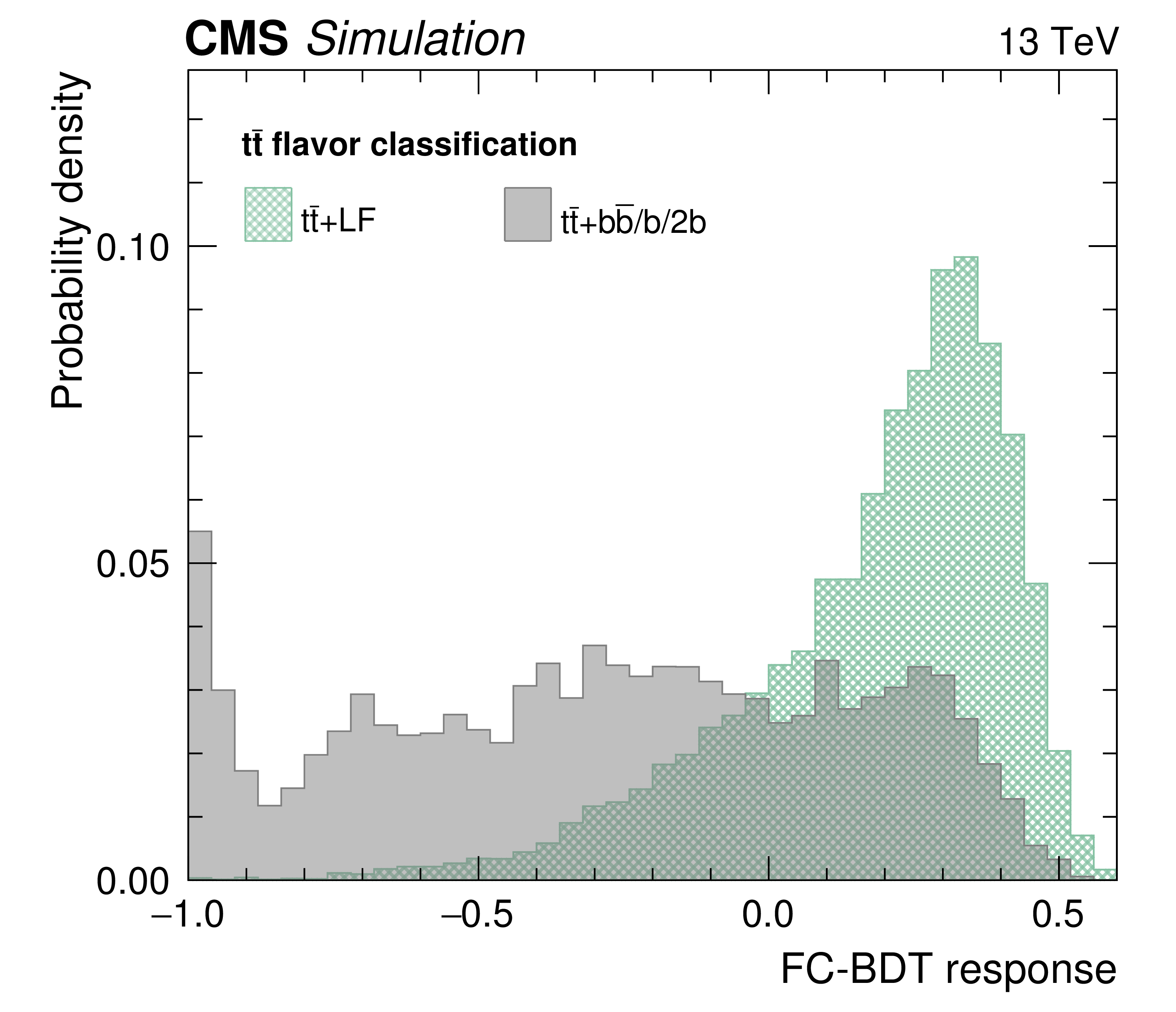
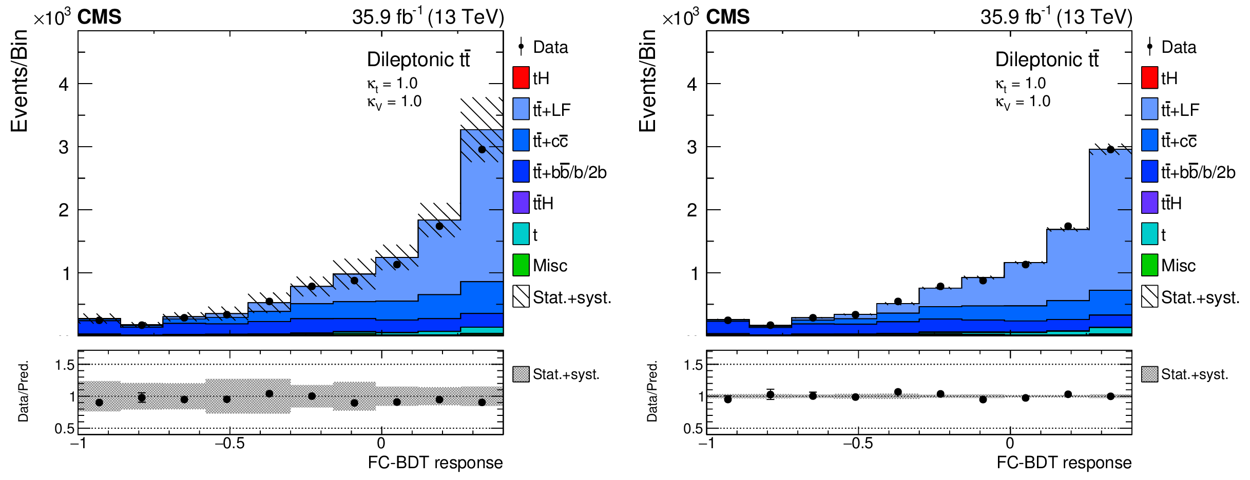
Figure 8:
Response values of the FC-BDT. The background consists of ${{{\mathrm {t}\overline {\mathrm {t}}}} {+} {{\mathrm {b}} {\overline {\mathrm {b}}}}}$, $ {{\mathrm {t}\overline {\mathrm {t}}}} +\mathrm {1\bar{b}}$, and $ {{\mathrm {t}\overline {\mathrm {t}}}} +\mathrm {2\bar{b}}$ events. |
png pdf |
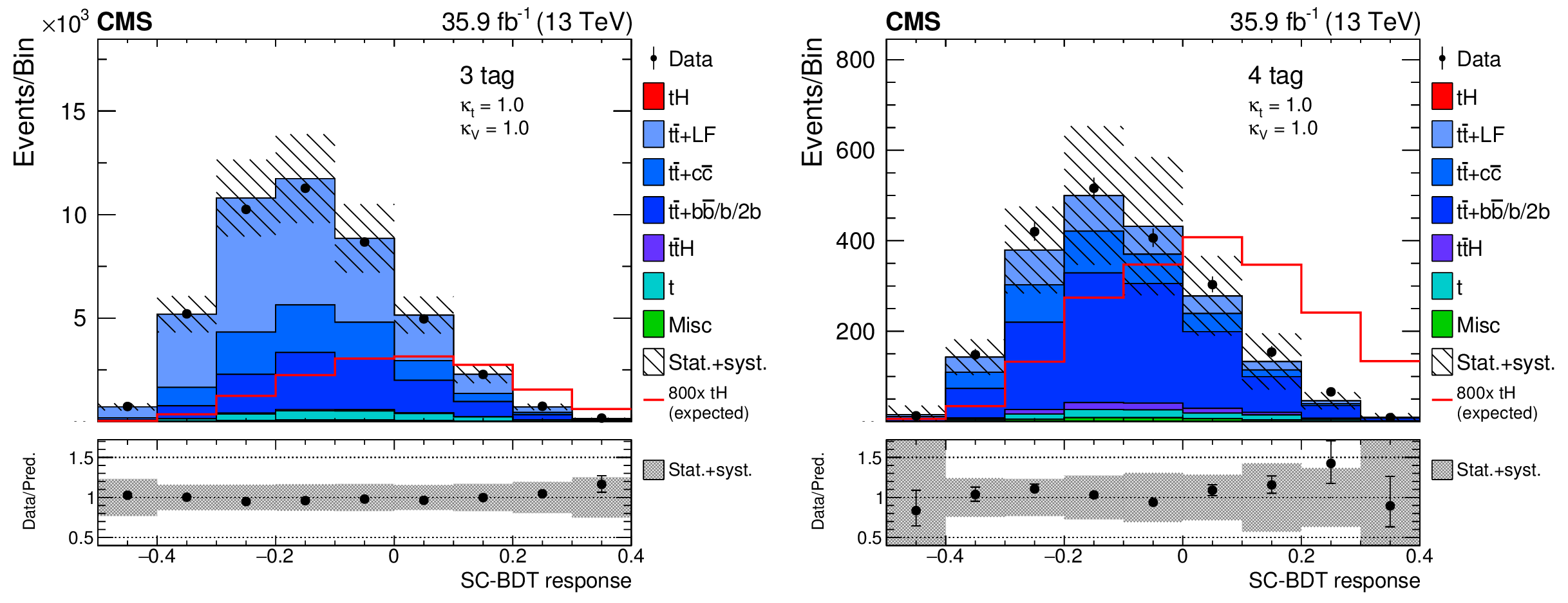
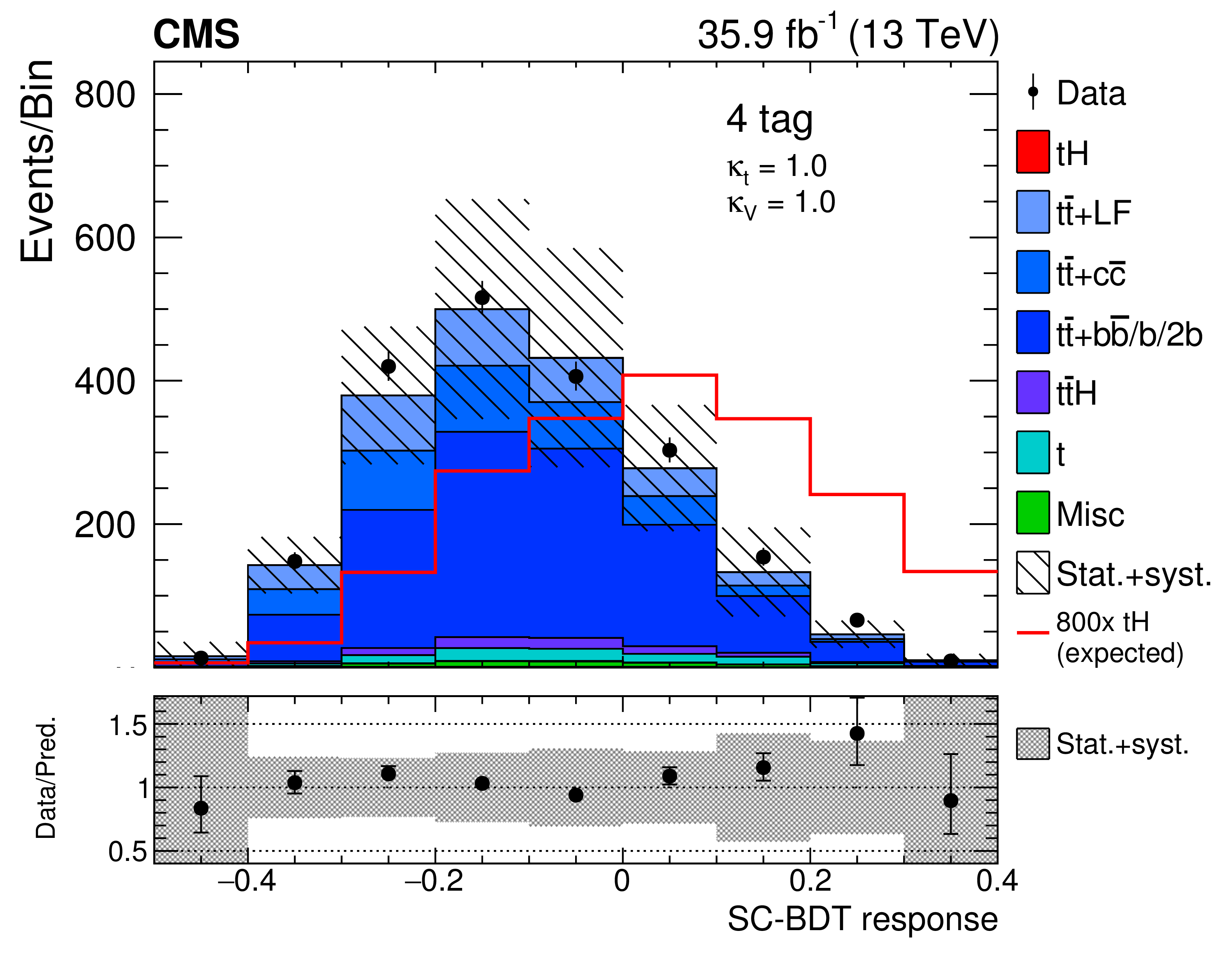
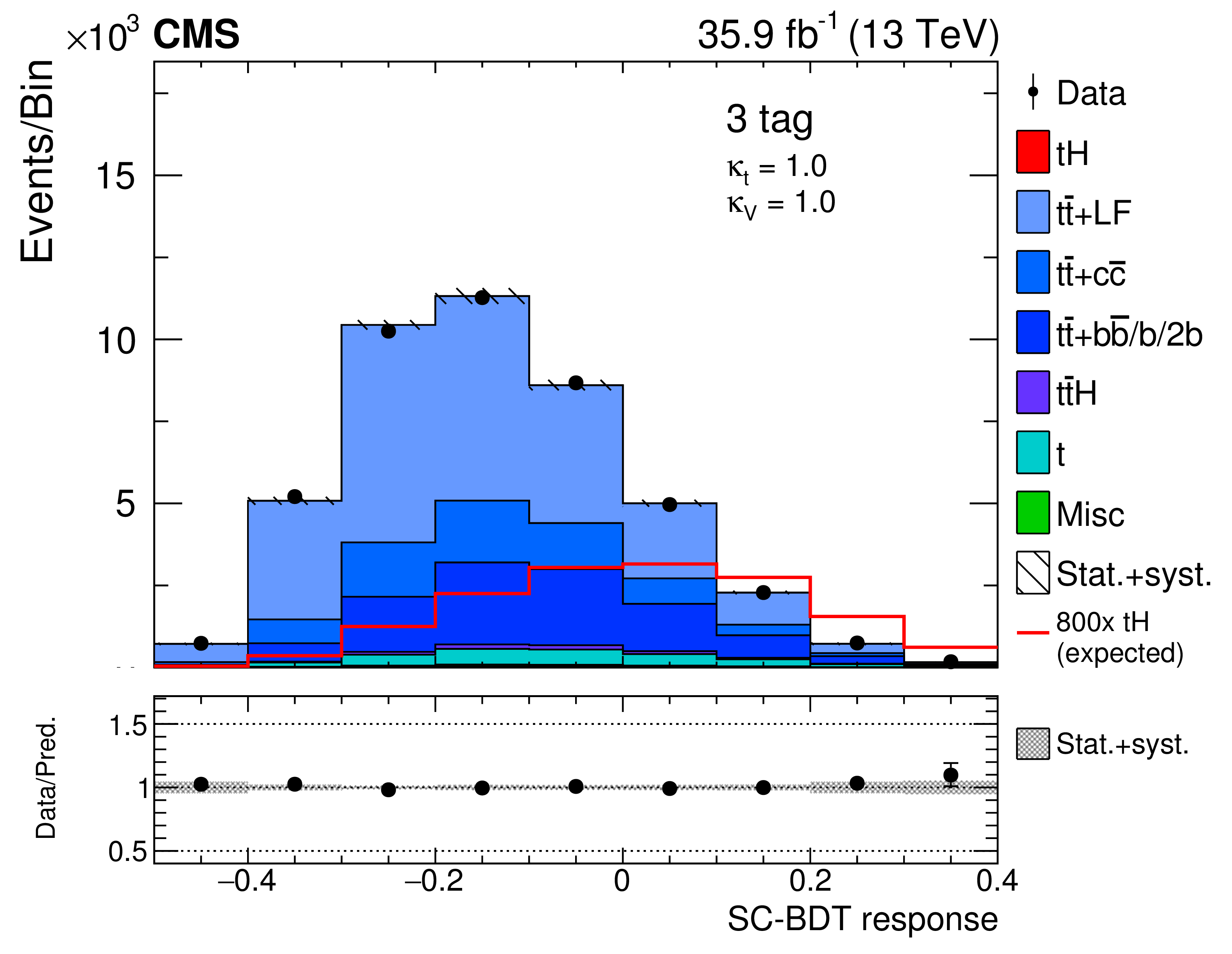
Figure 9:
Pre-fit classifier outputs of the signal classification BDT for the 3 tag channel (left) and the 4 tag channel (right), for 35.9 fb$^{-1}$. In the box below each distribution, the ratio of the observed and predicted event yields is shown. The shape of the $ {{\mathrm {t}} {\mathrm {H}}} $ signal is indicated with 800 times the SM. |

png pdf |
Figure 9-a:
Pre-fit classifier output of the signal classification BDT for the 3 tag channel, for 35.9 fb$^{-1}$. In the box below the distribution, the ratio of the observed and predicted event yields is shown. The shape of the $ {{\mathrm {t}} {\mathrm {H}}} $ signal is indicated with 800 times the SM. |
png pdf |
Figure 9-b:
Pre-fit classifier output of the signal classification BDT for the 4 tag channel, for 35.9 fb$^{-1}$. In the box below the distribution, the ratio of the observed and predicted event yields is shown. The shape of the $ {{\mathrm {t}} {\mathrm {H}}} $ signal is indicated with 800 times the SM. |
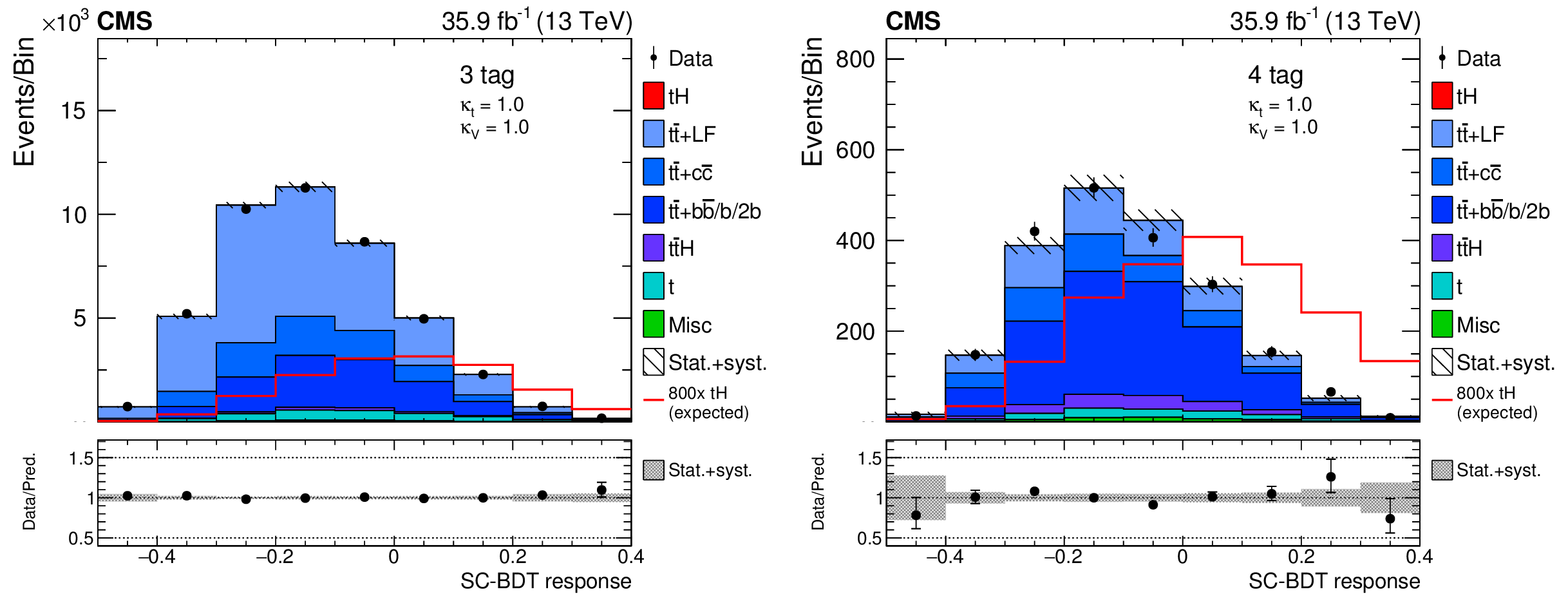
png pdf |
Figure 10:
Post-fit classifier outputs of the signal classification BDT as used in the maximum likelihood fit for the 3 tag channel (left) and the 4 tag channel (right). In the box below each distribution, the ratio of the observed and predicted event yields is shown. The shape of the $ {{\mathrm {t}} {\mathrm {H}}} $ signal is indicated with 800 times the SM. |
png pdf |
Figure 10-a:
Post-fit classifier output of the signal classification BDT as used in the maximum likelihood fit for the 3 tag channel. In the box below the distribution, the ratio of the observed and predicted event yields is shown. The shape of the $ {{\mathrm {t}} {\mathrm {H}}} $ signal is indicated with 800 times the SM. |

png pdf |
Figure 10-b:
Post-fit classifier output of the signal classification BDT as used in the maximum likelihood fit for the 4 tag channel. In the box below the distribution, the ratio of the observed and predicted event yields is shown. The shape of the $ {{\mathrm {t}} {\mathrm {H}}} $ signal is indicated with 800 times the SM. |
png pdf |
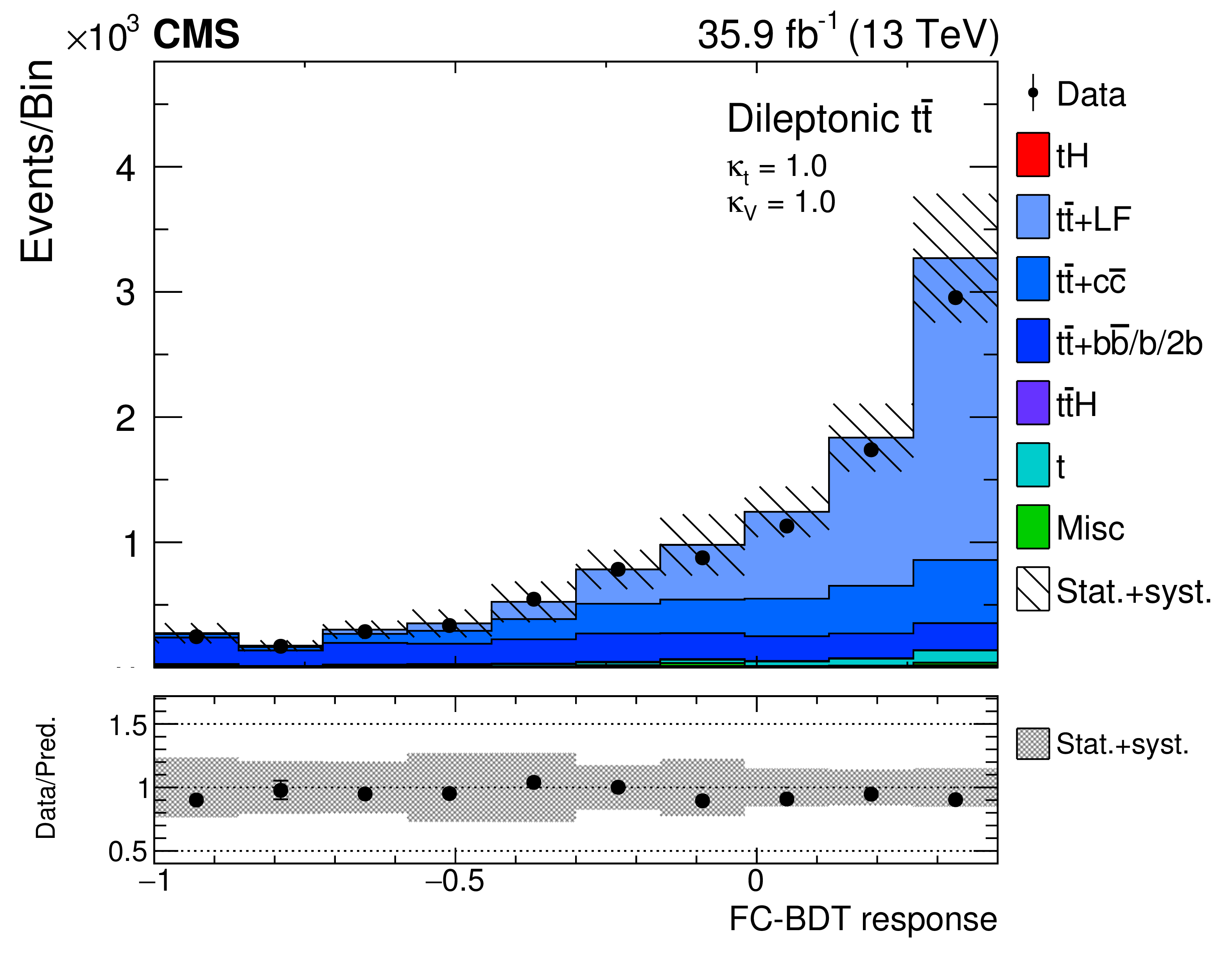
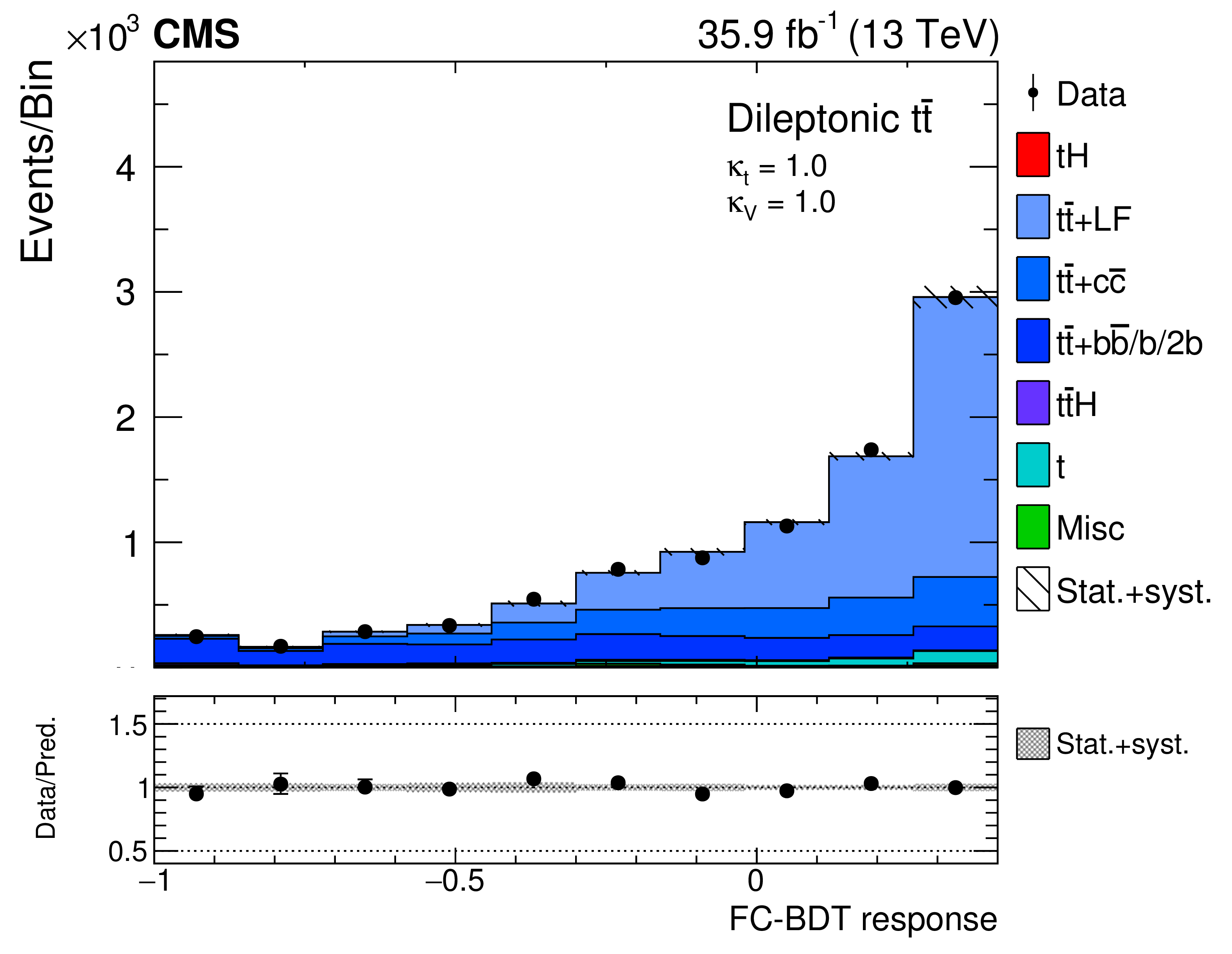
Figure 11:
Pre- (left) and post-fit (right) classifier outputs of the flavor classification BDT for the dilepton selection. In the box below each distribution, the ratio of the observed and predicted event yields is shown. |
png pdf |
Figure 11-a:
Pre-fit classifier output of the flavor classification BDT for the dilepton selection. In the box below the distribution, the ratio of the observed and predicted event yields is shown. |
png pdf |
Figure 11-b:
Post-fit classifier output of the flavor classification BDT for the dilepton selection. In the box below the distribution, the ratio of the observed and predicted event yields is shown. |
png pdf |
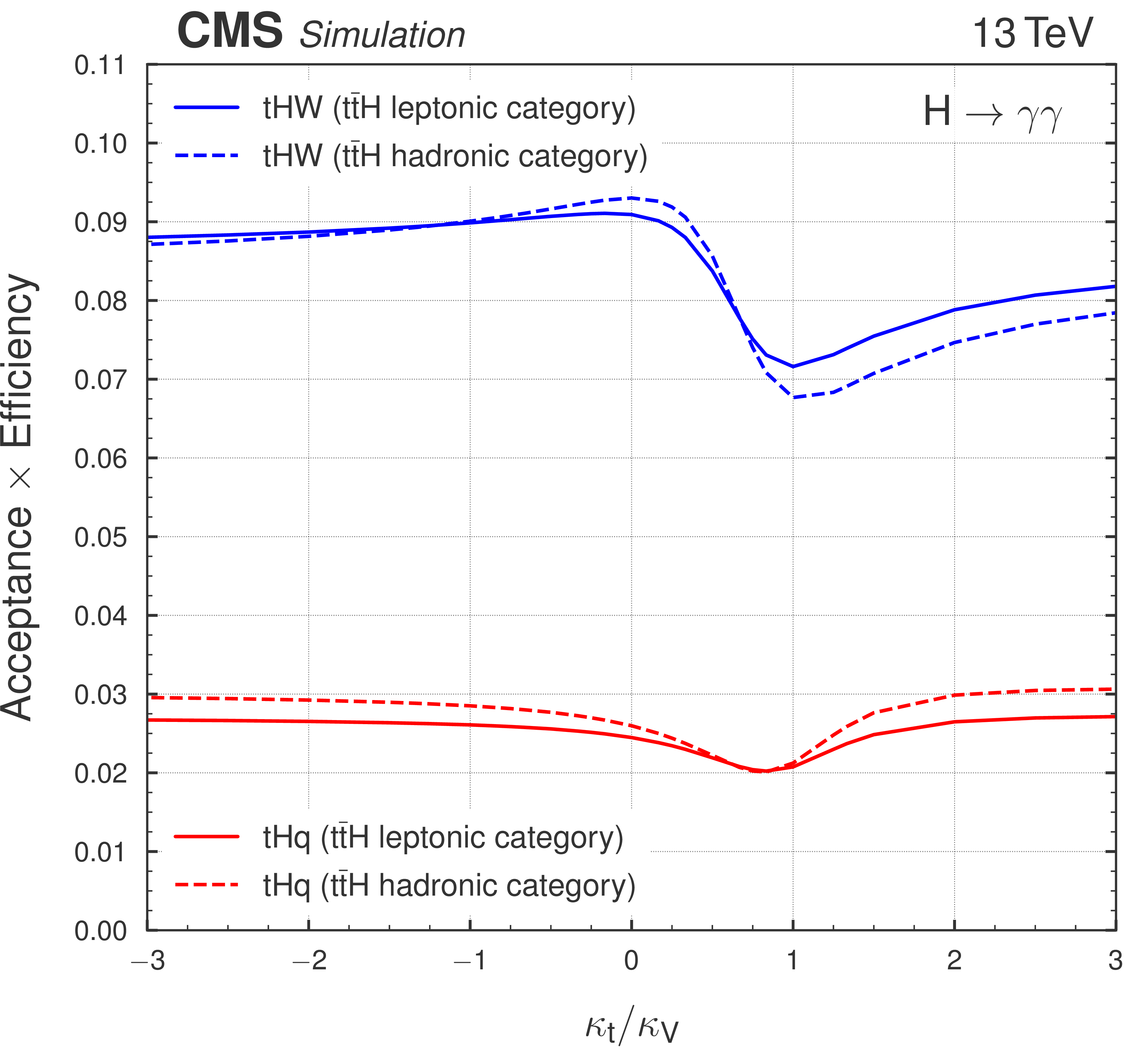
Figure 12:
Acceptance and selection efficiency for the $ {{\mathrm {t}} {\mathrm {H}} {\mathrm {q}}} $ (red) and ${{\mathrm {t}} {\mathrm {H}} {\mathrm {W}}} $ (blue) signal processes as a function of $ {\kappa _ {\mathrm {t}}} / {\kappa _\text {V}} $, for the ${{{\mathrm {t}\overline {\mathrm {t}}}} {\mathrm {H}}} $ leptonic (solid lines) and ${{{\mathrm {t}\overline {\mathrm {t}}}} {\mathrm {H}}}$ hadronic categories (dashed lines) of the $ {\mathrm {H}} \to {\gamma \gamma} $ measurement. |
png pdf |
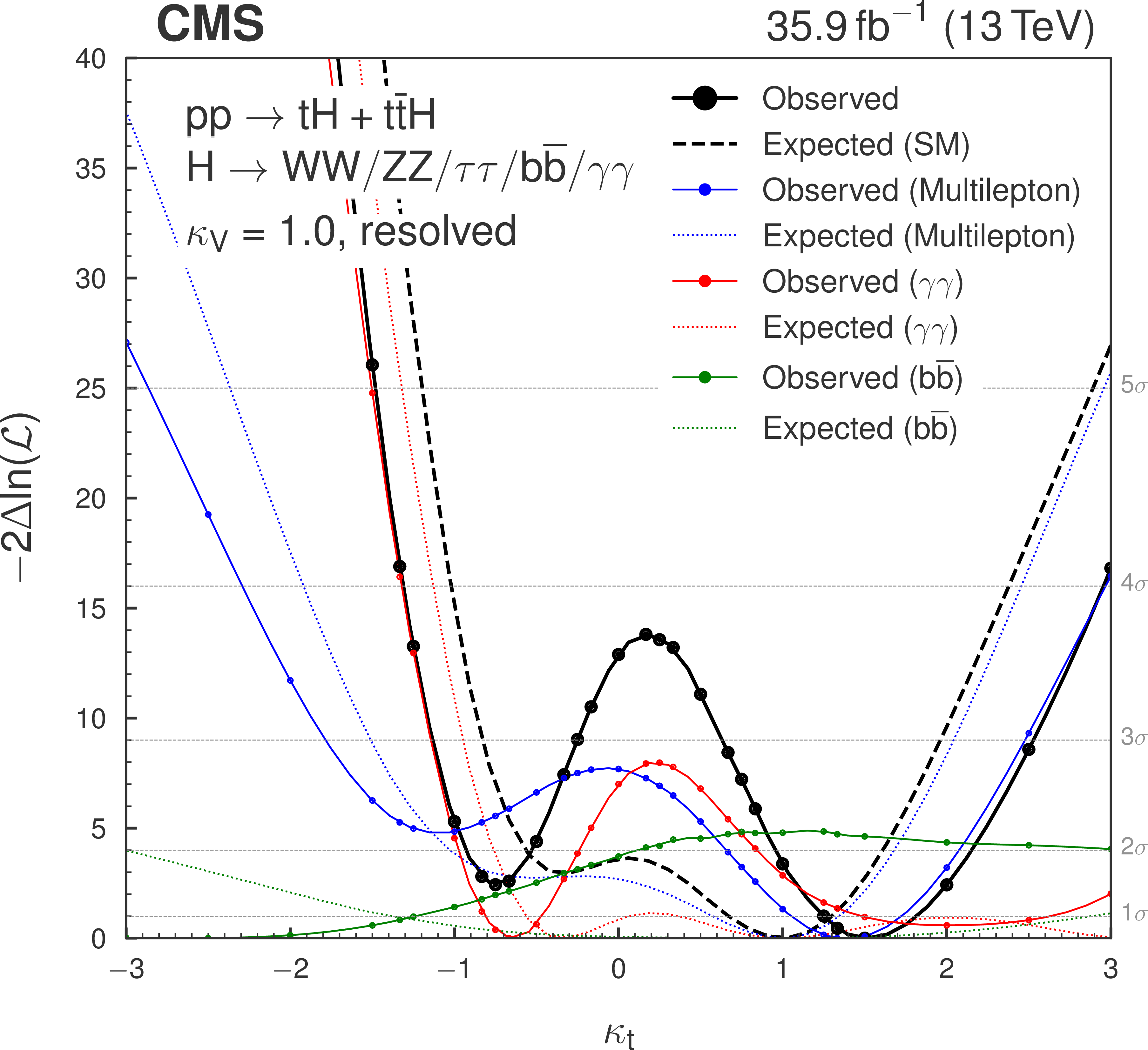
Figure 13:
Scan of $-2\Delta \ln{(\mathcal {L})}$ versus ${\kappa _ {\mathrm {t}}}$ for the data (black line) and the individual channels (blue, red, and green), compared to Asimov data sets corresponding to the SM expectations (dashed lines). |
png pdf |
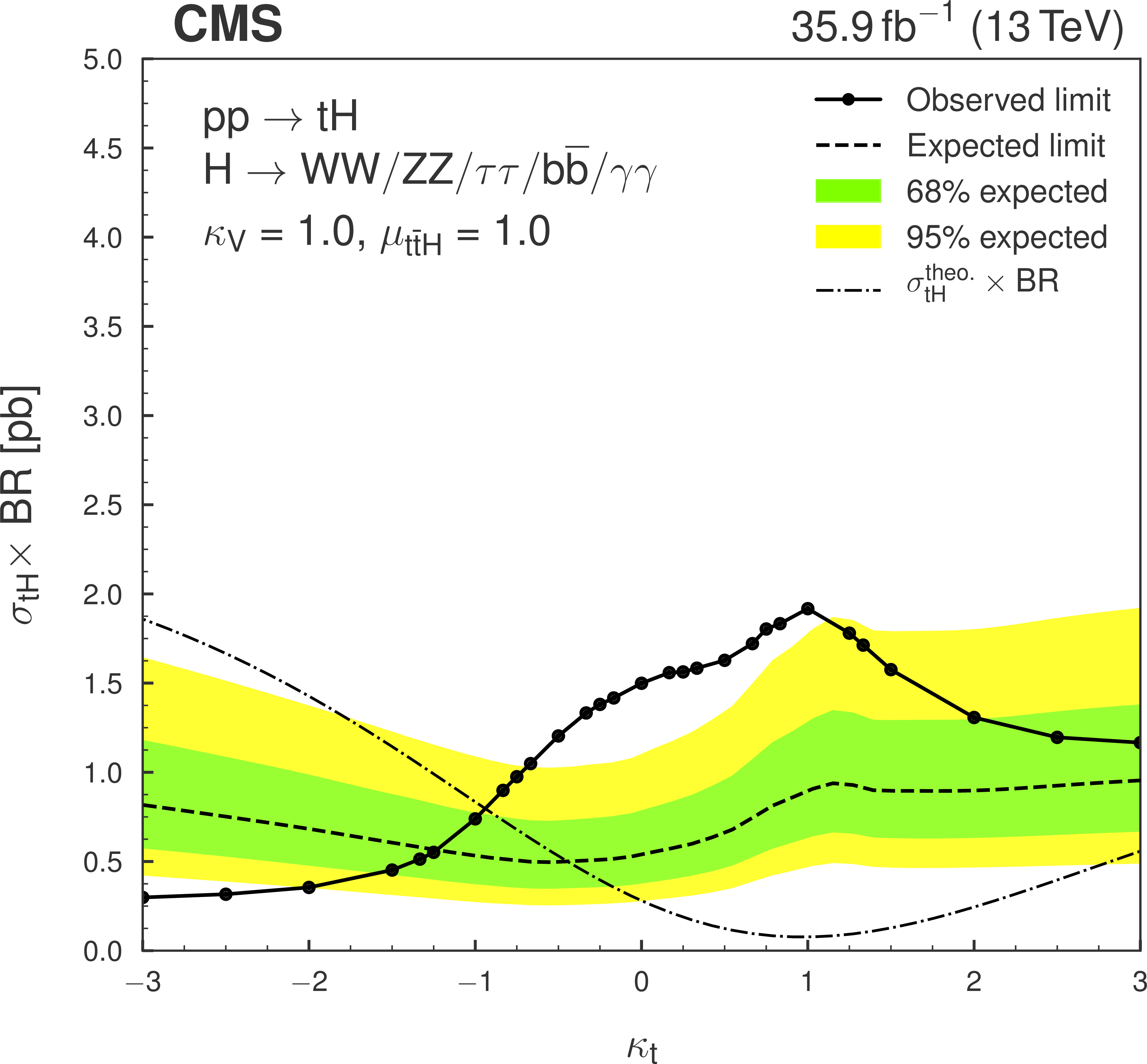
Figure 14:
Observed and expected 95% CL upper limit on the $ {{\mathrm {t}} {\mathrm {H}}} $ cross section times combined $ {\mathrm {H}} \to {\mathrm {W}} {\mathrm {W}}^*+ {{\tau} {\tau}} + {\mathrm {Z}} {\mathrm {Z}} ^*+ {{\mathrm {b}} {\overline {\mathrm {b}}}} + {\gamma \gamma} $ branching fraction for different values of the coupling ratio ${\kappa _ {\mathrm {t}}}$. The expected limit is calculated on a background-only data set, i.e., without $ {{\mathrm {t}} {\mathrm {H}}} $ contribution, but including a ${\kappa _ {\mathrm {t}}} $-dependent contribution from ${{{\mathrm {t}\overline {\mathrm {t}}}} {\mathrm {H}}}$. The ${{{\mathrm {t}\overline {\mathrm {t}}}} {\mathrm {H}}} $ normalization is kept fixed in the fit, while the $ {{\mathrm {t}} {\mathrm {H}}} $ signal strength is allowed to float. |
| Tables | |

png pdf |
Table 1:
Summary of the event selection for the multilepton channels. |

png pdf |
Table 2:
Data yields and expected backgrounds after the event selection for the three multilepton search channels in 35.9 fb$^{-1}$of integrated luminosity. Quoted uncertainties include statistical uncertainties reflecting the limited size of MC samples and data sidebands, and unconstrained systematic uncertainties. |
png pdf |
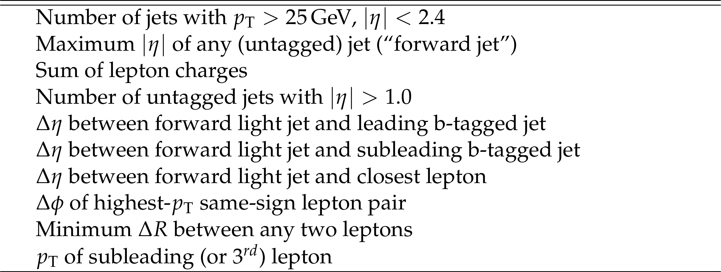
Table 3:
Input observables to the signal discrimination classifier. |

png pdf |
Table 4:
Summary of event selection for the single-lepton + $ {{\mathrm {b}} {\overline {\mathrm {b}}}} $ channels. |
png pdf |
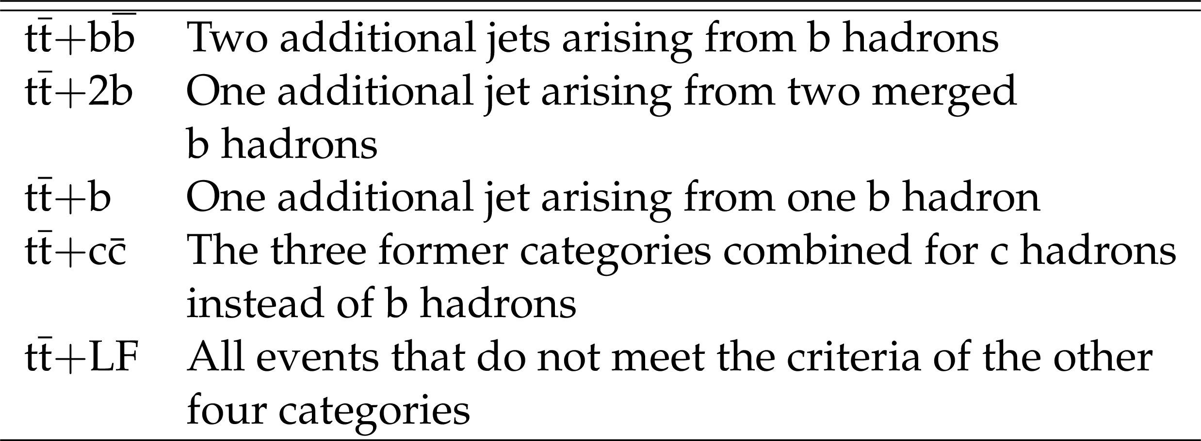
Table 5:
Subcategories of ${{{\mathrm {t}\overline {\mathrm {t}}}} {+}\text {jets}} $ backgrounds used in the analysis. |

png pdf |
Table 6:
Data yields and expected backgrounds after the event selection for the two signal regions and in the dilepton control region. Uncertainties include both systematic and statistical components. |

png pdf |
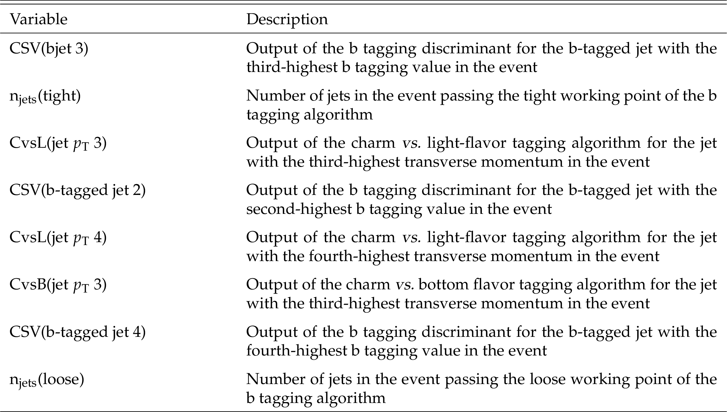
Table 7:
Classification variable description |
png pdf |
Table 8:
Input variables used in the training of the FC-BDT. The variables are sorted by their importance in the training within each category. In total, eight variables are used for the training of the FC-BDT. |
png pdf |
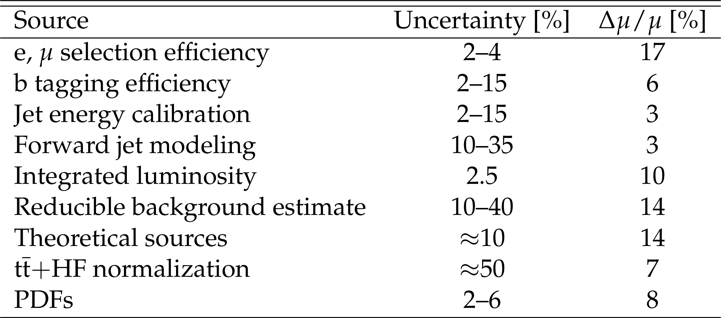
Table 9:
Summary of the main sources of systematic uncertainty. $\Delta \mu /\mu $ corresponds to the relative change in ${{\mathrm {t}} {\mathrm {H}} + {{{\mathrm {t}\overline {\mathrm {t}}}} {\mathrm {H}}}} $ signal yield induced by varying the systematic source within its associated uncertainty. |
png pdf |
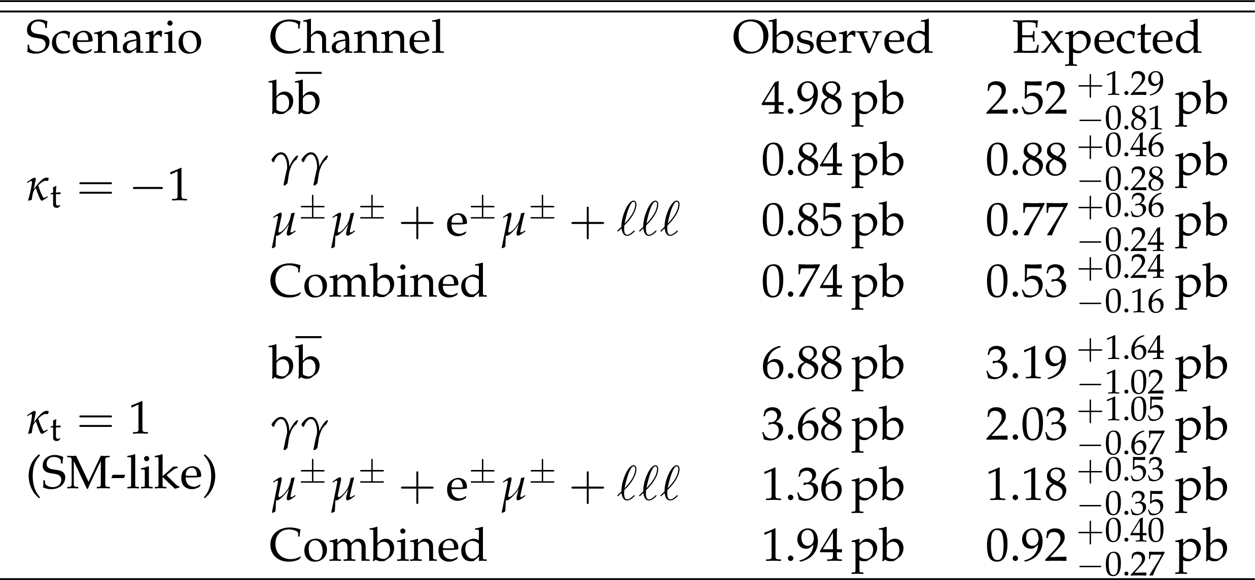
Table 10:
Expected and observed 95% CL upper limits on the $ {{\mathrm {t}} {\mathrm {H}}} $ production cross section times $ {\mathrm {H}} \to {\mathrm {W}} {\mathrm {W}}^*+ {{\tau} {\tau}} + {\mathrm {Z}} {\mathrm {Z}} ^*+ {{\mathrm {b}} {\overline {\mathrm {b}}}} + {\gamma \gamma} $ branching fraction for a scenario of inverted couplings ($ {\kappa _ {\mathrm {t}}} =-1.0$, top rows) and for an SM-like signal ($ {\kappa _ {\mathrm {t}}} =1.0$, bottom rows), in pb. The expected limit is calculated on a background-only data set, i.e., without $ {{\mathrm {t}} {\mathrm {H}}} $ contribution, but including a ${\kappa _ {\mathrm {t}}} $-dependent contribution from the ${{{\mathrm {t}\overline {\mathrm {t}}}} {\mathrm {H}}}$ production. The ${{{\mathrm {t}\overline {\mathrm {t}}}} {\mathrm {H}}} $ normalization is kept fixed in the fit, while the $ {{\mathrm {t}} {\mathrm {H}}} $ signal strength is allowed to float. Limits can be compared to the expected product of $ {{\mathrm {t}} {\mathrm {H}}} $ cross sections and branching fractions of 0.83 and 0.077 pb for the inverted top quark Yukawa coupling and for the SM, respectively. |
| Summary |
| Events from proton-proton collisions at $\sqrt{s} = $ 13 TeV compatible with the production of a Higgs boson (H) in association with a single top quark (t) have been studied to derive constraints on the magnitude and relative sign of Higgs boson couplings to top quarks and vector bosons. Dedicated analyses of multilepton final states and final states with single leptons and a pair of bottom quarks are combined with a reinterpretation of a measurement of Higgs bosons decaying to two photons for the final result. For standard model-like Higgs boson couplings to vector bosons, the data favor a positive value of the top quark Yukawa coupling, ${y_\mathrm{t}} $, by about 1.5 standard deviations and exclude values outside the ranges of about $[-0.9, -0.5]$ and $[1.0, 2.1]$ times ${y_\mathrm{t}} ^\mathrm{SM}$ at the 95% confidence level. An excess of events compared with the expected backgrounds is compatible with the standard model expectation of ${\mathrm{t}\mathrm{H}+{\mathrm{t\bar{t}}\mathrm{H}} } $ production. |
| Additional Figures | |
png pdf |
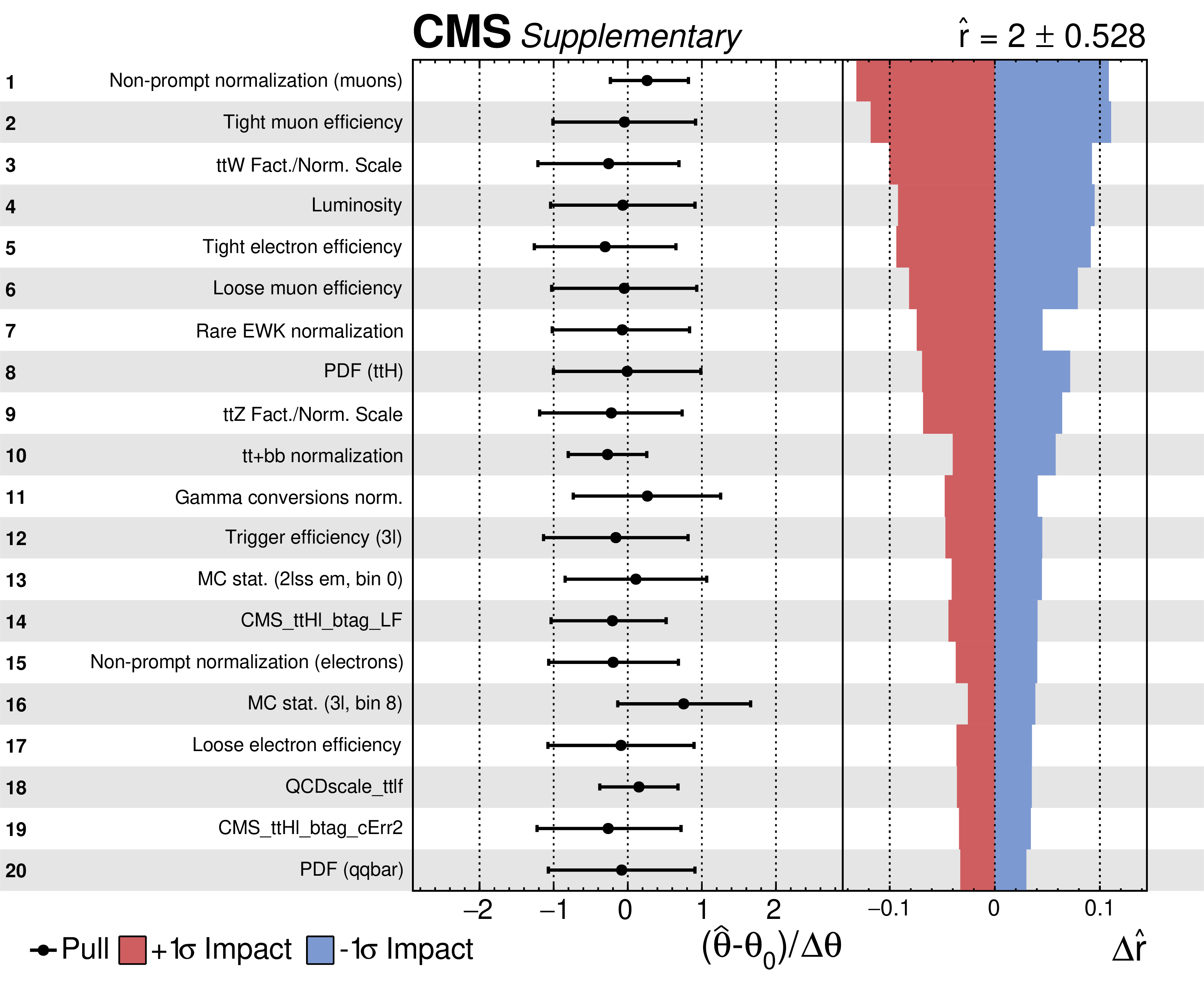
Additional Figure 1:
List of most important nuisance parameters, ordered by their impact on a fit with a common ${{\mathrm {t}} {\mathrm {H}} + {{{\mathrm {t}\overline {\mathrm {t}}}} {\mathrm {H}}}} $ signal strength floating. The impact is defined as the shift in best-fit signal strength when fixing each nuisance to its post-fit value plus or minus one standard deviation. Also shown is the pull for each nuisance parameter, defined as post-fit minus pre-fit values divided by the pre-fit uncertainties, with the post-fit uncertainty indicated. |
png pdf |
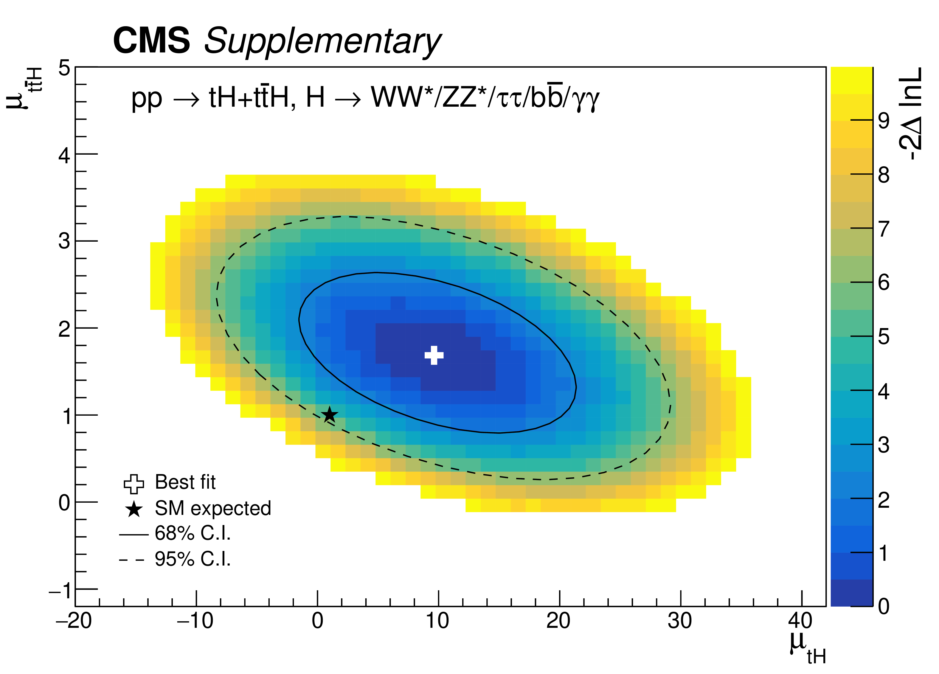
Additional Figure 2:
Scan of negative log-likelihood for a fit with two independently floating signal strengths for ${{\mathrm {t}} {\mathrm {H}}} $ ($\mu _ {{\mathrm {t}} {\mathrm {H}}} $) and ${{{\mathrm {t}\overline {\mathrm {t}}}} {\mathrm {H}}} $ ($\mu _ {{{\mathrm {t}\overline {\mathrm {t}}}} {\mathrm {H}}} $), for $ {\kappa _ {\mathrm {t}}} = $ 1.0 (SM). The best-fit value of $\mu _ {{\mathrm {t}} {\mathrm {H}}} = $ 9.63, $\mu _ {{{\mathrm {t}\overline {\mathrm {t}}}} {\mathrm {H}}} =$ 1.69 is indicated with a white cross. The SM expectation is indicated with a black cross and has a value of $-2\Delta \ln{\mathcal {L}}$ of 5.2, corresponding to a $p$-value of 7.6%, assuming it is distributed according to a $\chi ^2$ function with two degrees of freedom. |
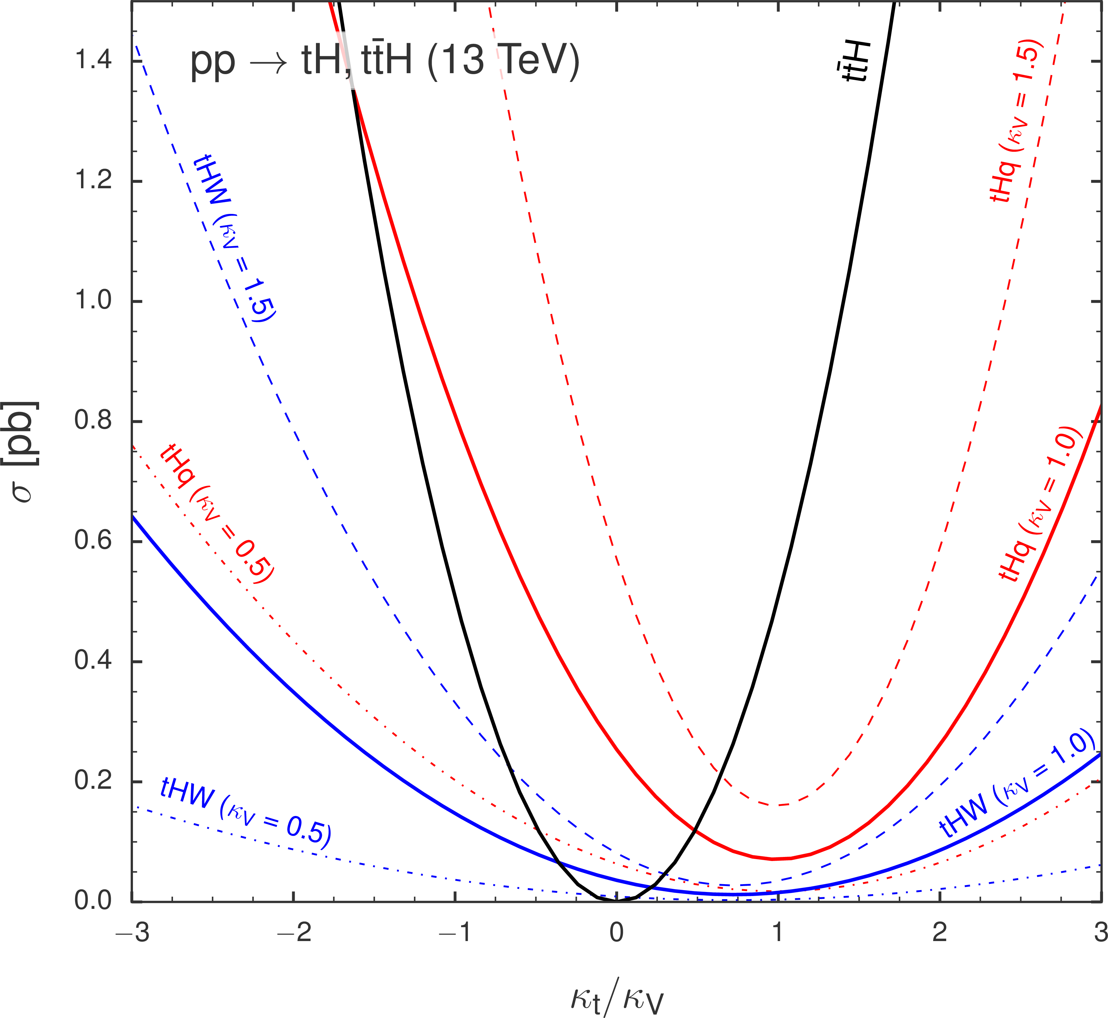
png pdf |
Additional Figure 3:
Production cross sections of ${{\mathrm {t}} {\mathrm {H}} {\mathrm {q}}} $ (red), ${{\mathrm {t}} {\mathrm {H}} {\mathrm {W}}} $ (blue), and ${{{\mathrm {t}\overline {\mathrm {t}}}} {\mathrm {H}}} $ (black) as a function of the ratio of coupling modifiers ${\kappa _ {\mathrm {t}}} $ and ${\kappa _\text {V}}$, for three different values of ${\kappa _\text {V}}$, for $\sqrt {s}= $ 13 TeV, see Refs. [17-19]. See also https://twiki.cern.ch/twiki/bin/view/LHCPhysics/LHCHXSWG2KAPPA. |
| References | ||||
| 1 | ATLAS Collaboration | Observation of a new particle in the search for the standard model Higgs boson with the ATLAS detector at the LHC | PLB 716 (2012) 1 | 1207.7214 |
| 2 | CMS Collaboration | Observation of a new boson at a mass of 125 GeV with the CMS experiment at the LHC | PLB 716 (2012) 30 | CMS-HIG-12-028 1207.7235 |
| 3 | CMS Collaboration | Observation of a new boson with mass near 125 GeV in pp collisions at $ \sqrt{s} = $ 7 and 8 TeV | JHEP 06 (2013) 081 | CMS-HIG-12-036 1303.4571 |
| 4 | ATLAS and CMS Collaborations | Combined measurement of the Higgs boson mass in $ pp $ collisions at $ \sqrt{s}= $ 7 and 8 TeV with the ATLAS and CMS experiments | PRL 114 (2015) 191803 | 1503.07589 |
| 5 | CMS Collaboration | Constraints on the spin-parity and anomalous HVV couplings of the Higgs boson in proton collisions at 7 and 8~ TeV | PRD 92 (2015) 012004 | CMS-HIG-14-018 1411.3441 |
| 6 | CMS Collaboration | Observation of $ \mathrm{t\overline{t}} $H production | PRL 120 (2018) 231801 | CMS-HIG-17-035 1804.02610 |
| 7 | ATLAS Collaboration | Observation of Higgs boson production in association with a top quark pair at the LHC with the ATLAS detector | PLB 784 (2018) 173 | 1806.00425 |
| 8 | CMS Collaboration | Observation of Higgs boson decay to bottom quarks | PRL 121 (2018) 121801 | CMS-HIG-18-016 1808.08242 |
| 9 | S. Biswas, E. Gabrielli, and B. Mele | Single top and Higgs associated production as a probe of the Htt coupling sign at the LHC | JHEP 01 (2013) 088 | 1211.0499 |
| 10 | B. Hespel, F. Maltoni, and E. Vryonidou | Higgs and Z boson associated production via gluon fusion in the SM and the 2HDM | JHEP 06 (2015) 065 | 1503.01656 |
| 11 | CMS Collaboration | Precise determination of the mass of the Higgs boson and tests of compatibility of its couplings with the standard model predictions using proton collisions at 7 and 8 $ {TeV} $ | EPJC 75 (2015) 212 | CMS-HIG-14-009 1412.8662 |
| 12 | ATLAS and CMS Collaborations | Measurements of the Higgs boson production and decay rates and constraints on its couplings from a combined ATLAS and CMS analysis of the LHC pp collision data at $ \sqrt{s}= $ 7 and 8 TeV | JHEP 08 (2016) 045 | 1606.02266 |
| 13 | J. Ellis and T. You | Updated global analysis of Higgs couplings | JHEP 06 (2013) 103 | 1303.3879 |
| 14 | F. Maltoni, K. Paul, T. Stelzer, and S. Willenbrock | Associated production of Higgs and single top at hadron colliders | PRD 64 (2001) 094023 | hep-ph/0106293 |
| 15 | M. Farina et al. | Lifting degeneracies in Higgs couplings using single top production in association with a Higgs boson | JHEP 05 (2013) 022 | 1211.3736 |
| 16 | P. Agrawal, S. Mitra, and A. Shivaji | Effect of anomalous couplings on the associated production of a single top quark and a Higgs boson at the LHC | JHEP 12 (2013) 077 | 1211.4362 |
| 17 | F. Demartin, F. Maltoni, K. Mawatari, and M. Zaro | Higgs production in association with a single top quark at the lhc | EPJC 75 (2015) 267 | 1504.00611 |
| 18 | LHC Higgs cross section working group | Handbook of LHC Higgs cross sections: 4. Deciphering the nature of the Higgs sector | 1610.07922 | |
| 19 | F. Demartin et al. | tWH associated production at the LHC | EPJC 77 (2017) 34 | 1607.05862 |
| 20 | A. Celis, V. Ilisie, and A. Pich | LHC constraints on two-Higgs doublet models | JHEP 07 (2013) 053 | 1302.4022 |
| 21 | CMS Collaboration | Search for the associated production of a Higgs boson with a single top quark in proton-proton collisions at $ \sqrt{s} = $ 8 TeV | JHEP 06 (2016) 177 | CMS-HIG-14-027 1509.08159 |
| 22 | CMS Collaboration | Measurements of Higgs boson properties in the diphoton decay channel in proton-proton collisions at $ \sqrt{s} = $ 13 TeV | Submitted to JHEP | CMS-HIG-16-040 1804.02716 |
| 23 | CMS Collaboration | Description and performance of track and primary-vertex reconstruction with the CMS tracker | JINST 9 (2014) P10009 | CMS-TRK-11-001 1405.6569 |
| 24 | CMS Collaboration | The CMS trigger system | JINST 12 (2017) P01020 | CMS-TRG-12-001 1609.02366 |
| 25 | CMS Collaboration | The CMS experiment at the CERN LHC | JINST 3 (2008) S08004 | CMS-00-001 |
| 26 | CMS Collaboration | Particle-flow reconstruction and global event description with the CMS detector | JINST 12 (2017) P10003 | CMS-PRF-14-001 1706.04965 |
| 27 | E. Chabanat and N. Estre | Deterministic annealing for vertex finding at CMS | in Computing in high energy physics and nuclear physics. Proceedings, Conference, CHEP'04, Interlaken, Switzerland, September 27-October 1, 2004, p. 2872005 | |
| 28 | Fruhwirth, R. and Waltenberger, W. and Vanlaer, P. | Adaptive vertex fitting | JPG 34 (2007) N343 | |
| 29 | CMS Collaboration | Performance of CMS muon reconstruction in $ {\mathrm{p}}{\mathrm{p}} $ collision events at $ \sqrt{s}= $ 7 TeV | JINST 7 (2012) P10002 | CMS-MUO-10-004 1206.4071 |
| 30 | CMS Collaboration | Performance of electron reconstruction and selection with the CMS detector in proton-proton collisions at $ \sqrt{s} = $ 8 TeV | JINST 10 (2015) P06005 | CMS-EGM-13-001 1502.02701 |
| 31 | CMS Collaboration | Performance of photon reconstruction and identification with the CMS detector in proton-proton collisions at $ \sqrt{s} = $ 8 TeV | JINST 10 (2015) P08010 | CMS-EGM-14-001 1502.02702 |
| 32 | M. Cacciari, G. P. Salam, and G. Soyez | The anti-$ {k_{\mathrm{T}}} $ jet clustering algorithm | JHEP 04 (2008) 063 | 0802.1189 |
| 33 | M. Cacciari, G. P. Salam, and G. Soyez | FastJet user manual | EPJC 72 (2012) 1896 | 1111.6097 |
| 34 | CMS Collaboration | Identification of heavy-flavour jets with the CMS detector in $ {\mathrm{p}}{\mathrm{p}} $ collisions at 13 TeV | JINST 13 (2018) P05011 | CMS-BTV-16-002 1712.07158 |
| 35 | GEANT4 Collaboration | GEANT4--a simulation toolkit | NIMA 506 (2003) 250 | |
| 36 | J. Alwall et al. | The automated computation of tree-level and next-to-leading order differential cross sections, and their matching to parton shower simulations | JHEP 07 (2014) 079 | 1405.0301 |
| 37 | J. Alwall et al. | Comparative study of various algorithms for the merging of parton showers and matrix elements in hadronic collisions | EPJC 53 (2008) 473 | 0706.2569 |
| 38 | NNPDF Collaboration | Parton distributions for the LHC run II | JHEP 04 (2015) 040 | 1410.8849 |
| 39 | M. Botje et al. | The PDF4LHC working group interim recommendations | 1101.0538 | |
| 40 | S. Alekhin et al. | The PDF4LHC working group interim report | 1101.0536 | |
| 41 | LHC Higgs cross section working group | Handbook of LHC Higgs cross sections: 3. Higgs properties | 1307.1347 | |
| 42 | R. Frederix and S. Frixione | Merging meets matching in MC@NLO | JHEP 12 (2012) 061 | 1209.6215 |
| 43 | P. Nason | A new method for combining NLO QCD with shower Monte Carlo algorithms | JHEP 11 (2004) 040 | hep-ph/0409146 |
| 44 | S. Frixione, P. Nason, and C. Oleari | Matching NLO QCD computations with parton shower simulations: the POWHEG method | JHEP 11 (2007) 070 | 0709.2092 |
| 45 | S. Alioli, P. Nason, C. Oleari, and E. Re | A general framework for implementing NLO calculations in shower Monte Carlo programs: the POWHEG BOX | JHEP 06 (2010) 043 | 1002.2581 |
| 46 | E. Re | Single-top Wt-channel production matched with parton showers using the POWHEG method | EPJC 71 (2011) 1547 | 1009.2450 |
| 47 | S. Alioli, P. Nason, C. Oleari, and E. Re | NLO single-top production matched with shower in POWHEG: $ s $- and $ t $-channel contributions | JHEP 09 (2009) 111 | 0907.4076 |
| 48 | T. Melia, P. Nason, R. Rontsch, and G. Zanderighi | $ \text{W}^{+}\text{W}^{-} $, WZ and ZZ production in the POWHEG BOX | JHEP 11 (2011) 078 | 1107.5051 |
| 49 | T. Sjostrand et al. | An introduction to PYTHIA 8.2 | CPC 191 (2015) 159 | 1410.3012 |
| 50 | CMS Collaboration | Evidence for associated production of a Higgs boson with a top quark pair in final states with electrons, muons, and hadronically decaying $ \tau $ leptons at $ \sqrt{s} = $ 13 TeV | JHEP 08 (2018) 066 | CMS-HIG-17-018 1803.05485 |
| 51 | H. Voss, A. Hocker, J. Stelzer, and F. Tegenfeldt | TMVA, the toolkit for multivariate data analysis with ROOT | in XIth International Workshop on Advanced Computing and Analysis Techniques in Physics Research (ACAT), p. 40 2007 [PoS(ACAT)040] | physics/0703039 |
| 52 | CMS Collaboration | Measurements of inclusive $ \mathrm{W} $ and $ \mathrm{Z} $ cross sections in $ {\mathrm{p}}{\mathrm{p}} $ collisions at $ \sqrt{s} = $ 7 TeV | JHEP 01 (2011) 080 | CMS-EWK-10-002 1012.2466 |
| 53 | CMS Collaboration | Jet energy scale and resolution in the CMS experiment in pp collisions at 8 TeV | JINST 12 (2017) P02014 | CMS-JME-13-004 1607.03663 |
| 54 | CMS Collaboration | CMS luminosity measurement for the 2016 data-taking period | CMS-PAS-LUM-17-001 | CMS-PAS-LUM-17-001 |
| 55 | V. D. Barger, J. Ohnemus, and R. J. N. Phillips | Event shape criteria for single lepton top signals | PRD 48 (1993) 3953 | hep-ph/9308216 |
| 56 | G. C. Fox and S. Wolfram | Observables for the analysis of event shapes in $ {e}^{+}{e}^{{-}} $ annihilation and other processes | PRL 41 (1978) 1581 | |
| 57 | CMS Collaboration | Measurement of $ \mathrm {t}\overline{\mathrm {t}} $ production with additional jet activity, including $ \mathrm {b} $ quark jets, in the dilepton decay channel using $ {\mathrm{p}}{\mathrm{p}} $ collisions at $ \sqrt{s} = $ 8 TeV | EPJC 76 (2016) 379 | CMS-TOP-12-041 1510.03072 |
| 58 | CMS Collaboration | Measurements of $ \mathrm{t\bar{t}} $ cross sections in association with b jets and inclusive jets and their ratio using dilepton final states in $ {\mathrm{p}}{\mathrm{p}} $ collisions at $ \sqrt{s} = $ 13 TeV | PLB 776 (2018) 355 | CMS-TOP-16-010 1705.10141 |
| 59 | CMS Collaboration | Measurement of the differential cross section for top quark pair production in $ {\mathrm{p}}{\mathrm{p}} $ collisions at $ \sqrt{s} = $ 8 TeV | EPJC 75 (2015) 542 | CMS-TOP-12-028 1505.04480 |
| 60 | CMS Collaboration | Measurement of the inelastic proton-proton cross section at $ \sqrt{s} = $ 13 TeV | JHEP 07 (2018) 161 | CMS-FSQ-15-005 1802.02613 |
| 61 | CMS Collaboration | Performance of the CMS missing transverse momentum reconstruction in pp data at $ \sqrt{s} = $ 8 TeV | JINST 10 (2015) P02006 | CMS-JME-13-003 1411.0511 |
| 62 | P. D. Dauncey, M. Kenzie, N. Wardle, and G. J. Davies | Handling uncertainties in background shapes: the discrete profiling method | JINST 10 (2015) P04015 | |
| 63 | CMS Collaboration | Observation of the diphoton decay of the Higgs boson and measurement of its properties | EPJC 74 (2014) 3076 | CMS-HIG-13-001 1407.0558 |
| 64 | The ATLAS Collaboration, The CMS Collaboration, The LHC Higgs Combination Group | Procedure for the LHC Higgs boson search combination in Summer 2011 | CMS-NOTE-2011-005 | |
| 65 | CMS Collaboration | Combined results of searches for the standard model Higgs boson in $ {\mathrm{p}}{\mathrm{p}} $ collisions at $ \sqrt{s} = $ 7 TeV | PLB 710 (2012) 26 | CMS-HIG-11-032 1202.1488 |
| 66 | J. S. Conway | Incorporating nuisance parameters in likelihoods for multisource spectra | 1103.0354 | |
| 67 | G. Cowan, K. Cranmer, E. Gross, and O. Vitells | Asymptotic formulae for likelihood-based tests of new physics | EPJC 71 (2011) 1554 | 1007.1727 |
| 68 | T. Junk | Confidence level computation for combining searches with small statistics | NIMA 434 (1999) 435 | hep-ex/9902006 |
| 69 | A. L. Read | Presentation of search results: The $ \textrm{CL}_{s} $ technique | JPG 28 (2002) 2693 | |
|
|
Compact Muon Solenoid LHC, CERN |
|

|

|

|

|

|