

Compact Muon Solenoid
LHC, CERN
| CMS-HIG-19-009 ; CERN-EP-2021-054 | ||
| Constraints on anomalous Higgs boson couplings to vector bosons and fermions in its production and decay using the four-lepton final state | ||
| CMS Collaboration | ||
| 25 April 2021 | ||
| Phys. Rev. D 104 (2021) 052004 | ||
| Abstract: Studies of $CP$ violation and anomalous couplings of the Higgs boson to vector bosons and fermions are presented. The data were acquired by the CMS experiment at the LHC and correspond to an integrated luminosity of 137 fb$^{-1}$ at a proton-proton collision energy of 13 TeV. The kinematic effects in the Higgs boson's four-lepton decay $\mathrm{H}\to4\ell$ and its production in association with two jets, a vector boson, or top quarks are analyzed, using a full detector simulation and matrix element techniques to identify the production mechanisms and to increase sensitivity to the Higgs boson tensor structure of the interactions. A simultaneous measurement is performed of up to five Higgs boson couplings to electroweak vector bosons (HVV), two couplings to gluons (Hgg), and two couplings to top quarks (Htt). The $CP$ measurement in the Htt interaction is combined with the recent measurement in the $\mathrm{H}\to\gamma\gamma$ channel. The results are presented in the framework of anomalous couplings and are also interpreted in the framework of effective field theory, including the first study of $CP$ properties of the Htt and effective Hgg couplings from a simultaneous analysis of the gluon fusion and top-associated processes. The results are consistent with the standard model of particle physics. | ||
| Links: e-print arXiv:2104.12152 [hep-ex] (PDF) ; CDS record ; inSPIRE record ; HepData record ; Physics Briefing ; CADI line (restricted) ; | ||
| Figures | |
png pdf |
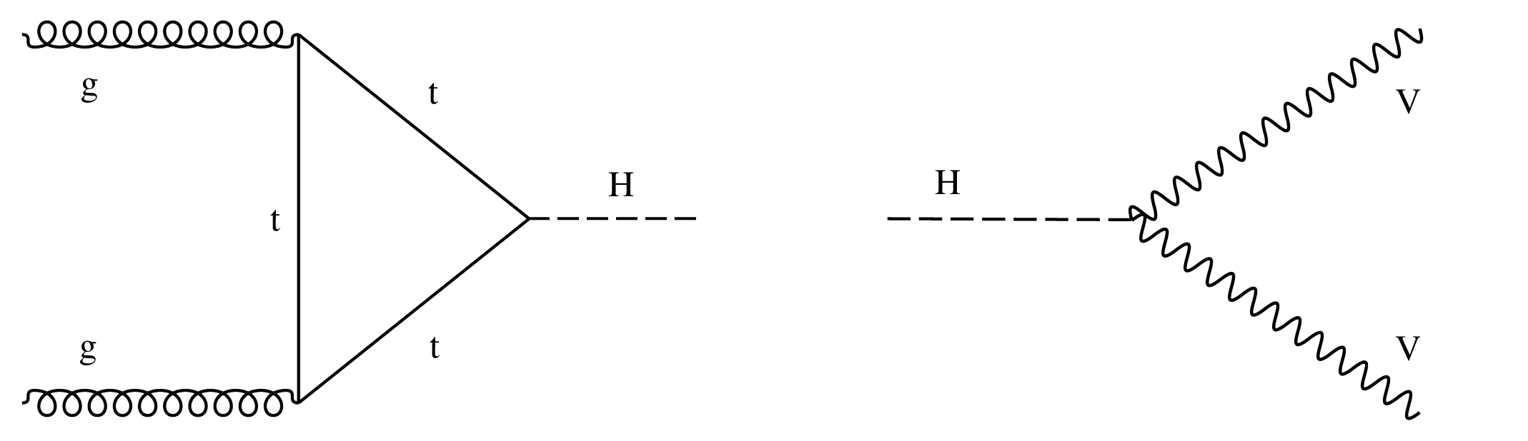
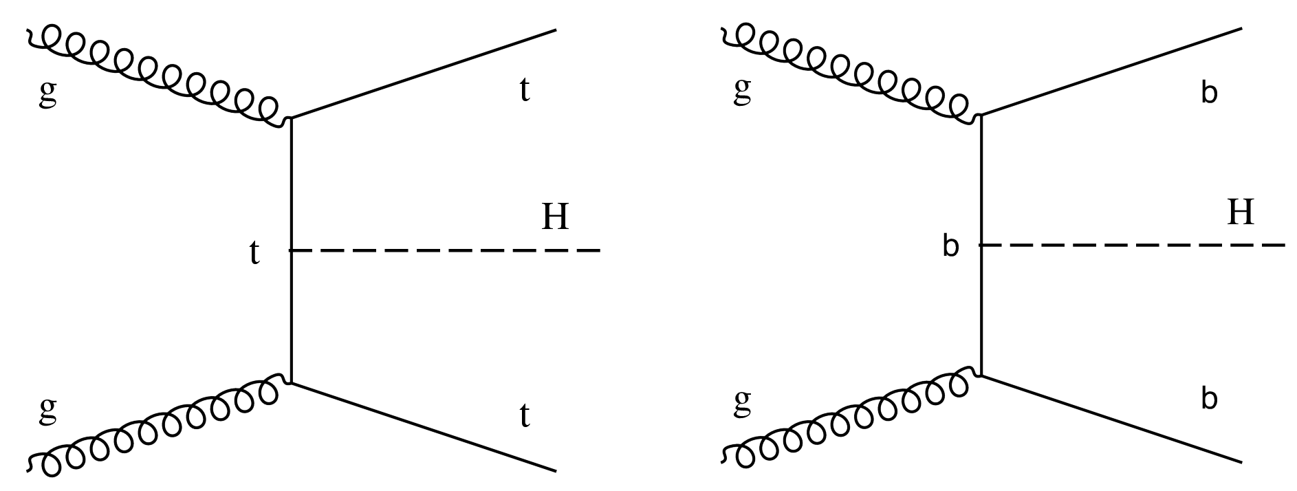
Figure 1:
Leading-order Feynman diagrams for the gluon fusion production mode (left) and $\mathrm{H} \to \mathrm{V} \mathrm{V} $ decay (right). |

png pdf |
Figure 1-a:
Leading-order Feynman diagram for the gluon fusion production mode. |
png pdf |
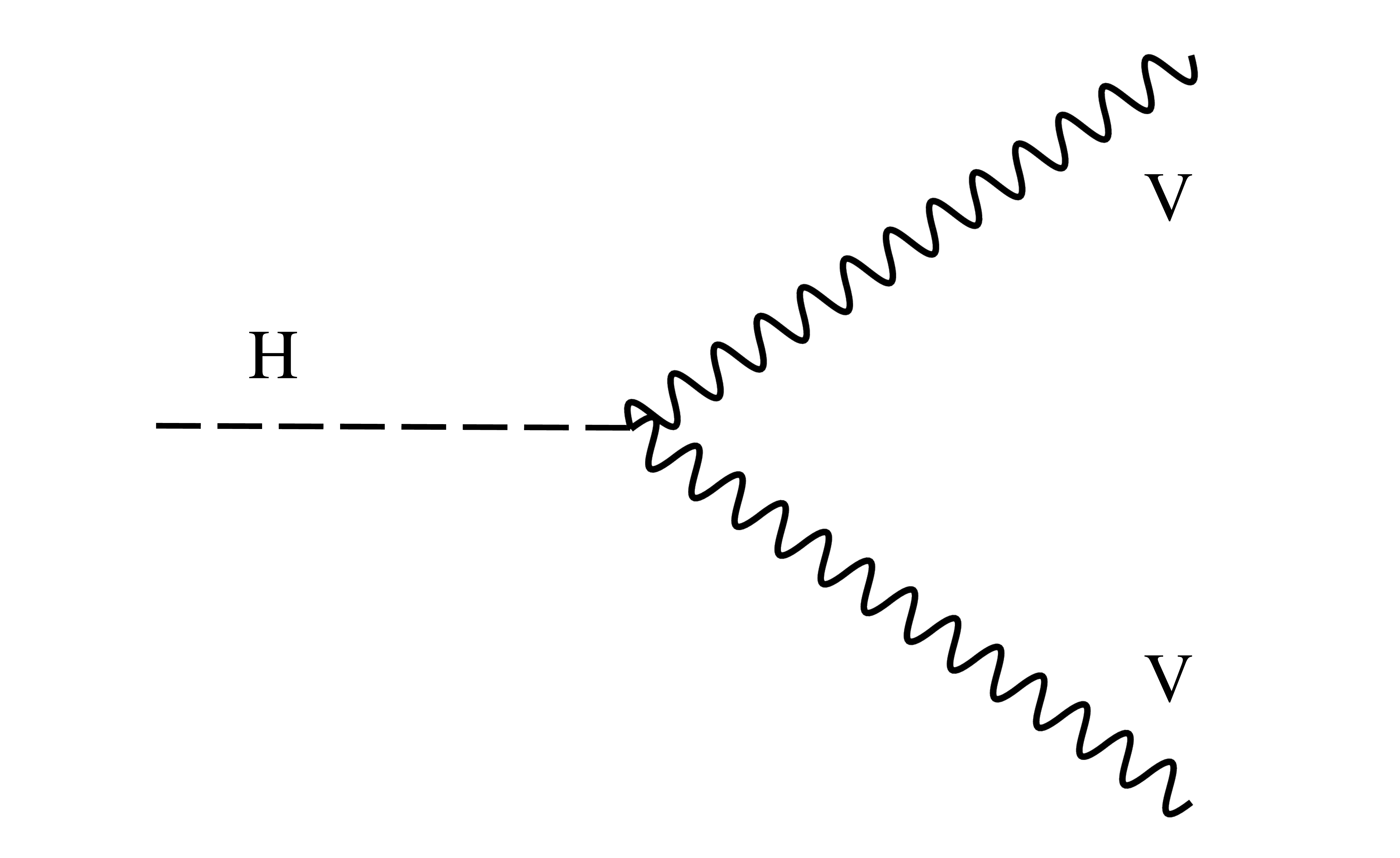
Figure 1-b:
Leading-order Feynman diagram for the $\mathrm{H} \to \mathrm{V} \mathrm{V} $ decay. |
png pdf |
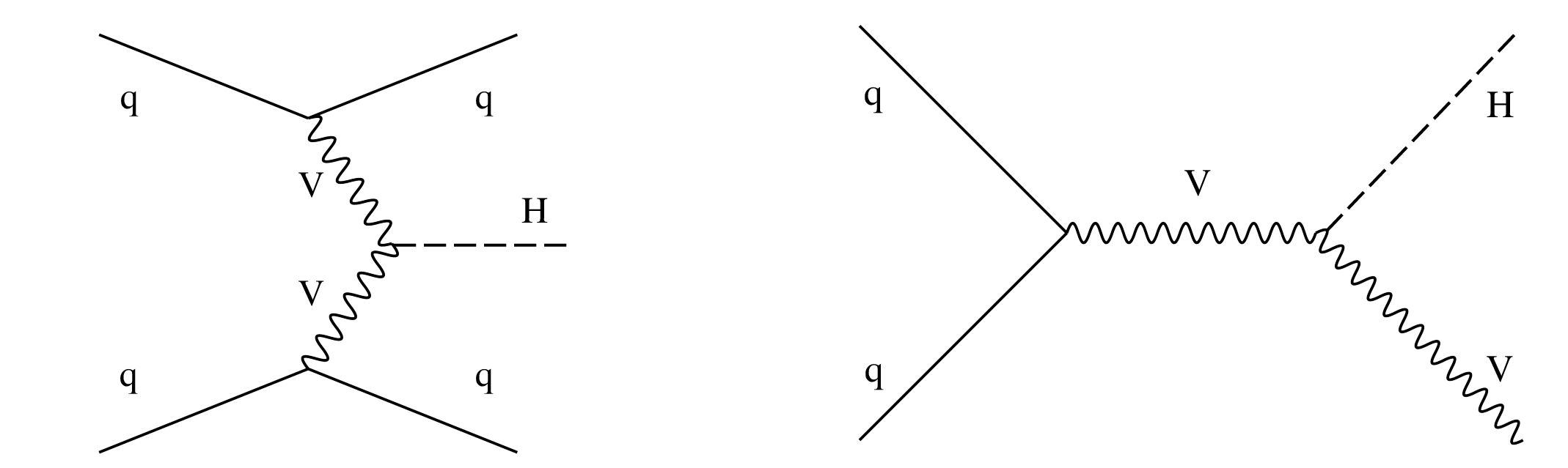
Figure 2:
Leading-order Feynman diagrams for the VBF (left) and VH (right) production modes. |
png pdf |
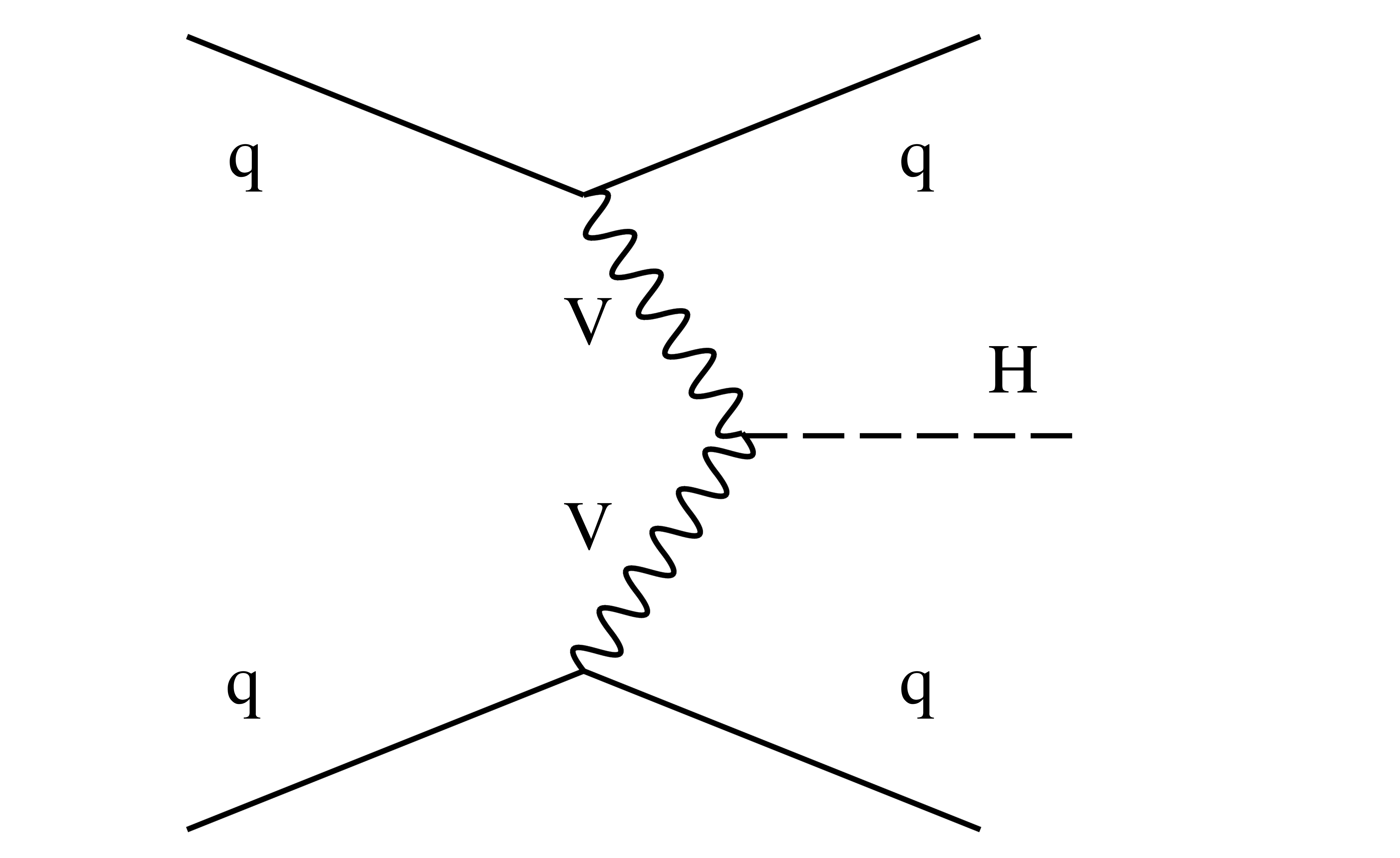
Figure 2-a:
Leading-order Feynman diagram for the VBF production mode. |

png pdf |
Figure 2-b:
Leading-order Feynman diagram for the VH production mode. |
png pdf |
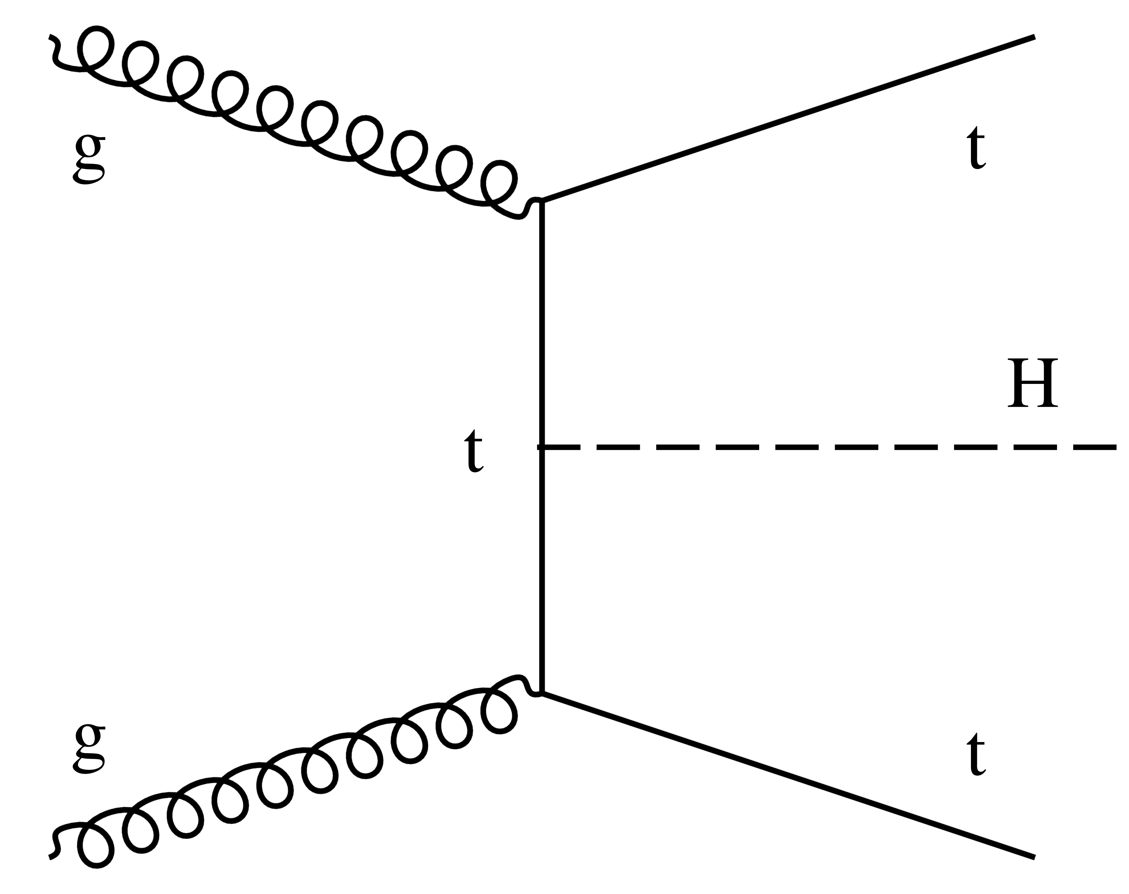
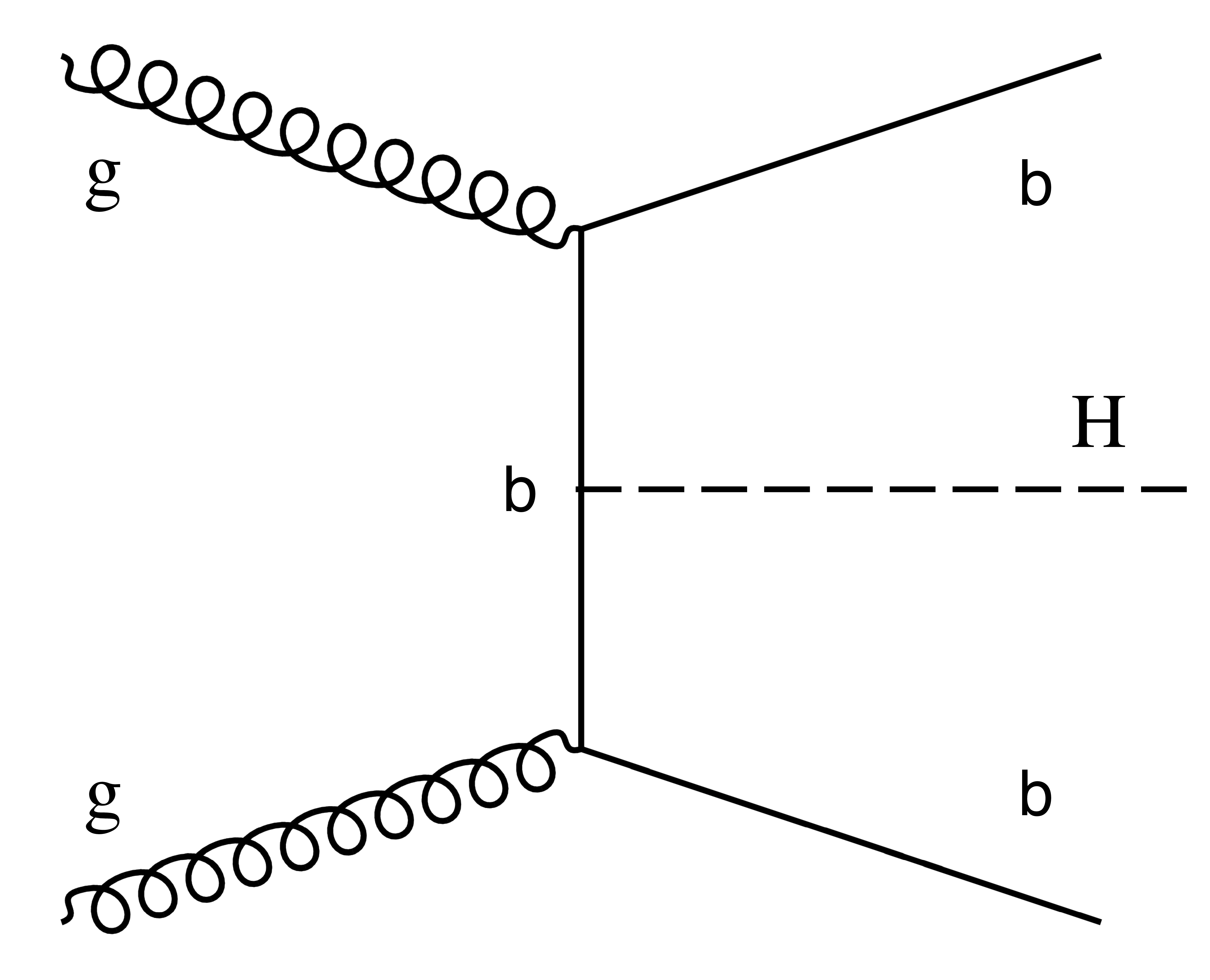
Figure 3:
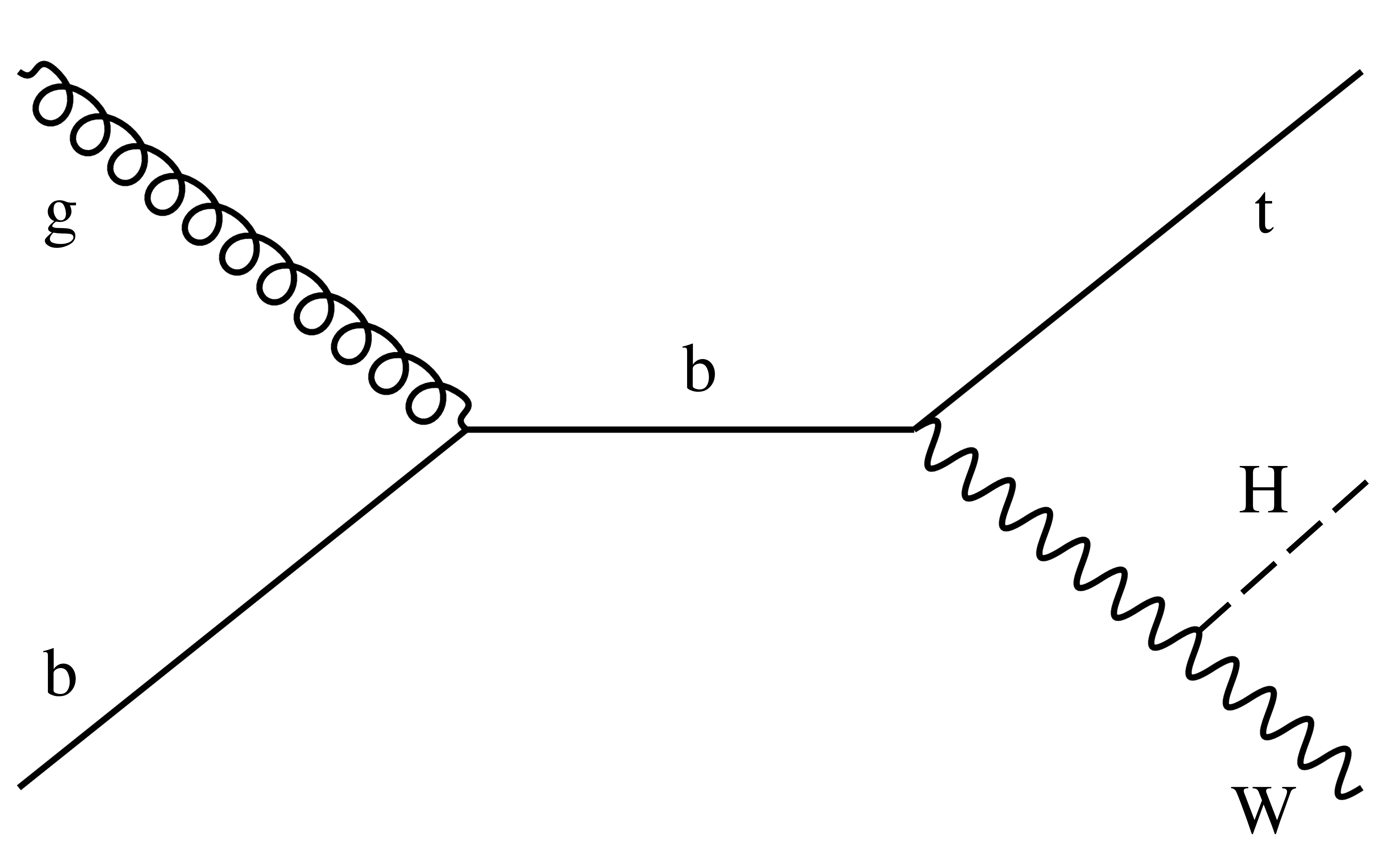
Examples of leading-order Feynman diagrams for the ttH (left) and bbH (right) production modes. |
png pdf |
Figure 3-a:
Example of leading-order Feynman diagram for the ttH production mode. |
png pdf |
Figure 3-b:
Example of leading-order Feynman diagram for the bbH production mode. |

png pdf |
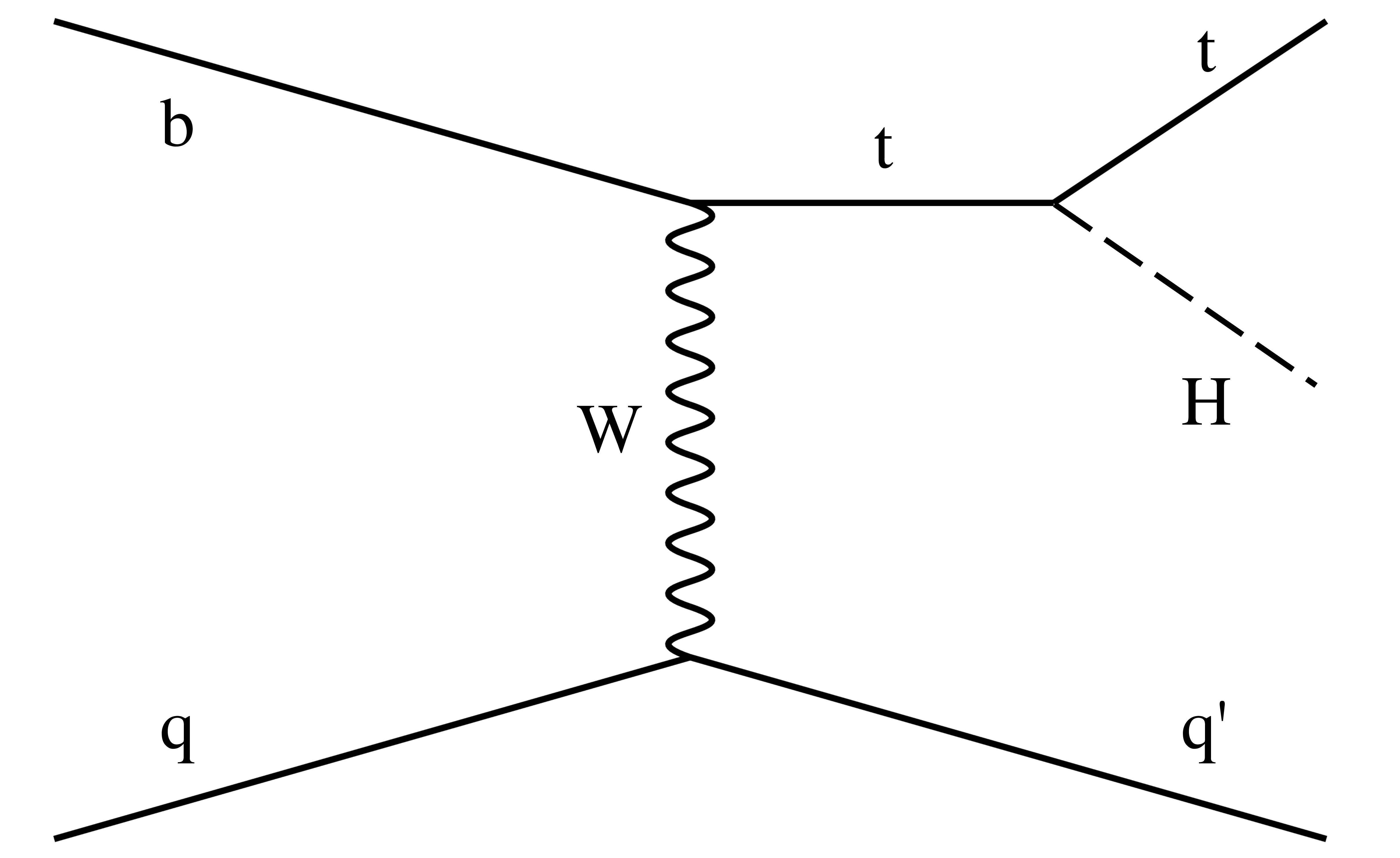
Figure 4:
Examples of leading-order Feynman diagrams for the tH production mode. |
png pdf |
Figure 4-a:
Example of leading-order Feynman diagram for the tH production mode. |
png pdf |
Figure 4-b:
Example of leading-order Feynman diagram for the tH production mode. |
png pdf |
Figure 5:
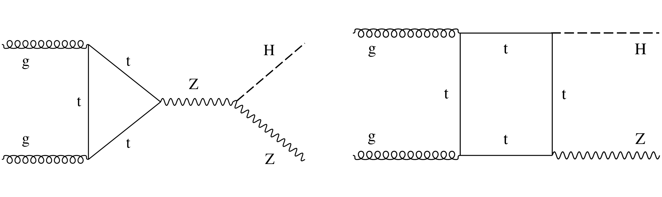
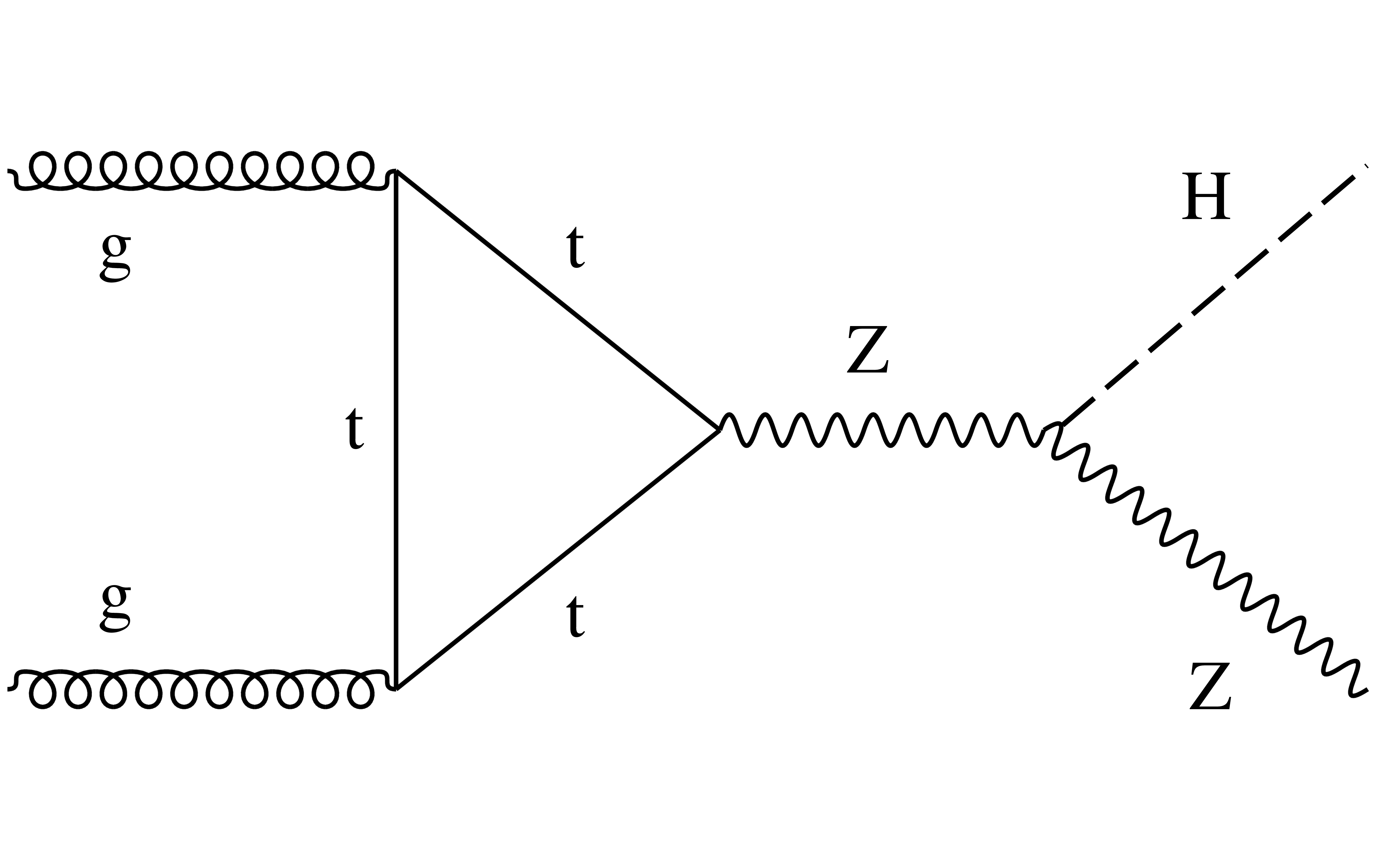
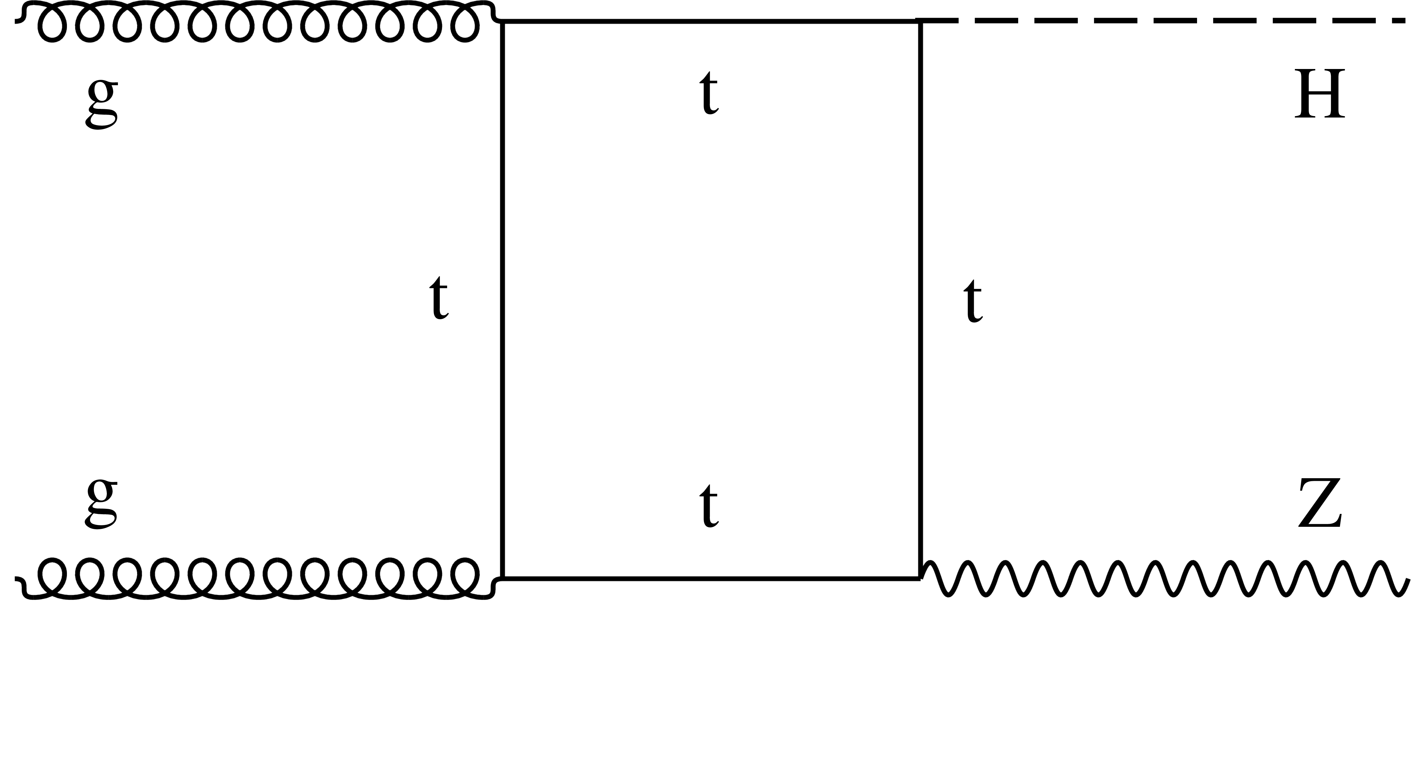
Leading-order Feynman diagrams for the $\mathrm{g} \mathrm{g} \to \mathrm{Z} \mathrm{H} $ production mode. |
png pdf |
Figure 5-a:
Leading-order Feynman diagram for the $\mathrm{g} \mathrm{g} \to \mathrm{Z} \mathrm{H} $ production mode. |
png pdf |
Figure 5-b:
Leading-order Feynman diagram for the $\mathrm{g} \mathrm{g} \to \mathrm{Z} \mathrm{H} $ production mode. |
png pdf |
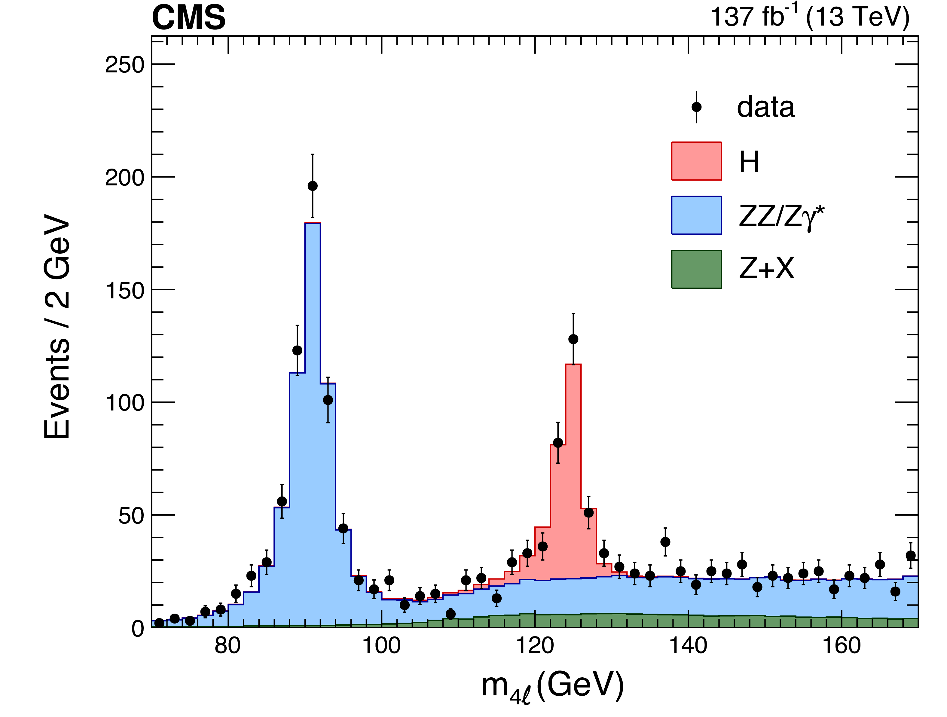
Figure 6:
Four-lepton invariant mass distribution of observed events (data points) and expectation from MC simulation or background estimates (histograms) in the region between 70 and 170 GeV [78]. The peaks from the Z and $\mathrm{H} \to 4\ell $ decays are visible near 91 and 125 GeV, respectively. |

png pdf |
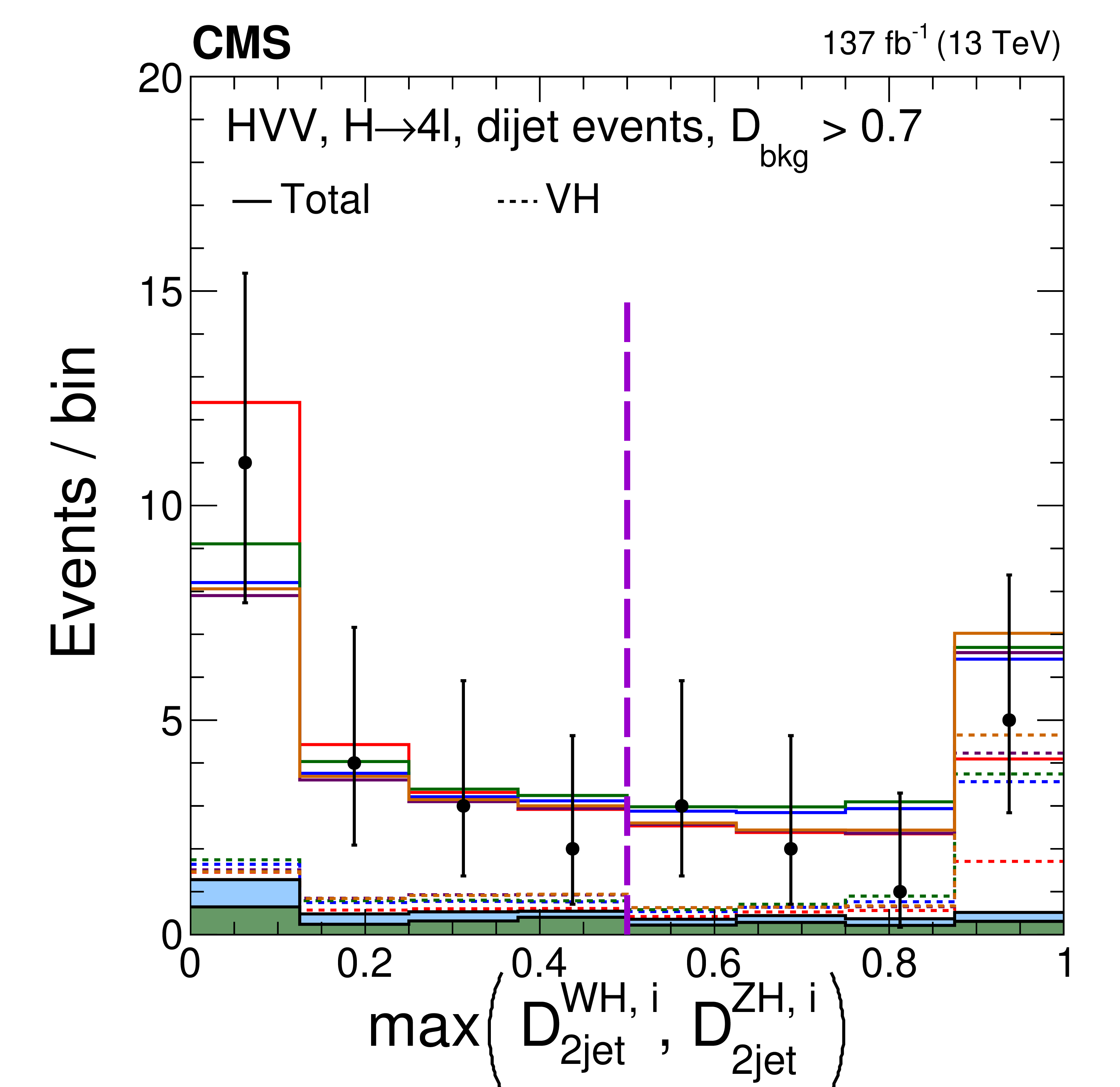
Figure 7:
The distributions of observed events (data points) and expectation (histograms) for $\max\left (\mathcal {D}_\mathrm {2jet}^{{\mathrm {VBF}},i} \right)$ (middle) and $\max\left (\mathcal {D}_\mathrm {2jet}^{{\mathrm{W} \mathrm{H}},i},\mathcal {D}_\mathrm {2jet}^{{\mathrm{Z} \mathrm{H}},i} \right)$ (right), where maximum is evaluated over the the SM and the four anomalous coupling hypotheses $i$, described in the legend (left). Only events with at least two reconstructed jets are shown, and the requirement $ {{\mathcal {D}}_{\text {bkg}}} > $ 0.7 is applied in order to enhance the signal contribution over the background, where ${{\mathcal {D}}_{\text {bkg}}}$ is calculated using decay information only. The expectation is shown for the total distribution, including background and all production mechanisms of the H boson, and for the VBF (middle) and VH (right) signals, which are enhanced in the region above 0.5, indicated with the vertical dashed line. |
png pdf |
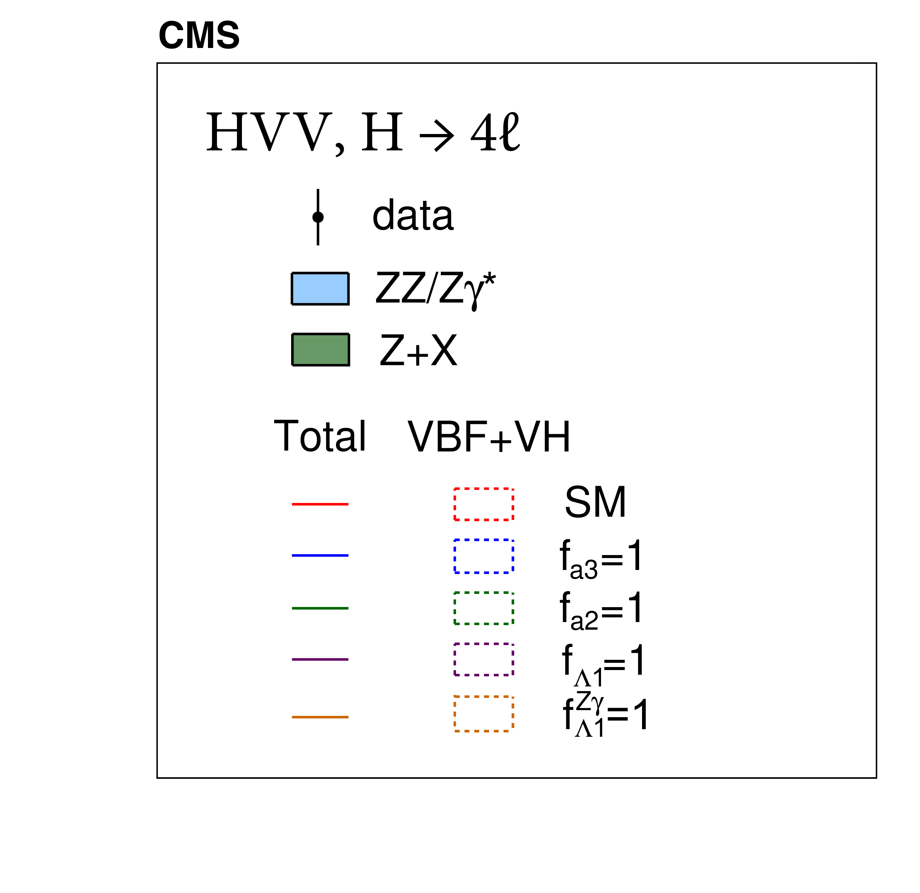
Figure 7-a:
Legend of the figure. |

png pdf |
Figure 7-b:
The distribution of observed events (data points) and expectation (histograms) for $\max\left (\mathcal {D}_\mathrm {2jet}^{{\mathrm {VBF}},i} \right)$, where maximum is evaluated over the the SM and the four anomalous coupling hypotheses $i$, described in the legend (Fig. 6-a). Only events with at least two reconstructed jets are shown, and the requirement $ {{\mathcal {D}}_{\text {bkg}}} > $ 0.7 is applied in order to enhance the signal contribution over the background, where ${{\mathcal {D}}_{\text {bkg}}}$ is calculated using decay information only. The expectation is shown for the total distribution, including background and all production mechanisms of the H boson, and for the VBF signal, which is enhanced in the region above 0.5, indicated with the vertical dashed line. |
png pdf |
Figure 7-c:
The distribution of observed events (data points) and expectation (histograms) for $\max\left (\mathcal {D}_\mathrm {2jet}^{{\mathrm{W} \mathrm{H}},i},\mathcal {D}_\mathrm {2jet}^{{\mathrm{Z} \mathrm{H}},i} \right)$, where maximum is evaluated over the the SM and the four anomalous coupling hypotheses $i$, described in the legend (Fig. 6-a). Only events with at least two reconstructed jets are shown, and the requirement $ {{\mathcal {D}}_{\text {bkg}}} > $ 0.7 is applied in order to enhance the signal contribution over the background, where ${{\mathcal {D}}_{\text {bkg}}}$ is calculated using decay information only. The expectation is shown for the total distribution, including background and all production mechanisms of the H boson, and for the VH signals, which are enhanced in the region above 0.5, indicated with the vertical dashed line. |

png pdf |
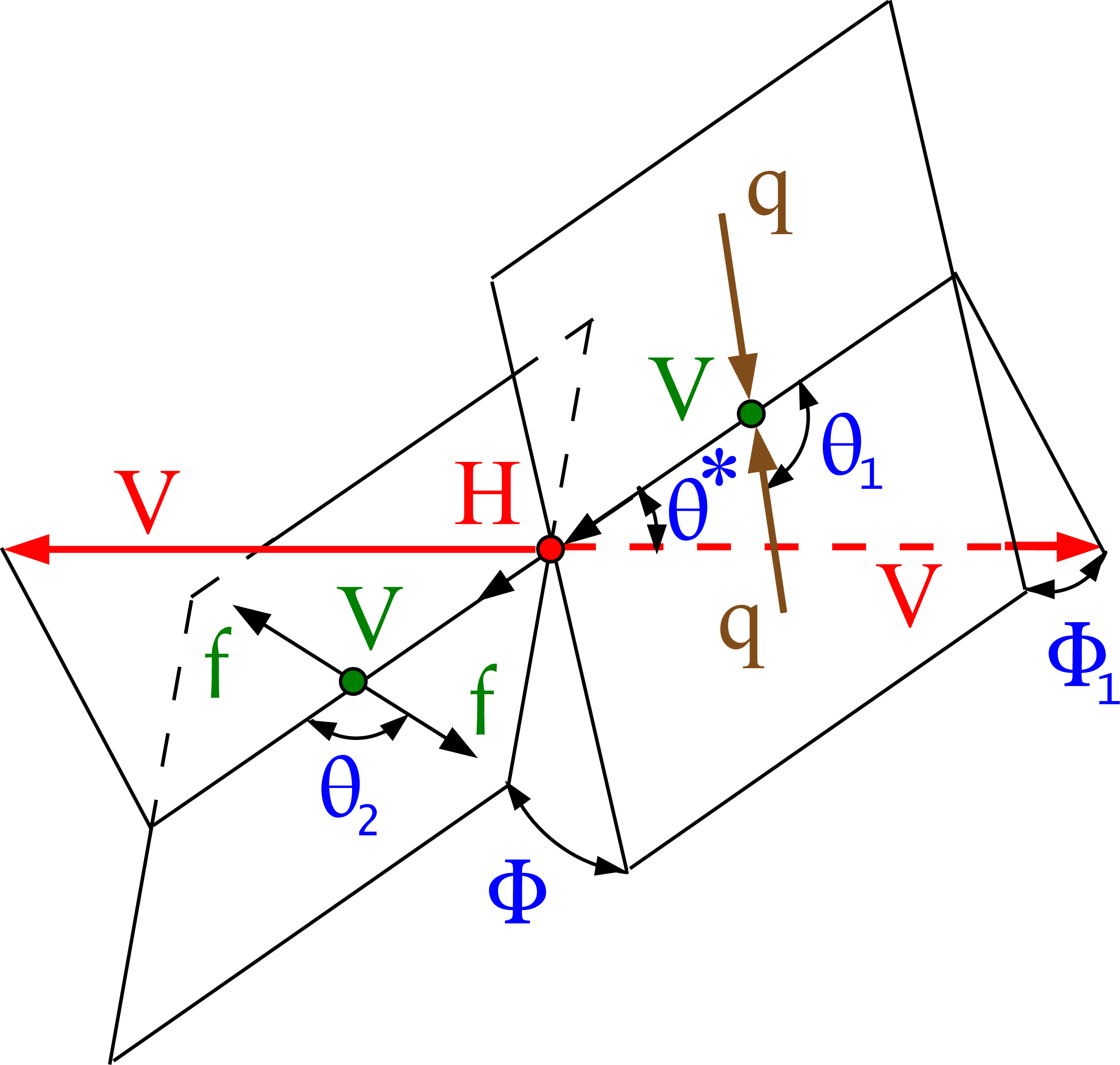
Figure 8:
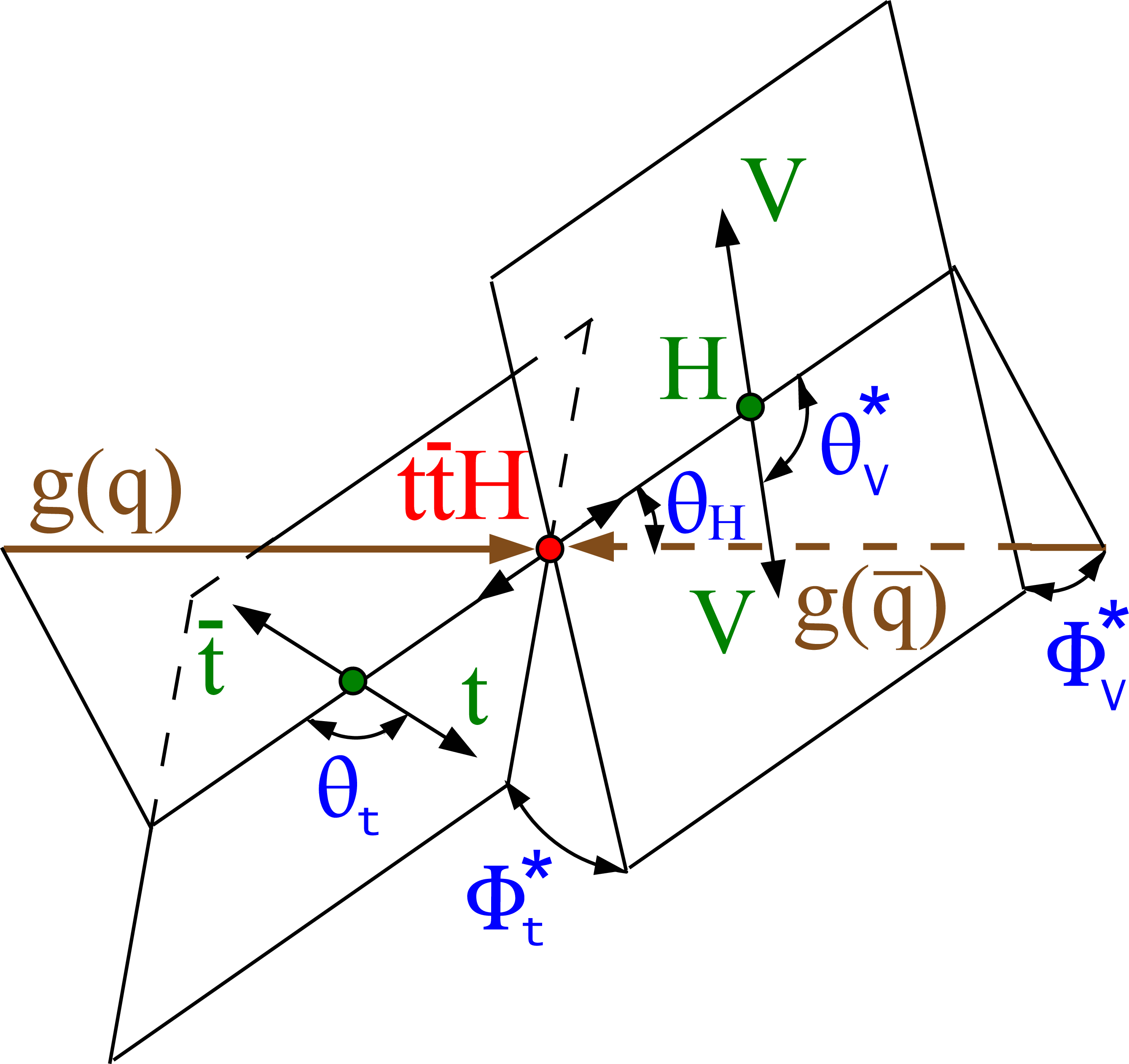
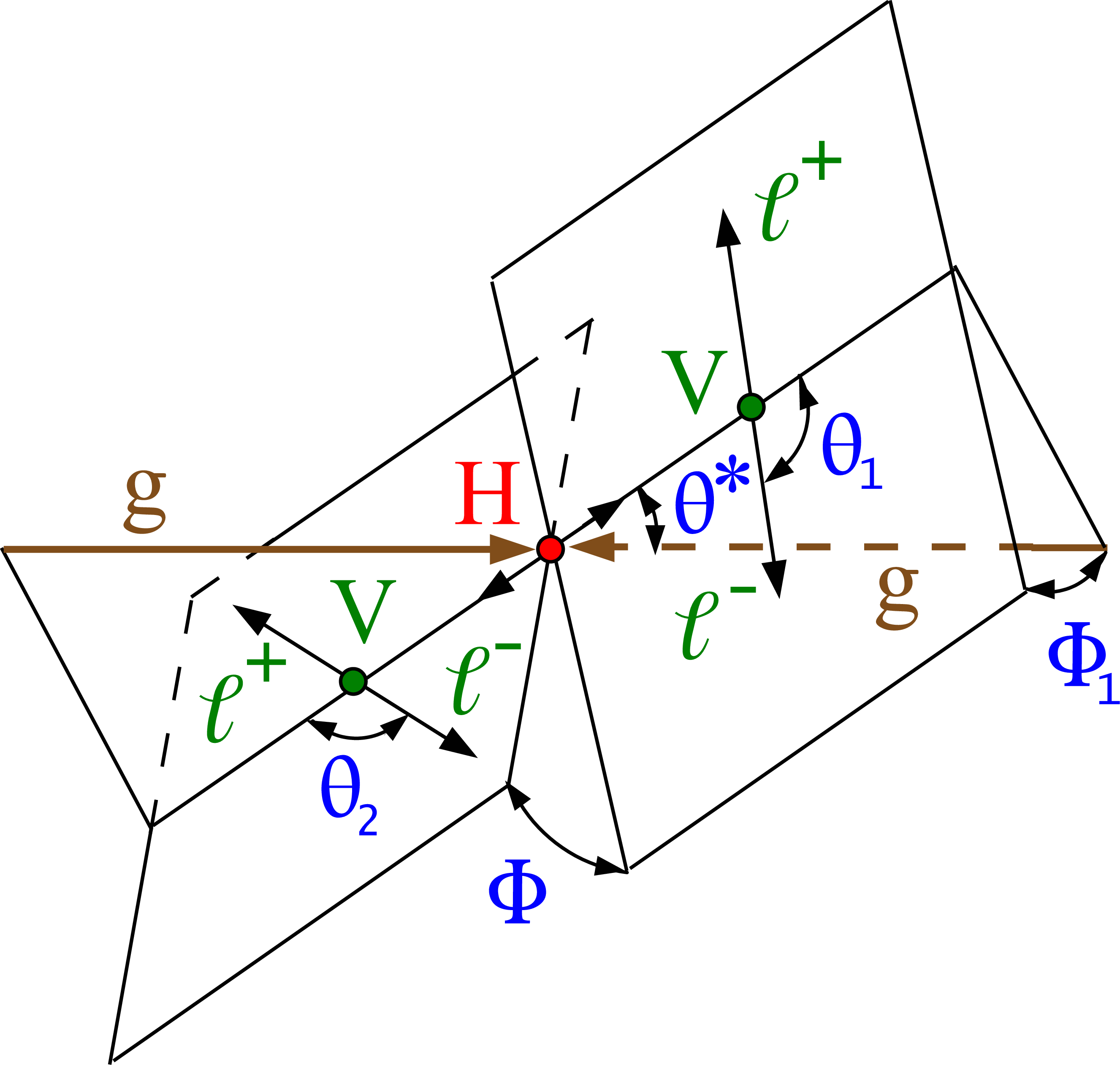
Four topologies of the H boson production and decay: gluon or EW vector boson fusion $ {\mathrm{q} \mathrm{q}} \to \mathrm{V} _1\mathrm{V} _2 ({\mathrm{q} \mathrm{q}}) \to \mathrm{H} ({\mathrm{q} \mathrm{q}}) \to ({\mathrm{V} \mathrm{V}}) ({\mathrm{q} \mathrm{q}})$ (upper left); associated production $ {\mathrm{q} \mathrm{q}} \to \mathrm{V} \to \mathrm{V} \mathrm{H} \to (\mathrm {ff})\ ({\mathrm{V} \mathrm{V}})$ (upper right); H boson production in association with the top quarks ttH or tH (lower left); and four-lepton decay $\mathrm{H} \to {\mathrm{V} \mathrm{V}} \to 4\ell $ where the incoming gluons gg indicate the collision axis (lower right), and which proceeds either with or without associated particles. The incoming partons are shown in brown and the intermediate or final-state particles are shown in red and green. The angles characterizing kinematic distributions are shown in blue and are defined in the respective rest frames [29,31,32]. The subsequent top quark decay is not shown. See Ref. [32] for details. |

png pdf |
Figure 8-a:
Topology for gluon or EW vector boson fusion H boson production, $ {\mathrm{q} \mathrm{q}} \to \mathrm{V} _1\mathrm{V} _2 ({\mathrm{q} \mathrm{q}}) \to \mathrm{H} ({\mathrm{q} \mathrm{q}}) \to ({\mathrm{V} \mathrm{V}}) ({\mathrm{q} \mathrm{q}})$. The incoming partons are shown in brown. The intermediate or final-state particles are shown in red and green. The angles characterizing kinematic distributions are shown in blue and are defined in the respective rest frames [29,31,32]. See Ref. [32] for details. |
png pdf |
Figure 8-b:
Topology for associated H boson production $ {\mathrm{q} \mathrm{q}} \to \mathrm{V} \to \mathrm{V} \mathrm{H} \to (\mathrm {ff})\ ({\mathrm{V} \mathrm{V}})$. The incoming partons are shown in brown. The intermediate or final-state particles are shown in red and green. The angles characterizing kinematic distributions are shown in blue and are defined in the respective rest frames [29,31,32]. See Ref. [32] for details. |
png pdf |
Figure 8-c:
Topology for four-lepton decay $\mathrm{H} \to {\mathrm{V} \mathrm{V}} \to 4\ell $. The incoming partons in brown indicate the collision axis. The intermediate or final-state particles are shown in red and green. The angles characterizing kinematic distributions are shown in blue and are defined in the respective rest frames [29,31,32]. The subsequent top quark decay is not shown. See Ref. [32] for details. |
png pdf |
Figure 8-d:
Topology for four-lepton decay $\mathrm{H} \to {\mathrm{V} \mathrm{V}} \to 4\ell $ where the incoming gluons gg in brown indicate the collision axis. The intermediate or final-state particles are shown in red and green. The angles characterizing kinematic distributions are shown in blue and are defined in the respective rest frames [29,31,32]. See Ref. [32] for details. |
png pdf |
Figure 9:
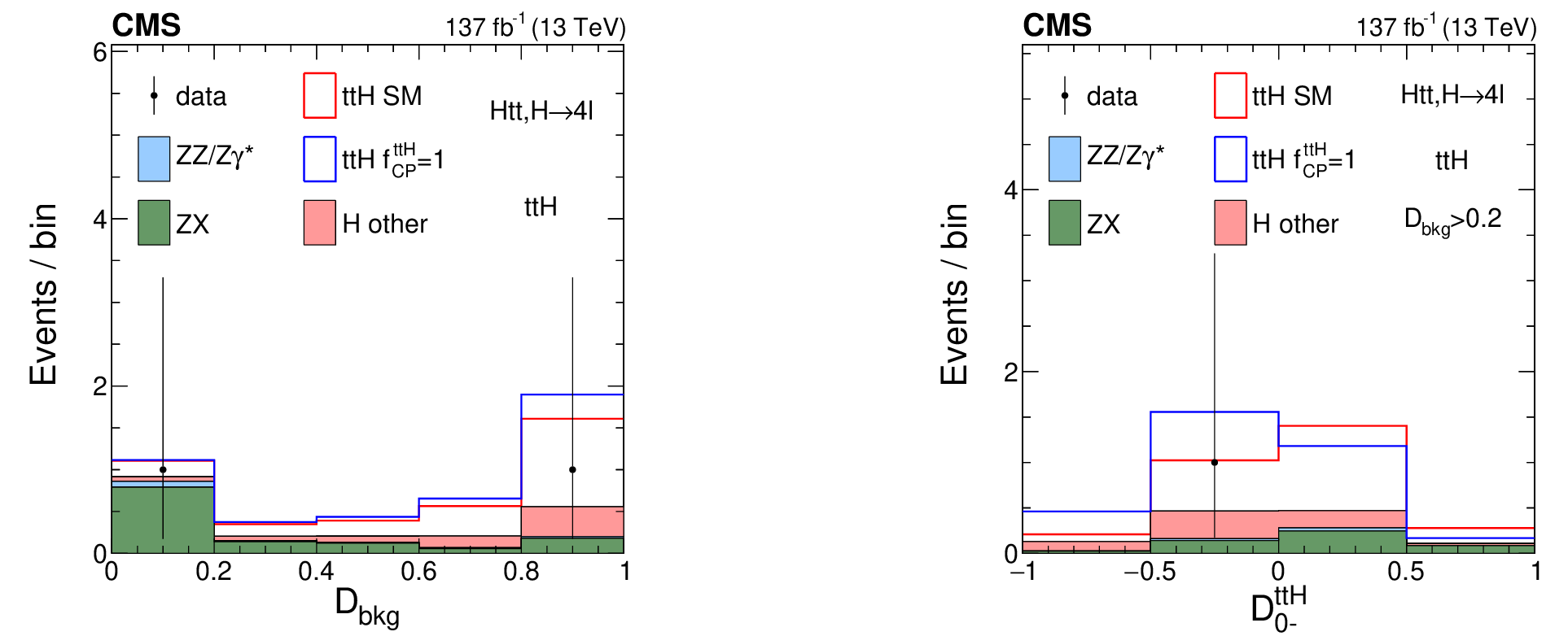
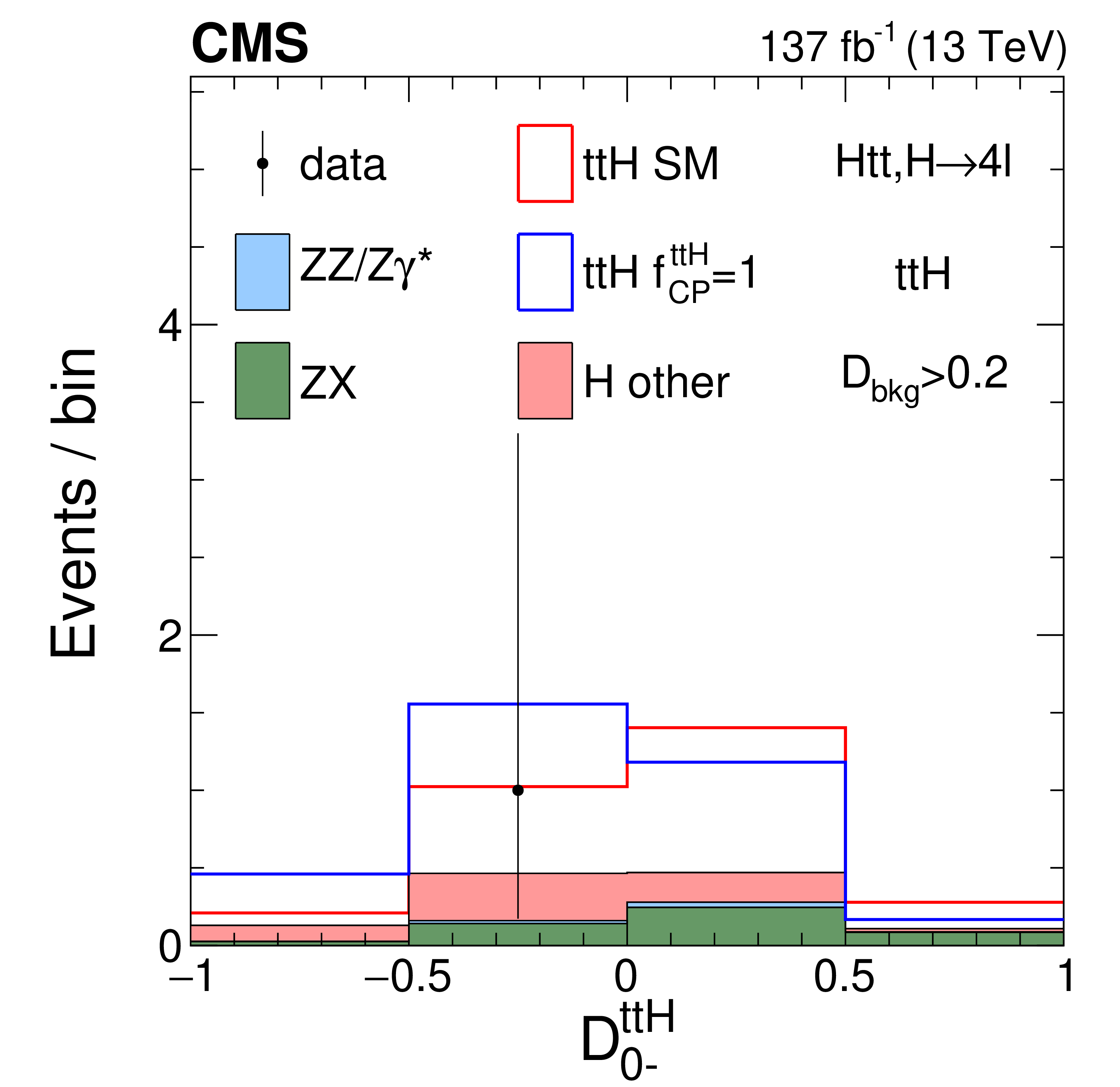
Distribution of the ${\mathcal {D}}_{\text {bkg}}$ (left) and $ \mathcal {D}_{\text {0-}}^{{{\mathrm{t} \mathrm{\bar{t}} \mathrm{H}}}}$ (right), discriminants in the sum of the ttH-leptonic and ttH-hadronic categories in Scheme 1. The latter distribution is shown with the requirement $ {{\mathcal {D}}_{\text {bkg}}} > $ 0.2 in order to enhance the signal over the background contribution. |

png pdf |
Figure 9-a:
Distribution of the ${\mathcal {D}}_{\text {bkg}}$ discriminant in the sum of the ttH-leptonic and ttH-hadronic categories in Scheme 1. |
png pdf |
Figure 9-b:
Distribution of the $ \mathcal {D}_{\text {0-}}^{{{\mathrm{t} \mathrm{\bar{t}} \mathrm{H}}}}$ discriminant in the sum of the ttH-leptonic and ttH-hadronic categories in Scheme 1. The distribution is shown with the requirement $ {{\mathcal {D}}_{\text {bkg}}} > $ 0.2 in order to enhance the signal over the background contribution. |
png pdf |
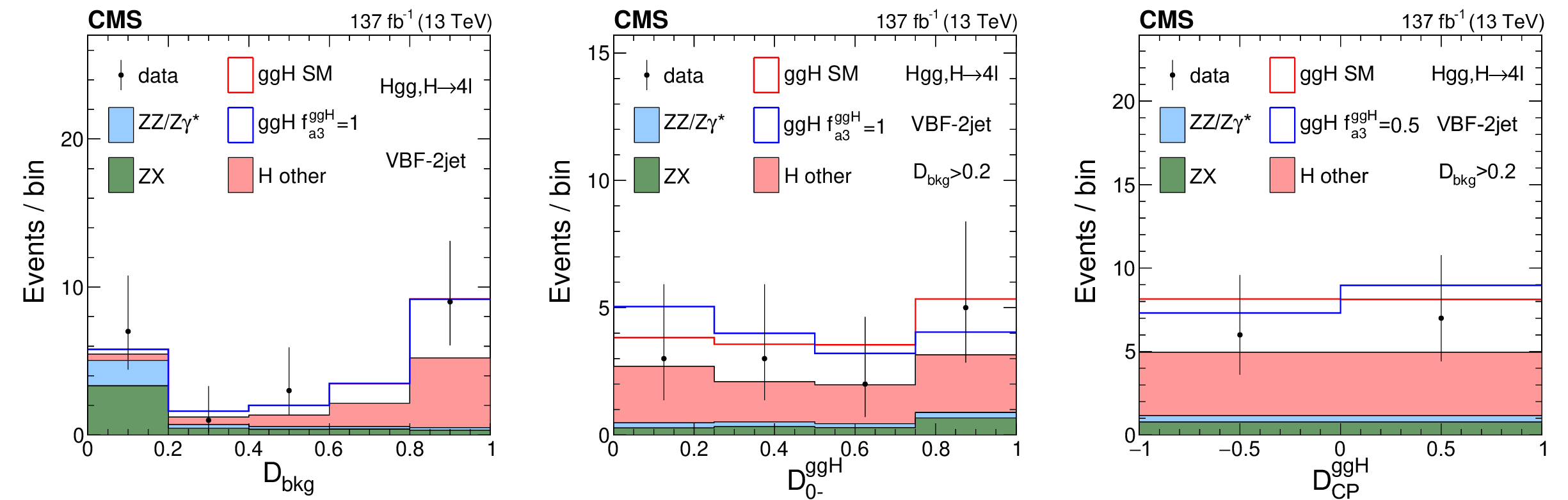
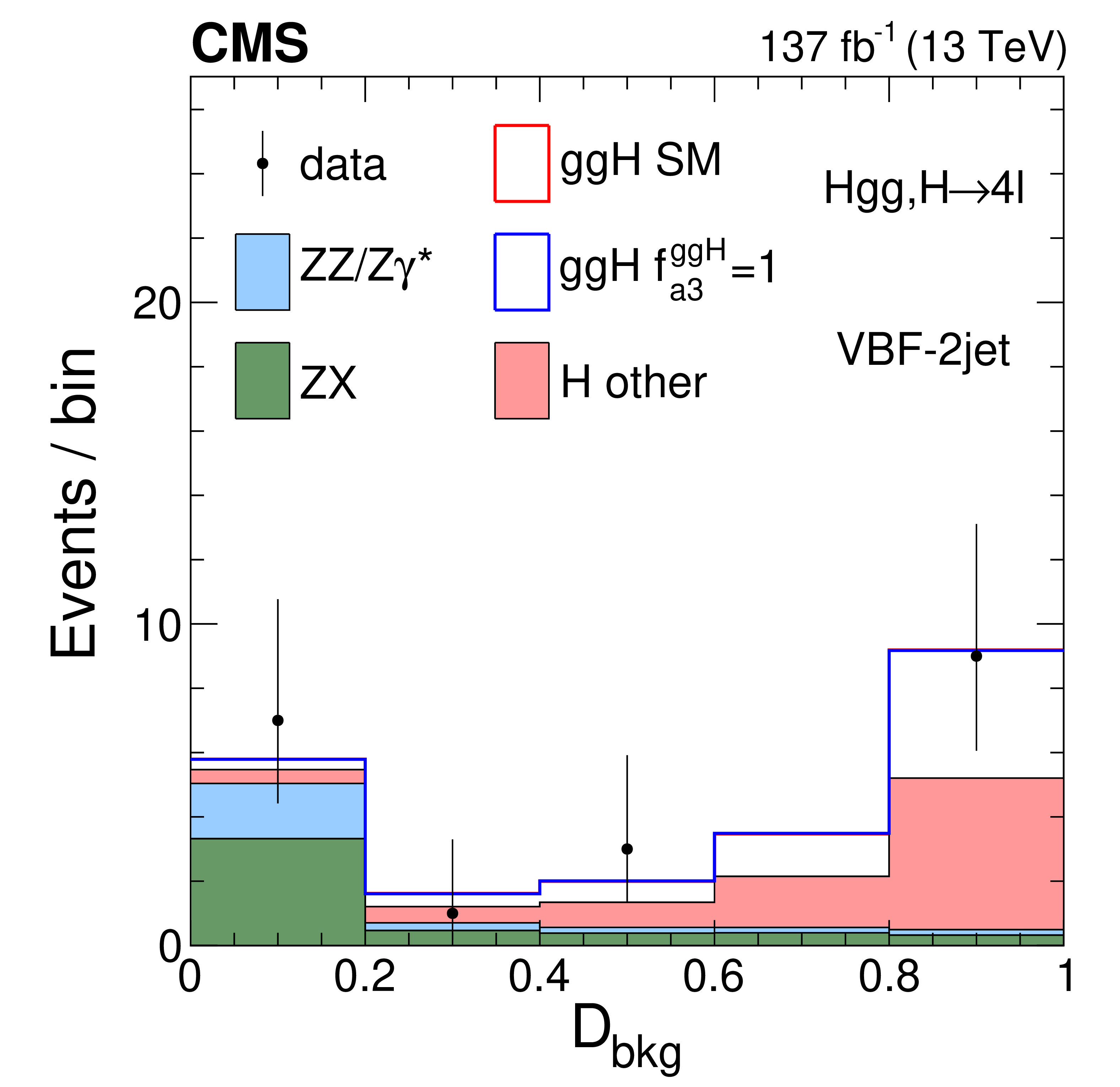
Figure 10:
Distribution of the ${{\mathcal {D}}_{\text {bkg}}}$ (left), $\mathcal {D}_\text {0-}^{{\mathrm{g} \mathrm{g} \mathrm{H}}}$ (middle), and $\mathcal {D}_{\text {CP}}^{{\mathrm{g} \mathrm{g} \mathrm{H}}}$ (right) discriminants in the VBF-2jet category in Scheme 1. The latter two distributions are shown with the requirement $ {{\mathcal {D}}_{\text {bkg}}} > $ 0.2 in order to enhance the signal over the background contribution. |
png pdf |
Figure 10-a:
Distribution of the ${{\mathcal {D}}_{\text {bkg}}}$ discriminant in the VBF-2jet category in Scheme 1. |
png pdf |
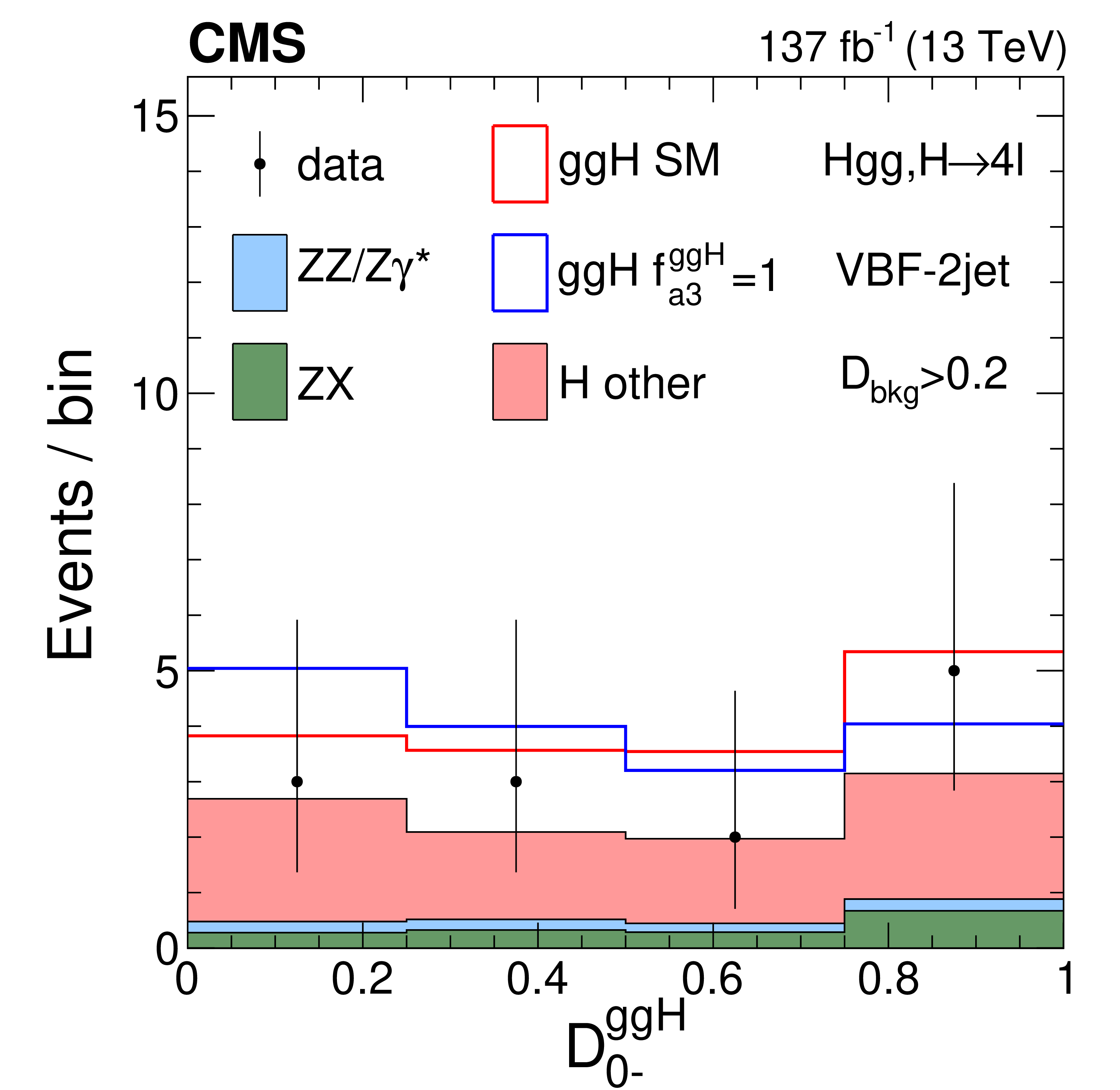
Figure 10-b:
Distribution of the $\mathcal {D}_\text {0-}^{{\mathrm{g} \mathrm{g} \mathrm{H}}}$ discriminant in the VBF-2jet category in Scheme 1. The distribution is shown with the requirement $ {{\mathcal {D}}_{\text {bkg}}} > $ 0.2 in order to enhance the signal over the background contribution. |
png pdf |
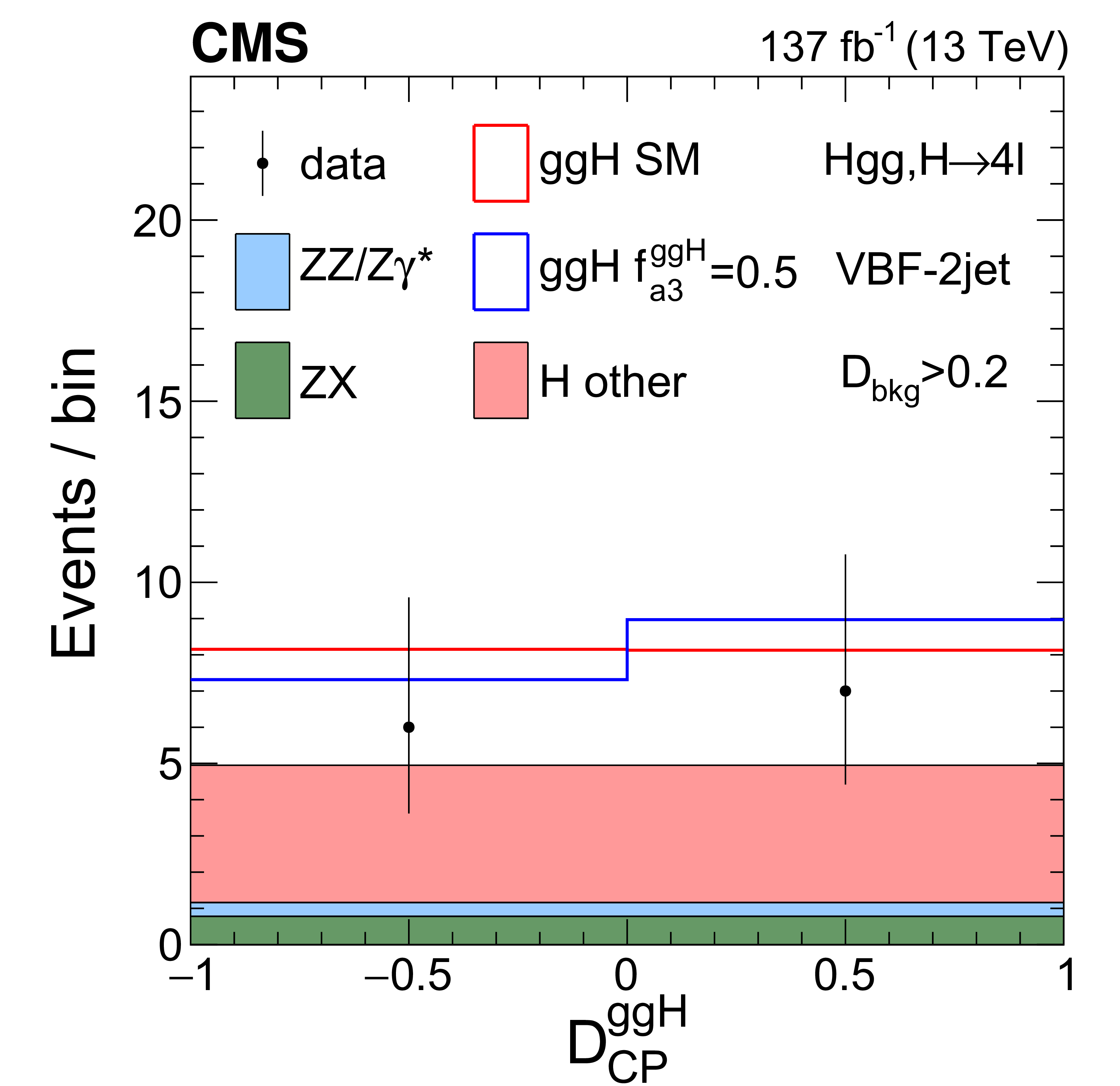
Figure 10-c:
Distribution of the $\mathcal {D}_{\text {CP}}^{{\mathrm{g} \mathrm{g} \mathrm{H}}}$ discriminant in the VBF-2jet category in Scheme 1. The distribution is shown with the requirement $ {{\mathcal {D}}_{\text {bkg}}} > $ 0.2 in order to enhance the signal over the background contribution. |
png pdf |
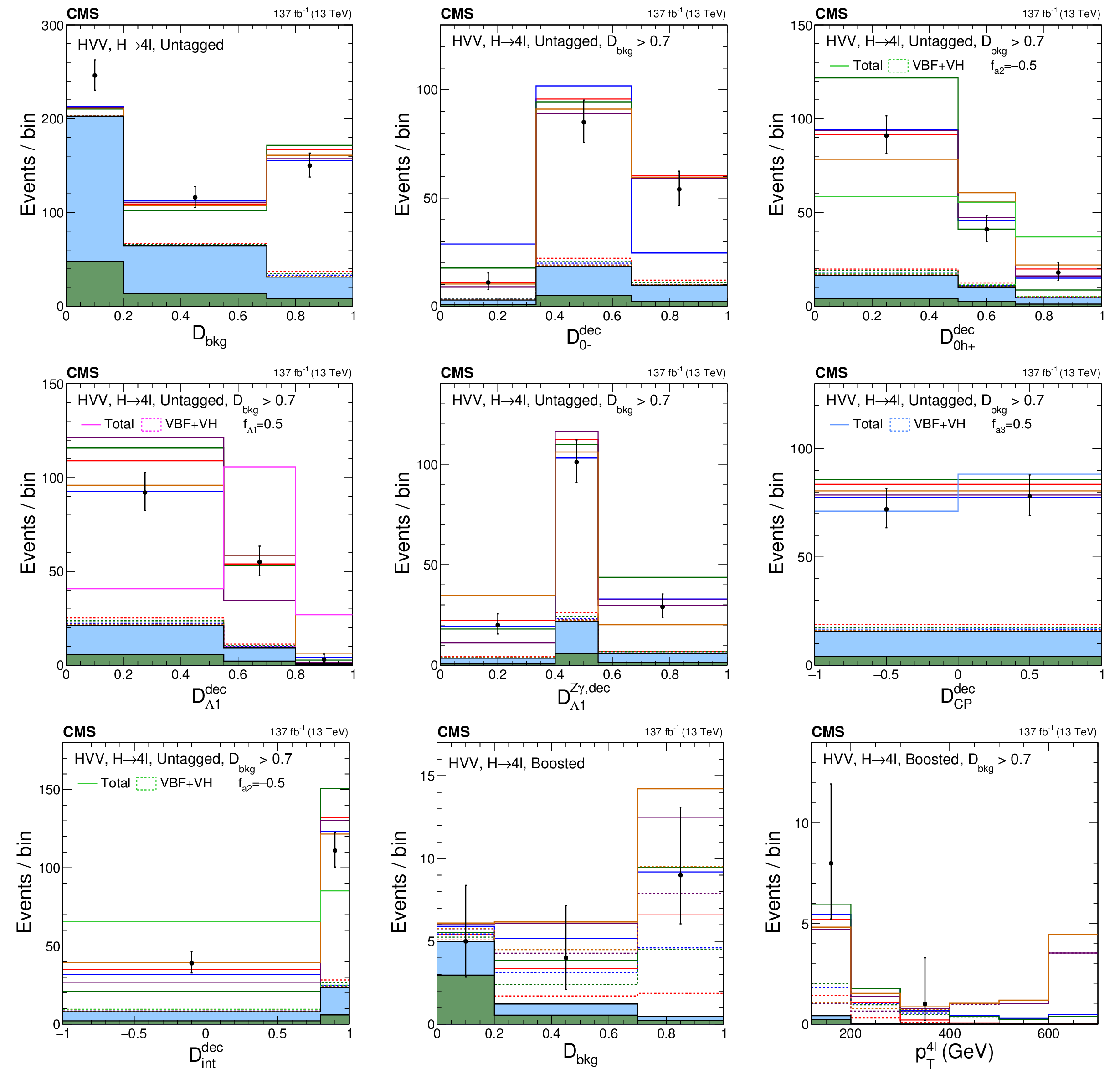
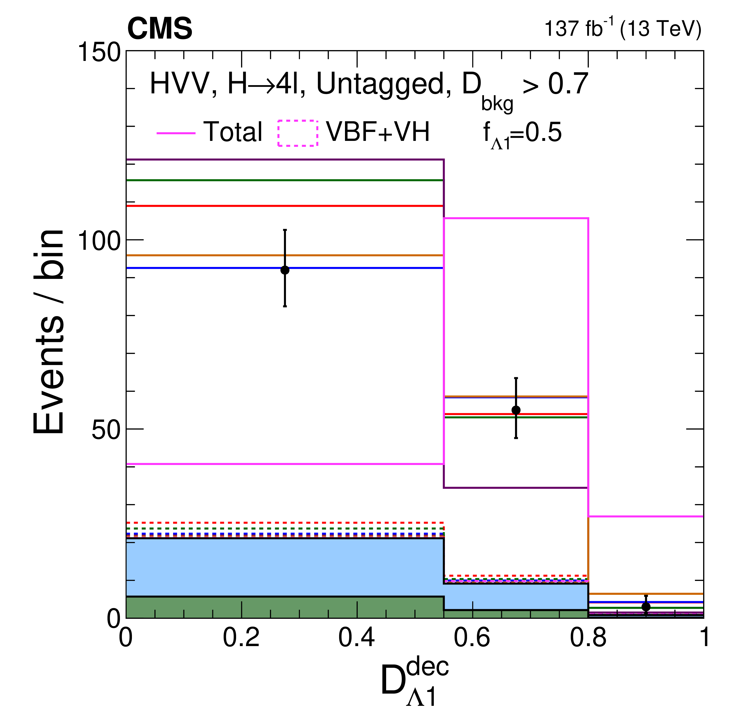
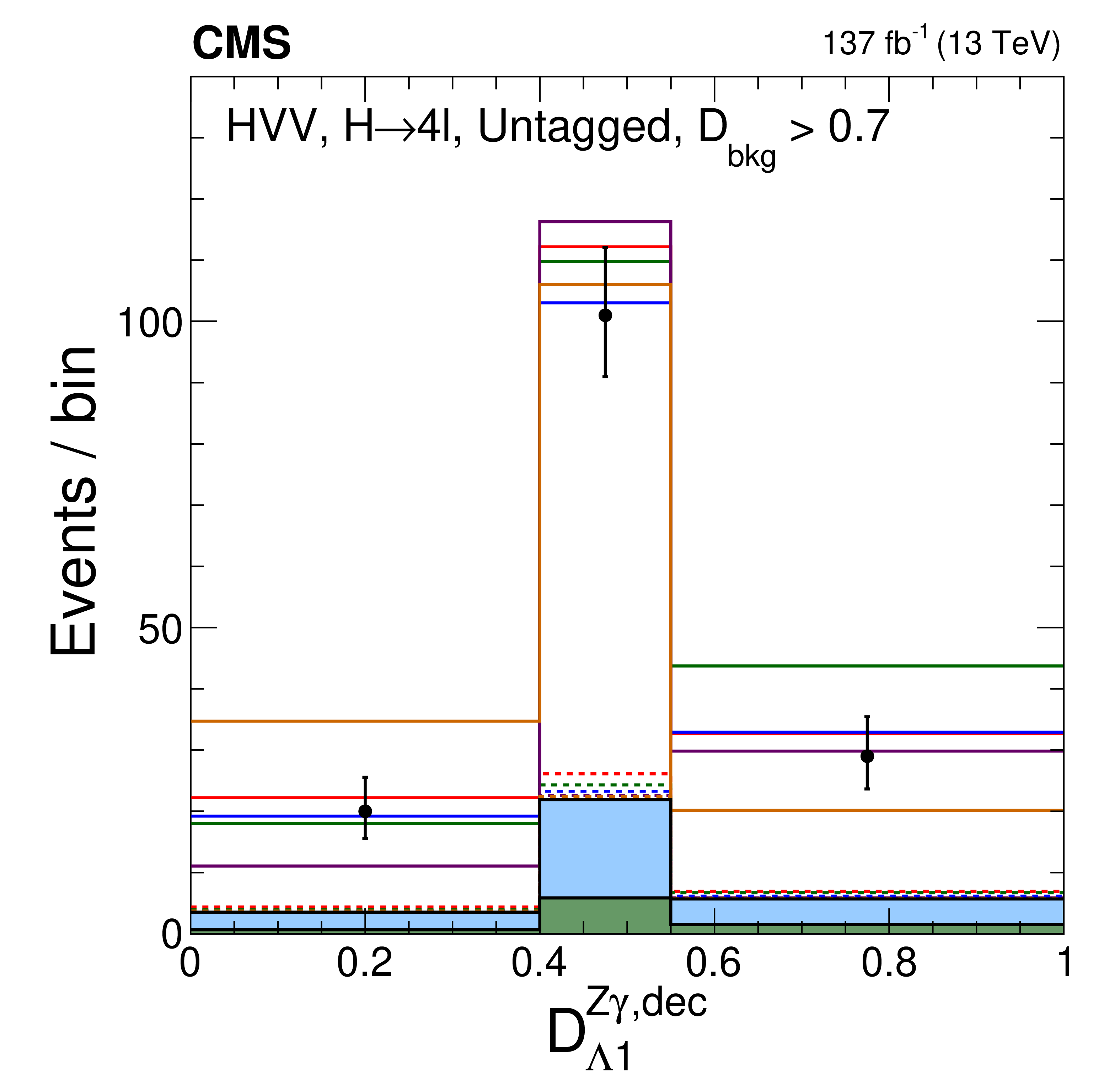
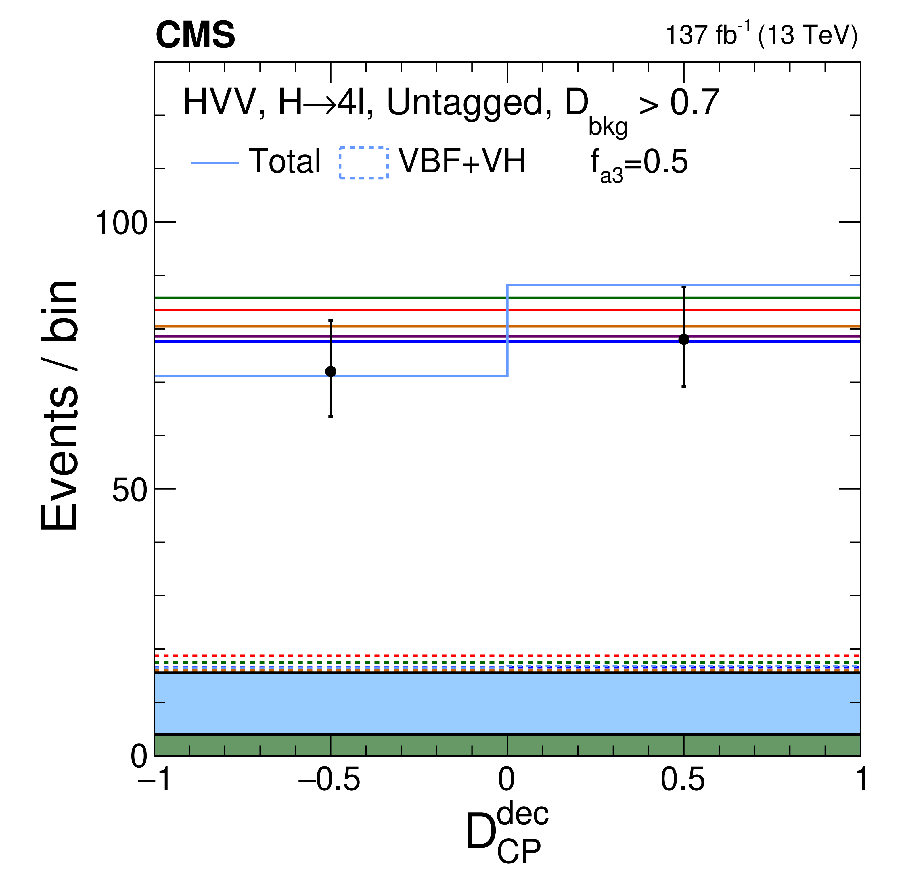
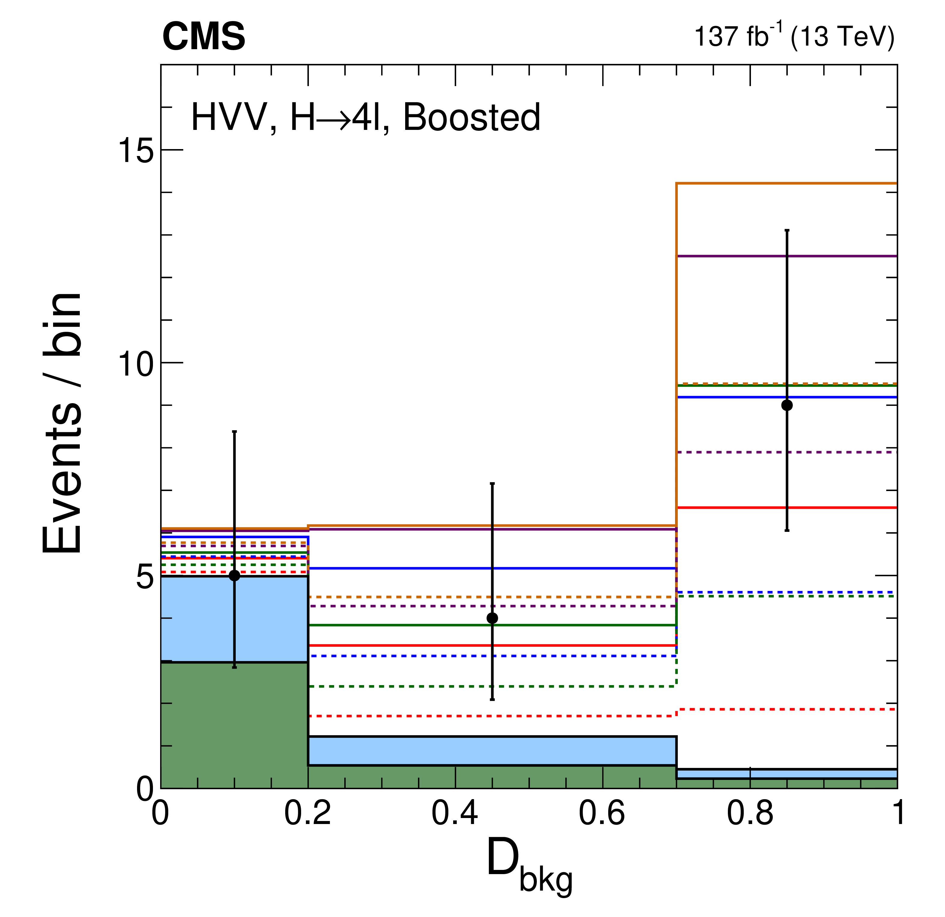
Figure 11:
Distributions of events in the observables used in categorization Scheme 2. The first seven plots are in the Untagged category: The upper left plot shows ${{\mathcal {D}}_{\text {bkg}}}$. The rest of the distributions are shown with the requirement $ {{\mathcal {D}}_{\text {bkg}}} > $ 0.7 in order to enhance the signal over the background contribution: $\mathcal {D}_{0-}^{\text {dec}}$ (upper middle), $\mathcal {D}_{0h+}^{\text {dec}}$ (upper right), $\mathcal {D}_{\Lambda 1}^{\text {dec}}$ (middle left), $\mathcal {D}_{\Lambda 1}^{\mathrm{Z} \gamma, \text {dec}}$ (middle middle), $\mathcal {D}_{\mathrm {CP}}^{\text {dec}}$, and $\mathcal {D}_\text {int}^{\text {dec}}$. The last two plots are shown in the Boosted category: ${{\mathcal {D}}_{\text {bkg}}}$ (lower middle) and $ {p_{\mathrm {T}}} ^{4\ell}$ with the requirement $ {{\mathcal {D}}_{\text {bkg}}} > $ 0.7 and overflow events included in the last bin (lower right). Observed data, background expectation, and five signal models are shown in the plots, as indicated in the legend of Fig. 7. In several cases, a sixth signal model with a mixture of the SM and BSM couplings is shown and is indicated in the legend explicitly. |
png pdf |
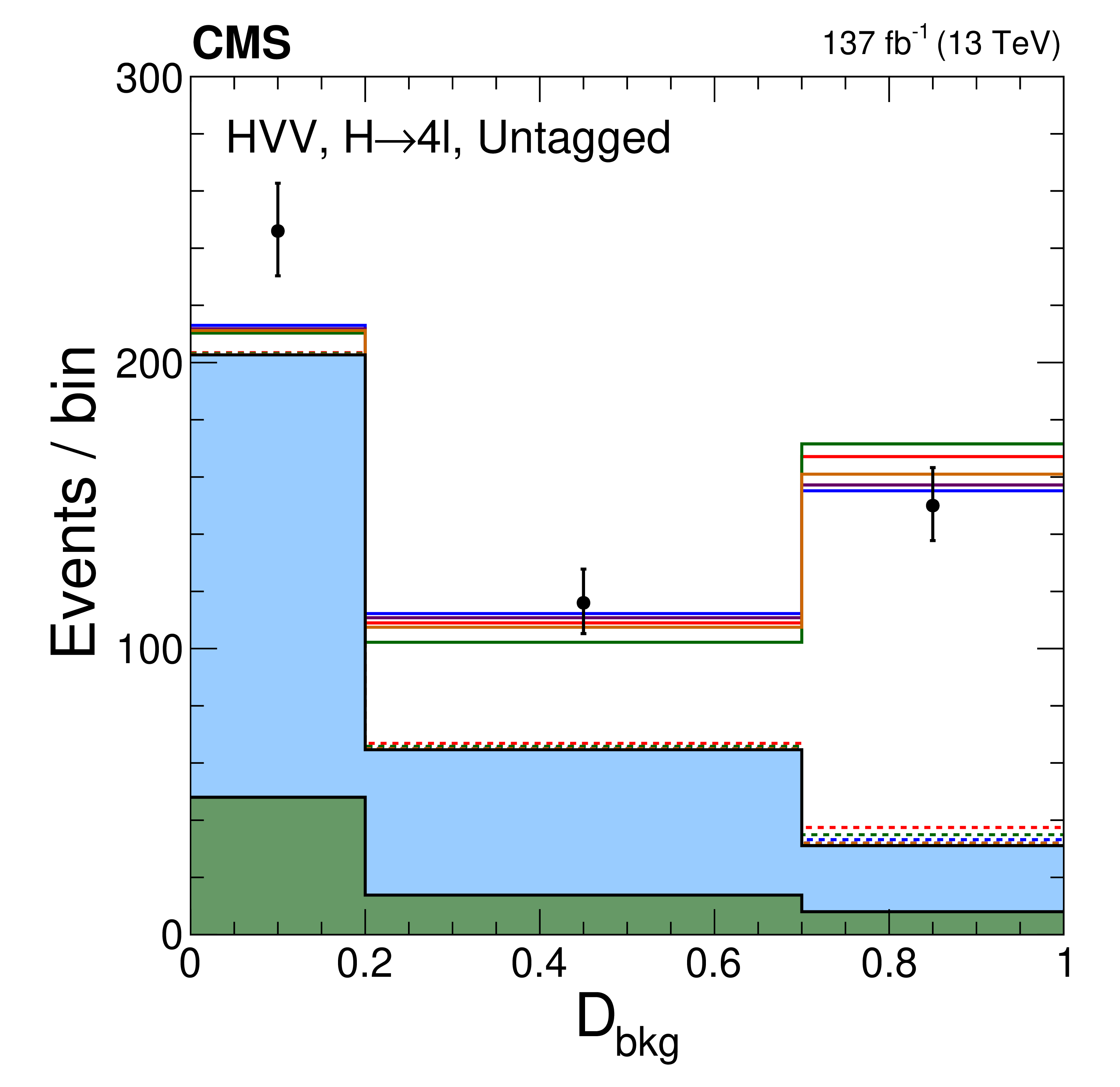
Figure 11-a:
Distribution of events for ${{\mathcal {D}}_{\text {bkg}}}$ in the Untagged category. Observed data, background expectation, and five signal models are shown in the plot, as indicated in the legend of Fig. 7. |
png pdf |
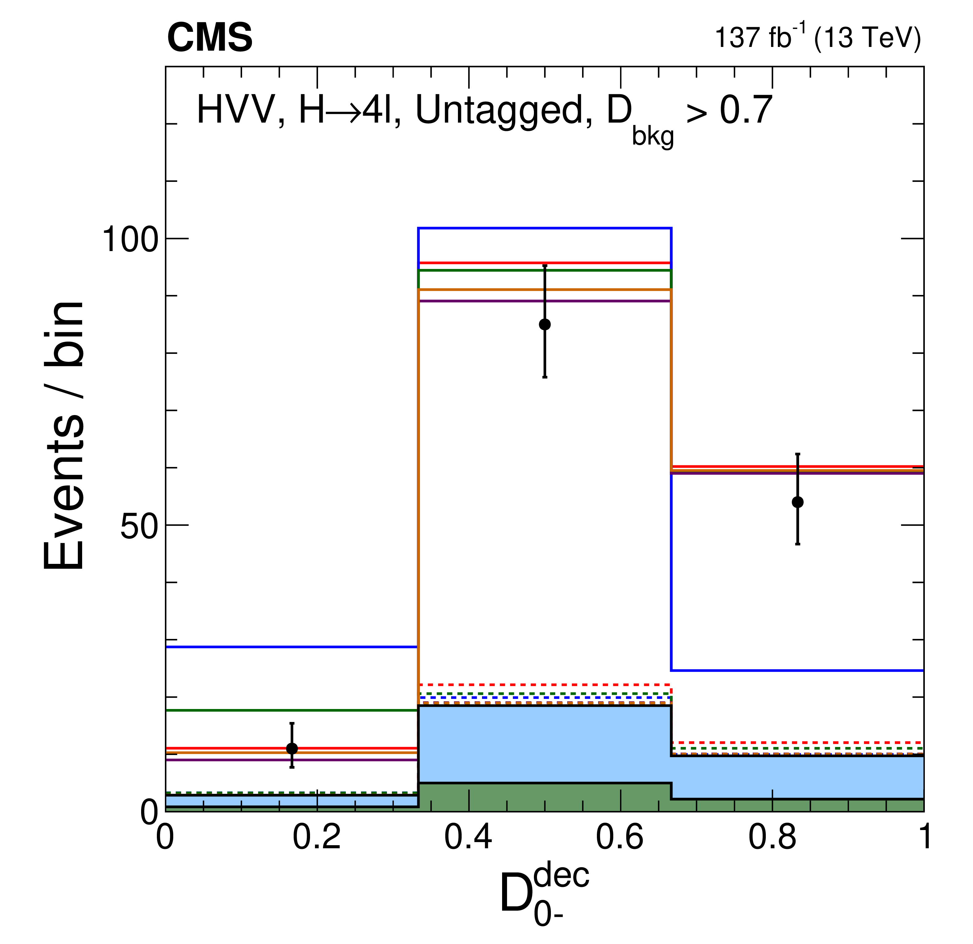
Figure 11-b:
Distribution of events for $\mathcal {D}_{0-}^{\text {dec}}$ in the Untagged category, with the requirement $ {{\mathcal {D}}_{\text {bkg}}} > $ 0.7 in order to enhance the signal over the background contribution. Observed data, background expectation, and five signal models are shown in the plot, as indicated in the legend of Fig. 7. |
png pdf |
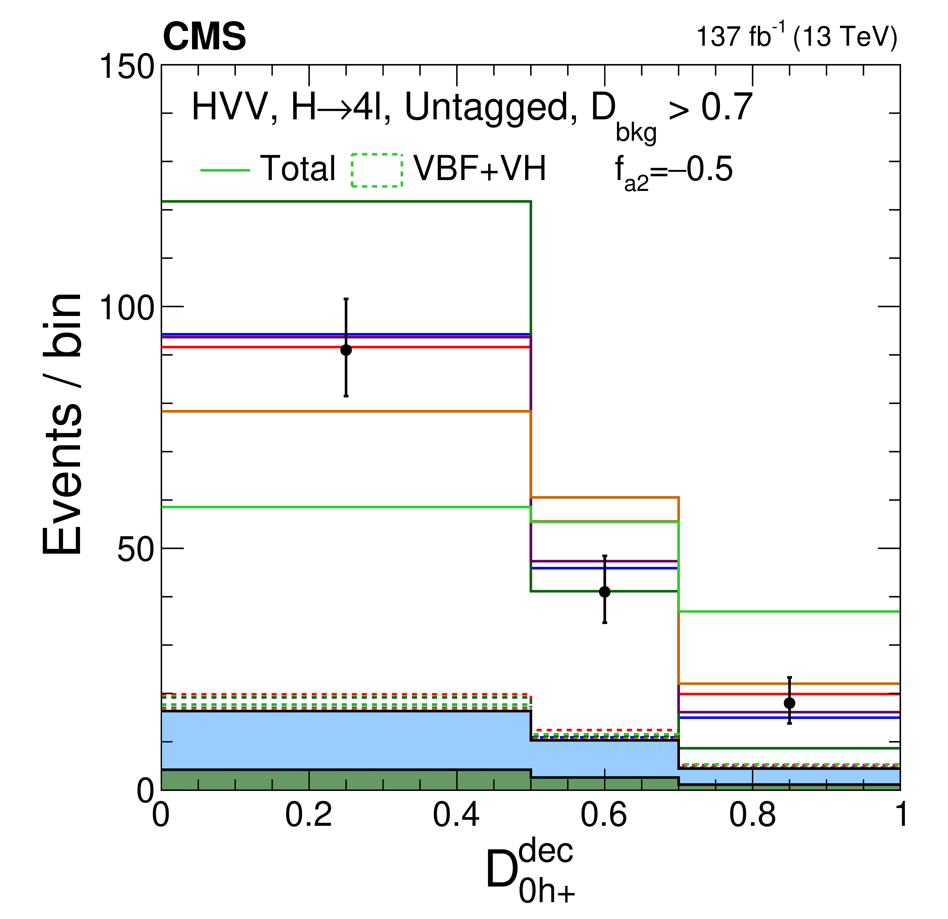
Figure 11-c:
Distribution of events for $\mathcal {D}_{0h+}^{\text {dec}}$ in the Untagged category, with the requirement $ {{\mathcal {D}}_{\text {bkg}}} > $ 0.7 in order to enhance the signal over the background contribution. Observed data, background expectation, and five signal models are shown in the plot, as indicated in the legend of Fig. 7. A sixth signal model with a mixture of the SM and BSM couplings is shown and is indicated in the legend explicitly. |
png pdf |
Figure 11-d:
Distribution of events for $\mathcal {D}_{\Lambda 1}^{\text {dec}}$ in the Untagged category, with the requirement $ {{\mathcal {D}}_{\text {bkg}}} > $ 0.7 in order to enhance the signal over the background contribution. Observed data, background expectation, and five signal models are shown in the plot, as indicated in the legend of Fig. 7. A sixth signal model with a mixture of the SM and BSM couplings is shown and is indicated in the legend explicitly. |
png pdf |
Figure 11-e:
Distribution of events for $\mathcal {D}_{\Lambda 1}^{\mathrm{Z} \gamma, \text {dec}}$ in the Boosted category, with the requirement $ {{\mathcal {D}}_{\text {bkg}}} > $ 0.7 and overflow events included in the last bin (lower right). Observed data, background expectation, and five signal models are shown in the plot, as indicated in the legend of Fig. 7. |
png pdf |
Figure 11-f:
Distribution of events for $\mathcal {D}_{\mathrm {CP}}^{\text {dec}}$ in the Untagged category, with the requirement $ {{\mathcal {D}}_{\text {bkg}}} > $ 0.7 in order to enhance the signal over the background contribution. Observed data, background expectation, and five signal models are shown in the plot, as indicated in the legend of Fig. 7. A sixth signal model with a mixture of the SM and BSM couplings is shown and is indicated in the legend explicitly. |

png pdf |
Figure 11-g:
Distribution of events for $\mathcal {D}_\text {int}^{\text {dec}}$ in the Untagged category, with the requirement $ {{\mathcal {D}}_{\text {bkg}}} > $ 0.7 in order to enhance the signal over the background contribution. Observed data, background expectation, and five signal models are shown in the plot, as indicated in the legend of Fig. 7. A sixth signal model with a mixture of the SM and BSM couplings is shown and is indicated in the legend explicitly. |
png pdf |
Figure 11-h:
Distribution of events for ${{\mathcal {D}}_{\text {bkg}}}$ in the Boosted category, with the requirement $ {{\mathcal {D}}_{\text {bkg}}} > $ 0.7. Observed data, background expectation, and five signal models are shown in the plot, as indicated in the legend of Fig. 7. |

png pdf |
Figure 11-i:
Distribution of events for $ {p_{\mathrm {T}}} ^{4\ell}$ in the Boosted category, with the requirement $ {{\mathcal {D}}_{\text {bkg}}} > $ 0.7. The overflow events included in the last bin. Observed data, background expectation, and five signal models are shown in the plot, as indicated in the legend of Fig. 7. |

png pdf |
Figure 12:
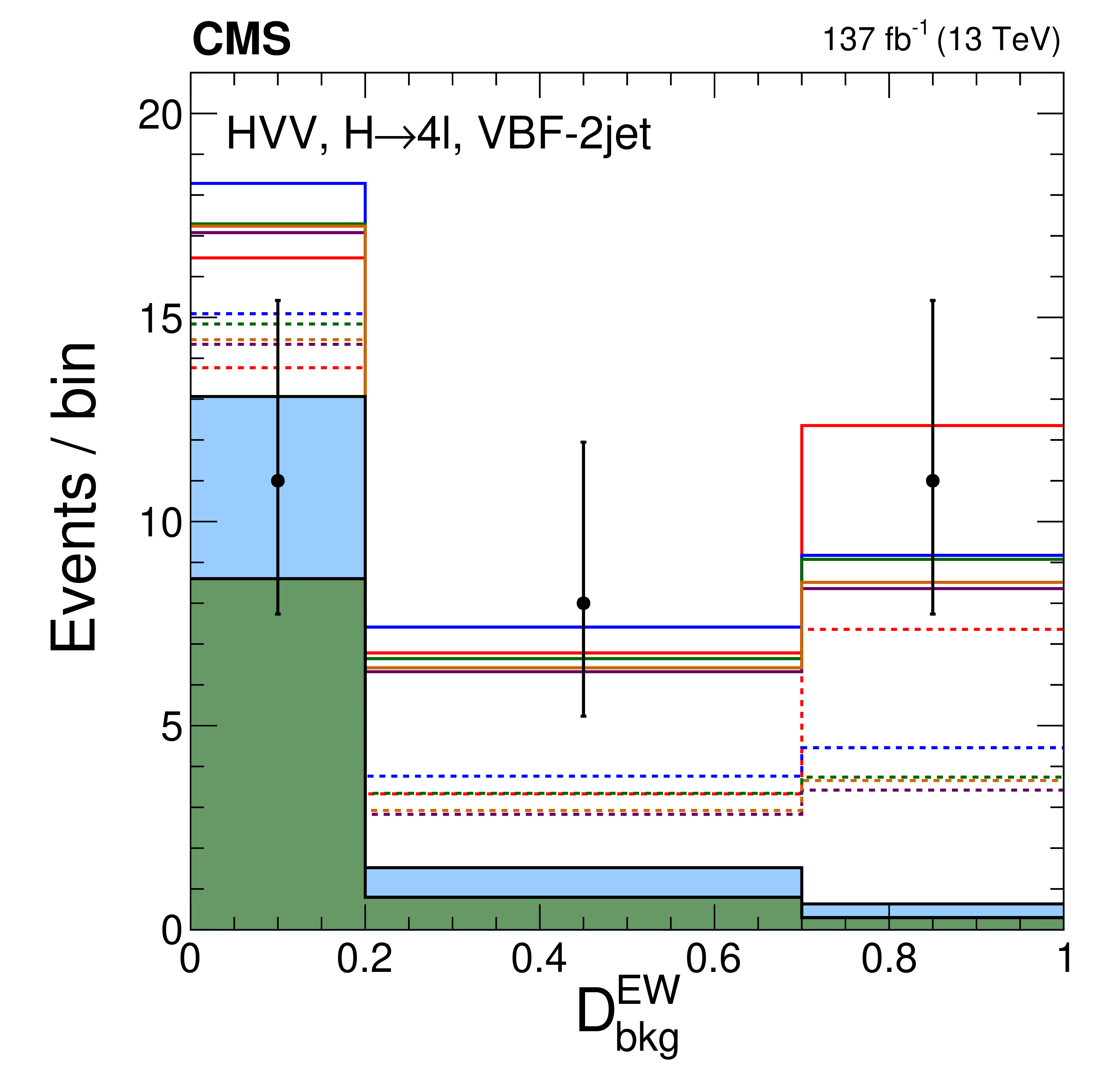
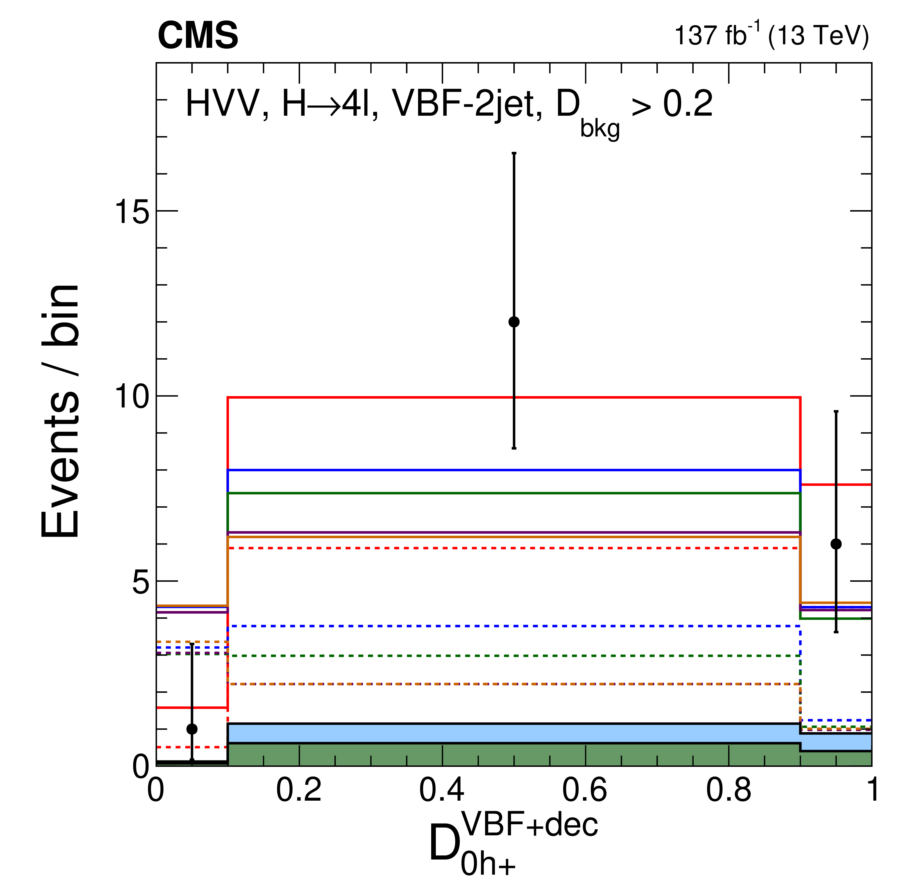
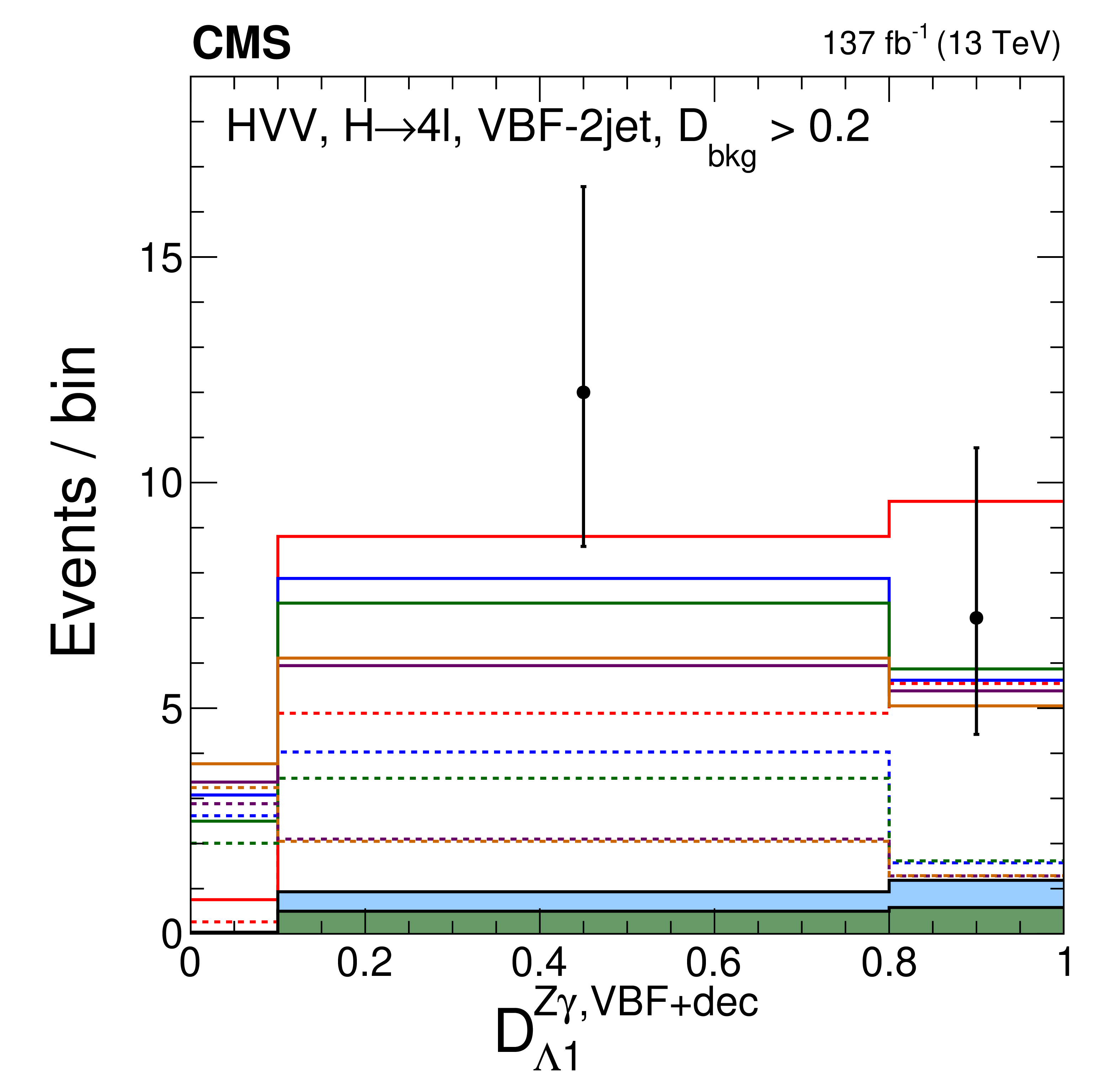
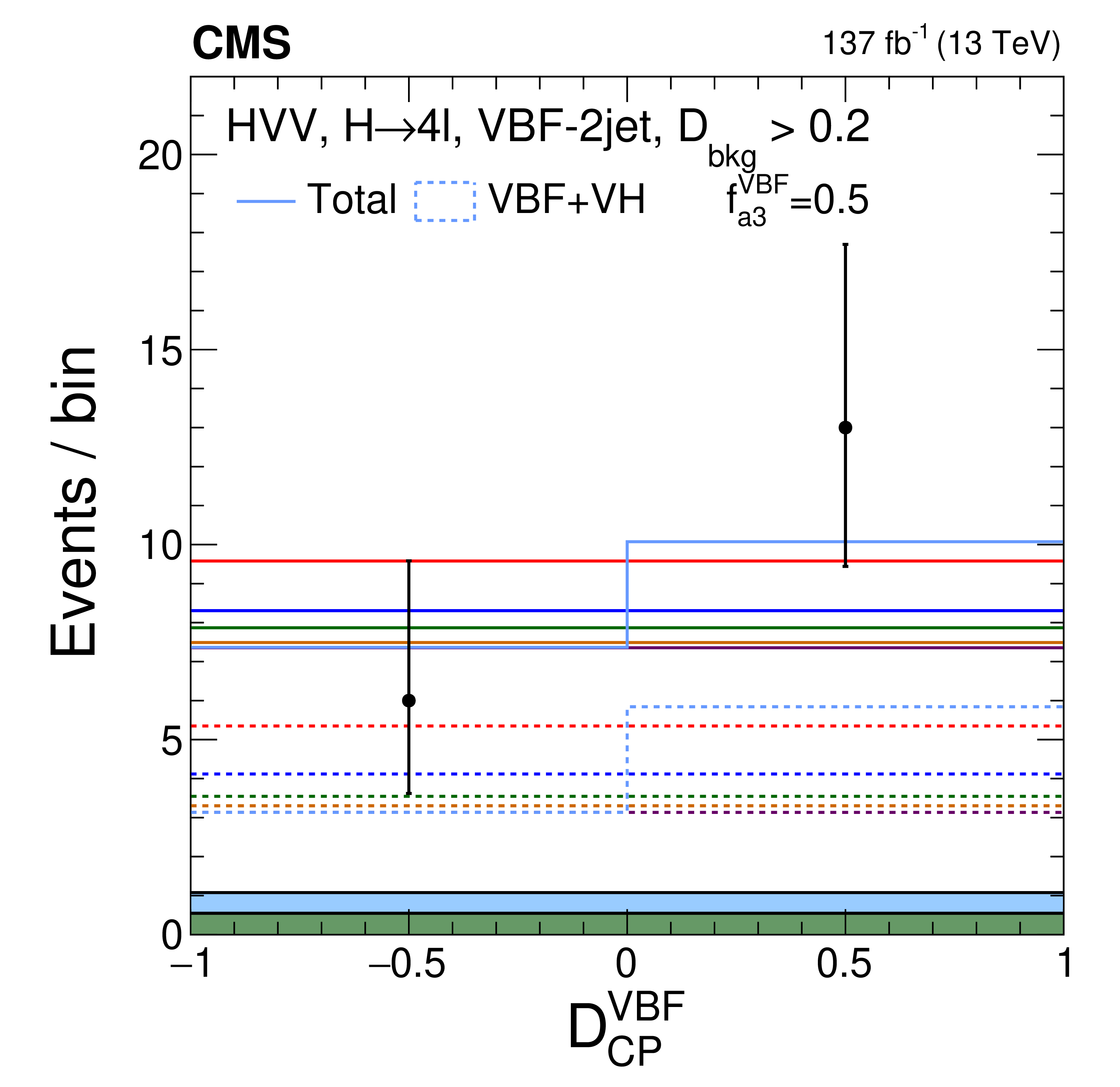
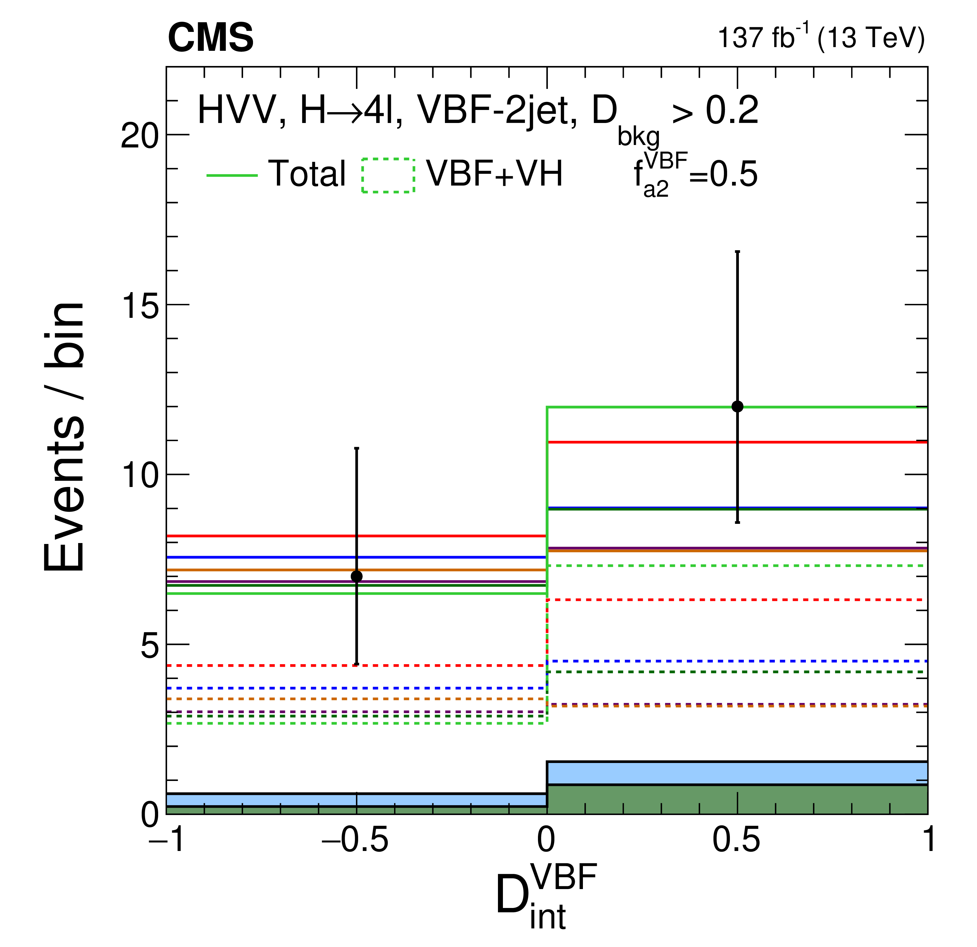
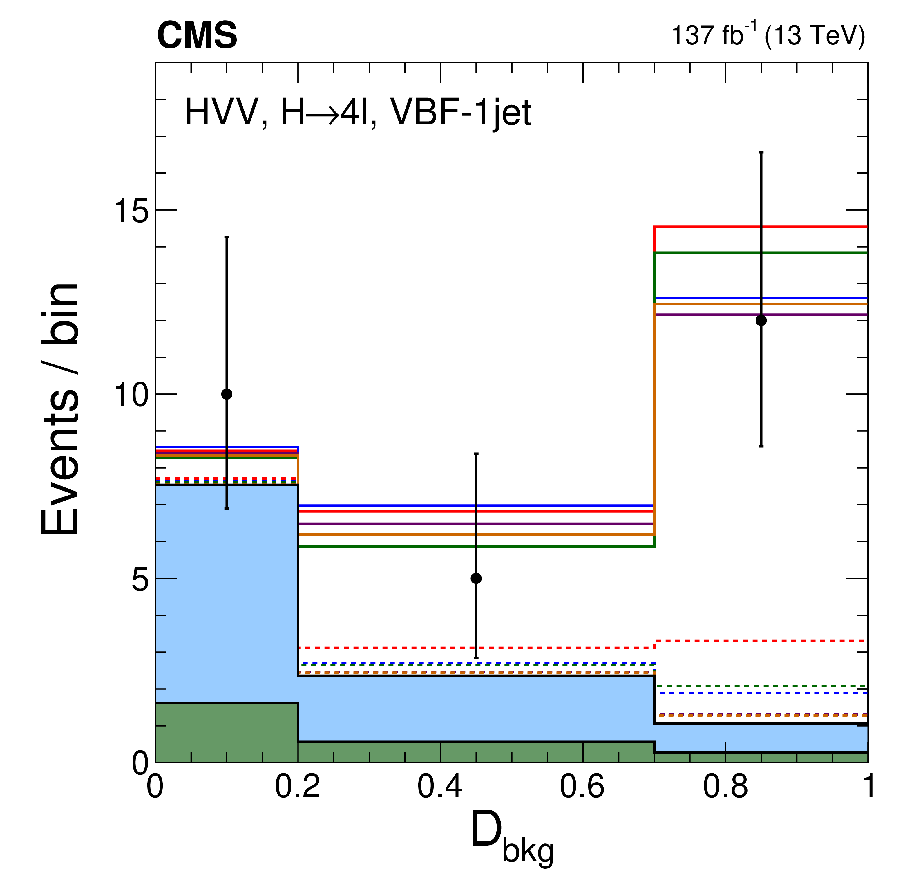
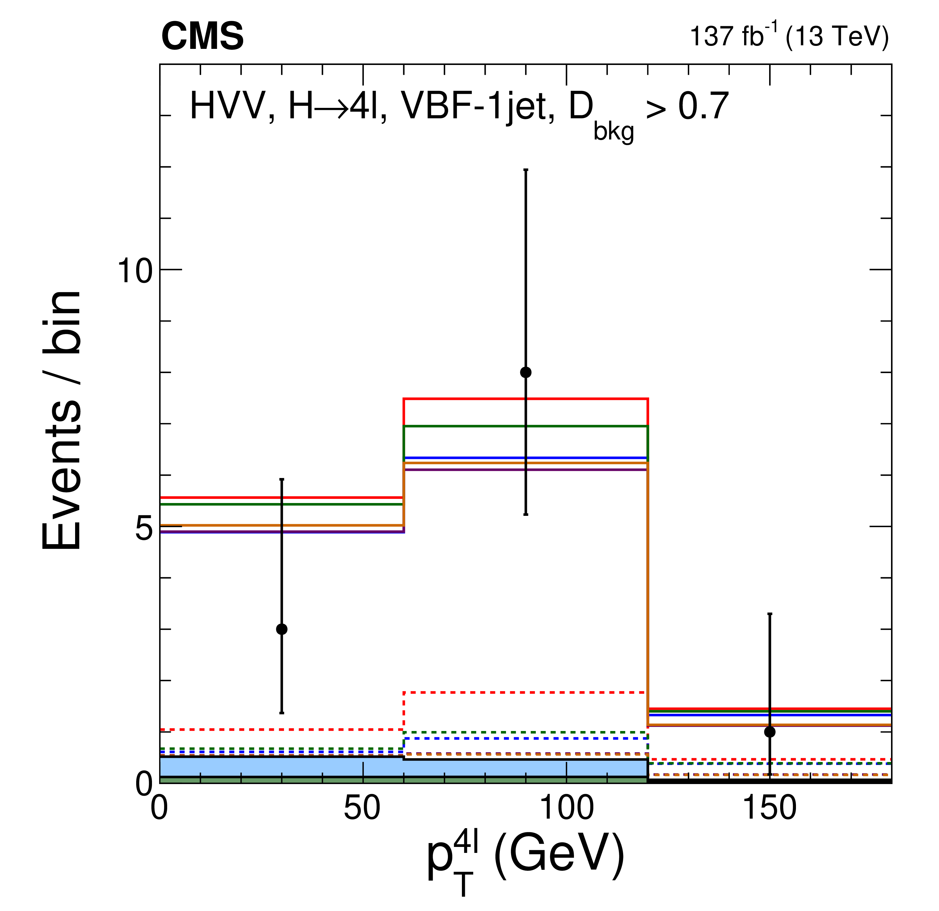
Distributions of events in the observables used in categorization Scheme 2. The first seven plots are in the VBF-2jet category: The upper left plot shows ${{\mathcal {D}}_{\text {bkg}}^{\mathrm {EW}}}$. The rest of the distributions are shown with the requirement $ {{\mathcal {D}}_{\text {bkg}}^{\mathrm {EW}}} > $ 0.2 in order to enhance the signal over the background contribution: $\mathcal {D}_{0-}^{\text {VBF}+\text {dec}}$ (upper middle), $\mathcal {D}_{0h+}^{\text {VBF}+\text {dec}}$ (upper right), $\mathcal {D}_{\Lambda 1}^{\text {VBF}+\text {dec}}$ (middle left), $\mathcal {D}_{\Lambda 1}^{\mathrm{Z} \gamma, \text {VBF}+\text {dec}}$ (middle middle), $\mathcal {D}_{\mathrm {CP}}^{\text {VBF}}$, and $\mathcal {D}_\text {int}^{\text {VBF}}$. The last two plots are shown in the VBF-1jet category: ${{\mathcal {D}}_{\text {bkg}}}$ (lower middle) and $ {p_{\mathrm {T}}} ^{4\ell}$ with the requirement $ {{\mathcal {D}}_{\text {bkg}}} > $ 0.7 and overflow events included in the last bin (lower right). Observed data, background expectation, and five signal models are shown in the plots, as indicated in the legend of Fig. 7. In several cases, a sixth signal model with a mixture of the SM and BSM couplings is shown and is indicated in the legend explicitly. |
png pdf |
Figure 12-a:
Distribution of events for ${{\mathcal {D}}_{\text {bkg}}^{\mathrm {EW}}}$ in the VBF-2jet category. Observed data, background expectation, and five signal models are shown in the plots, as indicated in the legend of Fig. 7. |

png pdf |
Figure 12-b:
Distribution of events for $\mathcal {D}_{0-}^{\text {VBF}+\text {dec}}$ in the VBF-2jet category with the requirement $ {{\mathcal {D}}_{\text {bkg}}^{\mathrm {EW}}} > $ 0.2 in order to enhance the signal over the background contribution. Observed data, background expectation, and five signal models are shown in the plots, as indicated in the legend of Fig. 7. |
png pdf |
Figure 12-c:
Distribution of events for $\mathcal {D}_{0h+}^{\text {VBF}+\text {dec}}$ in the VBF-2jet category with the requirement $ {{\mathcal {D}}_{\text {bkg}}^{\mathrm {EW}}} > $ 0.2 in order to enhance the signal over the background contribution. Observed data, background expectation, and five signal models are shown in the plots, as indicated in the legend of Fig. 7. |

png pdf |
Figure 12-d:
Distribution of events for $\mathcal {D}_{\Lambda 1}^{\text {VBF}+\text {dec}}$ in the VBF-2jet category with the requirement $ {{\mathcal {D}}_{\text {bkg}}^{\mathrm {EW}}} > $ 0.2 in order to enhance the signal over the background contribution. Observed data, background expectation, and five signal models are shown in the plots, as indicated in the legend of Fig. 7. |
png pdf |
Figure 12-e:
Distribution of events for $\mathcal {D}_{\Lambda 1}^{\mathrm{Z} \gamma, \text {VBF}+\text {dec}}$ in the VBF-1jet category with the requirement $ {{\mathcal {D}}_{\text {bkg}}} > $ 0.7. Observed data, background expectation, and five signal models are shown in the plots, as indicated in the legend of Fig. 7. |
png pdf |
Figure 12-f:
Distribution of events for $\mathcal {D}_{\mathrm {CP}}^{\text {VBF}}$ in the VBF-1jet category with the requirement $ {{\mathcal {D}}_{\text {bkg}}} > $ 0.7. Observed data, background expectation, and five signal models are shown in the plots, as indicated in the legend of Fig. 7. A sixth signal model with a mixture of the SM and BSM couplings is shown and is indicated in the legend explicitly. |
png pdf |
Figure 12-g:
Distribution of events for $\mathcal {D}_\text {int}^{\text {VBF}}$ in the VBF-2jet category with the requirement $ {{\mathcal {D}}_{\text {bkg}}^{\mathrm {EW}}} > $ 0.2 in order to enhance the signal over the background contribution. Observed data, background expectation, and five signal models are shown in the plots, as indicated in the legend of Fig. 7. A sixth signal model with a mixture of the SM and BSM couplings is shown and is indicated in the legend explicitly. |
png pdf |
Figure 12-h:
Distribution of events for ${{\mathcal {D}}_{\text {bkg}}}$ in the VBF-1jet category with the requirement $ {{\mathcal {D}}_{\text {bkg}}} > $ 0.7. Observed data, background expectation, and five signal models are shown in the plots, as indicated in the legend of Fig. 7. |
png pdf |
Figure 12-i:
Distribution of events for $ {p_{\mathrm {T}}} ^{4\ell}$ in the VBF-1jet category with the requirement $ {{\mathcal {D}}_{\text {bkg}}} > $ 0.7. The overflow events included in the last bin. Observed data, background expectation, and five signal models are shown in the plots, as indicated in the legend of Fig. 7. |
png pdf |
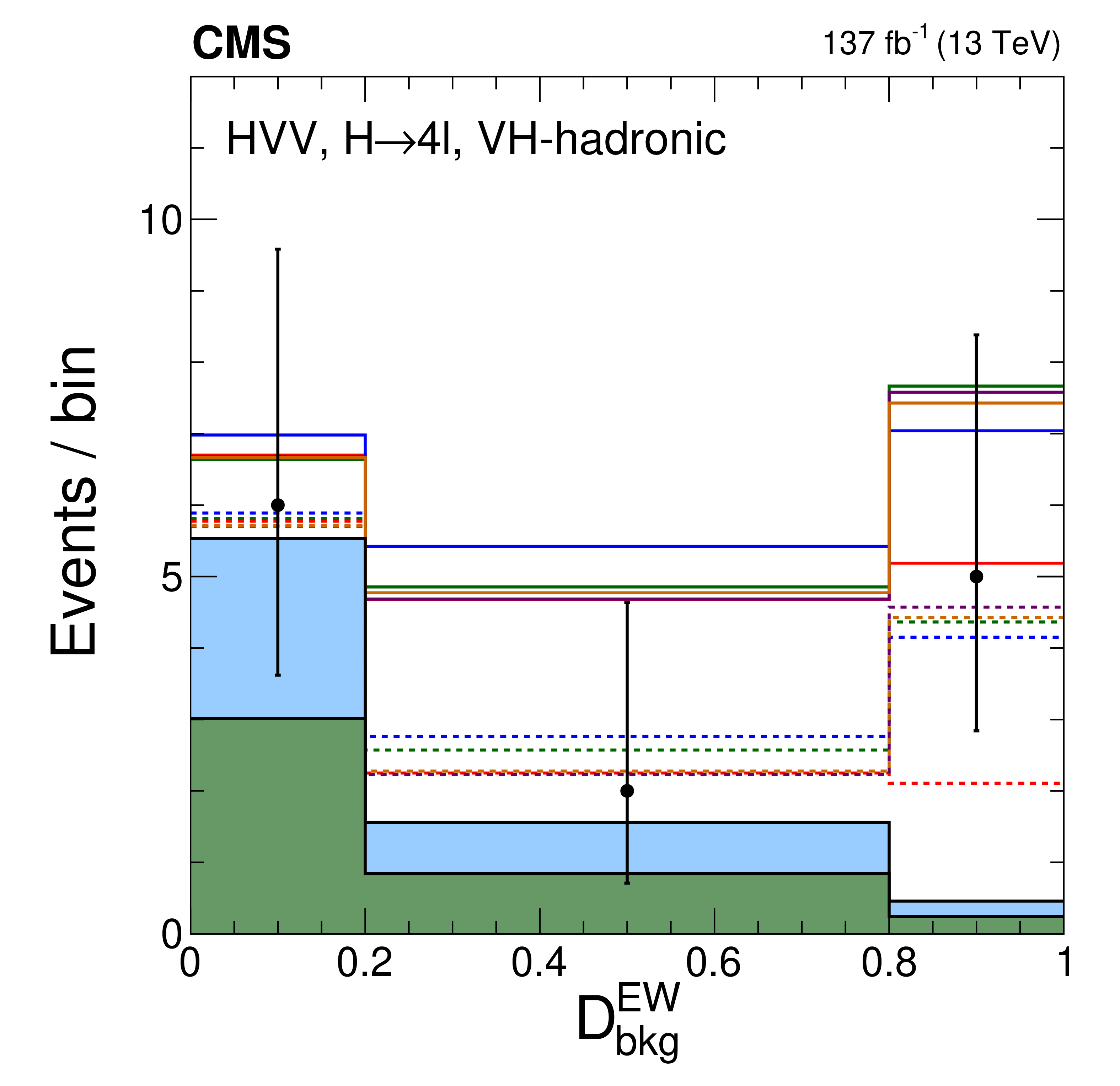
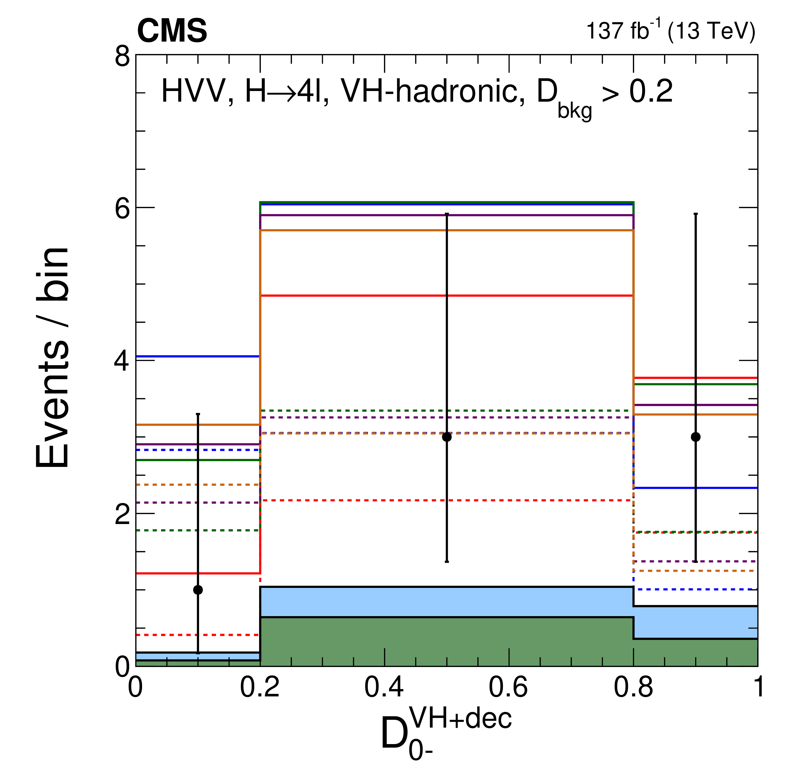
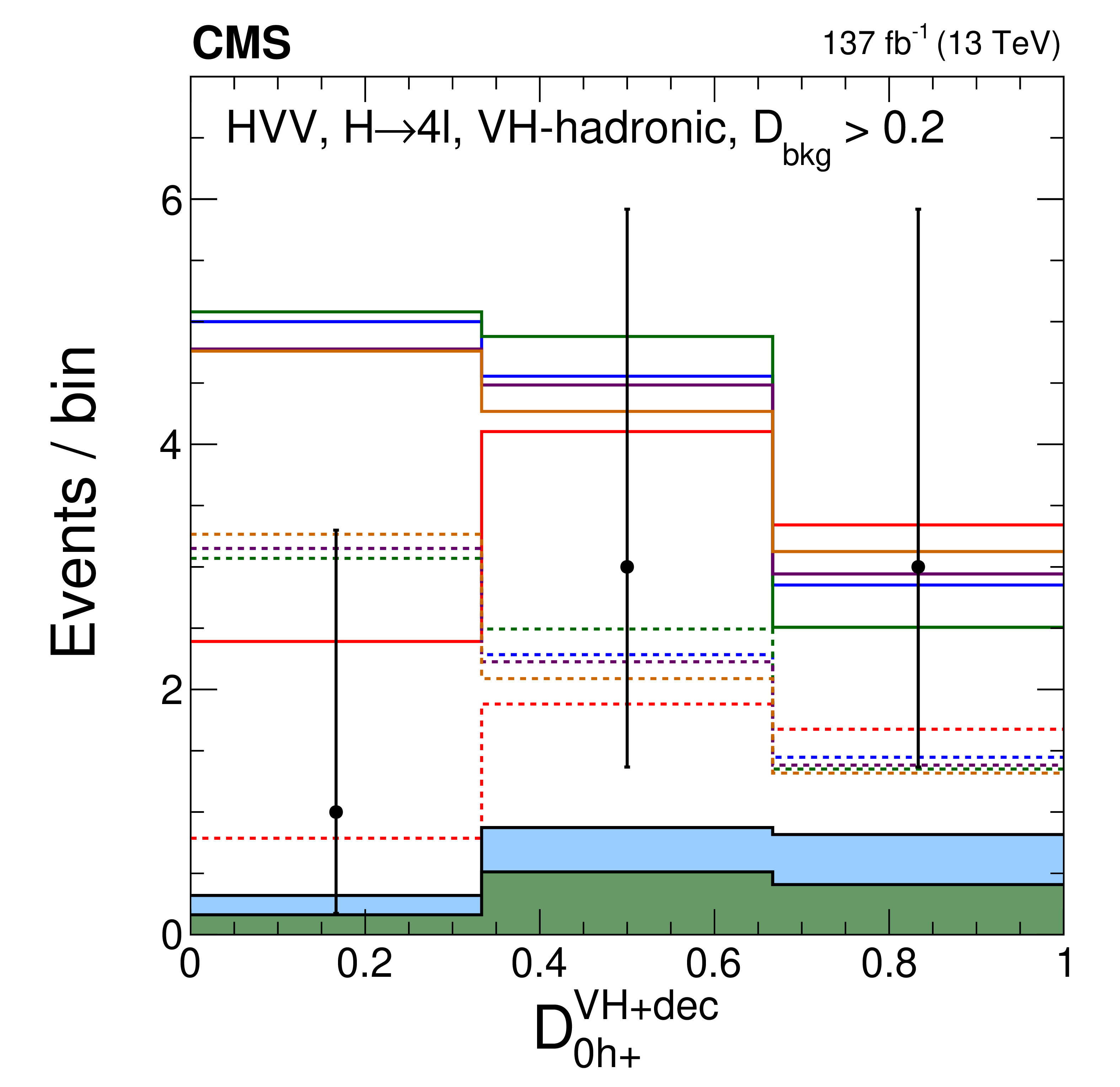
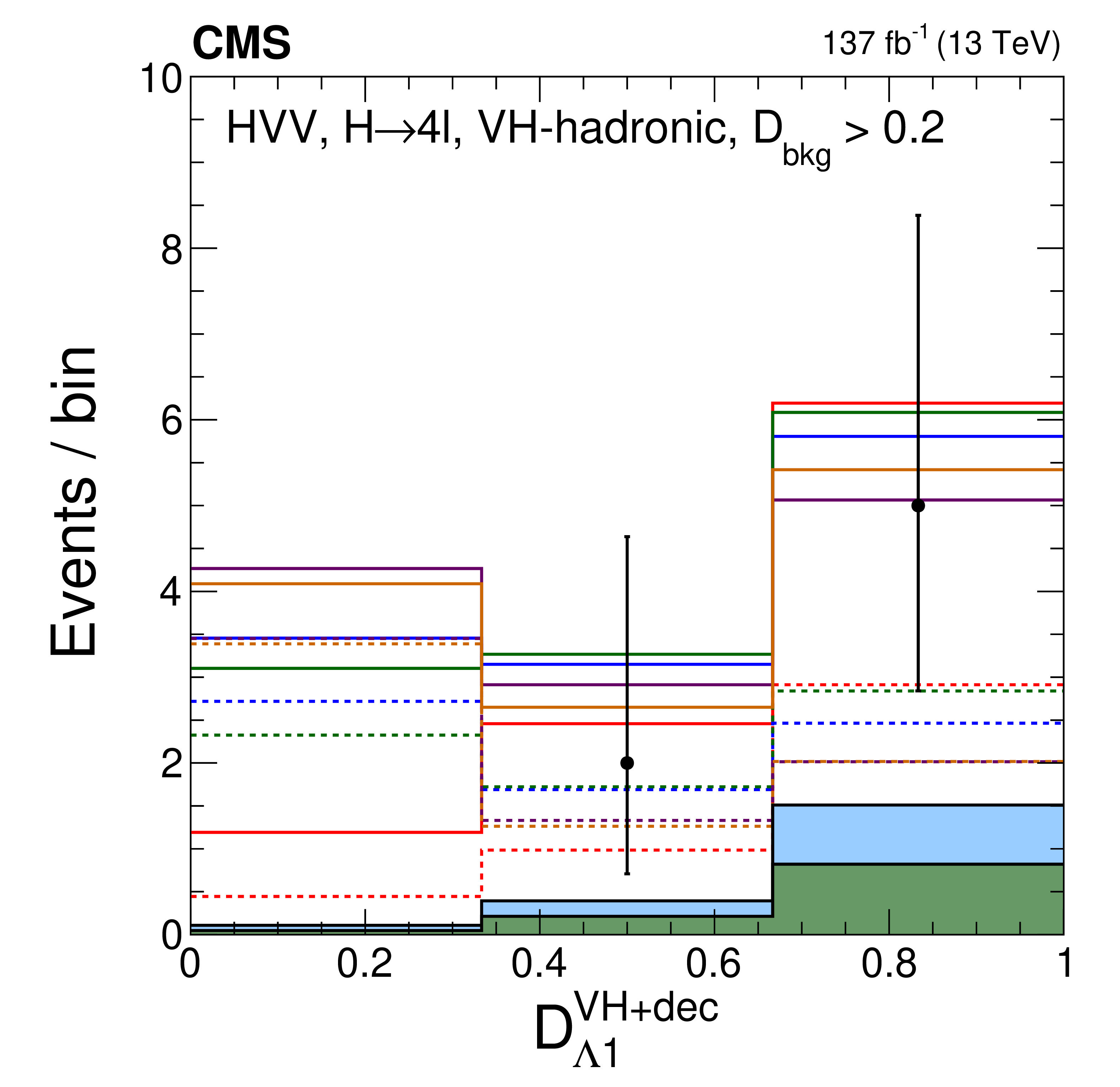
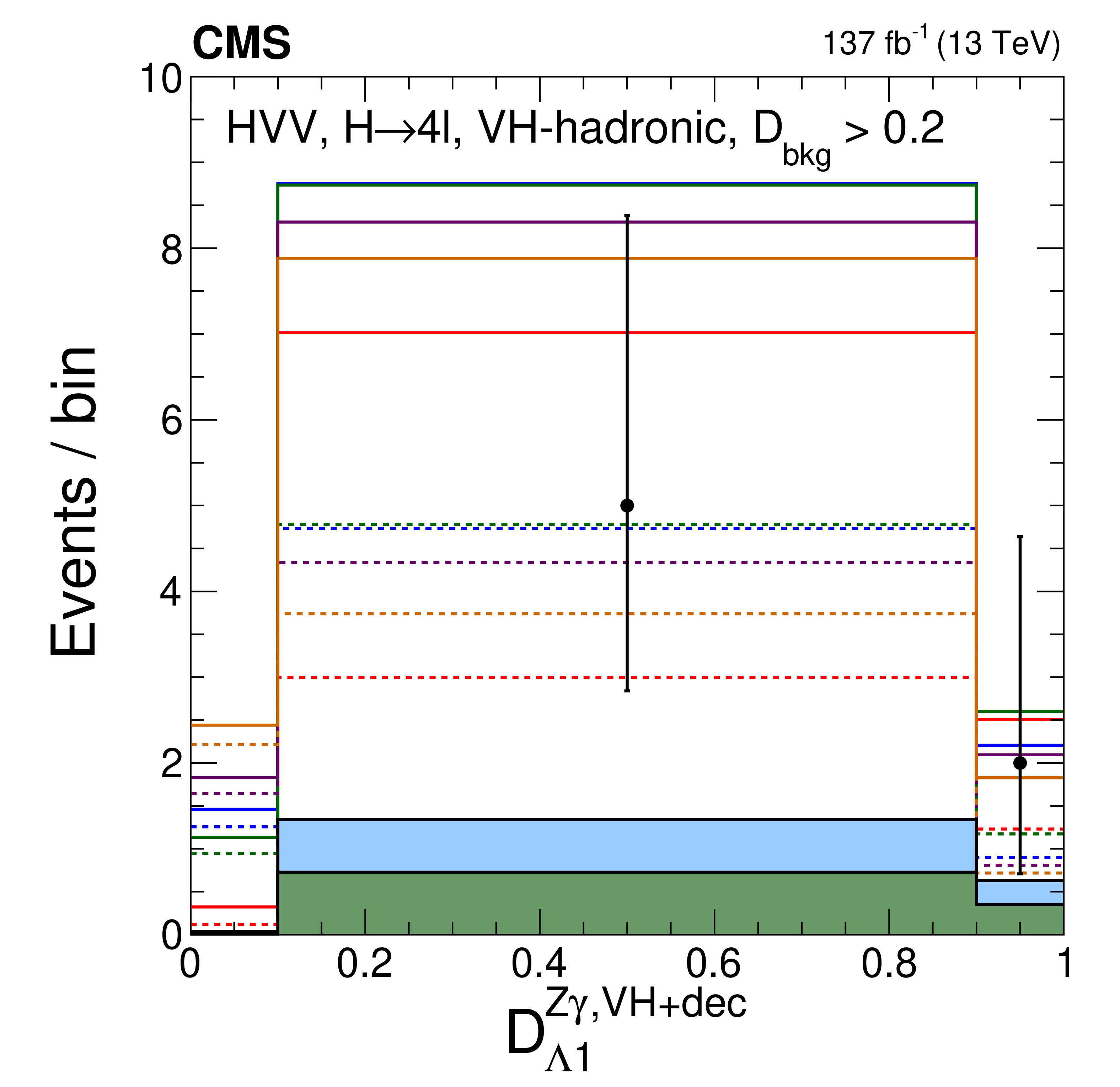
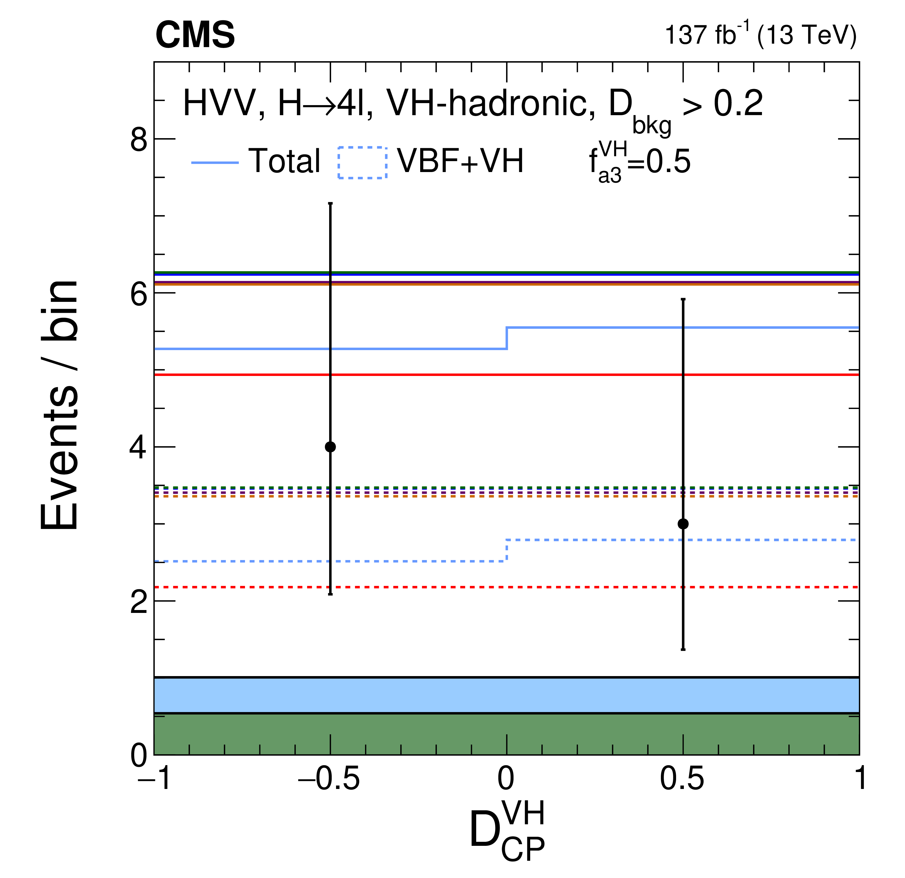
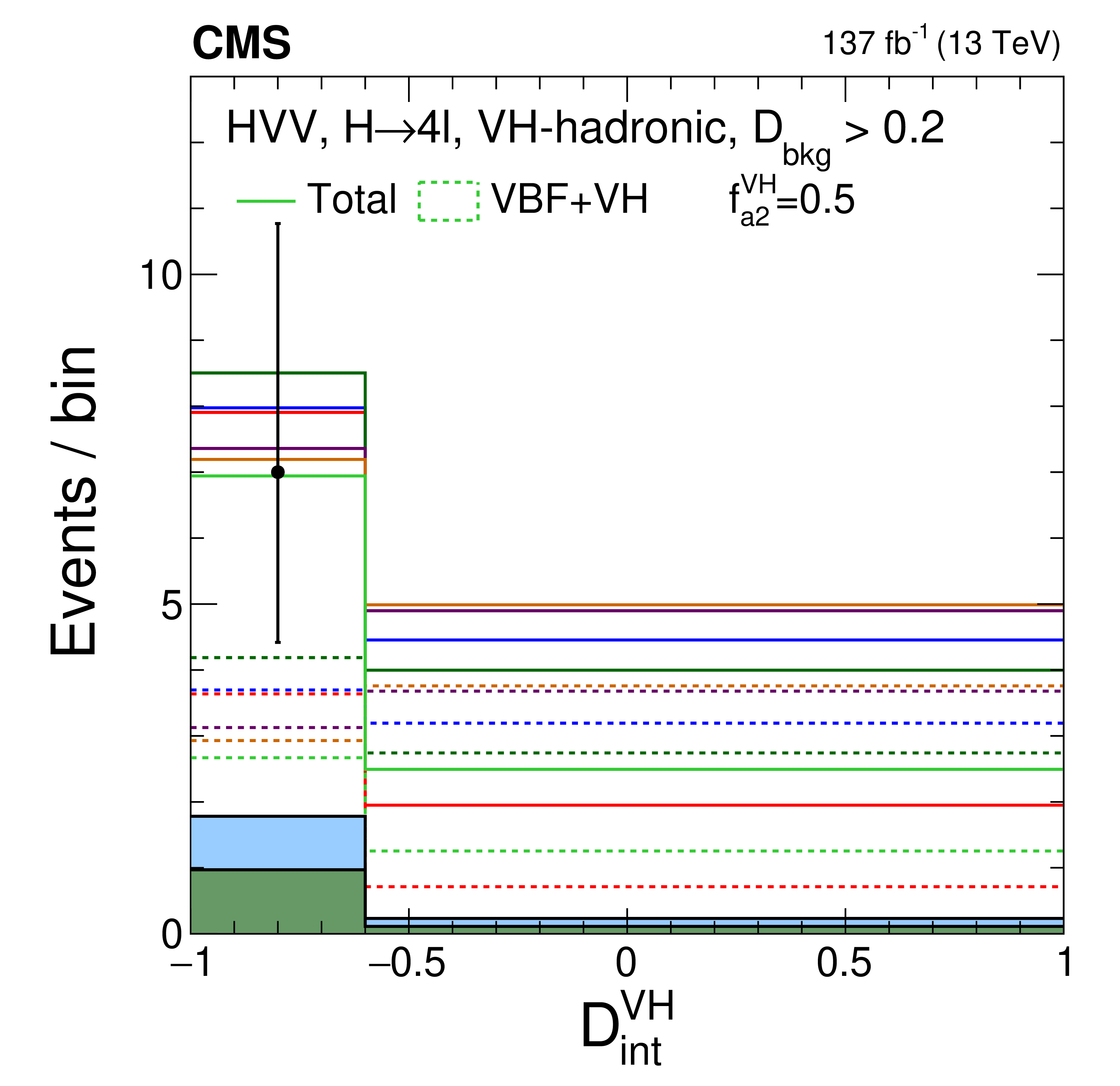
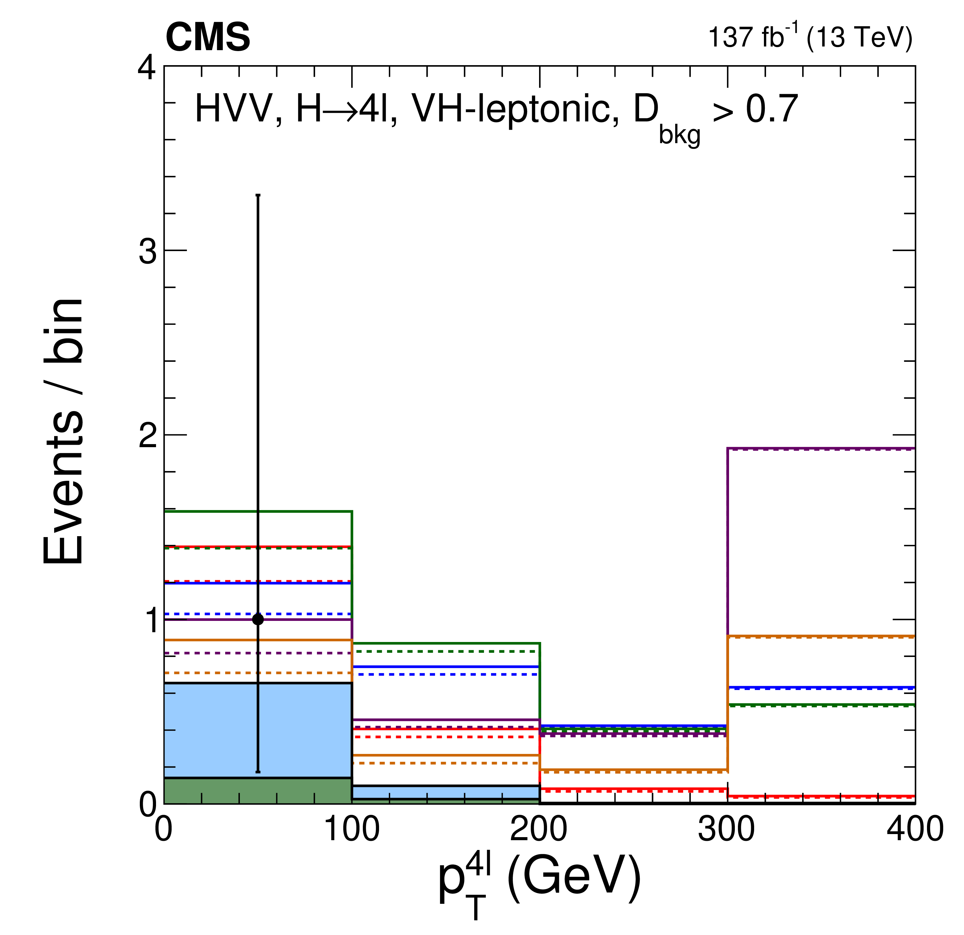
Figure 13:
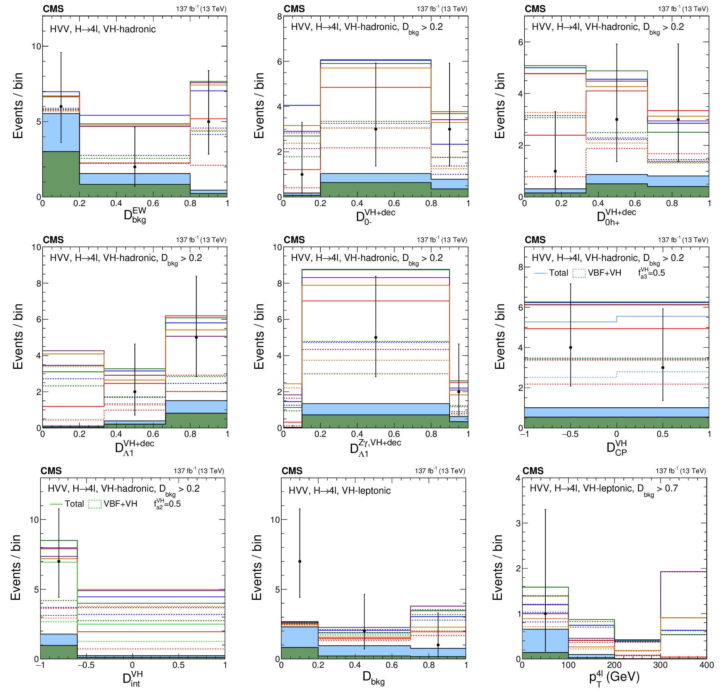
Distributions of events in the observables used in categorization Scheme 2. The first seven plots are in the VH-hadronic category: The upper left plot shows ${{\mathcal {D}}_{\text {bkg}}^{\mathrm {EW}}}$. The rest of the distributions are shown with the requirement $ {{\mathcal {D}}_{\text {bkg}}^{\mathrm {EW}}} > $ 0.2 in order to enhance the signal over the background contribution: $\mathcal {D}_{0-}^{{\mathrm{V} \mathrm{H}} +\text {dec}}$ (upper middle); $\mathcal {D}_{0h+}^{{\mathrm{V} \mathrm{H}} +\text {dec}}$ (upper right); $\mathcal {D}_{\Lambda 1}^{{\mathrm{V} \mathrm{H}} +\text {dec}}$ (middle left); $\mathcal {D}_{\Lambda 1}^{\mathrm{Z} \gamma, VH +\text {dec}}$ (middle middle); $\mathcal {D}_{\mathrm {CP}}^{{\mathrm{V} \mathrm{H}}}$, and $\mathcal {D}_\text {int}^{{\mathrm{V} \mathrm{H}}}$. The last two plots are shown in the VH-leptonic category: ${{\mathcal {D}}_{\text {bkg}}}$ (lower middle) and $ {p_{\mathrm {T}}} ^{4\ell}$ with the requirement $ {{\mathcal {D}}_{\text {bkg}}} > $ 0.7 and overflow events included in the last bin (lower right). Observed data, background expectation, and five signal models are shown in the plots as indicated in the legend of Fig. 7. In several cases, a sixth signal model with a mixture of the SM and BSM couplings is shown and is indicated in the legend explicitly. |
png pdf |
Figure 13-a:
Distribution of events for ${{\mathcal {D}}_{\text {bkg}}^{\mathrm {EW}}}$ in the VH-hadronic category. Observed data, background expectation, and five signal models are shown in the plots as indicated in the legend of Fig. 7. |
png pdf |
Figure 13-b:
Distribution of events for $\mathcal {D}_{0-}^{{\mathrm{V} \mathrm{H}} +\text {dec}}$ in the VH-hadronic category with the requirement $ {{\mathcal {D}}_{\text {bkg}}^{\mathrm {EW}}} > $ 0.2 in order to enhance the signal over the background contribution. Observed data, background expectation, and five signal models are shown in the plots as indicated in the legend of Fig. 7. |
png pdf |
Figure 13-c:
Distribution of events for $\mathcal {D}_{0h+}^{{\mathrm{V} \mathrm{H}} +\text {dec}}$ in the VH-hadronic category with the requirement $ {{\mathcal {D}}_{\text {bkg}}^{\mathrm {EW}}} > $ 0.2 in order to enhance the signal over the background contribution. Observed data, background expectation, and five signal models are shown in the plots as indicated in the legend of Fig. 7. |
png pdf |
Figure 13-d:
Distribution of events for $\mathcal {D}_{\Lambda 1}^{{\mathrm{V} \mathrm{H}} +\text {dec}}$ in the VH-hadronic category with the requirement $ {{\mathcal {D}}_{\text {bkg}}^{\mathrm {EW}}} > $ 0.2 in order to enhance the signal over the background contribution. Observed data, background expectation, and five signal models are shown in the plots as indicated in the legend of Fig. 7. |
png pdf |
Figure 13-e:
Distribution of events for $\mathcal {D}_{\Lambda 1}^{\mathrm{Z} \gamma, VH +\text {dec}}$ in the VH-hadronic category with the requirement $ {{\mathcal {D}}_{\text {bkg}}^{\mathrm {EW}}} > $ 0.2 in order to enhance the signal over the background contribution. Observed data, background expectation, and five signal models are shown in the plots as indicated in the legend of Fig. 7. |
png pdf |
Figure 13-f:
Distribution of events for $\mathcal {D}_{\mathrm {CP}}^{{\mathrm{V} \mathrm{H}}}$ in the VH-hadronic category with the requirement $ {{\mathcal {D}}_{\text {bkg}}^{\mathrm {EW}}} > $ 0.2 in order to enhance the signal over the background contribution. Observed data, background expectation, and five signal models are shown in the plots as indicated in the legend of Fig. 7. A sixth signal model with a mixture of the SM and BSM couplings is shown and is indicated in the legend explicitly. |
png pdf |
Figure 13-g:
Distribution of events for $\mathcal {D}_\text {int}^{{\mathrm{V} \mathrm{H}}}$ in the VH-hadronic category with the requirement $ {{\mathcal {D}}_{\text {bkg}}^{\mathrm {EW}}} > $ 0.2 in order to enhance the signal over the background contribution. Observed data, background expectation, and five signal models are shown in the plots as indicated in the legend of Fig. 7. A sixth signal model with a mixture of the SM and BSM couplings is shown and is indicated in the legend explicitly. |

png pdf |
Figure 13-h:
Distribution of events for ${{\mathcal {D}}_{\text {bkg}}}$ in the VH-leptonic category with the requirement $ {{\mathcal {D}}_{\text {bkg}}} > $ 0.7. Observed data, background expectation, and five signal models are shown in the plots as indicated in the legend of Fig. 7. |
png pdf |
Figure 13-i:
Distribution of events for $ {p_{\mathrm {T}}} ^{4\ell}$ in the VH-leptonic category with the requirement $ {{\mathcal {D}}_{\text {bkg}}} > $ 0.7. The overflow events included in the last bin. Observed data, background expectation, and five signal models are shown in the plots as indicated in the legend of Fig. 7. |
png pdf |
Figure 14:
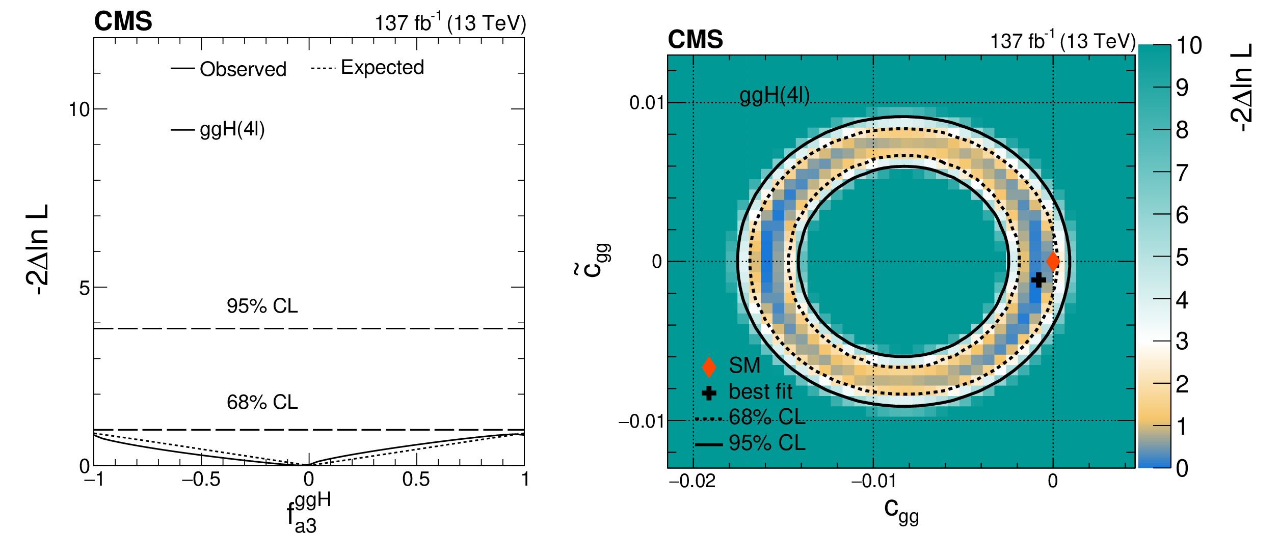
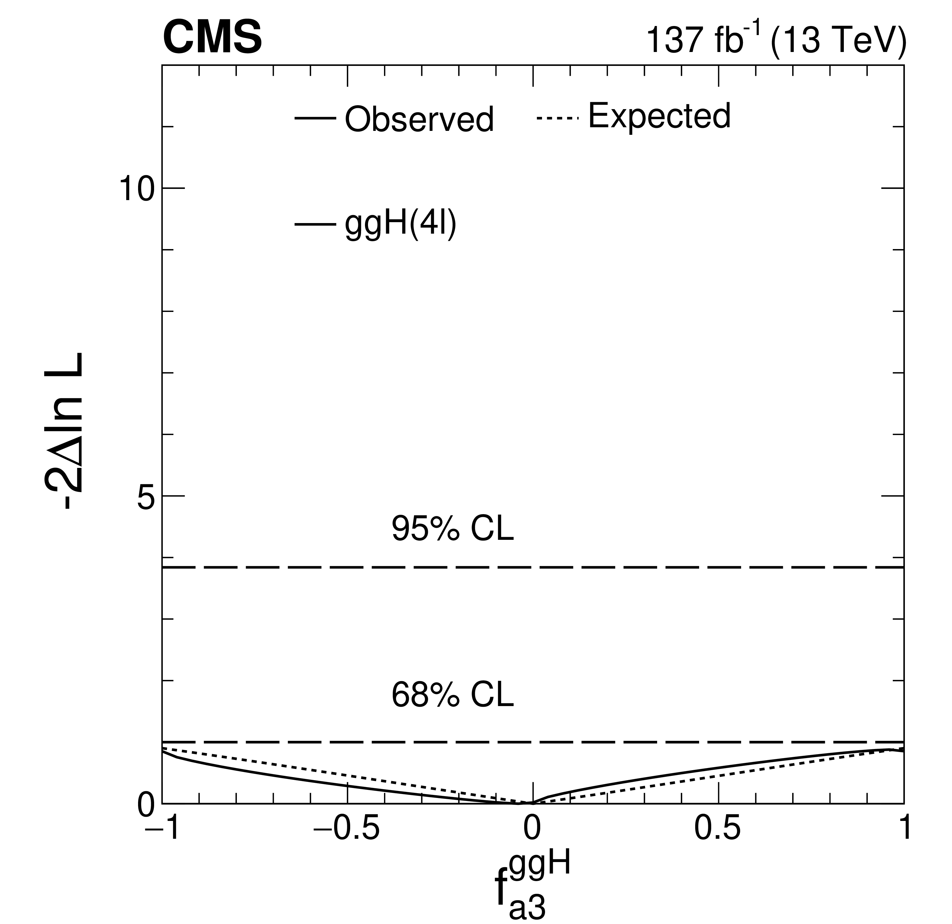
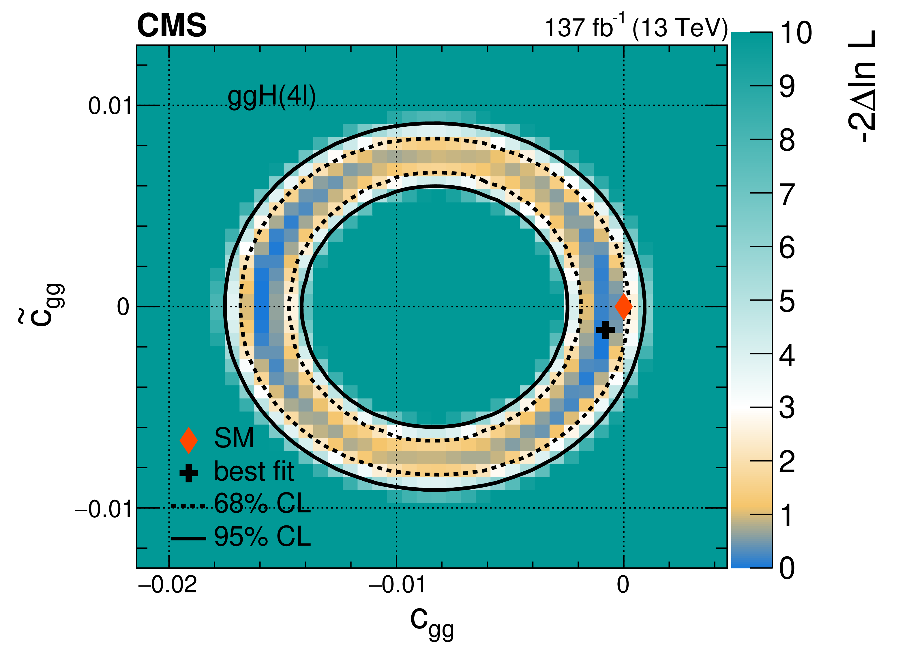
Constraints on the anomalous H boson couplings to gluons in the ggH process using the $\mathrm{H} \to 4\ell $ decay. Left: Observed (solid) and expected (dashed) likelihood scans of the $CP$-sensitive parameter $ {f_{a3}^{\mathrm{g} \mathrm{g} \mathrm{H}}} $. The dashed horizontal lines show 68 and 95% CL. Right: Observed confidence level intervals on the $c_{\mathrm{g} \mathrm{g}}$ and $\tilde{c}_{\mathrm{g} \mathrm{g}}$ couplings reinterpreted from the $ {f_{a3}^{\mathrm{g} \mathrm{g} \mathrm{H}}} $ and $\mu _{{\mathrm{g} \mathrm{g} \mathrm{H}}}$ measurement with $ {f_{a3}} $ and $ {\mu _{\mathrm{V}}} $ profiled, and with $\kappa _{\mathrm{t}}=\kappa _{\mathrm{b}}=1$. The dashed and solid lines show the 68 and 95% CL exclusion regions in two dimensions, respectively. |
png pdf |
Figure 14-a:
Constraints on the anomalous H boson couplings to gluons in the ggH process using the $\mathrm{H} \to 4\ell $ decay. Left: Observed (solid) and expected (dashed) likelihood scans of the $CP$-sensitive parameter $ {f_{a3}^{\mathrm{g} \mathrm{g} \mathrm{H}}} $. The dashed horizontal lines show 68 and 95% CL. Right: Observed confidence level intervals on the $c_{\mathrm{g} \mathrm{g}}$ and $\tilde{c}_{\mathrm{g} \mathrm{g}}$ couplings reinterpreted from the $ {f_{a3}^{\mathrm{g} \mathrm{g} \mathrm{H}}} $ and $\mu _{{\mathrm{g} \mathrm{g} \mathrm{H}}}$ measurement with $ {f_{a3}} $ and $ {\mu _{\mathrm{V}}} $ profiled, and with $\kappa _{\mathrm{t}}=\kappa _{\mathrm{b}}=1$. The dashed and solid lines show the 68 and 95% CL exclusion regions in two dimensions, respectively. |
png pdf |
Figure 14-b:
Constraints on the anomalous H boson couplings to gluons in the ggH process using the $\mathrm{H} \to 4\ell $ decay. Left: Observed (solid) and expected (dashed) likelihood scans of the $CP$-sensitive parameter $ {f_{a3}^{\mathrm{g} \mathrm{g} \mathrm{H}}} $. The dashed horizontal lines show 68 and 95% CL. Right: Observed confidence level intervals on the $c_{\mathrm{g} \mathrm{g}}$ and $\tilde{c}_{\mathrm{g} \mathrm{g}}$ couplings reinterpreted from the $ {f_{a3}^{\mathrm{g} \mathrm{g} \mathrm{H}}} $ and $\mu _{{\mathrm{g} \mathrm{g} \mathrm{H}}}$ measurement with $ {f_{a3}} $ and $ {\mu _{\mathrm{V}}} $ profiled, and with $\kappa _{\mathrm{t}}=\kappa _{\mathrm{b}}=1$. The dashed and solid lines show the 68 and 95% CL exclusion regions in two dimensions, respectively. |

png pdf |
Figure 15:
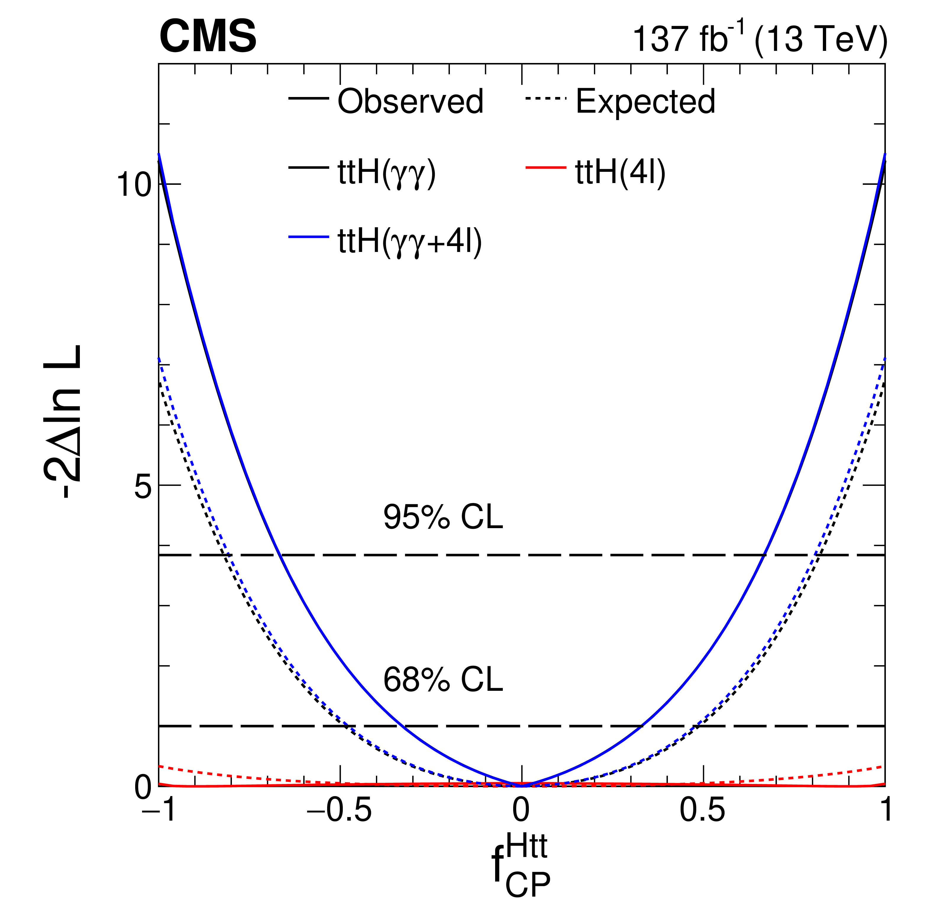
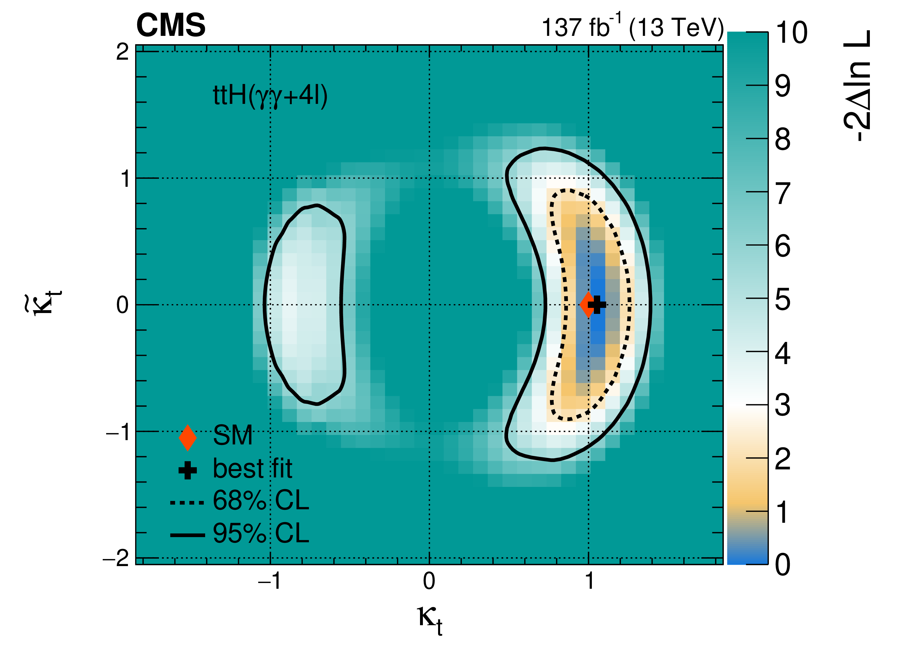
Constraints on the anomalous H boson couplings to top quarks in the ttH and tH processes using the $\mathrm{H} \to \gamma \gamma $ [26] and $\mathrm{H} \to 4\ell $ decays. Left: Observed (solid) and expected (dashed) likelihood scans of $ {f_\mathrm {CP}^{{\mathrm{H} \text {tt}}}} $ in the ttH and tH processes in the $\mathrm{H} \to 4\ell $ (red), $\gamma \gamma $ (black), and combined (blue) channels, where the combination is done without relating the signal strengths in the two processes. The dashed horizontal lines show 68 and 95% CL. Right: Observed confidence level intervals on the $\kappa _{\mathrm{t}}$ and $\tilde\kappa _{\mathrm{t}}$ couplings reinterpreted from the $ {f_\mathrm {CP}^{{\mathrm{H} \text {tt}}}} $, $\mu _{{\mathrm{t} \mathrm{\bar{t}} \mathrm{H}}}$, and $ {\mu _{\mathrm{V}}} $ measurements in the combined fit of the $\mathrm{H} \to 4\ell $ and $\gamma \gamma $ channels, with the signal strengths in the two channels related through the couplings as discussed in text. The dashed and solid lines show the 68 and 95% CL exclusion regions in two dimensions, respectively. |
png pdf |
Figure 15-a:
Constraints on the anomalous H boson couplings to top quarks in the ttH and tH processes using the $\mathrm{H} \to \gamma \gamma $ [26] and $\mathrm{H} \to 4\ell $ decays. Left: Observed (solid) and expected (dashed) likelihood scans of $ {f_\mathrm {CP}^{{\mathrm{H} \text {tt}}}} $ in the ttH and tH processes in the $\mathrm{H} \to 4\ell $ (red), $\gamma \gamma $ (black), and combined (blue) channels, where the combination is done without relating the signal strengths in the two processes. The dashed horizontal lines show 68 and 95% CL. Right: Observed confidence level intervals on the $\kappa _{\mathrm{t}}$ and $\tilde\kappa _{\mathrm{t}}$ couplings reinterpreted from the $ {f_\mathrm {CP}^{{\mathrm{H} \text {tt}}}} $, $\mu _{{\mathrm{t} \mathrm{\bar{t}} \mathrm{H}}}$, and $ {\mu _{\mathrm{V}}} $ measurements in the combined fit of the $\mathrm{H} \to 4\ell $ and $\gamma \gamma $ channels, with the signal strengths in the two channels related through the couplings as discussed in text. The dashed and solid lines show the 68 and 95% CL exclusion regions in two dimensions, respectively. |
png pdf |
Figure 15-b:
Constraints on the anomalous H boson couplings to top quarks in the ttH and tH processes using the $\mathrm{H} \to \gamma \gamma $ [26] and $\mathrm{H} \to 4\ell $ decays. Left: Observed (solid) and expected (dashed) likelihood scans of $ {f_\mathrm {CP}^{{\mathrm{H} \text {tt}}}} $ in the ttH and tH processes in the $\mathrm{H} \to 4\ell $ (red), $\gamma \gamma $ (black), and combined (blue) channels, where the combination is done without relating the signal strengths in the two processes. The dashed horizontal lines show 68 and 95% CL. Right: Observed confidence level intervals on the $\kappa _{\mathrm{t}}$ and $\tilde\kappa _{\mathrm{t}}$ couplings reinterpreted from the $ {f_\mathrm {CP}^{{\mathrm{H} \text {tt}}}} $, $\mu _{{\mathrm{t} \mathrm{\bar{t}} \mathrm{H}}}$, and $ {\mu _{\mathrm{V}}} $ measurements in the combined fit of the $\mathrm{H} \to 4\ell $ and $\gamma \gamma $ channels, with the signal strengths in the two channels related through the couplings as discussed in text. The dashed and solid lines show the 68 and 95% CL exclusion regions in two dimensions, respectively. |
png pdf |
Figure 16:
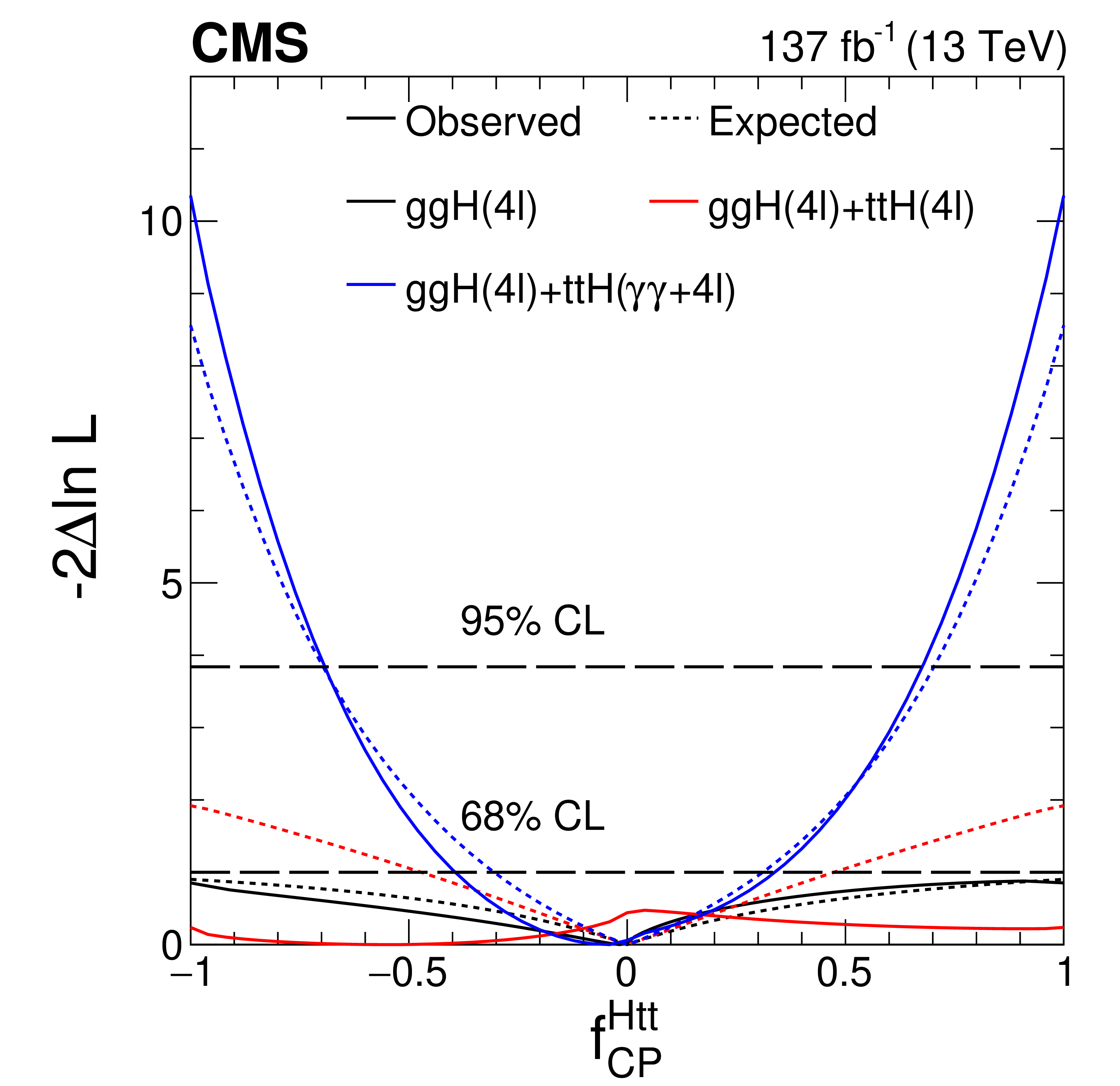
Constraints on the anomalous H boson couplings to top quarks in the ttH, tH, and ggH processes combined, assuming top quark dominance in the gluon fusion loop, using the $\mathrm{H} \to 4\ell $ and $\gamma \gamma $ decays. Observed (solid) and expected (dashed) likelihood scans of $ {f_\mathrm {CP}^{{\mathrm{H} \text {tt}}}} $ are shown in the ggH process with $\mathrm{H} \to 4\ell $ (black), ttH, tH, and ggH processes combined with $\mathrm{H} \to 4\ell $ (red), and in the ttH, tH, and ggH processes with $\mathrm{H} \to 4\ell $ and the ttH and tH processes with $\gamma \gamma $ combined (blue). Combination is done by relating the signal strengths in the three processes through the couplings in the loops in both production and decay, as discussed in the text. The dashed horizontal lines show 68 and 95% CL exclusion. |
png pdf |
Figure 17:
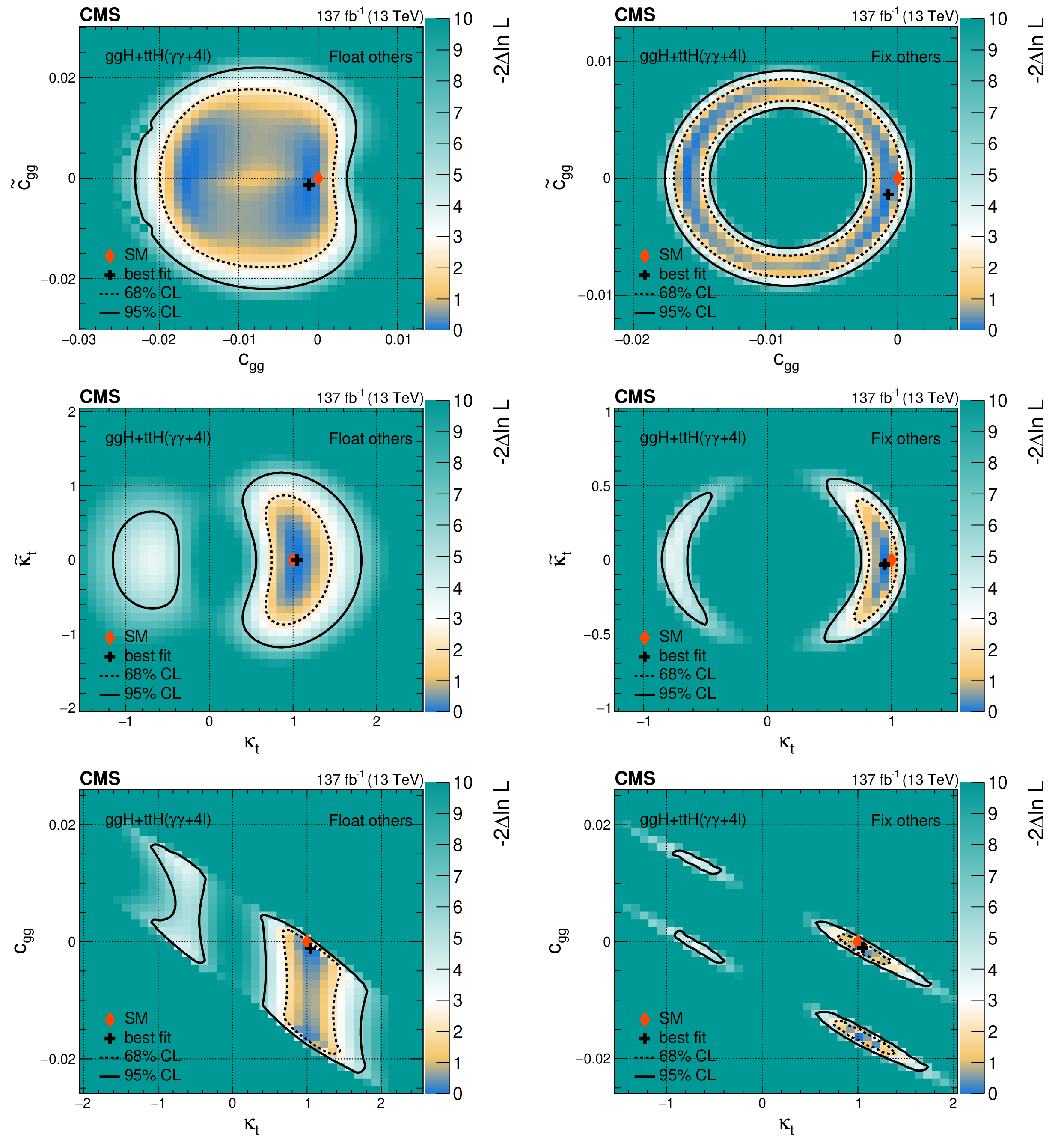
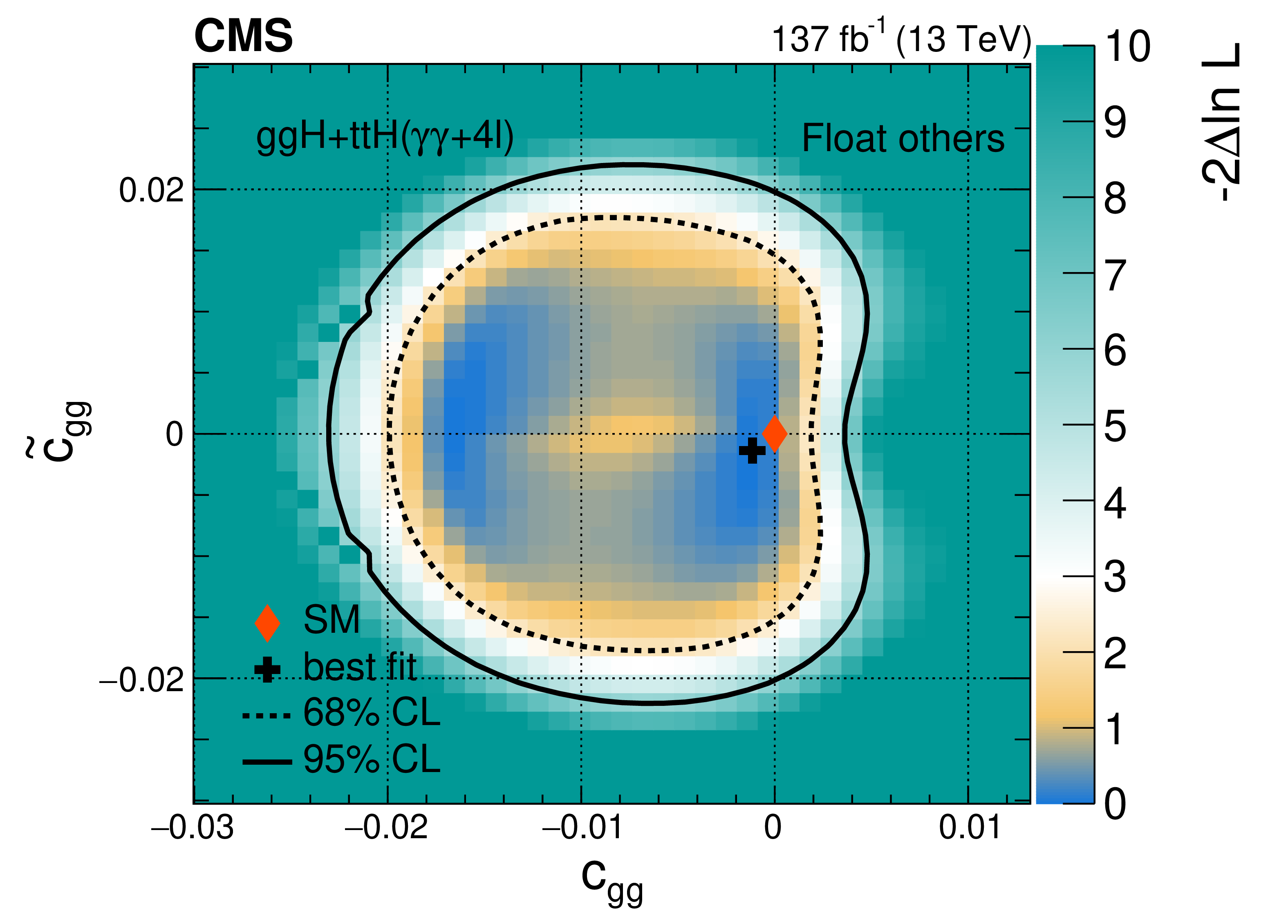
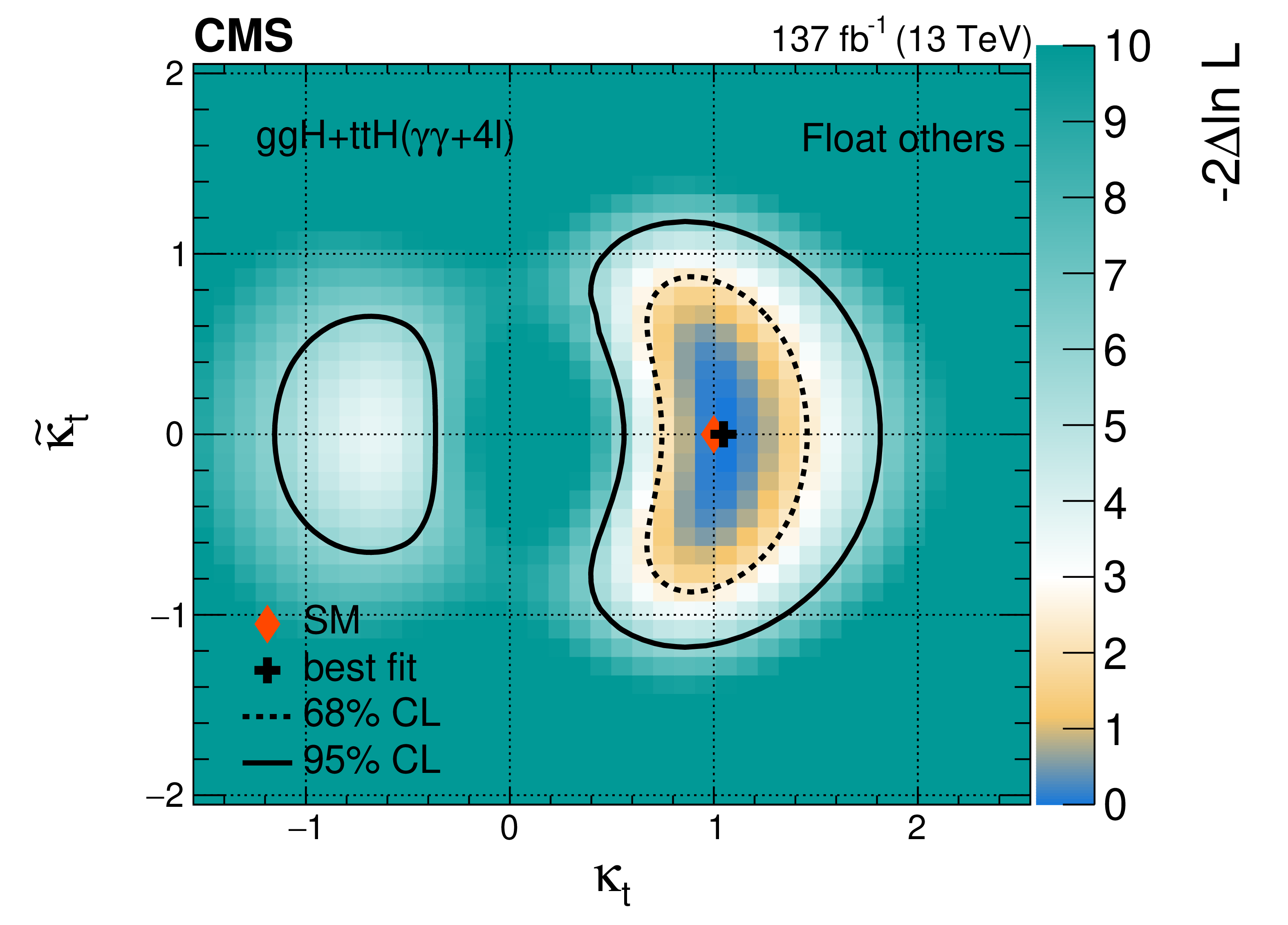
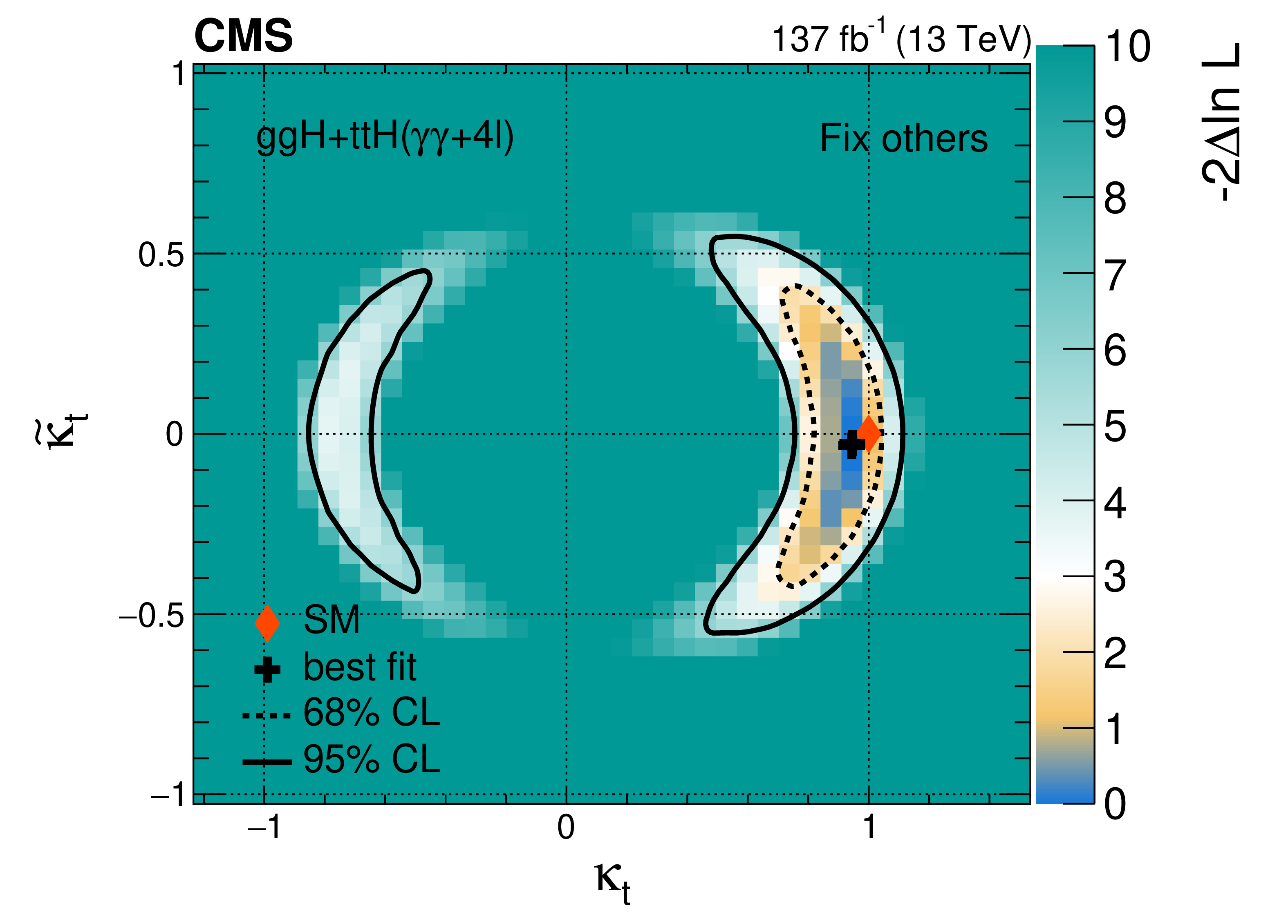
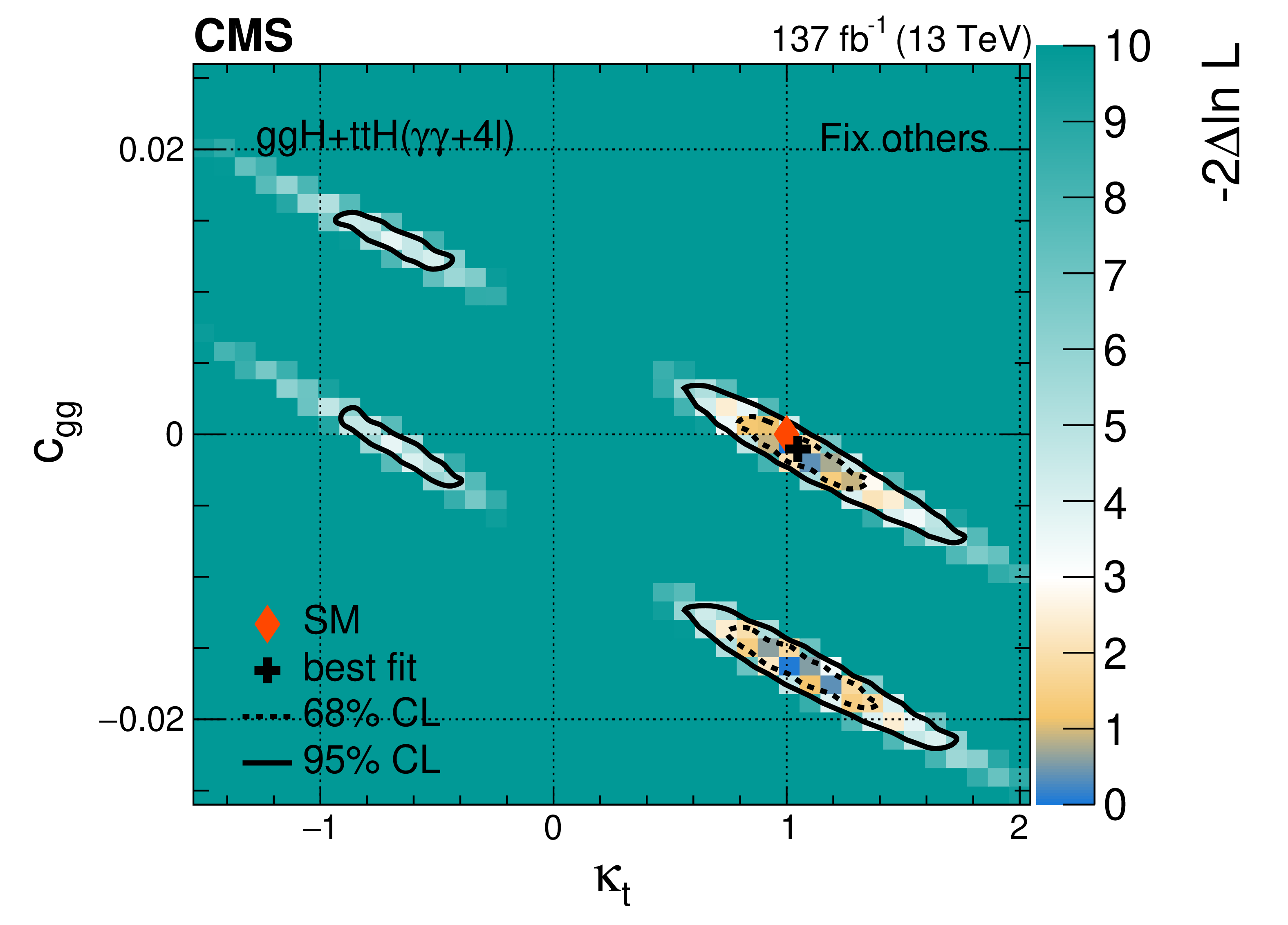
Constraints on the anomalous H boson couplings $c_{\mathrm{g} \mathrm{g}}$, $\tilde{c}_{\mathrm{g} \mathrm{g}}$, $\kappa _\mathrm{t} $, and $\tilde\kappa _\mathrm{t} $ in the ttH, tH, and ggH processes combined, using the $\mathrm{H} \to 4\ell $ and $\gamma \gamma $ decays. The constraints are shown for the pairs of parameters: $c_{\mathrm{g} \mathrm{g}}$ and $\tilde{c}_{\mathrm{g} \mathrm{g}}$ (upper), $\kappa _\mathrm{t} $ and $\tilde\kappa _\mathrm{t} $ (middle), $\kappa _\mathrm{t} $ and $c_{\mathrm{g} \mathrm{g}}$ (lower), and with the other two parameters either profiled (left) or fixed to the SM expectation (right). The dashed and solid lines show the 68 and 95% CL exclusion regions in two dimensions, respectively. |
png pdf |
Figure 17-a:
Constraints on the anomalous H boson couplings $c_{\mathrm{g} \mathrm{g}}$, $\tilde{c}_{\mathrm{g} \mathrm{g}}$, $\kappa _\mathrm{t} $, and $\tilde\kappa _\mathrm{t} $ in the ttH, tH, and ggH processes combined, using the $\mathrm{H} \to 4\ell $ and $\gamma \gamma $ decays. The constraints are shown for the pairs of parameters: $c_{\mathrm{g} \mathrm{g}}$ and $\tilde{c}_{\mathrm{g} \mathrm{g}}$ (upper), $\kappa _\mathrm{t} $ and $\tilde\kappa _\mathrm{t} $ (middle), $\kappa _\mathrm{t} $ and $c_{\mathrm{g} \mathrm{g}}$ (lower), and with the other two parameters either profiled (left) or fixed to the SM expectation (right). The dashed and solid lines show the 68 and 95% CL exclusion regions in two dimensions, respectively. |

png pdf |
Figure 17-b:
Constraints on the anomalous H boson couplings $c_{\mathrm{g} \mathrm{g}}$, $\tilde{c}_{\mathrm{g} \mathrm{g}}$, $\kappa _\mathrm{t} $, and $\tilde\kappa _\mathrm{t} $ in the ttH, tH, and ggH processes combined, using the $\mathrm{H} \to 4\ell $ and $\gamma \gamma $ decays. The constraints are shown for the pairs of parameters: $c_{\mathrm{g} \mathrm{g}}$ and $\tilde{c}_{\mathrm{g} \mathrm{g}}$ (upper), $\kappa _\mathrm{t} $ and $\tilde\kappa _\mathrm{t} $ (middle), $\kappa _\mathrm{t} $ and $c_{\mathrm{g} \mathrm{g}}$ (lower), and with the other two parameters either profiled (left) or fixed to the SM expectation (right). The dashed and solid lines show the 68 and 95% CL exclusion regions in two dimensions, respectively. |
png pdf |
Figure 17-c:
Constraints on the anomalous H boson couplings $c_{\mathrm{g} \mathrm{g}}$, $\tilde{c}_{\mathrm{g} \mathrm{g}}$, $\kappa _\mathrm{t} $, and $\tilde\kappa _\mathrm{t} $ in the ttH, tH, and ggH processes combined, using the $\mathrm{H} \to 4\ell $ and $\gamma \gamma $ decays. The constraints are shown for the pairs of parameters: $c_{\mathrm{g} \mathrm{g}}$ and $\tilde{c}_{\mathrm{g} \mathrm{g}}$ (upper), $\kappa _\mathrm{t} $ and $\tilde\kappa _\mathrm{t} $ (middle), $\kappa _\mathrm{t} $ and $c_{\mathrm{g} \mathrm{g}}$ (lower), and with the other two parameters either profiled (left) or fixed to the SM expectation (right). The dashed and solid lines show the 68 and 95% CL exclusion regions in two dimensions, respectively. |
png pdf |
Figure 17-d:
Constraints on the anomalous H boson couplings $c_{\mathrm{g} \mathrm{g}}$, $\tilde{c}_{\mathrm{g} \mathrm{g}}$, $\kappa _\mathrm{t} $, and $\tilde\kappa _\mathrm{t} $ in the ttH, tH, and ggH processes combined, using the $\mathrm{H} \to 4\ell $ and $\gamma \gamma $ decays. The constraints are shown for the pairs of parameters: $c_{\mathrm{g} \mathrm{g}}$ and $\tilde{c}_{\mathrm{g} \mathrm{g}}$ (upper), $\kappa _\mathrm{t} $ and $\tilde\kappa _\mathrm{t} $ (middle), $\kappa _\mathrm{t} $ and $c_{\mathrm{g} \mathrm{g}}$ (lower), and with the other two parameters either profiled (left) or fixed to the SM expectation (right). The dashed and solid lines show the 68 and 95% CL exclusion regions in two dimensions, respectively. |

png pdf |
Figure 17-e:
Constraints on the anomalous H boson couplings $c_{\mathrm{g} \mathrm{g}}$, $\tilde{c}_{\mathrm{g} \mathrm{g}}$, $\kappa _\mathrm{t} $, and $\tilde\kappa _\mathrm{t} $ in the ttH, tH, and ggH processes combined, using the $\mathrm{H} \to 4\ell $ and $\gamma \gamma $ decays. The constraints are shown for the pairs of parameters: $c_{\mathrm{g} \mathrm{g}}$ and $\tilde{c}_{\mathrm{g} \mathrm{g}}$ (upper), $\kappa _\mathrm{t} $ and $\tilde\kappa _\mathrm{t} $ (middle), $\kappa _\mathrm{t} $ and $c_{\mathrm{g} \mathrm{g}}$ (lower), and with the other two parameters either profiled (left) or fixed to the SM expectation (right). The dashed and solid lines show the 68 and 95% CL exclusion regions in two dimensions, respectively. |
png pdf |
Figure 17-f:
Constraints on the anomalous H boson couplings $c_{\mathrm{g} \mathrm{g}}$, $\tilde{c}_{\mathrm{g} \mathrm{g}}$, $\kappa _\mathrm{t} $, and $\tilde\kappa _\mathrm{t} $ in the ttH, tH, and ggH processes combined, using the $\mathrm{H} \to 4\ell $ and $\gamma \gamma $ decays. The constraints are shown for the pairs of parameters: $c_{\mathrm{g} \mathrm{g}}$ and $\tilde{c}_{\mathrm{g} \mathrm{g}}$ (upper), $\kappa _\mathrm{t} $ and $\tilde\kappa _\mathrm{t} $ (middle), $\kappa _\mathrm{t} $ and $c_{\mathrm{g} \mathrm{g}}$ (lower), and with the other two parameters either profiled (left) or fixed to the SM expectation (right). The dashed and solid lines show the 68 and 95% CL exclusion regions in two dimensions, respectively. |
png pdf |
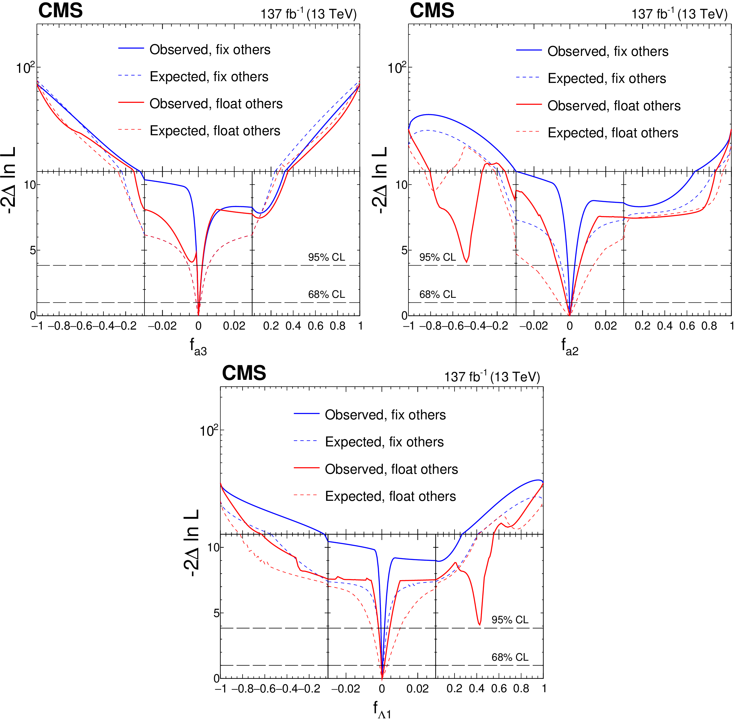
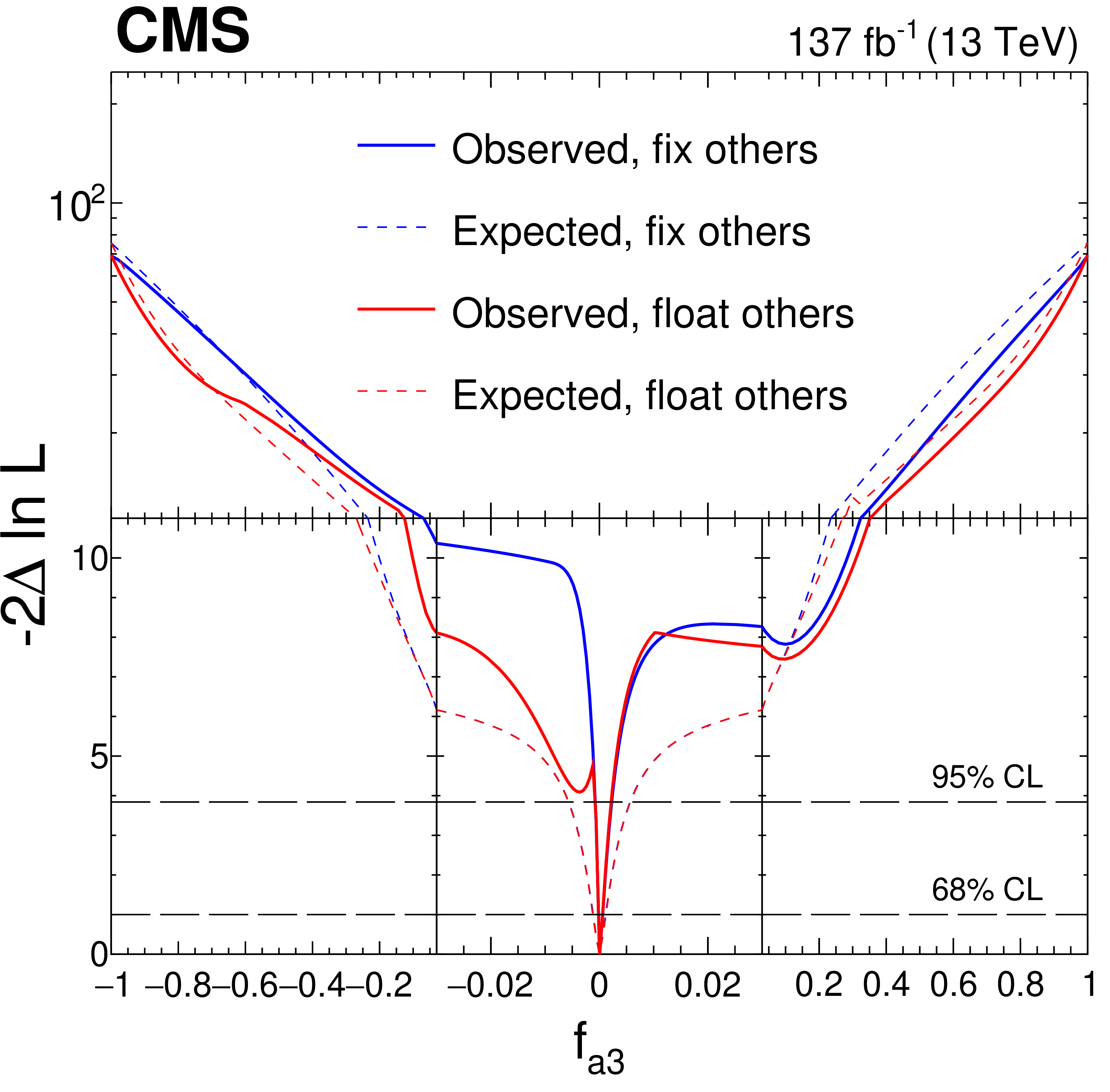
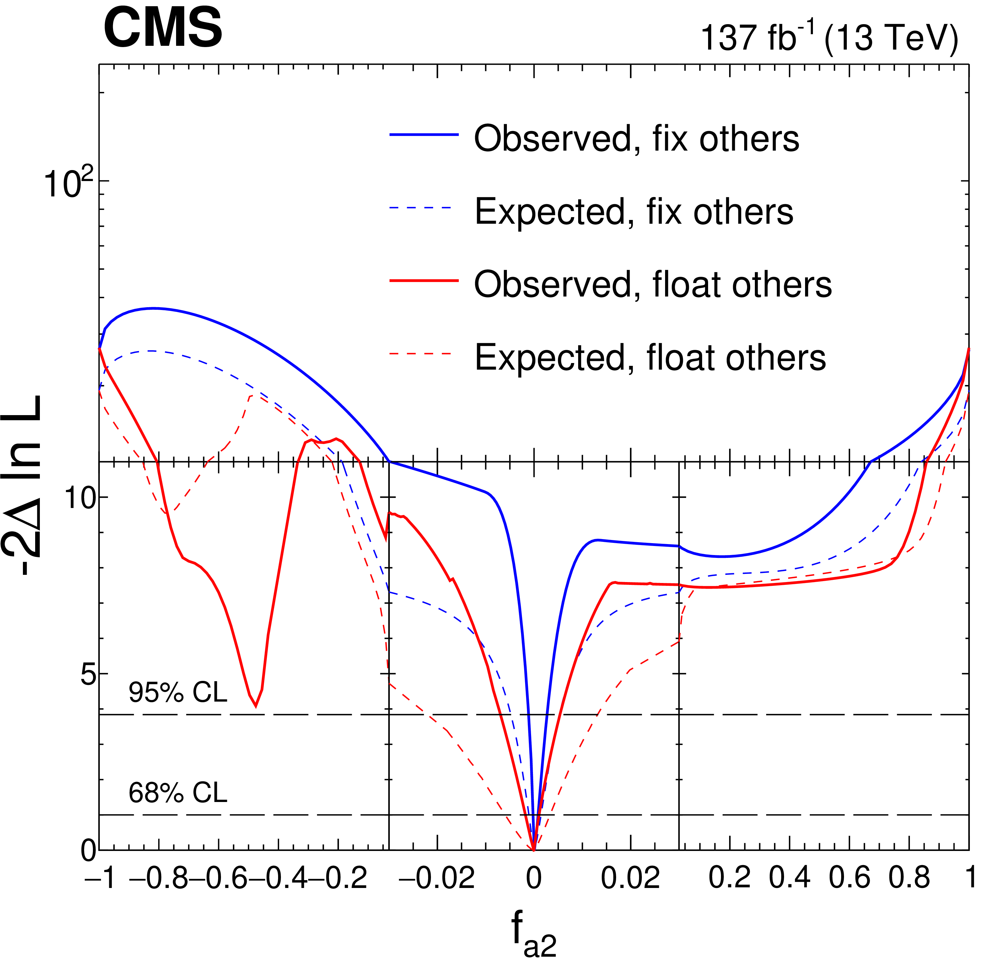
Figure 18:
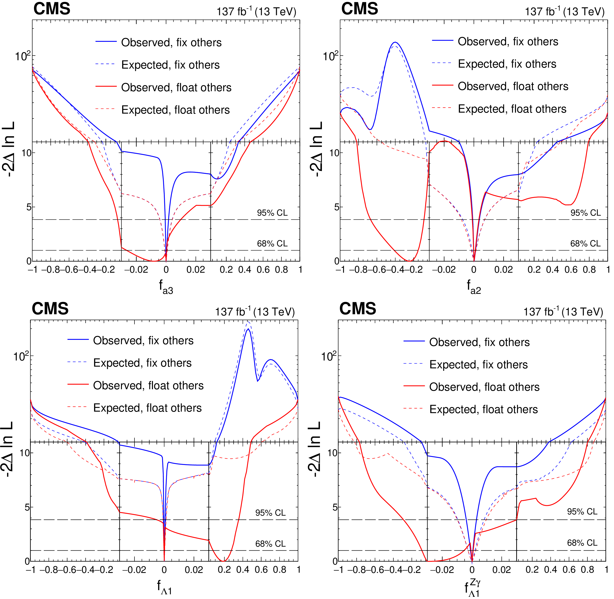
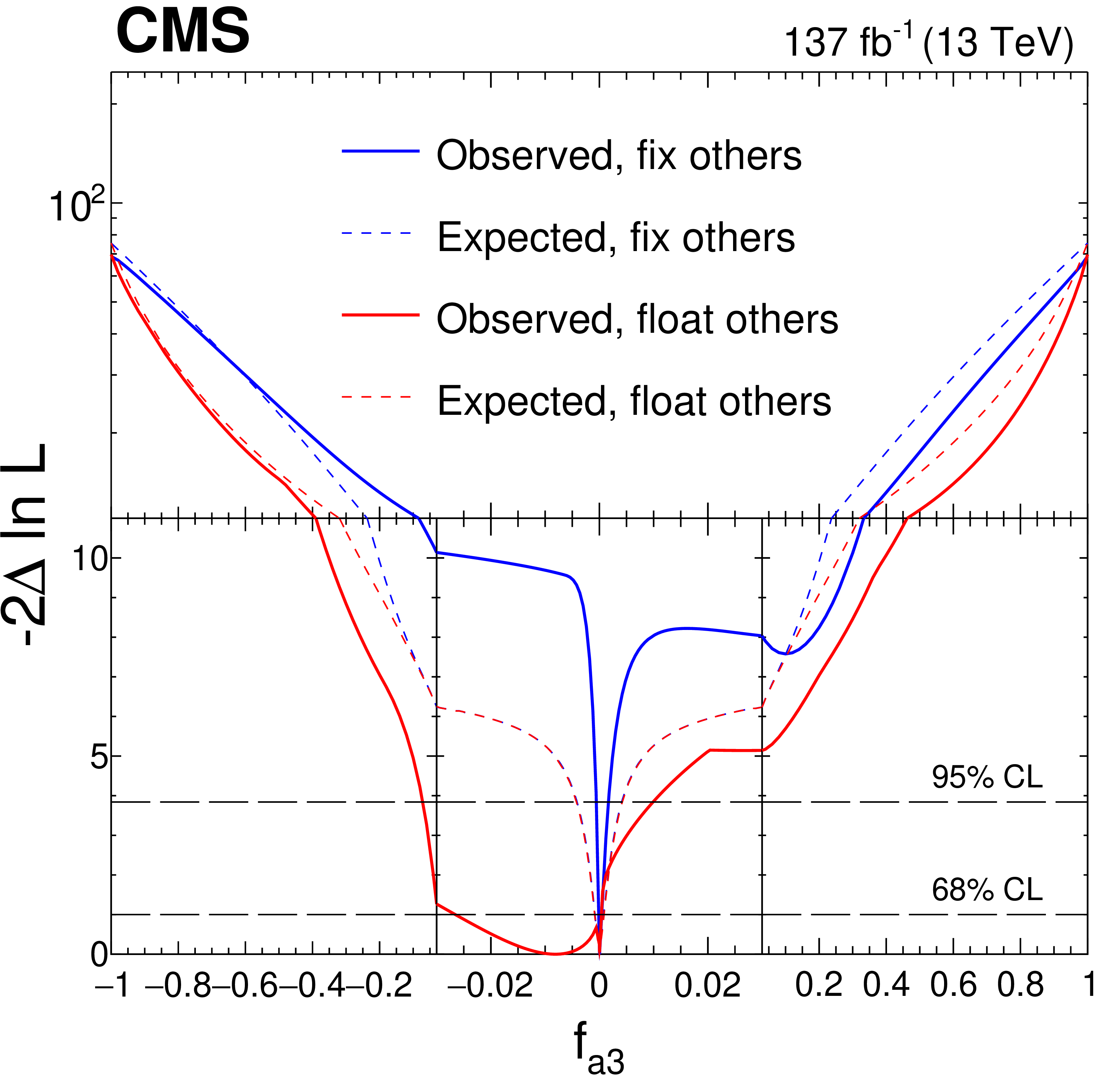
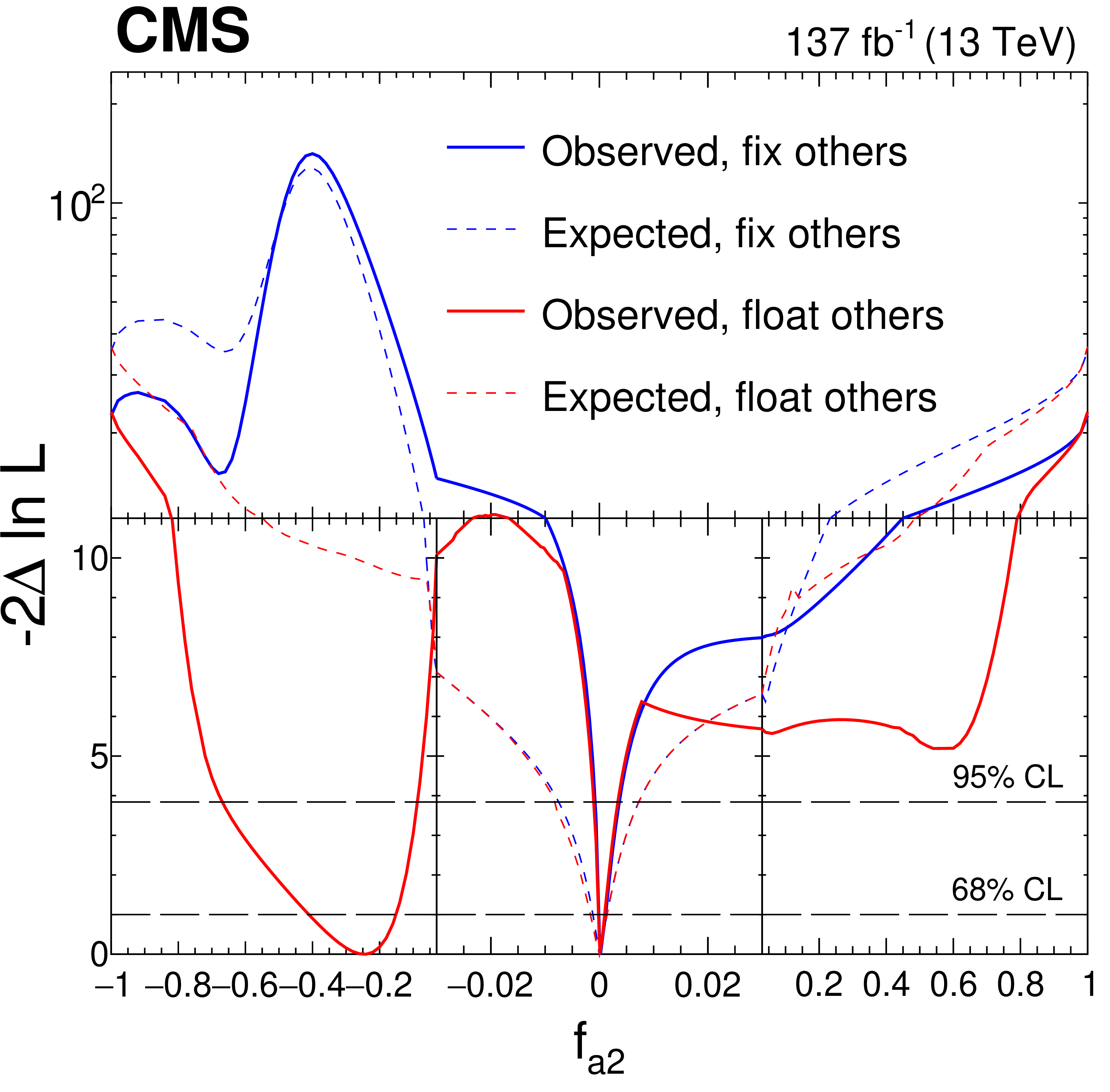
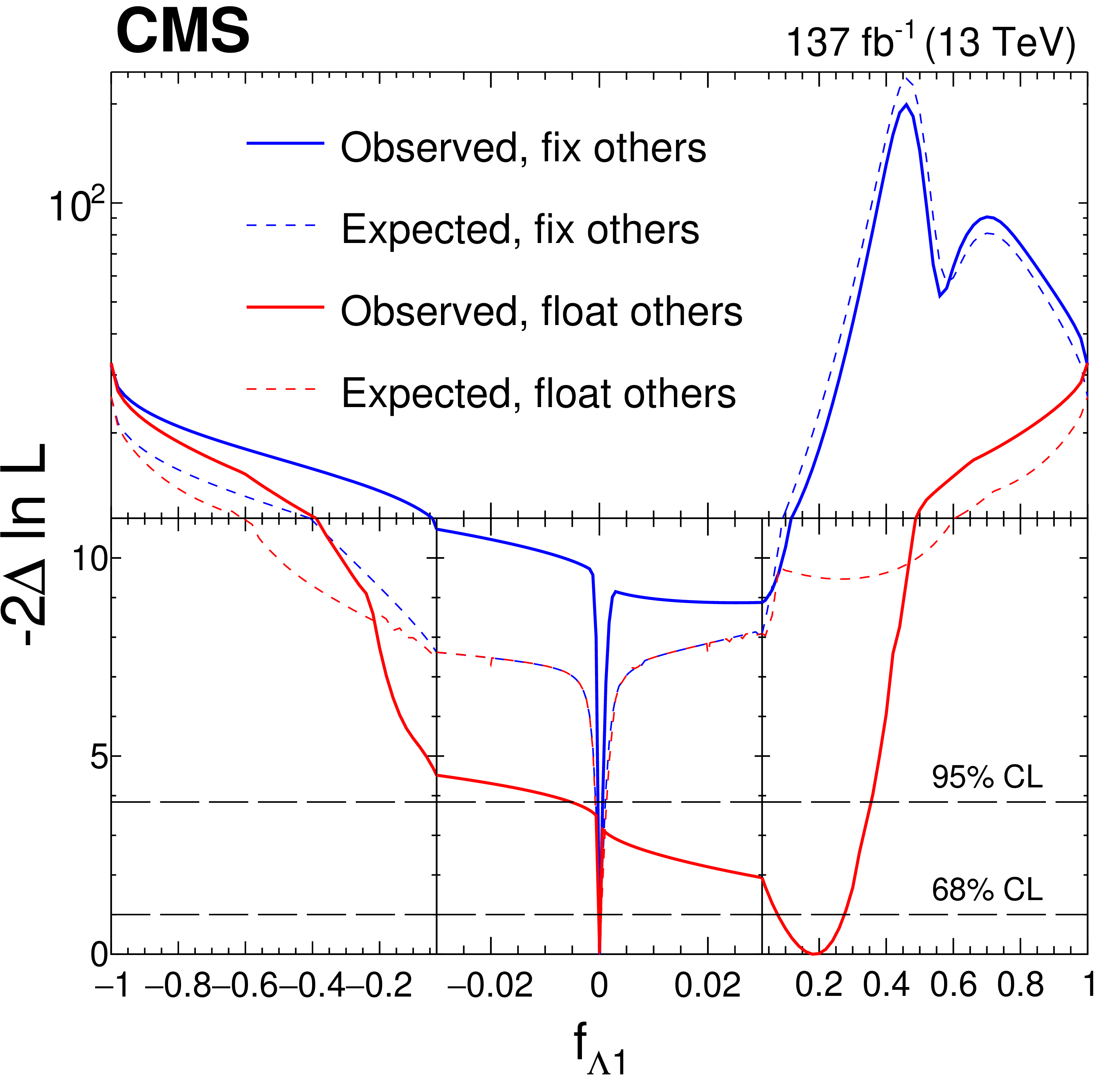
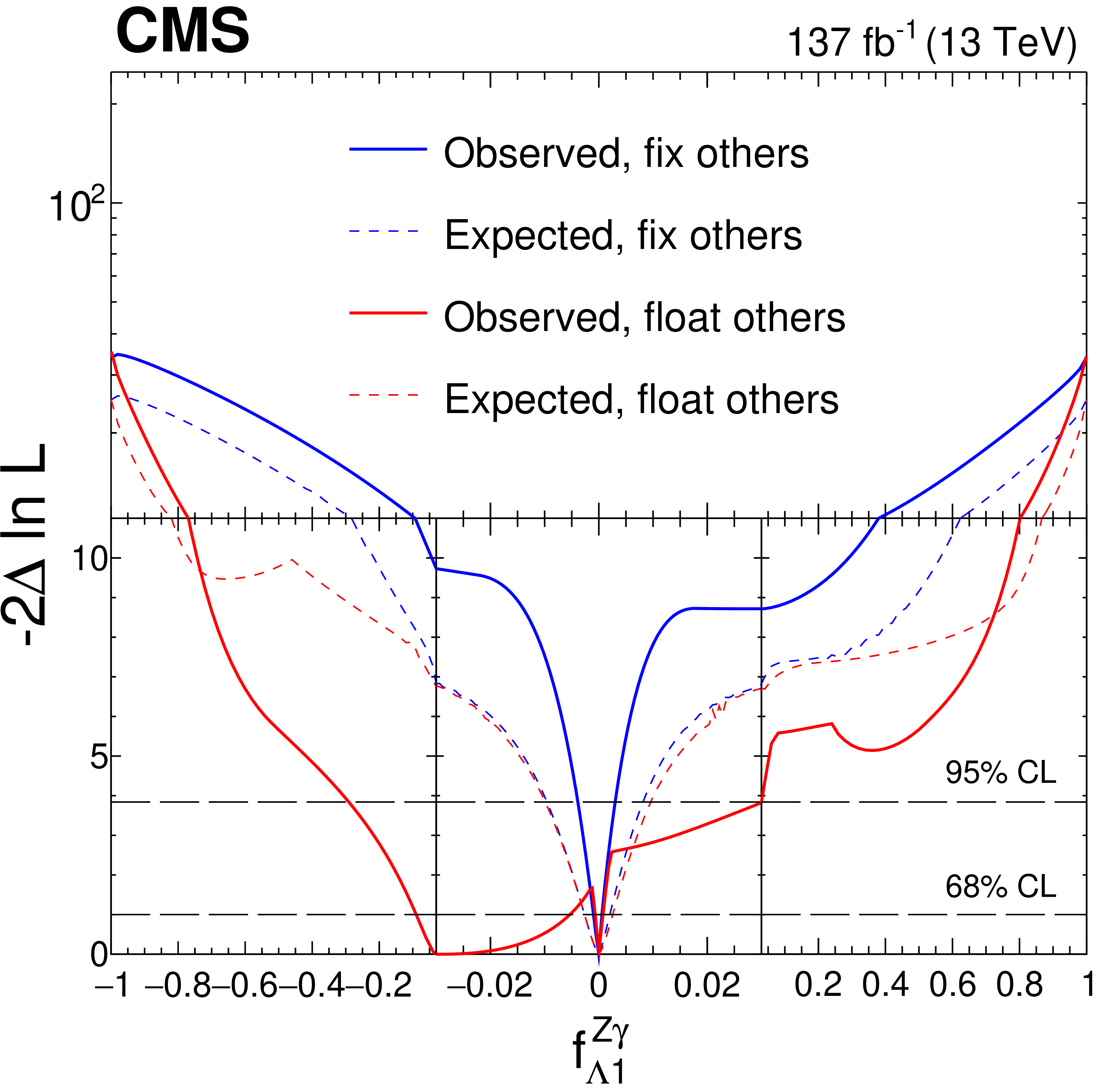
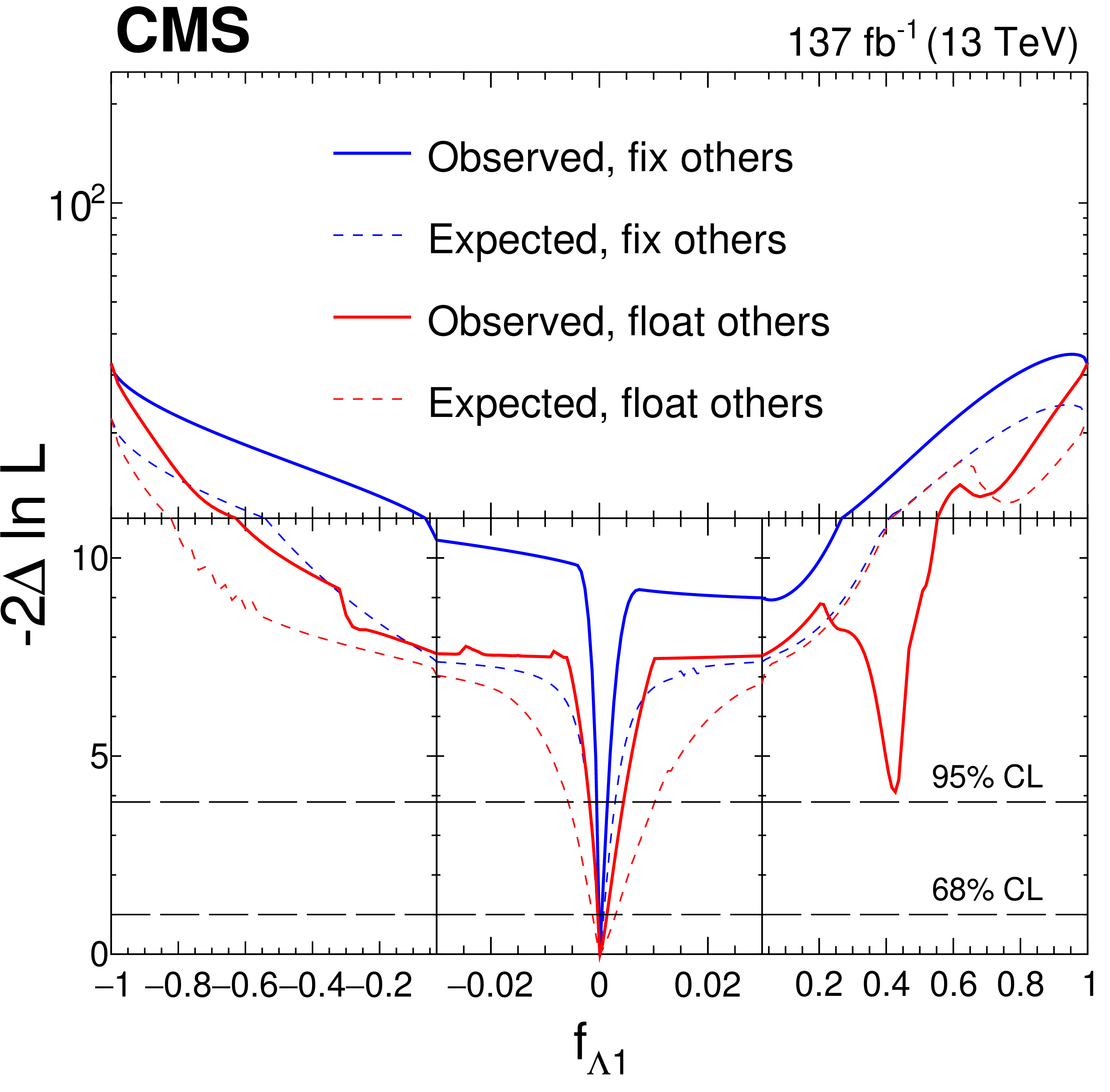
Observed (solid) and expected (dashed) likelihood scans of ${f_{a3}}$ (upper left), ${f_{a2}}$ (upper right), ${f_{\Lambda 1}}$ (lower left), and ${f_{\Lambda 1}^{\mathrm{Z} \gamma}}$ (lower right) in Approach 1 with the coupling relationship $a_i^{WW}=a_i^{ZZ}$. The results are shown for each coupling fraction separately with the other three anomalous coupling fractions either set to zero or left unconstrained in the fit. In all cases, the signal strength parameters have been left unconstrained. The dashed horizontal lines show the 68 and 95% CL regions. For better visibility of all features, the $x$ and $y$ axes are presented with variable scales. On the linear-scale $x$ axis, a zoom is applied in the range $-$0.03 to 0.03. The $y$ axis is shown in linear or logarithmic scale for values of $-2\ln\mathcal {L}$ below or above 11, respectively. |
png pdf |
Figure 18-a:
Observed (solid) and expected (dashed) likelihood scans of ${f_{a3}}$ (upper left), ${f_{a2}}$ (upper right), ${f_{\Lambda 1}}$ (lower left), and ${f_{\Lambda 1}^{\mathrm{Z} \gamma}}$ (lower right) in Approach 1 with the coupling relationship $a_i^{WW}=a_i^{ZZ}$. The results are shown for each coupling fraction separately with the other three anomalous coupling fractions either set to zero or left unconstrained in the fit. In all cases, the signal strength parameters have been left unconstrained. The dashed horizontal lines show the 68 and 95% CL regions. For better visibility of all features, the $x$ and $y$ axes are presented with variable scales. On the linear-scale $x$ axis, a zoom is applied in the range $-$0.03 to 0.03. The $y$ axis is shown in linear or logarithmic scale for values of $-2\ln\mathcal {L}$ below or above 11, respectively. |
png pdf |
Figure 18-b:
Observed (solid) and expected (dashed) likelihood scans of ${f_{a3}}$ (upper left), ${f_{a2}}$ (upper right), ${f_{\Lambda 1}}$ (lower left), and ${f_{\Lambda 1}^{\mathrm{Z} \gamma}}$ (lower right) in Approach 1 with the coupling relationship $a_i^{WW}=a_i^{ZZ}$. The results are shown for each coupling fraction separately with the other three anomalous coupling fractions either set to zero or left unconstrained in the fit. In all cases, the signal strength parameters have been left unconstrained. The dashed horizontal lines show the 68 and 95% CL regions. For better visibility of all features, the $x$ and $y$ axes are presented with variable scales. On the linear-scale $x$ axis, a zoom is applied in the range $-$0.03 to 0.03. The $y$ axis is shown in linear or logarithmic scale for values of $-2\ln\mathcal {L}$ below or above 11, respectively. |
png pdf |
Figure 18-c:
Observed (solid) and expected (dashed) likelihood scans of ${f_{a3}}$ (upper left), ${f_{a2}}$ (upper right), ${f_{\Lambda 1}}$ (lower left), and ${f_{\Lambda 1}^{\mathrm{Z} \gamma}}$ (lower right) in Approach 1 with the coupling relationship $a_i^{WW}=a_i^{ZZ}$. The results are shown for each coupling fraction separately with the other three anomalous coupling fractions either set to zero or left unconstrained in the fit. In all cases, the signal strength parameters have been left unconstrained. The dashed horizontal lines show the 68 and 95% CL regions. For better visibility of all features, the $x$ and $y$ axes are presented with variable scales. On the linear-scale $x$ axis, a zoom is applied in the range $-$0.03 to 0.03. The $y$ axis is shown in linear or logarithmic scale for values of $-2\ln\mathcal {L}$ below or above 11, respectively. |
png pdf |
Figure 18-d:
Observed (solid) and expected (dashed) likelihood scans of ${f_{a3}}$ (upper left), ${f_{a2}}$ (upper right), ${f_{\Lambda 1}}$ (lower left), and ${f_{\Lambda 1}^{\mathrm{Z} \gamma}}$ (lower right) in Approach 1 with the coupling relationship $a_i^{WW}=a_i^{ZZ}$. The results are shown for each coupling fraction separately with the other three anomalous coupling fractions either set to zero or left unconstrained in the fit. In all cases, the signal strength parameters have been left unconstrained. The dashed horizontal lines show the 68 and 95% CL regions. For better visibility of all features, the $x$ and $y$ axes are presented with variable scales. On the linear-scale $x$ axis, a zoom is applied in the range $-$0.03 to 0.03. The $y$ axis is shown in linear or logarithmic scale for values of $-2\ln\mathcal {L}$ below or above 11, respectively. |
png pdf |
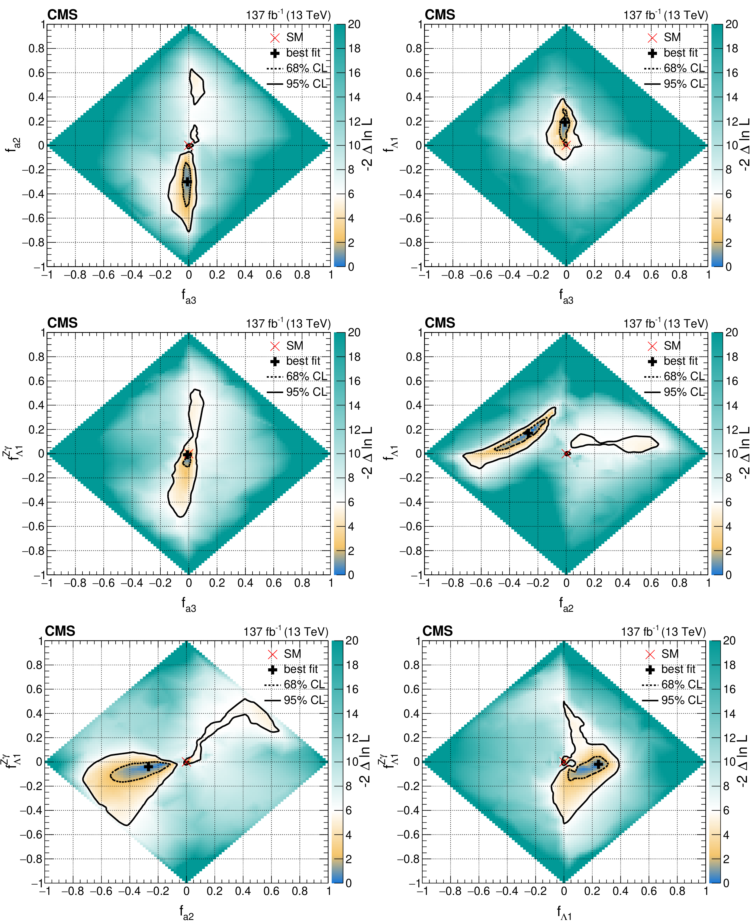
Figure 19:
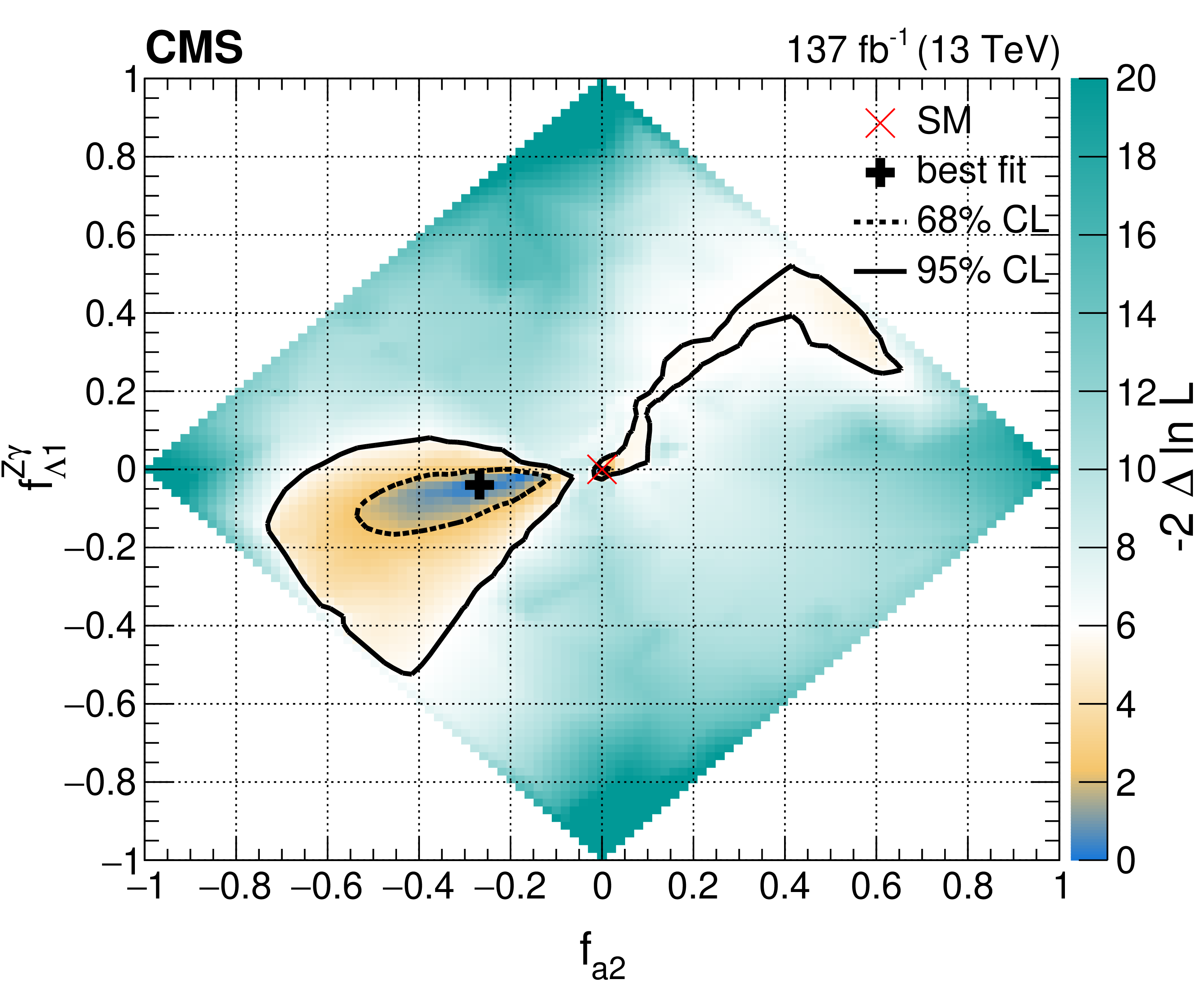
Observed two-dimensional likelihood scans of the four coupling parameters ${f_{a3}}$, ${f_{a2}}$, ${f_{\Lambda 1}}$, and ${f_{\Lambda 1}^{\mathrm{Z} \gamma}}$ in Approach 1 with the coupling relationship $a_i^{WW}=a_i^{ZZ}$. In each case, the other two anomalous couplings along with the signal strength parameters have been left unconstrained. The 68 and 95% CL regions are presented as contours with dashed and solid black lines, respectively. The best fit values and the SM expectations are indicated by markers. |

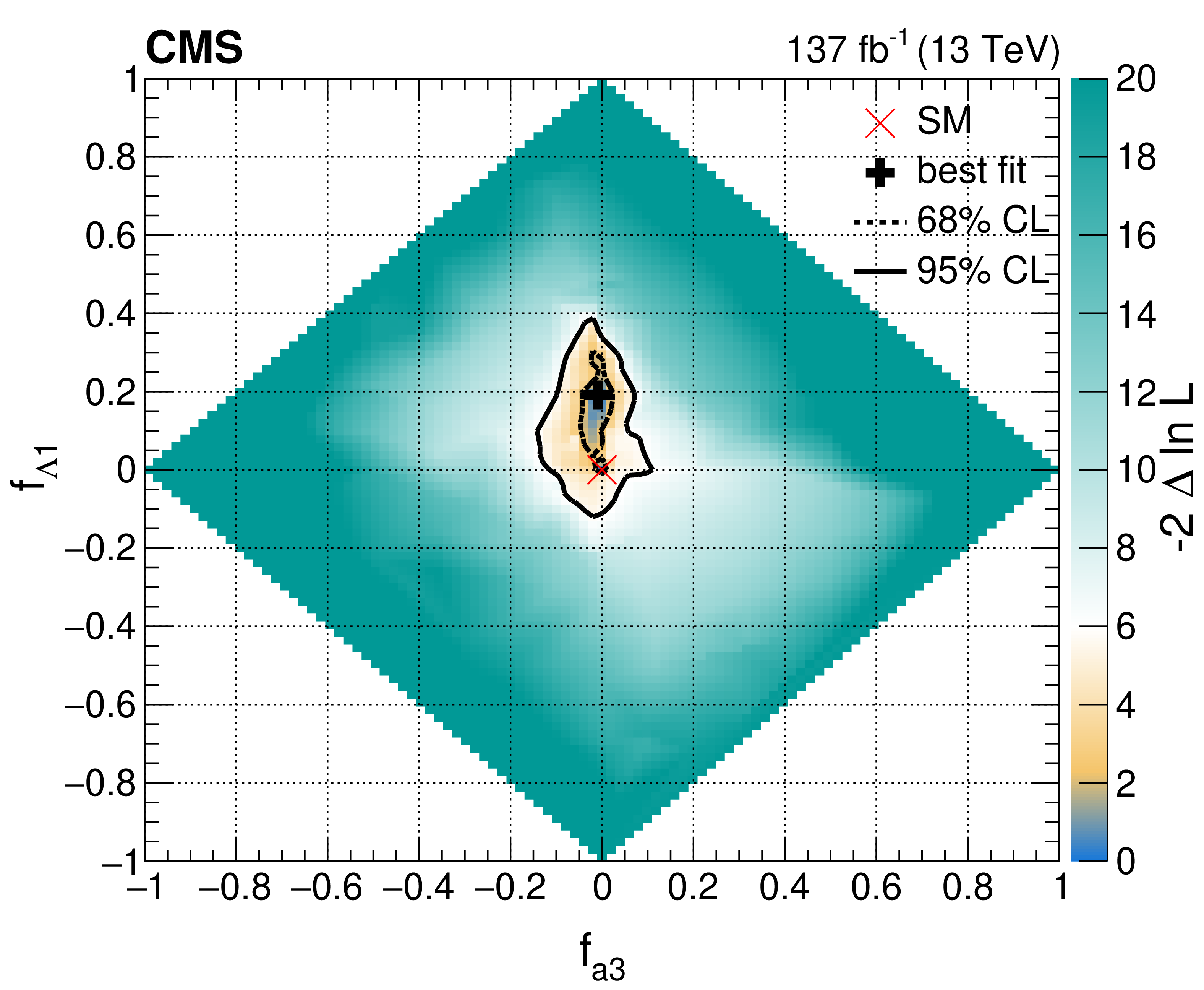
png pdf |
Figure 19-a:
Observed two-dimensional likelihood scans of the four coupling parameters ${f_{a3}}$, ${f_{a2}}$, ${f_{\Lambda 1}}$, and ${f_{\Lambda 1}^{\mathrm{Z} \gamma}}$ in Approach 1 with the coupling relationship $a_i^{WW}=a_i^{ZZ}$. In each case, the other two anomalous couplings along with the signal strength parameters have been left unconstrained. The 68 and 95% CL regions are presented as contours with dashed and solid black lines, respectively. The best fit values and the SM expectations are indicated by markers. |
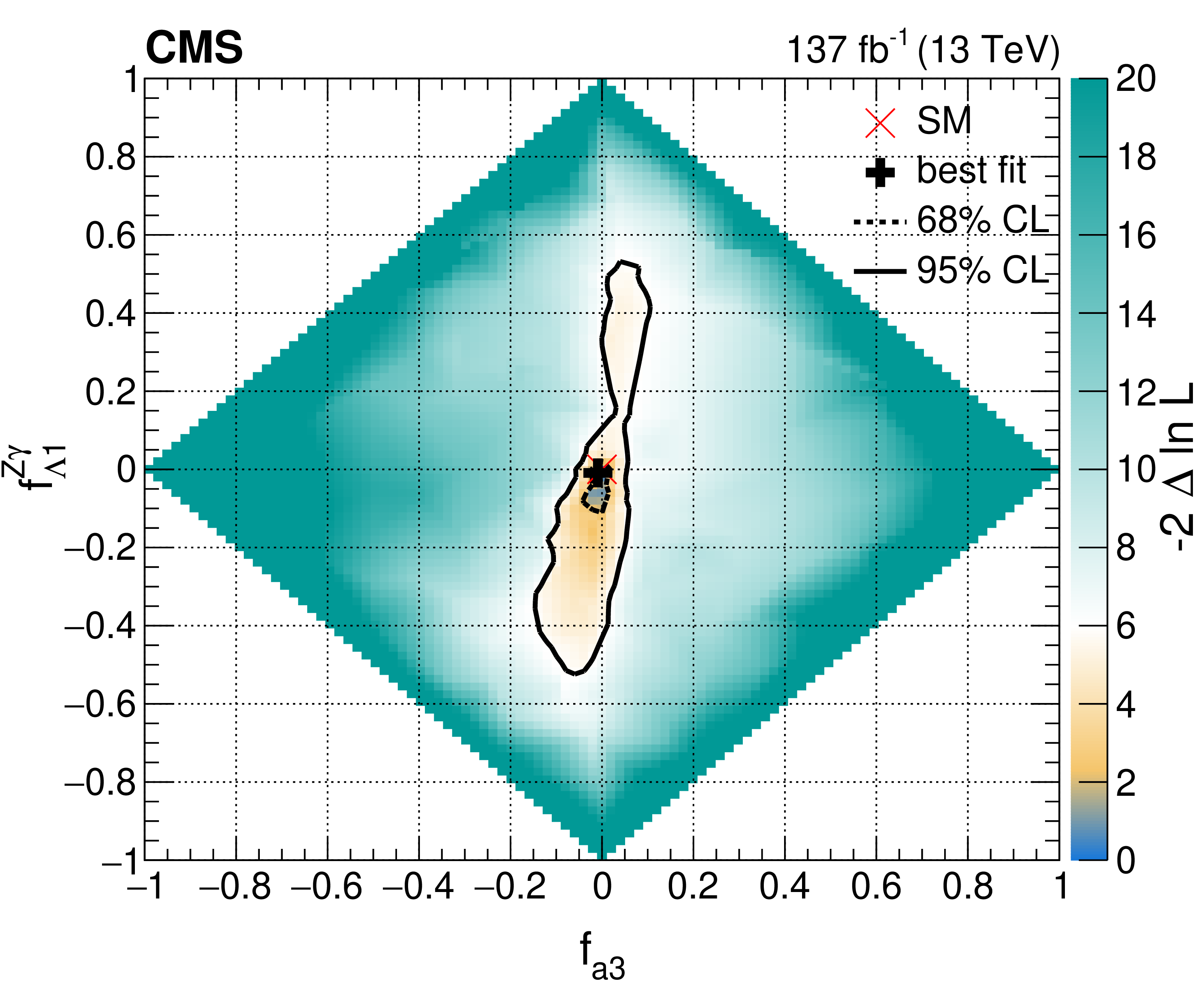
png pdf |
Figure 19-b:
Observed two-dimensional likelihood scans of the four coupling parameters ${f_{a3}}$, ${f_{a2}}$, ${f_{\Lambda 1}}$, and ${f_{\Lambda 1}^{\mathrm{Z} \gamma}}$ in Approach 1 with the coupling relationship $a_i^{WW}=a_i^{ZZ}$. In each case, the other two anomalous couplings along with the signal strength parameters have been left unconstrained. The 68 and 95% CL regions are presented as contours with dashed and solid black lines, respectively. The best fit values and the SM expectations are indicated by markers. |
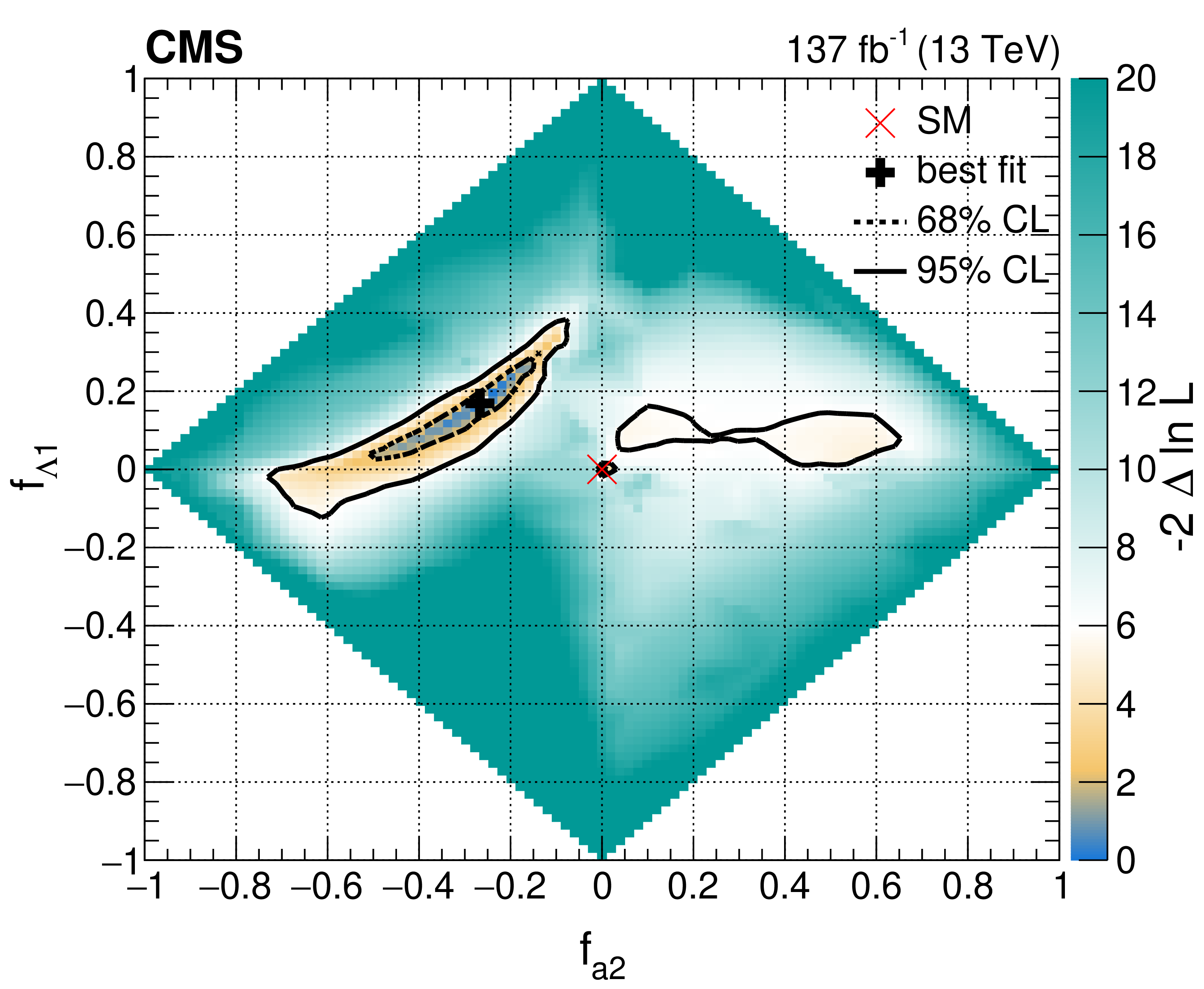
png pdf |
Figure 19-c:
Observed two-dimensional likelihood scans of the four coupling parameters ${f_{a3}}$, ${f_{a2}}$, ${f_{\Lambda 1}}$, and ${f_{\Lambda 1}^{\mathrm{Z} \gamma}}$ in Approach 1 with the coupling relationship $a_i^{WW}=a_i^{ZZ}$. In each case, the other two anomalous couplings along with the signal strength parameters have been left unconstrained. The 68 and 95% CL regions are presented as contours with dashed and solid black lines, respectively. The best fit values and the SM expectations are indicated by markers. |
png pdf |
Figure 19-d:
Observed two-dimensional likelihood scans of the four coupling parameters ${f_{a3}}$, ${f_{a2}}$, ${f_{\Lambda 1}}$, and ${f_{\Lambda 1}^{\mathrm{Z} \gamma}}$ in Approach 1 with the coupling relationship $a_i^{WW}=a_i^{ZZ}$. In each case, the other two anomalous couplings along with the signal strength parameters have been left unconstrained. The 68 and 95% CL regions are presented as contours with dashed and solid black lines, respectively. The best fit values and the SM expectations are indicated by markers. |
png pdf |
Figure 19-e:
Observed two-dimensional likelihood scans of the four coupling parameters ${f_{a3}}$, ${f_{a2}}$, ${f_{\Lambda 1}}$, and ${f_{\Lambda 1}^{\mathrm{Z} \gamma}}$ in Approach 1 with the coupling relationship $a_i^{WW}=a_i^{ZZ}$. In each case, the other two anomalous couplings along with the signal strength parameters have been left unconstrained. The 68 and 95% CL regions are presented as contours with dashed and solid black lines, respectively. The best fit values and the SM expectations are indicated by markers. |

png pdf |
Figure 19-f:
Observed two-dimensional likelihood scans of the four coupling parameters ${f_{a3}}$, ${f_{a2}}$, ${f_{\Lambda 1}}$, and ${f_{\Lambda 1}^{\mathrm{Z} \gamma}}$ in Approach 1 with the coupling relationship $a_i^{WW}=a_i^{ZZ}$. In each case, the other two anomalous couplings along with the signal strength parameters have been left unconstrained. The 68 and 95% CL regions are presented as contours with dashed and solid black lines, respectively. The best fit values and the SM expectations are indicated by markers. |
png pdf |
Figure 20:
Observed (solid) and expected (dashed) likelihood scans of ${f_{a3}}$ (upper left), ${f_{a2}}$ (upper right), and ${f_{\Lambda 1}}$ (lower) in Approach 2 within SMEFT with the symmetry relationship of couplings set in Eqs. (3-7). The results are shown for each coupling separately with the other anomalous coupling fractions either set to zero or left unconstrained in the fit. In all cases, the signal strength parameters have been left unconstrained. The dashed horizontal lines show the 68 and 95% CL regions. For better visibility of all features, the $x$ and $y$ axes are presented with variable scales. On the linear-scale $x$ axis, a zoom is applied in the range $-$0.03 to 0.03. The $y$ axis is shown in linear or logarithmic scale for values of $-2\ln\mathcal {L}$ below or above 11, respectively. |
png pdf |
Figure 20-a:
Observed (solid) and expected (dashed) likelihood scans of ${f_{a3}}$ (upper left), ${f_{a2}}$ (upper right), and ${f_{\Lambda 1}}$ (lower) in Approach 2 within SMEFT with the symmetry relationship of couplings set in Eqs. (3-7). The results are shown for each coupling separately with the other anomalous coupling fractions either set to zero or left unconstrained in the fit. In all cases, the signal strength parameters have been left unconstrained. The dashed horizontal lines show the 68 and 95% CL regions. For better visibility of all features, the $x$ and $y$ axes are presented with variable scales. On the linear-scale $x$ axis, a zoom is applied in the range $-$0.03 to 0.03. The $y$ axis is shown in linear or logarithmic scale for values of $-2\ln\mathcal {L}$ below or above 11, respectively. |
png pdf |
Figure 20-b:
Observed (solid) and expected (dashed) likelihood scans of ${f_{a3}}$ (upper left), ${f_{a2}}$ (upper right), and ${f_{\Lambda 1}}$ (lower) in Approach 2 within SMEFT with the symmetry relationship of couplings set in Eqs. (3-7). The results are shown for each coupling separately with the other anomalous coupling fractions either set to zero or left unconstrained in the fit. In all cases, the signal strength parameters have been left unconstrained. The dashed horizontal lines show the 68 and 95% CL regions. For better visibility of all features, the $x$ and $y$ axes are presented with variable scales. On the linear-scale $x$ axis, a zoom is applied in the range $-$0.03 to 0.03. The $y$ axis is shown in linear or logarithmic scale for values of $-2\ln\mathcal {L}$ below or above 11, respectively. |
png pdf |
Figure 20-c:
Observed (solid) and expected (dashed) likelihood scans of ${f_{a3}}$ (upper left), ${f_{a2}}$ (upper right), and ${f_{\Lambda 1}}$ (lower) in Approach 2 within SMEFT with the symmetry relationship of couplings set in Eqs. (3-7). The results are shown for each coupling separately with the other anomalous coupling fractions either set to zero or left unconstrained in the fit. In all cases, the signal strength parameters have been left unconstrained. The dashed horizontal lines show the 68 and 95% CL regions. For better visibility of all features, the $x$ and $y$ axes are presented with variable scales. On the linear-scale $x$ axis, a zoom is applied in the range $-$0.03 to 0.03. The $y$ axis is shown in linear or logarithmic scale for values of $-2\ln\mathcal {L}$ below or above 11, respectively. |
png pdf |
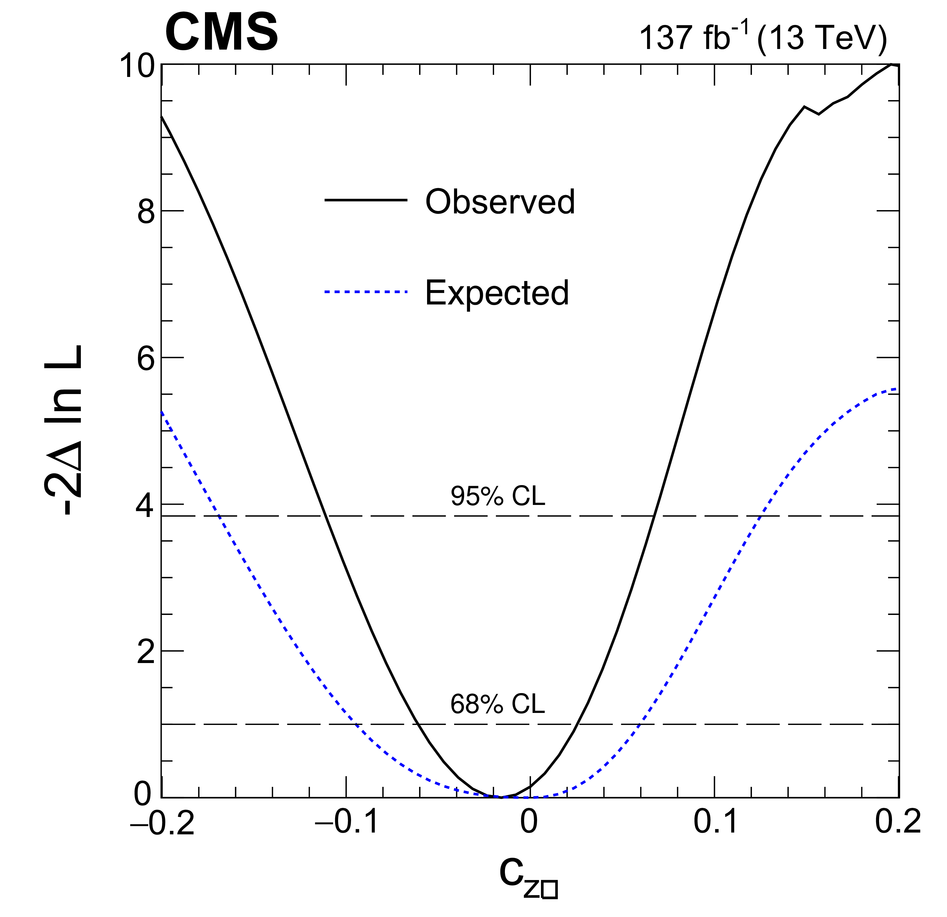
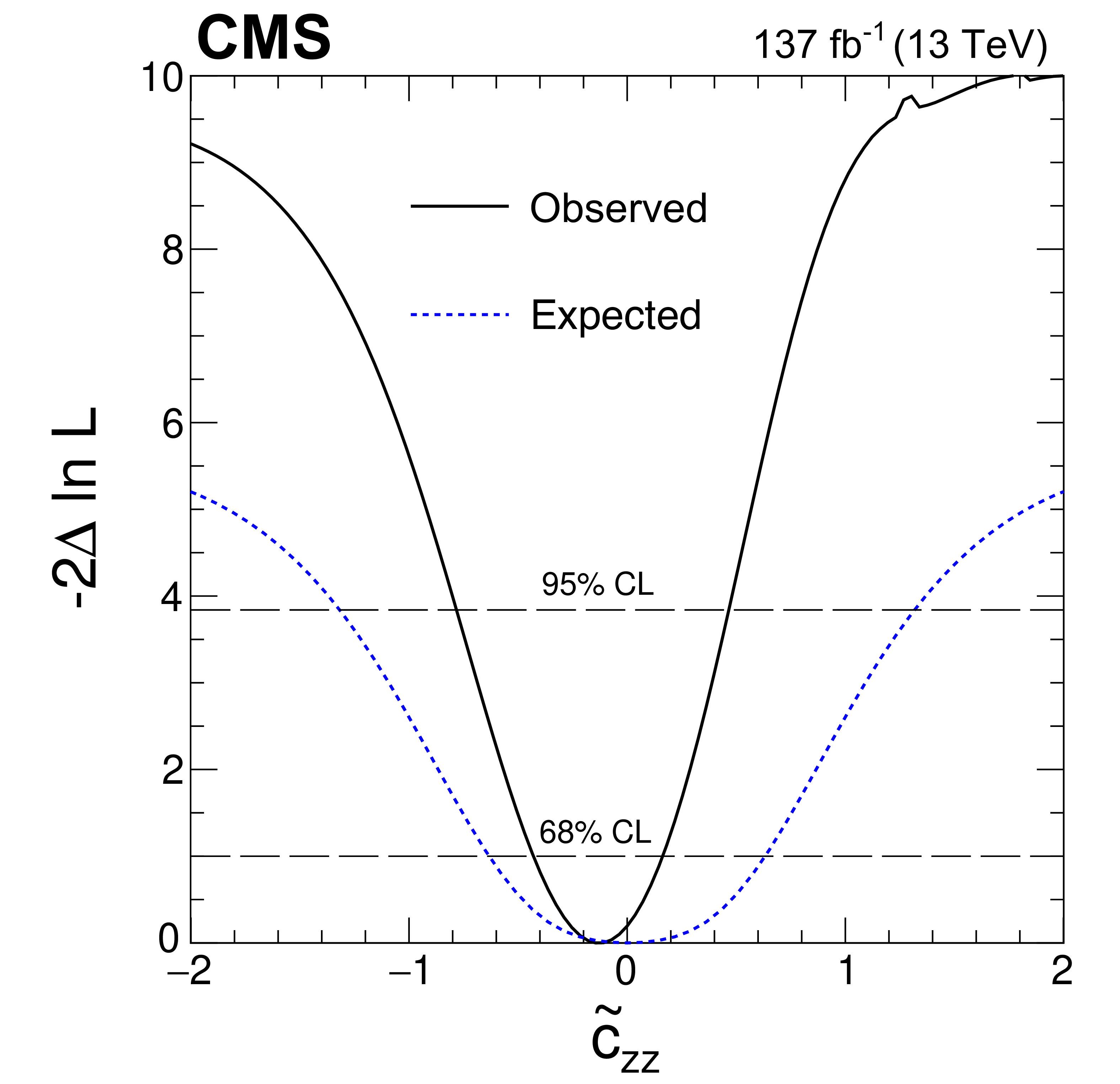
Figure 21:
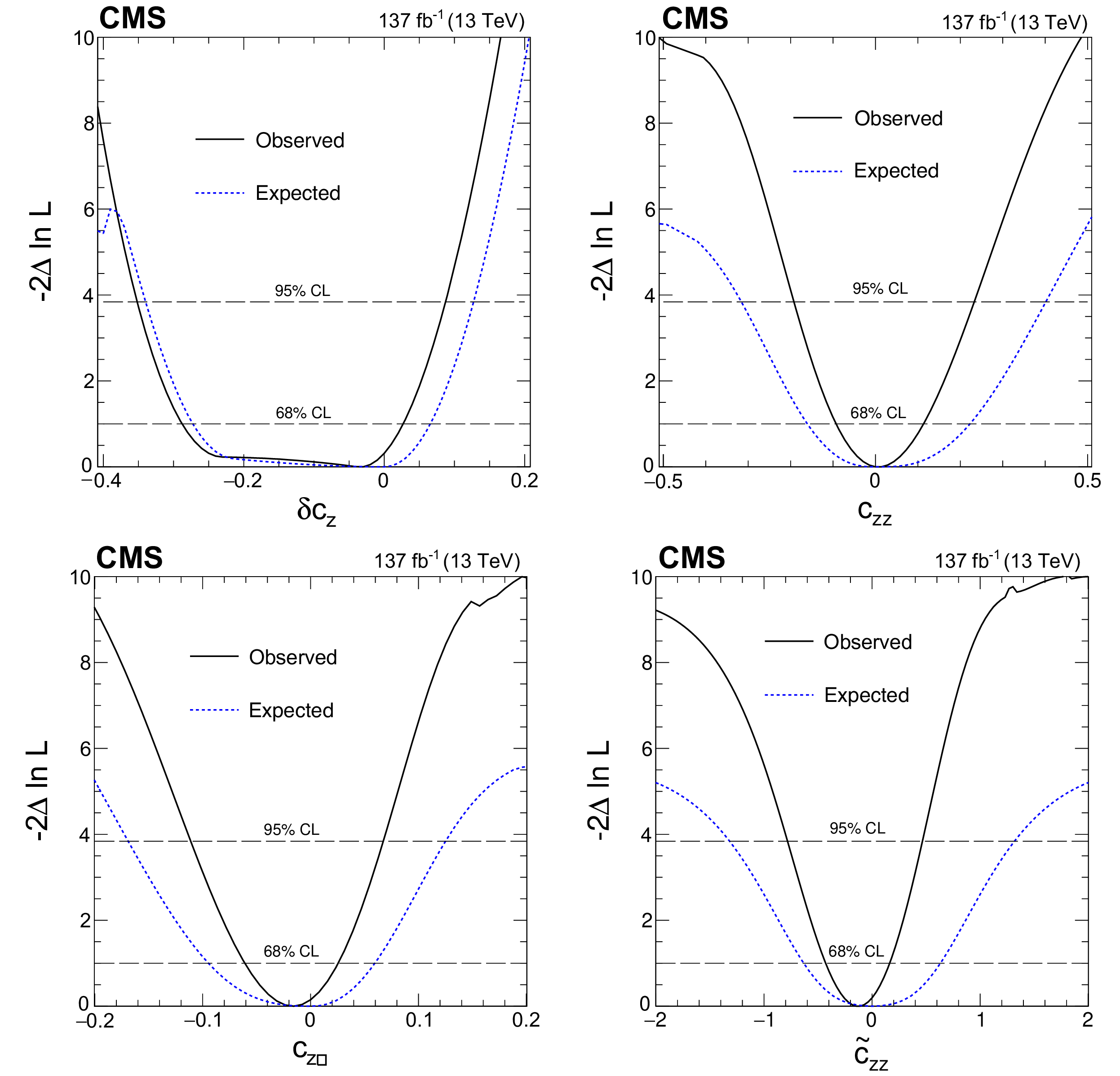
Observed (solid) and expected (dashed) constraints from a simultaneous fit of the SMEFT parameters $\delta c_\mathrm {z}$ (upper left), $c_\mathrm {zz}$ (upper right), $c_{\mathrm {z} \Box}$ (lower left), and $\tilde{c}_\mathrm {zz}$ (lower right) with the $c_{\mathrm{g} \mathrm{g}}$ and $\tilde{c}_{\mathrm{g} \mathrm{g}}$ couplings left unconstrained. |
png pdf |
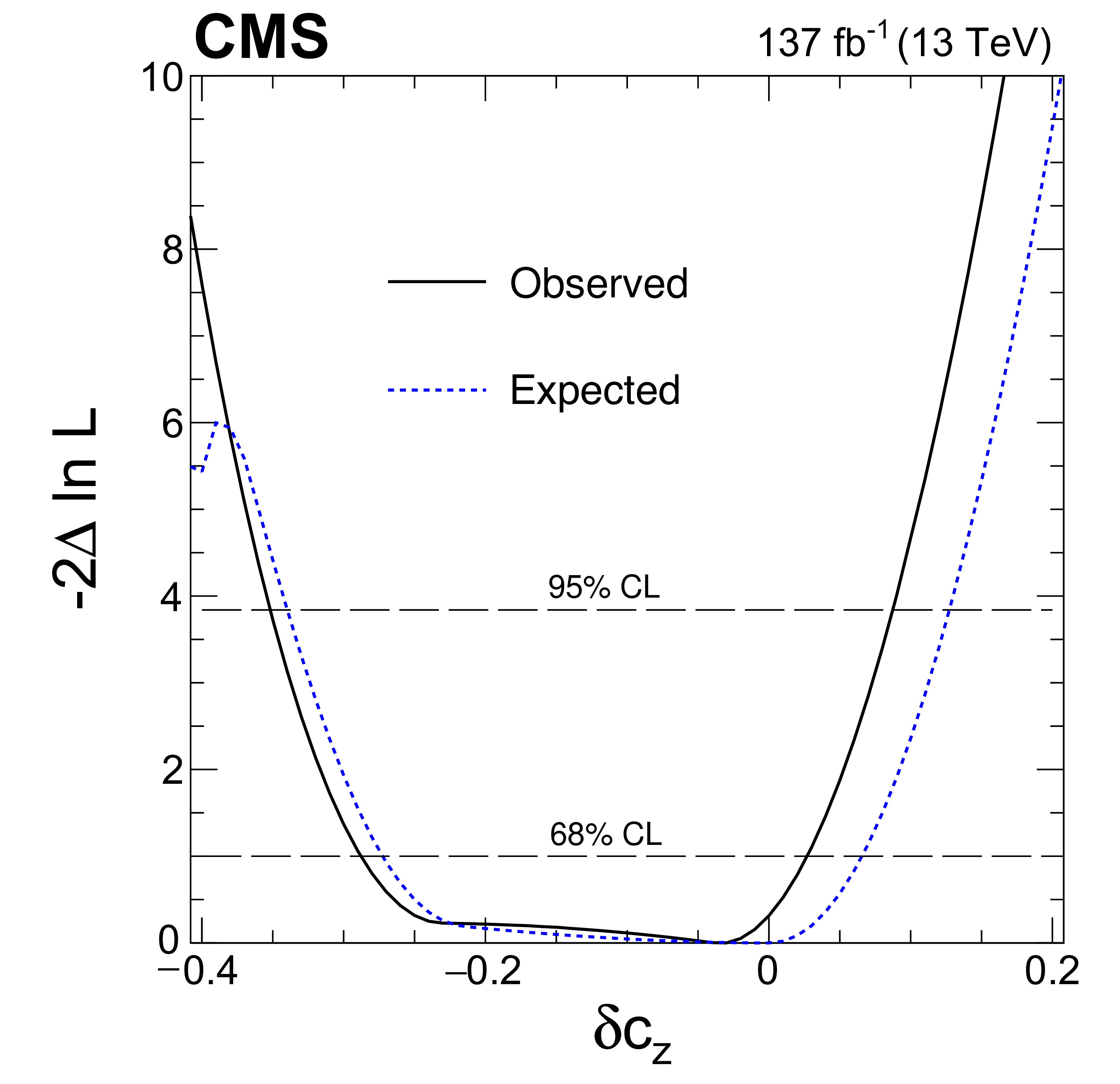
Figure 21-a:
Observed (solid) and expected (dashed) constraints from a simultaneous fit of the SMEFT parameters $\delta c_\mathrm {z}$ (upper left), $c_\mathrm {zz}$ (upper right), $c_{\mathrm {z} \Box}$ (lower left), and $\tilde{c}_\mathrm {zz}$ (lower right) with the $c_{\mathrm{g} \mathrm{g}}$ and $\tilde{c}_{\mathrm{g} \mathrm{g}}$ couplings left unconstrained. |
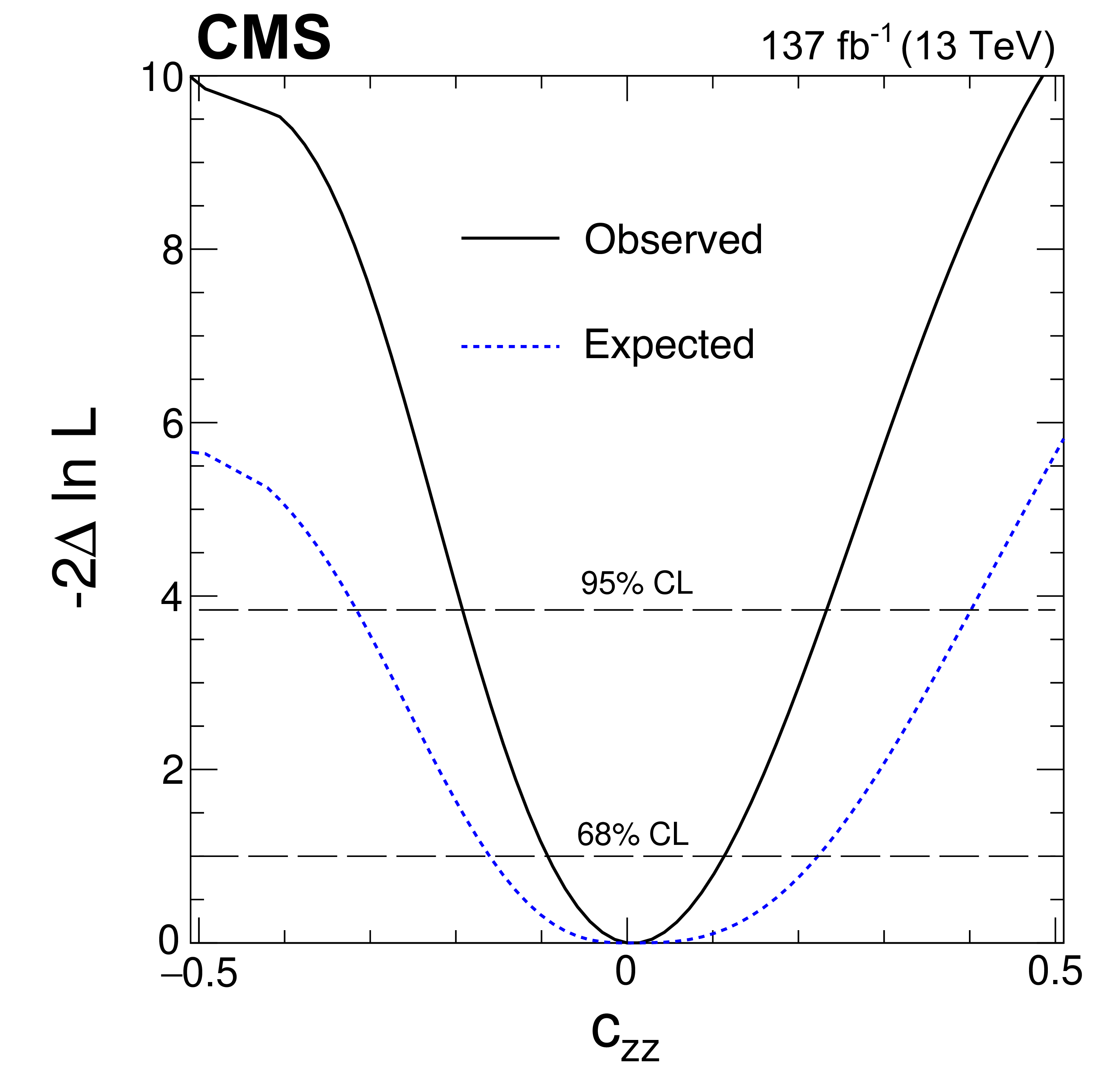
png pdf |
Figure 21-b:
Observed (solid) and expected (dashed) constraints from a simultaneous fit of the SMEFT parameters $\delta c_\mathrm {z}$ (upper left), $c_\mathrm {zz}$ (upper right), $c_{\mathrm {z} \Box}$ (lower left), and $\tilde{c}_\mathrm {zz}$ (lower right) with the $c_{\mathrm{g} \mathrm{g}}$ and $\tilde{c}_{\mathrm{g} \mathrm{g}}$ couplings left unconstrained. |
png pdf |
Figure 21-c:
Observed (solid) and expected (dashed) constraints from a simultaneous fit of the SMEFT parameters $\delta c_\mathrm {z}$ (upper left), $c_\mathrm {zz}$ (upper right), $c_{\mathrm {z} \Box}$ (lower left), and $\tilde{c}_\mathrm {zz}$ (lower right) with the $c_{\mathrm{g} \mathrm{g}}$ and $\tilde{c}_{\mathrm{g} \mathrm{g}}$ couplings left unconstrained. |
png pdf |
Figure 21-d:
Observed (solid) and expected (dashed) constraints from a simultaneous fit of the SMEFT parameters $\delta c_\mathrm {z}$ (upper left), $c_\mathrm {zz}$ (upper right), $c_{\mathrm {z} \Box}$ (lower left), and $\tilde{c}_\mathrm {zz}$ (lower right) with the $c_{\mathrm{g} \mathrm{g}}$ and $\tilde{c}_{\mathrm{g} \mathrm{g}}$ couplings left unconstrained. |
png pdf |
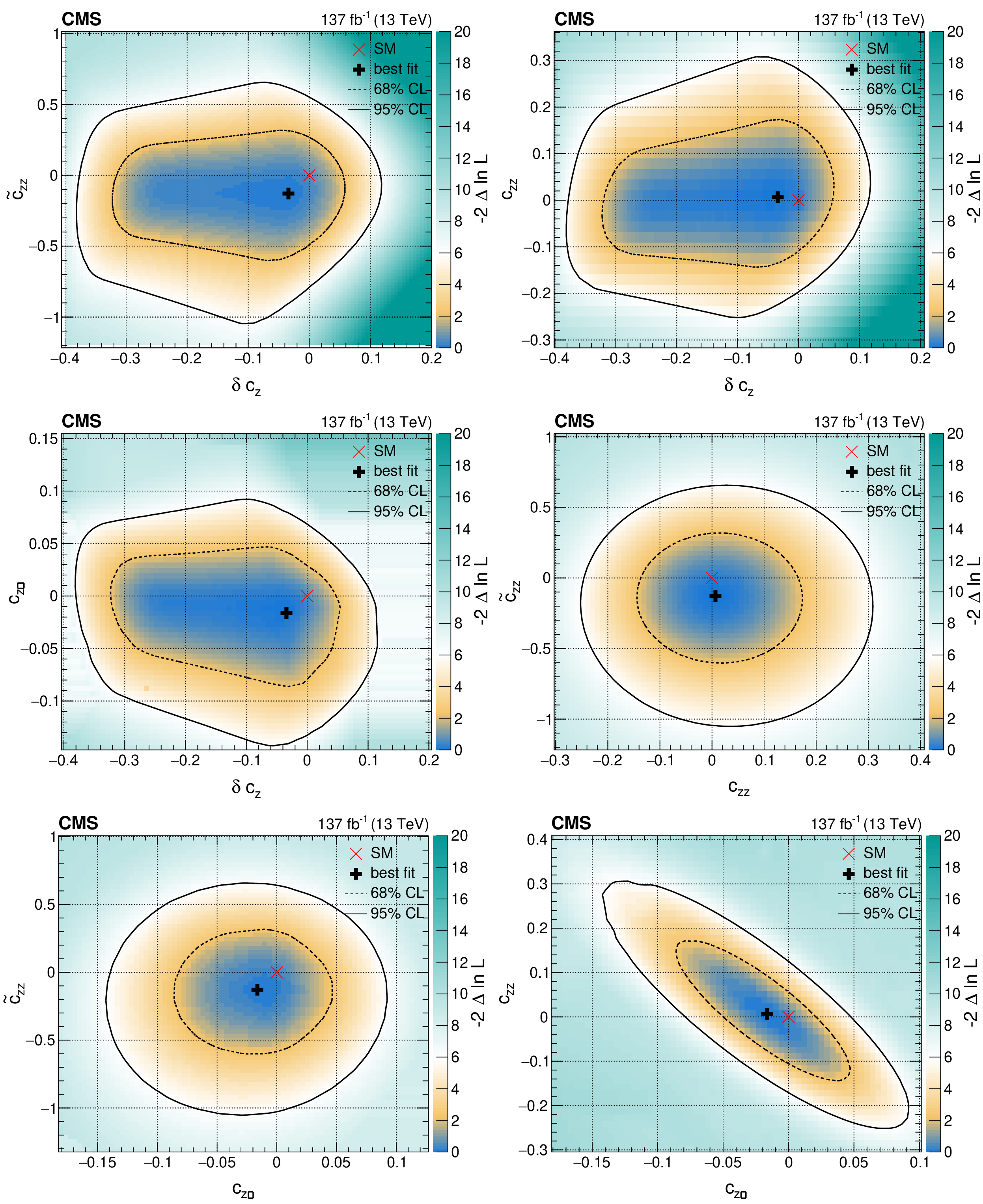
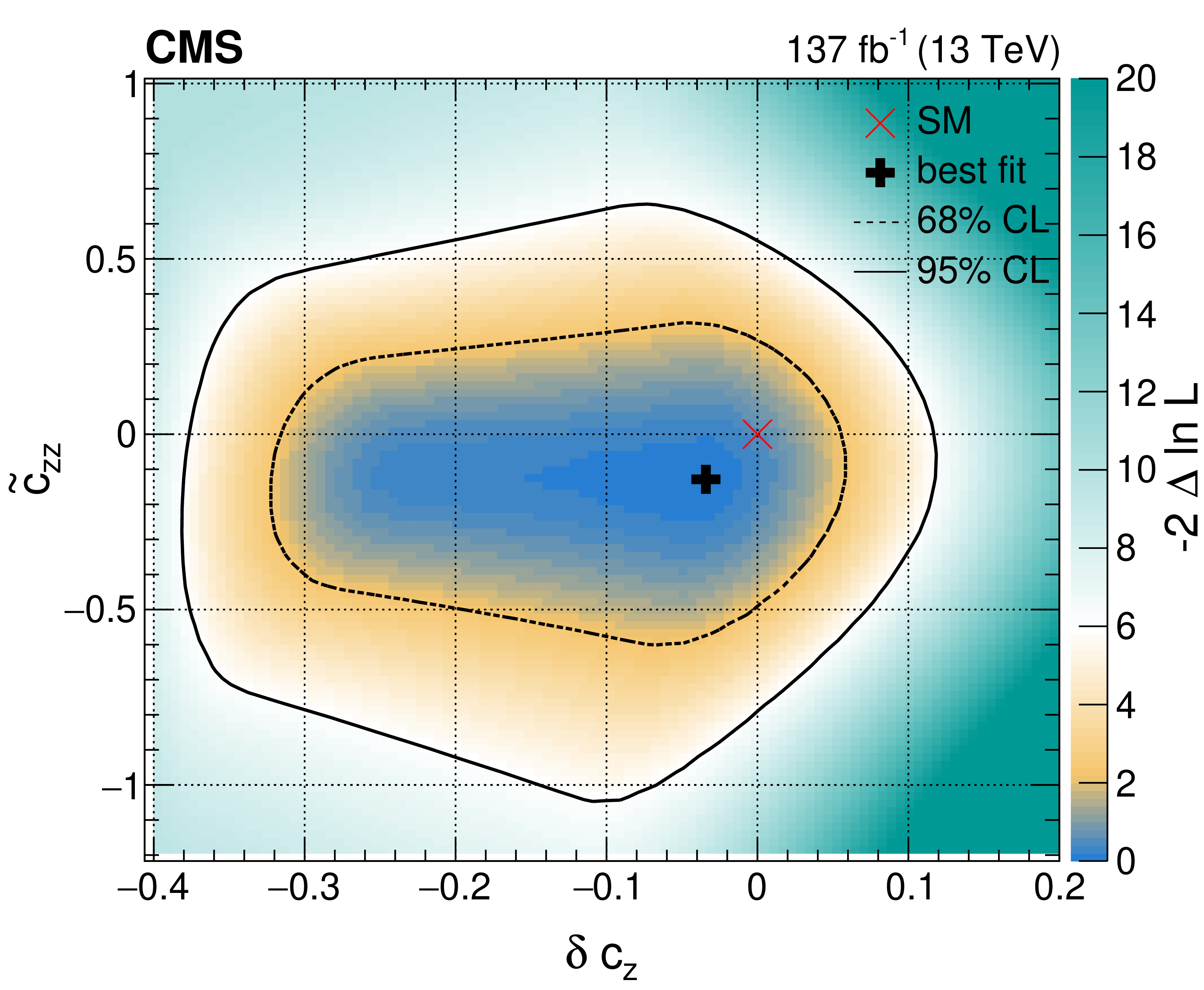
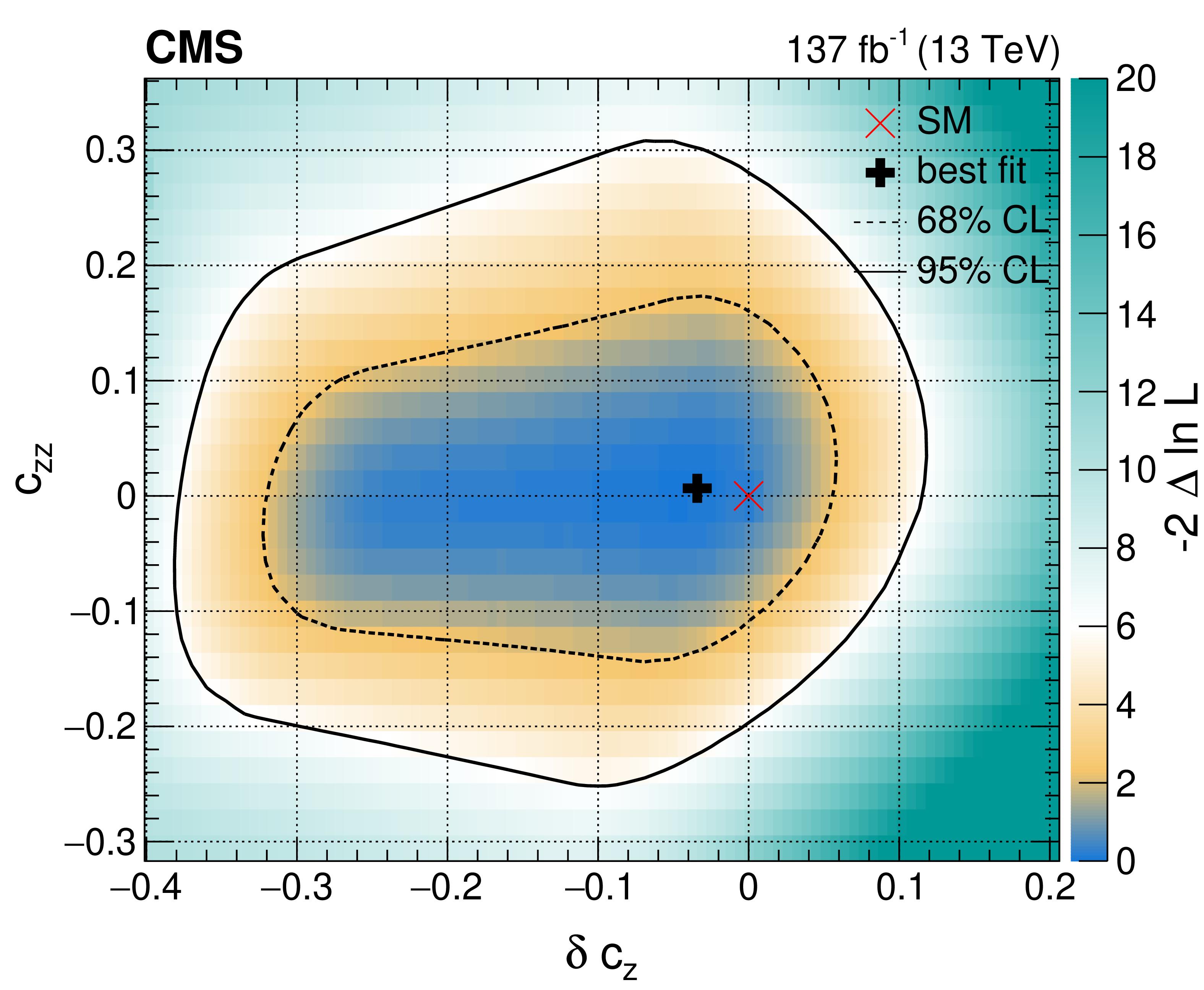
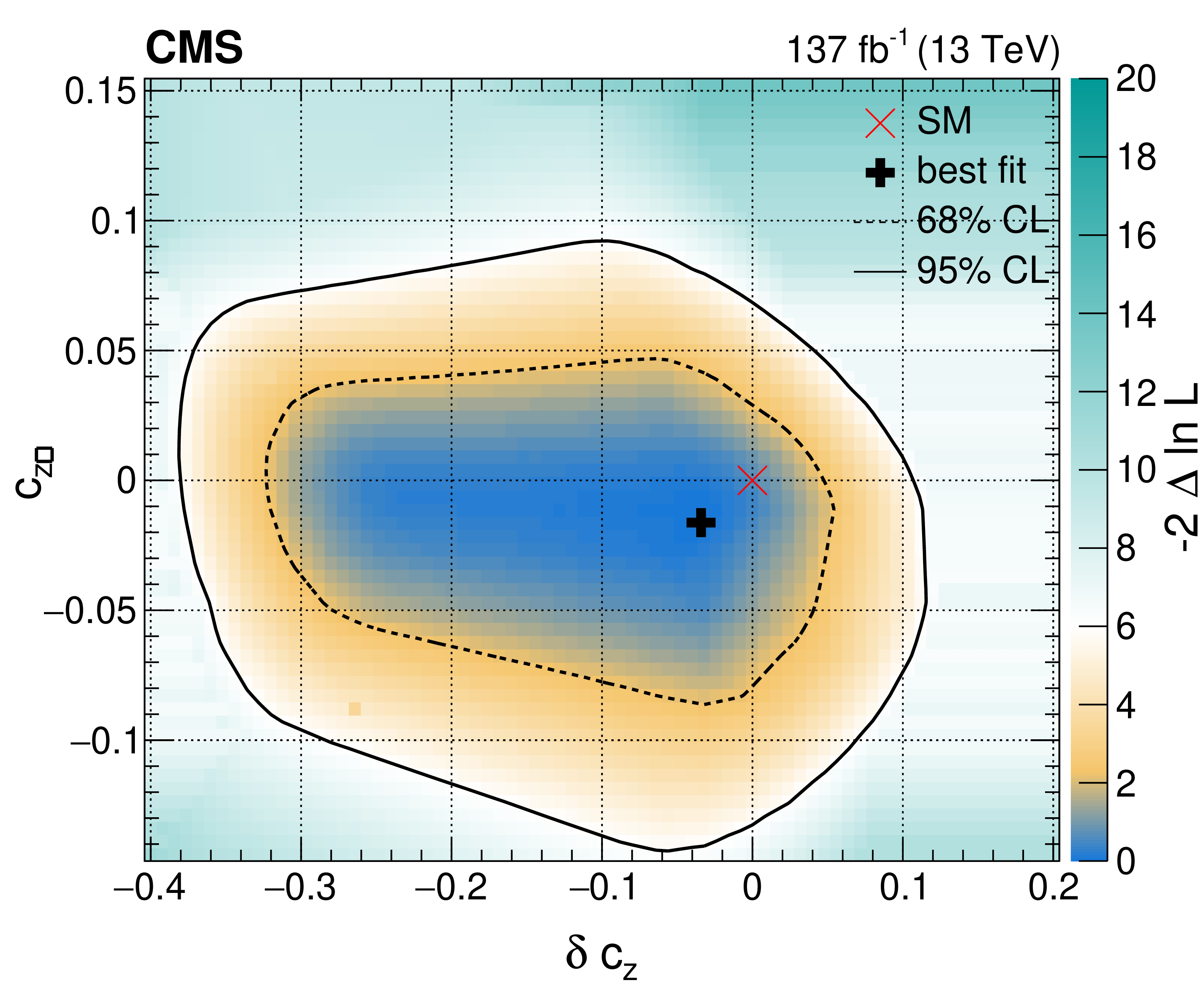
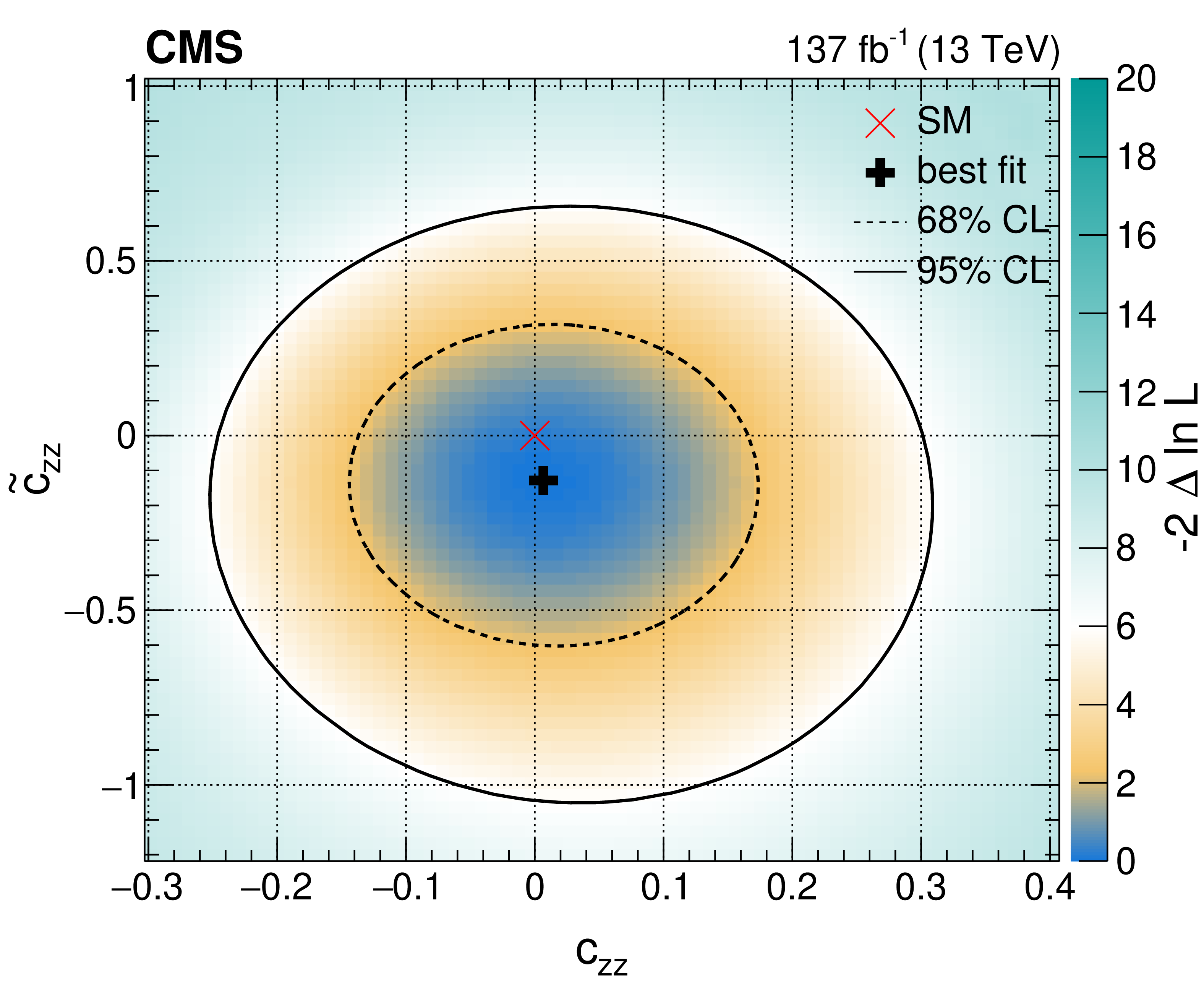
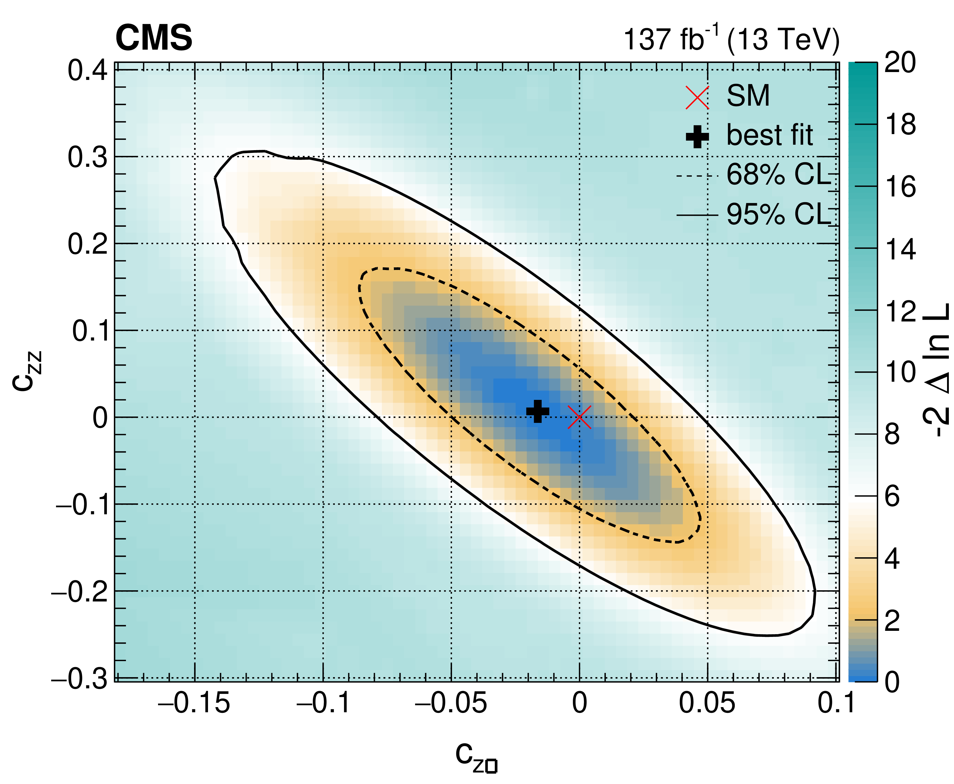
Figure 22:
Observed two-dimensional constraints from a simultaneous fit of the SMEFT parameters $\delta c_\mathrm {z}$, $c_\mathrm {zz}$, $c_{\mathrm {z} \Box}$, and $\tilde{c}_\mathrm {zz}$ with the $c_{\mathrm{g} \mathrm{g}}$ and $\tilde{c}_{\mathrm{g} \mathrm{g}}$ couplings left unconstrained. |
png pdf |
Figure 22-a:
Observed two-dimensional constraints from a simultaneous fit of the SMEFT parameters $\delta c_\mathrm {z}$, $c_\mathrm {zz}$, $c_{\mathrm {z} \Box}$, and $\tilde{c}_\mathrm {zz}$ with the $c_{\mathrm{g} \mathrm{g}}$ and $\tilde{c}_{\mathrm{g} \mathrm{g}}$ couplings left unconstrained. |
png pdf |
Figure 22-b:
Observed two-dimensional constraints from a simultaneous fit of the SMEFT parameters $\delta c_\mathrm {z}$, $c_\mathrm {zz}$, $c_{\mathrm {z} \Box}$, and $\tilde{c}_\mathrm {zz}$ with the $c_{\mathrm{g} \mathrm{g}}$ and $\tilde{c}_{\mathrm{g} \mathrm{g}}$ couplings left unconstrained. |
png pdf |
Figure 22-c:
Observed two-dimensional constraints from a simultaneous fit of the SMEFT parameters $\delta c_\mathrm {z}$, $c_\mathrm {zz}$, $c_{\mathrm {z} \Box}$, and $\tilde{c}_\mathrm {zz}$ with the $c_{\mathrm{g} \mathrm{g}}$ and $\tilde{c}_{\mathrm{g} \mathrm{g}}$ couplings left unconstrained. |
png pdf |
Figure 22-d:
Observed two-dimensional constraints from a simultaneous fit of the SMEFT parameters $\delta c_\mathrm {z}$, $c_\mathrm {zz}$, $c_{\mathrm {z} \Box}$, and $\tilde{c}_\mathrm {zz}$ with the $c_{\mathrm{g} \mathrm{g}}$ and $\tilde{c}_{\mathrm{g} \mathrm{g}}$ couplings left unconstrained. |

png pdf |
Figure 22-e:
Observed two-dimensional constraints from a simultaneous fit of the SMEFT parameters $\delta c_\mathrm {z}$, $c_\mathrm {zz}$, $c_{\mathrm {z} \Box}$, and $\tilde{c}_\mathrm {zz}$ with the $c_{\mathrm{g} \mathrm{g}}$ and $\tilde{c}_{\mathrm{g} \mathrm{g}}$ couplings left unconstrained. |
png pdf |
Figure 22-f:
Observed two-dimensional constraints from a simultaneous fit of the SMEFT parameters $\delta c_\mathrm {z}$, $c_\mathrm {zz}$, $c_{\mathrm {z} \Box}$, and $\tilde{c}_\mathrm {zz}$ with the $c_{\mathrm{g} \mathrm{g}}$ and $\tilde{c}_{\mathrm{g} \mathrm{g}}$ couplings left unconstrained. |
| Tables | |

png pdf |
Table 1:
List of anomalous HVV couplings $a_i^{\mathrm{V} \mathrm{V}}$ considered, the corresponding measured cross section fractions $f_{ai}^{\mathrm{V} \mathrm{V}}$ defined in Eq. (18), and the translation coefficients $\alpha _{ii}/\alpha _{11}$ in this definition with the relationship $a_i^{\mathrm{Z} \mathrm{Z}}=a_i^{\mathrm{W} \mathrm{W}}$ (Approach 1), and with the SMEFT relationship according to Eqs. (3-7) (Approach 2). In the case of the $\kappa _1$ and $\kappa _2^{\mathrm{Z} \gamma}$ couplings, the numerical values $\Lambda _{1}=\Lambda _{1}^{\mathrm{Z} \gamma} = $ 100 GeV are adopted in this calculation to make the coefficients have the same order of magnitude. |
png pdf |
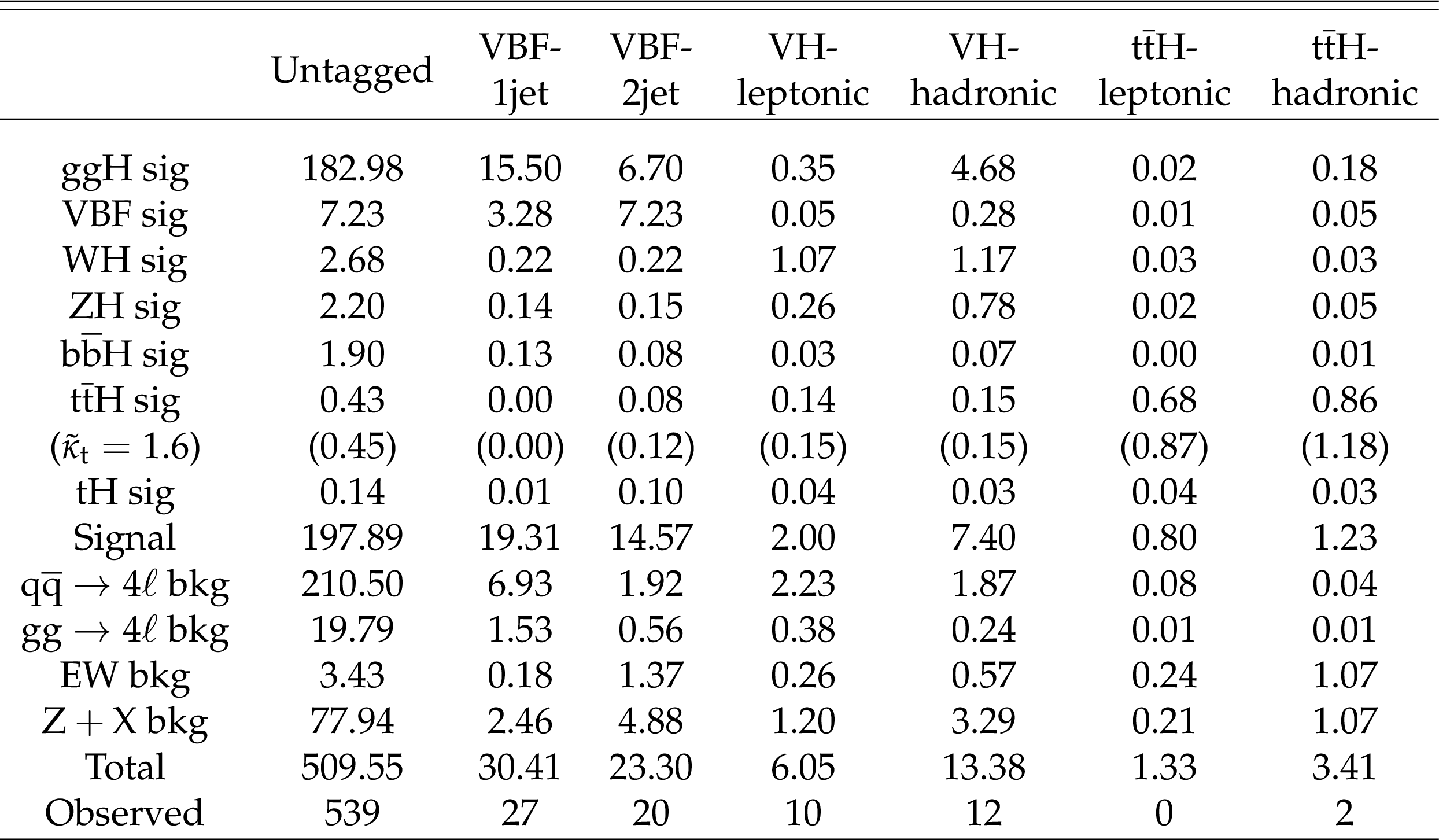
Table 2:
The numbers of events expected in the SM for different H signal (sig) and background (bkg) contributions and the observed number of events in each category defined in Scheme 1 targeting Hff and Hgg anomalous couplings. The ttH signal expectation is quoted for the SM and anomalous coupling ($\kappa _{\mathrm{t}}=0$, $\tilde\kappa _{\mathrm{t}}=1.6$) scenario, both generated with the same cross section. |
png pdf |
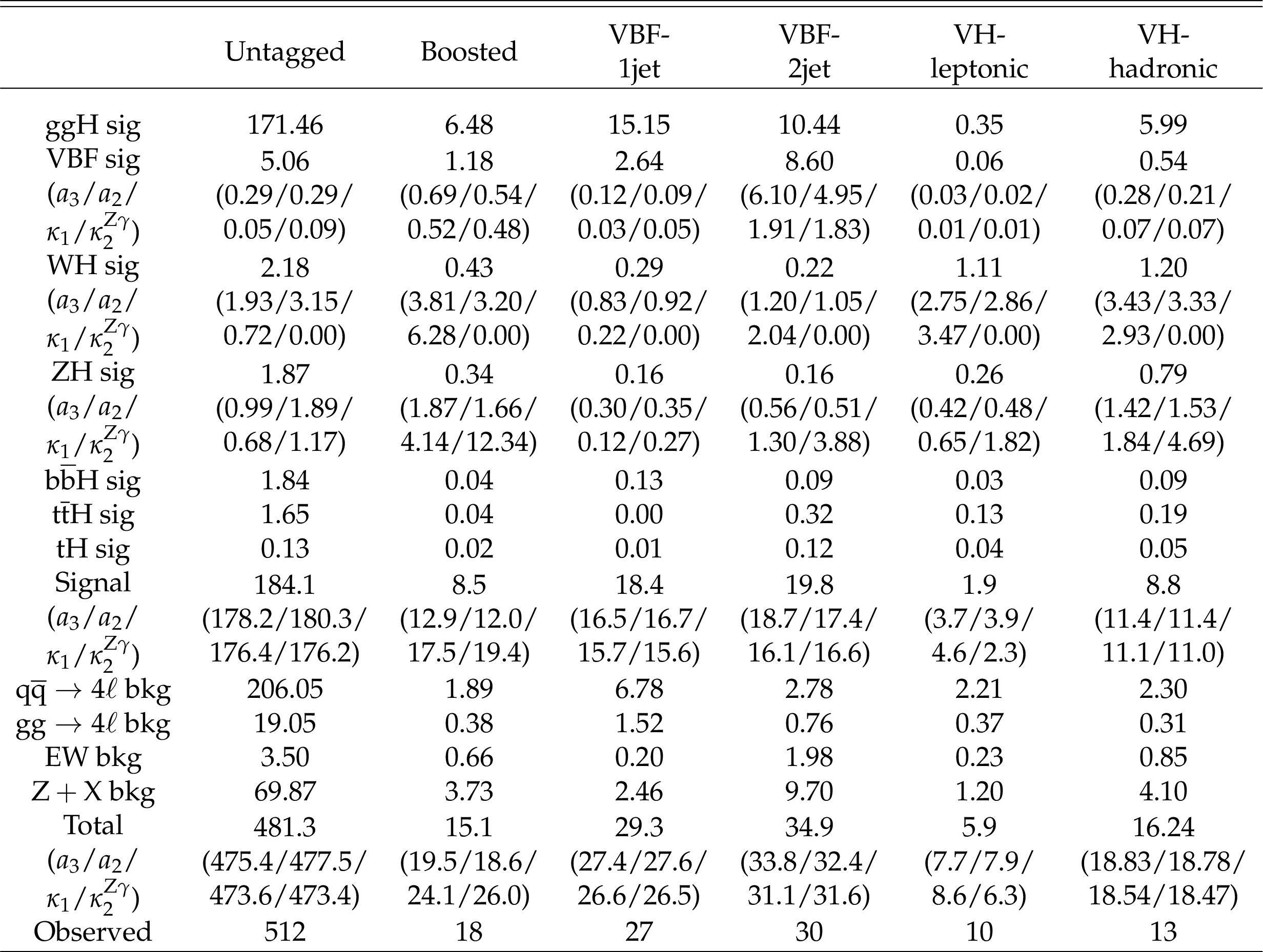
Table 3:
The numbers of events expected in the SM for different H signal (sig) and background (bkg) contributions and the observed number of events in each category defined in Scheme 2 targeting HVV anomalous couplings. The EW (VBF, WH, and ZH) signal expectation is quoted for the SM and four anomalous coupling ($a_3/a_2/\kappa _1/\kappa _2^{\mathrm{Z} \gamma}$) scenarios $f_{ai}=1$, all generated with the same total EW production cross section. |
png pdf |
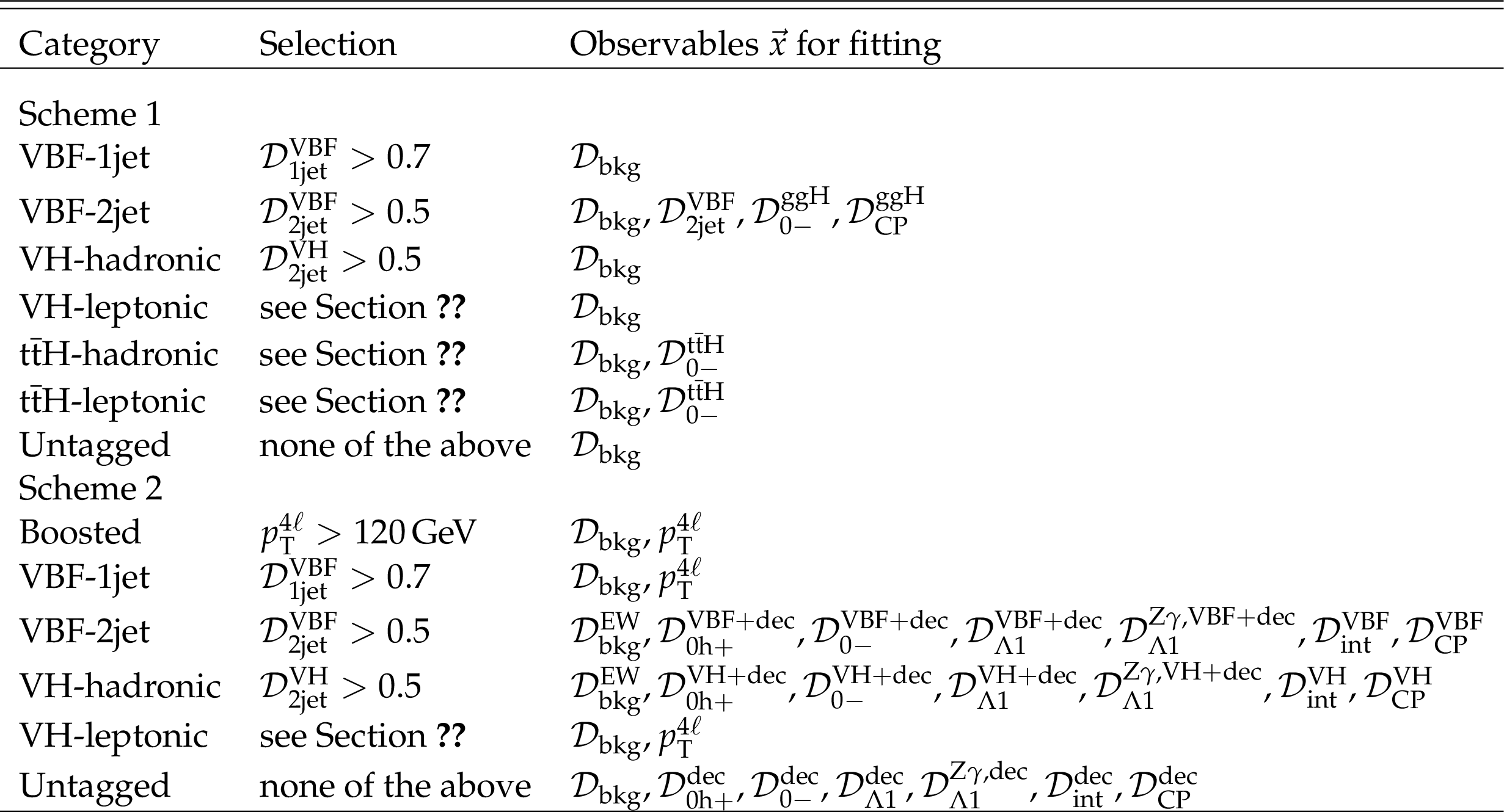
Table 4:
The list of kinematic observables used for category selection and fitting in categorization Schemes 1 and 2. Only the main features involving the kinematic discriminants in the category selection are listed, while complete details are given in Section 3. The Untagged category includes the events not selected in the other categories. |
png pdf |
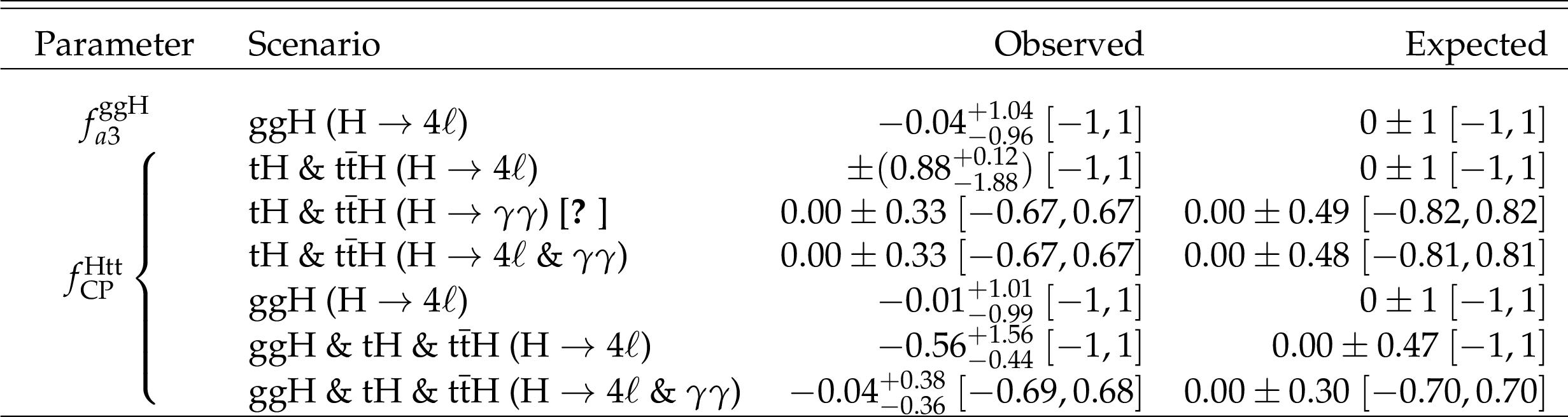
Table 5:
Constraints on the $ {f_{a3}^{\mathrm{g} \mathrm{g} \mathrm{H}}} $ and $ {f_\mathrm {CP}^{{\mathrm{H} \text {tt}}}} $ parameters with the best fit values and allowed $68%$ CL (quoted uncertainties) and 95% CL (within square brackets) intervals, limited to the physical range of $[-1, 1]$. The $ {f_\mathrm {CP}^{{\mathrm{H} \text {tt}}}} $ constraints obtained in this work are combined with those in the $\mathrm{H} \to \gamma \gamma $ channel [26]. The interpretation of the $ {f_{a3}^{\mathrm{g} \mathrm{g} \mathrm{H}}} $ result under the assumption of the top quark dominance in the gluon fusion loop are presented in terms of the $ {f_\mathrm {CP}^{{\mathrm{H} \text {tt}}}} $ parameter, where either ggH or its combination with tH and ttH results are shown. |
png pdf |
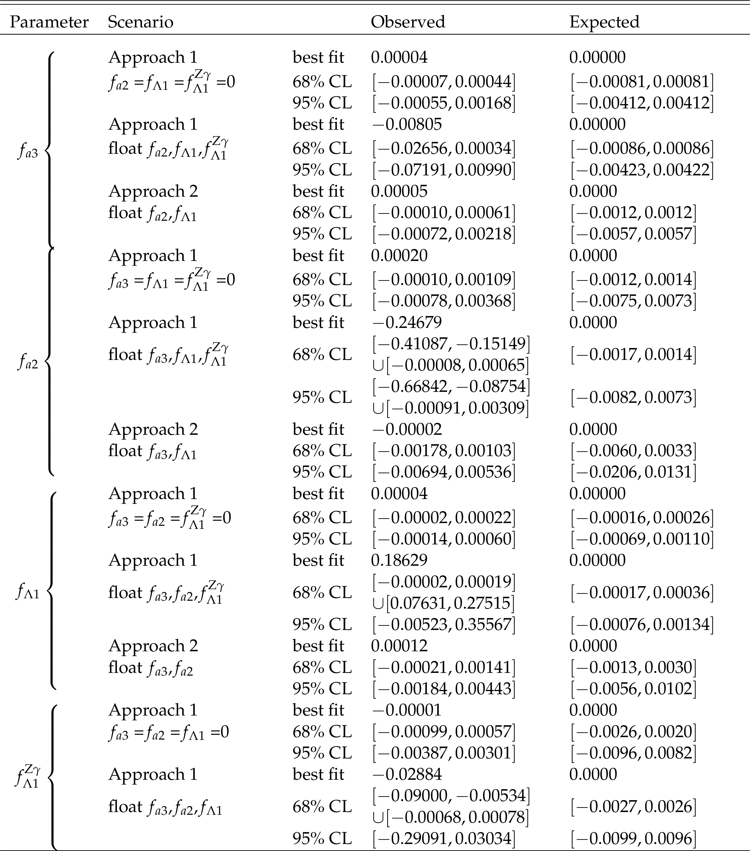
Table 6:
Summary of constraints on the anomalous HVV coupling parameters with the best fit values and allowed 68 and 95% CL intervals. Three scenarios are shown for each parameter: with three other anomalous HVV couplings set to zero (first), with three other anomalous HVV couplings left unconstrained (second), in Approach 1 with the relationship $a_i^{WW}=a_i^{ZZ}$ in both cases; and with two other anomalous HVV couplings left unconstrained (third), in Approach 2 within SMEFT with the symmetry relationship of couplings set in Eqs. (3-7). The $ {f_{\Lambda 1}^{\mathrm{Z} \gamma}} $ parameter is not independent in the latter scenario. |
png pdf |
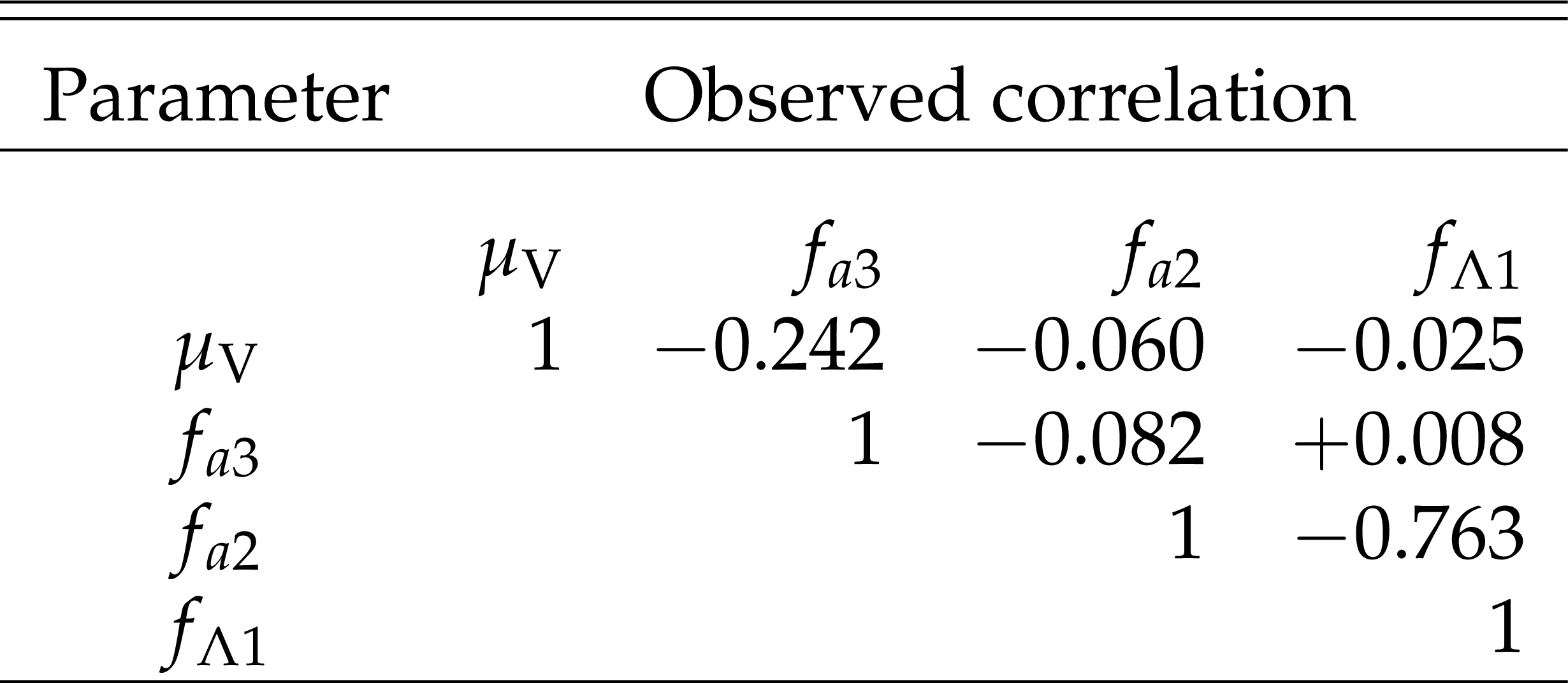
Table 7:
The observed correlation coefficients of the signal strength ${\mu _{\mathrm{V}}}$ and the ${f_{a3}}$, ${f_{a2}}$, ${f_{\Lambda 1}}$ parameters in Approach 2 within SMEFT with the symmetry relationship of couplings set in Eqs. (3-7). |

png pdf |
Table 8:
Summary of constraints on the Htt, Hgg, and HVV coupling parameters in the Higgs basis of SMEFT. The observed correlation coefficients are presented for the Htt & Hgg and HVV couplings in the fit configurations discussed in text and shown in Figs. 17 and 22, respectively. |
png pdf |
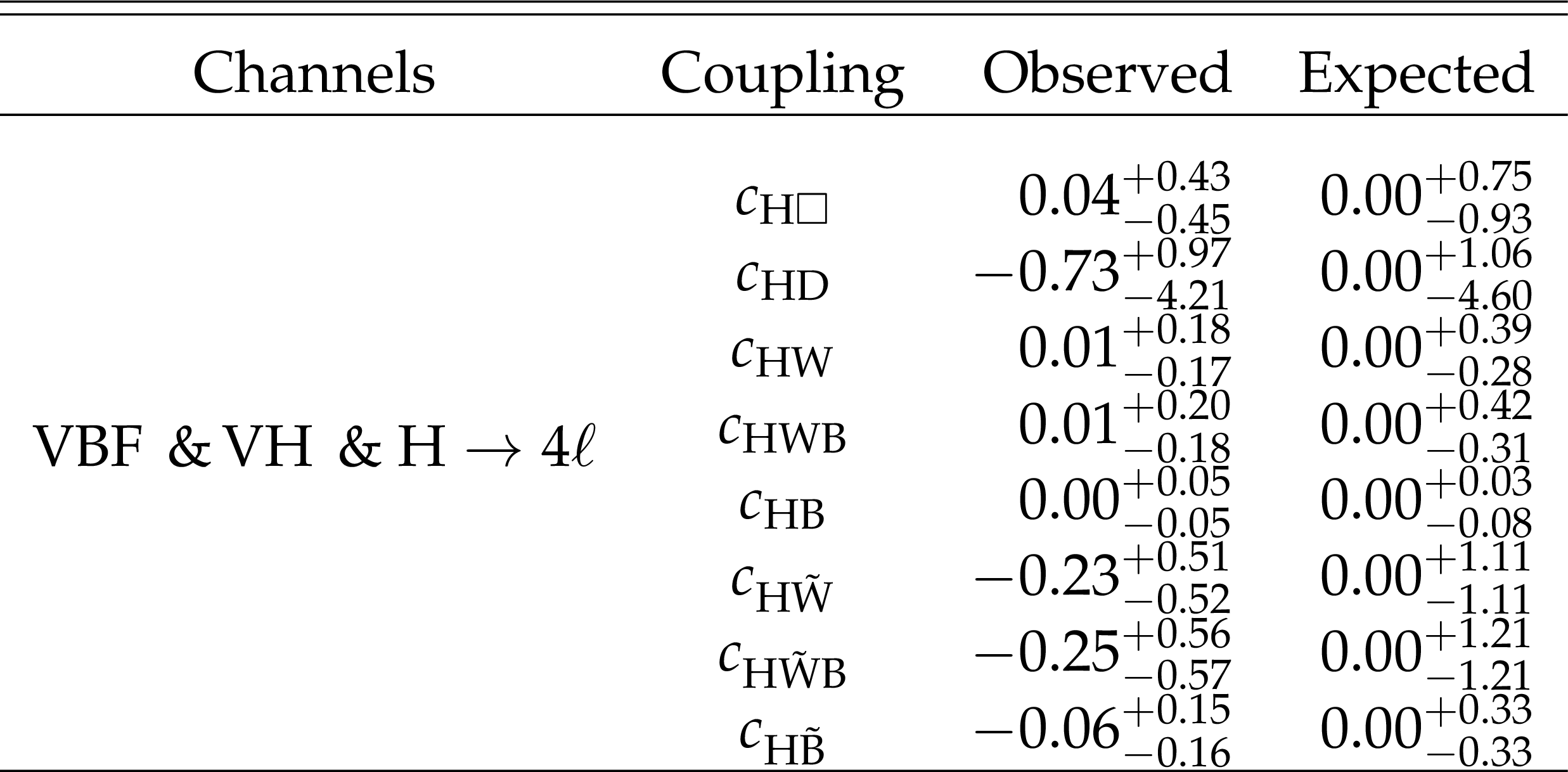
Table 9:
Summary of constraints on the HVV coupling parameters in the Warsaw basis of SMEFT. For each coupling constraint reported, three other independent operators are left unconstrained, where only one of the three operators $c_{\mathrm{H} \mathrm{W}}$, $c_{\mathrm{H} \mathrm{W} \mathrm {B}}$, and $c_{\mathrm{H} \mathrm {B}}$ is independent, and only one of $c_{\mathrm{H} \tilde{\mathrm{W}}}$, $c_{\mathrm{H} \tilde{\mathrm{W}}\mathrm {B}}$, and $c_{\mathrm{H} \tilde{\mathrm {B}}}$ is independent. |
| Summary |
|
In this paper, a comprehensive study of $CP$-violation, anomalous couplings, and the tensor structure of H boson interactions with electroweak gauge bosons, gluons, and fermions, using all accessible production mechanisms and the ${\mathrm{H}\to4\ell} $ decay mode, is presented. The results are based on the 2016-2018 data from ${\mathrm{p}}{\mathrm{p}}$ collisions recorded with the CMS detector during Run 2 of the LHC, corresponding to an integrated luminosity of 137 fb$^{-1}$ at a center-of-mass energy of 13 TeV. These results significantly surpass our results from Run 1 [13] in both precision and extent of coverage. The improvements result not only from a significantly increased sample of H bosons, but also from a detailed analysis of kinematic distributions of the particles associated with the H boson production in addition to kinematic distributions in its decay. These results also surpass our earlier studies of on-shell production of the H boson in this decay channel with a partial Run 2 dataset [16,17]. The parameterization of the H boson production and decay processes is based on a scattering amplitude or, equivalently, an effective field theory Lagrangian, with operators up to dimension six. Additional symmetries and prior measurements allow us to reduce the number of independent parameters and make a connection to the standard model effective field theory (SMEFT) formulation. Dedicated Monte Carlo programs and matrix-element re-weighting techniques provide modeling of all kinematic effects in the production and decay of the H boson, with any variation of parameters of the scattering amplitude and with full simulation of detector effects. Each production process of the H boson is identified using the kinematic features of its associated particles. The matrix element likelihood approach (MELA) is employed to construct observables that are optimal for the measurement of the targeted anomalous couplings in each process, including $CP$-sensitive observables. A maximum likelihood fit allows a simultaneous measurement of up to five HVV, two Hgg, and two Htt couplings. For the first time, we present a complete dedicated study of $CP$ properties in the H boson coupling to gluons through a loop of heavy particles using the $CP$-sensitive observables, while separating the electroweak and strong boson fusion processes. An interpretation of the loop contribution is made both with and without an assumption of top quark dominance, which allows a new heavy particle to contribute. In both cases, combination with the $CP$-sensitive measurement of the Htt coupling in the ttH and tH processes allows either simultaneous or separate measurements of the two effective point-like Hgg couplings and the two Htt couplings, both $CP$-odd and $CP$-even. For the ttH and tH processes, results in the ${\mathrm{H}\to4\ell} $ channel are combined with those in the $\mathrm{H}\to\gamma\gamma$ channel [26]. This is the first comprehensive study of $CP$ properties in the Hgg and Htt couplings from a simultaneous measurement of the ggH, ttH, and tH processes. Also for the first time, we present the measurement of $CP$ properties and the tensor structure of the H boson 's interactions with two electroweak bosons with up to five parameters measured simultaneously. The HVV coupling is analyzed in VBF and VH production and in $\mathrm{H}\to{\mathrm{V}\mathrm{V}} \to4\ell$ decay. The measurements are performed with two approaches. In the first approach, more lenient symmetry considerations are applied, which allow a less restrictive interpretation of results. In the second approach, SU(2)$\times$U(1) symmetry is invoked and the formulation becomes equivalent to SMEFT. The operator basis is chosen to coincide with the couplings of the mass eigenstates, which allows us to minimize the number of independent parameters. A translation of the SMEFT results to the Warsaw basis is also presented for easier comparison with other results. In all cases, we first present results in terms of the total cross section of a process and the fractional contribution of each anomalous coupling. These results are further re-interpreted in terms of direct constraints on the couplings by applying certain assumptions about the H boson total width. Each of the measurements presented here is limited by statistical precision and is consistent with the expectations for the standard model Higgs boson. |
| References | ||||
| 1 | ATLAS Collaboration | Observation of a new particle in the search for the Standard Model Higgs boson with the ATLAS detector at the LHC | PLB 716 (2012) 1 | 1207.7214 |
| 2 | CMS Collaboration | Observation of a new boson at a mass of 125 GeV with the CMS experiment at the LHC | PLB 716 (2012) 30 | CMS-HIG-12-028 1207.7235 |
| 3 | CMS Collaboration | Observation of a new boson with mass near 125 GeV in pp collisions at $ \sqrt{s}= $ 7 and~8 TeV | JHEP 06 (2013) 081 | CMS-HIG-12-036 1303.4571 |
| 4 | S. L. Glashow | Partial-symmetries of weak interactions | NP 22 (1961) 579 | |
| 5 | F. Englert and R. Brout | Broken symmetry and the mass of gauge vector mesons | PRL 13 (1964) 321 | |
| 6 | P. W. Higgs | Broken symmetries, massless particles and gauge fields | PL12 (1964) 132 | |
| 7 | P. W. Higgs | Broken symmetries and the masses of gauge bosons | PRL 13 (1964) 508 | |
| 8 | G. S. Guralnik, C. R. Hagen, and T. W. B. Kibble | Global conservation laws and massless particles | PRL 13 (1964) 585 | |
| 9 | S. Weinberg | A model of leptons | PRL 19 (1967) 1264 | |
| 10 | A. Salam | Weak and electromagnetic interactions | in Elementary particle physics: relativistic groups and analyticity, N. Svartholm, ed., Almqvist & Wiksell, Stockholm, 1968 Proceedings of the eighth Nobel symposium | |
| 11 | CMS Collaboration | On the mass and spin-parity of the Higgs boson candidate via its decays to $ \mathrm{Z} $ boson pairs | PRL 110 (2013) 081803 | CMS-HIG-12-041 1212.6639 |
| 12 | CMS Collaboration | Measurement of the properties of a Higgs boson in the four-lepton final state | PRD 89 (2014) 092007 | CMS-HIG-13-002 1312.5353 |
| 13 | CMS Collaboration | Constraints on the spin-parity and anomalous HVV couplings of the Higgs boson in proton collisions at 7 and 8 TeV | PRD 92 (2015) 012004 | CMS-HIG-14-018 1411.3441 |
| 14 | CMS Collaboration | Limits on the Higgs boson lifetime and width from its decay to four charged leptons | PRD 92 (2015) 072010 | CMS-HIG-14-036 1507.06656 |
| 15 | CMS Collaboration | Combined search for anomalous pseudoscalar HVV couplings in VH ($ \mathrm{H}\to\mathrm{b\bar{b}} $) production and $ \mathrm{H}\to\mathrm{VV} $ decay | PLB 759 (2016) 672 | CMS-HIG-14-035 1602.04305 |
| 16 | CMS Collaboration | Constraints on anomalous Higgs boson couplings using production and decay information in the four-lepton final state | PLB 775 (2017) 1 | CMS-HIG-17-011 1707.00541 |
| 17 | CMS Collaboration | Measurements of the Higgs boson width and anomalous HVV couplings from on-shell and off-shell production in the four-lepton final state | PRD (2019) 112003 | CMS-HIG-18-002 1901.00174 |
| 18 | CMS Collaboration | Constraints on anomalous $ HVV $ couplings from the production of Higgs bosons decaying to $ \tau $ lepton pairs | PRD 100 (2019) 112002 | CMS-HIG-17-034 1903.06973 |
| 19 | ATLAS Collaboration | Evidence for the spin-0 nature of the Higgs boson using ATLAS data | PLB 726 (2013) 120 | 1307.1432 |
| 20 | ATLAS Collaboration | Study of the spin and parity of the Higgs boson in diboson decays with the ATLAS detector | EPJC 75 (2015) 476 | 1506.05669 |
| 21 | ATLAS Collaboration | Test of CP invariance in vector-boson fusion production of the Higgs boson using the Optimal Observable method in the ditau decay channel with the ATLAS detector | EPJC 76 (2016) 658 | 1602.04516 |
| 22 | ATLAS Collaboration | Measurement of inclusive and differential cross sections in the $ \mathrm{H} \rightarrow \mathrm{Z}\mathrm{Z}^{*} \rightarrow 4\ell $ decay channel in pp collisions at $ \sqrt{s}=$ 13 TeV with the ATLAS detector | JHEP 10 (2017) 132 | 1708.02810 |
| 23 | ATLAS Collaboration | Measurement of the Higgs boson coupling properties in the $ H\rightarrow ZZ^{*} \rightarrow 4\ell $ decay channel at $ \sqrt{s} = $ 13 TeV with the ATLAS detector | JHEP 03 (2018) 095 | 1712.02304 |
| 24 | ATLAS Collaboration | Measurements of Higgs boson properties in the diphoton decay channel with 36 fb$ ^{-1} $ of pp collision data at $ \sqrt{s} = $ 13 TeV with the ATLAS detector | PRD 98 (2018) 052005 | 1802.04146 |
| 25 | ATLAS Collaboration | Test of CP invariance in vector-boson fusion production of the Higgs boson in the $ \mathrm {H}\rightarrow\tau\tau $ channel in proton$ - $proton collisions at $ \sqrt{s} = $ 13 TeV with the ATLAS detector | PLB 805 (2020) 135426 | 2002.05315 |
| 26 | CMS Collaboration | Measurements of $ \mathrm{t\bar{t}H} $ Production and the CP Structure of the Yukawa Interaction between the Higgs Boson and Top Quark in the Diphoton Decay Channel | PRL 125 (2020) 061801 | CMS-HIG-19-013 2003.10866 |
| 27 | ATLAS Collaboration | $ CP $ Properties of Higgs Boson Interactions with Top Quarks in the $ t\bar{t}H $ and $ tH $ Processes Using $ H \rightarrow \gamma\gamma $ with the ATLAS Detector | PRL 125 (2020) 061802 | 2004.04545 |
| 28 | LHC Higgs Cross Section Working Group | Handbook of LHC Higgs cross sections: 4. deciphering the nature of the Higgs sector | CERN (2016) | 1610.07922 |
| 29 | Y. Gao et al. | Spin determination of single-produced resonances at hadron colliders | PRD 81 (2010) 075022 | 1001.3396 |
| 30 | S. Bolognesi et al. | Spin and parity of a single-produced resonance at the LHC | PRD 86 (2012) 095031 | 1208.4018 |
| 31 | I. Anderson et al. | Constraining anomalous HVV interactions at proton and lepton colliders | PRD 89 (2014) 035007 | 1309.4819 |
| 32 | A. V. Gritsan, R. Rontsch, M. Schulze, and M. Xiao | Constraining anomalous Higgs boson couplings to the heavy flavor fermions using matrix element techniques | PRD 94 (2016) 055023 | 1606.03107 |
| 33 | A. V. Gritsan et al. | New features in the JHU generator framework: constraining Higgs boson properties from on-shell and off-shell production | PRD 102 (2020) 056022 | 2002.09888 |
| 34 | ATLAS Collaboration | Higgs boson production cross-section measurements and their EFT interpretation in the $ 4\ell $ decay channel at $ \sqrt{s}= $ 13 TeV with the ATLAS detector | EPJC 80 (2020) 957 | 2004.03447 |
| 35 | ATLAS Collaboration | Measurements of the Higgs boson inclusive and differential fiducial cross sections in the 4$ \ell $ decay channel at $ \sqrt{s} = $ 13 TeV | EPJC 80 (2020) 942 | 2004.03969 |
| 36 | C. A. Nelson | Correlation between decay planes in Higgs boson decays into a $ \mathrm{W} $ Pair (into a $ \mathrm{Z} $ Pair) | PRD 37 (1988) 1220 | |
| 37 | A. Soni and R. M. Xu | Probing CP violation via Higgs decays to four leptons | PRD 48 (1993) 5259 | hep-ph/9301225 |
| 38 | D. Chang, W.-Y. Keung, and I. Phillips | CP odd correlation in the decay of neutral Higgs boson into $ \mathrm{Z}\mathrm{Z} $, $ \mathrm{W^+}\mathrm{W^-} $, or $ \mathrm{t}\bar{\mathrm{t}} $ | PRD 48 (1993) 3225 | hep-ph/9303226 |
| 39 | V. D. Barger et al. | Higgs bosons: Intermediate mass range at e+ e- colliders | PRD 49 (1994) 79 | hep-ph/9306270 |
| 40 | T. Arens and L. M. Sehgal | Energy spectra and energy correlations in the decay $ \mathrm{H} \to \mathrm{ZZ} \to \mu^+\mu^- \mu^+\mu^- $ | Z. Phys. C 66 (1995) 89 | hep-ph/9409396 |
| 41 | S. Bar-Shalom et al. | Large tree level CP violation in $ e^{+} e^{-} \to t \bar{t} H^0 $ in the two Higgs doublet model | PRD 53 (1996) 1162 | hep-ph/9508314 |
| 42 | J. F. Gunion and X.-G. He | Determining the CP nature of a neutral Higgs boson at the LHC | PRL 76 (1996) 4468 | hep-ph/9602226 |
| 43 | T. Han and J. Jiang | CP violating $ \mathrm{ZZ}\mathrm{H} $ coupling at $ \mathrm{e}^{+}\mathrm{e}^{-} $ linear colliders | PRD 63 (2001) 096007 | hep-ph/0011271 |
| 44 | T. Plehn, D. L. Rainwater, and D. Zeppenfeld | Determining the structure of Higgs couplings at the LHC | PRL 88 (2002) 051801 | hep-ph/0105325 |
| 45 | S. Y. Choi, D. J. Miller, M. M. M uhlleitner, and P. M. Zerwas | Identifying the Higgs spin and parity in decays to Z pairs | PLB 553 (2003) 61 | hep-ph/0210077 |
| 46 | C. P. Buszello, I. Fleck, P. Marquard, and J. J. van der Bij | Prospective analysis of spin- and CP-sensitive variables in $ \mathrm{H} \to \mathrm{Z}\mathrm{Z} \to \ell_1^+ \ell_1^- \ell_2^+ \ell_2^- $ at the LHC | EPJC 32 (2004) 209 | hep-ph/0212396 |
| 47 | V. Hankele, G. Klamke, D. Zeppenfeld, and T. Figy | Anomalous Higgs boson couplings in vector boson fusion at the CERN LHC | PRD 74 (2006) 095001 | hep-ph/0609075 |
| 48 | E. Accomando et al. | Workshop on CP studies and non-standard Higgs physics | hep-ph/0608079 | |
| 49 | R. M. Godbole, D. J. Miller, and M. M. M uhlleitner | Aspects of CP violation in the $ \mathrm{H}\mathrm{Z}\mathrm{Z} $ coupling at the LHC | JHEP 12 (2007) 031 | 0708.0458 |
| 50 | K. Hagiwara, Q. Li, and K. Mawatari | Jet angular correlation in vector-boson fusion processes at hadron colliders | JHEP 07 (2009) 101 | 0905.4314 |
| 51 | A. De R\' ujula et al. | Higgs look-alikes at the LHC | PRD 82 (2010) 013003 | 1001.5300 |
| 52 | N. D. Christensen, T. Han, and Y. Li | Testing CP violation in ZZH interactions at the LHC | PLB 693 (2010) 28 | 1005.5393 |
| 53 | J. S. Gainer, K. Kumar, I. Low, and R. Vega-Morales | Improving the sensitivity of Higgs boson searches in the golden channel | JHEP 11 (2011) 027 | 1108.2274 |
| 54 | J. Ellis, D. S. Hwang, V. Sanz, and T. You | A fast track towards the `Higgs' spin and parity | JHEP 11 (2012) 134 | 1208.6002 |
| 55 | Y. Chen, N. Tran, and R. Vega-Morales | Scrutinizing the Higgs signal and background in the $ 2\mathrm{e}2\mu $ golden channel | JHEP 01 (2013) 182 | 1211.1959 |
| 56 | J. S. Gainer et al. | Geolocating the Higgs boson candidate at the LHC | PRL 111 (2013) 041801 | 1304.4936 |
| 57 | P. Artoisenet et al. | A framework for Higgs characterisation | JHEP 11 (2013) 043 | 1306.6464 |
| 58 | M. Chen et al. | Role of interference in unraveling the $ \mathrm{ZZ} $ couplings of the newly discovered boson at the LHC | PRD 89 (2014) 034002 | 1310.1397 |
| 59 | Y. Chen and R. Vega-Morales | Extracting Effective Higgs Couplings in the Golden Channel | JHEP 04 (2014) 057 | 1310.2893 |
| 60 | J. S. Gainer et al. | Beyond geolocating: Constraining higher dimensional operators in $ \mathrm{H} \to 4\ell $ with off-shell production and more | PRD 91 (2015) 035011 | 1403.4951 |
| 61 | M. Gonzalez-Alonso, A. Greljo, G. Isidori, and D. Marzocca | Pseudo-observables in Higgs decays | EPJC 75 (2015) 128 | 1412.6038 |
| 62 | M. J. Dolan, P. Harris, M. Jankowiak, and M. Spannowsky | Constraining $ CP $-violating Higgs sectors at the LHC using gluon fusion | PRD 90 (2014) 073008 | 1406.3322 |
| 63 | F. Demartin et al. | Higgs characterisation at NLO in QCD: CP properties of the top-quark Yukawa interaction | EPJC 74 (2014) 3065 | 1407.5089 |
| 64 | M. R. Buckley and D. Goncalves | Boosting the Direct CP Measurement of the Higgs-Top Coupling | PRL 116 (2016) 091801 | 1507.07926 |
| 65 | A. Greljo, G. Isidori, J. M. Lindert, and D. Marzocca | Pseudo-observables in electroweak Higgs production | EPJC 76 (2016) 158 | 1512.06135 |
| 66 | I. Brivio, T. Corbett, and M. Trott | The Higgs width in the SMEFT | JHEP 10 (2019) 056 | 1906.06949 |
| 67 | S. Weinberg | Baryon and lepton nonconserving processes | PRL 43 (1979) 1566 | |
| 68 | W. Buchmuller and D. Wyler | Effective Lagrangian analysis of new interactions and flavor conservation | NPB 268 (1986) 621 | |
| 69 | C. N. Leung, S. T. Love, and S. Rao | Low-energy manifestations of a new interaction scale: operator analysis | Z. Phys. C 31 (1986) 433 | |
| 70 | A. Dedes et al. | Feynman rules for the standard model effective field theory in R$ _{\xi} $ -gauges | JHEP 06 (2017) 143 | 1704.03888 |
| 71 | A. Falkowski et al. | Rosetta: an operator basis translator for Standard Model effective field theory | EPJC 75 (2015) 583 | 1508.05895 |
| 72 | Particle Data Group, P. A. Zyla et al. | Review of particle physics | Prog. Theor. Exp. Phys. 2020 (2020) 083C01 | |
| 73 | P. Sikivie, L. Susskind, M. B. Voloshin, and V. I. Zakharov | Isospin Breaking in Technicolor Models | NPB 173 (1980) 189 | |
| 74 | CMS Collaboration | The CMS experiment at the CERN LHC | JINST 3 (2008) S08004 | CMS-00-001 |
| 75 | CMS Collaboration | Performance of the CMS Level-1 trigger in proton-proton collisions at $ \sqrt{s} = $ 13 TeV | JINST 15 (2020) P10017 | CMS-TRG-17-001 2006.10165 |
| 76 | CMS Collaboration | The CMS trigger system | JINST 12 (2017) P01020 | CMS-TRG-12-001 1609.02366 |
| 77 | CMS Collaboration | Measurements of properties of the Higgs boson decaying into the four-lepton final state in pp collisions at $ \sqrt{s}=13{TeV} $ | JHEP 11 (2017) 047 | CMS-HIG-16-041 1706.09936 |
| 78 | CMS Collaboration | Measurements of production cross sections of the Higgs boson in the four-lepton final state in proton-proton collisions at $ \sqrt{s} = $ 13 TeV | Submitted to EPJC | CMS-HIG-19-001 2103.04956 |
| 79 | CMS Collaboration | Particle-flow reconstruction and global event description with the CMS detector | JINST 12 (2017) P10003 | CMS-PRF-14-001 1706.04965 |
| 80 | M. Cacciari, G. P. Salam, and G. Soyez | The anti-$ {k_{\mathrm{T}}} $ jet clustering algorithm | JHEP 04 (2008) 063 | 0802.1189 |
| 81 | M. Cacciari, G. P. Salam, and G. Soyez | FastJet user manual | EPJC 72 (2012) 1896 | 1111.6097 |
| 82 | CMS Collaboration | Identification of heavy-flavour jets with the CMS detector in pp collisions at 13 TeV | JINST 13 (2018) P05011 | CMS-BTV-16-002 1712.07158 |
| 83 | T. Sjostrand et al. | An introduction to PYTHIA 8.2 | CPC 191 (2015) 159 | 1410.3012 |
| 84 | CMS Collaboration | Event generator tunes obtained from underlying event and multiparton scattering measurements | EPJC 76 (2016) 155 | CMS-GEN-14-001 1512.00815 |
| 85 | CMS Collaboration | Extraction and validation of a new set of CMS PYTHIA8 tunes from underlying-event measurements | EPJC 80 (2020) 4 | CMS-GEN-17-001 1903.12179 |
| 86 | NNPDF Collaboration | Unbiased global determination of parton distributions and their uncertainties at NNLO and at LO | NPB 855 (2012) 153 | 1107.2652 |
| 87 | GEANT4 Collaboration | GEANT4 --- a simulation toolkit | NIMA 506 (2003) 250 | |
| 88 | J. M. Campbell and R. K. Ellis | MCFM for the Tevatron and the LHC | NPPS 205-206 (2010) 10 | 1007.3492 |
| 89 | S. Frixione, P. Nason, and C. Oleari | Matching NLO QCD computations with parton shower simulations: the POWHEG method | JHEP 11 (2007) 070 | 0709.2092 |
| 90 | E. Bagnaschi, G. Degrassi, P. Slavich, and A. Vicini | Higgs production via gluon fusion in the POWHEG approach in the SM and in the MSSM | JHEP 02 (2012) 088 | 1111.2854 |
| 91 | P. Nason and C. Oleari | NLO Higgs boson production via vector-boson fusion matched with shower in POWHEG | JHEP 02 (2010) 037 | 0911.5299 |
| 92 | G. Luisoni, P. Nason, C. Oleari, and F. Tramontano | $ \mathrm{H}\mathrm{W}^{\pm} $/$ \mathrm{H}\mathrm{Z} $ + 0 and 1 jet at NLO with the POWHEG BOX interfaced to GoSam and their merging within MiNLO | JHEP 10 (2013) 083 | 1306.2542 |
| 93 | H. B. Hartanto, B. Jager, L. Reina, and D. Wackeroth | Higgs boson production in association with top quarks in the POWHEG BOX | PRD 91 (2015) 094003 | 1501.04498 |
| 94 | J. Alwall et al. | The automated computation of tree-level and next-to-leading order differential cross sections, and their matching to parton shower simulations | JHEP 07 (2014) 079 | 1405.0301 |
| 95 | K. Hamilton, P. Nason, and G. Zanderighi | MINLO: multi-scale improved NLO | JHEP 10 (2012) 155 | 1206.3572 |
| 96 | CMS Collaboration | A measurement of the Higgs boson mass in the diphoton decay channel | PLB 805 (2020) 135425 | CMS-HIG-19-004 2002.06398 |
| 97 | M. Grazzini, S. Kallweit, and D. Rathlev | $ \mathrm{Z}\mathrm{Z} $ production at the LHC: fiducial cross sections and distributions in NNLO QCD | PLB 750 (2015) 407 | 1507.06257 |
| 98 | J. M. Campbell, R. K. Ellis, and C. Williams | Vector boson pair production at the LHC | JHEP 07 (2011) 018 | 1105.0020 |
| 99 | J. M. Campbell, R. K. Ellis, and C. Williams | Bounding the Higgs width at the LHC using full analytic results for $ \mathrm{g}\mathrm{g}\to \mathrm{e}^{-}\mathrm{e}^{+} \mu^{-} \mu^{+} $ | JHEP 04 (2014) 060 | 1311.3589 |
| 100 | J. M. Campbell and R. K. Ellis | Higgs constraints from vector boson fusion and scattering | JHEP 04 (2015) 030 | 1502.02990 |
| 101 | S. Catani and M. Grazzini | An NNLO subtraction formalism in hadron collisions and its application to Higgs boson production at the LHC | PRL 98 (2007) 222002 | hep-ph/0703012 |
| 102 | M. Grazzini | NNLO predictions for the Higgs boson signal in the $ \mathrm{H} \to \mathrm{WW} \to\ell\nu\ell\nu $ and $ \mathrm{H} \to \mathrm{ZZ} \to 4\ell $ decay channels | JHEP 02 (2008) 043 | 0801.3232 |
| 103 | M. Grazzini and H. Sargsyan | Heavy-quark mass effects in Higgs boson production at the LHC | JHEP 09 (2013) 129 | 1306.4581 |
| 104 | R. J. Barlow | Extended maximum likelihood | NIMA 297 (1990) 496 | |
| 105 | T. Chen and T.-Y. Li | Homotopy continuation method for solving systems of nonlinear and polynomial equations | Commun. Inf. Syst. 15 (2015) 119 | |
| 106 | T. Chen, T.-L. Lee, and T.-Y. Li | Hom4PS-3: A parallel numerical solver for systems of polynomial equations based on polyhedral homotopy continuation methods | in Proceedings of the Mathematical Software---ICMS 2014, p. 183 2014 | |
| 107 | T. Chen, T.-L. Lee, and T.-Y. Li | Mixed cell computation in Hom4PS-3 | J. Symb. Comput. 79, Part 3 (2017) 516 | |
| 108 | A. S. Nemirovsky and D. B. Yudin | Problem complexity and method efficiency in optimization | Wiley, 1983 | |
| 109 | Gurobi Optimization, LLC | Gurobi optimizer reference manual | 2018 \url http://www.gurobi.com | |
| 110 | W. Verkerke and D. P. Kirkby | The RooFit toolkit for data modeling | in Proceedings of the 13th International Conference for Computing in High-Energy and Nuclear Physics (CHEP03) 2003 [eConf C0303241, MOLT007] | physics/0306116 |
| 111 | R. Brun and F. Rademakers | ROOT: An object oriented data analysis framework | NIMA 389 (1997) 81 | |
| 112 | S. S. Wilks | The large-sample distribution of the likelihood ratio for testing composite hypotheses | Annals Math. Statist. 9 (1938) 60 | |
| 113 | CMS Collaboration | CMS luminosity measurements for the 2016 data taking period | CMS-PAS-LUM-17-001 | CMS-PAS-LUM-17-001 |
| 114 | CMS Collaboration | CMS luminosity measurement for the 2017 data taking period at $ \sqrt{s} $ 13 TeV | CMS-PAS-LUM-17-004 | CMS-PAS-LUM-17-004 |
| 115 | CMS Collaboration | CMS luminosity measurement for the 2018 data-taking period at $ \sqrt{s} = $ 13 TeV | CMS-PAS-LUM-18-002 | CMS-PAS-LUM-18-002 |
|
|
Compact Muon Solenoid LHC, CERN |
|

|

|

|

|

|