

Compact Muon Solenoid
LHC, CERN
| CMS-HIG-17-034 ; CERN-EP-2019-029 | ||
| Constraints on anomalous HVV couplings from the production of Higgs bosons decaying to $\tau$ lepton pairs | ||
| CMS Collaboration | ||
| 16 March 2019 | ||
| Phys. Rev. D 100 (2019) 112002 | ||
| Abstract: A study is presented of anomalous HVV interactions of the Higgs boson, including its CP properties. The study uses Higgs boson candidates produced mainly in vector boson fusion and gluon fusion that subsequently decay to a pair of $\tau$ leptons. The data were recorded by the CMS experiment at the LHC in 2016 at a center-of-mass energy of 13 TeV and correspond to an integrated luminosity of 35.9 fb$^{-1}$. A matrix element technique is employed for the analysis of anomalous interactions. The results are combined with those from the $\mathrm{H}\to 4\ell$ decay channel presented earlier, yielding the most stringent constraints on anomalous Higgs boson couplings to electroweak vector bosons expressed as effective cross-section fractions and phases: the CP-violating parameter $f_{a3}\cos(\phi_{a3})=(0.00 \pm 0.27 )\times10^{-3}$ and the CP-conserving parameters $f_{a2}\cos(\phi_{a2})=(0.08^{+1.04}_{-0.21})\times10^{-3}$, $f_{\Lambda1}\cos(\phi_{\Lambda1})=(0.00^{+0.53}_{-0.09})\times10^{-3}$, and $f_{\Lambda1}^{\mathrm{Z}\gamma}\cos(\phi_{\Lambda1}^{\mathrm{Z}\gamma})=(0.0^{+1.1}_{-1.3})\times10^{-3}$. The current data set does not allow for precise constraints on CP properties in the gluon fusion process. The results are consistent with standard model expectations. | ||
| Links: e-print arXiv:1903.06973 [hep-ex] (PDF) ; CDS record ; inSPIRE record ; HepData record ; CADI line (restricted) ; | ||
| Figures & Tables | Summary | Additional Figures | References | CMS Publications |
|---|
| Figures | |
png pdf |
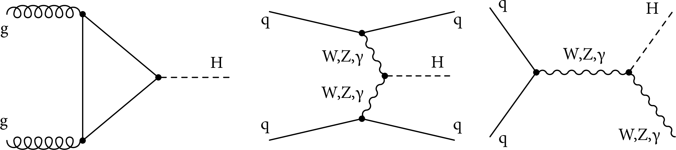
Figure 1:
Examples of leading-order Feynman diagrams for H boson production via the gluon fusion (left), vector boson fusion (middle), and associated production with a vector boson (right). The HWW and HZZ couplings may appear at tree level, as the SM predicts. Additionally, HWW, HZZ, HZ$\gamma$, H$ \gamma \gamma $, and Hgg couplings may be generated by loops of SM or unknown particles, as indicated in the left diagram but not shown explicitly in the middle and right diagrams. |
png pdf |
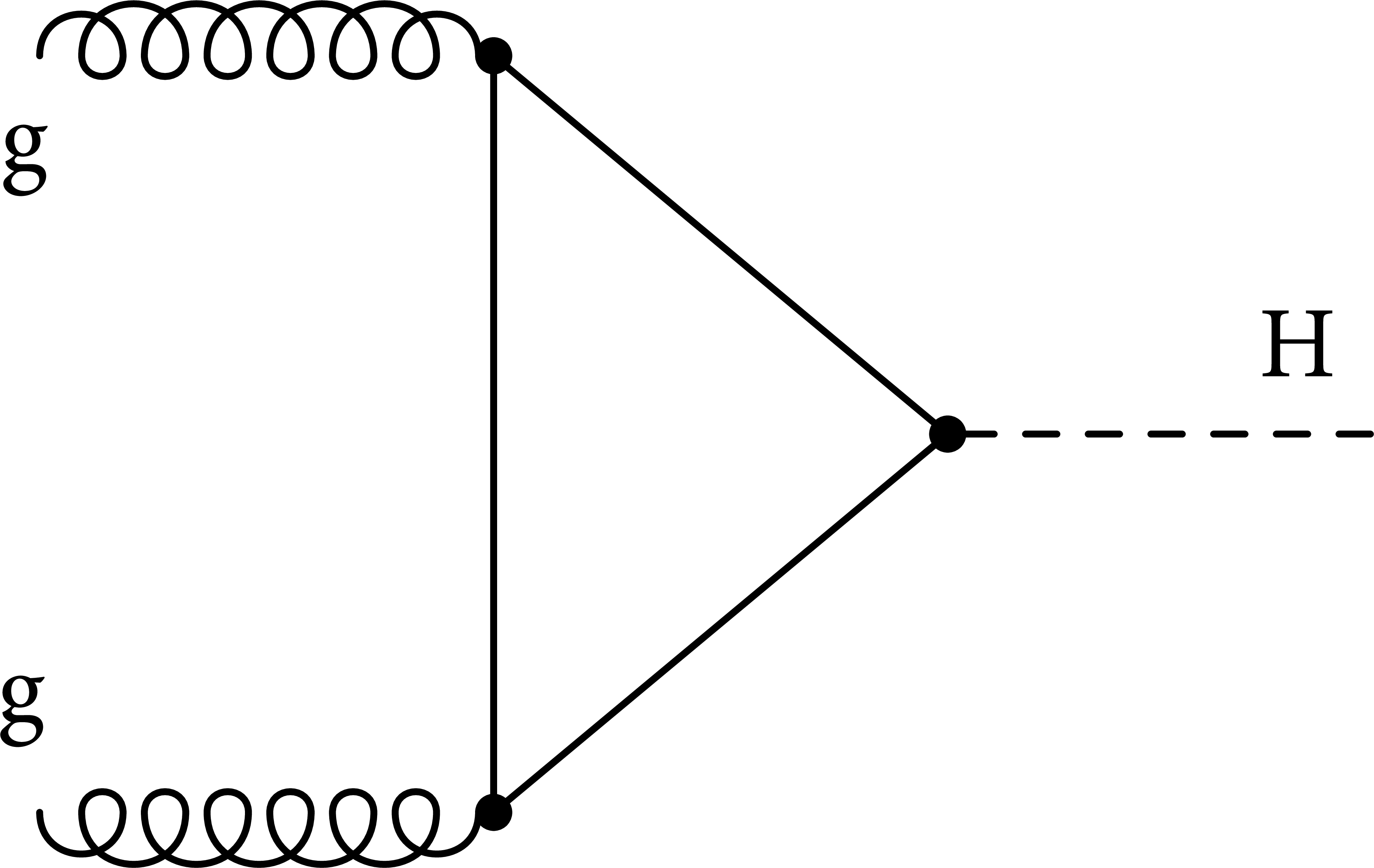
Figure 1-a:
Example of leading-order Feynman diagram for H boson production via the gluon fusion. The HWW, HZZ, HZ$\gamma$, H$ \gamma \gamma $, and Hgg couplings may be generated by loops of SM or unknown particles, as indicated in the diagram. |
png pdf |
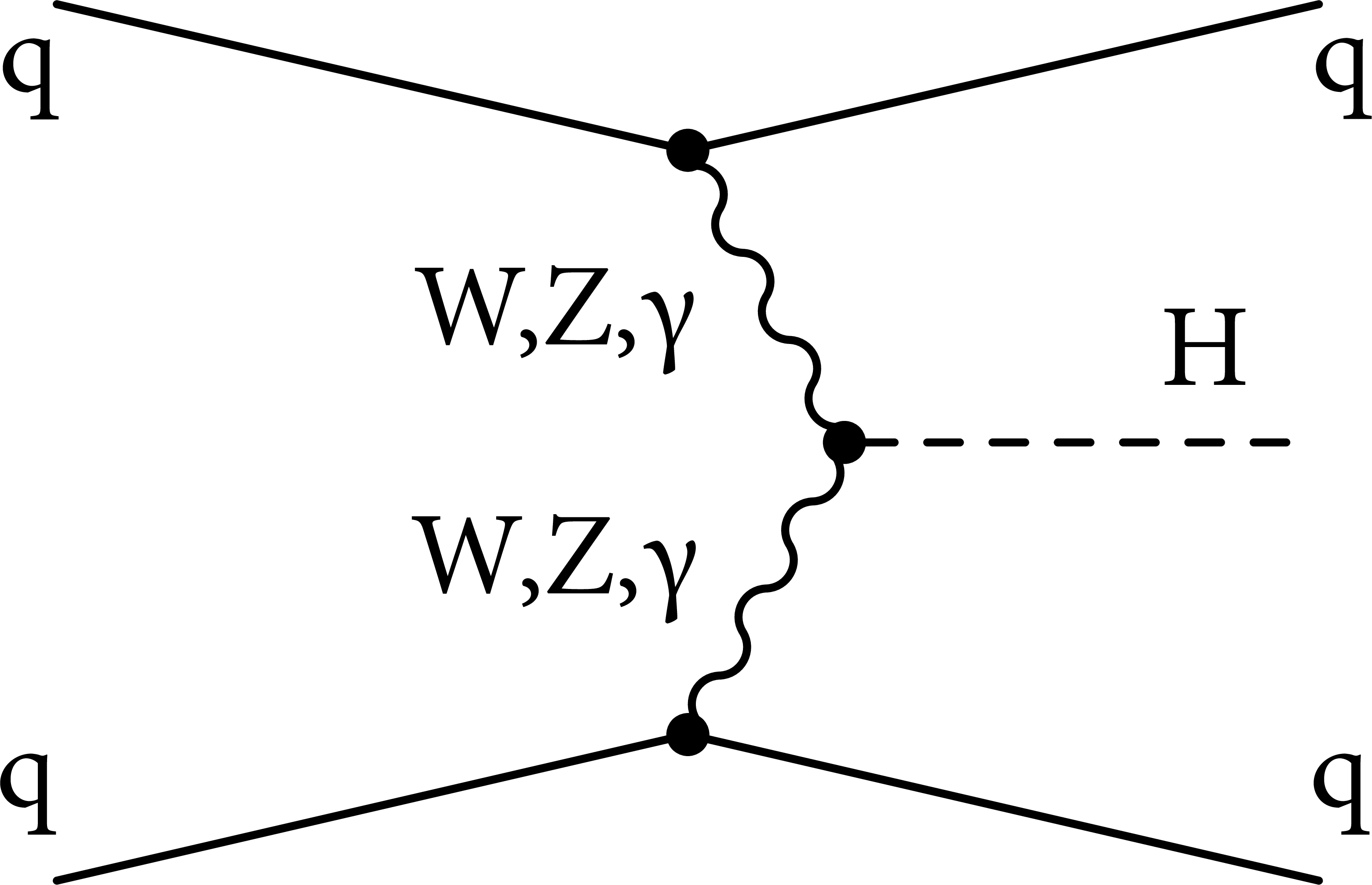
Figure 1-b:
Example of leading-order Feynman diagram for H boson production via vector boson fusion. The HWW and HZZ couplings may appear at tree level, as the SM predicts. |
png pdf |
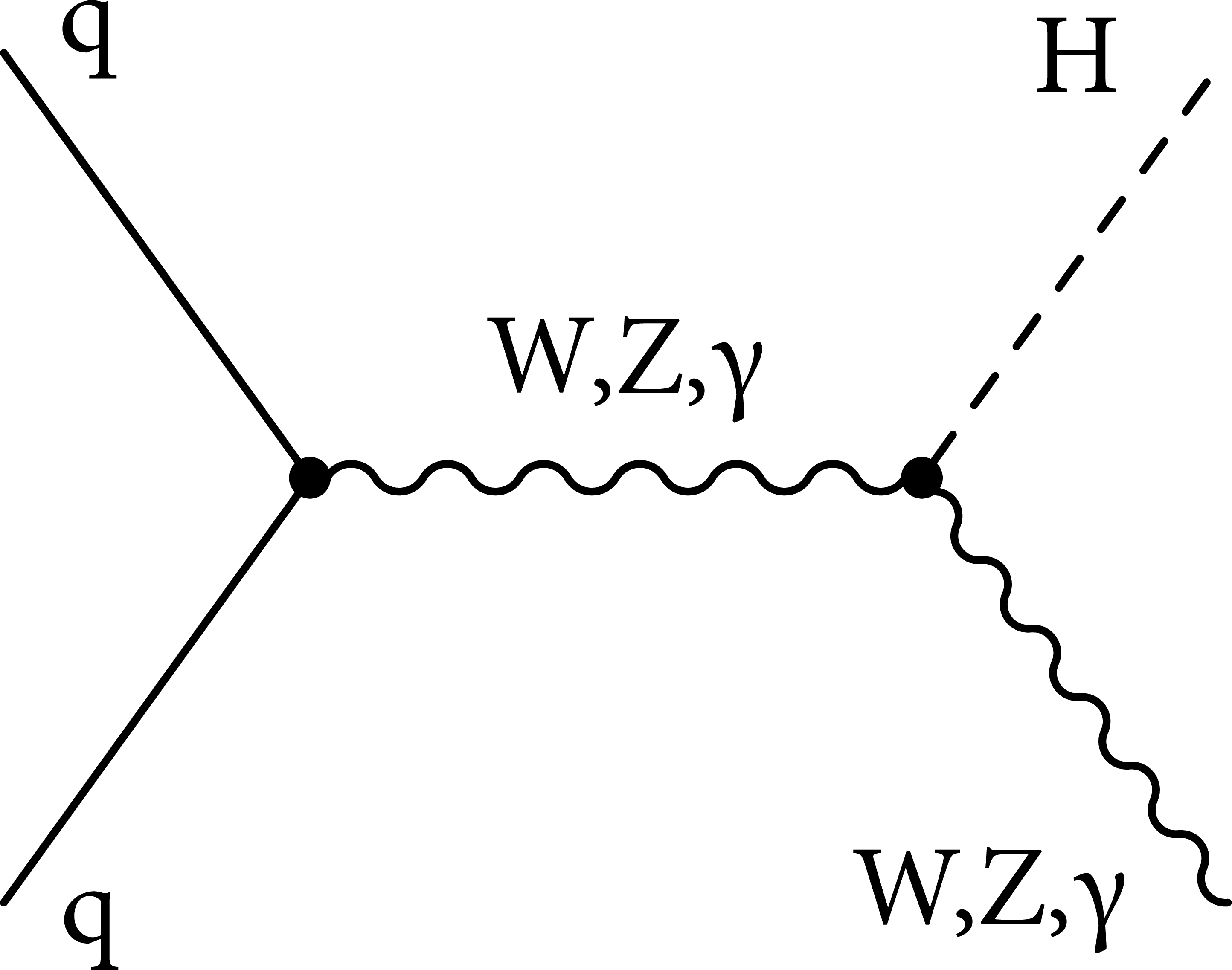
Figure 1-c:
Example of leading-order Feynman diagram for H boson production via associated production with a vector boson. The HWW and HZZ couplings may appear at tree level, as the SM predicts. |
png pdf |
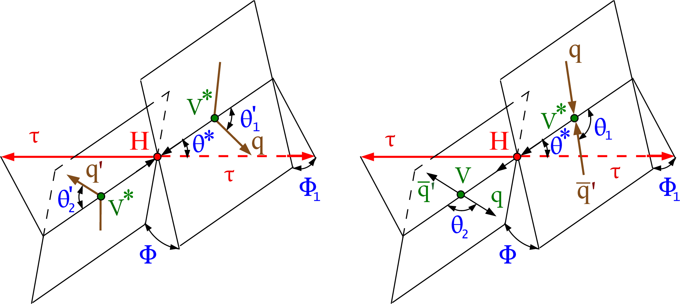
Figure 2:
Illustrations of H boson production in $ {\mathrm {q}}{{\mathrm {q}}^\prime}\to {\mathrm {g}} {\mathrm {g}} ({\mathrm {q}}{{\mathrm {q}}^\prime})\to {\mathrm {H}} ({\mathrm {q}}{{\mathrm {q}}^\prime})\to {\tau} {\tau}({\mathrm {q}}{{\mathrm {q}}^\prime})$ or VBF $ {\mathrm {q}}{{\mathrm {q}}^\prime}\to \mathrm {V}^*\mathrm {V}^*({\mathrm {q}}{{\mathrm {q}}^\prime})\to {\mathrm {H}} ({\mathrm {q}}{{\mathrm {q}}^\prime})\to {\tau} {\tau}({\mathrm {q}}{{\mathrm {q}}^\prime})$ (left) and in associated production $ {\mathrm {q}}\bar{{\mathrm {q}}}^\prime \to \mathrm {V}^*\to \mathrm {V} {\mathrm {H}} \to {\mathrm {q}}\bar{{\mathrm {q}}}^\prime {\tau} {\tau}$ (right). The $ {\mathrm {H}} \to {\tau} {\tau}$ decay is shown without further illustrating the $ {\tau}$ decay chain. Angles and invariant masses fully characterize the orientation of the production and two-body decay chain and are defined in suitable rest frames of the V and H bosons, except in the VBF case, where only the H boson rest frame is used [26,28]. |

png pdf |
Figure 2-a:
Illustration of H boson production in $ {\mathrm {q}}{{\mathrm {q}}^\prime}\to {\mathrm {g}} {\mathrm {g}} ({\mathrm {q}}{{\mathrm {q}}^\prime})\to {\mathrm {H}} ({\mathrm {q}}{{\mathrm {q}}^\prime})\to {\tau} {\tau}({\mathrm {q}}{{\mathrm {q}}^\prime})$ or VBF $ {\mathrm {q}}{{\mathrm {q}}^\prime}\to \mathrm {V}^*\mathrm {V}^*({\mathrm {q}}{{\mathrm {q}}^\prime})\to {\mathrm {H}} ({\mathrm {q}}{{\mathrm {q}}^\prime})\to {\tau} {\tau}({\mathrm {q}}{{\mathrm {q}}^\prime})$. The $ {\mathrm {H}} \to {\tau} {\tau}$ decay is shown without further illustrating the $ {\tau}$ decay chain. Angles and invariant masses fully characterize the orientation of the production and two-body decay chain and are defined in suitable rest frames of the V and H bosons, except in the VBF case, where only the H boson rest frame is used. |
png pdf |
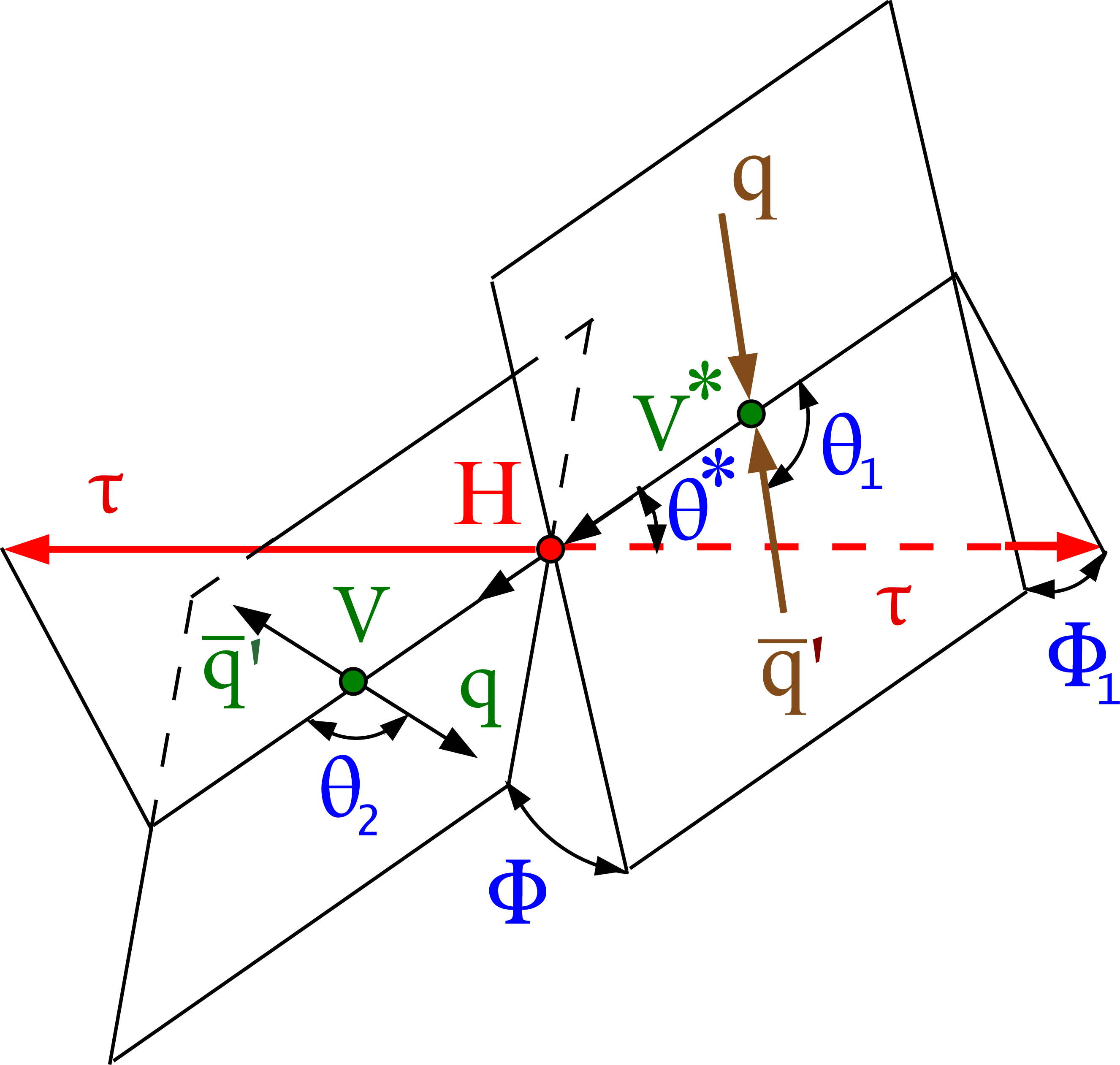
Figure 2-b:
Illustration of H boson production in associated production $ {\mathrm {q}}\bar{{\mathrm {q}}}^\prime \to \mathrm {V}^*\to \mathrm {V} {\mathrm {H}} \to {\mathrm {q}}\bar{{\mathrm {q}}}^\prime {\tau} {\tau}$. |
png pdf |
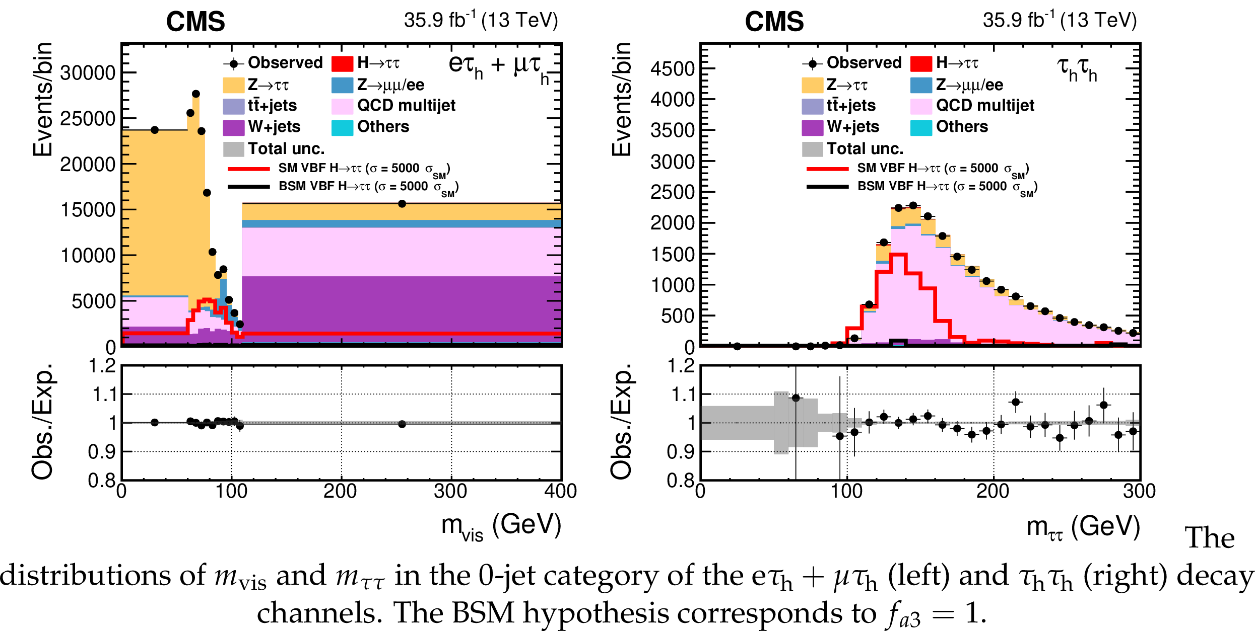
Figure 3:
The distributions of $ {m_\text {vis}} $ and $ {m_{{\tau} {\tau}}} $ in the 0-jet category of the $ {\mathrm {e}} {{\tau} _\mathrm {h}} + {{\mu}} {{\tau} _\mathrm {h}} $ (left) and $ {{\tau} _\mathrm {h}} {{\tau} _\mathrm {h}} $ (right) decay channels. The BSM hypothesis corresponds to $f_{a3}=$ 1. |

png pdf |
Figure 3-a:
The distribution of $ {m_\text {vis}} $ and $ {m_{{\tau} {\tau}}} $ in the 0-jet category of the $ {\mathrm {e}} {{\tau} _\mathrm {h}} + {{\mu}} {{\tau} _\mathrm {h}} $ decay channel. The BSM hypothesis corresponds to $f_{a3}=$ 1. |
png pdf |
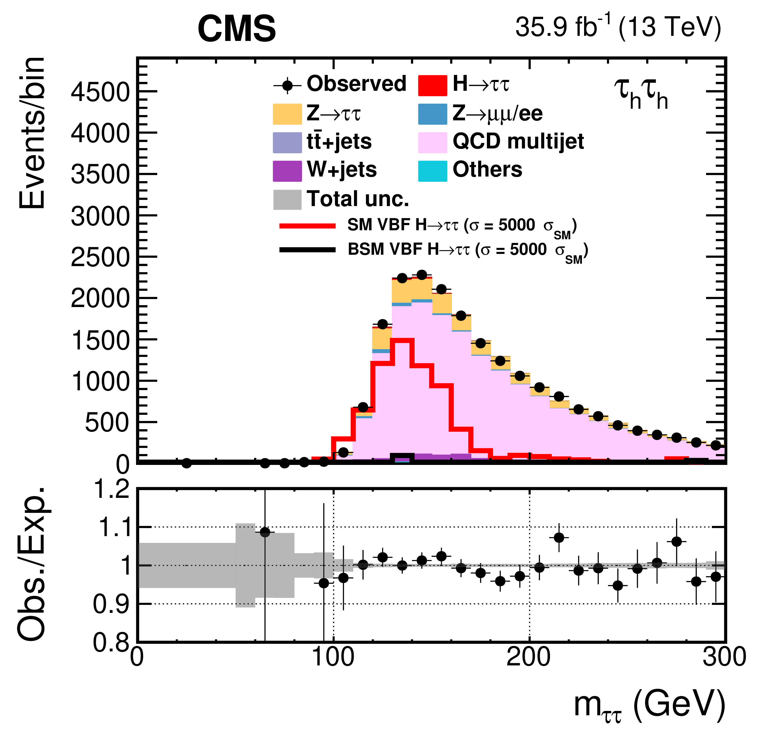
Figure 3-b:
The distribution of $ {m_\text {vis}} $ and $ {m_{{\tau} {\tau}}} $ in the 0-jet category of the $ {{\tau} _\mathrm {h}} {{\tau} _\mathrm {h}} $ decay channel. The BSM hypothesis corresponds to $f_{a3}=$ 1. |
png pdf |
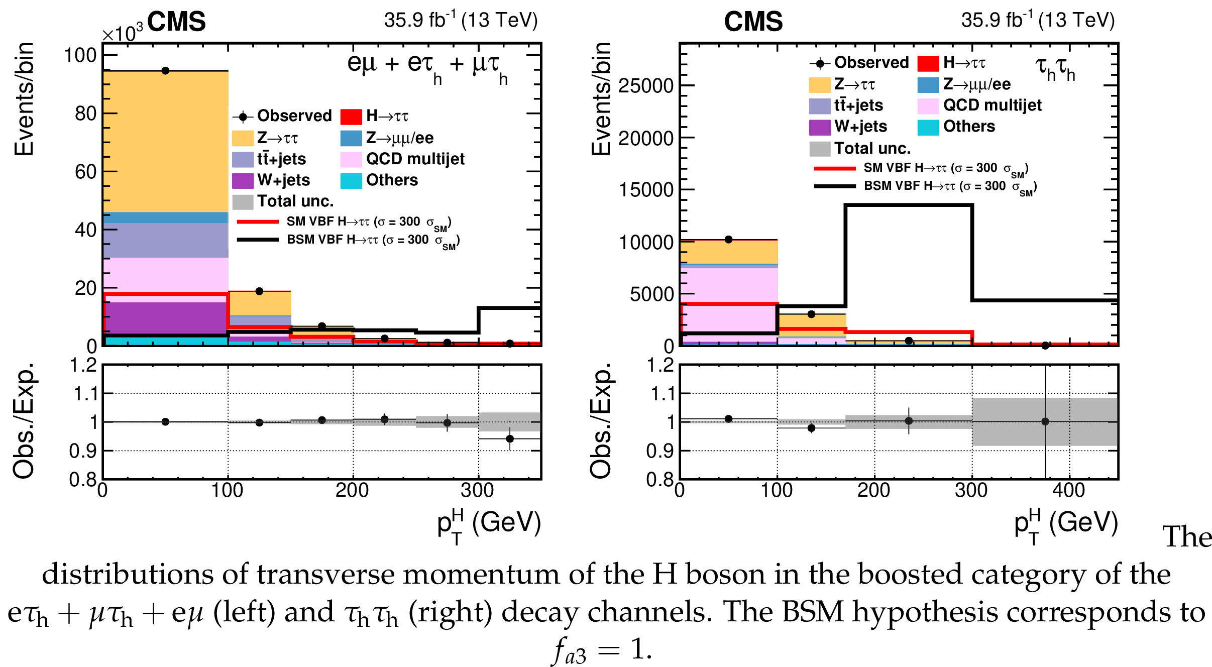
Figure 4:
The distributions of transverse momentum of the H boson in the boosted category of the $ {\mathrm {e}} {{\tau} _\mathrm {h}} + {{\mu}} {{\tau} _\mathrm {h}} + {\mathrm {e}} {{\mu}}$ (left) and $ {{\tau} _\mathrm {h}} {{\tau} _\mathrm {h}} $ (right) decay channels. The BSM hypothesis corresponds to $f_{a3}=$ 1. |
png pdf |
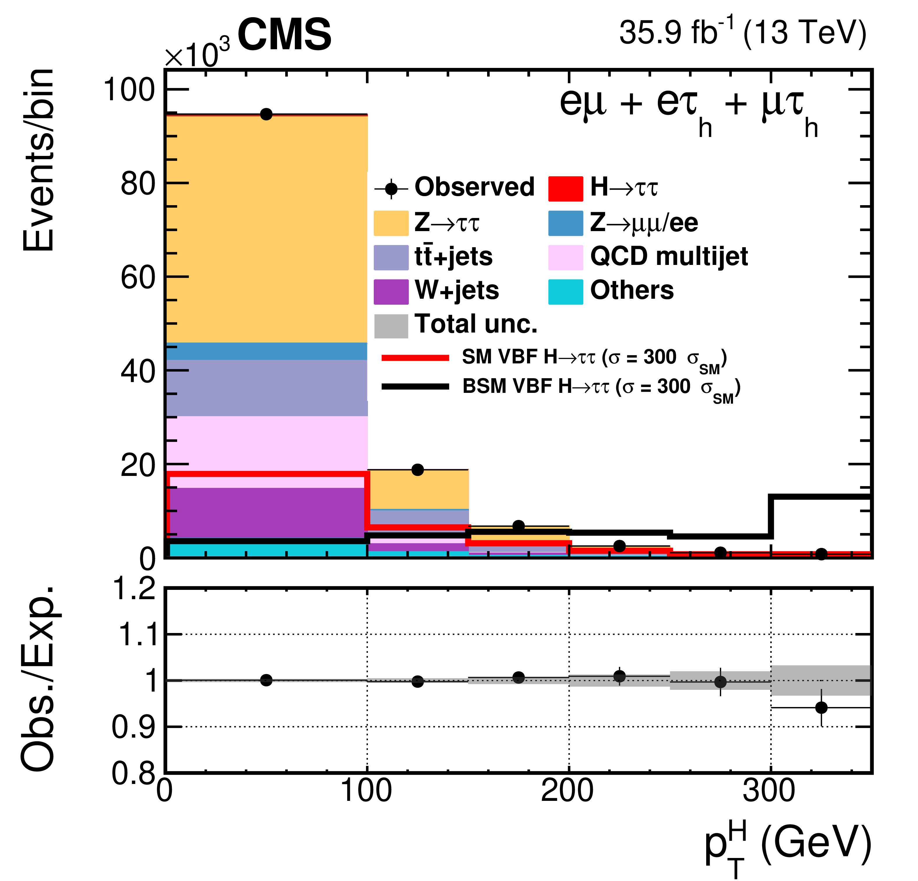
Figure 4-a:
The distribution of transverse momentum of the H boson in the boosted category of the $ {\mathrm {e}} {{\tau} _\mathrm {h}} + {{\mu}} {{\tau} _\mathrm {h}} + {\mathrm {e}} {{\mu}}$ decay channel. The BSM hypothesis corresponds to $f_{a3}=$ 1. |
png pdf |
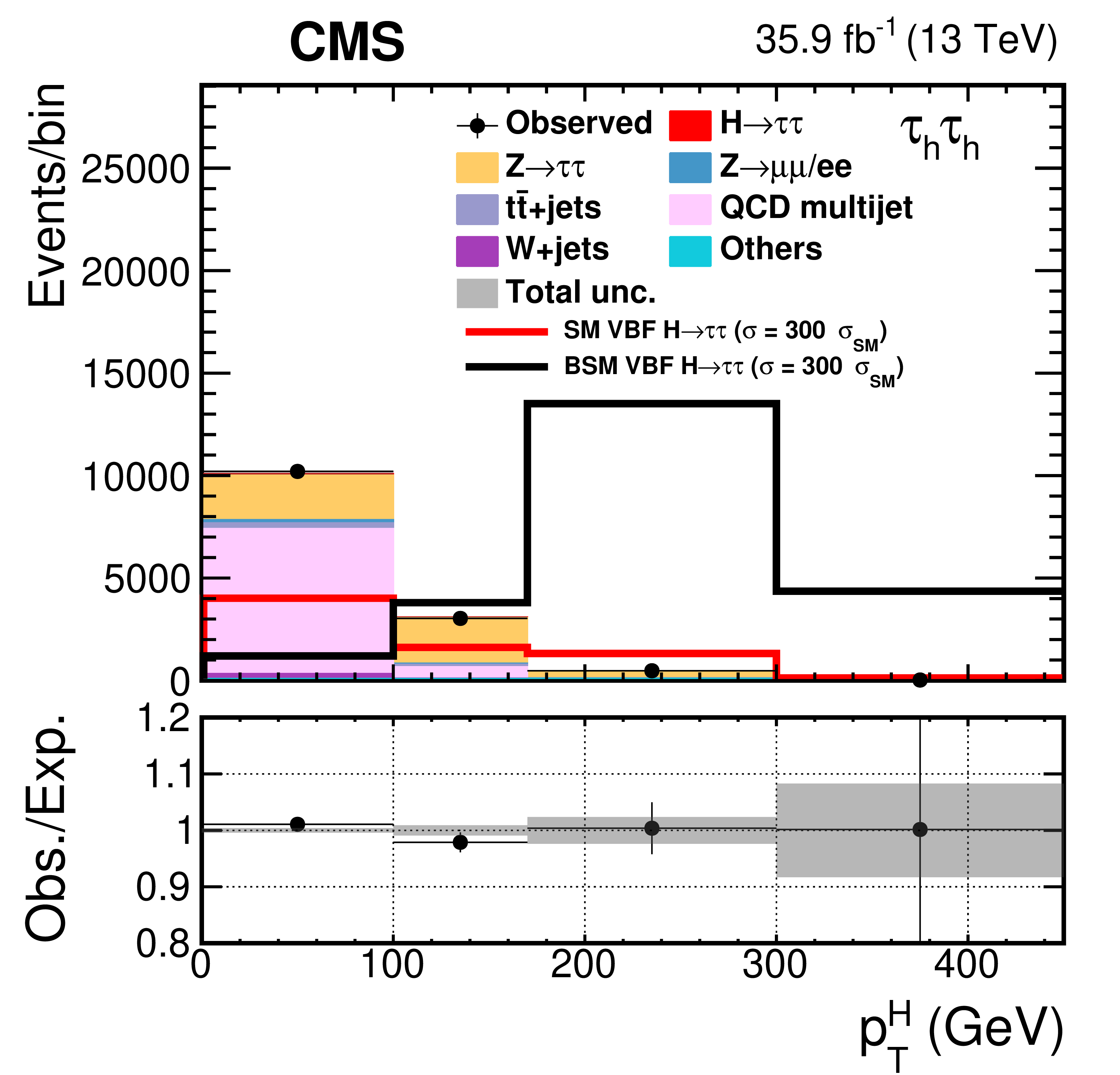
Figure 4-b:
The distribution of transverse momentum of the H boson in the boosted category of the $ {{\tau} _\mathrm {h}} {{\tau} _\mathrm {h}} $ decay channel. The BSM hypothesis corresponds to $f_{a3}=$ 1. |
png pdf |
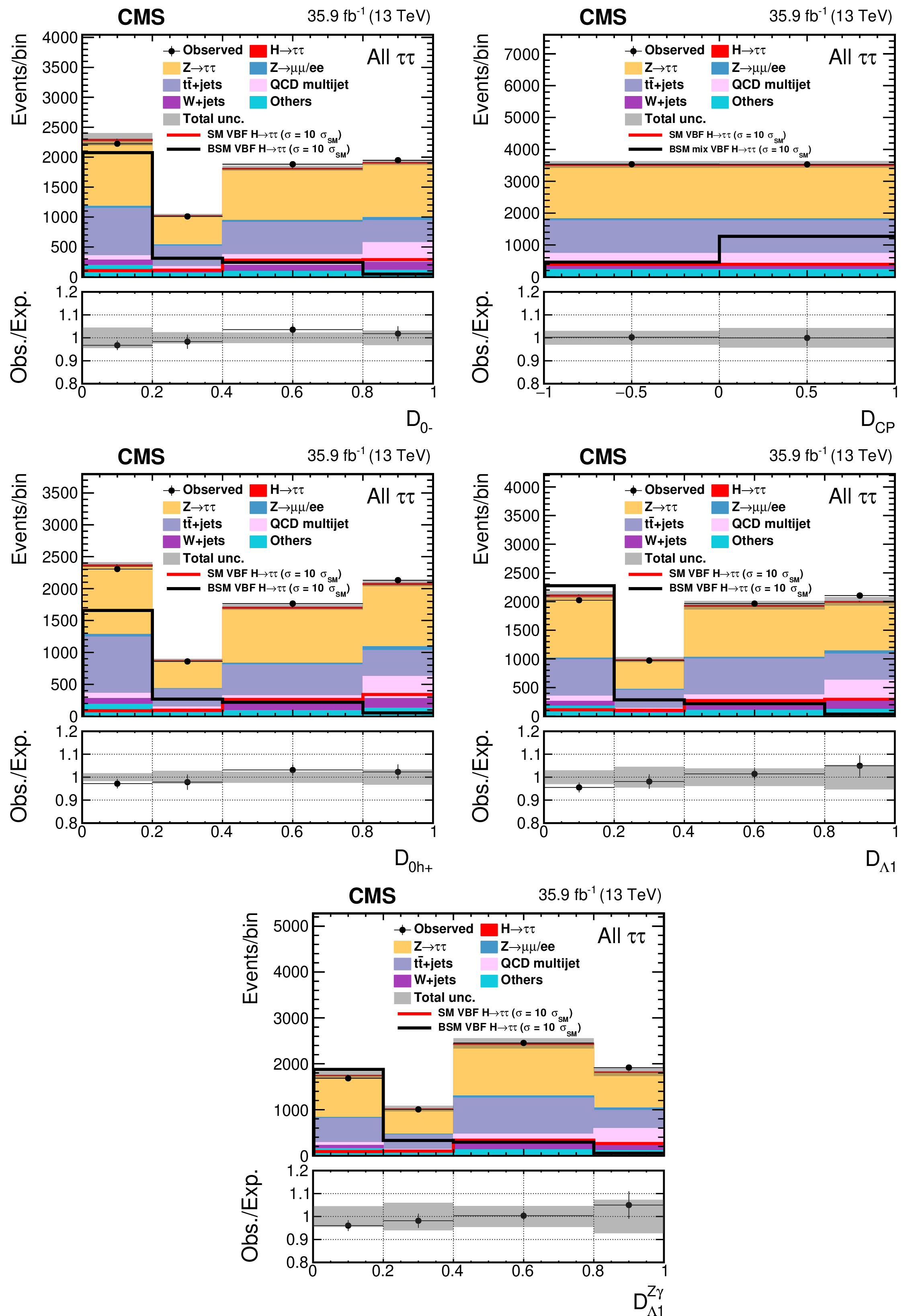
Figure 5:
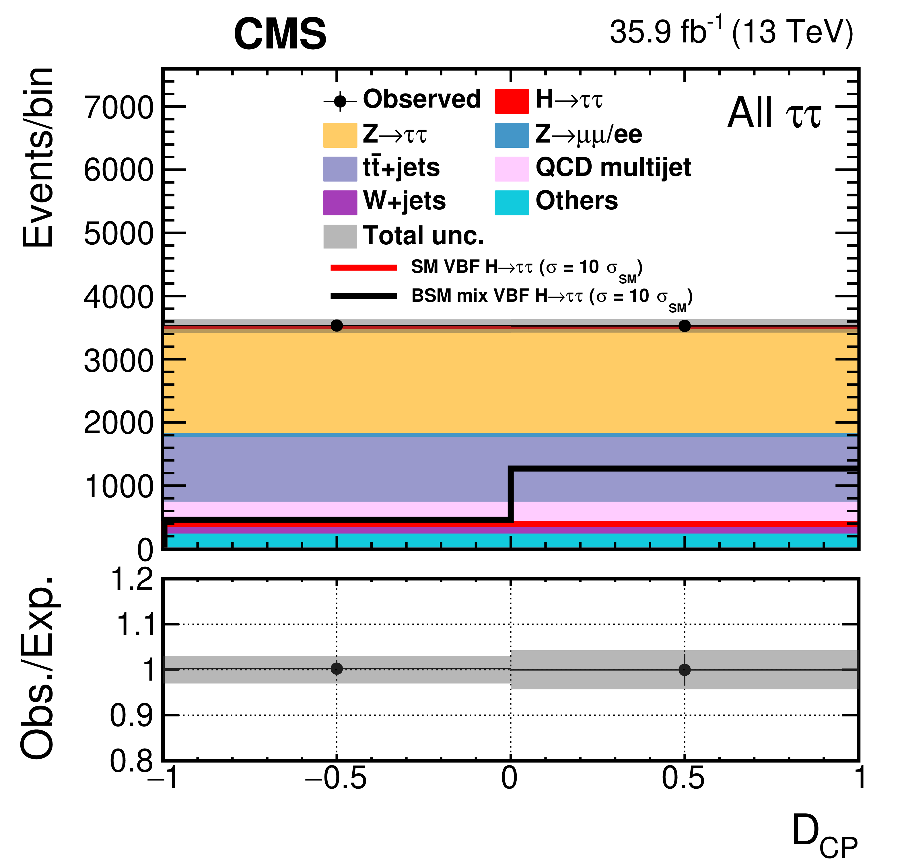
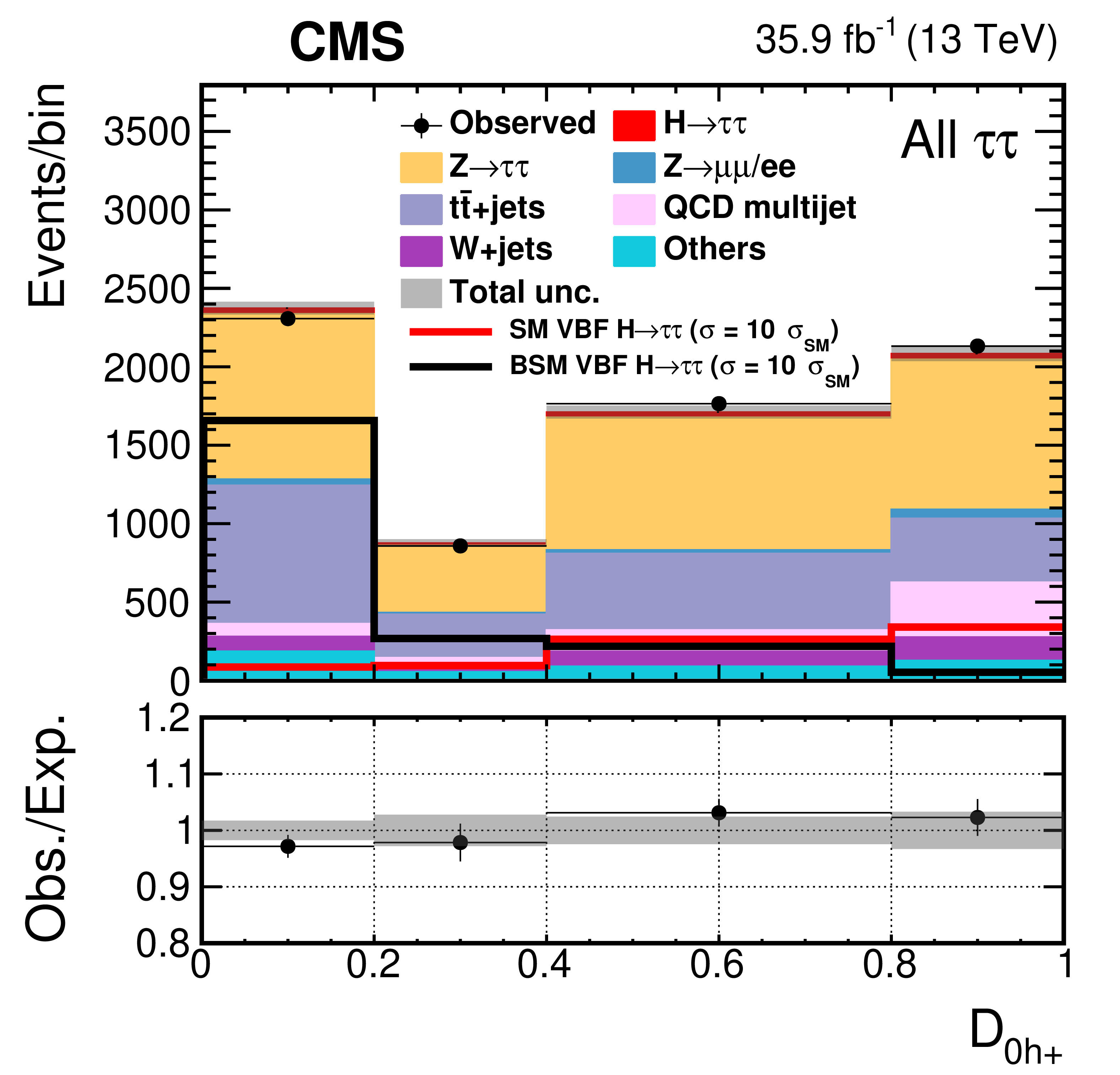
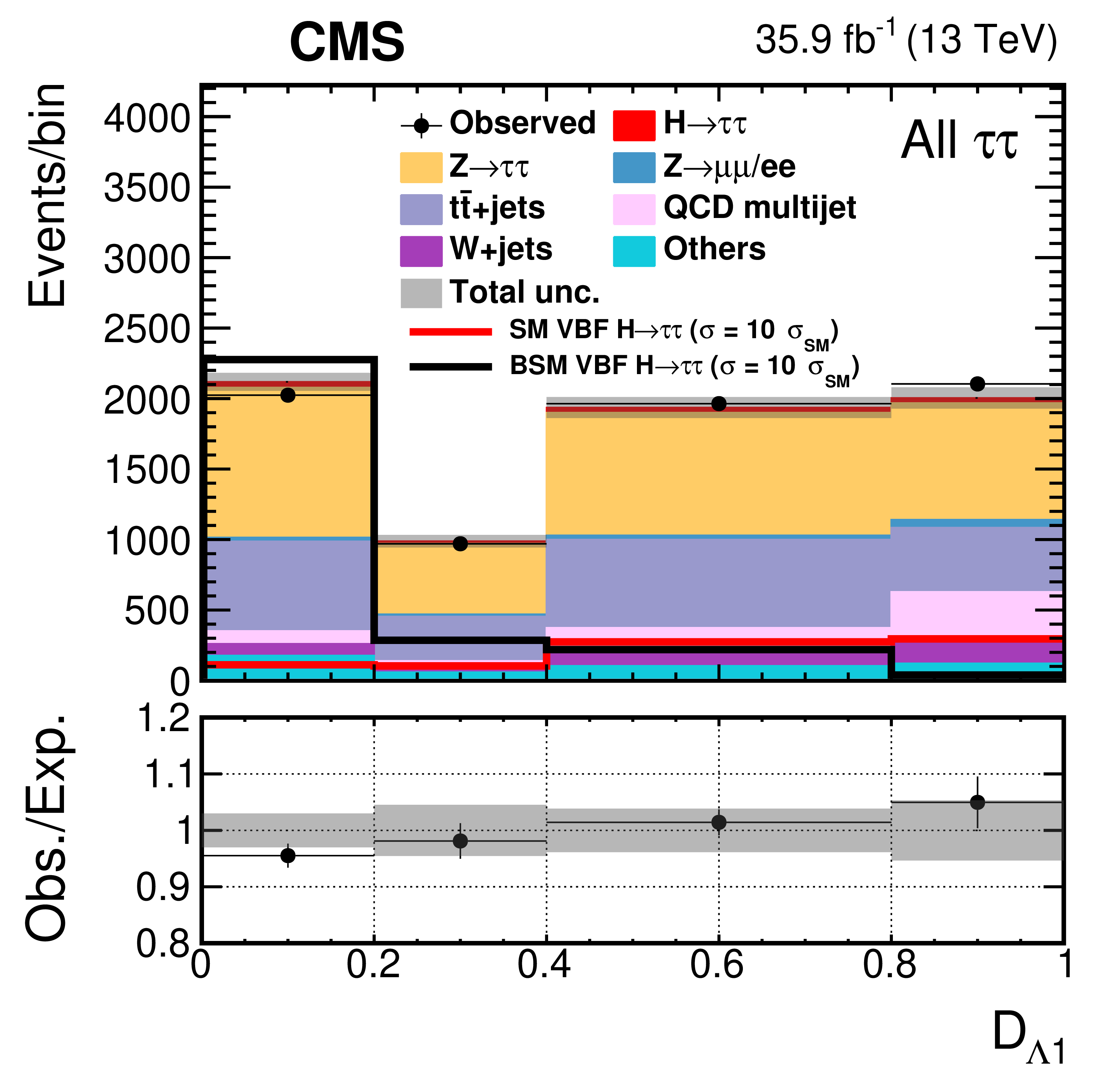
The distributions of $\mathcal {D}_\mathrm {0-}$, $\mathcal {D}_{CP}$, $\mathcal {D}_\mathrm {0h+}$, $\mathcal {D}_{\Lambda 1}$, and $\mathcal {D}_{\Lambda 1}^{{\mathrm {Z}} \gamma}$ in the VBF category. All four decay channels, $ {\mathrm {e}} {{\mu}}$, $ {\mathrm {e}} {{\tau} _\mathrm {h}} $, $ {{\mu}} {{\tau} _\mathrm {h}} $, and $ {{\tau} _\mathrm {h}} {{\tau} _\mathrm {h}} $, are summed. The BSM hypothesis depends on the variable shown: it corresponds to $f_{a3}=$ 1 for the $\mathcal {D}_\mathrm {0-}$ (upper left) distributions, the maximal mixing ("BSM mix") in VBF production for the $\mathcal {D}_{CP}$ distribution (upper right), $f_{a2}=$ 1 for the $\mathcal {D}_\mathrm {0h+}$ distribution (middle left), $f_{\Lambda 1}=$ 1 for the $\mathcal {D}_{\Lambda 1}$ distribution (middle right), and $f_{\Lambda 1}^{{\mathrm {Z}} \gamma}=$ 1 for the $\mathcal {D}_{\Lambda 1}^{{\mathrm {Z}} \gamma}$ distribution (lower). |

png pdf |
Figure 5-a:
The distribution of $\mathcal {D}_\mathrm {0-}$ in the VBF category. All four decay channels, $ {\mathrm {e}} {{\mu}}$, $ {\mathrm {e}} {{\tau} _\mathrm {h}} $, $ {{\mu}} {{\tau} _\mathrm {h}} $, and $ {{\tau} _\mathrm {h}} {{\tau} _\mathrm {h}} $, are summed. The BSM hypothesis shown corresponds to $f_{a3}=$ 1. |
png pdf |
Figure 5-b:
The distribution of $\mathcal {D}_{CP}$ in the VBF category. All four decay channels, $ {\mathrm {e}} {{\mu}}$, $ {\mathrm {e}} {{\tau} _\mathrm {h}} $, $ {{\mu}} {{\tau} _\mathrm {h}} $, and $ {{\tau} _\mathrm {h}} {{\tau} _\mathrm {h}} $, are summed. The BSM hypothesis shown corresponds to the maximal mixing ("BSM mix") in VBF production. |
png pdf |
Figure 5-c:
The distribution of $\mathcal {D}_\mathrm {0h+}$ in the VBF category. All four decay channels, $ {\mathrm {e}} {{\mu}}$, $ {\mathrm {e}} {{\tau} _\mathrm {h}} $, $ {{\mu}} {{\tau} _\mathrm {h}} $, and $ {{\tau} _\mathrm {h}} {{\tau} _\mathrm {h}} $, are summed. The BSM hypothesis shown corresponds to $f_{a2}=$ 1. |
png pdf |
Figure 5-d:
The distribution of $\mathcal {D}_{\Lambda 1}$ in the VBF category. All four decay channels, $ {\mathrm {e}} {{\mu}}$, $ {\mathrm {e}} {{\tau} _\mathrm {h}} $, $ {{\mu}} {{\tau} _\mathrm {h}} $, and $ {{\tau} _\mathrm {h}} {{\tau} _\mathrm {h}} $, are summed. The BSM hypothesis shown corresponds to $f_{\Lambda 1}=$ 1. |

png pdf |
Figure 5-e:
The distribution of $\mathcal {D}_{\Lambda 1}^{{\mathrm {Z}} \gamma}$ in the VBF category. All four decay channels, $ {\mathrm {e}} {{\mu}}$, $ {\mathrm {e}} {{\tau} _\mathrm {h}} $, $ {{\mu}} {{\tau} _\mathrm {h}} $, and $ {{\tau} _\mathrm {h}} {{\tau} _\mathrm {h}} $, are summed. The BSM hypothesis shown corresponds to $f_{\Lambda 1}^{{\mathrm {Z}} \gamma}=$ 1. |

png pdf |
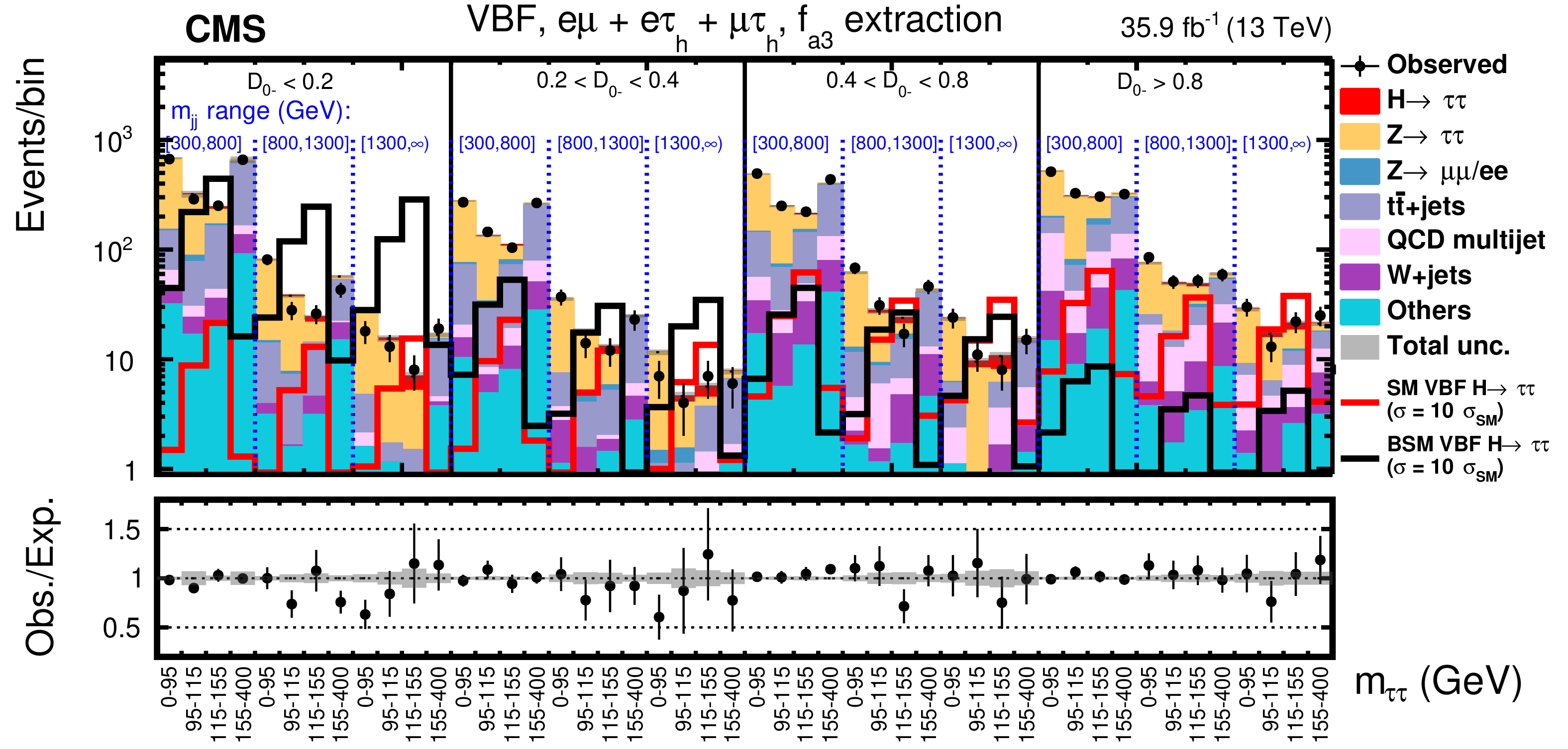
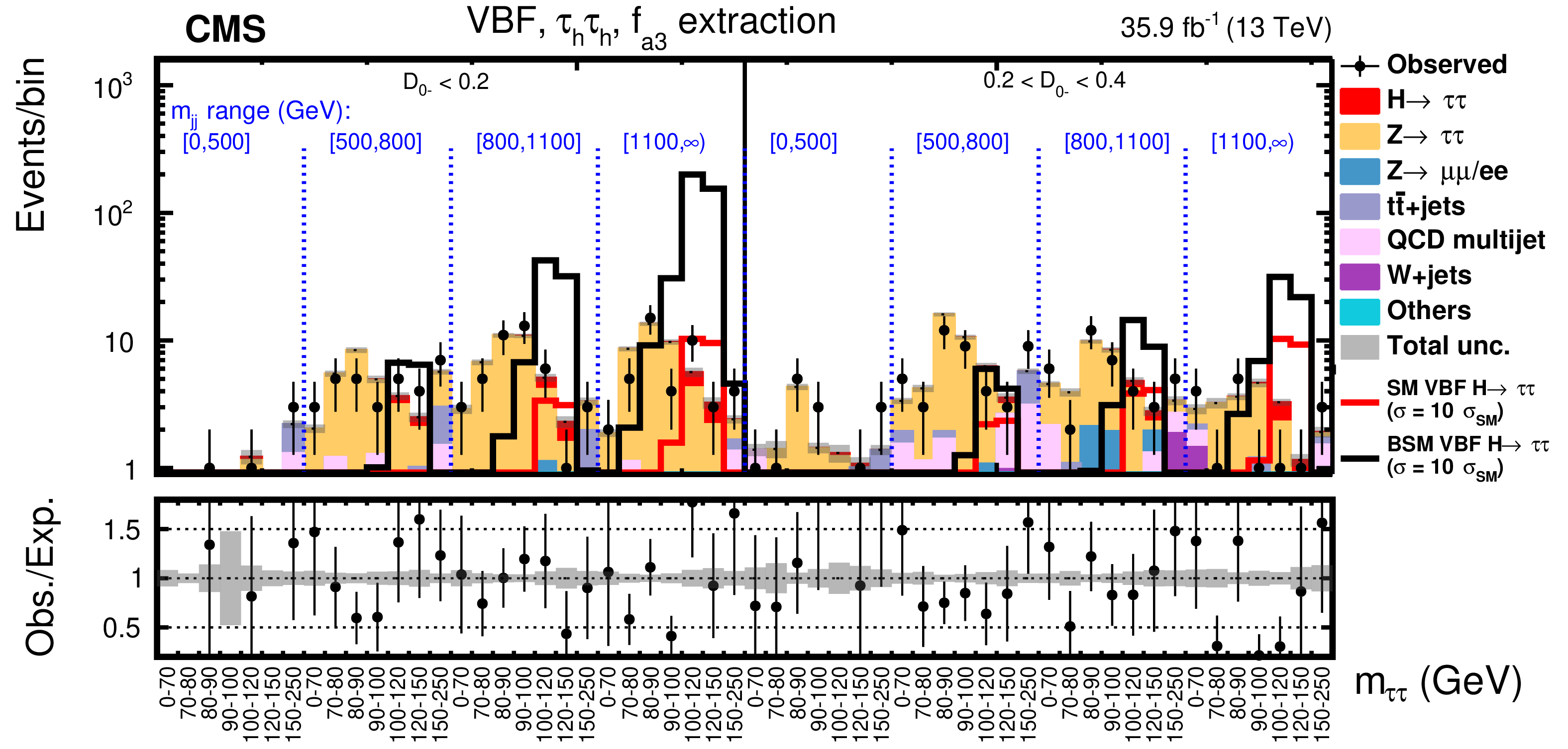
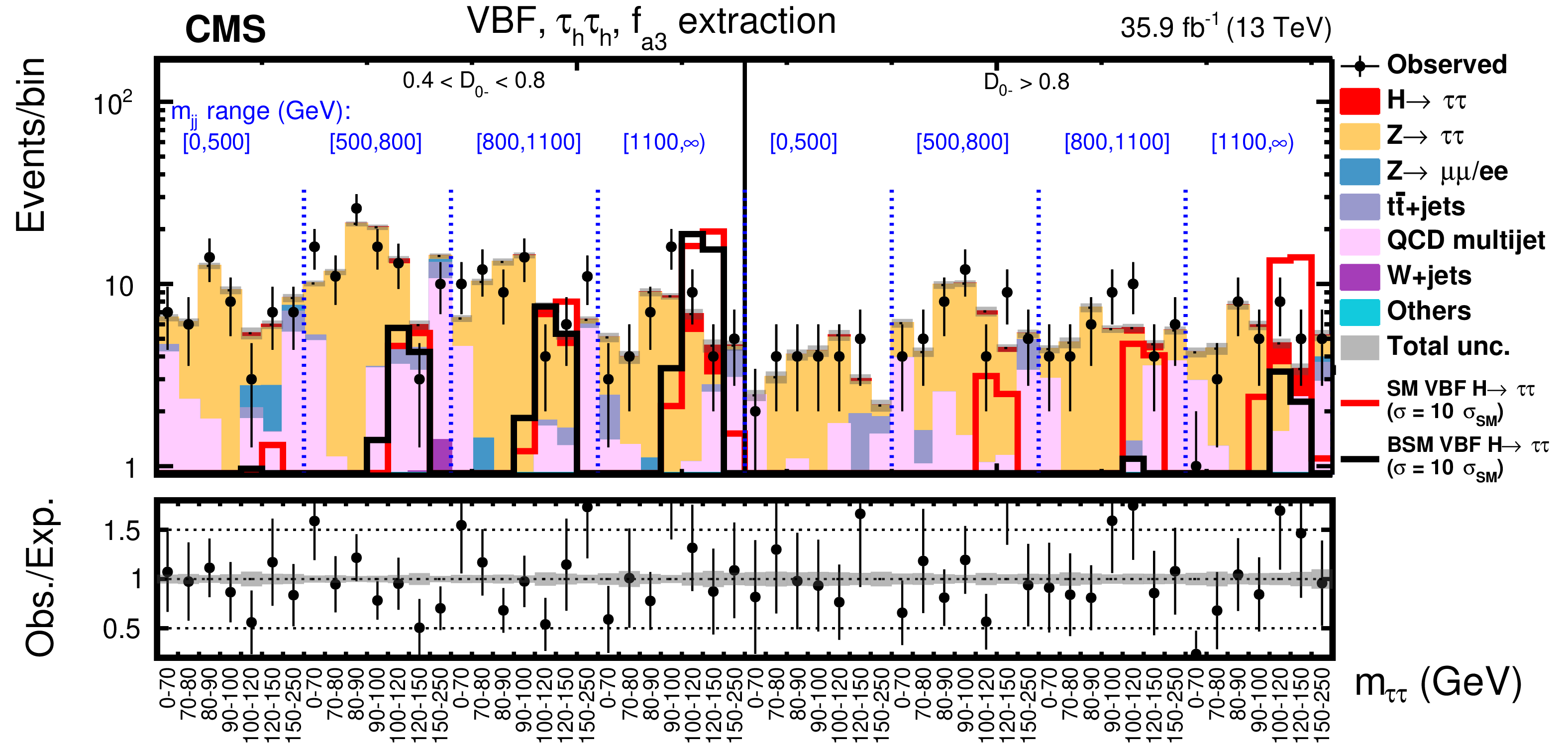
Figure 6:
Observed and expected distributions in the VBF category in bins of $ {m_{{\tau} {\tau}}} $, $ {m_{JJ}} $, and $\mathcal {D}_\mathrm {0-}$ in the $f_{a3}$ analysis for the $ {\mathrm {e}} {{\mu}}+ {\mathrm {e}} {{\tau} _\mathrm {h}} + {{\mu}} {{\tau} _\mathrm {h}} $ (upper) and $ {{\tau} _\mathrm {h}} {{\tau} _\mathrm {h}} $ (middle and lower) decay channels. |
png pdf |
Figure 6-a:
Observed and expected distributions in the VBF category in bins of $ {m_{{\tau} {\tau}}} $, $ {m_{JJ}} $, and $\mathcal {D}_\mathrm {0-}$ in the $f_{a3}$ analysis for the $ {\mathrm {e}} {{\mu}}+ {\mathrm {e}} {{\tau} _\mathrm {h}} + {{\mu}} {{\tau} _\mathrm {h}} $ decay channel. |
png pdf |
Figure 6-b:
Observed and expected distributions in the VBF category in bins of $ {m_{{\tau} {\tau}}} $, $ {m_{JJ}} $, and $\mathcal {D}_\mathrm {0-}$ in the $f_{a3}$ analysis for the $ {{\tau} _\mathrm {h}} {{\tau} _\mathrm {h}} $ decay channel. |
png pdf |
Figure 6-c:
Observed and expected distributions in the VBF category in bins of $ {m_{{\tau} {\tau}}} $, $ {m_{JJ}} $, and $\mathcal {D}_\mathrm {0-}$ in the $f_{a3}$ analysis for the $ {{\tau} _\mathrm {h}} {{\tau} _\mathrm {h}} $ decay channel. |
png pdf |
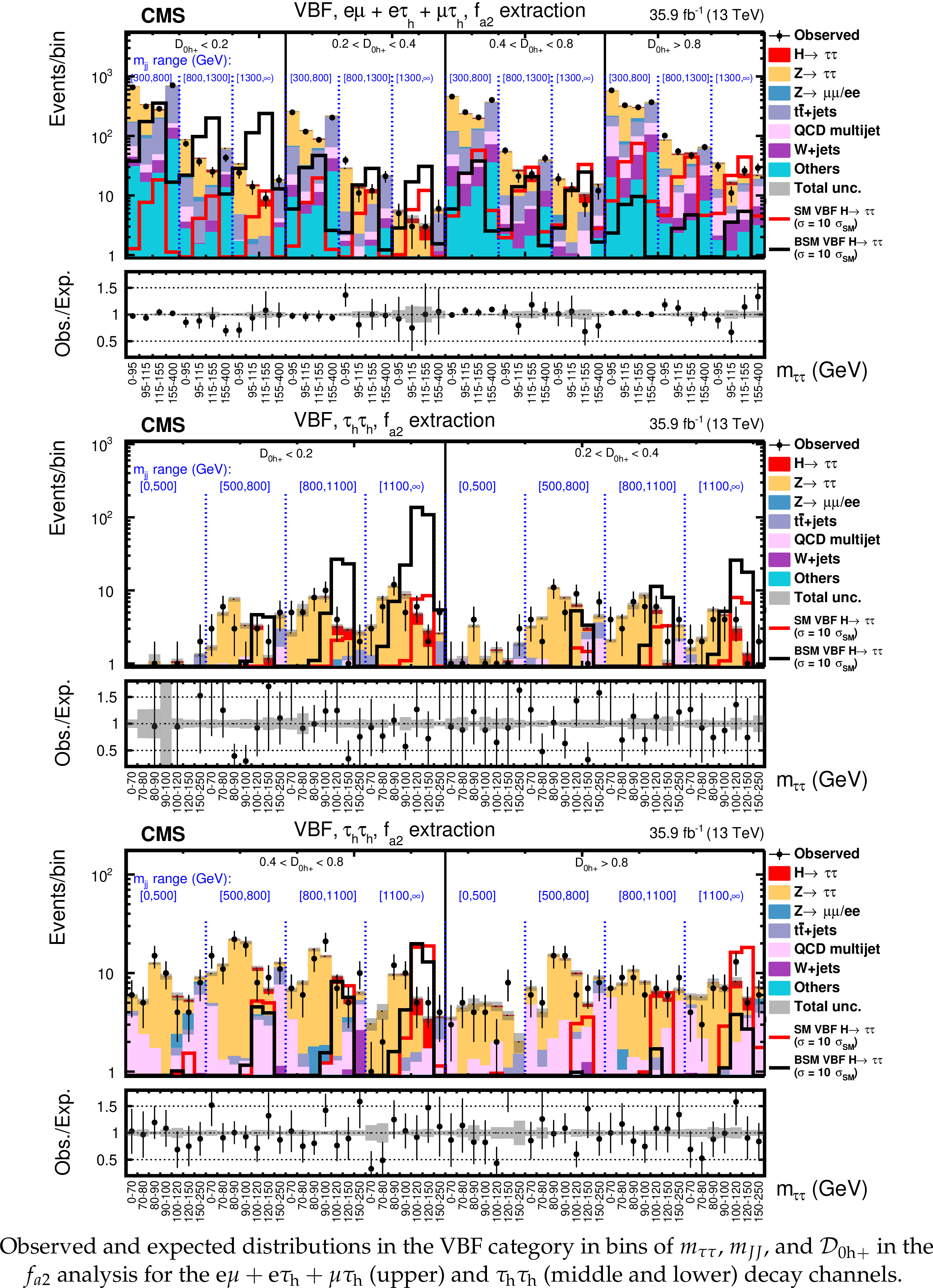
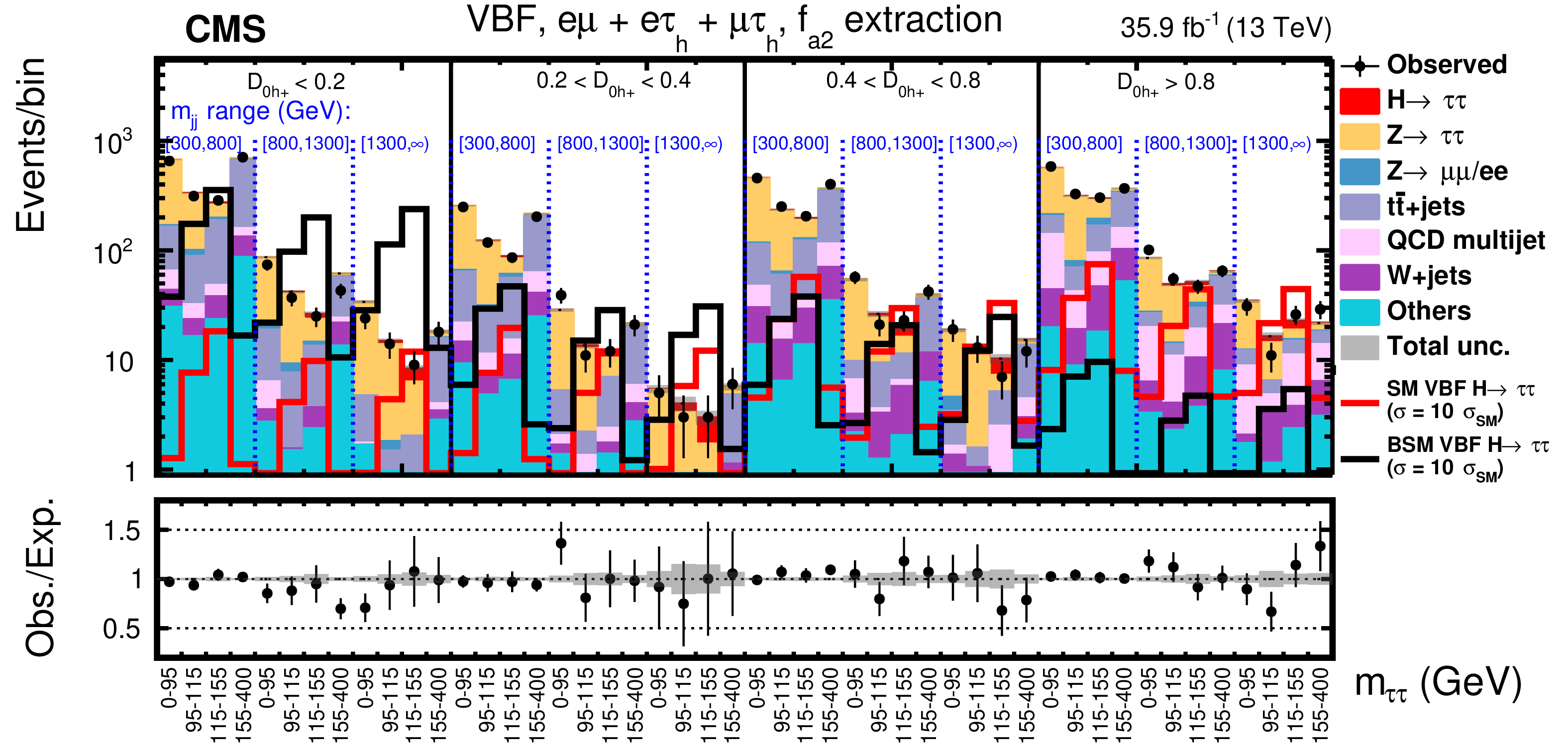
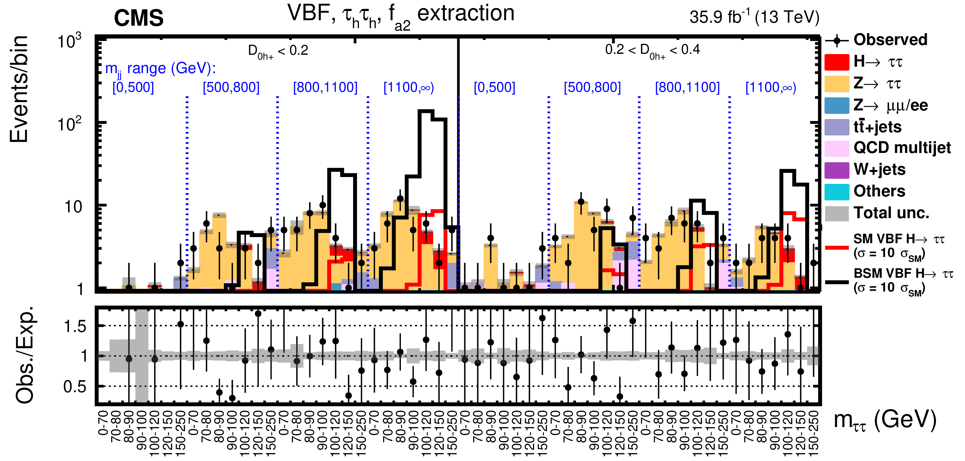
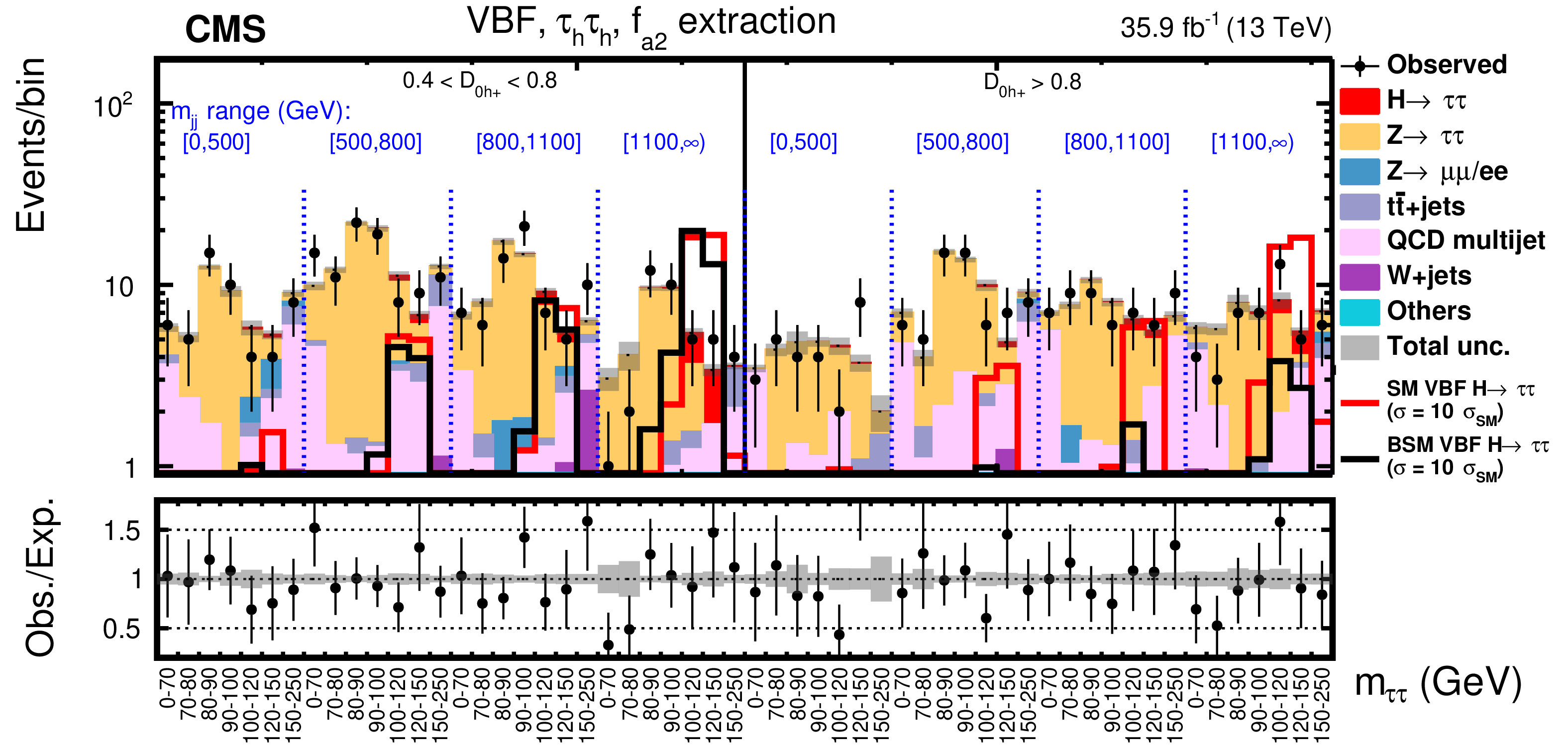
Figure 7:
Observed and expected distributions in the VBF category in bins of $ {m_{{\tau} {\tau}}} $, $ {m_{JJ}} $, and $\mathcal {D}_\mathrm {0h+}$ in the $f_{a2}$ analysis for the $ {\mathrm {e}} {{\mu}}+ {\mathrm {e}} {{\tau} _\mathrm {h}} + {{\mu}} {{\tau} _\mathrm {h}} $ (upper) and $ {{\tau} _\mathrm {h}} {{\tau} _\mathrm {h}} $ (middle and lower) decay channels. |
png pdf |
Figure 7-a:
Observed and expected distributions in the VBF category in bins of $ {m_{{\tau} {\tau}}} $, $ {m_{JJ}} $, and $\mathcal {D}_\mathrm {0h+}$ in the $f_{a2}$ analysis for the $ {\mathrm {e}} {{\mu}}+ {\mathrm {e}} {{\tau} _\mathrm {h}} + {{\mu}} {{\tau} _\mathrm {h}} $ decay channel. |
png pdf |
Figure 7-b:
Observed and expected distributions in the VBF category in bins of $ {m_{{\tau} {\tau}}} $, $ {m_{JJ}} $, and $\mathcal {D}_\mathrm {0h+}$ in the $f_{a2}$ analysis for the $ {{\tau} _\mathrm {h}} {{\tau} _\mathrm {h}} $ decay channel. |
png pdf |
Figure 7-c:
Observed and expected distributions in the VBF category in bins of $ {m_{{\tau} {\tau}}} $, $ {m_{JJ}} $, and $\mathcal {D}_\mathrm {0h+}$ in the $f_{a2}$ analysis for the $ {{\tau} _\mathrm {h}} {{\tau} _\mathrm {h}} $ decay channel. |
png pdf |
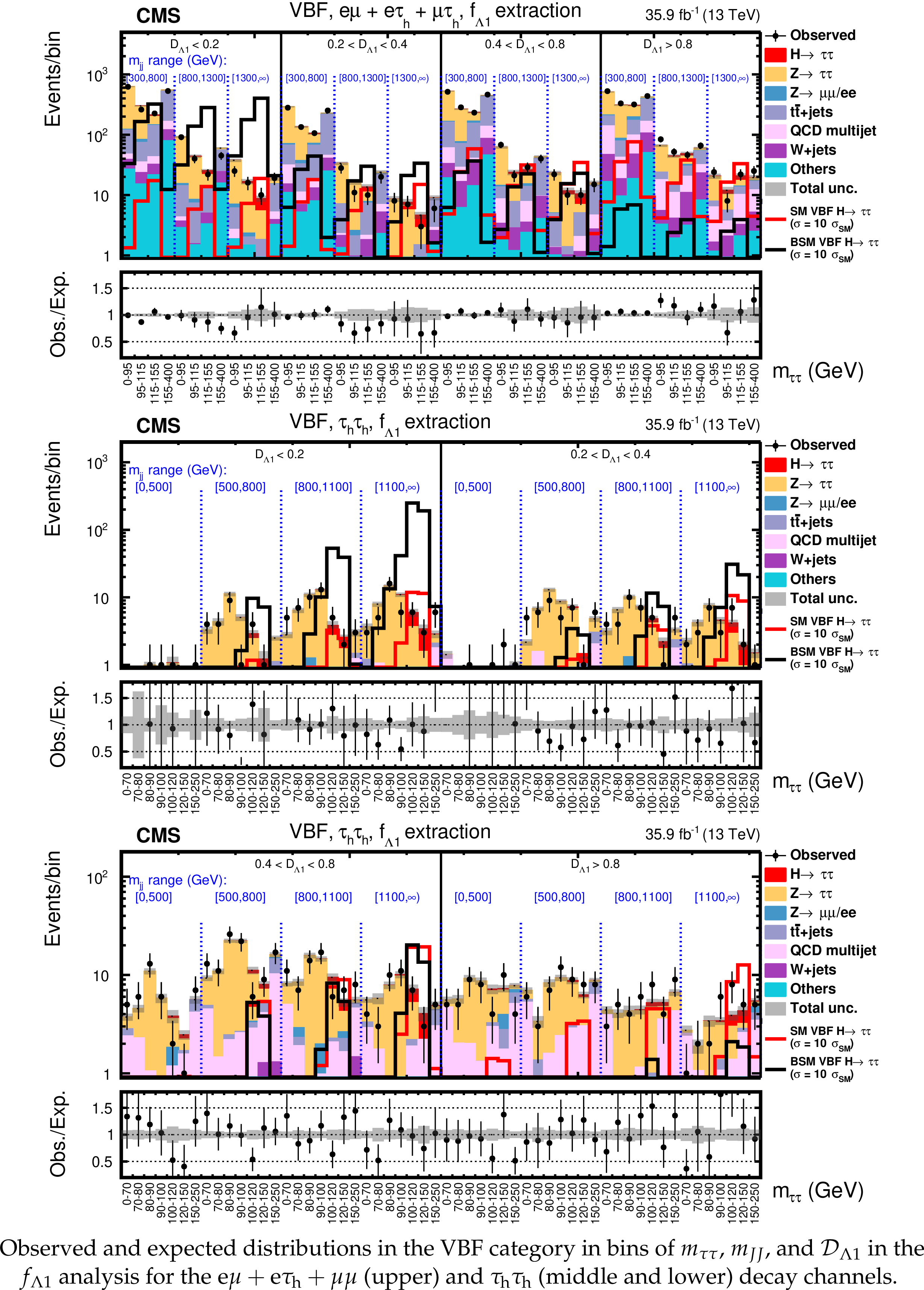
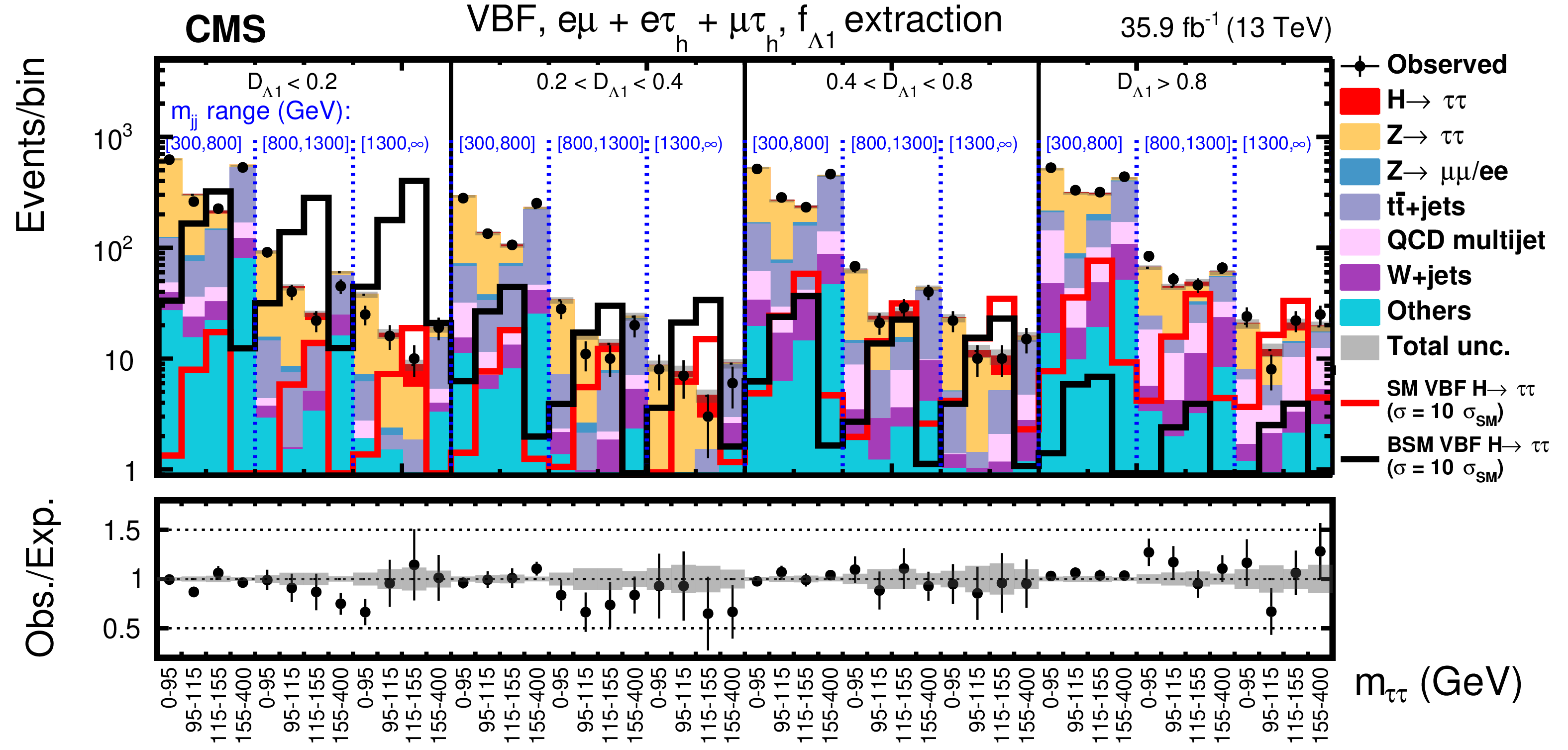
Figure 8:
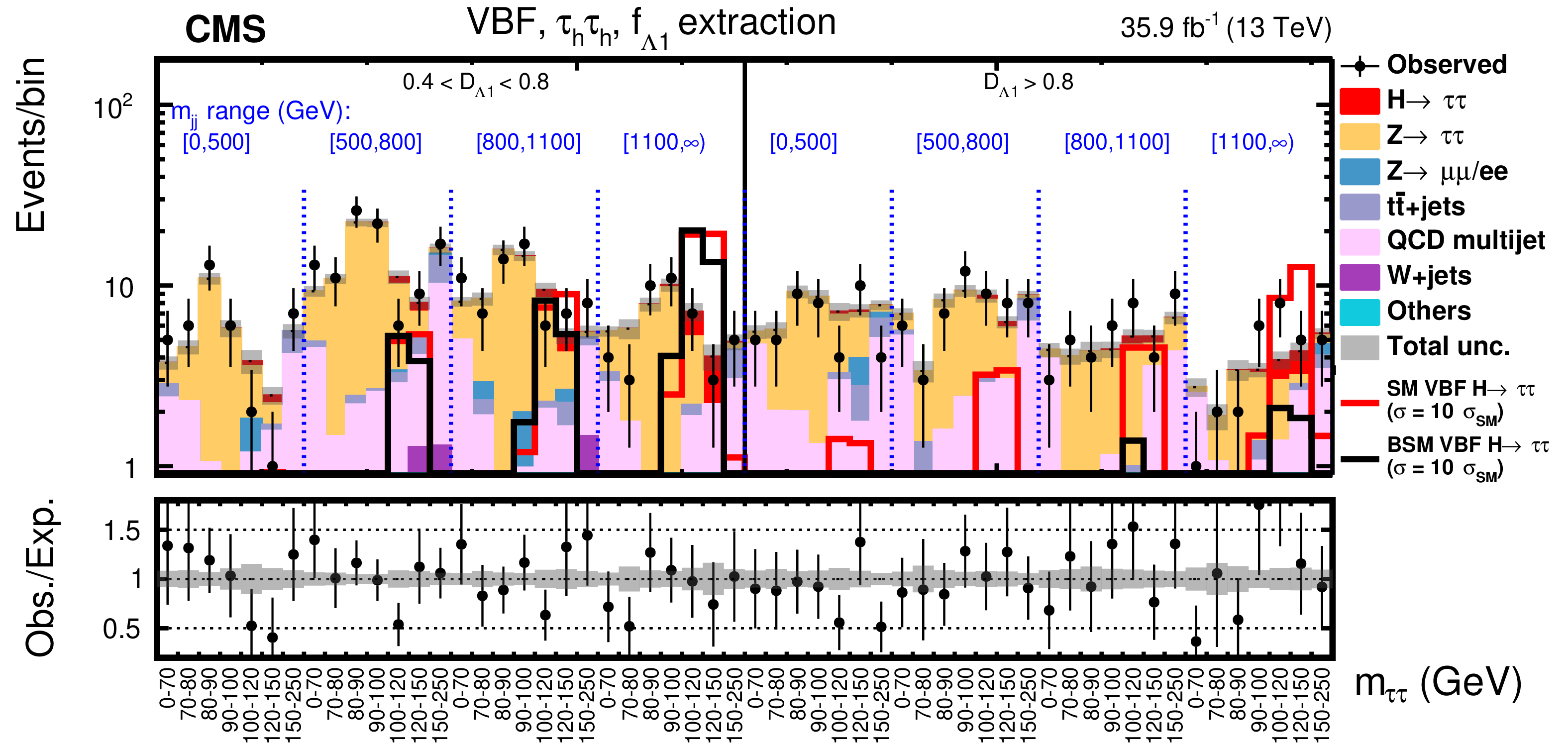
Observed and expected distributions in the VBF category in bins of $ {m_{{\tau} {\tau}}} $, $ {m_{JJ}} $, and $\mathcal {D}_{\Lambda 1}$ in the $f_{\Lambda 1}$ analysis for the $ {\mathrm {e}} {{\mu}}+ {\mathrm {e}} {{\tau} _\mathrm {h}} + {{\mu}} {{\mu}}$ (upper) and $ {{\tau} _\mathrm {h}} {{\tau} _\mathrm {h}} $ (middle and lower) decay channels. |
png pdf |
Figure 8-a:
Observed and expected distributions in the VBF category in bins of $ {m_{{\tau} {\tau}}} $, $ {m_{JJ}} $, and $\mathcal {D}_{\Lambda 1}$ in the $f_{\Lambda 1}$ analysis for the $ {\mathrm {e}} {{\mu}}+ {\mathrm {e}} {{\tau} _\mathrm {h}} + {{\mu}} {{\mu}}$ decay channel. |
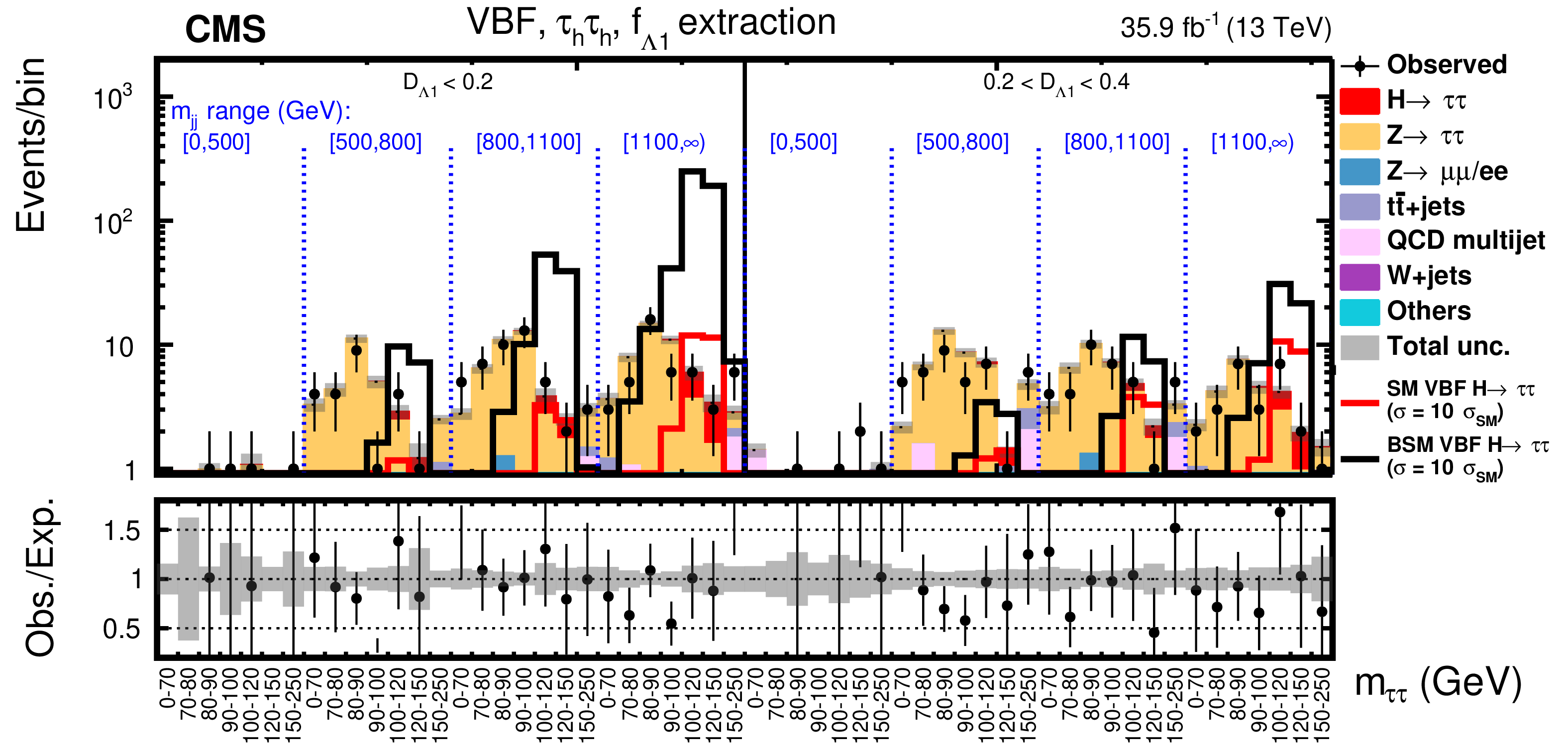
png pdf |
Figure 8-b:
Observed and expected distributions in the VBF category in bins of $ {m_{{\tau} {\tau}}} $, $ {m_{JJ}} $, and $\mathcal {D}_{\Lambda 1}$ in the $f_{\Lambda 1}$ analysis for the $ {{\tau} _\mathrm {h}} {{\tau} _\mathrm {h}} $ decay channel. |
png pdf |
Figure 8-c:
Observed and expected distributions in the VBF category in bins of $ {m_{{\tau} {\tau}}} $, $ {m_{JJ}} $, and $\mathcal {D}_{\Lambda 1}$ in the $f_{\Lambda 1}$ analysis for the $ {{\tau} _\mathrm {h}} {{\tau} _\mathrm {h}} $ decay channel. |
png pdf |
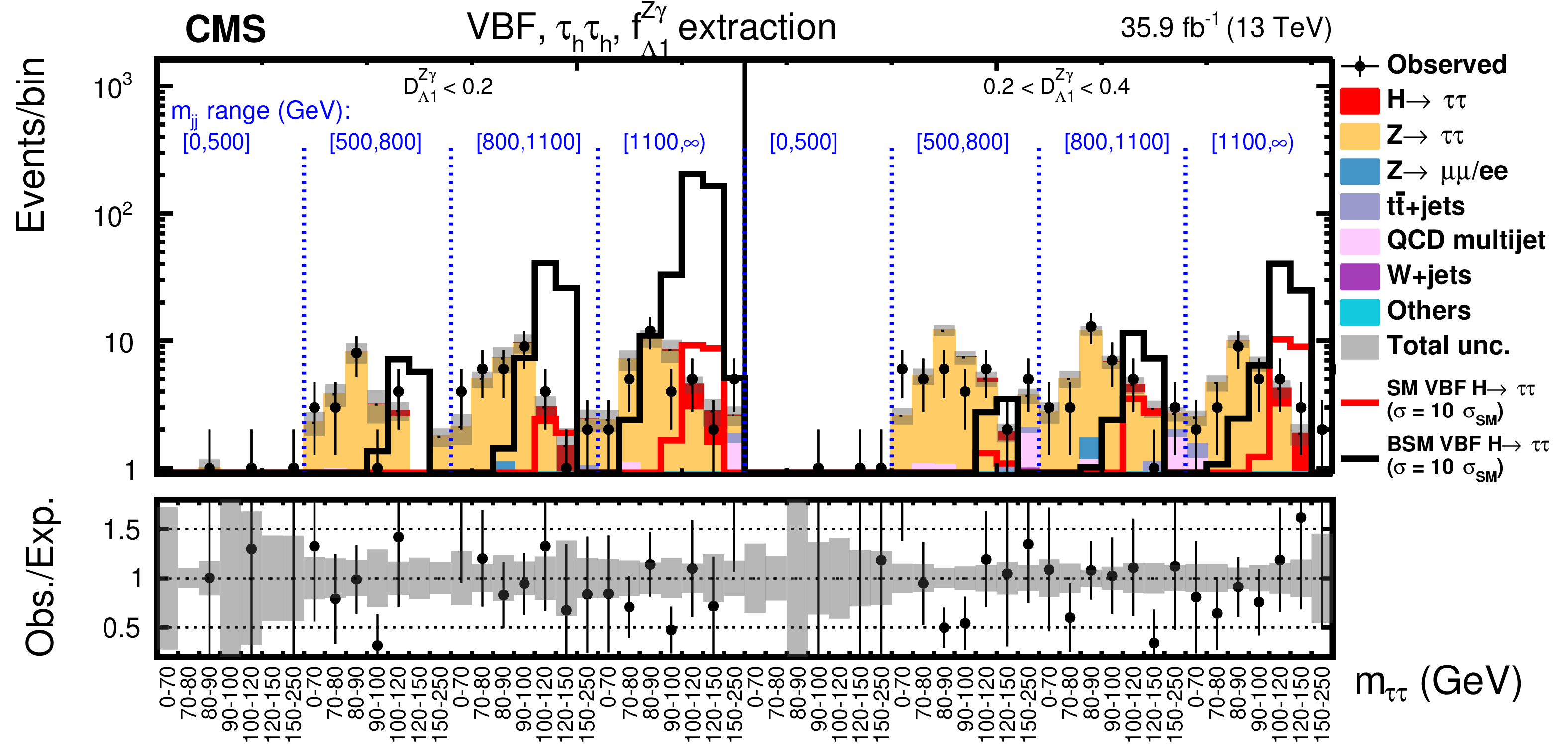
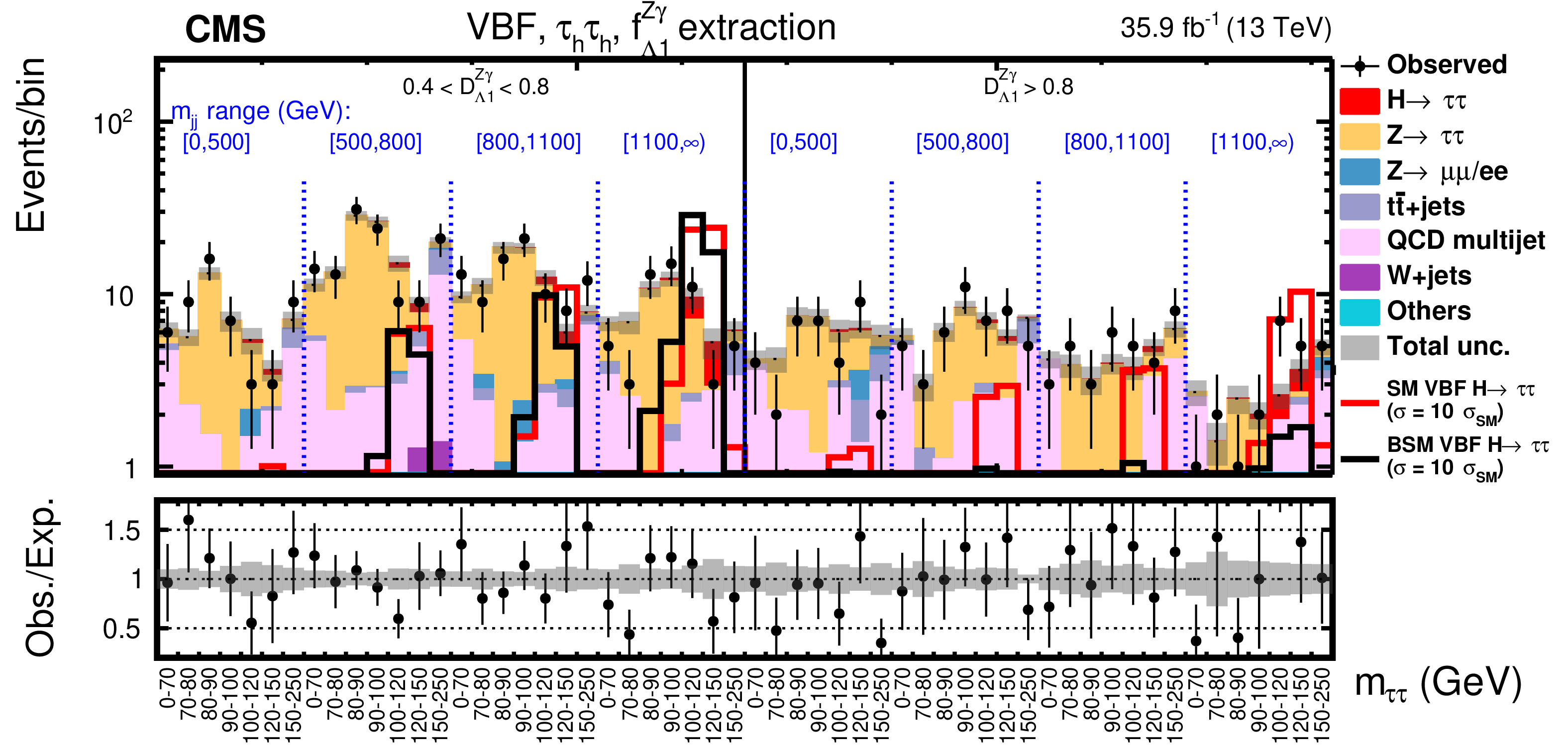
Figure 9:
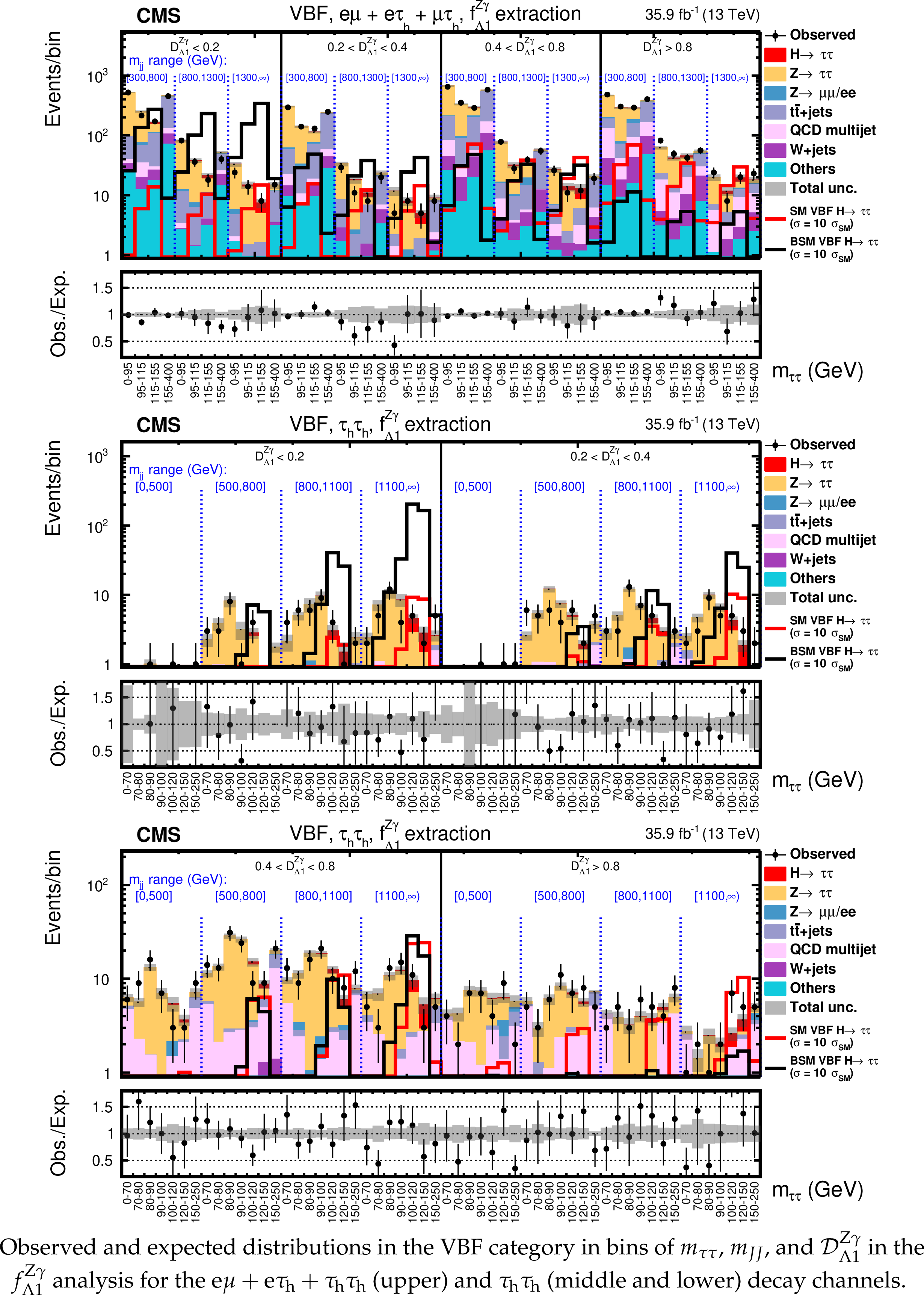
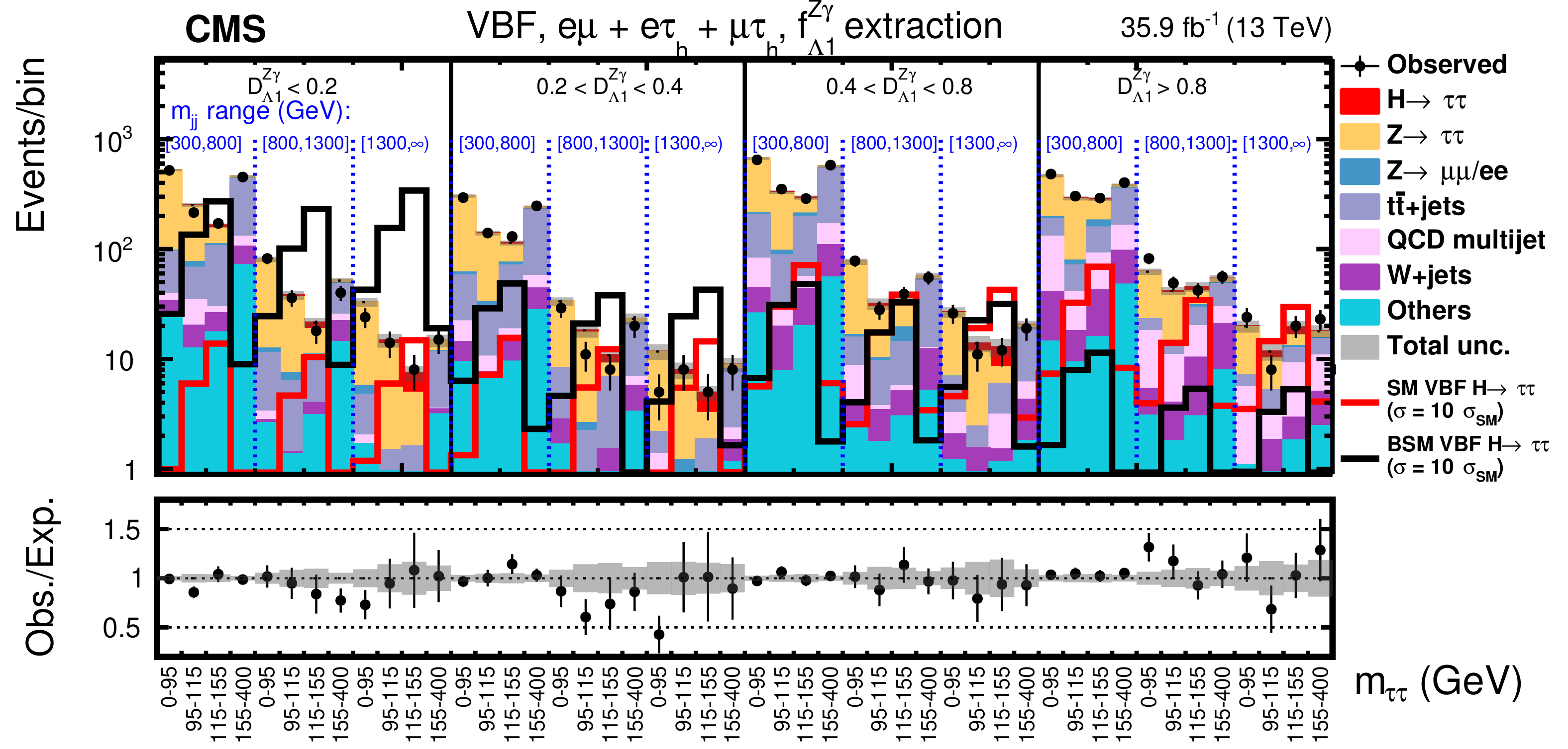
Observed and expected distributions in the VBF category in bins of $ {m_{{\tau} {\tau}}} $, $ {m_{JJ}} $, and $\mathcal {D}_{\Lambda 1}^{{\mathrm {Z}} \gamma}$ in the $f_{\Lambda 1}^{{\mathrm {Z}} \gamma}$ analysis for the $ {\mathrm {e}} {{\mu}}+ {\mathrm {e}} {{\tau} _\mathrm {h}} + {{\tau} _\mathrm {h}} {{\tau} _\mathrm {h}} $ (upper) and $ {{\tau} _\mathrm {h}} {{\tau} _\mathrm {h}} $ (middle and lower) decay channels. |
png pdf |
Figure 9-a:
Observed and expected distributions in the VBF category in bins of $ {m_{{\tau} {\tau}}} $, $ {m_{JJ}} $, and $\mathcal {D}_{\Lambda 1}^{{\mathrm {Z}} \gamma}$ in the $f_{\Lambda 1}^{{\mathrm {Z}} \gamma}$ analysis for the $ {\mathrm {e}} {{\mu}}+ {\mathrm {e}} {{\tau} _\mathrm {h}} + {{\tau} _\mathrm {h}} {{\tau} _\mathrm {h}} $ decay channel. |
png pdf |
Figure 9-b:
Observed and expected distributions in the VBF category in bins of $ {m_{{\tau} {\tau}}} $, $ {m_{JJ}} $, and $\mathcal {D}_{\Lambda 1}^{{\mathrm {Z}} \gamma}$ in the $f_{\Lambda 1}^{{\mathrm {Z}} \gamma}$ analysis for the $ {{\tau} _\mathrm {h}} {{\tau} _\mathrm {h}} $ decay channel. |
png pdf |
Figure 9-c:
Observed and expected distributions in the VBF category in bins of $ {m_{{\tau} {\tau}}} $, $ {m_{JJ}} $, and $\mathcal {D}_{\Lambda 1}^{{\mathrm {Z}} \gamma}$ in the $f_{\Lambda 1}^{{\mathrm {Z}} \gamma}$ analysis for the $ {{\tau} _\mathrm {h}} {{\tau} _\mathrm {h}} $ decay channel. |

png pdf |
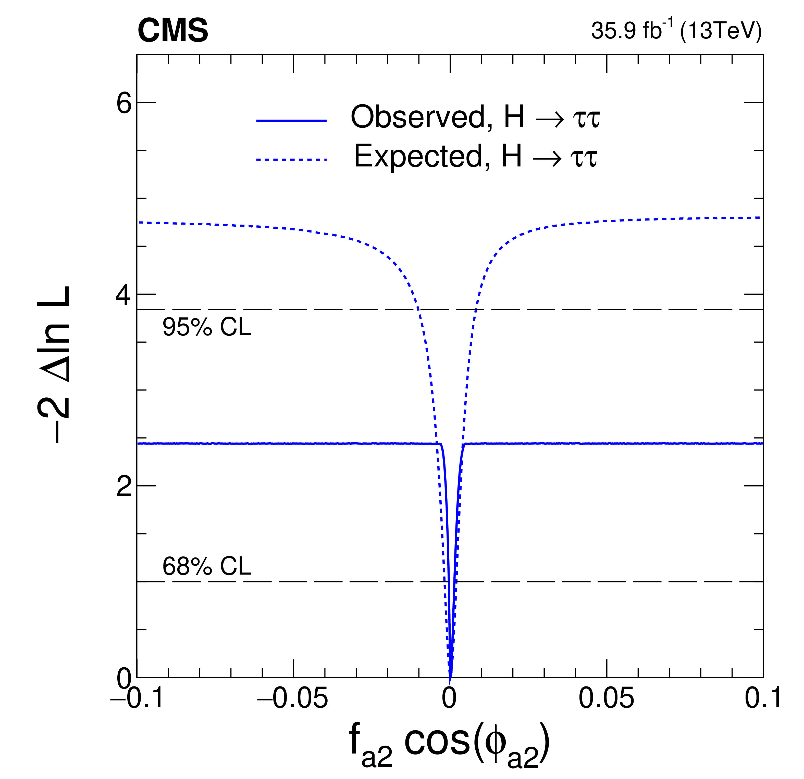
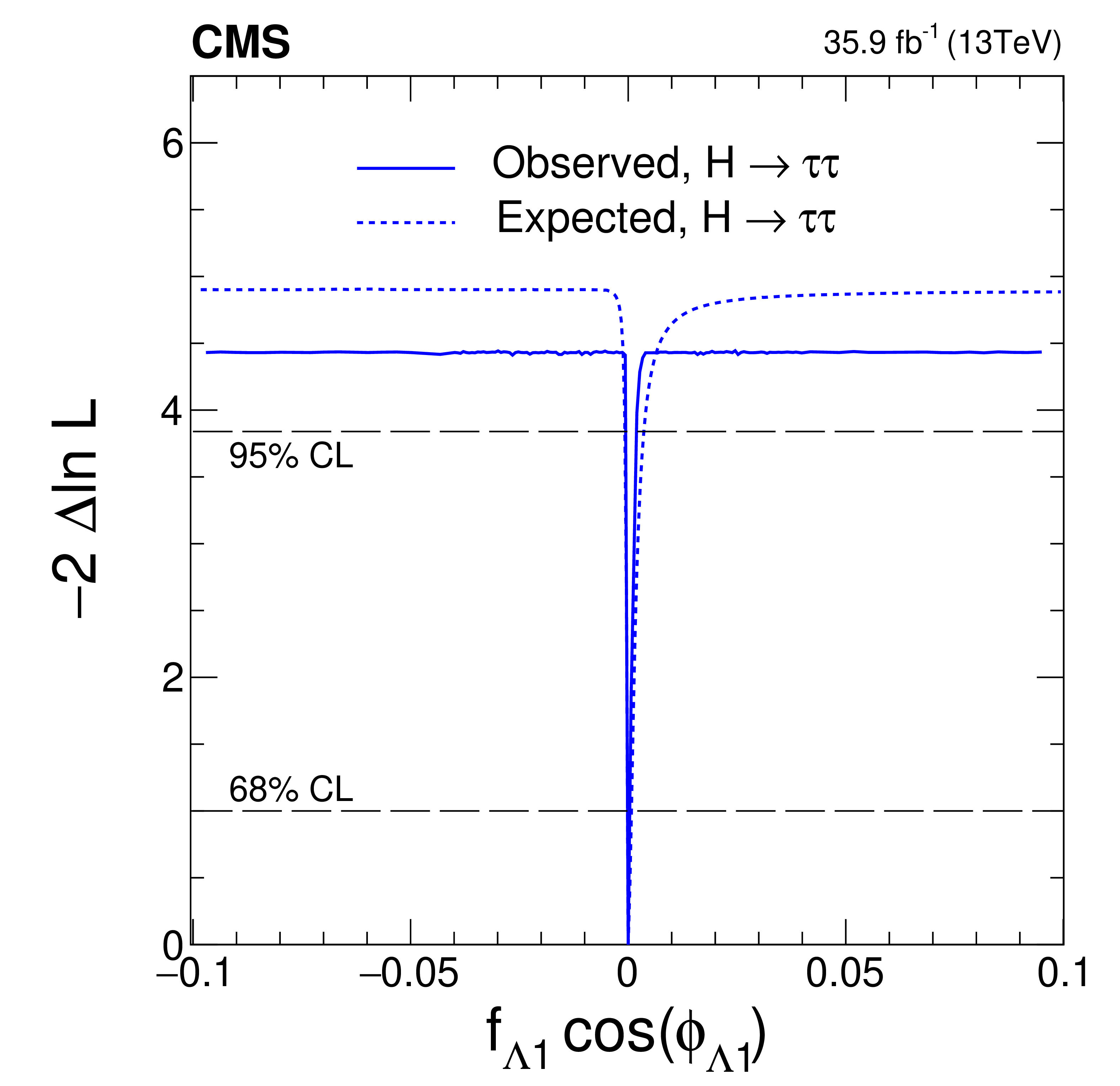
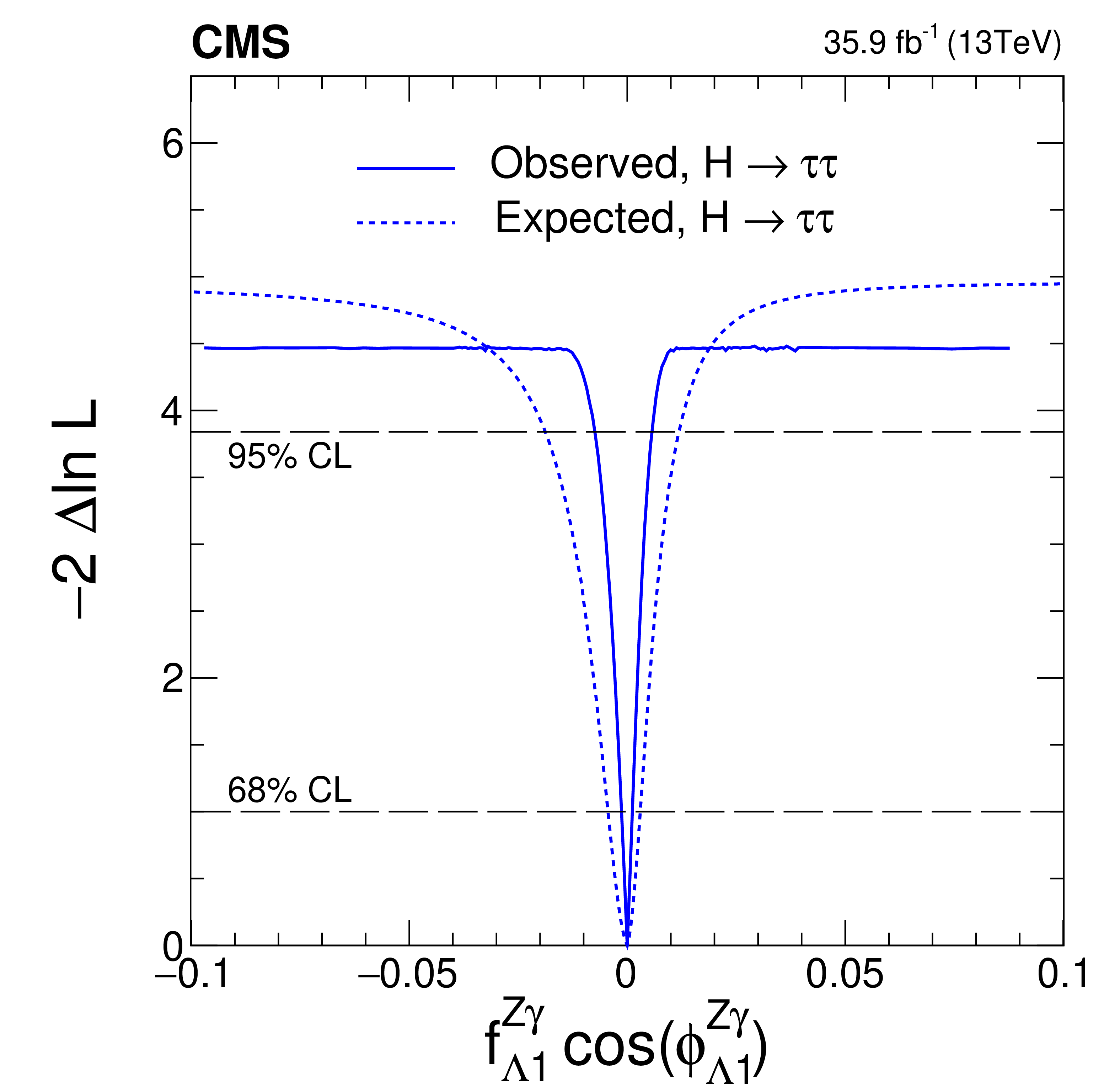
Figure 10:
Observed (solid) and expected (dashed) likelihood scans of $f_{a3}\cos(\phi _{a3})$ (top left), $f_{a2}\cos(\phi _{a2})$ (top right), $f_{\Lambda 1}\cos(\phi _{\Lambda 1})$ (bottom left), and $f_{\Lambda 1}^{{\mathrm {Z}} \gamma}\cos(\phi _{\Lambda 1}^{{\mathrm {Z}} \gamma})$ (bottom right). |

png pdf |
Figure 10-a:
Observed (solid) and expected (dashed) likelihood scans of $f_{a3}\cos(\phi _{a3})$. |
png pdf |
Figure 10-b:
Observed (solid) and expected (dashed) likelihood scans of $f_{a2}\cos(\phi _{a2})$. |
png pdf |
Figure 10-c:
Observed (solid) and expected (dashed) likelihood scans of $f_{\Lambda 1}\cos(\phi _{\Lambda 1})$. |
png pdf |
Figure 10-d:
Observed (solid) and expected (dashed) likelihood scans of $f_{\Lambda 1}^{{\mathrm {Z}} \gamma}\cos(\phi _{\Lambda 1}^{{\mathrm {Z}} \gamma})$. |
png pdf |
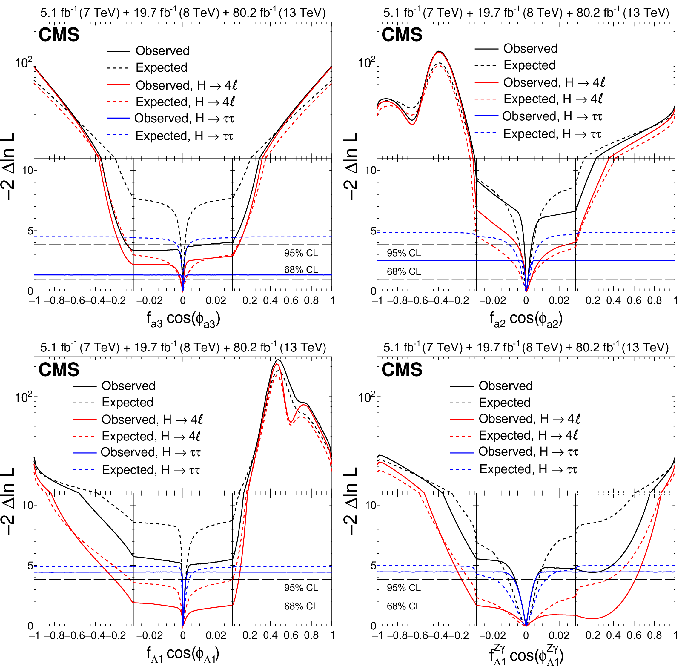
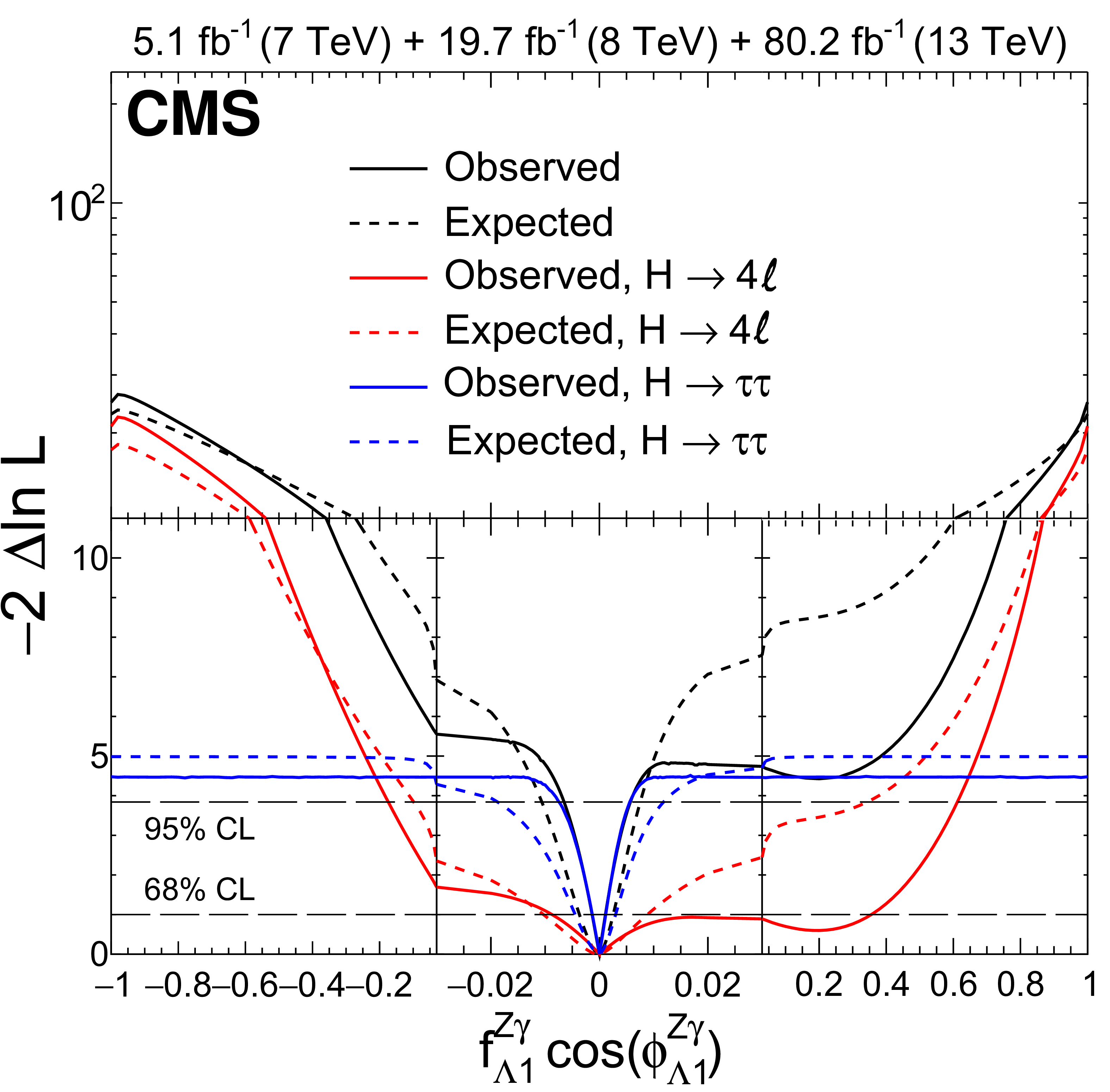
Figure 11:
Combination of results using the $ {\mathrm {H}} \to {\tau} {\tau}$ decay (presented in this paper) and the $ {\mathrm {H}} \to 4\ell $ decay [17]. The observed (solid) and expected (dashed) likelihood scans of $f_{a3}\cos(\phi _{a3})$ (top left), $f_{a2}\cos(\phi _{a2})$ (top right), $f_{\Lambda 1}\cos(\phi _{\Lambda 1})$ (bottom left), and $f_{\Lambda 1}^{{\mathrm {Z}} \gamma}\cos(\phi _{\Lambda 1}^{{\mathrm {Z}} \gamma})$ (bottom right) are shown. For better visibility of all features, the $x$- and $y$-axes are presented with variable scales. On the linear-scale $x$-axis, a zoom is applied in the range $-$0.03 to $+$0.03. The $y$-axis is shown in linear (logarithmic) scale for values of $-2 \Delta \ln{\mathcal L}$ below (above) 11. |

png pdf |
Figure 11-a:
Combination of results using the $ {\mathrm {H}} \to {\tau} {\tau}$ decay (presented in this paper) and the $ {\mathrm {H}} \to 4\ell $ decay [17]. Shown is the observed (solid) and expected (dashed) likelihood scan of $f_{a3}\cos(\phi _{a3})$. For better visibility of all features, the $x$- and $y$-axes are presented with variable scales. On the linear-scale $x$-axis, a zoom is applied in the range $-$0.03 to $+$0.03. The $y$-axis is shown in linear (logarithmic) scale for values of $-2 \Delta \ln{\mathcal L}$ below (above) 11. |
png pdf |
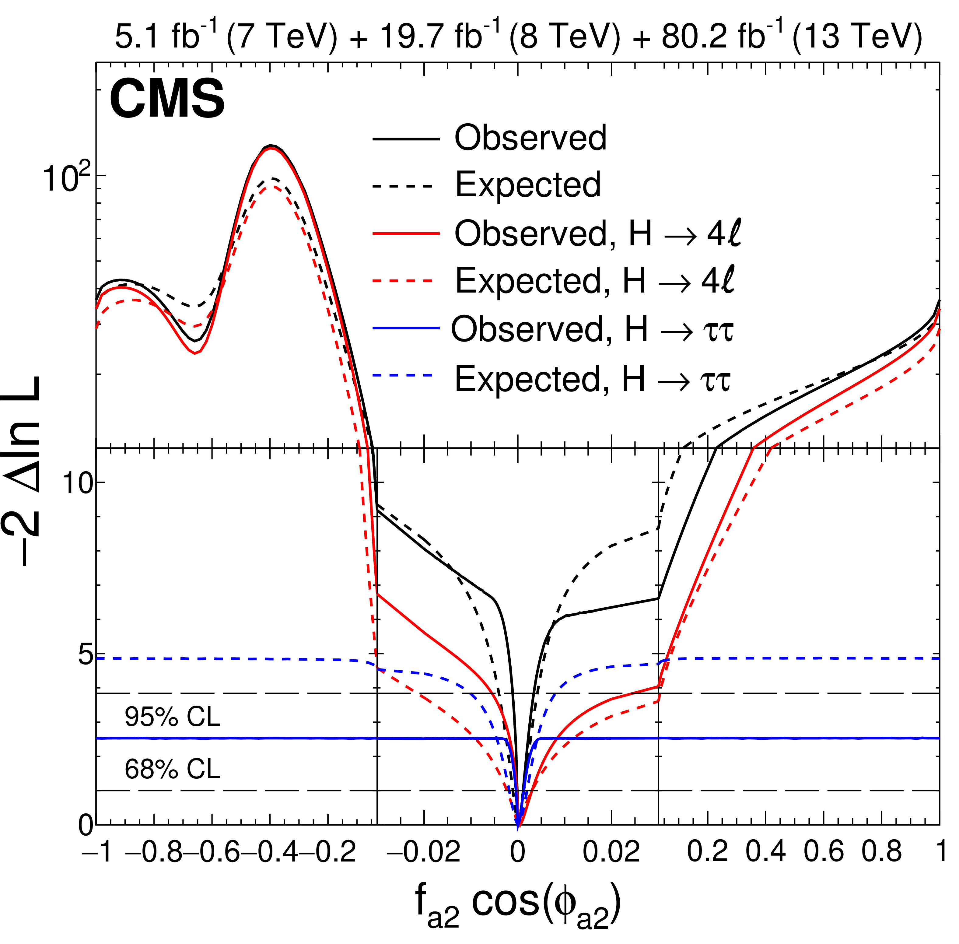
Figure 11-b:
Combination of results using the $ {\mathrm {H}} \to {\tau} {\tau}$ decay (presented in this paper) and the $ {\mathrm {H}} \to 4\ell $ decay [17]. Shown is the observed (solid) and expected (dashed) likelihood scan of $f_{a2}\cos(\phi _{a2})$. For better visibility of all features, the $x$- and $y$-axes are presented with variable scales. On the linear-scale $x$-axis, a zoom is applied in the range $-$0.03 to $+$0.03. The $y$-axis is shown in linear (logarithmic) scale for values of $-2 \Delta \ln{\mathcal L}$ below (above) 11. |
png pdf |
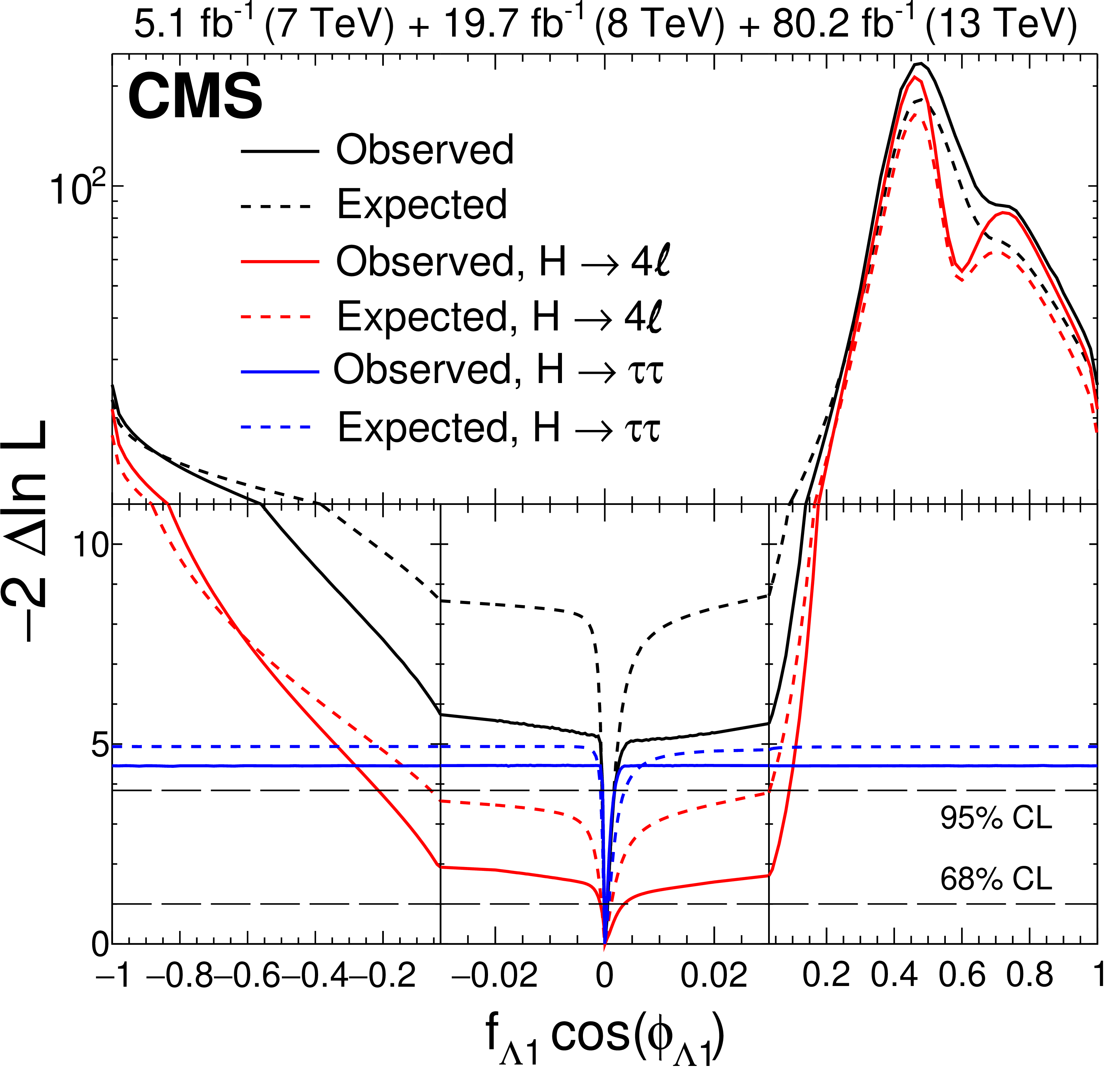
Figure 11-c:
Combination of results using the $ {\mathrm {H}} \to {\tau} {\tau}$ decay (presented in this paper) and the $ {\mathrm {H}} \to 4\ell $ decay [17]. Shown is the observed (solid) and expected (dashed) likelihood scan of $f_{\Lambda 1}\cos(\phi _{\Lambda 1})$. For better visibility of all features, the $x$- and $y$-axes are presented with variable scales. On the linear-scale $x$-axis, a zoom is applied in the range $-$0.03 to $+$0.03. The $y$-axis is shown in linear (logarithmic) scale for values of $-2 \Delta \ln{\mathcal L}$ below (above) 11. |
png pdf |
Figure 11-d:
Combination of results using the $ {\mathrm {H}} \to {\tau} {\tau}$ decay (presented in this paper) and the $ {\mathrm {H}} \to 4\ell $ decay [17]. Shown is the observed (solid) and expected (dashed) likelihood scan of $f_{\Lambda 1}^{{\mathrm {Z}} \gamma}\cos(\phi _{\Lambda 1}^{{\mathrm {Z}} \gamma})$. For better visibility of all features, the $x$- and $y$-axes are presented with variable scales. On the linear-scale $x$-axis, a zoom is applied in the range $-$0.03 to $+$0.03. The $y$-axis is shown in linear (logarithmic) scale for values of $-2 \Delta \ln{\mathcal L}$ below (above) 11. |
| Tables | |
png pdf |
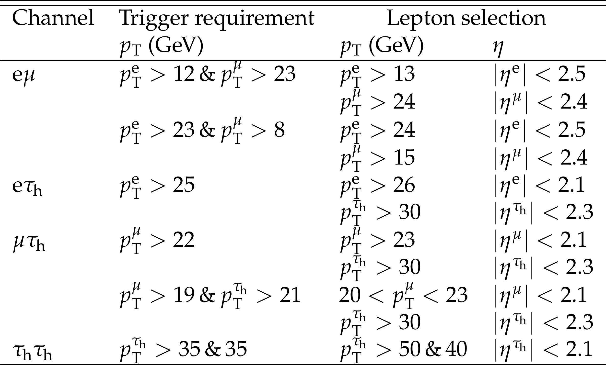
Table 1:
Kinematic selection criteria for the four decay channels. For the trigger threshold requirements, the numbers indicate the trigger thresholds in GeV. The lepton selection criteria include the transverse momentum threshold, pseudorapidity range, as well as isolation criteria. |

png pdf |
Table 2:
Allowed 68% CL (central values with uncertainties) and 95% CL (in square brackets) intervals on anomalous coupling parameters using the $ {\mathrm {H}} \to {\tau} {\tau}$ decay. The observed 95% CL constraints on $f_{a3}\cos(\phi _{a3})$ and $f_{a2}\cos(\phi _{a2})$ allow the full physics range $[-1,1]$. |
png pdf |
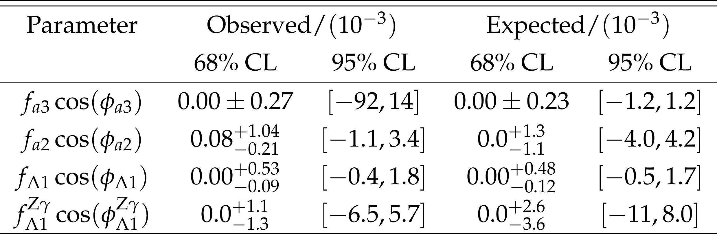
Table 3:
Allowed 68% CL (central values with uncertainties) and 95% CL (in square brackets) intervals on anomalous coupling parameters using a combination of the $ {\mathrm {H}} \to {\tau} {\tau}$ and $ {\mathrm {H}} \to 4\ell $ [17] decay channels. |

png pdf |
Table 4:
Summary of the allowed 95% CL intervals for the anomalous HVV couplings using the results in Table 3. The coupling ratios are assumed to be real and include the factor $\cos(\phi _{\Lambda 1})$ or $\cos(\phi _{\Lambda 1}^{{\mathrm {Z}} \gamma})= \pm $1. |
| Summary |
| A study is presented of anomalous HVV interactions of the H boson with vector bosons V, including CP violation, using its associated production with two hadronic jets in vector boson fusion, in the VH process, and in gluon fusion, and subsequently decaying to a pair of $\tau$ leptons. Constraints on the CP-violating parameter $f_{a3}$ and on the CP-conserving parameters $f_{a2}$, $f_{\Lambda1}$, and $f_{\Lambda1}^{\mathrm{Z}\gamma}$, defined in Eqs. (2) and (3), are set using matrix element techniques. The observed and expected limits on the parameters are summarized in Table 2. The 68% confidence level constraints are generally tighter than those from previous measurements using either production or decay information. Further constraints are obtained in the combination of the $\mathrm{H}\to\tau\tau$ and $\mathrm{H}\to 4\ell$ decay [17] channels and are summarized in Table 3. This combination places the most stringent constraints on anomalous H boson couplings: $f_{a3}\cos(\phi_{a3})=(0.00 \pm 0.27 )\times10^{-3}$, $f_{a2}\cos(\phi_{a2})=(0.08^{+1.04}_{-0.21})\times10^{-3}$, $f_{\Lambda1}\cos(\phi_{\Lambda1})=(0.00^{+0.53}_{-0.09})\times10^{-3}$, and $f_{\Lambda1}^{\mathrm{Z}\gamma}\cos(\phi_{\Lambda1}^{\mathrm{Z}\gamma})=(0.0^{+1.1}_{-1.3})\times10^{-3}$. A simultaneous measurement of $f_{a3}$ and $f_{a3}^{\mathrm{g}\mathrm{g}\mathrm{H}}$ parameters is performed, where the latter parameter, defined in Eqs. (2) and (4), is sensitive to CP violation effects in the gluon fusion process. The current data set does not allow for precise constraints on CP properties in the gluon fusion process. The results are consistent with expectations for the standard model H boson . |
| Additional Figures | |

png pdf |
Additional Figure 1:
Summary of confidence level intervals of anomalous coupling parameters in HVV interactions under the assumption that all the coupling ratios are real ($\phi _{ai}^{\mathrm {V} \mathrm {V}}=$ 0 or $\pi $). The HZZ+HWW coupling limits assume that $a_{i}^{{\mathrm {Z}} {\mathrm {Z}}}=a_{i}^{{\mathrm {W}} {\mathrm {W}}}$. The expected 68% and 95% CL regions are shown as green and yellow bands. The observed intervals for 68% CL are shown as points with error bars, and the hatched areas indicate the excluded regions at 95% CL. The limits on $f_{a2,3}^{{\mathrm {Z}} \gamma,\gamma \gamma}$ are from Ref. [13], and the limits on $f_{\Lambda Q}$ are from Ref. [14]. |
| References | ||||
| 1 | ATLAS Collaboration | Observation of a new particle in the search for the Standard Model Higgs boson with the ATLAS detector at the LHC | PLB 716 (2012) 1 | 1207.7214 |
| 2 | CMS Collaboration | Observation of a new boson at a mass of 125 GeV with the CMS experiment at the LHC | PLB 716 (2012) 30 | CMS-HIG-12-028 1207.7235 |
| 3 | CMS Collaboration | Observation of a new boson with mass near 125 GeV in pp collisions at $ \sqrt{s} = $ 7 and 8 TeV | JHEP 06 (2013) 081 | CMS-HIG-12-036 1303.4571 |
| 4 | S. L. Glashow | Partial-symmetries of weak interactions | NP 22 (1961) 579 | |
| 5 | F. Englert and R. Brout | Broken Symmetry and the Mass of Gauge Vector Mesons | PRL 13 (1964) 321 | |
| 6 | P. W. Higgs | Broken symmetries, massless particles and gauge fields | PL12 (1964) 132 | |
| 7 | P. W. Higgs | Broken symmetries and the masses of gauge bosons | PRL 13 (1964) 508 | |
| 8 | G. S. Guralnik, C. R. Hagen, and T. W. B. Kibble | Global conservation laws and massless particles | PRL 13 (1964) 585 | |
| 9 | S. Weinberg | A model of leptons | PRL 19 (1967) 1264 | |
| 10 | A. Salam | Weak and electromagnetic interactions | in Elementary particle physics: relativistic groups and analyticity, N. Svartholm, ed., p. 367 Almqvist \& Wiksell, Stockholm, 1968 Proceedings of the eighth Nobel symposium | |
| 11 | CMS Collaboration | On the mass and spin-parity of the Higgs boson candidate via its decays to Z boson pairs | PRL 110 (2013) 081803 | CMS-HIG-12-041 1212.6639 |
| 12 | CMS Collaboration | Measurement of the properties of a Higgs boson in the four-lepton final state | PRD 89 (2014) 092007 | CMS-HIG-13-002 1312.5353 |
| 13 | CMS Collaboration | Constraints on the spin-parity and anomalous HVV couplings of the Higgs boson in proton collisions at 7 and 8 TeV | PRD 92 (2015) 012004 | CMS-HIG-14-018 1411.3441 |
| 14 | CMS Collaboration | Limits on the Higgs boson lifetime and width from its decay to four charged leptons | PRD 92 (2015) 072010 | CMS-HIG-14-036 1507.06656 |
| 15 | CMS Collaboration | Combined search for anomalous pseudoscalar HVV couplings in VH(H $ \to \text{b}\bar{\text{b}} $) production and H $ \to $ VV decay | PLB 759 (2016) 672 | CMS-HIG-14-035 1602.04305 |
| 16 | CMS Collaboration | Constraints on anomalous Higgs boson couplings using production and decay information in the four-lepton final state | PLB 775 (2017) 1 | CMS-HIG-17-011 1707.00541 |
| 17 | CMS Collaboration | Measurements of the Higgs boson width and anomalous HVV couplings from on-shell and off-shell production in the four-lepton final state | Submitted to PRD | CMS-HIG-18-002 1901.00174 |
| 18 | ATLAS Collaboration | Evidence for the spin-0 nature of the Higgs boson using ATLAS data | PLB 726 (2013) 120 | 1307.1432 |
| 19 | ATLAS Collaboration | Study of the spin and parity of the Higgs boson in diboson decays with the ATLAS detector | EPJC 75 (2015) 476 | 1506.05669 |
| 20 | ATLAS Collaboration | Test of CP invariance in vector-boson fusion production of the Higgs boson using the optimal observable method in the ditau decay channel with the ATLAS detector | EPJC 76 (2016) 658 | 1602.04516 |
| 21 | ATLAS Collaboration | Measurement of inclusive and differential cross sections in the $ H \rightarrow ZZ^* \rightarrow 4\ell $ decay channel in $ pp $ collisions at $ \sqrt{s}= $ 13 TeV with the ATLAS detector | JHEP 10 (2017) 132 | 1708.02810 |
| 22 | ATLAS Collaboration | Measurement of the Higgs boson coupling properties in the $ H\rightarrow ZZ^{*} \rightarrow 4\ell $ decay channel at $ \sqrt{s} = $ 13 TeV with the ATLAS detector | JHEP 03 (2018) 095 | 1712.02304 |
| 23 | ATLAS Collaboration | Measurements of Higgs boson properties in the diphoton decay channel with 36 fb$ ^{-1} $ of $ pp $ collision data at $ \sqrt{s} = $ 13 TeV with the ATLAS detector | PRD 98 (2018) 052005 | 1802.04146 |
| 24 | CMS Collaboration | Observation of the Higgs boson decay to a pair of $ \tau $ leptons with the CMS detector | PLB 779 (2018) 283 | CMS-HIG-16-043 1708.00373 |
| 25 | S. Dawson et al. | Higgs working group report of the Snowmass 2013 community planning study | 1310.8361 | |
| 26 | Y. Gao et al. | Spin determination of single-produced resonances at hadron colliders | PRD 81 (2010) 075022 | 1001.3396 |
| 27 | S. Bolognesi et al. | Spin and parity of a single-produced resonance at the LHC | PRD 86 (2012) 095031 | 1208.4018 |
| 28 | I. Anderson et al. | Constraining anomalous HVV interactions at proton and lepton colliders | PRD 89 (2014) 035007 | 1309.4819 |
| 29 | A. V. Gritsan, R. Rontsch, M. Schulze, and M. Xiao | Constraining anomalous Higgs boson couplings to the heavy flavor fermions using matrix element techniques | PRD 94 (2016) 055023 | 1606.03107 |
| 30 | CMS Collaboration | The CMS trigger system | JINST 12 (2017) P01020 | CMS-TRG-12-001 1609.02366 |
| 31 | CMS Collaboration | The CMS experiment at the CERN LHC | JINST 3 (2008) S08004 | CMS-00-001 |
| 32 | CMS Collaboration | Particle-flow reconstruction and global event description with the CMS detector | JINST 12 (2017) P10003 | CMS-PRF-14-001 1706.04965 |
| 33 | M. Cacciari, G. P. Salam, and G. Soyez | The anti-$ {k_{\mathrm{T}}} $ jet clustering algorithm | JHEP 04 (2008) 063 | 0802.1189 |
| 34 | M. Cacciari, G. P. Salam, and G. Soyez | FastJet user manual | EPJC 72 (2012) 1896 | 1111.6097 |
| 35 | CMS Collaboration | Performance of electron reconstruction and selection with the CMS detector in proton-proton collisions at $ \sqrt{s} = $ 8 TeV | JINST 10 (2015) P06005 | CMS-EGM-13-001 1502.02701 |
| 36 | CMS Collaboration | Performance of the CMS muon detector and muon reconstruction with proton-proton collisons at $ \sqrt{s} = $ ~13 TeV | JINST 13 (2018) P06015 | CMS-MUO-16-001 1804.04528 |
| 37 | M. Cacciari, G. P. Salam | Dispelling the $ N^{3} $ myth for the $ k_t $ jet-finder | PLB 641 (2006) 57 | hep-ph/0512210 |
| 38 | CMS Collaboration | Reconstruction and identification of $ \tau $ lepton decays to hadrons and $ \nu_\tau $ at CMS | JINST 11 (2016) P01019 | CMS-TAU-14-001 1510.07488 |
| 39 | CMS Collaboration | Performance of reconstruction and identification of $ \tau $ leptons decaying to hadrons and $ \nu_\tau $ in pp collisions at $ \sqrt{s}= $ 13 TeV | JINST 13 (2018) P10005 | CMS-TAU-16-003 1809.02816 |
| 40 | CMS Collaboration | Performance of missing transverse momentum in pp collisions at $ \sqrt{s} = $ 13 TeV using the CMS detector | CDS | |
| 41 | L. Bianchini, J. Conway, E. K. Friis, and C. Veelken | Reconstruction of the Higgs mass in $ H \to \tau\tau $ events by dynamical likelihood techniques | J. Phys. Conf. Ser. 513 (2014) 022035 | |
| 42 | CMS Collaboration | Search for neutral MSSM Higgs bosons decaying to a pair of tau leptons in pp collisions | JHEP 10 (2014) 160 | CMS-HIG-13-021 1408.3316 |
| 43 | T. Plehn, D. L. Rainwater, and D. Zeppenfeld | Determining the structure of Higgs couplings at the LHC | PRL 88 (2002) 051801 | hep-ph/0105325 |
| 44 | V. Hankele, G. Klamke, D. Zeppenfeld, and T. Figy | Anomalous Higgs boson couplings in vector boson fusion at the CERN LHC | PRD 74 (2006) 095001 | hep-ph/0609075 |
| 45 | E. Accomando et al. | Workshop on CP Studies and Non-Standard Higgs Physics | hep-ph/0608079 | |
| 46 | K. Hagiwara, Q. Li, and K. Mawatari | Jet angular correlation in vector-boson fusion processes at hadron colliders | JHEP 07 (2009) 101 | 0905.4314 |
| 47 | A. De R\' ujula et al. | Higgs look-alikes at the LHC | PRD 82 (2010) 013003 | 1001.5300 |
| 48 | J. Ellis, D. S. Hwang, V. Sanz, and T. You | A fast track towards the `Higgs' spin and parity | JHEP 11 (2012) 134 | 1208.6002 |
| 49 | P. Artoisenet et al. | A framework for Higgs characterisation | JHEP 11 (2013) 043 | 1306.6464 |
| 50 | M. J. Dolan, P. Harris, M. Jankowiak, and M. Spannowsky | Constraining $ CP $-violating Higgs Sectors at the LHC using gluon fusion | PRD 90 (2014) 073008 | 1406.3322 |
| 51 | A. Greljo, G. Isidori, J. M. Lindert, and D. Marzocca | Pseudo-observables in electroweak Higgs production | EPJC 76 (2016) 158 | 1512.06135 |
| 52 | S. Frixione, P. Nason, and C. Oleari | Matching NLO QCD computations with parton shower simulations: the POWHEG method | JHEP 11 (2007) 070 | 0709.2092 |
| 53 | E. Bagnaschi, G. Degrassi, P. Slavich, and A. Vicini | Higgs production via gluon fusion in the POWHEG approach in the SM and in the MSSM | JHEP 02 (2012) 088 | 1111.2854 |
| 54 | P. Nason and C. Oleari | NLO Higgs boson production via vector-boson fusion matched with shower in POWHEG | JHEP 02 (2010) 037 | 0911.5299 |
| 55 | G. Luisoni, P. Nason, C. Oleari, and F. Tramontano | $ HW^{\pm} $/HZ + 0 and 1 jet at NLO with the POWHEG BOX interfaced to GoSam and their merging within MiNLO | JHEP 10 (2013) 083 | 1306.2542 |
| 56 | T. Sjostrand et al. | An introduction to PYTHIA 8.2 | CPC 191 (2015) 159 | 1410.3012 |
| 57 | NNPDF Collaboration | Unbiased global determination of parton distributions and their uncertainties at NNLO and at LO | NPB 855 (2012) 153 | 1107.2652 |
| 58 | GEANT4 Collaboration | GEANT4---a simulation toolkit | NIMA 506 (2003) 250 | |
| 59 | J. Alwall et al. | The automated computation of tree-level and next-to-leading order differential cross sections, and their matching to parton shower simulations | JHEP 07 (2014) 079 | 1405.0301 |
| 60 | J. Alwall et al. | Comparative study of various algorithms for the merging of parton showers and matrix elements in hadronic collisions | EPJC 53 (2008) 473 | 0706.2569 |
| 61 | R. Frederix and S. Frixione | Merging meets matching in MC@NLO | JHEP 12 (2012) 061 | 1209.6215 |
| 62 | CMS Collaboration | Event generator tunes obtained from underlying event and multiparton scattering measurements | EPJC 76 (2016) 155 | CMS-GEN-14-001 1512.00815 |
| 63 | J. Neyman and E. S. Pearson | On the problem of the most efficient tests of statistical hypotheses | Phil. Trans. R. Soc. Lond. A 231 (1933) 289 | |
| 64 | R. J. Barlow | Extended maximum likelihood | NIMA 297 (1990) 496 | |
| 65 | W. Verkerke and D. P. Kirkby | The RooFit toolkit for data modeling | in 13$^\textth$ International Conference for Computing in High-Energy and Nuclear Physics (CHEP03) 2003 CHEP-2003-MOLT007 | physics/0306116 |
| 66 | R. Brun and F. Rademakers | ROOT: An object oriented data analysis framework | NIMA 389 (1997) 81 | |
| 67 | S. S. Wilks | The large-sample distribution of the likelihood ratio for testing composite hypotheses | Ann. Math. Stat. 9 (1938) 60 | |
| 68 | J. S. Conway | Incorporating nuisance parameters in likelihoods for multisource spectra | in Proceedings of PHYSTAT 2011 Workshop on Statistical Issues Related to Discovery Claims in Search Experiments and Unfolding, p. 115 CERN-2011-006 | |
| 69 | CMS Collaboration | Identification of heavy-flavour jets with the CMS detector in pp collisions at 13 TeV | JINST 13 (2018) P05011 | CMS-BTV-16-002 1712.07158 |
| 70 | CMS Collaboration | Performance of the CMS missing transverse momentum reconstruction in pp data at $ \sqrt{s} = $ 8 TeV | JINST 10 (2015) P02006 | CMS-JME-13-003 1411.0511 |
| 71 | CMS Collaboration | CMS luminosity measurements for the 2016 data taking period | CMS-PAS-LUM-17-001 | CMS-PAS-LUM-17-001 |
| 72 | D. de Florian et al. | Handbook of LHC Higgs cross sections: 4. deciphering the nature of the Higgs sector | technical report | 1610.07922 |
| 73 | CMS Collaboration | Measurements of the $ \mathrm {p}\mathrm {p}\rightarrow \mathrm{Z}\mathrm{Z} $ production cross section and the $ \mathrm{Z}\rightarrow 4\ell $ branching fraction, and constraints on anomalous triple gauge couplings at $ \sqrt{s} = $ 13 TeV | EPJC 78 (2018) 165 | CMS-SMP-16-017 1709.08601 |
| 74 | CMS Collaboration | Cross section measurement of t-channel single top quark production in pp collisions at $ \sqrt s = $ 13 TeV | PLB 772 (2017) 752 | CMS-TOP-16-003 1610.00678 |
|
|
Compact Muon Solenoid LHC, CERN |
|

|

|

|

|

|