

Compact Muon Solenoid
LHC, CERN
| CMS-SUS-20-001 ; CERN-EP-2020-231 | ||
| Search for supersymmetry in final states with two oppositely charged same-flavor leptons and missing transverse momentum in proton-proton collisions at $\sqrt{s} = $ 13 TeV | ||
| CMS Collaboration | ||
| 15 December 2020 | ||
| JHEP 04 (2021) 123 | ||
| Abstract: A search for phenomena beyond the standard model in final states with two oppositely charged same-flavor leptons and missing transverse momentum is presented. The search uses a data sample of proton-proton collisions at $\sqrt{s} = $ 13 TeV, corresponding to an integrated luminosity of 137 fb$^{-1}$, collected by the CMS experiment at the LHC. Three potential signatures of physics beyond the standard model are explored: an excess of events with a lepton pair, whose invariant mass is consistent with the Z boson mass; a kinematic edge in the invariant mass distribution of the lepton pair; and the nonresonant production of two leptons. The observed event yields are consistent with those expected from standard model backgrounds. The results of the first search allow the exclusion of gluino masses up to 1875 GeV, as well as chargino (neutralino) masses up to 750 (800) GeV, while those of the searches for the other two signatures allow the exclusion of light-flavor (bottom) squark masses up to 1800 (1600) GeV and slepton masses up to 700 GeV, respectively, at 95% confidence level within certain supersymmetry scenarios. | ||
| Links: e-print arXiv:2012.08600 [hep-ex] (PDF) ; CDS record ; inSPIRE record ; CADI line (restricted) ; | ||
| Figures & Tables | Summary | Additional Figures & Tables | References | CMS Publications |
|---|
| Figures | |

png pdf |
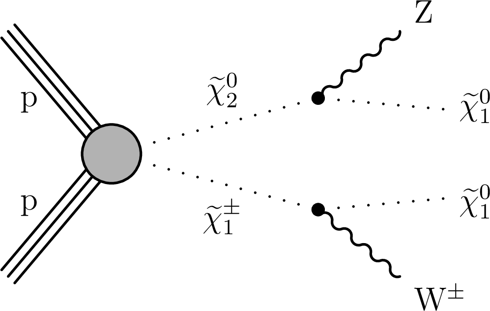
Figure 1:
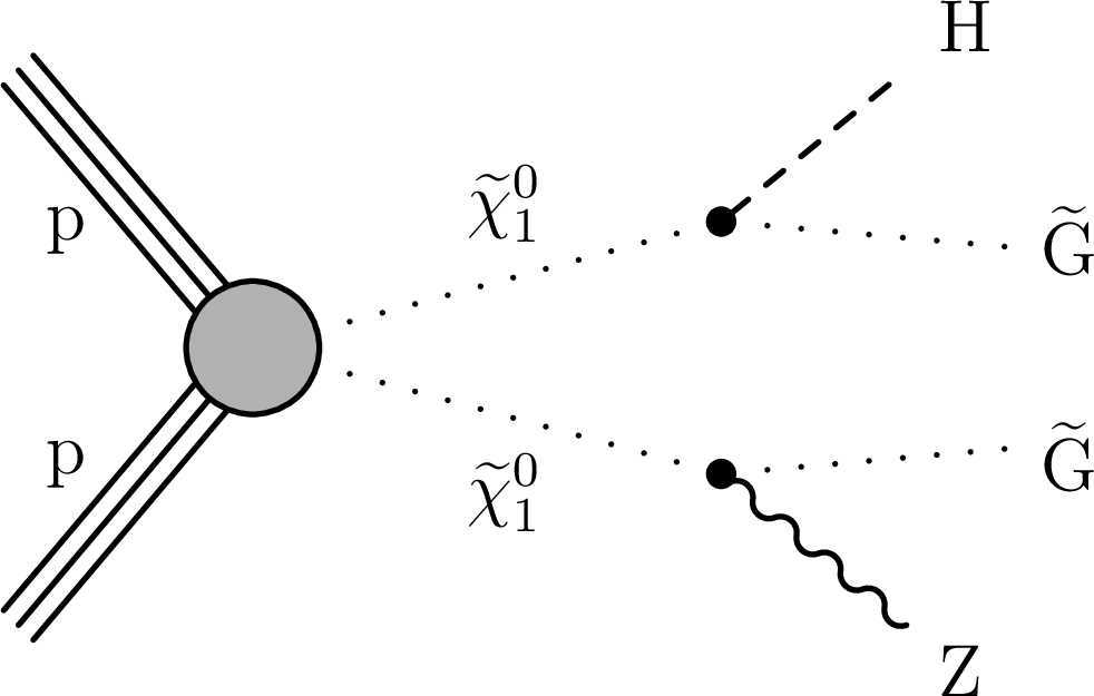
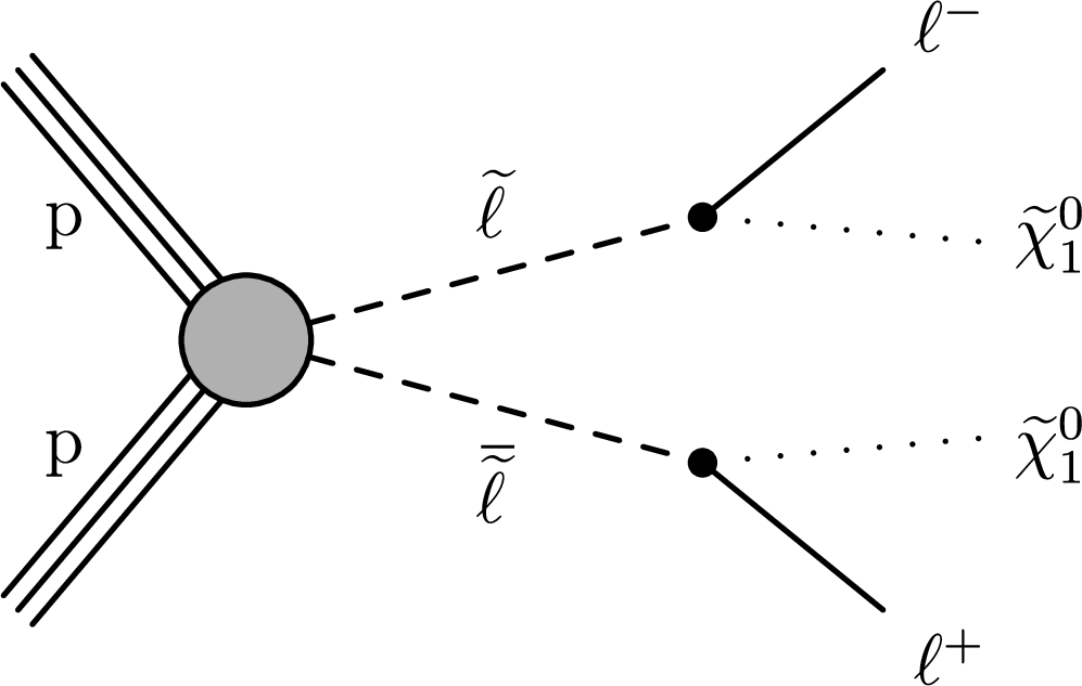
Diagrams for models of neutralino/chargino production (upper left), GMSB neutralino pair production with ZZ (upper right) and ZH bosons (lower left) in the final state, and direct slepton pair production (lower right). In the first GMSB neutralino pair production model, the $\tilde{\chi}^0_1$ is assumed to decay exclusively into a Z boson, while in the latter, the ZH final state is accompanied by the ZZ final state with 50% branching fractions of the $\tilde{\chi}^0_1$ decaying into an H or a Z boson. Only ZH and ZZ final states are taken into account in the analysis, since the contribution of the HH topology to our signal regions is expected to be negligible. Such models predict the SUSY particles to be produced via EW interactions, with limited if any production of accompanying quarks in the final state. |
png pdf |
Figure 1-a:
Diagram for neutralino/chargino production. The model predicts the SUSY particles to be produced via EW interactions, with limited if any production of accompanying quarks in the final state. |

png pdf |
Figure 1-b:
Diagram for GMSB neutralino pair production with ZZ bosons in the final state. The $\tilde{\chi}^0_1$ is assumed to decay exclusively into a Z boson. The model predicts the SUSY particles to be produced via EW interactions, with limited if any production of accompanying quarks in the final state. |
png pdf |
Figure 1-c:
Diagram for GMSB neutralino pair production with ZH bosons in the final state. The ZH final state is accompanied by the ZZ final state with 50% branching fractions of the $\tilde{\chi}^0_1$ decaying into an H or a Z boson. Only ZH and ZZ final states are taken into account in the analysis, since the contribution of the HH topology to our signal regions is expected to be negligible. The model predicts the SUSY particles to be produced via EW interactions, with limited if any production of accompanying quarks in the final state. |
png pdf |
Figure 1-d:
Diagram for direct slepton pair production. The model predicts the SUSY particles to be produced via EW interactions, with limited if any production of accompanying quarks in the final state. |

png pdf |
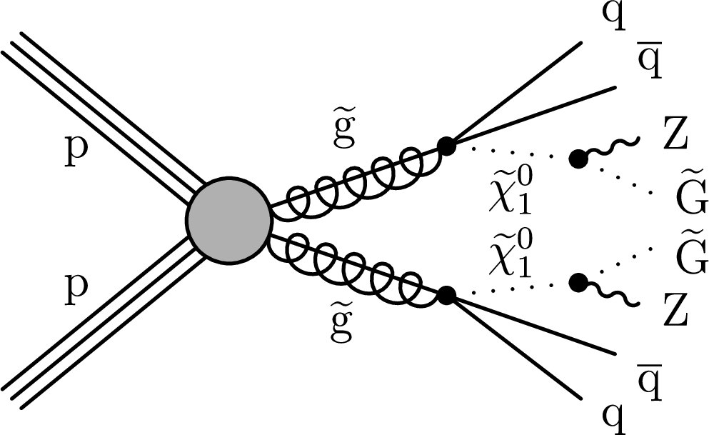
Figure 2:
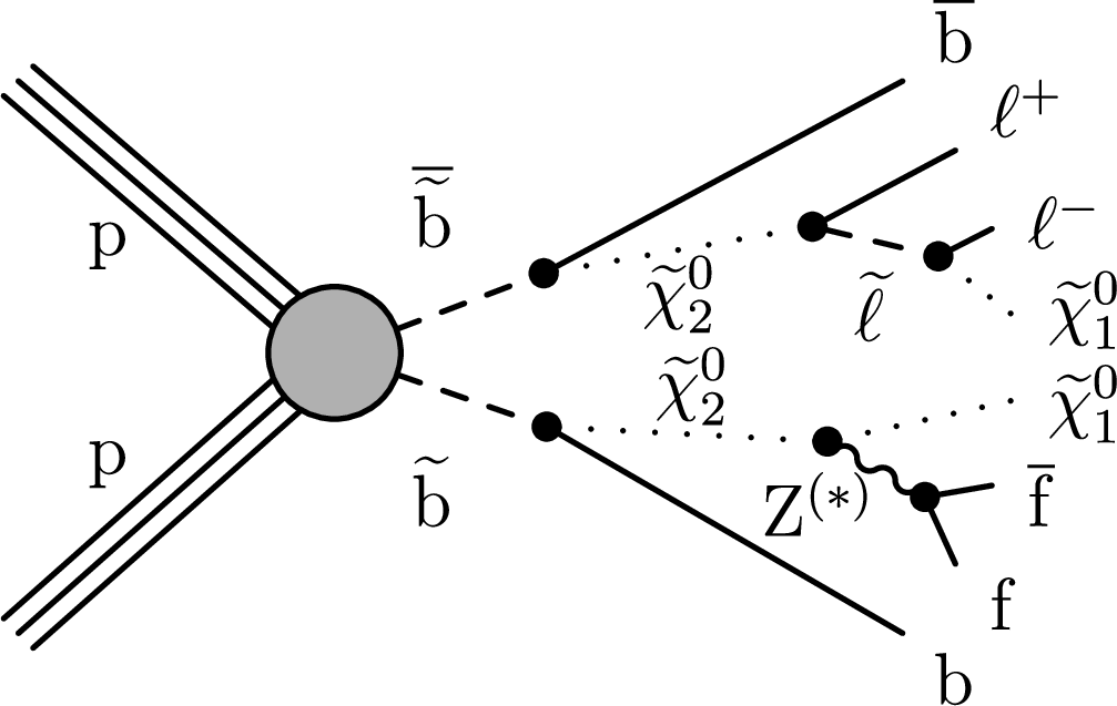
Diagram for GMSB gluino (${\mathrm{\tilde{g}}}$) pair production (left), where each ${\mathrm{\tilde{g}}}$ decays into a pair of quarks and a neutralino. The neutralino then decays to a Z boson and an LSP. Diagrams for sbottom $\tilde{\mathrm{b}}$ (center) and squark $\tilde{\mathrm{q}}$ (right) pair production are also shown. Such models feature a mass edge from the decay of a $\tilde{\chi}^0_2$ via an intermediate slepton, $\tilde{\ell}$. In the central diagram, a pair of b quarks is present in the final state. In these models we assume a fixed $\tilde{\chi}^0_1$ mass of 100 GeV, while the mass of the slepton is taken to be equidistant from the masses of the two neutralinos. Only the lightest $\tilde{\mathrm{b}}$ mass eigenstate, $\tilde{\mathrm{b}} _1$, is assumed to be involved in the models considered. All these models assume strong production of SUSY particles and predict an abundance of quarks in the final state. |
png pdf |
Figure 2-a:
Diagram for GMSB gluino (${\mathrm{\tilde{g}}}$) pair production, where each ${\mathrm{\tilde{g}}}$ decays into a pair of quarks and a neutralino. The neutralino then decays to a Z boson and an LSP. |
png pdf |
Figure 2-b:
Diagram for sbottom $\tilde{\mathrm{b}}$ pair production. Only the lightest $\tilde{\mathrm{b}}$ mass eigenstate, $\tilde{\mathrm{b}} _1$, is assumed to be involved. A pair of b quarks is present in the final state. Such model features a mass edge from the decay of a $\tilde{\chi}^0_2$ via an intermediate slepton, $\tilde{\ell}$. We assume a fixed $\tilde{\chi}^0_1$ mass of 100 GeV, while the mass of the slepton is taken to be equidistant from the masses of the two neutralinos. The model assumes strong production of SUSY particles and predicts an abundance of quarks in the final state. |

png pdf |
Figure 2-c:
Diagram for squark $\tilde{\mathrm{q}}$ pair production. Such model features a mass edge from the decay of a $\tilde{\chi}^0_2$ via an intermediate slepton, $\tilde{\ell}$. We assume a fixed $\tilde{\chi}^0_1$ mass of 100 GeV, while the mass of the slepton is taken to be equidistant from the masses of the two neutralinos. The model assumes strong production of SUSY particles and predicts an abundance of quarks in the final state. |
png pdf |
Figure 3:
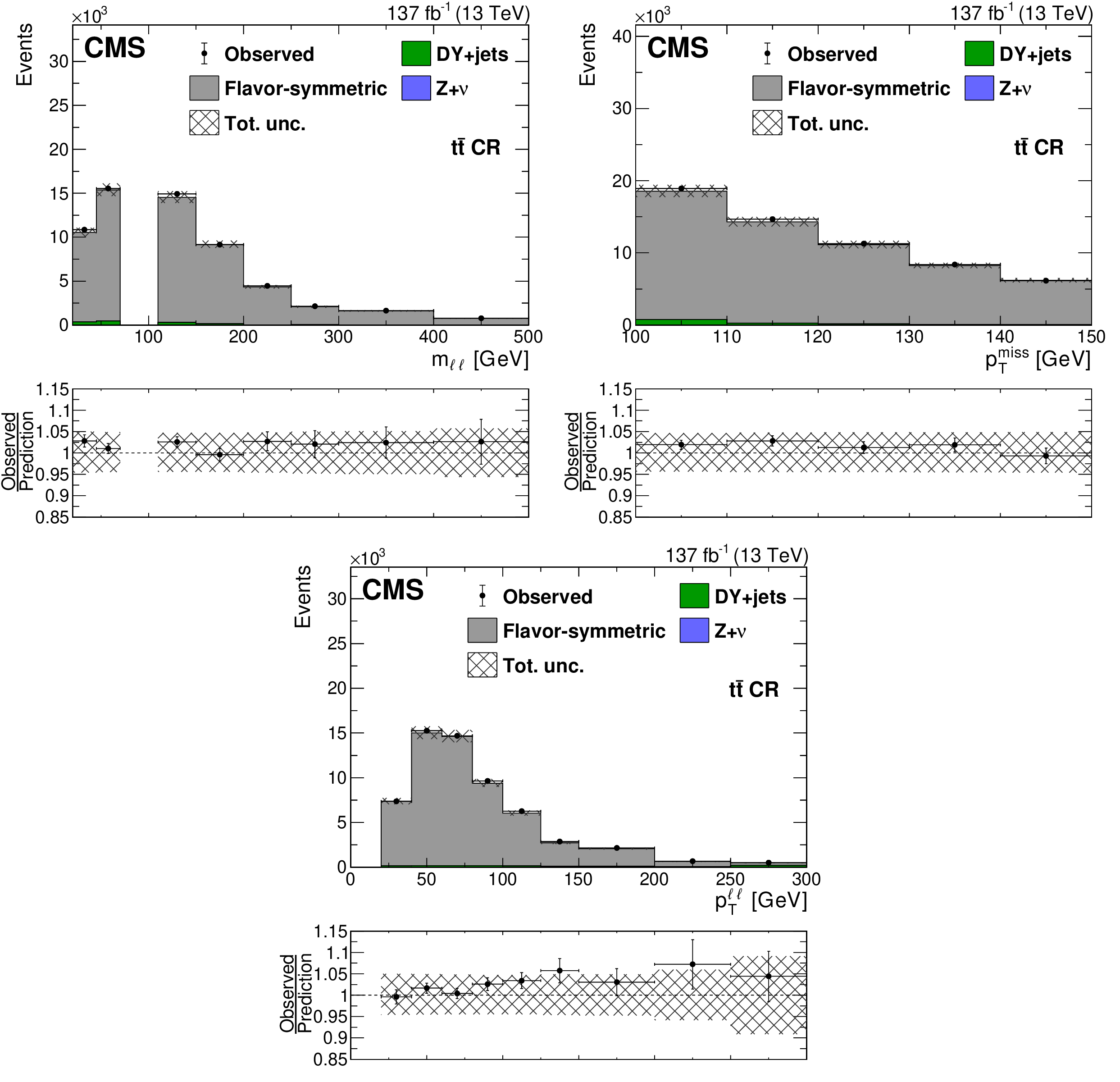
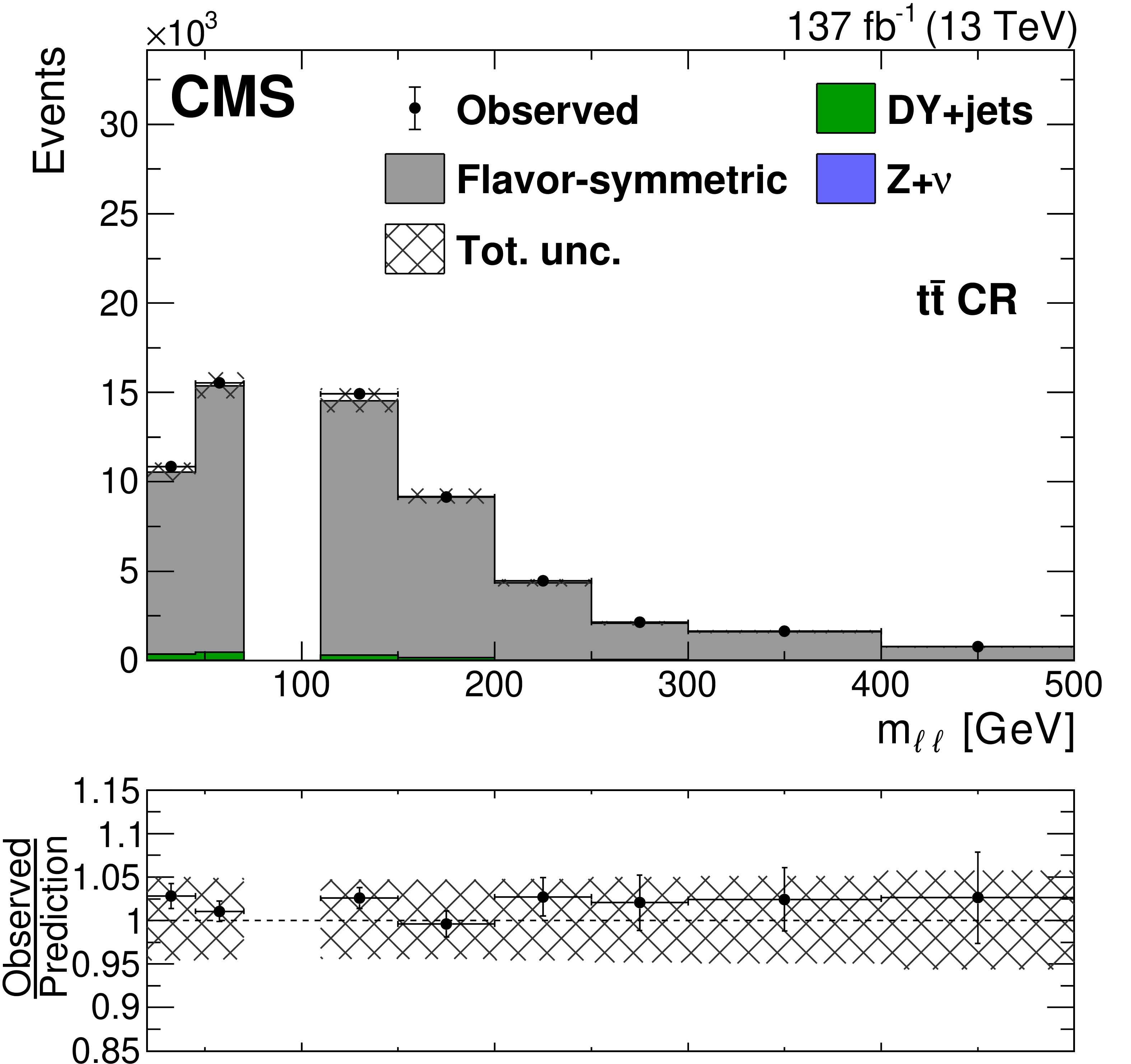
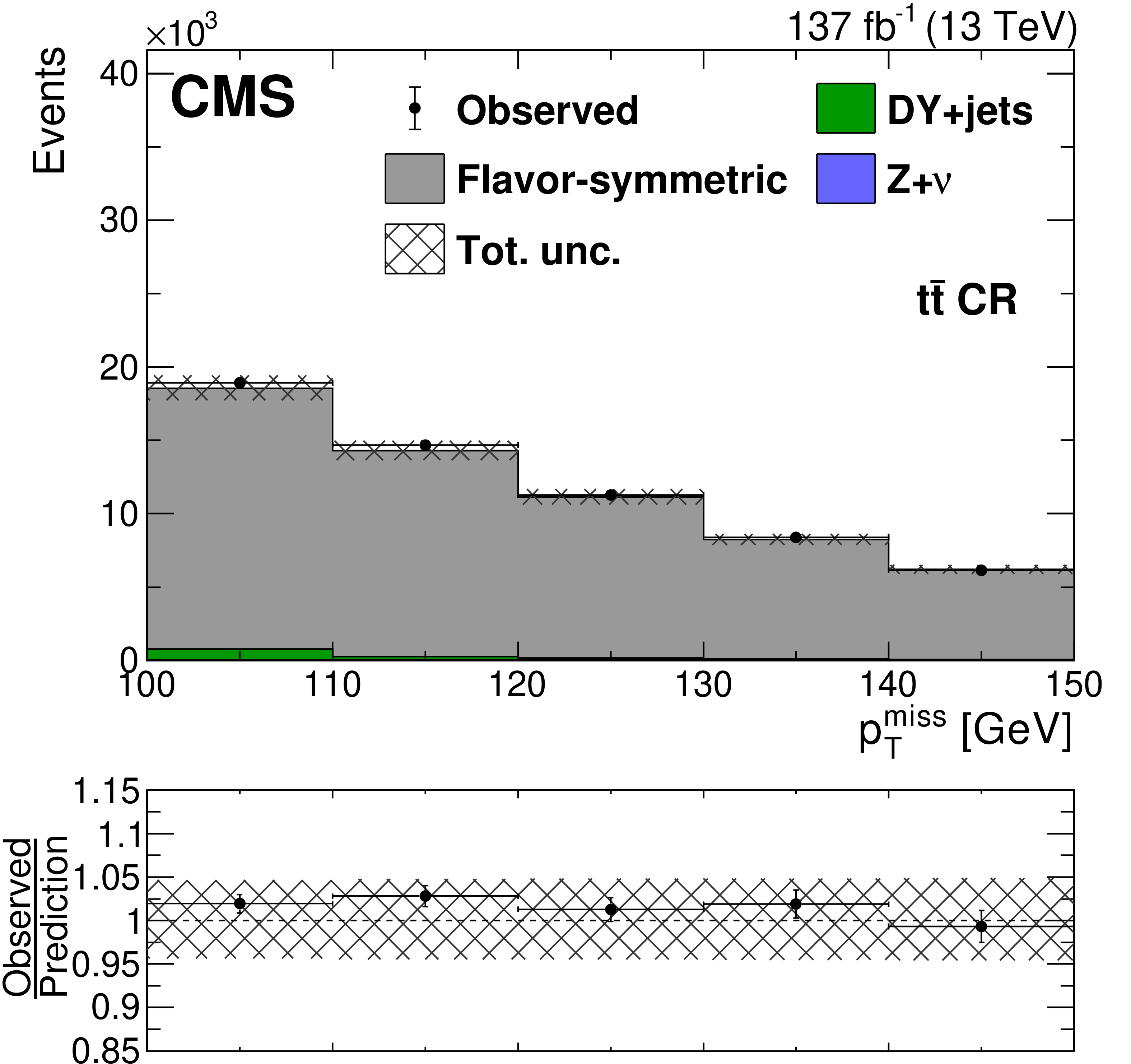
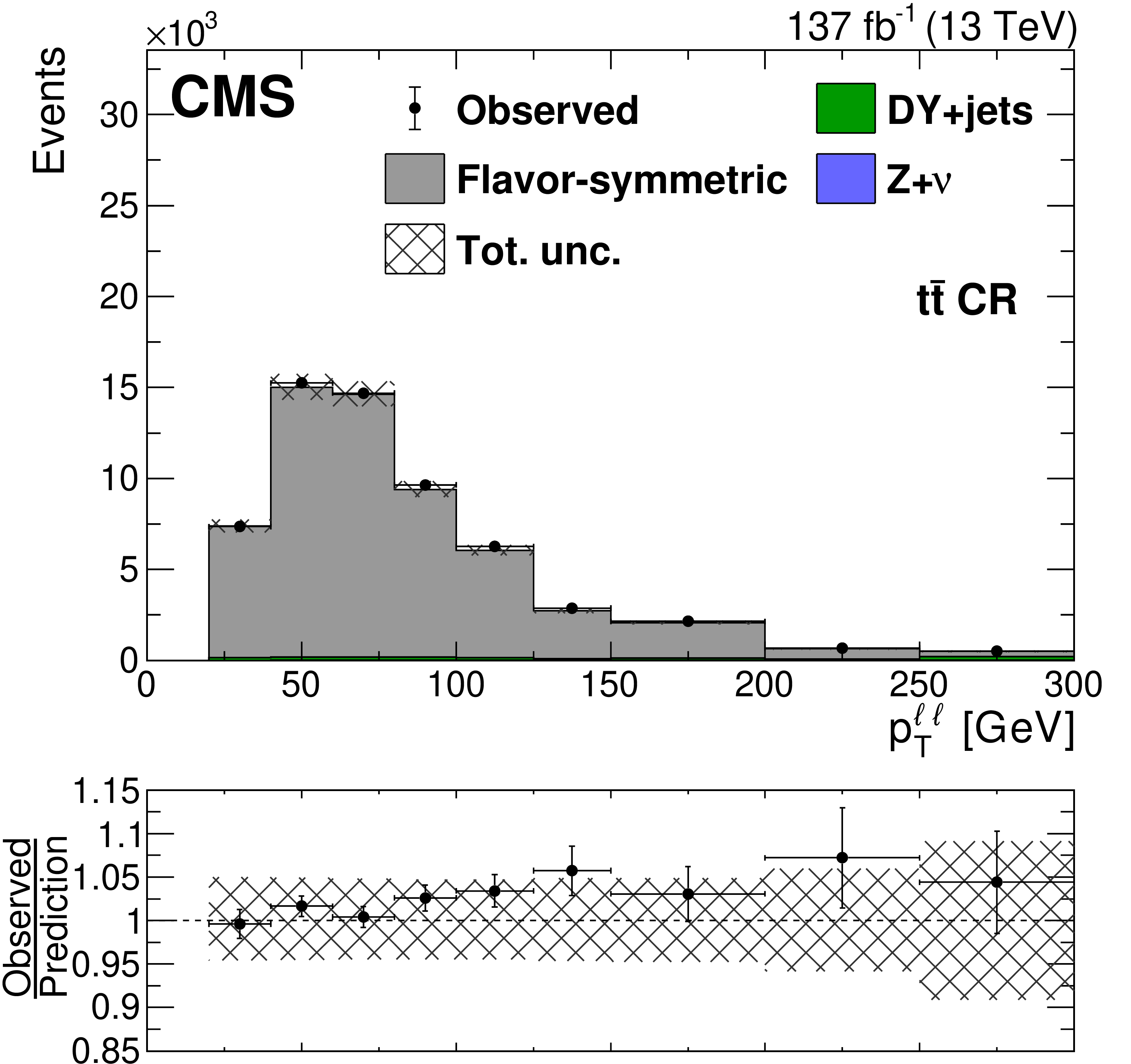
Distributions in ${m_{\ell \ell}}$ (upper left), ${{p_{\mathrm {T}}} ^\text {miss}}$ (upper right), and $ {p_{\mathrm {T}}} ^{\ell \ell}$ (lower) in a ${\mathrm{t} {}\mathrm{\bar{t}}} $-enriched CR in data. The flavor-symmetric background prediction obtained from data, as discussed in the main text, (gray solid histogram) is compared to data (black markers). Other backgrounds are estimated directly from simulation (green and blue solid histograms). The uncertainty band includes both the statistical and systematic contributions to the prediction. The last bin includes overflow events. |
png pdf |
Figure 3-a:
Distribution in ${m_{\ell \ell}}$ in a ${\mathrm{t} {}\mathrm{\bar{t}}} $-enriched CR in data. The flavor-symmetric background prediction obtained from data, as discussed in the main text, (gray solid histogram) is compared to data (black markers). Other backgrounds are estimated directly from simulation (green and blue solid histograms). The uncertainty band includes both the statistical and systematic contributions to the prediction. The last bin includes overflow events. |
png pdf |
Figure 3-b:
Distribution in ${{p_{\mathrm {T}}} ^\text {miss}}$ in a ${\mathrm{t} {}\mathrm{\bar{t}}} $-enriched CR in data. The flavor-symmetric background prediction obtained from data, as discussed in the main text, (gray solid histogram) is compared to data (black markers). Other backgrounds are estimated directly from simulation (green and blue solid histograms). The uncertainty band includes both the statistical and systematic contributions to the prediction. The last bin includes overflow events. |
png pdf |
Figure 3-c:
Distribution in $ {p_{\mathrm {T}}} ^{\ell \ell}$ in a ${\mathrm{t} {}\mathrm{\bar{t}}} $-enriched CR in data. The flavor-symmetric background prediction obtained from data, as discussed in the main text, (gray solid histogram) is compared to data (black markers). Other backgrounds are estimated directly from simulation (green and blue solid histograms). The uncertainty band includes both the statistical and systematic contributions to the prediction. The last bin includes overflow events. |
png pdf |
Figure 4:
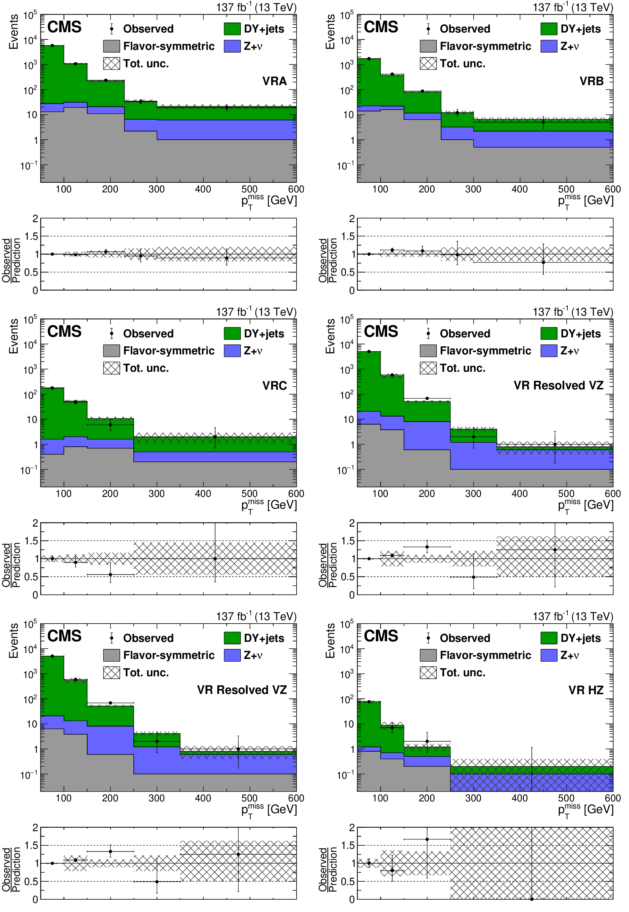
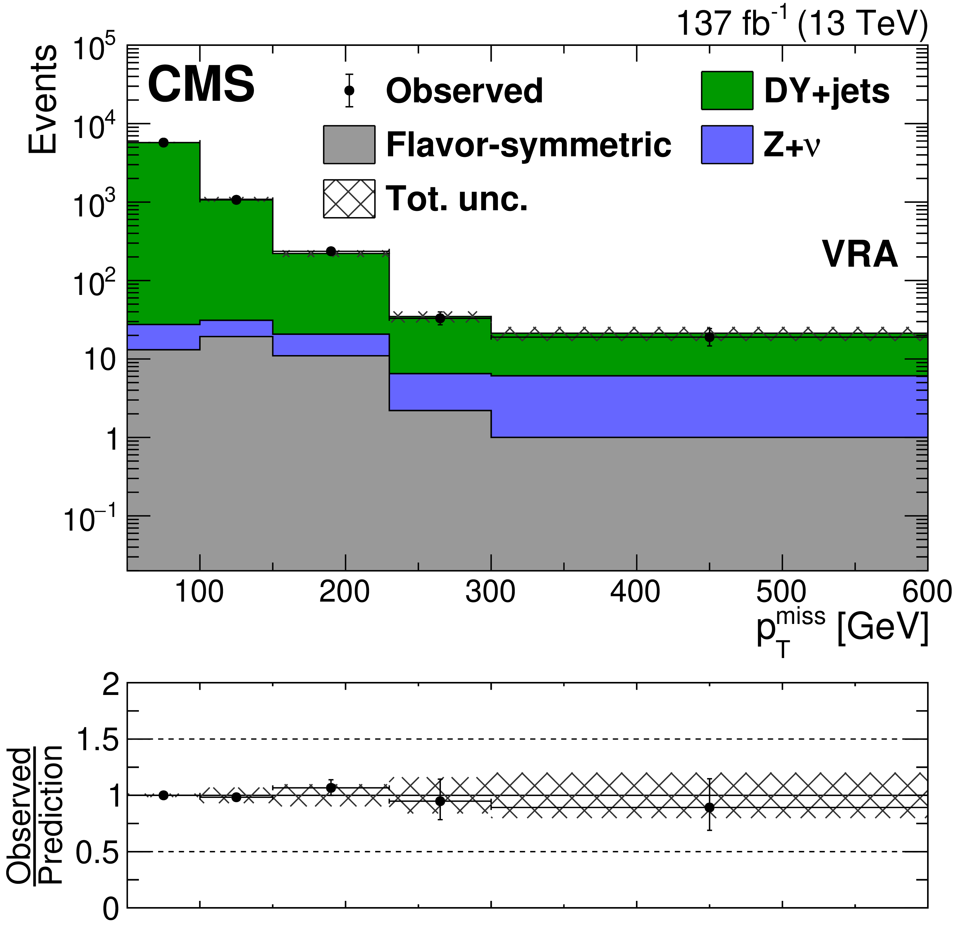
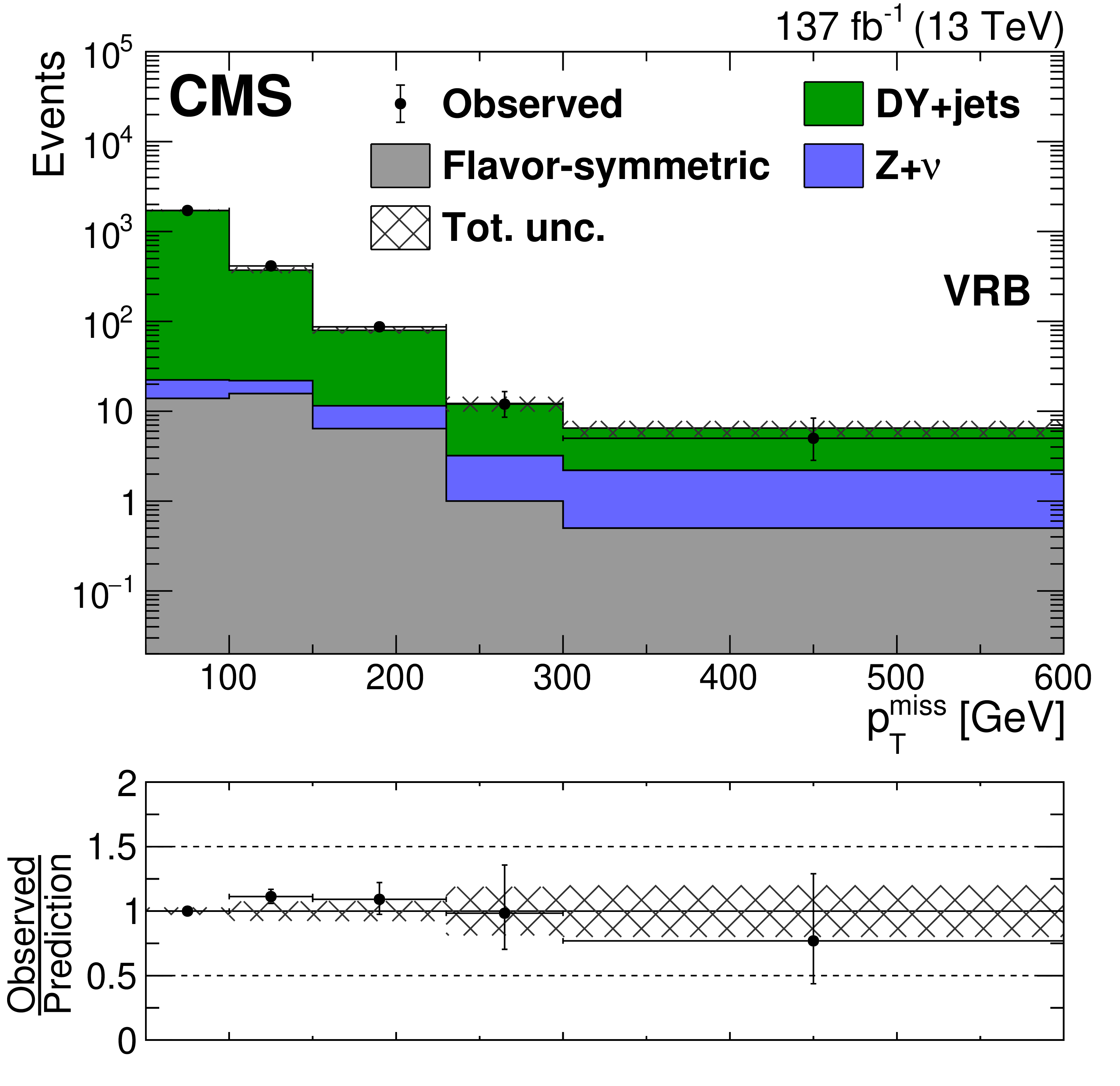
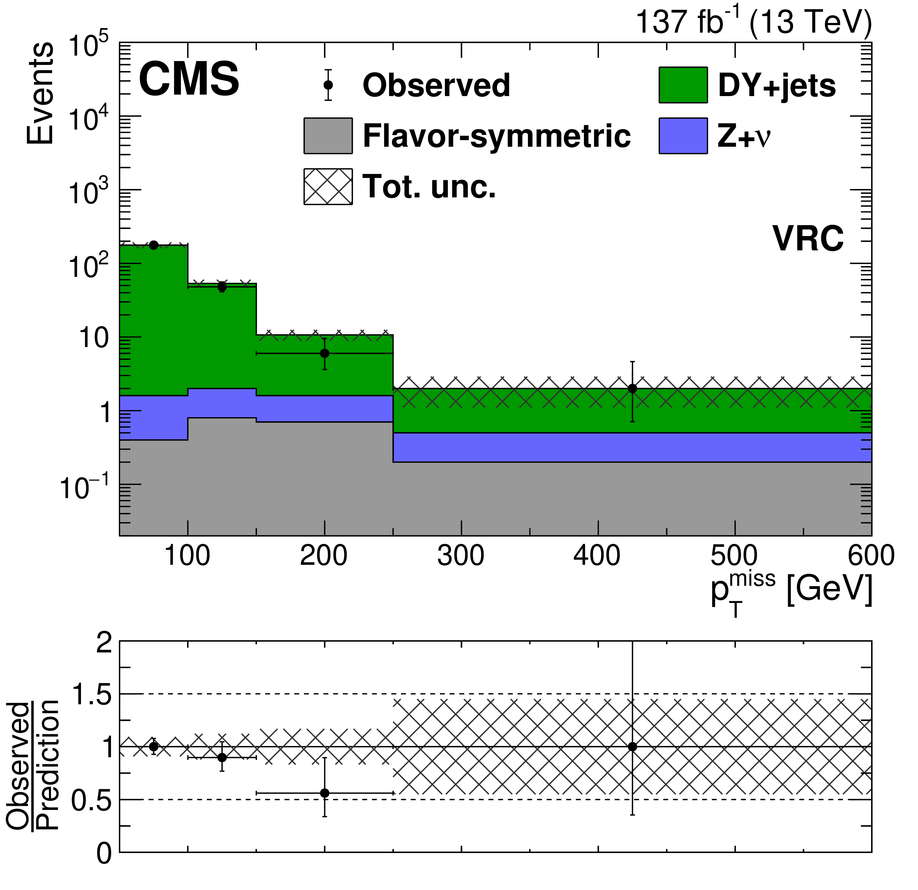
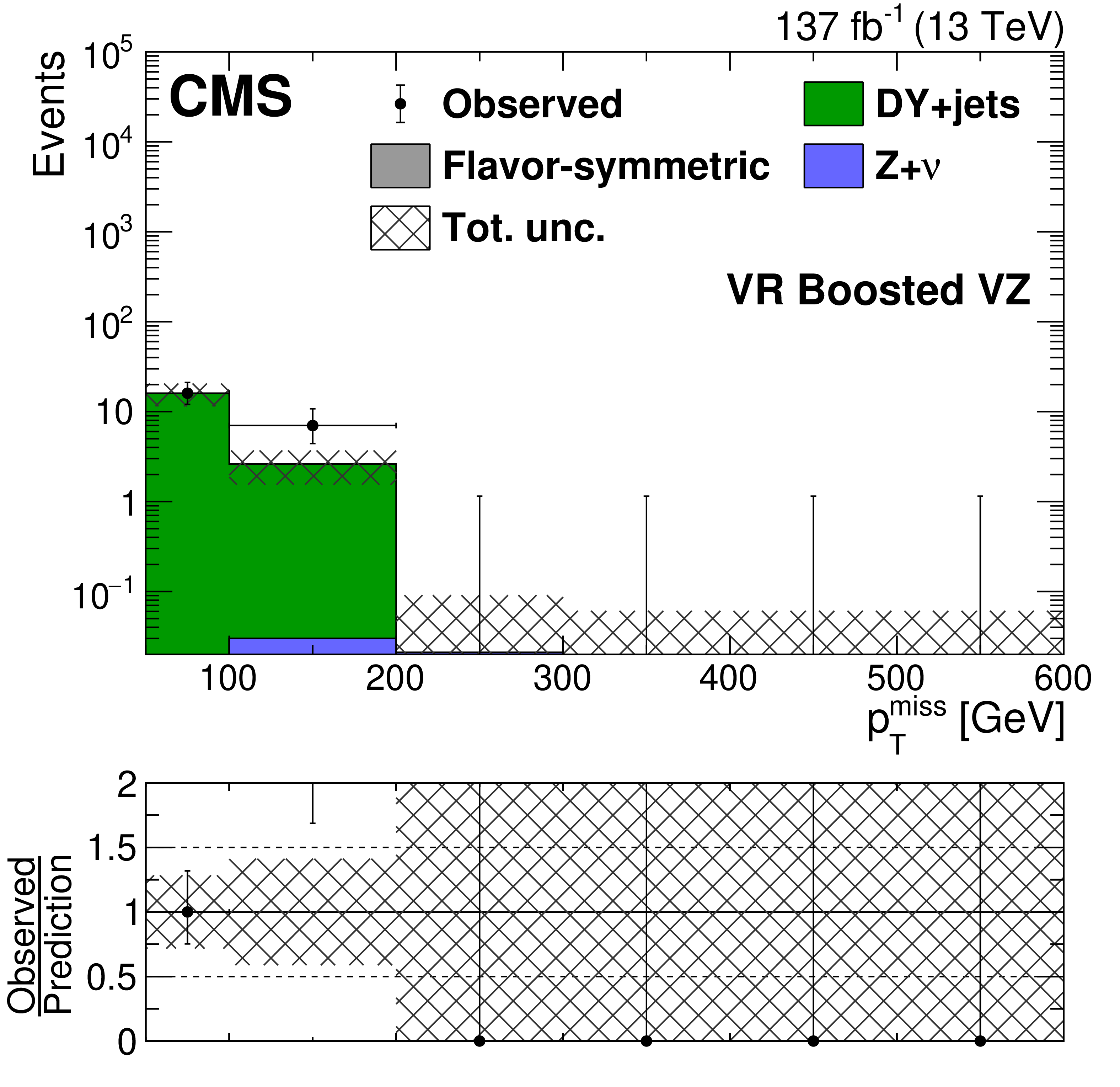
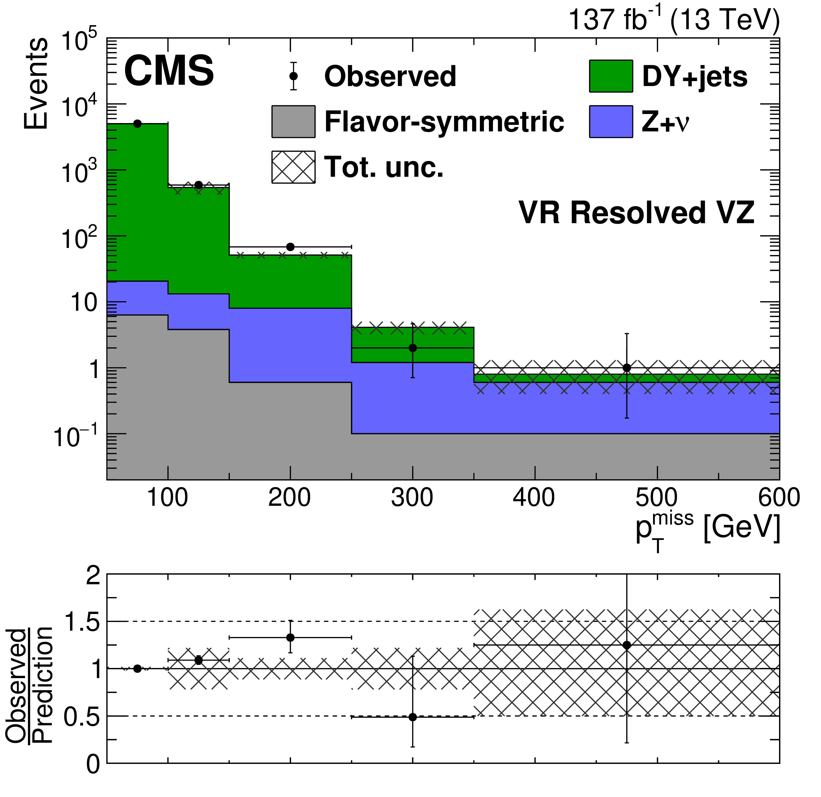
The ${{p_{\mathrm {T}}} ^\text {miss}}$ distribution observed in data (black markers) is compared to the background prediction (solid histograms) in the on-Z VRs. Comparison in the strong on-Z VRs associated to (upper left) SRA, (upper right) SRB, and (middle left) SRC. Comparison in the EW on-Z VRs: (middle right) boosted VZ, (lower left) resolved VZ, and (lower right) HZ. The uncertainty band includes both the systematic and statistical components of the uncertainty in the prediction. The last bin includes overflow events. |
png pdf |
Figure 4-a:
The ${{p_{\mathrm {T}}} ^\text {miss}}$ distribution observed in data (black markers) is compared to the background prediction (solid histograms) in the strong on-Z VRs associated to SRA. The uncertainty band includes both the systematic and statistical components of the uncertainty in the prediction. The last bin includes overflow events. |
png pdf |
Figure 4-b:
The ${{p_{\mathrm {T}}} ^\text {miss}}$ distribution observed in data (black markers) is compared to the background prediction (solid histograms) in the strong on-Z VRs associated to SRB. The uncertainty band includes both the systematic and statistical components of the uncertainty in the prediction. The last bin includes overflow events. |
png pdf |
Figure 4-c:
The ${{p_{\mathrm {T}}} ^\text {miss}}$ distribution observed in data (black markers) is compared to the background prediction (solid histograms) in the strong on-Z VRs associated to SRC. The uncertainty band includes both the systematic and statistical components of the uncertainty in the prediction. The last bin includes overflow events. |
png pdf |
Figure 4-d:
The ${{p_{\mathrm {T}}} ^\text {miss}}$ distribution observed in data (black markers) is compared to the background prediction (solid histograms) in the EW on-Z VRs associated to boosted VZ. The uncertainty band includes both the systematic and statistical components of the uncertainty in the prediction. The last bin includes overflow events. |
png pdf |
Figure 4-e:
The ${{p_{\mathrm {T}}} ^\text {miss}}$ distribution observed in data (black markers) is compared to the background prediction (solid histograms) in the EW on-Z VRs associated to resolved VZ. The uncertainty band includes both the systematic and statistical components of the uncertainty in the prediction. The last bin includes overflow events. |

png pdf |
Figure 4-f:
The ${{p_{\mathrm {T}}} ^\text {miss}}$ distribution observed in data (black markers) is compared to the background prediction (solid histograms) in the EW on-Z VRs associated to HZ. The uncertainty band includes both the systematic and statistical components of the uncertainty in the prediction. The last bin includes overflow events. |
png pdf root |
Figure 5:
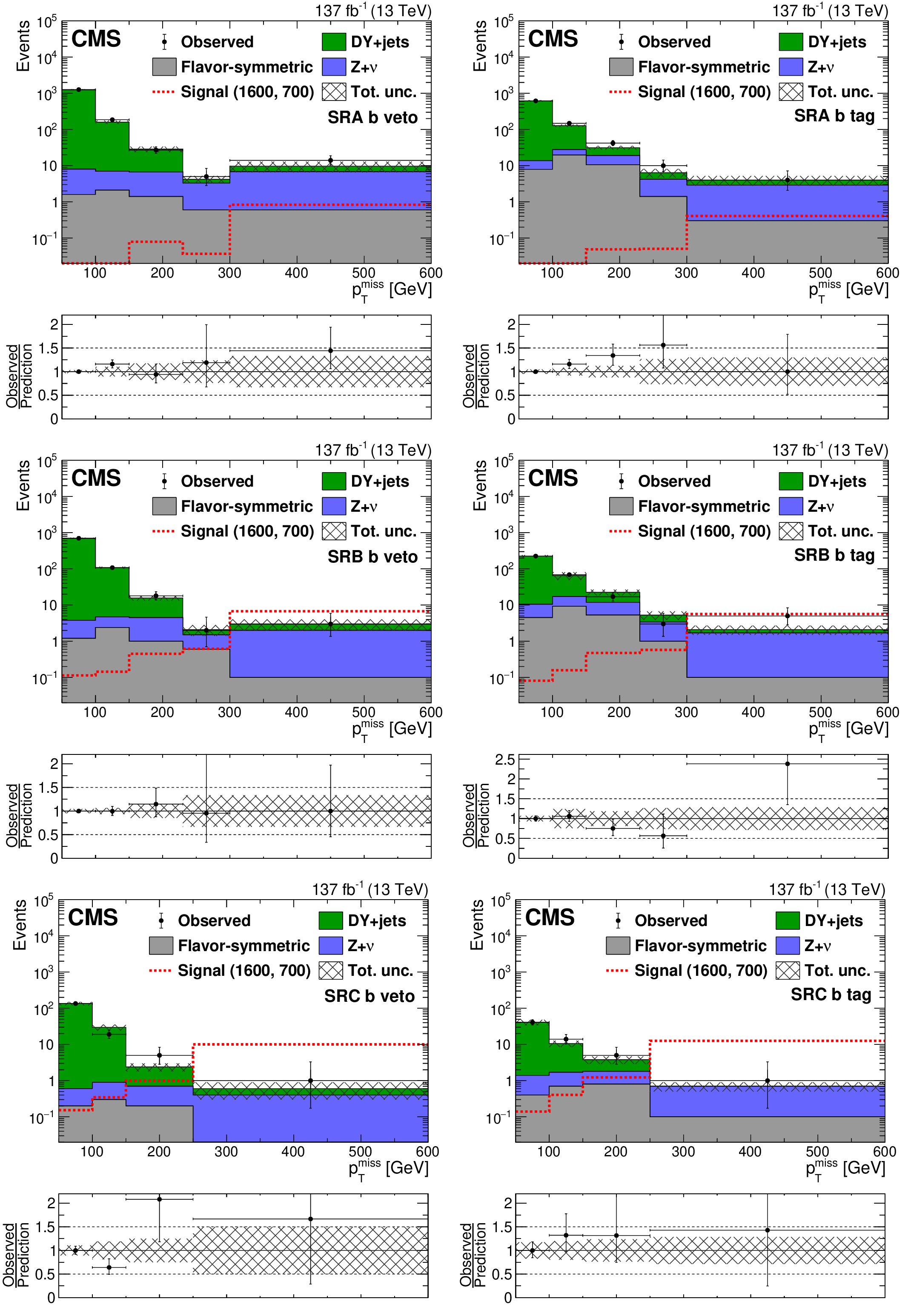
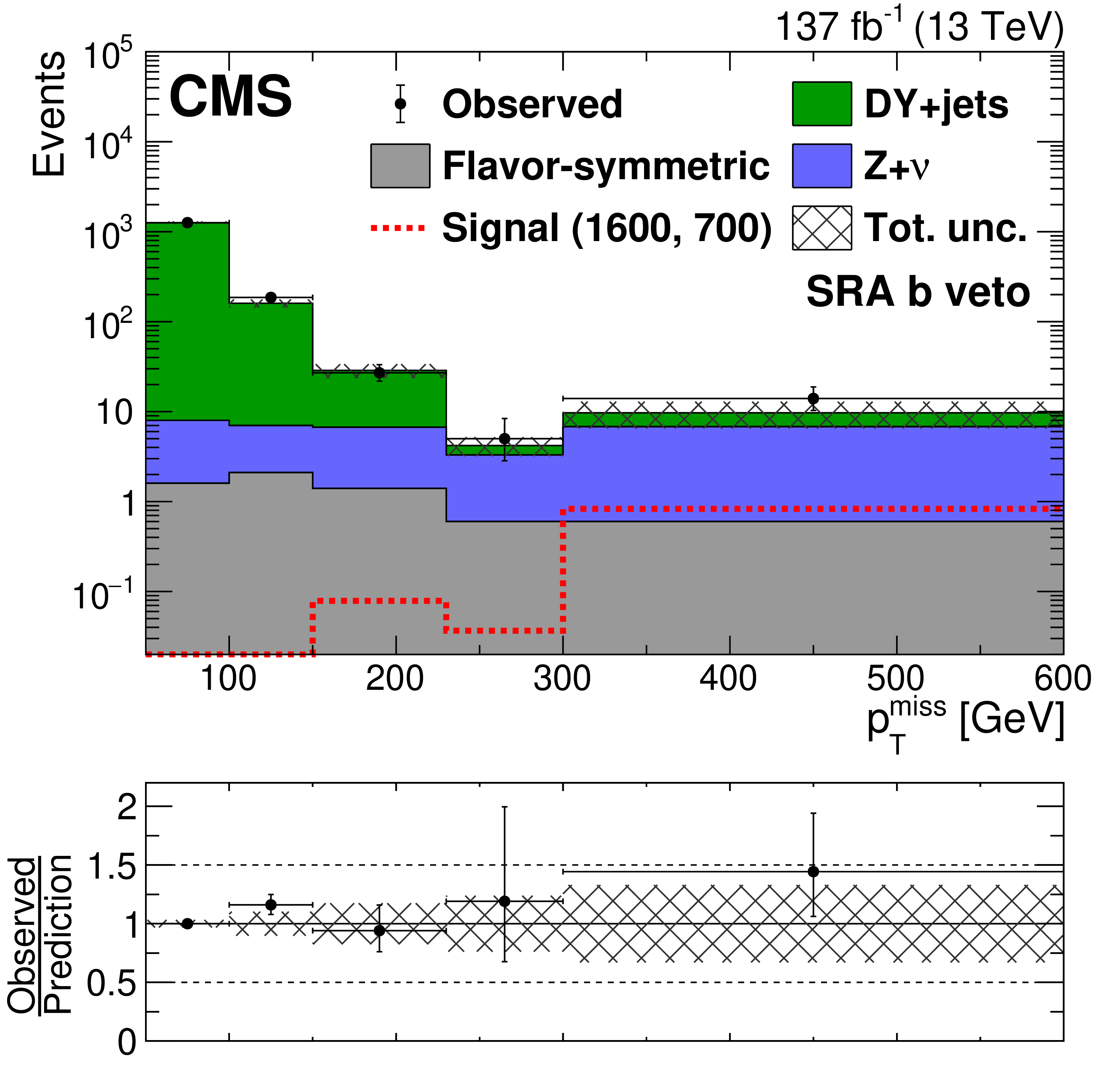
The ${{p_{\mathrm {T}}} ^\text {miss}}$ distribution in data is compared to the SM background prediction in the strong-production on-Z (upper) SRA, (middle) SRB, and (lower) SRC regions for (left) the b veto and (right) b tag categories before the fits to data discussed in Section 8. The lower panel of each plot shows the ratio of observed data to the SM prediction in each bin of ${{p_{\mathrm {T}}} ^\text {miss}}$. The hashed band in the upper panels shows the total uncertainty in the background prediction including statistical and systematic sources. The signal ${{p_{\mathrm {T}}} ^\text {miss}}$ distributions correspond to the gluino pair production model with the gluino ($\tilde{\chi}^0_1$) having a mass of 1600 (700) GeV. The ${{p_{\mathrm {T}}} ^\text {miss}}$ template prediction in each search region is normalized to the first ${{p_{\mathrm {T}}} ^\text {miss}}$ bin of each distribution in data. The last bin includes overflow events. |
png pdf root |
Figure 5-a:
The ${{p_{\mathrm {T}}} ^\text {miss}}$ distribution in data is compared to the SM background prediction in the strong-production on-Z SRA region for the b veto category before the fits to data discussed in Section 8. The lower panel shows the ratio of observed data to the SM prediction in each bin of ${{p_{\mathrm {T}}} ^\text {miss}}$. The hashed band in the upper panels shows the total uncertainty in the background prediction including statistical and systematic sources. The signal ${{p_{\mathrm {T}}} ^\text {miss}}$ distributions correspond to the gluino pair production model with the gluino ($\tilde{\chi}^0_1$) having a mass of 1600 (700) GeV. The ${{p_{\mathrm {T}}} ^\text {miss}}$ template prediction in each search region is normalized to the first ${{p_{\mathrm {T}}} ^\text {miss}}$ bin of each distribution in data. The last bin includes overflow events. |

png pdf root |
Figure 5-b:
The ${{p_{\mathrm {T}}} ^\text {miss}}$ distribution in data is compared to the SM background prediction in the strong-production on-Z SRA region for the b tag category before the fits to data discussed in Section 8. The lower panel shows the ratio of observed data to the SM prediction in each bin of ${{p_{\mathrm {T}}} ^\text {miss}}$. The hashed band in the upper panels shows the total uncertainty in the background prediction including statistical and systematic sources. The signal ${{p_{\mathrm {T}}} ^\text {miss}}$ distributions correspond to the gluino pair production model with the gluino ($\tilde{\chi}^0_1$) having a mass of 1600 (700) GeV. The ${{p_{\mathrm {T}}} ^\text {miss}}$ template prediction in each search region is normalized to the first ${{p_{\mathrm {T}}} ^\text {miss}}$ bin of each distribution in data. The last bin includes overflow events. |
png pdf root |
Figure 5-c:
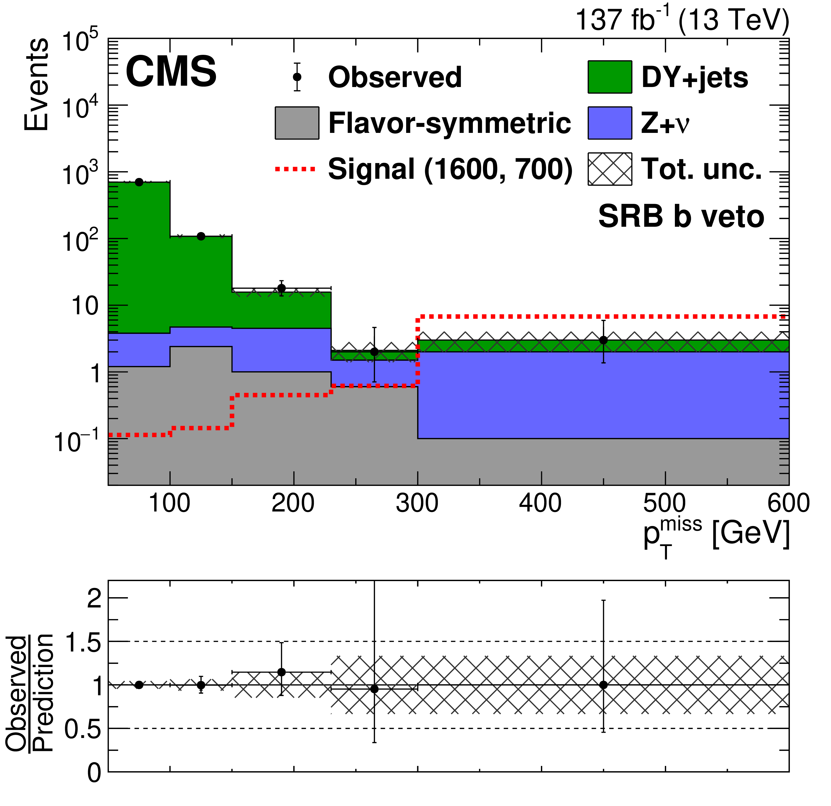
The ${{p_{\mathrm {T}}} ^\text {miss}}$ distribution in data is compared to the SM background prediction in the strong-production on-Z SRB region for the b veto category before the fits to data discussed in Section 8. The lower panel shows the ratio of observed data to the SM prediction in each bin of ${{p_{\mathrm {T}}} ^\text {miss}}$. The hashed band in the upper panels shows the total uncertainty in the background prediction including statistical and systematic sources. The signal ${{p_{\mathrm {T}}} ^\text {miss}}$ distributions correspond to the gluino pair production model with the gluino ($\tilde{\chi}^0_1$) having a mass of 1600 (700) GeV. The ${{p_{\mathrm {T}}} ^\text {miss}}$ template prediction in each search region is normalized to the first ${{p_{\mathrm {T}}} ^\text {miss}}$ bin of each distribution in data. The last bin includes overflow events. |
png pdf root |
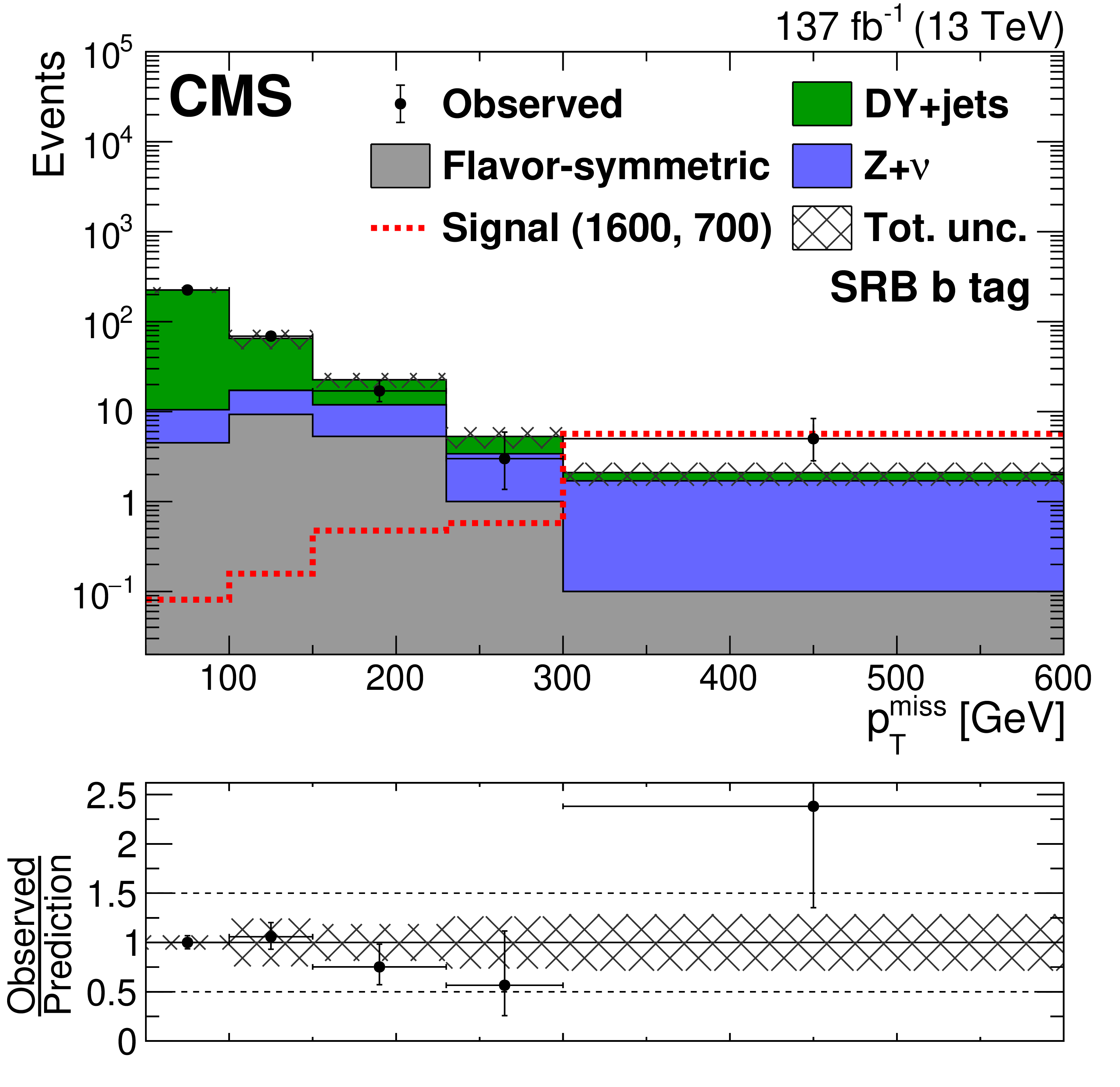
Figure 5-d:
The ${{p_{\mathrm {T}}} ^\text {miss}}$ distribution in data is compared to the SM background prediction in the strong-production on-Z SRB region for the b tag category before the fits to data discussed in Section 8. The lower panel shows the ratio of observed data to the SM prediction in each bin of ${{p_{\mathrm {T}}} ^\text {miss}}$. The hashed band in the upper panels shows the total uncertainty in the background prediction including statistical and systematic sources. The signal ${{p_{\mathrm {T}}} ^\text {miss}}$ distributions correspond to the gluino pair production model with the gluino ($\tilde{\chi}^0_1$) having a mass of 1600 (700) GeV. The ${{p_{\mathrm {T}}} ^\text {miss}}$ template prediction in each search region is normalized to the first ${{p_{\mathrm {T}}} ^\text {miss}}$ bin of each distribution in data. The last bin includes overflow events. |
png pdf root |
Figure 5-e:
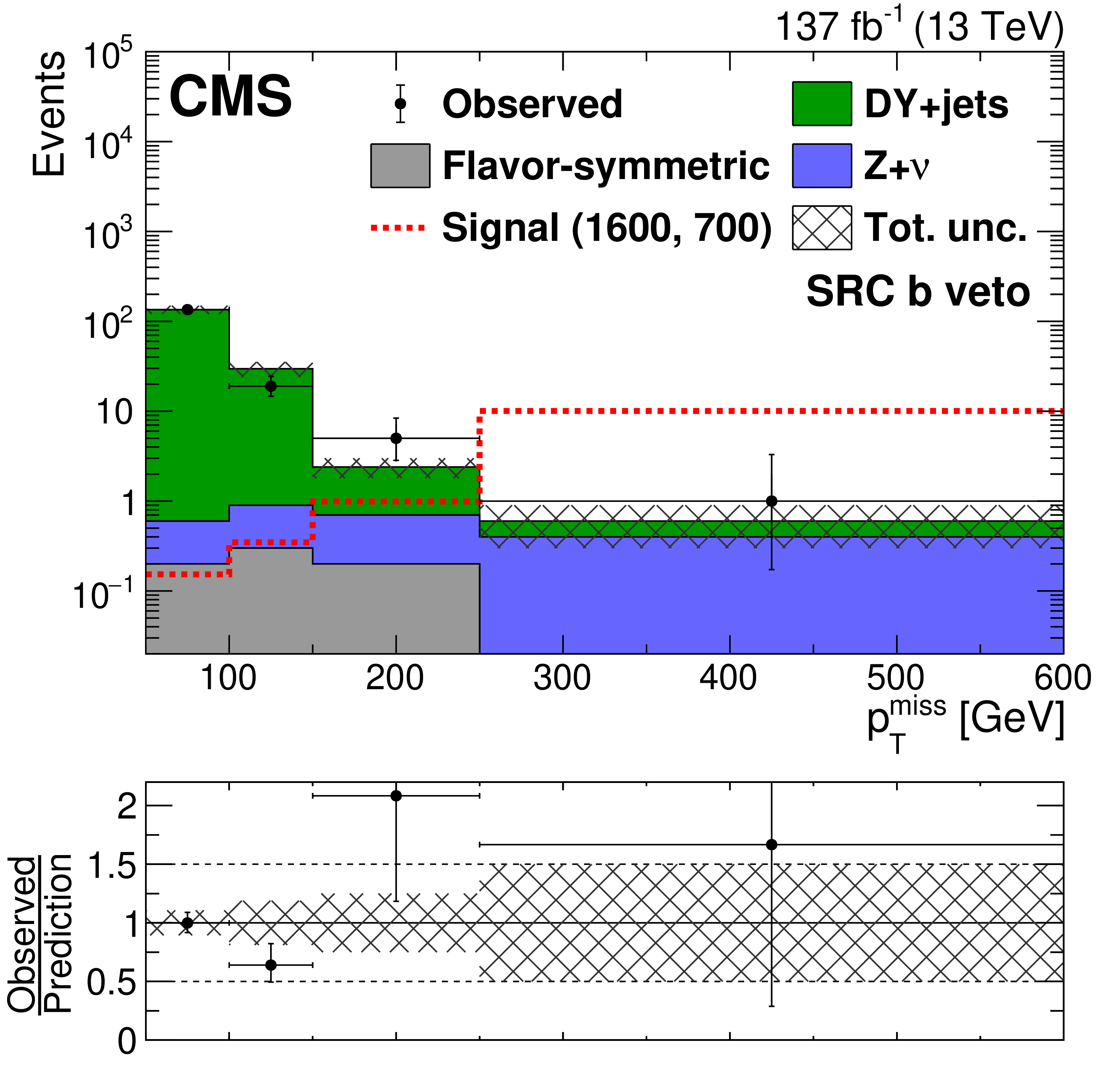
The ${{p_{\mathrm {T}}} ^\text {miss}}$ distribution in data is compared to the SM background prediction in the strong-production on-Z SRC region for the b veto category before the fits to data discussed in Section 8. The lower panel shows the ratio of observed data to the SM prediction in each bin of ${{p_{\mathrm {T}}} ^\text {miss}}$. The hashed band in the upper panels shows the total uncertainty in the background prediction including statistical and systematic sources. The signal ${{p_{\mathrm {T}}} ^\text {miss}}$ distributions correspond to the gluino pair production model with the gluino ($\tilde{\chi}^0_1$) having a mass of 1600 (700) GeV. The ${{p_{\mathrm {T}}} ^\text {miss}}$ template prediction in each search region is normalized to the first ${{p_{\mathrm {T}}} ^\text {miss}}$ bin of each distribution in data. The last bin includes overflow events. |
png pdf root |
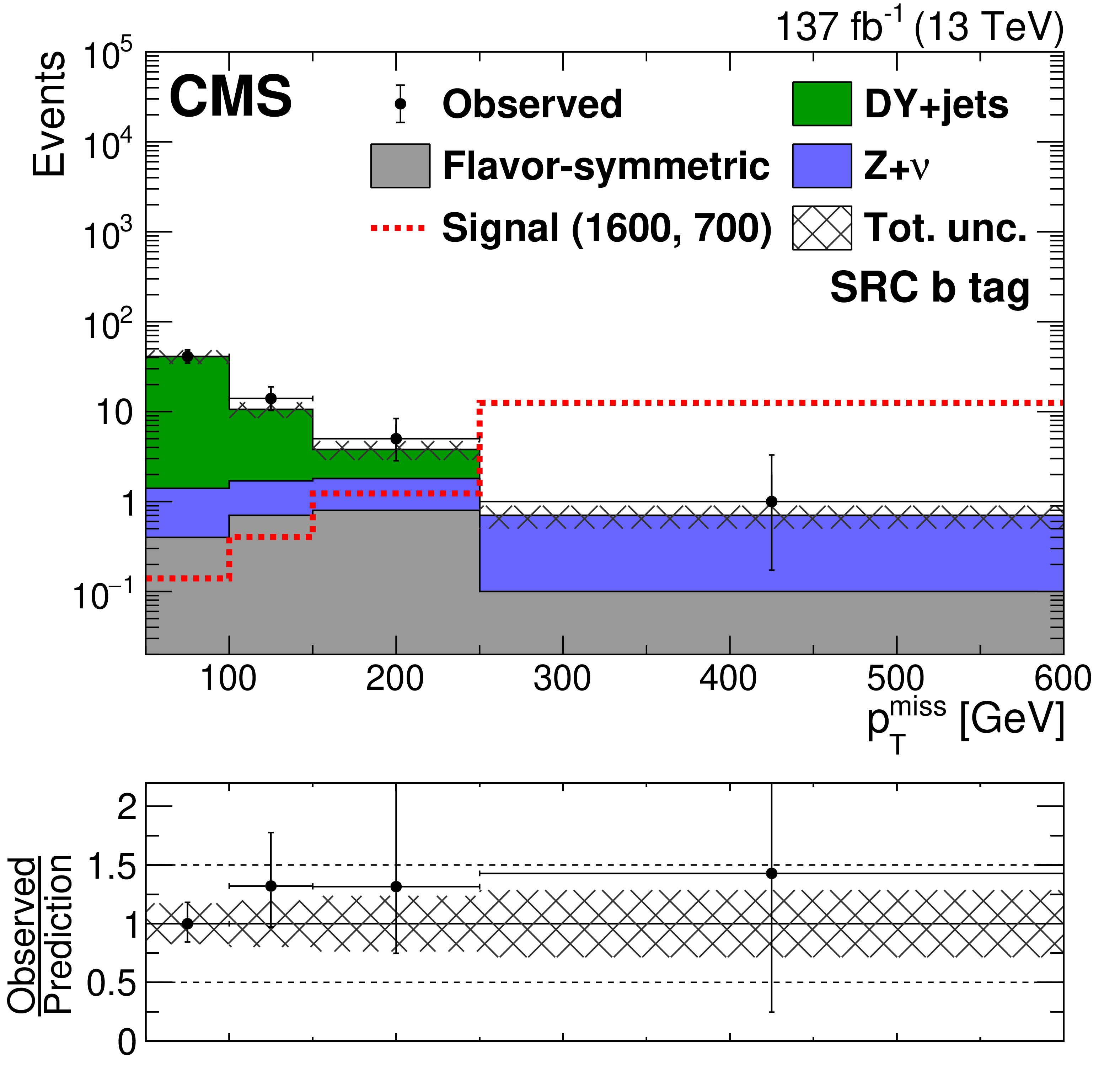
Figure 5-f:
The ${{p_{\mathrm {T}}} ^\text {miss}}$ distribution in data is compared to the SM background prediction in the strong-production on-Z SRC region for the b tag category before the fits to data discussed in Section 8. The lower panel shows the ratio of observed data to the SM prediction in each bin of ${{p_{\mathrm {T}}} ^\text {miss}}$. The hashed band in the upper panels shows the total uncertainty in the background prediction including statistical and systematic sources. The signal ${{p_{\mathrm {T}}} ^\text {miss}}$ distributions correspond to the gluino pair production model with the gluino ($\tilde{\chi}^0_1$) having a mass of 1600 (700) GeV. The ${{p_{\mathrm {T}}} ^\text {miss}}$ template prediction in each search region is normalized to the first ${{p_{\mathrm {T}}} ^\text {miss}}$ bin of each distribution in data. The last bin includes overflow events. |
png pdf root |
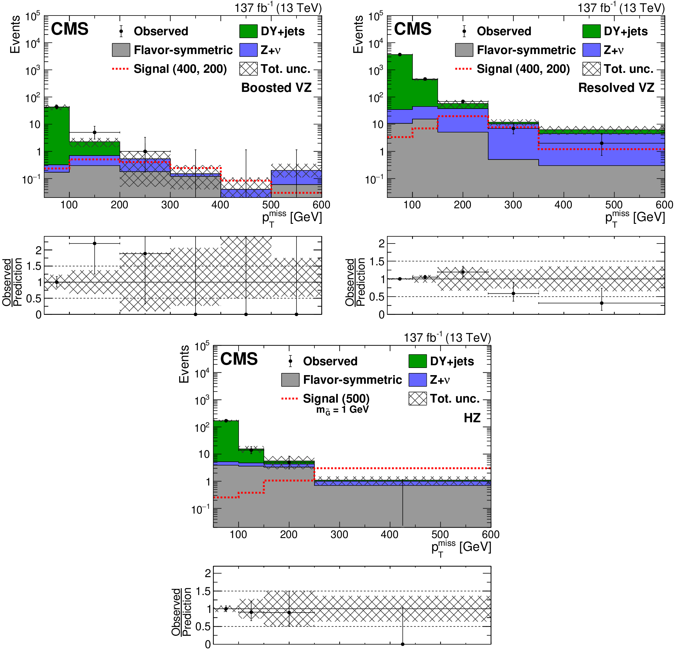
Figure 6:
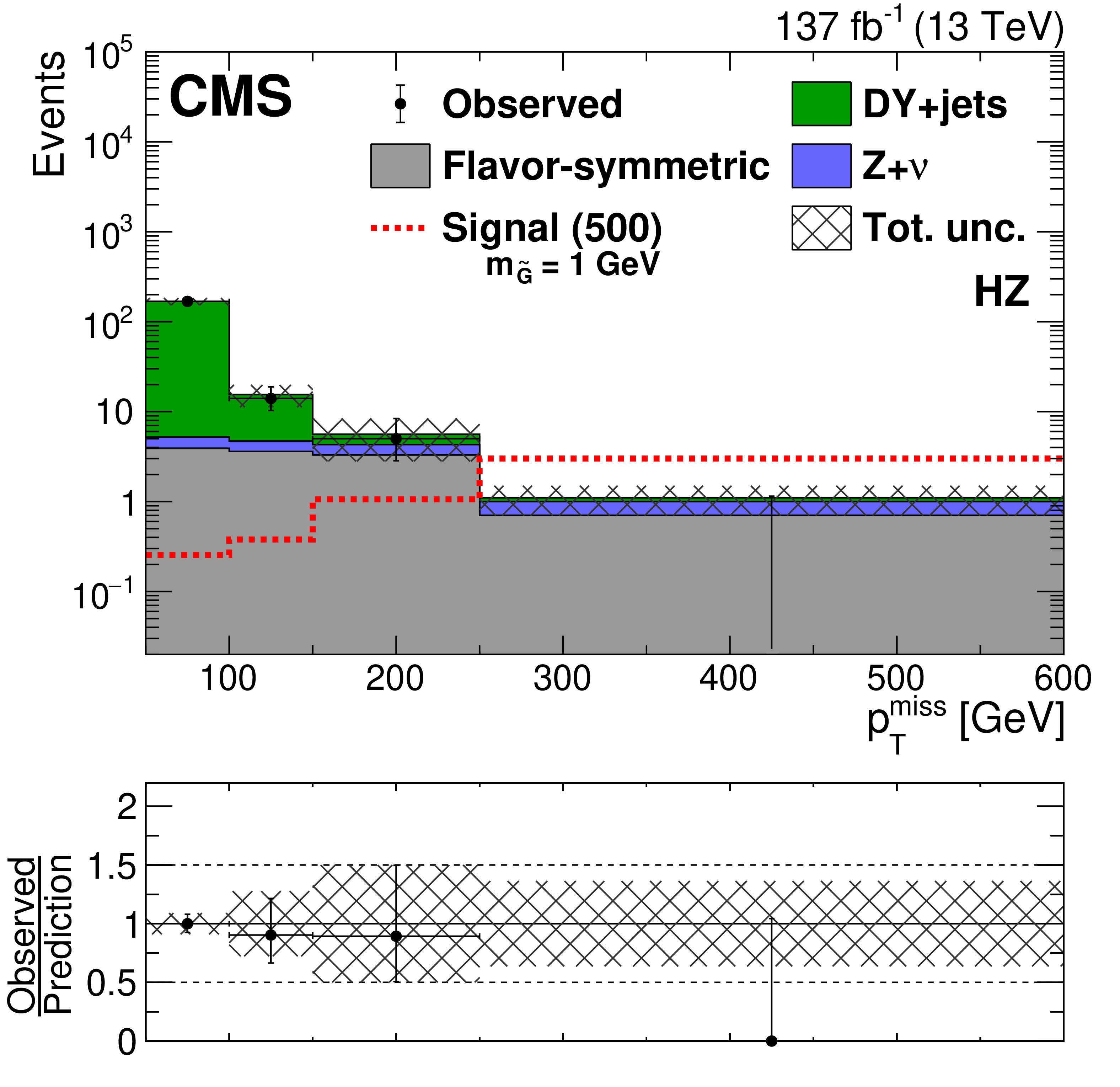
The ${{p_{\mathrm {T}}} ^\text {miss}}$ distribution in data is compared to the SM background prediction in the EW-production on-Z (upper left) boosted VZ, (upper right) resolved VZ, and (lower) HZ search regions before the fits to data described in Section 8. The lower panel of each figure shows the ratio of observed data to the SM prediction in each ${{p_{\mathrm {T}}} ^\text {miss}}$ bin. The hashed band shows the total uncertainty in the background prediction including statistical and systematic sources. The signal ${{p_{\mathrm {T}}} ^\text {miss}}$ distribution for the boosted and resolved VZ search regions correspond to the $\tilde{\chi}^{\pm}_1 \tilde{\chi}^0_2$ production model with a $\tilde{\chi}^{\pm}_1 /\tilde{\chi}^0_2$ ($\tilde{\chi}^0_1$) mass of 400 (200) GeV,while for the HZ search region the ${{p_{\mathrm {T}}} ^\text {miss}}$ distribution corresponds to a $\tilde{\chi}^0_1$ pair production model decaying into a Higgs boson, a Z boson and two $\tilde{\mathrm{G}}$ with the $\tilde{\chi}^0_1$ ($\tilde{\mathrm{G}}$) having a mass of 500 (1) GeV. The ${{p_{\mathrm {T}}} ^\text {miss}}$ template prediction in each search region is normalized to the first ${{p_{\mathrm {T}}} ^\text {miss}}$ bin of each distribution in data. The last bin includes overflow events. |
png pdf root |
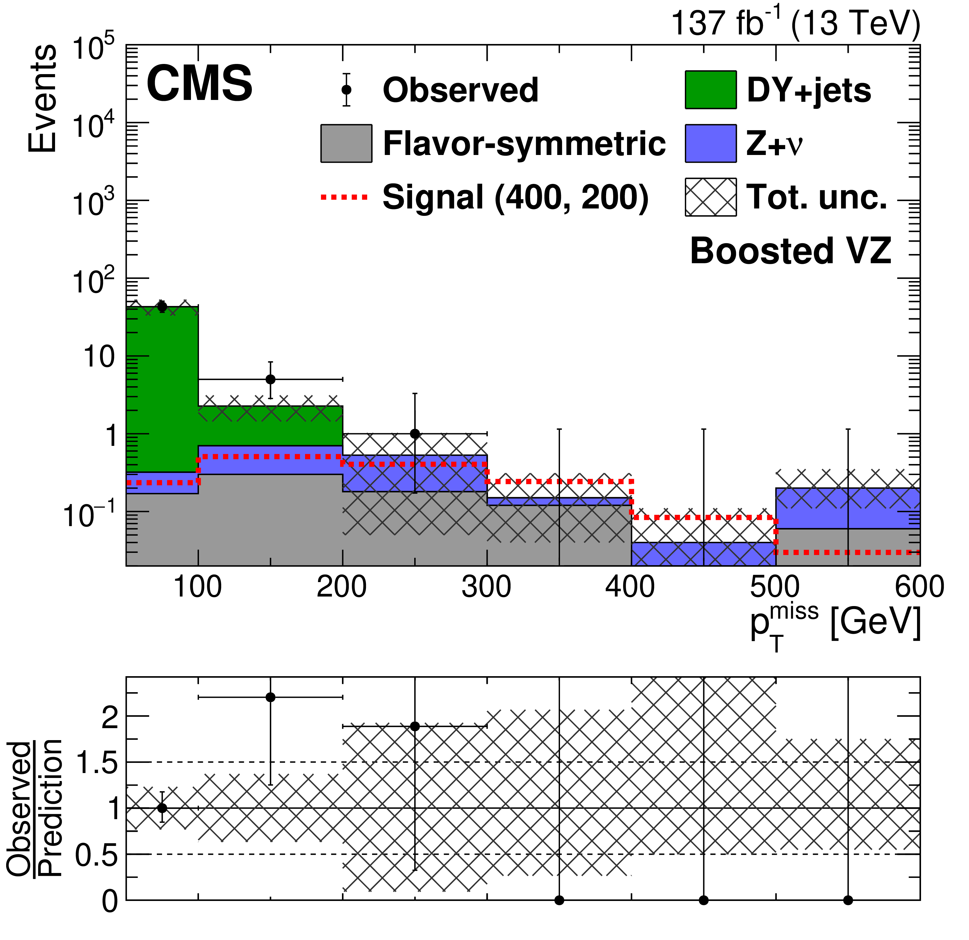
Figure 6-a:
The ${{p_{\mathrm {T}}} ^\text {miss}}$ distribution in data is compared to the SM background prediction in the EW-production on-Z boosted VZ search region before the fits to data described in Section 8. The lower panel shows the ratio of observed data to the SM prediction in each ${{p_{\mathrm {T}}} ^\text {miss}}$ bin. The hashed band shows the total uncertainty in the background prediction including statistical and systematic sources. The signal ${{p_{\mathrm {T}}} ^\text {miss}}$ distribution for the boosted and resolved VZ search regions correspond to the $\tilde{\chi}^{\pm}_1 \tilde{\chi}^0_2$ production model with a $\tilde{\chi}^{\pm}_1 /\tilde{\chi}^0_2$ ($\tilde{\chi}^0_1$) mass of 400 (200) GeV,while for the HZ search region the ${{p_{\mathrm {T}}} ^\text {miss}}$ distribution corresponds to a $\tilde{\chi}^0_1$ pair production model decaying into a Higgs boson, a Z boson and two $\tilde{\mathrm{G}}$ with the $\tilde{\chi}^0_1$ ($\tilde{\mathrm{G}}$) having a mass of 500 (1) GeV. The ${{p_{\mathrm {T}}} ^\text {miss}}$ template prediction in each search region is normalized to the first ${{p_{\mathrm {T}}} ^\text {miss}}$ bin of each distribution in data. The last bin includes overflow events. |
png pdf root |
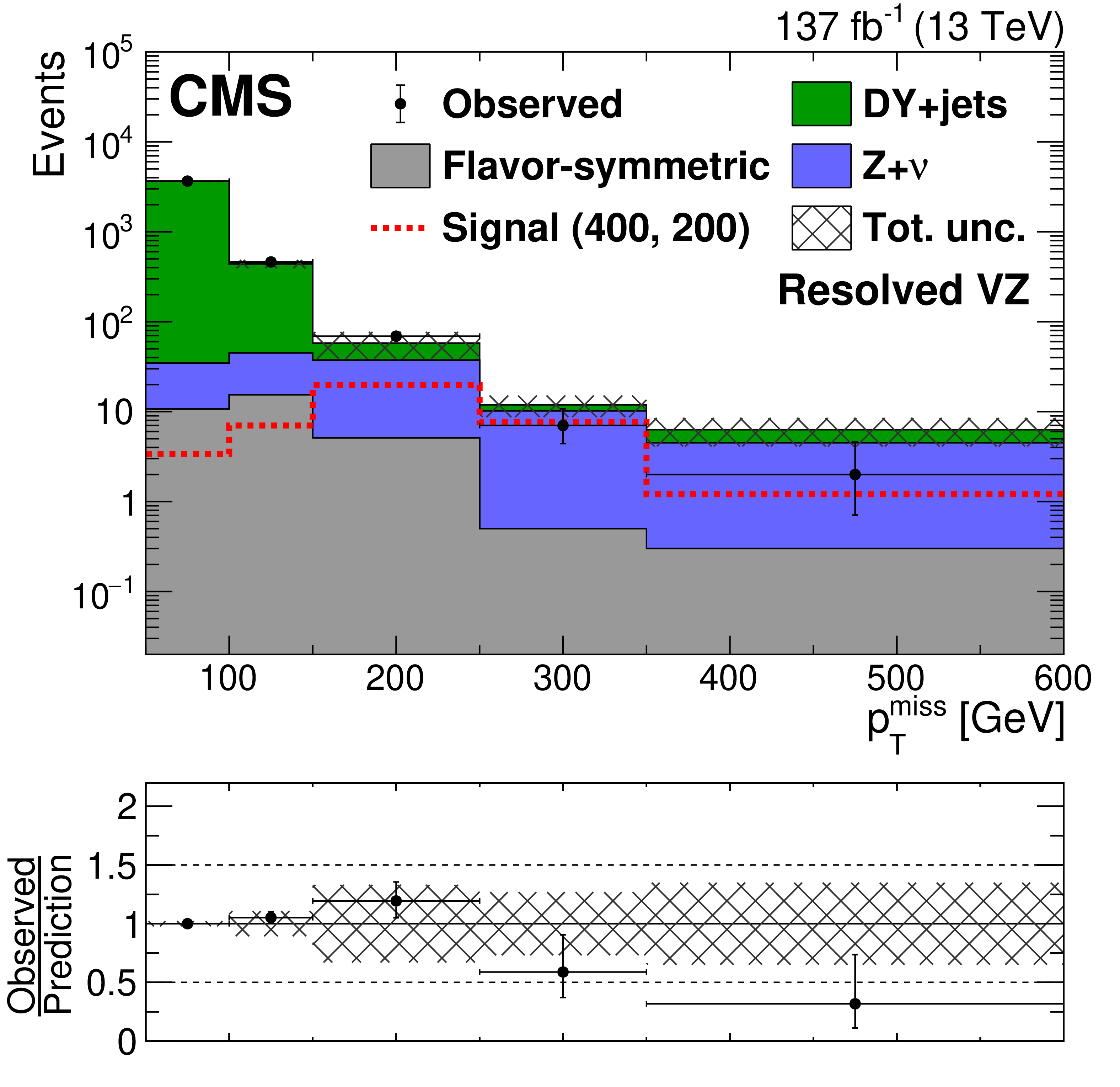
Figure 6-b:
The ${{p_{\mathrm {T}}} ^\text {miss}}$ distribution in data is compared to the SM background prediction in the EW-production on-Z resolved VZ search region before the fits to data described in Section 8. The lower panel shows the ratio of observed data to the SM prediction in each ${{p_{\mathrm {T}}} ^\text {miss}}$ bin. The hashed band shows the total uncertainty in the background prediction including statistical and systematic sources. The signal ${{p_{\mathrm {T}}} ^\text {miss}}$ distribution for the boosted and resolved VZ search regions correspond to the $\tilde{\chi}^{\pm}_1 \tilde{\chi}^0_2$ production model with a $\tilde{\chi}^{\pm}_1 /\tilde{\chi}^0_2$ ($\tilde{\chi}^0_1$) mass of 400 (200) GeV,while for the HZ search region the ${{p_{\mathrm {T}}} ^\text {miss}}$ distribution corresponds to a $\tilde{\chi}^0_1$ pair production model decaying into a Higgs boson, a Z boson and two $\tilde{\mathrm{G}}$ with the $\tilde{\chi}^0_1$ ($\tilde{\mathrm{G}}$) having a mass of 500 (1) GeV. The ${{p_{\mathrm {T}}} ^\text {miss}}$ template prediction in each search region is normalized to the first ${{p_{\mathrm {T}}} ^\text {miss}}$ bin of each distribution in data. The last bin includes overflow events. |
png pdf root |
Figure 6-c:
The ${{p_{\mathrm {T}}} ^\text {miss}}$ distribution in data is compared to the SM background prediction in the EW-production on-Z HZ search region before the fits to data described in Section 8. The lower panel shows the ratio of observed data to the SM prediction in each ${{p_{\mathrm {T}}} ^\text {miss}}$ bin. The hashed band shows the total uncertainty in the background prediction including statistical and systematic sources. The signal ${{p_{\mathrm {T}}} ^\text {miss}}$ distribution for the boosted and resolved VZ search regions correspond to the $\tilde{\chi}^{\pm}_1 \tilde{\chi}^0_2$ production model with a $\tilde{\chi}^{\pm}_1 /\tilde{\chi}^0_2$ ($\tilde{\chi}^0_1$) mass of 400 (200) GeV,while for the HZ search region the ${{p_{\mathrm {T}}} ^\text {miss}}$ distribution corresponds to a $\tilde{\chi}^0_1$ pair production model decaying into a Higgs boson, a Z boson and two $\tilde{\mathrm{G}}$ with the $\tilde{\chi}^0_1$ ($\tilde{\mathrm{G}}$) having a mass of 500 (1) GeV. The ${{p_{\mathrm {T}}} ^\text {miss}}$ template prediction in each search region is normalized to the first ${{p_{\mathrm {T}}} ^\text {miss}}$ bin of each distribution in data. The last bin includes overflow events. |
png pdf root |
Figure 7:
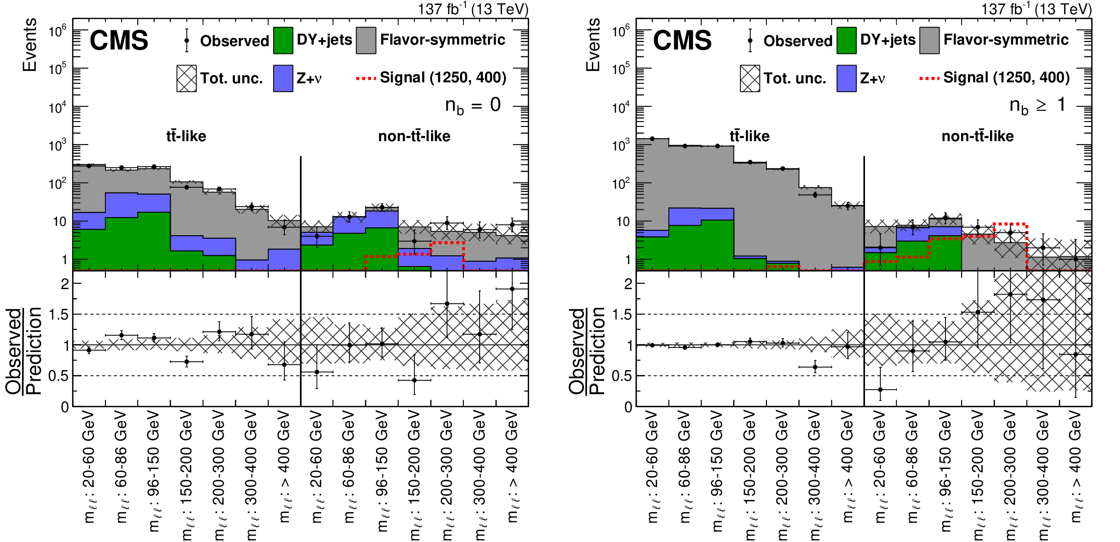
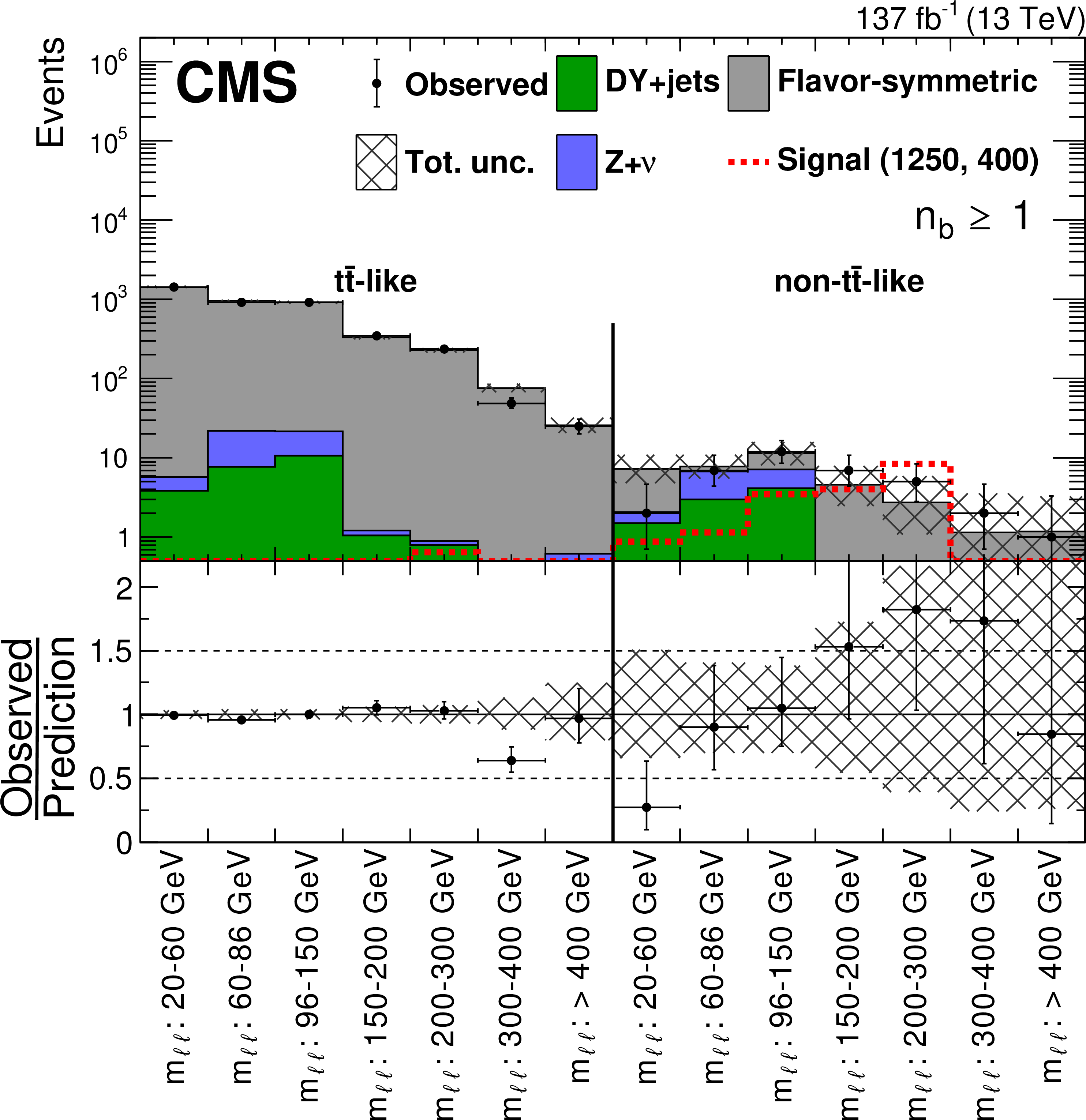
Results of the counting experiment in the edge search regions before the fits to data described in Section 8. In each search region, the number of observed events in data (black markers) is compared to the SM background prediction for the (left) b veto and (right) b tag categories. The hashed band shows the total uncertainty in the background prediction including statistical and systematic sources. The signal distribution corresponds to the $\tilde{\mathrm{b}}$ pair production model with the $\tilde{\mathrm{b}}$ ($\tilde{\chi}^0_2$) having a mass of 1250 (400) GeV. |

png pdf root |
Figure 7-a:
Results of the counting experiment in the edge search regions before the fits to data described in Section 8. In each search region, the number of observed events in data (black markers) is compared to the SM background prediction for the b veto category. The hashed band shows the total uncertainty in the background prediction including statistical and systematic sources. The signal distribution corresponds to the $\tilde{\mathrm{b}}$ pair production model with the $\tilde{\mathrm{b}}$ ($\tilde{\chi}^0_2$) having a mass of 1250 (400) GeV. |
png pdf root |
Figure 7-b:
Results of the counting experiment in the edge search regions before the fits to data described in Section 8. In each search region, the number of observed events in data (black markers) is compared to the SM background prediction for the b tag category. The hashed band shows the total uncertainty in the background prediction including statistical and systematic sources. The signal distribution corresponds to the $\tilde{\mathrm{b}}$ pair production model with the $\tilde{\mathrm{b}}$ ($\tilde{\chi}^0_2$) having a mass of 1250 (400) GeV. |
png pdf |
Figure 8:
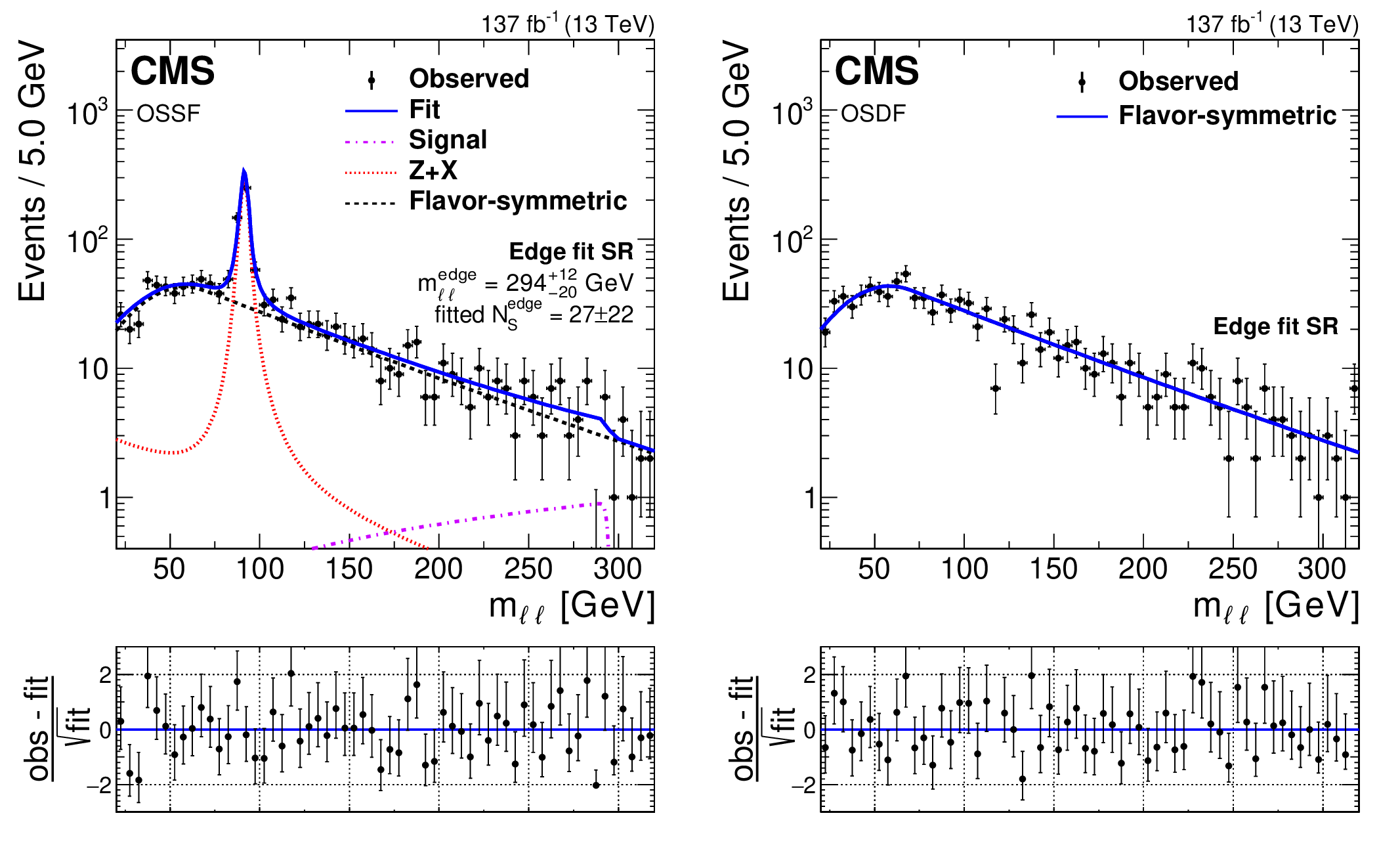
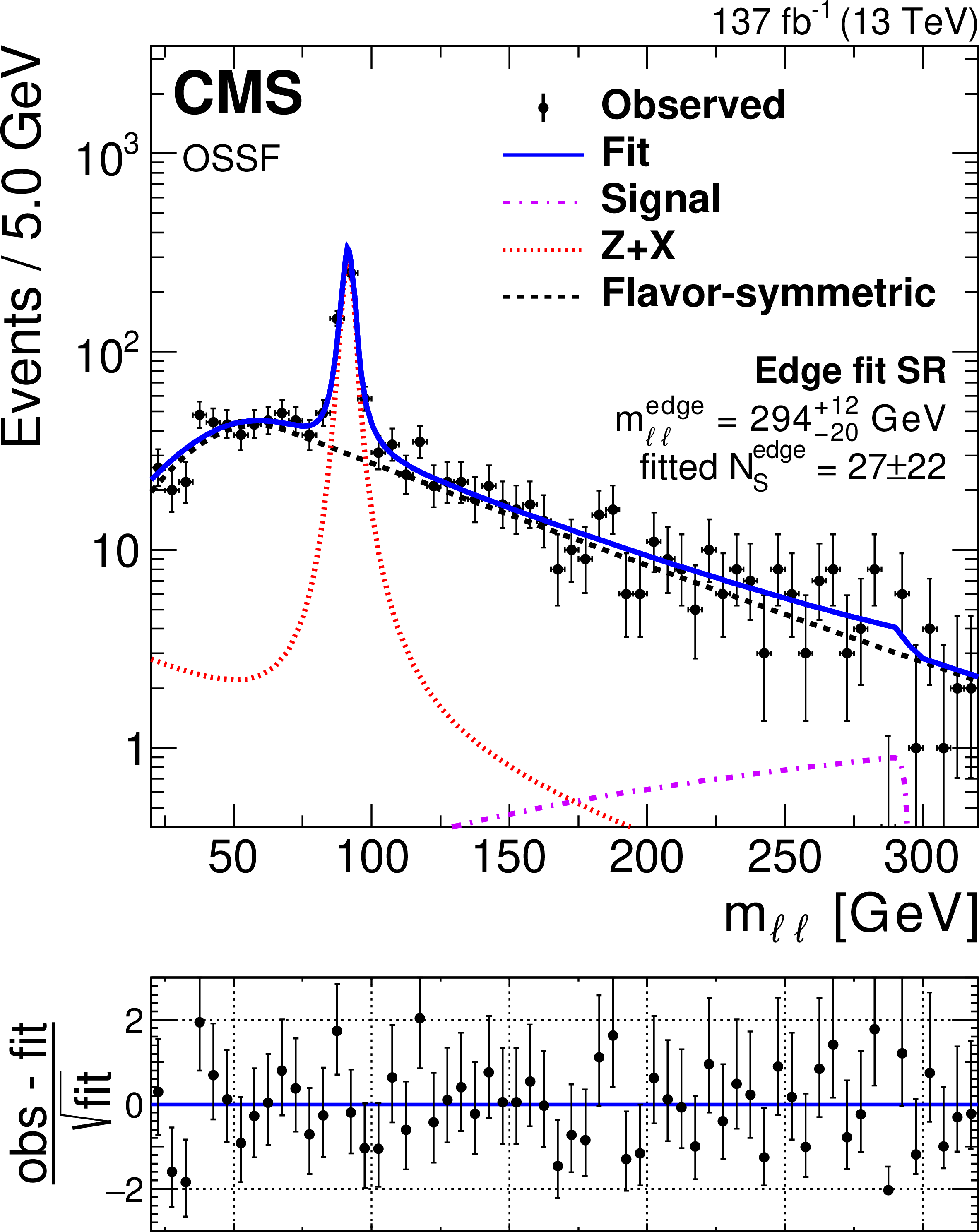
Fit the ${m_{\ell \ell}}$ distributions in data in the edge fit search regions under the signal+background hypothesis projected onto the (left) SF and (right) DF data samples. The fit shape is shown as a solid blue line. The individual fit components are indicated by the dashed and dotted lines. The flavor-symmetric background is shown as the black dashed line. The $\mathrm{Z} /\gamma ^*$+X background is displayed as the red dotted line. The extracted signal component is displayed as the purple dash-dotted line. The lower panel in each plot shows the difference between the observed data yield and the fit divided by the square root of the number of fitted events. |
png pdf |
Figure 8-a:
Fit the ${m_{\ell \ell}}$ distributions in data in the edge fit search regions under the signal+background hypothesis projected onto the SF data sample. The fit shape is shown as a solid blue line. The individual fit components are indicated by the dashed and dotted lines. The flavor-symmetric background is shown as the black dashed line. The $\mathrm{Z} /\gamma ^*$+X background is displayed as the red dotted line. The extracted signal component is displayed as the purple dash-dotted line. The lower panel shows the difference between the observed data yield and the fit divided by the square root of the number of fitted events. |

png pdf |
Figure 8-b:
Fit the ${m_{\ell \ell}}$ distribution in data in the edge fit search regions under the signal+background hypothesis projected onto the DF data sample. The fit shape is shown as a solid blue line. The lower panel shows the difference between the observed data yield and the fit divided by the square root of the number of fitted events. |
png pdf root |
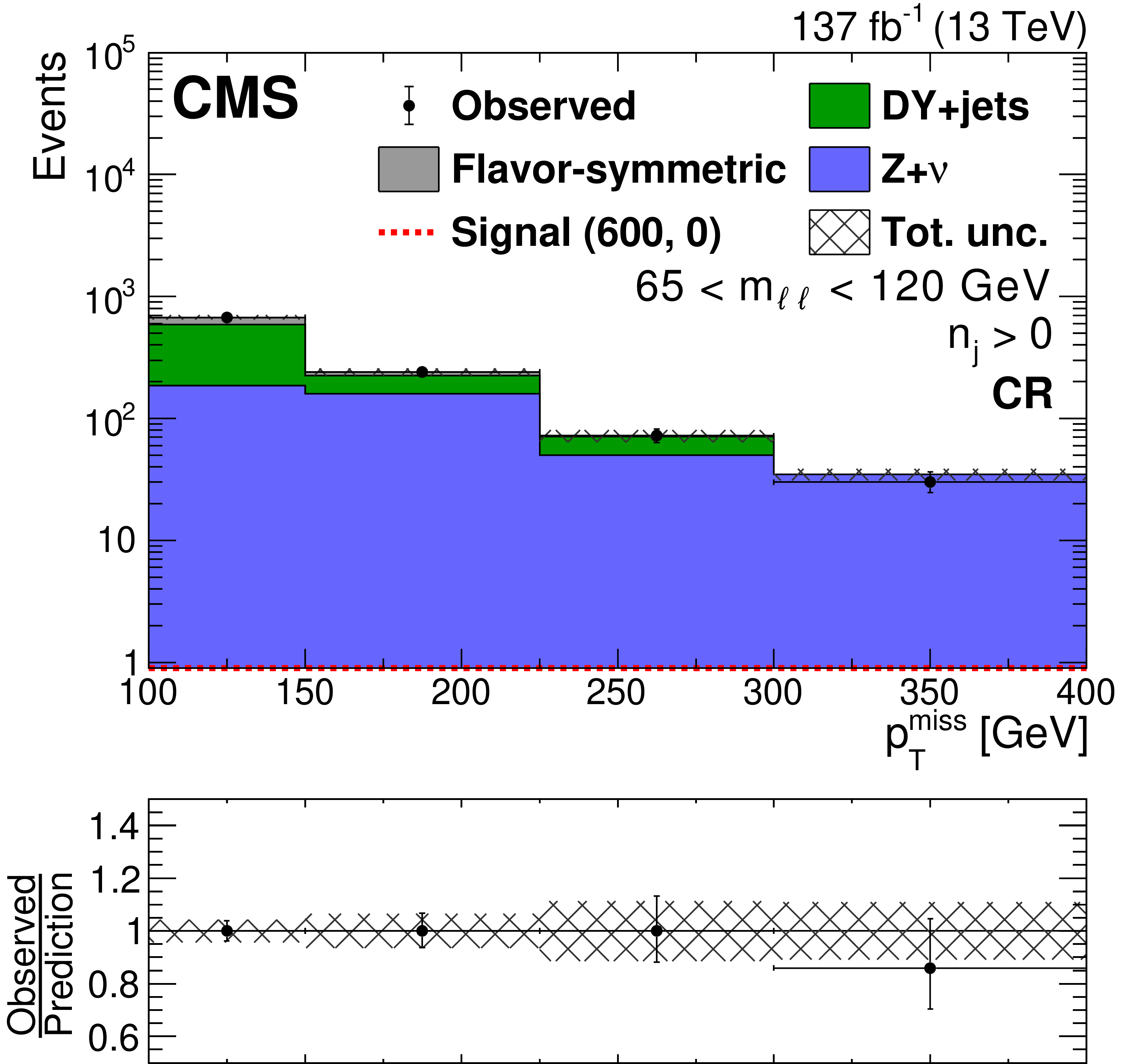
Figure 9:
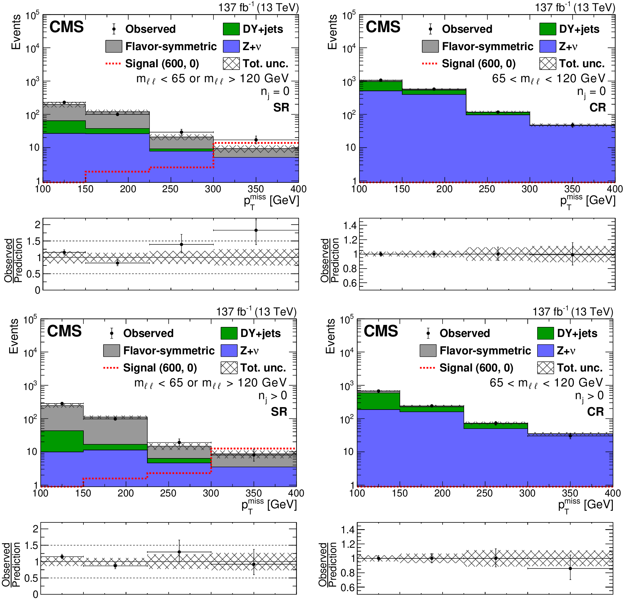
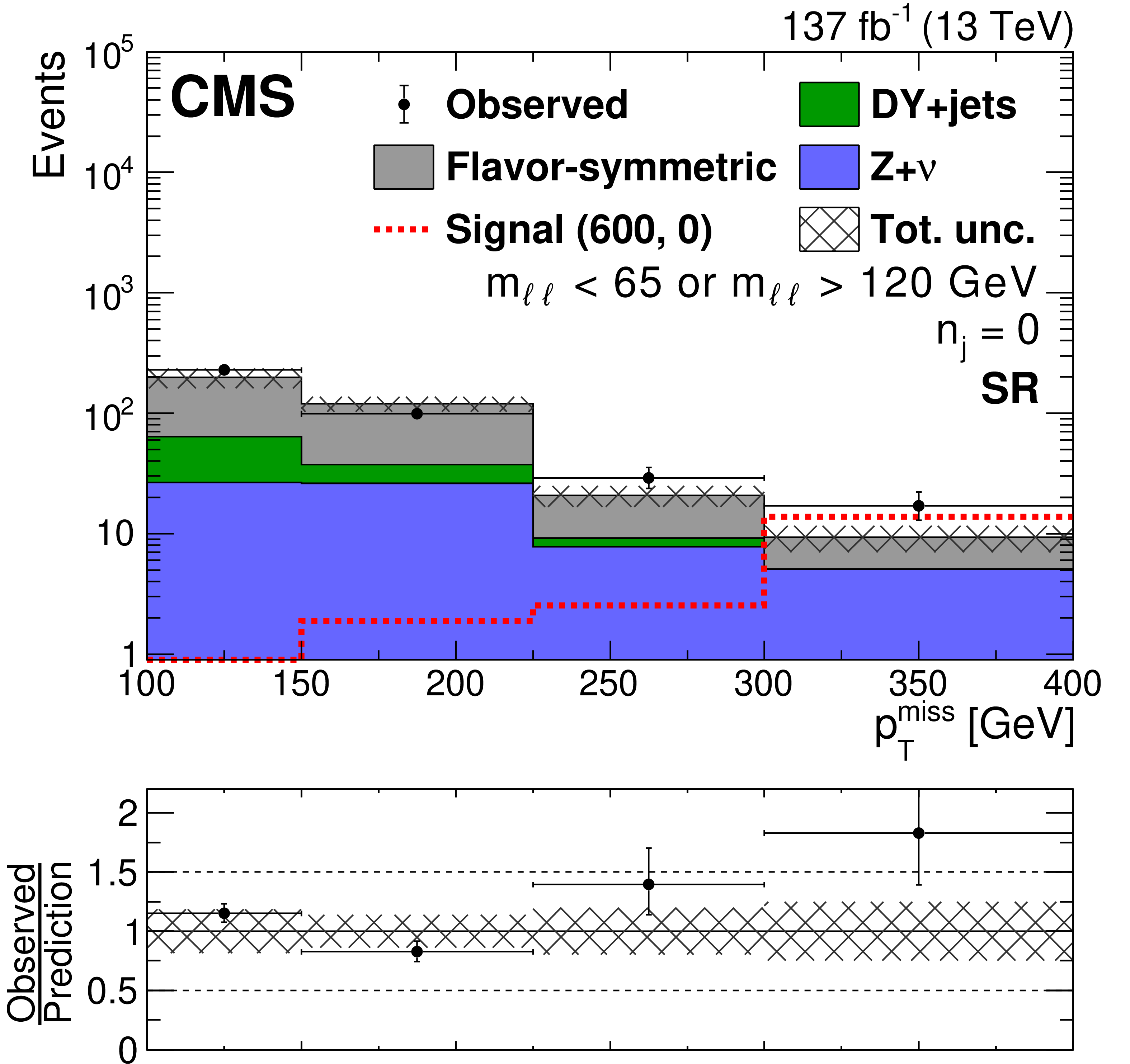
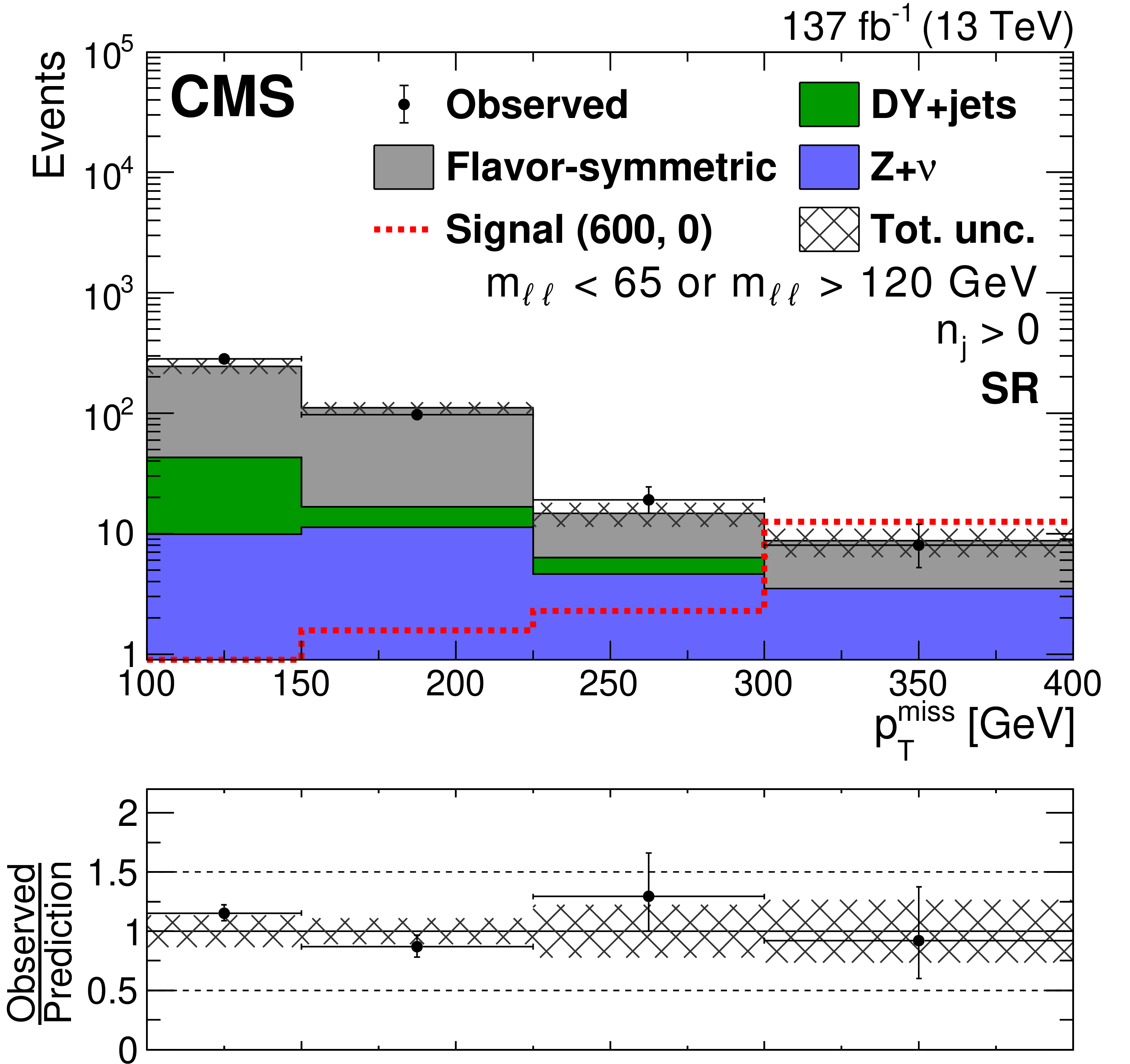
Distribution of ${{p_{\mathrm {T}}} ^\text {miss}}$ for events in the slepton (left) search regions and (right) control regions obtained by inverting the ${m_{\ell \ell}}$ selection used to obtain the DY background normalization for regions (upper) without jets and (lower) with jets. A background-only fit to data in the control region has been performed to determine the DY+jets contribution as discussed in Section 8. The lower panel of each plot shows the ratio of observed data to the SM prediction in each ${{p_{\mathrm {T}}} ^\text {miss}}$ bin. The hashed band shows the total uncertainty in the background prediction including statistical and systematic sources. The signal ${{p_{\mathrm {T}}} ^\text {miss}}$ distribution corresponds to the direct slepton pair production model with a slepton mass of 600 GeV and a massless $\tilde{\chi}^0_1$ particle. The last bin includes overflow events. |
png pdf root |
Figure 9-a:
Distribution of ${{p_{\mathrm {T}}} ^\text {miss}}$ for events in the slepton search region obtained by inverting the ${m_{\ell \ell}}$ selection used to obtain the DY background normalization for regions without jets. The lower panel shows the ratio of observed data to the SM prediction in each ${{p_{\mathrm {T}}} ^\text {miss}}$ bin. The hashed band shows the total uncertainty in the background prediction including statistical and systematic sources. The signal ${{p_{\mathrm {T}}} ^\text {miss}}$ distribution corresponds to the direct slepton pair production model with a slepton mass of 600 GeV and a massless $\tilde{\chi}^0_1$ particle. The last bin includes overflow events. |

png pdf root |
Figure 9-b:
Distribution of ${{p_{\mathrm {T}}} ^\text {miss}}$ for events in the slepton control region obtained by inverting the ${m_{\ell \ell}}$ selection used to obtain the DY background normalization for regions without jets. A background-only fit to data in the control region has been performed to determine the DY+jets contribution as discussed in Section 8. The lower panel shows the ratio of observed data to the SM prediction in each ${{p_{\mathrm {T}}} ^\text {miss}}$ bin. The hashed band shows the total uncertainty in the background prediction including statistical and systematic sources. The last bin includes overflow events. |
png pdf root |
Figure 9-c:
Distribution of ${{p_{\mathrm {T}}} ^\text {miss}}$ for events in the slepton search region obtained by inverting the ${m_{\ell \ell}}$ selection used to obtain the DY background normalization for regions with jets. The lower panel shows the ratio of observed data to the SM prediction in each ${{p_{\mathrm {T}}} ^\text {miss}}$ bin. The hashed band shows the total uncertainty in the background prediction including statistical and systematic sources. The signal ${{p_{\mathrm {T}}} ^\text {miss}}$ distribution corresponds to the direct slepton pair production model with a slepton mass of 600 GeV and a massless $\tilde{\chi}^0_1$ particle. The last bin includes overflow events. |
png pdf root |
Figure 9-d:
Distribution of ${{p_{\mathrm {T}}} ^\text {miss}}$ for events in the slepton control region obtained by inverting the ${m_{\ell \ell}}$ selection used to obtain the DY background normalization for regions with jets. A background-only fit to data in the control region has been performed to determine the DY+jets contribution as discussed in Section 8. The lower panel shows the ratio of observed data to the SM prediction in each ${{p_{\mathrm {T}}} ^\text {miss}}$ bin. The hashed band shows the total uncertainty in the background prediction including statistical and systematic sources. The last bin includes overflow events. |
png pdf root |
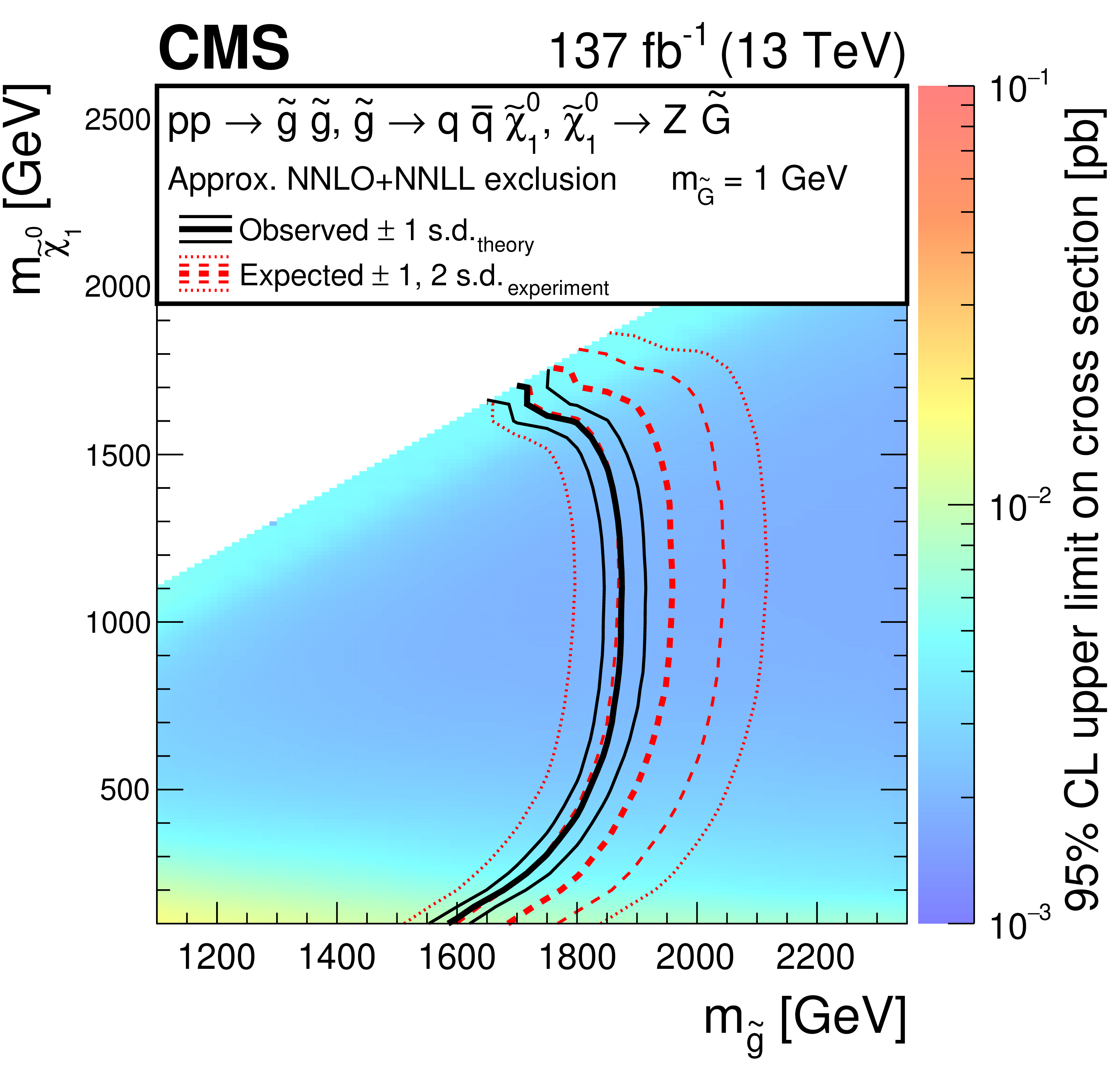
Figure 10:
Cross section upper limits and exclusion contours at 95% CL for an SMS model of GMSB gluino pair production, as a function of the ${\mathrm{\tilde{g}}}$ and $\tilde{\chi}^0_1$ masses, obtained from the results in the strong-production on-Z search regions. The area enclosed by the thick black curve represents the observed exclusion region, while the dashed red lines indicate the expected limits and their $ \pm $1 and $ \pm $2 s.d. ranges. The thin black lines show the effect of the theoretical uncertainties on the signal cross section. |
png pdf root |
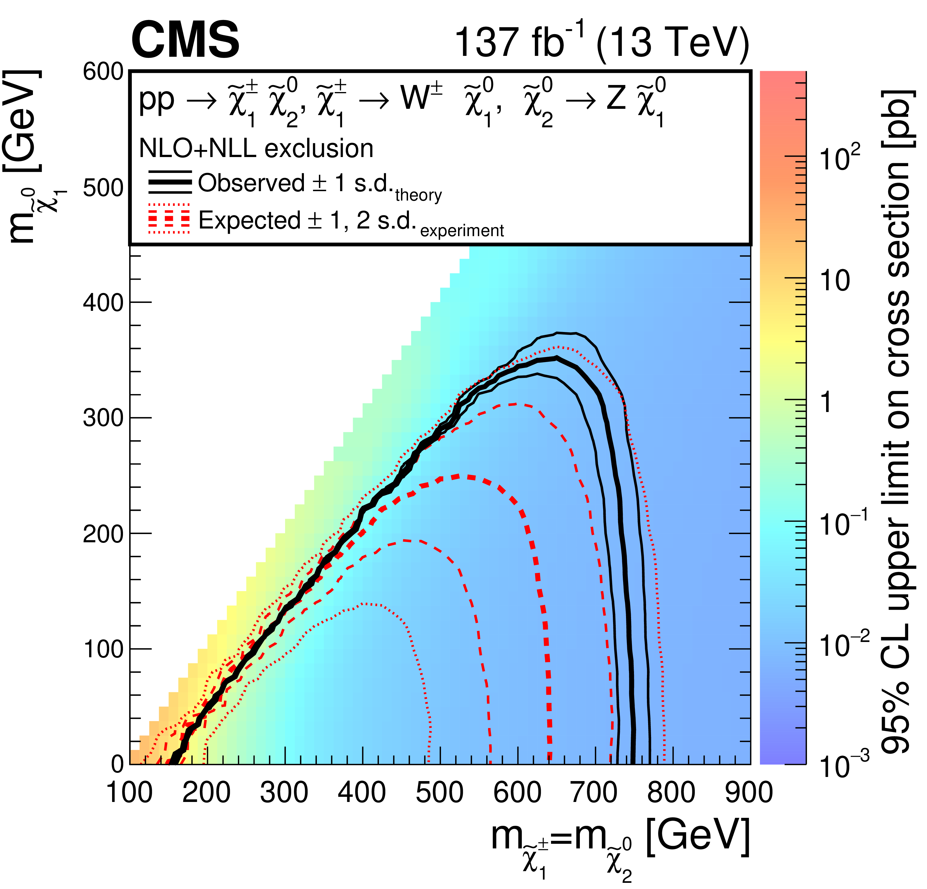
Figure 11:
Cross section upper limits and exclusion contours at 95% CL for an SMS model of $\tilde{\chi}^{\pm}_1 \tilde{\chi}^0_2$ production, with signatures containing a W and a Z bosons, as a function of the $\tilde{\chi}^{\pm}_1 /\tilde{\chi}^0_2$ and $\tilde{\chi}^0_1$ masses, obtained from the results in the EW-production on-Z search regions. The area enclosed by the thick black curve represents the observed exclusion region, while the dashed red lines indicate the expected limits and their $ \pm $1 and $ \pm $2 s.d. ranges. The thin black lines show the effect of the theoretical uncertainties on the signal cross section. |
png pdf |
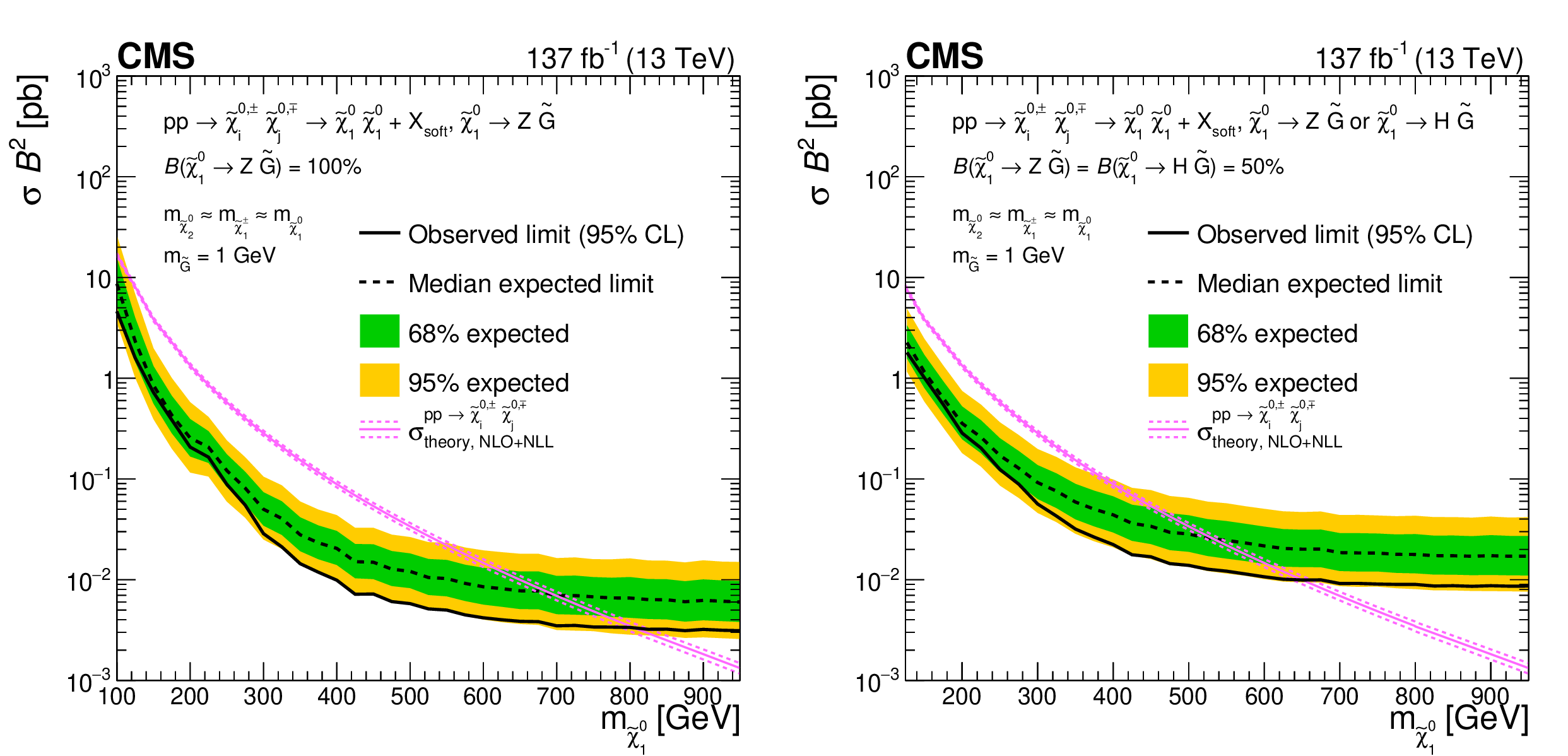
Figure 12:
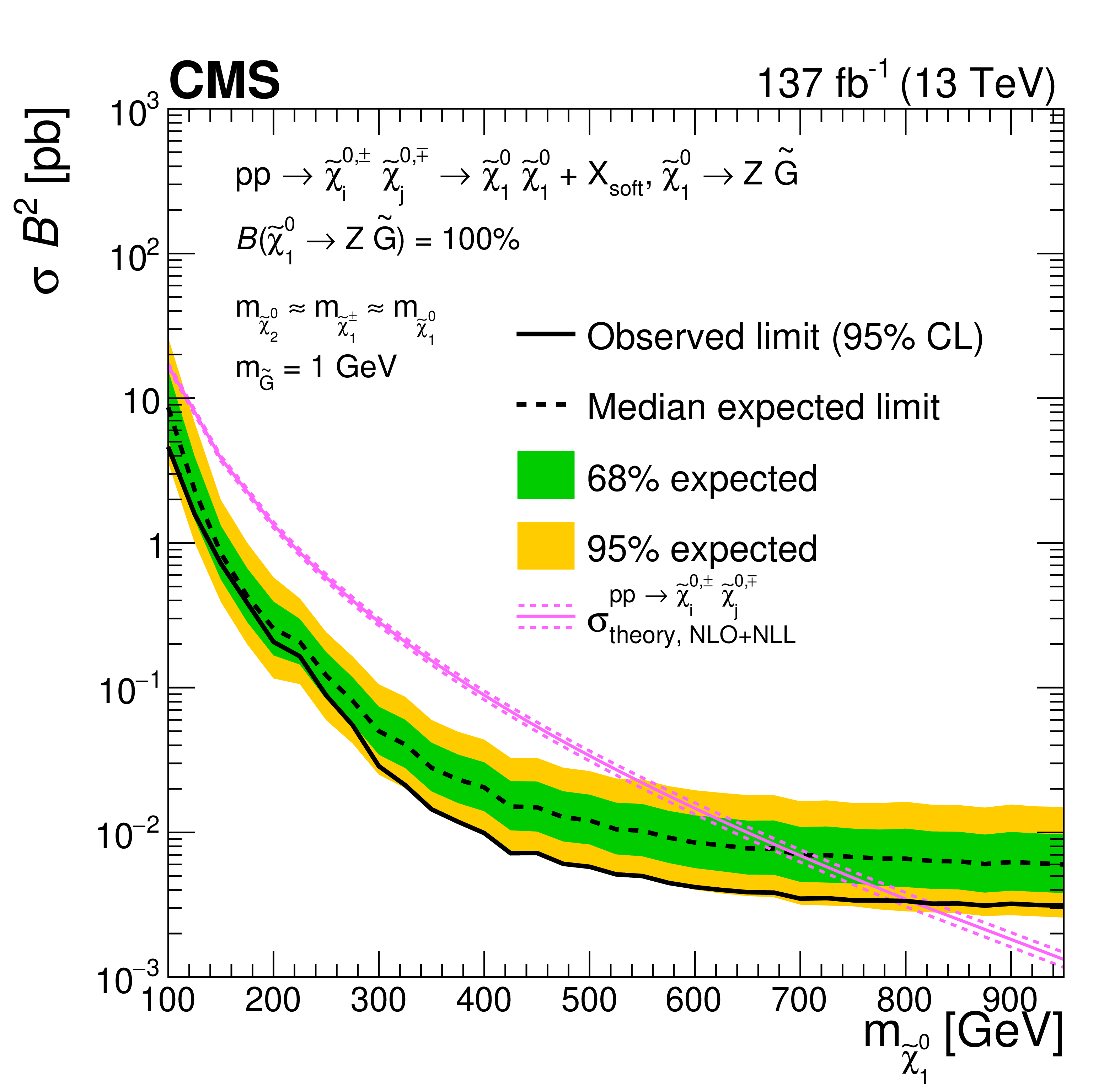
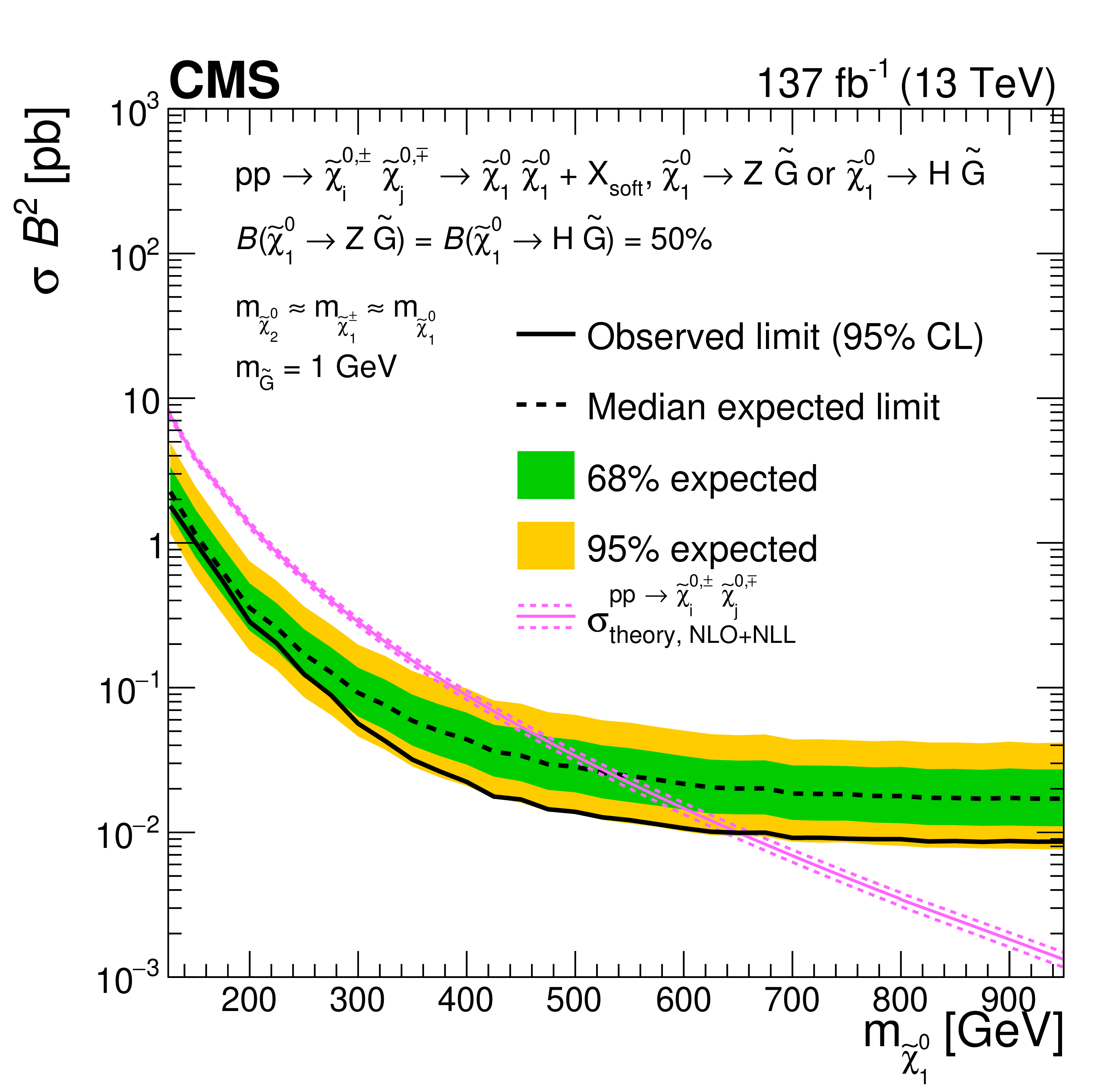
Production cross section upper limits at 95% CL as a function of the $\tilde{\chi}^0_1$ mass, for a model of EW $\tilde{\chi}^0_1$ pair production, where either (left) both $\tilde{\chi}^0_1$ decay into a Z boson with a 100% branching fraction ($\mathcal {B}$), or (right) each $\tilde{\chi}^0_1$ can decay to a Z or an H with equal probability. The model assumes the production of mass-degenerate neutralinos and charginos that decay into $\tilde{\chi}^0_1$ possibly emitting soft particles, labeled as $\mathrm{X} _{\text {soft}}$. The magenta curve shows the theoretical production cross section with its uncertainty. The solid (dashed) black line represents the observed (median expected) exclusion. The inner green (outer yellow) band indicates the region containing 68 (95)% of the distribution of limits expected under the background-only hypothesis. |
png pdf root |
Figure 12-a:
Production cross section upper limit at 95% CL as a function of the $\tilde{\chi}^0_1$ mass, for a model of EW $\tilde{\chi}^0_1$ pair production, where both $\tilde{\chi}^0_1$ decay into a Z boson with a 100% branching fraction ($\mathcal {B}$). The model assumes the production of mass-degenerate neutralinos and charginos that decay into $\tilde{\chi}^0_1$ possibly emitting soft particles, labeled as $\mathrm{X} _{\text {soft}}$. The magenta curve shows the theoretical production cross section with its uncertainty. The solid (dashed) black line represents the observed (median expected) exclusion. The inner green (outer yellow) band indicates the region containing 68 (95)% of the distribution of limits expected under the background-only hypothesis. |
png pdf root |
Figure 12-b:
Production cross section upper limit at 95% CL as a function of the $\tilde{\chi}^0_1$ mass, for a model of EW $\tilde{\chi}^0_1$ pair production, where each $\tilde{\chi}^0_1$ can decay to a Z or an H with equal probability. The model assumes the production of mass-degenerate neutralinos and charginos that decay into $\tilde{\chi}^0_1$ possibly emitting soft particles, labeled as $\mathrm{X} _{\text {soft}}$. The magenta curve shows the theoretical production cross section with its uncertainty. The solid (dashed) black line represents the observed (median expected) exclusion. The inner green (outer yellow) band indicates the region containing 68 (95)% of the distribution of limits expected under the background-only hypothesis. |
png pdf |
Figure 13:
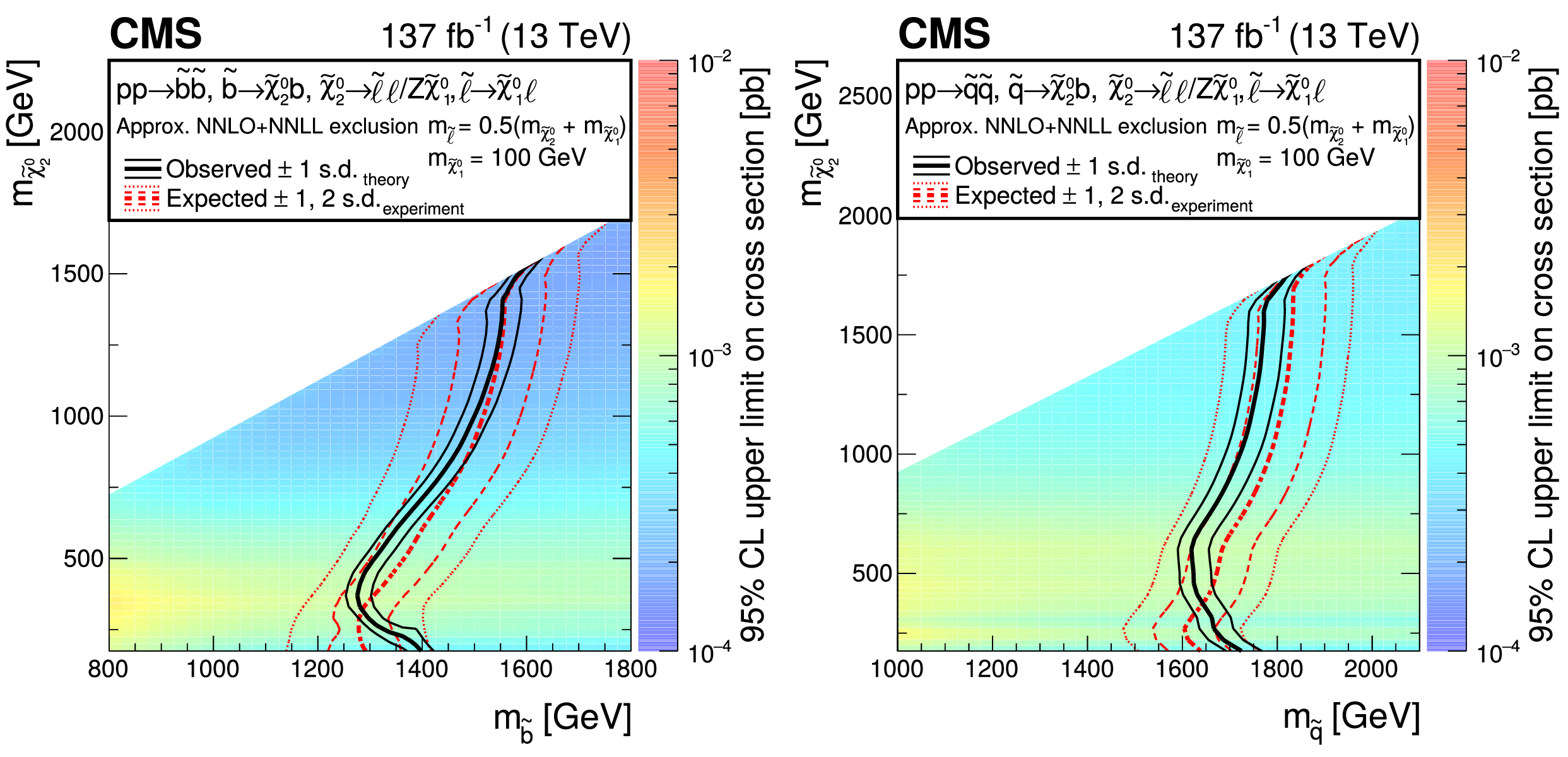
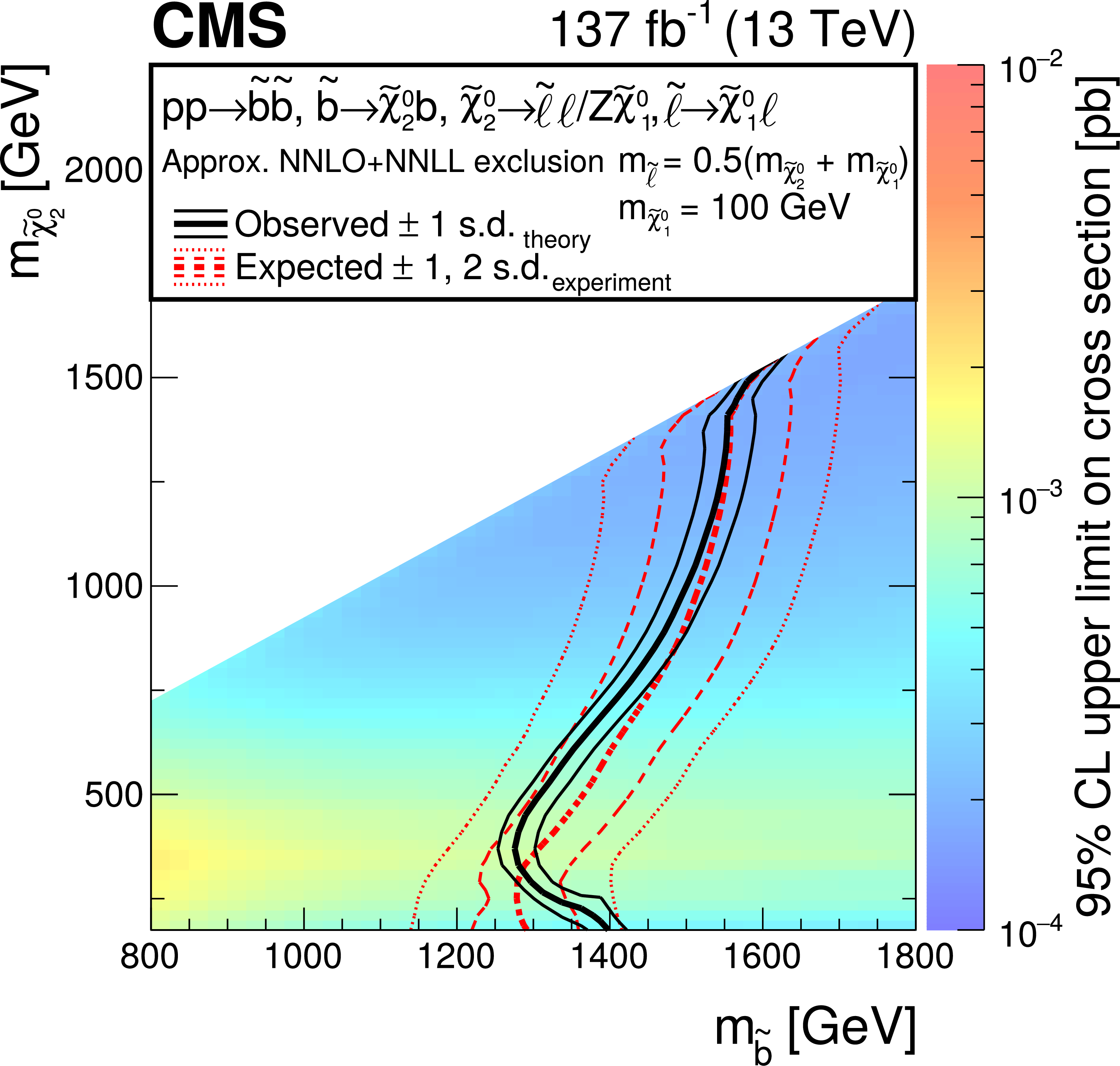
Cross section upper limits and exclusion contours at 95% CL for SMS models of (left) bottom and (right) light-flavor squark pair production. In these models, each squark decays into a quark and a $\tilde{\chi}^0_2$, and the $\tilde{\chi}^0_2$ then decays via an intermediate slepton, forming a kinematic edge in the ${m_{\ell \ell}}$ distribution. The limits are obtained from the results in the edge search regions, and are shown as a function of the (left) $\tilde{\mathrm{b}}$ or (right) $\tilde{\mathrm{q}}$ and $\tilde{\chi}^0_2$ masses. The thick black curve represents the observed upper limit on the squark mass, while the dashed red lines indicate the expected limits and their $ \pm $1 and $ \pm $2 s.d. ranges. The thin black lines show the effect of the theoretical uncertainties on the signal cross section. |
png pdf root |
Figure 13-a:
Cross section upper limits and exclusion contours at 95% CL for SMS models of bottom squark pair production. In these models, each squark decays into a quark and a $\tilde{\chi}^0_2$, and the $\tilde{\chi}^0_2$ then decays via an intermediate slepton, forming a kinematic edge in the ${m_{\ell \ell}}$ distribution. The limits are obtained from the results in the edge search regions, and are shown as a function of the $\tilde{\mathrm{b}}$ and $\tilde{\chi}^0_2$ masses. The thick black curve represents the observed upper limit on the squark mass, while the dashed red lines indicate the expected limits and their $ \pm $1 and $ \pm $2 s.d. ranges. The thin black lines show the effect of the theoretical uncertainties on the signal cross section. |

png pdf root |
Figure 13-b:
Cross section upper limits and exclusion contours at 95% CL for SMS models of light-flavor squark pair production. In these models, each squark decays into a quark and a $\tilde{\chi}^0_2$, and the $\tilde{\chi}^0_2$ then decays via an intermediate slepton, forming a kinematic edge in the ${m_{\ell \ell}}$ distribution. The limits are obtained from the results in the edge search regions, and are shown as a function of the $\tilde{\mathrm{q}}$ and $\tilde{\chi}^0_2$ masses. The thick black curve represents the observed upper limit on the squark mass, while the dashed red lines indicate the expected limits and their $ \pm $1 and $ \pm $2 s.d. ranges. The thin black lines show the effect of the theoretical uncertainties on the signal cross section. |
png pdf root |
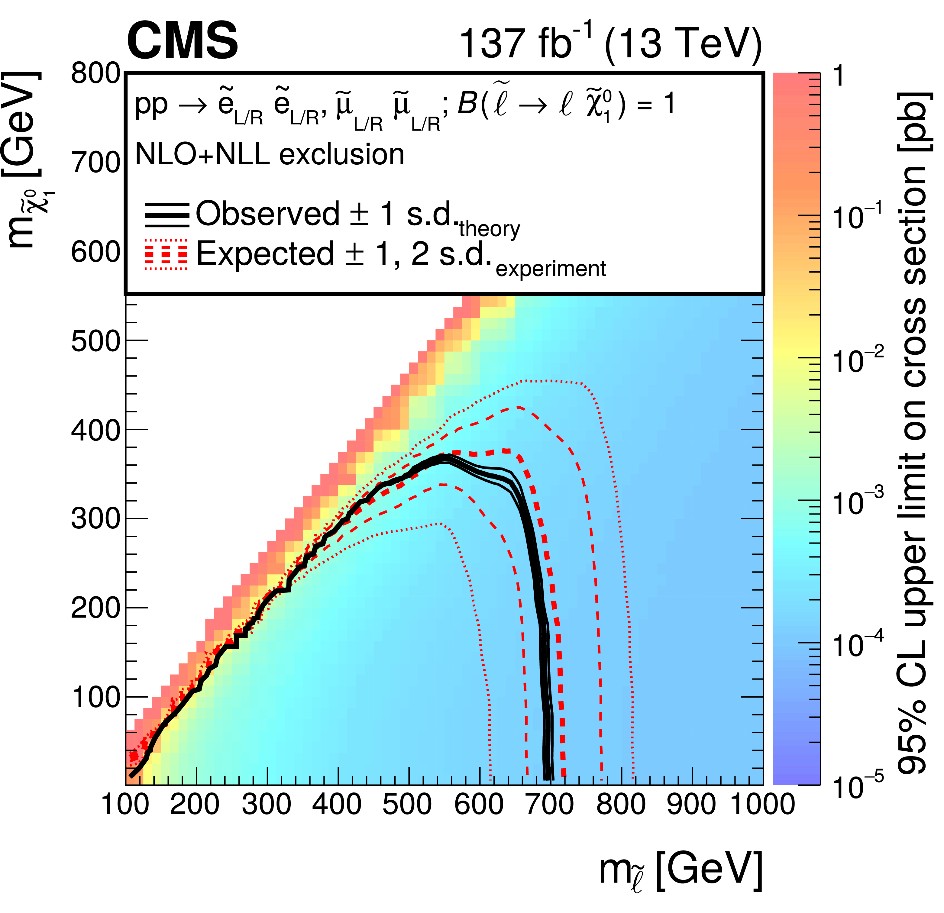
Figure 14:
Cross section upper limits and exclusion contours at 95% CL for an SMS model of slepton pair production, as a function of the slepton and $\tilde{\chi}^0_1$ masses, obtained from the results in the slepton search regions. The area enclosed by the thick black curve represents the observed exclusion region, while the dashed red lines indicate the expected limits and their $ \pm $1 and $ \pm $2 s.d. ranges. The thin black lines show the effect of the theoretical uncertainties in the signal cross section. |
| Tables | |
png pdf |
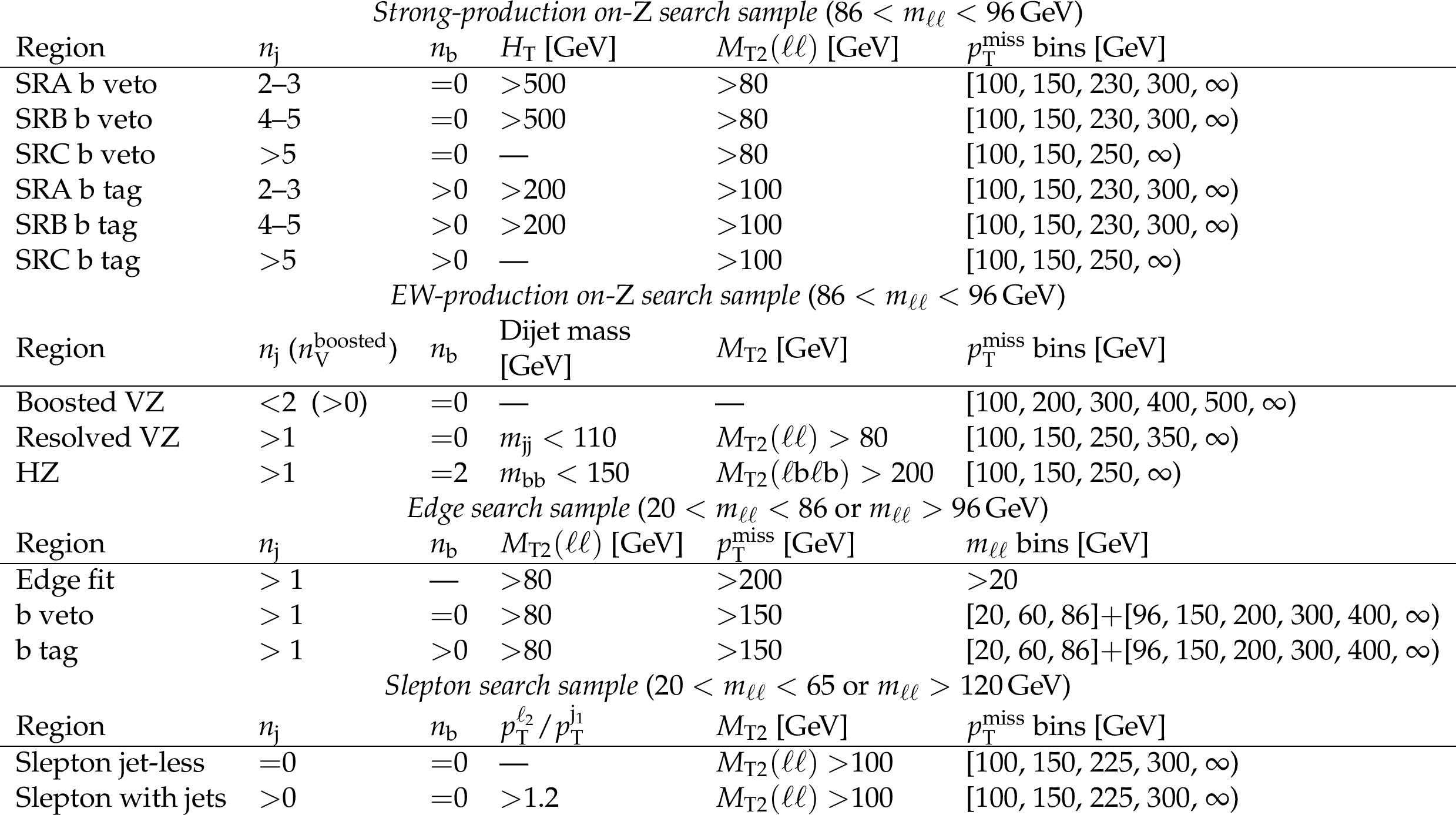
Table 1:
Summary of search category selections. In regions with the additional lepton veto selection, events containing additional leptons or charged isolated tracks are rejected. All the regions besides the edge search samples implement a veto to an additional lepton. The numbers in the rightmost column represent the edges of the bins that define the signal regions. Events in the edge search sample are further categorized as ${\mathrm{t} {}\mathrm{\bar{t}}} $-like and non-${\mathrm{t} {}\mathrm{\bar{t}}} $-like as described in Section 4.2.1. |
png pdf |
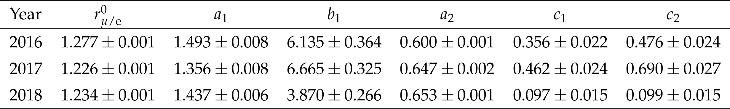
Table 2:
Summary of the ${r_{\mu /\mathrm{e}}}$ parameters obtained by fitting the lepton ${p_{\mathrm {T}}}$ and $\eta $, in a DY-enriched control region, for different data taking years. Only statistical uncertainties are shown. |
png pdf |
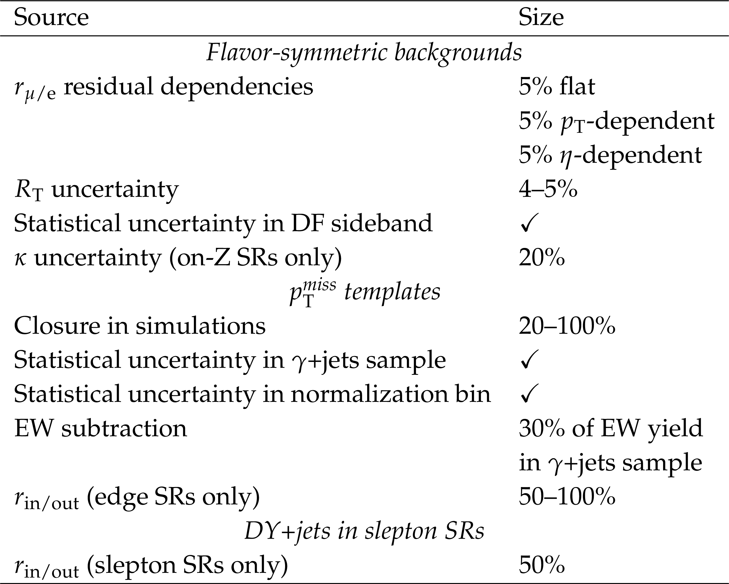
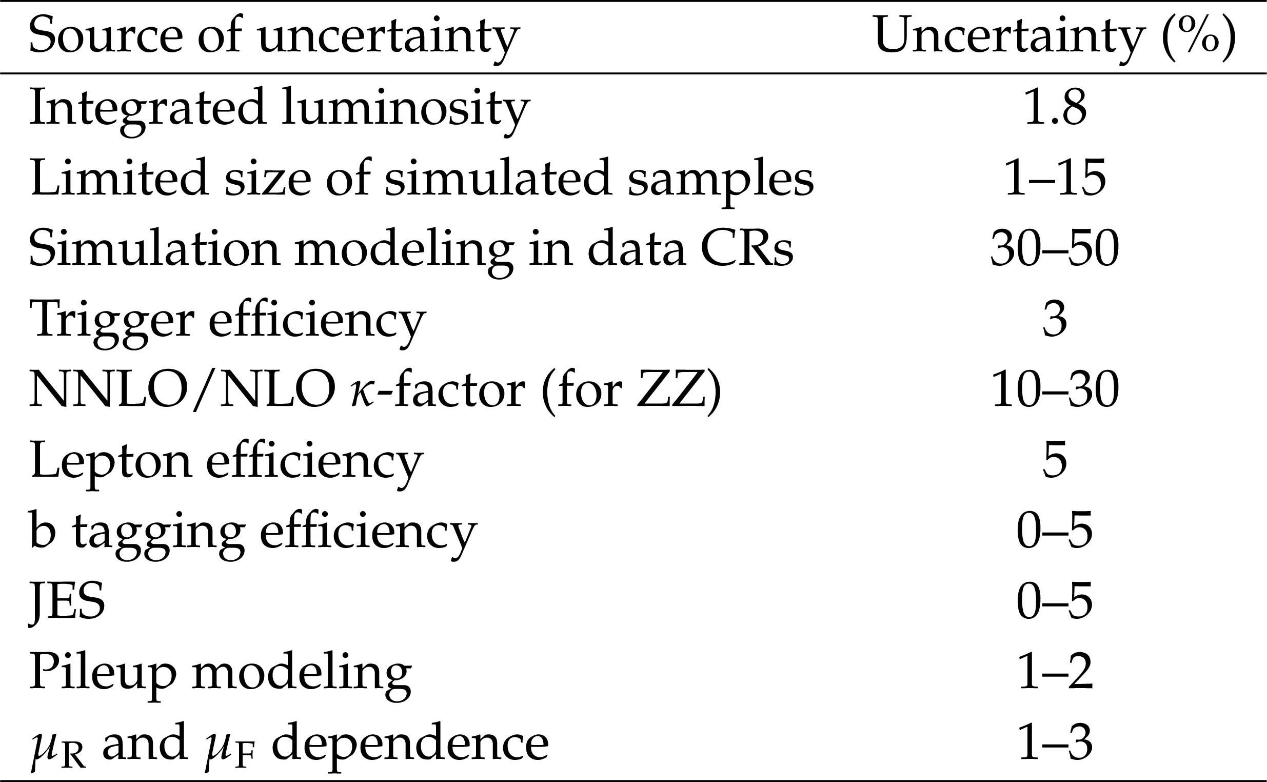
Table 3:
Summary of the uncertainties in background estimations performed on data. |
png pdf |
Table 4:
Summary of systematic uncertainties in the predicted Z+$\nu$ background yields, together with their typical sizes across the SRs. |
png pdf |
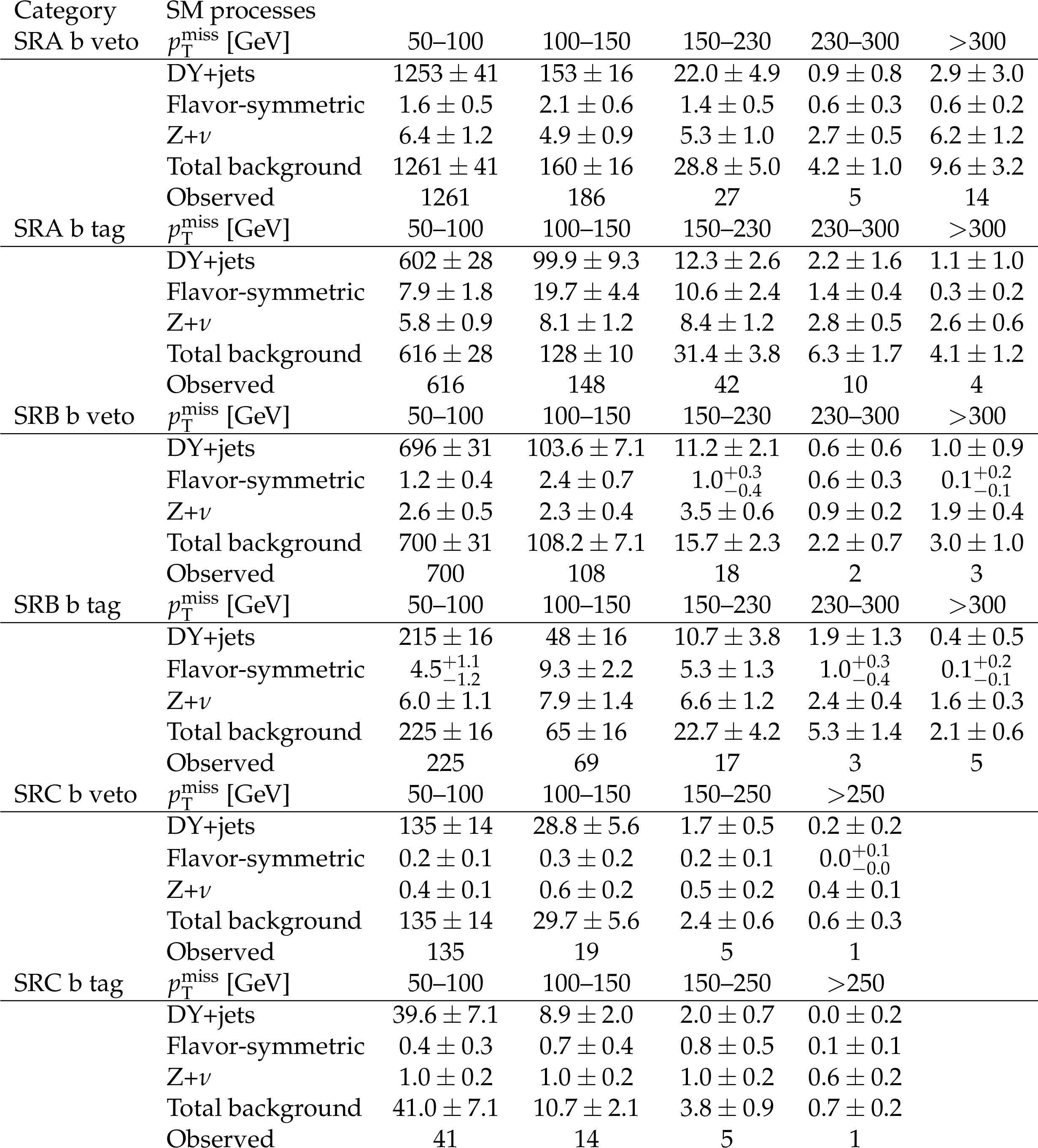
Table 5:
Predicted and observed event yields in the strong-production on-Z search regions, for each ${{p_{\mathrm {T}}} ^\text {miss}}$ bin as defined in Table 2 before the fits to data discussed in Section 8. Uncertainties include both statistical and systematic sources. The ${{p_{\mathrm {T}}} ^\text {miss}}$ template prediction in each SR is normalized to the first ${{p_{\mathrm {T}}} ^\text {miss}}$ bin of each distribution in data. |
png pdf |
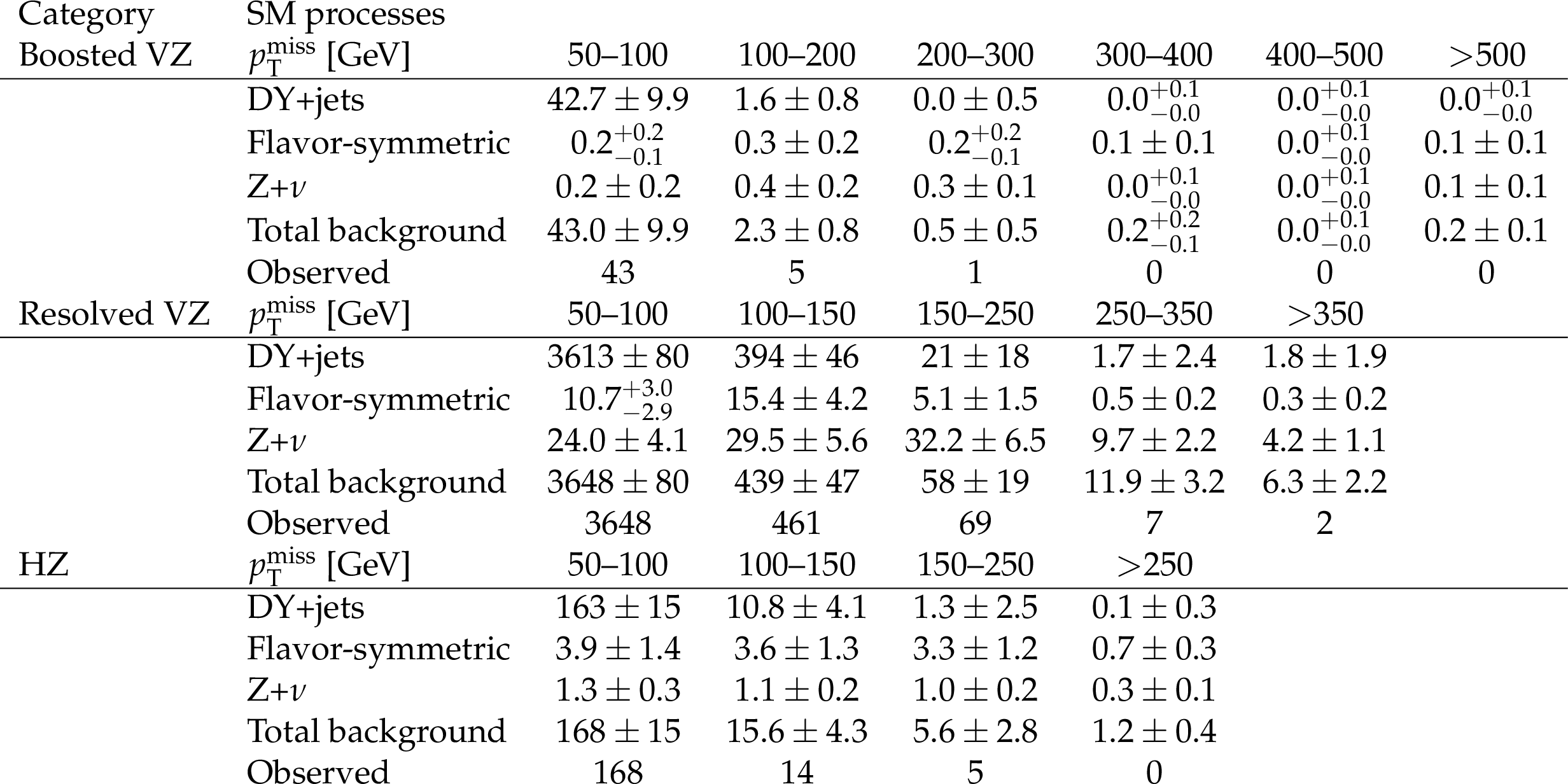
Table 6:
Predicted and observed event yields in the EW-production on-Z search regions, for each ${{p_{\mathrm {T}}} ^\text {miss}}$ \ bin as defined in Table 2 before the fits to data described in Section 8. Uncertainties include both statistical and systematic sources. The ${{p_{\mathrm {T}}} ^\text {miss}}$ template prediction in each SR is normalized to the first ${{p_{\mathrm {T}}} ^\text {miss}}$ bin of each distribution in data. |
png pdf |
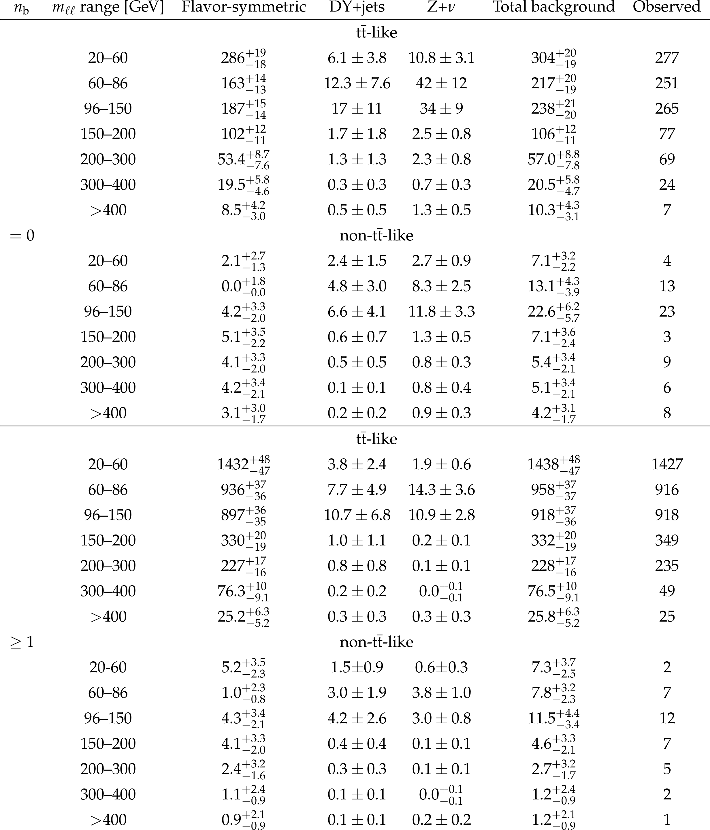
Table 7:
Predicted and observed yields in each bin of the edge search counting experiment as defined in Table 2 before the fits to data described in Section 8. Uncertainties include statistical and systematic sources. |
png pdf |
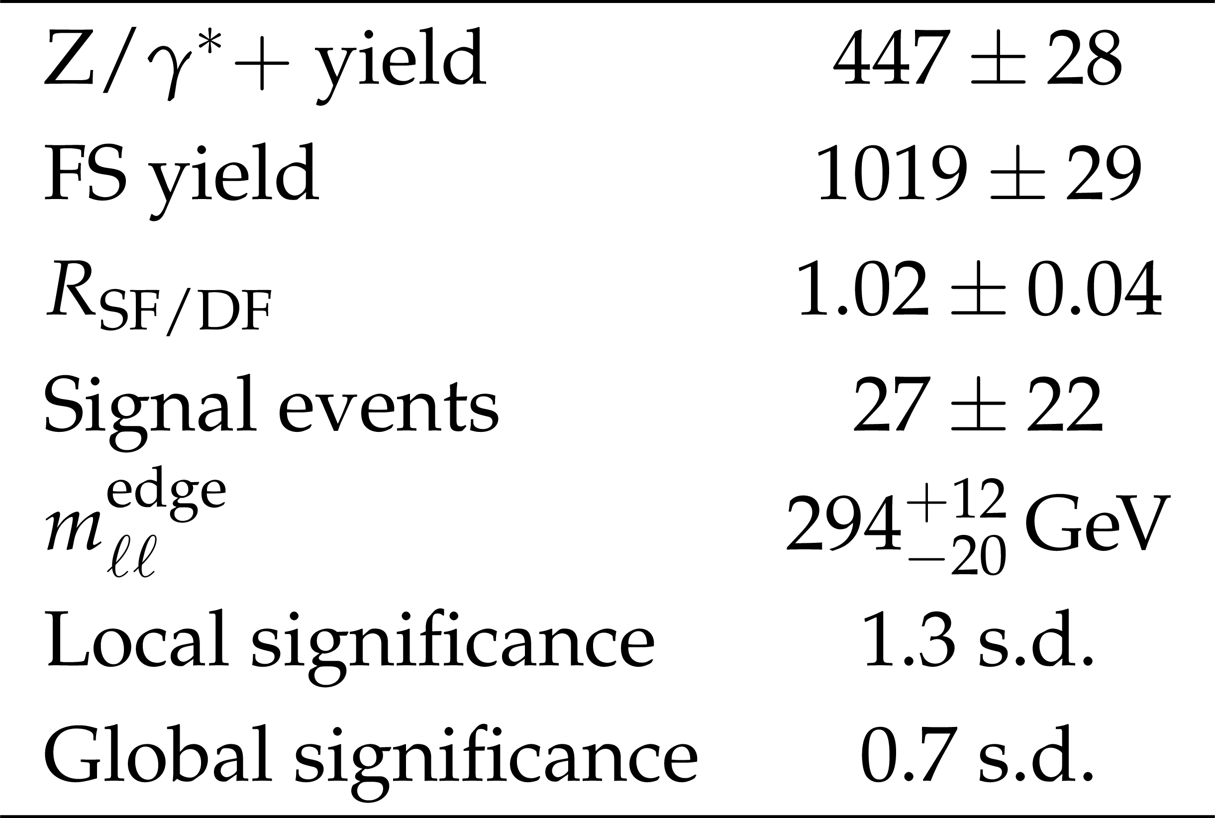
Table 8:
Results of the ${m_{\ell \ell}}$ unbinned maximum likelihood fit to data in the edge fit search region as defined in Table 2. The fitted yields of the $\mathrm{Z} /\gamma ^*$+X and flavor-symmetric background components are tabulated together with the fitted value of ${R_{\mathrm {SF/DF}}}$. The fitted signal contribution and the corresponding edge position are also shown. The local and global signal significances are expressed in terms of s.d. The uncertainties include both statistical and systematic sources. |
png pdf |
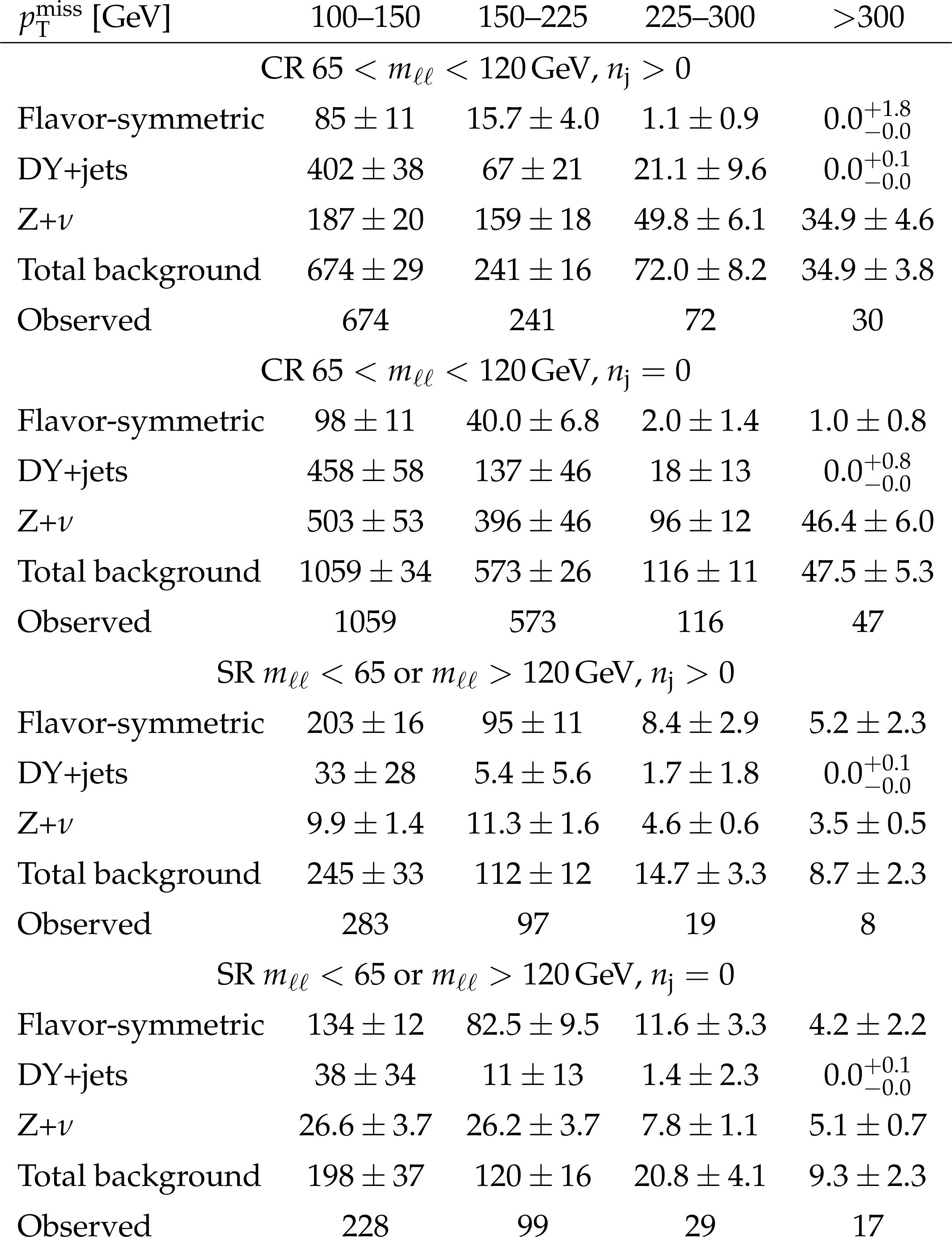
Table 9:
Predicted and observed event yields in the slepton search and control regions. A background-only fit to observation in the CR is performed to determine the DY+jets contribution as described in Section 8. Uncertainties include both statistical and systematic sources. |

png pdf |
Table 10:
Summary of the systematic uncertainties in the signal yields together with their typical sizes across the search regions and the SMS models under consideration. |
| Summary |
| A search is presented for phenomena beyond the standard model in events with two oppositely charged same-flavor leptons and missing transverse momentum in the final state. The search is performed in a sample of proton-proton collisions at $\sqrt{s} = $ 13 TeV collected with the CMS detector corresponding to an integrated luminosity of 137 fb$^{-1}$. Search regions are defined to be sensitive to a wide range of signatures. The observed event yields and distributions are found to be consistent with the expectations from the standard model. The results are used to set upper limits on the production cross sections of simplified models of supersymmetry. Gluino masses are excluded up to 1875 GeV, light-flavor (bottom) squark masses up to 1800 (1600) GeV, chargino (neutralino) masses up to 750 (800) GeV, and slepton masses up to 700 GeV, typically extending the reach over previous CMS results by a few hundred GeV. |
| Additional Figures | |

png pdf root |
Additional Figure 1:
Pre-fit background covariance matrix (left) and correlation matrix (right), for the slepton signal regions. |
png pdf root |
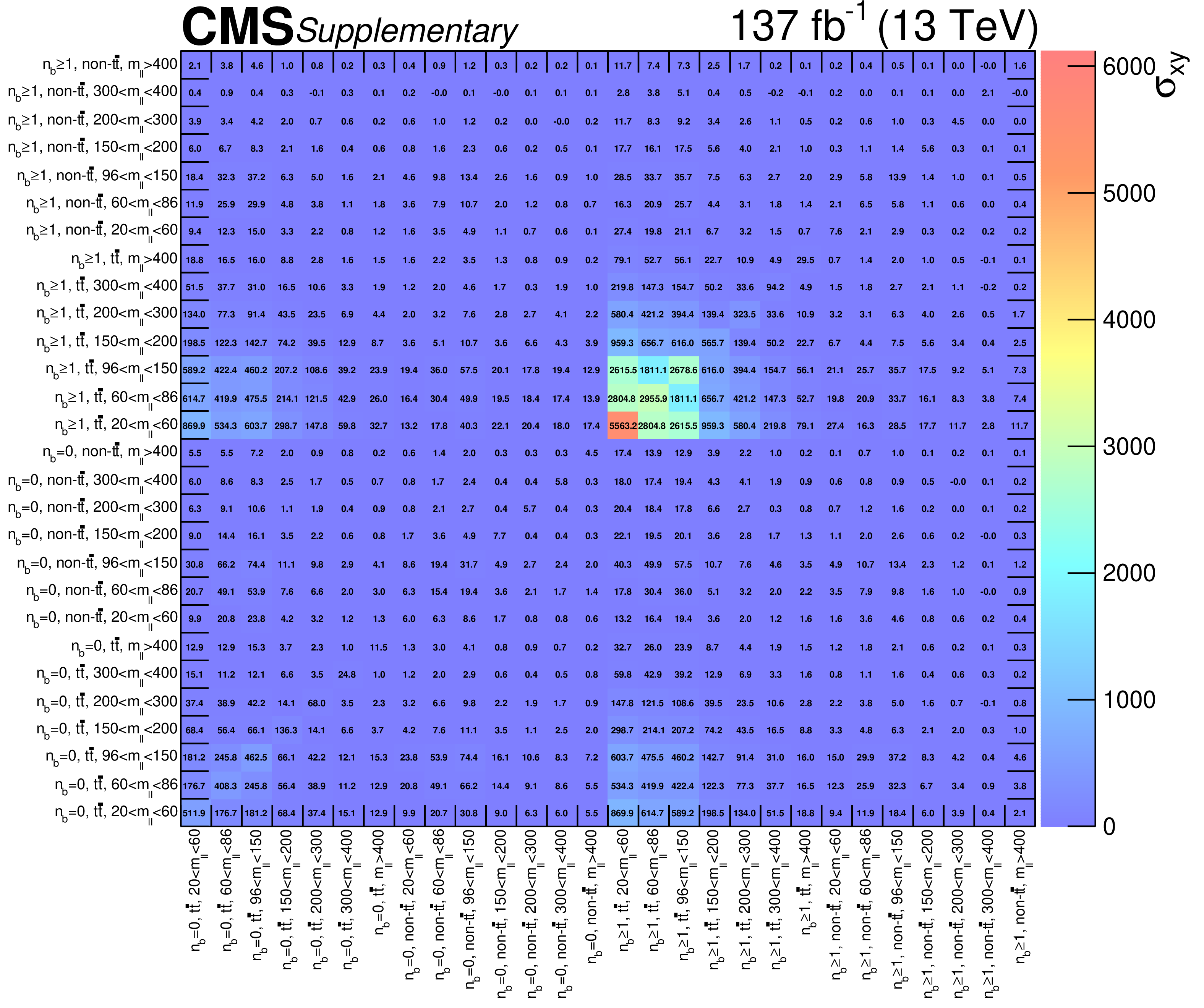
Additional Figure 2:
Pre-fit background covariance matrix for the edge signal regions. |

png pdf root |
Additional Figure 3:
Pre-fit background covariance matrix for the on-Z strong signal regions. |
png pdf root |
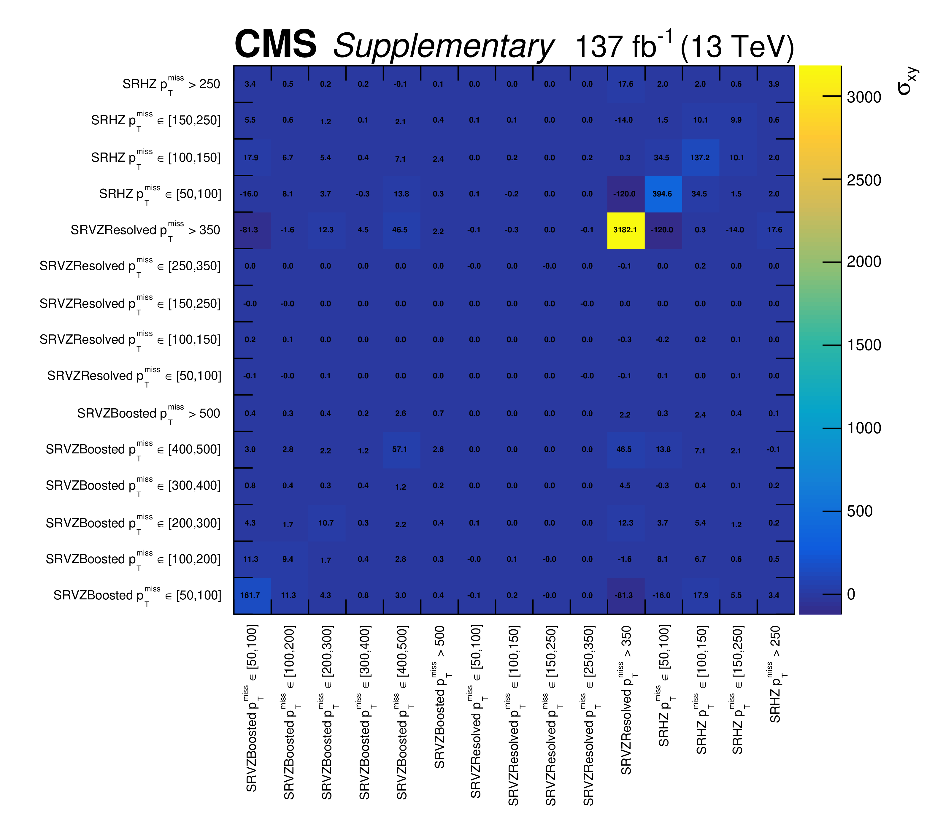
Additional Figure 4:
Pre-fit background covariance matrix for the on-Z electroweak signal regions. |
| Additional Tables | |
png pdf |
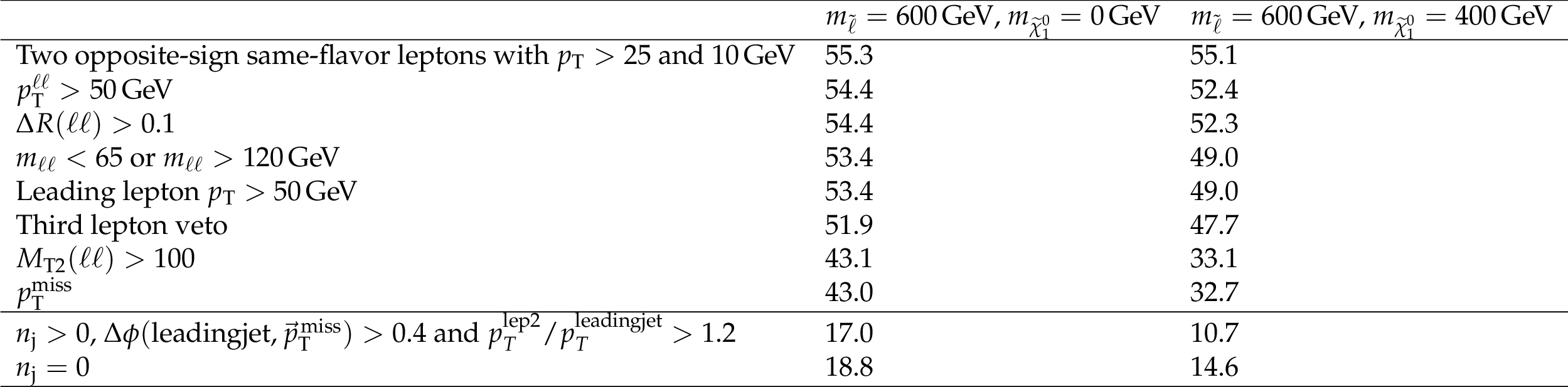
Additional Table 1:
Number of events slepton signal events selected after each selection criterion in the slepton signal regions for models assuming (middle column) $m_{{{\ell}}} = $ 600 GeV and $m_{\tilde{\chi}^{0}_{1}} = $ 0 GeV, and (right column) $m_{{{\ell}}} = $ 600 GeV and $m_{\tilde{\chi}^{0}_{1}} = $ 400 GeV, respectively. |
png pdf |
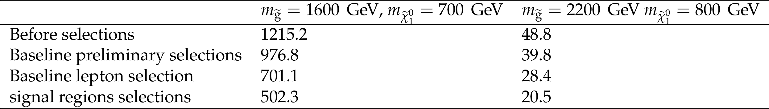
Additional Table 2:
Number of gluino production signal events selected after each selection criterion in the strong signal regions for models assuming (middle column) $m_{{\mathrm {\tilde{g}}}} = $ 1600 GeV, $m_{\tilde{\chi}^{0}_{1}} = $ 700 GeV and (right column) $m_{{\mathrm {\tilde{g}}}} = $ 2200 GeV, $m_{\tilde{\chi}^{0}_{1}} = $ 800 GeV |
png pdf |
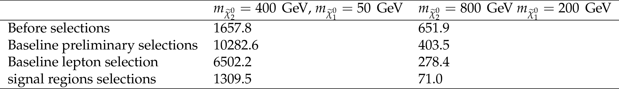
Additional Table 3:
Number of chargino-neutralino signal events selected after each selection criterion in the strong signal regions for models assuming (middle column) $m_{{\tilde{\chi}^{0}_{2}}} = $ 400 GeV, $m_{\tilde{\chi}^{0}_{1}} = $ 50 GeV and (right column) $m_{{\tilde{\chi}^{0}_{2}}} = $ 800 GeV, $m_{\tilde{\chi}^{0}_{1}} = $ 200 GeV |
png pdf |
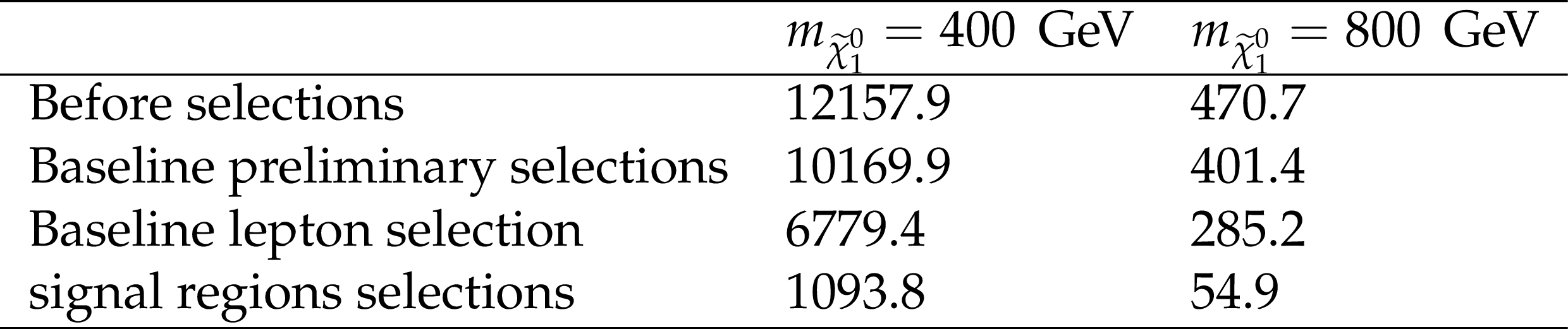
Additional Table 4:
Number of TChiZZ signal events selected after each selection criterion in the strong signal regions for models assuming (middle column) $m_{\tilde{\chi}^{0}_{1}} = $ 400 GeV and (right column) $m_{\tilde{\chi}^{0}_{1}} = $ 800 GeV |

png pdf |
Additional Table 5:
Number of HZ signal events (composite TChiHZ and TChiZZ with 50% branching fractions) selected after each selection criterion in the strong signal regions for models assuming (middle column) $m_{\tilde{\chi}^{0}_{1}} = $ 400 GeV and (right column) $m_{\tilde{\chi}^{0}_{1}} = $ 800 GeV |
png pdf |
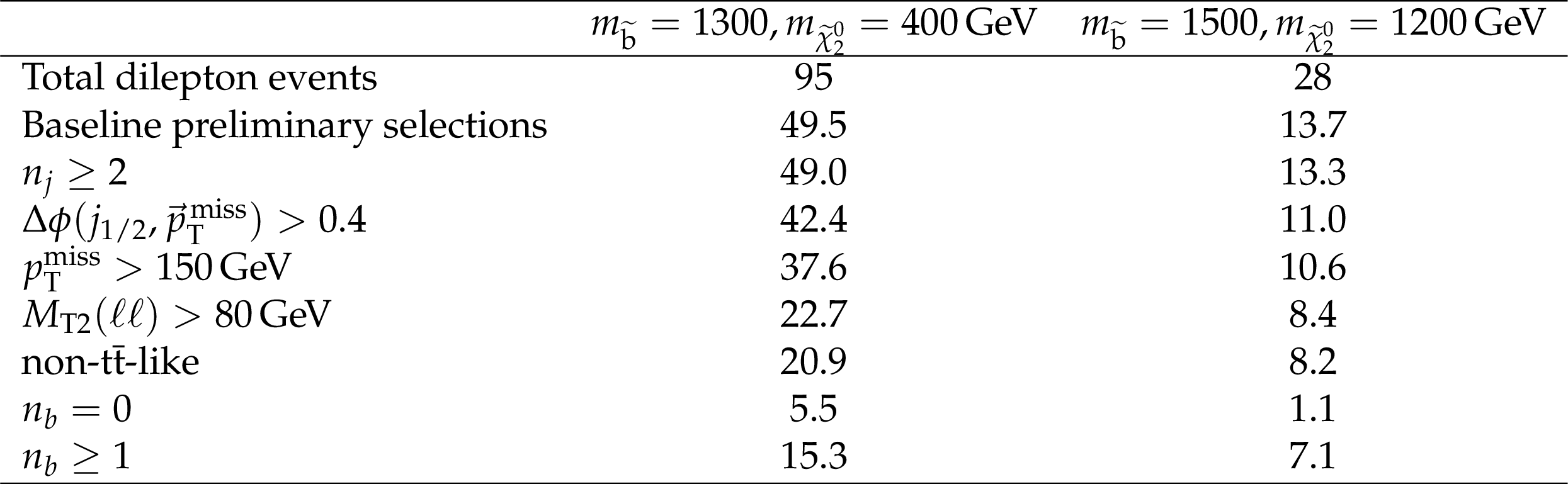
Additional Table 6:
Number of sbottom edge signal events selected after each selection criterion in the edge signal regions for models assuming (middle column) $m_{{\tilde{\mathrm {b}}}}=1300, m_{{\tilde{\chi}^{0}_{2}}} = $ 400 GeV and (right column) $m_{{\tilde{\mathrm {b}}}}=$ 1500, $m_{{\tilde{\chi}^{0}_{2}}} = $ 1200 GeV. Total dilepton events refers to luminosity $\times $ cross section $\times $ branching ratio. The last two lines are exclusive to each other. |
png pdf |
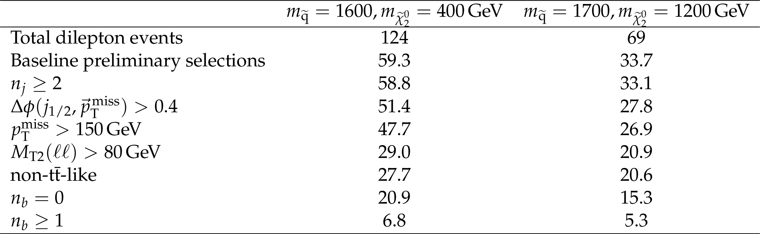
Additional Table 7:
Number of light squark edge signal events selected after each selection criterion in the edge signal regions for models assuming (middle column) $m_{{\mathrm {\tilde{q}}}}=1600, m_{{\tilde{\chi}^{0}_{2}}} = $ 400 GeV and (right column) $m_{{\mathrm {\tilde{q}}}}=$ 1700, $m_{{\tilde{\chi}^{0}_{2}}} = $ 1200 GeV. Total dilepton events refers to luminosity $\times $ cross section $\times $ branching ratio. The last two lines are exclusive to each other. |
| References | ||||
| 1 | G. Bertone, D. Hooper, and J. Silk | Particle dark matter: Evidence, candidates and constraints | PR 405 (2005) 279 | hep-ph/0404175 |
| 2 | P. Ramond | Dual theory for free fermions | PRD 3 (1971) 2415 | |
| 3 | Y. A. Golfand and E. P. Likhtman | Extension of the algebra of Poincare group generators and violation of P invariance | JEPTL 13 (1971) 323 | |
| 4 | A. Neveu and J. H. Schwarz | Factorizable dual model of pions | NPB 31 (1971) 86 | |
| 5 | D. V. Volkov and V. P. Akulov | Possible universal neutrino interaction | JEPTL 16 (1972)438 | |
| 6 | J. Wess and B. Zumino | A Lagrangian model invariant under supergauge transformations | PLB 49 (1974) 52 | |
| 7 | J. Wess and B. Zumino | Supergauge transformations in four dimensions | NPB 70 (1974) 39 | |
| 8 | P. Fayet | Supergauge invariant extension of the Higgs mechanism and a model for the electron and its neutrino | NPB 90 (1975) 104 | |
| 9 | H. P. Nilles | Supersymmetry, supergravity and particle physics | Phys. Rep. 110 (1984) 1 | |
| 10 | H. E. Haber and G. L. Kane | The search for supersymmetry: Probing physics beyond the standard model | PR 117 (1985) 75 | |
| 11 | G. R. Farrar and P. Fayet | Phenomenology of the production, decay, and detection of new hadronic states associated with supersymmetry | PLB 76 (1978) 575 | |
| 12 | I. Hinchliffe et al. | Precision SUSY measurements at CERN LHC | PRD 55 (1997) 5520 | hep-ph/9610544 |
| 13 | N. Arkani-Hamed et al. | MARMOSET: The path from LHC data to the new Standard Model via on-shell effective theories | hep-ph/0703088 | |
| 14 | J. Alwall, P. Schuster, and N. Toro | Simplified models for a first characterization of new physics at the LHC | PRD 79 (2009) 075020 | 0810.3921 |
| 15 | J. Alwall, M.-P. Le, M. Lisanti, and J. G. Wacker | Model-Independent Jets plus Missing Energy Searches | PRD 79 (2009) 015005 | 0809.3264 |
| 16 | LHC New Physics Working Group Collaboration | Simplified Models for LHC New Physics Searches | JPG 39 (2012) 105005 | 1105.2838 |
| 17 | ATLAS Collaboration | Search for electroweak production of charginos and sleptons decaying into final states with two leptons and missing transverse momentum in $ \sqrt{s}= $ 13 TeV pp collisions using the ATLAS detector | EPJC 80 (2020) 123 | 1908.08215 |
| 18 | ATLAS Collaboration | Search for supersymmetry in events containing a same-flavour opposite-sign dilepton pair, jets, and large missing transverse momentum in $ \sqrt{s} = $ 8 TeV pp collisions with the ATLAS detector | EPJC 75 (2015) 318 | 1503.03290 |
| 19 | ATLAS Collaboration | Search for the electroweak production of supersymmetric particles in $ \sqrt{s} = $ 8 TeV pp collisions with the ATLAS detector | PRD 93 (2016) 052002 | 1509.07152 |
| 20 | ATLAS Collaboration | Search for new phenomena in events containing a same-flavour opposite-sign dilepton pair, jets, and large missing transverse momentum in $ \sqrt{s} = $ 13 TeV pp collisions with the ATLAS detector | EPJC 77 (2017) 144 | 1611.05791 |
| 21 | CMS Collaboration | Search for new phenomena in final states with two opposite-charge, same-flavor leptons, jets, and missing transverse momentum in pp collisions at $ \sqrt{s}= $ 13 TeV | JHEP 03 (2018) 076 | CMS-SUS-16-034 1709.08908 |
| 22 | CMS Collaboration | Search for supersymmetric partners of electrons and muons in proton-proton collisions at $ \sqrt{s}= $ 13 TeV | PLB 790 (2019) 140 | CMS-SUS-17-009 1806.05264 |
| 23 | CMS Collaboration | Search for physics beyond the standard model in events with two leptons, jets, and missing transverse momentum in pp collisions at $ \sqrt{s} = $ 8 TeV | JHEP 04 (2015) 124 | CMS-SUS-14-014 1502.06031 |
| 24 | CMS Collaboration | Search for new physics in final states with two opposite-sign, same-flavor leptons, jets, and missing transverse momentum in pp collisions at $ \sqrt{s} = $ 13 TeV | JHEP 12 (2016) 013 | CMS-SUS-15-011 1607.00915 |
| 25 | CMS Collaboration | Search for new physics in events with opposite-sign leptons, jets, and missing transverse energy in pp collisions at $ \sqrt{s} = $ 7 TeV | PLB 718 (2013) 815 | CMS-SUS-11-011 1206.3949 |
| 26 | CMS Collaboration | Search for physics beyond the standard model in opposite-sign dilepton events in pp collisions at $ \sqrt{s} = $ 7 TeV | JHEP 06 (2011) 26 | CMS-SUS-10-007 1103.1348 |
| 27 | CMS Collaboration | Searches for electroweak production of charginos, neutralinos, and sleptons decaying to leptons and W, Z, and Higgs bosons in pp collisions at 8 TeV | EPJC 74 (2014) 3036 | CMS-SUS-13-006 1405.7570 |
| 28 | CMS Collaboration | Searches for electroweak neutralino and chargino production in channels with Higgs, Z, and W bosons in pp collisions at 8 TeV | PRD 90 (2014) 092007 | CMS-SUS-14-002 1409.3168 |
| 29 | CMS Collaboration | The CMS experiment at the CERN LHC | JINST 3 (2008) S08004 | CMS-00-001 |
| 30 | CMS Collaboration | The CMS trigger system | JINST 12 (2017) P01020 | CMS-TRG-12-001 1609.02366 |
| 31 | CMS Collaboration | Particle-flow reconstruction and global event description with the CMS detector | JINST 12 (2017) P10003 | CMS-PRF-14-001 1706.04965 |
| 32 | M. Cacciari, G. P. Salam, and G. Soyez | The anti-$ {k_{\mathrm{T}}}\ $ jet clustering algorithm | JHEP 04 (2008) 063 | 0802.1189 |
| 33 | M. Cacciari, G. P. Salam, and G. Soyez | FastJet user manual | EPJC 72 (2012) 1896 | 1111.6097 |
| 34 | CMS Collaboration | Performance of the CMS muon detector and muon reconstruction with proton-proton collisions at $ \sqrt{s}= $ 13 TeV | JINST 13 (2018) P06015 | CMS-MUO-16-001 1804.04528 |
| 35 | CMS Collaboration | Performance of electron reconstruction and selection with the CMS detector in proton-proton collisions at $ \sqrt{s} = $ 8 TeV | JINST 10 (2015) P06005 | CMS-EGM-13-001 1502.02701 |
| 36 | CMS Collaboration | Search for new physics in same-sign dilepton events in proton-proton collisions at $ \sqrt{s} = $ 13 TeV | EPJC 76 (2016) 439 | CMS-SUS-15-008 1605.03171 |
| 37 | CMS Collaboration | Performance of photon reconstruction and identification with the CMS detector in proton-proton collisions at $ \sqrt{s} = $ 8 TeV | JINST 10 (2015) P08010 | CMS-EGM-14-001 1502.02702 |
| 38 | M. Cacciari and G. P. Salam | Dispelling the N$ ^3 $ myth for the $ {k_{\mathrm{T}}}\ $ jet-finder | PLB 641 (2006) 57 | hep-ph/0512210 |
| 39 | CMS Collaboration | Jet energy scale and resolution in the CMS experiment in pp collisions at 8 TeV | JINST 12 (2017) P02014 | CMS-JME-13-004 1607.03663 |
| 40 | CMS Collaboration | Determination of jet energy calibration and transverse momentum resolution in CMS | JINST 6 (2011) P11002 | CMS-JME-10-011 1107.4277 |
| 41 | CMS Collaboration | Identification of heavy-flavour jets with the CMS detector in pp collisions at 13 TeV | JINST 13 (2018) P05011 | CMS-BTV-16-002 1712.07158 |
| 42 | J. M. Butterworth, A. R. Davison, M. Rubin, and G. P. Salam | Jet substructure as a new Higgs search channel at the LHC | PRL 100 (2008) 242001 | 0802.2470 |
| 43 | M. Dasgupta, A. Fregoso, S. Marzani, and G. P. Salam | Towards an understanding of jet substructure | JHEP 09 (2013) 029 | 1307.0007 |
| 44 | J. Thaler and K. Van Tilburg | Identifying boosted objects with $ N $-subjettiness | JHEP 03 (2011) 015 | 1011.2268 |
| 45 | CMS Collaboration | Identification of heavy, energetic, hadronically decaying particles using machine-learning techniques | JINST 15 (2020) P06005 | CMS-JME-18-002 2004.08262 |
| 46 | CMS Collaboration | Identification techniques for highly boosted W bosons that decay into hadrons | JHEP 12 (2014) 017 | CMS-JME-13-006 1410.4227 |
| 47 | J. Alwall et al. | The automated computation of tree-level and next-to-leading order differential cross sections, and their matching to parton shower simulations | JHEP 07 (2014) 079 | 1405.0301 |
| 48 | P. Nason | A new method for combining NLO QCD with shower Monte Carlo algorithms | JHEP 11 (2004) 040 | hep-ph/0409146 |
| 49 | S. Frixione, P. Nason, and C. Oleari | Matching NLO QCD computations with parton shower simulations: the POWHEG method | JHEP 11 (2007) 070 | 0709.2092 |
| 50 | S. Alioli, P. Nason, C. Oleari, and E. Re | NLO single-top production matched with shower in POWHEG: $ s $- and $ t $-channel contributions | JHEP 09 (2009) 111 | 0907.4076 |
| 51 | S. Gieseke, T. Kasprzik, and J. H. Kuhn | Vector-boson pair production and electroweak corrections in HERWIG++ | EPJC 74 (2014) 2988 | 1401.3964 |
| 52 | J. Baglio, L. D. Ninh, and M. M. Weber | Massive gauge boson pair production at the LHC: a next-to-leading order story | PRD 88 (2013) 113005 | 1307.4331 |
| 53 | A. Bierweiler, T. Kasprzik, and J. H. Kuhn | Vector-boson pair production at the LHC to $ \mathcal{O}(\alpha^3) $ accuracy | JHEP 12 (2013) 071 | 1305.5402 |
| 54 | J. M. Campbell and R. K. Ellis | An update on vector boson pair production at hadron colliders | PRD 60 (1999) 113006 | hep-ph/9905386 |
| 55 | J. M. Campbell, R. K. Ellis, and C. Williams | Vector boson pair production at the LHC | JHEP 07 (2011) 018 | 1105.0020 |
| 56 | J. M. Campbell, R. K. Ellis, and W. T. Giele | A multi-threaded version of MCFM | EPJC 75 (2015) 246 | 1503.06182 |
| 57 | T. Sjostrand et al. | An Introduction to PYTHIA 8.2 | CPC 191 (2015) 159 | 1410.3012 |
| 58 | J. Alwall et al. | Comparative study of various algorithms for the merging of parton showers and matrix elements in hadronic collisions | EPJC 53 (2008) 473 | 0706.2569 |
| 59 | R. Frederix and S. Frixione | Merging meets matching in MC@NLO | JHEP 12 (2012) 061 | 1209.6215 |
| 60 | CMS Collaboration | Event generator tunes obtained from underlying event and multiparton scattering measurements | EPJC 76 (2016) 155 | CMS-GEN-14-001 1512.00815 |
| 61 | CMS Collaboration | Extraction and validation of a new set of CMS PYTHIA8 tunes from underlying-event measurements | EPJC 80 (2020) 4 | CMS-GEN-17-001 1903.12179 |
| 62 | NNPDF Collaboration | Parton distributions for the LHC Run II | JHEP 04 (2015) 040 | 1410.8849 |
| 63 | NNPDF Collaboration | Parton distributions from high-precision collider data | EPJC 77 (2017) 663 | 1706.00428 |
| 64 | GEANT4 Collaboration | GEANT4--a simulation toolkit | NIMA 506 (2003) 250 | |
| 65 | S. Abdullin et al. | The fast simulation of the CMS detector at LHC | J. Phys. Conf. Ser. 331 (2011) 032049 | |
| 66 | A. Giammanco | The fast simulation of the CMS experiment | J. Phys. Conf. Ser. 513 (2014) 022012 | |
| 67 | E. Re | Single-top Wt-channel production matched with parton showers using the POWHEG method | EPJC 71 (2011) 1547 | 1009.2450 |
| 68 | M. Czakon and A. Mitov | Top++: a program for the calculation of the top-pair cross-section at hadron colliders | CPC 185 (2014) 2930 | 1112.5675 |
| 69 | F. Caola, K. Melnikov, R. Rontsch, and L. Tancredi | QCD corrections to ZZ production in gluon fusion at the LHC | PRD 92 (2015) 094028 | 1509.06734 |
| 70 | Y. Li and F. Petriello | Combining QCD and electroweak corrections to dilepton production in FEWZ | PRD 86 (2012) 094034 | 1208.5967 |
| 71 | W. Beenakker et al. | The production of charginos/neutralinos and sleptons at hadron colliders | PRL 83 (1999) 3780 | hep-ph/9906298 |
| 72 | G. Bozzi, B. Fuks, and M. Klasen | Threshold resummation for slepton-pair production at hadron colliders | NPB 777 (2007) 157 | |
| 73 | J. Debove, B. Fuks, and M. Klasen | Threshold resummation for gaugino pair production at hadron colliders | NPB 842 (2011) 51 | 1005.2909 |
| 74 | B. Fuks, M. Klasen, D. R. Lamprea, and M. Rothering | Gaugino production in proton-proton collisions at a center-of-mass energy of 8 TeV | JHEP 10 (2012) 081 | 1207.2159 |
| 75 | B. Fuks, M. Klasen, D. R. Lamprea, and M. Rothering | Precision predictions for electroweak superpartner production at hadron colliders with $ \sc $ Resummino | EPJC 73 (2013) 2480 | 1304.0790 |
| 76 | B. Fuks, M. Klasen, D. R. Lamprea, and M. Rothering | Revisiting slepton pair production at the Large Hadron Collider | JHEP 01 (2014) 168 | 1310.2621 |
| 77 | J. Fiaschi and M. Klasen | Neutralino-chargino pair production at NLO+NLL with resummation-improved parton density functions for LHC Run II | PRD 98 (2018) 055014 | 1805.11322 |
| 78 | J. Fiaschi and M. Klasen | Slepton pair production at the LHC in NLO+NLL with resummation-improved parton densities | JHEP 03 (2018) 094 | 1801.10357 |
| 79 | W. Beenakker, R. Hopker, M. Spira, and P. M. Zerwas | Squark and gluino production at hadron colliders | NPB 492 (1997) 51 | hep-ph/9610490 |
| 80 | W. Beenakker et al. | Stop production at hadron colliders | NPB 515 (1998) 3 | hep-ph/9710451 |
| 81 | A. Kulesza and L. Motyka | Threshold resummation for squark-antisquark and gluino-pair production at the LHC | PRL 102 (2009) 111802 | 0807.2405 |
| 82 | A. Kulesza and L. Motyka | Soft gluon resummation for the production of gluino-gluino and squark-antisquark pairs at the LHC | PRD 80 (2009) 095004 | 0905.4749 |
| 83 | W. Beenakker et al. | Soft-gluon resummation for squark and gluino hadroproduction | JHEP 12 (2009) 041 | 0909.4418 |
| 84 | W. Beenakker et al. | Supersymmetric top and bottom squark production at hadron colliders | JHEP 08 (2010) 098 | 1006.4771 |
| 85 | W. Beenakker et al. | Squark and gluino hadroproduction | Int. J. Mod. Phys. A 26 (2011) 2637 | 1105.1110 |
| 86 | W. Beenakker et al. | NNLL resummation for squark-antisquark pair production at the LHC | JHEP 01 (2012) 076 | 1110.2446 |
| 87 | W. Beenakker et al. | Towards NNLL resummation: hard matching coefficients for squark and gluino hadroproduction | JHEP 10 (2013) 120 | 1304.6354 |
| 88 | W. Beenakker et al. | NNLL resummation for squark and gluino production at the LHC | JHEP 12 (2014) 023 | 1404.3134 |
| 89 | W. Beenakker et al. | NNLL resummation for stop pair-production at the LHC | JHEP 05 (2016) 153 | 1601.02954 |
| 90 | W. Beenakker et al. | NNLL-fast: predictions for coloured supersymmetric particle production at the LHC with threshold and Coulomb resummation | JHEP 12 (2016) 133 | 1607.07741 |
| 91 | C. G. Lester and D. J. Summers | Measuring masses of semiinvisibly decaying particles pair produced at hadron colliders | PLB 463 (1999) 99 | hep-ph/9906349 |
| 92 | A. Barr, C. Lester, and P. Stephens | A variable for measuring masses at hadron colliders when missing energy is expected; $ M_{\mathrm{T2}} $: the truth behind the glamour | JPG 29 (2003) 2343 | hep-ph/0304226 |
| 93 | M. J. Oreglia | A study of the reactions $\psi' \to \gamma\gamma \psi$ | PhD thesis, Stanford University, 1980 SLAC Report SLAC-R-236, see Appendix D | |
| 94 | Particle Data Group, P. A. Zyla et al. | Review of particle physics | Prog. Theor. Exp. Phys. 2020 (2020) 083C01 | |
| 95 | E. Gross and O. Vitells | Trial factors or the look elsewhere effect in high energy physics | EPJC 70 (2010) 525 | 1005.1891 |
| 96 | T. Junk | Confidence level computation for combining searches with small statistics | NIMA 434 (1999) 435 | hep-ex/9902006 |
| 97 | A. L. Read | Presentation of search results: the $ \rm CL_s $ technique | JPG 28 (2002) 2693 | |
| 98 | G. Cowan, K. Cranmer, E. Gross, and O. Vitells | Asymptotic formulae for likelihood-based tests of new physics | EPJC 71 (2011) 1554 | 1007.1727 |
| 99 | ATLAS and CMS Collaborations | Procedure for the LHC Higgs boson search combination in summer 2011 | CMS-NOTE-2011-005 | |
| 100 | CMS Collaboration | CMS luminosity measurements for the 2016 data-taking period | ||
| 101 | CMS Collaboration | CMS luminosity measurement for the 2017 data-taking period at $ \sqrt{s} = $ 13 TeV | ||
| 102 | CMS Collaboration | CMS luminosity measurement for the 2018 data-taking period at $ \sqrt{s} = $ 13 TeV | ||
| 103 | M. Cacciari et al. | The $ \mathrm{t}\mathrm{\bar{t}} $ cross-section at 1.8 TeV and 1.96 TeV: a study of the systematics due to parton densities and scale dependence | JHEP 04 (2004) 068 | hep-ph/0303085 |
| 104 | S. Catani, D. de Florian, M. Grazzini, and P. Nason | Soft gluon resummation for Higgs boson production at hadron colliders | JHEP 07 (2003) 028 | hep-ph/0306211 |
| 105 | R. Frederix et al. | Four-lepton production at hadron colliders: MadGraph5+MCatNLO predictions with theoretical uncertainties | JHEP 02 (2012) 099 | 1110.4738 |
|
|
Compact Muon Solenoid LHC, CERN |
|

|

|

|

|

|