

Compact Muon Solenoid
LHC, CERN
| CMS-TOP-19-008 ; CERN-EP-2020-152 | ||
| Measurement of the top quark Yukawa coupling from $\mathrm{t\bar{t}}$ kinematic distributions in the dilepton final state in proton-proton collisions at $\sqrt{s} = $ 13 TeV | ||
| CMS Collaboration | ||
| 15 September 2020 | ||
| Phys. Rev. D 102 (2020) 092013 | ||
| Abstract: A measurement of the Higgs boson Yukawa coupling to the top quark is presented using proton-proton collision data at $\sqrt{s} = $ 13 TeV, corresponding to an integrated luminosity of 137 fb$^{-1}$, recorded with the CMS detector. The coupling strength with respect to the standard model value, ${Y_{\mathrm{t}}} $, is determined from kinematic distributions in $\mathrm{t\bar{t}}$ final states containing ee, ${\mu}{\mu}$, or e${\mu}$ pairs. Variations of the Yukawa coupling strength lead to modified distributions for $\mathrm{t\bar{t}}$ production. In particular, the distributions of the mass of the $\mathrm{t\bar{t}}$ system and the rapidity difference of the top quark and antiquark are sensitive to the value of ${Y_{\mathrm{t}}} $. The measurement yields a best fit value of ${Y_{\mathrm{t}}} =$ 1.16$^{+0.24}_{-0.35} $, bounding ${Y_{\mathrm{t}}} < $ 1.54 at a 95% confidence level. | ||
| Links: e-print arXiv:2009.07123 [hep-ex] (PDF) ; CDS record ; inSPIRE record ; CADI line (restricted) ; | ||
| Figures & Tables | Summary | Additional Figures | References | CMS Publications |
|---|
| Figures | |

png pdf |
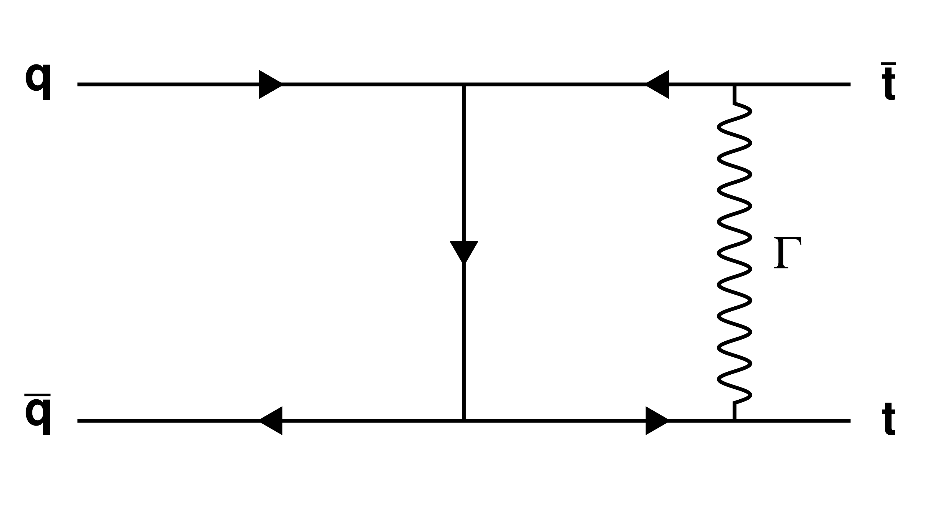
Figure 1:
Sample Feynman diagrams for EW contributions to gluon-induced and quark-induced top quark pair production, where $\Gamma $ stands for neutral vector and scalar bosons. |
png pdf |
Figure 1-a:
Sample Feynman diagram for EW contribution to quark-induced top quark pair production, where $\Gamma $ stands for neutral vector and scalar bosons. |

png pdf |
Figure 1-b:
Sample Feynman diagram for EW contribution to gluon-induced top quark pair production, where $\Gamma $ stands for neutral vector and scalar bosons. |

png pdf |
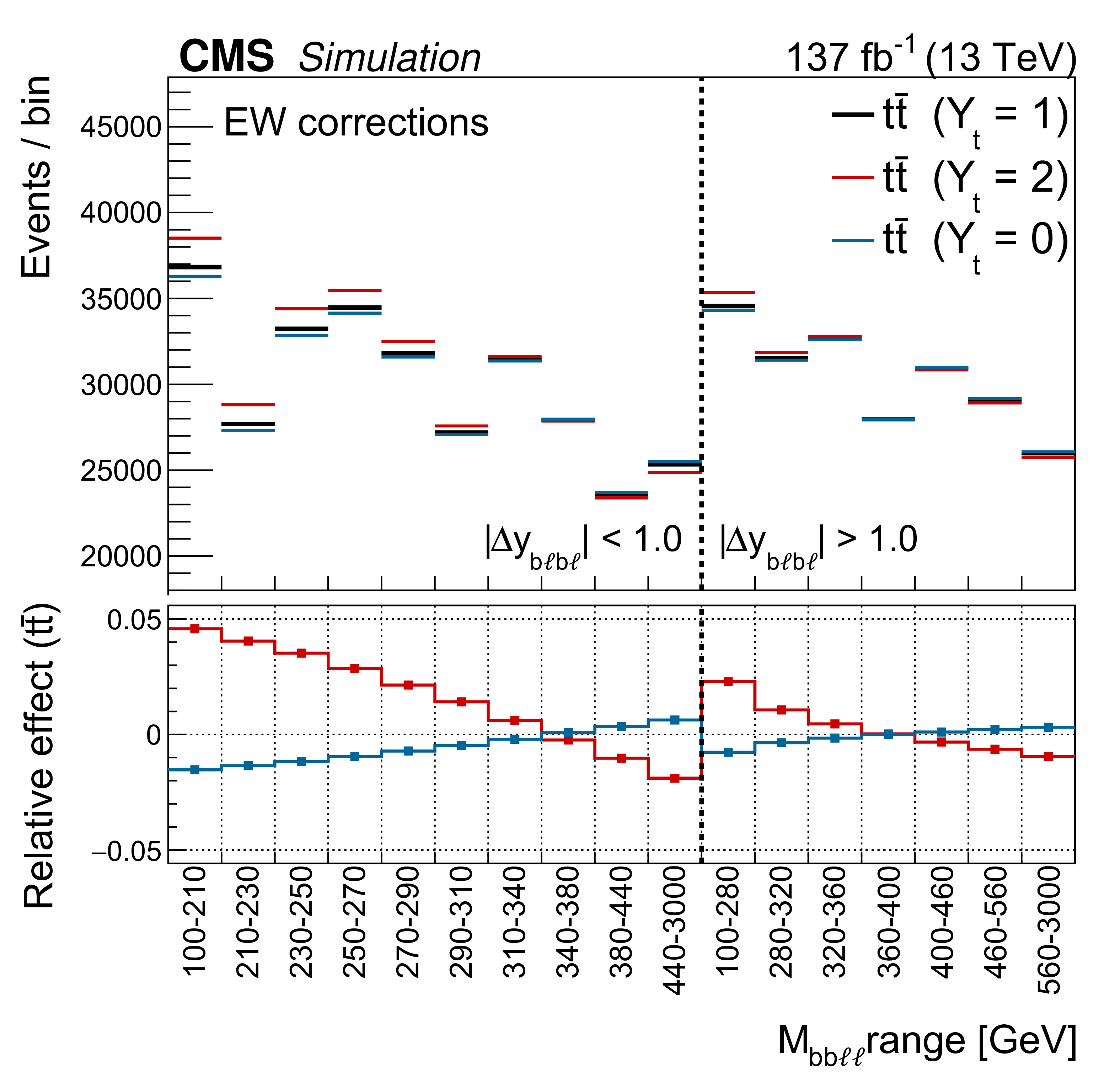
Figure 2:
Effect of the EW corrections on $\mathrm{t\bar{t}}$ differential kinematic distributions for different values of $ {Y_{\mathrm{t}}} $, after reweighting of simulated events. The effect is shown on the distribution of the invariant mass, ${M_{{\mathrm{t} {}\mathrm{\bar{t}}}}}$ (left), and the difference in rapidity between the top quark and antiquark, $\Delta y_{{\mathrm{t} {}\mathrm{\bar{t}}}}$ (right). |

png pdf |
Figure 2-a:
Effect of the EW corrections on the distribution of the invariant mass, ${M_{{\mathrm{t} {}\mathrm{\bar{t}}}}}$, for different values of $ {Y_{\mathrm{t}}} $, after reweighting of simulated events. |

png pdf |
Figure 2-b:
Effect of the EW corrections on the distribution of the difference in rapidity between the top quark and antiquark, $\Delta y_{{\mathrm{t} {}\mathrm{\bar{t}}}}$, for different values of $ {Y_{\mathrm{t}}} $, after reweighting of simulated events. |

png pdf |
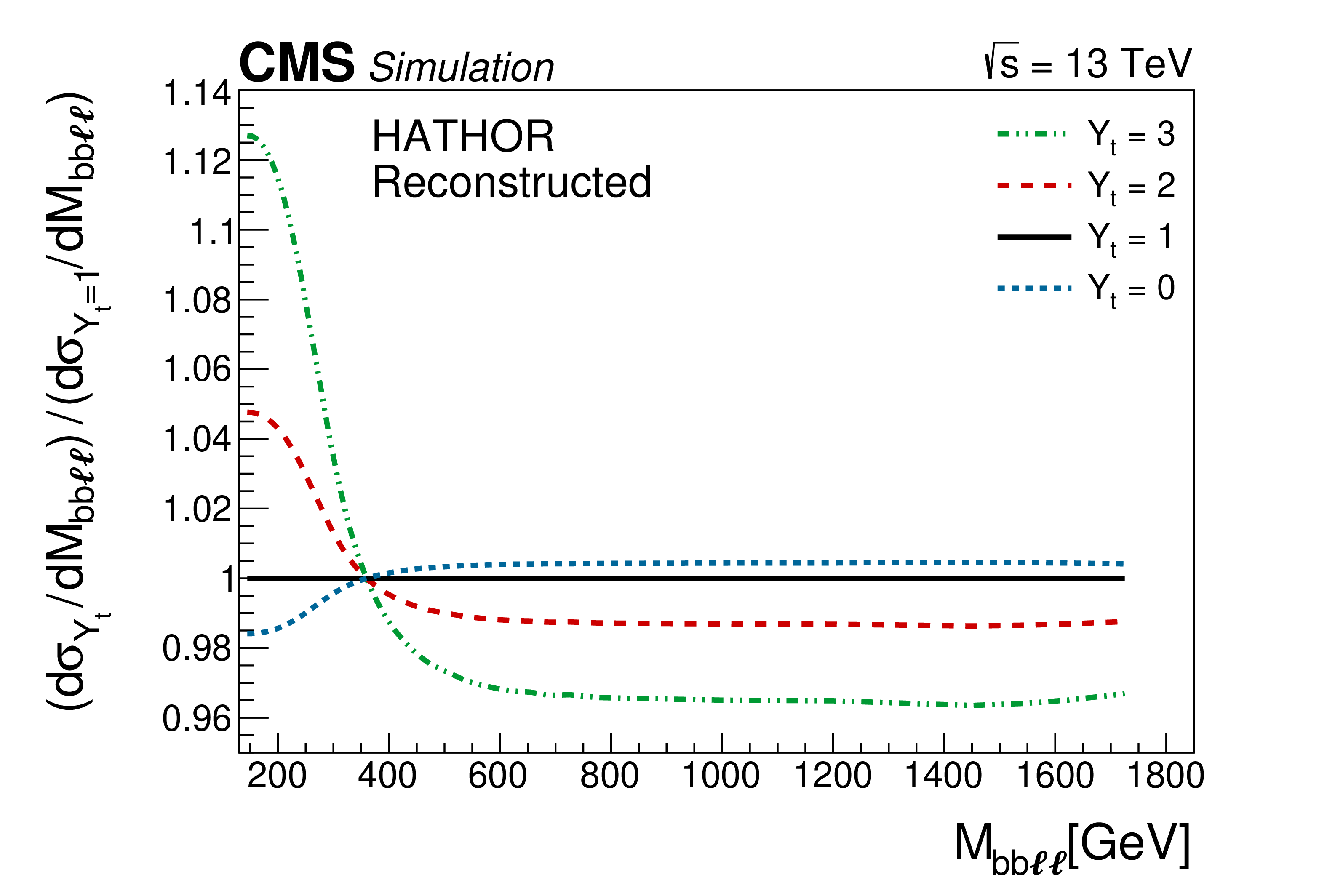
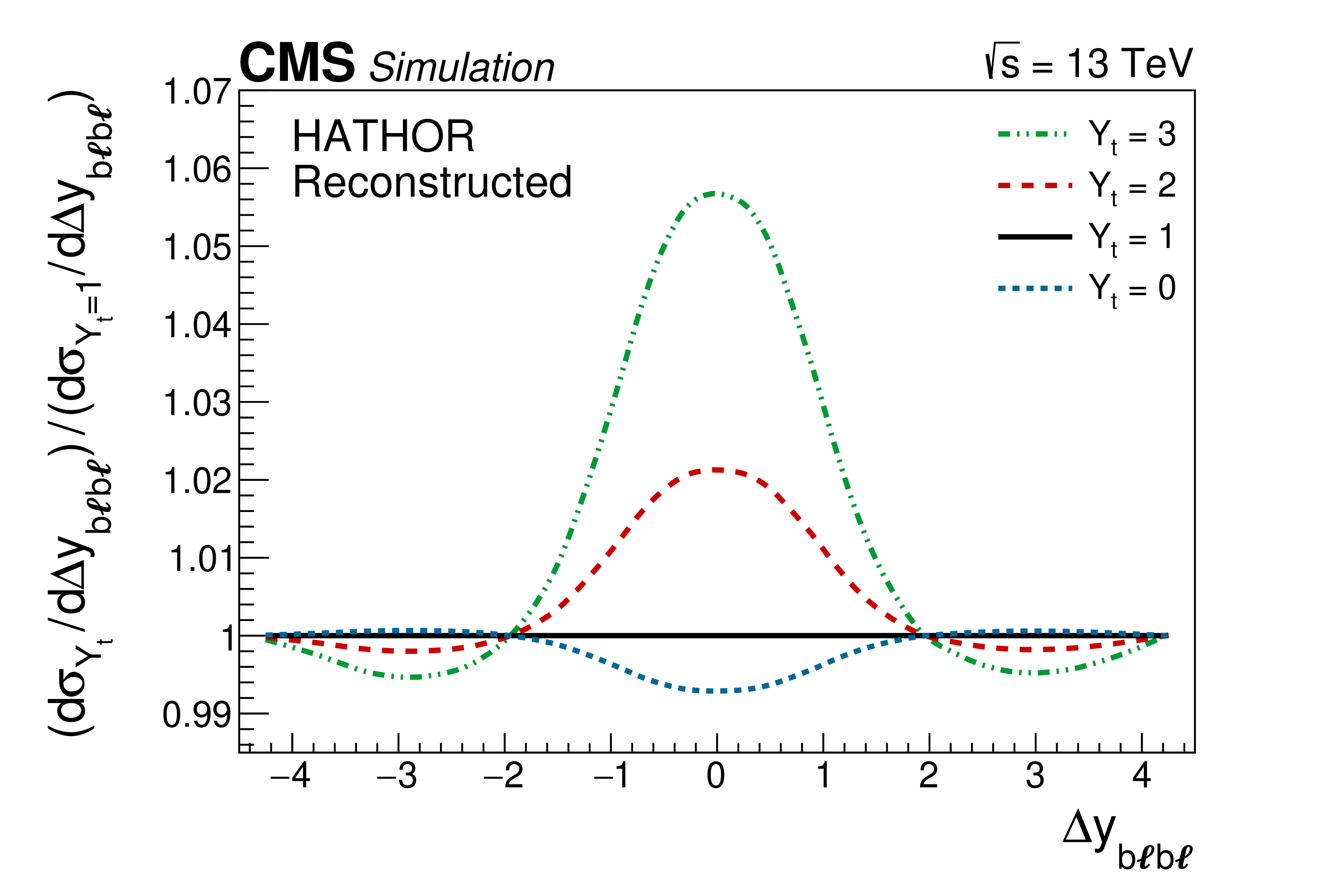
Figure 3:
The ratio of kinematic distributions with EW corrections (evaluated for various values of ${Y_{\mathrm{t}}}$) to the SM kinematic distribution (${Y_{\mathrm{t}}} =$ 1) is shown, demonstrating the sensitivity of these distributions to the Yukawa coupling. The plots on the left show the information at the generator level, while the plots on the right are obtained from reconstructed events. The axis scale is kept the same for the sake of comparison. |

png pdf |
Figure 3-a:
The ratio of the $ {M_{{\mathrm{b}}{\mathrm{b}}{\ell}{\ell}}}$ distribution with EW corrections (evaluated for various values of ${Y_{\mathrm{t}}}$) to the SM kinematic distribution (${Y_{\mathrm{t}}} =$ 1) is shown, demonstrating the sensitivity of these distributions to the Yukawa coupling. The plot shows the information at the generator level. The axis scale is kept the same for the sake of comparison. |
png pdf |
Figure 3-b:
The ratio of the $ {M_{{\mathrm{b}}{\mathrm{b}}{\ell}{\ell}}}$ distribution with EW corrections (evaluated for various values of ${Y_{\mathrm{t}}}$) to the SM kinematic distribution (${Y_{\mathrm{t}}} =$ 1) is shown, demonstrating the sensitivity of these distributions to the Yukawa coupling. The plot is obtained from reconstructed events. The axis scale is kept the same for the sake of comparison. |

png pdf |
Figure 3-c:
The ratio of the ${\Delta y_{{\mathrm{b}}\ell {\mathrm{b}}\ell}} $ distribution with EW corrections (evaluated for various values of ${Y_{\mathrm{t}}}$) to the SM kinematic distribution (${Y_{\mathrm{t}}} =$ 1) is shown, demonstrating the sensitivity of these distributions to the Yukawa coupling. The plot shows the information at the generator level. The axis scale is kept the same for the sake of comparison. |
png pdf |
Figure 3-d:
The ratio of the ${\Delta y_{{\mathrm{b}}\ell {\mathrm{b}}\ell}} $ distribution with EW corrections (evaluated for various values of ${Y_{\mathrm{t}}}$) to the SM kinematic distribution (${Y_{\mathrm{t}}} =$ 1) is shown, demonstrating the sensitivity of these distributions to the Yukawa coupling. The plot is obtained from reconstructed events. The axis scale is kept the same for the sake of comparison. |

png pdf |
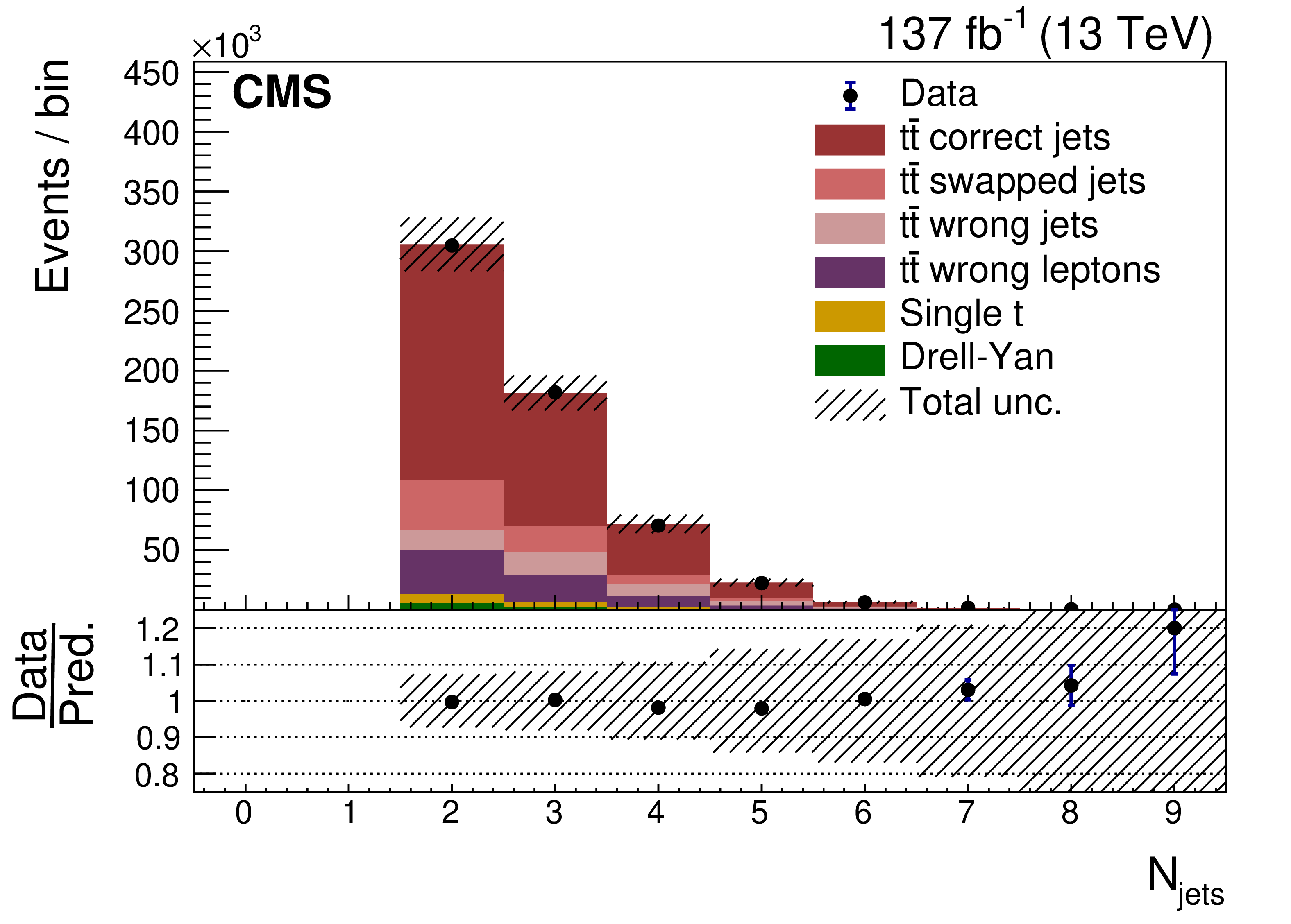
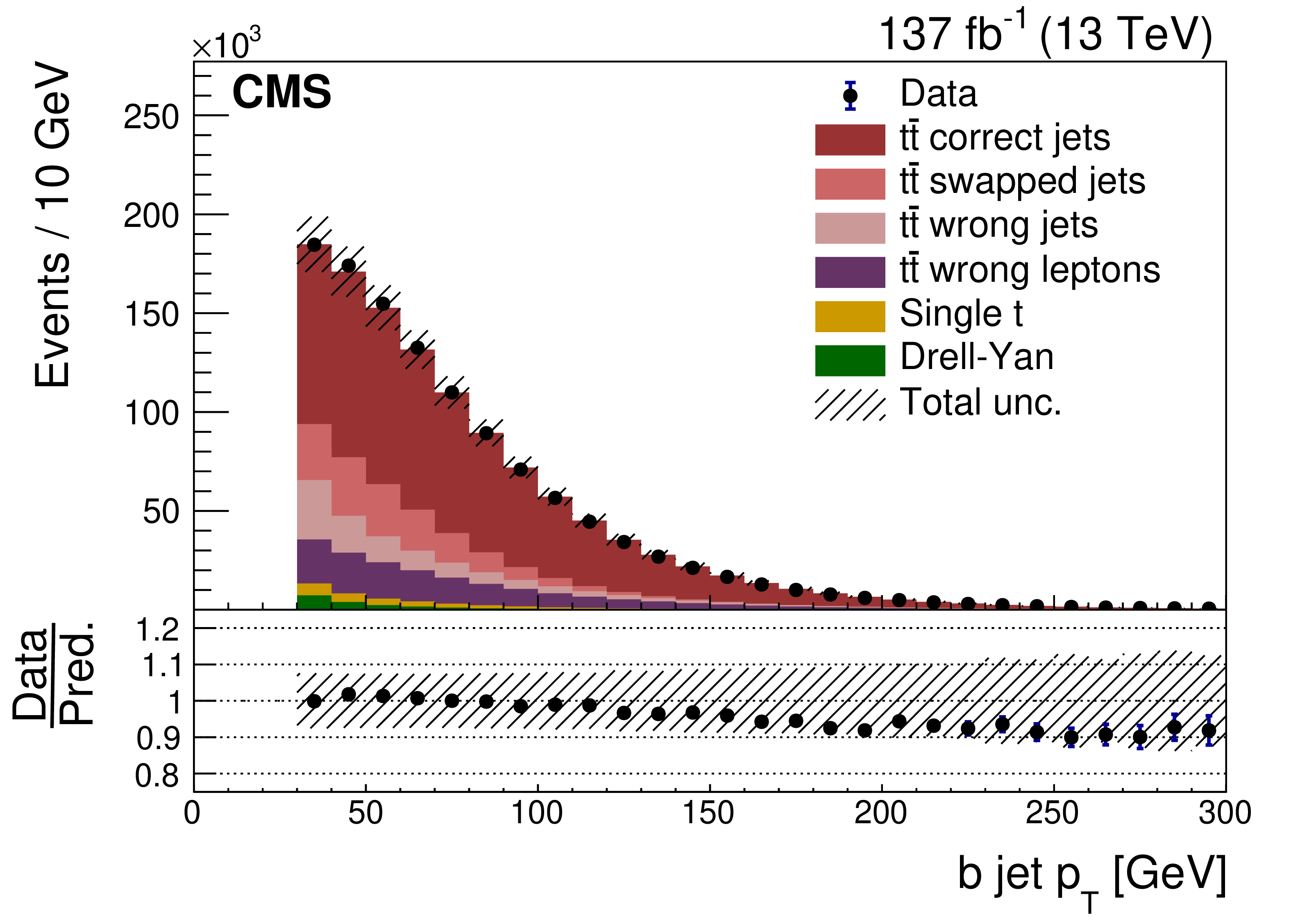
Figure 4:
Data-to-simulation comparisons for the jet multiplicity (upper left), ${{p_{\mathrm {T}}} ^\text {miss}}$ (upper right), lepton ${p_{\mathrm {T}}}$ (lower left), and b jet ${p_{\mathrm {T}}}$ (lower right). The uncertainty bands are derived by varying each uncertainty source up and down by one standard deviation (as described in Section 4) and summing the effects in quadrature. The signal simulation is divided into the following categories: events with correctly identified leptons and jets in which jets are correctly assigned (${\mathrm{t} {}\mathrm{\bar{t}}}$ correct jets), events with correctly identified leptons and jets in which jets are incorrectly assigned (${\mathrm{t} {}\mathrm{\bar{t}}}$ swapped jets), events with correctly identified leptons where the two b jets originating from top decays are not identified correctly (${\mathrm{t} {}\mathrm{\bar{t}}}$ wrong jets), and lastly events where the identified leptons are not those from W boson decay vertices (${\mathrm{t} {}\mathrm{\bar{t}}}$ wrong leptons). The lower panels show the ratio of data to the simulated events in each bin, with total uncertainty bands drawn around the nominal expected bin content. |
png pdf |
Figure 4-a:
Data-to-simulation comparison for the jet multiplicity. The uncertainty bands are derived by varying each uncertainty source up and down by one standard deviation (as described in Section 4) and summing the effects in quadrature. The signal simulation is divided into the following categories: events with correctly identified leptons and jets in which jets are correctly assigned (${\mathrm{t} {}\mathrm{\bar{t}}}$ correct jets), events with correctly identified leptons and jets in which jets are incorrectly assigned (${\mathrm{t} {}\mathrm{\bar{t}}}$ swapped jets), events with correctly identified leptons where the two b jets originating from top decays are not identified correctly (${\mathrm{t} {}\mathrm{\bar{t}}}$ wrong jets), and lastly events where the identified leptons are not those from W boson decay vertices (${\mathrm{t} {}\mathrm{\bar{t}}}$ wrong leptons). The lower panel shows the ratio of data to the simulated events in each bin, with total uncertainty bands drawn around the nominal expected bin content. |

png pdf |
Figure 4-b:
Data-to-simulation comparison for ${{p_{\mathrm {T}}} ^\text {miss}}$. The uncertainty bands are derived by varying each uncertainty source up and down by one standard deviation (as described in Section 4) and summing the effects in quadrature. The signal simulation is divided into the following categories: events with correctly identified leptons and jets in which jets are correctly assigned (${\mathrm{t} {}\mathrm{\bar{t}}}$ correct jets), events with correctly identified leptons and jets in which jets are incorrectly assigned (${\mathrm{t} {}\mathrm{\bar{t}}}$ swapped jets), events with correctly identified leptons where the two b jets originating from top decays are not identified correctly (${\mathrm{t} {}\mathrm{\bar{t}}}$ wrong jets), and lastly events where the identified leptons are not those from W boson decay vertices (${\mathrm{t} {}\mathrm{\bar{t}}}$ wrong leptons). The lower panel shows the ratio of data to the simulated events in each bin, with total uncertainty bands drawn around the nominal expected bin content. |

png pdf |
Figure 4-c:
Data-to-simulation comparison for the lepton ${p_{\mathrm {T}}}$. The uncertainty bands are derived by varying each uncertainty source up and down by one standard deviation (as described in Section 4) and summing the effects in quadrature. The signal simulation is divided into the following categories: events with correctly identified leptons and jets in which jets are correctly assigned (${\mathrm{t} {}\mathrm{\bar{t}}}$ correct jets), events with correctly identified leptons and jets in which jets are incorrectly assigned (${\mathrm{t} {}\mathrm{\bar{t}}}$ swapped jets), events with correctly identified leptons where the two b jets originating from top decays are not identified correctly (${\mathrm{t} {}\mathrm{\bar{t}}}$ wrong jets), and lastly events where the identified leptons are not those from W boson decay vertices (${\mathrm{t} {}\mathrm{\bar{t}}}$ wrong leptons). The lower panel shows the ratio of data to the simulated events in each bin, with total uncertainty bands drawn around the nominal expected bin content. |
png pdf |
Figure 4-d:
Data-to-simulation comparison for the b jet ${p_{\mathrm {T}}}$. The uncertainty bands are derived by varying each uncertainty source up and down by one standard deviation (as described in Section 4) and summing the effects in quadrature. The signal simulation is divided into the following categories: events with correctly identified leptons and jets in which jets are correctly assigned (${\mathrm{t} {}\mathrm{\bar{t}}}$ correct jets), events with correctly identified leptons and jets in which jets are incorrectly assigned (${\mathrm{t} {}\mathrm{\bar{t}}}$ swapped jets), events with correctly identified leptons where the two b jets originating from top decays are not identified correctly (${\mathrm{t} {}\mathrm{\bar{t}}}$ wrong jets), and lastly events where the identified leptons are not those from W boson decay vertices (${\mathrm{t} {}\mathrm{\bar{t}}}$ wrong leptons). The lower panel shows the ratio of data to the simulated events in each bin, with total uncertainty bands drawn around the nominal expected bin content. |

png pdf |
Figure 5:
The pre-fit agreement between data and MC simulation in the final kinematic binning. The solid lines divide the three data-taking periods, while the dashed lines divide the two ${{| \Delta y_{{\mathrm{b}}\ell {\mathrm{b}}\ell} |}}$ bins in each data-taking period, with ${M_{{\mathrm{b}}{\mathrm{b}}{\ell}{\ell}}}$ bin ranges displayed on the $x$ axis. The lower panel shows the ratio of data to the simulated events in each bin, with total uncertainty bands drawn around the nominal expected bin content, obtained by summing the contributions of all uncertainty sources in quadrature. |

png pdf |
Figure 6:
The EW correction rate modifier $R_\mathrm {EW}^\text {bin}$ in two separate ($ {M_{{\mathrm{b}}{\mathrm{b}}{\ell}{\ell}}}$, ${\Delta y_{{\mathrm{b}}\ell {\mathrm{b}}\ell}} $) bins from simulated 2017 data, demonstrating the quadratic dependence on ${Y_{\mathrm{t}}}$. All bins have an increasing or decreasing quadratic yield function, with the steepest dependence on ${Y_{\mathrm{t}}}$ found at lower values of ${M_{{\mathrm{b}}{\mathrm{b}}{\ell}{\ell}}}$. |

png pdf |
Figure 6-a:
The EW correction rate modifier $R_\mathrm {EW}^\text {bin}$ in bin ($ {M_{{\mathrm{b}}{\mathrm{b}}{\ell}{\ell}}} \in$ [100, 210] GeV, $|{\Delta y_{{\mathrm{b}}\ell {\mathrm{b}}\ell}}| < $ 1.0) bins from simulated 2017 data, demonstrating the quadratic dependence on ${Y_{\mathrm{t}}}$. All bins have an increasing or decreasing quadratic yield function, with the steepest dependence on ${Y_{\mathrm{t}}}$ found at lower values of ${M_{{\mathrm{b}}{\mathrm{b}}{\ell}{\ell}}}$. |

png pdf |
Figure 6-b:
The EW correction rate modifier $R_\mathrm {EW}^\text {bin}$ in bin ($ {M_{{\mathrm{b}}{\mathrm{b}}{\ell}{\ell}}} \in$ [440, 3000] GeV, $|{\Delta y_{{\mathrm{b}}\ell {\mathrm{b}}\ell}}| < $ 1.0) bins from simulated 2017 data, demonstrating the quadratic dependence on ${Y_{\mathrm{t}}}$. All bins have an increasing or decreasing quadratic yield function, with the steepest dependence on ${Y_{\mathrm{t}}}$ found at lower values of ${M_{{\mathrm{b}}{\mathrm{b}}{\ell}{\ell}}}$. |
png pdf |
Figure 7:
The effect of the Yukawa parameter ${Y_{\mathrm{t}}}$ on reconstructed event yield in the final binned distributions. The variation of ${Y_{\mathrm{t}}}$ induces a shape distortion in the kinematic distributions. The marginal effect relative to the standard model expectation ${Y_{\mathrm{t}}} =$ 1 is visualized in the lower panel. |
png pdf |
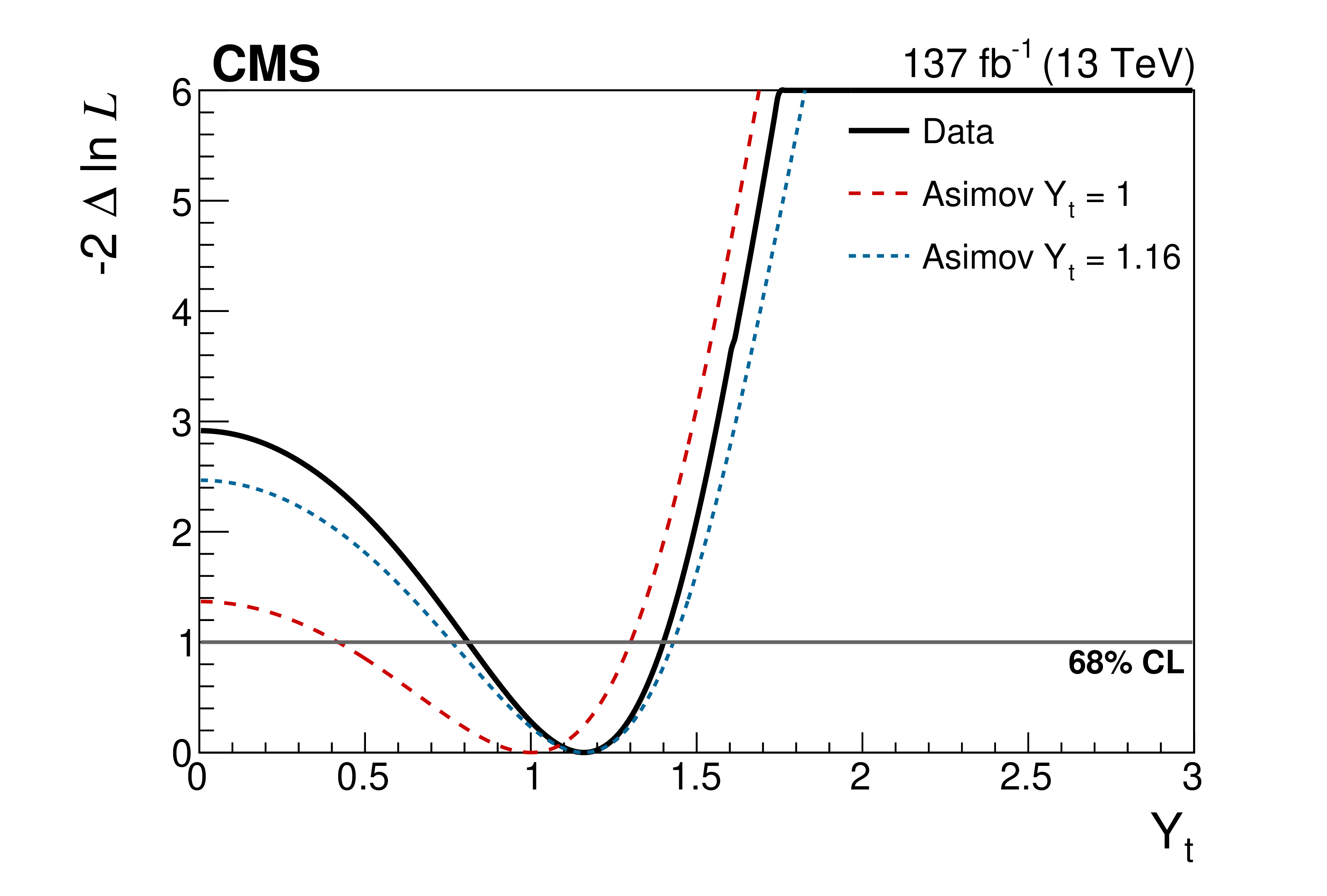
Figure 8:
The result of a profile likelihood scan, performed by fixing the value of $ {Y_{\mathrm{t}}} $ at values over the interval [0, 3] and taking the ratio of $-2\ln(\mathcal {L}({Y_{\mathrm{t}}}))$ to the best fit value $-2\ln(\mathcal {L}(\hat{\mathrm{t}}))$. The expected curves from fits to simulated Asimov data are shown produced for the SM value $ {Y_{\mathrm{t}}} =$ 1.0 (dashed) and for the final best fit value of $ {Y_{\mathrm{t}}} =$ 1.16 (dotted). |

png pdf |
Figure 9:
The comparison between data and MC simulation at the best fit value of $ {Y_{\mathrm{t}}} = $ 1.16 after performing the likelihood maximization, with shaded bands displaying the post-fit uncertainty. The solid lines separate the three data-taking periods, while the dashed lines indicate the boundaries of the two ${{| \Delta y_{{\mathrm{b}}\ell {\mathrm{b}}\ell} |}}$ bins in each data-taking period, with ${M_{{\mathrm{b}}{\mathrm{b}}{\ell}{\ell}}}$ bin ranges displayed on the $x$ axis. The lower panel shows the ratio of data to the simulated events in each bin, with total post-fit uncertainty bands drawn around the nominal expected bin content. |
png pdf |
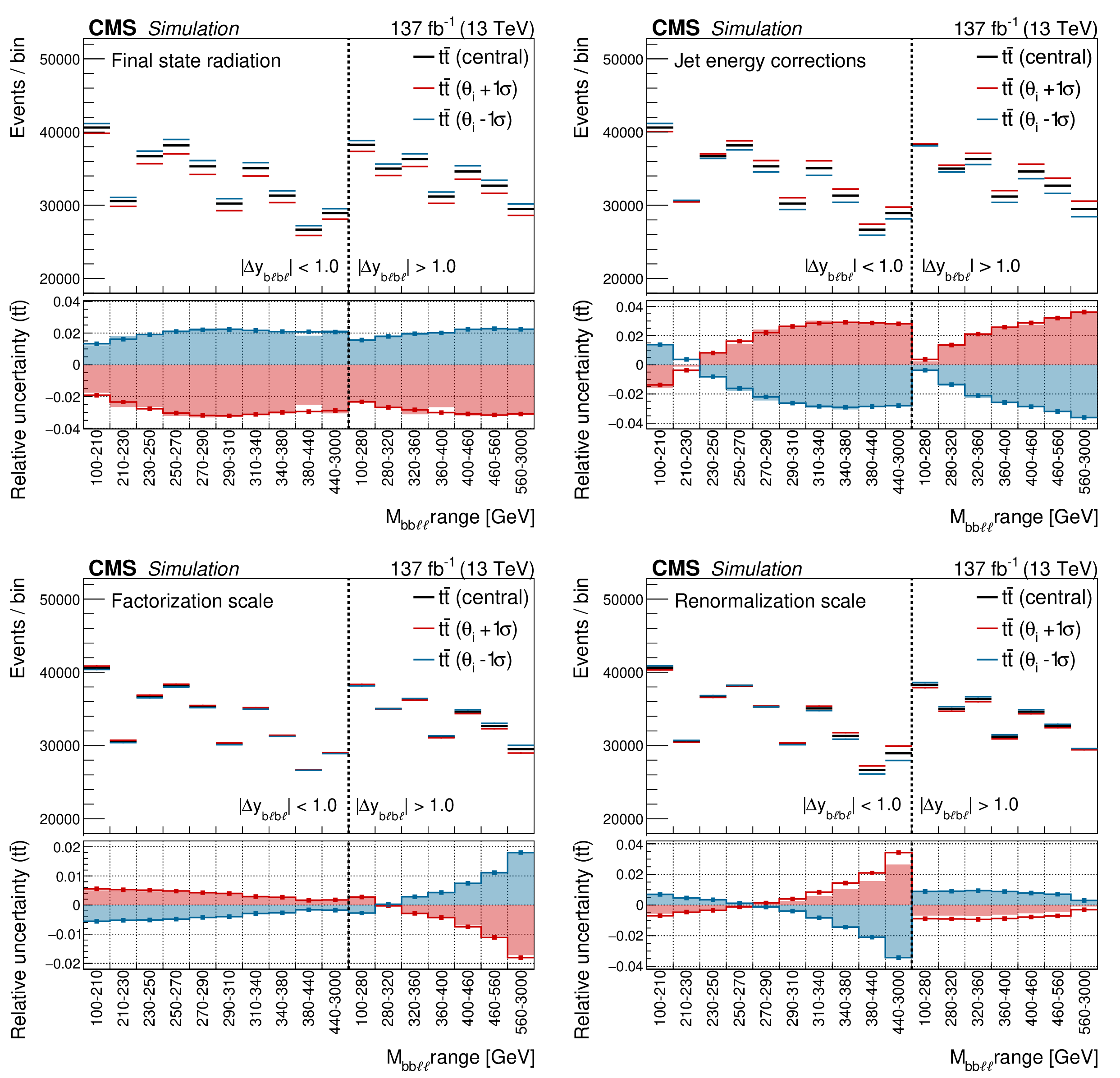
Figure 10:
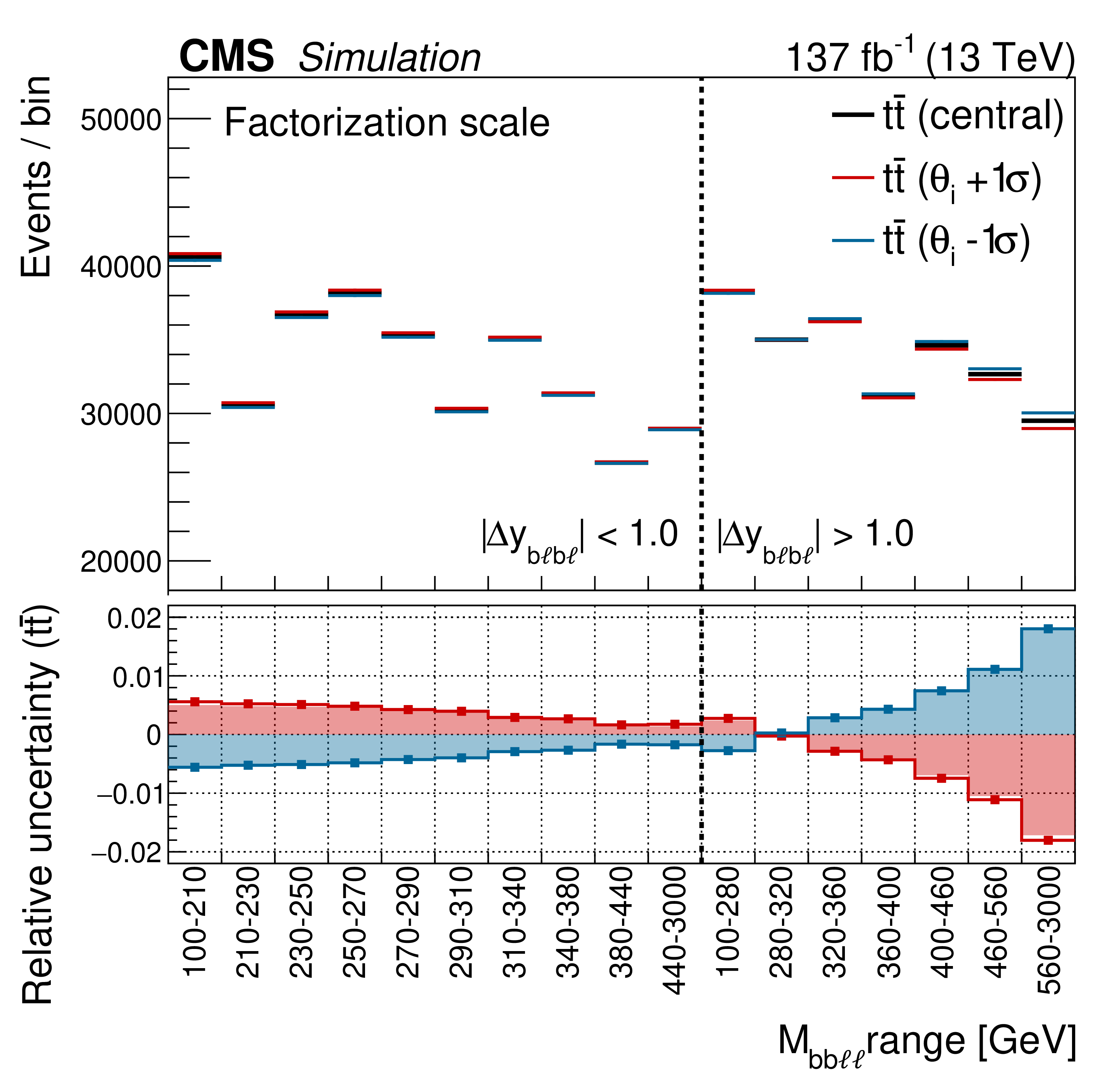
Templates are shown for the uncertainties associated with the final-state radiation in PYTHIA (upper left), the jet energy corrections (upper right), the factorization scale (lower left), and the renormalization scale (lower right). Along with the intrinsic uncertainty in the EW corrections, these are the limiting uncertainties in the fit. The shaded bars represent the raw template information, while the lines show the shapes after smoothing and symmetrization procedures have been applied. In the fit, the jet energy corrections are split into 26 different components, but for brevity only the total uncertainty is shown here. Variation between years is minimal for each of these uncertainties, although they are treated separately in the fit. |

png pdf |
Figure 10-a:
Templates are shown for the uncertainties associated with the final-state radiation in PYTHIA. Along with the intrinsic uncertainty in the EW corrections, these are the limiting uncertainties in the fit. The shaded bars represent the raw template information, while the lines show the shapes after smoothing and symmetrization procedures have been applied. In the fit, the jet energy corrections are split into 26 different components, but for brevity only the total uncertainty is shown here. Variation between years is minimal for each of these uncertainties, although they are treated separately in the fit. |

png pdf |
Figure 10-b:
Templates are shown for the uncertainties associated with the jet energy corrections. Along with the intrinsic uncertainty in the EW corrections, these are the limiting uncertainties in the fit. The shaded bars represent the raw template information, while the lines show the shapes after smoothing and symmetrization procedures have been applied. In the fit, the jet energy corrections are split into 26 different components, but for brevity only the total uncertainty is shown here. Variation between years is minimal for each of these uncertainties, although they are treated separately in the fit. |
png pdf |
Figure 10-c:
Templates are shown for the uncertainties associated with the factorization scale. Along with the intrinsic uncertainty in the EW corrections, these are the limiting uncertainties in the fit. The shaded bars represent the raw template information, while the lines show the shapes after smoothing and symmetrization procedures have been applied. In the fit, the jet energy corrections are split into 26 different components, but for brevity only the total uncertainty is shown here. Variation between years is minimal for each of these uncertainties, although they are treated separately in the fit. |

png pdf |
Figure 10-d:
Templates are shown for the uncertainties associated with the renormalization scale. Along with the intrinsic uncertainty in the EW corrections, these are the limiting uncertainties in the fit. The shaded bars represent the raw template information, while the lines show the shapes after smoothing and symmetrization procedures have been applied. In the fit, the jet energy corrections are split into 26 different components, but for brevity only the total uncertainty is shown here. Variation between years is minimal for each of these uncertainties, although they are treated separately in the fit. |
| Tables | |

png pdf |
Table 1:
Simulated signal, background, and data event yields for each of the three years and their combination. The rightmost column shows the fraction of each component relative to the total simulated sample yield across the full data set. The statistical uncertainty in the simulated event counts is given. |
| Summary |
| A measurement of the Higgs Yukawa coupling to the top quark is presented, based on data from proton-proton collisions collected by the CMS experiment. Data at a center-of-mass energy of 13 TeV is analyzed from the LHC Run 2, collected in 2016-18 and corresponding to an integrated luminosity of 137 fb$^{-1}$. The resulting best fit value of the top quark Yukawa coupling relative to the standard model is given by ${Y_{\mathrm{t}}} = $ 1.16 $^{+0.24}_{-0.35}$. This measurement uses the effects of virtual Higgs boson exchange on $\mathrm{t\bar{t}}$ kinematic properties to extract information about the coupling from kinematic distributions. Although the sensitivity is lower compared to constraints obtained from studying processes involving Higgs boson production in Refs. [9] and [11], this measurement avoids dependence on other Yukawa coupling values through additional branching assumptions, making it a compelling independent measurement. This measurement also achieves a slightly higher precision than the only other ${Y_{\mathrm{t}}} $ measurement that does not make additional branching fraction assumptions, performed in the search for production of four top quarks. The four top quark search places ${Y_{\mathrm{t}}} < $ 1.7 at a 95% confidence level [12] while this measurement achieves an approximate result of ${Y_{\mathrm{t}}} < $ 1.54. |
| Additional Figures | |

png pdf |
Additional Figure 1:
Nuisance parameter post-fit constraints and impacts are shown for the 30 uncertainties in the fit with the largest impact on the best fit value of ${Y_{{\mathrm {t}}}}$. This information is also provided for a fit using an Asimov dataset generated with $ {Y_{{\mathrm {t}}}} =$ 1 (expected), for the sake of comparison with the final fit result on data (observed). Impacts are calculated by repeating the fit with individual nuisance parameters held fixed and varied up and down by one standard deviation according to the their post-fit uncertainty, then recording the resulting effect on the best fit value of ${Y_{{\mathrm {t}}}}$. Note that some uncertainty sources are split into a correlated nuisance parameter and an uncorrelated parameter unique to each data-taking year, as indicated by the paranthetical expressions in the parameter names. This is done when the uncertainty in question has a partial correlation between years, or in some cases where the modelling was changed after 2016. In the case of partial correlations, this allows us to separately consider a correlated and uncorrelated effect from each nuisance parameter, in approximation. Uncertainties related to the jet energy corrections (JEC) come from several components, including the flavor dependence of the jet responses (FlavorQCD), corrections to initial and final state radiations (RelativeFSR), variations of JEC in different data taking periods (TimeEtaPt), variations of the single particle response in ECAL (SinglePionECAL), residual differences between samples used to derive the JEC (RelativeSample), a constant scale uncertainty for the biases of methods to study the jet energy response (AbsoluteMPFBias), together with differences between those methods in the calibration fits (RelativeBal). The word relative stands for relative $\eta $-dependent corrections, calibrating different detector regions relative to $ | \eta | < $ 1.3 using dijet events. More details can be found in Ref. [44]. |
| References | ||||
| 1 | ATLAS Collaboration | Observation of a new particle in the search for the standard model Higgs boson with the ATLAS detector at the LHC | PLB 716 (2012) 1 | 1207.7214 |
| 2 | CMS Collaboration | Observation of a new boson at a mass of 125 GeV with the CMS experiment at the LHC | PLB 716 (2012) 30 | CMS-HIG-12-028 1207.7235 |
| 3 | ATLAS Collaboration | Measurement of the top-quark mass in $ t\bar{t}+1 $-jet events collected with the ATLAS detector in $ pp $ collisions at $ \sqrt{s}= $ 8 TeV | JHEP 11 (2019) 150 | 1905.02302 |
| 4 | CMS Collaboration | Measurement of the top quark mass with lepton+jets final states using $ \mathrm {p} \mathrm {p} $ collisions at $ \sqrt{s}= $ 13 TeV | EPJC 78 (2018) 891 | CMS-TOP-17-007 1805.01428 |
| 5 | G. C. Branco et al. | Theory and phenomenology of two-Higgs-doublet models | PR 516 (2012) 1 | 1106.0034 |
| 6 | K. Agashe, R. Contino, and A. Pomarol | The minimal composite Higgs model | NPB 719 (2005) 165 | hep-ph/0412089 |
| 7 | LHC Higgs Cross Section Working Group | Handbook of LHC Higgs cross sections: 3. Higgs properties | CERN (2013) | 1307.1347 |
| 8 | CMS Collaboration | Search for associated production of a Higgs boson and a single top quark in proton-proton collisions at $ \sqrt{s}= $ 13 TeV | PRD 99 (2019) 092005 | CMS-HIG-18-009 1811.09696 |
| 9 | CMS Collaboration | Observation of $ \mathrm{t\overline{t}} $H production | PRL 120 (2018) 231801 | CMS-HIG-17-035 1804.02610 |
| 10 | ATLAS Collaboration | Observation of Higgs boson production in association with a top quark pair at the LHC with the ATLAS detector | PLB 784 (2018) 173 | 1806.00425 |
| 11 | CMS Collaboration | Combined measurements of Higgs boson couplings in proton-proton collisions at $ \sqrt{s}= $ 13 TeV | EPJC 79 (2019) 421 | CMS-HIG-17-031 1809.10733 |
| 12 | CMS Collaboration | Search for production of four top quarks in final states with same-sign or multiple leptons in proton-proton collisions at $ \sqrt{s}= $ 13 TeV | EPJC 80 (2020) 75 | CMS-TOP-18-003 1908.06463 |
| 13 | CMS Collaboration | Measurement of the top quark Yukawa coupling from $ \mathrm{t\bar{t}} $ kinematic distributions in the lepton+jets final state in proton-proton collisions at $ \sqrt{s} = $ 13 TeV | PRD 100 (2019) 072007 | CMS-TOP-17-004 1907.01590 |
| 14 | J. H. Kuhn, A. Scharf, and P. Uwer | Weak interactions in top-quark pair production at hadron colliders: an update | PRD 91 (2015) 014020 | 1305.5773 |
| 15 | M. Aliev et al. | HATHOR: HAdronic Top and Heavy quarks crOss section calculatoR | CPC 182 (2011) 1034 | 1007.1327 |
| 16 | CMS Collaboration | Particle-flow reconstruction and global event description with the cms detector | JINST 12 (2017) P10003 | CMS-PRF-14-001 1706.04965 |
| 17 | CMS Collaboration | The CMS trigger system | JINST 12 (2017) P01020 | CMS-TRG-12-001 1609.02366 |
| 18 | CMS Collaboration | The CMS experiment at the CERN LHC | JINST 3 (2008) S08004 | CMS-00-001 |
| 19 | P. Nason | A new method for combining NLO QCD with shower Monte Carlo algorithms | JHEP 11 (2004) 040 | hep-ph/0409146 |
| 20 | S. Frixione, P. Nason, and C. Oleari | Matching NLO QCD computations with parton shower simulations: the POWHEG method | JHEP 11 (2007) 070 | 0709.2092 |
| 21 | S. Alioli, P. Nason, C. Oleari, and E. Re | A general framework for implementing NLO calculations in shower Monte Carlo programs: the POWHEG BOX | JHEP 06 (2010) 043 | 1002.2581 |
| 22 | J. M. Campbell, R. K. Ellis, P. Nason, and E. Re | Top-pair production and decay at NLO matched with parton showers | JHEP 04 (2015) 114 | 1412.1828 |
| 23 | T. Sjostrand et al. | An introduction to PYTHIA 8.2 | CPC 191 (2015) 159 | 1410.3012 |
| 24 | P. Skands, S. Carrazza, and J. Rojo | Tuning PYTHIA 8.1: the Monash 2013 tune | EPJC 74 (2014) 3024 | 1404.5630 |
| 25 | CMS Collaboration | Extraction and validation of a new set of CMS PYTHIA8 tunes from underlying-event measurements | EPJC 80 (2020) 4 | CMS-GEN-17-001 1903.12179 |
| 26 | NNPDF Collaboration | Parton distributions for the LHC Run II | JHEP 04 (2015) 040 | 1410.8849 |
| 27 | NNPDF Collaboration | Parton distributions from high-precision collider data | EPJC 77 (2017) 663 | 1706.00428 |
| 28 | M. Czakon and A. Mitov | Top++: A program for the calculation of the top-pair cross-section at hadron colliders | CPC 185 (2014) 2930 | 1112.5675 |
| 29 | M. Botje et al. | The PDF4LHC working group interim recommendations | 1101.0538 | |
| 30 | A. D. Martin, W. J. Stirling, R. S. Thorne, and G. Watt | Parton distributions for the LHC | EPJC 63 (2009) 189 | 0901.0002 |
| 31 | A. D. Martin, W. J. Stirling, R. S. Thorne, and G. Watt | Uncertainties on $ {\alpha_S} $ in global PDF analyses and implications for predicted hadronic cross sections | EPJC 64 (2009) 653 | 0905.3531 |
| 32 | H.-L. Lai et al. | New parton distributions for collider physics | PRD 82 (2010) 074024 | 1007.2241 |
| 33 | J. Gao et al. | CT10 next-to-next-to-leading order global analysis of QCD | PRD 89 (2014) 033009 | 1302.6246 |
| 34 | NNPDF Collaboration | Parton distributions with LHC data | NPB 867 (2013) 244 | 1207.1303 |
| 35 | J. Alwall et al. | The automated computation of tree-level and next-to-leading order differential cross sections, and their matching to parton shower simulations | JHEP 07 (2014) 079 | 1405.0301 |
| 36 | M. L. Mangano, M. Moretti, F. Piccinini, and M. Treccani | Matching matrix elements and shower evolution for top-quark production in hadronic collisions | JHEP 01 (2007) 013 | hep-ph/0611129 |
| 37 | J. Alwall et al. | Comparative study of various algorithms for the merging of parton showers and matrix elements in hadronic collisions | EPJC 53 (2008) 473 | 0706.2569 |
| 38 | GEANT4 Collaboration | GEANT4--a simulation toolkit | NIMA 506 (2003) 250 | |
| 39 | W. Hollik and M. Kollar | NLO QED contributions to top-pair production at hadron collider | PRD 77 (2008) 014008 | 0708.1697 |
| 40 | M. Czakon et al. | Top-pair production at the LHC through NNLO QCD and NLO EW | JHEP 10 (2017) 186 | 1705.04105 |
| 41 | CMS Collaboration | Measurement of differential cross sections for the production of top quark pairs and of additional jets in lepton+jets events from pp collisions at $ \sqrt{s} = $ 13 TeV | PRD 97 (2018) 112003 | CMS-TOP-17-002 1803.08856 |
| 42 | M. Cacciari, G. P. Salam, and G. Soyez | The anti-$ {k_{\mathrm{T}}} $ jet clustering algorithm | JHEP 04 (2008) 063 | 0802.1189 |
| 43 | M. Cacciari, G. P. Salam, and G. Soyez | FastJet user manual | EPJC 72 (2012) 1896 | 1111.6097 |
| 44 | CMS Collaboration | Jet energy scale and resolution in the CMS experiment in pp collisions at 8 TeV | JINST 12 (2017) P02014 | CMS-JME-13-004 1607.03663 |
| 45 | CMS Collaboration | Identification of heavy-flavour jets with the CMS detector in pp collisions at 13 TeV | JINST 13 (2018) P05011 | CMS-BTV-16-002 1712.07158 |
| 46 | B. A. Betchart, R. Demina, and A. Harel | Analytic solutions for neutrino momenta in decay of top quarks | NIMA 736 (2014) 169 | 1305.1878 |
| 47 | CMS Collaboration | Precise determination of the mass of the Higgs boson and tests of compatibility of its couplings with the standard model predictions using proton collisions at 7 and 8 TeV | EPJC 75 (2015) 212 | CMS-HIG-14-009 1412.8662 |
| 48 | CMS Collaboration | CMS Luminosity Measurements for the 2016 Data Taking Period | CMS-PAS-LUM-17-001 | CMS-PAS-LUM-17-001 |
| 49 | CMS Collaboration | CMS luminosity measurement for the 2017 data-taking period at $ \sqrt{s} = $ 13 TeV | CMS-PAS-LUM-17-004 | CMS-PAS-LUM-17-004 |
| 50 | CMS Collaboration | CMS luminosity measurement for the 2018 data-taking period at $ \sqrt{s} = $ 13 TeV | CMS-PAS-LUM-18-002 | CMS-PAS-LUM-18-002 |
| 51 | ATLAS Collaboration | Measurement of the inelastic proton-proton cross section at $ \sqrt{s} = $ 13 TeV with the ATLAS detector at the LHC | PRL 117 (2016) 182002 | 1606.02625 |
| 52 | CMS Collaboration | Measurements of Inclusive $ W $ and $ Z $ Cross Sections in pp Collisions at $ \sqrt{s}= $ 7 TeV | JHEP 01 (2011) 080 | CMS-EWK-10-002 1012.2466 |
| 53 | CMS Collaboration | Performance of electron reconstruction and selection with the CMS detector in proton-proton collisions at $ \sqrt{s} = $ 8 TeV | JINST 10 (2015) P06005 | CMS-EGM-13-001 1502.02701 |
| 54 | CMS Collaboration | Performance of the CMS muon detector and muon reconstruction with proton-proton collisions at $ \sqrt{s}= $ 13 TeV | JINST 13 (2018) P06015 | CMS-MUO-16-001 1804.04528 |
| 55 | Particle Data Group, M. Tanabashi et al. | Review of particle physics | PRD 98 (2018) 030001 | |
| 56 | M. G. Bowler | $ {\rm e}^{+}{\rm e}^{-} $ Production of heavy quarks in the string model | Z. Phys. C 11 (1981) 169 | |
| 57 | CMS Collaboration | Measurement of the $ \mathrm{t}\overline{\mathrm{t}} $ production cross section, the top quark mass, and the strong coupling constant using dilepton events in pp collisions at $ \sqrt{s} = $ 13 TeV | EPJC 79 (2019) 368 | CMS-TOP-17-001 1812.10505 |
| 58 | M. Grazzini, S. Kallweit, and M. Wiesemann | Fully differential NNLO computations with MATRIX | EPJC 78 (2018) 537 | 1711.06631 |
| 59 | M. Czakon, D. Heymes, and A. Mitov | fastNLO tables for NNLO top-quark pair differential distributions | 1704.08551 | |
| 60 | M. Czakon, D. Heymes, and A. Mitov | High-precision differential predictions for top-quark pairs at the LHC | PRL 116 (2016) 082003 | 1511.00549 |
| 61 | M. Czakon et al. | A study of the impact of double-differential top distributions from CMS on parton distribution functions | 1912.08801 | |
| 62 | W. S. Cleveland | Robust locally weighted regression and smoothing scatterplots | J. Am. Stat. Assoc. 74 (1979) 829 | |
| 63 | G. Cowan, K. Cranmer, E. Gross, and O. Vitells | Asymptotic formulae for likelihood-based tests of new physics | EPJC 71 (2011) 1554 | 1007.1727 |
|
|
Compact Muon Solenoid LHC, CERN |
|

|

|

|

|

|