

Compact Muon Solenoid
LHC, CERN
| CMS-TOP-20-003 ; CERN-EP-2020-234 | ||
| First measurement of the cross section for top quark pair production with additional charm jets using dileptonic final states in pp collisions at $\sqrt{s} = $ 13 TeV | ||
| CMS Collaboration | ||
| 17 December 2020 | ||
| Phys. Lett. B. 820 (2021) 136565 | ||
| Abstract: The first measurement of the inclusive cross section for top quark pairs ($\mathrm{t\bar{t}}$) produced in association with two additional charm jets is presented. The analysis uses the dileptonic final states of $\mathrm{t\bar{t}}$ events produced in proton-proton collisions at a centre-of-mass energy of 13 TeV. The data correspond to an integrated luminosity of 41.5 fb$^{-1}$, recorded by the CMS experiment at the LHC. A new charm jet identification algorithm provides input to a neural network that is trained to distinguish among $\mathrm{t\bar{t}}$ events with two additional charm ($\mathrm{t\bar{t}}\mathrm{c}\mathrm{\bar{c}}$), bottom ($\mathrm{t\bar{t}}\mathrm{b}\mathrm{\bar{b}}$), and light-flavour or gluon ($\mathrm{t\bar{t}}\text{LL}$) jets. By means of a template fitting procedure, the inclusive $\mathrm{t\bar{t}}\mathrm{c}\mathrm{\bar{c}}$, $\mathrm{t\bar{t}}\mathrm{b}\mathrm{\bar{b}}$, and $\mathrm{t\bar{t}}\text{LL}$ cross sections are simultaneously measured, together with their ratios to the inclusive $\mathrm{t\bar{t}}$ + two jets cross section. This provides measurements of the $\mathrm{t\bar{t}}\mathrm{c}\mathrm{\bar{c}}$ and $\mathrm{t\bar{t}}\mathrm{b}\mathrm{\bar{b}}$ cross sections of 8.0 $\pm$ 1.1 (stat) $\pm$ 1.3 (syst) pb and 4.09 $\pm$ 0.34 (stat) $\pm$ 0.55 (syst) pb, respectively, in the full phase space. The results are consistent with expectations from the standard model. | ||
| Links: e-print arXiv:2012.09225 [hep-ex] (PDF) ; CDS record ; inSPIRE record ; CADI line (restricted) ; | ||
| Figures | |
png pdf |
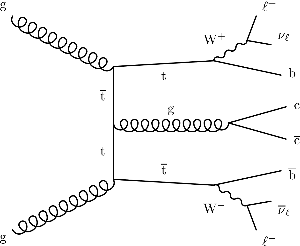
Figure 1:
Example of a Feynman diagram at the lowest order in QCD, describing the dileptonic decay channel of a top quark pair with an additional $\mathrm{c} \mathrm{\bar{c}} $ pair produced via gluon splitting. |
png pdf |
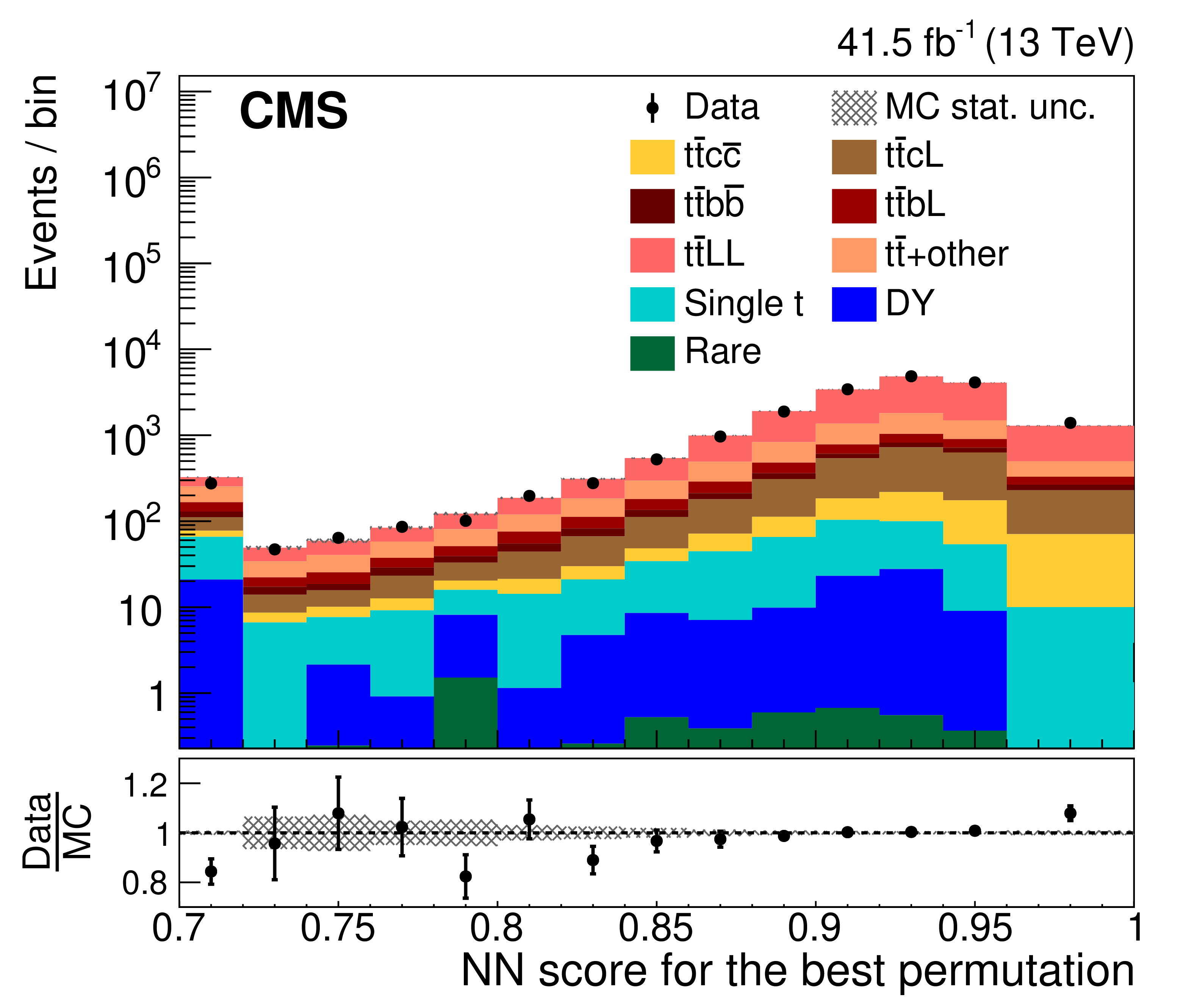
Figure 2:
Comparison between data (points) and simulated predictions (histograms) for the distribution of the NN score for the best permutations of jet-parton assignments found in each event. Underflow is included in the first bin. The lower panel shows the ratio of the yields in data to those predicted in simulations. The vertical bars represent the statistical uncertainties in data, while the hatched band show the statistical uncertainty in the simulated predictions. |
png pdf |
Figure 3:
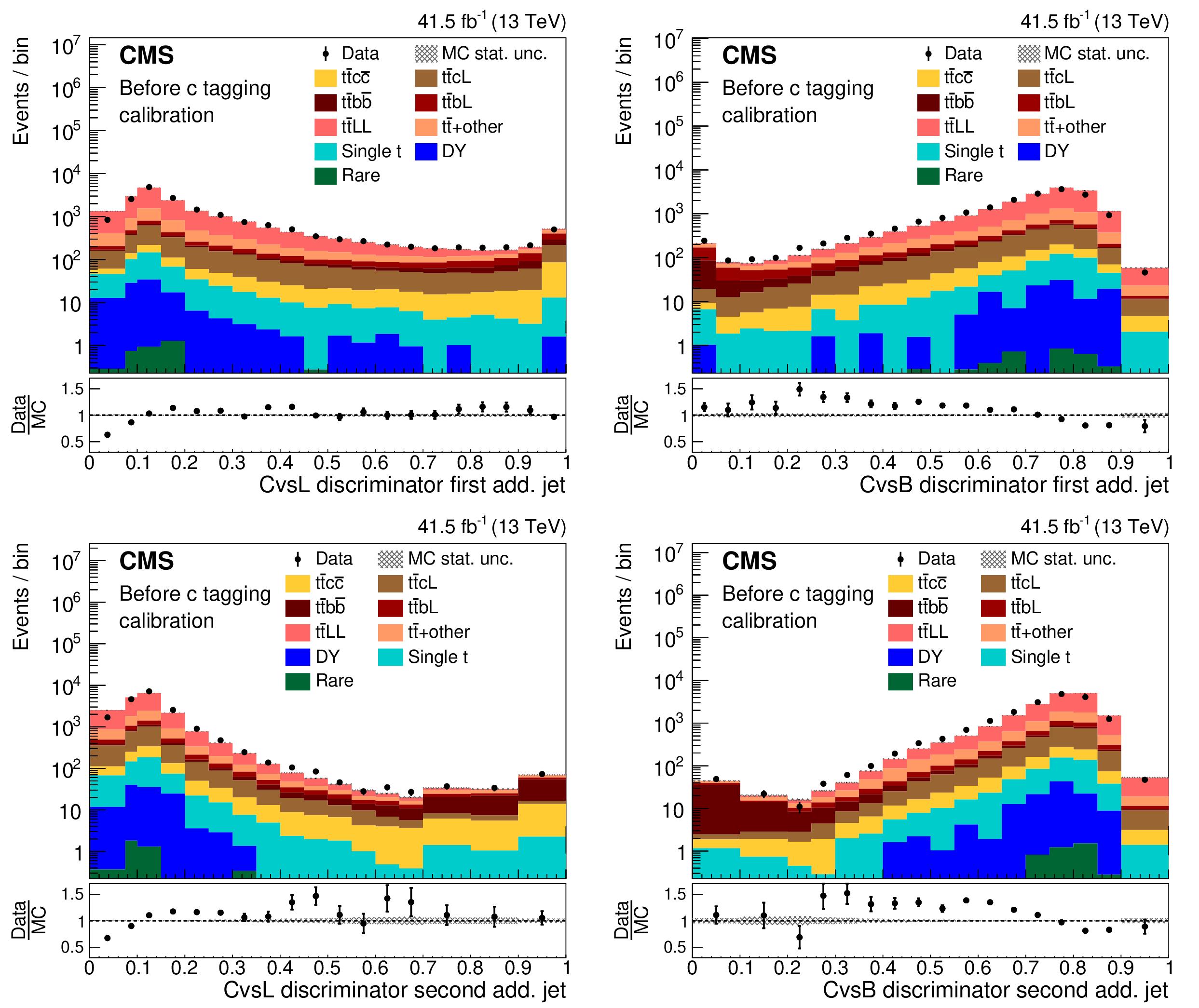
Comparison between data (points) and simulated predictions (histograms) for the CvsL (left column) and CvsB (right column) c tagging discriminator distributions of the first additional jet, before (upper row) and after (lower row) applying the c tagging calibration. The lower panels show the ratio of the yields in data to those predicted in simulations. The vertical bars represent the statistical uncertainties in data, while the hatched band show the statistical uncertainty in the simulated predictions. |
png pdf |
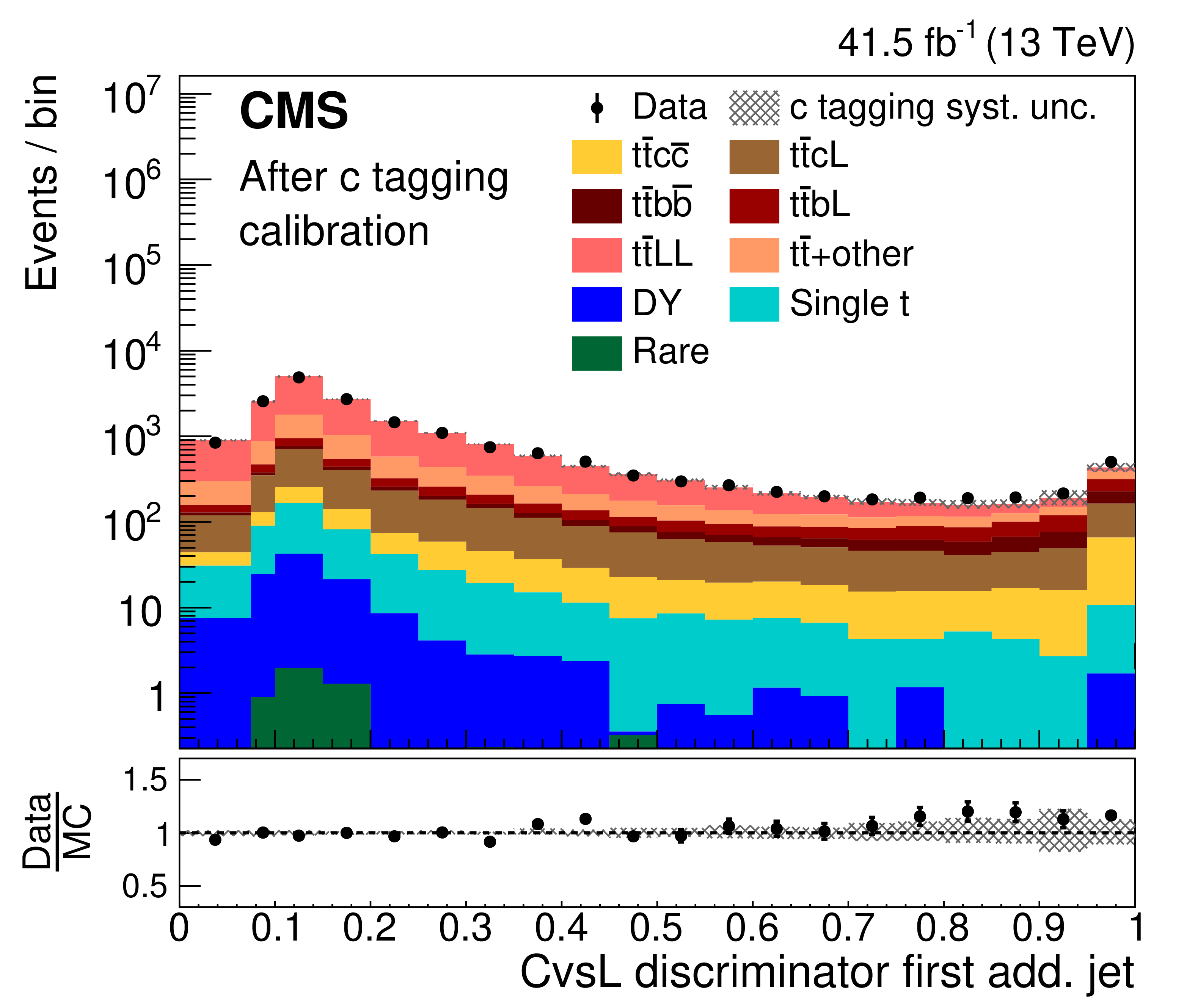
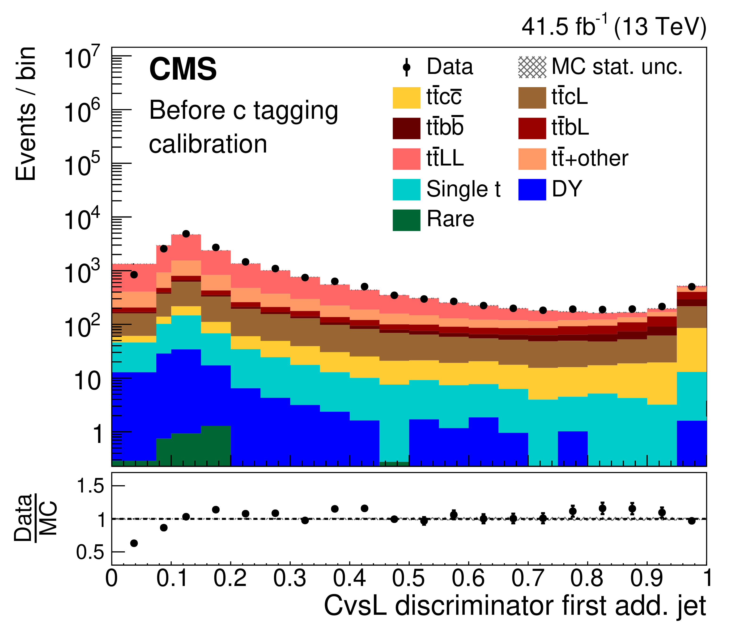
Figure 3-a:
Comparison between data (points) and simulated predictions (histograms) for the CvsL c tagging discriminator distribution of the first additional jet, before applying the c tagging calibration. The lower panel shows the ratio of the yields in data to those predicted in simulations. The vertical bars represent the statistical uncertainties in data, while the hatched band show the statistical uncertainty in the simulated predictions. |

png pdf |
Figure 3-b:
Comparison between data (points) and simulated predictions (histograms) for the CvsB c tagging discriminator distribution of the first additional jet, before applying the c tagging calibration. The lower panel shows the ratio of the yields in data to those predicted in simulations. The vertical bars represent the statistical uncertainties in data, while the hatched band show the statistical uncertainty in the simulated predictions. |
png pdf |
Figure 3-c:
Comparison between data (points) and simulated predictions (histograms) for the CvsL c tagging discriminator distribution of the first additional jet, after applying the c tagging calibration. The lower panel shows the ratio of the yields in data to those predicted in simulations. The vertical bars represent the statistical uncertainties in data, while the hatched band show the statistical uncertainty in the simulated predictions. |
png pdf |
Figure 3-d:
Comparison between data (points) and simulated predictions (histograms) for the CvsB c tagging discriminator distribution of the first additional jet, after applying the c tagging calibration. The lower panel shows the ratio of the yields in data to those predicted in simulations. The vertical bars represent the statistical uncertainties in data, while the hatched band show the statistical uncertainty in the simulated predictions. |

png pdf |
Figure 4:
Normalized two-dimensional distributions of $\Delta _{\mathrm{b}}^{\mathrm{c}}$ vs. $\Delta _{\text {L}}^{\mathrm{c}}$ in simulated dileptonic ${\mathrm{t} {}\mathrm{\bar{t}}} $ events, for each of the event categories outlined in Section 4. The colour scale on the right shows the normalized event yields. |
png pdf |
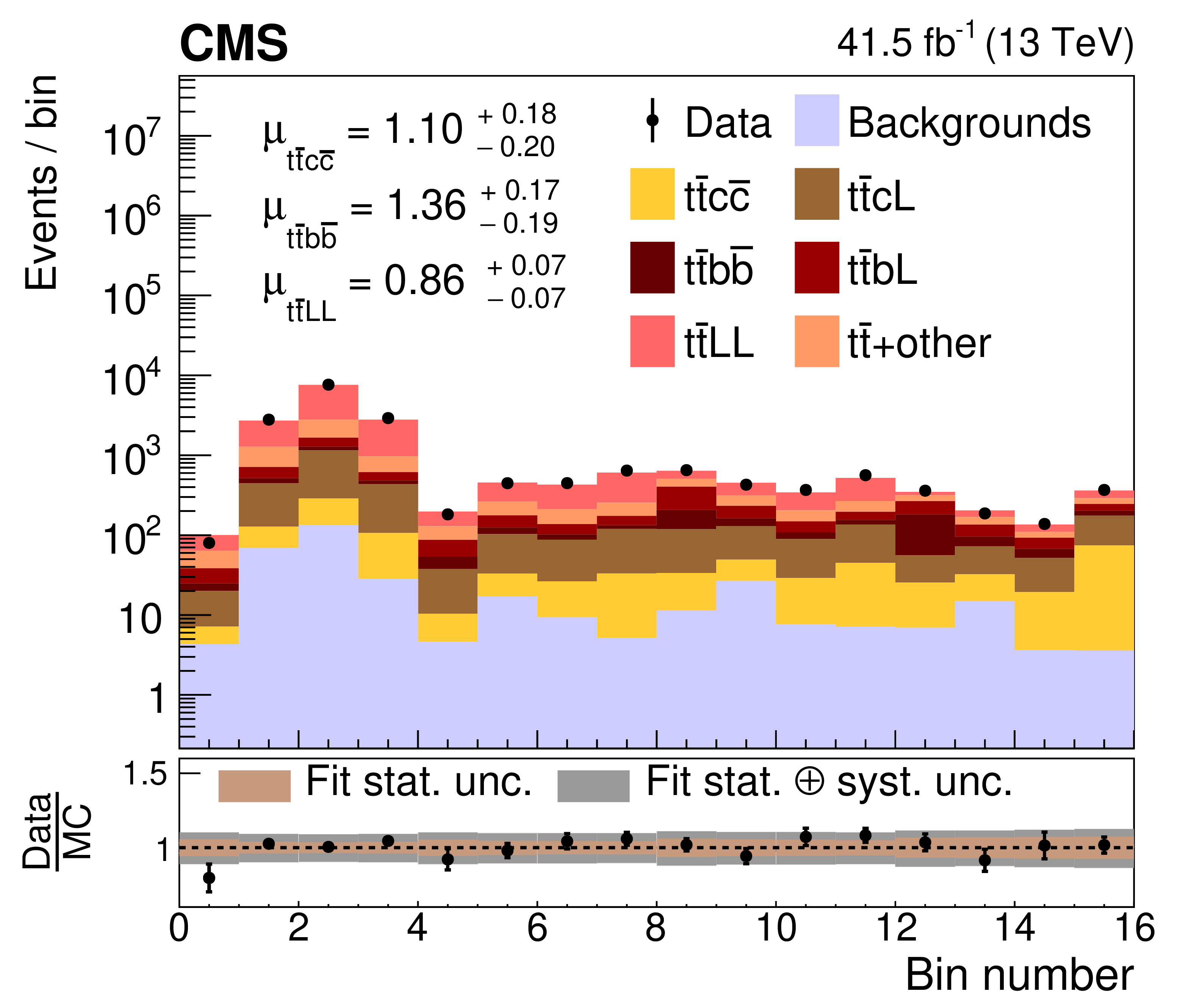
Figure 5:
A one-dimensional representation of the two-dimensional $\Delta _{\text {L}}^{\mathrm{c}}$ vs. $\Delta _{\mathrm{b}}^{\mathrm{c}}$ distributions, in the simulations (histograms) and in data (points), after normalizing the simulated templates according to the fitted cross sections. The lower panel shows the ratio of the yields in data to those predicted in the simulations. The brown and grey uncertainty bands denote, respectively, the statistical and total uncertainties from the fit. The factors ($\mu $) by which the templates of the different processes (using the POWHEG ME generator) are scaled, are also displayed, together with their combined statistical and systematic uncertainties. |
png pdf |
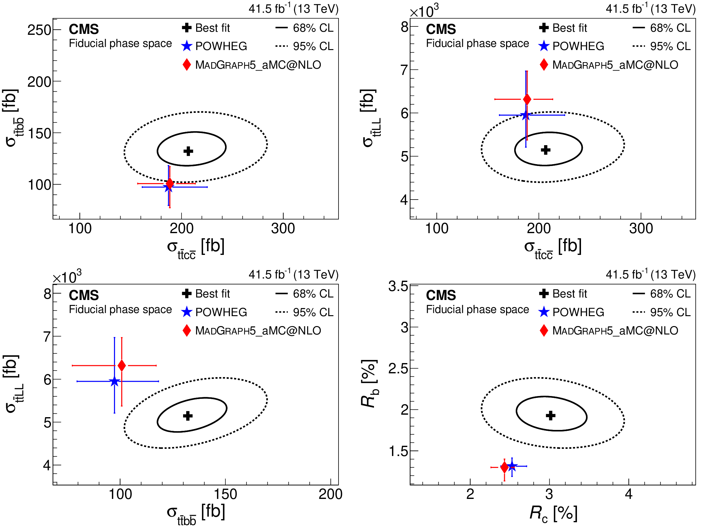
Figure 6:
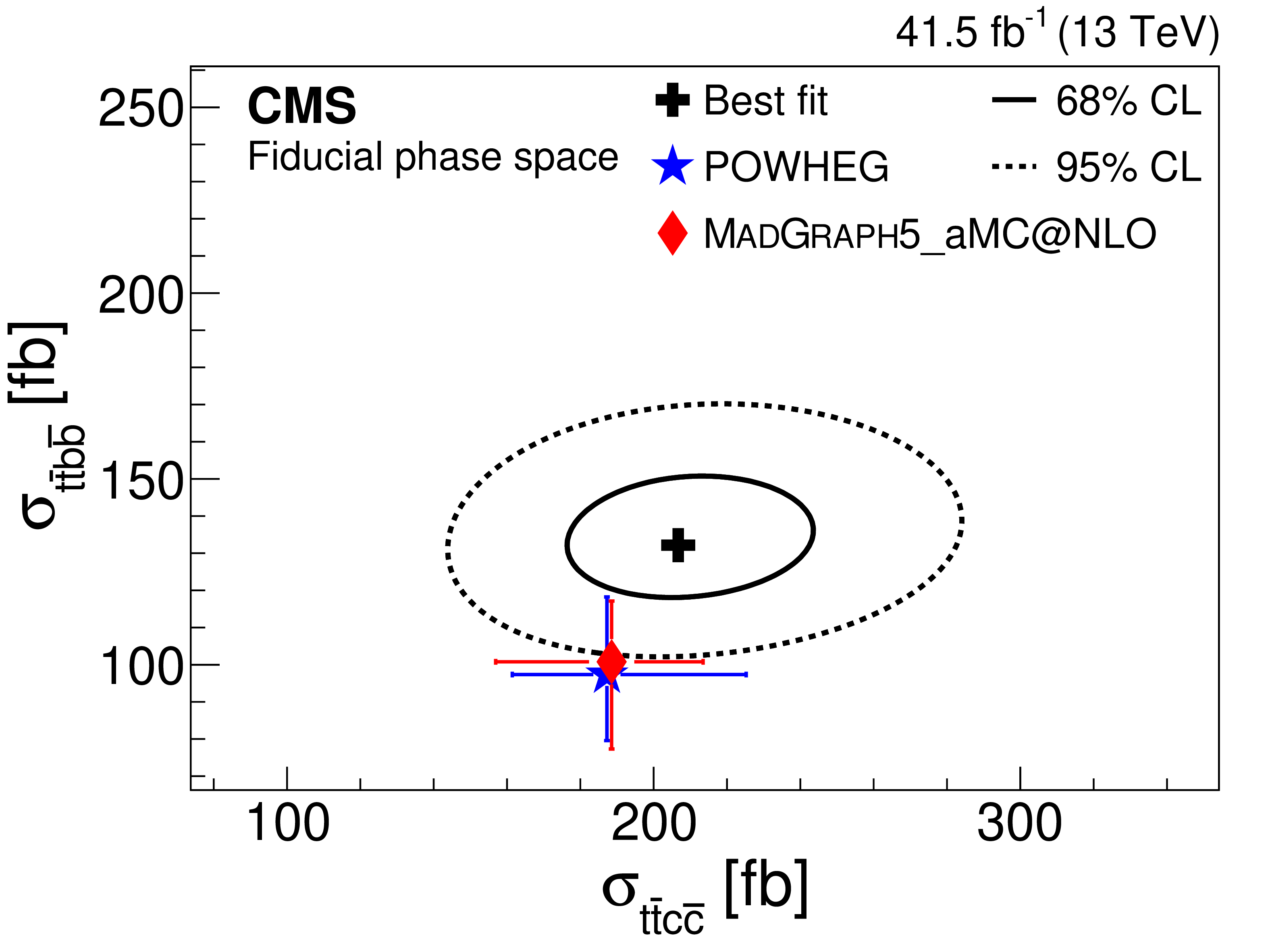
Results of the two-dimensional likelihood scans for several combinations of the parameters of interest in the fiducial phase space. The best-fit value (black cross) with the corresponding 68% (full) and 95% (dashed) confidence level (CL) contours are shown, compared to the theoretical predictions using either the POWHEG (blue star) or MadGraph 5_aMC@NLO (red diamond) ME generators. Uncertainties in the theoretical predictions are displayed by the horizontal and vertical bars on the markers. |
png pdf |
Figure 6-a:
Result of the two-dimensional likelihood scan for $\sigma_{\mathrm{t\bar{t}b\bar{b}}}$ [fb] versus $\sigma_{\mathrm{t\bar{t}c\bar{c}}}$ [fb] in the fiducial phase space. The best-fit value (black cross) with the corresponding 68% (full) and 95% (dashed) confidence level (CL) contours are shown, compared to the theoretical predictions using either the POWHEG (blue star) or MadGraph 5_aMC@NLO (red diamond) ME generators. Uncertainties in the theoretical predictions are displayed by the horizontal and vertical bars on the markers. |
png pdf |
Figure 6-b:
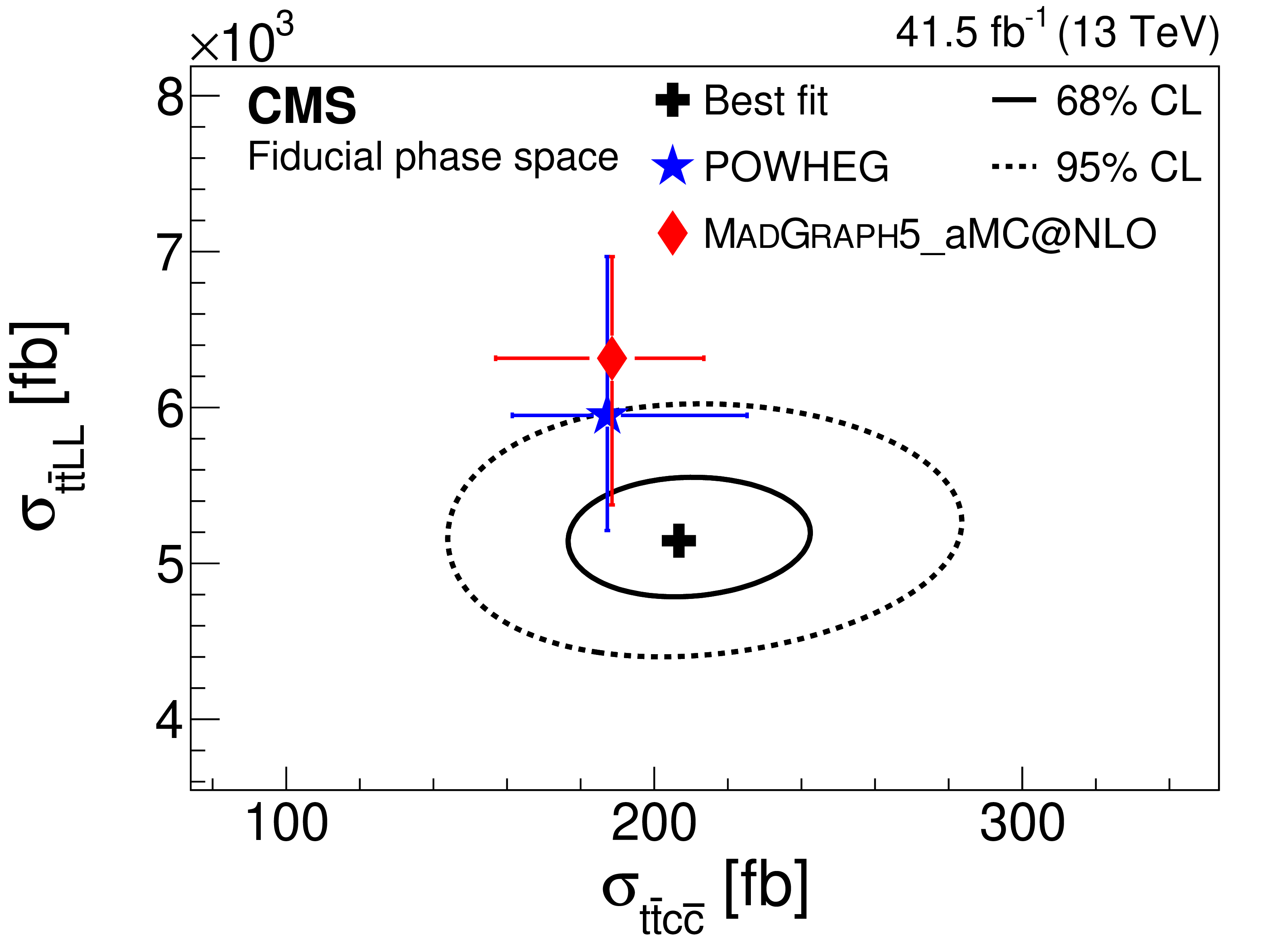
Result of the two-dimensional likelihood scan for $\sigma_{\mathrm{t\bar{t}LL}}$ [fb] versus $\sigma_{\mathrm{t\bar{t}c\bar{c}}}$ [fb] in the fiducial phase space. The best-fit value (black cross) with the corresponding 68% (full) and 95% (dashed) confidence level (CL) contours are shown, compared to the theoretical predictions using either the POWHEG (blue star) or MadGraph 5_aMC@NLO (red diamond) ME generators. Uncertainties in the theoretical predictions are displayed by the horizontal and vertical bars on the markers. |
png pdf |
Figure 6-c:
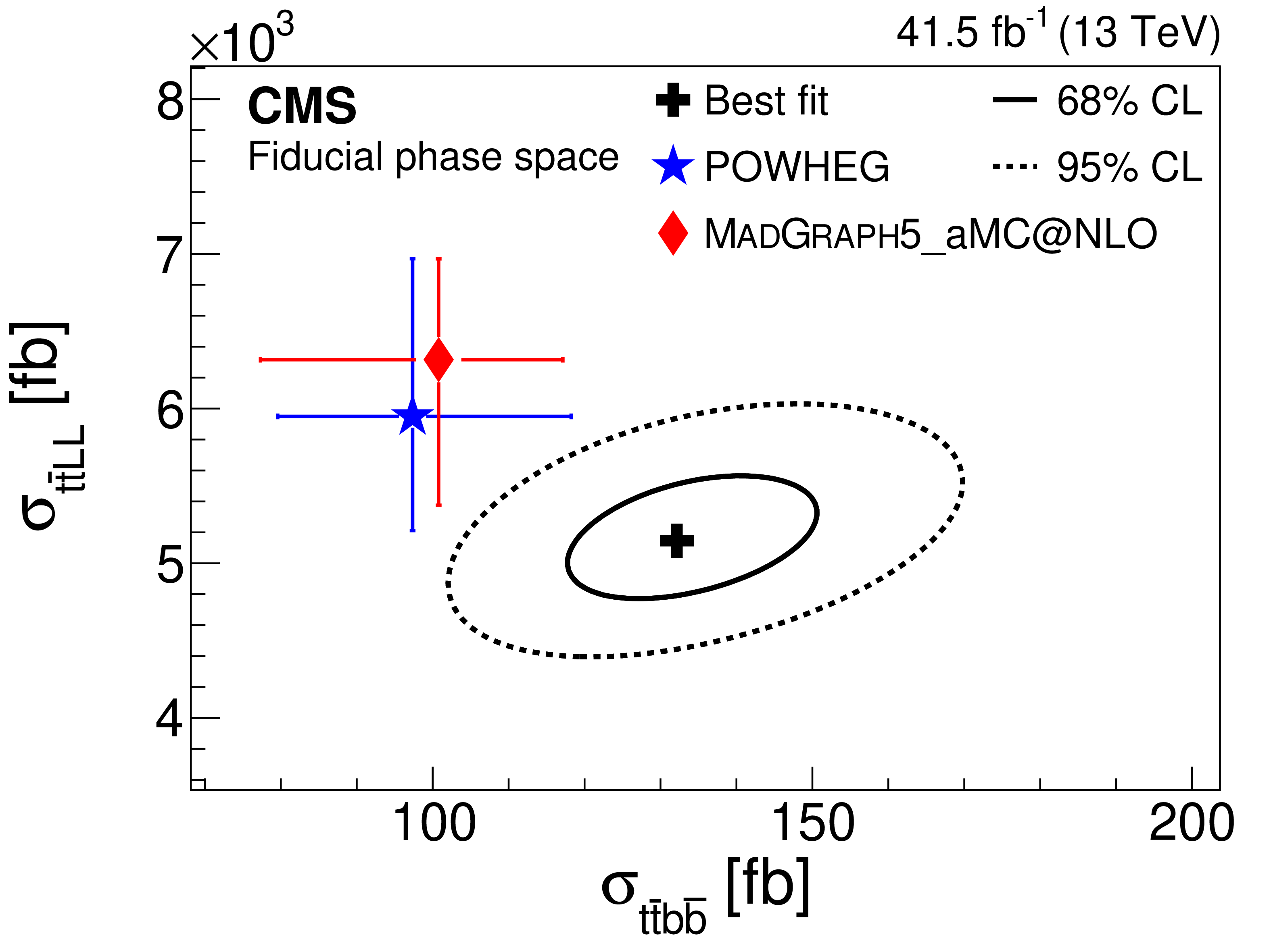
Result of the two-dimensional likelihood scan for $\sigma_{\mathrm{t\bar{t}LL}}$ [fb] versus $\sigma_{\mathrm{t\bar{t}b\bar{b}}}$ [fb] in the fiducial phase space. The best-fit value (black cross) with the corresponding 68% (full) and 95% (dashed) confidence level (CL) contours are shown, compared to the theoretical predictions using either the POWHEG (blue star) or MadGraph 5_aMC@NLO (red diamond) ME generators. Uncertainties in the theoretical predictions are displayed by the horizontal and vertical bars on the markers. |
png pdf |
Figure 6-d:
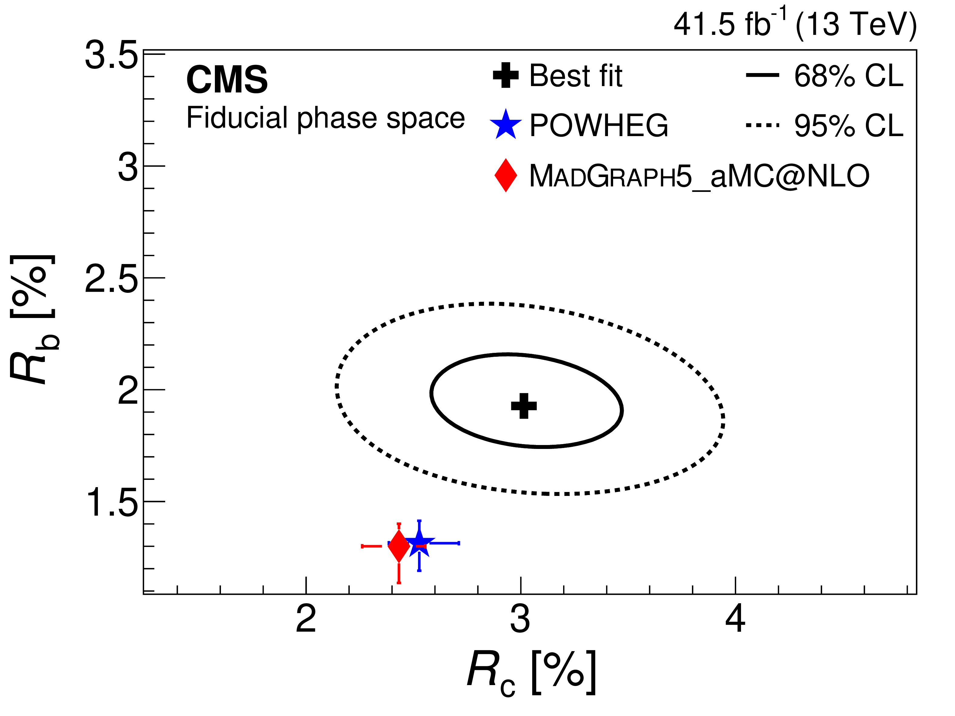
Result of the two-dimensional likelihood scan for $R_{\mathrm{b}}$ [%] versus $R_{\mathrm{c}}$ [%] in the fiducial phase space. The best-fit value (black cross) with the corresponding 68% (full) and 95% (dashed) confidence level (CL) contours are shown, compared to the theoretical predictions using either the POWHEG (blue star) or MadGraph 5_aMC@NLO (red diamond) ME generators. Uncertainties in the theoretical predictions are displayed by the horizontal and vertical bars on the markers. |
png pdf |
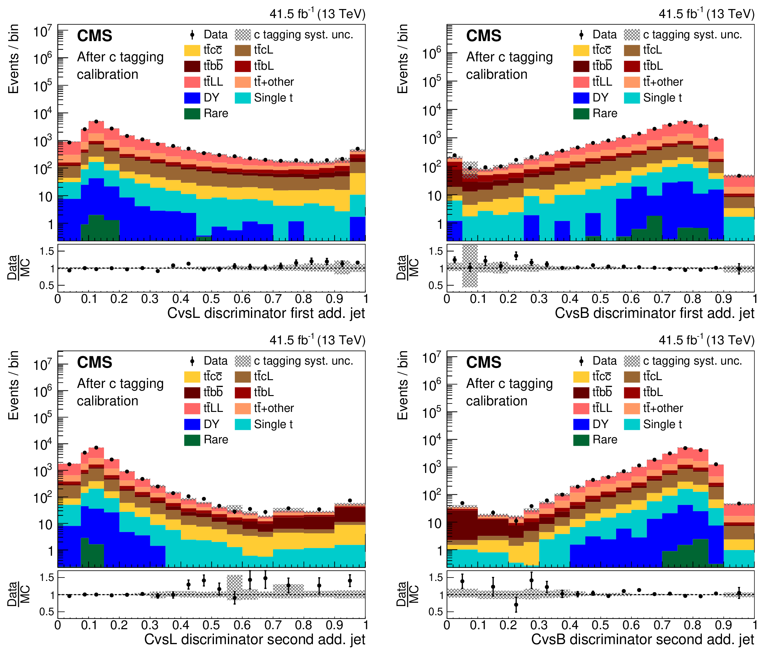
Figure 7:
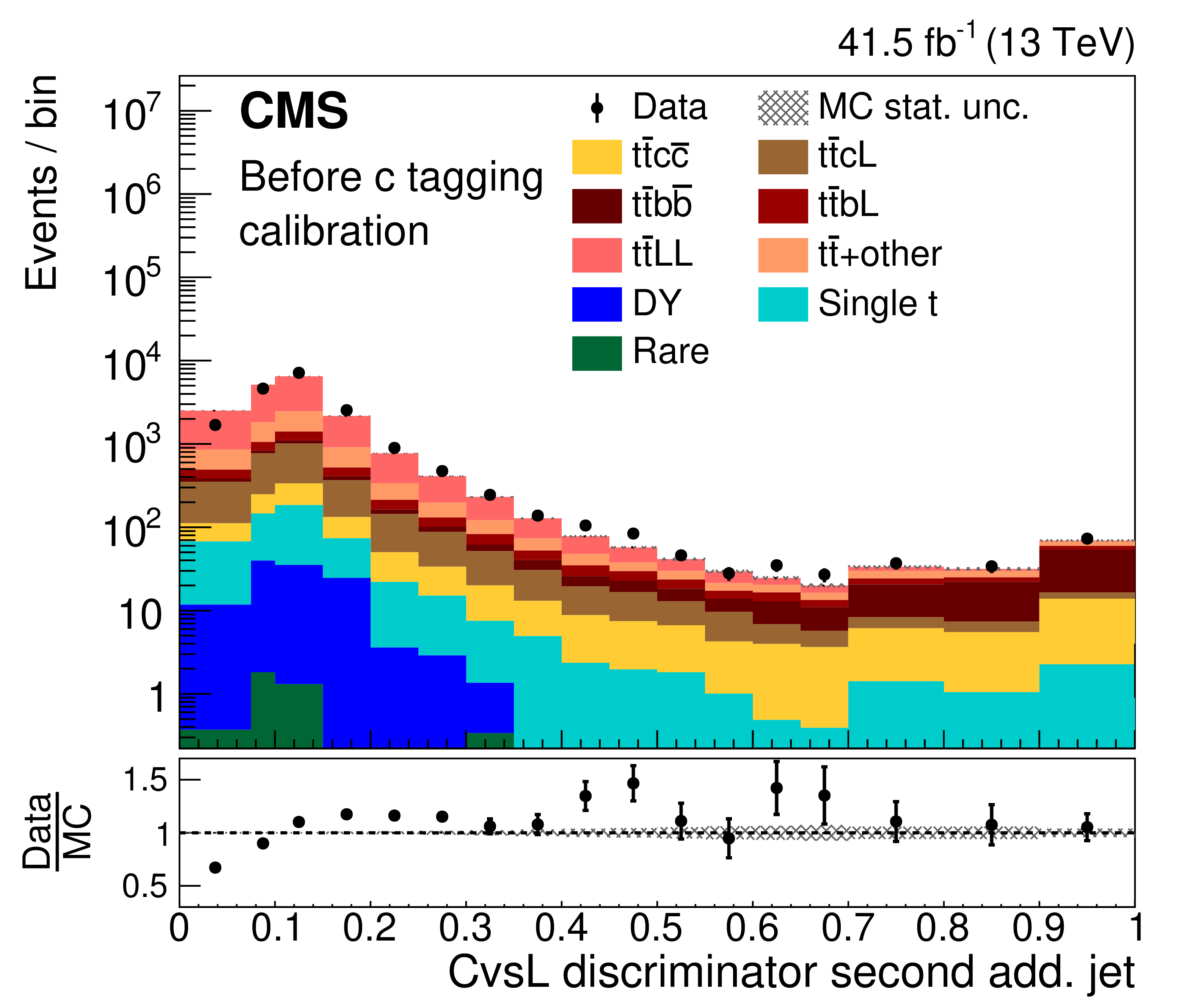
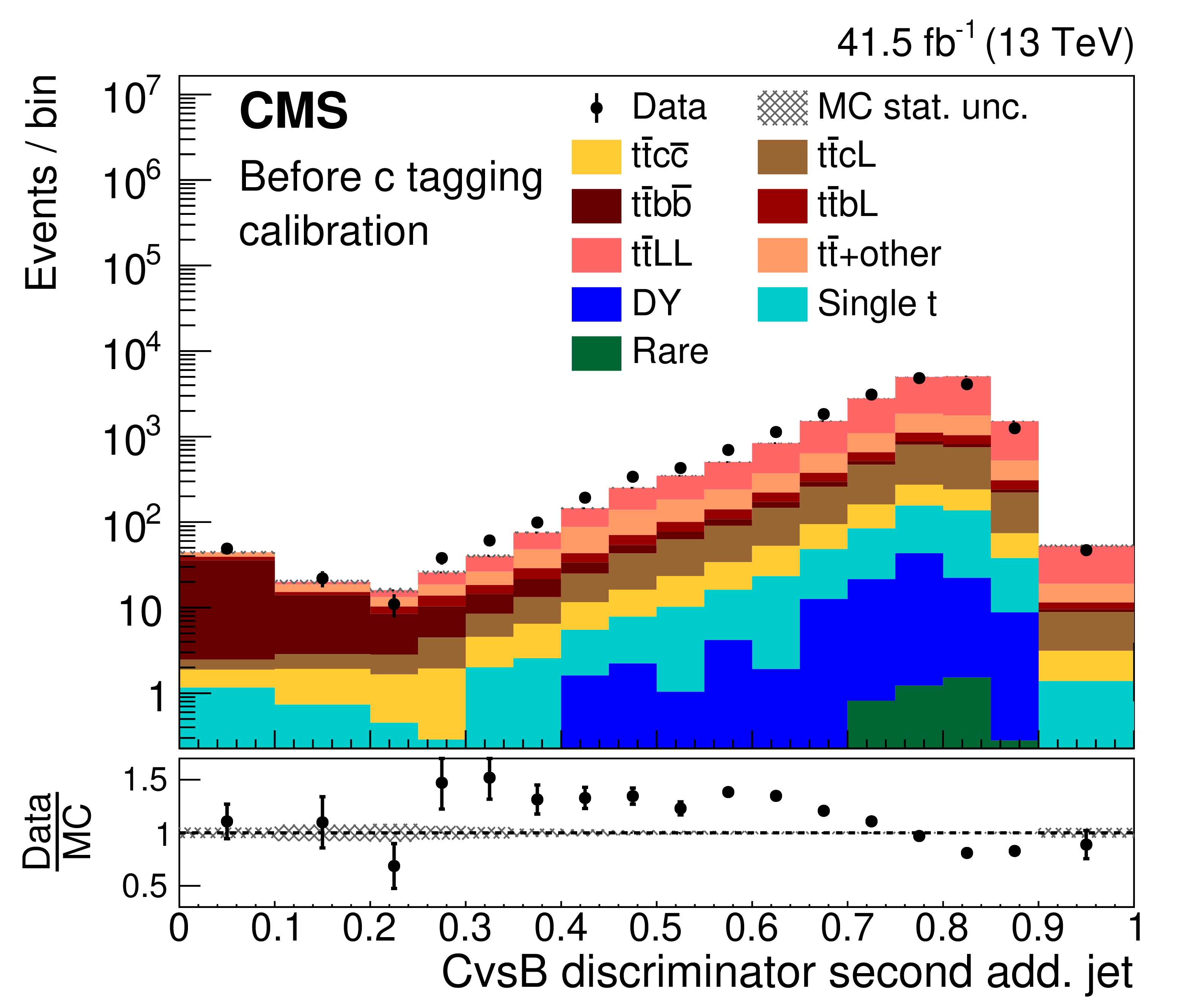
Comparison between data (points) and simulated predictions (histograms) for the CvsL (left column) and CvsB (right column) c tagging discriminator distributions of the first (upper row) and second (lower row) additional jet before applying the c tagging calibration. The lower panels show the ratio of the yields in data to those predicted in simulations. The vertical bars represent the statistical uncertainties in data, while the hatched bands show the statistical uncertainty in the simulated predictions. |
png pdf |
Figure 7-a:
Comparison between data (points) and simulated predictions (histograms) for the CvsL (left column) and CvsB (right column) c tagging discriminator distributions of the first (upper row) and second (lower row) additional jet before applying the c tagging calibration. The lower panels show the ratio of the yields in data to those predicted in simulations. The vertical bars represent the statistical uncertainties in data, while the hatched bands show the statistical uncertainty in the simulated predictions. |

png pdf |
Figure 7-b:
Comparison between data (points) and simulated predictions (histograms) for the CvsL (left column) and CvsB (right column) c tagging discriminator distributions of the first (upper row) and second (lower row) additional jet before applying the c tagging calibration. The lower panels show the ratio of the yields in data to those predicted in simulations. The vertical bars represent the statistical uncertainties in data, while the hatched bands show the statistical uncertainty in the simulated predictions. |
png pdf |
Figure 7-c:
Comparison between data (points) and simulated predictions (histograms) for the CvsL (left column) and CvsB (right column) c tagging discriminator distributions of the first (upper row) and second (lower row) additional jet before applying the c tagging calibration. The lower panels show the ratio of the yields in data to those predicted in simulations. The vertical bars represent the statistical uncertainties in data, while the hatched bands show the statistical uncertainty in the simulated predictions. |
png pdf |
Figure 7-d:
Comparison between data (points) and simulated predictions (histograms) for the CvsL (left column) and CvsB (right column) c tagging discriminator distributions of the first (upper row) and second (lower row) additional jet before applying the c tagging calibration. The lower panels show the ratio of the yields in data to those predicted in simulations. The vertical bars represent the statistical uncertainties in data, while the hatched bands show the statistical uncertainty in the simulated predictions. |

png pdf |
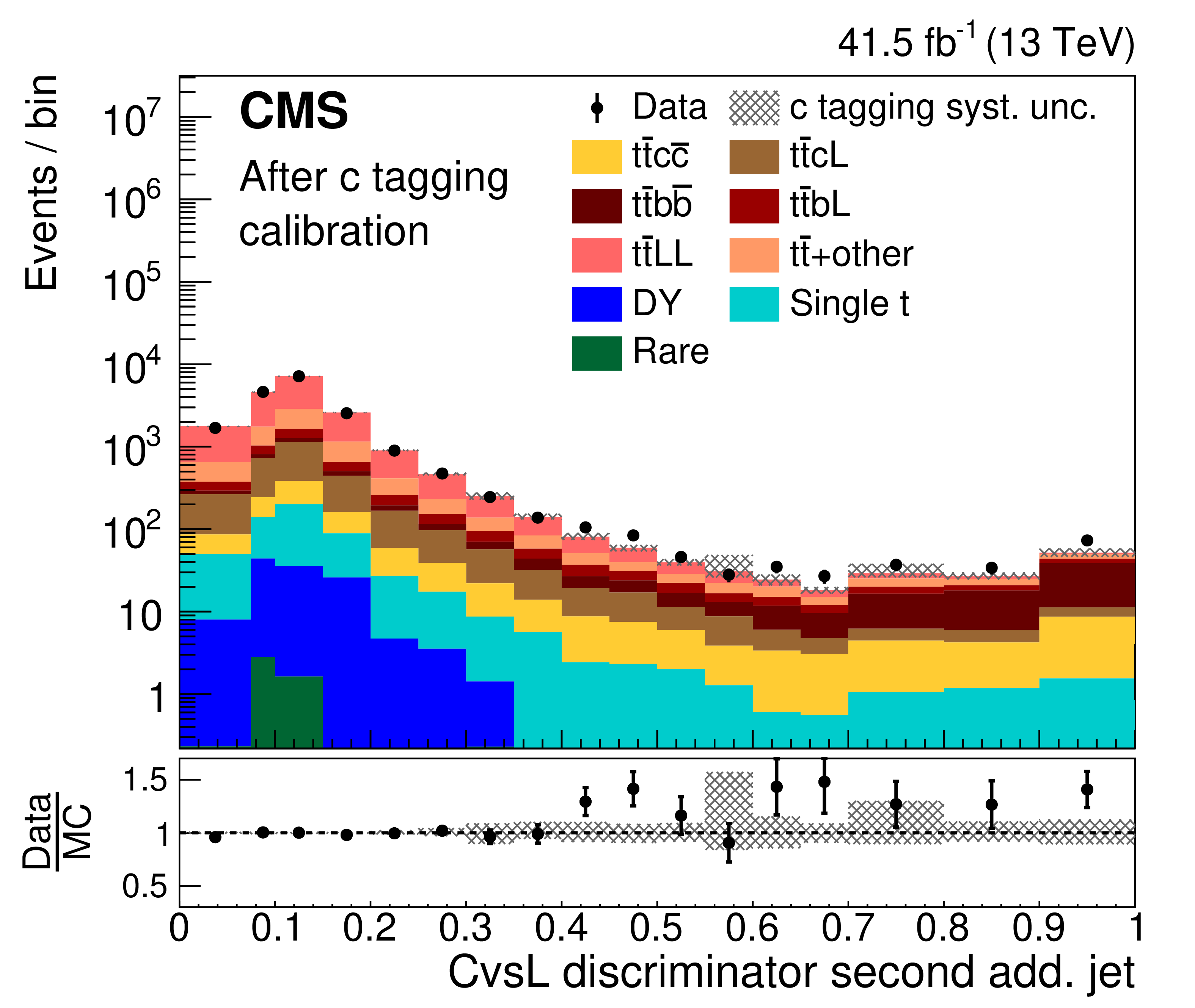
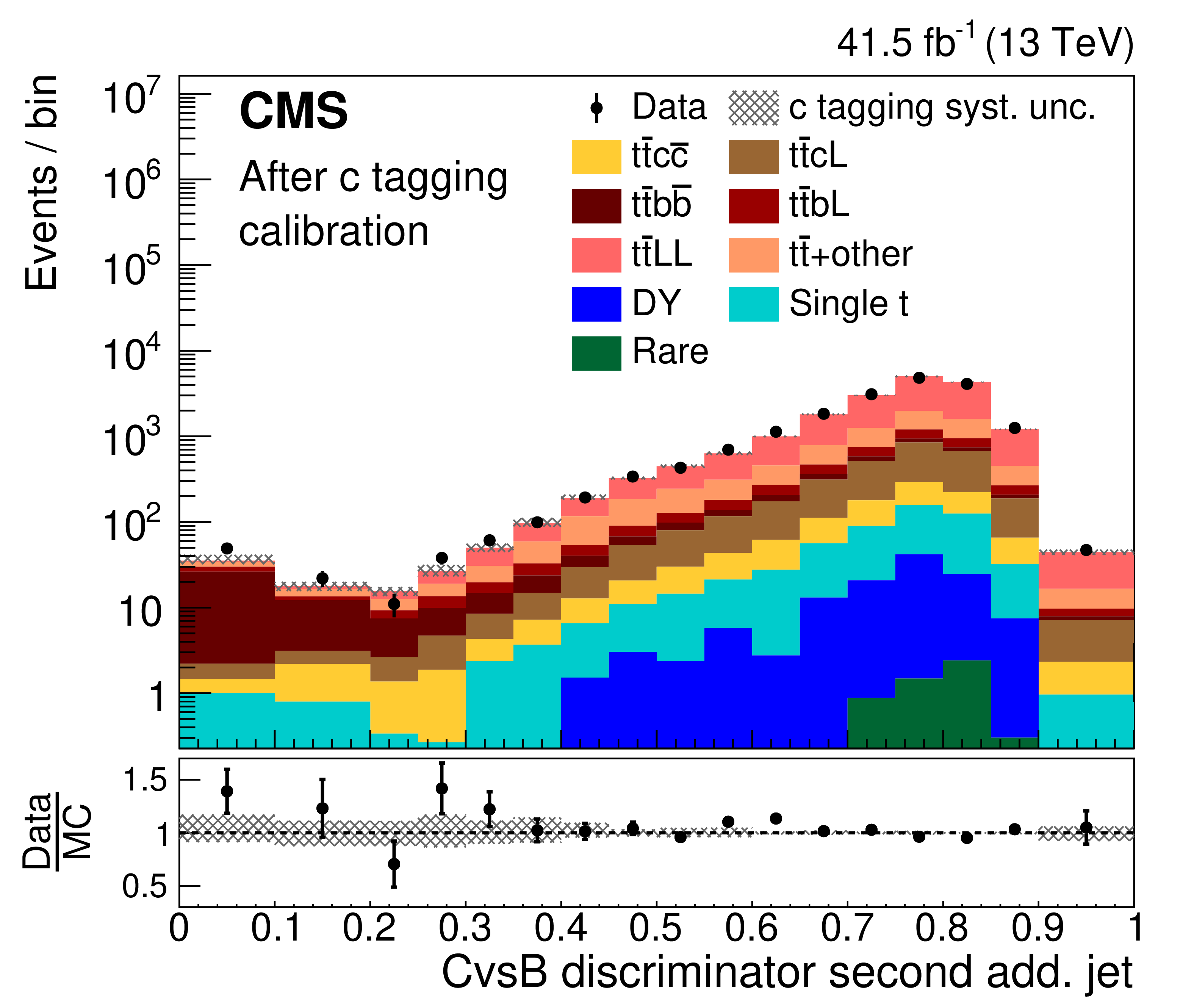
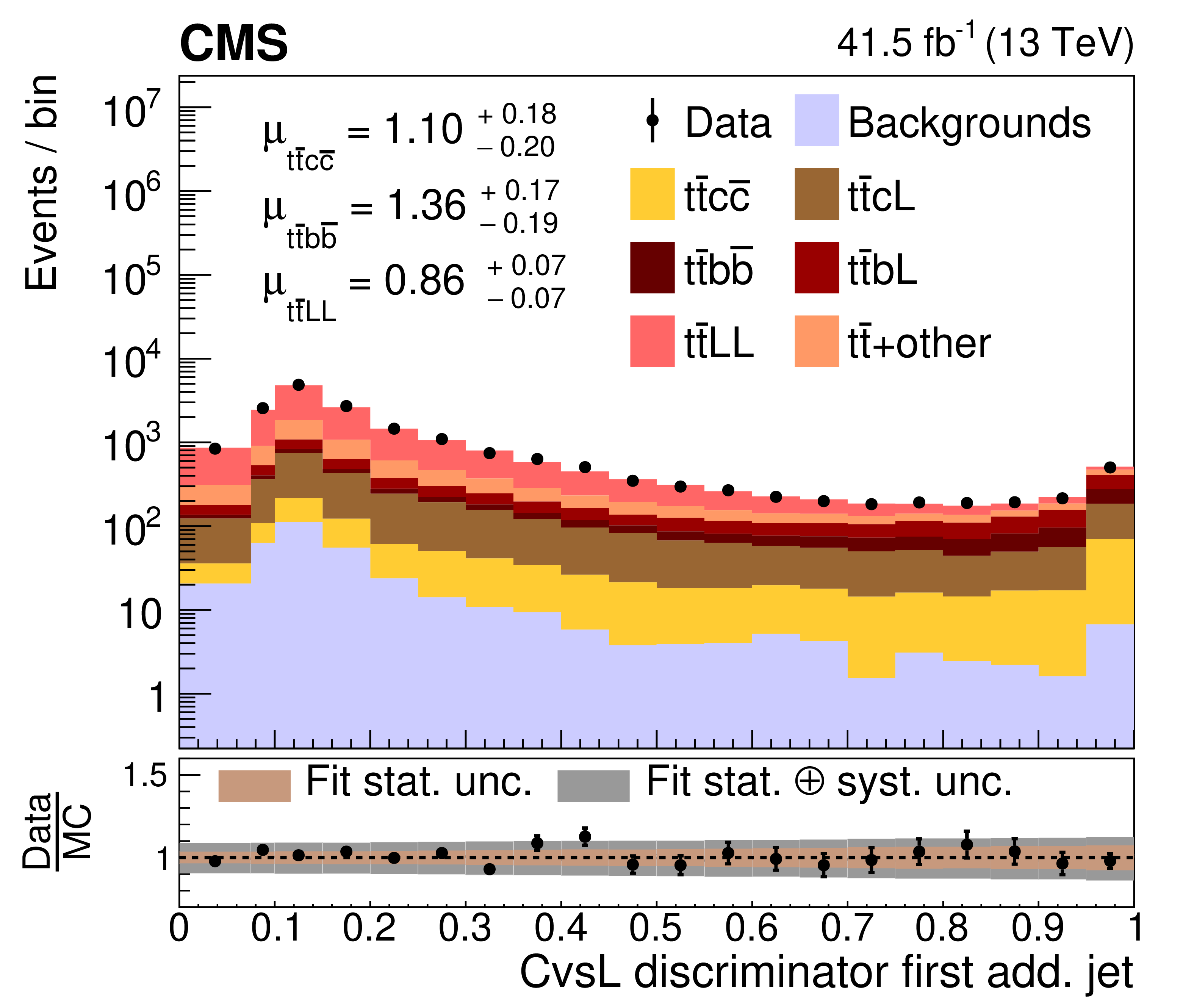
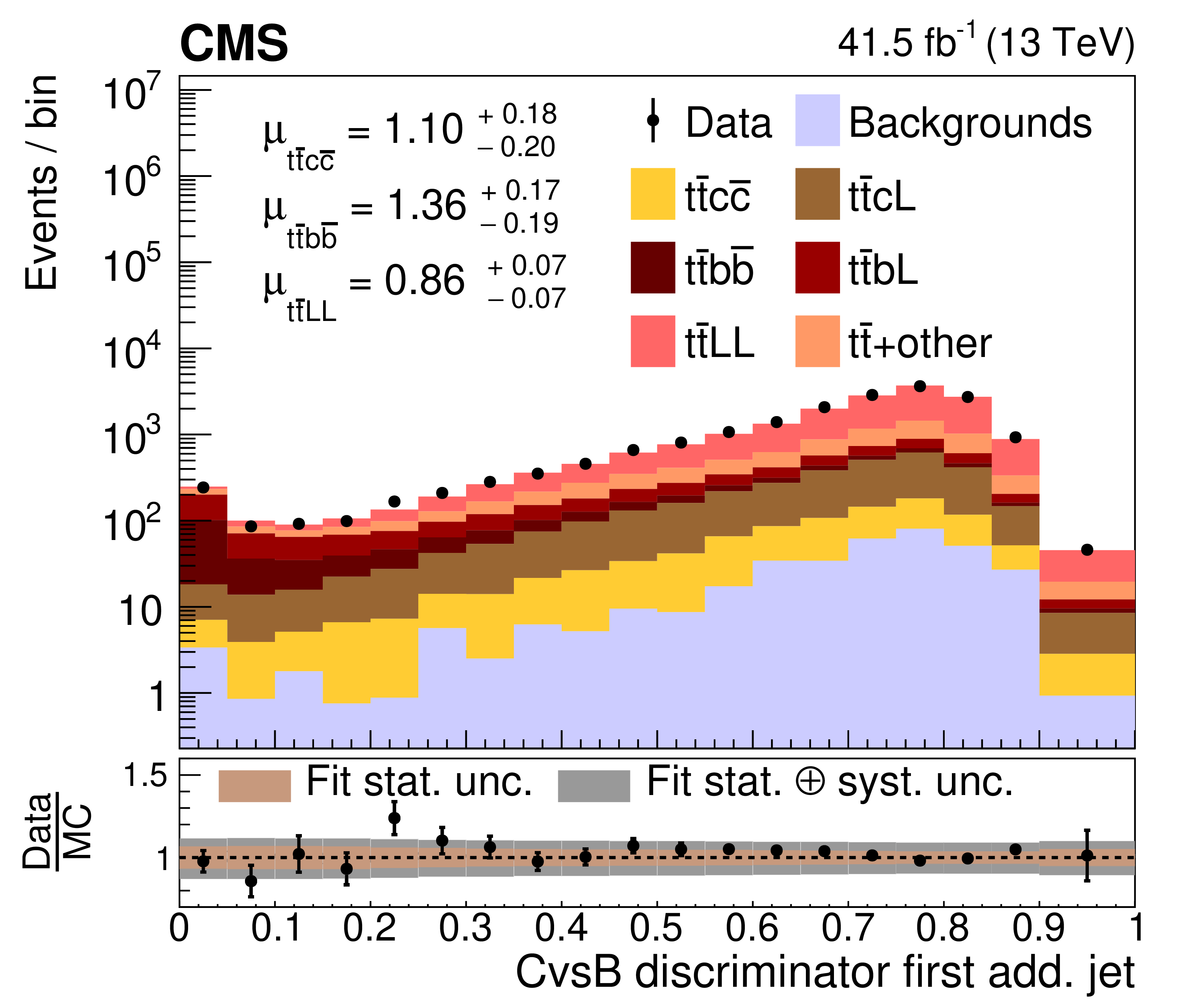
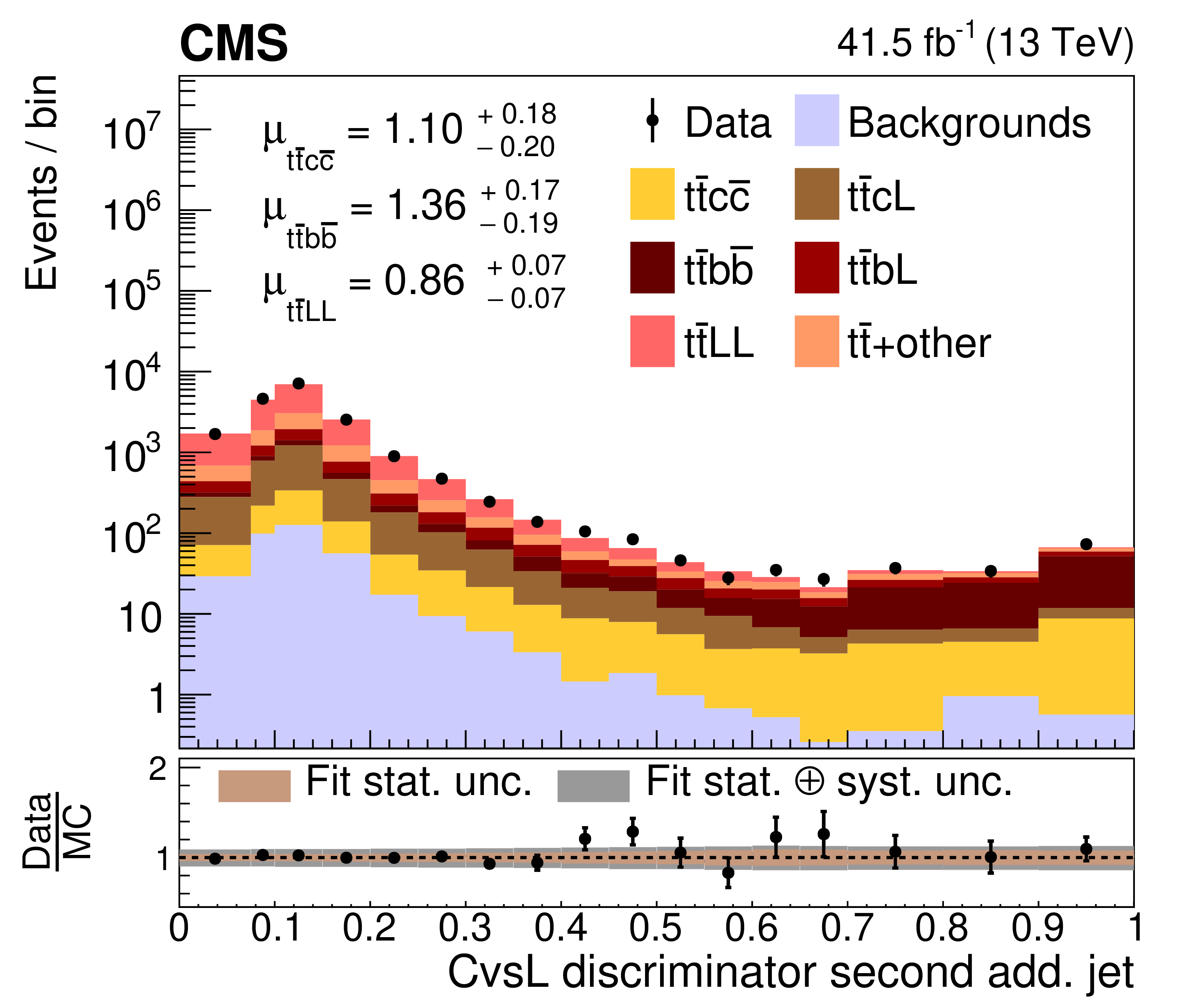
Figure 8:
Comparison between data (points) and simulated predictions (histograms) for the CvsL (left column) and CvsB (right column) c tagging discriminator distributions of the first (upper row) and second (lower row) additional jet, after normalizing the simulated templates according to the fitted cross sections. The lower panels show the ratio of the yields in data to those predicted in the simulations. The brown and grey uncertainty bands denote, respectively, the statistical and total uncertainties from the fit. The factors ($\mu $) by which the templates of the different processes (using the POWHEG ME generator) are scaled, are also displayed, together with their combined statistical and systematic uncertainties. |
png pdf |
Figure 8-a:
Comparison between data (points) and simulated predictions (histograms) for the CvsL (left column) and CvsB (right column) c tagging discriminator distributions of the first (upper row) and second (lower row) additional jet, after normalizing the simulated templates according to the fitted cross sections. The lower panels show the ratio of the yields in data to those predicted in the simulations. The brown and grey uncertainty bands denote, respectively, the statistical and total uncertainties from the fit. The factors ($\mu $) by which the templates of the different processes (using the POWHEG ME generator) are scaled, are also displayed, together with their combined statistical and systematic uncertainties. |
png pdf |
Figure 8-b:
Comparison between data (points) and simulated predictions (histograms) for the CvsL (left column) and CvsB (right column) c tagging discriminator distributions of the first (upper row) and second (lower row) additional jet, after normalizing the simulated templates according to the fitted cross sections. The lower panels show the ratio of the yields in data to those predicted in the simulations. The brown and grey uncertainty bands denote, respectively, the statistical and total uncertainties from the fit. The factors ($\mu $) by which the templates of the different processes (using the POWHEG ME generator) are scaled, are also displayed, together with their combined statistical and systematic uncertainties. |
png pdf |
Figure 8-c:
Comparison between data (points) and simulated predictions (histograms) for the CvsL (left column) and CvsB (right column) c tagging discriminator distributions of the first (upper row) and second (lower row) additional jet, after normalizing the simulated templates according to the fitted cross sections. The lower panels show the ratio of the yields in data to those predicted in the simulations. The brown and grey uncertainty bands denote, respectively, the statistical and total uncertainties from the fit. The factors ($\mu $) by which the templates of the different processes (using the POWHEG ME generator) are scaled, are also displayed, together with their combined statistical and systematic uncertainties. |

png pdf |
Figure 8-d:
Comparison between data (points) and simulated predictions (histograms) for the CvsL (left column) and CvsB (right column) c tagging discriminator distributions of the first (upper row) and second (lower row) additional jet, after normalizing the simulated templates according to the fitted cross sections. The lower panels show the ratio of the yields in data to those predicted in the simulations. The brown and grey uncertainty bands denote, respectively, the statistical and total uncertainties from the fit. The factors ($\mu $) by which the templates of the different processes (using the POWHEG ME generator) are scaled, are also displayed, together with their combined statistical and systematic uncertainties. |
| Tables | |

png pdf |
Table 1:
Selection efficiencies and acceptance factors for events in different signal categories. The values are obtained from simulated ${\mathrm{t} {}\mathrm{\bar{t}}} $ events. |
png pdf |
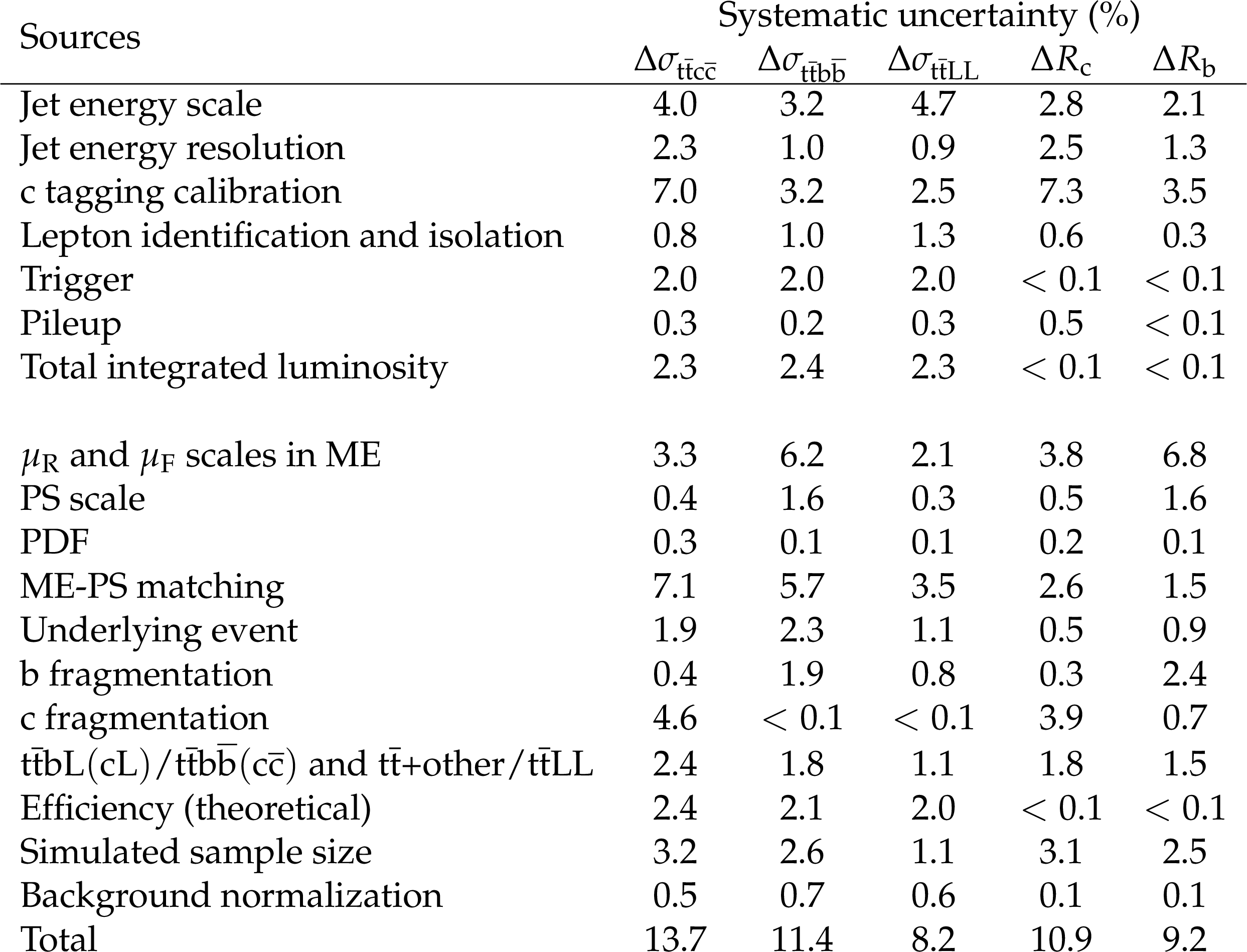
Table 2:
Sources of systematic uncertainties in the measured parameters and their individual impact in percent for the fiducial phase space. The upper (lower) rows of the table list uncertainties related to the experimental conditions (theoretical modelling). The last row gives the overall systematic uncertainty in each quantity, which results from the nuisance parameter variations in the fit and is not the quadrature sum of the individual components. |
png pdf |
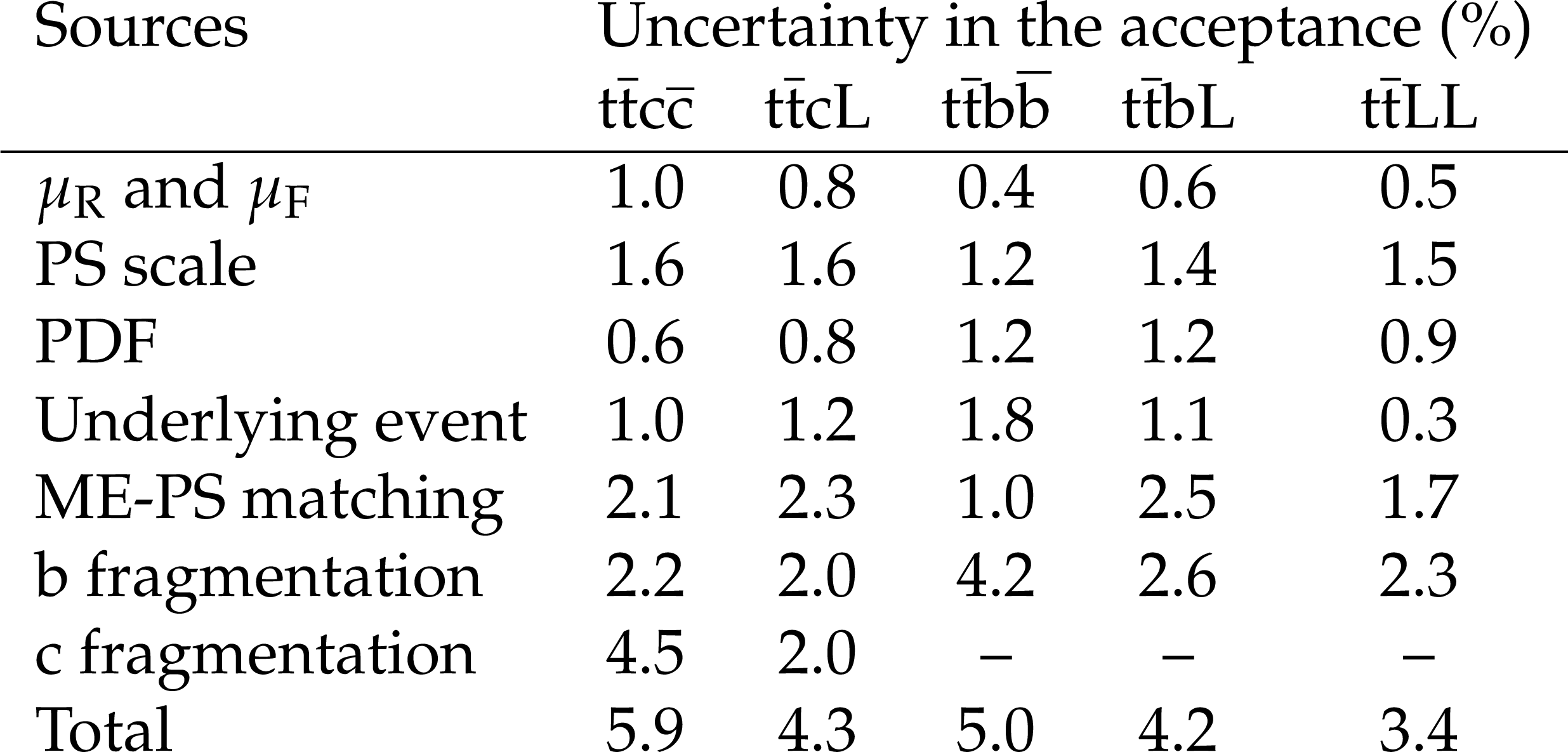
Table 3:
Sources of theoretical uncertainties in the acceptance, used to extrapolate the results from the fiducial to the full phase space, for different signal categories, together with their individual impact in percent. The last row of the table quotes the total relative uncertainty in the acceptance, calculated by adding in quadrature the effects from individual sources. |
png pdf |
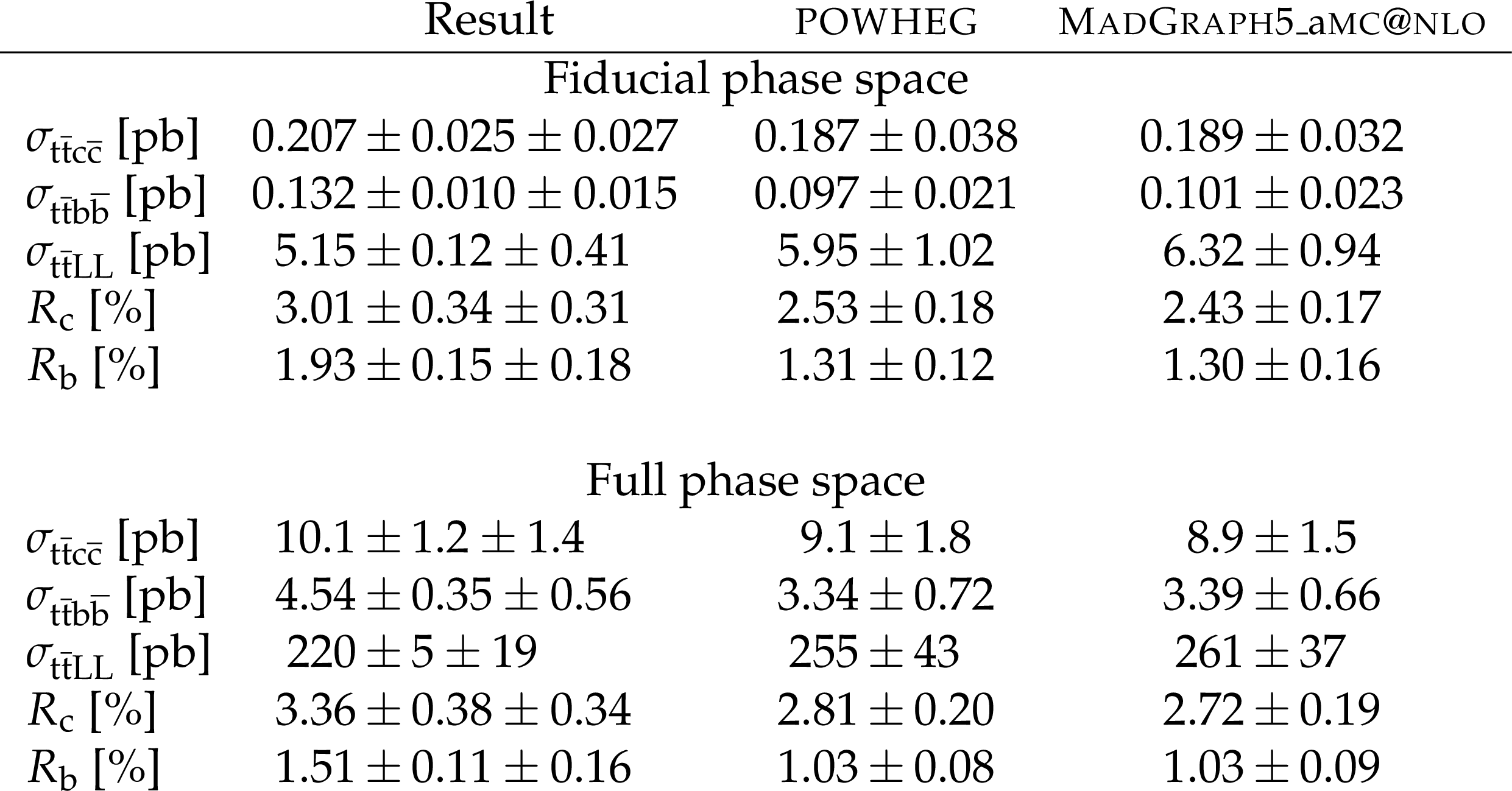
Table 4:
Measured parameter values in the fiducial (upper rows) and full (lower rows) phase spaces with their statistical and systematic uncertainties listed in that order. The last two columns display the expectations from the simulated ${\mathrm{t} {}\mathrm{\bar{t}}} $ samples using the POWHEG or MadGraph 5_aMC@NLO ME generators. The uncertainties quoted for these predictions include the contributions from the theoretical uncertainties listed in the lower rows of Table 2, as well as the uncertainty in the ${\mathrm{t} {}\mathrm{\bar{t}}} $ cross section. |
| Summary |
|
The production of a top quark pair ($\mathrm{t\bar{t}}$) in association with additional bottom or charm jets at the LHC provides challenges both in the theoretical modelling and experimental measurement of this process. Whereas $\mathrm{t\bar{t}}$ production with two additional bottom jets ($\mathrm{t\bar{t}}\mathrm{b}\mathrm{\bar{b}}$) has been measured by the ATLAS and CMS Collaborations at different centre-of-mass energies [6,7,8,9,10,11,12,13], this analysis presents the first measurement of the cross section for $\mathrm{t\bar{t}}$ production with two additional charm jets ($\mathrm{t\bar{t}}\mathrm{c}\mathrm{\bar{c}}$). The analysis is conducted using data from proton-proton collisions recorded by the CMS experiment at a centre-of-mass energy of 13 TeV, corresponding to an integrated luminosity of 41.5 fb$^{-1}$. The measurement is performed in the dileptonic channel of the $\mathrm{t\bar{t}}$ decays and relies on the use of recently developed charm jet identification algorithms (c tagging). A template fitting method is used, based on the outputs of a neural network classifier trained to identify the signal categories defined by the flavour of the additional jets. This allows the simultaneous extraction of the cross section for the $\mathrm{t\bar{t}}\mathrm{c}\mathrm{\bar{c}}$, $\mathrm{t\bar{t}}\mathrm{b}\mathrm{\bar{b}}$, and $\mathrm{t\bar{t}}$ with two additional light-flavour or gluon jets ($\mathrm{t\bar{t}}\text{LL}$) processes. A novel multidimensional calibration of the shape of the c tagging discriminator distributions is employed, such that this information can be reliably used in the neural network classifier. The $\mathrm{t\bar{t}}\mathrm{c}\mathrm{\bar{c}}$ cross section is measured for the first time to be 0.165 $\pm$ 0.023 (stat) $\pm$ 0.025 (syst) pb in the fiducial phase space (matching closely the sensitive region of the detector) and 8.0 $\pm$ 1.1 (stat) $\pm$ 1.3 (syst) pb in the full phase space. The ratio of the $\mathrm{t\bar{t}}\mathrm{c}\mathrm{\bar{c}}$ to the inclusive $\mathrm{t\bar{t}}$ + two jets cross section is found to be (2.42 $\pm$ 0.32 (stat) $\pm$ 0.29 (syst))% in the fiducial phase space and (2.69 $\pm$ 0.36 (stat) $\pm$ 0.32 (syst))% in the full phase space. Agreement is observed at the level of one to two standard deviations between the measured values and theoretical predictions for the $\mathrm{t\bar{t}}\mathrm{c}\mathrm{\bar{c}}$, $\mathrm{t\bar{t}}\mathrm{b}\mathrm{\bar{b}}$, and $\mathrm{t\bar{t}}\text{LL}$ processes. |
| References | ||||
| 1 | A. Bredenstein, A. Denner, S. Dittmaier, and S. Pozzorini | NLO QCD corrections to $ \mathrm{t\bar{t}b\bar{b}} $ production at the LHC: 1. Quark-antiquark annihilation | JHEP 08 (2008) 108 | 0807.1248 |
| 2 | A. Bredenstein, A. Denner, S. Dittmaier, and S. Pozzorini | NLO QCD corrections to $ {\mathrm{p}}{\mathrm{p}} \rightarrow \mathrm{t\bar{t}b\bar{b}} + X $ at the LHC | PRL 103 (2009) 012002 | 0905.0110 |
| 3 | F. Cascioli et al. | NLO matching for $ \mathrm{t\bar{t}b\bar{b}} $ production with massive $ \mathrm{b} $ quarks | PLB 734 (2014) 210 | 1309.5912 |
| 4 | T. Je\vzo, J. M. Lindert, N. Moretti, and S. Pozzorini | New NLOPS predictions for $ \mathrm{t\bar{t}}+\mathrm{b} $ jet production at the LHC | EPJC 78 (2018) 502 | 1802.00426 |
| 5 | F. Buccioni, S. Kallweit, S. Pozzorini, and M. F. Zoller | NLO QCD predictions for $ \mathrm{t\bar{t}b\bar{b}} $ production in association with a light jet at the LHC | JHEP 12 (2019) 015 | 1907.13624 |
| 6 | ATLAS Collaboration | Study of heavy-flavour quarks produced in association with top quark pairs at $ \sqrt{s} = $ 7 TeV using the ATLAS detector | PRD 89 (2014) 072012 | 1304.6386 |
| 7 | CMS Collaboration | Measurement of the cross section ratio $ \sigma_{\mathrm{t\bar{t}b\bar{b}}} / \sigma_{\mathrm{t\bar{t}jj}} $ in $ {\mathrm{p}}{\mathrm{p}} $ collisions at $ \sqrt{s} = $ 8 TeV | PLB 746 (2015) 132 | CMS-TOP-13-010 1411.5621 |
| 8 | ATLAS Collaboration | Measurements of fiducial cross sections for $ \mathrm{t\bar{t}} $ production with one or two additional $ \mathrm{b} $ jets in $ {\mathrm{p}}{\mathrm{p}} $ collisions at $ \sqrt{s} = $ 8 TeV using the ATLAS detector | EPJC 76 (2016) 11 | 1508.06868 |
| 9 | CMS Collaboration | Measurement of $ \mathrm{t\bar{t}} $ production with additional jet activity, including $ \mathrm{b} $ quark jets, in the dilepton decay channel using $ {\mathrm{p}}{\mathrm{p}} $ collisions at $ \sqrt{s} = $ 8 TeV | EPJC 76 (2016) 379 | CMS-TOP-12-041 1510.03072 |
| 10 | CMS Collaboration | Measurements of $ \mathrm{t\bar{t}} $ cross sections in association with $ \mathrm{b} $ jets and inclusive jets and their ratio using dilepton final states in $ {\mathrm{p}}{\mathrm{p}} $ collisions at $ \sqrt{s} = $ 13 TeV | PLB 776 (2018) 355 | CMS-TOP-16-010 1705.10141 |
| 11 | ATLAS Collaboration | Measurements of inclusive and differential fiducial cross sections of $ \mathrm{t\bar{t}} $ production with additional heavy-flavour jets in proton-proton collisions at $ \sqrt{s} = $ 13 TeV with the ATLAS detector | JHEP 04 (2019) 046 | 1811.12113 |
| 12 | CMS Collaboration | Measurement of the $ \mathrm{t\bar{t}b\bar{b}} $ production cross section in the all-jet final state in $ {\mathrm{p}}{\mathrm{p}} $ collisions at $ \sqrt{s} = $ 13 TeV | PLB 803 (2020) 135285 | CMS-TOP-18-011 1909.05306 |
| 13 | CMS Collaboration | Measurement of the cross section for $ \mathrm{t\bar{t}} $ production with additional jets and $ \mathrm{b} $ jets in $ {\mathrm{p}}{\mathrm{p}} $ collisions at $ \sqrt{s} = $ 13 TeV | JHEP 07 (2020) 125 | CMS-TOP-18-002 2003.06467 |
| 14 | CMS Collaboration | Identification of $ \mathrm{c} $ quark jets at the CMS experiment | CMS-PAS-BTV-16-001 | CMS-PAS-BTV-16-001 |
| 15 | CMS Collaboration | Identification of heavy-flavour jets with the CMS detector in $ {\mathrm{p}}{\mathrm{p}} $ collisions at 13 TeV | JINST 13 (2018) P05011 | CMS-BTV-16-002 1712.07158 |
| 16 | CMS Collaboration | CMS luminosity measurement for the 2017 data-taking period at $ \sqrt{s} = $ 13 TeV | CMS-PAS-LUM-17-004 | CMS-PAS-LUM-17-004 |
| 17 | CMS Collaboration | CMS technical design report for the pixel detector upgrade | CDS | |
| 18 | CMS Collaboration | Performance of b tagging algorithms in proton-proton collisions at 13 TeV with Phase 1 CMS detector | CDS | |
| 19 | CMS Collaboration | Observation of $ \mathrm{t\bar{t}}\mathrm{H} $ production | PRL 120 (2018) 231801 | CMS-HIG-17-035 1804.02610 |
| 20 | CMS Collaboration | Search for $ \mathrm{t\bar{t}}\mathrm{H} $ production in the $ \mathrm{H} \to \mathrm{b}\mathrm{\bar{b}} $ decay channel with leptonic $ \mathrm{t\bar{t}} $ decays in proton-proton collisions at $ \sqrt{s} = $ 13 TeV | JHEP 03 (2019) 026 | CMS-HIG-17-026 1804.03682 |
| 21 | ATLAS Collaboration | Observation of Higgs boson production in association with a top quark pair at the LHC with the ATLAS detector | PLB 784 (2018) 173 | 1806.00425 |
| 22 | ATLAS Collaboration | Search for the standard model Higgs boson produced in association with top quarks and decaying into a $ \mathrm{b}\mathrm{\bar{b}} $ pair in $ {\mathrm{p}}{\mathrm{p}} $ collisions at $ \sqrt{s} = $ 13 TeV with the ATLAS detector | PRD 97 (2018) 072016 | 1712.08895 |
| 23 | CMS Collaboration | Track impact parameter resolution in the 2017 dataset with the CMS phase-1 pixel detector | CDS | |
| 24 | CMS Collaboration | The CMS experiment at the CERN LHC | JINST 3 (2008) S08004 | CMS-00-001 |
| 25 | CMS Collaboration | The CMS trigger system | JINST 12 (2017) P01020 | CMS-TRG-12-001 1609.02366 |
| 26 | P. Nason | A new method for combining NLO QCD with shower Monte Carlo algorithms | JHEP 11 (2004) 040 | hep-ph/0409146 |
| 27 | S. Frixione, P. Nason, and C. Oleari | Matching NLO QCD computations with parton shower simulations: the POWHEG method | JHEP 11 (2007) 070 | 0709.2092 |
| 28 | S. Alioli, P. Nason, C. Oleari, and E. Re | A general framework for implementing NLO calculations in shower Monte Carlo programs: the POWHEG BOX | JHEP 06 (2010) 043 | 1002.2581 |
| 29 | J. M. Campbell, R. K. Ellis, P. Nason, and E. Re | Top-pair production and decay at NLO matched with parton showers | JHEP 04 (2015) 114 | 1412.1828 |
| 30 | S. Frixione, P. Nason, and G. Ridolfi | A positive-weight next-to-leading-order Monte Carlo for heavy-flavour hadroproduction | JHEP 09 (2007) 126 | 0707.3088 |
| 31 | T. Sjostrand et al. | An introduction to PYTHIA 8.2 | CPC 191 (2015) 159 | 1410.3012 |
| 32 | CMS Collaboration | Extraction and validation of a new set of CMS $ PYTHIA8 $ tunes from underlying-event measurements | EPJC 80 (2020) 4 | CMS-GEN-17-001 1903.12179 |
| 33 | NNPDF Collaboration | Parton distributions from high-precision collider data | EPJC 77 (2017) 663 | 1706.00428 |
| 34 | M. Cacciari et al. | Top-pair production at hadron colliders with next-to-next-to-leading logarithmic soft-gluon resummation | PLB 710 (2012) 612 | 1111.5869 |
| 35 | J. Alwall et al. | The automated computation of tree-level and next-to-leading order differential cross sections, and their matching to parton shower simulations | JHEP 07 (2014) 079 | 1405.0301 |
| 36 | R. Frederix and S. Frixione | Merging meets matching in MC@NLO | JHEP 12 (2012) 061 | 1209.6215 |
| 37 | J. Alwall et al. | Comparative study of various algorithms for the merging of parton showers and matrix elements in hadronic collisions | EPJC 53 (2008) 473 | 0706.2569 |
| 38 | GEANT4 Collaboration | GEANT4 --- a simulation toolkit | NIMA 506 (2003) 250 | |
| 39 | M. Cacciari and G. P. Salam | Pileup subtraction using jet areas | PLB 659 (2008) 119 | 0707.1378 |
| 40 | M. Cacciari, G. P. Salam, and G. Soyez | The anti-$ {k_{\mathrm{T}}} $ jet clustering algorithm | JHEP 04 (2008) 063 | 0802.1189 |
| 41 | M. Cacciari, G. P. Salam, and G. Soyez | FastJet user manual | EPJC 72 (2012) 1896 | 1111.6097 |
| 42 | CMS Collaboration | Particle-flow reconstruction and global event description with the CMS detector | JINST 12 (2017) P10003 | CMS-PRF-14-001 1706.04965 |
| 43 | CMS Collaboration | Jet energy scale and resolution in the CMS experiment in $ {\mathrm{p}}{\mathrm{p}} $ collisions at 8 TeV | JINST 12 (2017) P02014 | CMS-JME-13-004 1607.03663 |
| 44 | CMS Collaboration | Performance of missing transverse momentum reconstruction in proton-proton collisions at $ \sqrt{s} = $ 13 TeV using the CMS detector | JINST 14 (2019) P07004 | CMS-JME-17-001 1903.06078 |
| 45 | Particle Data Group, P. A. Zyla et al. | Review of particle physics | Prog. Theor. Exp. Phys. 2020 (2020) 083C01 | |
| 46 | F. Chollet et al. | Keras | 2015 Software available from GitHub. \url https://github.com/keras-team/keras | |
| 47 | A. Martìn et al. | TensorFlow: Large-scale machine learning on heterogeneous systems | 2015 Software available from tensorflow.org. \url https://www.tensorflow.org/ | |
| 48 | CMS Collaboration | A search for the standard model Higgs boson decaying to charm quarks | JHEP 03 (2020) 131 | CMS-HIG-18-031 1912.01662 |
| 49 | A. Savitzky and M. Golay | Smoothing and differentiation of data by simplified least squares procedures | Anal. Chem. 36 (1964) 1627 | |
| 50 | CMS Collaboration | Measurement of the inelastic proton-proton cross section at $ \sqrt{s} = $ 13 TeV | JHEP 07 (2018) 161 | CMS-FSQ-15-005 1802.02613 |
| 51 | M. Cacciari et al. | The $ \mathrm{t\bar{t}} $ cross section at 1.8 and $ 1.96 $ TeV: a study of the systematics due to parton densities and scale dependence | JHEP 04 (2004) 068 | hep-ph/0303085 |
| 52 | S. Catani, D. de Florian, M. Grazzini, and P. Nason | Soft gluon resummation for Higgs boson production at hadron colliders | JHEP 07 (2003) 028 | hep-ph/0306211 |
| 53 | CMS Collaboration | Electroweak production of two jets in association with a $ \mathrm{Z} $ boson in proton-proton collisions at $ \sqrt{s} = $ 13 TeV | EPJC 78 (2018) 589 | CMS-SMP-16-018 1712.09814 |
| 54 | CMS Collaboration | Measurement of the single top quark and antiquark production cross sections in the $ t $ channel and their ratio in proton-proton collisions at $ \sqrt{s}= $ 13 TeV | PLB 800 (2020) 135042 | CMS-TOP-17-011 1812.10514 |
|
|
Compact Muon Solenoid LHC, CERN |
|

|

|

|

|

|