

Compact Muon Solenoid
LHC, CERN
| CMS-HIG-18-031 ; CERN-EP-2019-257 | ||
| A search for the standard model Higgs boson decaying to charm quarks | ||
| CMS Collaboration | ||
| 3 December 2019 | ||
| JHEP 03 (2020) 131 | ||
| Abstract: A direct search for the standard model Higgs boson, H, produced in association with a vector boson, V (W or Z), and decaying to a charm quark pair is presented. The search uses a data set of proton-proton collisions corresponding to an integrated luminosity of 35.9 fb$^{-1}$, collected by the CMS experiment at the LHC in 2016, at a centre-of-mass energy of 13 TeV. The search is carried out in mutually exclusive channels targeting specific decays of the vector bosons: $\mathrm{W}\to \ell \nu$, $\mathrm{Z}\to \ell\ell$, and $\mathrm{Z}\to \nu\nu$, where $\ell$ is an electron or a muon. To fully exploit the topology of the H boson decay, two strategies are followed. In the first one, targeting lower vector boson transverse momentum, the H boson candidate is reconstructed via two resolved jets arising from the two charm quarks from the H boson decay. A second strategy identifies the case where the two charm quark jets from the H boson decay merge to form a single jet, which generally only occurs when the vector boson has higher transverse momentum. Both strategies make use of novel methods for charm jet identification, while jet substructure techniques are also exploited to suppress the background in the merged-jet topology. The two analyses are combined to yield a 95% confidence level observed (expected) upper limit on the cross section $\sigma\left({{\mathrm{V}}\mathrm{H}} \right)\mathcal{B}\left(\mathrm{H} \to \mathrm{c\bar{c}} \right)$ of 4.5 (2.4$^{+1.0}_{-0.7}$) pb, corresponding to 70 (37) times the standard model prediction. | ||
| Links: e-print arXiv:1912.01662 [hep-ex] (PDF) ; CDS record ; inSPIRE record ; CADI line (restricted) ; | ||
| Figures | |
png pdf |
Figure 1:
Efficiency to tag a c jet as a function of the b jet and light-flavour quark or gluon jet mistag rates. The working point adopted in the resolved-jet topology analysis to select the leading $\textit{CvsL}$ jets is shown with a white cross. The white lines correspond to c jet iso-efficiency curves. The plot makes use of jets with $ {p_{\mathrm {T}}} > $ 20 GeV that have been clustered with AK4 algorithm in a simulated ${\mathrm{t} \mathrm{\bar{t}}}$+jets sample before application of data-to-simulation reshaping scale factors. |

png pdf |
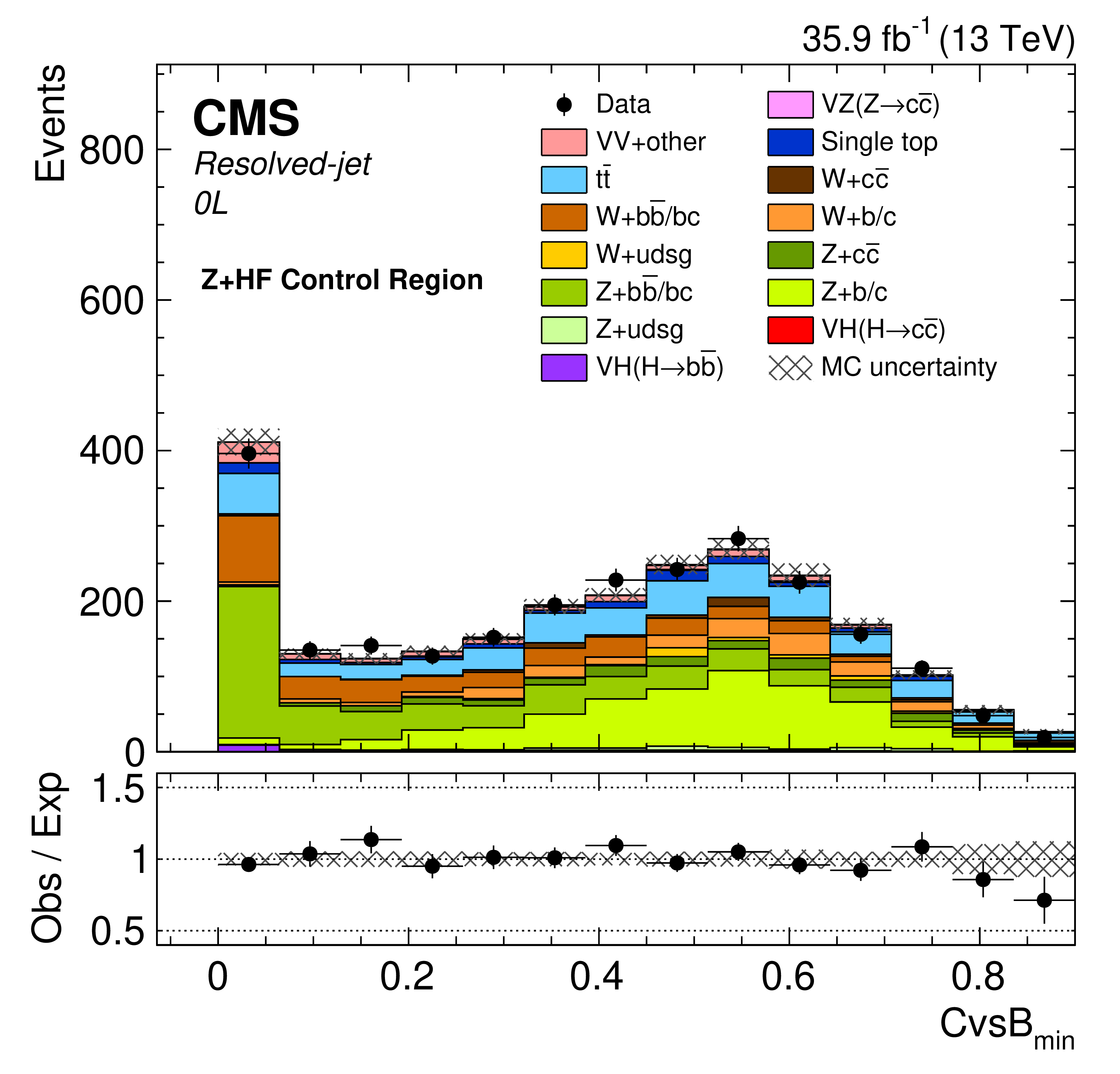
Figure 2:
Post-fit $\textit {CvsB}_{\text {min}}$ distributions in the CC (left panel) and HF (right panel) control regions for the 2L (${\mathrm{Z} (\mu \mu})$) low- ${{p_{\mathrm {T}}} (\mathrm{V})}$, 2L (${\mathrm{Z} (\mathrm{e} \mathrm{e})}$) high-$ {{p_{\mathrm {T}}} (\mathrm{V})}$, 1L (${\mathrm{W} (\mu \nu)}$), and 0L channels. |
png pdf |
Figure 2-a:
Post-fit $\textit {CvsB}_{\text {min}}$ distributions in the CC (left panel) and HF (right panel) control regions for the 2L (${\mathrm{Z} (\mu \mu})$) low- ${{p_{\mathrm {T}}} (\mathrm{V})}$, 2L (${\mathrm{Z} (\mathrm{e} \mathrm{e})}$) high-$ {{p_{\mathrm {T}}} (\mathrm{V})}$, 1L (${\mathrm{W} (\mu \nu)}$), and 0L channels. |
png pdf |
Figure 2-b:
Post-fit $\textit {CvsB}_{\text {min}}$ distributions in the CC (left panel) and HF (right panel) control regions for the 2L (${\mathrm{Z} (\mu \mu})$) low- ${{p_{\mathrm {T}}} (\mathrm{V})}$, 2L (${\mathrm{Z} (\mathrm{e} \mathrm{e})}$) high-$ {{p_{\mathrm {T}}} (\mathrm{V})}$, 1L (${\mathrm{W} (\mu \nu)}$), and 0L channels. |
png pdf |
Figure 2-c:
Post-fit $\textit {CvsB}_{\text {min}}$ distributions in the CC (left panel) and HF (right panel) control regions for the 2L (${\mathrm{Z} (\mu \mu})$) low- ${{p_{\mathrm {T}}} (\mathrm{V})}$, 2L (${\mathrm{Z} (\mathrm{e} \mathrm{e})}$) high-$ {{p_{\mathrm {T}}} (\mathrm{V})}$, 1L (${\mathrm{W} (\mu \nu)}$), and 0L channels. |
png pdf |
Figure 2-d:
Post-fit $\textit {CvsB}_{\text {min}}$ distributions in the CC (left panel) and HF (right panel) control regions for the 2L (${\mathrm{Z} (\mu \mu})$) low- ${{p_{\mathrm {T}}} (\mathrm{V})}$, 2L (${\mathrm{Z} (\mathrm{e} \mathrm{e})}$) high-$ {{p_{\mathrm {T}}} (\mathrm{V})}$, 1L (${\mathrm{W} (\mu \nu)}$), and 0L channels. |
png pdf |
Figure 2-e:
Post-fit $\textit {CvsB}_{\text {min}}$ distributions in the CC (left panel) and HF (right panel) control regions for the 2L (${\mathrm{Z} (\mu \mu})$) low- ${{p_{\mathrm {T}}} (\mathrm{V})}$, 2L (${\mathrm{Z} (\mathrm{e} \mathrm{e})}$) high-$ {{p_{\mathrm {T}}} (\mathrm{V})}$, 1L (${\mathrm{W} (\mu \nu)}$), and 0L channels. |
png pdf |
Figure 2-f:
Post-fit $\textit {CvsB}_{\text {min}}$ distributions in the CC (left panel) and HF (right panel) control regions for the 2L (${\mathrm{Z} (\mu \mu})$) low- ${{p_{\mathrm {T}}} (\mathrm{V})}$, 2L (${\mathrm{Z} (\mathrm{e} \mathrm{e})}$) high-$ {{p_{\mathrm {T}}} (\mathrm{V})}$, 1L (${\mathrm{W} (\mu \nu)}$), and 0L channels. |
png pdf |
Figure 2-g:
Post-fit $\textit {CvsB}_{\text {min}}$ distributions in the CC (left panel) and HF (right panel) control regions for the 2L (${\mathrm{Z} (\mu \mu})$) low- ${{p_{\mathrm {T}}} (\mathrm{V})}$, 2L (${\mathrm{Z} (\mathrm{e} \mathrm{e})}$) high-$ {{p_{\mathrm {T}}} (\mathrm{V})}$, 1L (${\mathrm{W} (\mu \nu)}$), and 0L channels. |
png pdf |
Figure 2-h:
Post-fit $\textit {CvsB}_{\text {min}}$ distributions in the CC (left panel) and HF (right panel) control regions for the 2L (${\mathrm{Z} (\mu \mu})$) low- ${{p_{\mathrm {T}}} (\mathrm{V})}$, 2L (${\mathrm{Z} (\mathrm{e} \mathrm{e})}$) high-$ {{p_{\mathrm {T}}} (\mathrm{V})}$, 1L (${\mathrm{W} (\mu \nu)}$), and 0L channels. |
png pdf |
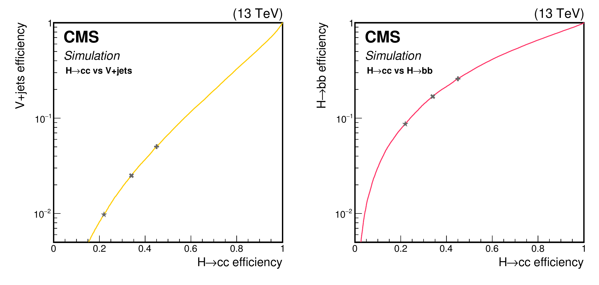
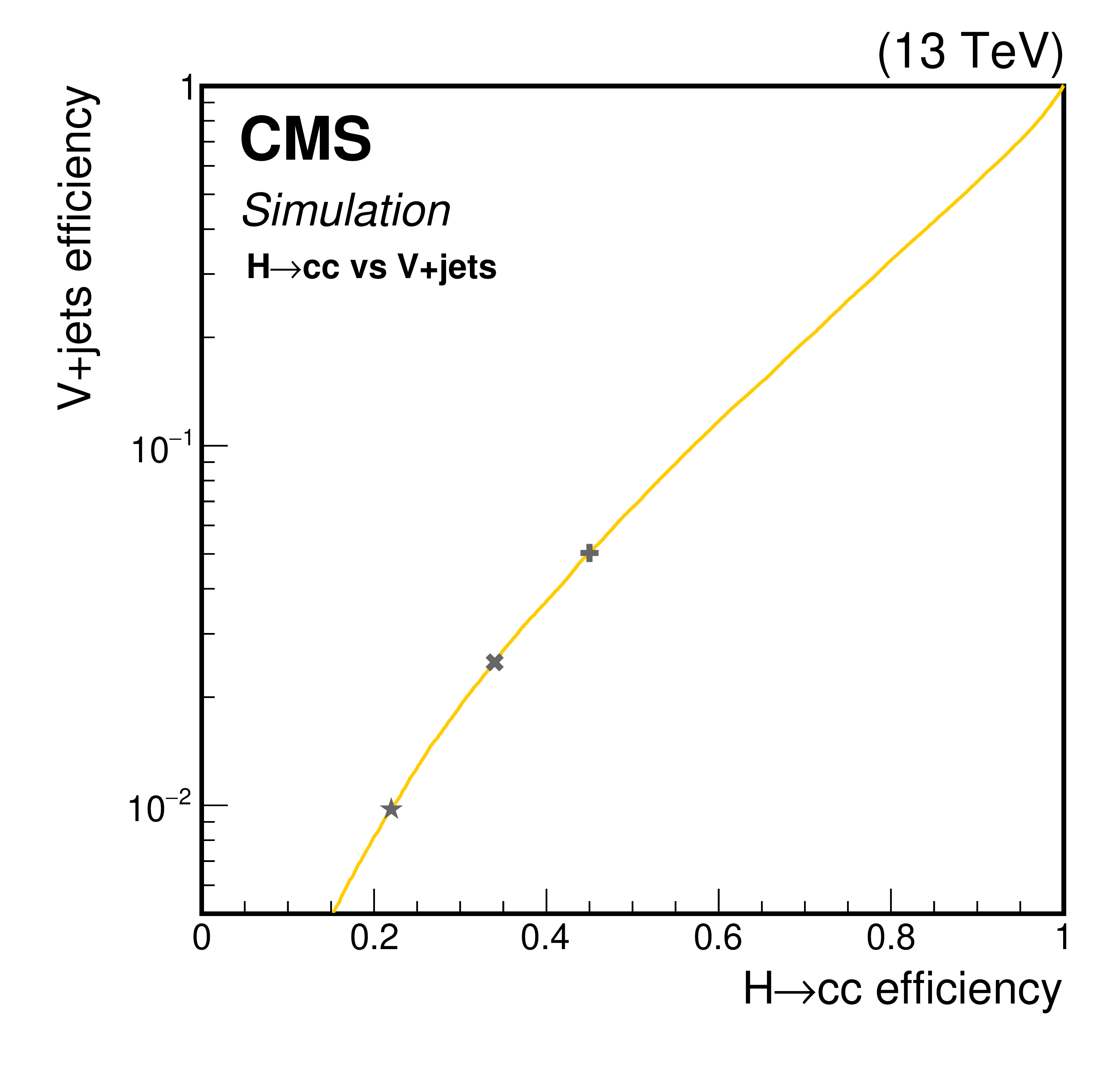
Figure 3:
The performance of the $\mathrm{c} \mathrm{\bar{c}} $ discriminant to identify a $\mathrm{c} \mathrm{\bar{c}} $ pair in terms of receiver operating characteristic curves, for large-$R$\ jets with $ {p_{\mathrm {T}}} > $ 200 GeV, before the application of data-to-simulation scale factors. Left: the efficiency to correctly identify a pair of c quarks from H boson decay vs. the efficiency of misidentifying quarks from the V+jets process. Right: the efficiency to correctly identify a pair of c quarks from H boson decay vs. the efficiency of misidentifying a pair of b quarks from H boson decay. The gray stars and crosses on the ROC curves represent the three working points used in the merged-jet topology analysis. |
png pdf |
Figure 3-a:
The performance of the $\mathrm{c} \mathrm{\bar{c}} $ discriminant to identify a $\mathrm{c} \mathrm{\bar{c}} $ pair in terms of receiver operating characteristic curves, for large-$R$\ jets with $ {p_{\mathrm {T}}} > $ 200 GeV, before the application of data-to-simulation scale factors. Left: the efficiency to correctly identify a pair of c quarks from H boson decay vs. the efficiency of misidentifying quarks from the V+jets process. Right: the efficiency to correctly identify a pair of c quarks from H boson decay vs. the efficiency of misidentifying a pair of b quarks from H boson decay. The gray stars and crosses on the ROC curves represent the three working points used in the merged-jet topology analysis. |

png pdf |
Figure 3-b:
The performance of the $\mathrm{c} \mathrm{\bar{c}} $ discriminant to identify a $\mathrm{c} \mathrm{\bar{c}} $ pair in terms of receiver operating characteristic curves, for large-$R$\ jets with $ {p_{\mathrm {T}}} > $ 200 GeV, before the application of data-to-simulation scale factors. Left: the efficiency to correctly identify a pair of c quarks from H boson decay vs. the efficiency of misidentifying quarks from the V+jets process. Right: the efficiency to correctly identify a pair of c quarks from H boson decay vs. the efficiency of misidentifying a pair of b quarks from H boson decay. The gray stars and crosses on the ROC curves represent the three working points used in the merged-jet topology analysis. |

png pdf |
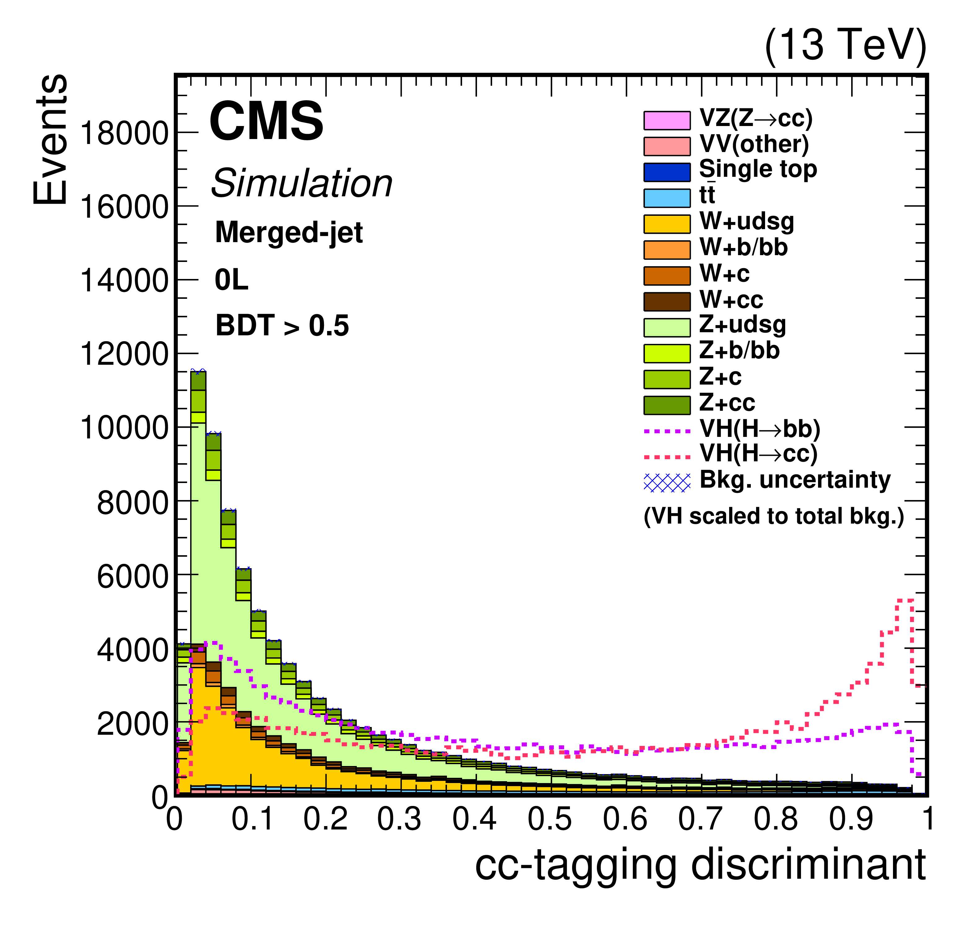
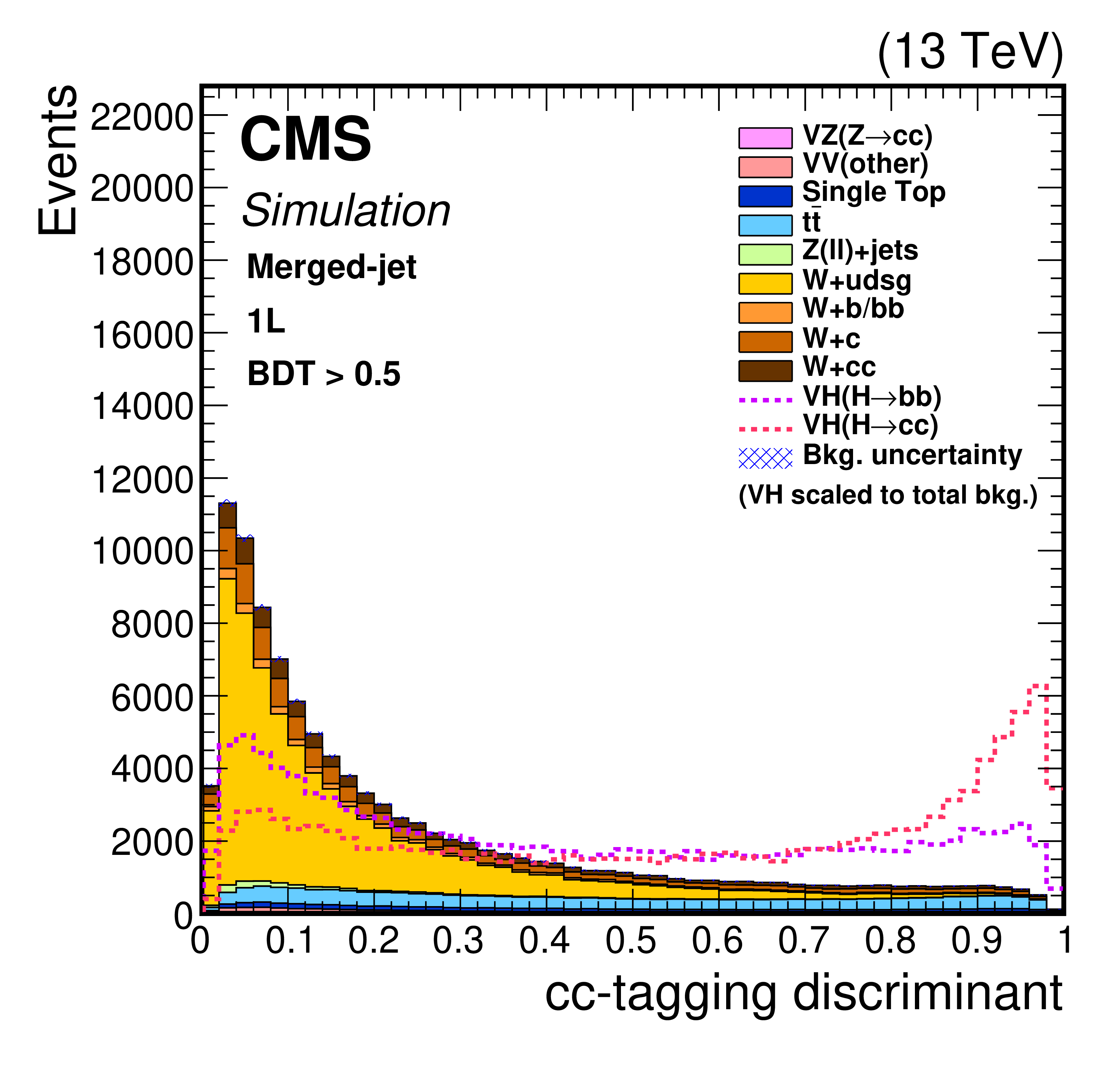
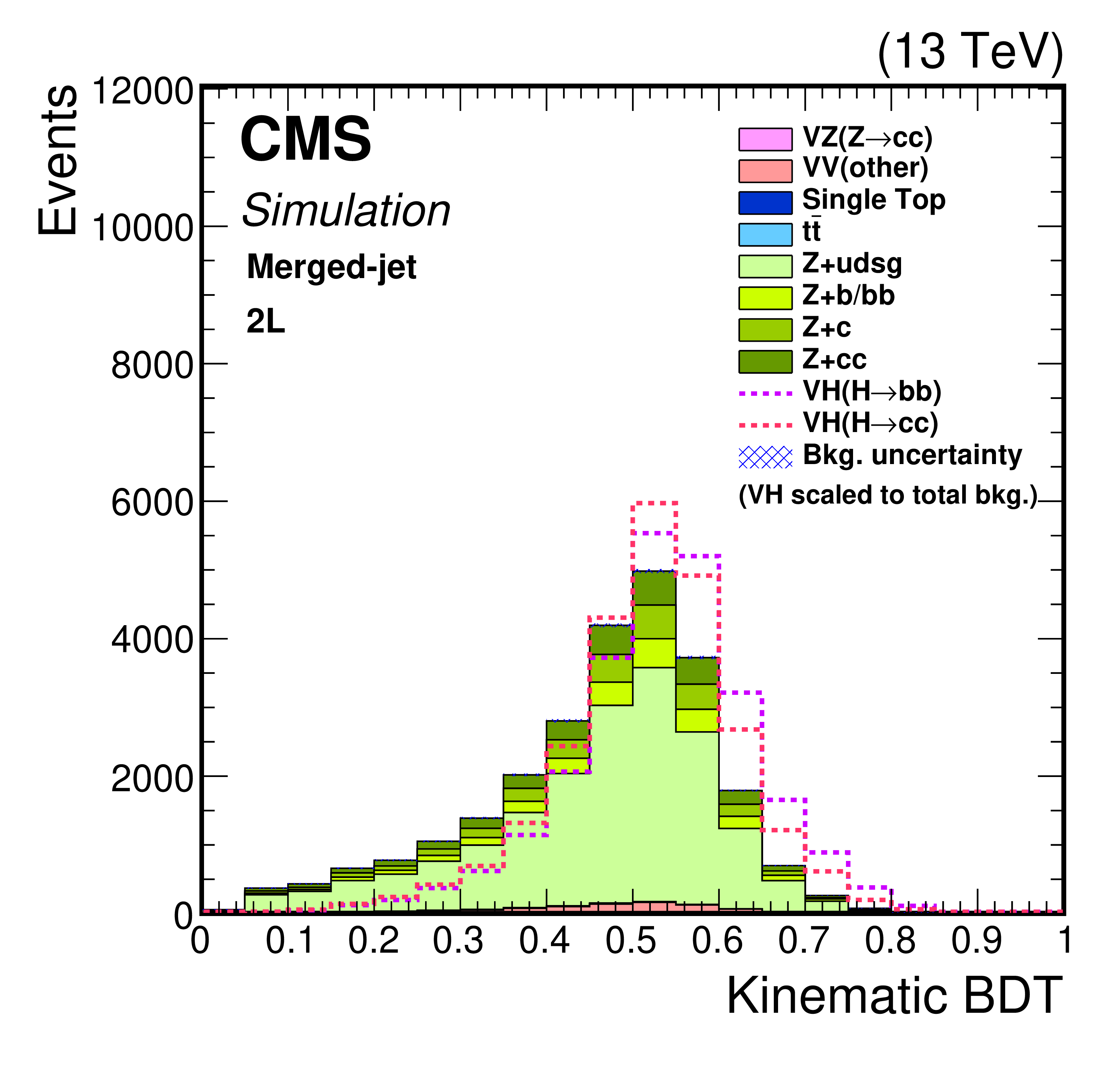
Figure 4:
The ${\mathrm{V} \mathrm{H} (\mathrm{H} \to \mathrm{c\bar{c}})}$ signal and background distributions of the kinematic BDT output (left), and the $\mathrm{c} \mathrm{\bar{c}} $ discriminant in events with BDT values greater than 0.5 (right), in the 0L (upper), 1L (middle) and 2L (lower) channels. The ${\mathrm{V} \mathrm{H} (\mathrm{H} \to \mathrm{c\bar{c}})}$ signal is normalised to the sum of all backgrounds. The ${\mathrm{V} \mathrm{H} (\mathrm{H} \to \mathrm{b} \mathrm{\bar{b}})} $ contribution, similarly normalised, is also shown. |

png pdf |
Figure 4-a:
The ${\mathrm{V} \mathrm{H} (\mathrm{H} \to \mathrm{c\bar{c}})}$ signal and background distributions of the kinematic BDT output (left), and the $\mathrm{c} \mathrm{\bar{c}} $ discriminant in events with BDT values greater than 0.5 (right), in the 0L (upper), 1L (middle) and 2L (lower) channels. The ${\mathrm{V} \mathrm{H} (\mathrm{H} \to \mathrm{c\bar{c}})}$ signal is normalised to the sum of all backgrounds. The ${\mathrm{V} \mathrm{H} (\mathrm{H} \to \mathrm{b} \mathrm{\bar{b}})} $ contribution, similarly normalised, is also shown. |
png pdf |
Figure 4-b:
The ${\mathrm{V} \mathrm{H} (\mathrm{H} \to \mathrm{c\bar{c}})}$ signal and background distributions of the kinematic BDT output (left), and the $\mathrm{c} \mathrm{\bar{c}} $ discriminant in events with BDT values greater than 0.5 (right), in the 0L (upper), 1L (middle) and 2L (lower) channels. The ${\mathrm{V} \mathrm{H} (\mathrm{H} \to \mathrm{c\bar{c}})}$ signal is normalised to the sum of all backgrounds. The ${\mathrm{V} \mathrm{H} (\mathrm{H} \to \mathrm{b} \mathrm{\bar{b}})} $ contribution, similarly normalised, is also shown. |

png pdf |
Figure 4-c:
The ${\mathrm{V} \mathrm{H} (\mathrm{H} \to \mathrm{c\bar{c}})}$ signal and background distributions of the kinematic BDT output (left), and the $\mathrm{c} \mathrm{\bar{c}} $ discriminant in events with BDT values greater than 0.5 (right), in the 0L (upper), 1L (middle) and 2L (lower) channels. The ${\mathrm{V} \mathrm{H} (\mathrm{H} \to \mathrm{c\bar{c}})}$ signal is normalised to the sum of all backgrounds. The ${\mathrm{V} \mathrm{H} (\mathrm{H} \to \mathrm{b} \mathrm{\bar{b}})} $ contribution, similarly normalised, is also shown. |
png pdf |
Figure 4-d:
The ${\mathrm{V} \mathrm{H} (\mathrm{H} \to \mathrm{c\bar{c}})}$ signal and background distributions of the kinematic BDT output (left), and the $\mathrm{c} \mathrm{\bar{c}} $ discriminant in events with BDT values greater than 0.5 (right), in the 0L (upper), 1L (middle) and 2L (lower) channels. The ${\mathrm{V} \mathrm{H} (\mathrm{H} \to \mathrm{c\bar{c}})}$ signal is normalised to the sum of all backgrounds. The ${\mathrm{V} \mathrm{H} (\mathrm{H} \to \mathrm{b} \mathrm{\bar{b}})} $ contribution, similarly normalised, is also shown. |
png pdf |
Figure 4-e:
The ${\mathrm{V} \mathrm{H} (\mathrm{H} \to \mathrm{c\bar{c}})}$ signal and background distributions of the kinematic BDT output (left), and the $\mathrm{c} \mathrm{\bar{c}} $ discriminant in events with BDT values greater than 0.5 (right), in the 0L (upper), 1L (middle) and 2L (lower) channels. The ${\mathrm{V} \mathrm{H} (\mathrm{H} \to \mathrm{c\bar{c}})}$ signal is normalised to the sum of all backgrounds. The ${\mathrm{V} \mathrm{H} (\mathrm{H} \to \mathrm{b} \mathrm{\bar{b}})} $ contribution, similarly normalised, is also shown. |

png pdf |
Figure 4-f:
The ${\mathrm{V} \mathrm{H} (\mathrm{H} \to \mathrm{c\bar{c}})}$ signal and background distributions of the kinematic BDT output (left), and the $\mathrm{c} \mathrm{\bar{c}} $ discriminant in events with BDT values greater than 0.5 (right), in the 0L (upper), 1L (middle) and 2L (lower) channels. The ${\mathrm{V} \mathrm{H} (\mathrm{H} \to \mathrm{c\bar{c}})}$ signal is normalised to the sum of all backgrounds. The ${\mathrm{V} \mathrm{H} (\mathrm{H} \to \mathrm{b} \mathrm{\bar{b}})} $ contribution, similarly normalised, is also shown. |
png pdf |
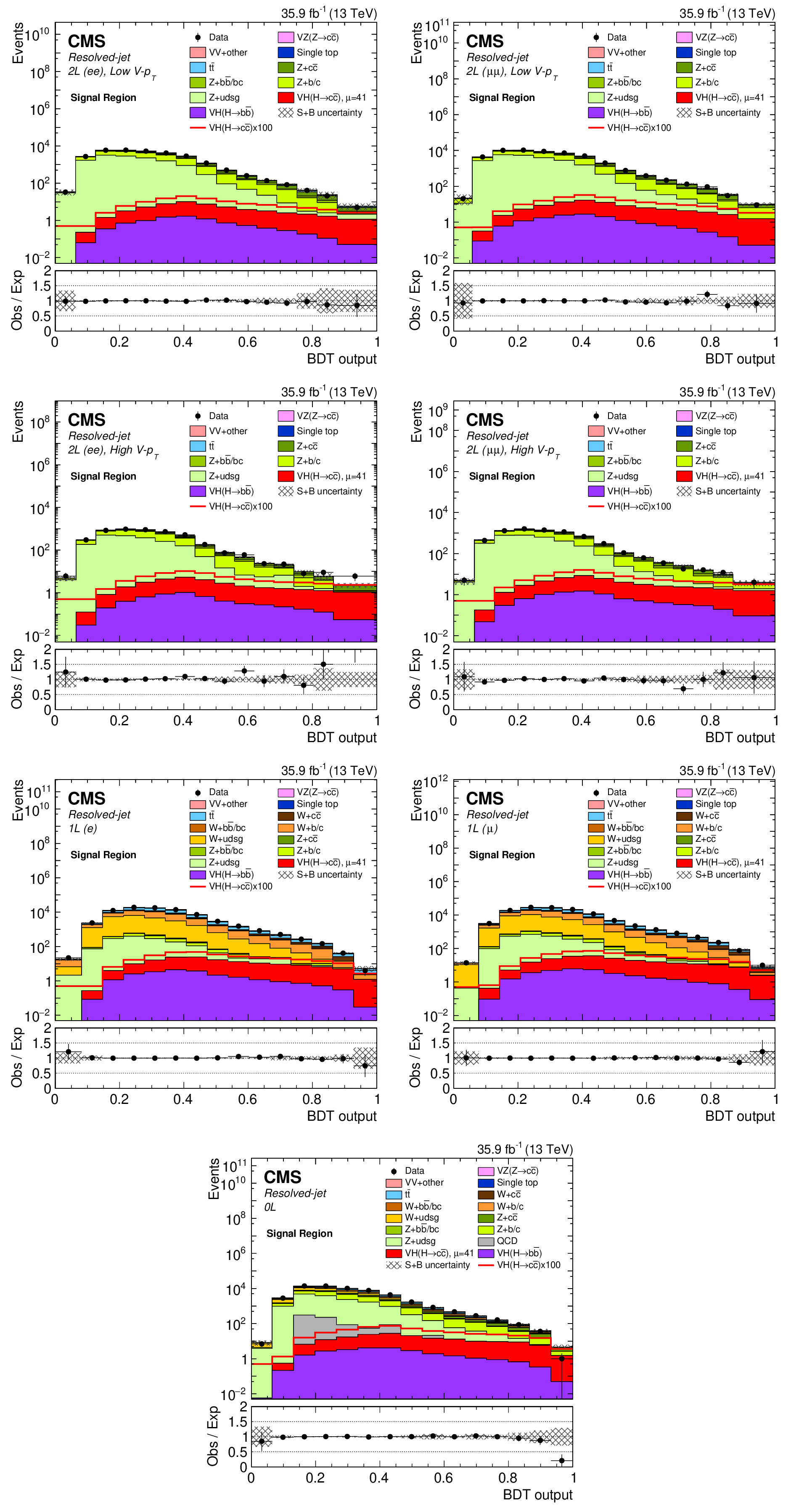
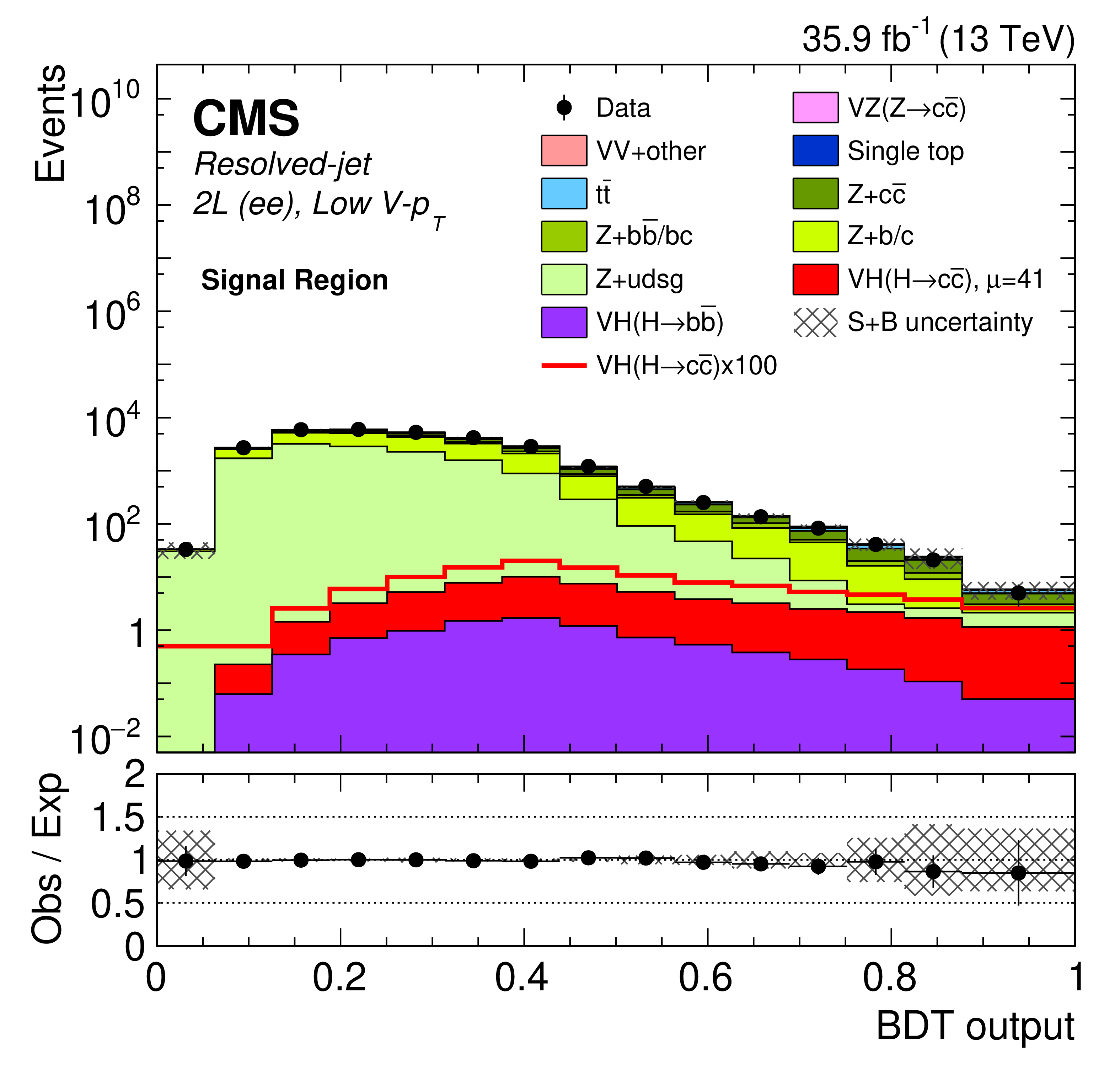
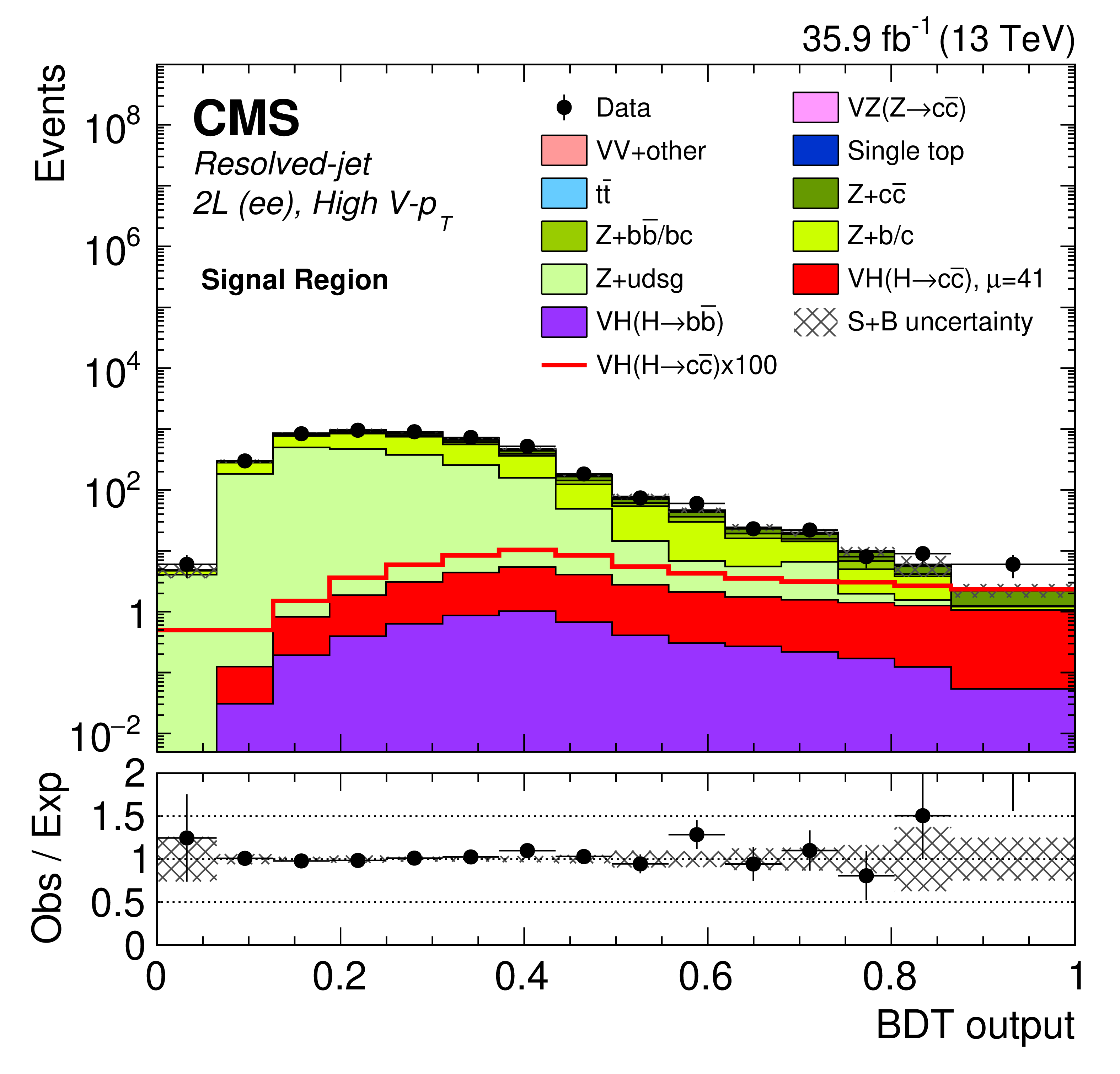
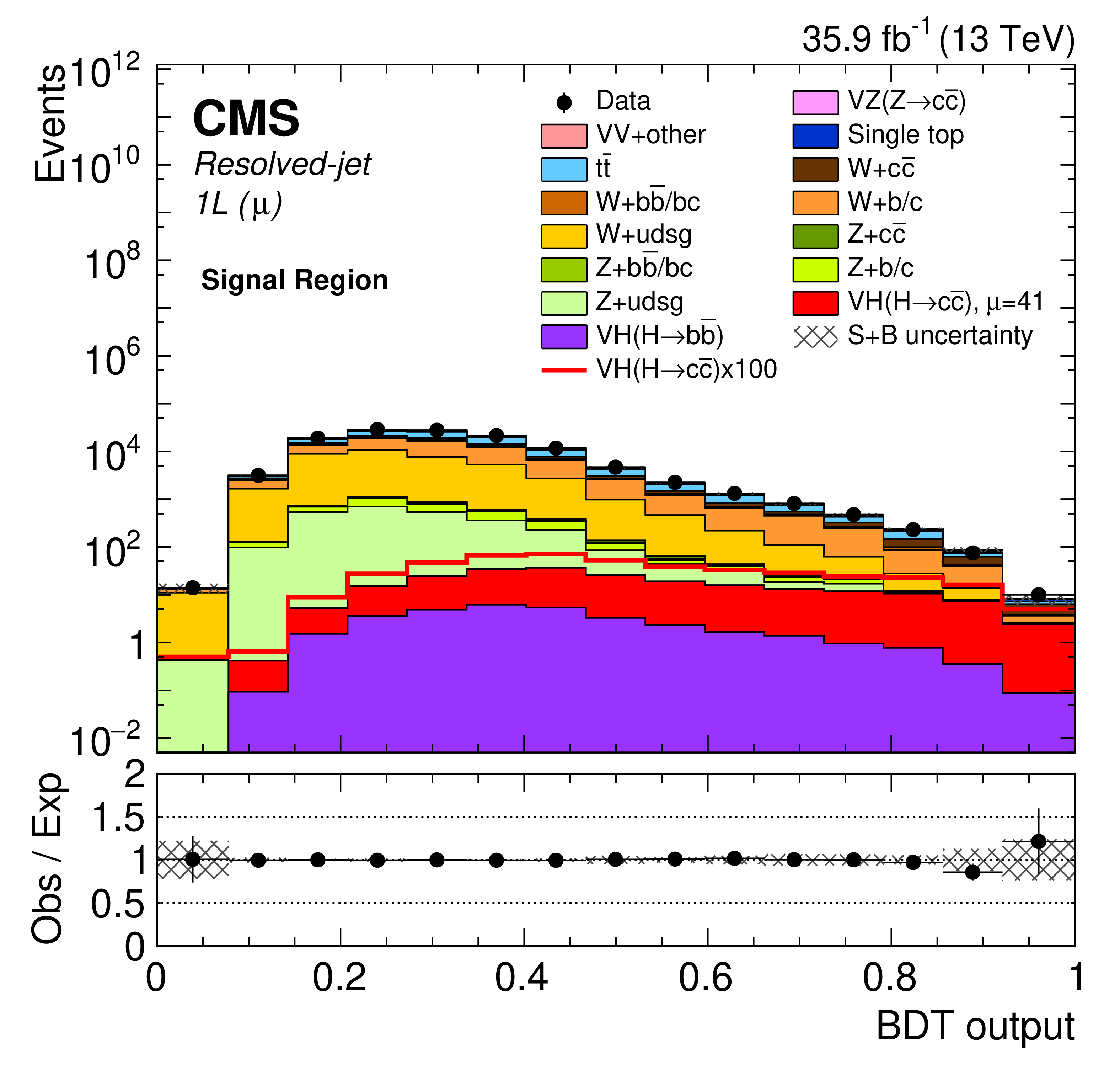
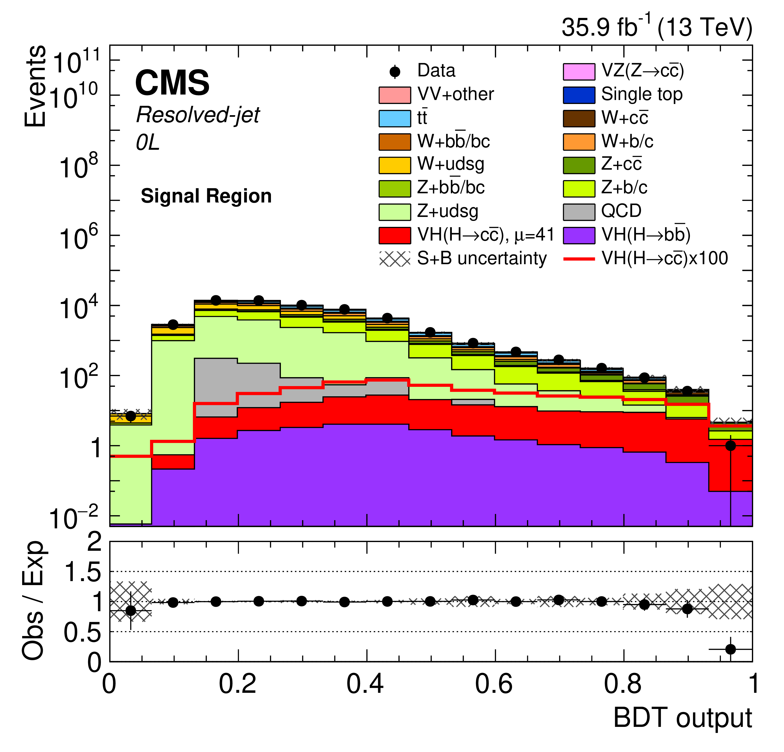
Figure 5:
Post-fit distributions of the BDT score in the signal region of the resolved-jet topology analysis for the 2L low-$ {{p_{\mathrm {T}}} (\mathrm{V})}, 2L high- {{p_{\mathrm {T}}} (\mathrm{V})}$, 1L, and 0L channels. The plain red histograms represent the signal contribution normalized by the post-fit value of $\mu _{{\mathrm{V} \mathrm{H} (\mathrm{H} \to \mathrm{c\bar{c}})}}$, while the red line histograms show the expected signal contribution multiplied by a factor 100. |
png pdf |
Figure 5-a:
Post-fit distributions of the BDT score in the signal region of the resolved-jet topology analysis for the 2L low-$ {{p_{\mathrm {T}}} (\mathrm{V})}, 2L high- {{p_{\mathrm {T}}} (\mathrm{V})}$, 1L, and 0L channels. The plain red histograms represent the signal contribution normalized by the post-fit value of $\mu _{{\mathrm{V} \mathrm{H} (\mathrm{H} \to \mathrm{c\bar{c}})}}$, while the red line histograms show the expected signal contribution multiplied by a factor 100. |

png pdf |
Figure 5-b:
Post-fit distributions of the BDT score in the signal region of the resolved-jet topology analysis for the 2L low-$ {{p_{\mathrm {T}}} (\mathrm{V})}, 2L high- {{p_{\mathrm {T}}} (\mathrm{V})}$, 1L, and 0L channels. The plain red histograms represent the signal contribution normalized by the post-fit value of $\mu _{{\mathrm{V} \mathrm{H} (\mathrm{H} \to \mathrm{c\bar{c}})}}$, while the red line histograms show the expected signal contribution multiplied by a factor 100. |
png pdf |
Figure 5-c:
Post-fit distributions of the BDT score in the signal region of the resolved-jet topology analysis for the 2L low-$ {{p_{\mathrm {T}}} (\mathrm{V})}, 2L high- {{p_{\mathrm {T}}} (\mathrm{V})}$, 1L, and 0L channels. The plain red histograms represent the signal contribution normalized by the post-fit value of $\mu _{{\mathrm{V} \mathrm{H} (\mathrm{H} \to \mathrm{c\bar{c}})}}$, while the red line histograms show the expected signal contribution multiplied by a factor 100. |

png pdf |
Figure 5-d:
Post-fit distributions of the BDT score in the signal region of the resolved-jet topology analysis for the 2L low-$ {{p_{\mathrm {T}}} (\mathrm{V})}, 2L high- {{p_{\mathrm {T}}} (\mathrm{V})}$, 1L, and 0L channels. The plain red histograms represent the signal contribution normalized by the post-fit value of $\mu _{{\mathrm{V} \mathrm{H} (\mathrm{H} \to \mathrm{c\bar{c}})}}$, while the red line histograms show the expected signal contribution multiplied by a factor 100. |

png pdf |
Figure 5-e:
Post-fit distributions of the BDT score in the signal region of the resolved-jet topology analysis for the 2L low-$ {{p_{\mathrm {T}}} (\mathrm{V})}, 2L high- {{p_{\mathrm {T}}} (\mathrm{V})}$, 1L, and 0L channels. The plain red histograms represent the signal contribution normalized by the post-fit value of $\mu _{{\mathrm{V} \mathrm{H} (\mathrm{H} \to \mathrm{c\bar{c}})}}$, while the red line histograms show the expected signal contribution multiplied by a factor 100. |
png pdf |
Figure 5-f:
Post-fit distributions of the BDT score in the signal region of the resolved-jet topology analysis for the 2L low-$ {{p_{\mathrm {T}}} (\mathrm{V})}, 2L high- {{p_{\mathrm {T}}} (\mathrm{V})}$, 1L, and 0L channels. The plain red histograms represent the signal contribution normalized by the post-fit value of $\mu _{{\mathrm{V} \mathrm{H} (\mathrm{H} \to \mathrm{c\bar{c}})}}$, while the red line histograms show the expected signal contribution multiplied by a factor 100. |
png pdf |
Figure 5-g:
Post-fit distributions of the BDT score in the signal region of the resolved-jet topology analysis for the 2L low-$ {{p_{\mathrm {T}}} (\mathrm{V})}, 2L high- {{p_{\mathrm {T}}} (\mathrm{V})}$, 1L, and 0L channels. The plain red histograms represent the signal contribution normalized by the post-fit value of $\mu _{{\mathrm{V} \mathrm{H} (\mathrm{H} \to \mathrm{c\bar{c}})}}$, while the red line histograms show the expected signal contribution multiplied by a factor 100. |
png pdf |
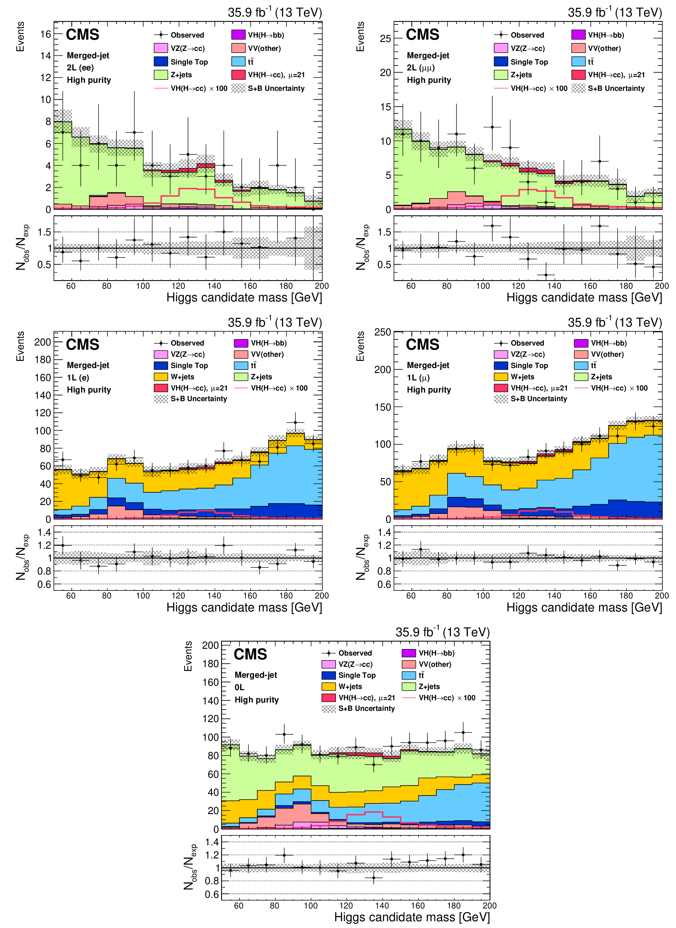
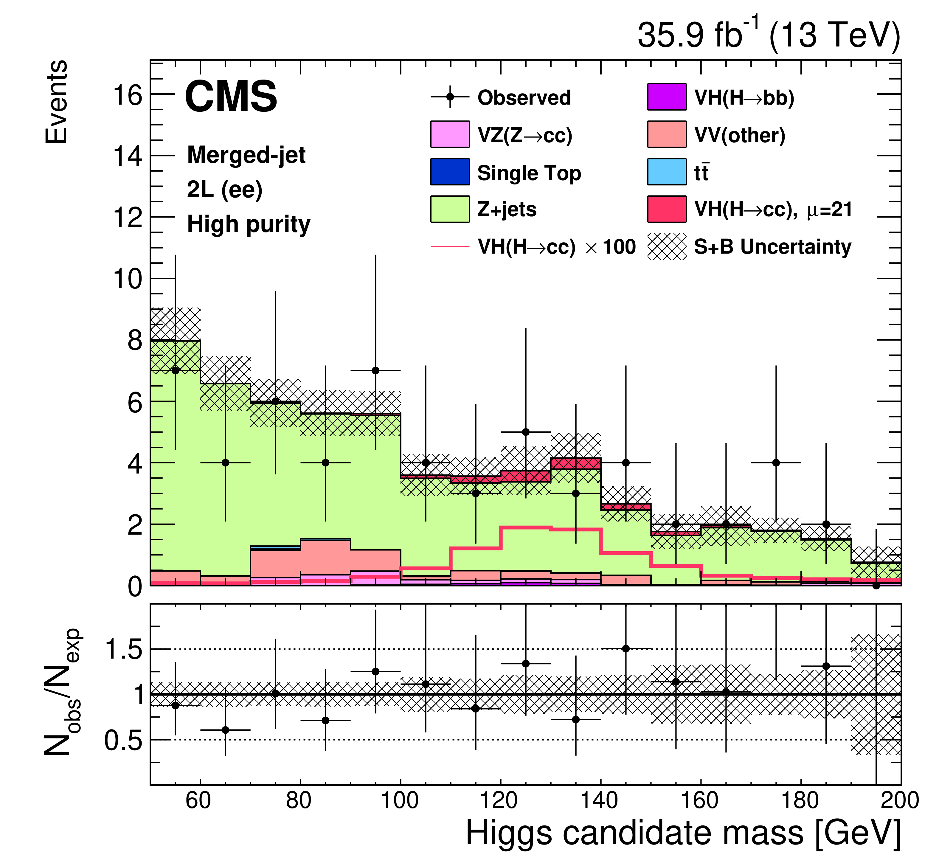
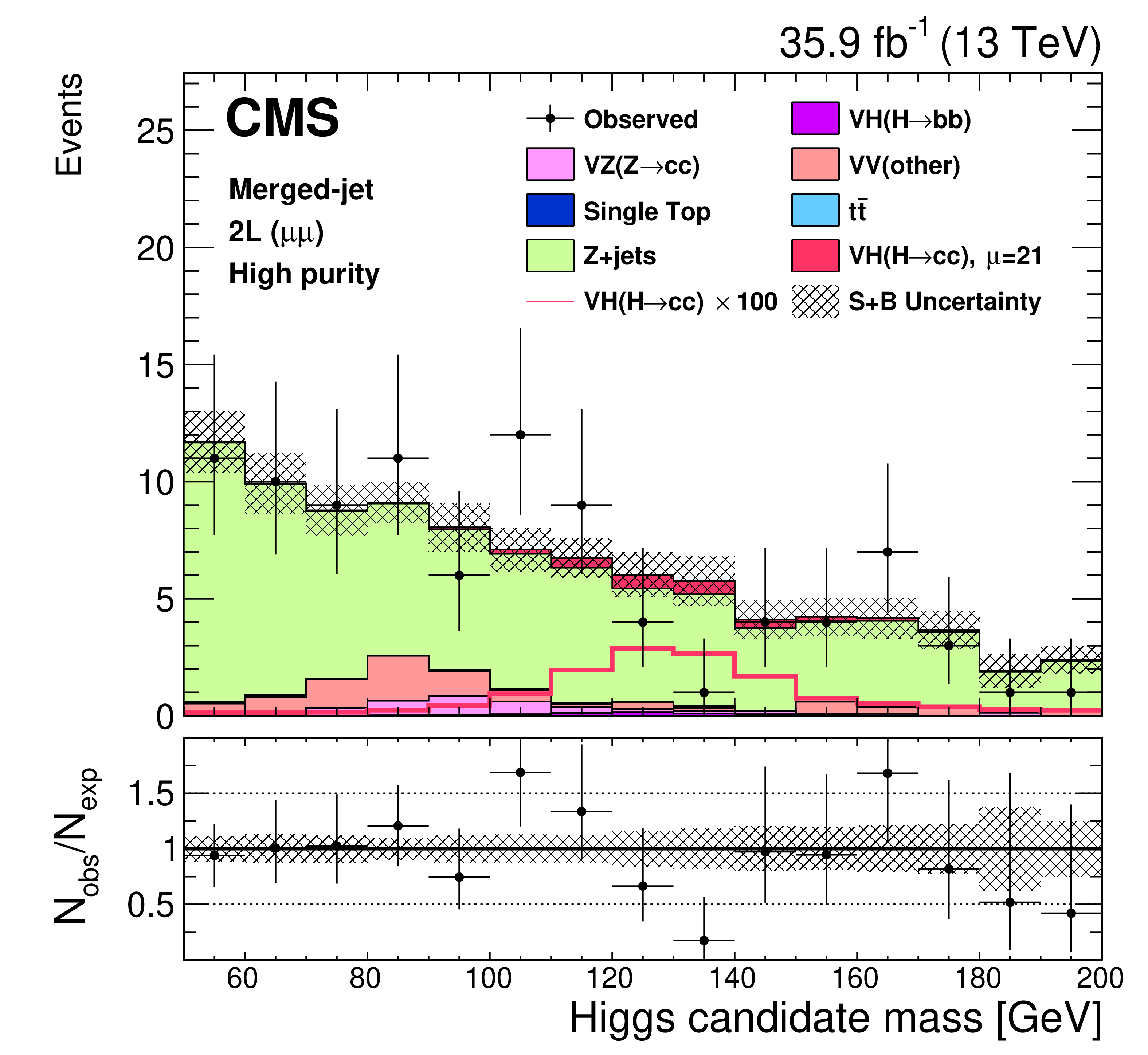
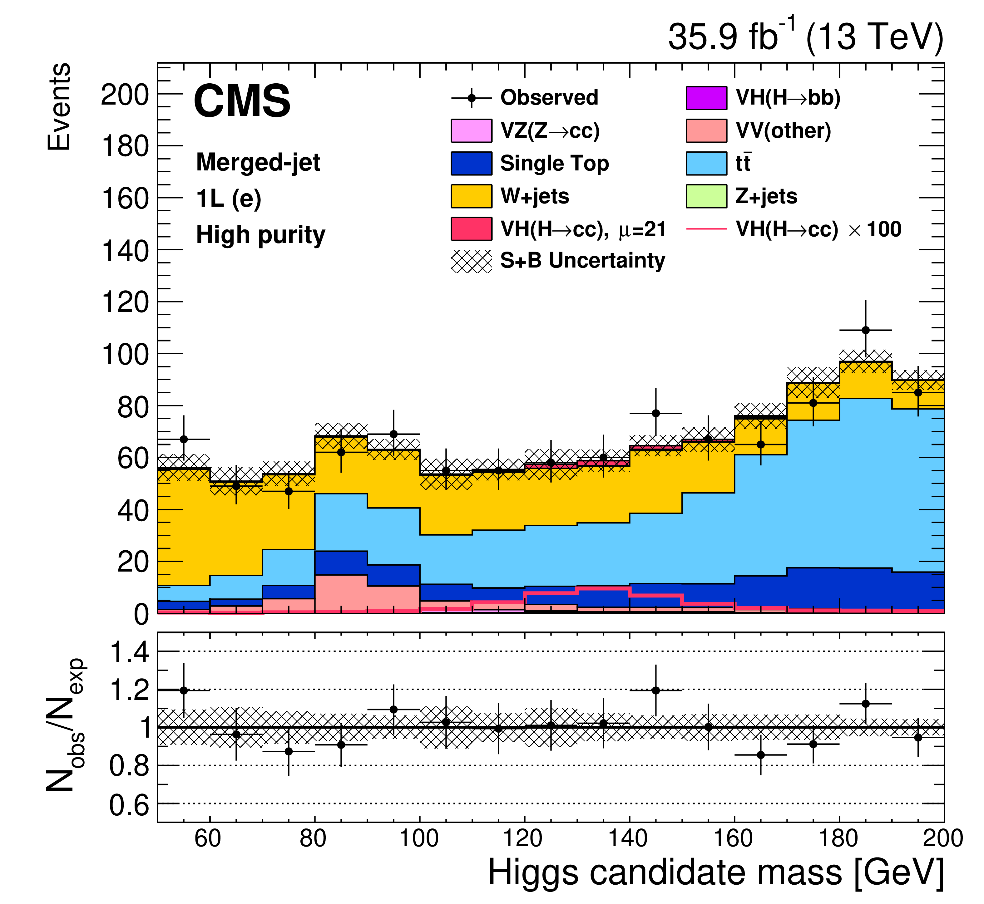
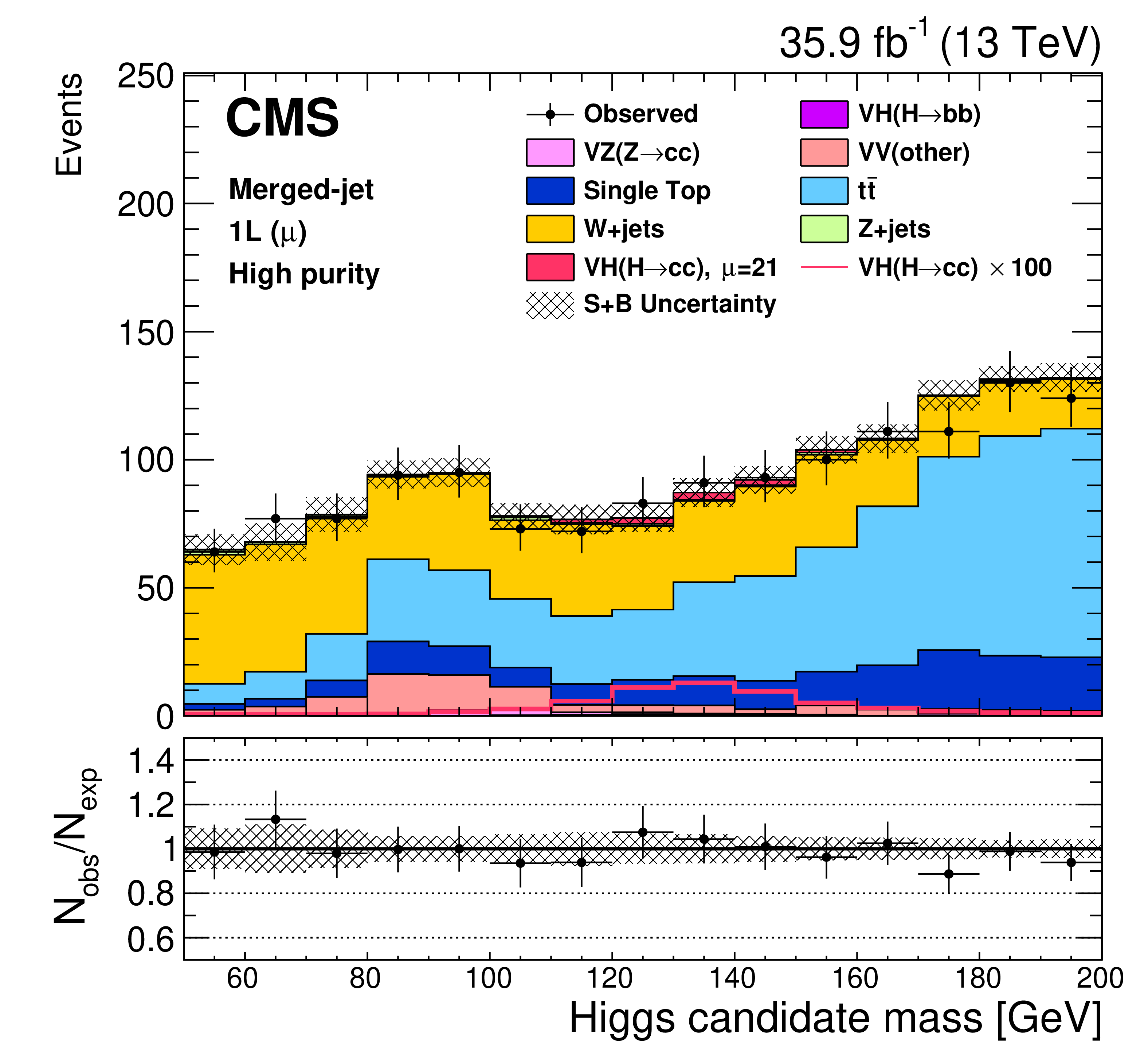
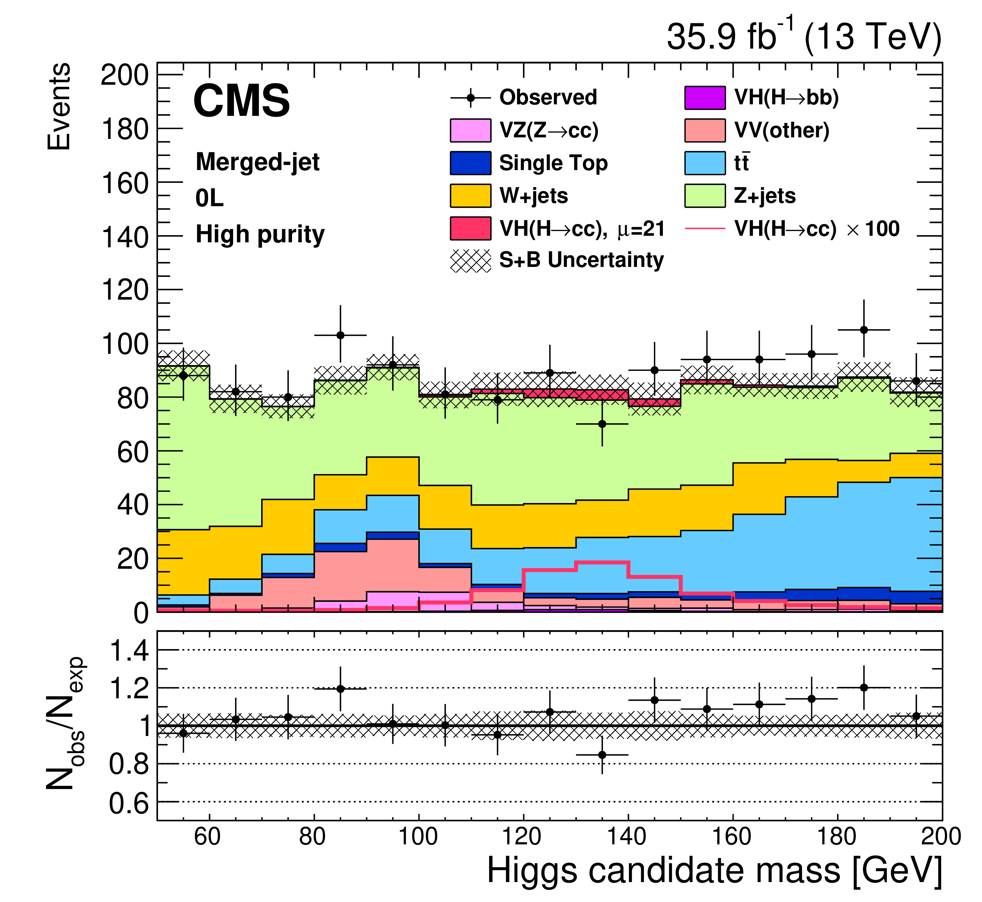
Figure 6:
The ${m_{\text {SD}}}$ distribution of H in data and simulation in the merged-jet topology analysis signal regions after the maximum likelihood fit, for events in the high purity category. Upper row: 2L channel, electrons (left) and muons (right); middle row: 1L channel, electron (left) and muon (right); lower row: 0L channel. The plain red histograms represent the signal contribution normalized by the post-fit value of $\mu _{{\mathrm{V} \mathrm{H} (\mathrm{H} \to \mathrm{c\bar{c}})}}$, while the red line histograms show the expected signal contribution multiplied by a factor 100. |
png pdf |
Figure 6-a:
The ${m_{\text {SD}}}$ distribution of H in data and simulation in the merged-jet topology analysis signal regions after the maximum likelihood fit, for events in the high purity category. Upper row: 2L channel, electrons (left) and muons (right); middle row: 1L channel, electron (left) and muon (right); lower row: 0L channel. The plain red histograms represent the signal contribution normalized by the post-fit value of $\mu _{{\mathrm{V} \mathrm{H} (\mathrm{H} \to \mathrm{c\bar{c}})}}$, while the red line histograms show the expected signal contribution multiplied by a factor 100. |
png pdf |
Figure 6-b:
The ${m_{\text {SD}}}$ distribution of H in data and simulation in the merged-jet topology analysis signal regions after the maximum likelihood fit, for events in the high purity category. Upper row: 2L channel, electrons (left) and muons (right); middle row: 1L channel, electron (left) and muon (right); lower row: 0L channel. The plain red histograms represent the signal contribution normalized by the post-fit value of $\mu _{{\mathrm{V} \mathrm{H} (\mathrm{H} \to \mathrm{c\bar{c}})}}$, while the red line histograms show the expected signal contribution multiplied by a factor 100. |
png pdf |
Figure 6-c:
The ${m_{\text {SD}}}$ distribution of H in data and simulation in the merged-jet topology analysis signal regions after the maximum likelihood fit, for events in the high purity category. Upper row: 2L channel, electrons (left) and muons (right); middle row: 1L channel, electron (left) and muon (right); lower row: 0L channel. The plain red histograms represent the signal contribution normalized by the post-fit value of $\mu _{{\mathrm{V} \mathrm{H} (\mathrm{H} \to \mathrm{c\bar{c}})}}$, while the red line histograms show the expected signal contribution multiplied by a factor 100. |
png pdf |
Figure 6-d:
The ${m_{\text {SD}}}$ distribution of H in data and simulation in the merged-jet topology analysis signal regions after the maximum likelihood fit, for events in the high purity category. Upper row: 2L channel, electrons (left) and muons (right); middle row: 1L channel, electron (left) and muon (right); lower row: 0L channel. The plain red histograms represent the signal contribution normalized by the post-fit value of $\mu _{{\mathrm{V} \mathrm{H} (\mathrm{H} \to \mathrm{c\bar{c}})}}$, while the red line histograms show the expected signal contribution multiplied by a factor 100. |
png pdf |
Figure 6-e:
The ${m_{\text {SD}}}$ distribution of H in data and simulation in the merged-jet topology analysis signal regions after the maximum likelihood fit, for events in the high purity category. Upper row: 2L channel, electrons (left) and muons (right); middle row: 1L channel, electron (left) and muon (right); lower row: 0L channel. The plain red histograms represent the signal contribution normalized by the post-fit value of $\mu _{{\mathrm{V} \mathrm{H} (\mathrm{H} \to \mathrm{c\bar{c}})}}$, while the red line histograms show the expected signal contribution multiplied by a factor 100. |
png pdf |
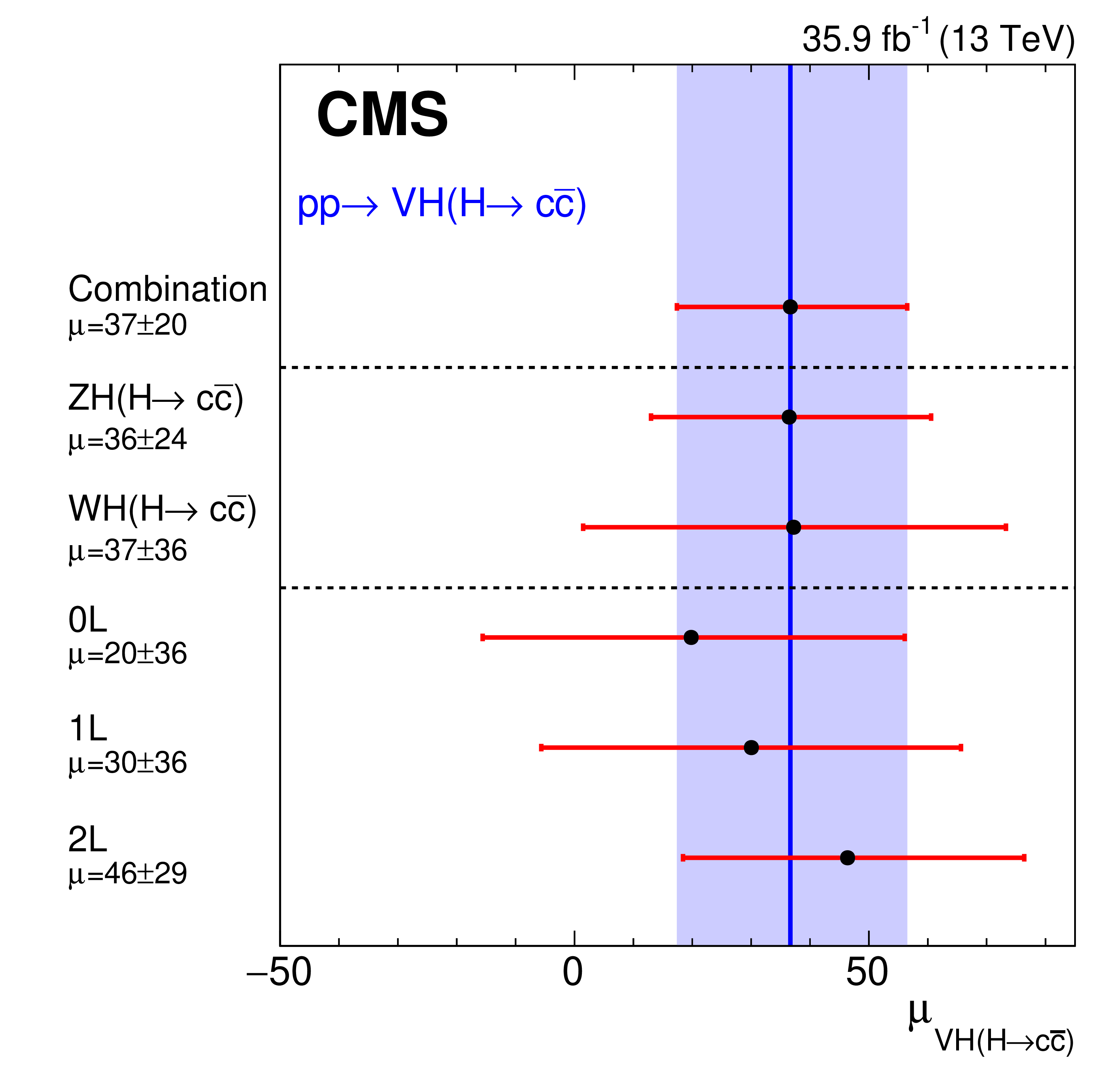
Figure 7:
The fitted signal strength $\mu $ for the ${\mathrm{Z} \mathrm{H} (\mathrm{H} \to \mathrm{c\bar{c}})}$ and ${\mathrm{W} \mathrm{H} (\mathrm{H} \to \mathrm{c\bar{c}})}$ processes, and in each individual channel (0L, 1L, and 2L). The vertical blue line corresponds to the best fit value of $\mu $ for the combination of all channels, while the light-purple band corresponds to the $ \pm $1$\sigma $ uncertainty in the measurement. |
png pdf |
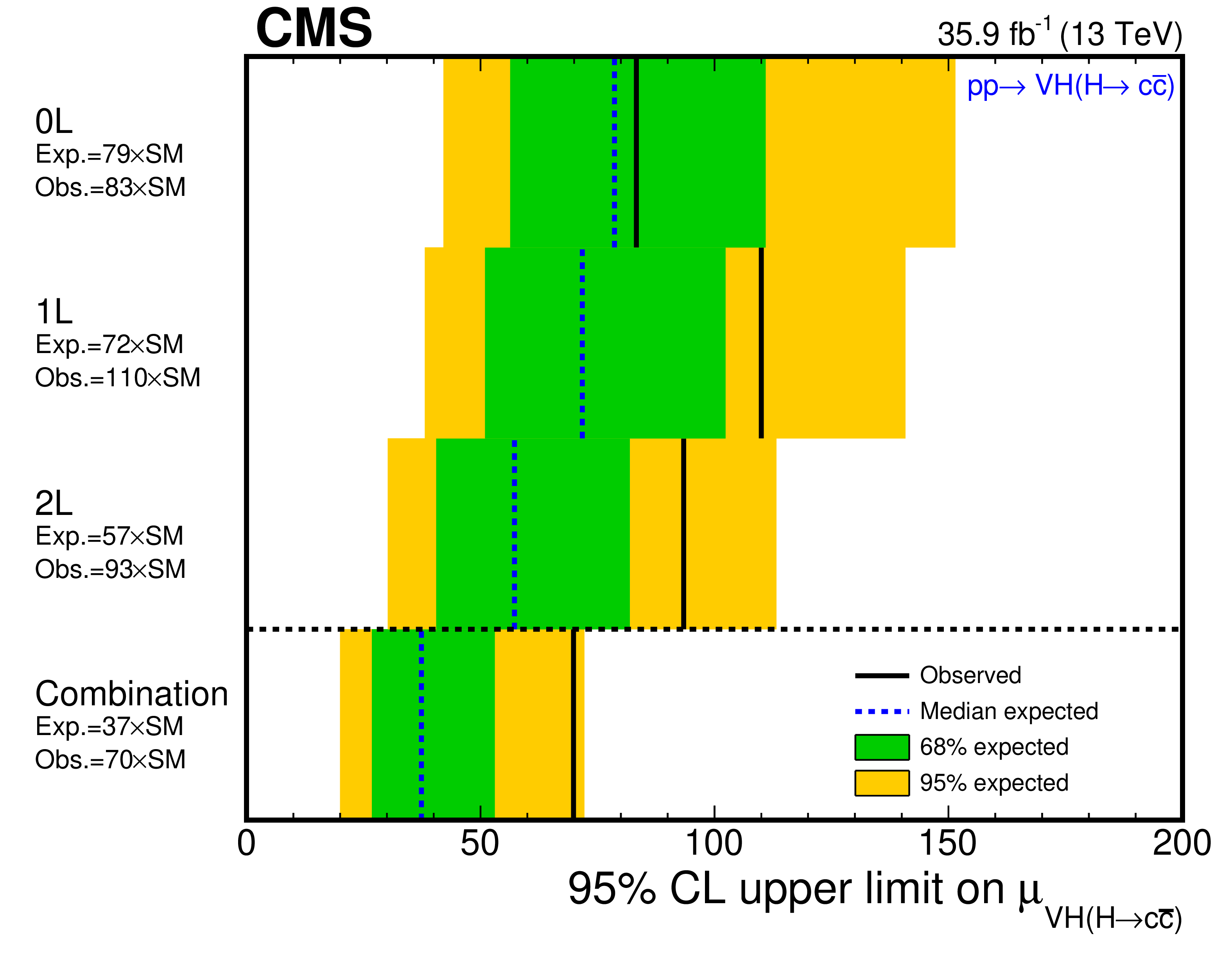
Figure 8:
The 95% CL upper limits on $\mu $ for the ${\mathrm{V} \mathrm{H} (\mathrm{H} \to \mathrm{c\bar{c}})} $ process from the combination of the resolved-jet and merged-jet topologies analyses in the different channels (0L, 1L, and 2L) and combined. The inner (green) and the outer (yellow) bands indicate the regions containing 68% and 95%, respectively, of the distribution of limits expected under the background-only hypothesis. |
| Tables | |
png pdf |
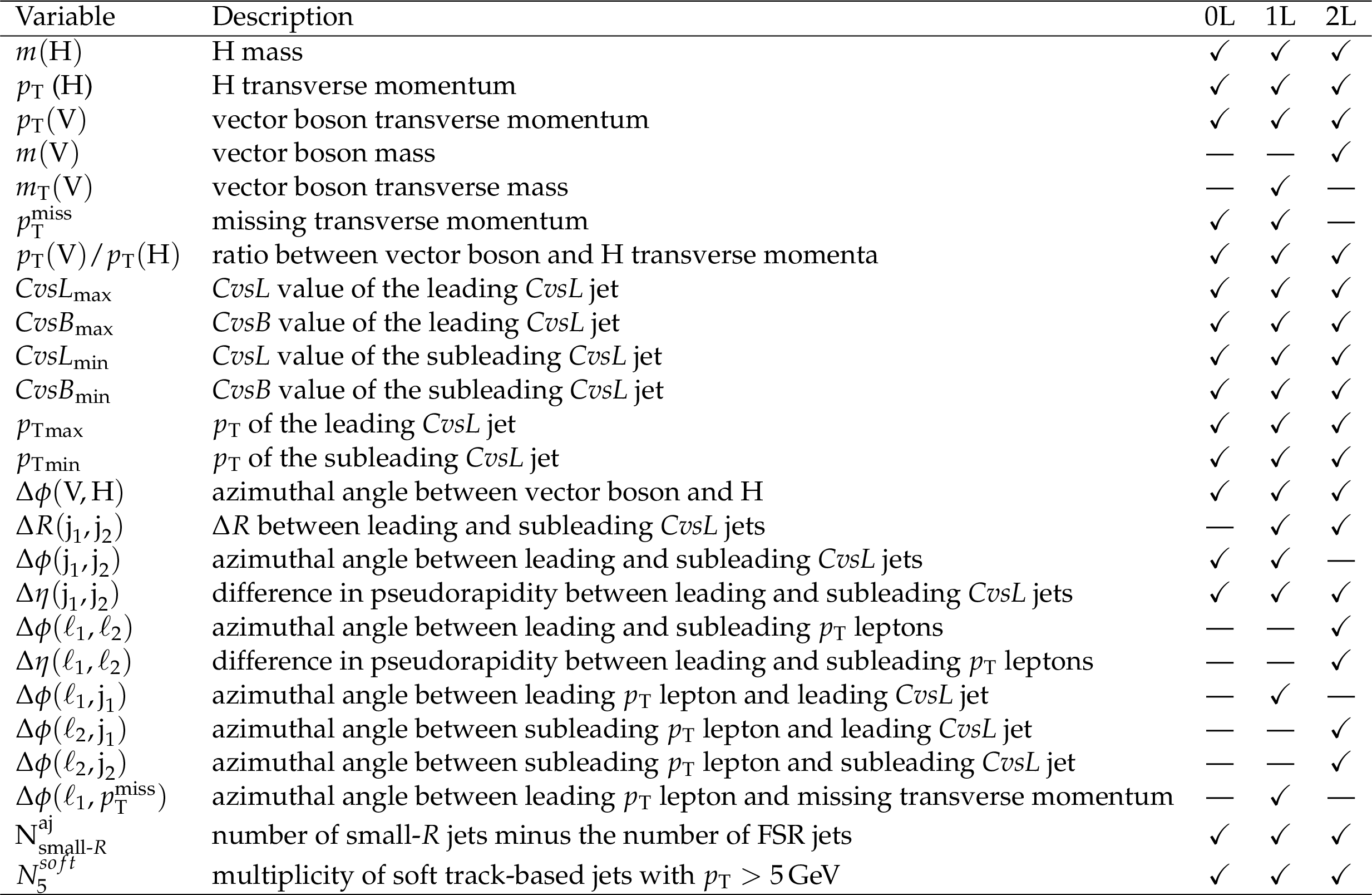
Table 1:
Variables employed in the training of the BDT used for each channel of the resolved-jet topology analysis. The 2L case has separate training for the low- and high-$ {{p_{\mathrm {T}}} (\mathrm{V})} $channels, but exploits the same input variables. |
png pdf |
Table 2:
Variables used in the kinematic BDT training for each channel of the merged-jet topology analysis. |
png pdf |
Table 3:
Summary of the systematic uncertainties for each channel. Uncertainties in the lepton identification and trigger efficiencies are treated as a normalisation uncertainty in the resolved-jet topology analysis and as a shape uncertainty in the merged-jet topology analysis. |
png pdf |
Table 4:
Summary of the impact of the statistical and systematic uncertainties on the signal strength modifier for combined analysis of the resolved-jet and merged-jet topologies. |
png pdf |
Table 5:
Observed and expected UL at 95% CL on the signal strength $\mu $ for the ${\mathrm{V} \mathrm{H} (\mathrm{H} \to \mathrm{c\bar{c}})} $ production for the resolved-jet and merged-jet topologies analyses, which have a significant overlap. The results are also shown separately for each analysis channel. |

png pdf |
Table 6:
The 95% CL upper limits on the signal strength $\mu _{{\mathrm{V} \mathrm{H} (\mathrm{H} \to \mathrm{c\bar{c}})}}$ for the ${\mathrm{V} \mathrm{H} (\mathrm{H} \to \mathrm{c\bar{c}})} $ process, for the resolved-jet topology analysis for $ {{p_{\mathrm {T}}} (\mathrm{V})} < $ 300 GeV, the merged-jet topology analysis for $ {{p_{\mathrm {T}}} (\mathrm{V})} \geq $ 300 GeV, and their combination. |
| Summary |
|
In this paper, we present the first search by the CMS Collaboration for the standard model (SM) Higgs boson H decaying to a pair of charm quarks, produced in association with a vector boson V (W or Z). The search uses proton-proton collision data at a centre-of-mass energy of 13 TeV collected with the CMS detector in 2016 and corresponding to an integrated luminosity of 35.9 fb$^{-1}$. The search is carried out in five modes, $\mathrm{Z(\mu\mu)H}$, $\mathrm{Z(ee)H}$, $\mathrm{Z(\nu\nu)H}$, $\mathrm{W(\mu\nu)H}$, and ${\mathrm{W}(\mathrm{e}\nu)\mathrm{H}} $, with two complementary analyses targeting different regions of phase space. The signal is extracted by statistically combining the results of the two analyses. Each analysis is first validated by carrying out a search for Z boson decay to a $\mathrm{c\bar{c}}$ pair and comparing the observed signal strength with the SM prediction. The Z boson signal strength for the combination of the two analyses is measured to be $\mu_{{\mathrm{V}\mathrm{Z}(\mathrm{Z}\to \mathrm{c\bar{c}})} }=\sigma/\sigma_\text{SM}=$ 0.55$^{+0.86}_{-0.84}$, with an observed (expected) significance of 0.7 (1.3) standard deviations. The measured best fit value of $\sigma\left({{\mathrm{V}}\mathrm{H}} \right)\mathcal{B}\left(\mathrm{H} \to \mathrm{c\bar{c}} \right)$ for the combination of the two analyses is 2.40$^{+1.12}_{-1.11}$ (stat) $^{+0.65}_{-0.61}$ (syst) pb, which corresponds to a best fit value of $\mu$ for SM $\mathrm{VH(H\to c\bar{c} )}$ production of $\mu_{\mathrm{V}\mathrm{H} cc}=\sigma/\sigma_\text{SM}=$ 37$^{+17}_{-17}$ (stat) $^{+11}_{-9}$ (syst), compatible within two standard deviations with the SM prediction. The larger measured $\mu_{\mathrm{VH(H\to c\bar{c} )}}$ value is due to a small excess observed in data in the resolved analysis, with a local significance of 2.1 standard deviations. The observed (expected) 95% CL upper limit on $\sigma\left({{\mathrm{V}}\mathrm{H}} \right)\mathcal{B}\left(\mathrm{H} \to \mathrm{c\bar{c}} \right)$ from the combination of the two analyses is 4.5 (2.4$^{+1.0}_{-0.7}$) pb. This limit can be translated into an observed (expected) upper limit on $\mu_{\mathrm{VH(H\to c\bar{c} )}}$ of 70 $(37^{+16}_{-11})$ at 95% CL by using the theoretical values of the cross section and branching fraction for the SM H boson with the mass of 125 GeV. This result is the most stringent limit on $\sigma\left({\mathrm{p}}{\mathrm{p}}\to \mathrm{H} \right)\mathcal{B}\left({\mathrm{H}\to\mathrm{c\bar{c}}} \right)$ to-date. |
| References | ||||
| 1 | ATLAS Collaboration | Observation of a new particle in the search for the standard model Higgs boson with the ATLAS detector at the LHC | PLB 716 (2012) 1 | 1207.7214 |
| 2 | CMS Collaboration | Observation of a new boson at a mass of 125 GeV with the CMS experiment at the LHC | PLB 716 (2012) 30 | CMS-HIG-12-028 1207.7235 |
| 3 | CMS Collaboration | Observation of a new boson with mass near 125 GeV in $ pp $ collisions at $ \sqrt{s} = $ 7 and 8 TeV | JHEP 06 (2013) 081 | CMS-HIG-12-036 1303.4571 |
| 4 | F. Englert and R. Brout | Broken symmetry and the mass of gauge vector mesons | PRL 13 (1964) 321 | |
| 5 | P. W. Higgs | Broken symmetries and the masses of gauge bosons | PRL 13 (1964) 508 | |
| 6 | G. S. Guralnik, C. R. Hagen, and T. W. B. Kibble | Global conservation laws and massless particles | PRL 13 (1964) 585 | |
| 7 | ATLAS and CMS Collaborations | Combined measurement of the Higgs boson mass in pp collisions at $ \sqrt{s}= $ 7 and 8 TeV with the ATLAS and CMS experiments | PRL 114 (2015) 191803 | 1503.07589 |
| 8 | CMS Collaboration | Measurements of properties of the Higgs boson decaying into the four-lepton final state in pp collisions at $ \sqrt{s}= $ 13 TeV | JHEP 11 (2017) 047 | CMS-HIG-16-041 1706.09936 |
| 9 | ATLAS Collaboration | Measurement of the four-lepton invariant mass spectrum in 13 TeV proton-proton collisions with the ATLAS detector | JHEP 04 (2019) 048 | 1902.05892 |
| 10 | ATLAS Collaboration | Measurement of Higgs boson production in the diphoton decay channel in pp collisions at center-of-mass energies of 7 and 8 TeV with the ATLAS detector | PRD 90 (2014) 112015 | 1408.7084 |
| 11 | CMS Collaboration | Observation of the diphoton decay of the Higgs boson and measurement of its properties | EPJC 74 (2014) 3076 | CMS-HIG-13-001 1407.0558 |
| 12 | ATLAS Collaboration | Measurements of Higgs boson production and couplings in the four-lepton channel in pp collisions at center-of-mass energies of 7 and 8 TeV with the ATLAS detector | PRD 91 (2015) 012006 | 1408.5191 |
| 13 | CMS Collaboration | Measurement of the properties of a Higgs boson in the four-lepton final state | PRD 89 (2014) 092007 | CMS-HIG-13-002 1312.5353 |
| 14 | ATLAS Collaboration | Observation and measurement of Higgs boson decays to WW$ ^* $ with the ATLAS detector | PRD 92 (2015) 012006 | 1412.2641 |
| 15 | ATLAS Collaboration | Study of (W/Z)H production and Higgs boson couplings using H $ \rightarrow $ WW$ ^{\ast} $ decays with the ATLAS detector | JHEP 08 (2015) 137 | 1506.06641 |
| 16 | CMS Collaboration | Measurement of Higgs boson production and properties in the WW decay channel with leptonic final states | JHEP 01 (2014) 096 | CMS-HIG-13-023 1312.1129 |
| 17 | ATLAS Collaboration | Evidence for the Higgs-boson Yukawa coupling to tau leptons with the ATLAS detector | JHEP 04 (2015) 117 | 1501.04943 |
| 18 | CMS Collaboration | Evidence for the 125 GeV Higgs boson decaying to a pair of $ \tau $ leptons | JHEP 05 (2014) 104 | CMS-HIG-13-004 1401.5041 |
| 19 | CMS Collaboration | Observation of the Higgs boson decay to a pair of tau leptons | PLB 779 (2017) 283 | CMS-HIG-16-043 1708.00373 |
| 20 | CMS Collaboration | Measurements of properties of the Higgs boson decaying to a W boson pair in pp collisions at $ \sqrt{s}= $ 13 TeV | PLB 791 (2019) 96 | CMS-HIG-16-042 1806.05246 |
| 21 | CMS Collaboration | Measurements of the Higgs boson width and anomalous HVV couplings from on-shell and off-shell production in the four-lepton final state | PRD 99 (2019) 112003 | CMS-HIG-18-002 1901.00174 |
| 22 | CMS Collaboration | Combined measurements of Higgs boson couplings in proton-proton collisions at $ \sqrt{s}=13 \text {Te}\text {V} $ | EPJC79 (2019) 421 | CMS-HIG-17-031 1809.10733 |
| 23 | ATLAS Collaboration | Measurements of the Higgs boson production and decay rates and coupling strengths using pp collision data at $ \sqrt{s}= $ 7 and 8 TeV in the ATLAS experiment | EPJC 76 (2016) 6 | 1507.04548 |
| 24 | CMS Collaboration | Precise determination of the mass of the Higgs boson and tests of compatibility of its couplings with the standard model predictions using proton collisions at 7 and 8 TeV | EPJC 75 (2015) 212 | CMS-HIG-14-009 1412.8662 |
| 25 | CMS Collaboration | Study of the mass and spin-parity of the Higgs boson candidate via its decays to Z boson pairs | PRL 110 (2013) 081803 | CMS-HIG-12-041 1212.6639 |
| 26 | ATLAS Collaboration | Evidence for the spin-0 nature of the Higgs boson using ATLAS data | PLB 726 (2013) 120 | 1307.1432 |
| 27 | ATLAS and CMS Collaborations | Measurements of the Higgs boson production and decay rates and constraints on its couplings from a combined ATLAS and CMS analysis of the LHC pp collision data at $ \sqrt{s}= $ 7 and 8 TeV | JHEP 08 (2016) 045 | 1606.02266 |
| 28 | ATLAS Collaboration | Combined measurement of differential and total cross sections in the $ H \rightarrow \gamma \gamma $ and the $ H \rightarrow ZZ^* \rightarrow 4\ell $ decay channels at $ \sqrt{s} = $ 13 TeV with the ATLAS detector | PLB786 (2018) 114 | 1805.10197 |
| 29 | ATLAS Collaboration | Measurement of the Higgs boson mass in the $ H\rightarrow ZZ^* \rightarrow 4\ell $ and $ H \rightarrow \gamma\gamma $ channels with $ \sqrt{s}=13 TeV pp $ collisions using the ATLAS detector | PLB 784 (2018) 345 | 1806.00242 |
| 30 | CMS Collaboration | Observation of $ \mathrm{t\overline{t}} $H production | PRL 120 (2018) 231801 | CMS-HIG-17-035 1804.02610 |
| 31 | ATLAS Collaboration | Observation of Higgs boson production in association with a top quark pair at the LHC with the ATLAS detector | PLB 784 (2018) 173 | 1806.00425 |
| 32 | CMS Collaboration | Observation of Higgs boson decay to bottom quarks | PRL 121 (2018) 121801 | CMS-HIG-18-016 1808.08242 |
| 33 | ATLAS Collaboration | Observation of $ H \rightarrow b\bar{b} $ decays and $ VH $ production with the ATLAS detector | PLB 786 (2018) 59 | 1808.08238 |
| 34 | ATLAS Collaboration | A search for the dimuon decay of the standard model Higgs boson in $ pp $ collisions at $ \sqrt{s} = $ 13 TeV with the ATLAS Detector | ATLAS-CONF-2019-028, CERN, Geneva, Jul | |
| 35 | CMS Collaboration | Search for the Higgs boson decaying to two muons in proton-proton collisions at $ \sqrt{s} = $ 13 TeV | PRL 122 (2019) 021801 | CMS-HIG-17-019 1807.06325 |
| 36 | D. Ghosh, R. S. Gupta, and G. Perez | Is the Higgs mechanism of fermion mass generation a fact? A Yukawa-less first-two-generation model | PLB 755 (2016) 504 | 1508.01501 |
| 37 | F. J. Botella, G. C. Branco, M. N. Rebelo, and J. I. Silva-Marcos | What if the masses of the first two quark families are not generated by the standard model Higgs boson? | PRD 94 (2016) 115031 | 1602.08011 |
| 38 | R. Harnik, J. Kopp, and J. Zupan | Flavor violating Higgs decays | JHEP 03 (2013) 026 | 1209.1397 |
| 39 | W. Altmannshofer et al. | Collider signatures of flavorful Higgs bosons | PRD 94 (2016) 115032 | 1610.02398 |
| 40 | G. Perez, Y. Soreq, E. Stamou, and K. Tobioka | Constraining the charm Yukawa and Higgs-quark coupling universality | PRD 92 (2015) 033016 | 1503.00290 |
| 41 | D. de Florian et al. | Handbook of LHC Higgs cross sections: 4. deciphering the nature of the Higgs sector | CERN-2017-002-M | 1610.07922 |
| 42 | ATLAS Collaboration | Search for the decay of the Higgs boson to charm quarks with the ATLAS experiment | PRL 120 (2018) 211802 | 1802.04329 |
| 43 | CMS Collaboration | Identification of heavy-flavour jets with the CMS detector in pp collisions at 13 TeV | JINST 13 (2018) P05011 | CMS-BTV-16-002 1712.07158 |
| 44 | CMS Collaboration | Machine learning-based identification of highly Lorentz-boosted hadronically decaying particles at the CMS experiment | CMS-PAS-JME-18-002 | CMS-PAS-JME-18-002 |
| 45 | CMS Collaboration | Performance of photon reconstruction and identification with the CMS detector in proton-proton collisions at $ \sqrt{s} = $ 8 TeV | JINST 10 (2015) P08010 | CMS-EGM-14-001 1502.02702 |
| 46 | CMS Collaboration | Performance of the CMS muon detector and muon reconstruction with proton-proton collisions at $ \sqrt{s} = $ 13 TeV | JINST 13 (2018) P06015 | CMS-MUO-16-001 1804.04528 |
| 47 | CMS Collaboration | The CMS trigger system | JINST 12 (2017) P01020 | CMS-TRG-12-001 1609.02366 |
| 48 | CMS Collaboration | The CMS experiment at the CERN LHC | JINST 3 (2008) S08004 | CMS-00-001 |
| 49 | GEANT4 Collaboration | GEANT4 --- A simulation toolkit | NIMA 506 (2003) 250 | |
| 50 | P. Nason | A new method for combining NLO QCD with shower Monte Carlo algorithms | JHEP 11 (2004) 040 | hep-ph/0409146 |
| 51 | S. Frixione, P. Nason, and C. Oleari | Matching NLO QCD computations with parton shower simulations: the POWHEG method | JHEP 11 (2007) 070 | 0709.2092 |
| 52 | S. Alioli, P. Nason, C. Oleari, and E. Re | A general framework for implementing NLO calculations in shower Monte Carlo programs: the POWHEG BOX | JHEP 06 (2010) 043 | 1002.2581 |
| 53 | K. Hamilton, P. Nason, and G. Zanderighi | MINLO: Multi-scale improved NLO | JHEP 10 (2012) 155 | 1206.3572 |
| 54 | G. Luisoni, P. Nason, C. Oleari, and F. Tramontano | HW$ ^{\pm} $/HZ + 0 and 1 jet at NLO with the POWHEG BOX interfaced to GoSam and their merging within MiNLO | JHEP 10 (2013) 083 | 1306.2542 |
| 55 | G. Ferrera, M. Grazzini, and F. Tramontano | Higher-order QCD effects for associated WH production and decay at the LHC | JHEP 04 (2014) 039 | 1312.1669 |
| 56 | G. Ferrera, M. Grazzini, and F. Tramontano | Associated ZH production at hadron colliders: the fully differential NNLO QCD calculation | PLB 740 (2015) 51 | 1407.4747 |
| 57 | G. Ferrera, M. Grazzini, and F. Tramontano | Associated WH production at hadron colliders: a fully exclusive QCD calculation at NNLO | PRL 107 (2011) 152003 | 1107.1164 |
| 58 | G. Ferrera, G. Somogyi, and F. Tramontano | Associated production of a Higgs boson decaying into bottom quarks at the LHC in full NNLO QCD | PLB 780 (2018) 346 | 1705.10304 |
| 59 | O. Brein, R. V. Harlander, and T. J. E. Zirke | vh@nnlo --- Higgs Strahlung at hadron colliders | CPC 184 (2013) 998 | 1210.5347 |
| 60 | R. V. Harlander, S. Liebler, and T. Zirke | Higgs Strahlung at the Large Hadron Collider in the 2-Higgs-doublet model | JHEP 02 (2014) 023 | 1307.8122 |
| 61 | A. Denner, S. Dittmaier, S. Kallweit, and A. Muck | HAWK 2.0: A Monte Carlo program for Higgs production in vector-boson fusion and Higgs strahlung at hadron colliders | CPC 195 (2015) 161 | 1412.5390 |
| 62 | J. Alwall et al. | The automated computation of tree-level and next-to-leading order differential cross sections, and their matching to parton shower simulations | JHEP 07 (2014) 079 | 1405.0301 |
| 63 | Y. Li and F. Petriello | Combining QCD and electroweak corrections to dilepton production in FEWZ | PRD 86 (2012) 094034 | 1208.5967 |
| 64 | CMS Collaboration | Evidence for the Higgs boson decay to a bottom quark-antiquark pair | PLB 780 (2018) 501 | CMS-HIG-16-044 1709.07497 |
| 65 | S. Kallweit et al. | NLO QCD+EW predictions for V+jets including off-shell vector-boson decays and multijet merging | JHEP 04 (2016) 021 | 1511.08692 |
| 66 | S. Frixione, P. Nason, and G. Ridolfi | A positive-weight next-to-leading-order Monte Carlo for heavy flavour hadroproduction | JHEP 09 (2007) 126 | 0707.3088 |
| 67 | E. Re | Single-top Wt-channel production matched with parton showers using the POWHEG method | EPJC 71 (2011) 1547 | 1009.2450 |
| 68 | R. Frederix, E. Re, and P. Torrielli | Single-top $ t $-channel hadroproduction in the four-flavour scheme with POWHEG and aMC@NLO | JHEP 09 (2012) 130 | 1207.5391 |
| 69 | S. Alioli, P. Nason, C. Oleari, and E. Re | NLO single-top production matched with shower in POWHEG: $ s $- and $ t $-channel contributions | JHEP 09 (2009) 111 | 0907.4076 |
| 70 | M. Czakon and A. Mitov | Top++: A program for the calculation of the top-pair cross-section at hadron colliders | CPC 185 (2014) 2930 | 1112.5675 |
| 71 | CMS Collaboration | Measurement of differential cross sections for top quark pair production using the $ \text{lepton}{+}\text{jets} $ final state in proton-proton collisions at 13 TeV | PRD 95 (2017) 092001 | CMS-TOP-16-008 1610.04191 |
| 72 | NNPDF Collaboration | Parton distributions from high-precision collider data | EPJC 77 (2017) 663 | 1706.00428 |
| 73 | T. Sjostrand et al. | An introduction to PYTHIA 8.2 | CPC 191 (2015) 159 | 1410.3012 |
| 74 | CMS Collaboration | Event generator tunes obtained from underlying event and multiparton scattering measurements | EPJC 76 (2016) 155 | CMS-GEN-14-001 1512.00815 |
| 75 | R. Frederix and S. Frixione | Merging meets matching in MC@NLO | JHEP 12 (2012) 061 | 1209.6215 |
| 76 | J. Alwall et al. | Comparative study of various algorithms for the merging of parton showers and matrix elements in hadronic collisions | EPJC 53 (2008) 473 | 0706.2569 |
| 77 | CMS Collaboration | Particle-flow reconstruction and global event description with the cms detector | JINST 12 (2017) P10003 | CMS-PRF-14-001 1706.04965 |
| 78 | M. Cacciari, G. P. Salam, and G. Soyez | The anti-$ {k_{\mathrm{T}}} $ jet clustering algorithm | JHEP 04 (2008) 063 | 0802.1189 |
| 79 | M. Cacciari, G. P. Salam, and G. Soyez | FastJet user manual | EPJC 72 (2012) 1896 | 1111.6097 |
| 80 | CMS Collaboration | Performance of missing transverse momentum reconstruction in proton-proton collisions at $ \sqrt{s} = $ 13 TeV using the CMS detector | JINST 14 (2019) P07004 | CMS-JME-17-001 1903.06078 |
| 81 | CMS Collaboration | Performance of electron reconstruction and selection with the CMS detector in proton-proton collisions at $ \sqrt{s} = $ 8 TeV | JINST 10 (2015) P06005 | CMS-EGM-13-001 1502.02701 |
| 82 | CMS Collaboration | Pileup mitigation at CMS in 13 TeV data | CMS-PAS-JME-18-001 | CMS-PAS-JME-18-001 |
| 83 | CMS Collaboration | Jet energy scale and resolution in the CMS experiment in pp collisions at 8 TeV | JINST 12 (2017) P02014 | CMS-JME-13-004 1607.03663 |
| 84 | CMS Collaboration | Jet algorithms performance in 13 TeV data | CMS-PAS-JME-16-003 | CMS-PAS-JME-16-003 |
| 85 | CMS Collaboration | Pileup removal algorithms | CMS-PAS-JME-14-001 | CMS-PAS-JME-14-001 |
| 86 | D. Bertolini, P. Harris, M. Low, and N. Tran | Pileup per particle identification | JHEP 10 (2014) 059 | 1407.6013 |
| 87 | Y. L. Dokshitzer, G. D. Leder, S. Moretti, and B. R. Webber | Better jet clustering algorithms | JHEP 08 (1997) 001 | hep-ph/9707323 |
| 88 | M. Dasgupta, A. Fregoso, S. Marzani, and G. P. Salam | Towards an understanding of jet substructure | JHEP 09 (2013) 029 | 1307.0007 |
| 89 | J. M. Butterworth, A. R. Davison, M. Rubin, and G. P. Salam | Jet substructure as a new Higgs search channel at the LHC | PRL 100 (2008) 242001 | 0802.2470 |
| 90 | A. J. Larkoski, S. Marzani, G. Soyez, and J. Thaler | Soft drop | JHEP 05 (2014) 146 | 1402.2657 |
| 91 | H. Voss, A. Hocker, J. Stelzer, and F. Tegenfeldt | TMVA, the toolkit for multivariate data analysis with ROOT | in XIth International Workshop on Advanced Computing and Analysis Techniques in Physics Research (ACAT), p. 40 2007 [PoS(ACAT)040] | physics/0703039 |
| 92 | T. Plehn, G. P. Salam, and M. Spannowsky | Fat jets for a light Higgs | PRL 104 (2010) 111801 | 0910.5472 |
| 93 | I. Goodfellow et al. | Generative adversarial nets | in Advances in Neural Information Processing Systems 27, Z. Ghahramani et al., eds., p. 2672 Curran Associates, Inc. | |
| 94 | A. L. Read | Presentation of search results: The CL$ _{\text{s}} $ technique | JPG 28 (2002) 2693 | |
| 95 | T. Junk | Confidence level computation for combining searches with small statistics | NIMA 434 (1999) 435 | hep-ex/9902006 |
| 96 | G. Cowan, K. Cranmer, E. Gross, and O. Vitells | Asymptotic formulae for likelihood-based tests of new physics | EPJC 71 (2011) 1554 | 1007.1727 |
| 97 | The ATLAS and CMS Collaborations, The LHC Higgs Combination Group | Procedure for the LHC Higgs boson search combination in Summer 2011 | CMS-NOTE-2011-005 | |
|
|
Compact Muon Solenoid LHC, CERN |
|

|

|

|

|

|