

Compact Muon Solenoid
LHC, CERN
| CMS-TOP-22-005 ; CERN-EP-2023-258 | ||
| Search for charged-lepton flavor violation in the production and decay of top quarks using trilepton final states in proton-proton collisions at $ \sqrt{s} = $ 13 TeV | ||
| CMS Collaboration | ||
| 5 December 2023 | ||
| Submitted to Phys. Rev. D | ||
| Abstract: A search is performed for charged-lepton flavor violating processes in top quark (t) production and decay. The data were collected by the CMS experiment from proton-proton collisions at a center-of-mass energy of 13 TeV and correspond to an integrated luminosity of 138 fb$ ^{-1} $. The selected events are required to contain one opposite-sign electron-muon pair, a third charged lepton (electron or muon), and at least one jet of which no more than one is associated with a bottom quark. Boosted decision trees are used to distinguish signal from background, exploiting differences in the kinematics of the final states particles. The data are consistent with the standard model expectation. Upper limits at 95% confidence level are placed in the context of effective field theory on the Wilson coefficients, which range between 0.024-0.424 TeV$^{-2}$ depending on the flavor of the associated light quark and the Lorentz structure of the interaction. These limits are converted to upper limits on branching fractions involving up (charm) quarks, $ \mathrm{t}\to\mathrm{e}\mu\mathrm{u} $ ($ \mathrm{t}\to\mathrm{e}\mu\mathrm{c} $), of 0.032 (0.498) $\times$10$^{-6} $, 0.022 (0.369) $\times$10$^{-6} $, and 0.012 (0.216) $\times$10$^{-6} $ for tensor-like, vector-like, and scalar-like interactions, respectively. | ||
| Links: e-print arXiv:2312.03199 [hep-ex] (PDF) ; CDS record ; inSPIRE record ; HepData record ; CADI line (restricted) ; | ||
| Figures | |
png pdf |
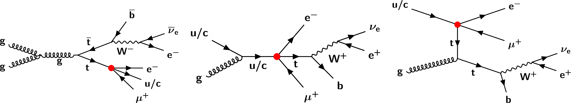
Figure 1:
Representative Feynman diagrams for the signal processes that are targeted by this analysis. Both top quark decay (left) and production (middle and right) CLFV processes are shown. The CLFV interaction vertex is shown as a solid red circle to indicate that it is not allowed in the SM. |
png pdf |
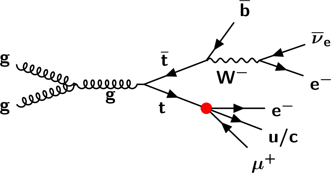
Figure 1-a:
Representative Feynman diagrams for the signal processes that are targeted by this analysis. Both top quark decay (left) and production (middle and right) CLFV processes are shown. The CLFV interaction vertex is shown as a solid red circle to indicate that it is not allowed in the SM. |

png pdf |
Figure 1-b:
Representative Feynman diagrams for the signal processes that are targeted by this analysis. Both top quark decay (left) and production (middle and right) CLFV processes are shown. The CLFV interaction vertex is shown as a solid red circle to indicate that it is not allowed in the SM. |
png pdf |
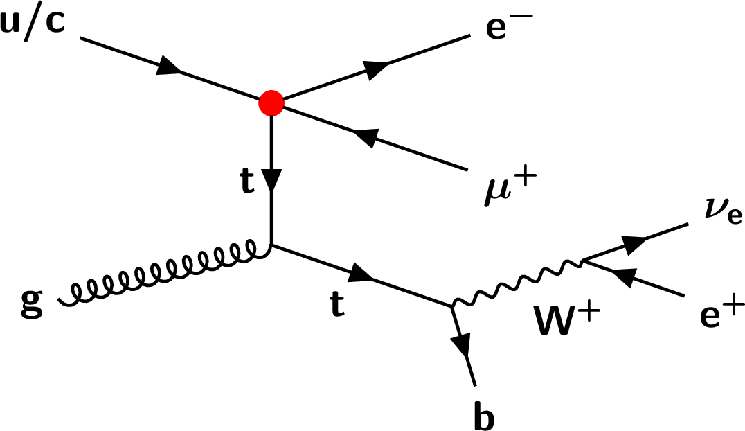
Figure 1-c:
Representative Feynman diagrams for the signal processes that are targeted by this analysis. Both top quark decay (left) and production (middle and right) CLFV processes are shown. The CLFV interaction vertex is shown as a solid red circle to indicate that it is not allowed in the SM. |

png pdf |
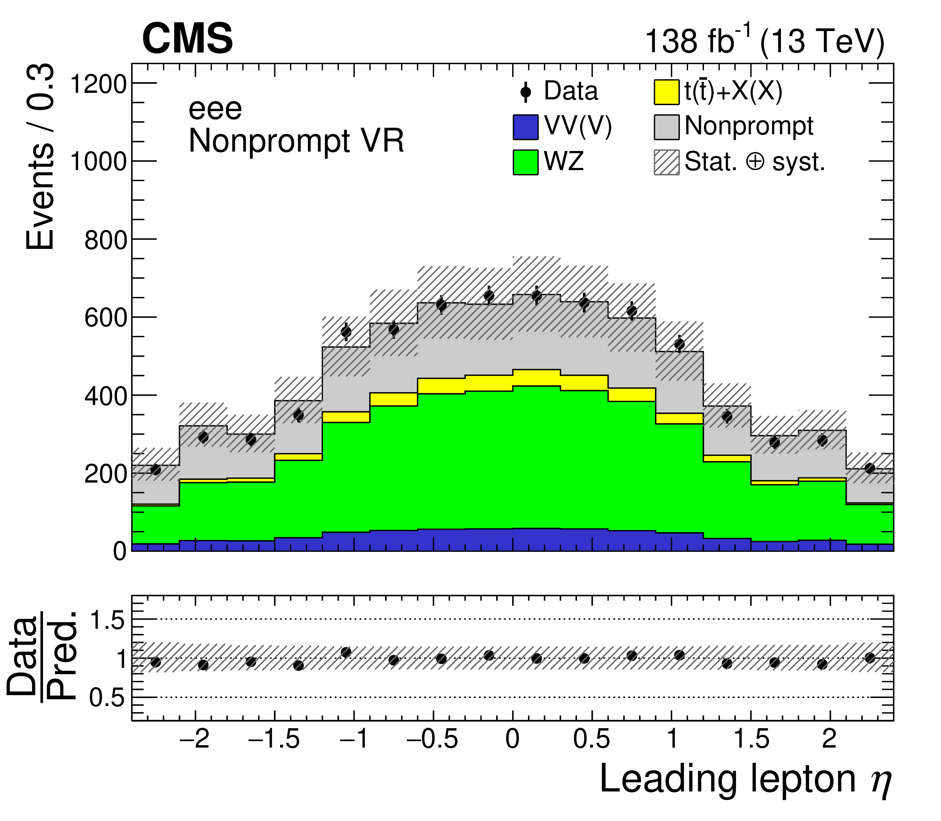
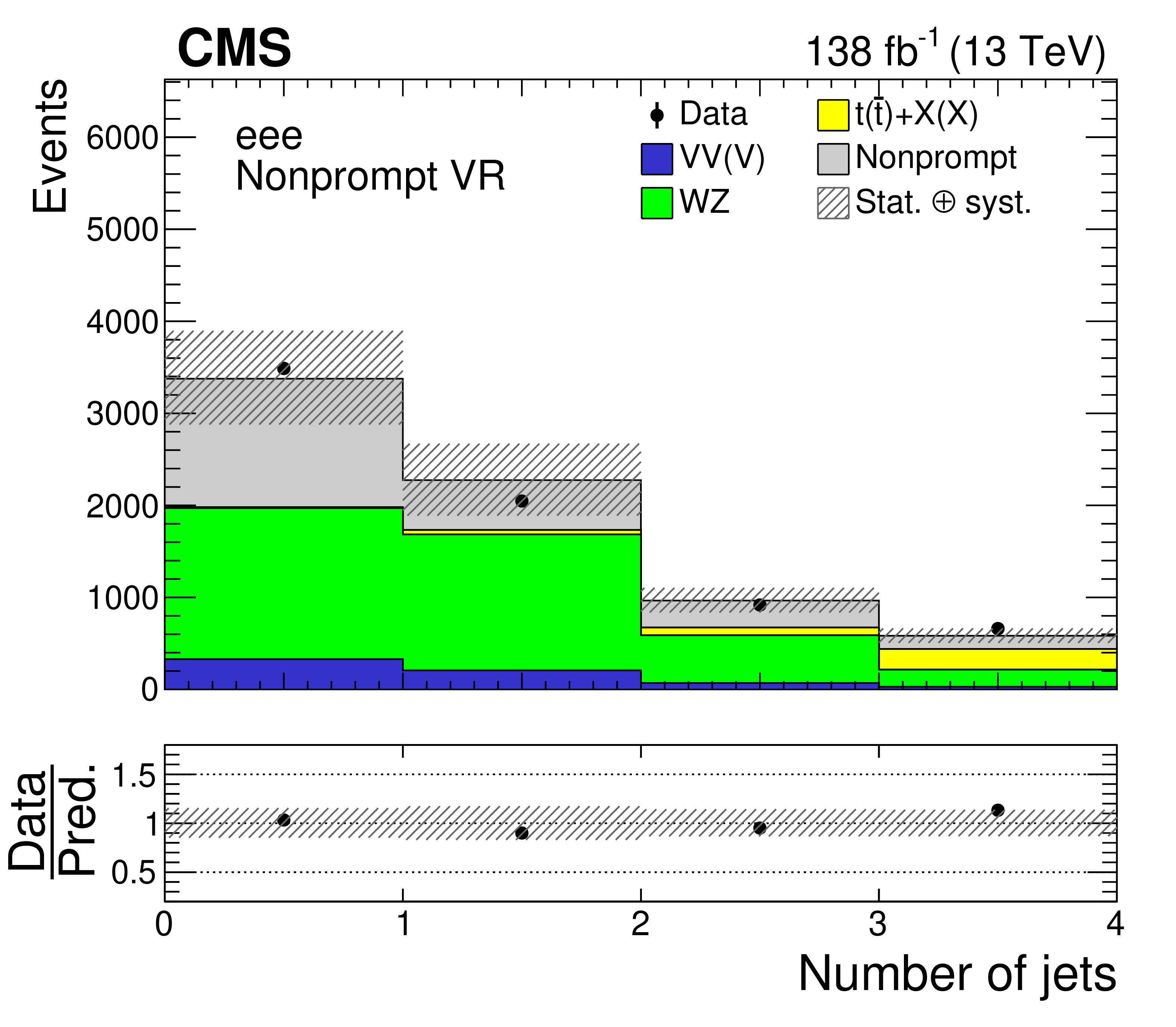
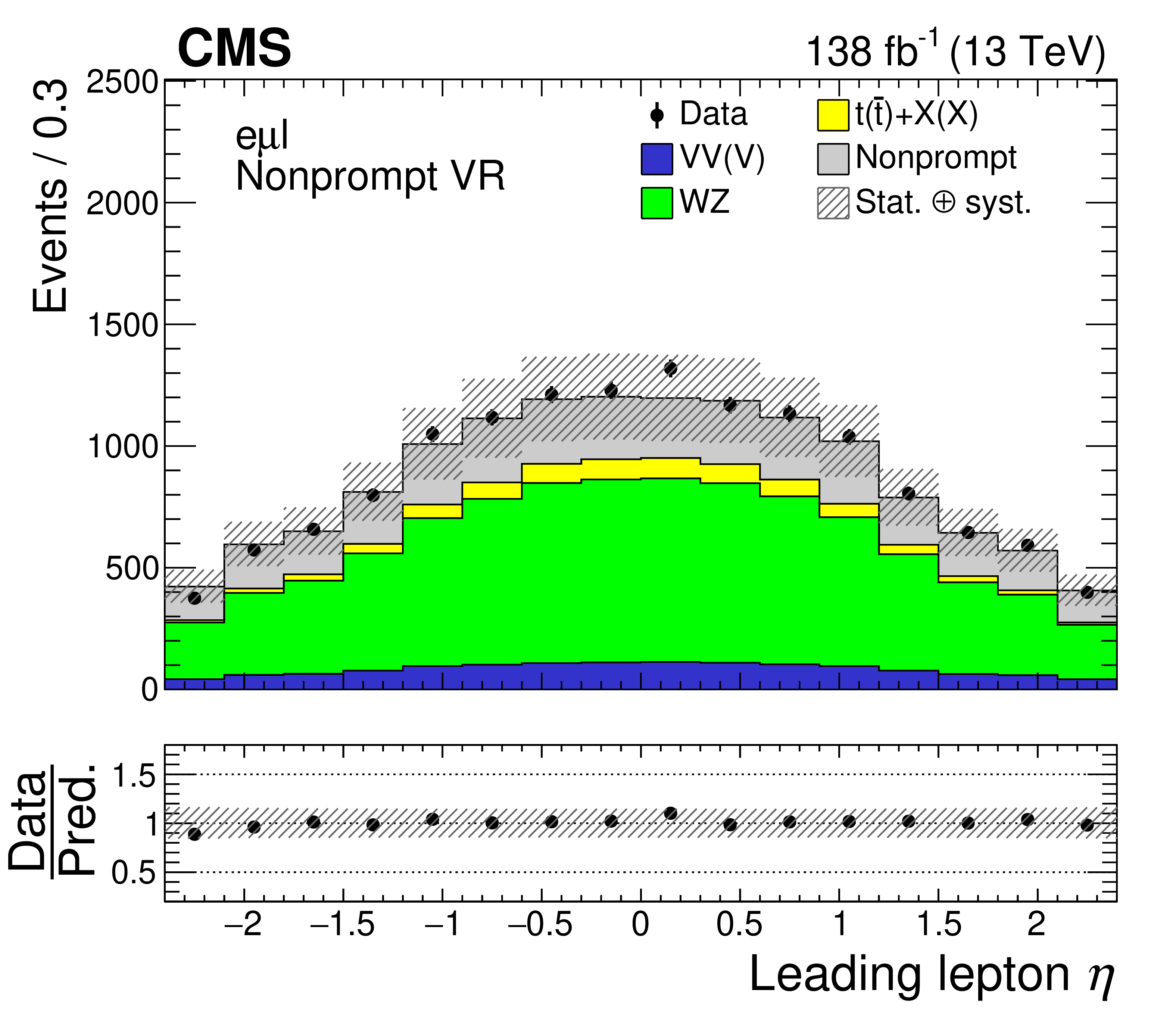
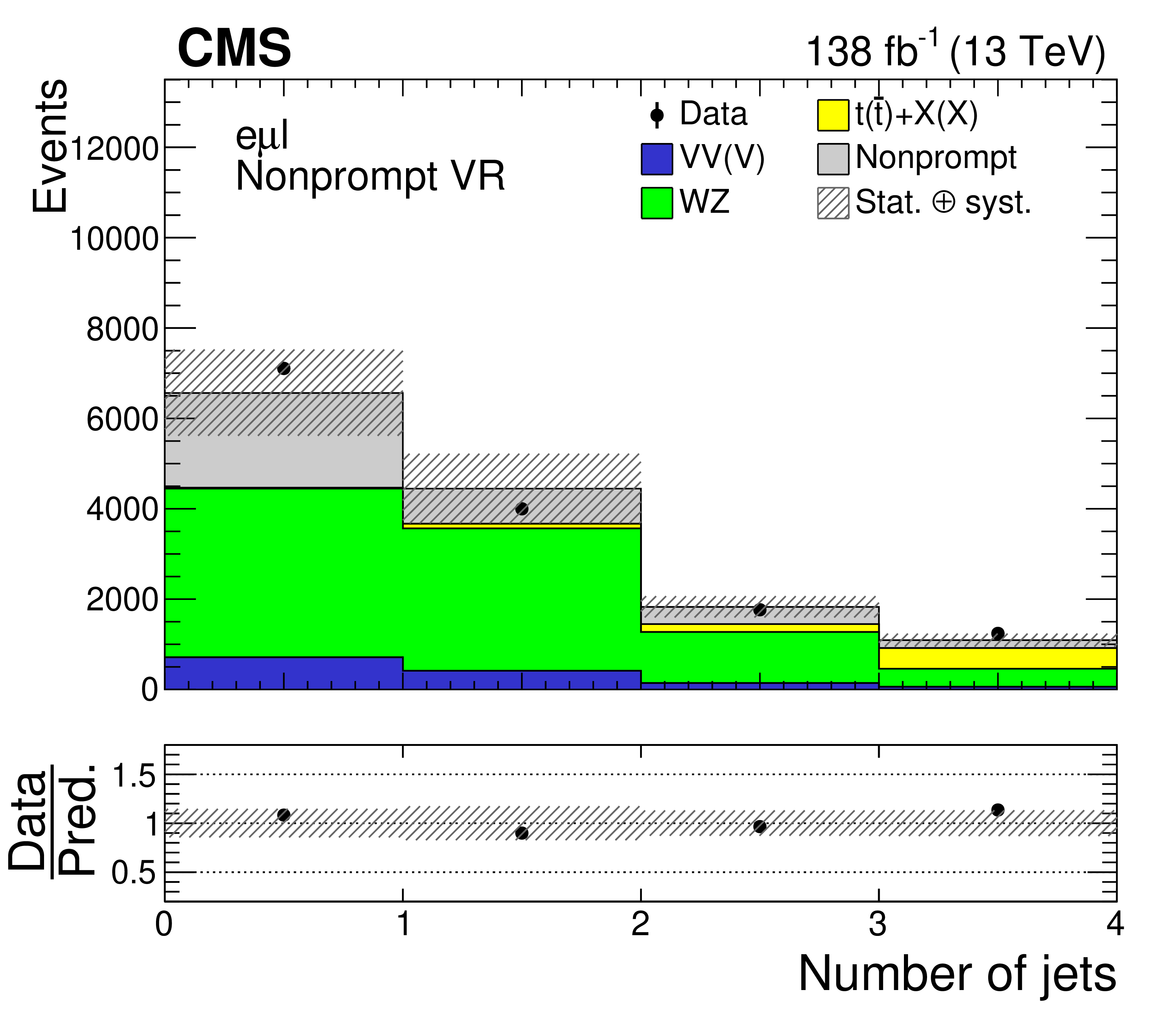
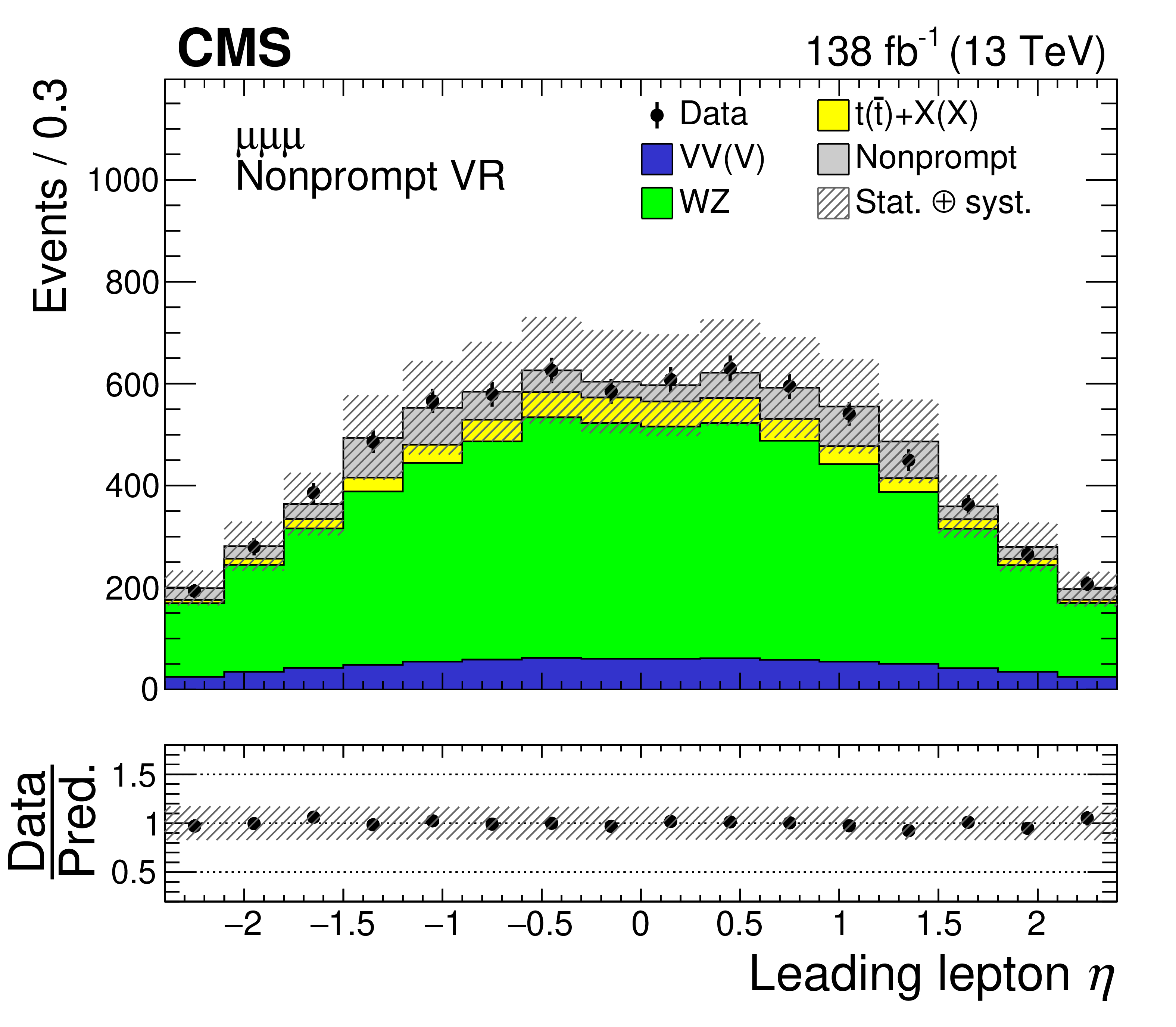
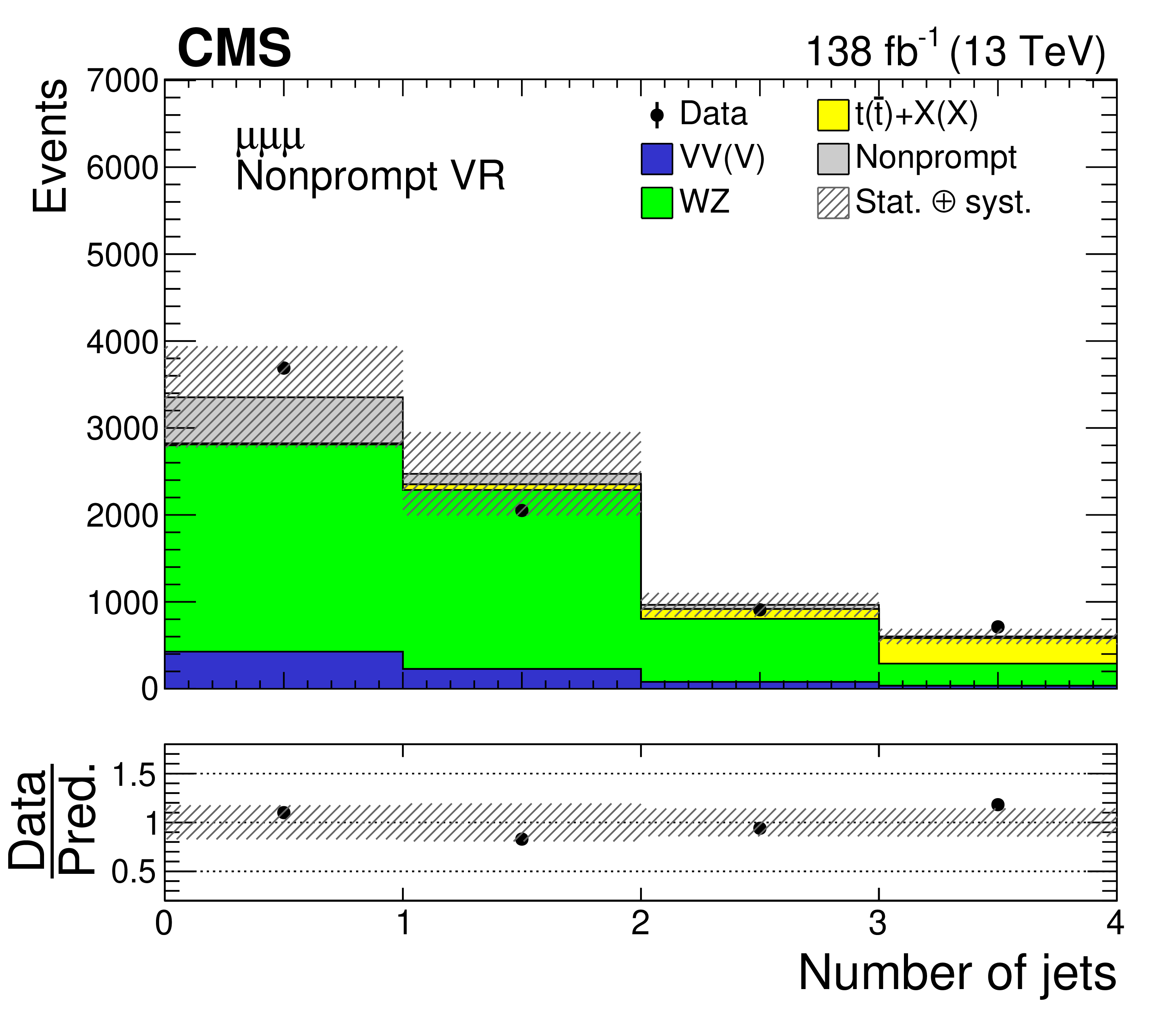
Figure 2:
Distributions of the leading lepton $ \eta $ (left column) and the jet multiplicity (right column) in the nonprompt VRs. Events in the $ \mathrm{e}\mathrm{e}\mathrm{e} $, $ \mathrm{e}\mu\ell $, and $ \mu\mu\mu $ nonprompt VRs are shown in the upper, middle, and lower row, respectively. The data are shown as filled points and the SM background predictions as histograms. The VV(V) background includes ZZ and triboson production, while the $ \mathrm{t}(\bar{\mathrm{t}})+\mathrm{X(X)} $ component includes $ {\mathrm{t}\overline{\mathrm{t}}} \mathrm{W} $, $ {\mathrm{t}\overline{\mathrm{t}}} \mathrm{Z} $, $ {\mathrm{t}\overline{\mathrm{t}}} \mathrm{H} $, $ \mathrm{t}\mathrm{Z}\mathrm{q} $, and smaller backgrounds containing one or two top quarks plus a boson or quark. The nonprompt background is estimated using control samples in data, while other backgrounds are estimated using MC simulation. The hatched bands indicate statistical and systematic uncertainties in the background predictions. The last bin of the right column histograms includes the overflow events. |
png pdf |
Figure 2-a:
Distributions of the leading lepton $ \eta $ (left column) and the jet multiplicity (right column) in the nonprompt VRs. Events in the $ \mathrm{e}\mathrm{e}\mathrm{e} $, $ \mathrm{e}\mu\ell $, and $ \mu\mu\mu $ nonprompt VRs are shown in the upper, middle, and lower row, respectively. The data are shown as filled points and the SM background predictions as histograms. The VV(V) background includes ZZ and triboson production, while the $ \mathrm{t}(\bar{\mathrm{t}})+\mathrm{X(X)} $ component includes $ {\mathrm{t}\overline{\mathrm{t}}} \mathrm{W} $, $ {\mathrm{t}\overline{\mathrm{t}}} \mathrm{Z} $, $ {\mathrm{t}\overline{\mathrm{t}}} \mathrm{H} $, $ \mathrm{t}\mathrm{Z}\mathrm{q} $, and smaller backgrounds containing one or two top quarks plus a boson or quark. The nonprompt background is estimated using control samples in data, while other backgrounds are estimated using MC simulation. The hatched bands indicate statistical and systematic uncertainties in the background predictions. The last bin of the right column histograms includes the overflow events. |
png pdf |
Figure 2-b:
Distributions of the leading lepton $ \eta $ (left column) and the jet multiplicity (right column) in the nonprompt VRs. Events in the $ \mathrm{e}\mathrm{e}\mathrm{e} $, $ \mathrm{e}\mu\ell $, and $ \mu\mu\mu $ nonprompt VRs are shown in the upper, middle, and lower row, respectively. The data are shown as filled points and the SM background predictions as histograms. The VV(V) background includes ZZ and triboson production, while the $ \mathrm{t}(\bar{\mathrm{t}})+\mathrm{X(X)} $ component includes $ {\mathrm{t}\overline{\mathrm{t}}} \mathrm{W} $, $ {\mathrm{t}\overline{\mathrm{t}}} \mathrm{Z} $, $ {\mathrm{t}\overline{\mathrm{t}}} \mathrm{H} $, $ \mathrm{t}\mathrm{Z}\mathrm{q} $, and smaller backgrounds containing one or two top quarks plus a boson or quark. The nonprompt background is estimated using control samples in data, while other backgrounds are estimated using MC simulation. The hatched bands indicate statistical and systematic uncertainties in the background predictions. The last bin of the right column histograms includes the overflow events. |
png pdf |
Figure 2-c:
Distributions of the leading lepton $ \eta $ (left column) and the jet multiplicity (right column) in the nonprompt VRs. Events in the $ \mathrm{e}\mathrm{e}\mathrm{e} $, $ \mathrm{e}\mu\ell $, and $ \mu\mu\mu $ nonprompt VRs are shown in the upper, middle, and lower row, respectively. The data are shown as filled points and the SM background predictions as histograms. The VV(V) background includes ZZ and triboson production, while the $ \mathrm{t}(\bar{\mathrm{t}})+\mathrm{X(X)} $ component includes $ {\mathrm{t}\overline{\mathrm{t}}} \mathrm{W} $, $ {\mathrm{t}\overline{\mathrm{t}}} \mathrm{Z} $, $ {\mathrm{t}\overline{\mathrm{t}}} \mathrm{H} $, $ \mathrm{t}\mathrm{Z}\mathrm{q} $, and smaller backgrounds containing one or two top quarks plus a boson or quark. The nonprompt background is estimated using control samples in data, while other backgrounds are estimated using MC simulation. The hatched bands indicate statistical and systematic uncertainties in the background predictions. The last bin of the right column histograms includes the overflow events. |
png pdf |
Figure 2-d:
Distributions of the leading lepton $ \eta $ (left column) and the jet multiplicity (right column) in the nonprompt VRs. Events in the $ \mathrm{e}\mathrm{e}\mathrm{e} $, $ \mathrm{e}\mu\ell $, and $ \mu\mu\mu $ nonprompt VRs are shown in the upper, middle, and lower row, respectively. The data are shown as filled points and the SM background predictions as histograms. The VV(V) background includes ZZ and triboson production, while the $ \mathrm{t}(\bar{\mathrm{t}})+\mathrm{X(X)} $ component includes $ {\mathrm{t}\overline{\mathrm{t}}} \mathrm{W} $, $ {\mathrm{t}\overline{\mathrm{t}}} \mathrm{Z} $, $ {\mathrm{t}\overline{\mathrm{t}}} \mathrm{H} $, $ \mathrm{t}\mathrm{Z}\mathrm{q} $, and smaller backgrounds containing one or two top quarks plus a boson or quark. The nonprompt background is estimated using control samples in data, while other backgrounds are estimated using MC simulation. The hatched bands indicate statistical and systematic uncertainties in the background predictions. The last bin of the right column histograms includes the overflow events. |
png pdf |
Figure 2-e:
Distributions of the leading lepton $ \eta $ (left column) and the jet multiplicity (right column) in the nonprompt VRs. Events in the $ \mathrm{e}\mathrm{e}\mathrm{e} $, $ \mathrm{e}\mu\ell $, and $ \mu\mu\mu $ nonprompt VRs are shown in the upper, middle, and lower row, respectively. The data are shown as filled points and the SM background predictions as histograms. The VV(V) background includes ZZ and triboson production, while the $ \mathrm{t}(\bar{\mathrm{t}})+\mathrm{X(X)} $ component includes $ {\mathrm{t}\overline{\mathrm{t}}} \mathrm{W} $, $ {\mathrm{t}\overline{\mathrm{t}}} \mathrm{Z} $, $ {\mathrm{t}\overline{\mathrm{t}}} \mathrm{H} $, $ \mathrm{t}\mathrm{Z}\mathrm{q} $, and smaller backgrounds containing one or two top quarks plus a boson or quark. The nonprompt background is estimated using control samples in data, while other backgrounds are estimated using MC simulation. The hatched bands indicate statistical and systematic uncertainties in the background predictions. The last bin of the right column histograms includes the overflow events. |
png pdf |
Figure 2-f:
Distributions of the leading lepton $ \eta $ (left column) and the jet multiplicity (right column) in the nonprompt VRs. Events in the $ \mathrm{e}\mathrm{e}\mathrm{e} $, $ \mathrm{e}\mu\ell $, and $ \mu\mu\mu $ nonprompt VRs are shown in the upper, middle, and lower row, respectively. The data are shown as filled points and the SM background predictions as histograms. The VV(V) background includes ZZ and triboson production, while the $ \mathrm{t}(\bar{\mathrm{t}})+\mathrm{X(X)} $ component includes $ {\mathrm{t}\overline{\mathrm{t}}} \mathrm{W} $, $ {\mathrm{t}\overline{\mathrm{t}}} \mathrm{Z} $, $ {\mathrm{t}\overline{\mathrm{t}}} \mathrm{H} $, $ \mathrm{t}\mathrm{Z}\mathrm{q} $, and smaller backgrounds containing one or two top quarks plus a boson or quark. The nonprompt background is estimated using control samples in data, while other backgrounds are estimated using MC simulation. The hatched bands indicate statistical and systematic uncertainties in the background predictions. The last bin of the right column histograms includes the overflow events. |

png pdf |
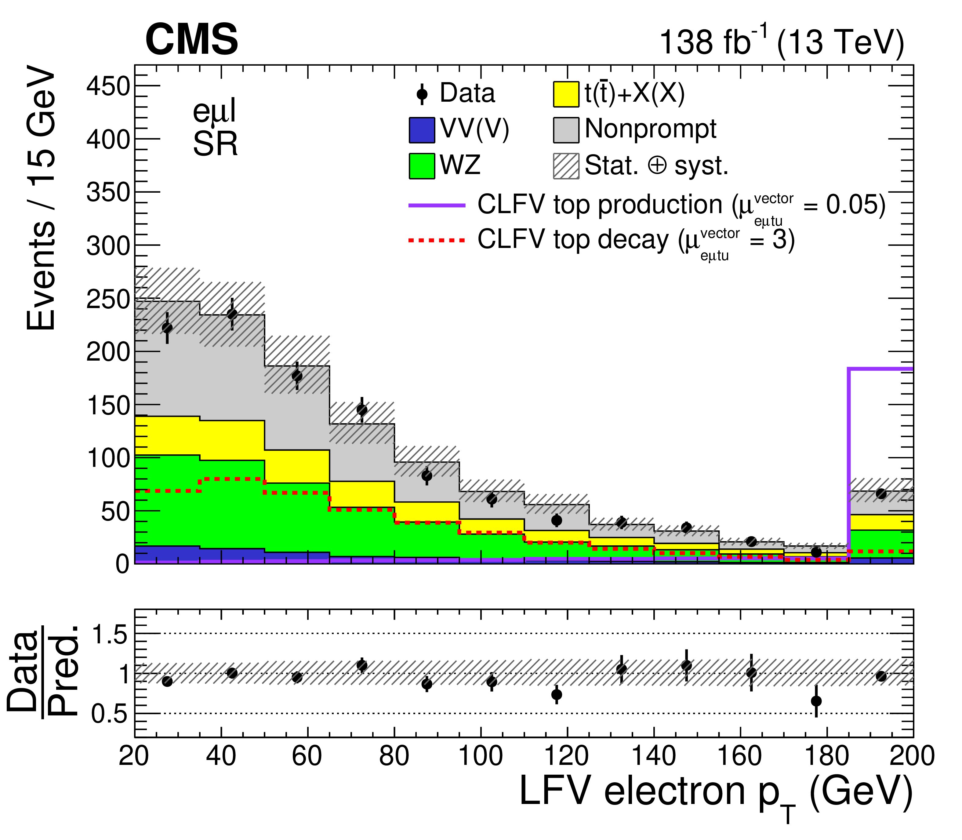
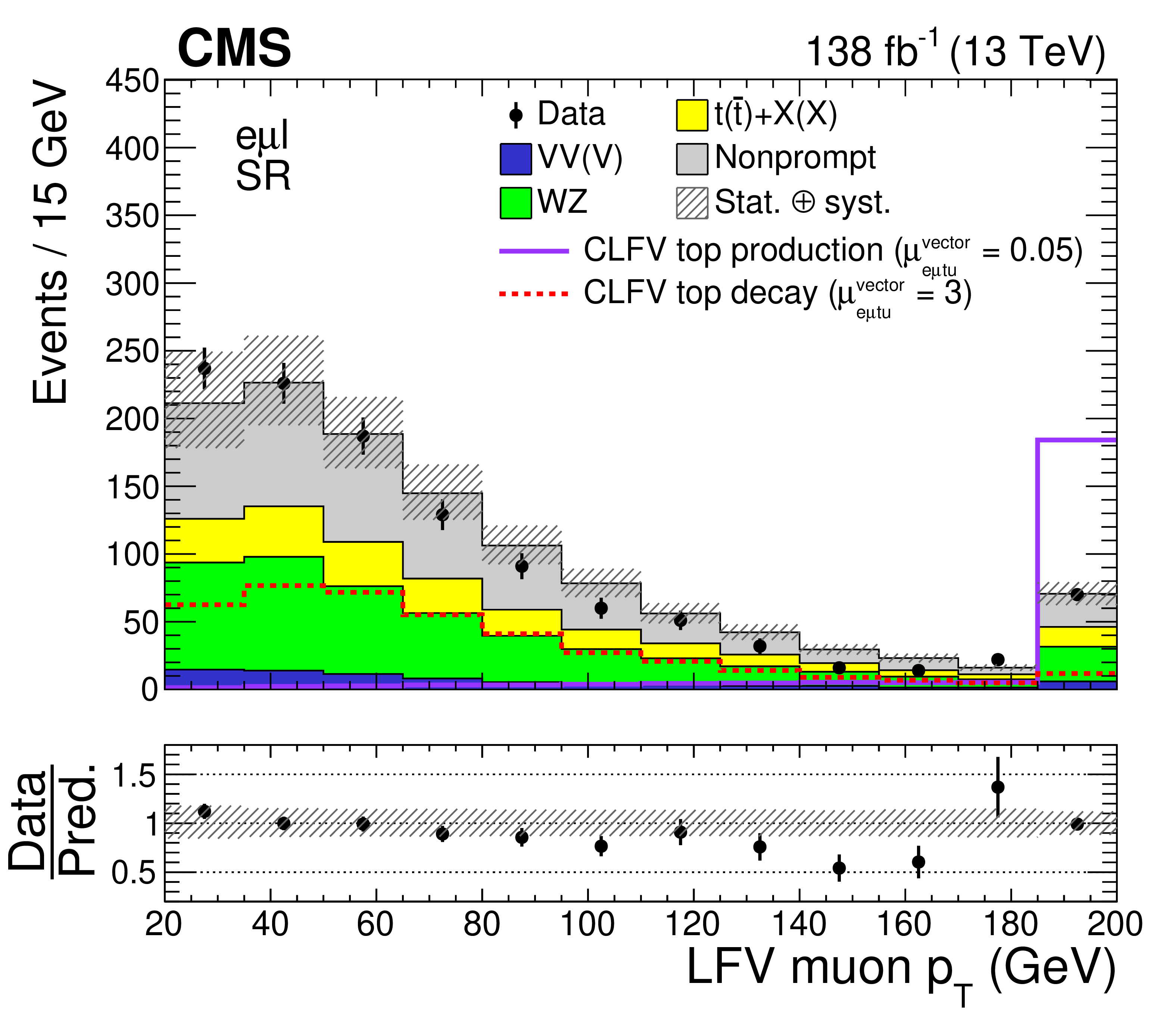
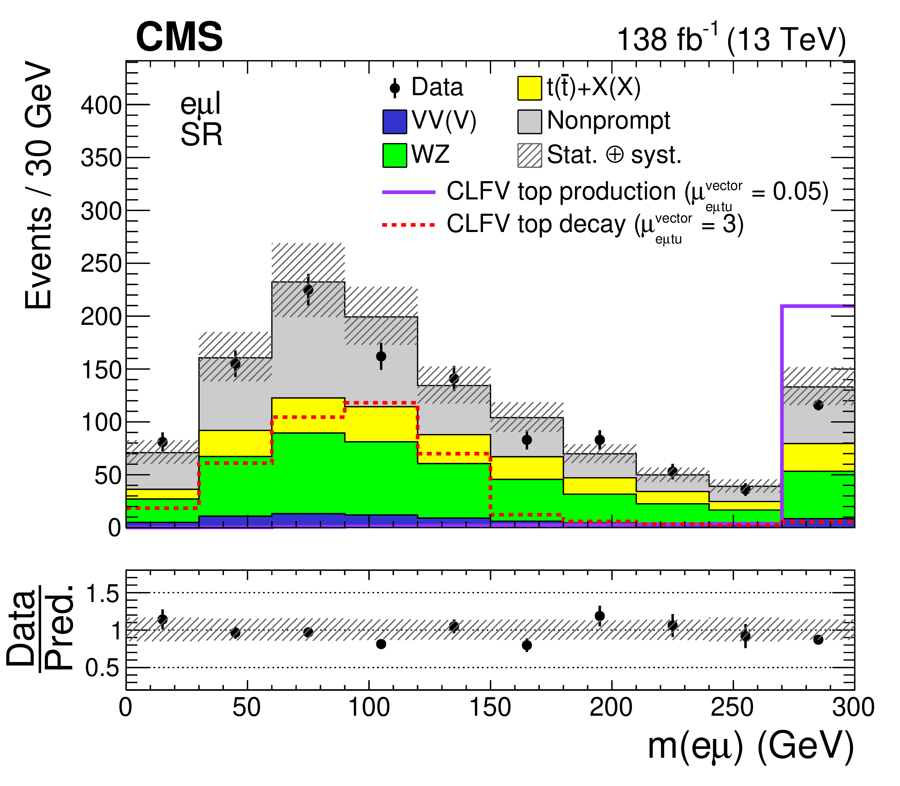
Figure 3:
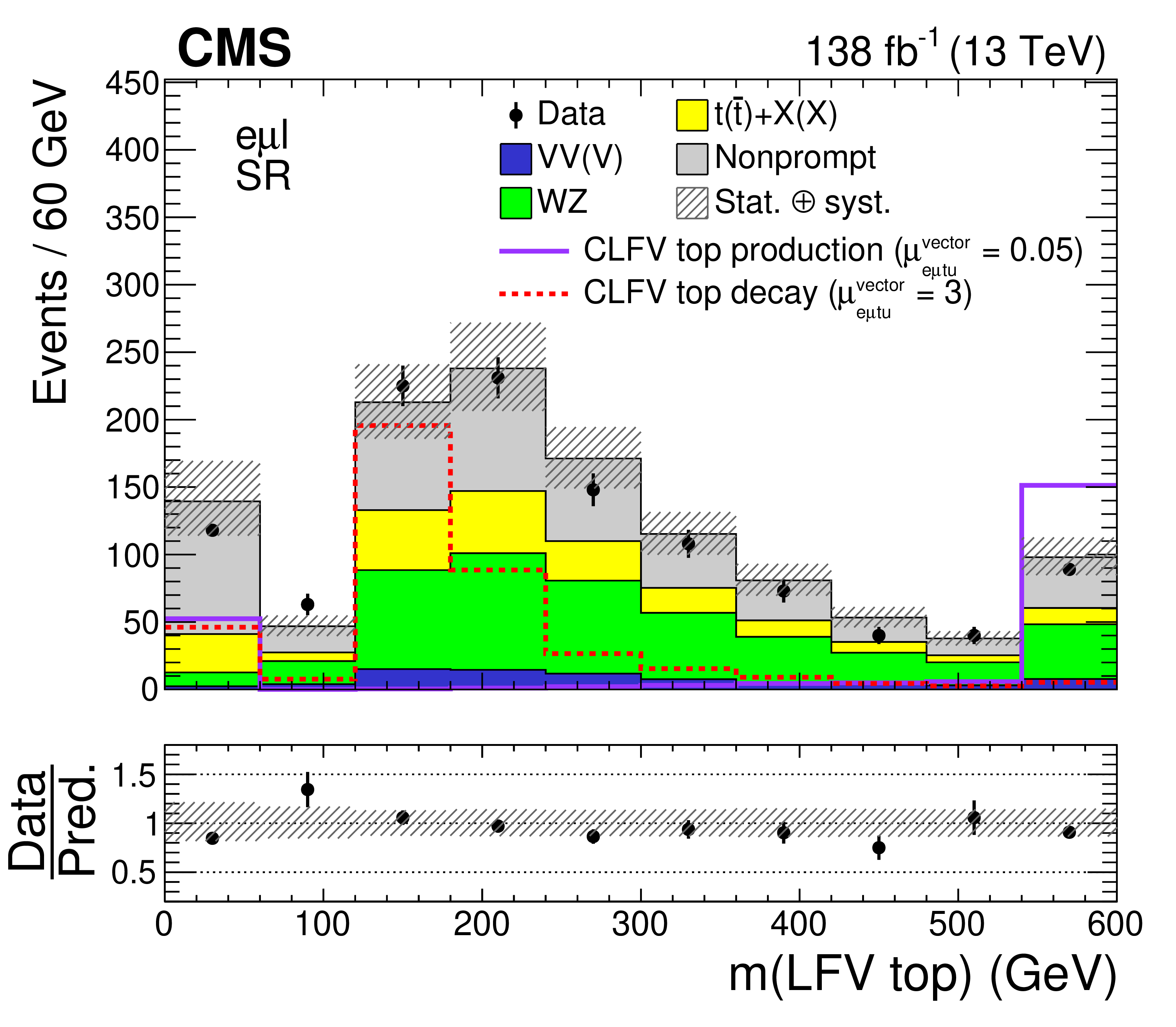
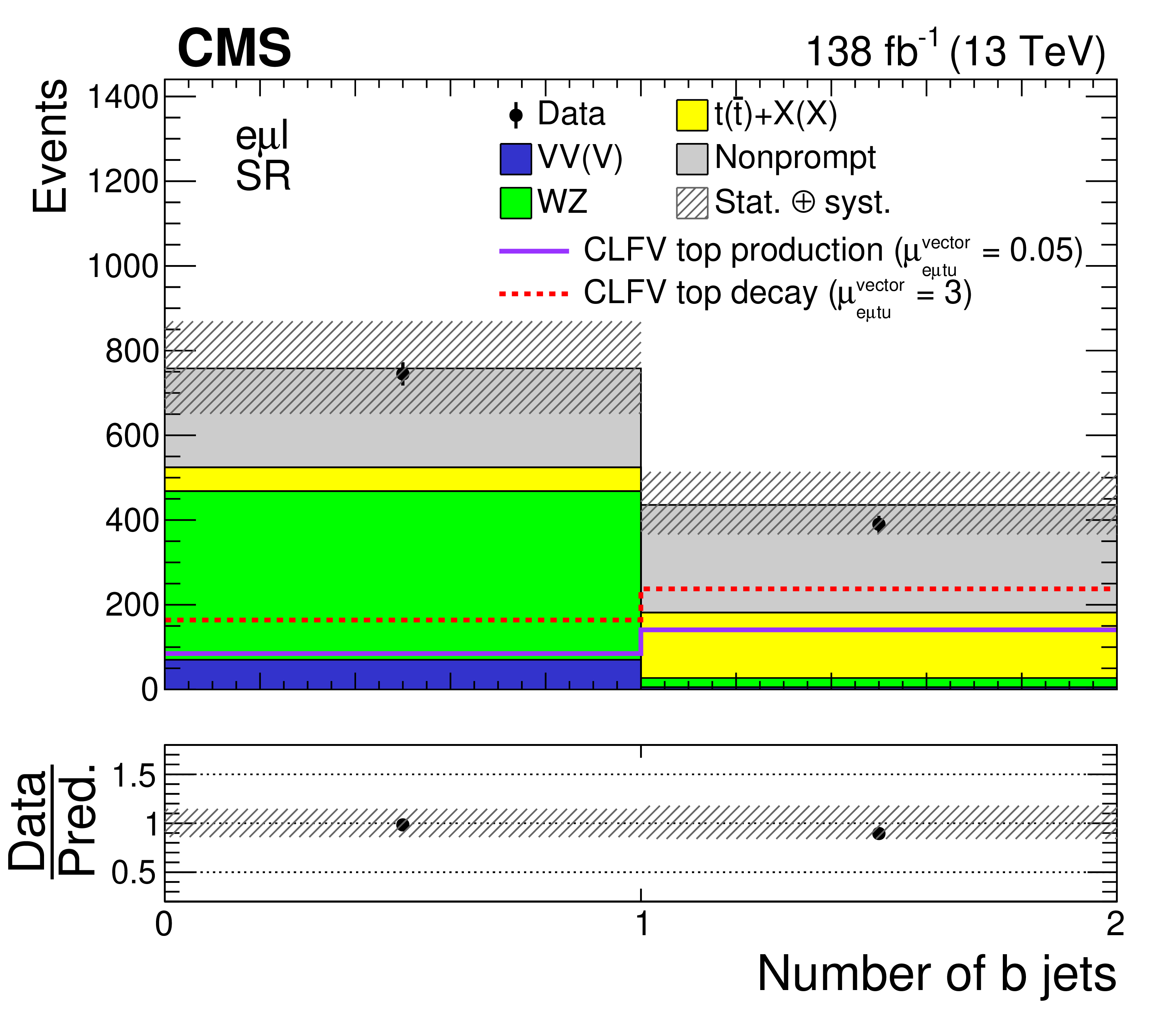
Distributions of kinematic variables in the SR: LFV electron $ p_{\mathrm{T}} $ (upper left), LFV muon $ p_{\mathrm{T}} $ (upper right), LFV $ \mathrm{e}\mu $ mass (middle left), LFV top quark mass (middle right), OSSF lepton pair mass (lower left), and b jet multiplicity (lower right). The CLFV top quark decay and production signals are shown as dotted red and solid purple lines, respectively. The original signal normalization, corresponding to $ C_{\mathrm{e}\mu\mathrm{t}\mathrm{u}}^{\text{vector}}/\Lambda^2=$ 1 TeV$^{-2}$, is scaled up (down) by a factor of 3 (20) for the CLFV top quark decay (production) signal for better visualization. The hatched bands indicate statistical and systematic uncertainties in the background predictions. The last bin of all but the lower-right histogram includes the overflow events. |
png pdf |
Figure 3-a:
Distributions of kinematic variables in the SR: LFV electron $ p_{\mathrm{T}} $ (upper left), LFV muon $ p_{\mathrm{T}} $ (upper right), LFV $ \mathrm{e}\mu $ mass (middle left), LFV top quark mass (middle right), OSSF lepton pair mass (lower left), and b jet multiplicity (lower right). The CLFV top quark decay and production signals are shown as dotted red and solid purple lines, respectively. The original signal normalization, corresponding to $ C_{\mathrm{e}\mu\mathrm{t}\mathrm{u}}^{\text{vector}}/\Lambda^2=$ 1 TeV$^{-2}$, is scaled up (down) by a factor of 3 (20) for the CLFV top quark decay (production) signal for better visualization. The hatched bands indicate statistical and systematic uncertainties in the background predictions. The last bin of all but the lower-right histogram includes the overflow events. |
png pdf |
Figure 3-b:
Distributions of kinematic variables in the SR: LFV electron $ p_{\mathrm{T}} $ (upper left), LFV muon $ p_{\mathrm{T}} $ (upper right), LFV $ \mathrm{e}\mu $ mass (middle left), LFV top quark mass (middle right), OSSF lepton pair mass (lower left), and b jet multiplicity (lower right). The CLFV top quark decay and production signals are shown as dotted red and solid purple lines, respectively. The original signal normalization, corresponding to $ C_{\mathrm{e}\mu\mathrm{t}\mathrm{u}}^{\text{vector}}/\Lambda^2=$ 1 TeV$^{-2}$, is scaled up (down) by a factor of 3 (20) for the CLFV top quark decay (production) signal for better visualization. The hatched bands indicate statistical and systematic uncertainties in the background predictions. The last bin of all but the lower-right histogram includes the overflow events. |
png pdf |
Figure 3-c:
Distributions of kinematic variables in the SR: LFV electron $ p_{\mathrm{T}} $ (upper left), LFV muon $ p_{\mathrm{T}} $ (upper right), LFV $ \mathrm{e}\mu $ mass (middle left), LFV top quark mass (middle right), OSSF lepton pair mass (lower left), and b jet multiplicity (lower right). The CLFV top quark decay and production signals are shown as dotted red and solid purple lines, respectively. The original signal normalization, corresponding to $ C_{\mathrm{e}\mu\mathrm{t}\mathrm{u}}^{\text{vector}}/\Lambda^2=$ 1 TeV$^{-2}$, is scaled up (down) by a factor of 3 (20) for the CLFV top quark decay (production) signal for better visualization. The hatched bands indicate statistical and systematic uncertainties in the background predictions. The last bin of all but the lower-right histogram includes the overflow events. |
png pdf |
Figure 3-d:
Distributions of kinematic variables in the SR: LFV electron $ p_{\mathrm{T}} $ (upper left), LFV muon $ p_{\mathrm{T}} $ (upper right), LFV $ \mathrm{e}\mu $ mass (middle left), LFV top quark mass (middle right), OSSF lepton pair mass (lower left), and b jet multiplicity (lower right). The CLFV top quark decay and production signals are shown as dotted red and solid purple lines, respectively. The original signal normalization, corresponding to $ C_{\mathrm{e}\mu\mathrm{t}\mathrm{u}}^{\text{vector}}/\Lambda^2=$ 1 TeV$^{-2}$, is scaled up (down) by a factor of 3 (20) for the CLFV top quark decay (production) signal for better visualization. The hatched bands indicate statistical and systematic uncertainties in the background predictions. The last bin of all but the lower-right histogram includes the overflow events. |

png pdf |
Figure 3-e:
Distributions of kinematic variables in the SR: LFV electron $ p_{\mathrm{T}} $ (upper left), LFV muon $ p_{\mathrm{T}} $ (upper right), LFV $ \mathrm{e}\mu $ mass (middle left), LFV top quark mass (middle right), OSSF lepton pair mass (lower left), and b jet multiplicity (lower right). The CLFV top quark decay and production signals are shown as dotted red and solid purple lines, respectively. The original signal normalization, corresponding to $ C_{\mathrm{e}\mu\mathrm{t}\mathrm{u}}^{\text{vector}}/\Lambda^2=$ 1 TeV$^{-2}$, is scaled up (down) by a factor of 3 (20) for the CLFV top quark decay (production) signal for better visualization. The hatched bands indicate statistical and systematic uncertainties in the background predictions. The last bin of all but the lower-right histogram includes the overflow events. |
png pdf |
Figure 3-f:
Distributions of kinematic variables in the SR: LFV electron $ p_{\mathrm{T}} $ (upper left), LFV muon $ p_{\mathrm{T}} $ (upper right), LFV $ \mathrm{e}\mu $ mass (middle left), LFV top quark mass (middle right), OSSF lepton pair mass (lower left), and b jet multiplicity (lower right). The CLFV top quark decay and production signals are shown as dotted red and solid purple lines, respectively. The original signal normalization, corresponding to $ C_{\mathrm{e}\mu\mathrm{t}\mathrm{u}}^{\text{vector}}/\Lambda^2=$ 1 TeV$^{-2}$, is scaled up (down) by a factor of 3 (20) for the CLFV top quark decay (production) signal for better visualization. The hatched bands indicate statistical and systematic uncertainties in the background predictions. The last bin of all but the lower-right histogram includes the overflow events. |
png pdf |
Figure 4:
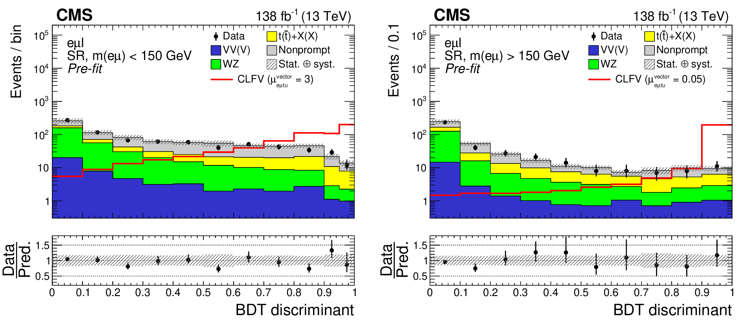
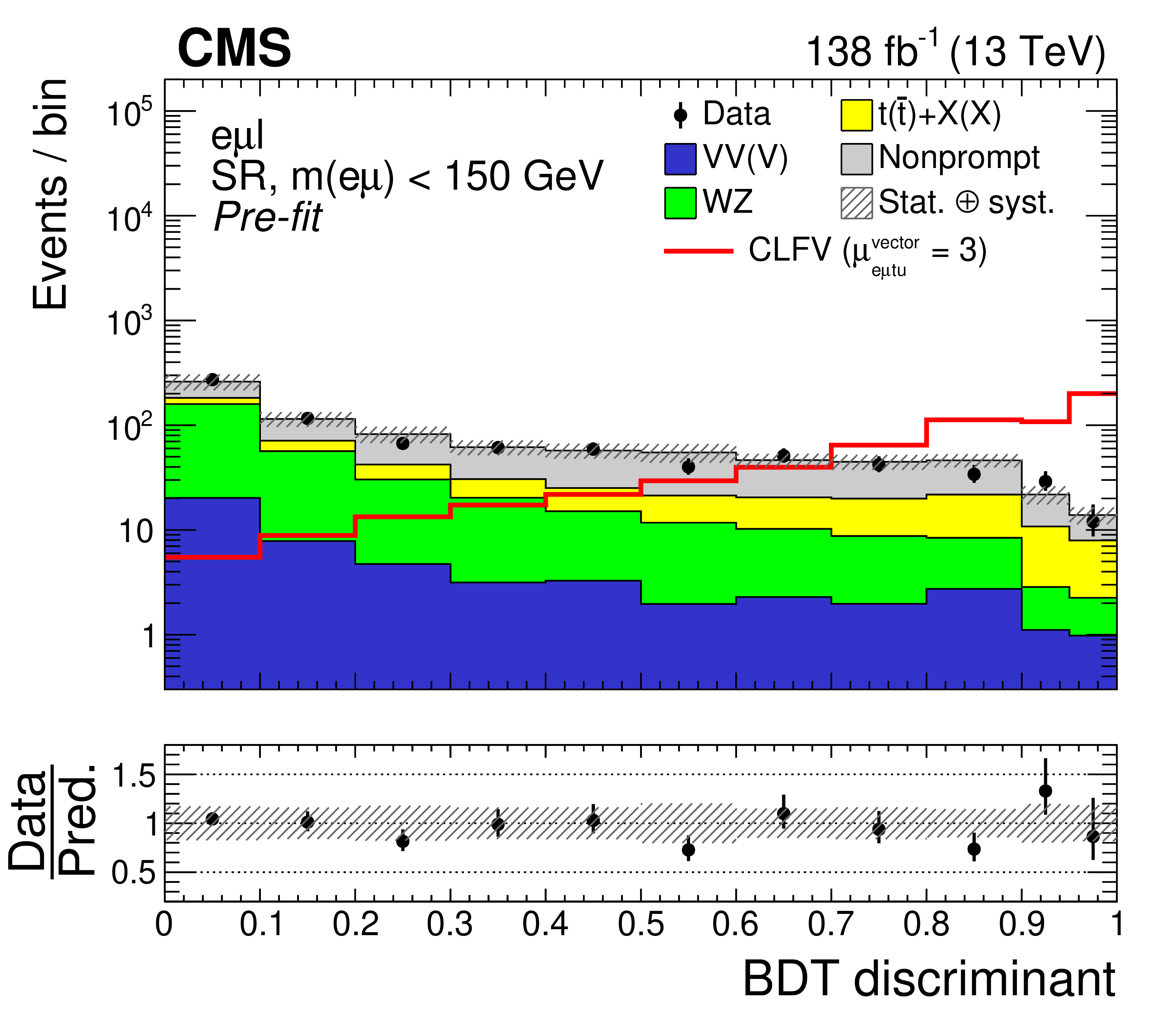
Distributions of the BDT discriminant targeting the CLFV top quark decay (left) and production (right) signal. Contributions from the two signal modes (production and decay) are combined within each SR and are shown as the solid red line. The pre-fit signal strength ($ \mu_{\mathrm{e}\mu\mathrm{t}\mathrm{u}}^{\text{vector}}= $ 1), corresponding to $ C_{\mathrm{e}\mu\mathrm{t}\mathrm{u}}^{\text{vector}}/\Lambda^2=$ 1 TeV$^{-2}$, is scaled up (down) by a factor of 3 (20) for the CLFV top quark decay (production) signal for better visualization. The hatched bands indicate statistical and systematic uncertainties in the background predictions. |
png pdf |
Figure 4-a:
Distributions of the BDT discriminant targeting the CLFV top quark decay (left) and production (right) signal. Contributions from the two signal modes (production and decay) are combined within each SR and are shown as the solid red line. The pre-fit signal strength ($ \mu_{\mathrm{e}\mu\mathrm{t}\mathrm{u}}^{\text{vector}}= $ 1), corresponding to $ C_{\mathrm{e}\mu\mathrm{t}\mathrm{u}}^{\text{vector}}/\Lambda^2=$ 1 TeV$^{-2}$, is scaled up (down) by a factor of 3 (20) for the CLFV top quark decay (production) signal for better visualization. The hatched bands indicate statistical and systematic uncertainties in the background predictions. |

png pdf |
Figure 4-b:
Distributions of the BDT discriminant targeting the CLFV top quark decay (left) and production (right) signal. Contributions from the two signal modes (production and decay) are combined within each SR and are shown as the solid red line. The pre-fit signal strength ($ \mu_{\mathrm{e}\mu\mathrm{t}\mathrm{u}}^{\text{vector}}= $ 1), corresponding to $ C_{\mathrm{e}\mu\mathrm{t}\mathrm{u}}^{\text{vector}}/\Lambda^2=$ 1 TeV$^{-2}$, is scaled up (down) by a factor of 3 (20) for the CLFV top quark decay (production) signal for better visualization. The hatched bands indicate statistical and systematic uncertainties in the background predictions. |

png pdf |
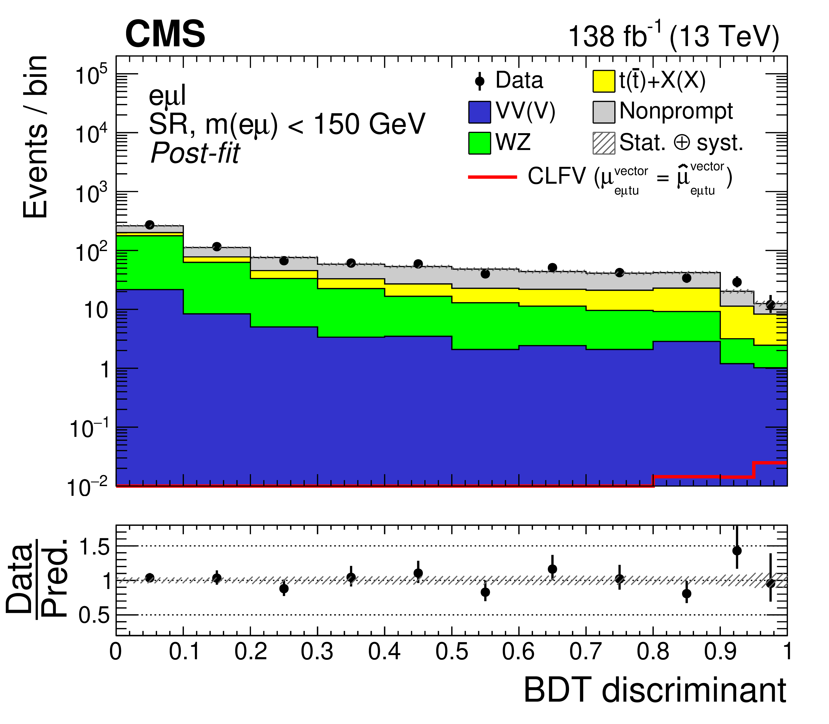
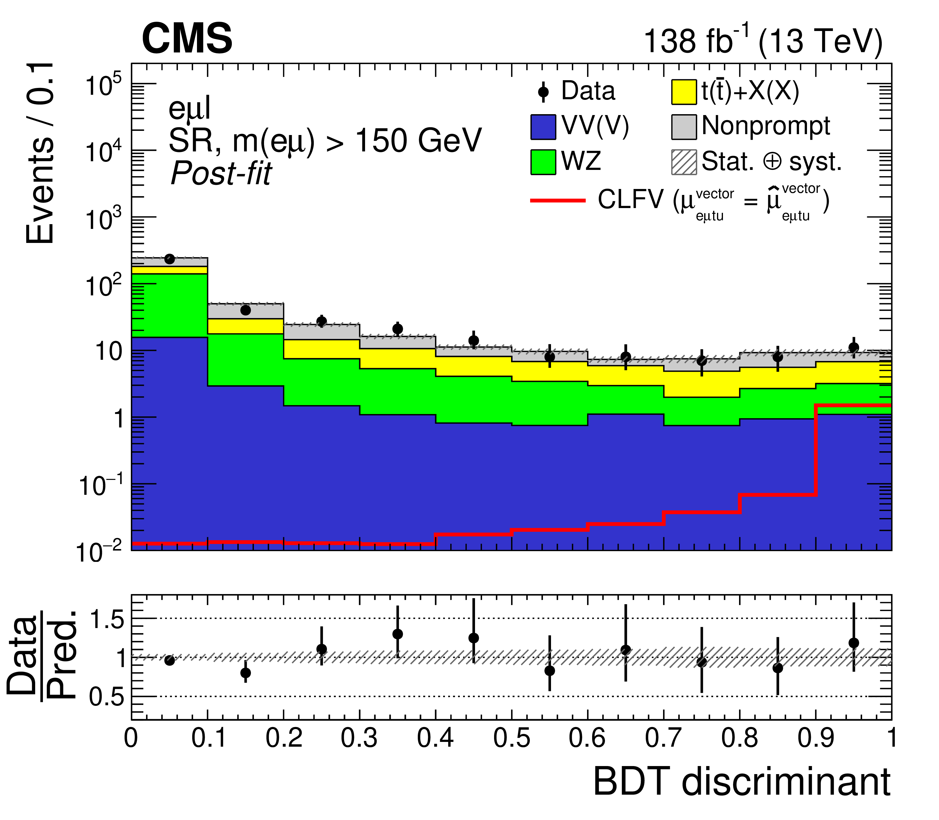
Figure 5:
Distributions of the post-fit BDT discriminant targeting the CLFV top quark decay (left) and production (right) signal. Contributions from the two signal modes (production and decay) are combined within each SR and are shown as the solid red line. The post-fit signal strength ($ \mu_{\mathrm{e}\mu\mathrm{t}\mathrm{u}}^{\text{vector}}=\hat{\mu}_{\mathrm{e}\mu\mathrm{t}\mathrm{u}}^{\text{vector}} $) is used to normalize the signal cross sections. The hatched bands indicate post-fit uncertainties (statistical and systematic) for the SM background predictions. |
png pdf |
Figure 5-a:
Distributions of the post-fit BDT discriminant targeting the CLFV top quark decay (left) and production (right) signal. Contributions from the two signal modes (production and decay) are combined within each SR and are shown as the solid red line. The post-fit signal strength ($ \mu_{\mathrm{e}\mu\mathrm{t}\mathrm{u}}^{\text{vector}}=\hat{\mu}_{\mathrm{e}\mu\mathrm{t}\mathrm{u}}^{\text{vector}} $) is used to normalize the signal cross sections. The hatched bands indicate post-fit uncertainties (statistical and systematic) for the SM background predictions. |
png pdf |
Figure 5-b:
Distributions of the post-fit BDT discriminant targeting the CLFV top quark decay (left) and production (right) signal. Contributions from the two signal modes (production and decay) are combined within each SR and are shown as the solid red line. The post-fit signal strength ($ \mu_{\mathrm{e}\mu\mathrm{t}\mathrm{u}}^{\text{vector}}=\hat{\mu}_{\mathrm{e}\mu\mathrm{t}\mathrm{u}}^{\text{vector}} $) is used to normalize the signal cross sections. The hatched bands indicate post-fit uncertainties (statistical and systematic) for the SM background predictions. |
png pdf |
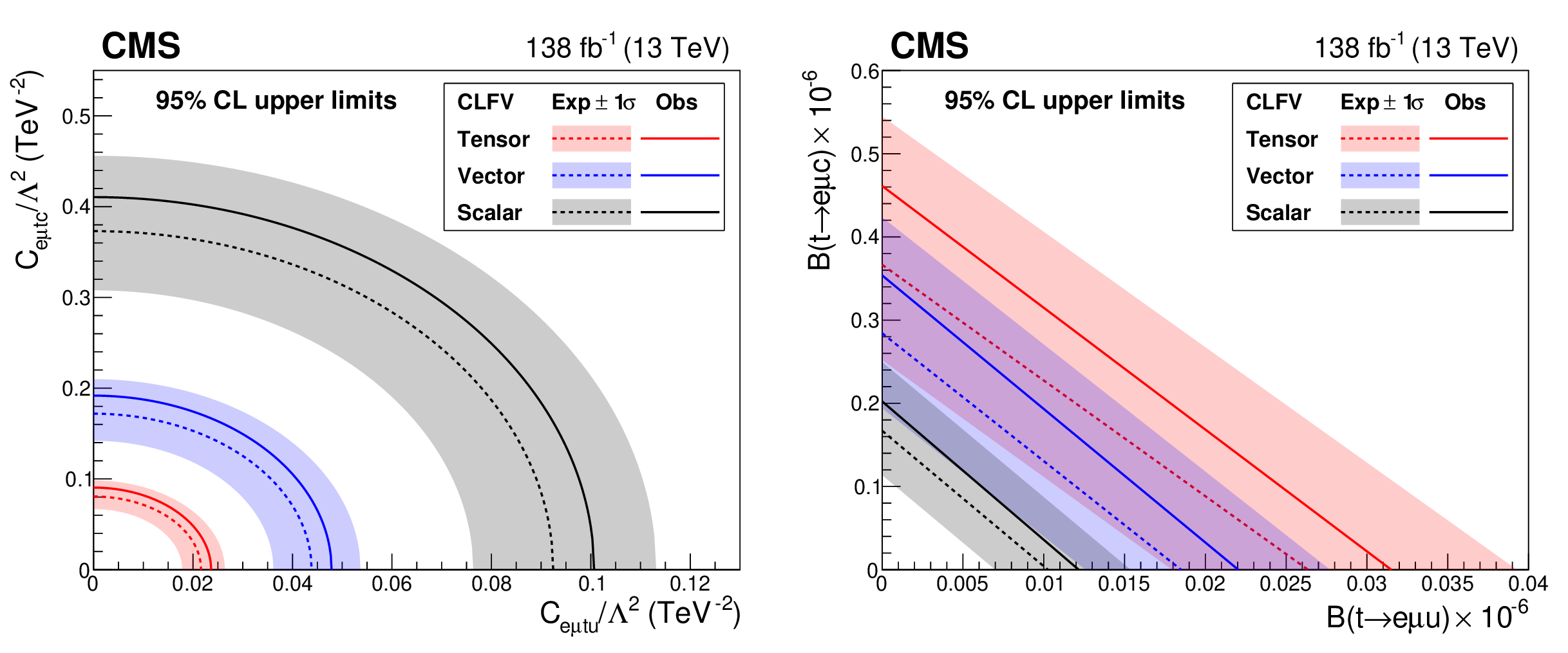
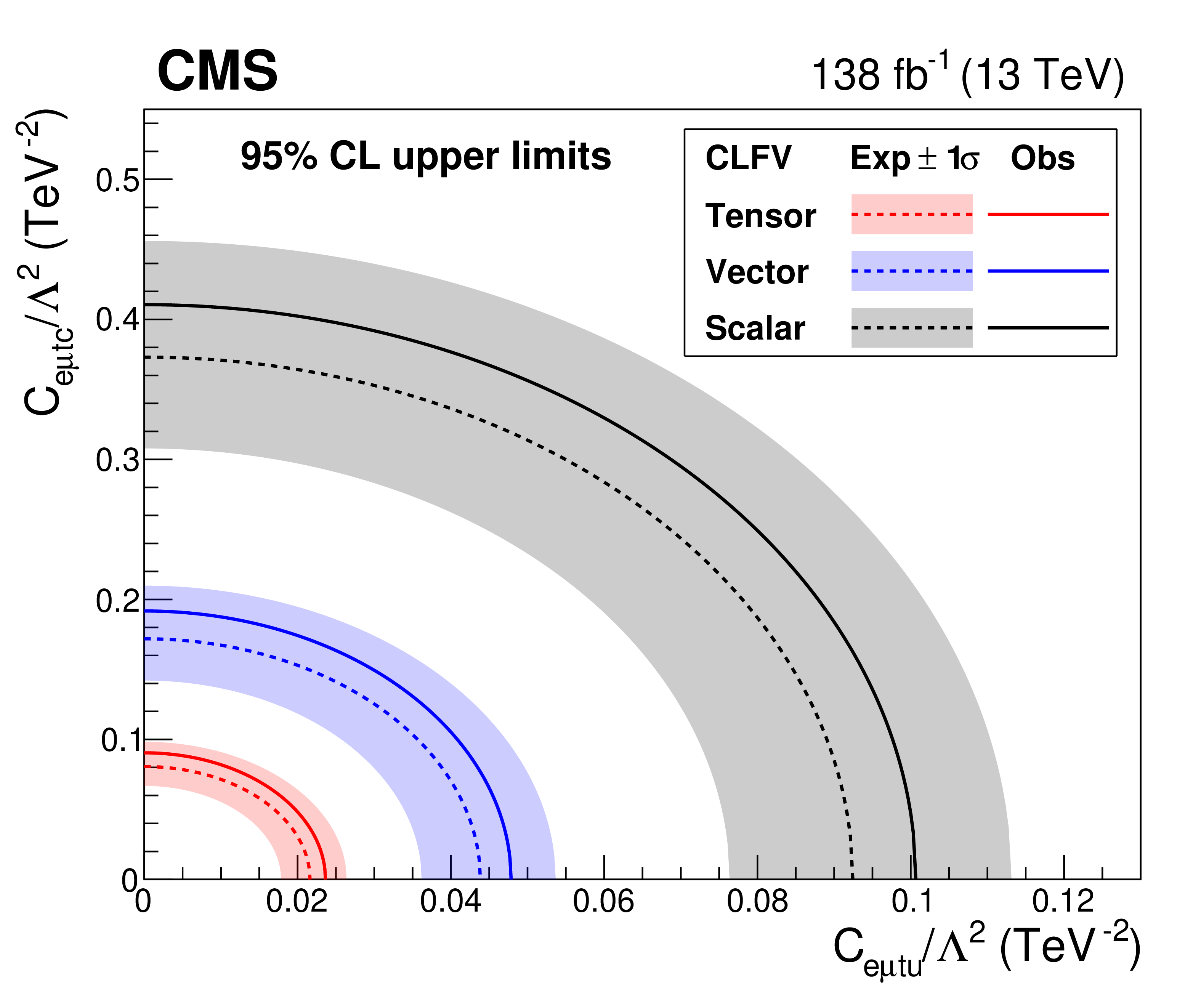
Figure 6:
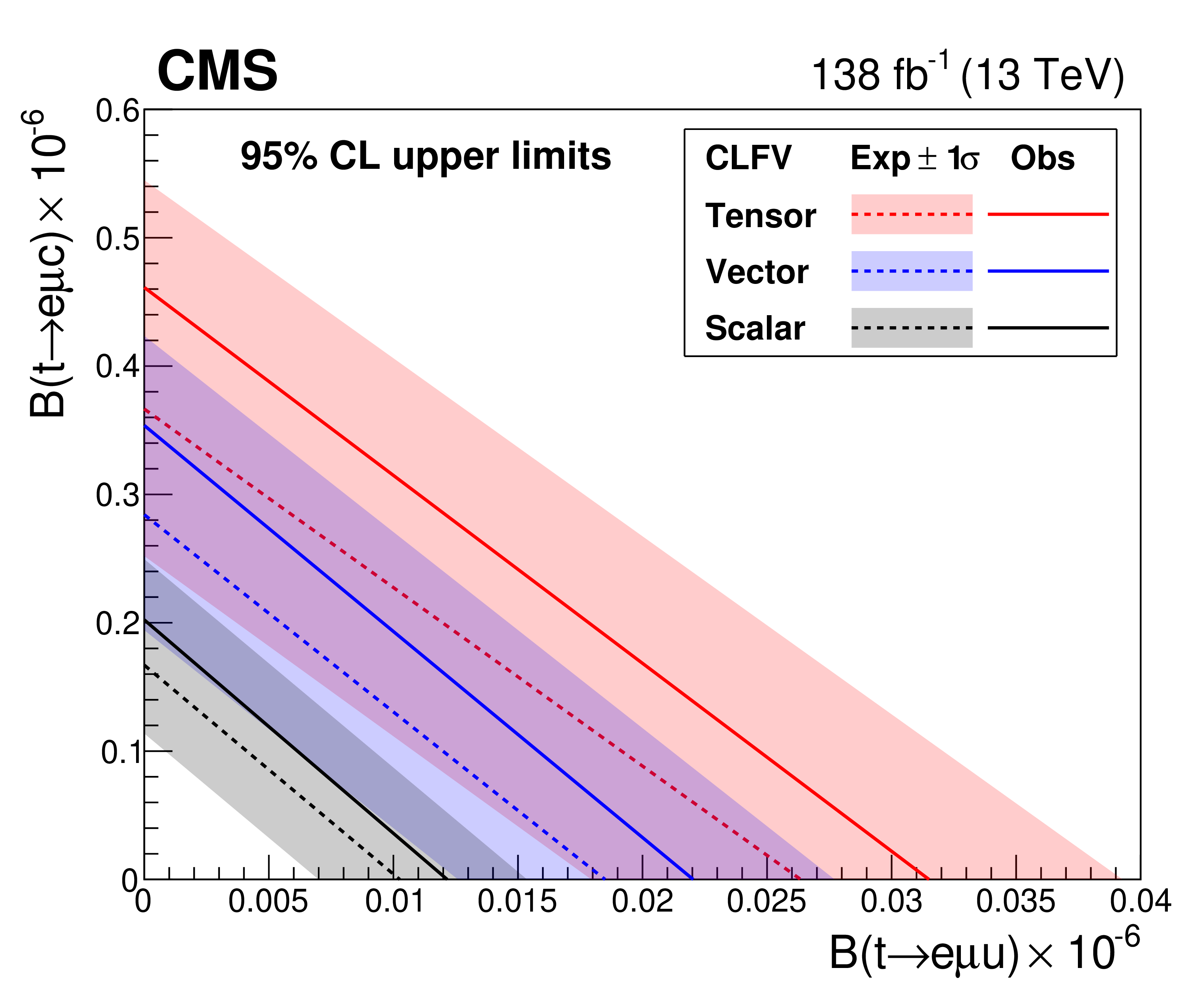
Two-dimensional 95% CL upper limits on the Wilson coefficients (left) and the branching fractions (right). The observed (expected) upper limits for tensor-, vector-, and scalar-like CLFV interactions are shown in red, blue, and black solid (dotted) lines, respectively. The shaded bands contain 68% of the distribution of the expected upper limits. |
png pdf |
Figure 6-a:
Two-dimensional 95% CL upper limits on the Wilson coefficients (left) and the branching fractions (right). The observed (expected) upper limits for tensor-, vector-, and scalar-like CLFV interactions are shown in red, blue, and black solid (dotted) lines, respectively. The shaded bands contain 68% of the distribution of the expected upper limits. |
png pdf |
Figure 6-b:
Two-dimensional 95% CL upper limits on the Wilson coefficients (left) and the branching fractions (right). The observed (expected) upper limits for tensor-, vector-, and scalar-like CLFV interactions are shown in red, blue, and black solid (dotted) lines, respectively. The shaded bands contain 68% of the distribution of the expected upper limits. |
| Tables | |

png pdf |
Table 1:
Summary of relevant dimension-6 operators considered in this analysis. Here, $ \varepsilon $ is the two-dimensional Levi-Civita symbol, $ \gamma^\mu $ the Dirac gamma matrices, and $ \sigma^{\mu\nu}=\frac{i}{2}[\gamma^\mu,\gamma^\nu] $. The $ \mathrm{q} $ and $ \mathrm{l} $ denote left-handed doublets for leptons and quarks, respectively, whereas u and e denote right-handed singlets for quarks and leptons, respectively. The indices $ i $ and $ j $ are lepton flavor indices that run from 1 to 2 with $ i \neq j $; $ k $ and $ l $ are quark flavor indices with the condition that one of them is 3 and the other one is 1 or 2. The four vector-like operators are merged in this analysis because the final-state particles produced by these operators have very similar kinematics. |
png pdf |
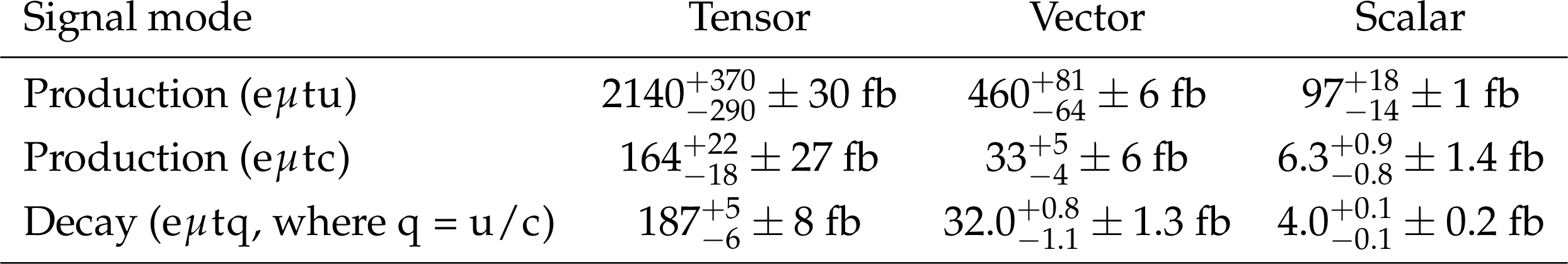
Table 2:
Theoretical cross sections for top quark production and decay for each CLFV coupling. The cross sections are calculated with $ C_{a}/\Lambda^2=$ 1 TeV$^{-2}$, $ m_{\mathrm{t}} = $ 172.5 GeV, $ \Gamma_{\mathrm{t}}^{\text{SM}} = $ 1.33 GeV. The cross section for the top quark decay process is the same for $ \mathrm{e}\mu\mathrm{t}\mathrm{u} $ and $ \mathrm{e}\mu\mathrm{t}\mathrm{c} $ couplings, therefore, only one cross section is quoted for each Lorentz structure. The first uncertainty represents the effect of QCD renormalization and factorization scales. The second uncertainty is the PDF uncertainty. |
png pdf |
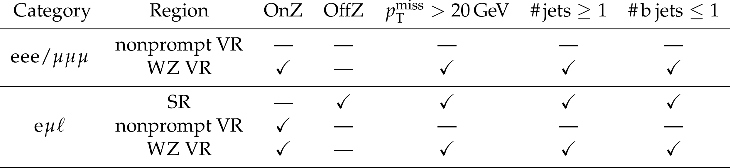
Table 3:
Summary of the selection criteria used to define different event regions. |
png pdf |
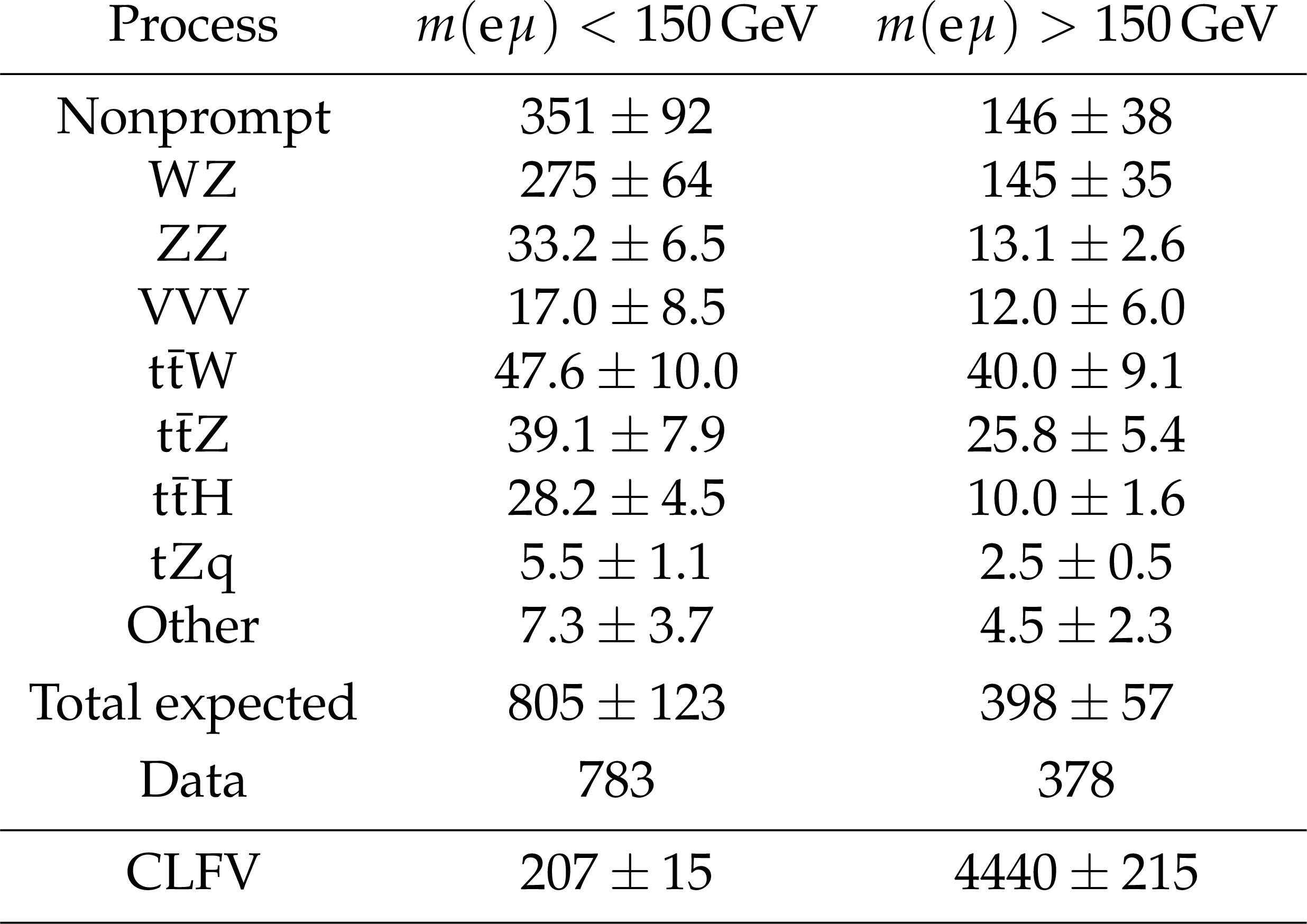
Table 4:
Expected background contributions and the number of events observed in data collected during 2016-2018. The quoted uncertainties include statistical and systematic sources, which are added in quadrature. The category ``Other" includes smaller background contributions containing one or two top quarks plus a boson or quark. The CLFV signal, generated with $ C_{\mathrm{e}\mu\mathrm{t}\mathrm{u}}^{\text{vector}}/\Lambda^2=$ 1 TeV$^{-2}$, is also listed for reference and includes contributions from both top quark production and decay modes. |
png pdf |
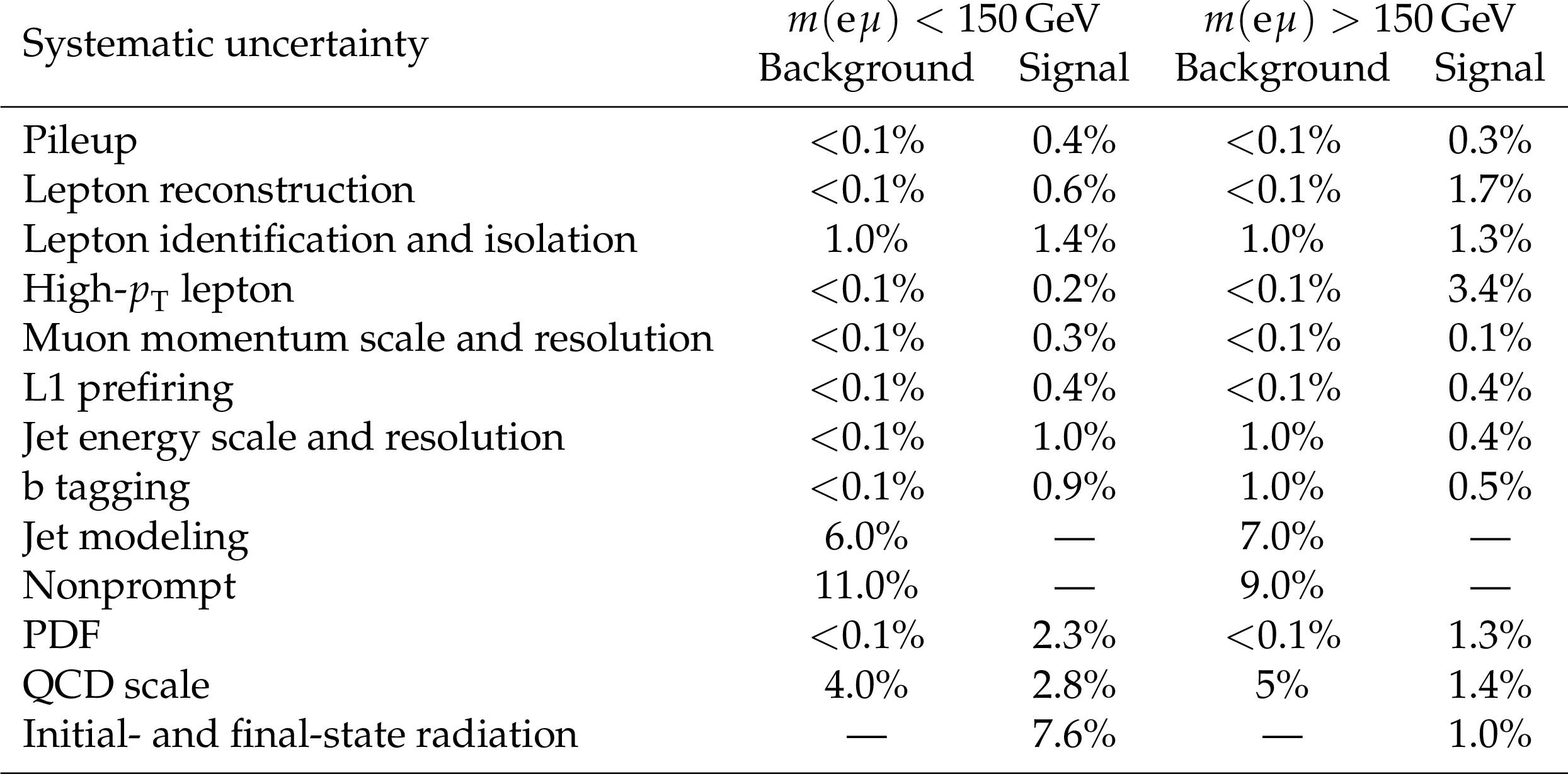
Table 5:
Summary of systematic uncertainties and the average change in signal and overall background yields in the SRs. Uncertainties that only contain normalization effects, such as luminosity uncertainties and uncertainties in theoretical cross sections, are not included in this table. |
png pdf |
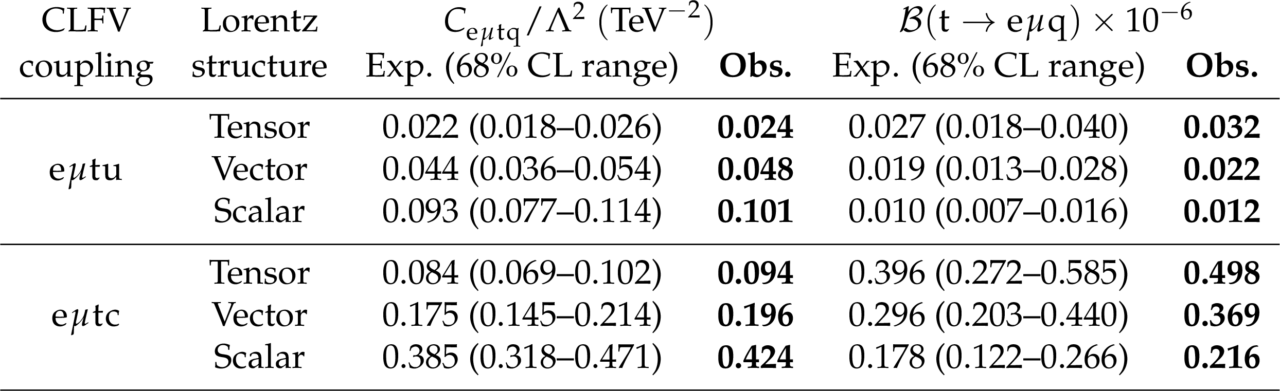
Table 6:
Upper limits at 95% CL on Wilson coefficients and the branching fractions for tensor-, vector-, and scalar-like CLFV interactions. The expected and observed upper limits are shown in regular and bold fonts, respectively. The intervals that contain 68% of the distribution of the expected upper limits are shown in parentheses. |
| Summary |
| This paper presents results from a search for charged-lepton flavor violation in both top quark production and decay processes. The data used were collected by the CMS experiment during 2016-2018 and correspond to an integrated luminosity of 138 fb$ ^{-1} $. Events were selected for analysis if they contain exactly three charged leptons--one electron and one muon of opposite electric charge as well as one additional electron or muon. Events must also contain at least one jet of which no more than one is associated with a bottom quark. An effective field theory approach is used for parametrizing the charged-lepton flavor violating interactions. Boosted decision trees are used to distinguish a possible signal from the background. No significant excess is observed over the prediction from the standard model. Upper limits at the 95% confidence level are set on the branching fractions involving up (charm) quarks, $ \mathrm{t}\to\mathrm{e}\mu\mathrm{u} $ ($ \mathrm{t}\to\mathrm{e}\mu\mathrm{c} $), of 0.032 (0.498) \times $10$^{-6} $, 0.022 (0.369) $\times $10$^{-6} $, and 0.012 (0.216) $\times $10$^{-6} $ for tensor, vector, and scalar interactions, respectively. These limits constitute the most stringent ones to date on these processes, improving the existing limits by roughly one order of magnitude. |
| References | ||||
| 1 | Super-Kamiokande Collaboration | Evidence for oscillation of atmospheric neutrinos | PRL 81 (1998) 1562 | hep-ex/9807003 |
| 2 | SNO Collaboration | Direct evidence for neutrino flavor transformation from neutral current interactions in the Sudbury Neutrino Observatory | PRL 89 (2002) 011301 | nucl-ex/0204008 |
| 3 | S. Davidson, S. Lacroix, and P. Verdier | LHC sensitivity to lepton flavour violating Z boson decays | JHEP 09 (2012) 092 | 1207.4894 |
| 4 | S. Davidson, M. L. Mangano, S. Perries, and V. Sordini | Lepton flavour violating top decays at the LHC | EPJC 75 (2015) 450 | 1507.07163 |
| 5 | LHCb Collaboration | Measurement of the ratios of branching fractions $ \mathcal{R}(D^{*}) $ and $ \mathcal{R}(D^{0}) $ | PRL 131 (2023) 111802 | 2302.02886 |
| 6 | T. J. Kim et al. | Correlation between $ {R}_{D^{\left(\ast \right)}} $ and top quark FCNC decays in leptoquark models | JHEP 07 (2019) 025 | 1812.08484 |
| 7 | CMS Collaboration | Search for charged-lepton flavor violation in top quark production and decay in pp collisions at $ \sqrt{s} = $ 13 TeV | JHEP 06 (2022) 082 | CMS-TOP-19-006 2201.07859 |
| 8 | B. Grzadkowski, M. Iskrzyński, M. Misiak, and J. Rosiek | Dimension-six terms in the Standard Model Lagrangian | JHEP 10 (2010) 85 | 1008.4884 |
| 9 | CMS Collaboration | The CMS experiment at the CERN LHC | JINST 3 (2008) S08004 | |
| 10 | CMS Collaboration | Performance of the CMS Level-1 trigger in proton-proton collisions at $ \sqrt{s} = $ 13 TeV | JINST 15 (2020) P10017 | CMS-TRG-17-001 2006.10165 |
| 11 | CMS Collaboration | The CMS trigger system | JINST 12 (2017) P01020 | CMS-TRG-12-001 1609.02366 |
| 12 | J. Alwall et al. | The automated computation of tree-level and next-to-leading order differential cross sections, and their matching to parton shower simulations | JHEP 07 (2014) 079 | 1405.0301 |
| 13 | I. Brivio, Y. Jiang, and M. Trott | The SMEFTsim package, theory and tools | JHEP 12 (2017) 070 | 1709.06492 |
| 14 | A. Dedes et al. | SmeftFR---Feynman rules generator for the Standard Model Effective Field Theory | Comput. Phys. Commun. 247 (2020) 106931 | 1904.03204 |
| 15 | P. Nason | A new method for combining NLO QCD with shower Monte Carlo algorithms | JHEP 11 (2004) 040 | hep-ph/0409146 |
| 16 | S. Frixione, P. Nason, and C. Oleari | Matching NLO QCD computations with parton shower simulations: the POWHEG method | JHEP 11 (2007) 070 | 0709.2092 |
| 17 | S. Alioli, P. Nason, C. Oleari, and E. Re | A general framework for implementing NLO calculations in shower Monte Carlo programs: the POWHEG box | JHEP 06 (2010) 043 | 1002.2581 |
| 18 | J. M. Campbell, R. K. Ellis, P. Nason, and E. Re | Top-pair production and decay at NLO matched with parton showers | JHEP 04 (2015) 114 | 1412.1828 |
| 19 | T. Sjöstrand et al. | An introduction to PYTHIA 8.2 | Comput. Phys. Commun. 191 (2015) 159 | 1410.3012 |
| 20 | NNPDF Collaboration | Parton distributions for the LHC Run II | JHEP 04 (2015) 040 | 1410.8849 |
| 21 | P. Skands, S. Carrazza, and J. Rojo | Tuning PYTHIA 8.1: the Monash 2013 tune | EPJC 74 (2014) 3024 | 1404.5630 |
| 22 | NNPDF Collaboration | Parton distributions from high-precision collider data | EPJC 77 (2017) 663 | 1706.00428 |
| 23 | CMS Collaboration | Extraction and validation of a new set of CMS PYTHIA8 tunes from underlying-event measurements | EPJC 80 (2020) 4 | CMS-GEN-17-001 1903.12179 |
| 24 | GEANT4 Collaboration | GEANT 4---a simulation toolkit | NIM A 506 (2003) 250 | |
| 25 | CMS Collaboration | Particle-flow reconstruction and global event description with the CMS detector | JINST 12 (2017) P10003 | CMS-PRF-14-001 1706.04965 |
| 26 | CMS Collaboration | Technical proposal for the Phase-II upgrade of the Compact Muon Solenoid | CMS Technical Proposal CERN-LHCC-2015-010, CMS-TDR-15-02, 2015 CDS |
|
| 27 | M. Cacciari, G. P. Salam, and G. Soyez | The anti-$ k_{\mathrm{T}} $ jet clustering algorithm | JHEP 04 (2008) 063 | 0802.1189 |
| 28 | M. Cacciari, G. P. Salam, and G. Soyez | FastJet user manual | EPJC 72 (2012) 1896 | 1111.6097 |
| 29 | M. Cacciari and G. P. Salam | Dispelling the $ N^{3} $ myth for the $ k_{\mathrm{T}} $ jet-finder | PLB 641 (2006) 57 | hep-ph/0512210 |
| 30 | CMS Collaboration | Jet energy scale and resolution in the CMS experiment in pp collisions at 8 TeV | JINST 12 (2017) P02014 | CMS-JME-13-004 1607.03663 |
| 31 | CMS Collaboration | Jet algorithms performance in 13 TeV data | CMS Physics Analysis Summary, 2017 CMS-PAS-JME-16-003 |
CMS-PAS-JME-16-003 |
| 32 | CMS Collaboration | Performance of missing transverse momentum reconstruction in proton-proton collisions at $ \sqrt{s} = $ 13 TeV using the CMS detector | JINST 14 (2019) P07004 | CMS-JME-17-001 1903.06078 |
| 33 | CMS Collaboration | Inclusive and differential cross section measurements of single top quark production in association with a Z boson in proton-proton collisions at $ \sqrt{s} = $ 13 TeV | JHEP 02 (2022) 107 | CMS-TOP-20-010 2111.02860 |
| 34 | CMS Collaboration | Identification of heavy-flavour jets with the CMS detector in pp collisions at 13 TeV | JINST 13 (2018) P05011 | CMS-BTV-16-002 1712.07158 |
| 35 | E. Bols et al. | Jet flavour classification using DeepJet | JINST 15 (2020) P12012 | 2008.10519 |
| 36 | CMS Collaboration | Performance of the DeepJet b tagging algorithm using 41.9 fb$ ^{-1} $ of data from proton-proton collisions at 13 TeV with Phase 1 CMS detector | CMS Detector Performance Note CMS-DP-2018-058, 2018 CDS |
|
| 37 | T. P. S. Gillam and C. G. Lester | Improving estimates of the number of `fake' leptons and other mis-reconstructed objects in hadron collider events: BoB's your UNCLE | JHEP 11 (2014) 031 | 1407.5624 |
| 38 | T. Chen and C. Guestrin | XGBoost: A scalable tree boosting system | in 22nd ACM SIGKDD Intern. Conf. on Knowledge Discovery and Data Mining, KDD '16, 2016 link |
1603.02754 |
| 39 | CMS Collaboration | Precision luminosity measurement in proton-proton collisions at $ \sqrt{s} = $ 13 TeV in 2015 and 2016 at CMS | EPJC 81 (2021) 800 | CMS-LUM-17-003 2104.01927 |
| 40 | CMS Collaboration | CMS luminosity measurement for the 2017 data-taking period at $ \sqrt{s} = $ 13 TeV | CMS Physics Analysis Summary, 2018 link |
CMS-PAS-LUM-17-004 |
| 41 | CMS Collaboration | CMS luminosity measurement for the 2018 data-taking period at $ \sqrt{s} = $ 13 TeV | CMS Physics Analysis Summary, 2019 link |
CMS-PAS-LUM-18-002 |
| 42 | CMS Collaboration | Measurement of the inelastic proton-proton cross section at $ \sqrt{s} = $ 13 TeV | JHEP 07 (2018) 161 | CMS-FSQ-15-005 1802.02613 |
| 43 | CMS Collaboration | Electron and photon reconstruction and identification with the CMS experiment at the CERN LHC | JINST 16 (2021) P05014 | CMS-EGM-17-001 2012.06888 |
| 44 | CMS Collaboration | Performance of the CMS muon detector and muon reconstruction with proton-proton collisions at $ \sqrt{s} = $ 13 TeV | JINST 13 (2018) P06015 | CMS-MUO-16-001 1804.04528 |
| 45 | CMS Collaboration | Measurements of inclusive W and Z cross sections in pp collisions at $ \sqrt{s} = $ 7 TeV | JHEP 01 (2011) 080 | CMS-EWK-10-002 1012.2466 |
| 46 | CMS Collaboration | Observation of single top quark production in association with a Z boson in proton-proton collisions at $ \sqrt {s} = $ 13 TeV | PRL 122 (2019) 132003 | CMS-TOP-18-008 1812.05900 |
| 47 | CMS Collaboration | Measurement of the Higgs boson production rate in association with top quarks in final states with electrons, muons, and hadronically decaying tau leptons at $ \sqrt{s} = $ 13 TeV | EPJC 81 (2021) 378 | CMS-HIG-19-008 2011.03652 |
| 48 | J. M. Campbell, R. K. Ellis, and C. Williams | Vector boson pair production at the LHC | JHEP 07 (2011) 018 | 1105.0020 |
| 49 | R. Frederix and I. Tsinikos | On improving NLO merging for $ \mathrm{t}\overline{\mathrm{t}}\mathrm{W} $ production | JHEP 11 (2021) 029 | 2108.07826 |
| 50 | A. Kulesza et al. | Associated top quark pair production with a heavy boson: differential cross sections at NLO+NNLL accuracy | EPJC 80 (2020) 428 | 2001.03031 |
| 51 | J. Butterworth et al. | PDF4LHC recommendations for LHC Run II | JPG 43 (2016) 023001 | 1510.03865 |
| 52 | R. J. Barlow and C. Beeston | Fitting using finite Monte Carlo samples | Comput. Phys. Commun. 77 (1993) 219 | |
| 53 | T. Junk | Confidence level computation for combining searches with small statistics | NIM A 434 (1999) 435 | hep-ex/9902006 |
| 54 | A. Read | Presentation of search results: The CL$ _s $ technique | JPG 28 (2002) 2693 | |
| 55 | G. Cowan, K. Cranmer, E. Gross, and O. Vitells | Asymptotic formulae for likelihood-based tests of new physics | EPJC 71 (2011) 1554 | 1007.1727 |
| 56 | J. Kile and A. Soni | Model-independent constraints on lepton-flavor-violating decays of the top quark | PRD 78 (2008) 094008 | 0807.4199 |
| 57 | CMS Collaboration | HEPData record for this analysis | link | |
|
|
Compact Muon Solenoid LHC, CERN |
|

|

|

|

|

|