

Compact Muon Solenoid
LHC, CERN
| CMS-TOP-19-006 ; CERN-EP-2021-248 | ||
| Search for charged-lepton flavor violation in top quark production and decay in pp collisions at $\sqrt{s} = $ 13 TeV | ||
| CMS Collaboration | ||
| 19 January 2022 | ||
| JHEP 06 (2022) 082 | ||
| Abstract: Results are presented from a search for charged-lepton flavor violating (CLFV) interactions in top quark production and decay in pp collisions at a center-of-mass energy of 13 TeV. The events are required to contain one oppositely charged electron-muon pair in the final state, along with at least one jet identified as originating from a bottom quark. The data correspond to an integrated luminosity of 138 fb$^{-1}$, collected by the CMS experiment at the LHC. This analysis includes both the production (q $\to$ e$\mu$t) and decay (t $\to$ e$ \mu$q) modes of the top quark through CLFV interactions, with q referring to an u or c quark. These interactions are parametrized using an effective field theory approach. With no significant excess over the standard model expectation, the results are interpreted in terms of vector-, scalar-, and tensor-like CLFV four-fermion effective interactions. Finally, observed exclusion limits are set at 95% confidence levels on the respective branching fractions of a top quark to an e$\mu$ pair and an up (charm) quark of 0.13 $\times $ 10$^{-6}$ (1.31 $\times $ 10$^{-6}$), 0.07 $\times $ 10$^{-6}$ (0.89 $\times $ 10$^{-6}$), and 0.25 $\times $ 10$^{-6}$ (2.59 $\times $ 10$^{-6}$) for vector, scalar, and tensor CLFV interactions, respectively. | ||
| Links: e-print arXiv:2201.07859 [hep-ex] (PDF) ; CDS record ; inSPIRE record ; HepData record ; Physics Briefing ; CADI line (restricted) ; | ||
| Figures | |
png pdf |
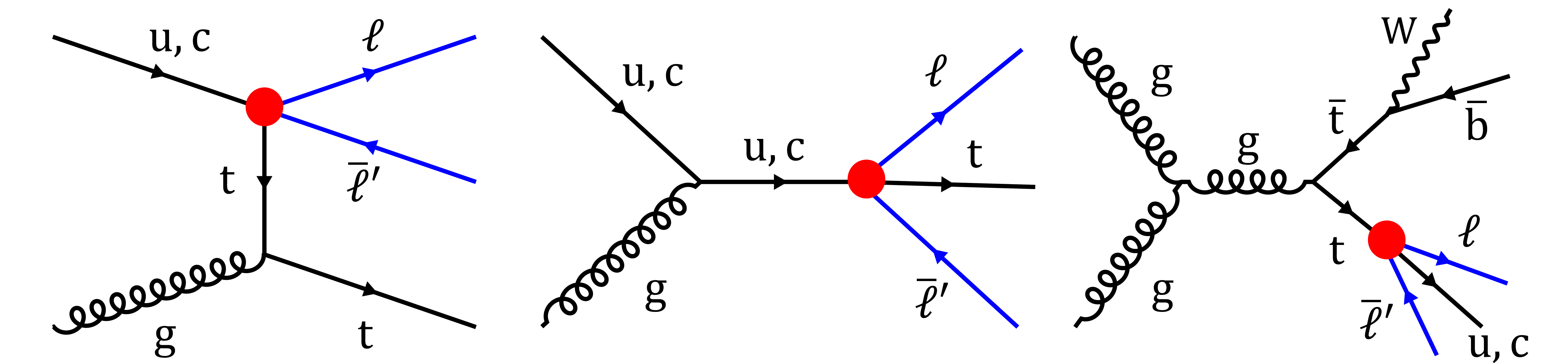
Figure 1:
Feynman diagrams for single top quark production (left and middle) and top quark decays in SM ${\mathrm{t} {}\mathrm{\bar{t}}}$ events (right) via CLFV interactions. The CLFV vertex is marked as a filled circle. |

png pdf |
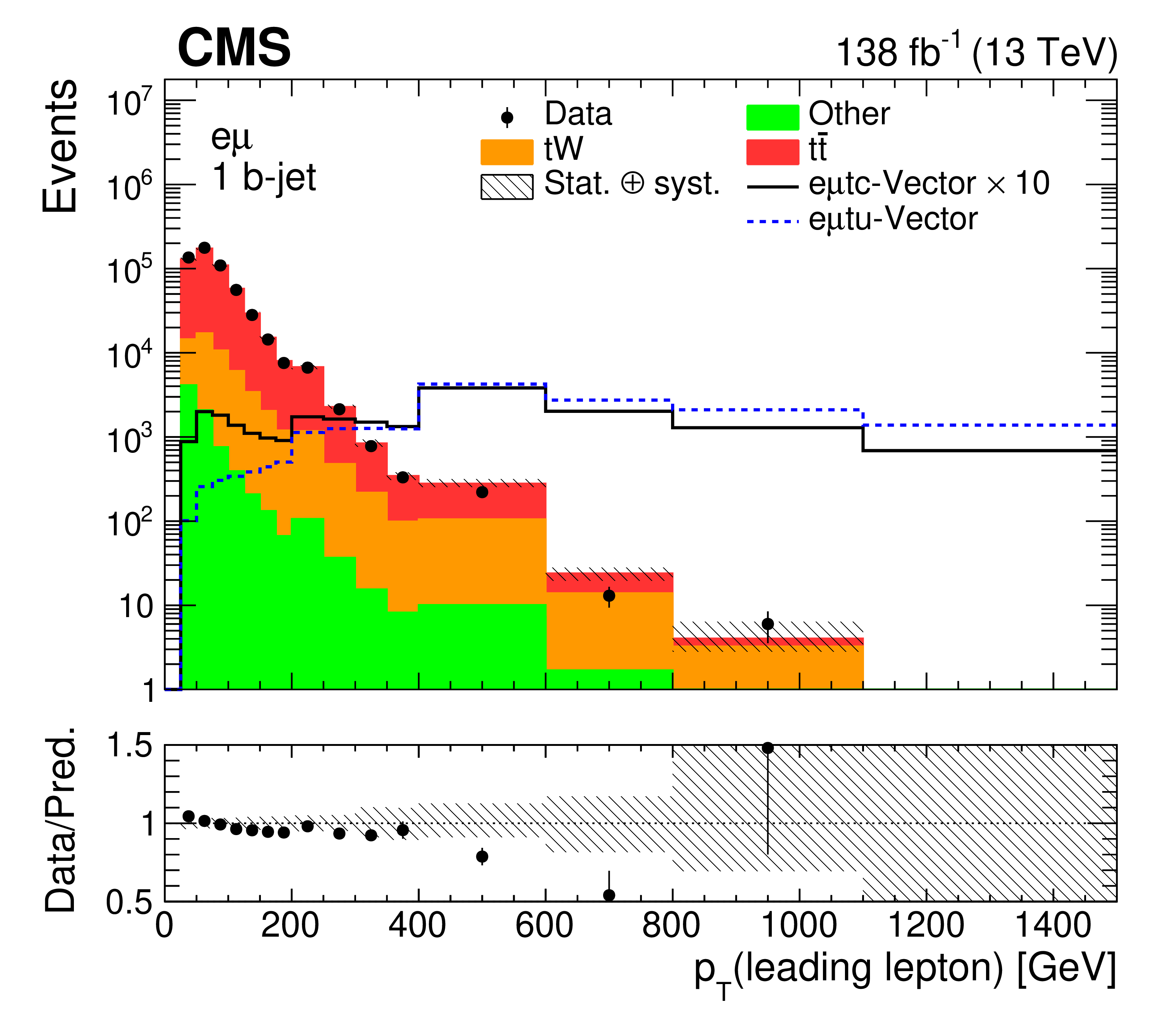
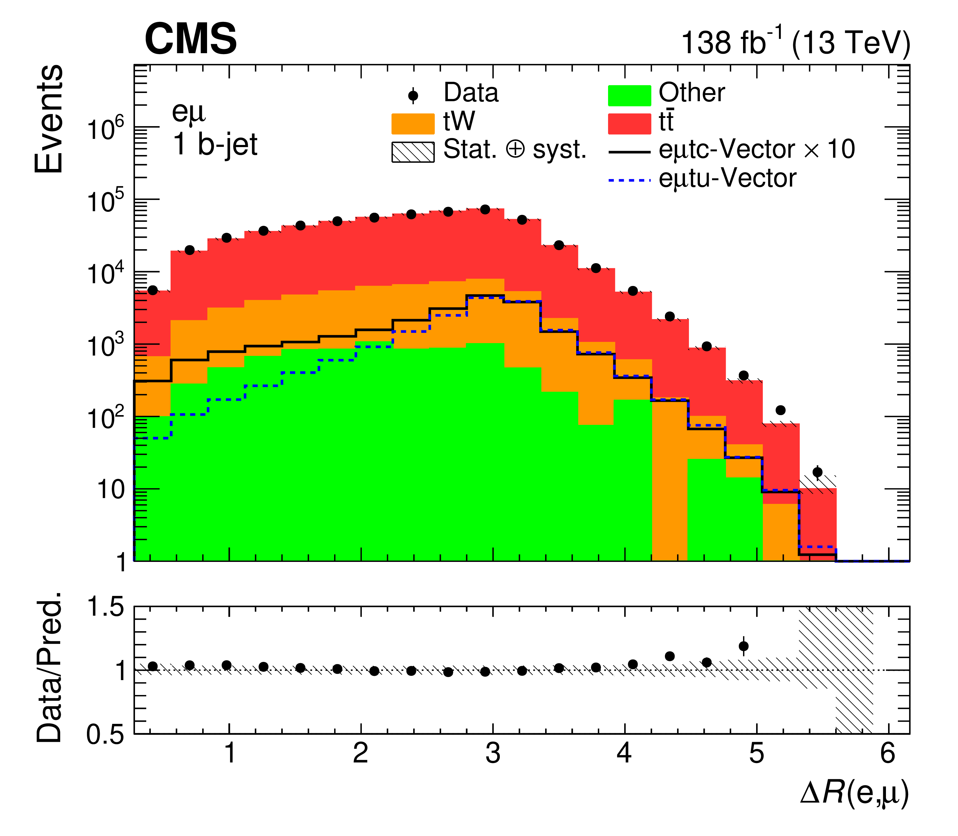
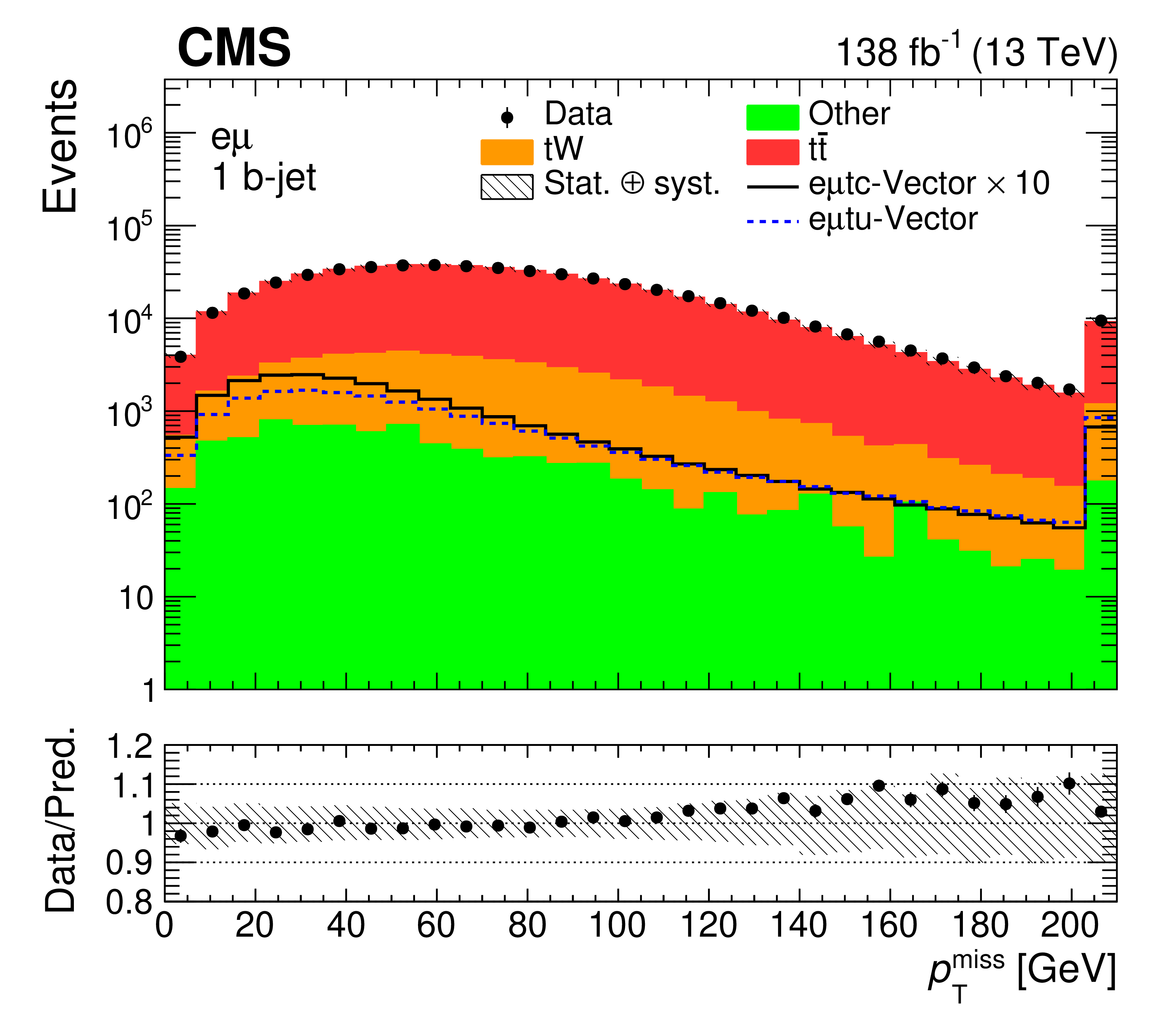
Figure 2:
The distributions of the leading lepton ${p_{\mathrm {T}}}$ (upper row), $\Delta R(\mathrm{e}, \mu)$ (middle row), and ${{p_{\mathrm {T}}} ^\text {miss}}$ (lower row) are shown for data (points) and simulation (histograms). Events with one or more b-tagged jets are shown in the left and right column, respectively. The hatched bands indicate the total uncertainty (statistical and systematic taken in quadrature) for the SM background predictions (cf. Section 6). Overflow events are added to the last bin. Examples of the predicted signal contribution for the vector type CLFV interactions via $\mathrm{e} \mu \mathrm{t} \mathrm{u} $ and $\mathrm{e} \mu \mathrm{t} \mathrm{c} $ vertices are shown, assuming $\text {C}_x/\Lambda ^2 =$ 1 TeV$ ^{-2}$. The signal production- and decay-mode contributions are summed. The $\mathrm{e} \mu \mathrm{t} \mathrm{c} $ signal cross section is scaled up by a factor of 10 for improved visualization. |
png pdf |
Figure 2-a:
The distributions of the leading lepton ${p_{\mathrm {T}}}$ (upper row), $\Delta R(\mathrm{e}, \mu)$ (middle row), and ${{p_{\mathrm {T}}} ^\text {miss}}$ (lower row) are shown for data (points) and simulation (histograms). Events with one or more b-tagged jets are shown in the left and right column, respectively. The hatched bands indicate the total uncertainty (statistical and systematic taken in quadrature) for the SM background predictions (cf. Section 6). Overflow events are added to the last bin. Examples of the predicted signal contribution for the vector type CLFV interactions via $\mathrm{e} \mu \mathrm{t} \mathrm{u} $ and $\mathrm{e} \mu \mathrm{t} \mathrm{c} $ vertices are shown, assuming $\text {C}_x/\Lambda ^2 =$ 1 TeV$ ^{-2}$. The signal production- and decay-mode contributions are summed. The $\mathrm{e} \mu \mathrm{t} \mathrm{c} $ signal cross section is scaled up by a factor of 10 for improved visualization. |

png pdf |
Figure 2-b:
The distributions of the leading lepton ${p_{\mathrm {T}}}$ (upper row), $\Delta R(\mathrm{e}, \mu)$ (middle row), and ${{p_{\mathrm {T}}} ^\text {miss}}$ (lower row) are shown for data (points) and simulation (histograms). Events with one or more b-tagged jets are shown in the left and right column, respectively. The hatched bands indicate the total uncertainty (statistical and systematic taken in quadrature) for the SM background predictions (cf. Section 6). Overflow events are added to the last bin. Examples of the predicted signal contribution for the vector type CLFV interactions via $\mathrm{e} \mu \mathrm{t} \mathrm{u} $ and $\mathrm{e} \mu \mathrm{t} \mathrm{c} $ vertices are shown, assuming $\text {C}_x/\Lambda ^2 =$ 1 TeV$ ^{-2}$. The signal production- and decay-mode contributions are summed. The $\mathrm{e} \mu \mathrm{t} \mathrm{c} $ signal cross section is scaled up by a factor of 10 for improved visualization. |
png pdf |
Figure 2-c:
The distributions of the leading lepton ${p_{\mathrm {T}}}$ (upper row), $\Delta R(\mathrm{e}, \mu)$ (middle row), and ${{p_{\mathrm {T}}} ^\text {miss}}$ (lower row) are shown for data (points) and simulation (histograms). Events with one or more b-tagged jets are shown in the left and right column, respectively. The hatched bands indicate the total uncertainty (statistical and systematic taken in quadrature) for the SM background predictions (cf. Section 6). Overflow events are added to the last bin. Examples of the predicted signal contribution for the vector type CLFV interactions via $\mathrm{e} \mu \mathrm{t} \mathrm{u} $ and $\mathrm{e} \mu \mathrm{t} \mathrm{c} $ vertices are shown, assuming $\text {C}_x/\Lambda ^2 =$ 1 TeV$ ^{-2}$. The signal production- and decay-mode contributions are summed. The $\mathrm{e} \mu \mathrm{t} \mathrm{c} $ signal cross section is scaled up by a factor of 10 for improved visualization. |

png pdf |
Figure 2-d:
The distributions of the leading lepton ${p_{\mathrm {T}}}$ (upper row), $\Delta R(\mathrm{e}, \mu)$ (middle row), and ${{p_{\mathrm {T}}} ^\text {miss}}$ (lower row) are shown for data (points) and simulation (histograms). Events with one or more b-tagged jets are shown in the left and right column, respectively. The hatched bands indicate the total uncertainty (statistical and systematic taken in quadrature) for the SM background predictions (cf. Section 6). Overflow events are added to the last bin. Examples of the predicted signal contribution for the vector type CLFV interactions via $\mathrm{e} \mu \mathrm{t} \mathrm{u} $ and $\mathrm{e} \mu \mathrm{t} \mathrm{c} $ vertices are shown, assuming $\text {C}_x/\Lambda ^2 =$ 1 TeV$ ^{-2}$. The signal production- and decay-mode contributions are summed. The $\mathrm{e} \mu \mathrm{t} \mathrm{c} $ signal cross section is scaled up by a factor of 10 for improved visualization. |
png pdf |
Figure 2-e:
The distributions of the leading lepton ${p_{\mathrm {T}}}$ (upper row), $\Delta R(\mathrm{e}, \mu)$ (middle row), and ${{p_{\mathrm {T}}} ^\text {miss}}$ (lower row) are shown for data (points) and simulation (histograms). Events with one or more b-tagged jets are shown in the left and right column, respectively. The hatched bands indicate the total uncertainty (statistical and systematic taken in quadrature) for the SM background predictions (cf. Section 6). Overflow events are added to the last bin. Examples of the predicted signal contribution for the vector type CLFV interactions via $\mathrm{e} \mu \mathrm{t} \mathrm{u} $ and $\mathrm{e} \mu \mathrm{t} \mathrm{c} $ vertices are shown, assuming $\text {C}_x/\Lambda ^2 =$ 1 TeV$ ^{-2}$. The signal production- and decay-mode contributions are summed. The $\mathrm{e} \mu \mathrm{t} \mathrm{c} $ signal cross section is scaled up by a factor of 10 for improved visualization. |
png pdf |
Figure 2-f:
The distributions of the leading lepton ${p_{\mathrm {T}}}$ (upper row), $\Delta R(\mathrm{e}, \mu)$ (middle row), and ${{p_{\mathrm {T}}} ^\text {miss}}$ (lower row) are shown for data (points) and simulation (histograms). Events with one or more b-tagged jets are shown in the left and right column, respectively. The hatched bands indicate the total uncertainty (statistical and systematic taken in quadrature) for the SM background predictions (cf. Section 6). Overflow events are added to the last bin. Examples of the predicted signal contribution for the vector type CLFV interactions via $\mathrm{e} \mu \mathrm{t} \mathrm{u} $ and $\mathrm{e} \mu \mathrm{t} \mathrm{c} $ vertices are shown, assuming $\text {C}_x/\Lambda ^2 =$ 1 TeV$ ^{-2}$. The signal production- and decay-mode contributions are summed. The $\mathrm{e} \mu \mathrm{t} \mathrm{c} $ signal cross section is scaled up by a factor of 10 for improved visualization. |
png pdf |
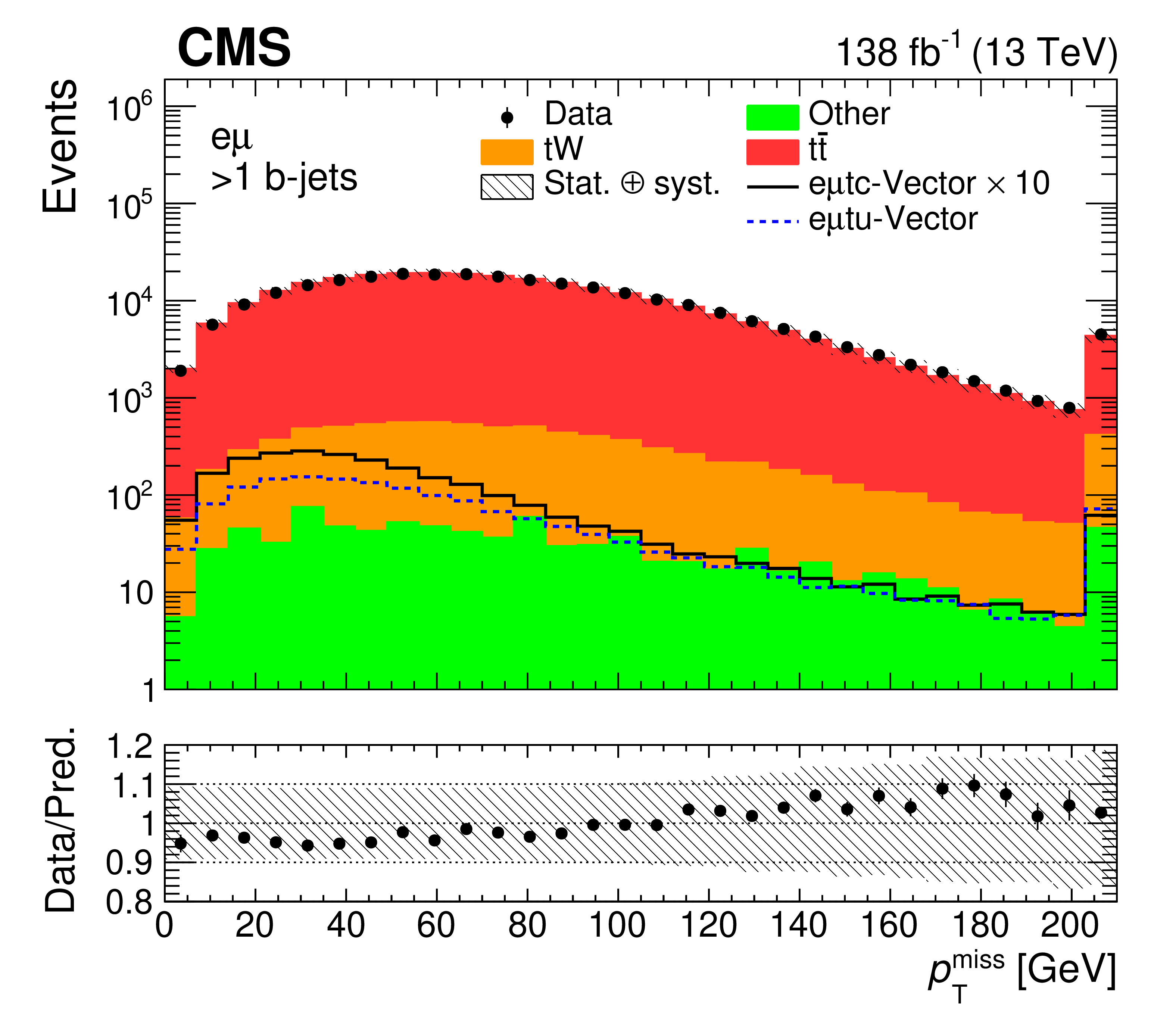
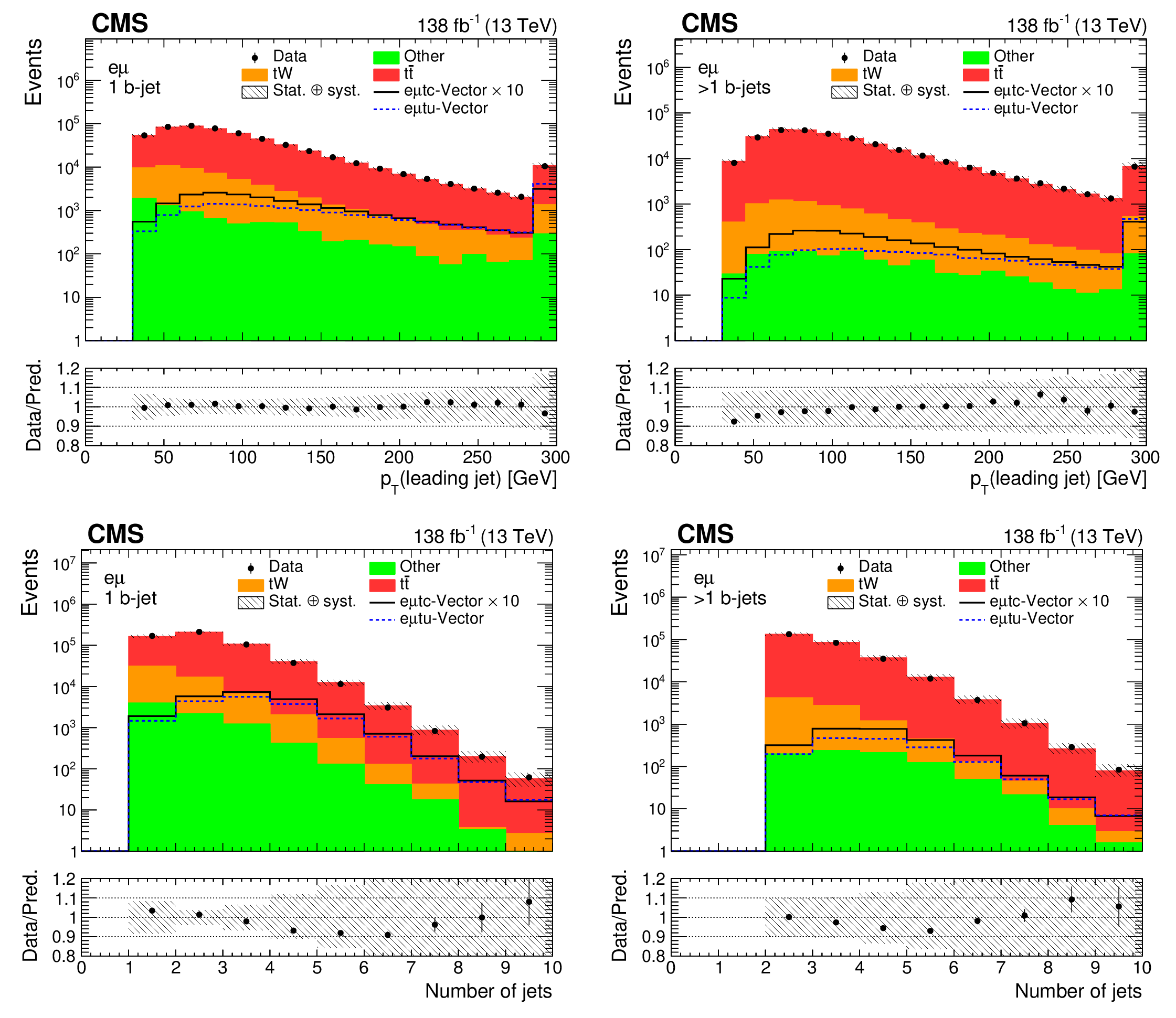
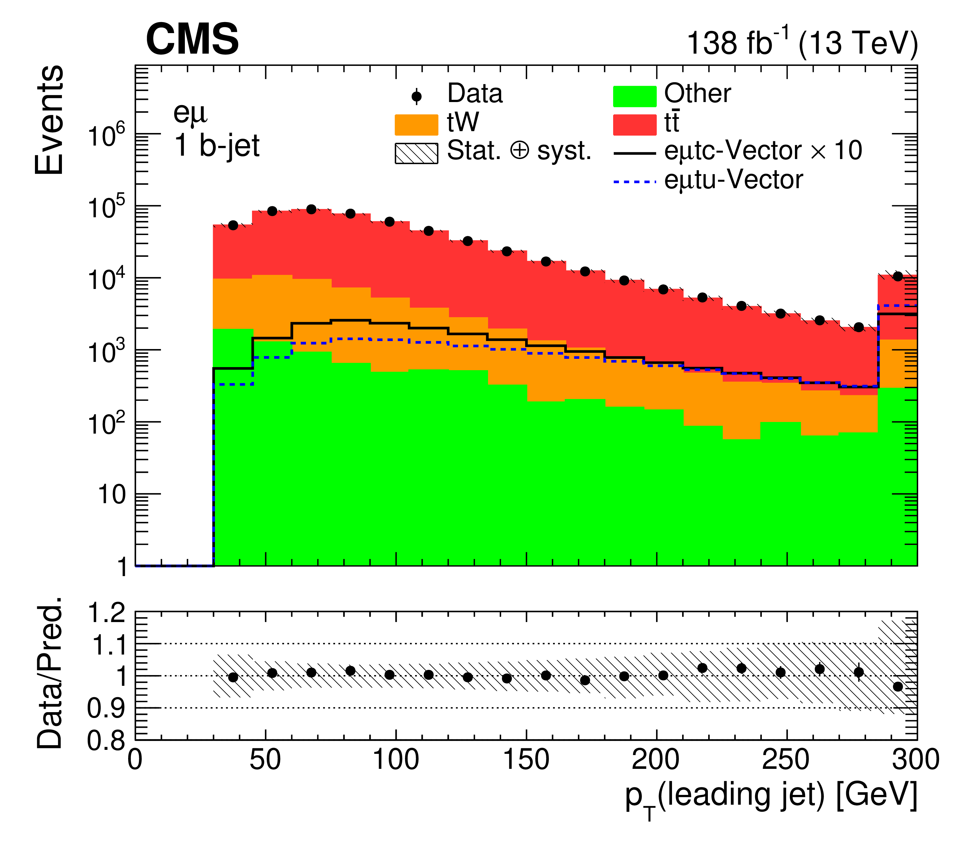
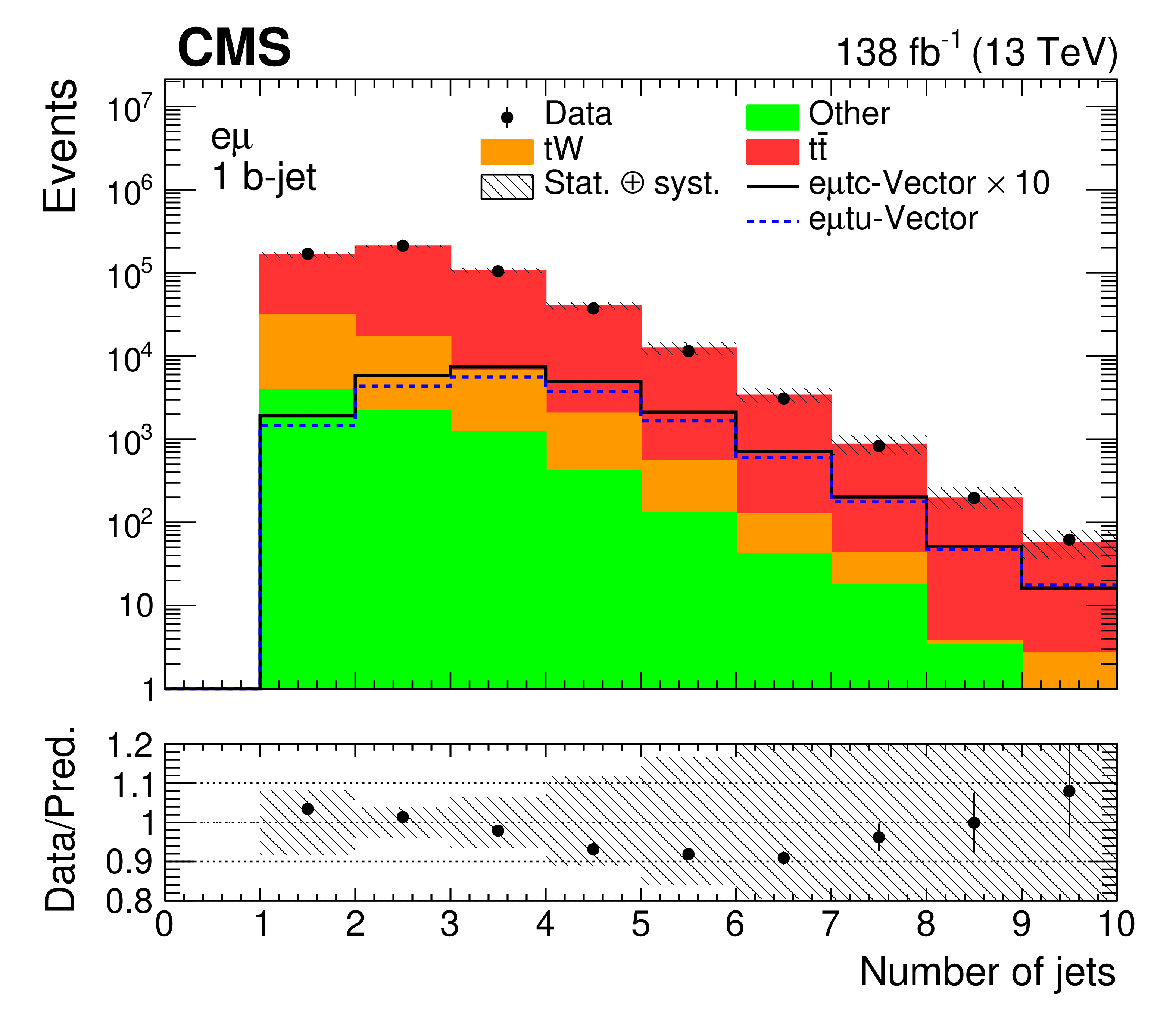
Figure 3:
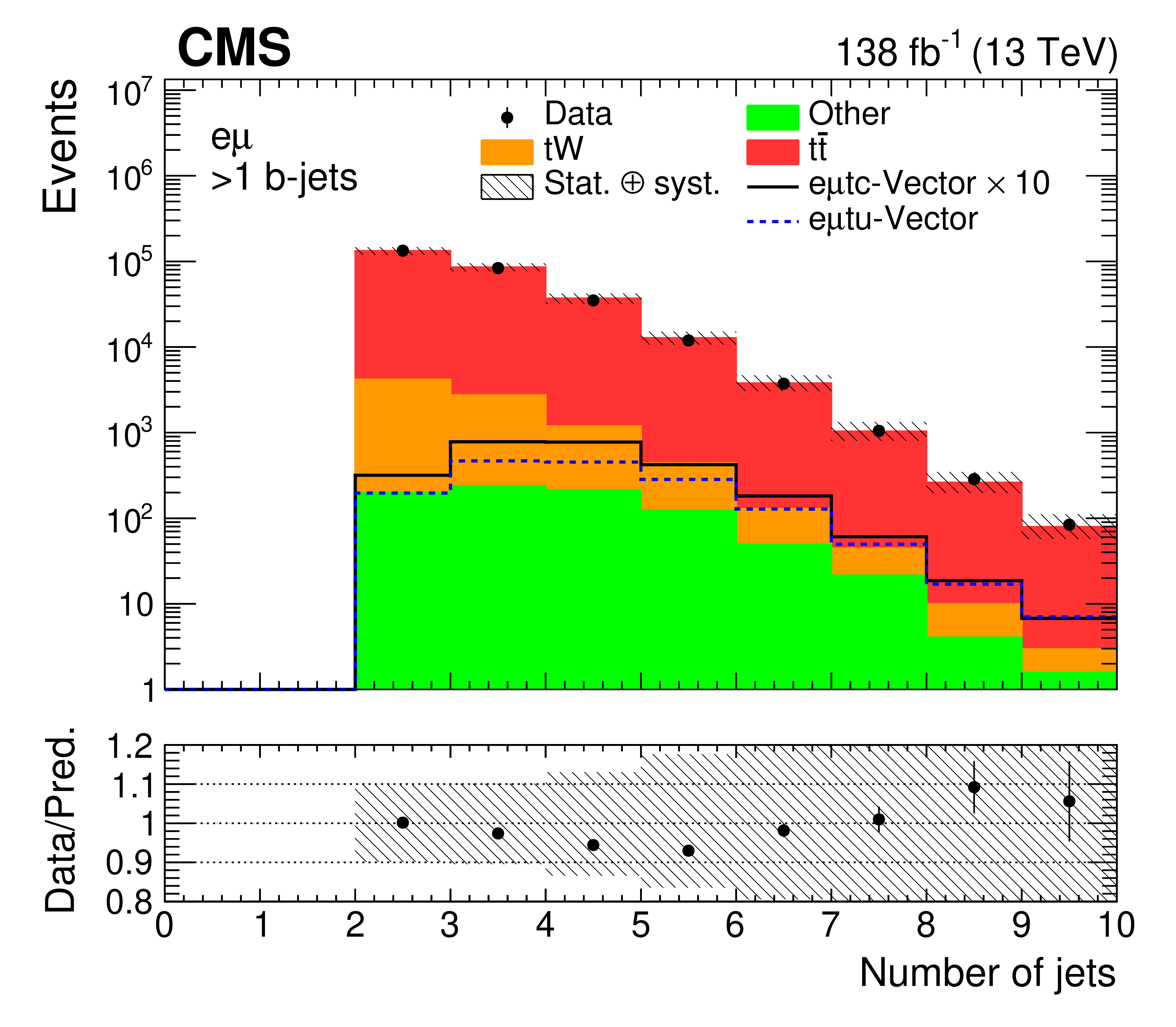
The distributions of the leading jet ${p_{\mathrm {T}}}$ (upper row) and the number of jets (lower row) are shown for data (points) and simulation (histograms). Events with one or more b-tagged jets are shown in the left and right column, respectively. The hatched bands indicate the total uncertainty (statistical and systematic taken in quadrature) for the SM background predictions (cf. Section 6). Overflow events are added to the last bin. Examples of the predicted signal contribution for the vector type CLFV interactions via $\mathrm{e} \mu \mathrm{t} \mathrm{u} $ and $\mathrm{e} \mu \mathrm{t} \mathrm{c} $ vertices are shown, assuming $\text {C}_x/\Lambda ^2 =$ 1 TeV$ ^{-2}$. The signal production- and decay-mode contributions are summed. The $\mathrm{e} \mu \mathrm{t} \mathrm{c} $ signal cross section is scaled up by a factor of 10 for improved visualization. |
png pdf |
Figure 3-a:
The distributions of the leading jet ${p_{\mathrm {T}}}$ (upper row) and the number of jets (lower row) are shown for data (points) and simulation (histograms). Events with one or more b-tagged jets are shown in the left and right column, respectively. The hatched bands indicate the total uncertainty (statistical and systematic taken in quadrature) for the SM background predictions (cf. Section 6). Overflow events are added to the last bin. Examples of the predicted signal contribution for the vector type CLFV interactions via $\mathrm{e} \mu \mathrm{t} \mathrm{u} $ and $\mathrm{e} \mu \mathrm{t} \mathrm{c} $ vertices are shown, assuming $\text {C}_x/\Lambda ^2 =$ 1 TeV$ ^{-2}$. The signal production- and decay-mode contributions are summed. The $\mathrm{e} \mu \mathrm{t} \mathrm{c} $ signal cross section is scaled up by a factor of 10 for improved visualization. |

png pdf |
Figure 3-b:
The distributions of the leading jet ${p_{\mathrm {T}}}$ (upper row) and the number of jets (lower row) are shown for data (points) and simulation (histograms). Events with one or more b-tagged jets are shown in the left and right column, respectively. The hatched bands indicate the total uncertainty (statistical and systematic taken in quadrature) for the SM background predictions (cf. Section 6). Overflow events are added to the last bin. Examples of the predicted signal contribution for the vector type CLFV interactions via $\mathrm{e} \mu \mathrm{t} \mathrm{u} $ and $\mathrm{e} \mu \mathrm{t} \mathrm{c} $ vertices are shown, assuming $\text {C}_x/\Lambda ^2 =$ 1 TeV$ ^{-2}$. The signal production- and decay-mode contributions are summed. The $\mathrm{e} \mu \mathrm{t} \mathrm{c} $ signal cross section is scaled up by a factor of 10 for improved visualization. |
png pdf |
Figure 3-c:
The distributions of the leading jet ${p_{\mathrm {T}}}$ (upper row) and the number of jets (lower row) are shown for data (points) and simulation (histograms). Events with one or more b-tagged jets are shown in the left and right column, respectively. The hatched bands indicate the total uncertainty (statistical and systematic taken in quadrature) for the SM background predictions (cf. Section 6). Overflow events are added to the last bin. Examples of the predicted signal contribution for the vector type CLFV interactions via $\mathrm{e} \mu \mathrm{t} \mathrm{u} $ and $\mathrm{e} \mu \mathrm{t} \mathrm{c} $ vertices are shown, assuming $\text {C}_x/\Lambda ^2 =$ 1 TeV$ ^{-2}$. The signal production- and decay-mode contributions are summed. The $\mathrm{e} \mu \mathrm{t} \mathrm{c} $ signal cross section is scaled up by a factor of 10 for improved visualization. |
png pdf |
Figure 3-d:
The distributions of the leading jet ${p_{\mathrm {T}}}$ (upper row) and the number of jets (lower row) are shown for data (points) and simulation (histograms). Events with one or more b-tagged jets are shown in the left and right column, respectively. The hatched bands indicate the total uncertainty (statistical and systematic taken in quadrature) for the SM background predictions (cf. Section 6). Overflow events are added to the last bin. Examples of the predicted signal contribution for the vector type CLFV interactions via $\mathrm{e} \mu \mathrm{t} \mathrm{u} $ and $\mathrm{e} \mu \mathrm{t} \mathrm{c} $ vertices are shown, assuming $\text {C}_x/\Lambda ^2 =$ 1 TeV$ ^{-2}$. The signal production- and decay-mode contributions are summed. The $\mathrm{e} \mu \mathrm{t} \mathrm{c} $ signal cross section is scaled up by a factor of 10 for improved visualization. |

png pdf |
Figure 4:
The BDT output distributions for data (points) and backgrounds (histograms) with the ratio of data to the total background yield, before (middle panel) and after (lower panel) the fit. Events with one or more b-tagged jets are shown in the left and right column, respectively. The hatched bands indicate the total uncertainty (statistical and systematic taken in quadrature) for the SM background predictions (cf. Section 6). Examples of the predicted signal contribution for the vector type CLFV interactions via $\mathrm{e} \mu \mathrm{t} \mathrm{u} $ and $\mathrm{e} \mu \mathrm{t} \mathrm{c} $ vertices are shown, assuming $\text {C}_x/\Lambda ^2 =$ 1 TeV$ ^{-2}$. The signal production- and decay-mode contributions are summed. The $\mathrm{e} \mu \mathrm{t} \mathrm{c} $ signal cross section is scaled up by a factor of 10 for improved visualization. |

png pdf |
Figure 4-a:
The BDT output distributions for data (points) and backgrounds (histograms) with the ratio of data to the total background yield, before (middle panel) and after (lower panel) the fit. Events with one or more b-tagged jets are shown in the left and right column, respectively. The hatched bands indicate the total uncertainty (statistical and systematic taken in quadrature) for the SM background predictions (cf. Section 6). Examples of the predicted signal contribution for the vector type CLFV interactions via $\mathrm{e} \mu \mathrm{t} \mathrm{u} $ and $\mathrm{e} \mu \mathrm{t} \mathrm{c} $ vertices are shown, assuming $\text {C}_x/\Lambda ^2 =$ 1 TeV$ ^{-2}$. The signal production- and decay-mode contributions are summed. The $\mathrm{e} \mu \mathrm{t} \mathrm{c} $ signal cross section is scaled up by a factor of 10 for improved visualization. |

png pdf |
Figure 4-b:
The BDT output distributions for data (points) and backgrounds (histograms) with the ratio of data to the total background yield, before (middle panel) and after (lower panel) the fit. Events with one or more b-tagged jets are shown in the left and right column, respectively. The hatched bands indicate the total uncertainty (statistical and systematic taken in quadrature) for the SM background predictions (cf. Section 6). Examples of the predicted signal contribution for the vector type CLFV interactions via $\mathrm{e} \mu \mathrm{t} \mathrm{u} $ and $\mathrm{e} \mu \mathrm{t} \mathrm{c} $ vertices are shown, assuming $\text {C}_x/\Lambda ^2 =$ 1 TeV$ ^{-2}$. The signal production- and decay-mode contributions are summed. The $\mathrm{e} \mu \mathrm{t} \mathrm{c} $ signal cross section is scaled up by a factor of 10 for improved visualization. |

png pdf |
Figure 5:
The observed 95% CL exclusion limits on the $\mathrm{e} \mu \mathrm{t} \mathrm{c} $; of the $\mathrm{e} \mu \mathrm{t} \mathrm{u} $ Wilson coefficient (left) and $\mathcal {B}(\mathrm{t} \to \mathrm{e} \mu \mathrm{c})$ as a function of $\mathcal {B}(\mathrm{t} \to \mathrm{e} \mu \mathrm{u})$ (right) for the vector-, scalar-, and tensor-like CLFV interactions. The hatched bands indicate the regions containing 68% of the distribution of limits expected under the background-only hypothesis. |

png pdf |
Figure 5-a:
The observed 95% CL exclusion limits on the $\mathrm{e} \mu \mathrm{t} \mathrm{c} $; of the $\mathrm{e} \mu \mathrm{t} \mathrm{u} $ Wilson coefficient (left) and $\mathcal {B}(\mathrm{t} \to \mathrm{e} \mu \mathrm{c})$ as a function of $\mathcal {B}(\mathrm{t} \to \mathrm{e} \mu \mathrm{u})$ (right) for the vector-, scalar-, and tensor-like CLFV interactions. The hatched bands indicate the regions containing 68% of the distribution of limits expected under the background-only hypothesis. |

png pdf |
Figure 5-b:
The observed 95% CL exclusion limits on the $\mathrm{e} \mu \mathrm{t} \mathrm{c} $; of the $\mathrm{e} \mu \mathrm{t} \mathrm{u} $ Wilson coefficient (left) and $\mathcal {B}(\mathrm{t} \to \mathrm{e} \mu \mathrm{c})$ as a function of $\mathcal {B}(\mathrm{t} \to \mathrm{e} \mu \mathrm{u})$ (right) for the vector-, scalar-, and tensor-like CLFV interactions. The hatched bands indicate the regions containing 68% of the distribution of limits expected under the background-only hypothesis. |
| Tables | |

png pdf |
Table 1:
Theoretical cross sections, in fb, for single top quark production and top quark decays via the vector, scalar, and tensor CLFV interactions, assuming a top quark mass of 172.5 GeV, the top quark decay width 1.33 GeV, $\Lambda = $ 1 TeV and $\text {C}^{\mathrm{e} \mu \mathrm{t} \mathrm{q}}_{x}=$ 1. The uncertainties from the QCD scales and PDF are given ($\sigma ^{+\text {scale}}_{-\text {scale}}$ $\pm$ PDF). |

png pdf |
Table 2:
The number of expected events from SM ${\mathrm{t} {}\mathrm{\bar{t}}}$, ${\mathrm{t} \mathrm{W}}$, and from the other backgrounds; and the total background expectation and the number of events observed in data collected during 2016-2018, after all selections in signal (1 b tagged) and control ($ > 1$ b tagged) regions. The total uncertainty, including both statistical and unfited systematic components, is quoted in quadrature for the expected backgrounds. The expected signal yields for single top quark production and top quark decays via the vector, scalar, and tensor CLFV interactions are also shown with their MC statistical uncertainties, assuming $\text {C}_x/\Lambda ^2 =$ 1 TeV$ ^{-2}$. |
png pdf |
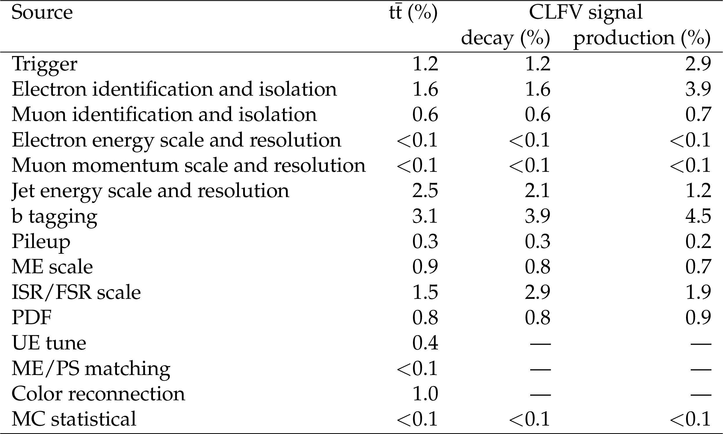
Table 3:
Summary of representative systematic uncertainties in selection efficiency for the SM ${\mathrm{t} {}\mathrm{\bar{t}}}$ process and for single top quark production and decays via vector $\mathrm{e} \mu \mathrm{t} \mathrm{u} $ CLFV interactions in the signal plus ${\mathrm{t} {}\mathrm{\bar{t}}}$ control regions. |

png pdf |
Table 4:
Expected and observed 95% CL upper limits on signal cross sections (production and decay modes), the CLFV Wilson coefficients, and top quark CLFV branching fractions. |
| Summary |
|
A search is reported for charged-lepton flavor violation in top quark production and decay. The analysis is based on pp collisions collected by the CMS detector at the LHC at a center-of-mass energy of 13 TeV, corresponding to an integrated luminosity of 138 fb$^{-1}$. Events are selected if they contain an oppositely charged electron-muon pair and at least one b-tagged jet. An effective field theory approach is used for parametrizing top quark lepton flavor violating interactions. The production and decay modes of the top quark through these effective interactions are included in this analysis. A boosted decision tree is used to distinguish signal from background. No significant excess is observed over the expectations from the standard model. Upper limits are set on the strength of the individual vector-, scalar-, and tensor-like four-fermion effective operators. These are converted to limits on the branching fractions of the top quark $\mathcal{B}(\mathrm{t} \to \mathrm{e}\mu \mathrm{q})$, q = u (c) quark, $ < $ 0.13$\times $10$^{-6}$ (1.31$\times $10$^{-6}$), 0.07$\times $10$^{-6}$ (0.89$\times $10$^{-6}$), and 0.25$\times $10$^{-6}$ (2.59$\times $10$^{-6}$) for vector, scalar, and tensor CLFV interactions, respectively. The resulting limits are the most restrictive bounds to date. |
| References | ||||
| 1 | S. Roy Choudhury and S. Choubey | Updated bounds on sum of neutrino masses in various cosmological scenarios | JCAP 09 (2018) 017 | 1806.10832 |
| 2 | J. L. Diaz-Cruz and J. J. Toscano | Lepton flavor violating decays of Higgs bosons beyond the standard model | PRD 62 (2000) 116005 | hep-ph/9910233 |
| 3 | A. Crivellin et al. | Lepton flavour violation in the MSSM: exact diagonalization vs mass expansion | JHEP 06 (2018) 003 | 1802.06803 |
| 4 | M. Malinsky, T. Ohlsson, Z.-z. Xing, and H. Zhang | Non-unitary neutrino mixing and CP violation in the minimal inverse seesaw model | PLB 679 (2009) 242 | 0905.2889 |
| 5 | L. Calibbi and G. Signorelli | Charged lepton flavour violation: an experimental and theoretical introduction | Riv. Nuovo Cim. 41 (2018) 71 | 1709.00294 |
| 6 | MEG Collaboration | New constraint on the existence of the $ \mu^{+} \rightarrow e^{+} \gamma $ decay | PRL 110 (2013) 201801 | 1303.0754 |
| 7 | S. Mihara, J. P. Miller, P. Paradisi, and G. Piredda | Charged lepton flavor violation experiments | Ann. Rev. Nucl. Part. Sci. 63 (2013) 531 | |
| 8 | ATLAS Collaboration | A search for lepton-flavor-violating decays of the Z boson into a $ \tau $-lepton and a light lepton with the ATLAS detector | PRD 98 (2018) 092010 | 1804.09568 |
| 9 | ATLAS Collaboration | Search for lepton-flavour-violating decays of the Higgs and Z bosons with the ATLAS detector | EPJC 77 (2017) 70 | 1604.07730 |
| 10 | CMS Collaboration | Search for lepton flavour violating decays of the Higgs boson to $ \mu\tau $ and e$ \tau $ in proton-proton collisions at $ \sqrt{s}= $ 13 TeV | JHEP 06 (2018) 001 | CMS-HIG-17-001 1712.07173 |
| 11 | CMS Collaboration | Search for lepton-flavor violating decays of the Higgs boson in the $ \mu\tau $ and e$ \tau $ final states in proton-proton collisions at $ \sqrt{s} = $ 13 TeV | PRD 104 (2021) 032013 | CMS-HIG-20-009 2105.03007 |
| 12 | CMS Collaboration | Search for lepton flavour violating decays of the Higgs boson to e$ \tau $ and e$ \mu $ in proton-proton collisions at $ \sqrt s= $ 8 TeV | PLB 763 (2016) 472 | CMS-HIG-14-040 1607.03561 |
| 13 | ATLAS Collaboration | Search for the Higgs boson decays $ h \to ee $ and $ h \to e\mu $ in pp collisions at $ \sqrt{s} = $ 13 TeV with the ATLAS detector | PLB 801 (2020) 135148 | 1909.10235 |
| 14 | Belle Collaboration | Measurement of the decay $ b\to d\ell\nu_\ell $ in fully reconstructed events and determination of the Cabibbo-Kobayashi-Maskawa matrix element $ |V_{cb}| $ | PRD 93 (2016) 032006 | 1510.03657 |
| 15 | LHCb Collaboration | Test of lepton universality in beauty-quark decays | Submitted to Nature Physics | 2103.11769 |
| 16 | S. L. Glashow, D. Guadagnoli, and K. Lane | Lepton flavor violation in b decays? | PRL 114 (2015) 091801 | 1411.0565 |
| 17 | S. Bi\ssmann, C. Grunwald, G. Hiller, and K. Kroninger | Top and beauty synergies in SMEFT-fits at present and future colliders | JHEP 06 (2021) 010 | 2012.10456 |
| 18 | B. Dumont, K. Nishiwaki, and R. Watanabe | LHC constraints and prospects for $ S_1 $ scalar leptoquark explaining the $ \bar B \to D^{(*)} \tau \bar\nu $ anomaly | PRD 94 (2016) 034001 | 1603.05248 |
| 19 | T. J. Kim et al. | Correlation between $ {R}_{D^{\left(\ast \right)}} $ and top quark FCNC decays in leptoquark models | JHEP 07 (2019) 025 | 1812.08484 |
| 20 | D. Barducci et al. | Interpreting top-quark LHC measurements in the standard-model effective field theory | 1802.07237 | |
| 21 | G. Durieux, F. Maltoni, and C. Zhang | Global approach to top-quark flavor-changing interactions | PRD 91 (2015) 074017 | 1412.7166 |
| 22 | S. Davidson, M. L. Mangano, S. Perries, and V. Sordini | Lepton flavour violating top decays at the LHC | EPJC 75 (2015) 450 | 1507.07163 |
| 23 | CMS Collaboration | The CMS experiment at the CERN LHC | JINST 3 (2008) S08004 | CMS-00-001 |
| 24 | CMS Collaboration | Performance of the CMS level-1 trigger in proton-proton collisions at $ \sqrt{s} = $ 13 TeV | JINST 15 (2020) P10017 | CMS-TRG-17-001 2006.10165 |
| 25 | CMS Collaboration | The CMS trigger system | JINST 12 (2017) P01020 | CMS-TRG-12-001 1609.02366 |
| 26 | P. Nason | A new method for combining NLO QCD with shower Monte Carlo algorithms | JHEP 11 (2004) 040 | hep-ph/0409146 |
| 27 | S. Frixione, P. Nason, and C. Oleari | Matching NLO QCD computations with parton shower simulations: the POWHEG method | JHEP 11 (2007) 070 | 0709.2092 |
| 28 | S. Alioli, P. Nason, C. Oleari, and E. Re | A general framework for implementing NLO calculations in shower Monte Carlo programs: the POWHEG BOX | JHEP 06 (2010) 043 | 1002.2581 |
| 29 | S. Frixione, P. Nason, and G. Ridolfi | A positive-weight next-to-leading-order Monte Carlo for heavy flavour hadroproduction | JHEP 09 (2007) 126 | 0707.3088 |
| 30 | J. Alwall et al. | The automated computation of tree-level and next-to-leading order differential cross sections, and their matching to parton shower simulations | JHEP 07 (2014) 079 | 1405.0301 |
| 31 | Y. Li and F. Petriello | Combining QCD and electroweak corrections to dilepton production in FEWZ | PRD 86 (2012) 094034 | 1208.5967 |
| 32 | N. Kidonakis | Two-loop soft anomalous dimensions for single top quark associated production with $ \mathrm{W^-} $ or $ \mathrm{H^-} $ | PRD 82 (2010) 054018 | hep-ph/1005.4451 |
| 33 | J. M. Campbell, R. K. Ellis, and C. Williams | Vector boson pair production at the LHC | JHEP 07 (2011) 018 | 1105.0020 |
| 34 | F. Maltoni, D. Pagani, and I. Tsinikos | Associated production of a top-quark pair with vector bosons at NLO in QCD: impact on $ \mathrm{t}\overline{\mathrm{t}}\mathrm{H} $ searches at the LHC | JHEP 02 (2016) 113 | 1507.05640 |
| 35 | M. Czakon and A. Mitov | Top++: A program for the calculation of the top-pair cross-section at hadron colliders | CPC 185 (2014) 2930 | 1112.5675 |
| 36 | M. Czakon et al. | Top-pair production at the LHC through NNLO QCD and NLO EW | JHEP 10 (2017) 186 | 1705.04105 |
| 37 | I. Brivio, Y. Jiang, and M. Trott | The SMEFTsim package, theory and tools | JHEP 12 (2017) 070 | 1709.06492 |
| 38 | A. Dedes et al. | SmeftFR --- feynman rules generator for the standard model effective field theory | CPC 247 (2020) 106931 | 1904.03204 |
| 39 | J. Kile and A. Soni | Model-independent constraints on lepton-flavor-violating decays of the top quark | PRD 78 (2008) 094008 | 0807.4199 |
| 40 | NNPDF Collaboration | Parton distributions for the LHC Run II | JHEP 04 (2015) 040 | 1410.8849 |
| 41 | NNPDF Collaboration | Parton distributions from high-precision collider data | EPJC 77 (2017) 663 | 1706.00428 |
| 42 | T. Sjostrand et al. | An introduction to PYTHIA 8.2 | CPC 191 (2015) 159 | 1410.3012 |
| 43 | CMS Collaboration | Event generator tunes obtained from underlying event and multiparton scattering measurements | EPJC 76 (2016) 155 | CMS-GEN-14-001 1512.00815 |
| 44 | CMS Collaboration | Extraction and validation of a new set of CMS PYTHIA8 tunes from underlying-event measurements | EPJC 80 (2020) 4 | CMS-GEN-17-001 1903.12179 |
| 45 | GEANT4 Collaboration | GEANT4 --- a simulation toolkit | NIMA 506 (2003) 250 | |
| 46 | CMS Collaboration | Particle-flow reconstruction and global event description with the CMS detector | JINST 12 (2017) P10003 | CMS-PRF-14-001 1706.04965 |
| 47 | M. Cacciari, G. P. Salam, and G. Soyez | The anti-$ {k_{\mathrm{T}}} $ jet clustering algorithm | JHEP 04 (2008) 063 | 0802.1189 |
| 48 | M. Cacciari, G. P. Salam, and G. Soyez | FastJet user manual | EPJC 72 (2012) 1896 | 1111.6097 |
| 49 | CMS Collaboration | Performance of electron reconstruction and selection with the CMS detector in proton-proton collisions at $ \sqrt{s} = $ 8 TeV | JINST 10 (2015) P06005 | CMS-EGM-13-001 1502.02701 |
| 50 | CMS Collaboration | Performance of the CMS muon detector and muon reconstruction with proton-proton collisions at $ \sqrt{s}= $ 13 TeV | JINST 13 (2018) P06015 | CMS-MUO-16-001 1804.04528 |
| 51 | CMS Collaboration | Performance of the reconstruction and identification of high-momentum muons in proton-proton collisions at $ \sqrt{s} = $ 13 TeV | JINST 15 (2020) P02027 | CMS-MUO-17-001 1912.03516 |
| 52 | M. Cacciari and G. P. Salam | Pileup subtraction using jet areas | PLB 659 (2008) 119 | 0707.1378 |
| 53 | CMS Collaboration | Jet energy scale and resolution in the CMS experiment in pp collisions at 8 TeV | JINST 12 (2017) P02014 | CMS-JME-13-004 1607.03663 |
| 54 | CMS Collaboration | Identification of heavy-flavour jets with the CMS detector in pp collisions at 13 TeV | JINST 13 (2018) P05011 | CMS-BTV-16-002 1712.07158 |
| 55 | CMS Collaboration | Performance of missing transverse momentum reconstruction in proton-proton collisions at $ \sqrt{s} = $ 13 TeV using the CMS detector | JINST 14 (2019) P07004 | CMS-JME-17-001 1903.06078 |
| 56 | CMS Collaboration | Measurements of $ \mathrm{t\overline{t}} $ differential cross sections in proton-proton collisions at $ \sqrt{s}= $ 13 TeV using events containing two leptons | JHEP 02 (2019) 149 | CMS-TOP-17-014 1811.06625 |
| 57 | H. Voss, A. Hocker, J. Stelzer, and F. Tegenfeldt | TMVA, the toolkit for multivariate data analysis with ROOT | in XIth International Workshop on Advanced Computing and Analysis Techniques in Physics Research (ACAT), p. 40 2007 | physics/0703039 |
| 58 | CMS Collaboration | Performance of CMS muon reconstruction in pp collision events at $ \sqrt{s}= $ 7 TeV | JINST 7 (2012) P10002 | CMS-MUO-10-004 1206.4071 |
| 59 | CMS Collaboration | Electron and photon reconstruction and identification with the CMS experiment at the CERN LHC | JINST 16 (2021) P05014 | CMS-EGM-17-001 2012.06888 |
| 60 | CMS Collaboration | Precision luminosity measurement in proton-proton collisions at $ \sqrt{s} = $ 13 TeV in 2015 and 2016 at CMS | EPJC 81 (2021) 800 | CMS-LUM-17-003 2104.01927 |
| 61 | CMS Collaboration | CMS luminosity measurement for the 2017 data-taking period at $ \sqrt{s} = $ 13 TeV | ||
| 62 | CMS Collaboration | CMS luminosity measurement for the 2018 data-taking period at $ \sqrt{s} = $ 13 TeV | ||
| 63 | CMS Collaboration | Measurement of the inelastic proton-proton cross section at $ \sqrt{s}= $ 13 TeV | JHEP 07 (2018) 161 | CMS-FSQ-15-005 1802.02613 |
| 64 | A. Kalogeropoulos and J. Alwall | The SysCalc code: A tool to derive theoretical systematic uncertainties | 1801.08401 | |
| 65 | CMS Collaboration | Measurement of the production cross section for single top quarks in association with W bosons in proton-proton collisions at $ \sqrt{s}= $ 13 TeV | JHEP 10 (2018) 117 | CMS-TOP-17-018 1805.07399 |
| 66 | R. Barlow and C. Beeston | Fitting using finite Monte Carlo samples | CPC 77 (1993) 219 | |
| 67 | T. Junk | Confidence level computation for combining searches with small statistics | Nucl. Instrum. Meth A 434 (1999) 435 | hep-ex/9902006 |
| 68 | A. L. Read | Presentation of search results: the CLs technique | JPG 28 (2002) 2693 | |
| 69 | CMS Collaboration | HEPData record for this analysis | link | |
|
|
Compact Muon Solenoid LHC, CERN |
|

|

|

|

|

|