

Compact Muon Solenoid
LHC, CERN
| CMS-TOP-20-010 ; CERN-EP-2021-210 | ||
| Inclusive and differential cross section measurements of single top quark production in association with a Z boson in proton-proton collisions at $\sqrt{s} = $ 13 TeV | ||
| CMS Collaboration | ||
| 4 November 2021 | ||
| JHEP 02 (2022) 107 | ||
| Abstract: Inclusive and differential cross sections of single top quark production in association with a Z boson are measured in proton-proton collisions at a center-of-mass energy of 13 TeV with a data sample corresponding to an integrated luminosity of 138 fb$^{-1}$ recorded by the CMS experiment. Events are selected based on the presence of three leptons, electrons or muons, associated with leptonic Z boson and top quark decays. The measurement yields an inclusive cross section of 87.9 $_{-7.3}^{+7.5}$ (stat) $_{-6.0}^{+7.3}$ (syst) fb for a dilepton invariant mass greater than 30 GeV, in agreement with standard model (SM) calculations and the most precise determination to date. The ratio between the cross sections for the top quark and the top antiquark production in association with a Z boson is measured as 2.37 $_{-0.42}^{+0.56}$ (stat) $_{-0.13}^{+0.27}$ (syst). Differential measurements at parton and particle levels are performed for the first time. Several kinematic observables are considered to study the modeling of the process. Results are compared to theoretical predictions with different assumptions on the source of the initial-state b quark and found to be in agreement, within the uncertainties. Additionally, the spin asymmetry, which is sensitive to the top quark polarization, is determined from the differential distribution of the polarization angle at parton level to be 0.54 $\pm$ 0.16 (stat) $\pm$ 0.06 (syst), in agreement with SM predictions. | ||
| Links: e-print arXiv:2111.02860 [hep-ex] (PDF) ; CDS record ; inSPIRE record ; HepData record ; CADI line (restricted) ; | ||
| Figures | |
png pdf |
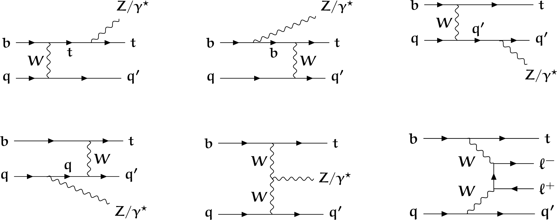
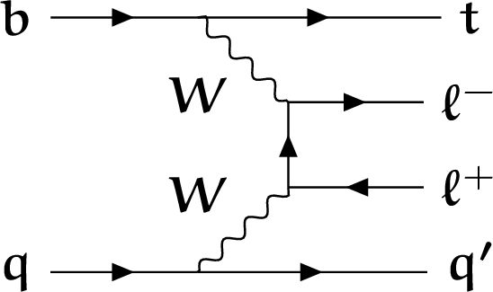
Figure 1:
Representative LO Feynman diagrams for the tZq production process. The production mechanism of nonresonant lepton pairs (lower right) is included in the signal definition to correctly account for interference effects. |

png pdf |
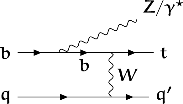
Figure 1-a:
Representative LO Feynman diagram for the tZq production process. |
png pdf |
Figure 1-b:
Representative LO Feynman diagram for the tZq production process. |
png pdf |
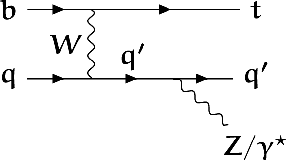
Figure 1-c:
Representative LO Feynman diagram for the tZq production process. |
png pdf |
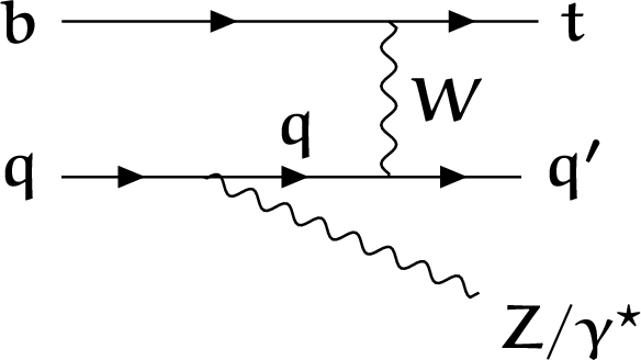
Figure 1-d:
Representative LO Feynman diagram for the tZq production process. |

png pdf |
Figure 1-e:
Representative LO Feynman diagram for the tZq production process. |
png pdf |
Figure 1-f:
Representative LO Feynman diagram for the production of nonresonant lepton pairs, which is included in the signal definition to correctly account for interference effects. |
png pdf |
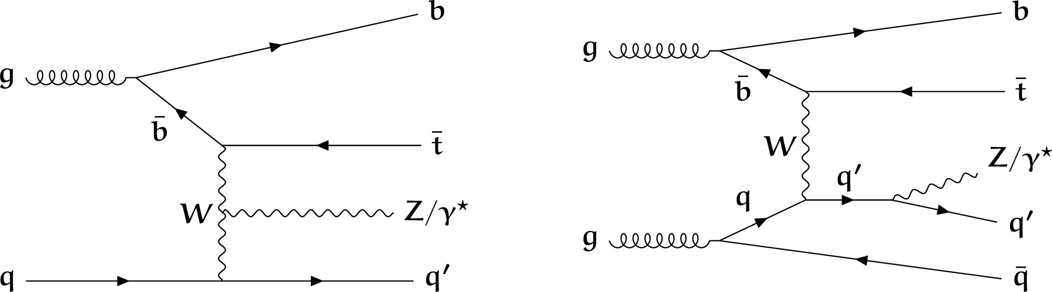
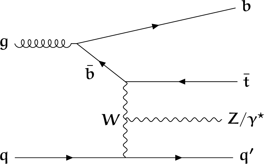
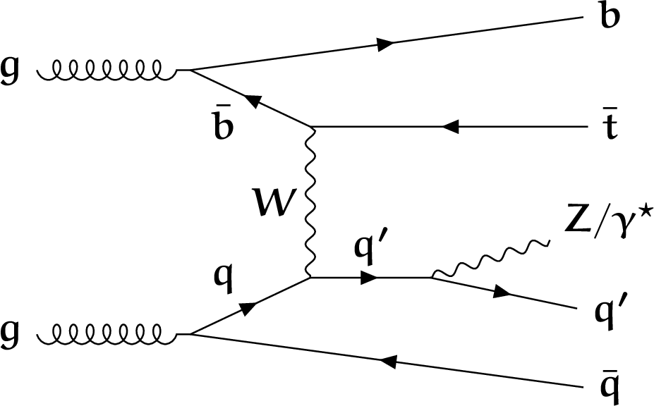
Figure 2:
An example of the LO (left) and NLO (right) Feynman diagrams for the tZq production process in the 4FS. The Z/$\gamma^{*}$ interference term is included in the MC event simulation. In the case of the NLO generation, the gg- and ${\mathrm{q} \mathrm{\bar{q}}}$-initiated processes are possible, with an additional quark or gluon present in the final state. |
png pdf |
Figure 2-a:
An example of the LO Feynman diagrams for the tZq production process in the 4FS. The Z/$\gamma^{*}$ interference term is included in the MC event simulation. |
png pdf |
Figure 2-b:
An example of the NLO Feynman diagrams for the tZq production process in the 4FS. The Z/$\gamma^{*}$ interference term is included in the MC event simulation. The gg- and ${\mathrm{q} \mathrm{\bar{q}}}$-initiated processes are possible, with an additional quark or gluon present in the final state. |
png pdf |
Figure 3:
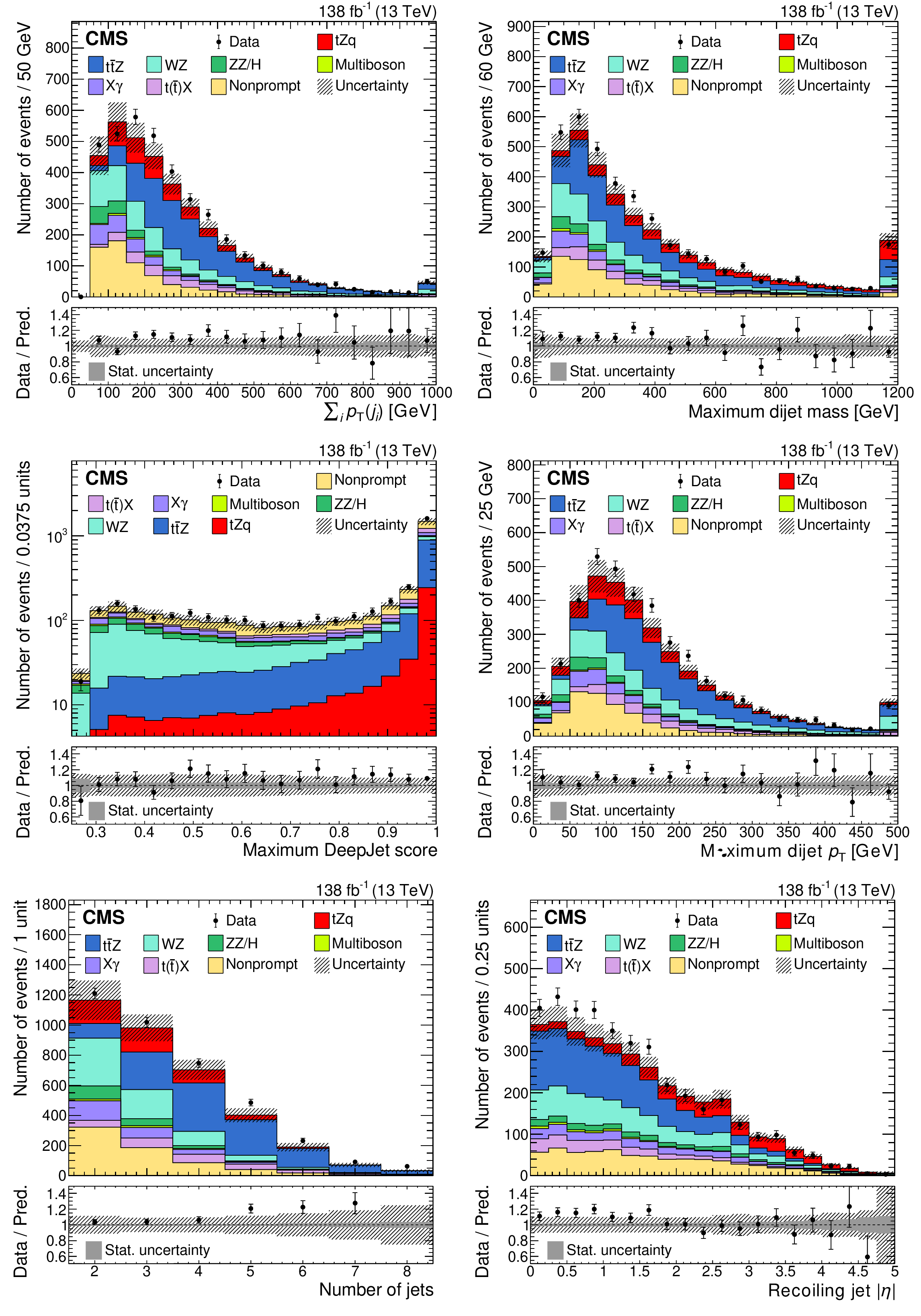
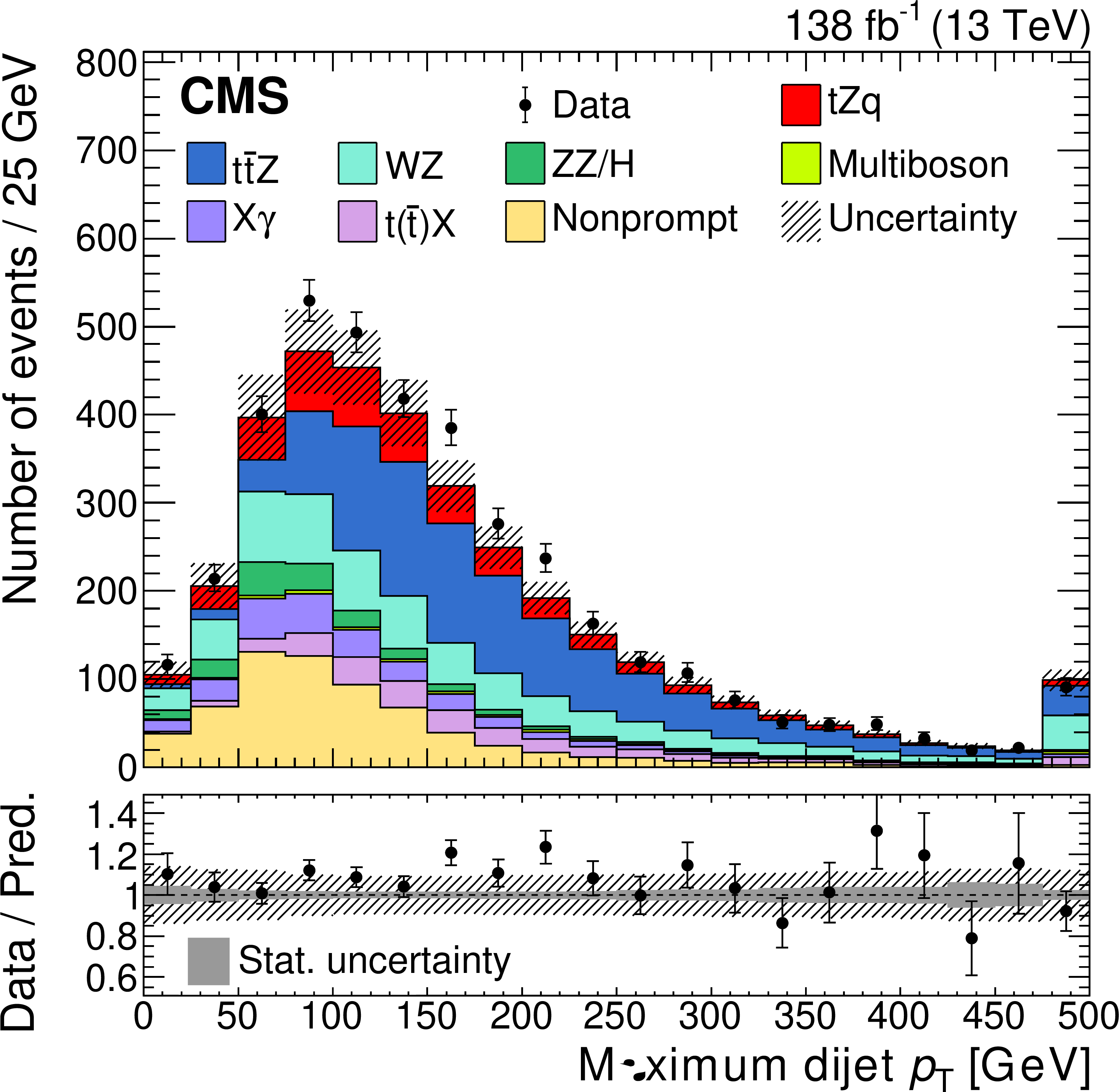
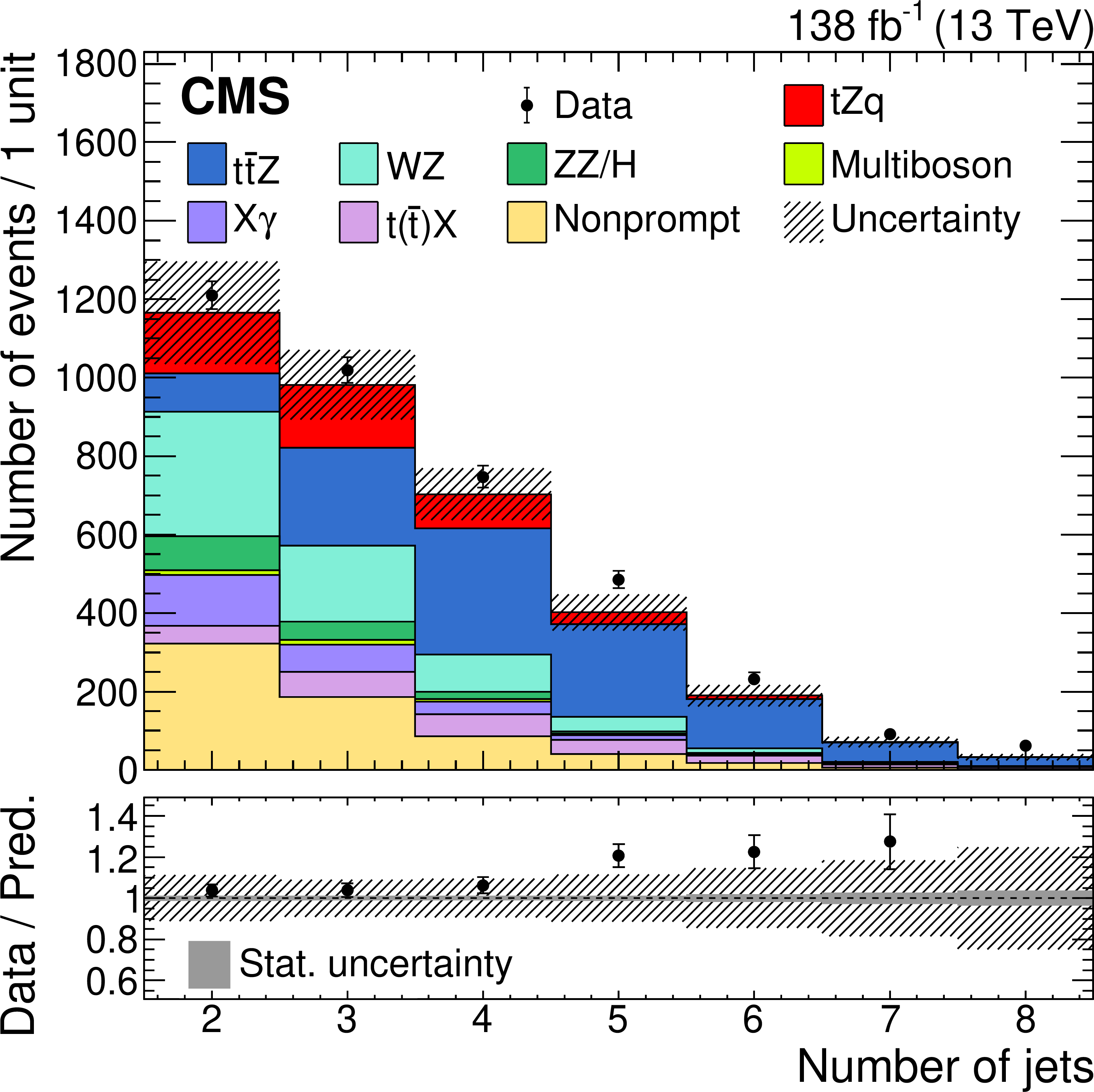
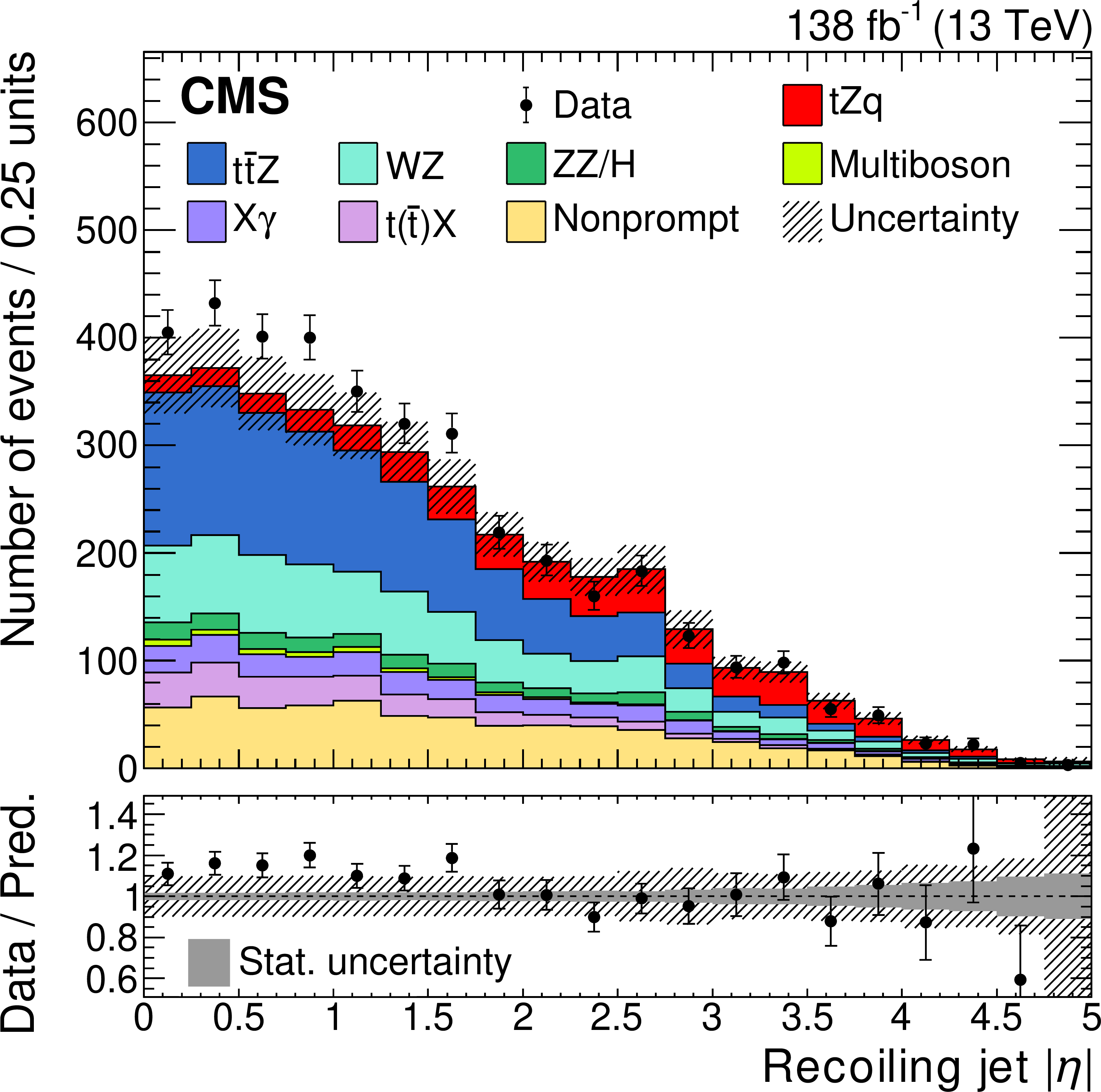
Distributions of the most powerful discriminating variables in the signal region for the data (points) and predictions (colored histograms), including the scalar ${p_{\mathrm {T}}}$ sum of all jets (upper left), the maximum invariant mass of any two-jet system (upper right), the maximum DeepJet score of any jet (middle left), the maximum ${p_{\mathrm {T}}}$ value of any two-jet system (middle right), the number of jets in the event (lower left), and the $ | \eta | $ of the recoiling jet (lower right). The last bins include the overflows. The lower panels show the ratio of the data to the sum of the predictions. The vertical lines on the data points represent the statistical uncertainty in the data; the shaded area corresponds to the total uncertainty in the prediction; the gray area in the ratio indicates the uncertainty related to the limited statistical precision in the prediction. |
png pdf |
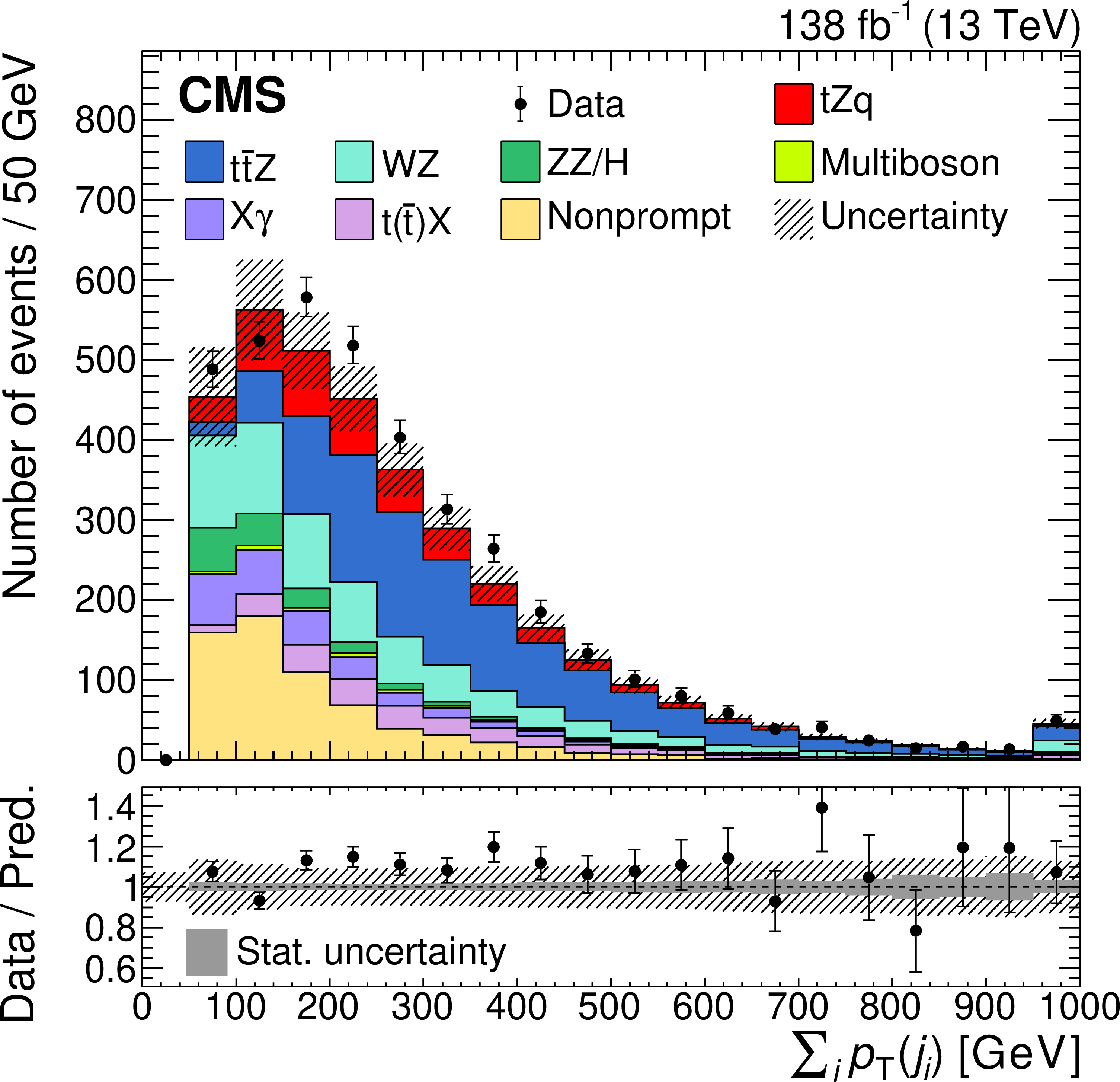
Figure 3-a:
Distribution of the scalar ${p_{\mathrm {T}}}$ sum of all jets, in the signal region for the data (points) and predictions (colored histograms). The last bins include the overflows. The lower panel shows the ratio of the data to the sum of the predictions. The vertical lines on the data points represent the statistical uncertainty in the data; the shaded area corresponds to the total uncertainty in the prediction; the gray area in the ratio indicates the uncertainty related to the limited statistical precision in the prediction. |
png pdf |
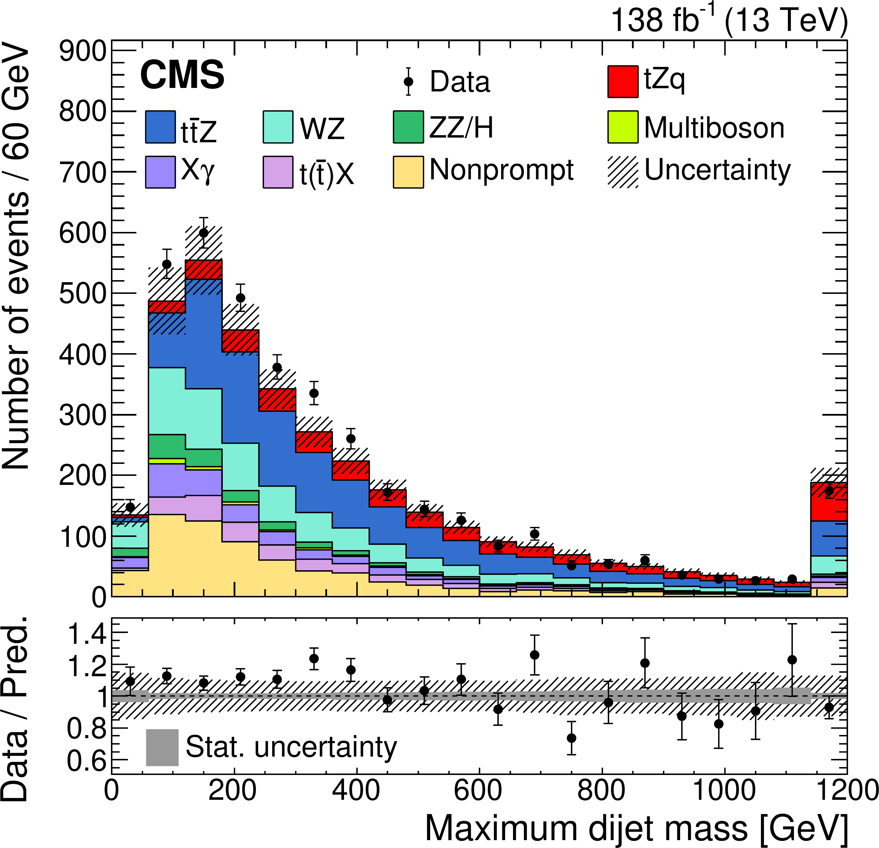
Figure 3-b:
Distribution of the maximum invariant mass of any two-jet system, in the signal region for the data (points) and predictions (colored histograms). The last bins include the overflows. The lower panel shows the ratio of the data to the sum of the predictions. The vertical lines on the data points represent the statistical uncertainty in the data; the shaded area corresponds to the total uncertainty in the prediction; the gray area in the ratio indicates the uncertainty related to the limited statistical precision in the prediction. |
png pdf |
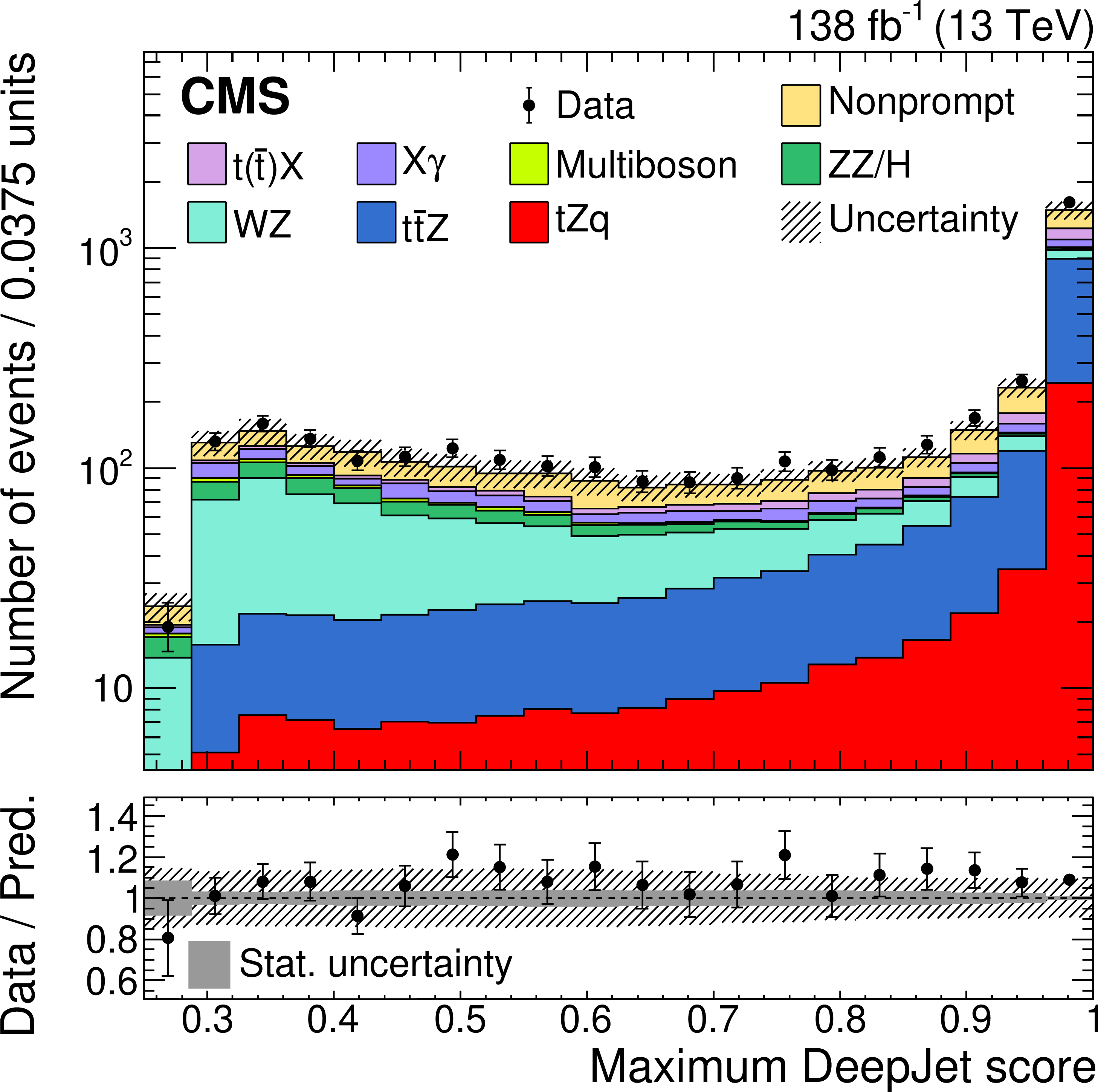
Figure 3-c:
Distribution of the maximum DeepJet score of any jet, in the signal region for the data (points) and predictions (colored histograms). The last bins include the overflows. The lower panel shows the ratio of the data to the sum of the predictions. The vertical lines on the data points represent the statistical uncertainty in the data; the shaded area corresponds to the total uncertainty in the prediction; the gray area in the ratio indicates the uncertainty related to the limited statistical precision in the prediction. |
png pdf |
Figure 3-d:
Distribution of the maximum ${p_{\mathrm {T}}}$ value of any two-jet system, in the signal region for the data (points) and predictions (colored histograms). The last bins include the overflows. The lower panel shows the ratio of the data to the sum of the predictions. The vertical lines on the data points represent the statistical uncertainty in the data; the shaded area corresponds to the total uncertainty in the prediction; the gray area in the ratio indicates the uncertainty related to the limited statistical precision in the prediction. |
png pdf |
Figure 3-e:
Distribution of the number of jets in the event, in the signal region for the data (points) and predictions (colored histograms). The last bins include the overflows. The lower panel shows the ratio of the data to the sum of the predictions. The vertical lines on the data points represent the statistical uncertainty in the data; the shaded area corresponds to the total uncertainty in the prediction; the gray area in the ratio indicates the uncertainty related to the limited statistical precision in the prediction. |
png pdf |
Figure 3-f:
Distribution of the $ | \eta | $ of the recoiling jet, in the signal region for the data (points) and predictions (colored histograms). The last bins include the overflows. The lower panel shows the ratio of the data to the sum of the predictions. The vertical lines on the data points represent the statistical uncertainty in the data; the shaded area corresponds to the total uncertainty in the prediction; the gray area in the ratio indicates the uncertainty related to the limited statistical precision in the prediction. |
png pdf |
Figure 4:
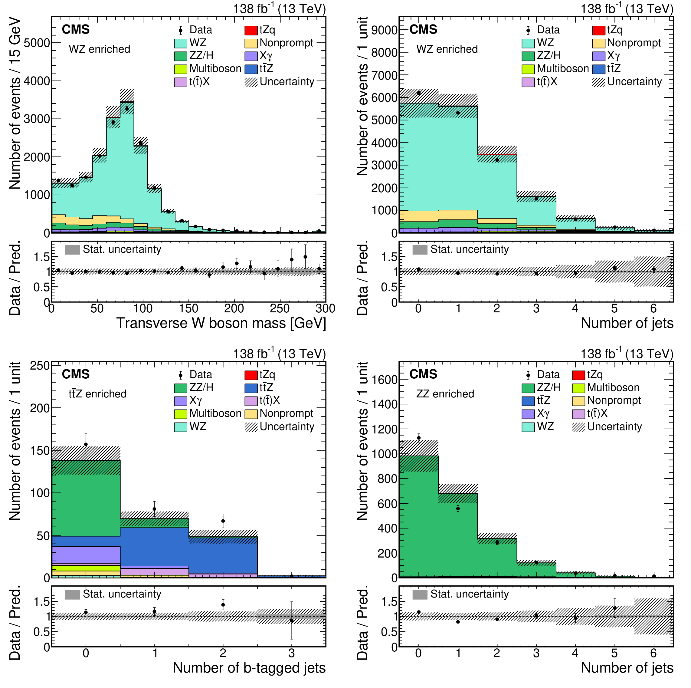
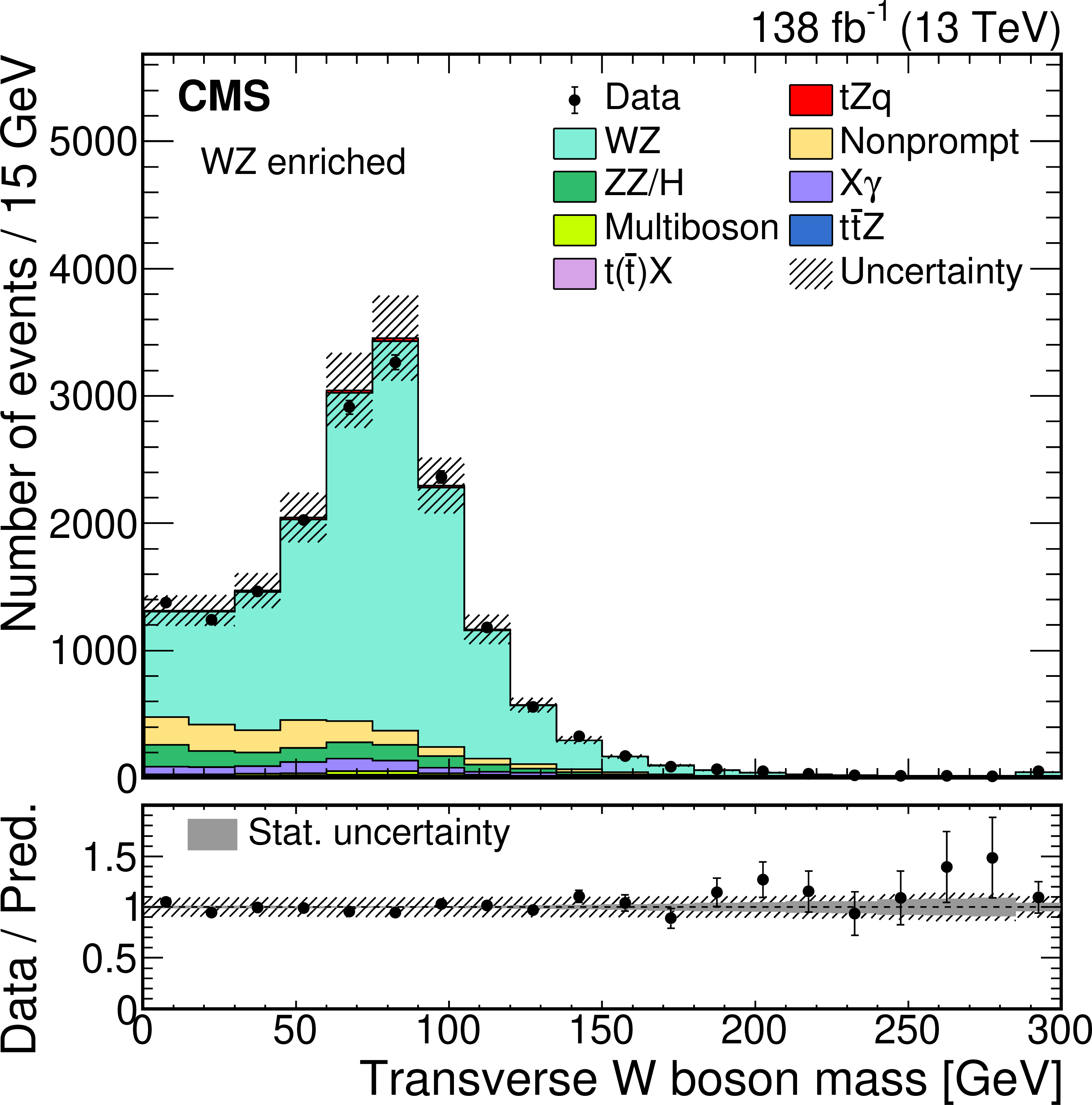
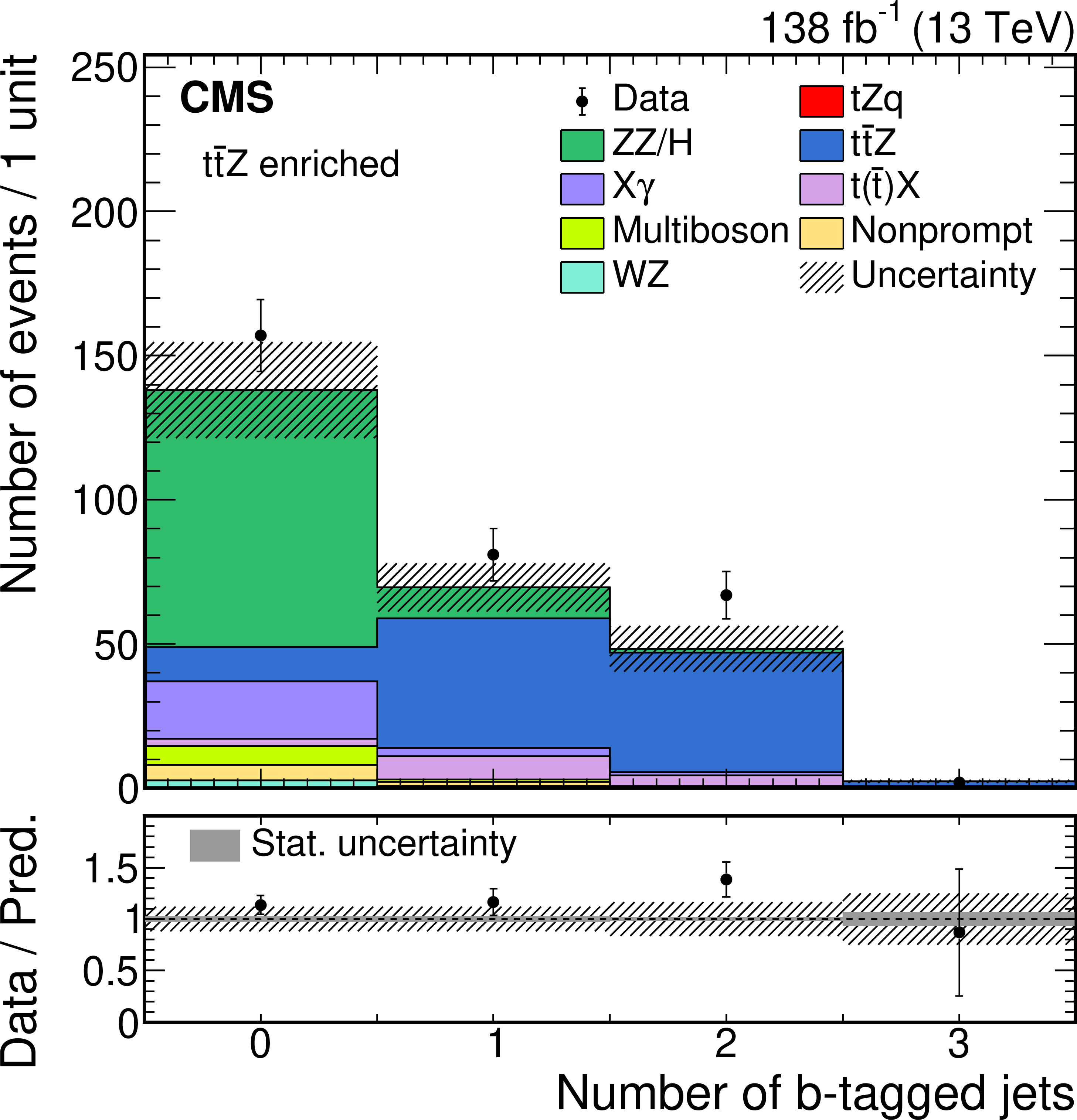
Distributions of the transverse W boson mass (upper left) and the number of selected jets (upper right) for the WZ-enriched control region, the number of b-tagged jets (lower left) in the ${\mathrm{t} \mathrm{\bar{t}}}$Z-enriched control region, and the number of jets (lower right) in the ZZ-enriched control region for the data (points) and predictions (colored histograms). The lower panels show the ratio of the data to the sum of the predictions. The vertical lines on the data points represent the statistical uncertainty in the data; the shaded area corresponds to the total uncertainty in the prediction; the gray area in the ratio indicates the uncertainty related to the limited statistical precision in the prediction. |
png pdf |
Figure 4-a:
Distribution of the transverse W boson mass in the WZ-enriched control region, for the data (points) and predictions (colored histograms). The lower panel shows the ratio of the data to the sum of the predictions. The vertical lines on the data points represent the statistical uncertainty in the data; the shaded area corresponds to the total uncertainty in the prediction; the gray area in the ratio indicates the uncertainty related to the limited statistical precision in the prediction. |

png pdf |
Figure 4-b:
Distribution of the number of selected jets in the WZ-enriched control region, for the data (points) and predictions (colored histograms). The lower panel shows the ratio of the data to the sum of the predictions. The vertical lines on the data points represent the statistical uncertainty in the data; the shaded area corresponds to the total uncertainty in the prediction; the gray area in the ratio indicates the uncertainty related to the limited statistical precision in the prediction. |
png pdf |
Figure 4-c:
Distribution of the number of b-tagged jets in the ${\mathrm{t} \mathrm{\bar{t}}}$Z-enriched control region, for the data (points) and predictions (colored histograms). The lower panel shows the ratio of the data to the sum of the predictions. The vertical lines on the data points represent the statistical uncertainty in the data; the shaded area corresponds to the total uncertainty in the prediction; the gray area in the ratio indicates the uncertainty related to the limited statistical precision in the prediction. |

png pdf |
Figure 4-d:
Distribution of the number of jets in the ZZ-enriched control region, for the data (points) and predictions (colored histograms). The lower panel shows the ratio of the data to the sum of the predictions. The vertical lines on the data points represent the statistical uncertainty in the data; the shaded area corresponds to the total uncertainty in the prediction; the gray area in the ratio indicates the uncertainty related to the limited statistical precision in the prediction. |
png pdf |
Figure 5:
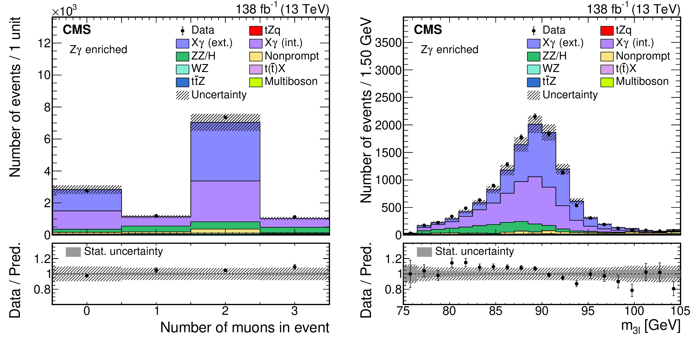
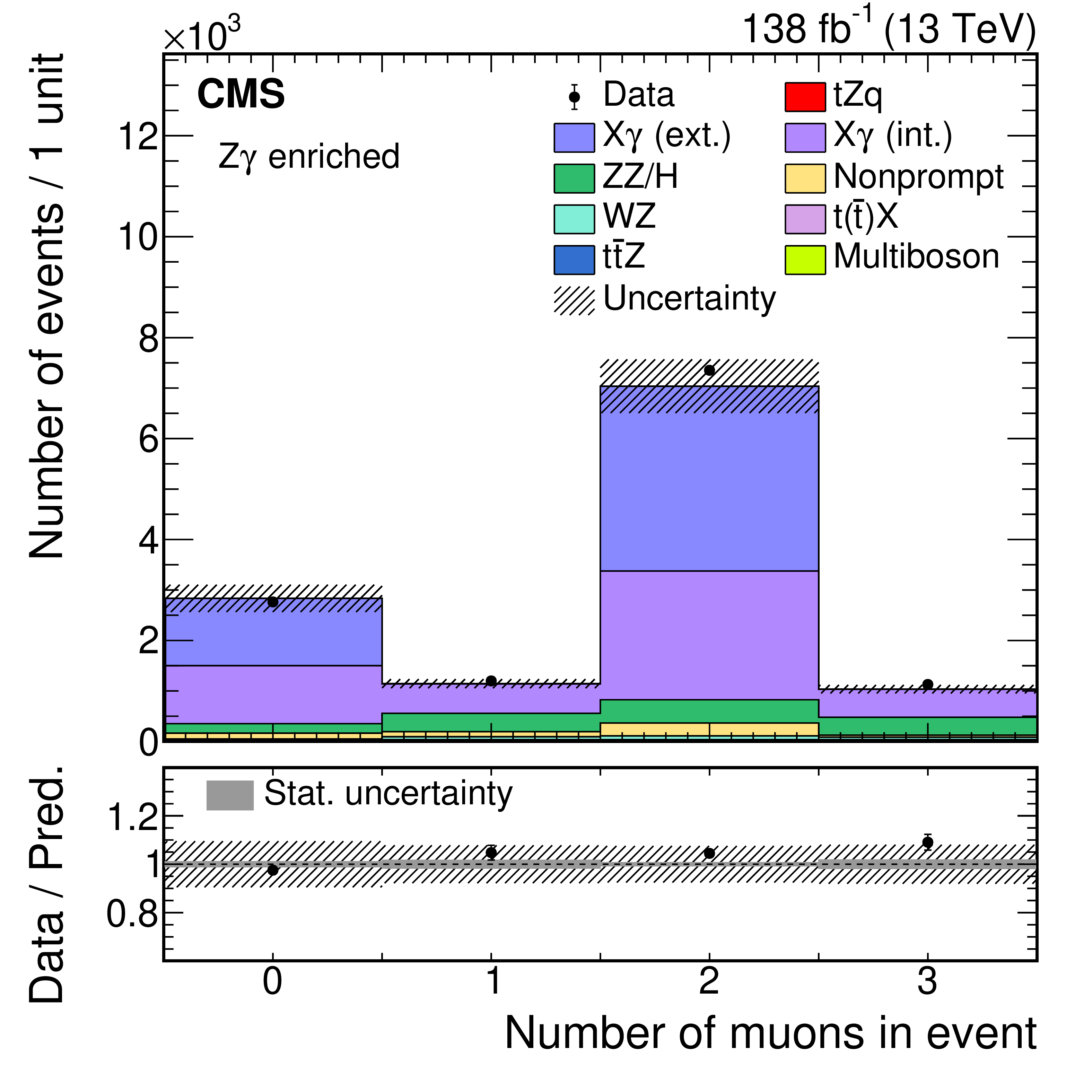
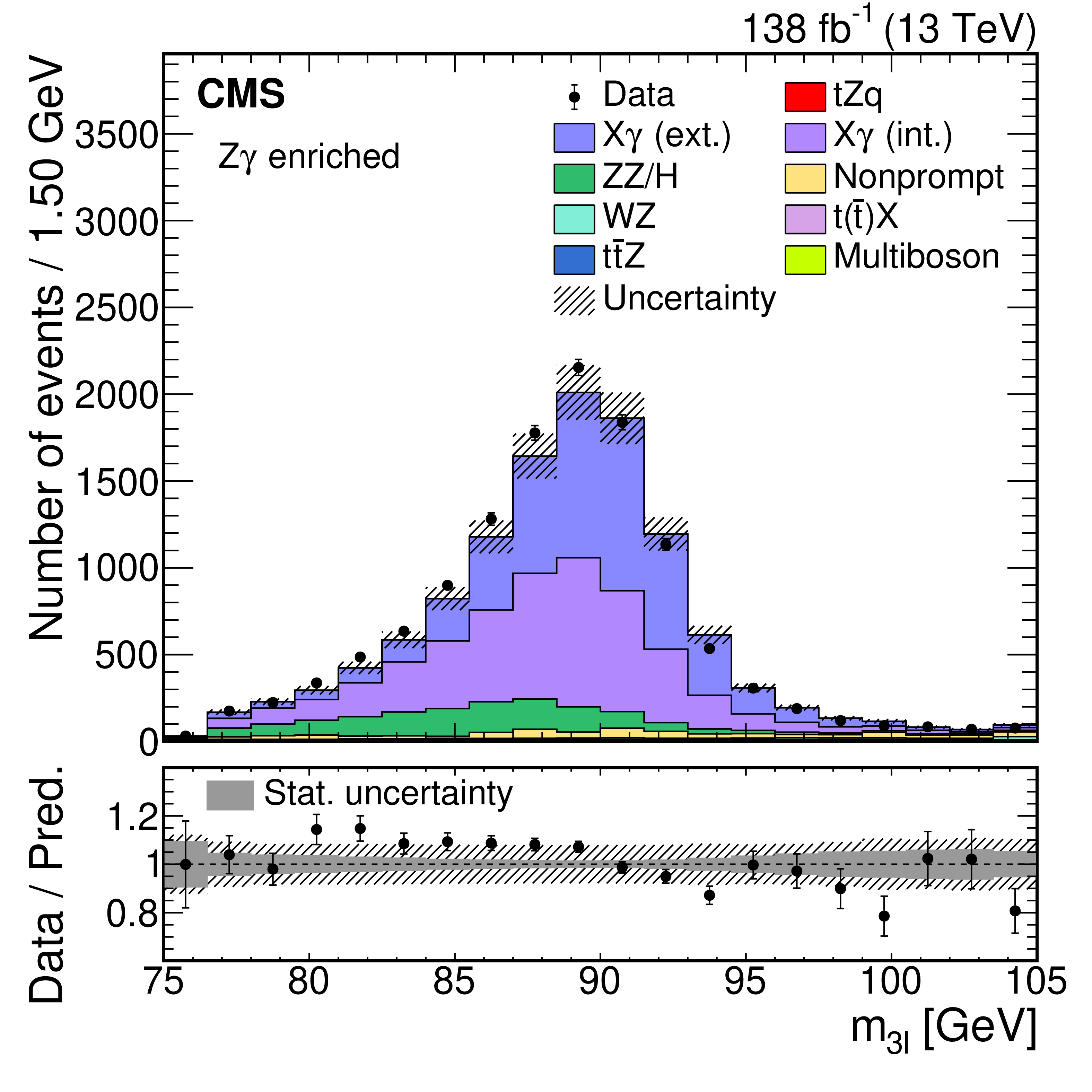
Distributions in the Z$\gamma$-enriched control region of the number of selected muons (left) and the invariant mass of the three-lepton system (right) for the data (points) and predictions (colored histograms). The contributions in the simulation from "external'' photon conversions, where a real photon converts into a pair of (mostly) electrons from its interaction in the detector material, and so-called "internal'' conversions, where a virtual photon decays into a pair of leptons, are shown separately. The lower panels show the ratio of the data to the sum of the predictions. The vertical lines on the data points represent the statistical uncertainty in the data; the shaded area corresponds to the total uncertainty in the prediction; the gray area in the ratio indicates the uncertainty related to the limited statistical precision in the prediction. |
png pdf |
Figure 5-a:
Distribution in the Z$\gamma$-enriched control region of the number of selected muons, for the data (points) and predictions (colored histograms). The contributions in the simulation from "external'' photon conversions, where a real photon converts into a pair of (mostly) electrons from its interaction in the detector material, and so-called "internal'' conversions, where a virtual photon decays into a pair of leptons, are shown separately. The lower panel shows the ratio of the data to the sum of the predictions. The vertical lines on the data points represent the statistical uncertainty in the data; the shaded area corresponds to the total uncertainty in the prediction; the gray area in the ratio indicates the uncertainty related to the limited statistical precision in the prediction. |
png pdf |
Figure 5-b:
Distribution in the Z$\gamma$-enriched control region of the invariant mass of the three-lepton system, for the data (points) and predictions (colored histograms). The contributions in the simulation from "external'' photon conversions, where a real photon converts into a pair of (mostly) electrons from its interaction in the detector material, and so-called "internal'' conversions, where a virtual photon decays into a pair of leptons, are shown separately. The lower panel shows the ratio of the data to the sum of the predictions. The vertical lines on the data points represent the statistical uncertainty in the data; the shaded area corresponds to the total uncertainty in the prediction; the gray area in the ratio indicates the uncertainty related to the limited statistical precision in the prediction. |
png pdf |
Figure 6:
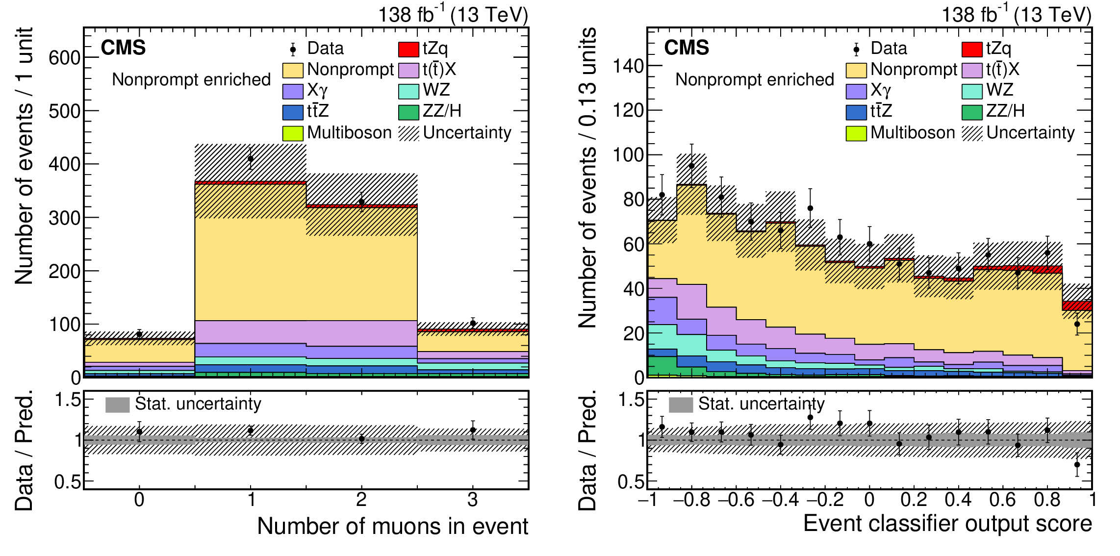
Distributions of the number of selected muons per event (left) and the output score of the multivariate classifier used for the signal extraction in the inclusive cross section measurement (right) in a control region enriched with nonprompt leptons for data (points) and predictions (colored histograms). The lower panels show the ratio of the data to the sum of the predictions. The vertical lines on the data points represent the statistical uncertainty in the data; the shaded area corresponds to the total uncertainty in the prediction; the gray area in the ratio indicates the uncertainty related to the limited statistical precision in the prediction. |
png pdf |
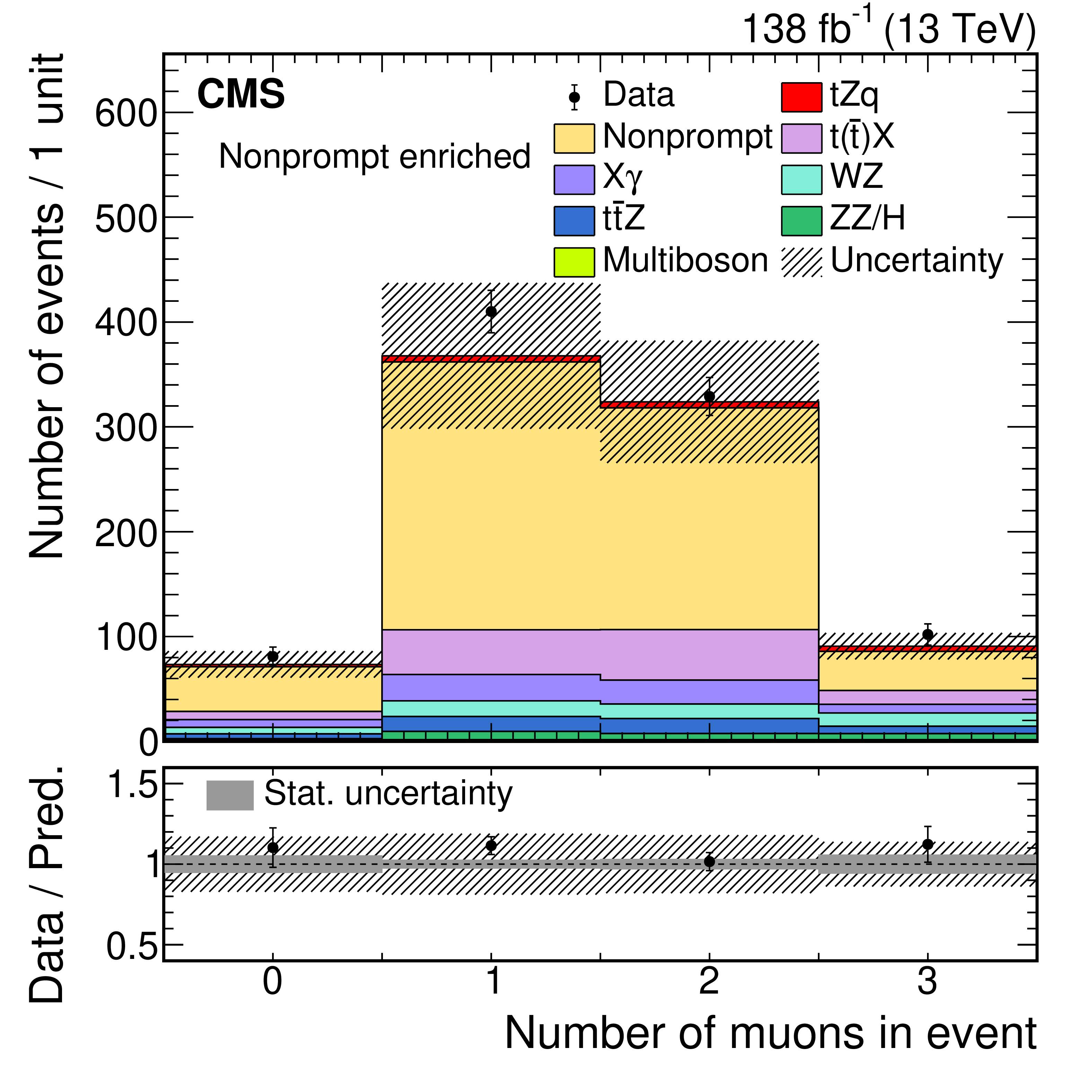
Figure 6-a:
Distribution of the number of selected muons per event in a control region enriched with nonprompt leptons for data (points) and predictions (colored histograms). The lower panel shows the ratio of the data to the sum of the predictions. The vertical lines on the data points represent the statistical uncertainty in the data; the shaded area corresponds to the total uncertainty in the prediction; the gray area in the ratio indicates the uncertainty related to the limited statistical precision in the prediction. |
png pdf |
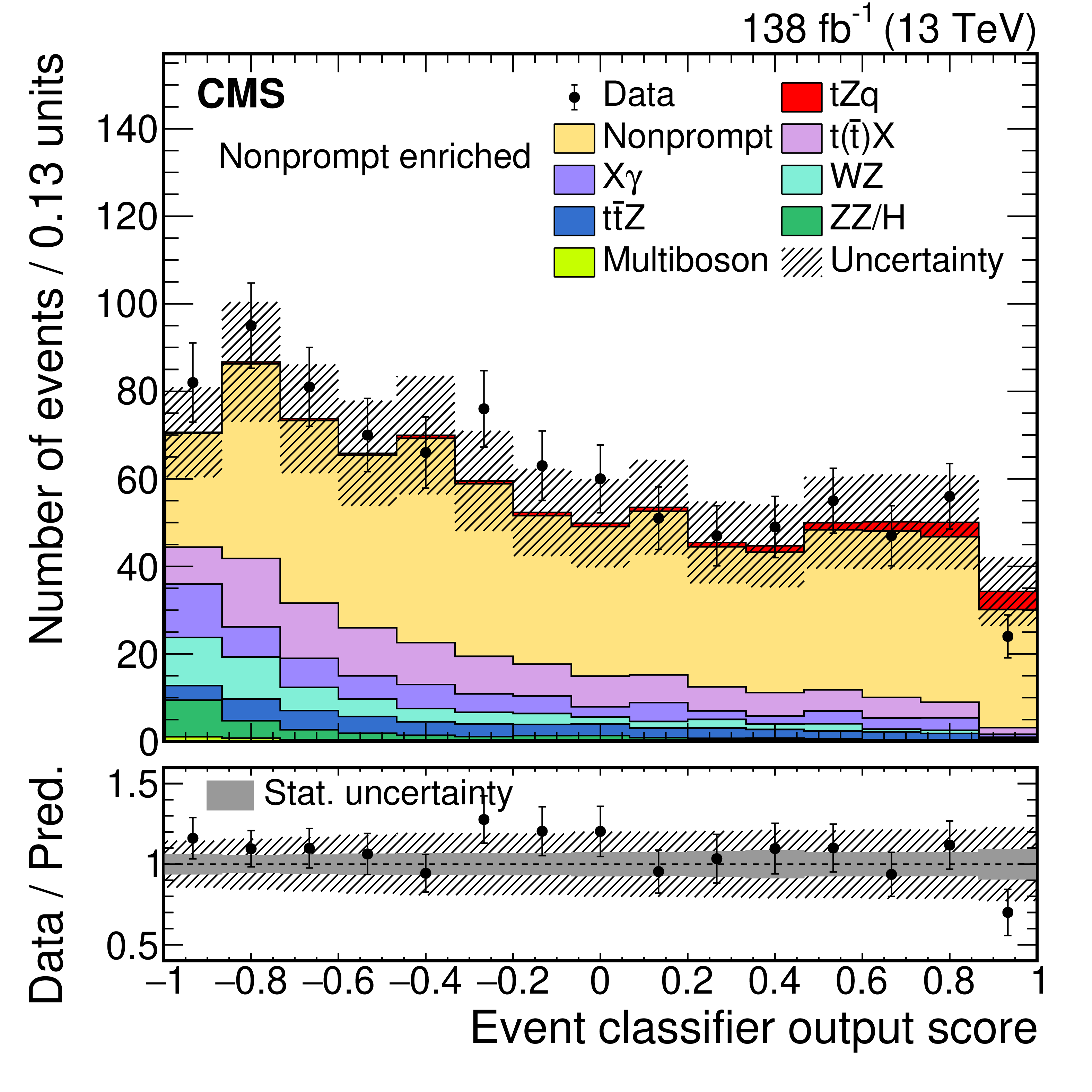
Figure 6-b:
Distribution of the output score of the multivariate classifier used for the signal extraction in the inclusive cross section measurement in a control region enriched with nonprompt leptons for data (points) and predictions (colored histograms). The lower panel shows the ratio of the data to the sum of the predictions. The vertical lines on the data points represent the statistical uncertainty in the data; the shaded area corresponds to the total uncertainty in the prediction; the gray area in the ratio indicates the uncertainty related to the limited statistical precision in the prediction. |
png pdf |
Figure 7:
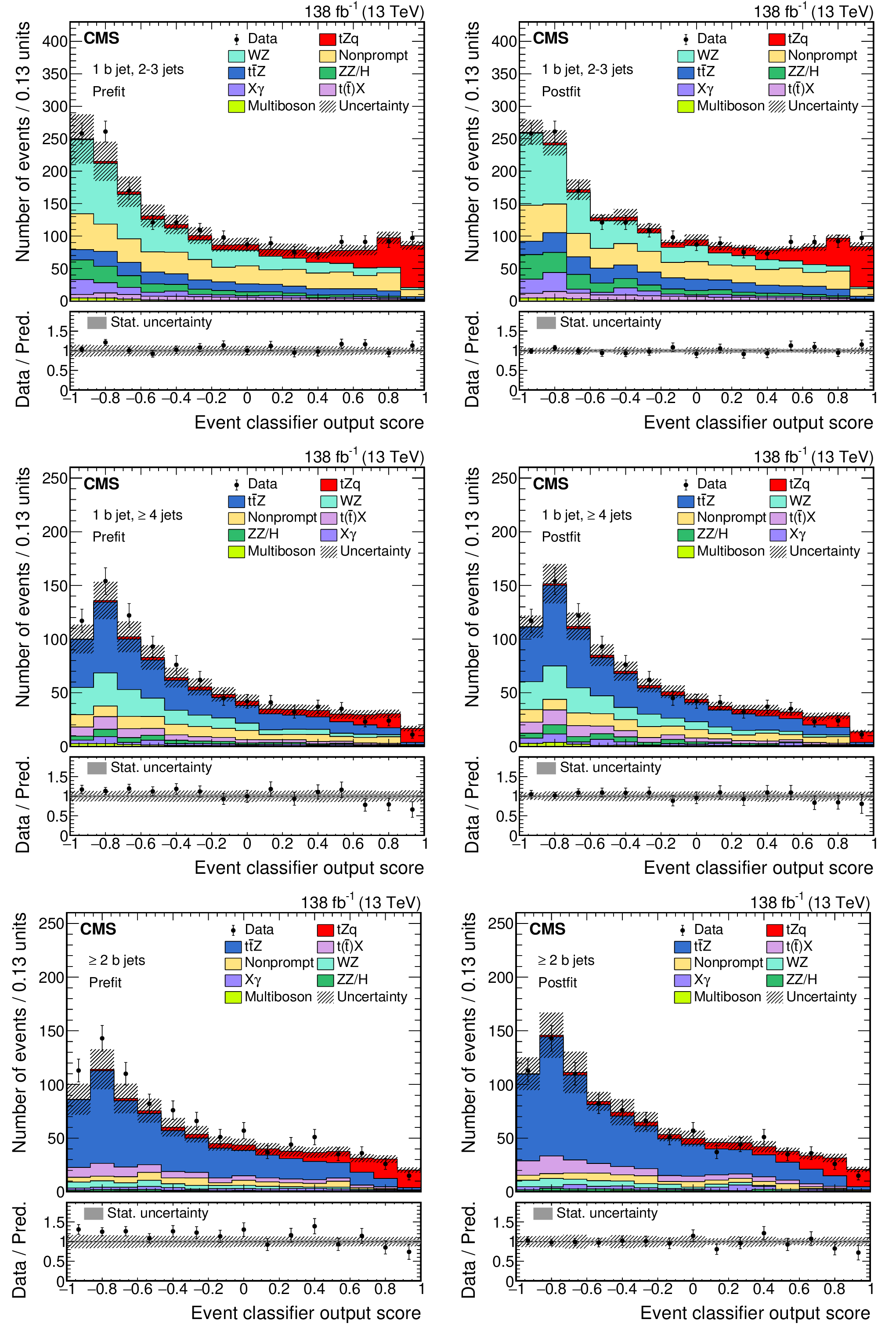
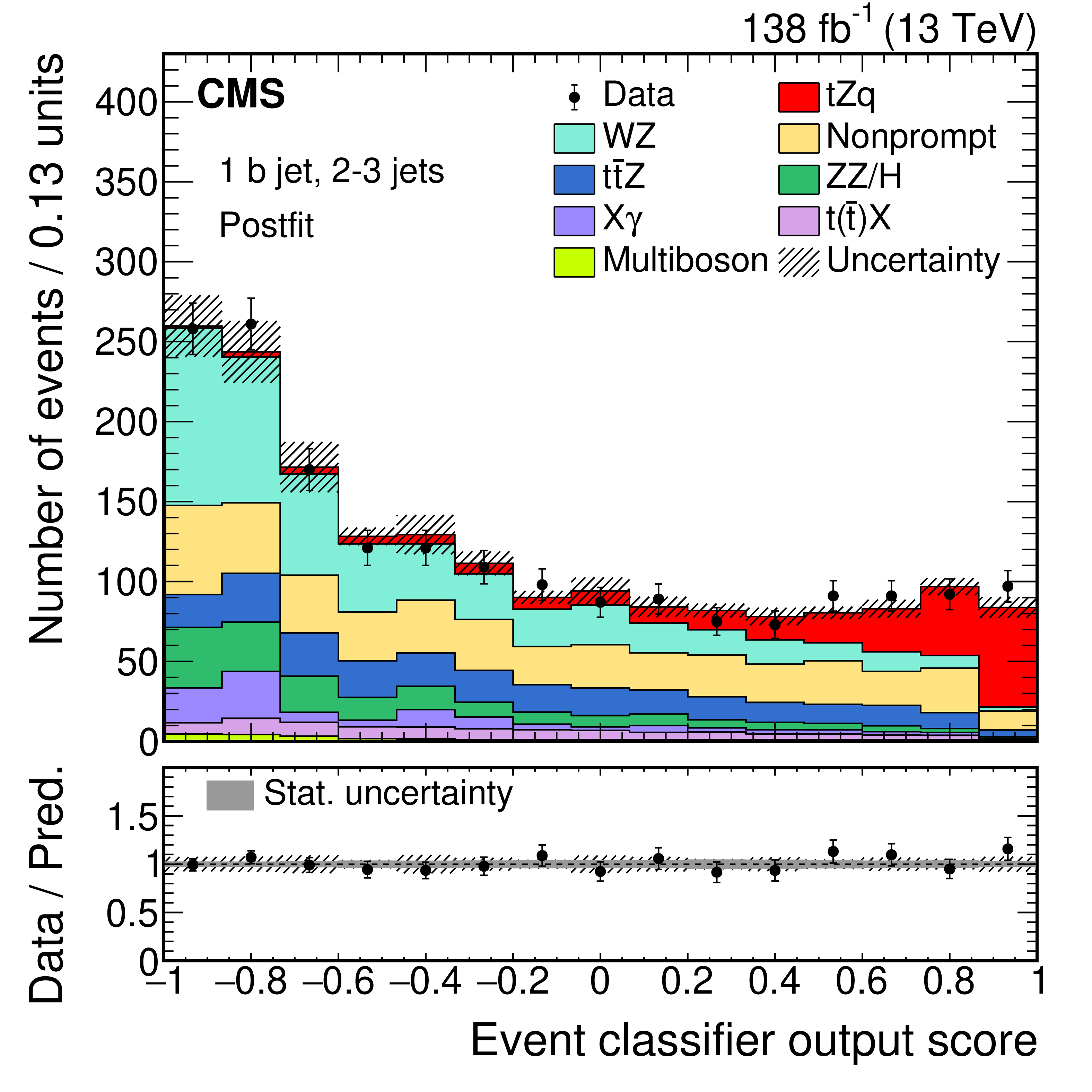
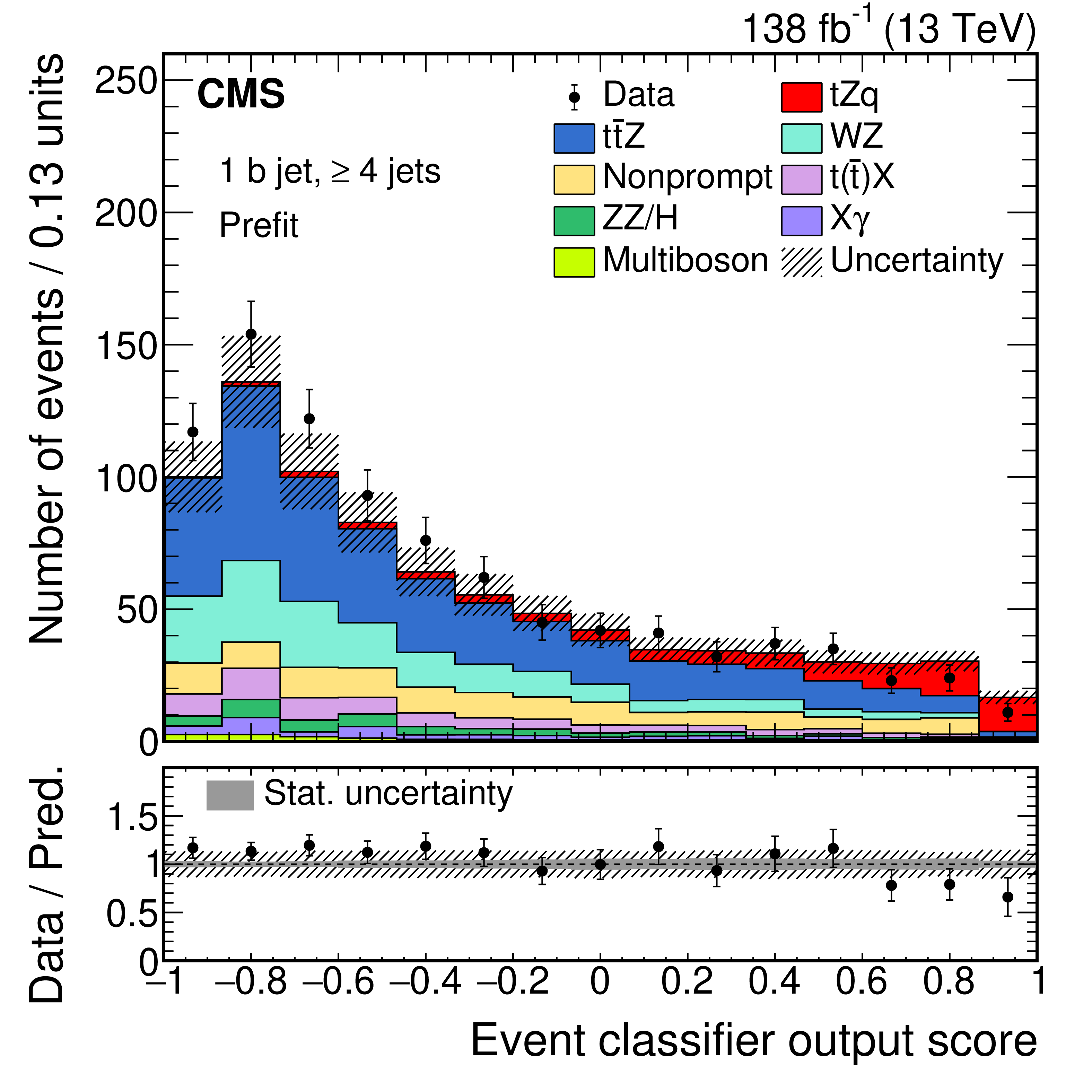
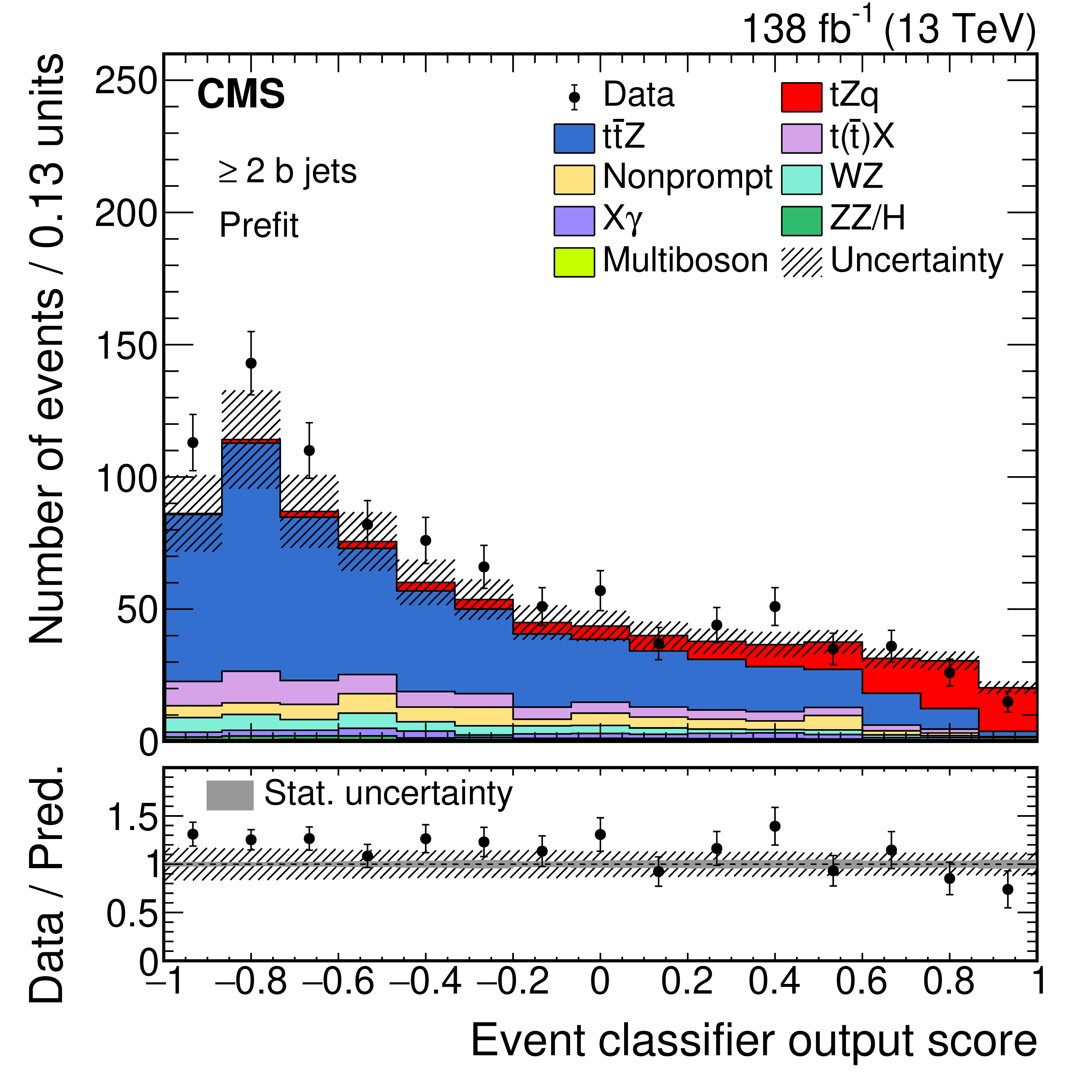
Distributions of the event BDT discriminant in the signal region for data (points) and predictions (colored histograms). The results are shown for prefit (left) and postfit (right) distributions in mutually exclusive signal subregions: exactly one b-tagged jet, 2-3 jets (upper); exactly one b-tagged jet, $\geq $4 jets (middle); and $\geq $2 b-tagged jets (lower). The lower panels show the ratio of the data to the sum of the predictions. The vertical lines on the data points represent the statistical uncertainty in the data; the shaded area corresponds to the total uncertainty in the prediction; the gray area in the ratio indicates the uncertainty related to the limited statistical precision in the prediction. |

png pdf |
Figure 7-a:
Prefit distribution of the event BDT discriminant for data (points) and predictions (colored histograms) in the exclusive signal subregion with exactly one b-tagged jet, 2-3 jets. The lower panel shows the ratio of the data to the sum of the predictions. The vertical lines on the data points represent the statistical uncertainty in the data; the shaded area corresponds to the total uncertainty in the prediction; the gray area in the ratio indicates the uncertainty related to the limited statistical precision in the prediction. |
png pdf |
Figure 7-b:
Postfit distribution of the event BDT discriminant for data (points) and predictions (colored histograms) in the exclusive signal subregion with exactly one b-tagged jet, 2-3 jets. The lower panel shows the ratio of the data to the sum of the predictions. The vertical lines on the data points represent the statistical uncertainty in the data; the shaded area corresponds to the total uncertainty in the prediction; the gray area in the ratio indicates the uncertainty related to the limited statistical precision in the prediction. |
png pdf |
Figure 7-c:
Prefit distribution of the event BDT discriminant for data (points) and predictions (colored histograms) in the exclusive signal subregion with exactly one b-tagged jet, $\geq $4 jets. The lower panel shows the ratio of the data to the sum of the predictions. The vertical lines on the data points represent the statistical uncertainty in the data; the shaded area corresponds to the total uncertainty in the prediction; the gray area in the ratio indicates the uncertainty related to the limited statistical precision in the prediction. |

png pdf |
Figure 7-d:
Postfit distribution of the event BDT discriminant for data (points) and predictions (colored histograms) in the exclusive signal subregion with exactly one b-tagged jet, $\geq $4 jets. The lower panel shows the ratio of the data to the sum of the predictions. The vertical lines on the data points represent the statistical uncertainty in the data; the shaded area corresponds to the total uncertainty in the prediction; the gray area in the ratio indicates the uncertainty related to the limited statistical precision in the prediction. |
png pdf |
Figure 7-e:
Prefit distribution of the event BDT discriminant for data (points) and predictions (colored histograms) in the exclusive signal subregion with $\geq $2 b-tagged jets. The lower panel shows the ratio of the data to the sum of the predictions. The vertical lines on the data points represent the statistical uncertainty in the data; the shaded area corresponds to the total uncertainty in the prediction; the gray area in the ratio indicates the uncertainty related to the limited statistical precision in the prediction. |
png pdf |
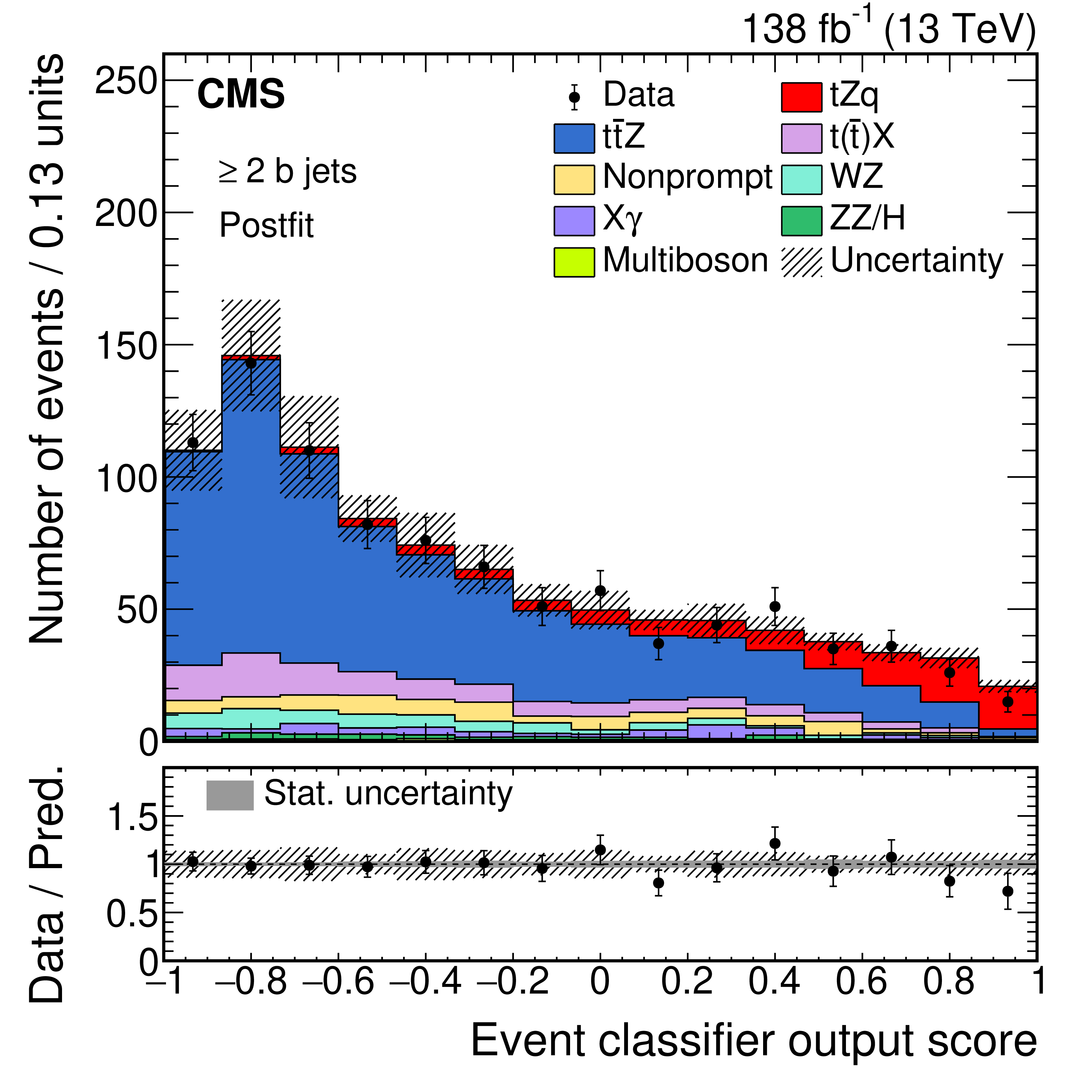
Figure 7-f:
Postfit distribution of the event BDT discriminant for data (points) and predictions (colored histograms) in the exclusive signal subregion with $\geq $2 b-tagged jets. The lower panel shows the ratio of the data to the sum of the predictions. The vertical lines on the data points represent the statistical uncertainty in the data; the shaded area corresponds to the total uncertainty in the prediction; the gray area in the ratio indicates the uncertainty related to the limited statistical precision in the prediction. |

png pdf |
Figure 8:
Summary of the dominant systematic uncertainties affecting the inclusive tZq cross section measurement. The left column lists the sources of systematic uncertainty, treated as nuisance parameters in the fit, in order of importance. In the middle column, the black points with the horizontal bars show for each source the difference between the observed best fit value ($\hat{\theta}$) and the nominal value ($\theta _0$), divided by the expected standard deviation ($\Delta \theta $). The right column plots the change in the tZq signal strength $\mu $ if a nuisance parameter is varied one standard deviation up (red), or down (blue). The gray, red, and blue bands display the same quantity as their corresponding markers, but using a simulated data set where all nuisance parameters are set to their expected values. |
png pdf |
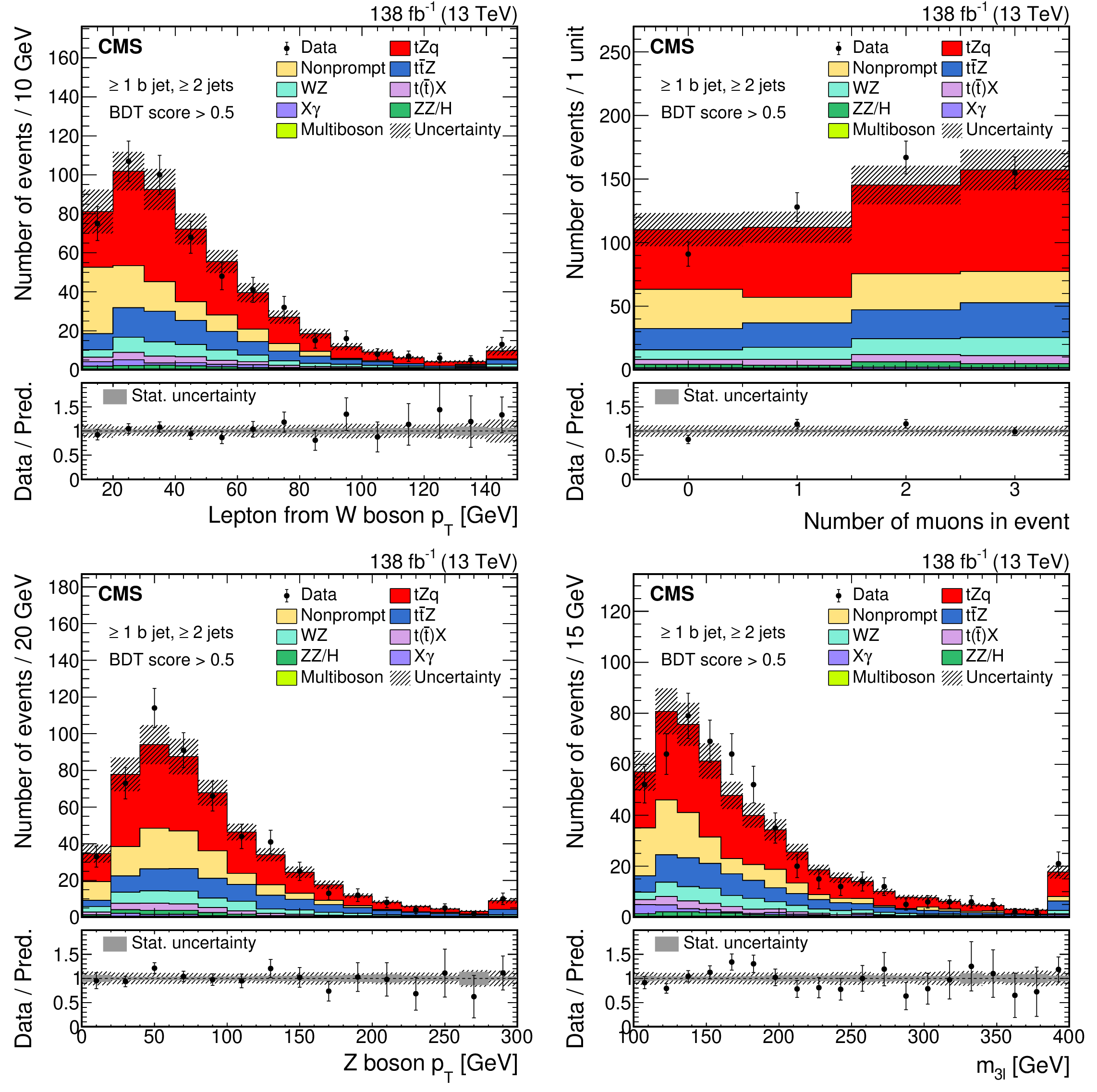
Figure 9:
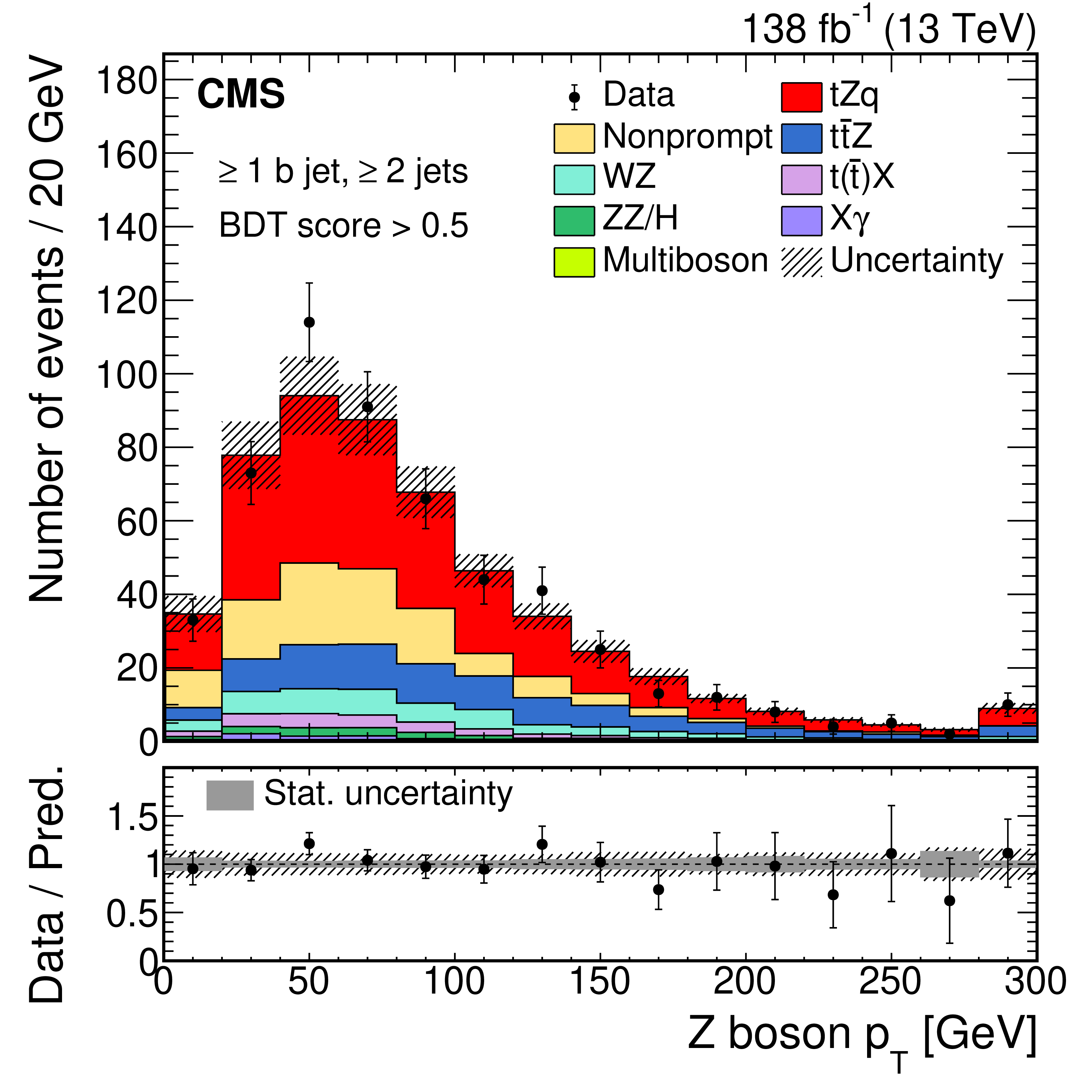
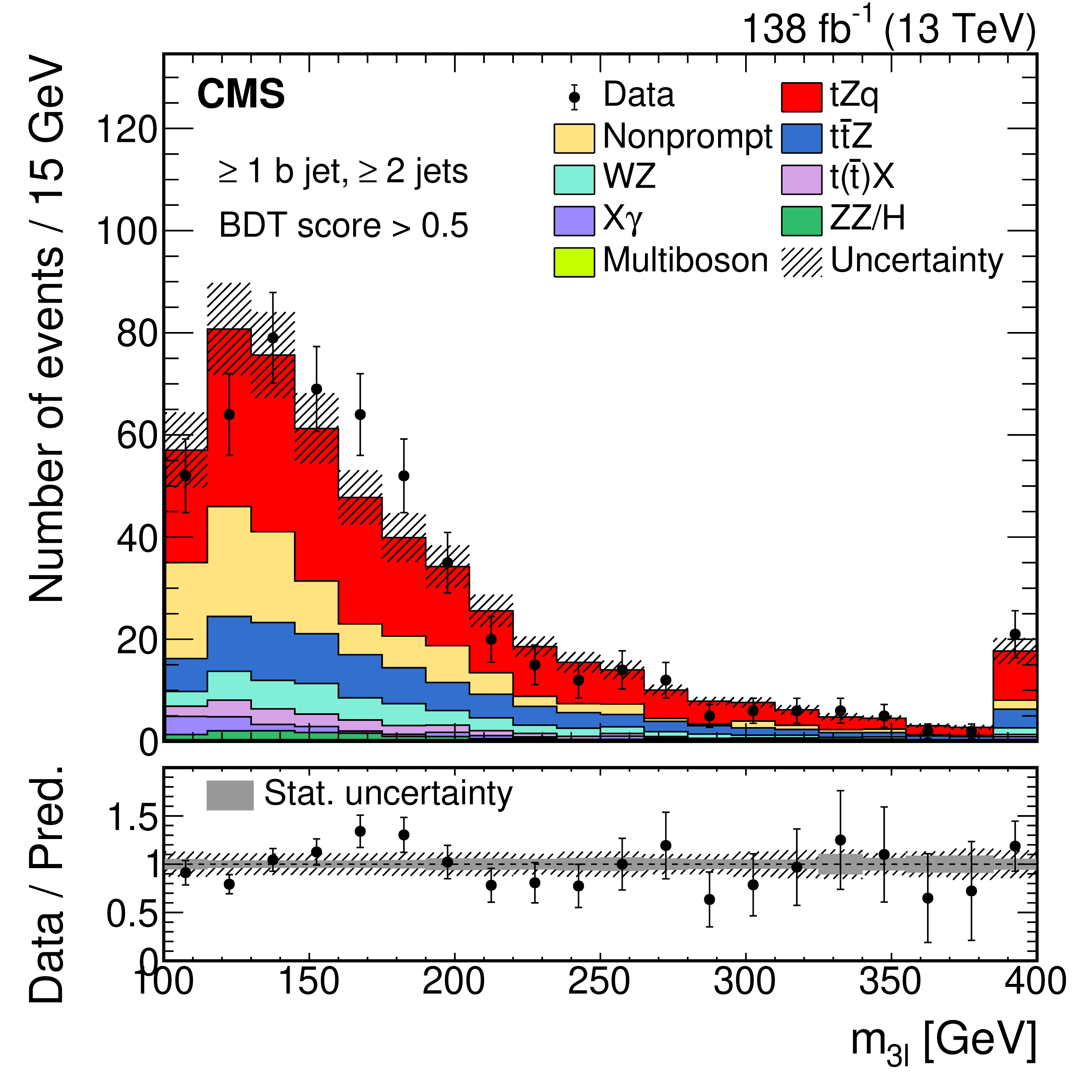
Distributions at the detector level of some of the important variables used in the tZq analysis from a tZq-enriched region for the data (points) and predictions (colored histograms). The selection criteria discussed in Section 4 have been used, along with the requirement that the event BDT discriminant be greater than 0.5. The variables shown are as follows: transverse momentum of the lepton associated with the decay of the top quark (upper left), number of muons in the event (upper right), reconstructed transverse momentum of the Z boson (lower left) and transverse mass of the W boson (lower right). The lower panels show the ratio of the data to the sum of the predictions. The vertical lines on the data points represent the statistical uncertainty in the data; the shaded area corresponds to the total uncertainty in the prediction; the gray area in the ratio indicates the uncertainty related to the limited statistical precision in the prediction. |
png pdf |
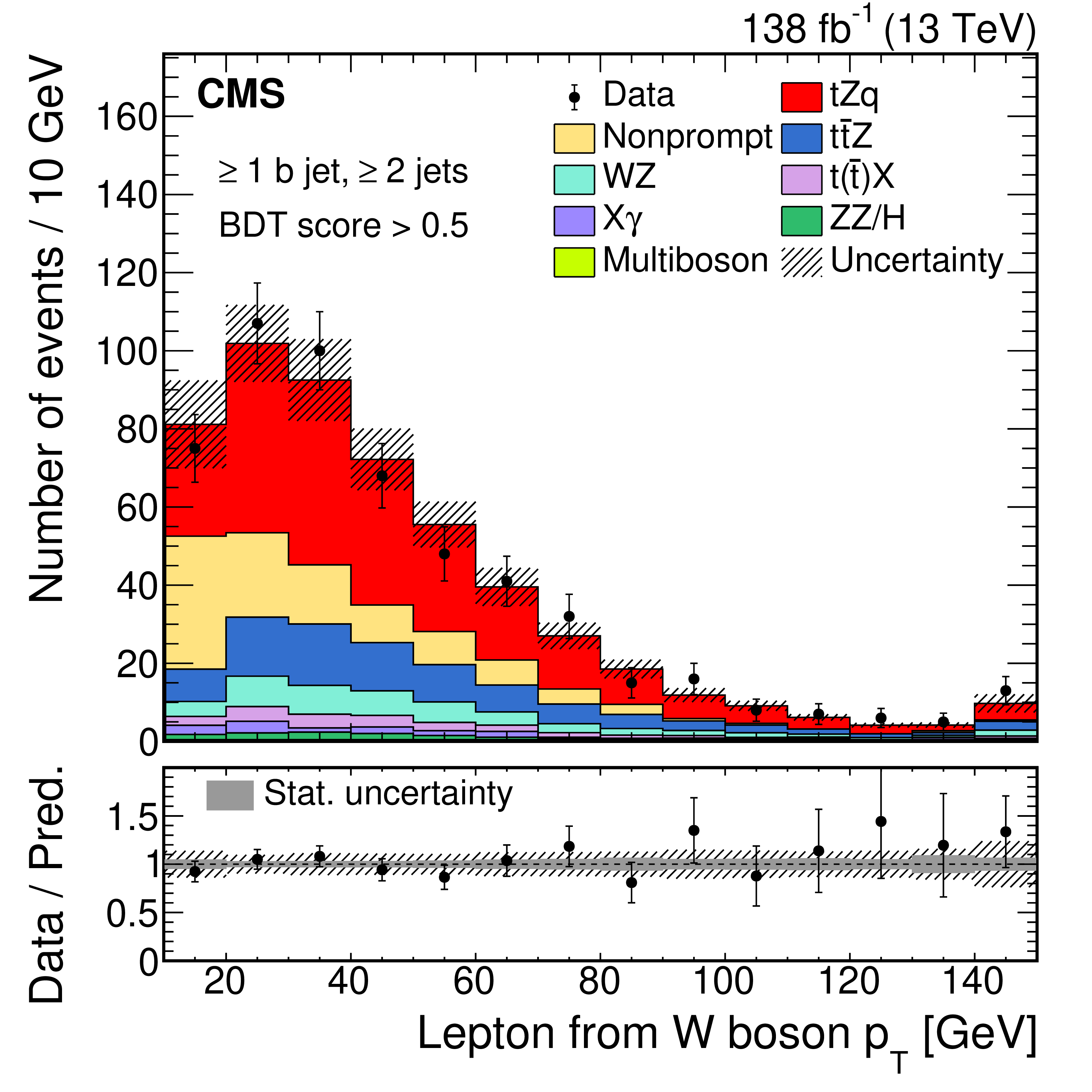
Figure 9-a:
Distribution at the detector level of the transverse momentum of the lepton associated with the decay of the top quark, which is an important variable used in the tZq analysis from a tZq-enriched region for the data (points) and predictions (colored histograms). The selection criteria discussed in Section 4 have been used, along with the requirement that the event BDT discriminant be greater than 0.5. The lower panel shows the ratio of the data to the sum of the predictions. The vertical lines on the data points represent the statistical uncertainty in the data; the shaded area corresponds to the total uncertainty in the prediction; the gray area in the ratio indicates the uncertainty related to the limited statistical precision in the prediction. |
png pdf |
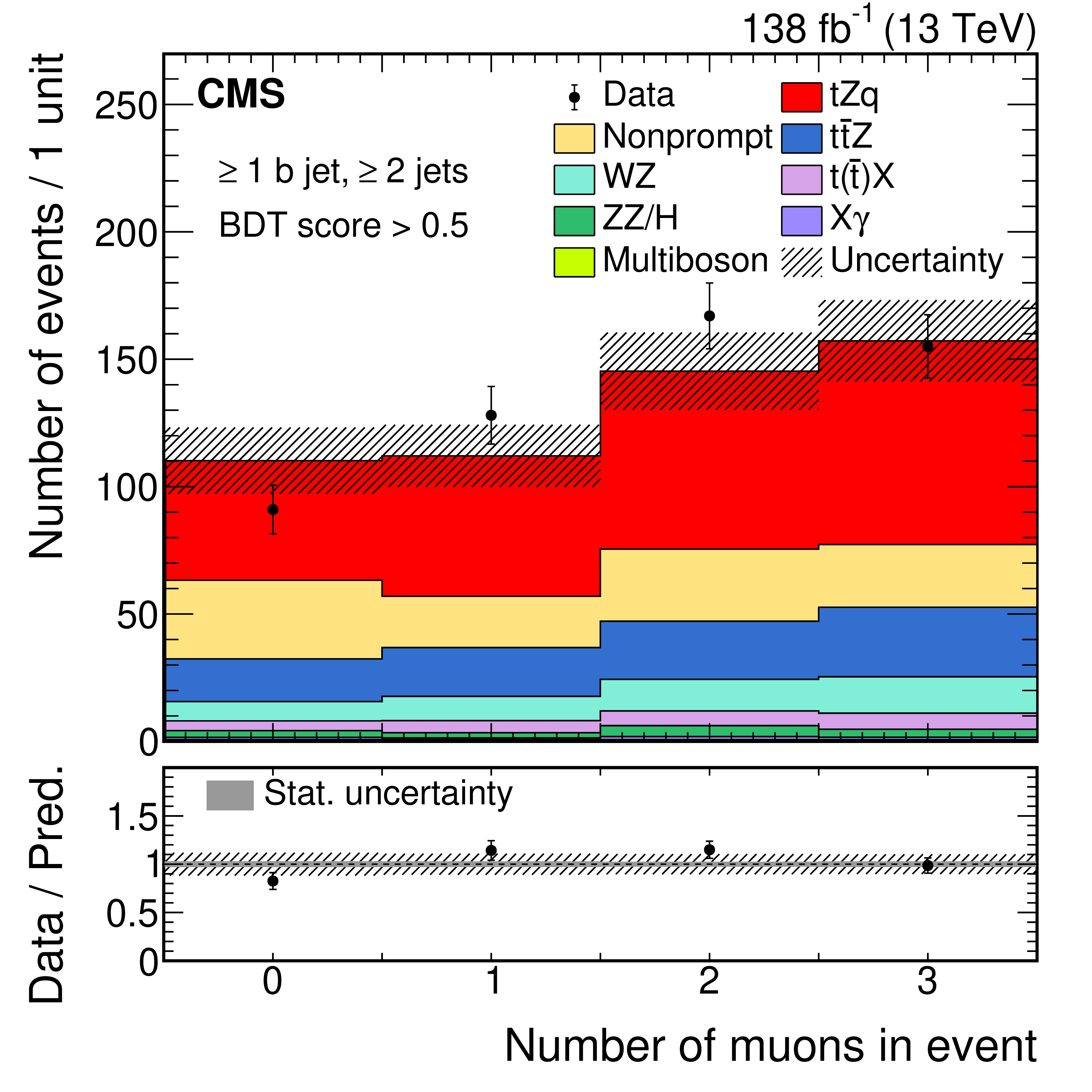
Figure 9-b:
Distribution at the detector level of the number of muons in the event, which is an important variable used in the tZq analysis from a tZq-enriched region for the data (points) and predictions (colored histograms). The selection criteria discussed in Section 4 have been used, along with the requirement that the event BDT discriminant be greater than 0.5. The lower panel shows the ratio of the data to the sum of the predictions. The vertical lines on the data points represent the statistical uncertainty in the data; the shaded area corresponds to the total uncertainty in the prediction; the gray area in the ratio indicates the uncertainty related to the limited statistical precision in the prediction. |
png pdf |
Figure 9-c:
Distribution at the detector level of the reconstructed transverse momentum of the Z boson, which is an important variable used in the tZq analysis from a tZq-enriched region for the data (points) and predictions (colored histograms). The selection criteria discussed in Section 4 have been used, along with the requirement that the event BDT discriminant be greater than 0.5. The lower panel shows the ratio of the data to the sum of the predictions. The vertical lines on the data points represent the statistical uncertainty in the data; the shaded area corresponds to the total uncertainty in the prediction; the gray area in the ratio indicates the uncertainty related to the limited statistical precision in the prediction. |
png pdf |
Figure 9-d:
Distribution at the detector level of the transverse mass of the W boson, which is an important variable used in the tZq analysis from a tZq-enriched region for the data (points) and predictions (colored histograms). The selection criteria discussed in Section 4 have been used, along with the requirement that the event BDT discriminant be greater than 0.5. The lower panel shows the ratio of the data to the sum of the predictions. The vertical lines on the data points represent the statistical uncertainty in the data; the shaded area corresponds to the total uncertainty in the prediction; the gray area in the ratio indicates the uncertainty related to the limited statistical precision in the prediction. |

png pdf |
Figure 10:
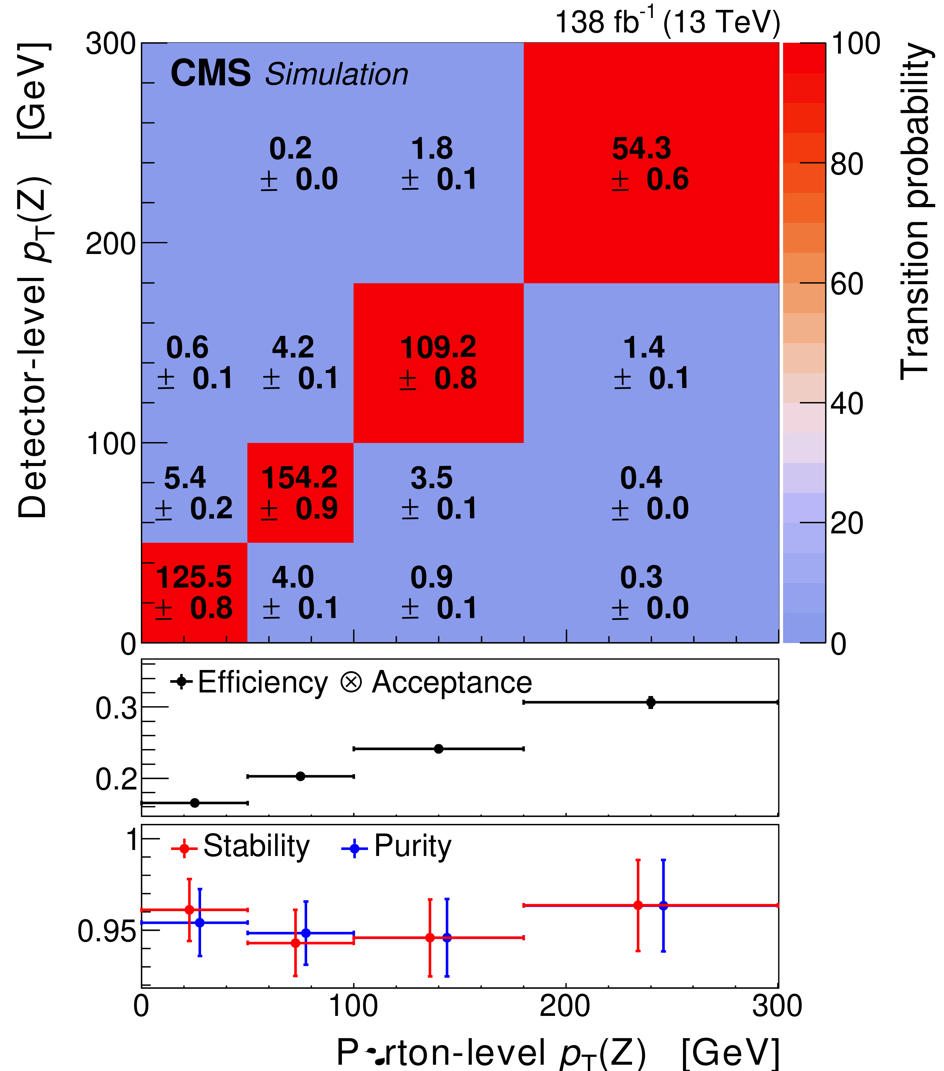
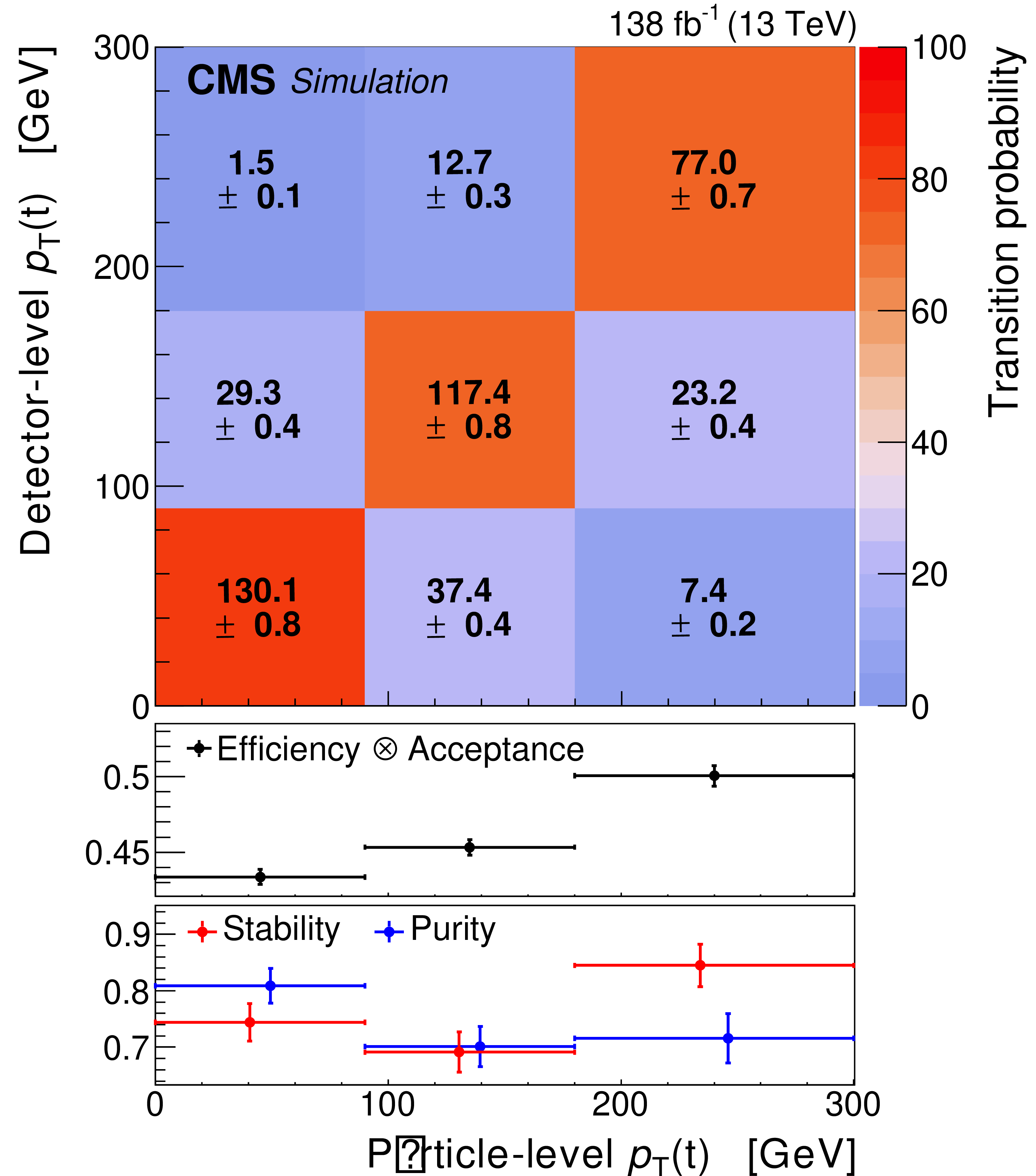
Response matrices for ${{p_{\mathrm {T}}} (\mathrm{Z})}$ at the parton level (left) and ${{p_{\mathrm {T}}} (\mathrm{t})}$ at the particle level (right) for tZq events in the full and visible phase space, respectively. The expected number of reconstructed events is given for each bin. The color indicates the transition probability for an event in a generator-level bin to have a reconstructed value corresponding to a given detector-level bin. The efficiency times acceptance values of reconstructing events are plotted in the middle panels. The lower panels show the stability and purity values as defined in the text. The vertical bars on the points give the statistical uncertainty and the horizontal bars show the bin width. |
png pdf |
Figure 10-a:
Response matrix for ${{p_{\mathrm {T}}} (\mathrm{Z})}$ at the parton level for tZq events in the full and visible phase space, respectively. The expected number of reconstructed events is given for each bin. The color indicates the transition probability for an event in a generator-level bin to have a reconstructed value corresponding to a given detector-level bin. The efficiency times acceptance values of reconstructing events are plotted in the middle panels. The lower panels show the stability and purity values as defined in the text. The vertical bars on the points give the statistical uncertainty and the horizontal bars show the bin width. |
png pdf |
Figure 10-b:
Response matrix for ${{p_{\mathrm {T}}} (\mathrm{t})}$ at the particle level for tZq events in the full and visible phase space, respectively. The expected number of reconstructed events is given for each bin. The color indicates the transition probability for an event in a generator-level bin to have a reconstructed value corresponding to a given detector-level bin. The efficiency times acceptance values of reconstructing events are plotted in the middle panels. The lower panels show the stability and purity values as defined in the text. The vertical bars on the points give the statistical uncertainty and the horizontal bars show the bin width. |
png pdf |
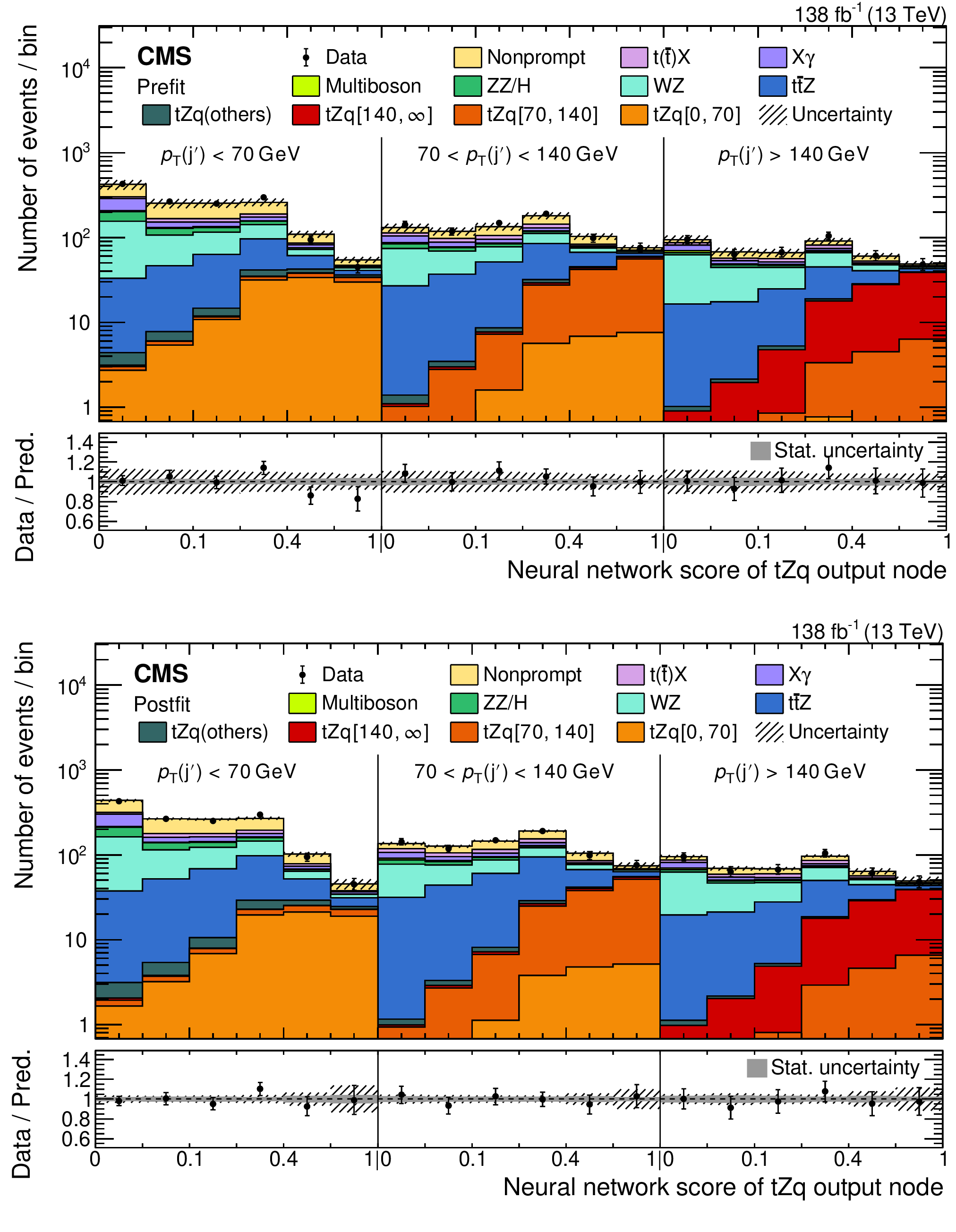
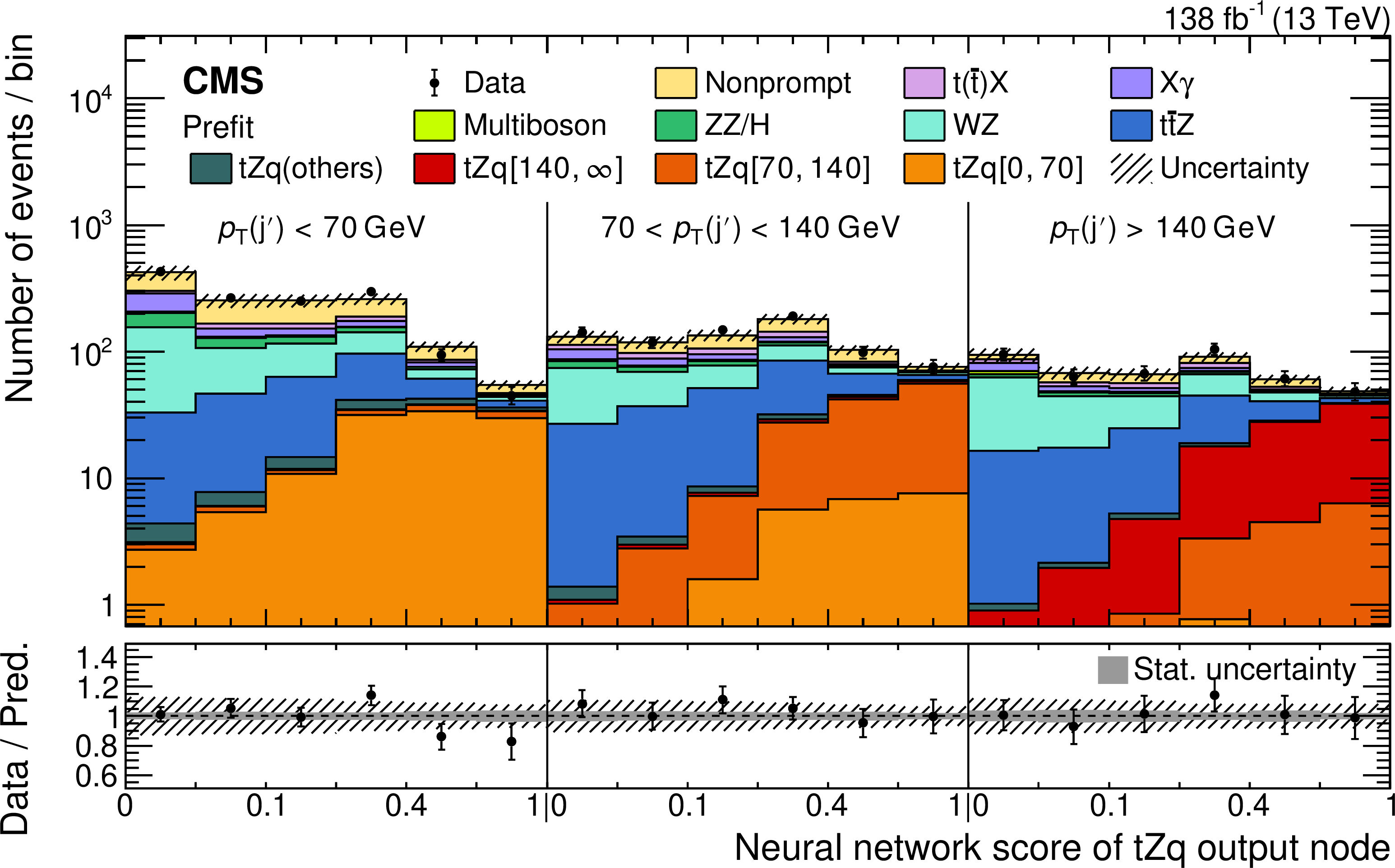
Figure 11:
Prefit (upper) and postfit (lower) distributions of the neural network score from the tZq output node for events in the signal region with fewer than four jets, used for the ${{p_{\mathrm {T}}} (\mathrm {j}')}$ differential cross section measurement at the particle level. The data are shown by the points and the predictions by the colored histograms. The vertical lines on the points represent the statistical uncertainty in the data, and the hatched region the total uncertainty in the prediction. The events are split into three subregions based on the value of ${{p_{\mathrm {T}}} (\mathrm {j}')}$ measured at the detector level. Three different tZq templates, defined by the same intervals of ${{p_{\mathrm {T}}} (\mathrm {j}')}$ at the particle level and shown in different shades of orange and red, are used to model the contribution of each particle-level bin. Reconstructed tZq events that are outside the fiducial phase space are labeled as " tZq (others)'' and represent a minor contribution. The lower panels show the ratio of the data to the sum of the predictions, with the gray band indicating the uncertainty from the finite number of MC events. |
png pdf |
Figure 11-a:
Prefit distribution of the neural network score from the tZq output node for events in the signal region with fewer than four jets, used for the ${{p_{\mathrm {T}}} (\mathrm {j}')}$ differential cross section measurement at the particle level. The data are shown by the points and the predictions by the colored histograms. The vertical lines on the points represent the statistical uncertainty in the data, and the hatched region the total uncertainty in the prediction. The events are split into three subregions based on the value of ${{p_{\mathrm {T}}} (\mathrm {j}')}$ measured at the detector level. Three different tZq templates, defined by the same intervals of ${{p_{\mathrm {T}}} (\mathrm {j}')}$ at the particle level and shown in different shades of orange and red, are used to model the contribution of each particle-level bin. Reconstructed tZq events that are outside the fiducial phase space are labeled as " tZq (others)'' and represent a minor contribution. The lower panel shows the ratio of the data to the sum of the predictions, with the gray band indicating the uncertainty from the finite number of MC events. |
png pdf |
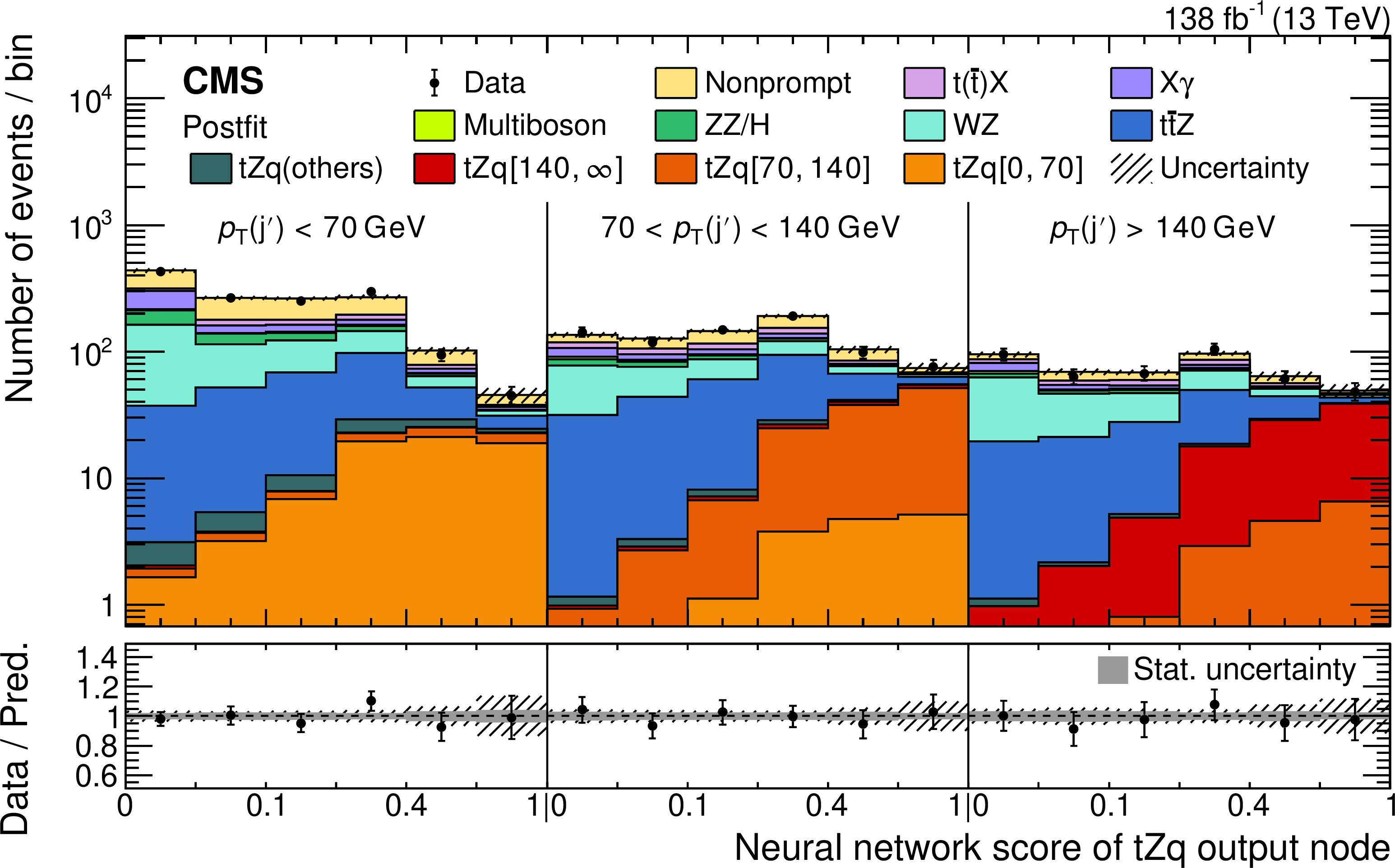
Figure 11-b:
Postfit distribution of the neural network score from the tZq output node for events in the signal region with fewer than four jets, used for the ${{p_{\mathrm {T}}} (\mathrm {j}')}$ differential cross section measurement at the particle level. The data are shown by the points and the predictions by the colored histograms. The vertical lines on the points represent the statistical uncertainty in the data, and the hatched region the total uncertainty in the prediction. The events are split into three subregions based on the value of ${{p_{\mathrm {T}}} (\mathrm {j}')}$ measured at the detector level. Three different tZq templates, defined by the same intervals of ${{p_{\mathrm {T}}} (\mathrm {j}')}$ at the particle level and shown in different shades of orange and red, are used to model the contribution of each particle-level bin. Reconstructed tZq events that are outside the fiducial phase space are labeled as " tZq (others)'' and represent a minor contribution. The lower panel shows the ratio of the data to the sum of the predictions, with the gray band indicating the uncertainty from the finite number of MC events. |

png pdf |
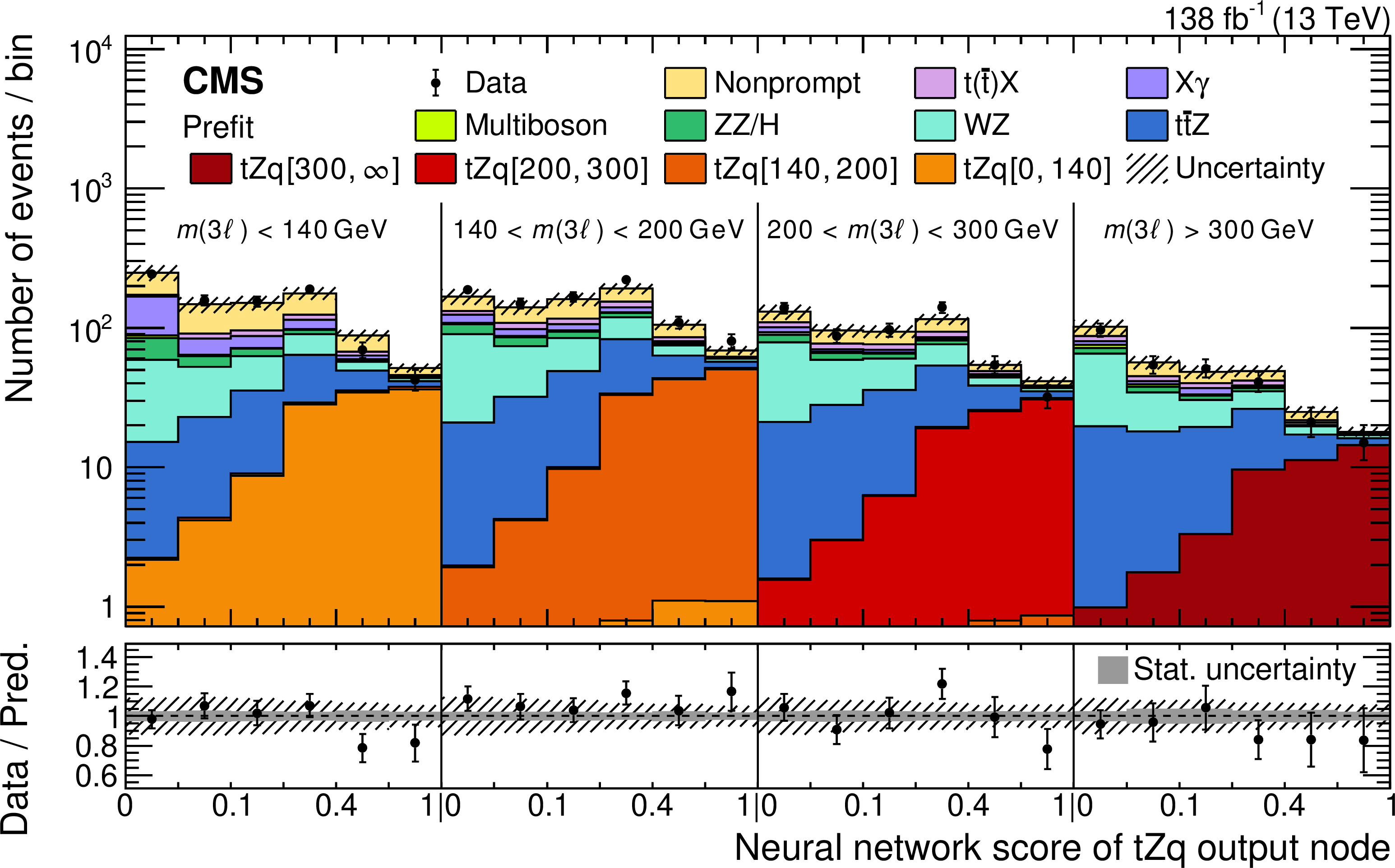
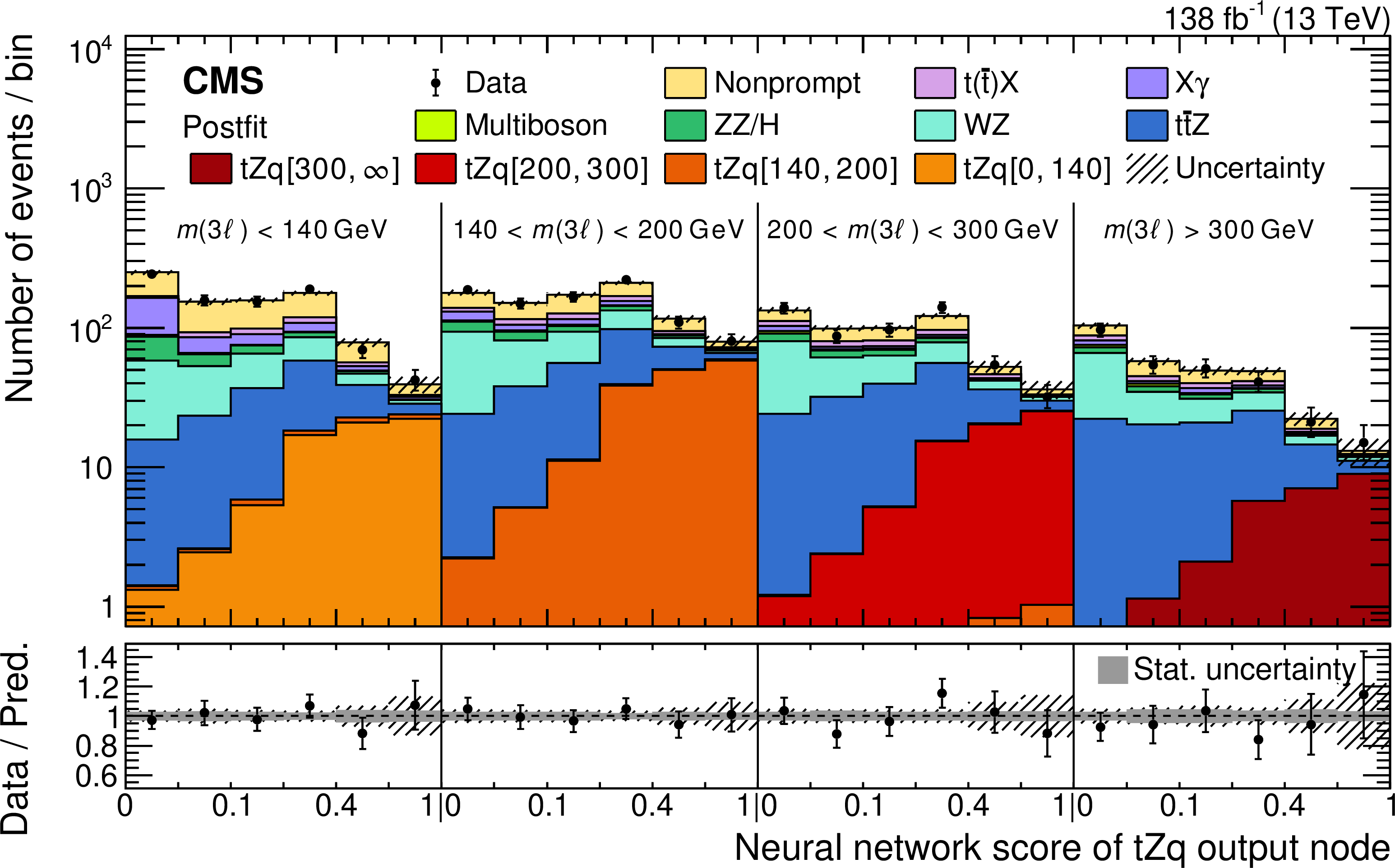
Figure 12:
Prefit (upper) and postfit (lower) distributions of the neural network score from the tZq output node for events in the signal region with fewer than four jets, used for the ${m(3\ell)}$ differential cross section measurement at the parton level. The data are shown by the points and the predictions by the colored histograms. The vertical lines on the points represent the statistical uncertainty in the data, and the hatched region the total uncertainty in the prediction. The events are split into four subregions based on the value of ${m(3\ell)}$ measured at the detector level. Four different tZq templates, defined by the same intervals of ${m(3\ell)}$ at the parton level and shown in different shades of orange and red, are used to model the contribution of each parton-level bin. The lower panels show the ratio of the data to the sum of the predictions, with the gray band indicating the uncertainty from the finite number of MC events. |
png pdf |
Figure 12-a:
Prefit distribution of the neural network score from the tZq output node for events in the signal region with fewer than four jets, used for the ${m(3\ell)}$ differential cross section measurement at the parton level. The data are shown by the points and the predictions by the colored histograms. The vertical lines on the points represent the statistical uncertainty in the data, and the hatched region the total uncertainty in the prediction. The events are split into four subregions based on the value of ${m(3\ell)}$ measured at the detector level. Four different tZq templates, defined by the same intervals of ${m(3\ell)}$ at the parton level and shown in different shades of orange and red, are used to model the contribution of each parton-level bin. The lower panel shows the ratio of the data to the sum of the predictions, with the gray band indicating the uncertainty from the finite number of MC events. |
png pdf |
Figure 12-b:
Postfit distribution of the neural network score from the tZq output node for events in the signal region with fewer than four jets, used for the ${m(3\ell)}$ differential cross section measurement at the parton level. The data are shown by the points and the predictions by the colored histograms. The vertical lines on the points represent the statistical uncertainty in the data, and the hatched region the total uncertainty in the prediction. The events are split into four subregions based on the value of ${m(3\ell)}$ measured at the detector level. Four different tZq templates, defined by the same intervals of ${m(3\ell)}$ at the parton level and shown in different shades of orange and red, are used to model the contribution of each parton-level bin. The lower panel shows the ratio of the data to the sum of the predictions, with the gray band indicating the uncertainty from the finite number of MC events. |

png pdf |
Figure 13:
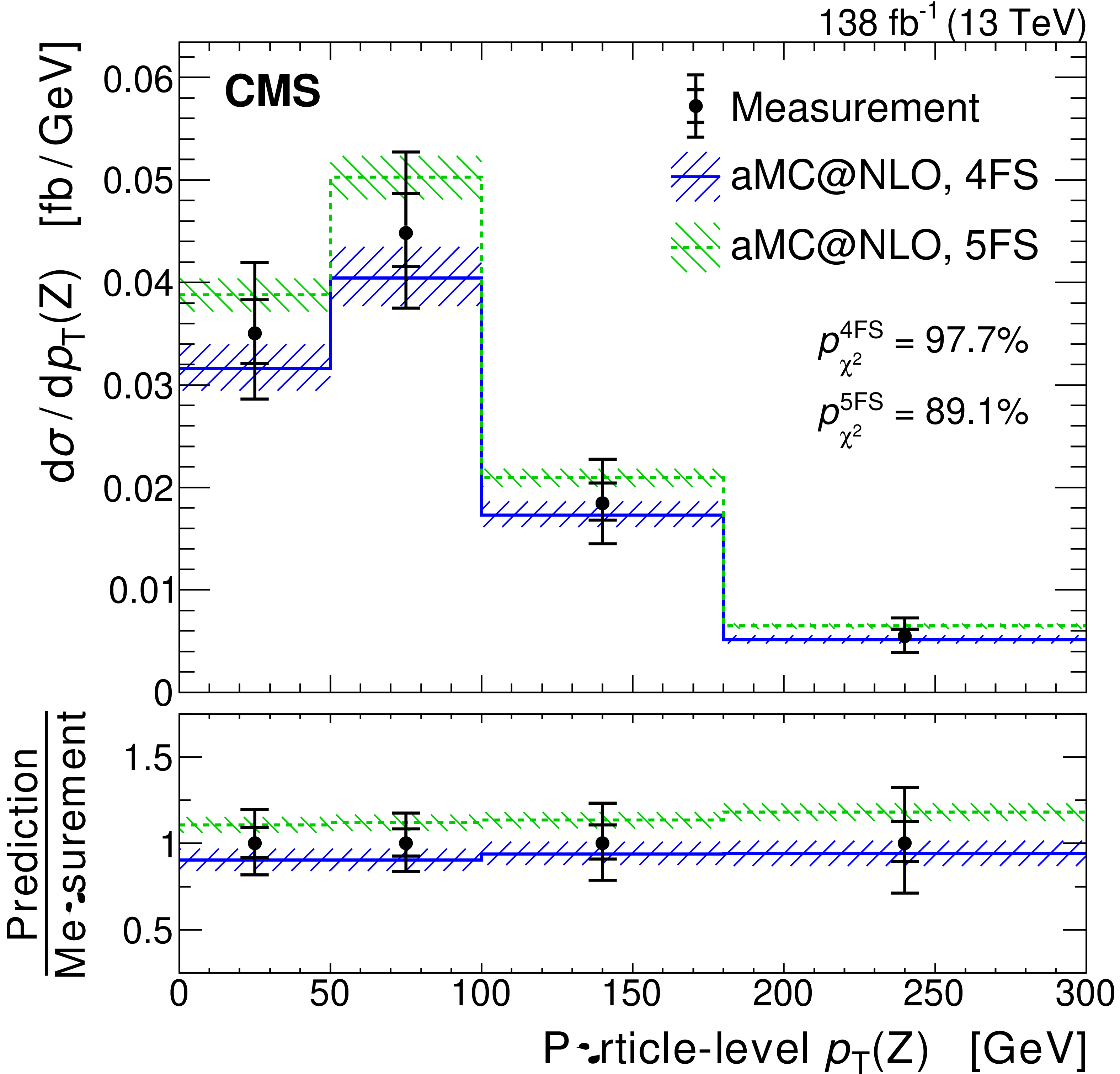
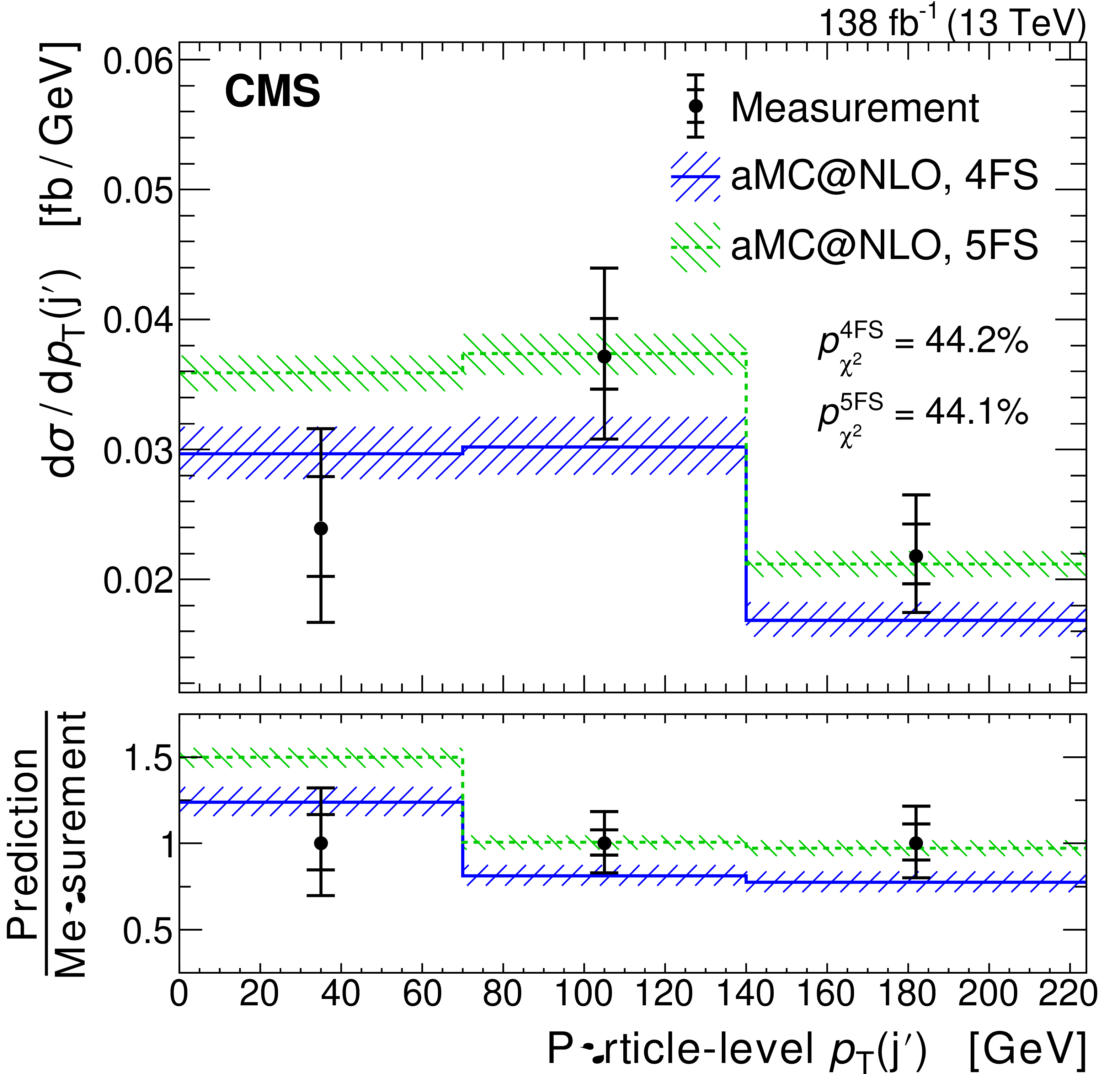
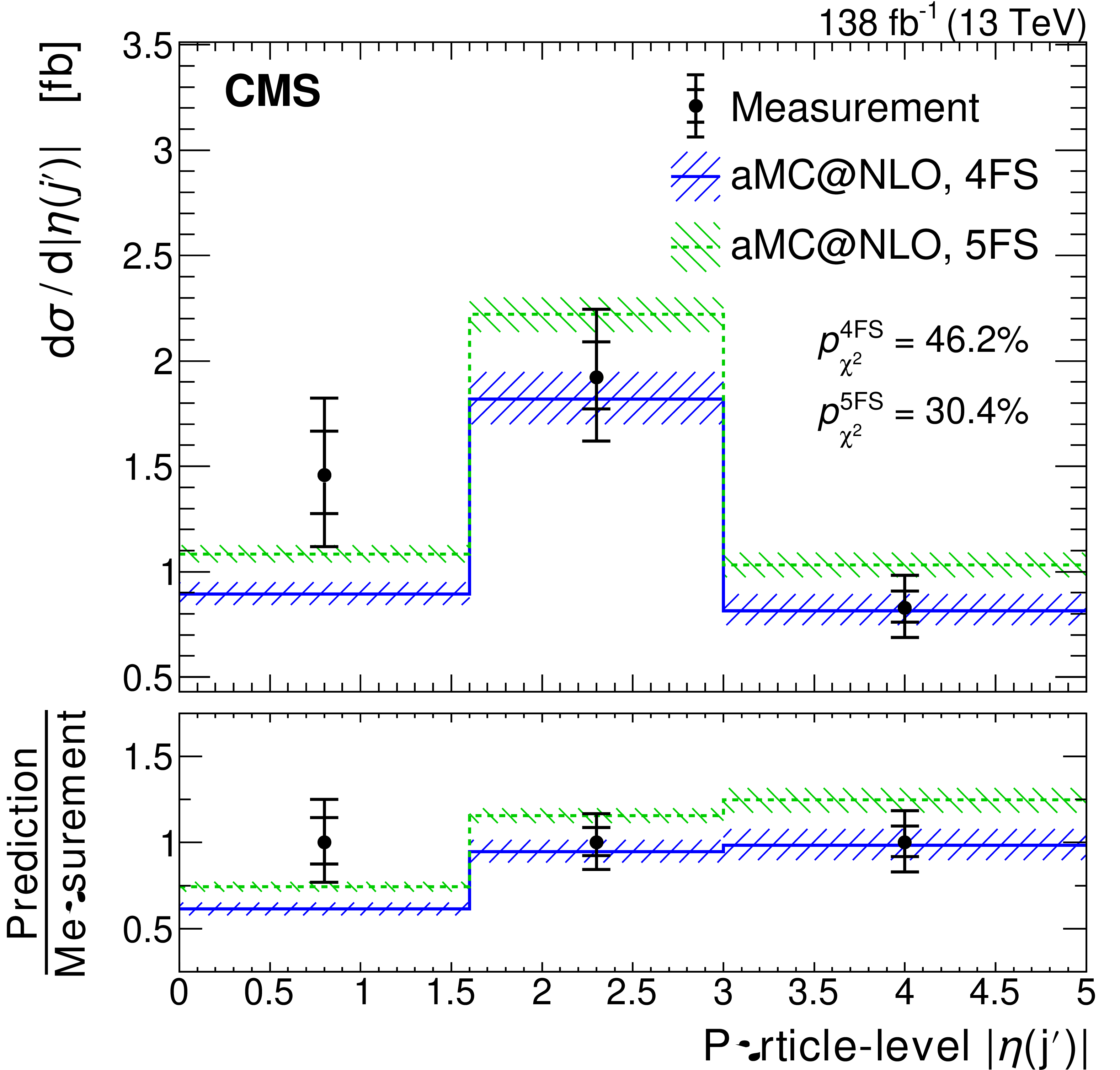
Absolute differential cross sections as a function of ${{p_{\mathrm {T}}} (\mathrm{Z})}$ measured at the parton (upper left) and particle levels (upper right), as well as a function of ${{p_{\mathrm {T}}} (\mathrm {j}')}$ (lower left) and $ | \eta (\mathrm {j}') | $ (lower right) at the particle level. The observed values are shown as black points, with the inner and outer vertical bars giving the systematic and total uncertainties, respectively. The SM predictions for the tZq process are based on events simulated in the 5FS (green) and 4FS (blue). The $p$-values of the ${{\chi ^2}}$ tests are given to quantify their compatibility with the measurement. The lower panels show the ratio of the simulation to the measurement. |

png pdf |
Figure 13-a:
Absolute differential cross sections as a function of ${{p_{\mathrm {T}}} (\mathrm{Z})}$ measured at the parton level. The observed values are shown as black points, with the inner and outer vertical bars giving the systematic and total uncertainties, respectively. The SM predictions for the tZq process are based on events simulated in the 5FS (green) and 4FS (blue). The $p$-values of the ${{\chi ^2}}$ tests are given to quantify their compatibility with the measurement. The lower panel shows the ratio of the simulation to the measurement. |
png pdf |
Figure 13-b:
Absolute differential cross sections as a function of ${{p_{\mathrm {T}}} (\mathrm{Z})}$ measured at the particle level. The observed values are shown as black points, with the inner and outer vertical bars giving the systematic and total uncertainties, respectively. The SM predictions for the tZq process are based on events simulated in the 5FS (green) and 4FS (blue). The $p$-values of the ${{\chi ^2}}$ tests are given to quantify their compatibility with the measurement. The lower panel shows the ratio of the simulation to the measurement. |
png pdf |
Figure 13-c:
Absolute differential cross sections as a function of ${{p_{\mathrm {T}}} (\mathrm {j}')}$ at the particle level. The observed values are shown as black points, with the inner and outer vertical bars giving the systematic and total uncertainties, respectively. The SM predictions for the tZq process are based on events simulated in the 5FS (green) and 4FS (blue). The $p$-values of the ${{\chi ^2}}$ tests are given to quantify their compatibility with the measurement. The lower panel shows the ratio of the simulation to the measurement. |
png pdf |
Figure 13-d:
Absolute differential cross sections as a function of $ | \eta (\mathrm {j}') | $ at the particle level. The observed values are shown as black points, with the inner and outer vertical bars giving the systematic and total uncertainties, respectively. The SM predictions for the tZq process are based on events simulated in the 5FS (green) and 4FS (blue). The $p$-values of the ${{\chi ^2}}$ tests are given to quantify their compatibility with the measurement. The lower panel shows the ratio of the simulation to the measurement. |
png pdf |
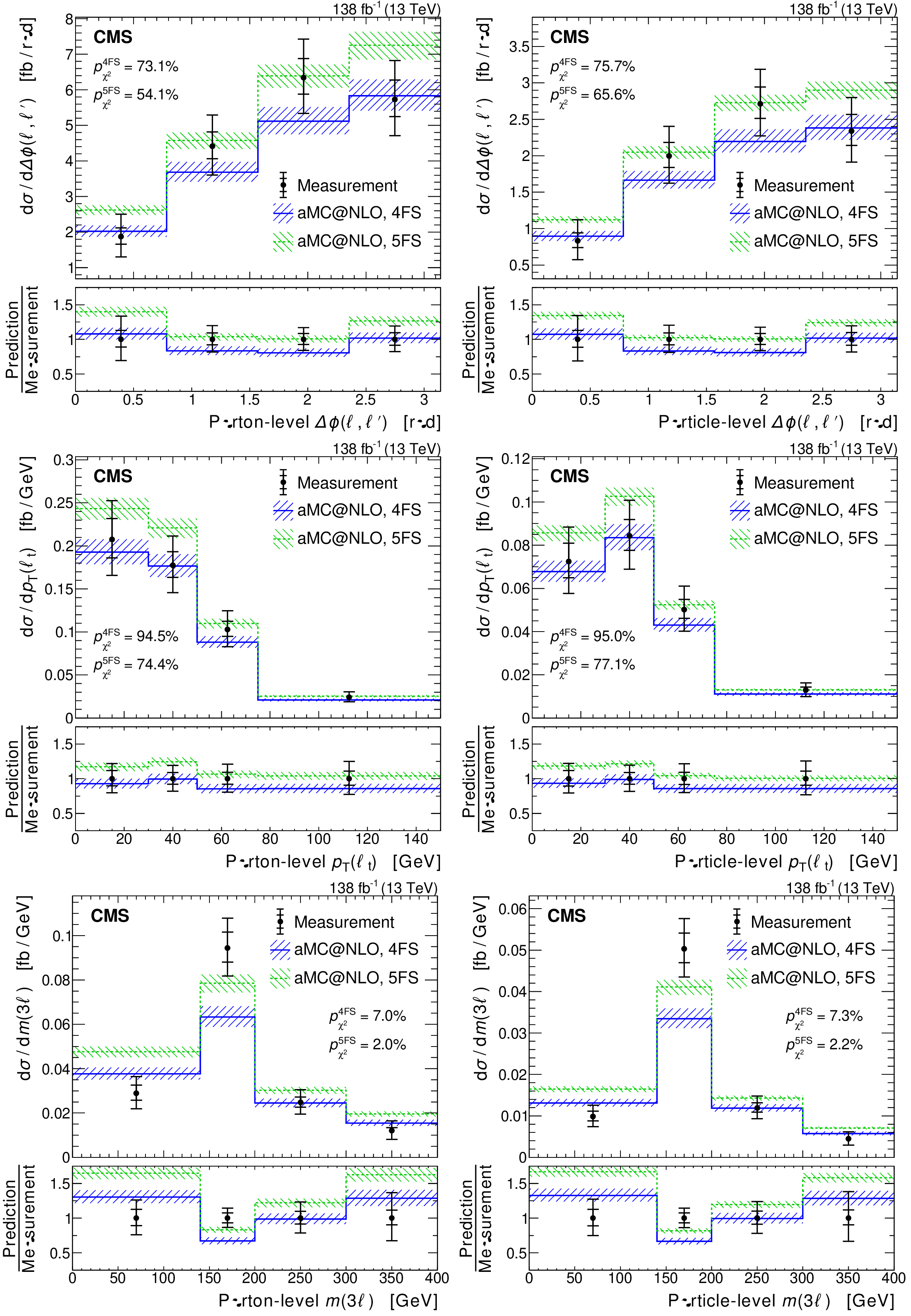
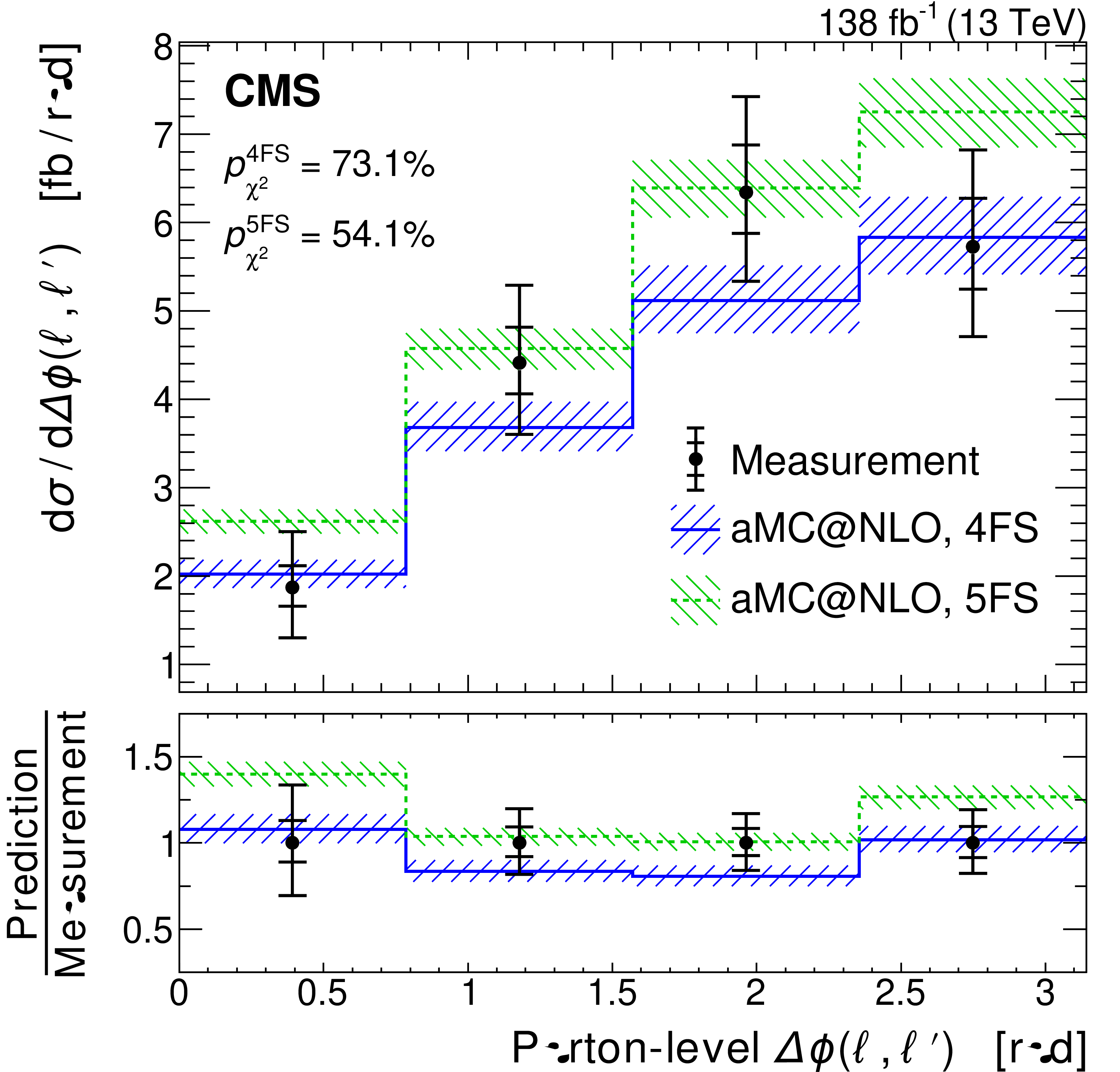
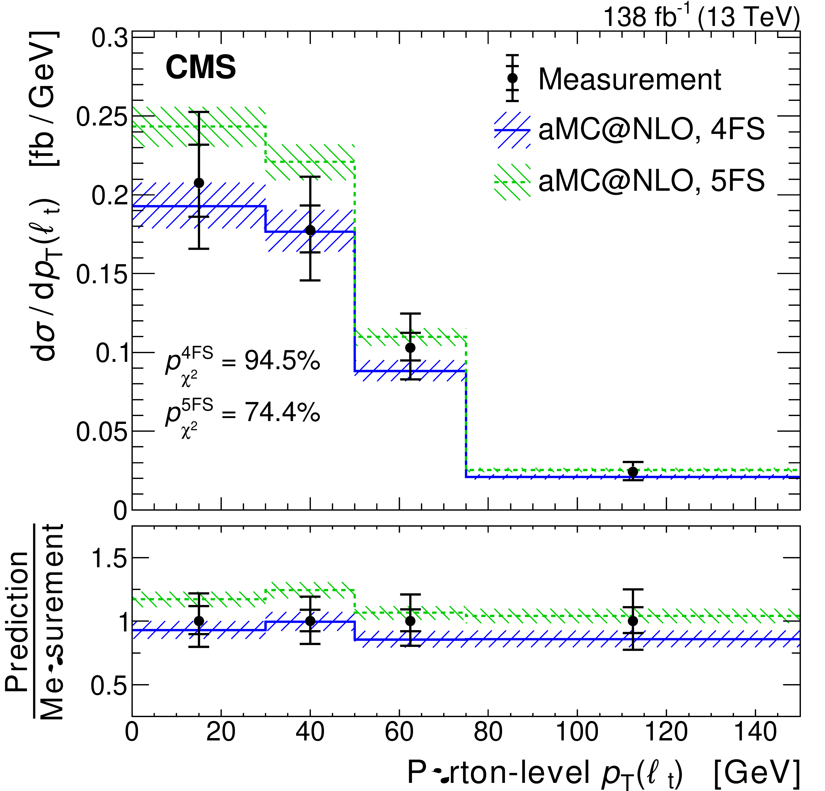
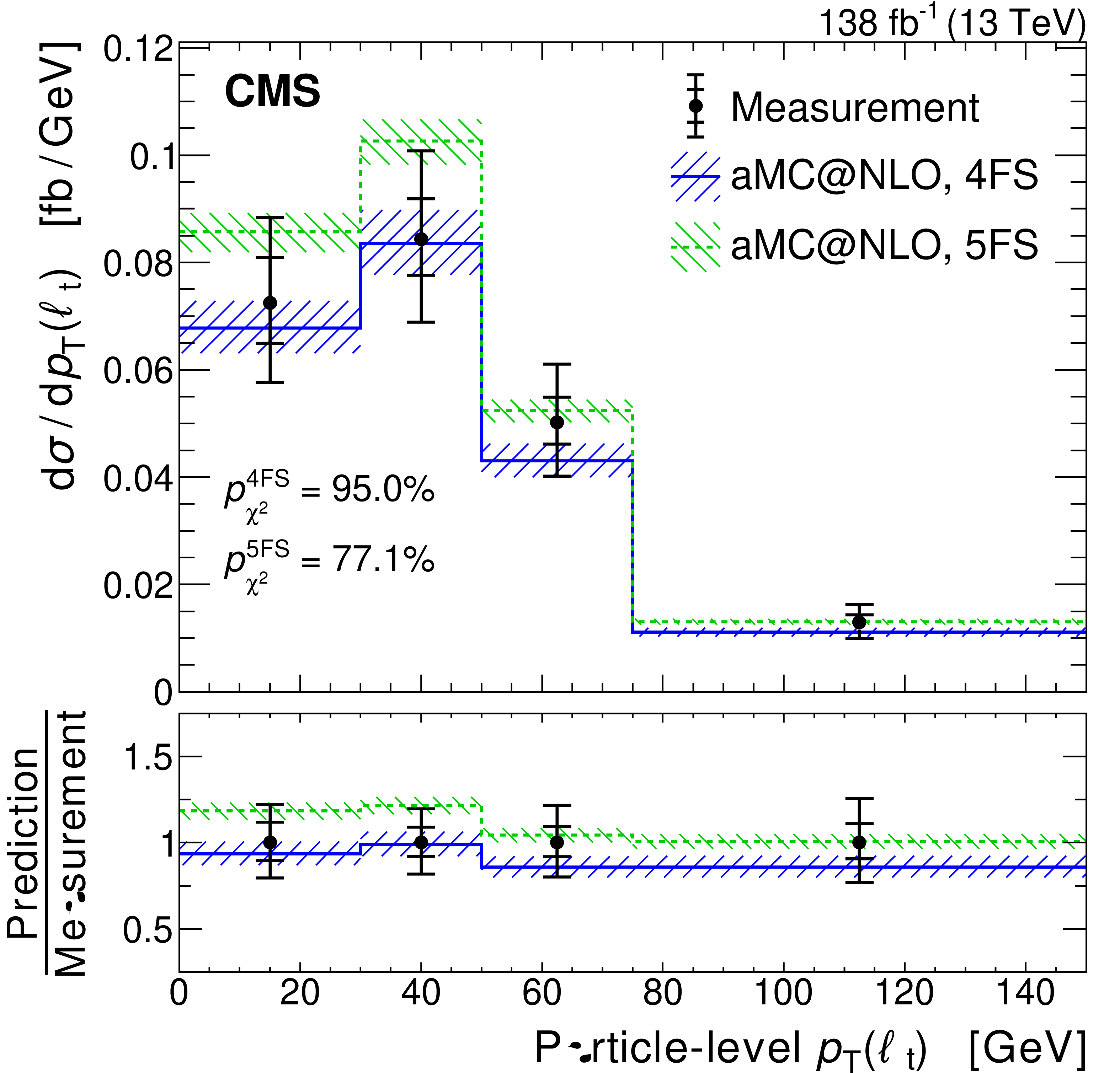
Figure 14:
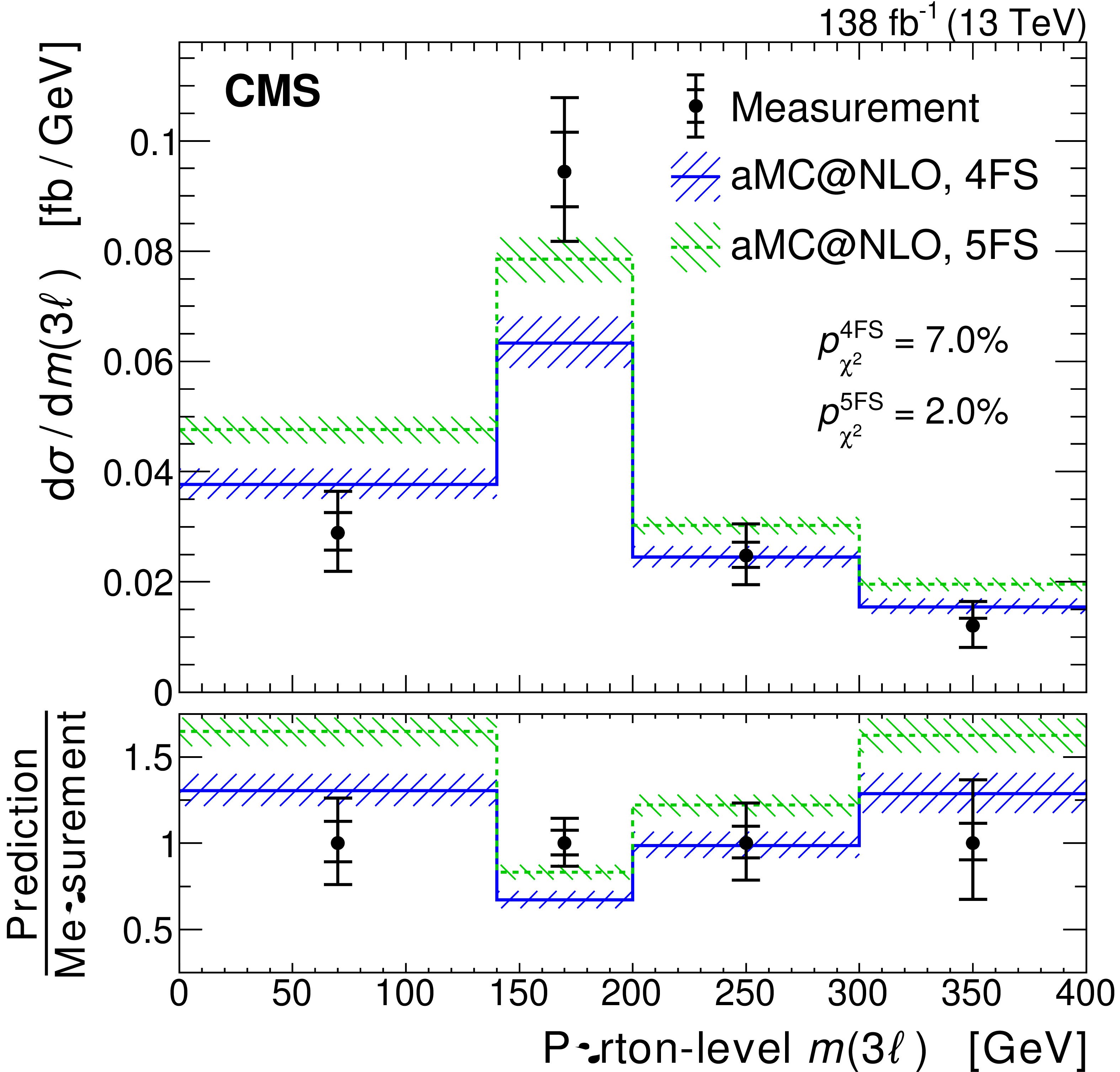
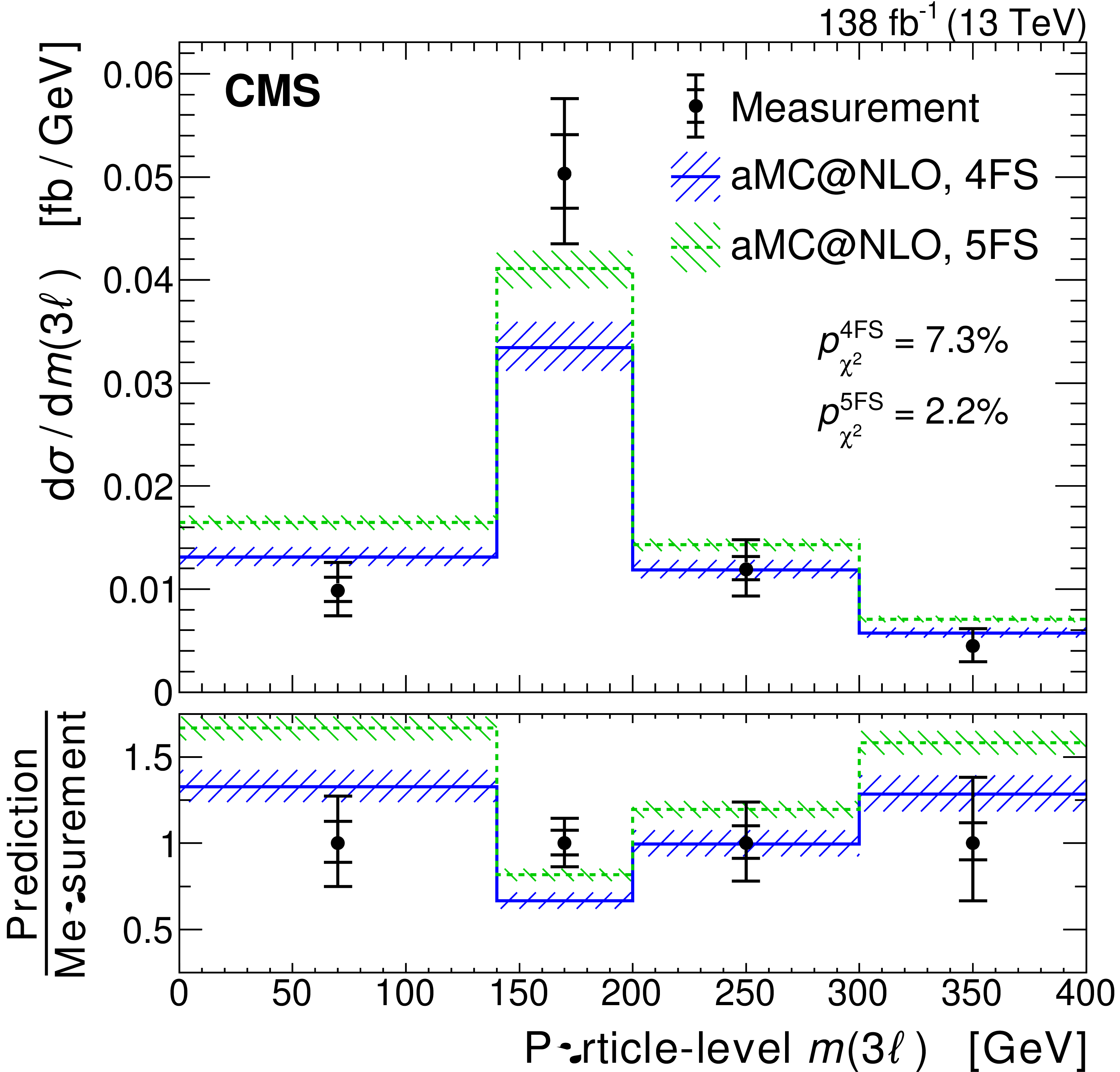
Absolute differential cross sections at the parton (left) and particle level (right) measured as a function of ${{\Delta \phi} (\ell,\ell ')}$ (upper), ${{p_{\mathrm {T}}} (\ell _{\mathrm{t}})}$ (middle) and ${m(3\ell)}$ (lower). The observed values are shown as black points, with the inner and outer vertical bars giving the systematic and total uncertainties, respectively. The SM predictions for the tZq process are based on events simulated in the 5FS (green) and 4FS (blue). The $p$-values of the ${{\chi ^2}}$ tests are given to quantify their compatibility with the measurement. The lower panels show the ratio of the simulation to the measurement. |
png pdf |
Figure 14-a:
Absolute differential cross sections at the parton level measured as a function of ${{\Delta \phi} (\ell,\ell ')}$. The observed values are shown as black points, with the inner and outer vertical bars giving the systematic and total uncertainties, respectively. The SM predictions for the tZq process are based on events simulated in the 5FS (green) and 4FS (blue). The $p$-values of the ${{\chi ^2}}$ tests are given to quantify their compatibility with the measurement. The lower panel shows the ratio of the simulation to the measurement. |

png pdf |
Figure 14-b:
Absolute differential cross sections at the particle level measured as a function of ${{\Delta \phi} (\ell,\ell ')}$. The observed values are shown as black points, with the inner and outer vertical bars giving the systematic and total uncertainties, respectively. The SM predictions for the tZq process are based on events simulated in the 5FS (green) and 4FS (blue). The $p$-values of the ${{\chi ^2}}$ tests are given to quantify their compatibility with the measurement. The lower panel shows the ratio of the simulation to the measurement. |
png pdf |
Figure 14-c:
Absolute differential cross sections at the parton level measured as a function of ${{p_{\mathrm {T}}} (\ell _{\mathrm{t}})}$. The observed values are shown as black points, with the inner and outer vertical bars giving the systematic and total uncertainties, respectively. The SM predictions for the tZq process are based on events simulated in the 5FS (green) and 4FS (blue). The $p$-values of the ${{\chi ^2}}$ tests are given to quantify their compatibility with the measurement. The lower panel shows the ratio of the simulation to the measurement. |
png pdf |
Figure 14-d:
Absolute differential cross sections at the particle level measured as a function of ${{p_{\mathrm {T}}} (\ell _{\mathrm{t}})}$. The observed values are shown as black points, with the inner and outer vertical bars giving the systematic and total uncertainties, respectively. The SM predictions for the tZq process are based on events simulated in the 5FS (green) and 4FS (blue). The $p$-values of the ${{\chi ^2}}$ tests are given to quantify their compatibility with the measurement. The lower panel shows the ratio of the simulation to the measurement. |
png pdf |
Figure 14-e:
Absolute differential cross sections at the parton level measured as a function of ${m(3\ell)}$. The observed values are shown as black points, with the inner and outer vertical bars giving the systematic and total uncertainties, respectively. The SM predictions for the tZq process are based on events simulated in the 5FS (green) and 4FS (blue). The $p$-values of the ${{\chi ^2}}$ tests are given to quantify their compatibility with the measurement. The lower panel shows the ratio of the simulation to the measurement. |
png pdf |
Figure 14-f:
Absolute differential cross sections at the particle level measured as a function of ${m(3\ell)}$. The observed values are shown as black points, with the inner and outer vertical bars giving the systematic and total uncertainties, respectively. The SM predictions for the tZq process are based on events simulated in the 5FS (green) and 4FS (blue). The $p$-values of the ${{\chi ^2}}$ tests are given to quantify their compatibility with the measurement. The lower panel shows the ratio of the simulation to the measurement. |
png pdf |
Figure 15:
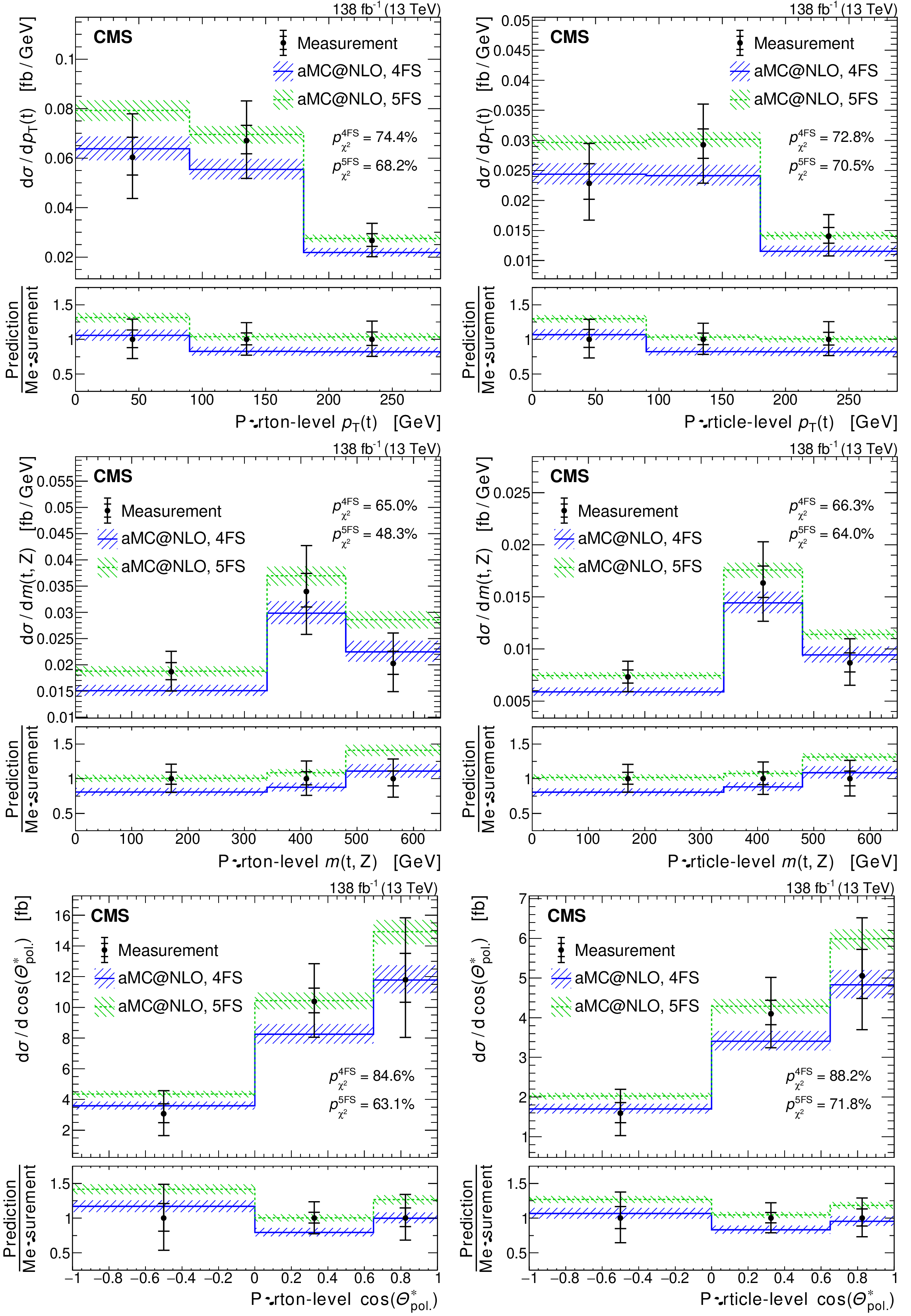
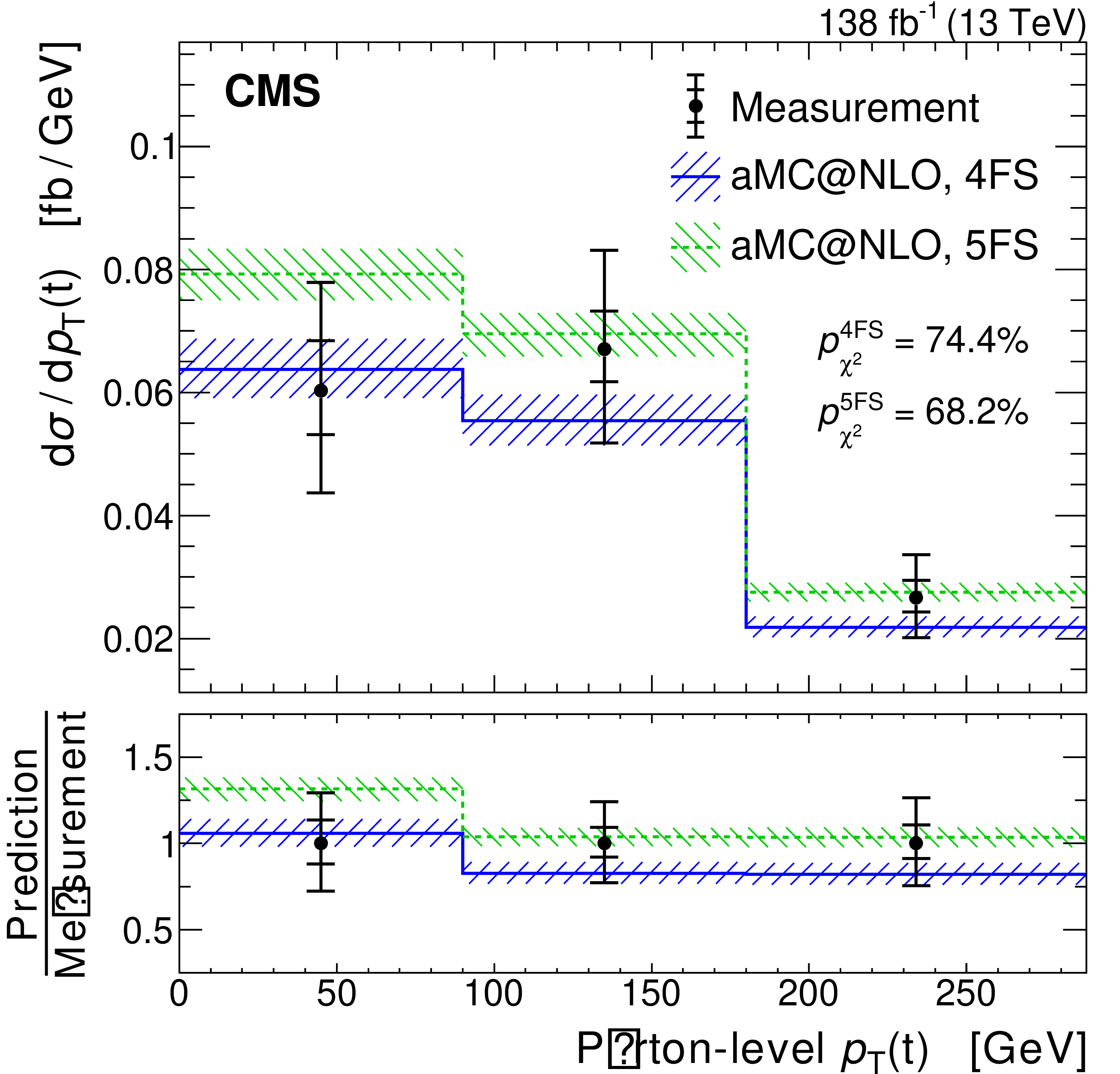
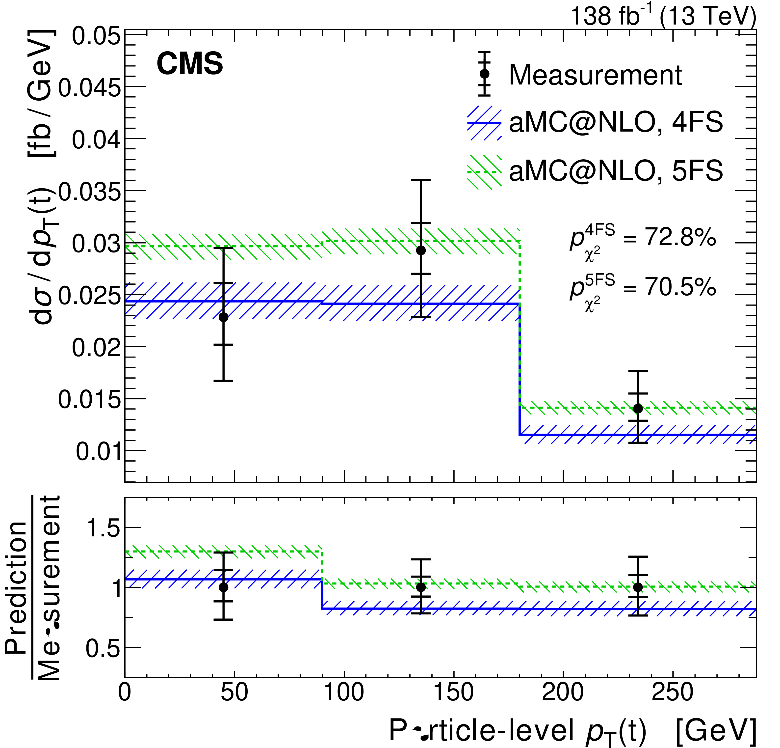
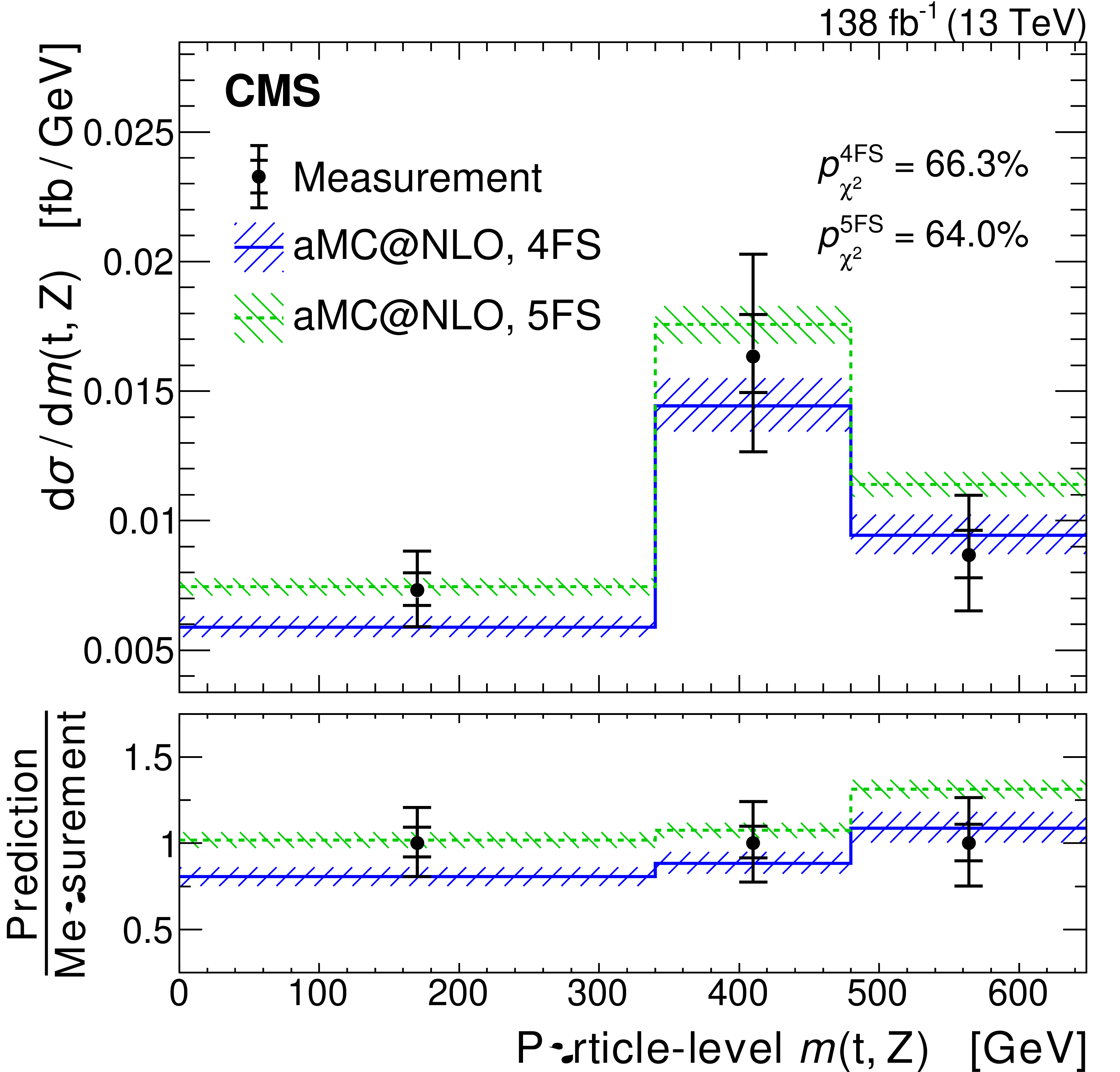
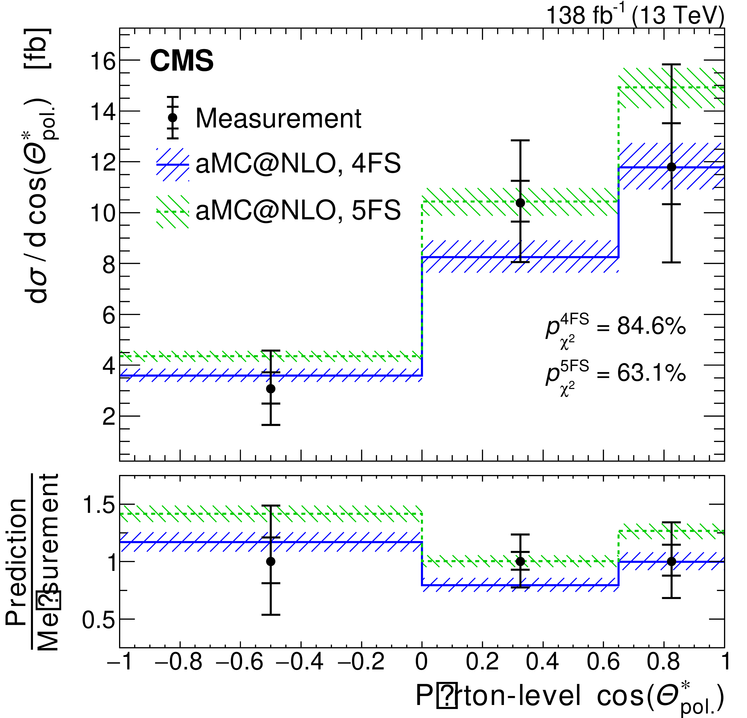
Absolute differential cross sections at the parton (left) and particle level (right) measured as a function of ${{p_{\mathrm {T}}} (\mathrm{t})}$ (upper), ${m(\mathrm{t},\mathrm{Z})}$ (middle) and ${\cos(\theta ^{\star}_{\text {pol}})}$ (lower). The observed values are shown as black points, with the inner and outer vertical bars giving the systematic and total uncertainties, respectively. The SM predictions for the tZq process are based on events simulated in the 5FS (green) and 4FS (blue). The $p$-values of the ${{\chi ^2}}$ tests are given to quantify their compatibility with the measurement. The lower panels show the ratio of the simulation to the measurement. |
png pdf |
Figure 15-a:
Absolute differential cross sections at the parton level measured as a function of ${{p_{\mathrm {T}}} (\mathrm{t})}$. The observed values are shown as black points, with the inner and outer vertical bars giving the systematic and total uncertainties, respectively. The SM predictions for the tZq process are based on events simulated in the 5FS (green) and 4FS (blue). The $p$-values of the ${{\chi ^2}}$ tests are given to quantify their compatibility with the measurement. The lower panel shows the ratio of the simulation to the measurement. |
png pdf |
Figure 15-b:
Absolute differential cross sections at the particle level measured as a function of ${{p_{\mathrm {T}}} (\mathrm{t})}$. The observed values are shown as black points, with the inner and outer vertical bars giving the systematic and total uncertainties, respectively. The SM predictions for the tZq process are based on events simulated in the 5FS (green) and 4FS (blue). The $p$-values of the ${{\chi ^2}}$ tests are given to quantify their compatibility with the measurement. The lower panel shows the ratio of the simulation to the measurement. |

png pdf |
Figure 15-c:
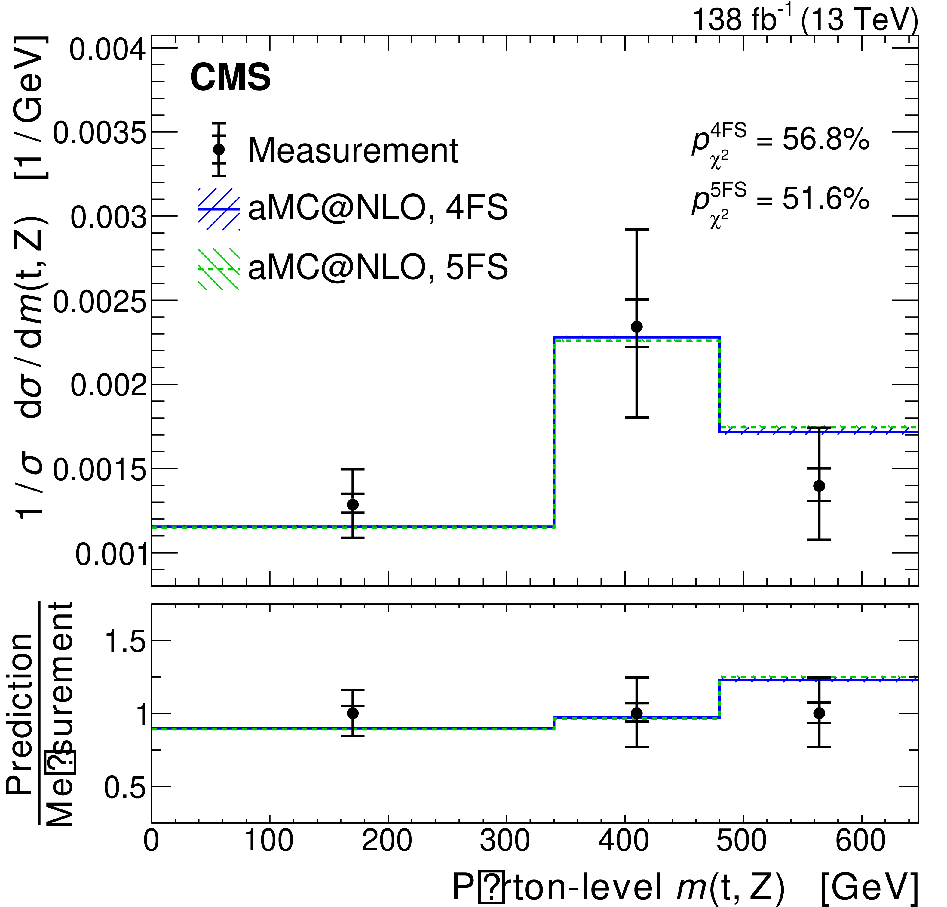
Absolute differential cross sections at the parton level measured as a function of ${m(\mathrm{t},\mathrm{Z})}$. The observed values are shown as black points, with the inner and outer vertical bars giving the systematic and total uncertainties, respectively. The SM predictions for the tZq process are based on events simulated in the 5FS (green) and 4FS (blue). The $p$-values of the ${{\chi ^2}}$ tests are given to quantify their compatibility with the measurement. The lower panel shows the ratio of the simulation to the measurement. |
png pdf |
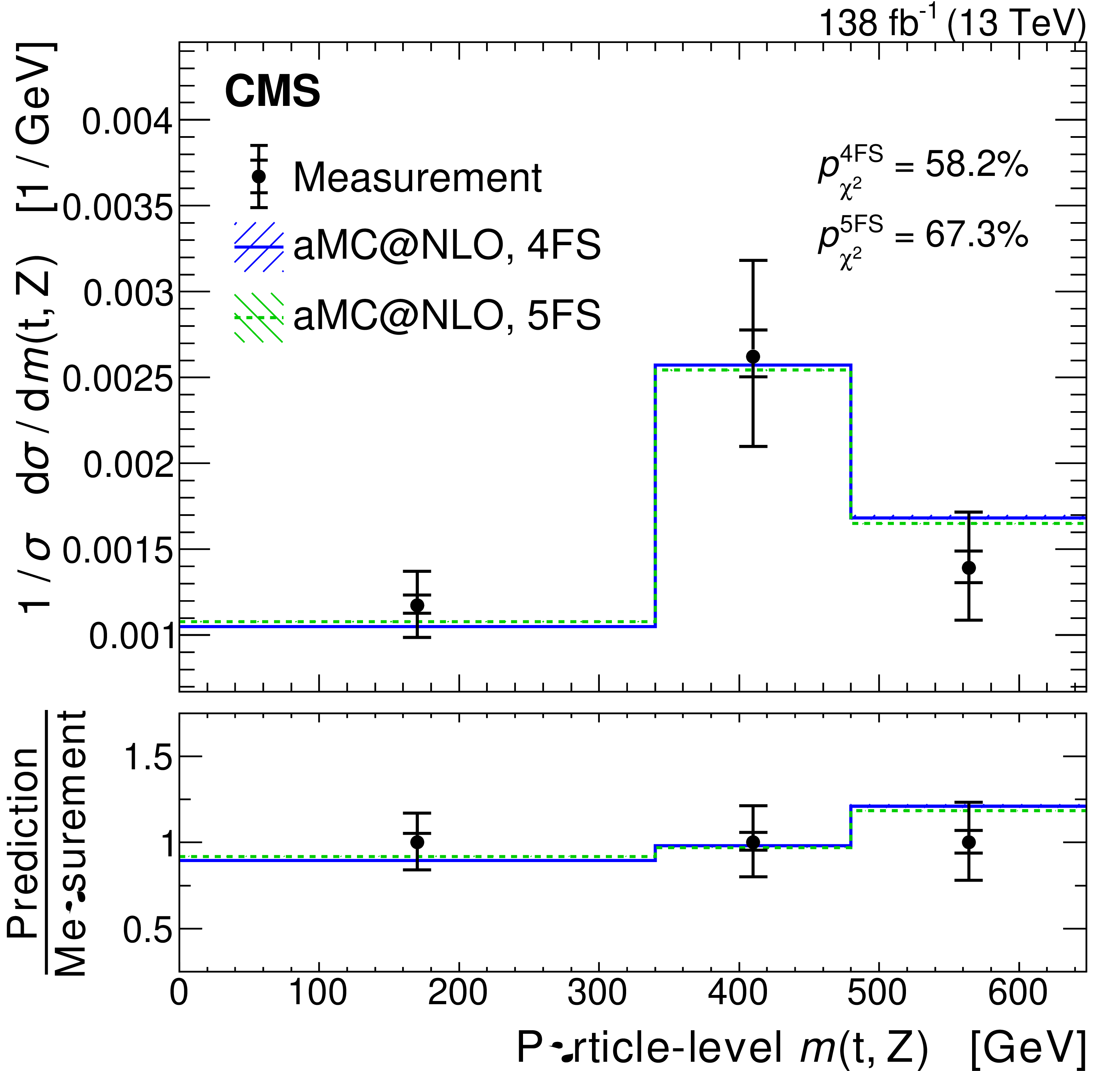
Figure 15-d:
Absolute differential cross sections at the particle level measured as a function of ${m(\mathrm{t},\mathrm{Z})}$. The observed values are shown as black points, with the inner and outer vertical bars giving the systematic and total uncertainties, respectively. The SM predictions for the tZq process are based on events simulated in the 5FS (green) and 4FS (blue). The $p$-values of the ${{\chi ^2}}$ tests are given to quantify their compatibility with the measurement. The lower panel shows the ratio of the simulation to the measurement. |
png pdf |
Figure 15-e:
Absolute differential cross sections at the parton level measured as a function of ${\cos(\theta ^{\star}_{\text {pol}})}$. The observed values are shown as black points, with the inner and outer vertical bars giving the systematic and total uncertainties, respectively. The SM predictions for the tZq process are based on events simulated in the 5FS (green) and 4FS (blue). The $p$-values of the ${{\chi ^2}}$ tests are given to quantify their compatibility with the measurement. The lower panel shows the ratio of the simulation to the measurement. |

png pdf |
Figure 15-f:
Absolute differential cross sections at the particle level measured as a function of ${\cos(\theta ^{\star}_{\text {pol}})}$. The observed values are shown as black points, with the inner and outer vertical bars giving the systematic and total uncertainties, respectively. The SM predictions for the tZq process are based on events simulated in the 5FS (green) and 4FS (blue). The $p$-values of the ${{\chi ^2}}$ tests are given to quantify their compatibility with the measurement. The lower panel shows the ratio of the simulation to the measurement. |
png pdf |
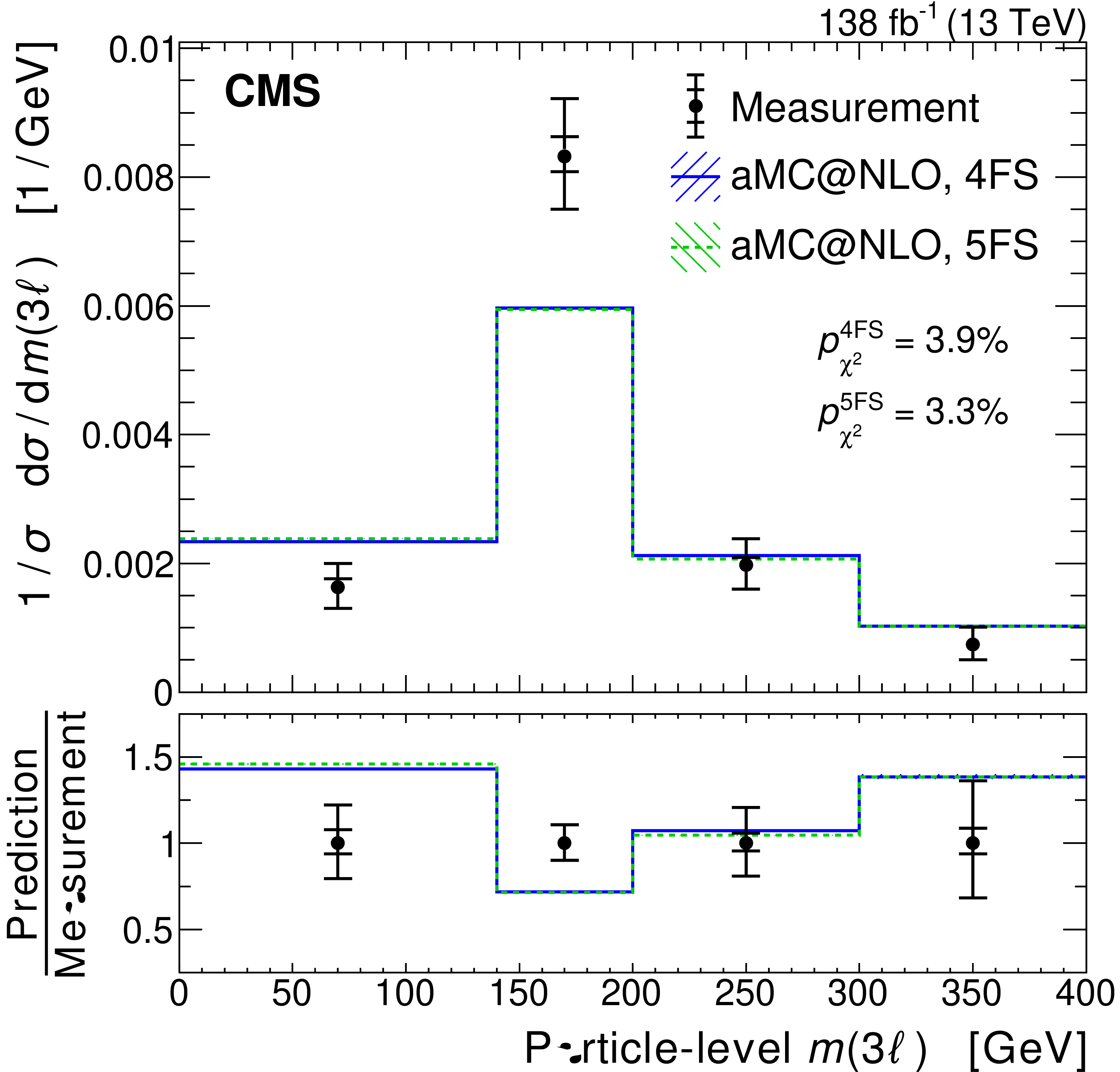
Figure 16:
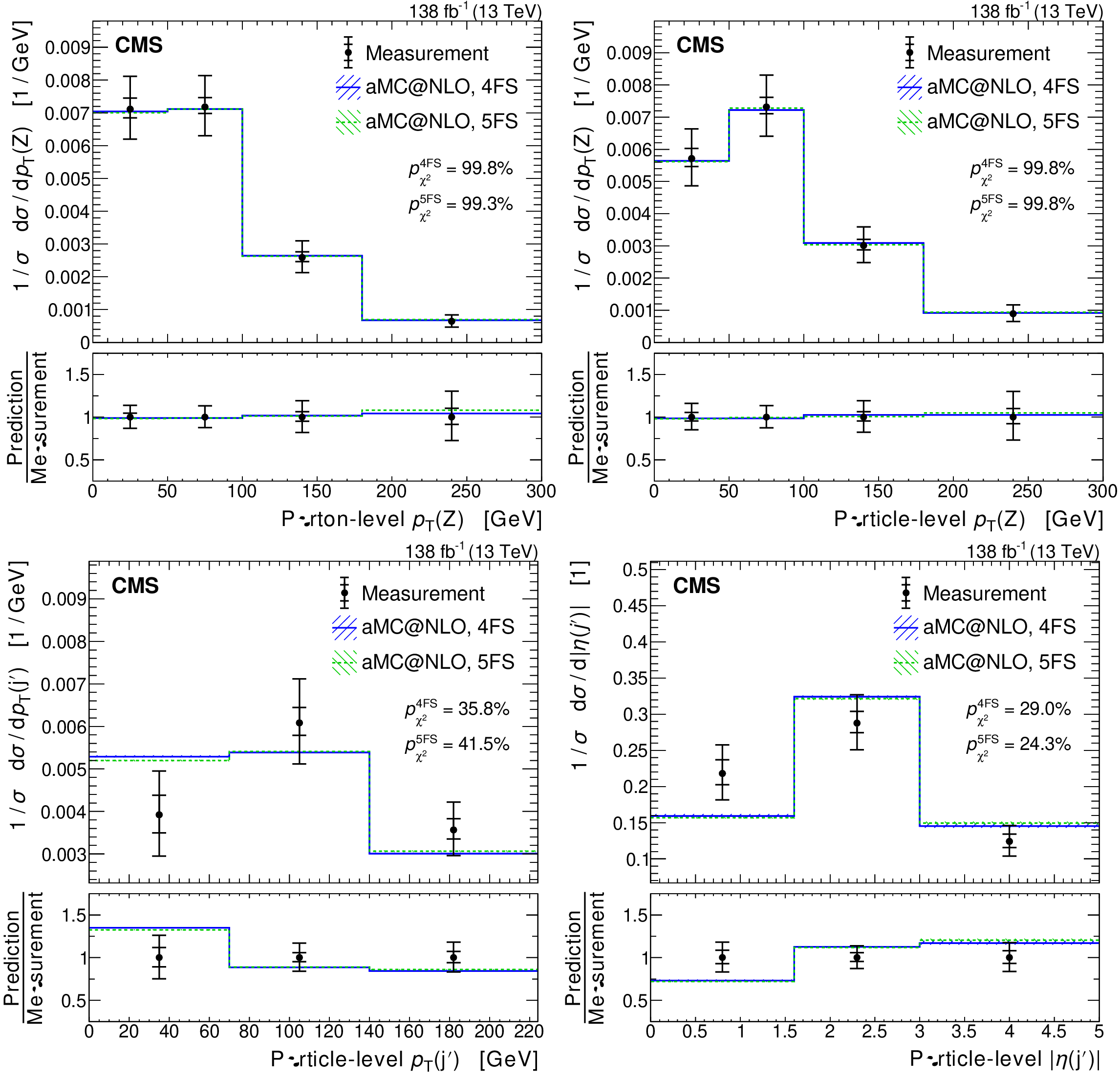
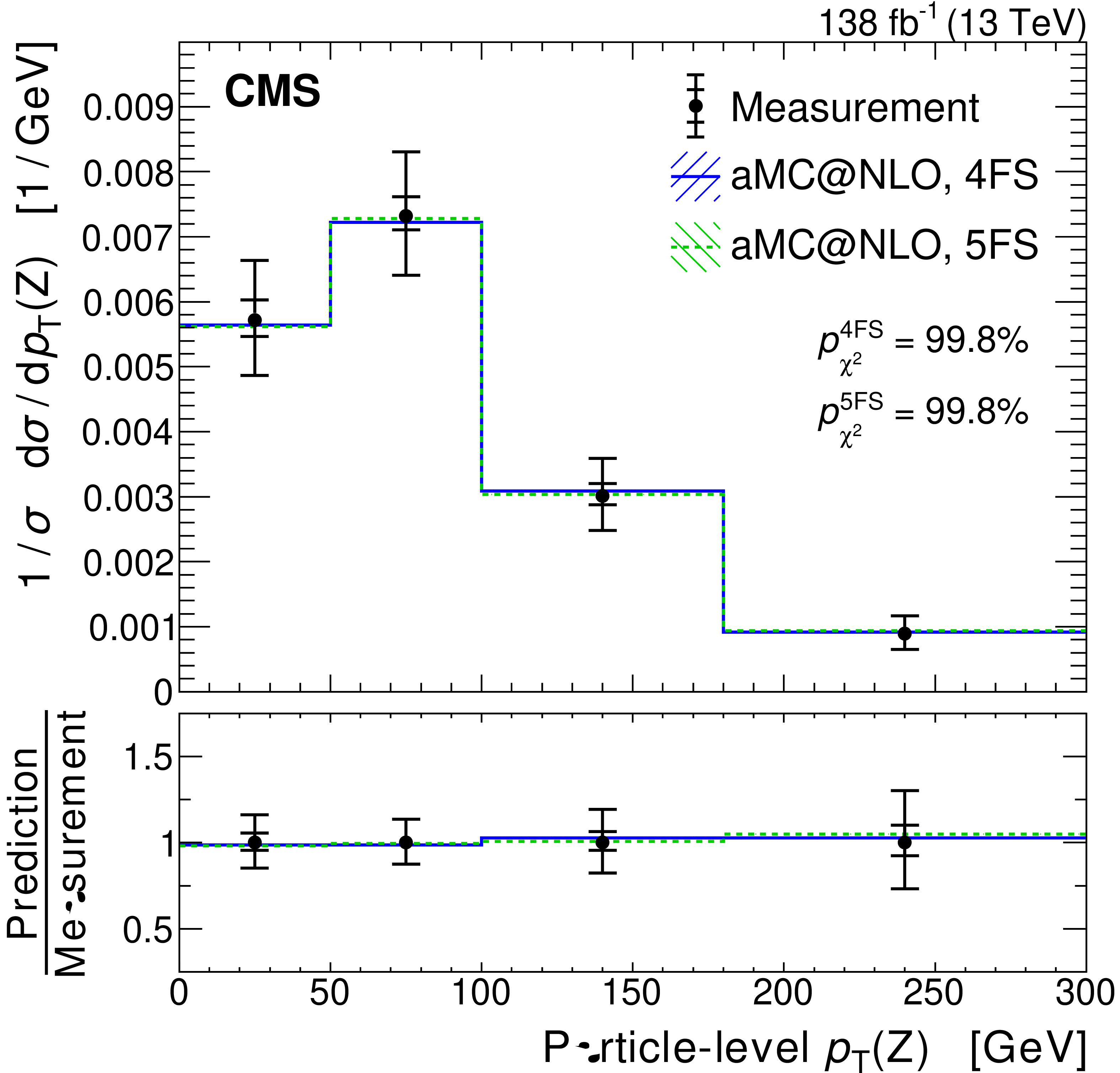
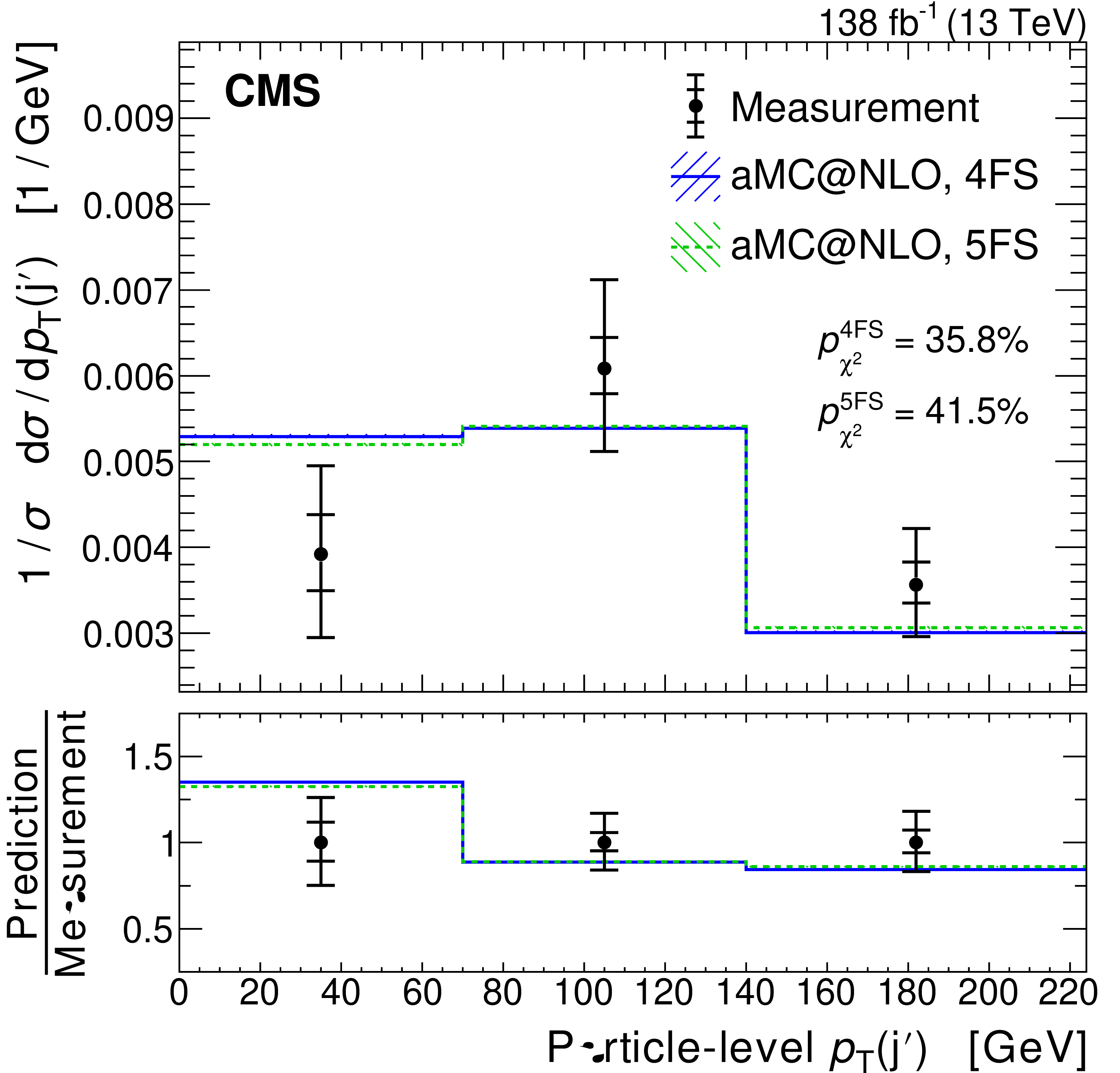
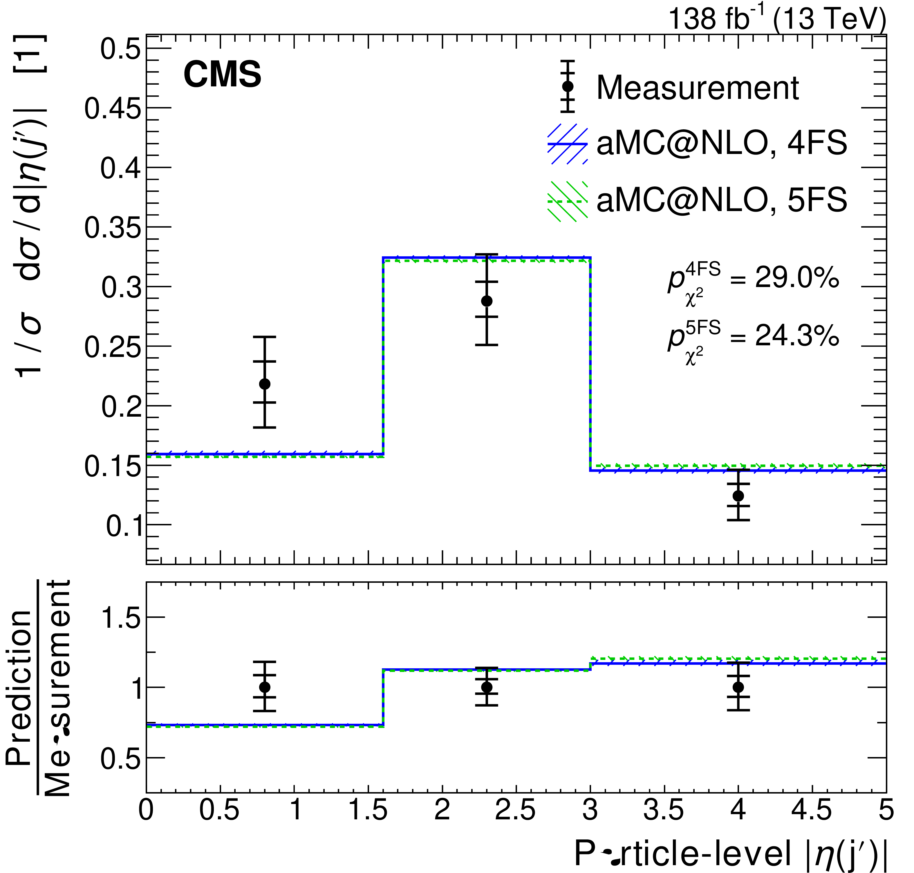
Normalized differential cross sections measured as a function of ${{p_{\mathrm {T}}} (\mathrm{Z})}$ at the parton (upper left) and particle level (upper right), as well as a function of ${{p_{\mathrm {T}}} (\mathrm {j}')}$ (lower left) and $ | \eta (\mathrm {j}') | $ (lower right) at the particle level. The observed values are shown as black points, with the inner and outer vertical bars giving the systematic and total uncertainties, respectively. The SM predictions for the tZq process are based on events simulated in the 5FS (green) and 4FS (blue). The $p$-values of the ${{\chi ^2}}$ tests are given to quantify their compatibility with the measurement. The lower panels show the ratio of the simulation to the measurement. |

png pdf |
Figure 16-a:
Normalized differential cross sections measured as a function of ${{p_{\mathrm {T}}} (\mathrm{Z})}$ at the parton level. The observed values are shown as black points, with the inner and outer vertical bars giving the systematic and total uncertainties, respectively. The SM predictions for the tZq process are based on events simulated in the 5FS (green) and 4FS (blue). The $p$-values of the ${{\chi ^2}}$ tests are given to quantify their compatibility with the measurement. The lower panel shows the ratio of the simulation to the measurement. |
png pdf |
Figure 16-b:
Normalized differential cross sections measured as a function of ${{p_{\mathrm {T}}} (\mathrm{Z})}$ at the particle level. The observed values are shown as black points, with the inner and outer vertical bars giving the systematic and total uncertainties, respectively. The SM predictions for the tZq process are based on events simulated in the 5FS (green) and 4FS (blue). The $p$-values of the ${{\chi ^2}}$ tests are given to quantify their compatibility with the measurement. The lower panel shows the ratio of the simulation to the measurement. |
png pdf |
Figure 16-c:
Normalized differential cross sections measured as a function of ${{p_{\mathrm {T}}} (\mathrm {j}')}$ at the particle level. The observed values are shown as black points, with the inner and outer vertical bars giving the systematic and total uncertainties, respectively. The SM predictions for the tZq process are based on events simulated in the 5FS (green) and 4FS (blue). The $p$-values of the ${{\chi ^2}}$ tests are given to quantify their compatibility with the measurement. The lower panel shows the ratio of the simulation to the measurement. |
png pdf |
Figure 16-d:
Normalized differential cross sections measured as a function of $ | \eta (\mathrm {j}') | $ at the particle level. The observed values are shown as black points, with the inner and outer vertical bars giving the systematic and total uncertainties, respectively. The SM predictions for the tZq process are based on events simulated in the 5FS (green) and 4FS (blue). The $p$-values of the ${{\chi ^2}}$ tests are given to quantify their compatibility with the measurement. The lower panel shows the ratio of the simulation to the measurement. |
png pdf |
Figure 17:
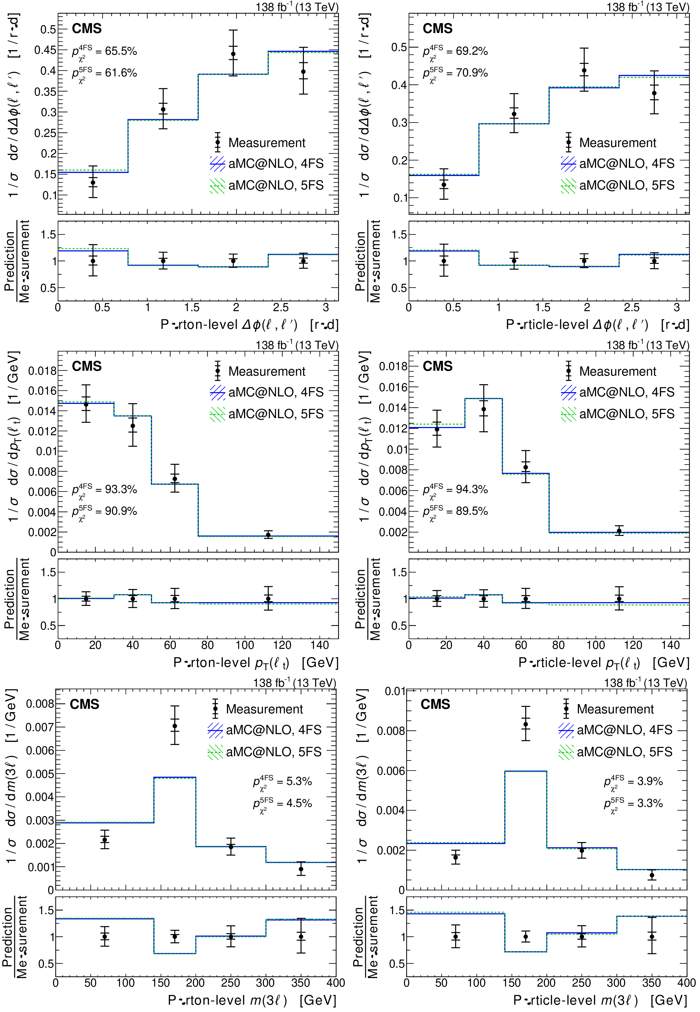
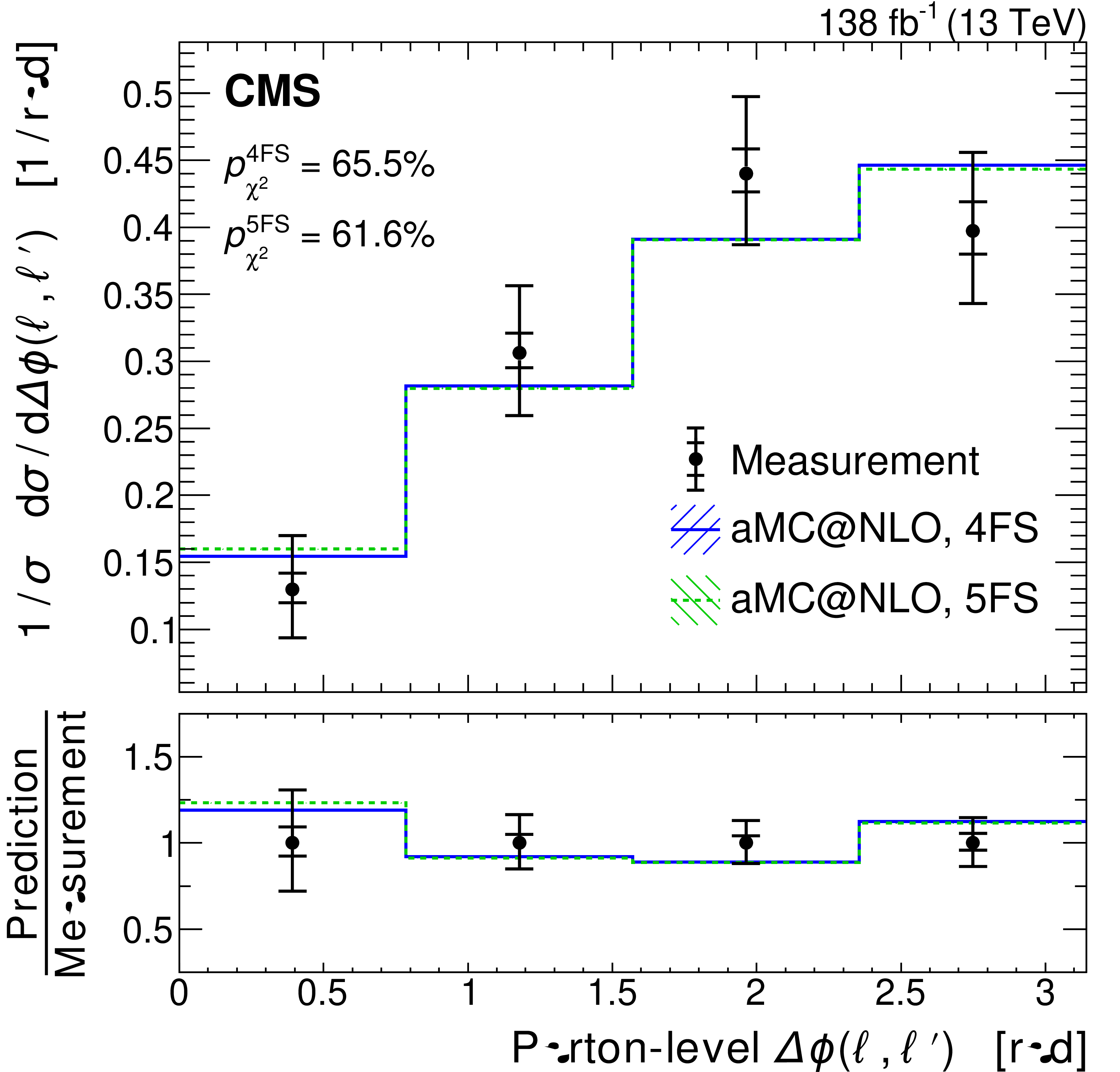
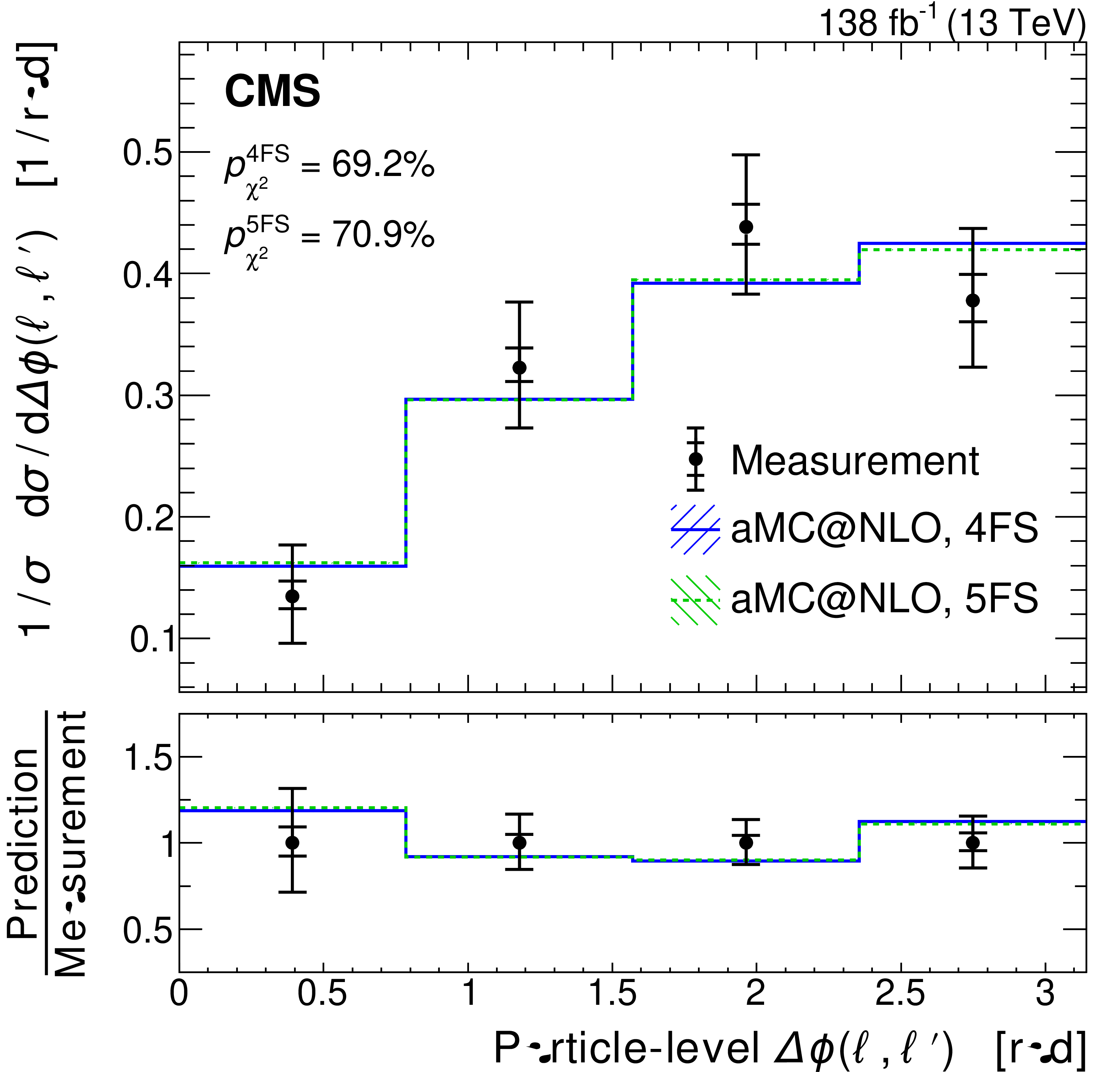
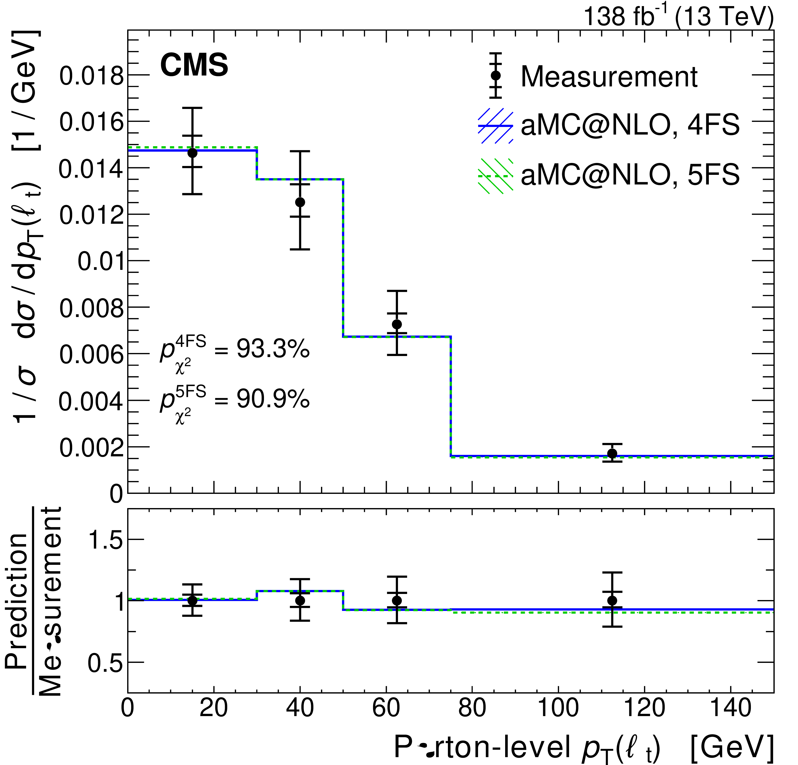
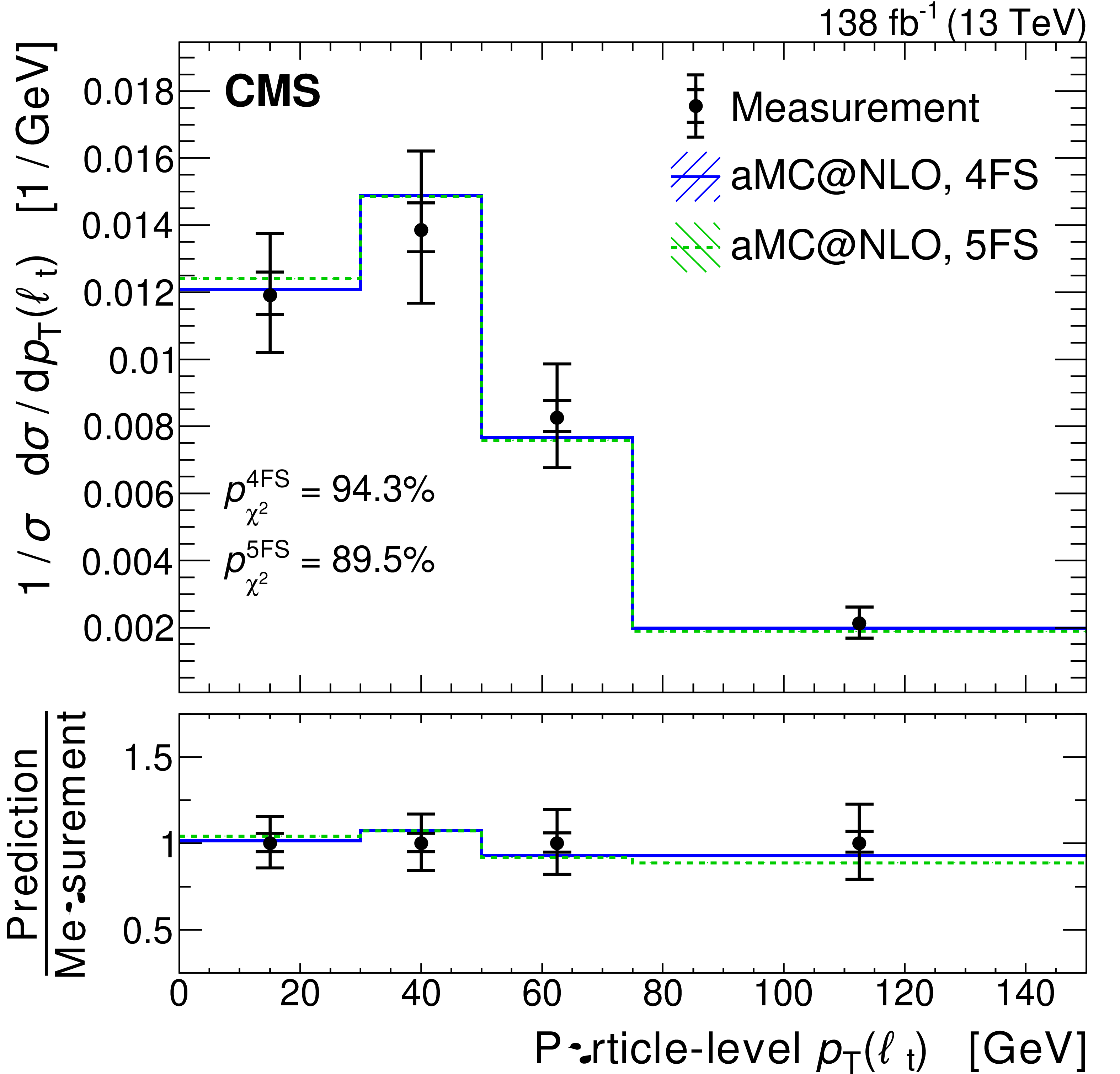
Normalized differential cross sections measured at the parton (left) and particle level (right) as a function of ${{\Delta \phi} (\ell,\ell ')}$ (upper), ${{p_{\mathrm {T}}} (\ell _{\mathrm{t}})}$ (middle) and ${m(3\ell)}$ (lower). The observed values are shown as black points, with the inner and outer vertical bars giving the systematic and total uncertainties, respectively. The SM predictions for the tZq process are based on events simulated in the 5FS (green) and 4FS (blue). The $p$-values of the ${{\chi ^2}}$ tests are given to quantify their compatibility with the measurement. The lower panels show the ratio of the simulation to the measurement. |
png pdf |
Figure 17-a:
Normalized differential cross sections measured at the parton level as a function of ${{\Delta \phi} (\ell,\ell ')}$. The observed values are shown as black points, with the inner and outer vertical bars giving the systematic and total uncertainties, respectively. The SM predictions for the tZq process are based on events simulated in the 5FS (green) and 4FS (blue). The $p$-values of the ${{\chi ^2}}$ tests are given to quantify their compatibility with the measurement. The lower panel shows the ratio of the simulation to the measurement. |
png pdf |
Figure 17-b:
Normalized differential cross sections measured at the particle level as a function of ${{\Delta \phi} (\ell,\ell ')}$. The observed values are shown as black points, with the inner and outer vertical bars giving the systematic and total uncertainties, respectively. The SM predictions for the tZq process are based on events simulated in the 5FS (green) and 4FS (blue). The $p$-values of the ${{\chi ^2}}$ tests are given to quantify their compatibility with the measurement. The lower panel shows the ratio of the simulation to the measurement. |
png pdf |
Figure 17-c:
Normalized differential cross sections measured at the parton level as a function of ${{p_{\mathrm {T}}} (\ell _{\mathrm{t}})}$. The observed values are shown as black points, with the inner and outer vertical bars giving the systematic and total uncertainties, respectively. The SM predictions for the tZq process are based on events simulated in the 5FS (green) and 4FS (blue). The $p$-values of the ${{\chi ^2}}$ tests are given to quantify their compatibility with the measurement. The lower panel shows the ratio of the simulation to the measurement. |
png pdf |
Figure 17-d:
Normalized differential cross sections measured at the particle level as a function of ${{p_{\mathrm {T}}} (\ell _{\mathrm{t}})}$. The observed values are shown as black points, with the inner and outer vertical bars giving the systematic and total uncertainties, respectively. The SM predictions for the tZq process are based on events simulated in the 5FS (green) and 4FS (blue). The $p$-values of the ${{\chi ^2}}$ tests are given to quantify their compatibility with the measurement. The lower panel shows the ratio of the simulation to the measurement. |

png pdf |
Figure 17-e:
Normalized differential cross sections measured at the parton level as a function of ${m(3\ell)}$. The observed values are shown as black points, with the inner and outer vertical bars giving the systematic and total uncertainties, respectively. The SM predictions for the tZq process are based on events simulated in the 5FS (green) and 4FS (blue). The $p$-values of the ${{\chi ^2}}$ tests are given to quantify their compatibility with the measurement. The lower panel shows the ratio of the simulation to the measurement. |
png pdf |
Figure 17-f:
Normalized differential cross sections measured at the particle level as a function of ${m(3\ell)}$. The observed values are shown as black points, with the inner and outer vertical bars giving the systematic and total uncertainties, respectively. The SM predictions for the tZq process are based on events simulated in the 5FS (green) and 4FS (blue). The $p$-values of the ${{\chi ^2}}$ tests are given to quantify their compatibility with the measurement. The lower panel shows the ratio of the simulation to the measurement. |
png pdf |
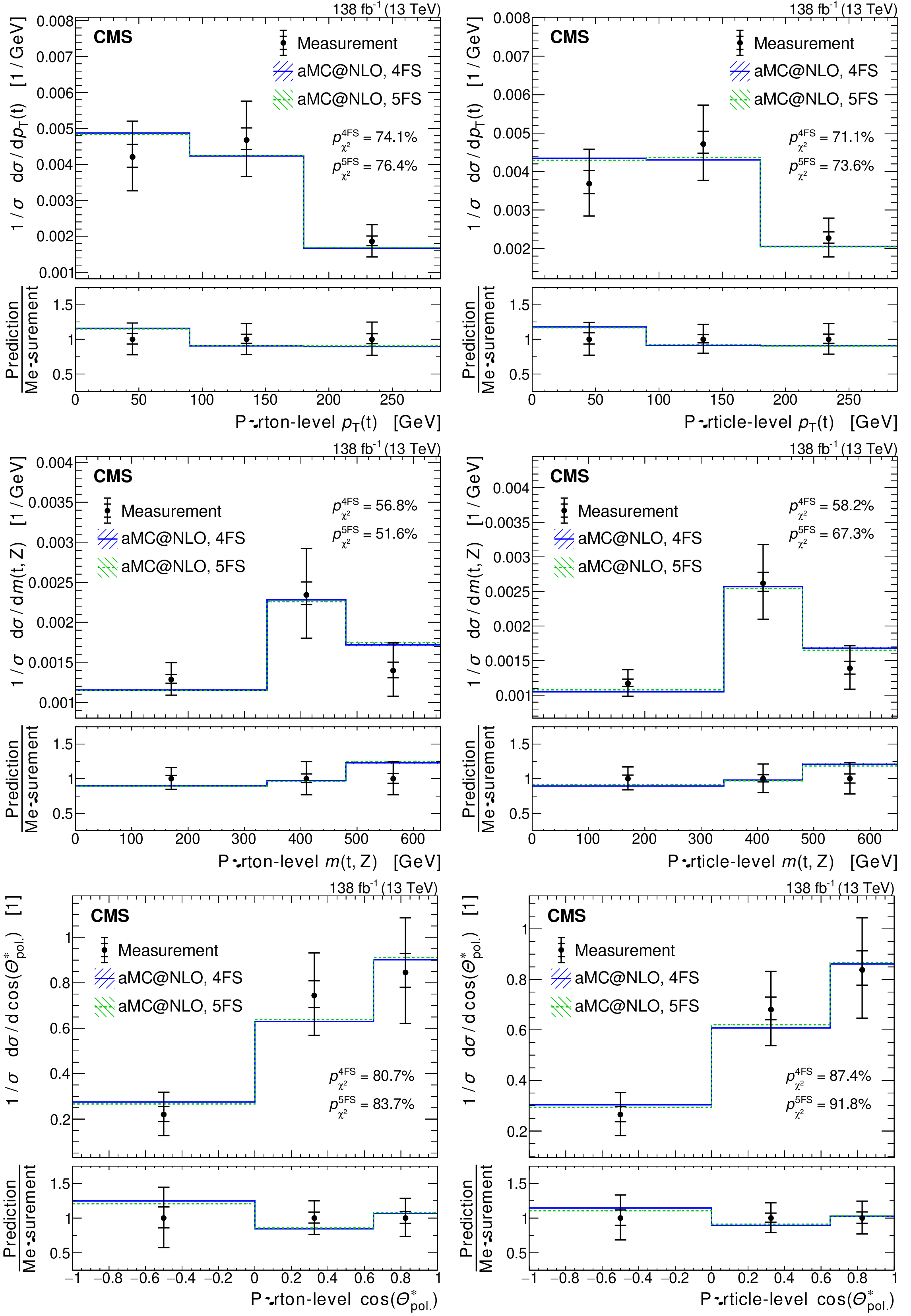
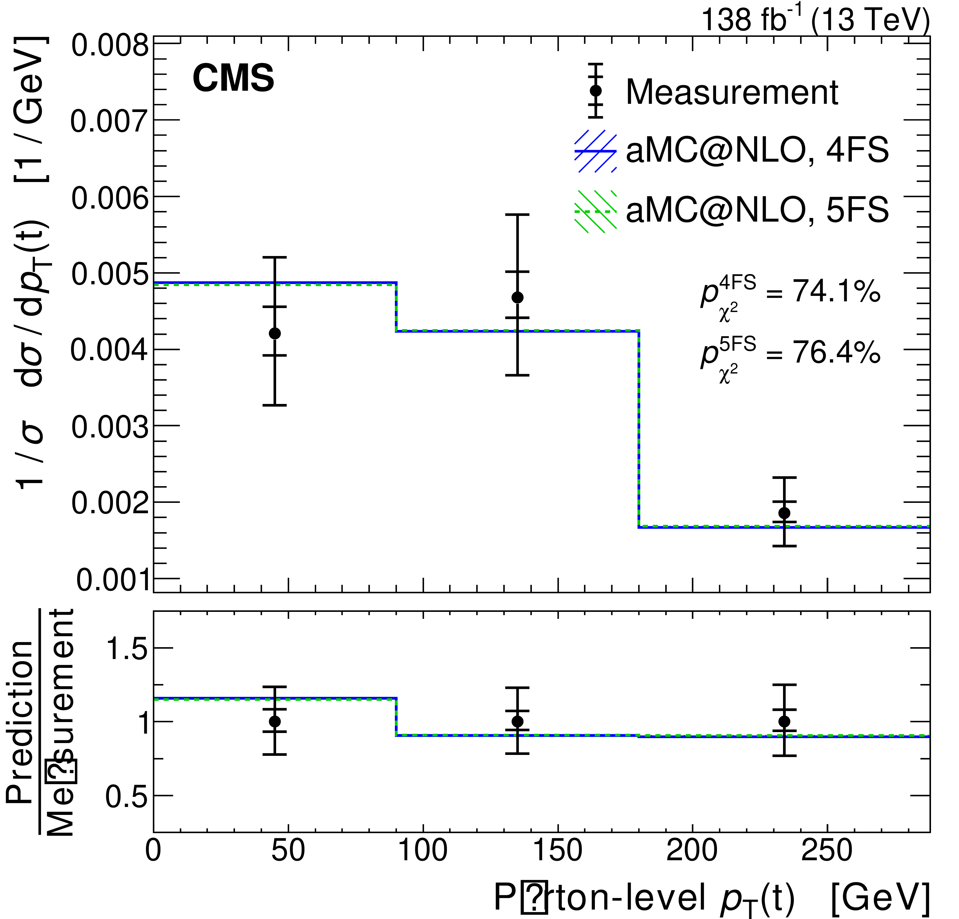
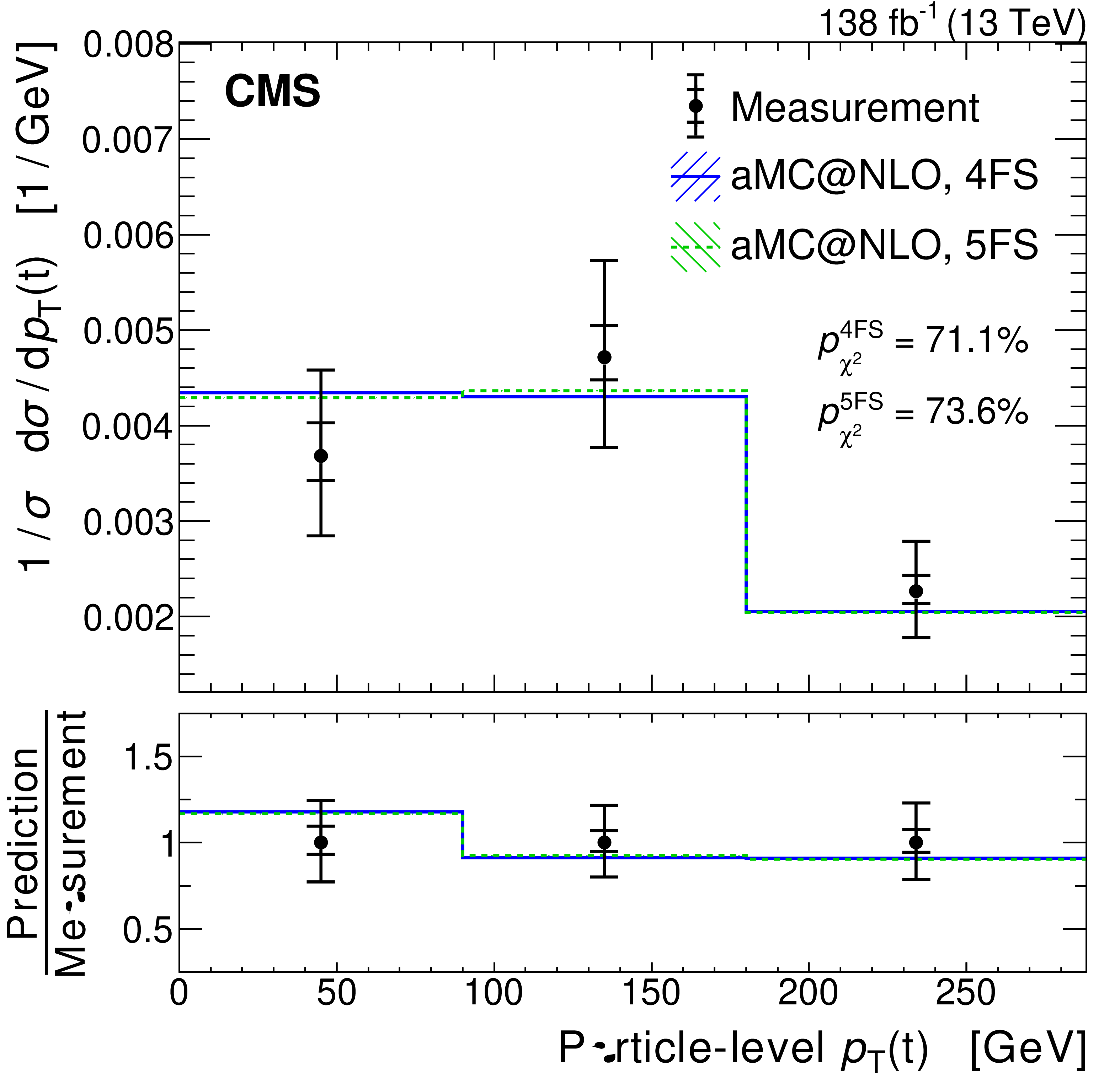
Figure 18:
Normalized differential cross sections measured at the parton (left) and particle level (right) as a function of ${{p_{\mathrm {T}}} (\mathrm{t})}$ (upper), ${m(\mathrm{t},\mathrm{Z})}$ (middle) and ${\cos(\theta ^{\star}_{\text {pol}})}$ (lower). The observed values are shown as black points, with the inner and outer vertical bars giving the systematic and total uncertainties, respectively. The SM predictions for the tZq process are based on events simulated in the 5FS (green) and 4FS (blue). The $p$-values of the ${{\chi ^2}}$ tests are given to quantify their compatibility with the measurement. The lower panels show the ratio of the simulation to the measurement. |
png pdf |
Figure 18-a:
Normalized differential cross sections measured at the parton level as a function of ${{p_{\mathrm {T}}} (\mathrm{t})}$. The observed values are shown as black points, with the inner and outer vertical bars giving the systematic and total uncertainties, respectively. The SM predictions for the tZq process are based on events simulated in the 5FS (green) and 4FS (blue). The $p$-values of the ${{\chi ^2}}$ tests are given to quantify their compatibility with the measurement. The lower panel shows the ratio of the simulation to the measurement. |
png pdf |
Figure 18-b:
Normalized differential cross sections measured at the particle level as a function of ${{p_{\mathrm {T}}} (\mathrm{t})}$. The observed values are shown as black points, with the inner and outer vertical bars giving the systematic and total uncertainties, respectively. The SM predictions for the tZq process are based on events simulated in the 5FS (green) and 4FS (blue). The $p$-values of the ${{\chi ^2}}$ tests are given to quantify their compatibility with the measurement. The lower panel shows the ratio of the simulation to the measurement. |
png pdf |
Figure 18-c:
Normalized differential cross sections measured at the parton level as a function of ${m(\mathrm{t},\mathrm{Z})}$. The observed values are shown as black points, with the inner and outer vertical bars giving the systematic and total uncertainties, respectively. The SM predictions for the tZq process are based on events simulated in the 5FS (green) and 4FS (blue). The $p$-values of the ${{\chi ^2}}$ tests are given to quantify their compatibility with the measurement. The lower panel shows the ratio of the simulation to the measurement. |
png pdf |
Figure 18-d:
Normalized differential cross sections measured at the particle level as a function of ${m(\mathrm{t},\mathrm{Z})}$. The observed values are shown as black points, with the inner and outer vertical bars giving the systematic and total uncertainties, respectively. The SM predictions for the tZq process are based on events simulated in the 5FS (green) and 4FS (blue). The $p$-values of the ${{\chi ^2}}$ tests are given to quantify their compatibility with the measurement. The lower panel shows the ratio of the simulation to the measurement. |

png pdf |
Figure 18-e:
Normalized differential cross sections measured at the parton level as a function of ${\cos(\theta ^{\star}_{\text {pol}})}$. The observed values are shown as black points, with the inner and outer vertical bars giving the systematic and total uncertainties, respectively. The SM predictions for the tZq process are based on events simulated in the 5FS (green) and 4FS (blue). The $p$-values of the ${{\chi ^2}}$ tests are given to quantify their compatibility with the measurement. The lower panel shows the ratio of the simulation to the measurement. |

png pdf |
Figure 18-f:
Normalized differential cross sections measured at the particle level as a function of ${\cos(\theta ^{\star}_{\text {pol}})}$. The observed values are shown as black points, with the inner and outer vertical bars giving the systematic and total uncertainties, respectively. The SM predictions for the tZq process are based on events simulated in the 5FS (green) and 4FS (blue). The $p$-values of the ${{\chi ^2}}$ tests are given to quantify their compatibility with the measurement. The lower panel shows the ratio of the simulation to the measurement. |
png pdf |
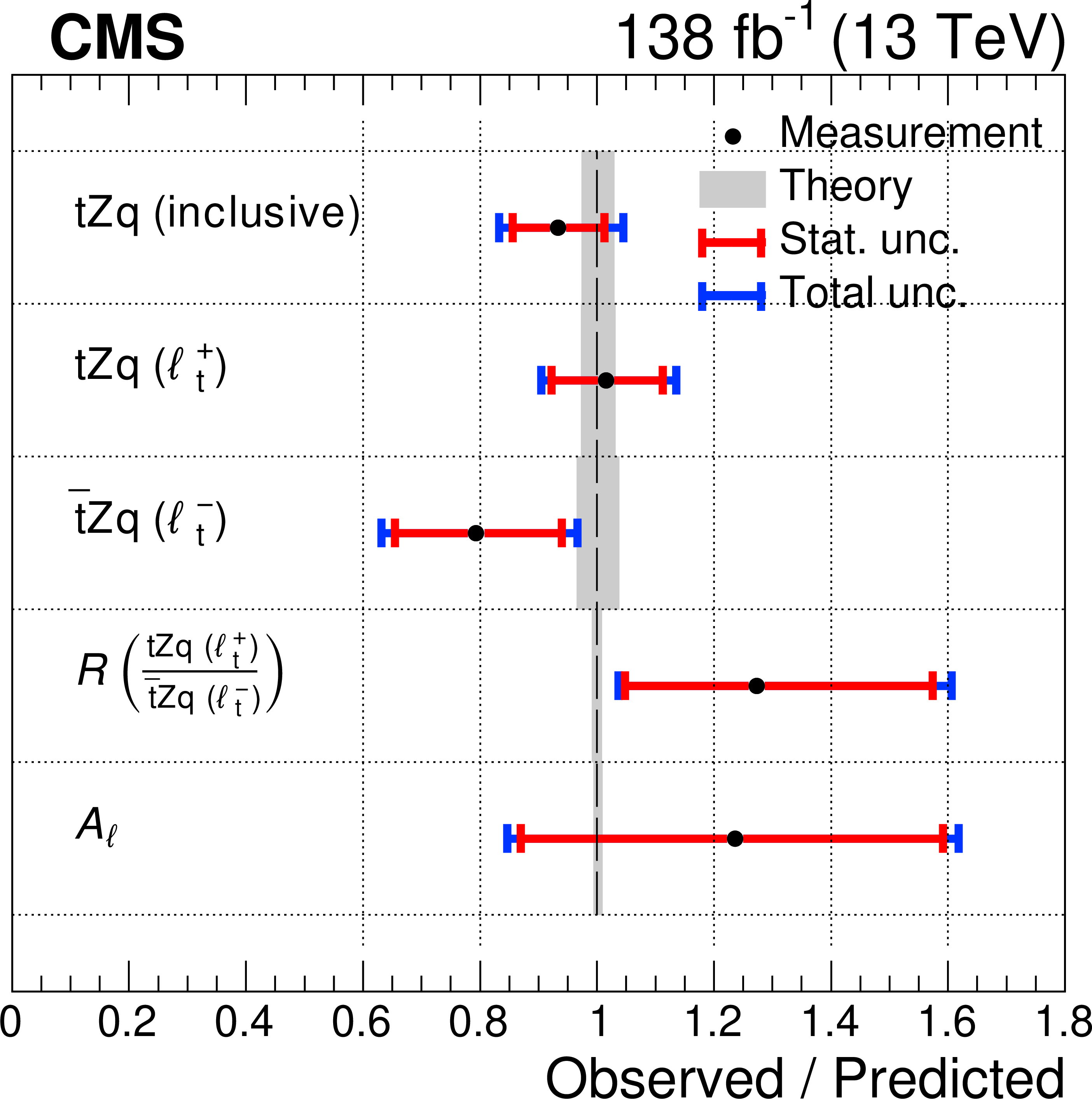
Figure 19:
Measured values of the inclusive tZq cross section (first row), top quark and antiquark cross sections (second and third rows) and their ratio (fourth row), together with the top quark spin asymmetry in the tZq process (last row). Each row shows the ratio between the observed and the SM predicted values. The black points show the central values, while the blue and yellow bars refer to the statistical and total uncertainties in the measurements, respectively. Uncertainties in the predictions are indicated by the gray bands. |
png pdf |
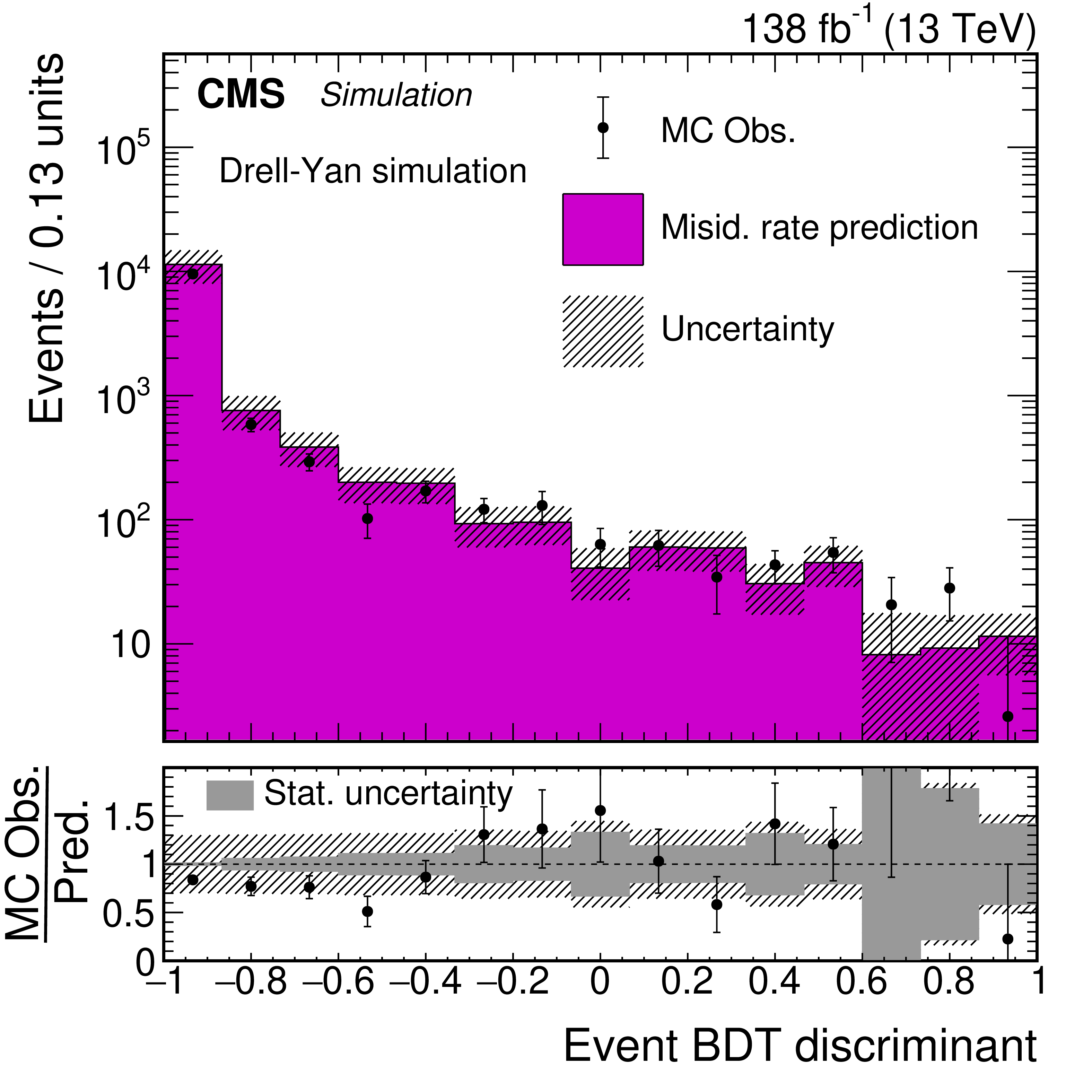
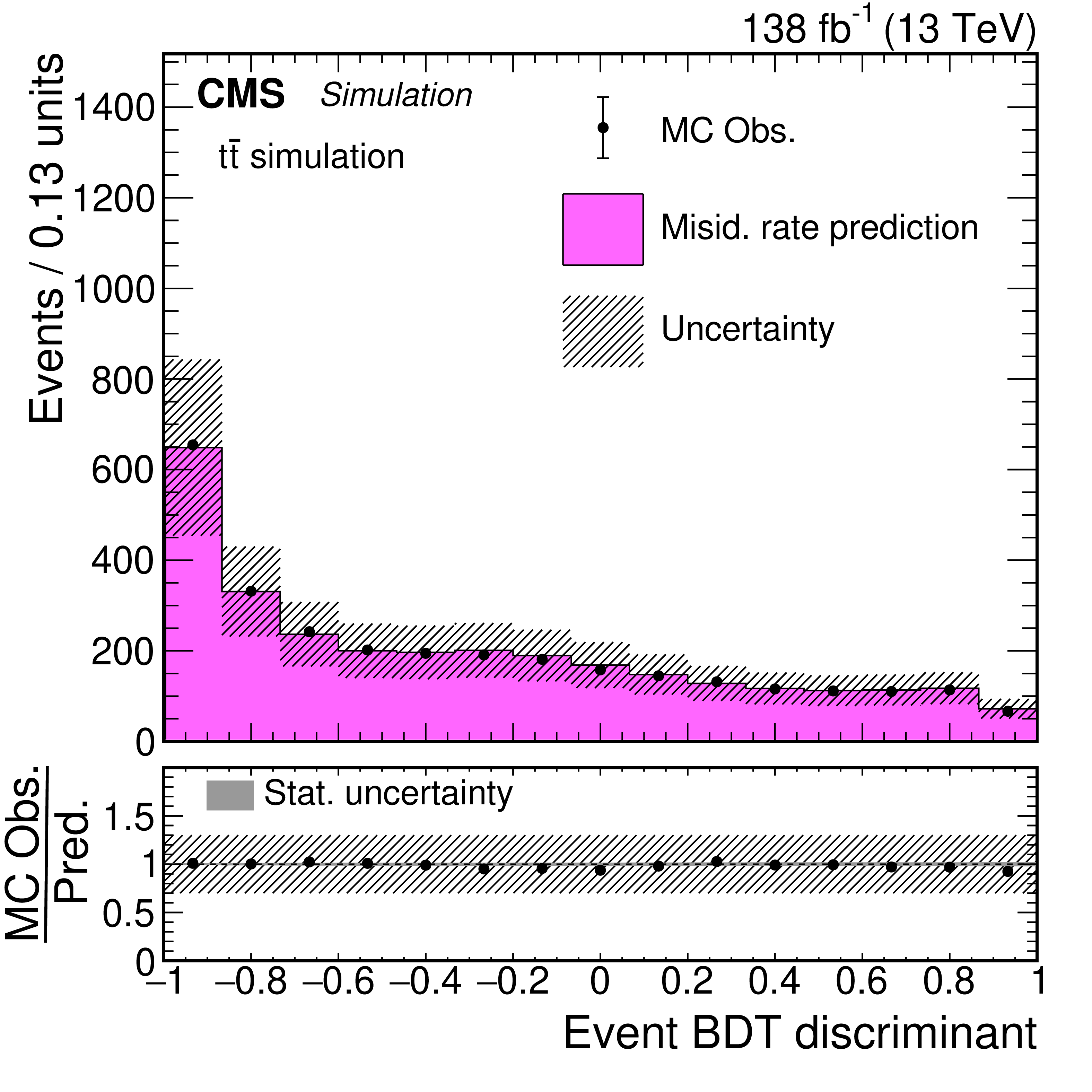
Figure A1:
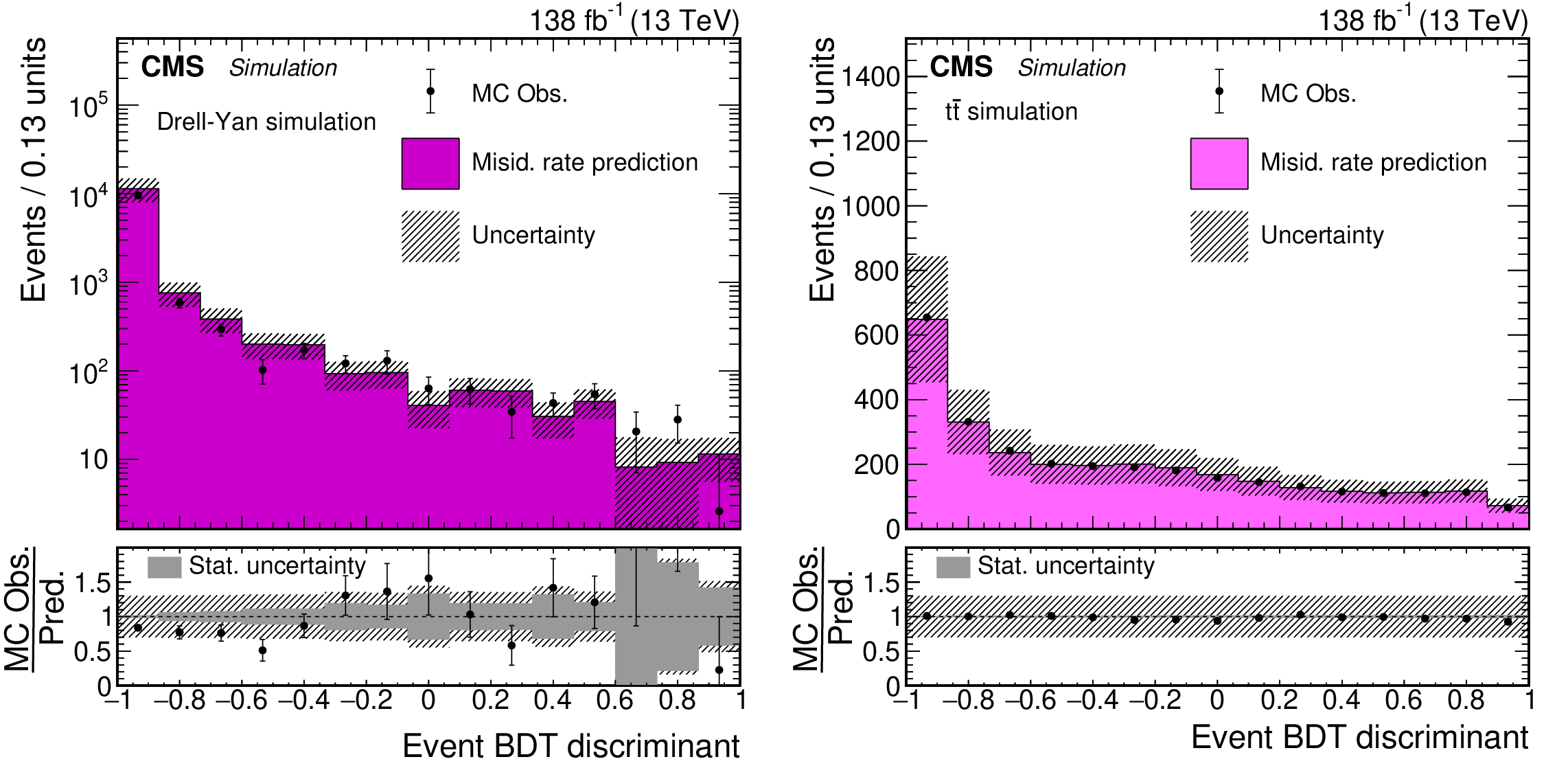
The event BDT discriminant distributions for simulated (left) trilepton DY events and (right) ${\mathrm{t} \mathrm{\bar{t}}}$ events. The black points give the nonprompt-lepton predictions from the simulation, while the colored histograms represent a similar prediction estimated with the misidentification rate method applied to the same events. The lower panels plot the ratio of the observed MC prediction to the prediction from the misidentification rate method. The vertical bars on the points show the statistical uncertainty in the observed MC distribution. The hatched bands represent the total uncertainty in the misidentification rate predictions and the shaded band its statistical component in the ratio. |
png pdf |
Figure A1-a:
The event BDT discriminant distribution for simulated trilepton DY events. The black points give the nonprompt-lepton predictions from the simulation, while the colored histograms represent a similar prediction estimated with the misidentification rate method applied to the same events. The lower panel plots the ratio of the observed MC prediction to the prediction from the misidentification rate method. The vertical bars on the points show the statistical uncertainty in the observed MC distribution. The hatched bands represent the total uncertainty in the misidentification rate predictions and the shaded band its statistical component in the ratio. |
png pdf |
Figure A1-b:
The event BDT discriminant distribution for ${\mathrm{t} \mathrm{\bar{t}}}$ events. The black points give the nonprompt-lepton predictions from the simulation, while the colored histograms represent a similar prediction estimated with the misidentification rate method applied to the same events. The lower panel plots the ratio of the observed MC prediction to the prediction from the misidentification rate method. The vertical bars on the points show the statistical uncertainty in the observed MC distribution. The hatched bands represent the total uncertainty in the misidentification rate predictions and the shaded band its statistical component in the ratio. |
png pdf |
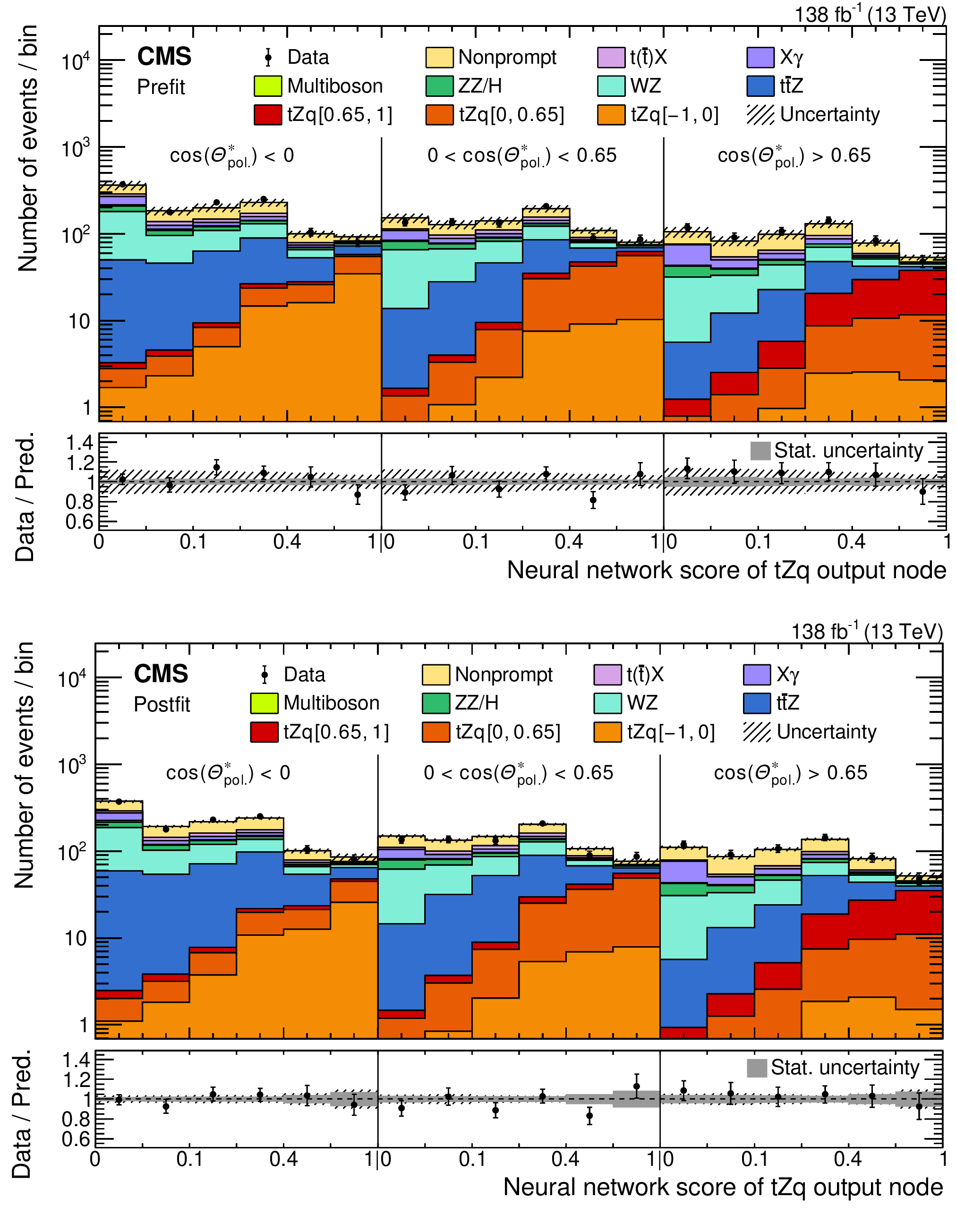
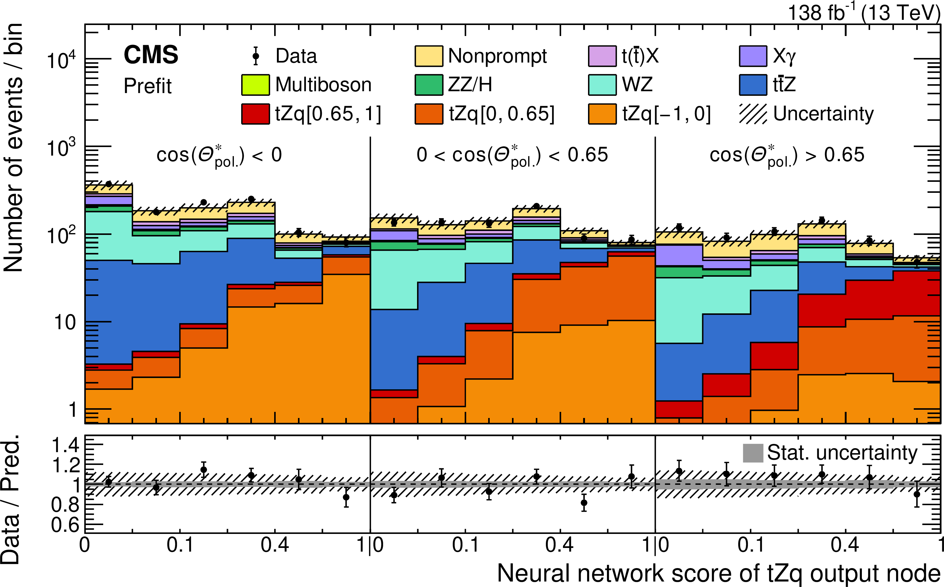
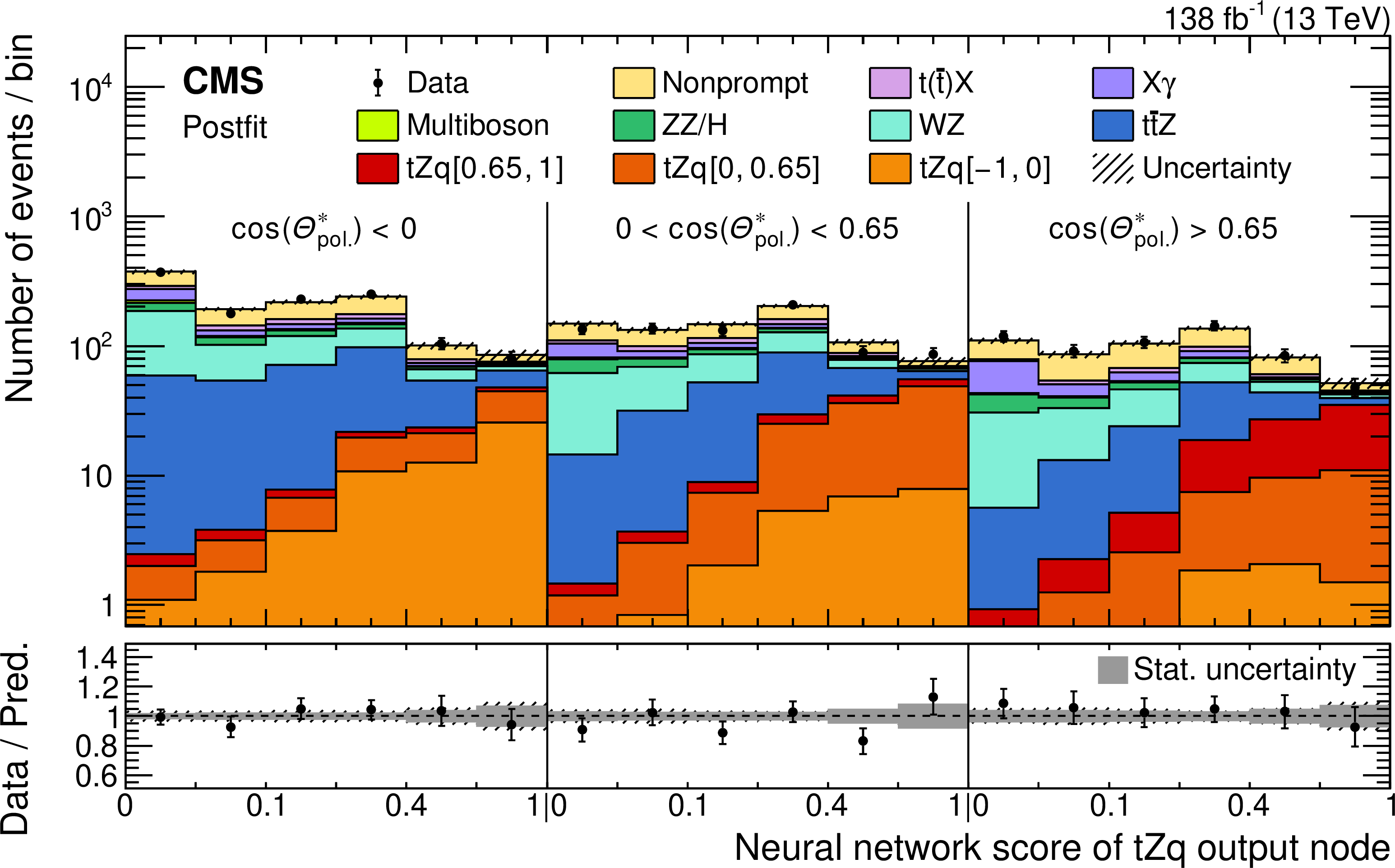
Figure C1:
Prefit (upper) and postfit (lower) distributions of the neural network score from the tZq output node for events in the signal region with fewer than four jets, used for the measurement of the spin asymmetry from the ${\cos(\theta ^{\star}_{\text {pol}})}$ distribution at the parton level. The data are shown by the points and the predictions by the colored histograms. The vertical lines on the points represent the statistical uncertainty in the data, and the hatched region the total uncertainty in the prediction. The events are split into three subregions based on the value of ${\cos(\theta ^{\star}_{\text {pol}})}$ measured at the detector level. Three different tZq templates, defined by the same intervals of ${\cos(\theta ^{\star}_{\text {pol}})}$ at parton level and shown in different shades of orange and red, are used to model the contribution of each parton-level bin. The lower panels show the ratio of the data to the sum of the predictions, with the gray band indicating the uncertainty from the finite number of MC events. |
png pdf |
Figure C1-a:
Prefit distribution of the neural network score from the tZq output node for events in the signal region with fewer than four jets, used for the measurement of the spin asymmetry from the ${\cos(\theta ^{\star}_{\text {pol}})}$ distribution at the parton level. The data are shown by the points and the predictions by the colored histograms. The vertical lines on the points represent the statistical uncertainty in the data, and the hatched region the total uncertainty in the prediction. The events are split into three subregions based on the value of ${\cos(\theta ^{\star}_{\text {pol}})}$ measured at the detector level. Three different tZq templates, defined by the same intervals of ${\cos(\theta ^{\star}_{\text {pol}})}$ at parton level and shown in different shades of orange and red, are used to model the contribution of each parton-level bin. The lower panel shows the ratio of the data to the sum of the predictions, with the gray band indicating the uncertainty from the finite number of MC events. |
png pdf |
Figure C1-b:
Postfit distribution of the neural network score from the tZq output node for events in the signal region with fewer than four jets, used for the measurement of the spin asymmetry from the ${\cos(\theta ^{\star}_{\text {pol}})}$ distribution at the parton level. The data are shown by the points and the predictions by the colored histograms. The vertical lines on the points represent the statistical uncertainty in the data, and the hatched region the total uncertainty in the prediction. The events are split into three subregions based on the value of ${\cos(\theta ^{\star}_{\text {pol}})}$ measured at the detector level. Three different tZq templates, defined by the same intervals of ${\cos(\theta ^{\star}_{\text {pol}})}$ at parton level and shown in different shades of orange and red, are used to model the contribution of each parton-level bin. The lower panel shows the ratio of the data to the sum of the predictions, with the gray band indicating the uncertainty from the finite number of MC events. |
png pdf |
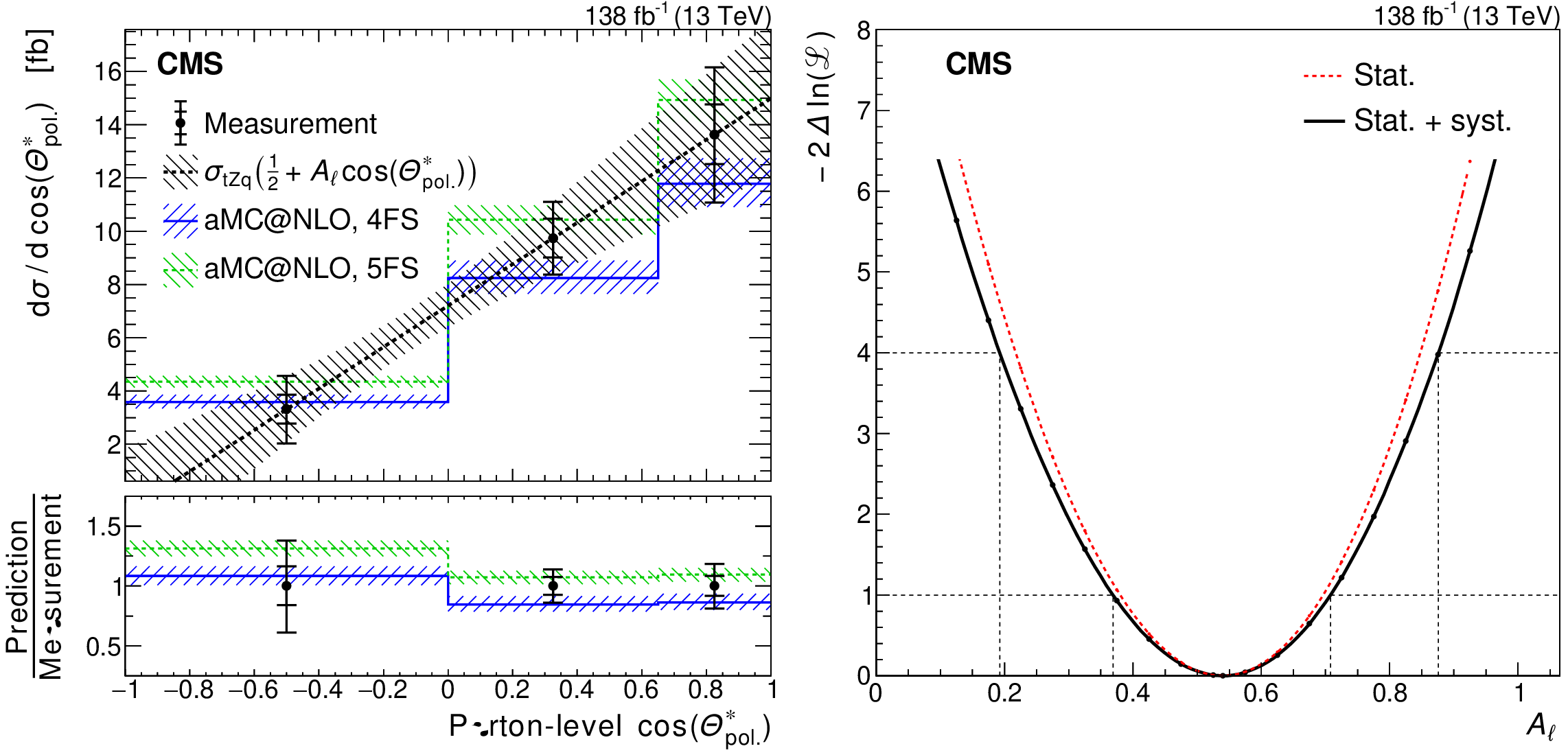
Figure C2:
The left plot shows the measured absolute ${\cos(\theta ^{\star}_{\text {pol}})}$ differential cross section at the parton level used in the extraction of the top quark spin asymmetry. The generator-level bins are parameterized according to Eq. (3), shown as a dashed black line in the plot, such that the spin asymmetry is directly used as a free parameter in the fit. The observed values of the generator-level bins are shown as black points with the inner and outer vertical bars giving the systematic and total uncertainties, respectively. The SM predictions for events simulated in the 5FS (dashed green line) and 4FS (solid blue line) are plotted as well. The hatched regions indicate the corresponding uncertainties, respectively. The lower panel displays the ratio of the MC prediction to the measurement. On the right, the negative log likelihood in the fit for the spin asymmetry ${A_{\ell}}$ is shown when considering only the statistical uncertainties (dashed red line) or the combined statistical and systematic uncertainties (solid black line). The dotted black lines indicate the one (inner) and two (outer) standard deviation confidence intervals, respectively. |
png pdf |
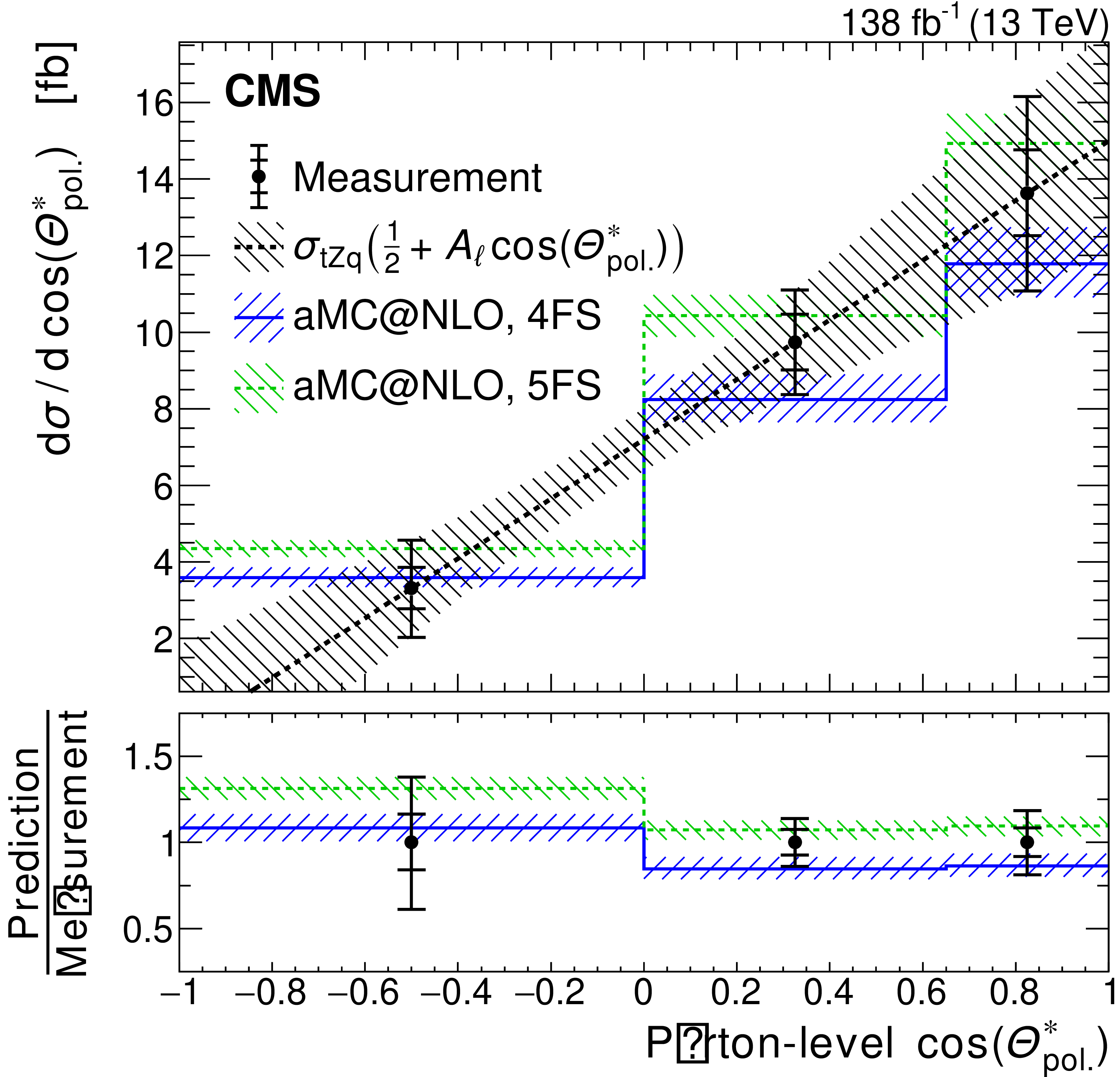
Figure C2-a:
The plot shows the measured absolute ${\cos(\theta ^{\star}_{\text {pol}})}$ differential cross section at the parton level used in the extraction of the top quark spin asymmetry. The generator-level bins are parameterized according to Eq. (3), shown as a dashed black line in the plot, such that the spin asymmetry is directly used as a free parameter in the fit. The observed values of the generator-level bins are shown as black points with the inner and outer vertical bars giving the systematic and total uncertainties, respectively. The SM predictions for events simulated in the 5FS (dashed green line) and 4FS (solid blue line) are plotted as well. The hatched regions indicate the corresponding uncertainties, respectively. The lower panel displays the ratio of the MC prediction to the measurement. |
png pdf |
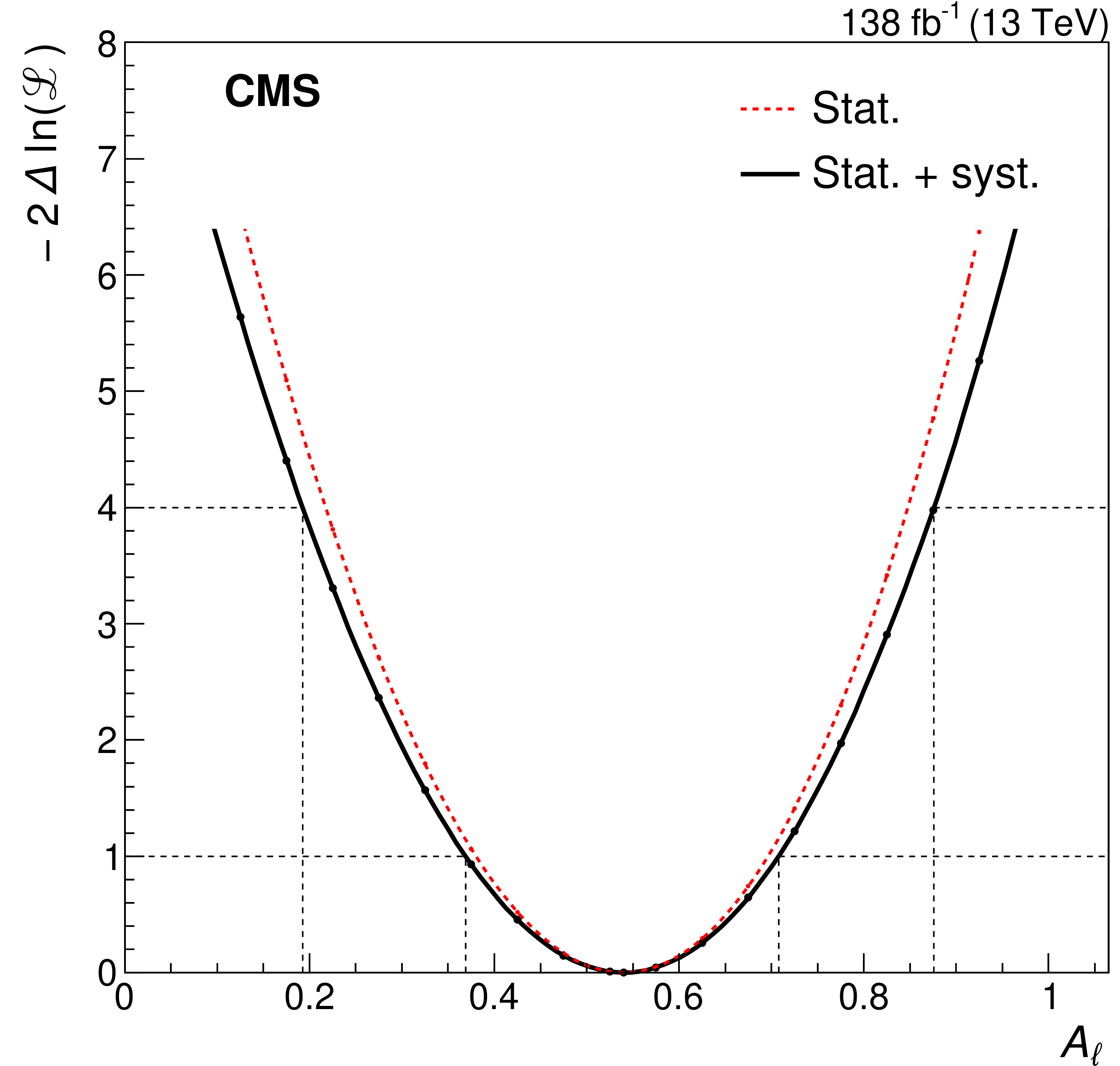
Figure C2-b:
The negative log likelihood in the fit for the spin asymmetry ${A_{\ell}}$ is shown when considering only the statistical uncertainties (dashed red line) or the combined statistical and systematic uncertainties (solid black line). The dotted black lines indicate the one (inner) and two (outer) standard deviation confidence intervals, respectively. |
| Tables | |
png pdf |
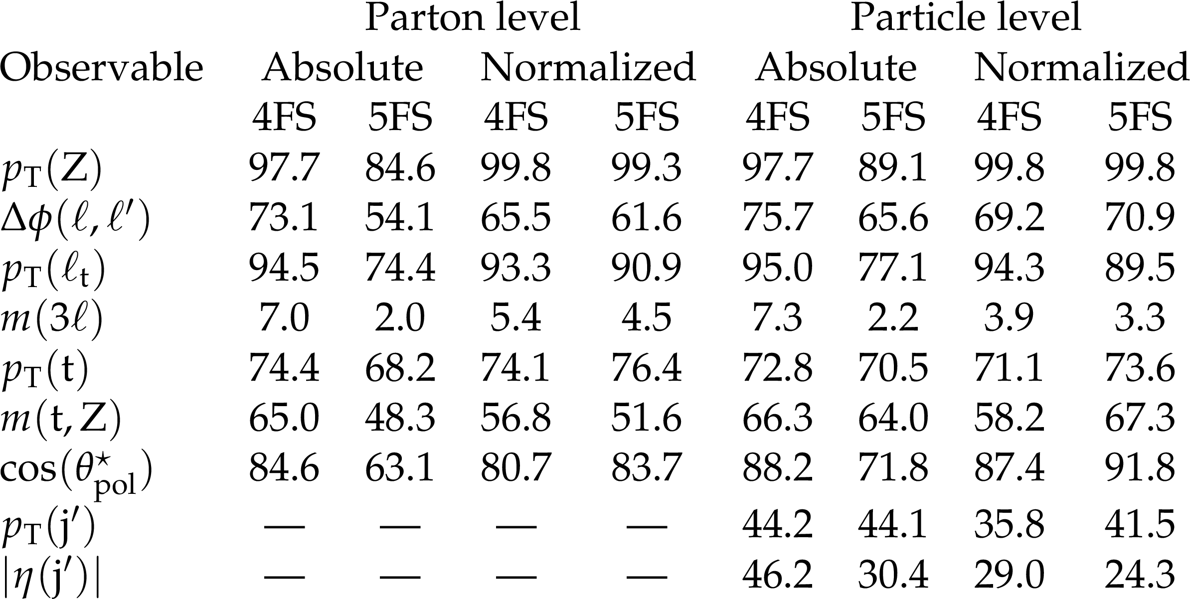
Table B1:
Summary of the $p$-values from the ${{\chi ^2}}$ test between the unfolded measurements and theoretical predictions from the 4FS and 5FS. The test is performed on the measurements of the absolute and normalized differential cross sections at the parton and particle levels for the observables given in the first column. All numbers are given in percent. |
| Summary |
| Inclusive and differential cross section measurements of single top quark production in association with a Z boson (${\mathrm{t}\mathrm{Z}\mathrm{q}} $) are presented using events with three leptons (electrons or muons). The data sample for this measurement was collected by the CMS experiment at the LHC in proton-proton collisions at a center-of-mass energy of 13 TeV and corresponds to an integrated luminosity of 138 fb$^{-1}$. Including nonresonant lepton pairs, an inclusive cross section of $ {{\sigma_{\mathrm{tZq}}}} =$ 87.9 $_{-7.3}^{+7.5}$ (stat) $_{-6.0}^{+7.3}$ (syst) fb is obtained for dilepton invariant masses greater than 30 GeV. This result is the most precise inclusive tZq cross section measurement to date, with a relative precision about 25% better than previous published results. For the first time, the inclusive tZq cross sections are also measured separately for top quark and antiquark production, obtaining $ {\sigma_{{\mathrm{t}\mathrm{Z}\mathrm{q}} (\ell^+_\mathrm{t})}} = $ 62.2 $_{-5.7}^{+5.9}$ (stat) $_{-3.7}^{+4.4}$ (syst) fb and $ {\sigma_{{\mathrm{\bar{t}}\mathrm{Z}\mathrm{q}} (\ell^-_\mathrm{t})}} = $ 26.1 $_{-4.6}^{+4.8}$ (stat) $_{-2.8}^{+3.0}$ (syst) fb, respectively, with the ratio of 2.37 $_{-0.42}^{+0.56}$ (stat) $_{-0.13}^{+0.27}$ (syst). The measured values compared to the theoretical predictions are summarized in Fig. 19.The differential tZq cross sections are measured for the first time at the parton and particle levels using a binned maximum-likelihood-based unfolding. The studied observables are the transverse momenta of the top quark, the Z boson, and the lepton associated with the top quark decay, as well as the invariant masses of the three leptons and the t+Z system. Also used as observables are the difference in azimuthal angle between the two leptons from the Z boson decay, the cosine of the top quark polarization angle, and, at the particle level, the transverse momentum and absolute pseudorapidity of the recoiling jet. The results are mostly compatible with the standard model predictions using both the four- and five-flavor schemes, while the sensitivity is not sufficient to show a preference for one or the other. From the differential distribution of the top quark polarization angle, the top quark spin asymmetry is measured to be $ A_{\ell} = $ 0.54 $\pm$ 0.16 (stat) $\pm$ 0.06 (syst), in agreement with the standard model prediction. |
| References | ||||
| 1 | CMS Collaboration | Observation of single top quark production in association with a Z boson in proton-proton collisions at $ \sqrt{s} = $ 13 TeV | PRL 122 (2019) 132003 | CMS-TOP-18-008 1812.05900 |
| 2 | ATLAS Collaboration | Observation of the associated production of a top quark and a Z boson in pp collisions at $ \sqrt{s} = $ 13 TeV with the ATLAS detector | JHEP 07 (2020) 124 | 2002.07546 |
| 3 | C. Degrande et al. | Single-top associated production with a Z or H boson at the LHC: the SMEFT interpretation | JHEP 10 (2018) 005 | 1804.07773 |
| 4 | CMS Collaboration | Measurement of differential cross sections and charge ratios for t-channel single top quark production in proton-proton collisions at $ \sqrt{s} = $ 13 TeV | EPJC 80 (2020) 370 | CMS-TOP-17-023 1907.08330 |
| 5 | CMS Collaboration | Measurement of top quark polarisation in t-channel single top quark production | JHEP 04 (2016) 073 | CMS-TOP-13-001 1511.02138 |
| 6 | ATLAS Collaboration | Analysis of the Wtb vertex from the measurement of triple-differential angular decay rates of single top quarks produced in the t~channel at $ \sqrt{s} = $ 8 TeV with the ATLAS detector | JHEP 12 (2017) 017 | 1707.05393 |
| 7 | ATLAS Collaboration | Measurement of the production cross section of a single top quark in association with a Z boson in proton-proton collisions at 13 TeV with the ATLAS detector | PLB 780 (2018) 557 | 1710.03659 |
| 8 | CMS Collaboration | Measurement of the associated production of a single top quark and a Z boson in pp collisions at $ \sqrt{s} = $ 13 TeV | PLB 779 (2018) 358 | CMS-TOP-16-020 1712.02825 |
| 9 | CMS Collaboration | Precision luminosity measurement in proton-proton collisions at $ \sqrt{s} = $ 13 TeV in 2015 and 2016 at CMS | EPJC 81 (2021) 800 | CMS-LUM-17-003 2104.01927 |
| 10 | CMS Collaboration | HEPData record for this analysis | link | |
| 11 | CMS Collaboration | Measurement of inclusive and differential Higgs boson production cross sections in the diphoton decay channel in proton-proton collisions at $ \sqrt{s} = $ 13 TeV | JHEP 01 (2019) 183 | CMS-HIG-17-025 1807.03825 |
| 12 | CMS Collaboration | The CMS experiment at the CERN LHC | JINST 3 (2008) S08004 | |
| 13 | CMS Collaboration | The CMS trigger system | JINST 12 (2017) P01020 | CMS-TRG-12-001 1609.02366 |
| 14 | D. Pagani, I. Tsinikos, and E. Vryonidou | NLO QCD+EW predictions for tHj and tZj production at the LHC | JHEP 08 (2020) 082 | 2006.10086 |
| 15 | J. Alwall et al. | The automated computation of tree-level and next-to-leading order differential cross sections, and their matching to parton shower simulations | JHEP 07 (2014) 079 | 1405.0301 |
| 16 | R. Frederix and S. Frixione | Merging meets matching in MCatNLO | JHEP 12 (2012) 061 | 1209.6215 |
| 17 | P. Nason | A new method for combining NLO QCD with shower Monte Carlo algorithms | JHEP 11 (2004) 040 | hep-ph/0409146 |
| 18 | S. Frixione, P. Nason, and C. Oleari | Matching NLO QCD computations with parton shower simulations: the POWHEG method | JHEP 11 (2007) 070 | 0709.2092 |
| 19 | S. Alioli, P. Nason, C. Oleari, and E. Re | A general framework for implementing NLO calculations in shower Monte Carlo programs: the POWHEG BOX | JHEP 06 (2010) 043 | 1002.2581 |
| 20 | H. B. Hartanto, B. Jager, L. Reina and D. Wackeroth | Higgs boson production in association with top quarks in the POWHEG BOX | PRD 91 (2015) 094003 | 1501.04498 |
| 21 | J. M. Campbell and R. K. Ellis | MCFM for the Tevatron and the LHC | NPB (Proc. Suppl.) 205 (2010) 10 | 1007.3492 |
| 22 | T. Sjostrand et al. | An introduction to PYTHIA 8.2 | CPC 191 (2015) 159 | 1410.3012 |
| 23 | CMS Collaboration | Extraction and validation of a new set of CMS PYTHIA 8 tunes from underlying-event measurements | EPJC 80 (2020) | CMS-GEN-17-001 1903.12179 |
| 24 | P. Skands, S. Carrazza, and J. Rojo | Tuning PYTHIA 8.1: the Monash 2013 tune | EPJC 74 (2014) | 1404.5630 |
| 25 | CMS Collaboration | Event generator tunes obtained from underlying event and multiparton scattering measurements | EPJC 76 (2016) | CMS-GEN-14-001 1512.00815 |
| 26 | CMS Collaboration | Investigations of the impact of the parton shower tuning in PYTHIA 8 in the modelling of $ \mathrm{t\bar{t}} $ at $ \sqrt{s}= $ 8 and 13 TeV | CMS-PAS-TOP-16-021 | CMS-PAS-TOP-16-021 |
| 27 | NNPDF Collaboration | Parton distributions from high-precision collider data | EPJC 77 (2017) 663 | 1706.00428 |
| 28 | NNPDF Collaboration | Parton distributions for the LHC Run II | JHEP 04 (2015) 040 | 1410.8849 |
| 29 | CMS Collaboration | Pileup mitigation at CMS in 13 TeV data | JINST 15 (2020) P09018 | CMS-JME-18-001 2003.00503 |
| 30 | CMS Collaboration | Measurement of the inelastic proton-proton cross section at $ \sqrt{s} = $ 13 TeV | JHEP 07 (2018) 161 | CMS-FSQ-15-005 1802.02613 |
| 31 | GEANT4 Collaboration | GEANT4-a simulation toolkit | NIMA 506 (2003) 250 | |
| 32 | CMS Collaboration | Particle-flow reconstruction and global event description with the CMS detector | JINST 12 (2017) P10003 | CMS-PRF-14-001 1706.04965 |
| 33 | CMS Collaboration | Performance of missing transverse momentum reconstruction in proton-proton collisions at $ \sqrt{s} = $ 13 TeV using the CMS detector | JINST 14 (2019) P07004 | CMS-JME-17-001 1903.06078 |
| 34 | M. Cacciari, G. P. Salam, and G. Soyez | The anti-$ {k_{\mathrm{T}}} $ jet clustering algorithm | JHEP 04 (2008) 063 | 0802.1189 |
| 35 | M. Cacciari, G. P. Salam, and G. Soyez | FastJet user manual | EPJC 72 (2012) 1896 | 1111.6097 |
| 36 | CMS Collaboration | Jet energy scale and resolution in the CMS experiment in pp collisions at 8 TeV | JINST 12 (2017) P02014 | CMS-JME-13-004 1607.03663 |
| 37 | CMS Collaboration | Identification of heavy-flavour jets with the CMS detector in pp collisions at 13 TeV | JINST 13 (2018) P05011 | CMS-BTV-16-002 1712.07158 |
| 38 | E. Bols et al. | Jet flavour classification using DeepJet | JINST 15 (2020) P12012 | 2008.10519 |
| 39 | CMS Collaboration | Performance of the DeepJet b-tagging algorithm using 41.9 fb$^{-1}$ of data from proton-proton collisions at 13 TeV with Phase~1 CMS detector | CDS | |
| 40 | CMS Collaboration | Performance of electron reconstruction and selection with the CMS detector in proton-proton collisions at $ \sqrt{s} = $ 8 TeV | JINST 10 (2015) P06005 | CMS-EGM-13-001 1502.02701 |
| 41 | CMS Collaboration | Performance of the CMS muon detector and muon reconstruction with proton-proton collisions at $ \sqrt{s} = $ 13 TeV | JINST 13 (2018) P06015 | CMS-MUO-16-001 1804.04528 |
| 42 | K. Rehermann and B. Tweedie | Efficient identification of boosted semileptonic top quarks at the LHC | JHEP 03 (2011) 059 | 1007.2221 |
| 43 | CMS Collaboration | Search for new physics in same-sign dilepton events in proton-proton collisions at $ \sqrt{s} = $ 13 TeV | EPJC 76 (2016) 8 | CMS-SUS-15-008 1605.03171 |
| 44 | H. Voss, A. Hocker, J. Stelzer, and F. Tegenfeldt | TMVA, the toolkit for multivariate data aynalysis with ROOT | in XIth International Workshop on Advanced Computing and Analysis Techniques in Physics Research (ACAT) 2007 [PoS(ACAT)040] | physics/0703039 |
| 45 | CMS Collaboration | Measurement of the t-channel single top quark production cross section in pp collisions at $ \sqrt{s} = $ 7 TeV | PRL 107 (2011) 091802 | CMS-TOP-10-008 1106.3052 |
| 46 | M. Je\.zabek and J. H. Kuhn | V-A tests through leptons from polarised top quarks | PLB 329 (1994) 317 | hep-ph/9403366 |
| 47 | J. A. Aguilar-Saavedra and J. Bernabéu | W polarisation beyond helicity fractions in top quark decays | NPB 840 (2010) 349 | 1005.5382 |
| 48 | CMS Collaboration | Measurements of the pp $\to$ WZ inclusive and differential production cross section and constraints on charged anomalous triple gauge couplings at $ \sqrt{s} = $ 13 TeV | JHEP 04 (2019) 122 | CMS-SMP-18-002 1901.03428 |
| 49 | CMS Collaboration | Measurement of top quark pair production in association with a Z boson in proton-proton collisions at $ \sqrt{s} = $ 13 TeV | JHEP 03 (2020) 056 | CMS-TOP-18-009 1907.11270 |
| 50 | CMS Collaboration | CMS luminosity measurement for the 2017 data-taking period at $ \sqrt{s} = $ 13 TeV | CMS-PAS-LUM-17-004 | CMS-PAS-LUM-17-004 |
| 51 | CMS Collaboration | CMS luminosity measurement for the 2018 data-taking period at $ \sqrt{s} = $ 13 TeV | CMS-PAS-LUM-18-002 | CMS-PAS-LUM-18-002 |
| 52 | CMS Collaboration | Measurements of the pp $\to$ ZZ production cross section and the Z $\to$ 4$\ell $ branching fraction, and constraints on anomalous triple gauge couplings at $ \sqrt{s} = $ 13 TeV | EPJC 78 (2018) 165 | CMS-SMP-16-017 1709.08601 |
| 53 | S. Argyropoulos and T. Sjostrand | Effects of color reconnection on $ \mathrm{t\bar{t}} $ final states at the LHC | JHEP 11 (2014) 043 | 1407.6653 |
| 54 | CMS Collaboration | Observation of the production of three massive gauge bosons at $ \sqrt{s} = $ 13 TeV | PRL 125 (2020) 151802 | CMS-SMP-19-014 2006.11191 |
| 55 | J. S. Conway | Incorporating nuisance parameters in likelihoods for multisource spectra | link | |
| 56 | CMS Collaboration | Measurement of the single top quark and antiquark production cross sections in the t~channel and their ratio in proton-proton collisions at $ \sqrt{s} = $ 13 TeV | PLB 800 (2020) 135042 | CMS-TOP-17-011 1812.10514 |
| 57 | M. Cacciari, G. P. Salam, and G. Soyez | The catchment area of jets | JHEP 04 (2008) 005 | 0802.1188 |
| 58 | M. Abadi et al. | Tensorflow: large-scale machine learning on heterogeneous systems | Software available from tensorflow.org | |
| 59 | F. Maltoni, G. Ridolfi, and M. Ubiali | b-initiated processes at the LHC: a reappraisal | JHEP 07 (2012) 022 | 1203.6393 |
| 60 | M. Lim, F. Maltoni, G. Ridolfi, and M. Ubiali | Anatomy of double heavy-quark initiated processes | JHEP 09 (2016) 132 | 1605.09411 |
|
|
Compact Muon Solenoid LHC, CERN |
|

|

|

|

|

|