

Compact Muon Solenoid
LHC, CERN
| CMS-B2G-19-006 ; CERN-EP-2021-009 | ||
| Search for a heavy vector resonance decaying to a Z boson and a Higgs boson in proton-proton collisions at $\sqrt{s} = $ 13 TeV | ||
| CMS Collaboration | ||
| 16 February 2021 | ||
| Eur. Phys. J. C 81 (2021) 688 | ||
| Abstract: This paper describes the search for a heavy vector resonance decaying into a Z boson and the standard model Higgs boson, where the Z boson is identified through its leptonic decays to electrons, muons, or neutrinos, and the Higgs boson is identified through its hadronic decays. The search is performed in a Lorentz-boosted regime for resonances with masses larger than 800 GeV. The data samples of proton-proton collisions were collected from 2016 to 2018 at a center-of-mass energy of 13 TeV by the CMS experiment at CERN and correspond to an integrated luminosity of 137 fb$^{-1}$. Upper limits are derived on the production of a narrow heavy resonance Z' as a function of the Z' mass, and a mass below 3.5 and 3.7 TeV is excluded at 95% confidence level in models where the heavy vector boson couples exclusively to fermions and to bosons, respectively. These are the most stringent limits placed on the Heavy Vector Triplet Z' model to date. If the heavy vector boson couples exclusively to standard model bosons, upper limits on the product of the cross section and branching fraction are set between 23 and 0.3 fb for a Z' mass between 0.8 and 4.6 TeV, respectively. This is the first limit set on a heavy vector boson coupling exclusively to standard model bosons in its production and decay. | ||
| Links: e-print arXiv:2102.08198 [hep-ex] (PDF) ; CDS record ; inSPIRE record ; HepData record ; CADI line (restricted) ; | ||
| Figures | |

png pdf |
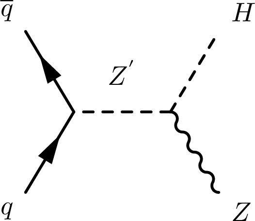
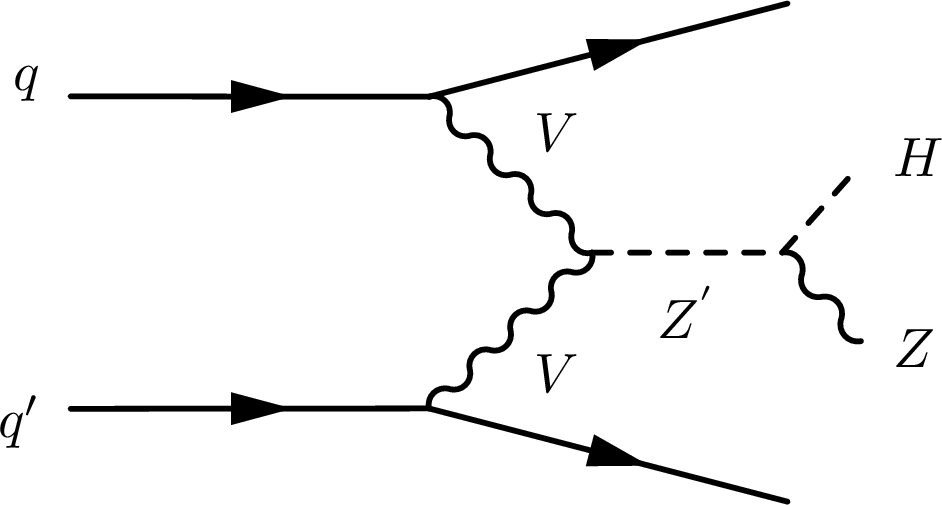
Figure 1:
The leading order Feynman diagrams of the heavy resonance Z' production through ${\mathrm{q} \mathrm{\bar{q}}}$ annihilation (left) and vector boson fusion (right), decaying to a Z boson (Z) and a Higgs boson (H). |
png pdf |
Figure 1-a:
The leading order Feynman diagram of the heavy resonance Z' production through ${\mathrm{q} \mathrm{\bar{q}}}$ annihilation, decaying to a Z boson (Z) and a Higgs boson (H). |
png pdf |
Figure 1-b:
The leading order Feynman diagram of the heavy resonance Z' production through vector boson fusion, decaying to a Z boson (Z) and a Higgs boson (H). |

png pdf |
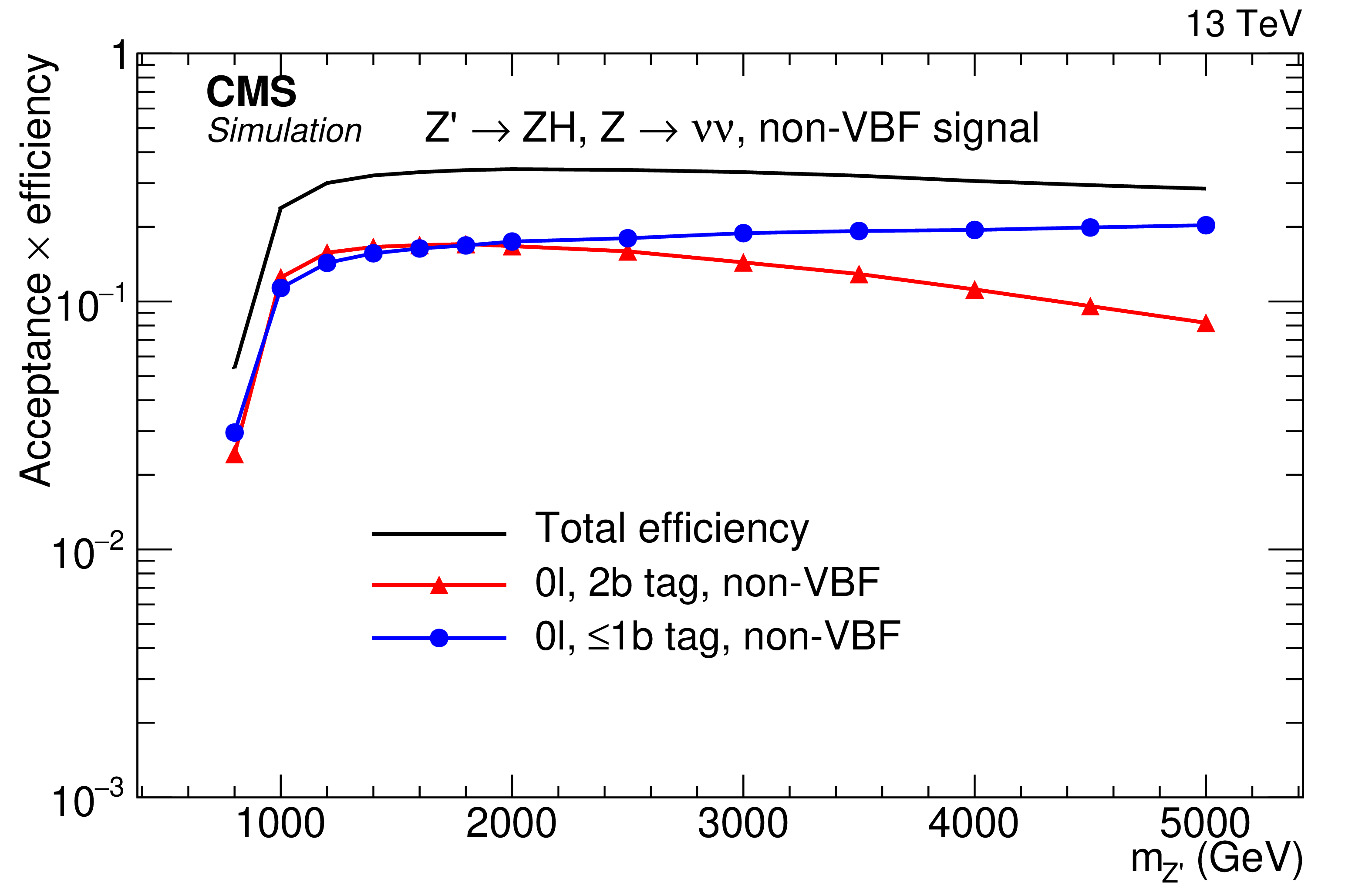
Figure 2:
The product of signal acceptance and efficiency in the 0$\ell $ (left column) and 2$\ell $ (right column) categories for the signal produced via ${\mathrm{q} \mathrm{\bar{q}}}$ annihilation (upper row) and vector boson fusion (lower row). |
png pdf |
Figure 2-a:
The product of signal acceptance and efficiency in the 0$\ell $ category for the signal produced via ${\mathrm{q} \mathrm{\bar{q}}}$ annihilation. |

png pdf |
Figure 2-b:
The product of signal acceptance and efficiency in the 2$\ell $ category for the signal produced via ${\mathrm{q} \mathrm{\bar{q}}}$ annihilation. |

png pdf |
Figure 2-c:
The product of signal acceptance and efficiency in the 0$\ell $ category for the signal produced via vector boson fusion. |

png pdf |
Figure 2-d:
The product of signal acceptance and efficiency in the 2$\ell $ category for the signal produced via vector boson fusion. |

png pdf |
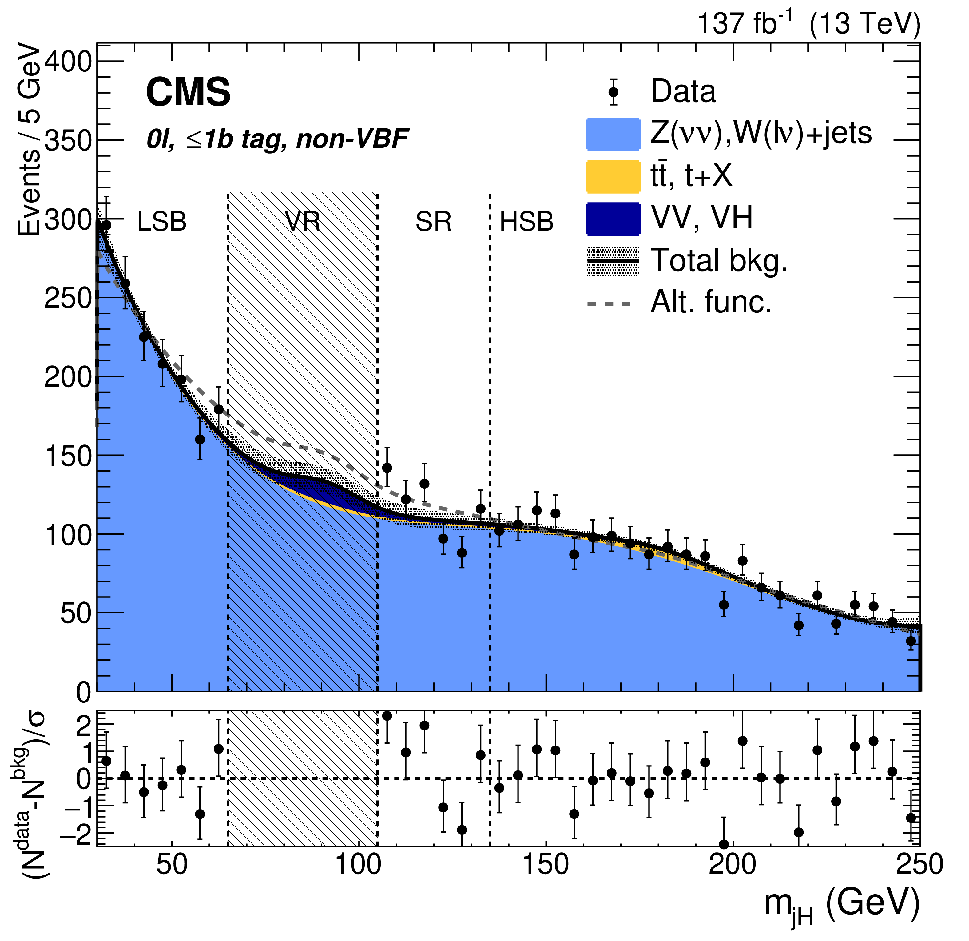
Figure 3:
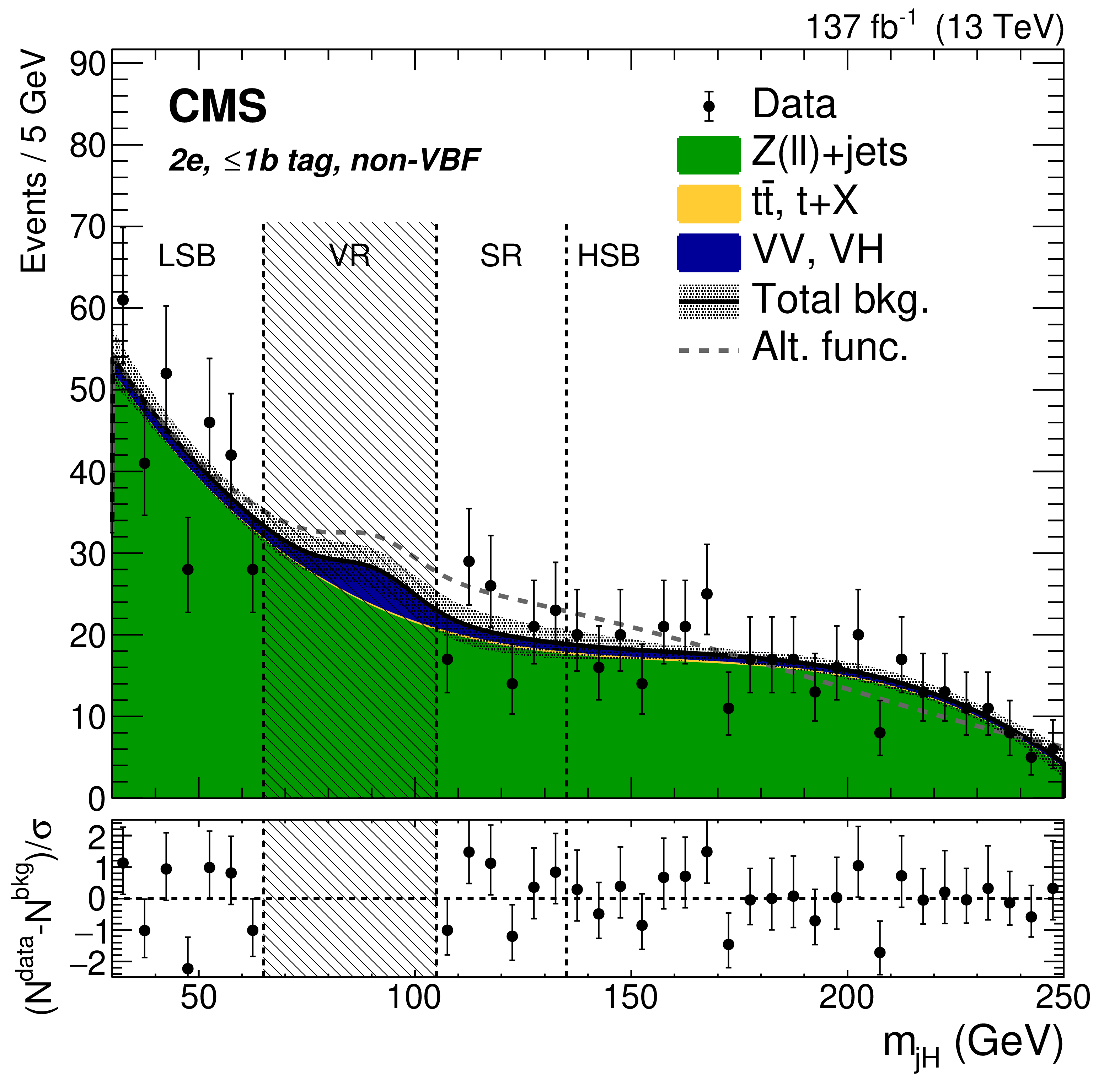
Fit to the ${m_{{j_{\mathrm{H}}}}}$ distribution in data in the 2b tag (left column) and $\leq $1b tag (right column) non-VBF categories, for 0$\ell $ (upper row), 2e (middle row), and 2$\mu$ (lower row). The shaded bands around the total background estimate represent the uncertainty from the fit to data in the jet mass SBs. The observed data are indicated by black markers. The vertical shaded band indicates the VR region, which is blinded and not used in the fit to avoid potential contamination from VV resonant signals. The dashed vertical lines separate the LSB, VR, SR, and HSB. The bottom panel shows $(N^{\text {data}}-N^{\text {bkg}})/\sigma $ for each bin, where $\sigma $ is the statistical uncertainty in data. |

png pdf |
Figure 3-a:
Fit to the ${m_{{j_{\mathrm{H}}}}}$ distribution in data in the 2b tag non-VBF category, for 0$\ell$. The shaded bands around the total background estimate represent the uncertainty from the fit to data in the jet mass SBs. The observed data are indicated by black markers. The vertical shaded band indicates the VR region, which is blinded and not used in the fit to avoid potential contamination from VV resonant signals. The dashed vertical lines separate the LSB, VR, SR, and HSB. The bottom panel shows $(N^{\text {data}}-N^{\text {bkg}})/\sigma $ for each bin, where $\sigma $ is the statistical uncertainty in data. |
png pdf |
Figure 3-b:
Fit to the ${m_{{j_{\mathrm{H}}}}}$ distribution in data in the $\leq $1b tag non-VBF category, for 0$\ell$. The shaded bands around the total background estimate represent the uncertainty from the fit to data in the jet mass SBs. The observed data are indicated by black markers. The vertical shaded band indicates the VR region, which is blinded and not used in the fit to avoid potential contamination from VV resonant signals. The dashed vertical lines separate the LSB, VR, SR, and HSB. The bottom panel shows $(N^{\text {data}}-N^{\text {bkg}})/\sigma $ for each bin, where $\sigma $ is the statistical uncertainty in data. |

png pdf |
Figure 3-c:
Fit to the ${m_{{j_{\mathrm{H}}}}}$ distribution in data in the 2b tag non-VBF category, for 2e. The shaded bands around the total background estimate represent the uncertainty from the fit to data in the jet mass SBs. The observed data are indicated by black markers. The vertical shaded band indicates the VR region, which is blinded and not used in the fit to avoid potential contamination from VV resonant signals. The dashed vertical lines separate the LSB, VR, SR, and HSB. The bottom panel shows $(N^{\text {data}}-N^{\text {bkg}})/\sigma $ for each bin, where $\sigma $ is the statistical uncertainty in data. |
png pdf |
Figure 3-d:
Fit to the ${m_{{j_{\mathrm{H}}}}}$ distribution in data in the $\leq $1b tag non-VBF category, for 2e. The shaded bands around the total background estimate represent the uncertainty from the fit to data in the jet mass SBs. The observed data are indicated by black markers. The vertical shaded band indicates the VR region, which is blinded and not used in the fit to avoid potential contamination from VV resonant signals. The dashed vertical lines separate the LSB, VR, SR, and HSB. The bottom panel shows $(N^{\text {data}}-N^{\text {bkg}})/\sigma $ for each bin, where $\sigma $ is the statistical uncertainty in data. |

png pdf |
Figure 3-e:
Fit to the ${m_{{j_{\mathrm{H}}}}}$ distribution in data in the 2b tag non-VBF category, for 2$\mu$. The shaded bands around the total background estimate represent the uncertainty from the fit to data in the jet mass SBs. The observed data are indicated by black markers. The vertical shaded band indicates the VR region, which is blinded and not used in the fit to avoid potential contamination from VV resonant signals. The dashed vertical lines separate the LSB, VR, SR, and HSB. The bottom panel shows $(N^{\text {data}}-N^{\text {bkg}})/\sigma $ for each bin, where $\sigma $ is the statistical uncertainty in data. |

png pdf |
Figure 3-f:
Fit to the ${m_{{j_{\mathrm{H}}}}}$ distribution in data in the $\leq $1b tag non-VBF category, for 2$\mu$. The shaded bands around the total background estimate represent the uncertainty from the fit to data in the jet mass SBs. The observed data are indicated by black markers. The vertical shaded band indicates the VR region, which is blinded and not used in the fit to avoid potential contamination from VV resonant signals. The dashed vertical lines separate the LSB, VR, SR, and HSB. The bottom panel shows $(N^{\text {data}}-N^{\text {bkg}})/\sigma $ for each bin, where $\sigma $ is the statistical uncertainty in data. |
png pdf |
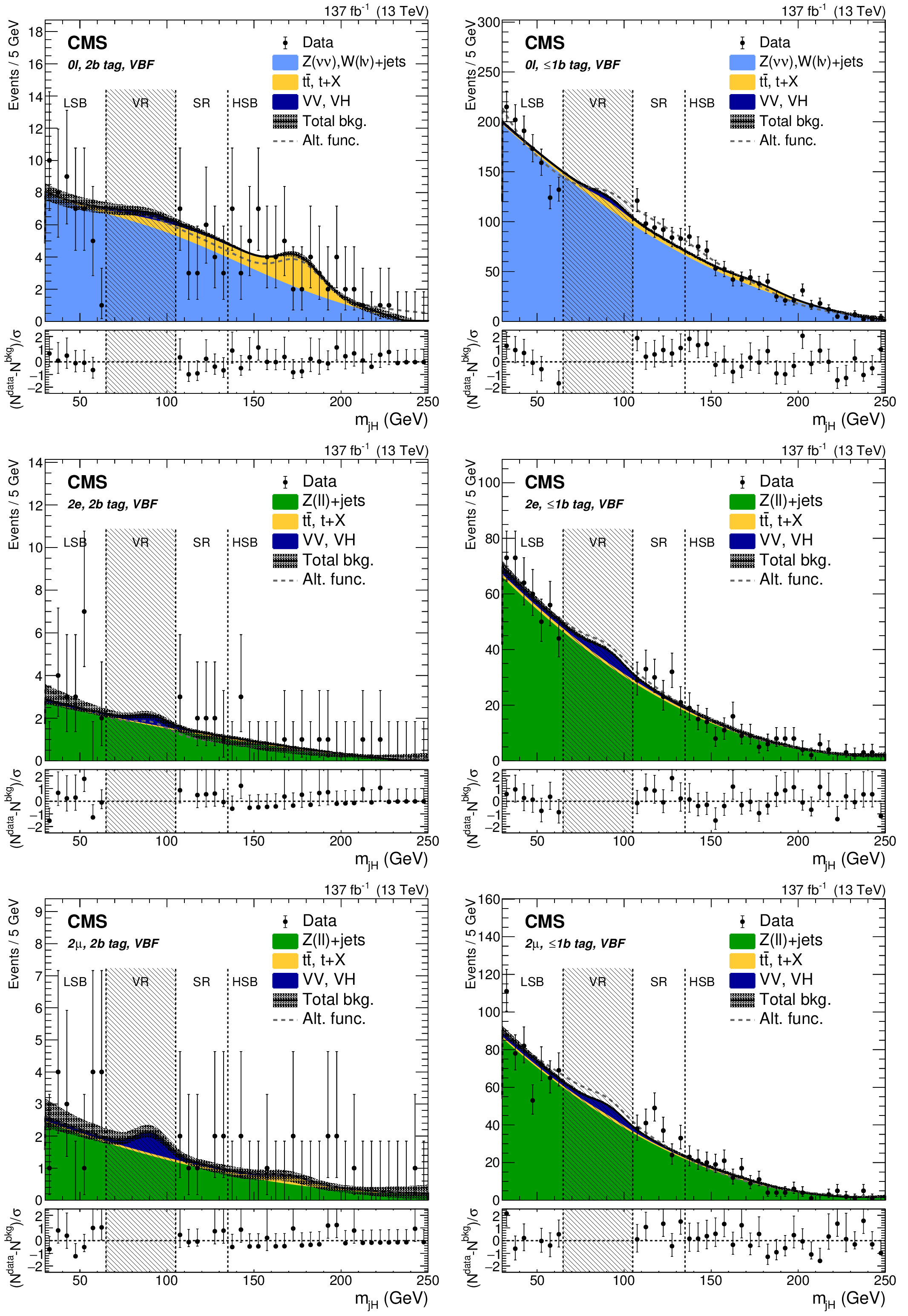
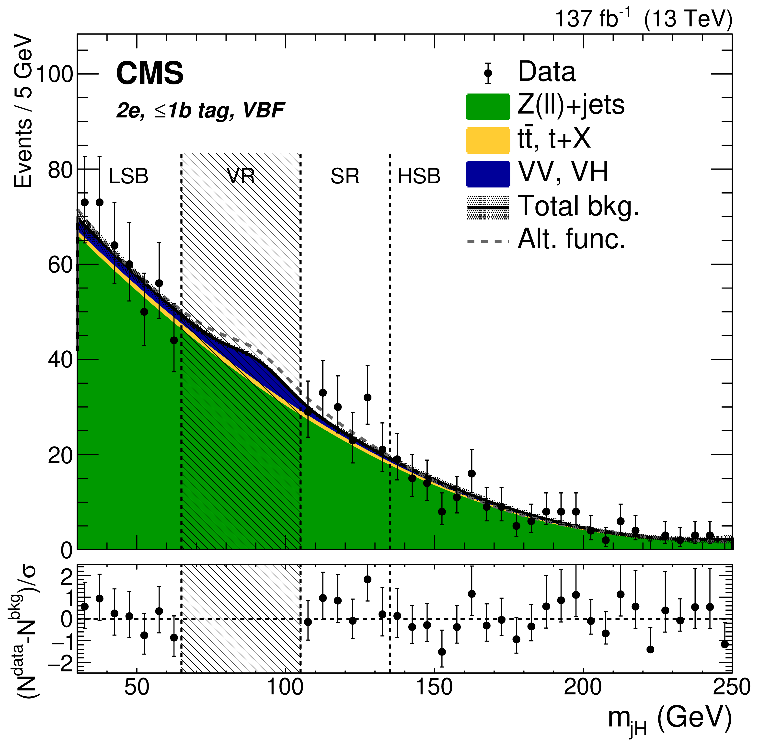
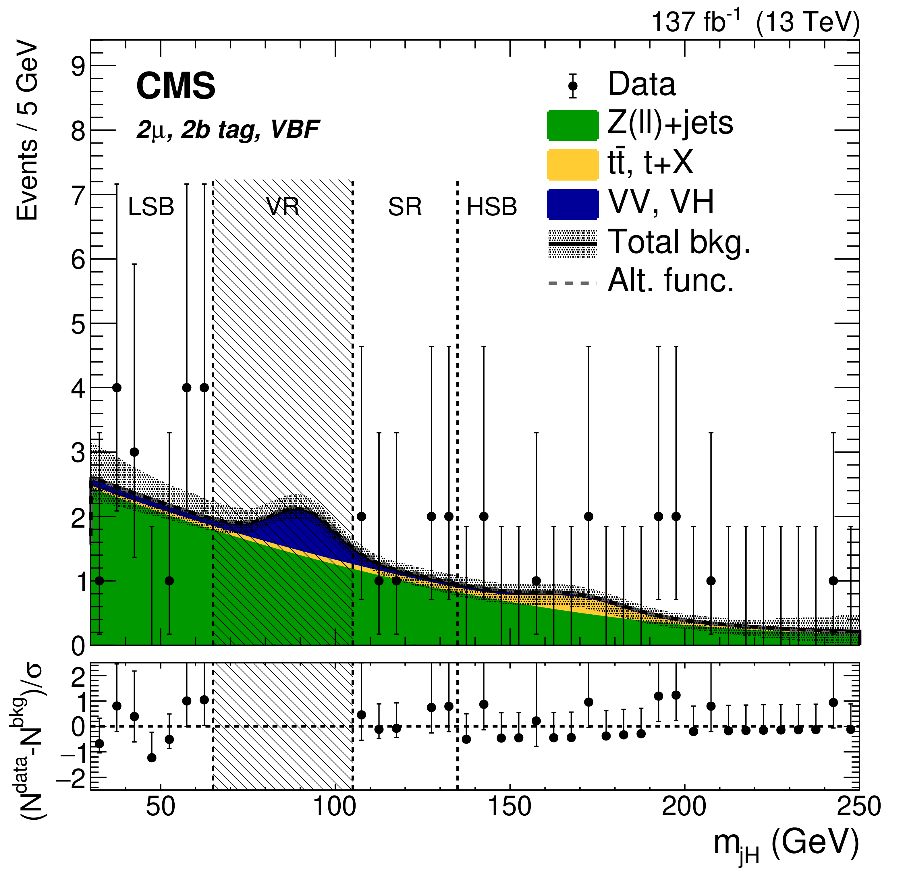
Figure 4:
Fit to the ${m_{{j_{\mathrm{H}}}}}$ distribution in data in the 2b tag (left column) and $\leq $1b tag (right column) VBF categories, for 0$\ell $ (upper row), 2e (middle row), and 2$\mu$ (lower row). The shaded bands around the total background estimate represent the uncertainty from the fit to data in the jet mass SBs. The observed data are indicated by black markers. The observed data are indicated by black markers. The vertical shaded band indicates the VR region, which is blinded and not used in the fit to avoid potential contamination from VV resonant signals. The dashed vertical lines separate the LSB, VR, SR, and HSB. The bottom panel shows $(N^{\text {data}}-N^{\text {bkg}})/\sigma $ for each bin, where $\sigma $ is the statistical uncertainty in data. |
png pdf |
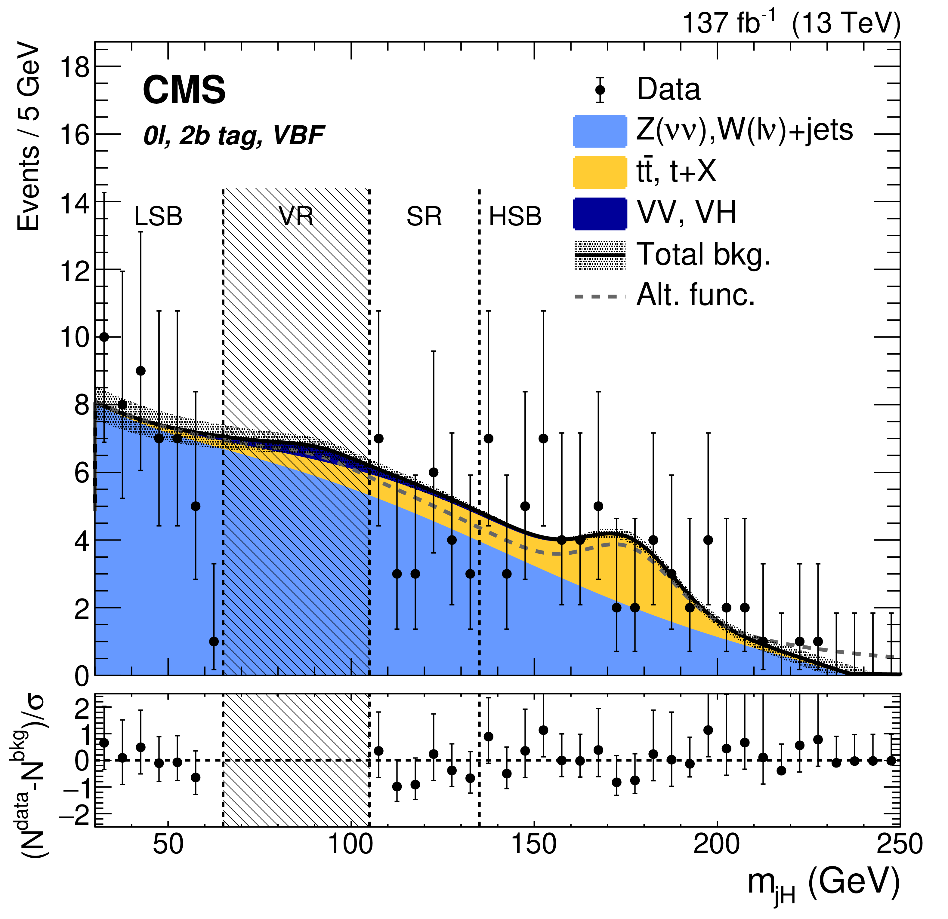
Figure 4-a:
Fit to the ${m_{{j_{\mathrm{H}}}}}$ distribution in data in the 2b tag tag VBF category, for 0$\ell $. The shaded bands around the total background estimate represent the uncertainty from the fit to data in the jet mass SBs. The observed data are indicated by black markers. The observed data are indicated by black markers. The vertical shaded band indicates the VR region, which is blinded and not used in the fit to avoid potential contamination from VV resonant signals. The dashed vertical lines separate the LSB, VR, SR, and HSB. The bottom panel shows $(N^{\text {data}}-N^{\text {bkg}})/\sigma $ for each bin, where $\sigma $ is the statistical uncertainty in data. |

png pdf |
Figure 4-b:
Fit to the ${m_{{j_{\mathrm{H}}}}}$ distribution in data in the $\leq $1b tag VBF category, for 0$\ell $. The shaded bands around the total background estimate represent the uncertainty from the fit to data in the jet mass SBs. The observed data are indicated by black markers. The observed data are indicated by black markers. The vertical shaded band indicates the VR region, which is blinded and not used in the fit to avoid potential contamination from VV resonant signals. The dashed vertical lines separate the LSB, VR, SR, and HSB. The bottom panel shows $(N^{\text {data}}-N^{\text {bkg}})/\sigma $ for each bin, where $\sigma $ is the statistical uncertainty in data. |
png pdf |
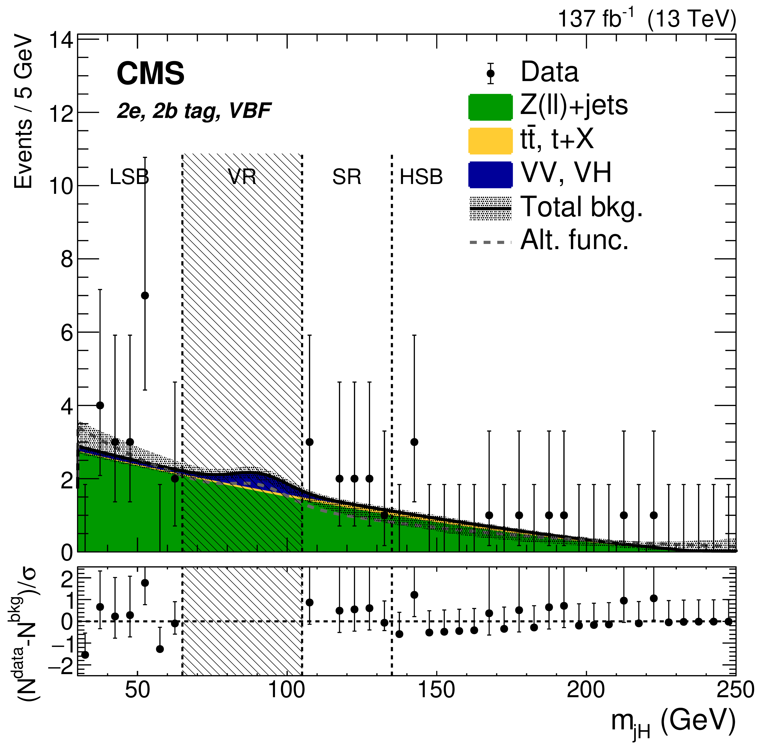
Figure 4-c:
Fit to the ${m_{{j_{\mathrm{H}}}}}$ distribution in data in the 2b tag tag VBF category, for 2e. The shaded bands around the total background estimate represent the uncertainty from the fit to data in the jet mass SBs. The observed data are indicated by black markers. The observed data are indicated by black markers. The vertical shaded band indicates the VR region, which is blinded and not used in the fit to avoid potential contamination from VV resonant signals. The dashed vertical lines separate the LSB, VR, SR, and HSB. The bottom panel shows $(N^{\text {data}}-N^{\text {bkg}})/\sigma $ for each bin, where $\sigma $ is the statistical uncertainty in data. |
png pdf |
Figure 4-d:
Fit to the ${m_{{j_{\mathrm{H}}}}}$ distribution in data in the $\leq $1b tag VBF category, for 2e. The shaded bands around the total background estimate represent the uncertainty from the fit to data in the jet mass SBs. The observed data are indicated by black markers. The observed data are indicated by black markers. The vertical shaded band indicates the VR region, which is blinded and not used in the fit to avoid potential contamination from VV resonant signals. The dashed vertical lines separate the LSB, VR, SR, and HSB. The bottom panel shows $(N^{\text {data}}-N^{\text {bkg}})/\sigma $ for each bin, where $\sigma $ is the statistical uncertainty in data. |
png pdf |
Figure 4-e:
Fit to the ${m_{{j_{\mathrm{H}}}}}$ distribution in data in the 2b tag tag VBF category, for 2$\mu$. The shaded bands around the total background estimate represent the uncertainty from the fit to data in the jet mass SBs. The observed data are indicated by black markers. The observed data are indicated by black markers. The vertical shaded band indicates the VR region, which is blinded and not used in the fit to avoid potential contamination from VV resonant signals. The dashed vertical lines separate the LSB, VR, SR, and HSB. The bottom panel shows $(N^{\text {data}}-N^{\text {bkg}})/\sigma $ for each bin, where $\sigma $ is the statistical uncertainty in data. |

png pdf |
Figure 4-f:
Fit to the ${m_{{j_{\mathrm{H}}}}}$ distribution in data in the $\leq $1b tag VBF category, for 2$\mu$. The shaded bands around the total background estimate represent the uncertainty from the fit to data in the jet mass SBs. The observed data are indicated by black markers. The observed data are indicated by black markers. The vertical shaded band indicates the VR region, which is blinded and not used in the fit to avoid potential contamination from VV resonant signals. The dashed vertical lines separate the LSB, VR, SR, and HSB. The bottom panel shows $(N^{\text {data}}-N^{\text {bkg}})/\sigma $ for each bin, where $\sigma $ is the statistical uncertainty in data. |
png pdf |
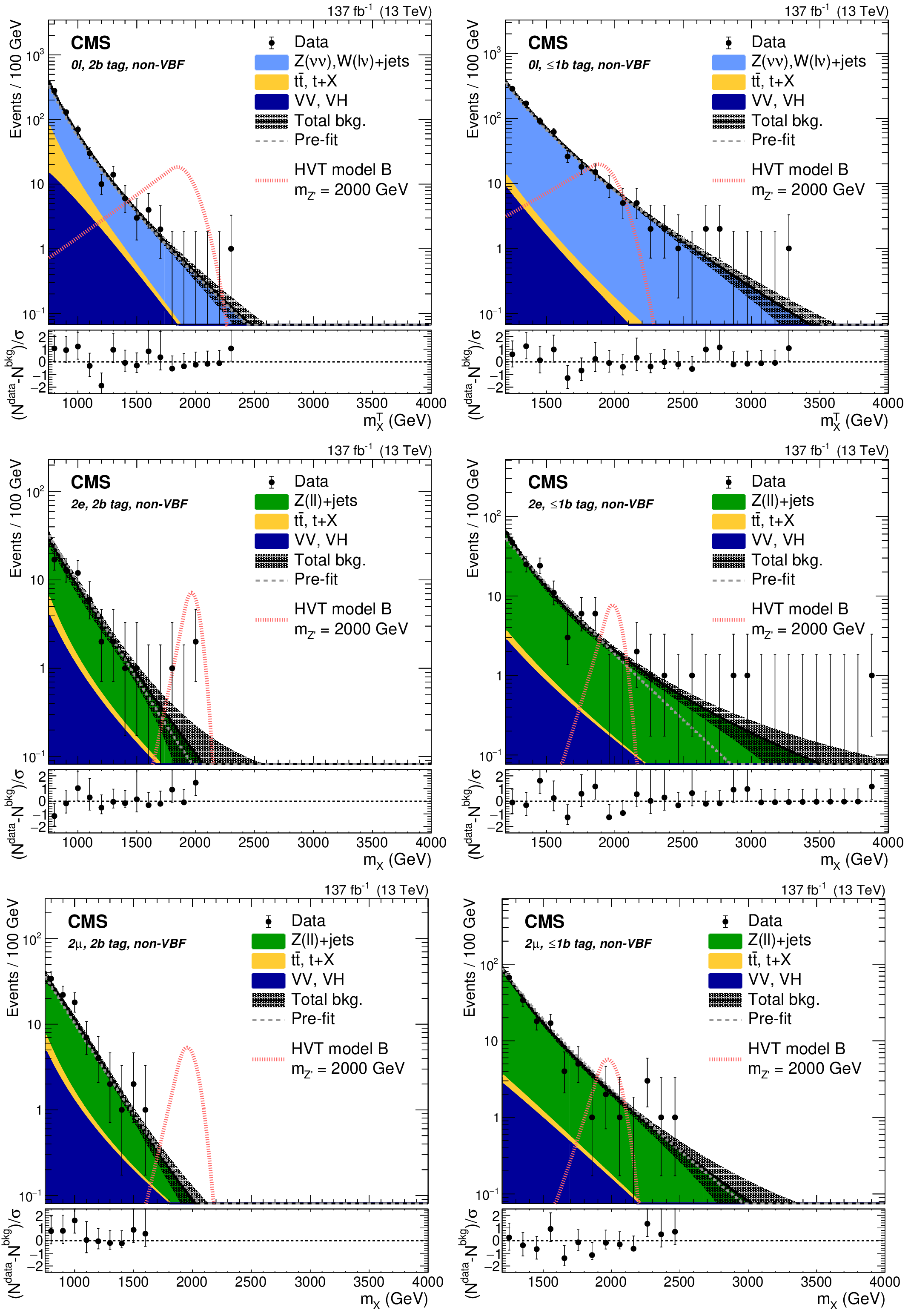
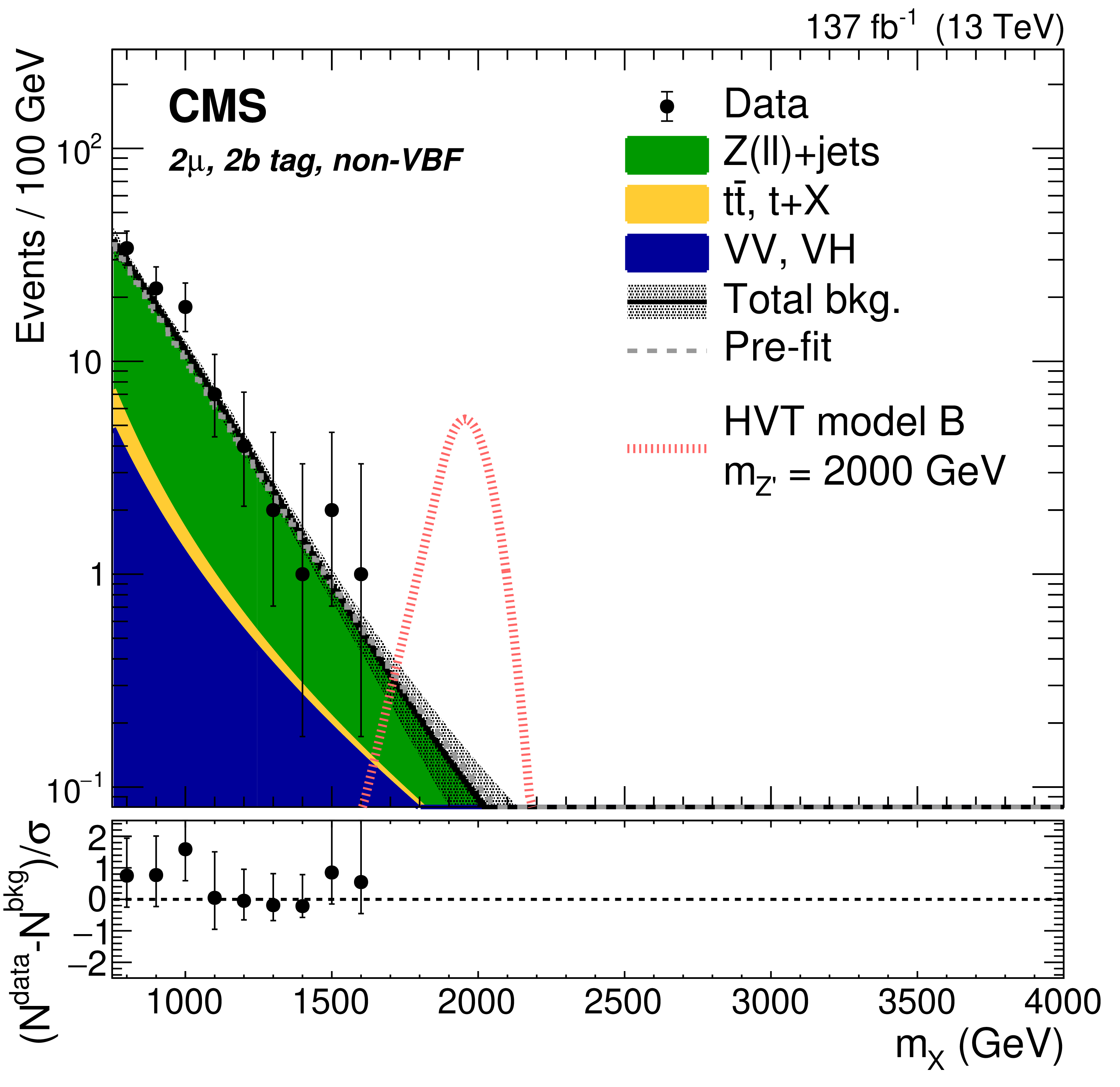
Figure 5:
Distributions in data in the 2b tag (left column) and $\leq $1b tag (right column) non-VBF categories, of ${m_{{\mathrm {X}}}^{\text {T}}}$ for 0$\ell $ (upper row), and ${m_{{\mathrm {X}}}}$ for 2e (middle row), and 2$\mu$ (lower row). The distributions are shown up to 4000 GeV, which corresponds to the event with the highest ${m_{{\mathrm {X}}}}$ or ${m_{{\mathrm {X}}}^{\text {T}}}$ observed in the SR. The shaded bands represent the uncertainty from the background estimation. The observed data are represented by black markers, and the potential contribution of a resonance produced in the context of the HVT model B at $ {m_{\mathrm{Z'}}} = $ 2000 GeV is shown as a dotted red line. The bottom panel shows $(N^{\text {data}}-N^{\text {bkg}})/\sigma $ for each bin, where $\sigma $ is the statistical uncertainty in data. |

png pdf |
Figure 5-a:
Distribution in data in the 2b tag tag non-VBF category, of ${m_{{\mathrm {X}}}^{\text {T}}}$ for 0$\ell $. The distribution is shown up to 4000 GeV, which corresponds to the event with the highest ${m_{{\mathrm {X}}}}$ or ${m_{{\mathrm {X}}}^{\text {T}}}$ observed in the SR. The shaded bands represent the uncertainty from the background estimation. The observed data are represented by black markers, and the potential contribution of a resonance produced in the context of the HVT model B at $ {m_{\mathrm{Z'}}} = $ 2000 GeV is shown as a dotted red line. The bottom panel shows $(N^{\text {data}}-N^{\text {bkg}})/\sigma $ for each bin, where $\sigma $ is the statistical uncertainty in data. |
png pdf |
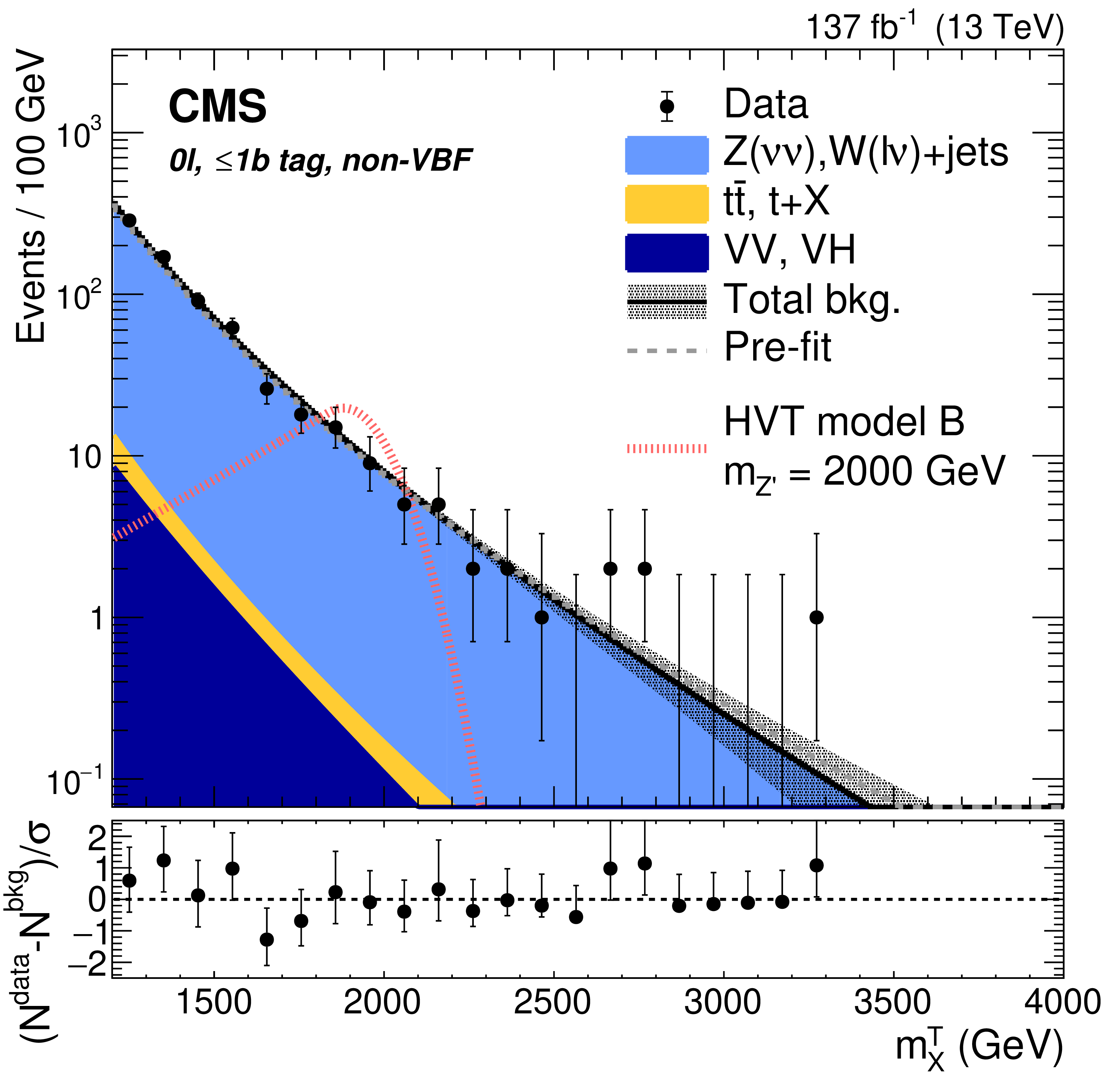
Figure 5-b:
Distribution in data in the $\leq $1b tag non-VBF category, of ${m_{{\mathrm {X}}}^{\text {T}}}$ for 0$\ell $. The distribution is shown up to 4000 GeV, which corresponds to the event with the highest ${m_{{\mathrm {X}}}}$ or ${m_{{\mathrm {X}}}^{\text {T}}}$ observed in the SR. The shaded bands represent the uncertainty from the background estimation. The observed data are represented by black markers, and the potential contribution of a resonance produced in the context of the HVT model B at $ {m_{\mathrm{Z'}}} = $ 2000 GeV is shown as a dotted red line. The bottom panel shows $(N^{\text {data}}-N^{\text {bkg}})/\sigma $ for each bin, where $\sigma $ is the statistical uncertainty in data. |

png pdf |
Figure 5-c:
Distribution in data in the 2b tag tag non-VBF category, of ${m_{{\mathrm {X}}}}$ for 2e. The distribution is shown up to 4000 GeV, which corresponds to the event with the highest ${m_{{\mathrm {X}}}}$ or ${m_{{\mathrm {X}}}^{\text {T}}}$ observed in the SR. The shaded bands represent the uncertainty from the background estimation. The observed data are represented by black markers, and the potential contribution of a resonance produced in the context of the HVT model B at $ {m_{\mathrm{Z'}}} = $ 2000 GeV is shown as a dotted red line. The bottom panel shows $(N^{\text {data}}-N^{\text {bkg}})/\sigma $ for each bin, where $\sigma $ is the statistical uncertainty in data. |
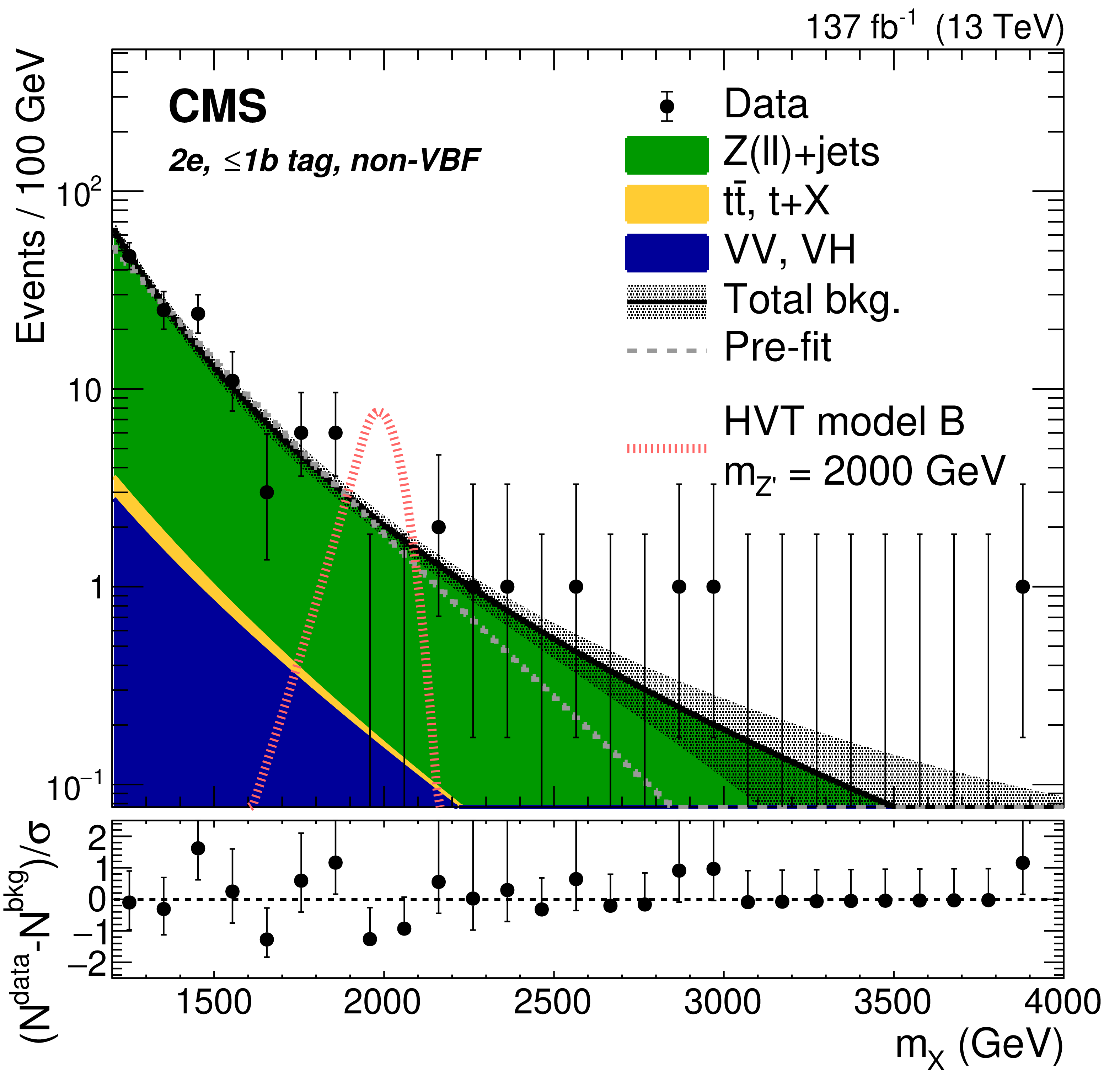
png pdf |
Figure 5-d:
Distribution in data in the $\leq $1b tag non-VBF category, of ${m_{{\mathrm {X}}}}$ for 2e. The distribution is shown up to 4000 GeV, which corresponds to the event with the highest ${m_{{\mathrm {X}}}}$ or ${m_{{\mathrm {X}}}^{\text {T}}}$ observed in the SR. The shaded bands represent the uncertainty from the background estimation. The observed data are represented by black markers, and the potential contribution of a resonance produced in the context of the HVT model B at $ {m_{\mathrm{Z'}}} = $ 2000 GeV is shown as a dotted red line. The bottom panel shows $(N^{\text {data}}-N^{\text {bkg}})/\sigma $ for each bin, where $\sigma $ is the statistical uncertainty in data. |
png pdf |
Figure 5-e:
Distribution in data in the 2b tag tag non-VBF category, of${m_{{\mathrm {X}}}}$ for 2$\mu$. The distribution is shown up to 4000 GeV, which corresponds to the event with the highest ${m_{{\mathrm {X}}}}$ or ${m_{{\mathrm {X}}}^{\text {T}}}$ observed in the SR. The shaded bands represent the uncertainty from the background estimation. The observed data are represented by black markers, and the potential contribution of a resonance produced in the context of the HVT model B at $ {m_{\mathrm{Z'}}} = $ 2000 GeV is shown as a dotted red line. The bottom panel shows $(N^{\text {data}}-N^{\text {bkg}})/\sigma $ for each bin, where $\sigma $ is the statistical uncertainty in data. |

png pdf |
Figure 5-f:
Distribution in data in the $\leq $1b tag non-VBF category, of ${m_{{\mathrm {X}}}}$ for 2$\mu$. The distribution is shown up to 4000 GeV, which corresponds to the event with the highest ${m_{{\mathrm {X}}}}$ or ${m_{{\mathrm {X}}}^{\text {T}}}$ observed in the SR. The shaded bands represent the uncertainty from the background estimation. The observed data are represented by black markers, and the potential contribution of a resonance produced in the context of the HVT model B at $ {m_{\mathrm{Z'}}} = $ 2000 GeV is shown as a dotted red line. The bottom panel shows $(N^{\text {data}}-N^{\text {bkg}})/\sigma $ for each bin, where $\sigma $ is the statistical uncertainty in data. |
png pdf |
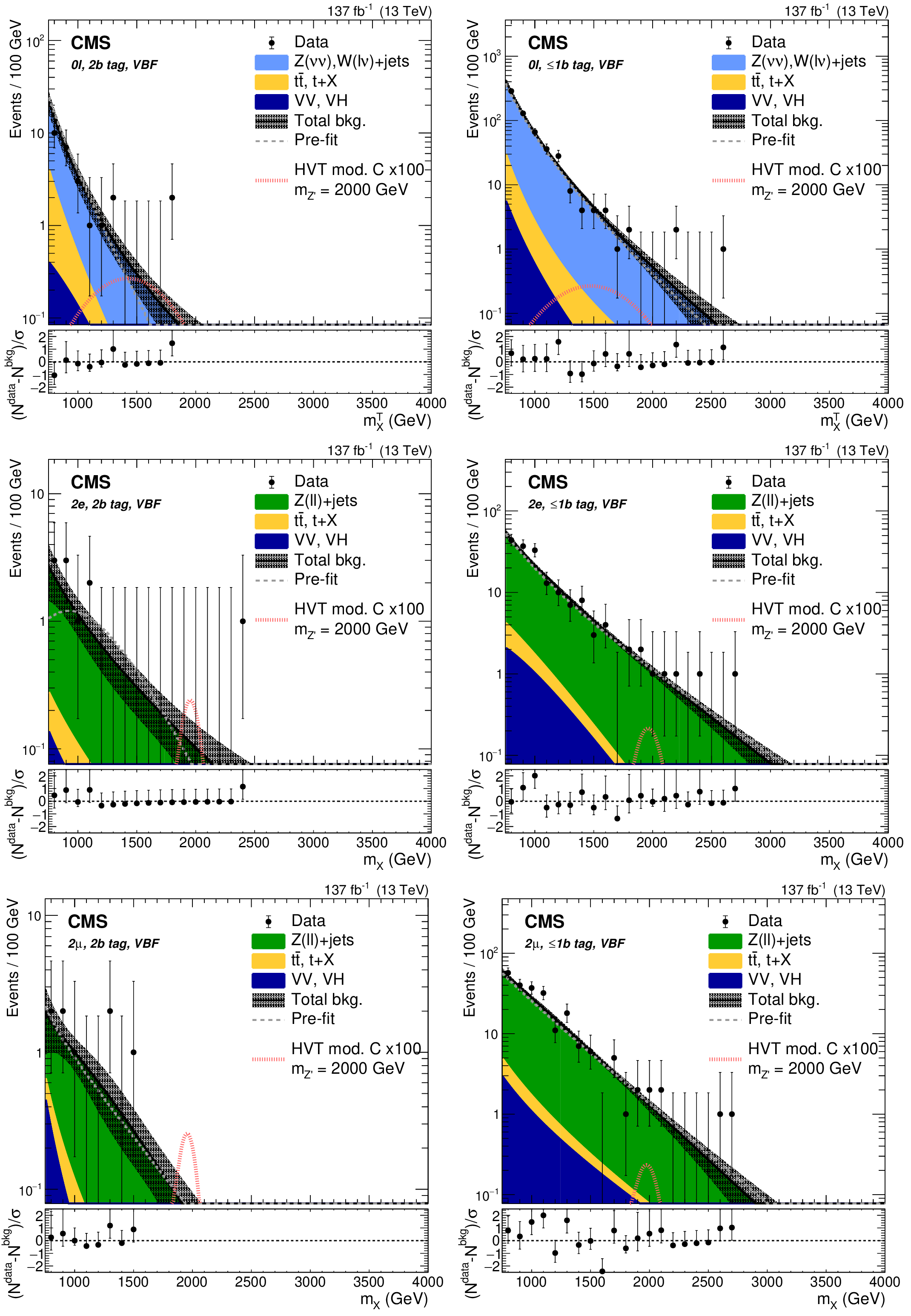
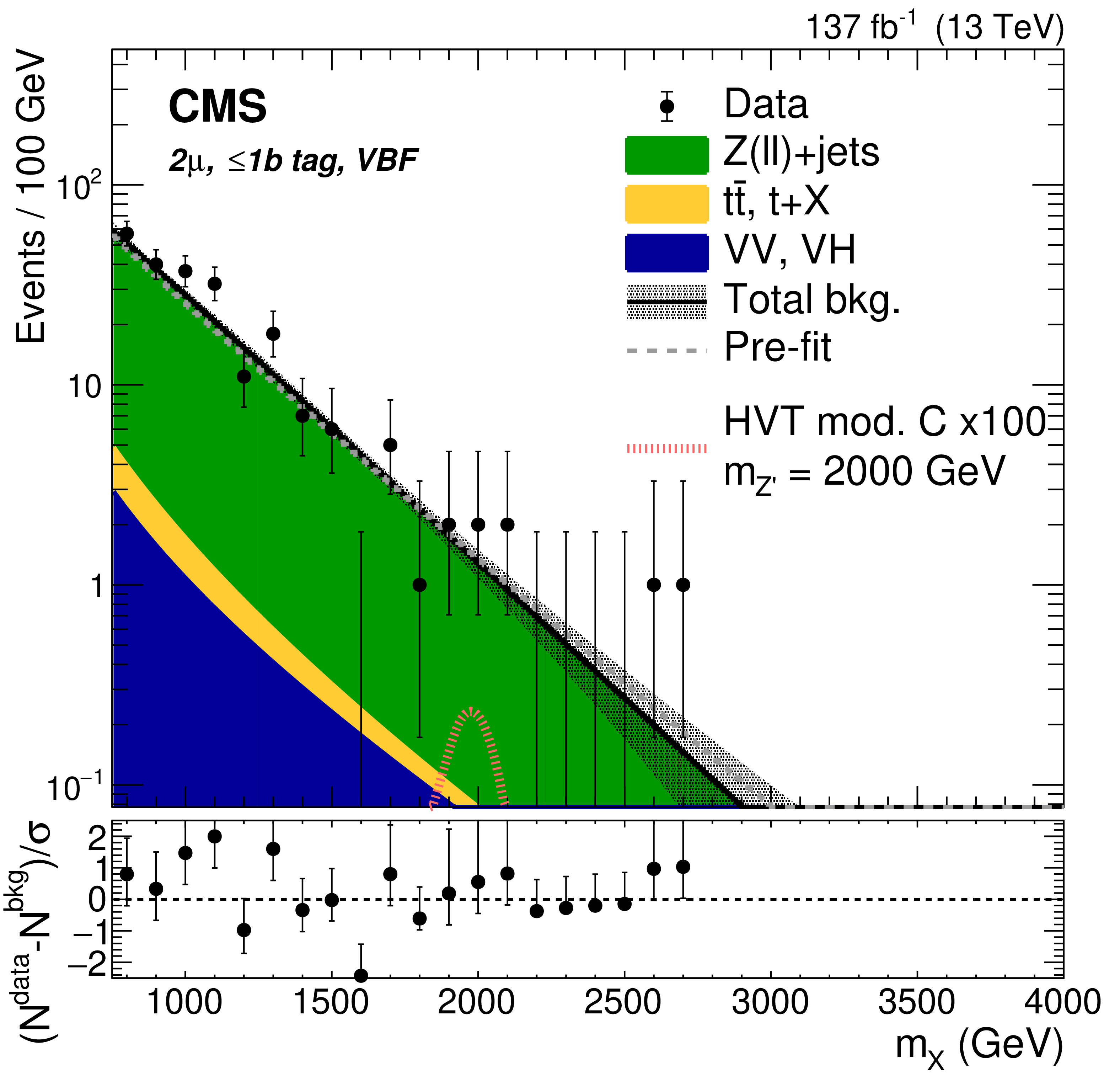
Figure 6:
Distributions in data in the 2b tag (left column) and $\leq $1b tag (right column) VBF categories, of ${m_{{\mathrm {X}}}^{\text {T}}}$ for 0$\ell $ (upper row), and ${m_{{\mathrm {X}}}}$ for 2e (middle row), and 2$\mu$ (lower row). The distributions are shown up to 4000 GeV, which corresponds to the event with the highest ${m_{{\mathrm {X}}}}$ or ${m_{{\mathrm {X}}}^{\text {T}}}$ observed in the SR. The shaded bands represent the uncertainty from the background estimation. The observed data are represented by black markers, and the potential contribution of a resonance produced in the context of the HVT model C at $ {m_{\mathrm{Z'}}} = $ 2000 GeV is shown as a dotted red line. The bottom panel shows $(N^{\text {data}}-N^{\text {bkg}})/\sigma $ for each bin, where $\sigma $ is the statistical uncertainty in data. |

png pdf |
Figure 6-a:
Distribution in data in the 2b tag tag VBF category, of ${m_{{\mathrm {X}}}^{\text {T}}}$ for 0$\ell $. The distribution is shown up to 4000 GeV, which corresponds to the event with the highest ${m_{{\mathrm {X}}}}$ or ${m_{{\mathrm {X}}}^{\text {T}}}$ observed in the SR. The shaded bands represent the uncertainty from the background estimation. The observed data are represented by black markers, and the potential contribution of a resonance produced in the context of the HVT model C at $ {m_{\mathrm{Z'}}} = $ 2000 GeV is shown as a dotted red line. The bottom panel shows $(N^{\text {data}}-N^{\text {bkg}})/\sigma $ for each bin, where $\sigma $ is the statistical uncertainty in data. |

png pdf |
Figure 6-b:
Distribution in data in the $\leq $1b tag VBF category, of ${m_{{\mathrm {X}}}^{\text {T}}}$ for 0$\ell $. The distribution is shown up to 4000 GeV, which corresponds to the event with the highest ${m_{{\mathrm {X}}}}$ or ${m_{{\mathrm {X}}}^{\text {T}}}$ observed in the SR. The shaded bands represent the uncertainty from the background estimation. The observed data are represented by black markers, and the potential contribution of a resonance produced in the context of the HVT model C at $ {m_{\mathrm{Z'}}} = $ 2000 GeV is shown as a dotted red line. The bottom panel shows $(N^{\text {data}}-N^{\text {bkg}})/\sigma $ for each bin, where $\sigma $ is the statistical uncertainty in data. |

png pdf |
Figure 6-c:
Distribution in data in the 2b tag tag VBF category, of ${m_{{\mathrm {X}}}}$ for 2e. The distribution is shown up to 4000 GeV, which corresponds to the event with the highest ${m_{{\mathrm {X}}}}$ or ${m_{{\mathrm {X}}}^{\text {T}}}$ observed in the SR. The shaded bands represent the uncertainty from the background estimation. The observed data are represented by black markers, and the potential contribution of a resonance produced in the context of the HVT model C at $ {m_{\mathrm{Z'}}} = $ 2000 GeV is shown as a dotted red line. The bottom panel shows $(N^{\text {data}}-N^{\text {bkg}})/\sigma $ for each bin, where $\sigma $ is the statistical uncertainty in data. |

png pdf |
Figure 6-d:
Distribution in data in the $\leq $1b tag VBF category, of ${m_{{\mathrm {X}}}}$ for 2e. The distribution is shown up to 4000 GeV, which corresponds to the event with the highest ${m_{{\mathrm {X}}}}$ or ${m_{{\mathrm {X}}}^{\text {T}}}$ observed in the SR. The shaded bands represent the uncertainty from the background estimation. The observed data are represented by black markers, and the potential contribution of a resonance produced in the context of the HVT model C at $ {m_{\mathrm{Z'}}} = $ 2000 GeV is shown as a dotted red line. The bottom panel shows $(N^{\text {data}}-N^{\text {bkg}})/\sigma $ for each bin, where $\sigma $ is the statistical uncertainty in data. |

png pdf |
Figure 6-e:
Distribution in data in the 2b tag tag VBF category, of ${m_{{\mathrm {X}}}}$ for 2$\mu$. The distribution is shown up to 4000 GeV, which corresponds to the event with the highest ${m_{{\mathrm {X}}}}$ or ${m_{{\mathrm {X}}}^{\text {T}}}$ observed in the SR. The shaded bands represent the uncertainty from the background estimation. The observed data are represented by black markers, and the potential contribution of a resonance produced in the context of the HVT model C at $ {m_{\mathrm{Z'}}} = $ 2000 GeV is shown as a dotted red line. The bottom panel shows $(N^{\text {data}}-N^{\text {bkg}})/\sigma $ for each bin, where $\sigma $ is the statistical uncertainty in data. |
png pdf |
Figure 6-f:
Distribution in data in the $\leq $1b tag VBF category, of ${m_{{\mathrm {X}}}}$ for 2$\mu$. The distribution is shown up to 4000 GeV, which corresponds to the event with the highest ${m_{{\mathrm {X}}}}$ or ${m_{{\mathrm {X}}}^{\text {T}}}$ observed in the SR. The shaded bands represent the uncertainty from the background estimation. The observed data are represented by black markers, and the potential contribution of a resonance produced in the context of the HVT model C at $ {m_{\mathrm{Z'}}} = $ 2000 GeV is shown as a dotted red line. The bottom panel shows $(N^{\text {data}}-N^{\text {bkg}})/\sigma $ for each bin, where $\sigma $ is the statistical uncertainty in data. |

png pdf |
Figure 7:
Observed and expected 95% CL upper limit on $\sigma {\mathcal {B}}({\mathrm{Z'} \to \mathrm{Z} \mathrm{H}})$ with all categories combined, for the non-VBF signal (left) and VBF signal (right), including all statistical and systematic uncertainties. The inner green band and the outer yellow band indicate the regions containing 68 and 95%, respectively, of the distribution of expected limits under the background-only hypothesis. The solid curves and their shaded areas correspond to the product of the cross section and the branching fractions predicted by the HVT models A and B (left) and HVT model C (right), and their relative uncertainties. The CMS search for a heavy resonance using 2016 data and the same final state [14] is shown as a comparison. |

png pdf |
Figure 7-a:
Observed and expected 95% CL upper limit on $\sigma {\mathcal {B}}({\mathrm{Z'} \to \mathrm{Z} \mathrm{H}})$ with all categories combined, for the non-VBF signal, including all statistical and systematic uncertainties. The inner green band and the outer yellow band indicate the regions containing 68 and 95%, respectively, of the distribution of expected limits under the background-only hypothesis. The solid curves and their shaded areas correspond to the product of the cross section and the branching fractions predicted by the HVT models A and B, and their relative uncertainties. The CMS search for a heavy resonance using 2016 data and the same final state [14] is shown as a comparison. |

png pdf |
Figure 7-b:
Observed and expected 95% CL upper limit on $\sigma {\mathcal {B}}({\mathrm{Z'} \to \mathrm{Z} \mathrm{H}})$ with all categories combined, for the VBF signal, including all statistical and systematic uncertainties. The inner green band and the outer yellow band indicate the regions containing 68 and 95%, respectively, of the distribution of expected limits under the background-only hypothesis. The solid curves and their shaded areas correspond to the product of the cross section and the branching fractions predicted by the HVT models C, and their relative uncertainties. |

png pdf |
Figure 8:
Observed exclusion limit in the space of the HVT model parameters [$ {g_\text {V}} {c_\text {H}} $, $g^2 {c_\text {F}} / {g_\text {V}} $], described in the text, for three different mass hypotheses of 2.0, 3.0, and 4.0 TeV for the non-VBF signal. The shaded bands indicate the side of each contour that is excluded. The benchmark scenarios corresponding to HVT models A and B are represented by a purple cross and a red point, respectively. The region of the parameter space where the natural resonance width ($\Gamma _{Z'}$) is larger than the typical experimental resolution of 4%, for which the narrow-width approximation is not valid, is shaded in grey. |
| Tables | |

png pdf |
Table 1:
List of the 12 event categories used in the analysis. |

png pdf |
Table 2:
Scale factors derived for the normalization of the ${\mathrm{t} \mathrm{\bar{t}}}$ and single top quark backgrounds for different event categories. Uncertainties due to the limited size of the event samples (stat.) and systematic effects (syst.) are reported as well. The scale factors of the 2e and 2$\mu$ categories are derived using the 1e1$\mu $ top quark control region as described in the text. |

png pdf |
Table 3:
The expected and observed numbers of background events in the signal region for all event categories. The V+jets background uncertainties originate from the variation of the parameters within the fit uncertainties (fit) and the difference between the nominal and alternative function choice for the fit to ${m_{{j_{\mathrm{H}}}}}$ (alt). The ${\mathrm{t} \mathrm{\bar{t}}}$ and single top quark uncertainties arise from the ${m_{{j_{\mathrm{H}}}}}$ modeling, the statistical component of the top quark SF uncertainties, and the extrapolation uncertainty from the control region to the SR. The VV and VH normalization uncertainties come from the ${m_{{j_{\mathrm{H}}}}}$ modeling. |

png pdf |
Table 4:
Summary of systematic uncertainties for the background and signal samples. The entries labeled with $\dagger $ are also propagated to the shapes of the distributions. Uncertainties marked with $\ddagger $ impact the signal cross section. Uncertainties in the same line are treated as correlated. All uncertainties except for in the integrated luminosity are considered correlated across the three years of data taking. |
| Summary |
| A search for a heavy resonance with a mass between 0.8 and 5.0 TeV, decaying to a Z boson and a Higgs boson, has been described. The data samples were collected by the CMS experiment in the period 2016-2018 at $\sqrt{s} = $ 13 TeV and correspond to an integrated luminosity of 137 fb$^{-1}$. In the final states explored the Z boson decays leptonically, resulting in events with either zero or two electrons or muons. Higgs bosons with a large Lorentz boost are reconstructed via their decays to hadrons. For models with a narrow spin-1 resonance, a new heavy vector boson Z' with mass below 3.5 and 3.7 TeV is excluded at 95% confidence level in models where the heavy vector boson couples predominantly to fermions and bosons, respectively. These are the most stringent limits placed on the Heavy Vector Triplet Z' model to date. If the heavy vector boson couples exclusively to standard model bosons, upper limits on the product of the cross section and branching fraction are set between 23 and 0.3 fb for a Z' mass between 0.8 and 4.6 TeV, respectively. This is the first limit set on a heavy vector boson coupling exclusively to standard model bosons in its production and decay. |
| References | ||||
| 1 | ATLAS Collaboration | Observation of a new particle in the search for the standard model Higgs boson with the ATLAS detector at the LHC | PLB 716 (2012) 1 | 1207.7214 |
| 2 | CMS Collaboration | Observation of a new boson at a mass of 125 GeV with the CMS experiment at the LHC | PLB 716 (2012) 30 | CMS-HIG-12-028 1207.7235 |
| 3 | CMS Collaboration | Observation of a new boson with mass near 125 GeV in pp collisions at $ \sqrt{s} = $ 7 and 8 TeV | JHEP 06 (2013) 081 | CMS-HIG-12-036 1303.4571 |
| 4 | ATLAS and CMS Collaboration | Combined measurement of the Higgs boson mass in pp collisions at $ \sqrt{s}= $ 7 and 8 TeV with the ATLAS and CMS experiments | PRL 114 (2015) 191803 | 1503.07589 |
| 5 | CMS Collaboration | A measurement of the Higgs boson mass in the diphoton decay channel | PLB 805 (2020) 135425 | CMS-HIG-19-004 2002.06398 |
| 6 | ATLAS Collaboration | Evidence for the spin-0 nature of the Higgs boson using ATLAS data | PLB 726 (2013) 120 | 1307.1432 |
| 7 | ATLAS and CMS Collaboration | Measurements of the Higgs boson production and decay rates and constraints on its couplings from a combined ATLAS and CMS analysis of the LHC pp collision data at $ \sqrt{s} = $ 7 and 8 TeV | JHEP 08 (2016) 045 | 1606.02266 |
| 8 | T. Han, H. E. Logan, B. McElrath, and L.-T. Wang | Phenomenology of the little Higgs model | PRD 67 (2003) 095004 | hep-ph/0301040 |
| 9 | M. Schmaltz and D. Tucker-Smith | Little Higgs theories | Ann. Rev. Nucl. Part. Sci. 55 (2005) 229 | |
| 10 | M. Perelstein | Little Higgs models and their phenomenology | Prog. Part. NP 58 (2007) 247 | hep-ph/0512128 |
| 11 | R. Contino, D. Pappadopulo, D. Marzocca, and R. Rattazzi | On the effect of resonances in composite Higgs phenomenology | JHEP 10 (2011) 081 | 1109.1570 |
| 12 | D. Marzocca, M. Serone, and J. Shu | General composite Higgs models | JHEP 08 (2012) 013 | 1205.0770 |
| 13 | B. Bellazzini, C. Csaki, and J. Serra | Composite Higgses | EPJC 74 (2014) 2766 | 1401.2457 |
| 14 | CMS Collaboration | Search for heavy resonances decaying into a vector boson and a Higgs boson in final states with charged leptons, neutrinos, and b quarks at $ \sqrt{s} = $ 13 TeV | JHEP 11 (2018) 172 | CMS-B2G-17-004 1807.02826 |
| 15 | ATLAS Collaboration | Search for heavy resonances decaying into a $ W $ or $ Z $ boson and a Higgs boson in final states with leptons and $ b $-jets in 36 fb$ ^{-1} $ of $ \sqrt s = $ 13 TeV pp collisions with the ATLAS detector | JHEP 03 (2018) 174 | 1712.06518 |
| 16 | CMS Collaboration | Combination of CMS searches for heavy resonances decaying to pairs of bosons or leptons | PLB 798 (2019) 134952 | CMS-B2G-18-006 1906.00057 |
| 17 | ATLAS Collaboration | Combination of searches for heavy resonances decaying into bosonic and leptonic final states using 36 fb$ ^{-1} $ of proton-proton collision data at $ \sqrt{s} = $ 13 TeV with the ATLAS detector | PRD 98 (2018) 052008 | 1808.02380 |
| 18 | T. Dorigo | Hadron collider searches for diboson resonances | Prog. Part. NP 100 (2018) 211 | 1802.00354 |
| 19 | D. Pappadopulo, A. Thamm, R. Torre, and A. Wulzer | Heavy vector triplets: bridging theory and data | JHEP 09 (2014) 060 | 1402.4431 |
| 20 | V. D. Barger, W.-Y. Keung, and E. Ma | A gauge model with light W and Z bosons | PRD 22 (1980) 727 | |
| 21 | CMS Collaboration | Search for heavy resonances decaying into two Higgs bosons or into a Higgs boson and a W or Z boson in proton-proton collisions at 13 TeV | JHEP 01 (2019) 051 | CMS-B2G-17-006 1808.01365 |
| 22 | ATLAS Collaboration | Search for heavy resonances decaying to a W or Z boson and a Higgs boson in the $ q\overline{q}(')b\overline{b} $ final state in pp collisions at $ \sqrt{s}= $ 13 TeV with the ATLAS detector | PLB 774 (2017) 494 | 1707.06958 |
| 23 | CMS Collaboration | Search for heavy resonances that decay into a vector boson and a Higgs boson in hadronic final states at $ \sqrt{s} = $ 13 TeV | EPJC 77 (2017) 636 | CMS-B2G-17-002 1707.01303 |
| 24 | ATLAS Collaboration | Search for resonances decaying into a weak vector boson and a Higgs boson in the fully hadronic final state produced in proton-proton collisions at $ \sqrt{s} = $ 13 TeV with the ATLAS detector | Submitted to JHEP | 2007.05293 |
| 25 | CMS Collaboration | The CMS experiment at the CERN LHC | JINST 3 (2008) S08004 | CMS-00-001 |
| 26 | CMS Collaboration | The CMS trigger system | JINST 12 (2017) P01020 | CMS-TRG-12-001 1609.02366 |
| 27 | J. Alwall et al. | The automated computation of tree-level and next-to-leading order differential cross sections, and their matching to parton shower simulations | JHEP 07 (2014) 079 | 1405.0301 |
| 28 | J. Alwall et al. | Comparative study of various algorithms for the merging of parton showers and matrix elements in hadronic collisions | EPJC 53 (2008) 473 | 0706.2569 |
| 29 | J. M. Lindert et al. | Precise predictions for V+~jets dark matter backgrounds | EPJC 77 (2017) 829 | 1705.04664 |
| 30 | P. Nason | A new method for combining NLO QCD with shower Monte Carlo algorithms | JHEP 11 (2004) 040 | hep-ph/0409146 |
| 31 | S. Frixione, P. Nason, and C. Oleari | Matching NLO QCD computations with Parton Shower simulations: the POWHEG method | JHEP 11 (2007) 070 | 0709.2092 |
| 32 | S. Alioli, P. Nason, C. Oleari, and E. Re | A general framework for implementing NLO calculations in shower Monte Carlo programs: the POWHEG BOX | JHEP 06 (2010) 043 | 1002.2581 |
| 33 | R. Frederix, E. Re, and P. Torrielli | Single-top t-channel hadroproduction in the four-flavour scheme with POWHEG and aMC@NLO | JHEP 09 (2012) 130 | 1207.5391 |
| 34 | E. Re | Single-top Wt-channel production matched with parton showers using the POWHEG method | EPJC 71 (2011) 1547 | 1009.2450 |
| 35 | J. M. Campbell, R. K. Ellis, P. Nason, and E. Re | Top-pair production and decay at NLO matched with parton showers | JHEP 04 (2015) 114 | 1412.1828 |
| 36 | M. Czakon and A. Mitov | Top++: A program for the calculation of the top-pair cross-section at hadron colliders | CPC 185 (2014) 2930 | 1112.5675 |
| 37 | NNPDF Collaboration | Parton distributions for the LHC run II | JHEP 04 (2015) 040 | 1410.8849 |
| 38 | NNPDF Collaboration | Parton distributions from high-precision collider data | EPJC 77 (2017) | 1706.00428 |
| 39 | T. Sjostrand et al. | An introduction to PYTHIA 8.2 | CPC 191 (2015) 159 | 1410.3012 |
| 40 | P. Skands, S. Carrazza, and J. Rojo | Tuning PYTHIA 8.1: the Monash 2013 Tune | EPJC 74 (2014) 3024 | 1404.5630 |
| 41 | CMS Collaboration | Event generator tunes obtained from underlying event and multiparton scattering measurements | EPJC 76 (2016) 155 | CMS-GEN-14-001 1512.00815 |
| 42 | CMS Collaboration | Extraction and validation of a new set of CMS PYTHIA8 tunes from underlying-event measurements | EPJC 80 (2020) 4 | CMS-GEN-17-001 1903.12179 |
| 43 | CMS Collaboration | Investigations of the impact of the parton shower tuning in PYTHIA8 in the modelling of $ \mathrm{t\overline{t}} $ at $ \sqrt{s} = $ 8 and 13 TeV | CMS-PAS-TOP-16-021 | CMS-PAS-TOP-16-021 |
| 44 | GEANT4 Collaboration | GEANT4--a simulation toolkit | NIMA 506 (2003) 250 | |
| 45 | CMS Collaboration | Particle-flow reconstruction and global event description with the CMS detector | JINST 12 (2017) P10003 | CMS-PRF-14-001 1706.04965 |
| 46 | M. Cacciari, G. P. Salam, and G. Soyez | The anti-$ {k_{\mathrm{T}}} $ jet clustering algorithm | JHEP 04 (2008) 063 | 0802.1189 |
| 47 | M. Cacciari, G. P. Salam, and G. Soyez | FastJet user manual | EPJC 72 (2012) 1896 | 1111.6097 |
| 48 | M. Cacciari, G. P. Salam, and G. Soyez | The catchment area of jets | JHEP 04 (2008) 005 | 0802.1188 |
| 49 | CMS Collaboration | Pileup mitigation at CMS in 13 TeV data | JINST 15 (2020) P09018 | CMS-JME-18-001 2003.00503 |
| 50 | M. Cacciari and G. P. Salam | Pileup subtraction using jet areas | PLB 659 (2008) 119 | 0707.1378 |
| 51 | D. Bertolini, P. Harris, M. Low, and N. Tran | Pileup per particle identification | JHEP 10 (2014) 059 | 1407.6013 |
| 52 | CMS Collaboration | Jet energy scale and resolution in the CMS experiment in pp collisions at 8 TeV | JINST 12 (2017) P02014 | CMS-JME-13-004 1607.03663 |
| 53 | CMS Collaboration | Performance of missing transverse momentum reconstruction in proton-proton collisions at $ \sqrt{s}= $ 13 TeV using the CMS detector | JINST 14 (2019) P07004 | CMS-JME-17-001 1903.06078 |
| 54 | M. Dasgupta, A. Fregoso, S. Marzani, and G. P. Salam | Towards an understanding of jet substructure | JHEP 09 (2013) 029 | 1307.0007 |
| 55 | J. M. Butterworth, A. R. Davison, M. Rubin, and G. P. Salam | Jet substructure as a new Higgs search channel at the LHC | PRL 100 (2008) 242001 | 0802.2470 |
| 56 | A. J. Larkoski, S. Marzani, G. Soyez, and J. Thaler | Soft drop | JHEP 05 (2014) 146 | 1402.2657 |
| 57 | CMS Collaboration | Identification techniques for highly boosted W bosons that decay into hadrons | JHEP 12 (2014) 017 | CMS-JME-13-006 1410.4227 |
| 58 | CMS Collaboration | Identification of heavy-flavour jets with the CMS detector in pp collisions at 13 TeV | JINST 13 (2018) P05011 | CMS-BTV-16-002 1712.07158 |
| 59 | CMS Collaboration | Performance of electron reconstruction and selection with the CMS detector in proton-proton collisions at $ \sqrt{s} = $ 8 TeV | JINST 10 (2015) P06005 | CMS-EGM-13-001 1502.02701 |
| 60 | CMS Collaboration | Performance of the CMS muon detector and muon reconstruction with proton-proton collisions at $ \sqrt{s} = $ 13 TeV | JINST 13 (2018) P06015 | CMS-MUO-16-001 1804.04528 |
| 61 | CMS Collaboration | Performance of reconstruction and identification of $ \tau $ leptons decaying to hadrons and $ \nu\tau $ in pp collisions at $ \sqrt{s} = $ 13 TeV | JINST 13 (2018) P10005 | CMS-TAU-16-003 1809.02816 |
| 62 | CMS Collaboration | Search for a heavy resonance decaying into a Z boson and a vector boson in the $ \nu\overline\nu\mathrm{q}\overline{\mathrm{q}} $ final state | JHEP 07 (2018) 075 | CMS-B2G-17-005 1803.03838 |
| 63 | CMS Collaboration | Search for a heavy resonance decaying into a Z boson and a Z or W boson in $ 2\ell $2q final states at $ \sqrt{s}= $ 13 TeV | JHEP 09 (2018) 101 | CMS-B2G-17-013 1803.10093 |
| 64 | R. A. Fisher | Statistical methods for research workers | Oliver and Boyd, Edinburgh, 1925 ISBN 0-05-002170-2 | |
| 65 | M. J. Oreglia | A study of the reactions $\psi' \to \gamma\gamma \psi$ | PhD thesis, Stanford University, 1980 SLAC Report SLAC-R-236, see A | |
| 66 | M. Baehr et al. | Herwig++ physics and manual | EPJC 58 (2008) 639 | 0803.0883 |
| 67 | J. Butterworth et al. | PDF4LHC recommendations for LHC Run II | JPG 43 (2016) 023001 | 1510.03865 |
| 68 | CMS Collaboration | Performance of the CMS Level-1 trigger in proton-proton collisions at $ \sqrt{s} = $ 13 TeV | JINST 15 (2020) P10017 | CMS-TRG-17-001 2006.10165 |
| 69 | CMS Collaboration | CMS luminosity measurement for the 2016 data-taking period | CMS-PAS-LUM-15-001 | CMS-PAS-LUM-15-001 |
| 70 | CMS Collaboration | CMS luminosity measurement for the 2017 data-taking period at $ \sqrt{s}= $ 13 TeV | CMS-PAS-LUM-17-004 | CMS-PAS-LUM-17-004 |
| 71 | CMS Collaboration | CMS luminosity measurement for the 2018 data-taking period at $ \sqrt{s}= $ 13 TeV | CMS-PAS-LUM-18-002 | CMS-PAS-LUM-18-002 |
| 72 | T. Junk | Confidence level computation for combining searches with small statistics | NIMA 434 (1999) 435 | hep-ex/9902006 |
| 73 | A. L. Read | Presentation of search results: the CLs technique | JPG 28 (2002) 2693 | |
| 74 | CMS and ATLAS Collaborations, LHC Higgs Combination Group | Procedure for the LHC Higgs boson search combination in Summer 2011 | CMS-NOTE-2011-005 | |
| 75 | G. Cowan, K. Cranmer, E. Gross, and O. Vitells | Asymptotic formulae for likelihood-based tests of new physics | EPJC 71 (2011) 1554 | 1007.1727 |
|
|
Compact Muon Solenoid LHC, CERN |
|

|

|

|

|

|