

Compact Muon Solenoid
LHC, CERN
| CMS-BTV-20-001 ; CERN-EP-2021-177 | ||
| A new calibration method for charm jet identification validated with proton-proton collision events at $\sqrt{s} = $ 13 TeV | ||
| CMS Collaboration | ||
| 4 November 2021 | ||
| JINST 17 (2022) P03014 | ||
| Abstract: Many measurements at the LHC require efficient identification of heavy-flavour jets, i.e., jets originating from bottom (b) or charm (c) quarks. An overview of the algorithms used to identify c jets is described and a novel method to calibrate them is presented. This new method adjusts the entire distributions of the outputs obtained when the algorithms are applied to jets of different flavours. It is based on an iterative approach exploiting three distinct control regions that are enriched with either b jets, c jets, or light-flavour and gluon jets. Results are presented in the form of correction factors evaluated using proton-proton collision data with an integrated luminosity of 41.5 fb$^{-1}$ at $\sqrt{s} = $ 13 TeV, collected by the CMS experiment in 2017. The closure of the method is tested by applying the measured correction factors on simulated data sets and checking the agreement between the adjusted simulation and collision data. Furthermore, a validation is performed by testing the method on pseudodata, which emulate different miscalibration conditions. The calibrated results enable the use of the full distributions of heavy-flavour identification algorithm outputs, e.g. as inputs to machine-learning models. Thus, they are expected to increase the sensitivity of future physics analyses. | ||
| Links: e-print arXiv:2111.03027 [hep-ex] (PDF) ; CDS record ; inSPIRE record ; HepData record ; CADI line (restricted) ; | ||
| Figures | |
png pdf |
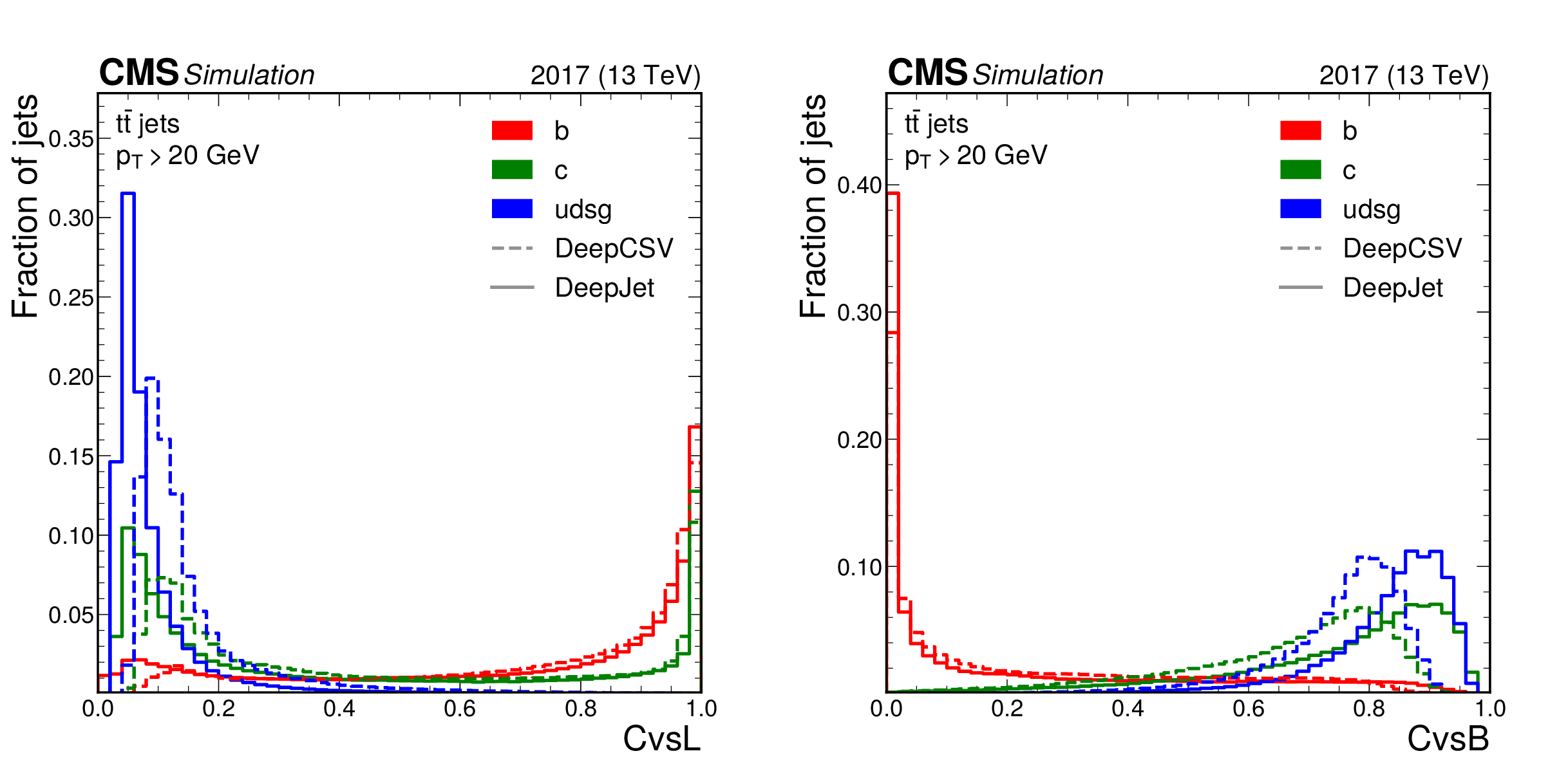
Figure 1:
Unit-normalised distributions of the CvsL (left) and CvsB (right) discriminators for the DeepCSV (dashed) and DeepJet (solid) algorithms using jets from simulated hadronic ${\mathrm{t} \mathrm{\bar{t}}}$ events with $ {p_{\mathrm {T}}} > $ 20 GeV and $ {| \eta |} < $ 2.5. The distributions are shown for b (red), c (green) and light-flavour jets (blue) separately. |
png pdf |
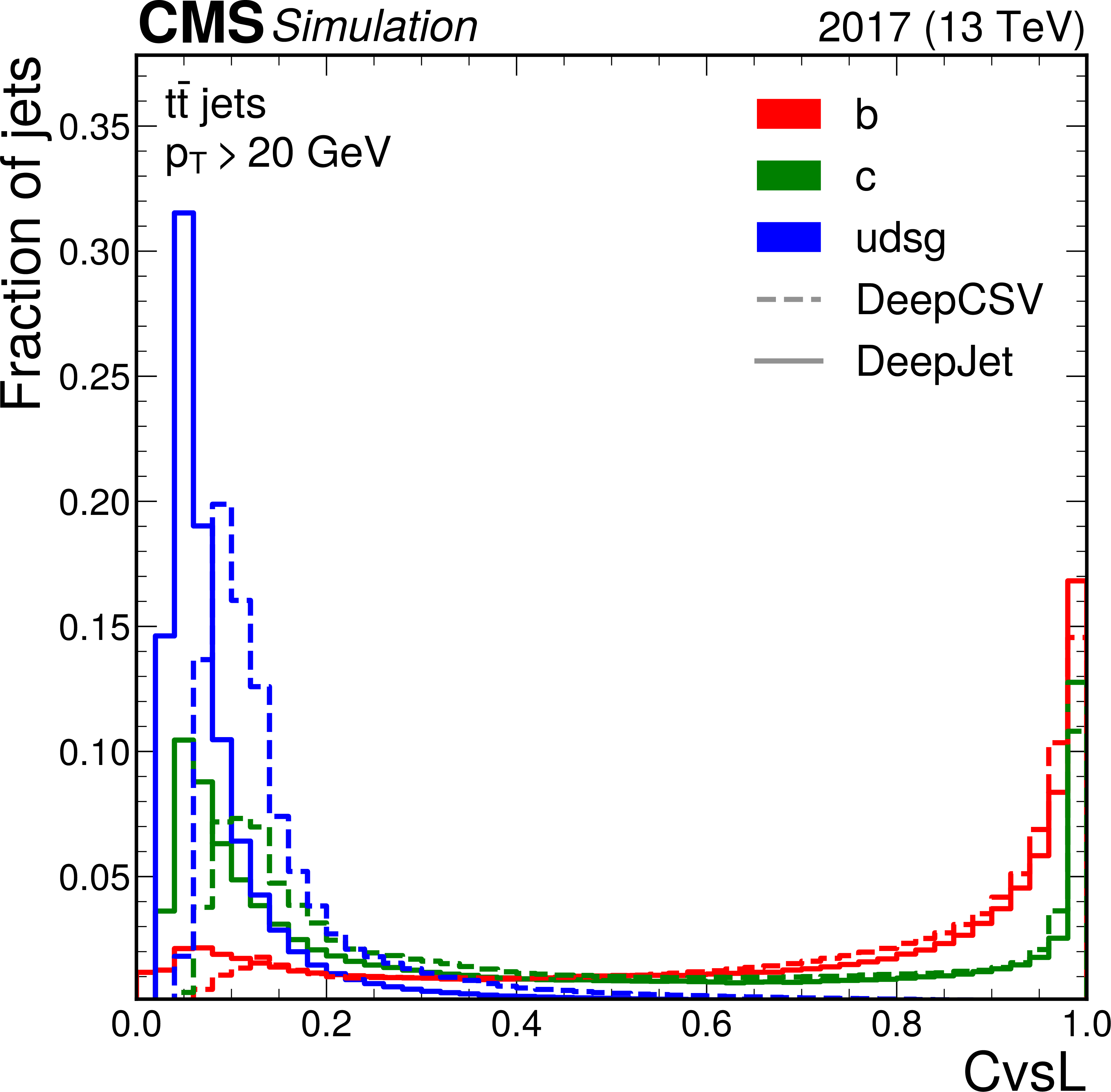
Figure 1-a:
Unit-normalised distributions of the CvsL discriminator for the DeepCSV (dashed) and DeepJet (solid) algorithms using jets from simulated hadronic ${\mathrm{t} \mathrm{\bar{t}}}$ events with $ {p_{\mathrm {T}}} > $ 20 GeV and $ {| \eta |} < $ 2.5. The distributions are shown for b (red), c (green) and light-flavour jets (blue) separately. |
png pdf |
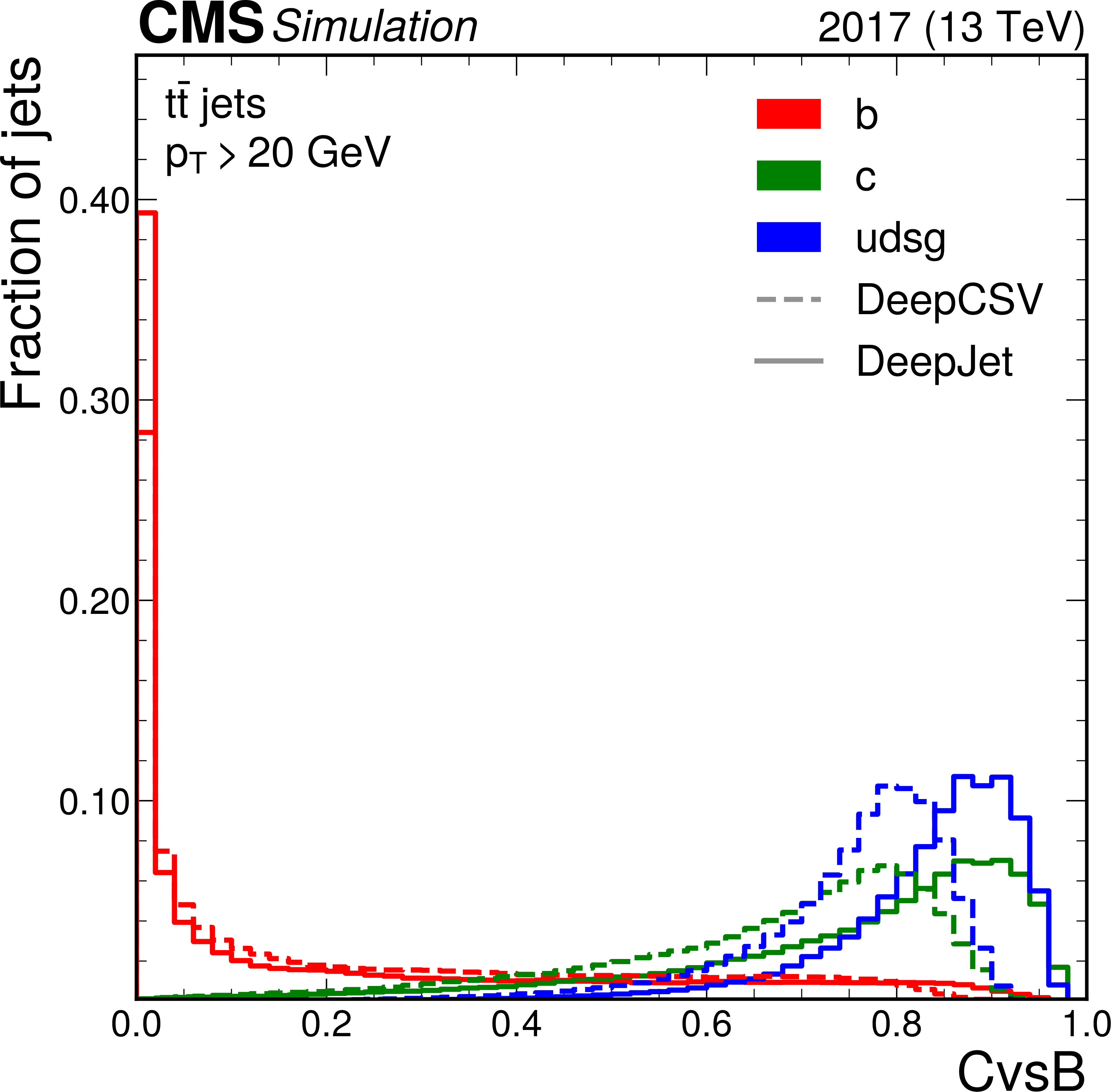
Figure 1-b:
Unit-normalised distributions of the CvsB discriminator for the DeepCSV (dashed) and DeepJet (solid) algorithms using jets from simulated hadronic ${\mathrm{t} \mathrm{\bar{t}}}$ events with $ {p_{\mathrm {T}}} > $ 20 GeV and $ {| \eta |} < $ 2.5. The distributions are shown for b (red), c (green) and light-flavour jets (blue) separately. |
png pdf |
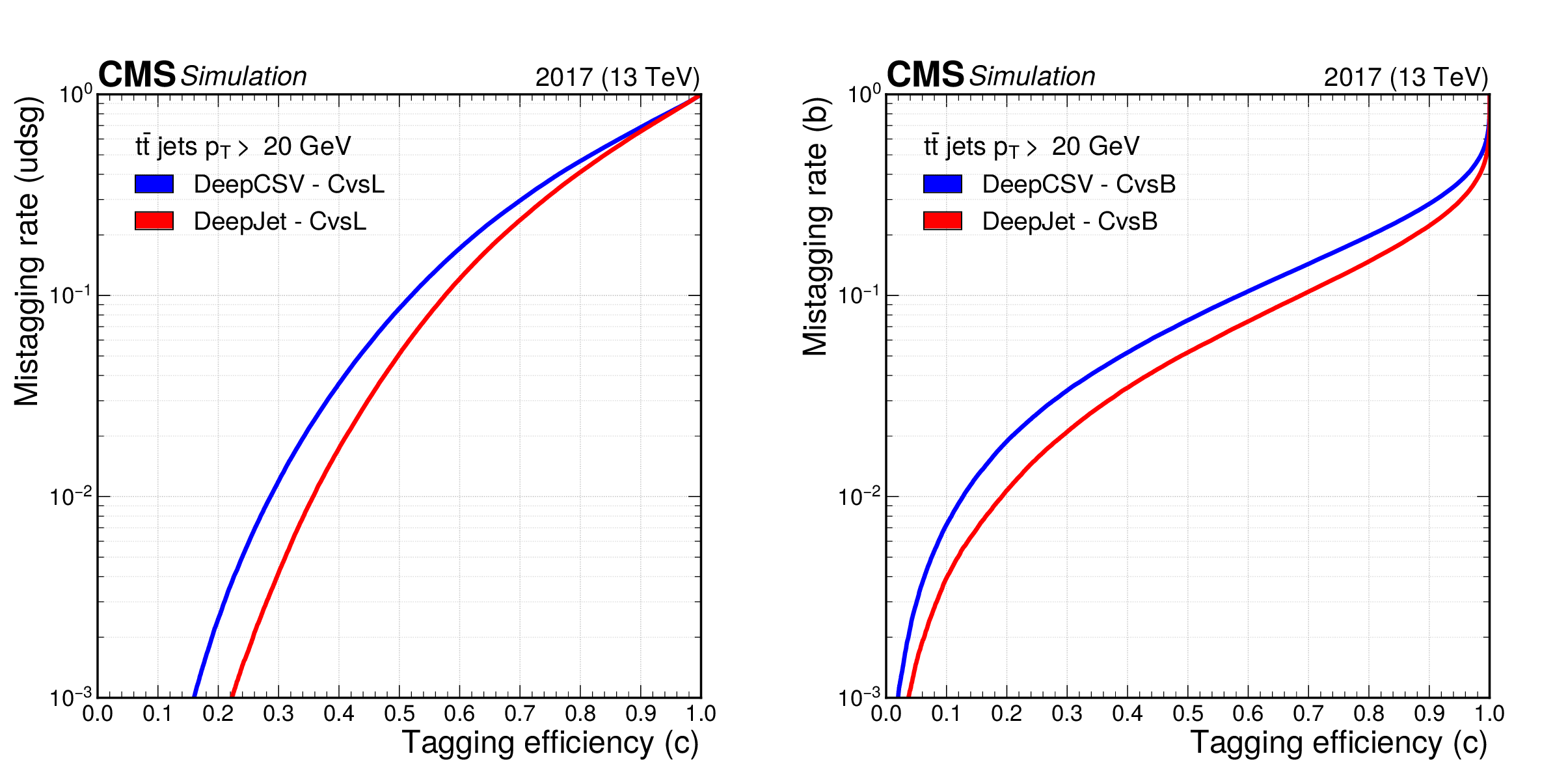
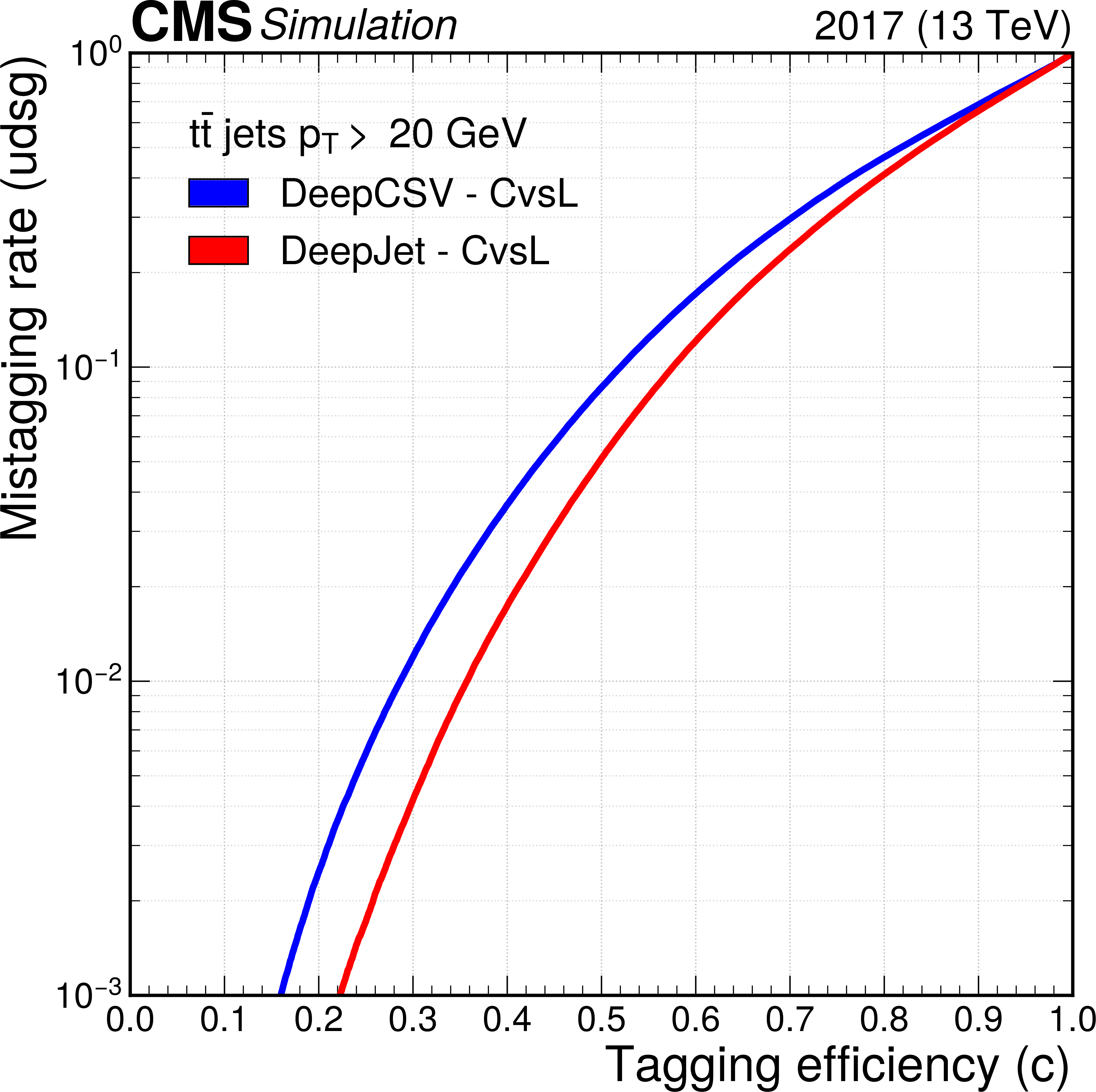
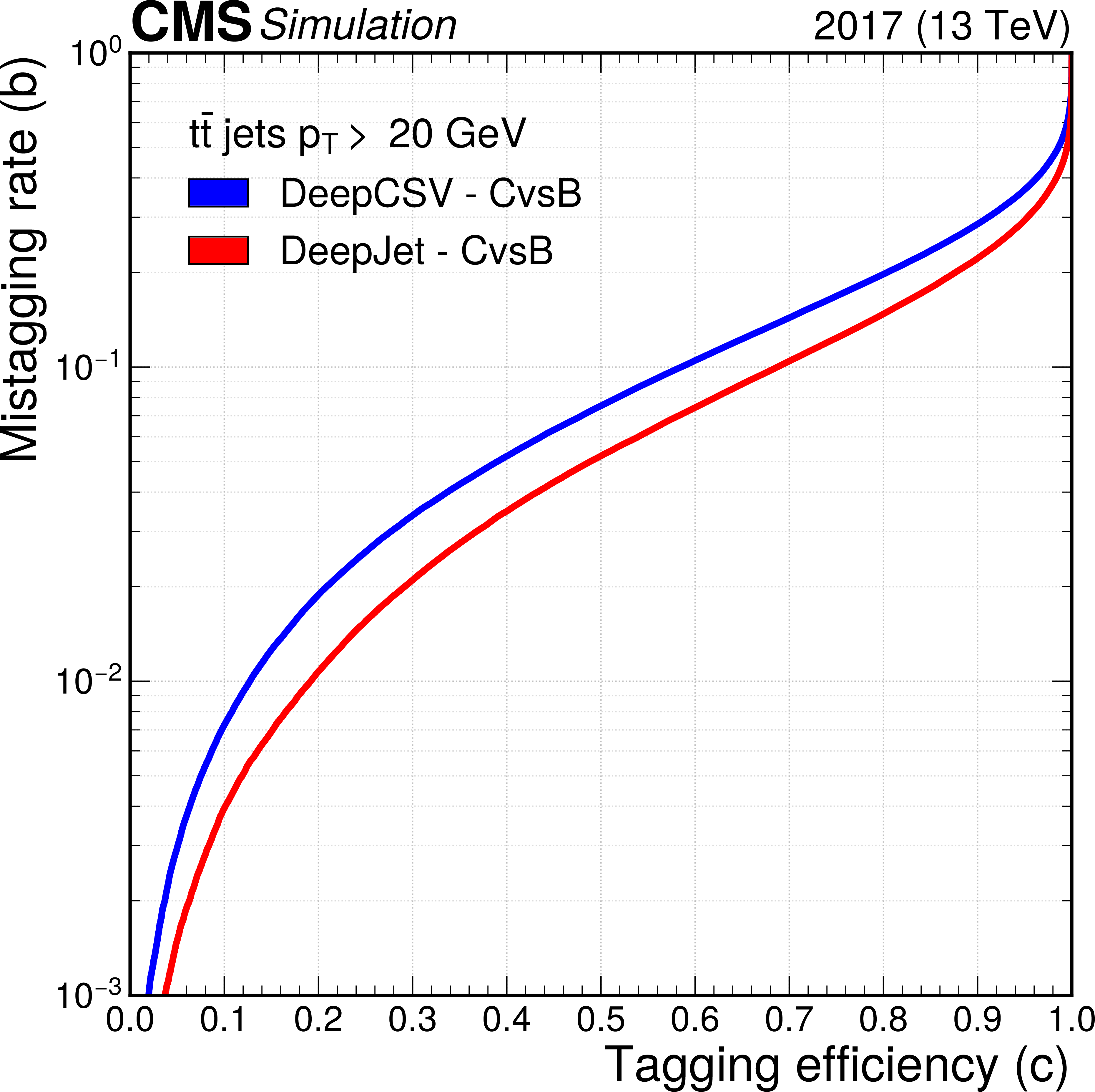
Figure 2:
The ROC curves showing the individual performance of the CvsL (left) and CvsB (right) discriminators for the DeepCSV (blue) and DeepJet (red) algorithms using jets from simulated hadronic ${\mathrm{t} \mathrm{\bar{t}}}$ events with $ {p_{\mathrm {T}}} > $ 20 GeV and $ {| \eta |} < $ 2.5. |
png pdf |
Figure 2-a:
The ROC curves showing the individual performance of the CvsL discriminator for the DeepCSV (blue) and DeepJet (red) algorithms using jets from simulated hadronic ${\mathrm{t} \mathrm{\bar{t}}}$ events with $ {p_{\mathrm {T}}} > $ 20 GeV and $ {| \eta |} < $ 2.5. |
png pdf |
Figure 2-b:
The ROC curves showing the individual performance of the CvsB discriminator for the DeepCSV (blue) and DeepJet (red) algorithms using jets from simulated hadronic ${\mathrm{t} \mathrm{\bar{t}}}$ events with $ {p_{\mathrm {T}}} > $ 20 GeV and $ {| \eta |} < $ 2.5. |
png pdf |
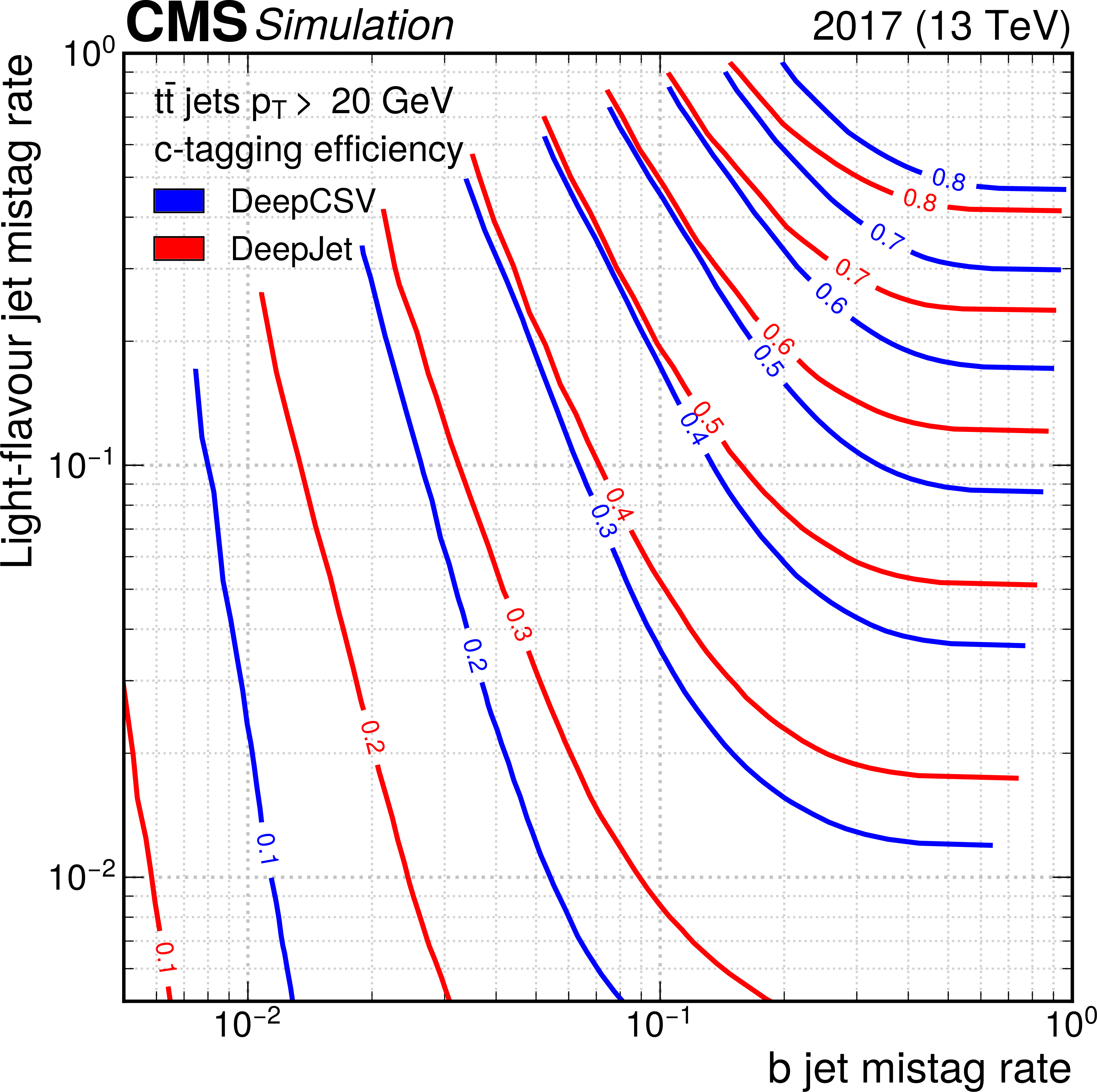
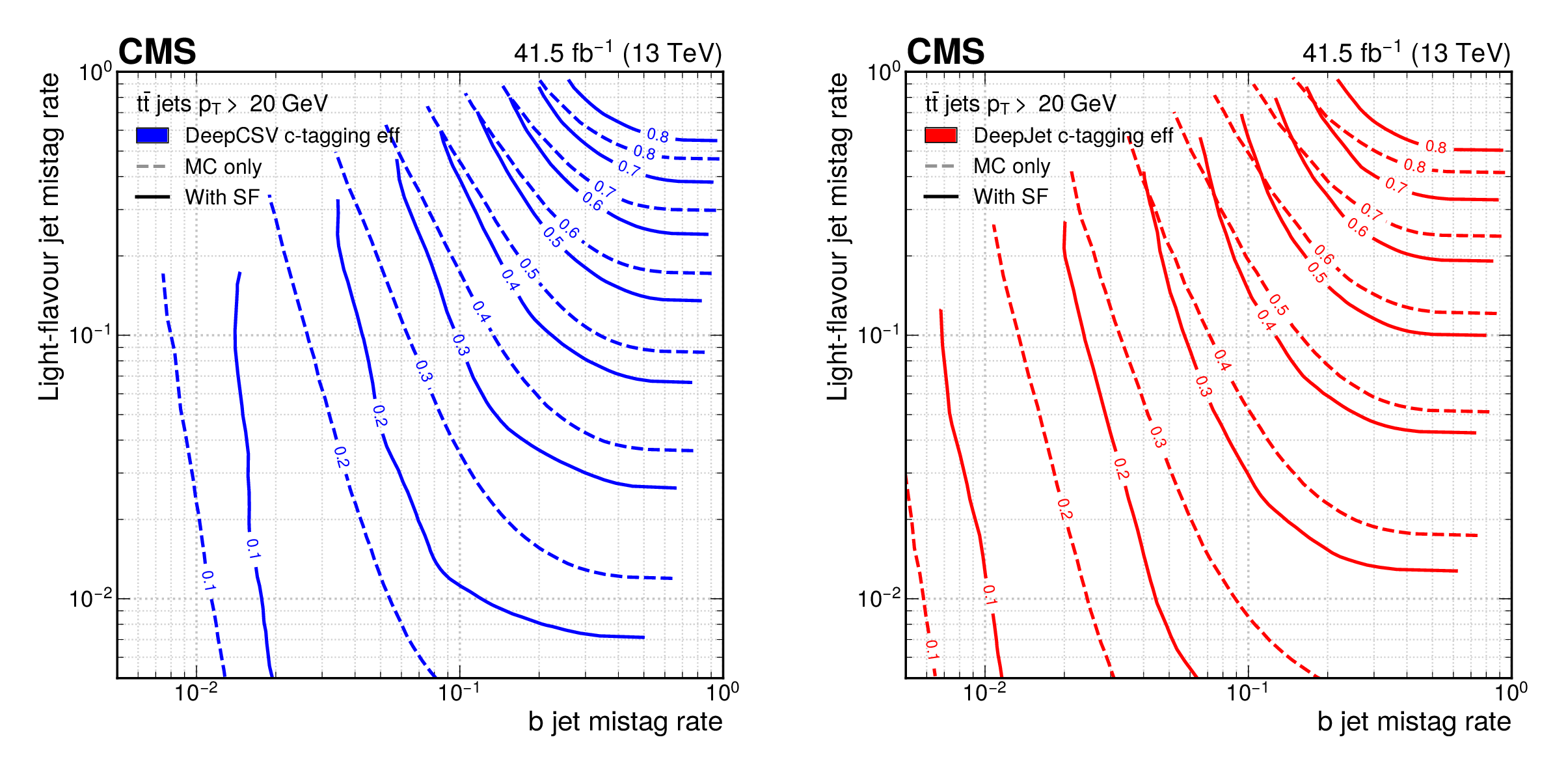
Figure 3:
Two-dimensional ROC contours showing the c tagging efficiency as simultaneous functions of b jet and light-flavour jet mistagging rates for DeepCSV (blue lines) and DeepJet (red lines) algorithms using jets with $ {p_{\mathrm {T}}} > $ 20 GeV and $ {| \eta |} < $ 2.5, from simulated hadronically decaying ${\mathrm{t} \mathrm{\bar{t}}}$ events. Each line represents points in the plane that correspond to a fixed value of the c tagging efficiency, which is shown as a number at the centre of each line. |
png pdf |
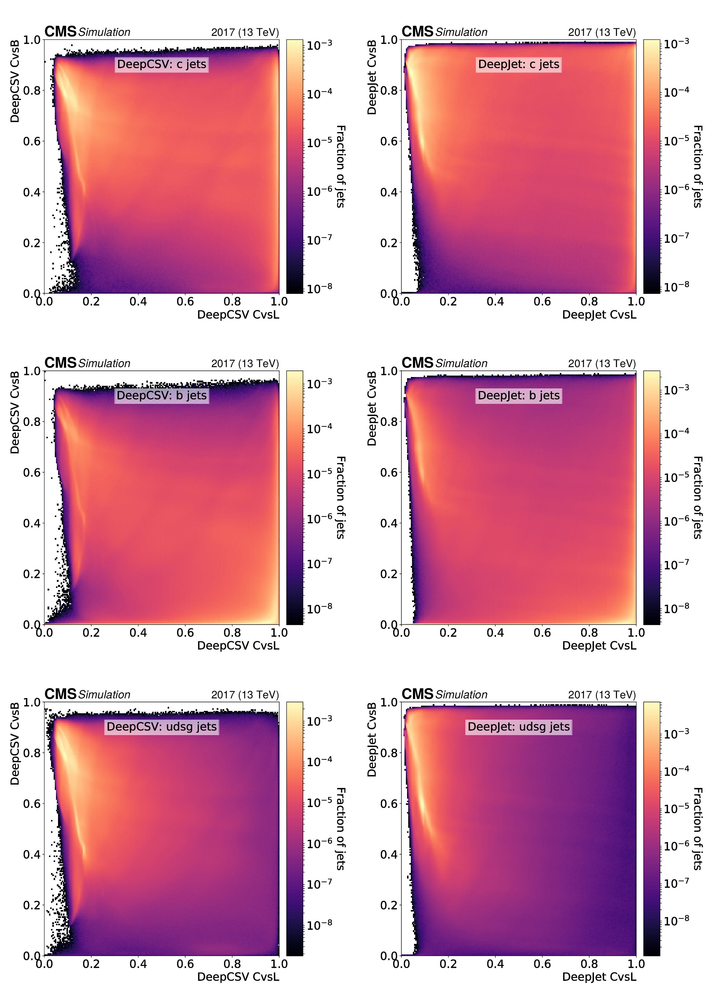
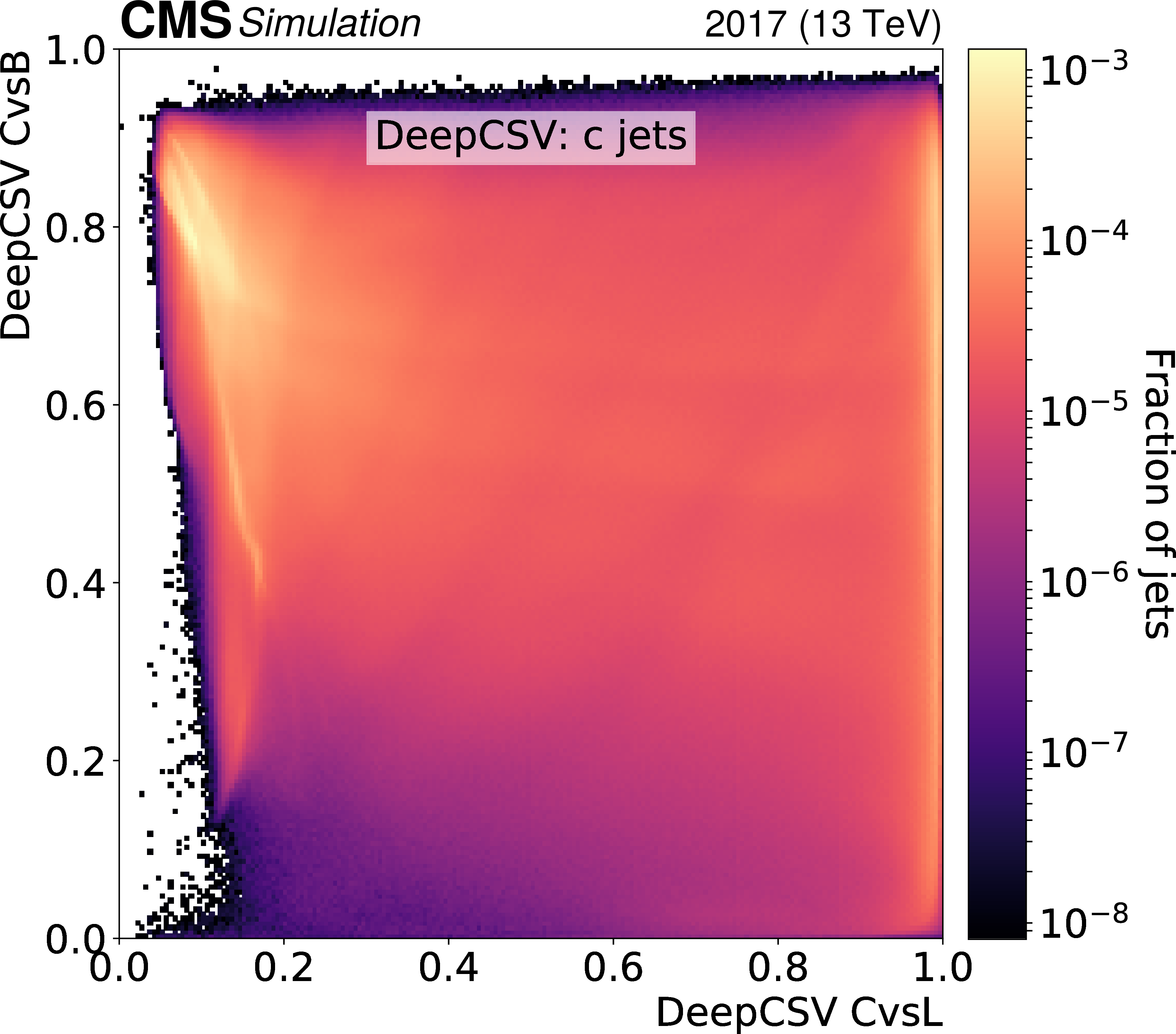
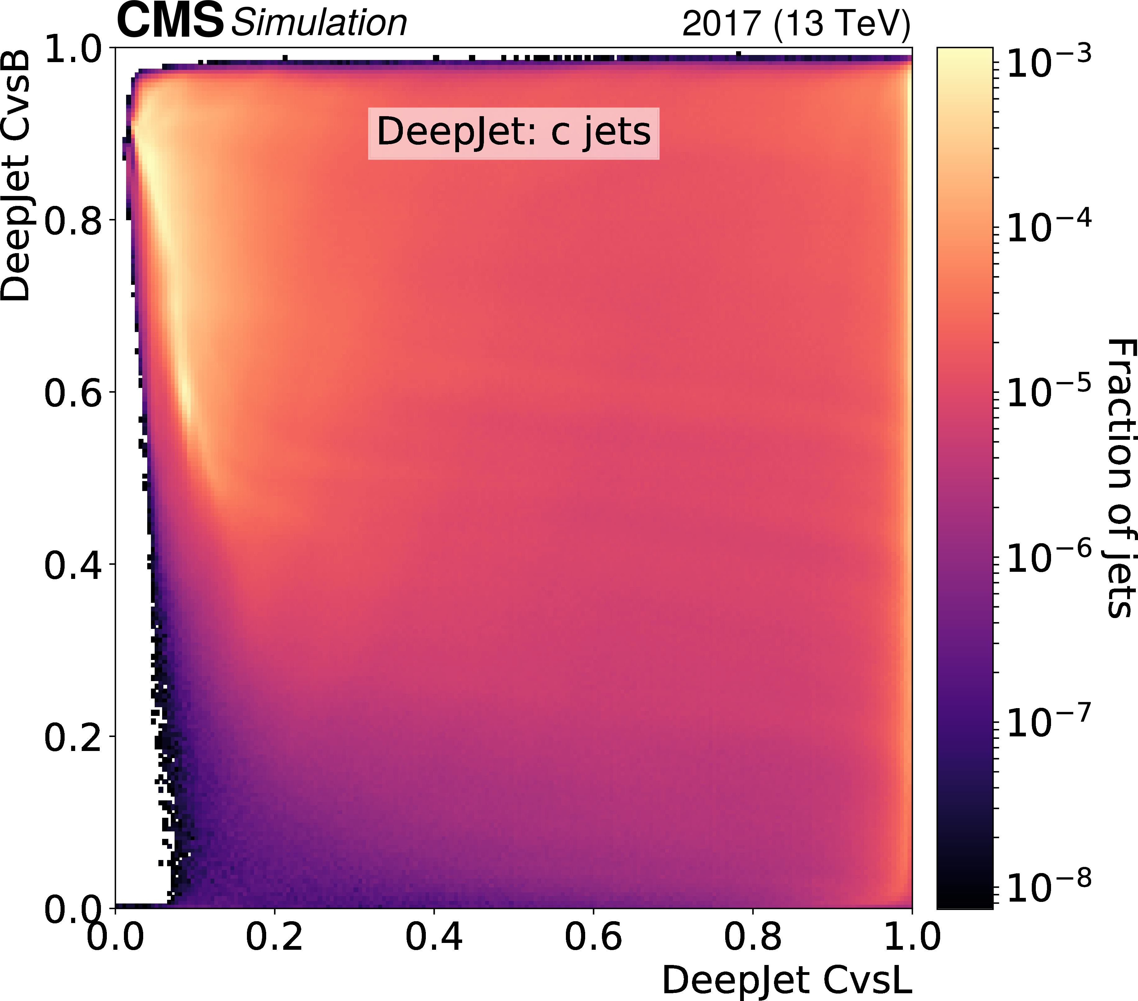
Figure 4:
Normalised 2D distributions showing the CvsL and CvsB discriminators on the $x$ and $y$ axes, respectively. Distributions are shown using c (upper), b (middle) and light-flavour (lower) jets with $ {p_{\mathrm {T}}} > $ 20 GeV and $ {| \eta |} < $ 2.5 from simulated hadronically decaying ${\mathrm{t} \mathrm{\bar{t}}}$ events. The left-hand column shows the discriminators of the DeepCSV algorithm, whereas the right-hand column shows those of the DeepJet algorithm. |
png pdf |
Figure 4-a:
Normalised 2D distributions showing the CvsL and CvsB discriminators on the $x$ and $y$ axes, respectively. Distributions are shown using c jets with $ {p_{\mathrm {T}}} > $ 20 GeV and $ {| \eta |} < $ 2.5 from simulated hadronically decaying ${\mathrm{t} \mathrm{\bar{t}}}$ events. The discriminators of the DeepCSV algorithm are shown. |
png pdf |
Figure 4-b:
Normalised 2D distributions showing the CvsL and CvsB discriminators on the $x$ and $y$ axes, respectively. Distributions are shown using c jets with $ {p_{\mathrm {T}}} > $ 20 GeV and $ {| \eta |} < $ 2.5 from simulated hadronically decaying ${\mathrm{t} \mathrm{\bar{t}}}$ events. The discriminators of the DeepJet algorithm are shown. |
png pdf |
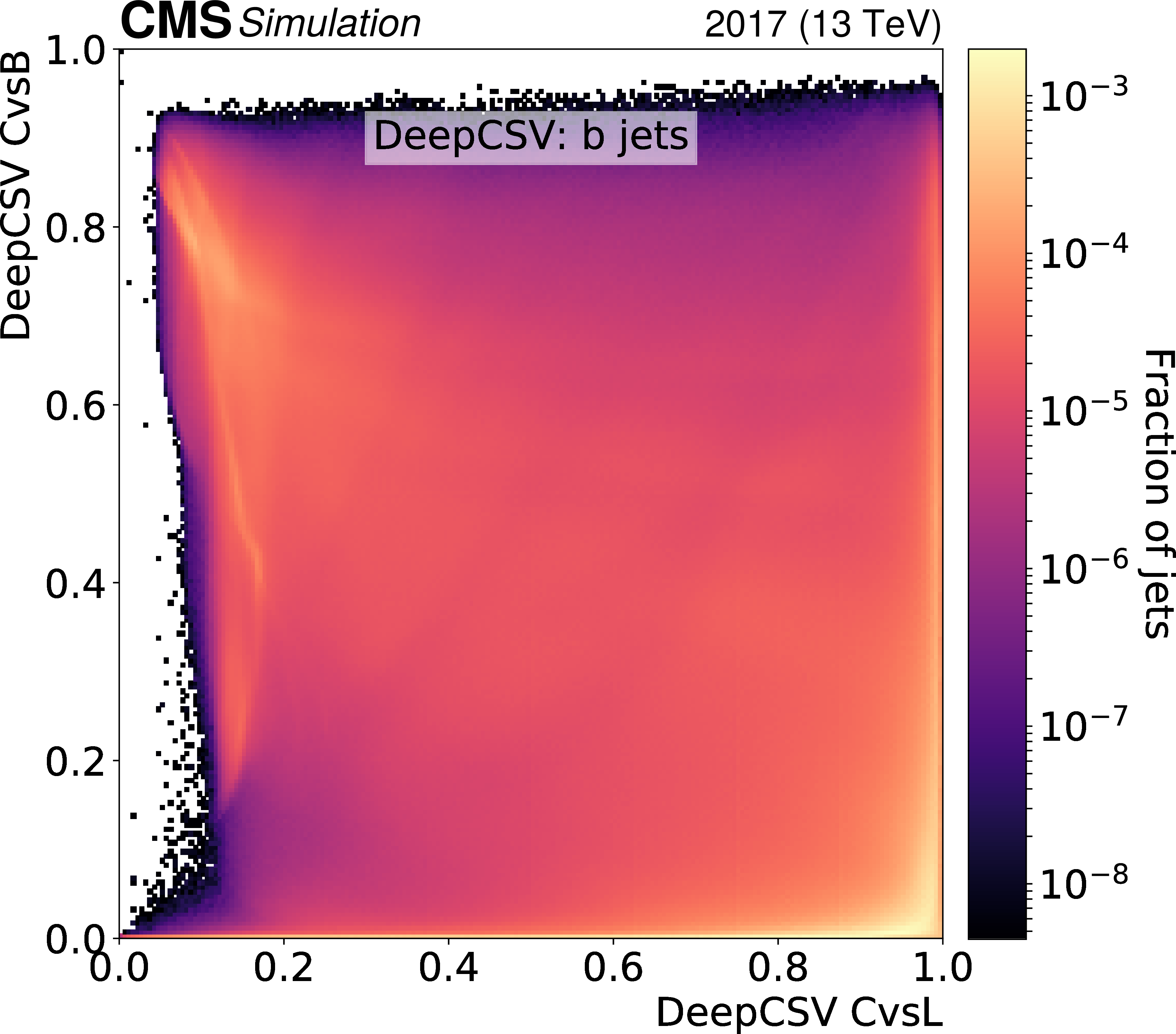
Figure 4-c:
Normalised 2D distributions showing the CvsL and CvsB discriminators on the $x$ and $y$ axes, respectively. Distributions are shown using b jets with $ {p_{\mathrm {T}}} > $ 20 GeV and $ {| \eta |} < $ 2.5 from simulated hadronically decaying ${\mathrm{t} \mathrm{\bar{t}}}$ events. The discriminators of the DeepCSV algorithm are shown. |
png pdf |
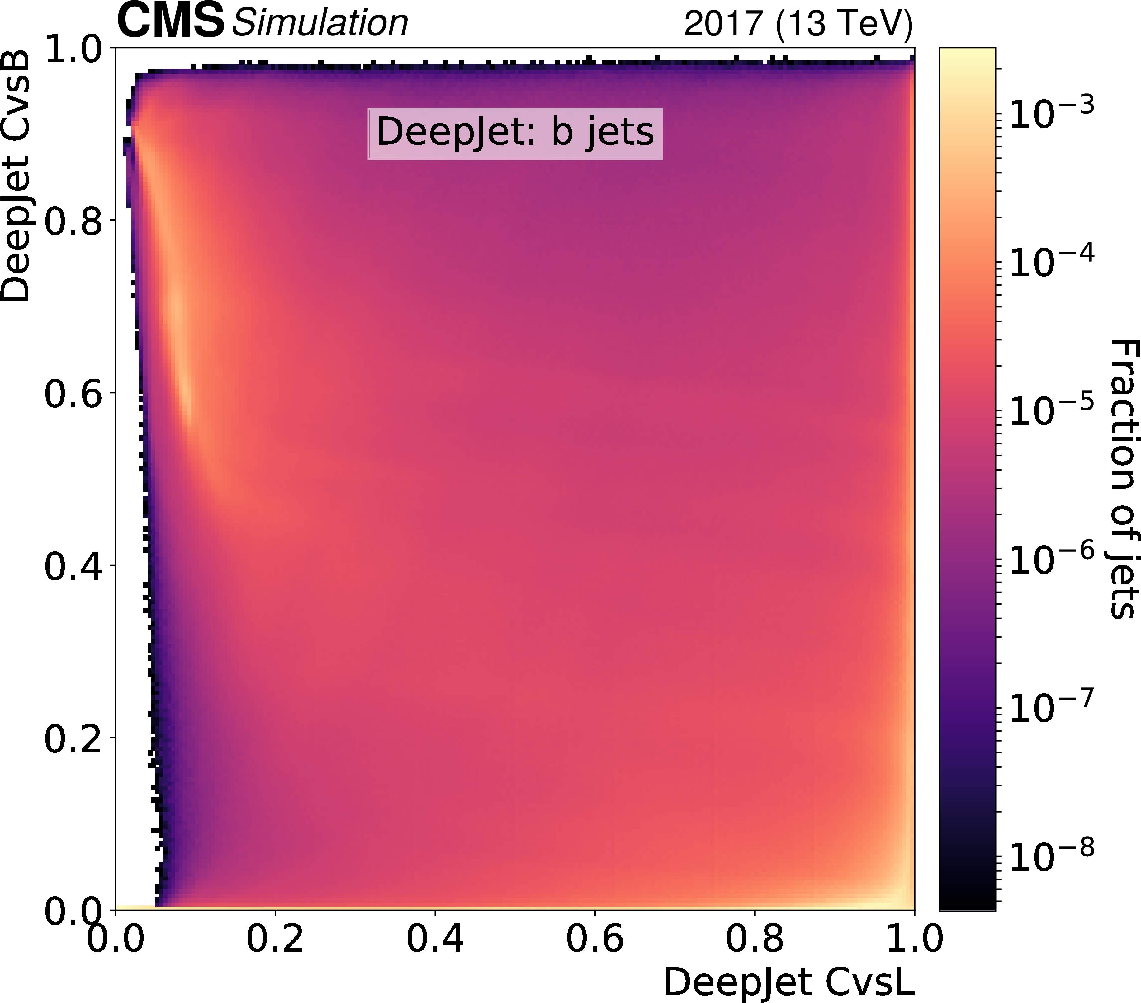
Figure 4-d:
Normalised 2D distributions showing the CvsL and CvsB discriminators on the $x$ and $y$ axes, respectively. Distributions are shown using b jets with $ {p_{\mathrm {T}}} > $ 20 GeV and $ {| \eta |} < $ 2.5 from simulated hadronically decaying ${\mathrm{t} \mathrm{\bar{t}}}$ events. The discriminators of the DeepJet algorithm are shown. |

png pdf |
Figure 4-e:
Normalised 2D distributions showing the CvsL and CvsB discriminators on the $x$ and $y$ axes, respectively. Distributions are shown using light-flavour jets with $ {p_{\mathrm {T}}} > $ 20 GeV and $ {| \eta |} < $ 2.5 from simulated hadronically decaying ${\mathrm{t} \mathrm{\bar{t}}}$ events. The discriminators of the DeepCSV algorithm are shown. |

png pdf |
Figure 4-f:
Normalised 2D distributions showing the CvsL and CvsB discriminators on the $x$ and $y$ axes, respectively. Distributions are shown using light-flavour jets with $ {p_{\mathrm {T}}} > $ 20 GeV and $ {| \eta |} < $ 2.5 from simulated hadronically decaying ${\mathrm{t} \mathrm{\bar{t}}}$ events. The discriminators of the DeepJet algorithm are shown. |
png pdf |
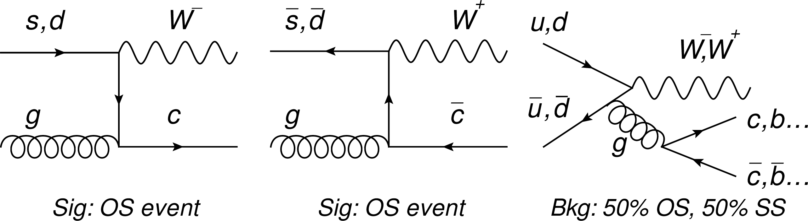
Figure 5:
Feynman diagrams showing production of charm quarks in association with a W boson (left and middle) and the major background (right). |
png pdf |
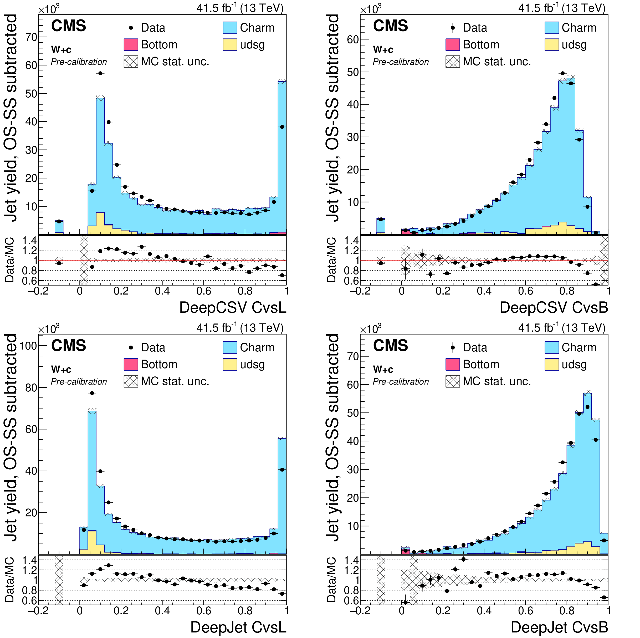
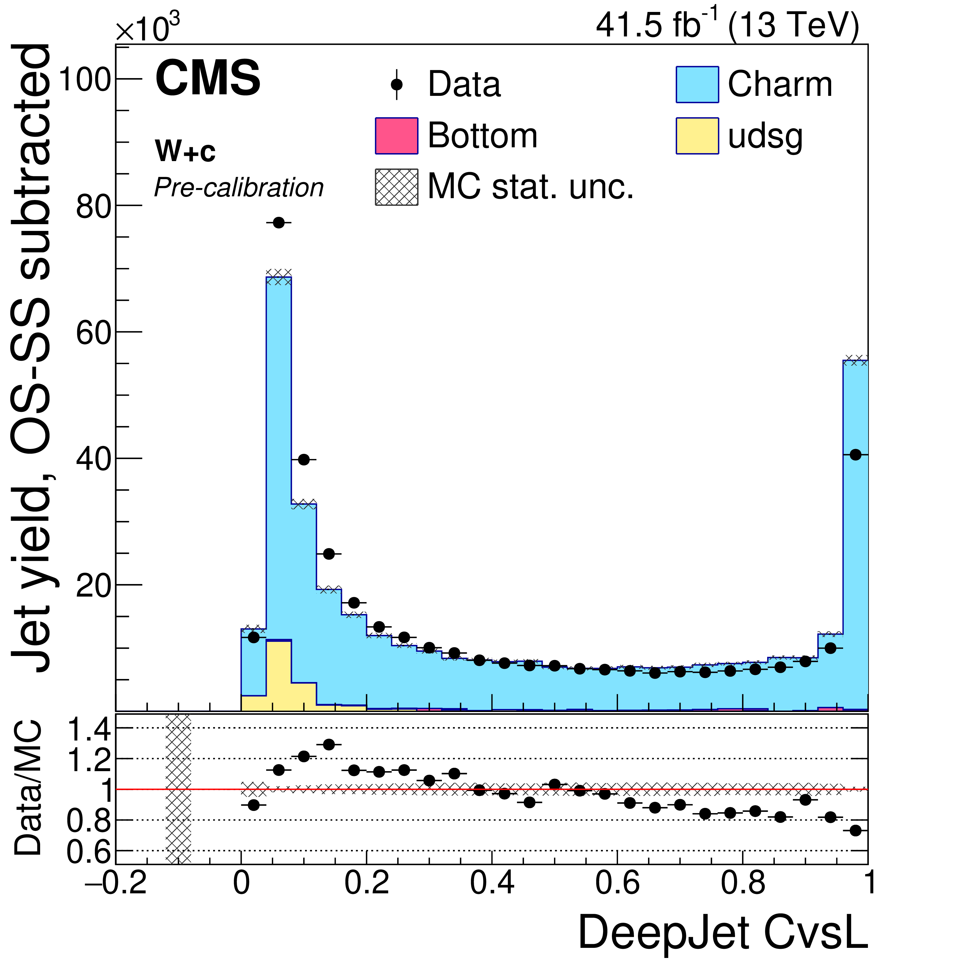
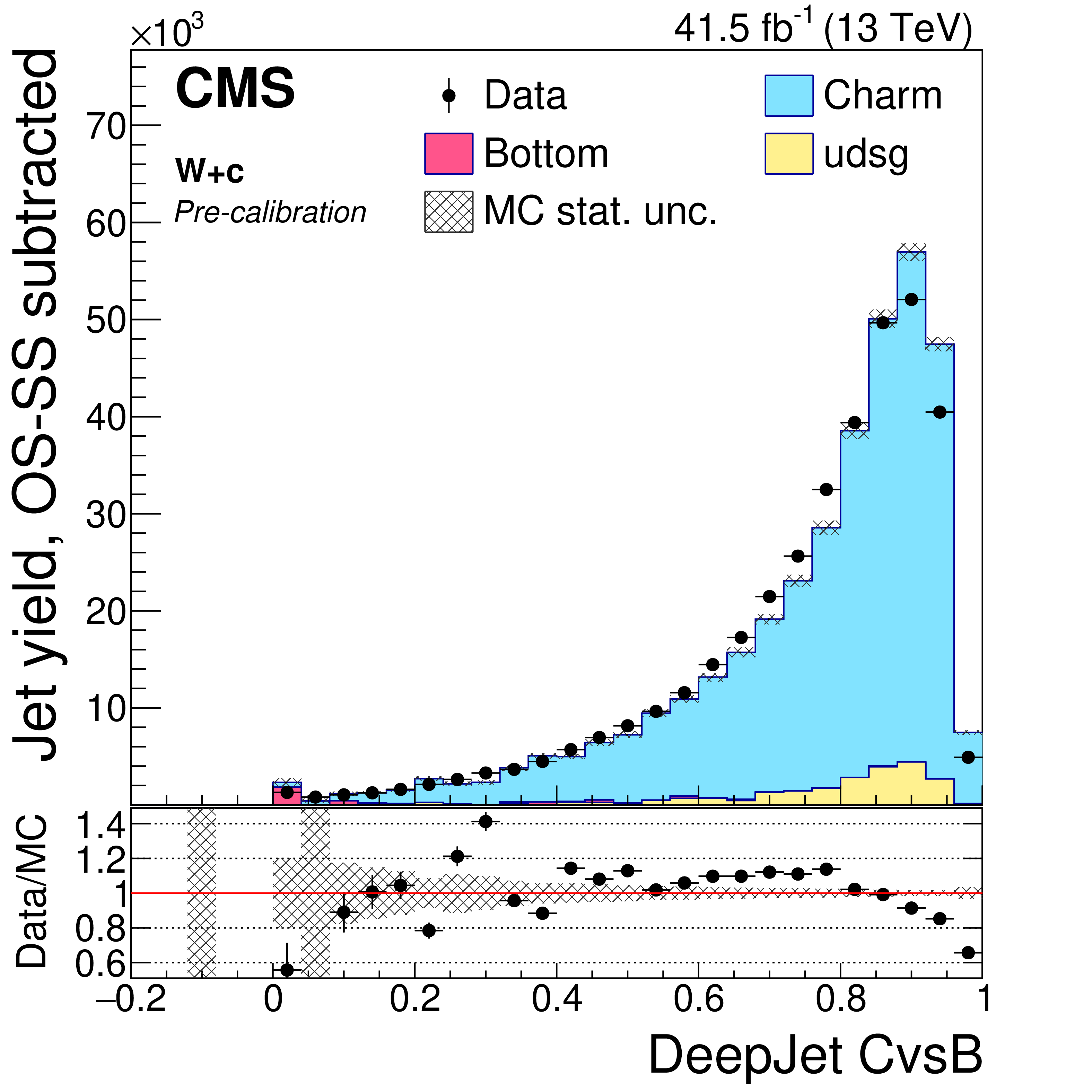
Figure 6:
Precalibration distributions of CvsL (left) and CvsB (right) obtained from the DeepCSV (upper) and DeepJet (lower) taggers for jets selected in the W+c (OS-SS) selection. The bin corresponding to a tagger value of $-1$ is plotted at $-0.1$. Vertical error bars in data represent statistical uncertainties in data. |
png pdf |
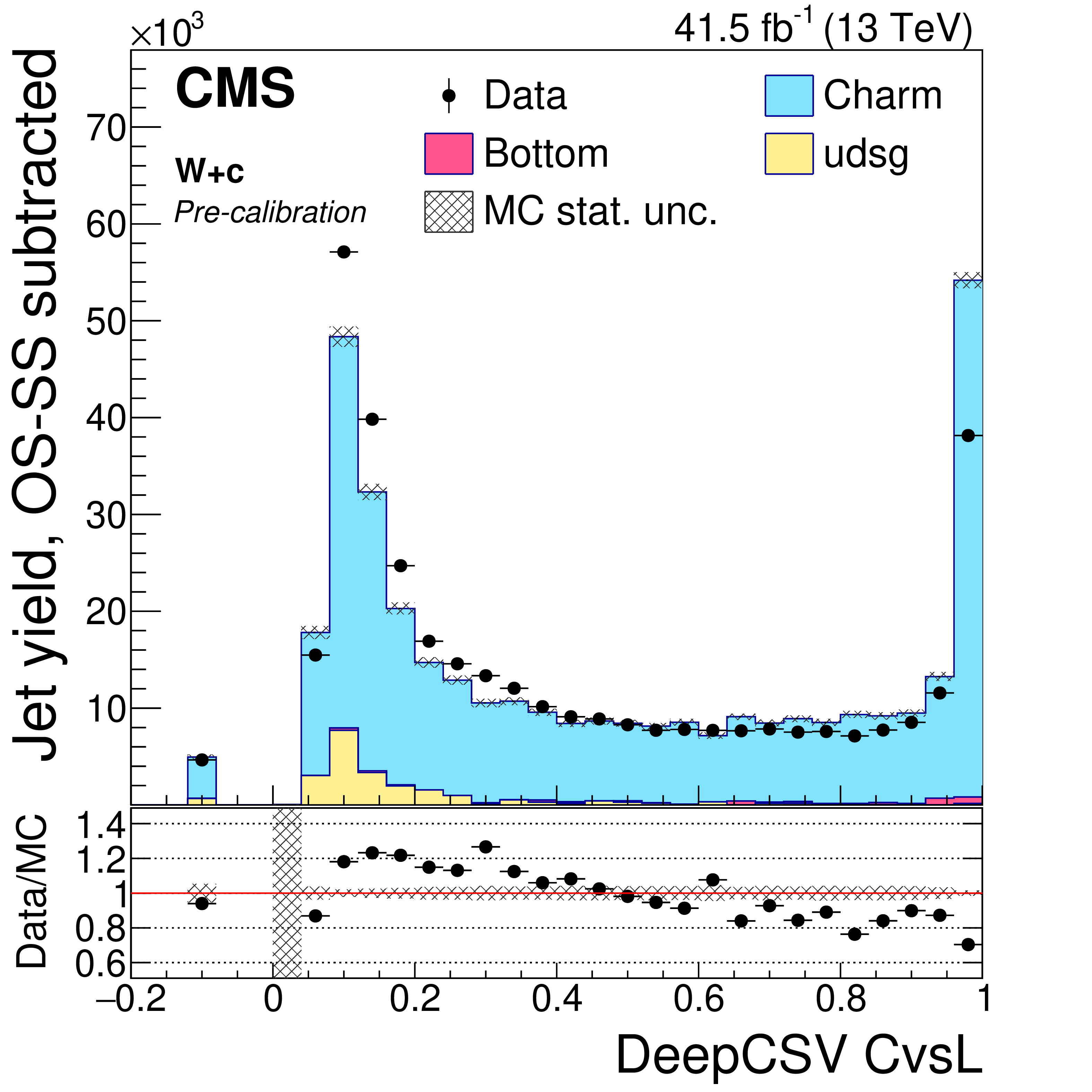
Figure 6-a:
Precalibration distributions of CvsL obtained from the DeepCSV tagger for jets selected in the W+c (OS-SS) selection. The bin corresponding to a tagger value of $-1$ is plotted at $-0.1$. Vertical error bars in data represent statistical uncertainties in data. |
png pdf |
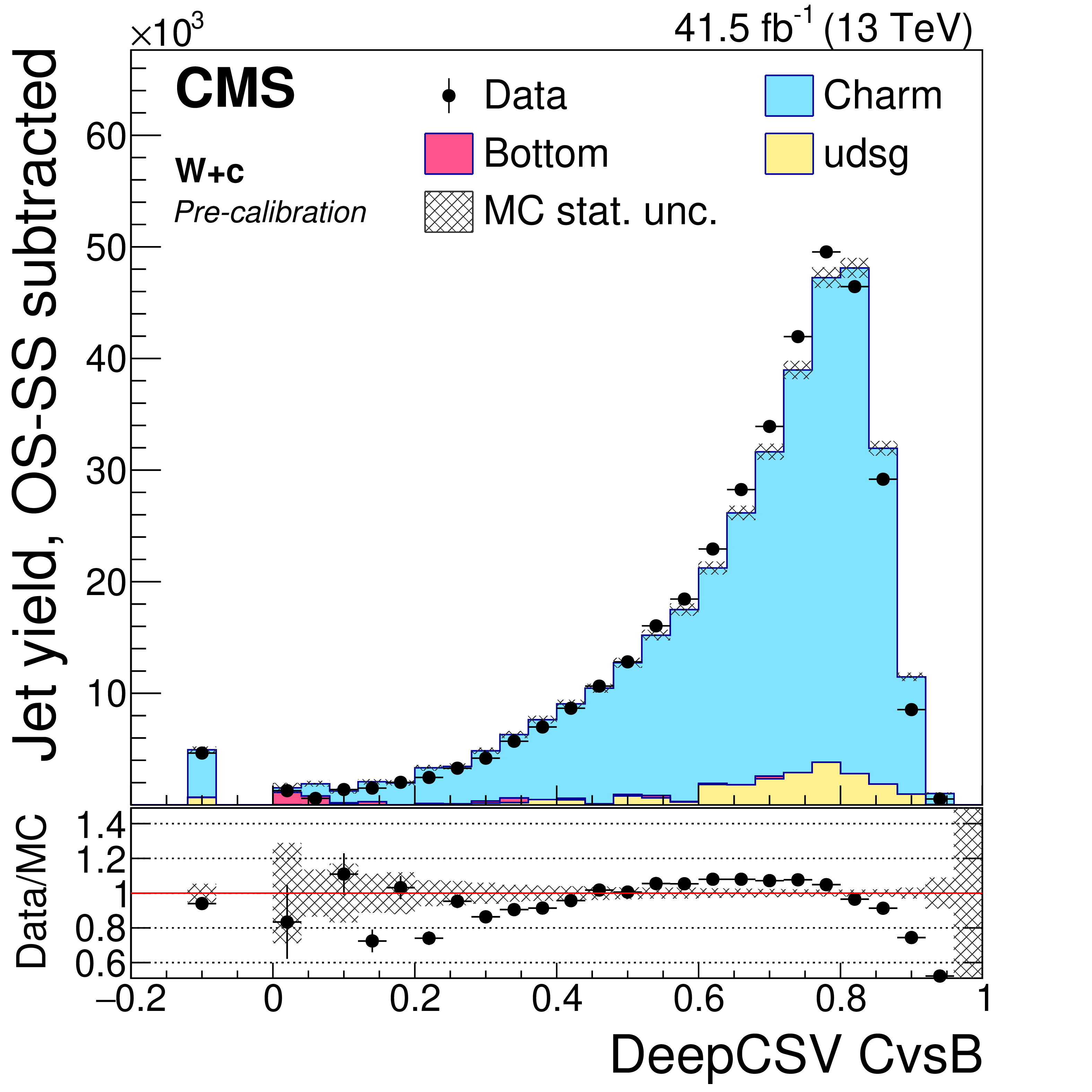
Figure 6-b:
Precalibration distributions of CvsB obtained from the DeepCSV tagger for jets selected in the W+c (OS-SS) selection. The bin corresponding to a tagger value of $-1$ is plotted at $-0.1$. Vertical error bars in data represent statistical uncertainties in data. |
png pdf |
Figure 6-c:
Precalibration distributions of CvsL obtained from the DeepJet tagger for jets selected in the W+c (OS-SS) selection. The bin corresponding to a tagger value of $-1$ is plotted at $-0.1$. Vertical error bars in data represent statistical uncertainties in data. |
png pdf |
Figure 6-d:
Precalibration distributions of CvsB obtained from the DeepJet tagger for jets selected in the W+c (OS-SS) selection. The bin corresponding to a tagger value of $-1$ is plotted at $-0.1$. Vertical error bars in data represent statistical uncertainties in data. |

png pdf |
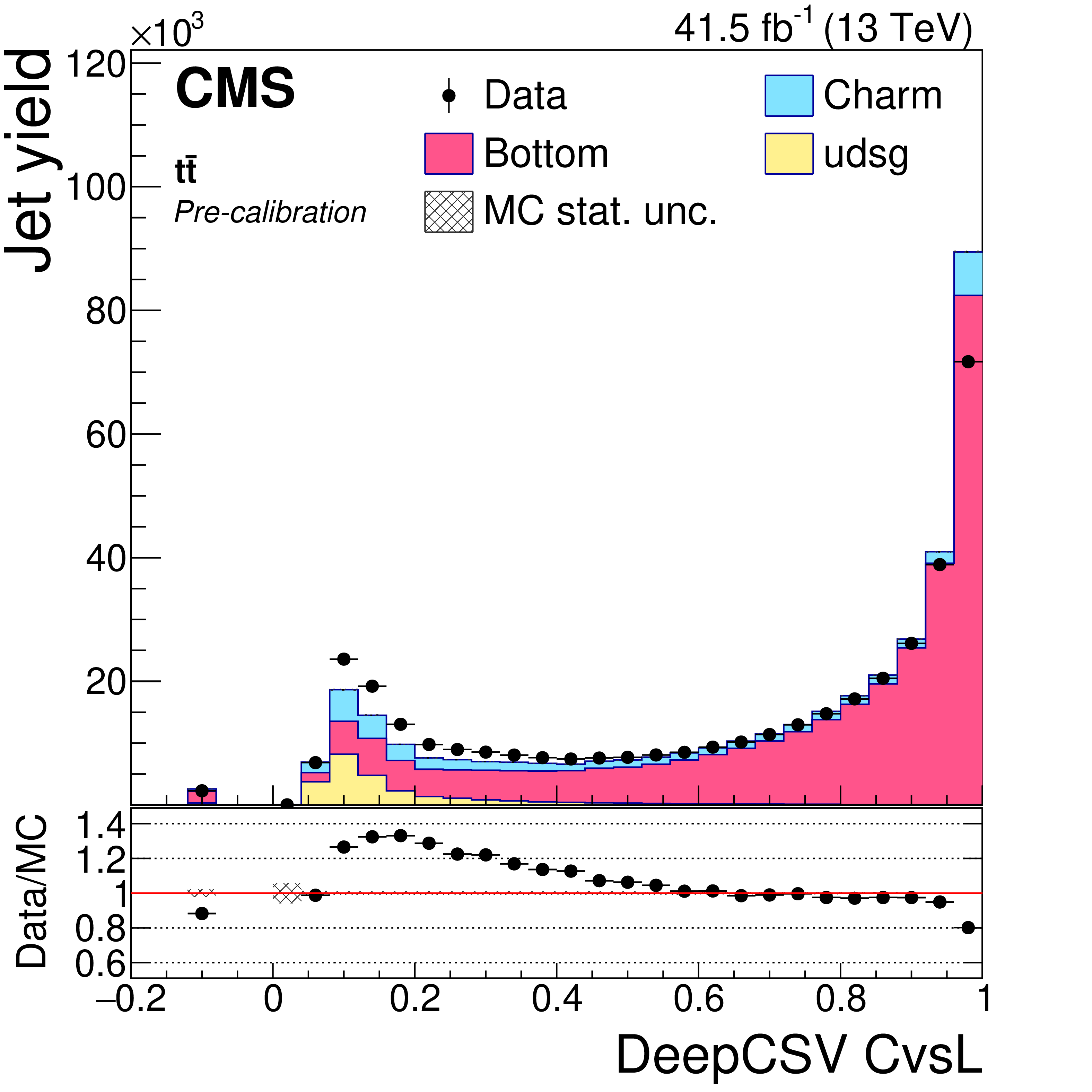
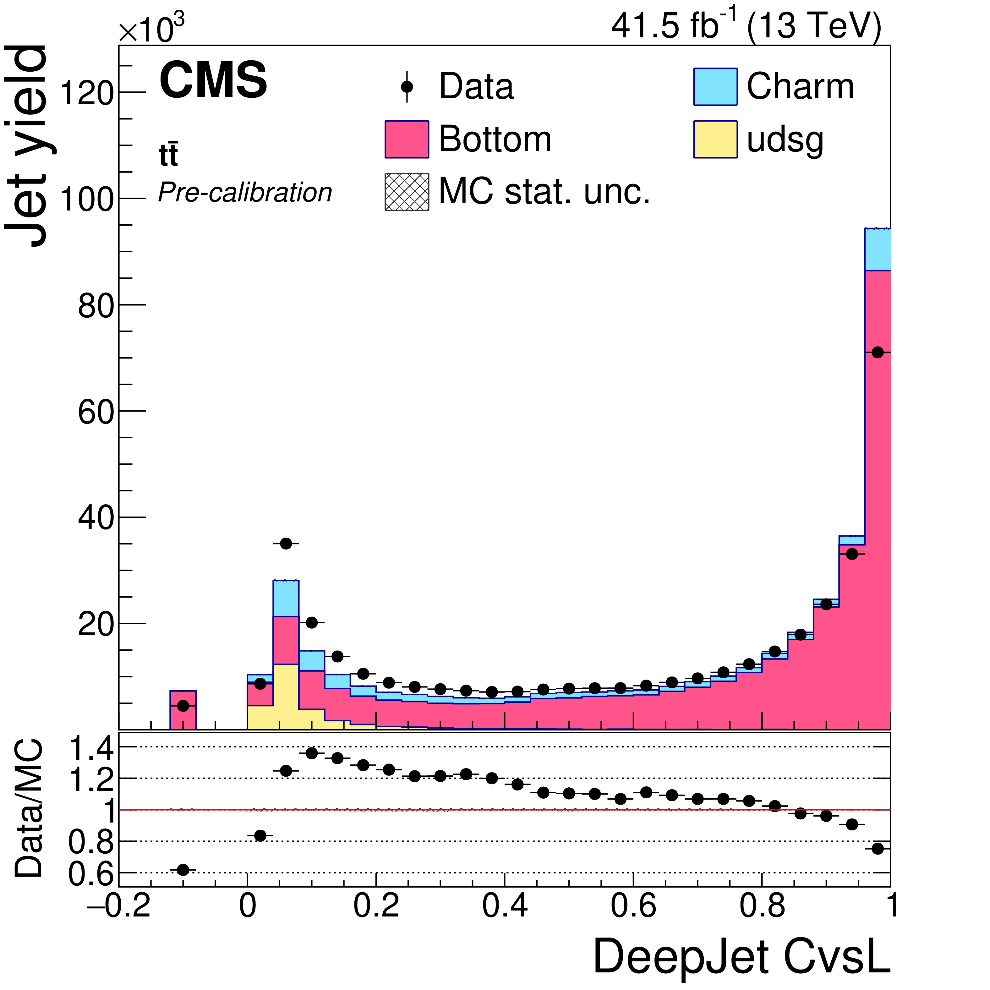
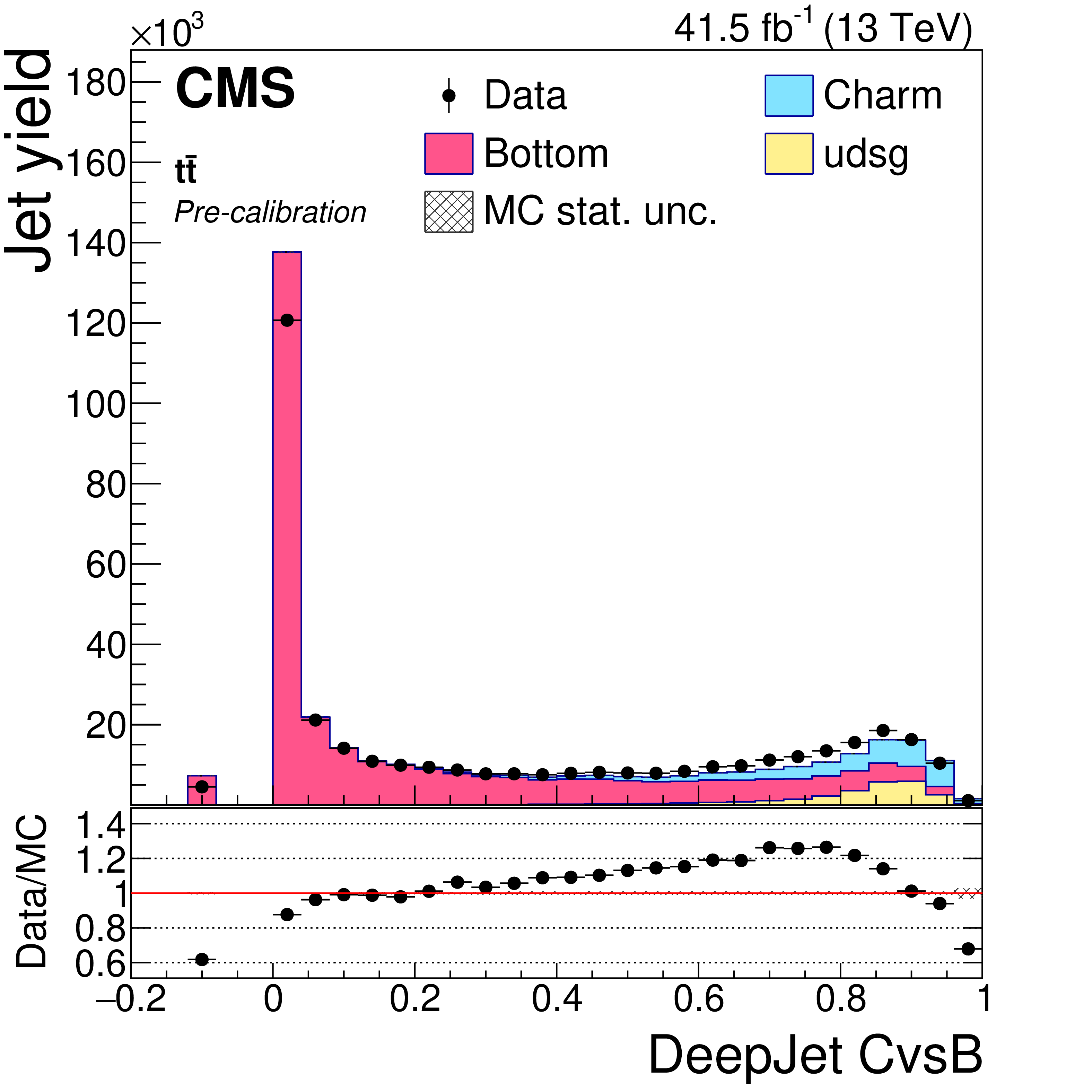
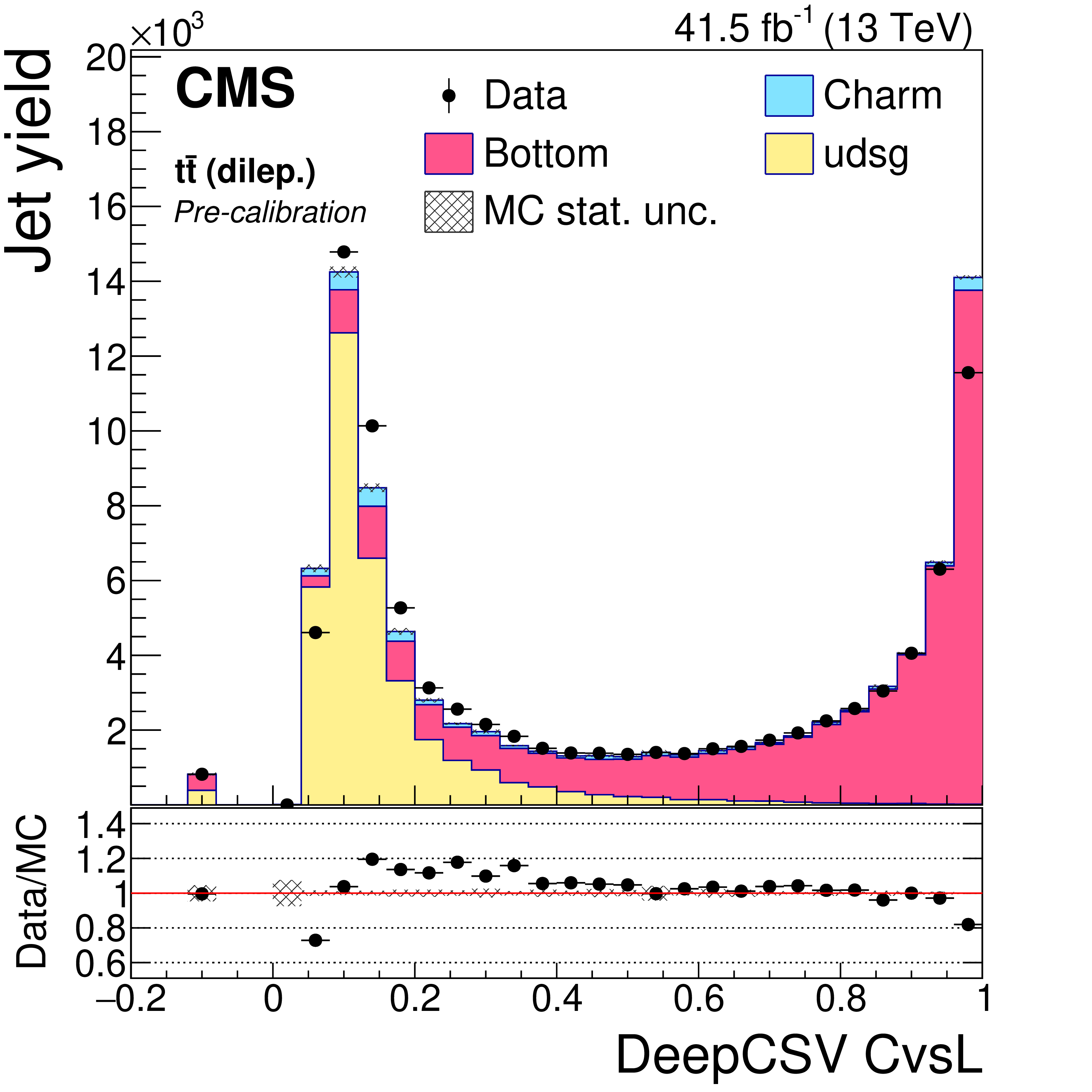
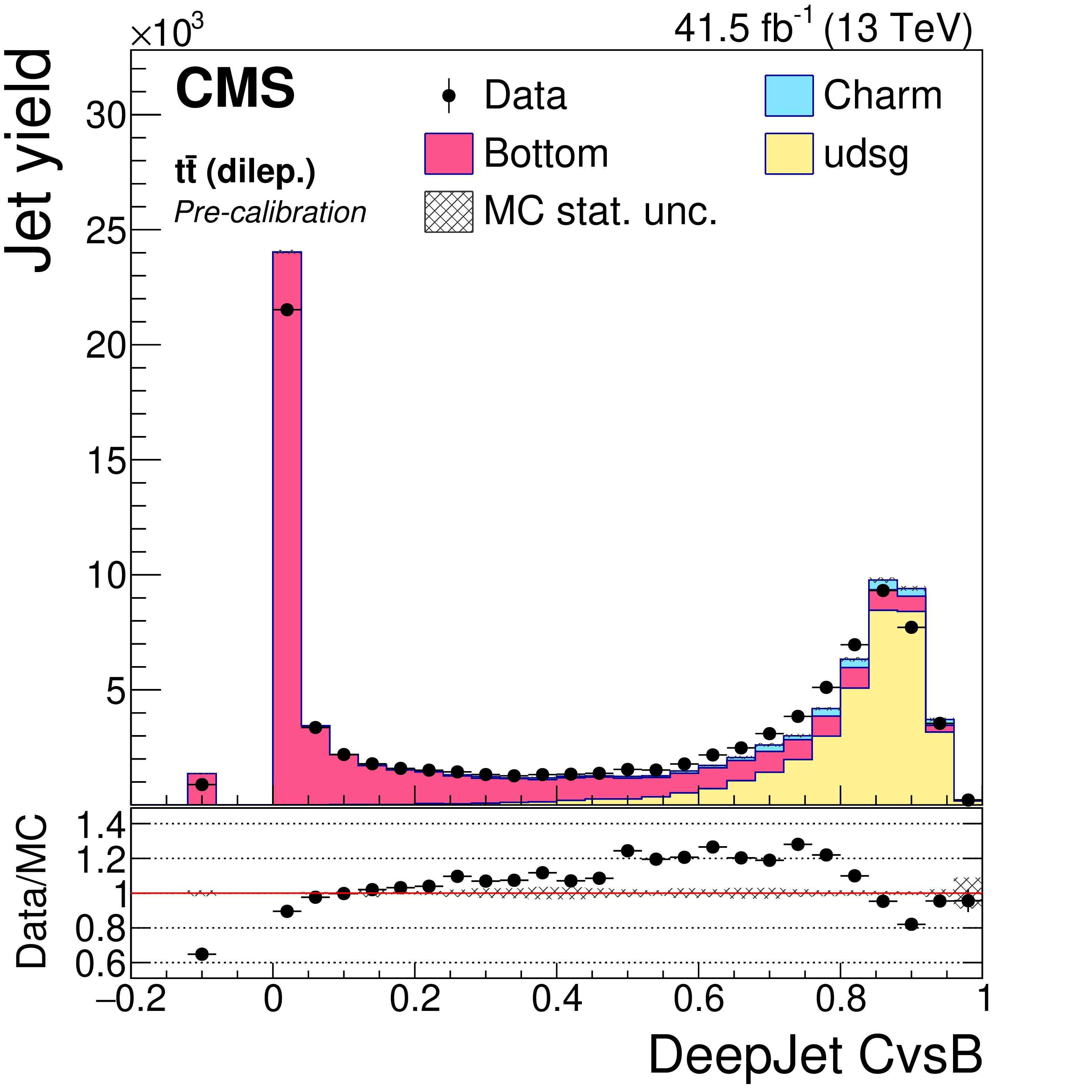
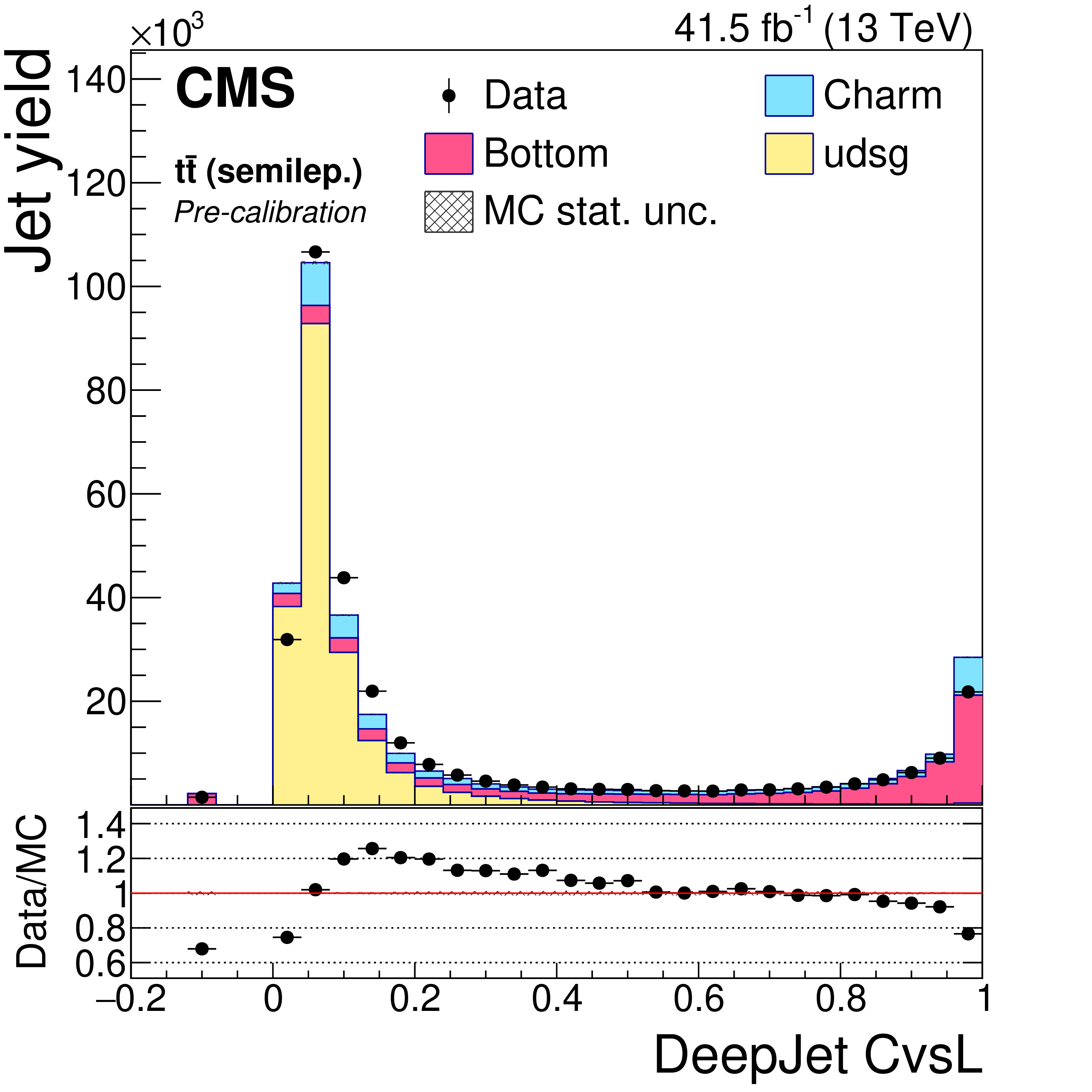
Figure 7:
Precalibration distributions of CvsL (left) and CvsB (right) obtained from the DeepCSV (upper) and DeepJet (lower) taggers for jets in the ${\mathrm{t} \mathrm{\bar{t}}}$ selection. The bin corresponding to a tagger value of $-1$ is plotted at $-0.1$. Vertical error bars in data represent statistical uncertainties in data. |
png pdf |
Figure 7-a:
Precalibration distributions of CvsL obtained from the DeepCSV taggers for jets in the ${\mathrm{t} \mathrm{\bar{t}}}$ selection. The bin corresponding to a tagger value of $-1$ is plotted at $-0.1$. Vertical error bars in data represent statistical uncertainties in data. |

png pdf |
Figure 7-b:
Precalibration distributions of CvsB obtained from the DeepCSV taggers for jets in the ${\mathrm{t} \mathrm{\bar{t}}}$ selection. The bin corresponding to a tagger value of $-1$ is plotted at $-0.1$. Vertical error bars in data represent statistical uncertainties in data. |
png pdf |
Figure 7-c:
Precalibration distributions of CvsL obtained from the DeepJet taggers for jets in the ${\mathrm{t} \mathrm{\bar{t}}}$ selection. The bin corresponding to a tagger value of $-1$ is plotted at $-0.1$. Vertical error bars in data represent statistical uncertainties in data. |
png pdf |
Figure 7-d:
Precalibration distributions of CvsB obtained from the DeepJet taggers for jets in the ${\mathrm{t} \mathrm{\bar{t}}}$ selection. The bin corresponding to a tagger value of $-1$ is plotted at $-0.1$. Vertical error bars in data represent statistical uncertainties in data. |

png pdf |
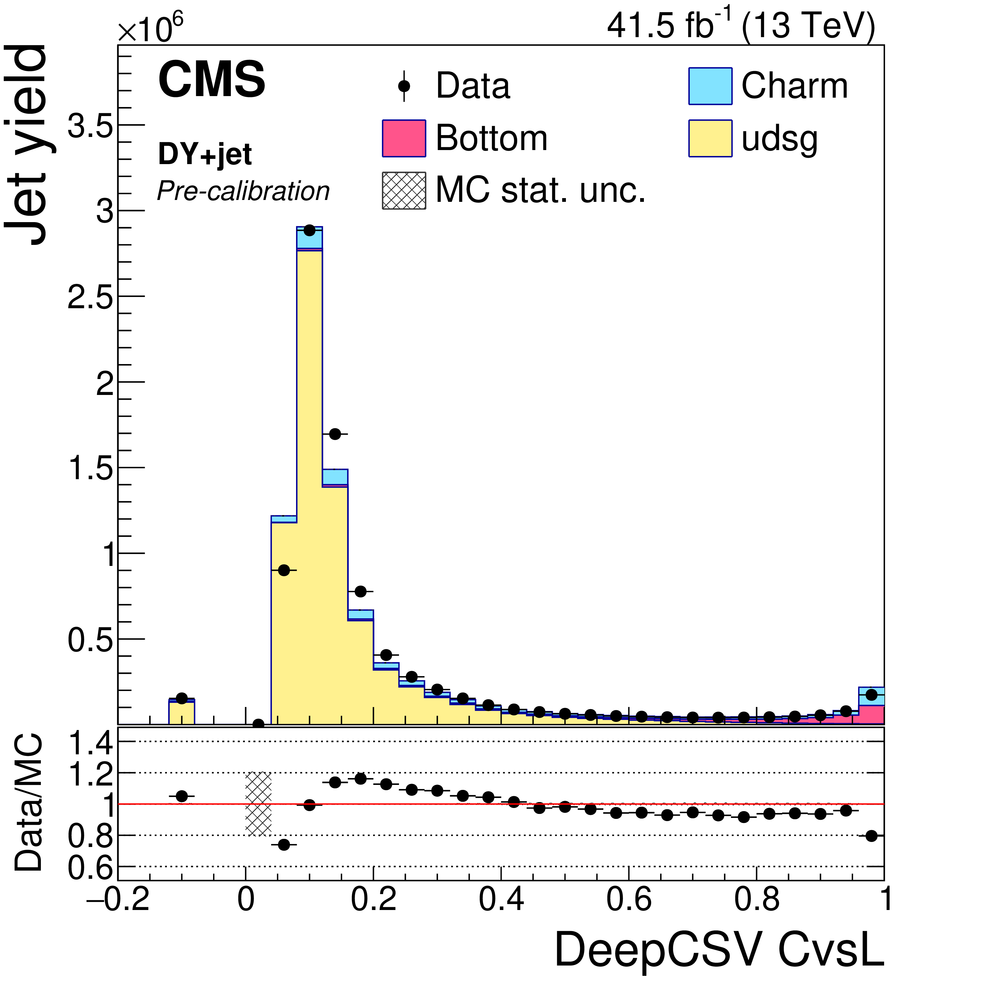
Figure 8:
Precalibration distributions of CvsL (left) and CvsB (right) obtained from the DeepCSV (upper) and DeepJet (lower) tagger for jets in the DY+jets selection. The bin corresponding to a tagger value of $-1$ is plotted at $-0.1$. Vertical error bars in data represent statistical uncertainties in data. |
png pdf |
Figure 8-a:
Precalibration distributions of CvsL obtained from the DeepCSV tagger for jets in the DY+jets selection. The bin corresponding to a tagger value of $-1$ is plotted at $-0.1$. Vertical error bars in data represent statistical uncertainties in data. |

png pdf |
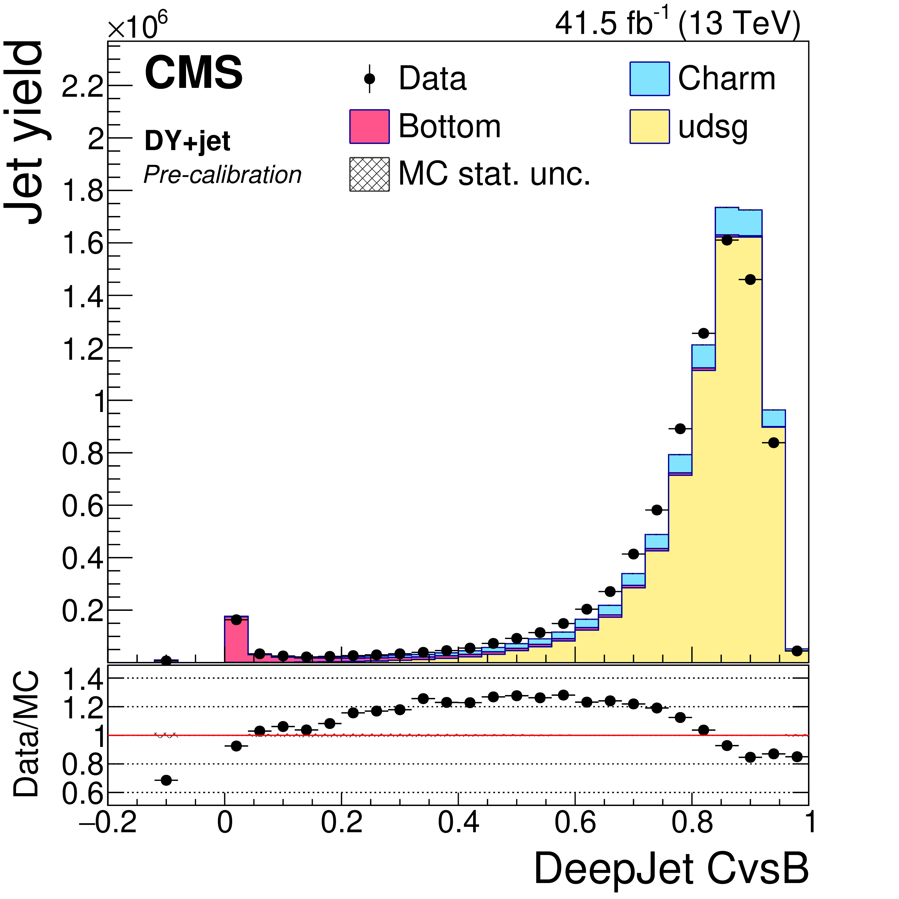
Figure 8-b:
Precalibration distributions of CvsB obtained from the DeepJet tagger for jets in the DY+jets selection. The bin corresponding to a tagger value of $-1$ is plotted at $-0.1$. Vertical error bars in data represent statistical uncertainties in data. |
png pdf |
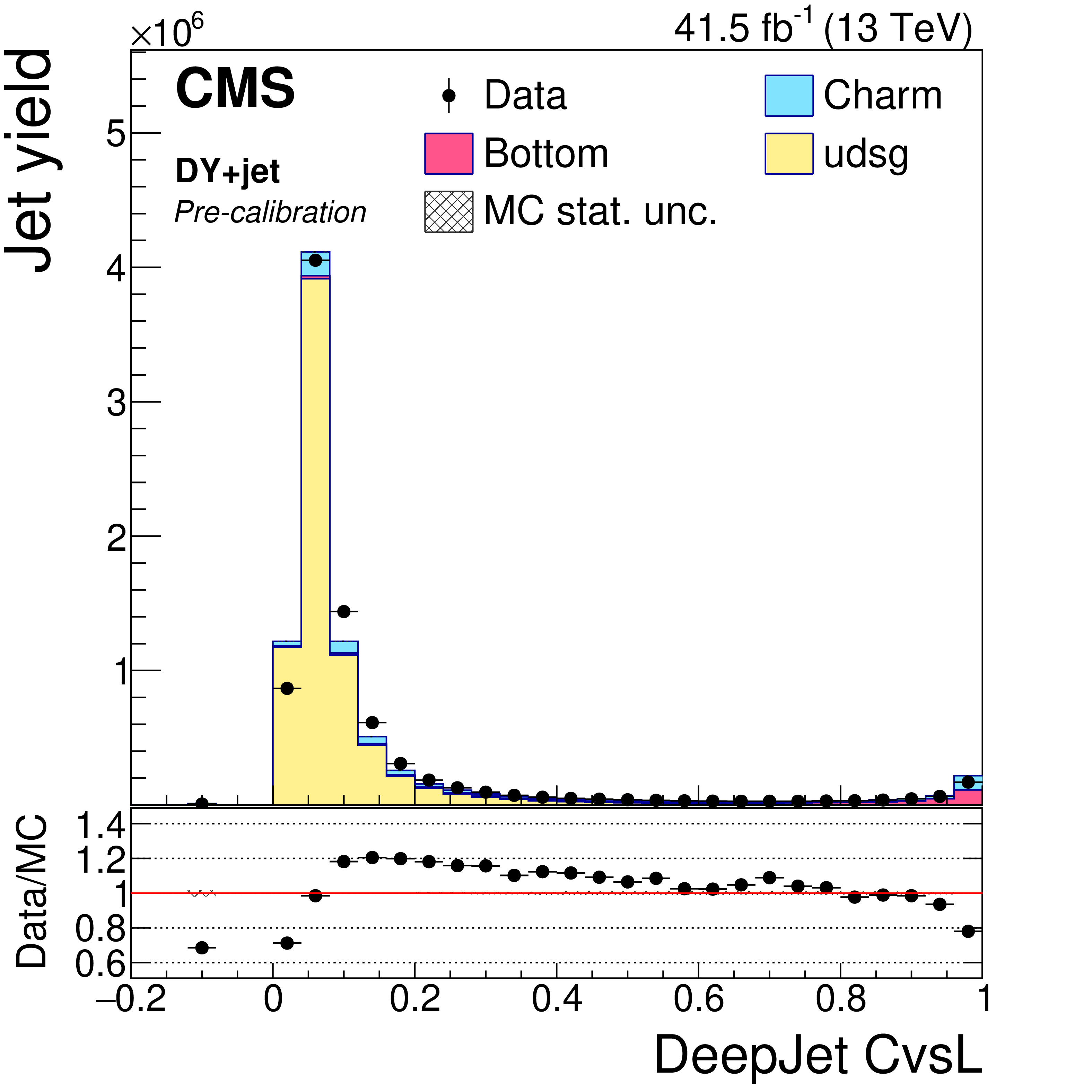
Figure 8-c:
Precalibration distributions of CvsL obtained from the DeepCSV tagger for jets in the DY+jets selection. The bin corresponding to a tagger value of $-1$ is plotted at $-0.1$. Vertical error bars in data represent statistical uncertainties in data. |
png pdf |
Figure 8-d:
Precalibration distributions of CvsB obtained from the DeepJet tagger for jets in the DY+jets selection. The bin corresponding to a tagger value of $-1$ is plotted at $-0.1$. Vertical error bars in data represent statistical uncertainties in data. |
png pdf |
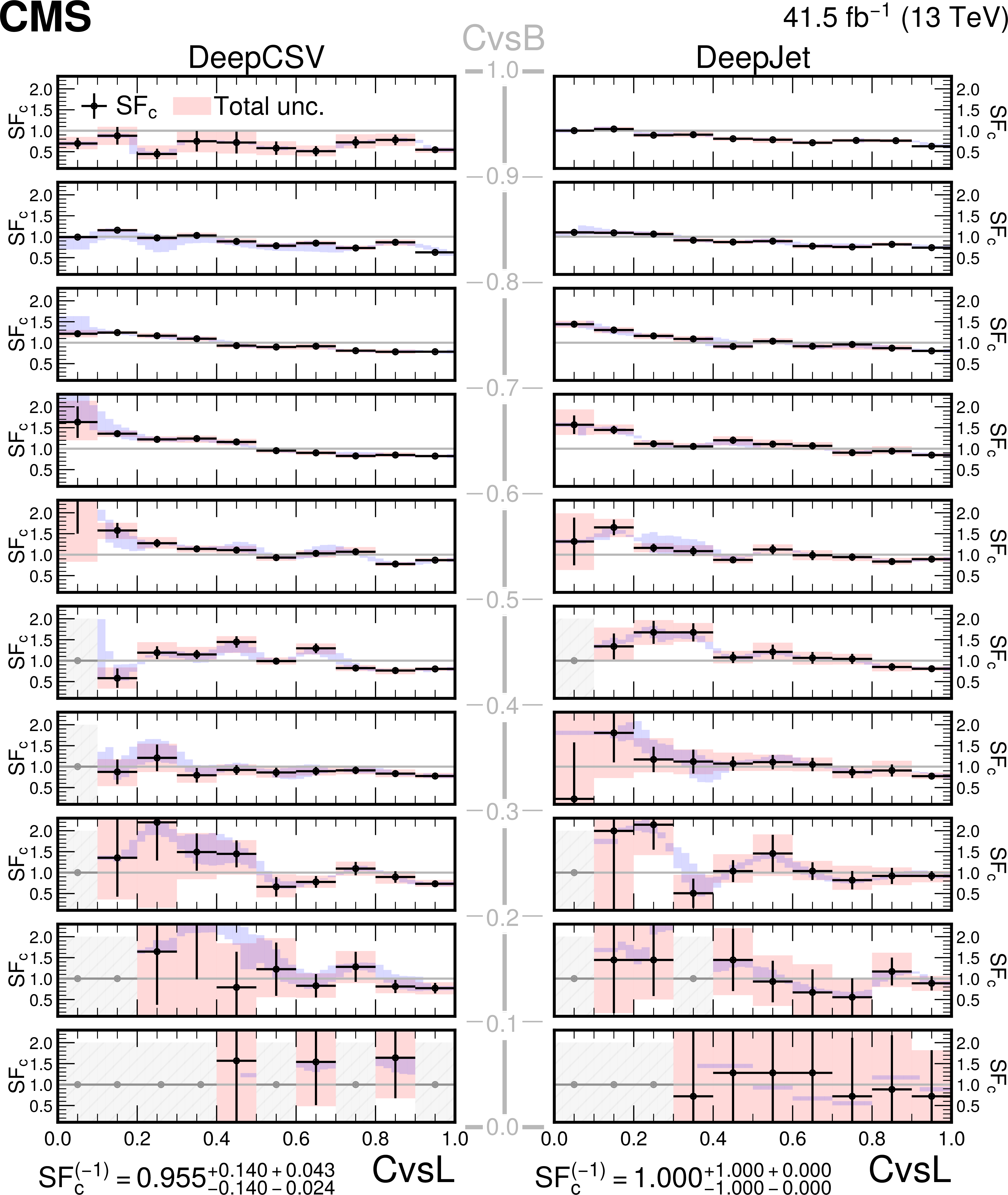
Figure 9:
The shape calibration SF values as a function of CvsL for DeepCSV- (left) and DeepJet- (right) based c taggers for c jets in different ranges of CvsB are shown. The black datapoints indicate the nominal SF values at the nodal points obtained with a fixed bin width along CvsB and an adaptive binning scheme along CvsL. The total uncertainty in the SFs at the nodal points is denoted by the red envelopes around the nominal values, whereas the statistical uncertainties alone are denoted by the black vertical lines. Grey datapoints with the hatched uncertainties denote bins with jet counts or signal purity insufficient for the SF evaluation. The blue envelopes indicate the range of all nominal interpolated SF values in the corresponding CvsB range. The quantity, SF$_ {{\mathrm{c}}}^{(-1)}$, denotes the SF for c jets with the default discriminator value, along with the statistical (first term) and systematic (second term) uncertainties. |

png pdf |
Figure 10:
The shape calibration SF values as a function of CvsL for DeepCSV- (left) and DeepJet- (right) based c taggers for b jets in different ranges of CvsB are shown. The black datapoints indicate the nominal SF values at the nodal points obtained with a fixed bin width along CvsB and an adaptive binning scheme along CvsL. The total uncertainty in the SFs at the nodal points is denoted by the red envelopes around the nominal values, whereas the statistical uncertainties alone are denoted by the black vertical lines. Grey datapoints with the hatched uncertainties denote bins with jet counts or signal purity insufficient for the SF evaluation. The blue envelopes indicate the range of all nominal interpolated SF values in the corresponding CvsB range. The quantity, SF$_{{\mathrm{b}}}^{(-1)}$, denotes the SF for b jets with the default discriminator value, along with the statistical (first term) and systematic (second term) uncertainties. |
png pdf |
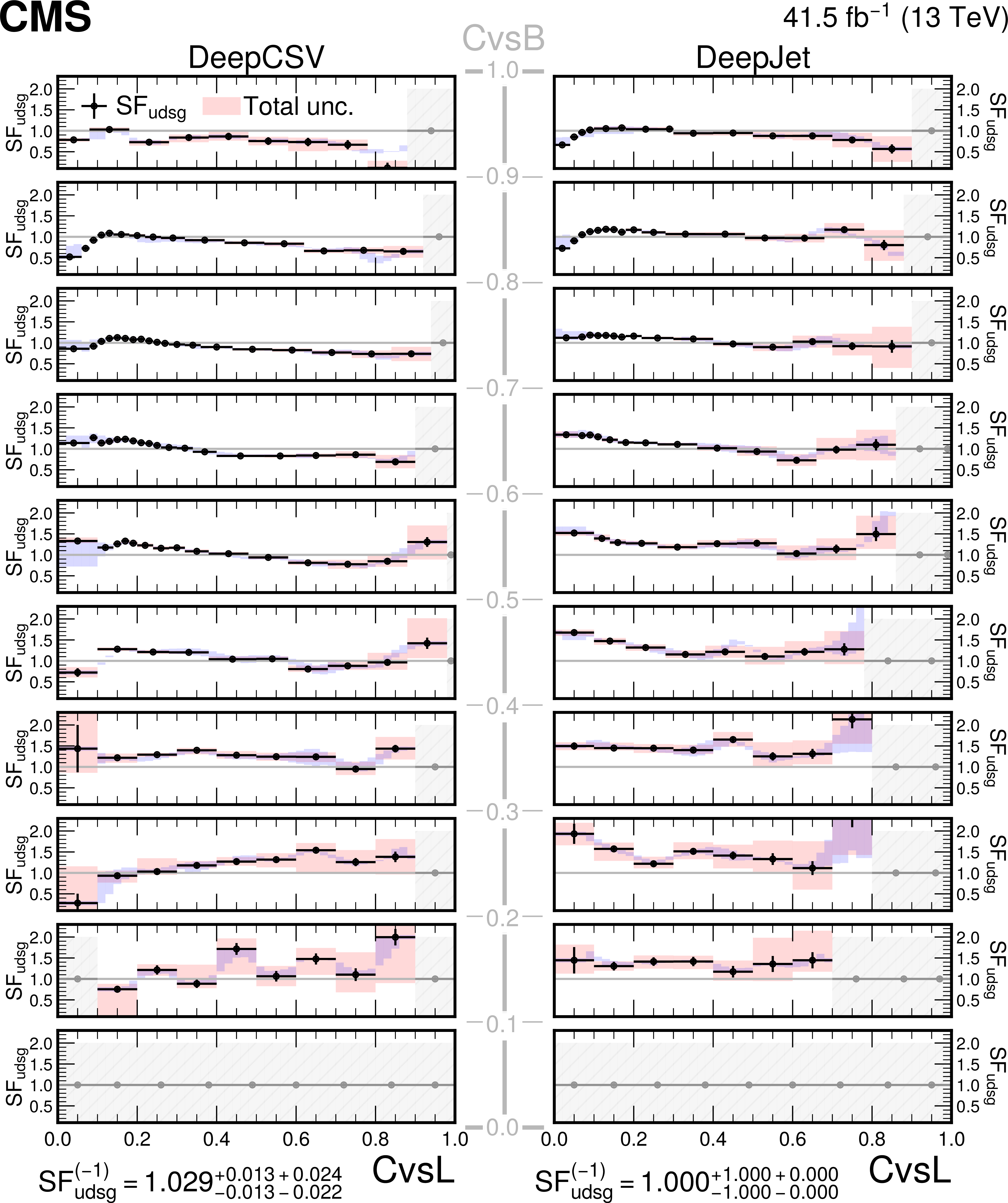
Figure 11:
The shape calibration SF values as a function of CvsL for DeepCSV- (left) and DeepJet- (right) based c taggers for light-flavour jets in different ranges of CvsB are shown. The black datapoints indicate the nominal SF values at the nodal points obtained with a fixed bin width along CvsB and an adaptive binning scheme along CvsL. The total uncertainty in the SFs at the nodal points is denoted by the red envelopes around the nominal values, whereas the statistical uncertainties alone are denoted by the black vertical lines. Grey datapoints with the hatched uncertainties denote bins with jet counts or signal purity insufficient for the SF evaluation. The blue envelopes indicate the range of all nominal interpolated SF values in the corresponding CvsB range. The quantity, SF$_\text {udsg}^{(-1)}$, denotes the SF for light-flavour jets with the default discriminator value, along with the statistical (first term) and systematic (second term) uncertainties. |
png pdf |
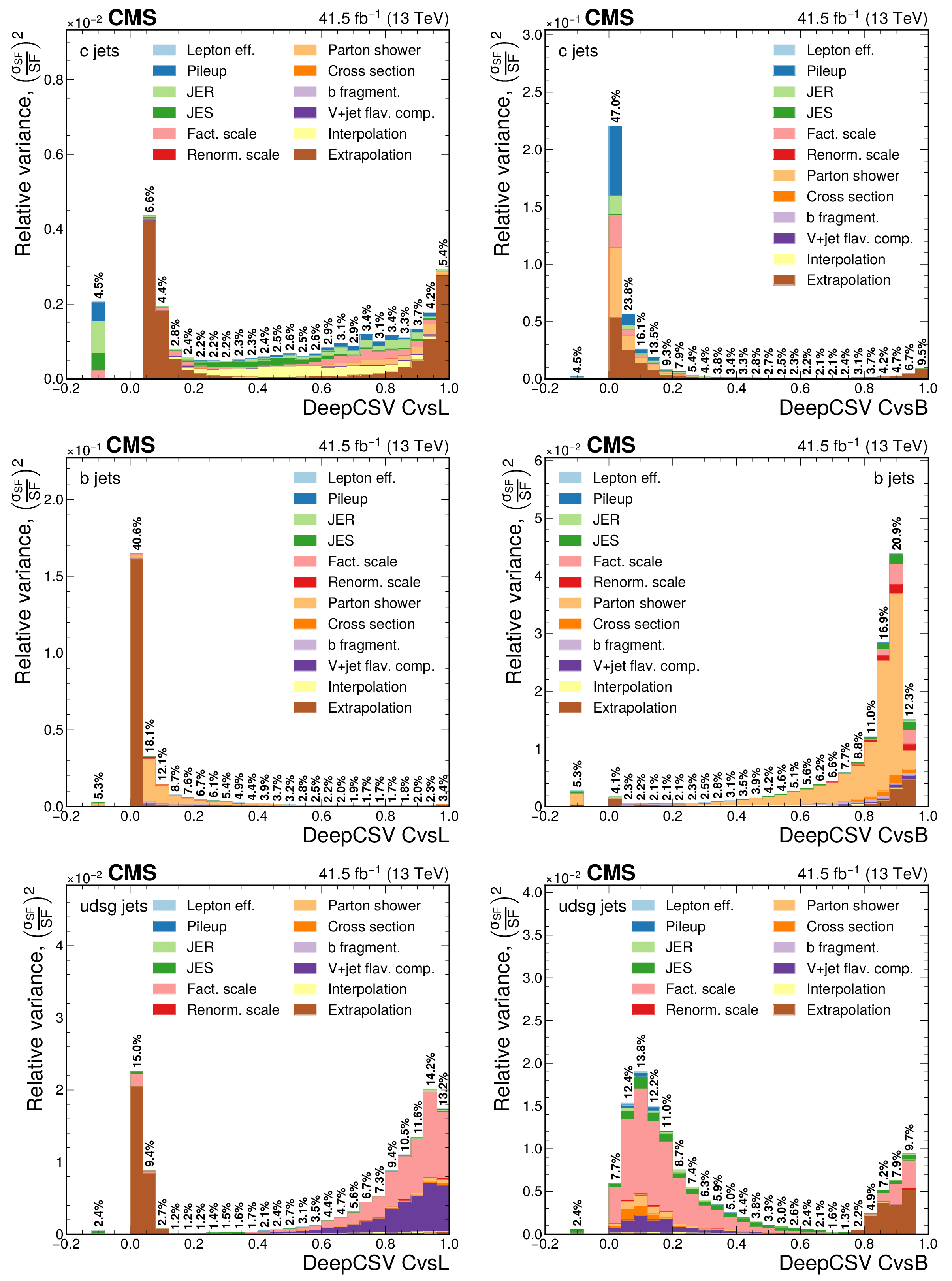
Figure 12:
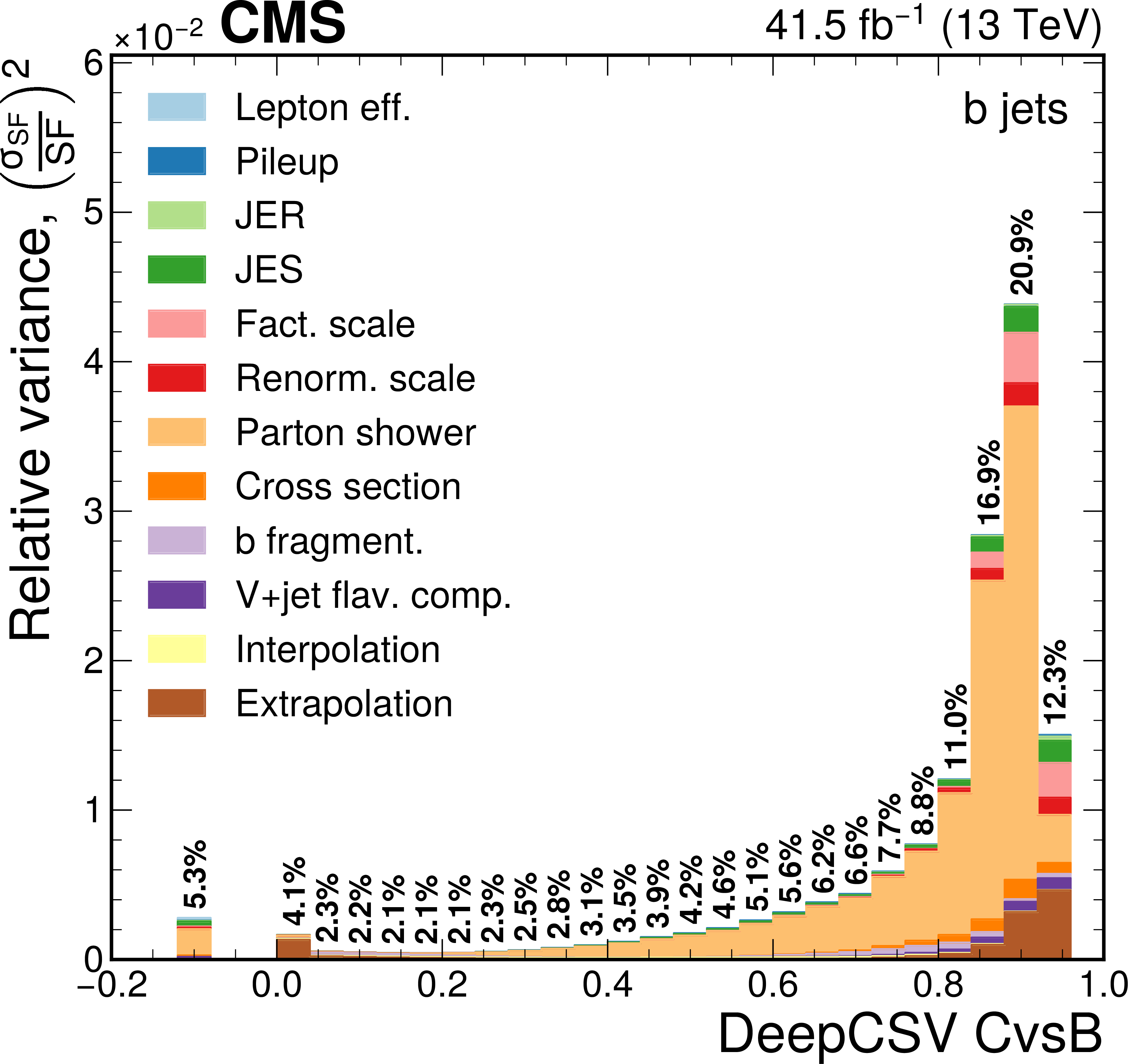
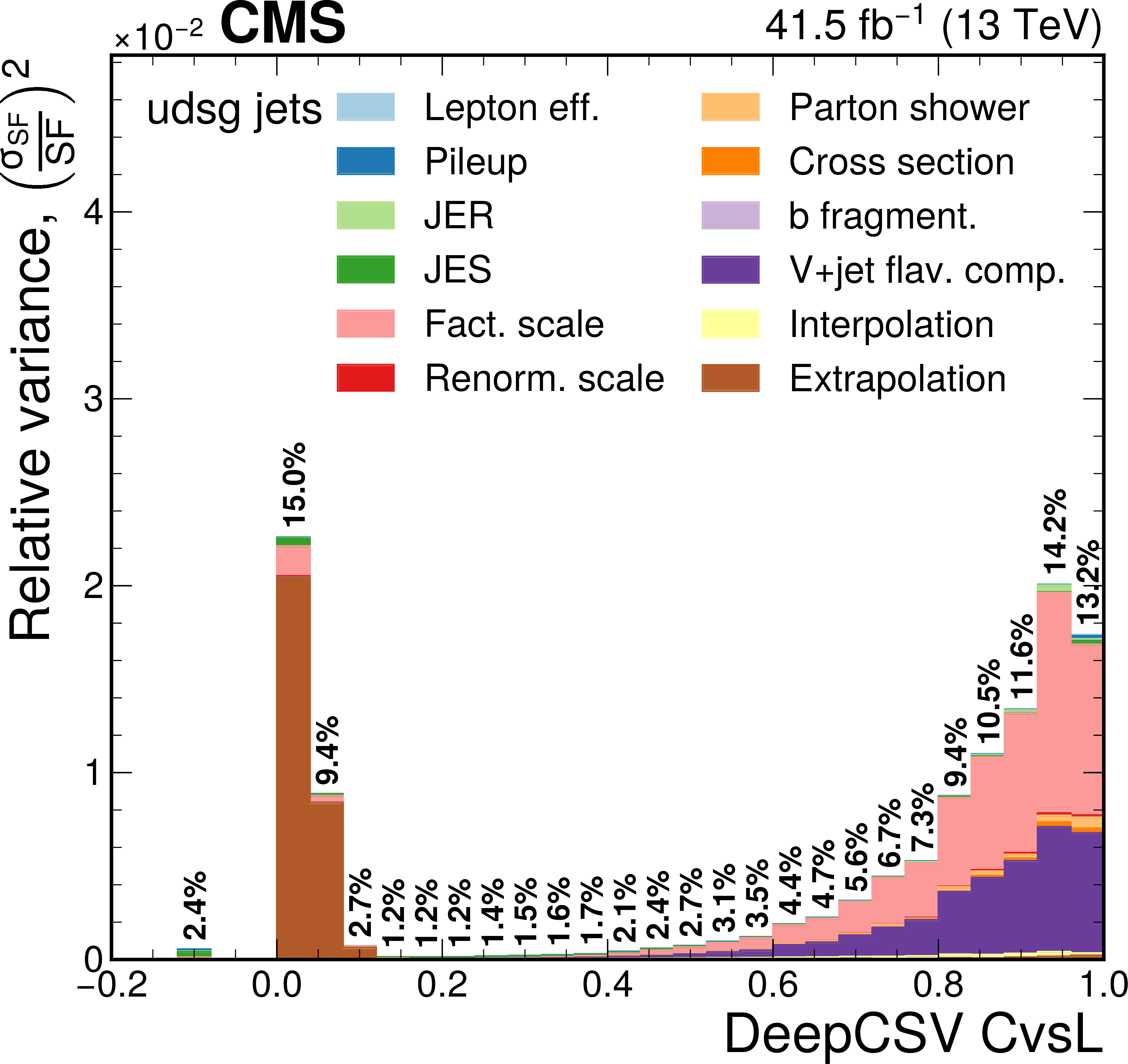
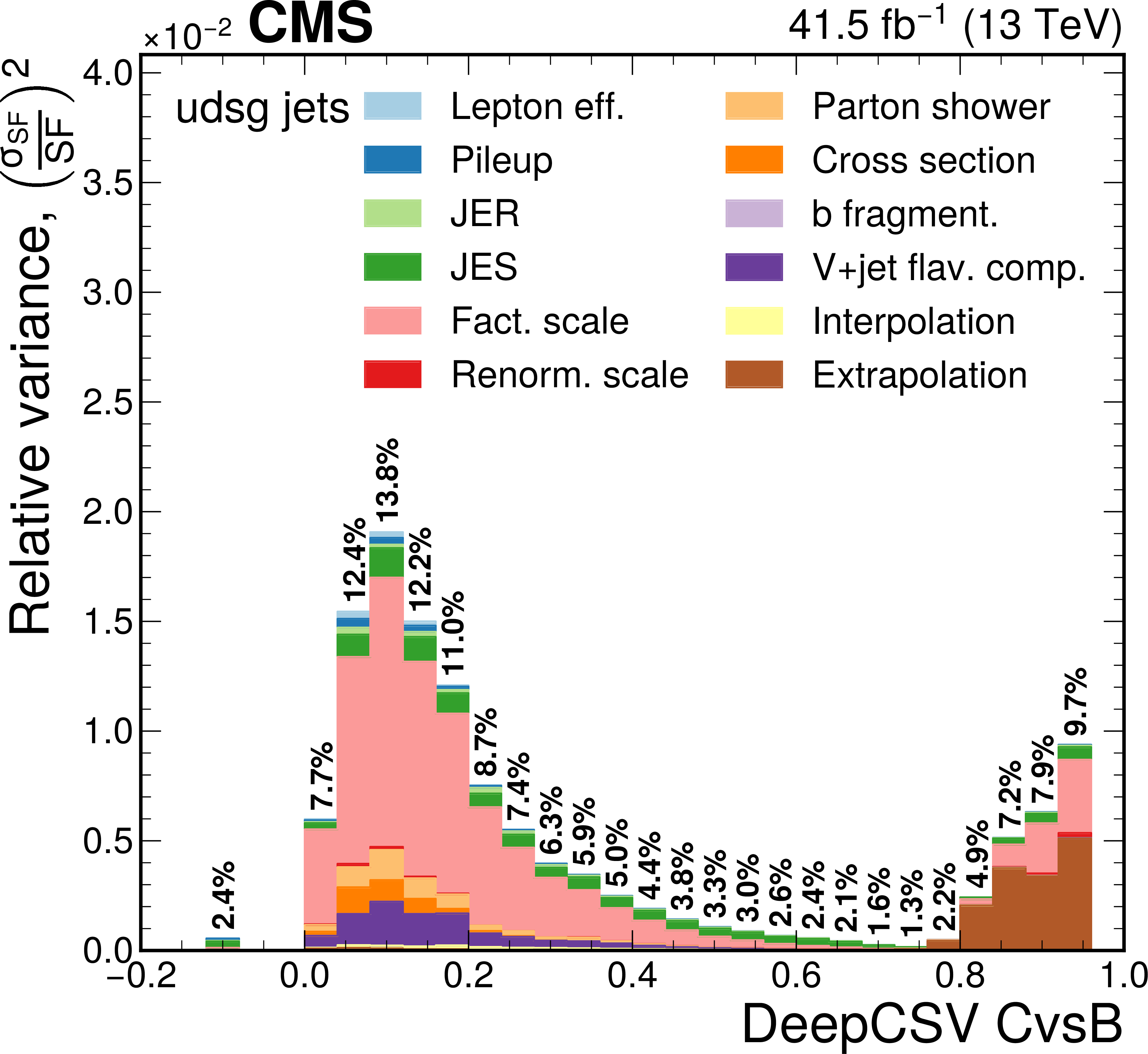
Contribution of each source of the SF uncertainty, calculated as the square of the relative uncertainty in the jet yield and expressed as the maximum of the up and down variations, at various values of the DeepCSV CvsL (left) and CvsB (right) discriminators for c (upper), b (middle), and light (lower) flavours. The effective total relative uncertainty values ($\sqrt {\Sigma ({\sigma _{\text {SF}}}/{\text {SF}} )^2}$) per bin are also shown in bold text, for reference. The bin corresponding to a tagger value of $-1$ is plotted at $-0.1$. Statistical uncertainties are not shown. |

png pdf |
Figure 12-a:
Contribution of each source of the SF uncertainty, calculated as the square of the relative uncertainty in the jet yield and expressed as the maximum of the up and down variations, at various values of the DeepCSV CvsL discriminators for c flavour. The effective total relative uncertainty values ($\sqrt {\Sigma ({\sigma _{\text {SF}}}/{\text {SF}} )^2}$) per bin are also shown in bold text, for reference. The bin corresponding to a tagger value of $-1$ is plotted at $-0.1$. Statistical uncertainties are not shown. |

png pdf |
Figure 12-b:
Contribution of each source of the SF uncertainty, calculated as the square of the relative uncertainty in the jet yield and expressed as the maximum of the up and down variations, at various values of the DeepCSV CvsB discriminators for c flavour. The effective total relative uncertainty values ($\sqrt {\Sigma ({\sigma _{\text {SF}}}/{\text {SF}} )^2}$) per bin are also shown in bold text, for reference. The bin corresponding to a tagger value of $-1$ is plotted at $-0.1$. Statistical uncertainties are not shown. |
png pdf |
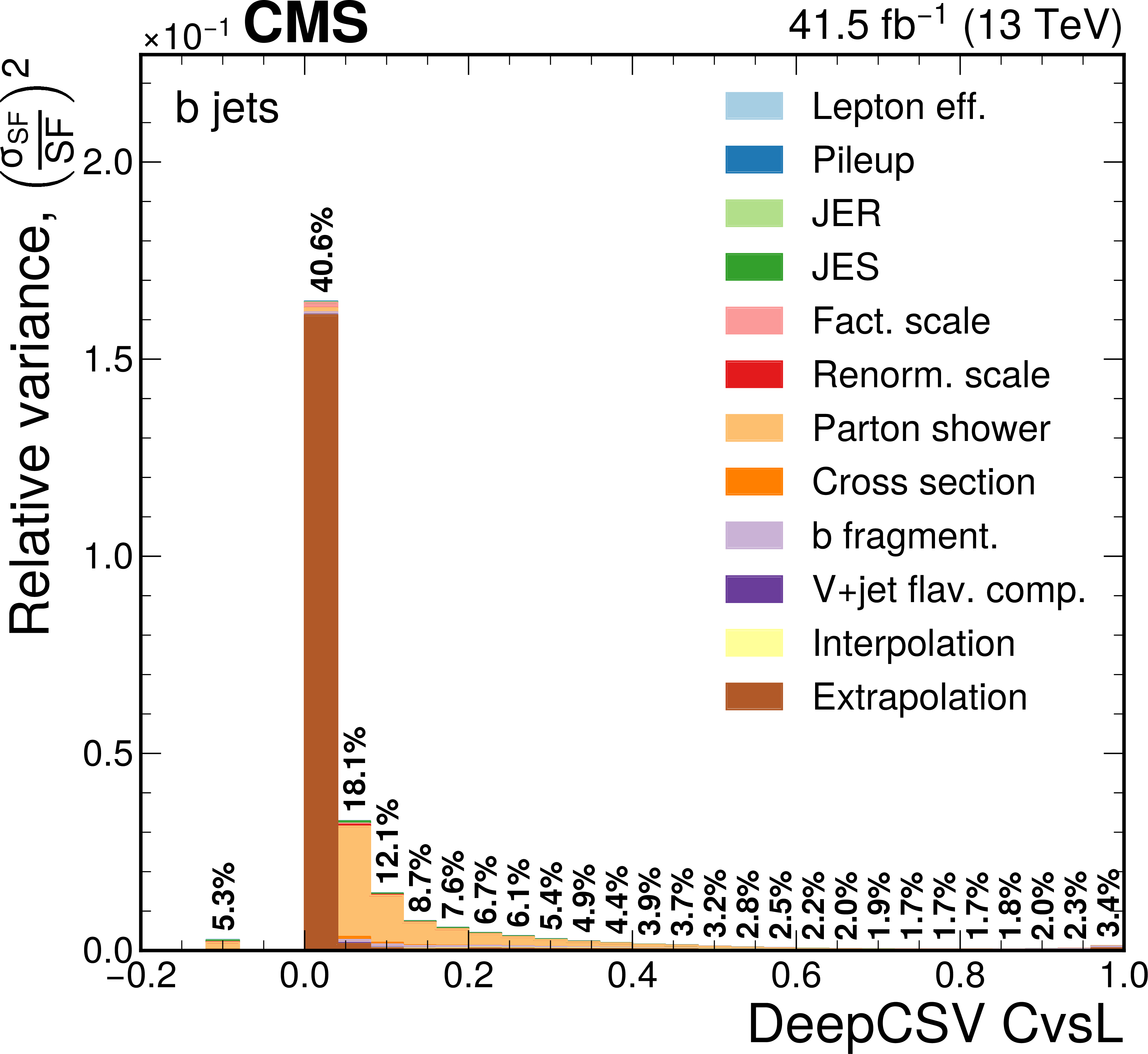
Figure 12-c:
Contribution of each source of the SF uncertainty, calculated as the square of the relative uncertainty in the jet yield and expressed as the maximum of the up and down variations, at various values of the DeepCSV CvsL discriminators for b flavour. The effective total relative uncertainty values ($\sqrt {\Sigma ({\sigma _{\text {SF}}}/{\text {SF}} )^2}$) per bin are also shown in bold text, for reference. The bin corresponding to a tagger value of $-1$ is plotted at $-0.1$. Statistical uncertainties are not shown. |
png pdf |
Figure 12-d:
Contribution of each source of the SF uncertainty, calculated as the square of the relative uncertainty in the jet yield and expressed as the maximum of the up and down variations, at various values of the DeepCSV CvsB discriminators for b flavour. The effective total relative uncertainty values ($\sqrt {\Sigma ({\sigma _{\text {SF}}}/{\text {SF}} )^2}$) per bin are also shown in bold text, for reference. The bin corresponding to a tagger value of $-1$ is plotted at $-0.1$. Statistical uncertainties are not shown. |
png pdf |
Figure 12-e:
Contribution of each source of the SF uncertainty, calculated as the square of the relative uncertainty in the jet yield and expressed as the maximum of the up and down variations, at various values of the DeepCSV CvsL discriminators for light flavours. The effective total relative uncertainty values ($\sqrt {\Sigma ({\sigma _{\text {SF}}}/{\text {SF}} )^2}$) per bin are also shown in bold text, for reference. The bin corresponding to a tagger value of $-1$ is plotted at $-0.1$. Statistical uncertainties are not shown. |
png pdf |
Figure 12-f:
Contribution of each source of the SF uncertainty, calculated as the square of the relative uncertainty in the jet yield and expressed as the maximum of the up and down variations, at various values of the DeepCSV CvsB discriminators for light flavours. The effective total relative uncertainty values ($\sqrt {\Sigma ({\sigma _{\text {SF}}}/{\text {SF}} )^2}$) per bin are also shown in bold text, for reference. The bin corresponding to a tagger value of $-1$ is plotted at $-0.1$. Statistical uncertainties are not shown. |

png pdf |
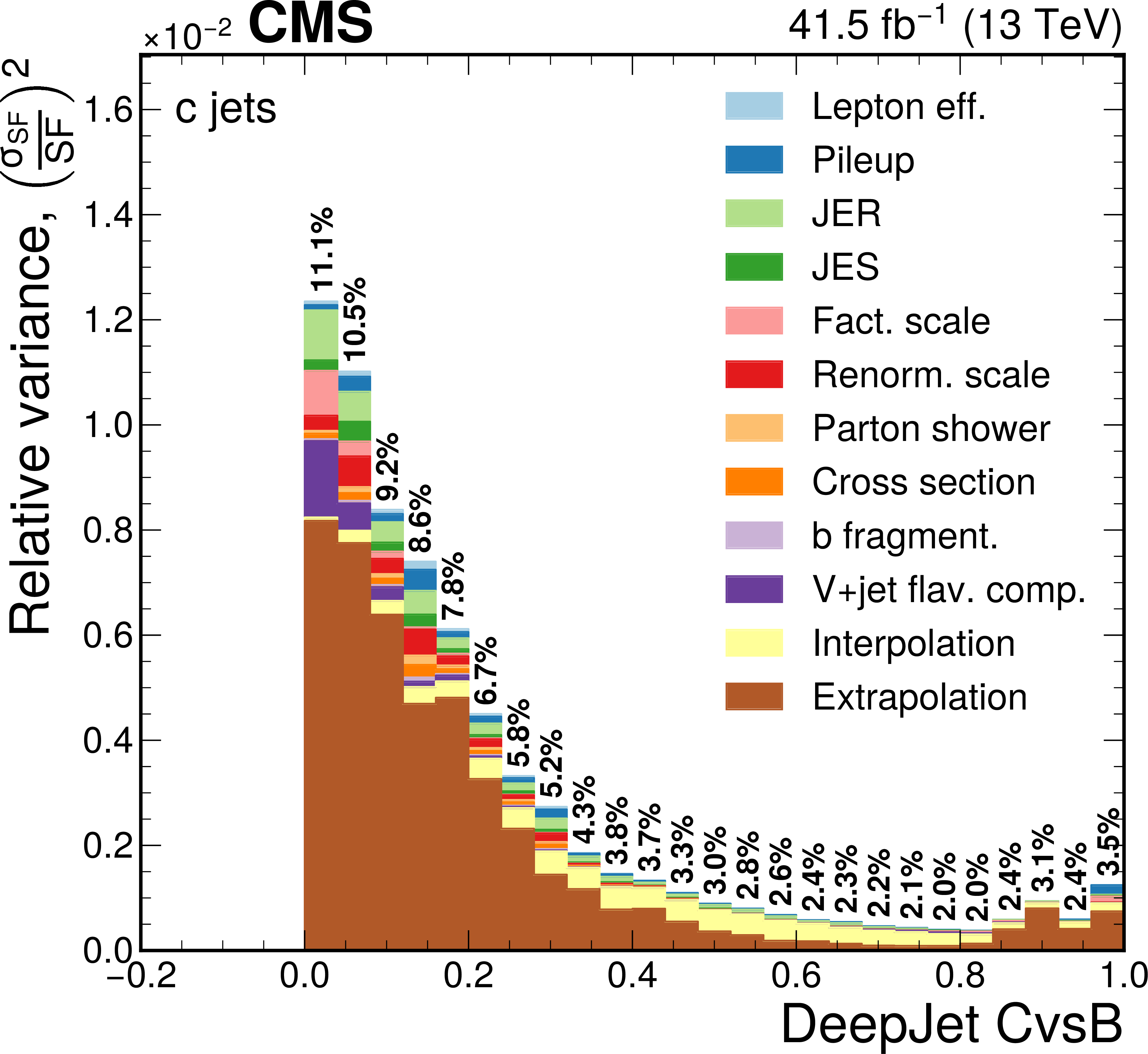
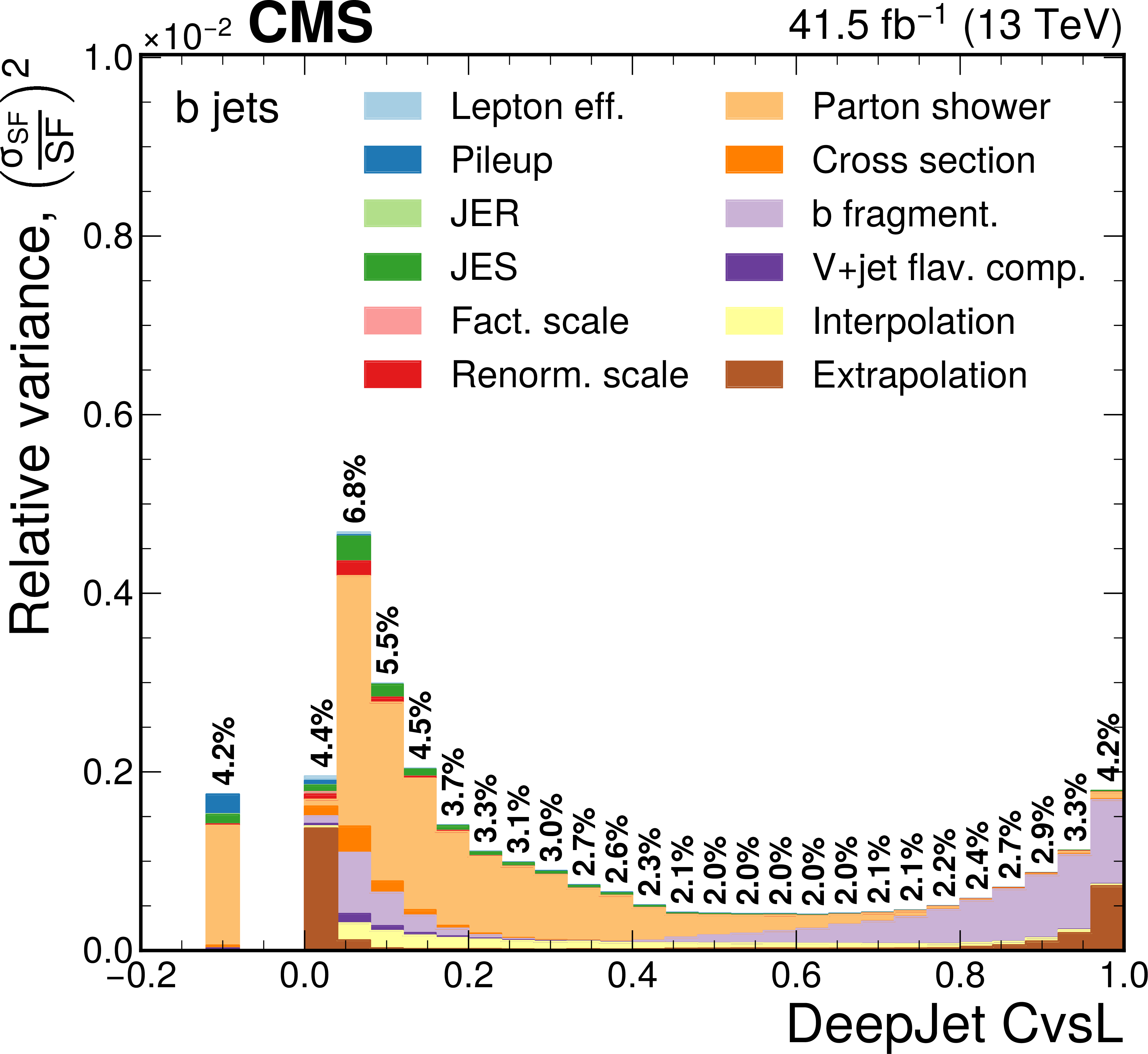
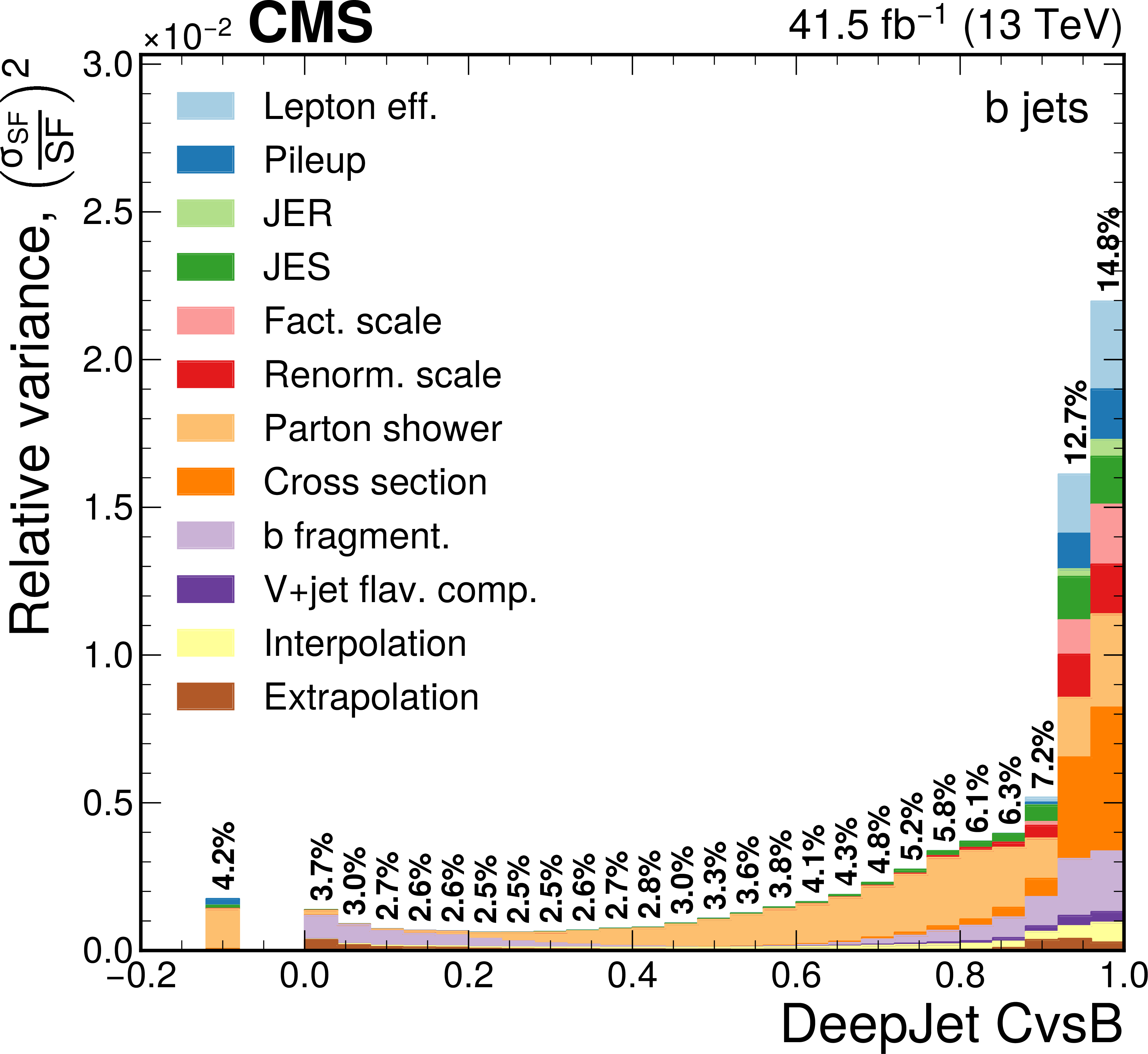
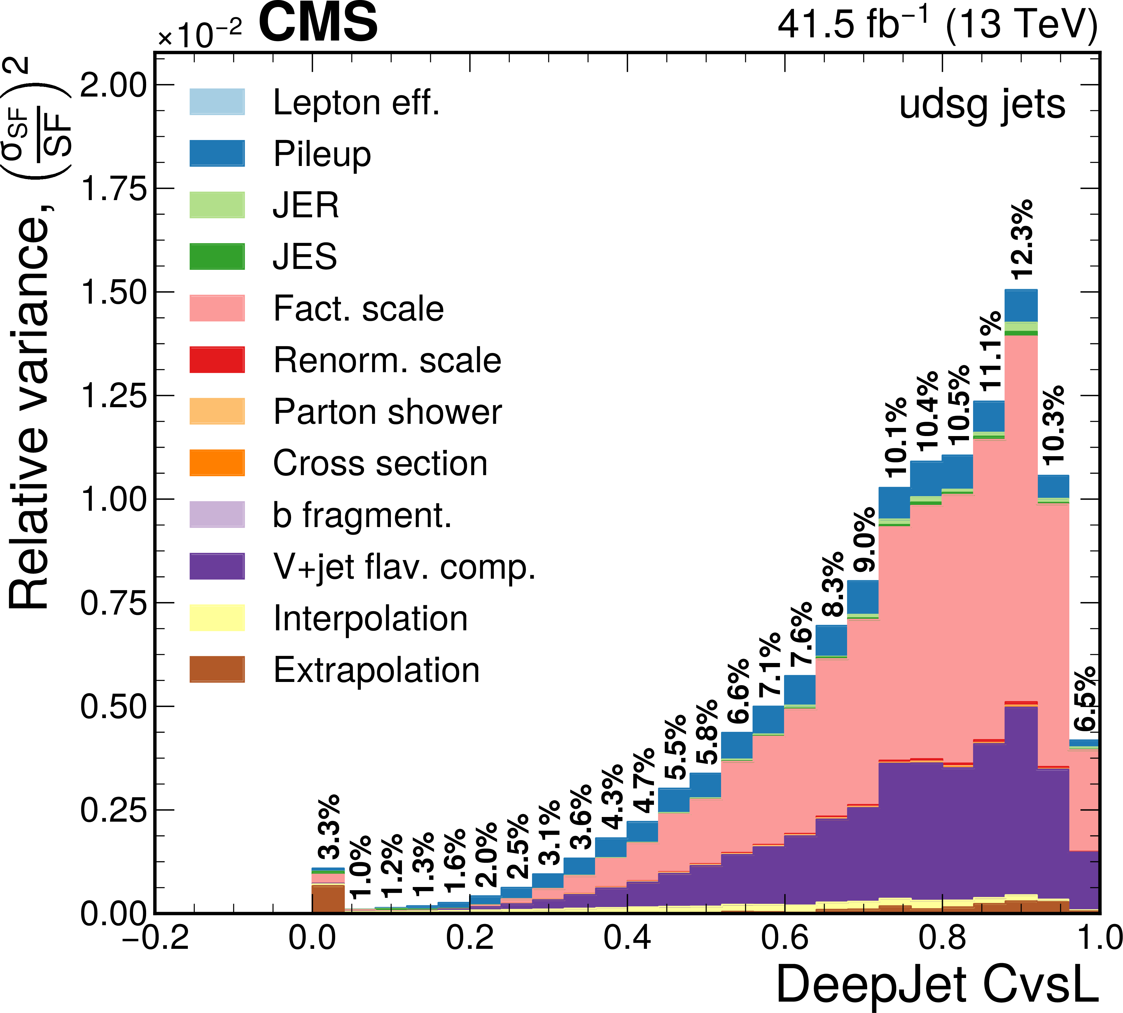
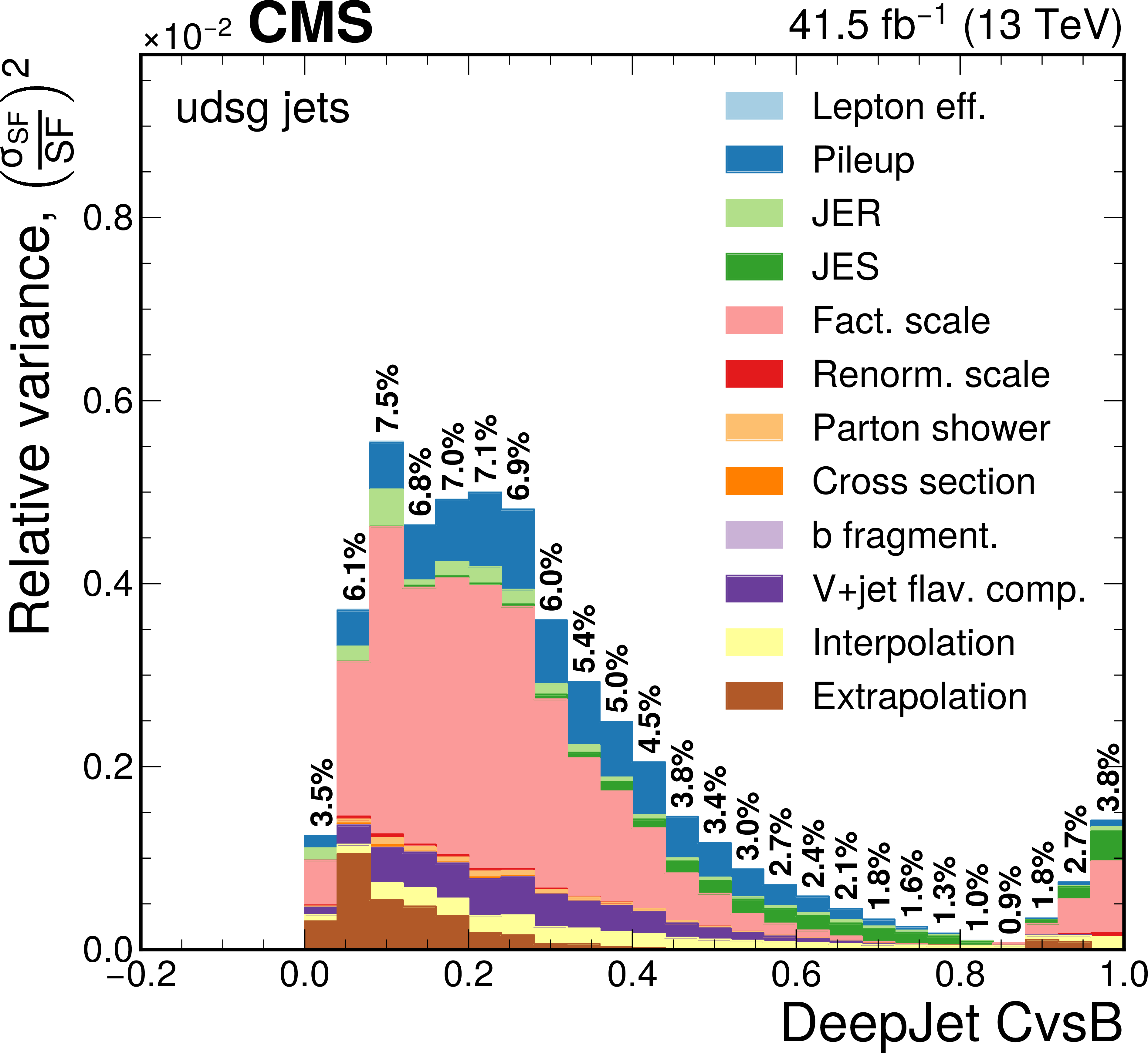
Figure 13:
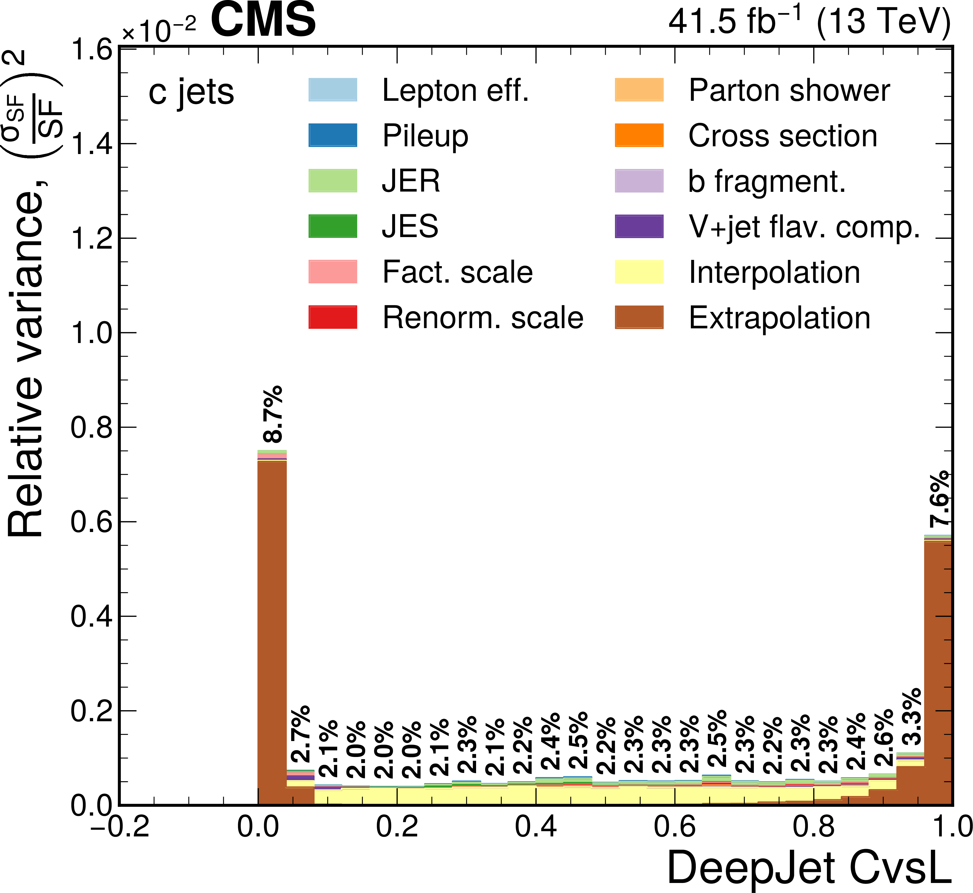
Contribution of each source of the SF uncertainty, calculated as the square of the relative uncertainty in the jet yield and expressed as the maximum of the up and down variations, at various values of the DeepJet CvsL (left) and CvsB (right) discriminators for c (upper), b (middle), and light (lower) flavours. The effective total relative uncertainty values ($\sqrt {\Sigma ( {\sigma _{\text {SF}}}/{\text {SF}})^2}$) per bin are also shown in bold text, for reference. The bin corresponding to a tagger value of $-1$ is plotted at $-0.1$. Statistical uncertainties are not shown. |
png pdf |
Figure 13-a:
Contribution of each source of the SF uncertainty, calculated as the square of the relative uncertainty in the jet yield and expressed as the maximum of the up and down variations, at various values of the DeepJet CvsL discriminators for c flavour. The effective total relative uncertainty values ($\sqrt {\Sigma ( {\sigma _{\text {SF}}}/{\text {SF}})^2}$) per bin are also shown in bold text, for reference. The bin corresponding to a tagger value of $-1$ is plotted at $-0.1$. Statistical uncertainties are not shown. |
png pdf |
Figure 13-b:
Contribution of each source of the SF uncertainty, calculated as the square of the relative uncertainty in the jet yield and expressed as the maximum of the up and down variations, at various values of the DeepJet CvsB discriminators for c flavour. The effective total relative uncertainty values ($\sqrt {\Sigma ( {\sigma _{\text {SF}}}/{\text {SF}})^2}$) per bin are also shown in bold text, for reference. The bin corresponding to a tagger value of $-1$ is plotted at $-0.1$. Statistical uncertainties are not shown. |
png pdf |
Figure 13-c:
Contribution of each source of the SF uncertainty, calculated as the square of the relative uncertainty in the jet yield and expressed as the maximum of the up and down variations, at various values of the DeepJet CvsL discriminators for b flavour. The effective total relative uncertainty values ($\sqrt {\Sigma ( {\sigma _{\text {SF}}}/{\text {SF}})^2}$) per bin are also shown in bold text, for reference. The bin corresponding to a tagger value of $-1$ is plotted at $-0.1$. Statistical uncertainties are not shown. |
png pdf |
Figure 13-d:
Contribution of each source of the SF uncertainty, calculated as the square of the relative uncertainty in the jet yield and expressed as the maximum of the up and down variations, at various values of the DeepJet CvsB discriminators for b flavour. The effective total relative uncertainty values ($\sqrt {\Sigma ( {\sigma _{\text {SF}}}/{\text {SF}})^2}$) per bin are also shown in bold text, for reference. The bin corresponding to a tagger value of $-1$ is plotted at $-0.1$. Statistical uncertainties are not shown. |
png pdf |
Figure 13-e:
Contribution of each source of the SF uncertainty, calculated as the square of the relative uncertainty in the jet yield and expressed as the maximum of the up and down variations, at various values of the DeepJet CvsL discriminators for light flavours. The effective total relative uncertainty values ($\sqrt {\Sigma ( {\sigma _{\text {SF}}}/{\text {SF}})^2}$) per bin are also shown in bold text, for reference. The bin corresponding to a tagger value of $-1$ is plotted at $-0.1$. Statistical uncertainties are not shown. |
png pdf |
Figure 13-f:
Contribution of each source of the SF uncertainty, calculated as the square of the relative uncertainty in the jet yield and expressed as the maximum of the up and down variations, at various values of the DeepJet CvsB discriminators for light flavours. The effective total relative uncertainty values ($\sqrt {\Sigma ( {\sigma _{\text {SF}}}/{\text {SF}})^2}$) per bin are also shown in bold text, for reference. The bin corresponding to a tagger value of $-1$ is plotted at $-0.1$. Statistical uncertainties are not shown. |
png pdf |
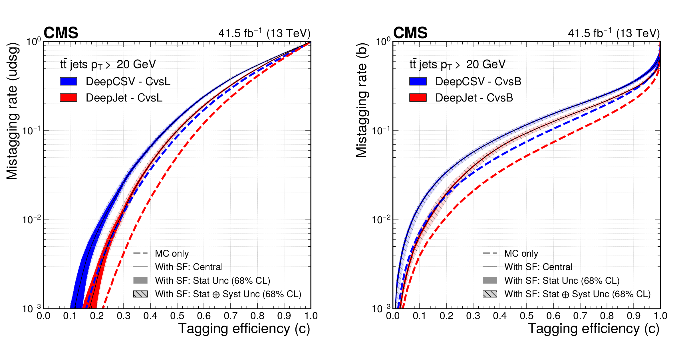
Figure 14:
The ROC curves showing the individual performance of the CvsL (left) and CvsB (right) discriminators for the DeepCSV (blue) and DeepJet (red) algorithms for simulated jets (the dashed lines) and the estimation of the same for jets in data (the solid lines). The solid uncertainty bands around the solid lines represent statistical uncertainties only, and the hatched semi-transparent bands represent statistical and systematic uncertainties added in quadrature. |
png pdf |
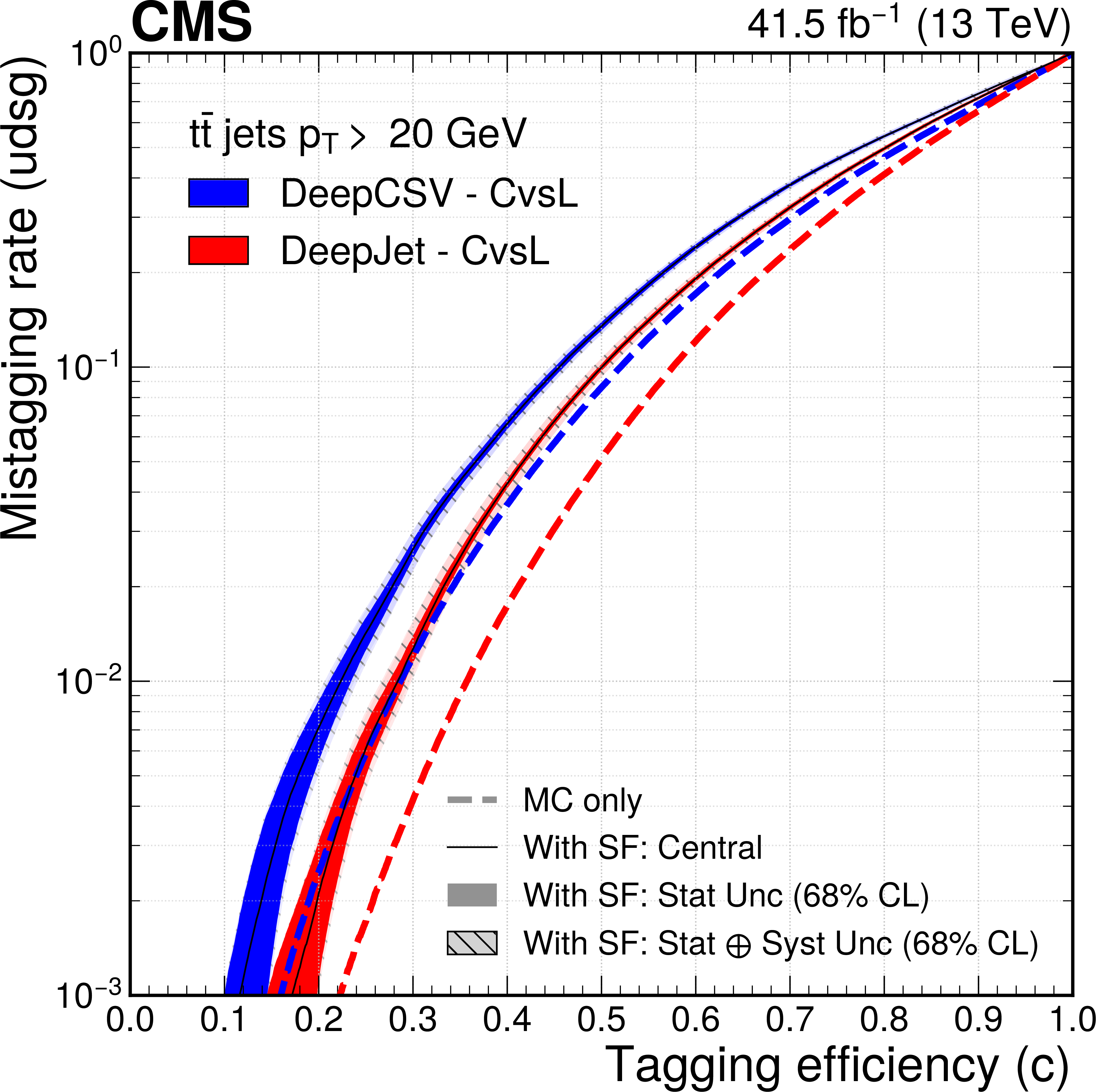
Figure 14-a:
The ROC curves showing the individual performance of the CvsL discriminator for the DeepCSV (blue) and DeepJet (red) algorithms for simulated jets (the dashed lines) and the estimation of the same for jets in data (the solid lines). The solid uncertainty bands around the solid lines represent statistical uncertainties only, and the hatched semi-transparent bands represent statistical and systematic uncertainties added in quadrature. |
png pdf |
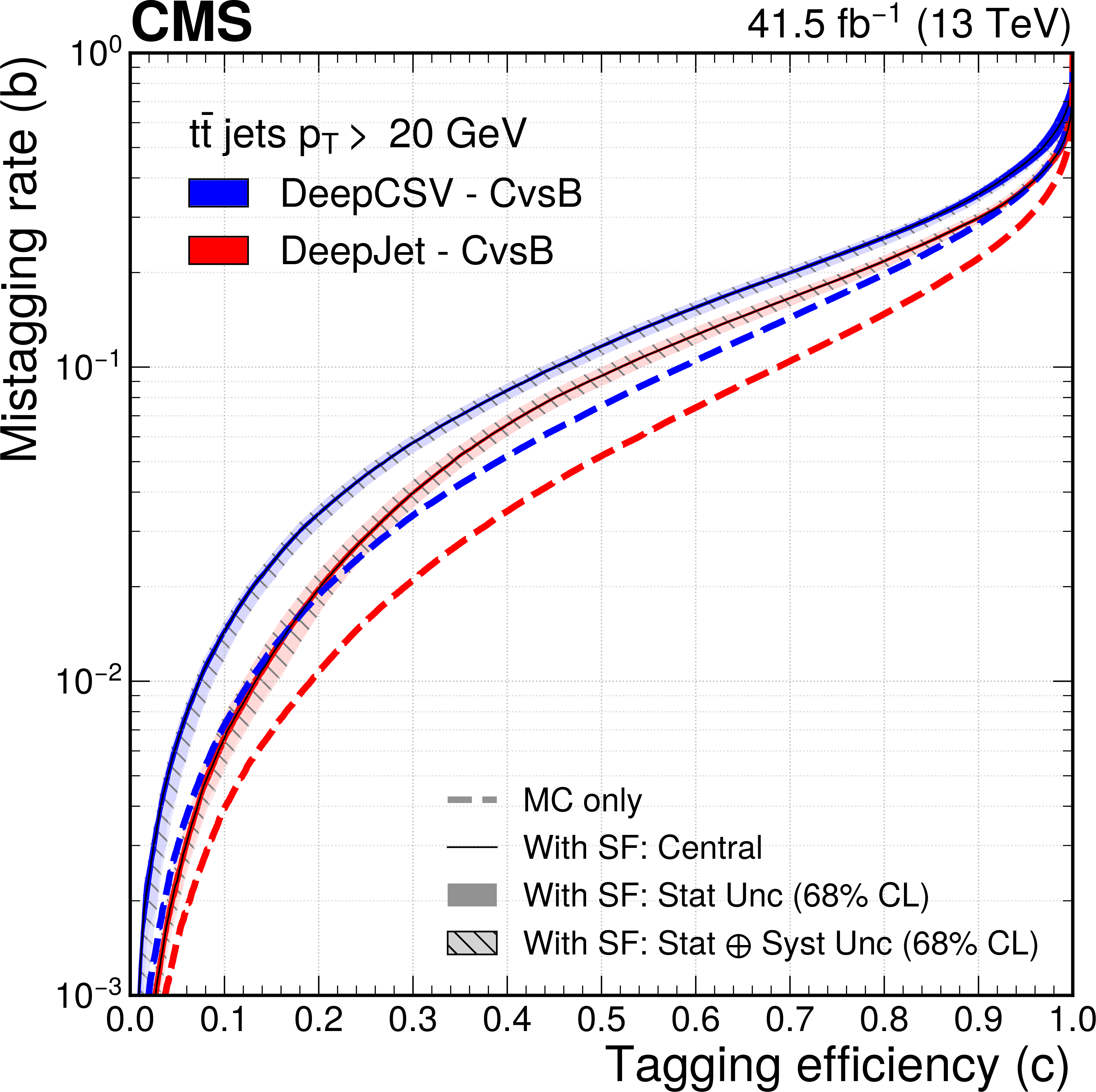
Figure 14-b:
The ROC curves showing the individual performance of the CvsB discriminator for the DeepCSV (blue) and DeepJet (red) algorithms for simulated jets (the dashed lines) and the estimation of the same for jets in data (the solid lines). The solid uncertainty bands around the solid lines represent statistical uncertainties only, and the hatched semi-transparent bands represent statistical and systematic uncertainties added in quadrature. |
png pdf |
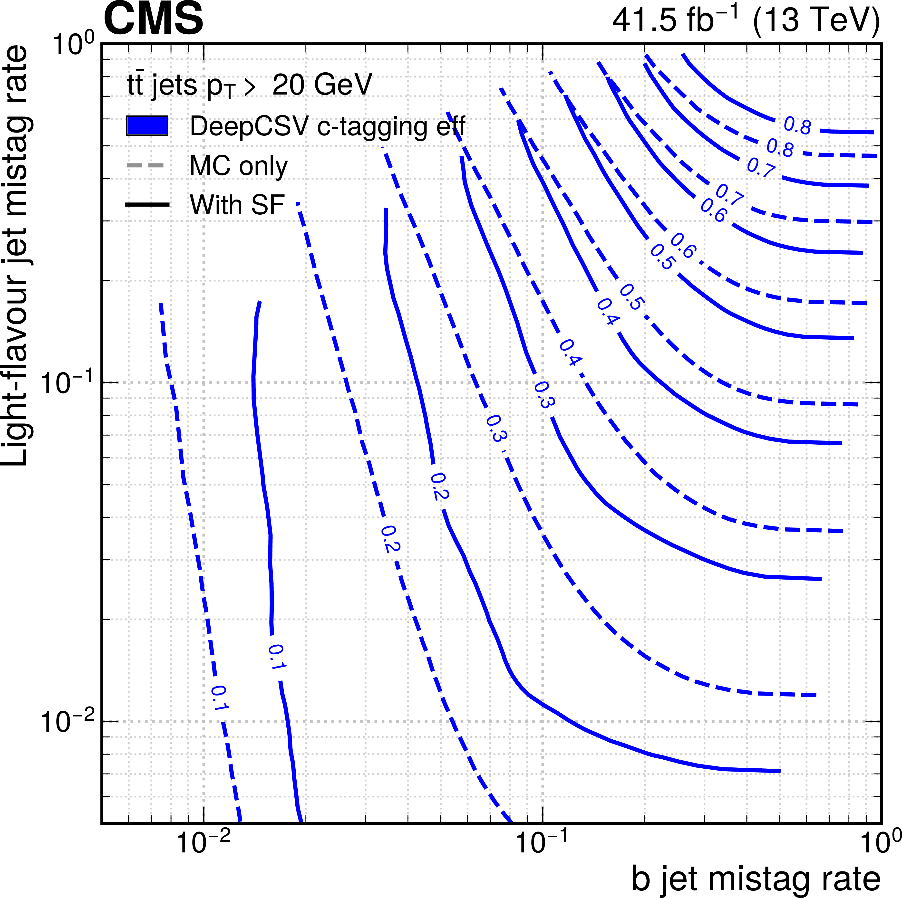
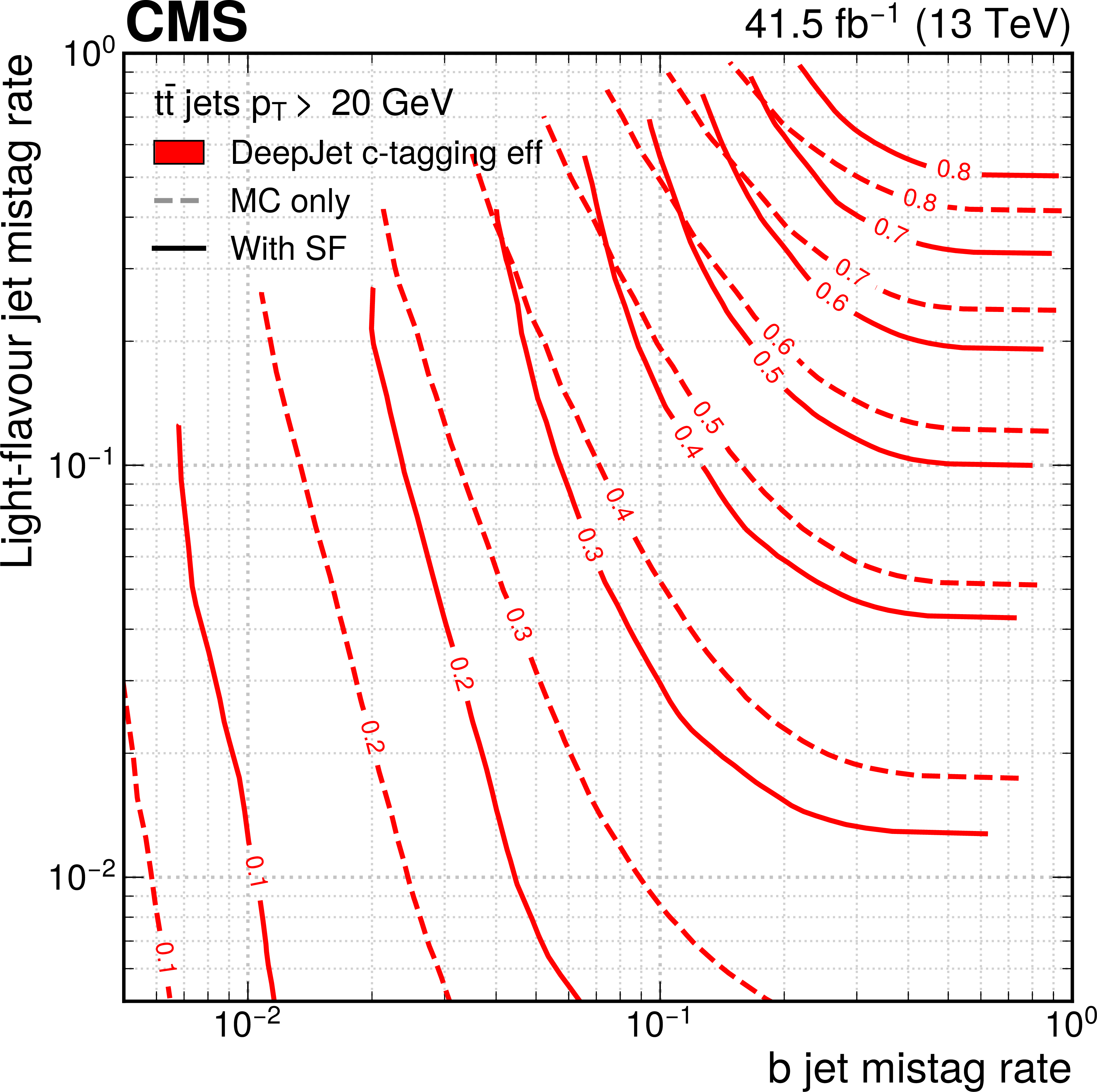
Figure 15:
The ROC contours showing c tagging efficiencies as functions of b and light-flavour jet misidentification rates, for the DeepCSV (left) and DeepJet (right) algorithms for simulated jets (the dashed lines) and the estimation of the same for jets in data (the solid lines). Each line represents points in the plane that correspond to a fixed value of the c tagging efficiency, which is shown as a number at the centre of each line. |
png pdf |
Figure 15-a:
The ROC contours showing c tagging efficiencies as functions of b and light-flavour jet misidentification rates, for the DeepCSV algorithm for simulated jets (the dashed lines) and the estimation of the same for jets in data (the solid lines). Each line represents points in the plane that correspond to a fixed value of the c tagging efficiency, which is shown as a number at the centre of each line. |
png pdf |
Figure 15-b:
The ROC contours showing c tagging efficiencies as functions of b and light-flavour jet misidentification rates, for the DeepJet algorithm for simulated jets (the dashed lines) and the estimation of the same for jets in data (the solid lines). Each line represents points in the plane that correspond to a fixed value of the c tagging efficiency, which is shown as a number at the centre of each line. |
png pdf |
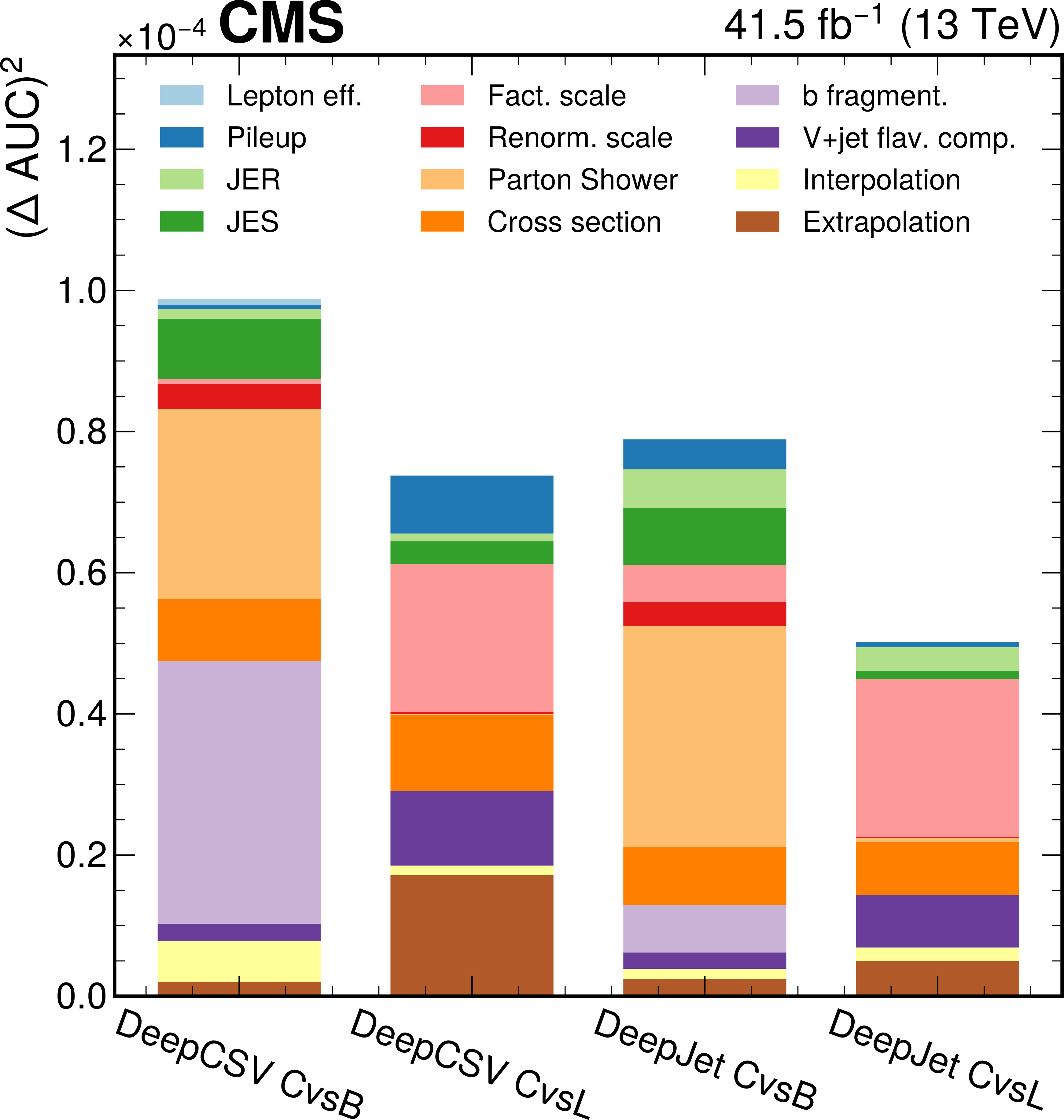
Figure 16:
Relative contributions of each source of uncertainty to the total uncertainty (statistical + systematic) for both CvsL and CvsB discrimination and for both DeepCSV and DeepJet taggers, quantified by the square of the change in area under ROC curves. |

png pdf |
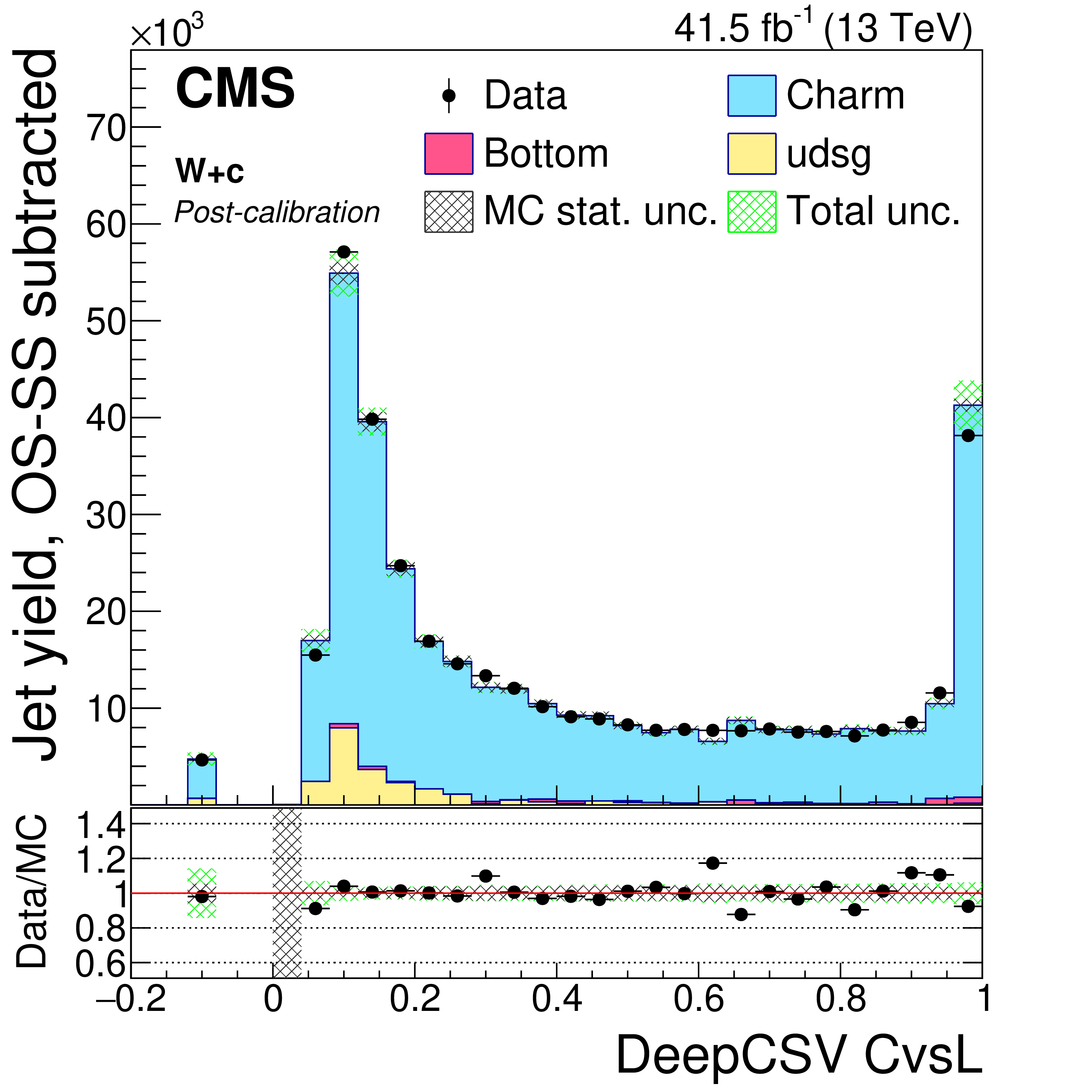
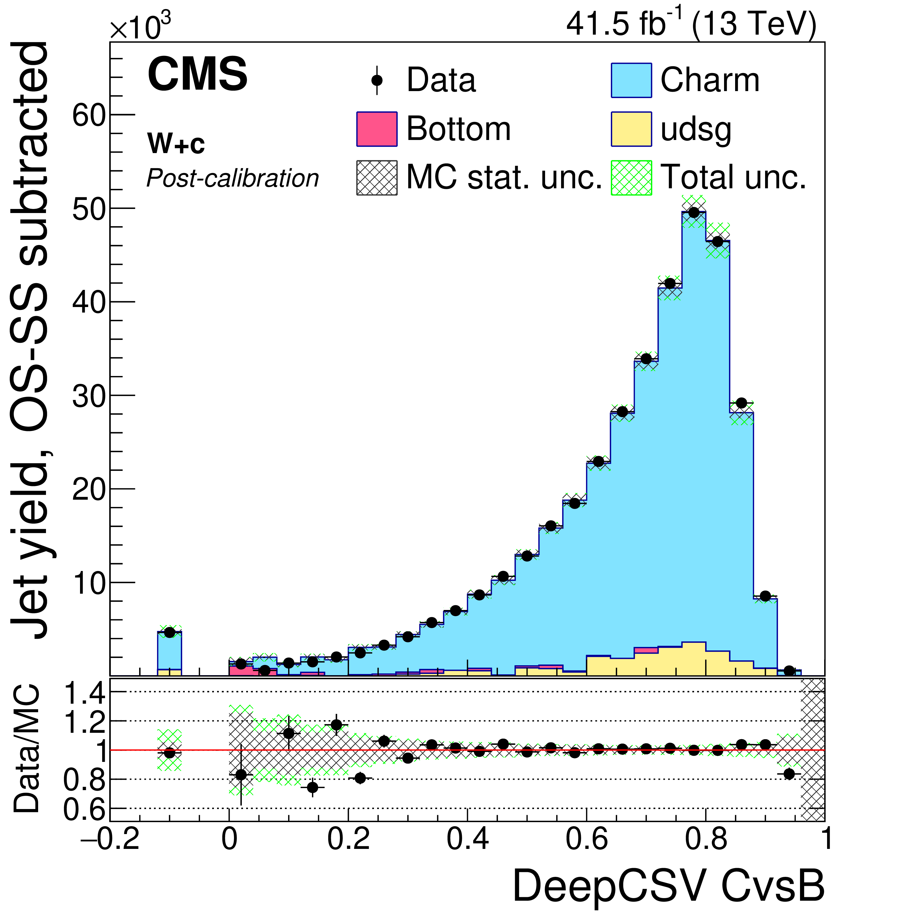
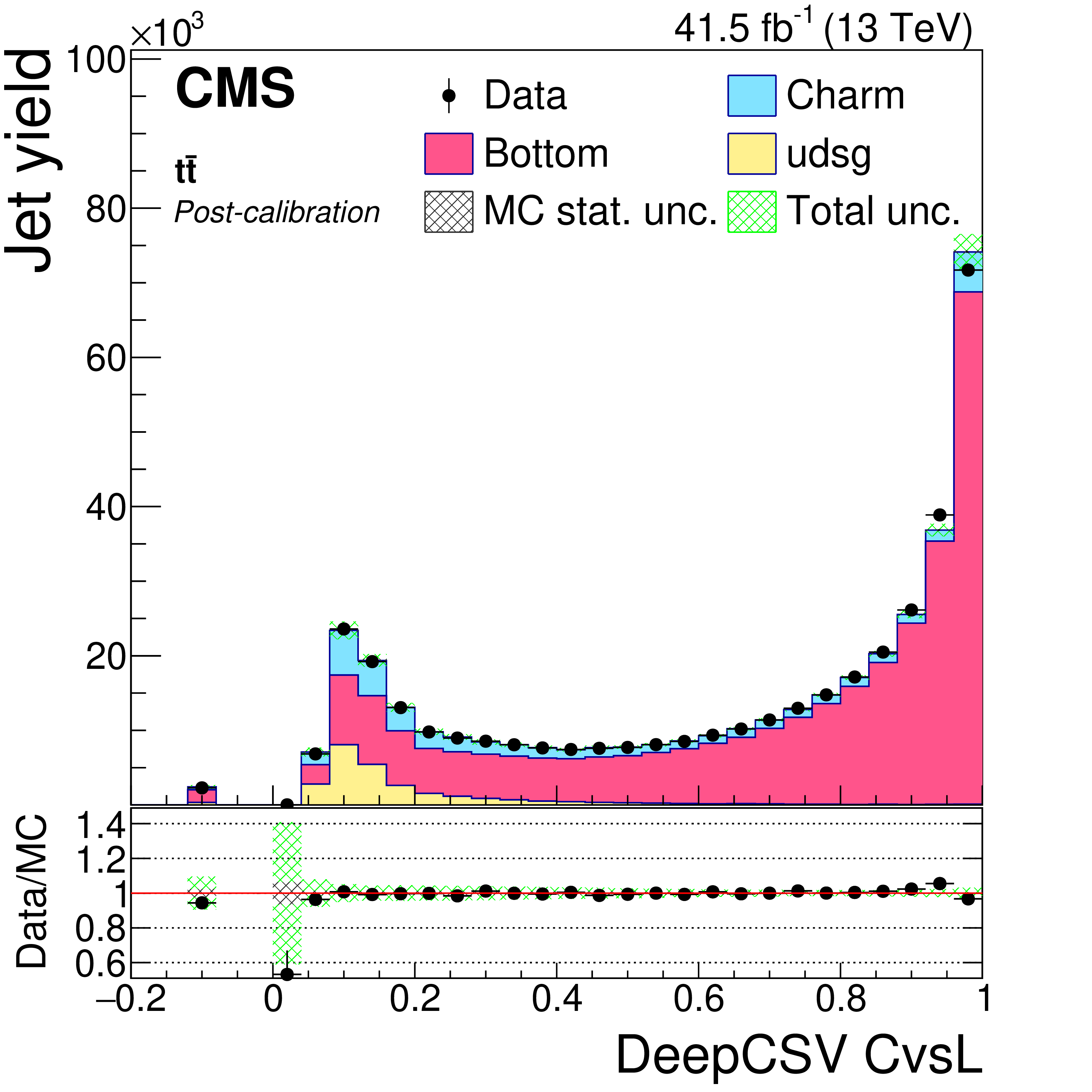
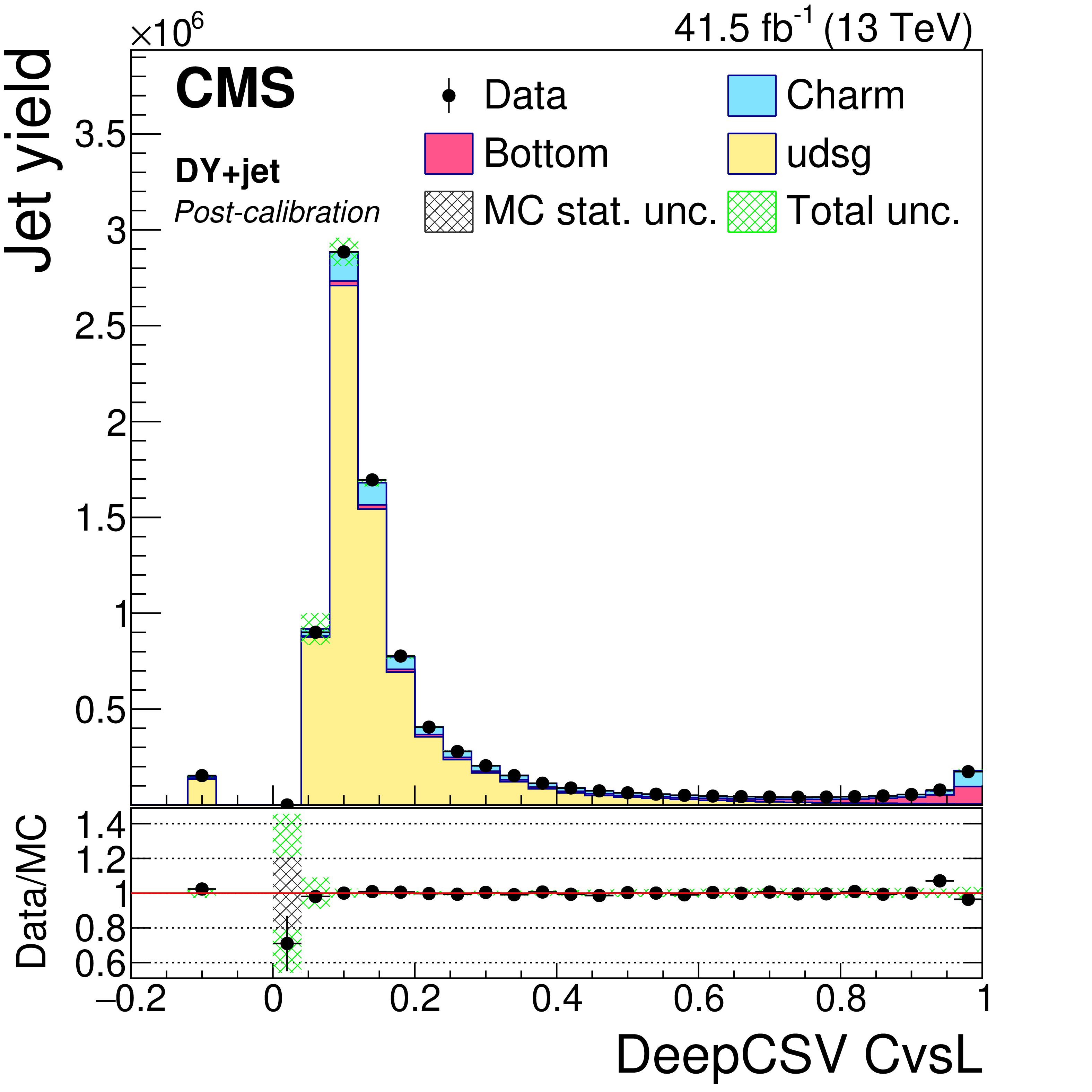
Figure 17:
Post-calibration DeepCSV CvsL (left) and CvsB (right) distributions of jet samples selected from W+c (upper), ${\mathrm{t} \mathrm{\bar{t}}}$ semi- and dileptonic (middle), and DY+jets (lower) events after application of DeepCSV c tagger shape calibration SFs. The bin corresponding to a tagger value of $-1$ is plotted at $-0.1$. Vertical error bars in data represent statistical uncertainties in data. |
png pdf |
Figure 17-a:
Post-calibration DeepCSV CvsL distribution of jet samples selected from W+c events after application of DeepCSV c tagger shape calibration SFs. The bin corresponding to a tagger value of $-1$ is plotted at $-0.1$. Vertical error bars in data represent statistical uncertainties in data. |
png pdf |
Figure 17-b:
Post-calibration DeepCSV CvsB distribution of jet samples selected from W+c events after application of DeepCSV c tagger shape calibration SFs. The bin corresponding to a tagger value of $-1$ is plotted at $-0.1$. Vertical error bars in data represent statistical uncertainties in data. |
png pdf |
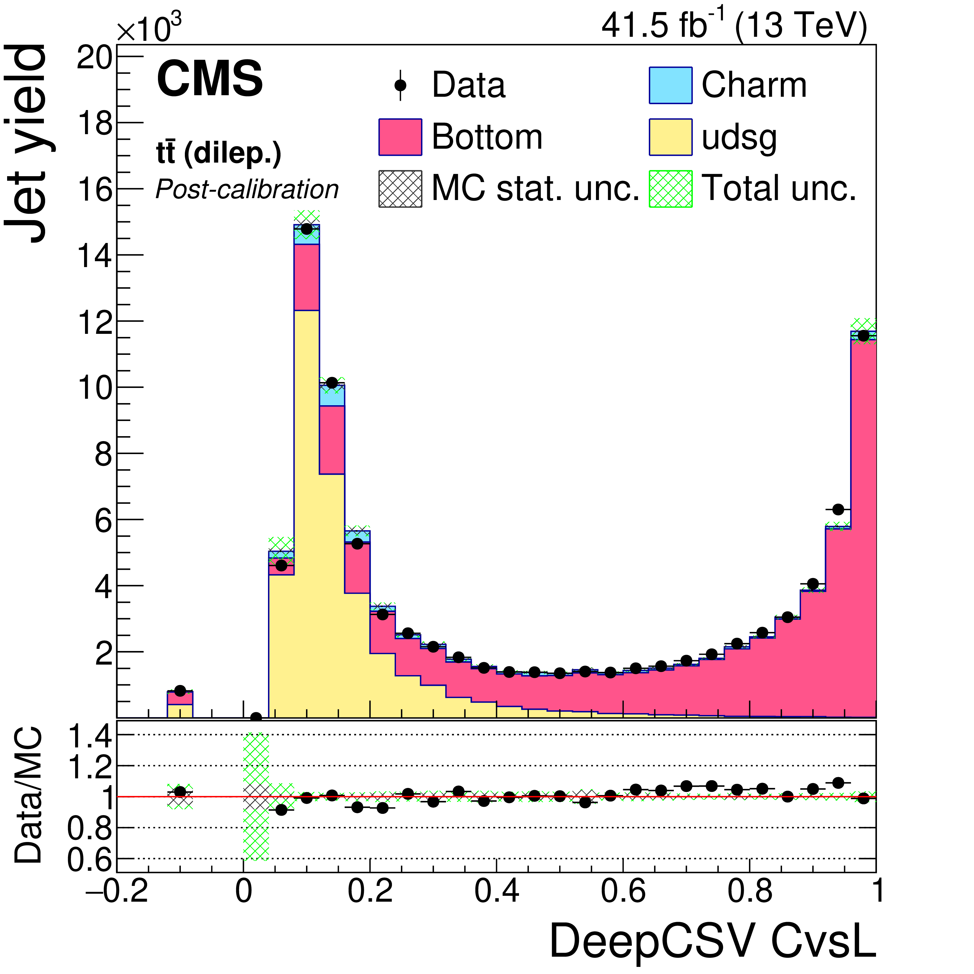
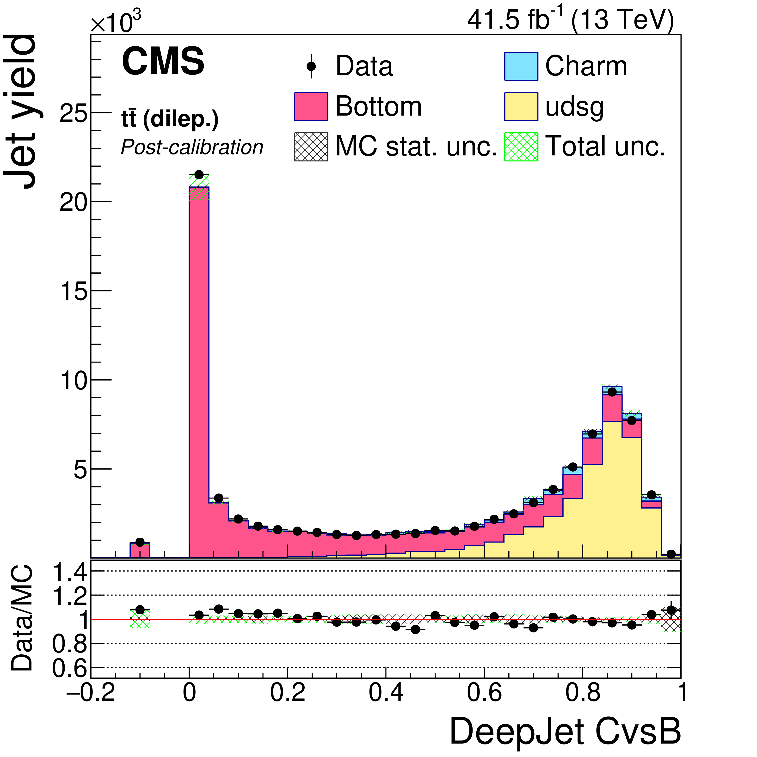
Figure 17-c:
Post-calibration DeepCSV CvsL distribution of jet samples selected from ${\mathrm{t} \mathrm{\bar{t}}}$ semi- and dileptonic events after application of DeepCSV c tagger shape calibration SFs. The bin corresponding to a tagger value of $-1$ is plotted at $-0.1$. Vertical error bars in data represent statistical uncertainties in data. |

png pdf |
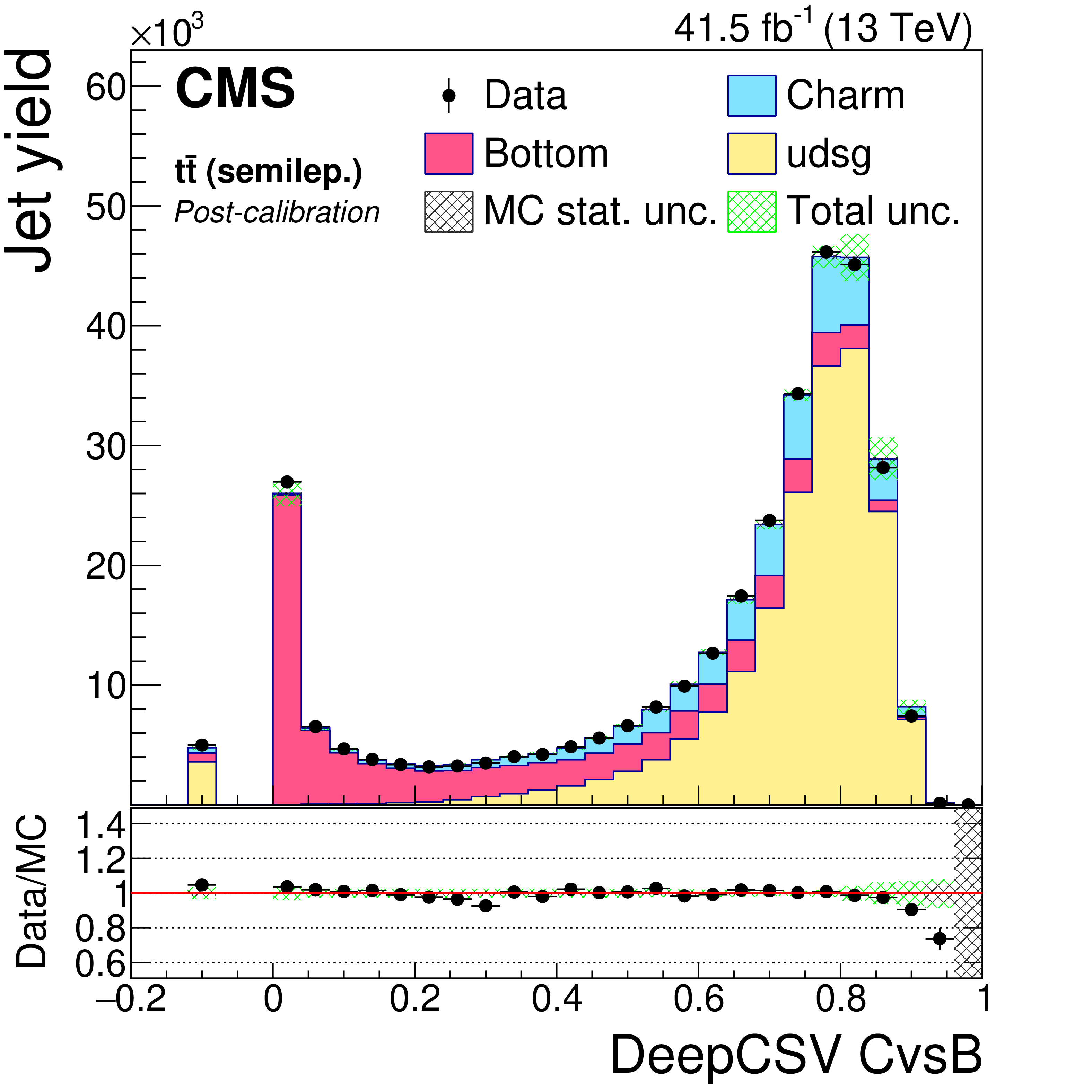
Figure 17-d:
Post-calibration DeepCSV CvsB distribution of jet samples selected from ${\mathrm{t} \mathrm{\bar{t}}}$ semi- and dileptonic events after application of DeepCSV c tagger shape calibration SFs. The bin corresponding to a tagger value of $-1$ is plotted at $-0.1$. Vertical error bars in data represent statistical uncertainties in data. |
png pdf |
Figure 17-e:
Post-calibration DeepCSV CvsL distribution of jet samples selected from DY+jets events after application of DeepCSV c tagger shape calibration SFs. The bin corresponding to a tagger value of $-1$ is plotted at $-0.1$. Vertical error bars in data represent statistical uncertainties in data. |
png pdf |
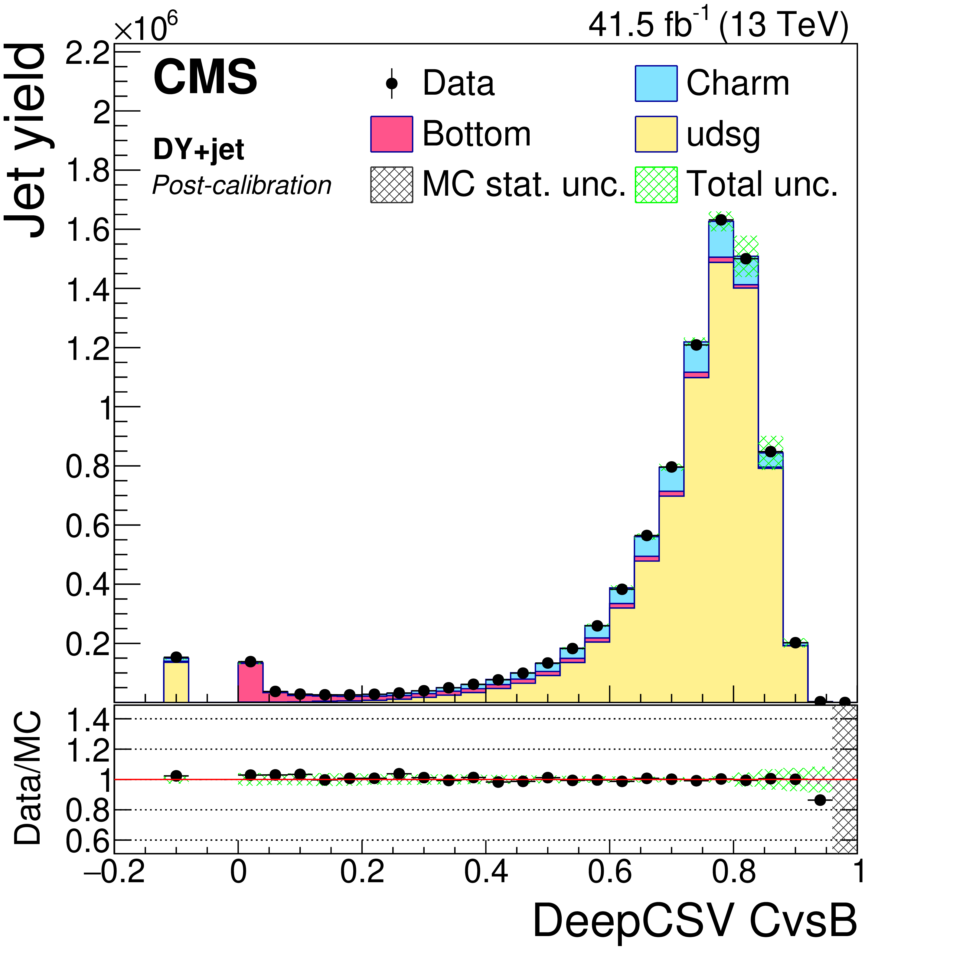
Figure 17-f:
Post-calibration DeepCSV CvsB distribution of jet samples selected from DY+jets events after application of DeepCSV c tagger shape calibration SFs. The bin corresponding to a tagger value of $-1$ is plotted at $-0.1$. Vertical error bars in data represent statistical uncertainties in data. |
png pdf |
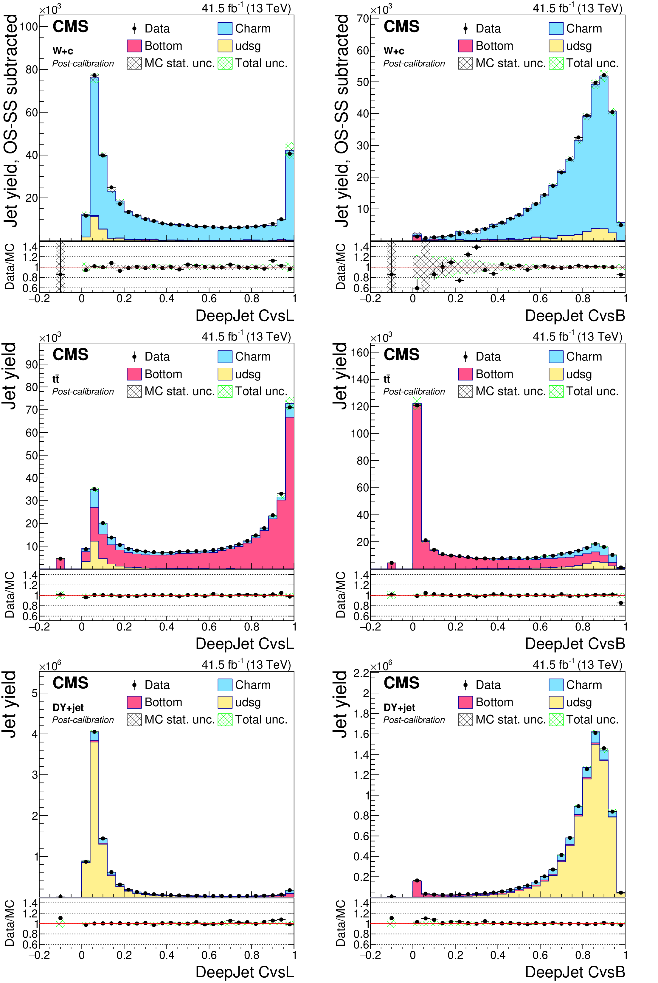
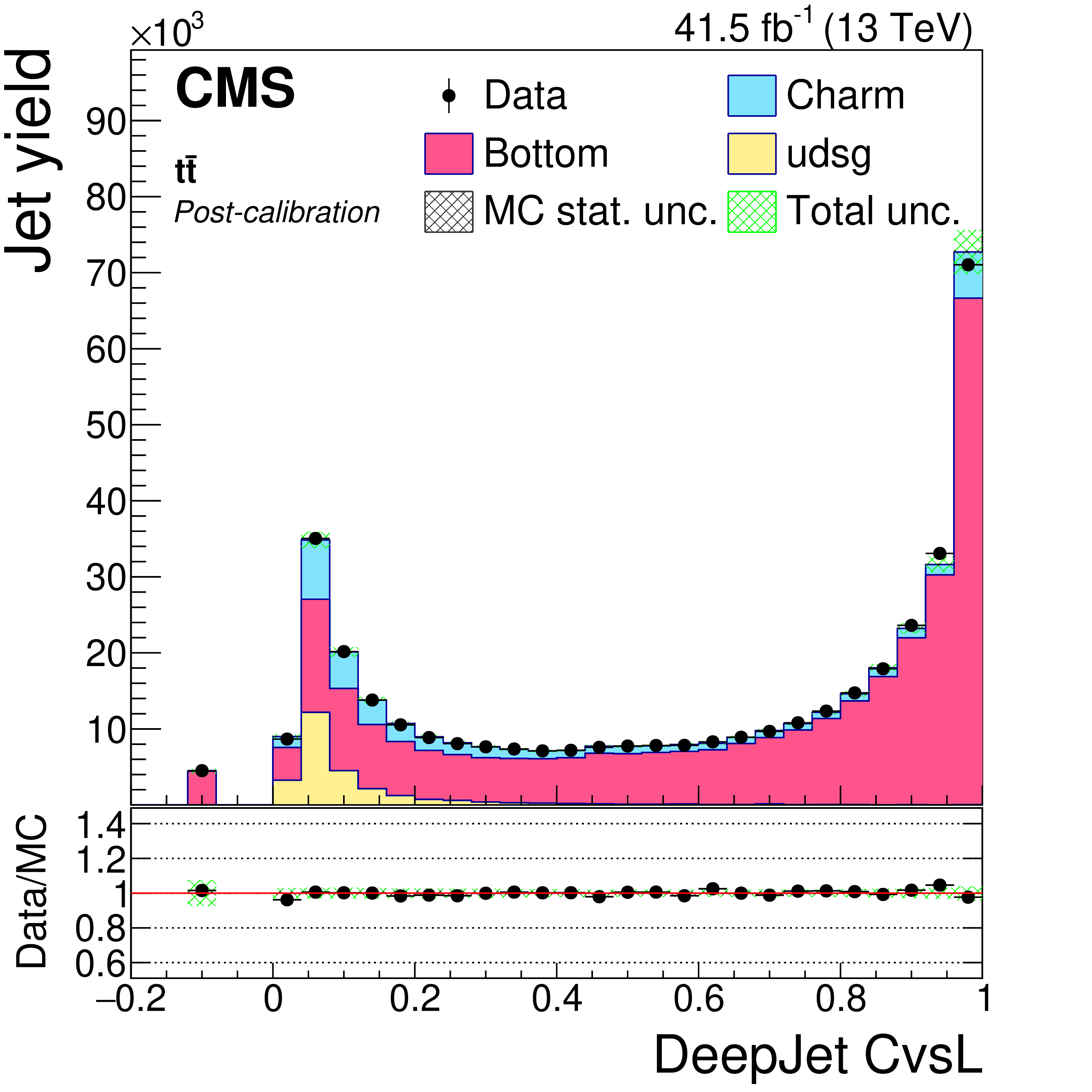
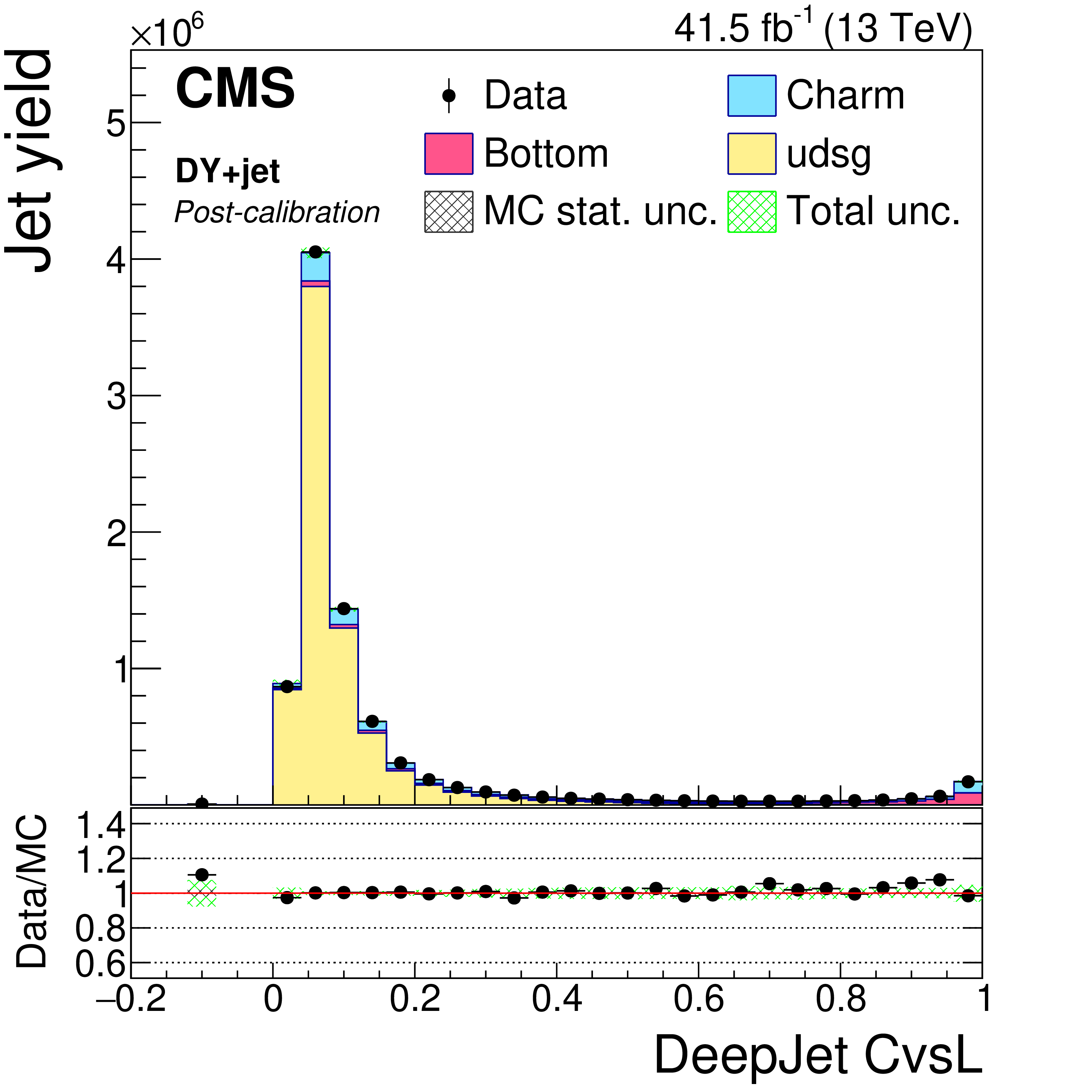
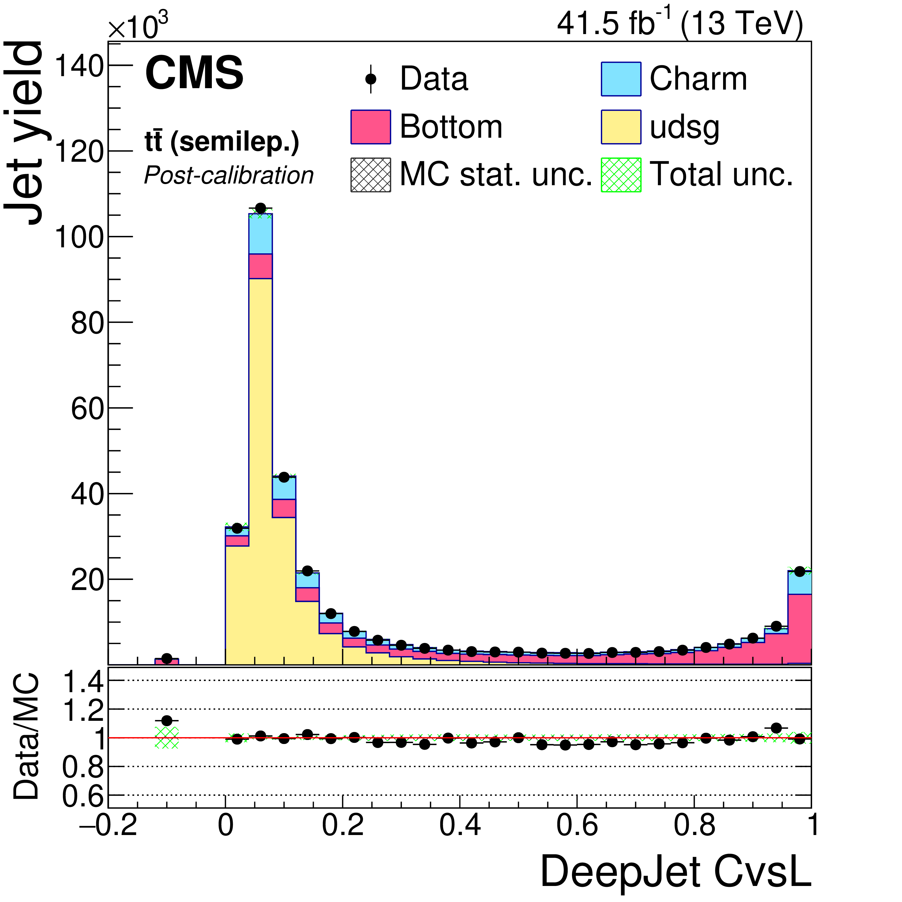
Figure 18:
Post-calibration DeepJet CvsL (left) and CvsB (right) distributions of jet samples selected from W+c (upper), ${\mathrm{t} \mathrm{\bar{t}}}$ semi- and dileptonic (middle), and DY+jets (lower) events after application of DeepJet c tagger shape calibration SFs. The bin corresponding to a tagger value of $-1$ is plotted at $-0.1$. Vertical error bars in data represent statistical uncertainties in data. |
png pdf |
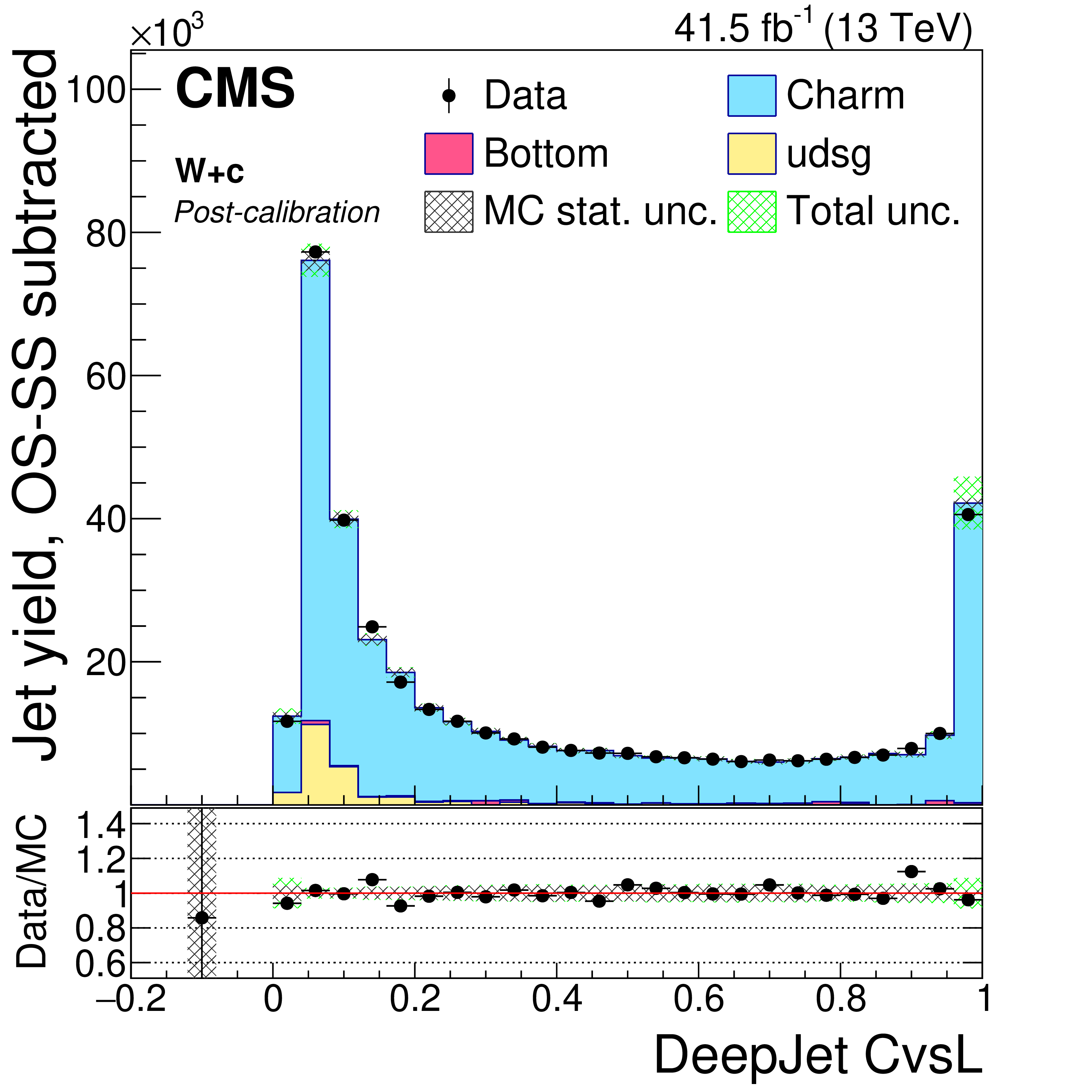
Figure 18-a:
Post-calibration DeepJet CvsL CvsB distribution of jet samples selected from W+c events after application of DeepJet c tagger shape calibration SFs. The bin corresponding to a tagger value of $-1$ is plotted at $-0.1$. Vertical error bars in data represent statistical uncertainties in data. |
png pdf |
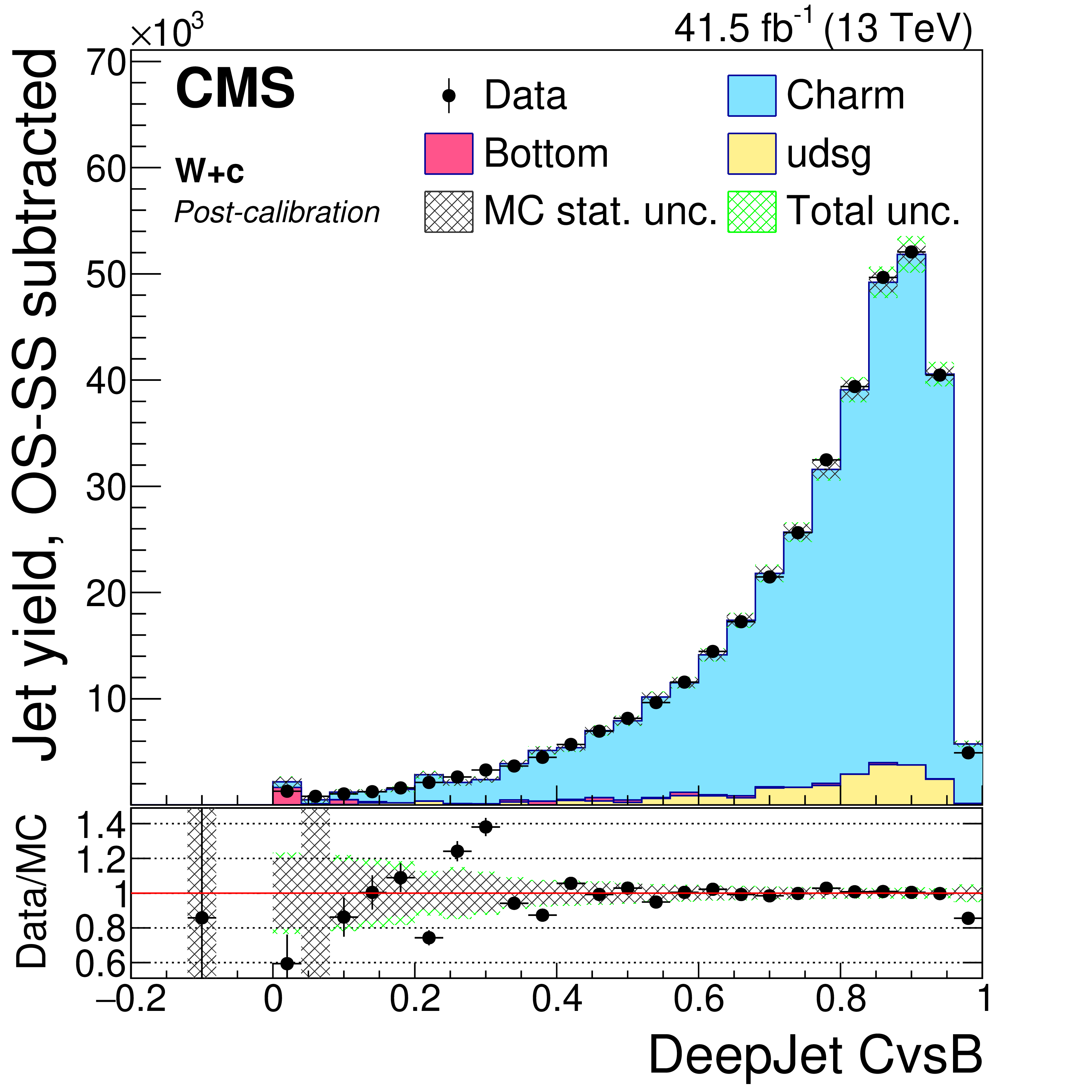
Figure 18-b:
Post-calibration DeepJet CvsL CvsB distribution of jet samples selected from W+c events after application of DeepJet c tagger shape calibration SFs. The bin corresponding to a tagger value of $-1$ is plotted at $-0.1$. Vertical error bars in data represent statistical uncertainties in data. |
png pdf |
Figure 18-c:
Post-calibration DeepJet CvsL CvsB distribution of jet samples selected from ${\mathrm{t} \mathrm{\bar{t}}}$ semi- and dileptonic events after application of DeepJet c tagger shape calibration SFs. The bin corresponding to a tagger value of $-1$ is plotted at $-0.1$. Vertical error bars in data represent statistical uncertainties in data. |

png pdf |
Figure 18-d:
Post-calibration DeepJet CvsL CvsB distribution of jet samples selected from ${\mathrm{t} \mathrm{\bar{t}}}$ semi- and dileptonic events after application of DeepJet c tagger shape calibration SFs. The bin corresponding to a tagger value of $-1$ is plotted at $-0.1$. Vertical error bars in data represent statistical uncertainties in data. |
png pdf |
Figure 18-e:
Post-calibration DeepJet CvsL CvsB distribution of jet samples selected from DY+jets events after application of DeepJet c tagger shape calibration SFs. The bin corresponding to a tagger value of $-1$ is plotted at $-0.1$. Vertical error bars in data represent statistical uncertainties in data. |

png pdf |
Figure 18-f:
Post-calibration DeepJet CvsL CvsB distribution of jet samples selected from DY+jets events after application of DeepJet c tagger shape calibration SFs. The bin corresponding to a tagger value of $-1$ is plotted at $-0.1$. Vertical error bars in data represent statistical uncertainties in data. |
png pdf |
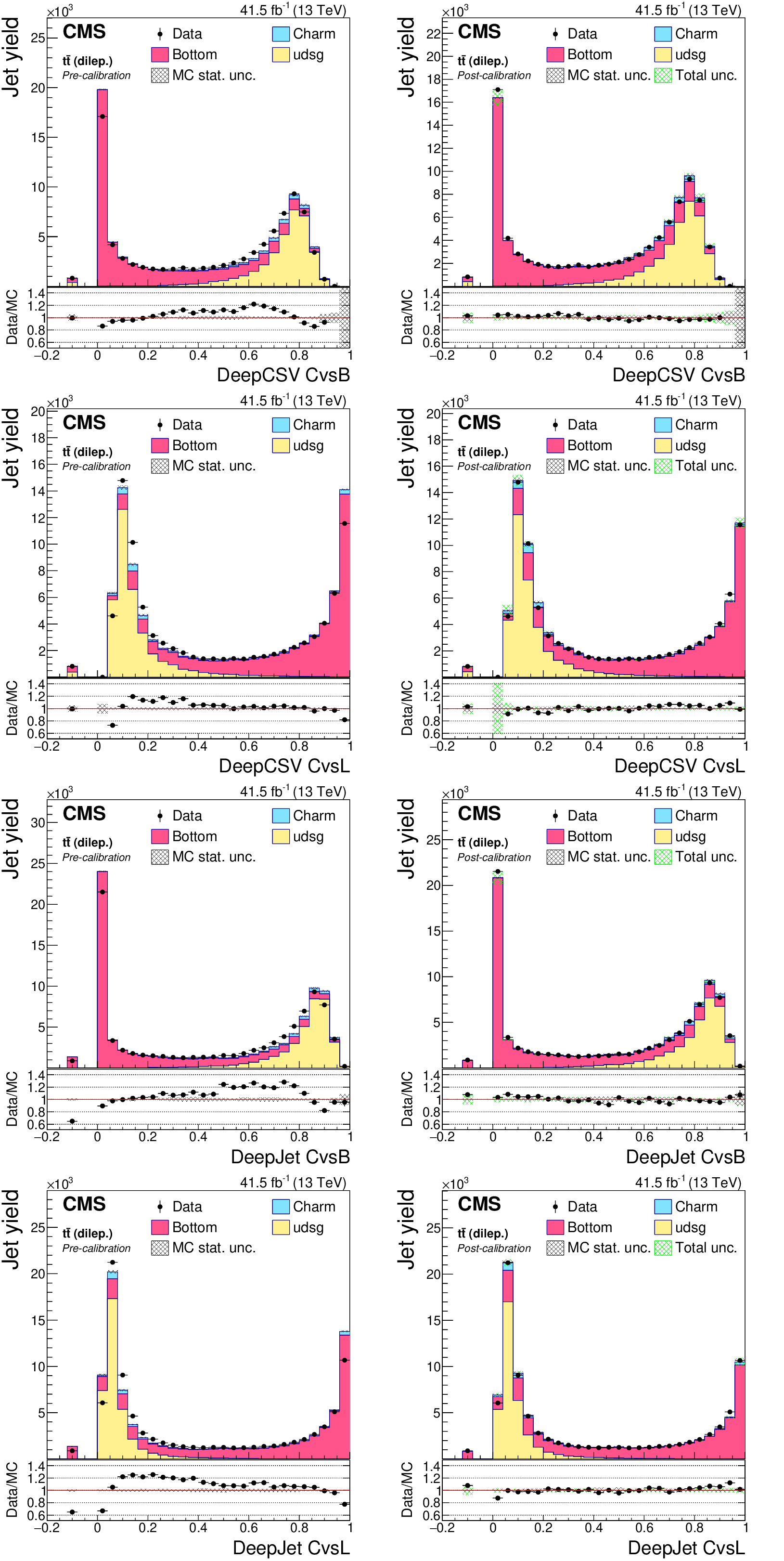
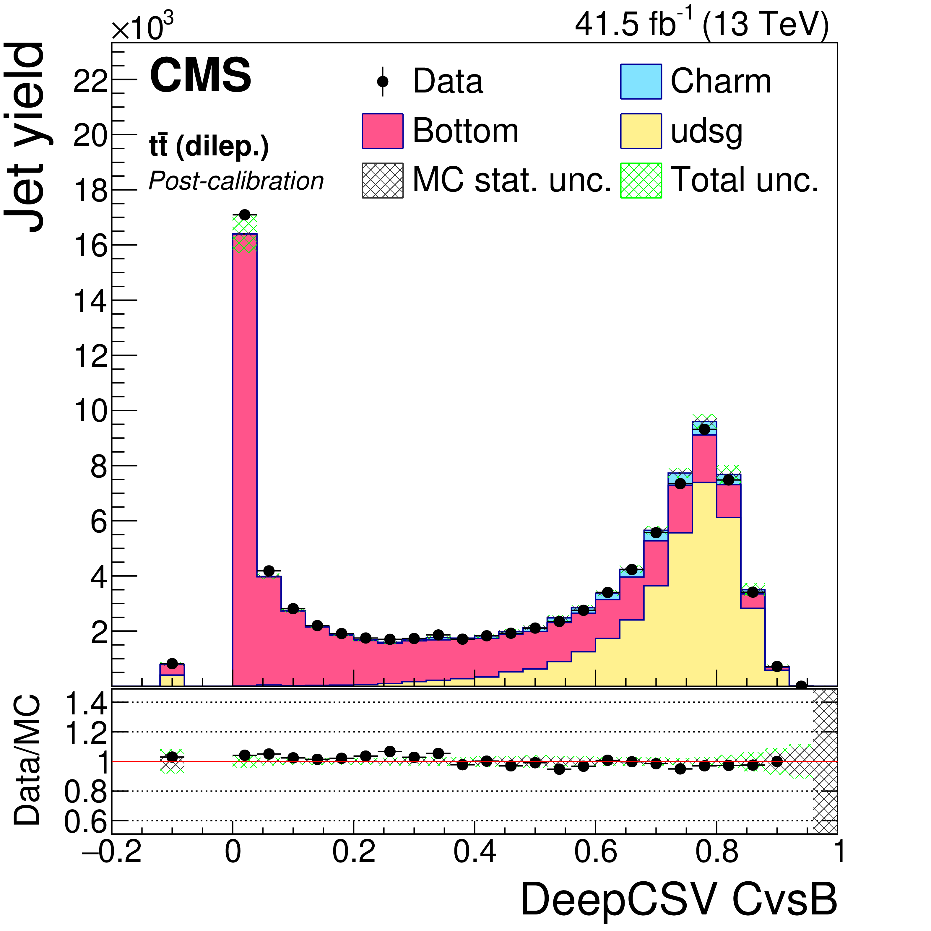
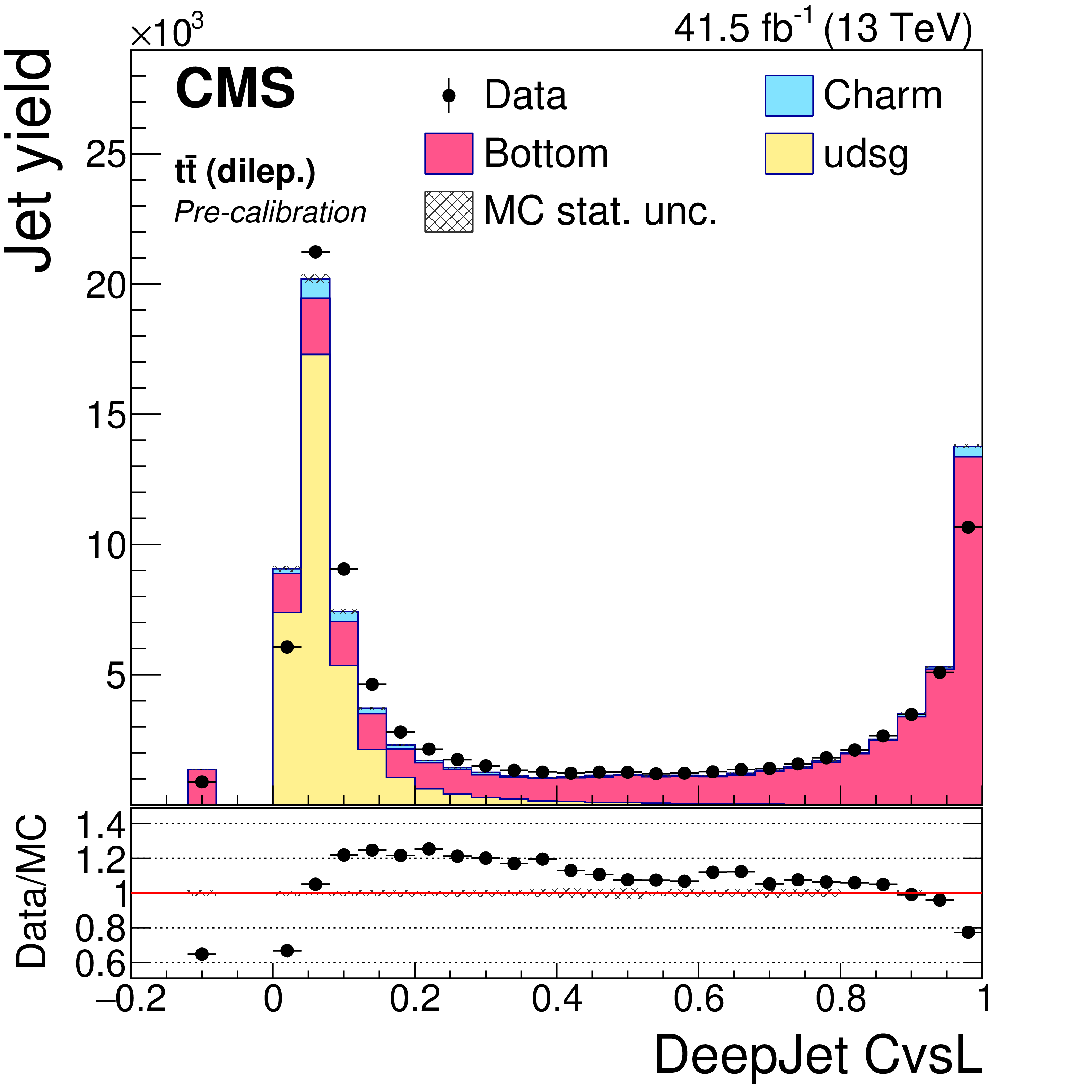
Figure 19:
DeepCSV CvsB (first row), DeepCSV CvsL (second row), DeepJet CvsB (third row) and DeepJet CvsL (fourth row) discriminators of dileptonic ${\mathrm{t} \mathrm{\bar{t}}}$ jets not biased with soft muons, before (left) and after (right) application of SFs. The bin corresponding to a tagger value of $-1$ is plotted at $-0.1$. Vertical error bars in data represent statistical uncertainties in data. |

png pdf |
Figure 19-a:
DeepCSV CvsB discriminator of dileptonic ${\mathrm{t} \mathrm{\bar{t}}}$ jets not biased with soft muons, before application of SFs. The bin corresponding to a tagger value of $-1$ is plotted at $-0.1$. Vertical error bars in data represent statistical uncertainties in data. |
png pdf |
Figure 19-b :
DeepCSV CvsB discriminator of dileptonic ${\mathrm{t} \mathrm{\bar{t}}}$ jets not biased with soft muons, after application of SFs. The bin corresponding to a tagger value of $-1$ is plotted at $-0.1$. Vertical error bars in data represent statistical uncertainties in data. |
png pdf |
Figure 19-c:
DeepCSV CvsL discriminator of dileptonic ${\mathrm{t} \mathrm{\bar{t}}}$ jets not biased with soft muons, before application of SFs. The bin corresponding to a tagger value of $-1$ is plotted at $-0.1$. Vertical error bars in data represent statistical uncertainties in data. |
png pdf |
Figure 19-d:
DeepCSV CvsL discriminator of dileptonic ${\mathrm{t} \mathrm{\bar{t}}}$ jets not biased with soft muons, after application of SFs. The bin corresponding to a tagger value of $-1$ is plotted at $-0.1$. Vertical error bars in data represent statistical uncertainties in data. |
png pdf |
Figure 19-e:
DeepJet CvsB discriminator of dileptonic ${\mathrm{t} \mathrm{\bar{t}}}$ jets not biased with soft muons, before application of SFs. The bin corresponding to a tagger value of $-1$ is plotted at $-0.1$. Vertical error bars in data represent statistical uncertainties in data. |
png pdf |
Figure 19-f:
DeepJet CvsB discriminator of dileptonic ${\mathrm{t} \mathrm{\bar{t}}}$ jets not biased with soft muons, after application of SFs. The bin corresponding to a tagger value of $-1$ is plotted at $-0.1$. Vertical error bars in data represent statistical uncertainties in data. |
png pdf |
Figure 19-g:
DeepJet CvsL discriminator of dileptonic ${\mathrm{t} \mathrm{\bar{t}}}$ jets not biased with soft muons, before application of SFs. The bin corresponding to a tagger value of $-1$ is plotted at $-0.1$. Vertical error bars in data represent statistical uncertainties in data. |
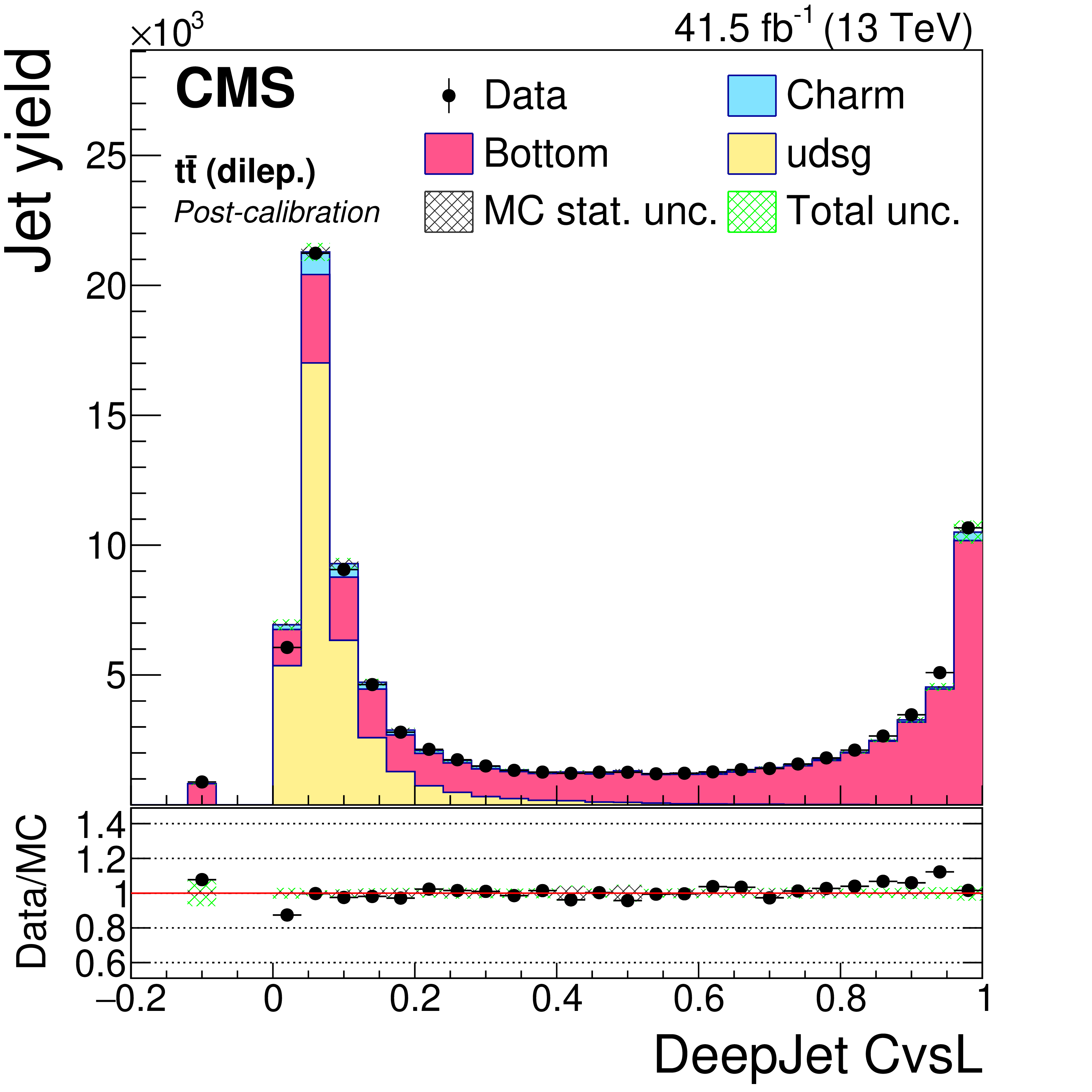
png pdf |
Figure 19-h:
DeepJet CvsL discriminator of dileptonic ${\mathrm{t} \mathrm{\bar{t}}}$ jets not biased with soft muons, after application of SFs. The bin corresponding to a tagger value of $-1$ is plotted at $-0.1$. Vertical error bars in data represent statistical uncertainties in data. |
png pdf |
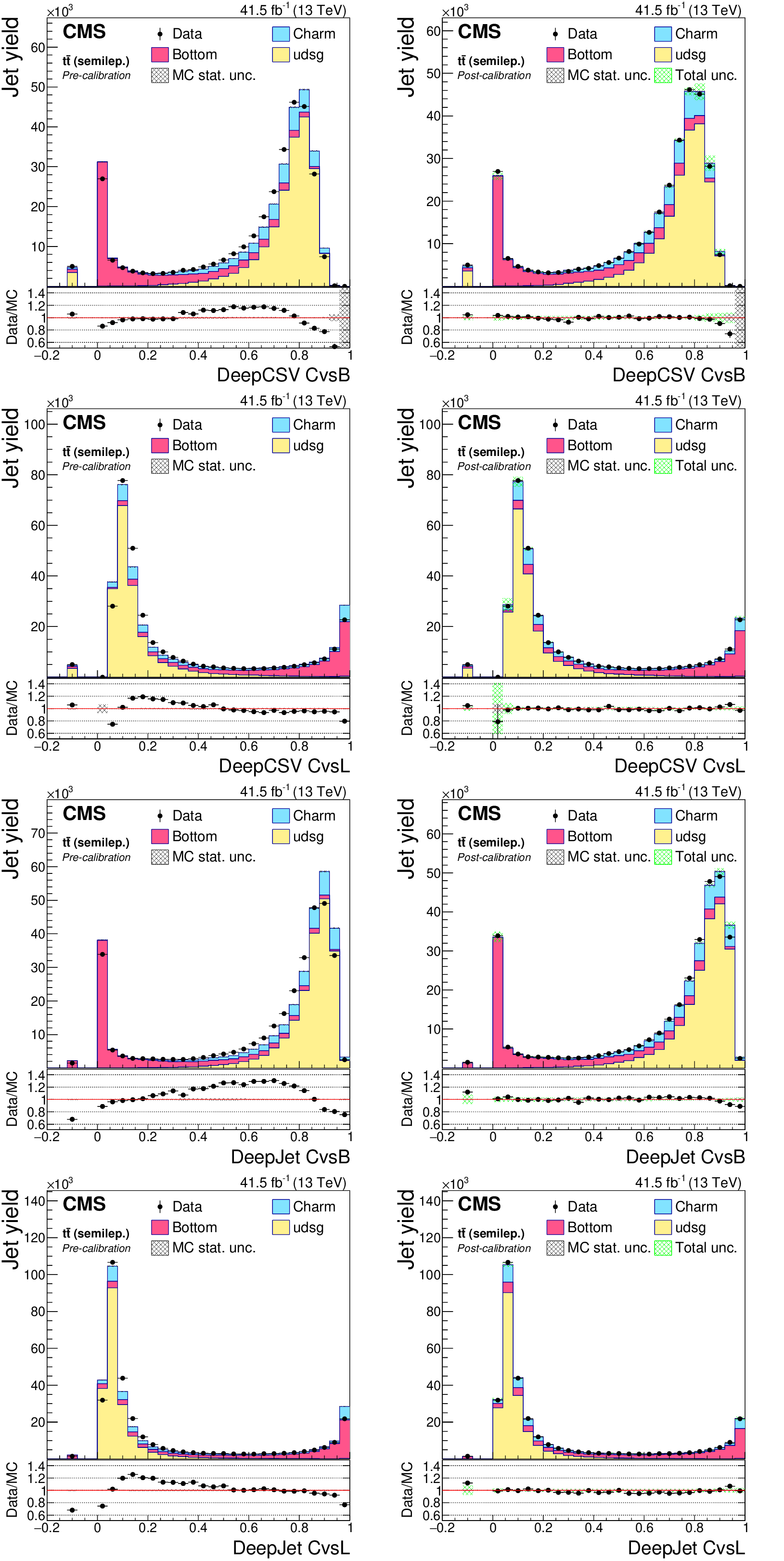
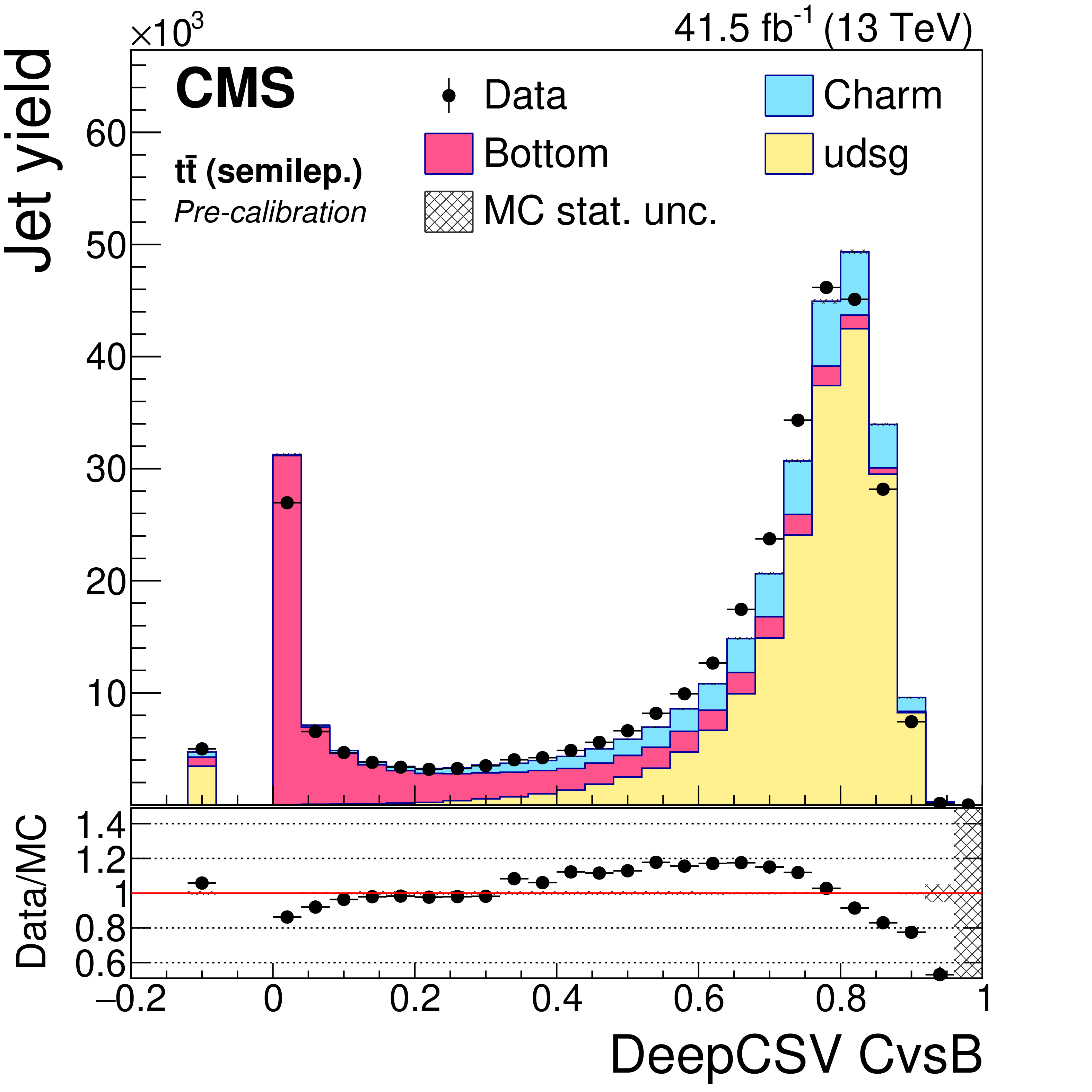
Figure 20:
DeepCSV CvsB (first row), DeepCSV CvsL (second row), DeepJet CvsB (third row) and DeepJet CvsL (last row) discriminators of semileptonic ${\mathrm{t} \mathrm{\bar{t}}}$ jets not biased with soft muons, before (left) and after (right) application of SFs. The bin corresponding to a tagger value of $-1$ is plotted at $-0.1$. Vertical error bars in data represent statistical uncertainties in data. |
png pdf |
Figure 20-a:
DeepCSV CvsB discriminator of semileptonic ${\mathrm{t} \mathrm{\bar{t}}}$ jets not biased with soft muons, before application of SFs. The bin corresponding to a tagger value of $-1$ is plotted at $-0.1$. Vertical error bars in data represent statistical uncertainties in data. |
png pdf |
Figure 20-b:
DeepCSV CvsB discriminator of semileptonic ${\mathrm{t} \mathrm{\bar{t}}}$ jets not biased with soft muons, after application of SFs. The bin corresponding to a tagger value of $-1$ is plotted at $-0.1$. Vertical error bars in data represent statistical uncertainties in data. |
png pdf |
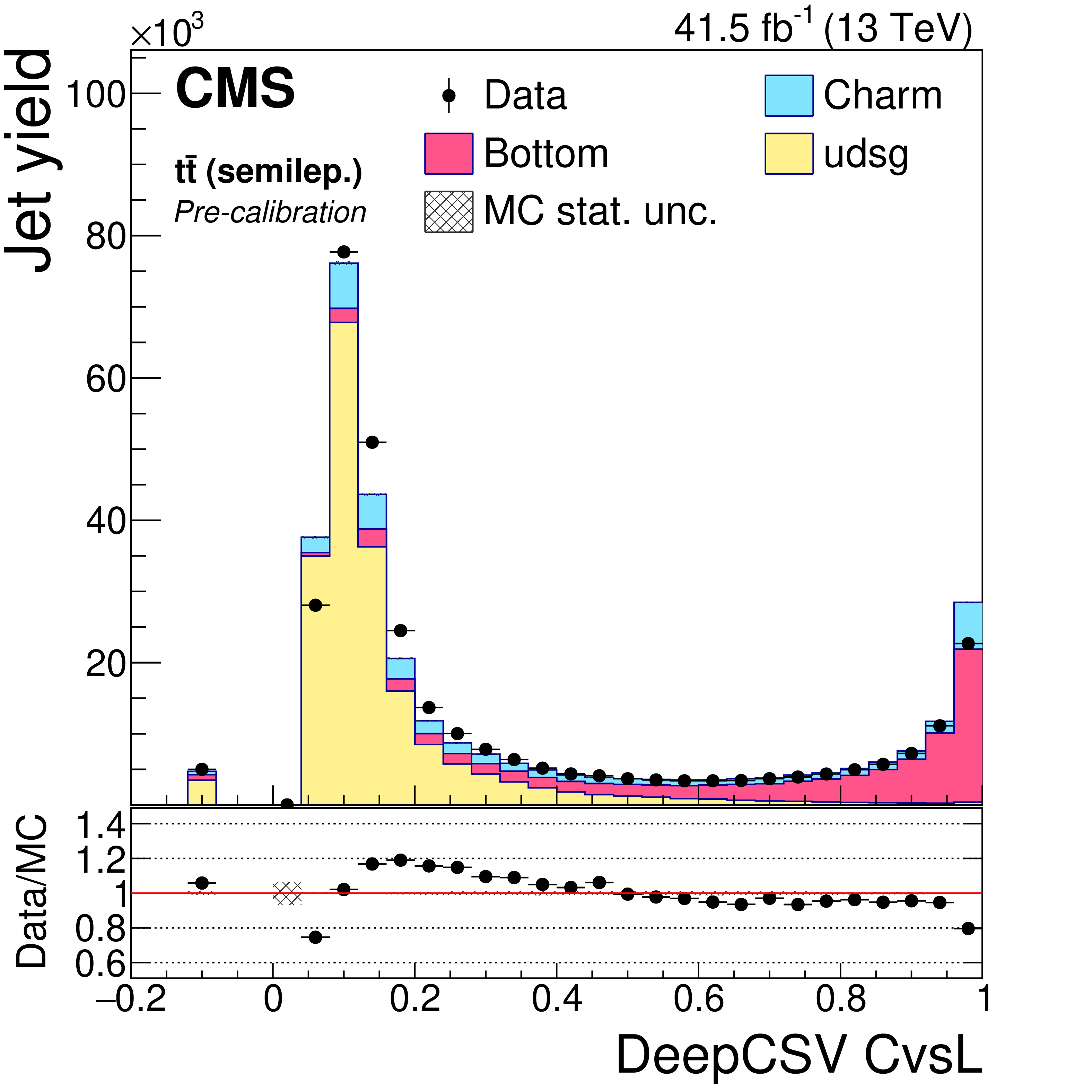
Figure 20-c:
DeepCSV CvsL discriminator of semileptonic ${\mathrm{t} \mathrm{\bar{t}}}$ jets not biased with soft muons, before application of SFs. The bin corresponding to a tagger value of $-1$ is plotted at $-0.1$. Vertical error bars in data represent statistical uncertainties in data. |
png pdf |
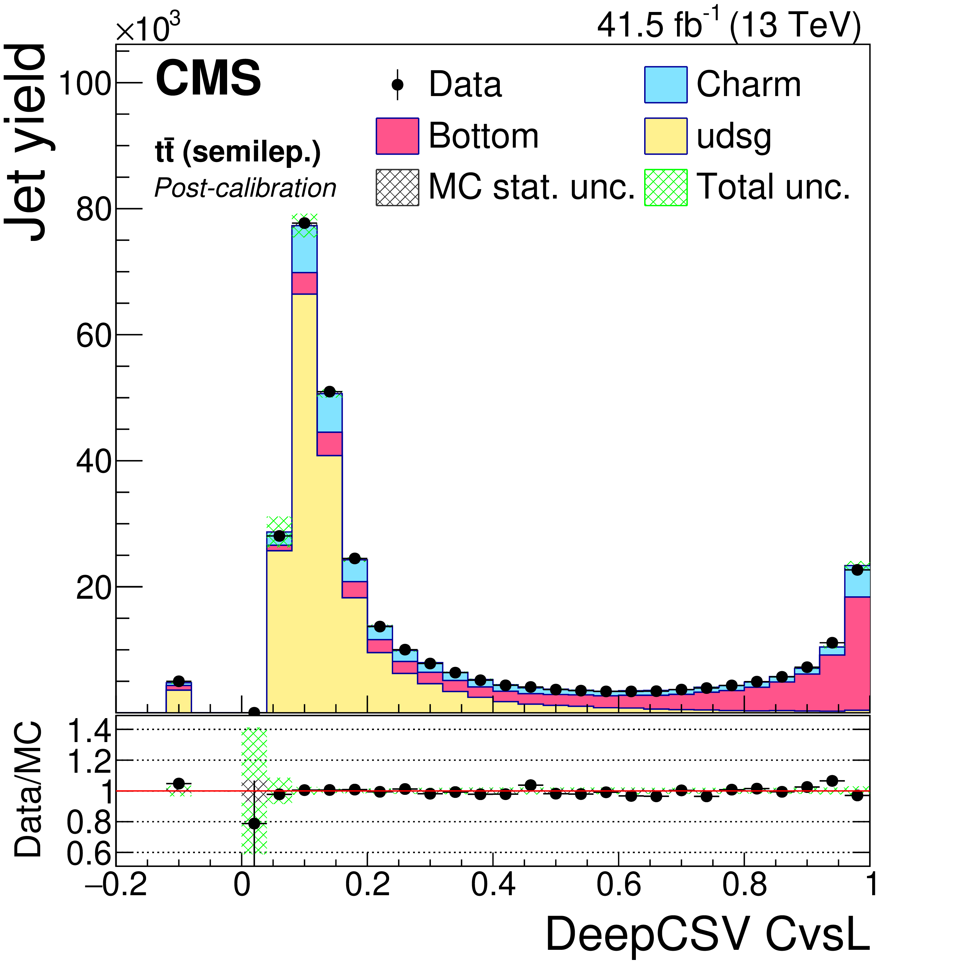
Figure 20-d:
DeepCSV CvsL discriminator of semileptonic ${\mathrm{t} \mathrm{\bar{t}}}$ jets not biased with soft muons, after application of SFs. The bin corresponding to a tagger value of $-1$ is plotted at $-0.1$. Vertical error bars in data represent statistical uncertainties in data. |
png pdf |
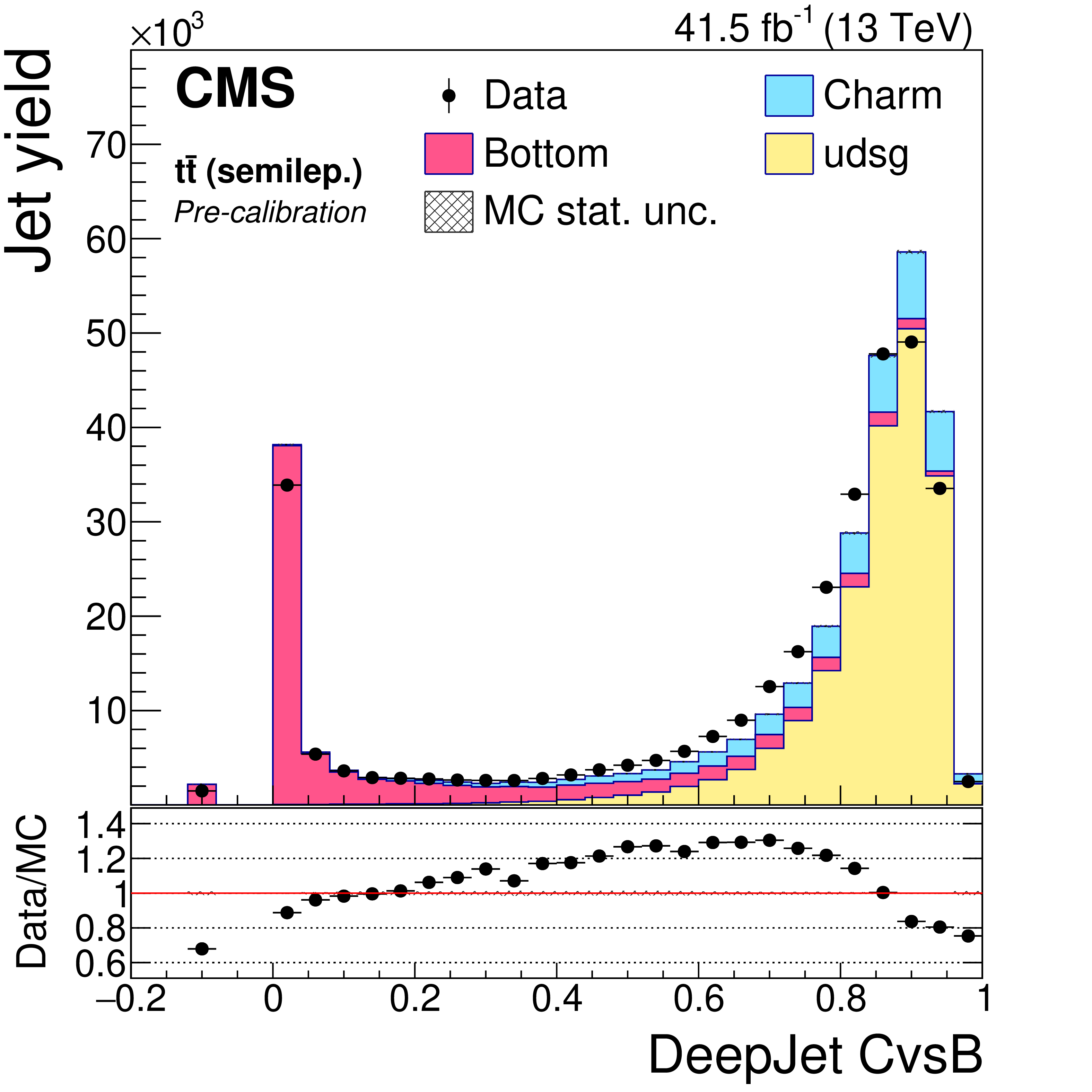
Figure 20-e:
DeepJet CvsB discriminator of semileptonic ${\mathrm{t} \mathrm{\bar{t}}}$ jets not biased with soft muons, before application of SFs. The bin corresponding to a tagger value of $-1$ is plotted at $-0.1$. Vertical error bars in data represent statistical uncertainties in data. |

png pdf |
Figure 20-f:
DeepJet CvsB discriminator of semileptonic ${\mathrm{t} \mathrm{\bar{t}}}$ jets not biased with soft muons, after application of SFs. The bin corresponding to a tagger value of $-1$ is plotted at $-0.1$. Vertical error bars in data represent statistical uncertainties in data. |
png pdf |
Figure 20-g:
DeepJet CvsL discriminator of semileptonic ${\mathrm{t} \mathrm{\bar{t}}}$ jets not biased with soft muons, before application of SFs. The bin corresponding to a tagger value of $-1$ is plotted at $-0.1$. Vertical error bars in data represent statistical uncertainties in data. |
png pdf |
Figure 20-h:
DeepJet CvsL discriminator of semileptonic ${\mathrm{t} \mathrm{\bar{t}}}$ jets not biased with soft muons, after application of SFs. The bin corresponding to a tagger value of $-1$ is plotted at $-0.1$. Vertical error bars in data represent statistical uncertainties in data. |
png pdf |
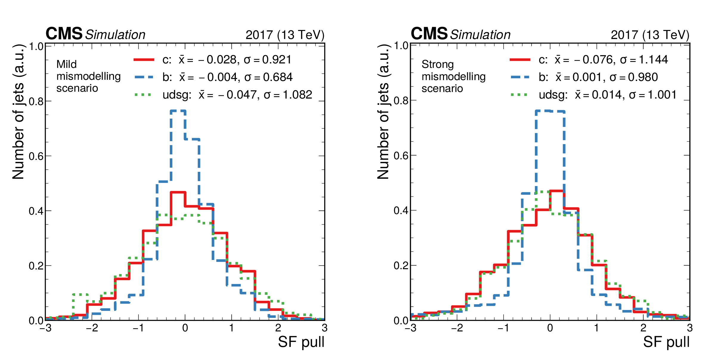
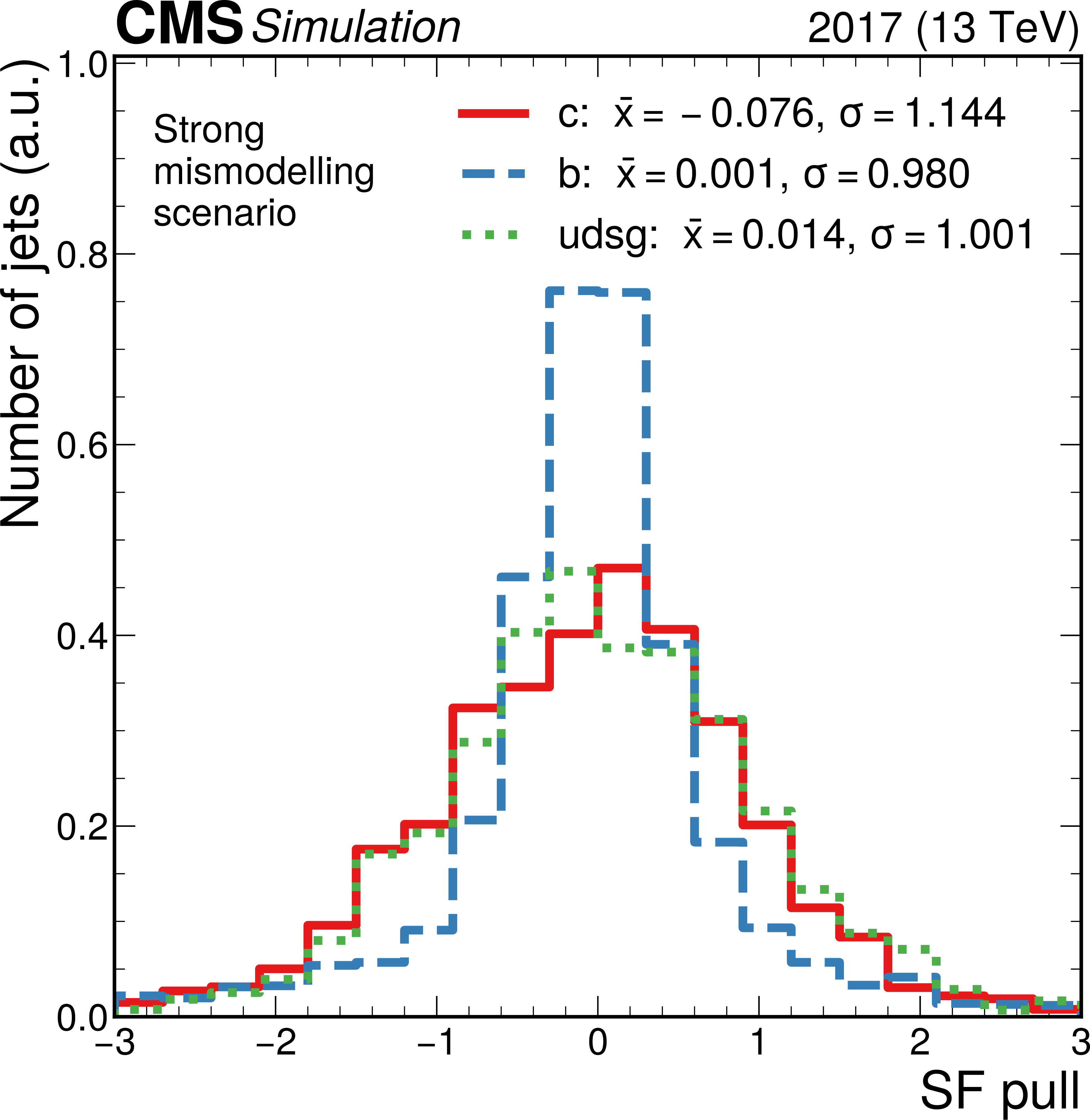
Figure 21:
Distribution of the SF pulls, quantified as the differences between the injected SFs and the SFs retrieved by the fits in units of the statistical uncertainties in the latter ($[\mathrm {SF}_\text {extracted}-\mathrm {SF}_\text {injected}]/\sigma _{\text {extracted}}$), across all bins in the CvsL-CvsB plane, for the SF map with "mild'' (left) and "strong'' (right) SFs. |
png pdf |
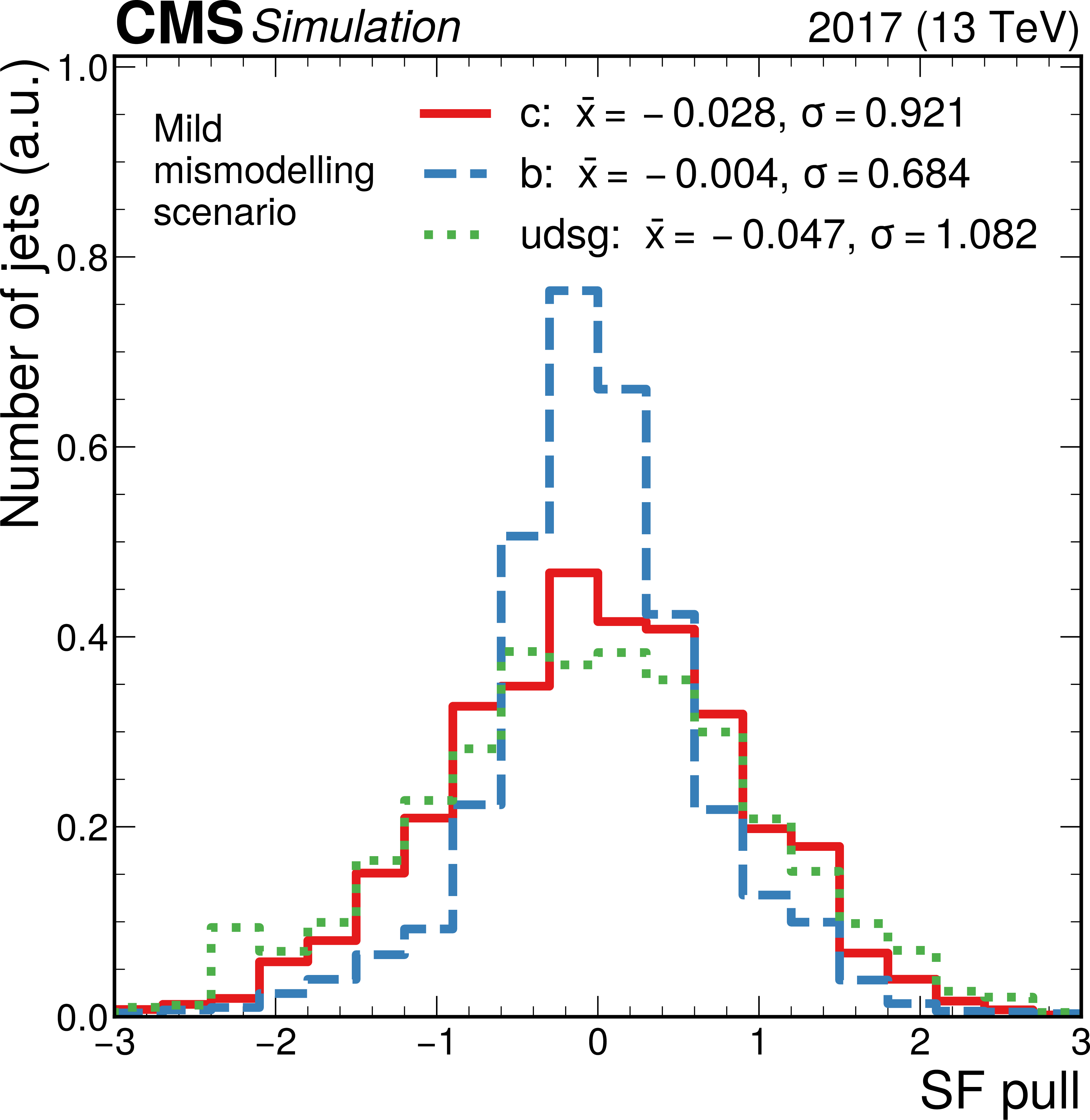
Figure 21-a:
Distribution of the SF pulls, quantified as the differences between the injected SFs and the SFs retrieved by the fits in units of the statistical uncertainties in the latter ($[\mathrm {SF}_\text {extracted}-\mathrm {SF}_\text {injected}]/\sigma _{\text {extracted}}$), across all bins in the CvsL-CvsB plane, for the SF map with "mild'' SFs. |
png pdf |
Figure 21-b:
Distribution of the SF pulls, quantified as the differences between the injected SFs and the SFs retrieved by the fits in units of the statistical uncertainties in the latter ($[\mathrm {SF}_\text {extracted}-\mathrm {SF}_\text {injected}]/\sigma _{\text {extracted}}$), across all bins in the CvsL-CvsB plane, for the SF map with "strong'' SFs. |
| Tables | |
png pdf |
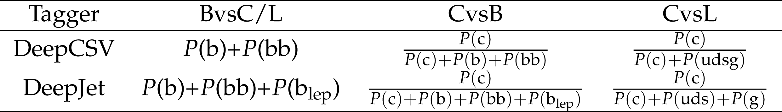
Table 1:
Summary of the heavy-flavour tagging definitions for both b and c tagging using the DeepCSV and DeepJet taggers. $P$(a) represents the probability of having an a-type jet (see text). |
png pdf |
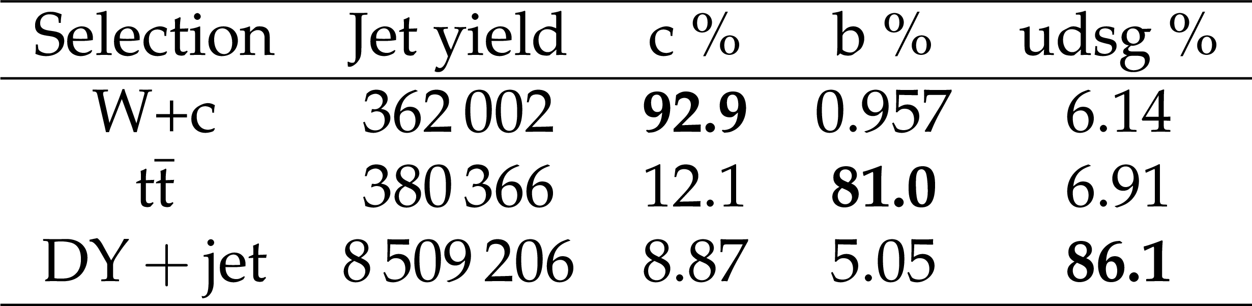
Table 2:
The combined jet yield and contribution of each jet flavour to each selection is shown. The jet yield is reported from data, whereas the per-flavour contribution is determined from simulation. The "purity'' of each selection (row) is highlighted in bold text. |
| Summary |
|
This paper presents a novel method to calibrate the full differential shape of the discriminator distributions used for charm (c) jet identification at CMS. The method uses three different sets of event selection criteria, targeting topologies enriched in W+c, top quark pairs, and Drell-Yan+jet events. These topologies are highly enriched in c, bottom (b) and light-flavour jets, respectively, resulting in purities of a given jet-flavour that range between 81 and 93%. By employing an iterative fitting approach in each of these three regions, scale factors (SFs) are derived to match the simulated discriminator distributions to those observed in data. Since the c tagging algorithm is composed of two discriminators, one to discriminate c from b jets (CvsB) and another to discriminate c from light-flavour and gluon jets (CvsL), the SFs are derived as functions of CvsL and CvsB discriminator values. An adaptive binning is used to optimise the granularity of the provided calibration with respect to the statistical uncertainty in each bin. Finally, an interpolation is performed to obtain more representative corrections over the entire two-dimensional plane. Validation and closure tests confirm the robustness of the method. Although this paper reports calibration results with only 2017 data, similar calibrations are obtained with 2016 and 2018 data separately that are used for the analysis of data collected in the respective years. The calibration of the full differential discriminator shape allows the use of the c tagging discriminators as inputs to multivariate techniques (based on machine learning) or by fitting the discriminator shapes to data to extract observables that are sensitive to the jet flavour. The shape calibration extends the use of c tagging algorithms beyond the application of discrete working points, and facilitates more advanced uses for c jet identification in physics analyses. |
| References | ||||
| 1 | CMS Collaboration | Identification of b-quark jets with the CMS experiment | JINST 8 (2013) P04013 | CMS-BTV-12-001 1211.4462 |
| 2 | CMS Collaboration | Identification of heavy-flavour jets with the CMS detector in pp collisions at 13 TeV | JINST 13 (2018) P05011 | CMS-BTV-16-002 1712.07158 |
| 3 | CMS Collaboration | Identification of c-quark jets at the CMS experiment | CMS-PAS-BTV-16-001 | CMS-PAS-BTV-16-001 |
| 4 | E. Bols et al. | Jet flavour classification using DeepJet | JINST 15 (2020) P12012 | 2008.10519 |
| 5 | CMS Collaboration | Performance of the DeepJet b tagging algorithm using 41.9/fb of data from proton-proton collisions at 13 TeV with Phase 1 CMS detector | CDS | |
| 6 | D. Guest et al. | Jet flavor classification in high-energy physics with deep neural networks | PRD 94 (2016) 112002 | 1607.08633 |
| 7 | CMS Collaboration | Observation of Higgs boson decay to bottom quarks | PRL 121 (2018) 121801 | CMS-HIG-18-016 1808.08242 |
| 8 | S. Moortgat | When charm and beauty adjoin the top. First measurement of the cross section of top quark pair production with additional charm jets with the CMS experiment | PhD thesis, Vrije U., Brussels, May, 2019 CERN-THESIS-2019-051 | |
| 9 | CMS Collaboration | A search for the standard model Higgs boson decaying to charm quarks | JHEP 03 (2020) 131 | CMS-HIG-18-031 1912.01662 |
| 10 | CMS Collaboration | CMS technical design report for the pixel detector upgrade | CDS | |
| 11 | CMS Collaboration | Track impact parameter resolution for the full pseudo rapidity coverage in the 2017 dataset with the CMS Phase-1 pixel detector | CDS | |
| 12 | CMS Collaboration | The CMS experiment at the CERN LHC | JINST 3 (2008) S08004 | CMS-00-001 |
| 13 | CMS Collaboration | The CMS trigger system | JINST 12 (2017) P01020 | CMS-TRG-12-001 1609.02366 |
| 14 | CMS Collaboration | Performance of the CMS Level-1 trigger in proton-proton collisions at $ \sqrt{s} = $ 13 TeV | JINST 15 (2020) P10017 | CMS-TRG-17-001 2006.10165 |
| 15 | CMS Collaboration | CMS luminosity measurement for the 2017 data-taking period at $ \sqrt{s} = $ 13 TeV | ||
| 16 | T. Sjostrand et al. | An introduction to PYTHIA 8.2 | CPC 191 (2015) 159 | 1410.3012 |
| 17 | P. Skands, S. Carrazza, and J. Rojo | Tuning PYTHIA 8.1: the Monash 2013 tune | EPJC 74 (2014) 3024 | 1404.5630 |
| 18 | NNPDF Collaboration | Parton distributions for the LHC Run II | JHEP 04 (2015) 040 | 1410.8849 |
| 19 | P. Nason | A new method for combining NLO QCD with shower Monte Carlo algorithms | JHEP 11 (2004) 040 | hep-ph/0409146 |
| 20 | S. Frixione, P. Nason, and C. Oleari | Matching NLO QCD computations with parton shower simulations: the POWHEG method | JHEP 11 (2007) 070 | 0709.2092 |
| 21 | S. Alioli, P. Nason, C. Oleari, and E. Re | A general framework for implementing NLO calculations in shower Monte Carlo programs: the POWHEG BOX | JHEP 06 (2010) 043 | 1002.2581 |
| 22 | J. M. Campbell, R. K. Ellis, P. Nason, and E. Re | Top-pair production and decay at NLO matched with parton showers | JHEP 04 (2015) 114 | 1412.1828 |
| 23 | J. Alwall et al. | The automated computation of tree-level and next-to-leading order differential cross sections, and their matching to parton shower simulations | JHEP 07 (2014) 079 | 1405.0301 |
| 24 | J. Alwall et al. | Comparative study of various algorithms for the merging of parton showers and matrix elements in hadronic collisions | EPJC 53 (2008) 473 | 0706.2569 |
| 25 | Y. Li and F. Petriello | Combining QCD and electroweak corrections to dilepton production in FEWZ | PRD 86 (2012) 094034 | 1208.5967 |
| 26 | S. Frixione et al. | Single-top hadroproduction in association with a W boson | JHEP 07 (2008) 029 | 0805.3067 |
| 27 | E. Re | Single-top Wt-channel production matched with parton showers using the POWHEG method | EPJC 71 (2011) 1547 | 1009.2450 |
| 28 | N. Kidonakis | NNLL threshold resummation for top-pair and single-top production | Phys. Part. Nucl. 45 (2014) 714 | 1210.7813 |
| 29 | J. M. Campbell and R. K. Ellis | MCFM for the Tevatron and the LHC | NPPS 205-206 (2010) 10 | 1007.3492 |
| 30 | T. Gehrmann et al. | W$ ^+ $W$ ^- $ production at hadron colliders in next to next to leading order QCD | PRL 113 (2014) 212001 | 1408.5243 |
| 31 | GEANT4 Collaboration | GEANT4---a simulation toolkit | NIMA 506 (2003) 250 | |
| 32 | CMS Collaboration | Particle-flow reconstruction and global event description with the CMS detector | JINST 12 (2017) P10003 | CMS-PRF-14-001 1706.04965 |
| 33 | CMS Collaboration | Performance of missing transverse momentum reconstruction in proton-proton collisions at $ \sqrt{s} = $ 13 TeV using the CMS detector | JINST 14 (2019) P07004 | CMS-JME-17-001 1903.06078 |
| 34 | M. Cacciari, G. P. Salam, and G. Soyez | The anti-$ {k_{\mathrm{T}}} $ jet clustering algorithm | JHEP 04 (2008) 063 | 0802.1189 |
| 35 | M. Cacciari, G. P. Salam, and G. Soyez | FastJet user manual | EPJC 72 (2012) 1896 | 1111.6097 |
| 36 | CMS Collaboration | Jet energy scale and resolution in the CMS experiment in pp collisions at 8 TeV | JINST 12 (2017) P02014 | CMS-JME-13-004 1607.03663 |
| 37 | CMS Collaboration | Pileup mitigation at CMS in 13 TeV data | JINST 15 (2020) P09018 | CMS-JME-18-001 2003.00503 |
| 38 | M. Cacciari and G. P. Salam | Pileup subtraction using jet areas | PLB 659 (2008) 119 | 0707.1378 |
| 39 | CMS Collaboration | Measurement of $ {\text{B}}\overline{\text{B}} $ angular correlations based on secondary vertex reconstruction at $ \sqrt{s}= $ 7 TeV | JHEP 03 (2011) 136 | CMS-BPH-10-010 1102.3194 |
| 40 | CMS Collaboration | Measurement of associated production of a W boson and a charm quark in proton-proton collisions at $ \sqrt{s} = $ 13 TeV | EPJC 79 (2019) 269 | CMS-SMP-17-014 1811.10021 |
| 41 | CMS Collaboration | Electron and photon reconstruction and identification with the CMS experiment at the CERN LHC | JINST 16 (2021) P05014 | CMS-EGM-17-001 2012.06888 |
| 42 | P. Virtanen et al. | SciPy 1.0: Fundamental algorithms for scientific computing in Python | Nature Methods 17 (2020) 261 | |
| 43 | C. B. Barber, D. P. Dobkin, and H. Huhdanpaa | The quickhull algorithm for convex hulls | ACM Trans. Math. Softw 22 (1996) 469 | |
| 44 | P. Bézier | Numerical control: mathematics and applications | Wiley, London | |
| 45 | R. Clough and J. Tocher | Finite element stiffness matricess for analysis of plate bending | in Proc. of the First Conf. on Matrix Methods in Struct. Mech. (1965) | |
| 46 | G. M. Nielson | A method for interpolating scattered data based upon a minimum norm network | Math. Comput. 40 (1983) 253 | |
| 47 | R. J. Renka and A. K. Cline | A triangle-based $ C^1 $ interpolation method | Rocky Mountain J. Math. 14 (1984) 223 | |
| 48 | CMS Collaboration | Performance of the CMS muon detector and muon reconstruction with proton-proton collisions at $ \sqrt{s}= $ 13 TeV | JINST 13 (2018) P06015 | CMS-MUO-16-001 1804.04528 |
| 49 | CMS Collaboration | Performance of the reconstruction and identification of high-momentum muons in proton-proton collisions at $ \sqrt{s} = $ 13 TeV | JINST 15 (2020) P02027 | CMS-MUO-17-001 1912.03516 |
| 50 | CMS Collaboration | Measurement of the inelastic proton-proton cross section at $\sqrt{s}= $ 13 TeV | JHEP 07 (2018) 161 | CMS-FSQ-15-005 1802.02613 |
| 51 | M. G. Bowler | e+ e- production of heavy quarks in the string model | Z. Phys. C 11 (1981) 169 | |
| 52 | B. Andersson, G. Gustafson, G. Ingelman, and T. Sjostrand | Parton fragmentation and string dynamics | PR 97 (1983) 31 | |
| 53 | T. Sjostrand | Jet fragmentation of nearby partons | NPB 248 (1984) 469 | |
| 54 | ALEPH Collaboration | Study of the fragmentation of $ \mathrm{b} $ quarks into B mesons at the $ \mathrm{Z} $ peak | PLB 512 (2001) 30 | hep-ex/0106051 |
| 55 | DELPHI Collaboration | A study of the $ \mathrm{b} $ quark fragmentation function with the DELPHI detector at LEP I and an averaged distribution obtained at the $ \mathrm{Z} $ pole | EPJC 71 (2011) 1557 | 1102.4748 |
| 56 | OPAL Collaboration | Inclusive analysis of the $ \mathrm{b} $ quark fragmentation function in $ \mathrm{Z} $ decays at LEP | EPJC 29 (2003) 463 | hep-ex/0210031 |
| 57 | SLD Collaboration | Measurement of the $ \mathrm{b} $ quark fragmentation function in $ {\mathrm{Z^0}} $ decays | PRD 65 (2002) 092006 | hep-ex/0202031 |
| 58 | CMS Collaboration | Measurement of the associated production of a Z boson with charm or bottom quark jets in proton-proton collisions at $ \sqrt{s} = $ 13 TeV | PRD 102 (2020) 032007 | CMS-SMP-19-004 2001.06899 |
| 59 | CMS Collaboration | HEPData record for this measurement | link | |
|
|
Compact Muon Solenoid LHC, CERN |
|

|

|

|

|

|