

Compact Muon Solenoid
LHC, CERN
| CMS-HIG-20-010 ; CERN-EP-2022-117 | ||
| Search for nonresonant Higgs boson pair production in final state with two bottom quarks and two tau leptons in proton-proton collisions at $\sqrt{s} = $ 13 TeV | ||
| CMS Collaboration | ||
| 19 June 2022 | ||
| Phys. Lett. B 842 (2023) 137531 | ||
| Abstract: A search for the nonresonant production of Higgs boson pairs (HH) via gluon-gluon and vector boson fusion processes in final states with two bottom quarks and two tau leptons is presented. The search uses data from proton-proton collisions at a center-of-mass energy of $\sqrt{s} = $ 13 TeV recorded with the CMS detector at the LHC, corresponding to an integrated luminosity of 138 fb$^{-1}$. Events in which at least one tau lepton decays hadronically are considered and multiple machine learning techniques are used to identify and extract the signal. The data are found to be consistent, within uncertainties, with the standard model (SM) predictions. Upper limits on the HH production cross section are set to constrain the parameter space for anomalous Higgs boson couplings. The observed (expected) upper limit at 95% confidence level corresponds to 3.3 (5.2) times the SM prediction for the inclusive HH cross section and to 124 (154) times the SM prediction for the vector boson fusion HH cross section. At 95% confidence level, the Higgs field self-coupling is constrained to be within $-$1.7 and 8.7 times the SM expectation, and the coupling of two Higgs bosons to two vector bosons is constrained to be within $-$0.4 and 2.6 times the SM expectation. | ||
| Links: e-print arXiv:2206.09401 [hep-ex] (PDF) ; CDS record ; inSPIRE record ; HepData record ; CADI line (restricted) ; | ||
| Figures | |
png pdf |
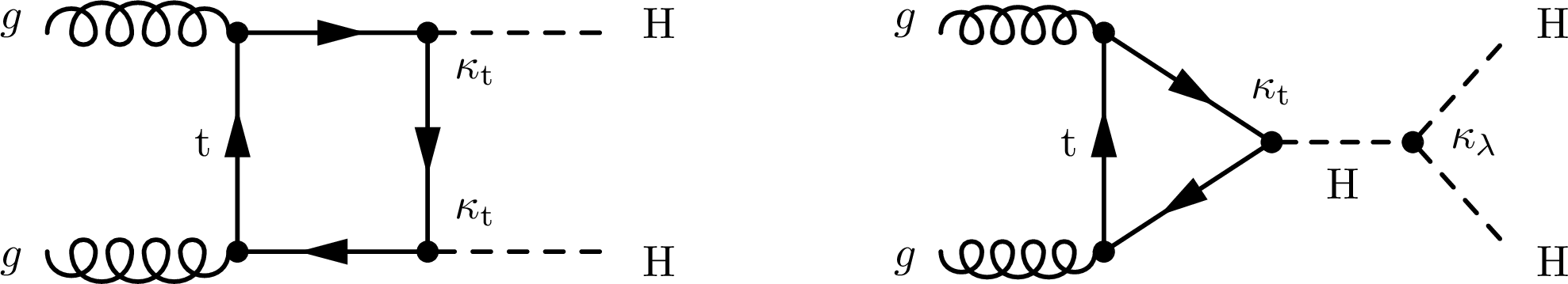
Figure 1:
Feynman diagrams contributing to HH production via gluon-gluon fusion in the SM at leading order. The different H interactions are labelled by the coupling modifiers $\kappa $. |
png pdf |
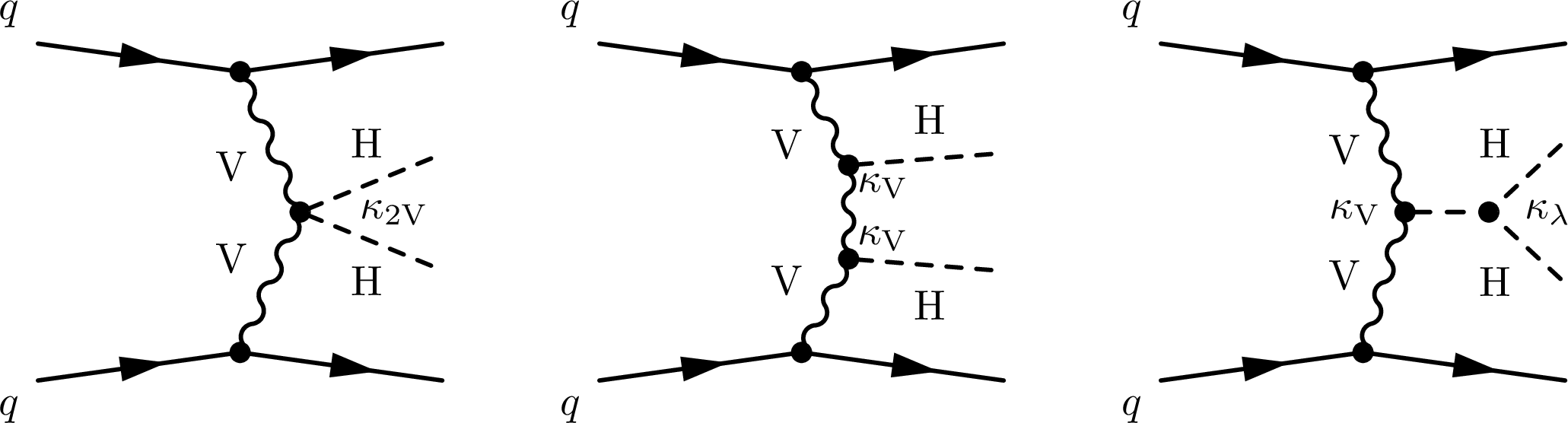
Figure 2:
Feynman diagrams contributing to Higgs boson pair production via vector boson fusion in the SM at leading order. The different H interactions are labelled with the coupling modifiers $\kappa $. |

png pdf |
Figure 3:
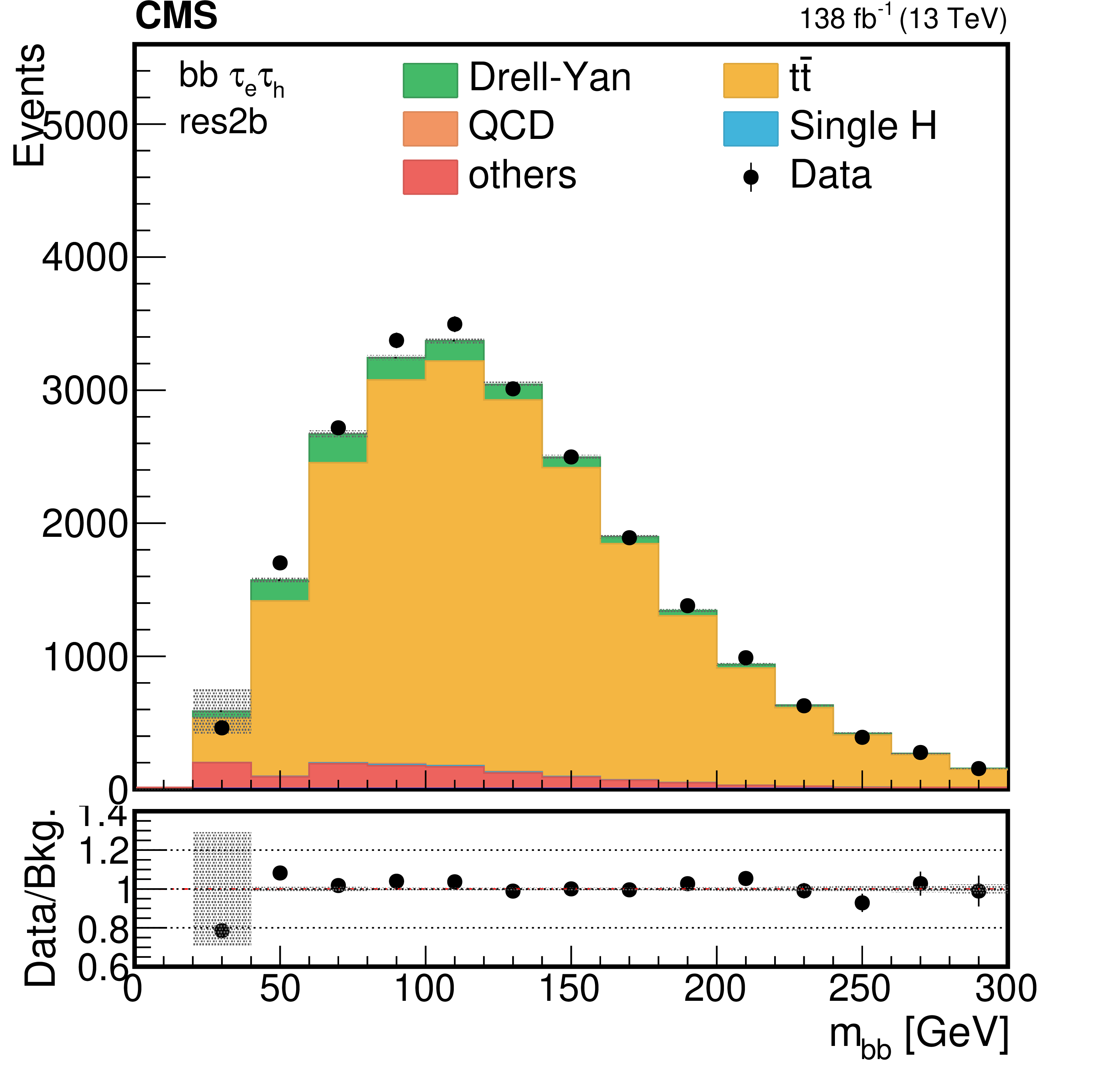
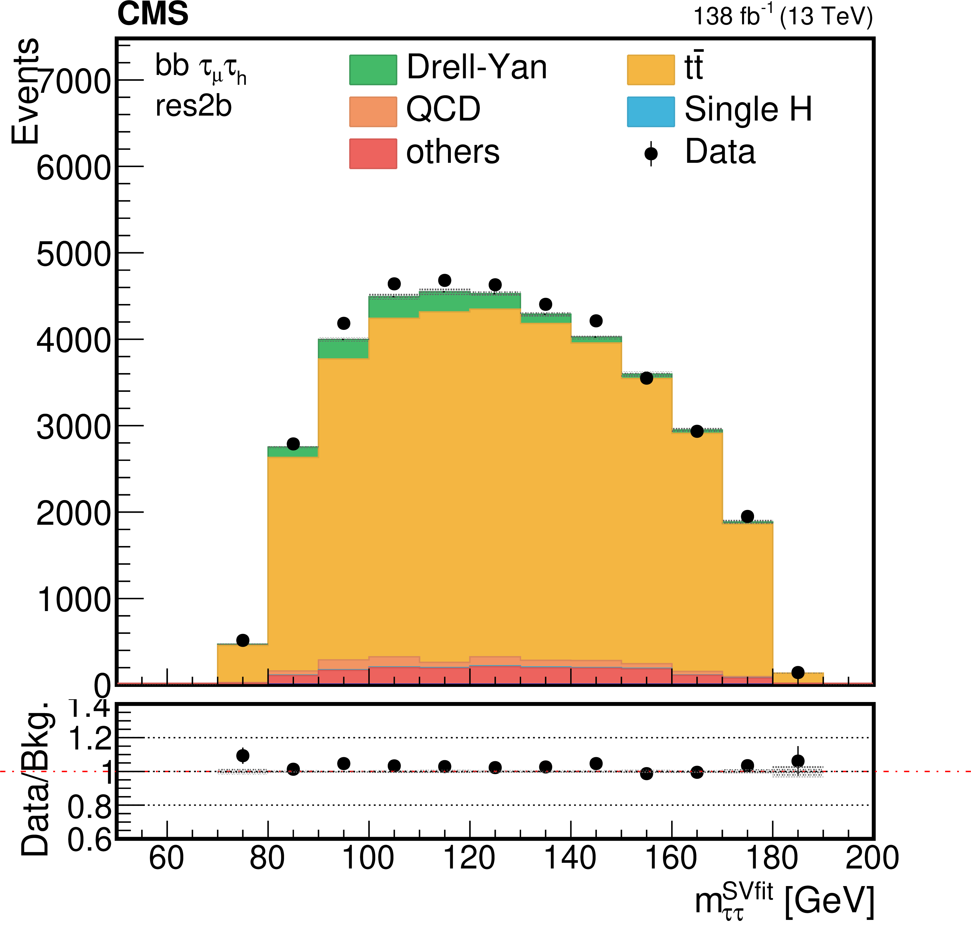
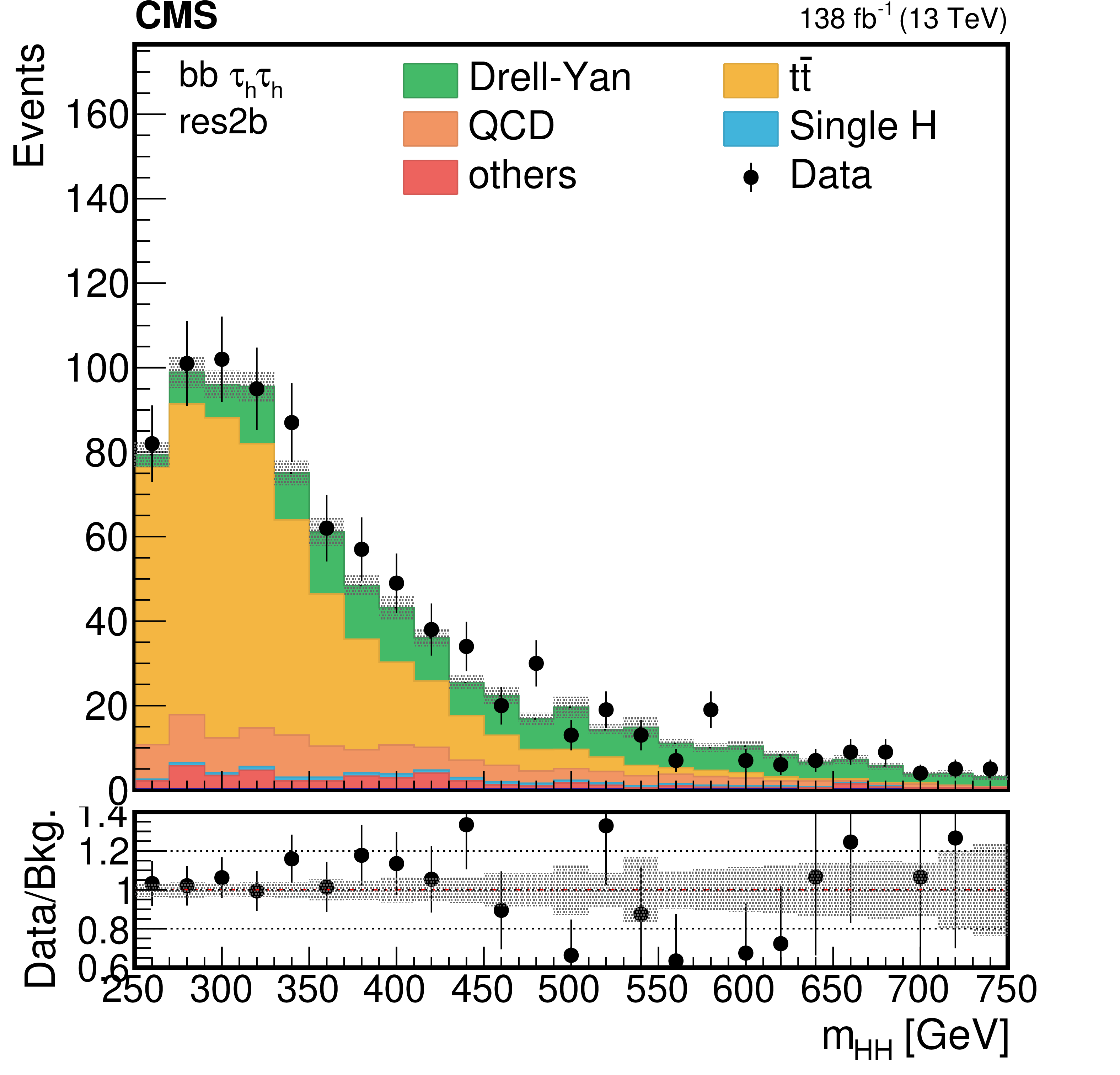
Distributions of the reconstructed mass of the bb (upper left), $\tau \tau $ (upper right) and HH (lower) pairs in the most sensitive category of the analysis (res2b). Events are shown in the ${\tau _{\mathrm{e}} {\tau _\mathrm {h}}}$ (upper left), ${\tau _{\mu} {\tau _\mathrm {h}}}$ (upper right) and ${{\tau _\mathrm {h}} {\tau _\mathrm {h}}}$ (lower) channels for the full 2016-2018 data set, after the selection on the reconstructed masses of the $\tau \tau $ and bb pairs, as described in Section 5. The shaded band in the plots represents the statistical uncertainty only. |
png pdf |
Figure 3-a:
Distribution of the reconstructed mass of the bb pairs in the most sensitive category of the analysis (res2b). Events are shown in the ${\tau _{\mathrm{e}} {\tau _\mathrm {h}}}$ channel for the full 2016-2018 data set, after the selection on the reconstructed masses of the $\tau \tau $ and bb pairs, as described in Section 5. The shaded band represents the statistical uncertainty only. |
png pdf |
Figure 3-b:
Distribution of the reconstructed mass of the $\tau \tau $ pairs in the most sensitive category of the analysis (res2b). Events are shown in the ${\tau _{\mu} {\tau _\mathrm {h}}}$ channel for the full 2016-2018 data set, after the selection on the reconstructed masses of the $\tau \tau $ and bb pairs, as described in Section 5. The shaded band represents the statistical uncertainty only. |
png pdf |
Figure 3-c:
Distribution of the reconstructed mass of the HH pairs in the most sensitive category of the analysis (res2b). Events are shown in the ${{\tau _\mathrm {h}} {\tau _\mathrm {h}}}$ channel for the full 2016-2018 data set, after the selection on the reconstructed masses of the $\tau \tau $ and bb pairs, as described in Section 5. The shaded band represents the statistical uncertainty only. |
png pdf |
Figure 4:
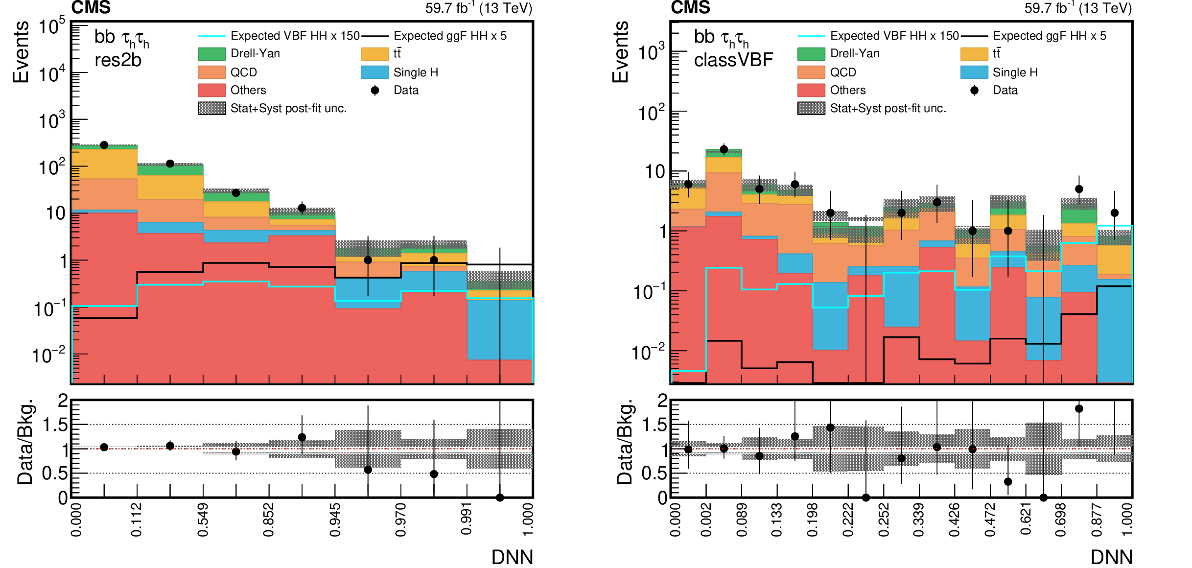
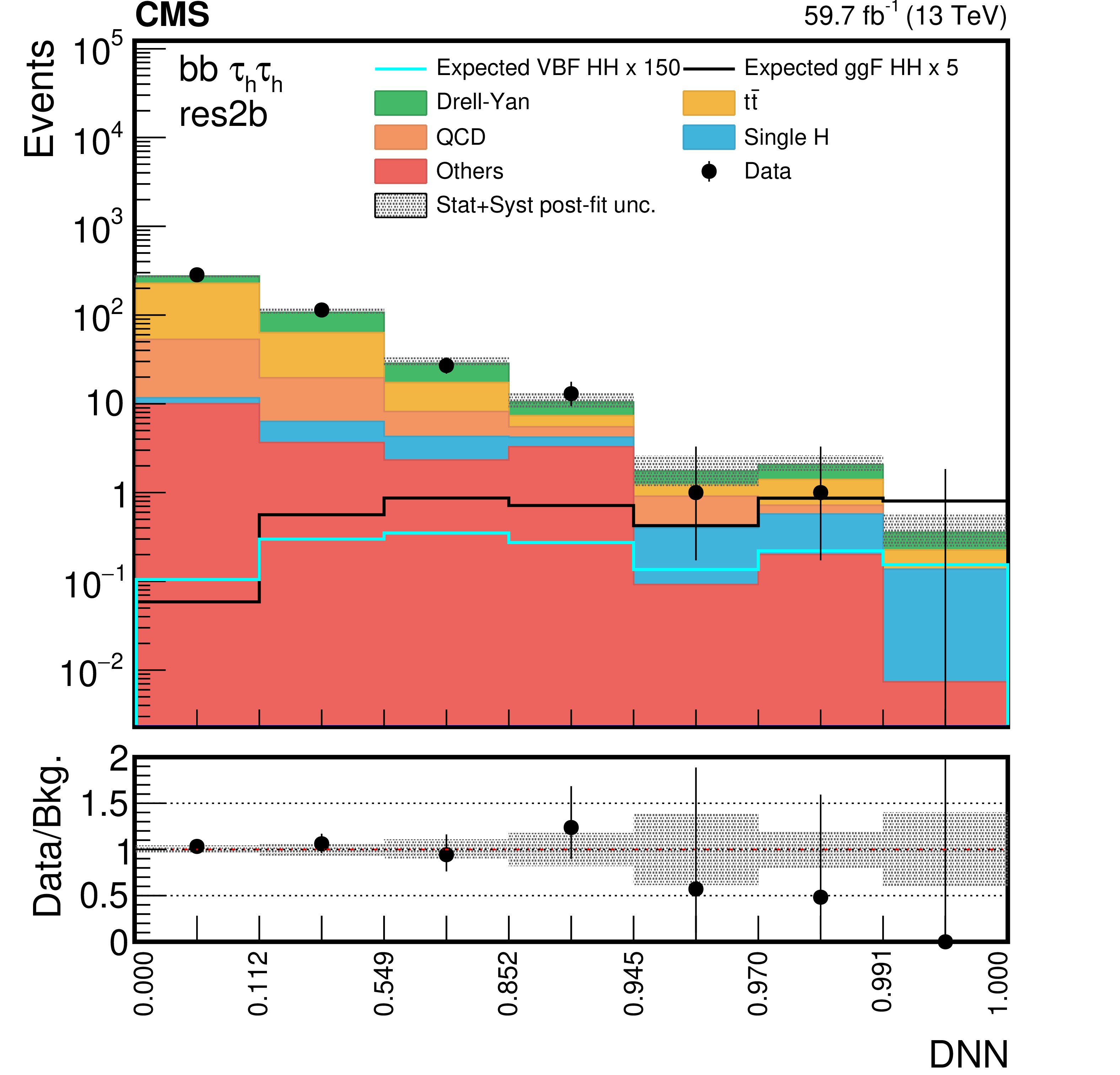
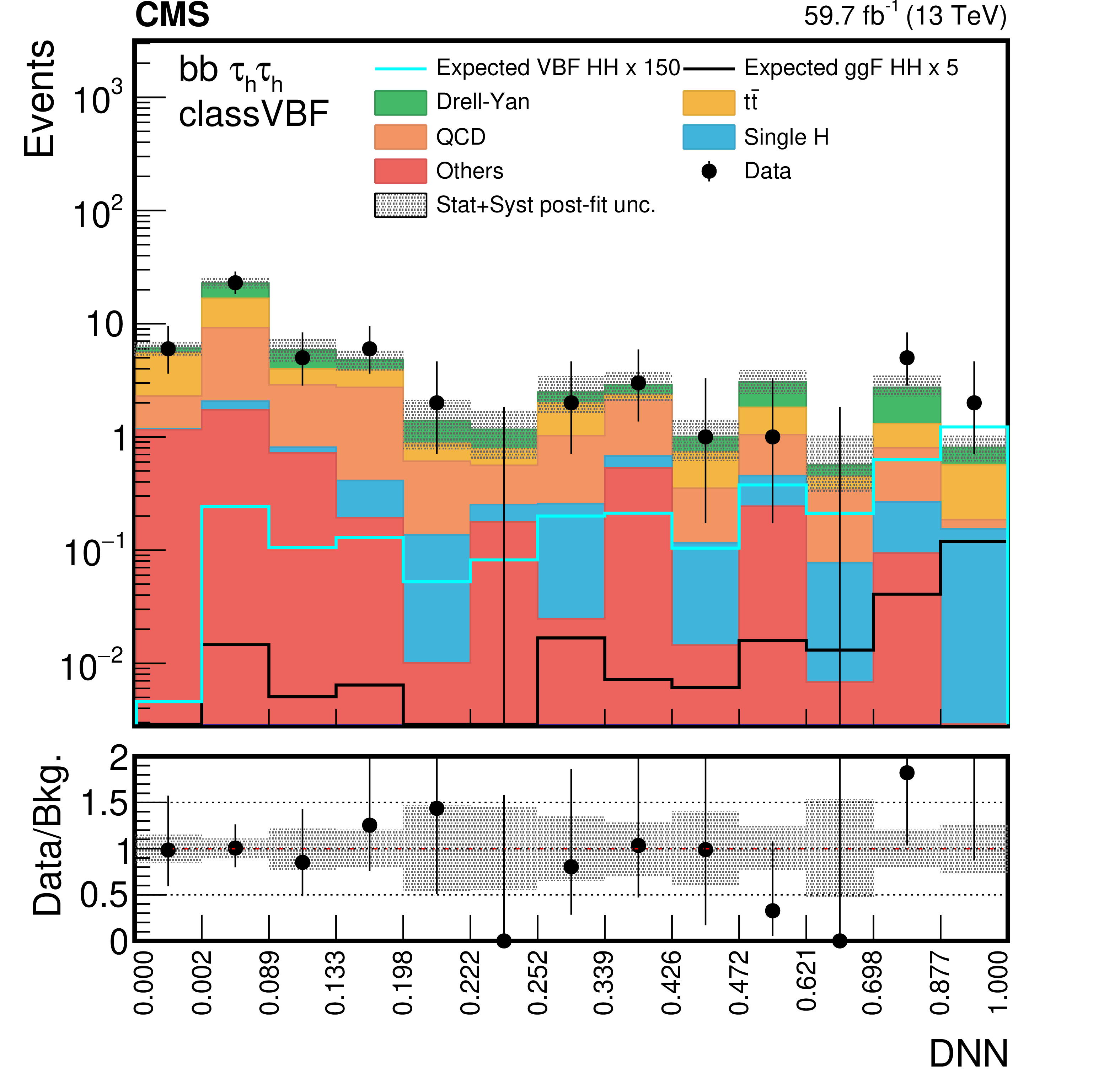
The postfit DNN distributions in the ${{\tau _\mathrm {h}} {\tau _\mathrm {h}}}$ channel in 2018 for the most sensitive category in the ggF (left) and VBF (right) searches. The shaded band in the plots represents the statistical plus systematic uncertainty. The expected SM distributions for the ggF and VBF HH signals are shown superimposed on the figures. |
png pdf |
Figure 4-a:
The postfit DNN distribution in the ${{\tau _\mathrm {h}} {\tau _\mathrm {h}}}$ channel in 2018 for the most sensitive category in the ggF search. The shaded band represents the statistical plus systematic uncertainty. The expected SM distributions for the ggF and VBF HH signals are shown superimposed on the figure. |
png pdf |
Figure 4-b:
The postfit DNN distribution in the ${{\tau _\mathrm {h}} {\tau _\mathrm {h}}}$ channel in 2018 for the most sensitive category in the VBF search. The shaded band represents the statistical plus systematic uncertainty. The expected SM distributions for the ggF and VBF HH signals are shown superimposed on the figure. |
png pdf |
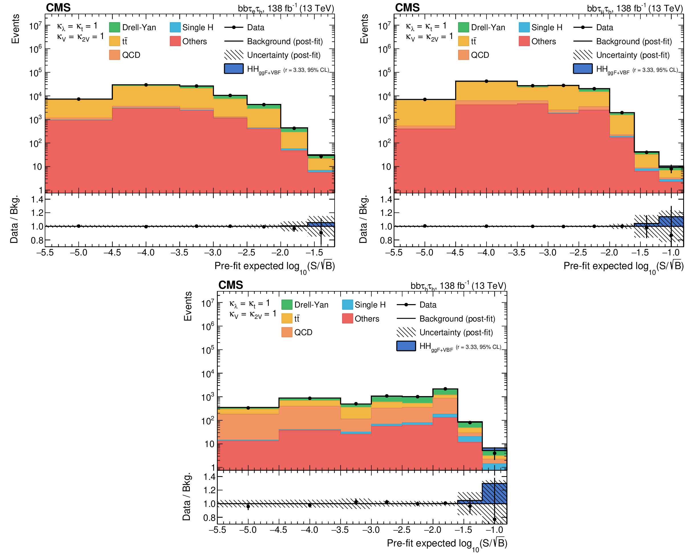
Figure 5:
Combination of bins of all postfit distributions, ordered according to the expected signal-to-square-root-background ratio, where the signal is the SM HH signal expected in that bin and the background is the prefit background estimate in the same bin, separately for the ${\tau _{\mathrm{e}} {\tau _\mathrm {h}}}$ channel (upper left), the ${\tau _{\mu} {\tau _\mathrm {h}}}$ channel (upper right), and ${{\tau _\mathrm {h}} {\tau _\mathrm {h}}}$ channel (lower). The ratio also shows the signal scaled to the observed exclusion limit (as shown in Table 2). |
png pdf |
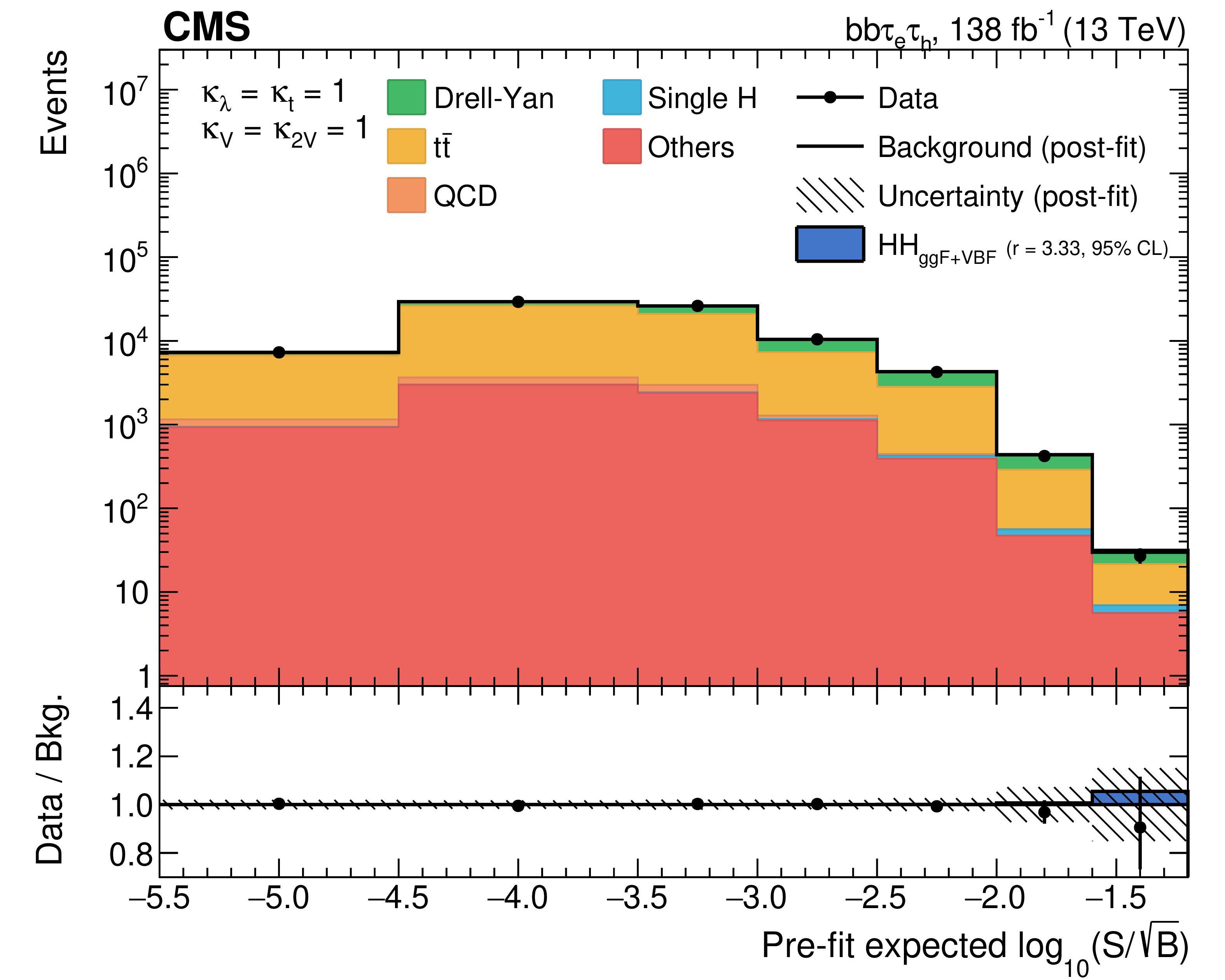
Figure 5-a:
Combination of bins of all postfit distributions, ordered according to the expected signal-to-square-root-background ratio, where the signal is the SM HH signal expected in that bin and the background is the prefit background estimate in the same bin, for the ${\tau _{\mathrm{e}} {\tau _\mathrm {h}}}$ channel. The ratio also shows the signal scaled to the observed exclusion limit (as shown in Table 2). |

png pdf |
Figure 5-b:
Combination of bins of all postfit distributions, ordered according to the expected signal-to-square-root-background ratio, where the signal is the SM HH signal expected in that bin and the background is the prefit background estimate in the same bin, for the ${\tau _{\mu} {\tau _\mathrm {h}}}$ channel. The ratio also shows the signal scaled to the observed exclusion limit (as shown in Table 2). |
png pdf |
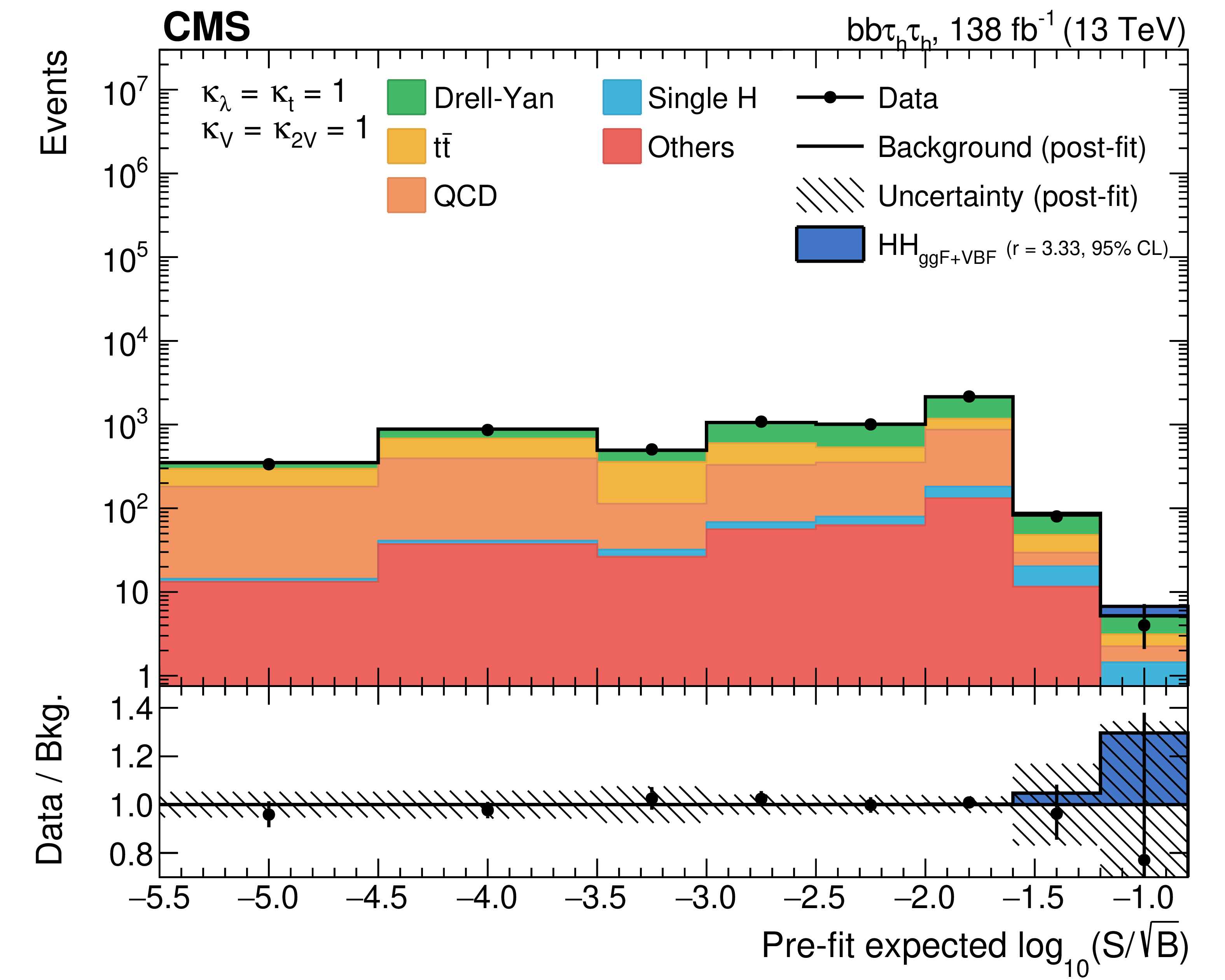
Figure 5-c:
Combination of bins of all postfit distributions, ordered according to the expected signal-to-square-root-background ratio, where the signal is the SM HH signal expected in that bin and the background is the prefit background estimate in the same bin, for the ${{\tau _\mathrm {h}} {\tau _\mathrm {h}}}$ channel. The ratio also shows the signal scaled to the observed exclusion limit (as shown in Table 2). |
png pdf |
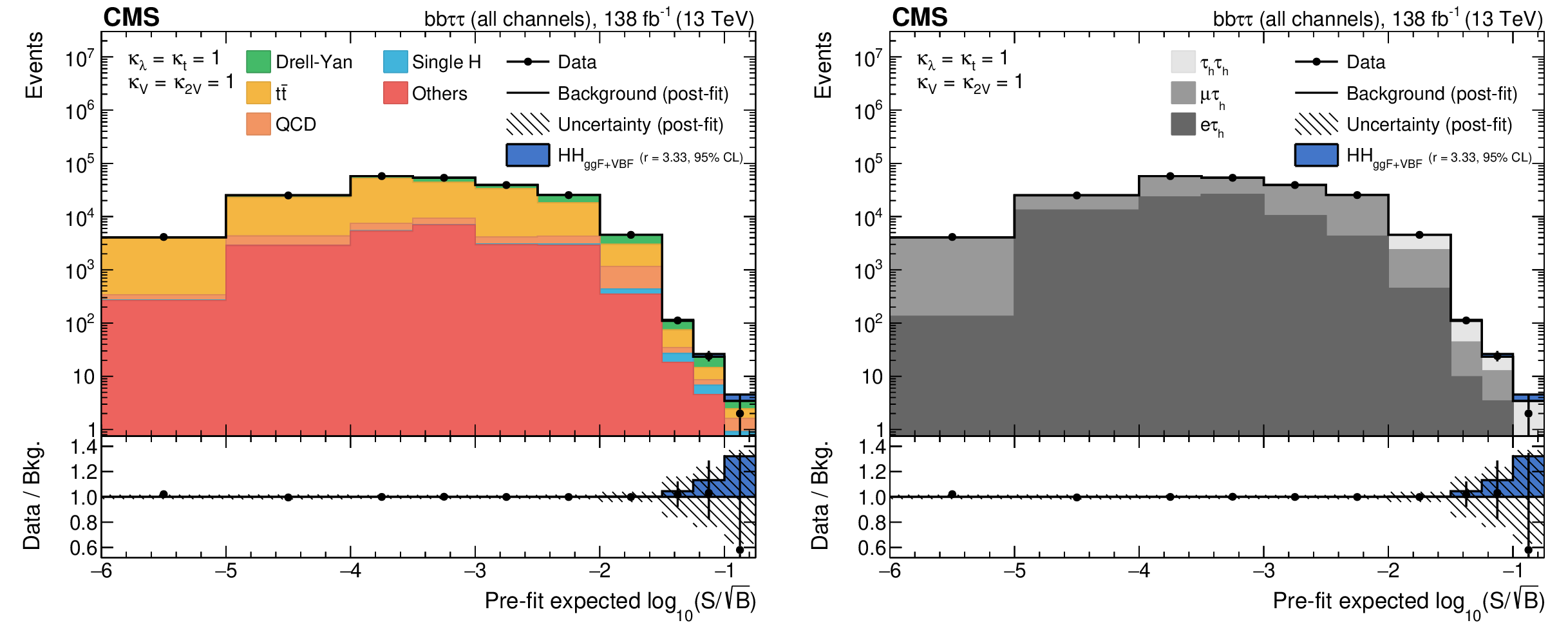
Figure 6:
Combination of bins of all postfit distributions, ordered according to the expected signal-to-square-root-background ratio, where the signal is the SM HH signal expected in that bin and the background is the prefit background estimate in the same bin, separately for the background contribution split into physics processes (left), and split into the three considered final state channels (right). The ratio also shows the signal scaled to the observed exclusion limit (as shown in Table 2). |

png pdf |
Figure 6-a:
Combination of bins of all postfit distributions, ordered according to the expected signal-to-square-root-background ratio, where the signal is the SM HH signal expected in that bin and the background is the prefit background estimate in the same bin, for the background contribution split into physics processes. The ratio also shows the signal scaled to the observed exclusion limit (as shown in Table 2). |

png pdf |
Figure 6-b:
Combination of bins of all postfit distributions, ordered according to the expected signal-to-square-root-background ratio, where the signal is the SM HH signal expected in that bin and the background is the prefit background estimate in the same bin, for the background contribution split into the three considered final state channels. The ratio also shows the signal scaled to the observed exclusion limit (as shown in Table 2). |
png pdf |
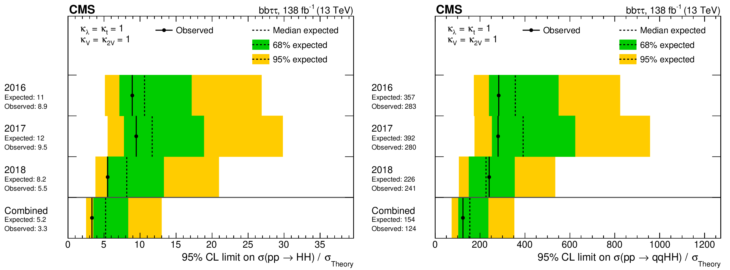
Figure 7:
The expected and observed limits on the ratio of experimentally estimated ggF plus VBF ($\sigma ({{\mathrm{p}} {\mathrm{p}}} \to {\mathrm{H} \mathrm{H}})$, left) and VBF only ($\sigma ({{\mathrm{p}} {\mathrm{p}}} \to \mathrm{q} \mathrm{q} {\mathrm{H} \mathrm{H}})$, right) HH production cross section and the expectation from the SM ($\sigma _{\text {Theory}}$) at 95% CL, separated into different years and combined for the full 2016-2018 data set. |
png pdf |
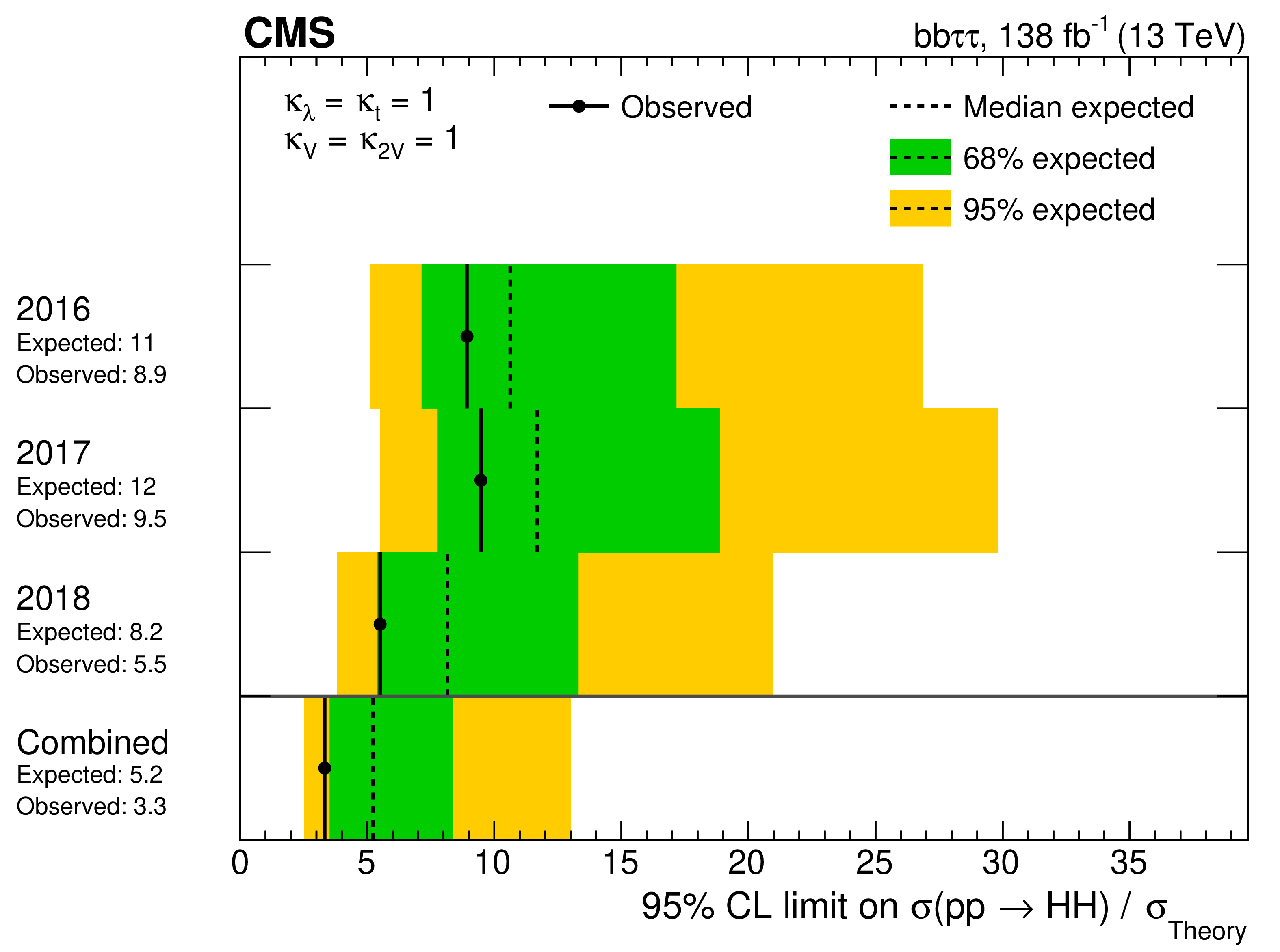
Figure 7-a:
The expected and observed limits on the ratio of experimentally estimated ggF plus VBF ($\sigma ({{\mathrm{p}} {\mathrm{p}}} \to {\mathrm{H} \mathrm{H}})$) HH production cross section and the expectation from the SM ($\sigma _{\text {Theory}}$) at 95% CL, separated into different years and combined for the full 2016-2018 data set. |
png pdf |
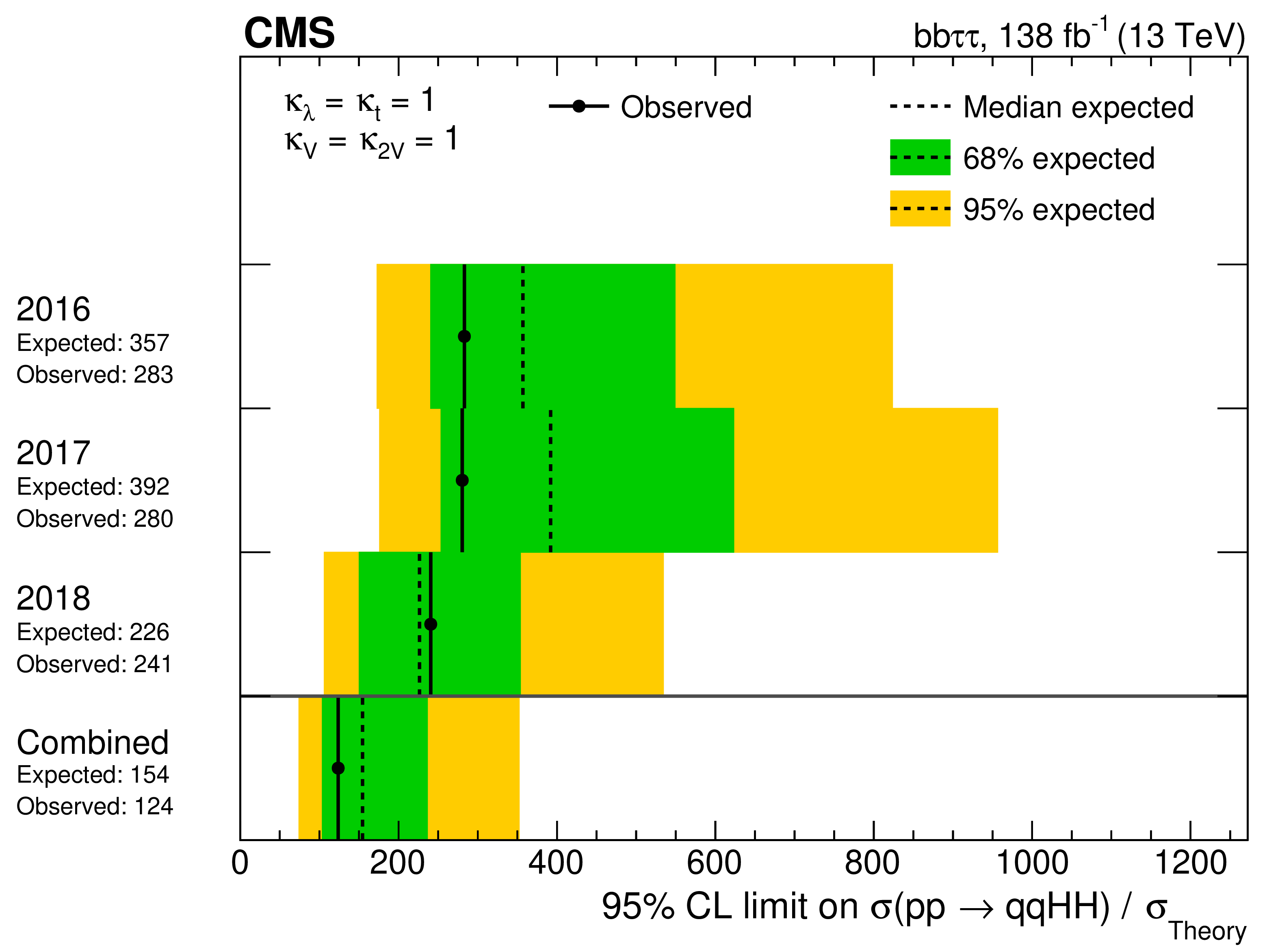
Figure 7-b:
The expected and observed limits on the ratio of experimentally estimated VBF only ($\sigma ({{\mathrm{p}} {\mathrm{p}}} \to \mathrm{q} \mathrm{q} {\mathrm{H} \mathrm{H}})$) HH production cross section and the expectation from the SM ($\sigma _{\text {Theory}}$) at 95% CL, separated into different years and combined for the full 2016-2018 data set. |
png pdf |
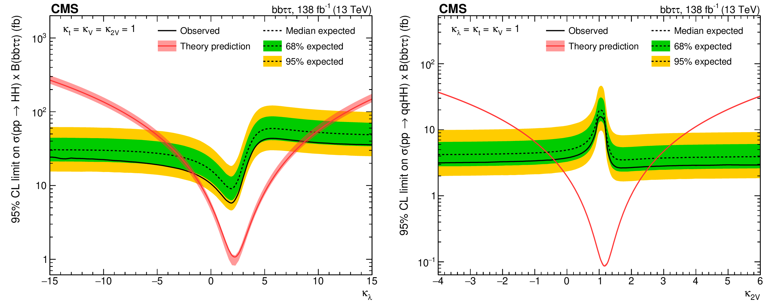
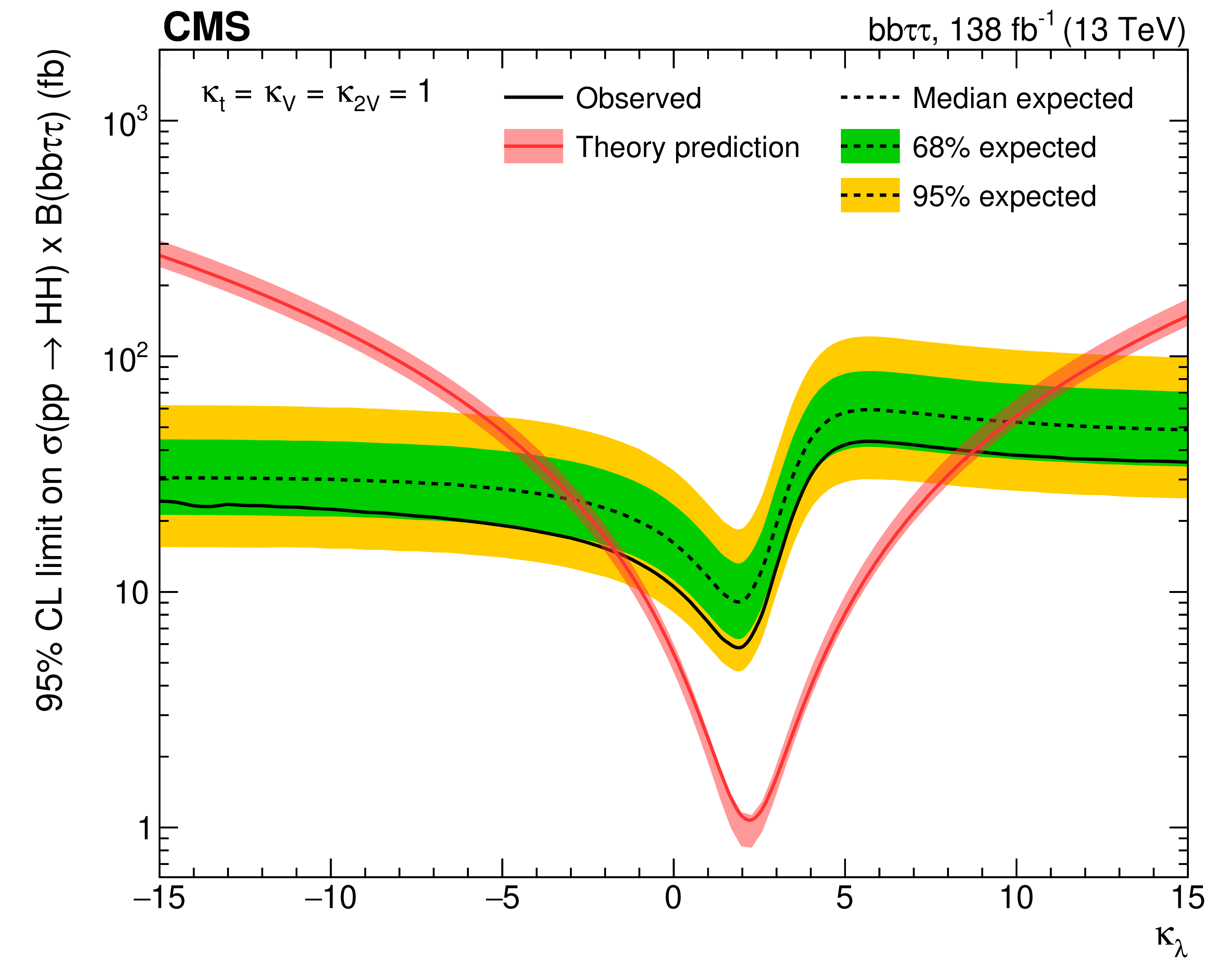
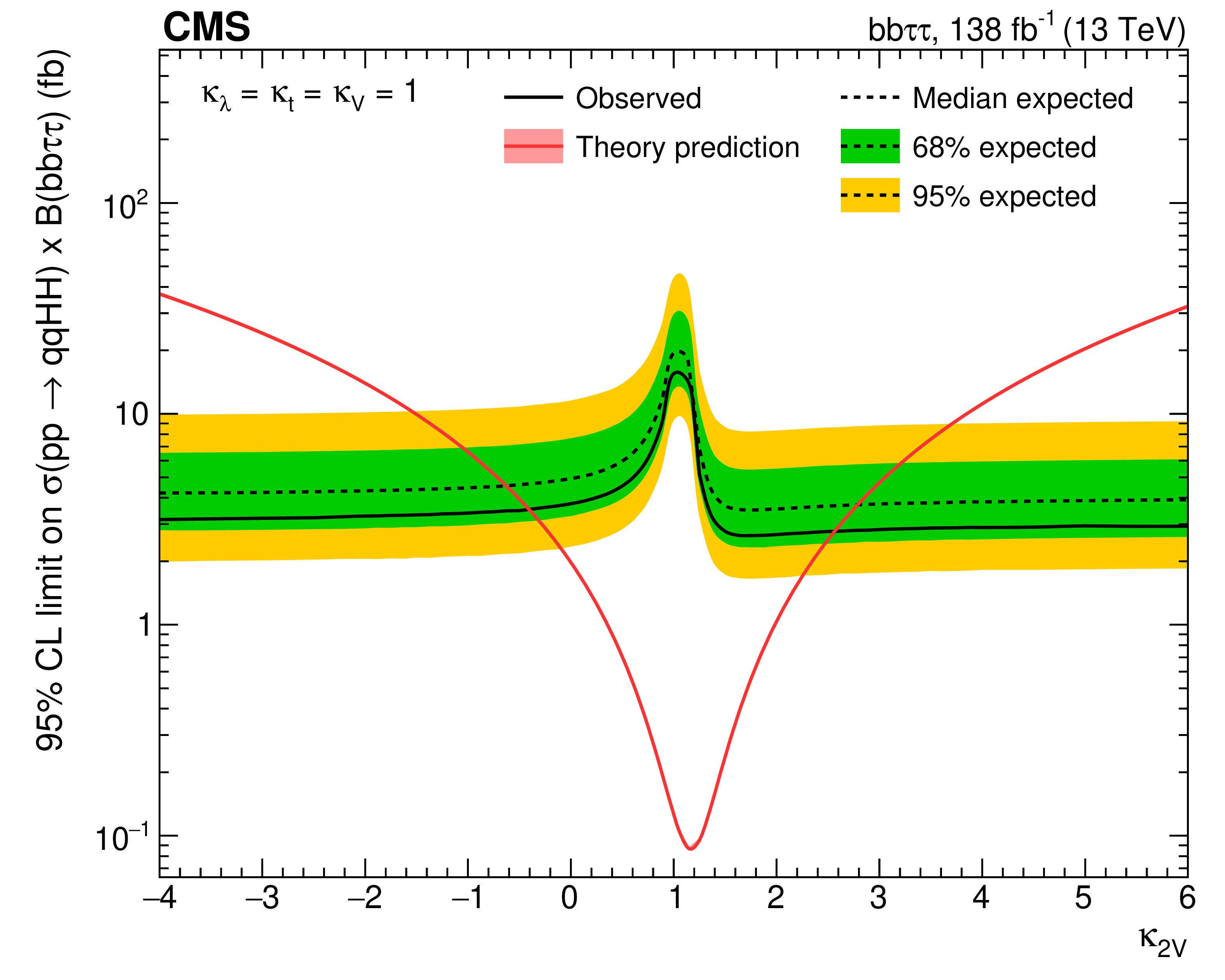
Figure 8:
(left) Observed and expected upper limits at 95% CL as functions of $\kappa _{\lambda}$ on the ggF plus VBF HH cross section times the ${\mathrm{b} \mathrm{b} \tau \tau}$ branching fraction. (right) Observed and expected upper limits at 95% CL as functions of $\kappa _{2{\mathrm{V}}}$ on the VBF only HH cross section times the ${\mathrm{b} \mathrm{b} \tau \tau}$ branching fraction. In both cases all other couplings are set to their SM expectation. The red solid line shows the theoretical prediction for the HH production cross section and its uncertainty (red shaded band). |
png pdf |
Figure 8-a:
Observed and expected upper limits at 95% CL as functions of $\kappa _{\lambda}$ on the ggF plus VBF HH cross section times the ${\mathrm{b} \mathrm{b} \tau \tau}$ branching fraction. All other couplings are set to their SM expectation. The red solid line shows the theoretical prediction for the HH production cross section and its uncertainty (red shaded band). |
png pdf |
Figure 8-b:
Observed and expected upper limits at 95% CL as functions of $\kappa _{2{\mathrm{V}}}$ on the VBF only HH cross section times the ${\mathrm{b} \mathrm{b} \tau \tau}$ branching fraction. All other couplings are set to their SM expectation. The red solid line shows the theoretical prediction for the HH production cross section and its uncertainty (red shaded band). |
png pdf |
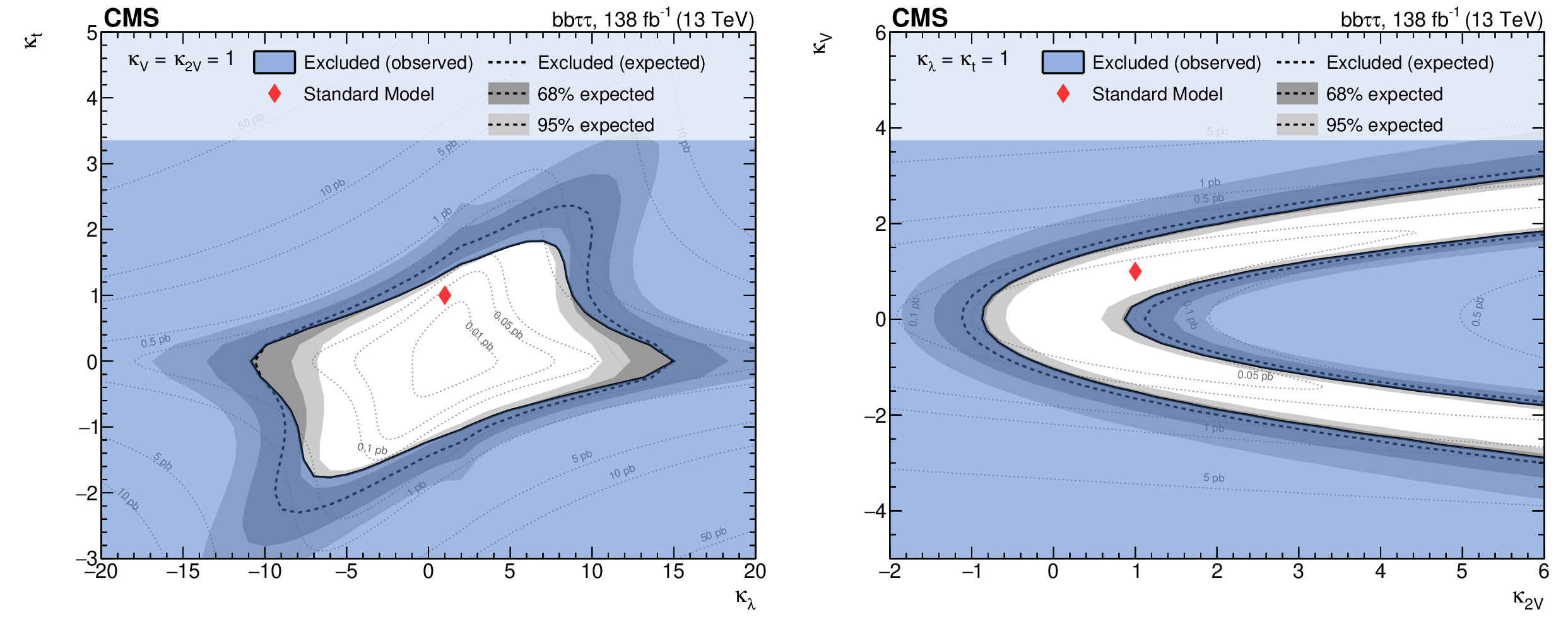
Figure 9:
(left) Two-dimensional exclusion regions as a function of the $\kappa _{\lambda}$ and $\kappa _t$ couplings for the full 2016-2018 combination, with both $\kappa _{2{\mathrm{V}}}$ and $\kappa _{{\mathrm{V}}}$ are fixed to unity. (right) Two-dimensional exclusion regions as a function of $\kappa _{2{\mathrm{V}}}$ and $\kappa _{{\mathrm{V}}}$, with both $\kappa _{\lambda}$ and $\kappa _t$ are set to unity. Expected uncertainties on exclusion boundaries are inferred from uncertainty bands of the limit calculation, and are denoted by dark and light-grey areas. The blue area marks parameter combinations that are observed to be excluded. For visual guidance, theoretical cross section values are illustrated by thin, labeled contour lines with the SM prediction denoted by a red diamond. |
png pdf |
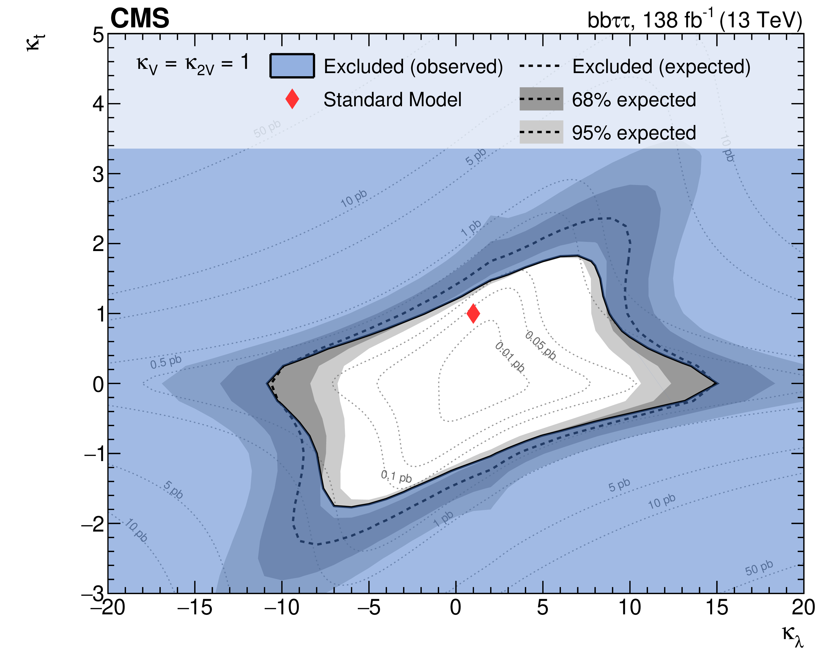
Figure 9-a:
Two-dimensional exclusion regions as a function of the $\kappa _{\lambda}$ and $\kappa _t$ couplings for the full 2016-2018 combination, with both $\kappa _{2{\mathrm{V}}}$ and $\kappa _{{\mathrm{V}}}$ are fixed to unity. Expected uncertainties on exclusion boundaries are inferred from uncertainty bands of the limit calculation, and are denoted by dark and light-grey areas. The blue area marks parameter combinations that are observed to be excluded. For visual guidance, theoretical cross section values are illustrated by thin, labeled contour lines with the SM prediction denoted by a red diamond. |
png pdf |
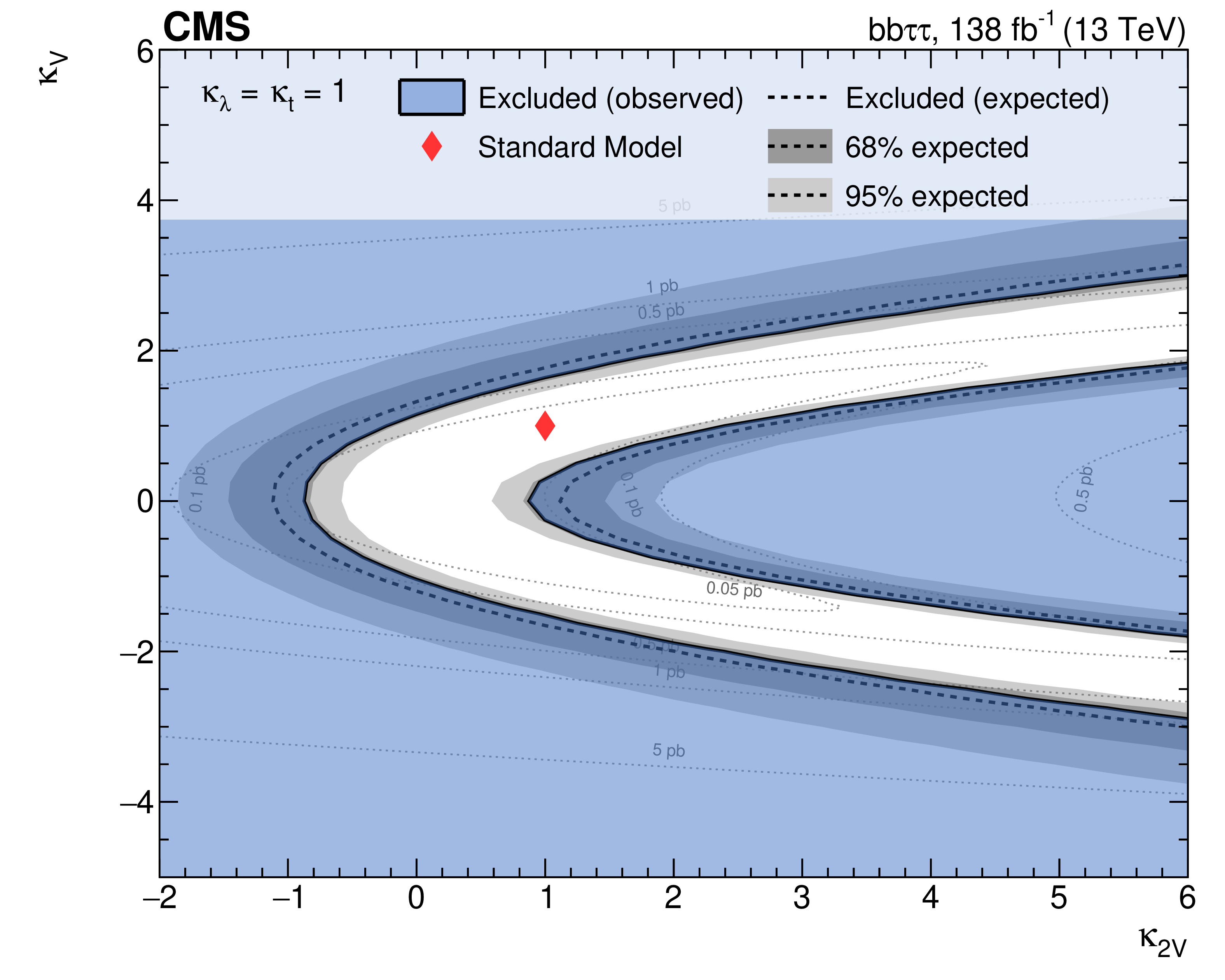
Figure 9-b:
Two-dimensional exclusion regions as a function of $\kappa _{2{\mathrm{V}}}$ and $\kappa _{{\mathrm{V}}}$, with both $\kappa _{\lambda}$ and $\kappa _t$ are set to unity. Expected uncertainties on exclusion boundaries are inferred from uncertainty bands of the limit calculation, and are denoted by dark and light-grey areas. The blue area marks parameter combinations that are observed to be excluded. For visual guidance, theoretical cross section values are illustrated by thin, labeled contour lines with the SM prediction denoted by a red diamond. |
png pdf |
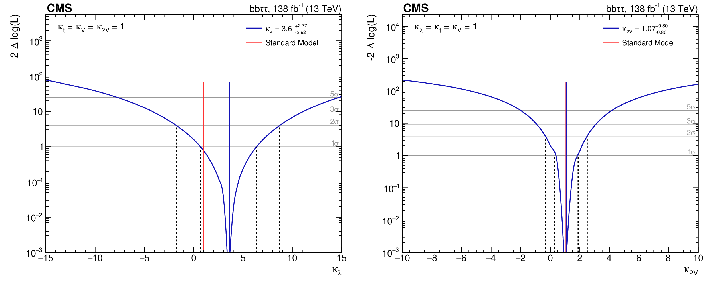
Figure 10:
Observed likelihood scan as a function of $\kappa _{\lambda}$ (left) and $\kappa _{2{\mathrm{V}}}$ (right) for the full 2016-2018 combination. The dashed lines show the intersection with threshold values one and four, corresponding to 68 and 95% confidence intervals, respectively. |
png pdf |
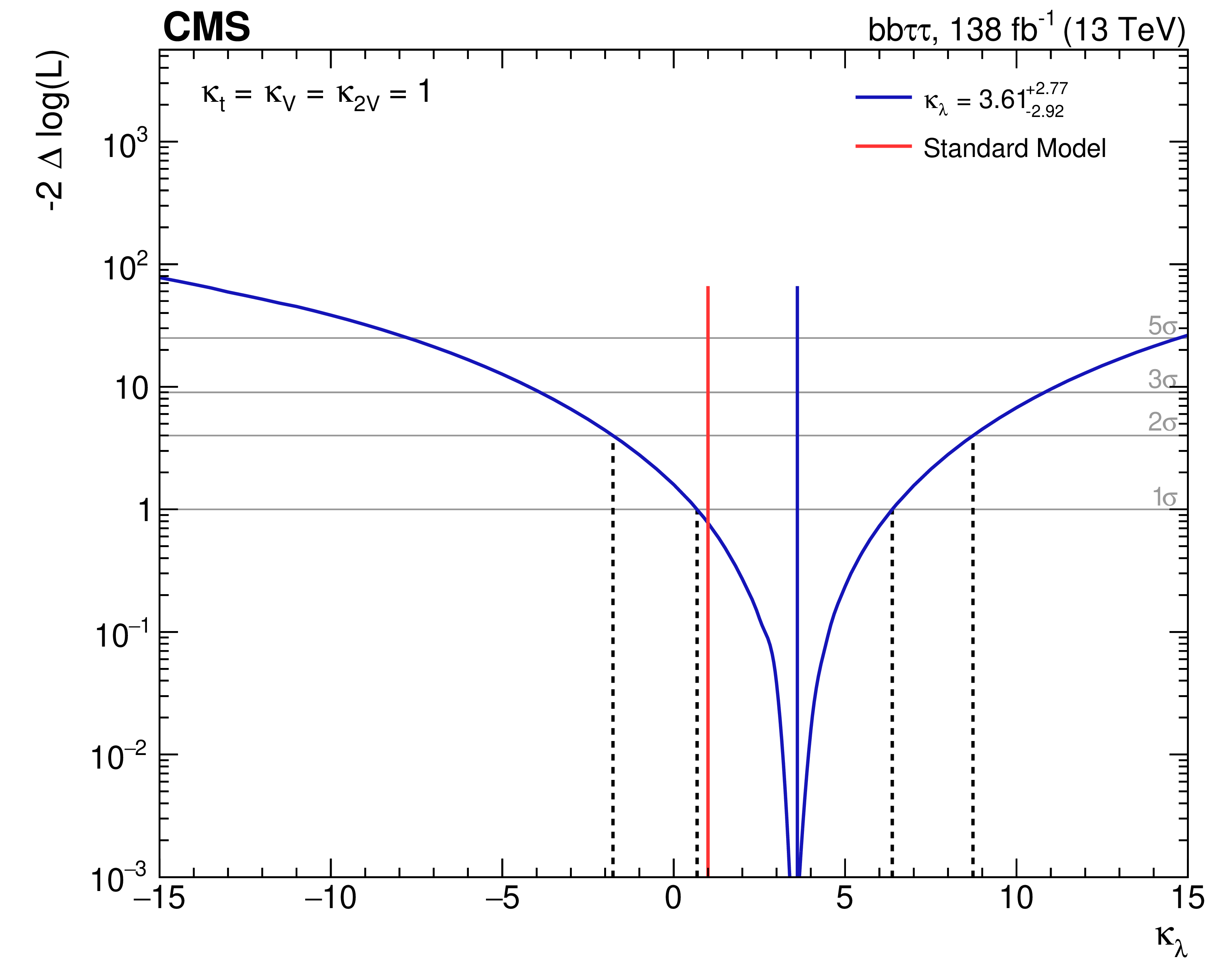
Figure 10-a:
Observed likelihood scan as a function of $\kappa _{\lambda}$ for the full 2016-2018 combination. The dashed lines show the intersection with threshold values one and four, corresponding to 68 and 95% confidence intervals, respectively. |
png pdf |
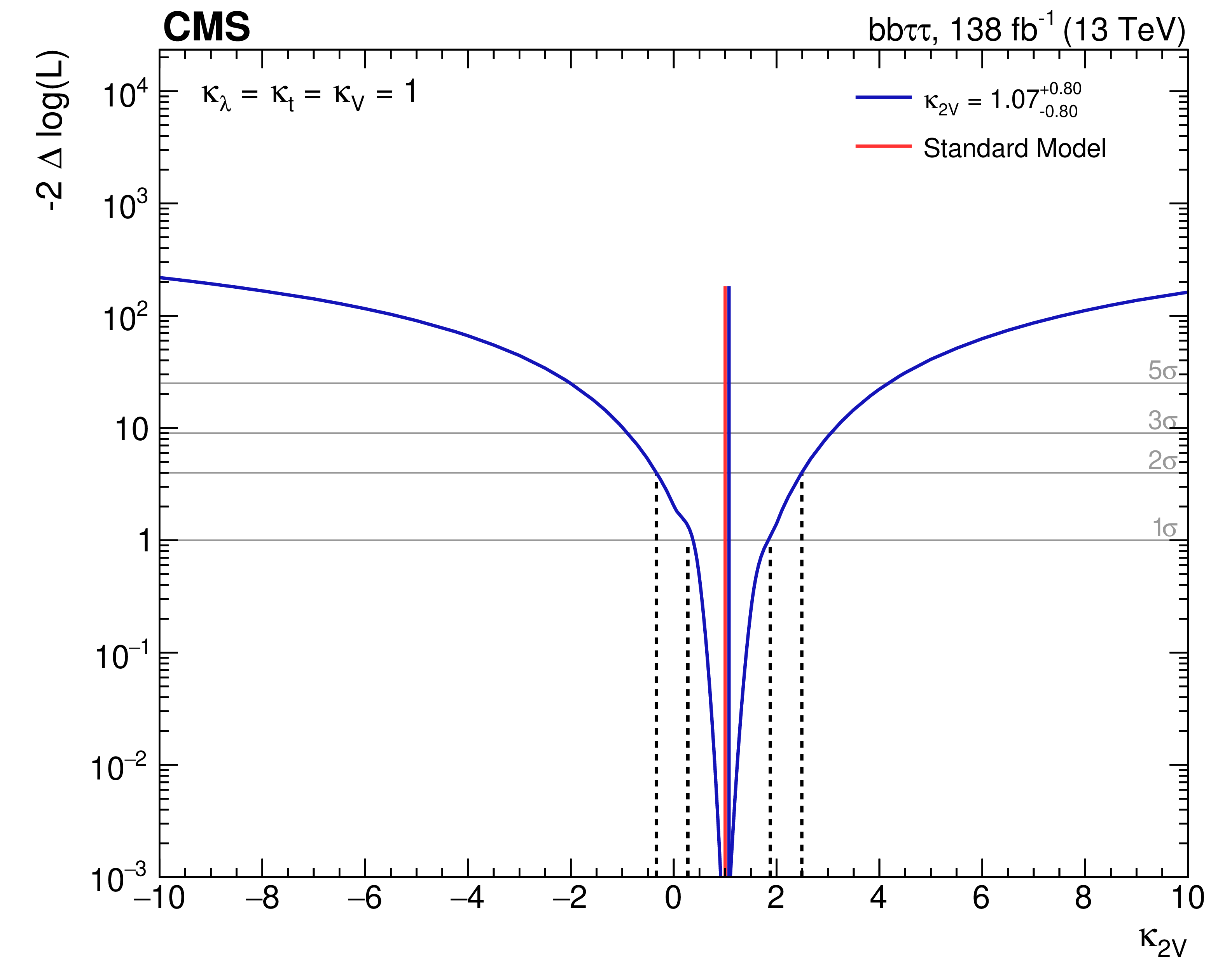
Figure 10-b:
Observed likelihood scan as a function of $\kappa _{2{\mathrm{V}}}$ for the full 2016-2018 combination. The dashed lines show the intersection with threshold values one and four, corresponding to 68 and 95% confidence intervals, respectively. |
| Tables | |

png pdf |
Table 1:
Summary of selections applied to the $\tau \tau $ candidate pair. Trigger thresholds in parentheses refer to the 2017-2018 data-taking period when different from 2016. |
png pdf |
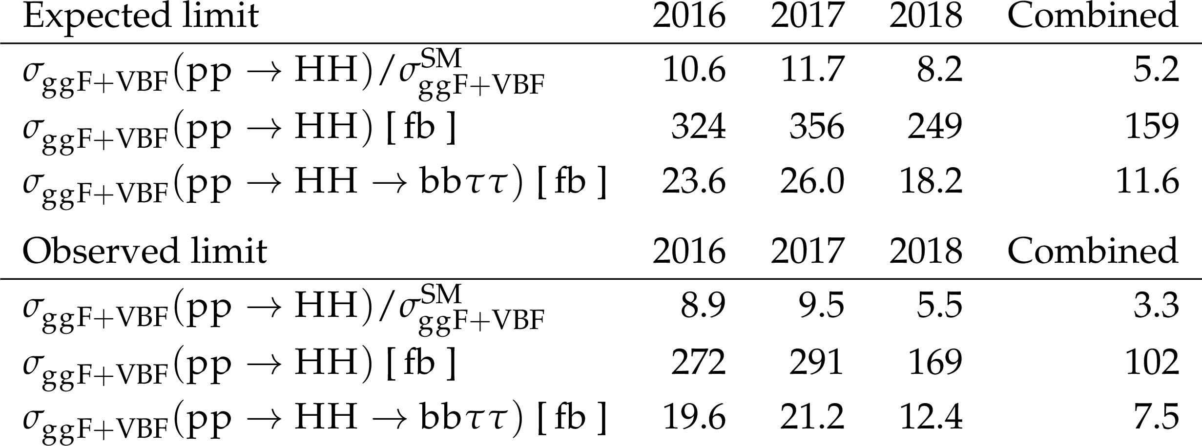
Table 2:
Expected and observed upper limits at 95% CL for the SM point ($\kappa _{\lambda}=$ 1), where $\sigma _{{\mathrm{g} \mathrm{g} \text {F}} +\text {VBF}}^{\text {SM}}=$ 32.776 fb represents the sum of the ggF plus VBF HH cross sections. |
png pdf |
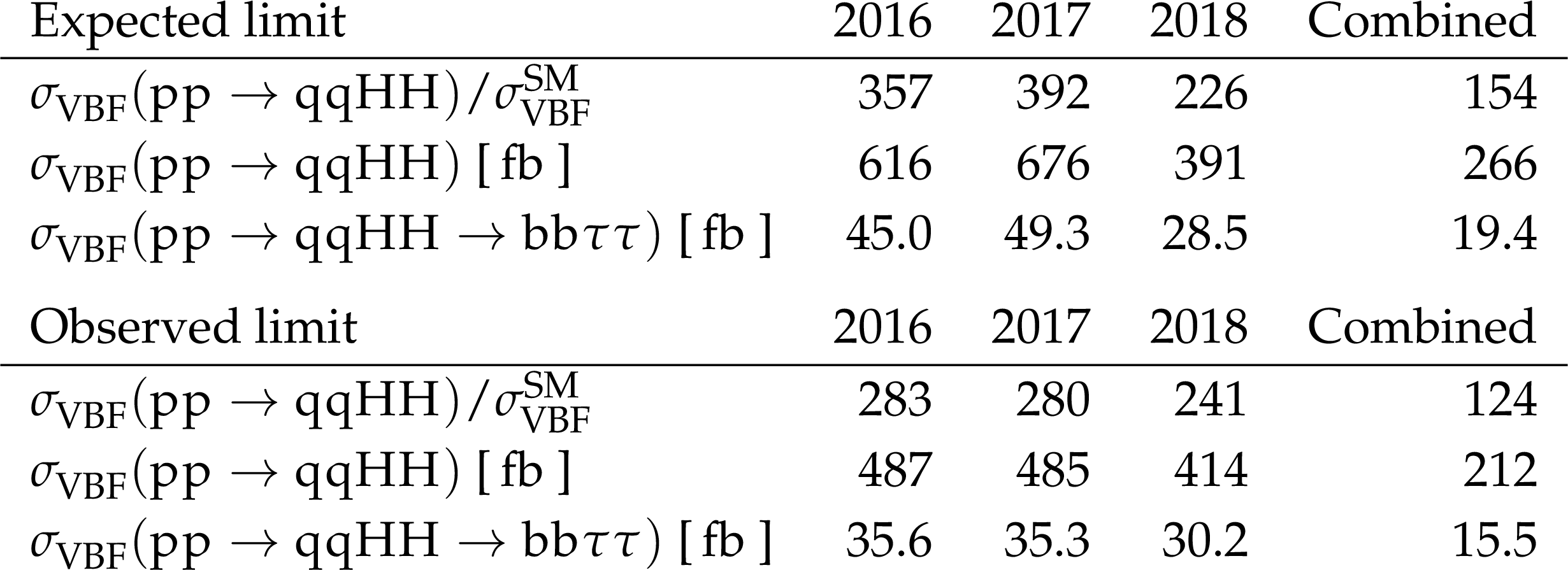
Table 3:
Expected and observed upper limits at 95% CL for the SM point ($\kappa _{2{\mathrm{V}}}=$ 1), where $\sigma _{\text {VBF}}^{\text {SM}}=$ 1.726 fb represents the VBF only HH cross section. |
| Summary |
|
A search for nonresonant Higgs boson pair (HH) production via gluon-gluon fusion (ggF) and vector boson fusion (VBF) processes in final states with two bottom quarks and two tau leptons was presented. The search uses the full 2016-2018 data set of proton-proton collisions at a center-of-mass energy of $\sqrt{s} = $ 13 TeV recorded with the CMS detector at the LHC, corresponding to an integrated luminosity of 138 fb$^{-1}$. The three decay modes of the $\tau\tau$ pair with the largest branching fraction have been selected, requiring one tau lepton to be always decaying hadronically and the other one either leptonically or hadronically. Upper limits at 95% confidence level (CL) on the inclusive ggF plus VBF HH production cross section are set, as well as on the VBF only HH production cross section. This analysis benefits from an improved trigger strategy as well as from a series of techniques developed especially for this search: among others, several neural networks to identify the b jets from the H decay, to categorize the events, and to perform signal extraction. Moreover, this analysis builds up on the improvements made by the CMS Collaboration in the jet and tau lepton identification and reconstruction algorithms. All these techniques enable the achievement of particularly stringent results on the HH production cross sections. The observed (expected) 95% CL upper limit on HH total production cross section corresponds to 3.3 (5.2) times the theoretical SM prediction. The observed (expected) 95% CL upper limit for the VBF only HH SM cross section corresponds to 124 (154) times the theoretical SM prediction. The observed (expected) 95% CL constraints on $\kappa_{\lambda}$ and $\kappa_{2\mathrm{V}}$, derived from limits on the HH production cross section times the ${\mathrm{b}\mathrm{b}\tau\tau}$ branching fraction, are found to be $-$1.7 $< \kappa_{\lambda} <$ 8.7 ($-$2.9 $ < \kappa_{\lambda} < $ 9.8) and $-$0.4 $ < \kappa_{2\mathrm{V}} < $ 2.6 ($-$0.6 $ < \kappa_{2\mathrm{V}} < $ 2.8), respectively. |
| References | ||||
| 1 | ATLAS Collaboration | Observation of a new particle in the search for the Standard Model Higgs boson with the ATLAS detector at the LHC | PLB 716 (2012) 1 | 1207.7214 |
| 2 | CMS Collaboration | Observation of a new boson at a mass of 125 GeV with the CMS experiment at the LHC | PLB 716 (2012) 30 | CMS-HIG-12-028 1207.7235 |
| 3 | CMS Collaboration | Observation of a new boson with mass near 125 GeV in proton-proton collisions at $ \sqrt{s}= $ 7 and 8 TeV | JHEP 06 (2013) 081 | CMS-HIG-12-036 1303.4571 |
| 4 | CMS Collaboration | A measurement of the higgs boson mass in the diphoton decay channel | PLB 805 (2020) 135425 | CMS-HIG-19-004 2002.06398 |
| 5 | ATLAS, CMS Collaboration | Measurements of the Higgs boson production and decay rates and constraints on its couplings from a combined ATLAS and CMS analysis of the LHC proton-proton collision data at $ \sqrt{s}= $ 7 and 8 TeV | JHEP 08 (2016) 045 | 1606.02266 |
| 6 | M. Grazzini et al. | Higgs boson pair production at NNLO with top quark mass effects | JHEP 05 (2018) 59 | 1803.0246 |
| 7 | J. Baglio et al. | $ gg\rightarrowHH $: Combined uncertainties | \hrefhttp://www.arXiv.org/abs/.11626v3\textttarXiv:.11626v3, 2021 PRD 103 (2021) 056002 |
|
| 8 | F. A. Dreyer and A. Karlberg | Vector-boson fusion Higgs pair production at N$^{3}$LO | PRD 98 (2018) 114016 | 1811.07906 |
| 9 | B. Di Micco et al. | Higgs boson pair production at colliders: status and perspectives | Rev. Phys. 5 (2020) 100045 | 1910.00012 |
| 10 | CMS Collaboration | Identification of hadronic tau lepton decays using a deep neural network | 2022. Submitted to JINST | CMS-TAU-20-001 2201.08458 |
| 11 | CMS Collaboration | Search for Higgs boson pair production in events with two bottom quarks and two tau leptons in proton-proton collisions at $ \sqrt{s} = $ 13 TeV | PLB 778 (2017) 101 | CMS-HIG-17-002 1707.02909 |
| 12 | ATLAS Collaboration | Search for resonant and nonresonant Higgs boson pair production in the $ \mathrm{b}\mathrm{\bar{b}}\tau^{+}\tau^{-} $ decay channel in proton-proton collisions at $ \sqrt{s} = $ 13 TeV with the ATLAS detector | PRL 121 (2018) 191801 | 1808.00336 |
| 13 | E. Bols et al. | Jet flavour classification using DeepJet | JINST 15 (2020) P12012 | 2008.10519 |
| 14 | CMS Collaboration | HEPData record for this analysis | link | |
| 15 | CMS Collaboration | Performance of the CMS Level-1 trigger in proton-proton collisions at $ \sqrt{s} = $ 13 TeV | JINST 15 (2020) P10017 | CMS-TRG-17-001 2006.10165 |
| 16 | CMS Collaboration | The CMS trigger system | JINST 12 (2017) P01020 | CMS-TRG-12-001 1609.02366 |
| 17 | CMS Collaboration | The CMS experiment at the CERN LHC | JINST 3 (2008) S08004 | CMS-00-001 |
| 18 | CMS Collaboration | Precision luminosity measurement in proton-proton collisions at $ \sqrt{s} = $ 13 TeV in 2015 and 2016 at CMS | EPJC 81 (2021) 800 | CMS-LUM-17-003 2104.01927 |
| 19 | CMS Collaboration | CMS luminosity measurement for the 2017 data-taking period at $ \sqrt{s} = $ 13 TeV | CMS-PAS-LUM-17-004 | CMS-PAS-LUM-17-004 |
| 20 | CMS Collaboration | CMS luminosity measurement for the 2018 data-taking period at $ \sqrt{s} = $ 13 TeV | CMS-PAS-LUM-18-002 | CMS-PAS-LUM-18-002 |
| 21 | J. Alwall et al. | The automated computation of tree-level and next-to-leading order differential cross sections, and their matching to parton shower simulations | JHEP 07 (2014) 79 | 1405.0301 |
| 22 | S. Frixione, P. Nason, and C. Oleari | Matching NLO QCD computations with parton shower simulations: the POWHEG method | JHEP 11 (2007) 070 | 0709.2092 |
| 23 | E. Re | Single-top Wt-channel production matched with parton showers using the POWHEG method | EPJC 71 (2011) 1547 | 1009.2450 |
| 24 | J. M. Campbell, R. K. Ellis, P. Nason, and E. Re | Top-pair production and decay at NLO matched with parton showers | JHEP 04 (2015) 114 | 1412.1828 |
| 25 | G. Heinrich et al. | Probing the trilinear Higgs boson coupling in di-Higgs production at NLO QCD including parton shower effects | JHEP 06 (2019) 66 | 1903.08137 |
| 26 | J. Alwall et al. | Comparative study of various algorithms for the merging of parton showers and matrix elements in hadronic collisions | EPJC 53 (2007) 473 | 0706.2569 |
| 27 | R. Frederix and S. Frixione | Merging meets matching in MC@NLO | JHEP 12 (2012) 61 | 1209.6215 |
| 28 | T. Sjöstrand et al. | An introduction to PYTHIA 8.2 | Comp. Phys. Commun. 191 (2015) 159 | 1410.3012 |
| 29 | CMS Collaboration | Event generator tunes obtained from underlying event and multiparton scattering measurements | EPJC 76 (2016) 155 | CMS-GEN-14-001 1512.00815 |
| 30 | CMS Collaboration | Extraction and validation of a new set of CMS PYTHIA-8 tunes from underlying-event measurements | EPJC 80 (2020) 4 | CMS-GEN-17-001 1903.12179 |
| 31 | R. D. Ball et al. | Parton distributions for the LHC run II | JHEP 04 (2015) 40 | 1410.8849 |
| 32 | R. D. Ball et al. | Parton distributions from high-precision collider data | EPJC 77 (2017) 663 | 1706.00428 |
| 33 | GEANT4 Collaboration | GEANT4---a simulation toolkit | NIMA 506 (2003) 250 | |
| 34 | CMS Collaboration | Particle-flow reconstruction and global event description with the CMS detector | JINST 12 (2017) P10003 | CMS-PRF-14-001 1706.04965 |
| 35 | CMS Collaboration | Performance of missing transverse momentum reconstruction in proton-proton collisions at $ \sqrt{s} = $ 13 TeV using the CMS detector | JINST 14 (2019) P07004 | CMS-JME-17-001 1903.06078 |
| 36 | CMS Collaboration | Technical proposal for the Phase-II upgrade of the Compact Muon Solenoid | CMS-PAS-TDR-15-002 | CMS-PAS-TDR-15-002 |
| 37 | CMS Collaboration | Electron and photon reconstruction and identification with the CMS experiment at the CERN LHC | JINST 16 (2021) P05014 | CMS-EGM-17-001 2012.06888 |
| 38 | CMS Collaboration | ECAL 2016 refined calibration and Run2 summary plots | CDS | |
| 39 | CMS Collaboration | Performance of the CMS muon detector and muon reconstruction with proton-proton collisions at $ \sqrt{s}= $ 13 TeV | JINST 13 (2018) P06015 | CMS-MUO-16-001 1804.04528 |
| 40 | CMS Collaboration | Performance of $ \tau $-lepton reconstruction and identification in CMS | JINST 7 (2012) P01001 | CMS-TAU-11-001 1109.6034 |
| 41 | CMS Collaboration | Reconstruction and identification of $ \tau $ lepton decays to hadrons and $ \nu_\tau $ at CMS | JINST 11 (2016) P01019 | CMS-TAU-14-001 1510.07488 |
| 42 | CMS Collaboration | Performance of reconstruction and identification of $ \tau $ leptons decaying to hadrons and $ \nu_\tau $ in proton-proton collisions at $ \sqrt{s}= $ 13 TeV | JINST 13 (2018) P10005 | CMS-TAU-16-003 1809.02816 |
| 43 | M. Cacciari, G. P. Salam, and G. Soyez | The anti-$ {k_{\mathrm{T}}} $ jet clustering algorithm | JHEP 04 (2008) 063 | 0802.1189 |
| 44 | M. Cacciari, G. P. Salam, and G. Soyez | FastJet user manual | EPJC 72 (2012) 1896 | 1111.6097 |
| 45 | Y. L. Dokshitzer, G. D. Leder, S. Moretti, and B. R. Webber | Better jet clustering algorithms | JHEP 08 (1997) 001 | hep-ph/9707323 |
| 46 | M. Wobisch and T. Wengler | Hadronization corrections to jet cross-sections in deep inelastic scattering | in Proceedings of the Workshop on Monte Carlo Generators for HERA Physics, Hamburg, 1998 | hep-ph/9907280 |
| 47 | M. Dasgupta, A. Fregoso, S. Marzani, and G. P. Salam | Towards an understanding of jet substructure | JHEP 09 (2013) 029 | 1307.0007 |
| 48 | J. M. Butterworth, A. R. Davison, M. Rubin, and G. P. Salam | Jet substructure as a new Higgs search channel at the LHC | PRL 100 (2008) 242001 | 0802.2470 |
| 49 | CMS Collaboration | Pileup mitigation at CMS in $ \sqrt{s} = $ 13 TeV data | JINST 15 (2020) P09018 | CMS-JME-18-001 2003.00503 |
| 50 | D. Bertolini, P. Harris, M. Low, and N. Tran | Pileup per particle identification | JHEP 10 (2014) 059 | 1407.6013 |
| 51 | CMS Collaboration | Jet energy scale and resolution in the CMS experiment in proton-proton collisions at $ \sqrt{s} = $ 8 TeV | JINST 12 (2017) P02014 | CMS-JME-13-004 1607.03663 |
| 52 | CMS Collaboration | Jet energy scale and resolution measurement with Run-2 legacy data collected by CMS at $ \sqrt{s} = $ 13 TeV | CDS | |
| 53 | L. Bianchini, J. Conway, E. K. Friis, and C. Veelken | Reconstruction of the Higgs mass in $ \mathrm{H}{}\to\tau\tau $ events by dynamical likelihood techniques | J. Phys.: Conf. Ser. 513 (2014) 022035 | |
| 54 | G. C. Strong | On the impact of selected modern deep-learning techniques to the performance and celerity of classification models in an experimental high-energy physics use case | Mach. Learn.: Sci. Technol. (2020) | 2002.01427 |
| 55 | S. J. Hanson | A stochastic version of the delta rule | Physica D 42 (1990) 265 | |
| 56 | N. Srivastava et al. | Dropout: a simple way to prevent neural networks from overfitting | JMLR 15 (2014) 1929 | |
| 57 | F. Rosenblatt | The perceptron: a probabilistic model for information storage and organization in the brain | Psychological Review 65 (1957) 386 | |
| 58 | S. Linnainmaa | Taylor expansion of the accumulated rounding error | BIT Numerical Mathematics 16 (1976) 146 | |
| 59 | P. J. Werbos | Applications of advances in nonlinear sensitivity analysis | in Proc. 10th IFIP Conf., 31/8--4/9, NYC, p. 762 1981 | |
| 60 | D. E. Rumelhart, G. E. Hinton, and R. J. Williams | Learning representations by back-propagating errors | Nature 323 (1986) 533 | |
| 61 | CMS Collaboration | Prospects for HH measurements at the HL-LHC | CMS-PAS-FTR-18-019 | CMS-PAS-FTR-18-019 |
| 62 | E. M. Cepeda et al. | Higgs physics at the HL-LHC and HE-LHC | CERN Yellow Rep. Monogr. 7 (2018) 221 | 1902.00134 |
| 63 | D. de Florian et al. | Handbook of LHC Higgs cross sections: 4. Deciphering the Nature of the Higgs sector | CERN Yellow Rep: Monogr. 2 (2017) 21 | 1610.07922 |
| 64 | B. Cabouat and T. Sjöstrand | Some dipole shower studies | EPJC 78 (2018) 226 | 1710.00391v2 |
| 65 | T. Junk | Confidence level computation for combining searches with small statistics | NIMA 434 (1999) 435 | hep-ex/9902006 |
| 66 | A. L. Read | Presentation of search results: the CL$ _{\text{s}} $ technique | JPG 28 (2002) 2693 | |
| 67 | G. Cowan, K. Cranmer, E. Gross, and O. Vitells | Asymptotic formulae for likelihood-based tests of new physics | EPJC 71 (2011) 1554 | 1007.1727 |
| 68 | J. B. Močkus and L. J. Močkus | Bayesian approach to global optimization and application to multiobjective and constrained problems | Journal of Optimization Theory and Applications 70 (1991) 157 | 2108.00002 |
|
|
Compact Muon Solenoid LHC, CERN |
|

|

|

|

|

|