

Compact Muon Solenoid
LHC, CERN
| CMS-HIG-22-002 ; CERN-EP-2023-061 | ||
| Search for the lepton-flavor violating decay of the Higgs boson and additional Higgs bosons in the e$ \mu $ final state in proton-proton collisions at $ \sqrt{s} = $ 13 TeV | ||
| CMS Collaboration | ||
| 29 May 2023 | ||
| Phys. Rev. D 108 (2023) 072004 | ||
| Abstract: A search for the lepton-flavor violating decay of the Higgs boson and potential additional Higgs bosons with a mass in the range 110-160 GeV to an $ \mathrm{e}^{\pm}\mu^{\mp} $ pair is presented. The search is performed with a proton-proton collision dataset at a center-of-mass energy of 13 TeV collected by the CMS experiment at the LHC, corresponding to an integrated luminosity of 138 fb$ ^{-1} $. No excess is observed for the Higgs boson. The observed (expected) upper limit on the $ \mathrm{e}^{\pm}\mu^{\mp} $ branching fraction for it is determined to be 4.4 (4.7) $\times$ 10$^{-5} $ at 95% confidence level, the most stringent limit set thus far from direct searches. The largest excess of events over the expected background in the full mass range of the search is observed at an $ \mathrm{e}^{\pm}\mu^{\mp} $ invariant mass of approximately 146 GeV with a local (global) significance of 3.8 (2.8) standard deviations. | ||
| Links: e-print arXiv:2305.18106 [hep-ex] (PDF) ; CDS record ; inSPIRE record ; HepData record ; CADI line (restricted) ; | ||
| Figures & Tables | Summary | Additional Figures & Tables | References | CMS Publications |
|---|
| Figures | |
png pdf |
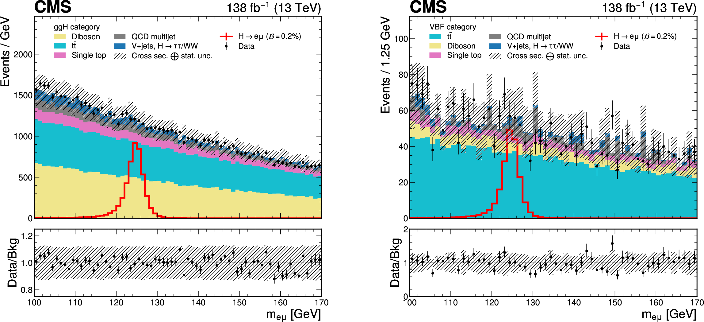
Figure 1:
The $ {m_{\mathrm{e}\mu}} $ distributions of the data, simulated backgrounds and signals of $ {\mathrm{H}\to\mathrm{e}\mu} $ in the ggH (left) and the VBF categories (right). A $ {\mathcal{B}(\mathrm{H}\to\mathrm{e}\mu)}= $ 0.2% is assumed for the signal for illustration. The lower panel in each plot shows the ratio of the data to the total estimated background. The uncertainty band corresponds to the background uncertainties, adding in quadrature the statistical and the SM cross section uncertainties. |
png pdf |
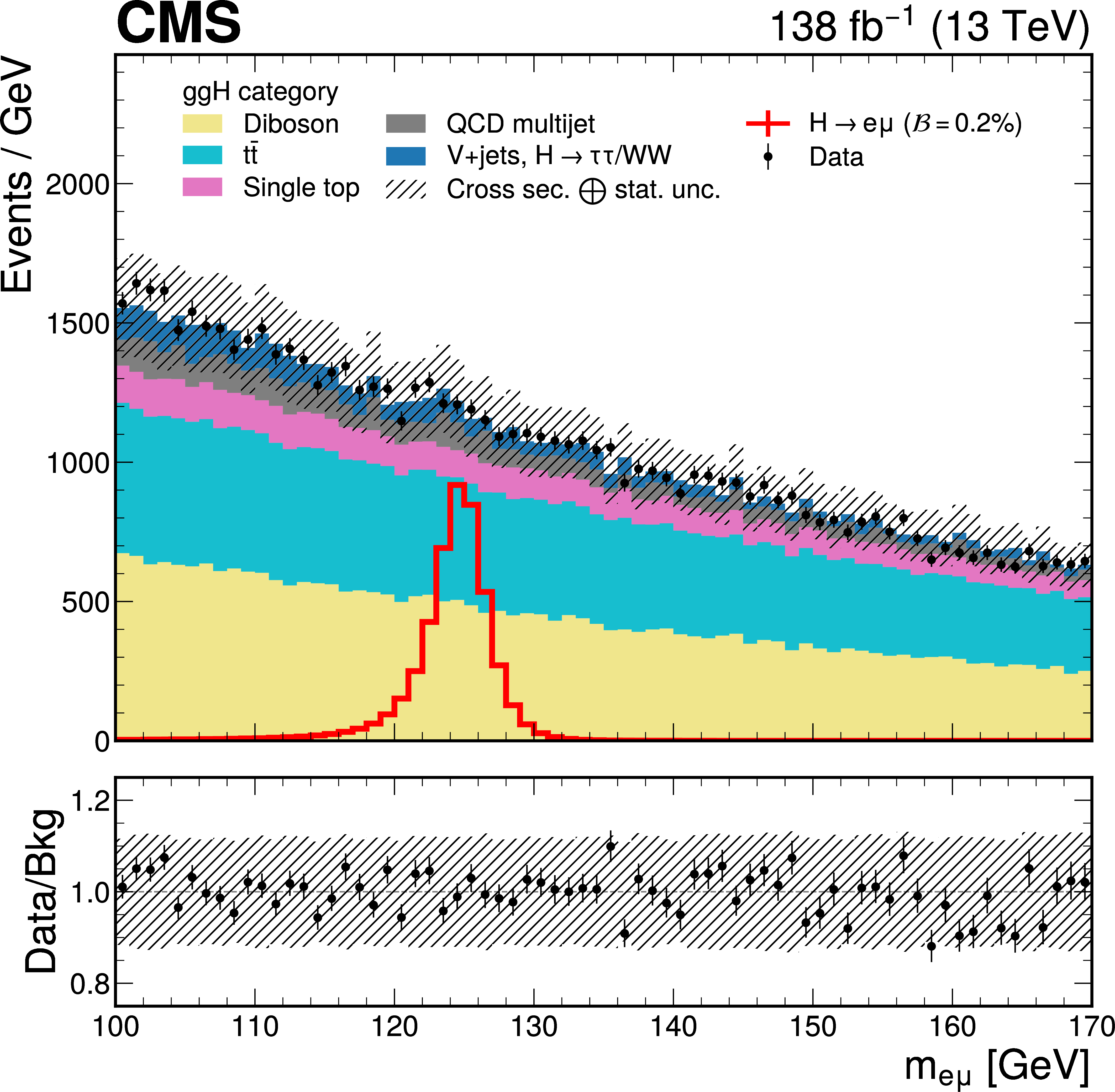
Figure 1-a:
The $ {m_{\mathrm{e}\mu}} $ distributions of the data, simulated backgrounds and signals of $ {\mathrm{H}\to\mathrm{e}\mu} $ in the ggH category. A $ {\mathcal{B}(\mathrm{H}\to\mathrm{e}\mu)}= $ 0.2% is assumed for the signal for illustration. The lower panel in each plot shows the ratio of the data to the total estimated background. The uncertainty band corresponds to the background uncertainties, adding in quadrature the statistical and the SM cross section uncertainties. |

png pdf |
Figure 1-b:
The $ {m_{\mathrm{e}\mu}} $ distributions of the data, simulated backgrounds and signals of $ {\mathrm{H}\to\mathrm{e}\mu} $ in the VBF category. A $ {\mathcal{B}(\mathrm{H}\to\mathrm{e}\mu)}= $ 0.2% is assumed for the signal for illustration. The lower panel in each plot shows the ratio of the data to the total estimated background. The uncertainty band corresponds to the background uncertainties, adding in quadrature the statistical and the SM cross section uncertainties. |
png pdf |
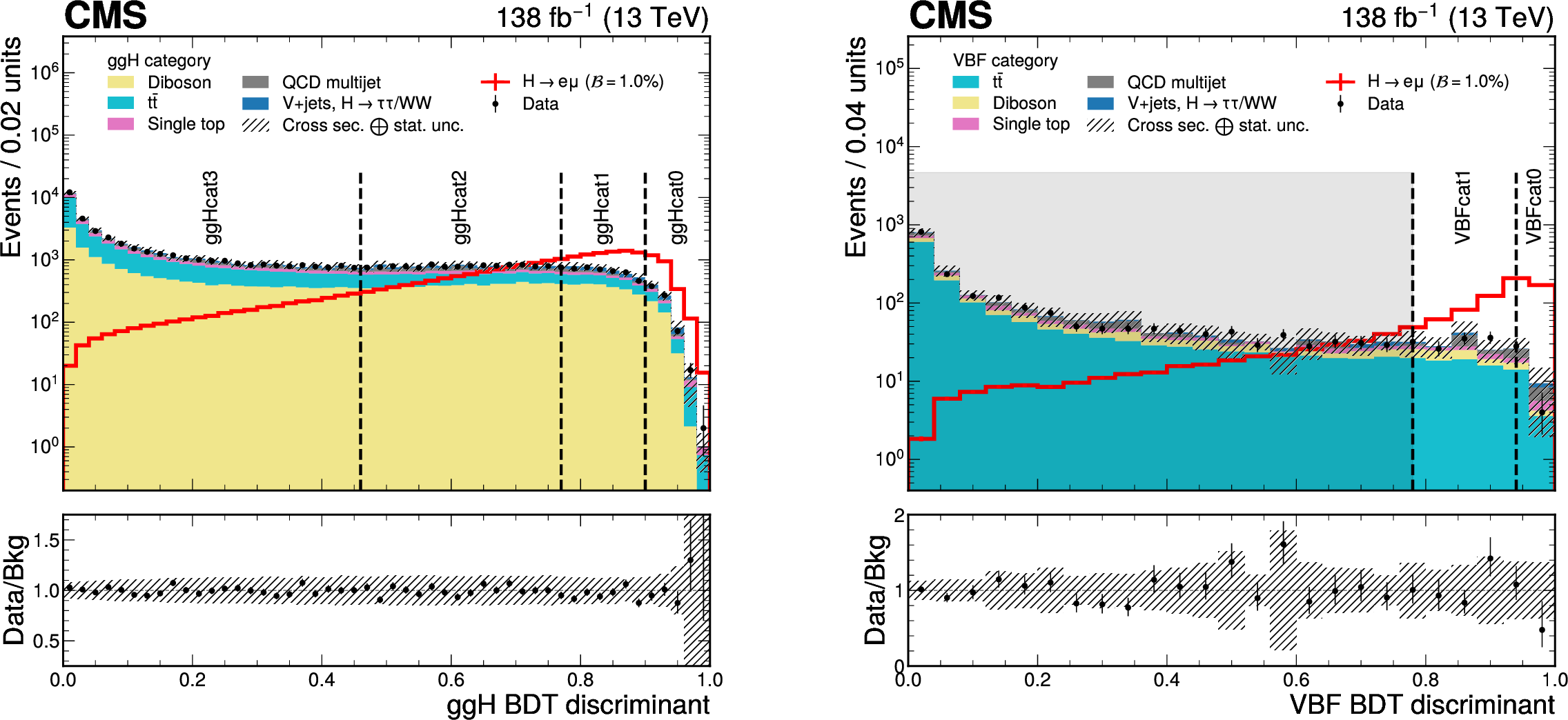
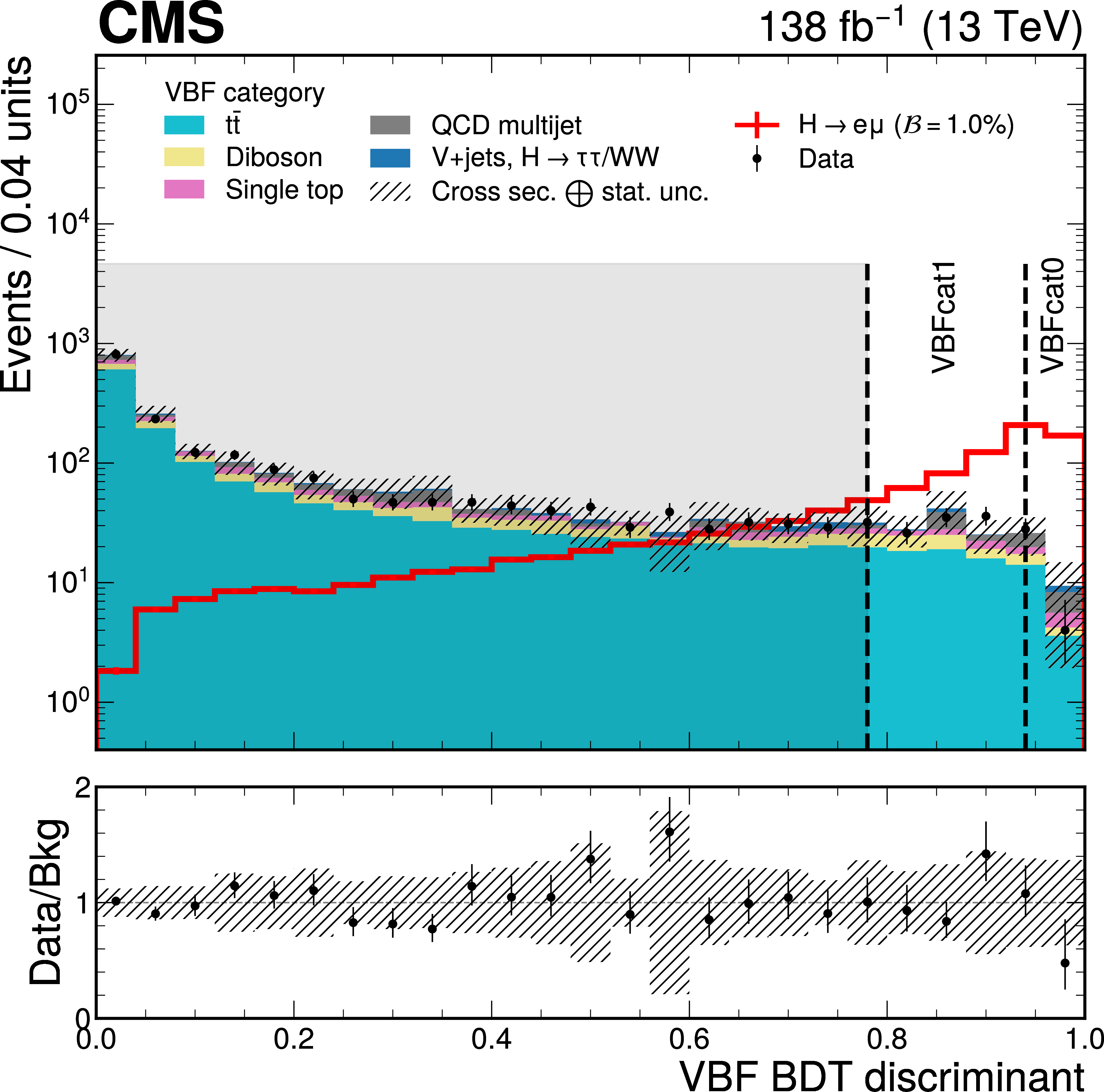
Figure 2:
The ggH and VBF BDT discriminant distributions of the data, simulated backgrounds and signals of $ {\mathrm{H}\to\mathrm{e}\mu} $ for each BDT trained in the ggH (left) and the VBF categories (right). A $ \mathcal{B}(\mathrm{H}\to\mathrm{e}\mu) =$ 1.0% is assumed for the signal for illustration. The lower panel in each plot shows the ratio of the data to the total estimated background. The uncertainty band corresponds to the background uncertainties, adding in quadrature the statistical and the SM cross section uncertainties. Vertical lines in the plots illustrate boundaries of the subcategories: ggH cat 0-3 and VBF cat 0-1, as defined in Section 6.2. Events in the shaded region of the VBF category with a VBF BDT discriminant less than 0.78 are discarded since their sensitivity is an order of magnitude lower than other subcategories. |
png pdf |
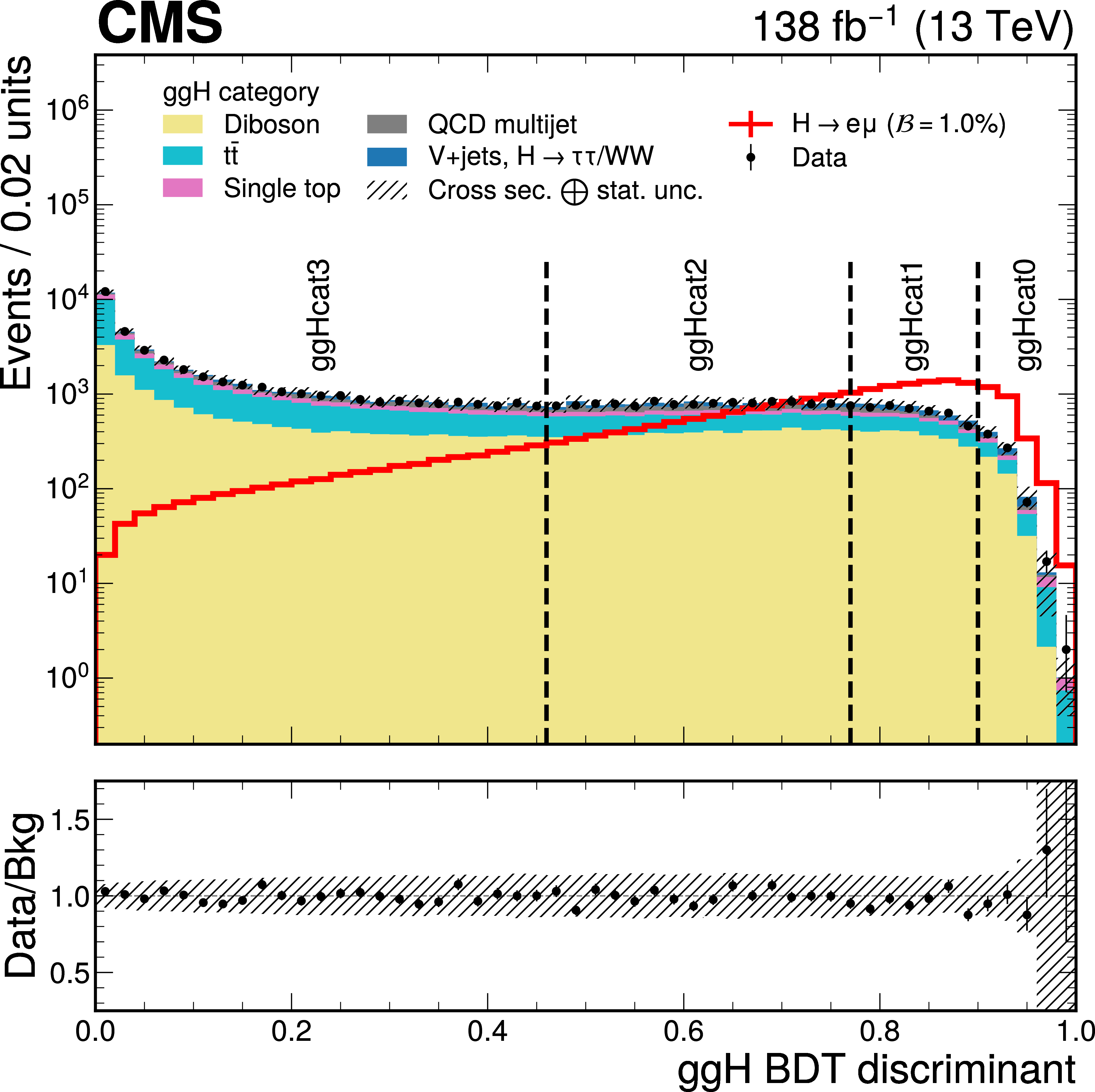
Figure 2-a:
The BDT discriminant distribution of the data, simulated backgrounds and signals of $ {\mathrm{H}\to\mathrm{e}\mu} $ for each BDT trained in the ggH category. A $ \mathcal{B}(\mathrm{H}\to\mathrm{e}\mu) =$ 1.0% is assumed for the signal for illustration. The lower panel shows the ratio of the data to the total estimated background. The uncertainty band corresponds to the background uncertainties, adding in quadrature the statistical and the SM cross section uncertainties. The vertical lines in the plot illustrate boundaries of the subcategories: ggH cat 0-3, as defined in Section 6.2. |
png pdf |
Figure 2-b:
The BDT discriminant distribution of the data, simulated backgrounds and signals of $ {\mathrm{H}\to\mathrm{e}\mu} $ for each BDT trained in the VBF category. A $ \mathcal{B}(\mathrm{H}\to\mathrm{e}\mu) =$ 1.0% is assumed for the signal for illustration. The lower panel shows the ratio of the data to the total estimated background. The uncertainty band corresponds to the background uncertainties, adding in quadrature the statistical and the SM cross section uncertainties. The vertical lines in the plot illustrate boundaries of the subcategories: VBF cat 0-1, as defined in Section 6.2. Events in the shaded region of the VBF category with a VBF BDT discriminant less than 0.78 are discarded since their sensitivity is an order of magnitude lower than other subcategories. |
png pdf |
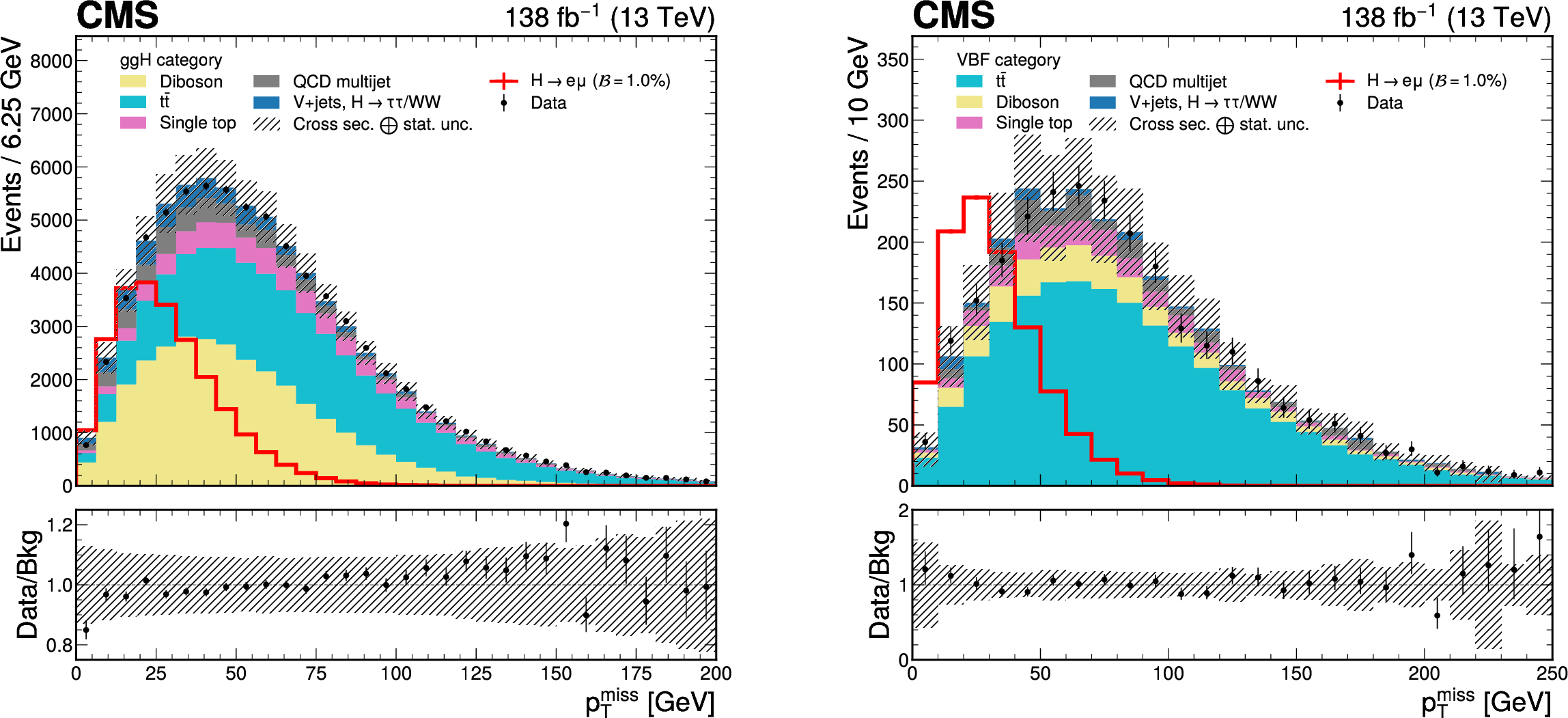
Figure 3:
The $ p_{\mathrm{T}}^\text{miss} $ distributions of the data, simulated backgrounds and signals of $ {\mathrm{H}\to\mathrm{e}\mu} $ in the ggH (left) and the VBF categories (right). A $ \mathcal{B}(\mathrm{H}\to\mathrm{e}\mu)= $ 1.0% is assumed for the signal for illustration. The lower panel in each plot shows the ratio of the data to the total estimated background. The uncertainty band corresponds to the background uncertainties, adding in quadrature the statistical and the SM cross section uncertainties. |
png pdf |
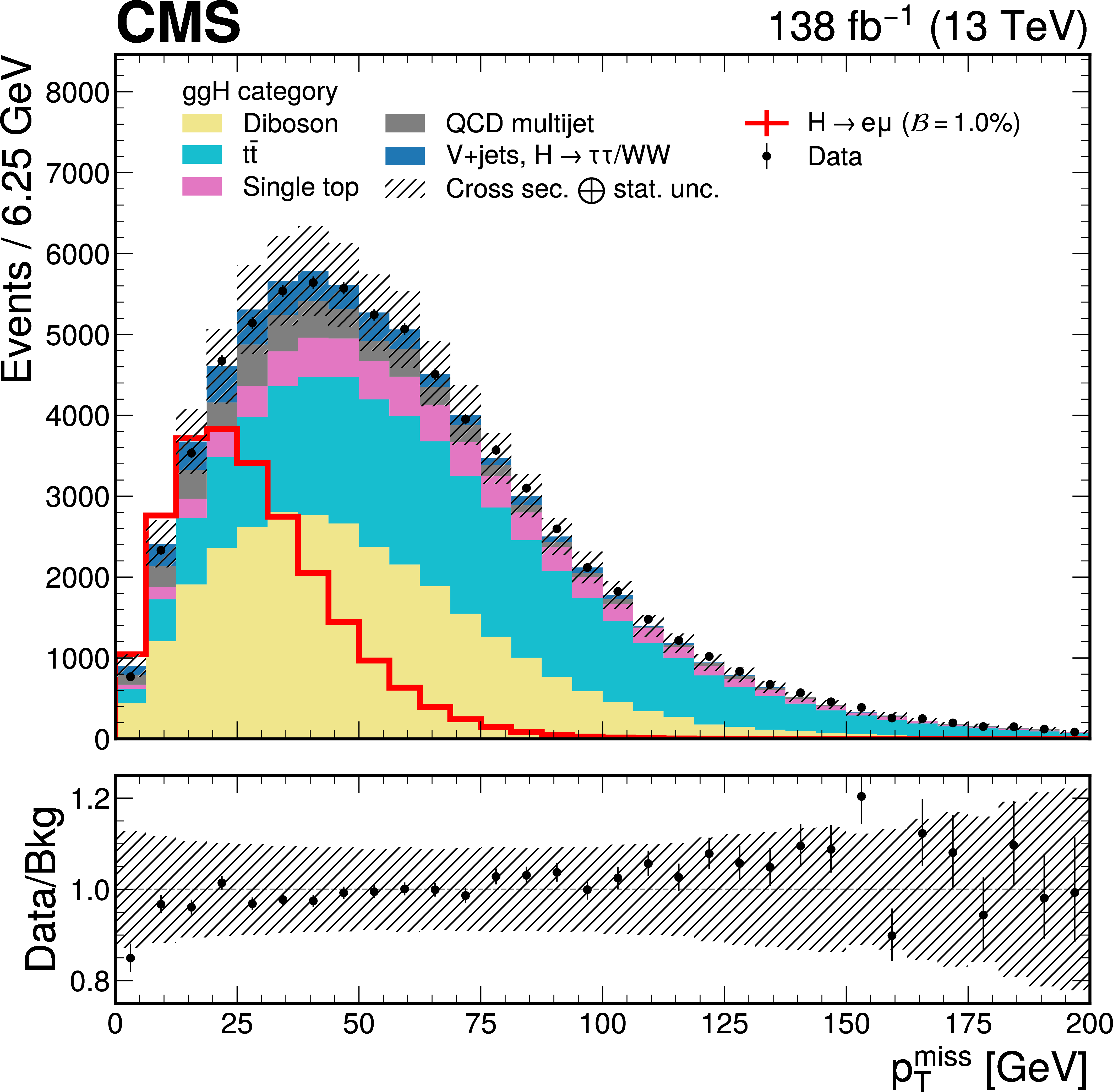
Figure 3-a:
The $ p_{\mathrm{T}}^\text{miss} $ distributions of the data, simulated backgrounds and signals of $ {\mathrm{H}\to\mathrm{e}\mu} $ in the ggH category. A $ \mathcal{B}(\mathrm{H}\to\mathrm{e}\mu)= $ 1.0% is assumed for the signal for illustration. The lower panel shows the ratio of the data to the total estimated background. The uncertainty band corresponds to the background uncertainties, adding in quadrature the statistical and the SM cross section uncertainties. |
png pdf |
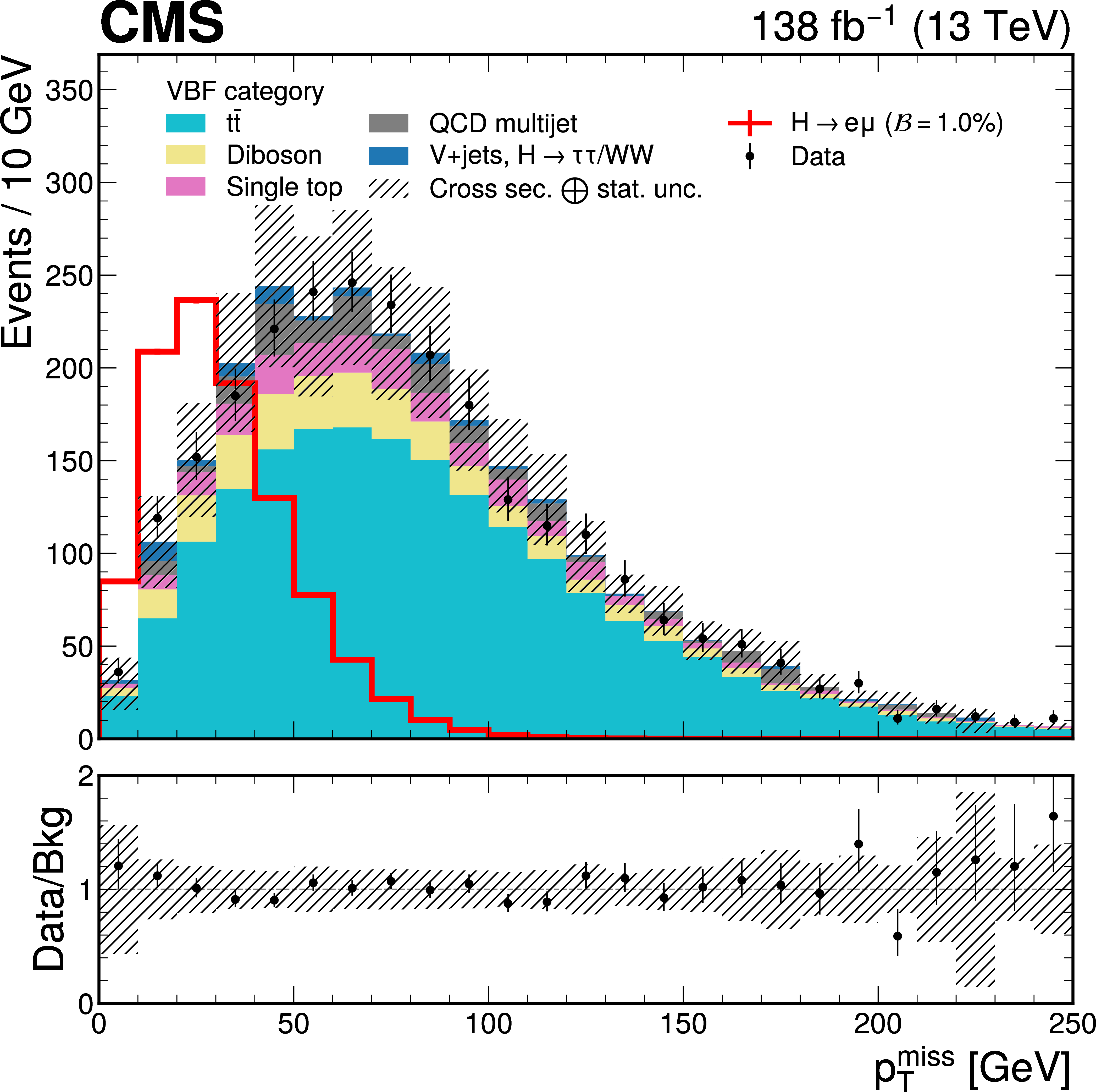
Figure 3-b:
The $ p_{\mathrm{T}}^\text{miss} $ distributions of the data, simulated backgrounds and signals of $ {\mathrm{H}\to\mathrm{e}\mu} $ in the VBF category. A $ \mathcal{B}(\mathrm{H}\to\mathrm{e}\mu)= $ 1.0% is assumed for the signal for illustration. The lower panel shows the ratio of the data to the total estimated background. The uncertainty band corresponds to the background uncertainties, adding in quadrature the statistical and the SM cross section uncertainties. |

png pdf |
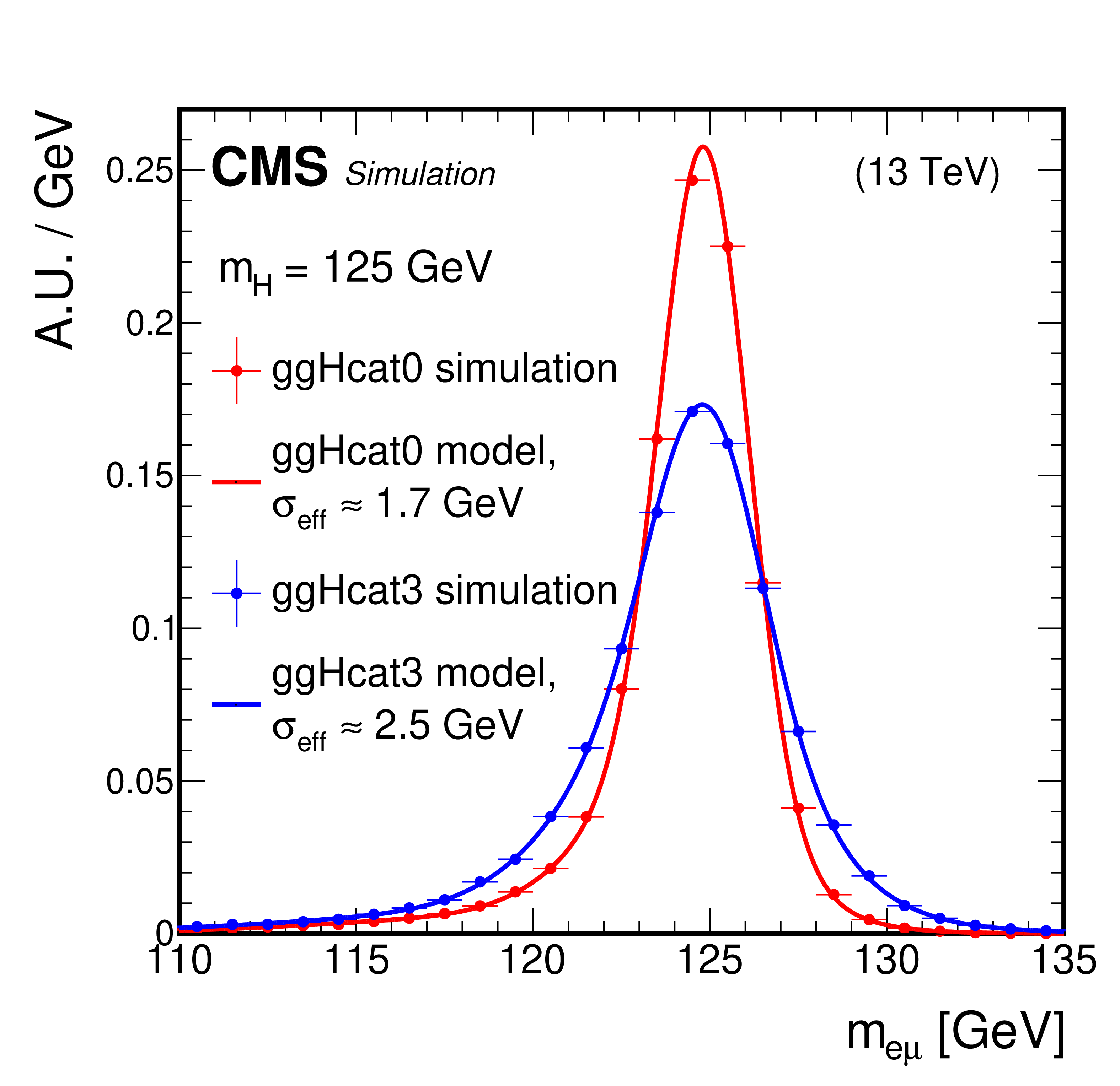
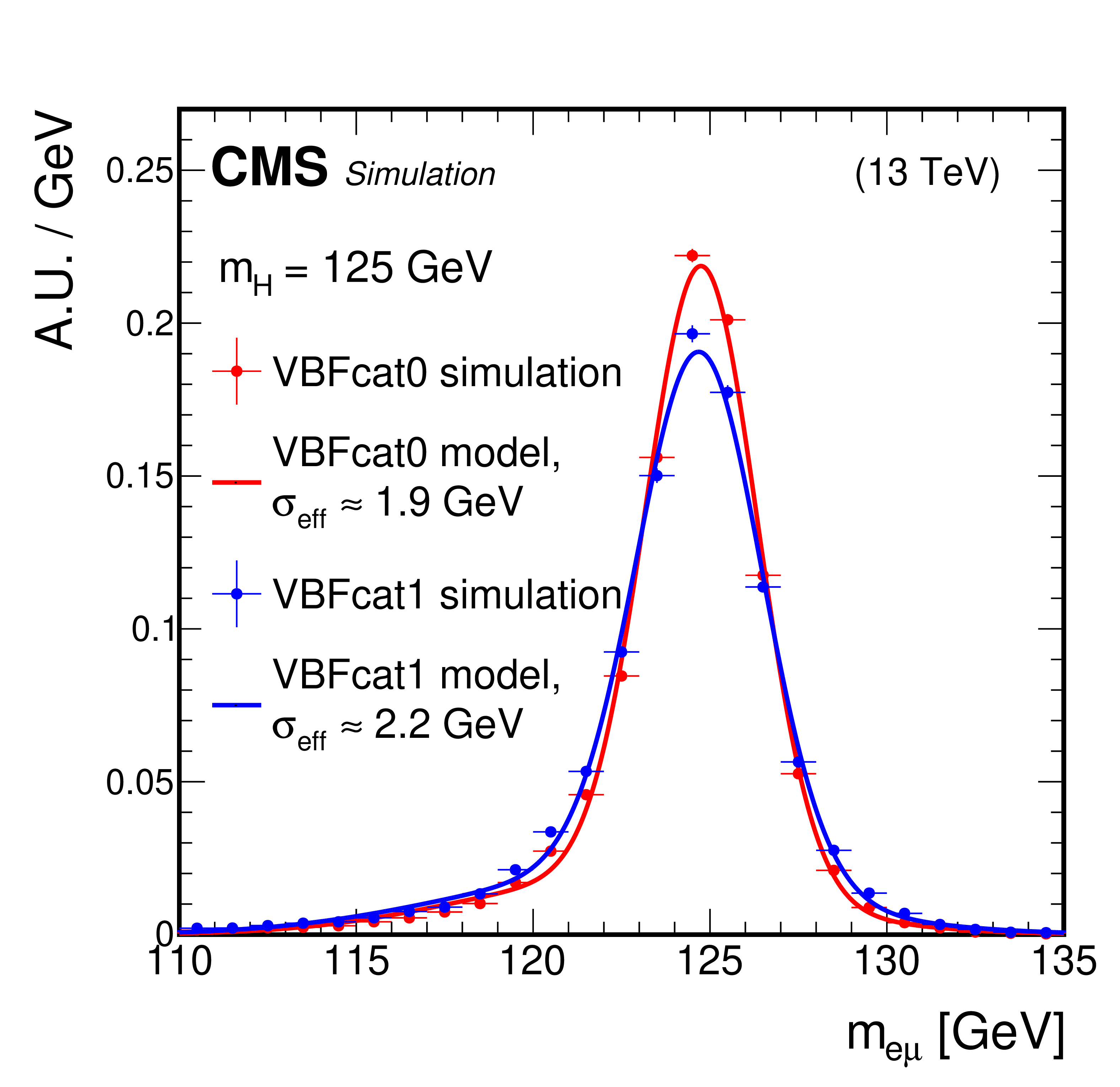
Figure 4:
Example fits of the signal models to the simulated $ {{\mathrm{H}\to\mathrm{e}\mu}} $ signal in the analysis categories ggH cat 0 and ggH cat 3 (left), as well as VBF cat 0 and VBF cat 1 (right), summing events from both the ggH and VBF production modes. Half of the smallest symmetric $ {m_{\mathrm{e}\mu}} $ interval that contains 68% of the signal events, $ {\sigma_{\text{eff}}} $, is shown in the legends for each signal as an illustration of the signal resolution. The signal resolution in general improves with the signal purity of the analysis categories. |
png pdf |
Figure 4-a:
Example fits of the signal models to the simulated $ {{\mathrm{H}\to\mathrm{e}\mu}} $ signal in the analysis categories ggH cat 0 and ggH cat 3, summing events from both the ggH and VBF production modes. Half of the smallest symmetric $ {m_{\mathrm{e}\mu}} $ interval that contains 68% of the signal events, $ {\sigma_{\text{eff}}} $, is shown in the legends for each signal as an illustration of the signal resolution. The signal resolution in general improves with the signal purity of the analysis categories. |
png pdf |
Figure 4-b:
Example fits of the signal models to the simulated $ {{\mathrm{H}\to\mathrm{e}\mu}} $ signal in the analysis categories VBF cat 0 and VBF cat 1, summing events from both the ggH and VBF production modes. Half of the smallest symmetric $ {m_{\mathrm{e}\mu}} $ interval that contains 68% of the signal events, $ {\sigma_{\text{eff}}} $, is shown in the legends for each signal as an illustration of the signal resolution. The signal resolution in general improves with the signal purity of the analysis categories. |
png pdf |
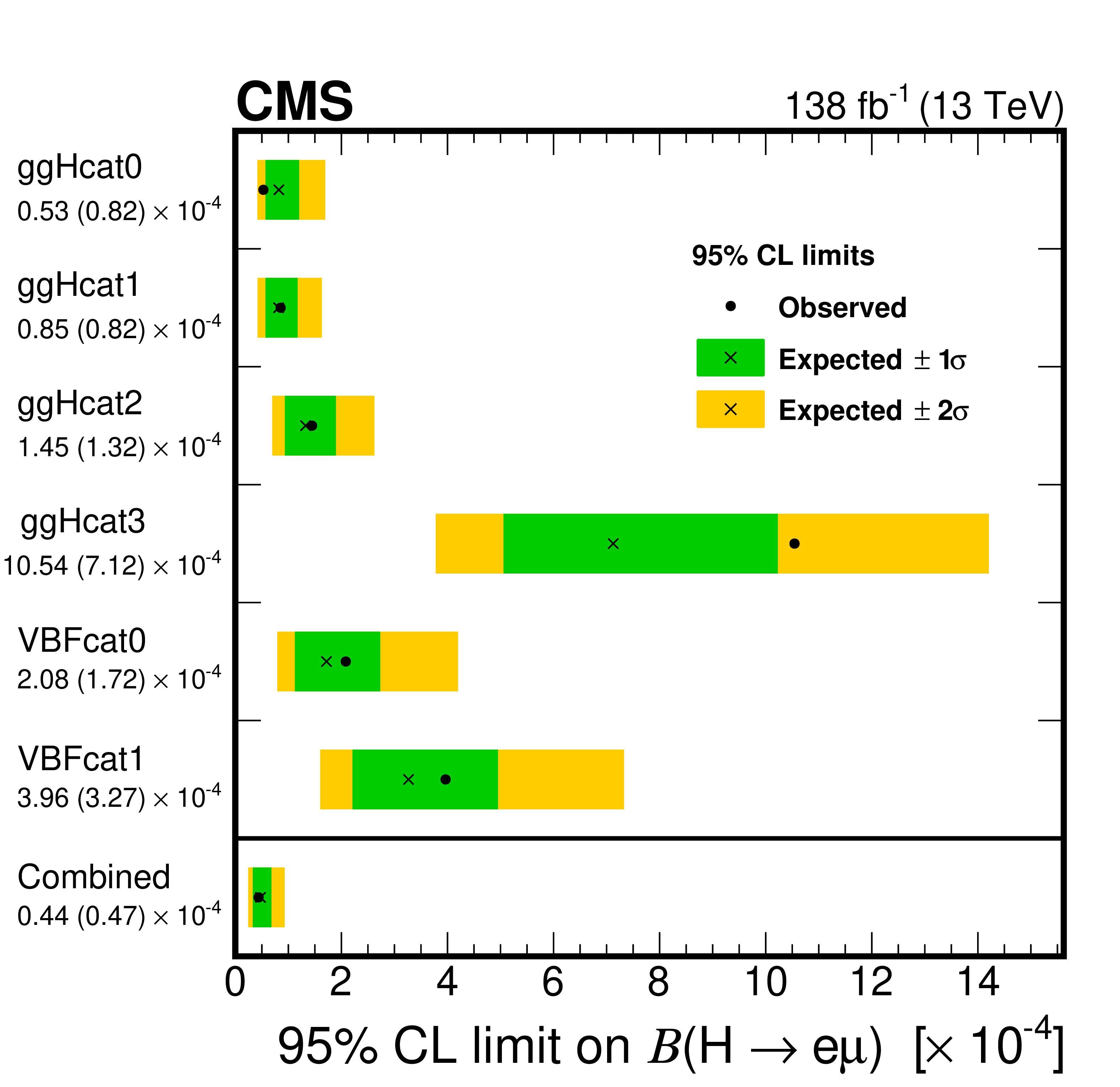
Figure 5:
Observed (expected) 95% CL upper limits on $ {\mathcal{B}(\mathrm{H}\to\mathrm{e}\mu)} $ for each individual analysis category (as shown in the left axis label) and for the combination of all analysis categories. |
png pdf |
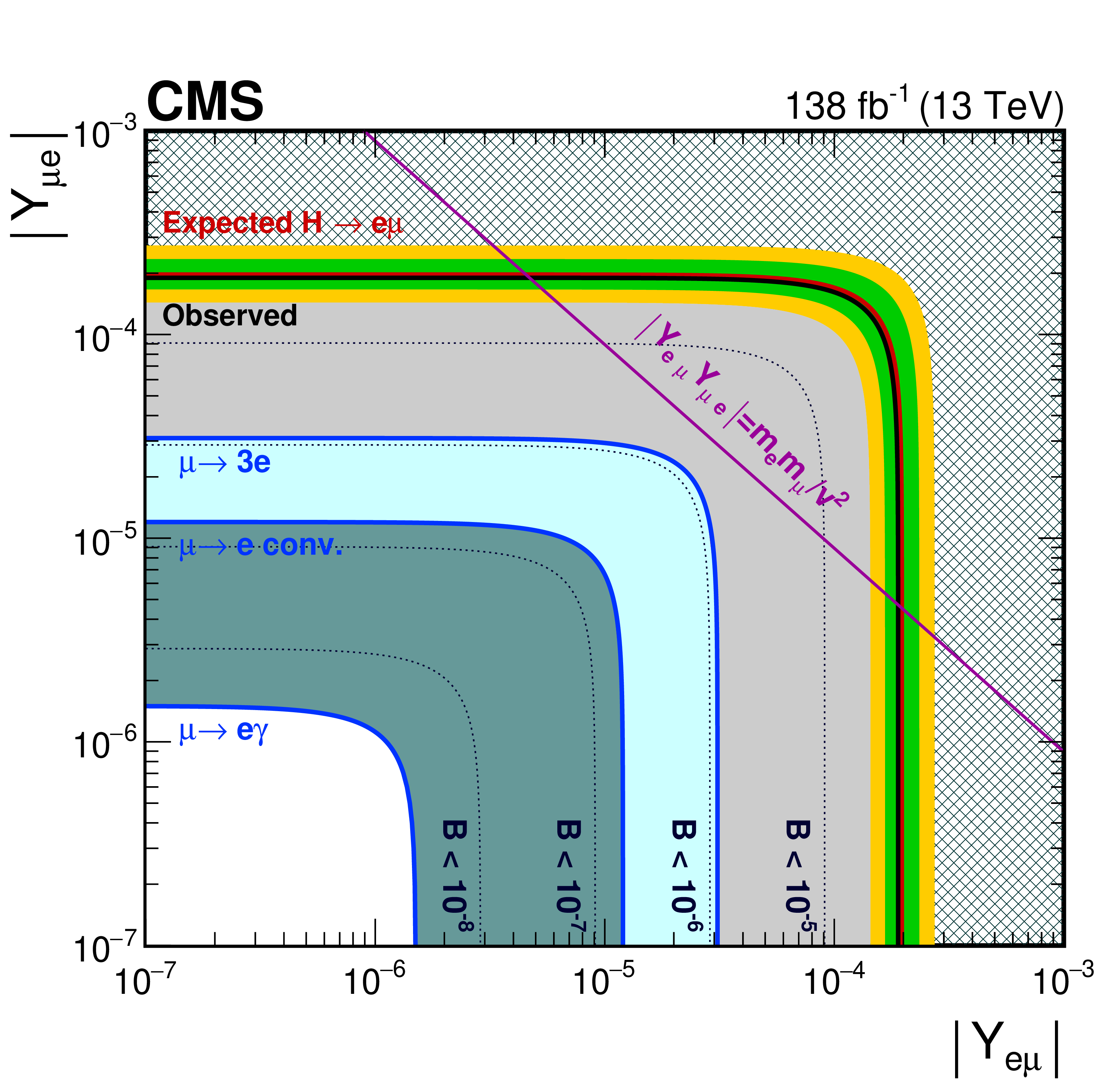
Figure 6:
Constraints on the lepton-flavor violating Yukawa couplings, $ {|Y_{\mathrm{e}\mu}|} $ and $ {|Y_{\mu\mathrm{e}}|} $. The observed (expected) limit in black (red) line is derived from the limit on $ {\mathcal{B}(\mathrm{H}\to\mathrm{e}\mu)} $ in this analysis. The green (yellow) band indicates the one (two) standard deviation uncertainty in the expected limit. The hashed region is excluded by this direct search. Other shaded regions represent indirect constraints derived from the null searches for $ {\mu\to3\mathrm{e}} $ (gray) [89], $ {\mu\to\mathrm{e}} $ conversion (light blue) [90], and $ {\mu\to\mathrm{e}\gamma} $ (dark green) [31]. The flavor-diagonal Yukawa couplings, $ {|Y_{\mathrm{e}\mathrm{e}}|} $ and $ {|Y_{\mu\mu}|} $, are assumed to be at their SM values in the calculation of these indirect limits. The purple line is the theoretical naturalness limit of $ {|Y_{\mathrm{e}\mu}Y_{\mu\mathrm{e}}|\leq{m_{\mathrm{e}}}m_{\mu}/v^2} $, where $ {v} $ is the vacuum expectation value of the Higgs field. Dotted lines represent the corresponding constraints on $ {|Y_{\mathrm{e}\mu}|} $ and $ {|Y_{\mu\mathrm{e}}|} $ at upper limits on $ {{\mathcal{B}(\mathrm{H}\to\mathrm{e}\mu)}} $ at 10$^{-5}$, 10$^{-6}$, 10$^{-7}$, and 10$^{-8} $, respectively. |
png pdf |
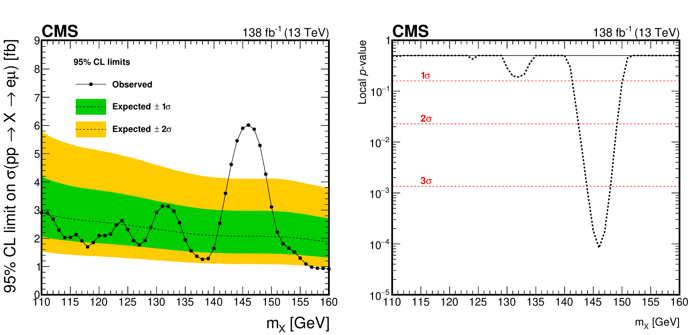
Figure 7:
Left: the observed (expected) 95% CL upper limits on $ {\sigma(\mathrm{p}\mathrm{p} \to \mathrm{X} \to \mathrm{e} \mu)} $ as a function of the hypothesised $ {m_{\mathrm{X}}} $ assuming the relative SM-like production cross sections of the ggH and VBF production modes. Right: the observed local $ p $-values against the background-only hypothesis are shown as a function of the hypothesised $ {m_{\mathrm{X}}} $. |
png pdf |
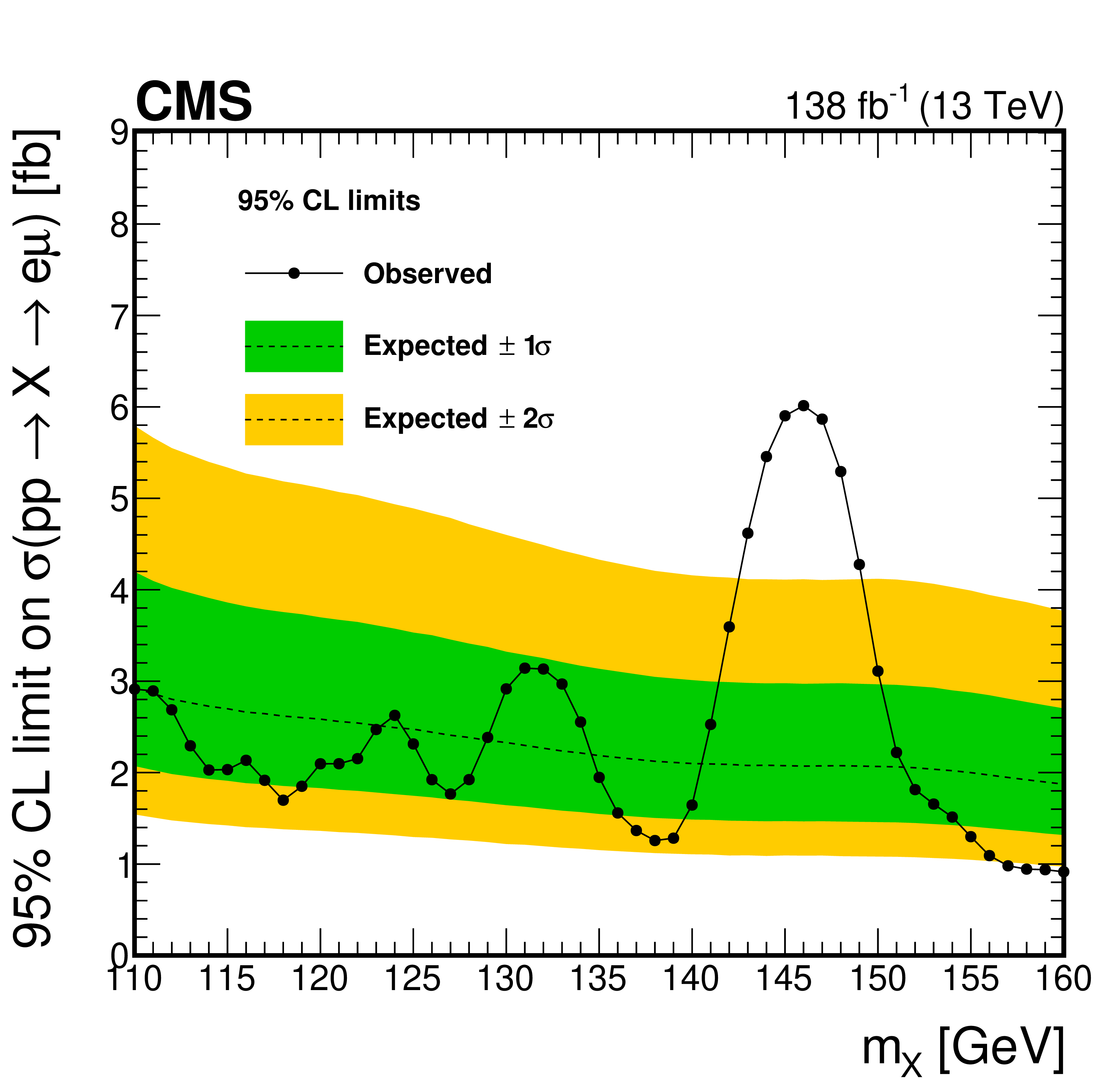
Figure 7-a:
The observed (expected) 95% CL upper limits on $ {\sigma(\mathrm{p}\mathrm{p} \to \mathrm{X} \to \mathrm{e} \mu)} $ as a function of the hypothesised $ {m_{\mathrm{X}}} $ assuming the relative SM-like production cross sections of the ggH and VBF production modes. |
png pdf |
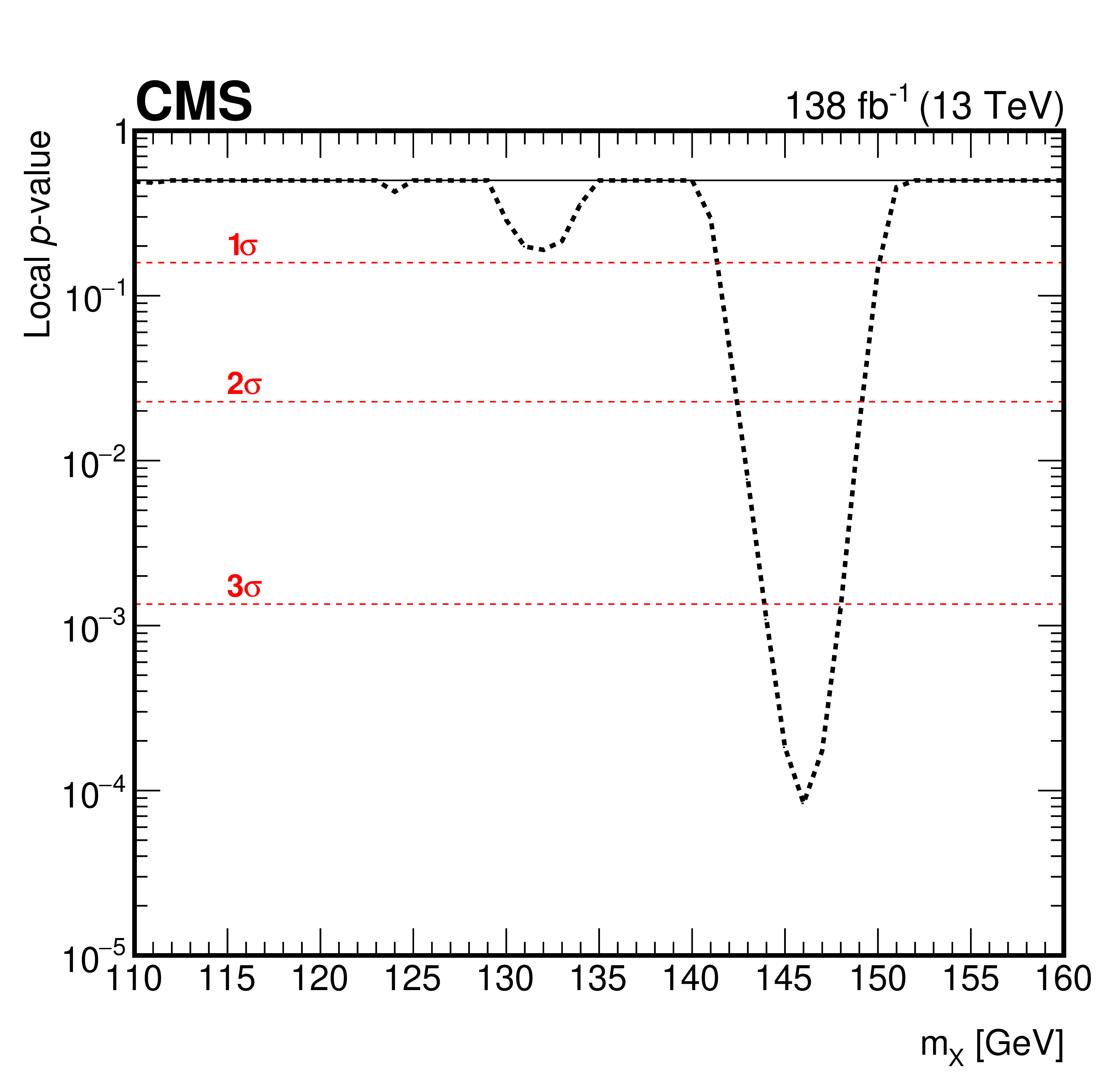
Figure 7-b:
The observed local $ p $-values against the background-only hypothesis are shown as a function of the hypothesised $ {m_{\mathrm{X}}} $. |
png pdf |
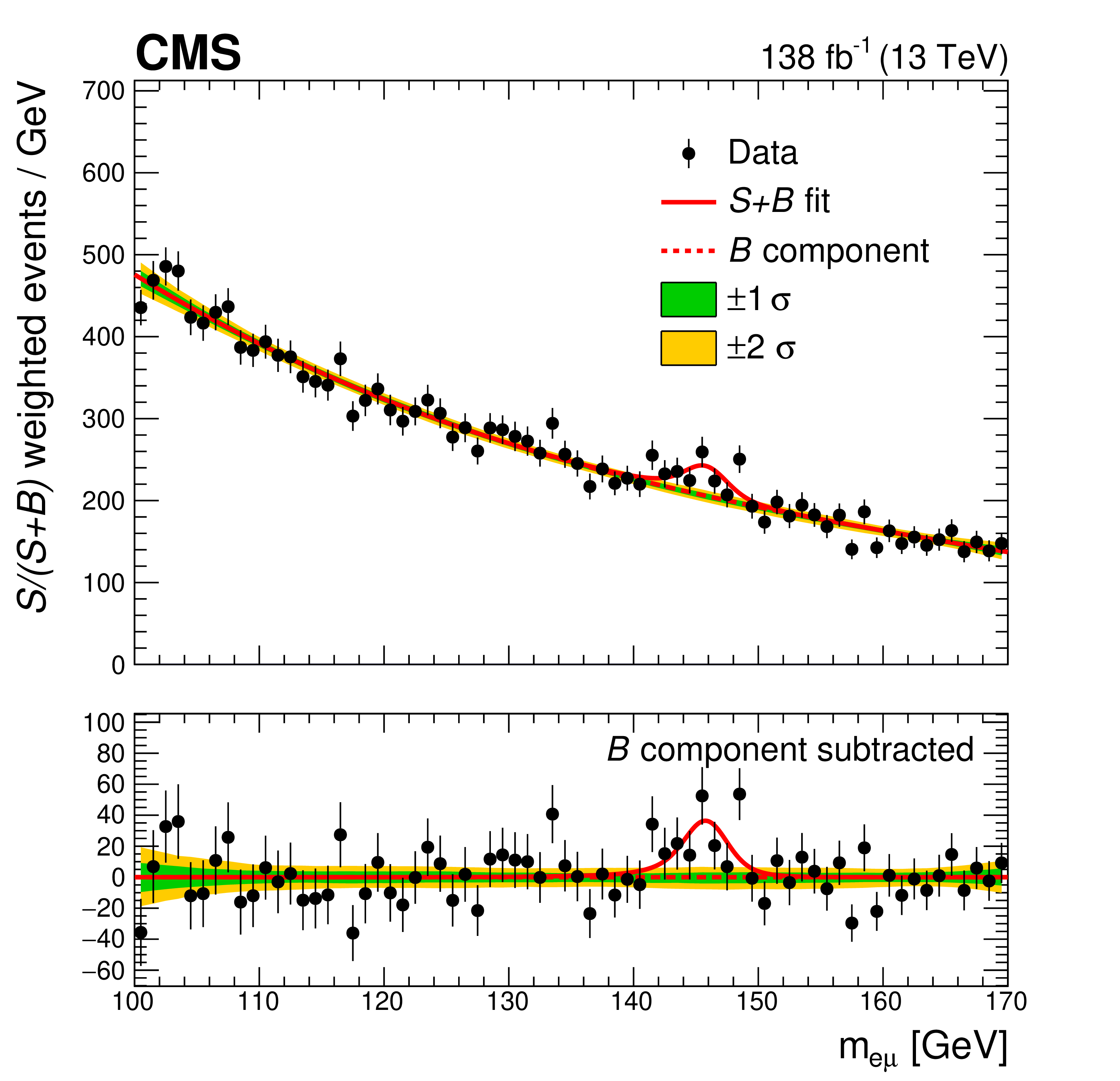
Figure 8:
The $ {m_{\mathrm{e}\mu}} $ distribution of the observed data is shown, with the $ S{+}B $ fit at $ m_{\mathrm{X}}= $ 146 GeV in red solid line, and the background component of the fit in red dotted line. Events and fit in each category are weighted by $ {S/(S+B)} $. The one and two standard deviation uncertainty bands of the background component are shown in green and yellow. The lower panel shows the residuals after subtracting the background component of the fit from data. |
png pdf |
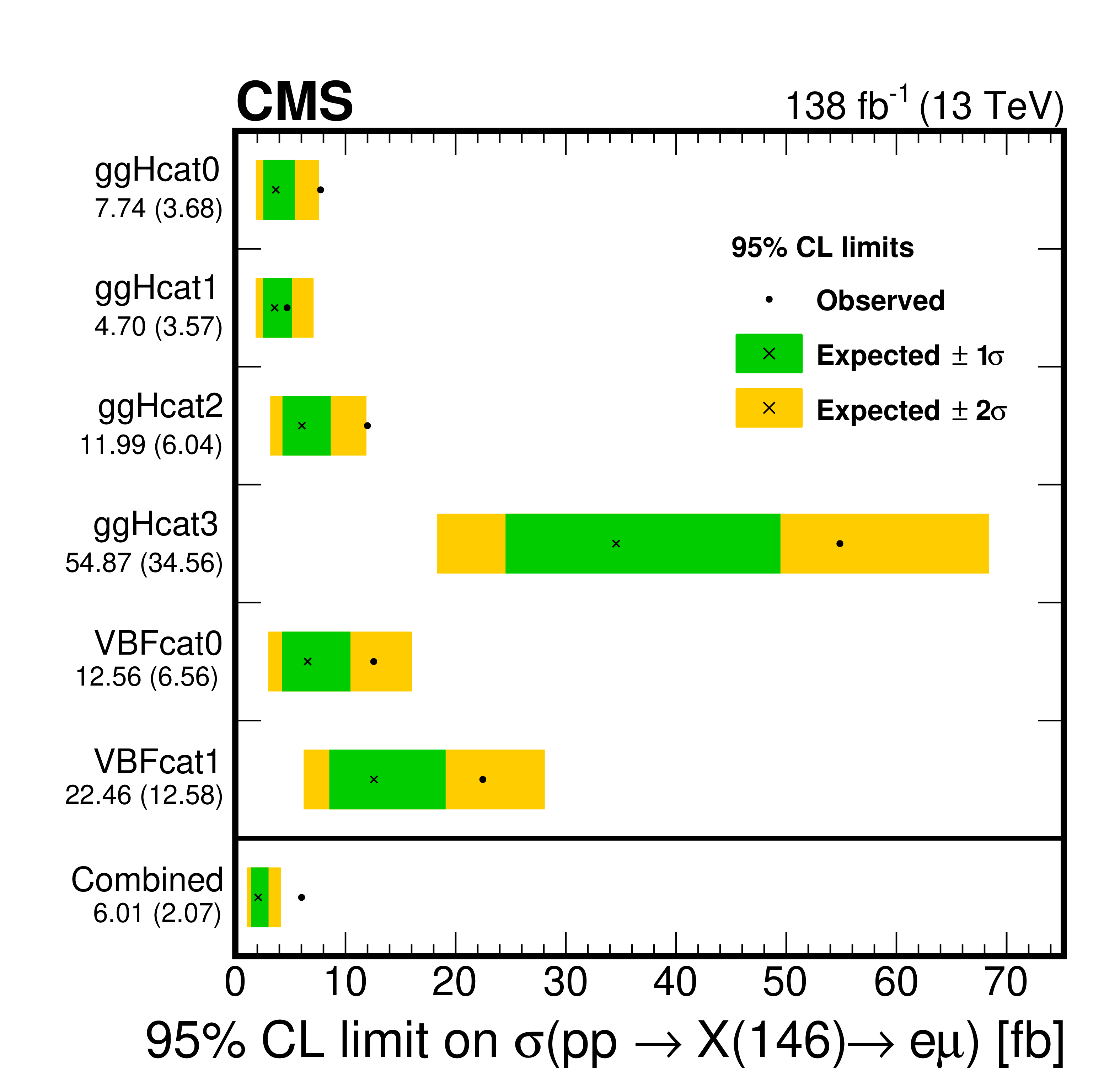
Figure 9:
Observed (expected) 95% CL upper limits on $ {\sigma(\mathrm{p}\mathrm{p} \to \mathrm{X}(146) \to \mathrm{e} \mu)} $ for each individual analysis category (as shown in the left axis label) and for the combination of all analysis categories assuming the relative SM-like production cross sections of the ggH and VBF production modes. |
| Tables | |
png pdf |
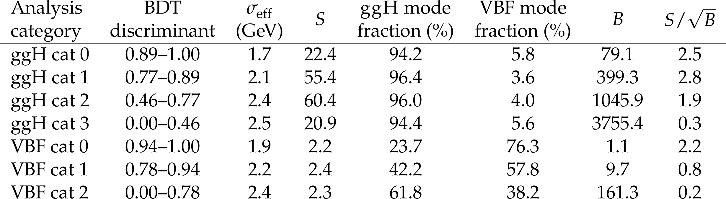
Table 1:
Range of the ggH (VBF) BDT discriminant to define the ggH (VBF) subcategories, and the corresponding expected background ($ {B} $), and signal yield of $ \mathrm{H}\to\mathrm{e}\mu $ at $ \mathcal{B}= $ 10$^{-4} $ ($ {S} $) at an integrated luminosity of 138 fb$ ^{-1} $. The yields are estimated by the number of MC events within a $ {m_{\mathrm{e}\mu}} $ interval of 125 GeV $\pm\sigma_\text{eff} $, where $ {\sigma_\text{eff}} $ is half of the smallest symmetric interval that contains 68% of the signal events in each category. The fraction contributions of the expected signal yields from the ggH and VBF production mode are listed. An estimate of the expected significance in each category by $ {S/\sqrt{B}} $ is also listed. |
png pdf |
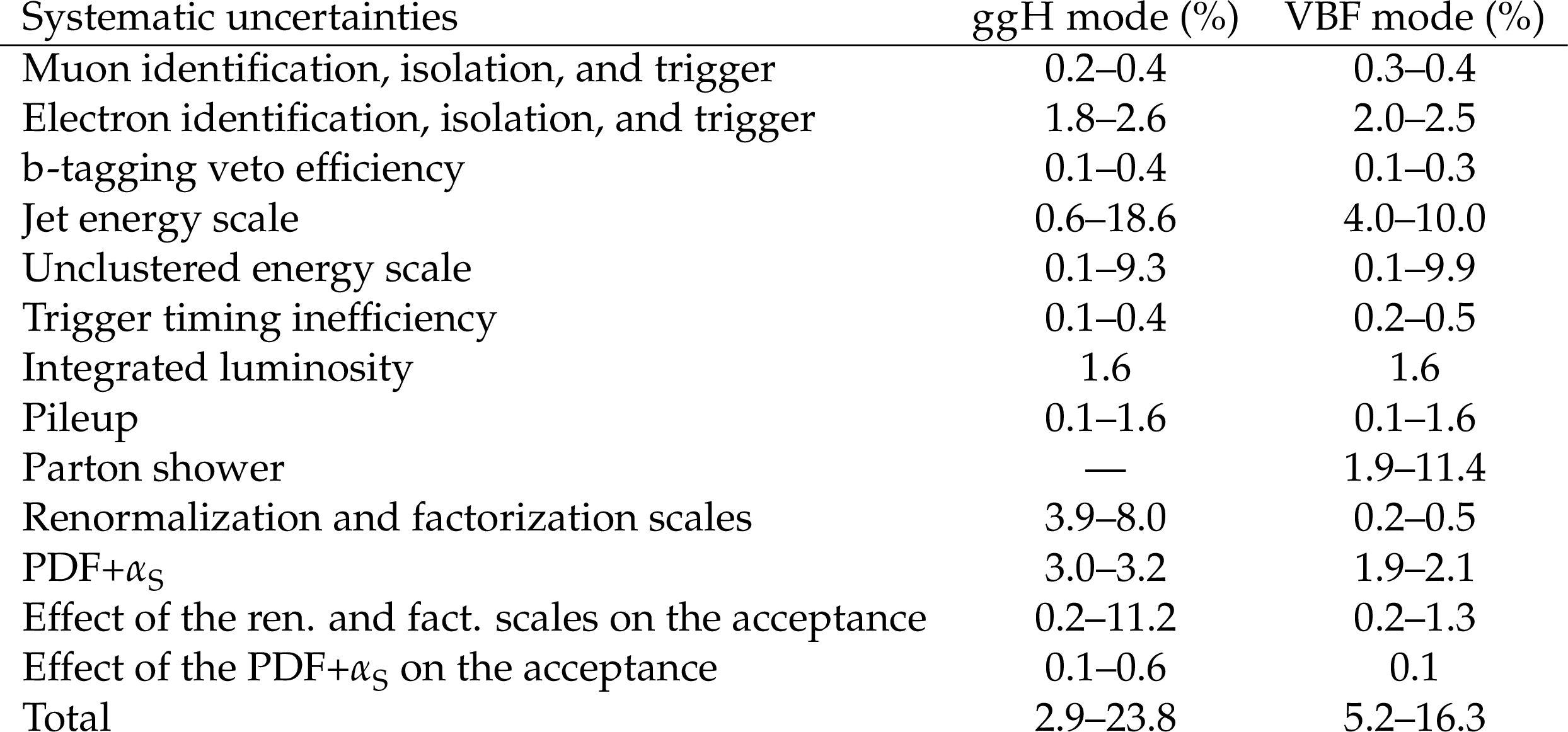
Table 2:
Systematic uncertainties in the expected signal yields from different sources for the ggH and VBF production modes. All the uncertainties are treated as correlated among categories. |

png pdf |
Table 3:
Observed and expected 95% CL upper limits on $ {\mathcal{B}(\mathrm{H}\to\mathrm{e}\mu)} $ at for each individual analysis category and for the combination of all analysis categories. |
png pdf |
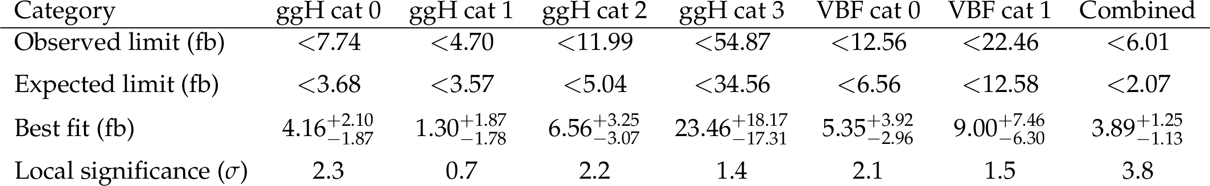
Table 4:
Observed (expected) 95% CL upper limits, best fit, and local significance in unit of standard deviation ($ {\sigma} $) of $ {\sigma(\mathrm{p}\mathrm{p} \to \mathrm{X}(146) \to \mathrm{e} \mu)} $ for each individual analysis category and for the combination of all analysis categories. |
| Summary |
| Searches for the lepton-flavor violation decay of H and X with a $ {m_{\mathrm{X}}} $ in the range 110-160 GeV have been performed in the $ \mathrm{e} \mu $ final state in data collected by the CMS experiment. The data correspond to an integrated luminosity of 138 fb$ ^{-1} $ of pp collisions at a center-of-mass energy of 13 TeV. The observed (expected) upper limit on the branching fraction of the H decay $ {\mathcal{B}(\mathrm{H}\to\mathrm{e}\mu)} $ is found to be 4.4 (4.7) $\times$ 10$^{-5} $ at 95% confidence level, which is the most stringent direct limit set thus far. Upper limits on the cross sections of $ {\mathrm{p}\mathrm{p} \to \mathrm{X} \to \mathrm{e} \mu} $ are set in the $ {m_{\mathrm{X}}} $ range 110-160 GeV at 95% confidence level. This is the first result of a direct search for $ {\mathrm{X}\to\mathrm{e}\mu} $, with $ {m_{\mathrm{X}}} $ below twice the W boson mass. The largest excess of events over the expected background is observed with a local (global) significance of 3.8 (2.8) standard deviations at an invariant mass of the $ \mathrm{e} \mu $ final state of around 146 GeV. The observed significance of this excess is insufficient to draw any conclusions. More data will be needed to clarify the nature of the excess. |
| Additional Figures | |
png pdf |
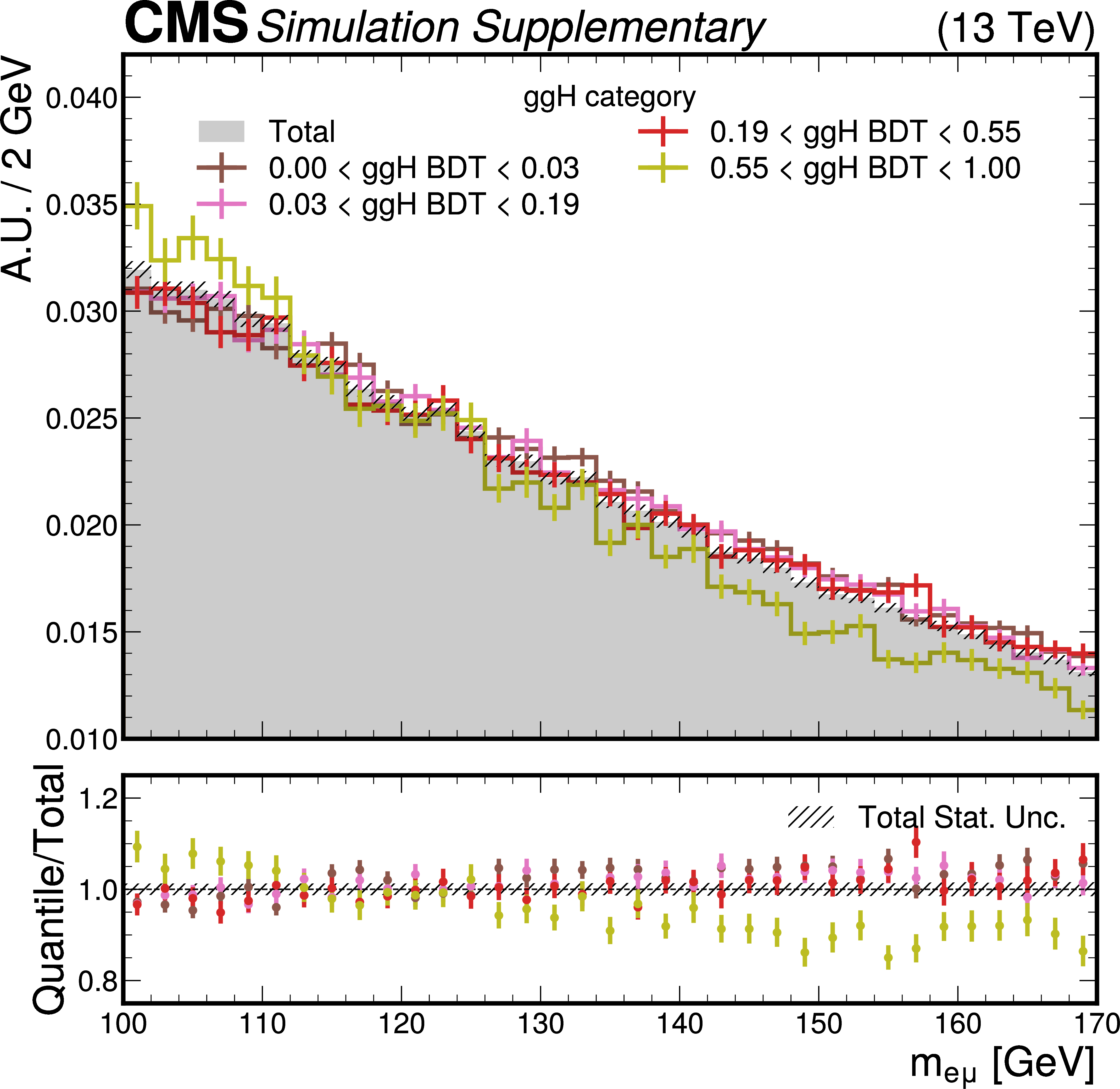
Additional Figure 1:
To investigate whether there is sculpting of the $ m_{\mathrm{e}\mu} $ spectrum near the $ m_{\mathrm{H}} $ or $ m_{\mathrm{X}} $ of the signal samples, we look at the $ m_{\mathrm{e}\mu} $ distributions in different ranges of the $ {\mathrm{g}\mathrm{g}\mathrm{H}} $ BDT discriminant in the $ {\mathrm{g}\mathrm{g}\mathrm{H}} $ category. The upper panel shows the $ m_{\mathrm{e}\mu} $ density distributions of the MC background samples in quantiles of the $ {\mathrm{g}\mathrm{g}\mathrm{H}} $ BDT discriminant with the same expected yield. The total $ m_{\mathrm{e}\mu} $ density distribution is also plotted. The lower panel shows the ratio of each quantile to the total density distribution. No localized patterns at $ {m_{\mathrm{e}\mu}=} $ 110, 120, 125, 130, 140, 150, 160 GeV, corresponding to the $ m_{\mathrm{H}} $ or $ m_{\mathrm{X}} $ of the signal samples used in the BDT trainings, is observed for events with high or low BDT discriminants. This demonstrates that the BDTs do not preferentially identify events near $ m_{\mathrm{H}} $ or $ m_{\mathrm{X}} $ as signal. |
png pdf |
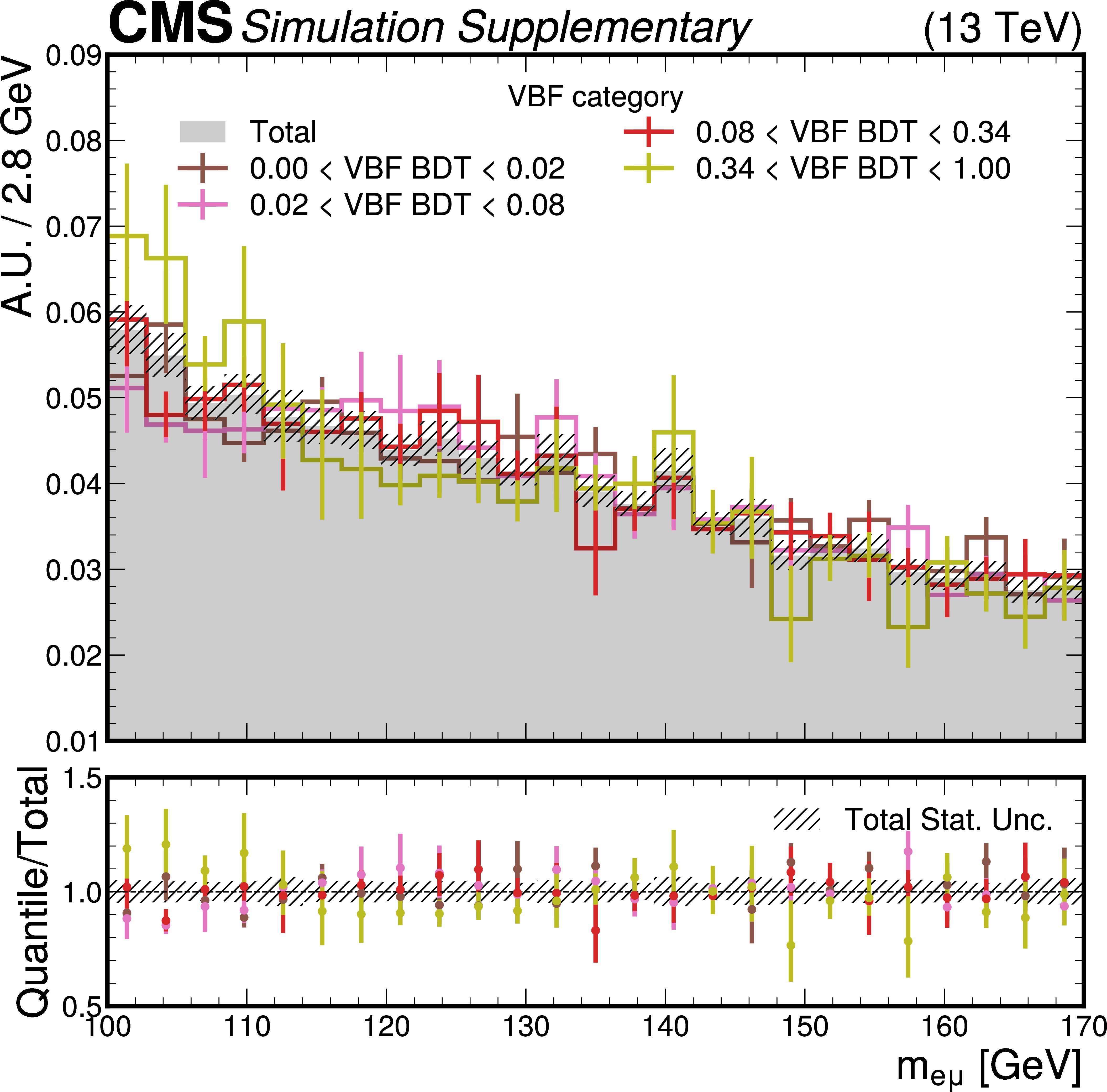
Additional Figure 2:
To investigate whether there is sculpting of the $ m_{\mathrm{e}\mu} $ spectrum near the $ m_{\mathrm{H}} $ or $ m_{\mathrm{X}} $ of the signal samples, we look at the $ m_{\mathrm{e}\mu} $ distributions in different ranges of the VBF BDT discriminant in the VBF category. The upper panel shows the $ m_{\mathrm{e}\mu} $ density distributions of the MC background samples in quantiles of the VBF BDT discriminant with the same expected yield. The total $ m_{\mathrm{e}\mu} $ density distribution is also plotted. The lower panel shows the ratio of each quantile to the total density distribution. No localized patterns at $ {m_{\mathrm{e}\mu}=} $ 110, 120, 125, 130, 140, 150, 160 GeV, corresponding to the $ m_{\mathrm{H}} $ or $ m_{\mathrm{X}} $ of the signal samples used in the BDT trainings, is observed for events with high or low BDT discriminants. This demonstrates that the BDTs do not preferentially identify events near $ m_{\mathrm{H}} $ or $ m_{\mathrm{X}} $ as signal. |
png pdf |
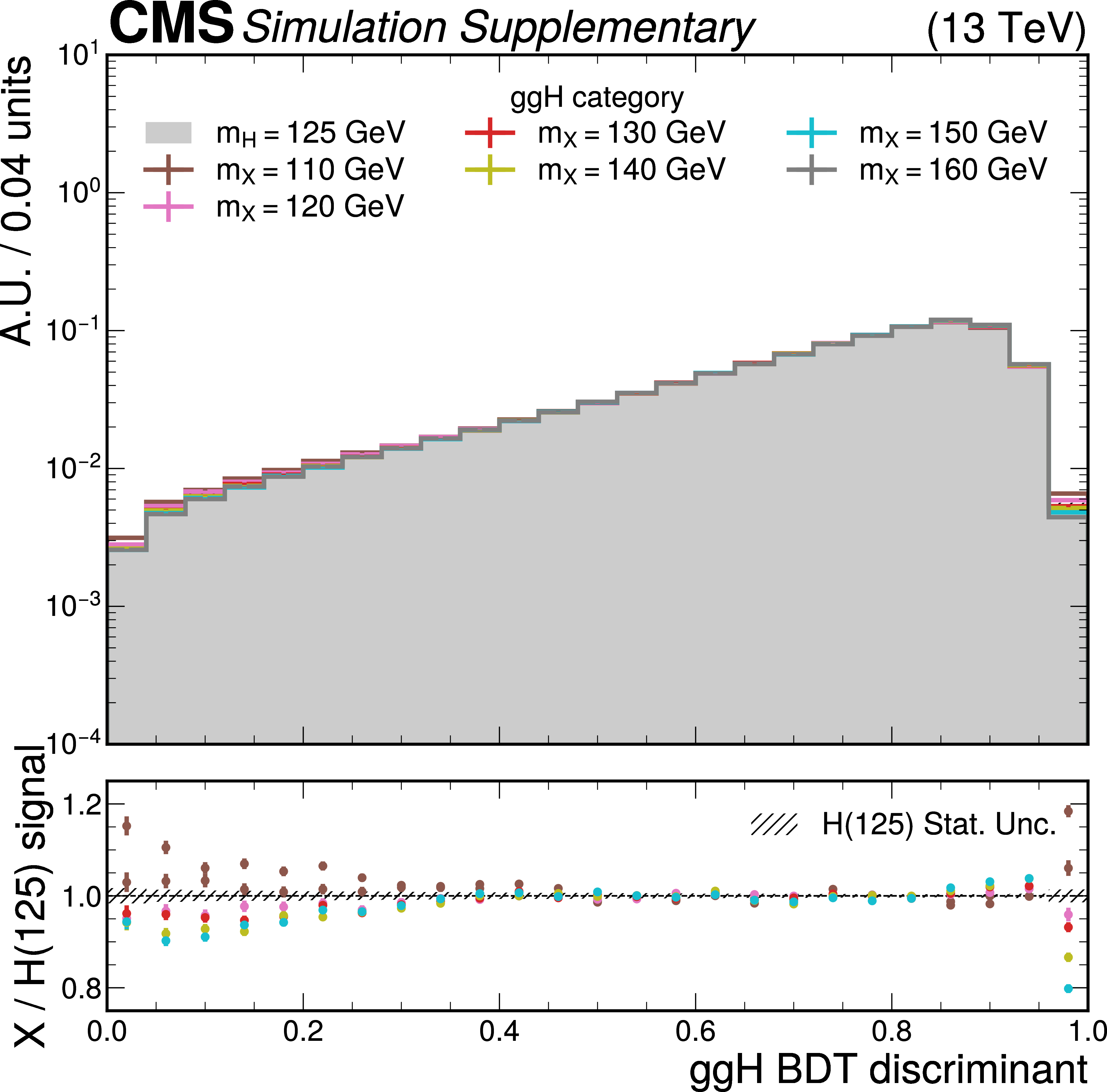
Additional Figure 3:
The $ {\mathrm{g}\mathrm{g}\mathrm{H}} $ discriminant density distributions of the MC signal samples in the $ {\mathrm{g}\mathrm{g}\mathrm{H}} $ category are shown. The lower panel shows the ratios of the $ {{\mathrm{X}\to\mathrm{e}\mu}} $ samples to the $ {{\mathrm{H}\to\mathrm{e}\mu}} $ samples. The uncertainty band corresponds to the statistical uncertainties of the $ {{\mathrm{H}\to\mathrm{e}\mu}} $ samples. |
png pdf |
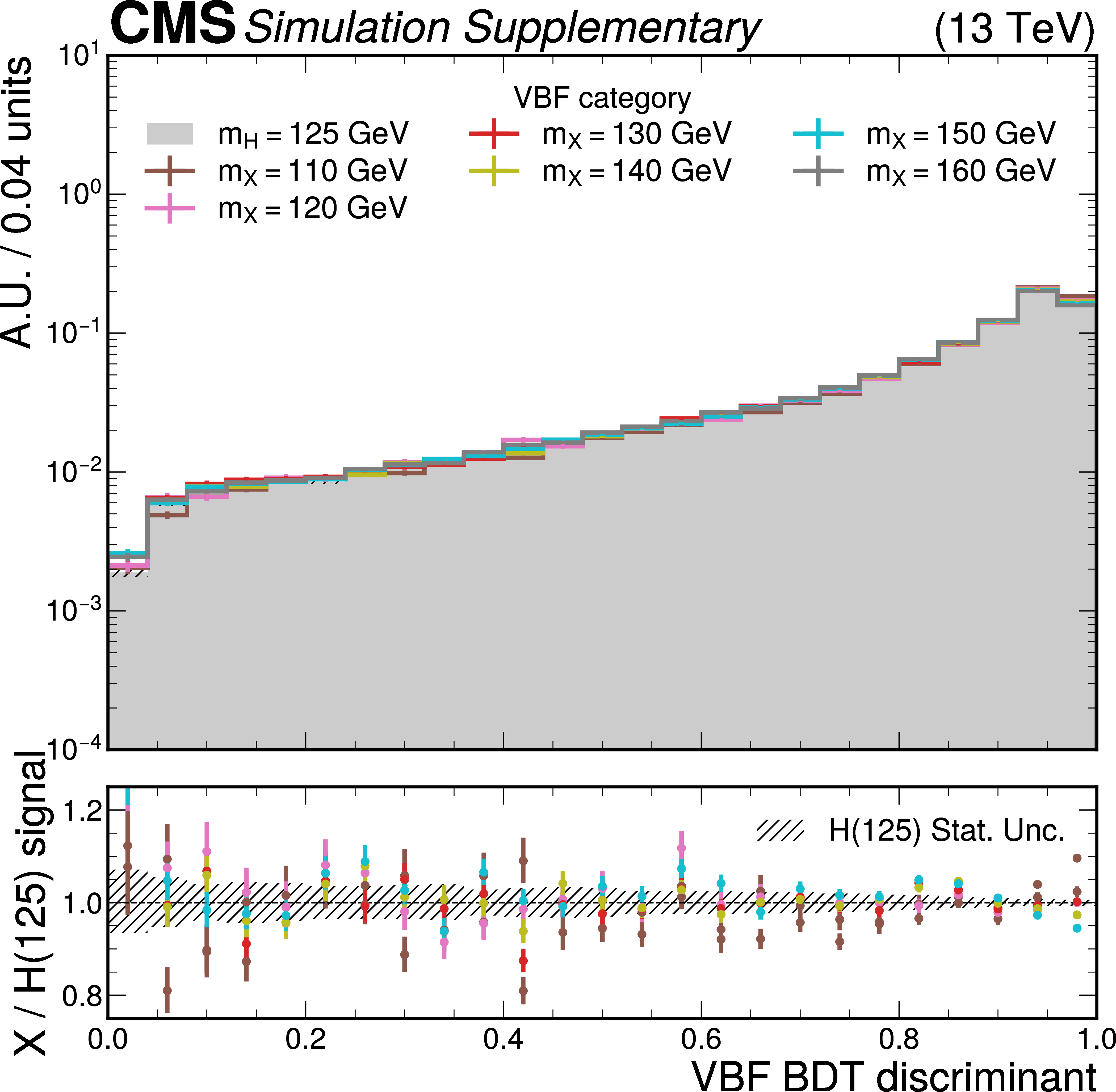
Additional Figure 4:
The VBF discriminant density distributions of the MC signal samples in the VBF category are shown. The lower panel shows the ratios of the $ {{\mathrm{X}\to\mathrm{e}\mu}} $ samples to the $ {{\mathrm{H}\to\mathrm{e}\mu}} $ samples. The uncertainty band corresponds to the statistical uncertainties of the $ {{\mathrm{H}\to\mathrm{e}\mu}} $ samples. |
png pdf |
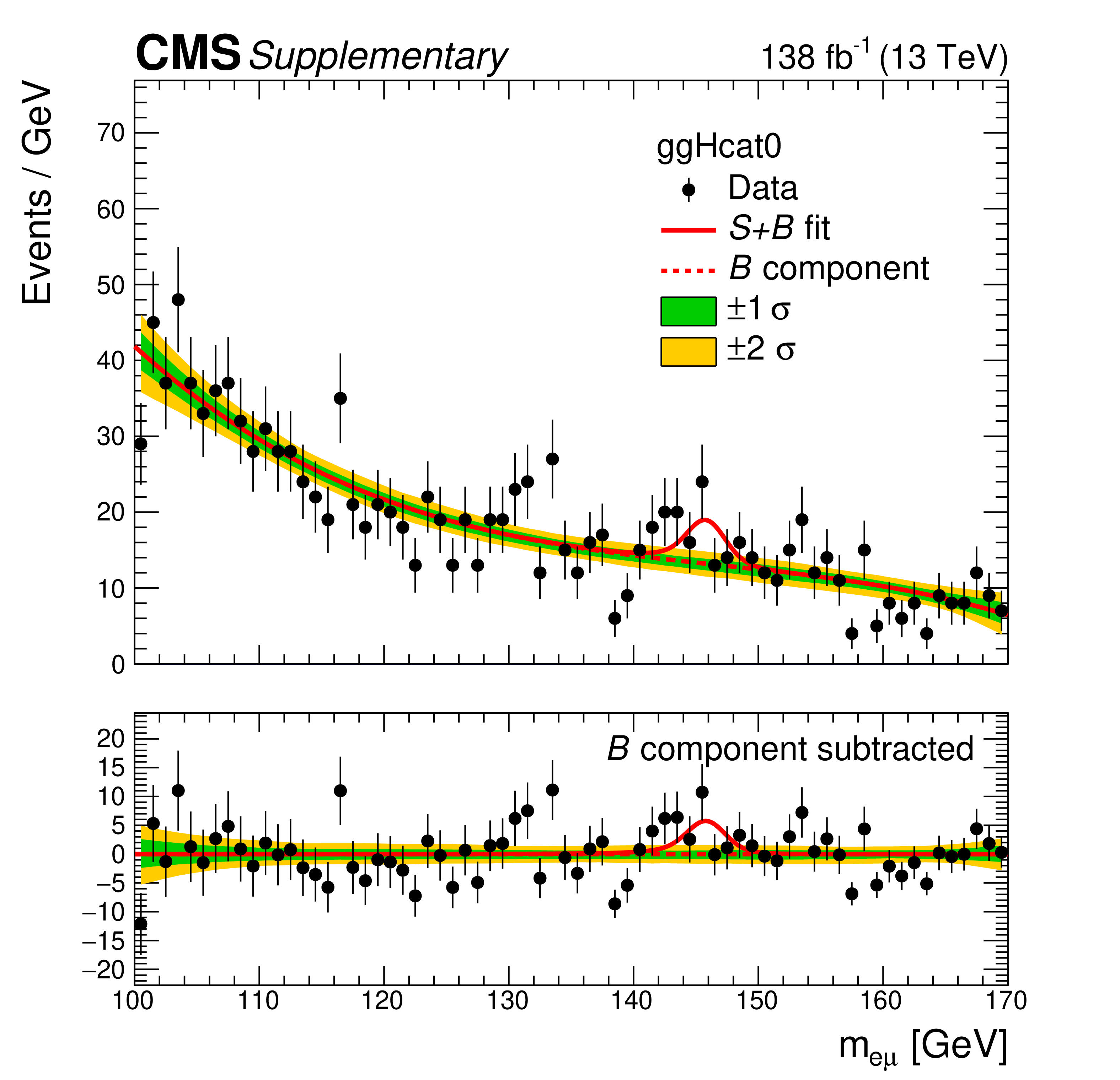
Additional Figure 5:
The $ m_{\mathrm{e}\mu} $ distribution of the observed data in the category $ {\mathrm{g}\mathrm{g}\mathrm{H}} $ cat 0 is shown, with the $ S{+}B $ fit at $ m_{\mathrm{X}}= $ 146 GeV in solid red line, and the background component of the fit in dotted red line. The green and yellow bands represent the one and two standard deviations of the background component. The lower panel shows the residuals after subtracting the background component of the fit from data. |
png pdf |
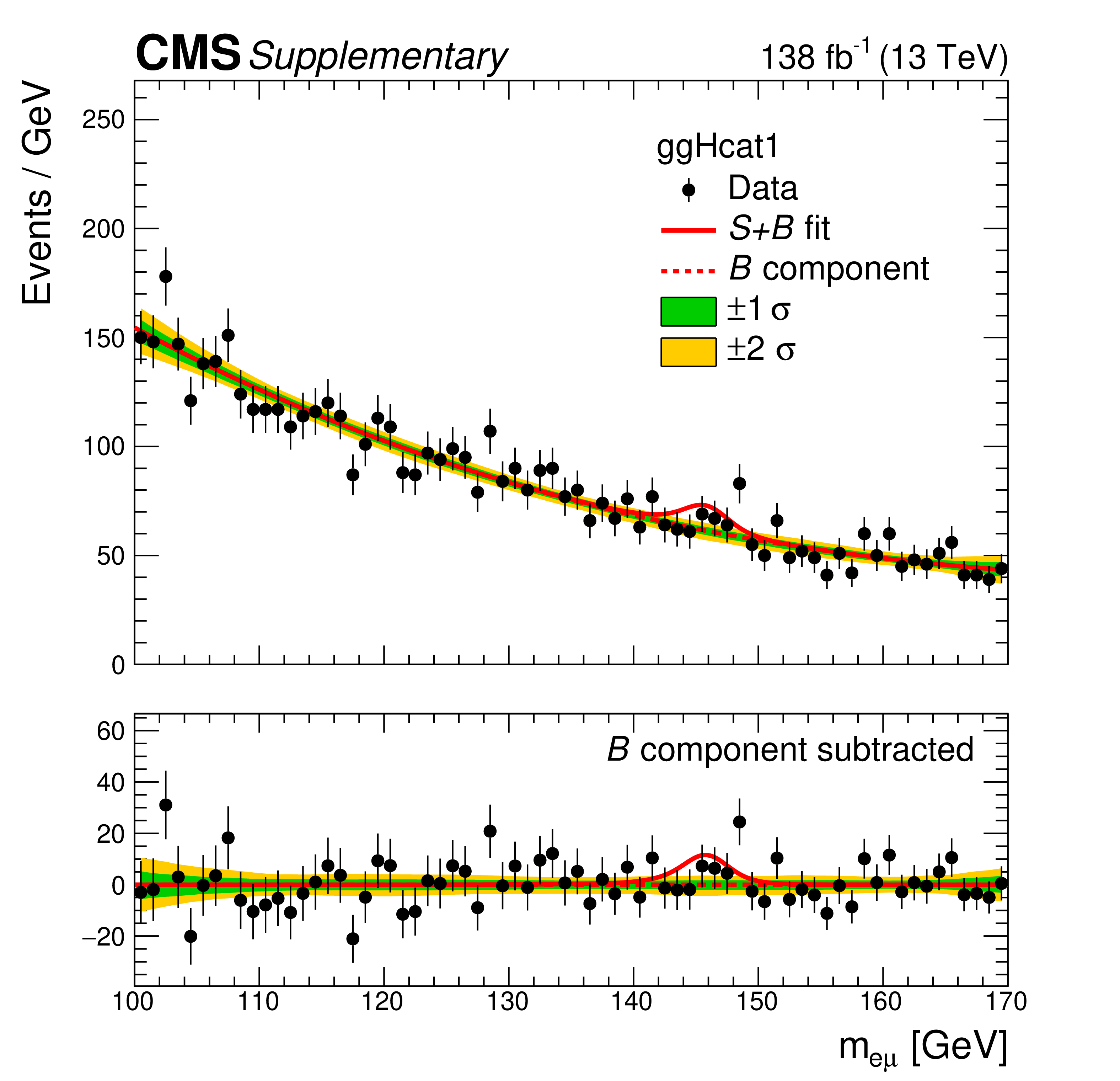
Additional Figure 6:
The $ m_{\mathrm{e}\mu} $ distribution of the observed data in the category $ {\mathrm{g}\mathrm{g}\mathrm{H}} $ cat 1 is shown, with the $ S{+}B $ fit at $ m_{\mathrm{X}}= $ 146 GeV in solid red line, and the background component of the fit in dotted red line. The green and yellow bands represent the one and two standard deviations of the background component. The lower panel shows the residuals after subtracting the background component of the fit from data. |
png pdf |
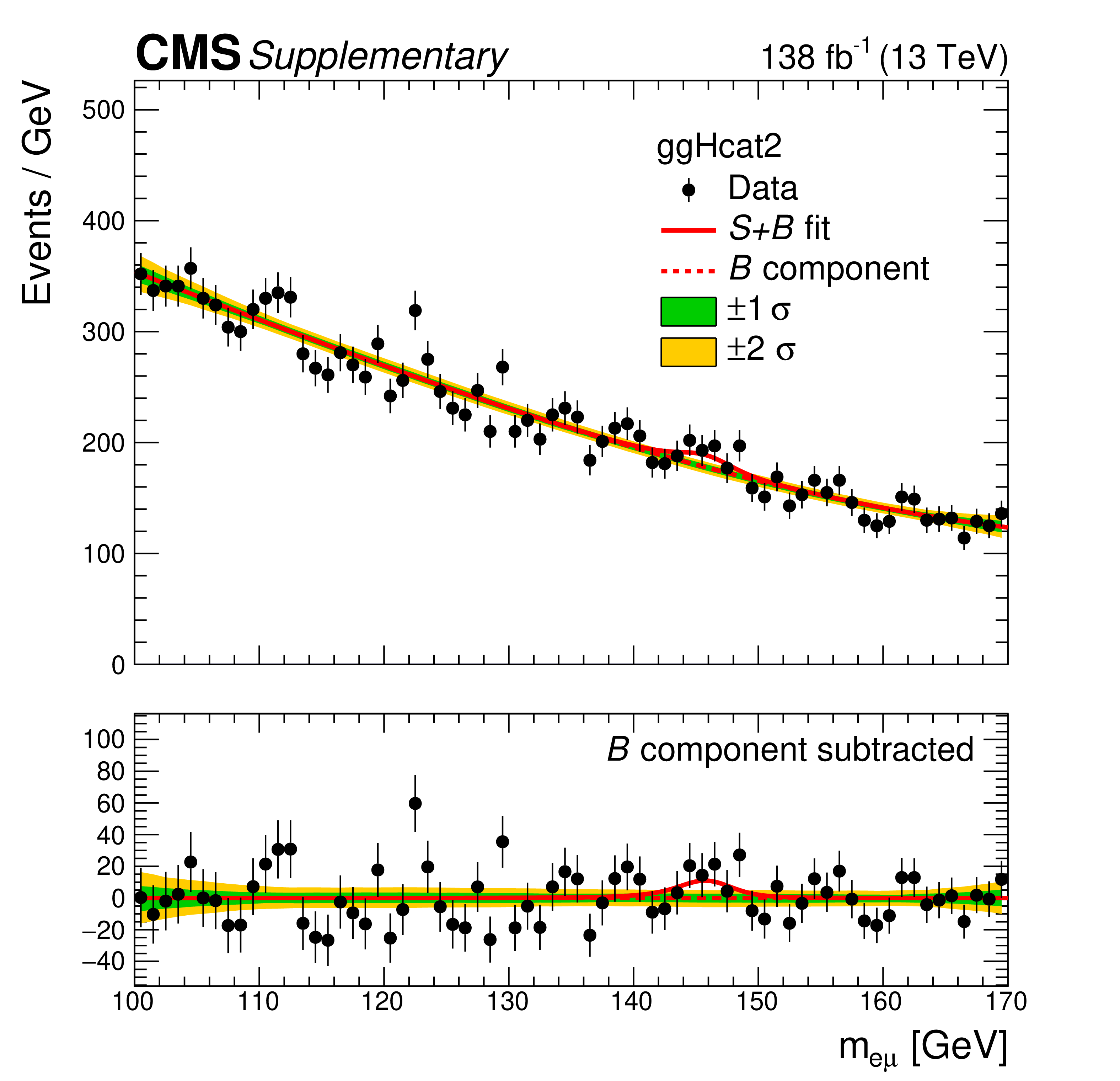
Additional Figure 7:
The $ m_{\mathrm{e}\mu} $ distribution of the observed data in the category $ {\mathrm{g}\mathrm{g}\mathrm{H}} $ cat 2 is shown, with the $ S{+}B $ fit at $ m_{\mathrm{X}}= $ 146 GeV in solid red line, and the background component of the fit in dotted red line. The green and yellow bands represent the one and two standard deviations of the background component. The lower panel shows the residuals after subtracting the background component of the fit from data. |
png pdf |
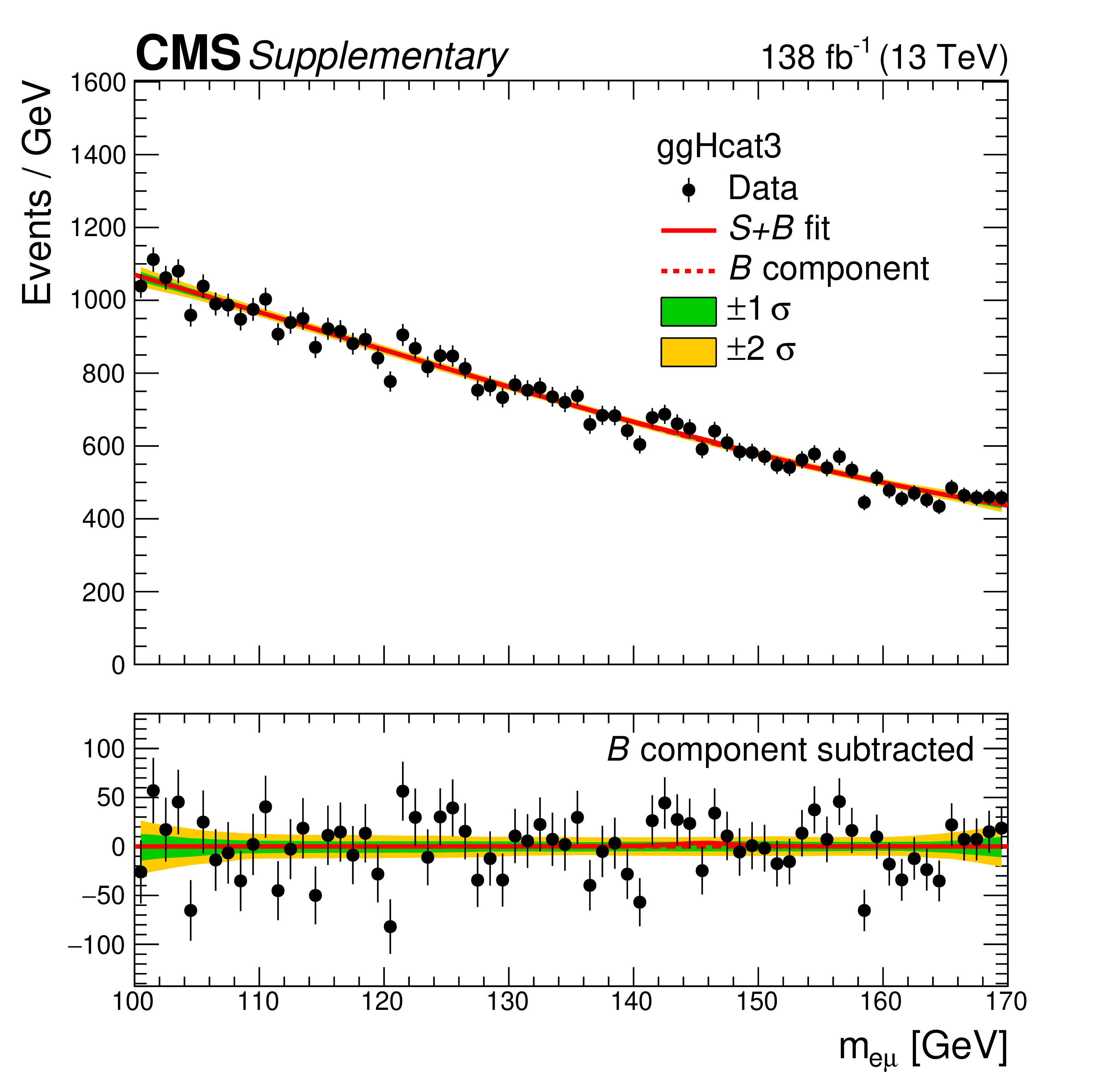
Additional Figure 8:
The $ m_{\mathrm{e}\mu} $ distribution of the observed data in the category $ {\mathrm{g}\mathrm{g}\mathrm{H}} $ cat 3 is shown, with the $ S{+}B $ fit at $ m_{\mathrm{X}}= $ 146 GeV in solid red line, and the background component of the fit in dotted red line. The green and yellow bands represent the one and two standard deviations of the background component. The lower panel shows the residuals after subtracting the background component of the fit from data. |
png pdf |
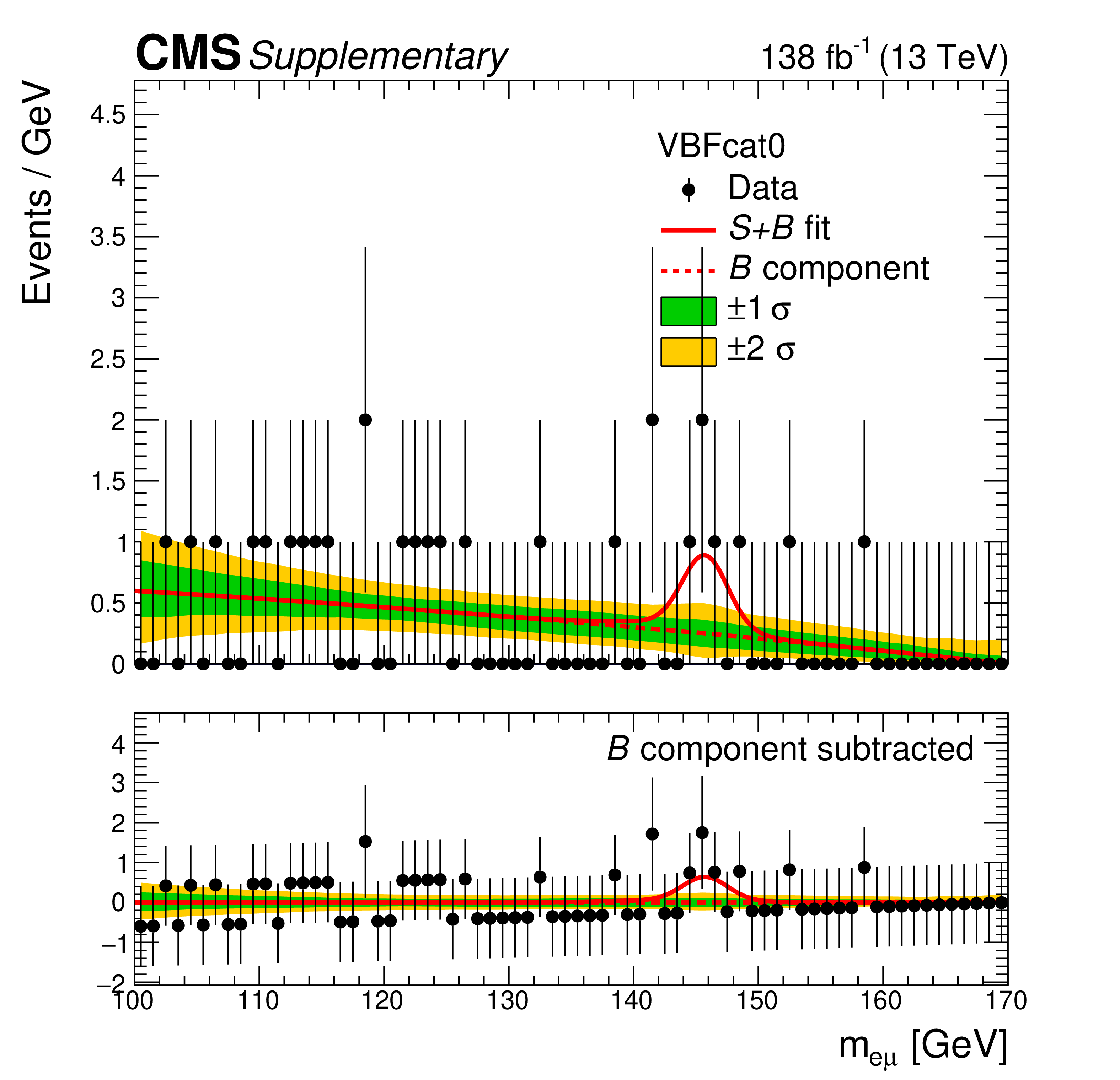
Additional Figure 9:
The $ m_{\mathrm{e}\mu} $ distribution of the observed data in the category VBF cat 0 is shown, with the $ S{+}B $ fit at $ m_{\mathrm{X}}= $ 146 GeV in solid red line, and the background component of the fit in dotted red line. The green and yellow bands represent the one and two standard deviations of the background component. The lower panel shows the residuals after subtracting the background component of the fit from data. |
png pdf |
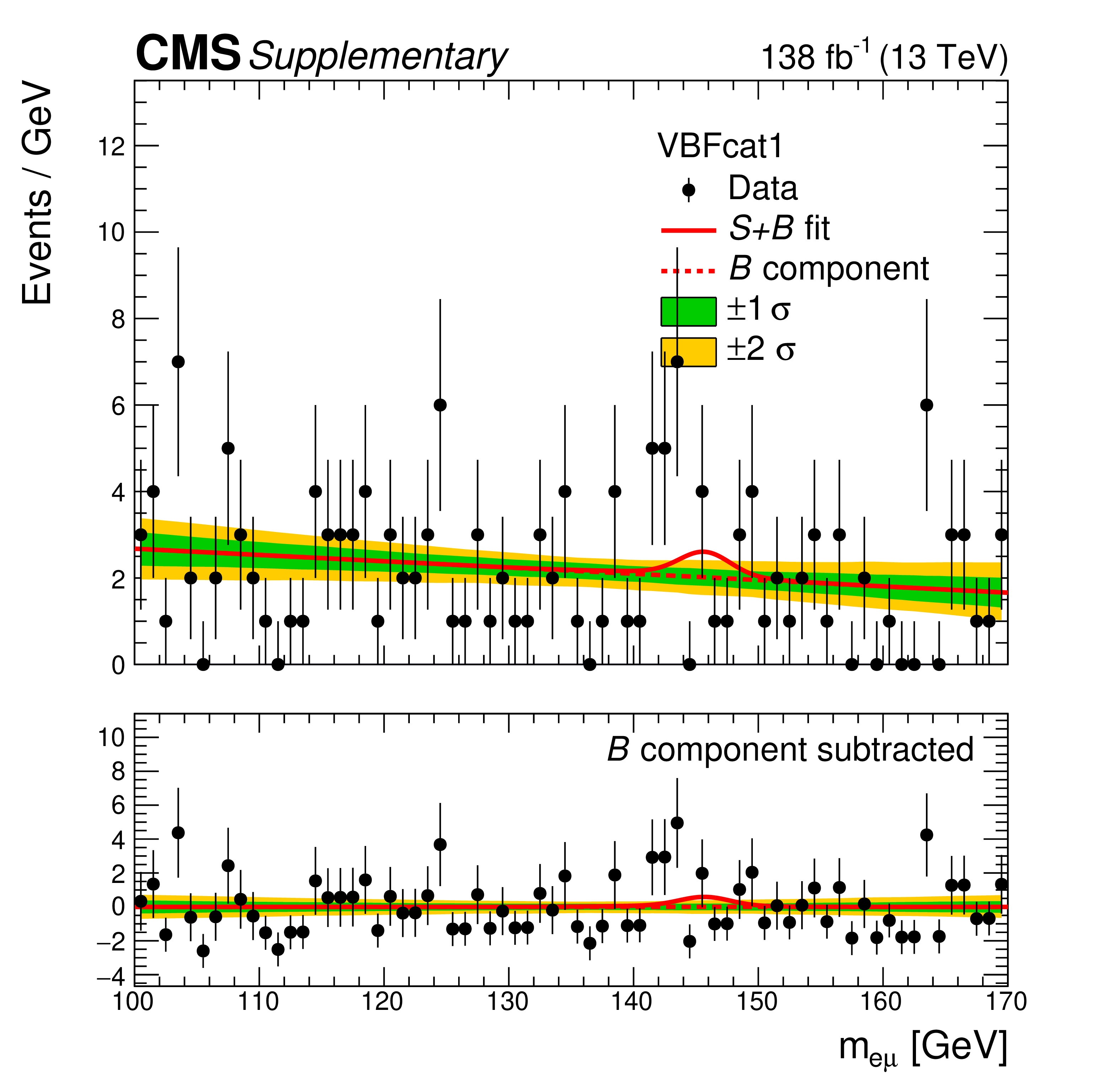
Additional Figure 10:
The $ m_{\mathrm{e}\mu} $ distribution of the observed data in the category VBF cat 1 is shown, with the $ S{+}B $ fit at $ m_{\mathrm{X}}= $ 146 GeV in solid red line, and the background component of the fit in dotted red line. The green and yellow bands represent the one and two standard deviations of the background component. The lower panel shows the residuals after subtracting the background component of the fit from data. |
png pdf |
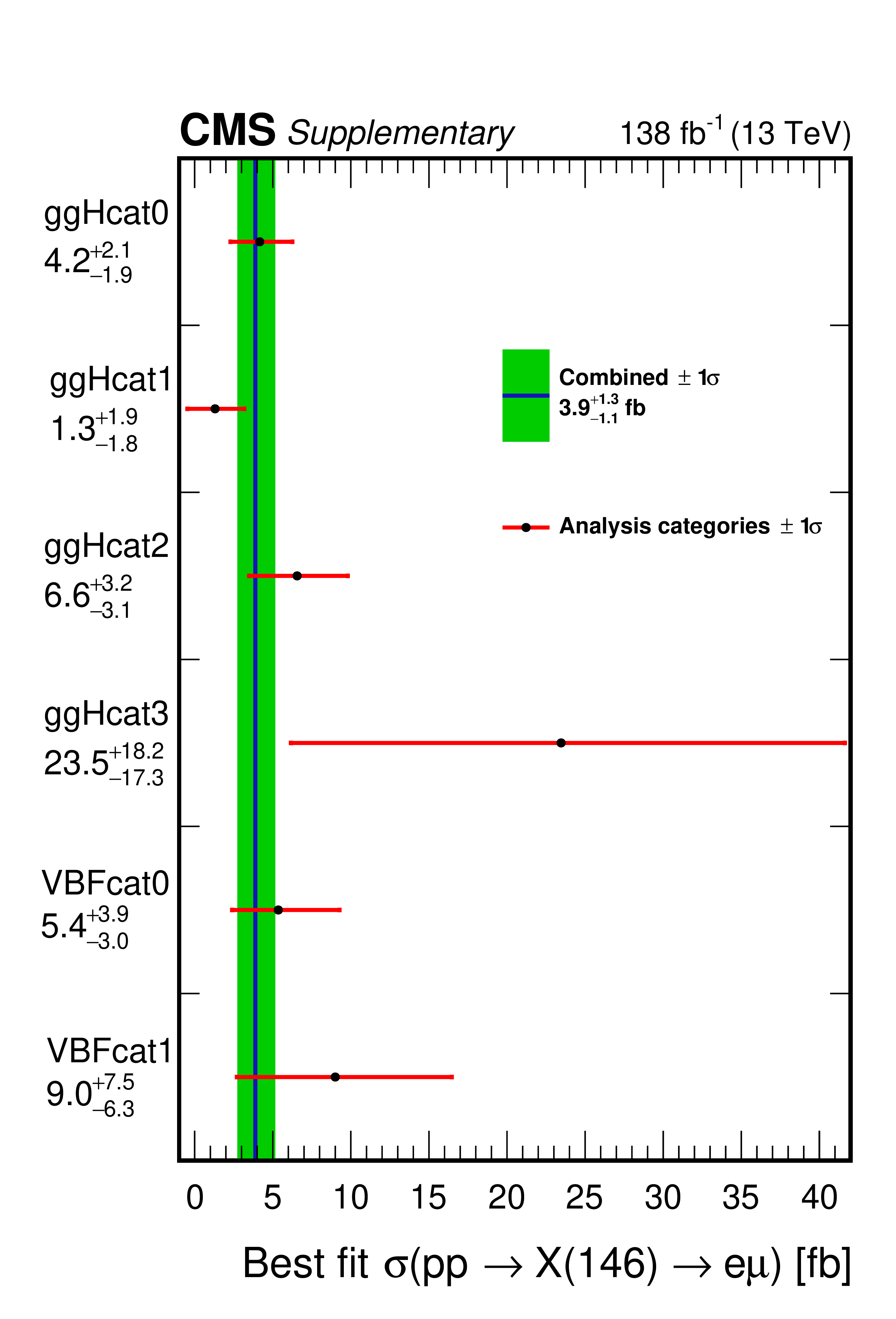
Additional Figure 11:
Best fit of $ {\sigma(\mathrm{p}\mathrm{p} \to \mathrm{X}(146) \to \mathrm{e} \mu)} $ for each analysis category (black point) compared to the best fit for the combination of all analysis categories (blue line). The one standard deviation uncertainty of the per-category best fit is shown in red line and the one standard deviation uncertainty of the combined best fit is shown in green band. |
| Additional Tables | |

png pdf |
Additional Table 1:
The efficiency times acceptance of the signal rate for each analysis category and $ m_{\mathrm{X}} $ hypothesised. |
png pdf |
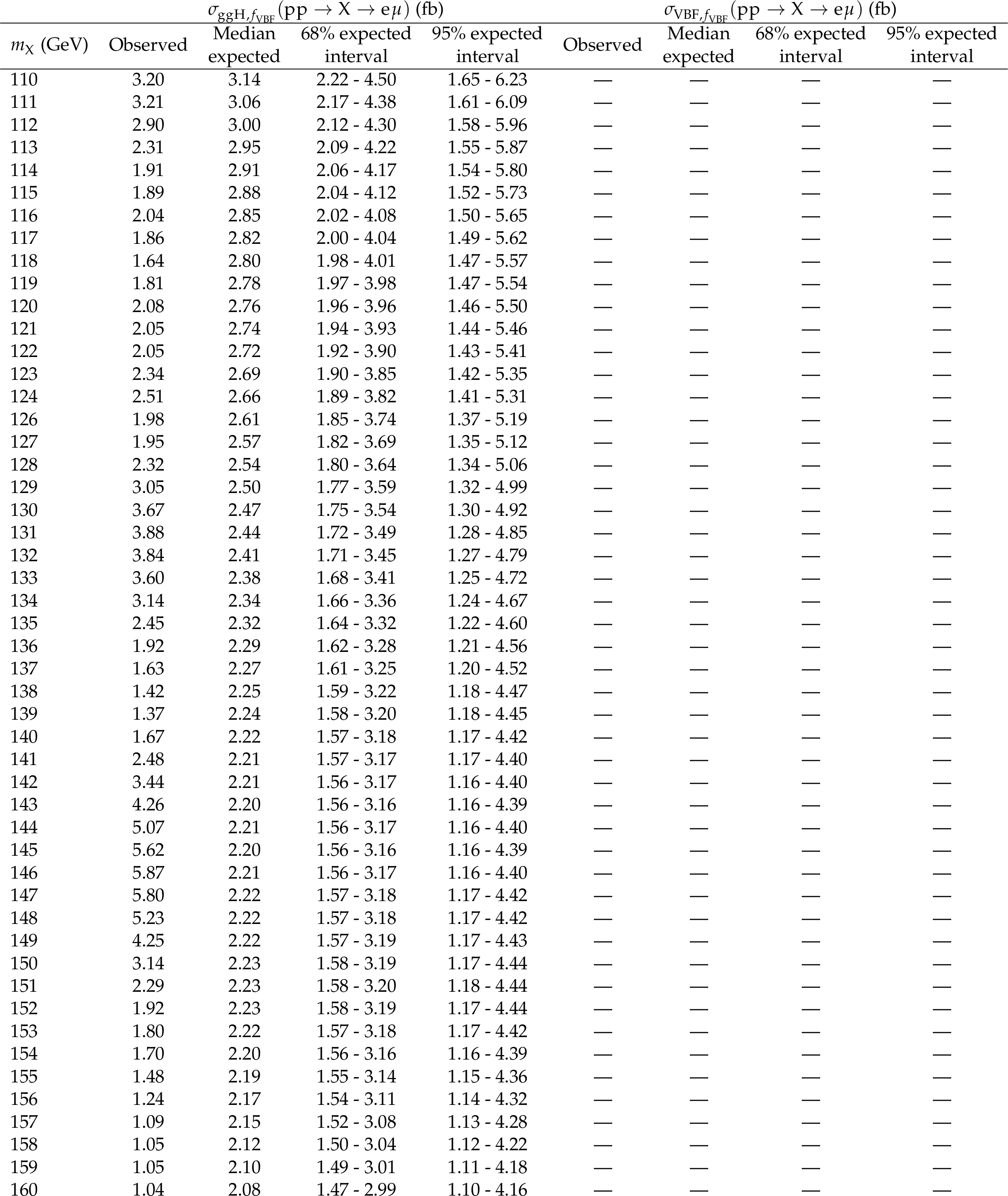
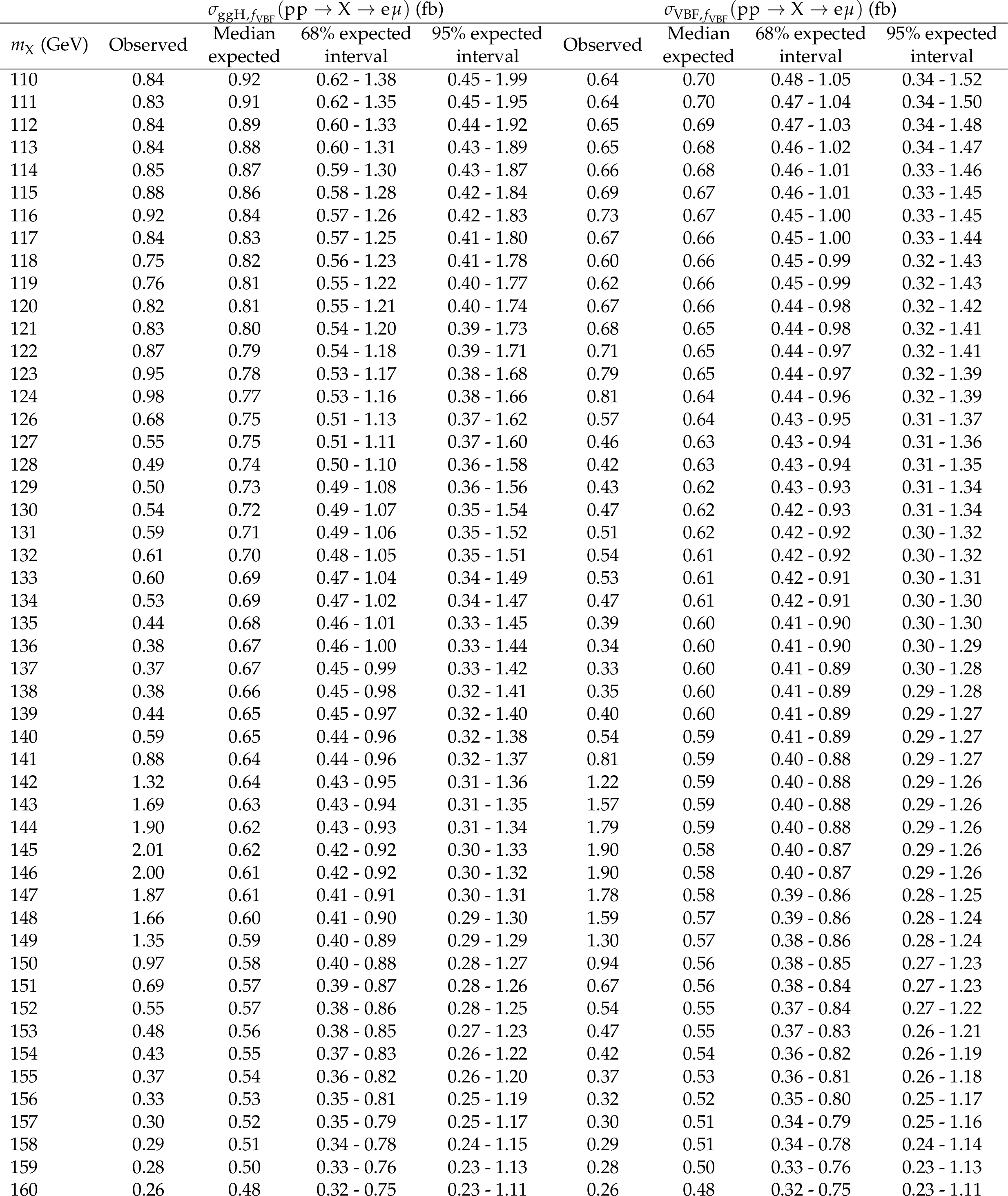
Additional Table 2:
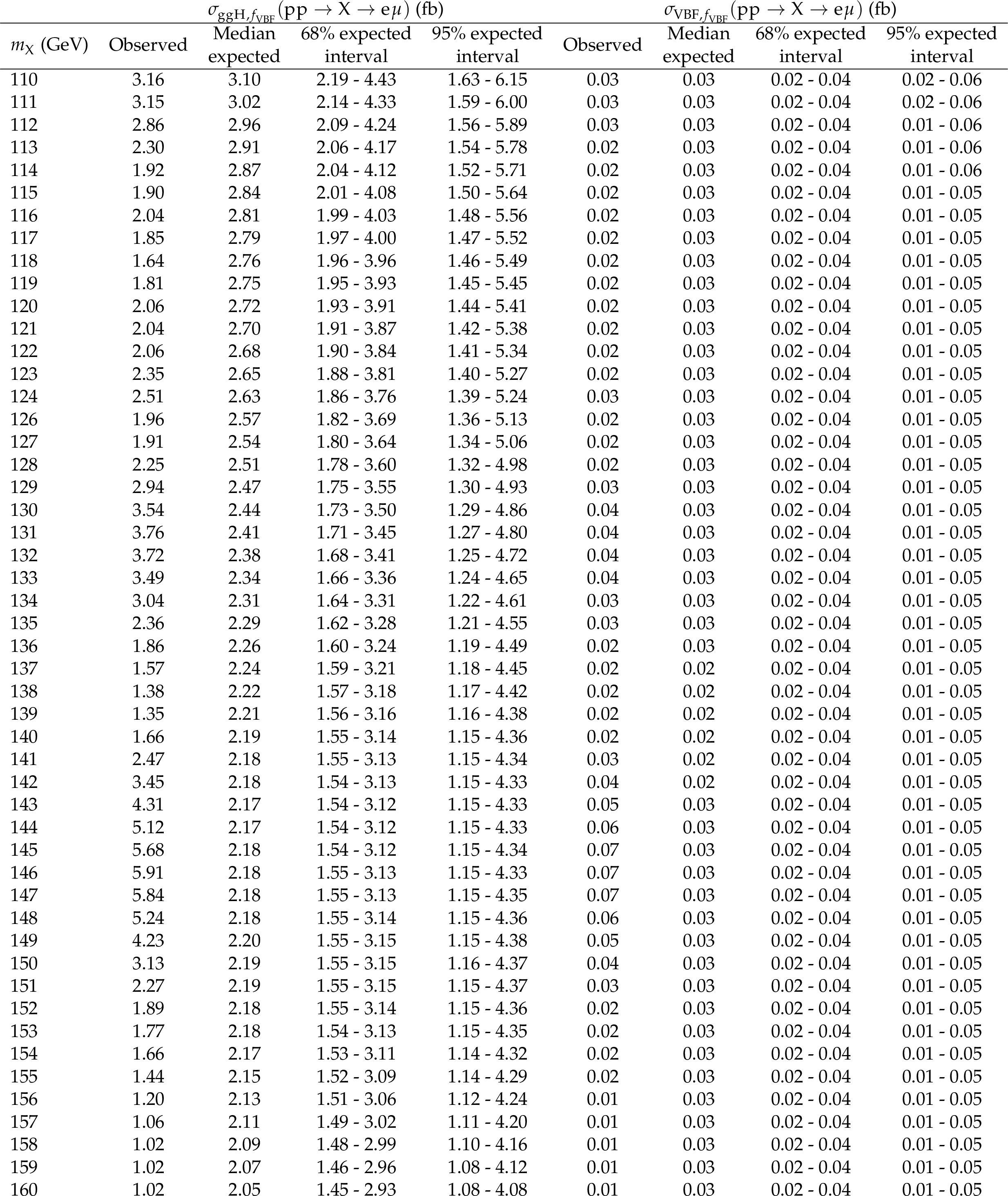
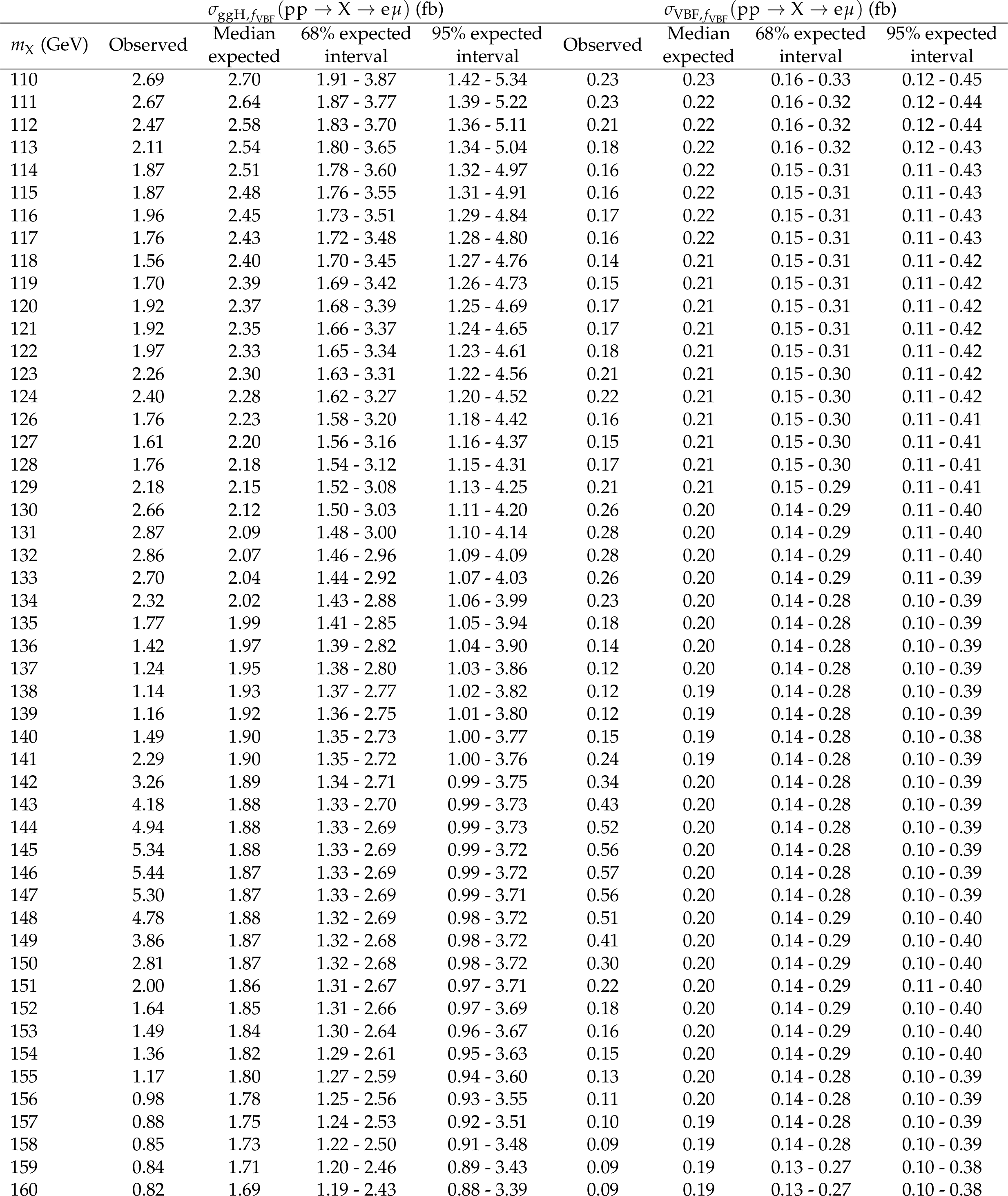
The observed and expected 95% CL upper limits on $ {\sigma_{{\mathrm{g}\mathrm{g}\mathrm{H}},f_{\mathrm{VBF}}}({\mathrm{p}\mathrm{p} \to \mathrm{X} \to \mathrm{e} \mu})} $ and $ {\sigma_{\mathrm{VBF},f_{\mathrm{VBF}}}({\mathrm{p}\mathrm{p} \to \mathrm{X} \to \mathrm{e} \mu})} $ with $ {f_{\mathrm{VBF}}=} $ 0.0. |
png pdf |
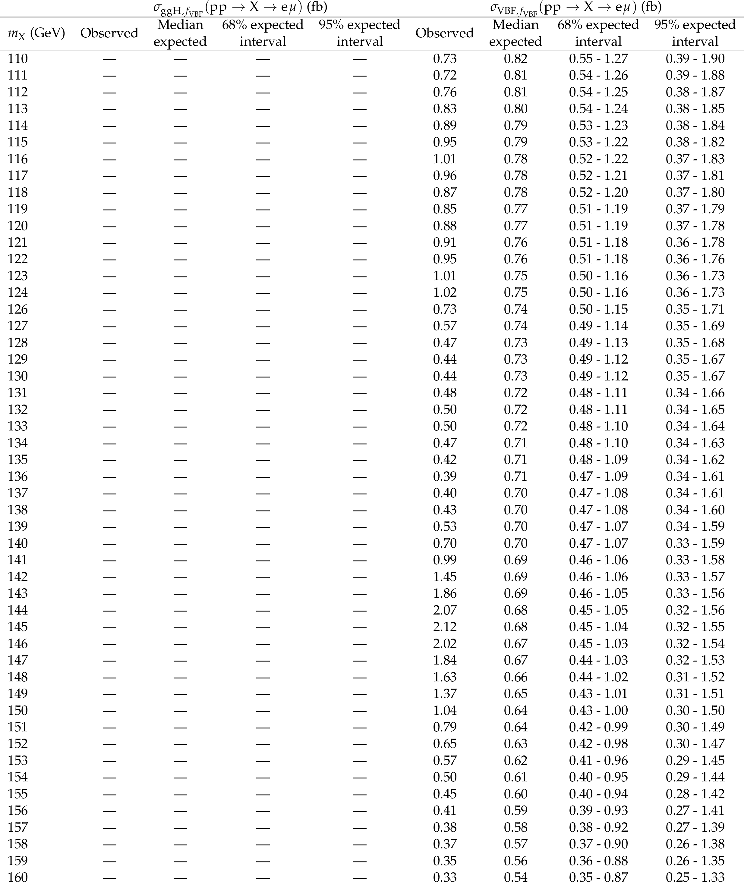
Additional Table 3:
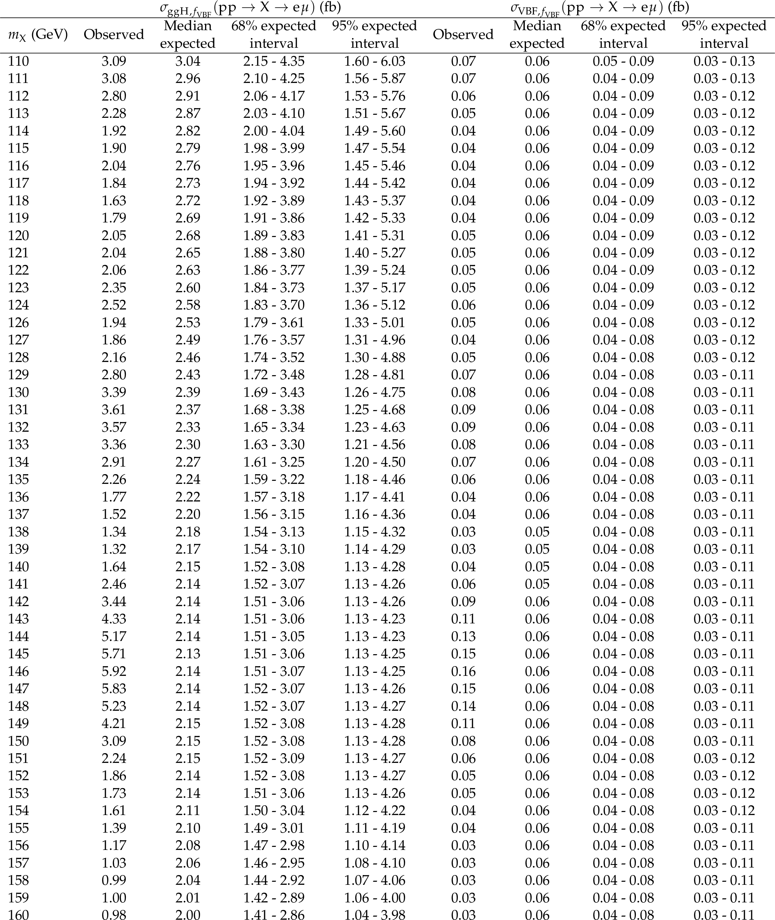
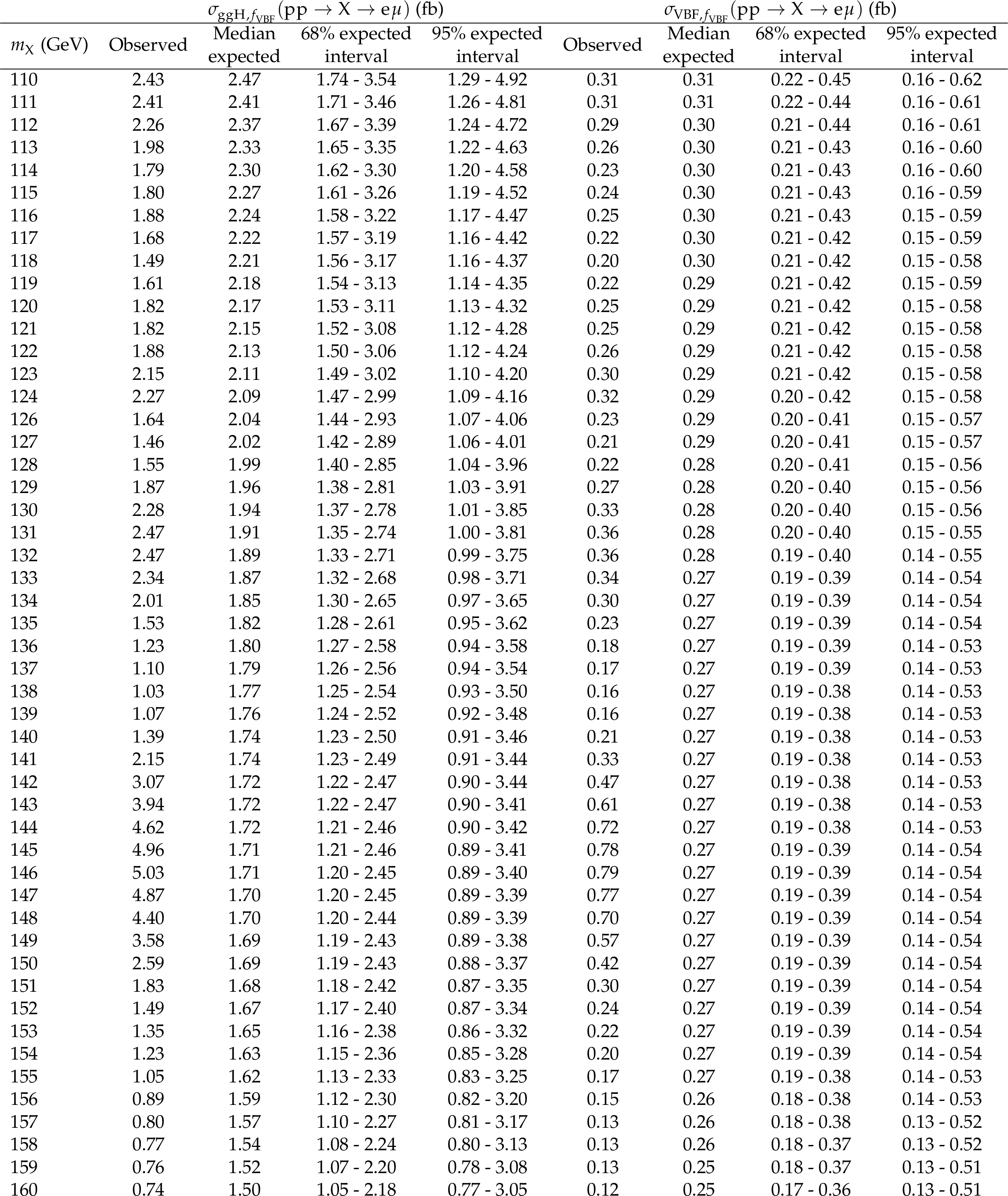
The observed and expected 95% CL upper limits on $ {\sigma_{{\mathrm{g}\mathrm{g}\mathrm{H}},f_{\mathrm{VBF}}}({\mathrm{p}\mathrm{p} \to \mathrm{X} \to \mathrm{e} \mu})} $ and $ {\sigma_{\mathrm{VBF},f_{\mathrm{VBF}}}({\mathrm{p}\mathrm{p} \to \mathrm{X} \to \mathrm{e} \mu})} $ with $ {f_{\mathrm{VBF}}=} $ 0.1. |
png pdf |
Additional Table 4:
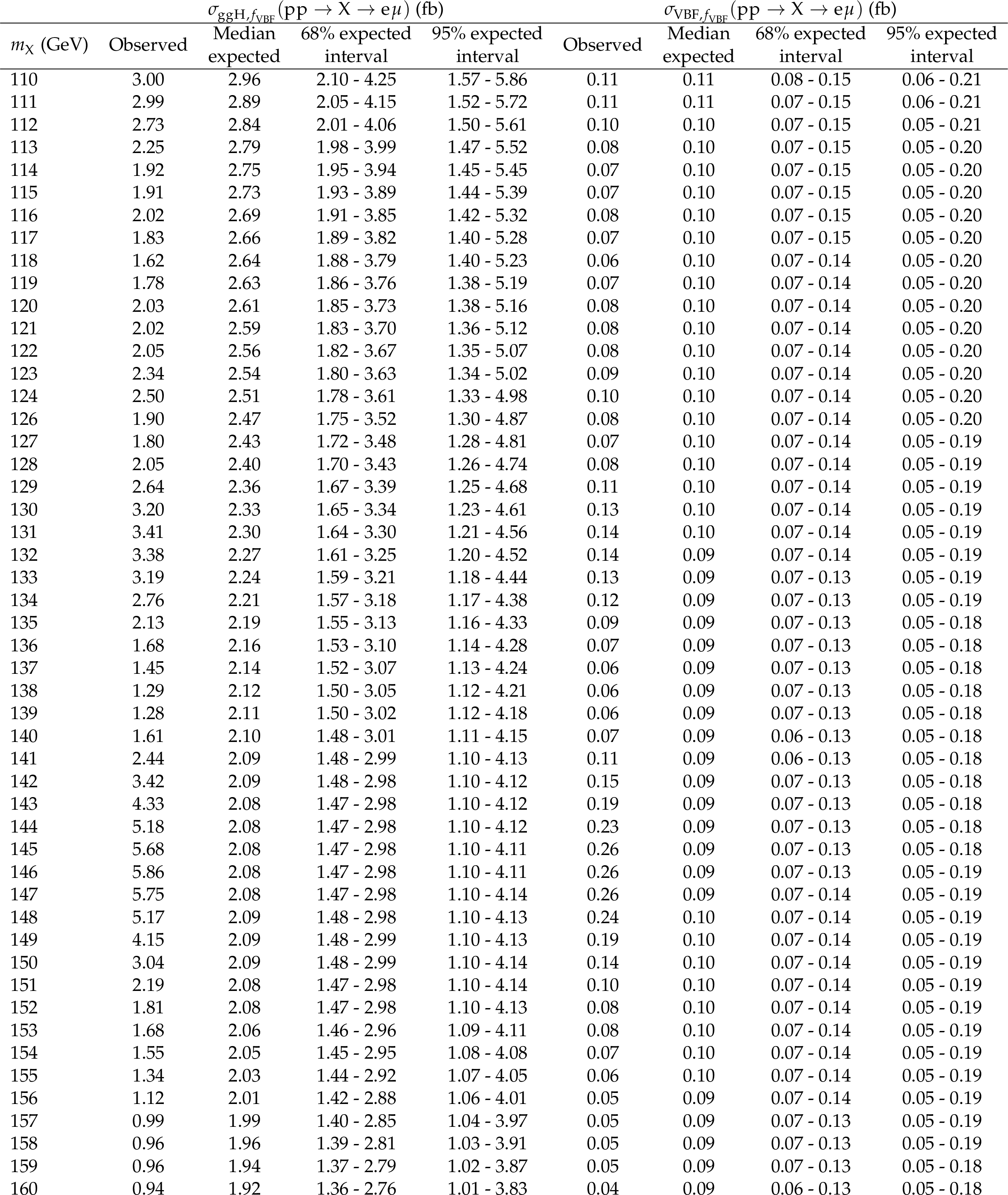
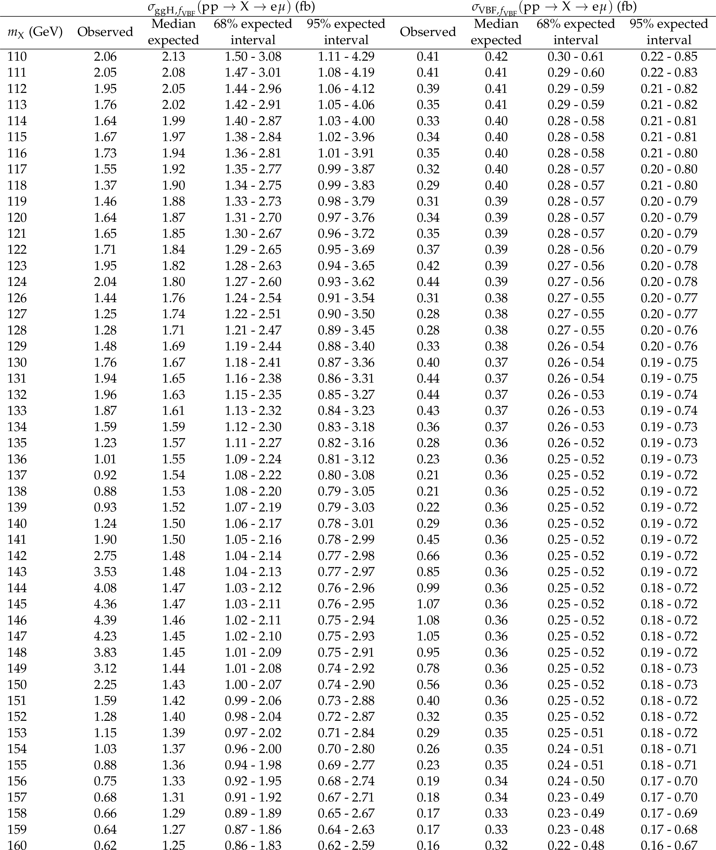
The observed and expected 95% CL upper limits on $ {\sigma_{{\mathrm{g}\mathrm{g}\mathrm{H}},f_{\mathrm{VBF}}}({\mathrm{p}\mathrm{p} \to \mathrm{X} \to \mathrm{e} \mu})} $ and $ {\sigma_{\mathrm{VBF},f_{\mathrm{VBF}}}({\mathrm{p}\mathrm{p} \to \mathrm{X} \to \mathrm{e} \mu})} $ with $ {f_{\mathrm{VBF}}=} $ 0.2. |
png pdf |
Additional Table 5:
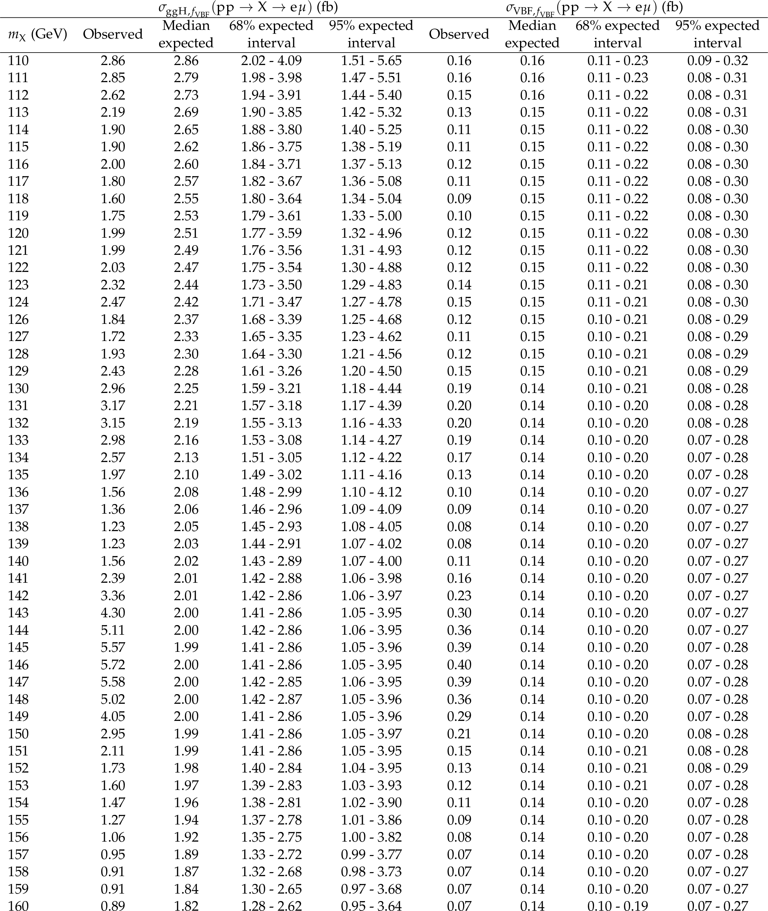
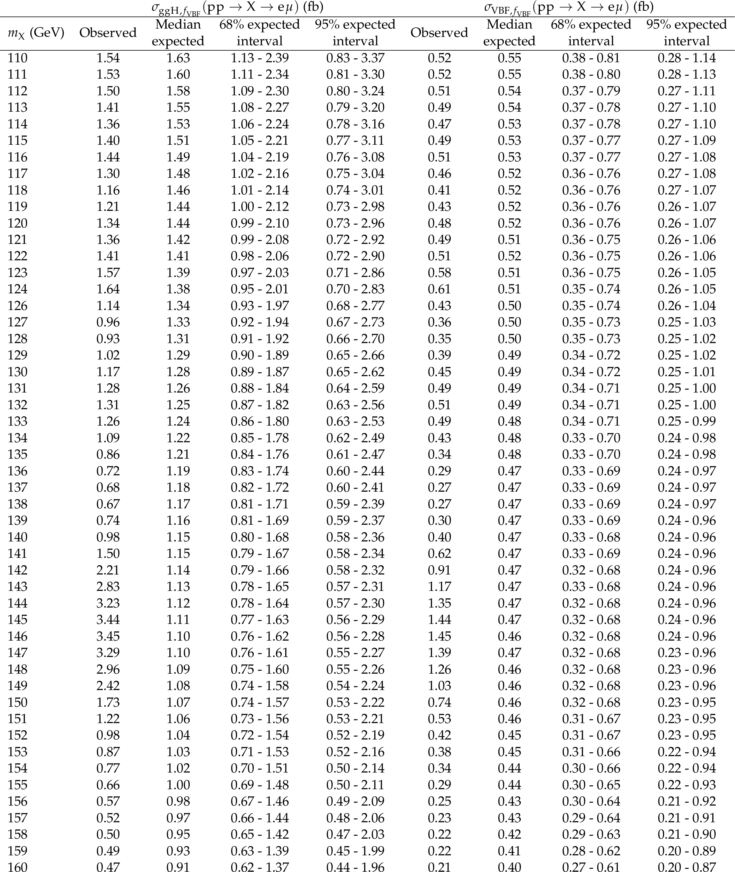
The observed and expected 95% CL upper limits on $ {\sigma_{{\mathrm{g}\mathrm{g}\mathrm{H}},f_{\mathrm{VBF}}}({\mathrm{p}\mathrm{p} \to \mathrm{X} \to \mathrm{e} \mu})} $ and $ {\sigma_{\mathrm{VBF},f_{\mathrm{VBF}}}({\mathrm{p}\mathrm{p} \to \mathrm{X} \to \mathrm{e} \mu})} $ with $ {f_{\mathrm{VBF}}=} $ 0.3. |
png pdf |
Additional Table 6:
The observed and expected 95% CL upper limits on $ {\sigma_{{\mathrm{g}\mathrm{g}\mathrm{H}},f_{\mathrm{VBF}}}({\mathrm{p}\mathrm{p} \to \mathrm{X} \to \mathrm{e} \mu})} $ and $ {\sigma_{\mathrm{VBF},f_{\mathrm{VBF}}}({\mathrm{p}\mathrm{p} \to \mathrm{X} \to \mathrm{e} \mu})} $ with $ {f_{\mathrm{VBF}}=} $ 0.4. |
png pdf |
Additional Table 7:
The observed and expected 95% CL upper limits on $ {\sigma_{{\mathrm{g}\mathrm{g}\mathrm{H}},f_{\mathrm{VBF}}}({\mathrm{p}\mathrm{p} \to \mathrm{X} \to \mathrm{e} \mu})} $ and $ {\sigma_{\mathrm{VBF},f_{\mathrm{VBF}}}({\mathrm{p}\mathrm{p} \to \mathrm{X} \to \mathrm{e} \mu})} $ with $ {f_{\mathrm{VBF}}=} $ 0.5. |
png pdf |
Additional Table 8:
The observed and expected 95% CL upper limits on $ {\sigma_{{\mathrm{g}\mathrm{g}\mathrm{H}},f_{\mathrm{VBF}}}({\mathrm{p}\mathrm{p} \to \mathrm{X} \to \mathrm{e} \mu})} $ and $ {\sigma_{\mathrm{VBF},f_{\mathrm{VBF}}}({\mathrm{p}\mathrm{p} \to \mathrm{X} \to \mathrm{e} \mu})} $ with $ {f_{\mathrm{VBF}}=} $ 0.6. |
png pdf |
Additional Table 9:
The observed and expected 95% CL upper limits on $ {\sigma_{{\mathrm{g}\mathrm{g}\mathrm{H}},f_{\mathrm{VBF}}}({\mathrm{p}\mathrm{p} \to \mathrm{X} \to \mathrm{e} \mu})} $ and $ {\sigma_{\mathrm{VBF},f_{\mathrm{VBF}}}({\mathrm{p}\mathrm{p} \to \mathrm{X} \to \mathrm{e} \mu})} $ with $ {f_{\mathrm{VBF}}=} $ 0.7. |
png pdf |
Additional Table 10:
The observed and expected 95% CL upper limits on $ {\sigma_{{\mathrm{g}\mathrm{g}\mathrm{H}},f_{\mathrm{VBF}}}({\mathrm{p}\mathrm{p} \to \mathrm{X} \to \mathrm{e} \mu})} $ and $ {\sigma_{\mathrm{VBF},f_{\mathrm{VBF}}}({\mathrm{p}\mathrm{p} \to \mathrm{X} \to \mathrm{e} \mu})} $ with $ {f_{\mathrm{VBF}}=} $ 0.8. |
png pdf |
Additional Table 11:
The observed and expected 95% CL upper limits on $ {\sigma_{{\mathrm{g}\mathrm{g}\mathrm{H}},f_{\mathrm{VBF}}}({\mathrm{p}\mathrm{p} \to \mathrm{X} \to \mathrm{e} \mu})} $ and $ {\sigma_{\mathrm{VBF},f_{\mathrm{VBF}}}({\mathrm{p}\mathrm{p} \to \mathrm{X} \to \mathrm{e} \mu})} $ with $ {f_{\mathrm{VBF}}=} $ 0.9. |
png pdf |
Additional Table 12:
The observed and expected 95% CL upper limits on $ {\sigma_{{\mathrm{g}\mathrm{g}\mathrm{H}},f_{\mathrm{VBF}}}({\mathrm{p}\mathrm{p} \to \mathrm{X} \to \mathrm{e} \mu})} $ and $ {\sigma_{\mathrm{VBF},f_{\mathrm{VBF}}}({\mathrm{p}\mathrm{p} \to \mathrm{X} \to \mathrm{e} \mu})} $ with $ {f_{\mathrm{VBF}}=} $ 1.0. |
| References | ||||
| 1 | ATLAS Collaboration | Observation of a new particle in the search for the standard model Higgs boson with the ATLAS detector at the LHC | PLB 716 (2012) 1 | 1207.7214 |
| 2 | CMS Collaboration | Observation of a new boson at a mass of 125 GeV with the CMS experiment at the LHC | PLB 716 (2012) 30 | CMS-HIG-12-028 1207.7235 |
| 3 | CMS Collaboration | Observation of a new boson with mass near 125 GeV in pp collisions at $ \sqrt{s} $ = 7 and 8 TeV | JHEP 06 (2013) 081 | CMS-HIG-12-036 1303.4571 |
| 4 | ATLAS Collaboration | A detailed map of Higgs boson interactions by the ATLAS experiment ten years after the discovery | Nature 607 (2022) 52 | 2207.00092 |
| 5 | CMS Collaboration | A portrait of the Higgs boson by the CMS experiment ten years after the discovery | Nature 607 (2022) 60 | CMS-HIG-22-001 2207.00043 |
| 6 | ATLAS Collaboration | Measurements of the Higgs boson production and decay rates and coupling strengths using pp collision data at $ \sqrt{s}= $ 7 and 8 TeV in the ATLAS experiment | EPJC 76 (2016) 6 | 1507.04548 |
| 7 | CMS Collaboration | Precise determination of the mass of the Higgs boson and tests of compatibility of its couplings with the standard model predictions using proton collisions at 7 and 8 TeV | EPJC 75 (2015) 212 | CMS-HIG-14-009 1412.8662 |
| 8 | CMS Collaboration | Study of the mass and spin-parity of the Higgs boson candidate via its decays to Z boson pairs | PRL 110 (2013) 081803 | CMS-HIG-12-041 1212.6639 |
| 9 | ATLAS Collaboration | Evidence for the spin-0 nature of the Higgs boson using ATLAS data | PLB 726 (2013) 120 | 1307.1432 |
| 10 | CMS Collaboration | Constraints on the spin-parity and anomalous HVV couplings of the Higgs boson in proton collisions at 7 and 8 TeV | PRD 92 (2015) 012004 | CMS-HIG-14-018 1411.3441 |
| 11 | CMS Collaboration | Measurements of properties of the Higgs boson decaying into the four-lepton final state in pp collisions at $ \sqrt{s}= $ 13 TeV | JHEP 11 (2017) 047 | CMS-HIG-16-041 1706.09936 |
| 12 | J. D. Bjorken and S. Weinberg | A mechanism for nonconservation of muon number | PRL 38 (1977) 622 | |
| 13 | G. C. Branco et al. | Theory and phenomenology of two-higgs-doublet models | Physics Reports 516 (2012) 1 | 1106.0034 |
| 14 | H. Ishimori et al. | Non-Abelian discrete symmetries in particle physics | Prog. Theor. Phys. Suppl. 183 (2010) 1 | 1003.3552 |
| 15 | G. Perez and L. Randall | Natural neutrino masses and mixings from warped geometry | JHEP 01 (2009) 077 | 0805.4652 |
| 16 | S. Casagrande et al. | Flavor physics in the Randall-Sundrum model: I. Theoretical setup and electroweak precision tests | JHEP 10 (2008) 094 | 0807.4937 |
| 17 | A. J. Buras, B. Duling, and S. Gori | The impact of Kaluza-Klein fermions on standard model fermion couplings in a RS model with custodial protection | JHEP 09 (2009) 076 | 0905.2318 |
| 18 | M. Blanke et al. | $ \Delta F= $ 2 observables and fine-tuning in a warped extra dimension with custodial protection | JHEP 03 (2009) 001 | 0809.1073 |
| 19 | M. E. Albrecht et al. | Electroweak and flavour structure of a warped extra dimension with custodial protection | JHEP 09 (2009) 064 | 0903.2415 |
| 20 | K. Agashe and R. Contino | Composite Higgs-mediated FCNC | PRD 80 (2009) 075016 | 0906.1542 |
| 21 | A. Azatov, M. Toharia, and L. Zhu | Higgs mediated FCNC's in warped extra dimensions | PRD 80 (2009) 035016 | 0906.1990 |
| 22 | J. L. Diaz-Cruz and J. J. Toscano | Lepton flavor violating decays of Higgs bosons beyond the standard model | PRD 62 (2000) 116005 | hep-ph/9910233 |
| 23 | T. Han and D. Marfatia | $ h\rightarrow\mu\tau $ at hadron colliders | PRL 86 (2001) 1442 | hep-ph/0008141 |
| 24 | A. Arhrib, Y. Cheng, and O. C. W. Kong | Comprehensive analysis on lepton flavor violating Higgs boson to $ \mu^\mp \tau^\pm $ decay in supersymmetry without $ R $ parity | PRD 87 (2013) 015025 | 1210.8241 |
| 25 | J. A. Aguilar Saavedra | A minimal set of top-Higgs anomalous couplings | NPB 821 (2009) 215 | 0904.2387 |
| 26 | A. Goudelis, O. Lebedev, and J. H. Park | Higgs-induced lepton flavor violation | PLB 707 (2012) 369 | 1111.1715 |
| 27 | D. McKeen, M. Pospelov, and A. Ritz | Modified Higgs branching ratios versus CP and lepton flavor violation | PRD 86 (2012) 113004 | 1208.4597 |
| 28 | A. Pilaftsis | Lepton flavor nonconservation in $ \mathrm{H}^{0} $ decays | PLB 285 (1992) 68 | |
| 29 | J. G. Körner, A. Pilaftsis, and K. Schilcher | Leptonic CP asymmetries in flavor changing $ \mathrm{H}^{0} $ decays | PRD 47 (1993) 1080 | hep-ph/9301289 |
| 30 | O. U. Shanker | Flavor violation, scalar particles and leptoquarks | NPB 206 (1982) 253 | |
| 31 | B. McWilliams and L.-F. Li | Virtual effects of Higgs particles | NPB 179 (1981) 62 | |
| 32 | MEG Collaboration | Search for the lepton flavour violating decay $ \mu ^+ \rightarrow \mathrm {e}^+ \gamma $ with the full dataset of the MEG experiment | EPJC 76 (2016) 434 | 1605.05081 |
| 33 | R. Harnik, J. Kopp, and J. Zupan | Flavor violating Higgs decays | JHEP 03 (2013) 026 | 1209.1397 |
| 34 | ATLAS Collaboration | A search for the dimuon decay of the Standard Model Higgs boson with the ATLAS detector | PLB 812 (2021) 135980 | 2007.07830 |
| 35 | CMS Collaboration | Evidence for Higgs boson decay to a pair of muons | JHEP 01 (2021) 148 | CMS-HIG-19-006 2009.04363 |
| 36 | ATLAS Collaboration | Search for the Higgs boson decays $ H \to ee $ and $ H \to e\mu $ in $ pp $ collisions at $ \sqrt{s} = $ 13 TeV with the ATLAS detector | PLB 801 (2019) 135148 | 1909.10235 |
| 37 | R. Primulando, J. Julio, and P. Uttayarat | Collider constraints on lepton flavor violation in the 2HDM | PRD 101 (2020) 055021 | 1912.08533 |
| 38 | CMS Collaboration | The CMS experiment at the CERN LHC | JINST 3 (2008) S08004 | |
| 39 | CMS Collaboration | Performance of the CMS Level-1 trigger in proton-proton collisions at $ \sqrt{s} = $ 13 TeV | JINST 15 (2020) P10017 | CMS-TRG-17-001 2006.10165 |
| 40 | CMS Collaboration | The CMS trigger system | JINST 12 (2017) P01020 | CMS-TRG-12-001 1609.02366 |
| 41 | T. Sjöstrand et al. | An introduction to PYTHIA 8.2 | Comput. Phys. Commun. 191 (2015) 159 | 1410.3012 |
| 42 | CMS Collaboration | Extraction and validation of a new set of CMS PYTHIA 8 tunes from underlying-event measurements | EPJC 80 (2020) 4 | CMS-GEN-17-001 1903.12179 |
| 43 | NNPDF Collaboration | Parton distributions from high-precision collider data | EPJC 77 (2017) 663 | 1706.00428 |
| 44 | GEANT 4 Collaboration | GEANT 4 --- a simulation toolkit | NIM A 506 (2003) 250 | |
| 45 | H. M. Georgi, S. L. Glashow, M. E. Machacek, and D. V. Nanopoulos | Higgs bosons from two gluon annihilation in proton-proton collisions | PRL 40 (1978) 692 | |
| 46 | R. N. Cahn, S. D. Ellis, R. Kleiss, and W. J. Stirling | Transverse momentum signatures for heavy Higgs bosons | PRD 35 (1987) 1626 | |
| 47 | S. L. Glashow, D. V. Nanopoulos, and A. Yildiz | Associated production of Higgs bosons and Z particles | PRD 18 (1978) 1724 | |
| 48 | P. Nason | A new method for combining NLO QCD with shower Monte Carlo algorithms | JHEP 11 (2004) 040 | hep-ph/0409146 |
| 49 | S. Frixione, P. Nason, and C. Oleari | Matching NLO QCD computations with parton shower simulations: the POWHEG method | JHEP 11 (2007) 070 | 0709.2092 |
| 50 | S. Alioli, P. Nason, C. Oleari, and E. Re | A general framework for implementing NLO calculations in shower Monte Carlo programs: the POWHEG BOX | JHEP 06 (2010) 043 | 1002.2581 |
| 51 | S. Alioli et al. | Jet pair production in POWHEG | JHEP 04 (2011) 081 | 1012.3380 |
| 52 | S. Alioli, P. Nason, C. Oleari, and E. Re | NLO Higgs boson production via gluon fusion matched with shower in POWHEG | JHEP 04 (2009) 002 | 0812.0578 |
| 53 | E. Bagnaschi, G. Degrassi, P. Slavich, and A. Vicini | Higgs production via gluon fusion in the POWHEG approach in the SM and in the MSSM | JHEP 02 (2012) 088 | 1111.2854 |
| 54 | G. Heinrich et al. | NLO predictions for Higgs boson pair production with full top quark mass dependence matched to parton showers | JHEP 08 (2017) 088 | 1703.09252 |
| 55 | G. Buchalla et al. | Higgs boson pair production in non-linear effective field theory with full $ m_t $-dependence at NLO QCD | JHEP 09 (2018) 057 | 1806.05162 |
| 56 | J. Bellm et al. | Herwig 7.0/Herwig++ 3.0 release note | EPJC 76 (2016) 196 | 1512.01178 |
| 57 | CMS Collaboration | Development and validation of HERWIG 7 tunes from CMS underlying-event measurements | EPJC 81 (2021) 312 | CMS-GEN-19-001 2011.03422 |
| 58 | B. Jager et al. | Parton-shower effects in Higgs production via vector-boson Fusion | no.~8, 756, 2020 EPJC 80 (2020) |
2003.12435 |
| 59 | J. Alwall et al. | The automated computation of tree-level and next-to-leading order differential cross sections, and their matching to parton shower simulations | JHEP 07 (2014) 079 | 1405.0301 |
| 60 | J. Alwall et al. | Comparative study of various algorithms for the merging of parton showers and matrix elements in hadronic collisions | EPJC 53 (2008) 473 | 0706.2569 |
| 61 | R. Frederix and S. Frixione | Merging meets matching in MC@NLO | JHEP 12 (2012) 061 | 1209.6215 |
| 62 | CMS Collaboration | Particle-flow reconstruction and global event description with the CMS detector | JINST 12 (2017) P10003 | CMS-PRF-14-001 1706.04965 |
| 63 | CMS Collaboration | Technical proposal for the Phase-II upgrade of the Compact Muon Solenoid | CMS Technical Proposal CERN-LHCC-2015-010, CMS-TDR-15-02, 2015 CDS |
|
| 64 | CMS Collaboration | Electron and photon reconstruction and identification with the CMS experiment at the CERN LHC | JINST 16 (2021) P05014 | CMS-EGM-17-001 2012.06888 |
| 65 | CMS Collaboration | ECAL 2016 refined calibration and Run2 summary plots | CMS Detector Performance Summary CMS-DP-2020-021, 2020 CDS |
|
| 66 | CMS Collaboration | Performance of the CMS muon detector and muon reconstruction with proton-proton collisions at $ \sqrt{s}= $ 13 TeV | JINST 13 (2018) P06015 | CMS-MUO-16-001 1804.04528 |
| 67 | M. Cacciari, G. P. Salam, and G. Soyez | The catchment area of jets | JHEP 04 (2008) 005 | 0802.1188 |
| 68 | M. Cacciari, G. P. Salam, and G. Soyez | The anti-$ k_{\mathrm{T}} $ jet clustering algorithm | JHEP 04 (2008) 063 | 0802.1189 |
| 69 | M. Cacciari, G. P. Salam, and G. Soyez | Fastjet user manual | EPJC 72 (2012) 1896 | 1111.6097 |
| 70 | CMS Collaboration | Jet energy scale and resolution in the CMS experiment in pp collisions at 8 TeV | JINST 12 (2017) P02014 | CMS-JME-13-004 1607.03663 |
| 71 | E. Bols et al. | Jet flavour classification using DeepJet | JINST 15 (2020) P12012 | 2008.10519 |
| 72 | CMS Collaboration | Performance of reconstruction and identification of $ \tau $ leptons decaying to hadrons and $ \nu_\tau $ in pp collisions at $ \sqrt{s}= $ 13 TeV | JINST 13 (2018) P10005 | CMS-TAU-16-003 1809.02816 |
| 73 | CMS Collaboration | Identification of hadronic tau lepton decays using a deep neural network | JINST 17 (2022) P07023 | CMS-TAU-20-001 2201.08458 |
| 74 | CMS Collaboration | Performance of missing transverse momentum reconstruction in proton-proton collisions at $ \sqrt{s} = $ 13 TeV using the CMS detector | JINST 14 (2019) P07004 | CMS-JME-17-001 1903.06078 |
| 75 | CMS Collaboration | Search for lepton-flavor violating decays of the Higgs boson in the $ \mu\tau $ and e$ \tau $ final states in proton-proton collisions at $ \sqrt{s} $ = 13 TeV | PRD 104 (2021) 032013 | CMS-HIG-20-009 2105.03007 |
| 76 | T. Chen and C. Guestrin | XGBoost: A scalable tree boosting system | in nd ACM SIGKDD Intern. Conf. on Knowledge Discovery and Data Mining, KDD '16, New York, 2016 In Proc. 2 (2016) 785 |
|
| 77 | D. de Florian et al. | Handbook of LHC Higgs cross sections: 4. Deciphering the nature of the Higgs sector | CERN Report CERN-2017-002-M, 2016 link |
1610.07922 |
| 78 | F. Schissler and D. Zeppenfeld | Parton shower effects on W and Z production via vector boson fusion at NLO QCD | JHEP 04 (2013) 057 | 1302.2884 |
| 79 | G. Cowan, K. Cranmer, E. Gross, and O. Vitells | Asymptotic formulae for likelihood-based tests of new physics | EPJC 71 (2011) 1554 | 1007.1727 |
| 80 | S. S. Wilks | The large-sample distribution of the likelihood ratio for testing composite hypotheses | Ann. Math. Statist. 9 (1938) 60 | |
| 81 | CMS Collaboration | Measurements of production cross sections of the Higgs boson in the four-lepton final state in proton-proton collisions at $ \sqrt{s} = $ 13 TeV | EPJC 81 (2021) 488 | CMS-HIG-19-001 2103.04956 |
| 82 | CMS Collaboration | Measurements of inclusive W and Z cross sections in pp collisions at $ \sqrt{s}= $ 7 TeV | JHEP 01 (2011) 080 | CMS-EWK-10-002 1012.2466 |
| 83 | CMS Collaboration | Identification of heavy-flavour jets with the CMS detector in pp collisions at 13 TeV | JINST 13 (2018) P05011 | CMS-BTV-16-002 1712.07158 |
| 84 | CMS Collaboration | Performance of b tagging algorithms in proton-proton collisions at 13 TeV with Phase 1 CMS detector | CMS Detector Performance Note CMS-DP-2018-033, 2018 CDS |
|
| 85 | CMS Collaboration | Precision luminosity measurement in proton-proton collisions at $ \sqrt{s} = $ 13 TeV in 2015 and 2016 at CMS | EPJC 81 (2021) 800 | CMS-LUM-17-003 2104.01927 |
| 86 | CMS | CMS luminosity measurement for the 2017 data-taking period at $ \sqrt{s} = $ 13 TeV | CMS Physics Analysis Summary, 1960 CMS-PAS-LUM-17-004 |
CMS-PAS-LUM-17-004 |
| 87 | CMS | CMS luminosity measurement for the 2018 data-taking period at $ \sqrt{s} = $ 13 TeV | CMS Physics Analysis Summary, 2018 CMS-PAS-LUM-18-002 |
CMS-PAS-LUM-18-002 |
| 88 | T. Junk | Confidence level computation for combining searches with small statistics | NIM A 434 (1999) 435 | hep-ex/9902006 |
| 89 | A. L. Read | Presentation of search results: The $ \text{CL}_\text{s} $ technique | JPG 28 (2002) 2693 | |
| 90 | CMS Collaboration | HEPData record for this analysis | link | |
| 91 | A. Denner et al. | Standard model Higgs-boson branching ratios with uncertainties | EPJC 71 (2011) 1753 | 1107.5909 |
| 92 | SINDRUM Collaboration | Search for the decay $ \mu^+ \rightarrow \mathrm {e}^+ \mathrm {e}^+ \mathrm {e}^- $ | NPB 299 (1988) 1 | |
| 93 | R. Kitano, M. Koike, and Y. Okada | Detailed calculation of lepton flavor violating muon electron conversion rate for various nuclei | PRD 66 (2002) 096002 | hep-ph/0203110 |
|
|
Compact Muon Solenoid LHC, CERN |
|

|

|

|

|

|