

Compact Muon Solenoid
LHC, CERN
| CMS-HIG-20-009 ; CERN-EP-2021-061 | ||
| Search for lepton-flavor violating decays of the Higgs boson in the $\mu\tau $ and e$\tau $ final states in proton-proton collisions at $\sqrt{s} = $ 13 TeV | ||
| CMS Collaboration | ||
| 7 May 2021 | ||
| Phys. Rev. D 104 (2021) 032013 | ||
| Abstract: A search is presented for lepton-flavor violating decays of the Higgs boson to $\mu\tau$ and e$\tau $. The data set corresponds to an integrated luminosity of 137 fb$^{-1}$ collected at the LHC in proton-proton collisions at a center-of-mass energy of 13 TeV. No significant excess has been found, and the results are interpreted in terms of upper limits on lepton-flavor violating branching fractions of the Higgs boson. The observed (expected) upper limits on the branching fractions are, respectively, ${\mathcal{B}(\mathrm{H}\to\mu\tau)} < $ 0.15 (0.15)% and ${\mathcal{B}(\mathrm{H}\to\mathrm{e}\tau)} < $ 0.22 (0.16)% at 95% confidence level. | ||
| Links: e-print arXiv:2105.03007 [hep-ex] (PDF) ; CDS record ; inSPIRE record ; HepData record ; CADI line (restricted) ; | ||
| Figures | |
png pdf |
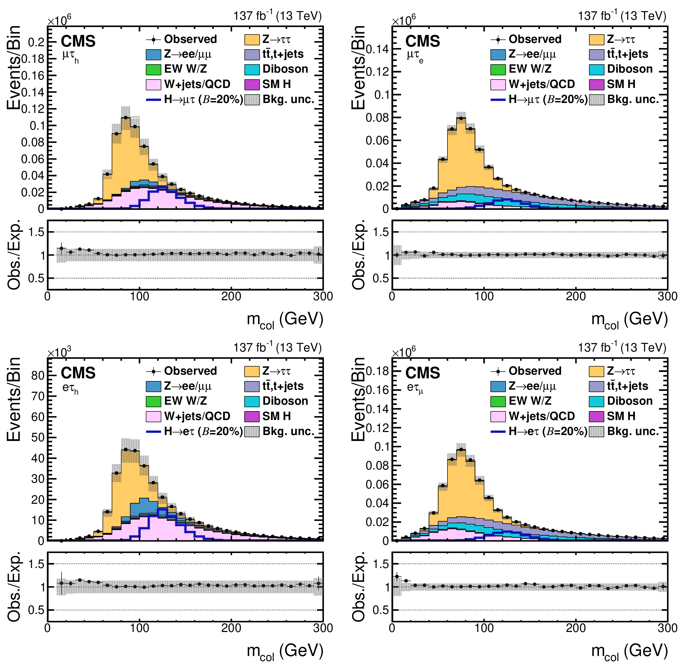
Figure 1:
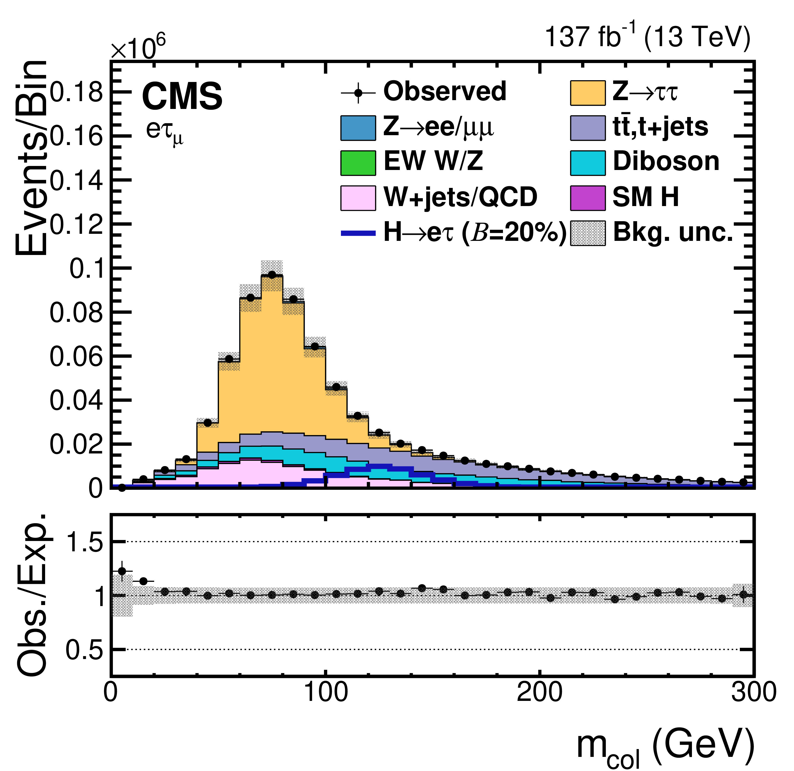
Collinear mass distributions for the data and background processes. A $ {\mathcal {B}(\mathrm{H} \to \mu \tau)} =$ 20% and $ {\mathcal {B}(\mathrm{H} \to \mathrm{e} \tau)} =$ 20% are assumed for the two signal processes. The channels are ${\mathrm{H} \to \mu {\tau _\mathrm {h}}}$ (upper row left), ${\mathrm{H} \to \mu \tau _{\mathrm{e}}}$ (upper row right), ${\mathrm{H} \to \mathrm{e} {\tau _\mathrm {h}}}$ (lower row left), and ${\mathrm{H} \to \mathrm{e} \tau _{\mu}}$ (lower row right). The lower panel in each plot shows the ratio of data and estimated background. The uncertainty band corresponds to the background uncertainty in which the statistical and systematic uncertainties are added in quadrature. |
png pdf |
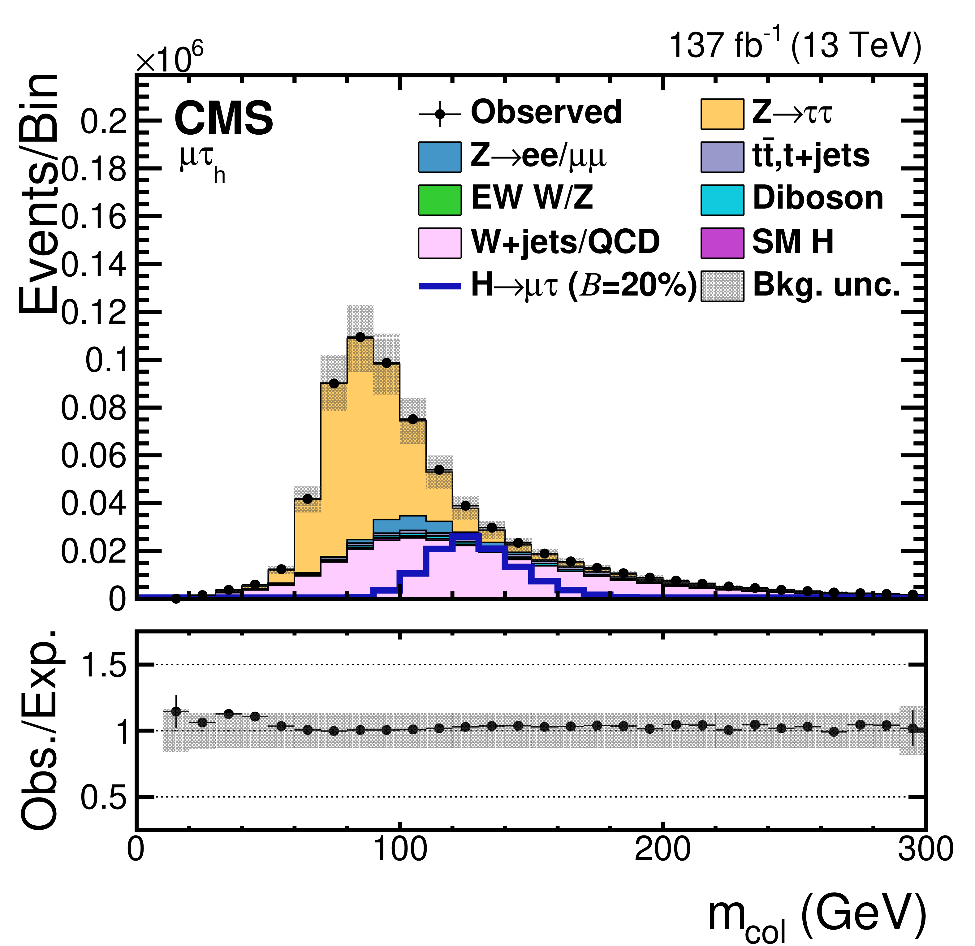
Figure 1-a:
Collinear mass distributions for the data and background processes. A $ {\mathcal {B}(\mathrm{H} \to \mu \tau)} =$ 20% and $ {\mathcal {B}(\mathrm{H} \to \mathrm{e} \tau)} =$ 20% are assumed for the two signal processes. The channel is ${\mathrm{H} \to \mu {\tau _\mathrm {h}}}$. The lower panel shows the ratio of data and estimated background. The uncertainty band corresponds to the background uncertainty in which the statistical and systematic uncertainties are added in quadrature. |
png pdf |
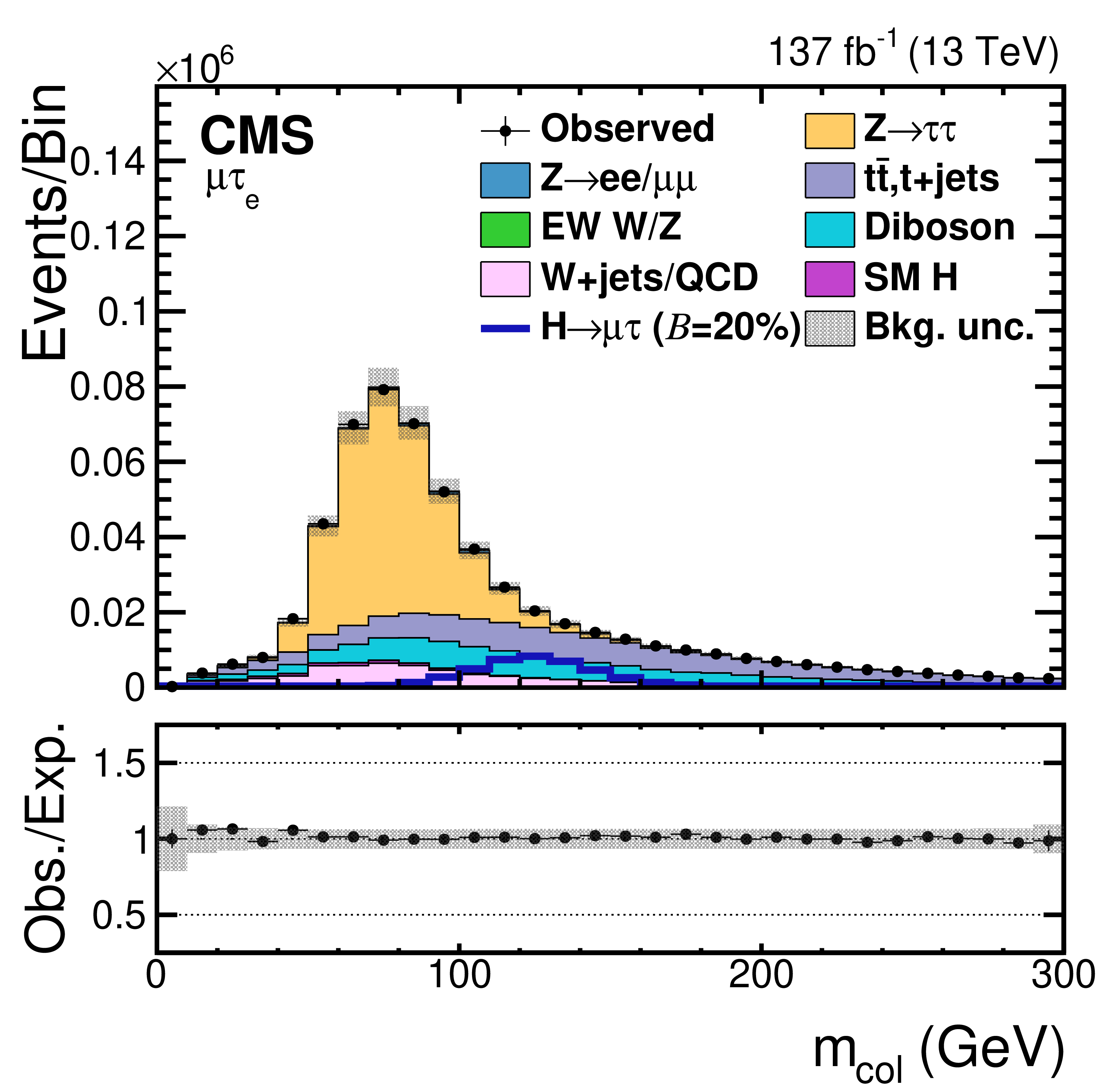
Figure 1-b:
Collinear mass distributions for the data and background processes. A $ {\mathcal {B}(\mathrm{H} \to \mu \tau)} =$ 20% and $ {\mathcal {B}(\mathrm{H} \to \mathrm{e} \tau)} =$ 20% are assumed for the two signal processes. The channel is ${\mathrm{H} \to \mu \tau _{\mathrm{e}}}$. The lower panel shows the ratio of data and estimated background. The uncertainty band corresponds to the background uncertainty in which the statistical and systematic uncertainties are added in quadrature. |
png pdf |
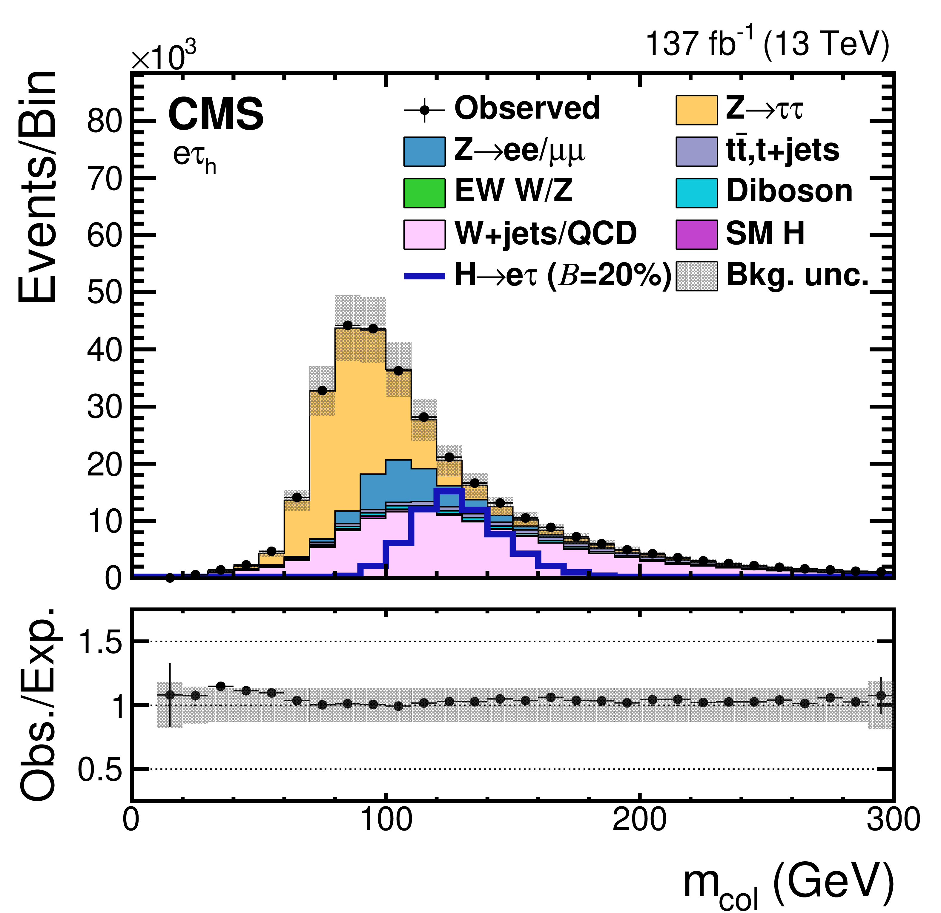
Figure 1-c:
Collinear mass distributions for the data and background processes. A $ {\mathcal {B}(\mathrm{H} \to \mu \tau)} =$ 20% and $ {\mathcal {B}(\mathrm{H} \to \mathrm{e} \tau)} =$ 20% are assumed for the two signal processes. The channel is ${\mathrm{H} \to \mathrm{e} {\tau _\mathrm {h}}}$. The lower panel shows the ratio of data and estimated background. The uncertainty band corresponds to the background uncertainty in which the statistical and systematic uncertainties are added in quadrature. |
png pdf |
Figure 1-d:
Collinear mass distributions for the data and background processes. A $ {\mathcal {B}(\mathrm{H} \to \mu \tau)} =$ 20% and $ {\mathcal {B}(\mathrm{H} \to \mathrm{e} \tau)} =$ 20% are assumed for the two signal processes. The channel is ${\mathrm{H} \to \mathrm{e} \tau _{\mu}}$. The lower panel shows the ratio of data and estimated background. The uncertainty band corresponds to the background uncertainty in which the statistical and systematic uncertainties are added in quadrature. |
png pdf |
Figure 2:
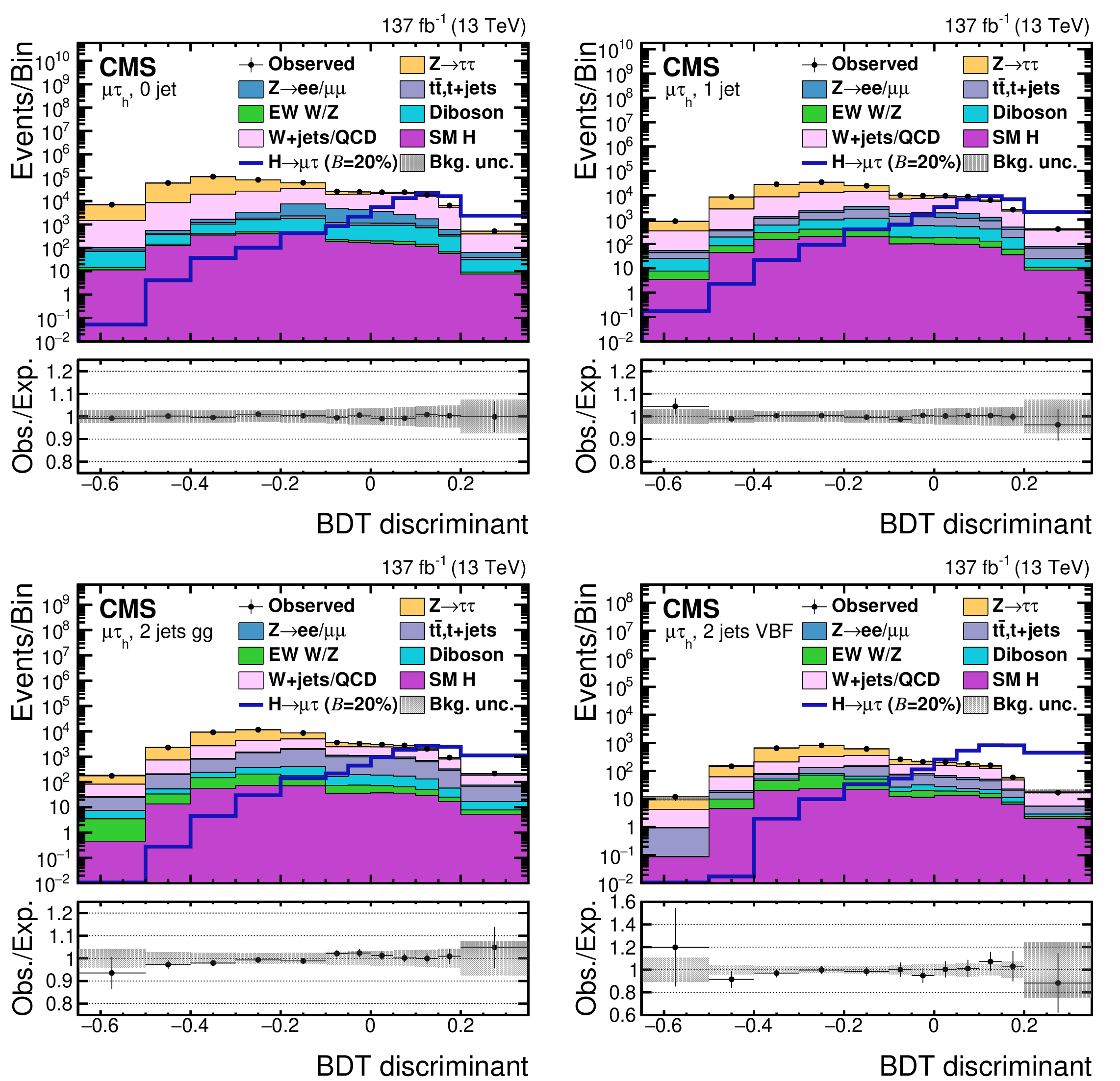
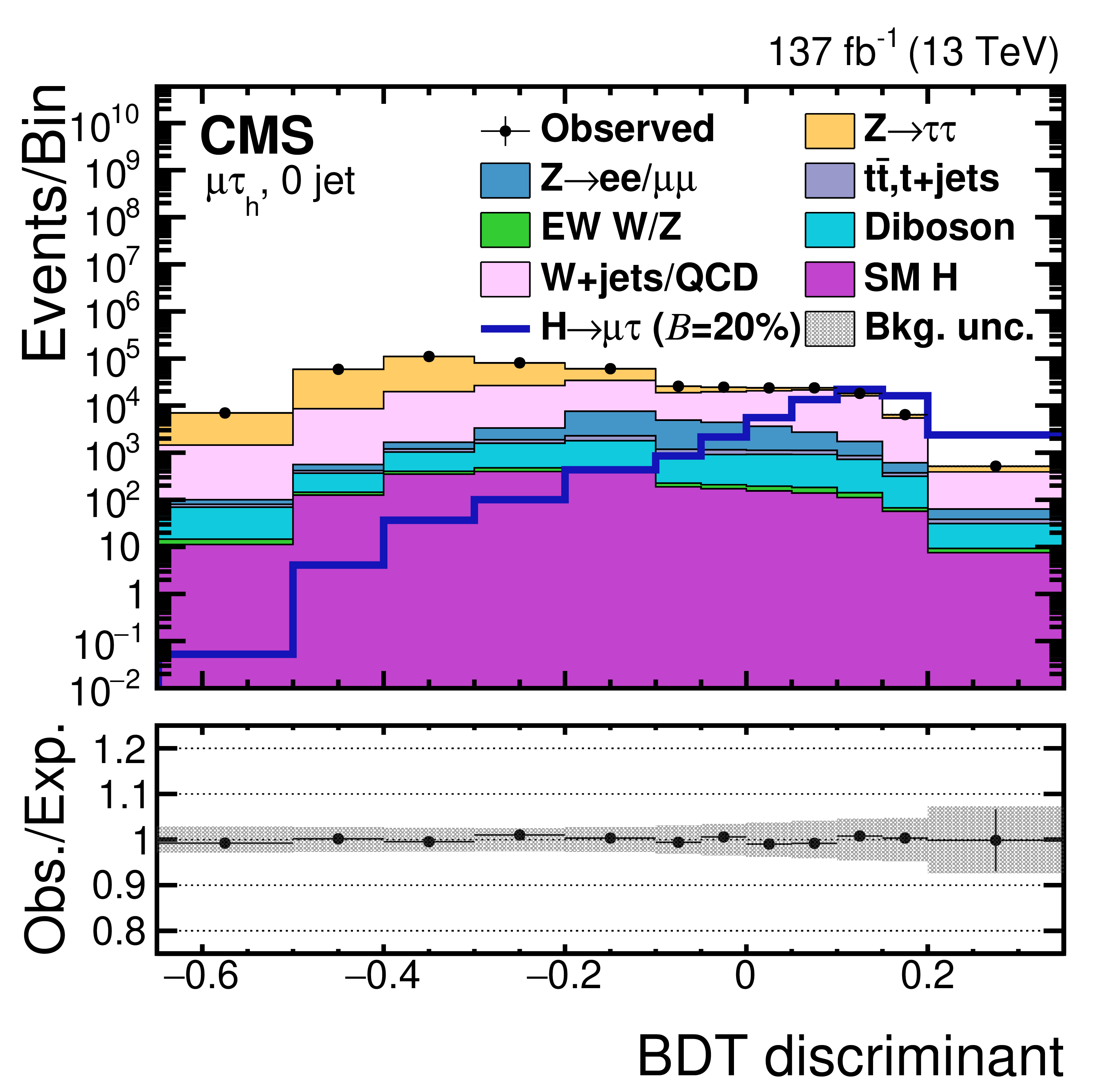
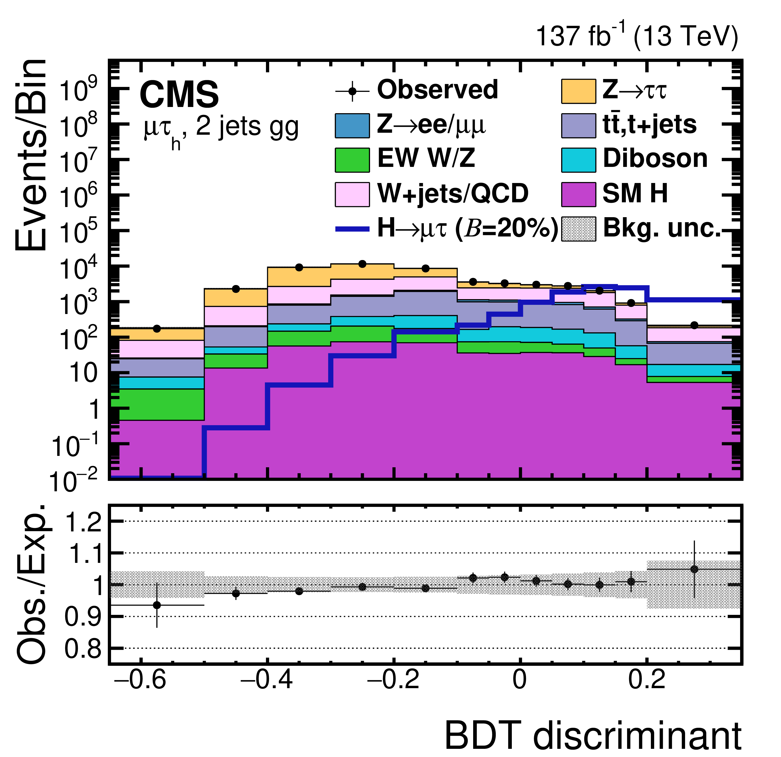
BDT discriminant distributions for the data and background processes in the ${\mathrm{H} \to \mu {\tau _\mathrm {h}}}$ channel. A $ {\mathcal {B}(\mathrm{H} \to \mu \tau)} =$ 20% is assumed for the signal. The channel categories are 0 jets (upper row left), 1 jet (upper row right), 2 jets ggH (lower row left), and 2 jets VBF (lower row right). The lower panel in each plot shows the ratio of data and estimated background. The uncertainty band corresponds to the background uncertainty in which the post-fit statistical and systematic uncertainties are added in quadrature. |
png pdf |
Figure 2-a:
BDT discriminant distributions for the data and background processes in the ${\mathrm{H} \to \mu {\tau _\mathrm {h}}}$ channel. A $ {\mathcal {B}(\mathrm{H} \to \mu \tau)} =$ 20% is assumed for the signal. The channel categories are 0 jet. The lower panel shows the ratio of data and estimated background. The uncertainty band corresponds to the background uncertainty in which the post-fit statistical and systematic uncertainties are added in quadrature. |

png pdf |
Figure 2-b:
BDT discriminant distributions for the data and background processes in the ${\mathrm{H} \to \mu {\tau _\mathrm {h}}}$ channel. A $ {\mathcal {B}(\mathrm{H} \to \mu \tau)} =$ 20% is assumed for the signal. The channel categories are 1 jet. The lower panel shows the ratio of data and estimated background. The uncertainty band corresponds to the background uncertainty in which the post-fit statistical and systematic uncertainties are added in quadrature. |
png pdf |
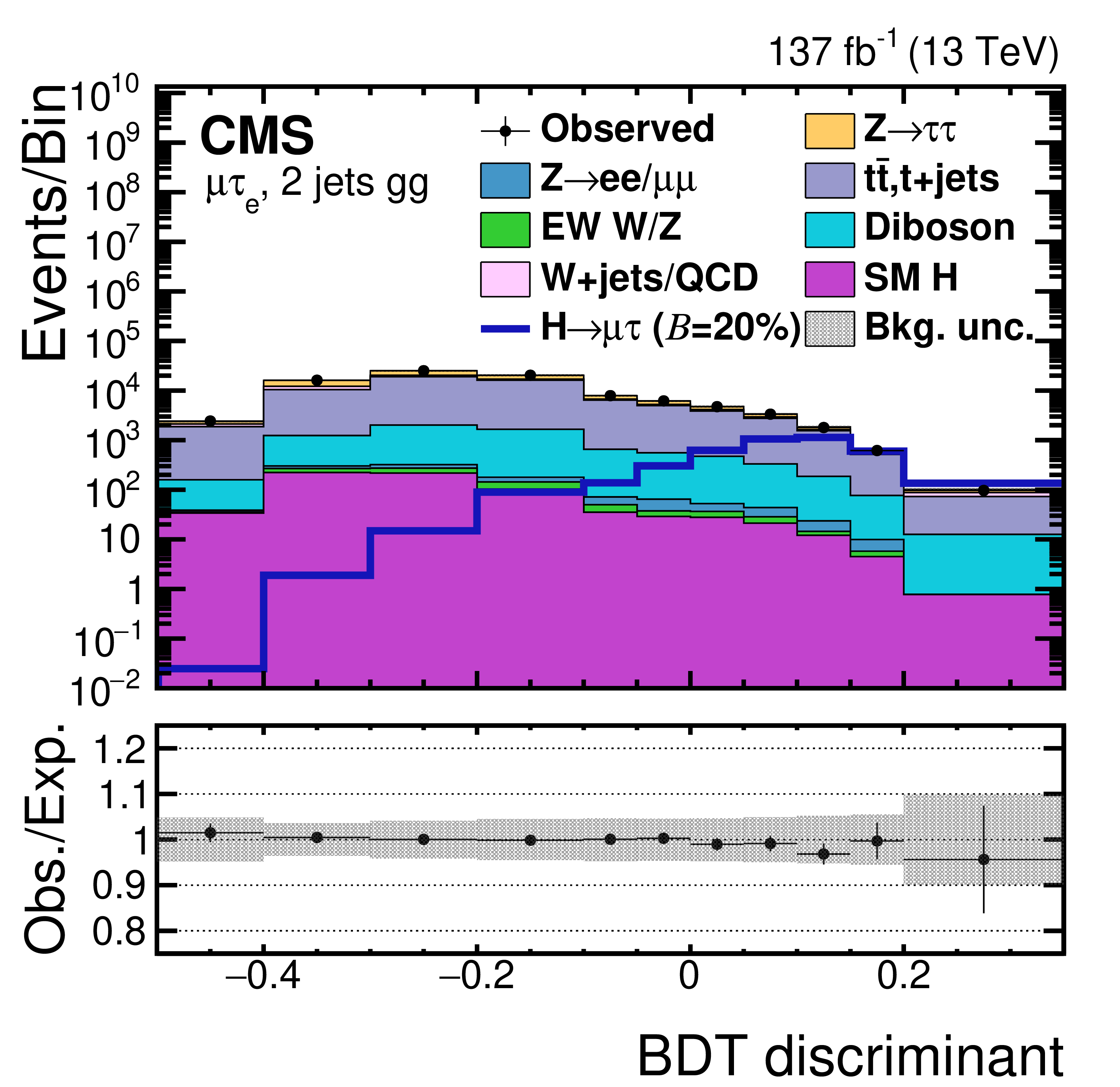
Figure 2-c:
BDT discriminant distributions for the data and background processes in the ${\mathrm{H} \to \mu {\tau _\mathrm {h}}}$ channel. A $ {\mathcal {B}(\mathrm{H} \to \mu \tau)} =$ 20% is assumed for the signal. The channel categories are 2 jets ggH. The lower panel shows the ratio of data and estimated background. The uncertainty band corresponds to the background uncertainty in which the post-fit statistical and systematic uncertainties are added in quadrature. |
png pdf |
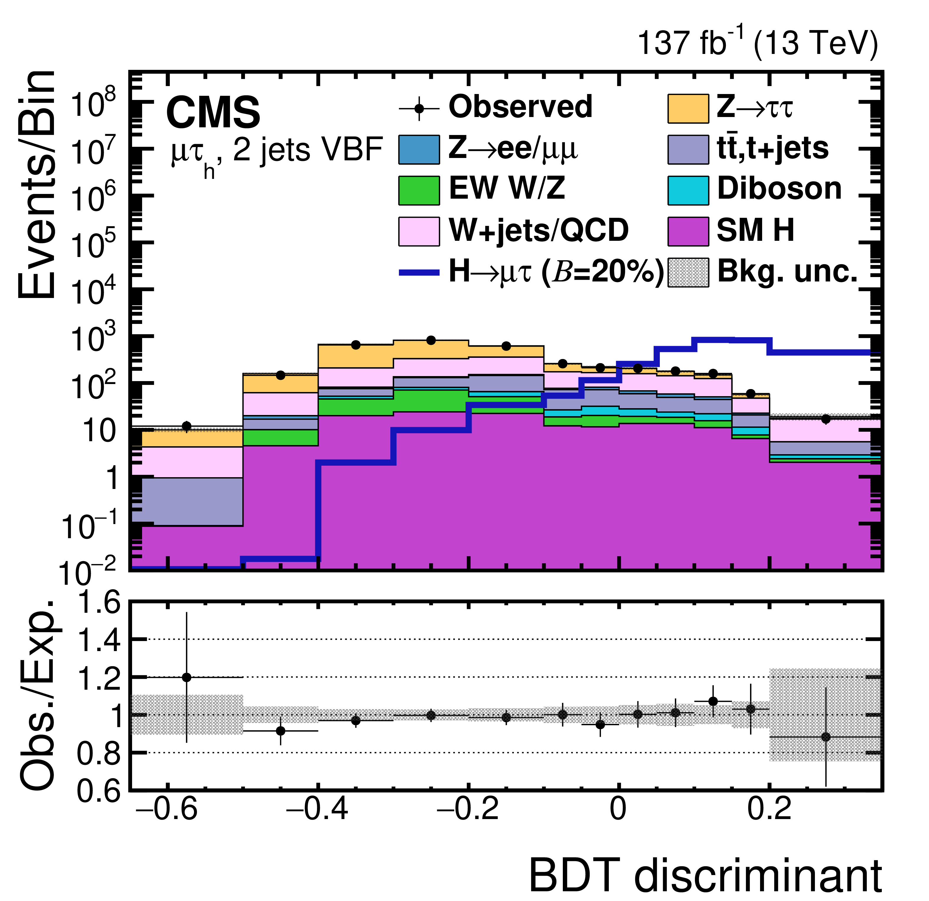
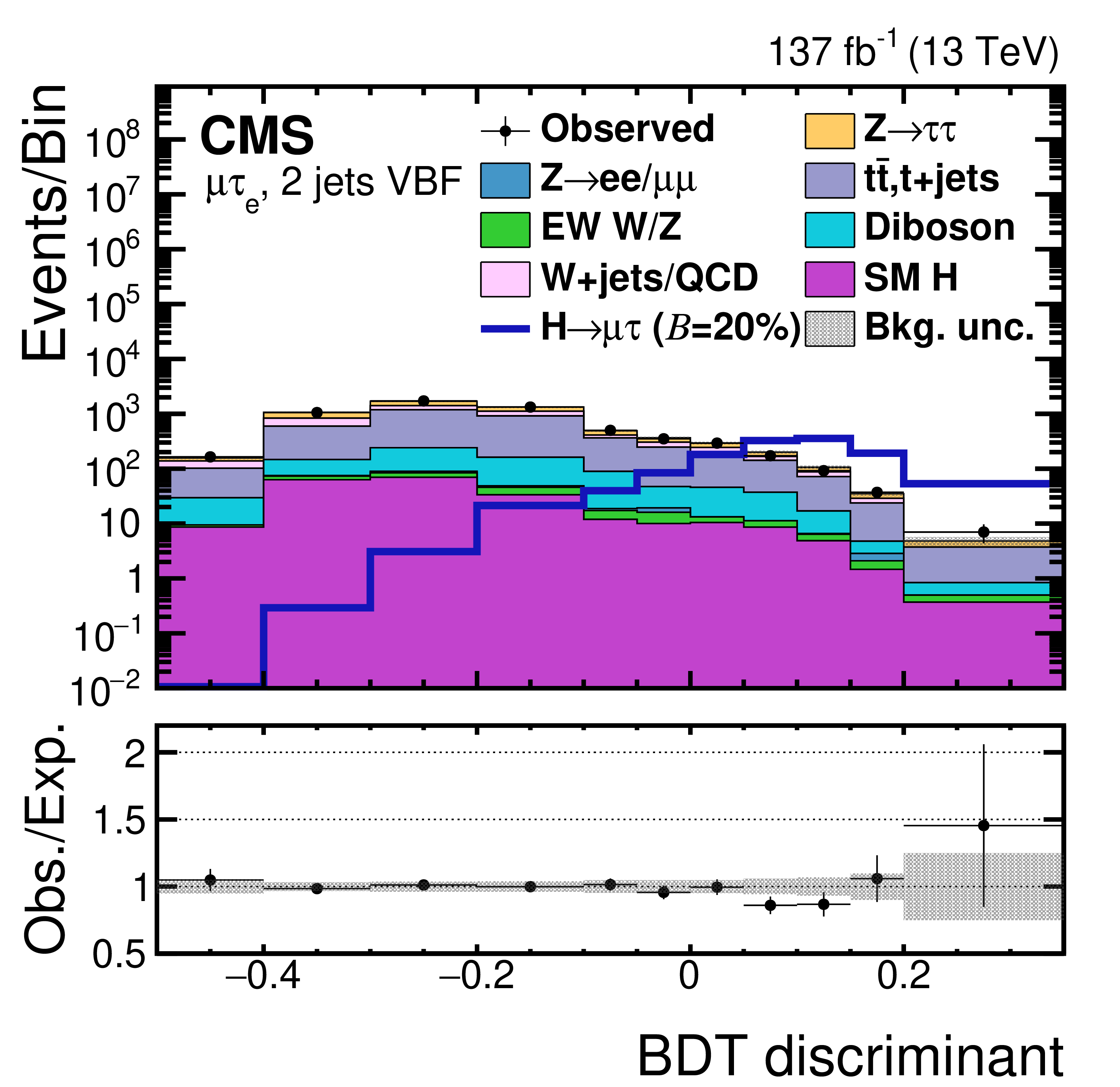
Figure 2-d:
BDT discriminant distributions for the data and background processes in the ${\mathrm{H} \to \mu {\tau _\mathrm {h}}}$ channel. A $ {\mathcal {B}(\mathrm{H} \to \mu \tau)} =$ 20% is assumed for the signal. The channel categories are 2 jets VBF. The lower panel shows the ratio of data and estimated background. The uncertainty band corresponds to the background uncertainty in which the post-fit statistical and systematic uncertainties are added in quadrature. |
png pdf |
Figure 3:
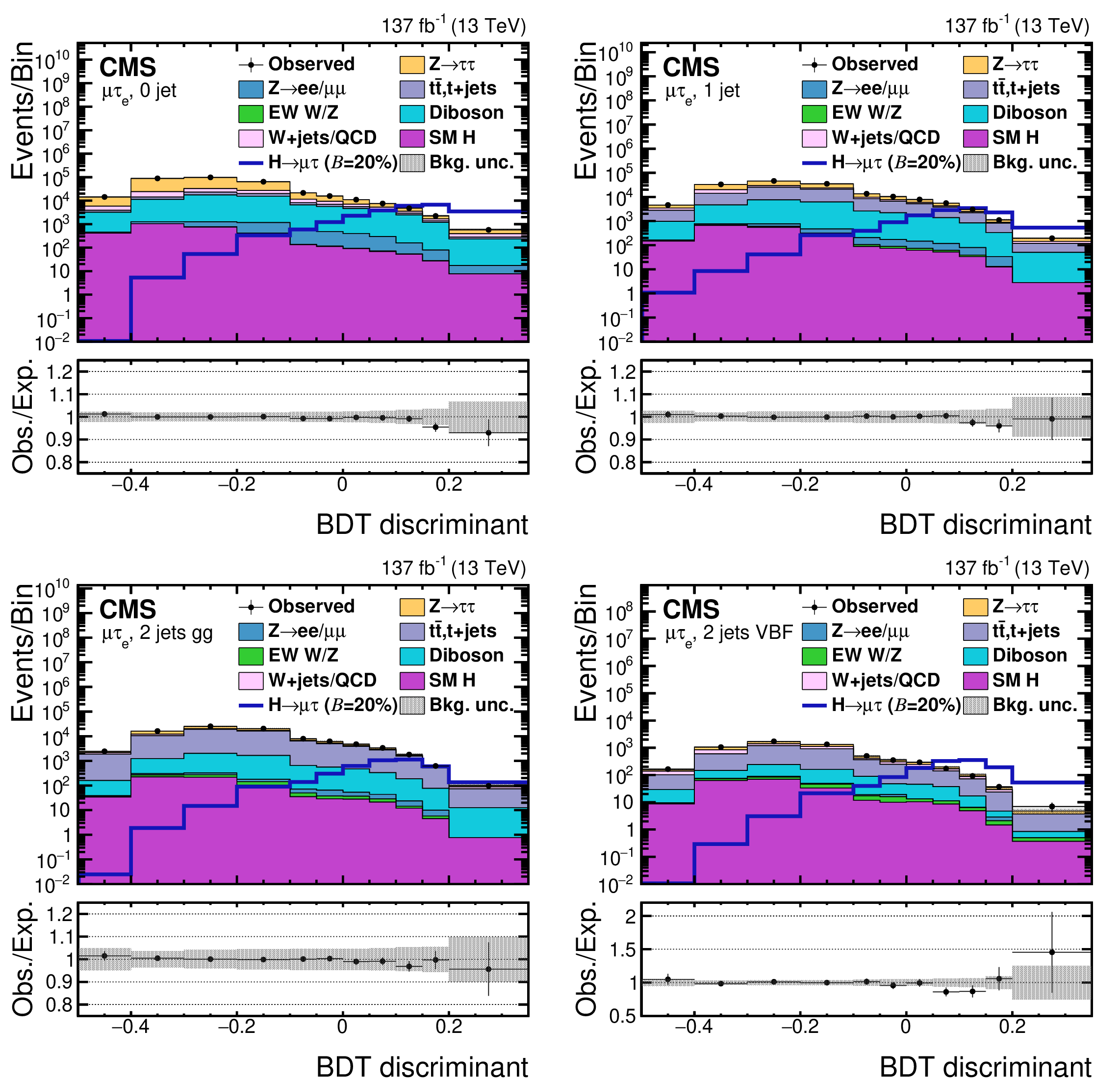
BDT discriminant distributions for the data and background processes in the ${\mathrm{H} \to \mu \tau _{\mathrm{e}}}$ channel. A $ {\mathcal {B}(\mathrm{H} \to \mu \tau)} =$ 20% is assumed for the signal. The channel categories are 0 jets (upper row left), 1 jet (upper row right), 2 jets ggH (lower row left), and 2 jets VBF (lower row right). The lower panel in each plot shows the ratio of data and estimated background. The uncertainty band corresponds to the background uncertainty in which the post-fit statistical and systematic uncertainties are added in quadrature. |
png pdf |
Figure 3-a:
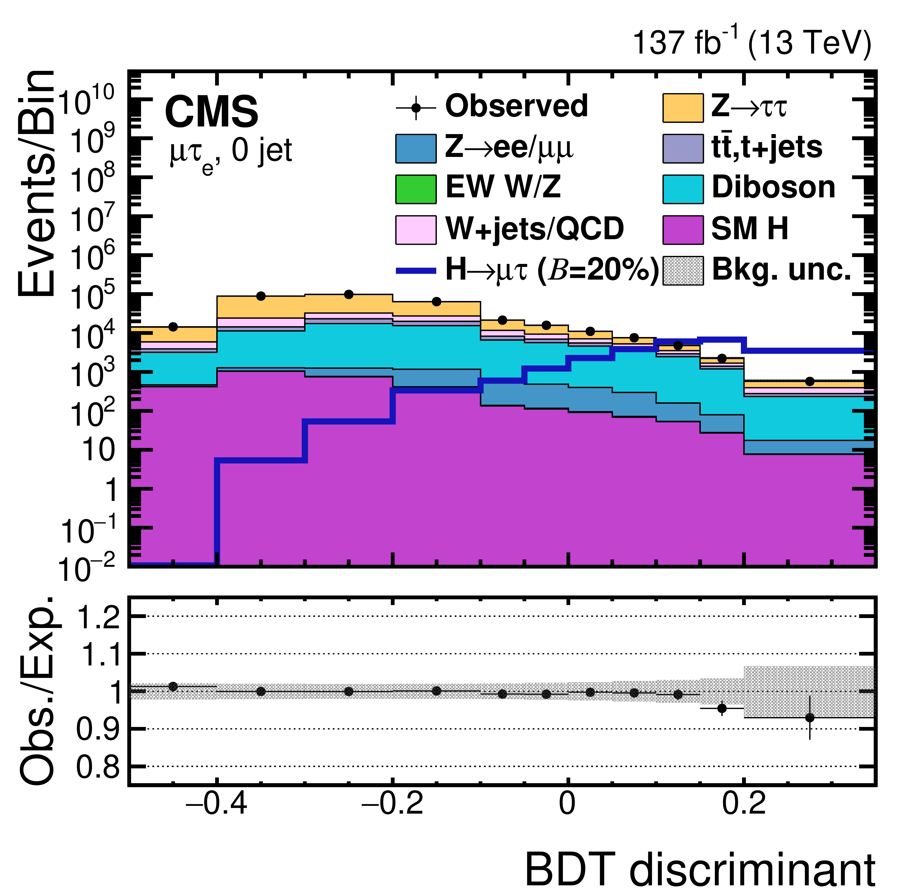
BDT discriminant distributions for the data and background processes in the ${\mathrm{H} \to \mu \tau _{\mathrm{e}}}$ channel. A $ {\mathcal {B}(\mathrm{H} \to \mu \tau)} =$ 20% is assumed for the signal. The channel categories are 0 jet. The lower panel shows the ratio of data and estimated background. The uncertainty band corresponds to the background uncertainty in which the post-fit statistical and systematic uncertainties are added in quadrature. |
png pdf |
Figure 3-b:
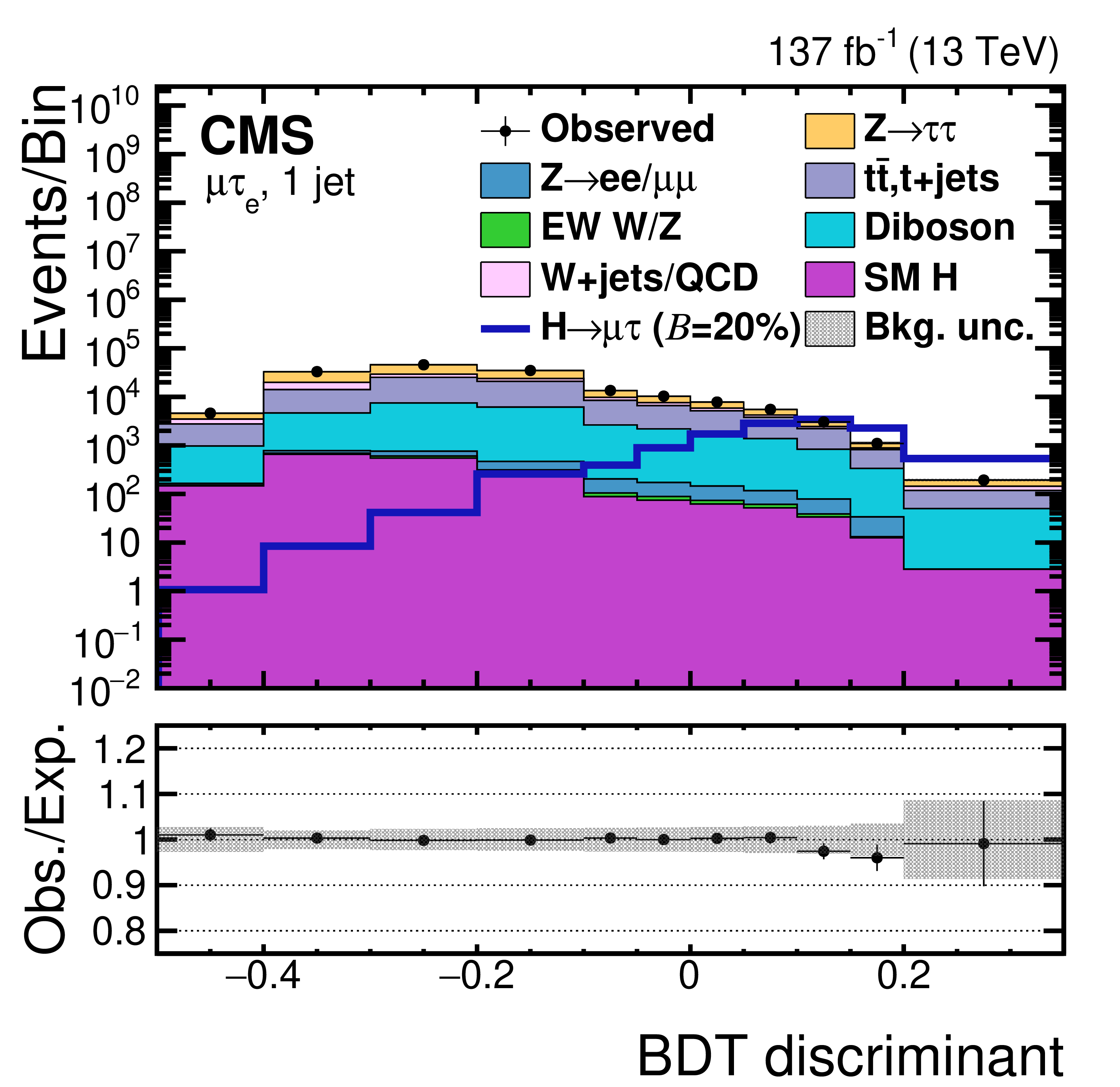
BDT discriminant distributions for the data and background processes in the ${\mathrm{H} \to \mu \tau _{\mathrm{e}}}$ channel. A $ {\mathcal {B}(\mathrm{H} \to \mu \tau)} =$ 20% is assumed for the signal. The channel categories are 1 jet. The lower panel shows the ratio of data and estimated background. The uncertainty band corresponds to the background uncertainty in which the post-fit statistical and systematic uncertainties are added in quadrature. |
png pdf |
Figure 3-c:
BDT discriminant distributions for the data and background processes in the ${\mathrm{H} \to \mu \tau _{\mathrm{e}}}$ channel. A $ {\mathcal {B}(\mathrm{H} \to \mu \tau)} =$ 20% is assumed for the signal. The channel categories are 2 jets ggH. The lower panel shows the ratio of data and estimated background. The uncertainty band corresponds to the background uncertainty in which the post-fit statistical and systematic uncertainties are added in quadrature. |
png pdf |
Figure 3-d:
BDT discriminant distributions for the data and background processes in the ${\mathrm{H} \to \mu \tau _{\mathrm{e}}}$ channel. A $ {\mathcal {B}(\mathrm{H} \to \mu \tau)} =$ 20% is assumed for the signal. The channel categories are 2 jets VBF. The lower panel shows the ratio of data and estimated background. The uncertainty band corresponds to the background uncertainty in which the post-fit statistical and systematic uncertainties are added in quadrature. |
png pdf |
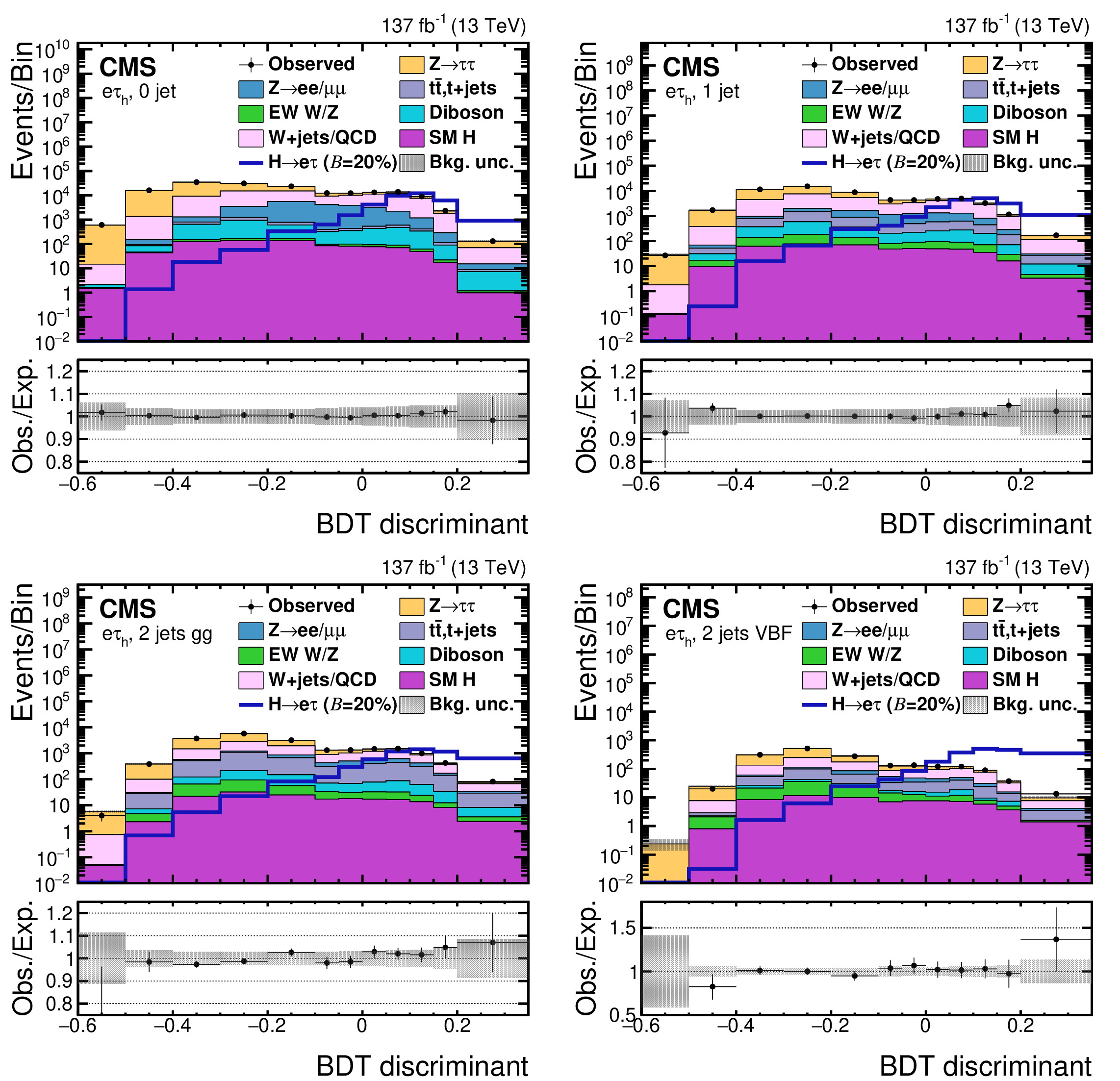
Figure 4:
BDT discriminant distributions for the data and background processes in the ${\mathrm{H} \to \mathrm{e} {\tau _\mathrm {h}}}$ channel. A $ {\mathcal {B}(\mathrm{H} \to \mathrm{e} \tau)} =$ 20% is assumed for the signal. The channel categories are 0 jets (upper row left), 1 jet (upper row right), 2 jets ggH (lower row left), and 2 jets VBF (lower row right). The lower panel in each plot shows the ratio of data and estimated background. The uncertainty band corresponds to the background uncertainty in which the post-fit statistical and systematic uncertainties are added in quadrature. |

png pdf |
Figure 4-a:
BDT discriminant distributions for the data and background processes in the ${\mathrm{H} \to \mathrm{e} {\tau _\mathrm {h}}}$ channel. A $ {\mathcal {B}(\mathrm{H} \to \mathrm{e} \tau)} =$ 20% is assumed for the signal. The channel categories are 0 jet. The lower panel shows the ratio of data and estimated background. The uncertainty band corresponds to the background uncertainty in which the post-fit statistical and systematic uncertainties are added in quadrature. |
png pdf |
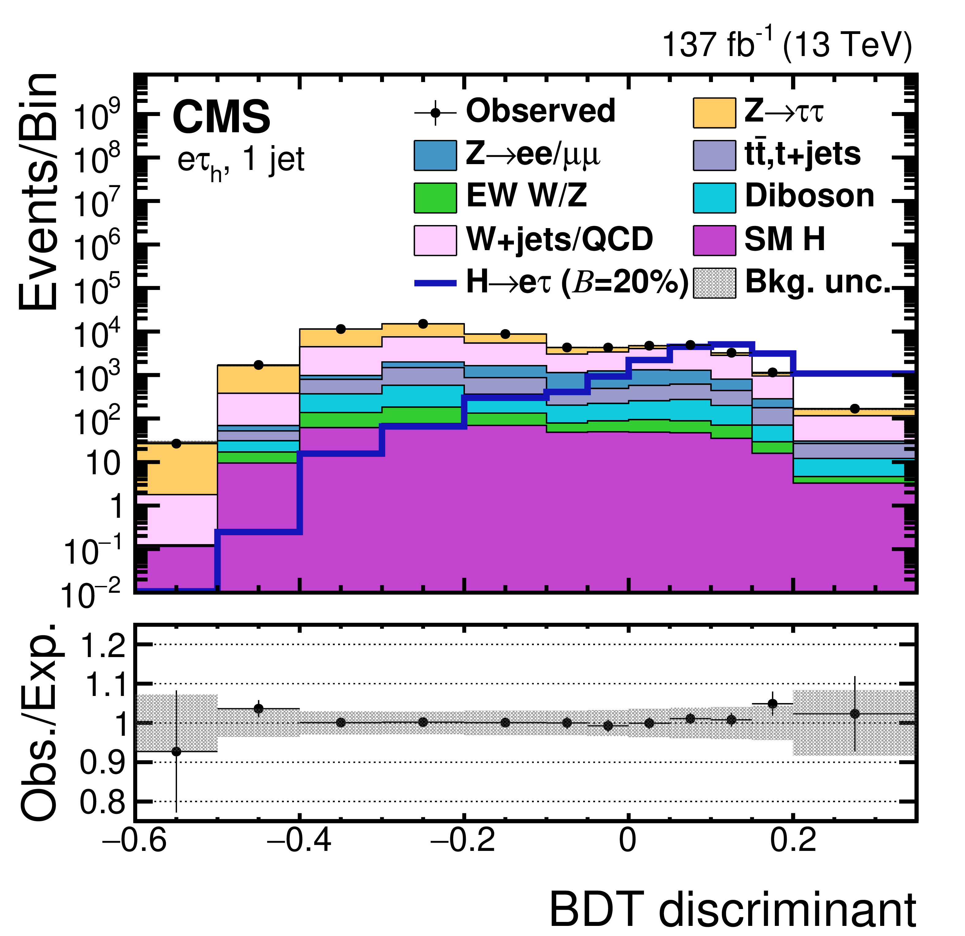
Figure 4-b:
BDT discriminant distributions for the data and background processes in the ${\mathrm{H} \to \mathrm{e} {\tau _\mathrm {h}}}$ channel. A $ {\mathcal {B}(\mathrm{H} \to \mathrm{e} \tau)} =$ 20% is assumed for the signal. The channel categories are 1 jet. The lower panel shows the ratio of data and estimated background. The uncertainty band corresponds to the background uncertainty in which the post-fit statistical and systematic uncertainties are added in quadrature. |
png pdf |
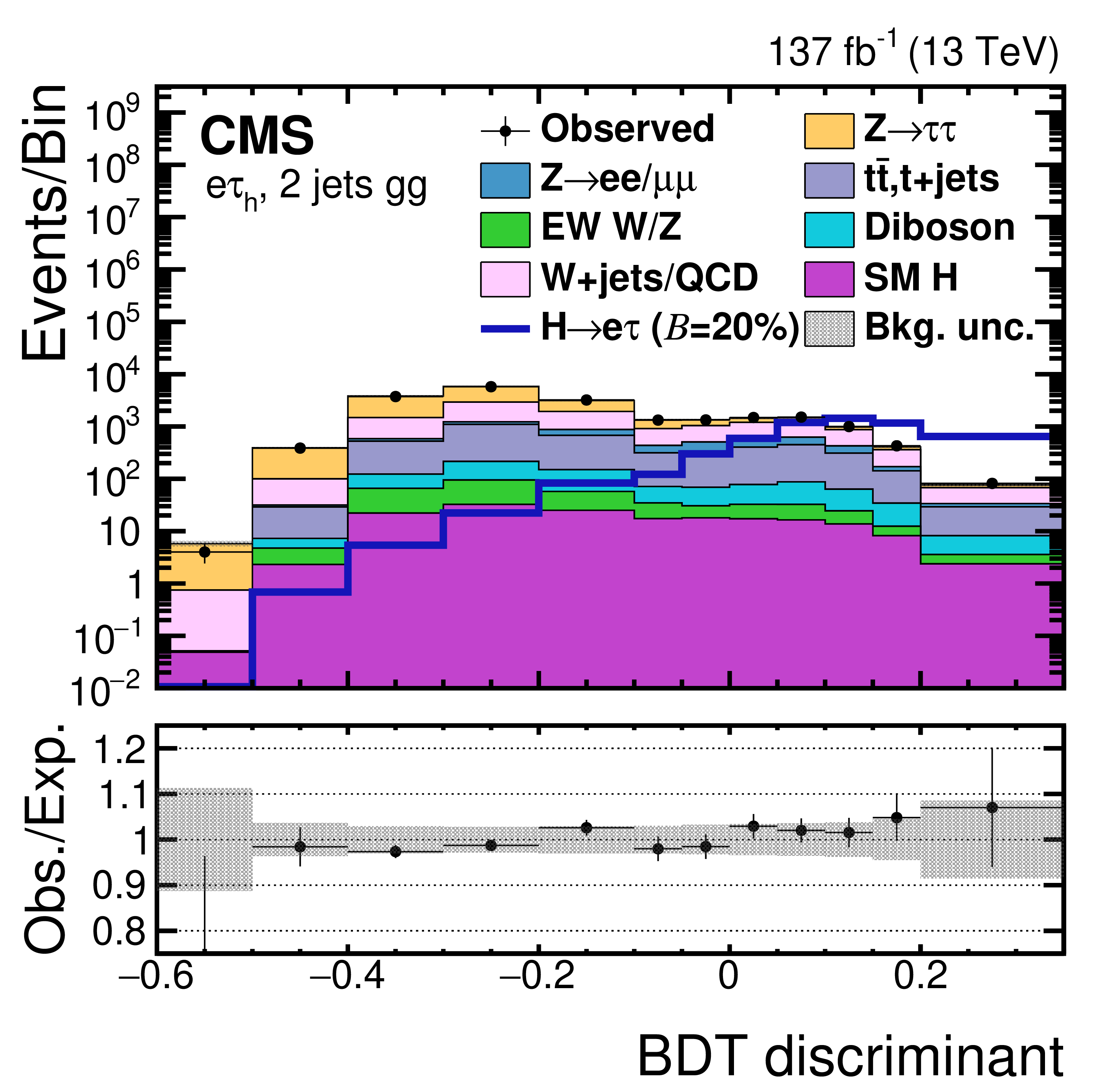
Figure 4-c:
BDT discriminant distributions for the data and background processes in the ${\mathrm{H} \to \mathrm{e} {\tau _\mathrm {h}}}$ channel. A $ {\mathcal {B}(\mathrm{H} \to \mathrm{e} \tau)} =$ 20% is assumed for the signal. The channel categories are 2 jets ggH. The lower panel shows the ratio of data and estimated background. The uncertainty band corresponds to the background uncertainty in which the post-fit statistical and systematic uncertainties are added in quadrature. |

png pdf |
Figure 4-d:
BDT discriminant distributions for the data and background processes in the ${\mathrm{H} \to \mathrm{e} {\tau _\mathrm {h}}}$ channel. A $ {\mathcal {B}(\mathrm{H} \to \mathrm{e} \tau)} =$ 20% is assumed for the signal. The channel categories are 2 jets VBF. The lower panel shows the ratio of data and estimated background. The uncertainty band corresponds to the background uncertainty in which the post-fit statistical and systematic uncertainties are added in quadrature. |
png pdf |
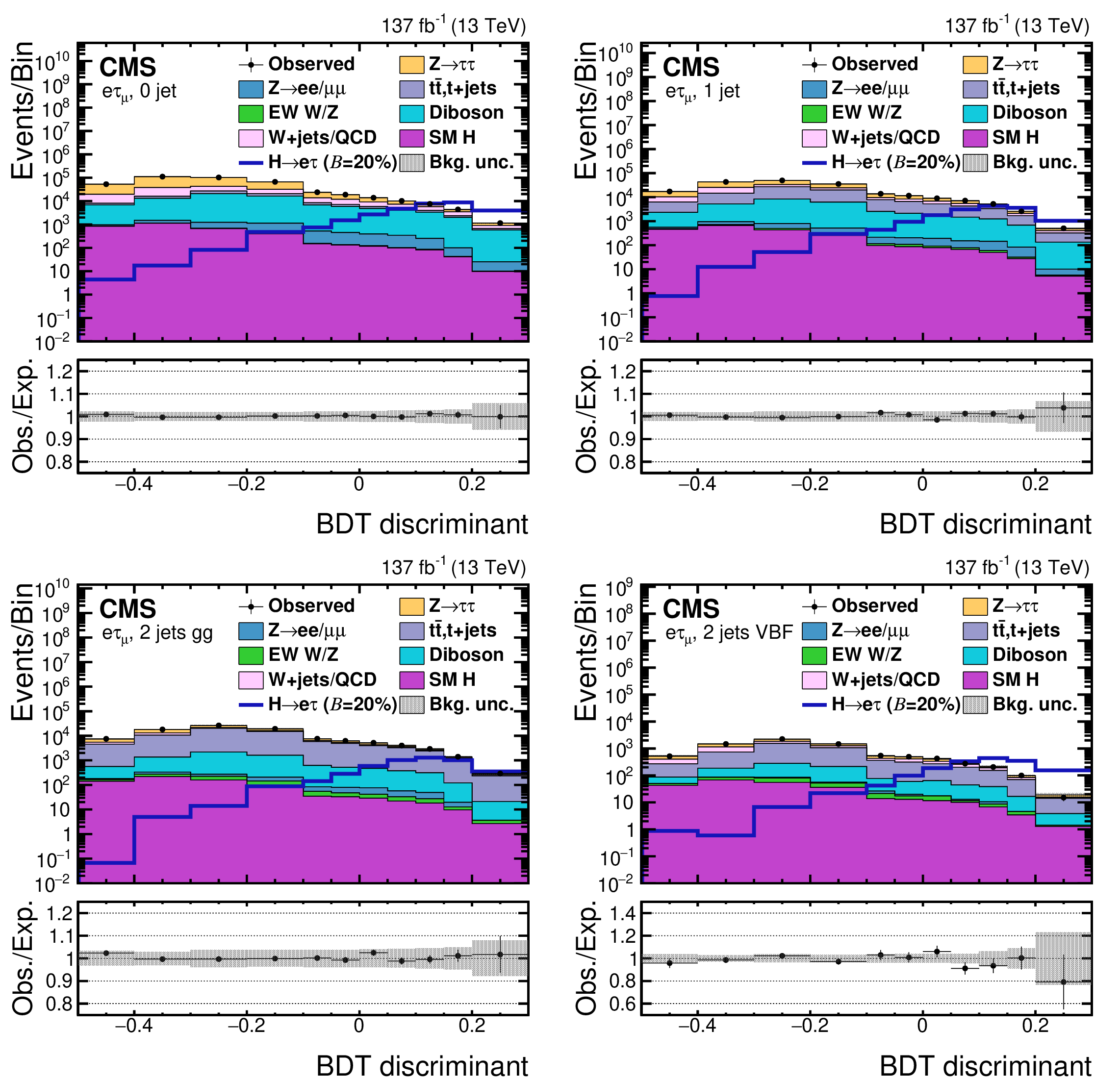
Figure 5:
BDT discriminant distributions for the data and background processes in the ${\mathrm{H} \to \mathrm{e} \tau _{\mu}}$ channel. A $ {\mathcal {B}(\mathrm{H} \to \mathrm{e} \tau)} =$ 20% is assumed for the signal. The channel categories are 0 jets (upper row left), 1 jet (upper row right), 2 jets ggH (lower row left), and 2 jets VBF (lower row right). The lower panel in each plot shows the ratio of data and estimated background. The uncertainty band corresponds to the background uncertainty in which the post-fit statistical and systematic uncertainties are added in quadrature. |
png pdf |
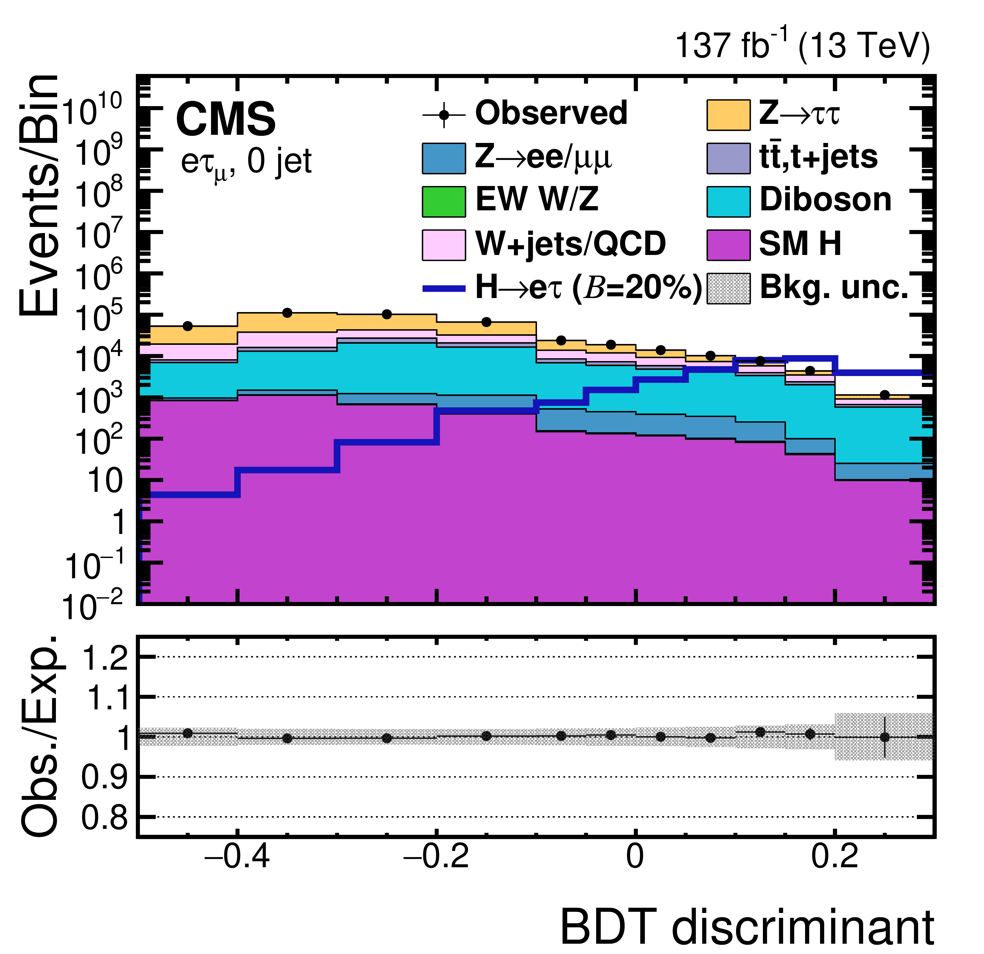
Figure 5-a:
BDT discriminant distributions for the data and background processes in the ${\mathrm{H} \to \mathrm{e} \tau _{\mu}}$ channel. A $ {\mathcal {B}(\mathrm{H} \to \mathrm{e} \tau)} =$ 20% is assumed for the signal. The channel categories are 0 jet. The lower panel in each plot shows the ratio of data and estimated background. The uncertainty band corresponds to the background uncertainty in which the post-fit statistical and systematic uncertainties are added in quadrature. |
png pdf |
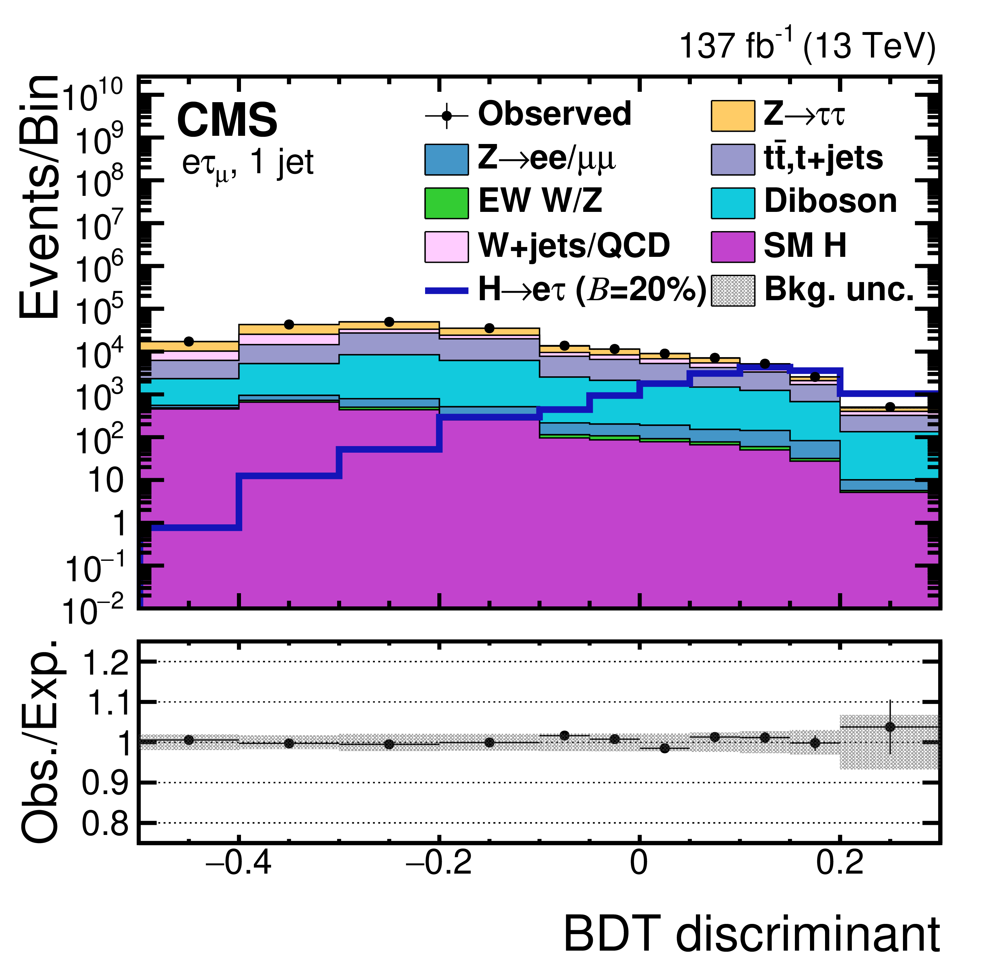
Figure 5-b:
BDT discriminant distributions for the data and background processes in the ${\mathrm{H} \to \mathrm{e} \tau _{\mu}}$ channel. A $ {\mathcal {B}(\mathrm{H} \to \mathrm{e} \tau)} =$ 20% is assumed for the signal. The channel categories are 1 jet. The lower panel in each plot shows the ratio of data and estimated background. The uncertainty band corresponds to the background uncertainty in which the post-fit statistical and systematic uncertainties are added in quadrature. |
png pdf |
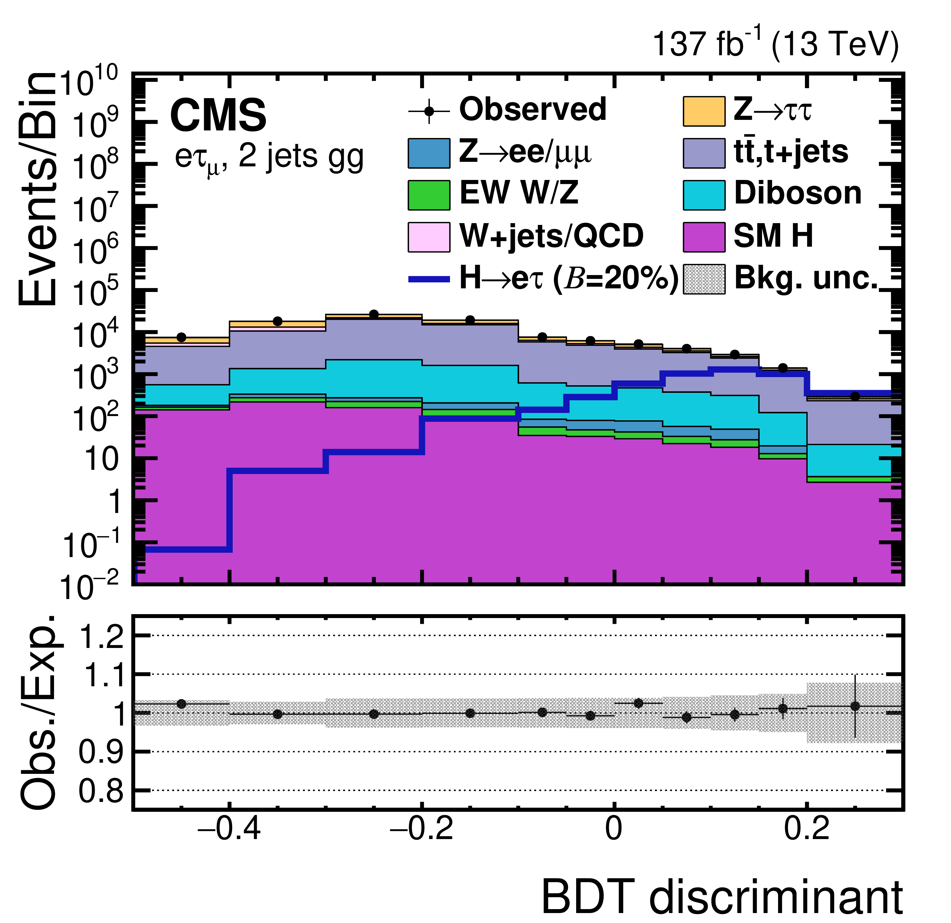
Figure 5-c:
BDT discriminant distributions for the data and background processes in the ${\mathrm{H} \to \mathrm{e} \tau _{\mu}}$ channel. A $ {\mathcal {B}(\mathrm{H} \to \mathrm{e} \tau)} =$ 20% is assumed for the signal. The channel categories are 2 jets ggH. The lower panel in each plot shows the ratio of data and estimated background. The uncertainty band corresponds to the background uncertainty in which the post-fit statistical and systematic uncertainties are added in quadrature. |
png pdf |
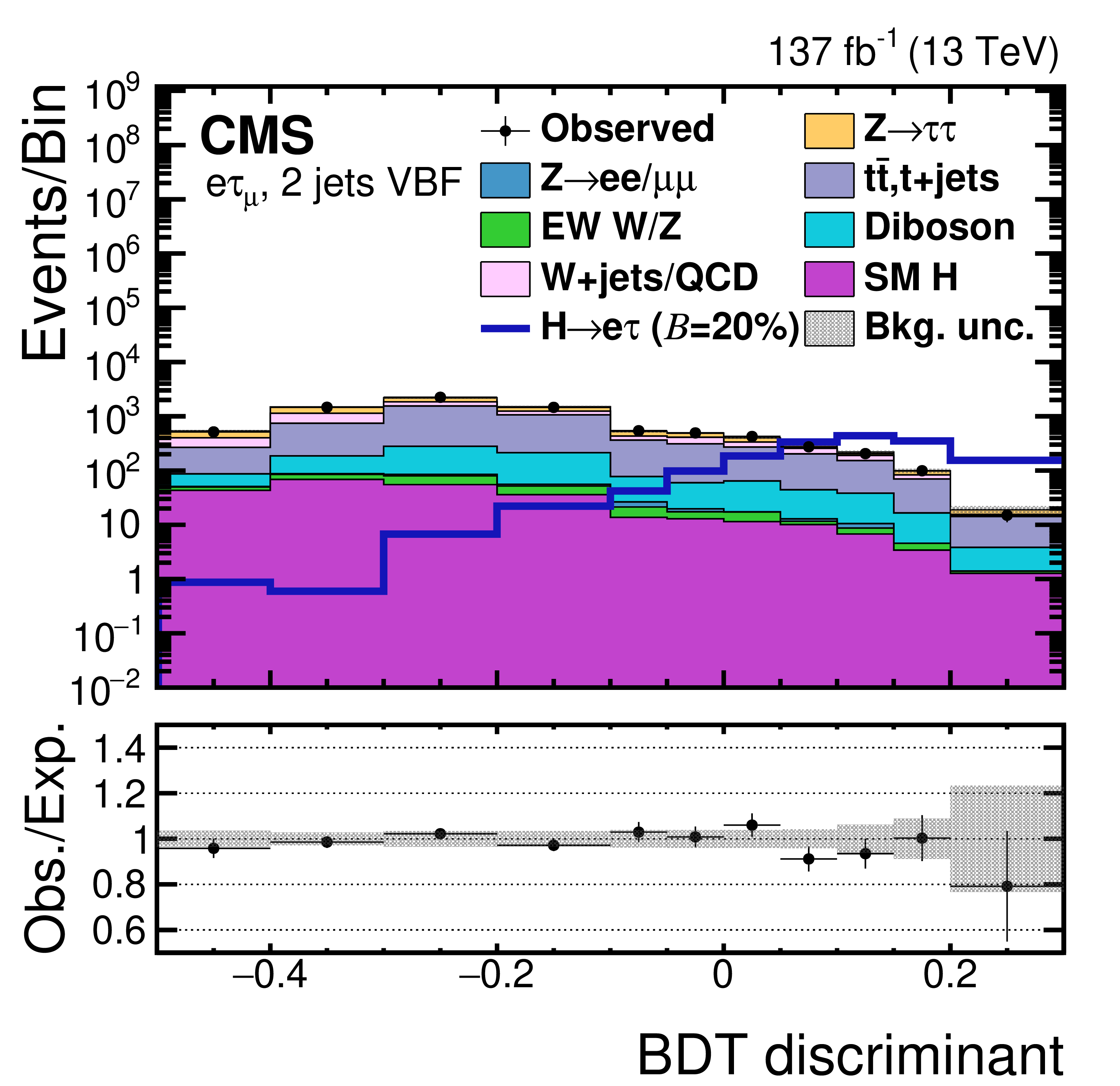
Figure 5-d:
BDT discriminant distributions for the data and background processes in the ${\mathrm{H} \to \mathrm{e} \tau _{\mu}}$ channel. A $ {\mathcal {B}(\mathrm{H} \to \mathrm{e} \tau)} =$ 20% is assumed for the signal. The channel categories are 2 jets VBF. The lower panel in each plot shows the ratio of data and estimated background. The uncertainty band corresponds to the background uncertainty in which the post-fit statistical and systematic uncertainties are added in quadrature. |

png pdf |
Figure 6:
The ${m_{\text {col}}}$ distribution in VR with same electric charge for both leptons (left), W+jets VR (middle), and ${\mathrm{t} {}\mathrm{\bar{t}}}$ VR (right). In each distribution, the VR's dominant background is shown, and all the other backgrounds are grouped into "Other bkg.''. A $ {\mathcal {B}(\mathrm{H} \to \mu \tau)} =$ 20% is assumed for the signal. The lower panel in each plot shows the ratio of data and estimated background. The uncertainty band corresponds to the background uncertainty in which the post-fit statistical and systematic uncertainties are added in quadrature. |

png pdf |
Figure 6-a:
The ${m_{\text {col}}}$ distribution in VR with same electric charge for both leptons. The VR's dominant background is shown, and all the other backgrounds are grouped into "Other bkg.''. A $ {\mathcal {B}(\mathrm{H} \to \mu \tau)} =$ 20% is assumed for the signal. The lower panel shows the ratio of data and estimated background. The uncertainty band corresponds to the background uncertainty in which the post-fit statistical and systematic uncertainties are added in quadrature. |
png pdf |
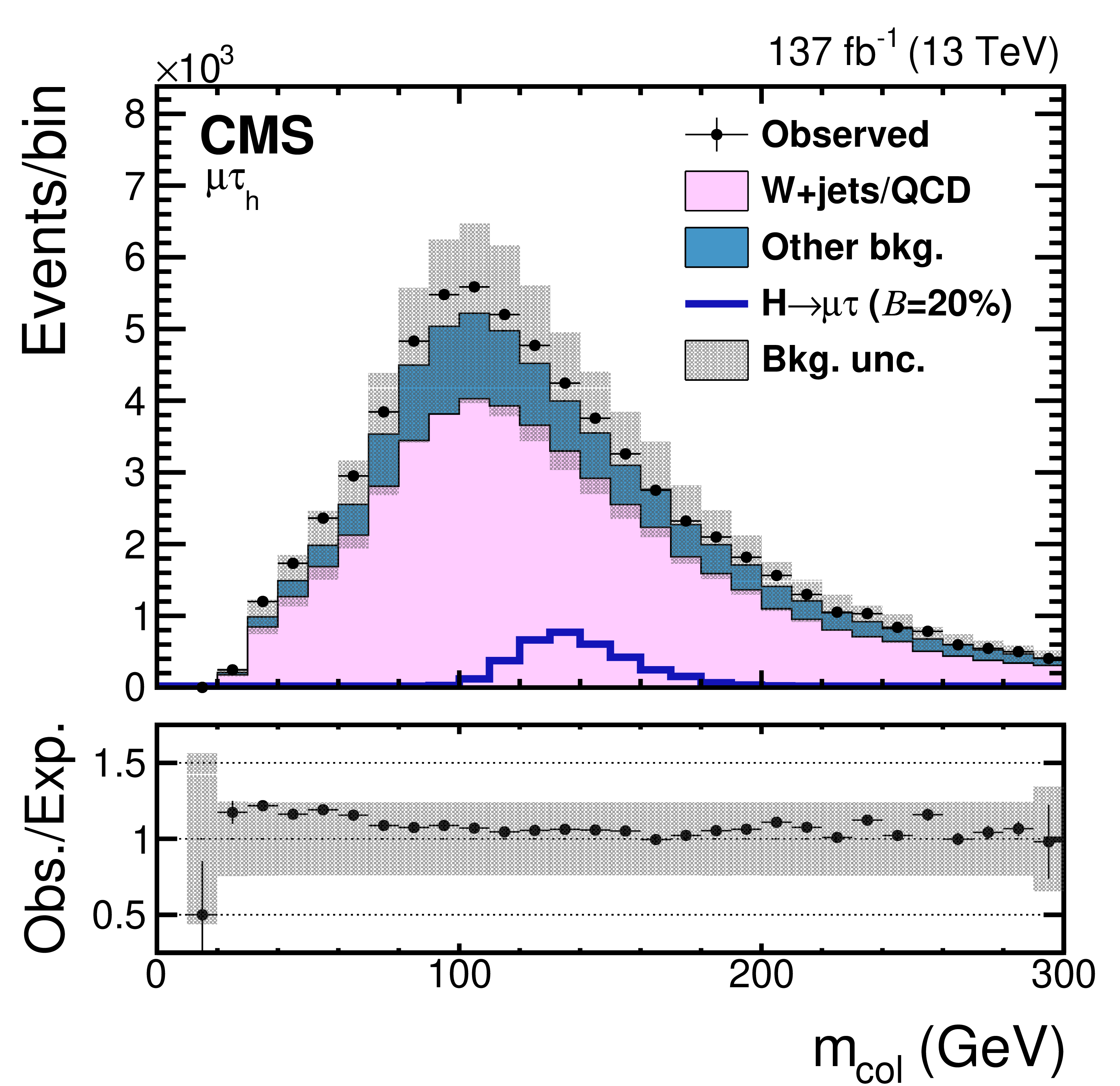
Figure 6-b:
The ${m_{\text {col}}}$ distribution in the W+jets VR. The VR's dominant background is shown, and all the other backgrounds are grouped into "Other bkg.''. A $ {\mathcal {B}(\mathrm{H} \to \mu \tau)} =$ 20% is assumed for the signal. The lower panel shows the ratio of data and estimated background. The uncertainty band corresponds to the background uncertainty in which the post-fit statistical and systematic uncertainties are added in quadrature. |
png pdf |
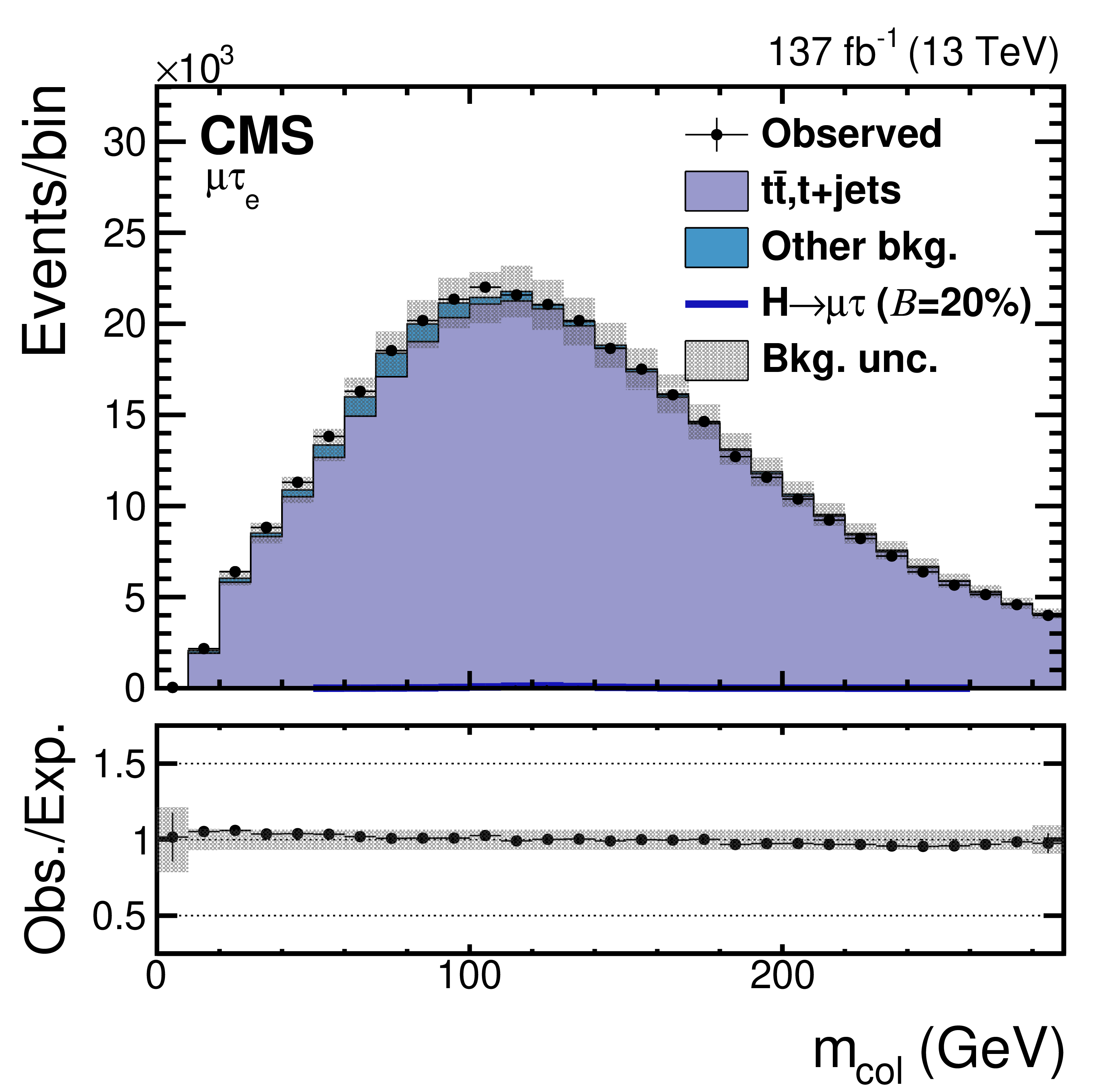
Figure 6-c:
The ${m_{\text {col}}}$ distribution in the ${\mathrm{t} {}\mathrm{\bar{t}}}$ VR. The VR's dominant background is shown, and all the other backgrounds are grouped into "Other bkg.''. A $ {\mathcal {B}(\mathrm{H} \to \mu \tau)} =$ 20% is assumed for the signal. The lower panel shows the ratio of data and estimated background. The uncertainty band corresponds to the background uncertainty in which the post-fit statistical and systematic uncertainties are added in quadrature. |

png pdf |
Figure 7:
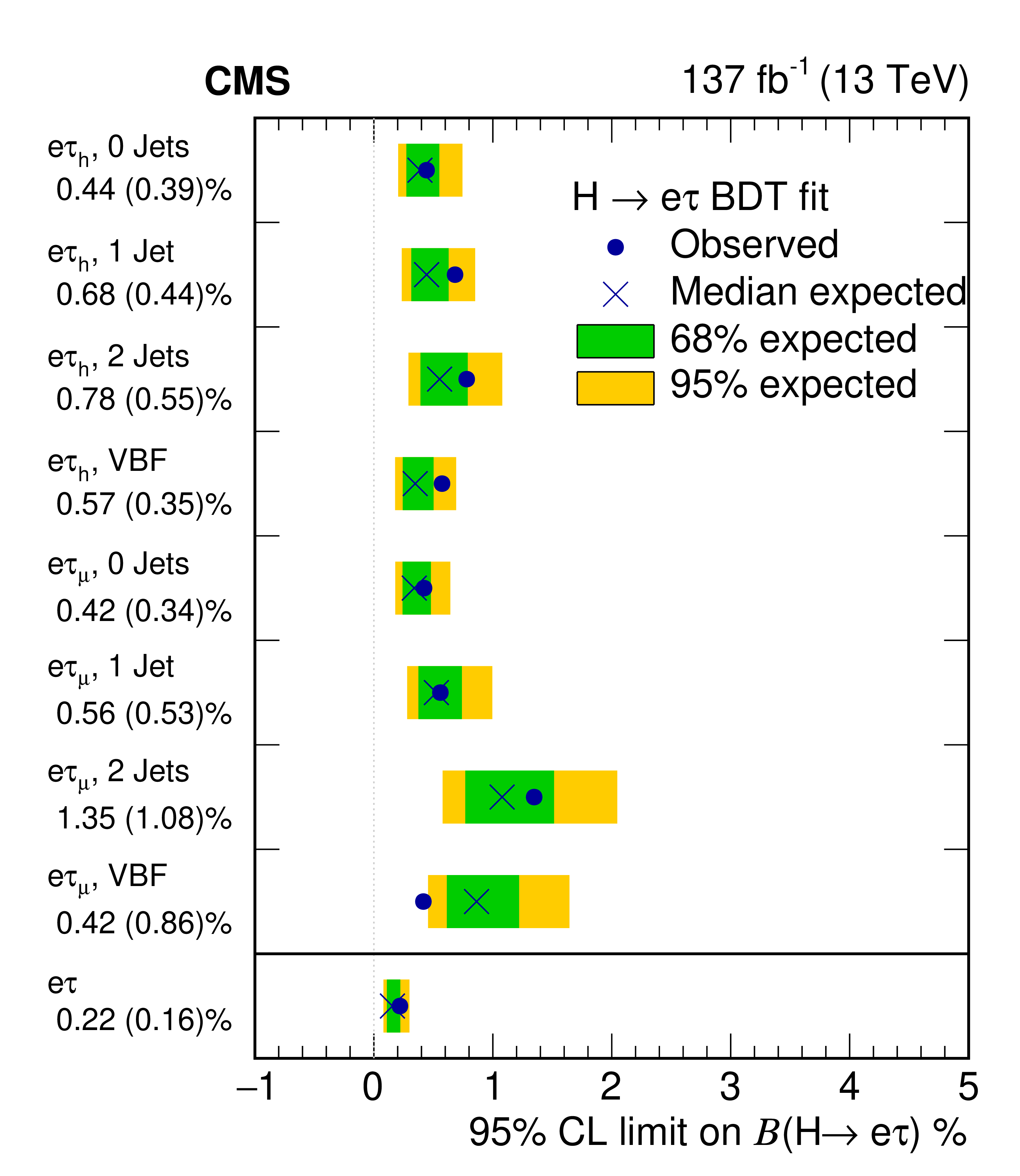
Observed (expected) 95% CL upper limits on the ${\mathcal {B}(\mathrm{H} \to \mu \tau)}$ (left) and ${\mathcal {B}(\mathrm{H} \to \mathrm{e} \tau)}$ (right) for each individual category and combined. The categories from top to bottom row are ${\mu {\tau _\mathrm {h}}}$ 0Jets, ${\mu {\tau _\mathrm {h}}}$ 1Jet, ${\mu {\tau _\mathrm {h}}}$ 2 Jets, ${\mu {\tau _\mathrm {h}}}$ VBF, ${\mu \tau _{\mathrm{e}}}$ 0Jets, ${\mu \tau _{\mathrm{e}}}$ 1Jet, ${\mu \tau _{\mathrm{e}}}$ 2 Jets, ${\mu \tau _{\mathrm{e}}}$ VBF, and ${\mu \tau}$ combined (left) and e${\tau _\mathrm {h}}$ 0Jets, e${\tau _\mathrm {h}}$ 1Jet, e${\tau _\mathrm {h}}$ 2 Jets, e${\tau _\mathrm {h}}$ VBF, e$ \tau _{\mu}$ 0Jets, e$ \tau _{\mu}$ 1Jet, e$ \tau _{\mu}$ 2 Jets, e$ \tau _{\mu}$ VBF, and e$\tau$ combined (right). |

png pdf |
Figure 7-a:
Observed (expected) 95% CL upper limits on the ${\mathcal {B}(\mathrm{H} \to \mu \tau)}$ for each individual category and combined. The categories from top to bottom row are ${\mu {\tau _\mathrm {h}}}$ 0Jets, ${\mu {\tau _\mathrm {h}}}$ 1Jet, ${\mu {\tau _\mathrm {h}}}$ 2 Jets, ${\mu {\tau _\mathrm {h}}}$ VBF, ${\mu \tau _{\mathrm{e}}}$ 0Jets, ${\mu \tau _{\mathrm{e}}}$ 1Jet, ${\mu \tau _{\mathrm{e}}}$ 2 Jets, ${\mu \tau _{\mathrm{e}}}$ VBF, and ${\mu \tau}$ combined. |
png pdf |
Figure 7-b:
Observed (expected) 95% CL upper limits on the ${\mathcal {B}(\mathrm{H} \to \mathrm{e} \tau)}$ for each individual category and combined. The categories from top to bottom row are e${\tau _\mathrm {h}}$ 0Jets, e${\tau _\mathrm {h}}$ 1Jet, e${\tau _\mathrm {h}}$ 2 Jets, e${\tau _\mathrm {h}}$ VBF, e$ \tau _{\mu}$ 0Jets, e$ \tau _{\mu}$ 1Jet, e$ \tau _{\mu}$ 2 Jets, e$ \tau _{\mu}$ VBF, and e$\tau$ combined. |
png pdf |
Figure 8:
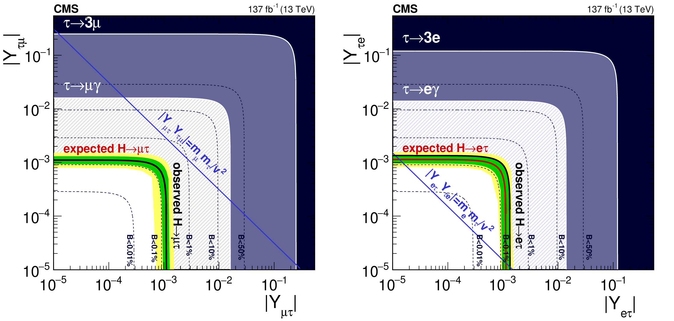
Expected (red line) and observed (black solid line) 95% CL upper limits on the LFV Yukawa couplings, $ {{| Y_{\mu \tau} |}} $ vs. $ {{| Y_{\tau \mu} |}} $ (left) and $ {{| Y_{\mathrm{e} \tau} |}} $ vs. $ {{| Y_{\tau \mathrm{e}} |}} $ (right). The $ {{| Y_{\mu \tau} |}} $ or $ {{| Y_{\mathrm{e} \tau} |}} $ couplings correspond to left chiral muon or electron and right chiral $\tau$ lepton, while $ {{| Y_{\tau \mu} |}} $ or $ {{| Y_{\tau \mathrm{e}} |}} $ couplings correspond to left chiral $\tau$ lepton and right chiral muon or electron. In the left plot, the expected limit is covered by the observed limit as they have similar values. The flavor diagonal Yukawa couplings are approximated by their SM values. The green and yellow bands indicate the range that is expected to contain 68% and 95% of all observed limit variations from the expected limit. The shaded regions are constraints obtained from null searches for $\tau \to 3\mu $ or $\tau \to 3\mathrm{e} $ (dark blue) [92] and $\tau \to \mu \gamma $ or $\tau \to \mathrm{e} \gamma $ (purple) [93]. The blue diagonal line is the theoretical naturalness limit $ {| Y_{ij}Y_{ji} |} = {m_i}m_j/v^2$ [11]. |
png pdf |
Figure 8-a:
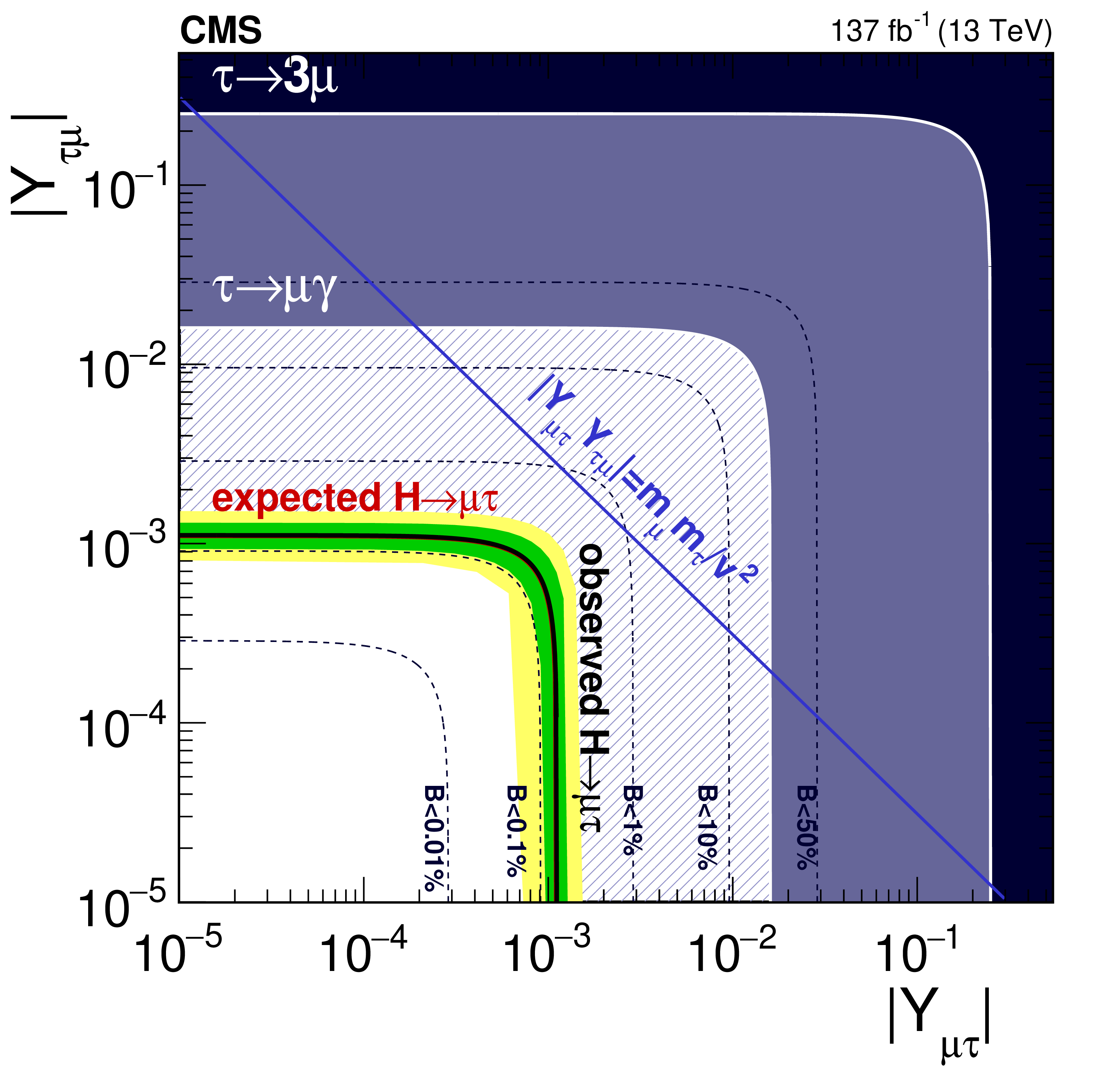
Expected (red line) and observed (black solid line) 95% CL upper limits on the LFV Yukawa couplings, $ {{| Y_{\mu \tau} |}} $ vs. $ {{| Y_{\tau \mu} |}} $. The $ {{| Y_{\mu \tau} |}} $ or $ {{| Y_{\mathrm{e} \tau} |}} $ couplings correspond to left chiral muon or electron and right chiral $\tau$ lepton, while $ {{| Y_{\tau \mu} |}} $ or $ {{| Y_{\tau \mathrm{e}} |}} $ couplings correspond to left chiral $\tau$ lepton and right chiral muon or electron. The expected limit is covered by the observed limit as they have similar values. The flavor diagonal Yukawa couplings are approximated by their SM values. The green and yellow bands indicate the range that is expected to contain 68% and 95% of all observed limit variations from the expected limit. The shaded regions are constraints obtained from null searches for $\tau \to 3\mu $ or $\tau \to 3\mathrm{e} $ (dark blue) [92] and $\tau \to \mu \gamma $ or $\tau \to \mathrm{e} \gamma $ (purple) [93]. The blue diagonal line is the theoretical naturalness limit $ {| Y_{ij}Y_{ji} |} = {m_i}m_j/v^2$ [11]. |
png pdf |
Figure 8-b:
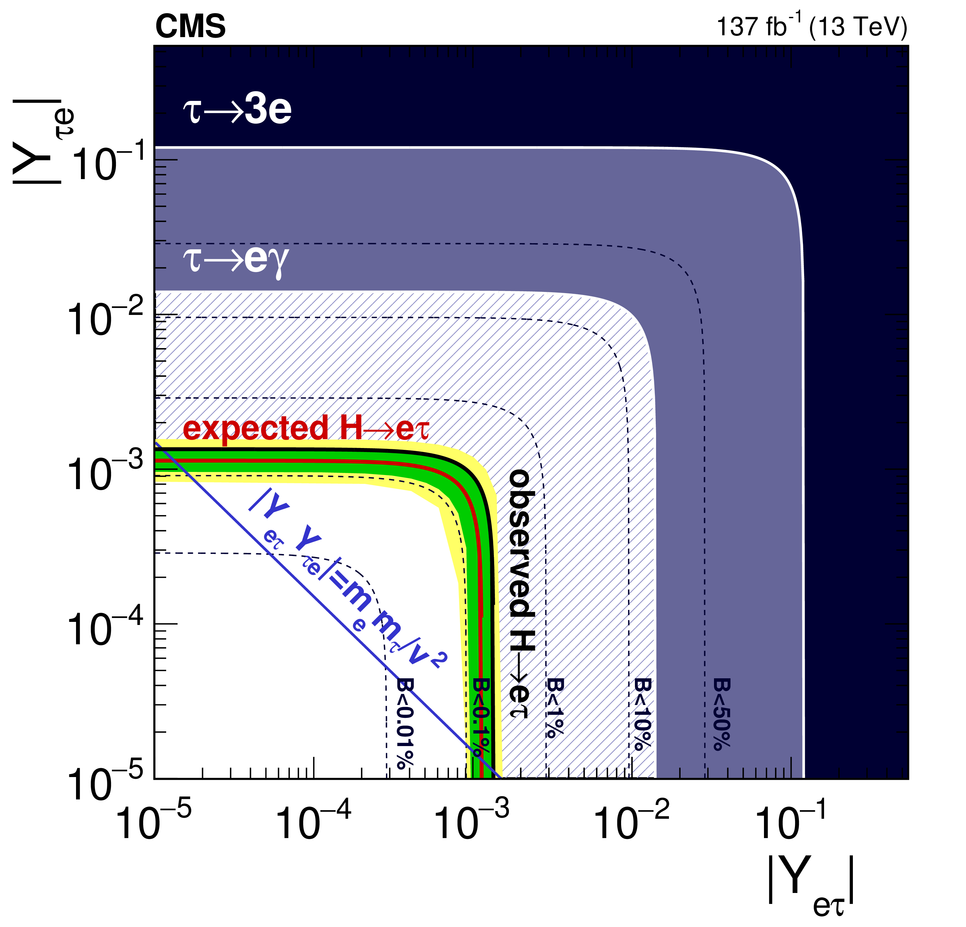
Expected (red line) and observed (black solid line) 95% CL upper limits on the LFV Yukawa couplings, $ {{| Y_{\mathrm{e} \tau} |}} $ vs. $ {{| Y_{\tau \mathrm{e}} |}} $. The $ {{| Y_{\mu \tau} |}} $ or $ {{| Y_{\mathrm{e} \tau} |}} $ couplings correspond to left chiral muon or electron and right chiral $\tau$ lepton, while $ {{| Y_{\tau \mu} |}} $ or $ {{| Y_{\tau \mathrm{e}} |}} $ couplings correspond to left chiral $\tau$ lepton and right chiral muon or electron. The flavor diagonal Yukawa couplings are approximated by their SM values. The green and yellow bands indicate the range that is expected to contain 68% and 95% of all observed limit variations from the expected limit. The shaded regions are constraints obtained from null searches for $\tau \to 3\mu $ or $\tau \to 3\mathrm{e} $ (dark blue) [92] and $\tau \to \mu \gamma $ or $\tau \to \mathrm{e} \gamma $ (purple) [93]. The blue diagonal line is the theoretical naturalness limit $ {| Y_{ij}Y_{ji} |} = {m_i}m_j/v^2$ [11]. |
| Tables | |

png pdf |
Table 1:
Event selection criteria for the ${\mathrm{H} \to \mu \tau}$ channels. |
png pdf |
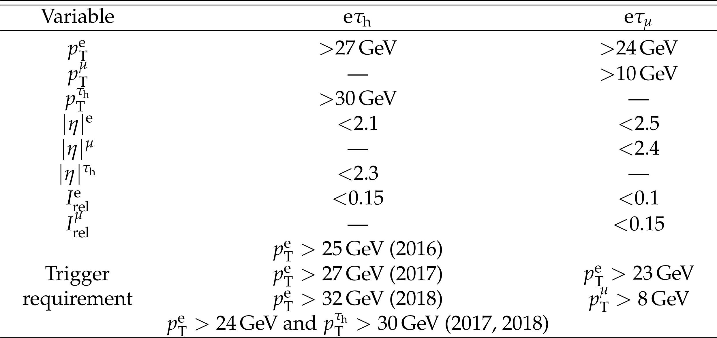
Table 2:
Event selection criteria for the ${\mathrm{H} \to \mathrm{e} \tau}$ channels. |

png pdf |
Table 3:
Systematic uncertainties in the expected event yields. All uncertainties are treated as correlated among categories, except those with two values separated by the $\oplus $ sign. In this case, the first value is the correlated uncertainty and the second value is the uncorrelated uncertainty for each category. |
png pdf |
Table 4:
Observed and expected upper limits at 95% CL and best fit branching fractions for each individual jet category, and their combinations, in the ${\mathrm{H} \to \mu \tau}$ channel. |

png pdf |
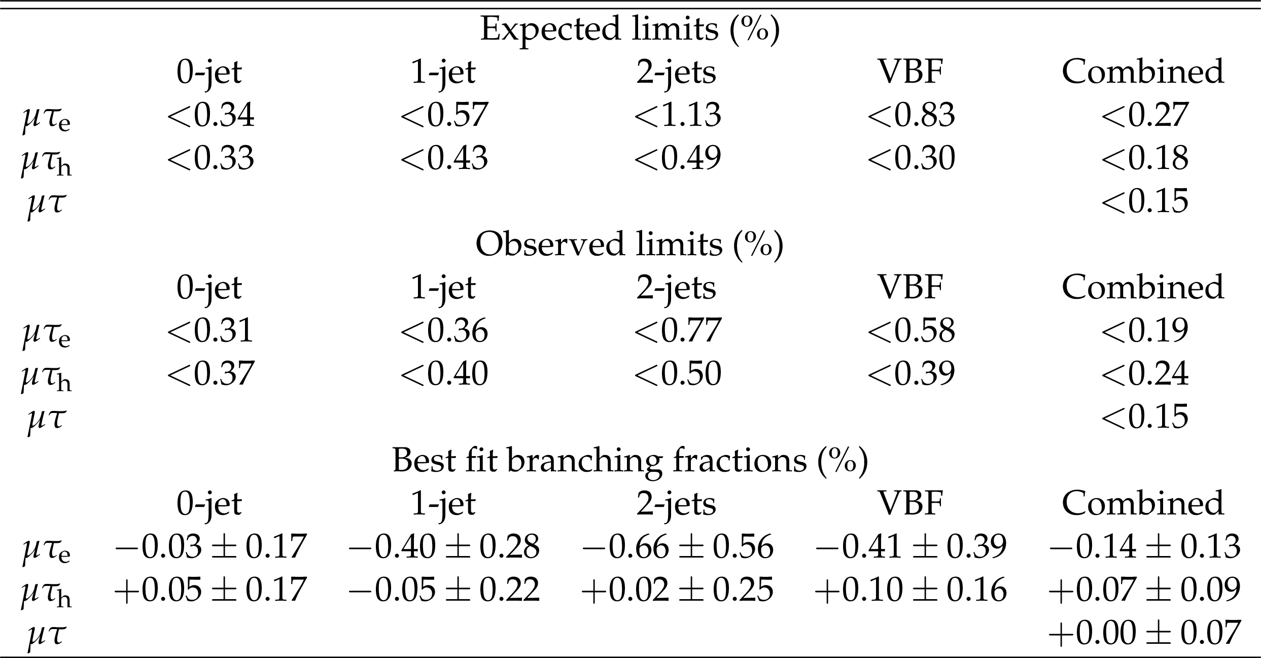
Table 5:
Observed and expected upper limits at 95% CL and best fit branching fractions for each individual jet category, and their combinations, in the ${\mathrm{H} \to \mathrm{e} \tau}$ channel. |
png pdf |
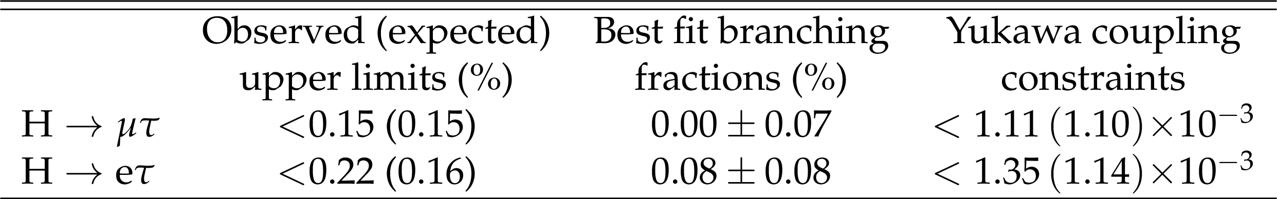
Table 6:
Summary of observed and expected upper limits at 95% CL, best fit branching fractions and corresponding constraints on Yukawa couplings for the ${\mathrm{H} \to \mu \tau}$ and ${\mathrm{H} \to \mathrm{e} \tau}$ channels. |
| Summary |
| A search for lepton-flavor violation has been performed in the $\mu\tau$ and e$\tau$ final states of the Higgs boson in data collected by the CMS experiment. The data correspond to an integrated luminosity of 137 fb$^{-1}$ of proton-proton collisions at a center-of-mass energy of 13 TeV. The results are extracted through a maximum likelihood fit to a boosted decision tree output, trained to distinguish the expected signal from backgrounds. The observed (expected) upper limits on the branching fraction of the Higgs boson to $\mu\tau$ are 0.15 (0.15)% and to e$\tau$ are 0.22 (0.16)%, respectively, at 95% confidence level. Upper limits on the off-diagonal $\mu\tau$ and e$\tau$ couplings are derived from these constraints, $\sqrt{\smash[b]{|Y_{\mu\tau}| ^{2}+|{Y_{\tau\mu}}| ^{2}}} < $ 1.11 ${\times}10^{-3}$ and $\sqrt{\smash[b]{|{Y_{\mathrm{e}\tau}}| ^{2}+|{Y_{\tau\mathrm{e}}}| ^{2}}} < $ 1.35 ${\times}10^{-3}$. These results constitute an improvement over the previous limits from CMS and ATLAS experiments. |
| References | ||||
| 1 | ATLAS Collaboration | Measurements of the Higgs boson production and decay rates and coupling strengths using pp collision data at $ \sqrt{s}= $ 7 and 8 TeV in the ATLAS experiment | EPJC 76 (2016) 6 | 1507.04548 |
| 2 | CMS Collaboration | Precise determination of the mass of the Higgs boson and tests of compatibility of its couplings with the standard model predictions using proton collisions at 7 and 8 TeV | EPJC 75 (2015) 212 | CMS-HIG-14-009 1412.8662 |
| 3 | CMS Collaboration | Study of the mass and spin-parity of the Higgs boson candidate via its decays to Z boson pairs | PRL 110 (2013) 081803 | CMS-HIG-12-041 1212.6639 |
| 4 | ATLAS Collaboration | Evidence for the spin-0 nature of the Higgs boson using ATLAS data | PLB 726 (2013) 120 | 1307.1432 |
| 5 | CMS Collaboration | Constraints on the spin-parity and anomalous HVV couplings of the Higgs boson in proton collisions at 7 and 8 TeV | PRD 92 (2015) 012004 | CMS-HIG-14-018 1411.3441 |
| 6 | CMS Collaboration | Measurements of properties of the Higgs boson decaying into the four-lepton final state in pp collisions at $ \sqrt{s}= $ 13 TeV | JHEP 11 (2017) 047 | CMS-HIG-16-041 1706.09936 |
| 7 | ATLAS Collaboration | Observation of a new particle in the search for the standard model Higgs boson with the ATLAS detector at the LHC | PLB 716 (2012) 1 | 1207.7214 |
| 8 | CMS Collaboration | Observation of a new boson at a mass of 125 GeV with the CMS experiment at the LHC | PLB 716 (2012) 30 | CMS-HIG-12-028 1207.7235 |
| 9 | CMS Collaboration | Observation of a new boson with mass near 125 GeV in pp collisions at $ \sqrt{s} = $ 7 and 8 TeV | JHEP 06 (2013) 081 | CMS-HIG-12-036 1303.4571 |
| 10 | CMS Collaboration | Combined measurements of Higgs boson couplings in proton-proton collisions at $ \sqrt{s}= $ 13 TeV | EPJC 79 (2019) 421 | CMS-HIG-17-031 1809.10733 |
| 11 | R. Harnik, J. Kopp, and J. Zupan | Flavor violating Higgs decays | JHEP 03 (2013) 026 | 1209.1397 |
| 12 | J. D. Bjorken and S. Weinberg | A mechanism for nonconservation of muon number | PRL 38 (1977) 622 | |
| 13 | J. L. Diaz-Cruz and J. J. Toscano | Lepton flavor violating decays of Higgs bosons beyond the standard model | PRD 62 (2000) 116005 | hep-ph/9910233 |
| 14 | T. Han and D. Marfatia | $ \mathit{h} {\rightarrow} {\mu} {\tau} $ at hadron colliders | PRL 86 (2001) 1442 | hep-ph/0008141 |
| 15 | A. Arhrib, Y. Cheng, and O. C. W. Kong | Comprehensive analysis on lepton flavor violating Higgs boson to $ \mu^\mp \tau^\pm $ decay in supersymmetry without $ R $ parity | PRD 87 (2013) 015025 | 1210.8241 |
| 16 | K. Agashe and R. Contino | Composite Higgs-mediated FCNC | PRD 80 (2009) 075016 | 0906.1542 |
| 17 | A. Azatov, M. Toharia, and L. Zhu | Higgs mediated FCNC's in warped extra dimensions | PRD 80 (2009) 035016 | 0906.1990 |
| 18 | H. Ishimori et al. | Non-Abelian discrete symmetries in particle physics | Prog. Theor. Phys. Suppl. 183 (2010) 1 | 1003.3552 |
| 19 | G. Perez and L. Randall | Natural neutrino masses and mixings from warped geometry | JHEP 01 (2009) 077 | 0805.4652 |
| 20 | S. Casagrande et al. | Flavor physics in the Randall-Sundrum model: I. Theoretical setup and electroweak precision tests | JHEP 10 (2008) 094 | 0807.4937 |
| 21 | A. J. Buras, B. Duling, and S. Gori | The impact of Kaluza-Klein fermions on standard model fermion couplings in a RS model with custodial protection | JHEP 09 (2009) 076 | 0905.2318 |
| 22 | M. Blanke et al. | $ \Delta F= $ 2 observables and fine-tuning in a warped extra dimension with custodial protection | JHEP 03 (2009) 001 | 0809.1073 |
| 23 | M. E. Albrecht et al. | Electroweak and flavour structure of a warped extra dimension with custodial protection | JHEP 09 (2009) 064 | 0903.2415 |
| 24 | G. F. Giudice and O. Lebedev | Higgs-dependent Yukawa couplings | PLB 665 (2008) 79 | 0804.1753 |
| 25 | J. A. Aguilar Saavedra | A minimal set of top-Higgs anomalous couplings | NPB 821 (2009) 215 | 0904.2387 |
| 26 | A. Goudelis, O. Lebedev, and J. h. Park | Higgs-induced lepton flavor violation | PLB 707 (2012) 369 | 1111.1715 |
| 27 | D. McKeen, M. Pospelov, and A. Ritz | Modified Higgs branching ratios versus CP and lepton flavor violation | PRD 86 (2012) 113004 | 1208.4597 |
| 28 | A. Pilaftsis | Lepton flavor nonconservation in $ \text{H}^{0} $ decays | PLB 285 (1992) 68 | |
| 29 | J. G. Korner, A. Pilaftsis, and K. Schilcher | Leptonic CP asymmetries in flavor changing $ \text{H}^{0} $ decays | PRD 47 (1993) 1080 | hep-ph/9301289 |
| 30 | CMS Collaboration | Search for lepton flavour violating decays of the Higgs boson to $ \mu\tau $ and e$ \tau $ in proton-proton collisions at $ \sqrt{s}= $ 13 TeV | JHEP 06 (2018) 001 | CMS-HIG-17-001 1712.07173 |
| 31 | ATLAS Collaboration | Searches for lepton-flavour-violating decays of the Higgs boson in $ \sqrt{s}= $ 13 TeV pp collisions with the ATLAS detector | PLB 800 (2020) 135069 | 1907.06131 |
| 32 | O. U. Shanker | Flavor violation, scalar particles and leptoquarks | NPB 206 (1982) 253 | |
| 33 | B. McWilliams and L.-F. Li | Virtual effects of Higgs particles | NPB 179 (1981) 62 | |
| 34 | G. Blankenburg, J. Ellis, and G. Isidori | Flavour-changing decays of a 125 GeV Higgs-like particle | PLB 712 (2012) 386 | 1202.5704 |
| 35 | MEG Collaboration | New constraint on the existence of the $ \mu^+ \to e^+\gamma $ decay | PRL 110 (2013) 201801 | 1303.0754 |
| 36 | A. Celis, V. Cirigliano, and E. Passemar | Lepton flavor violation in the Higgs sector and the role of hadronic $ \tau $-lepton decays | PRD 89 (2014) 013008 | 1309.3564 |
| 37 | CMS Collaboration | Search for lepton flavour violating decays of the Higgs boson to e$ \tau $ and e$ \mu $ in proton-proton collisions at $ \sqrt s= $ 8 TeV | PLB 763 (2016) 472 | CMS-HIG-14-040 1607.03561 |
| 38 | CMS Collaboration | Performance of the CMS Level-1 trigger in proton-proton collisions at $ \sqrt{s} = $ 13 TeV | JINST 15 (2020) P10017 | CMS-TRG-17-001 2006.10165 |
| 39 | CMS Collaboration | The CMS trigger system | JINST 12 (2017) P01020 | CMS-TRG-12-001 1609.02366 |
| 40 | CMS Collaboration | The CMS experiment at the CERN LHC | JINST 3 (2008) S08004 | CMS-00-001 |
| 41 | T. Sjostrand et al. | An introduction to PYTHIA 8.2 | CPC 191 (2015) 159 | 1410.3012 |
| 42 | CMS Collaboration | Event generator tunes obtained from underlying event and multiparton scattering measurements | EPJC 76 (2016) 155 | CMS-GEN-14-001 1512.00815 |
| 43 | CMS Collaboration | Extraction and validation of a new set of CMS PYTHIA8 tunes from underlying-event measurements | EPJC 80 (2020) 4 | CMS-GEN-17-001 1903.12179 |
| 44 | NNPDF Collaboration | Parton distributions from high-precision collider data | EPJC 77 (2017) 663 | 1706.00428 |
| 45 | GEANT 4 Collaboration | GEANT4 --- a simulation toolkit | NIMA 506 (2003) 250 | |
| 46 | H. M. Georgi, S. L. Glashow, M. E. Machacek, and D. V. Nanopoulos | Higgs bosons from two gluon annihilation in proton-proton collisions | PRL 40 (1978) 692 | |
| 47 | R. N. Cahn, S. D. Ellis, R. Kleiss, and W. J. Stirling | Transverse momentum signatures for heavy Higgs bosons | PRD 35 (1987) 1626 | |
| 48 | S. L. Glashow, D. V. Nanopoulos, and A. Yildiz | Associated production of Higgs bosons and Z particles | PRD 18 (1978) 1724 | |
| 49 | P. Nason | A new method for combining NLO QCD with shower monte carlo algorithms | JHEP 11 (2004) 040 | hep-ph/0409146 |
| 50 | S. Frixione, P. Nason, and C. Oleari | Matching NLO QCD computations with parton shower simulations: the POWHEG method | JHEP 11 (2007) 070 | 0709.2092 |
| 51 | S. Alioli, P. Nason, C. Oleari, and E. Re | A general framework for implementing NLO calculations in shower monte carlo programs: the POWHEG BOX | JHEP 06 (2010) 043 | 1002.2581 |
| 52 | S. Alioli et al. | Jet pair production in POWHEG | JHEP 04 (2011) 081 | 1012.3380 |
| 53 | S. Alioli, P. Nason, C. Oleari, and E. Re | NLO Higgs boson production via gluon fusion matched with shower in POWHEG | JHEP 04 (2009) 002 | 0812.0578 |
| 54 | E. Bagnaschi, G. Degrassi, P. Slavich, and A. Vicini | Higgs production via gluon fusion in the POWHEG approach in the SM and in the MSSM | JHEP 02 (2012) 088 | 1111.2854 |
| 55 | G. Heinrich et al. | NLO predictions for Higgs boson pair production with full top quark mass dependence matched to parton showers | JHEP 08 (2017) 088 | 1703.09252 |
| 56 | G. Buchalla et al. | Higgs boson pair production in non-linear effective field theory with full $ m_t $-dependence at NLO QCD | JHEP 09 (2018) 057 | 1806.05162 |
| 57 | J. Alwall et al. | The automated computation of tree-level and next-to-leading order differential cross sections, and their matching to parton shower simulations | JHEP 07 (2014) 079 | 1405.0301 |
| 58 | J. Alwall et al. | Comparative study of various algorithms for the merging of parton showers and matrix elements in hadronic collisions | EPJC 53 (2008) 473 | 0706.2569 |
| 59 | R. Frederix and S. Frixione | Merging meets matching in MC@NLO | JHEP 12 (2012) 061 | 1209.6215 |
| 60 | CMS Collaboration | Particle-flow reconstruction and global event description with the CMS detector | JINST 12 (2017) P10003 | CMS-PRF-14-001 1706.04965 |
| 61 | M. Cacciari, G. P. Salam, and G. Soyez | The anti-$ {k_{\mathrm{T}}} $ jet clustering algorithm | JHEP 04 (2008) 063 | 0802.1189 |
| 62 | M. Cacciari, G. P. Salam, and G. Soyez | Fastjet user manual | EPJC 72 (2012) 1896 | 1111.6097 |
| 63 | CMS Collaboration | Electron and photon reconstruction and identification with the CMS experiment at the CERN LHC | (12, 2020) | CMS-EGM-17-001 2012.06888 |
| 64 | CMS Collaboration | Performance of electron reconstruction and selection with the CMS detector in proton-proton collisions at $ \$ \sqrt{s} = $ $ 8 TeV | JINST 10 (2015) P06005 | CMS-EGM-13-001 1502.02701 |
| 65 | CMS Collaboration | Performance of the CMS muon detector and muon reconstruction with proton-proton collisions at $ \sqrt{s}= $ 13 TeV | JINST 13 (2018) P06015 | CMS-MUO-16-001 1804.04528 |
| 66 | M. Cacciari, G. P. Salam, and G. Soyez | The catchment area of jets | JHEP 04 (2008) 005 | 0802.1188 |
| 67 | CMS Collaboration | Performance of reconstruction and identification of $ \tau $ leptons decaying to hadrons and $ \nu_\tau $ in pp collisions at $ \sqrt{s}= $ 13 TeV | JINST 13 (2018) P10005 | CMS-TAU-16-003 1809.02816 |
| 68 | CMS Collaboration | Performance of the DeepTau algorithm for the discrimination of taus against jets, electrons, and muons | CMS-DP-2019-033 | |
| 69 | CMS Collaboration | Jet algorithms performance in 13 TeV data | CMS-PAS-JME-16-003 | CMS-PAS-JME-16-003 |
| 70 | CMS Collaboration | Identification of heavy-flavour jets with the CMS detector in pp collisions at 13 TeV | JINST 13 (2018) P05011 | CMS-BTV-16-002 1712.07158 |
| 71 | M. Cacciari and G. P. Salam | Pileup subtraction using jet areas | PLB 659 (2008) 119 | 0707.1378 |
| 72 | CMS Collaboration | Jet energy scale and resolution in the CMS experiment in pp collisions at 8 TeV | JINST 12 (2017) P02014 | CMS-JME-13-004 1607.03663 |
| 73 | CMS Collaboration | Performance of missing transverse momentum reconstruction in proton-proton collisions at $ \sqrt{s} = $ 13 TeV using the CMS detector | JINST 14 (2019) P07004 | CMS-JME-17-001 1903.06078 |
| 74 | K. Ellis, I. Hinchliffe, Soldate, and J. van der Bij | Higgs decay to $ \tau^+\tau^- $: A possible signature of intermediate mass Higgs bosons at high eergy hadron colliders | NPB 297 (1988) 221 | |
| 75 | H. Voss, A. Hocker, J. Stelzer, and F. Tegenfeldt | TMVA, the toolkit for multivariate data analysis with ROOT | in XIth International Workshop on Advanced Computing and Analysis Techniques in Physics Research (ACAT), p. 40 2007 [PoS(ACAT)040] | physics/0703039 |
| 76 | CMS Collaboration | An embedding technique to determine $ \tau\tau $ backgrounds in proton-proton collision data | JINST 14 (2019) P06032 | CMS-TAU-18-001 1903.01216 |
| 77 | CMS Collaboration | Observation of the Higgs boson decay to a pair of $ \tau $ leptons with the CMS detector | PLB 779 (2018) 283 | CMS-HIG-16-043 1708.00373 |
| 78 | J. S. Conway | Nuisance parameters in likelihoods for multisource spectra | in Proceedings of PHYSTAT 2011 Workshop on Statistical Issues Related to Discovery Claims in Search Experiments and Unfolding, H. Propser and L. Lyons, eds., CERN | |
| 79 | CMS Collaboration | Measurements of inclusive W and Z cross sections in pp collisions at $ \sqrt{s}= $ 7 TeV | JHEP 01 (2011) 080 | CMS-EWK-10-002 1012.2466 |
| 80 | CMS Collaboration | Performance of CMS muon reconstruction in pp collision events at $ \sqrt{s}= $ 7 TeV | JINST 7 (2012) P10002 | CMS-MUO-10-004 1206.4071 |
| 81 | CMS Collaboration | Reconstruction and identification of $ \tau $ lepton decays to hadrons and $ \nu_\tau $ at CMS | JINST 11 (2016) P01019 | CMS-TAU-14-001 1510.07488 |
| 82 | D. de Florian et al. | Handbook of LHC Higgs cross sections: 4. Deciphering the nature of the Higgs sector | CERN-2017-002-M | 1610.07922 |
| 83 | R. J. Barlow and C. Beeston | Fitting using finite Monte Carlo samples | CPC 77 (1993) 219 | |
| 84 | CMS Collaboration | CMS luminosity measurements for the 2016 data-taking period | CMS-PAS-LUM-17-001 | |
| 85 | CMS Collaboration | CMS luminosity measurement for the 2017 data-taking period at $ \sqrt{s} = $ 13 TeV | CMS-PAS-LUM-17-004 | |
| 86 | CMS Collaboration | CMS luminosity measurement for the 2018 data-taking period at $ \sqrt{s} = $ 13 TeV | CMS-PAS-LUM-18-002 | |
| 87 | T. Junk | Confidence level computation for combining searches with small statistics | NIMA 434 (1999) 435 | hep-ex/9902006 |
| 88 | A. L. Read | Presentation of search results: The $ \text{CL}_\text{s} $ technique | JPG 28 (2002) 2693 | |
| 89 | G. Cowan, K. Cranmer, E. Gross, and O. Vitells | Asymptotic formulae for likelihood-based tests of new physics | EPJC 71 (2011) 1554 | 1007.1727 |
| 90 | A. Denner et al. | Standard model Higgs-boson branching ratios with uncertainties | EPJC 71 (2011) 1753 | 1107.5909 |
| 91 | CMS Collaboration | HEPData record for this analysis | link | |
| 92 | K. Hayasaka et al. | Search for lepton flavor violating $ \tau $ decays into three leptons with 719 million produced $ \tau^{+}\tau^{-} $ pairs | PLB 687 (2010) 139 | 1001.3221 |
| 93 | Belle Collaboration | New search for $ \tau \to \mu \gamma $ and $ \tau \to e \gamma $ decays at Belle | PLB 666 (2008) 16 | 0705.0650 |
|
|
Compact Muon Solenoid LHC, CERN |
|

|

|

|

|

|