

Compact Muon Solenoid
LHC, CERN
| CMS-SUS-21-009 ; CERN-EP-2023-127 | ||
| Search for new physics in multijet events with at least one photon and large missing transverse momentum in proton-proton collisions at 13 TeV | ||
| CMS Collaboration | ||
| 28 July 2023 | ||
| JHEP 10 (2023) 046 | ||
| Abstract: A search for new physics in final states consisting of at least one photon, multiple jets, and large missing transverse momentum is presented, using proton-proton collision events at a center-of-mass energy of 13 TeV. The data correspond to an integrated luminosity of 137 fb$ ^{-1} $, recorded by the CMS experiment at the CERN LHC from 2016 to 2018. The events are divided into mutually exclusive bins characterized by the missing transverse momentum, the number of jets, the number of b-tagged jets, and jets consistent with the presence of hadronically decaying W, Z, or Higgs bosons. The observed data are found to be consistent with the prediction from standard model processes. The results are interpreted in the context of simplified models of pair production of supersymmetric particles via strong and electroweak interactions. Depending on the details of the signal models, gluinos and squarks of masses up to 2.35 and 1.43 TeV, respectively, and electroweakinos of masses up to 1.23 TeV are excluded at 95% confidence level. | ||
| Links: e-print arXiv:2307.16216 [hep-ex] (PDF) ; CDS record ; inSPIRE record ; CADI line (restricted) ; | ||
| Figures & Tables | Summary | Additional Figures & Tables | References | CMS Publications |
|---|
| Figures | |
png pdf |
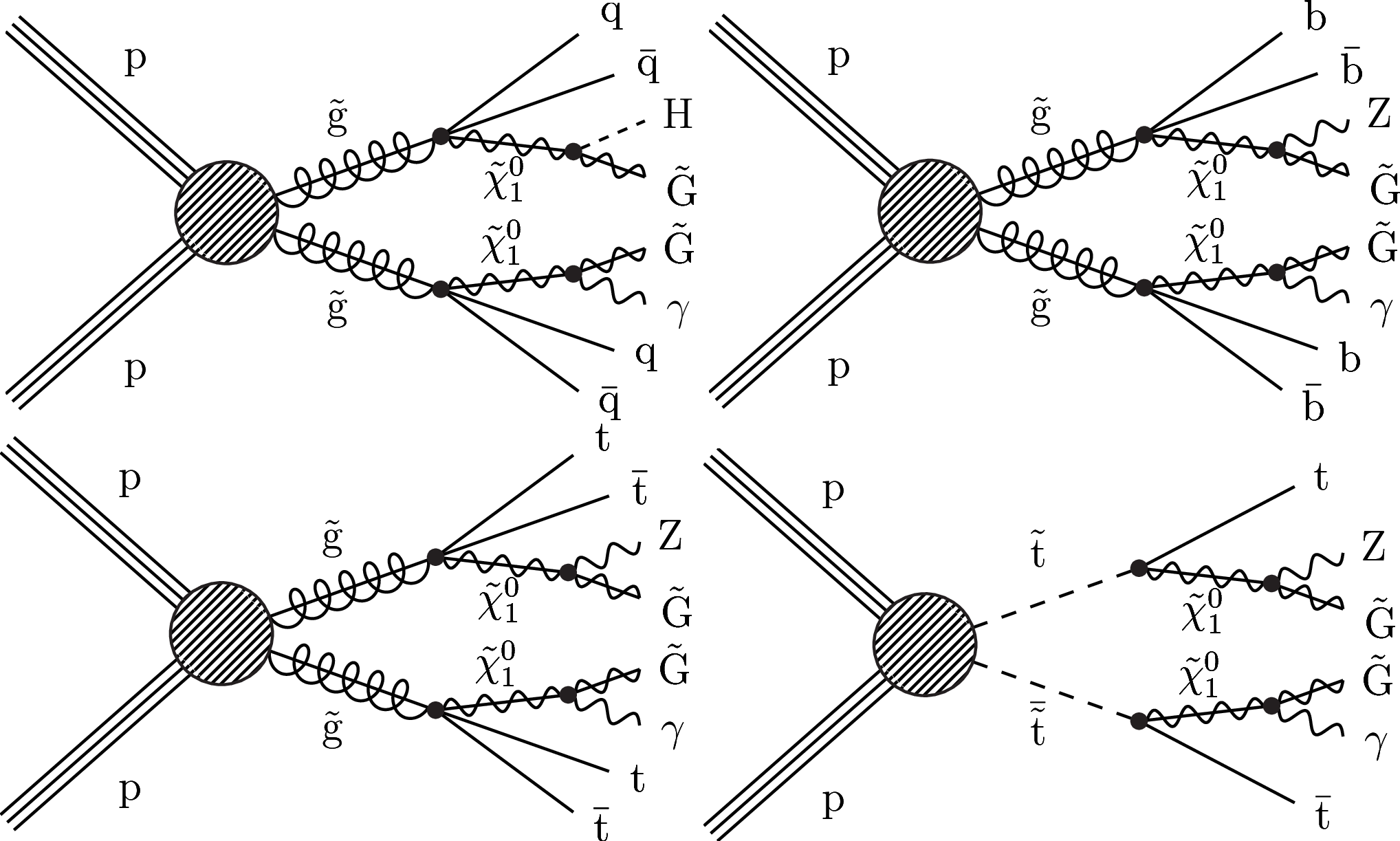
Figure 1:
Diagrams of simplified models of gluino pair production: T5qqqqHG (upper left), T5bbbbZG (upper right), T5ttttZG (lower left), and top squark pair production: T6ttZG (lower right). The models are defined in the text. |
png pdf |
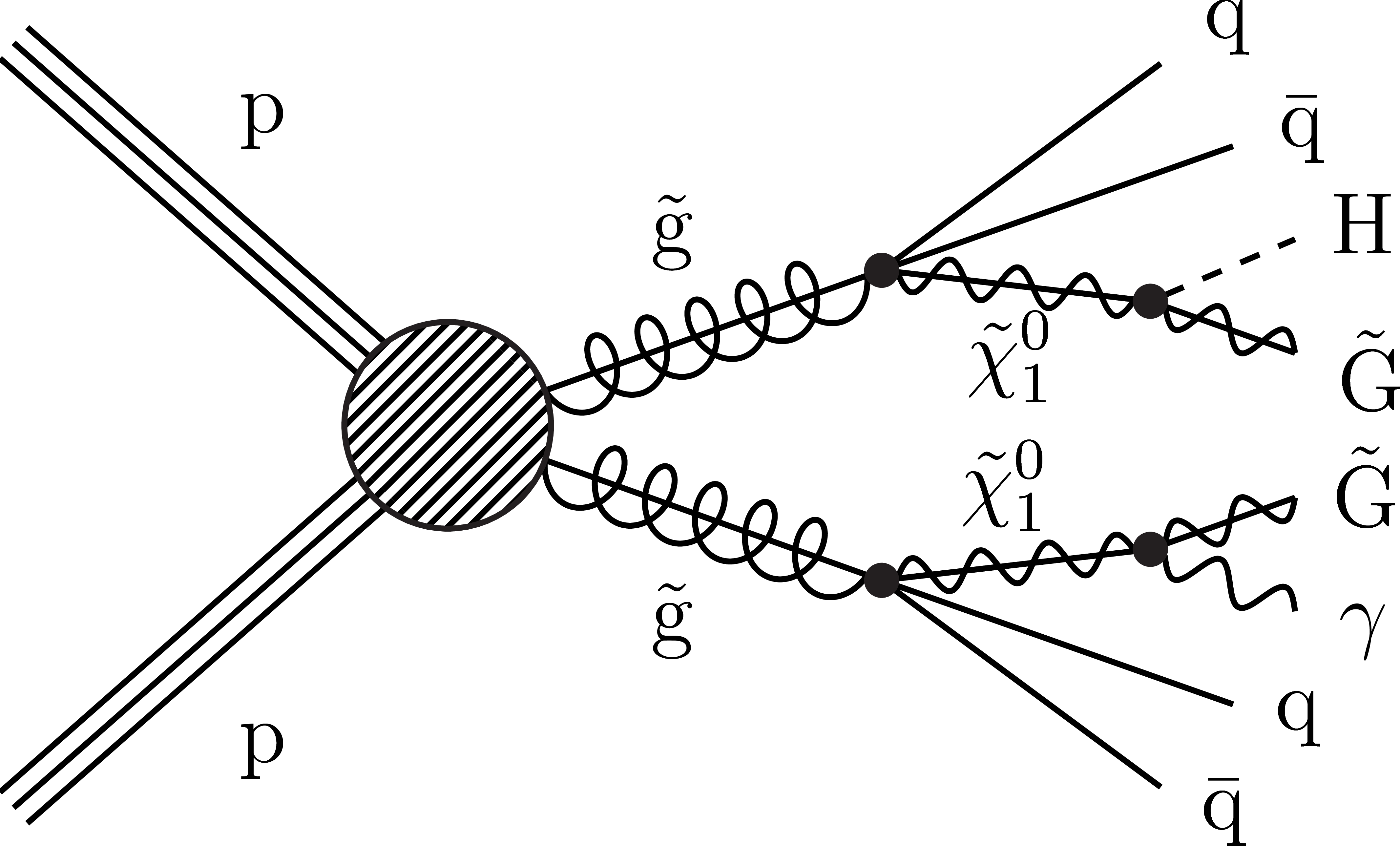
Figure 1-a:
Diagram representing the T5qqqqHG simplified model of gluino pair production. |

png pdf |
Figure 1-b:
Diagram representing the T5bbbbZG simplified model of gluino pair production. |
png pdf |
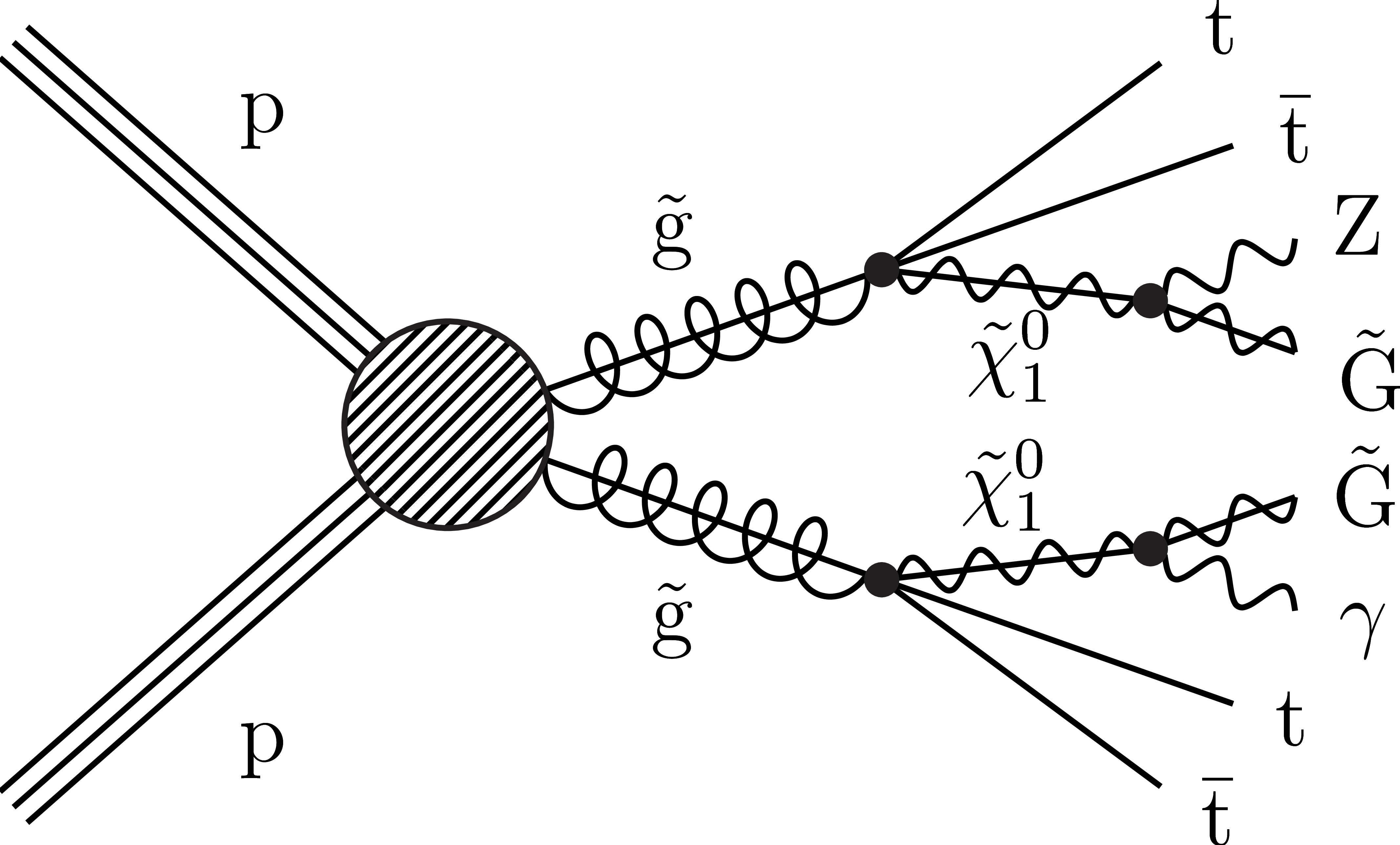
Figure 1-c:
Diagram representing the T5ttttZG simplified model of gluino pair production. |
png pdf |
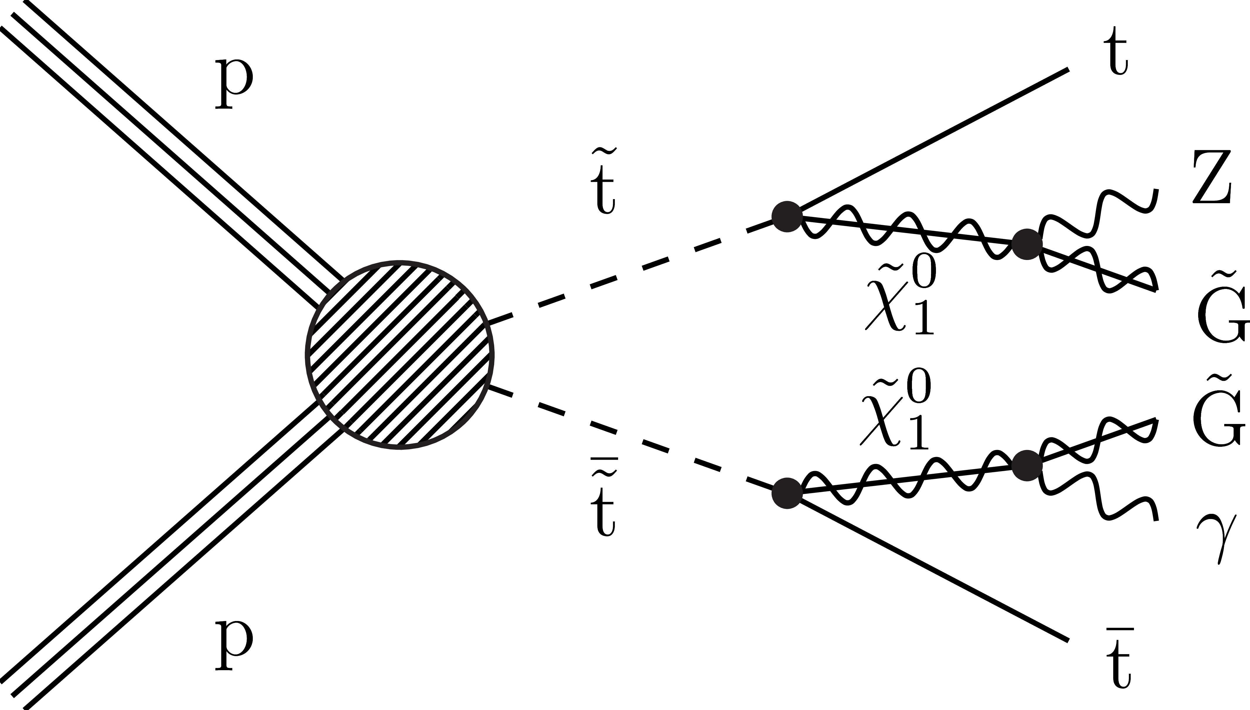
Figure 1-d:
Diagram representing the T6ttZG simplified model of top squark pair production. |

png pdf |
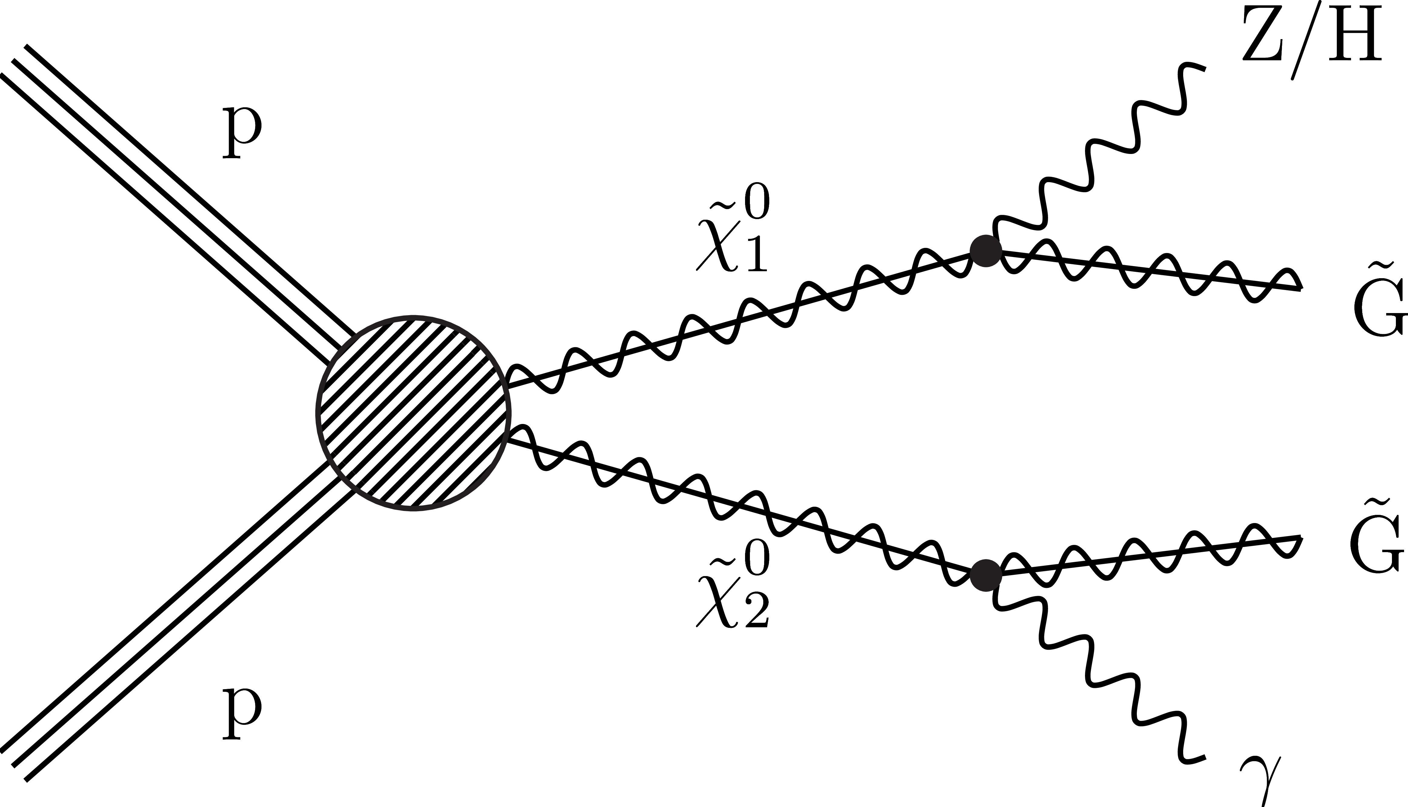
Figure 2:
Diagrams of simplified models of electroweakino pair production: TChiWG (upper), TChiNG (lower left), and TChiNGnn (lower right). Only the $ \tilde{\chi}_{1}^{\pm}\tilde{\chi}_{1}^{0} $ and $ \tilde{\chi}_{1}^{\pm}\tilde{\chi}_{1}^{\mp} $ cases are shown for the TChiWG and TChiNG models, respectively. The models are defined in the text. ``Soft'' indicates particles with momentum too low to be detectable. |

png pdf |
Figure 2-a:
Diagram representing the TChiWG simplified model of electroweakino pair production. Only the $ \tilde{\chi}_{1}^{\pm}\tilde{\chi}_{1}^{0} $ case is shown. |

png pdf |
Figure 2-b:
Diagram representing the TChiNG simplified model of electroweakino pair production. Only the $ \tilde{\chi}_{1}^{\pm}\tilde{\chi}_{1}^{\mp} $ case is shown. ``Soft'' indicates particles with momentum too low to be detectable. |
png pdf |
Figure 2-c:
Diagram representing the TChiNGnn simplified model of electroweakino pair production. |

png pdf |
Figure 3:
The definitions and indexing schemes for the SP (left) and EW (right) SRs and low-$ p_{\mathrm{T}}^\text{miss} $ CRs, in the planes of $ p_{\mathrm{T}}^\text{miss} $, $ N_{\text{jets}} $, and $ N_{\mathrm{b}\text{-tags}} $ (left) and $ p_{\mathrm{T}}^\text{miss} $, $ \text{V}\text{-}$ and $\mathrm{H}\text{-tag} $ (right). The gray blocks correspond to the low-$ p_{\mathrm{T}}^\text{miss} $ CRs, the blue blocks to the SP SRs, and the red blocks to the EW SRs. |

png pdf |
Figure 3-a:
The definitions and indexing schemes for the SP SR and low-$ p_{\mathrm{T}}^\text{miss} $ CRs, in the plane of $ p_{\mathrm{T}}^\text{miss} $, $ N_{\text{jets}} $, and $ N_{\mathrm{b}\text{-tags}} $. The gray blocks correspond to the low-$ p_{\mathrm{T}}^\text{miss} $ CRs and the blue blocks to the SP SRs. |

png pdf |
Figure 3-b:
The definitions and indexing schemes for the EW SRs and low-$ p_{\mathrm{T}}^\text{miss} $ CRs, in the plane of $ p_{\mathrm{T}}^\text{miss} $, $ \text{V}\text{- and }\mathrm{H}\text{-tag} $. The gray blocks correspond to the low-$ p_{\mathrm{T}}^\text{miss} $ CRs and the red blocks to the EW SRs. |

png pdf |
Figure 4:
Left: the relative contributions of events with light lepton(s) or $ \tau_\mathrm{h} $ candidate(s) in the SRs and CRs (upper panel), and the corresponding transfer factors (TFs; see text), along with their statistical uncertainties (lower panel). Right: a comparison between the expected and predicted lost lepton event yields from simulated $ \mathrm{W}\gamma{+}\text{jets} $ and $ \mathrm{t}\overline{\mathrm{t}}\gamma{+}\text{jets} $ processes in each of the SR bins. The vertical error bars indicate the statistical uncertainty in the simulation and the hashed bands in the lower panel indicate the systematic uncertainties. |

png pdf |
Figure 4-a:
The relative contributions of events with light lepton(s) or $ \tau_\mathrm{h} $ candidate(s) in the SRs and CRs (upper panel), and the corresponding transfer factors (TFs; see text), along with their statistical uncertainties (lower panel). |

png pdf |
Figure 4-b:
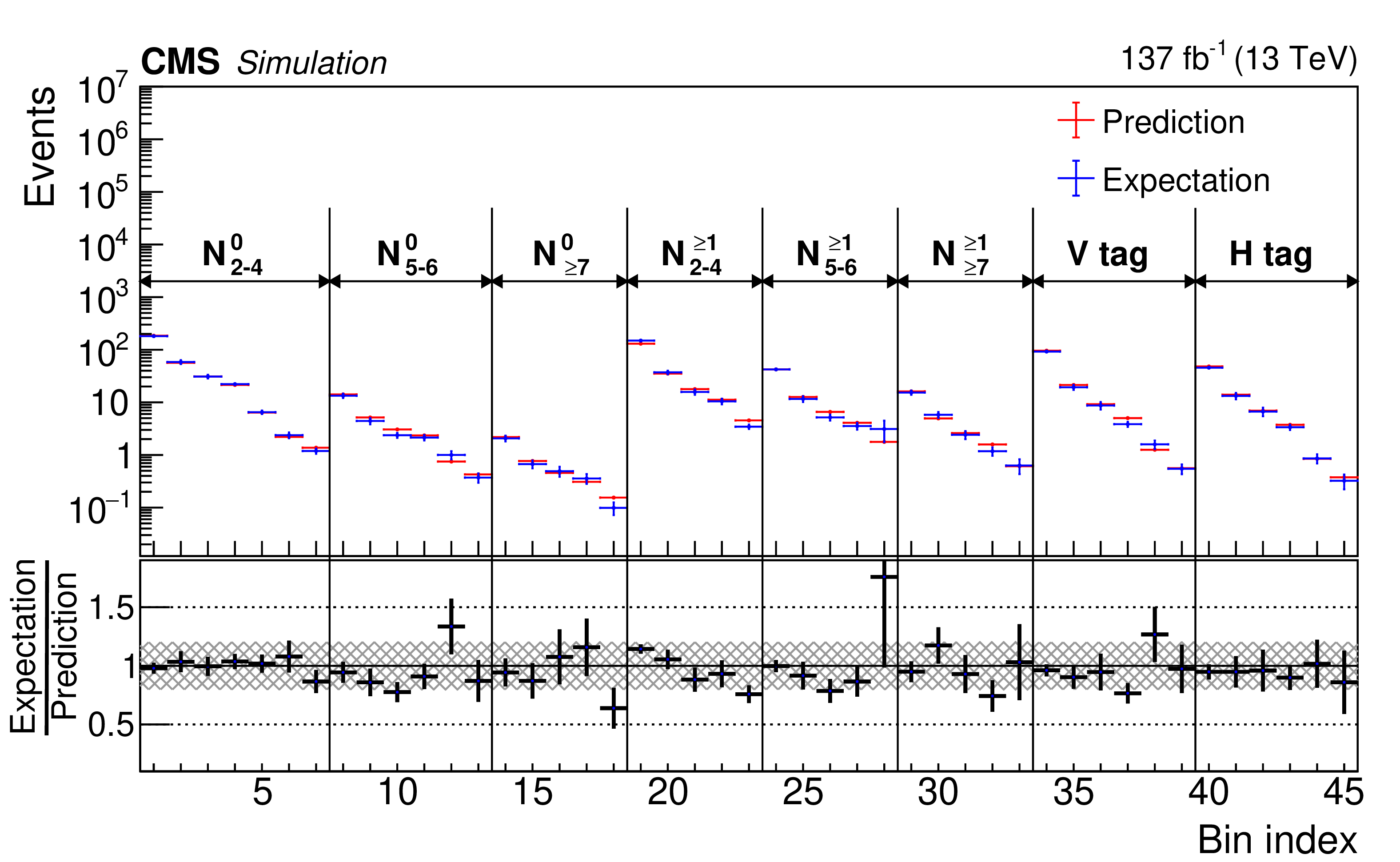
A comparison between the expected and predicted lost lepton event yields from simulated $ \mathrm{W}\gamma{+}\text{jets} $ and $ \mathrm{t}\overline{\mathrm{t}}\gamma{+}\text{jets} $ processes in each of the SR bins. The vertical error bars indicate the statistical uncertainty in the simulation and the hashed bands in the lower panel indicate the systematic uncertainties. |
png pdf |
Figure 5:
A comparison of the number of events with an electron misidentified as a photon in the SRs and the number estimated using the single-electron CRs with simulated samples. The ratio of the expected and predicted event yields in each SR is shown in the lower panel. The shaded region in the lower panel indicates the systematic uncertainties in the predicted number of background events. |

png pdf |
Figure 6:
The distributions of the dilepton invariant mass (left) and the magnitude of the dilepton $ {\vec p}_{\mathrm{T}} $ plus the $ {\vec p}_{\mathrm{T}}^{\kern1pt\text{miss}} $ (right) for $ \ell\ell\gamma $ events in data and simulation. The error bars represent the statistical uncertainty in the data events. In the lower panel, the shaded region shows the statistical uncertainty in the simulation. |

png pdf |
Figure 6-a:
The distribution of the magnitude of the dilepton $ {\vec p}_{\mathrm{T}} $ plus the $ {\vec p}_{\mathrm{T}}^{\kern1pt\text{miss}} $ for $ \ell\ell\gamma $ events in data and simulation. The error bars represent the statistical uncertainty in the data events. In the lower panel, the shaded region shows the statistical uncertainty in the simulation. |

png pdf |
Figure 6-b:
The distribution of the magnitude of the dilepton $ {\vec p}_{\mathrm{T}} $ plus the $ {\vec p}_{\mathrm{T}}^{\kern1pt\text{miss}} $ for $ \ell\ell\gamma $ events in data and simulation. The error bars represent the statistical uncertainty in the data events. In the lower panel, the shaded region shows the statistical uncertainty in the simulation. |

png pdf |
Figure 7:
A comparison between $ \kappa $ estimated from simulation and from data in the zero-photon CR. The values are given for each $ N_{\text{jets}} $, $ N_{\mathrm{b}\text{-tags}} $, $ \text{V}\text{-tag} $, and $ \mathrm{H}\text{-tag} $ bin, represented as $ r $. The blue bands in the lower panel represent the relative systematic uncertainty in $ \kappa $. |

png pdf |
Figure 8:
The numbers of predicted background events and observed events in the SRs and low-$ p_{\mathrm{T}}^\text{miss} $ CRs. The lost-lepton, electron misidentified as photon, $ \mathrm{Z}\gamma{+}\text{jets} $, and $ \gamma{+}\text{jets} $ and QCD multijet backgrounds are stacked histograms. The observed numbers of events in data are presented as black points. For illustration, the expected event yields are presented for the signal model T5bbbbZG, for small (blue) and large (purple) differences in the masses of the $ \mathrm{\tilde{g}} $ and NLSP. Also shown is the expected distribution of events for the signal model TChiWG (red). The numerical values in parentheses in the legend entries for the signal models indicate the $ \mathrm{\tilde{g}} $ and NLSP mass values in GeVns for strong production and the NLSP mass value for electroweak production. The lower panel shows the ratio of the observed number of data events and the predicted backgrounds. The error bars represent the statistical uncertainty in the data events, and the shaded band represents the statistical and systematic uncertainties in the predicted background. The $ p_{\mathrm{T}}^\text{miss} $ bin 200-300 GeV is used for the estimation of the $ \gamma{+}\text{jets} $ and QCD multijet background. |
png pdf |
Figure 9:
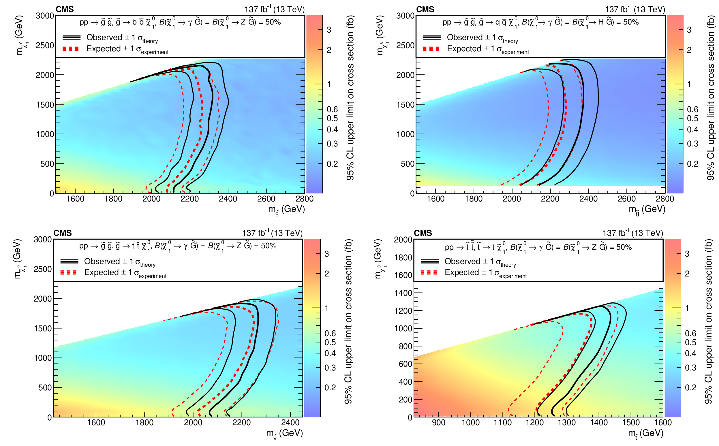
The 95% CL upper limits on the production cross sections for $ \mathrm{\tilde{g}} $ pairs, with $ \mathrm{\tilde{g}}\to\mathrm{b}\overline{\mathrm{b}}\tilde{\chi}_{1}^{0} $ followed by $ \tilde{\chi}_{1}^{0}\to\mathrm{Z}\tilde{\mathrm{G}} $ or $ \tilde{\chi}_{1}^{0}\to\gamma\tilde{\mathrm{G}} $ (upper left, T5bbbbZG model), $ \mathrm{\tilde{g}}\to\mathrm{q}\overline{\mathrm{q}}\tilde{\chi}_{1}^{0} $ followed by $ \tilde{\chi}_{1}^{0}\to\mathrm{H}\tilde{\mathrm{G}} $ or $ \tilde{\chi}_{1}^{0}\to\gamma\tilde{\mathrm{G}} $ (upper right, T5qqqqHG model), $ \mathrm{\tilde{g}}\to{\mathrm{t}\overline{\mathrm{t}}} \tilde{\chi}_{1}^{0} $ followed by $ \tilde{\chi}_{1}^{0}\to\mathrm{Z}\tilde{\mathrm{G}} $ or $ \tilde{\chi}_{1}^{0}\to\gamma\tilde{\mathrm{G}} $ (lower left, T5ttttZG model), or top squark pairs assuming the top squark decays to a top quark and a $ \tilde{\chi}_{1}^{0} $ followed by $ \tilde{\chi}_{1}^{0}\to\mathrm{Z}\tilde{\mathrm{G}} $ or $ \tilde{\chi}_{1}^{0}\to\gamma\tilde{\mathrm{G}} $ (lower right, T6ttZG model). The thick black curve represents the observed exclusion contour and the thin black curves show the effect of varying the signal cross section within the theoretical uncertainties by $ \pm $1$\sigma_{\text{theory}} $. The thick red curve indicates the expected exclusion contour and the thin red curves show the variations from $ \pm$1$\sigma_{\text{experiment}} $ uncertainties. |

png pdf |
Figure 9-a:
The 95% CL upper limits on the production cross sections for $ \mathrm{\tilde{g}} $ pairs, with $ \mathrm{\tilde{g}}\to\mathrm{b}\overline{\mathrm{b}}\tilde{\chi}_{1}^{0} $ followed by $ \tilde{\chi}_{1}^{0}\to\mathrm{Z}\tilde{\mathrm{G}} $ or $ \tilde{\chi}_{1}^{0}\to\gamma\tilde{\mathrm{G}} $ (T5bbbbZG model). The thick black curve represents the observed exclusion contour and the thin black curves show the effect of varying the signal cross section within the theoretical uncertainties by $ \pm $1$\sigma_{\text{theory}} $. The thick red curve indicates the expected exclusion contour and the thin red curves show the variations from $ \pm$1$\sigma_{\text{experiment}} $ uncertainties. |

png pdf |
Figure 9-b:
The 95% CL upper limits on the production cross sections for $ \mathrm{\tilde{g}}\to\mathrm{q}\overline{\mathrm{q}}\tilde{\chi}_{1}^{0} $ followed by $ \tilde{\chi}_{1}^{0}\to\mathrm{H}\tilde{\mathrm{G}} $ or $ \tilde{\chi}_{1}^{0}\to\gamma\tilde{\mathrm{G}} $ (T5qqqqHG model). The thick black curve represents the observed exclusion contour and the thin black curves show the effect of varying the signal cross section within the theoretical uncertainties by $ \pm $1$\sigma_{\text{theory}} $. The thick red curve indicates the expected exclusion contour and the thin red curves show the variations from $ \pm$1$\sigma_{\text{experiment}} $ uncertainties. |

png pdf |
Figure 9-c:
The 95% CL upper limits on the production cross sections for $ \mathrm{\tilde{g}}\to{\mathrm{t}\overline{\mathrm{t}}} \tilde{\chi}_{1}^{0} $ followed by $ \tilde{\chi}_{1}^{0}\to\mathrm{Z}\tilde{\mathrm{G}} $ or $ \tilde{\chi}_{1}^{0}\to\gamma\tilde{\mathrm{G}} $ (T5ttttZG model). The thick black curve represents the observed exclusion contour and the thin black curves show the effect of varying the signal cross section within the theoretical uncertainties by $ \pm $1$\sigma_{\text{theory}} $. The thick red curve indicates the expected exclusion contour and the thin red curves show the variations from $ \pm$1$\sigma_{\text{experiment}} $ uncertainties. |

png pdf |
Figure 9-d:
The 95% CL upper limits on the production cross sections for top squark pairs assuming the top squark decays to a top quark and a $ \tilde{\chi}_{1}^{0} $ followed by $ \tilde{\chi}_{1}^{0}\to\mathrm{Z}\tilde{\mathrm{G}} $ or $ \tilde{\chi}_{1}^{0}\to\gamma\tilde{\mathrm{G}} $ (T6ttZG model). The thick black curve represents the observed exclusion contour and the thin black curves show the effect of varying the signal cross section within the theoretical uncertainties by $ \pm $1$\sigma_{\text{theory}} $. The thick red curve indicates the expected exclusion contour and the thin red curves show the variations from $ \pm$1$\sigma_{\text{experiment}} $ uncertainties. |

png pdf |
Figure 10:
The expected and observed limits on the electroweakino mass in the TChiWG (upper), TChiNG (lower left), and TChiNGnn (lower right) models at 95% CL. For the TChiNG model (lower left), scenarios with degenerate charginos and neutralinos leading to the combined process $ \tilde{\chi}_{1}^{\pm}\tilde{\chi}_{1}^{\mp}+\tilde{\chi}_{1}^{0}\tilde{\chi}_{2}^{0}+(\tilde{\chi}_{1}^{0}/\tilde{\chi}_{2}^{0})\tilde{\chi}_{1}^{\pm} $ (red) or the single process $ \tilde{\chi}_{1}^{0}\tilde{\chi}_{2}^{0} $ (blue) are considered. |

png pdf |
Figure 10-a:
The expected and observed limits on the electroweakino mass in the TChiWG model at 95% CL. |

png pdf |
Figure 10-b:
The expected and observed limits on the electroweakino mass in the TChiNG model at 95% CL. For this model, scenarios with degenerate charginos and neutralinos leading to the combined process $ \tilde{\chi}_{1}^{\pm}\tilde{\chi}_{1}^{\mp}+\tilde{\chi}_{1}^{0}\tilde{\chi}_{2}^{0}+(\tilde{\chi}_{1}^{0}/\tilde{\chi}_{2}^{0})\tilde{\chi}_{1}^{\pm} $ (red) or the single process $ \tilde{\chi}_{1}^{0}\tilde{\chi}_{2}^{0} $ (blue) are considered. |

png pdf |
Figure 10-c:
The expected and observed limits on the electroweakino mass in the TChiNGnn model at 95% CL. |
| Tables | |
png pdf |
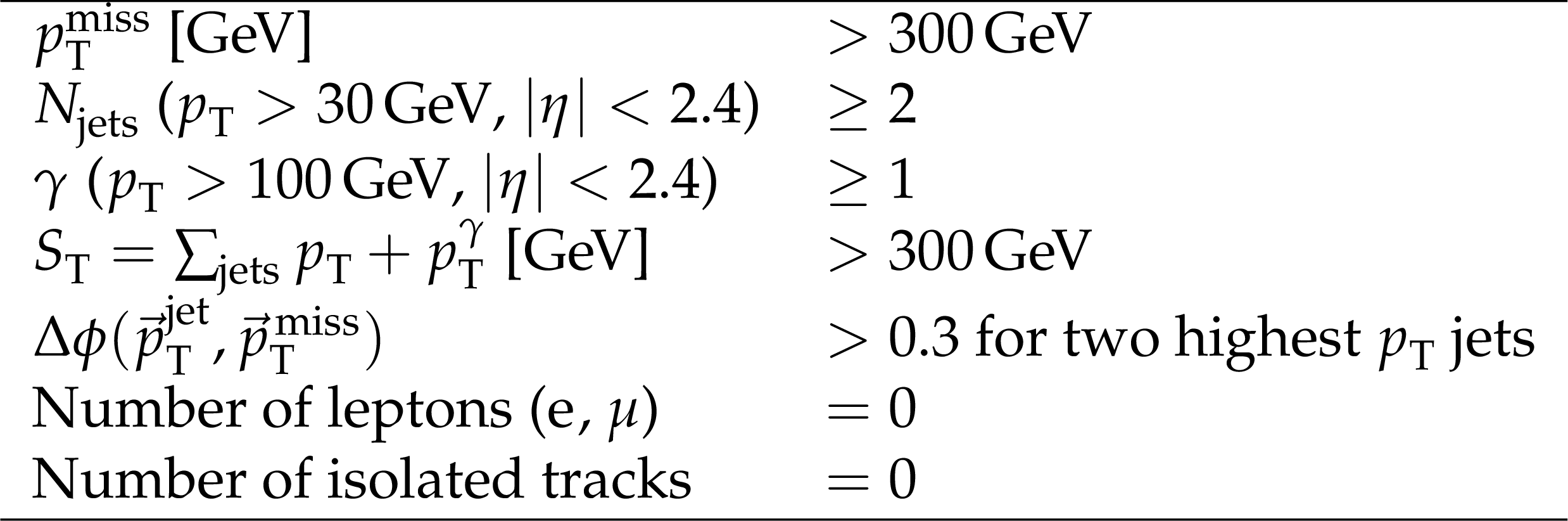
Table 1:
Summary of the baseline selection criteria used to identify events of interest for this search. |
png pdf |
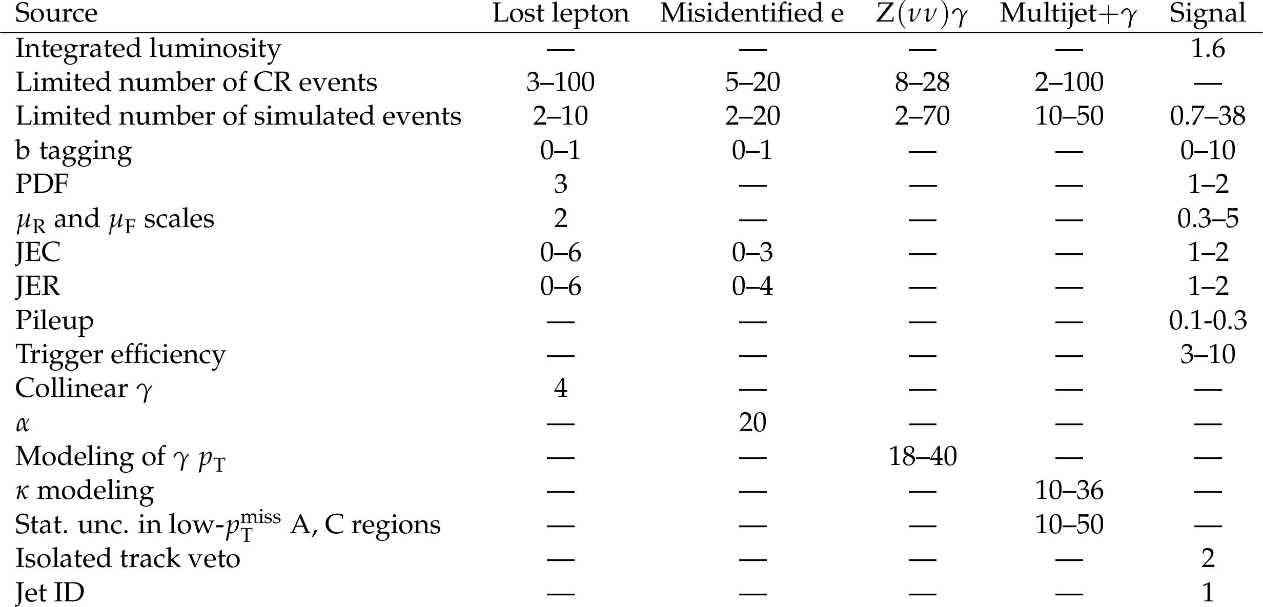
Table 2:
The systematic uncertainties in the predicted background and signal event yields (in %). A dash indicates that the source of uncertainty is not applicable or negligible. |

png pdf |
Table A1:
The number of events predicted and observed for the signal regions and the low-$ p_{\mathrm{T}}^\text{miss} $ regions used for the estimation of the $ \gamma{+}\text{jets} $ and QCD multijet backgrounds. |
| Summary |
| A search for supersymmetry (SUSY) is presented using events with final states containing at least one photon, large missing transverse momentum, and jets that may or may not arise from b quarks. These signatures are motivated by models with gauge-mediated SUSY breaking (GMSB), in which the lightest SUSY particle (LSP) is a gravitino ($ \tilde{\mathrm{G}} $) and the next-to-LSP (NLSP) is a chargino ($ \tilde{\chi}_{1}^{\pm} $) or neutralino ($ \tilde{\chi}_{1}^{0} $), collectively called electroweakinos. Several simplified models of strong production of pairs of gluinos ($ \mathrm{\tilde{g}} $) and top squarks ($ \tilde{\mathrm{t}} $) are considered, with the gluino decaying to a pair of quarks along with an NLSP or the top squark decaying to a top quark and an NLSP; the NLSP then decays to a neutral gauge boson (photon, Z boson, or Higgs boson) and an LSP. Models of pair production of electroweakinos are also considered, with the neutralinos decaying as described above, and the charginos decaying to a W boson and an LSP. Compared to previous searches, this search achieves increased sensitivity to scenarios with small mass differences between the gluino and the NLSP with dedicated search regions based on identifying boosted massive bosons. In addition, the search strategy is expanded to provide sensitivity to the production of electroweakino pairs. The observations are consistent with the standard model expectations and 95% confidence level upper limits are set on the production cross sections of SUSY particles. In the GMSB simplified models, the lower gluino mass limit reaches up to 2.35 TeV for models with $ \mathrm{\tilde{g}}\to\mathrm{q}\overline{\mathrm{q}}\tilde{\chi}_{1}^{0} $ followed by $ \tilde{\chi}_{1}^{0}\to\mathrm{H}\tilde{\mathrm{G}} $ or $ \gamma\tilde{\mathrm{G}} $ with equal probability, and the top squark mass limit reaches up to 1.43 TeV for models with $ \tilde{\mathrm{t}} \to \mathrm{t} \tilde{\chi}_{1}^{0} $ followed by $ \tilde{\chi}_{1}^{0}\to\mathrm{Z}\tilde{\mathrm{G}} $ or $ \gamma\tilde{\mathrm{G}} $ with equal probability. These results extend the previous mass limits [27] on gluinos and top squarks by 150--200 GeV. For electroweakino pair production, chargino and neutralino masses up to 1.23 TeV are excluded, assuming wino-like electroweakinos with decays $ \tilde{\chi}_{1}^{\pm}\to\mathrm{W}\tilde{\mathrm{G}} $ and $ \tilde{\chi}_{1}^{0}\to\gamma\tilde{\mathrm{G}} $. The higgsino-like electroweakino mass limits reach up to 1.05 TeV for models with $ \tilde{\chi}_{1}^{0}\to\gamma\tilde{\mathrm{G}} $, $ \mathrm{Z}\tilde{\mathrm{G}} $, or $ \mathrm{H}\tilde{\mathrm{G}} $ with 50, 25, and 25% branching fractions, respectively. These are the best mass limits to date on electroweakino production with photons in the final state. |
| Additional Figures | |

png pdf |
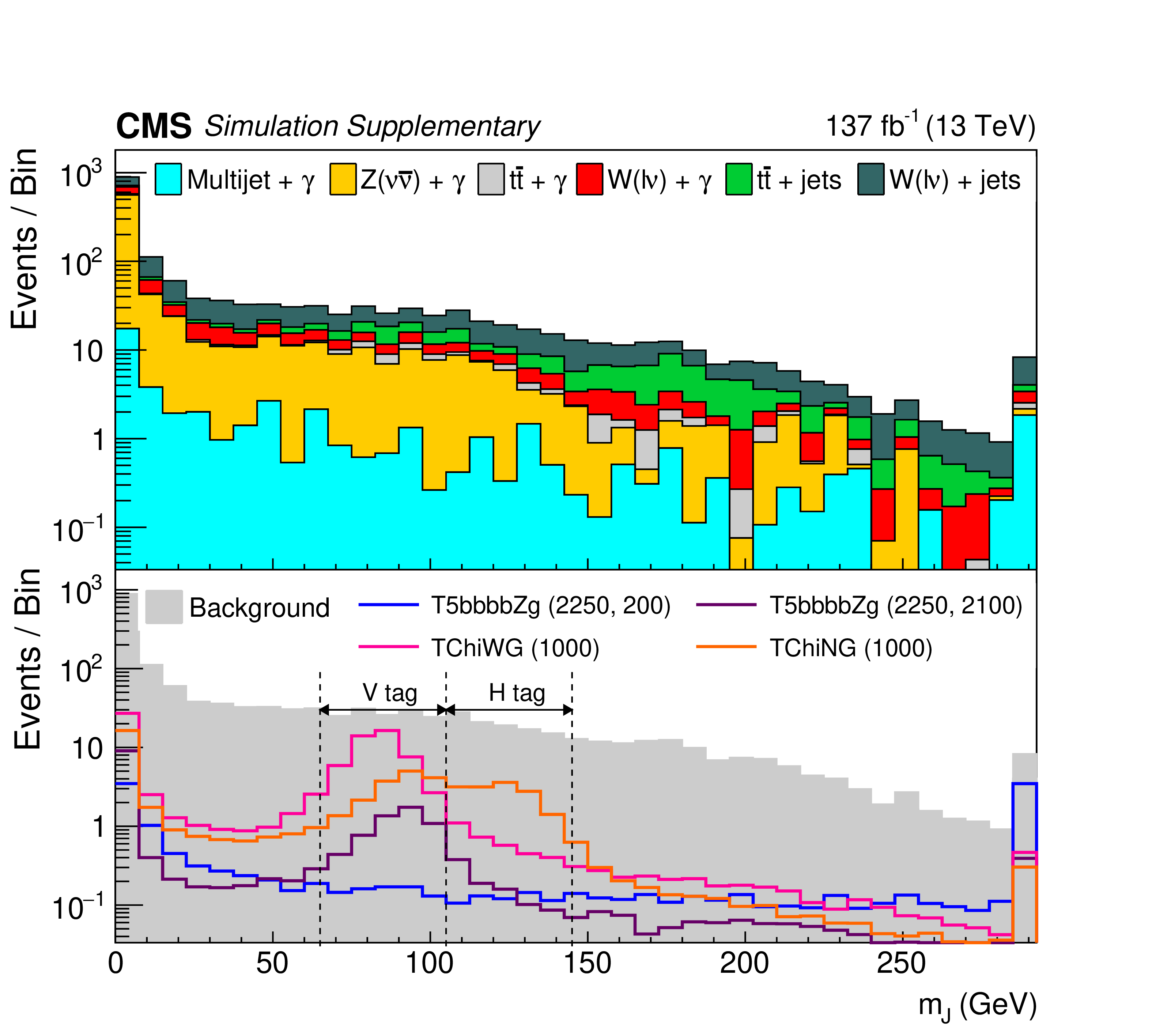
Additional Figure 1:
Distributions of the total number of AK4 jets (left) and the soft drop mass for the leading AK8 jet (right). The upper panel shows the distributions from simulated SM background contributions. The lower panel shows the distributions for several signal models (T5bbbbZg, TChiWG, and TChiNG) overlaid on the total simulated background distribution. The numerical values in parentheses in the legend entries for the signal models indicate the $ \mathrm{\tilde{g}} $ and NLSP mass values in GeVns for strong production and the NLSP mass value for electroweak production. |

png pdf |
Additional Figure 1-a:
Distributions of the total number of AK4 jets (left) and the soft drop mass for the leading AK8 jet (right). The upper panel shows the distributions from simulated SM background contributions. The lower panel shows the distributions for several signal models (T5bbbbZg, TChiWG, and TChiNG) overlaid on the total simulated background distribution. The numerical values in parentheses in the legend entries for the signal models indicate the $ \mathrm{\tilde{g}} $ and NLSP mass values in GeVns for strong production and the NLSP mass value for electroweak production. |
png pdf |
Additional Figure 1-b:
Distributions of the total number of AK4 jets (left) and the soft drop mass for the leading AK8 jet (right). The upper panel shows the distributions from simulated SM background contributions. The lower panel shows the distributions for several signal models (T5bbbbZg, TChiWG, and TChiNG) overlaid on the total simulated background distribution. The numerical values in parentheses in the legend entries for the signal models indicate the $ \mathrm{\tilde{g}} $ and NLSP mass values in GeVns for strong production and the NLSP mass value for electroweak production. |

png pdf |
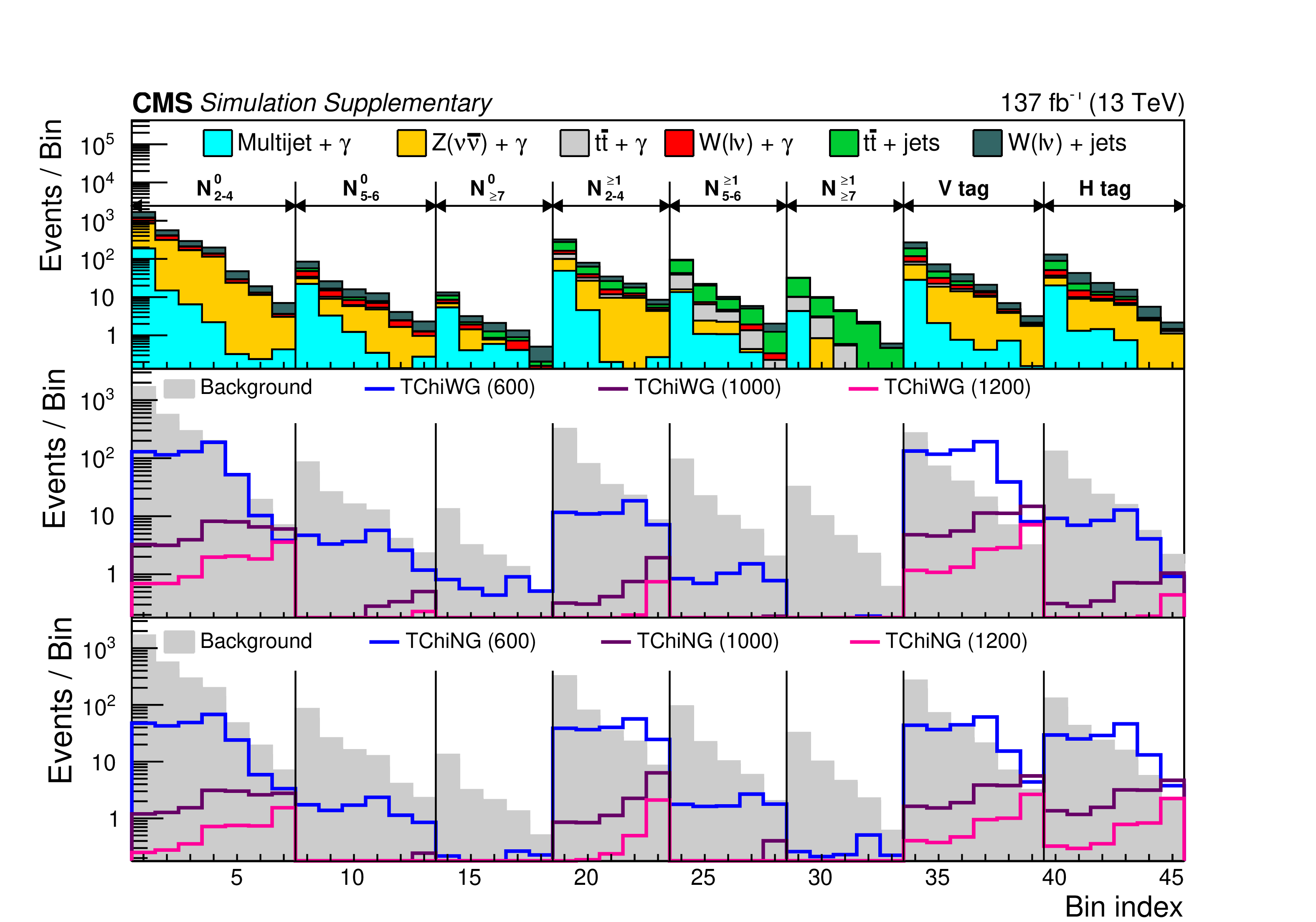
Additional Figure 2:
The expected event yields in the SRs and low-$ p_{\mathrm{T}}^\text{miss} $ CRs. The upper panel shows the distributions from simulated SM background contributions. The middle (bottom) panel shows the distributions for T5bbbbZg (T5qqqqHg) signal models, overlaid on the total simulated background distribution. The numerical values in parentheses in the legend entries for the signal models indicate the $ \mathrm{\tilde{g}} $ and NLSP mass values in GeVns. |

png pdf |
Additional Figure 3:
The expected event yields in the SRs and low-$ p_{\mathrm{T}}^\text{miss} $ CRs. The upper panel shows the distributions from simulated SM background contributions. The middle (bottom) panel shows the distributions for T5ttttZg (T6ttZg) signal models, overlaid on the total simulated background distribution. The numerical values in parentheses in the legend entries for the signal models indicate the $ \mathrm{\tilde{g}} $ ($ \tilde{\mathrm{t}} $) and NLSP mass values in GeVns. |
png pdf |
Additional Figure 4:
The expected event yields in the SRs and low-$ p_{\mathrm{T}}^\text{miss} $ CRs. The upper panel shows the distributions from simulated SM background contributions. The middle (bottom) panel shows the distributions for TChiWG (TChiNG) signal models, overlaid on the total simulated background distribution. The numerical values in parentheses in the legend entries for the signal models indicate the NLSP mass value in GeVns. |

png pdf |
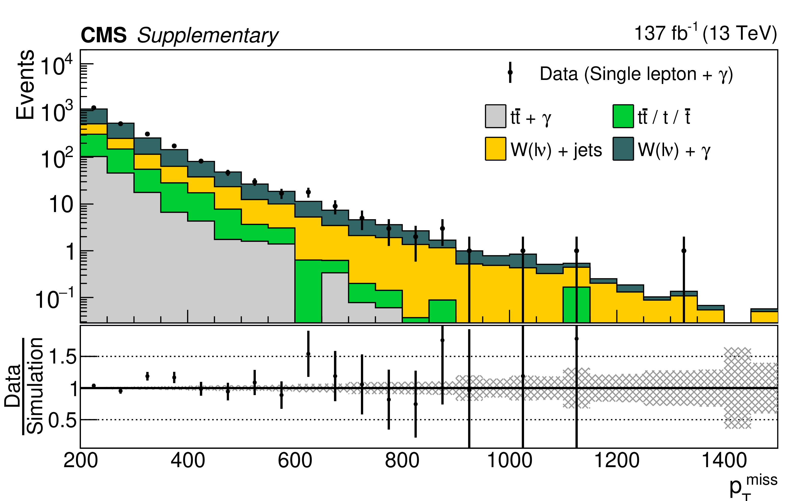
Additional Figure 5:
Distributions of the $ p_{\mathrm{T}}^\text{miss} $ (left) and the total number of AK4 jets (right) for single lepton + $ \gamma $ events in data and simulation. The lower panel presents the statistical uncertainty in the simulation as a shaded region, while the black points indicate the ratio of the data and simulation, with the error bars reflecting only the statistical uncertainty in the data. |
png pdf |
Additional Figure 5-a:
Distributions of the $ p_{\mathrm{T}}^\text{miss} $ (left) and the total number of AK4 jets (right) for single lepton + $ \gamma $ events in data and simulation. The lower panel presents the statistical uncertainty in the simulation as a shaded region, while the black points indicate the ratio of the data and simulation, with the error bars reflecting only the statistical uncertainty in the data. |

png pdf |
Additional Figure 5-b:
Distributions of the $ p_{\mathrm{T}}^\text{miss} $ (left) and the total number of AK4 jets (right) for single lepton + $ \gamma $ events in data and simulation. The lower panel presents the statistical uncertainty in the simulation as a shaded region, while the black points indicate the ratio of the data and simulation, with the error bars reflecting only the statistical uncertainty in the data. |

png pdf |
Additional Figure 6:
Distributions of $ m_{\mathrm{T}}({\vec p}_{\mathrm{T}}^{\mathrm{e}}, {\vec p}_{\mathrm{T}}^{\kern1pt\text{miss}}) $ in the single electron control region in simulation. The distributions for several T5bbbbZg signal models are overlaid on the SM background. The numerical values in parentheses in the legend entries for the signal models indicate the $ \mathrm{\tilde{g}} $ and NLSP mass values in GeVns. |

png pdf |
Additional Figure 7:
The normalized distributions of the $ p_{\mathrm{T}}^\text{miss} $ (upper left), the total number of AK4 jets (upper right), & the number of b-tagged jets (lower) for simulated $ \mathrm{Z}(\ell\ell)\gamma $ and $ \mathrm{Z}(\nu\nu)\gamma $ events. The $ p_{\mathrm{T}}^\text{miss} $ for $ \mathrm{Z}(\ell\ell)\gamma $ events is defined as the vector sum of the dilepton $ p_{\mathrm{T}} $ and the standard $ p_{\mathrm{T}}^\text{miss} $. The lower panels show the ratio of the simulated $ \mathrm{Z}(\ell\ell)\gamma $ and $ \mathrm{Z}(\nu\nu)\gamma $ events. |

png pdf |
Additional Figure 7-a:
The normalized distributions of the $ p_{\mathrm{T}}^\text{miss} $ (upper left), the total number of AK4 jets (upper right), & the number of b-tagged jets (lower) for simulated $ \mathrm{Z}(\ell\ell)\gamma $ and $ \mathrm{Z}(\nu\nu)\gamma $ events. The $ p_{\mathrm{T}}^\text{miss} $ for $ \mathrm{Z}(\ell\ell)\gamma $ events is defined as the vector sum of the dilepton $ p_{\mathrm{T}} $ and the standard $ p_{\mathrm{T}}^\text{miss} $. The lower panels show the ratio of the simulated $ \mathrm{Z}(\ell\ell)\gamma $ and $ \mathrm{Z}(\nu\nu)\gamma $ events. |

png pdf |
Additional Figure 7-b:
The normalized distributions of the $ p_{\mathrm{T}}^\text{miss} $ (upper left), the total number of AK4 jets (upper right), & the number of b-tagged jets (lower) for simulated $ \mathrm{Z}(\ell\ell)\gamma $ and $ \mathrm{Z}(\nu\nu)\gamma $ events. The $ p_{\mathrm{T}}^\text{miss} $ for $ \mathrm{Z}(\ell\ell)\gamma $ events is defined as the vector sum of the dilepton $ p_{\mathrm{T}} $ and the standard $ p_{\mathrm{T}}^\text{miss} $. The lower panels show the ratio of the simulated $ \mathrm{Z}(\ell\ell)\gamma $ and $ \mathrm{Z}(\nu\nu)\gamma $ events. |

png pdf |
Additional Figure 7-c:
The normalized distributions of the $ p_{\mathrm{T}}^\text{miss} $ (upper left), the total number of AK4 jets (upper right), & the number of b-tagged jets (lower) for simulated $ \mathrm{Z}(\ell\ell)\gamma $ and $ \mathrm{Z}(\nu\nu)\gamma $ events. The $ p_{\mathrm{T}}^\text{miss} $ for $ \mathrm{Z}(\ell\ell)\gamma $ events is defined as the vector sum of the dilepton $ p_{\mathrm{T}} $ and the standard $ p_{\mathrm{T}}^\text{miss} $. The lower panels show the ratio of the simulated $ \mathrm{Z}(\ell\ell)\gamma $ and $ \mathrm{Z}(\nu\nu)\gamma $ events. |

png pdf |
Additional Figure 8:
Distribution of the number of b-tagged jets for $ \ell\ell\gamma $ events in data and simulation. In the upper panel, the data are scaled by the correction factor $ \beta $ to remove the contribution of $ \mathrm{t}\overline{\mathrm{t}}\gamma{+}\text{jets} $ events. The lower panel shows the ratio between data and simulation. |
png pdf |
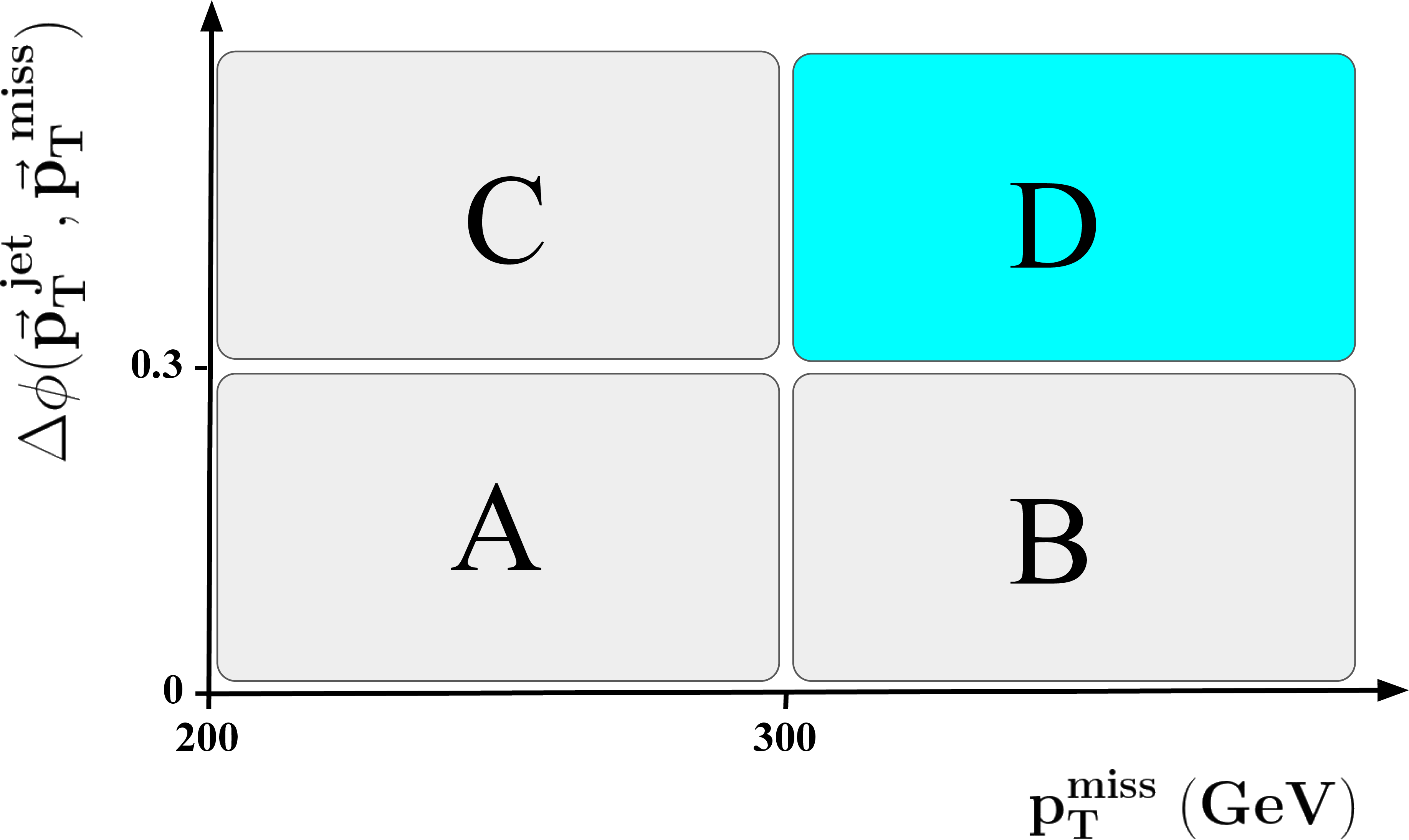
Additional Figure 9:
A schematic diagram of the $ p_{\mathrm{T}}^\text{miss}-\Delta\phi({\vec p}_{\mathrm{T}}^{\text{jet}},{\vec p}_{\mathrm{T}}^{\kern1pt\text{miss}}) $ plane used in the ABCD method to estimate the multijet + $ \gamma $ background. The region labeled D is the SR and the other regions are the CRs. |
png pdf |
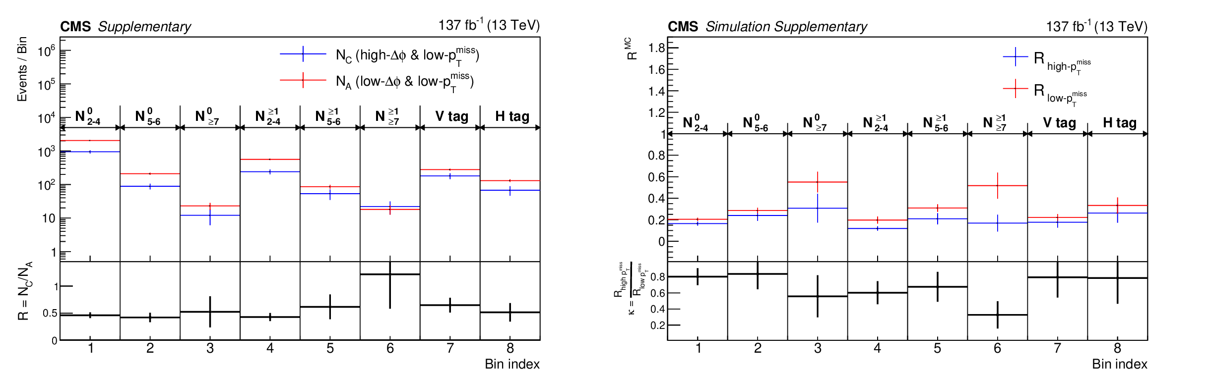
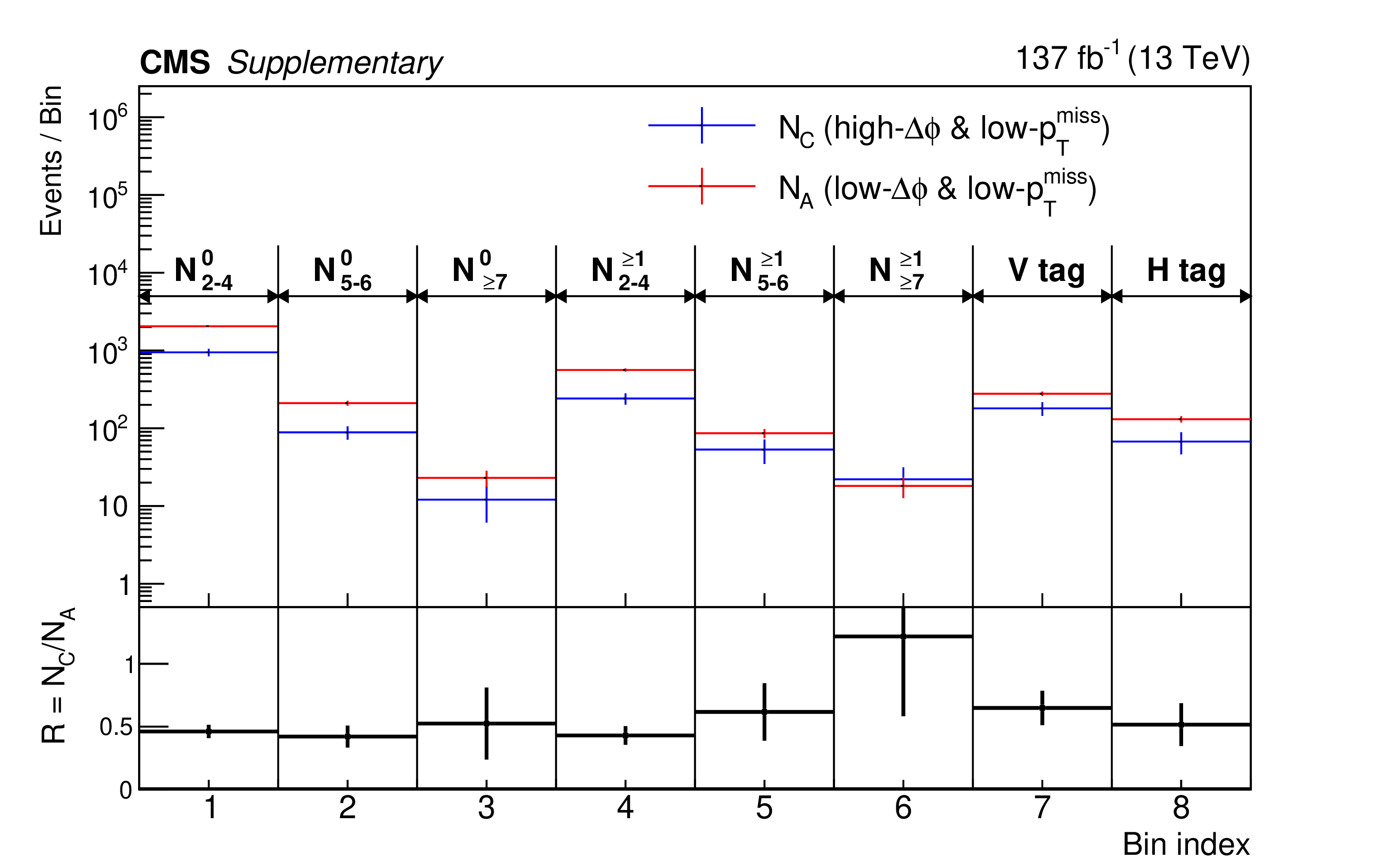
Additional Figure 10:
Left: the upper panel shows the event yield in the low-$ p_{\mathrm{T}}^\text{miss} $ CRs as a function of the signal region bins in $ N_{\text{jets}} $, $ N_{\mathrm{b}\text{-tags}} $, $ \text{V}\text{-tag} $, and $ \mathrm{H}\text{-tag} $; the the lower panel shows the ratio of the A and C regions, defined as $ R_{\text{low-}p_{\mathrm{T}}^\text{miss}} $. Right: the upper panel shows $ R_{\text{low-}p_{\mathrm{T}}^\text{miss}} $ and $ R_{\text{high-}p_{\mathrm{T}}^\text{miss}} $ from the simulation in the signal region bins; the lower panel shows the ratio of the two, defined as $ \kappa $. |
png pdf |
Additional Figure 10-a:
Left: the upper panel shows the event yield in the low-$ p_{\mathrm{T}}^\text{miss} $ CRs as a function of the signal region bins in $ N_{\text{jets}} $, $ N_{\mathrm{b}\text{-tags}} $, $ \text{V}\text{-tag} $, and $ \mathrm{H}\text{-tag} $; the the lower panel shows the ratio of the A and C regions, defined as $ R_{\text{low-}p_{\mathrm{T}}^\text{miss}} $. Right: the upper panel shows $ R_{\text{low-}p_{\mathrm{T}}^\text{miss}} $ and $ R_{\text{high-}p_{\mathrm{T}}^\text{miss}} $ from the simulation in the signal region bins; the lower panel shows the ratio of the two, defined as $ \kappa $. |

png pdf |
Additional Figure 10-b:
Left: the upper panel shows the event yield in the low-$ p_{\mathrm{T}}^\text{miss} $ CRs as a function of the signal region bins in $ N_{\text{jets}} $, $ N_{\mathrm{b}\text{-tags}} $, $ \text{V}\text{-tag} $, and $ \mathrm{H}\text{-tag} $; the the lower panel shows the ratio of the A and C regions, defined as $ R_{\text{low-}p_{\mathrm{T}}^\text{miss}} $. Right: the upper panel shows $ R_{\text{low-}p_{\mathrm{T}}^\text{miss}} $ and $ R_{\text{high-}p_{\mathrm{T}}^\text{miss}} $ from the simulation in the signal region bins; the lower panel shows the ratio of the two, defined as $ \kappa $. |

png pdf |
Additional Figure 11:
The product of signal acceptance and efficiency for the signal models T5bbbbZg (upper left), T5qqqqHg (upper right), T5ttttZg (lower left), and T6ttZg (lower right). |

png pdf root |
Additional Figure 11-a:
The product of signal acceptance and efficiency for the signal models T5bbbbZg (upper left), T5qqqqHg (upper right), T5ttttZg (lower left), and T6ttZg (lower right). |

png pdf root |
Additional Figure 11-b:
The product of signal acceptance and efficiency for the signal models T5bbbbZg (upper left), T5qqqqHg (upper right), T5ttttZg (lower left), and T6ttZg (lower right). |

png pdf root |
Additional Figure 11-c:
The product of signal acceptance and efficiency for the signal models T5bbbbZg (upper left), T5qqqqHg (upper right), T5ttttZg (lower left), and T6ttZg (lower right). |

png pdf root |
Additional Figure 11-d:
The product of signal acceptance and efficiency for the signal models T5bbbbZg (upper left), T5qqqqHg (upper right), T5ttttZg (lower left), and T6ttZg (lower right). |

png pdf |
Additional Figure 12:
The product of signal acceptance and efficiency for the signal models TChiWG (left) and TChiNG (right), in the 2D representation of the NLSP mass and the bin index. |

png pdf root |
Additional Figure 12-a:
The product of signal acceptance and efficiency for the signal models TChiWG (left) and TChiNG (right), in the 2D representation of the NLSP mass and the bin index. |

png pdf root |
Additional Figure 12-b:
The product of signal acceptance and efficiency for the signal models TChiWG (left) and TChiNG (right), in the 2D representation of the NLSP mass and the bin index. |

png pdf |
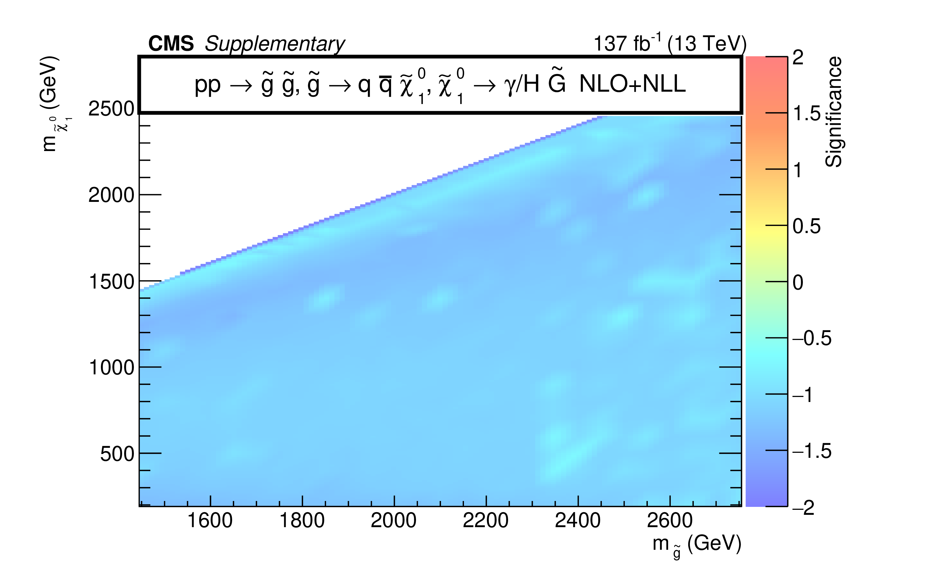
Additional Figure 13:
The observed significance for the signal models T5bbbbZg (upper left), T5qqqqHg (upper right), T5ttttZg (lower left), and T6ttZg (lower right). The negative significance values occur because of a deficiency of observed data relative to the prediction in sensitive bins. |

png pdf |
Additional Figure 13-a:
The observed significance for the signal models T5bbbbZg (upper left), T5qqqqHg (upper right), T5ttttZg (lower left), and T6ttZg (lower right). The negative significance values occur because of a deficiency of observed data relative to the prediction in sensitive bins. |
png pdf |
Additional Figure 13-b:
The observed significance for the signal models T5bbbbZg (upper left), T5qqqqHg (upper right), T5ttttZg (lower left), and T6ttZg (lower right). The negative significance values occur because of a deficiency of observed data relative to the prediction in sensitive bins. |

png pdf |
Additional Figure 13-c:
The observed significance for the signal models T5bbbbZg (upper left), T5qqqqHg (upper right), T5ttttZg (lower left), and T6ttZg (lower right). The negative significance values occur because of a deficiency of observed data relative to the prediction in sensitive bins. |

png pdf |
Additional Figure 13-d:
The observed significance for the signal models T5bbbbZg (upper left), T5qqqqHg (upper right), T5ttttZg (lower left), and T6ttZg (lower right). The negative significance values occur because of a deficiency of observed data relative to the prediction in sensitive bins. |

png pdf |
Additional Figure 14:
The observed significance for the signal models TChiWG (left) and TChiNG (right). |

png pdf |
Additional Figure 14-a:
The observed significance for the signal models TChiWG (left) and TChiNG (right). |

png pdf |
Additional Figure 14-b:
The observed significance for the signal models TChiWG (left) and TChiNG (right). |

png pdf root |
Additional Figure 15:
The covariance matrix for the signal regions and the low-$ p_{\mathrm{T}}^\text{miss} $ CRs, derived from the CR-only fit under the background-only hypothesis. |

png pdf root |
Additional Figure 16:
The correlation matrix for the signal regions and the low-$ p_{\mathrm{T}}^\text{miss} $ CRs, derived from the CR-only fit under the background-only hypothesis. |
| Additional Tables | |
png pdf |
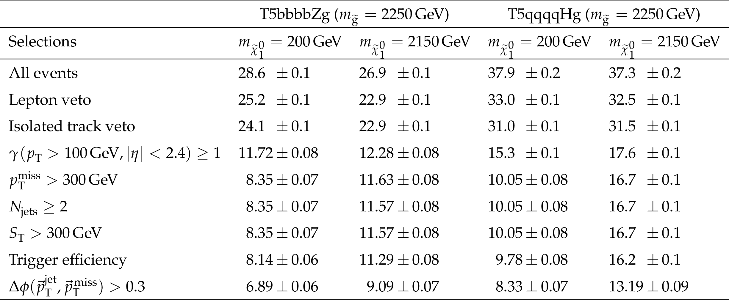
Additional Table 1:
Cutflows for T5bbbbZg & T5qqqqHg signal samples. The event yields are scaled to 137 fb$ ^{-1} $. |

png pdf |
Additional Table 2:
Cutflows for T5ttttZg & T6ttZg signal samples. The event yields are scaled to 137 fb$ ^{-1} $. |

png pdf |
Additional Table 3:
Cutflows for TChiWG & TChiNG signal samples. The event yields are scaled to 137 fb$ ^{-1} $. |
| References | ||||
| 1 | F. Zwicky | Die Rotverschiebung von extragalaktischen Nebeln | Helv. Phys. Acta 6 (1933) 110 | |
| 2 | V. C. Rubin and W. K. Ford Jr | Rotation of the Andromeda nebula from a spectroscopic survey of emission regions | Astrophys. J. 159 (1970) 379 | |
| 3 | R. Barbieri and G. F. Giudice | Upper bounds on supersymmetric particle masses | NPB 306 (1988) 63 | |
| 4 | S. Dimopoulos and G. F. Giudice | Naturalness constraints in supersymmetric theories with nonuniversal soft terms | PLB 357 (1995) 573 | hep-ph/9507282 |
| 5 | R. Barbieri and D. Pappadopulo | S-particles at their naturalness limits | JHEP 10 (2009) 061 | 0906.4546 |
| 6 | M. Papucci, J. T. Ruderman, and A. Weiler | Natural SUSY endures | JHEP 09 (2012) 035 | 1110.6926 |
| 7 | P. Ramond | Dual theory for free fermions | PRD 3 (1971) 2415 | |
| 8 | Yu. A. Golfand and E. P. Likhtman | Extension of the algebra of Poincaré group generators and violation of P invariance | JETP Lett. 13 (1971) 323 | |
| 9 | A. Neveu and J. H. Schwarz | Factorizable dual model of pions | NPB 31 (1971) 86 | |
| 10 | D. V. Volkov and V. P. Akulov | Possible universal neutrino interaction | JETP Lett. 16 (1972) 438 | |
| 11 | J. Wess and B. Zumino | A Lagrangian model invariant under supergauge transformations | PLB 49 (1974) 52 | |
| 12 | J. Wess and B. Zumino | Supergauge transformations in four dimensions | NPB 70 (1974) 39 | |
| 13 | P. Fayet | Supergauge invariant extension of the Higgs mechanism and a model for the electron and its neutrino | NPB 90 (1975) 104 | |
| 14 | H. P. Nilles | Supersymmetry, supergravity and particle physics | Phys. Rep. 110 (1984) 1 | |
| 15 | G. R. Farrar and P. Fayet | Phenomenology of the production, decay, and detection of new hadronic states associated with supersymmetry | PLB 76 (1978) 575 | |
| 16 | D. Emmanuel-Costa, P. Fileviez Perez, and R. Gonzalez Felipe | Natural gauge and gravitational coupling unification and the superpartner masses | PLB 648 (2007) 60 | hep-ph/0610178 |
| 17 | H. Baer et al. | Radiative natural SUSY with a 125 GeV Higgs boson | PRL 109 (2012) 161802 | 1207.3343 |
| 18 | P. Fayet | Mixing between gravitational and weak interactions through the massive gravitino | PLB 70 (1977) 461 | |
| 19 | H. Baer, M. Brhlik, C.-h. Chen, and X. Tata | Signals for the minimal gauge mediated supersymmetry breaking model at the Fermilab Tevatron collider | PRD 55 (1997) 4463 | hep-ph/9610358 |
| 20 | N. Arkani-Hamed et al. | MARMOSET: The path from LHC data to the new standard model via on-shell effective theories | hep-ph/0703088 | |
| 21 | J. Alwall, P. C. Schuster, and N. Toro | Simplified models for a first characterization of new physics at the LHC | PRD 79 (2009) 075020 | 0810.3921 |
| 22 | J. Alwall, M.-P. Le, M. Lisanti, and J. G. Wacker | Model-independent jets plus missing energy searches | PRD 79 (2009) 015005 | 0809.3264 |
| 23 | D. Alves et al. | Simplified models for LHC new physics searches | JPG 39 (2012) 105005 | 1105.2838 |
| 24 | CMS Collaboration | Interpretation of searches for supersymmetry with simplified models | PRD 88 (2013) 052017 | CMS-SUS-11-016 1301.2175 |
| 25 | CMS Collaboration | Search for gauge-mediated supersymmetry in events with at least one photon and missing transverse momentum in pp collisions at $ \sqrt{s} = $ 13 TeV | PLB 780 (2018) 118 | CMS-SUS-16-046 1711.08008 |
| 26 | CMS Collaboration | Search for supersymmetry in events with at least one photon, missing transverse momentum, and large transverse event activity in proton-proton collisions at $ \sqrt{s}= $ 13 TeV | JHEP 12 (2017) 142 | CMS-SUS-16-047 1707.06193 |
| 27 | CMS Collaboration | Search for supersymmetry in events with a photon, jets, b-jets, and missing transverse momentum in proton-proton collisions at 13 TeV | EPJC 79 (2019) 444 | CMS-SUS-18-002 1901.06726 |
| 28 | ATLAS Collaboration | Search for supersymmetry in a final state containing two photons and missing transverse momentum in $ \sqrt{s} = $ 13 TeV pp collisions at the LHC using the ATLAS detector | EPJC 76 (2016) 517 | 1606.09150 |
| 29 | ATLAS Collaboration | Search for photonic signatures of gauge-mediated supersymmetry in 13 TeV pp collisions with the ATLAS detector | PRD 97 (2018) 092006 | 1802.03158 |
| 30 | ATLAS Collaboration | Search for new phenomena in final states with photons, jets and missing transverse momentum in pp collisions at $ \sqrt{s} = $ 13 TeV with the ATLAS detector | JHEP 07 (2023) 021 | 2206.06012 |
| 31 | CMS Collaboration | HEPData record for this analysis | link | |
| 32 | CMS Collaboration | The CMS experiment at the CERN LHC | JINST 3 (2008) S08004 | |
| 33 | CMS Collaboration | The CMS trigger system | JINST 12 (2017) P01020 | CMS-TRG-12-001 1609.02366 |
| 34 | CMS Collaboration | Particle-flow reconstruction and global event description with the CMS detector | JINST 12 (2017) P10003 | CMS-PRF-14-001 1706.04965 |
| 35 | CMS Collaboration | Technical proposal for the Phase-II upgrade of the Compact Muon Solenoid | CMS Technical Proposal CERN-LHCC-2015-010, CMS-TDR-15-02, 2015 CDS |
|
| 36 | M. Cacciari, G. P. Salam, and G. Soyez | The anti-$ k_{\mathrm{T}} $ jet clustering algorithm | JHEP 04 (2008) 063 | 0802.1189 |
| 37 | M. Cacciari, G. P. Salam, and G. Soyez | FastJet user manual | EPJC 72 (2012) 1896 | 1111.6097 |
| 38 | M. Cacciari and G. P. Salam | Pileup subtraction using jet areas | PLB 659 (2008) 119 | 0707.1378 |
| 39 | CMS Collaboration | Pileup mitigation at CMS in 13 TeV data | JINST 15 (2020) P09018 | CMS-JME-18-001 2003.00503 |
| 40 | CMS Collaboration | Jet energy scale and resolution in the CMS experiment in pp collisions at 8 TeV | JINST 12 (2017) P02014 | CMS-JME-13-004 1607.03663 |
| 41 | CMS Collaboration | Jet algorithms performance in 13 TeV data | CMS Physics Analysis Summary, 2017 CMS-PAS-JME-16-003 |
CMS-PAS-JME-16-003 |
| 42 | A. J. Larkoski, S. Marzani, G. Soyez, and J. Thaler | Soft drop | JHEP 05 (2014) 146 | 1402.2657 |
| 43 | CMS Collaboration | Identification of heavy-flavour jets with the CMS detector in pp collisions at 13 TeV | JINST 13 (2018) P05011 | CMS-BTV-16-002 1712.07158 |
| 44 | CMS Collaboration | Performance of missing transverse momentum reconstruction in proton-proton collisions at $ \sqrt{s} = $ 13 TeV using the CMS detector | JINST 14 (2019) P07004 | CMS-JME-17-001 1903.06078 |
| 45 | CMS Collaboration | Electron and photon reconstruction and identification with the CMS experiment at the CERN LHC | JINST 16 (2021) P05014 | CMS-EGM-17-001 2012.06888 |
| 46 | CMS Collaboration | Performance of the CMS muon detector and muon reconstruction with proton-proton collisions at $ \sqrt{s} = $ 13 TeV | JINST 13 (2018) P06015 | CMS-MUO-16-001 1804.04528 |
| 47 | J. Alwall et al. | The automated computation of tree-level and next-to-leading order differential cross sections, and their matching to parton shower simulations | JHEP 07 (2014) 079 | 1405.0301 |
| 48 | J. Alwall et al. | Comparative study of various algorithms for the merging of parton showers and matrix elements in hadronic collisions | EPJC 53 (2008) 473 | 0706.2569 |
| 49 | T. Sjöstrand et al. | An Introduction to PYTHIA 8.2 | Comput. Phys. Commun. 191 (2015) 159 | 1410.3012 |
| 50 | NNPDF Collaboration | Parton distributions for the LHC Run II | JHEP 04 (2015) 040 | 1410.8849 |
| 51 | NNPDF Collaboration | Parton distributions from high-precision collider data | EPJC 77 (2017) 663 | 1706.00428 |
| 52 | CMS Collaboration | Event generator tunes obtained from underlying event and multiparton scattering measurements | EPJC 76 (2016) 155 | CMS-GEN-14-001 1512.00815 |
| 53 | CMS Collaboration | Extraction and validation of a new set of CMS PYTHIA8 tunes from underlying-event measurements | EPJC 80 (2020) 4 | CMS-GEN-17-001 1903.12179 |
| 54 | R. Frederix and S. Frixione | Merging meets matching in MC@NLO | JHEP 12 (2012) 061 | 1209.6215 |
| 55 | A. Kulesza and L. Motyka | Soft gluon resummation for the production of gluino-gluino and squark-antisquark pairs at the LHC | PRD 80 (2009) 095004 | 0905.4749 |
| 56 | W. Beenakker et al. | Soft-gluon resummation for squark and gluino hadroproduction | JHEP 12 (2009) 041 | 0909.4418 |
| 57 | W. Beenakker et al. | NNLL resummation for squark-antisquark pair production at the LHC | JHEP 01 (2012) 076 | 1110.2446 |
| 58 | W. Beenakker et al. | Towards NNLL resummation: hard matching coefficients for squark and gluino hadroproduction | JHEP 10 (2013) 120 | 1304.6354 |
| 59 | W. Beenakker et al. | NNLL resummation for squark and gluino production at the LHC | JHEP 12 (2014) 023 | 1404.3134 |
| 60 | W. Beenakker et al. | NNLL resummation for stop pair-production at the LHC | JHEP 05 (2016) 153 | 1601.02954 |
| 61 | W. Beenakker et al. | NNLL-fast: predictions for coloured supersymmetric particle production at the LHC with threshold and Coulomb resummation | JHEP 12 (2016) 133 | 1607.07741 |
| 62 | GEANT4 Collaboration | GEANT 4---a simulation toolkit | NIM A 506 (2003) 250 | |
| 63 | S. Abdullin et al. | The fast simulation of the CMS detector at LHC | J. Phys. Conf. Ser. 331 (2011) 032049 | |
| 64 | A. Giammanco | The fast simulation of the CMS experiment | J. Phys. Conf. Ser. 513 (2014) 022012 | |
| 65 | CMS Collaboration | Measurement of the inclusive and differential $ {\mathrm{t}\overline{\mathrm{t}}} \gamma $ cross sections in the single-lepton channel and EFT interpretation at $ \sqrt{s} = $ 13 TeV | JHEP 12 (2021) 180 | CMS-TOP-18-010 2107.01508 |
| 66 | M. Cacciari et al. | The $ \mathrm{t} \overline{\mathrm{t}} $ cross-section at 1.8 TeV and 1.96 TeV: A study of the systematics due to parton densities and scale dependence | JHEP 04 (2004) 068 | hep-ph/0303085 |
| 67 | S. Catani, D. de Florian, M. Grazzini, and P. Nason | Soft gluon resummation for Higgs boson production at hadron colliders | JHEP 07 (2003) 028 | hep-ph/0306211 |
| 68 | CMS Collaboration | Measurements of inclusive $ {\mathrm{W}} $ and $ {\mathrm{Z}} $ cross sections in $ {\mathrm{p}\mathrm{p}} $ collisions at $ \sqrt{s}= $ 7 TeV | JHEP 01 (2011) 080 | CMS-EWK-10-002 1012.2466 |
| 69 | A. Denner, S. Dittmaier, M. Hecht, and C. Pasold | NLO QCD and electroweak corrections to Z+$\gamma $ production with leptonic Z-boson decays | JHEP 02 (2016) 057 | 1510.08742 |
| 70 | CMS Collaboration | Precision luminosity measurement in proton-proton collisions at $ \sqrt{s} = $ 13 TeV in 2015 and 2016 at CMS | EPJC 81 (2021) 800 | CMS-LUM-17-003 2104.01927 |
| 71 | CMS Collaboration | CMS luminosity measurement for the 2017 data-taking period at $ \sqrt{s} = $ 13 TeV | CMS Physics Analysis Summary, 2018 CMS-PAS-LUM-17-004 |
CMS-PAS-LUM-17-004 |
| 72 | CMS Collaboration | CMS luminosity measurement for the 2018 data-taking period at $ \sqrt{s} = $ 13 TeV | CMS Physics Analysis Summary, 2019 CMS-PAS-LUM-18-002 |
CMS-PAS-LUM-18-002 |
| 73 | CMS Collaboration | Search for supersymmetry in proton-proton collisions at 13 TeV in final states with jets and missing transverse momentum | JHEP 10 (2019) 244 | CMS-SUS-19-006 1908.04722 |
| 74 | T. Junk | Confidence level computation for combining searches with small statistics | NIM A 434 (1999) 435 | hep-ex/9902006 |
| 75 | A. L. Read | Presentation of search results: the $ \text{CL}_\text{s} $ technique | JPG 28 (2002) 2693 | |
| 76 | G. Cowan, K. Cranmer, E. Gross, and O. Vitells | Asymptotic formulae for likelihood-based tests of new physics | EPJC 71 (2011) 1554 | 1007.1727 |
|
|
Compact Muon Solenoid LHC, CERN |
|

|

|

|

|

|