

Compact Muon Solenoid
LHC, CERN
| CMS-TAU-18-001 ; CERN-EP-2019-012 | ||
| An embedding technique to determine $\tau\tau$ backgrounds in proton-proton collision data | ||
| CMS Collaboration | ||
| 3 March 2019 | ||
| JINST 14 (2019) P06032 | ||
| Abstract: An embedding technique is presented to estimate standard model ${\tau_{\mathrm{h}} \tau_{\mathrm{h}} }$ backgrounds from data with minimal simulation input. In the data, the muons are removed from reconstructed $\mu\mu$ events and replaced with simulated tau leptons with the same kinematic properties. In this way a set of hybrid events is obtained that does not rely on simulation except for the decay of the tau leptons. The challenges in describing the underlying event or the production of associated jets in the simulation are avoided. The technique described in this paper was developed for CMS. Its validation and the inherent uncertainties are also discussed. The demonstration of the performance of the technique is based on a sample of proton-proton collisions collected by CMS in 2017 at $\sqrt{s} = $ 13 TeV corresponding to an integrated luminosity of 41.5 fb$^{-1}$. | ||
| Links: e-print arXiv:1903.01216 [hep-ex] (PDF) ; CDS record ; inSPIRE record ; CADI line (restricted) ; | ||
| Figures & Tables | Summary | Additional Figures | References | CMS Publications |
|---|
| Figures | |
png pdf |
Figure 1:
Schematic view of the four main steps of the $ {\tau}$-embedding technique, as described in Section 5. A ${{{\mathrm {Z}} \to {{\mu}} {{\mu}}}}$ candidate event is selected in data ("${{{\mathrm {Z}} \to {{\mu}} {{\mu}}}}$ Selection''), all energy deposits associated with the muons are removed from the event record ("${{{\mathrm {Z}} \to {{\mu}} {{\mu}}}}$ Cleaning''), and two tau lepton decays are simulated in an otherwise empty detector ("${{{\mathrm {Z}} \to {\tau} {\tau}}}$ Simulation''). Finally all energy deposits of the simulated tau lepton decays are combined with the original reconstructed event record ("${{{\mathrm {Z}} \to {\tau} {\tau}}}$ Hybrid''). In the example, one of the simulated tau leptons decays into a muon and the other one into hadrons. |

png pdf |
Figure 2:
(Left) invariant mass, $ {m_{\mu \mu}} $, of the selected dimuon Z boson candidates and (right) $ {p_{\mathrm {T}}} $ of the trailing muon after the event selection, as described in Section 5.1. |
png pdf |
Figure 2-a:
Invariant mass, $ {m_{\mu \mu}} $, of the selected dimuon Z boson candidates, as described in Section 5.1. |

png pdf |
Figure 2-b:
$ {p_{\mathrm {T}}} $ of the trailing muon after the event selection, as described in Section 5.1. |
png pdf |
Figure 3:
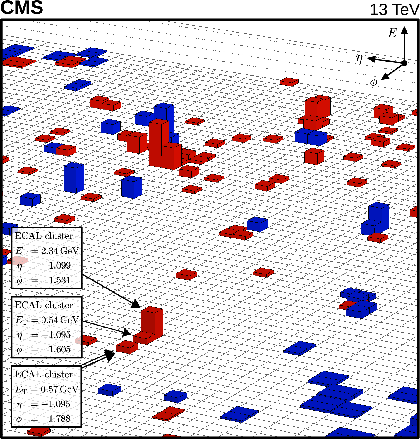
Display of a ${{{\mathrm {Z}} \to {{\mu}} {{\mu}}}}$ candidate event in the 2017 data set, in the $\eta $-$\phi $ plane at the surface of the calorimeters (left) before and (right) after the hits and energy deposits associated with the muons have been removed from the reconstructed event record. The red crosses indicate the intercepts of the reconstructed muon trajectories with the calorimeter surface. The red (blue) boxes correspond to clusters in the ECAL (HCAL). |
png pdf |
Figure 3-a:
Display of a ${{{\mathrm {Z}} \to {{\mu}} {{\mu}}}}$ candidate event in the 2017 data set, in the $\eta $-$\phi $ plane at the surface of the calorimeters before the hits and energy deposits associated with the muons have been removed from the reconstructed event record. The red crosses indicate the intercepts of the reconstructed muon trajectories with the calorimeter surface. The red (blue) boxes correspond to clusters in the ECAL (HCAL). |
png pdf |
Figure 3-b:
Display of a ${{{\mathrm {Z}} \to {{\mu}} {{\mu}}}}$ candidate event in the 2017 data set, in the $\eta $-$\phi $ plane at the surface of the calorimeters after the hits and energy deposits associated with the muons have been removed from the reconstructed event record. The red crosses indicate the intercepts of the reconstructed muon trajectories with the calorimeter surface. The red (blue) boxes correspond to clusters in the ECAL (HCAL). |
png pdf |
Figure 4:
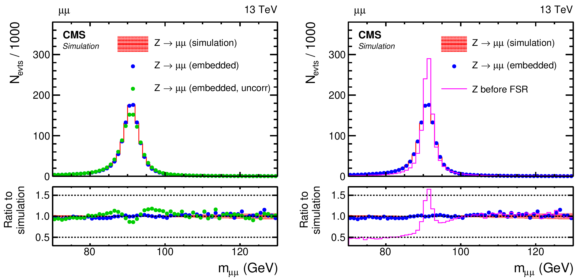
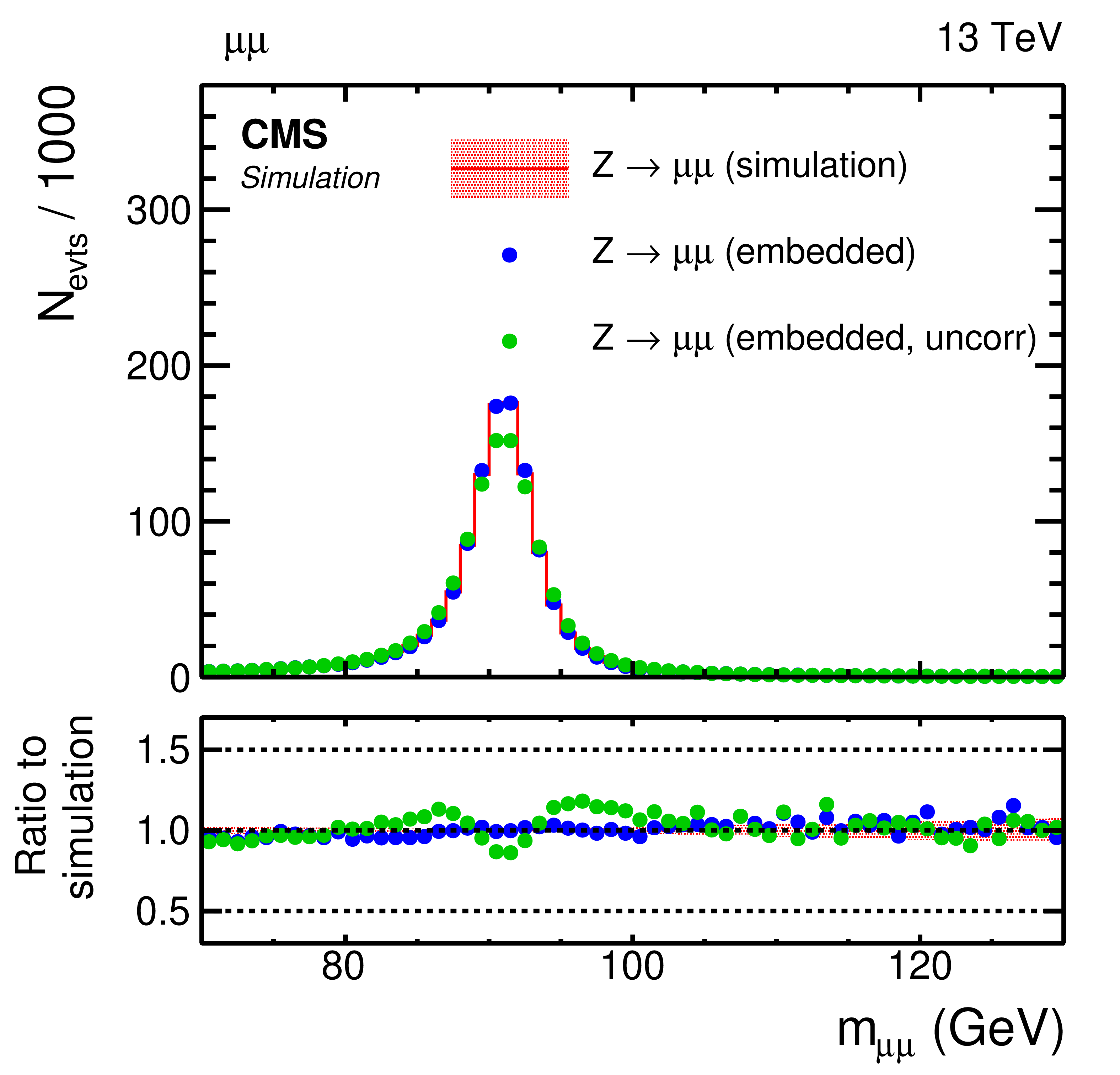
Comparison of the reconstructed invariant mass, $ {m_{\mu \mu}} $, of the selected muons from a simulated ${{{\mathrm {Z}} \to {{\mu}} {{\mu}}}}$ sample with the corresponding $ {{\mu}}$-embedded event sample. On the left the (red histogram) simulated ${{{\mathrm {Z}} \to {{\mu}} {{\mu}}}}$ sample and the $ {{\mu}}$-embedded event sample (blue dots) with and (green dots) without the correction for the effects of the finite detector resolution, as described in the text, are shown. On the right (magenta histogram) $ {m_{\mu \mu}} $ from the simulated ${{{\mathrm {Z}} \to {{\mu}} {{\mu}}}}$ sample before FSR is shown in addition, to illustrate the effect. |
png pdf |
Figure 4-a:
Comparison of the reconstructed invariant mass, $ {m_{\mu \mu}} $, of the selected muons from a simulated ${{{\mathrm {Z}} \to {{\mu}} {{\mu}}}}$ sample with the corresponding $ {{\mu}}$-embedded event sample. The (red histogram) simulated ${{{\mathrm {Z}} \to {{\mu}} {{\mu}}}}$ sample and the $ {{\mu}}$-embedded event sample (blue dots) with and (green dots) without the correction for the effects of the finite detector resolution, as described in the text, are shown. |

png pdf |
Figure 4-b:
Comparison of the reconstructed invariant mass, $ {m_{\mu \mu}} $, of the selected muons from a simulated ${{{\mathrm {Z}} \to {{\mu}} {{\mu}}}}$ sample with the corresponding $ {{\mu}}$-embedded event sample. The (magenta histogram) $ {m_{\mu \mu}} $ from the simulated ${{{\mathrm {Z}} \to {{\mu}} {{\mu}}}}$ sample before FSR is shown to illustrate the effect. |

png pdf |
Figure 5:
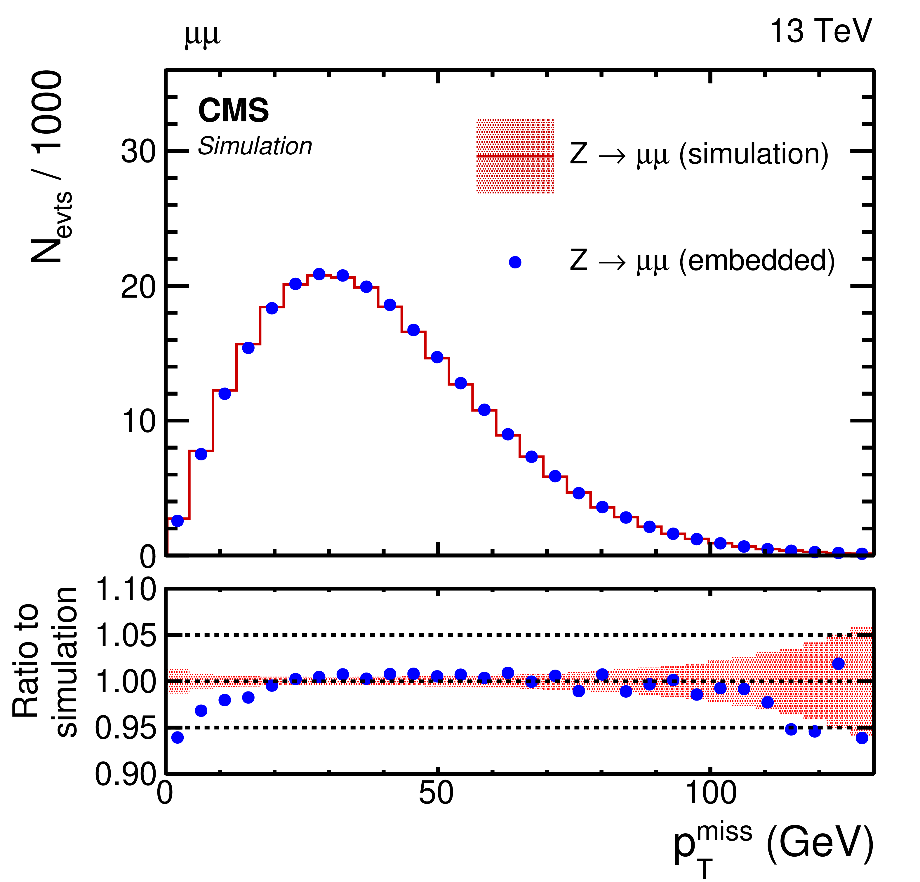
Comparison of $ {{\mu}}$-embedded events with exactly the same ${{{\mathrm {Z}} \to {{\mu}} {{\mu}}}}$ events from simulation. Shown are the (upper left) $\eta $ and (upper right) $ {p_{\mathrm {T}}} $ distributions of the leading muon in $ {p_{\mathrm {T}}} $, (middle left) $ {{p_{\mathrm {T}}} ^\text {miss}} $, (middle right) $ {m_{\text {jj}}} $, (lower left) jet and, (lower right) b jet multiplicities, as described in the text. |

png pdf |
Figure 5-a:
Comparison of $ {{\mu}}$-embedded events with exactly the same ${{{\mathrm {Z}} \to {{\mu}} {{\mu}}}}$ events from simulation. Shown is the $\eta $ distribution of the leading muon in $ {p_{\mathrm {T}}} $, as described in the text. |

png pdf |
Figure 5-b:
Comparison of $ {{\mu}}$-embedded events with exactly the same ${{{\mathrm {Z}} \to {{\mu}} {{\mu}}}}$ events from simulation. Shown is the $ {p_{\mathrm {T}}} $ distribution of the leading muon in $ {p_{\mathrm {T}}} $, as described in the text. |
png pdf |
Figure 5-c:
Comparison of $ {{\mu}}$-embedded events with exactly the same ${{{\mathrm {Z}} \to {{\mu}} {{\mu}}}}$ events from simulation. Shown is $ {{p_{\mathrm {T}}} ^\text {miss}} $, as described in the text. |
png pdf |
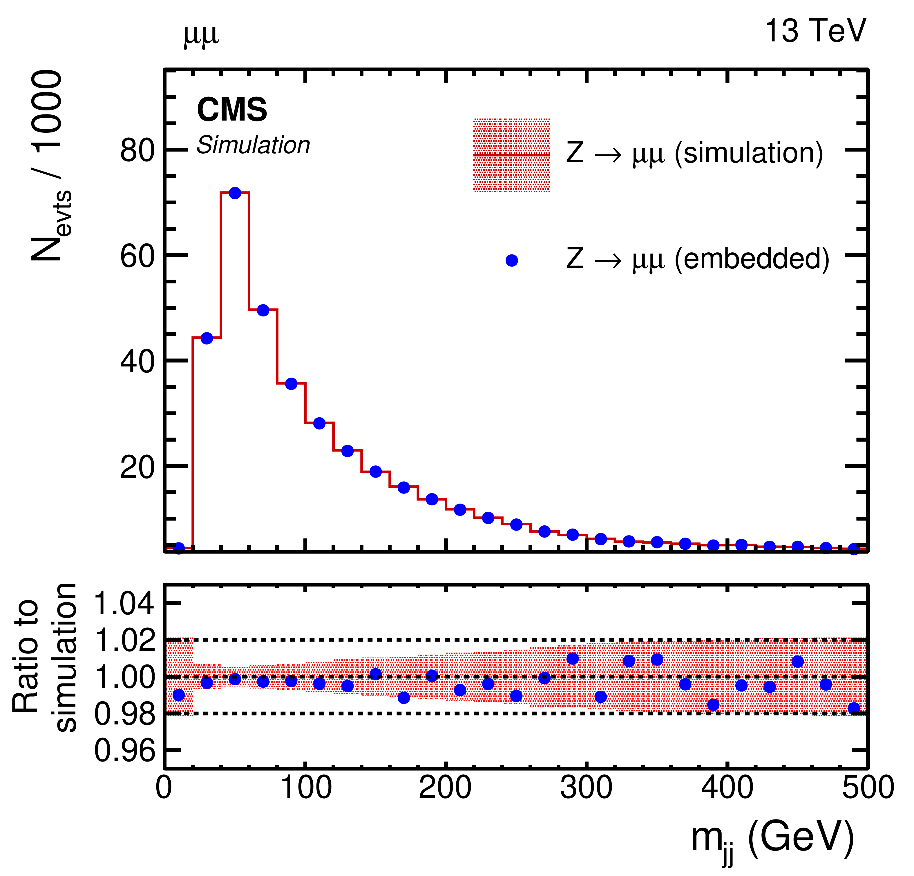
Figure 5-d:
Comparison of $ {{\mu}}$-embedded events with exactly the same ${{{\mathrm {Z}} \to {{\mu}} {{\mu}}}}$ events from simulation. Shown is $ {m_{\text {jj}}} $, as described in the text. |
png pdf |
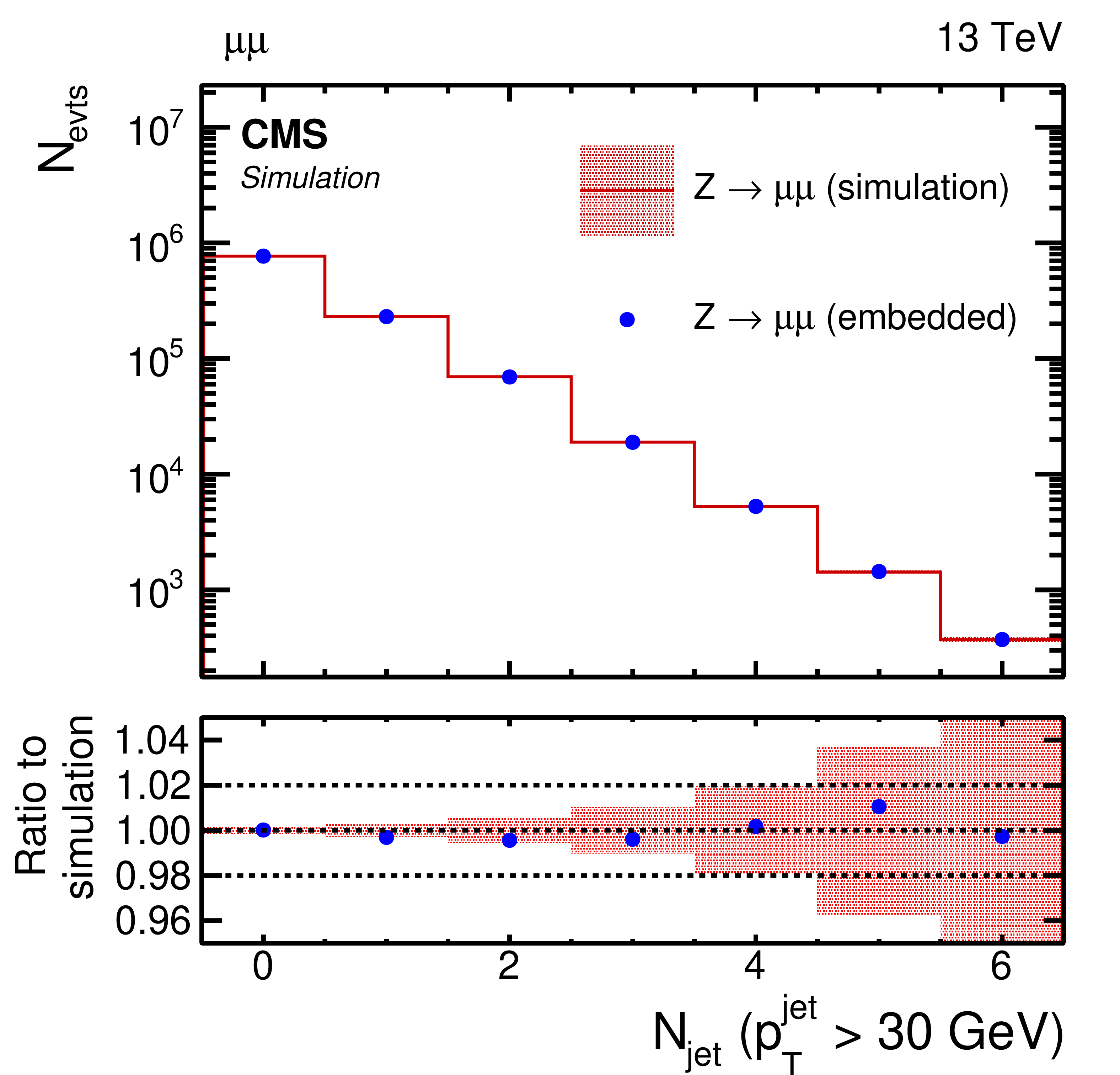
Figure 5-e:
Comparison of $ {{\mu}}$-embedded events with exactly the same ${{{\mathrm {Z}} \to {{\mu}} {{\mu}}}}$ events from simulation. Shown is the jet multiplicity, as described in the text. |
png pdf |
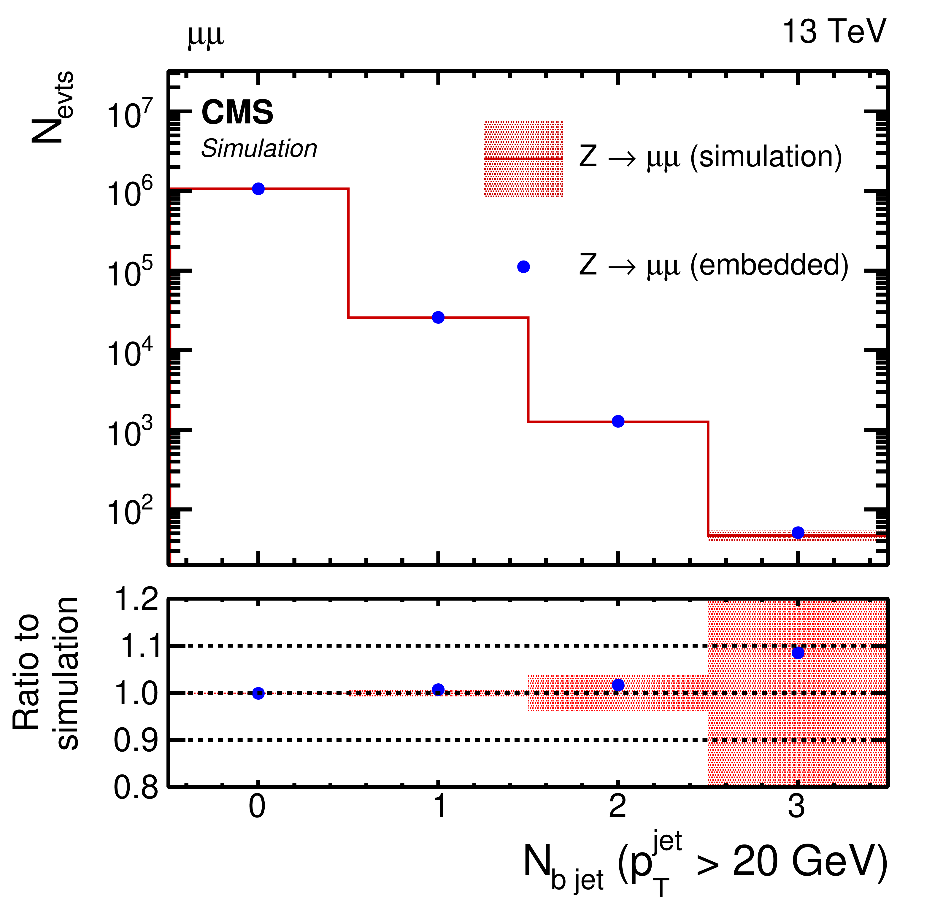
Figure 5-f:
Comparison of $ {{\mu}}$-embedded events with exactly the same ${{{\mathrm {Z}} \to {{\mu}} {{\mu}}}}$ events from simulation. Shown is the b-jet multiplicity, as described in the text. |
png pdf |
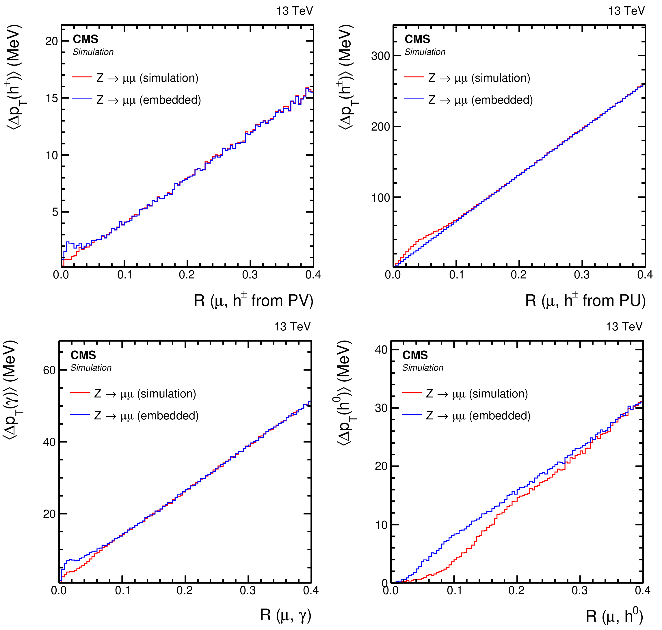
Figure 6:
Comparison of $ {{\mu}}$-embedded events with exactly the same ${{{\mathrm {Z}} \to {{\mu}} {{\mu}}}}$ events from simulation. Shown is the mean transverse momentum (energy) flux per muon, from all reconstructed particles with the distance $R$ from the muon, split by (upper left) charged hadrons from the PV and (upper right) PU vertices, (lower left) photons, and (lower right) neutral hadrons. The distributions are shown for the $ {\mu ^-} $ and for events with $ {m_{\mu \mu}} $ close to the nominal Z boson mass. |
png pdf |
Figure 6-a:
Comparison of $ {{\mu}}$-embedded events with exactly the same ${{{\mathrm {Z}} \to {{\mu}} {{\mu}}}}$ events from simulation. Shown is the mean transverse momentum (energy) flux per muon, from all reconstructed particles with the distance $R$ from the muon, split by charged hadrons from the PV vertices. The distribution is shown for the $ {\mu ^-} $ and for events with $ {m_{\mu \mu}} $ close to the nominal Z boson mass. |
png pdf |
Figure 6-b:
Comparison of $ {{\mu}}$-embedded events with exactly the same ${{{\mathrm {Z}} \to {{\mu}} {{\mu}}}}$ events from simulation. Shown is the mean transverse momentum (energy) flux per muon, from all reconstructed particles with the distance $R$ from the muon, split by charged hadrons from the PU vertices. The distribution is shown for the $ {\mu ^-} $ and for events with $ {m_{\mu \mu}} $ close to the nominal Z boson mass. |
png pdf |
Figure 6-c:
Comparison of $ {{\mu}}$-embedded events with exactly the same ${{{\mathrm {Z}} \to {{\mu}} {{\mu}}}}$ events from simulation. Shown is the mean transverse momentum (energy) flux per muon, from all reconstructed particles with the distance $R$ from the muon, split by photons. The distribution is shown for the $ {\mu ^-} $ and for events with $ {m_{\mu \mu}} $ close to the nominal Z boson mass. |
png pdf |
Figure 6-d:
Comparison of $ {{\mu}}$-embedded events with exactly the same ${{{\mathrm {Z}} \to {{\mu}} {{\mu}}}}$ events from simulation. Shown is the mean transverse momentum (energy) flux per muon, from all reconstructed particles with the distance $R$ from the muon, split by neutral hadrons. The distribution is shown for the $ {\mu ^-} $ and for events with $ {m_{\mu \mu}} $ close to the nominal Z boson mass. |
png pdf |
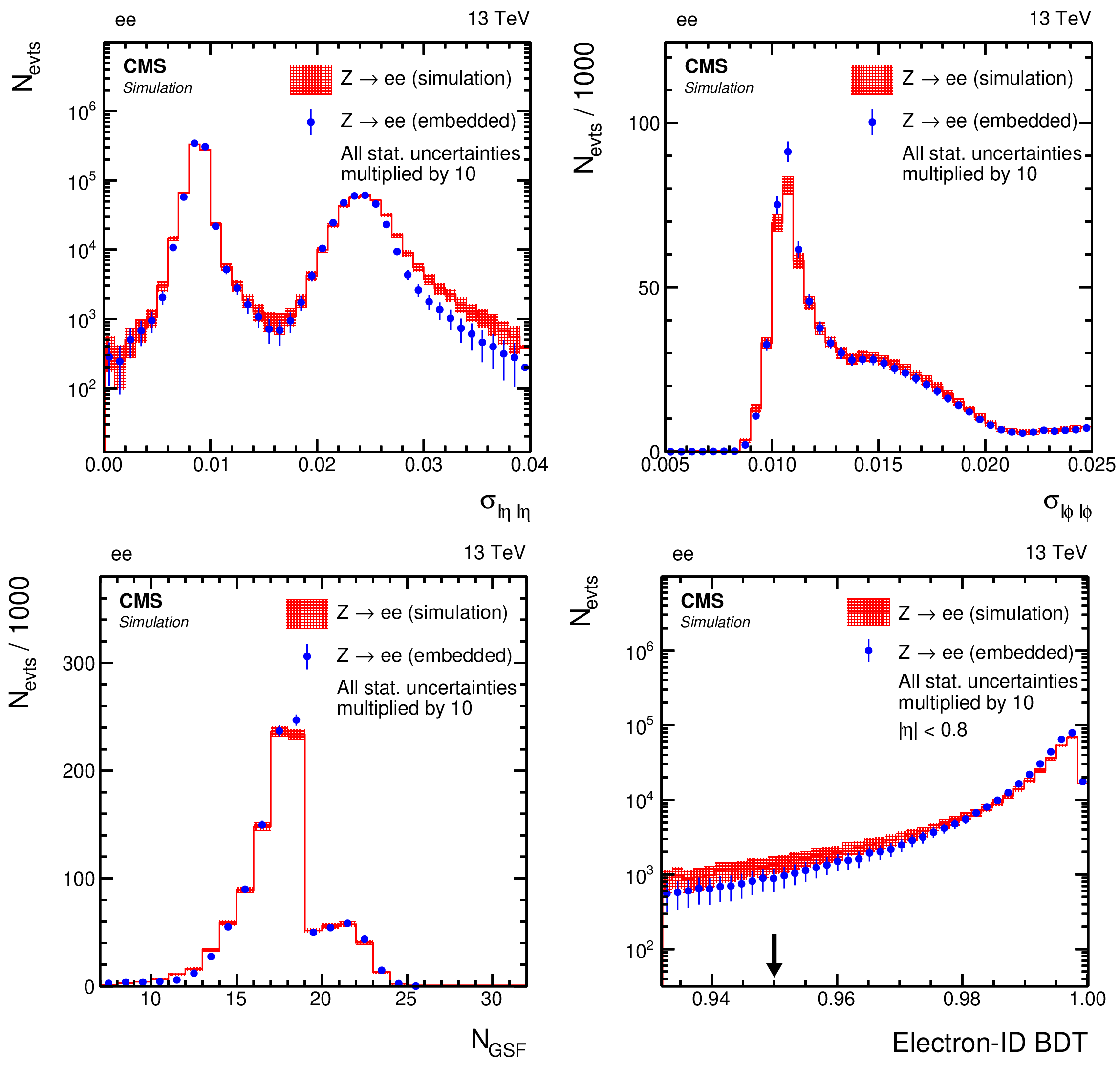
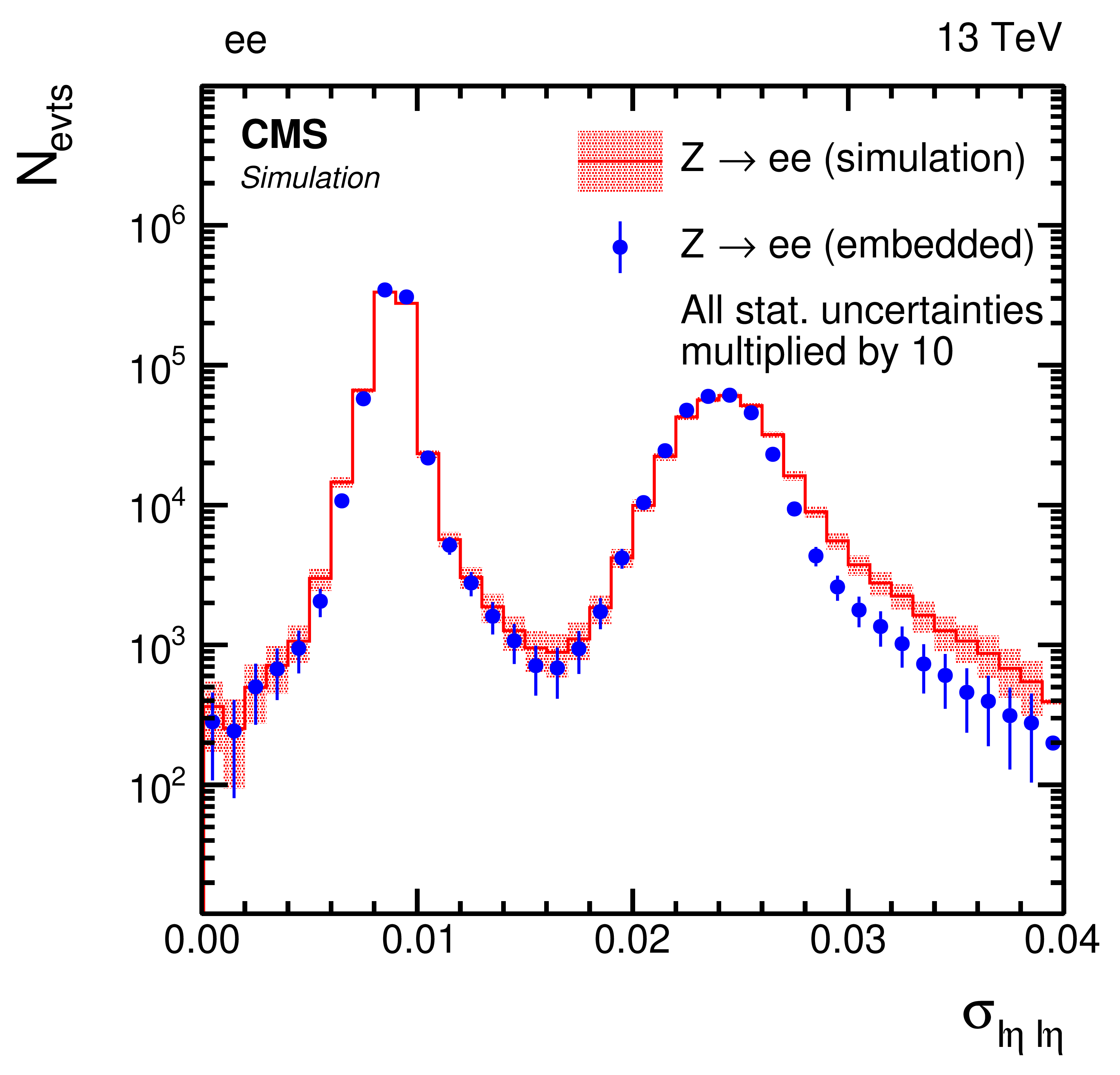
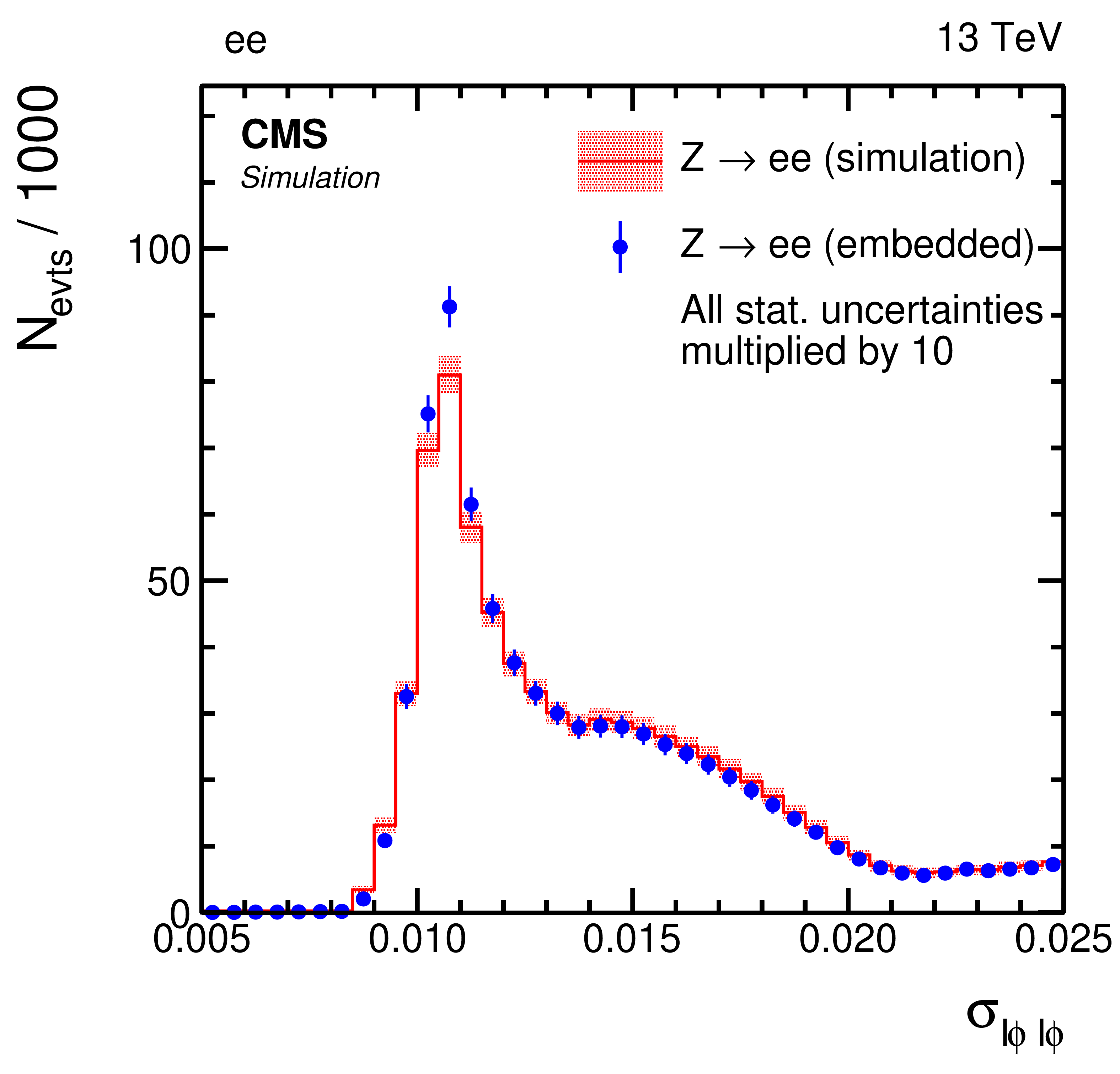
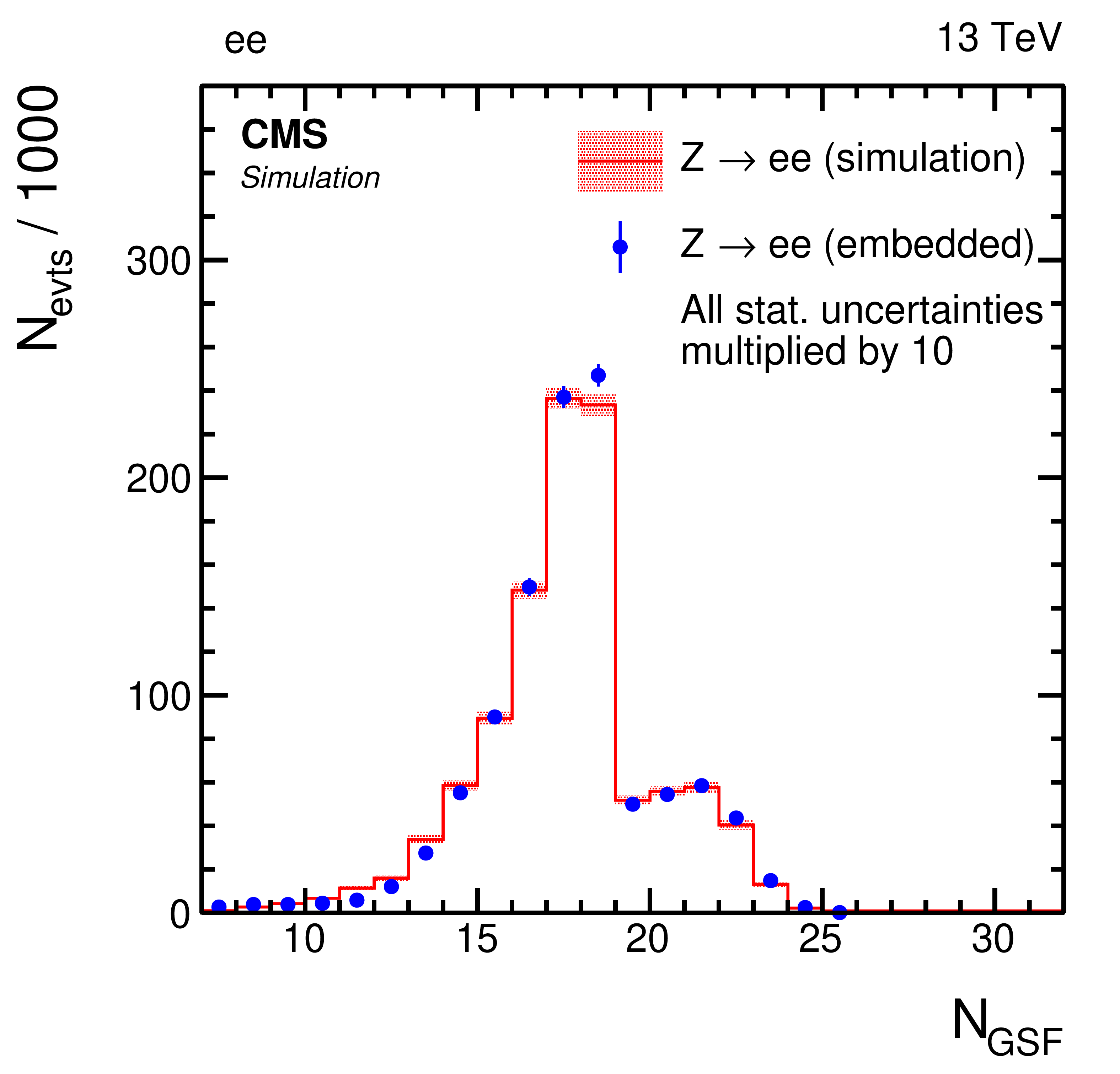
Figure 7:
Comparison of e-embedded events with a statistically independent sample of simulated ${{{\mathrm {Z}} \to {\mathrm {e}} {\mathrm {e}}}}$ events. Shown are distributions of the energy-weighted standard deviations of a 5$\times $5 crystal array in (upper left) $\eta $, $\sigma _{i\eta i\eta}$, and (upper right) $\phi $, $\sigma _{i\phi i\phi}$, as described in the text, (lower left) the number $N_{\mathrm {GSF}}$ of detector hits, used for the Gaussian Sum Filter algorithm [27] as described in Section 3, and (lower right) the multivariate discriminator for the identification of electrons (electron-ID BDT). The black arrow, shown in addition to the electron-ID BDT distribution, indicates the working point with 80% efficiency in the displayed electron $\eta $ region. For better visibility, the statistical uncertainties of both samples, red-shaded band for simulated ${{{\mathrm {Z}} \to {\mathrm {e}} {\mathrm {e}}}}$ events, and blue vertical bars for e-embedded events, are multiplied by 10 for the figures. |
png pdf |
Figure 7-a:
Comparison of e-embedded events with a statistically independent sample of simulated ${{{\mathrm {Z}} \to {\mathrm {e}} {\mathrm {e}}}}$ events. Shown are distributions of the energy-weighted standard deviations of a 5$\times $5 crystal array in $\eta $, $\sigma _{i\eta i\eta}$, as described in the text. For better visibility, the statistical uncertainties of both samples, red-shaded band for simulated ${{{\mathrm {Z}} \to {\mathrm {e}} {\mathrm {e}}}}$ events, and blue vertical bars for e-embedded events, are multiplied by 10. |
png pdf |
Figure 7-b:
Comparison of e-embedded events with a statistically independent sample of simulated ${{{\mathrm {Z}} \to {\mathrm {e}} {\mathrm {e}}}}$ events. Shown are distributions of the energy-weighted standard deviations of a 5$\times $5 crystal array in $\phi $, $\sigma _{i\phi i\phi}$, as described in the text. For better visibility, the statistical uncertainties of both samples, red-shaded band for simulated ${{{\mathrm {Z}} \to {\mathrm {e}} {\mathrm {e}}}}$ events, and blue vertical bars for e-embedded events, are multiplied by 10. |
png pdf |
Figure 7-c:
Comparison of e-embedded events with a statistically independent sample of simulated ${{{\mathrm {Z}} \to {\mathrm {e}} {\mathrm {e}}}}$ events. Shown are distributions of the energy-weighted standard deviations of a 5$\times $5 crystal array in the number $N_{\mathrm {GSF}}$ of detector hits, used for the Gaussian Sum Filter algorithm [27] as described in Section 3. For better visibility, the statistical uncertainties of both samples, red-shaded band for simulated ${{{\mathrm {Z}} \to {\mathrm {e}} {\mathrm {e}}}}$ events, and blue vertical bars for e-embedded events, are multiplied by 10. |
png pdf |
Figure 7-d:
Comparison of e-embedded events with a statistically independent sample of simulated ${{{\mathrm {Z}} \to {\mathrm {e}} {\mathrm {e}}}}$ events. Shown are distributions of the energy-weighted standard deviations of a 5$\times $5 crystal array in the multivariate discriminator for the identification of electrons (electron-ID BDT). The black arrow, shown in addition to the electron-ID BDT distribution, indicates the working point with 80% efficiency in the displayed electron $\eta $ region. For better visibility, the statistical uncertainties of both samples, red-shaded band for simulated ${{{\mathrm {Z}} \to {\mathrm {e}} {\mathrm {e}}}}$ events, and blue vertical bars for e-embedded events, are multiplied by 10. |
png pdf |
Figure 8:
Comparison of the e-embedded events with a statistically independent sample of simulated ${{{\mathrm {Z}} \to {\mathrm {e}} {\mathrm {e}}}}$ events. Shown are the distributions of (left) $m_{{{\mathrm {e}} {\mathrm {e}}}}$ and (right) $ {p_{\mathrm {T}}} $ of the leading electron in $ {p_{\mathrm {T}}} $. The blue vertical bars and red-shaded bands correspond to the statistical uncertainty of each sample. The effect of a variation of the electron energy scale of $\pm $1% is also shown by the green lines. |
png pdf |
Figure 8-a:
Comparison of the e-embedded events with a statistically independent sample of simulated ${{{\mathrm {Z}} \to {\mathrm {e}} {\mathrm {e}}}}$ events. Shown is the distribution of $m_{{{\mathrm {e}} {\mathrm {e}}}}$. The blue vertical bars and red-shaded bands correspond to the statistical uncertainty of each sample. The effect of a variation of the electron energy scale of $\pm $1% is also shown by the green lines. |
png pdf |
Figure 8-b:
Comparison of the e-embedded events with a statistically independent sample of simulated ${{{\mathrm {Z}} \to {\mathrm {e}} {\mathrm {e}}}}$ events. Shown is the distribution of the $ {p_{\mathrm {T}}} $ of the leading electron in $ {p_{\mathrm {T}}} $. The blue vertical bars and red-shaded bands correspond to the statistical uncertainty of each sample. The effect of a variation of the electron energy scale of $\pm $1% is also shown by the green lines. |
png pdf |
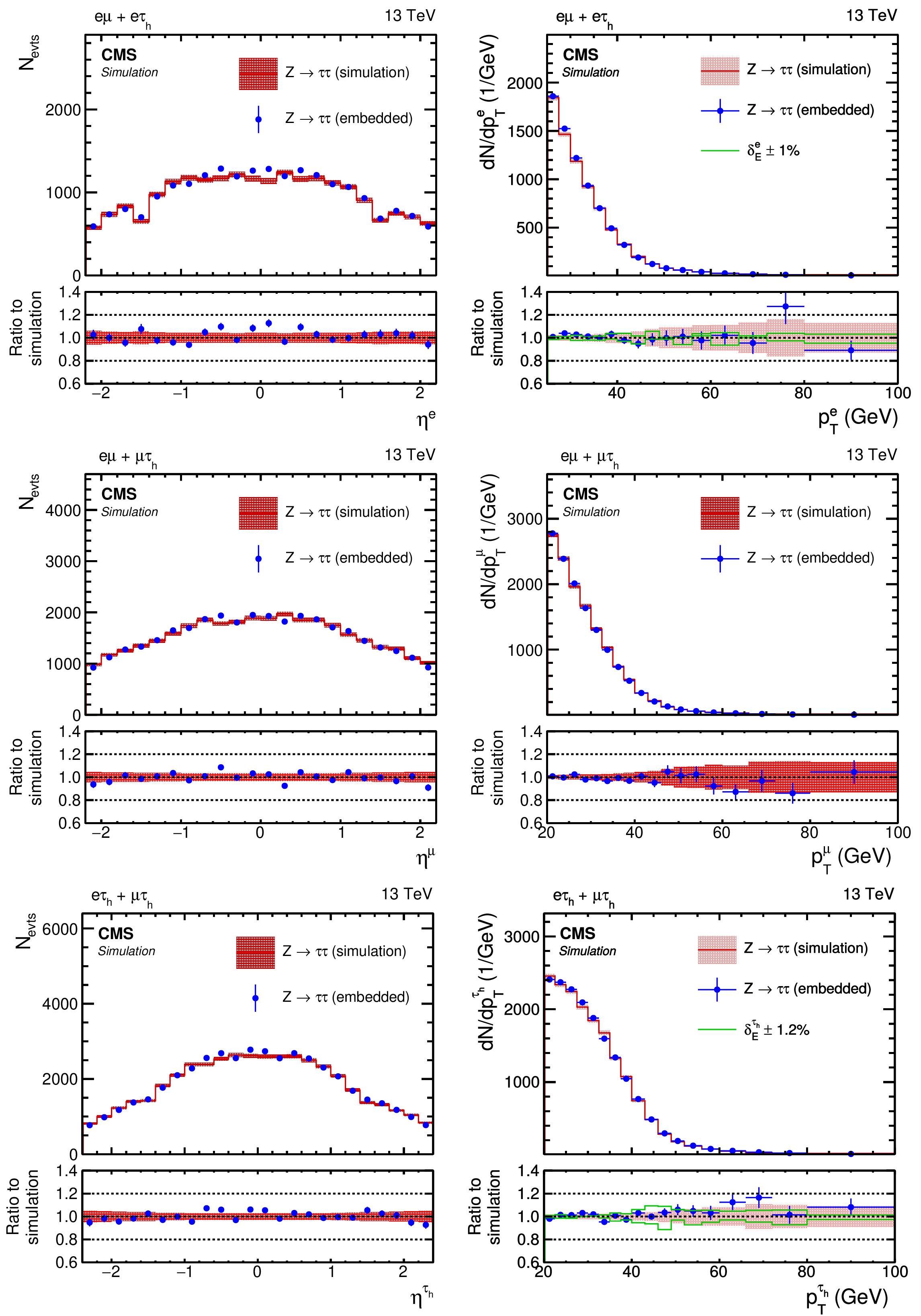
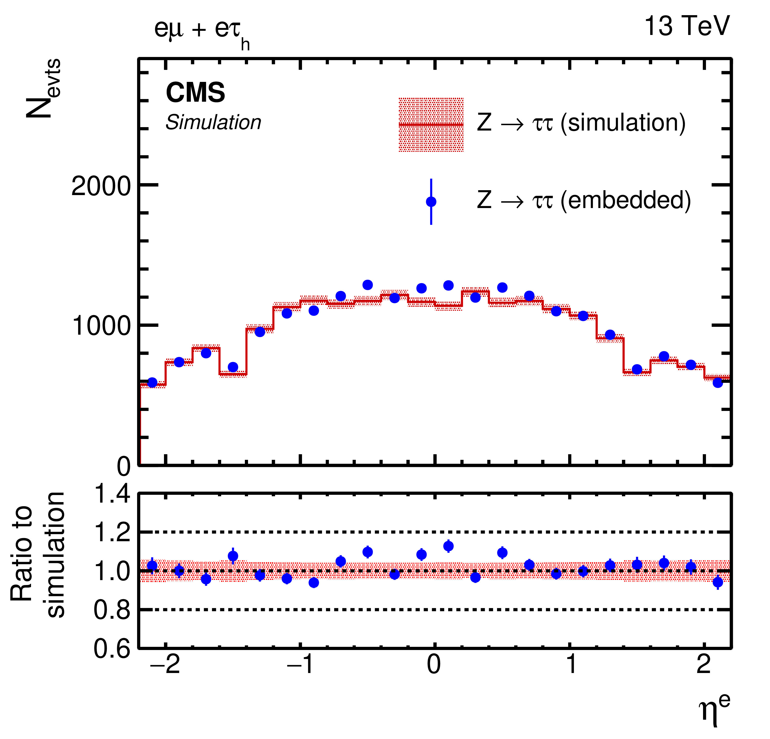
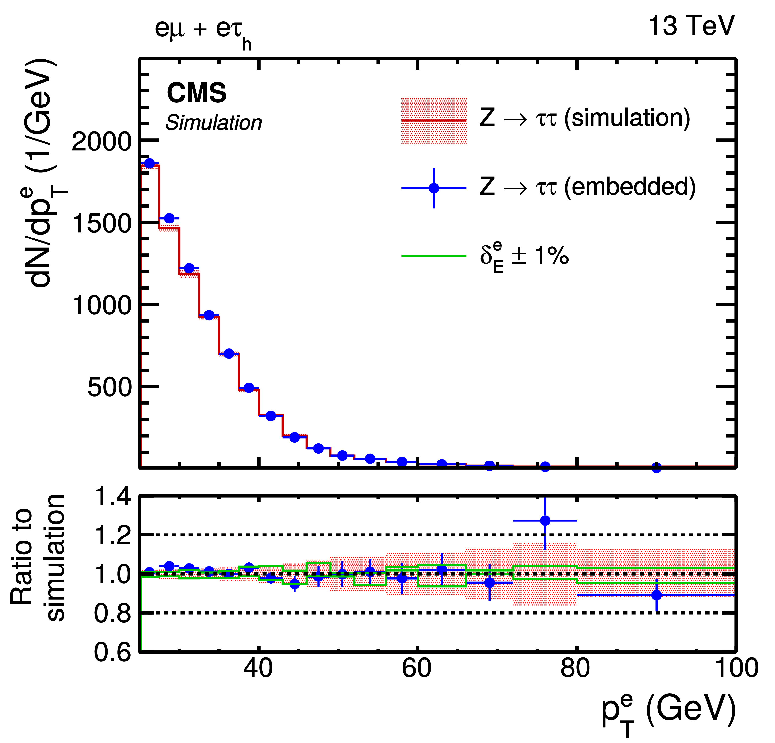
Figure 9:
Comparison of $ {\tau}$-embedded events with a statistically independent sample of simulated ${{{\mathrm {Z}} \to {\tau} {\tau}}}$ events. Shown are the (left) $\eta $ and (right) $ {p_{\mathrm {T}}} $ distributions of the (upper row) electron in the $ {{\mathrm {e}} {\mu}} {+} {{\mathrm {e}} {\tau}_{\text {h}}} $ final states, (middle row) muon in $ {{\mathrm {e}} {\mu}} {+} {{\mu} {\tau}_{\text {h}}} $ final states, and (lower row) $ {\tau}_{\text {h}} $ candidate in the $ {{\mathrm {e}} {\tau}_{\text {h}}} {+} {{\mu} {\tau}_{\text {h}}} $ final states. The blue vertical bars and red-shaded bands correspond to the statistical uncertainty of each sample. The effect of a variation of the electron ($ {\tau}_{\text {h}} $) energy scale of $\pm $1.0% ($\pm $1.2%) is shown by the green lines. |
png pdf |
Figure 9-a:
Comparison of $ {\tau}$-embedded events with a statistically independent sample of simulated ${{{\mathrm {Z}} \to {\tau} {\tau}}}$ events. Shown is the $\eta $ distribution of the electron in the $ {{\mathrm {e}} {\mu}} {+} {{\mathrm {e}} {\tau}_{\text {h}}} $ final states. The blue vertical bars and red-shaded bands correspond to the statistical uncertainty of each sample. |
png pdf |
Figure 9-b:
Comparison of $ {\tau}$-embedded events with a statistically independent sample of simulated ${{{\mathrm {Z}} \to {\tau} {\tau}}}$ events. Shown is the $ {p_{\mathrm {T}}} $ distribution of the electron in the $ {{\mathrm {e}} {\mu}} {+} {{\mathrm {e}} {\tau}_{\text {h}}} $ final states. The blue vertical bars and red-shaded bands correspond to the statistical uncertainty of each sample. The effect of a variation of the electron ($ {\tau}_{\text {h}} $) energy scale of $\pm $1.0% ($\pm $1.2%) is shown by the green lines. |

png pdf |
Figure 9-c:
Comparison of $ {\tau}$-embedded events with a statistically independent sample of simulated ${{{\mathrm {Z}} \to {\tau} {\tau}}}$ events. Shown is the $\eta $ distribution of the muon in $ {{\mathrm {e}} {\mu}} {+} {{\mu} {\tau}_{\text {h}}} $ final states. The blue vertical bars and red-shaded bands correspond to the statistical uncertainty of each sample. |
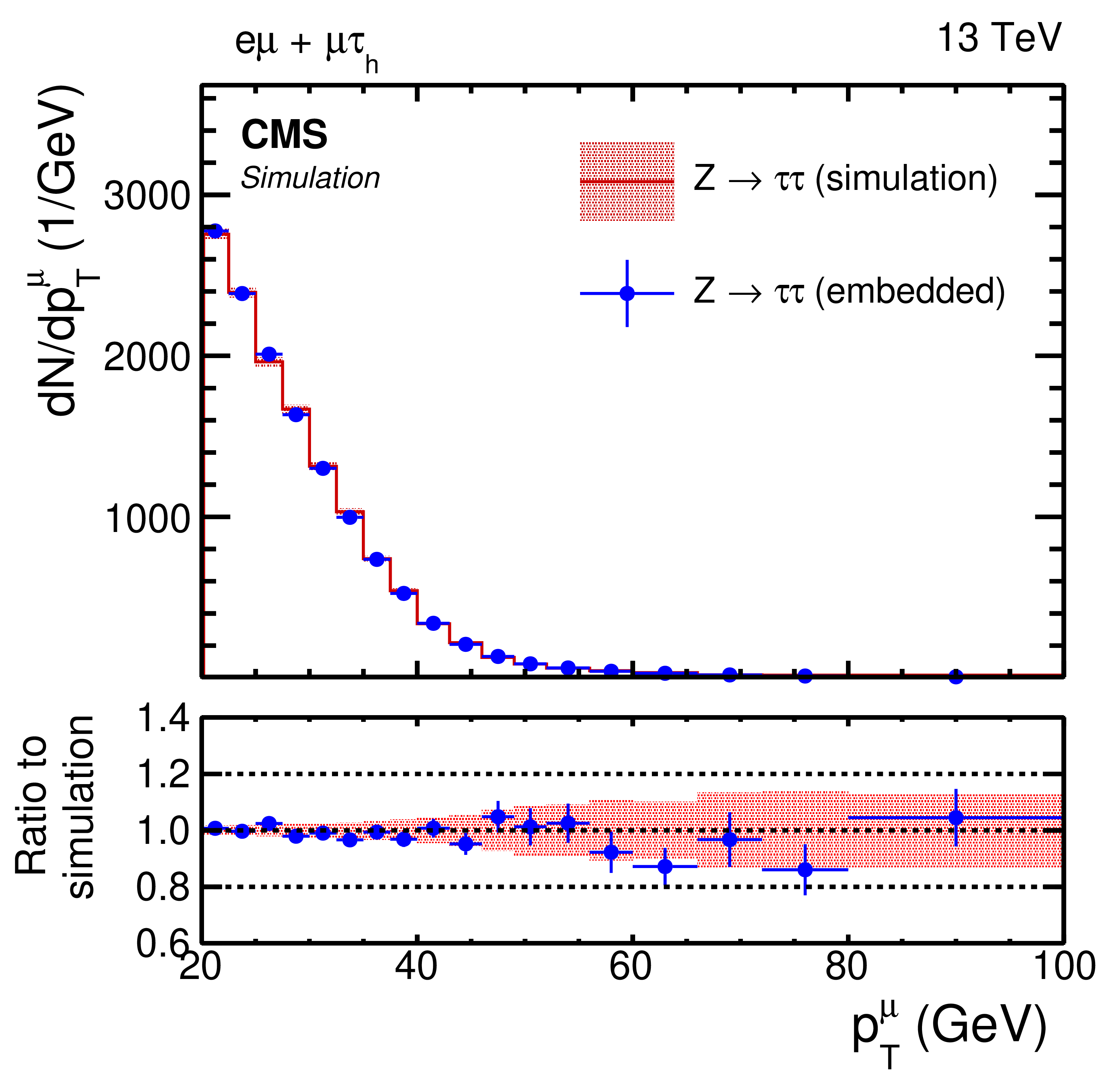
png pdf |
Figure 9-d:
Comparison of $ {\tau}$-embedded events with a statistically independent sample of simulated ${{{\mathrm {Z}} \to {\tau} {\tau}}}$ events. Shown is the $ {p_{\mathrm {T}}} $ distribution of the muon in $ {{\mathrm {e}} {\mu}} {+} {{\mu} {\tau}_{\text {h}}} $ final states. The blue vertical bars and red-shaded bands correspond to the statistical uncertainty of each sample. |
png pdf |
Figure 9-e:
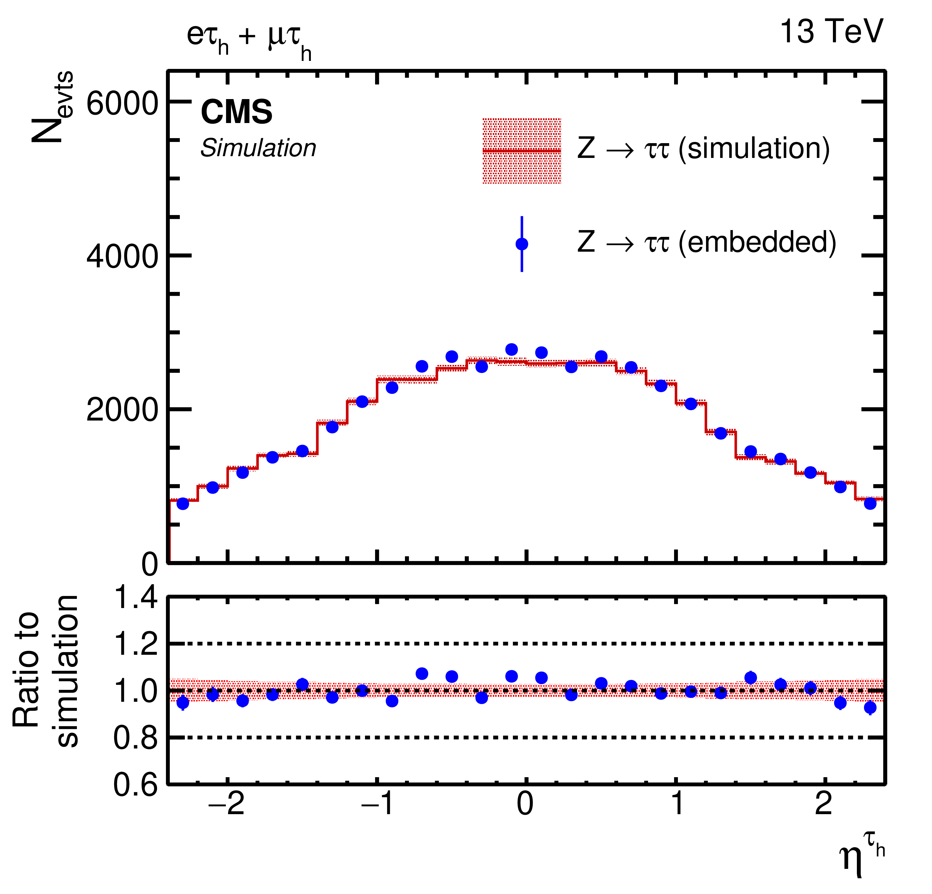
Comparison of $ {\tau}$-embedded events with a statistically independent sample of simulated ${{{\mathrm {Z}} \to {\tau} {\tau}}}$ events. Shown is the $\eta $ distribution of the $ {\tau}_{\text {h}} $ candidate in the $ {{\mathrm {e}} {\tau}_{\text {h}}} {+} {{\mu} {\tau}_{\text {h}}} $ final states. The blue vertical bars and red-shaded bands correspond to the statistical uncertainty of each sample. |
png pdf |
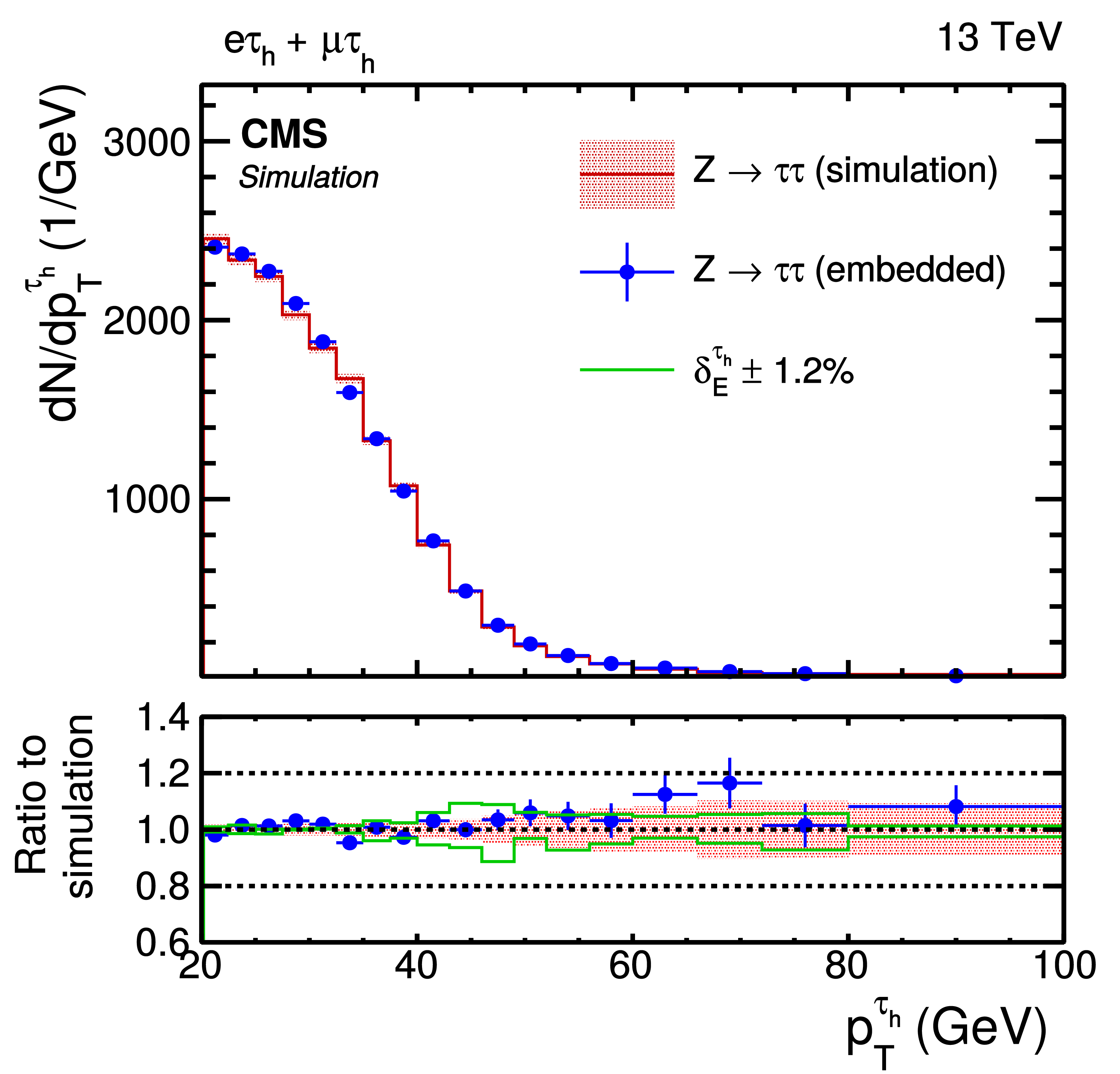
Figure 9-f:
Comparison of $ {\tau}$-embedded events with a statistically independent sample of simulated ${{{\mathrm {Z}} \to {\tau} {\tau}}}$ events. Shown is the $ {p_{\mathrm {T}}} $ distribution of the $ {\tau}_{\text {h}} $ candidate in the $ {{\mathrm {e}} {\tau}_{\text {h}}} {+} {{\mu} {\tau}_{\text {h}}} $ final states. The blue vertical bars and red-shaded bands correspond to the statistical uncertainty of each sample. The effect of a variation of the electron ($ {\tau}_{\text {h}} $) energy scale of $\pm $1.0% ($\pm $1.2%) is shown by the green lines. |
png pdf |
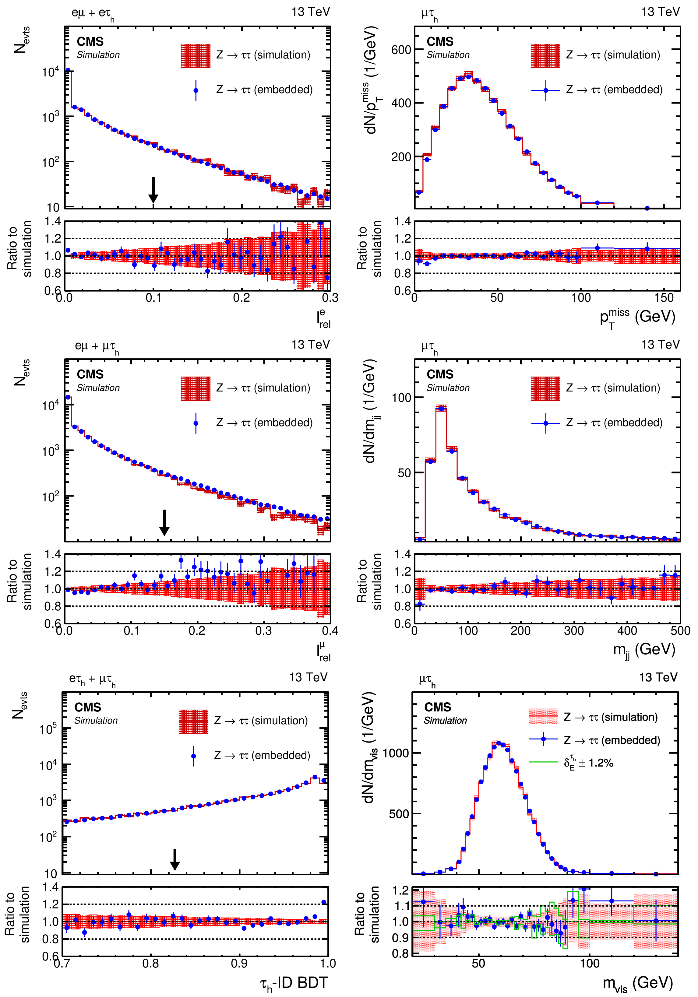
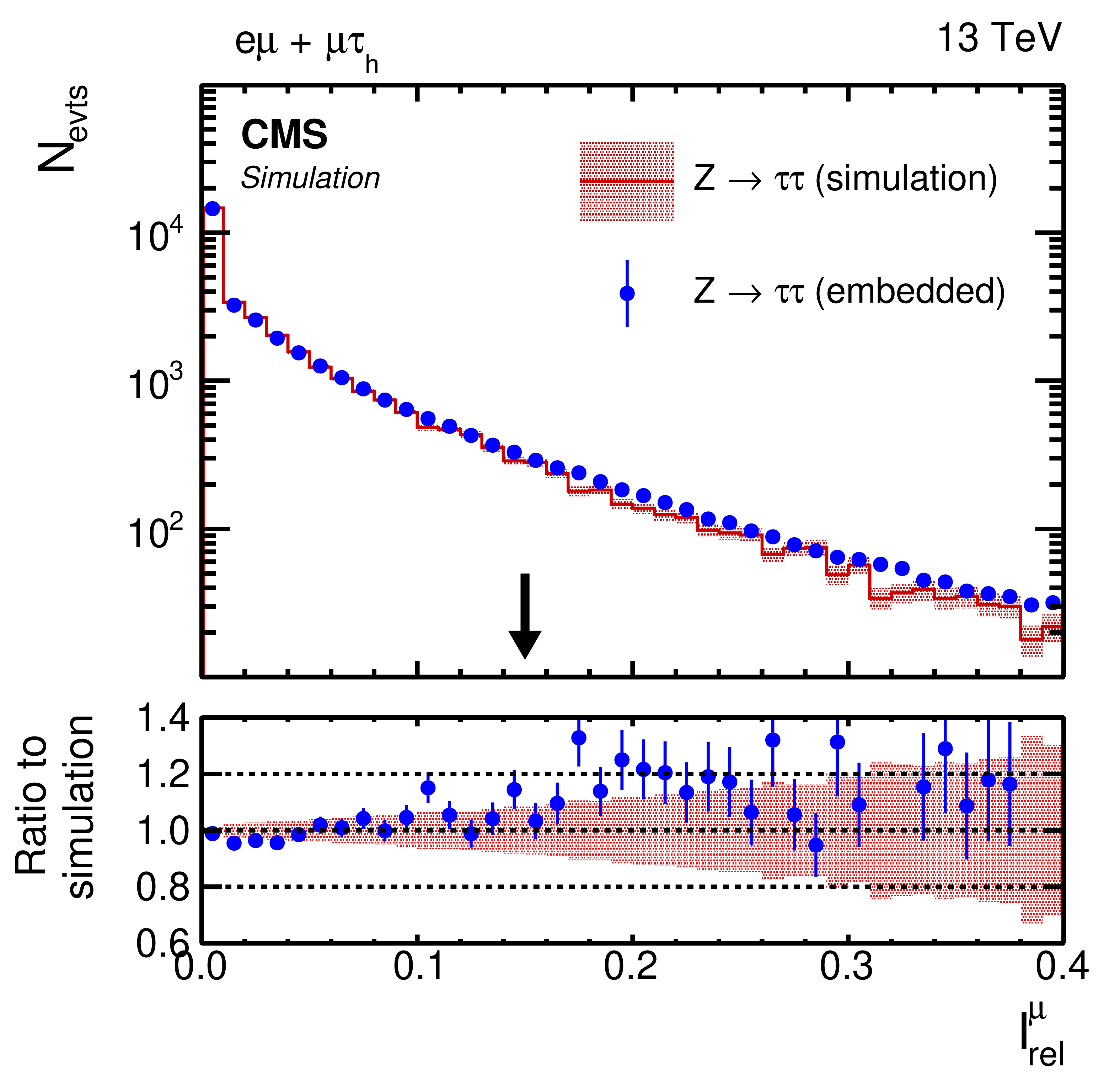
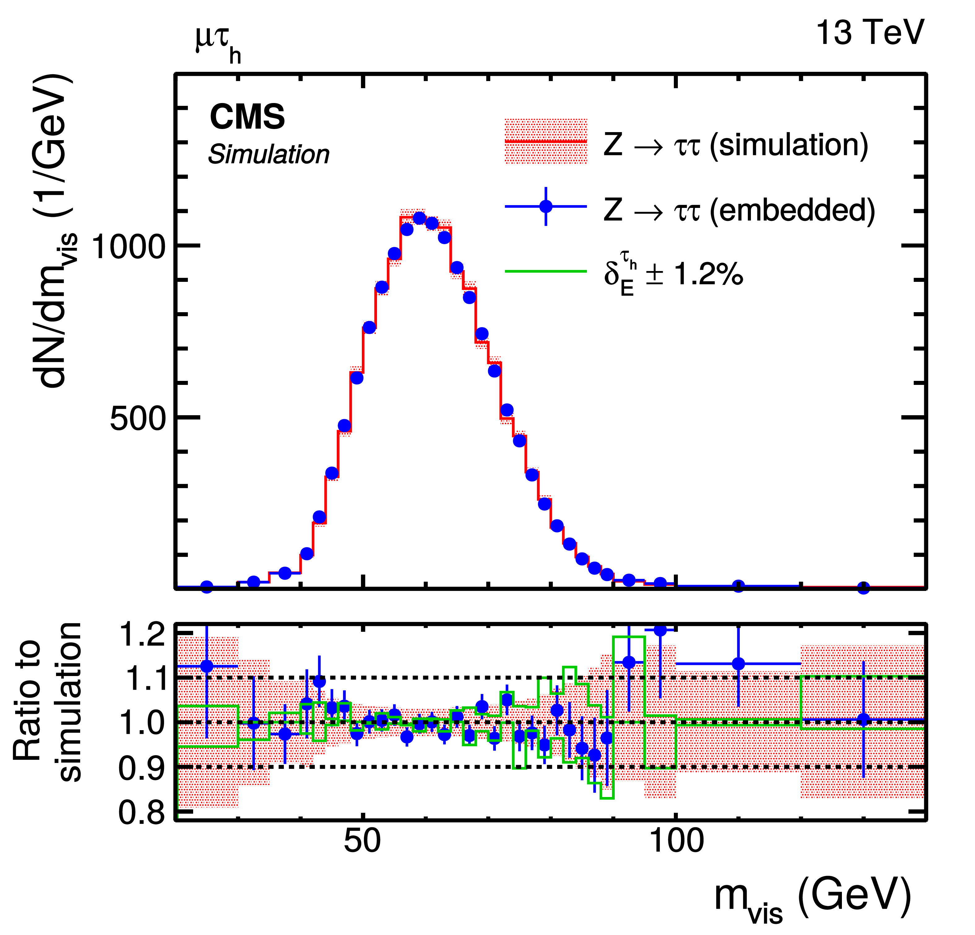
Figure 10:
Comparison of $ {\tau}$-embedded events with a statistically independent sample of simulated ${{{\mathrm {Z}} \to {\tau} {\tau}}}$ events. Shown are distributions of (upper left) $ {I_{\text {rel}}^{{\mathrm {e}}}} $, (upper right) $ {{p_{\mathrm {T}}} ^\text {miss}} $, (middle left) $ {I_{\text {rel}}^{{\mu}}} $, (middle right) $ {m_{\text {jj}}} $, (lower left) $ {\tau}_{\text {h}} $-ID BDT, and $ {m_{\text {vis}}} $, as discussed in the text. The black arrows indicate the working points usually used in the target analyses. The blue vertical bars and red-shaded bands correspond to the statistical uncertainty of each sample. The effect of a variation of the $ {\tau}_{\text {h}} $ energy scale of $\pm $1.2% is shown by the green lines. |
png pdf |
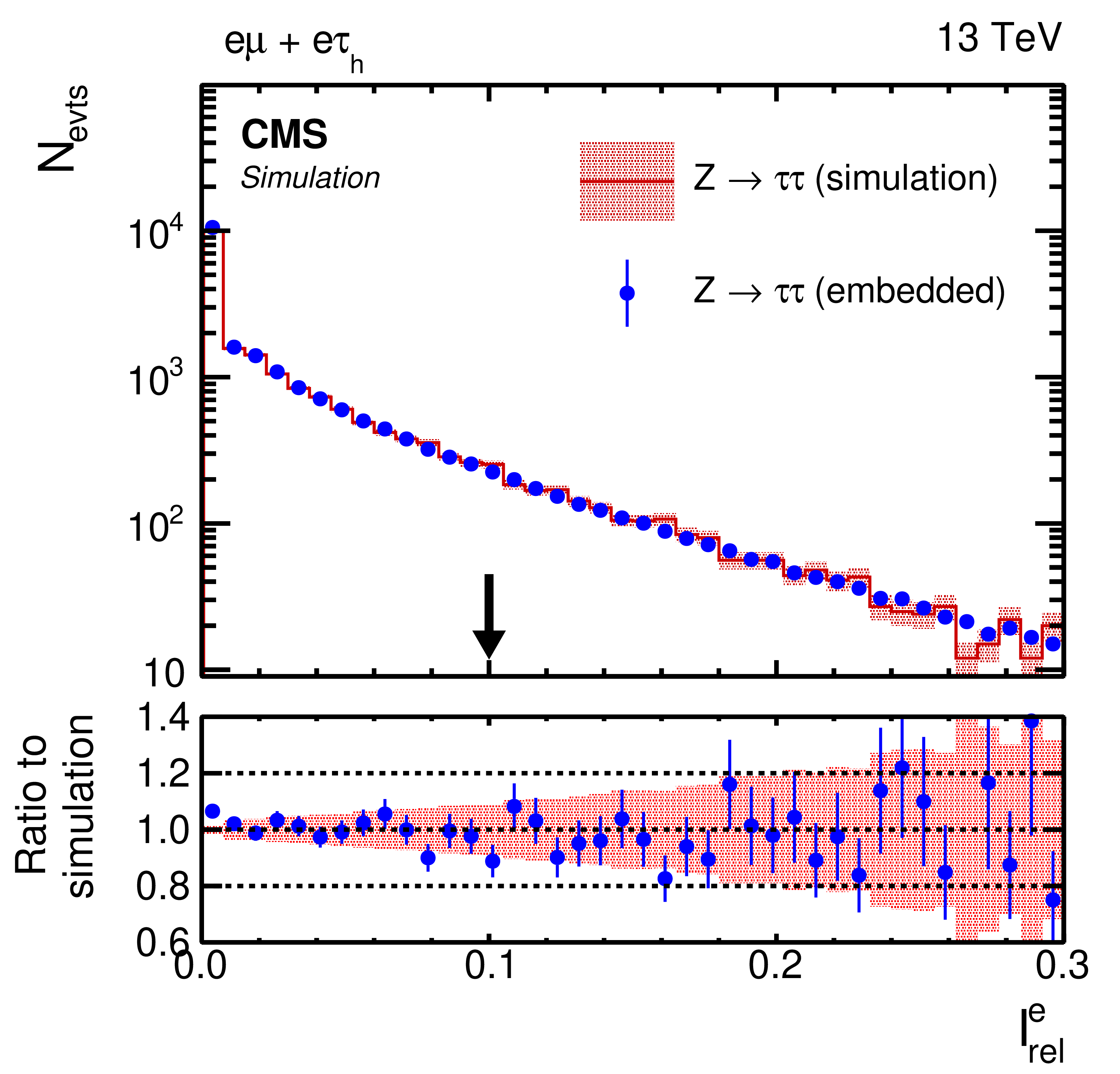
Figure 10-a:
Comparison of $ {\tau}$-embedded events with a statistically independent sample of simulated ${{{\mathrm {Z}} \to {\tau} {\tau}}}$ events. Shown is the distribution of $ {I_{\text {rel}}^{{\mathrm {e}}}} $, as discussed in the text. The black arrow indicates the working points usually used in the target analyses. The blue vertical bars and red-shaded bands correspond to the statistical uncertainty of each sample. |
png pdf |
Figure 10-b:
Comparison of $ {\tau}$-embedded events with a statistically independent sample of simulated ${{{\mathrm {Z}} \to {\tau} {\tau}}}$ events. Shown is the distribution of $ {{p_{\mathrm {T}}} ^\text {miss}} $, as discussed in the text. The blue vertical bars and red-shaded bands correspond to the statistical uncertainty of each sample. |
png pdf |
Figure 10-c:
Comparison of $ {\tau}$-embedded events with a statistically independent sample of simulated ${{{\mathrm {Z}} \to {\tau} {\tau}}}$ events. Shown is the distribution of $ {I_{\text {rel}}^{{\mu}}} $, as discussed in the text. The black arrow indicates the working points usually used in the target analyses. The blue vertical bars and red-shaded bands correspond to the statistical uncertainty of each sample. |
png pdf |
Figure 10-d:
Comparison of $ {\tau}$-embedded events with a statistically independent sample of simulated ${{{\mathrm {Z}} \to {\tau} {\tau}}}$ events. Shown is the distribution of $ {m_{\text {jj}}} $, as discussed in the text. The blue vertical bars and red-shaded bands correspond to the statistical uncertainty of each sample. |

png pdf |
Figure 10-e:
Comparison of $ {\tau}$-embedded events with a statistically independent sample of simulated ${{{\mathrm {Z}} \to {\tau} {\tau}}}$ events. Shown is the distribution of $ {\tau}_{\text {h}} $-ID BDT, as discussed in the text. The black arrow indicates the working points usually used in the target analyses. The blue vertical bars and red-shaded bands correspond to the statistical uncertainty of each sample. |
png pdf |
Figure 10-f:
Comparison of $ {\tau}$-embedded events with a statistically independent sample of simulated ${{{\mathrm {Z}} \to {\tau} {\tau}}}$ events. Shown is the distribution of $ {m_{\text {vis}}} $, as discussed in the text. The blue vertical bars and red-shaded bands correspond to the statistical uncertainty of each sample. The effect of a variation of the $ {\tau}_{\text {h}} $ energy scale of $\pm $1.2% is shown by the green lines. |
png pdf |
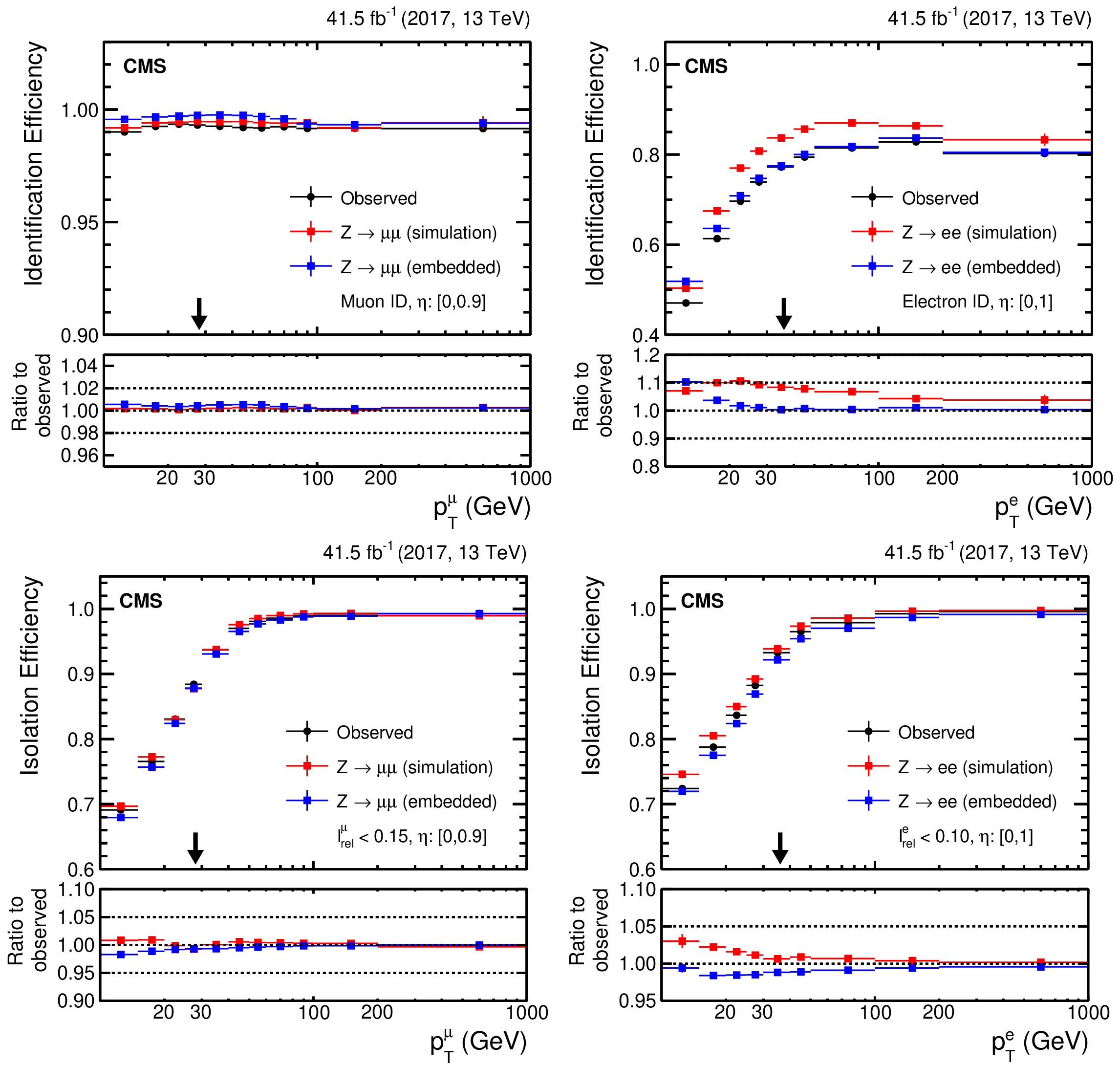
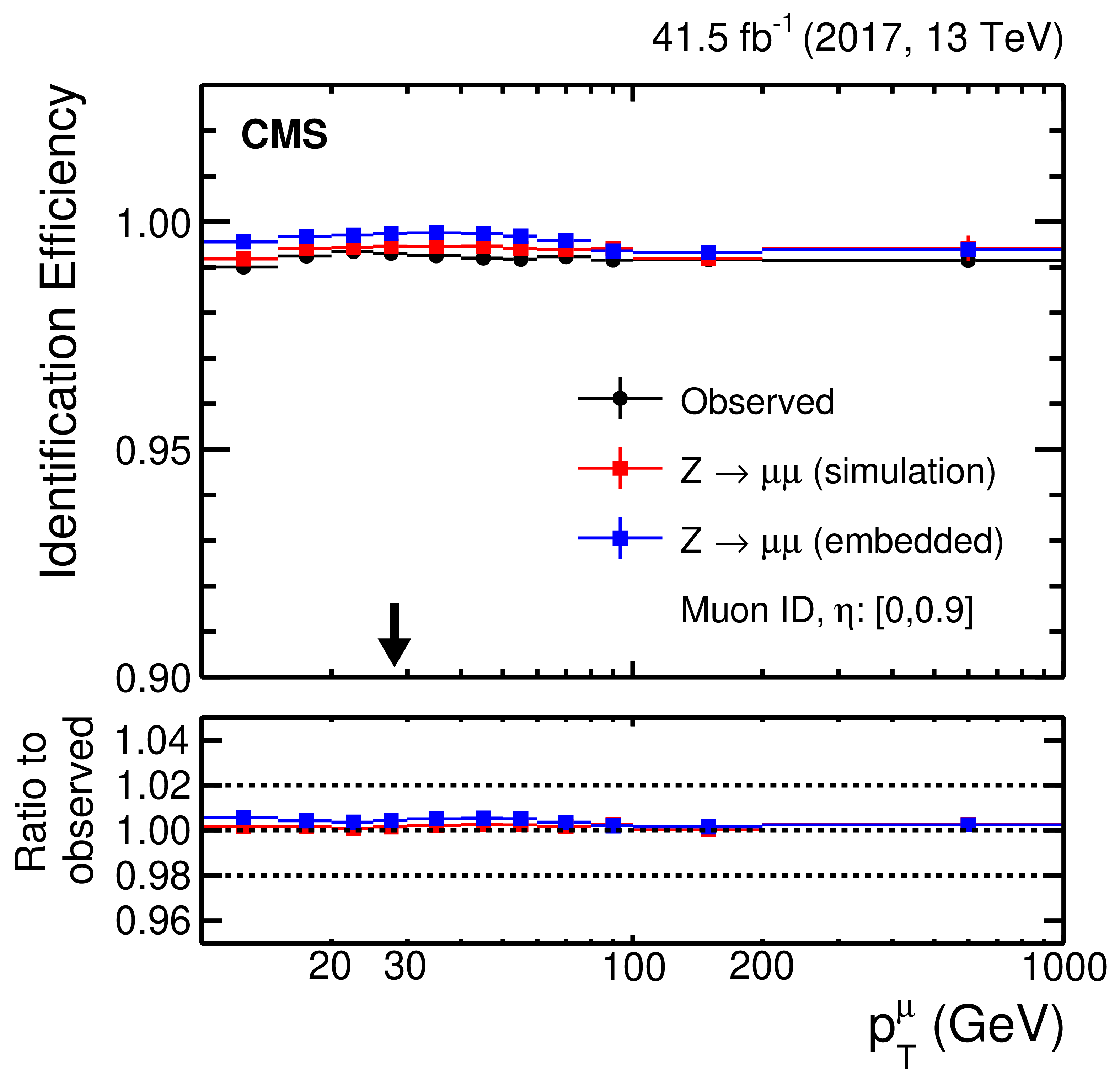
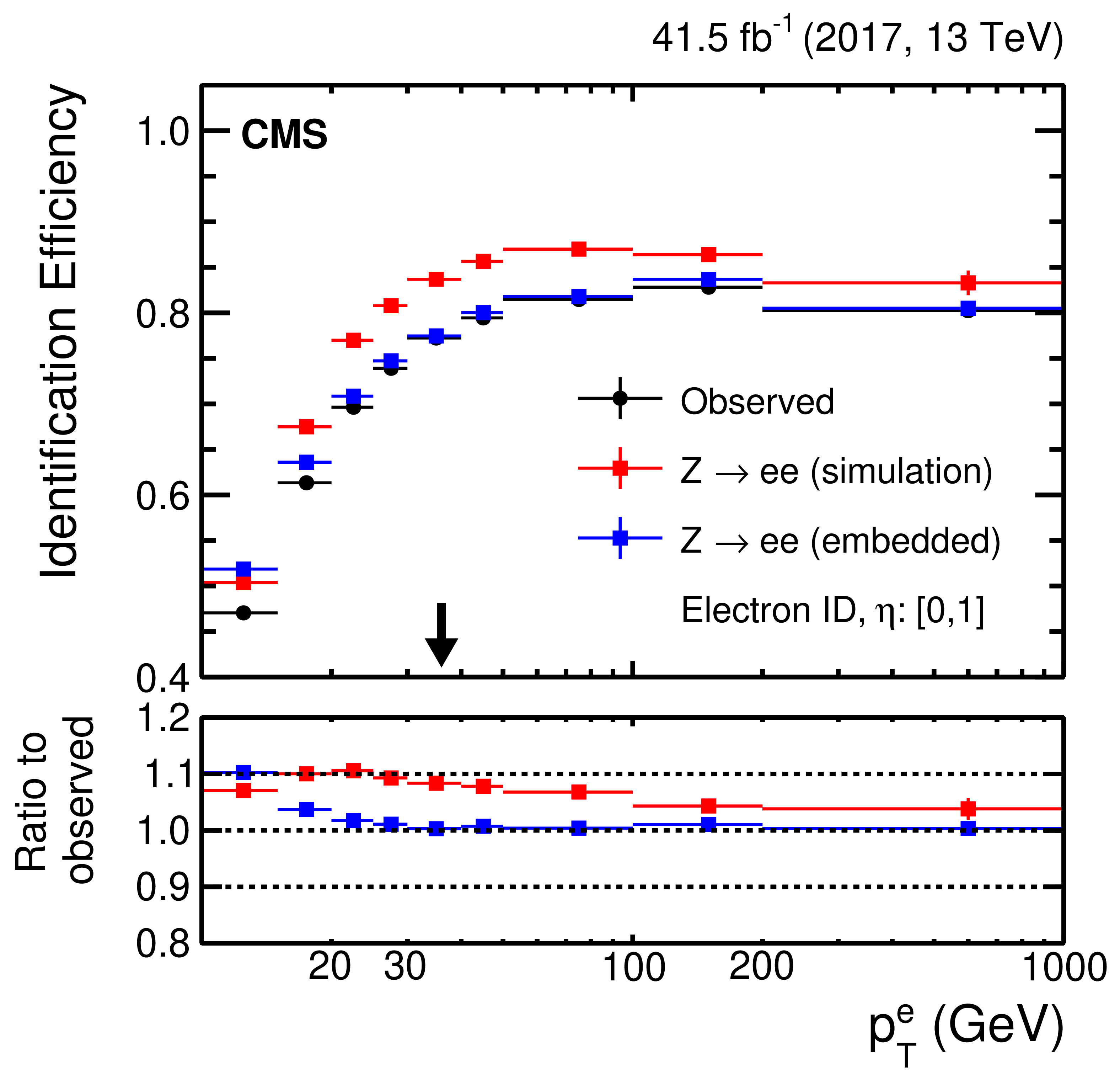
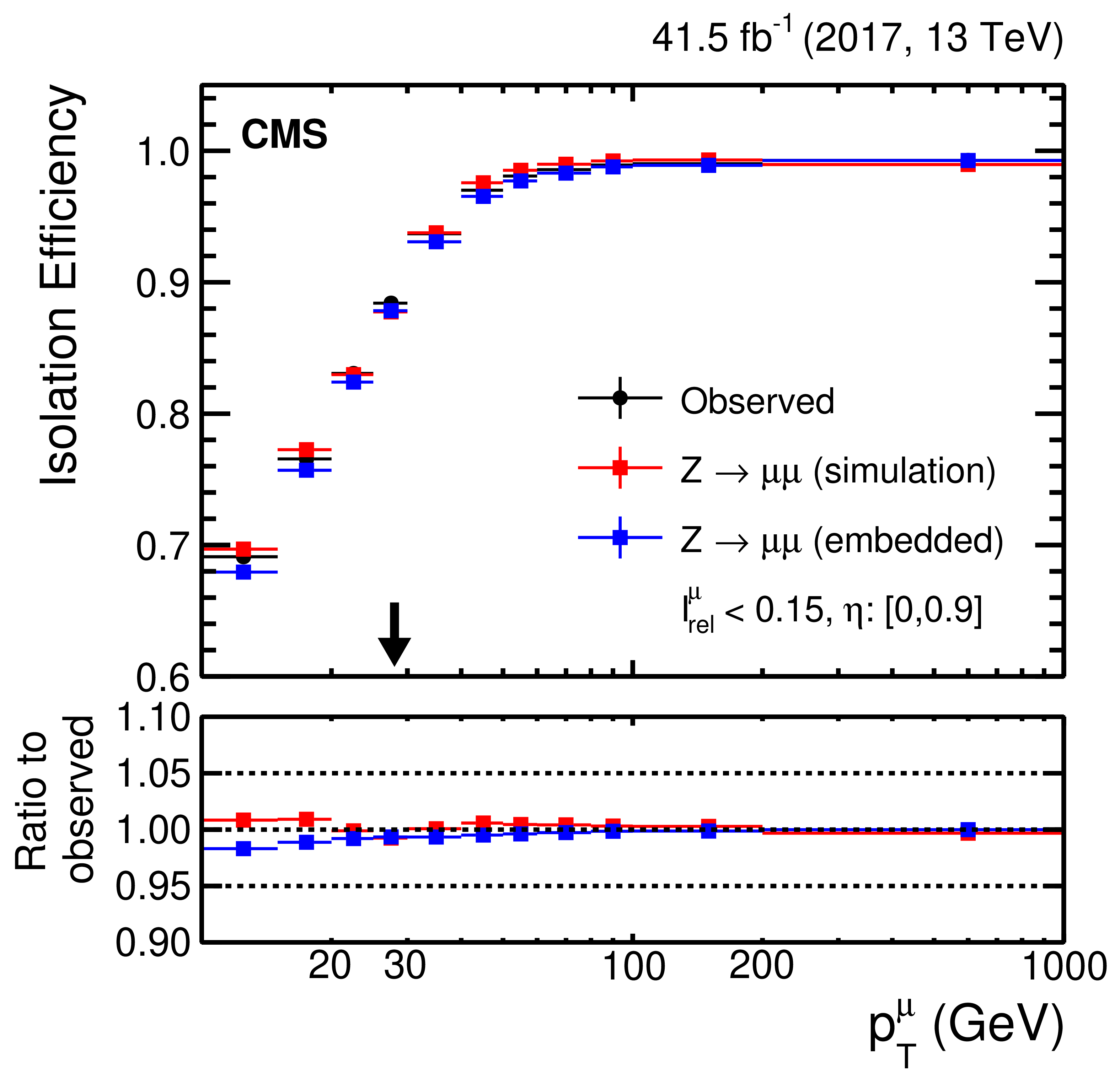
Figure 11:
(Left column) muon and (right column) electron (upper row) identification and (lower row) isolation efficiencies as a function of the $ {p_{\mathrm {T}}} $ of the corresponding lepton in the central region of the detector. The black arrows indicate typical trigger thresholds of the target analyses. In the upper panel of each subfigure, the black dots correspond to the efficiencies obtained in data, the blue dots to the efficiencies obtained in the corresponding embedded event sample, and the red dots to the efficiencies obtained from the simulation. The lower panels show the ratios of the (blue) embedded event sample and (red) simulation, to the efficiency observed in data, which corresponds to the correction factors. |
png pdf |
Figure 11-a:
Muon identification efficiency as a function of the $ {p_{\mathrm {T}}} $ of the corresponding lepton in the central region of the detector. The black arrow indicates a typical trigger threshold of the target analyses. In the upper panel, the black dots correspond to the efficiencies obtained in data, the blue dots to the efficiencies obtained in the corresponding embedded event sample, and the red dots to the efficiencies obtained from the simulation. The lower panel shows the ratios of the (blue) embedded event sample and (red) simulation, to the efficiency observed in data, which corresponds to the correction factors. |
png pdf |
Figure 11-b:
Electron identification efficiency as a function of the $ {p_{\mathrm {T}}} $ of the corresponding lepton in the central region of the detector. The black arrow indicates a typical trigger threshold of the target analyses. In the upper panel, the black dots correspond to the efficiencies obtained in data, the blue dots to the efficiencies obtained in the corresponding embedded event sample, and the red dots to the efficiencies obtained from the simulation. The lower panel shows the ratios of the (blue) embedded event sample and (red) simulation, to the efficiency observed in data, which corresponds to the correction factors. |
png pdf |
Figure 11-c:
Muon isolation efficiency as a function of the $ {p_{\mathrm {T}}} $ of the corresponding lepton in the central region of the detector. The black arrow indicates a typical trigger threshold of the target analyses. In the upper panel, the black dots correspond to the efficiencies obtained in data, the blue dots to the efficiencies obtained in the corresponding embedded event sample, and the red dots to the efficiencies obtained from the simulation. The lower panel shows the ratios of the (blue) embedded event sample and (red) simulation, to the efficiency observed in data, which corresponds to the correction factors. |
png pdf |
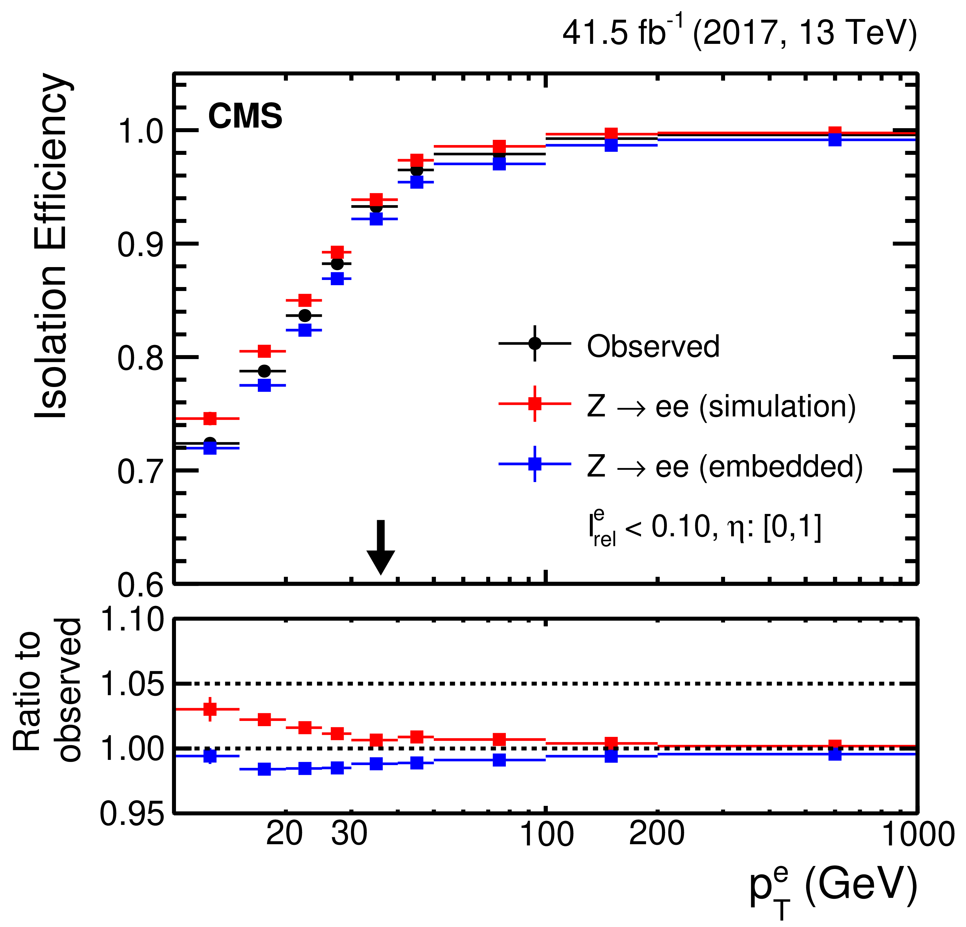
Figure 11-d:
Electron isolation efficiency as a function of the $ {p_{\mathrm {T}}} $ of the corresponding lepton in the central region of the detector. The black arrow indicates a typical trigger threshold of the target analyses. In the upper panel, the black dots correspond to the efficiencies obtained in data, the blue dots to the efficiencies obtained in the corresponding embedded event sample, and the red dots to the efficiencies obtained from the simulation. The lower panel shows the ratios of the (blue) embedded event sample and (red) simulation, to the efficiency observed in data, which corresponds to the correction factors. |
png pdf |
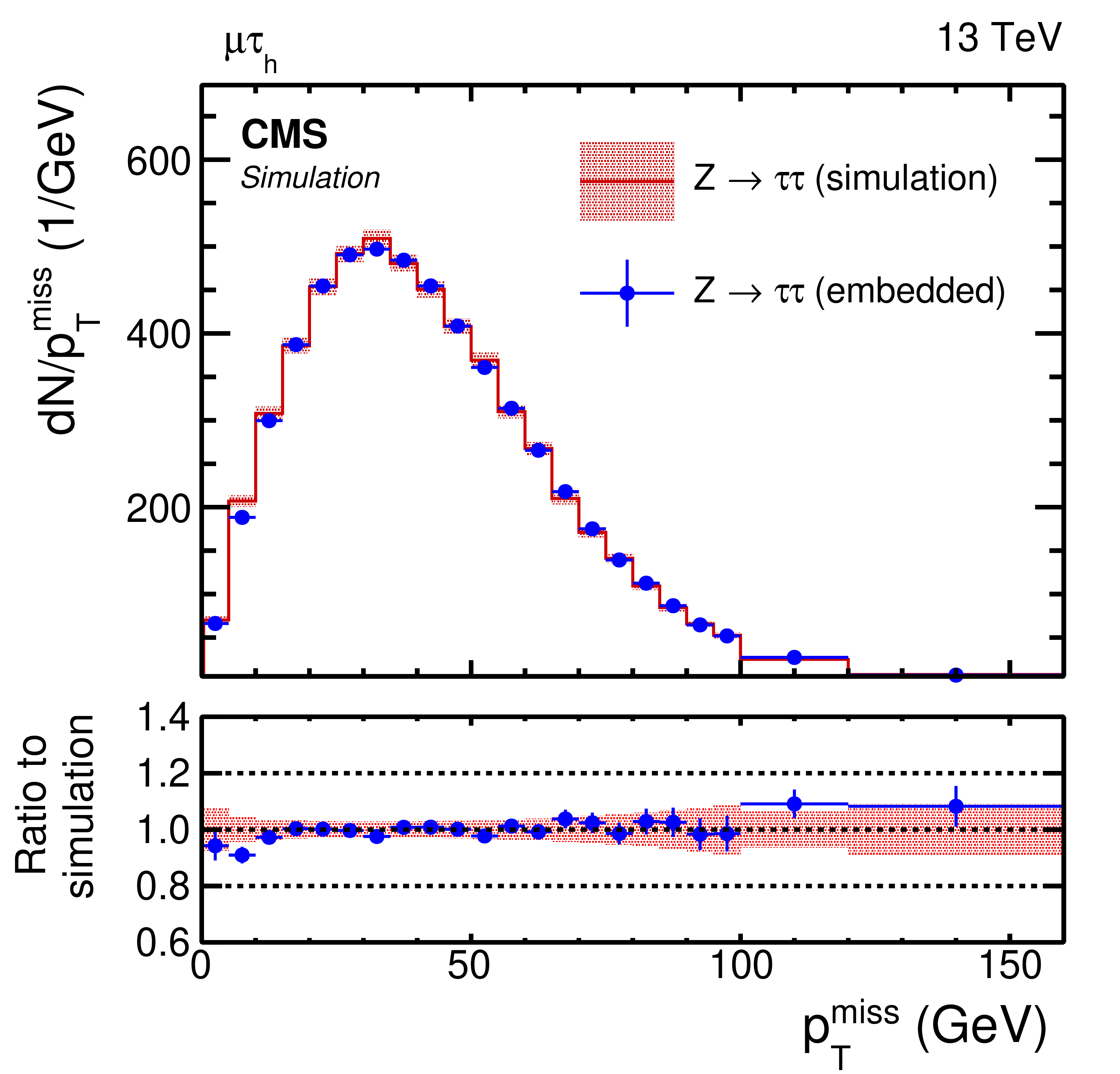
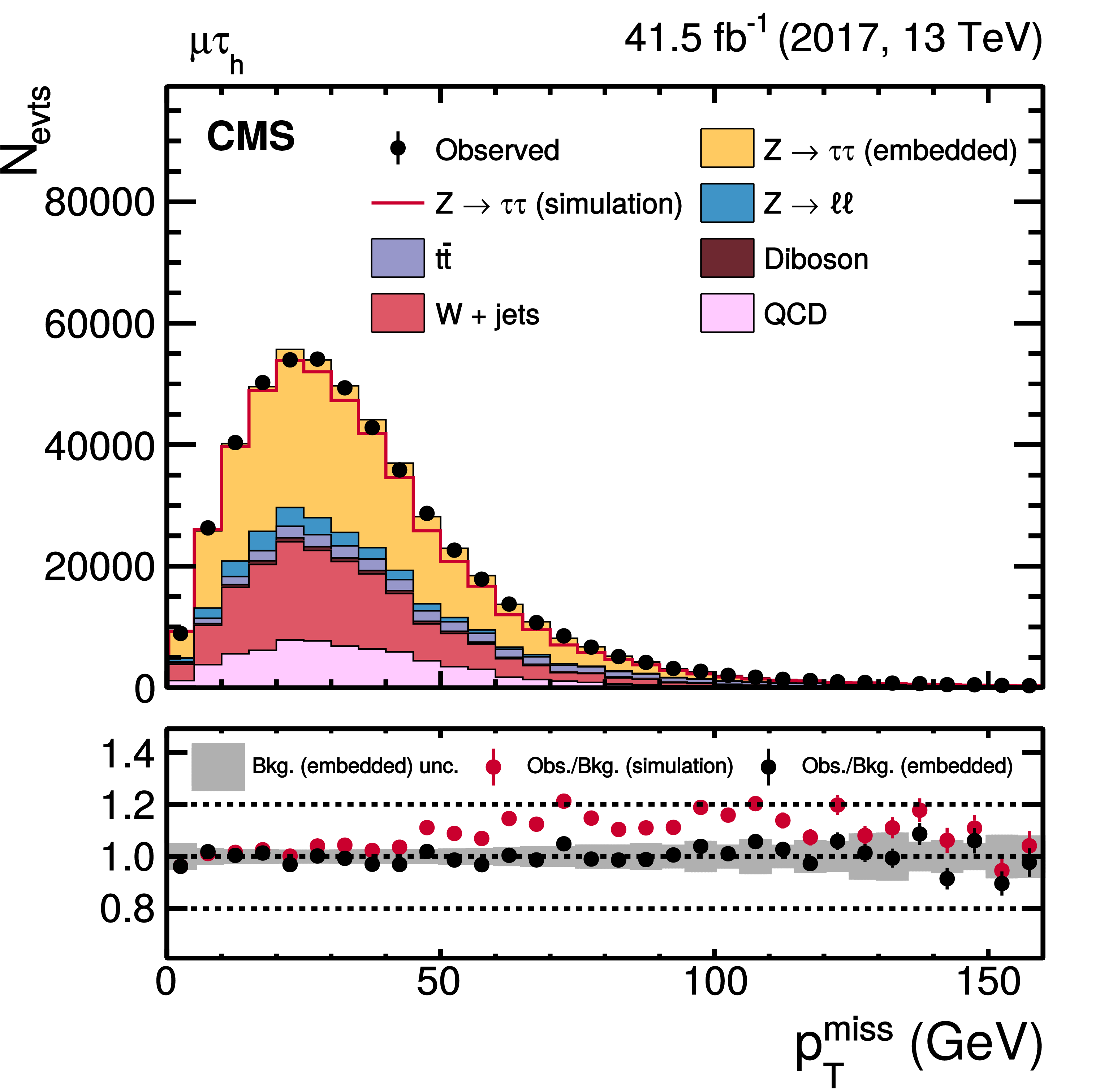
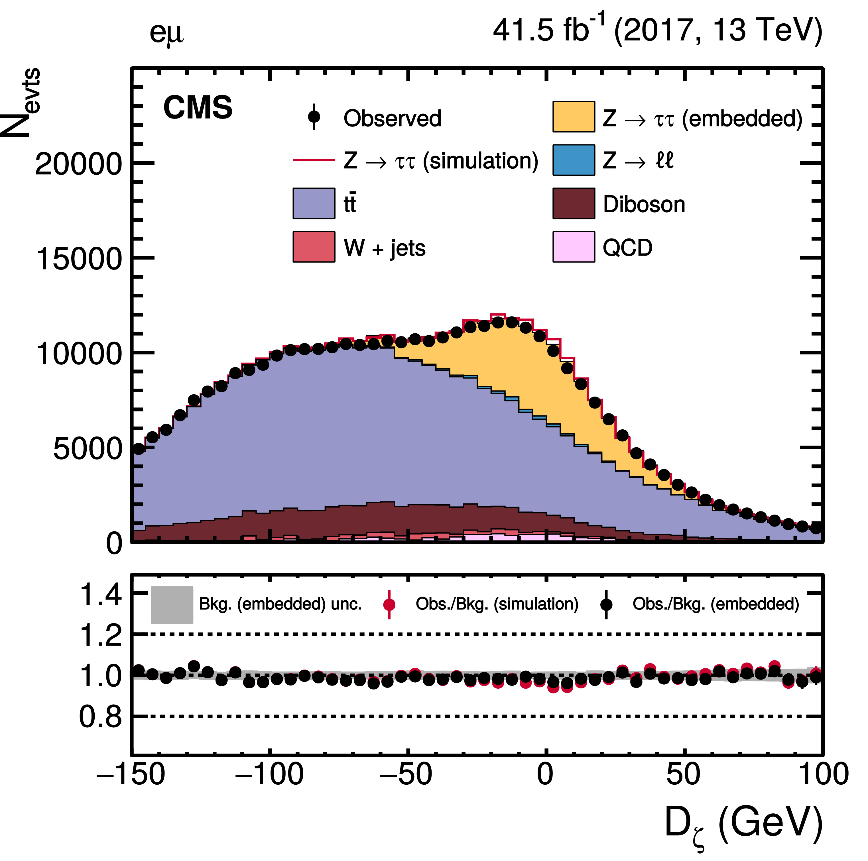
Figure 12:
Distributions of (upper left) $ {{p_{\mathrm {T}}} ^\text {miss}} $ in the $ {{\mu} {\tau}_{\text {h}}} $ final state, (upper right) $ {D_{\zeta}} $ in the $ {{\mathrm {e}} {\mu}} $ final state, (lower left) $ {m_{\text {T}}^{{\mathrm {e}}}} $ in the $ {{\mathrm {e}} {\tau}_{\text {h}}} $ final state, and (lower right) $ {m_{\text {T}}^{{\mu}}} $ in the $ {{\mu} {\tau}_{\text {h}}} $ final state. The distributions are shown prior to the maximum likelihood fit described in the text. For these figures, no uncertainties that affect the shape of the distributions have been included in the uncertainty model. The background estimation purely from the CMS simulation is shown as an additional red line. |
png pdf |
Figure 12-a:
Distribution of $ {{p_{\mathrm {T}}} ^\text {miss}} $ in the $ {{\mu} {\tau}_{\text {h}}} $ final state. The distribution is shown prior to the maximum likelihood fit described in the text. No uncertainties that affect the shape of the distribution have been included in the uncertainty model. The background estimation purely from the CMS simulation is shown as an additional red line. |
png pdf |
Figure 12-b:
Distribution of $ {D_{\zeta}} $ in the $ {{\mathrm {e}} {\mu}} $ final state. The distribution is shown prior to the maximum likelihood fit described in the text. No uncertainties that affect the shape of the distribution have been included in the uncertainty model. The background estimation purely from the CMS simulation is shown as an additional red line. |

png pdf |
Figure 12-c:
Distribution of $ {m_{\text {T}}^{{\mathrm {e}}}} $ in the $ {{\mathrm {e}} {\tau}_{\text {h}}} $ final state. The distribution is shown prior to the maximum likelihood fit described in the text. No uncertainties that affect the shape of the distribution have been included in the uncertainty model. The background estimation purely from the CMS simulation is shown as an additional red line. |
png pdf |
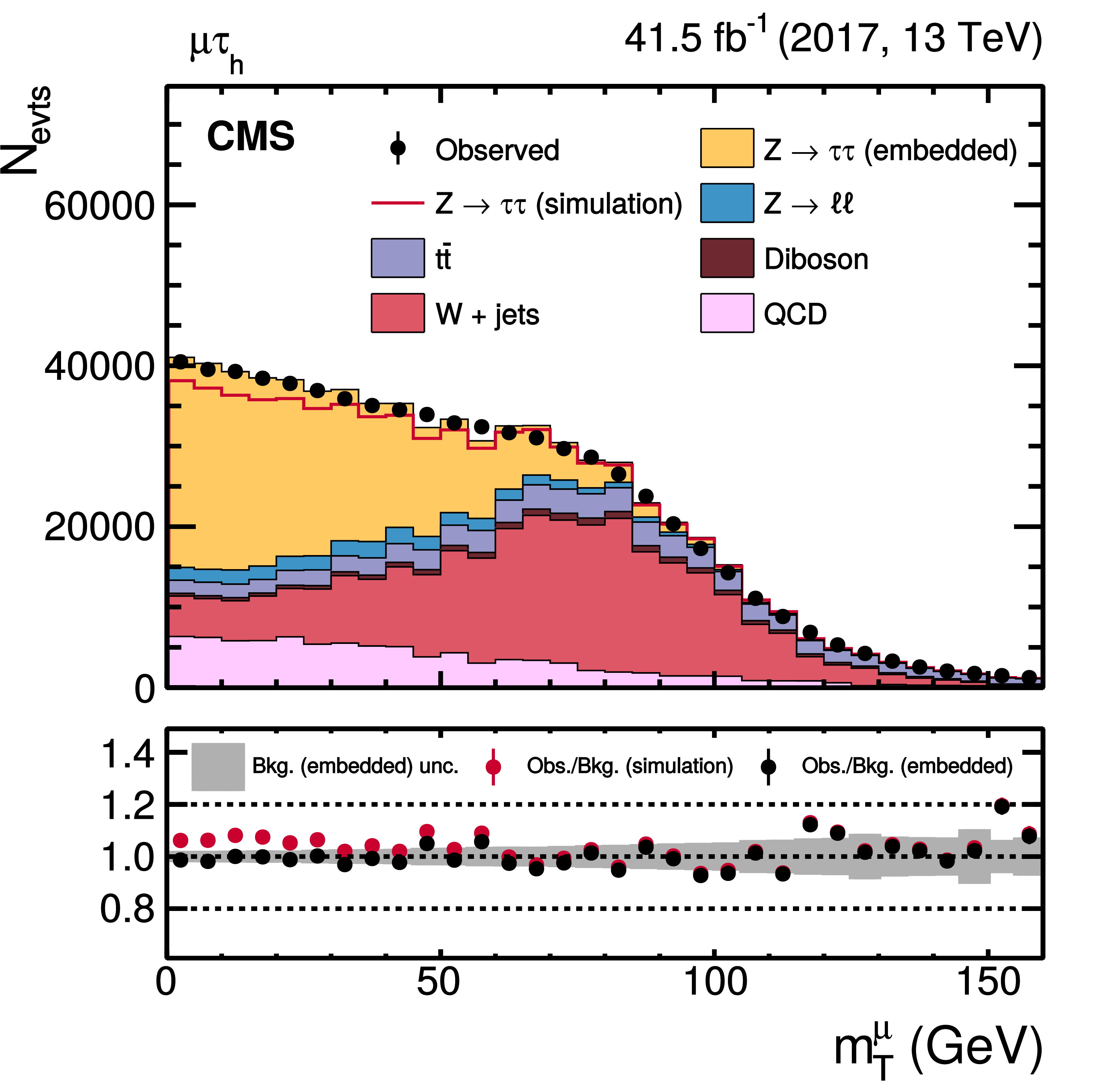
Figure 12-d:
Distribution of $ {m_{\text {T}}^{{\mu}}} $ in the $ {{\mu} {\tau}_{\text {h}}} $ final state. The distribution is shown prior to the maximum likelihood fit described in the text. No uncertainties that affect the shape of the distribution have been included in the uncertainty model. The background estimation purely from the CMS simulation is shown as an additional red line. |
png pdf |
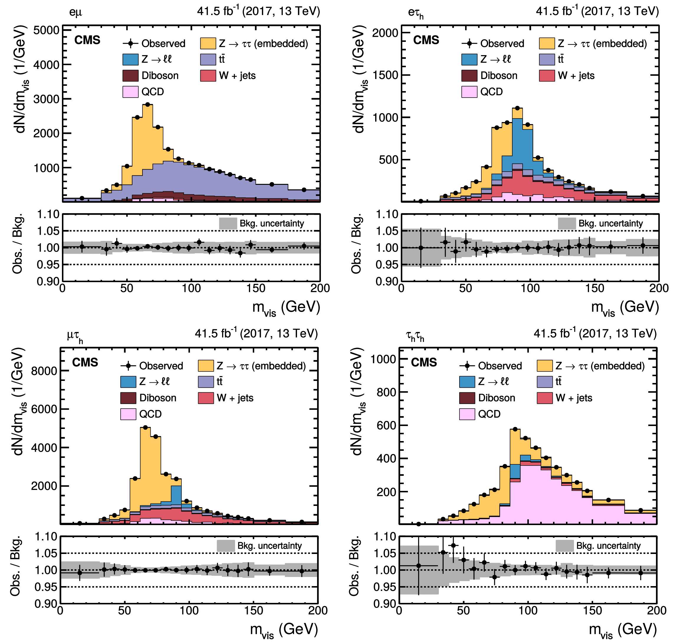
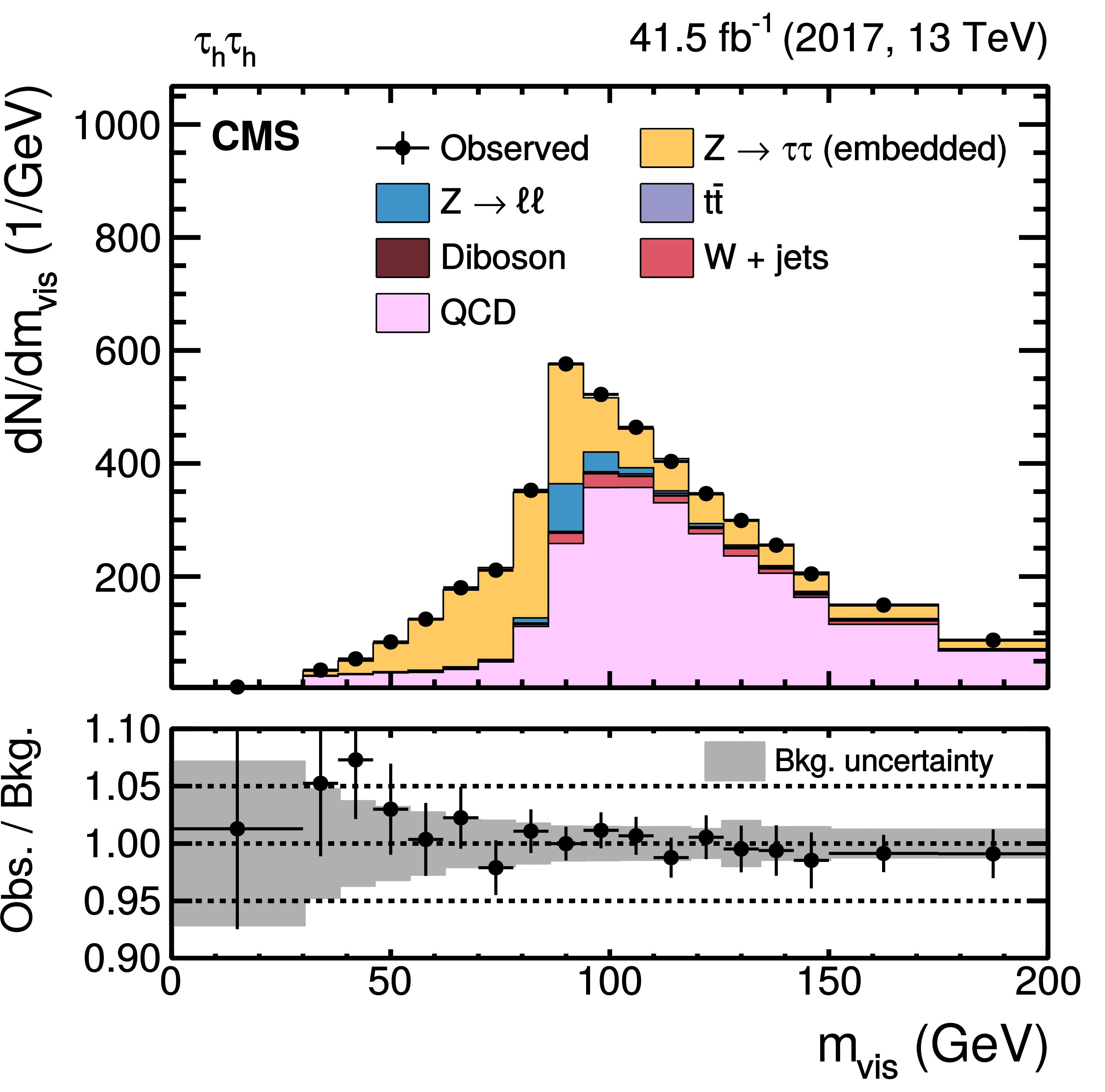
Figure 13:
Invariant mass distribution of the visible $ {\tau} {\tau}$ decay products, $ {m_{\text {vis}}} $, in the (upper left) $ {{\mathrm {e}} {\mu}} $, (upper right) $ {{\mathrm {e}} {\tau}_{\text {h}}} $, (lower left) $ {{\mu} {\tau}_{\text {h}}} $, and (lower right) $ {{\tau}_{\text {h}} {\tau}_{\text {h}}} $ final states, after a fit to the data exploiting a typical uncertainty model as, {e.g.}, discussed in Ref. [45]. |

png pdf |
Figure 13-a:
Invariant mass distribution of the visible $ {\tau} {\tau}$ decay products, $ {m_{\text {vis}}} $, in the $ {{\mathrm {e}} {\mu}} $ final state, after a fit to the data exploiting a typical uncertainty model as, {e.g.}, discussed in Ref. [45]. |

png pdf |
Figure 13-b:
Invariant mass distribution of the visible $ {\tau} {\tau}$ decay products, $ {m_{\text {vis}}} $, in the $ {{\mathrm {e}} {\tau}_{\text {h}}} $ final state, after a fit to the data exploiting a typical uncertainty model as, {e.g.}, discussed in Ref. [45]. |

png pdf |
Figure 13-c:
Invariant mass distribution of the visible $ {\tau} {\tau}$ decay products, $ {m_{\text {vis}}} $, in the $ {{\mu} {\tau}_{\text {h}}} $ final state, after a fit to the data exploiting a typical uncertainty model as, {e.g.}, discussed in Ref. [45]. |
png pdf |
Figure 13-d:
Invariant mass distribution of the visible $ {\tau} {\tau}$ decay products, $ {m_{\text {vis}}} $, in the $ {{\tau}_{\text {h}} {\tau}_{\text {h}}} $ final state, after a fit to the data exploiting a typical uncertainty model as, {e.g.}, discussed in Ref. [45]. |

png pdf |
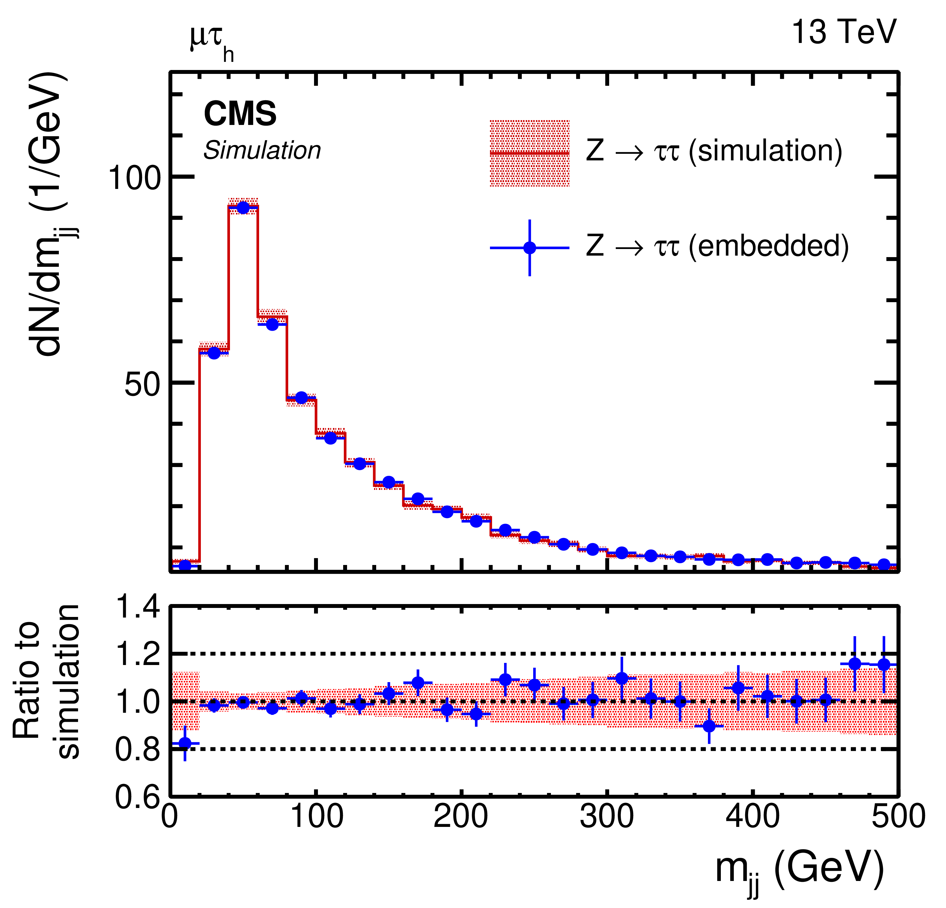
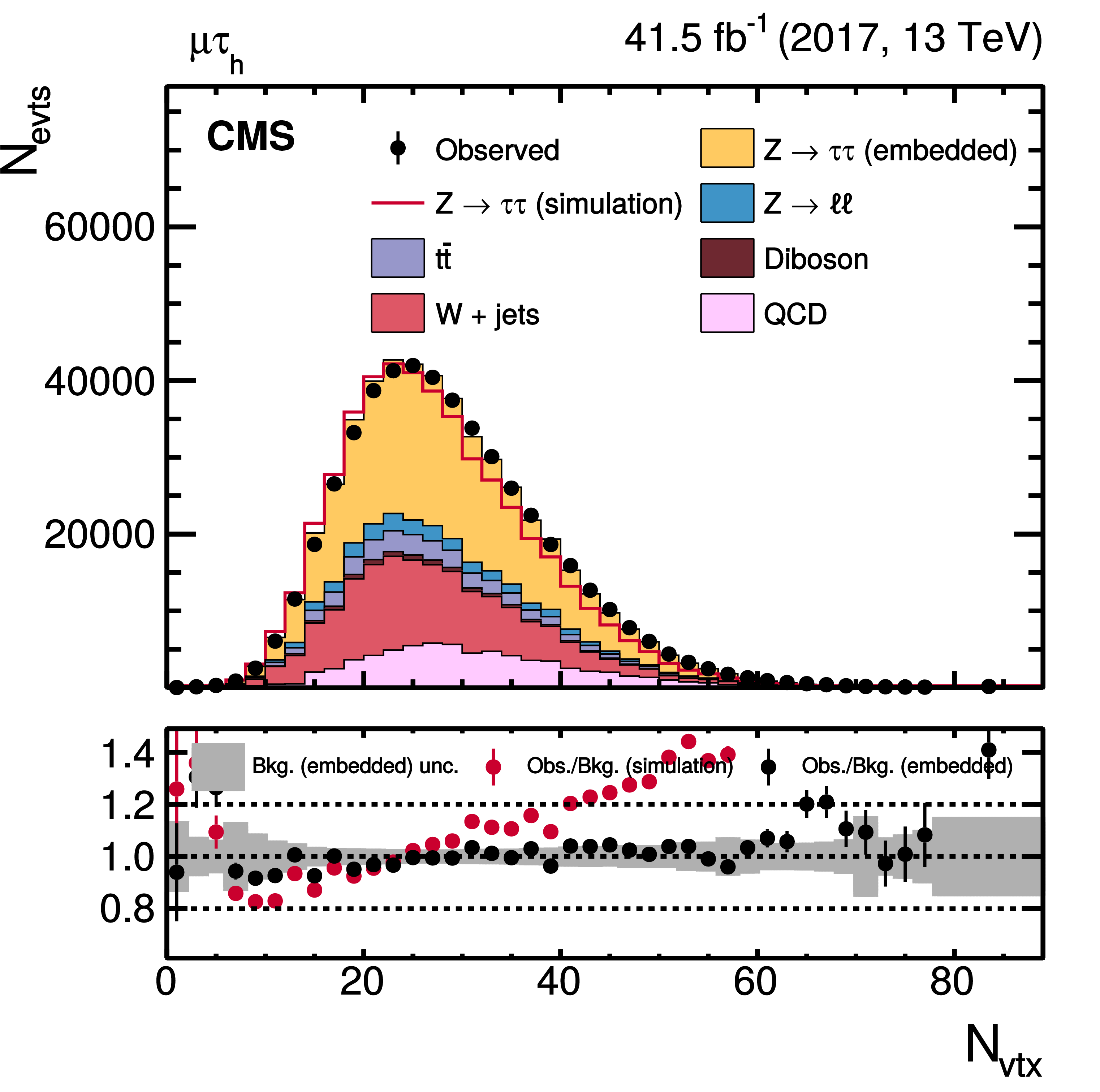
Figure 14:
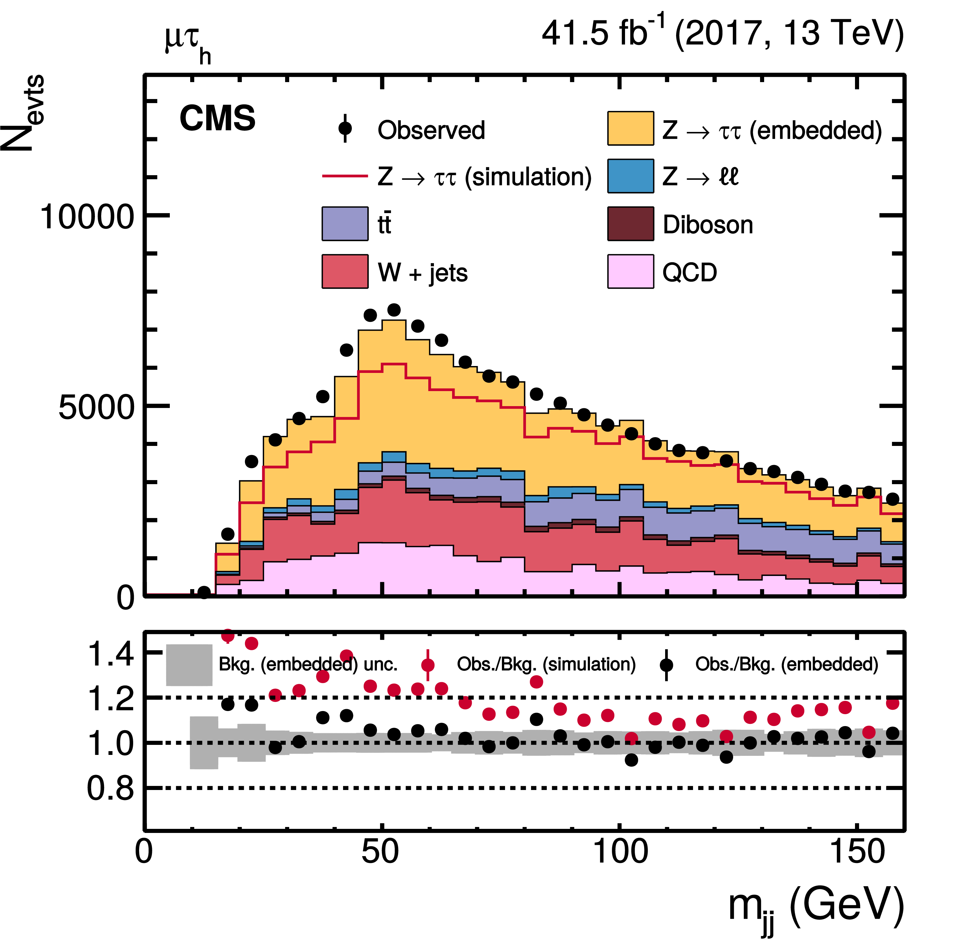
Distributions of (left) $ {m_{\text {jj}}} $ and (right) the number of reconstructed primary vertices $N_{\text {vtx}}$ in the $ {{\mu} {\tau}_{\text {h}}} $ final state. |
png pdf |
Figure 14-a:
Distribution of $ {m_{\text {jj}}} $ in the $ {{\mu} {\tau}_{\text {h}}} $ final state. |
png pdf |
Figure 14-b:
Distribution of the number of reconstructed primary vertices $N_{\text {vtx}}$ in the $ {{\mu} {\tau}_{\text {h}}} $ final state. |
png pdf |
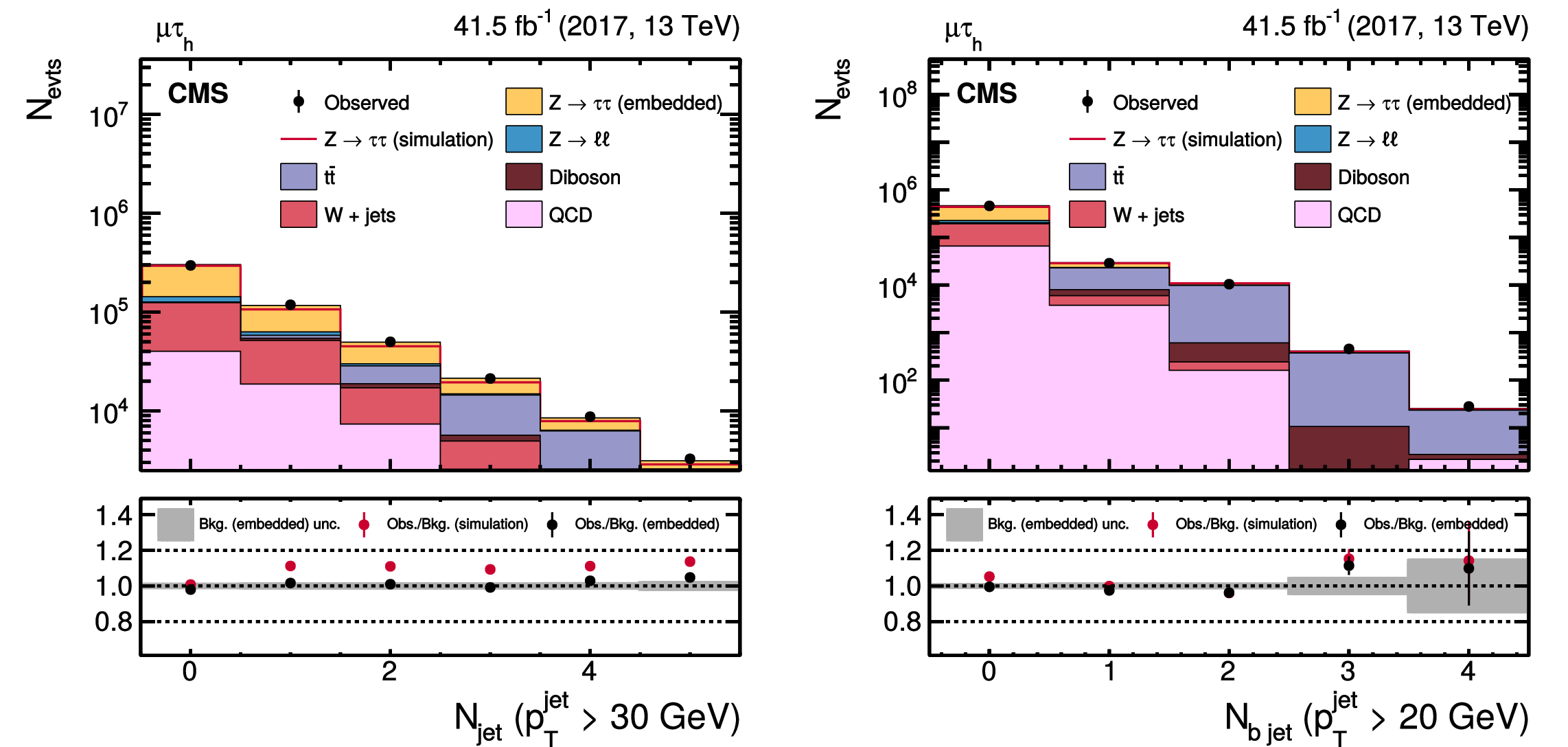
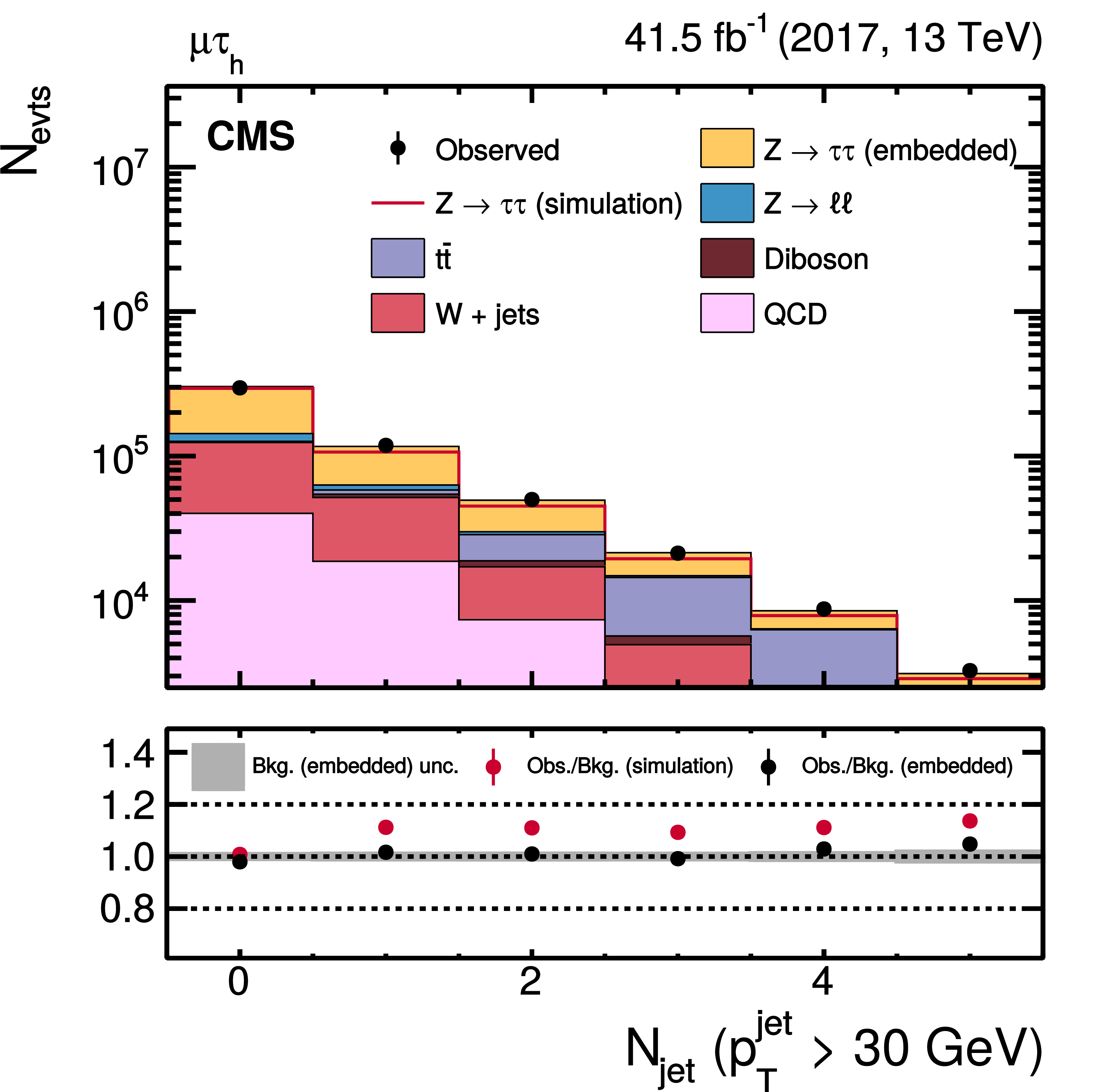
Figure 15:
Distributions of the (left) jet and (right) b-jet multiplicity, as described in the text, in the $ {{\mu} {\tau}_{\text {h}}} $ final state. |
png pdf |
Figure 15-a:
Distribution of the jet multiplicity, as described in the text, in the $ {{\mu} {\tau}_{\text {h}}} $ final state. |
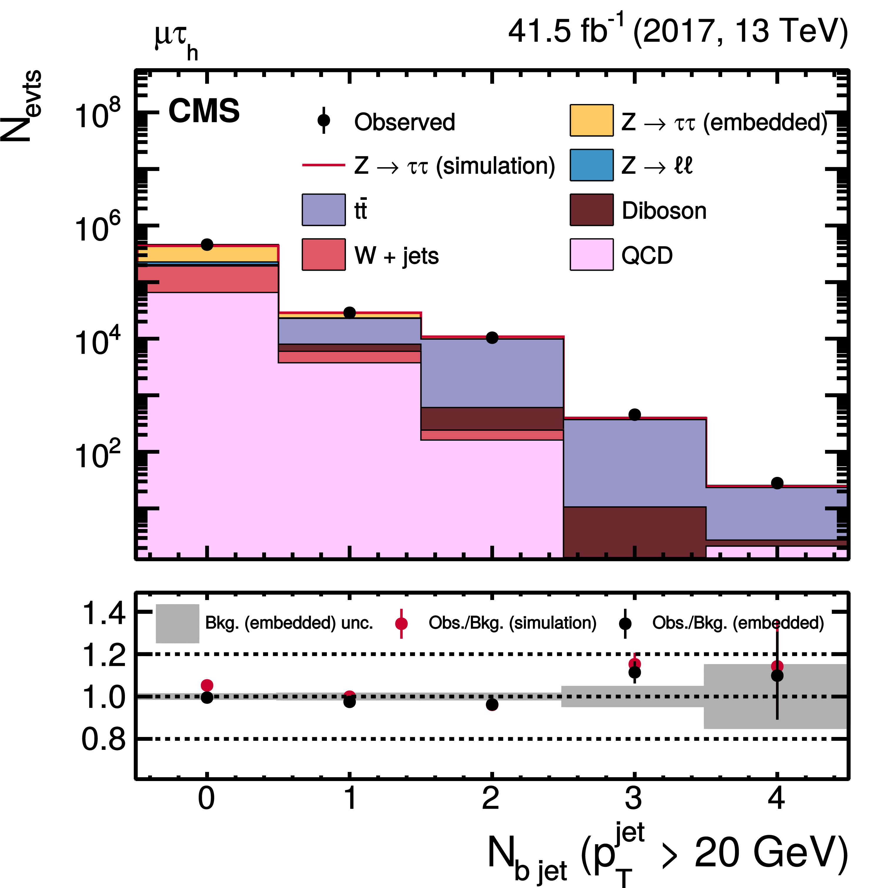
png pdf |
Figure 15-b:
Distribution of the b-jet multiplicity, as described in the text, in the $ {{\mu} {\tau}_{\text {h}}} $ final state. |
png pdf |
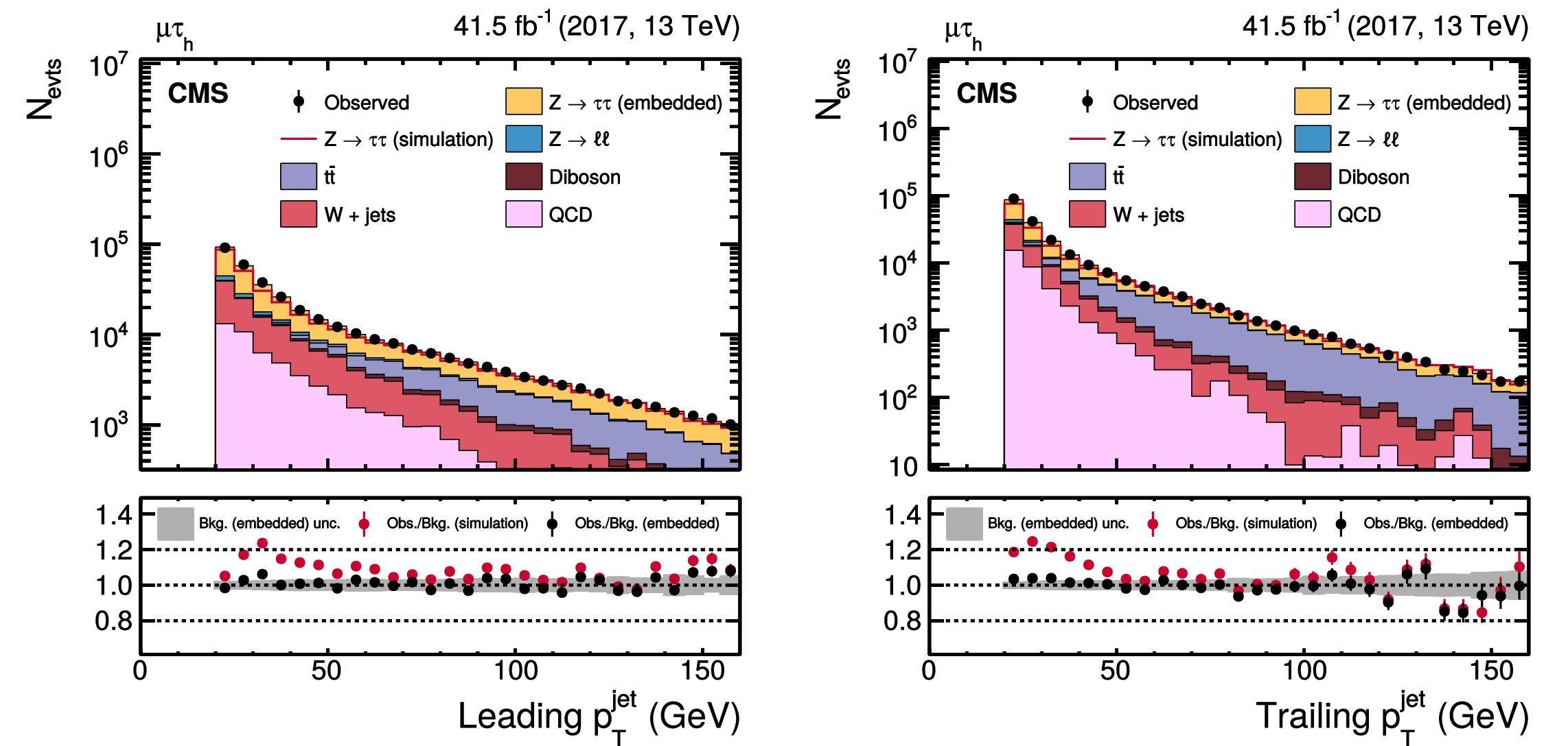
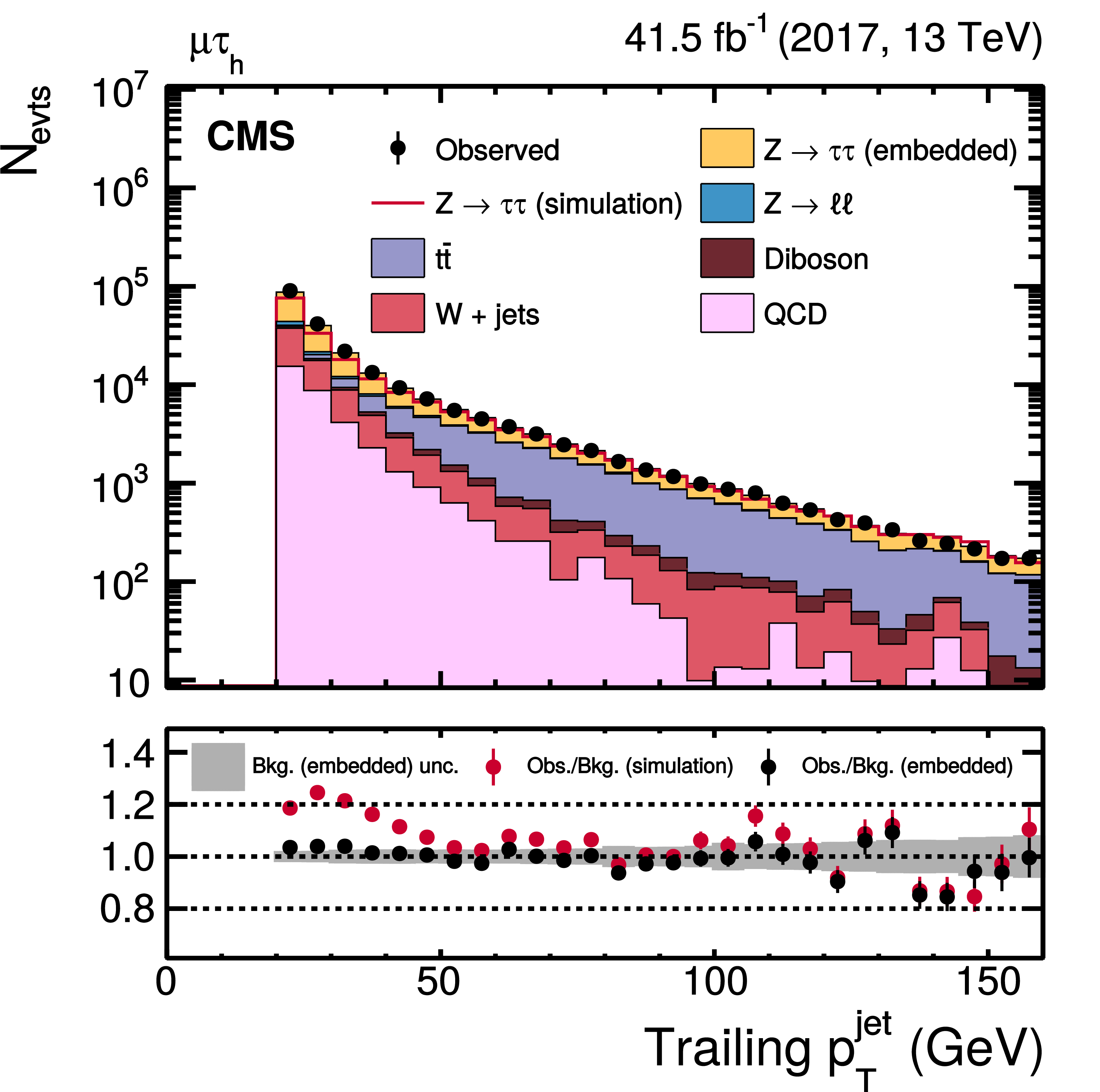
Figure 16:
Distributions of the $ {p_{\mathrm {T}}} $ of the (left) leading and (right) trailing jet for events with more than one jet in the $ {{\mu} {\tau}_{\text {h}}} $ final state. |
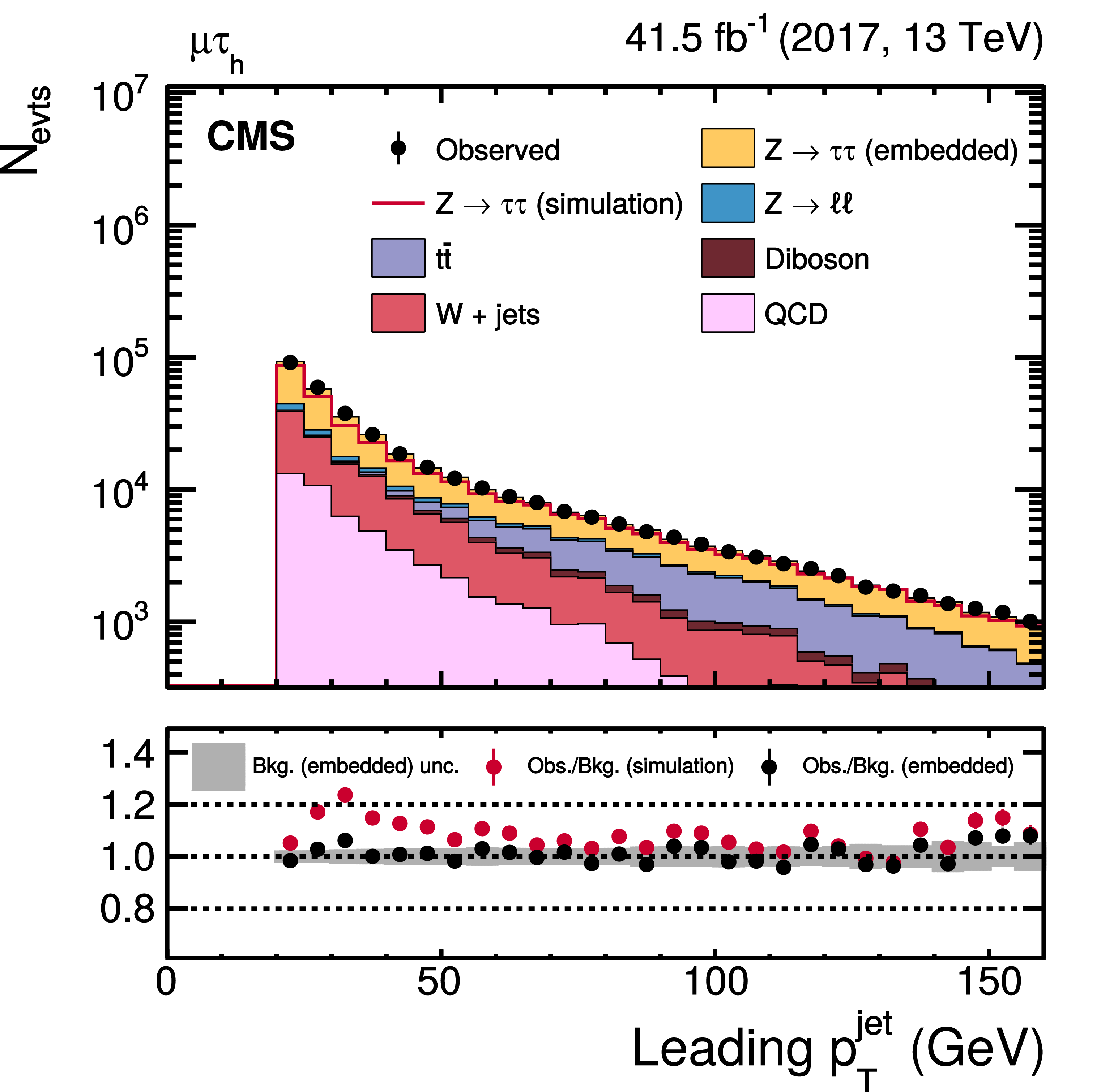
png pdf |
Figure 16-a:
Distribution of the $ {p_{\mathrm {T}}} $ of the leading jet for events with more than one jet in the $ {{\mu} {\tau}_{\text {h}}} $ final state. |
png pdf |
Figure 16-b:
Distribution of the $ {p_{\mathrm {T}}} $ of the trailing jet for events with more than one jet in the $ {{\mu} {\tau}_{\text {h}}} $ final state. |
| Tables | |
png pdf |
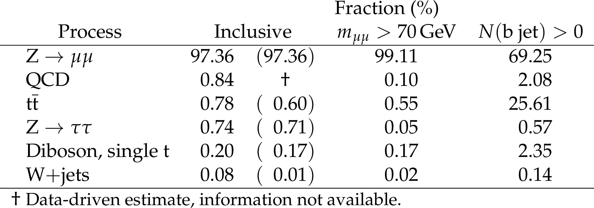
Table 1:
Expected event composition after the selection of two muons, as described in Section 5.1. The compositions after adding selections on $ {m_{\mu \mu}} > $ 70 GeV or on the number of b jets with $ {p_{\mathrm {T}}} > $ 20 GeV in the event are shown in column 3 and 4 respectively. In the second column the fraction of events where the corresponding process has two genuine muons in the final state is given in parentheses. |
png pdf |
Table 2:
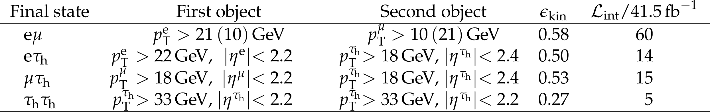
Kinematic range of eligibility for each $ {\tau}$-embedded event sample in the $ {{\mathrm {e}} {\mu}} $, $ {{\mathrm {e}} {\tau}_{\text {h}}} $, $ {{\mu} {\tau}_{\text {h}}} $, and $ {{\tau}_{\text {h}} {\tau}_{\text {h}}} $ final states. The expression "First/Second object'' refers to the final state label used in the first column. Also given are the probability of the simulated tau lepton pair to pass the kinematic filtering ($\epsilon _{\text {kin}}$), described in the text, and the equivalent of the integrated luminosity $\mathcal {L}_{\text {int}}$, of the corresponding $ {\tau}$-embedded event sample, in multiples of the data set, from which the embedded event sample has been created. |
png pdf |
Table 3:
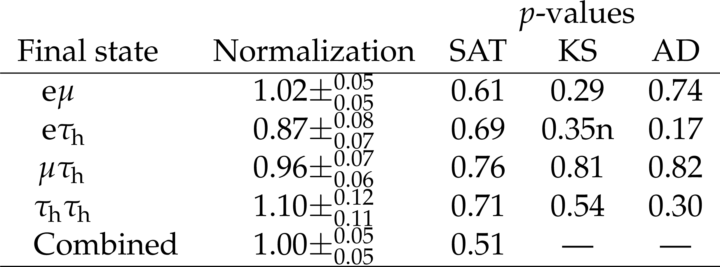
Normalization of the $ {\tau}$-embedded event samples and $p$-values of the saturated model (SAT), Kolmogorov-Smirnov (KS) and Anderson-Darling (AD) test, as discussed in the text, separated by $ {\tau} {\tau}$ final state, as introduced in Section 5 and (where applicable) for all channels combined. The $p$-values have a statistical precision better than 0.5%. |
| Summary |
|
The $\tau$-embedding technique developed for the CMS experiment is described and its validation and relevant uncertainties are discussed. The 13 TeV proton-proton collisions collected by CMS in 2017 are used to demonstrate the performance of the technique with the data sample corresponding to an integrated luminosity of 41.5 fb$^{-1}$. The main goal of the procedure is to estimate the background from $\mathrm{Z} \to \tau\tau$ events using recorded $\mathrm{Z} \to \mu\mu$ events. The estimate also includes events from $\mathrm{t\bar{t}}$ and diboson production with two tau leptons in the final state. Recorded $\mu\mu$ events are selected, the muons are removed from the reconstructed event record, and replaced with simulated tau leptons with the same kinematic properties as the removed muons. In that way hybrid events are obtained, which rely on the simulation only for the decay of the tau leptons. Challenges in describing the underlying event or the production of associated jets in the simulation, as well as the costly simulation of PU events thus are avoided. The embedding technique decreases the uncertainties inherent in a typical simulation process, such as the uncertainties in the missing transverse momentum, jet energy scale and resolution, b tagging efficiency, and misidentification probability. A number of validation tests for $\mu$-, e-, and $\tau$-embedding, as well as several goodness-of-fit tests, show good agreement of embedded distributions with those obtained using simulated and recorded data events. The embedding technique avoids time-consuming simulations of events that becomes critical for the planned High-Luminosity LHC upgrade, where typical pileup of 140-200 collisions per bunch crossing is expected. |
| Additional Figures | |
png pdf |
Additional Figure 1:
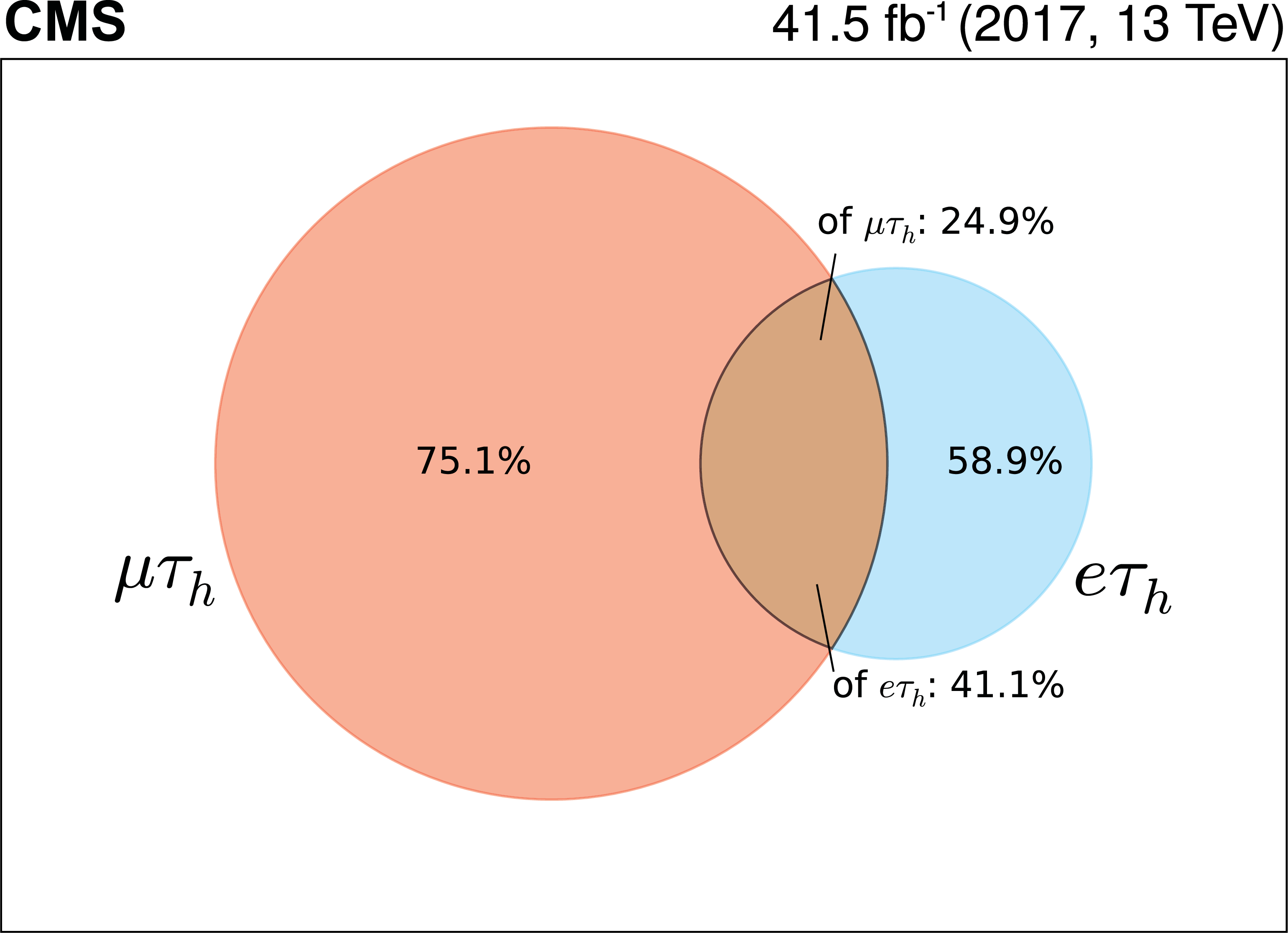
Event overlap between the $ {{{\mu}} {\tau}_{\text {h}}} $ and $ {{\mathrm {e}} {\tau}_{\text {h}}} $ final states after the event selections described in Section 7.3 of the paper, presented in form of a Venn diagram. The sizes of the circles correspond to the number of events passing the selection requirements of each final state. For the overlapping events, the same recorded $ {{\mu}} {{\mu}}$ event is used. As only the muons are replaced by corresponding tau lepton decays the rest of the event is expected to be identical, when compared on an event-by-event basis. |

png pdf |
Additional Figure 2:
Event overlap between the $ {{{\mu}} {\tau}_{\text {h}}} $ and $ {{\mathrm {e}} {\mu}} $ final states after the event selections described in Section 7.3 of the paper, presented in form of a Venn diagram. The sizes of the circles correspond to the number of events passing the selection requirements of each final state. For the overlapping events, the same recorded $ {{\mu}} {{\mu}}$ event is used. As only the muons are replaced by corresponding tau lepton decays the rest of the event is expected to be identical, when compared on an event-by-event basis. |
png pdf |
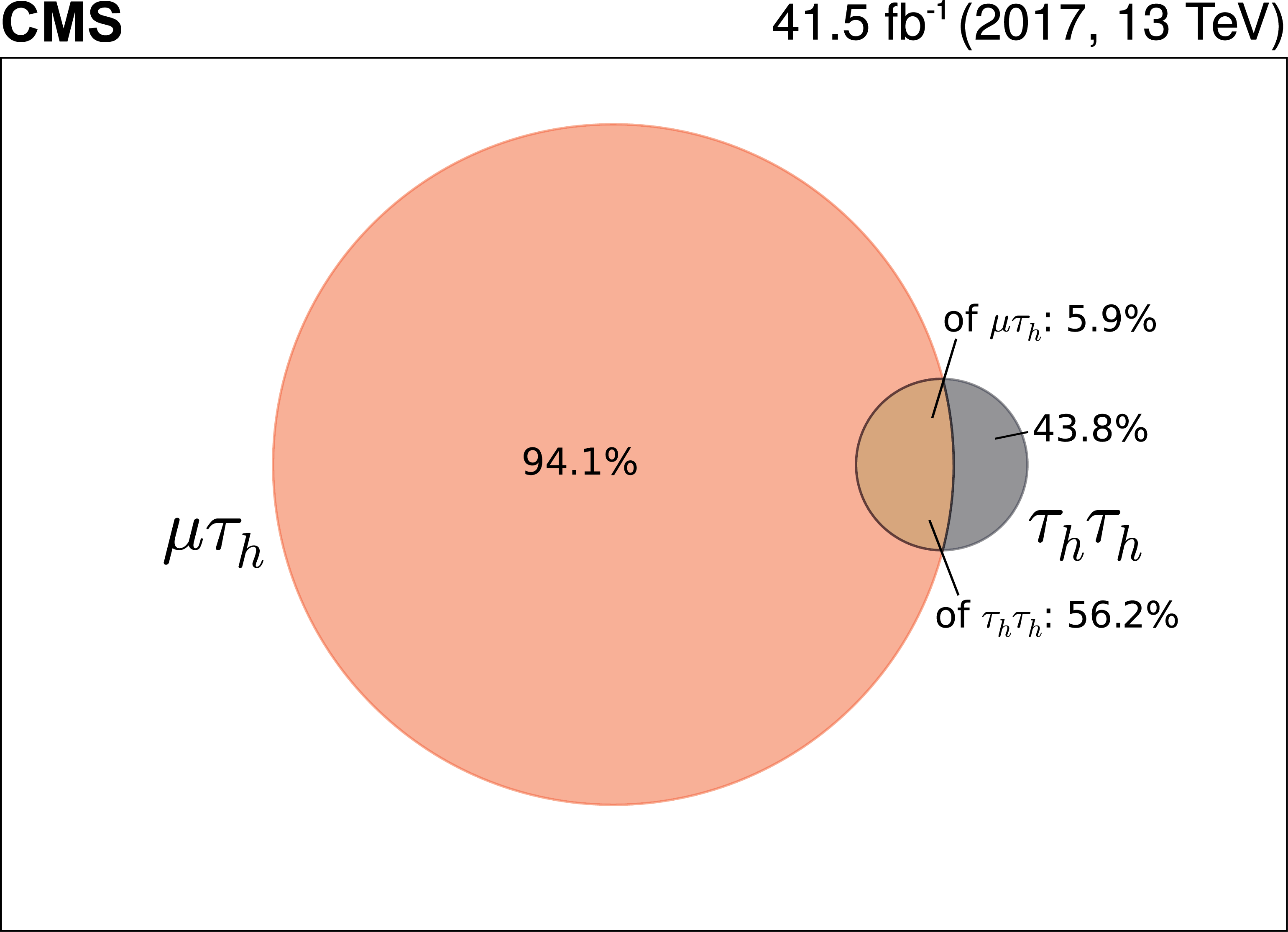
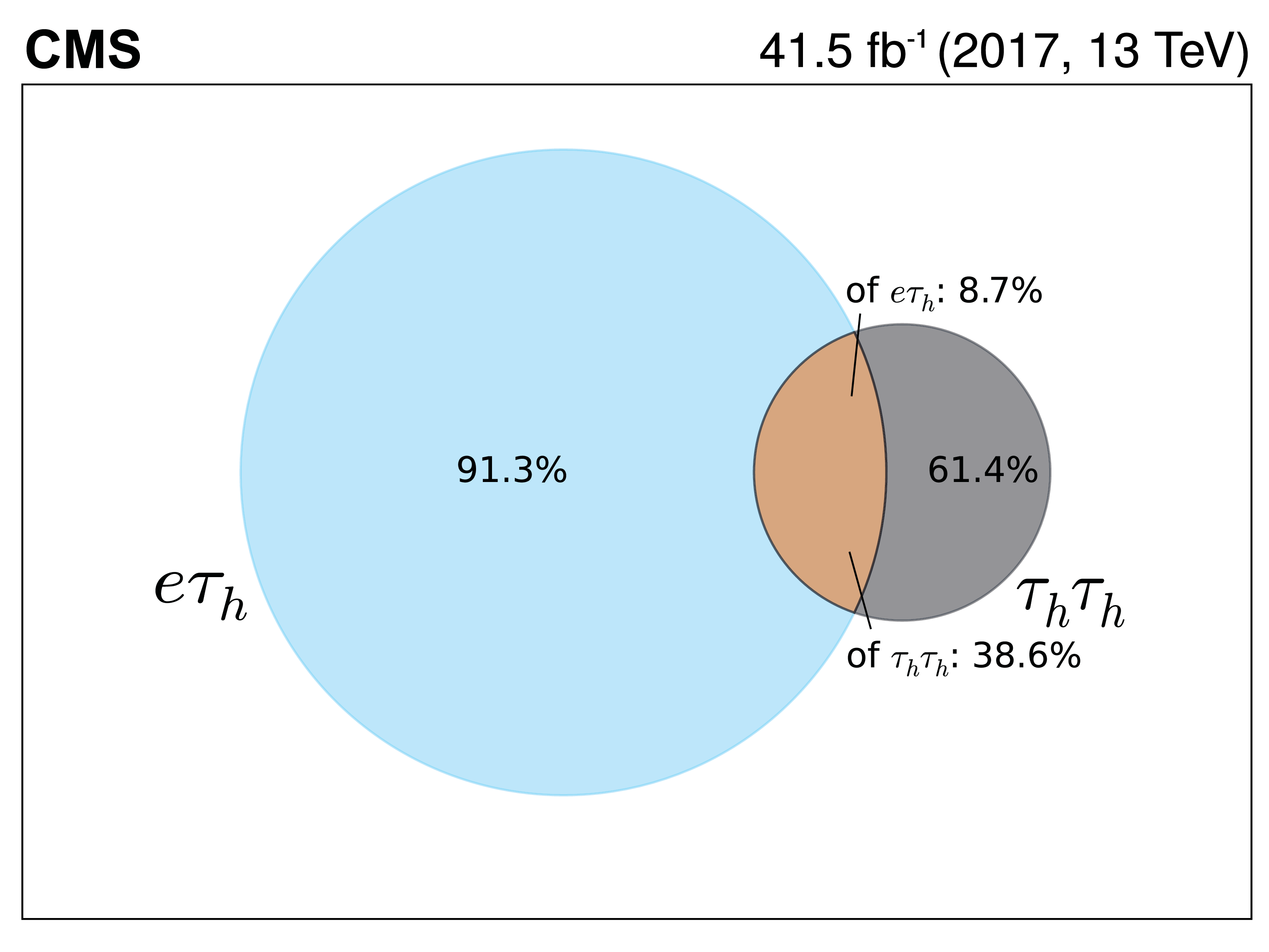
Additional Figure 3:
Event overlap between the $ {{{\mu}} {\tau}_{\text {h}}} $ and $ {{\tau}_{\text {h}} {\tau}_{\text {h}}} $ final states after the event selections described in Section 7.3 of the paper, presented in form of a Venn diagram. The sizes of the circles correspond to the number of events passing the selection requirements of each final state. For the overlapping events, the same recorded $ {{\mu}} {{\mu}}$ event is used. As only the muons are replaced by corresponding tau lepton decays the rest of the event is expected to be identical, when compared on an event-by-event basis. |
png pdf |
Additional Figure 4:
Event overlap between the $ {{\mathrm {e}} {\tau}_{\text {h}}} $ and $ {{\mathrm {e}} {\mu}} $ final states after the event selections described in Section 7.3 of the paper, presented in form of a Venn diagram. The sizes of the circles correspond to the number of events passing the selection requirements of each final state. For the overlapping events, the same recorded $ {{\mu}} {{\mu}}$ event is used. As only the muons are replaced by corresponding tau lepton decays the rest of the event is expected to be identical, when compared on an event-by-event basis. |
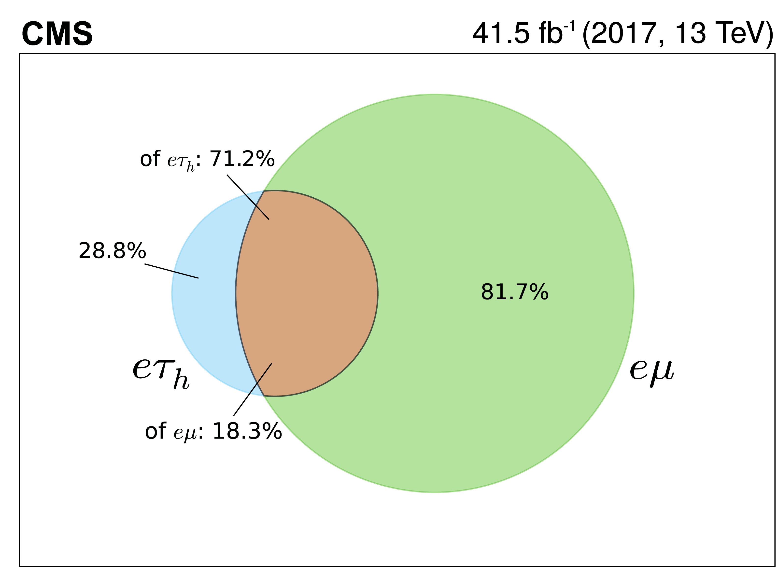
png pdf |
Additional Figure 5:
Event overlap between the $ {{\mathrm {e}} {\tau}_{\text {h}}} $ and $ {{\tau}_{\text {h}} {\tau}_{\text {h}}} $ final states after the event selections described in Section 7.3 of the paper, presented in form of a Venn diagram. The sizes of the circles correspond to the number of events passing the selection requirements of each final state. For the overlapping events, the same recorded $ {{\mu}} {{\mu}}$ event is used. As only the muons are replaced by corresponding tau lepton decays the rest of the event is expected to be identical, when compared on an event-by-event basis. |
png pdf |
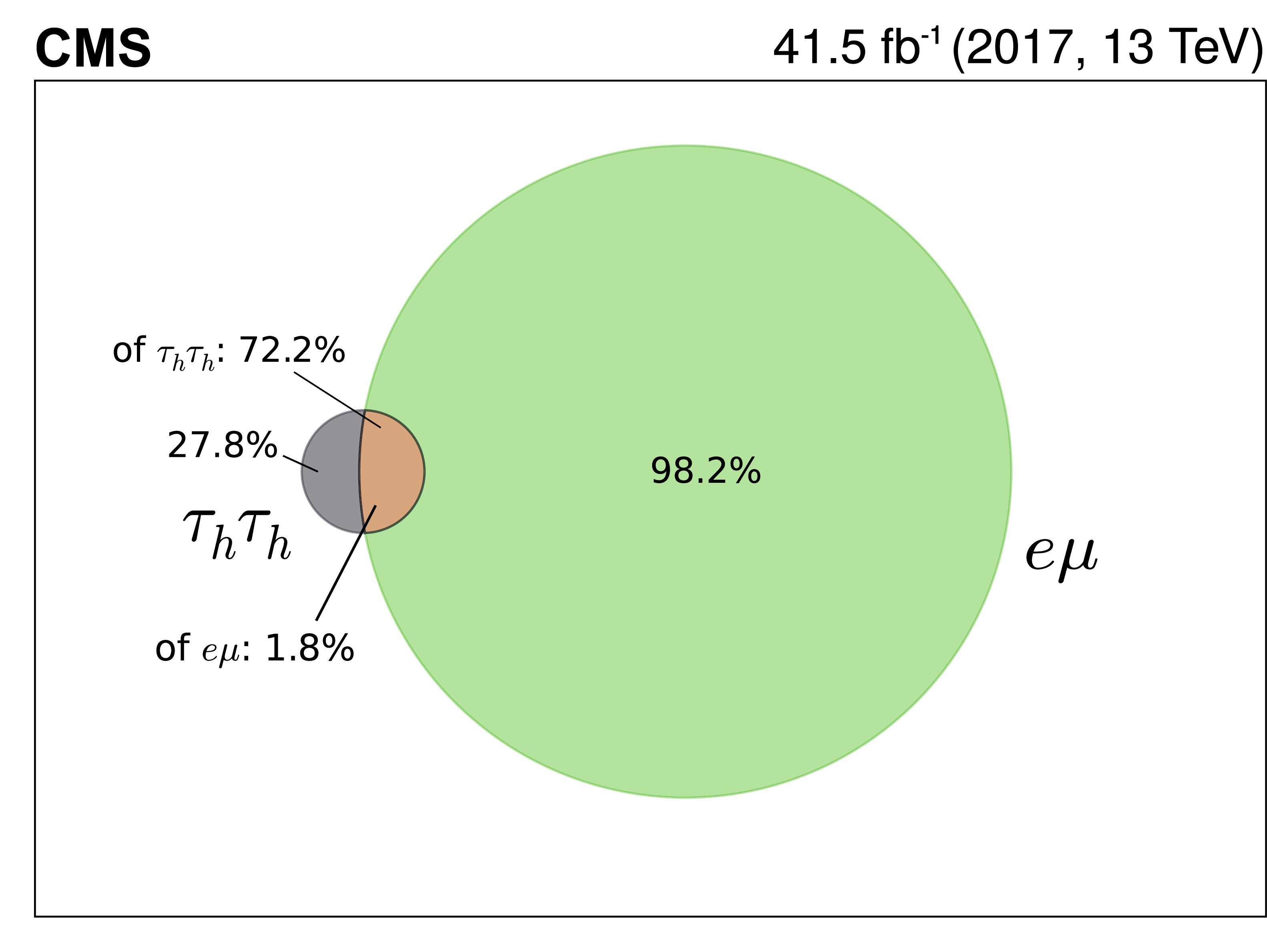
Additional Figure 6:
Event overlap between the $ {{\tau}_{\text {h}} {\tau}_{\text {h}}} $ and $ {{\mathrm {e}} {\mu}} $ final states after the event selections described in Section 7.3 of the paper, presented in form of a Venn diagram. The sizes of the circles correspond to the number of events passing the selection requirements of each corresponding final state. Since the selection for the $ {{\tau}_{\text {h}} {\tau}_{\text {h}}} $ ($ {{\mathrm {e}} {\mu}} $) final state is tightest (loosest), the corresponding number of selected events is smallest (largest). Here 72.2% of the selected events in the $ {{\tau}_{\text {h}} {\tau}_{\text {h}}} $ final state are also selected in the $ {{\mathrm {e}} {\mu}} $ final state, while the same events constitute only 1.8% of all selected events in the $ {{\mathrm {e}} {\mu}} $ final state. For the overlapping events, the same recorded $ {{\mu}} {{\mu}}$ event is used. As only the muons are replaced by corresponding tau lepton decays the rest of the event is expected to be identical, when compared on an event-by-event basis. |
png pdf |
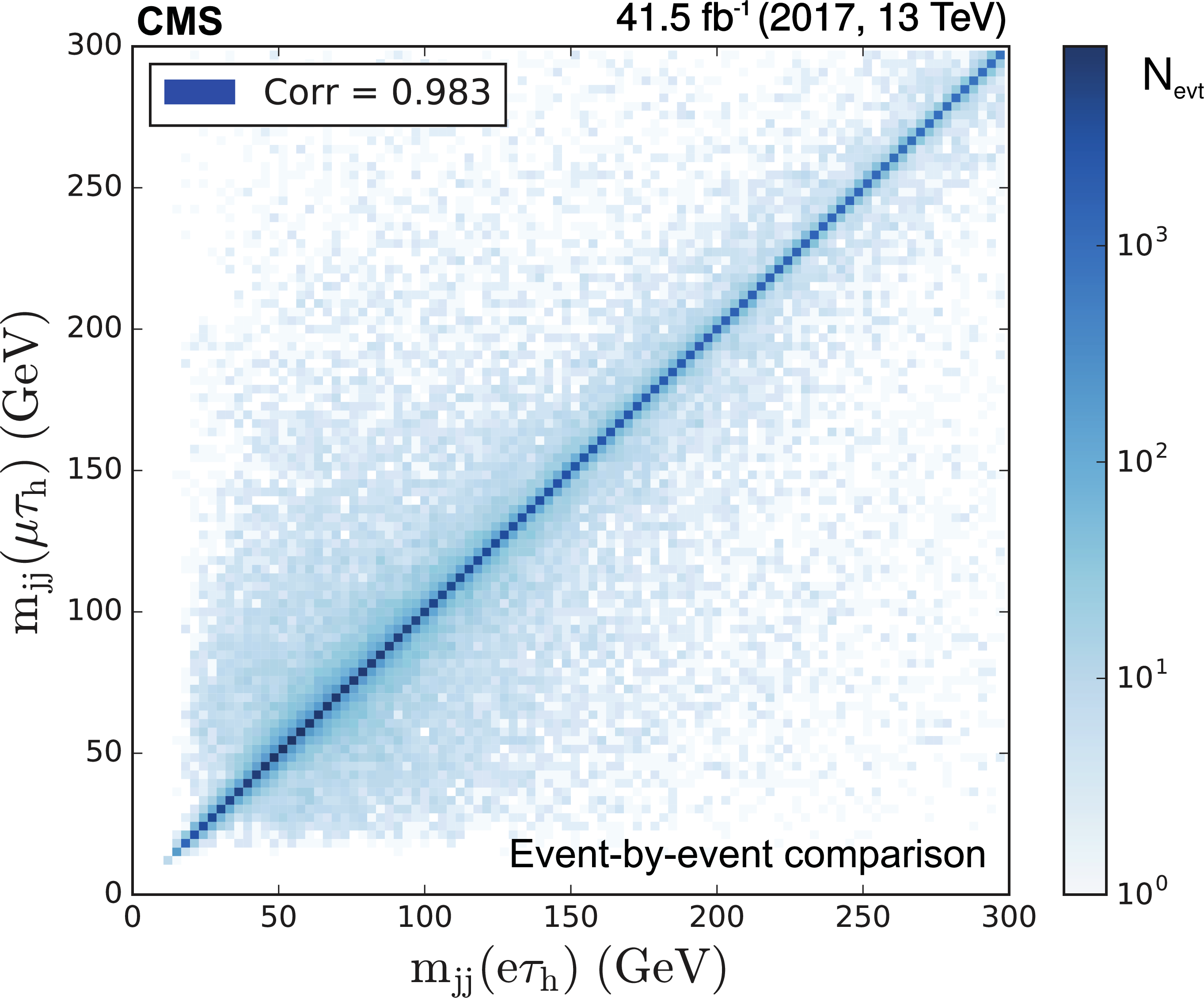
Additional Figure 7:
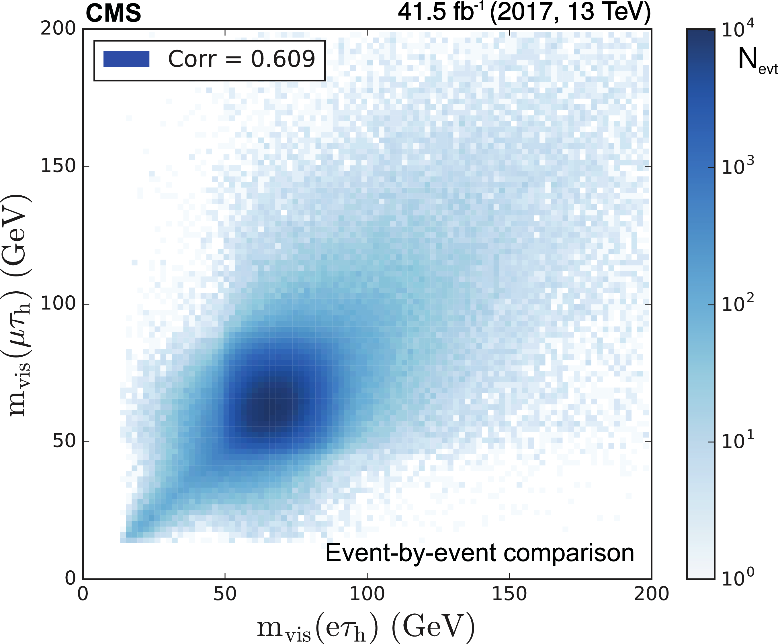
Event-by-event comparison of the mass of the two leading jets in $ {p_{\mathrm {T}}} $, $ {m_{\text {jj}}} $, for those events that are selected in both, the $ {{{\mu}} {\tau}_{\text {h}}} $ and $ {{\mathrm {e}} {\tau}_{\text {h}}} $ final state, where $ {m_{\text {jj}}} $ is calculated from the remaining part of the same recorded $ {{\mu}} {{\mu}}$ event. The overlap is 24.9% of the selected $ {{{\mu}} {\tau}_{\text {h}}} $ events and 41.1% of the selected $ {{\mathrm {e}} {\tau}_{\text {h}}} $ events. The linear correlation coefficient is $0.98$. In the target analyses quantities are not compared on an event-by-event basis, but based on unsorted distributions, to which also non-overlapping events contribute. |

png pdf |
Additional Figure 8:
Event-by-event comparison of the absolute value of the difference in $\eta $ between the two leading jets in $ {p_{\mathrm {T}}} $, $ {| \Delta \eta _{jj} |}$, for those events that are selected in both, the $ {{{\mu}} {\tau}_{\text {h}}} $ and $ {{\mathrm {e}} {\tau}_{\text {h}}} $ final state, where $ {| \Delta \eta _{\text {jj}} |}$ is calculated from the remaining part of the same recorded $ {{\mu}} {{\mu}}$ event. The overlap is 24.9% of the selected $ {{{\mu}} {\tau}_{\text {h}}} $ events and 41.1% of the selected $ {{\mathrm {e}} {\tau}_{\text {h}}} $ events. The linear correlation coefficient is 0.98. In the target analyses quantities are not compared on an event-by-event basis, but based on unsorted distributions, to which also non-overlapping events contribute. |
png pdf |
Additional Figure 9:
Event-by-event comparison of the visible mass of the tau lepton decay products, $ {m_{\text {vis}}} $, for those events that are selected in both, the $ {{{\mu}} {\tau}_{\text {h}}} $ and $ {{\mathrm {e}} {\tau}_{\text {h}}} $ final state. The overlap is 24.9% of the selected $ {{{\mu}} {\tau}_{\text {h}}} $ events and 41.1% of the selected $ {{\mathrm {e}} {\tau}_{\text {h}}} $ events. The linear correlation coefficient is 0.61. The reduction of the correlation originates from a partial randomization due to the independent simulation of the tau lepton decays. In the target analyses quantities are not compared on an event-by-event basis, but based on unsorted distributions, to which also non-overlapping events contribute. |
png pdf |
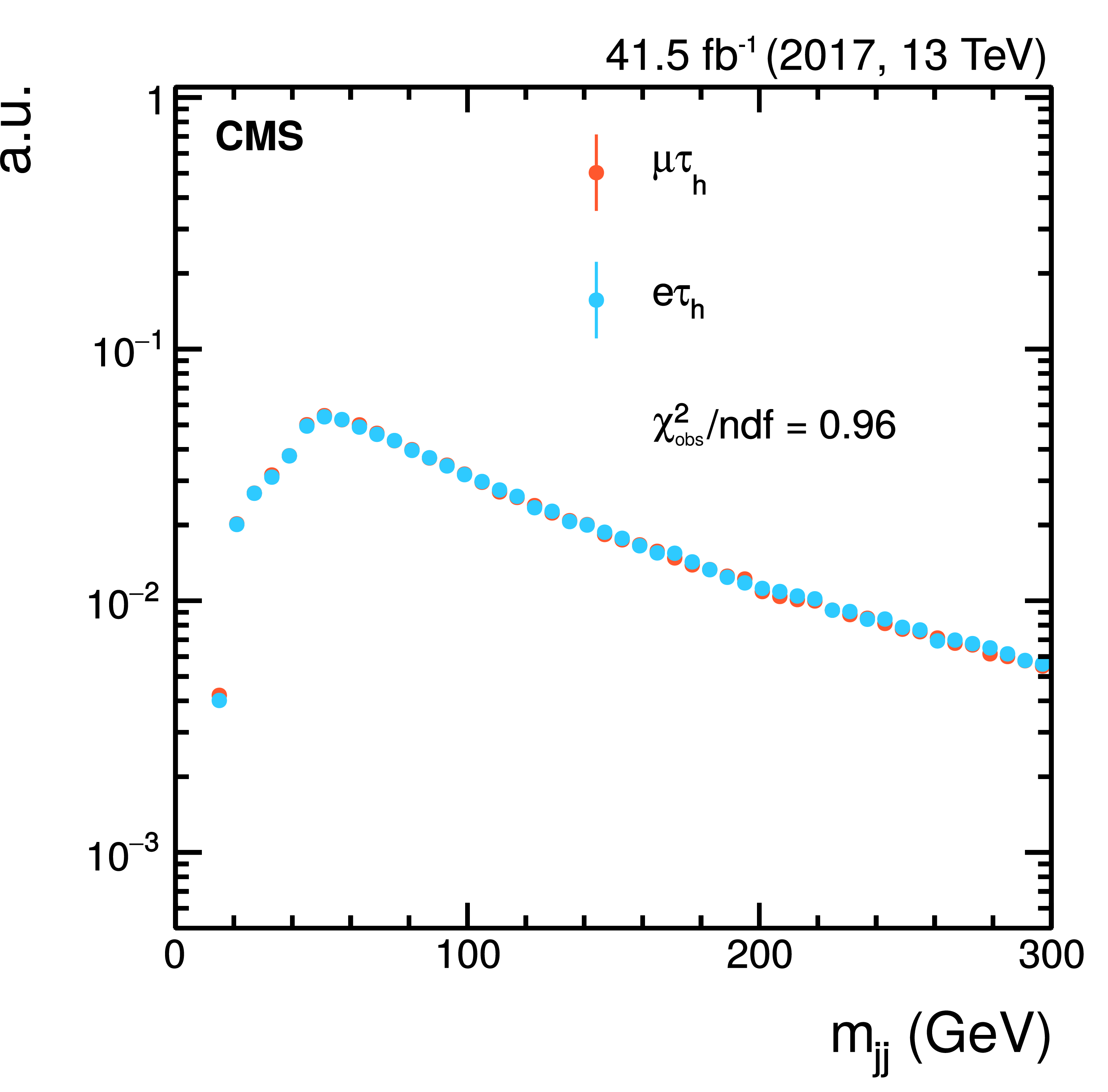
Additional Figure 10:
Comparison of the distributions of $ {m_{\text {jj}}} $ for all events passing the selection in the $ {{\mathrm {e}} {\tau}_{\text {h}}} $ and $ {{{\mu}} {\tau}_{\text {h}}} $ final states. Both distributions are scaled to unity. The $\chi _{\text {obs}}^{2}$ divided by the number of degrees of freedom (ndf) indicating the statistical compatibility of both distributions is also given. |
png pdf |
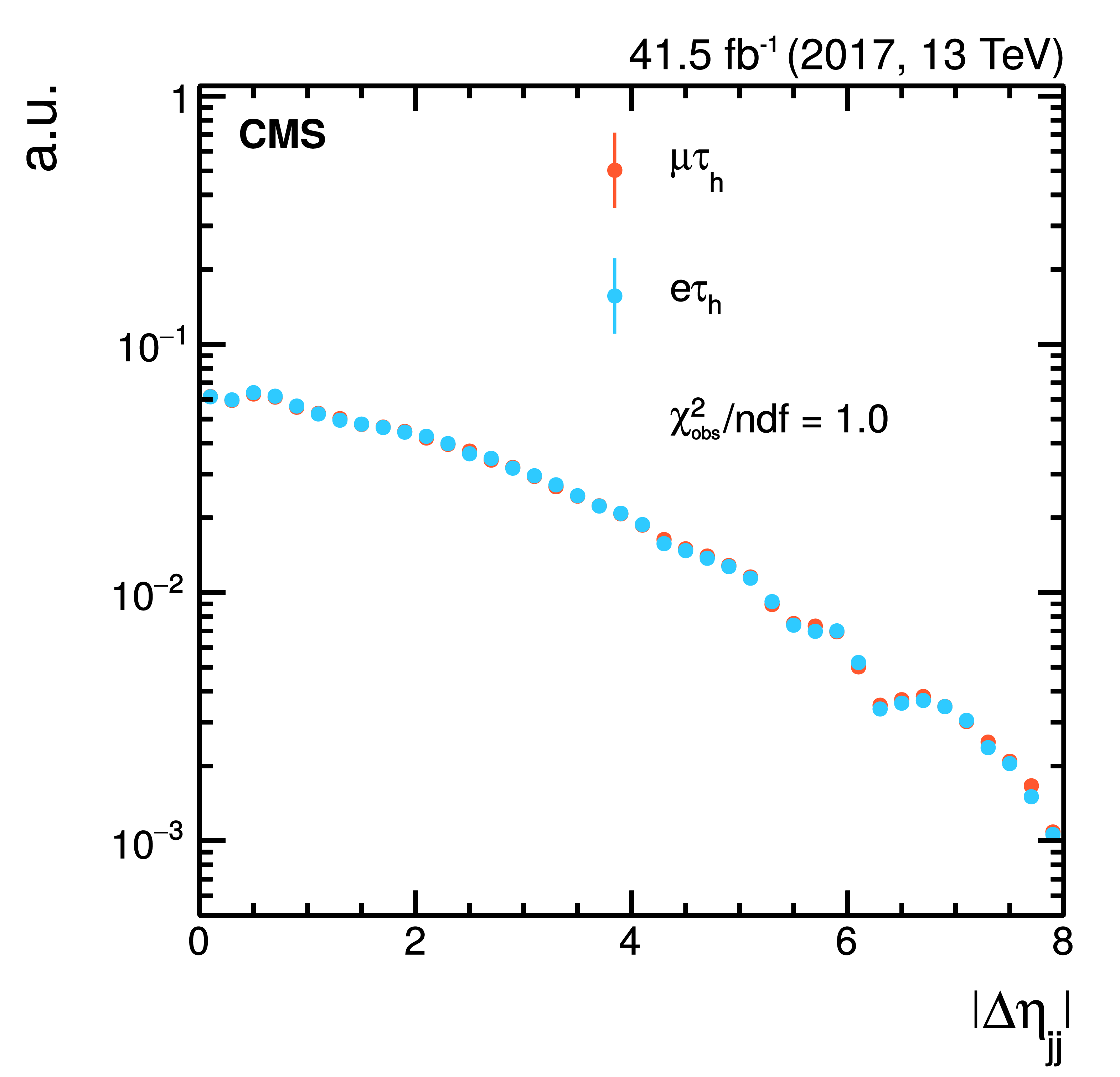
Additional Figure 11:
Comparison of the distributions of $ {| \Delta \eta _{\text {jj}} |}$ for all events passing the selection in the $ {{\mathrm {e}} {\tau}_{\text {h}}} $ and $ {{{\mu}} {\tau}_{\text {h}}} $ final states. The distributions are scaled to unity. The $\chi _{\text {obs}}^{2}$ divided by the number of degrees of freedom (ndf) indicating the statistical compatibility of both distributions is also given. |
png pdf |
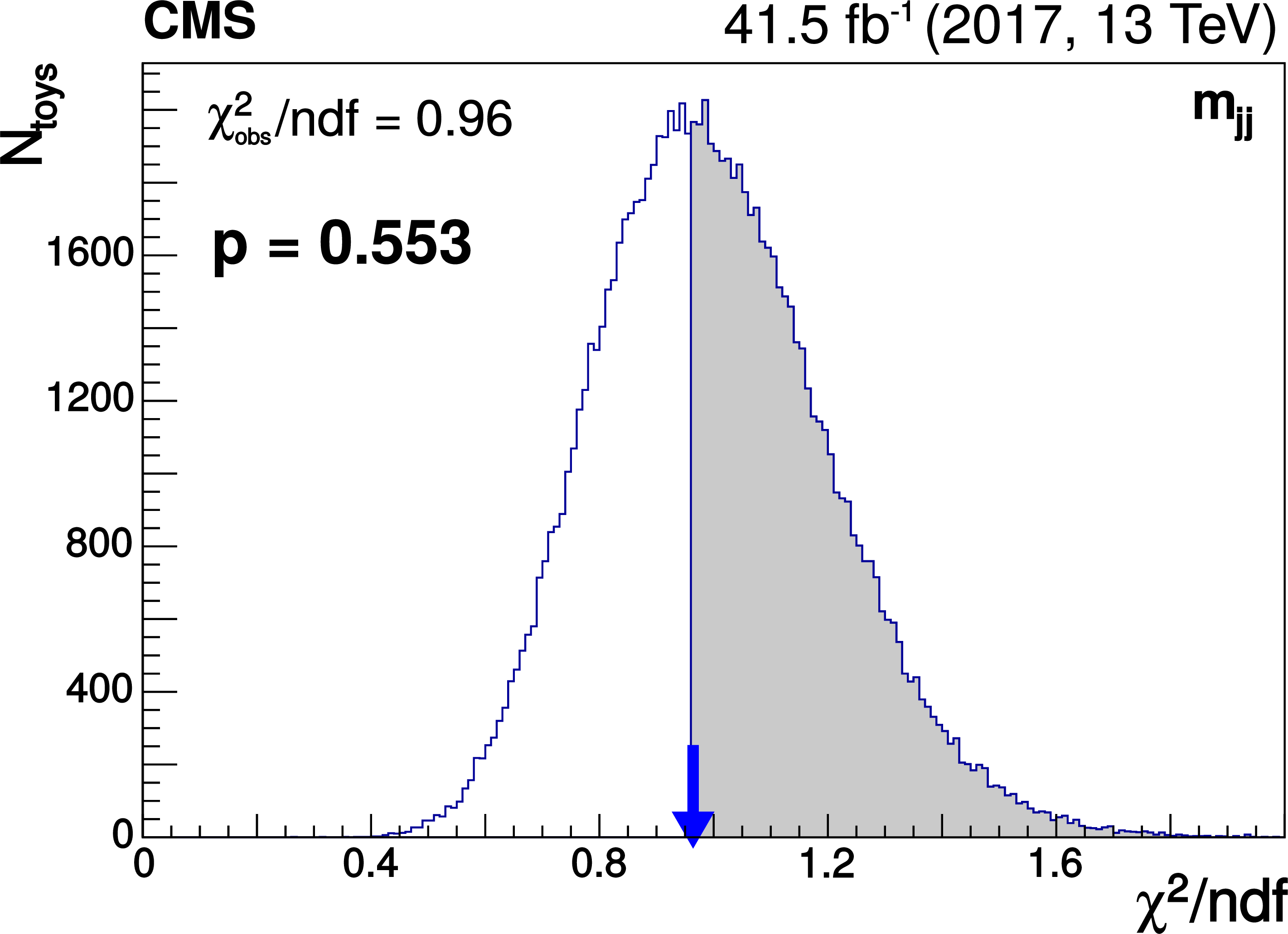
Additional Figure 12:
Quantification of the remaining correlation between the distributions shown in Addtional Figure 10. The histogram results from 100000 pseudo-experiments derived from a Poisson randomization in each bin of the $ {m_{\text {jj}}} $ distribution in the $ {{{\mu}} {\tau}_{\text {h}}} $ final state. For each pseudo-experiment the value of $\chi ^{2}/\text {ndf}$ with respect to the original distribution is calculated. The $\chi _{\text {obs}}^{2}/\text {ndf}$ as observed for the comparison of the distributions in the $ {{\mathrm {e}} {\tau}_{\text {h}}} $ and $ {{{\mu}} {\tau}_{\text {h}}} $ final states in Addtional Figure 10 is indicated by the blue arrow. The integral over the histogram from $\chi _{\text {obs}}^{2}/\text {ndf}$ to $+\infty $ (illustrated by the gray shaded area) results in a p-value of 0.553, revealing good compatibility and no remaining correlation across the distributions in the $ {{\mathrm {e}} {\tau}_{\text {h}}} $ and $ {{{\mu}} {\tau}_{\text {h}}} $ final states. Such a correlation would have resulted in a systematically higher p-value. |

png pdf |
Additional Figure 13:
Quantification of the remaining correlation between the distributions shown in Addtional Figure 11. The histogram results from 100000 pseudo-experiments derived from a Poisson randomization in each bin of the $ {| \Delta \eta _{\text {jj}} |}$ distribution in the $ {{{\mu}} {\tau}_{\text {h}}} $ final state. For each pseudo-experiment the value of $\chi ^{2}/\text {ndf}$ with respect to the original distribution is calculated. The $\chi _{\text {obs}}^{2}/\text {ndf}$ as observed for the comparison of the distributions in the $ {{\mathrm {e}} {\tau}_{\text {h}}} $ and $ {{{\mu}} {\tau}_{\text {h}}} $ final states in Addtional Figure 11 is indicated by the blue arrow. The integral over the histogram from $\chi _{\text {obs}}^{2}/\text {ndf}$ to $+\infty $ (illustrated by the gray shaded area) results in a p-value of 0.488, revealing good compatibility and no remaining correlation across the distributions in the $ {{\mathrm {e}} {\tau}_{\text {h}}} $ and $ {{{\mu}} {\tau}_{\text {h}}} $ final states. Such a correlation would have resulted in a systematically higher p-value. |
| References | ||||
| 1 | ATLAS Collaboration | Search for the Standard Model Higgs boson in the $ \mathrm{H} $ to $ \tau^{+} \tau^{-} $ decay mode in $ \sqrt{s}= $ 7 TeV pp collisions with ATLAS | JHEP 09 (2012) 070 | 1206.5971 |
| 2 | ATLAS Collaboration | Evidence for the Higgs-boson Yukawa coupling to tau leptons with the ATLAS detector | JHEP 04 (2015) 117 | 1501.04943 |
| 3 | CMS Collaboration | Search for neutral Higgs bosons decaying to tau pairs in $ {\mathrm{p}}{\mathrm{p}} $ collisions at $ \sqrt{s} = $ 7 TeV | PLB 713 (2012) 68 | CMS-HIG-11-029 1202.4083 |
| 4 | CMS Collaboration | Observation of a new boson at a mass of 125 GeV with the CMS experiment at the LHC | PLB 716 (2012) 30 | CMS-HIG-12-028 1207.7235 |
| 5 | CMS Collaboration | Evidence for the 125 GeV Higgs boson decaying to a pair of $ \tau $ leptons | JHEP 05 (2014) 104 | CMS-HIG-13-004 1401.5041 |
| 6 | CMS Collaboration | Observation of a new boson with mass near 125 GeV in $ {\mathrm{p}}{\mathrm{p}} $ collisions at $ \sqrt{s} = $ 7 and 8 TeV | JHEP 06 (2013) 081 | CMS-HIG-12-036 1303.4571 |
| 7 | CMS Collaboration | Measurement of Higgs boson production and properties in the WW decay channel with leptonic final states | JHEP 01 (2014) 096 | CMS-HIG-13-023 1312.1129 |
| 8 | ATLAS Collaboration | Search for the neutral Higgs bosons of the minimal supersymmetric standard model in $ {\mathrm{p}}{\mathrm{p}} $ collisions at $ \sqrt{s} = $ 7 TeV with the ATLAS detector | JHEP 02 (2013) 095 | 1211.6956 |
| 9 | CMS Collaboration | Search for neutral minimal supersymmetric standard model Higgs bosons decaying to tau pairs in $ {\mathrm{p}}{\mathrm{p}} $ collisions at $ \sqrt{s} = $ 7 TeV | PRL 106 (2011) 231801 | CMS-HIG-10-002 1104.1619 |
| 10 | CMS Collaboration | Search for neutral MSSM Higgs bosons decaying to a pair of tau leptons in pp collisions | JHEP 10 (2014) 160 | CMS-HIG-13-021 1408.3316 |
| 11 | CMS Collaboration | Searches for a heavy scalar boson H decaying to a pair of 125 GeV Higgs bosons hh or for a heavy pseudoscalar boson A decaying to Zh, in the final states with $ h \to \tau \tau $ | PLB 755 (2016) 217 | CMS-HIG-14-034 1510.01181 |
| 12 | ATLAS Collaboration | Search for charged Higgs bosons decaying via $ \mathrm{H}^{\pm} \rightarrow \tau^{\pm}\nu $ in fully hadronic final states using pp collision data at $ \sqrt{s} = $ 8 TeV with the ATLAS detector | JHEP 03 (2015) 088 | 1412.6663 |
| 13 | CMS Collaboration | Search for a charged Higgs boson in $ {\mathrm{p}}{\mathrm{p}} $ collisions at $ \sqrt{s} = $ 8 TeV | JHEP 11 (2015) 018 | CMS-HIG-14-023 1508.07774 |
| 14 | CMS Collaboration | Measurements of inclusive $ \mathrm{W} $ and $ \mathrm{Z} $ cross sections in $ {\mathrm{p}}{\mathrm{p}} $ collisions at $ \sqrt{s} = $ 7 TeV | JHEP 01 (2011) 080 | CMS-EWK-10-002 1012.2466 |
| 15 | CMS Collaboration | Search for additional neutral MSSM Higgs bosons in the $ \tau\tau $ final state in proton-proton collisions at $ \sqrt{s}= $ 13 TeV | JHEP 09 (2018) 007 | CMS-HIG-17-020 1803.06553 |
| 16 | ATLAS Collaboration | Modelling $ \mathrm{Z}\rightarrow\tau\tau $ processes in ATLAS with $ \tau $-embedded $ \mathrm{Z}\rightarrow\mu\mu $ data | JINST 10 (2015) P09018 | 1506.05623 |
| 17 | CMS Collaboration | Description and performance of track and primary-vertex reconstruction with the CMS tracker | JINST 9 (2014) P10009 | CMS-TRK-11-001 1405.6569 |
| 18 | CMS Collaboration | Performance of electron reconstruction and selection with the CMS detector in proton-proton collisions at $ \sqrt{s} = $ 8 TeV | JINST 10 (2015) P06005 | CMS-EGM-13-001 1502.02701 |
| 19 | CMS Collaboration | Performance of the CMS muon detector and muon reconstruction with proton-proton collisions at $ \sqrt{s}= $ 13 TeV | JINST 13 (2018) P06015 | CMS-MUO-16-001 1804.04528 |
| 20 | CMS Collaboration | Performance of photon reconstruction and identification with the CMS detector in proton-proton collisions at $ \sqrt{s} = $ 8 TeV | JINST 10 (2015) P08010 | CMS-EGM-14-001 1502.02702 |
| 21 | CMS Collaboration | The CMS trigger system | JINST 12 (2017) P01020 | CMS-TRG-12-001 1609.02366 |
| 22 | CMS Collaboration | The CMS experiment at the CERN LHC | JINST 3 (2008) S08004 | CMS-00-001 |
| 23 | CMS Collaboration | Particle-flow reconstruction and global event description with the CMS detector | JINST 12 (2017) P10003 | CMS-PRF-14-001 1706.04965 |
| 24 | K. Rose | Deterministic annealing for clustering, compression, classification, regression, and related optimization problems | Proceedings of the IEEE 86 (1998) 2210 | |
| 25 | M. Cacciari, G. P. Salam, and G. Soyez | The anti-$ {k_{\mathrm{T}}} $ jet clustering algorithm | JHEP 04 (2008) 063 | 0802.1189 |
| 26 | M. Cacciari, G. P. Salam, and G. Soyez | FastJet user manual | EPJC 72 (2012) 1896 | 1111.6097 |
| 27 | W. Adam, R. Fruhwirth, A. Strandlie, and T. Todorov | Reconstruction of electrons with the Gaussian-sum filter in the CMS tracker at the LHC | JPG 31 (2005) N9 | |
| 28 | M. Cacciari and G. P. Salam | Pileup subtraction using jet areas | PLB 659 (2008) 119 | 0707.1378 |
| 29 | M. Cacciari, G. P. Salam, and G. Soyez | The catchment area of jets | JHEP 04 (2008) 005 | 0802.1188 |
| 30 | CMS Collaboration | Identification of heavy-flavour jets with the CMS detector in pp collisions at 13 TeV | JINST 13 (2018) P05011 | CMS-BTV-16-002 1712.07158 |
| 31 | CMS Collaboration | Reconstruction and identification of $ \tau $ lepton decays to hadrons and $ \nu_\tau $ at CMS | JINST 11 (2016) P01019 | CMS-TAU-14-001 1510.07488 |
| 32 | CMS Collaboration | Performance of reconstruction and identification of $ \tau $ leptons decaying to hadrons and $ \nu_\tau $ in pp collisions at $ \sqrt{s}= $ 13 TeV | JINST 13 (2018) P10005 | CMS-TAU-16-003 1809.02816 |
| 33 | J. Alwall et al. | MadGraph 5: going beyond | JHEP 06 (2011) 128 | 1106.0522 |
| 34 | J. Alwall et al. | The automated computation of tree-level and next-to-leading order differential cross sections, and their matching to parton shower simulations | JHEP 07 (2014) 079 | 1405.0301 |
| 35 | P. Nason | A new method for combining NLO QCD with shower Monte Carlo algorithms | JHEP 11 (2004) 040 | hep-ph/0409146 |
| 36 | S. Frixione, P. Nason, and C. Oleari | Matching NLO QCD computations with parton shower simulations: the POWHEG method | JHEP 11 (2007) 070 | 0709.2092 |
| 37 | S. Alioli, P. Nason, C. Oleari, and E. Re | NLO Higgs boson production via gluon fusion matched with shower in POWHEG | JHEP 04 (2009) 002 | 0812.0578 |
| 38 | S. Alioli, P. Nason, C. Oleari, and E. Re | A general framework for implementing NLO calculations in shower Monte Carlo programs: the POWHEG BOX | JHEP 06 (2010) 043 | 1002.2581 |
| 39 | S. Alioli et al. | Jet pair production in POWHEG | JHEP 04 (2011) 081 | 1012.3380 |
| 40 | E. Bagnaschi, G. Degrassi, P. Slavich, and A. Vicini | Higgs production via gluon fusion in the POWHEG approach in the SM and in the MSSM | JHEP 02 (2012) 088 | 1111.2854 |
| 41 | NNPDF Collaboration | Parton distributions for the LHC run II | JHEP 04 (2015) 040 | 1410.8849 |
| 42 | CMS Collaboration | Event generator tunes obtained from underlying event and multiparton scattering measurements | EPJC 76 (2016) 155 | CMS-GEN-14-001 1512.00815 |
| 43 | T. Sjostrand et al. | An introduction to PYTHIA 8.2 | CPC 191 (2015) 159 | 1410.3012 |
| 44 | GEANT4 Collaboration | GEANT4--a simulation toolkit | NIMA 506 (2003) 250 | |
| 45 | CMS Collaboration | Measurement of the $ \mathrm{Z}/ \gamma^{*} \to \tau\tau $ cross section in pp collisions at $ \sqrt{s} = $ 13 TeV and validation of $ \tau $ lepton analysis techniques | EPJC 78 (2018) 708 | CMS-HIG-15-007 1801.03535 |
| 46 | CDF Collaboration | Search for neutral Higgs bosons of the minimal supersymmetric standard model decaying to $ \tau $ pairs in $ {\mathrm{p}}\bar{{\mathrm{p}}} $ collisions at $ \sqrt{s} = $ 1.96 TeV | PRL 96 (2006) 011802 | hep-ex/0508051 |
| 47 | S. Baker and R. D. Cousins | Clarification of the use of chi square and likelihood functions in fits to histograms | NIM221 (1984) 437 | |
| 48 | A. N. Kolmogorov | Sulla determinazione empirica di una legge di distribuzione | Giornale dell'Istituto Italiano degli Attuari 4 (1933) 83 | |
| 49 | N. Smirnov | Table for estimating the goodness of fit of empirical distributions | Ann. Math. Statist. 19 (1948) 279 | |
| 50 | T. W. Anderson and D. A. Darling | A test of goodness of fit | J. Am. Stat. Assoc. 49 (1954) 765 | |
|
|
Compact Muon Solenoid LHC, CERN |
|

|

|

|

|

|