

Compact Muon Solenoid
LHC, CERN
| CMS-TOP-19-001 ; CERN-EP-2020-211 | ||
| Search for new physics in top quark production with additional leptons in proton-proton collisions at $\sqrt{s} = $ 13 TeV using effective field theory | ||
| CMS Collaboration | ||
| 7 December 2020 | ||
| JHEP 03 (2021) 095 | ||
| Abstract: Events containing one or more top quarks produced with additional prompt leptons are used to search for new physics within the framework of an effective field theory (EFT). The data correspond to an integrated luminosity of ${\mathcal{L}}$ of proton-proton collisions at a center-of-mass energy of 13 TeV at the LHC, collected by the CMS experiment in 2017. The selected events are required to have either two leptons with the same charge or more than two leptons; jets, including identified bottom quark jets, are also required, and the selected events are divided into categories based on the multiplicities of these objects. Sixteen dimension-six operators that can affect processes involving top quarks produced with additional charged leptons are considered in this analysis. Constructed to target EFT effects directly, the analysis applies a novel approach in which the observed yields are parameterized in terms of the Wilson coefficients (WCs) of the EFT operators. A simultaneous fit of the 16 WCs to the data is performed and two standard deviation confidence intervals for the WCs are extracted; the standard model expectations for the WC values are within these intervals for all of the WCs probed. | ||
| Links: e-print arXiv:2012.04120 [hep-ex] (PDF) ; CDS record ; inSPIRE record ; CADI line (restricted) ; | ||
| Figures & Tables | Summary | Additional Figures | References | CMS Publications |
|---|
| Figures | |
png pdf |
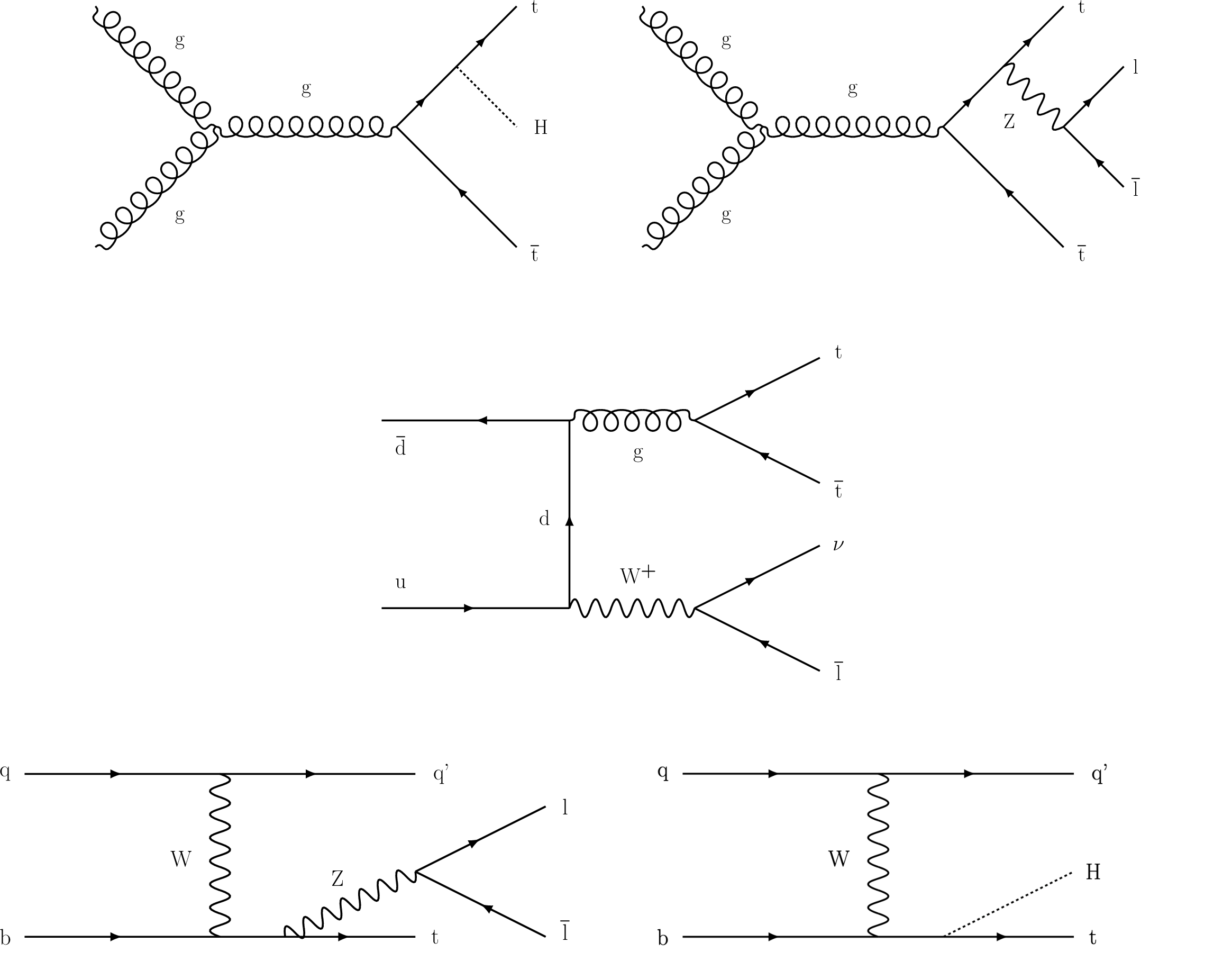
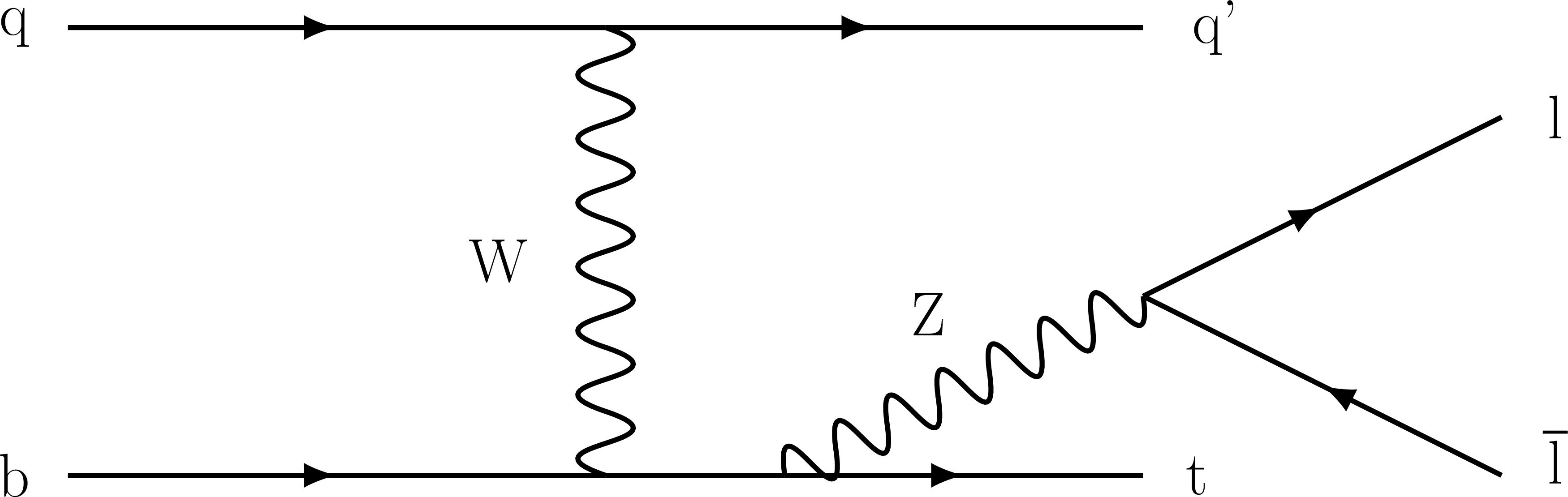
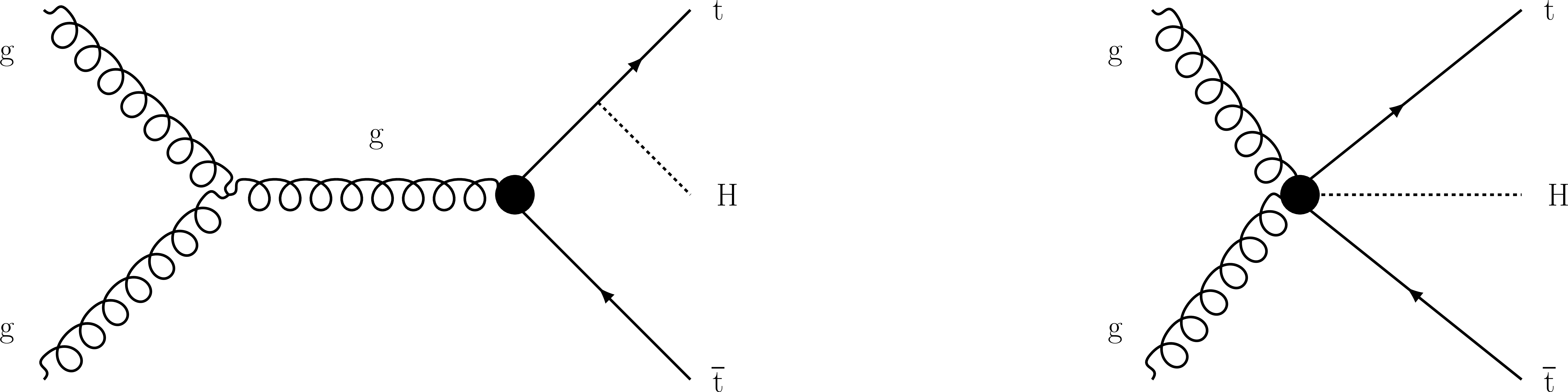
Figure 1:
Example diagrams for the five signal processes considered in this analysis: ${\mathrm{t} \mathrm{\bar{t}} \mathrm{H}}$, ${\mathrm{t} \mathrm{\bar{t}} \ell \bar{\ell}}$, ${\mathrm{t} \mathrm{\bar{t}} \ell \nu}$, ${\mathrm{t} \ell \bar{\ell} \mathrm{q}}$, and ${\mathrm{t} \mathrm{H} \mathrm{q}}$. |
png pdf |
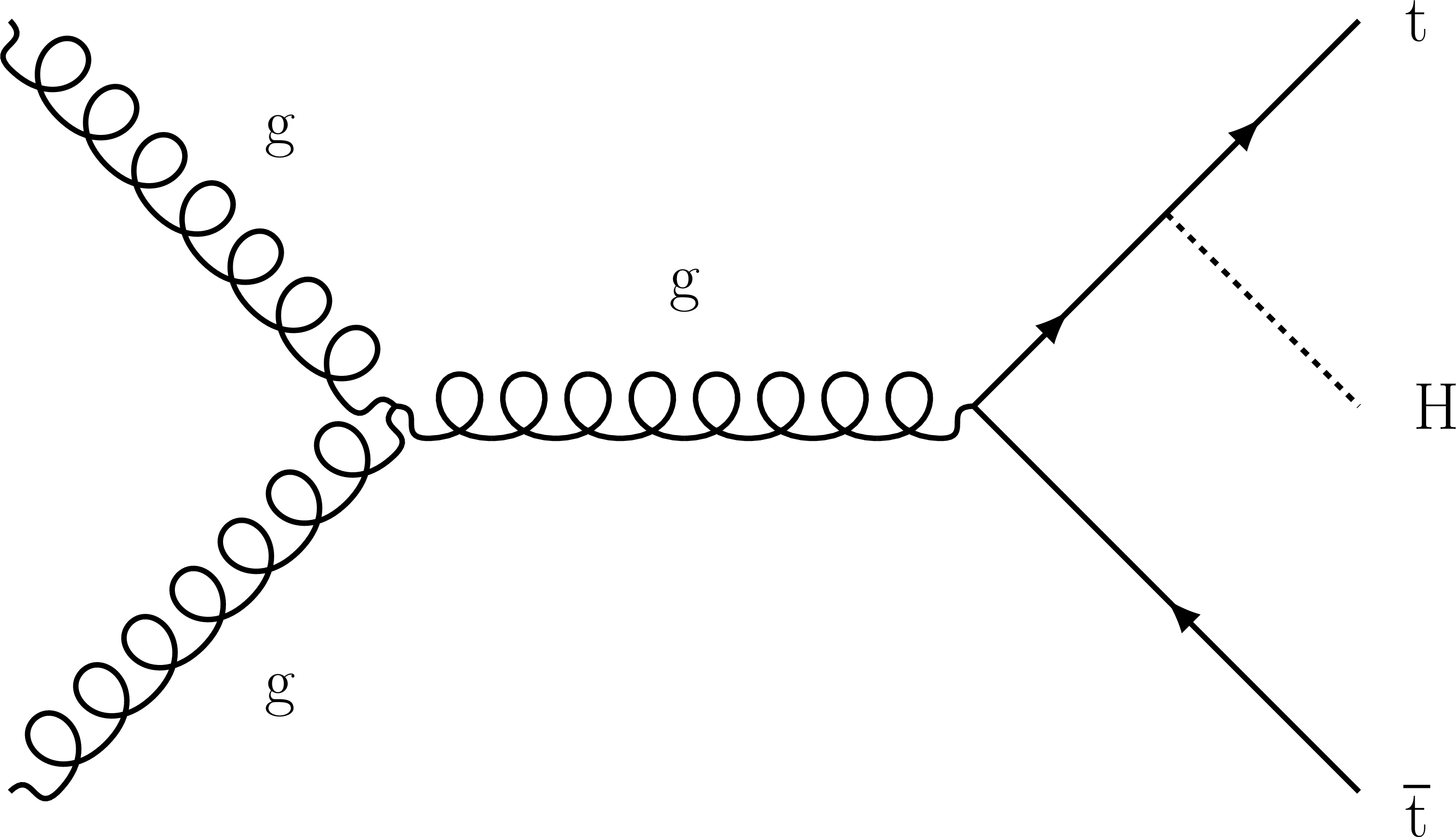
Figure 1-a:
Example diagram for the ${\mathrm{t} \mathrm{\bar{t}} \mathrm{H}}$ signal process. |
png pdf |
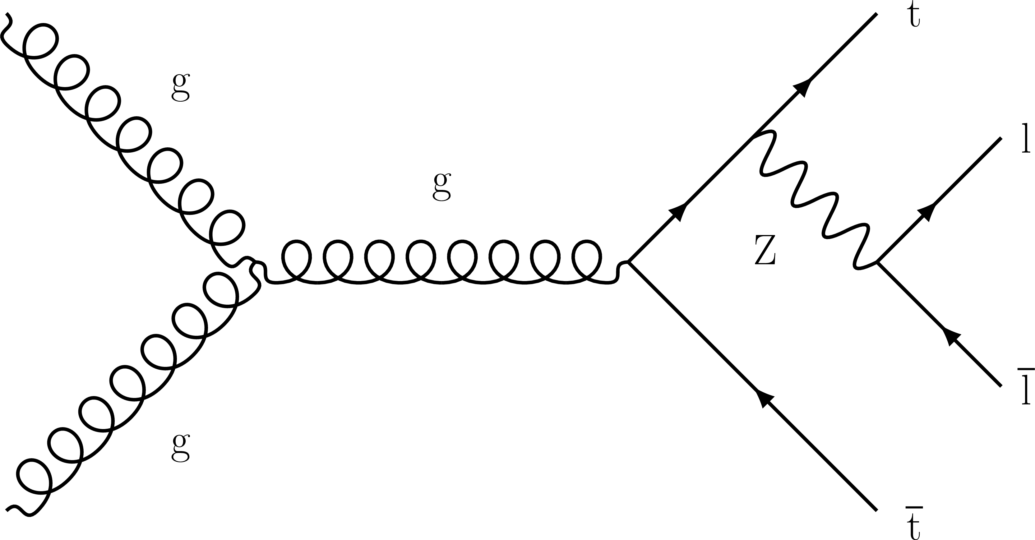
Figure 1-b:
Example diagram for the ${\mathrm{t} \mathrm{\bar{t}} \ell \bar{\ell}}$ signal process. |
png pdf |
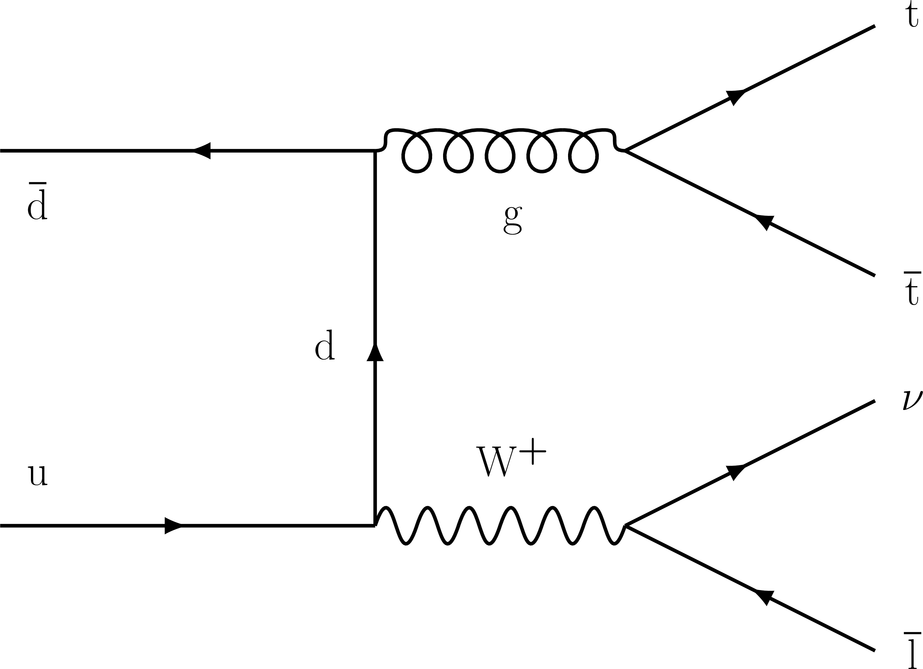
Figure 1-c:
Example diagram for the ${\mathrm{t} \mathrm{\bar{t}} \ell \nu}$ signal process. |
png pdf |
Figure 1-d:
Example diagram for the ${\mathrm{t} \ell \bar{\ell} \mathrm{q}}$ signal process. |

png pdf |
Figure 1-e:
Example diagram for the ${\mathrm{t} \mathrm{H} \mathrm{q}}$ signal process. |
png pdf |
Figure 2:
Example diagrams showing two of the vertices associated with the $ \mathcal{O}_{\mathcal{uG}} $ operator. This operator, whose definition can be found in Table 1, gives rise to vertices involving top quarks, gluons, and the Higgs boson; as illustrated here, these interactions can contribute to the ${\mathrm{t} \mathrm{\bar{t}} \mathrm{H}}$ process. |

png pdf |
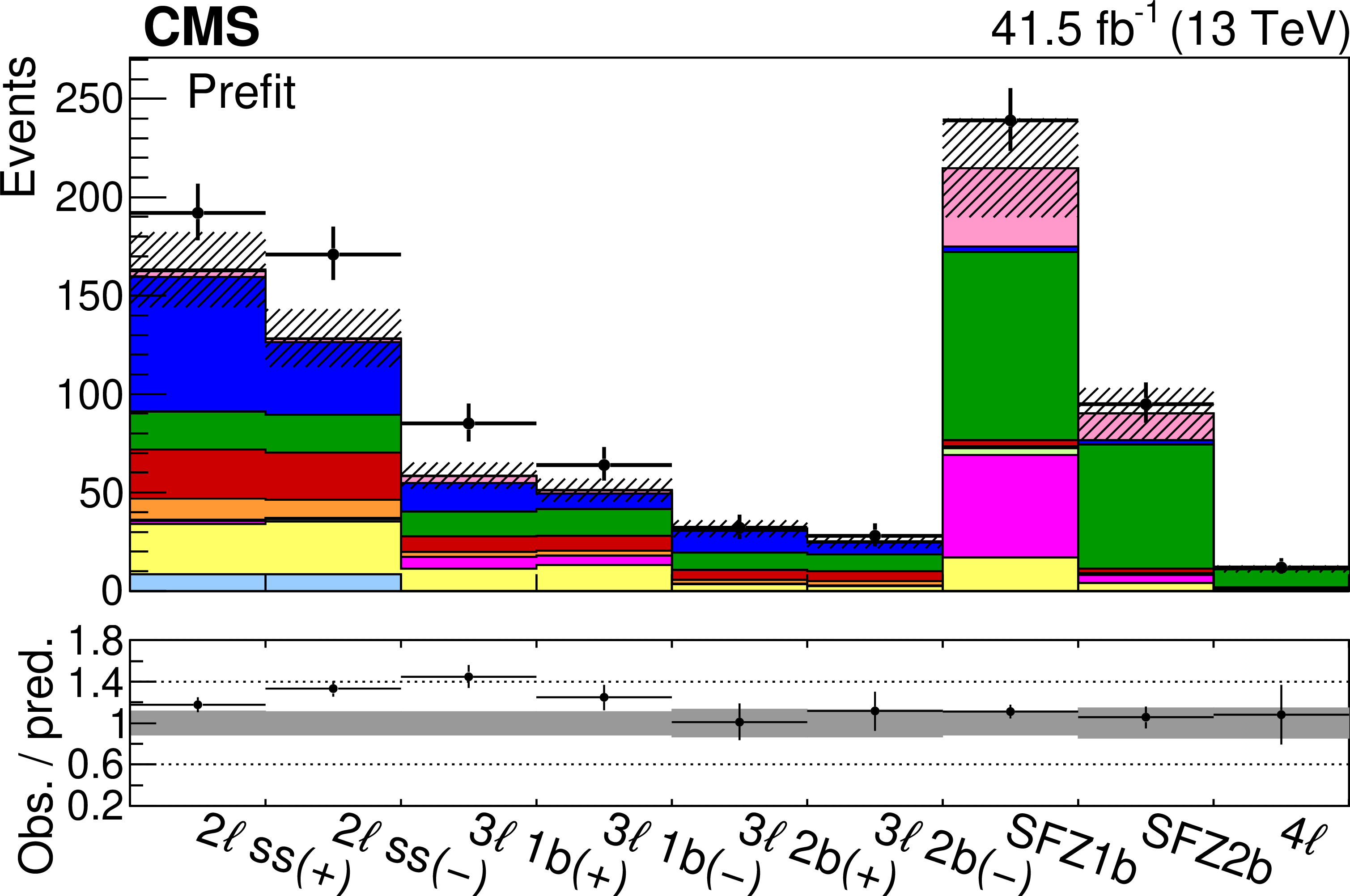
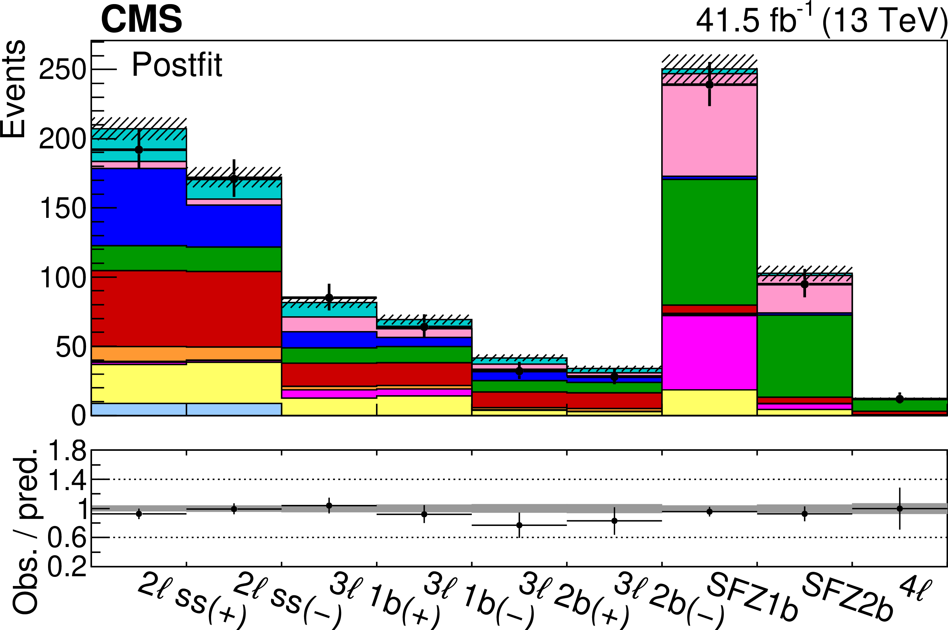
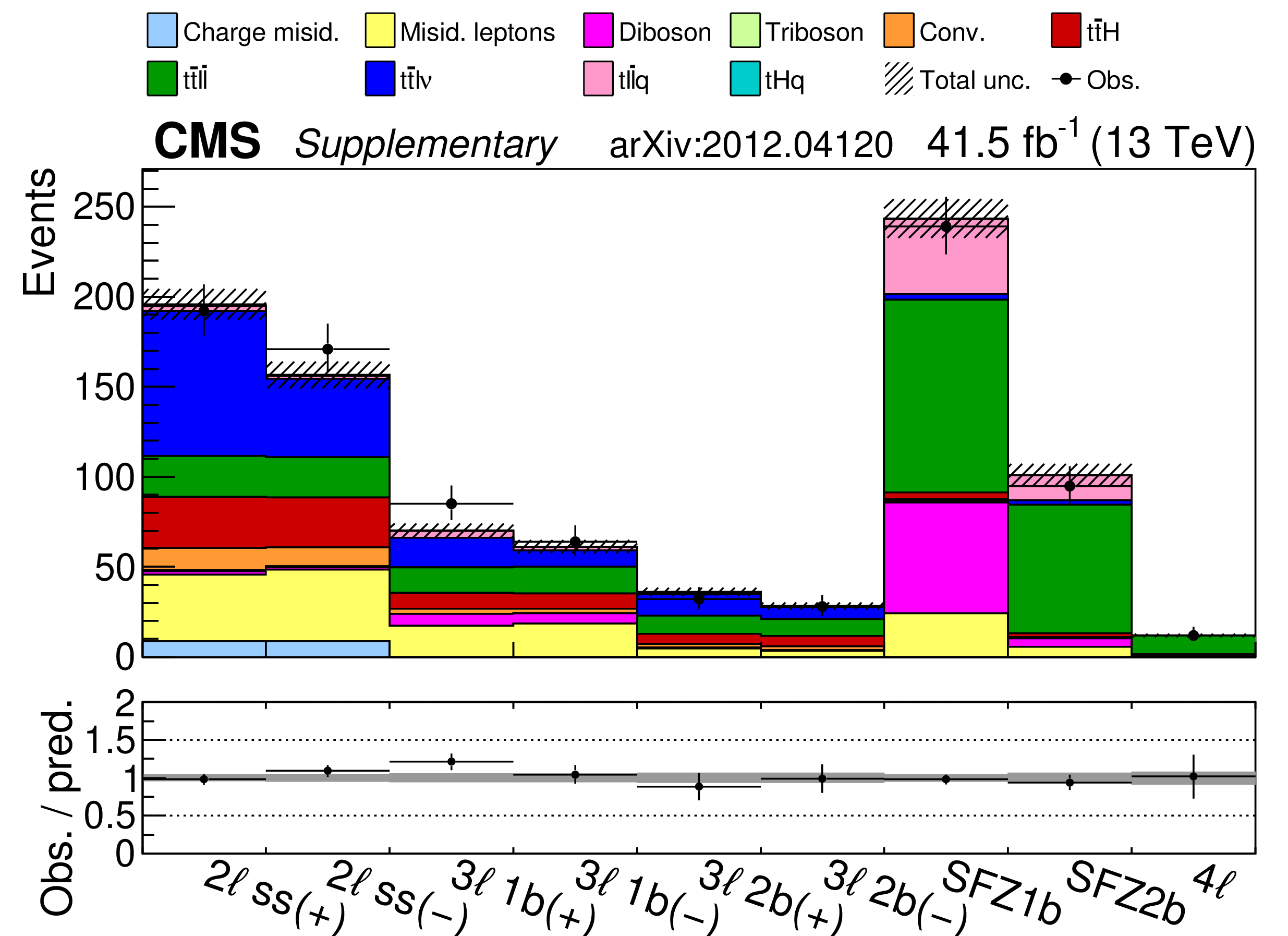
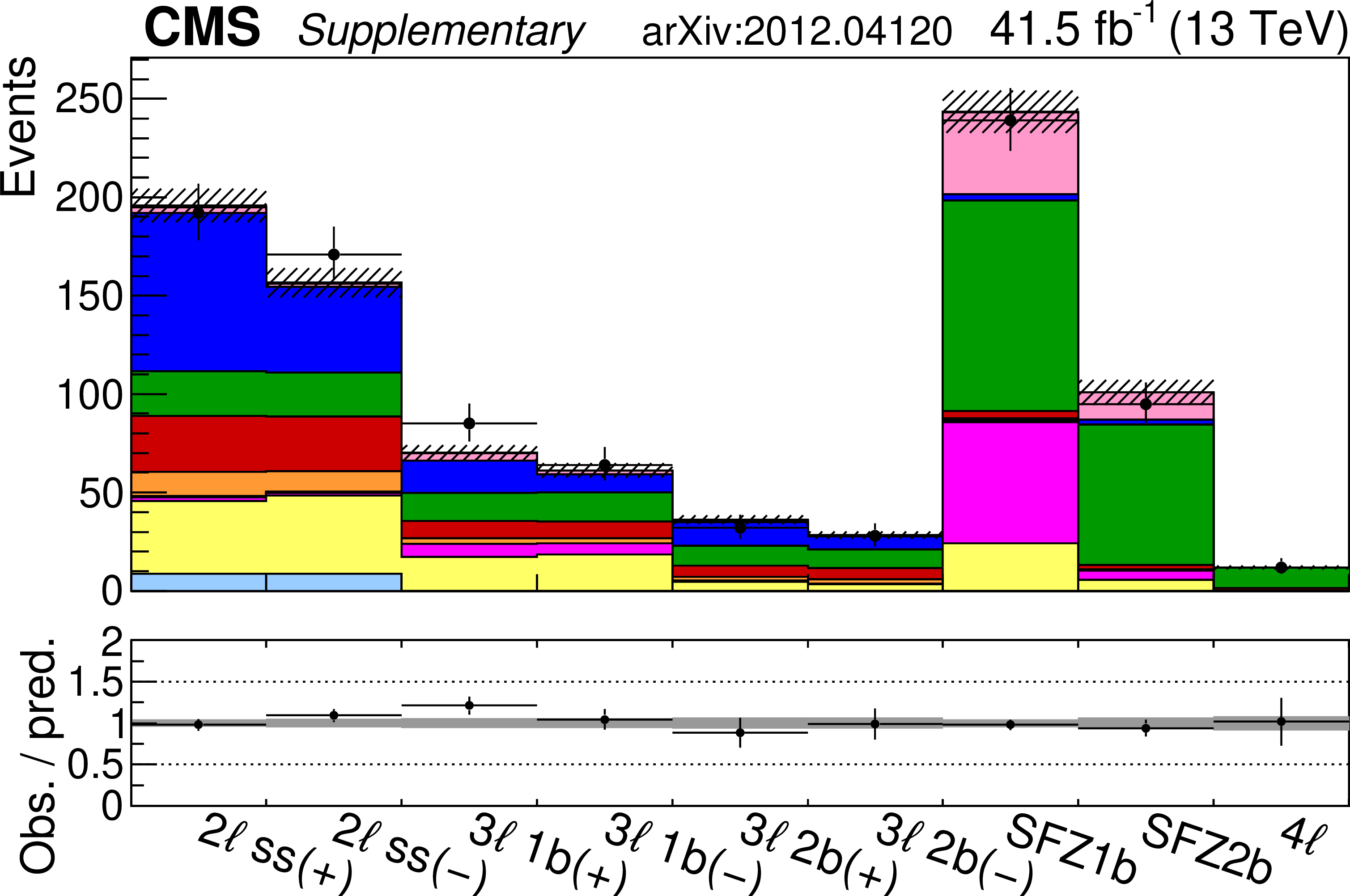
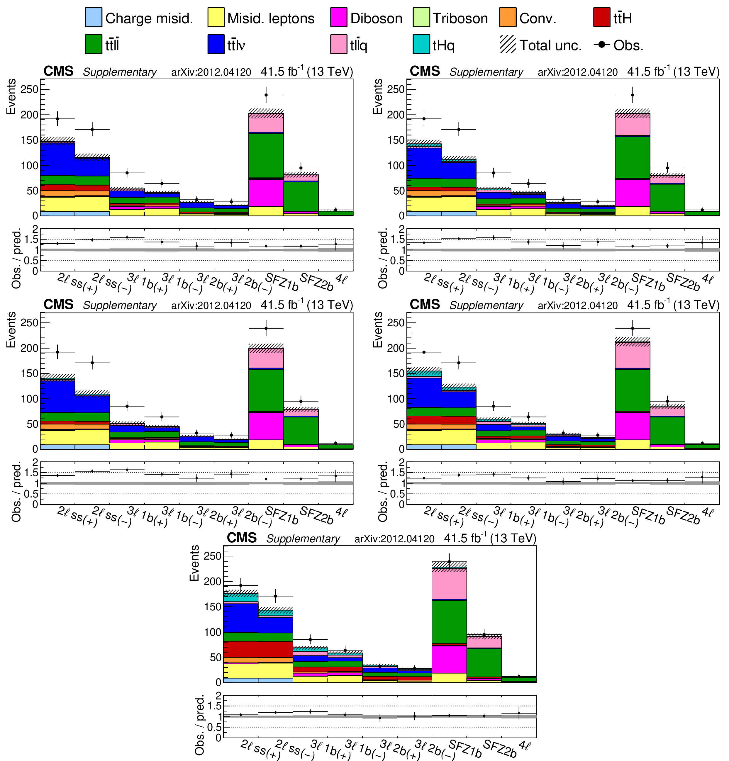
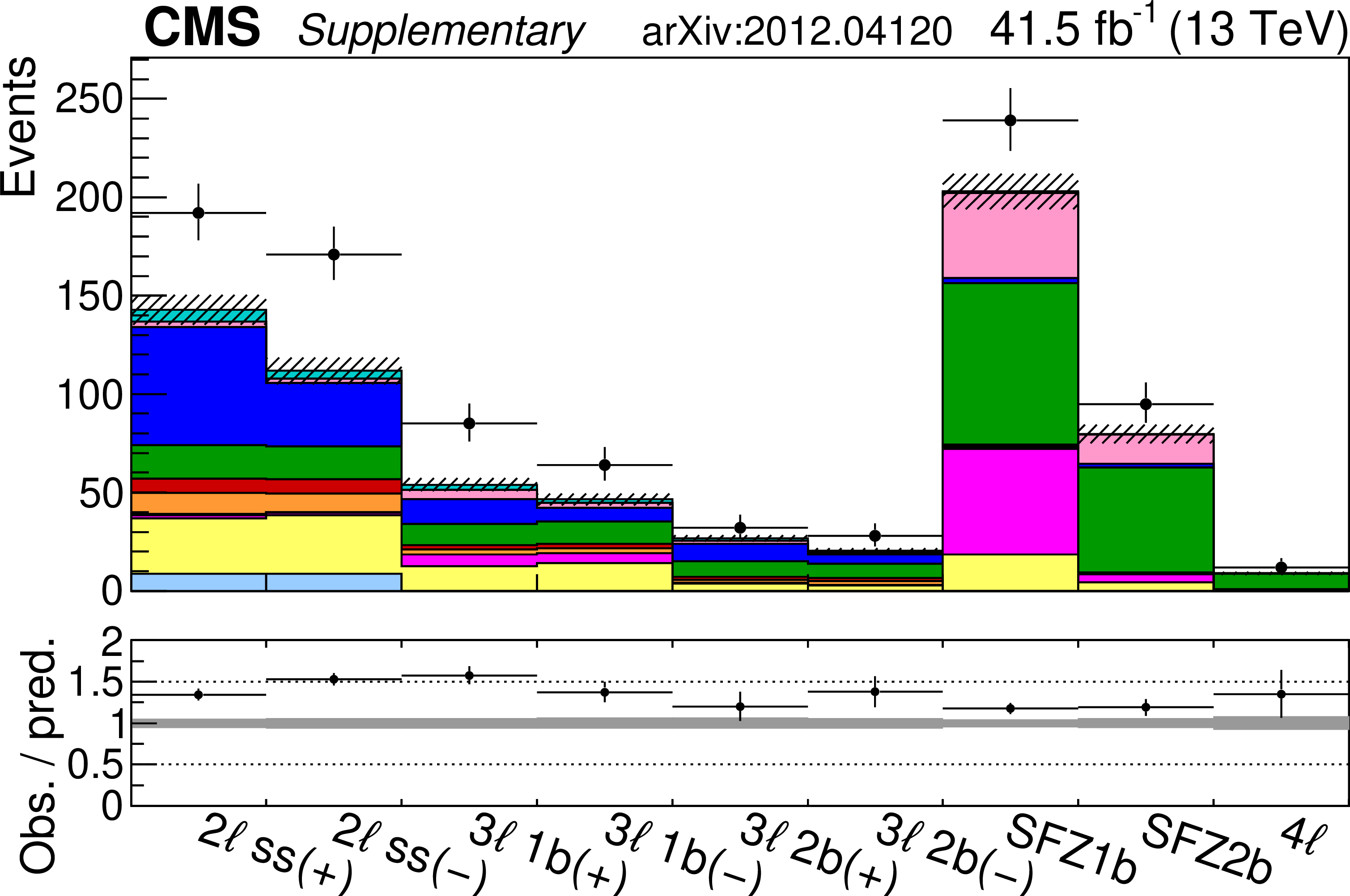
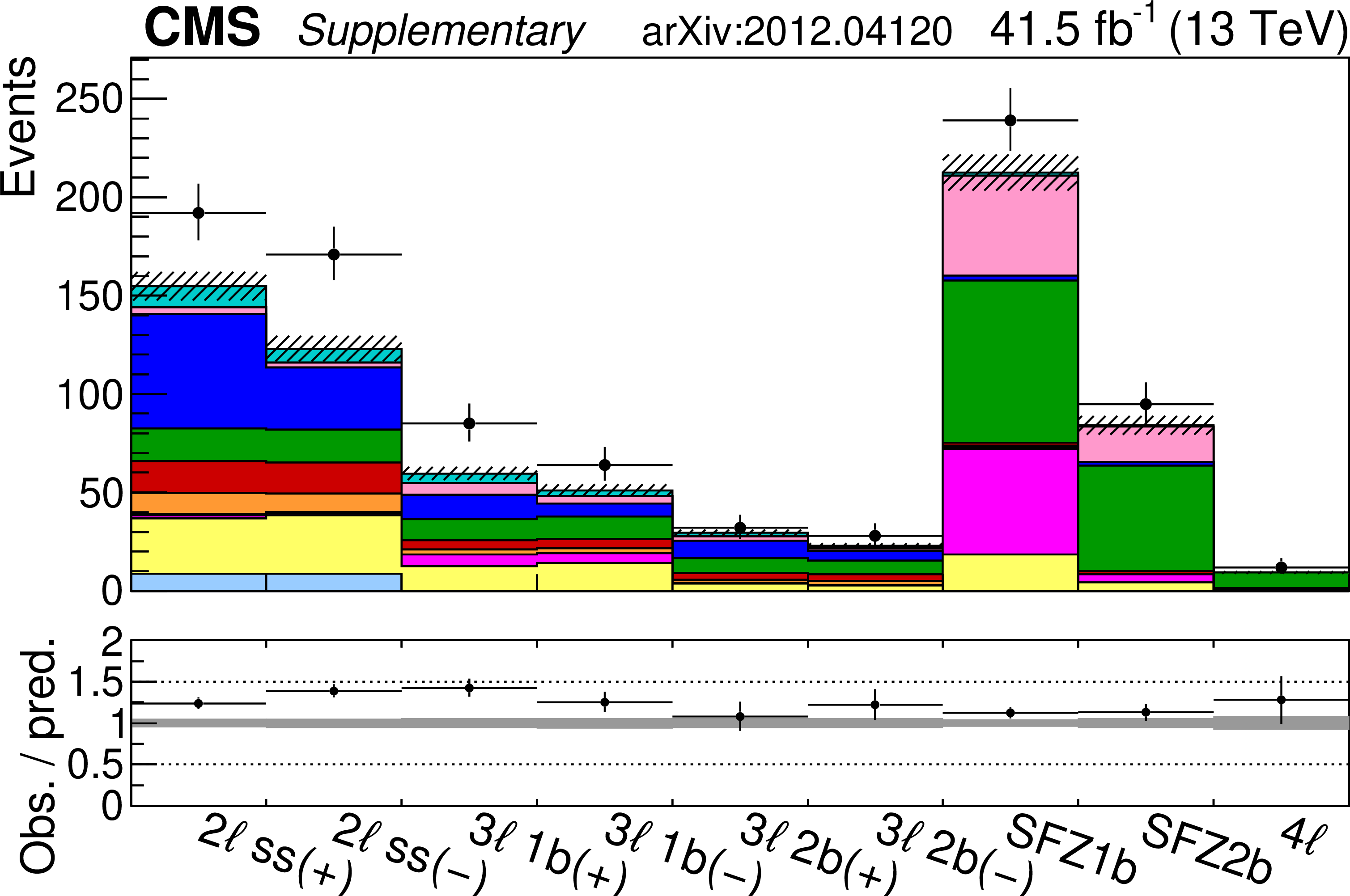
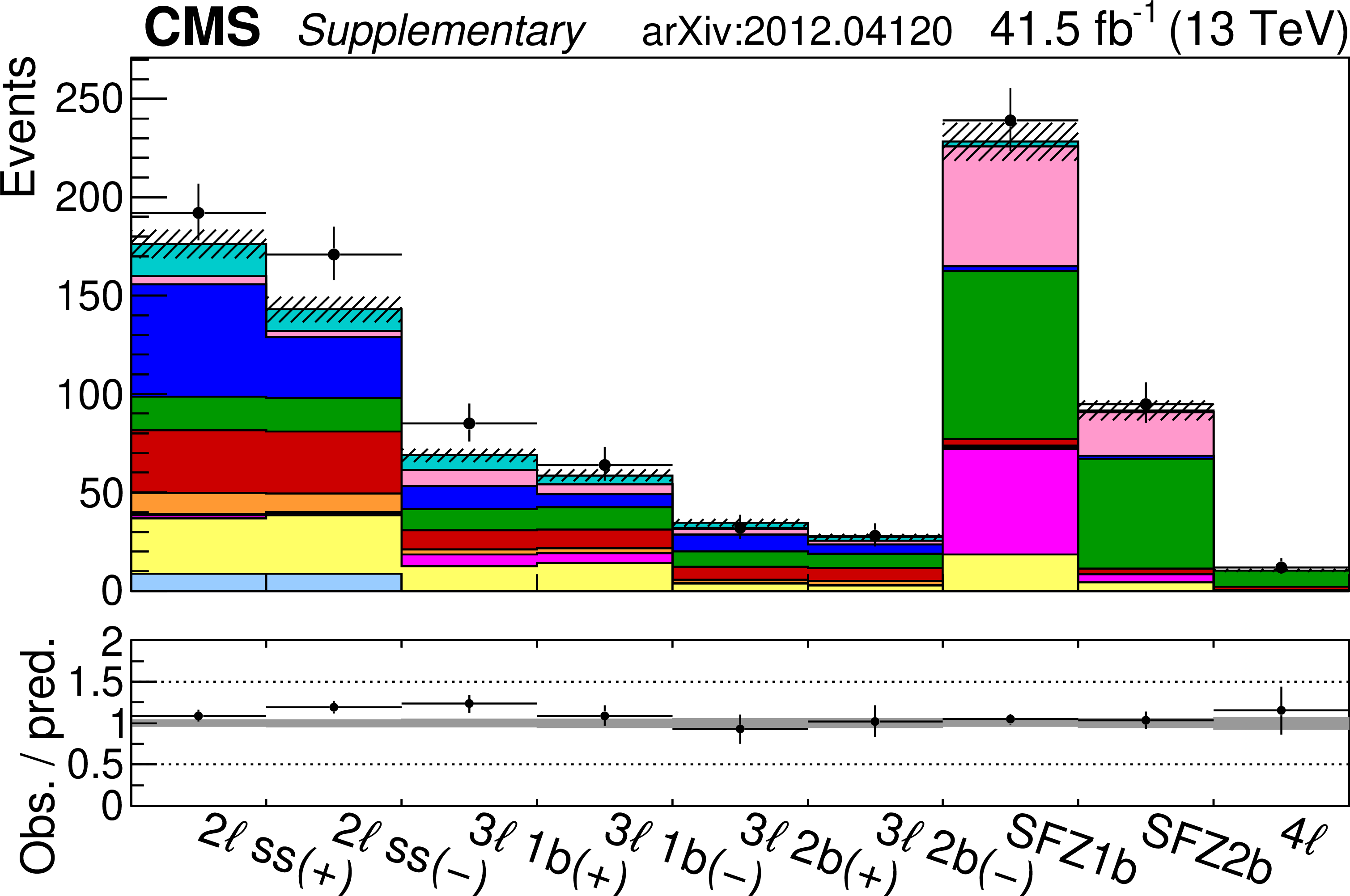
Figure 3:
Expected yields prefit (left) and postfit (right). The postfit values of the WCs are obtained from performing the fit over all WCs simultaneously. "Conv." refers to the photon conversion background, "Charge misid." is the lepton charge mismeasurement background, and "Misid. leptons" is the background from misidentified leptons. The jet multiplicity bins have been combined here, however, the fit is performed using all 35 event categories outlined in Section 5.4. The lower panel is the ratio of the observation over the prediction. |

png pdf |
Figure 3-a:
Legends for the following figures. "Conv." refers to the photon conversion background, "Charge misid." is the lepton charge mismeasurement background, and "Misid. leptons" is the background from misidentified leptons. |
png pdf |
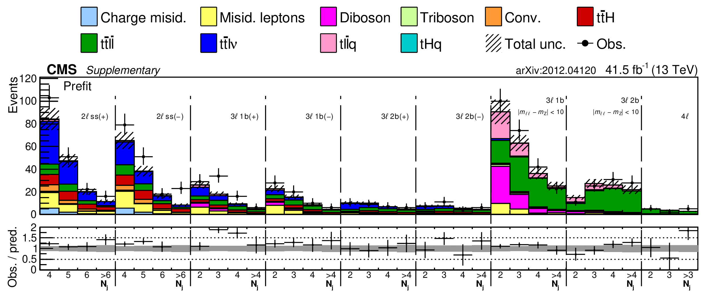
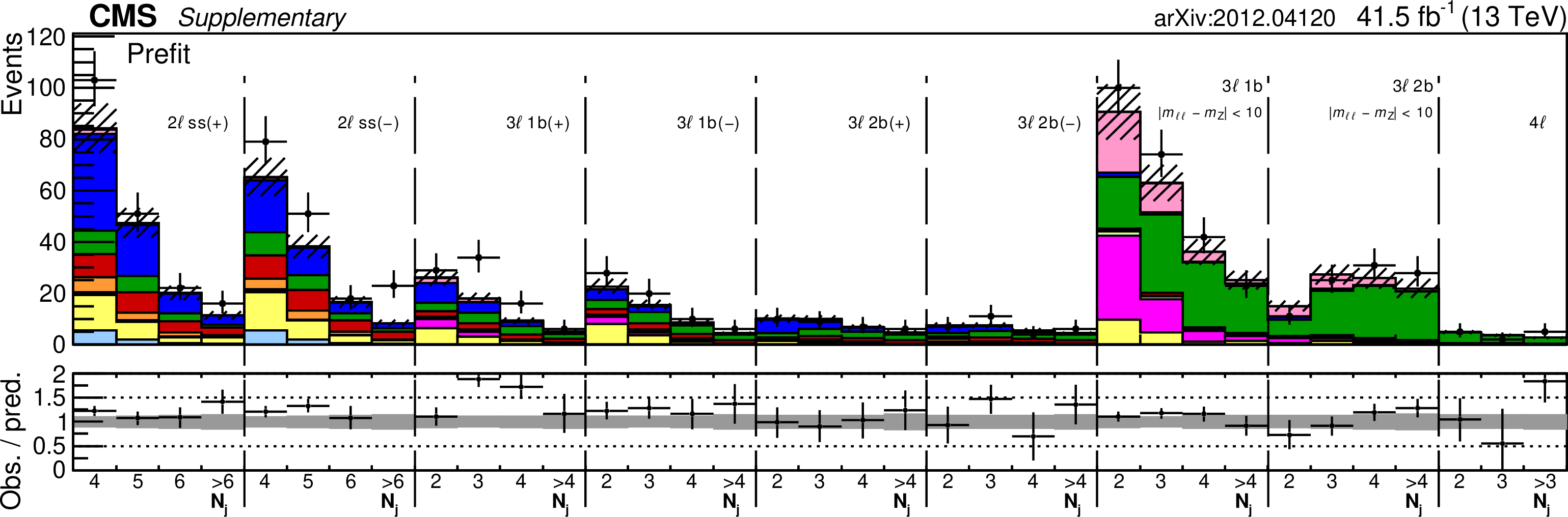
Figure 3-b:
Expected yields prefit. The jet multiplicity bins have been combined here, however, the fit is performed using all 35 event categories outlined in Section 5.4. The lower panel is the ratio of the observation over the prediction. |
png pdf |
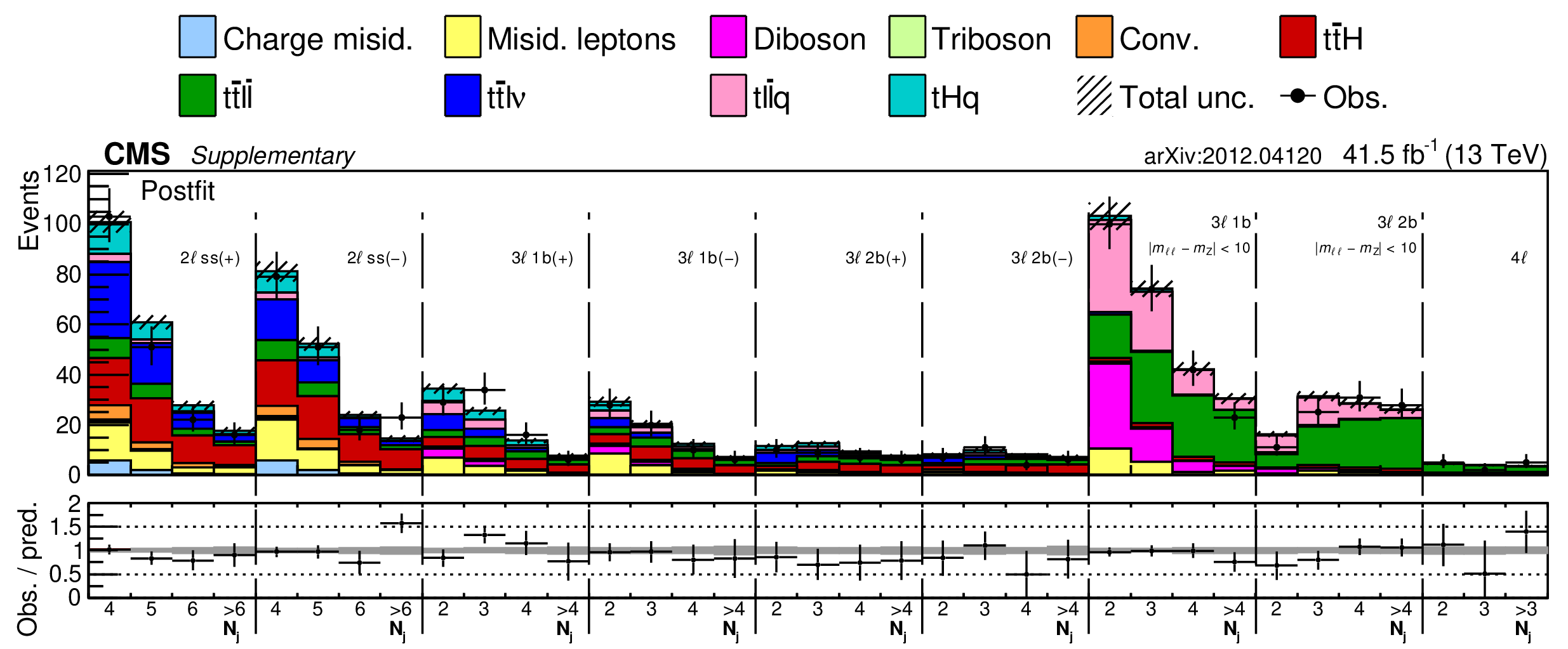
Figure 3-c:
Expected yields prefit postfit. The postfit values of the WCs are obtained from performing the fit over all WCs simultaneously. The jet multiplicity bins have been combined here, however, the fit is performed using all 35 event categories outlined in Section 5.4. The lower panel is the ratio of the observation over the prediction. |
png pdf |
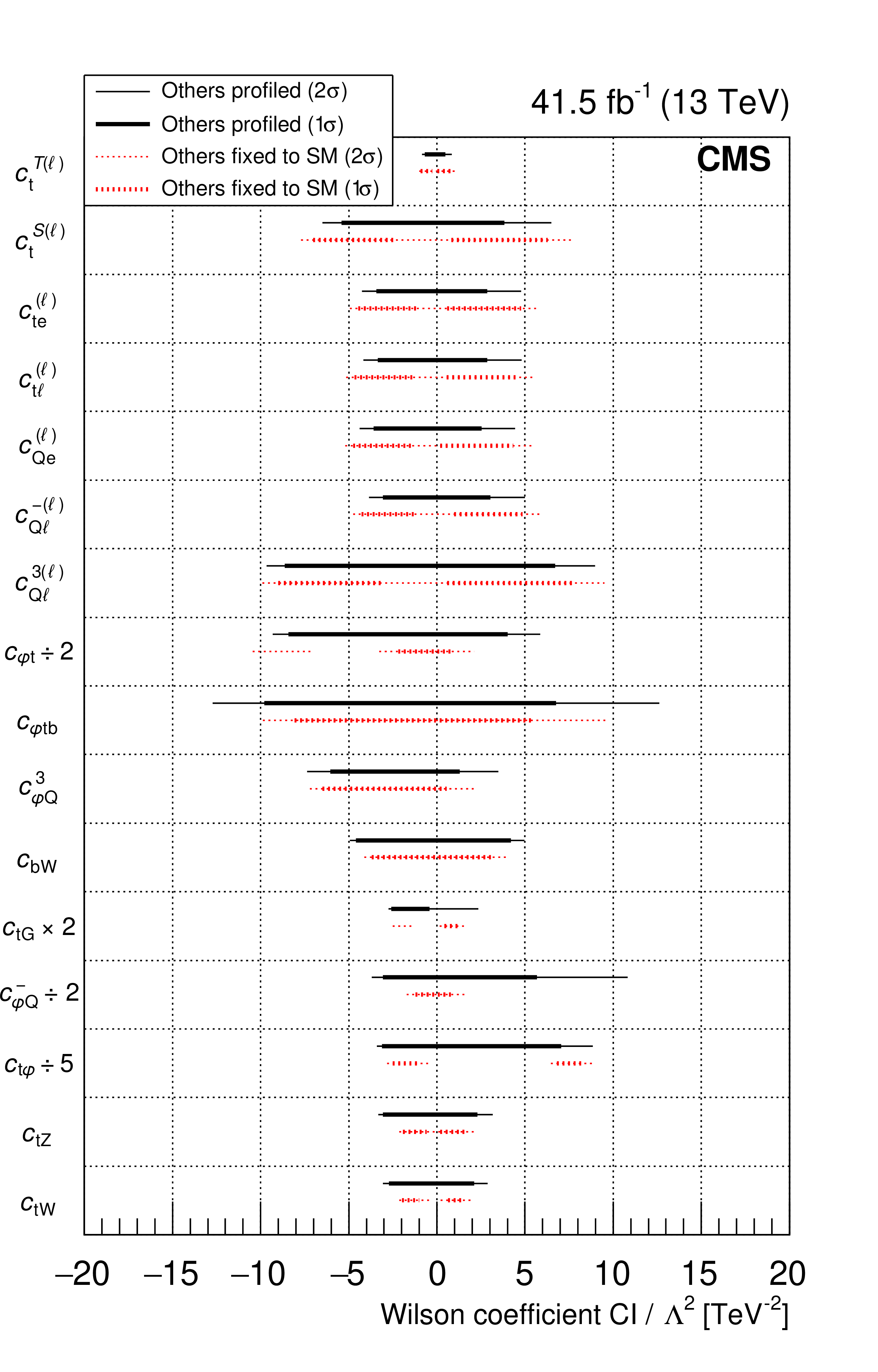
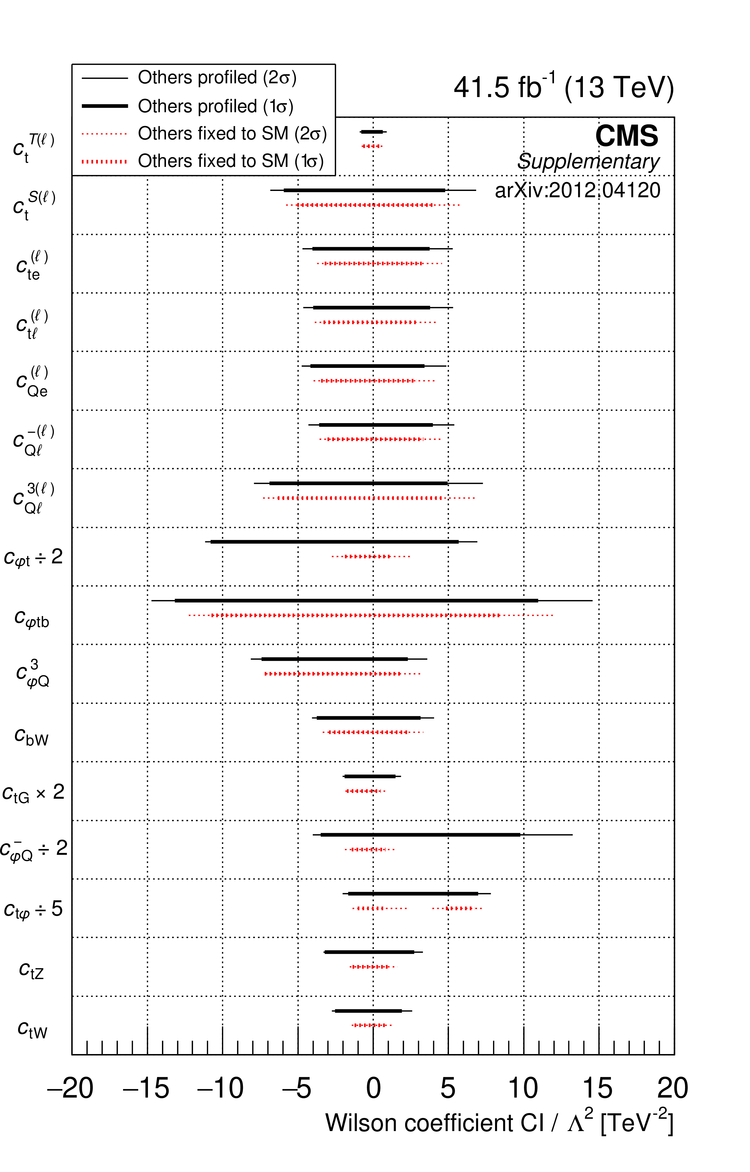
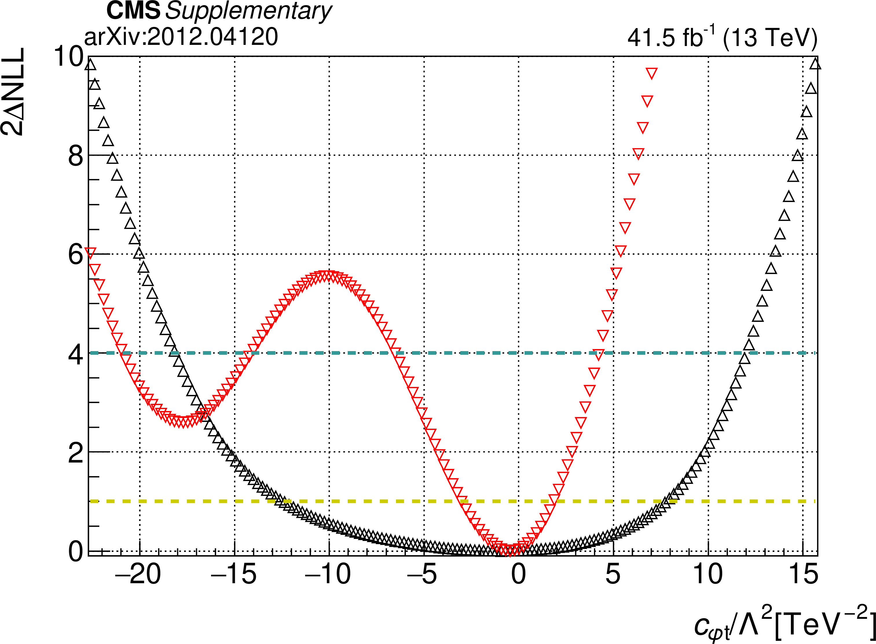
Figure 4:
Observed WC 1$\sigma $ (thick line) and 2$\sigma $ (thin line) confidence intervals (CIs). Solid lines correspond to the other WCs profiled, while dashed lines correspond to the other WCs fixed to the SM value of zero. In order to make the figure more readable, the ${{c _{\varphi \mathrm{t}}}}$ interval is scaled by 1/2, the ${{c _{\mathrm{t} G}}}$ interval is scaled by 2, the ${{c ^{-}_{\varphi Q}}}$ interval is scaled by 1/2, and the ${{c _{\mathrm{t} \varphi}}}$ interval is scaled by 1/5. |
png pdf |
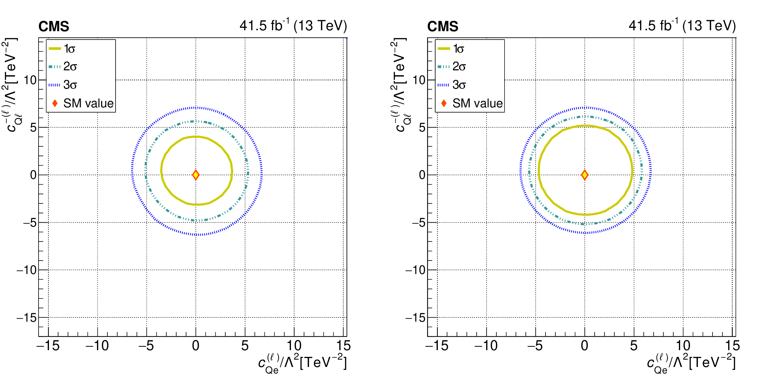
Figure 5:
The observed 1$\sigma $, 2$\sigma $, and 3$\sigma $ confidence contours of a 2D scan for ${{c ^{-(\ell)}_{Q\ell}}}$ and ${{c ^{(\ell)}_{Q\mathrm{e}}}}$ with the other WCs profiled (left), and fixed to their SM values (right). Diamond markers are shown for the SM prediction. |
png pdf |
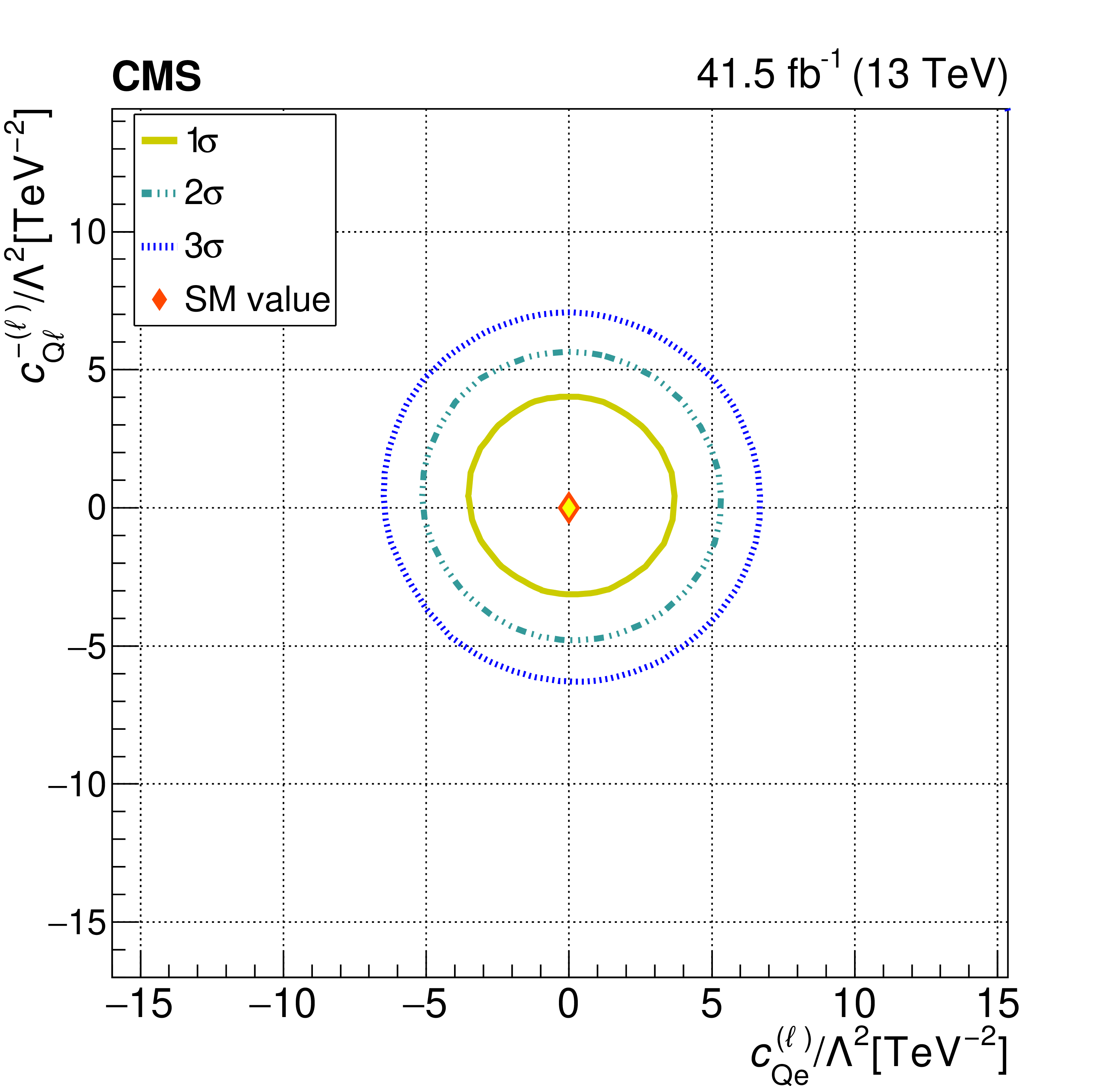
Figure 5-a:
The observed 1$\sigma $, 2$\sigma $, and 3$\sigma $ confidence contours of a 2D scan for ${{c ^{-(\ell)}_{Q\ell}}}$ and ${{c ^{(\ell)}_{Q\mathrm{e}}}}$ with the other WCs profiled. Diamond markers are shown for the SM prediction. |

png pdf |
Figure 5-b:
The observed 1$\sigma $, 2$\sigma $, and 3$\sigma $ confidence contours of a 2D scan for ${{c ^{-(\ell)}_{Q\ell}}}$ and ${{c ^{(\ell)}_{Q\mathrm{e}}}}$ with the other WCs fixed to their SM values. Diamond markers are shown for the SM prediction. |
png pdf |
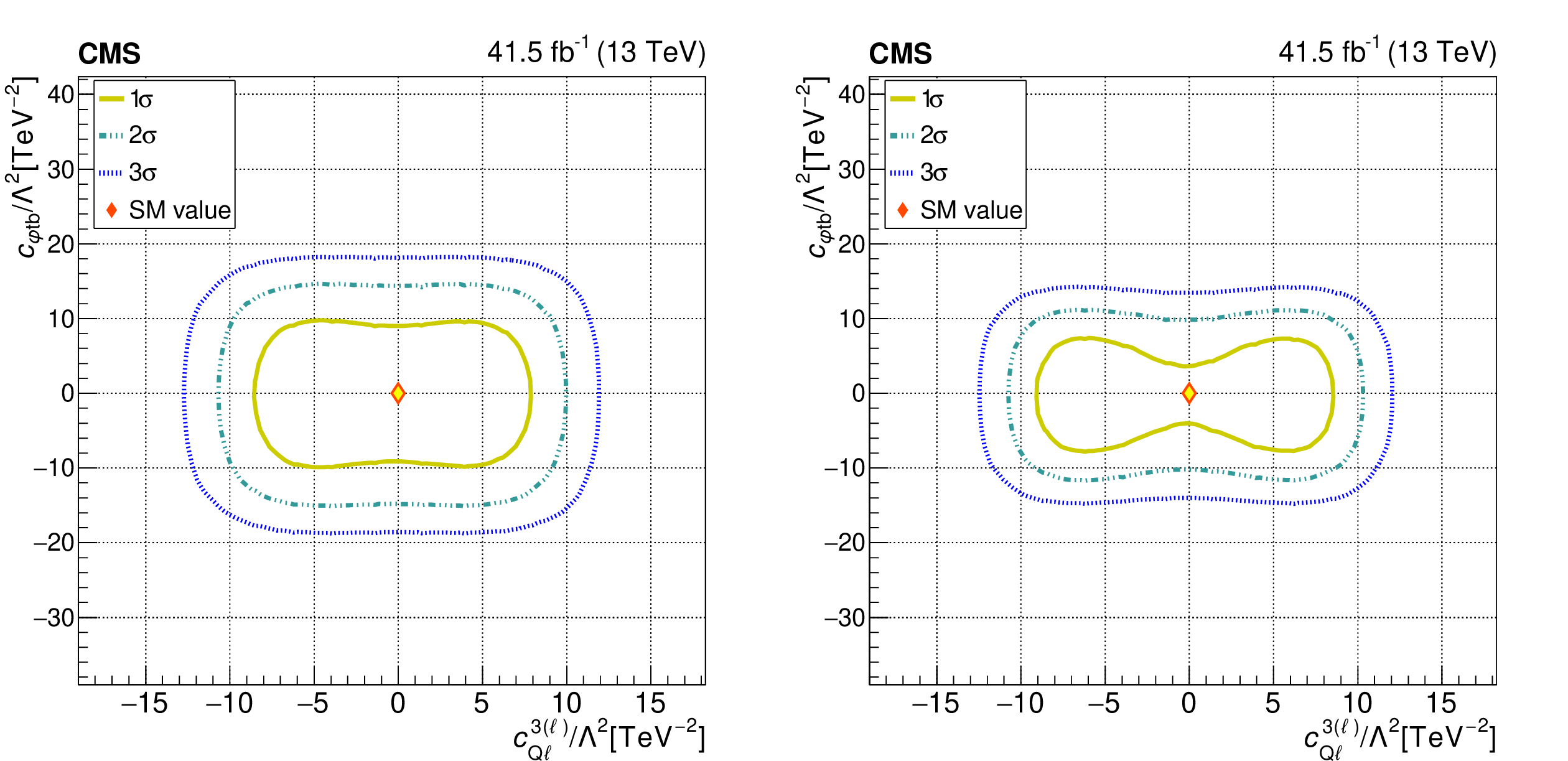
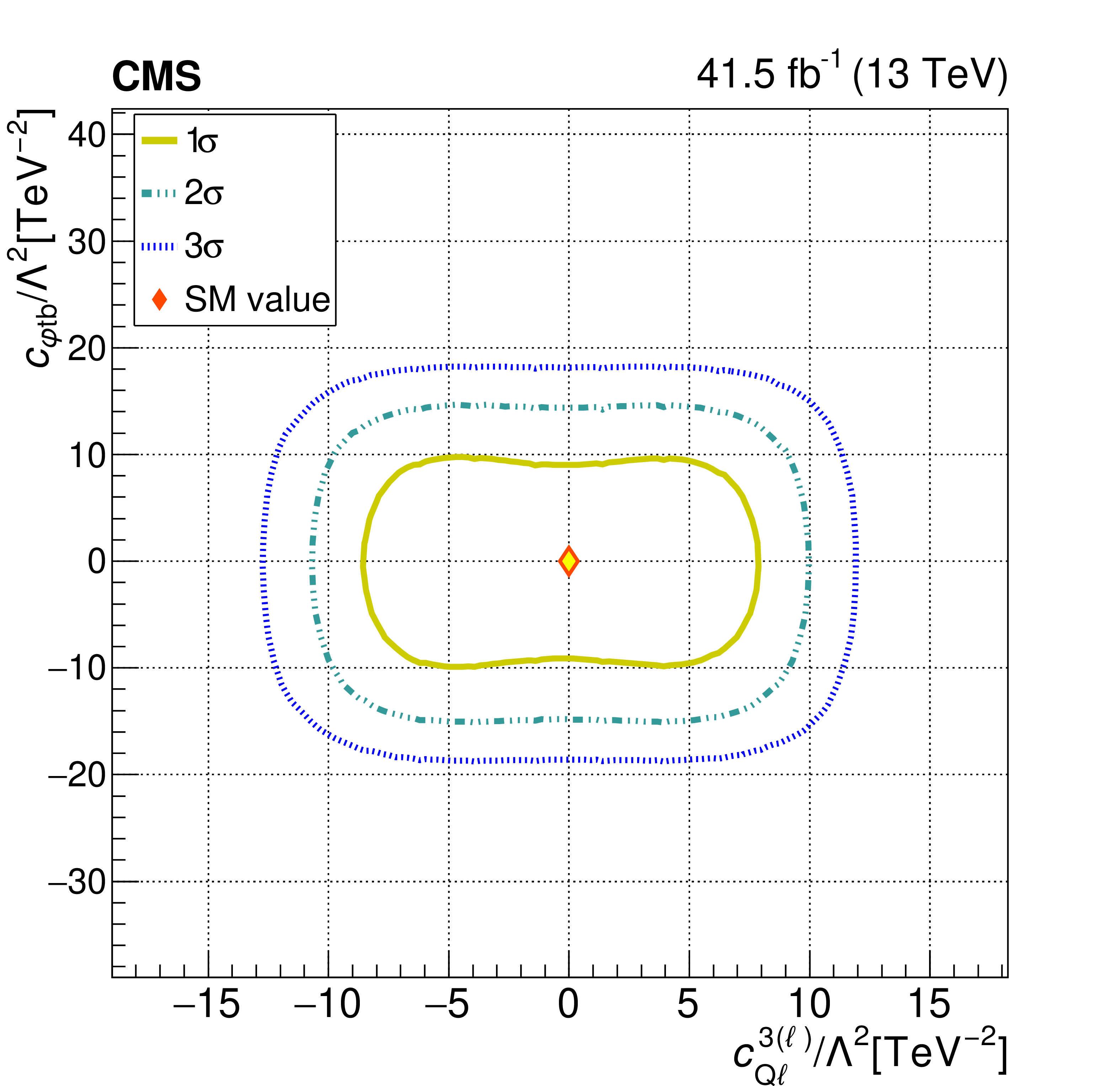
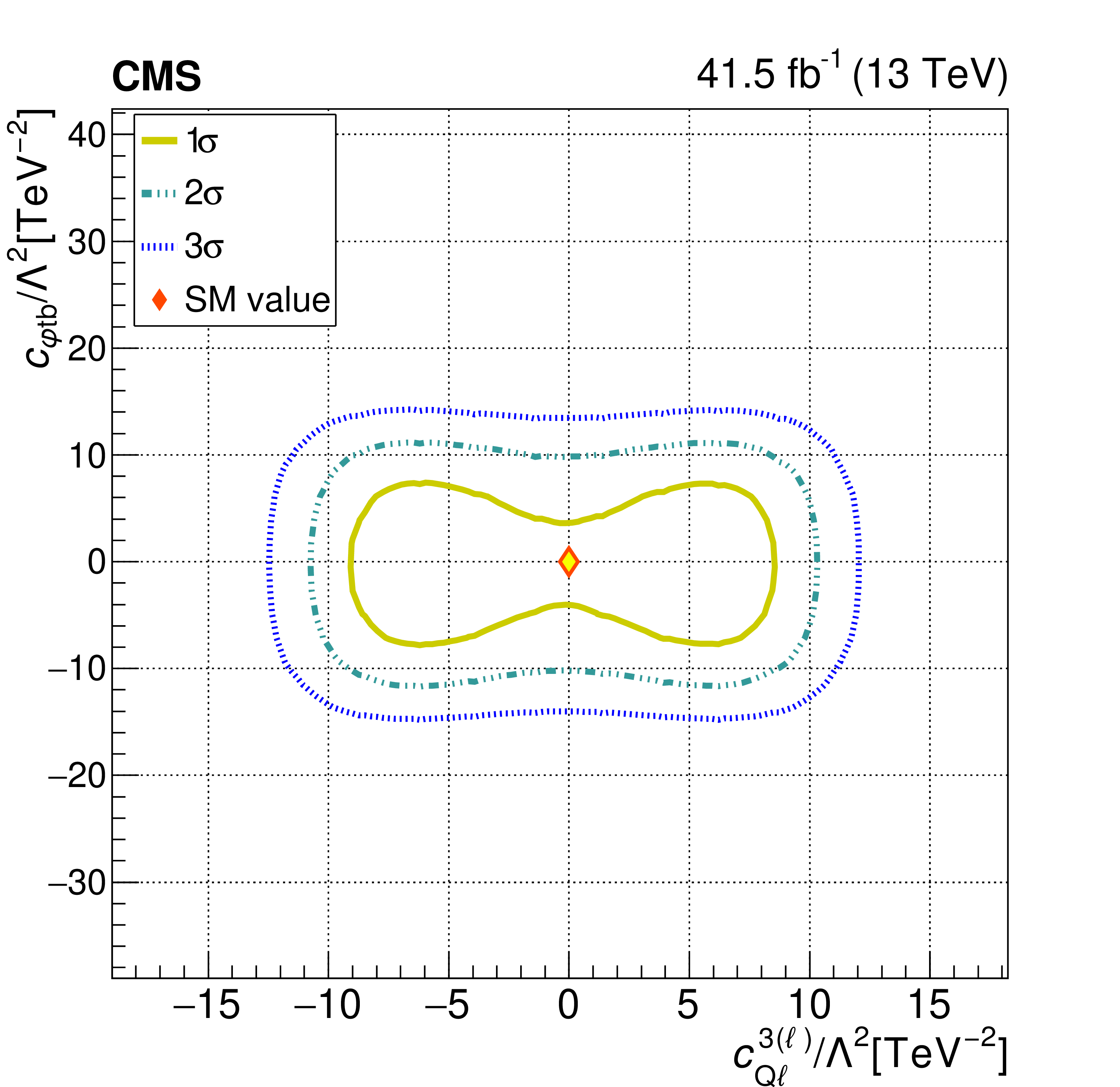
Figure 6:
The observed 1$\sigma $, 2$\sigma $, and 3$\sigma $ confidence contours of a 2D scan for ${{c _{\varphi \mathrm{t} \mathrm{b}}}}$ and ${c ^{3(\ell)}_{Q\ell}}$ with the other WCs profiled (left), and fixed to their SM values (right). Diamond markers are shown for the SM prediction. |
png pdf |
Figure 6-a:
The observed 1$\sigma $, 2$\sigma $, and 3$\sigma $ confidence contours of a 2D scan for ${{c _{\varphi \mathrm{t} \mathrm{b}}}}$ and ${c ^{3(\ell)}_{Q\ell}}$ with the other WCs profiled. Diamond markers are shown for the SM prediction. |
png pdf |
Figure 6-b:
The observed 1$\sigma $, 2$\sigma $, and 3$\sigma $ confidence contours of a 2D scan for ${{c _{\varphi \mathrm{t} \mathrm{b}}}}$ and ${c ^{3(\ell)}_{Q\ell}}$ with the other WCs fixed to their SM values. Diamond markers are shown for the SM prediction. |
png pdf |
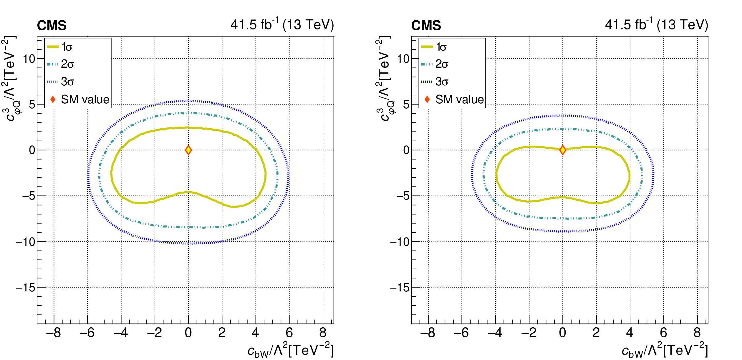
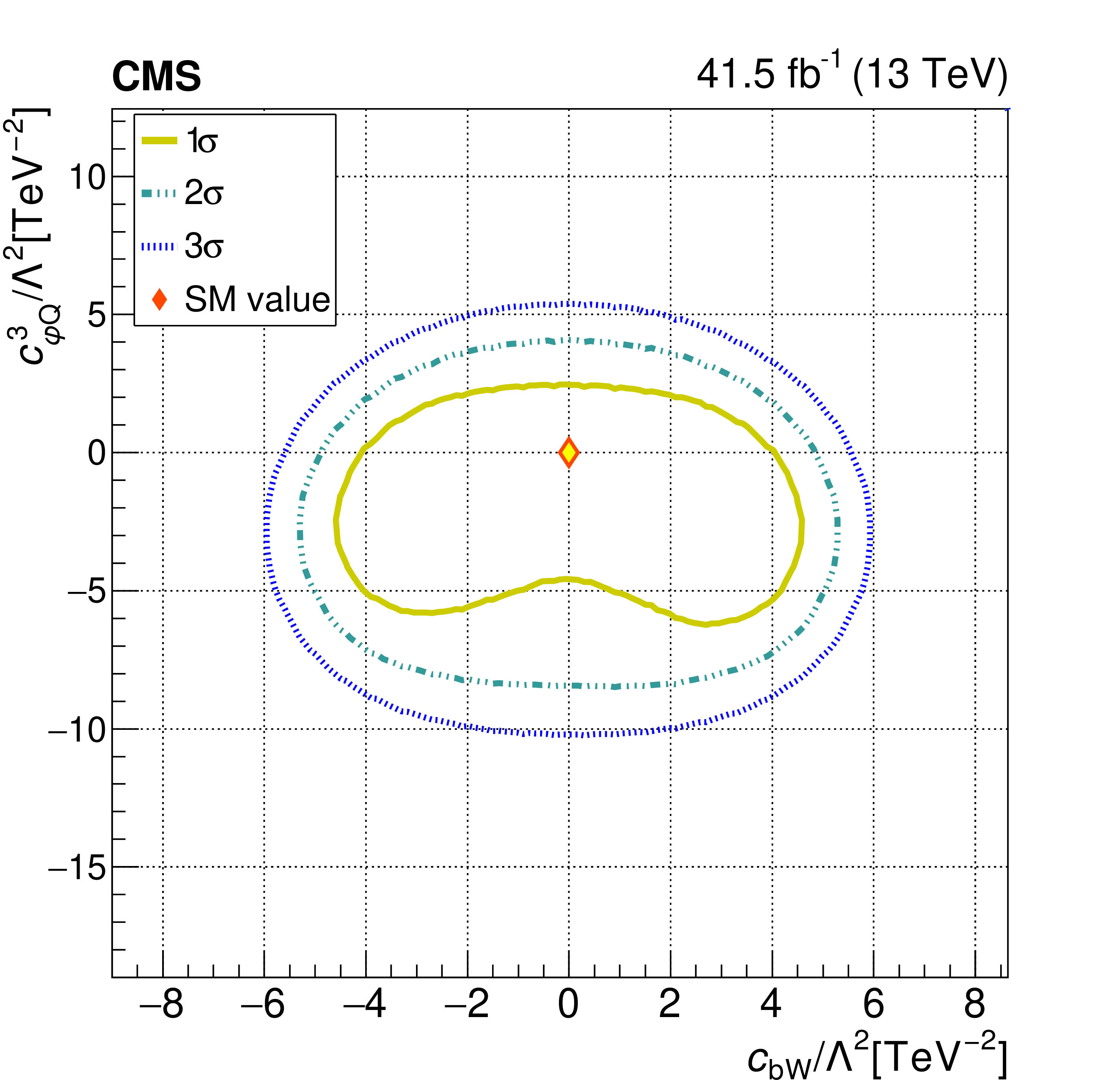
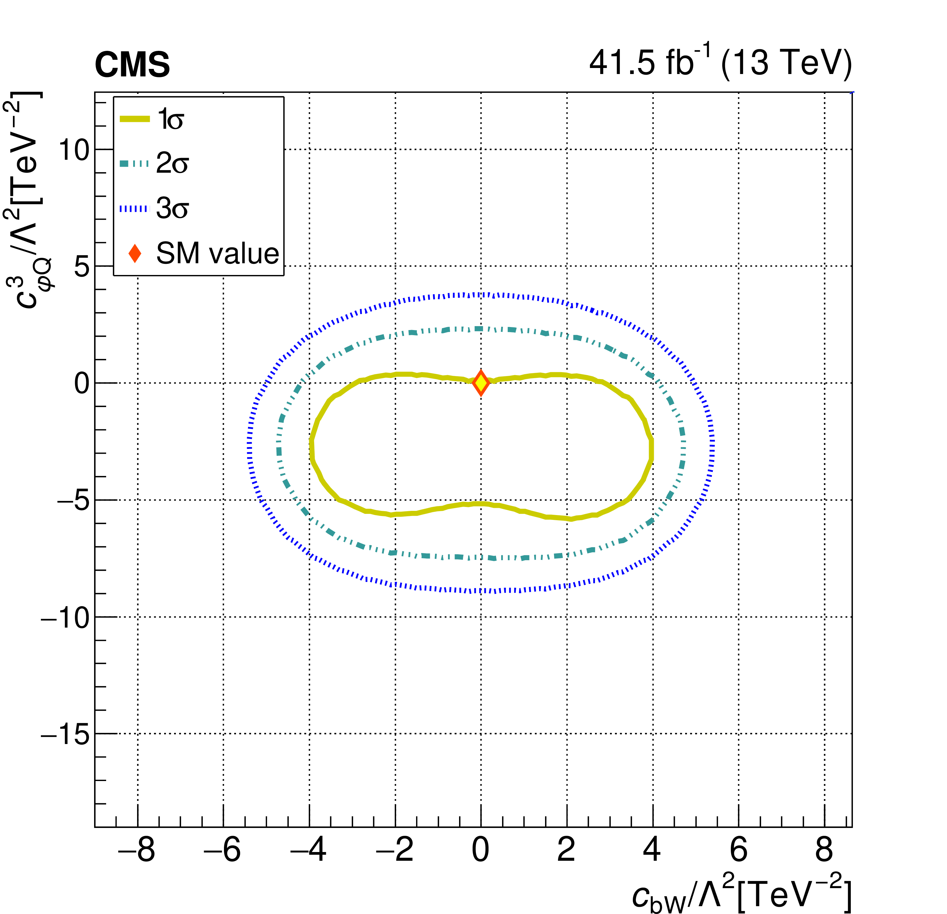
Figure 7:
The observed 1$\sigma $, 2$\sigma $, and 3$\sigma $ confidence contours of a 2D scan for ${{c ^{3}_{\varphi Q}}}$ and ${{c _{\mathrm{b} \mathrm{W}}}}$ with the other WCs profiled (left), and fixed to their SM values (right). Diamond markers are shown for the SM prediction. |
png pdf |
Figure 7-a:
The observed 1$\sigma $, 2$\sigma $, and 3$\sigma $ confidence contours of a 2D scan for ${{c ^{3}_{\varphi Q}}}$ and ${{c _{\mathrm{b} \mathrm{W}}}}$ with the other WCs profiled. Diamond markers are shown for the SM prediction. |
png pdf |
Figure 7-b:
The observed 1$\sigma $, 2$\sigma $, and 3$\sigma $ confidence contours of a 2D scan for ${{c ^{3}_{\varphi Q}}}$ and ${{c _{\mathrm{b} \mathrm{W}}}}$ with the other WCs fixed to their SM values. Diamond markers are shown for the SM prediction. |
png pdf |
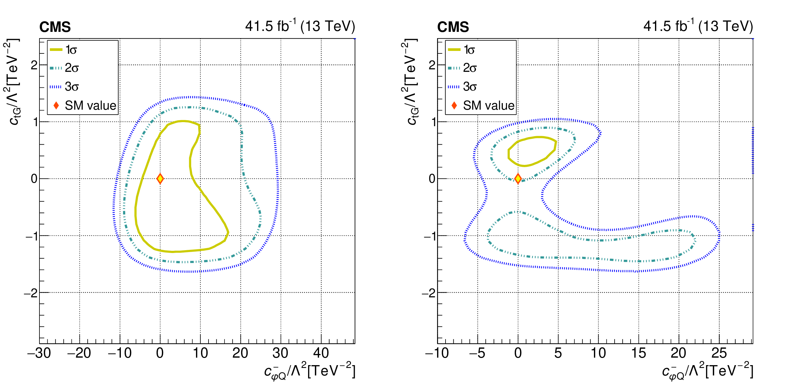
Figure 8:
The observed 1$\sigma $, 2$\sigma $, and 3$\sigma $ confidence contours of a 2D scan for ${{c _{\mathrm{t} G}}}$ and ${{c ^{-}_{\varphi Q}}}$ with the other WCs profiled (left), and fixed to their SM values (right). Diamond markers are shown for the SM prediction. The range on the right plot is modified to emphasize the 1$\sigma $ contour. |

png pdf |
Figure 8-a:
The observed 1$\sigma $, 2$\sigma $, and 3$\sigma $ confidence contours of a 2D scan for ${{c _{\mathrm{t} G}}}$ and ${{c ^{-}_{\varphi Q}}}$ with the other WCs profiled. Diamond markers are shown for the SM prediction. The range on the right plot is modified to emphasize the 1$\sigma $ contour. |
png pdf |
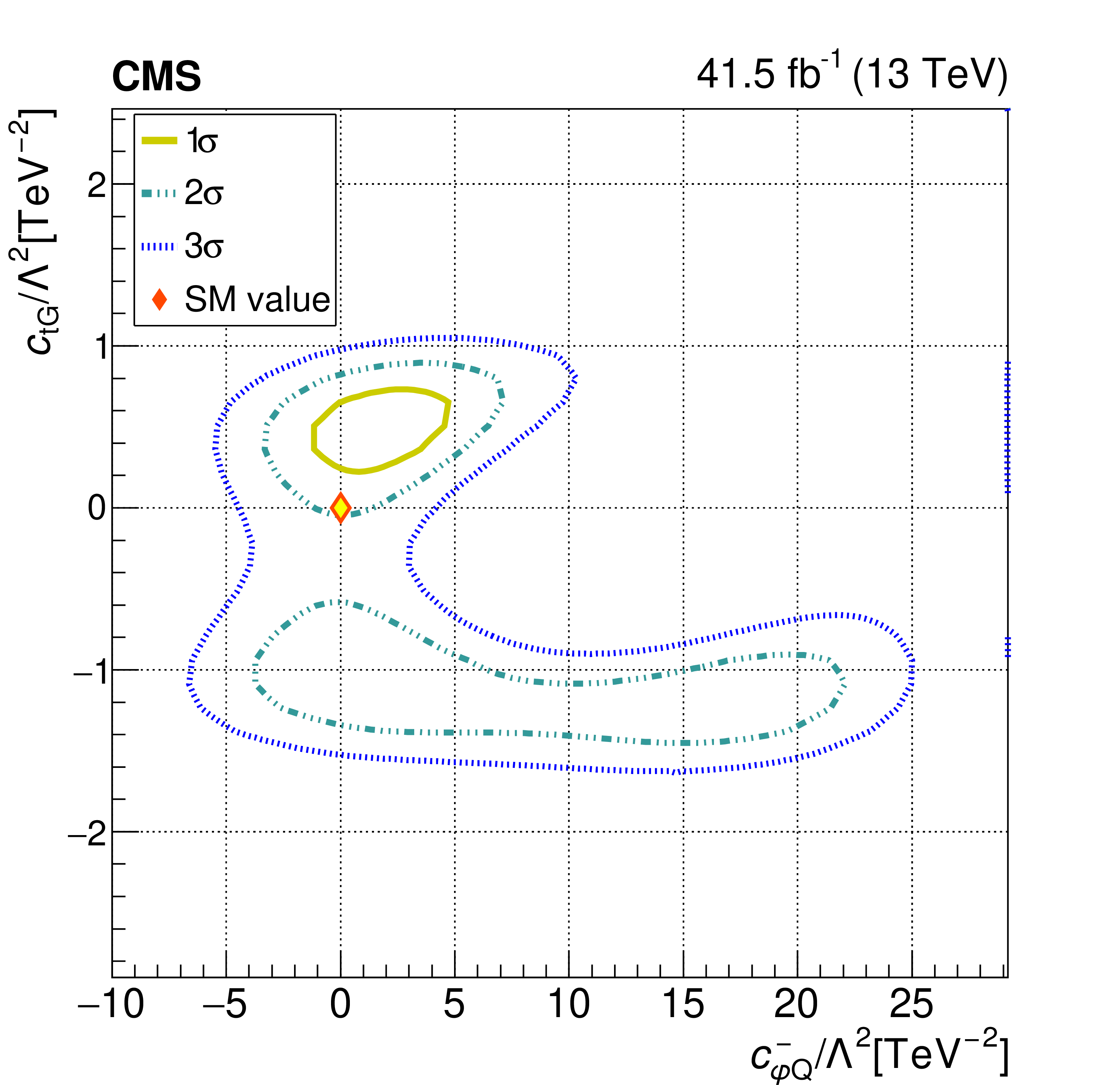
Figure 8-b:
The observed 1$\sigma $, 2$\sigma $, and 3$\sigma $ confidence contours of a 2D scan for ${{c _{\mathrm{t} G}}}$ and ${{c ^{-}_{\varphi Q}}}$ with the other WCs fixed to their SM values. Diamond markers are shown for the SM prediction. The range on the right plot is modified to emphasize the 1$\sigma $ contour. |
png pdf |
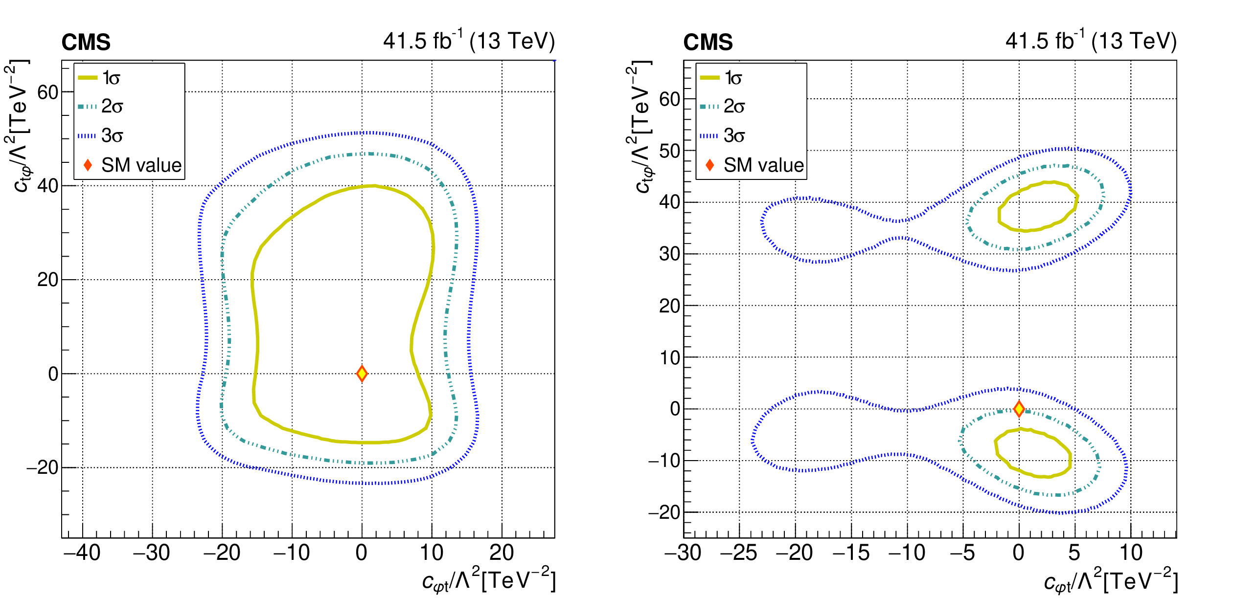
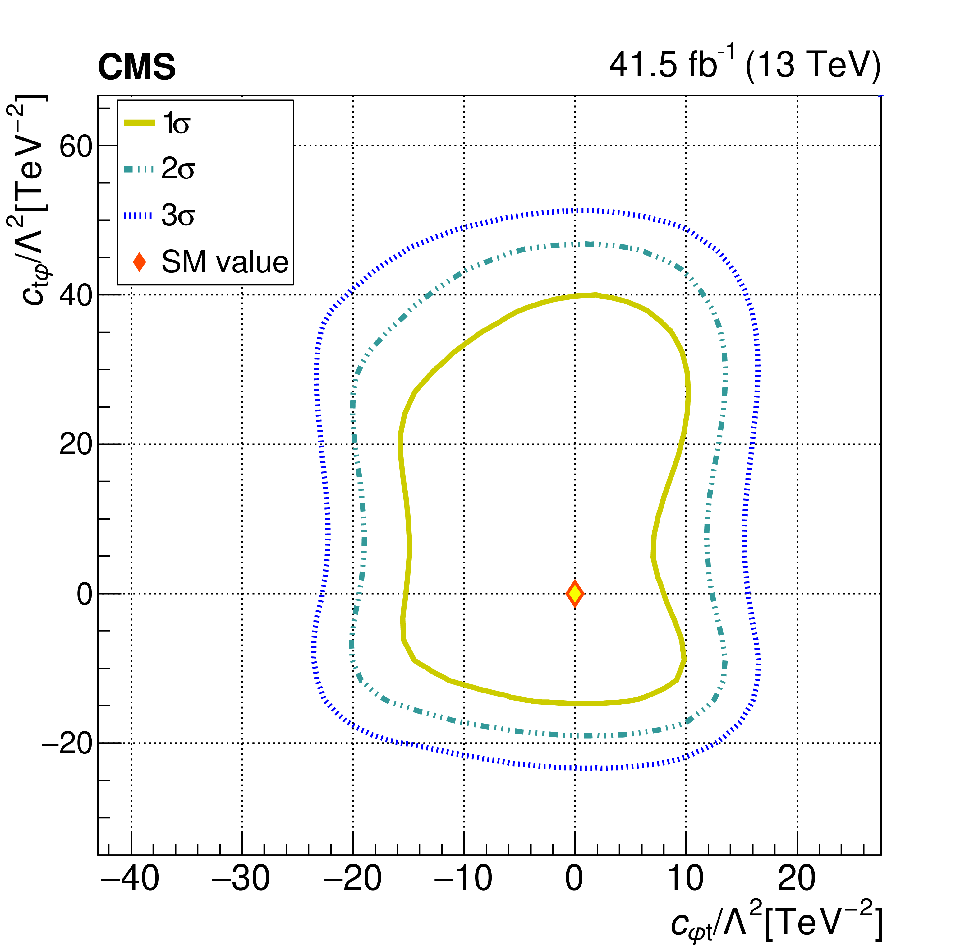
Figure 9:
The observed 1$\sigma $, 2$\sigma $, and 3$\sigma $ confidence contours of a 2D scan for ${{c _{\mathrm{t} \varphi}}}$ and ${{c _{\varphi \mathrm{t}}}}$ with the other WCs profiled (left), and fixed to their SM values (right). Diamond markers are shown for the SM prediction. The range on the right plot is modified to emphasize the 1$\sigma $ contour. |
png pdf |
Figure 9-a:
The observed 1$\sigma $, 2$\sigma $, and 3$\sigma $ confidence contours of a 2D scan for ${{c _{\mathrm{t} \varphi}}}$ and ${{c _{\varphi \mathrm{t}}}}$ with the other WCs profiled. Diamond markers are shown for the SM prediction. The range on the right plot is modified to emphasize the 1$\sigma $ contour. |
png pdf |
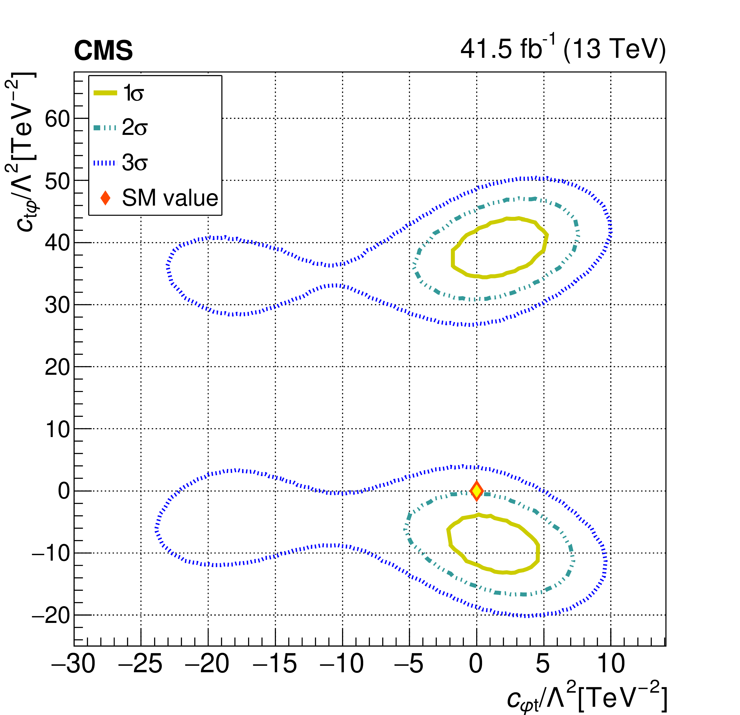
Figure 9-b:
The observed 1$\sigma $, 2$\sigma $, and 3$\sigma $ confidence contours of a 2D scan for ${{c _{\mathrm{t} \varphi}}}$ and ${{c _{\varphi \mathrm{t}}}}$ with the other WCs fixed to their SM values. Diamond markers are shown for the SM prediction. The range on the right plot is modified to emphasize the 1$\sigma $ contour. |
png pdf |
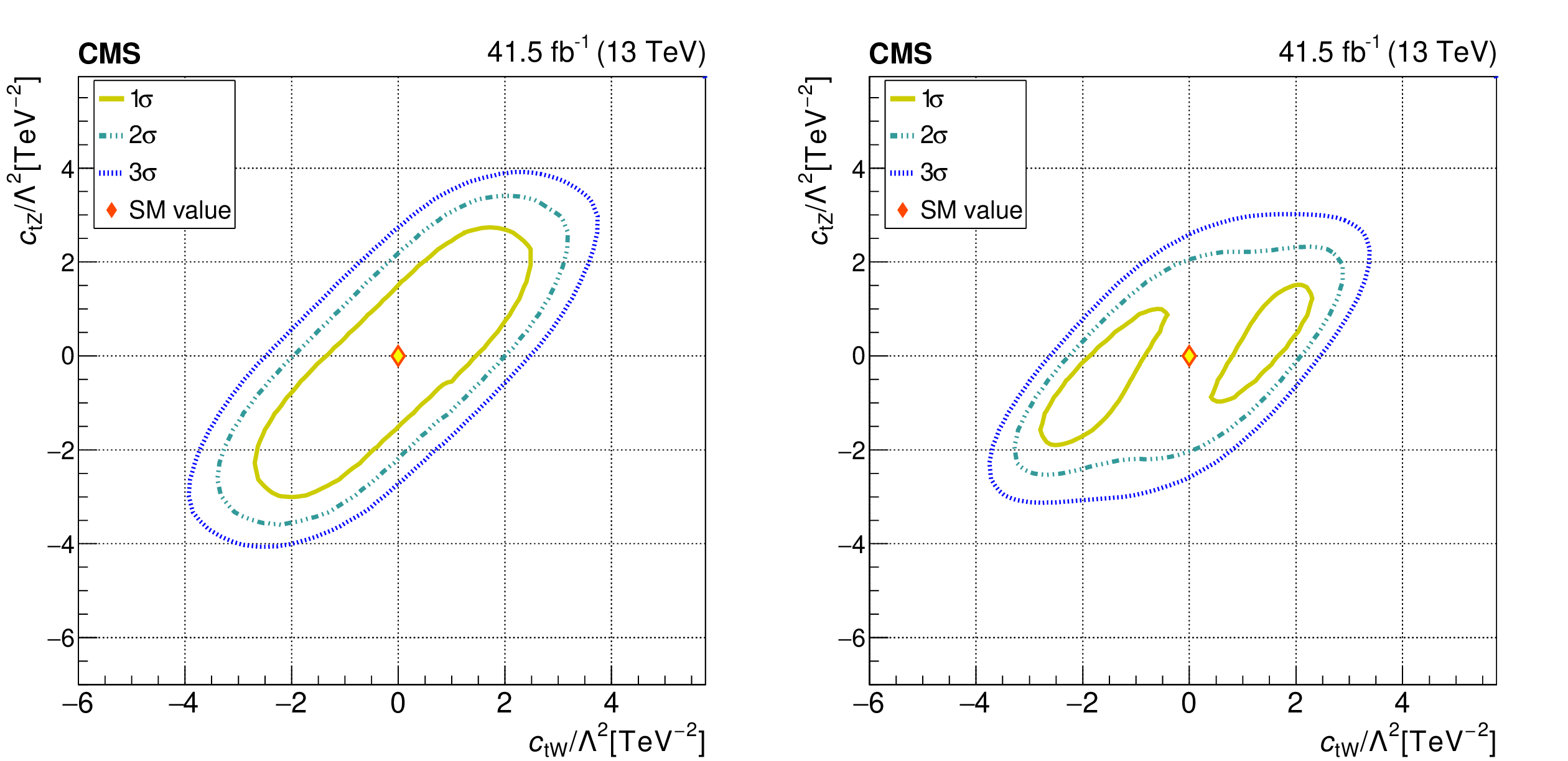
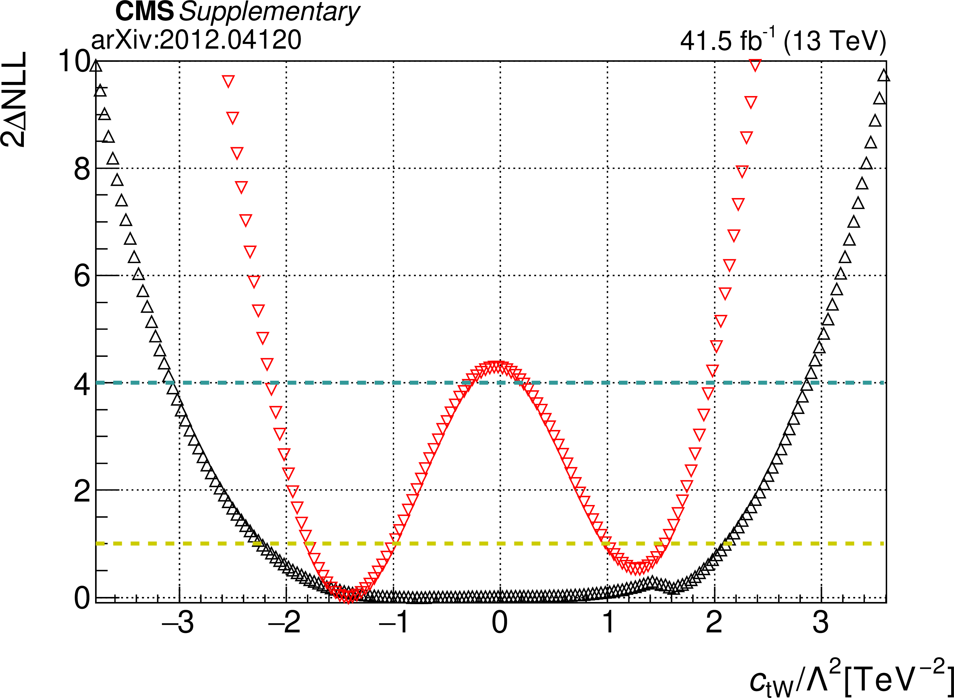
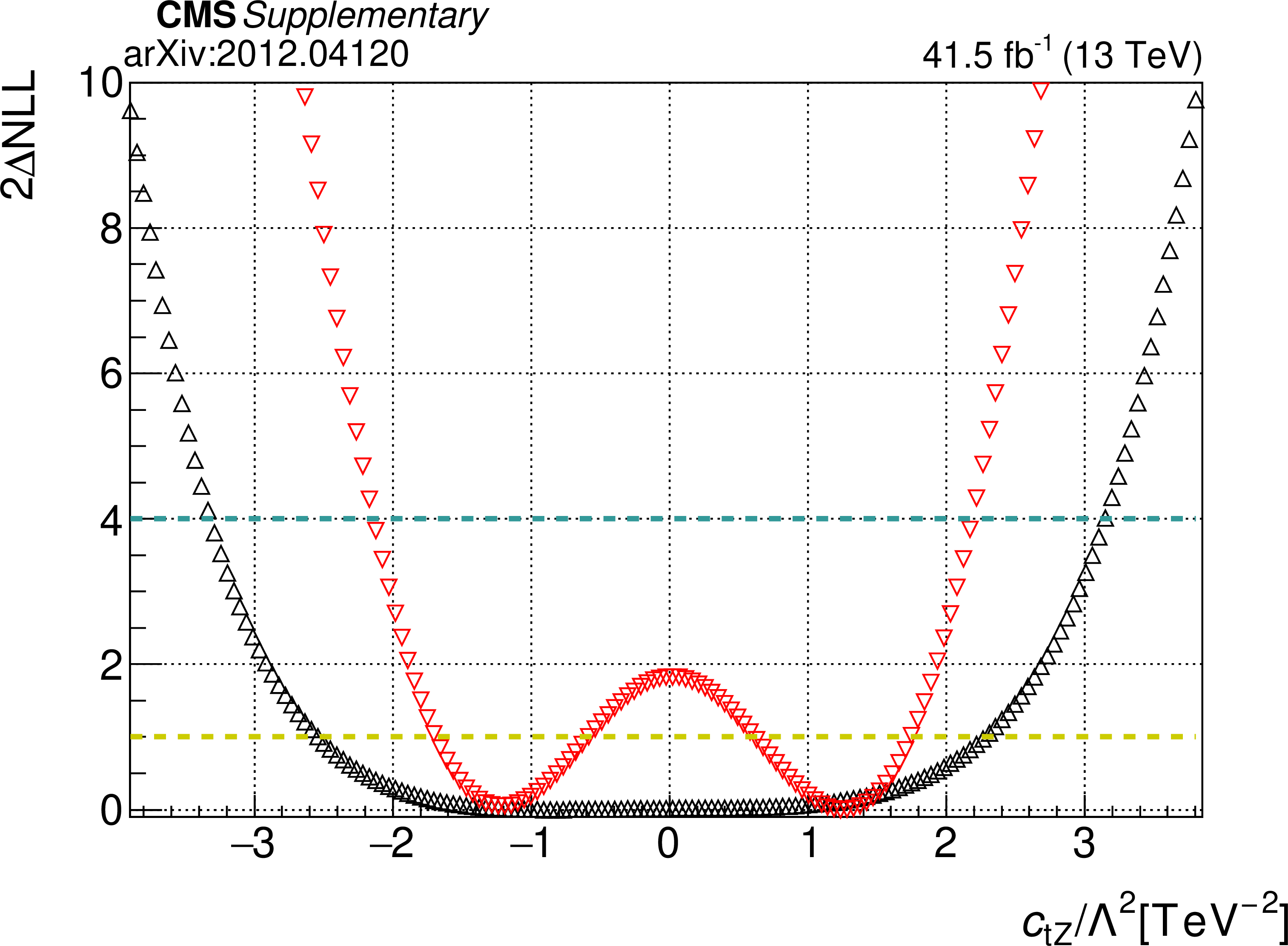
Figure 10:
The observed 1$\sigma $, 2$\sigma $, and 3$\sigma $ confidence contours of a 2D scan for ${{c _{\mathrm{t} \mathrm{Z}}}}$ and ${{c _{\mathrm{t} \mathrm{W}}}}$ with the other WCs profiled (left), and fixed to their SM values (right). Diamond markers are shown for the SM prediction. |

png pdf |
Figure 10-a:
The observed 1$\sigma $, 2$\sigma $, and 3$\sigma $ confidence contours of a 2D scan for ${{c _{\mathrm{t} \mathrm{Z}}}}$ and ${{c _{\mathrm{t} \mathrm{W}}}}$ with the other WCs profiled. Diamond markers are shown for the SM prediction. |
png pdf |
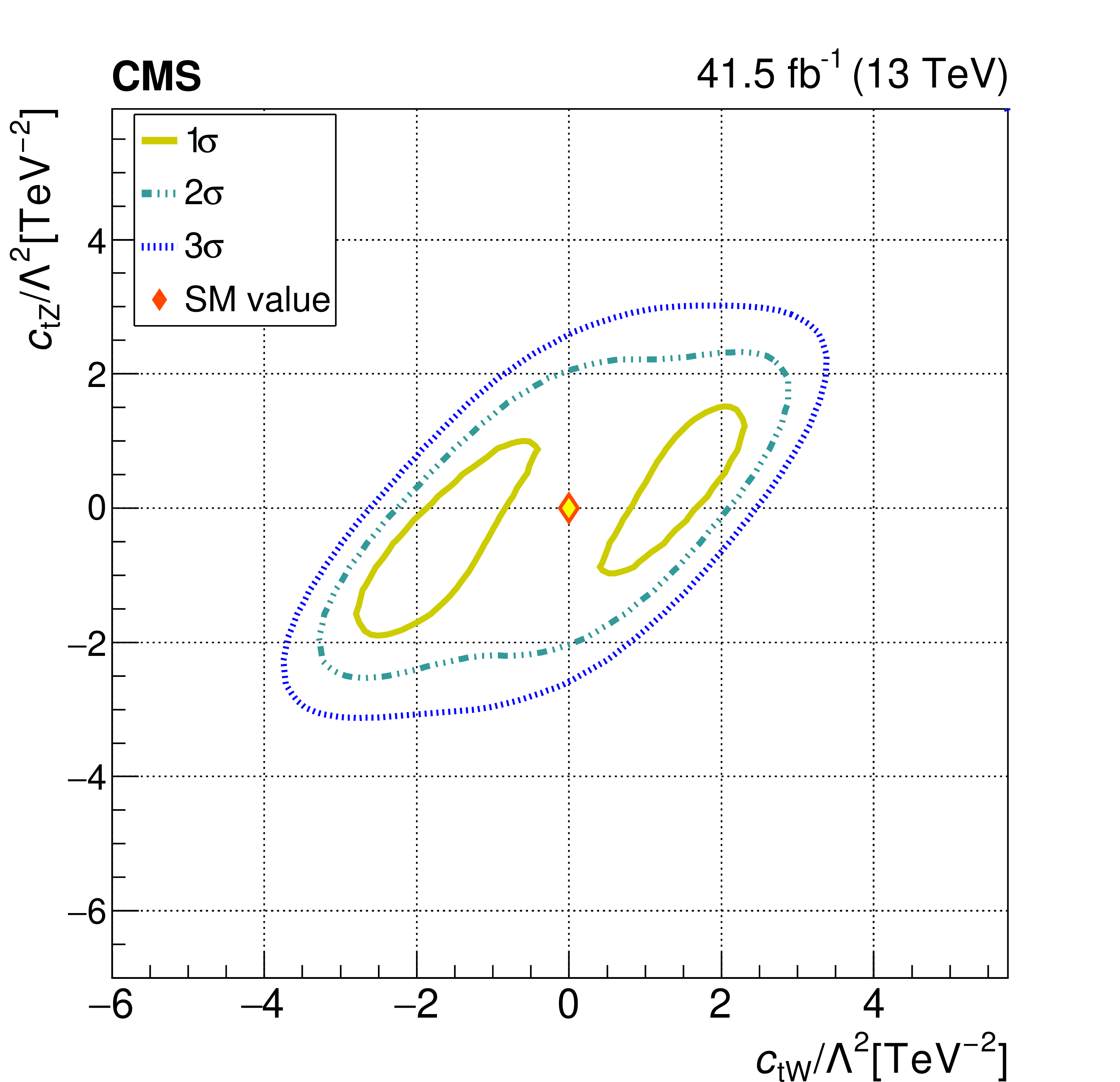
Figure 10-b:
The observed 1$\sigma $, 2$\sigma $, and 3$\sigma $ confidence contours of a 2D scan for ${{c _{\mathrm{t} \mathrm{Z}}}}$ and ${{c _{\mathrm{t} \mathrm{W}}}}$ with the other WCs fixed to their SM values. Diamond markers are shown for the SM prediction. |
png pdf |
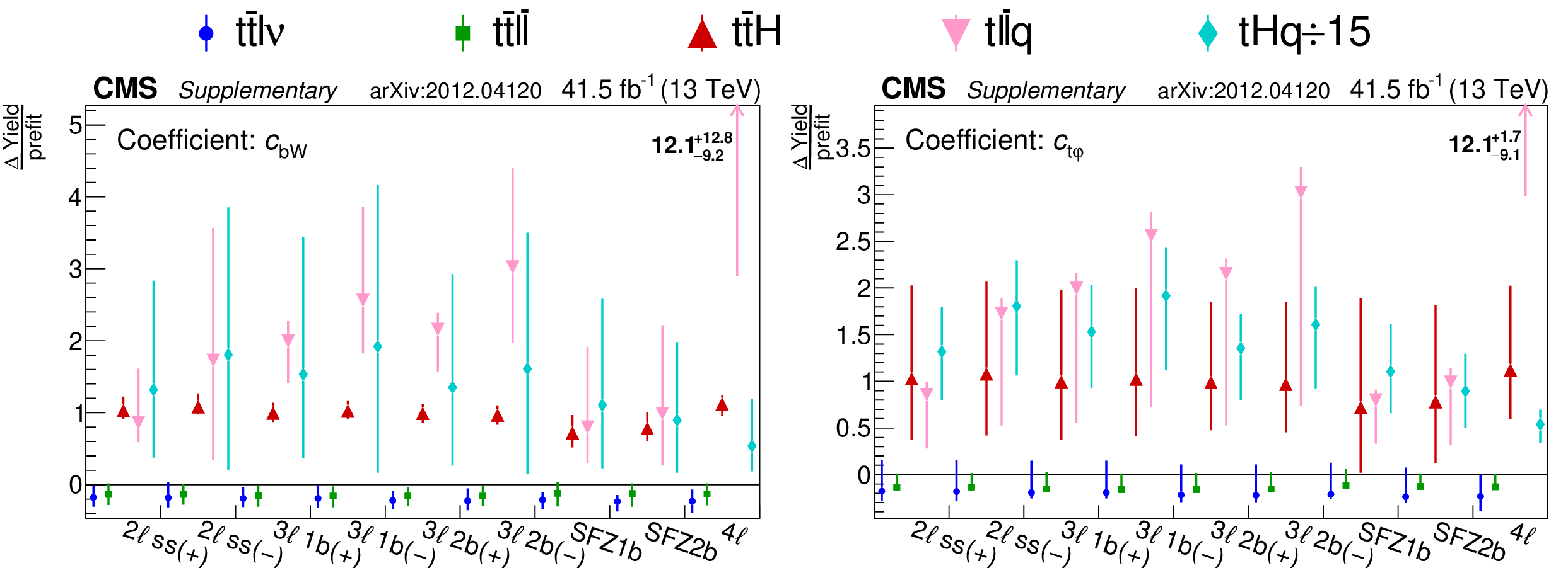
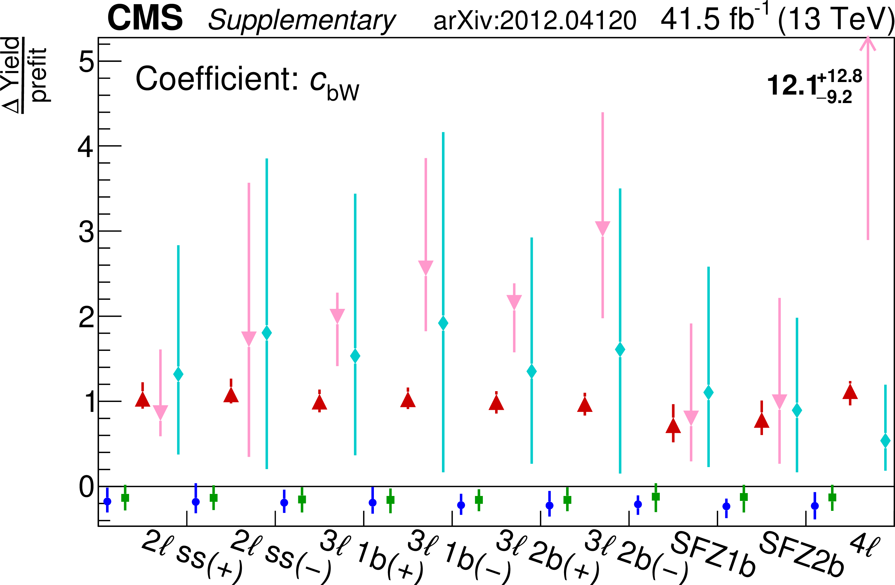
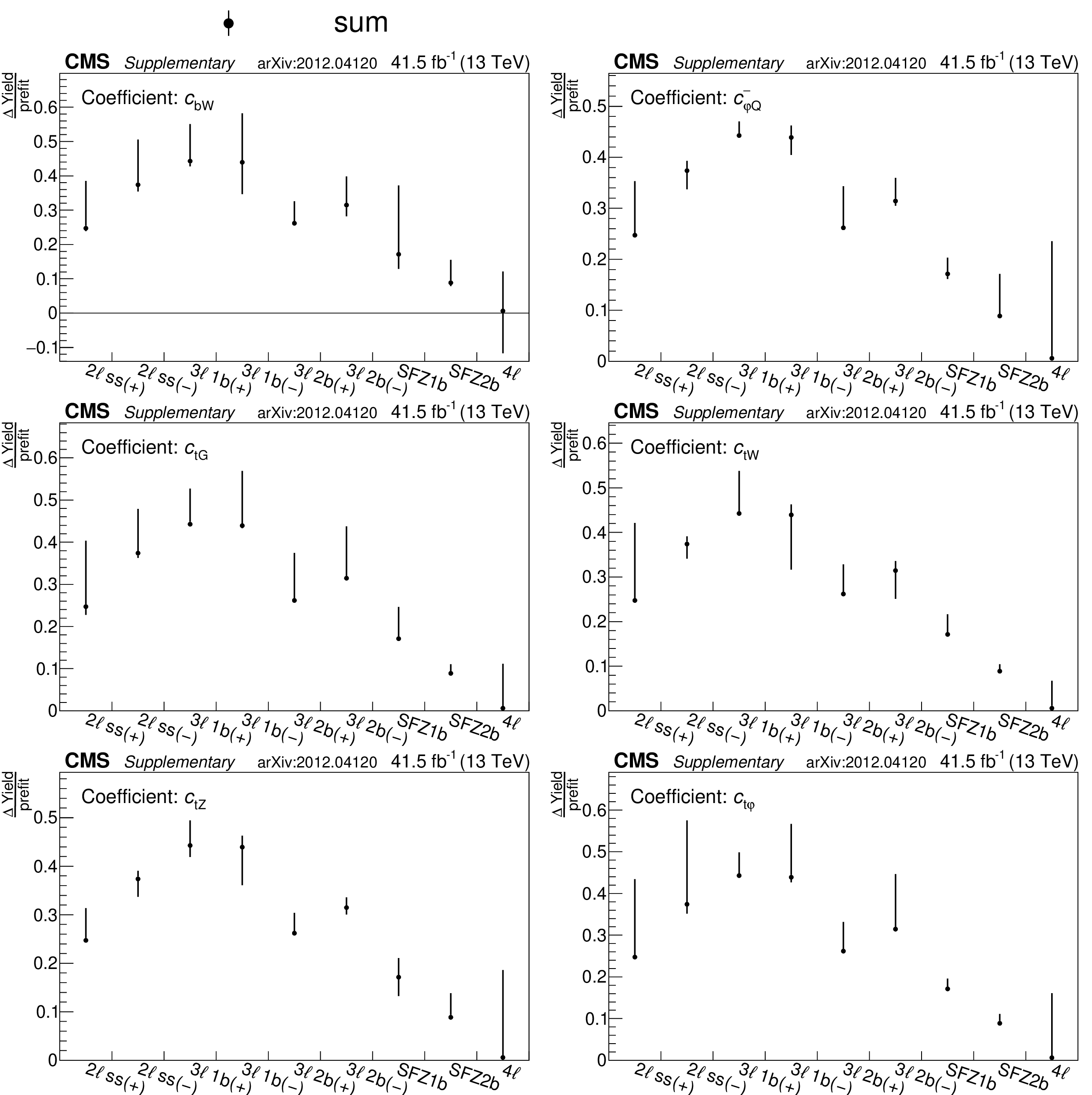
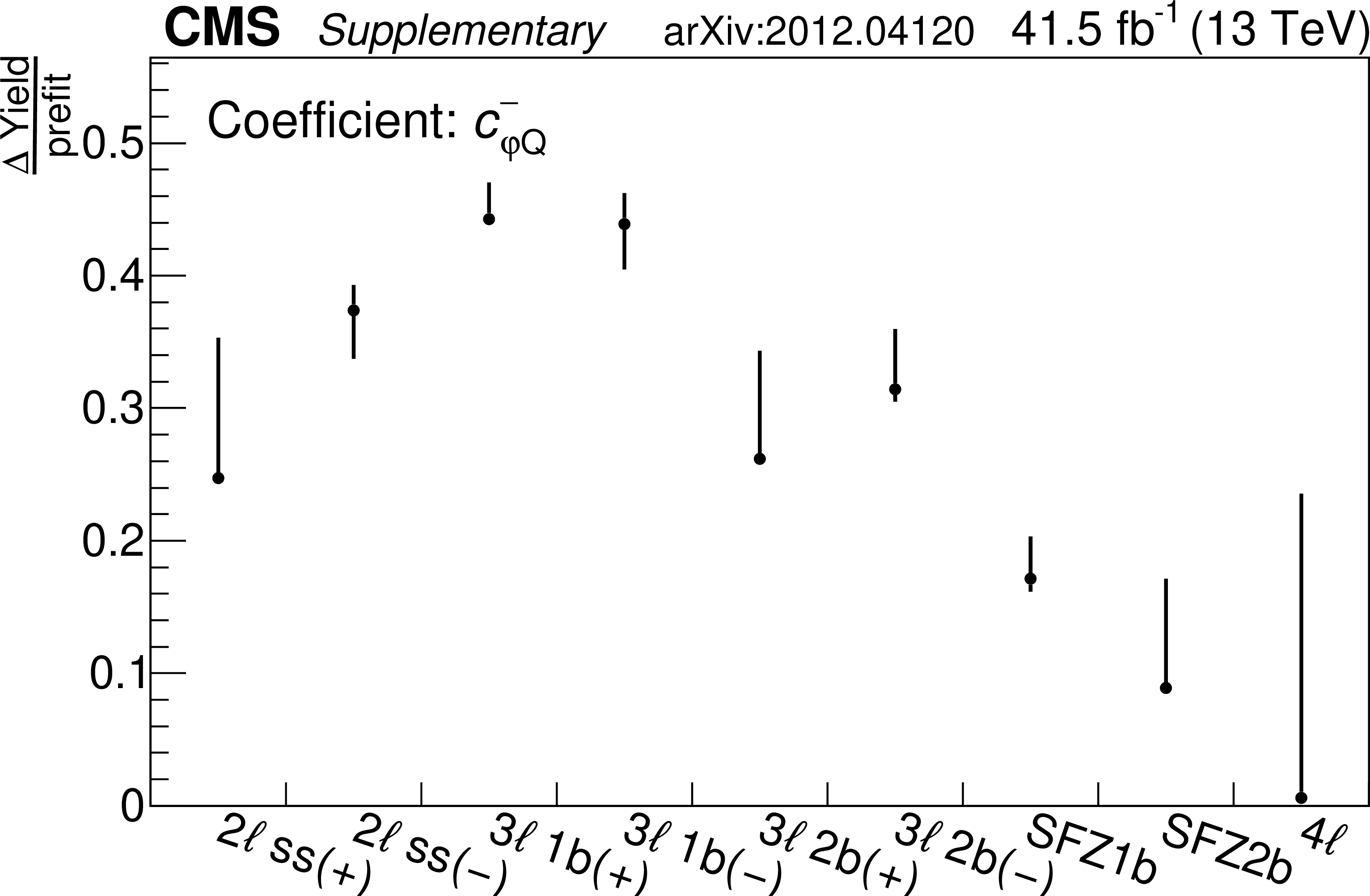
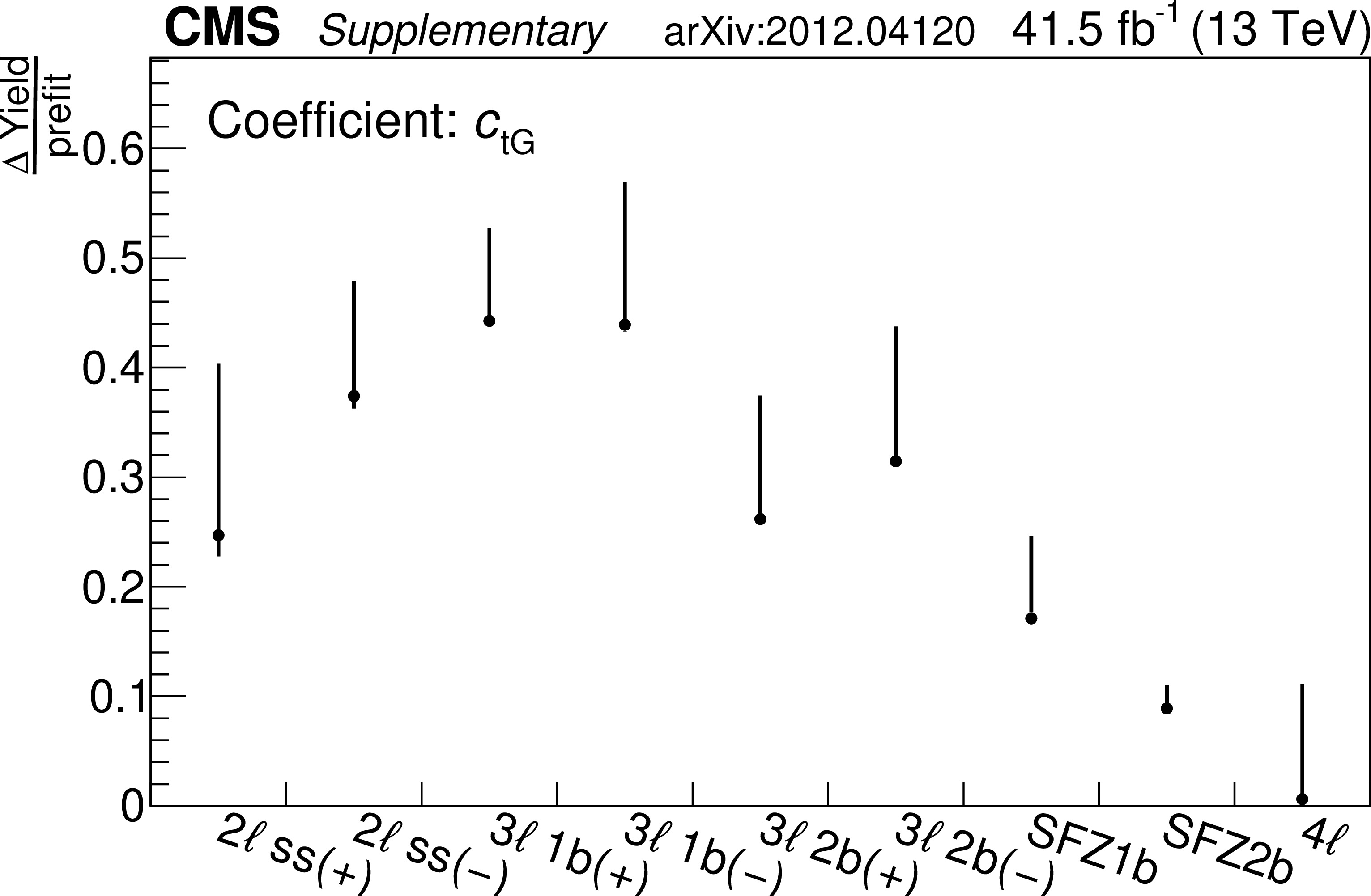
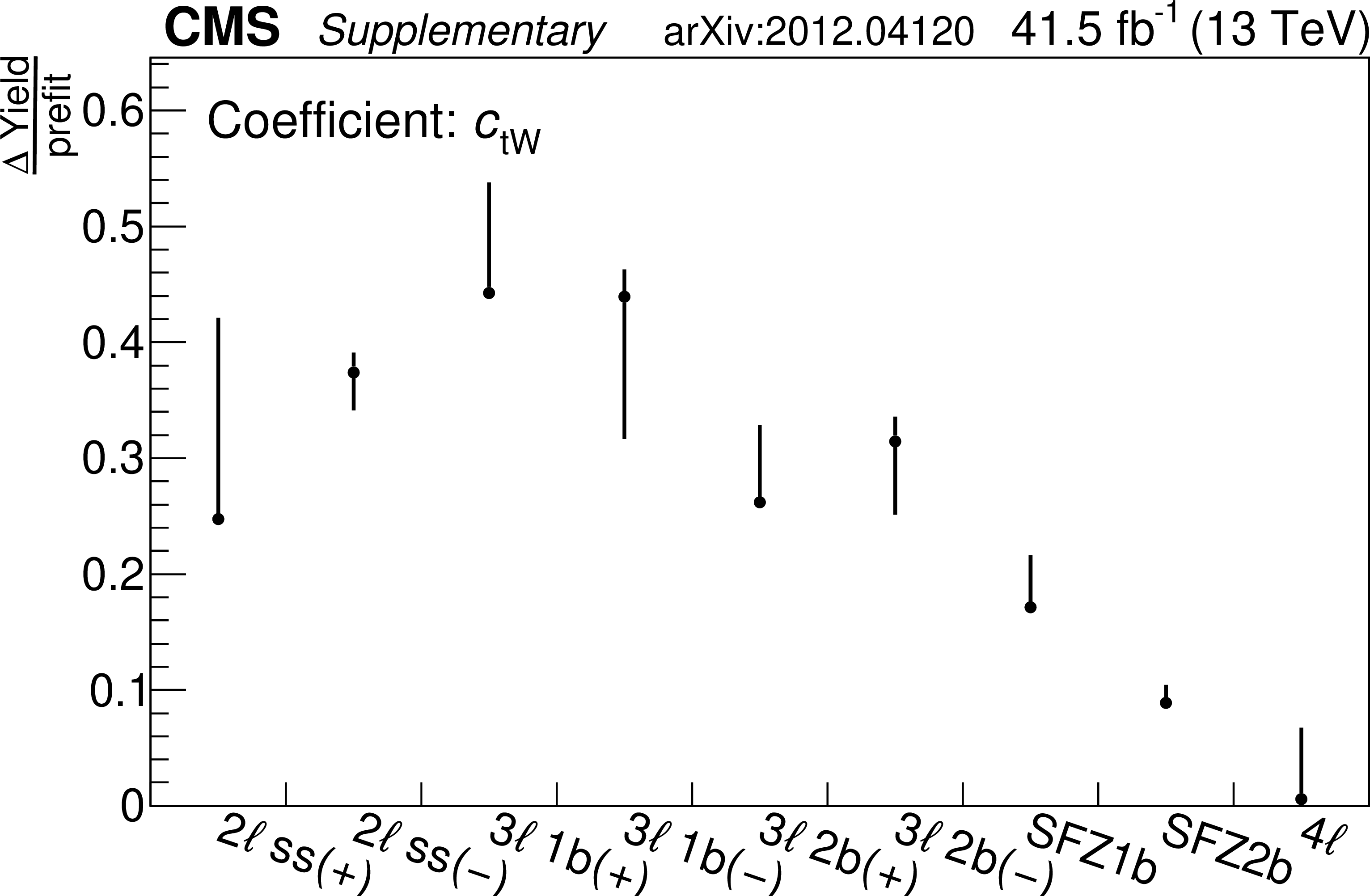
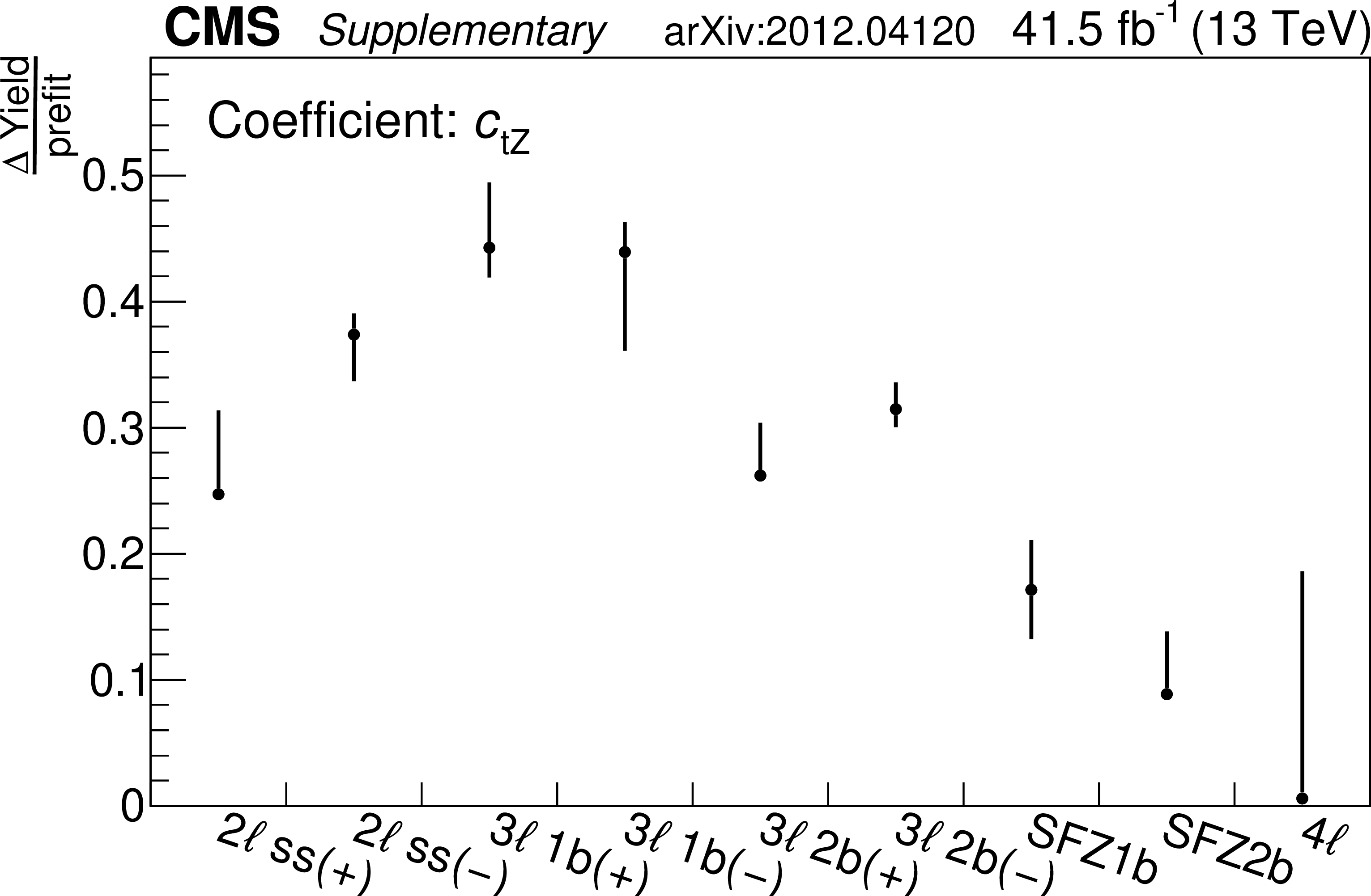
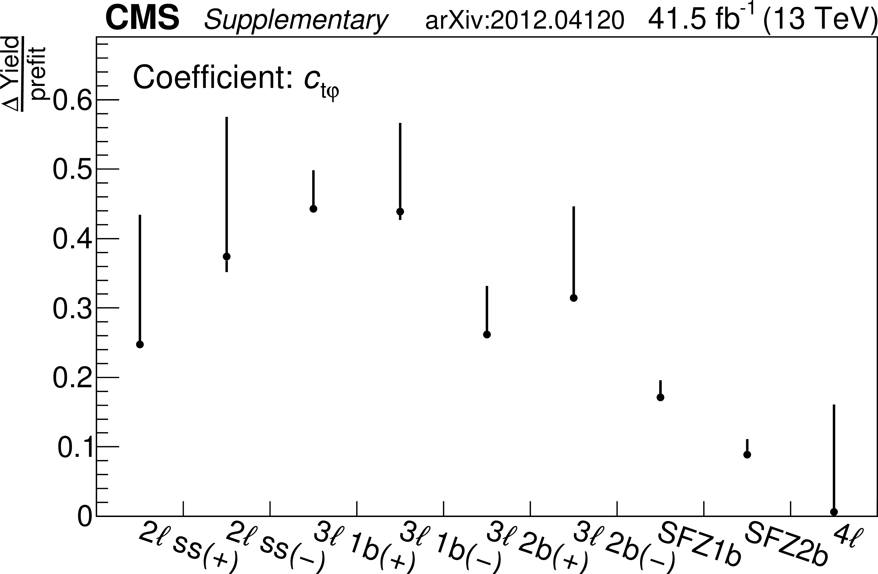
Figure 11:
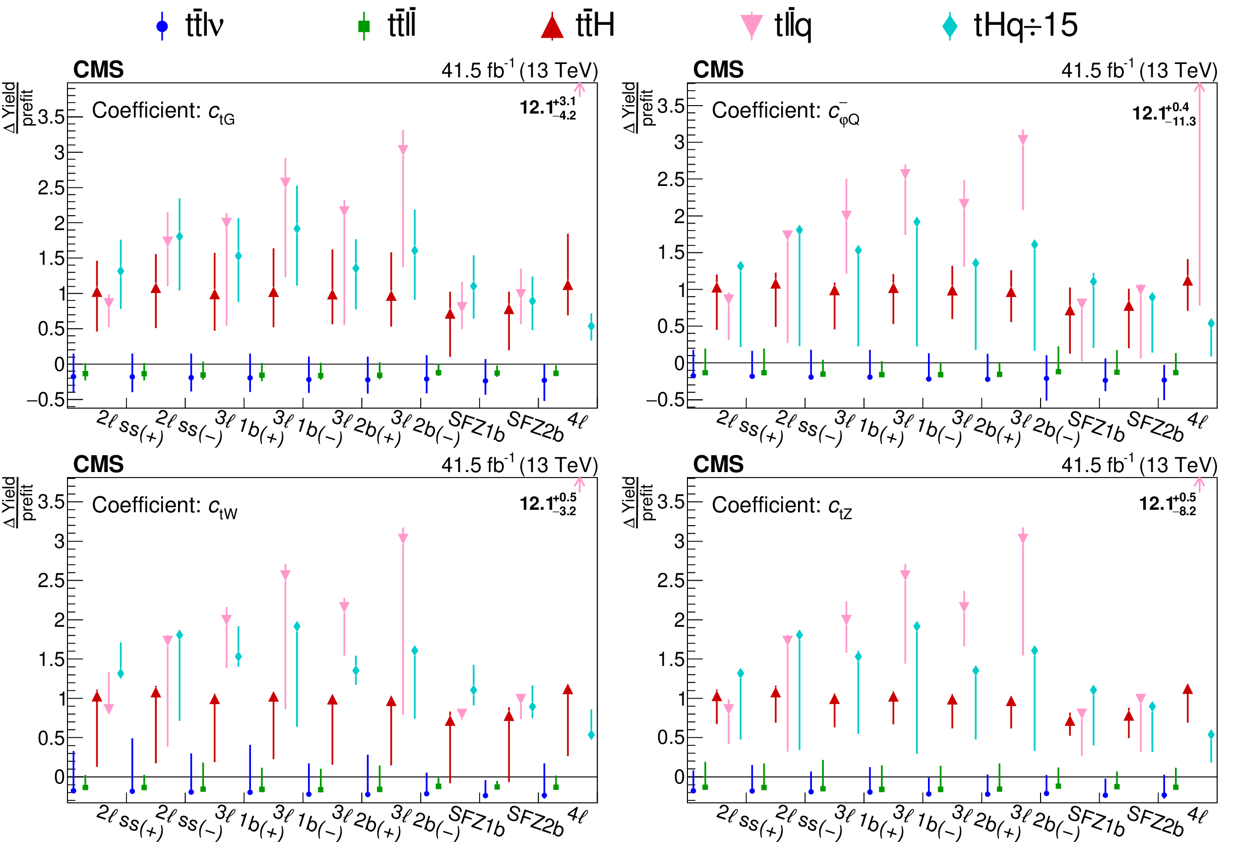
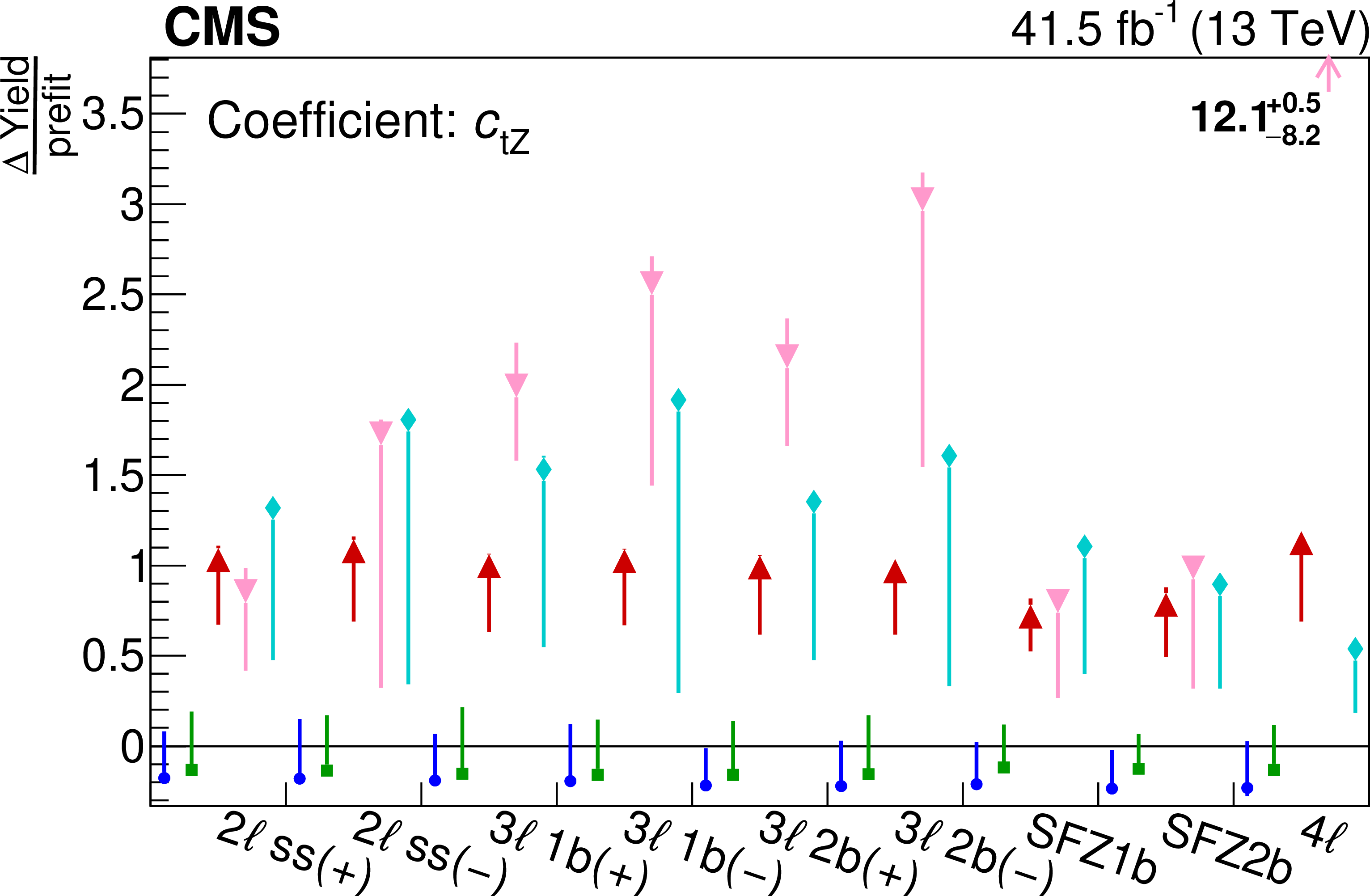
Plots showing the relative change in the expected yield for the signal processes in each event category. The "$\Delta $Yield/prefit'' is the difference in expected yield before fit (prefit) and after fit (postfit), normalized to the prefit yield of the process in the corresponding category. The vertical bars represent the maximum variation for a given WC within the corresponding 2$\sigma $ confidence interval. The values in upper right of each plot are to indicate the variation for ${\mathrm{t} \ell \bar{\ell} \mathrm{q}}$ in the 4$\ell $ category. |

png pdf |
Figure 11-a:
Legends for the following figures. |

png pdf |
Figure 11-b:
Plots showing the relative change in the expected yield for the ${{c _{\mathrm{t} G}}}$ signal process. The "$\Delta $Yield/prefit'' is the difference in expected yield before fit (prefit) and after fit (postfit), normalized to the prefit yield of the process in the corresponding category. The vertical bars represent the maximum variation for a given WC within the corresponding 2$\sigma $ confidence interval. The values in upper right of the plot are to indicate the variation for ${\mathrm{t} \ell \bar{\ell} \mathrm{q}}$ in the 4$\ell $ category. |

png pdf |
Figure 11-c:
Plots showing the relative change in the expected yield for the ${{c ^{-}_{\varphi Q}}}$ signal process. The "$\Delta $Yield/prefit'' is the difference in expected yield before fit (prefit) and after fit (postfit), normalized to the prefit yield of the process in the corresponding category. The vertical bars represent the maximum variation for a given WC within the corresponding 2$\sigma $ confidence interval. The values in upper right of the plot are to indicate the variation for ${\mathrm{t} \ell \bar{\ell} \mathrm{q}}$ in the 4$\ell $ category. |

png pdf |
Figure 11-d:
Plots showing the relative change in the expected yield for the ${{c _{\mathrm{t} \mathrm{W}}}}$ signal process. The "$\Delta $Yield/prefit'' is the difference in expected yield before fit (prefit) and after fit (postfit), normalized to the prefit yield of the process in the corresponding category. The vertical bars represent the maximum variation for a given WC within the corresponding 2$\sigma $ confidence interval. The values in upper right of the plot are to indicate the variation for ${\mathrm{t} \ell \bar{\ell} \mathrm{q}}$ in the 4$\ell $ category. |
png pdf |
Figure 11-e:
Plots showing the relative change in the expected yield for the ${{c _{\mathrm{t} \mathrm{Z}}}}$ signal process. The "$\Delta $Yield/prefit'' is the difference in expected yield before fit (prefit) and after fit (postfit), normalized to the prefit yield of the process in the corresponding category. The vertical bars represent the maximum variation for a given WC within the corresponding 2$\sigma $ confidence interval. The values in upper right of the plot are to indicate the variation for ${\mathrm{t} \ell \bar{\ell} \mathrm{q}}$ in the 4$\ell $ category. |
| Tables | |
png pdf |
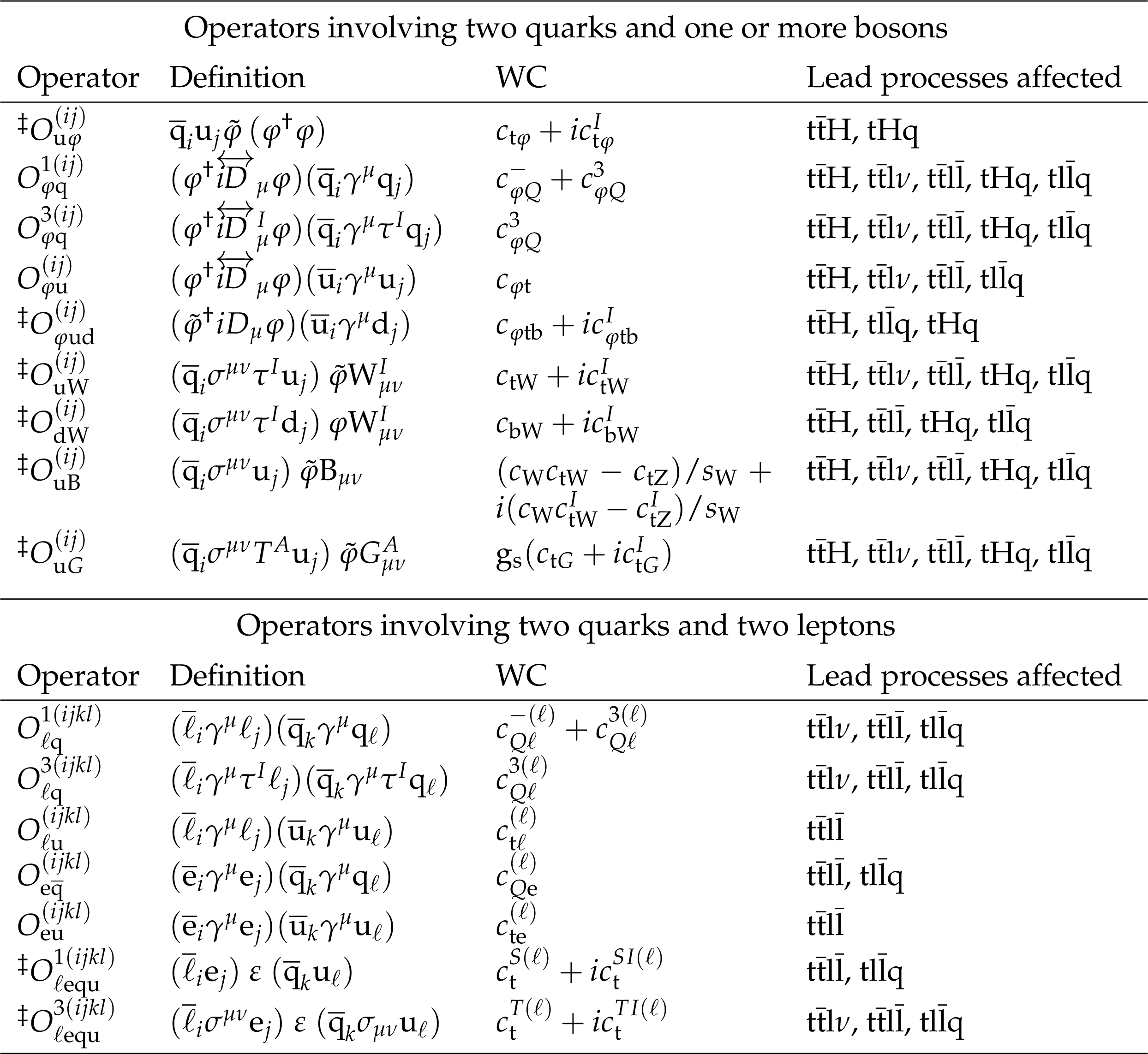
Table 1:
List of operators that have effects on ${\mathrm{t} \mathrm{\bar{t}} \mathrm{H}}$, ${\mathrm{t} \mathrm{\bar{t}} \ell \bar{\ell}}$, ${\mathrm{t} \mathrm{\bar{t}} \ell \nu}$, ${\mathrm{t} \ell \bar{\ell} \mathrm{q}}$, and ${\mathrm{t} \mathrm{H} \mathrm{q}}$ processes at order $1/\Lambda ^2$ that are considered in this analysis. The couplings are assumed to involve only third-generation quarks. The quantity $T^A=\frac {1}{2}\lambda ^A$ denotes the eight Gell-Mann matrices, and $\tau ^I$ are the Pauli matrices. The field $\varphi $ is the Higgs boson doublet, and $\tilde{\varphi}=\varepsilon \varphi ^*$, where $\varepsilon \equiv i\tau ^2$. The $\ell $ and q represent the left-handed lepton and quark doublets, respectively, while e represents the right-handed lepton, and u and d represent the right-handed quark singlets. Furthermore, $(\varphi ^{\dagger}i\overleftrightarrow {D}_\mu \varphi) \equiv \varphi ^\dagger (iD_\mu \varphi)-(iD_\mu \varphi ^\dagger)\varphi $ and $(\varphi ^{\dagger}i\overleftrightarrow {D}^I_\mu \varphi) \equiv \varphi ^{\dagger}\tau ^I(iD_\mu \varphi)-(iD_\mu \varphi ^\dagger)\tau ^I\varphi $. The W boson field strength is $\mathrm{W} _{\mu \nu}^I=\partial _\mu \mathrm{W} _\nu ^I-\partial _\nu \mathrm{W} ^I_\mu +g\varepsilon _{IJK}\mathrm{W} ^J_\mu \mathrm{W} ^K_\nu $, and $G_{\mu \nu}^A=\partial _\mu G_\nu ^A-\partial _\nu G^A_\mu +g_sf^{ABC}G^B_\mu G^C_\nu $ is the gluon field strength. The abbreviations ${s_{\mathrm {W}}}$ and ${c_{\mathrm {W}}}$ denote the sine and cosine of the weak mixing angle (in the unitary gauge), respectively. The leading processes affected by the operators are also listed (the details of the criteria used for this determination are described in the text). |
png pdf |
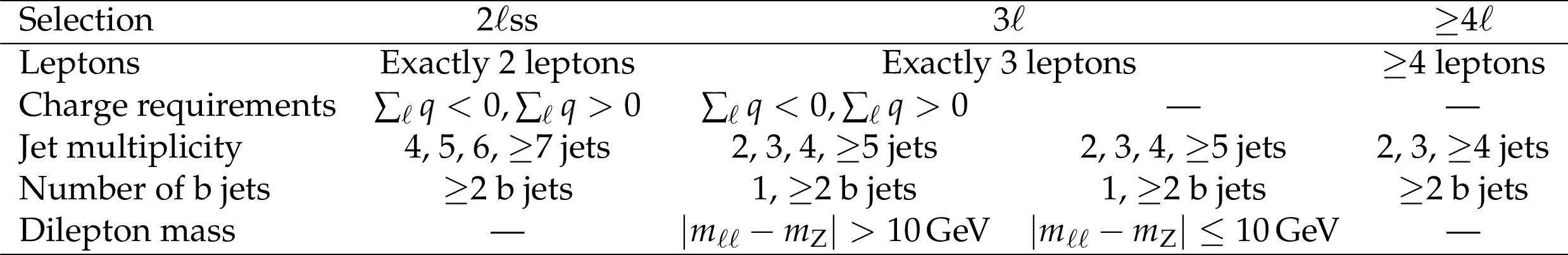
Table 2:
Requirements for the different event categories. Requirements separated by commas indicate a division into subcategories. The b jet requirement on individual jets varies based on the lepton category, as described in the text. |
png pdf |
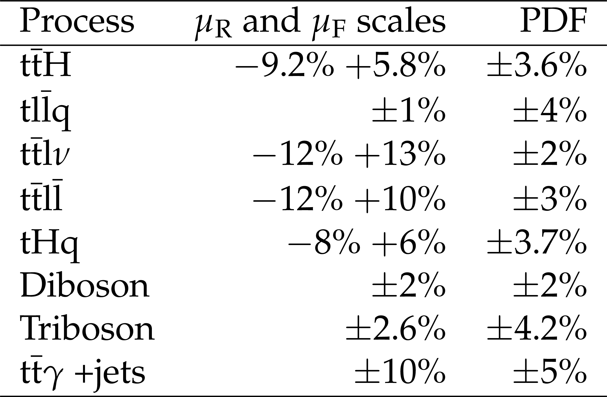
Table 3:
Cross section (rate) uncertainties used for the fit. Each column in the table is an independent source of uncertainty. Uncertainties in the same column for different processes (different rows) are fully correlated. |

png pdf |
Table 4:
Summary for the systematic uncertainties. Here "shape" means that the systematic uncertainty causes a change in the relative expected yield of the jet and/or b jet bins. Except where noted, each row in this table will be treated as a single, independent NP. Impacts of various systematic variations on a subset of WCs are also quoted. Percentages represent the change in a WC divided by the symmetrized 2$\sigma $ confidence interval. A value of 100% indicates the particular systematic variation adds an uncertainty equal to the WC interval. The percentages for the b and c jet tags are the sum of all their respective subcategories. |

png pdf |
Table 5:
The 2$\sigma $ confidence intervals on the WCs. The intervals are found by scanning over a single WC while either treating the other 15 profiled, or fixing the other 15 to the SM value of zero. |
| Summary |
|
A search for new physics has been performed in the production of at least one top quark in association with additional leptons, jets, and b jets, in the context of an effective field theory. The events were produced in proton-proton collisions corresponding to an integrated luminosity of ${\mathcal{L}}$. The expected yield in each category was parameterized in terms of 16 Wilson coefficients (WCs) associated with effective field theory operators relevant to the dominant processes in the data. A simultaneous fit was performed of the 16 WCs to the data. For each WC, an interval over which the model predictions agree with the observed yields at the 2 standard deviation level was extracted by either keeping the other WCs fixed to zero or treating the other WCs as unconstrained nuisance parameters. Two-dimensional contours were produced for some of the WCs, to illustrate correlations between various WCs. The results from fitting the WCs in the dimension-six model to the data were consistent with the standard model at the level of 2 standard deviations. |
| Additional Figures | |
png pdf |
Additional Figure 1:
Observed Wilson Coefficient (WC) 1$\sigma$ (thick line) and 2$\sigma$ (thin line) confidence intervals (CIs) for the Asimov data. Solid lines correspond to the other WCs profiled, while dashed lines correspond to the other WCs fixed to the SM value of zero. In order to make the this figure more readable, the ${{c _{\varphi \mathrm{t}}}}$ interval is scaled by 1/2, the ${{c _{\mathrm{t} G}}}$ interval is scaled by 2, the ${{c ^{-}_{\varphi Q}}}$ interval is scaled by 1/2, and the ${{c _{\mathrm{t} \varphi}}}$ interval is scaled by 1/5. In some cases, intervals have two degenerate, or near degenerate, negative log-likelihood minima, but in all cases a minimum exists at zero (SM), as expected. |
png pdf |
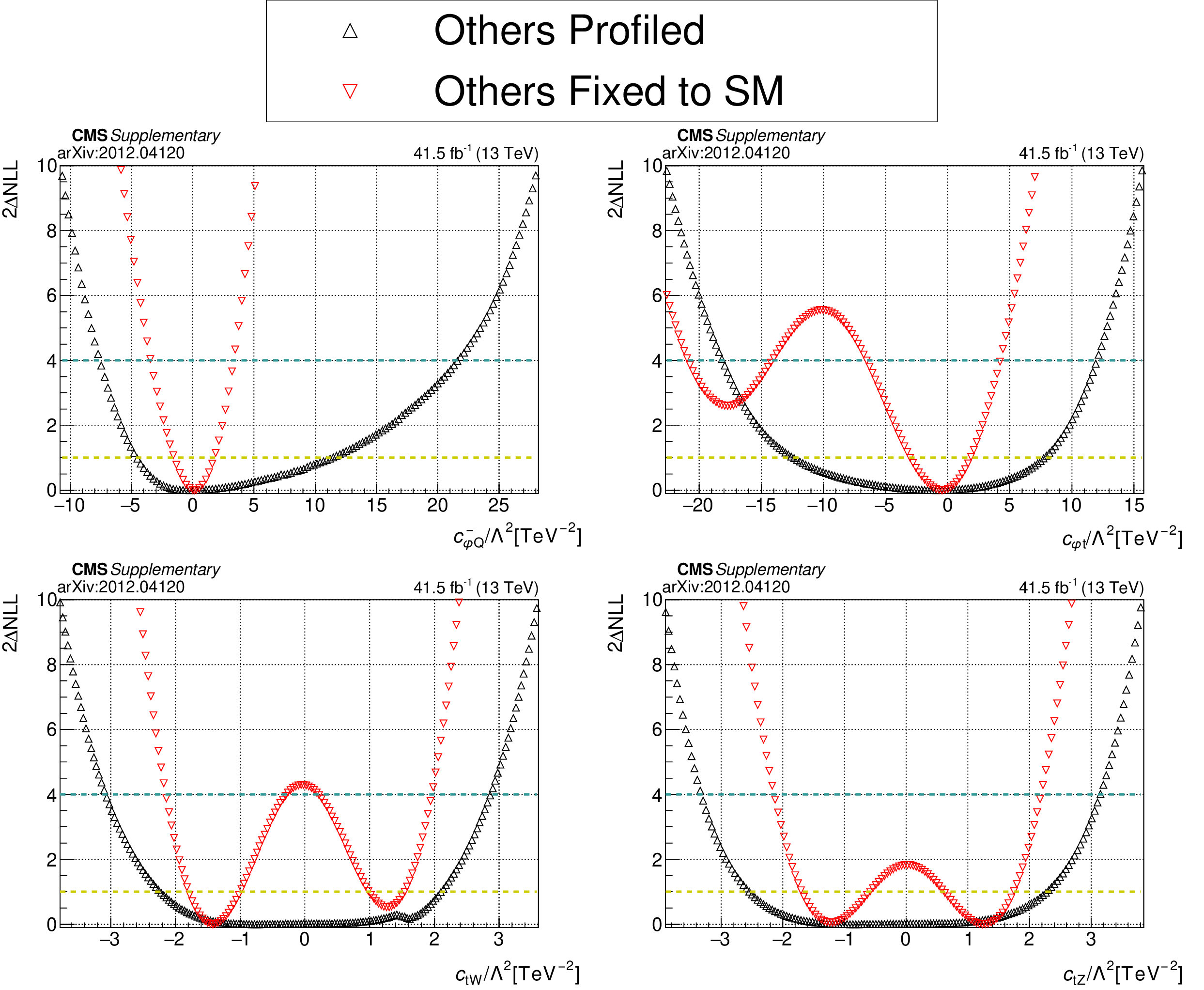
Additional Figure 2:
The 1D likelihood scans of each of the 16 Wilson coefficients (WCs) for ${{c ^{-}_{\varphi Q}}}$, ${{c _{\varphi \mathrm{t}}}}$, ${{c _{\mathrm{t} G}}}$, ${{c _{\mathrm{t} \mathrm{W}}}}$, and ${{c _{\mathrm{t} \mathrm{Z}}}}$. These fits were made by either profiling the other WCs, or by fixing the other coefficients to their SM value of 0. These two results are overlaid with lines at the 1$\sigma$ and 2$\sigma$ uncertainty value for both. |
png pdf |
Additional Figure 2-a:
Legend for the following figures. These fits were made by either profiling the other WCs, or by fixing the other coefficients to their SM value of 0. These two results are overlaid with lines at the 1$\sigma$ and 2$\sigma$ uncertainty value for both. |

png pdf |
Additional Figure 2-b:
The 1D likelihood scans of each of the 16 Wilson coefficients (WCs) for ${{c ^{-}_{\varphi Q}}}$. |
png pdf |
Additional Figure 2-c:
The 1D likelihood scans of each of the 16 Wilson coefficients (WCs) for ${{c _{\varphi \mathrm{t}}}}$. |
png pdf |
Additional Figure 2-d:
The 1D likelihood scans of each of the 16 Wilson coefficients (WCs) for ${{c _{\mathrm{t} G}}}$. |
png pdf |
Additional Figure 2-e:
The 1D likelihood scans of each of the 16 Wilson coefficients (WCs) for ${{c _{\mathrm{t} \mathrm{Z}}}}$. |
png pdf |
Additional Figure 3:
Plots showing the relative change in the expected yield for the signal processes in each event category. The ``$\Delta$Yield'' refers to the change in expected yield before fitting (prefit) and after (postfit). The yield difference is normalized to the prefit yield of the process in the corresponding category. The vertical bars represent the maximum variation for a given Wilson Coefficient within the corresponding 2$\sigma$ confidence interval. The values in upper right of each plot are to indicate the variation for $\mathrm{t\ell\overline{\ell}q}$ in the 4$\ell$ category. |

png pdf |
Additional Figure 3-a:
Legends for the following figures. |
png pdf |
Additional Figure 3-b:
Plots showing the relative change in the expected yield for the signal processes in each event category. The ``$\Delta$Yield'' refers to the change in expected yield before fitting (prefit) and after (postfit). The yield difference is normalized to the prefit yield of the process in the corresponding category. The vertical bars represent the maximum variation for the ${{c _{\mathrm{b} \mathrm{W}}}}$ Wilson Coefficient within the corresponding 2$\sigma$ confidence interval. The value in upper right of the plot are to indicates the variation for $\mathrm{t\ell\overline{\ell}q}$ in the 4$\ell$ category. |

png pdf |
Additional Figure 3-c:
Plot showing the relative change in the expected yield for the signal processes in each event category. The ``$\Delta$Yield'' refers to the change in expected yield before fitting (prefit) and after (postfit). The yield difference is normalized to the prefit yield of the process in the corresponding category. The vertical bars represent the maximum variation for the ${{c _{\mathrm{t} \varphi }}}$ Wilson Coefficient within the corresponding 2$\sigma$ confidence interval. The value in upper right of the plot are to indicates the variation for $\mathrm{t\ell\overline{\ell}q}$ in the 4$\ell$ category. |
png pdf |
Additional Figure 4:
Plots showing the relative change in the expected yield for the sum of the signal processes in each event category. The ``$\Delta$Yield'' refers to the change in expected yield before fitting (prefit) and after (postfit). The yield difference is normalized to the prefit yield of the process in the corresponding category. The vertical bars represent the maximum variation for a given Wilson Coefficient within the corresponding 2$\sigma$ confidence interval. The values in upper right of each plot are to indicate the variation for $\mathrm{t \ell\ell q}$ in the 4$\ell$ category. |

png pdf |
Additional Figure 4-a:
Plot showing the relative change in the expected yield for the sum of the signal processes in each event category. The ``$\Delta$Yield'' refers to the change in expected yield before fitting (prefit) and after (postfit). The yield difference is normalized to the prefit yield of the process in the corresponding category. The vertical bars represent the maximum variation for the ${{c _{\mathrm{b} \mathrm{W}}}}$ Wilson Coefficient within the corresponding 2$\sigma$ confidence interval. The value in upper right of the plot is to indicate the variation for $\mathrm{t \ell\ell q}$ in the 4$\ell$ category. |
png pdf |
Additional Figure 4-b:
Plot showing the relative change in the expected yield for the sum of the signal processes in each event category. The ``$\Delta$Yield'' refers to the change in expected yield before fitting (prefit) and after (postfit). The yield difference is normalized to the prefit yield of the process in the corresponding category. The vertical bars represent the maximum variation for the ${{c ^{-}_{\varphi Q}}}$ Wilson Coefficient within the corresponding 2$\sigma$ confidence interval. The value in upper right of the plot is to indicate the variation for $\mathrm{t \ell\ell q}$ in the 4$\ell$ category. |
png pdf |
Additional Figure 4-c:
Plot showing the relative change in the expected yield for the sum of the signal processes in each event category. The ``$\Delta$Yield'' refers to the change in expected yield before fitting (prefit) and after (postfit). The yield difference is normalized to the prefit yield of the process in the corresponding category. The vertical bars represent the maximum variation for the ${{c _{\mathrm{t} \mathrm{G}}}}$ Wilson Coefficient within the corresponding 2$\sigma$ confidence interval. The value in upper right of the plot is to indicate the variation for $\mathrm{t \ell\ell q}$ in the 4$\ell$ category. |
png pdf |
Additional Figure 4-d:
Plot showing the relative change in the expected yield for the sum of the signal processes in each event category. The ``$\Delta$Yield'' refers to the change in expected yield before fitting (prefit) and after (postfit). The yield difference is normalized to the prefit yield of the process in the corresponding category. The vertical bars represent the maximum variation for the ${{c _{\mathrm{t} \mathrm{W}}}}$ Wilson Coefficient within the corresponding 2$\sigma$ confidence interval. The value in upper right of the plot is to indicate the variation for $\mathrm{t \ell\ell q}$ in the 4$\ell$ category. |
png pdf |
Additional Figure 4-e:
Plot showing the relative change in the expected yield for the sum of the signal processes in each event category. The ``$\Delta$Yield'' refers to the change in expected yield before fitting (prefit) and after (postfit). The yield difference is normalized to the prefit yield of the process in the corresponding category. The vertical bars represent the maximum variation for the ${{c _{\mathrm{t} \mathrm{Z}}}}$ Wilson Coefficient within the corresponding 2$\sigma$ confidence interval. The value in upper right of the plot is to indicate the variation for $\mathrm{t \ell\ell q}$ in the 4$\ell$ category. |
png pdf |
Additional Figure 4-f:
Plot showing the relative change in the expected yield for the sum of the signal processes in each event category. The ``$\Delta$Yield'' refers to the change in expected yield before fitting (prefit) and after (postfit). The yield difference is normalized to the prefit yield of the process in the corresponding category. The vertical bars represent the maximum variation for the ${{c _{\mathrm{t} \varphi }}}$ Wilson Coefficient within the corresponding 2$\sigma$ confidence interval. The value in upper right of the plot is to indicate the variation for $\mathrm{t \ell\ell q}$ in the 4$\ell$ category. |
png pdf |
Additional Figure 5:
Expected yields when setting the Wilson Coefficients (WCs) to the SM value of zero and all nuisance parameters to their best fit values. The nuisance parameters are all kept at their final postfit values. The postfit values of the WCs are obtained from performing the fit over all WCs simultaneously. "Conv." refers to the photon conversion background, "Charge misid." is the lepton charge mismeasurement background, and "Misid. leptons" is the background from misidentified leptons. |

png pdf |
Additional Figure 5-a:
Legend for the figure. "Conv." refers to the photon conversion background, "Charge misid." is the lepton charge mismeasurement background, and "Misid. leptons" is the background from misidentified leptons. |
png pdf |
Additional Figure 5-b:
Expected yields when setting the Wilson Coefficients (WCs) to the SM value of zero and all nuisance parameters to their best fit values. The nuisance parameters are all kept at their final postfit values. The postfit values of the WCs are obtained from performing the fit over all WCs simultaneously. |
png pdf |
Additional Figure 6:
Expected yields when setting the Wilson Coefficients (WCs) to 1/6 (left) and 2/6 (right) of their final values on the first row, 3/6 (left) and 4/6 (right) of their final values on the second row, and 5/6 of their final values on the last row. The nuisance parameters are all kept at their final postfit values. The postfit values of the WCs are obtained from performing the fit over all WCs simultaneously. "Conv." refers to the photon conversion background, "Charge misid." is the lepton charge mismeasurement background, and "Misid. leptons" is the background from misidentified leptons. |

png pdf |
Additional Figure 6-a:
Legend for the following figures. "Conv." refers to the photon conversion background, "Charge misid." is the lepton charge mismeasurement background, and "Misid. leptons" is the background from misidentified leptons. |

png pdf |
Additional Figure 6-b:
Expected yields when setting the Wilson Coefficients (WCs) to 1/6 of their final values on the first row. The nuisance parameters are all kept at their final postfit values. The postfit values of the WCs are obtained from performing the fit over all WCs simultaneously. |

png pdf |
Additional Figure 6-c:
Expected yields when setting the Wilson Coefficients (WCs) to 2/6 of their final values on the first row. The nuisance parameters are all kept at their final postfit values. The postfit values of the WCs are obtained from performing the fit over all WCs simultaneously. |
png |
Additional Figure 6-d:
Expected yields when setting the Wilson Coefficients (WCs) to 3/6 of their final values on the first row. The nuisance parameters are all kept at their final postfit values. The postfit values of the WCs are obtained from performing the fit over all WCs simultaneously. |
png pdf |
Additional Figure 6-e:
Expected yields when setting the Wilson Coefficients (WCs) to 4/6 of their final values on the first row. The nuisance parameters are all kept at their final postfit values. The postfit values of the WCs are obtained from performing the fit over all WCs simultaneously. |
png pdf |
Additional Figure 6-f:
Expected yields when setting the Wilson Coefficients (WCs) to 5/6 of their final values on the first row. The nuisance parameters are all kept at their final postfit values. The postfit values of the WCs are obtained from performing the fit over all WCs simultaneously. |
png pdf |
Additional Figure 7:
Expected yields when setting the Wilson Coefficients (WCs) to the SM value of zero and all nuisance parameters to their initial values (no correlations are accounted for) for all 35 analysis bins. "Conv." refers to the photon conversion background, "Charge misid." is the lepton charge mismeasurement background, and "Misid. leptons" is the background from misidentified leptons. |

png pdf |
Additional Figure 7-a:
Legend for the figure. "Conv." refers to the photon conversion background, "Charge misid." is the lepton charge mismeasurement background, and "Misid. leptons" is the background from misidentified leptons. |
png pdf |
Additional Figure 7-b:
Expected yields when setting the Wilson Coefficients (WCs) to the SM value of zero and all nuisance parameters to their initial values (no correlations are accounted for) for all 35 analysis bins. |
png pdf |
Additional Figure 8:
Expected yields when setting the Wilson Coefficients (WCs) to their best fit vales for all 35 analysis bins. The postfit values of the WCs are obtained from performing the fit over all WCs simultaneously. "Conv." refers to the photon conversion background, "Charge misid." is the lepton charge mismeasurement background, and "Misid. leptons" is the background from misidentified leptons. |

png pdf |
Additional Figure 8-a:
Legend for the figure. "Conv." refers to the photon conversion background, "Charge misid." is the lepton charge mismeasurement background, and "Misid. leptons" is the background from misidentified leptons. |

png pdf |
Additional Figure 8-b:
Expected yields when setting the Wilson Coefficients (WCs) to their best fit vales for all 35 analysis bins. The postfit values of the WCs are obtained from performing the fit over all WCs simultaneously. |
| References | ||||
| 1 | J. L. Feng | Dark matter candidates from particle physics and methods of detection | Ann. Rev. Astron. Astrophys. 48 (2010) 495 | 1003.0904 |
| 2 | T. A. Porter, R. P. Johnson, and P. W. Graham | Dark matter searches with astroparticle data | Ann. Rev. Astron. Astrophys. 49 (2011) 155 | 1104.2836 |
| 3 | P. J. E. Peebles and B. Ratra | The cosmological constant and dark energy | Rev. Mod. Phys. 75 (2003) 559 | astro-ph/0207347 |
| 4 | Particle Data Group | Review of particle physics | PTEP 2020 (2020) 083C01 | |
| 5 | E. Witten | Dynamical breaking of supersymmetry | NPB 188 (1981) 513 | |
| 6 | J. Alimena et al. | Searching for long-lived particles beyond the standard model at the Large Hadron Collider | JPG 47 (2020) 090501 | 1903.04497 |
| 7 | O. Matsedonskyi, G. Panico, and A. Wulzer | Light top partners for a light composite Higgs | JHEP 01 (2013) 164 | 1204.6333 |
| 8 | W. Buchmuller and D. Wyler | Effective Lagrangian analysis of new interactions and flavor conservation | NPB 268 (1986) 621 | |
| 9 | B. Grzadkowski, M. Iskrzynski, M. Misiak, and J. Rosiek | Dimension-six terms in the standard model Lagrangian | JHEP 10 (2010) 085 | 1008.4884 |
| 10 | A. Falkowski and R. Rattazzi | Which EFT | JHEP 10 (2019) 255 | 1902.05936 |
| 11 | C. Degrande et al. | Effective field theory: a modern approach to anomalous couplings | Annals Phys. 335 (2013) 21 | 1205.4231 |
| 12 | CDF Collaboration | Observation of top quark production in $ \bar{p}p $ collisions | PRL 74 (1995) 2626 | hep-ex/9503002 |
| 13 | D0 Collaboration | Observation of the top quark | PRL 74 (1995) 2632 | hep-ex/9503003 |
| 14 | CMS Collaboration | Observation of $ \mathrm{t\overline{t}} $H production | PRL 120 (2018) 231801 | CMS-HIG-17-035 1804.02610 |
| 15 | ATLAS Collaboration | Observation of Higgs boson production in association with a top quark pair at the LHC with the ATLAS detector | PLB 784 (2018) 173 | 1806.00425 |
| 16 | CMS Collaboration | Measurement of the cross section for top quark pair production in association with a W or Z boson in proton-proton collisions at $ \sqrt{s} = $ 13 TeV | JHEP 08 (2018) 011 | CMS-TOP-17-005 1711.02547 |
| 17 | CMS Collaboration | Observation of single top quark production in association with a $ Z $ boson in proton-proton collisions at $ \sqrt {s} = $ 13 TeV | PRL 122 (2019) 132003 | CMS-TOP-18-008 1812.05900 |
| 18 | ATLAS Collaboration | Measurement of the $ t\bar{t}Z $ and $ t\bar{t}W $ cross sections in proton-proton collisions at $ \sqrt{s}= $ 13 TeV with the ATLAS detector | PRD 99 (2019) 072009 | 1901.03584 |
| 19 | CMS Collaboration | Measurements of $ \mathrm{t\overline{t}} $ differential cross sections in proton-proton collisions at $ \sqrt{s}= $ 13 TeV using events containing two leptons | JHEP 02 (2019) 149 | CMS-TOP-17-014 1811.06625 |
| 20 | CMS Collaboration | Search for new physics in top quark production in dilepton final states in proton-proton collisions at $ \sqrt{s} = $ 13 TeV | EPJC 79 (2019) 886 | CMS-TOP-17-020 1903.11144 |
| 21 | CMS Collaboration | Measurement of the top quark polarization and $ \mathrm{t\bar{t}} $ spin correlations using dilepton final states in proton-proton collisions at $ \sqrt{s} = $ 13 TeV | PRD 100 (2019) 072002 | CMS-TOP-18-006 1907.03729 |
| 22 | CMS Collaboration | Measurement of top quark pair production in association with a Z boson in proton-proton collisions at $ \sqrt{s}= $ 13 TeV | JHEP 03 (2020) 056 | CMS-TOP-18-009 1907.11270 |
| 23 | ATLAS Collaboration | Search for flavour-changing neutral currents in processes with one top quark and a photon using 81 fb$ ^{-1} $ of $ pp $ collisions at $ \sqrt{s} = $ 13 TeV with the ATLAS experiment | PLB 800 (2020) 135082 | 1908.08461 |
| 24 | ATLAS Collaboration | Search for flavour-changing neutral current top-quark decays $ t\to qZ $ in proton-proton collisions at $ \sqrt{s}= $ 13 TeV with the ATLAS detector | JHEP 07 (2018) 176 | 1803.09923 |
| 25 | A. Buckley et al. | Constraining top quark effective theory in the LHC Run II era | JHEP 04 (2016) 015 | 1512.03360 |
| 26 | N. P. Hartland et al. | A Monte Carlo global analysis of the standard model effective field theory: the top quark sector | JHEP 04 (2019) 100 | 1901.05965 |
| 27 | I. Brivio et al. | O new physics, where art thou? A global search in the top sector | JHEP 02 (2020) 131 | 1910.03606 |
| 28 | CMS Collaboration | The CMS experiment at the CERN LHC | JINST 3 (2008) S08004 | CMS-00-001 |
| 29 | CMS Collaboration | The CMS trigger system | JINST 12 (2017) P01020 | CMS-TRG-12-001 1609.02366 |
| 30 | CMS Collaboration | CMS luminosity measurement for the 2017 data-taking period at $ \sqrt{s} = $ 13 TeV | CMS-PAS-LUM-17-004 | CMS-PAS-LUM-17-004 |
| 31 | J. Alwall et al. | The automated computation of tree-level and next-to-leading order differential cross sections, and their matching to parton shower simulations | JHEP 07 (2014) 079 | 1405.0301 |
| 32 | R. Frederix and S. Frixione | Merging meets matching in MC@NLO | JHEP 12 (2012) 061 | 1209.6215 |
| 33 | J. Alwall et al. | Comparative study of various algorithms for the merging of parton showers and matrix elements in hadronic collisions | EPJC 53 (2008) 473 | 0706.2569 |
| 34 | P. Nason | A new method for combining NLO QCD with shower Monte Carlo algorithms | JHEP 11 (2004) 040 | hep-ph/0409146 |
| 35 | S. Frixione, P. Nason, and C. Oleari | Matching NLO QCD computations with parton shower simulations: the POWHEG method | JHEP 11 (2007) 070 | 0709.2092 |
| 36 | S. Alioli, P. Nason, C. Oleari, and E. Re | A general framework for implementing NLO calculations in shower Monte Carlo programs: the POWHEG BOX | JHEP 06 (2010) 043 | 1002.2581 |
| 37 | R. Frederix, E. Re, and P. Torrielli | Single-top t-channel hadroproduction in the four-flavour scheme with POWHEG and aMC@NLO | JHEP 09 (2012) 130 | 1207.5391 |
| 38 | E. Re | Single-top Wt-channel production matched with parton showers using the POWHEG method | EPJC 71 (2011) 1547 | 1009.2450 |
| 39 | T. Melia, P. Nason, R. Rontsch, and G. Zanderighi | W$ ^+ $W$ ^- $, WZ and ZZ production in the POWHEG BOX | JHEP 11 (2011) 078 | 1107.5051 |
| 40 | S. Frixione, P. Nason, and G. Ridolfi | A positive-weight next-to-leading-order Monte Carlo for heavy flavour hadroproduction | JHEP 09 (2007) 126 | 0707.3088 |
| 41 | T. Sjostrand et al. | An introduction to PYTHIA 8.2 | CPC 191 (2015) 159 | 1410.3012 |
| 42 | P. Skands, S. Carrazza, and J. Rojo | Tuning PYTHIA 8.1: the Monash 2013 tune | EPJC 74 (2014) 3024 | 1404.5630 |
| 43 | CMS Collaboration | Extraction and validation of a new set of CMS PYTHIA8 tunes from underlying-event measurements | EPJC 80 (2020) 4 | CMS-GEN-17-001 1903.12179 |
| 44 | NNPDF Collaboration | Parton distributions for the LHC Run II | JHEP 04 (2015) 040 | 1410.8849 |
| 45 | \GEANTfour Collaboration | GEANT4--a simulation toolkit | NIMA 506 (2003) 250 | |
| 46 | D. Barducci et al. | Interpreting top-quark LHC measurements in the standard-model effective field theory | 2018 | 1802.07237 |
| 47 | LHC Higgs Cross Section Working Group | Handbook of LHC Higgs cross sections: 4. deciphering the nature of the Higgs sector | CERN (2016) | 1610.07922 |
| 48 | CMS Collaboration | Particle-flow reconstruction and global event description with the cms detector | JINST 12 (2017) P10003 | CMS-PRF-14-001 1706.04965 |
| 49 | CMS Collaboration | Performance of missing transverse momentum reconstruction in proton-proton collisions at $ \sqrt{s} = $ 13 TeV using the CMS detector | JINST 14 (2019) P07004 | CMS-JME-17-001 1903.06078 |
| 50 | M. Cacciari, G. P. Salam, and G. Soyez | The anti-$ k_{\mathrm{t}} $ jet clustering algorithm | JHEP 04 (2008) 063 | 0802.1189 |
| 51 | M. Cacciari, G. P. Salam, and G. Soyez | FastJet user manual | EPJC 72 (2012) 1896 | 1111.6097 |
| 52 | CMS Collaboration | Technical Proposal for the Phase-II Upgrade of the CMS Detector | CMS-PAS-TDR-15-002 | CMS-PAS-TDR-15-002 |
| 53 | CMS Collaboration | Performance of electron reconstruction and selection with the CMS detector in proton-proton collisions at $ \sqrt{s} = $ 8 TeV | JINST 10 (2015) P06005 | CMS-EGM-13-001 1502.02701 |
| 54 | CMS Collaboration | Performance of the CMS muon detector and muon reconstruction with proton-proton collisions at $ \sqrt{s}= $ 13 TeV | JINST 13 (2018) P06015 | CMS-MUO-16-001 1804.04528 |
| 55 | CMS Collaboration | Performance of CMS muon reconstruction in $ {\mathrm{p}}{\mathrm{p}} $ collision events at $ \sqrt{s} = $ 7 TeV | JINST 7 (2012) P10002 | CMS-MUO-10-004 1206.4071 |
| 56 | CMS Collaboration | Evidence for associated production of a Higgs boson with a top quark pair in final states with electrons, muons, and hadronically decaying $ \tau $ leptons at $ \sqrt{s} = $ 13 TeV | JHEP 08 (2018) 066 | CMS-HIG-17-018 1803.05485 |
| 57 | CMS Collaboration | Jet energy scale and resolution in the CMS experiment in pp collisions at 8 TeV | JINST 12 (2017) P02014 | CMS-JME-13-004 1607.03663 |
| 58 | CMS Collaboration | Identification of b quark jets with the CMS experiment | JINST 8 (2013) P04013 | CMS-BTV-12-001 1211.4462 |
| 59 | CMS Collaboration | Identification of heavy-flavour jets with the CMS detector in pp collisions at 13 TeV | JINST 13 (2018) P05011 | CMS-BTV-16-002 1712.07158 |
| 60 | J. Butterworth et al. | PDF4LHC recommendations for LHC Run II | JPG 43 (2016) 023001 | 1510.03865 |
| 61 | CMS Collaboration | Measurements of inclusive $ \mathrm{W} $ and $ \mathrm{Z} $ cross sections in $ {\mathrm{p}}{\mathrm{p}} $ collisions at $ \sqrt{s}= $ 7 TeV | JHEP 01 (2011) 080 | CMS-EWK-10-002 1012.2466 |
| 62 | ATLAS Collaboration | Measurement of the inelastic proton-proton cross section at $ \sqrt{s} = $ 13 TeV with the ATLAS detector at the LHC | PRL 117 (2016) 182002 | 1606.02625 |
|
|
Compact Muon Solenoid LHC, CERN |
|

|

|

|

|

|