

Compact Muon Solenoid
LHC, CERN
| CMS-B2G-17-015 ; CERN-EP-2018-313 | ||
| Search for a heavy resonance decaying to a top quark and a vector-like top quark in the lepton+jets final state in pp collisions at $\sqrt{s} = $ 13 TeV | ||
| CMS Collaboration | ||
| 16 December 2018 | ||
| Eur. Phys. J. C 79 (2019) 208 | ||
| Abstract: A search is presented for a heavy spin-1 resonance Z' decaying to a top quark and a vector-like top quark partner T in the lepton+jets final state. The search is performed using a data set of pp collisions at a centre-of-mass energy of 13 TeV corresponding to an integrated luminosity of 35.9 fb$^{-1}$ as recorded by the CMS experiment at the CERN LHC in the year 2016. The analysis is optimised for final states arising from the T decay modes to a top quark and a Higgs or Z boson (${\text{T}} \to \mathrm{H}\mathrm{t}, \mathrm{Z}\mathrm{t}$). The event selection makes use of resolved and merged top quark decay products, as well as decays of boosted Higgs bosons and Z and W bosons using jet substructure techniques. No significant deviation from the standard model background expectation is observed. Exclusion limits on the product of the cross section and branching fraction for $\mathrm{Z'} \to \mathrm{t} {\text{T}} , {\text{T}} \to \mathrm{H}\mathrm{t}, \mathrm{Z}\mathrm{t}, \mathrm{W}\mathrm{b}$ are presented for various combinations of the Z' resonance mass and the vector-like T quark mass. These results represent the most stringent limits to date for the decay mode $\mathrm{Z'} \to \mathrm{tT} \to \mathrm{t}\mathrm{H}\mathrm{t}$. In a benchmark model with extra dimensions, invoking a heavy spin-1 resonance ${\mathrm{G}^*} $, masses of the ${\mathrm{G}^*} $ between 1.5 and 2.3 TeV and between 2.0 and 2.4 TeV are excluded for T masses of 1.2 and 1.5 TeV, respectively. | ||
| Links: e-print arXiv:1812.06489 [hep-ex] (PDF) ; CDS record ; inSPIRE record ; CADI line (restricted) ; | ||
| Figures | |

png pdf |
Figure 1:
Leading order Feynman diagram for the production of a spin-1 resonance Z' and its decay, along with the possible decays of the vector-like quark T. |

png pdf |
Figure 2:
Distribution of the soft drop mass of jets as reconstructed with the anti-$ {k_{\mathrm {T}}}$ jet algorithm with $R=0.8$ after the event selection. Events are shown in the combined lepton+jets channel, with contributions from data, simulated signal samples, and the simulated SM backgrounds. The expected signal distribution from various T decay modes is shown for the example mass configuration $ {M_{{\mathrm {Z}'}}} = $ 1.5 TeV and $ {M_{{\text {T}}}} = $ 1.3 TeV with a nominal cross section $\sigma ({\mathrm {Z}'}\to {\mathrm {t}} {\text {T}})$ of 1 pb. The lower panel shows the ratio of data to predicted background. Here the darker grey band indicates the statistical uncertainty, whilst the lighter grey band shows the combined statistical and systematic uncertainty. |

png pdf |
Figure 3:
Distribution of the smallest $ {\chi ^2} $ discriminator in each event for the combination of both top tag and no top tag categories, after the $ {{\mathrm {t}\overline {\mathrm {t}}}} $ reconstruction, combining both lepton channels. The expected signal distribution is shown for various $ {M_{{\mathrm {Z}'}}} $ masses for a fixed mass $ {M_{{\text {T}}}} = $ 1.3 TeV in the $ {{\text {T}} \to {\mathrm {H}} {\mathrm {t}}}$ decay channel, each with a nominal cross section $\sigma ({\mathrm {Z}'}\to {\mathrm {t}} {\text {T}})$ of 1 pb. The lower panel shows the ratio of data to predicted background. Here the darker grey band indicates the statistical uncertainty, whilst the lighter grey band shows the combined statistical and systematic uncertainty. |

png pdf |
Figure 4:
Distribution of the reconstructed Z' boson mass in the $\mu$+jets channel (upper row) and e+jets channel (lower row) for the $ {{\mathrm {t}\overline {\mathrm {t}}}} $-enriched control region (left) and for the W+jets-enriched region (right). The expected signal distribution is shown for various $ {M_{{\mathrm {Z}'}}} $ masses for a fixed mass $ {M_{{\text {T}}}} = $ 1.3 TeV in the $ {{\text {T}} \to {\mathrm {H}} {\mathrm {t}}}$ decay channel, each with a nominal cross section $\sigma ({\mathrm {Z}'}\to {\mathrm {t}} {\text {T}})$ of 1 pb. The lower panel shows the ratio of data to predicted background. Here the darker grey band indicates the statistical uncertainty, whilst the lighter grey band shows the combined statistical and systematic uncertainty. |

png pdf |
Figure 4-a:
Distribution of the reconstructed Z' boson mass in the $\mu$+jets channel for the $ {{\mathrm {t}\overline {\mathrm {t}}}} $-enriched control region. The expected signal distribution is shown for various $ {M_{{\mathrm {Z}'}}} $ masses for a fixed mass $ {M_{{\text {T}}}} = $ 1.3 TeV in the $ {{\text {T}} \to {\mathrm {H}} {\mathrm {t}}}$ decay channel, each with a nominal cross section $\sigma ({\mathrm {Z}'}\to {\mathrm {t}} {\text {T}})$ of 1 pb. The lower panel shows the ratio of data to predicted background. Here the darker grey band indicates the statistical uncertainty, whilst the lighter grey band shows the combined statistical and systematic uncertainty. |
png pdf |
Figure 4-b:
Distribution of the reconstructed Z' boson mass in the $\mu$+jets channel for the W+jets-enriched region. The expected signal distribution is shown for various $ {M_{{\mathrm {Z}'}}} $ masses for a fixed mass $ {M_{{\text {T}}}} = $ 1.3 TeV in the $ {{\text {T}} \to {\mathrm {H}} {\mathrm {t}}}$ decay channel, each with a nominal cross section $\sigma ({\mathrm {Z}'}\to {\mathrm {t}} {\text {T}})$ of 1 pb. The lower panel shows the ratio of data to predicted background. Here the darker grey band indicates the statistical uncertainty, whilst the lighter grey band shows the combined statistical and systematic uncertainty. |

png pdf |
Figure 4-c:
Distribution of the reconstructed Z' boson mass in the e+jets channel for the $ {{\mathrm {t}\overline {\mathrm {t}}}} $-enriched control region. The expected signal distribution is shown for various $ {M_{{\mathrm {Z}'}}} $ masses for a fixed mass $ {M_{{\text {T}}}} = $ 1.3 TeV in the $ {{\text {T}} \to {\mathrm {H}} {\mathrm {t}}}$ decay channel, each with a nominal cross section $\sigma ({\mathrm {Z}'}\to {\mathrm {t}} {\text {T}})$ of 1 pb. The lower panel shows the ratio of data to predicted background. Here the darker grey band indicates the statistical uncertainty, whilst the lighter grey band shows the combined statistical and systematic uncertainty. |
png pdf |
Figure 4-d:
Distribution of the reconstructed Z' boson mass in the e+jets channel for the W+jets-enriched region. The expected signal distribution is shown for various $ {M_{{\mathrm {Z}'}}} $ masses for a fixed mass $ {M_{{\text {T}}}} = $ 1.3 TeV in the $ {{\text {T}} \to {\mathrm {H}} {\mathrm {t}}}$ decay channel, each with a nominal cross section $\sigma ({\mathrm {Z}'}\to {\mathrm {t}} {\text {T}})$ of 1 pb. The lower panel shows the ratio of data to predicted background. Here the darker grey band indicates the statistical uncertainty, whilst the lighter grey band shows the combined statistical and systematic uncertainty. |

png pdf |
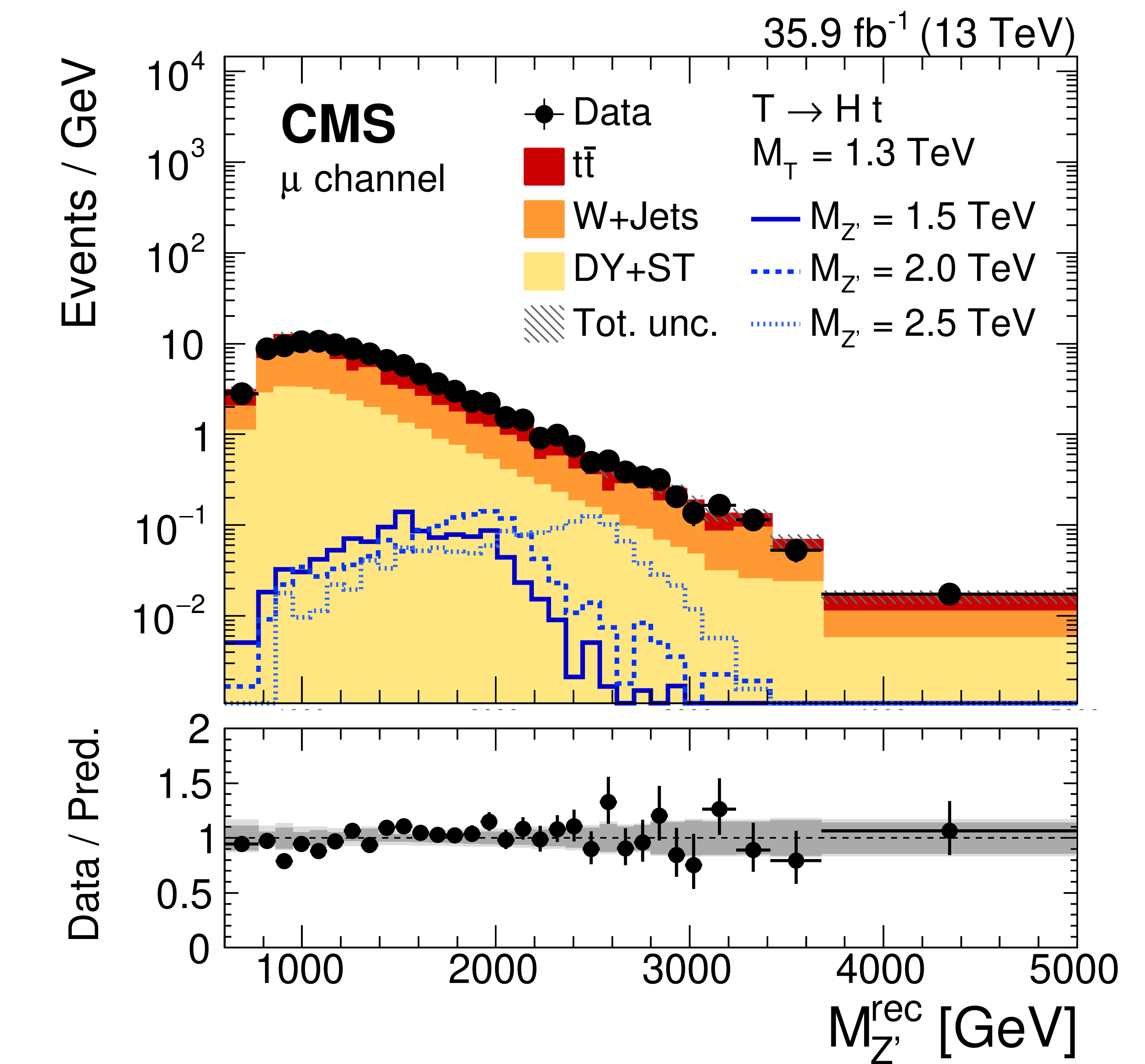
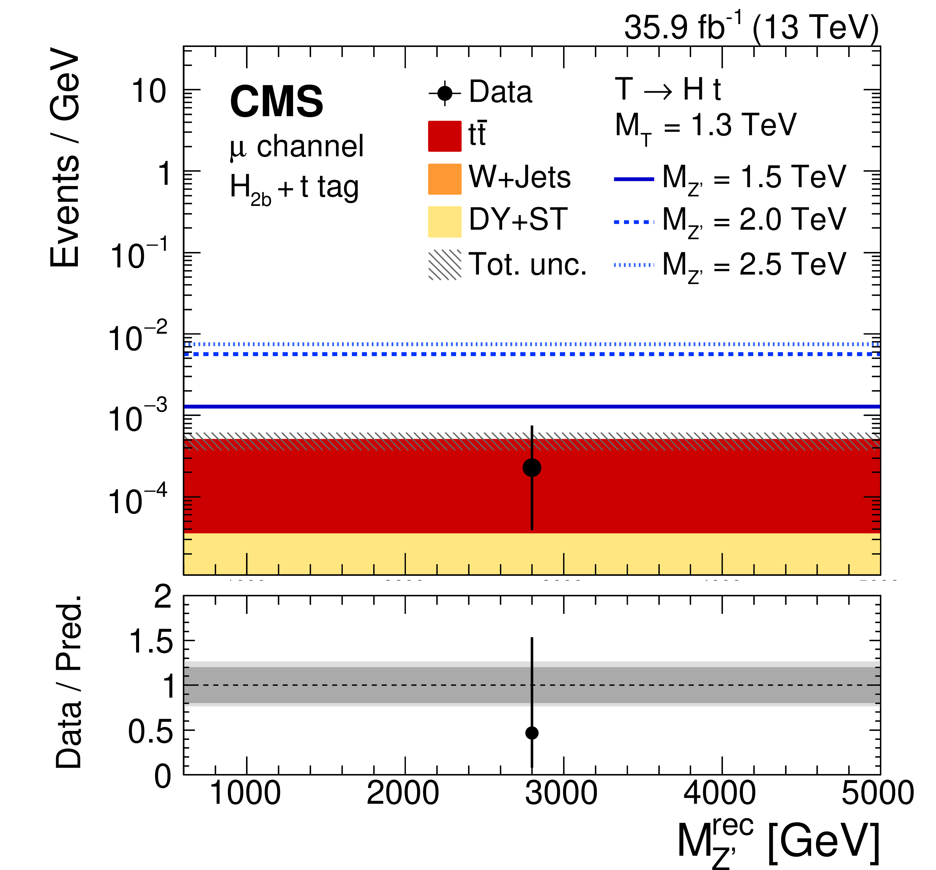
Figure 5:
Distribution of the reconstructed Z' resonance mass after the full selection in the $\mu$+jets channel for the data, the expected SM background, and for the signal with different Z' masses for a fixed T mass of 1.3 TeV. In the left (right) column the results in the top tag (no top tag) category are shown. Different rows display the distributions of events accepted by different taggers as well as the signal for the respective T decays: $ {{\mathrm {H}} _{2 {\mathrm {b}}}} $ tagger and $ {{\text {T}} \to {\mathrm {H}} {\mathrm {t}}}$ decay (upper), $ {{\mathrm {H}} _{1 {\mathrm {b}}}} $ tagger and $ {{\text {T}} \to {\mathrm {H}} {\mathrm {t}}}$ decay (middle), and $ {\mathrm {Z}} / {\mathrm {W}}$ tagger and $ {{\text {T}} \to {\mathrm {Z}} {\mathrm {t}}}$ decay (lower). The signal histograms correspond to a nominal cross section $\sigma ({\mathrm {Z}'}\to {\mathrm {t}} {\text {T}})$ of 1 pb. The lower panel shows the ratio of data to predicted background. Here the darker grey band indicates the statistical uncertainty, whilst the lighter grey band shows the combined statistical and systematic uncertainty. |
png pdf |
Figure 5-a:
Distribution of the reconstructed Z' resonance mass after the full selection in the $\mu$+jets channel for the data, the expected SM background, and for the signal with different Z' masses for a fixed T mass of 1.3 TeV. The results in the top tag category are shown. The plot displays the distribution of events accepted by the $ {{\mathrm {H}} _{2 {\mathrm {b}}}} $ tagger as well as the signal for the $ {{\text {T}} \to {\mathrm {H}} {\mathrm {t}}}$ decay. The signal histograms correspond to a nominal cross section $\sigma ({\mathrm {Z}'}\to {\mathrm {t}} {\text {T}})$ of 1 pb. The lower panel shows the ratio of data to predicted background. Here the darker grey band indicates the statistical uncertainty, whilst the lighter grey band shows the combined statistical and systematic uncertainty. |

png pdf |
Figure 5-b:
Distribution of the reconstructed Z' resonance mass after the full selection in the $\mu$+jets channel for the data, the expected SM background, and for the signal with different Z' masses for a fixed T mass of 1.3 TeV. The results in the no top tag category are shown. The plot displays the distribution of events accepted by the $ {{\mathrm {H}} _{2 {\mathrm {b}}}} $ tagger as well as the signal for the $ {{\text {T}} \to {\mathrm {H}} {\mathrm {t}}}$ decay. The signal histograms correspond to a nominal cross section $\sigma ({\mathrm {Z}'}\to {\mathrm {t}} {\text {T}})$ of 1 pb. The lower panel shows the ratio of data to predicted background. Here the darker grey band indicates the statistical uncertainty, whilst the lighter grey band shows the combined statistical and systematic uncertainty. |

png pdf |
Figure 5-c:
Distribution of the reconstructed Z' resonance mass after the full selection in the $\mu$+jets channel for the data, the expected SM background, and for the signal with different Z' masses for a fixed T mass of 1.3 TeV. The results in the top tag category are shown. The plot displays the distribution of events accepted by the $ {{\mathrm {H}} _{1 {\mathrm {b}}}} $ tagger as well as the signal for the $ {{\text {T}} \to {\mathrm {H}} {\mathrm {t}}}$ decay. The signal histograms correspond to a nominal cross section $\sigma ({\mathrm {Z}'}\to {\mathrm {t}} {\text {T}})$ of 1 pb. The lower panel shows the ratio of data to predicted background. Here the darker grey band indicates the statistical uncertainty, whilst the lighter grey band shows the combined statistical and systematic uncertainty. |

png pdf |
Figure 5-d:
Distribution of the reconstructed Z' resonance mass after the full selection in the $\mu$+jets channel for the data, the expected SM background, and for the signal with different Z' masses for a fixed T mass of 1.3 TeV. The results in the no top tag category are shown. The plot displays the distribution of events accepted by the $ {{\mathrm {H}} _{1 {\mathrm {b}}}} $ tagger as well as the signal for the $ {{\text {T}} \to {\mathrm {H}} {\mathrm {t}}}$ decay. The signal histograms correspond to a nominal cross section $\sigma ({\mathrm {Z}'}\to {\mathrm {t}} {\text {T}})$ of 1 pb. The lower panel shows the ratio of data to predicted background. Here the darker grey band indicates the statistical uncertainty, whilst the lighter grey band shows the combined statistical and systematic uncertainty. |

png pdf |
Figure 5-e:
Distribution of the reconstructed Z' resonance mass after the full selection in the $\mu$+jets channel for the data, the expected SM background, and for the signal with different Z' masses for a fixed T mass of 1.3 TeV. The results in the top tag category are shown. The plot displays the distribution of events accepted by the $ {\mathrm {Z}} / {\mathrm {W}}$ tagger as well as the signal for the $ {{\text {T}} \to {\mathrm {Z}} {\mathrm {t}}}$ decay. The signal histograms correspond to a nominal cross section $\sigma ({\mathrm {Z}'}\to {\mathrm {t}} {\text {T}})$ of 1 pb. The lower panel shows the ratio of data to predicted background. Here the darker grey band indicates the statistical uncertainty, whilst the lighter grey band shows the combined statistical and systematic uncertainty. |

png pdf |
Figure 5-f:
Distribution of the reconstructed Z' resonance mass after the full selection in the $\mu$+jets channel for the data, the expected SM background, and for the signal with different Z' masses for a fixed T mass of 1.3 TeV. The results in the no top tag category are shown. The plot displays the distribution of events accepted by the $ {\mathrm {Z}} / {\mathrm {W}}$ tagger as well as the signal for the $ {{\text {T}} \to {\mathrm {Z}} {\mathrm {t}}}$ decay. The signal histograms correspond to a nominal cross section $\sigma ({\mathrm {Z}'}\to {\mathrm {t}} {\text {T}})$ of 1 pb. The lower panel shows the ratio of data to predicted background. Here the darker grey band indicates the statistical uncertainty, whilst the lighter grey band shows the combined statistical and systematic uncertainty. |

png pdf |
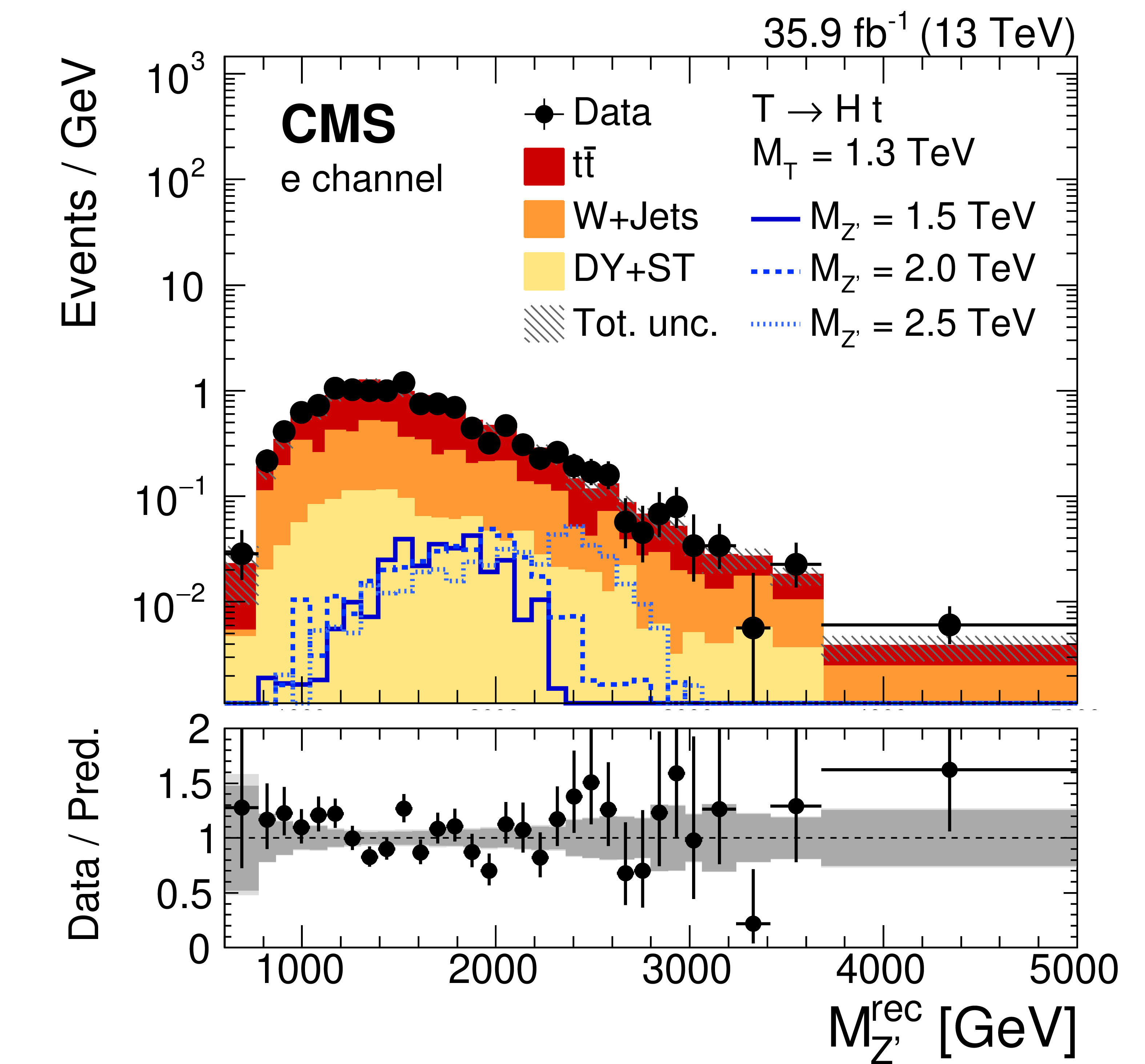
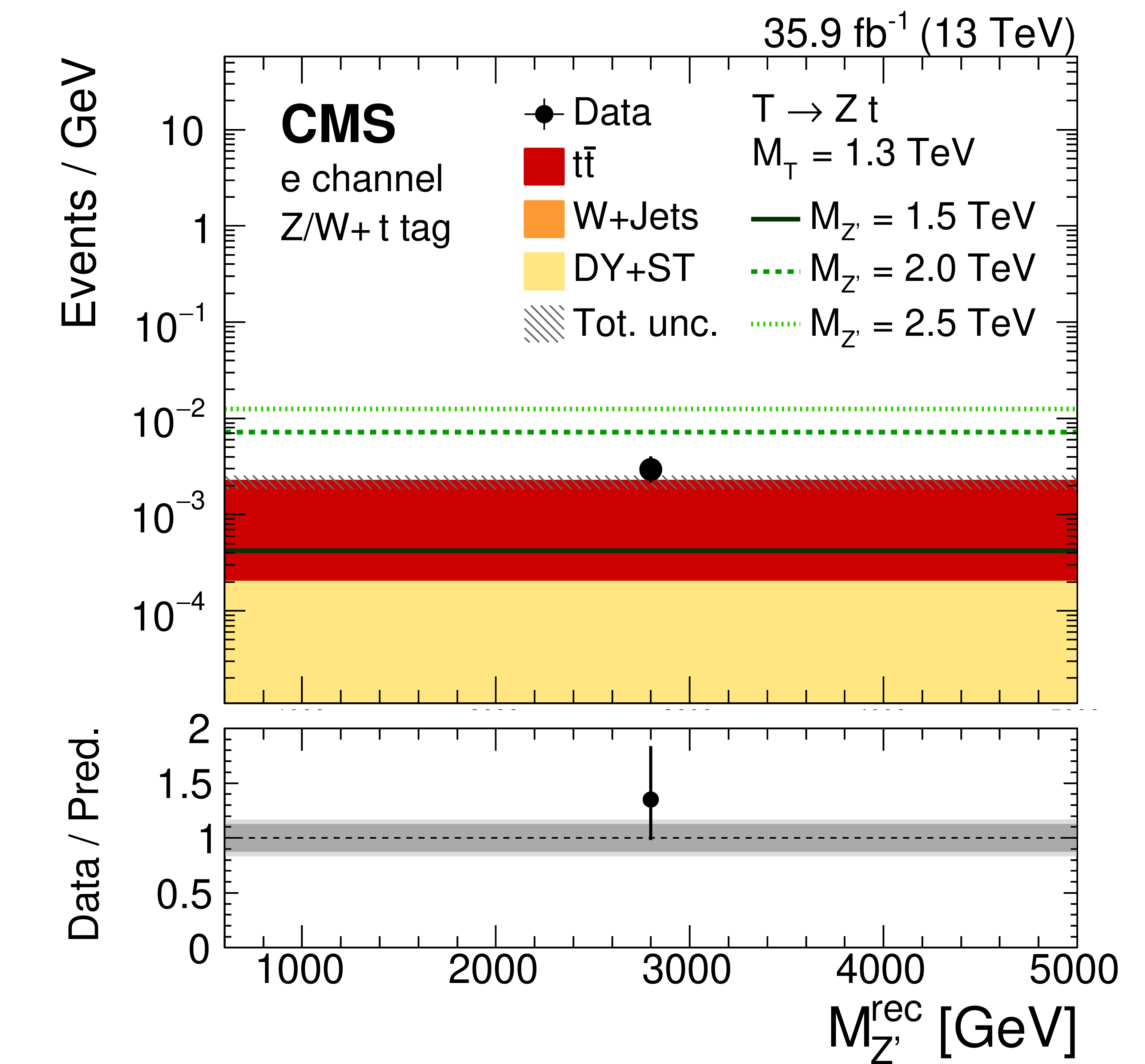
Figure 6:
Distribution of the reconstructed Z' resonance mass after the full selection in the e+jets channel for the data, the expected SM background, and for the signal with different Z' masses for a fixed T mass of 1.3 TeV. In the left (right) column the results in the top tag (no top tag) category are shown. Different rows display the distributions of events accepted by different taggers as well as the signal for the respective T decays: $ {{\mathrm {H}} _{2 {\mathrm {b}}}} $ tagger and $ {{\text {T}} \to {\mathrm {H}} {\mathrm {t}}}$ decay (upper), $ {{\mathrm {H}} _{1 {\mathrm {b}}}} $ tagger and $ {{\text {T}} \to {\mathrm {H}} {\mathrm {t}}}$ decay (middle), and $ {\mathrm {Z}} / {\mathrm {W}}$ tagger and $ {{\text {T}} \to {\mathrm {Z}} {\mathrm {t}}}$ decay (lower). The signal histograms correspond to a nominal cross section $\sigma ({\mathrm {Z}'}\to {\mathrm {t}} {\text {T}})$ of 1 pb. The lower panel shows the ratio of data to predicted background. Here the darker grey band indicates the statistical uncertainty, whilst the lighter grey band shows the combined statistical and systematic uncertainty. |

png pdf |
Figure 6-a:
Distribution of the reconstructed Z' resonance mass after the full selection in the e+jets channel for the data, the expected SM background, and for the signal with different Z' masses for a fixed T mass of 1.3 TeV. Results in the top tag category are shown. The plot displays the distribution of events accepted by the $ {{\mathrm {H}} _{2 {\mathrm {b}}}} $ tagger as well as the signal for the $ {{\text {T}} \to {\mathrm {H}} {\mathrm {t}}}$ decay. The signal histogram corresponds to a nominal cross section $\sigma ({\mathrm {Z}'}\to {\mathrm {t}} {\text {T}})$ of 1 pb. The lower panel shows the ratio of data to predicted background. Here the darker grey band indicates the statistical uncertainty, whilst the lighter grey band shows the combined statistical and systematic uncertainty. |

png pdf |
Figure 6-b:
Distribution of the reconstructed Z' resonance mass after the full selection in the e+jets channel for the data, the expected SM background, and for the signal with different Z' masses for a fixed T mass of 1.3 TeV. Results in the no top tag category are shown. The plot displays the distribution of events accepted by the $ {{\mathrm {H}} _{2 {\mathrm {b}}}} $ tagger as well as the signal for the $ {{\text {T}} \to {\mathrm {H}} {\mathrm {t}}}$ decay. The signal histogram corresponds to a nominal cross section $\sigma ({\mathrm {Z}'}\to {\mathrm {t}} {\text {T}})$ of 1 pb. The lower panel shows the ratio of data to predicted background. Here the darker grey band indicates the statistical uncertainty, whilst the lighter grey band shows the combined statistical and systematic uncertainty. |

png pdf |
Figure 6-c:
Distribution of the reconstructed Z' resonance mass after the full selection in the e+jets channel for the data, the expected SM background, and for the signal with different Z' masses for a fixed T mass of 1.3 TeV. Results in the top tag category are shown. The plot displays the distribution of events accepted by the $ {{\mathrm {H}} _{1 {\mathrm {b}}}} $ tagger as well as the signal for the $ {{\text {T}} \to {\mathrm {H}} {\mathrm {t}}}$ decay. The signal histogram corresponds to a nominal cross section $\sigma ({\mathrm {Z}'}\to {\mathrm {t}} {\text {T}})$ of 1 pb. The lower panel shows the ratio of data to predicted background. Here the darker grey band indicates the statistical uncertainty, whilst the lighter grey band shows the combined statistical and systematic uncertainty. |

png pdf |
Figure 6-d:
Distribution of the reconstructed Z' resonance mass after the full selection in the e+jets channel for the data, the expected SM background, and for the signal with different Z' masses for a fixed T mass of 1.3 TeV. Results in the no top tag category are shown. The plot displays the distribution of events accepted by the $ {{\mathrm {H}} _{1 {\mathrm {b}}}} $ tagger as well as the signal for the $ {{\text {T}} \to {\mathrm {H}} {\mathrm {t}}}$ decay. The signal histogram corresponds to a nominal cross section $\sigma ({\mathrm {Z}'}\to {\mathrm {t}} {\text {T}})$ of 1 pb. The lower panel shows the ratio of data to predicted background. Here the darker grey band indicates the statistical uncertainty, whilst the lighter grey band shows the combined statistical and systematic uncertainty. |
png pdf |
Figure 6-e:
Distribution of the reconstructed Z' resonance mass after the full selection in the e+jets channel for the data, the expected SM background, and for the signal with different Z' masses for a fixed T mass of 1.3 TeV. Results in the top tag category are shown. The plot displays the distribution of events accepted by the $ {\mathrm {Z}} / {\mathrm {W}}$ tagger as well as the signal for the $ {{\text {T}} \to {\mathrm {Z}} {\mathrm {t}}}$ decay. The signal histogram corresponds to a nominal cross section $\sigma ({\mathrm {Z}'}\to {\mathrm {t}} {\text {T}})$ of 1 pb. The lower panel shows the ratio of data to predicted background. Here the darker grey band indicates the statistical uncertainty, whilst the lighter grey band shows the combined statistical and systematic uncertainty. |

png pdf |
Figure 6-f:
Distribution of the reconstructed Z' resonance mass after the full selection in the e+jets channel for the data, the expected SM background, and for the signal with different Z' masses for a fixed T mass of 1.3 TeV. Results in the no top tag category are shown. The plot displays the distribution of events accepted by the $ {\mathrm {Z}} / {\mathrm {W}}$ tagger as well as the signal for the $ {{\text {T}} \to {\mathrm {Z}} {\mathrm {t}}}$ decay. The signal histogram corresponds to a nominal cross section $\sigma ({\mathrm {Z}'}\to {\mathrm {t}} {\text {T}})$ of 1 pb. The lower panel shows the ratio of data to predicted background. Here the darker grey band indicates the statistical uncertainty, whilst the lighter grey band shows the combined statistical and systematic uncertainty. |

png pdf |
Figure 7:
Observed exclusion limits at 95% CL on the production cross section for various ($ {M_{{\mathrm {Z}'}}}, {M_{{\text {T}}}} $) combinations for the decay channels $ {{\text {T}} \to {\mathrm {H}} {\mathrm {t}}}$ (upper left), $ {{\text {T}} \to {\mathrm {Z}} {\mathrm {t}}}$ (upper right), and $ {{\text {T}} \to {\mathrm {W}} {\mathrm {b}}}$ (lower). The white area in the upper left indicates the region where the $ {{\mathrm {Z}'}\to {\mathrm {t}} {\text {T}}}$ decay is kinematically forbidden, while in the lower right $ {{\mathrm {Z}'}\to {\mathrm {t}} {\text {T}}}$ is suppressed by the preferred $ {\mathrm {Z}'}\to {\text {T}} {\text {T}} $ mode. Other white areas indicate regions where signal samples have not been generated. |

png pdf |
Figure 7-a:
Observed exclusion limits at 95% CL on the production cross section for various ($ {M_{{\mathrm {Z}'}}}, {M_{{\text {T}}}} $) combinations for the decay channel $ {{\text {T}} \to {\mathrm {H}} {\mathrm {t}}}$. The white area in the upper left indicates the region where the $ {{\mathrm {Z}'}\to {\mathrm {t}} {\text {T}}}$ decay is kinematically forbidden, while in the lower right $ {{\mathrm {Z}'}\to {\mathrm {t}} {\text {T}}}$ is suppressed by the preferred $ {\mathrm {Z}'}\to {\text {T}} {\text {T}} $ mode. Other white areas indicate regions where signal samples have not been generated. |

png pdf |
Figure 7-b:
Observed exclusion limits at 95% CL on the production cross section for various ($ {M_{{\mathrm {Z}'}}}, {M_{{\text {T}}}} $) combinations for the decay channel $ {{\text {T}} \to {\mathrm {Z}} {\mathrm {t}}}$. The white area in the upper left indicates the region where the $ {{\mathrm {Z}'}\to {\mathrm {t}} {\text {T}}}$ decay is kinematically forbidden, while in the lower right $ {{\mathrm {Z}'}\to {\mathrm {t}} {\text {T}}}$ is suppressed by the preferred $ {\mathrm {Z}'}\to {\text {T}} {\text {T}} $ mode. Other white areas indicate regions where signal samples have not been generated. |

png pdf |
Figure 7-c:
Observed exclusion limits at 95% CL on the production cross section for various ($ {M_{{\mathrm {Z}'}}}, {M_{{\text {T}}}} $) combinations for the decay channel $ {{\text {T}} \to {\mathrm {W}} {\mathrm {b}}}$. The white area in the upper left indicates the region where the $ {{\mathrm {Z}'}\to {\mathrm {t}} {\text {T}}}$ decay is kinematically forbidden, while in the lower right $ {{\mathrm {Z}'}\to {\mathrm {t}} {\text {T}}}$ is suppressed by the preferred $ {\mathrm {Z}'}\to {\text {T}} {\text {T}} $ mode. Other white areas indicate regions where signal samples have not been generated. |

png pdf |
Figure 8:
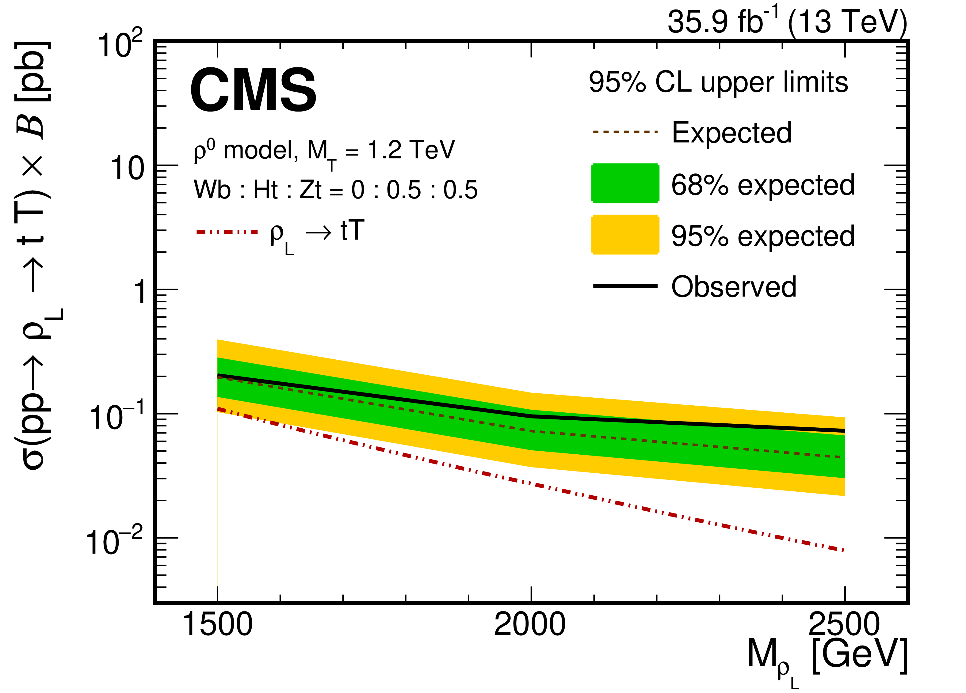
Exclusion limits at 95% CL on the product of the cross section and branching fraction for three T masses of 1.2 TeV (upper row), 1.5 TeV (lower left), and 2.1 TeV (lower right), as a function of the resonance mass. The branching fraction is defined as $\mathcal {B}= \mathcal {B}({{\text {T}} \to {\mathrm {W}} {\mathrm {b}}}) + \mathcal {B}({{\text {T}} \to {\mathrm {H}} {\mathrm {t}}}) + \mathcal {B}({{\text {T}} \to {\mathrm {Z}} {\mathrm {t}}})$. Observed and expected limits are compared to the predictions from two different theory benchmark models: the $ {\mathrm {G}^*} $ model (upper left and lower row), and the left-handed $ {\rho _{\mathrm {L}}} $ in the $ {\rho ^0} $ model (upper right). |

png pdf |
Figure 8-a:
Exclusion limits at 95% CL on the product of the cross section and branching fraction for three T masses of 1.2 TeV, as a function of the resonance mass. The branching fraction is defined as $\mathcal {B}= \mathcal {B}({{\text {T}} \to {\mathrm {W}} {\mathrm {b}}}) + \mathcal {B}({{\text {T}} \to {\mathrm {H}} {\mathrm {t}}}) + \mathcal {B}({{\text {T}} \to {\mathrm {Z}} {\mathrm {t}}})$. Observed and expected limits are compared to the predictions from the $ {\mathrm {G}^*} $ model. |
png pdf |
Figure 8-b:
Exclusion limits at 95% CL on the product of the cross section and branching fraction for three T masses of 1.2 TeV, as a function of the resonance mass. The branching fraction is defined as $\mathcal {B}= \mathcal {B}({{\text {T}} \to {\mathrm {W}} {\mathrm {b}}}) + \mathcal {B}({{\text {T}} \to {\mathrm {H}} {\mathrm {t}}}) + \mathcal {B}({{\text {T}} \to {\mathrm {Z}} {\mathrm {t}}})$. Observed and expected limits are compared to the predictions from the left-handed $ {\rho _{\mathrm {L}}} $ in the $ {\rho ^0} $ model. |

png pdf |
Figure 8-c:
Exclusion limits at 95% CL on the product of the cross section and branching fraction for three T masses of 1.5 TeV, as a function of the resonance mass. The branching fraction is defined as $\mathcal {B}= \mathcal {B}({{\text {T}} \to {\mathrm {W}} {\mathrm {b}}}) + \mathcal {B}({{\text {T}} \to {\mathrm {H}} {\mathrm {t}}}) + \mathcal {B}({{\text {T}} \to {\mathrm {Z}} {\mathrm {t}}})$. Observed and expected limits are compared to the predictions from the $ {\mathrm {G}^*} $ model. |

png pdf |
Figure 8-d:
Exclusion limits at 95% CL on the product of the cross section and branching fraction for three T masses of 2.1 TeV, as a function of the resonance mass. The branching fraction is defined as $\mathcal {B}= \mathcal {B}({{\text {T}} \to {\mathrm {W}} {\mathrm {b}}}) + \mathcal {B}({{\text {T}} \to {\mathrm {H}} {\mathrm {t}}}) + \mathcal {B}({{\text {T}} \to {\mathrm {Z}} {\mathrm {t}}})$. Observed and expected limits are compared to the predictions from the $ {\mathrm {G}^*} $ model. |

png pdf |
Figure 9:
Model-independent observed exclusion limits at 95% CL on the product of the cross section and branching fraction $\mathcal {B}= \mathcal {B}({{\text {T}} \to {\mathrm {W}} {\mathrm {b}}}) + \mathcal {B}({{\text {T}} \to {\mathrm {H}} {\mathrm {t}}}) + \mathcal {B}({{\text {T}} \to {\mathrm {Z}} {\mathrm {t}}})$ for an example mass configuration of $ {M_{{\mathrm {Z}'}}} =1.5$ TeV and $ {M_{{\text {T}}}} =1.3$ TeV as a function of the branching fractions $\mathcal {B}({{\text {T}} \to {\mathrm {H}} {\mathrm {t}}})$ and $\mathcal {B}({{\text {T}} \to {\mathrm {Z}} {\mathrm {t}}})$. |
| Tables | |

png pdf |
Table 1:
Signal selection efficiency for the three T decay modes in each category for a signal with $ {M_{{\mathrm {Z}'}}} = $ 1.5 TeV and $ {M_{{\text {T}}}} = $ 1.3 TeV, taking into account branching fractions $\mathcal {B}({\mathrm {t}} {\mathrm {H}} {\mathrm {t}}\to {\ell \text {+jets}}) = 0.294$, $\mathcal {B}({\mathrm {t}} {\mathrm {Z}} {\mathrm {t}}\to {\ell \text {+jets}}) = 0.317$, and $\mathcal {B}({\mathrm {t}} {\mathrm {W}} {\mathrm {b}}\to {\ell \text {+jets}}) = 0.255$ [64], where $ {\ell \text {+jets}}$ is a final state with exactly one electron or muon, including electrons and muons from tau lepton decays. The last row of the table shows the total selection efficiency summed over all six categories. |

png pdf |
Table 2:
Signal selection efficiency after each step in the selection requirements for a signal with $ {M_{{\mathrm {Z}'}}} = $ 1.5 TeV and $ {M_{{\text {T}}}} = $ 1.3 TeV, taking into account branching fractions $\mathcal {B}({\mathrm {t}} {\mathrm {H}} {\mathrm {t}}\to {\ell \text {+jets}}) = 0.294$, $\mathcal {B}({\mathrm {t}} {\mathrm {Z}} {\mathrm {t}}\to {\ell \text {+jets}}) = 0.317$, and $\mathcal {B}({\mathrm {t}} {\mathrm {W}} {\mathrm {b}}\to {\ell \text {+jets}}) = 0.255$ [64], where $ {\ell \text {+jets}}$ is a final state with exactly one electron or muon, including electrons and muons from tau lepton decays. |
png pdf |
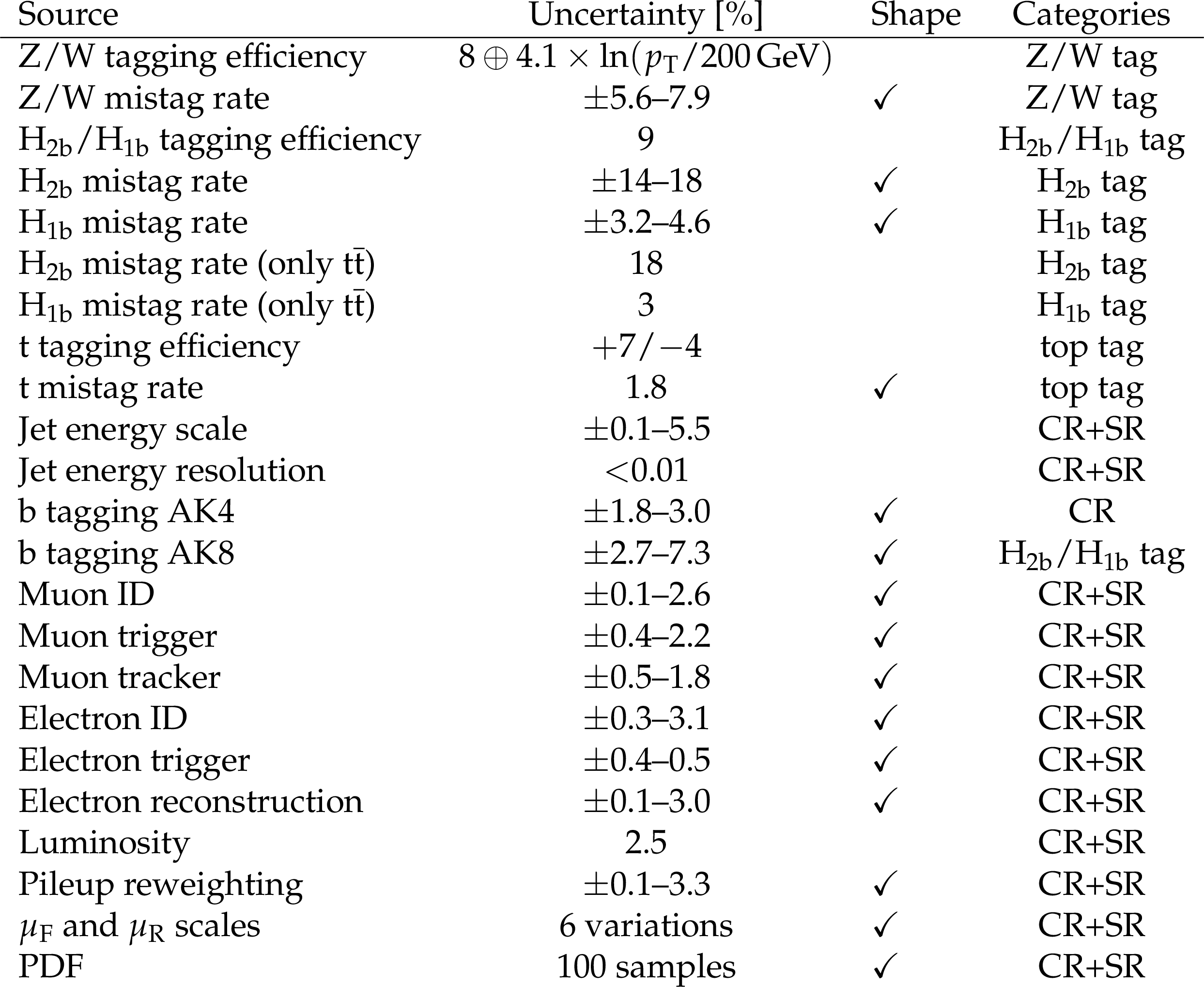
Table 3:
List of systematic uncertainties considered in the statistical analysis, with the size of their impact, the type(s) of effect they have, and the categories they affect. The impact size of each uncertainty is based on a signal sample with $ {M_{{\mathrm {Z}'}}} = $ 1.5 TeV and $ {M_{{\text {T}}}} = $ 1.3 TeV. All uncertainties affect the normalizations of the $ {M_{{\mathrm {Z}'}}^{\text {rec}}} $ distributions. The ones also affecting the shapes are indicated by a tick mark. Uncertainties that affect control regions are denoted by CR, whilst those that affect signal regions are denoted by SR. |
| Summary |
| A search for a heavy spin-1 resonance Z' decaying to a standard model top quark and a vector-like quark partner T has been presented. The data used in this search were recorded with the CMS detector at the LHC at $\sqrt{s} = $ 13 TeV and correspond to an integrated luminosity of 35.9 fb$^{-1}$. The analysis is primarily optimised to study the decay modes of the vector-like quark to a Higgs boson and a top quark (${{\text{T}} \to \mathrm{H}\mathrm{t}}$), and to a Z boson and a top quark (${{\text{T}} \to \mathrm{Z}\mathrm{t}}$), although the decay to a W boson and a bottom quark (${{\text{T}} \to \mathrm{W}\mathrm{b}}$) is also considered. This is the first direct search for the decay $\mathrm{Z'} \to \mathrm{tT} \to \mathrm{t}\mathrm{H}\mathrm{t}$. No significant excess of events over the expectation from standard model backgrounds is found. Limits on the production cross section are presented for a narrow Z' resonance in the mass range from 1.5 to 4.0 TeV and a narrow T resonance in the mass range from 0.7 to 3.0 TeV. Interpretation of these limits within the context of the ${\mathrm{G}^*} $ benchmark model results in the exclusion of ${\mathrm{G}^*} $ resonance masses in the range from 1.5 to 2.3 TeV and from 2.0 to 2.4 TeV, for a T mass of 1.2 and 1.5 TeV, respectively. The presented limits are the most stringent to date for the decay mode $\mathrm{Z'} \to \mathrm{tT} \to \mathrm{t}\mathrm{H}\mathrm{t}$. |
| References | ||||
| 1 | D. Greco and D. Liu | Hunting composite vector resonances at the LHC: naturalness facing data | JHEP 12 (2014) 126 | 1410.2883 |
| 2 | C. Bini, R. Contino, and N. Vignaroli | Heavy-light decay topologies as a new strategy to discover a heavy gluon | JHEP 01 (2012) 157 | 1110.6058 |
| 3 | L. Randall and R. Sundrum | A large mass hierarchy from a small extra dimension | PRL 83 (1999) 3370 | hep-ph/9905221 |
| 4 | L. Randall and R. Sundrum | An alternative to compactification | PRL 83 (1999) 4690 | hep-th/9906064 |
| 5 | ATLAS Collaboration | A search for $ \mathrm{t}\overline{\mathrm{t}} $ resonances using lepton-plus-jets events in proton-proton collisions at $ \sqrt{s}= $ 8 TeV with the ATLAS detector | JHEP 08 (2015) 148 | 1505.07018 |
| 6 | CMS Collaboration | Searches for new physics using the $ \mathrm{t}\overline{\mathrm{t}} $ invariant mass distribution in pp collisions at $ \sqrt{s}= $ 8 TeV | PRL 111 (2013) 211804 | CMS-B2G-13-001 1309.2030 |
| 7 | CMS Collaboration | Search for resonant $ \mathrm{t}\overline{\mathrm{t}} $ production in proton-proton collisions at $ \sqrt{s}= $ 8 TeV | PRD 93 (2016) 012001 | CMS-B2G-13-008 1506.03062 |
| 8 | ATLAS Collaboration | Search for heavy particles decaying into top-quark-pairs using lepton-plus-jets events in proton-proton collisions at $ \sqrt{s} = $ 13 TeV with the ATLAS detector | EPJC 78 (2018) 565 | 1804.10823 |
| 9 | CMS Collaboration | Search for $ \mathrm{t}\overline{\mathrm{t}} $ resonances in highly boosted lepton+jets and fully hadronic final states in proton-proton collisions at $ \sqrt{s}= $ 13 TeV | JHEP 07 (2017) 001 | CMS-B2G-16-015 1704.03366 |
| 10 | CMS Collaboration | Search for resonant $ \mathrm{t}\overline{\mathrm{t}} $ production in proton-proton collisions at $ \sqrt{s}= $ 13 TeV | Submitted to JHEP | CMS-B2G-17-017 1810.05905 |
| 11 | J. A. Aguilar-Saavedra, R. Benbrik, S. Heinemeyer, and M. P\'erez-Victoria | Handbook of vector-like quarks: mixing and single production | PRD 88 (2013) 094010 | 1306.0572 |
| 12 | R. Contino, D. Marzocca, D. Pappadopulo, and R. Rattazzi | On the effect of resonances in composite Higgs phenomenology | JHEP 10 (2011) 081 | 1109.1570 |
| 13 | D. Barducci et al. | Exploring Drell-Yan signals from the 4D composite Higgs model at the LHC | JHEP 04 (2013) 152 | 1210.2927 |
| 14 | A. De Simone, O. Matsedonskyi, R. Rattazzi, and A. Wulzer | A first top partner hunter's guide | JHEP 04 (2013) 004 | 1211.5663 |
| 15 | D. Barducci and C. Delaunay | Bounding wide composite vector resonances at the LHC | JHEP 02 (2016) 055 | 1511.01101 |
| 16 | H. Davoudiasl, J. L. Hewett, and T. G. Rizzo | Bulk gauge fields in the Randall--Sundrum model | PLB 473 (2000) 43 | hep-ph/9911262 |
| 17 | CMS Collaboration | Search for a heavy resonance decaying to a top quark and a vector-like top quark at $ \sqrt{s}= $ 13 TeV | JHEP 09 (2017) 053 | CMS-B2G-16-013 1703.06352 |
| 18 | CMS Collaboration | Search for single production of a vector-like T quark decaying to a Z boson and a top quark in proton-proton collisions at $ \sqrt s = $ 13 TeV | PLB 781 (2018) 574 | CMS-B2G-17-007 1708.01062 |
| 19 | ATLAS Collaboration | Search for pair production of vector-like top quarks in events with one lepton, jets, and missing transverse momentum in $ \sqrt{s}= $ 13 TeV pp collisions with the ATLAS detector | JHEP 08 (2017) 052 | 1705.10751 |
| 20 | ATLAS Collaboration | Search for pair production of heavy vector-like quarks decaying to high-p$ _{\mathrm{T}} $ W bosons and b quarks in the lepton-plus-jets final state in pp collisions at $ \sqrt{s}= $ 13 TeV with the ATLAS detector | JHEP 10 (2017) 141 | 1707.03347 |
| 21 | ATLAS Collaboration | Search for pair production of up-type vector-like quarks and for four-top-quark events in final states with multiple b-jets with the ATLAS detector | JHEP 07 (2018) 089 | 1803.09678 |
| 22 | ATLAS Collaboration | Search for pair- and single-production of vector-like quarks in final states with at least one Z boson decaying into a pair of electrons or muons in pp collision data collected with the ATLAS detector at $ \sqrt{s} = $ 13 TeV | Submitted to PRD | 1806.10555 |
| 23 | ATLAS Collaboration | Search for pair production of heavy vector-like quarks decaying into hadronic final states in pp collisions at $ \sqrt{s} = $ 13 TeV with the ATLAS detector | PRD 98 (2018) 092005 | 1808.01771 |
| 24 | ATLAS Collaboration | Combination of the searches for pair-produced vector-like partners of the third-generation quarks at $ \sqrt{s} = $ 13 TeV with the ATLAS detector | PRL 121 (2018) 211801 | 1808.02343 |
| 25 | CMS Collaboration | Search for pair production of vector-like quarks in the bW$ \overline{\mathrm{b}} $W channel from proton-proton collisions at $ \sqrt{s} = $ 13 TeV | PLB 779 (2018) 82 | CMS-B2G-17-003 1710.01539 |
| 26 | CMS Collaboration | Search for vector-like T and B quark pairs in final states with leptons at $ \sqrt{s} = $ 13 TeV | JHEP 08 (2018) 177 | CMS-B2G-17-011 1805.04758 |
| 27 | CMS Collaboration | CMS luminosity measurements for the 2016 data taking period | CMS-PAS-LUM-17-001 | CMS-PAS-LUM-17-001 |
| 28 | CMS Collaboration | Jet algorithms performance in 13 TeV data | CMS-PAS-JME-16-003 | CMS-PAS-JME-16-003 |
| 29 | CMS Collaboration | The CMS trigger system | JINST 12 (2017) P01020 | CMS-TRG-12-001 1609.02366 |
| 30 | CMS Collaboration | The CMS experiment at the CERN LHC | JINST 3 (2008) S08004 | CMS-00-001 |
| 31 | CMS Collaboration | Particle-flow reconstruction and global event description with the CMS detector | JINST 12 (2017) P10003 | CMS-PRF-14-001 1706.04965 |
| 32 | M. Cacciari, G. P. Salam, and G. Soyez | The anti-$ {k_{\mathrm{T}}} $ jet clustering algorithm | JHEP 04 (2008) 063 | 0802.1189 |
| 33 | M. Cacciari, G. P. Salam, and G. Soyez | FastJet user manual | EPJC 72 (2012) 1896 | 1111.6097 |
| 34 | CMS Collaboration | Performance of CMS muon reconstruction in pp collision events at $ \sqrt{s}= $ 7 TeV | JINST 7 (2012) P10002 | CMS-MUO-10-004 1206.4071 |
| 35 | CMS Collaboration | Performance of the CMS muon detector and muon reconstruction with proton-proton collisions at $ \sqrt{s} = $ 13 TeV | JINST 13 (2018) P06015 | CMS-MUO-16-001 1804.04528 |
| 36 | CMS Collaboration | Performance of electron reconstruction and selection with the CMS detector in proton-proton collisions at $ \sqrt{s}= $ 8 TeV | JINST 10 (2015) P06005 | CMS-EGM-13-001 1502.02701 |
| 37 | CMS Collaboration | Jet energy scale and resolution in the CMS experiment in pp collisions at 8 TeV | JINST 12 (2017) P02014 | CMS-JME-13-004 1607.03663 |
| 38 | CMS Collaboration | Filtering out noise in HCAL barrel and endcaps | CDS | |
| 39 | CMS Collaboration | Identification of heavy-flavour jets with the CMS detector in pp collisions at 13 TeV | JINST 13 (2018) P05011 | CMS-BTV-16-002 1712.07158 |
| 40 | J. Thaler and K. Van Tilburg | Identifying boosted objects with N-subjettiness | JHEP 03 (2011) 015 | 1011.2268 |
| 41 | M. Dasgupta, A. Fregoso, S. Marzani, and G. P. Salam | Towards an understanding of jet substructure | JHEP 09 (2013) 029 | 1307.0007 |
| 42 | J. M. Butterworth, A. R. Davison, M. Rubin, and G. P. Salam | Jet substructure as a new Higgs search channel at the LHC | PRL 100 (2008) 242001 | 0802.2470 |
| 43 | A. J. Larkoski, S. Marzani, G. Soyez, and J. Thaler | Soft drop | JHEP 05 (2014) 146 | 1402.2657 |
| 44 | J. Alwall et al. | The automated computation of tree-level and next-to-leading order differential cross sections, and their matching to parton shower simulations | JHEP 07 (2014) 079 | 1405.0301 |
| 45 | T. Sjostrand et al. | An introduction to PYTHIA 8.2 | CPC 191 (2015) 159 | 1410.3012 |
| 46 | P. Skands, S. Carrazza, and J. Rojo | Tuning PYTHIA 8.1: the Monash 2013 tune | EPJC 74 (2014) 3024 | 1404.5630 |
| 47 | CMS Collaboration | Event generator tunes obtained from underlying event and multiparton scattering measurements | EPJC 76 (2016) 155 | CMS-GEN-14-001 1512.00815 |
| 48 | R. Frederix and S. Frixione | Merging meets matching in MC@NLO | JHEP 12 (2012) 061 | 1209.6215 |
| 49 | S. Frixione, P. Nason, and G. Ridolfi | A positive-weight next-to-leading-order Monte Carlo for heavy flavour hadroproduction | JHEP 09 (2007) 126 | 0707.3088 |
| 50 | J. M. Campbell, R. K. Ellis, P. Nason, and E. Re | Top-pair production and decay at NLO matched with parton showers | JHEP 04 (2015) 114 | 1412.1828 |
| 51 | S. Alioli, P. Nason, C. Oleari, and E. Re | NLO single-top production matched with shower in POWHEG: $ s $- and $ t $-channel contributions | JHEP 09 (2009) 111 | 0907.4076 |
| 52 | E. Re | Single-top W$ t $-channel production matched with parton showers using the POWHEG method | EPJC. 71 (2011) 1547 | 1009.2450 |
| 53 | P. Nason | A new method for combining NLO QCD with shower Monte Carlo algorithms | JHEP 11 (2004) 040 | hep-ph/0409146 |
| 54 | S. Frixione, P. Nason, and C. Oleari | Matching NLO QCD computations with parton shower simulations: the POWHEG method | JHEP 11 (2007) 070 | 0709.2092 |
| 55 | S. Alioli, P. Nason, C. Oleari, and E. Re | A general framework for implementing NLO calculations in shower Monte Carlo programs: the POWHEG BOX | JHEP 06 (2010) 043 | 1002.2581 |
| 56 | S. Alioli, S.-O. Moch, and P. Uwer | Hadronic top-quark pair-production with one jet and parton showering | JHEP 01 (2012) 137 | 1110.5251 |
| 57 | R. Frederix, E. Re, and P. Torrielli | Single-top t-channel hadroproduction in the four-flavour scheme with POWHEG and aMC@NLO | JHEP 09 (2012) 130 | 1207.5391 |
| 58 | CMS Collaboration | Measurement of normalized differential $ \mathrm{t}\overline{\mathrm{t}} $ cross sections in the dilepton channel from pp collisions at $ \sqrt{s}= $ 13 TeV | JHEP 04 (2018) 060 | CMS-TOP-16-007 1708.07638 |
| 59 | CMS Collaboration | Measurement of differential cross sections for top quark pair production using the lepton+jets final state in proton-proton collisions at 13 TeV | PRD 95 (2017) 092001 | CMS-TOP-16-008 1610.04191 |
| 60 | CMS Collaboration | Investigations of the impact of the parton shower tuning in PYTHIA 8 in the modelling of $ \mathrm{t\overline{t}} $ at $ \sqrt{s}= $ 8 and 13 TeV | CMS-PAS-TOP-16-021 | CMS-PAS-TOP-16-021 |
| 61 | NNPDF Collaboration | Parton distributions for the LHC Run II | JHEP 04 (2015) 040 | 1410.8849 |
| 62 | GEANT4 Collaboration | GEANT4--a simulation toolkit | NIMA 506 (2003) 250 | |
| 63 | CMS Collaboration | Description and performance of track and primary-vertex reconstruction with the CMS tracker | JINST 9 (2014) P10009 | CMS-TRK-11-001 1405.6569 |
| 64 | Particle Data Group, M. Tanabashi et al. | Review of particle physics | PRD 98 (2018) 030001 | |
| 65 | M. Bahr et al. | Herwig++ physics and manual | EPJC 58 (2008) 639 | 0803.0883 |
| 66 | M. Cacciari et al. | The $ \mathrm{t\bar{t}} $ cross-section at 1.8 TeV and 1.96 TeV: a study of the systematics due to parton densities and scale dependence | JHEP 04 (2004) 068 | hep-ph/0303085 |
| 67 | S. Catani, D. de Florian, M. Grazzini, and P. Nason | Soft gluon resummation for Higgs boson production at hadron colliders | JHEP 07 (2003) 028 | hep-ph/0306211 |
| 68 | J. Butterworth et al. | PDF4LHC recommendations for LHC Run II | JPG 43 (2016) 023001 | 1510.03865 |
| 69 | S. Carrazza, J. I. Latorre, J. Rojo, and G. Watt | A compression algorithm for the combination of PDF sets | EPJC 75 (2015) 474 | 1504.06469 |
| 70 | R. J. Barlow and C. Beeston | Fitting using finite Monte Carlo samples | CPC 77 (1993) 219 | |
| 71 | D. Lindley | Kendall's Advanced Theory of Statistics, volume 2B, Bayesian Inference, 2nd edn | volume 168 Blackwell Publishing Ltd | |
| 72 | L. Demortier, S. Jain, and H. B. Prosper | Reference priors for high energy physics | PRD 82 (2010) 034002 | 1002.1111 |
| 73 | T. Muller, J. Ott, and J. Wagner-Kuhr | Theta--A framework for template-based modeling and inference | link | |
|
|
Compact Muon Solenoid LHC, CERN |
|

|

|

|

|

|