

Compact Muon Solenoid
LHC, CERN
| CMS-B2G-21-002 ; CERN-EP-2021-253 | ||
| Search for resonances decaying to three W bosons in the hadronic final state in proton-proton collisions at $\sqrt{s} = $ 13 TeV | ||
| CMS Collaboration | ||
| 24 December 2021 | ||
| Phys. Rev. D 106 (2022) 012002 | ||
| Abstract: A search for Kaluza-Klein excited vector boson resonances, W$ _{\mathrm{KK}} $, decaying in cascade to three W bosons via a scalar radion R, W$ _{\mathrm{KK}} $ $\to$ WR $\to$ WWW, with two or three massive jets is presented. The search is performed with proton-proton collision data recorded at $\sqrt{s} = $ 13 TeV, collected by the CMS experiment at the CERN LHC, during 2016-2018, corresponding to an integrated luminosity of 138 fb$^{-1}$. Two final states are simultaneously probed, one where the two W bosons produced by the R decay are reconstructed as separate, large-radius, massive jets, and one where they are merged in a single large-radius jet. The data observed are in agreement with the standard model expectations. Limits are set on the product of the W$ _{\mathrm{KK}} $ resonance cross section and branching fraction to three W bosons in an extended warped extra-dimensional model and are the first of their kind at the LHC. | ||
| Links: e-print arXiv:2112.13090 [hep-ex] (PDF) ; CDS record ; inSPIRE record ; HepData record ; Physics Briefing ; CADI line (restricted) ; | ||
| Figures | |

png pdf |
Figure 1:
Schematic diagrams of the decay of a KK excitation of a W boson (W$ _{\mathrm {KK}} $) to the final states considered in this analysis. Left: three individually reconstructed W bosons; right: one individually reconstructed W boson and two W bosons reconstructed as a single large-radius jet, which is predominant for $ {{m}_{\mathrm{R}}} \le 0.2\, {{m}_{{\mathrm{W} _{\mathrm {KK}}}}} $. |
png pdf |
Figure 2:
Variables discriminating between signal and background in simulation. Left column, upper to lower rows: the distributions of ${m_{\mathrm {jj}}}$, ${m^{\text {max}}_{\text {j}}}$, and deep-WH (for highest-mass jet with $ {m^{\text {max}}_{\text {j}}} > $ 100 GeV) for preselected events with $ {N_{\text {j}}} =$ 2. Right column, upper to lower rows: the distributions of ${m_{\mathrm {jjj}}}$, ${m^{\text {max}}_{\text {j}}}$, and deep-W (for highest-mass jet with 60 $ < {m^{\text {max}}_{\text {j}}} < $ 100 GeV) for preselected events with $ {N_{\text {j}}} =$ 3. The signal processes are scaled to 500 times their theoretical cross section for visibility. |

png pdf |
Figure 2-a:
The distribution of ${m_{\mathrm {jj}}}$ for preselected events with $ {N_{\text {j}}} =$ 2. The signal processes are scaled to 500 times their theoretical cross section for visibility. |
png pdf |
Figure 2-b:
The distribution of ${m_{\mathrm {jjj}}}$ for preselected events with $ {N_{\text {j}}} =$ 3. The signal processes are scaled to 500 times their theoretical cross section for visibility. |

png pdf |
Figure 2-c:
The distribution of ${m^{\text {max}}_{\text {j}}}$ for preselected events with $ {N_{\text {j}}} =$ 2. The signal processes are scaled to 500 times their theoretical cross section for visibility. |

png pdf |
Figure 2-d:
The distribution of ${m^{\text {max}}_{\text {j}}}$ for preselected events with $ {N_{\text {j}}} =$ 3. The signal processes are scaled to 500 times their theoretical cross section for visibility. |
png pdf |
Figure 2-e:
The distribution of deep-WH (for highest-mass jet with $ {m^{\text {max}}_{\text {j}}} > $ 100 GeV) for preselected events with $ {N_{\text {j}}} =$ 2. The signal processes are scaled to 500 times their theoretical cross section for visibility. |

png pdf |
Figure 2-f:
The distribution of deep-W (for highest-mass jet with 60 $ < {m^{\text {max}}_{\text {j}}} < $ 100 GeV) for preselected events with $ {N_{\text {j}}} =$ 3. The signal processes are scaled to 500 times their theoretical cross section for visibility. |
png pdf |
Figure 3:
Schematic of the 2D jet mass regions for two-jet events (left) and 3D jet mass regions for three-jet events (right), indicating the location of the six orthogonal signal regions SR1-6, indicated by the colored areas. The SR4 and SR5 differ by the requirement of exactly three and two W-tagged jets, respectively. |

png pdf |
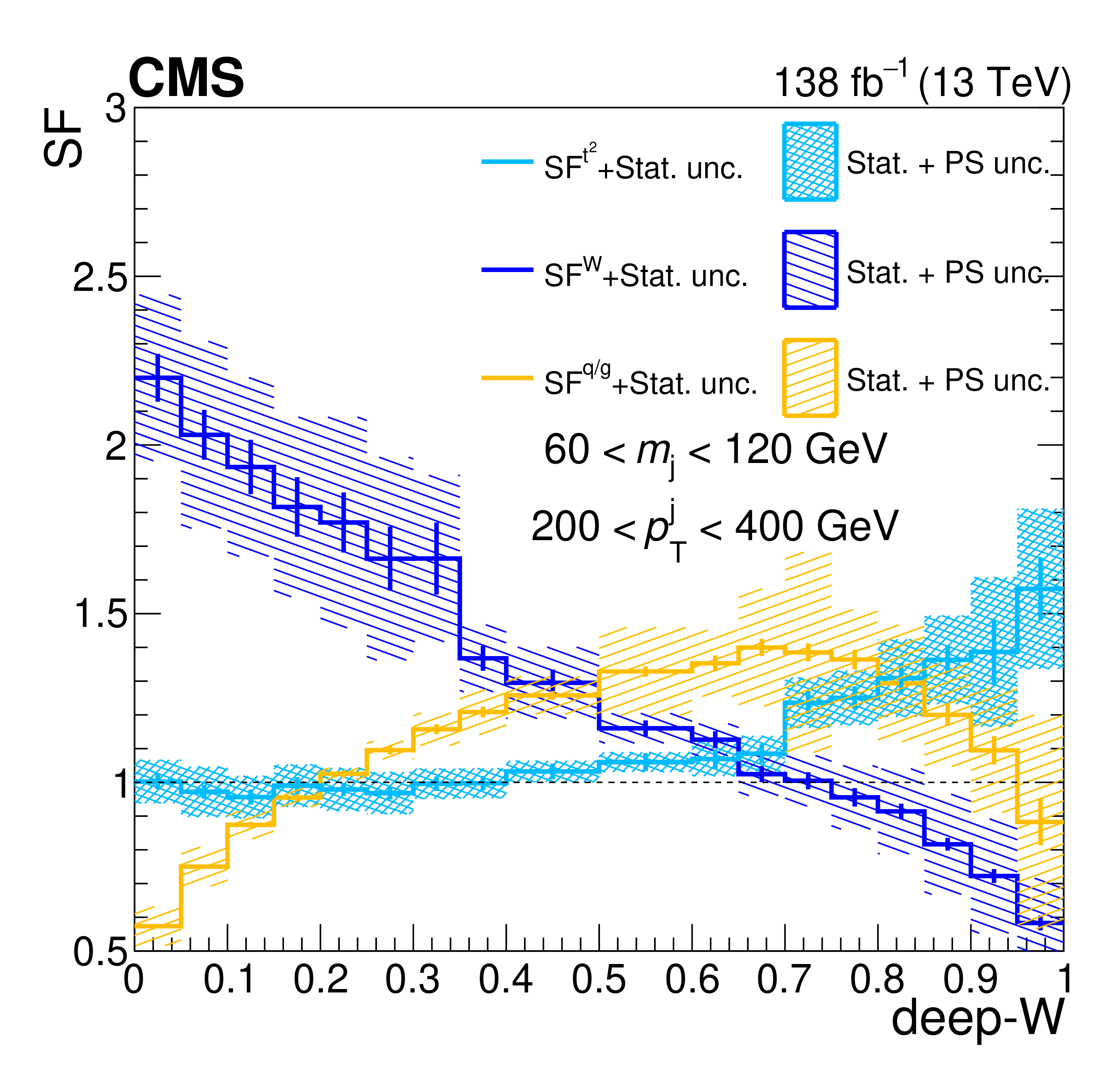
Figure 4:
Measured scale factors (SFs) for the deep-W and deep-WH discriminants. Upper row: SFs for W (dark blue), $\mathrm{t} ^2$ (light blue), and q/g (yellow) matched jets in the low-$ {m_{\text {j}}}$ bins, LL (left) and LH (right), as functions of the deep-W discriminant value. Lower row: SFs for $\mathrm{t} ^2$ (light blue), $\mathrm{t} ^{3,4}$ (green), and q/g (yellow) matched jets in the high-$ {m_{\text {j}}}$ bins, HL (left) and HH (right), as functions of the deep-WH discriminant value. For each discriminant value bin, the sum of the SF-corrected jet yields is required to be equal to the observed data. The statistical and parton shower (PS) uncertainties are shown by the shaded bands. |
png pdf |
Figure 4-a:
Measured scale factors (SFs) for W (dark blue), $\mathrm{t} ^2$ (light blue), and q/g (yellow) matched jets in the low-$ {m_{\text {j}}}$ bins, LL, as functions of the deep-W discriminant value. For each discriminant value bin, the sum of the SF-corrected jet yields is required to be equal to the observed data. The statistical and parton shower (PS) uncertainties are shown by the shaded bands. |

png pdf |
Figure 4-b:
Measured scale factors (SFs) for W (dark blue), $\mathrm{t} ^2$ (light blue), and q/g (yellow) matched jets in the low-$ {m_{\text {j}}}$ bins, LH, as functions of the deep-W discriminant value. For each discriminant value bin, the sum of the SF-corrected jet yields is required to be equal to the observed data. The statistical and parton shower (PS) uncertainties are shown by the shaded bands. |

png pdf |
Figure 4-c:
Measured scale factors (SFs) for $\mathrm{t} ^2$ (light blue), $\mathrm{t} ^{3,4}$ (green), and q/g (yellow) matched jets in the high-$ {m_{\text {j}}}$ bins, HL, as functions of the deep-WH discriminant value. For each discriminant value bin, the sum of the SF-corrected jet yields is required to be equal to the observed data. The statistical and parton shower (PS) uncertainties are shown by the shaded bands. |

png pdf |
Figure 4-d:
Measured scale factors (SFs) for $\mathrm{t} ^2$ (light blue), $\mathrm{t} ^{3,4}$ (green), and q/g (yellow) matched jets in the high-$ {m_{\text {j}}}$ bins, HH, as functions of the deep-WH discriminant value. For each discriminant value bin, the sum of the SF-corrected jet yields is required to be equal to the observed data. The statistical and parton shower (PS) uncertainties are shown by the shaded bands. |

png pdf |
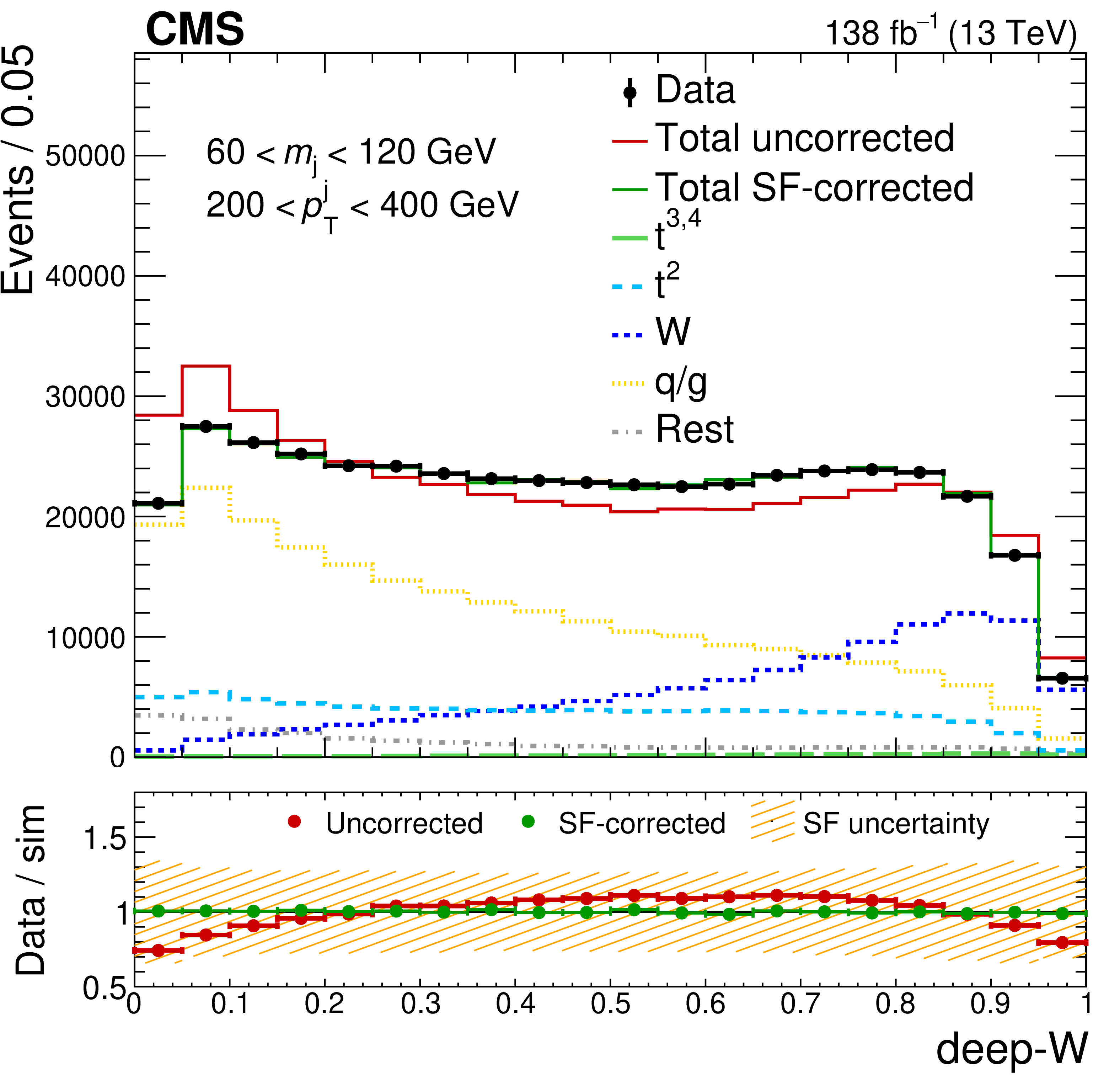
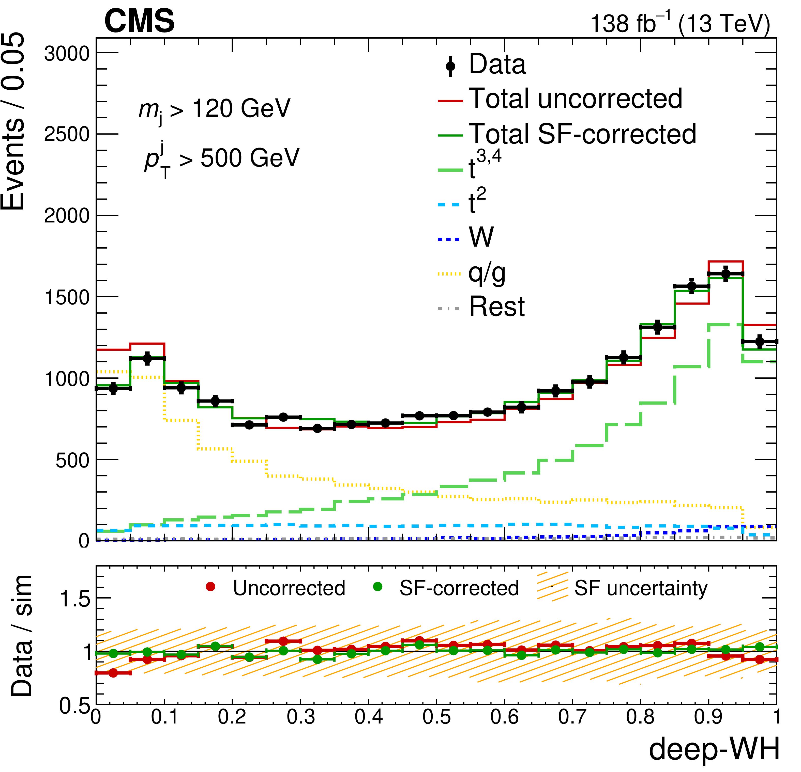
Figure 5:
DeepAK8 discriminants of the jet with highest mass in the single-lepton sideband. The deep-W spectra in the LL (upper left) and LH (upper right) samples are presented together with the deep-WH spectra in the HL (lower left) and HH (lower right) samples. The W boson jets are shown in dark blue, $\mathrm{t} ^2$ in light blue, $\mathrm{t} ^{3,4}$ in green, q/g in yellow, and the "Rest'' jet types (jets not matching any of the categories) in gray. Before corrections (red), discrepancies between the prediction and the data can be observed, in particular at low and high discriminant values. The corrected distributions after application of the scale factors (SFs) are shown in dark green. The lower panels show the data-to-simulation ratios before and after corrections. The SF uncertainties are indicated by the shaded bands. |
png pdf |
Figure 5-a:
Spectrum of the deep-W discriminant for the jet with highest mass in the LL single-lepton sideband sample. The W boson jets are shown in dark blue, $\mathrm{t} ^2$ in light blue, $\mathrm{t} ^{3,4}$ in green, q/g in yellow, and the "Rest'' jet types (jets not matching any of the categories) in gray. Before corrections (red), discrepancies between the prediction and the data can be observed, in particular at low and high discriminant values. The corrected distributions after application of the scale factors (SFs) are shown in dark green. The lower panel shows the data-to-simulation ratio before and after corrections. The SF uncertainties are indicated by the shaded bands. |

png pdf |
Figure 5-b:
Spectrum of the deep-W discriminant for the jet with highest mass in the LH single-lepton sideband sample. The W boson jets are shown in dark blue, $\mathrm{t} ^2$ in light blue, $\mathrm{t} ^{3,4}$ in green, q/g in yellow, and the "Rest'' jet types (jets not matching any of the categories) in gray. Before corrections (red), discrepancies between the prediction and the data can be observed, in particular at low and high discriminant values. The corrected distributions after application of the scale factors (SFs) are shown in dark green. The lower panel shows the data-to-simulation ratio before and after corrections. The SF uncertainties are indicated by the shaded bands. |

png pdf |
Figure 5-c:
Spectrum of the deep-WH discriminant for the jet with highest mass in the HL single-lepton sideband sample. The W boson jets are shown in dark blue, $\mathrm{t} ^2$ in light blue, $\mathrm{t} ^{3,4}$ in green, q/g in yellow, and the "Rest'' jet types (jets not matching any of the categories) in gray. Before corrections (red), discrepancies between the prediction and the data can be observed, in particular at low and high discriminant values. The corrected distributions after application of the scale factors (SFs) are shown in dark green. The lower panel shows the data-to-simulation ratio before and after corrections. The SF uncertainties are indicated by the shaded bands. |
png pdf |
Figure 5-d:
Spectrum of the deep-WH discriminant for the jet with highest mass in the HH single-lepton sideband sample. The W boson jets are shown in dark blue, $\mathrm{t} ^2$ in light blue, $\mathrm{t} ^{3,4}$ in green, q/g in yellow, and the "Rest'' jet types (jets not matching any of the categories) in gray. Before corrections (red), discrepancies between the prediction and the data can be observed, in particular at low and high discriminant values. The corrected distributions after application of the scale factors (SFs) are shown in dark green. The lower panel shows the data-to-simulation ratio before and after corrections. The SF uncertainties are indicated by the shaded bands. |

png pdf |
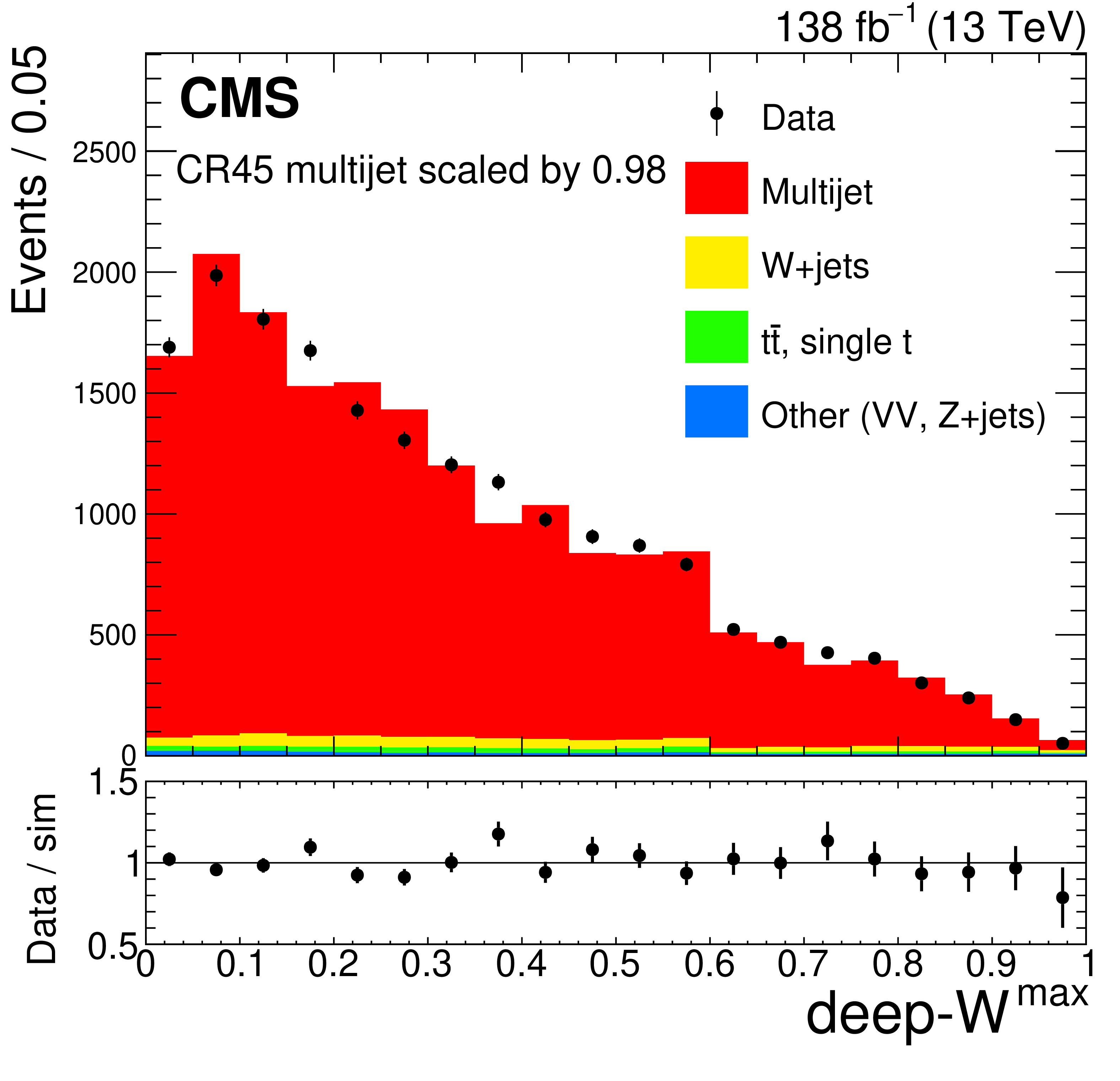
Figure 6:
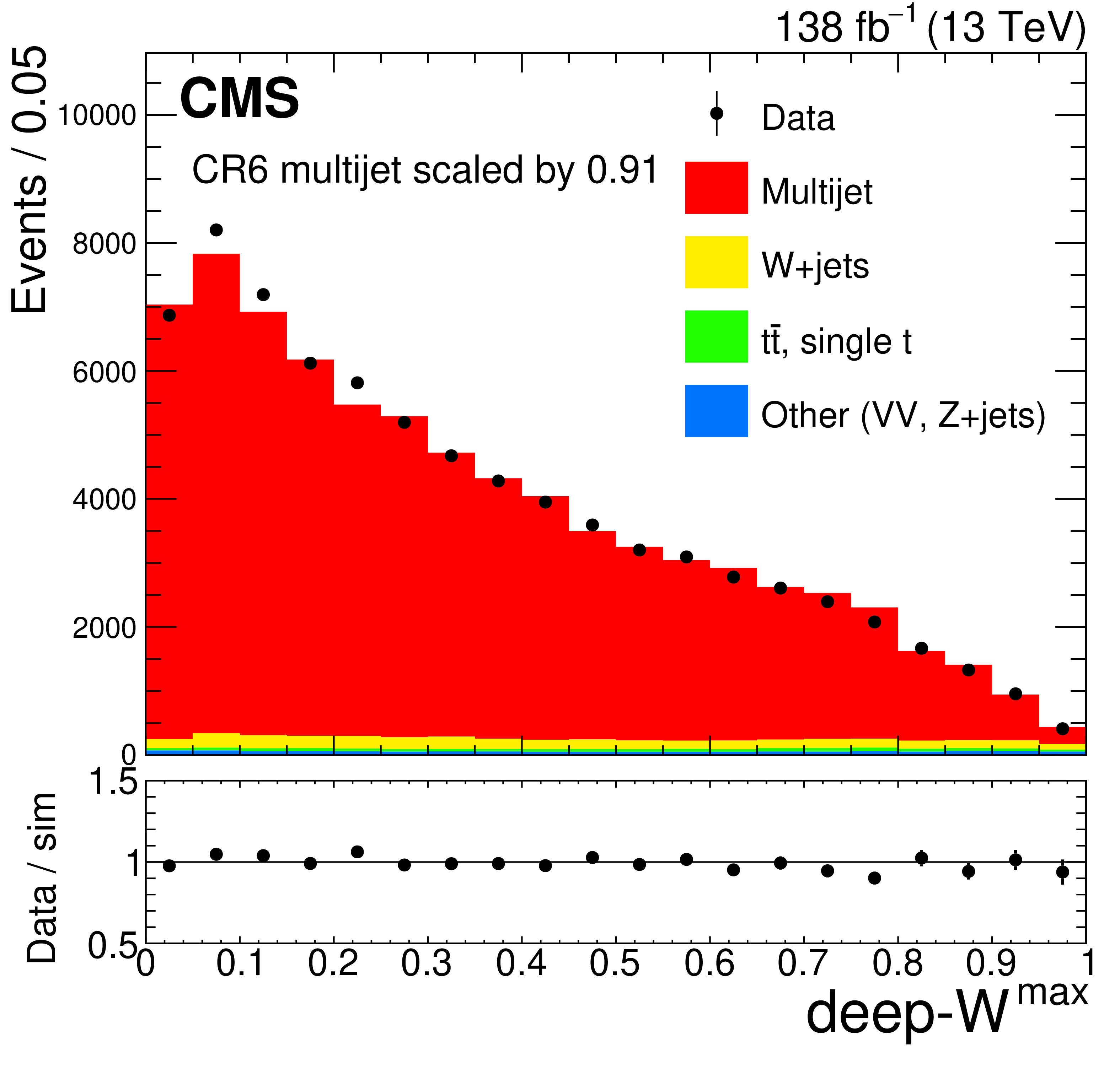
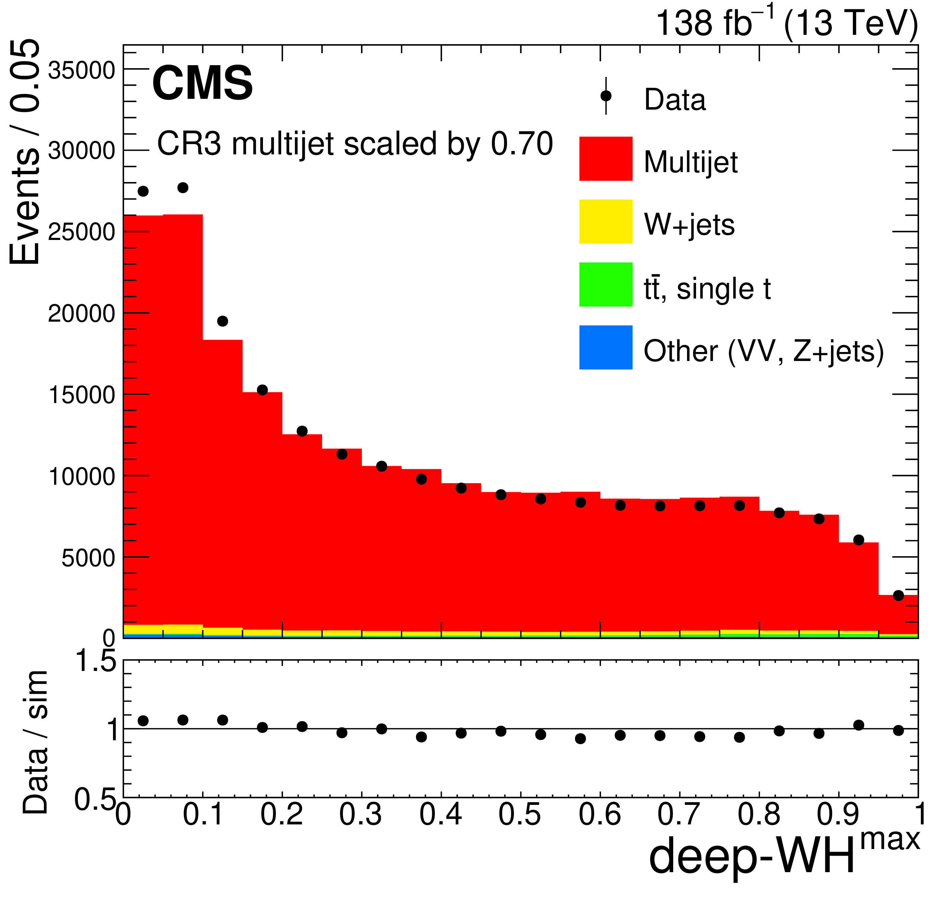
Comparison between data (black markers) and simulated background events (histograms) of the deep-W (WH) distributions for the highest-mass jet after SF application. The control regions CR1, CR2, CR3 are shown in the left column, upper to lower rows, while CR45 and CR6 are presented right column, upper and middle rows, respectively. The lower panels show the data-to-simulation ratio. |

png pdf |
Figure 6-a:
Comparison between data (black markers) and simulated background events (histograms) of the deep-W distributions for the highest-mass jet after SF application in the CR1 control region. The lower panel shows the data-to-simulation ratio. |
png pdf |
Figure 6-b:
Comparison between data (black markers) and simulated background events (histograms) of the deep-W distributions for the highest-mass jet after SF application in the CR45 control region. The lower panel shows the data-to-simulation ratio. |

png pdf |
Figure 6-c:
Comparison between data (black markers) and simulated background events (histograms) of the deep-WH distributions for the highest-mass jet after SF application in the CR2 control region. The lower panel shows the data-to-simulation ratio. |
png pdf |
Figure 6-d:
Comparison between data (black markers) and simulated background events (histograms) of the deep-W distributions for the highest-mass jet after SF application in the CR6 control region. The lower panel shows the data-to-simulation ratio. |
png pdf |
Figure 6-e:
Comparison between data (black markers) and simulated background events (histograms) of the deep-WH distributions for the highest-mass jet after SF application in the CR3 control region. The lower panel shows the data-to-simulation ratio. |
png pdf |
Figure 7:
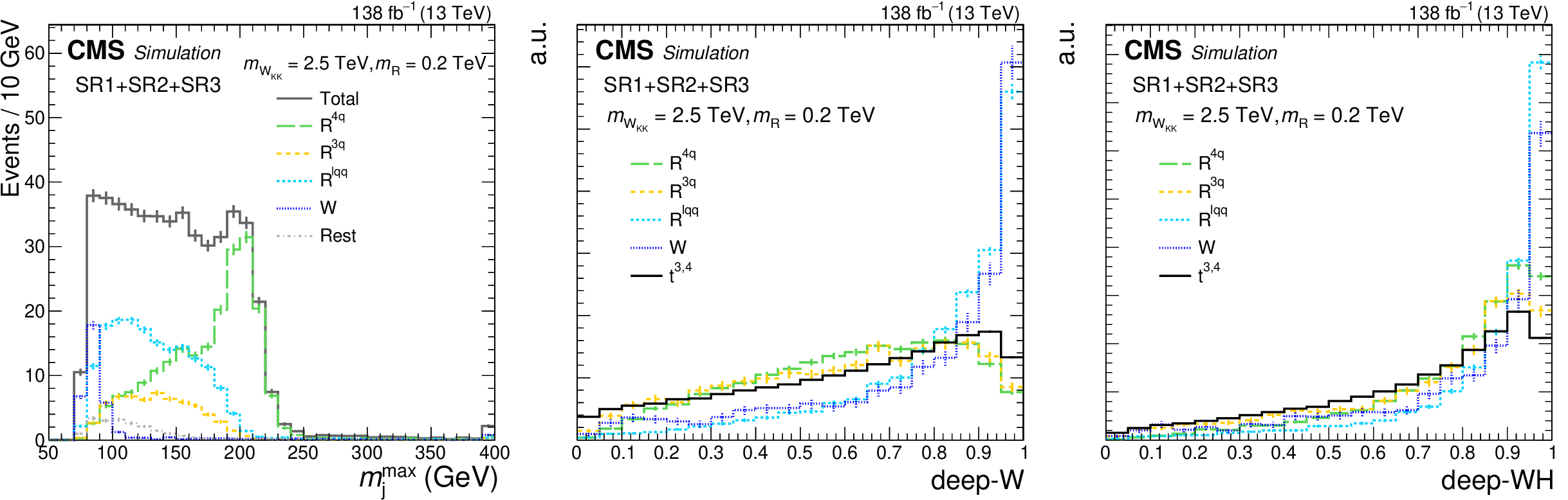
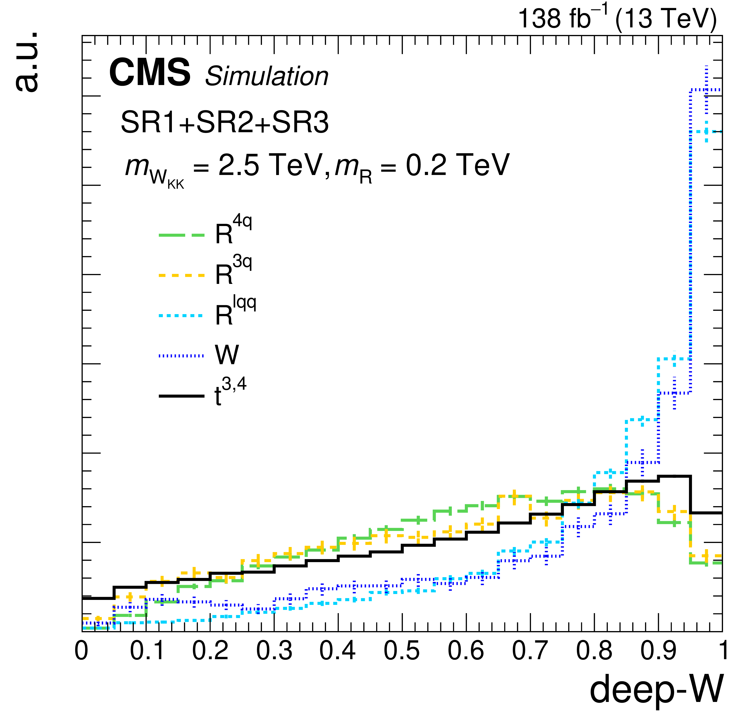
Shape comparison for different jet types in simulation. Left : the ${m^{\text {max}}_{\text {j}}}$ distributions for SR1-3 events without deep-W (WH) constraints. Center and right : the deep-W and deep-WH distributions normalized to unity for the shown components, respectively. The $\mathrm{t} ^{3,4}$ jets from the preselected sample, normalized to unity, are superimposed to compare shapes with the ${\mathrm{R} ^{3\mathrm{q}}}$ and ${\mathrm{R} ^{4\mathrm{q}}}$ distributions. |

png pdf |
Figure 7-a:
The ${m^{\text {max}}_{\text {j}}}$ distributions for SR1-3 events without deep-W (WH) constraints. |
png pdf |
Figure 7-b:
The deep-W distributions normalized to unity for the shown components. The $\mathrm{t} ^{3,4}$ jets from the preselected sample, normalized to unity, are superimposed to compare shapes with the ${\mathrm{R} ^{3\mathrm{q}}}$ and ${\mathrm{R} ^{4\mathrm{q}}}$ distributions. |

png pdf |
Figure 7-c:
The deep-WH distributions normalized to unity for the shown components. The $\mathrm{t} ^{3,4}$ jets from the preselected sample, normalized to unity, are superimposed to compare shapes with the ${\mathrm{R} ^{3\mathrm{q}}}$ and ${\mathrm{R} ^{4\mathrm{q}}}$ distributions. |
png pdf |
Figure 8:
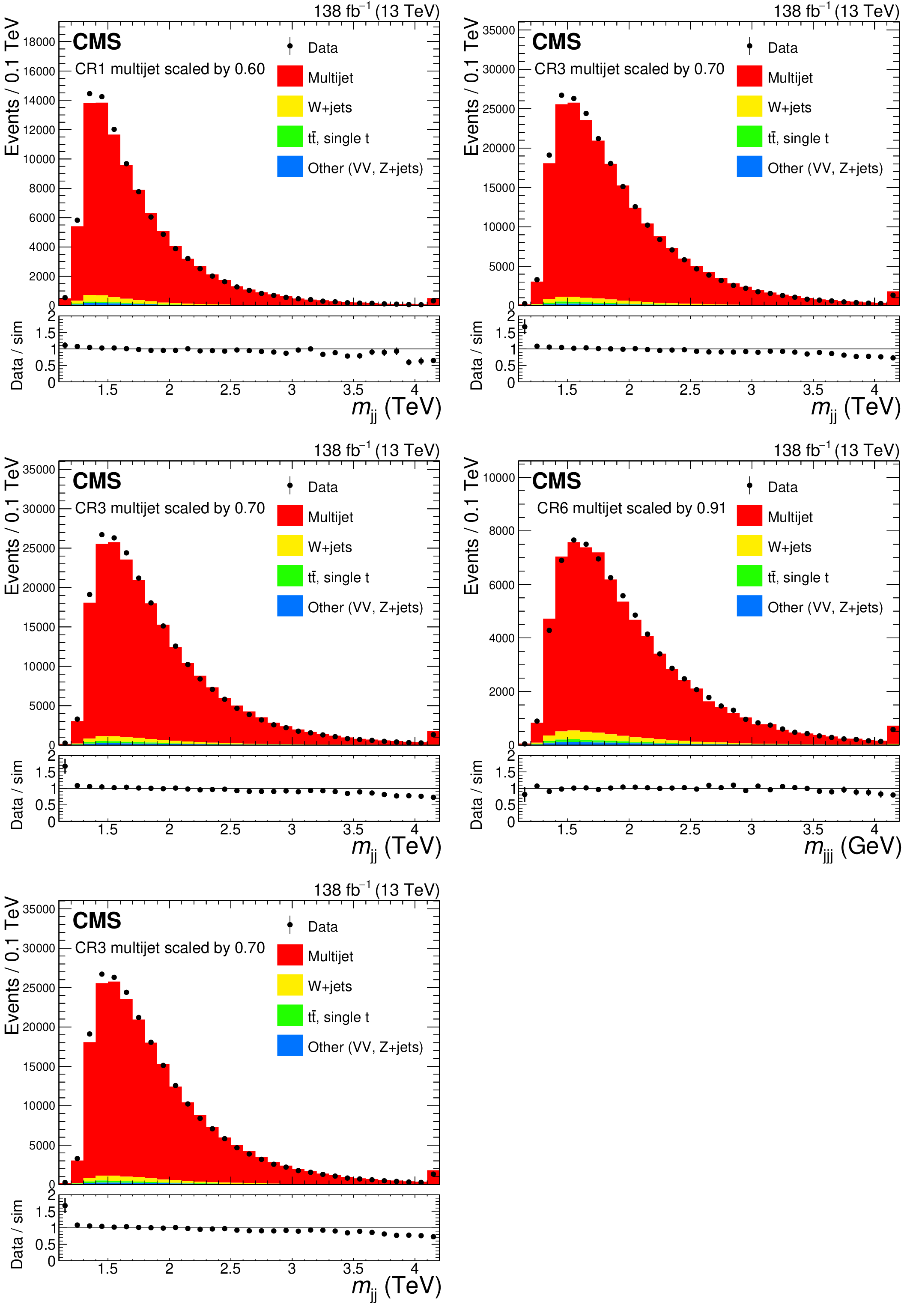
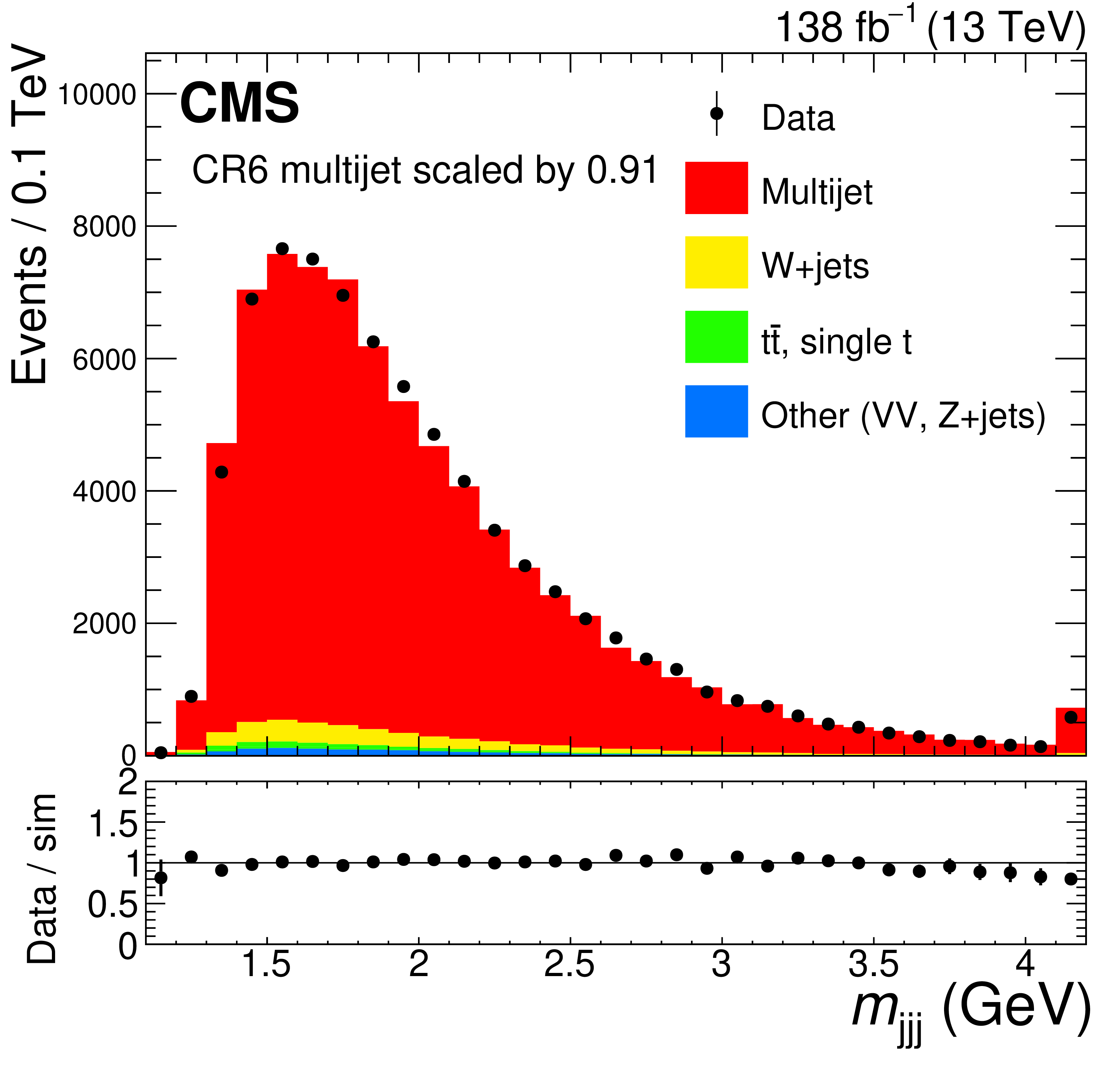
Invariant mass distributions of the reconstructed triboson systems for control regions in data (black markers) and simulated events (histograms). The ${m_{\mathrm {jj}}}$ distributions for CR1, CR2, CR3 are presented in the left column, upper to lower rows, respectively; the ${m_{\mathrm {jjj}}}$ distributions for control regions CR45 and CR6 are presented in the right column, upper and middle rows, respectively. The simulation is corrected by SFs, and the QCD multijet background is scaled to the data yields. |

png pdf |
Figure 8-a:
Invariant mass ${m_{\mathrm {jj}}}$ distributions of the reconstructed triboson systems for the CR1 control region in data (black markers) and simulated events (histograms). The simulation is corrected by SFs, and the QCD multijet background is scaled to the data yields. |

png pdf |
Figure 8-b:
Invariant mass ${m_{\mathrm {jjj}}}$ distributions of the reconstructed triboson systems for the CR45 control region in data (black markers) and simulated events (histograms). The simulation is corrected by SFs, and the QCD multijet background is scaled to the data yields. |

png pdf |
Figure 8-c:
Invariant mass ${m_{\mathrm {jj}}}$ distributions of the reconstructed triboson systems for the CR2 control region in data (black markers) and simulated events (histograms). The simulation is corrected by SFs, and the QCD multijet background is scaled to the data yields. |
png pdf |
Figure 8-d:
Invariant mass ${m_{\mathrm {jjj}}}$ distributions of the reconstructed triboson systems for the CR6 control region in data (black markers) and simulated events (histograms). The simulation is corrected by SFs, and the QCD multijet background is scaled to the data yields. |

png pdf |
Figure 8-e:
Invariant mass ${m_{\mathrm {jj}}}$ distributions of the reconstructed triboson systems for the CR3 control region in data (black markers) and simulated events (histograms). The simulation is corrected by SFs, and the QCD multijet background is scaled to the data yields. |

png pdf |
Figure 9:
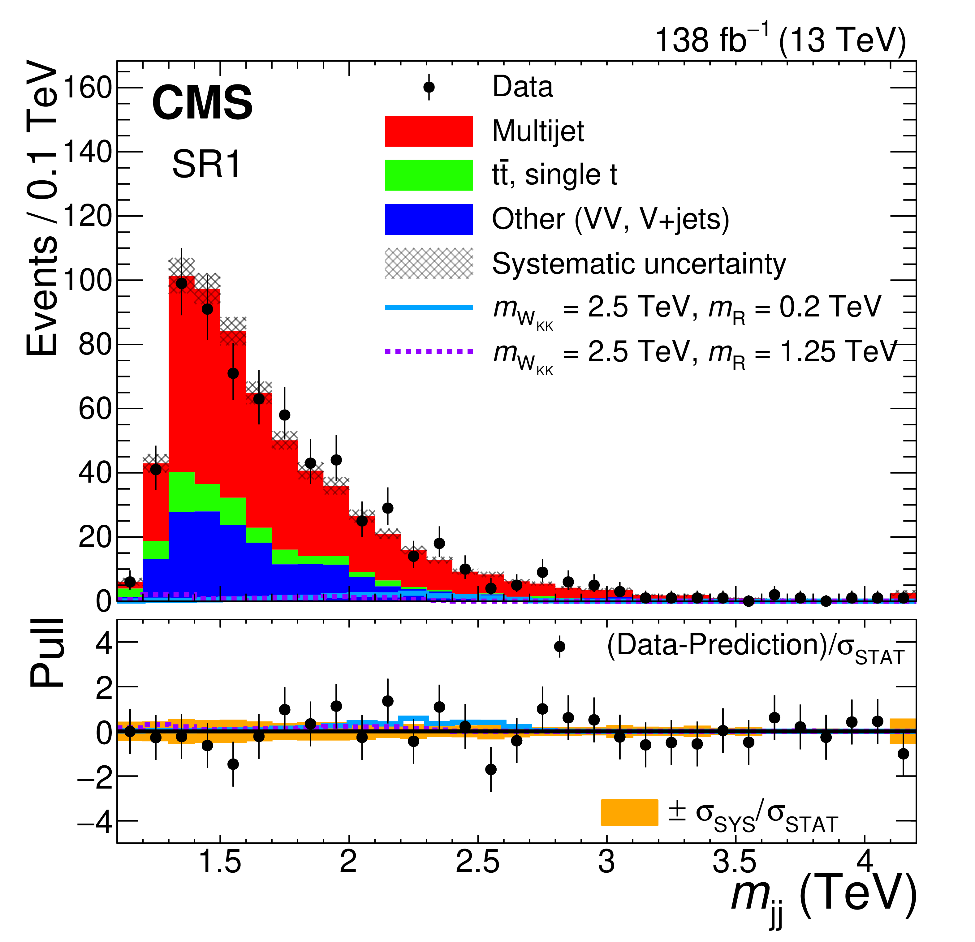
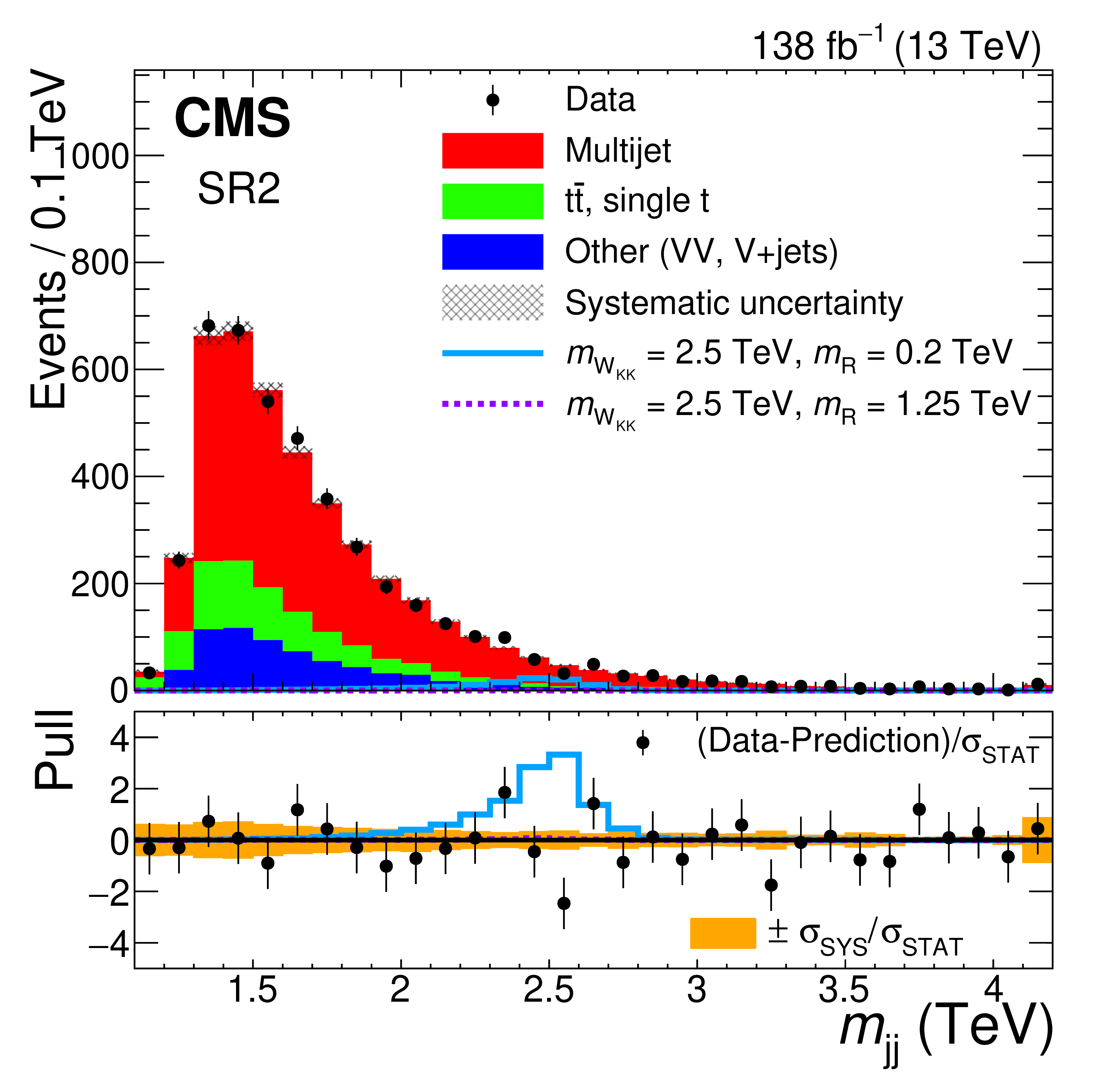
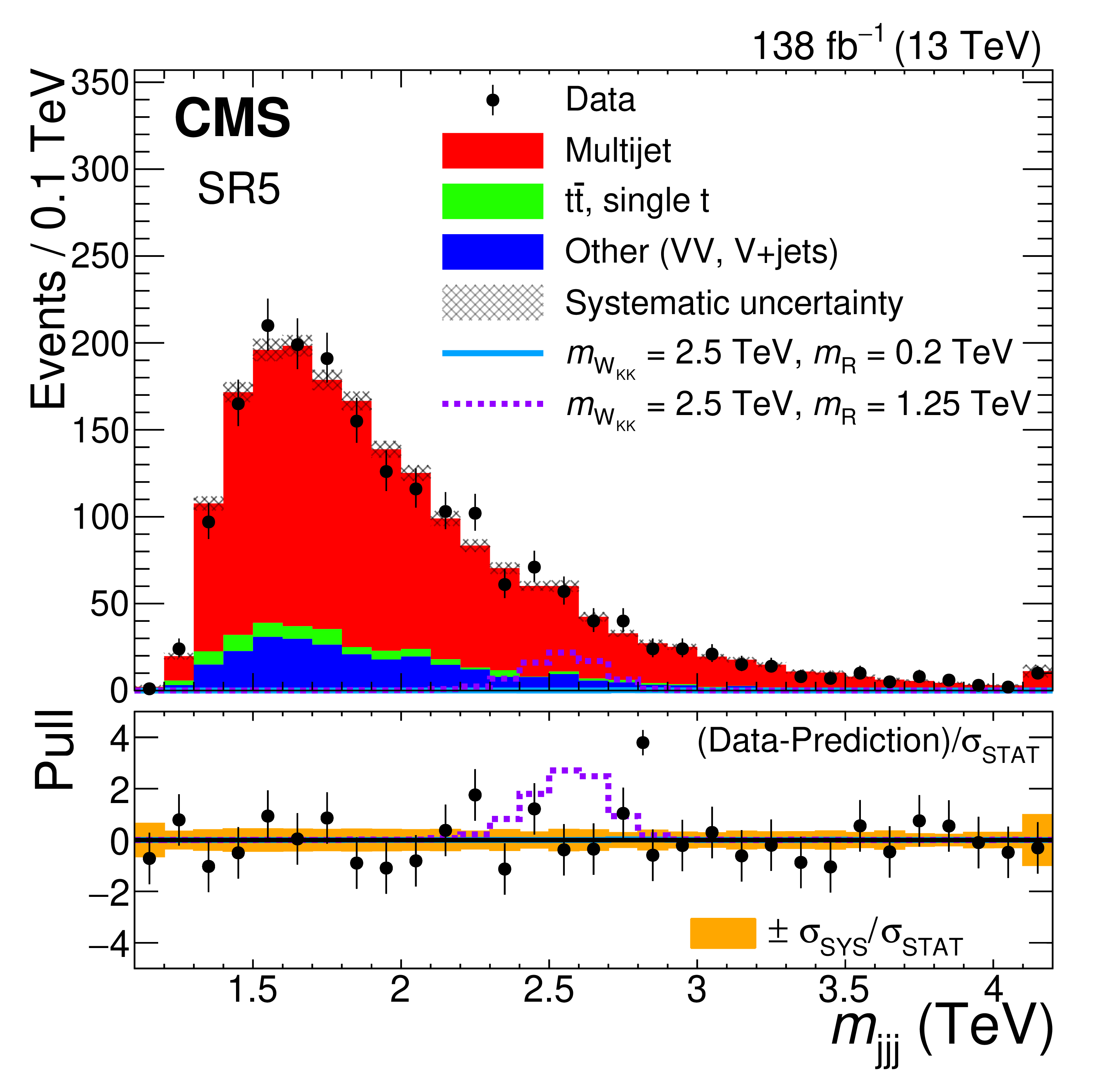
Post-fit distributions of the invariant mass of the reconstructed triboson system (${m_{\mathrm {jj}}}$, ${m_{\mathrm {jjj}}}$) in data (black markers) and simulation (histograms) for all SRs (SRs 1-3 in the left column and SRs 4-6 in the right column). Systematic uncertainties are indicated by the shaded bands. Signal examples are superimposed, normalized to the theoretical prediction for the production cross section of $ {{m}_{{\mathrm{W} _{\mathrm {KK}}}}} = $ 2.5 TeV with $ {{m}_{\mathrm{R}}} = $ 0.2 TeV (solid light blue line) and 1.25 TeV (dashed purple line). The bottom panels show the pull distributions, indicating the difference between the data and background prediction, divided by the statistical uncertainty in the background, with error bars representing the statistical uncertainty and shaded bands showing the one standard deviation systematic uncertainty, normalized by the statistical uncertainty. |
png pdf |
Figure 9-a:
Post-fit distributions of the invariant mass of the reconstructed triboson system (${m_{\mathrm {jj}}}$) in data (black markers) and simulation (histograms) for SR1. Systematic uncertainties are indicated by the shaded bands. Signal examples are superimposed, normalized to the theoretical prediction for the production cross section of $ {{m}_{{\mathrm{W} _{\mathrm {KK}}}}} = $ 2.5 TeV with $ {{m}_{\mathrm{R}}} = $ 0.2 TeV (solid light blue line) and 1.25 TeV (dashed purple line). The bottom panel shows the pull distributions, indicating the difference between the data and background prediction, divided by the statistical uncertainty in the background, with error bars representing the statistical uncertainty and shaded bands showing the one standard deviation systematic uncertainty, normalized by the statistical uncertainty. |

png pdf |
Figure 9-b:
Post-fit distributions of the invariant mass of the reconstructed triboson system (${m_{\mathrm {jjj}}}$) in data (black markers) and simulation (histograms) for SR4. Systematic uncertainties are indicated by the shaded bands. Signal examples are superimposed, normalized to the theoretical prediction for the production cross section of $ {{m}_{{\mathrm{W} _{\mathrm {KK}}}}} = $ 2.5 TeV with $ {{m}_{\mathrm{R}}} = $ 0.2 TeV (solid light blue line) and 1.25 TeV (dashed purple line). The bottom panel shows the pull distributions, indicating the difference between the data and background prediction, divided by the statistical uncertainty in the background, with error bars representing the statistical uncertainty and shaded bands showing the one standard deviation systematic uncertainty, normalized by the statistical uncertainty. |
png pdf |
Figure 9-c:
Post-fit distributions of the invariant mass of the reconstructed triboson system (${m_{\mathrm {jj}}}$) in data (black markers) and simulation (histograms) for SR2. Systematic uncertainties are indicated by the shaded bands. Signal examples are superimposed, normalized to the theoretical prediction for the production cross section of $ {{m}_{{\mathrm{W} _{\mathrm {KK}}}}} = $ 2.5 TeV with $ {{m}_{\mathrm{R}}} = $ 0.2 TeV (solid light blue line) and 1.25 TeV (dashed purple line). The bottom panel shows the pull distributions, indicating the difference between the data and background prediction, divided by the statistical uncertainty in the background, with error bars representing the statistical uncertainty and shaded bands showing the one standard deviation systematic uncertainty, normalized by the statistical uncertainty. |
png pdf |
Figure 9-d:
Post-fit distributions of the invariant mass of the reconstructed triboson system (${m_{\mathrm {jjj}}}$) in data (black markers) and simulation (histograms) for SR5. Systematic uncertainties are indicated by the shaded bands. Signal examples are superimposed, normalized to the theoretical prediction for the production cross section of $ {{m}_{{\mathrm{W} _{\mathrm {KK}}}}} = $ 2.5 TeV with $ {{m}_{\mathrm{R}}} = $ 0.2 TeV (solid light blue line) and 1.25 TeV (dashed purple line). The bottom panel shows the pull distributions, indicating the difference between the data and background prediction, divided by the statistical uncertainty in the background, with error bars representing the statistical uncertainty and shaded bands showing the one standard deviation systematic uncertainty, normalized by the statistical uncertainty. |

png pdf |
Figure 9-e:
Post-fit distributions of the invariant mass of the reconstructed triboson system (${m_{\mathrm {jj}}}$) in data (black markers) and simulation (histograms) for SR3. Systematic uncertainties are indicated by the shaded bands. Signal examples are superimposed, normalized to the theoretical prediction for the production cross section of $ {{m}_{{\mathrm{W} _{\mathrm {KK}}}}} = $ 2.5 TeV with $ {{m}_{\mathrm{R}}} = $ 0.2 TeV (solid light blue line) and 1.25 TeV (dashed purple line). The bottom panel shows the pull distributions, indicating the difference between the data and background prediction, divided by the statistical uncertainty in the background, with error bars representing the statistical uncertainty and shaded bands showing the one standard deviation systematic uncertainty, normalized by the statistical uncertainty. |

png pdf |
Figure 9-f:
Post-fit distributions of the invariant mass of the reconstructed triboson system (${m_{\mathrm {jjj}}}$) in data (black markers) and simulation (histograms) for SR6. Systematic uncertainties are indicated by the shaded bands. Signal examples are superimposed, normalized to the theoretical prediction for the production cross section of $ {{m}_{{\mathrm{W} _{\mathrm {KK}}}}} = $ 2.5 TeV with $ {{m}_{\mathrm{R}}} = $ 0.2 TeV (solid light blue line) and 1.25 TeV (dashed purple line). The bottom panel shows the pull distributions, indicating the difference between the data and background prediction, divided by the statistical uncertainty in the background, with error bars representing the statistical uncertainty and shaded bands showing the one standard deviation systematic uncertainty, normalized by the statistical uncertainty. |
png pdf |
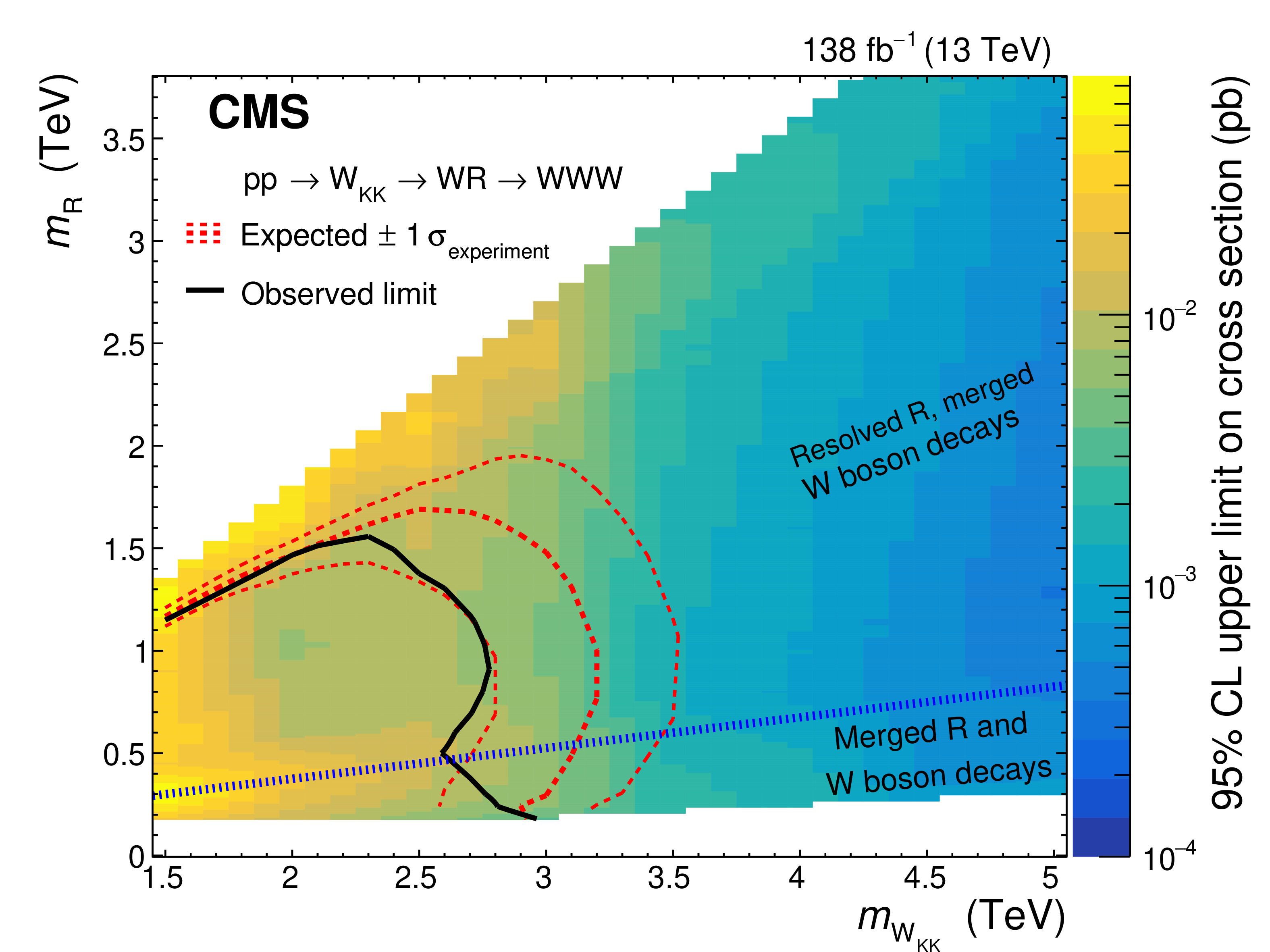
Figure 10:
Expected (red dashed lines) and observed (solid black line) lower limits at 95% CL on the W$ _{\mathrm {KK}} $ and R resonance masses for the particular parameters of the explored model. The colored area indicates the observed upper limit on the product of the signal cross section and the branching fraction to three W bosons. The blue dashed line indicates the border between the merged and resolved decay topologies probed. A signal with ${{m}_{\mathrm{R}}}$ lower than 180 GeV is not considered in this search to maintain on-shell W bosons, while for $ {{m}_{{\mathrm{W} _{\mathrm {KK}}}}} > $ 3 TeV, we only consider $ {{m}_{\mathrm{R}}} > $ 0.06 ${{m}_{{\mathrm{W} _{\mathrm {KK}}}}} $. |
| Tables | |

png pdf |
Table 1:
Summary of the selection requirements for each of the signal regions. |

png |
Table 2:
Matching criteria used to place a jet in one of the SM jet categories (left four columns) or merged radion jet categories (right two columns). Each column lists the $\Delta R$ conditions demanded between the reconstructed jet (j) and the generator-level parton in order to match a jet with a particular jet substructure. Lower indexes enumerate partons and indicate the particle from whose decay they originate (e.g., $\mathrm{t} \to \mathrm{b} _\mathrm{t} \mathrm{q} _{1\mathrm{W}}\mathrm{q} _{2\mathrm{W}}$). Schematic diagrams for each jet type are shown below each column. |

png pdf |
Table 3:
Sources of systematic uncertainties accounted for in the analysis. The first three sets of uncertainty sources originate from the tagger calibration. It is also indicated whether the uncertainties are evaluated for background (B) and/or signal (S), whether the uncertainty affects shape and/or rate, and the total number of nuisance parameters used per source. |
| Summary |
| A search for resonances decaying in cascade via a radion R to three W bosons, ${\mathrm{W}_{\mathrm{KK}}} \to \mathrm{W}\mathrm{R} \to \mathrm{W}\mathrm{W}\mathrm{W}$, in the all-hadronic final state has been presented. The search is performed in proton-proton collision data at a center-of-mass energy of 13 TeV, corresponding to a total integrated luminosity of 138 fb$^{-1}$. The final states include two or three massive, large-radius jets containing the decay products of the hadronically decaying W bosons. The two-jet case corresponds to events where the radion decay products are reconstructed as a single merged jet. The three-jet case corresponds to events where each W boson from the radion decay is reconstructed as a single merged jet. In this analysis and the analysis in the single-lepton channel reported in Ref. [10], previously unexplored signatures are probed, using novel jet substructure techniques. In particular, a dedicated radion tagger based on a neural network, targeting simultaneously three different radion decay topologies, has been developed. This tagger has been calibrated with a novel "matrix method''. These techniques are also applicable to the identification of $\mathrm{H} \to4\mathrm{q}$ and $\mathrm{H} \to \mathrm{q}\mathrm{q}{\ell} \nu$ decays of Lorentz-boosted Higgs bosons. Exclusion limits are set on the product of the production cross section and the branching fraction to three W bosons in an extended warped extra-dimensional model. This result, together with an analysis in the single-lepton channel [10], are the first of their kind, and constrain the parameters of this model for the first time. |
| References | ||||
| 1 | CMS Collaboration | Identification of heavy, energetic, hadronically decaying particles using machine-learning techniques | JINST 15 (2020) P06005 | CMS-JME-18-002 2004.08262 |
| 2 | CMS Collaboration | A search for the standard model Higgs boson decaying to charm quarks | JHEP 03 (2020) 131 | CMS-HIG-18-031 1912.01662 |
| 3 | K. Agashe, P. Du, S. Hong, and R. Sundrum | Flavor universal resonances and warped gravity | JHEP 01 (2017) 016 | 1608.00526 |
| 4 | K. S. Agashe et al. | LHC signals from cascade decays of warped vector resonances | JHEP 05 (2017) 078 | 1612.00047 |
| 5 | K. Agashe et al. | Dedicated strategies for triboson signals from cascade decays of vector resonances | PRD 99 (2019) 075016 | 1711.09920 |
| 6 | K. Agashe et al. | Detecting a boosted diboson resonance | JHEP 11 (2018) 027 | 1809.07334 |
| 7 | Y.-P. Kuang, H.-Y. Ren, and L.-H. Xia | Further investigation of the model-independent probe of heavy neutral Higgs bosons at LHC Run 2 | CPC 40 (2016) 023101 | 1506.08007 |
| 8 | Y.-P. Kuang, H.-Y. Ren, and L.-H. Xia | Model-independent probe of anomalous heavy neutral Higgs bosons at the LHC | PRD 90 (2014) 115002 | 1404.6367 |
| 9 | W. D. Goldberger and M. B. Wise | Modulus stabilization with bulk fields | PRL 83 (1999) 4922 | hep-ph/9907447 |
| 10 | CMS Collaboration | Search for resonances decaying to triple W-boson final states in proton-proton collisions at $ \sqrt{s} = $ 13 TeV | 2021. To be submitted to PRL. | |
| 11 | CMS Collaboration | HEPData record for this analysis | link | |
| 12 | CMS Collaboration | Performance of the CMS Level-1 trigger in proton-proton collisions at $ \sqrt{s} = $ 13 TeV | JINST 15 (2020) P10017 | CMS-TRG-17-001 2006.10165 |
| 13 | CMS Collaboration | The CMS trigger system | JINST 12 (2017) P01020 | CMS-TRG-12-001 1609.02366 |
| 14 | CMS Collaboration | The CMS experiment at the CERN LHC | JINST 3 (2008) S08004 | CMS-00-001 |
| 15 | CMS Collaboration | Precision luminosity measurement in proton-proton collisions at $ \sqrt{s} = $ 13 TeV in 2015 and 2016 at CMS | EPJC 81 (2021) 800 | CMS-LUM-17-003 2104.01927 |
| 16 | CMS Collaboration | CMS luminosity measurement for the 2017 data-taking period at $ \sqrt{s} = $ 13 TeV | CMS-PAS-LUM-17-004 | CMS-PAS-LUM-17-004 |
| 17 | CMS Collaboration | CMS luminosity measurement for the 2018 data-taking period at $ \sqrt{s} = $ 13 TeV | CMS-PAS-LUM-18-002 | CMS-PAS-LUM-18-002 |
| 18 | J. Alwall et al. | The automated computation of tree-level and next-to-leading order differential cross sections, and their matching to parton shower simulations | JHEP 07 (2014) 079 | 1405.0301 |
| 19 | P. Nason | A new method for combining NLO QCD with shower Monte Carlo algorithms | JHEP 11 (2004) 040 | hep-ph/0409146 |
| 20 | S. Frixione, P. Nason, and C. Oleari | Matching NLO QCD computations with parton shower simulations: the POWHEG method | JHEP 11 (2007) 070 | 0709.2092 |
| 21 | S. Alioli, P. Nason, C. Oleari, and E. Re | A general framework for implementing NLO calculations in shower Monte Carlo programs: the POWHEG BOX | JHEP 06 (2010) 043 | 1002.2581 |
| 22 | S. Alioli, S.-O. Moch, and P. Uwer | Hadronic top-quark pair-production with one jet and parton showering | JHEP 01 (2012) 137 | 1110.5251 |
| 23 | S. Alioli, P. Nason, C. Oleari, and E. Re | NLO single-top production matched with shower in POWHEG: $ s $- and $ t $-channel contributions | JHEP 09 (2009) 111 | 0907.4076 |
| 24 | R. Frederix, E. Re, and P. Torrielli | Single-top $ t $-channel hadroproduction in the four-flavour scheme with POWHEG and aMC@NLO | JHEP 09 (2012) 130 | 1207.5391 |
| 25 | J. Alwall et al. | Comparative study of various algorithms for the merging of parton showers and matrix elements in hadronic collisions | EPJC 53 (2008) 473 | 0706.2569 |
| 26 | NNPDF Collaboration | Parton distributions for the LHC run II | JHEP 04 (2015) 040 | 1410.8849 |
| 27 | NNPDF Collaboration | Parton distributions from high-precision collider data | EPJC 77 (2017) 663 | 1706.00428 |
| 28 | T. Sjostrand et al. | An introduction to PYTHIA 8.2 | CPC 191 (2015) 159 | 1410.3012 |
| 29 | CMS Collaboration | Event generator tunes obtained from underlying event and multiparton scattering measurements | EPJC 76 (2016) 155 | CMS-GEN-14-001 1512.00815 |
| 30 | CMS Collaboration | Extraction and validation of a new set of CMS PYTHIA8 tunes from underlying-event measurements | EPJC 80 (2020) 4 | CMS-GEN-17-001 1903.12179 |
| 31 | GEANT4 Collaboration | GEANT4--a simulation toolkit | NIMA 506 (2003) 250 | |
| 32 | J. Allison et al. | GEANT4 developments and applications | IEEE Trans. Nucl. Sci. 53 (2006) 270 | |
| 33 | CMS Collaboration | Measurement of the inclusive W and Z production cross sections in pp collisions at $ \sqrt{s} = $ 7 TeV with the CMS experiment | JHEP 10 (2011) 132 | CMS-EWK-10-005 1107.4789 |
| 34 | M. Cacciari, G. P. Salam, and G. Soyez | The anti-$ {k_{\mathrm{T}}} $ jet clustering algorithm | JHEP 04 (2008) 063 | 0802.1189 |
| 35 | M. Cacciari, G. P. Salam, and G. Soyez | FastJet user manual | EPJC 72 (2012) 1896 | 1111.6097 |
| 36 | CMS Collaboration | Particle-flow reconstruction and global event description with the CMS detector | JINST 12 (2017) P10003 | CMS-PRF-14-001 1706.04965 |
| 37 | CMS Collaboration | Pileup mitigation at CMS in 13 TeV data | JINST 15 (2020) P09018 | CMS-JME-18-001 2003.00503 |
| 38 | D. Bertolini, P. Harris, M. Low, and N. Tran | Pileup Per Particle Identification | JHEP 10 (2014) 059 | 1407.6013 |
| 39 | CMS Collaboration | Jet energy scale and resolution in the CMS experiment in pp collisions at 8 TeV | JINST 12 (2017) P02014 | CMS-JME-13-004 1607.03663 |
| 40 | CMS Collaboration | Jet algorithms performance in 13 TeV data | CMS-PAS-JME-16-003 | CMS-PAS-JME-16-003 |
| 41 | CMS Collaboration | Identification of heavy-flavour jets with the CMS detector in pp collisions at 13 TeV | JINST 13 (2018) P05011 | CMS-BTV-16-002 1712.07158 |
| 42 | CMS Collaboration | Performance of missing transverse momentum reconstruction in proton-proton collisions at $ \sqrt{s} = $ 13 TeV using the CMS detector | JINST 14 (2019) P07004 | CMS-JME-17-001 1903.06078 |
| 43 | M. Dasgupta, A. Fregoso, S. Marzani, and G. P. Salam | Towards an understanding of jet substructure | JHEP 09 (2013) 029 | 1307.0007 |
| 44 | J. M. Butterworth, A. R. Davison, M. Rubin, and G. P. Salam | Jet substructure as a new Higgs search channel at the LHC | PRL 100 (2008) 242001 | 0802.2470 |
| 45 | A. J. Larkoski, S. Marzani, G. Soyez, and J. Thaler | Soft drop | JHEP 05 (2014) 146 | 1402.2657 |
| 46 | CMS Collaboration | Identification techniques for highly boosted W bosons that decay into hadrons | JHEP 12 (2014) 017 | CMS-JME-13-006 1410.4227 |
| 47 | CMS Collaboration | Performance of the CMS muon detector and muon reconstruction with proton-proton collisions at $ \sqrt{s}=$ 13 TeV | JINST 13 (2018) P06015 | CMS-MUO-16-001 1804.04528 |
| 48 | CMS Collaboration | Performance of electron reconstruction and selection with the CMS detector in proton-proton collisions at $ \sqrt{s} = $ 8 TeV | JINST 10 (2015) P06005 | CMS-EGM-13-001 1502.02701 |
| 49 | D. Krohn, J. Thaler, and L. Wang | Jet trimming | JHEP 02 (2010) 084 | 0912.1342 |
| 50 | J. Thaler and K. Van Tilburg | Maximizing boosted top identification by minimizing $ N $-subjettiness | JHEP 02 (2012) 093 | 1108.2701 |
| 51 | J. Bellm et al. | Herwig 7.0/Herwig++ 3.0 release note | EPJC 76 (2015) 196 | 1512.01178 |
| 52 | CMS Collaboration | Measurement of differential cross sections for top quark pair production using the lepton+jets final state in proton-proton collisions at 13 TeV | PRD 95 (2017) 092001 | CMS-TOP-16-008 1610.04191 |
| 53 | CMS Collaboration | Measurement of $ \mathrm{t\bar{t}} $ normalised multi-differential cross sections in pp collisions at $ \sqrt s = $ 13 TeV, and simultaneous determination of the strong coupling strength, top quark pole mass, and parton distribution functions | EPJC 80 (2020) 658 | CMS-TOP-18-004 1904.05237 |
| 54 | CMS Collaboration | Measurement of the inelastic proton-proton cross section at $ \sqrt{s}= $ 13 TeV | JHEP 07 (2018) 161 | CMS-FSQ-15-005 1802.02613 |
| 55 | M. Bahr et al. | Herwig++ physics and manual | EPJC 58 (2008) 639 | 0803.0883 |
| 56 | T. Junk | Confidence level computation for combining searches with small statistics | NIMA 434 (1999) 435 | hep-ex/9902006 |
| 57 | A. L. Read | Presentation of search results: The CLs technique | JPG 28 (2002) 2693 | |
| 58 | ATLAS and CMS Collaborations, and the LHC Higgs Combination Group | Procedure for the LHC Higgs boson search combination in Summer 2011 | CMS-NOTE-2011-005 | |
| 59 | G. Cowan, K. Cranmer, E. Gross, and O. Vitells | Asymptotic formulae for likelihood-based tests of new physics | EPJC 71 (2011) 1554 | 1007.1727 |
|
|
Compact Muon Solenoid LHC, CERN |
|

|

|

|

|

|