

Compact Muon Solenoid
LHC, CERN
| CMS-TOP-18-004 ; CERN-EP-2019-028 | ||
| Measurement of $\mathrm{t\bar{t}}$ normalised multi-differential cross sections in pp collisions at $\sqrt{s} = $ 13 TeV, and simultaneous determination of the strong coupling strength, top quark pole mass, and parton distribution functions | ||
| CMS Collaboration | ||
| 10 April 2019 | ||
| Eur. Phys. J. C 80 (2020) 658 | ||
| Abstract: Normalised multi-differential cross sections for top quark pair ($\mathrm{t\bar{t}}$) production are measured in proton-proton collisions at a centre-of-mass energy of 13 TeV using events containing two oppositely charged leptons. The analysed data were recorded with the CMS detector in 2016 and correspond to an integrated luminosity of 35.9 fb$^{-1}$. The double-differential $\mathrm{t\bar{t}}$ cross section is measured as a function of the kinematic properties of the top quark and of the $\mathrm{t\bar{t}}$ system at parton level in the full phase space. A triple-differential measurement is performed as a function of the invariant mass and rapidity of the $\mathrm{t\bar{t}}$ system and the multiplicity of additional jets at particle level. The data are compared to predictions of Monte Carlo event generators that complement next-to-leading-order (NLO) quantum chromodynamics (QCD) calculations with parton showers. Together with a fixed-order NLO QCD calculation, the triple-differential measurement is used to extract values of the strong coupling strength ${\alpha_S}$ and the top quark pole mass ($m_{\mathrm{t}}^{\text{pole}}$) using several sets of parton distribution functions (PDFs). Furthermore, a simultaneous fit of the PDFs, ${\alpha_S}$, and $m_{\mathrm{t}}^{\text{pole}}$ is performed at NLO, demonstrating that the new data have significant impact on the gluon PDF, and at the same time allow an accurate determination of ${\alpha_S}$ and $m_{\mathrm{t}}^{\text{pole}}$. | ||
| Links: e-print arXiv:1904.05237 [hep-ex] (PDF) ; CDS record ; inSPIRE record ; CADI line (restricted) ; | ||
| Figures | |
png pdf |
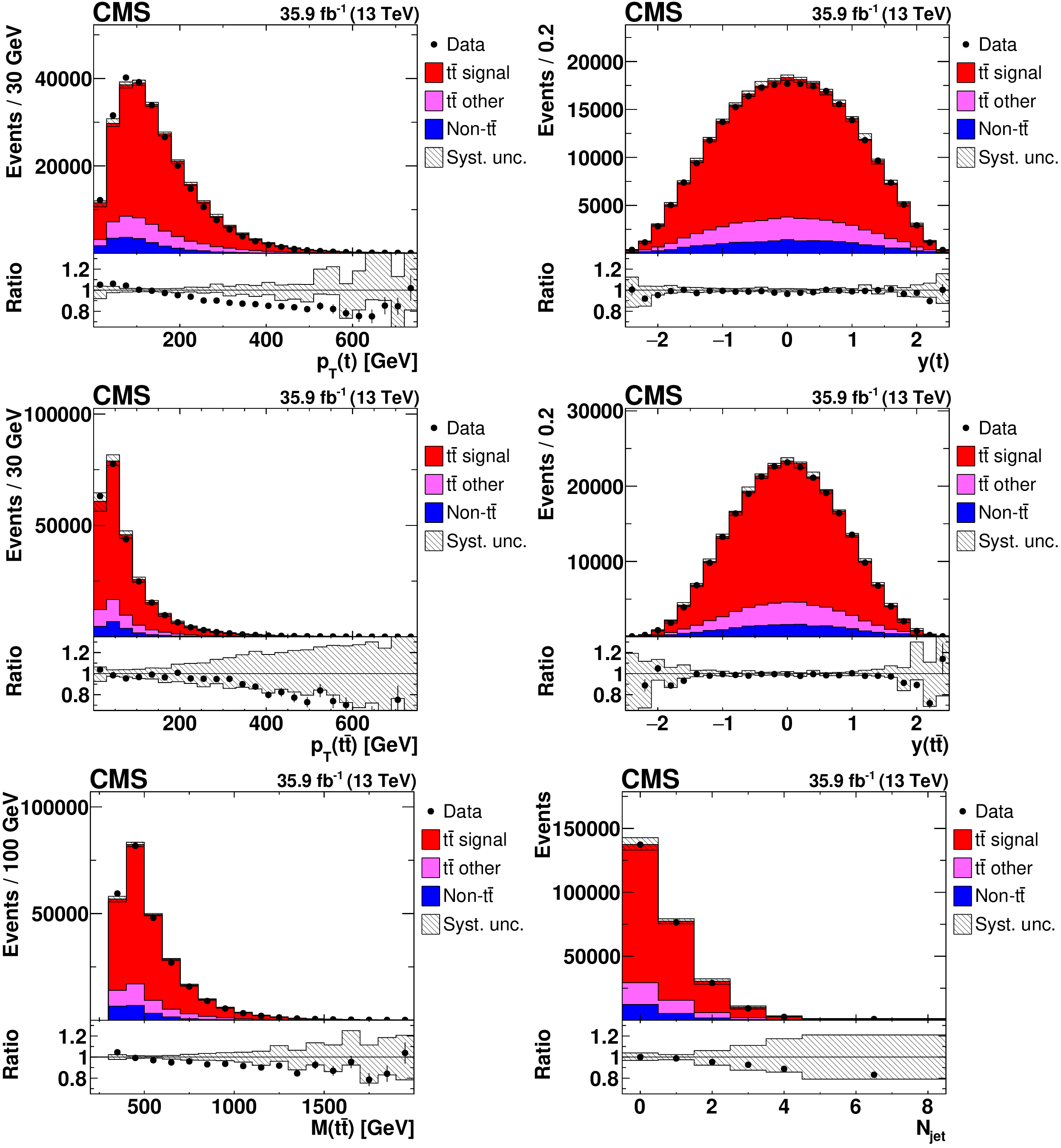
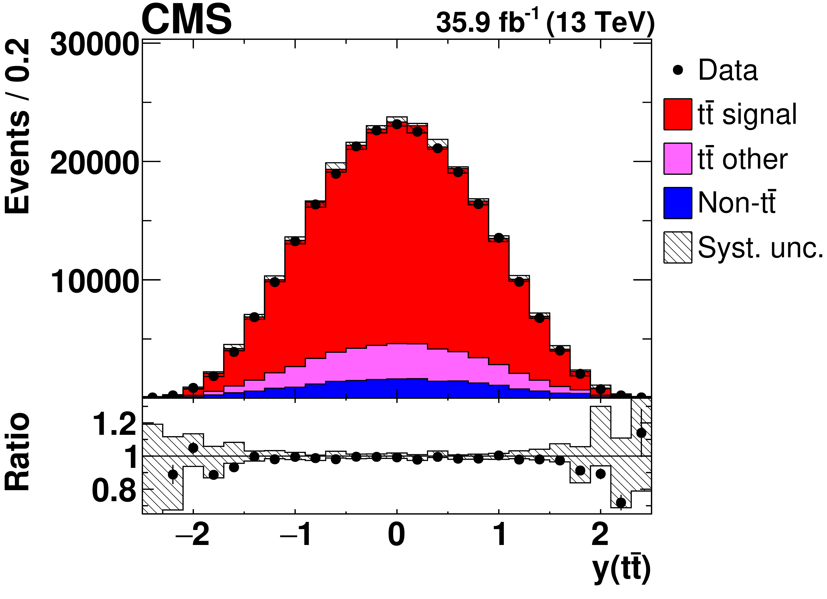
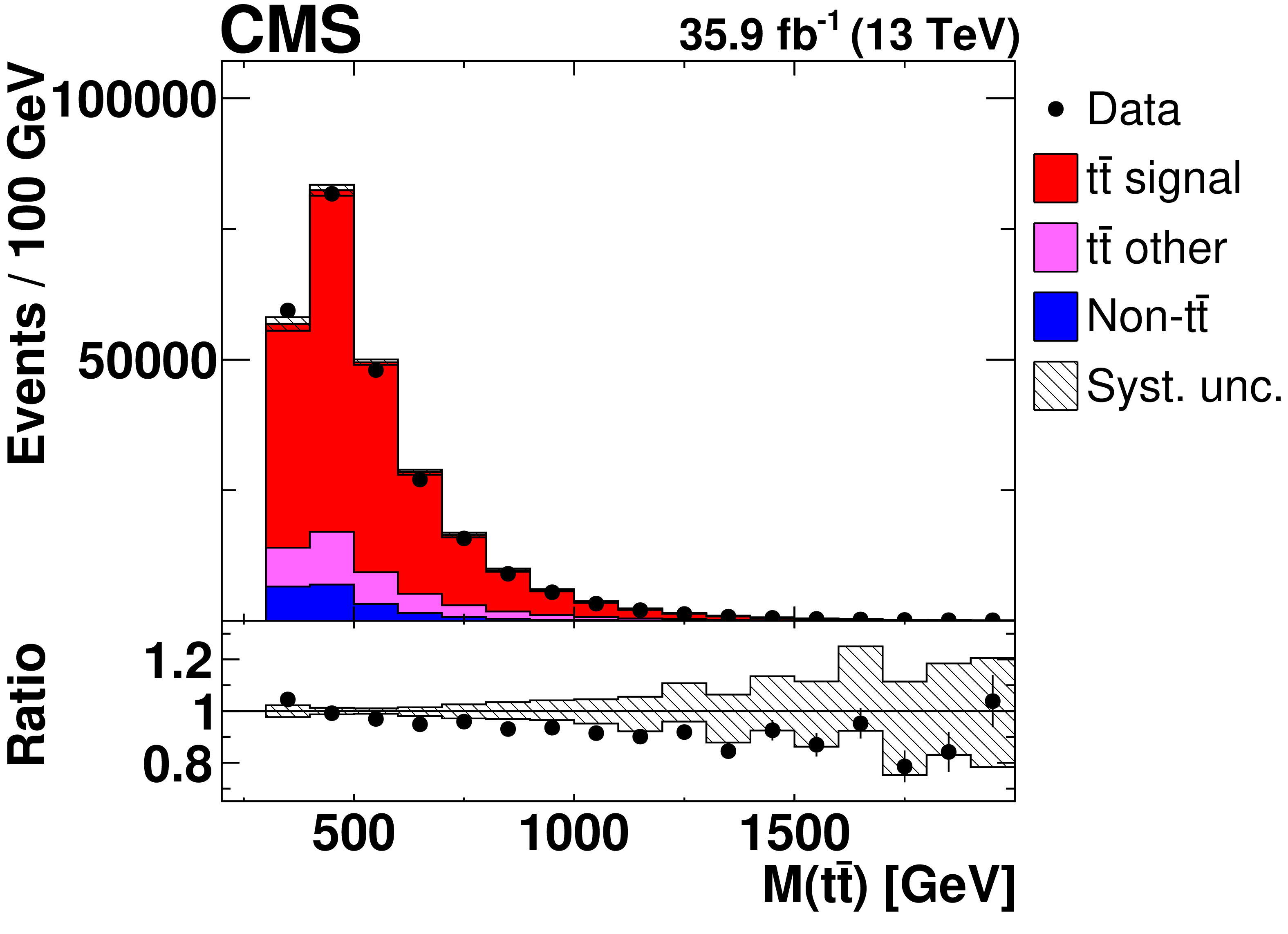
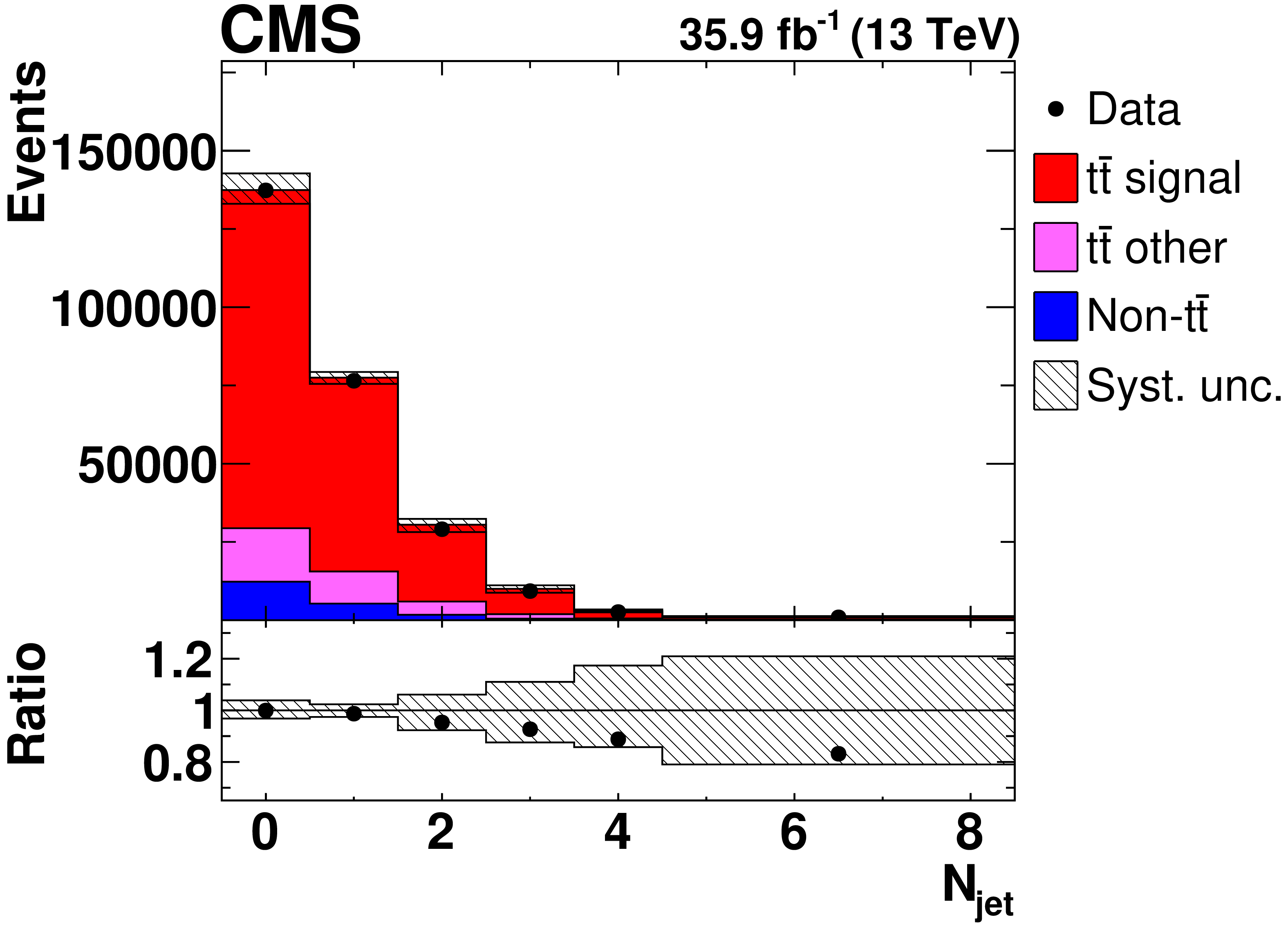
Figure 1:
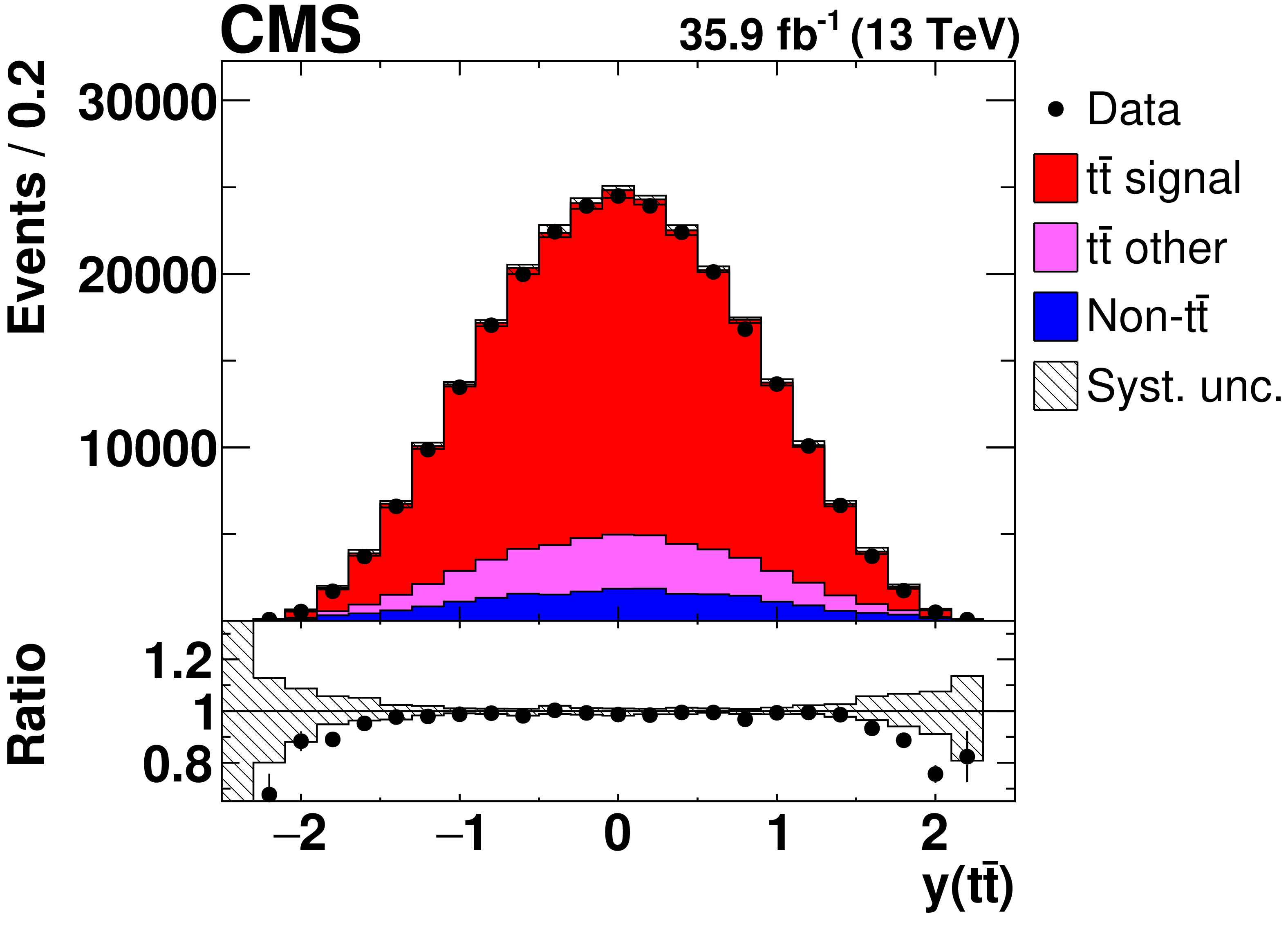
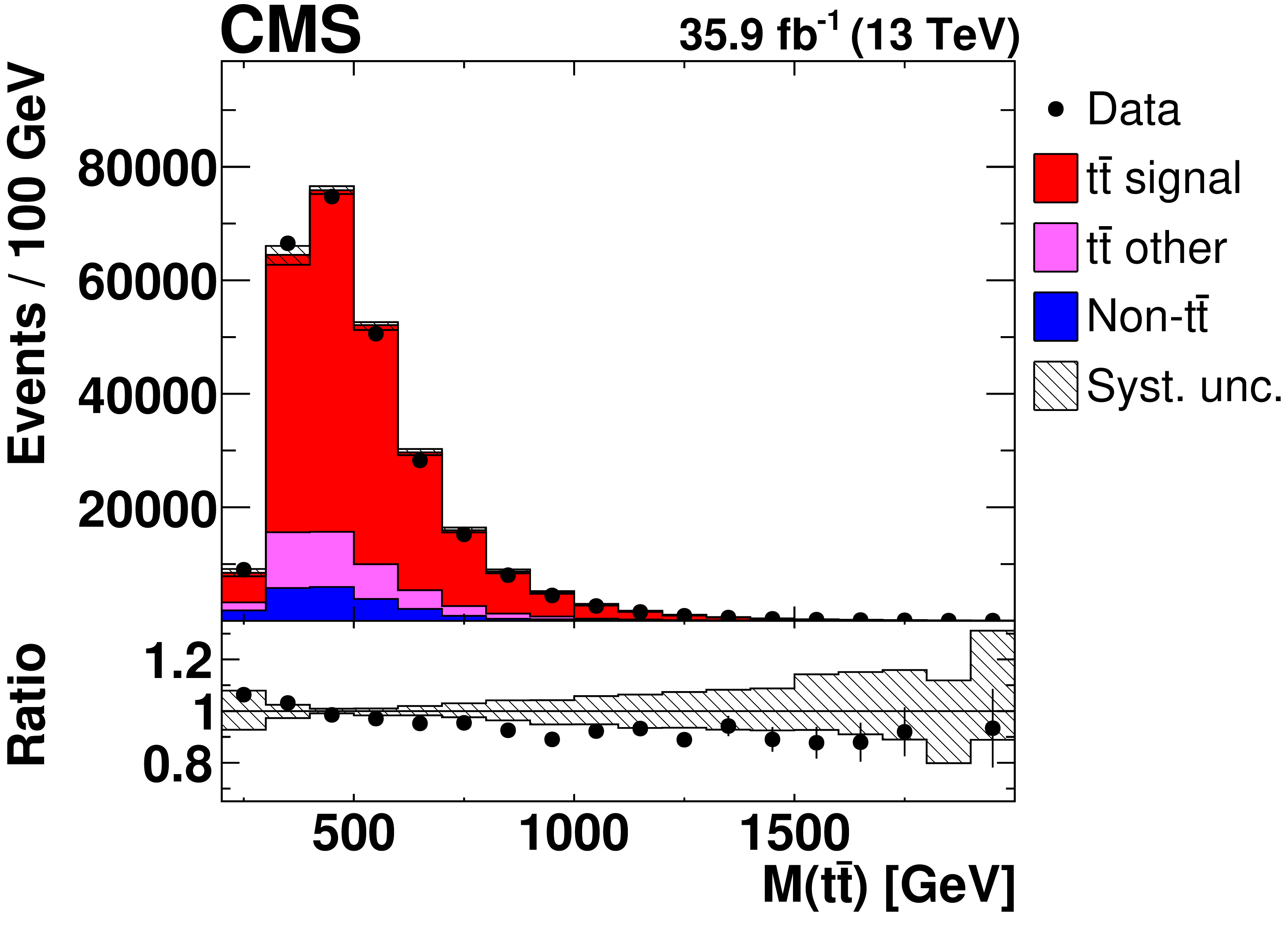
Distributions of $ {p_{\mathrm {T}}} ({\mathrm {t}})$ (upper left), $y({\mathrm {t}})$ (upper right), $ {p_{\mathrm {T}}} ({{\mathrm {t}\overline {\mathrm {t}}}})$ (middle left), $y({{\mathrm {t}\overline {\mathrm {t}}}})$ (middle right), ${M({{\mathrm {t}\overline {\mathrm {t}}}})}$ (lower left), and ${N_{\text {jet}}}$ (lower right) in selected events after the kinematic reconstruction, at detector level. The experimental data with the vertical bars corresponding to their statistical uncertainties are plotted together with distributions of simulated signal and different background processes. The hatched regions correspond to the estimated shape uncertainties in the signal and backgrounds (as detailed in Section 7). The lower panel in each plot shows the ratio of the observed data event yields to those expected in the simulation. |
png pdf |
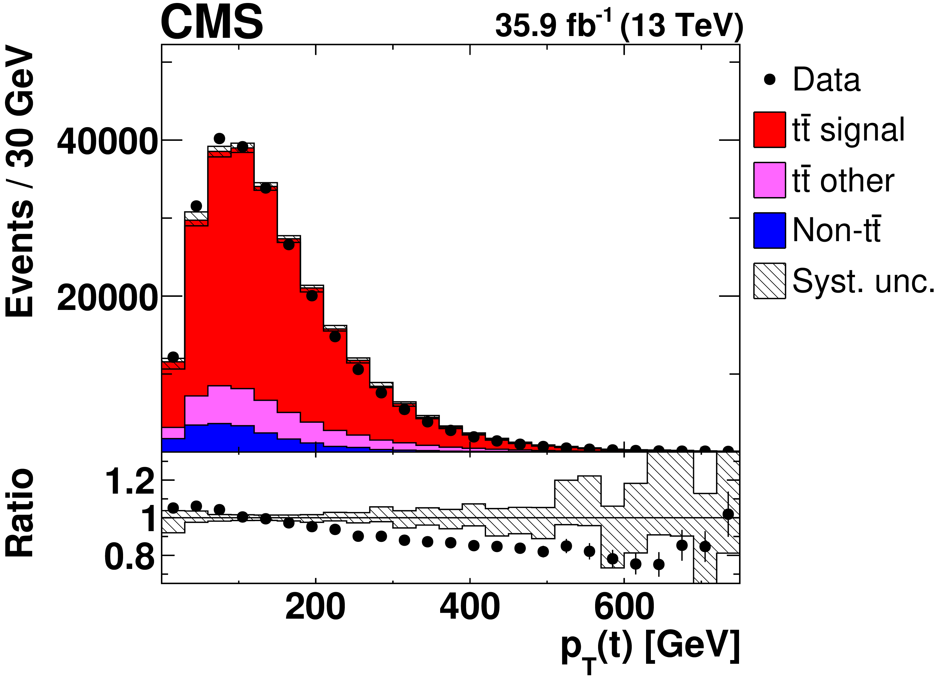
Figure 1-a:
Distribution of $ {p_{\mathrm {T}}} ({\mathrm {t}})$ in selected events after the kinematic reconstruction, at detector level. The experimental data with the vertical bars corresponding to their statistical uncertainties are plotted together with distributions of simulated signal and different background processes. The hatched regions correspond to the estimated shape uncertainties in the signal and backgrounds (as detailed in Section 7). The lower panel shows the ratio of the observed data event yields to those expected in the simulation. |
png pdf |
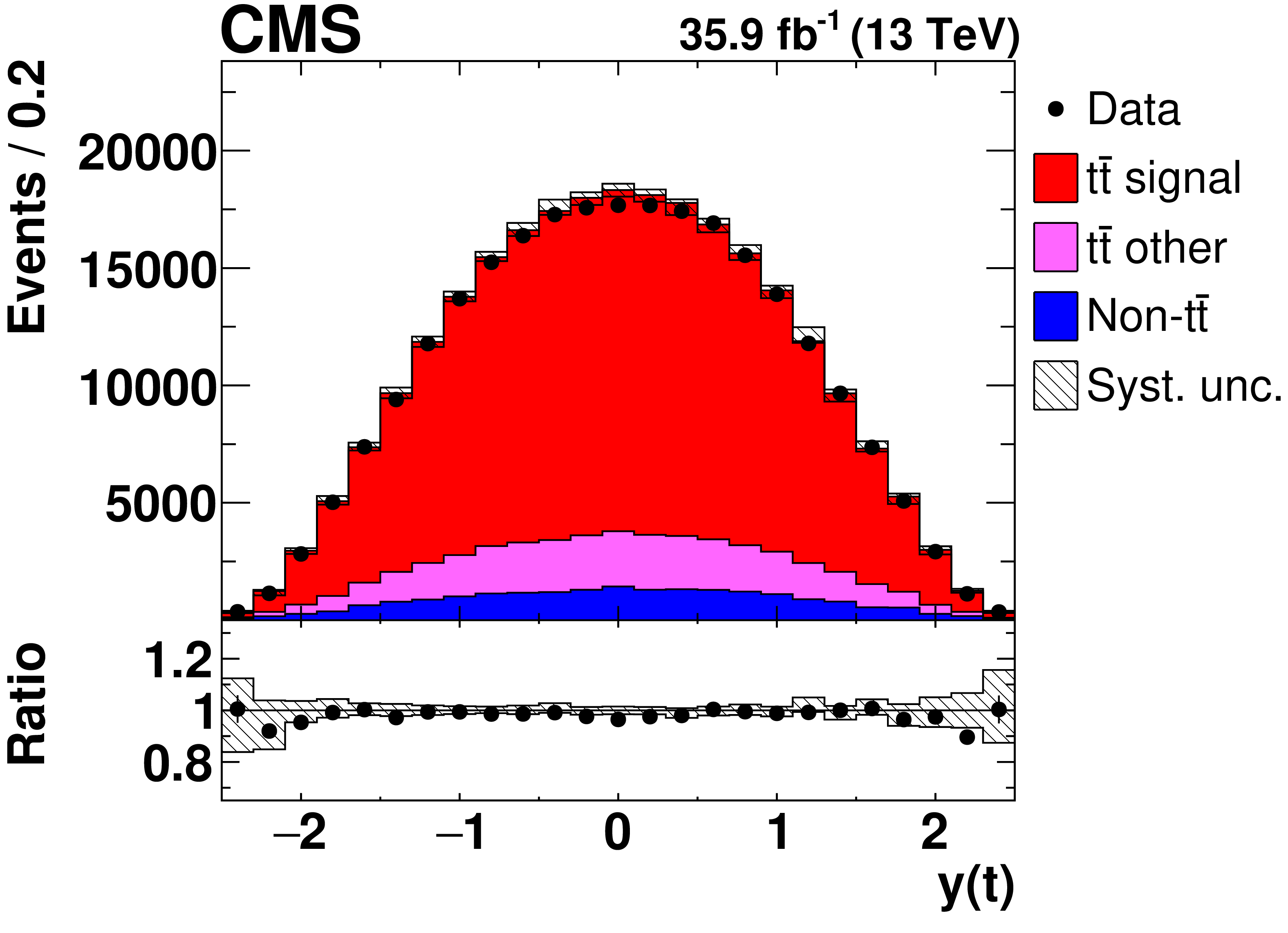
Figure 1-b:
Distribution of $y({\mathrm {t}})$ in selected events after the kinematic reconstruction, at detector level. The experimental data with the vertical bars corresponding to their statistical uncertainties are plotted together with distributions of simulated signal and different background processes. The hatched regions correspond to the estimated shape uncertainties in the signal and backgrounds (as detailed in Section 7). The lower panel shows the ratio of the observed data event yields to those expected in the simulation. |
png pdf |
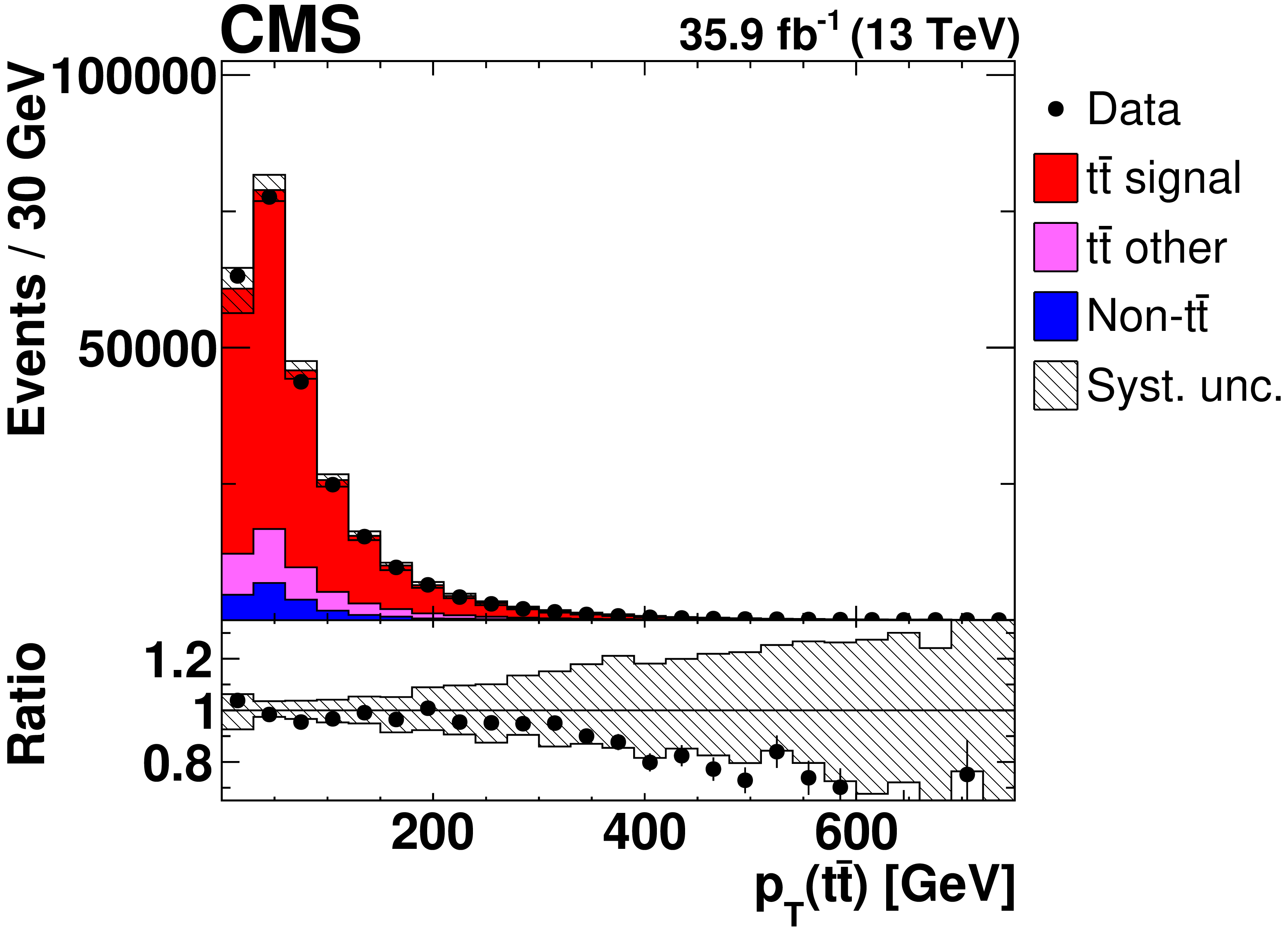
Figure 1-c:
Distribution of $ {p_{\mathrm {T}}} ({{\mathrm {t}\overline {\mathrm {t}}}})$ in selected events after the kinematic reconstruction, at detector level. The experimental data with the vertical bars corresponding to their statistical uncertainties are plotted together with distributions of simulated signal and different background processes. The hatched regions correspond to the estimated shape uncertainties in the signal and backgrounds (as detailed in Section 7). The lower panel shows the ratio of the observed data event yields to those expected in the simulation. |
png pdf |
Figure 1-d:
Distribution of $y({{\mathrm {t}\overline {\mathrm {t}}}})$ in selected events after the kinematic reconstruction, at detector level. The experimental data with the vertical bars corresponding to their statistical uncertainties are plotted together with distributions of simulated signal and different background processes. The hatched regions correspond to the estimated shape uncertainties in the signal and backgrounds (as detailed in Section 7). The lower panel shows the ratio of the observed data event yields to those expected in the simulation. |
png pdf |
Figure 1-e:
Distribution of ${M({{\mathrm {t}\overline {\mathrm {t}}}})}$ in selected events after the kinematic reconstruction, at detector level. The experimental data with the vertical bars corresponding to their statistical uncertainties are plotted together with distributions of simulated signal and different background processes. The hatched regions correspond to the estimated shape uncertainties in the signal and backgrounds (as detailed in Section 7). The lower panel shows the ratio of the observed data event yields to those expected in the simulation. |
png pdf |
Figure 1-f:
Distribution of ${N_{\text {jet}}}$ in selected events after the kinematic reconstruction, at detector level. The experimental data with the vertical bars corresponding to their statistical uncertainties are plotted together with distributions of simulated signal and different background processes. The hatched regions correspond to the estimated shape uncertainties in the signal and backgrounds (as detailed in Section 7). The lower panel shows the ratio of the observed data event yields to those expected in the simulation. |
png pdf |
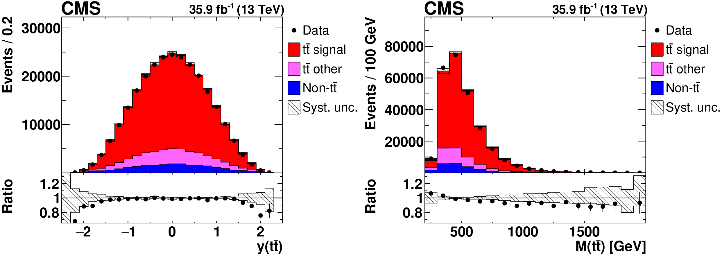
Figure 2:
Distributions of $y({{\mathrm {t}\overline {\mathrm {t}}}})$ (left) and ${M({{\mathrm {t}\overline {\mathrm {t}}}})}$ (right) in selected events after the loose kinematic reconstruction. Details can be found in the caption of Fig. 1. |
png pdf |
Figure 2-a:
Distribution of $y({{\mathrm {t}\overline {\mathrm {t}}}})$ in selected events after the loose kinematic reconstruction. Details can be found in the caption of Fig. 1. |
png pdf |
Figure 2-b:
Distribution of ${M({{\mathrm {t}\overline {\mathrm {t}}}})}$ in selected events after the loose kinematic reconstruction. Details can be found in the caption of Fig. 1. |
png pdf |
Figure 3:
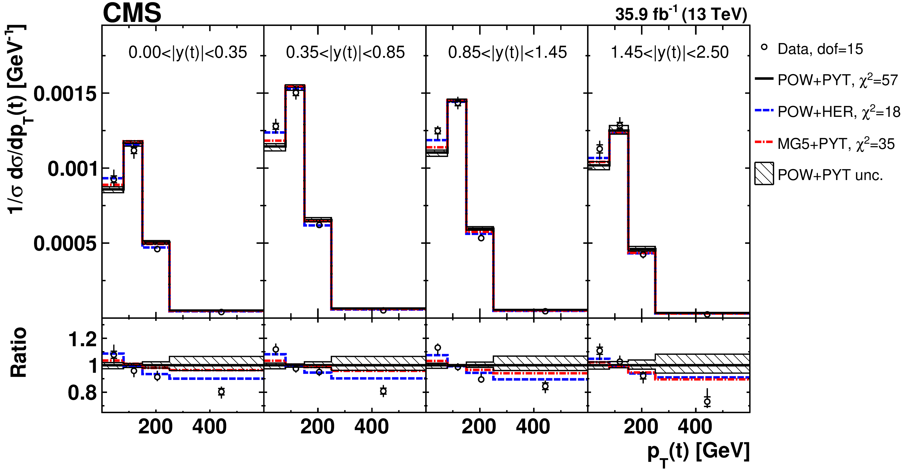
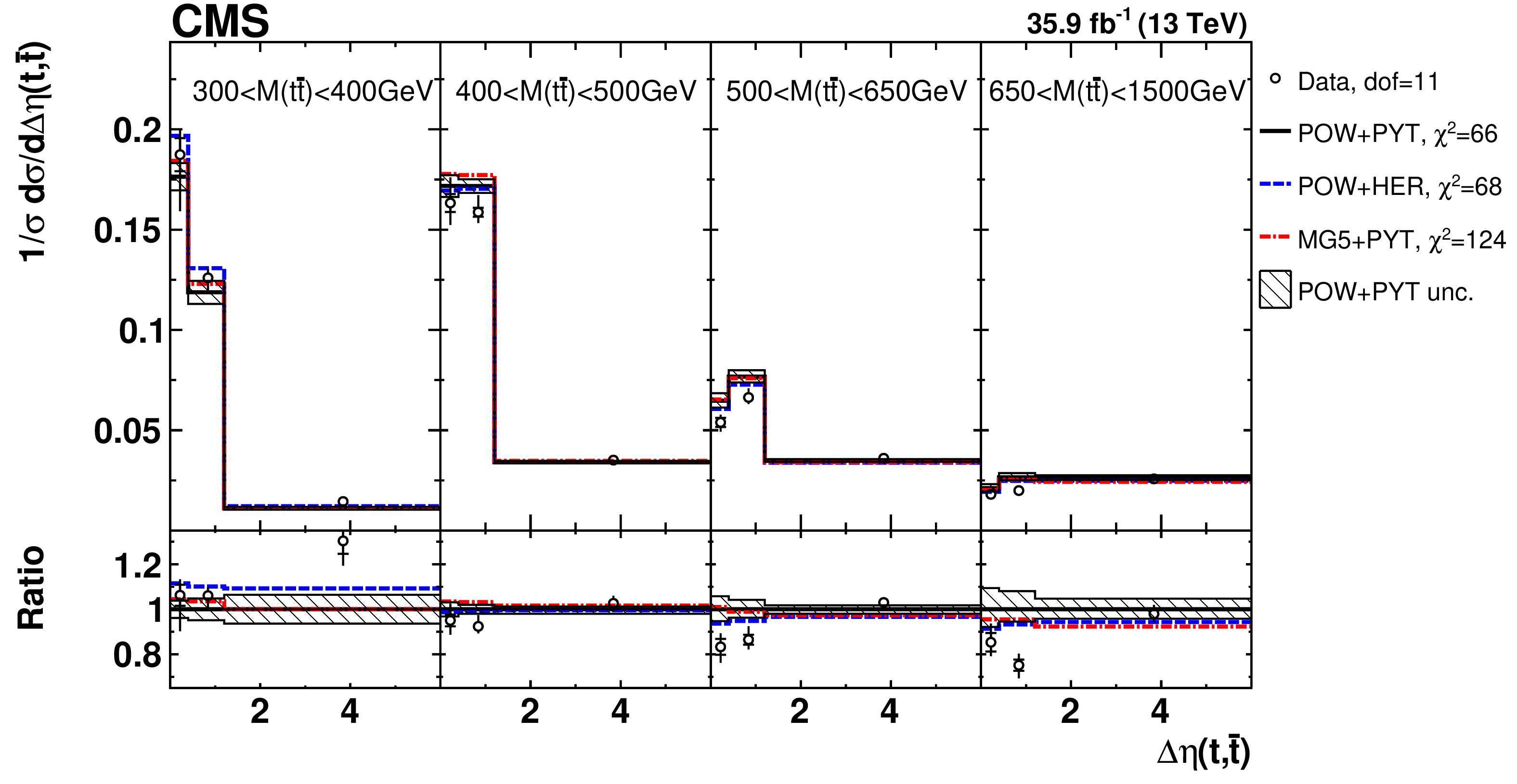
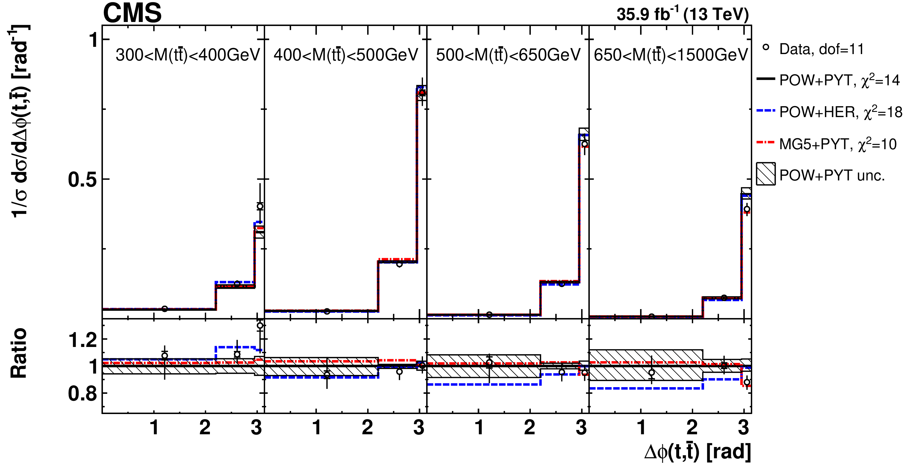
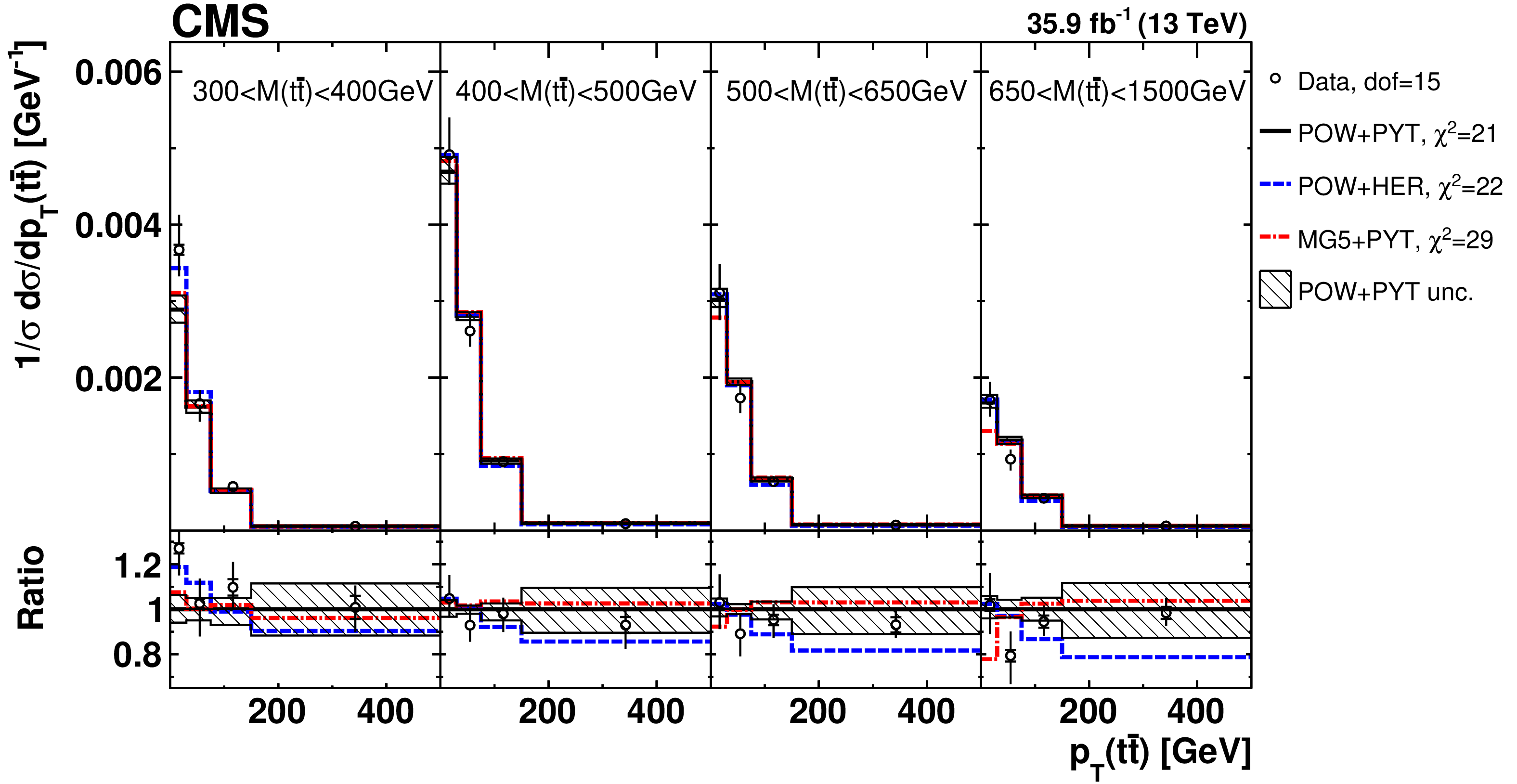
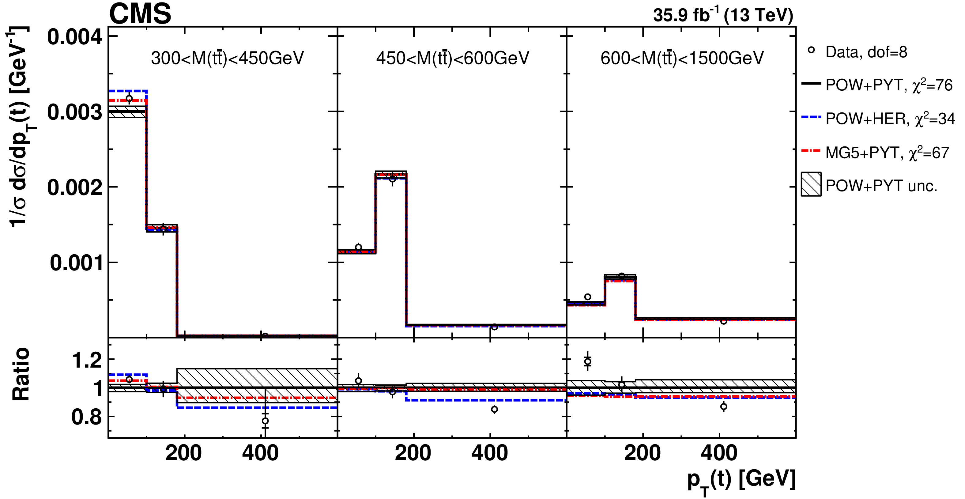
Comparison of the measured [ ${y({\mathrm {t}})}$, ${{p_{\mathrm {T}}} ({\mathrm {t}})}$ ] cross sections {to the theoretical predictions calculated using POWHEG + PYTHIA (`POW+PYT'), POWHEG + HERWIG++ (`POW+HER'), and MG5\_aMC@NLO + PYTHIA (`MG5+PYT') event generators.} The inner vertical bars on the data points represent the statistical uncertainties and the full bars include also the systematic uncertainties added in quadrature. For each MC model, values of ${\chi ^2}$ which take into account the bin-to-bin correlations and dof for the comparison with the data are reported. The hatched regions correspond to the theoretical uncertainties in POWHEG + PYTHIA (see Section 7). In the lower panel, the ratios of the data and other simulations to the `POW+PYT' predictions are shown. |

png pdf |
Figure 4:
Comparison of the measured [ ${M({{\mathrm {t}\overline {\mathrm {t}}}})}$, ${y({\mathrm {t}})}$ ] cross sections {to the theoretical predictions calculated using MC event generators} (further details can be found in the Fig. 3 caption). |
png pdf |
Figure 5:
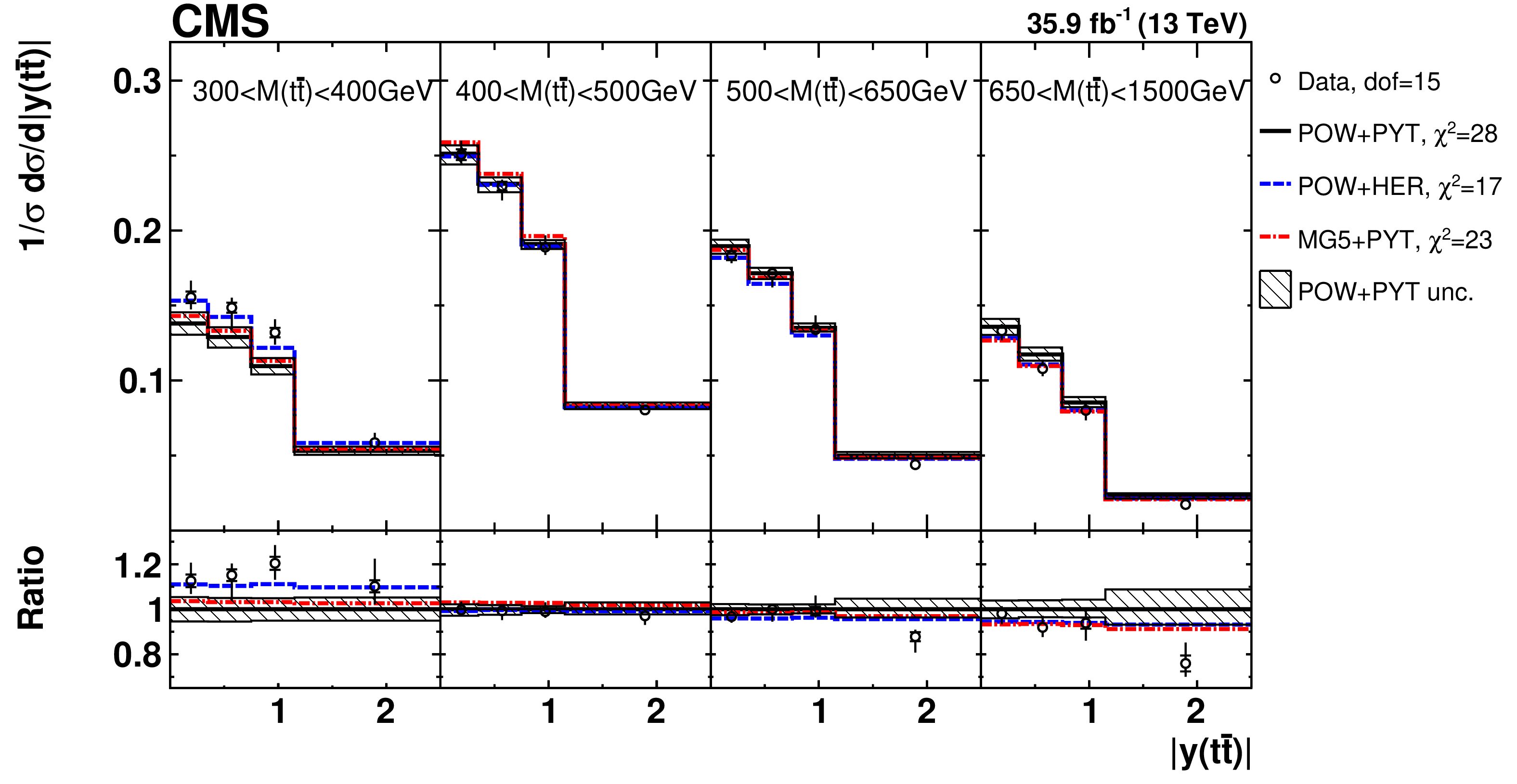
Comparison of the measured [ ${M({{\mathrm {t}\overline {\mathrm {t}}}})}$, ${y({{\mathrm {t}\overline {\mathrm {t}}}})}$ ] cross sections {to the theoretical predictions calculated using MC event generators} (further details can be found in the Fig. 3 caption). |
png pdf |
Figure 6:
Comparison of the measured [ ${M({{\mathrm {t}\overline {\mathrm {t}}}})}$, ${\Delta \eta ({\mathrm {t}}, {\overline {\mathrm {t}}})}$ ] cross sections {to the theoretical predictions calculated using MC event generators} (further details can be found in the Fig. 3 caption). |
png pdf |
Figure 7:
Comparison of the measured [ ${M({{\mathrm {t}\overline {\mathrm {t}}}})}$, ${\Delta \phi ({\mathrm {t}}, {\overline {\mathrm {t}}})}$ ] cross sections {to the theoretical predictions calculated using MC event generators} (further details can be found in the Fig. 3 caption). |
png pdf |
Figure 8:
Comparison of the measured [ ${M({{\mathrm {t}\overline {\mathrm {t}}}})}$, ${{p_{\mathrm {T}}} ({{\mathrm {t}\overline {\mathrm {t}}}})}$ ] cross sections {to the theoretical predictions calculated using MC event generators} (further details can be found in the Fig. 3 caption). |
png pdf |
Figure 9:
Comparison of the measured [ ${M({{\mathrm {t}\overline {\mathrm {t}}}})}$, ${{p_{\mathrm {T}}} ({\mathrm {t}})}$ ] cross sections {to the theoretical predictions calculated using MC event generators} (further details can be found in the Fig. 3 caption). |
png pdf |
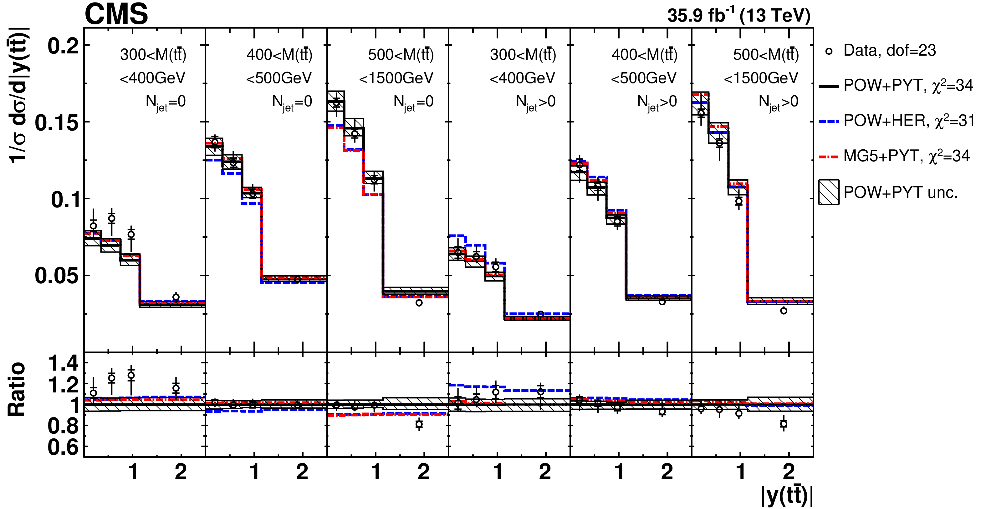
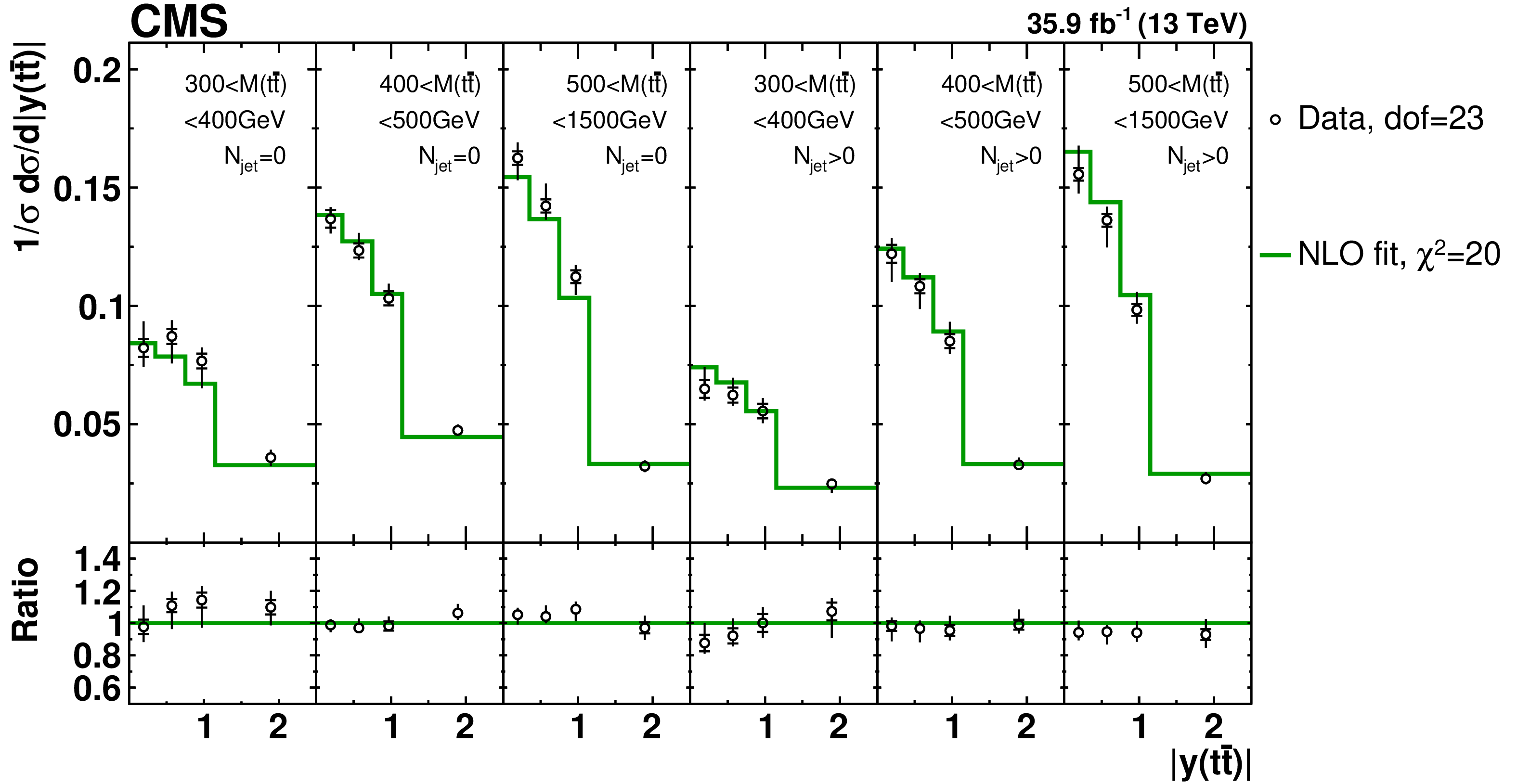
Figure 10:
Comparison of the measured [ ${N^{0,1+}_{\text {jet}}}$, ${M({{\mathrm {t}\overline {\mathrm {t}}}})}$, ${y({{\mathrm {t}\overline {\mathrm {t}}}})}$ ] cross sections {to the theoretical predictions calculated using MC event generators} (further details can be found in the Fig. 3 caption). |
png pdf |
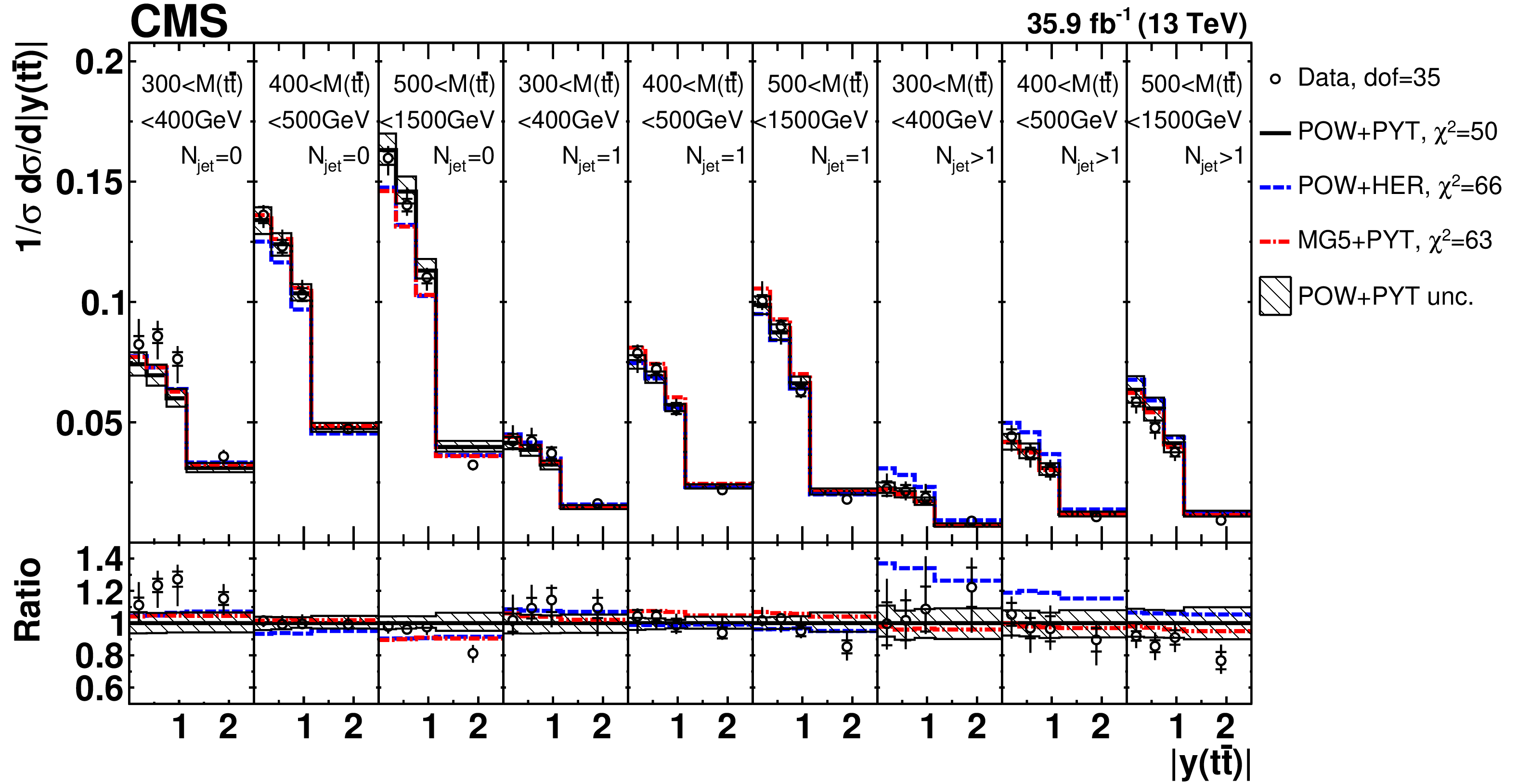
Figure 11:
Comparison of the measured [ ${N^{0,1,2+}_{\text {jet}}}$, ${M({{\mathrm {t}\overline {\mathrm {t}}}})}$, ${y({{\mathrm {t}\overline {\mathrm {t}}}})}$ ] cross sections {to the theoretical predictions calculated using MC event generators} (further details can be found in the Fig. 3 caption). |
png pdf |
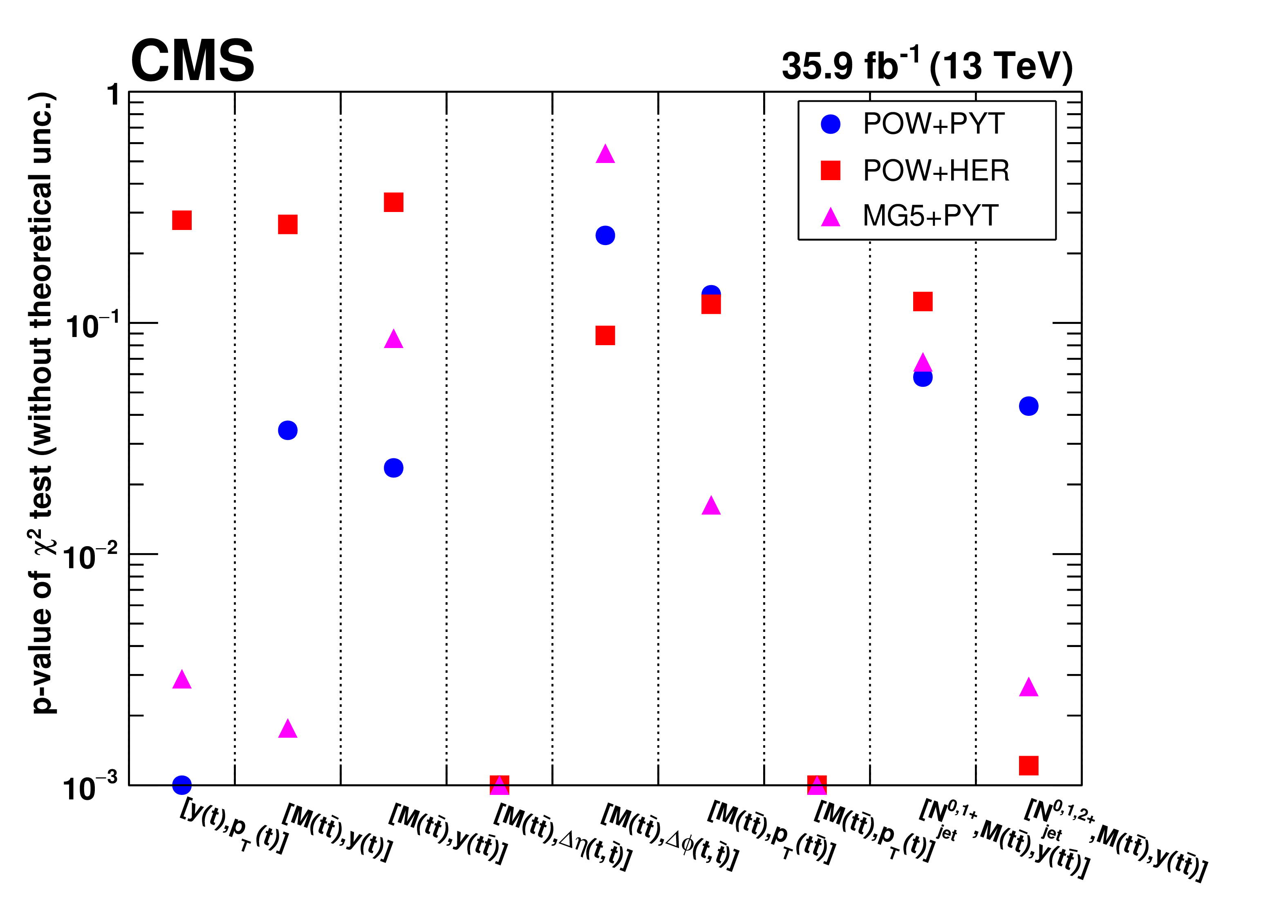
Figure 12:
Assessment of compatibility of various MC predictions with the data. The plot show the $p$-values of ${\chi ^2}$-tests between data and predictions. Only the data uncertainties are taken into account in the ${\chi ^2}$-tests while uncertainties on the theoretical calculations are ignored. Points with $p \le $ 0.001 are shown at $p = $ 0.001. |
png pdf |
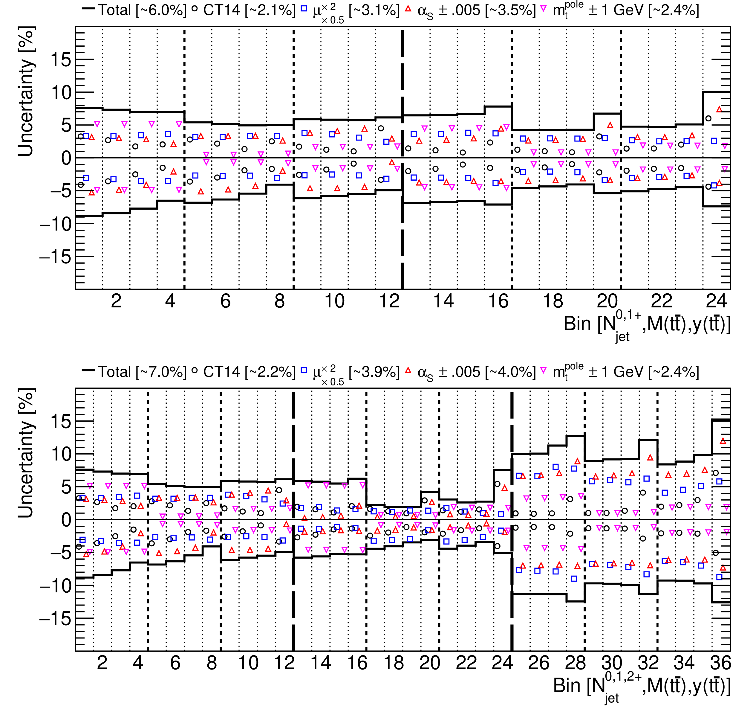
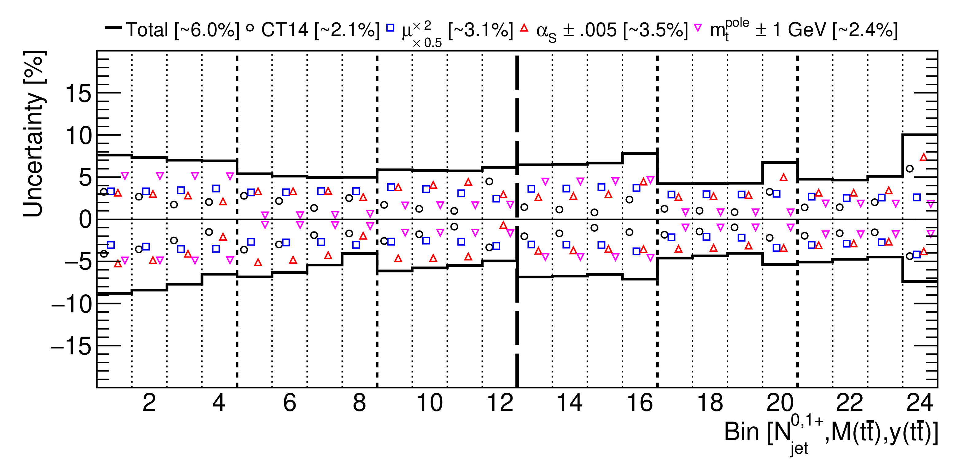
Figure 13:
The theoretical uncertainties for [ ${N^{0,1+}_{\text {jet}}}$, ${M({{\mathrm {t}\overline {\mathrm {t}}}})}$, ${y({{\mathrm {t}\overline {\mathrm {t}}}})}$ ] (upper) and [ ${N^{0,1,2+}_{\text {jet}}}$, ${M({{\mathrm {t}\overline {\mathrm {t}}}})}$, ${y({{\mathrm {t}\overline {\mathrm {t}}}})}$ ] (lower) cross sections, arising from PDF, ${{\alpha _S} (m_{{\mathrm {Z}}})}$, and ${m_{{\mathrm {t}}}^{\text {pole}}}$ variations, as well as the total theoretical uncertainties, with their bin-averaged values shown in brackets. The bins are the same as in Figs. 10 and 11. |
png pdf |
Figure 13-a:
The theoretical uncertainties for [ ${N^{0,1+}_{\text {jet}}}$, ${M({{\mathrm {t}\overline {\mathrm {t}}}})}$, ${y({{\mathrm {t}\overline {\mathrm {t}}}})}$ ] cross sections, arising from PDF, ${{\alpha _S} (m_{{\mathrm {Z}}})}$, and ${m_{{\mathrm {t}}}^{\text {pole}}}$ variations, as well as the total theoretical uncertainties, with their bin-averaged values shown in brackets. The bins are the same as in Figs. 10 and 11. |

png pdf |
Figure 13-b:
The theoretical uncertainties for [ ${N^{0,1,2+}_{\text {jet}}}$, ${M({{\mathrm {t}\overline {\mathrm {t}}}})}$, ${y({{\mathrm {t}\overline {\mathrm {t}}}})}$ ] cross sections, arising from PDF, ${{\alpha _S} (m_{{\mathrm {Z}}})}$, and ${m_{{\mathrm {t}}}^{\text {pole}}}$ variations, as well as the total theoretical uncertainties, with their bin-averaged values shown in brackets. The bins are the same as in Figs. 10 and 11. |
png pdf |
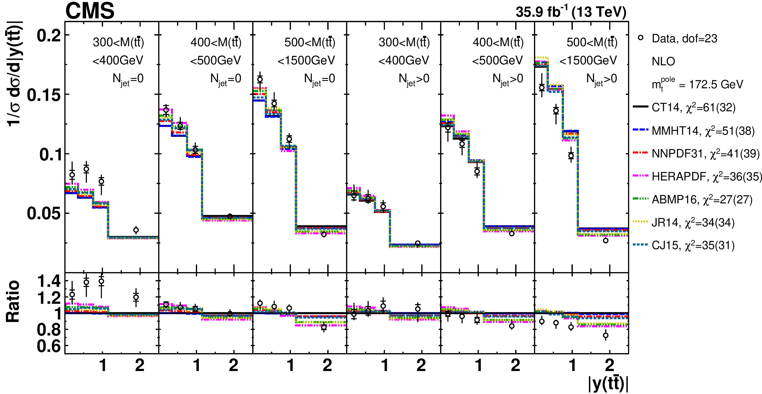
Figure 14:
Comparison of the measured [ ${N^{0,1+}_{\text {jet}}}$, ${M({{\mathrm {t}\overline {\mathrm {t}}}})}$, ${y({{\mathrm {t}\overline {\mathrm {t}}}})}$ ] cross sections to NLO predictions obtained using different PDF sets (further details can be found in Fig. 3). For each theoretical prediction, values of ${\chi ^2}$ and dof for the comparison to the data are reported, while additional ${\chi ^2}$ values that include PDF uncertainties are shown in parentheses. |
png pdf |
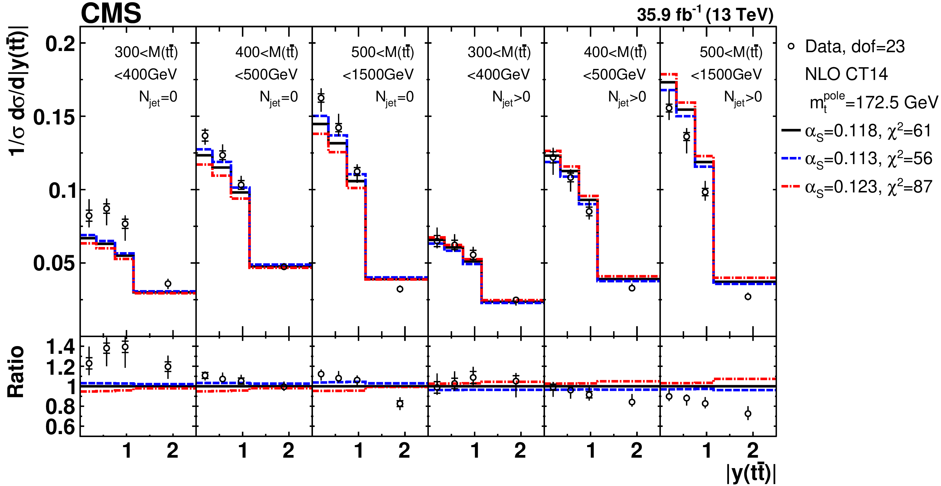
Figure 15:
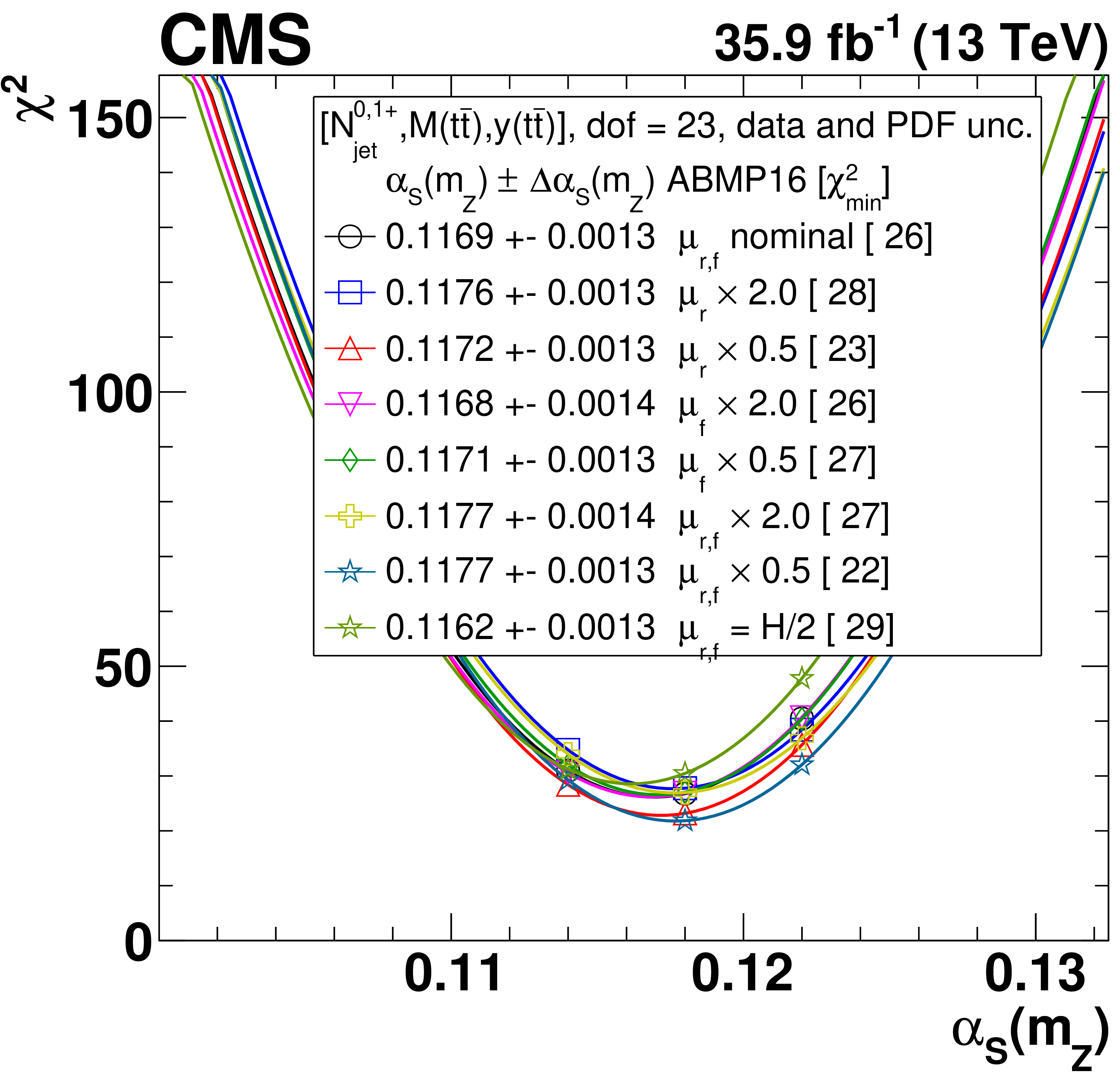
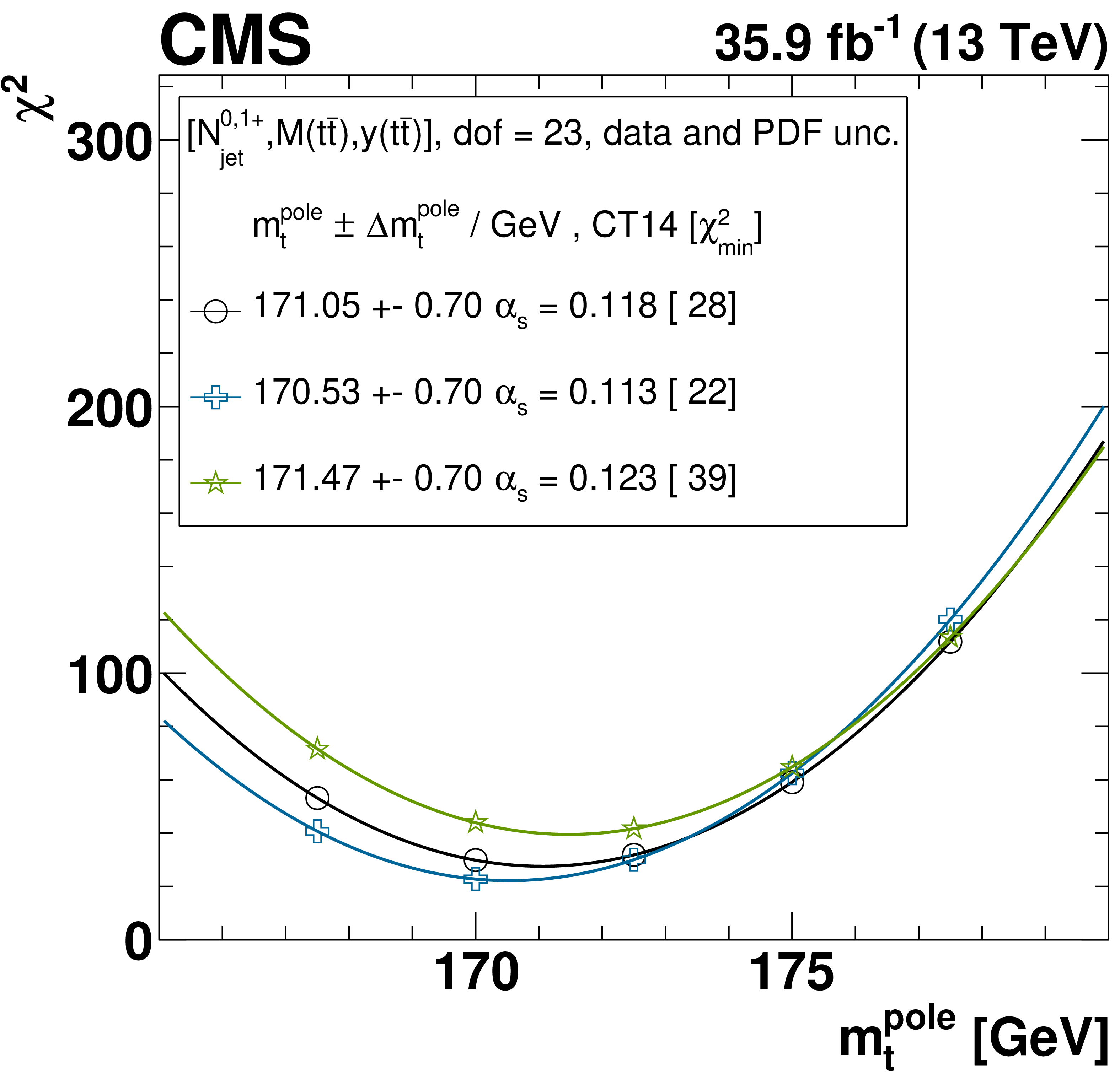
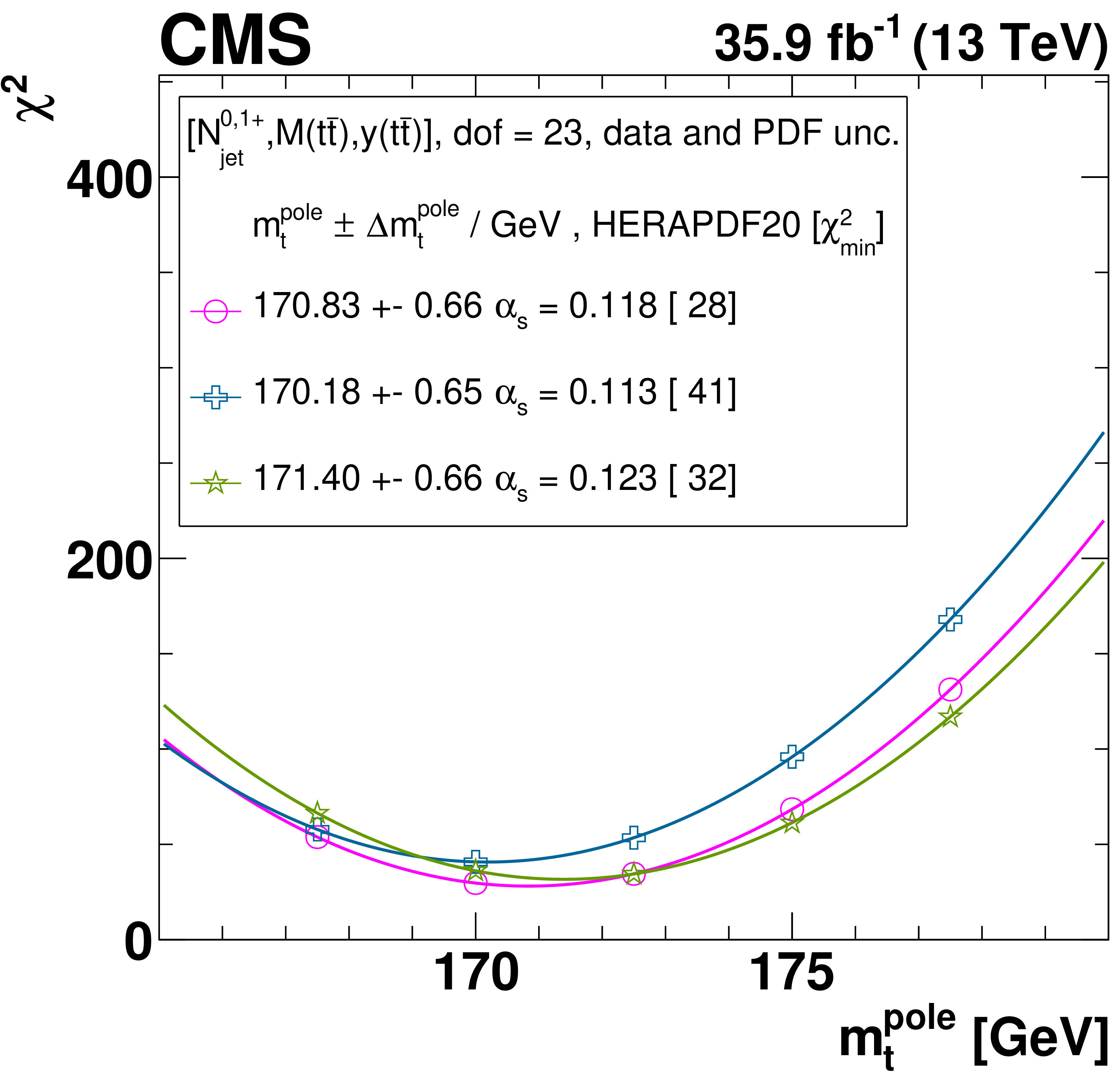
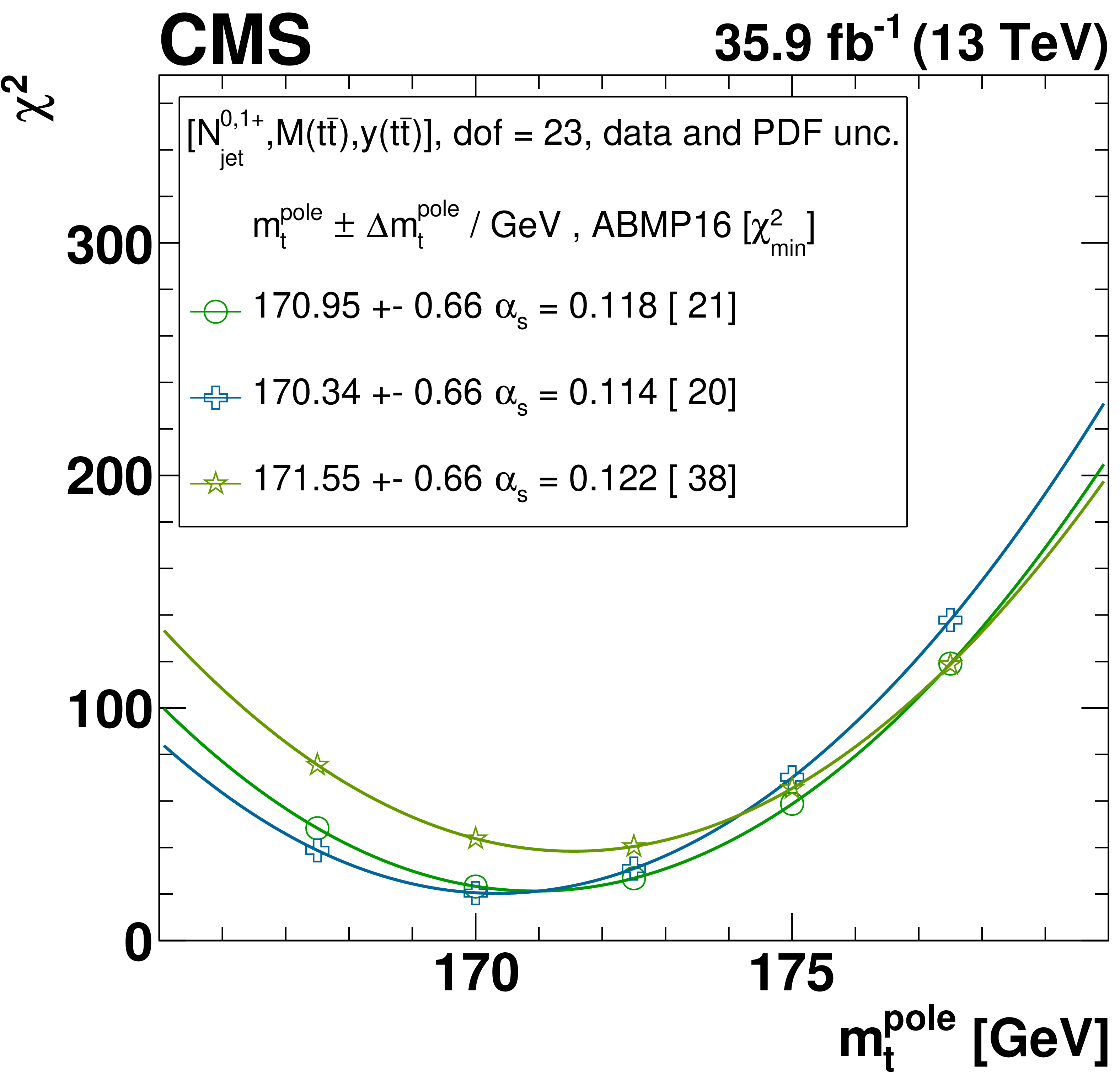
Comparison of the measured [ ${N^{0,1+}_{\text {jet}}}$, ${M({{\mathrm {t}\overline {\mathrm {t}}}})}$, ${y({{\mathrm {t}\overline {\mathrm {t}}}})}$ ] cross sections to NLO predictions obtained using different $ {{\alpha _S} (m_{{\mathrm {Z}}})} $ values (further details can be found in Fig. 3). For each theoretical prediction, values of ${\chi ^2}$ and dof for the comparison to the data are reported. |
png pdf |
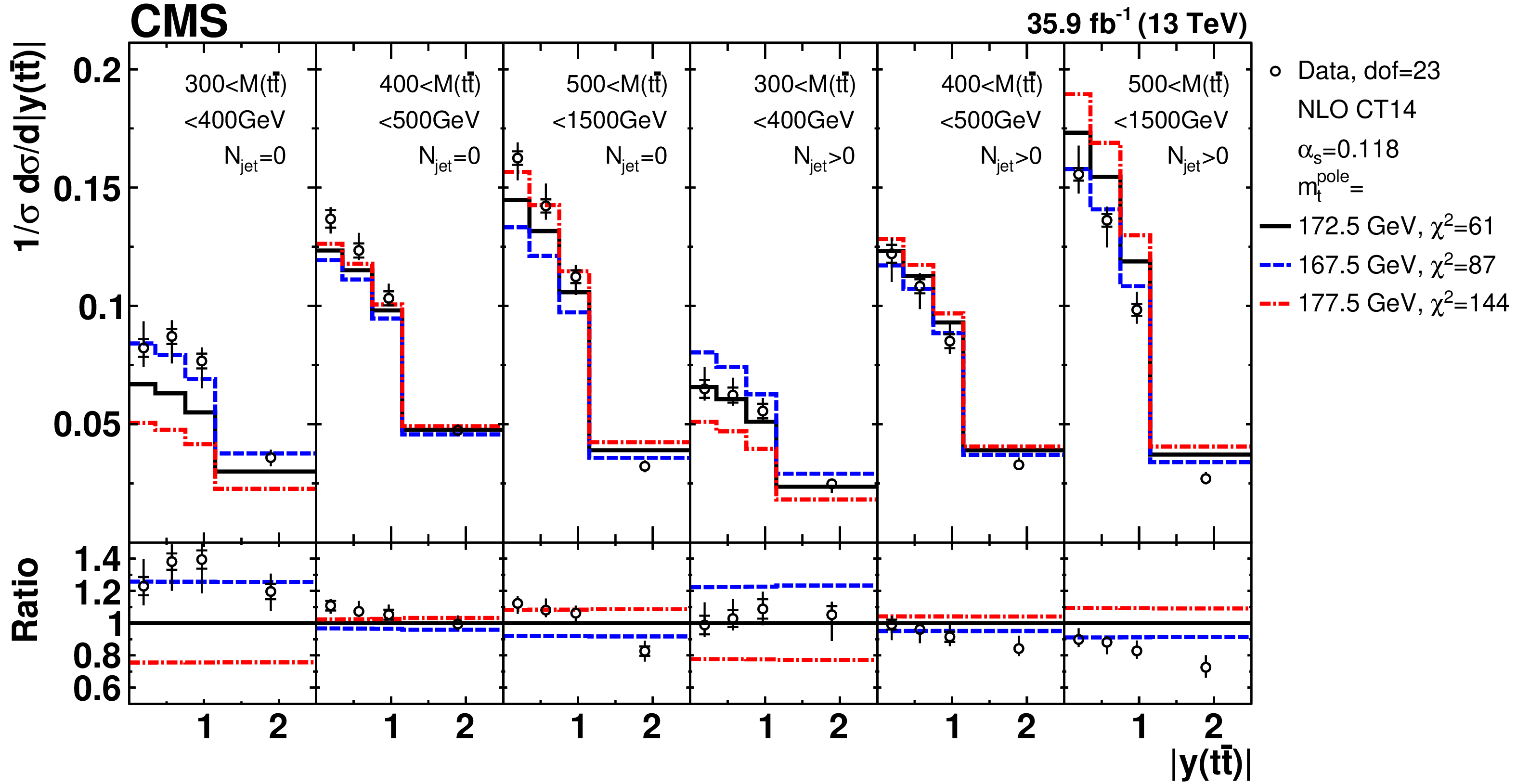
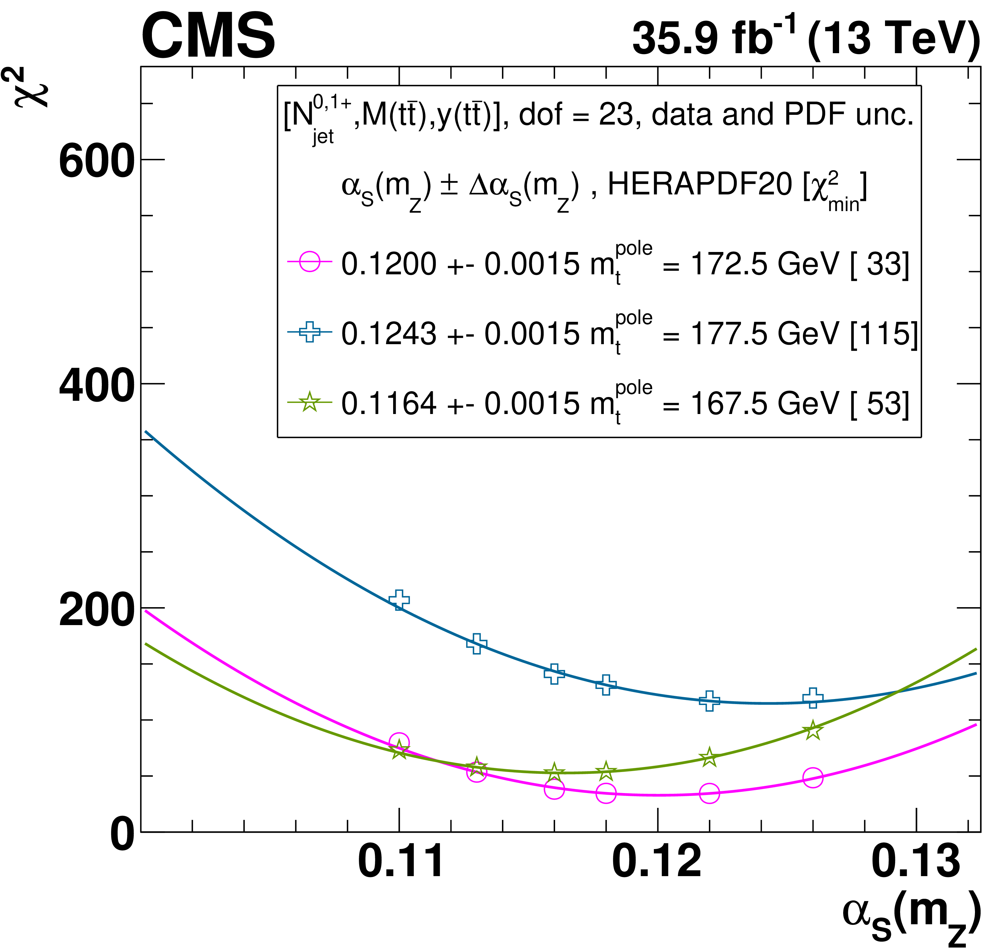
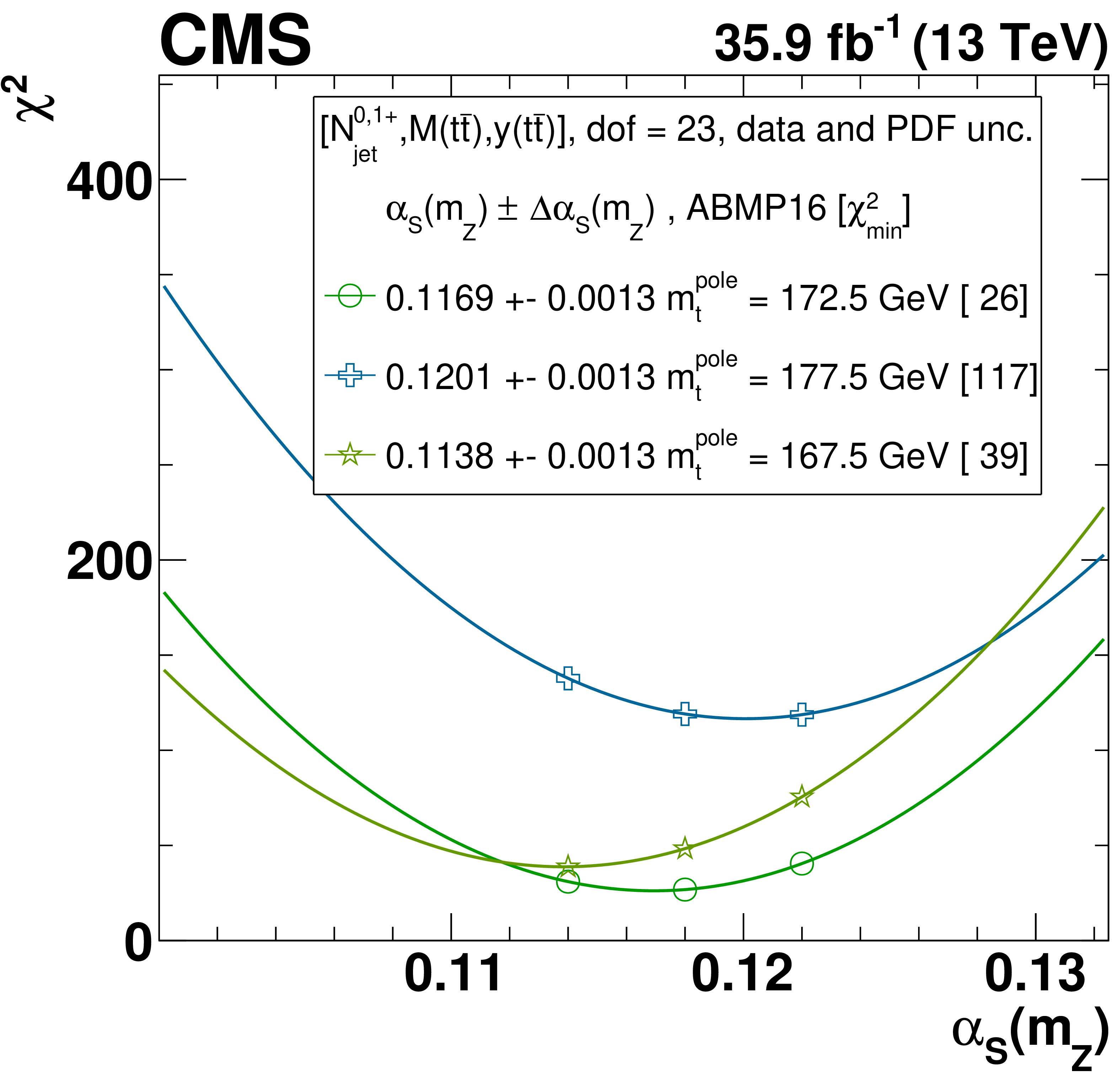
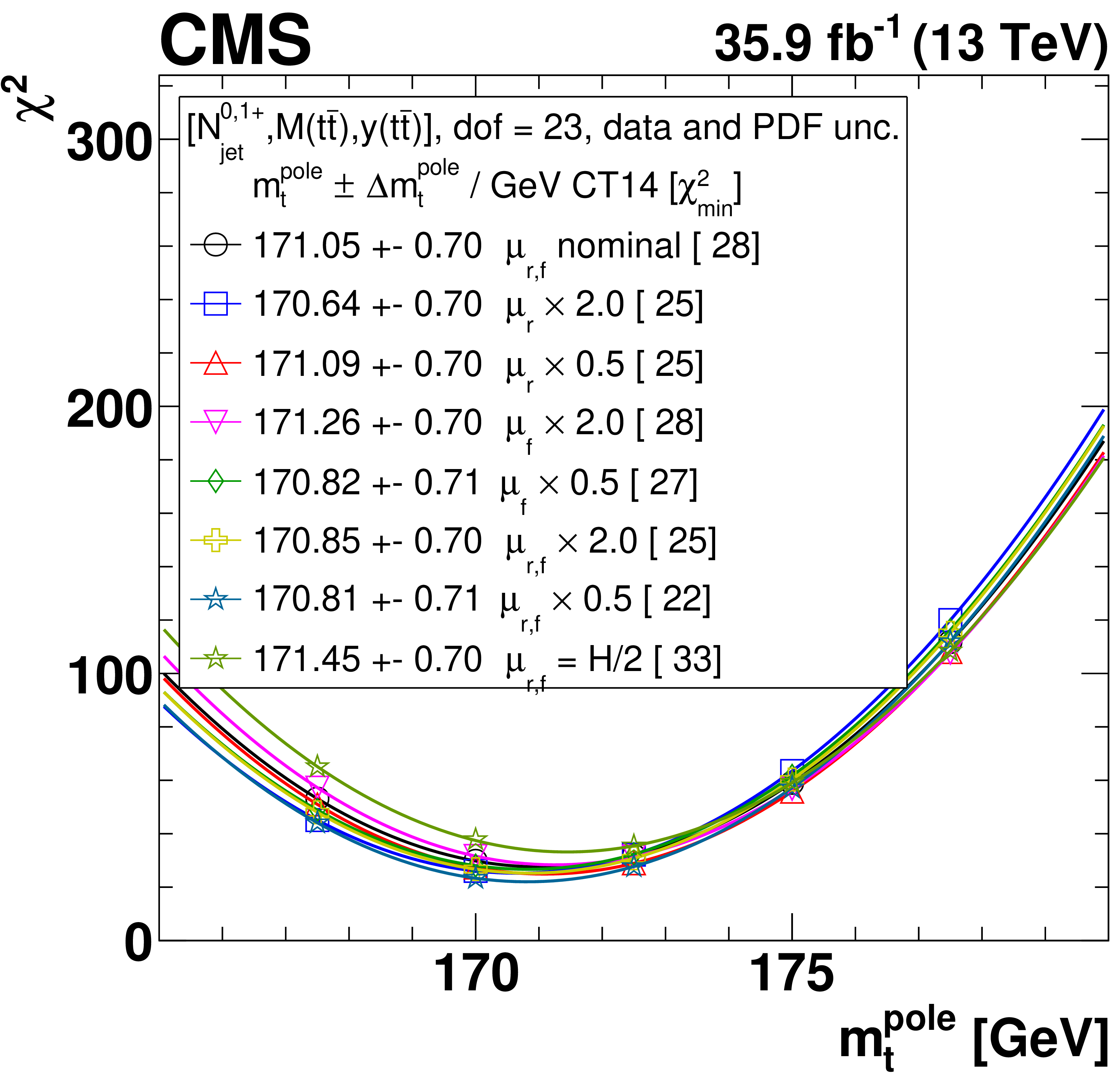
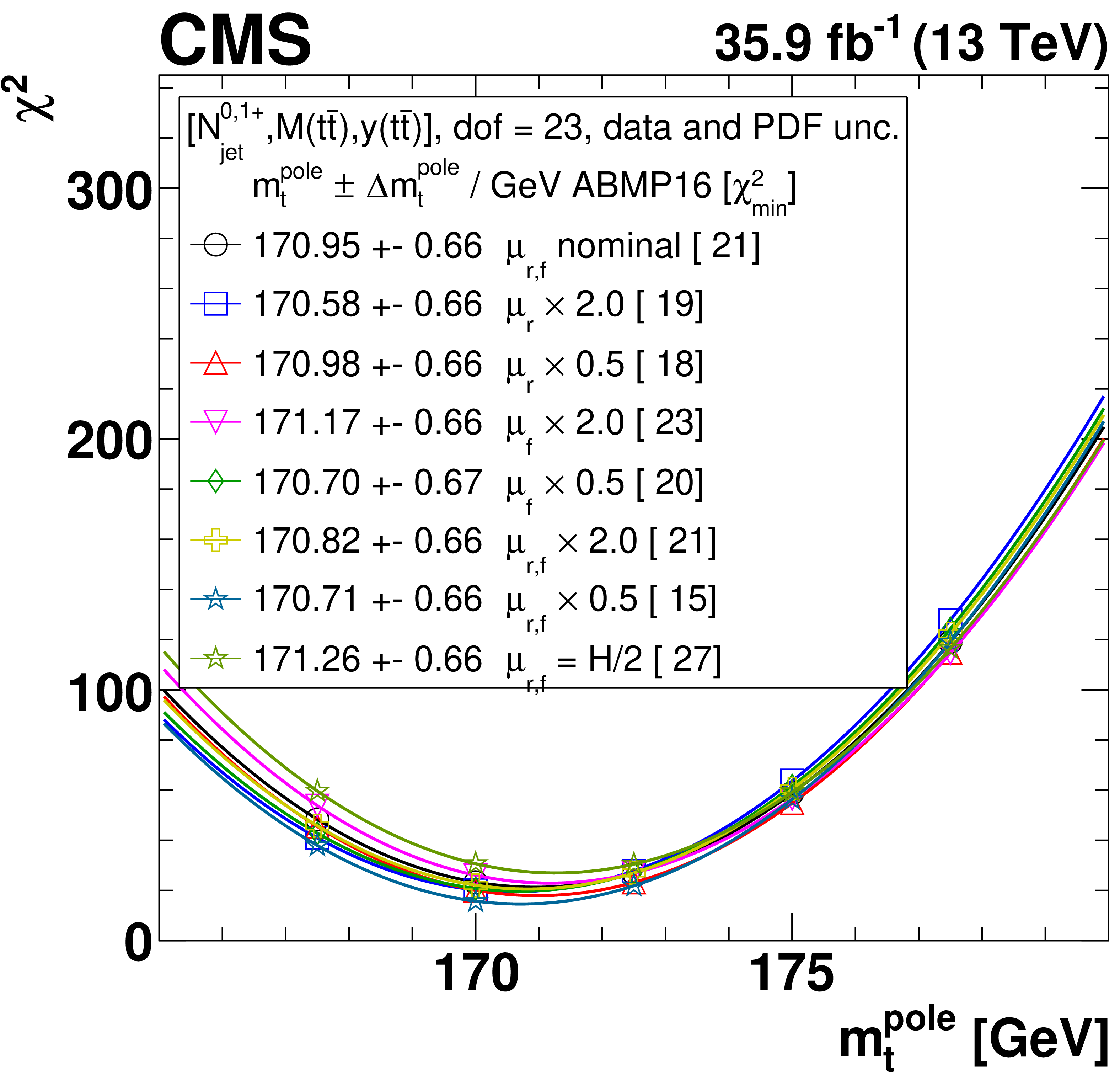
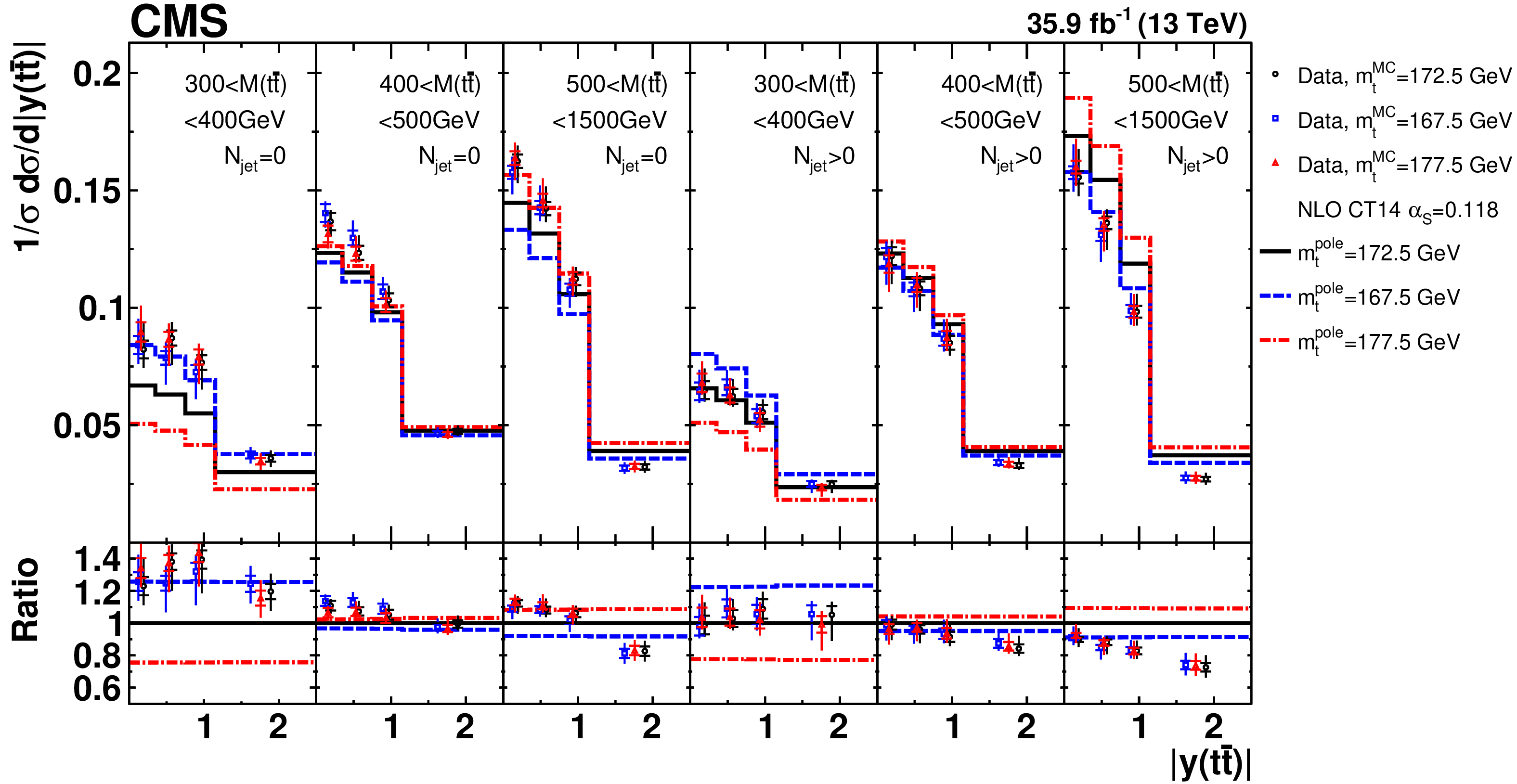
Figure 16:
Comparison of the measured [ ${N^{0,1+}_{\text {jet}}}$, ${M({{\mathrm {t}\overline {\mathrm {t}}}})}$, ${y({{\mathrm {t}\overline {\mathrm {t}}}})}$ ] cross sections to NLO predictions obtained using different ${m_{{\mathrm {t}}}^{\text {pole}}}$ values (further details can be found in Fig. 3). For each theoretical prediction, values of ${\chi ^2}$ and dof for the comparison to the data are reported. |
png pdf |
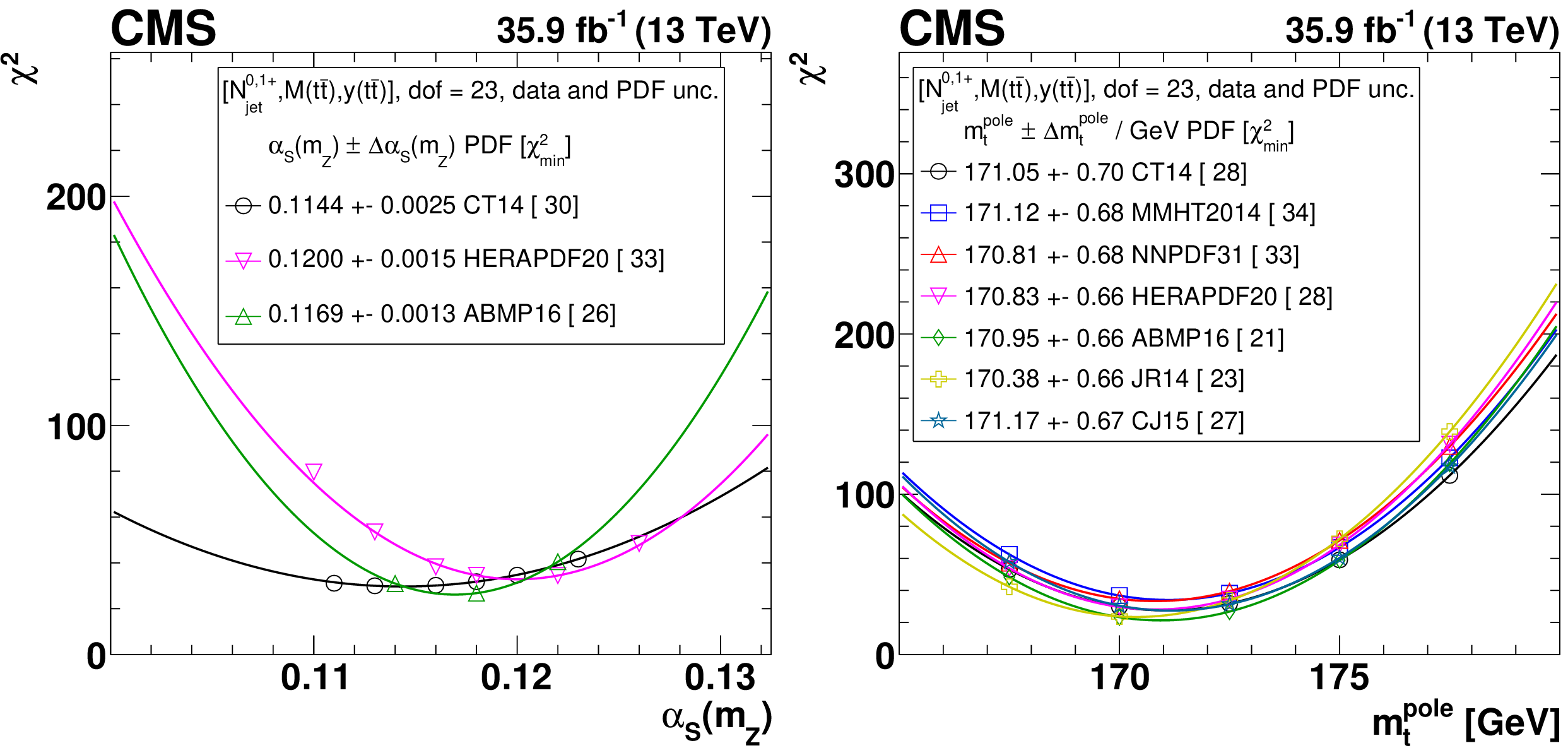
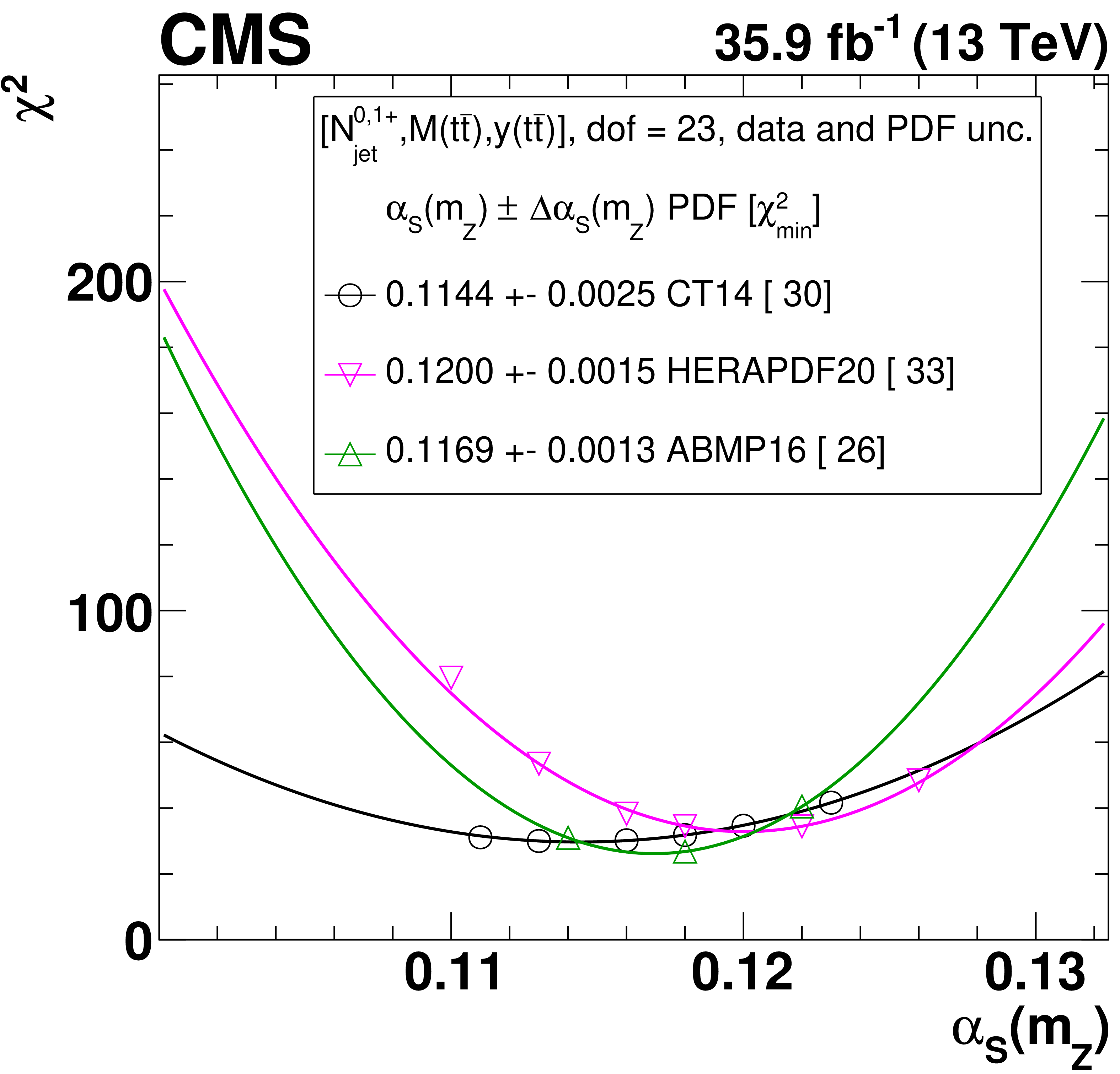
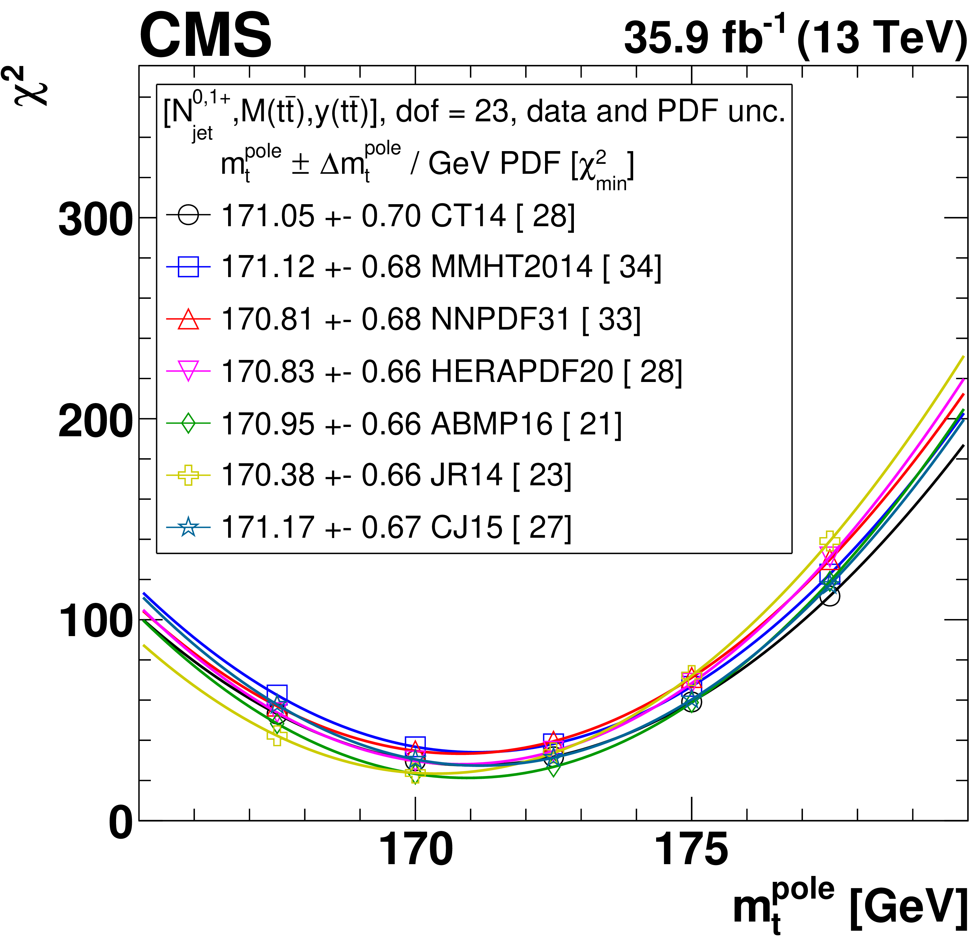
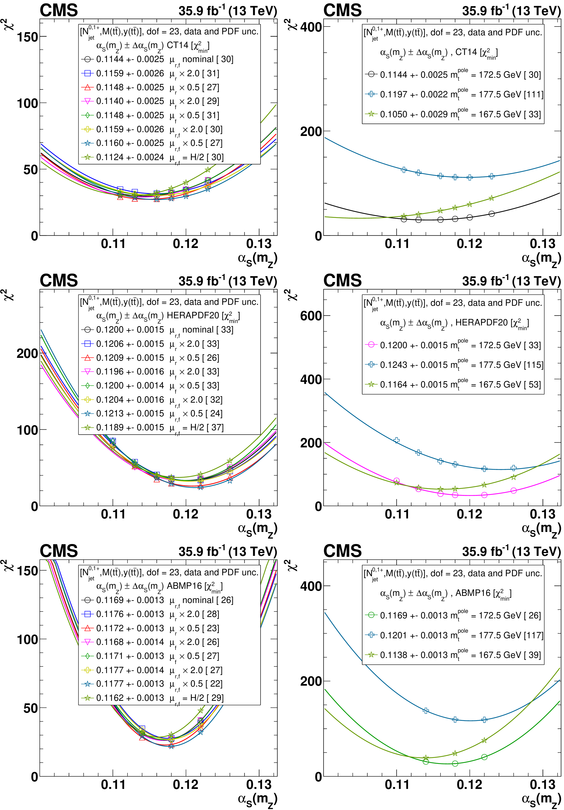
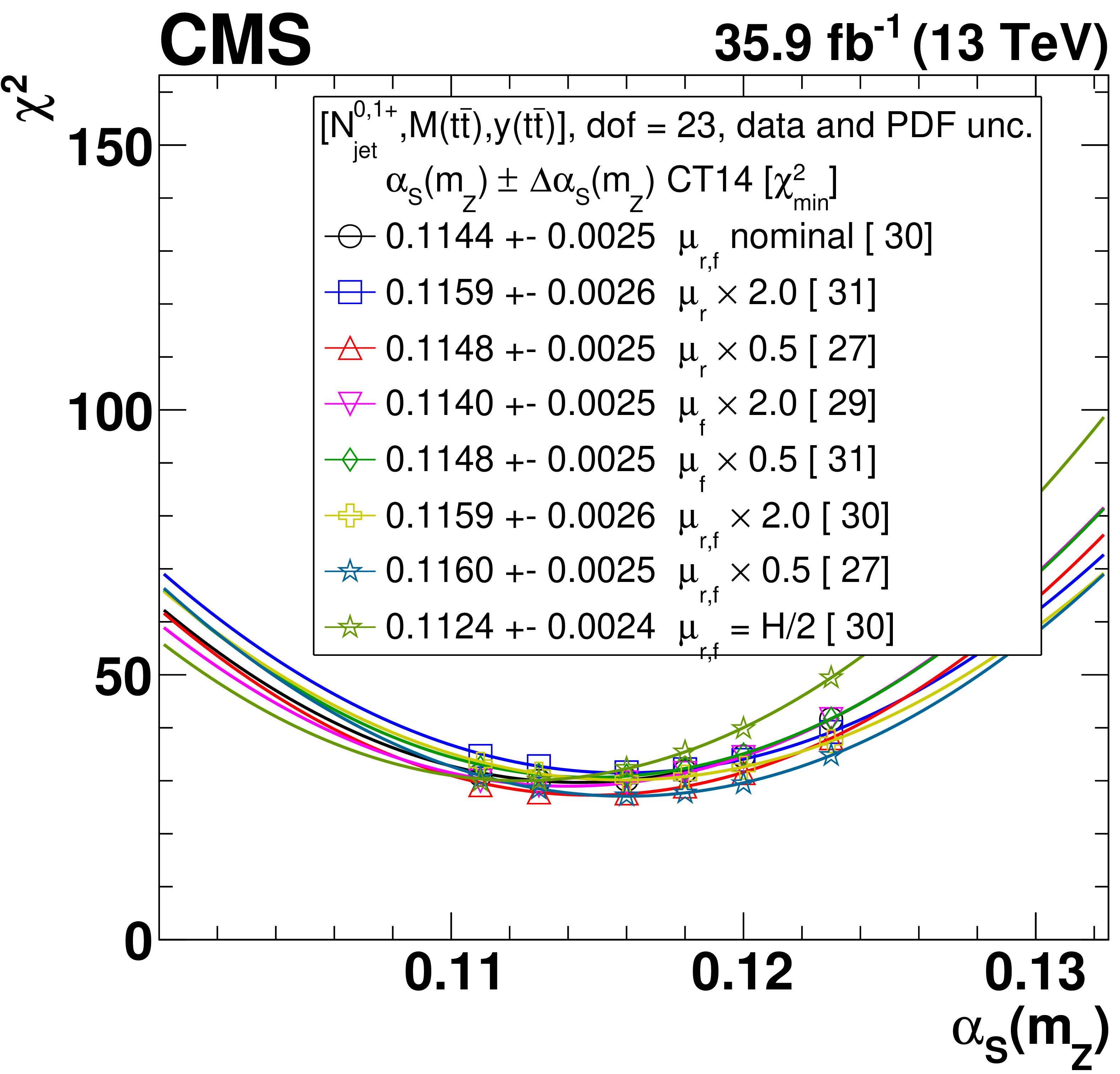
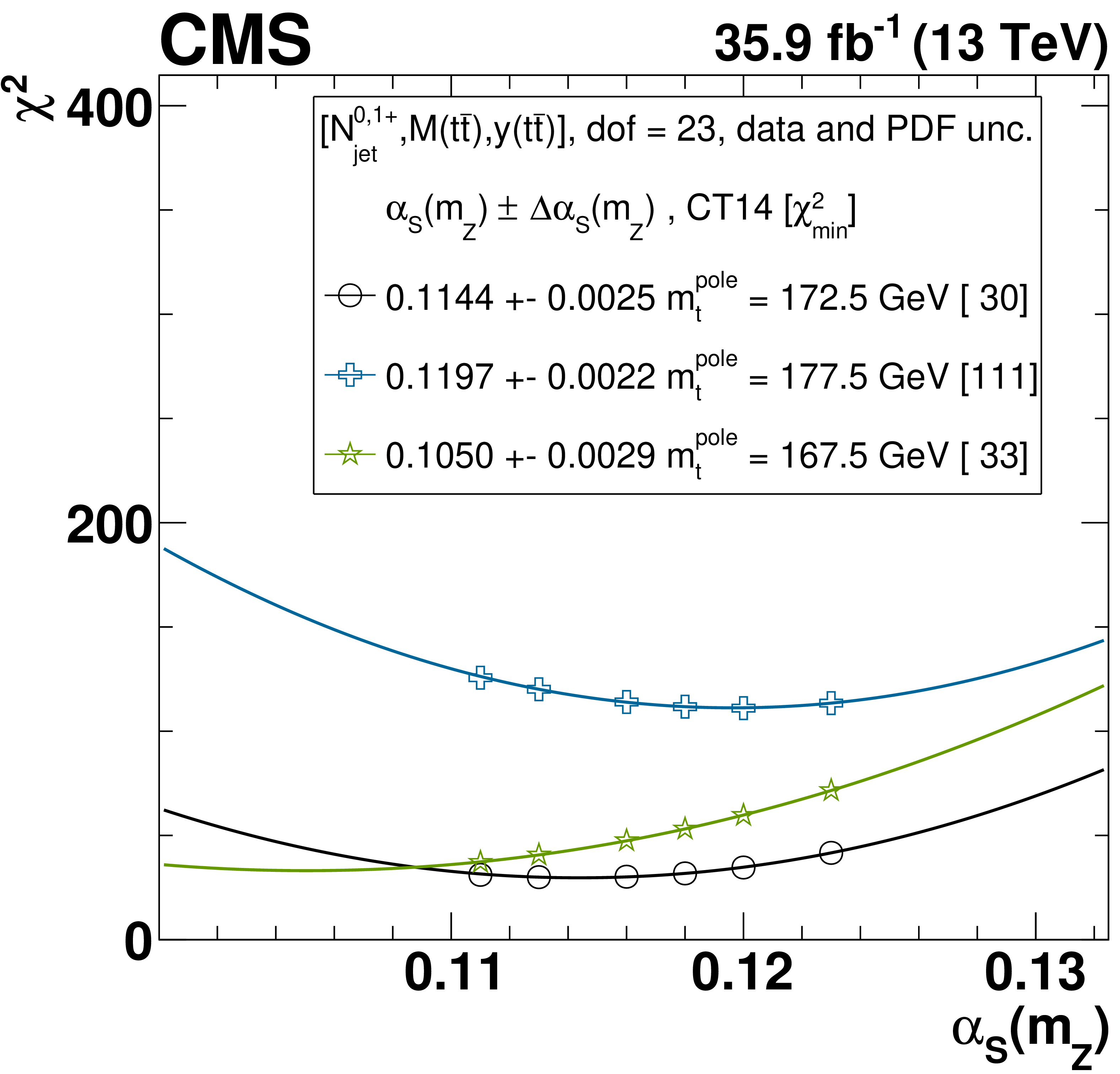
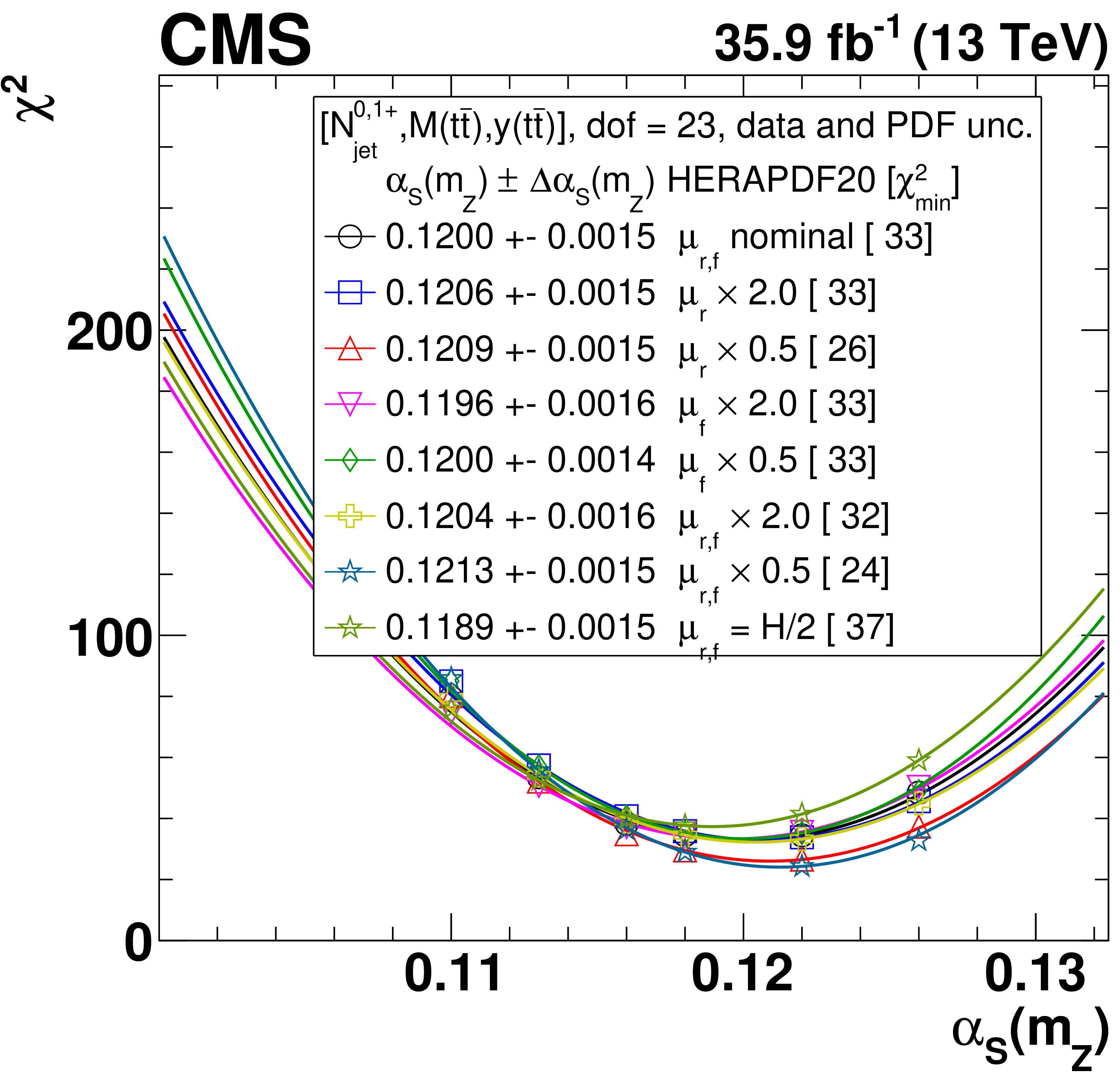
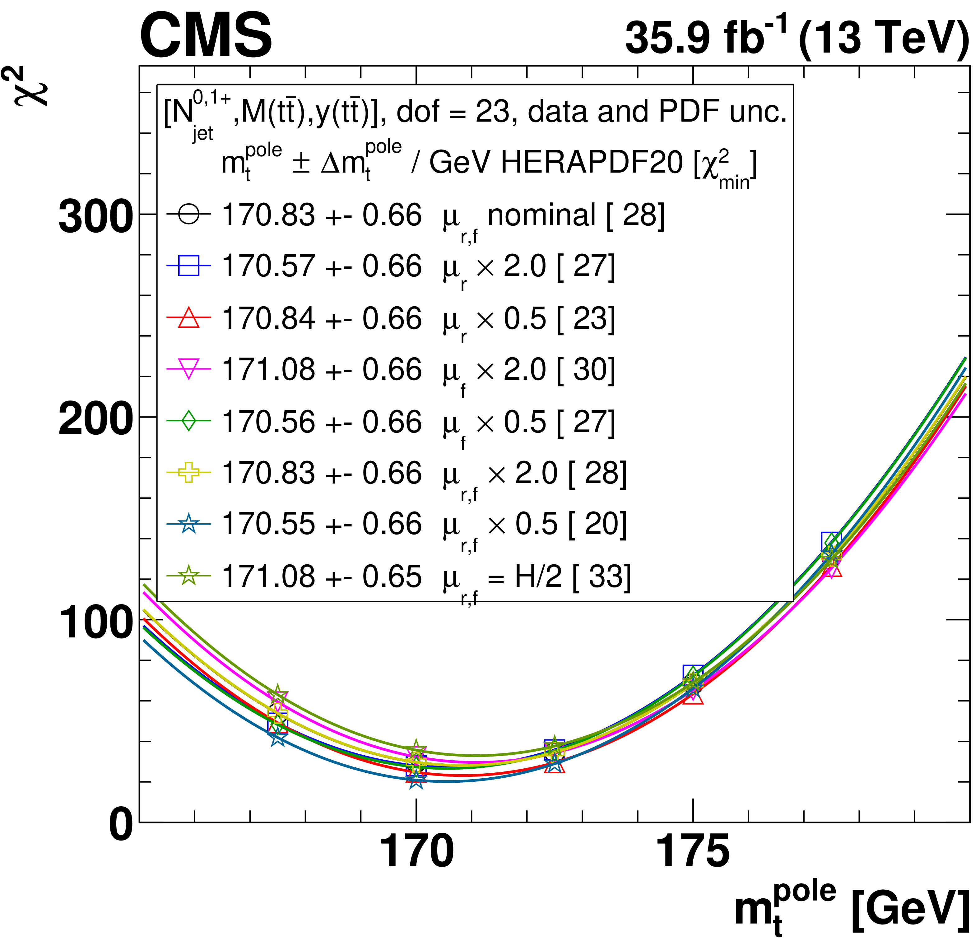
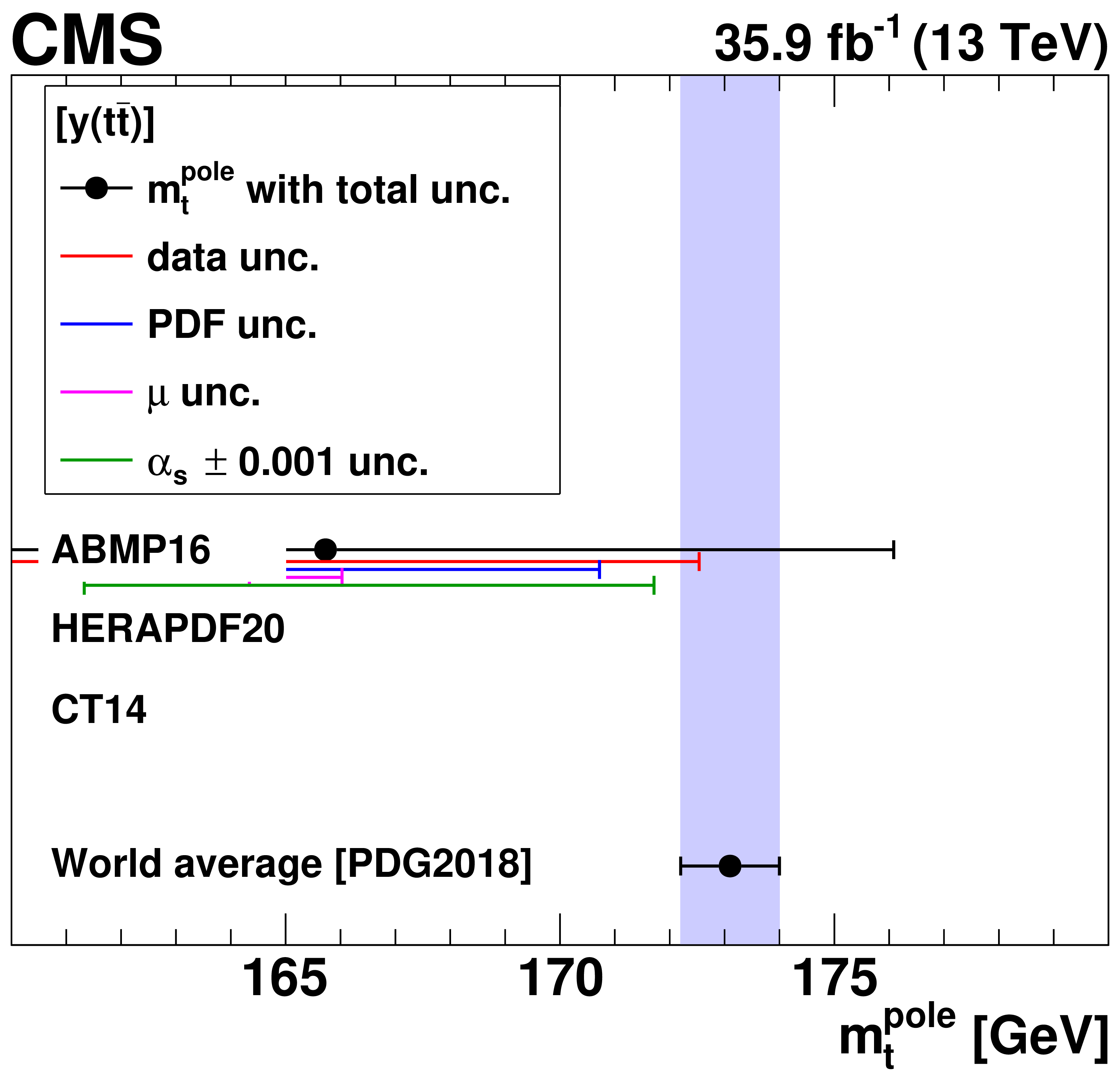
Figure 17:
The $ {{\alpha _S} (m_{{\mathrm {Z}}})} $ (left) and ${m_{{\mathrm {t}}}^{\text {pole}}}$ (right) extraction at NLO from the measured [ ${N^{0,1+}_{\text {jet}}}$, ${M({{\mathrm {t}\overline {\mathrm {t}}}})}$, ${y({{\mathrm {t}\overline {\mathrm {t}}}})}$ ] cross sections using different PDF sets. The extracted $ {{\alpha _S} (m_{{\mathrm {Z}}})} $ and ${m_{{\mathrm {t}}}^{\text {pole}}}$ values are reported for each PDF set, and the estimated minimum ${\chi ^2}$ value is shown in brackets. Further details are given in the text. |
png pdf |
Figure 17-a:
The $ {{\alpha _S} (m_{{\mathrm {Z}}})} $ extraction at NLO from the measured [ ${N^{0,1+}_{\text {jet}}}$, ${M({{\mathrm {t}\overline {\mathrm {t}}}})}$, ${y({{\mathrm {t}\overline {\mathrm {t}}}})}$ ] cross sections using different PDF sets. The extracted $ {{\alpha _S} (m_{{\mathrm {Z}}})} $ and ${m_{{\mathrm {t}}}^{\text {pole}}}$ values are reported for each PDF set, and the estimated minimum ${\chi ^2}$ value is shown in brackets. Further details are given in the text. |
png pdf |
Figure 17-b:
The ${m_{{\mathrm {t}}}^{\text {pole}}}$ extraction at NLO from the measured [ ${N^{0,1+}_{\text {jet}}}$, ${M({{\mathrm {t}\overline {\mathrm {t}}}})}$, ${y({{\mathrm {t}\overline {\mathrm {t}}}})}$ ] cross sections using different PDF sets. The extracted $ {{\alpha _S} (m_{{\mathrm {Z}}})} $ and ${m_{{\mathrm {t}}}^{\text {pole}}}$ values are reported for each PDF set, and the estimated minimum ${\chi ^2}$ value is shown in brackets. Further details are given in the text. |
png pdf |
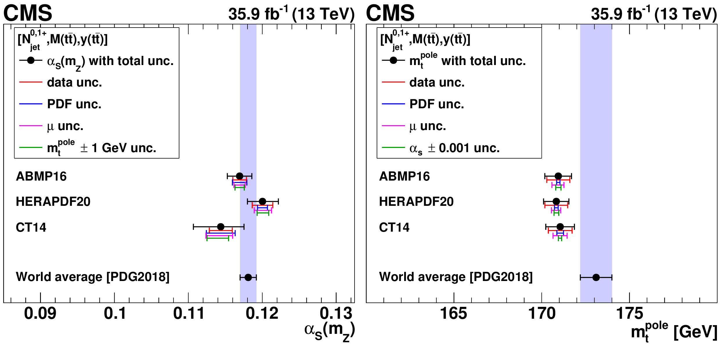
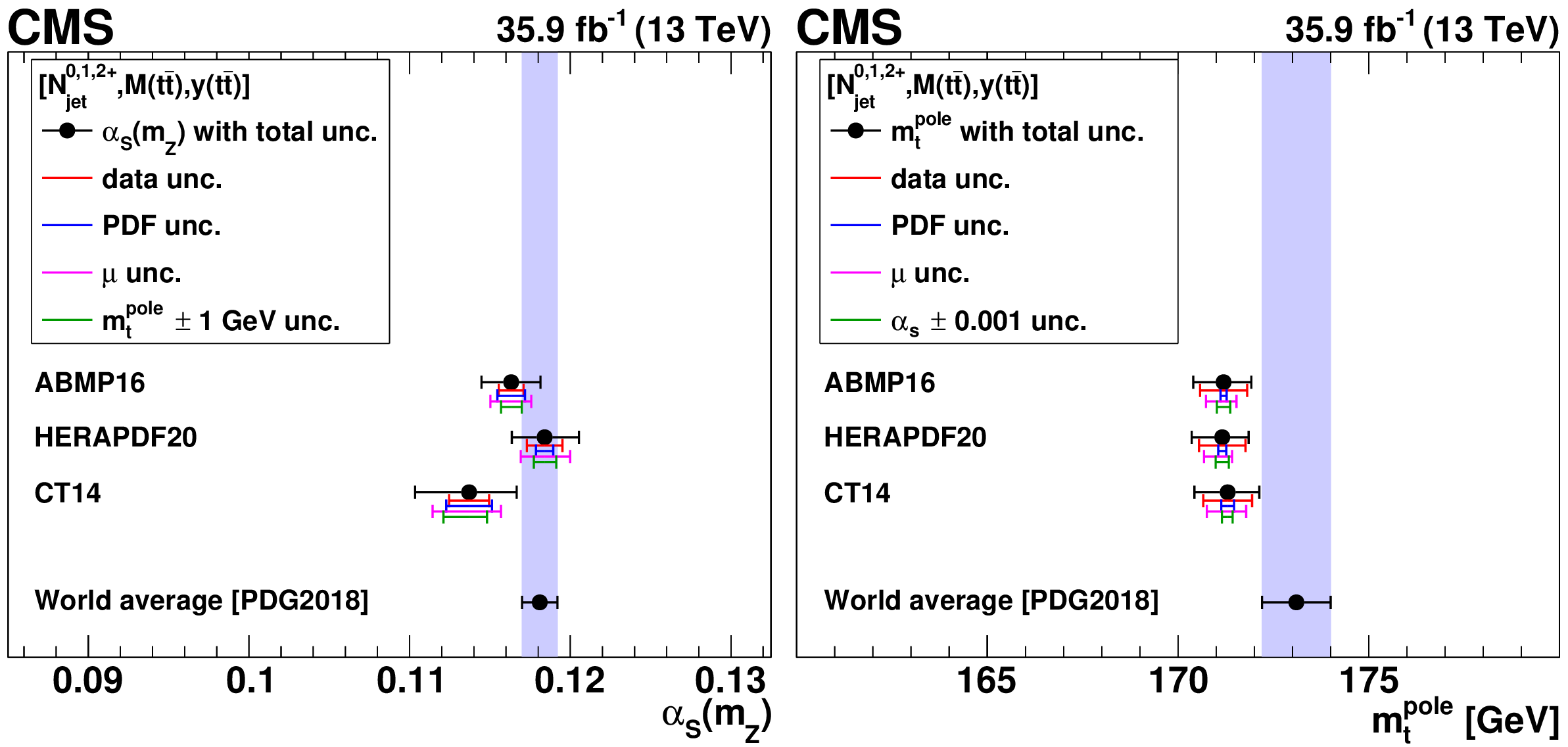
Figure 18:
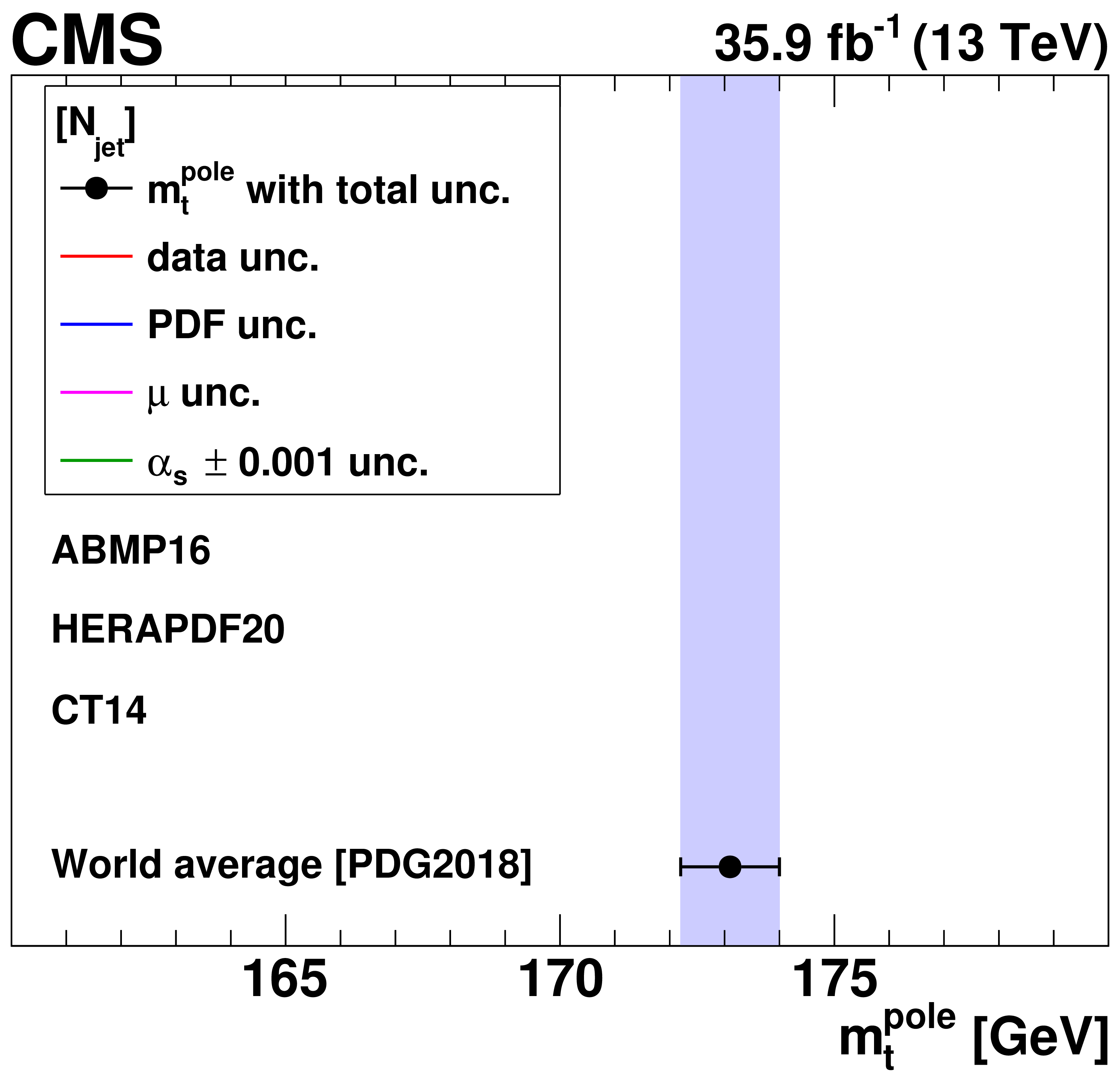
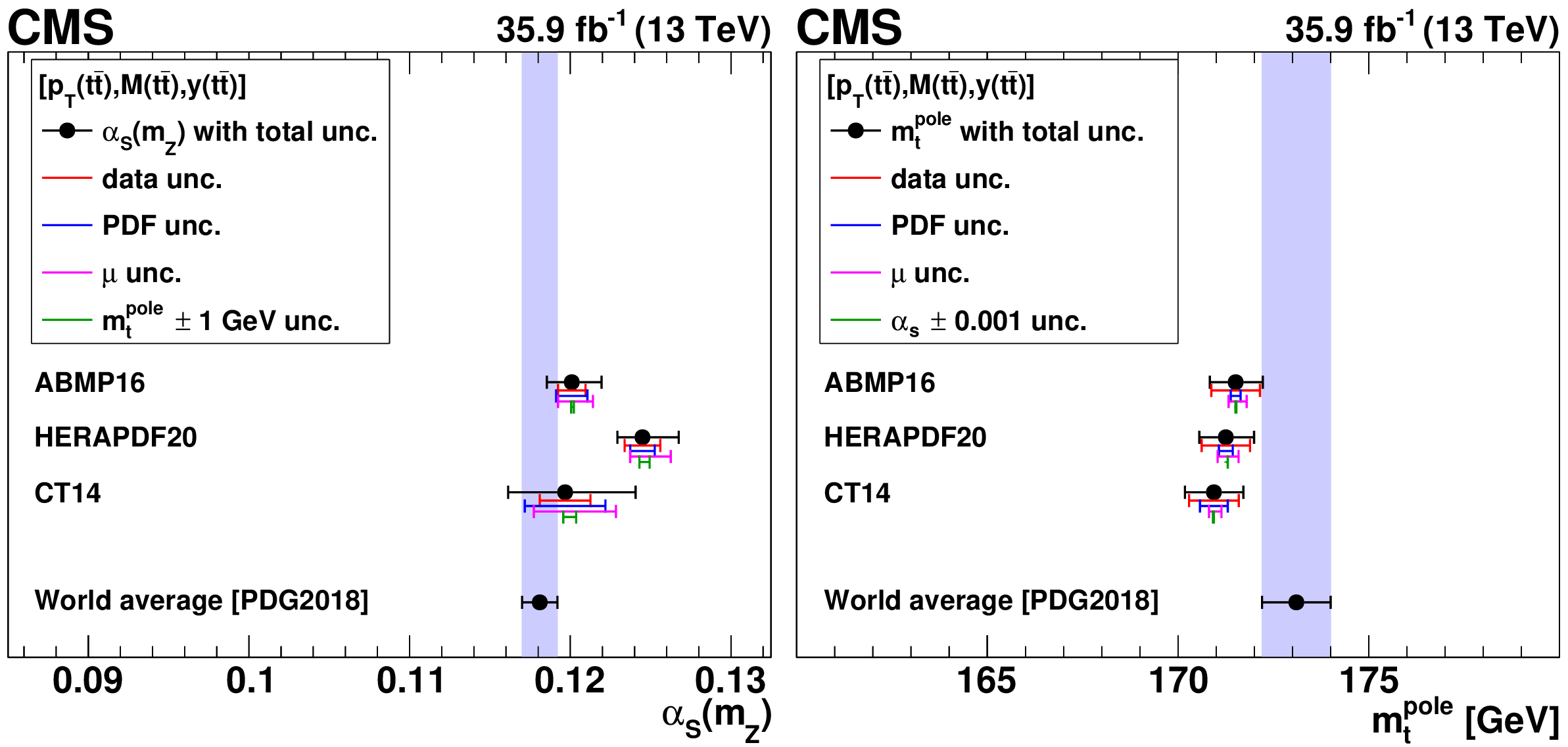
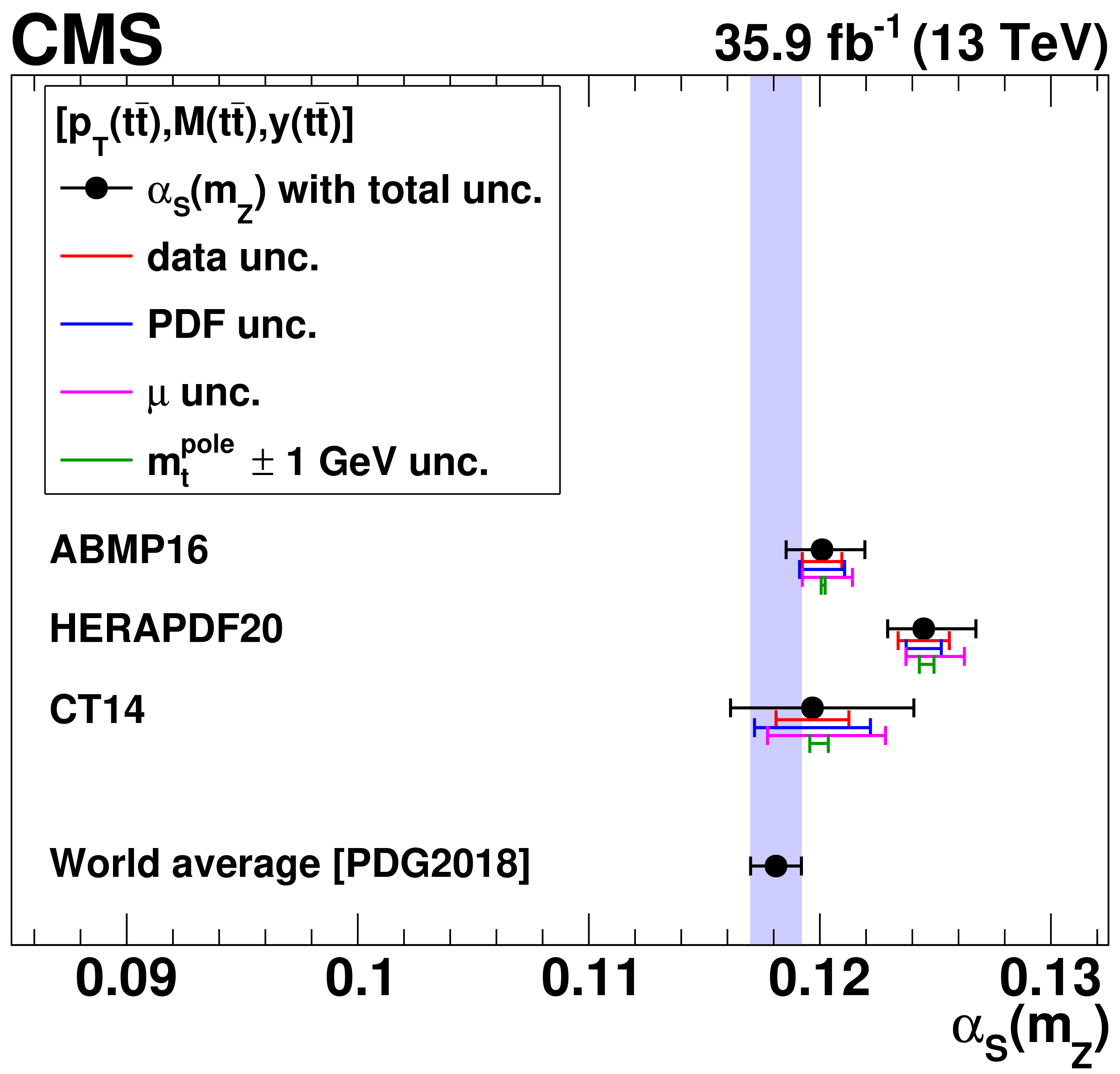
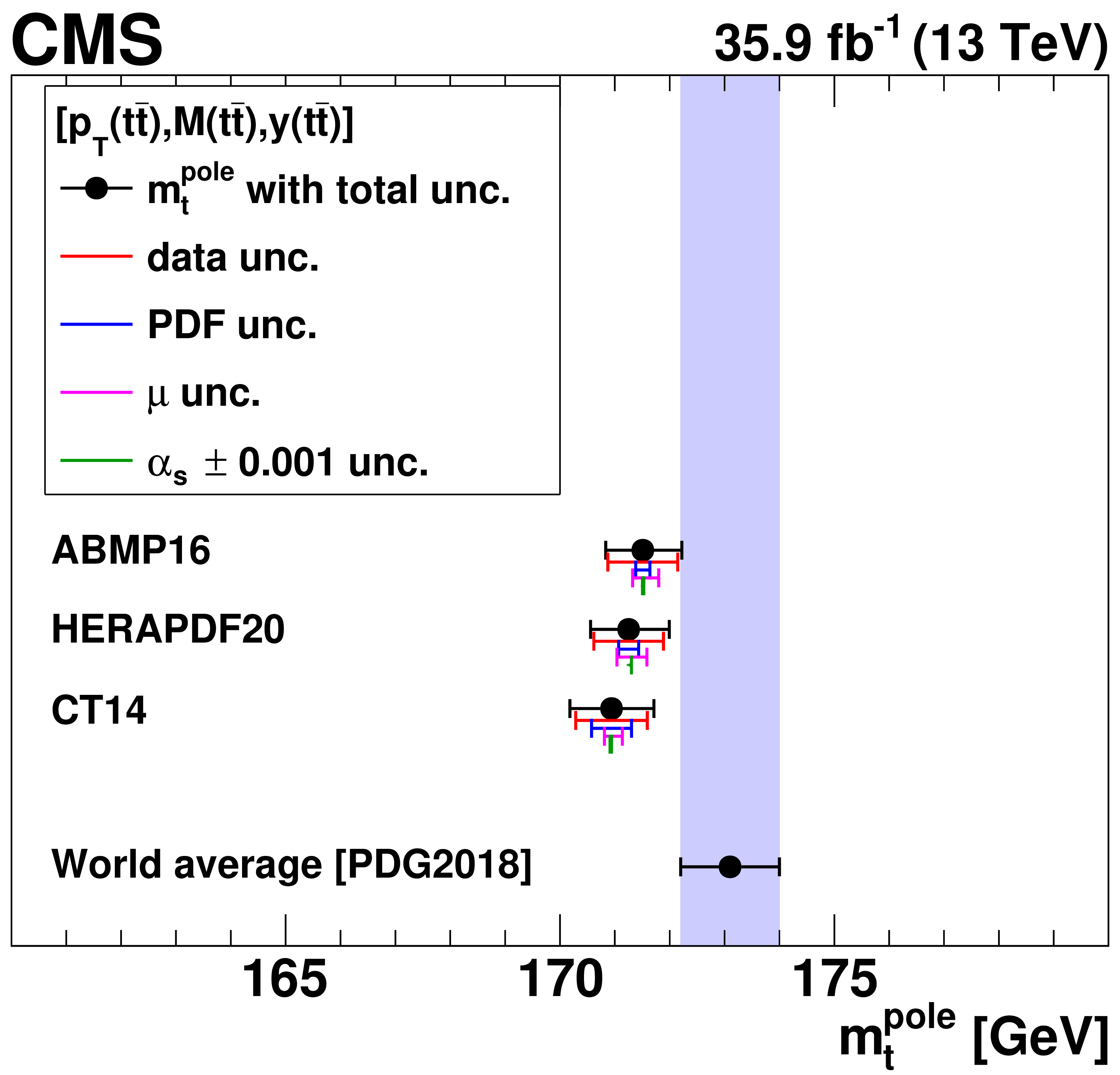
The ${{\alpha _S} (m_{{\mathrm {Z}}})}$ (left) and $ {m_{{\mathrm {t}}}^{\text {pole}}} $ (right) values extracted at NLO using different PDFs. The contributions to the total uncertainty arising from the data, PDF, scale, and $ {{\alpha _S} (m_{{\mathrm {Z}}})} $ uncertainties are shown separately. The world average values $ {{\alpha _S} (m_{{\mathrm {Z}}})} = $ 0.1181 $\pm$ 0.0011 and $ {m_{{\mathrm {t}}}^{\text {pole}}} = $ 173.1 $\pm$ 0.9 GeV from Ref. [94] are shown for reference. |

png pdf |
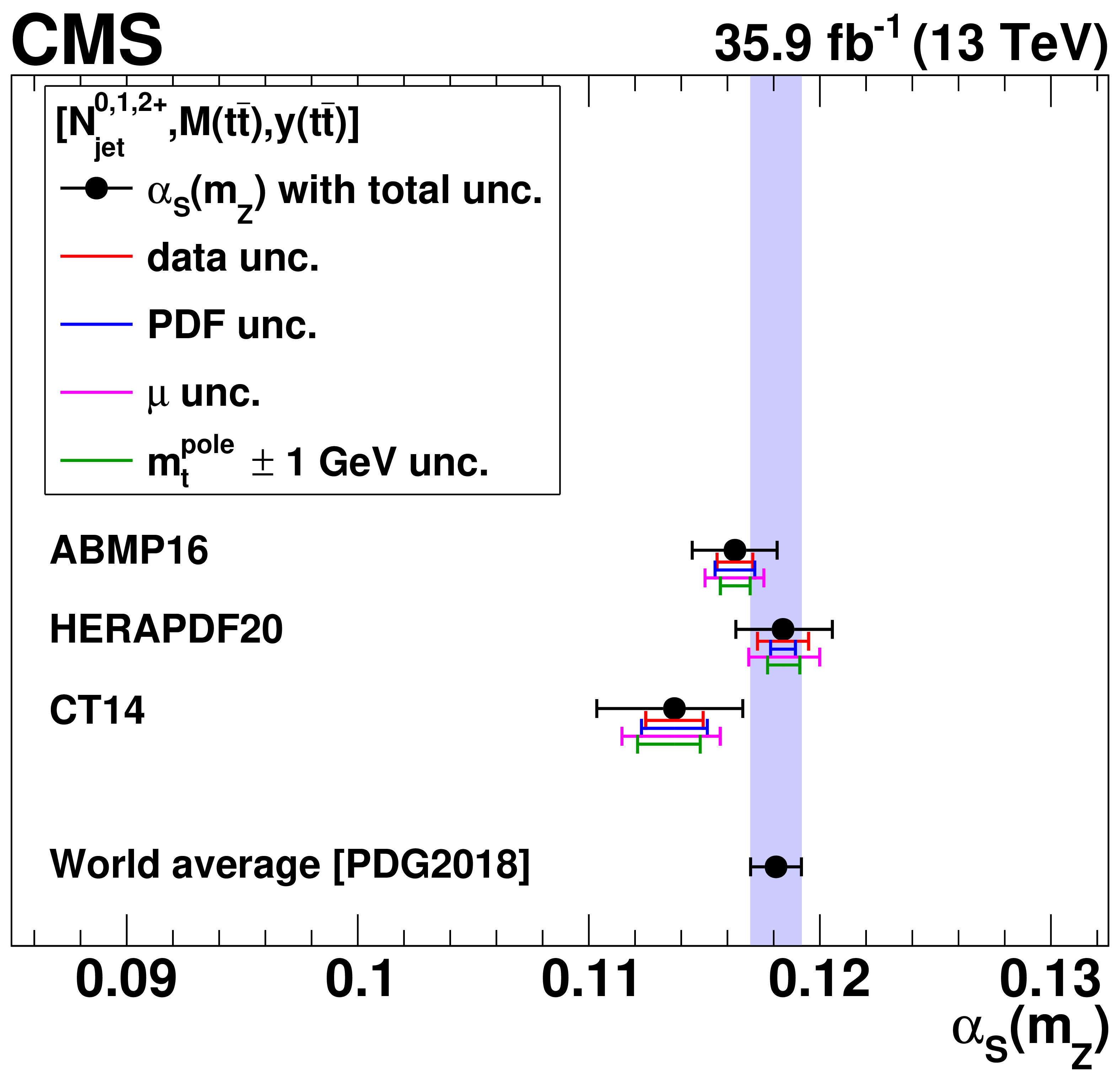
Figure 18-a:
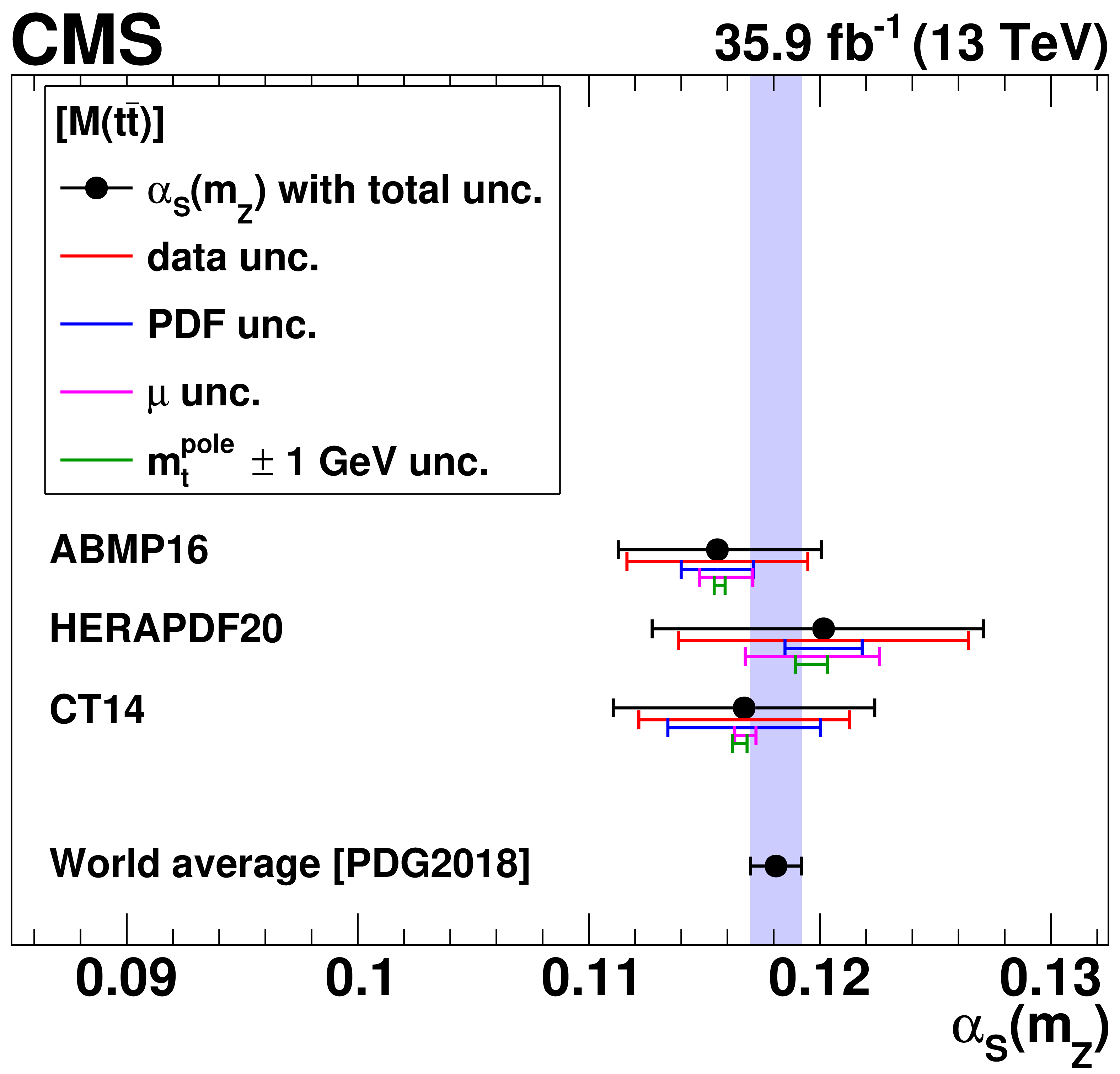
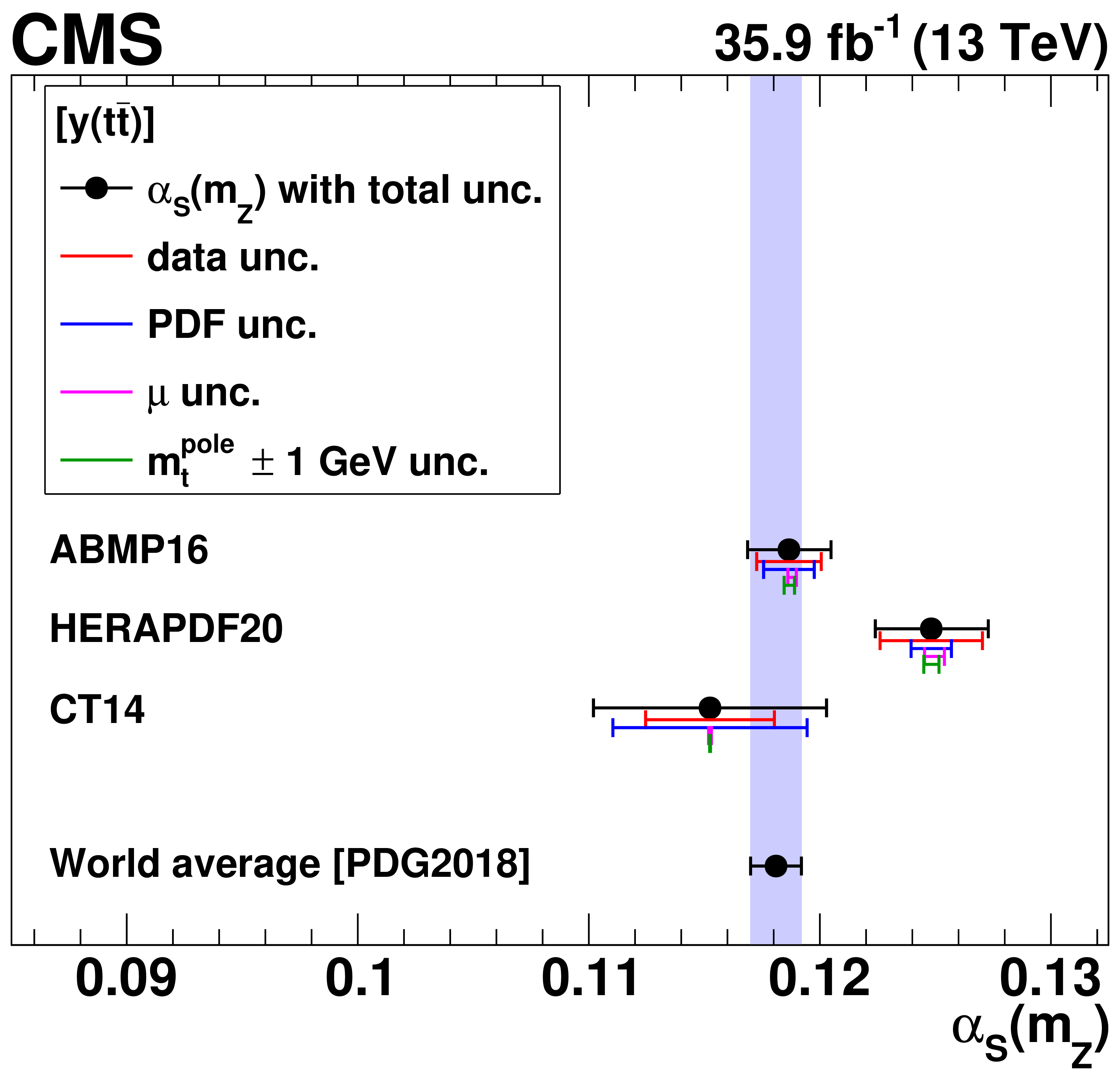
The ${{\alpha _S} (m_{{\mathrm {Z}}})}$ values extracted at NLO using different PDFs. The contributions to the total uncertainty arising from the data, PDF, scale, and $ {{\alpha _S} (m_{{\mathrm {Z}}})} $ uncertainties are shown separately. The world average value $ {{\alpha _S} (m_{{\mathrm {Z}}})} = $ 0.1181 $\pm$ 0.0011 from Ref. [94] is shown for reference. |

png pdf |
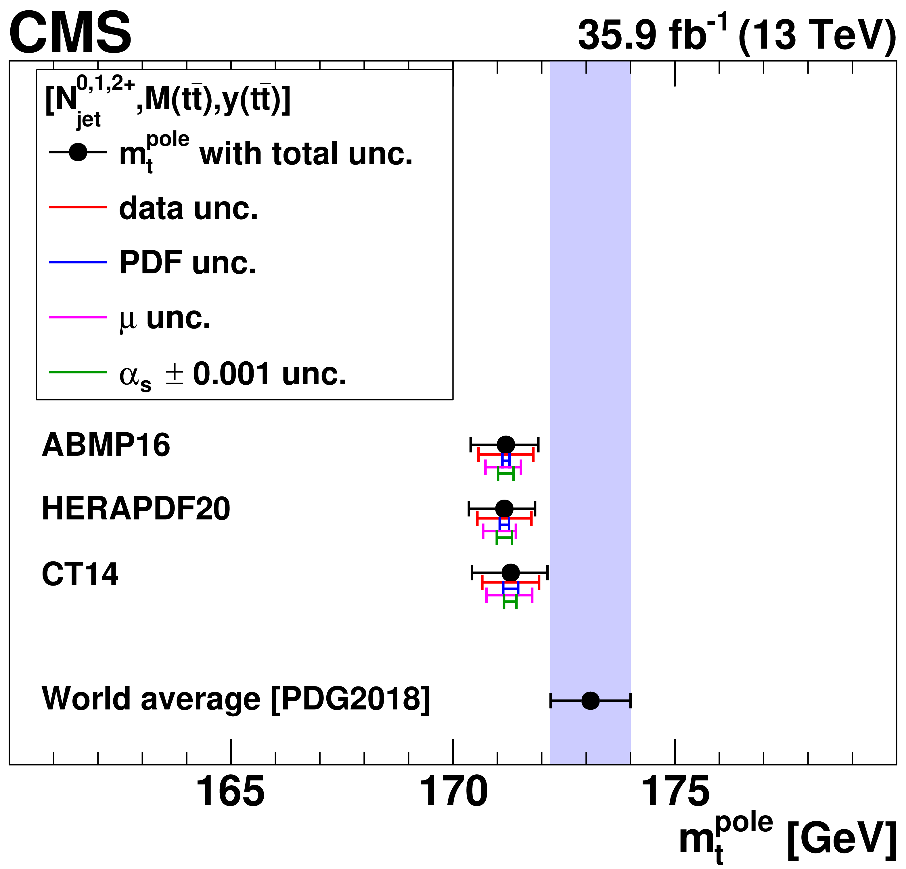
Figure 18-b:
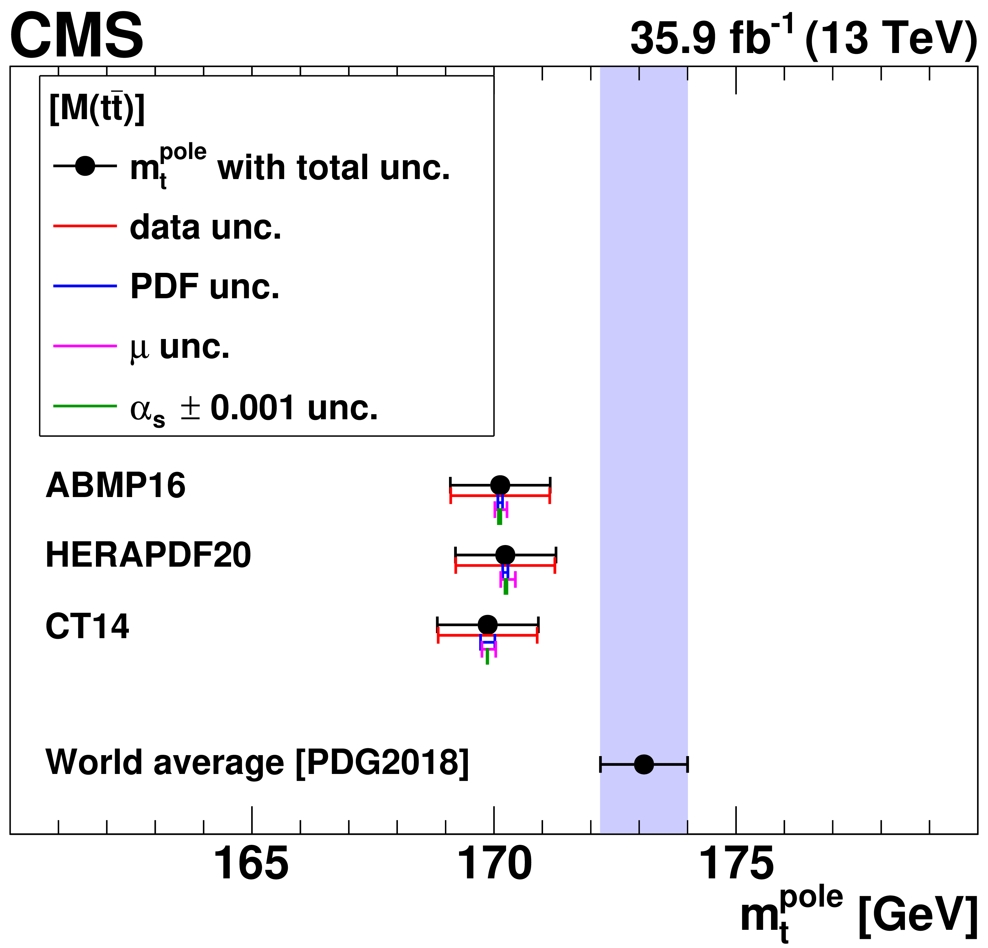
The $ {m_{{\mathrm {t}}}^{\text {pole}}} $ values extracted at NLO using different PDFs. The contributions to the total uncertainty arising from the data, PDF, scale, and $ {{\alpha _S} (m_{{\mathrm {Z}}})} $ uncertainties are shown separately. The world average value $ {m_{{\mathrm {t}}}^{\text {pole}}} = $ 173.1 $\pm$ 0.9 GeV from Ref. [94] is shown for reference. |
png pdf |
Figure 19:
Comparison of the measured [ ${N^{0,1+}_{\text {jet}}}$, ${M({{\mathrm {t}\overline {\mathrm {t}}}})}$, ${y({{\mathrm {t}\overline {\mathrm {t}}}})}$ ] cross sections to the NLO predictions using the parameter values from the simultaneous PDF, ${\alpha _S}$, and ${m_{{\mathrm {t}}}^{\text {pole}}}$ fit (further details can be found in Fig. 3). Values of ${\chi ^2}$ and dof are reported. |
png pdf |
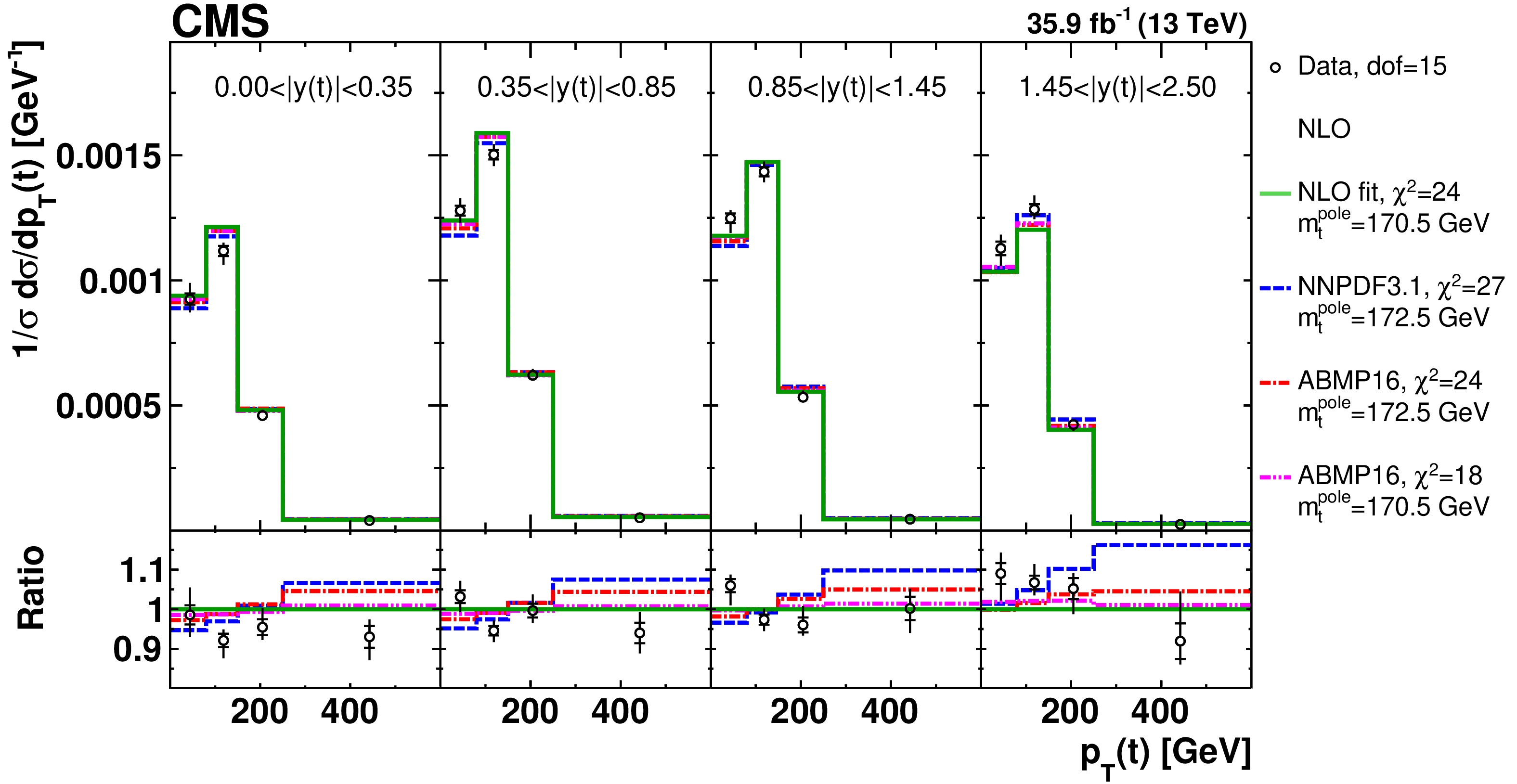
Figure 20:
Comparison of the measured [ ${y({\mathrm {t}})}$, ${{p_{\mathrm {T}}} ({\mathrm {t}})}$ ] cross sections to the NLO predictions using the parameter values from the simultaneous PDF, ${\alpha _S}$ and ${m_{{\mathrm {t}}}^{\text {pole}}}$ fit of the [ ${N^{0,1+}_{\text {jet}}}$, ${M({{\mathrm {t}\overline {\mathrm {t}}}})}$, ${y({{\mathrm {t}\overline {\mathrm {t}}}})}$ ] cross sections, as well as the predictions obtained using the NNPDF3.1 and ABMP16 PDF sets with different values of ${m_{{\mathrm {t}}}^{\text {pole}}}$ (see Fig. 3 for further details). In the lower panel, the ratios of the data and theoretical predictions to the predictions from the fit are shown. For each theoretical prediction, values of ${\chi ^2}$ and dof for the comparison to the data are reported. |
png pdf |
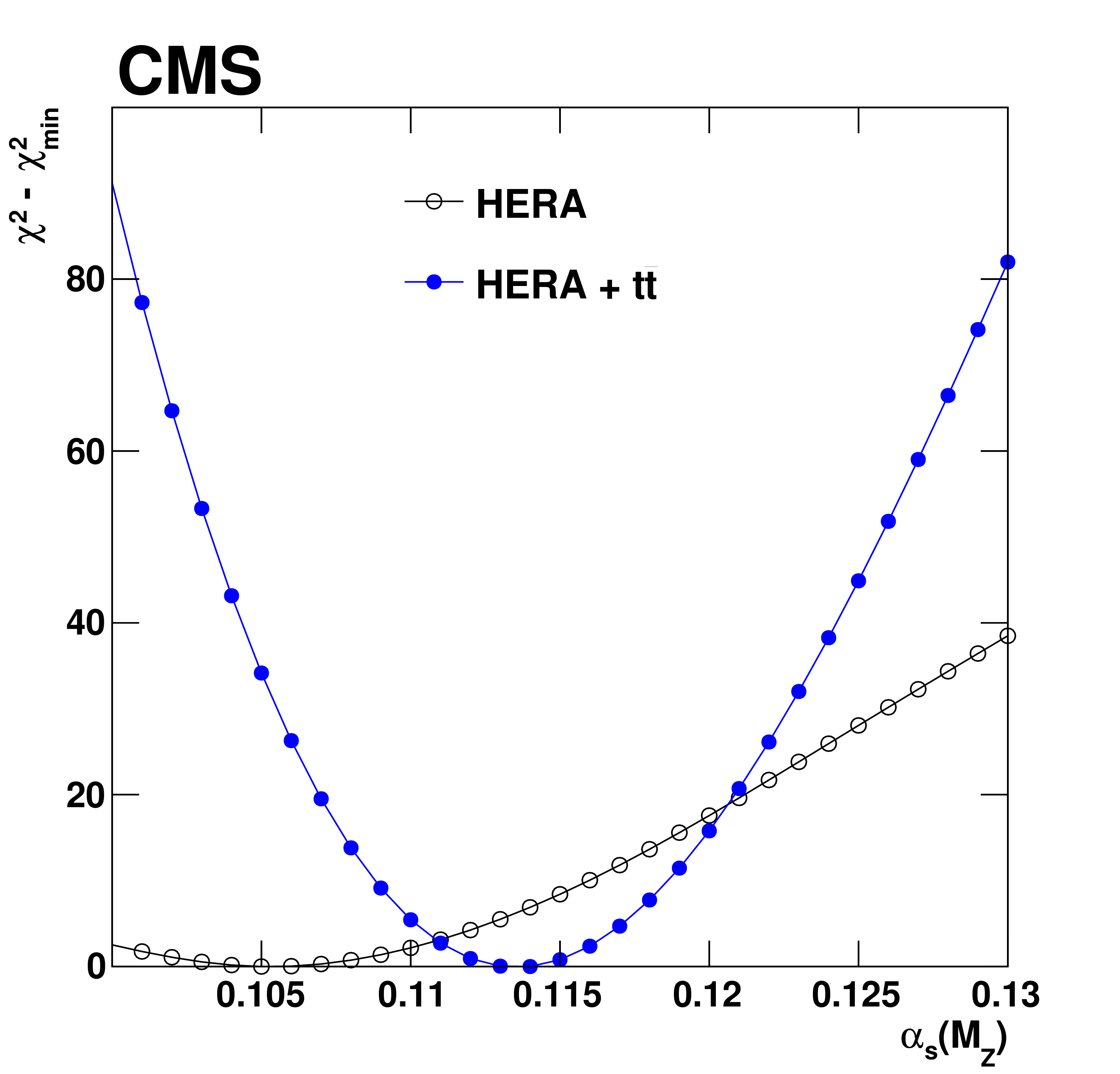
Figure 21:
$\Delta \chi ^2 = \chi ^2 - \chi ^2_{\text {min}}$ as a function of ${{\alpha _S} (m_{{\mathrm {Z}}})}$ in the QCD analysis using the HERA DIS data only, or HERA and ${{\mathrm {t}\overline {\mathrm {t}}}}$ data. |
png pdf |
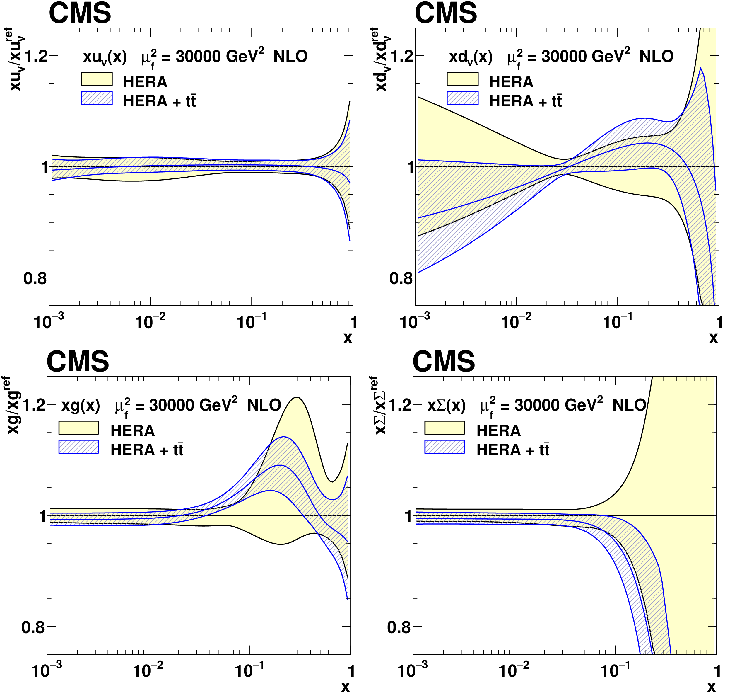
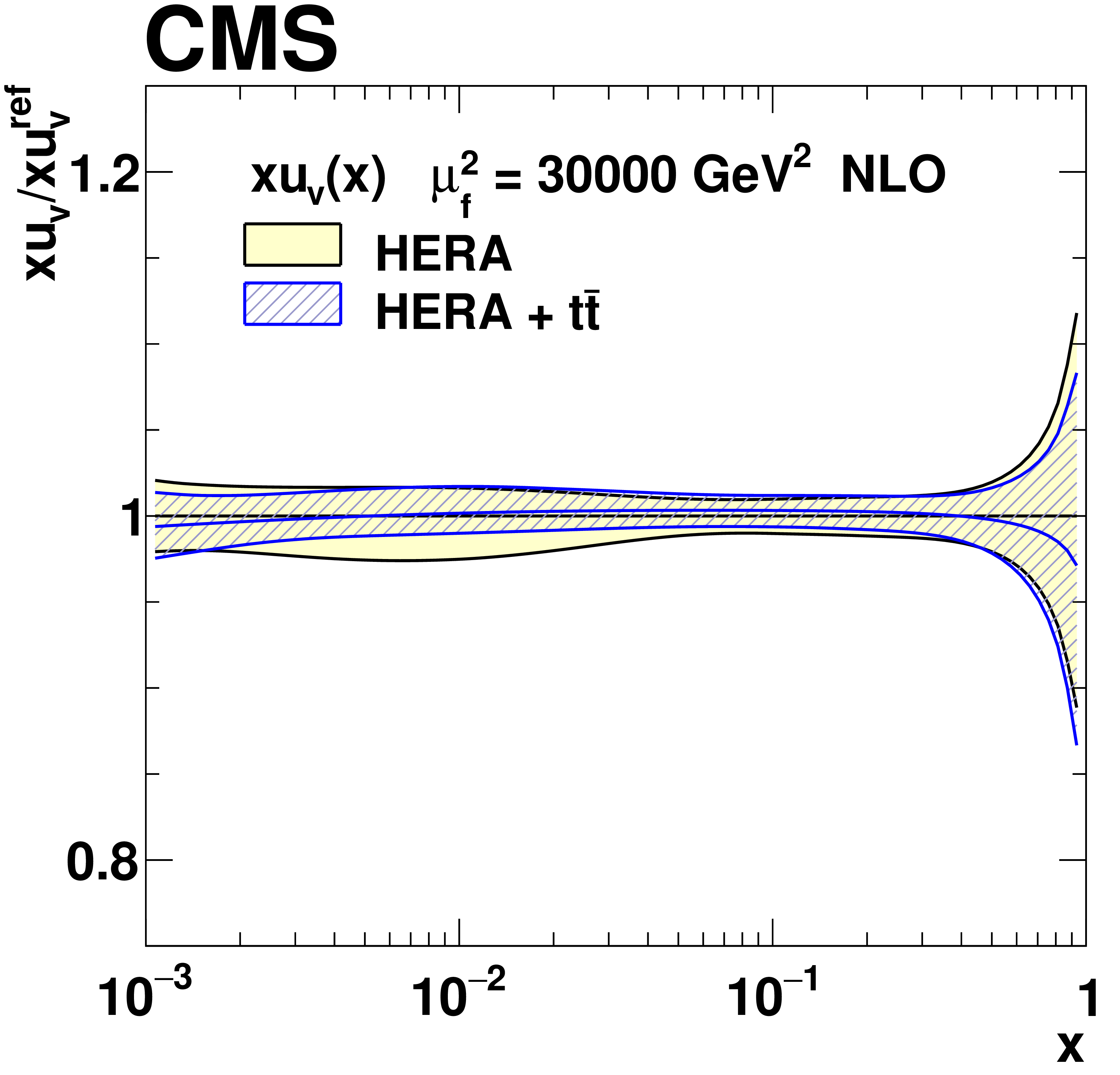
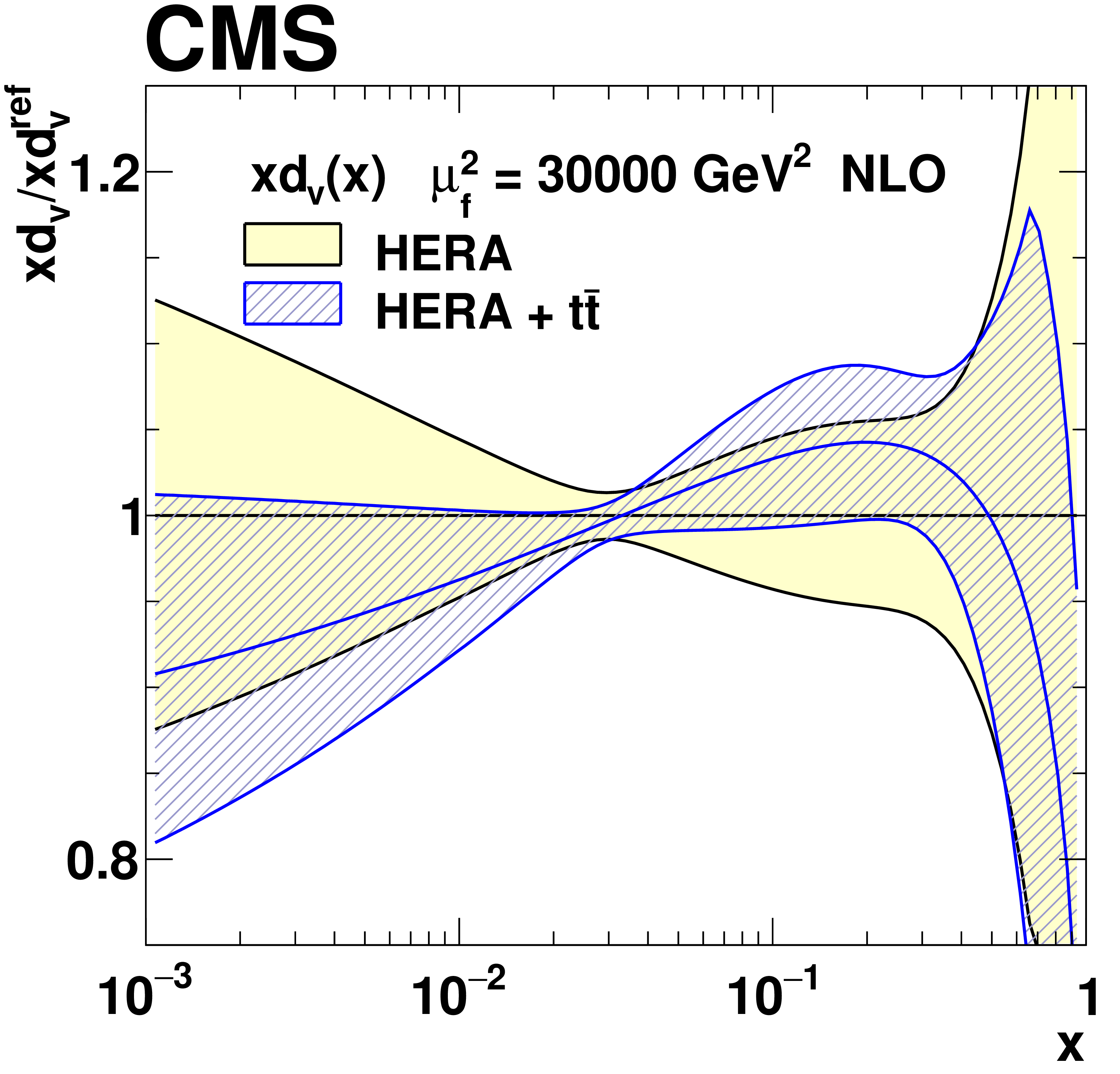
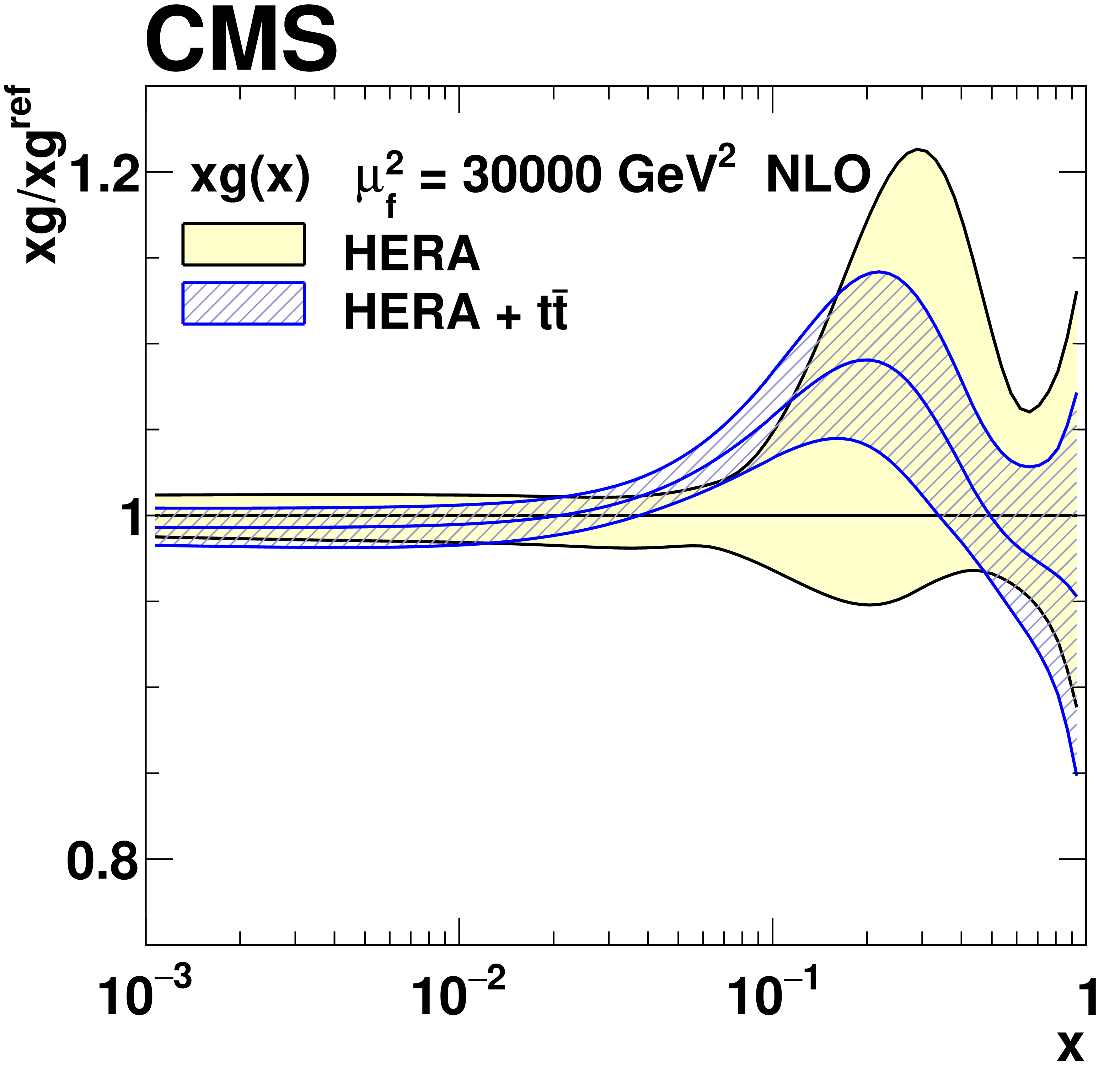
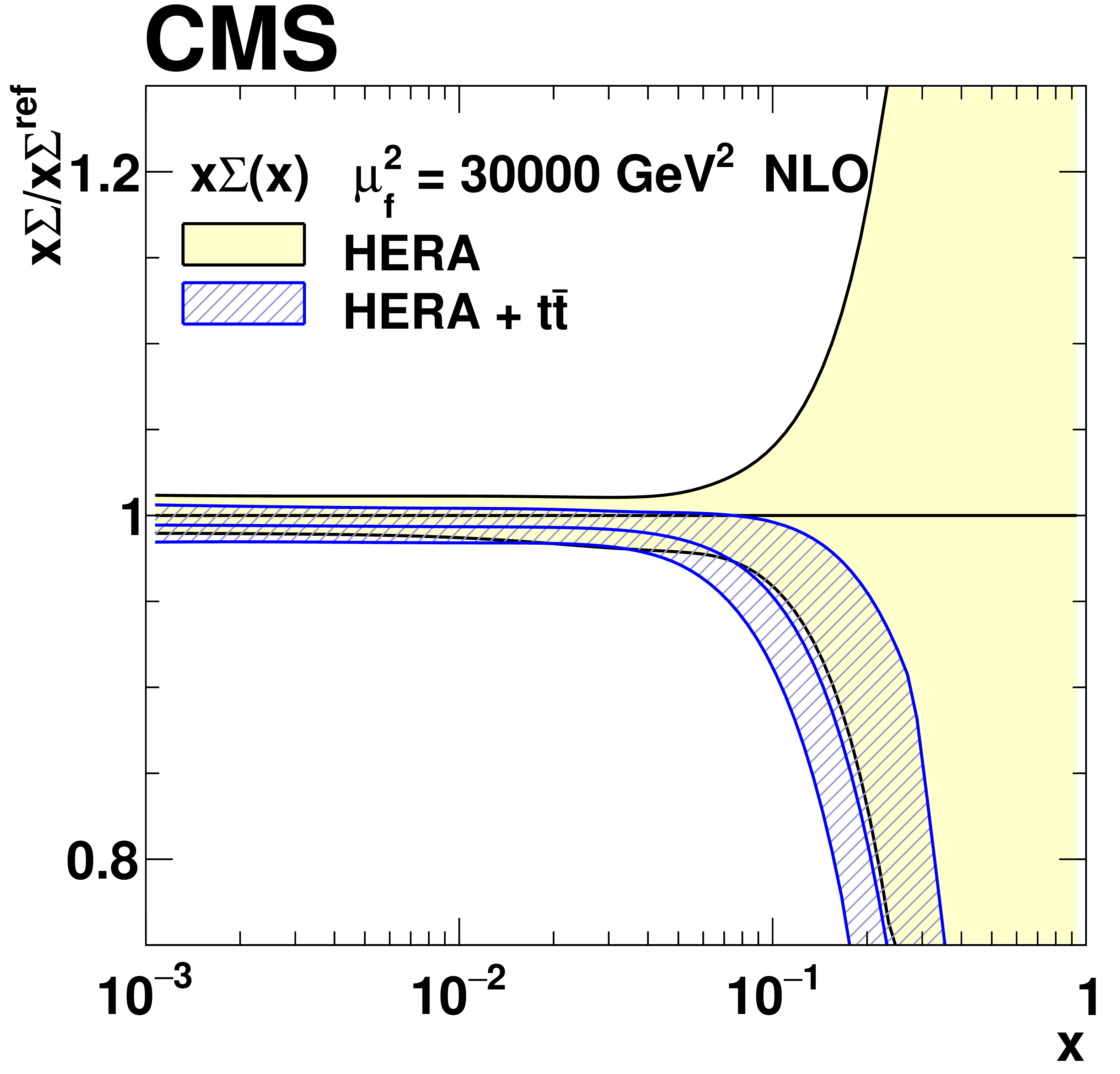
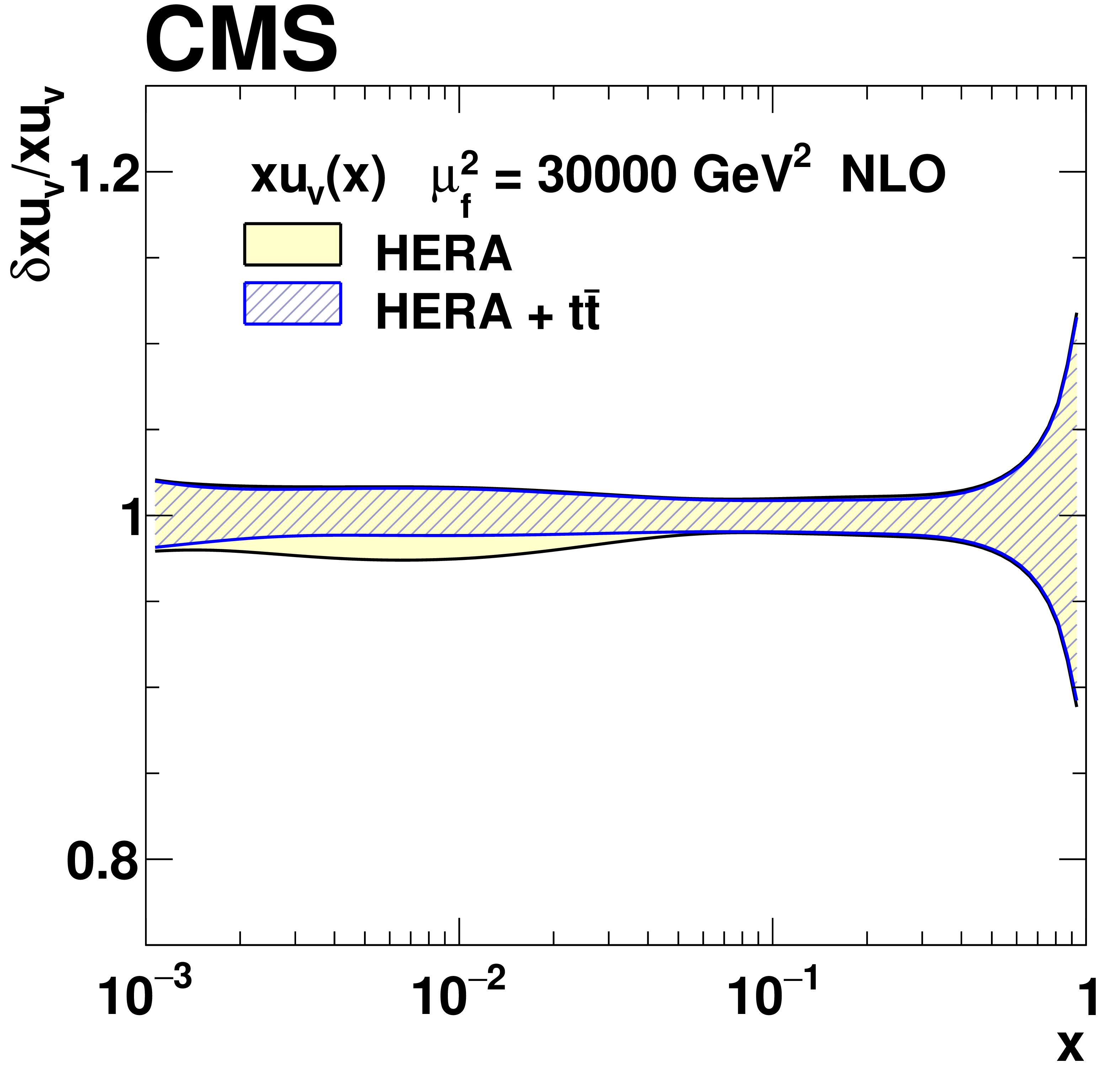
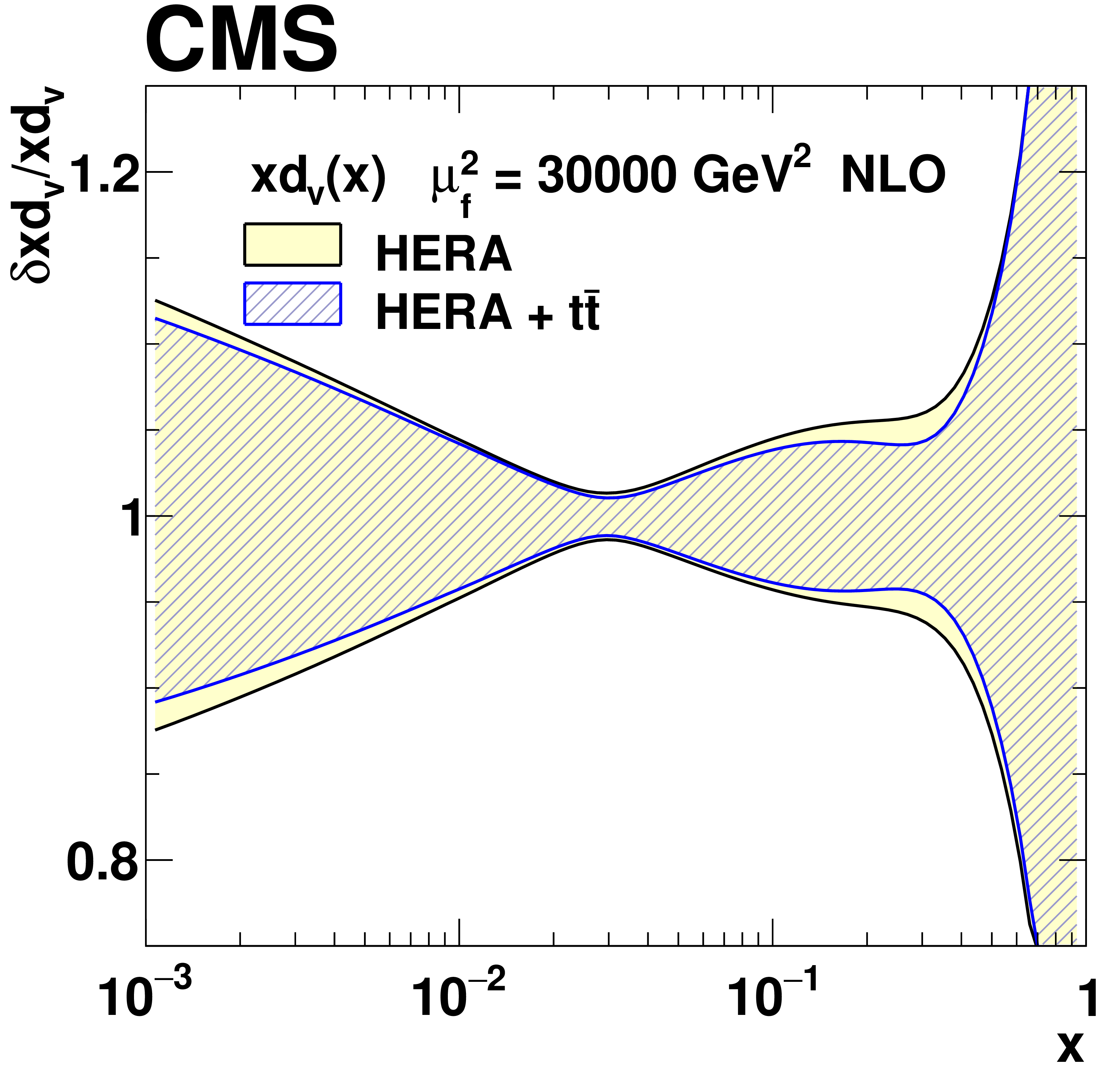
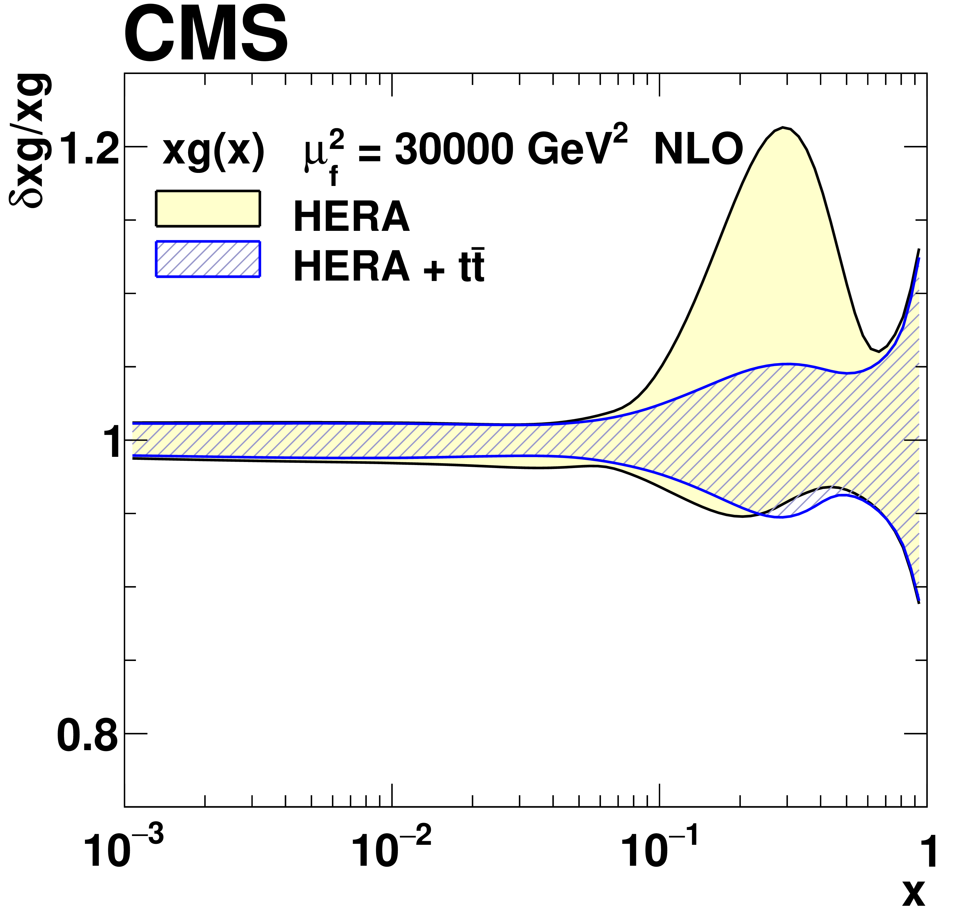
Figure 22:
The PDFs with their total uncertainties in the fit using the HERA DIS data only, and the HERA DIS and ${{\mathrm {t}\overline {\mathrm {t}}}}$ data. The results are normalised to the PDFs obtained using the HERA DIS data only. |
png pdf |
Figure 22-a:
The $xu_{\text{V}}(x)$ PDF with total uncertainties in the fit using the HERA DIS data only, and the HERA DIS and ${{\mathrm {t}\overline {\mathrm {t}}}}$ data. The results are normalised to the PDFs obtained using the HERA DIS data only. |
png pdf |
Figure 22-b:
The $xd_{\text{V}}(x)$ PDF with total uncertainties in the fit using the HERA DIS data only, and the HERA DIS and ${{\mathrm {t}\overline {\mathrm {t}}}}$ data. The results are normalised to the PDFs obtained using the HERA DIS data only. |
png pdf |
Figure 22-c:
The $xg(x)$ PDF with total uncertainties in the fit using the HERA DIS data only, and the HERA DIS and ${{\mathrm {t}\overline {\mathrm {t}}}}$ data. The results are normalised to the PDFs obtained using the HERA DIS data only. |
png pdf |
Figure 22-d:
The $x\Sigma(x)$ PDF with total uncertainties in the fit using the HERA DIS data only, and the HERA DIS and ${{\mathrm {t}\overline {\mathrm {t}}}}$ data. The results are normalised to the PDFs obtained using the HERA DIS data only. |

png pdf |
Figure 23:
The relative total PDF uncertainties in the fit using the HERA DIS data only, and the HERA DIS and ${{\mathrm {t}\overline {\mathrm {t}}}}$ data. |
png pdf |
Figure 23-a:
The relative total $x\Sigma(x)$ PDF uncertainties in the fit using the HERA DIS data only, and the HERA DIS and ${{\mathrm {t}\overline {\mathrm {t}}}}$ data. |
png pdf |
Figure 23-b:
The relative total PDF uncertainties in the fit using the HERA DIS data only, and the HERA DIS and ${{\mathrm {t}\overline {\mathrm {t}}}}$ data. |
png pdf |
Figure 23-c:
The relative total PDF uncertainties in the fit using the HERA DIS data only, and the HERA DIS and ${{\mathrm {t}\overline {\mathrm {t}}}}$ data. |

png pdf |
Figure 23-d:
The relative total PDF uncertainties in the fit using the HERA DIS data only, and the HERA DIS and ${{\mathrm {t}\overline {\mathrm {t}}}}$ data. |
png pdf |
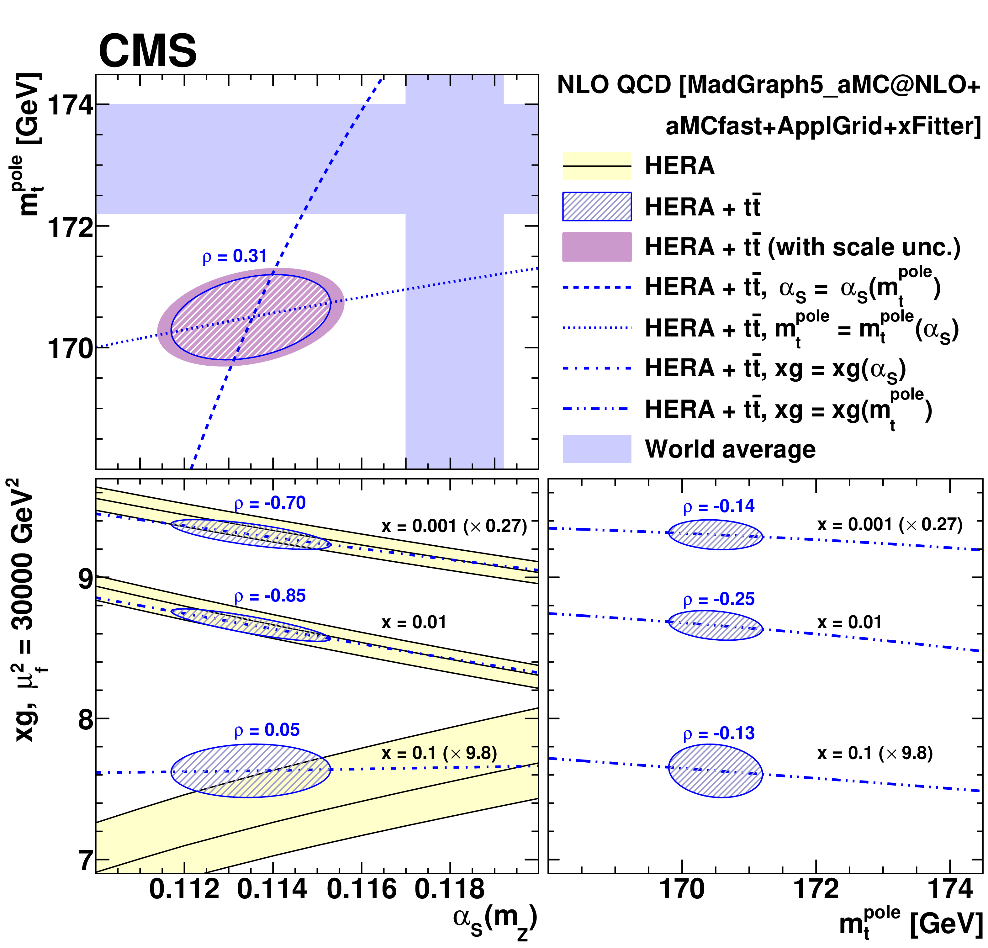
Figure 24:
{The extracted values and their correlations for ${\alpha _S}$ and ${m_{{\mathrm {t}}}^{\text {pole}}}$ (upper left), ${\alpha _S}$ and gluon PDF (lower left), and ${m_{{\mathrm {t}}}^{\text {pole}}}$ and gluon PDF (lower, right). The gluon PDF is shown at the scale $\mu _\mathrm {f}^2 = $ 30 GeV$ ^2$ for several values of $x$. For the extracted ${\alpha _S}$ and ${m_{{\mathrm {t}}}^{\text {pole}}}$ values, also shown are the additional uncertainties arising from the dependence on scale variations (see Eq. (8) and Table 2). The correlation coefficients $\rho $ are also displayed. Furthermore, values of ${\alpha _S}({m_{{\mathrm {t}}}^{\text {pole}}}$, gluon PDF) extracted using fixed values of ${m_{{\mathrm {t}}}^{\text {pole}}} ({\alpha _S})$ are displayed as dashed, dotted, or dash-dotted lines. The world average values $ {{\alpha _S} (m_{{\mathrm {Z}}})} = $ 0.1181 $\pm$ 0.0011 and $ {m_{{\mathrm {t}}}^{\text {pole}}} = $ 173.1 $\pm$ 0.9 GeV from Ref. [94] are shown for reference.} |
png pdf |
Figure B1:
The $\alpha _s$ extraction from the measured [ ${N^{0,1+}_{\text {jet}}}$, ${M({{\mathrm {t}\overline {\mathrm {t}}}})}$, ${y({{\mathrm {t}\overline {\mathrm {t}}}})}$ ] cross sections using varied scale and ${m_{{\mathrm {t}}}^{\text {pole}}}$ settings, and CT14 (upper), HERAPDF2.0 (middle), and ABMP16 (lower) PDF sets. Details can be found in the caption of Fig. 17. |
png pdf |
Figure B1-a:
The $\alpha _s$ extraction from the measured [ ${N^{0,1+}_{\text {jet}}}$, ${M({{\mathrm {t}\overline {\mathrm {t}}}})}$, ${y({{\mathrm {t}\overline {\mathrm {t}}}})}$ ] cross sections using varied scale and ${m_{{\mathrm {t}}}^{\text {pole}}}$ settings, and the CT14 PDF set. Details can be found in the caption of Fig. 17. |
png pdf |
Figure B1-b:
The $\alpha _s$ extraction from the measured [ ${N^{0,1+}_{\text {jet}}}$, ${M({{\mathrm {t}\overline {\mathrm {t}}}})}$, ${y({{\mathrm {t}\overline {\mathrm {t}}}})}$ ] cross sections using varied scale and ${m_{{\mathrm {t}}}^{\text {pole}}}$ settings, and the CT14 PDF set. Details can be found in the caption of Fig. 17. |
png pdf |
Figure B1-c:
The $\alpha _s$ extraction from the measured [ ${N^{0,1+}_{\text {jet}}}$, ${M({{\mathrm {t}\overline {\mathrm {t}}}})}$, ${y({{\mathrm {t}\overline {\mathrm {t}}}})}$ ] cross sections using varied scale and ${m_{{\mathrm {t}}}^{\text {pole}}}$ settings, and the HERAPDF2.0 PDF set. Details can be found in the caption of Fig. 17. |
png pdf |
Figure B1-d:
The $\alpha _s$ extraction from the measured [ ${N^{0,1+}_{\text {jet}}}$, ${M({{\mathrm {t}\overline {\mathrm {t}}}})}$, ${y({{\mathrm {t}\overline {\mathrm {t}}}})}$ ] cross sections using varied scale and ${m_{{\mathrm {t}}}^{\text {pole}}}$ settings, and the HERAPDF2.0 PDF set. Details can be found in the caption of Fig. 17. |
png pdf |
Figure B1-e:
The $\alpha _s$ extraction from the measured [ ${N^{0,1+}_{\text {jet}}}$, ${M({{\mathrm {t}\overline {\mathrm {t}}}})}$, ${y({{\mathrm {t}\overline {\mathrm {t}}}})}$ ] cross sections using varied scale and ${m_{{\mathrm {t}}}^{\text {pole}}}$ settings, and the ABMP16 PDF set. Details can be found in the caption of Fig. 17. |
png pdf |
Figure B1-f:
The $\alpha _s$ extraction from the measured [ ${N^{0,1+}_{\text {jet}}}$, ${M({{\mathrm {t}\overline {\mathrm {t}}}})}$, ${y({{\mathrm {t}\overline {\mathrm {t}}}})}$ ] cross sections using varied scale and ${m_{{\mathrm {t}}}^{\text {pole}}}$ settings, and the ABMP16 PDF set. Details can be found in the caption of Fig. 17. |
png pdf |
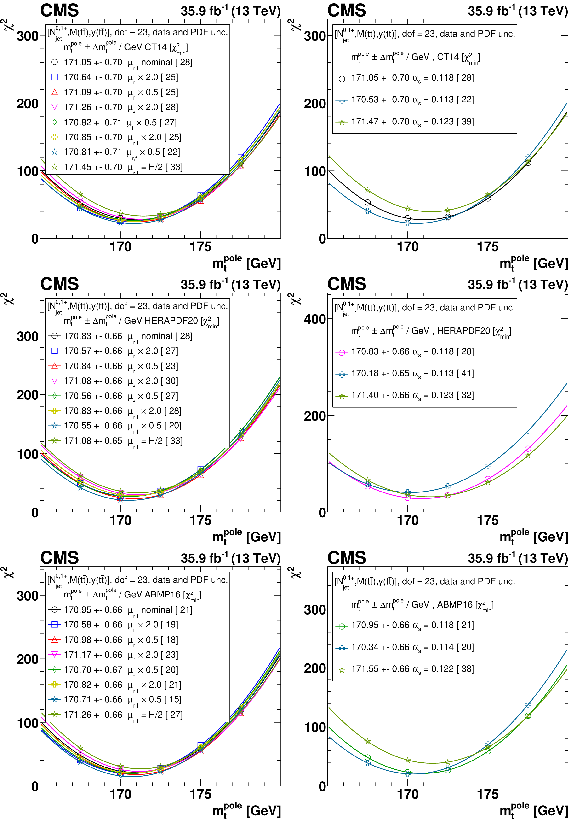
Figure B2:
The $ {m_{{\mathrm {t}}}^{\text {pole}}} $ extraction from the measured [ ${N^{0,1+}_{\text {jet}}}$, ${M({{\mathrm {t}\overline {\mathrm {t}}}})}$, ${y({{\mathrm {t}\overline {\mathrm {t}}}})}$ ] cross sections using varied scale and $ {{\alpha _S} (m_{{\mathrm {Z}}})} $ settings, and CT14 (upper), HERAPDF2.0 (middle), and ABMP16 (lower) PDF sets. Details can be found in the caption of Fig. 17. |
png pdf |
Figure B2-a:
The $ {m_{{\mathrm {t}}}^{\text {pole}}} $ extraction from the measured [ ${N^{0,1+}_{\text {jet}}}$, ${M({{\mathrm {t}\overline {\mathrm {t}}}})}$, ${y({{\mathrm {t}\overline {\mathrm {t}}}})}$ ] cross sections using varied scale and $ {{\alpha _S} (m_{{\mathrm {Z}}})} $ settings, and the CT14 PDF set. Details can be found in the caption of Fig. 17. |
png pdf |
Figure B2-b:
The $ {m_{{\mathrm {t}}}^{\text {pole}}} $ extraction from the measured [ ${N^{0,1+}_{\text {jet}}}$, ${M({{\mathrm {t}\overline {\mathrm {t}}}})}$, ${y({{\mathrm {t}\overline {\mathrm {t}}}})}$ ] cross sections using varied scale and $ {{\alpha _S} (m_{{\mathrm {Z}}})} $ settings, and the CT14 PDF set. Details can be found in the caption of Fig. 17. |
png pdf |
Figure B2-c:
The $ {m_{{\mathrm {t}}}^{\text {pole}}} $ extraction from the measured [ ${N^{0,1+}_{\text {jet}}}$, ${M({{\mathrm {t}\overline {\mathrm {t}}}})}$, ${y({{\mathrm {t}\overline {\mathrm {t}}}})}$ ] cross sections using varied scale and $ {{\alpha _S} (m_{{\mathrm {Z}}})} $ settings, and the HERAPDF2.0 PDF set. Details can be found in the caption of Fig. 17. |
png pdf |
Figure B2-d:
The $ {m_{{\mathrm {t}}}^{\text {pole}}} $ extraction from the measured [ ${N^{0,1+}_{\text {jet}}}$, ${M({{\mathrm {t}\overline {\mathrm {t}}}})}$, ${y({{\mathrm {t}\overline {\mathrm {t}}}})}$ ] cross sections using varied scale and $ {{\alpha _S} (m_{{\mathrm {Z}}})} $ settings, and the HERAPDF2.0 PDF set. Details can be found in the caption of Fig. 17. |
png pdf |
Figure B2-e:
The $ {m_{{\mathrm {t}}}^{\text {pole}}} $ extraction from the measured [ ${N^{0,1+}_{\text {jet}}}$, ${M({{\mathrm {t}\overline {\mathrm {t}}}})}$, ${y({{\mathrm {t}\overline {\mathrm {t}}}})}$ ] cross sections using varied scale and $ {{\alpha _S} (m_{{\mathrm {Z}}})} $ settings, and the ABMP16 PDF set. Details can be found in the caption of Fig. 17. |
png pdf |
Figure B2-f:
The $ {m_{{\mathrm {t}}}^{\text {pole}}} $ extraction from the measured [ ${N^{0,1+}_{\text {jet}}}$, ${M({{\mathrm {t}\overline {\mathrm {t}}}})}$, ${y({{\mathrm {t}\overline {\mathrm {t}}}})}$ ] cross sections using varied scale and $ {{\alpha _S} (m_{{\mathrm {Z}}})} $ settings, and the ABMP16 PDF set. Details can be found in the caption of Fig. 17. |
png pdf |
Figure B3:
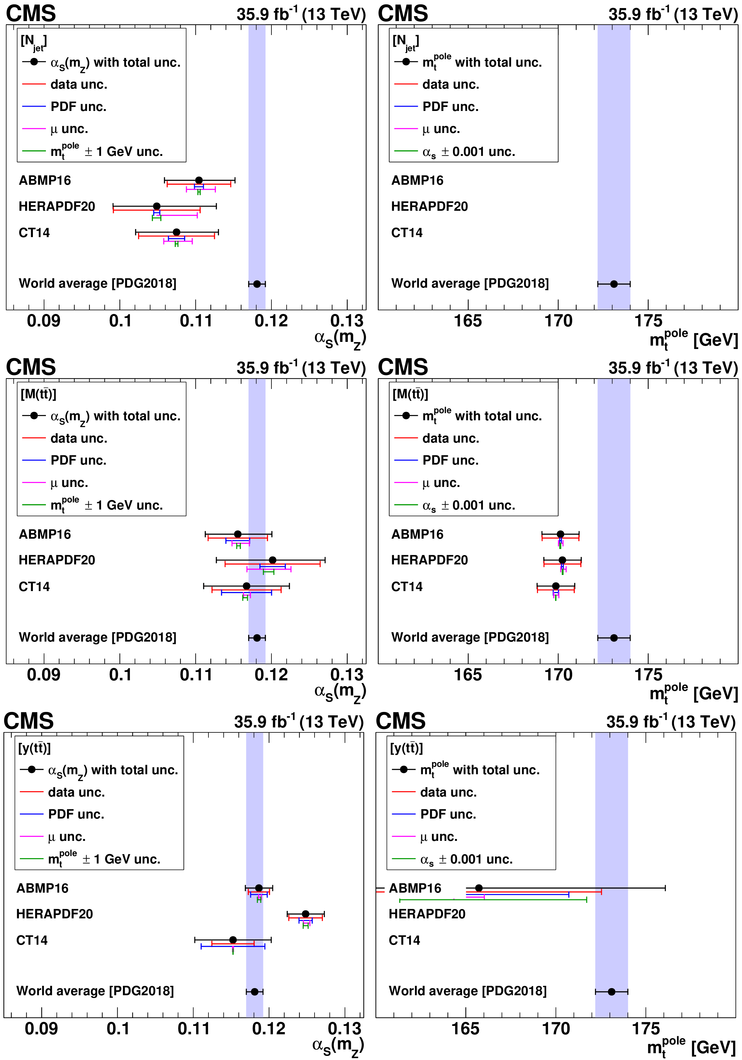
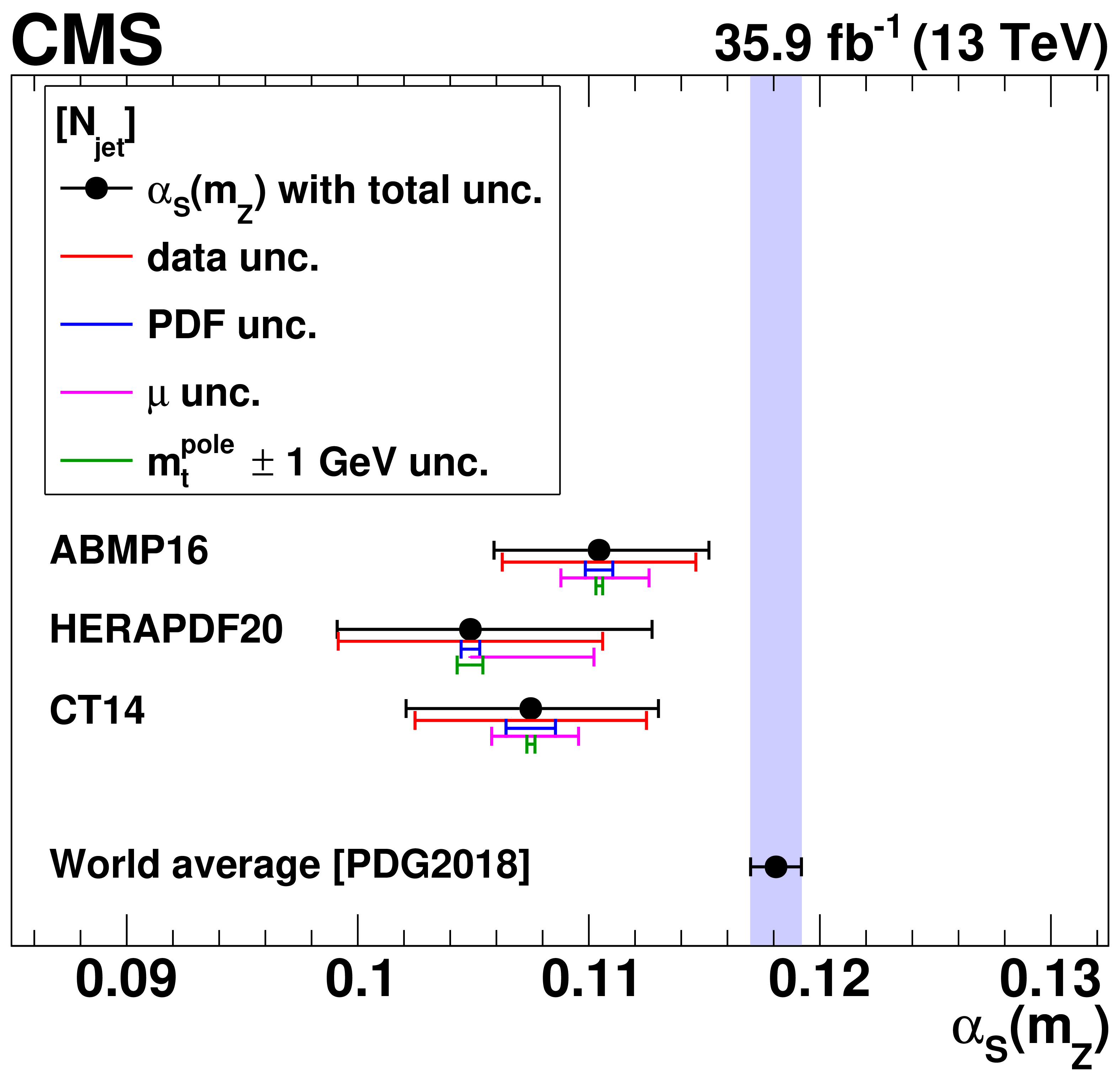
The ${{\alpha _S} (m_{{\mathrm {Z}}})}$ (left) and ${m_{{\mathrm {t}}}^{\text {pole}}}$ (right) values extracted using different single-differential cross sections, for ${N_{\text {jet}}}$ (upper), ${M({{\mathrm {t}\overline {\mathrm {t}}}})}$ (middle), and $ {| {y({{\mathrm {t}\overline {\mathrm {t}}}})} |}$ (lower) measurements. For central values outside the displayed ${m_{{\mathrm {t}}}^{\text {pole}}}$ range, no result is shown. Details can be found in the caption of Fig. 18. |
png pdf |
Figure B3-a:
The ${{\alpha _S} (m_{{\mathrm {Z}}})}$ values extracted using different single-differential cross sections, for the ${N_{\text {jet}}}$ measurement. Details can be found in the caption of Fig. 18. |
png pdf |
Figure B3-b:
The ${m_{{\mathrm {t}}}^{\text {pole}}}$ values extracted using different single-differential cross sections, for the ${N_{\text {jet}}}$ measurement. For central values outside the displayed ${m_{{\mathrm {t}}}^{\text {pole}}}$ range, no result is shown. Details can be found in the caption of Fig. 18. |
png pdf |
Figure B3-c:
The ${{\alpha _S} (m_{{\mathrm {Z}}})}$ values extracted using different single-differential cross sections, for the ${M({{\mathrm {t}\overline {\mathrm {t}}}})}$ measurement. Details can be found in the caption of Fig. 18. |
png pdf |
Figure B3-d:
The ${m_{{\mathrm {t}}}^{\text {pole}}}$ values extracted using different single-differential cross sections, for the ${M({{\mathrm {t}\overline {\mathrm {t}}}})}$ measurement. For central values outside the displayed ${m_{{\mathrm {t}}}^{\text {pole}}}$ range, no result is shown. Details can be found in the caption of Fig. 18. |
png pdf |
Figure B3-e:
The ${{\alpha _S} (m_{{\mathrm {Z}}})}$ values extracted using different single-differential cross sections, for the $ {| {y({{\mathrm {t}\overline {\mathrm {t}}}})} |}$ measurement. Details can be found in the caption of Fig. 18. |
png pdf |
Figure B3-f:
The ${m_{{\mathrm {t}}}^{\text {pole}}}$ values extracted using different single-differential cross sections, for the $ {| {y({{\mathrm {t}\overline {\mathrm {t}}}})} |}$ measurement. For central values outside the displayed ${m_{{\mathrm {t}}}^{\text {pole}}}$ range, no result is shown. Details can be found in the caption of Fig. 18. |
png pdf |
Figure B4:
The ${{\alpha _S} (m_{{\mathrm {Z}}})}$ (left) and $ {m_{{\mathrm {t}}}^{\text {pole}}} $ (right) values extracted from the triple-differential [ ${N^{0,1,2+}_{\text {jet}}}$, ${M({{\mathrm {t}\overline {\mathrm {t}}}})}$, ${y({{\mathrm {t}\overline {\mathrm {t}}}})}$ ] cross sections. Details can be found in the caption of Fig. 18. |
png pdf |
Figure B4-a:
The ${{\alpha _S} (m_{{\mathrm {Z}}})}$ values extracted from the triple-differential [ ${N^{0,1,2+}_{\text {jet}}}$, ${M({{\mathrm {t}\overline {\mathrm {t}}}})}$, ${y({{\mathrm {t}\overline {\mathrm {t}}}})}$ ] cross sections. Details can be found in the caption of Fig. 18. |
png pdf |
Figure B4-b:
The $ {m_{{\mathrm {t}}}^{\text {pole}}} $ values extracted from the triple-differential [ ${N^{0,1,2+}_{\text {jet}}}$, ${M({{\mathrm {t}\overline {\mathrm {t}}}})}$, ${y({{\mathrm {t}\overline {\mathrm {t}}}})}$ ] cross sections. Details can be found in the caption of Fig. 18. |
png pdf |
Figure B5:
The ${{\alpha _S} (m_{{\mathrm {Z}}})}$ (left) and $ {m_{{\mathrm {t}}}^{\text {pole}}} $ (right) values extracted from the triple-differential [ ${{{p_{\mathrm {T}}} ({{\mathrm {t}\overline {\mathrm {t}}}})}}$, ${M({{\mathrm {t}\overline {\mathrm {t}}}})}$, ${y({{\mathrm {t}\overline {\mathrm {t}}}})}$}] cross sections. Details can be found in the caption of Fig. 18. |
png pdf |
Figure B5-a:
The ${{\alpha _S} (m_{{\mathrm {Z}}})}$ values extracted from the triple-differential [ ${{{p_{\mathrm {T}}} ({{\mathrm {t}\overline {\mathrm {t}}}})}}$, ${M({{\mathrm {t}\overline {\mathrm {t}}}})}$, ${y({{\mathrm {t}\overline {\mathrm {t}}}})}$}] cross sections. Details can be found in the caption of Fig. 18. |
png pdf |
Figure B5-b:
The $ {m_{{\mathrm {t}}}^{\text {pole}}} $ values extracted from the triple-differential [ ${{{p_{\mathrm {T}}} ({{\mathrm {t}\overline {\mathrm {t}}}})}}$, ${M({{\mathrm {t}\overline {\mathrm {t}}}})}$, ${y({{\mathrm {t}\overline {\mathrm {t}}}})}$}] cross sections. Details can be found in the caption of Fig. 18. |
png pdf |
Figure C1:
Comparison of the measured [ ${N^{0,1+}_{\text {jet}}}$, ${M({{\mathrm {t}\overline {\mathrm {t}}}})}$, ${y({{\mathrm {t}\overline {\mathrm {t}}}})}$ ] cross sections obtained using different values of ${m_{{\mathrm {t}}}^{\text {MC}}}$ to NLO predictions obtained using different ${m_{{\mathrm {t}}}^{\text {pole}}}$ values (further details can be found in Fig. 3). |
| Tables | |

png pdf |
Table 1:
The ${\chi ^2}$ values (taking into account data uncertainties and ignoring theoretical uncertainties) and dof of the measured cross sections with respect {to the predictions of various MC generators.} |

png pdf |
Table 2:
The individual contributions to the uncertainties for the ${{\alpha _S} (m_{{\mathrm {Z}}})}$ and ${m_{{\mathrm {t}}}^{\text {pole}}}$ determination. |

png pdf |
Table 3:
The global and partial ${\chi ^2}$/dof values for all variants of the QCD analysis. The variant of the fit that uses the HERA DIS only is denoted as `Nominal fit'. For the HERA measurements, the energy of the proton beam, $E_{{\mathrm {p}}}$, is listed for each data set, with the electron energy being $E_{{\mathrm {e}}} = $ 27.5 GeV, CC and NC standing for charged and neutral current, respectively. The correlated ${\chi ^2}$ and the log-penalty $\chi ^2$ entries refer to the ${\chi ^2}$ contributions from the nuisance parameters and from the logarithmic term, respectively, as described in the text. |
png pdf |
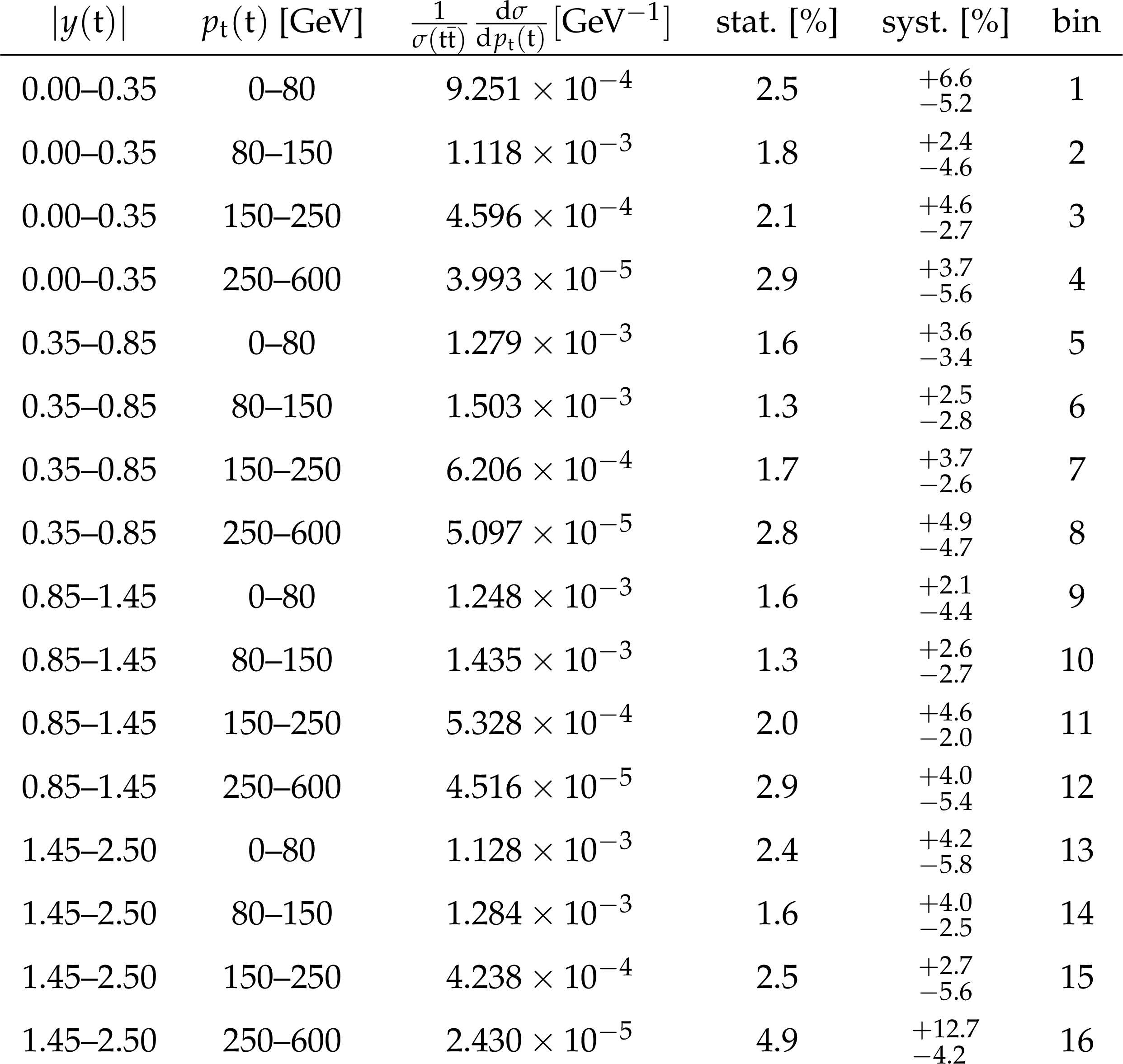
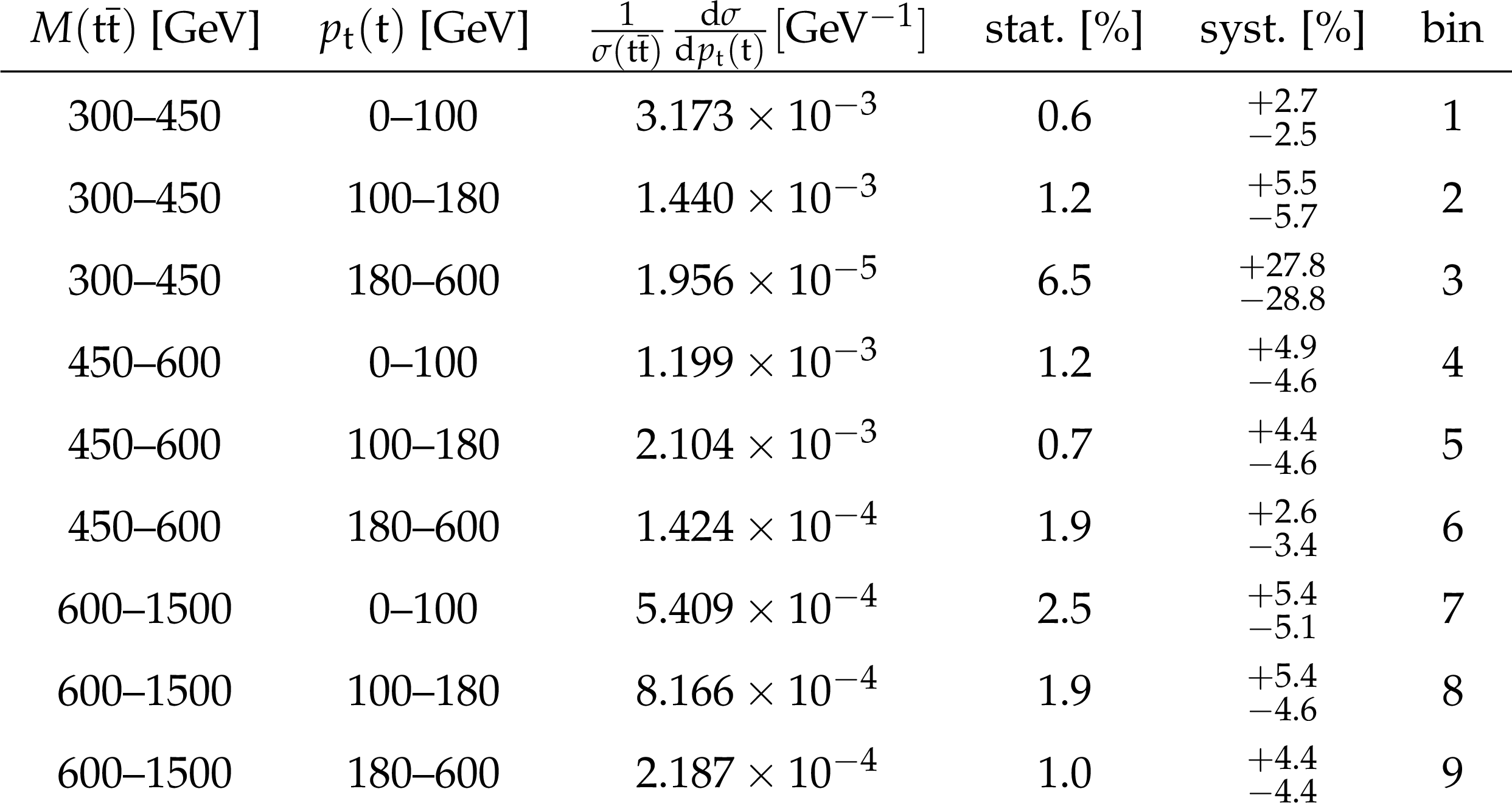
Table A1:
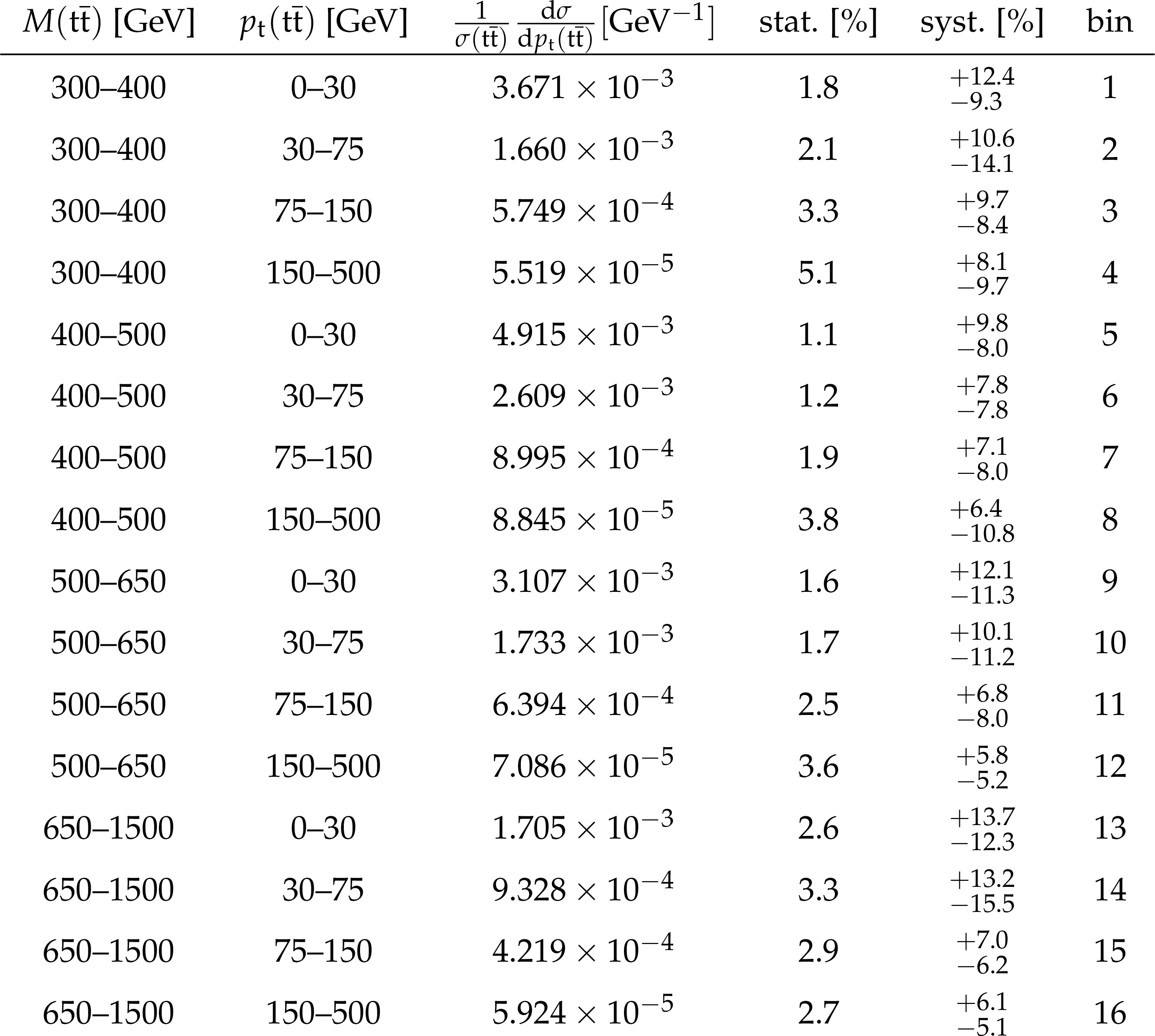
The measured [ ${y({\mathrm {t}})}$, ${{p_{\mathrm {T}}} ({\mathrm {t}})}$ ] cross sections, along with their relative statistical and systematic uncertainties. |
png pdf |
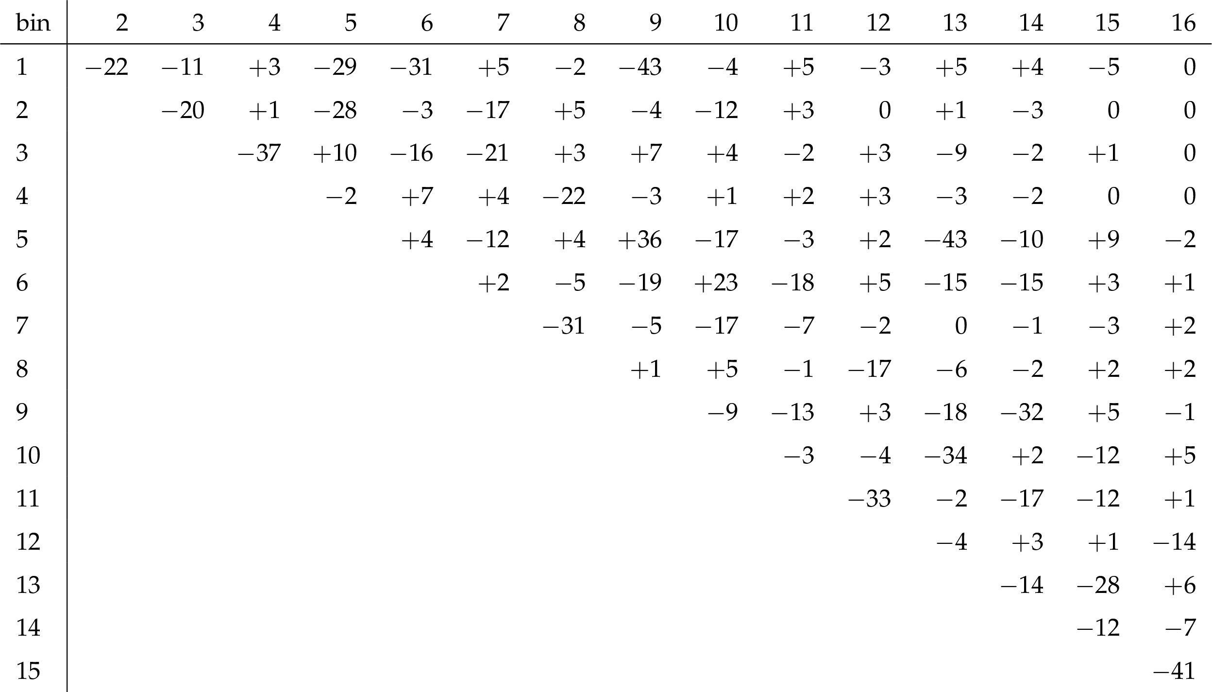
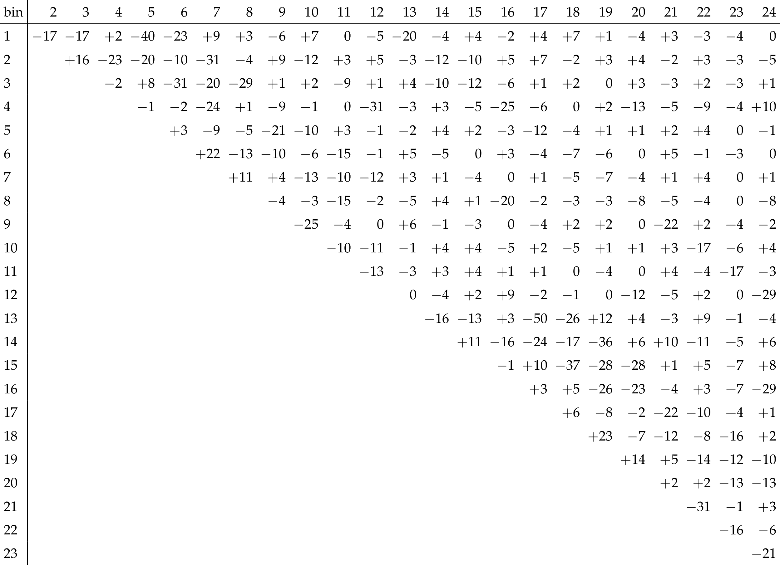
Table A2:
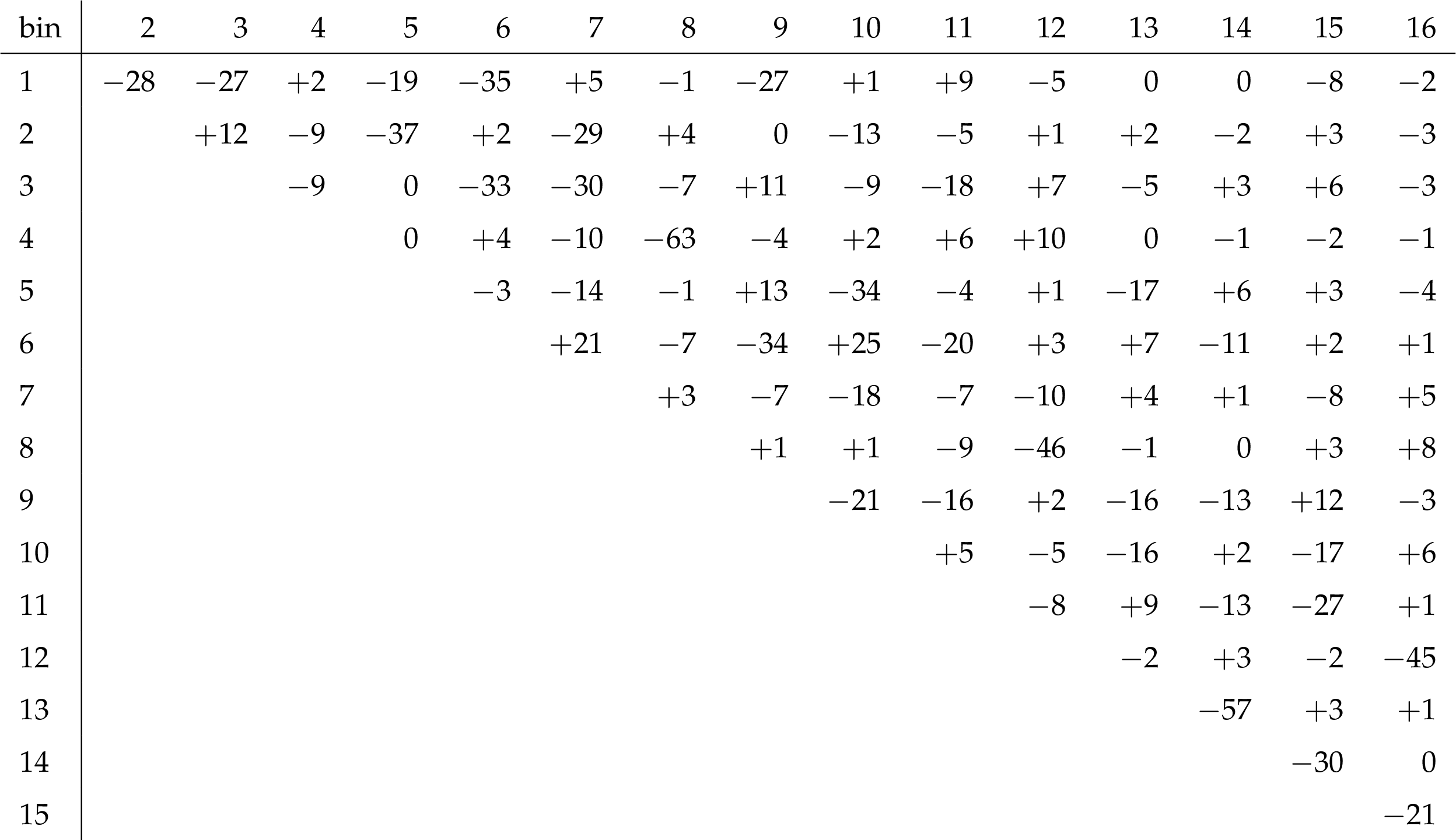
The correlation matrix of statistical uncertainties for the measured [ ${y({\mathrm {t}})}$, ${{p_{\mathrm {T}}} ({\mathrm {t}})}$ ] cross sections. The values are expressed as percentages. For bin indices see A.1. |
png pdf |
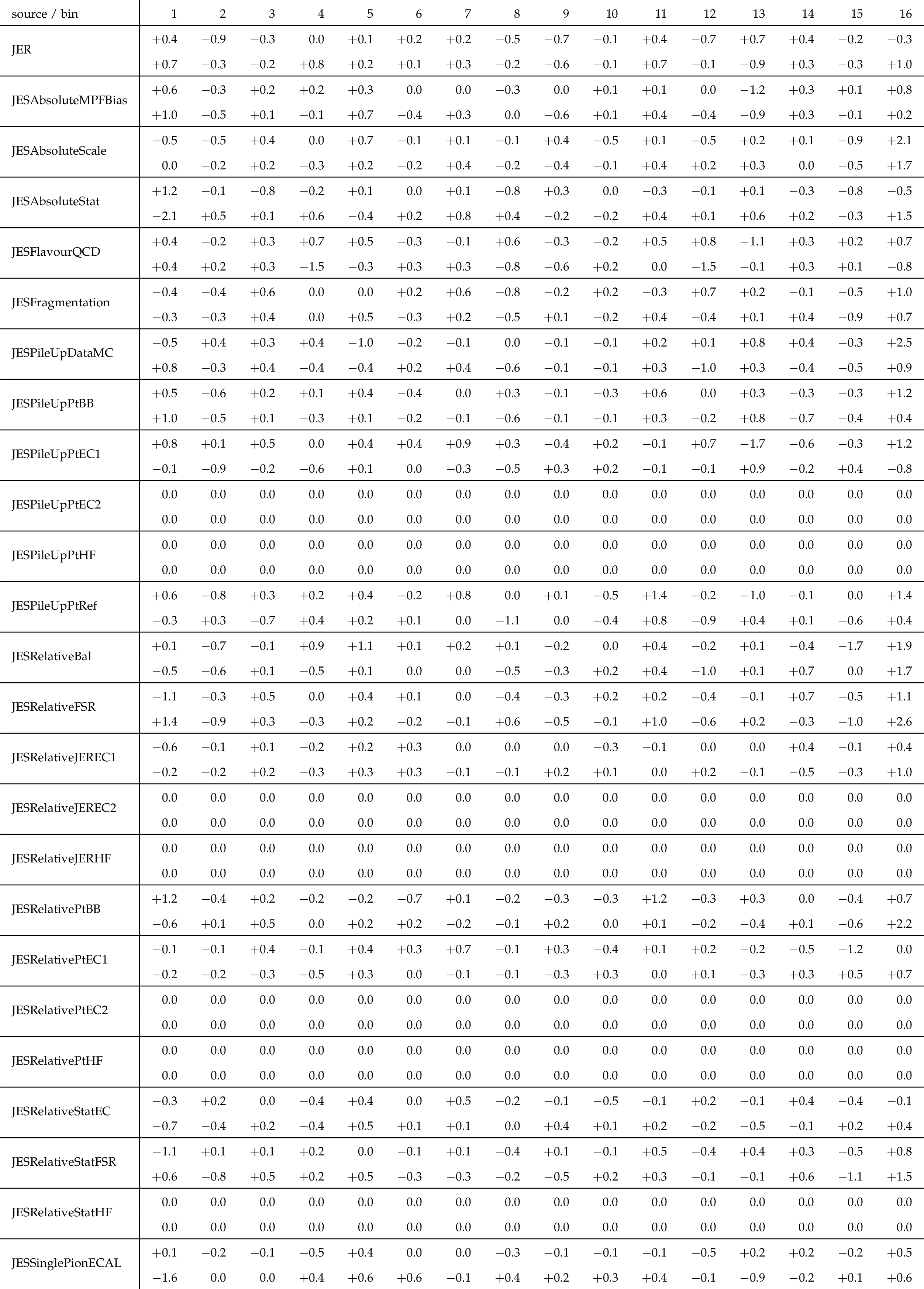
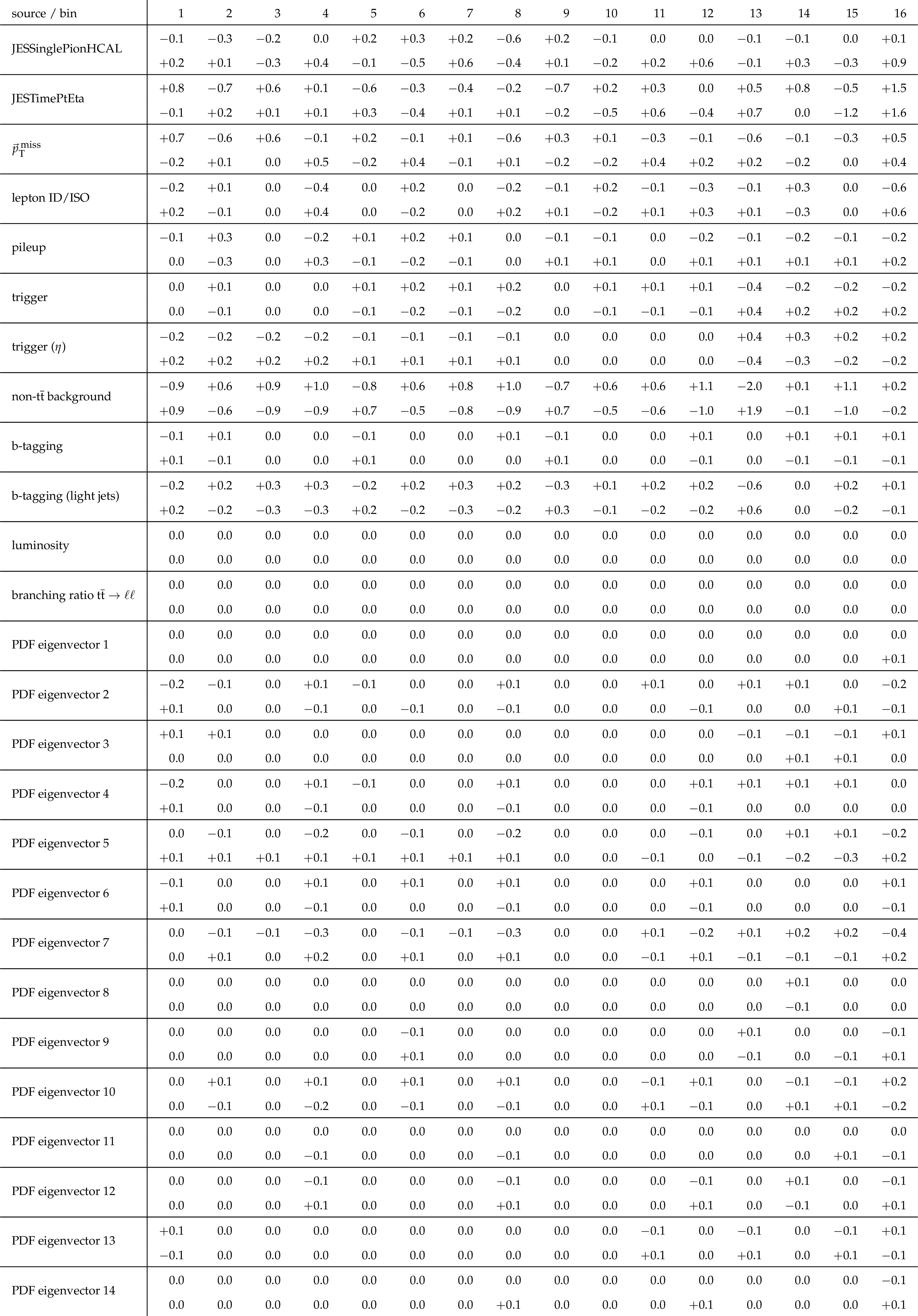
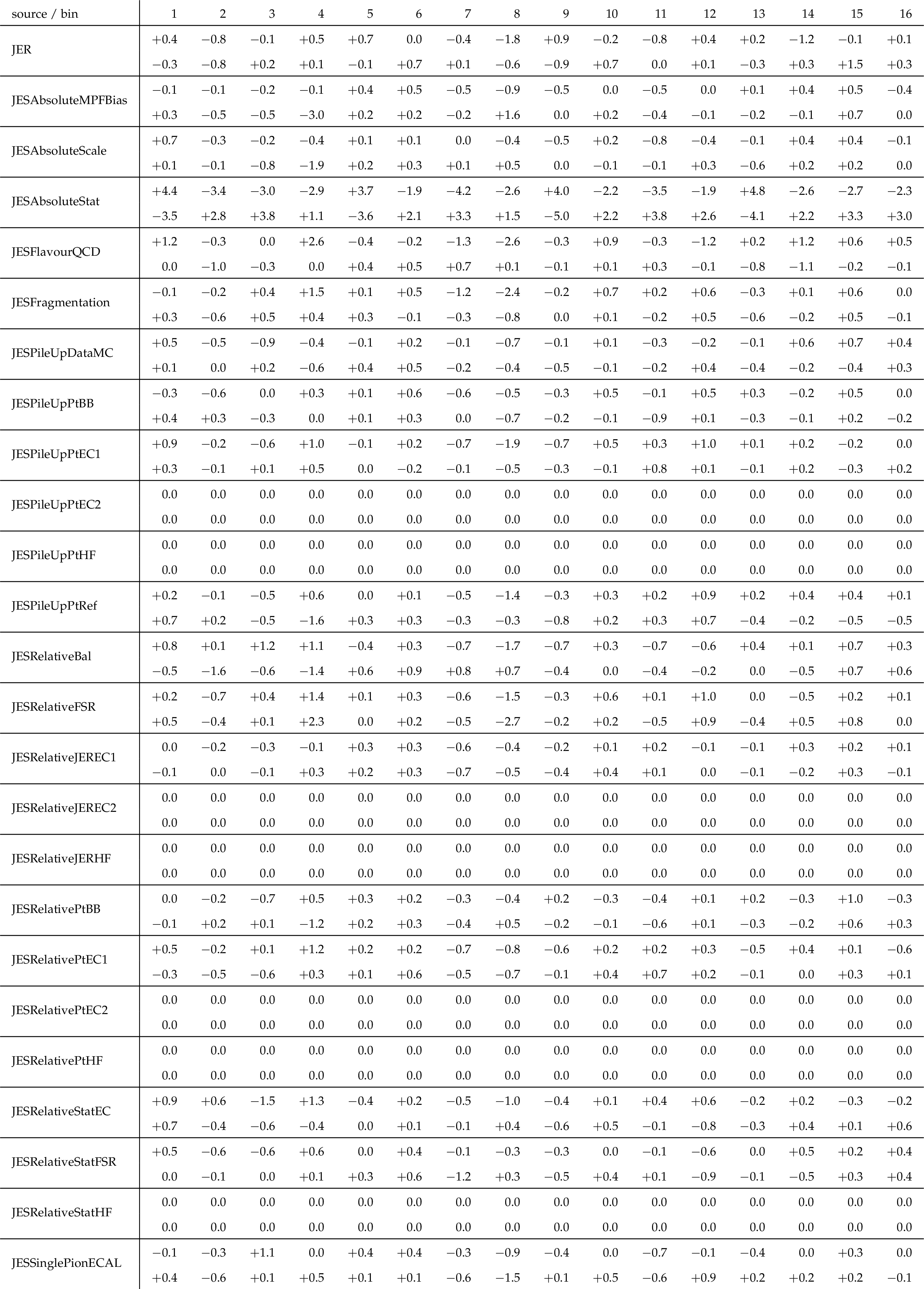
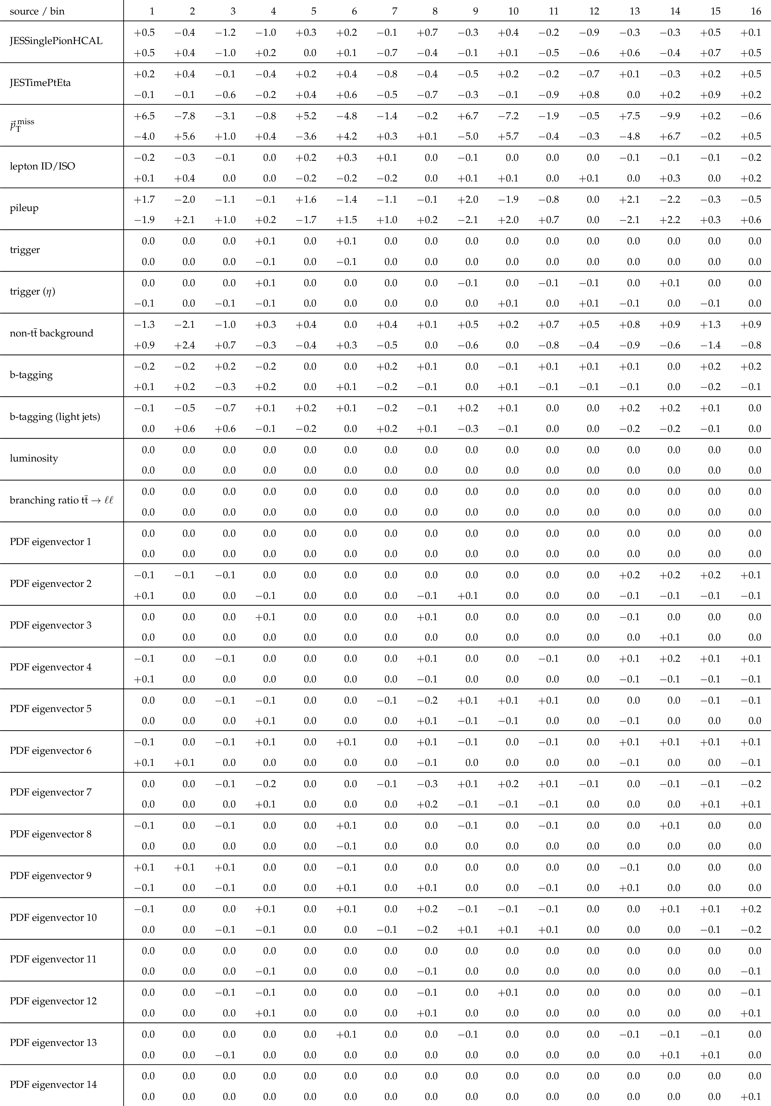
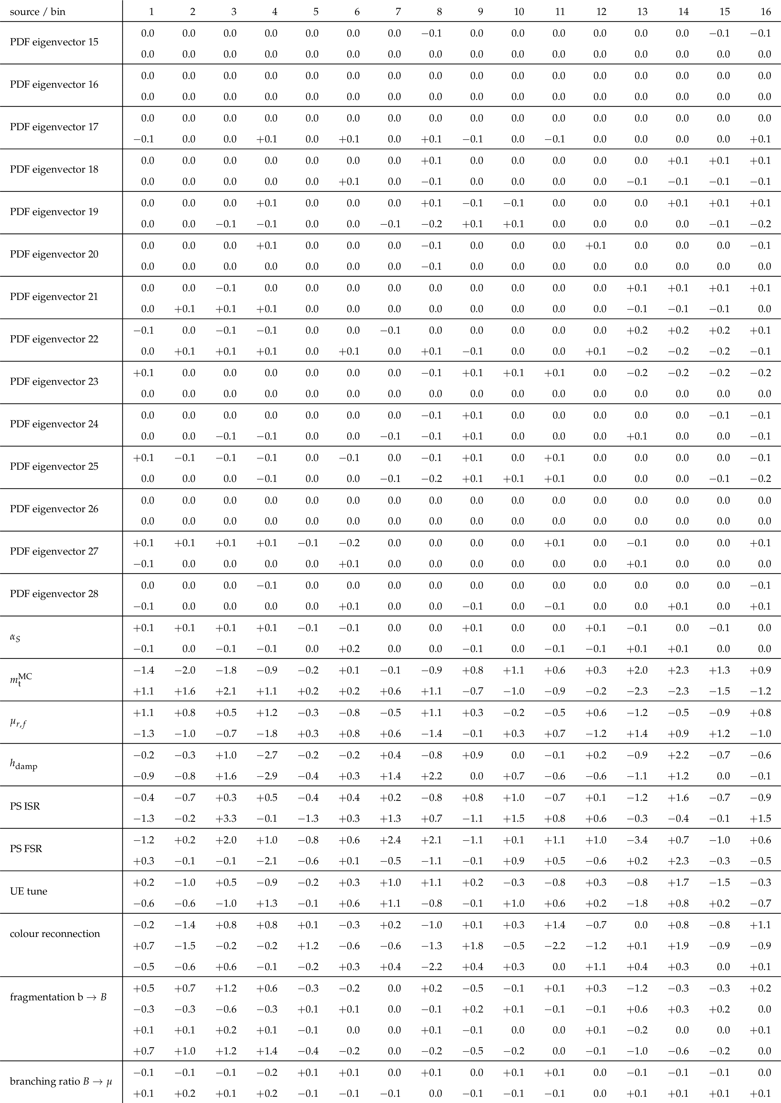
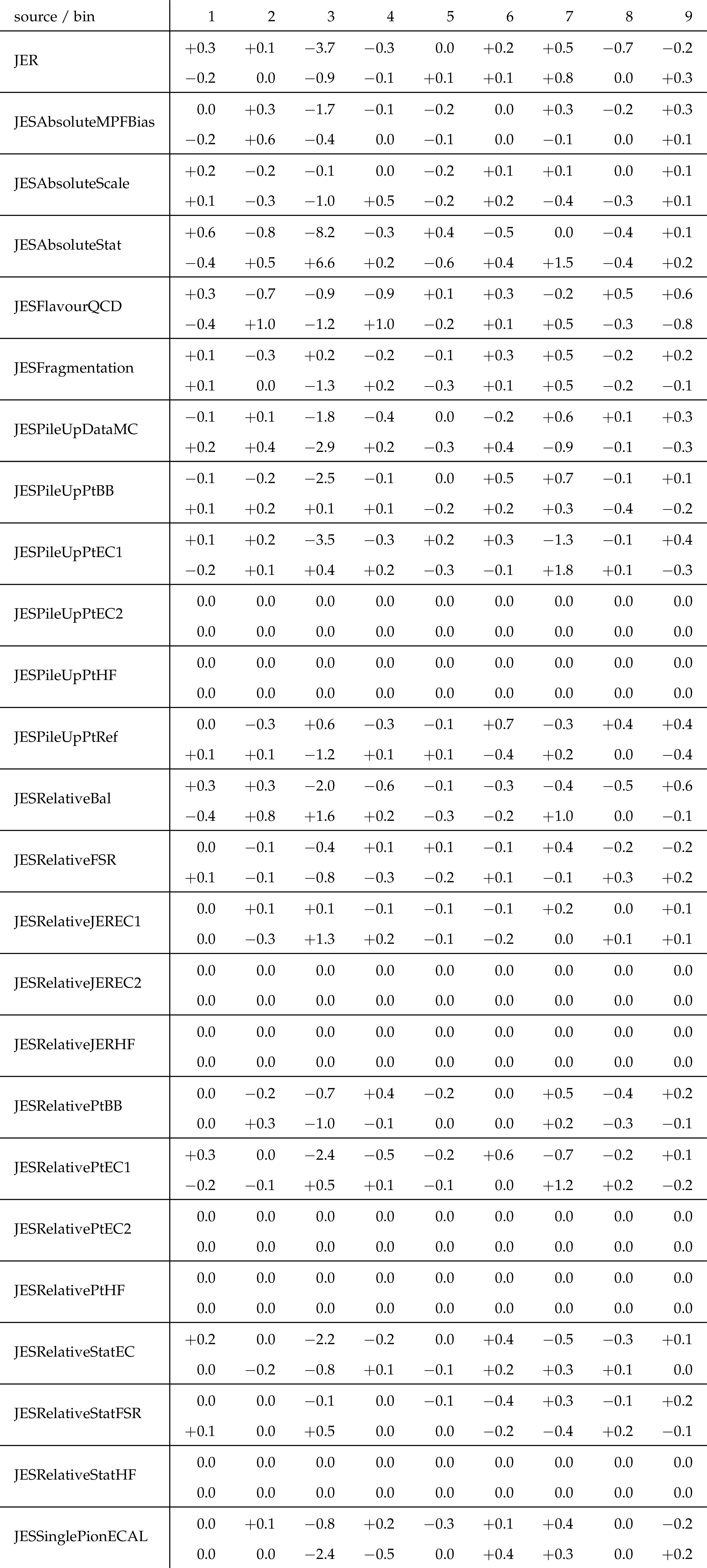
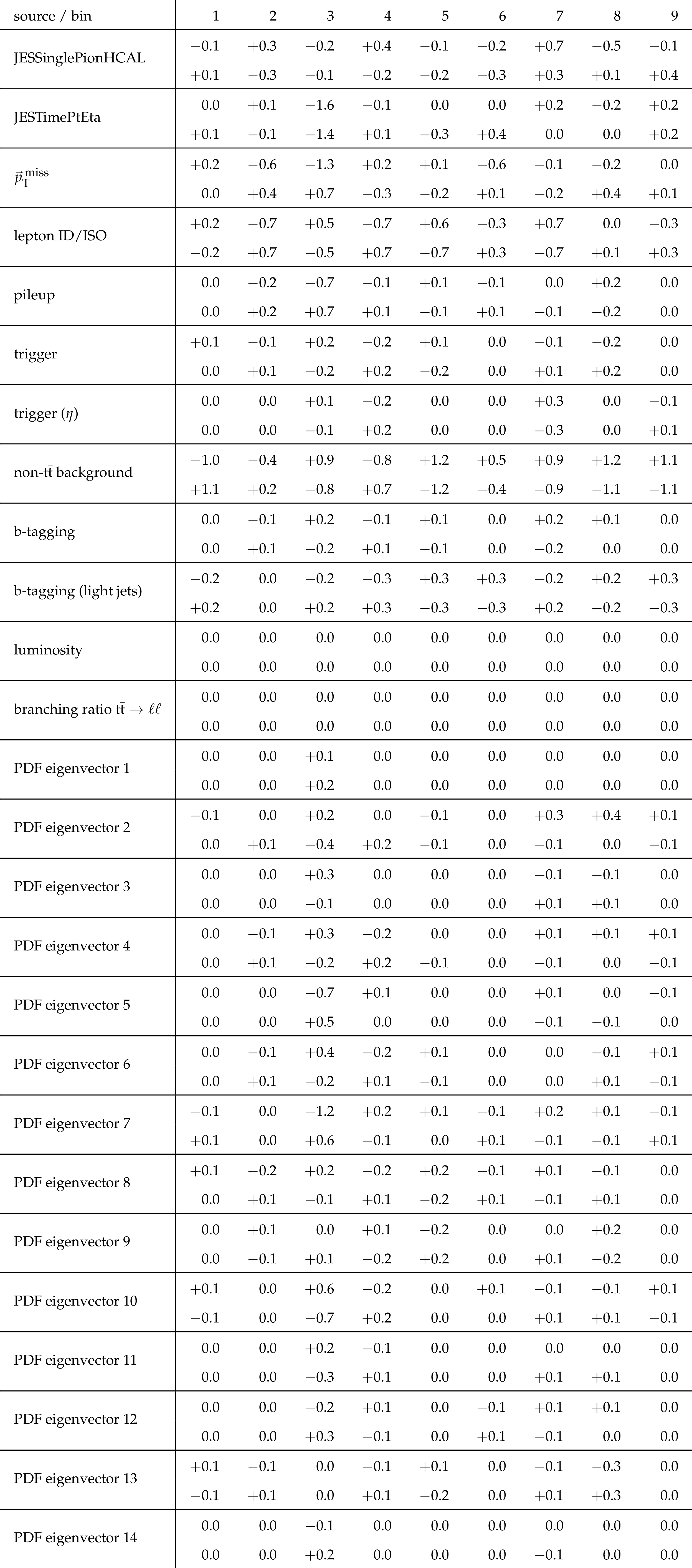
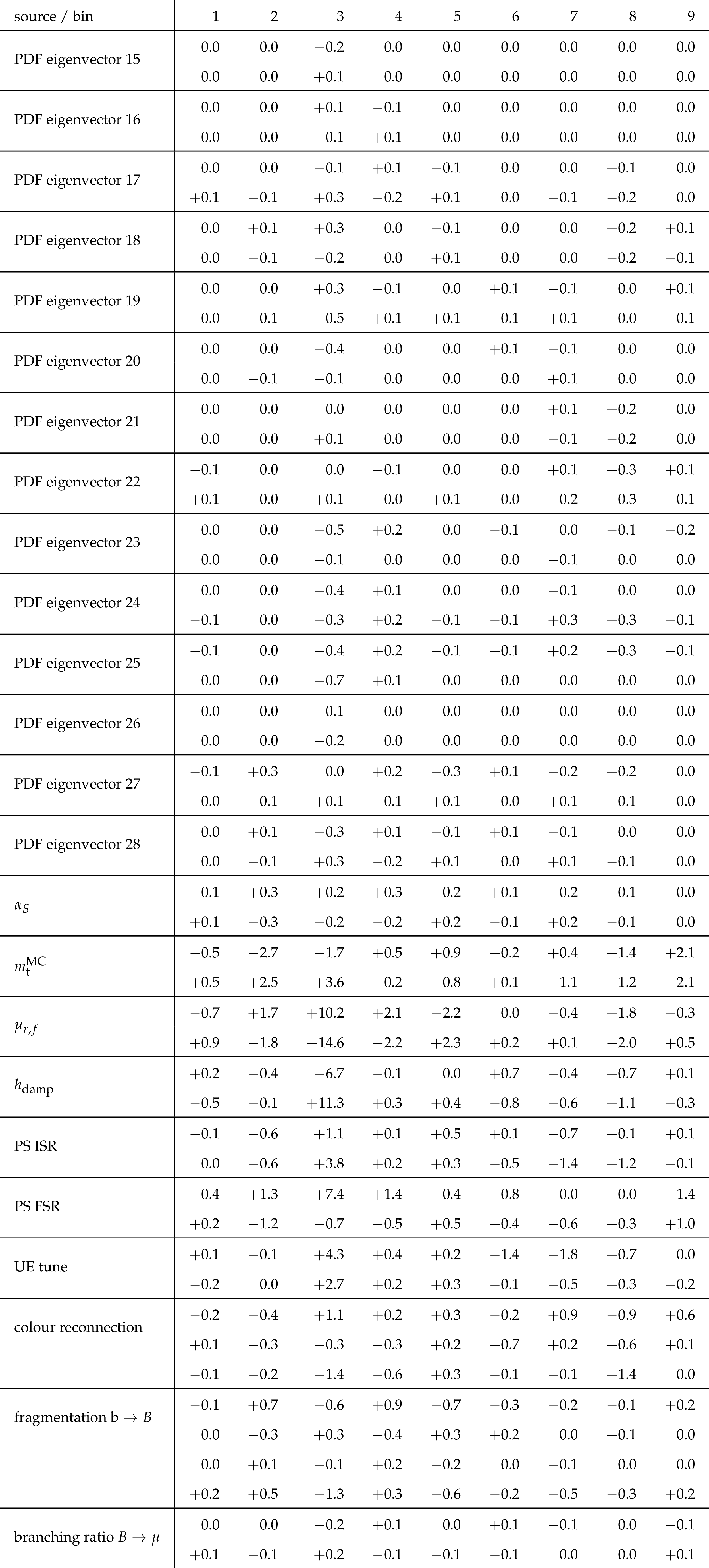
Table A3:
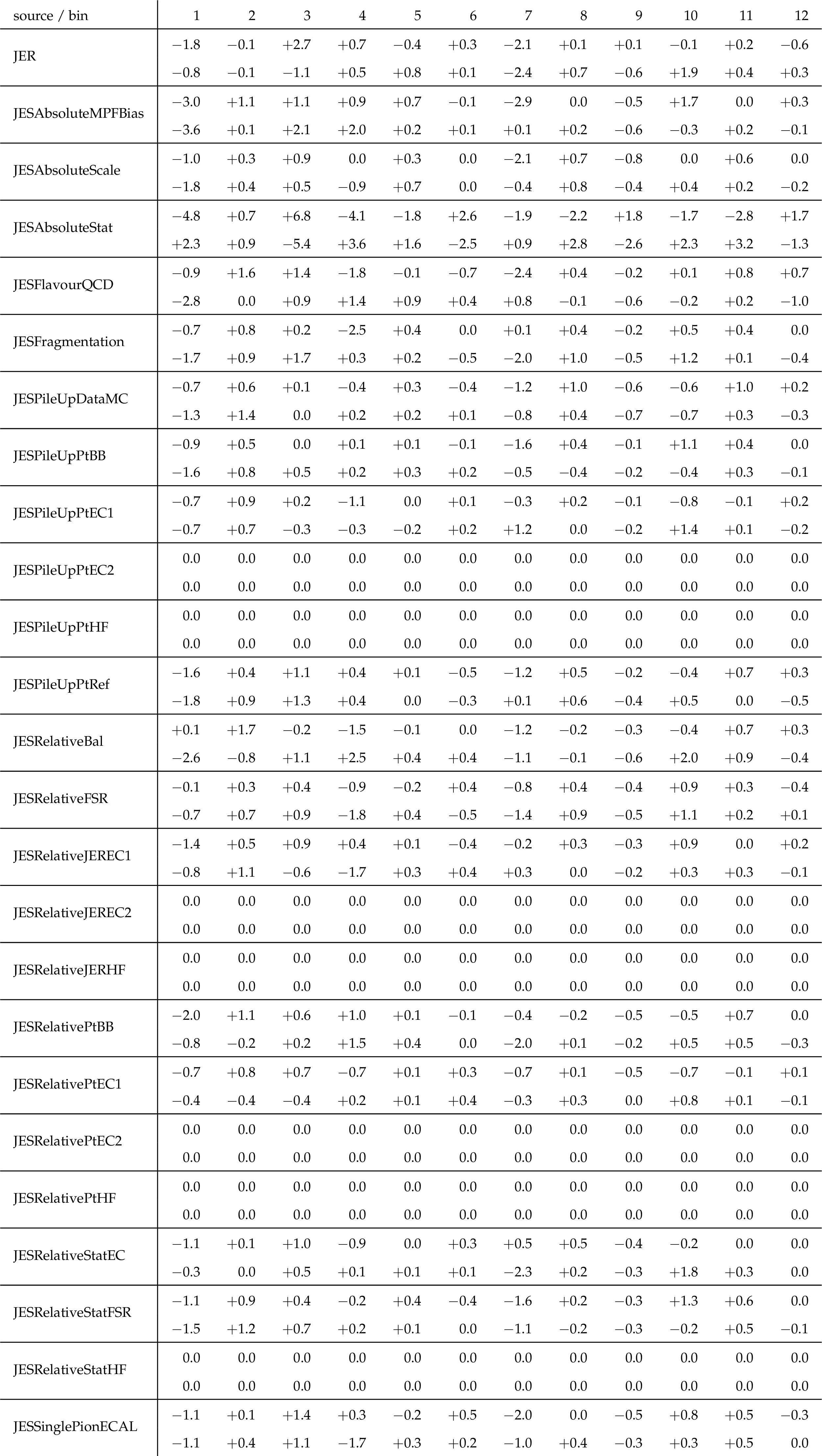
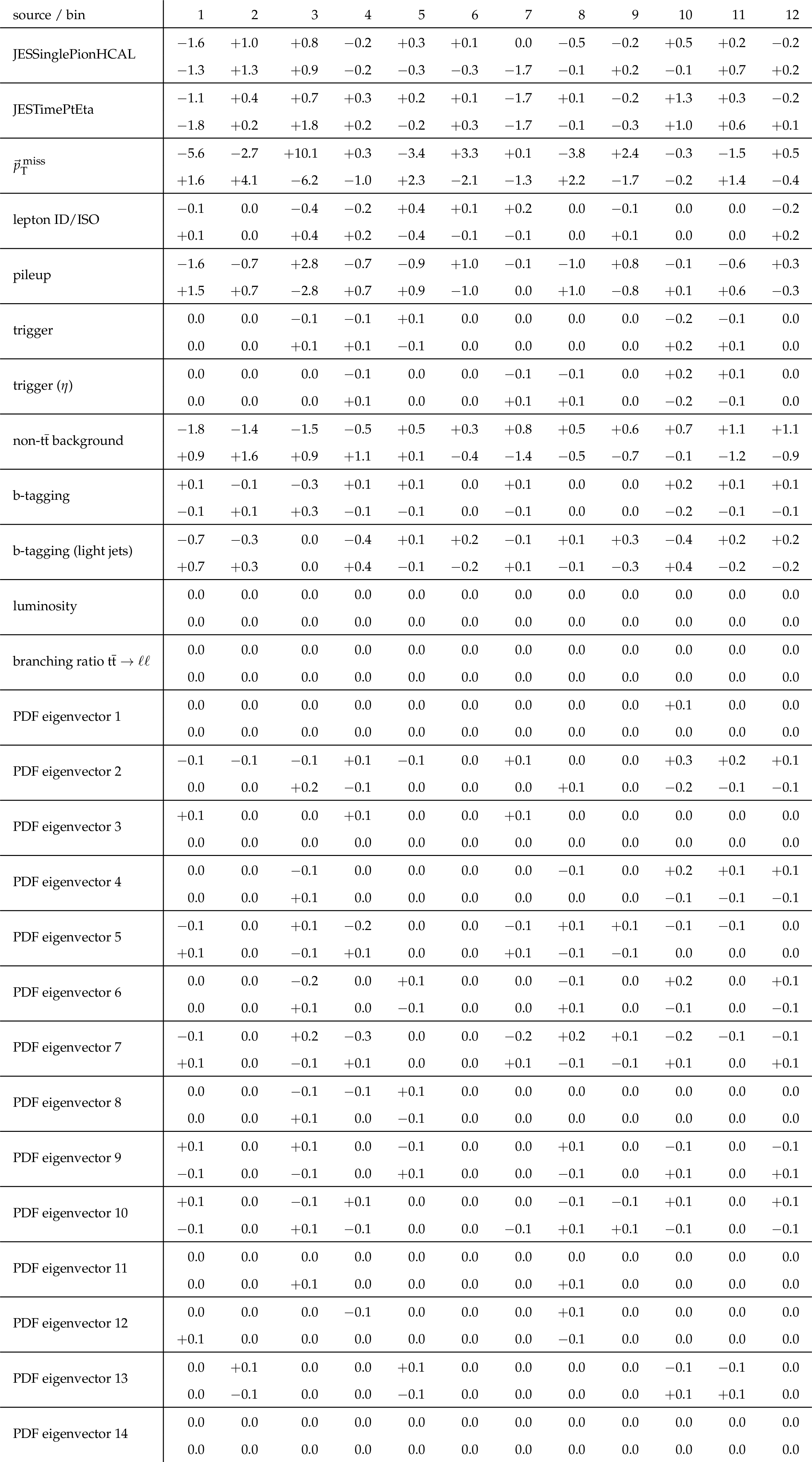
Sources and values of the relative systematic uncertainties in percent of the measured [ ${y({\mathrm {t}})}$, ${{p_{\mathrm {T}}} ({\mathrm {t}})}$ ] cross sections. For bin indices see A.1. |
png pdf |
Table A4:
A.3 continued. |
png pdf |
Table A5:
A.3 continued. |
png pdf |
Table A6:
The measured [ ${M({{\mathrm {t}\overline {\mathrm {t}}}})}$, ${y({\mathrm {t}})}$ ] cross sections, along with their relative statistical and systematic uncertainties. |
png pdf |
Table A7:
The correlation matrix of statistical uncertainties for the measured [ ${M({{\mathrm {t}\overline {\mathrm {t}}}})}$, ${y({\mathrm {t}})}$ ] cross sections. The values are expressed as percentages. For bin indices see A.6. |
png pdf |
Table A8:
Sources and values of the relative systematic uncertainties in percent of the measured [ ${M({{\mathrm {t}\overline {\mathrm {t}}}})}$, ${y({\mathrm {t}})}$ ] cross sections. For bin indices see A.6. |
png pdf |
Table A9:
A.8 continued. |
png pdf |
Table A10:
A.8 continued. |
png pdf |
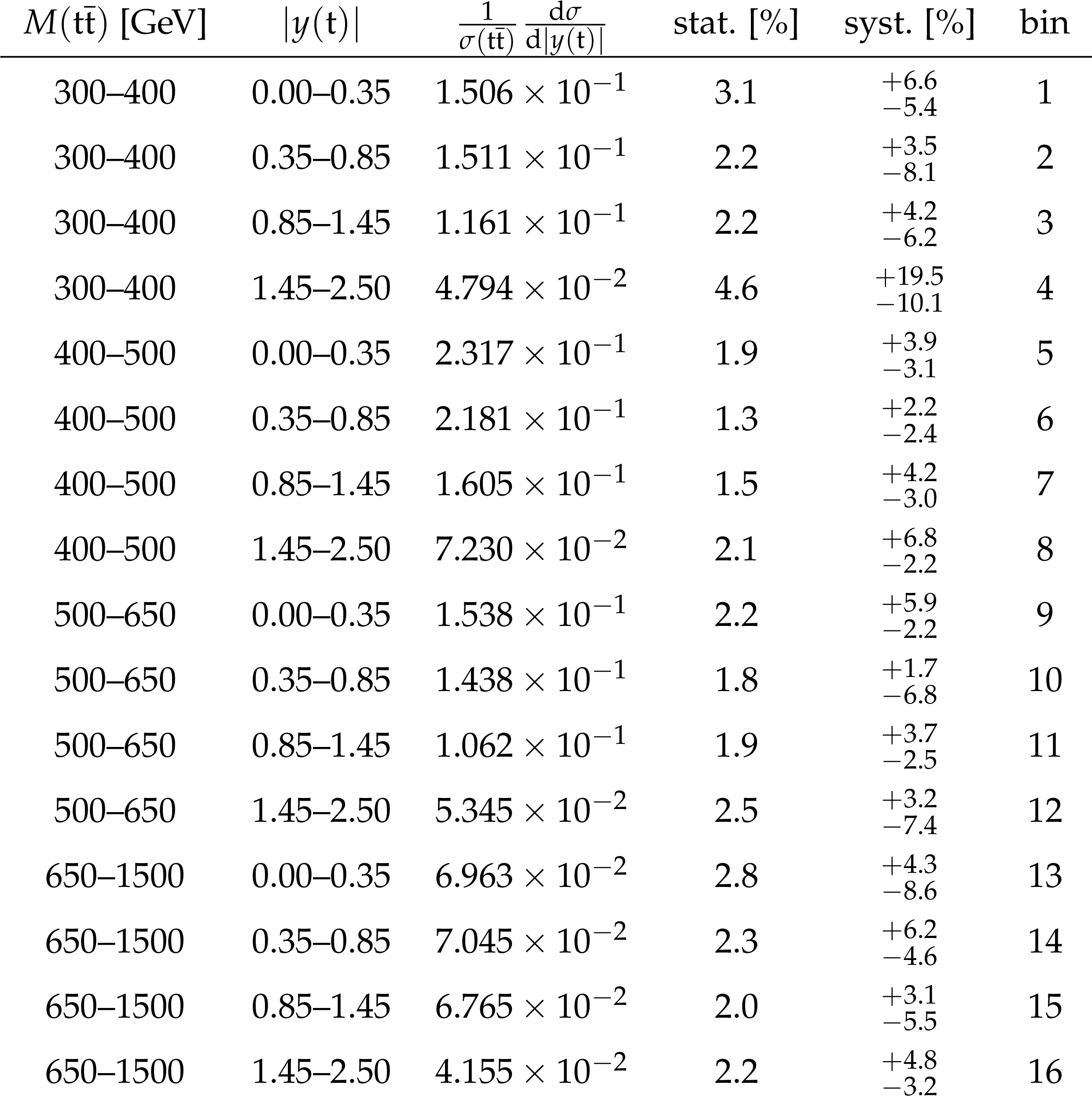
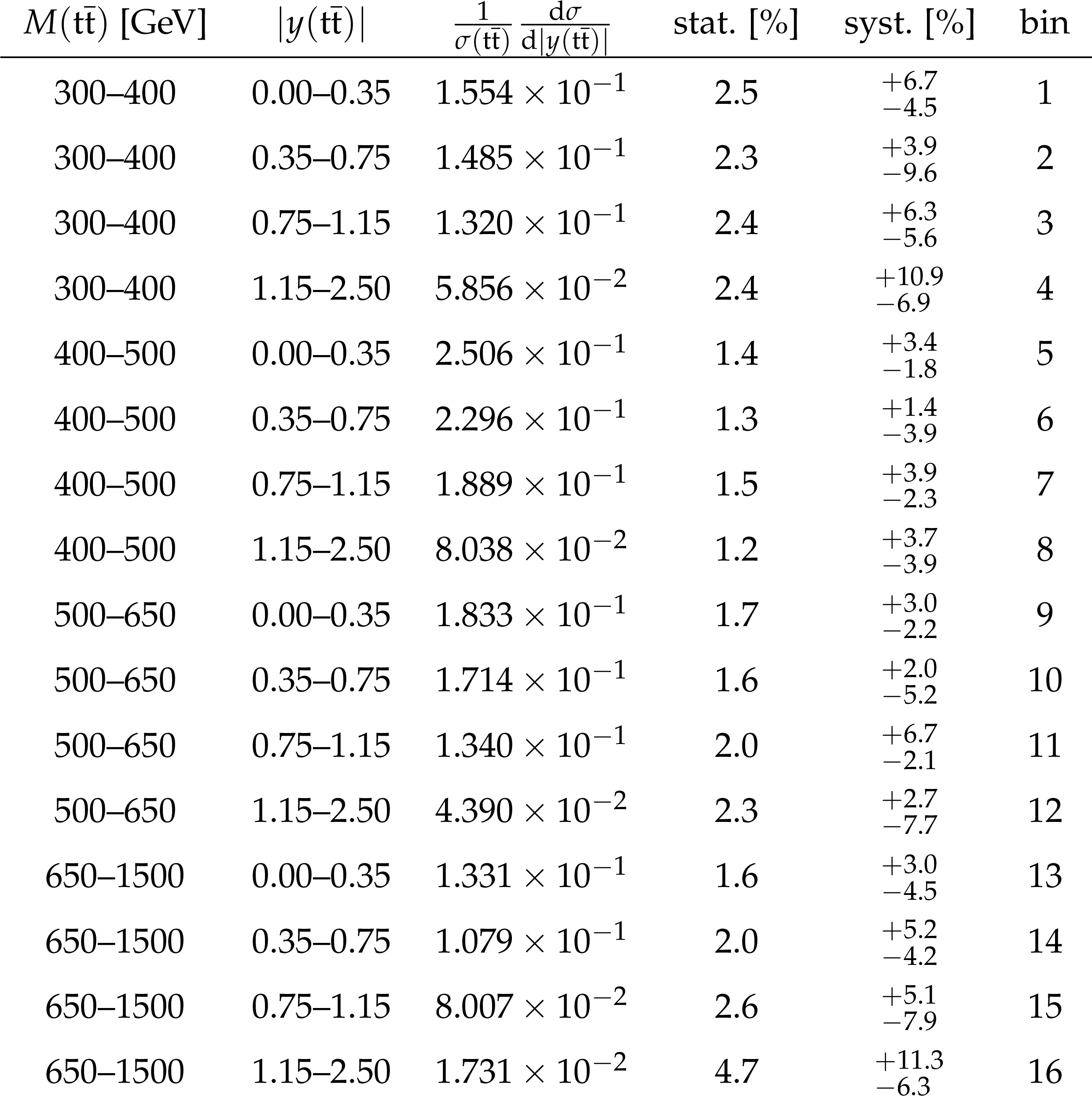
Table A11:
The measured [ ${M({{\mathrm {t}\overline {\mathrm {t}}}})}$, ${y({{\mathrm {t}\overline {\mathrm {t}}}})}$ ] cross sections, along with their relative statistical and systematic uncertainties. |
png pdf |
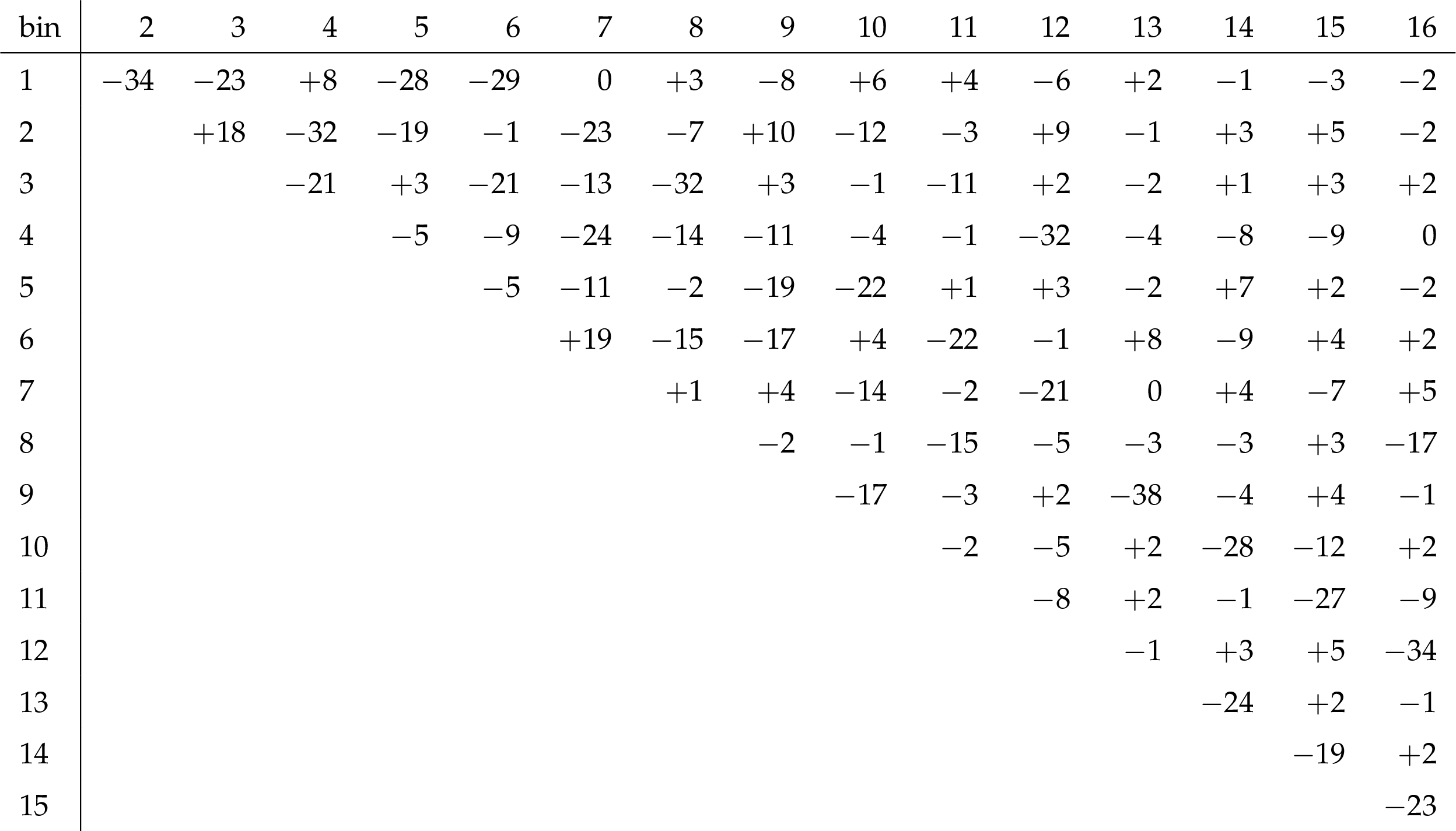
Table A12:
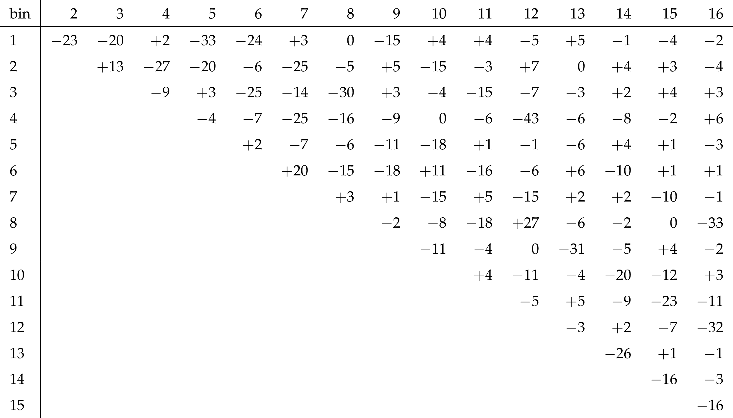
The correlation matrix of statistical uncertainties for the measured [ ${M({{\mathrm {t}\overline {\mathrm {t}}}})}$, ${y({{\mathrm {t}\overline {\mathrm {t}}}})}$ ] cross sections. The values are expressed as percentages. For bin indices see A.11. |
png pdf |
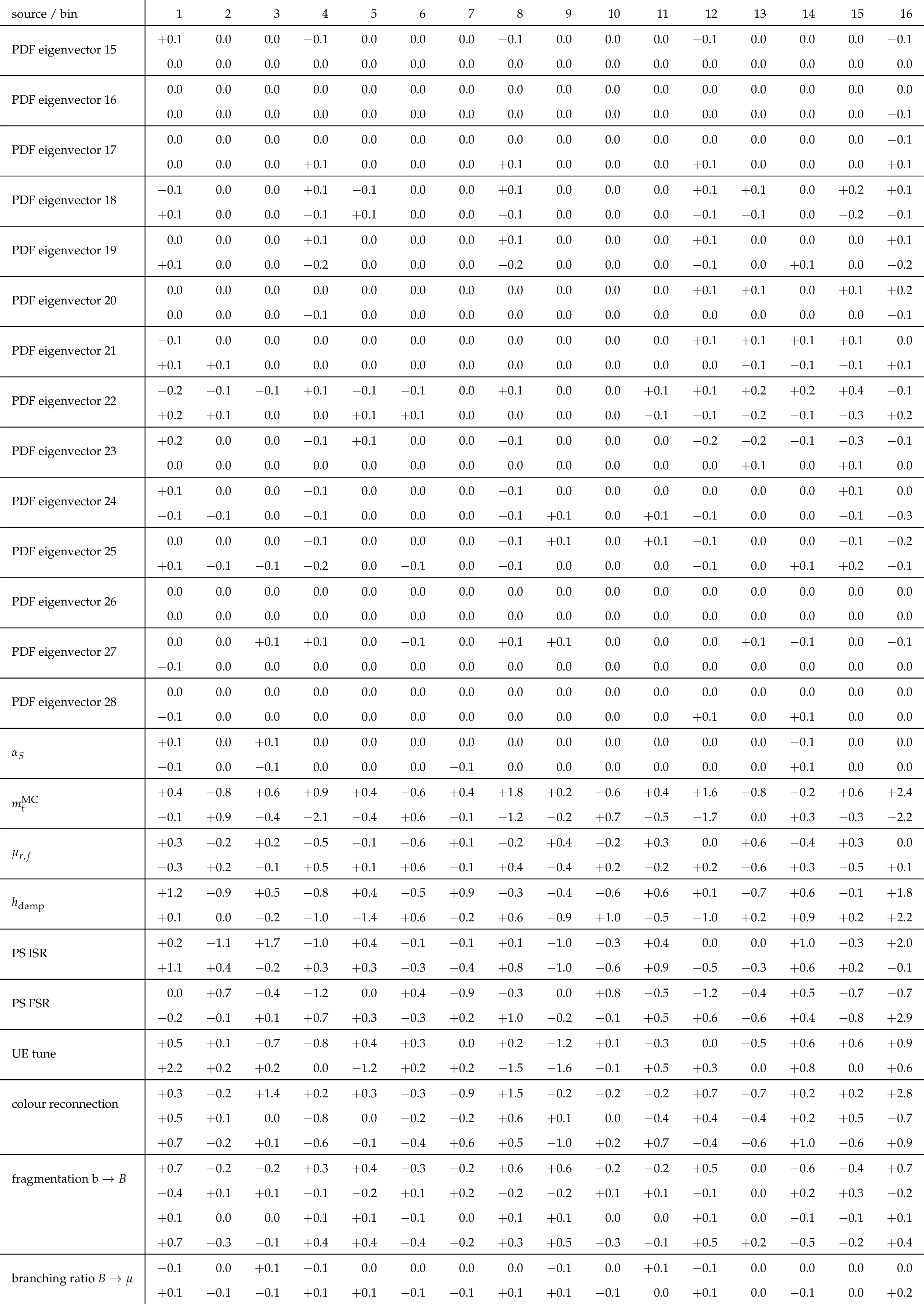
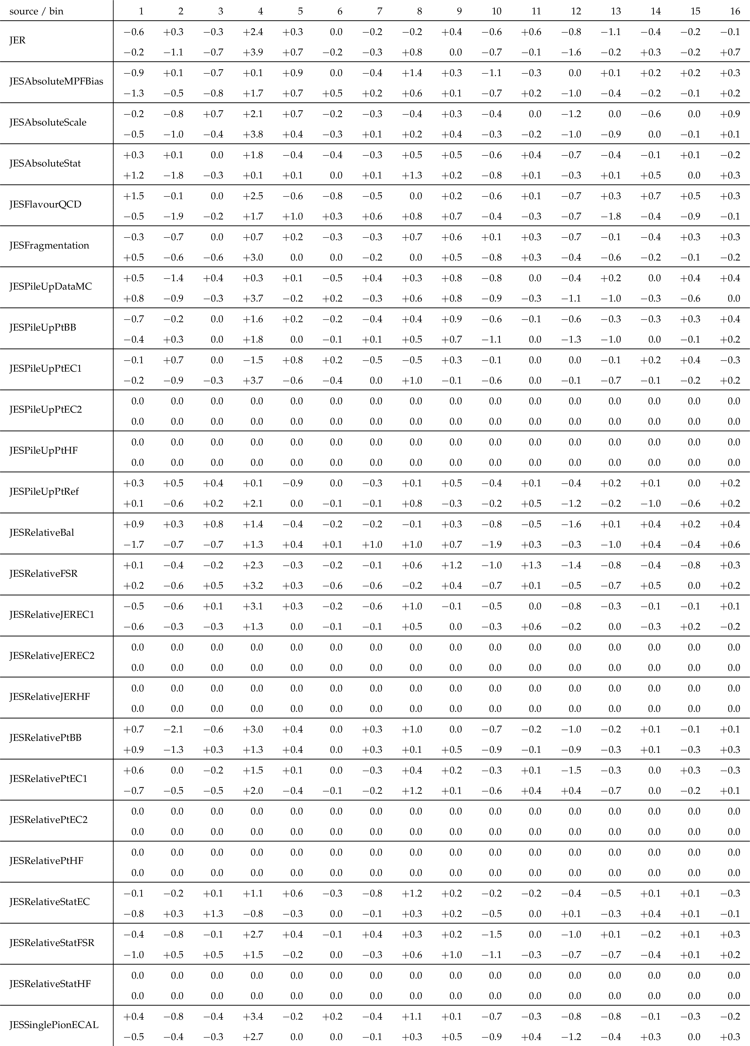
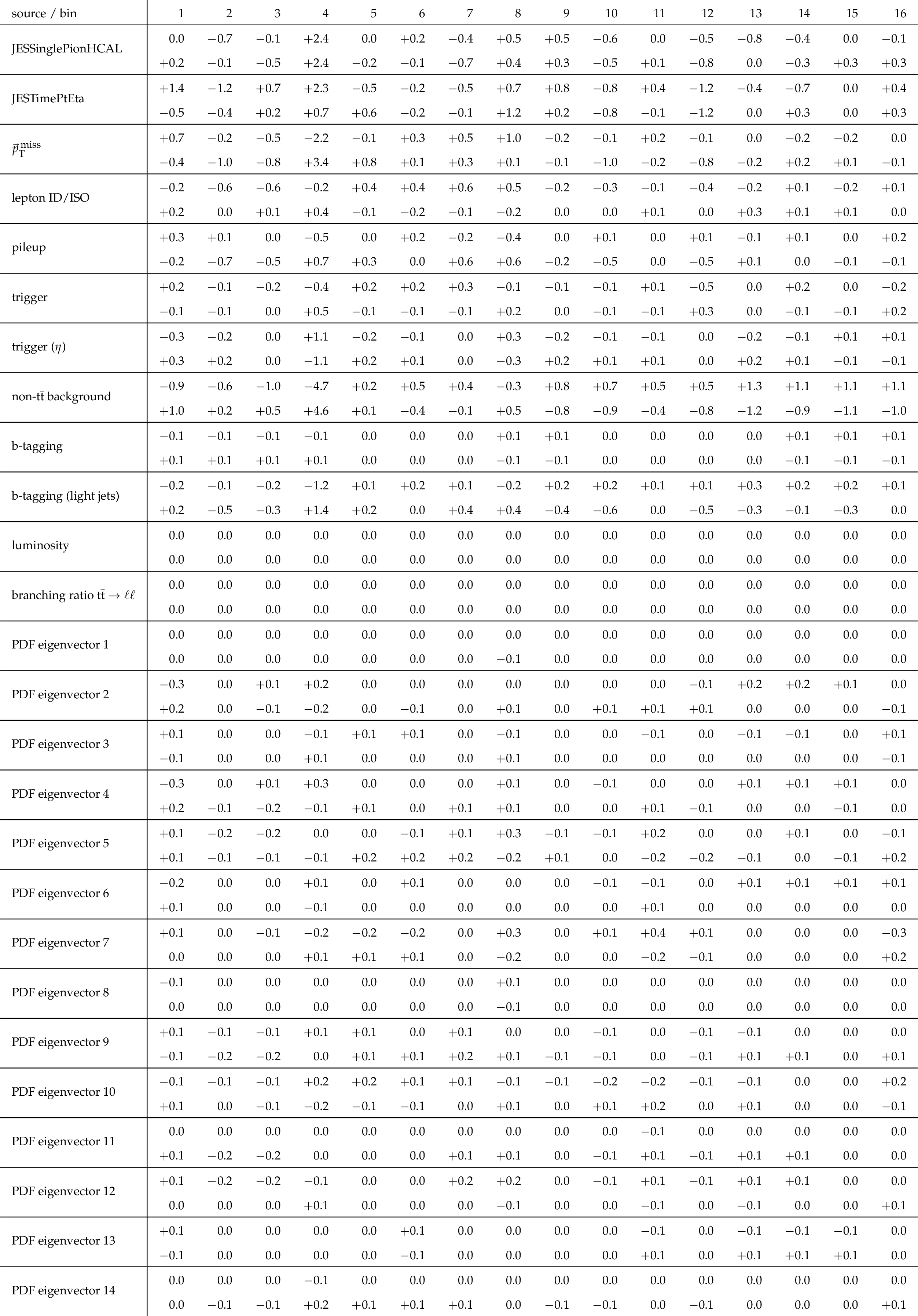
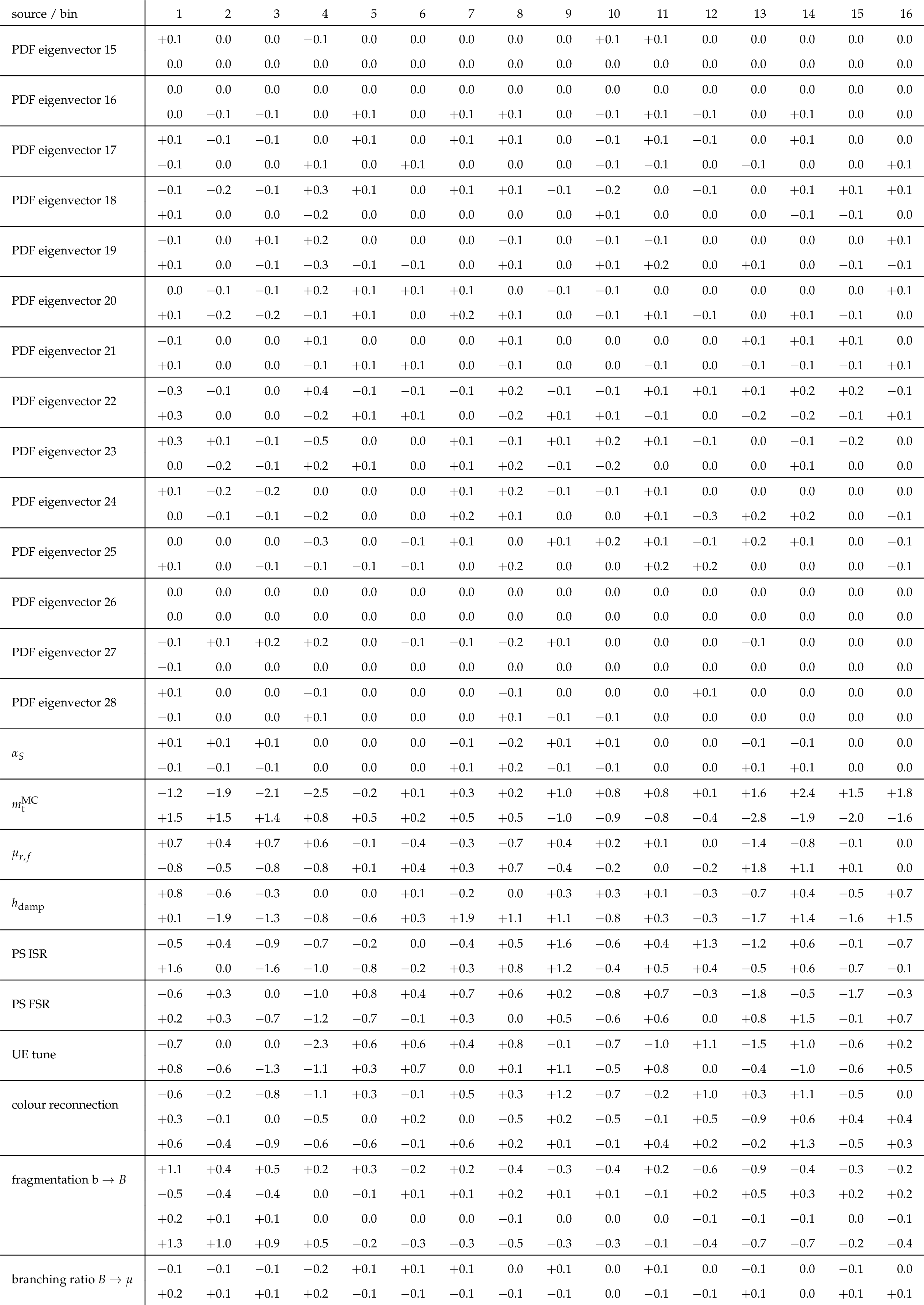
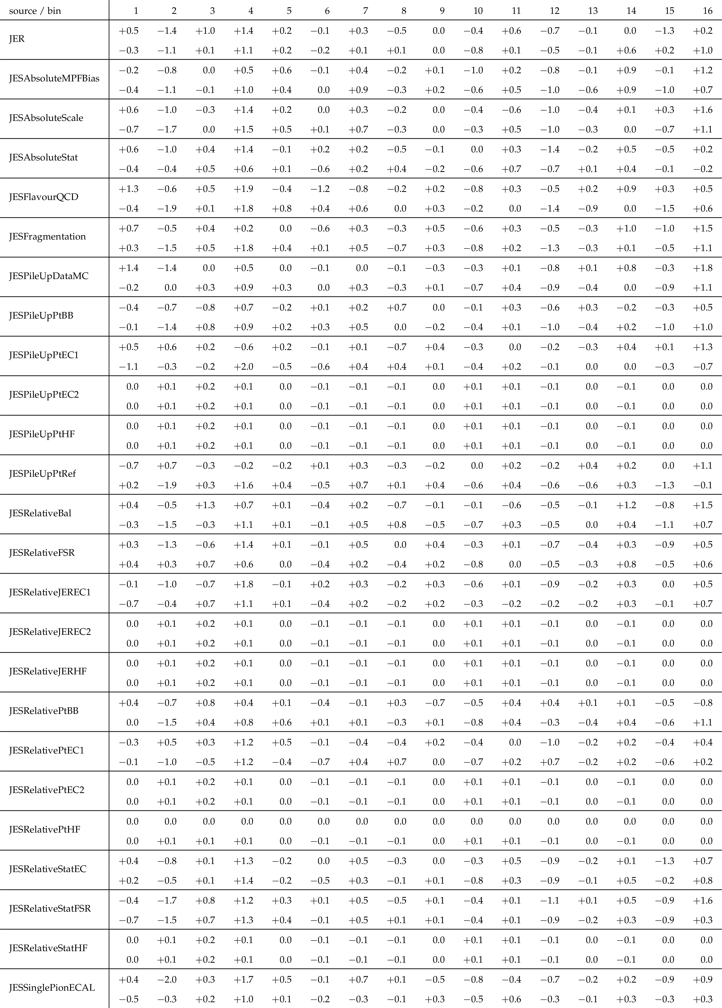
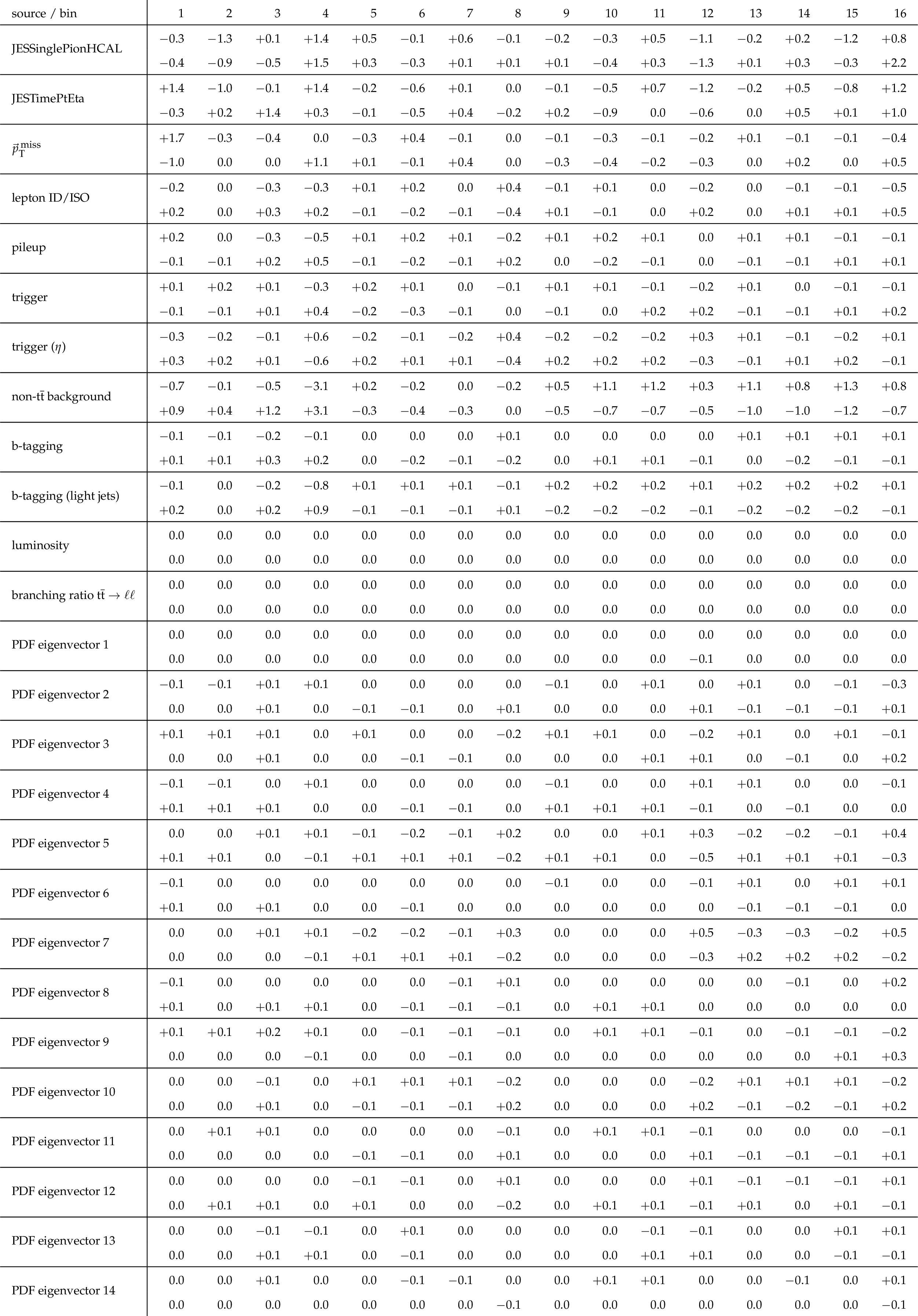
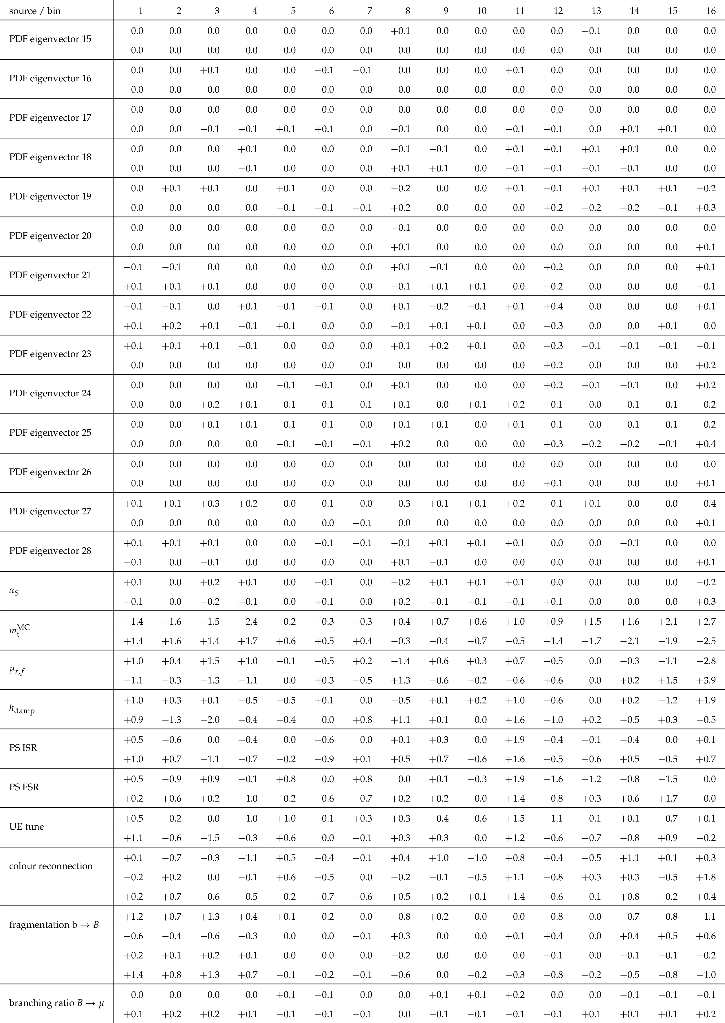
Table A13:
Sources and values of the relative systematic uncertainties in percent of the measured [ ${M({{\mathrm {t}\overline {\mathrm {t}}}})}$, ${y({{\mathrm {t}\overline {\mathrm {t}}}})}$ ] cross sections. For bin indices see A.11. |
png pdf |
Table A14:
A.13 continued. |
png pdf |
Table A15:
A.13 continued. |

png pdf |
Table A16:
The measured [ ${M({{\mathrm {t}\overline {\mathrm {t}}}})}$, ${\Delta \eta ({\mathrm {t}}, {\overline {\mathrm {t}}})}$ ] cross sections, along with their relative statistical and systematic uncertainties. |

png pdf |
Table A17:
The correlation matrix of statistical uncertainties for the measured [ ${M({{\mathrm {t}\overline {\mathrm {t}}}})}$, ${\Delta \eta ({\mathrm {t}}, {\overline {\mathrm {t}}})}$ ] cross sections. The values are expressed as percentages. For bin indices see A.16. |
png pdf |
Table A18:
Sources and values of the relative systematic uncertainties in percent of the measured [ ${M({{\mathrm {t}\overline {\mathrm {t}}}})}$, ${\Delta \eta ({\mathrm {t}}, {\overline {\mathrm {t}}})}$ ] cross sections. For bin indices see A.16. |
png pdf |
Table A19:
A.18 continued. |
png pdf |
Table A20:
A.18 continued. |
png pdf |
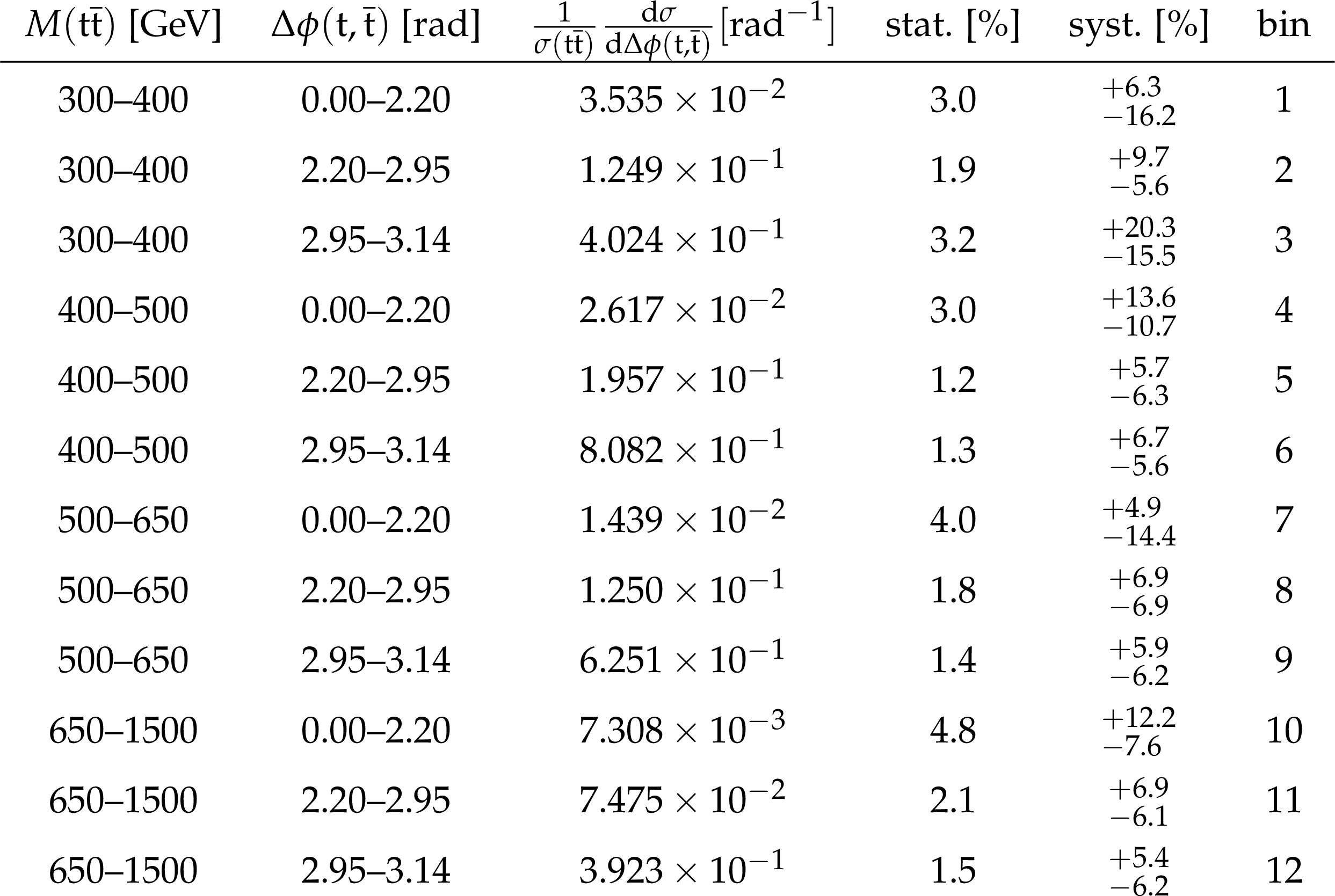
Table A21:
The measured [ ${M({{\mathrm {t}\overline {\mathrm {t}}}})}$, ${\Delta \phi ({\mathrm {t}}, {\overline {\mathrm {t}}})}$ ] cross sections, along with their relative statistical and systematic uncertainties. |
png pdf |
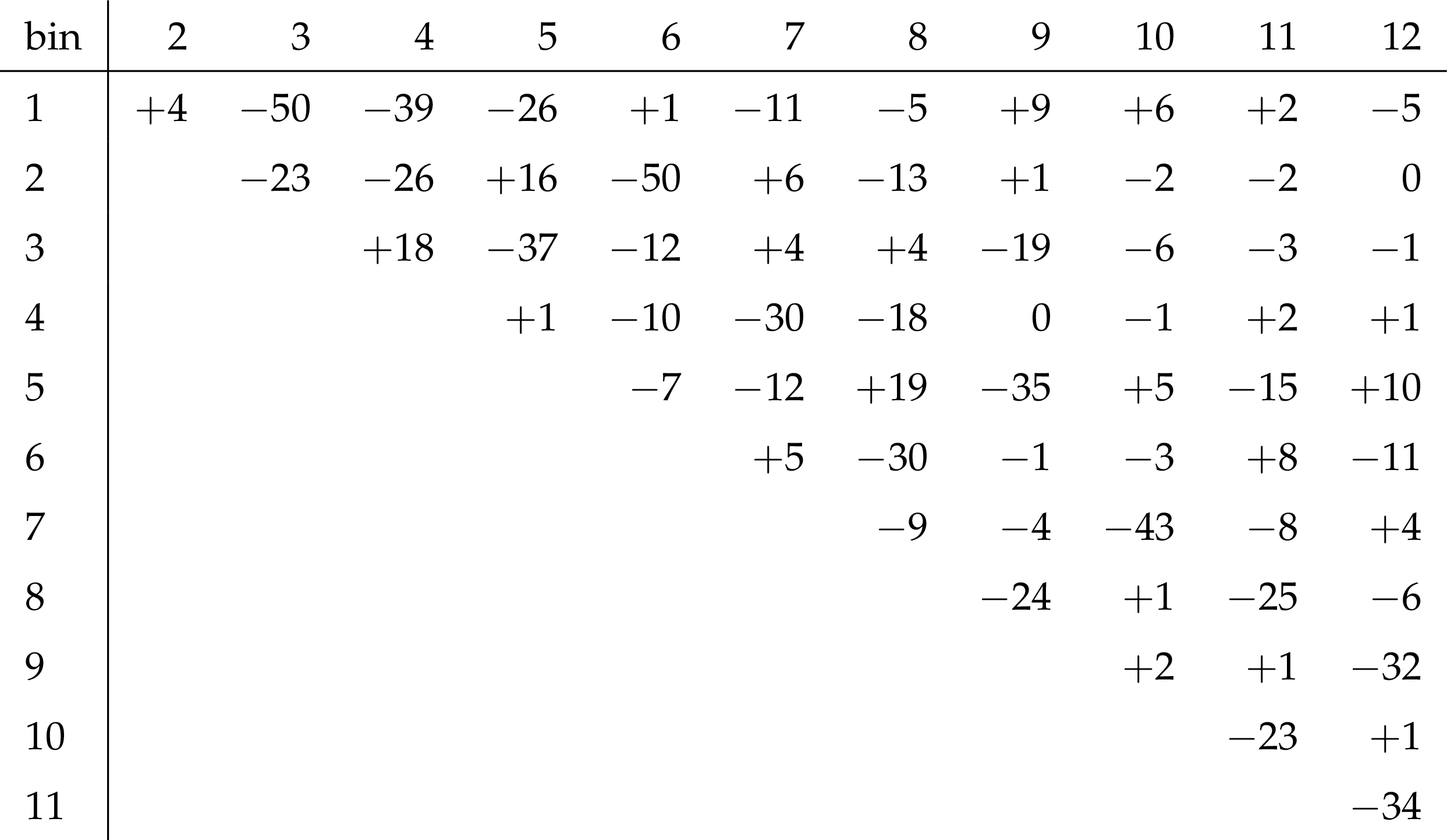
Table A22:
The correlation matrix of statistical uncertainties for the measured [ ${M({{\mathrm {t}\overline {\mathrm {t}}}})}$, ${\Delta \phi ({\mathrm {t}}, {\overline {\mathrm {t}}})}$ ] cross sections. The values are expressed as percentages. For bin indices see A.21. |
png pdf |
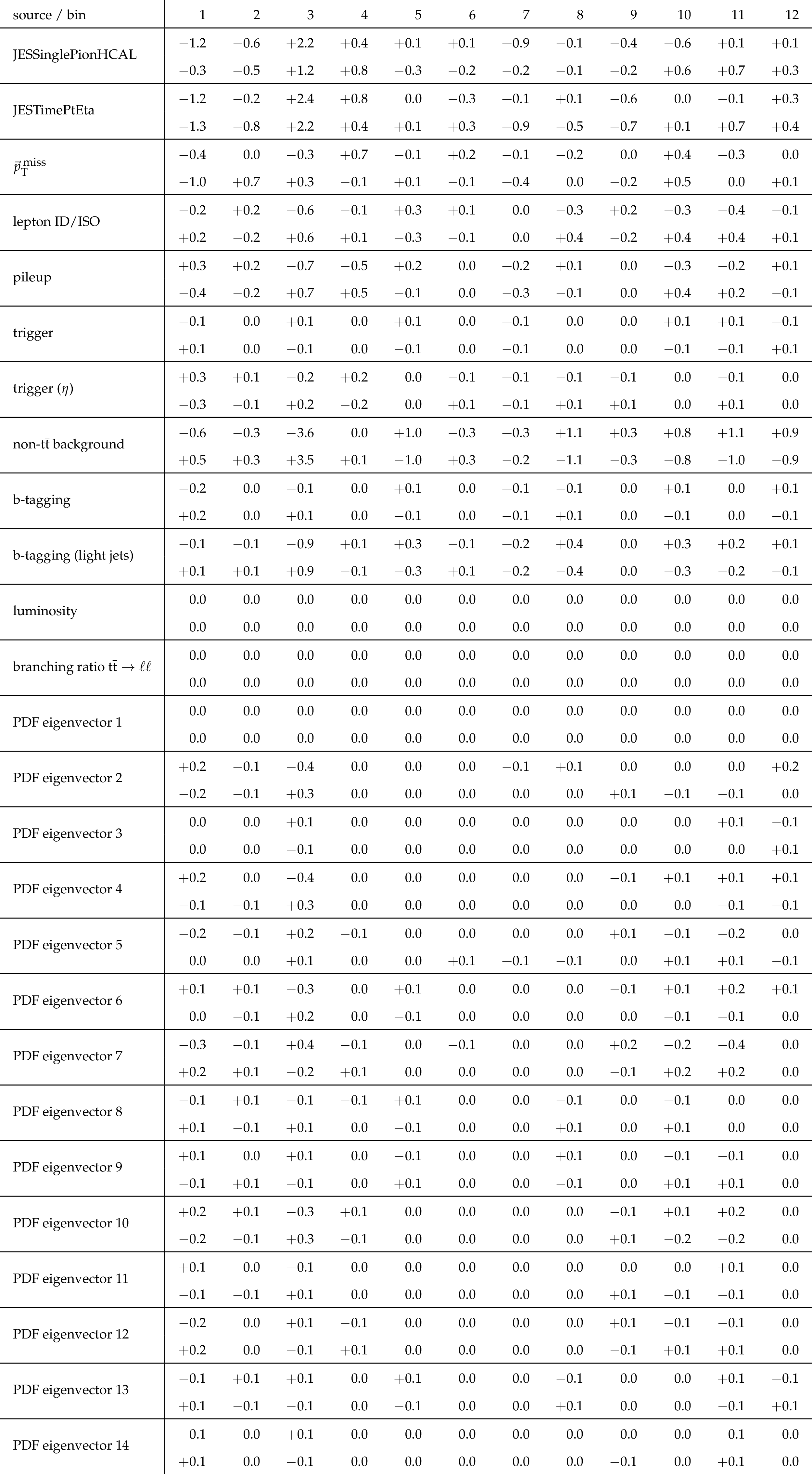
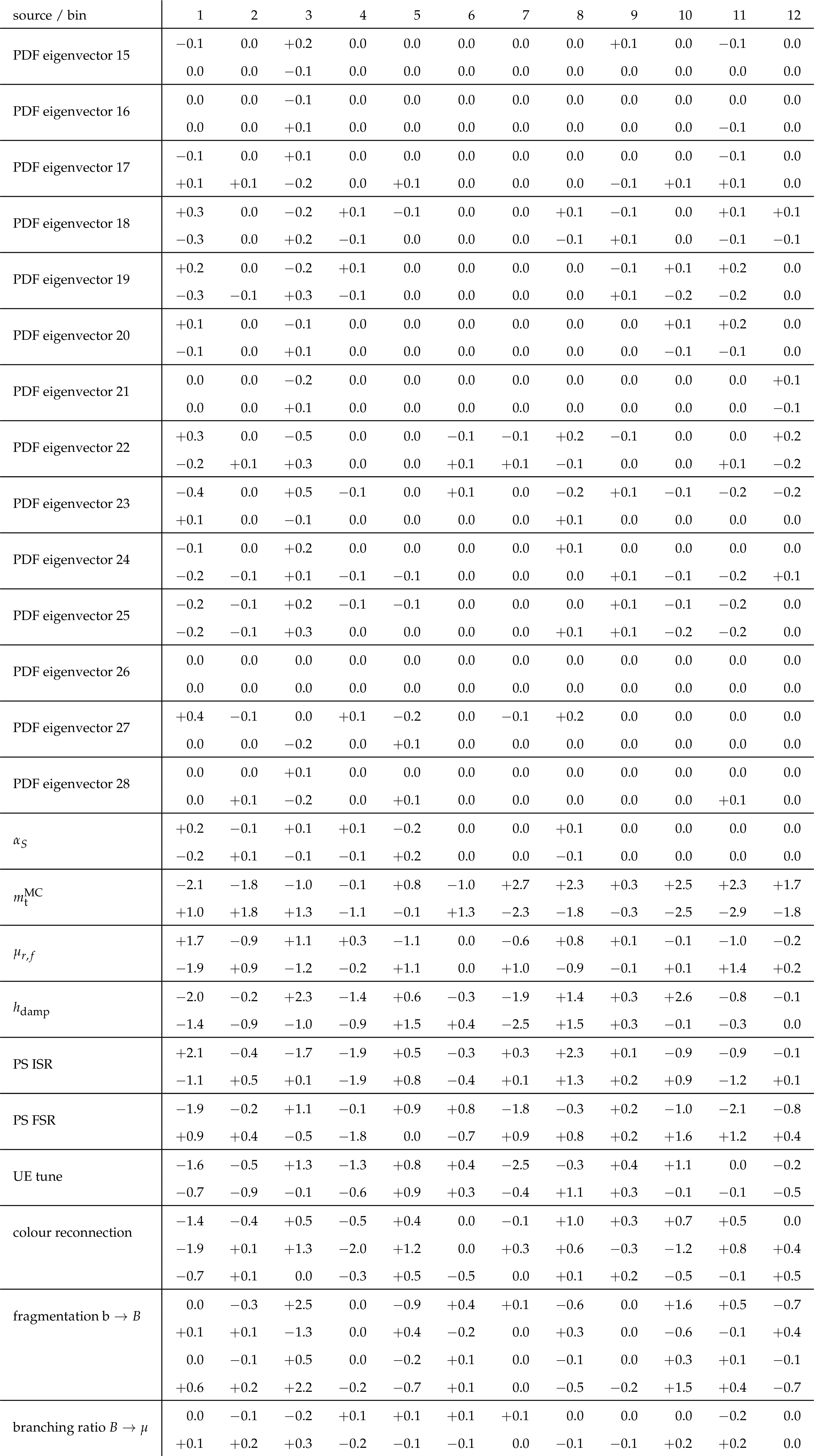
Table A23:
Sources and values of the relative systematic uncertainties in percent of the measured [ ${M({{\mathrm {t}\overline {\mathrm {t}}}})}$, ${\Delta \phi ({\mathrm {t}}, {\overline {\mathrm {t}}})}$ ] cross sections. For bin indices see A.21. |
png pdf |
Table A24:
A.23 continued. |

png pdf |
Table A25:
A.23 continued. |
png pdf |
Table A26:
The measured [ ${M({{\mathrm {t}\overline {\mathrm {t}}}})}$, ${{p_{\mathrm {T}}} ({{\mathrm {t}\overline {\mathrm {t}}}})}$ ] cross sections, along with their relative statistical and systematic uncertainties. |
png pdf |
Table A27:
The correlation matrix of statistical uncertainties for the measured [ ${M({{\mathrm {t}\overline {\mathrm {t}}}})}$, ${{p_{\mathrm {T}}} ({{\mathrm {t}\overline {\mathrm {t}}}})}$ ] cross sections. The values are expressed as percentages. For bin indices see A.26. |
png pdf |
Table A28:
Sources and values of the relative systematic uncertainties in percent of the measured [ ${M({{\mathrm {t}\overline {\mathrm {t}}}})}$, ${{p_{\mathrm {T}}} ({{\mathrm {t}\overline {\mathrm {t}}}})}$ ] cross sections. For bin indices see A.26. |
png pdf |
Table A29:
A.28 continued. |
png pdf |
Table A30:
A.28 continued. |
png pdf |
Table A31:
The measured [ ${M({{\mathrm {t}\overline {\mathrm {t}}}})}$, ${{p_{\mathrm {T}}} ({\mathrm {t}})}$ ] cross sections, along with their relative statistical and systematic uncertainties. |

png pdf |
Table A32:
The correlation matrix of statistical uncertainties for the measured [ ${M({{\mathrm {t}\overline {\mathrm {t}}}})}$, ${{p_{\mathrm {T}}} ({\mathrm {t}})}$ ] cross sections. The values are expressed as percentages. For bin indices see A.31. |
png pdf |
Table A33:
Sources and values of the relative systematic uncertainties in percent of the measured [ ${M({{\mathrm {t}\overline {\mathrm {t}}}})}$, ${{p_{\mathrm {T}}} ({\mathrm {t}})}$ ] cross sections. For bin indices see A.31. |
png pdf |
Table A34:
A.33 continued. |
png pdf |
Table A35:
A.33 continued. |

png pdf |
Table A36:
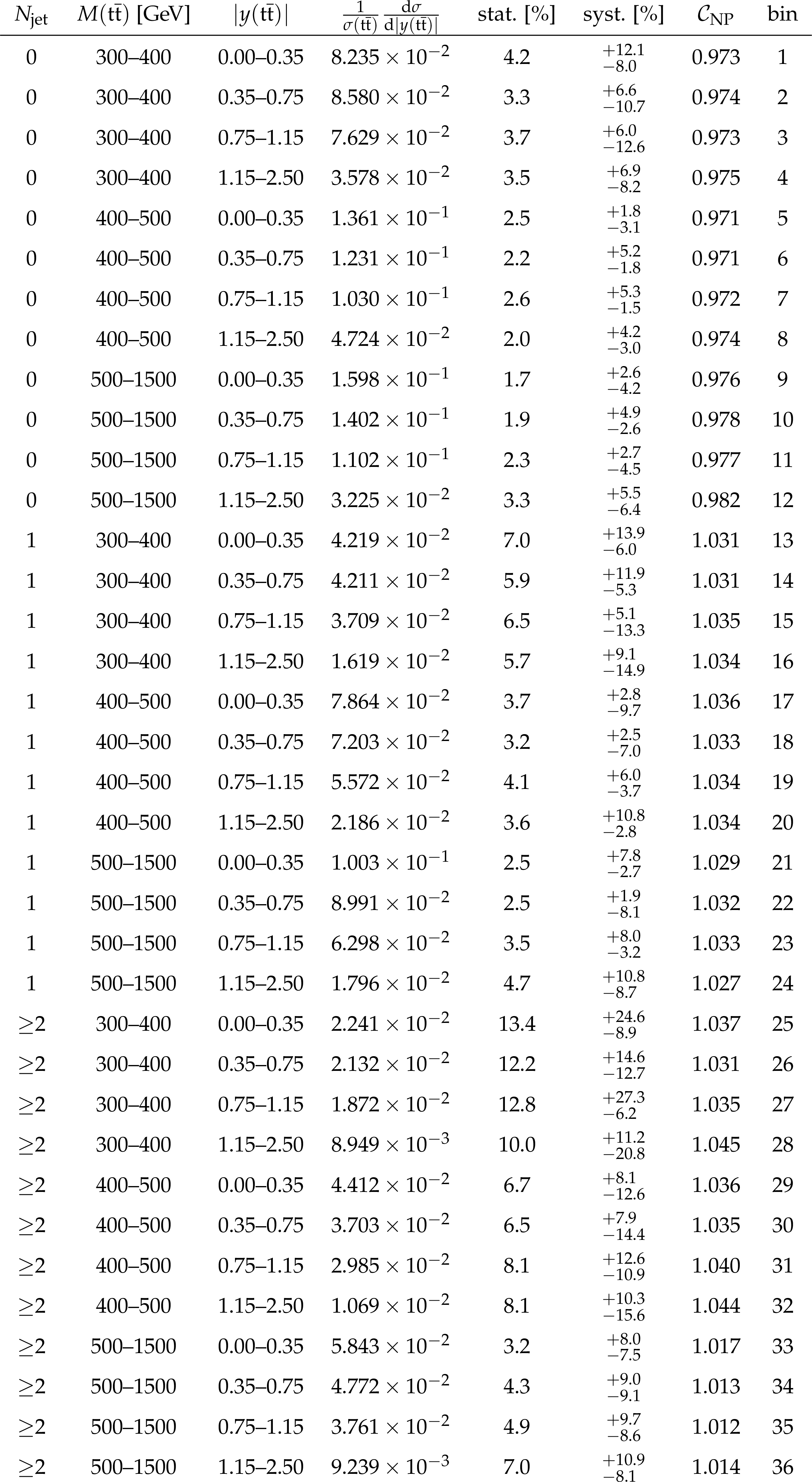
The measured [ ${N^{0,1+}_{\text {jet}}}$, ${M({{\mathrm {t}\overline {\mathrm {t}}}})}$, ${y({{\mathrm {t}\overline {\mathrm {t}}}})}$ ] cross sections, along with their relative statistical and systematic uncertainties, and NP corrections (see Section 9). |
png pdf |
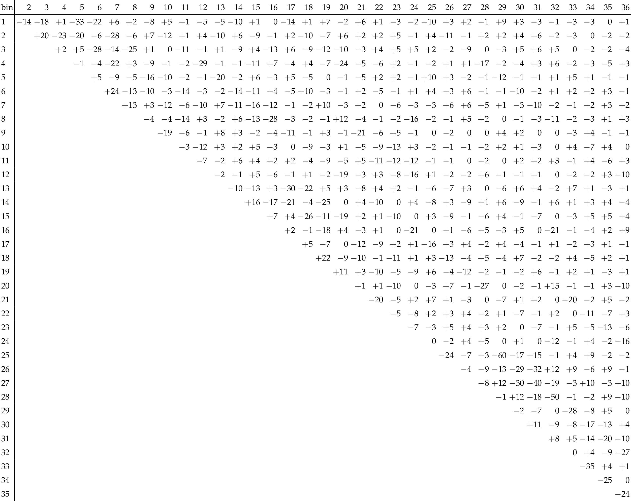
Table A37:
The correlation matrix of statistical uncertainties for the measured [ ${N^{0,1+}_{\text {jet}}}$, ${M({{\mathrm {t}\overline {\mathrm {t}}}})}$, ${y({{\mathrm {t}\overline {\mathrm {t}}}})}$ ] cross sections. The values are expressed as percentages. For bin indices see A.36. |
png pdf |
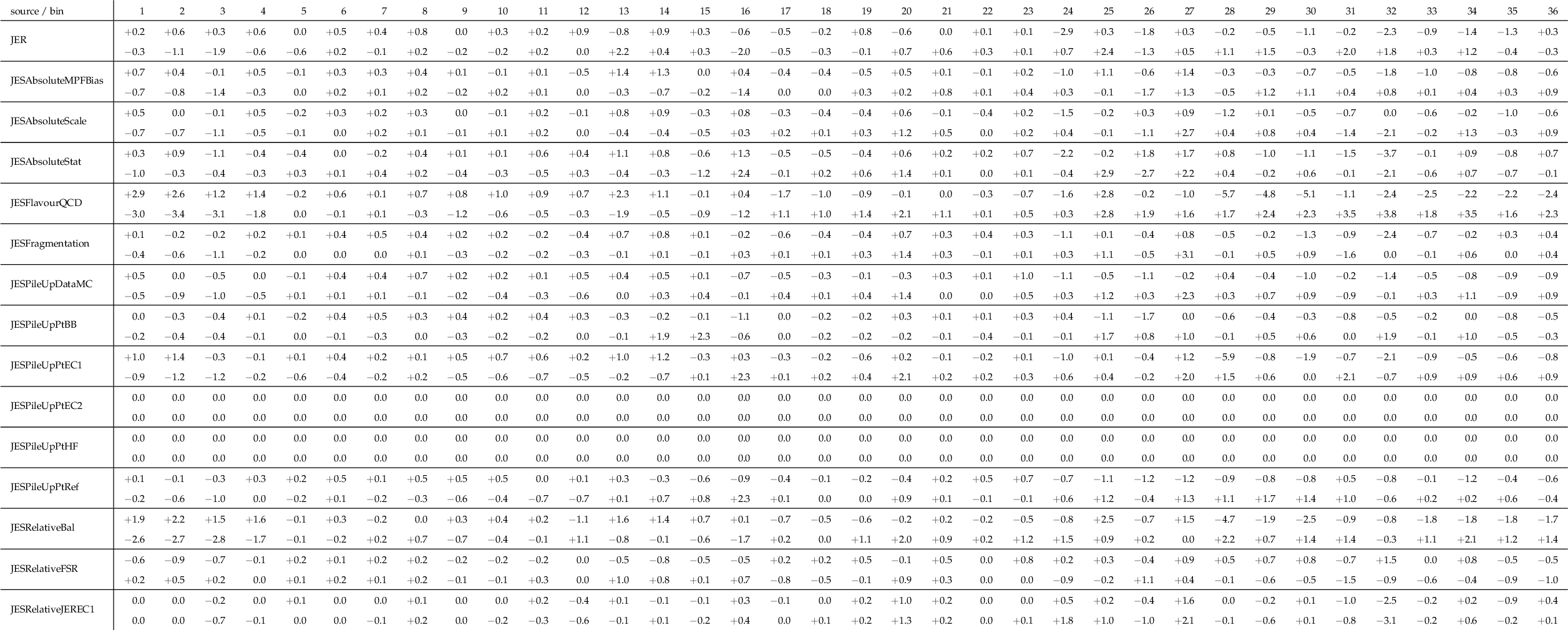
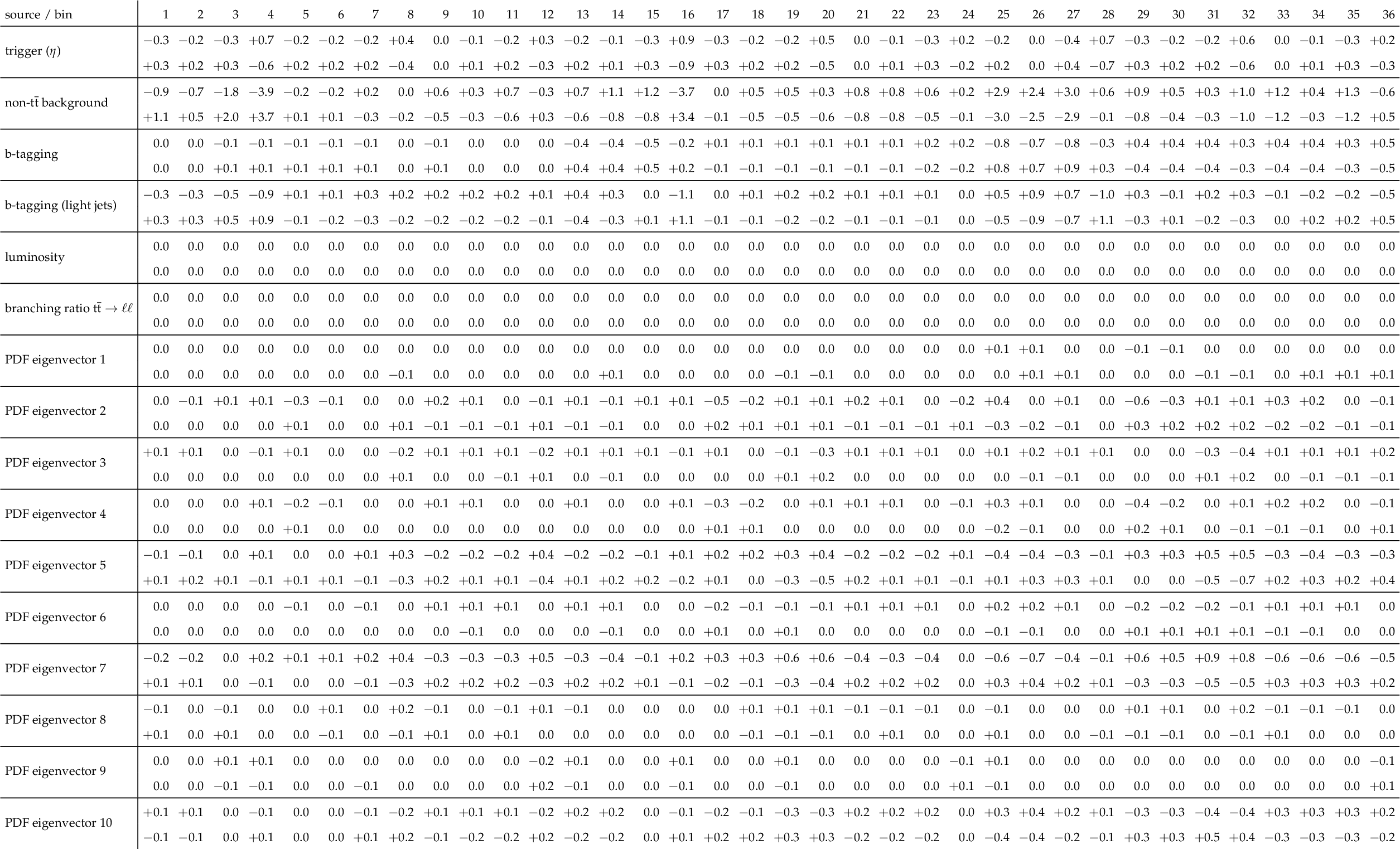
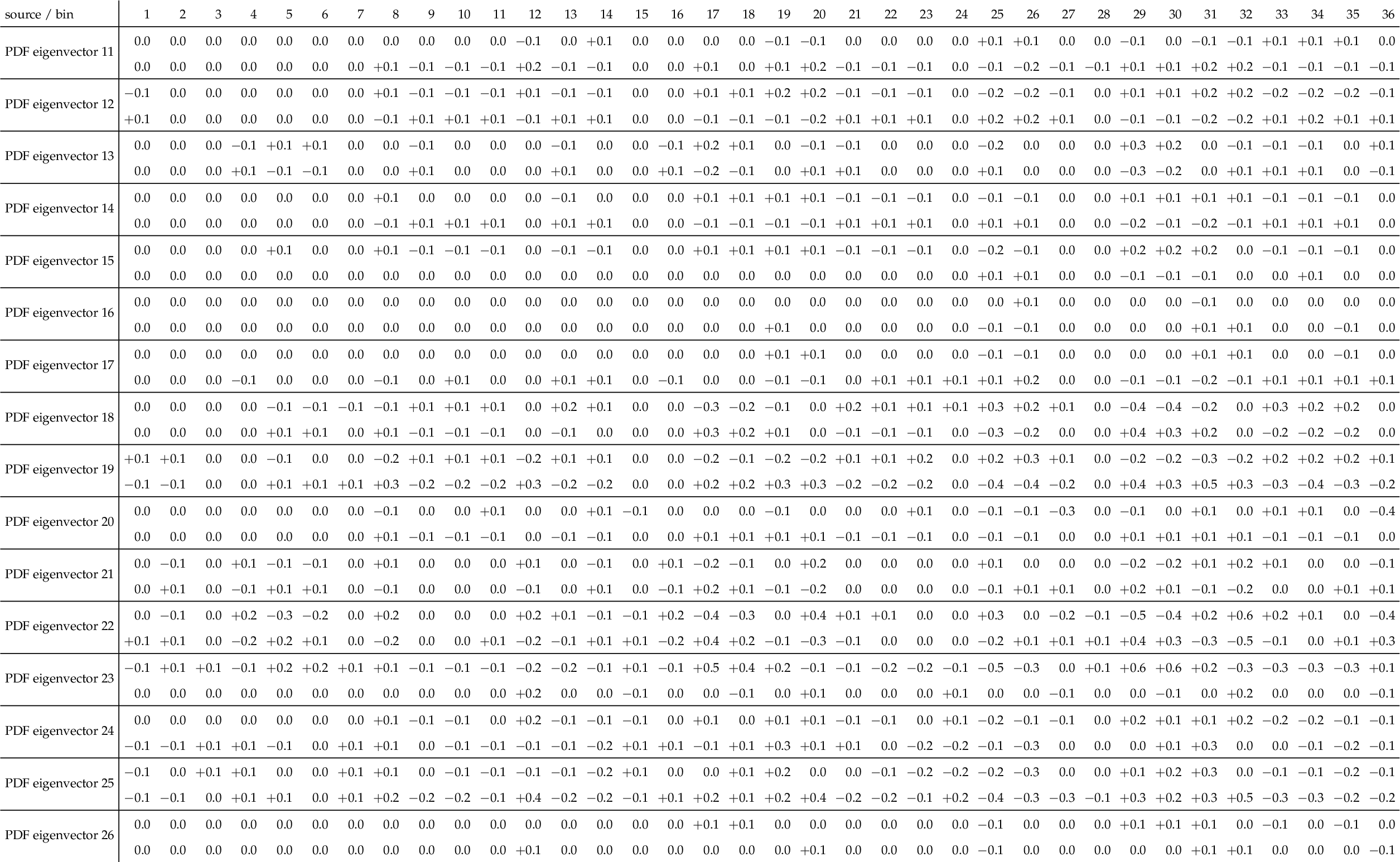
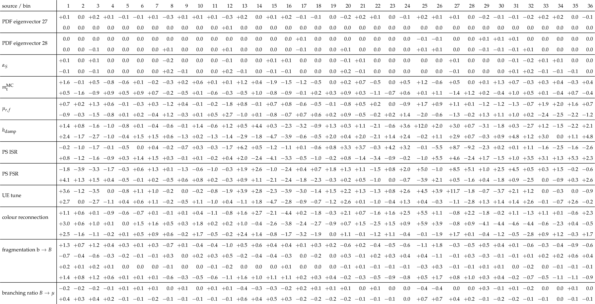
Table A38:
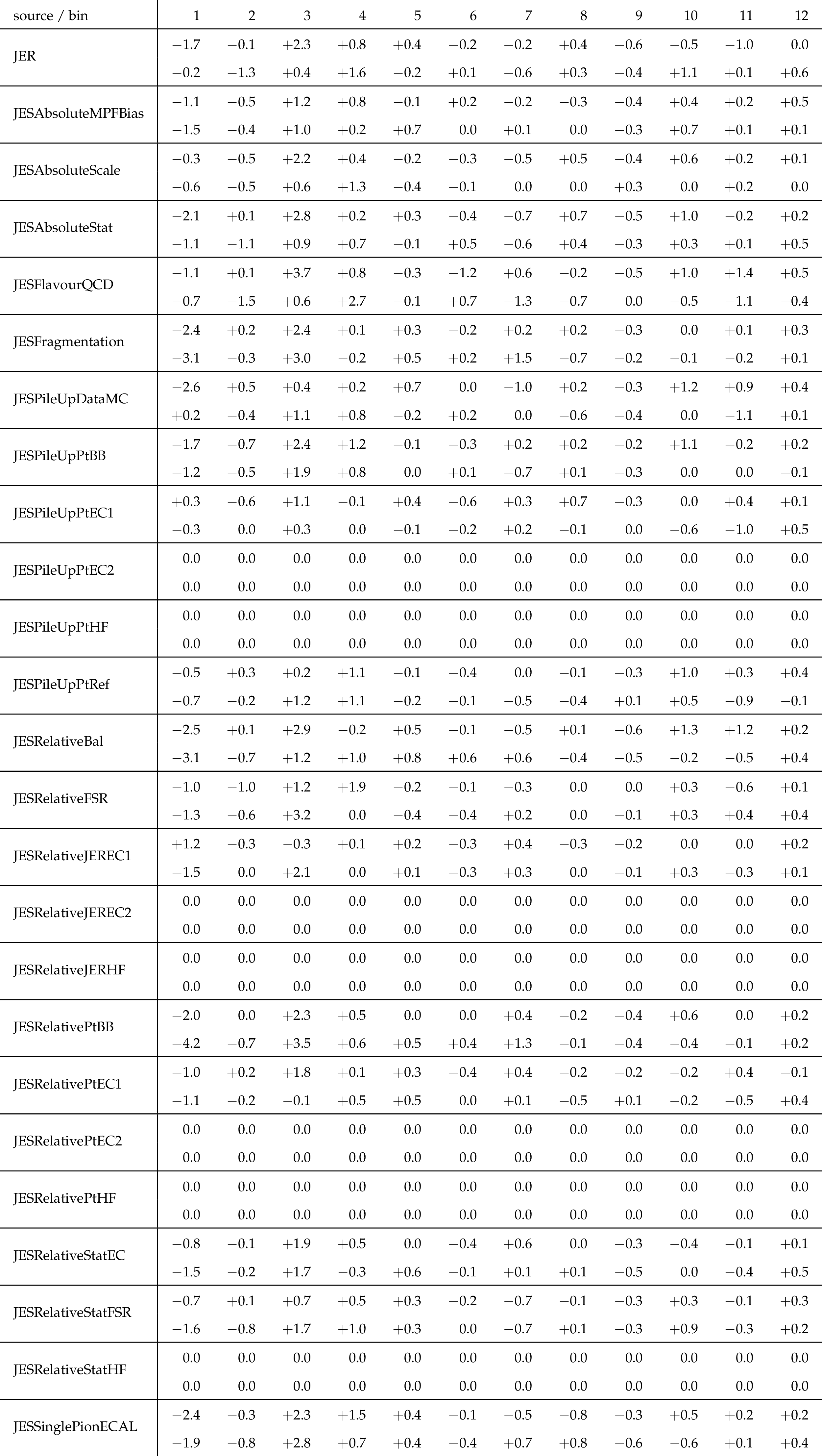
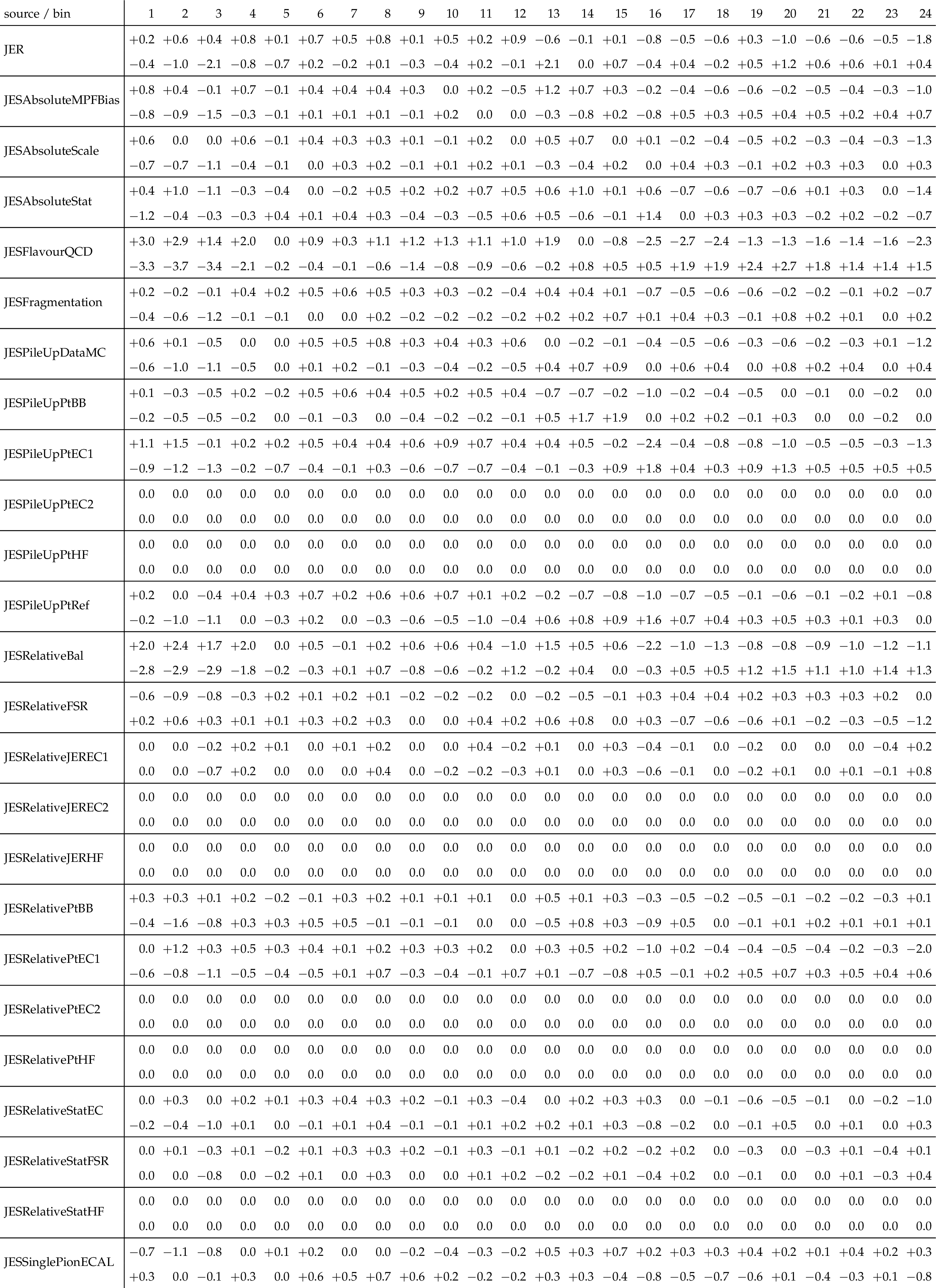
Sources and values of the relative systematic uncertainties in percent of the measured [ ${N^{0,1+}_{\text {jet}}}$, ${M({{\mathrm {t}\overline {\mathrm {t}}}})}$, ${y({{\mathrm {t}\overline {\mathrm {t}}}})}$ ] cross sections. For bin indices see A.36. |
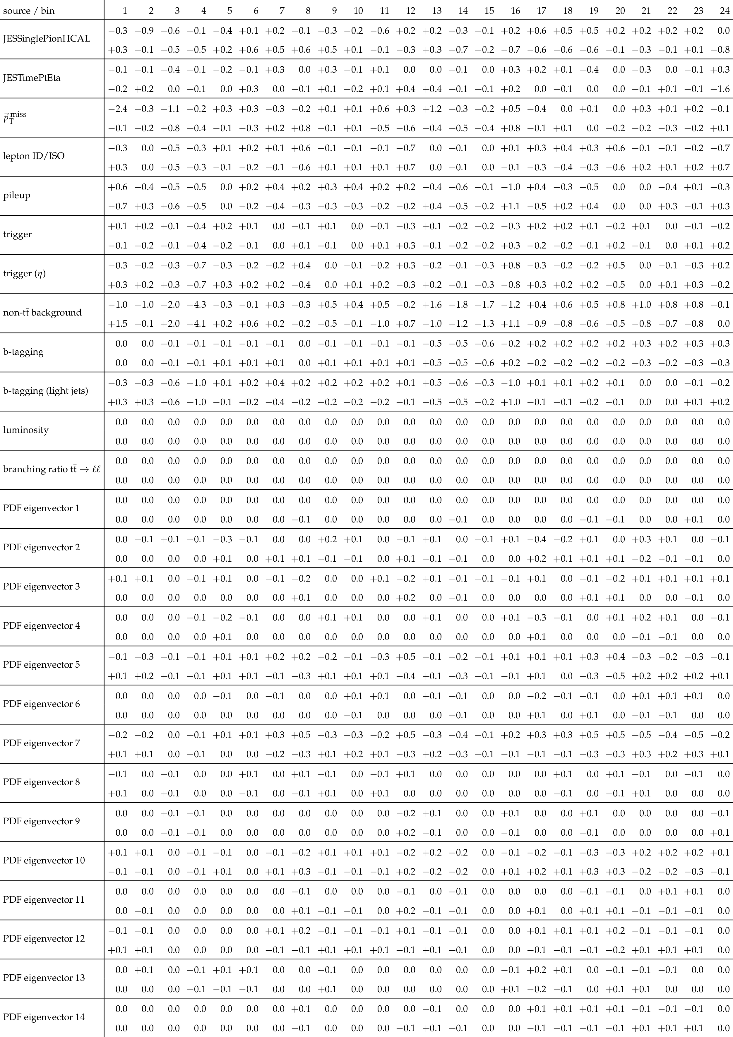
png pdf |
Table A39:
A.38 continued. |

png pdf |
Table A40:
A.38 continued. |
png pdf |
Table A41:
The measured [ ${N^{0,1,2+}_{\text {jet}}}$, ${M({{\mathrm {t}\overline {\mathrm {t}}}})}$, ${y({{\mathrm {t}\overline {\mathrm {t}}}})}$ ] cross sections, along with their relative statistical and systematic uncertainties, and NP corrections (see Section 9). |
png pdf |
Table A42:
The correlation matrix of statistical uncertainties for the measured [ ${N^{0,1,2+}_{\text {jet}}}$, ${M({{\mathrm {t}\overline {\mathrm {t}}}})}$, ${y({{\mathrm {t}\overline {\mathrm {t}}}})}$ ] cross sections. The values are expressed as percentages. For bin indices see A.41. |
png pdf |
Table A43:
Sources and values of the relative systematic uncertainties in percent of the measured [ ${N^{0,1,2+}_{\text {jet}}}$, ${M({{\mathrm {t}\overline {\mathrm {t}}}})}$, ${y({{\mathrm {t}\overline {\mathrm {t}}}})}$ ] cross sections. For bin indices see A.41. |

png pdf |
Table A44:
A.43 continued. |
png pdf |
Table A45:
A.43 continued. |
png pdf |
Table A46:
A.43 continued. |
png pdf |
Table A47:
A.43 continued. |
| Summary |
|
A measurement was presented of normalised multi-differential $\mathrm{t\bar{t}}$ production cross sections in pp collisions at $\sqrt{s} = $ 13 TeV, performed using events containing two oppositely charged leptons (electron or muon). The analysed data were recorded in 2016 with the CMS detector at the LHC, and correspond to an integrated luminosity of 35.9 fb$^{-1}$. The normalised $\mathrm{t\bar{t}}$ cross section is measured in the full phase space as a function of different pairs of kinematic variables that describe either the top quark or the $\mathrm{t\bar{t}}$ system. None of the central predictions of the tested Monte Carlo models is able to correctly describe all the distributions. The data exhibit softer transverse momentum ${p_{\mathrm{T}}}(t)$ distributions than given by the theoretical predictions, as was reported in previous single-differential and double-differential $\mathrm{t\bar{t}}$ cross section measurements. The effect of the softer ${p_{\mathrm{T}}}(t)$ spectra in the data relative to the predictions is enhanced at larger values of the invariant mass of the $\mathrm{t\bar{t}}$ system. {The predicted ${p_{\mathrm{T}}}(t)$ slopes are strongly sensitive to the parton distribution functions (PDFs) and the top quark pole mass $m_{\mathrm{t}}^{\text{pole}}$ value used in the calculations, and the description of the data can be improved by changing these parameters. The measured $\mathrm{t\bar{t}}$ cross sections as a function of the invariant mass and rapidity of the $\mathrm{t\bar{t}}$ system, and the multiplicity of additional jets, have been incorporated into two specific fits of QCD parameters at next-to-leading order, after applying corrections for nonperturbative effects, together with the inclusive deep inelastic scattering data from HERA. When fitting only $\alpha_S$ and $m_{\mathrm{t}}^{\text{pole}}$ to the data, using external PDFs, the two parameters are determined with high accuracy and rather weak correlation between them, however, the extracted $\alpha_S$ values depend on the PDF set. In a simultaneous fit of $\alpha_S$, $m_{\mathrm{t}}^{\text{pole}}$, and PDFs, the inclusion of the new multi-differential $\mathrm{t\bar{t}}$ measurements has a significant impact on the extracted gluon PDF at large values of $x$, where $x$ is the fraction of the proton momentum carried by a parton, and at the same time allows an accurate determination of $\alpha_S$ and $m_{\mathrm{t}}^{\text{pole}}$. |
| References | ||||
| 1 | M. Czakon, M. L. Mangano, A. Mitov, and J. Rojo | Constraints on the gluon PDF from top quark pair production at hadron colliders | JHEP 07 (2013) 167 | 1303.7215 |
| 2 | M. Guzzi, K. Lipka, and S. Moch | Top-quark pair production at hadron colliders: differential cross section and phenomenological applications with DiffTop | JHEP 01 (2015) 082 | 1406.0386 |
| 3 | M. Czakon et al. | Pinning down the large-x gluon with NNLO top-quark pair differential distributions | JHEP 04 (2017) 044 | 1611.08609 |
| 4 | V. A. Novikov et al. | Charmonium and Gluons: Basic Experimental Facts and Theoretical Introduction | PR 41 (1978) 1 | |
| 5 | R. Tarrach | The Pole Mass in Perturbative QCD | NPB 183 (1981) 384 | |
| 6 | M. C. Smith and S. S. Willenbrock | Top quark pole mass | PRL 79 (1997) 3825 | hep-ph/9612329 |
| 7 | S. Alioli et al. | A new observable to measure the top-quark mass at hadron colliders | EPJC 73 (2013) 2438 | 1303.6415 |
| 8 | CDF Collaboration | First measurement of the $ {{\rm t}{\bar {\rm t}}} $ differential cross section $ d\sigma/dM_{{{\rm t}{\bar {\rm t}}}} $ in $ \rm{{\rm p}{\bar {\rm p}}} $ collisions at $ \sqrt{s} = $ 1.96 TeV | PRL 102 (2009) 222003 | 0903.2850 |
| 9 | D0 Collaboration | Measurement of differential $ \rm{t\bar{t}} $ production cross sections in $ \rm{p\bar{p}} $ collisions | PRD 90 (2014) 092006 | 1401.5785 |
| 10 | ATLAS Collaboration | Measurements of top quark pair relative differential cross-sections with ATLAS in pp collisions at $ \sqrt{s} = $ 7 TeV | EPJC 73 (2013) 2261 | 1207.5644 |
| 11 | CMS Collaboration | Measurement of differential top-quark pair production cross sections in pp collisions at $ \sqrt{s} = $ 7 TeV | EPJC 73 (2013) 2339 | CMS-TOP-11-013 1211.2220 |
| 12 | ATLAS Collaboration | Measurements of normalized differential cross-sections for $ {{\rm t}{\bar {\rm t}}} $ production in pp collisions at $ \sqrt{s} = $ 7 TeV using the ATLAS detector | PRD 90 (2014) 072004 | 1407.0371 |
| 13 | ATLAS Collaboration | Differential top-antitop cross-section measurements as a function of observables constructed from final-state particles using pp collisions at $ \sqrt{s}= $ 7 TeV in the ATLAS detector | JHEP 06 (2015) 100 | 1502.05923 |
| 14 | ATLAS Collaboration | Measurement of top quark pair differential cross-sections in the dilepton channel in pp collisions at $ \sqrt{s} = $ 7 and 8 TeV with ATLAS | PRD 94 (2016) 092003 | 1607.07281 |
| 15 | CMS Collaboration | Measurement of the differential cross section for top quark pair production in pp collisions at $ \sqrt{s} = $ 8 TeV | EPJC 75 (2015) 542 | CMS-TOP-12-028 1505.04480 |
| 16 | ATLAS Collaboration | Measurements of top-quark pair differential cross-sections in the lepton+jets channel in pp collisions at $ \sqrt{s}= $ 8 TeV using the ATLAS detector | EPJC 76 (2016) 538 | 1511.04716 |
| 17 | ATLAS Collaboration | Measurement of the differential cross-section of highly boosted top quarks as a function of their transverse momentum in $ \sqrt{s} = $ 8 TeV proton-proton collisions using the ATLAS detector | PRD 93 (2016) 032009 | 1510.03818 |
| 18 | CMS Collaboration | Measurement of the $ \mathrm{t\bar{t}} $ production cross section in the all-jets final state in pp collisions at $ \sqrt{s}= $ 8 TeV | EPJC 76 (2016) 128 | CMS-TOP-14-018 1509.06076 |
| 19 | CMS Collaboration | Measurement of the integrated and differential $ \mathrm{t \bar{t}} $ production cross sections for high-$ p_{\mathrm{T}} $ top quarks in pp collisions at $ \sqrt{s} = $ 8 TeV | PRD 94 (2016) 072002 | CMS-TOP-14-012 1605.00116 |
| 20 | CMS Collaboration | Measurement of double-differential cross sections for top quark pair production in pp collisions at $ \sqrt{s} = $ 8 TeV and impact on parton distribution functions | EPJC 77 (2017) 459 | CMS-TOP-14-013 1703.01630 |
| 21 | CMS Collaboration | Measurement of differential cross sections for top quark pair production using the lepton+jets final state in proton-proton collisions at 13 TeV | PRD 95 (2017) 092001 | CMS-TOP-16-008 1610.04191 |
| 22 | CMS Collaboration | Measurement of differential cross sections for the production of top quark pairs and of additional jets in lepton+jets events from pp collisions at $ \sqrt{s} = $ 13 TeV | PRD 97 (2018) 112003 | CMS-TOP-17-002 1803.08856 |
| 23 | ATLAS Collaboration | Measurement of jet activity produced in top-quark events with an electron, a muon and two b-tagged jets in the final state in pp collisions at $ \sqrt{s}= $ 13 TeV with the ATLAS detector | EPJC 77 (2017) 220 | 1610.09978 |
| 24 | ATLAS Collaboration | Measurements of top-quark pair differential cross-sections in the e$ \mu $ channel in pp collisions at $ \sqrt{s} = $ 13 TeV using the ATLAS detector | EPJC 77 (2017) 292 | 1612.05220 |
| 25 | CMS Collaboration | Measurement of normalized differential $ \mathrm{t}\overline{\mathrm{t}} $ cross sections in the dilepton channel from pp collisions at $ \sqrt{s}= $ 13 TeV | JHEP 04 (2018) 060 | CMS-TOP-16-007 1708.07638 |
| 26 | CMS Collaboration | Measurements of $ \mathrm{t\overline{t}} $ differential cross sections in proton-proton collisions at $ \sqrt{s}= $ 13 TeV using events containing two leptons | JHEP 02 (2019) 149 | CMS-TOP-17-014 1811.06625 |
| 27 | CMS Collaboration | Measurement of $ \mathrm {t}\overline{\mathrm {t}} $ production with additional jet activity, including b quark jets, in the dilepton decay channel using pp collisions at $ \sqrt{s} = $ 8 TeV | EPJC 76 (2016) 379 | CMS-TOP-12-041 1510.03072 |
| 28 | ATLAS Collaboration | Measurement of jet activity in top quark events using the e$ \mu $ final state with two b-tagged jets in pp collisions at $ \sqrt{s}= $ 8 TeV with the ATLAS detector | JHEP 09 (2016) 074 | 1606.09490 |
| 29 | D0 Collaboration | Determination of the pole and $ \overline{MS} $ masses of the top quark from the $ t\bar{t} $ cross section | PLB 703 (2011) 422 | 1104.2887 |
| 30 | CMS Collaboration | Determination of the top-quark pole mass and strong coupling constant from the $ {\rm t}\bar{{\rm t}} $ production cross section in pp collisions at $ \sqrt{s} = $ 7 TeV | PLB 728 (2014) 496 | CMS-TOP-12-022 1307.1907 |
| 31 | ATLAS Collaboration | Measurement of the $ {\rm t}\bar{{\rm t}} $ production cross-section using e$ \mu $ events with b-tagged jets in pp collisions at $ \sqrt{s} = $ 7 and 8 TeV with the ATLAS detector | EPJC 74 (2014) 3109 | 1406.5375 |
| 32 | D0 Collaboration | Measurement of the inclusive $ {\rm t}\bar{{\rm t}} $ production cross section in $ \rm{p\bar{p}} $ collisions at $ \sqrt{s}= $ 1.96 TeV and determination of the top quark pole mass | PRD 94 (2016) 092004 | 1605.06168 |
| 33 | CMS Collaboration | Measurement of the $ {\rm t}\bar{{\rm t}} $ production cross section in the e$ \mu $ channel in proton-proton collisions at $ \sqrt{s} = $ 7 and 8 TeV | JHEP 08 (2016) 029 | CMS-TOP-13-004 1603.02303 |
| 34 | CMS Collaboration | Measurement of the $ \mathrm{t}\overline{\mathrm{t}} $ production cross section, the top quark mass, and the strong coupling constant using dilepton events in pp collisions at $ \sqrt{s}= $ 13 TeV | Submitted to EPJC | CMS-TOP-17-001 1812.10505 |
| 35 | S. Frixione, P. Nason, and C. Oleari | Matching NLO QCD computations with parton shower simulations: the POWHEG method | JHEP 11 (2007) 070 | 0709.2092 |
| 36 | E. Re | Single-top Wt-channel production matched with parton showers using the POWHEG method | EPJC 71 (2011) 1547 | 1009.2450 |
| 37 | J. Alwall et al. | The automated computation of tree-level and next-to-leading order differential cross sections, and their matching to parton shower simulations | JHEP 07 (2014) 079 | 1405.0301 |
| 38 | T. Sjostrand, S. Mrenna, and P. Z. Skands | PYTHIA 6.4 physics and manual | JHEP 05 (2006) 026 | hep-ph/0603175 |
| 39 | T. Sjostrand et al. | An introduction to PYTHIA 8.2 | CPC 191 (2015) 159 | 1410.3012 |
| 40 | CMS Collaboration | The CMS trigger system | JINST 12 (2017) P01020 | CMS-TRG-12-001 1609.02366 |
| 41 | CMS Collaboration | The CMS experiment at the CERN LHC | JINST 3 (2008) S08004 | CMS-00-001 |
| 42 | NNPDF Collaboration | Unbiased global determination of parton distributions and their uncertainties at NNLO and LO | NPB 855 (2012) 153 | 1107.2652 |
| 43 | Particle Data Group, C. Patrignani et al. | Review of particle physics | CPC 40 (2016) 100001 | |
| 44 | S. Frixione, P. Nason, and G. Ridolfi | A positive-weight next-to-leading-order Monte Carlo for heavy flavour hadroproduction | JHEP 09 (2007) 126 | 0707.3088 |
| 45 | S. Alioli, P. Nason, C. Oleari, and E. Re | A general framework for implementing NLO calculations in shower Monte Carlo programs: the POWHEG BOX | JHEP 06 (2010) 043 | 1002.2581 |
| 46 | CMS Collaboration | Investigations of the impact of the parton shower tuning in PYTHIA in the modelling of $ \mathrm{t\overline{t}} $ at $ \sqrt{s}= $ 8 and 13 TeV | CMS-PAS-TOP-16-021 | CMS-PAS-TOP-16-021 |
| 47 | CMS Collaboration | Event generator tunes obtained from underlying event and multiparton scattering measurements | EPJC 76 (2016) 155 | CMS-GEN-14-001 1512.00815 |
| 48 | P. Skands, S. Carrazza, and J. Rojo | Tuning PYTHIA 8.1: the Monash 2013 Tune | EPJC 74 (2014) 3024 | 1404.5630 |
| 49 | P. Artoisenet, R. Frederix, O. Mattelaer, and R. Rietkerk | Automatic spin-entangled decays of heavy resonances in Monte Carlo simulations | JHEP 03 (2013) 015 | 1212.3460 |
| 50 | R. Frederix and S. Frixione | Merging meets matching in MC@NLO | JHEP 12 (2012) 061 | 1209.6215 |
| 51 | M. Bahr et al. | Herwig++ physics and manual | EPJC 58 (2008) 639 | 0803.0883 |
| 52 | M. H. Seymour and A. Siodmok | Constraining MPI models using $ \sigma_{eff} $ and recent Tevatron and LHC underlying event data | JHEP 10 (2013) 113 | 1307.5015 |
| 53 | S. Alioli, P. Nason, C. Oleari, and E. Re | NLO single-top production matched with shower in $ POWHEG: s $- and $ t $-channel contributions | JHEP 09 (2009) 111 | 0907.4076 |
| 54 | J. Alwall et al. | Comparative study of various algorithms for the merging of parton showers and matrix elements in hadronic collisions | EPJC 53 (2008) 473 | 0706.2569 |
| 55 | N. Kidonakis | Two-loop soft anomalous dimensions for single top quark associated production with $ \mathrm{W^-} $ or $ \mathrm{H^-} $ | PRD 82 (2010) 054018 | hep-ph/1005.4451 |
| 56 | Y. Li and F. Petriello | Combining QCD and electroweak corrections to dilepton production in FEWZ | PRD 86 (2012) 094034 | 1208.5967 |
| 57 | J. M. Campbell, R. K. Ellis, and C. Williams | Vector boson pair production at the LHC | JHEP 07 (2011) 018 | 1105.0020 |
| 58 | M. Czakon and A. Mitov | Top++: a program for the calculation of the top-pair cross-section at hadron colliders | CPC 185 (2014) 2930 | 1112.5675 |
| 59 | S. Dulat et al. | New parton distribution functions from a global analysis of quantum chromodynamics | PRD 93 (2016) 033006 | 1506.07443 |
| 60 | ATLAS Collaboration | Measurement of the inelastic proton-proton cross section at $ \sqrt{s} = $ 13 TeV with the ATLAS detector at the LHC | PRL 117 (2016) 182002 | 1606.02625 |
| 61 | GEANT4 Collaboration | GEANT4---a simulation toolkit | NIMA 506 (2003) 250 | |
| 62 | CMS Collaboration | Particle-flow reconstruction and global event description with the CMS detector | JINST 12 (2017) P10003 | CMS-PRF-14-001 1706.04965 |
| 63 | M. Cacciari, G. P. Salam, and G. Soyez | The catchment area of jets | JHEP 04 (2008) 005 | 0802.1188 |
| 64 | CMS Collaboration | Performance of electron reconstruction and selection with the CMS detector in proton-proton collisions at $ \sqrt{s} = $ 8 TeV | JINST 10 (2015) P06005 | CMS-EGM-13-001 1502.02701 |
| 65 | M. Cacciari, G. P. Salam, and G. Soyez | The anti-$ {k_{\mathrm{T}}} $ jet clustering algorithm | JHEP 04 (2008) 063 | 0802.1189 |
| 66 | M. Cacciari, G. P. Salam, and G. Soyez | FastJet user manual | EPJC 72 (2012) 1896 | 1111.6097 |
| 67 | CMS Collaboration | Jet energy scale and resolution in the CMS experiment in pp collisions at 8 TeV | JINST 12 (2017) P02014 | CMS-JME-13-004 1607.03663 |
| 68 | CMS Collaboration | Identification of heavy-flavour jets with the CMS detector in pp collisions at 13 TeV | JINST 13 (2018) P05011 | CMS-BTV-16-002 1712.07158 |
| 69 | S. Schmitt | TUnfold: an algorithm for correcting migration effects in high energy physics | JINST 7 (2012) T10003 | 1205.6201 |
| 70 | A. N. Tikhonov | Solution of incorrectly formulated problems and the regularization method | Sov. Math. Dokl. 4 (1963) 1035 | |
| 71 | S. Schmitt | Data unfolding methods in high energy physics | EPJWeb Conf. 137 (2017) 11008 | 1611.01927 |
| 72 | CMS Collaboration | Measurement of the Drell-Yan cross section in pp collisions at $ \sqrt{s}= $ 7 TeV | JHEP 10 (2011) 007 | CMS-EWK-10-007 1108.0566 |
| 73 | CMS Collaboration | Measurement of the top quark pair production cross section in proton-proton collisions at $ \sqrt{s} = $ 13 TeV | PRL 116 (2016) 052002 | CMS-TOP-15-003 1510.05302 |
| 74 | CMS Collaboration | CMS luminosity measurements for the 2016 data taking period | CMS-PAS-LUM-17-001 | |
| 75 | S. Argyropoulos and T. Sjostrand | Effects of color reconnection on $ {\rm t}\bar{{\rm t}} $ final states at the LHC | JHEP 11 (2014) 043 | 1407.6653 |
| 76 | J. R. Christiansen and P. Z. Skands | String formation beyond leading colour | JHEP 08 (2015) 003 | 1505.01681 |
| 77 | M. G. Bowler | $ {\rm e}^{+}{\rm e}^{-} $ Production of heavy quarks in the string model | Z. Phys. C 11 (1981) 169 | |
| 78 | C. Peterson, D. Schlatter, I. Schmitt, and P. M. Zerwas | Scaling violations in inclusive $ {{\rm e}}^{+}{{\rm e}}^{{-}} $ annihilation spectra | PRD 27 (1983) 105 | |
| 79 | M. L. Mangano, P. Nason, and G. Ridolfi | Heavy quark correlations in hadron collisions at next-to-leading order | NPB 373 (1992) 295 | |
| 80 | S. Dittmaier, P. Uwer, and S. Weinzierl | NLO QCD corrections to $ {\rm t}\bar{{\rm t}} $+jet production at hadron colliders | PRL 98 (2007) 262002 | hep-ph/0703120 |
| 81 | G. Bevilacqua, M. Czakon, C. G. Papadopoulos, and M. Worek | Dominant QCD Backgrounds in Higgs Boson Analyses at the LHC: A Study of pp $ \to {\rm t}\bar{{\rm t}} $ + 2 jets at Next-To-Leading Order | PRL 104 (2010) 162002 | 1002.4009 |
| 82 | G. Bevilacqua, M. Czakon, C. G. Papadopoulos, and M. Worek | Hadronic top-quark pair production in association with two jets at Next-to-Leading Order QCD | PRD 84 (2011) 114017 | 1108.2851 |
| 83 | S. Hoche et al. | Next-to-leading order QCD predictions for top-quark pair production with up to three jets | EPJC 77 (2017) 145 | 1607.06934 |
| 84 | M. Czakon, D. Heymes, and A. Mitov | High-precision differential predictions for top-quark pairs at the LHC | PRL 116 (2016) 082003 | 1511.00549 |
| 85 | M. Czakon, D. Heymes, and A. Mitov | Dynamical scales for multi-TeV top-pair production at the LHC | JHEP 04 (2017) 071 | 1606.03350 |
| 86 | S. Alekhin, J. Blumlein, and S. Moch | NLO PDFs from the ABMP16 fit | EPJC 78 (2018) 477 | 1803.07537 |
| 87 | A. Accardi et al. | Constraints on large-$ x $ parton distributions from new weak boson production and deep-inelastic scattering data | PRD 93 (2016) 114017 | 1602.03154 |
| 88 | H1, ZEUS Collaboration | Combination of measurements of inclusive deep inelastic $ {e^{\pm}p} $ scattering cross sections and QCD analysis of HERA data | EPJC 75 (2015) 580 | 1506.06042 |
| 89 | P. Jimenez-Delgado and E. Reya | Delineating parton distributions and the strong coupling | PRD 89 (2014) 074049 | 1403.1852 |
| 90 | L. A. Harland-Lang, A. D. Martin, P. Motylinski, and R. S. Thorne | Parton distributions in the LHC era: MMHT 2014 PDFs | EPJC 75 (2015) 204 | 1412.3989 |
| 91 | NNPDF Collaboration | Parton distributions from high-precision collider data | EPJC 77 (2017) 663 | 1706.00428 |
| 92 | A. Buckley et al. | $ \lhapdf6: $ parton density access in the LHC precision era | EPJC 75 (2015) 132 | 1412.7420 |
| 93 | M. Cacciari et al. | Updated predictions for the total production cross sections of top and of heavier quark pairs at the Tevatron and at the LHC | JHEP 09 (2008) 127 | 0804.2800 |
| 94 | Particle Data Group, M. Tanabashi et al. | Review of particle physics | PRD 98 (2018) 030001 | |
| 95 | Y. Kiyo et al. | Top-quark pair production near threshold at LHC | EPJC 60 (2009) 375 | 0812.0919 |
| 96 | J. H. Kuhn, A. Scharf, and P. Uwer | Weak Interactions in Top-Quark Pair Production at Hadron Colliders: An Update | PRD 91 (2015) 014020 | 1305.5773 |
| 97 | M. Czakon et al. | Top-pair production at the LHC through NNLO QCD and NLO EW | JHEP 10 (2017) 186 | 1705.04105 |
| 98 | S. Alekhin et al. | HERAFitter | EPJC 75 (2015) 304 | 1410.4412 |
| 99 | Y. L. Dokshitzer | Calculation of the structure functions for deep inelastic scattering and $ {\rm e}^{+}{\rm e}^{-} $ annihilation by perturbation theory in quantum chromodynamics | Sov. Phys. JETP 46 (1977)641 | |
| 100 | V. N. Gribov and L. N. Lipatov | Deep inelastic ep scattering in perturbation theory | Sov. J. NP 15 (1972)438 | |
| 101 | G. Altarelli and G. Parisi | Asymptotic freedom in parton language | NPB 126 (1977) 298 | |
| 102 | G. Curci, W. Furmanski, and R. Petronzio | Evolution of parton densities beyond leading order: the nonsinglet case | NPB 175 (1980) 27 | |
| 103 | W. Furmanski and R. Petronzio | Singlet parton densities beyond leading order | PLB 97 (1980) 437 | |
| 104 | S. Moch, J. A. M. Vermaseren, and A. Vogt | The three-loop splitting functions in QCD: the nonsinglet case | NPB 688 (2004) 101 | hep-ph/0403192 |
| 105 | A. Vogt, S. Moch, and J. A. M. Vermaseren | The three-loop splitting functions in QCD: the singlet case | NPB 691 (2004) 129 | hep-ph/0404111 |
| 106 | M. Botje | QCDNUM: Fast QCD evolution and convolution | CPC 182 (2011) 490 | 1005.1481 |
| 107 | R. S. Thorne and R. G. Roberts | An ordered analysis of heavy flavor production in deep inelastic scattering | PRD 57 (1998) 6871 | hep-ph/9709442 |
| 108 | R. S. Thorne | A variable-flavor number scheme for NNLO | PRD 73 (2006) 054019 | hep-ph/0601245 |
| 109 | R. S. Thorne | Effect of changes of variable flavor number scheme on parton distribution functions and predicted cross sections | PRD 86 (2012) 074017 | 1201.6180 |
| 110 | V. Bertone et al. | aMCfast: automation of fast NLO computations for PDF fits | JHEP 08 (2014) 166 | 1406.7693 |
| 111 | T. Carli et al. | A posteriori inclusion of parton density functions in NLO QCD final-state calculations at hadron colliders: The $ \applgrid $ project | EPJC 66 (2010) 503 | 0911.2985 |
| 112 | A. D. Martin, W. J. Stirling, R. S. Thorne, and G. Watt | Parton distributions for the LHC | EPJC 63 (2009) 189 | 0901.0002 |
| 113 | CMS Collaboration | Measurement of the muon charge asymmetry in inclusive $ \rm{pp} \to \rm{W}+\rm{X} $ production at $ \sqrt s = $ 7 TeV and an improved determination of light parton distribution functions | PRD 90 (2014) 032004 | CMS-SMP-12-021 1312.6283 |
| 114 | H1 Collaboration | Inclusive deep inelastic scattering at high $ Q^2 $ with longitudinally polarised lepton beams at HERA | JHEP 09 (2012) 061 | 1206.7007 |
| 115 | W. T. Giele and S. Keller | Implications of hadron collider observables on parton distribution function uncertainties | PRD 58 (1998) 094023 | hep-ph/9803393 |
| 116 | W. T. Giele, S. A. Keller, and D. A. Kosower | Parton distribution function uncertainties | hep-ph/0104052 | |
|
|
Compact Muon Solenoid LHC, CERN |
|

|

|

|

|

|