

Compact Muon Solenoid
LHC, CERN
| CMS-EXO-22-008 ; CERN-EP-2023-220 | ||
| Search for narrow trijet resonances in proton-proton collisions at $ \sqrt{s} = $ 13 TeV | ||
| CMS Collaboration | ||
| 21 October 2023 | ||
| Submitted to Phys. Rev. Lett. | ||
| Abstract: The first search for narrow resonances decaying to three well-separated hadronic jets is presented. The search uses proton-proton collision data corresponding to an integrated luminosity of 138 fb$ ^{-1} $ at $ \sqrt{s}= $ 13 TeV, collected at the CERN LHC. No significant deviations from the background predictions are observed between 1.75-9.00 TeV. The results provide the first mass limits on a right-handed boson $ \mathrm{Z}_{R} $ decaying to three gluons, an excited quark decaying via a vector boson to three quarks, as well as updated limits on a Kaluza-Klein gluon decaying via a radion to three gluons. | ||
| Links: e-print arXiv:2310.14023 [hep-ex] (PDF) ; CDS record ; inSPIRE record ; HepData record ; Physics Briefing ; CADI line (restricted) ; | ||
| Figures | Summary | Additional Figures | References | CMS Publications |
|---|
| Figures | |
png pdf |
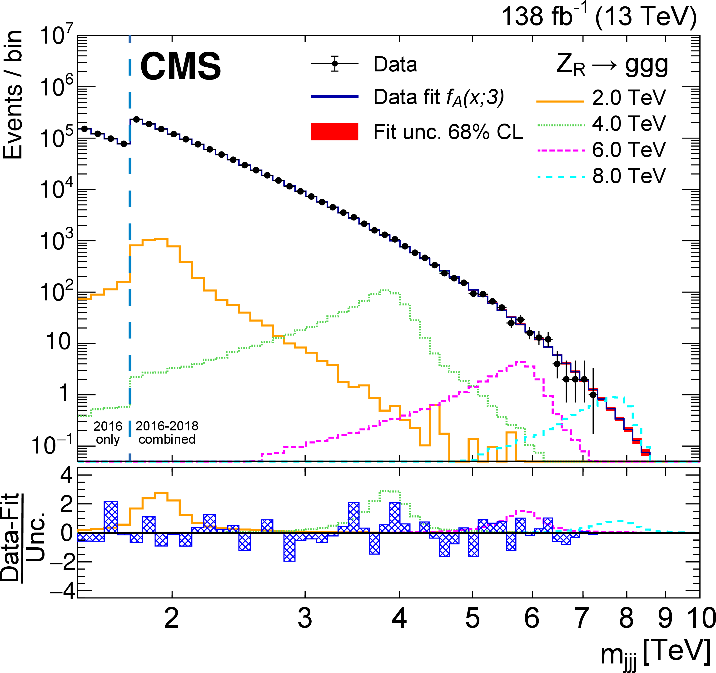
Figure 1:
The observed $ m_{\mathrm{jjj}} $ distribution and the background-only fit to the data using the $ f_A $ fit function. Uncertainties in the fit that correspond to the 68% confidence level are depicted with the red band. The expected $ m_{\mathrm{jjj}} $ distributions for $ \mathrm{Z}_{R} $ signal masses of 2.0, 4.0, 6.0, and 8.0 TeV, with nominal width of $ {\sim} 3% $, are also shown. For illustration purposes, the normalizations correspond to $ \sigma\mathcal{B} $ values of 200, 50, 20, and 20 fb, respectively. Only 2016 data are shown for $ m_{\mathrm{jjj}} < $ 1.76 TeV because of the higher trigger thresholds in 2017 and 2018. In the bottom panel, the blue hatched bars show the difference between the observed data and the background prediction divided by the statistical uncertainty, along with expectations for the example $ \mathrm{Z}_{R} $ signal points. |
png pdf |
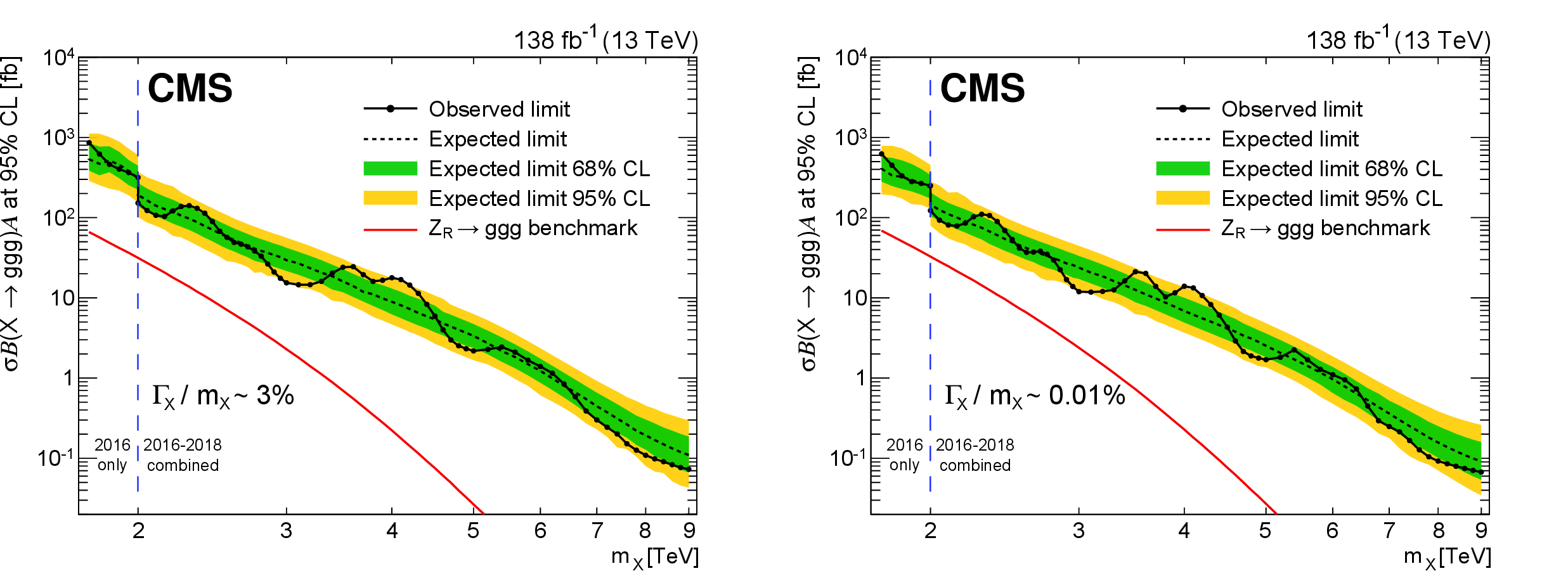
Figure 2:
Limits at 95% CL on $ \sigma\mathcal{B}(\mathrm{X}\to\mathrm{g}\mathrm{g}\mathrm{g})\mathcal{A} $ for the nominal (left) and narrow-width (right) scenarios. Only 2016 data are used to derive limits below 2.0 TeV because of the higher trigger thresholds in 2017 and 2018. Theoretical predictions assuming SM-like couplings are depicted with red curves. |
png pdf |
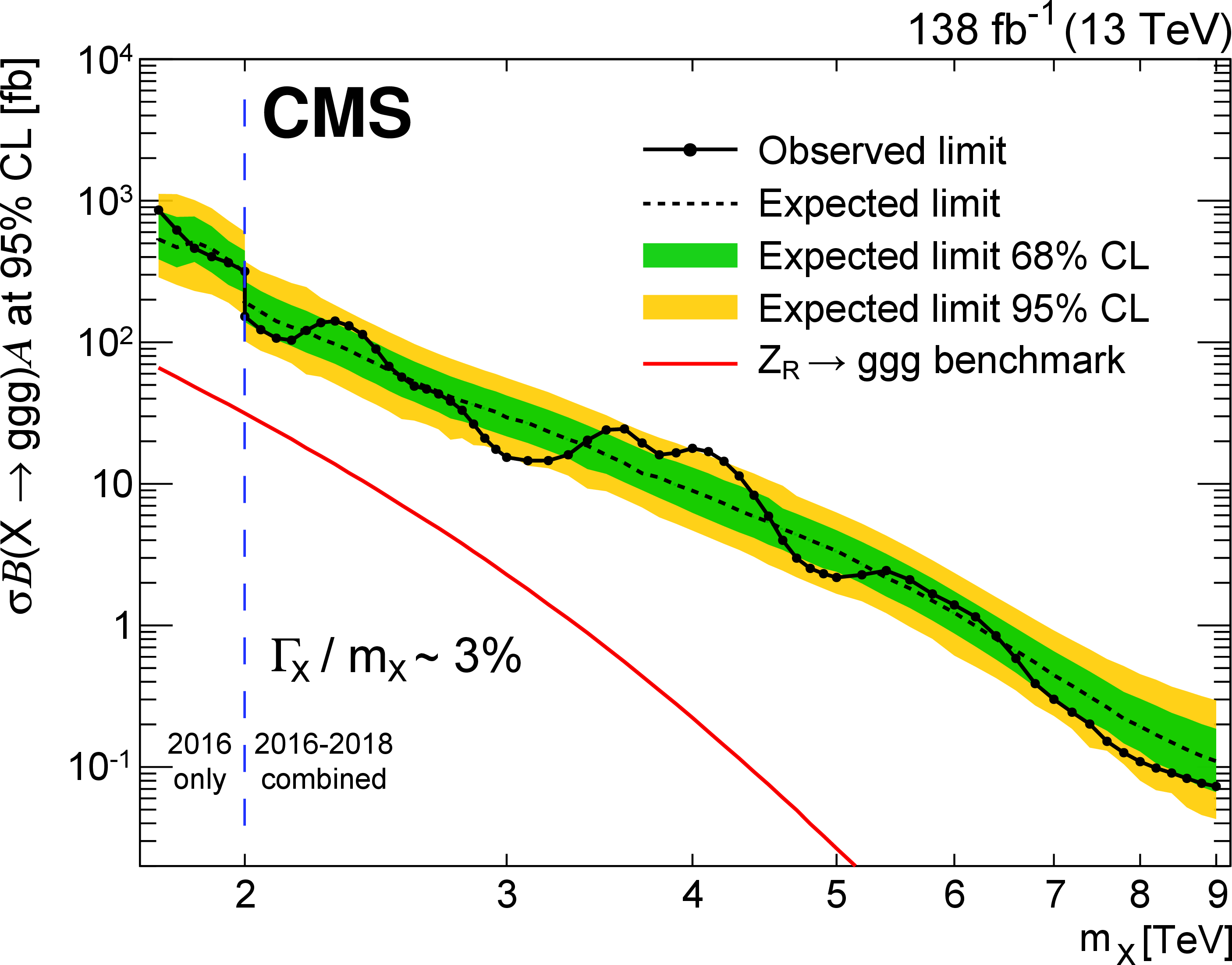
Figure 2-a:
Limits at 95% CL on $ \sigma\mathcal{B}(\mathrm{X}\to\mathrm{g}\mathrm{g}\mathrm{g})\mathcal{A} $ for the nominal scenario. Only 2016 data are used to derive limits below 2.0 TeV because of the higher trigger thresholds in 2017 and 2018. Theoretical predictions assuming SM-like couplings are depicted with red curves. |
png pdf |
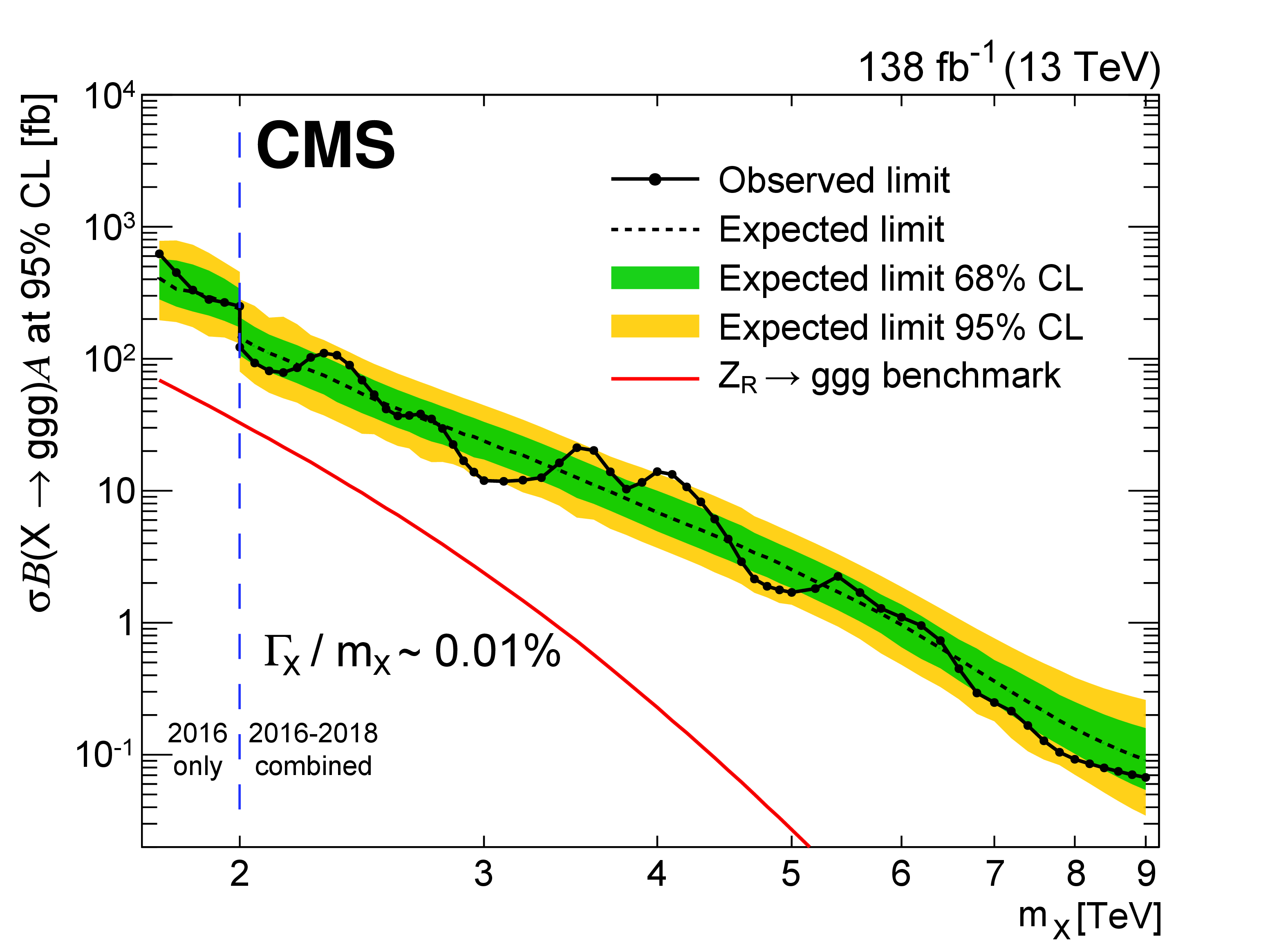
Figure 2-b:
Limits at 95% CL on $ \sigma\mathcal{B}(\mathrm{X}\to\mathrm{g}\mathrm{g}\mathrm{g})\mathcal{A} $ for the narrow-width scenario. Only 2016 data are used to derive limits below 2.0 TeV because of the higher trigger thresholds in 2017 and 2018. Theoretical predictions assuming SM-like couplings are depicted with red curves. |
png pdf |
Figure 3:
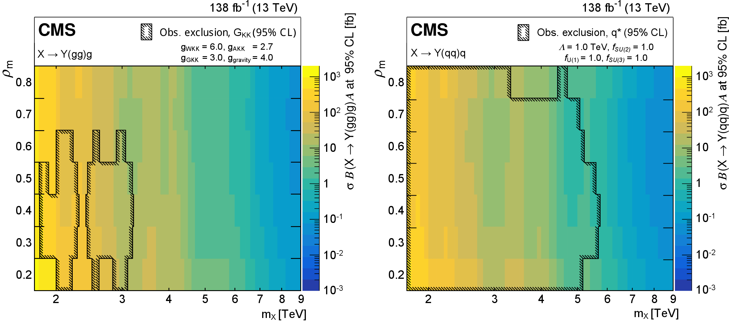
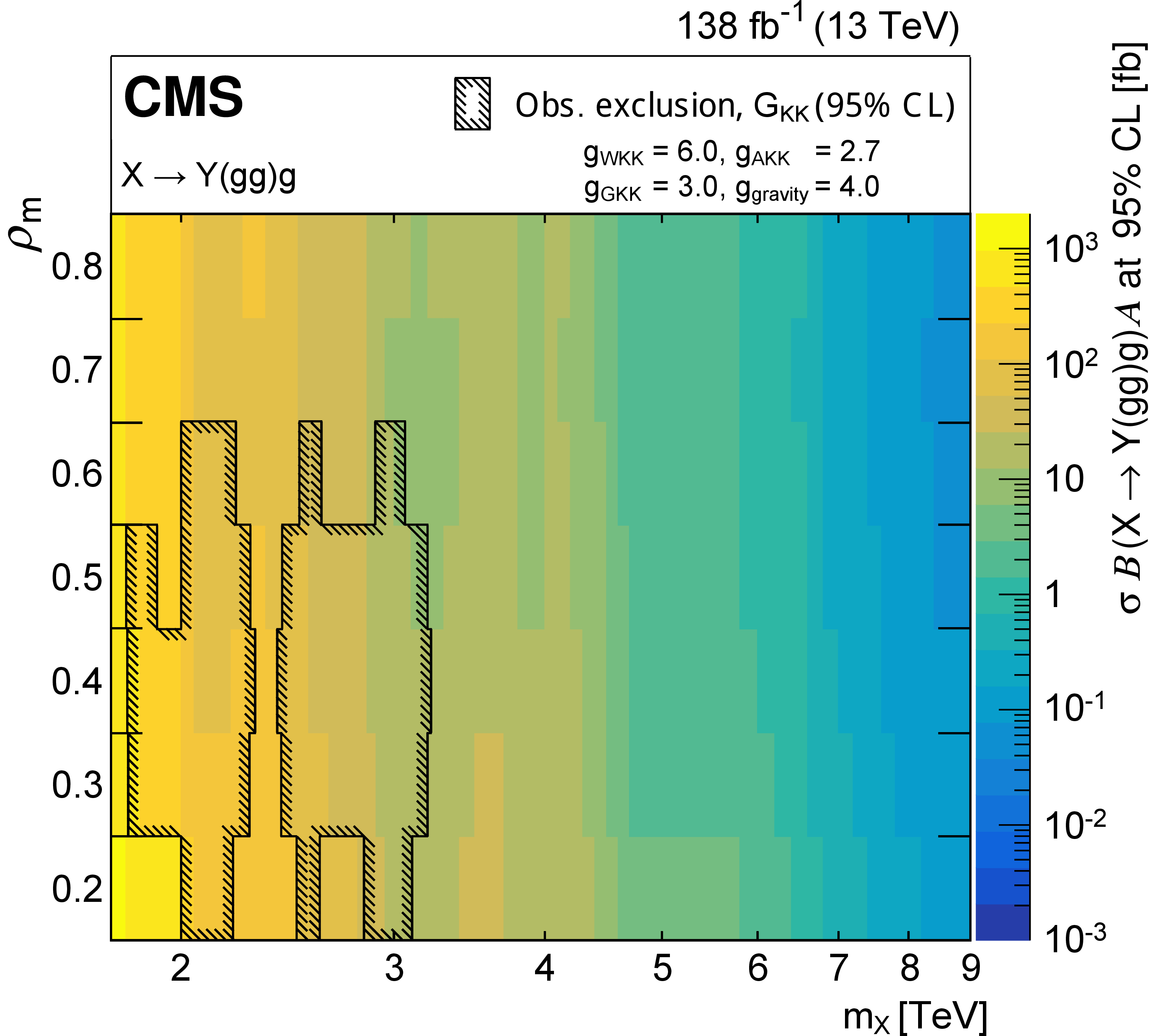
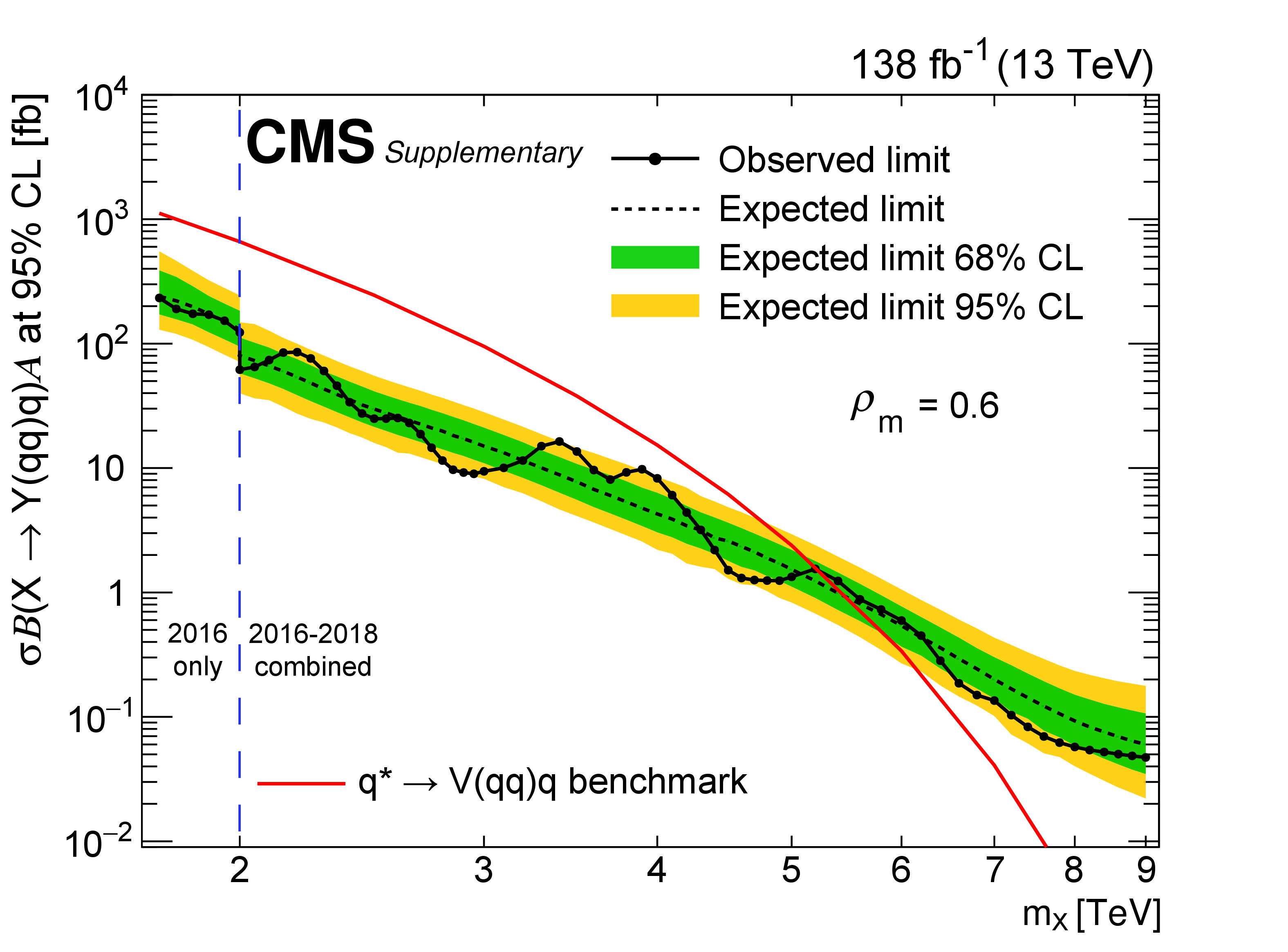
Observed limits at 95% CL as a function of $ m_{\mathrm{X}} $ and $ \rho_{\mathrm{m}} $ on $ \sigma\mathcal{B}(\mathrm{X}\to{\mathrm{Y}}(\mathrm{g}\mathrm{g})\mathrm{g})\mathcal{A} $ (left) and $ \sigma\mathcal{B}(\mathrm{X}\to{\mathrm{Y}}(\mathrm{q}\mathrm{q})\mathrm{q})\mathcal{A} $ (right). Only 2016 data are used to derive limits below 2.0 TeV because of the higher trigger thresholds in 2017 and 2018. The legend shows the model parameters for the chosen benchmark [23,24], and their corresponding mass exclusion ranges are depicted with areas inside the black hatched contours. |
png pdf |
Figure 3-a:
Observed limits at 95% CL as a function of $ m_{\mathrm{X}} $ and $ \rho_{\mathrm{m}} $ on $ \sigma\mathcal{B}(\mathrm{X}\to{\mathrm{Y}}(\mathrm{g}\mathrm{g})\mathrm{g})\mathcal{A} $. Only 2016 data are used to derive limits below 2.0 TeV because of the higher trigger thresholds in 2017 and 2018. The legend shows the model parameters for the chosen benchmark [23], and their corresponding mass exclusion ranges are depicted with areas inside the black hatched contours. |
png pdf |
Figure 3-b:
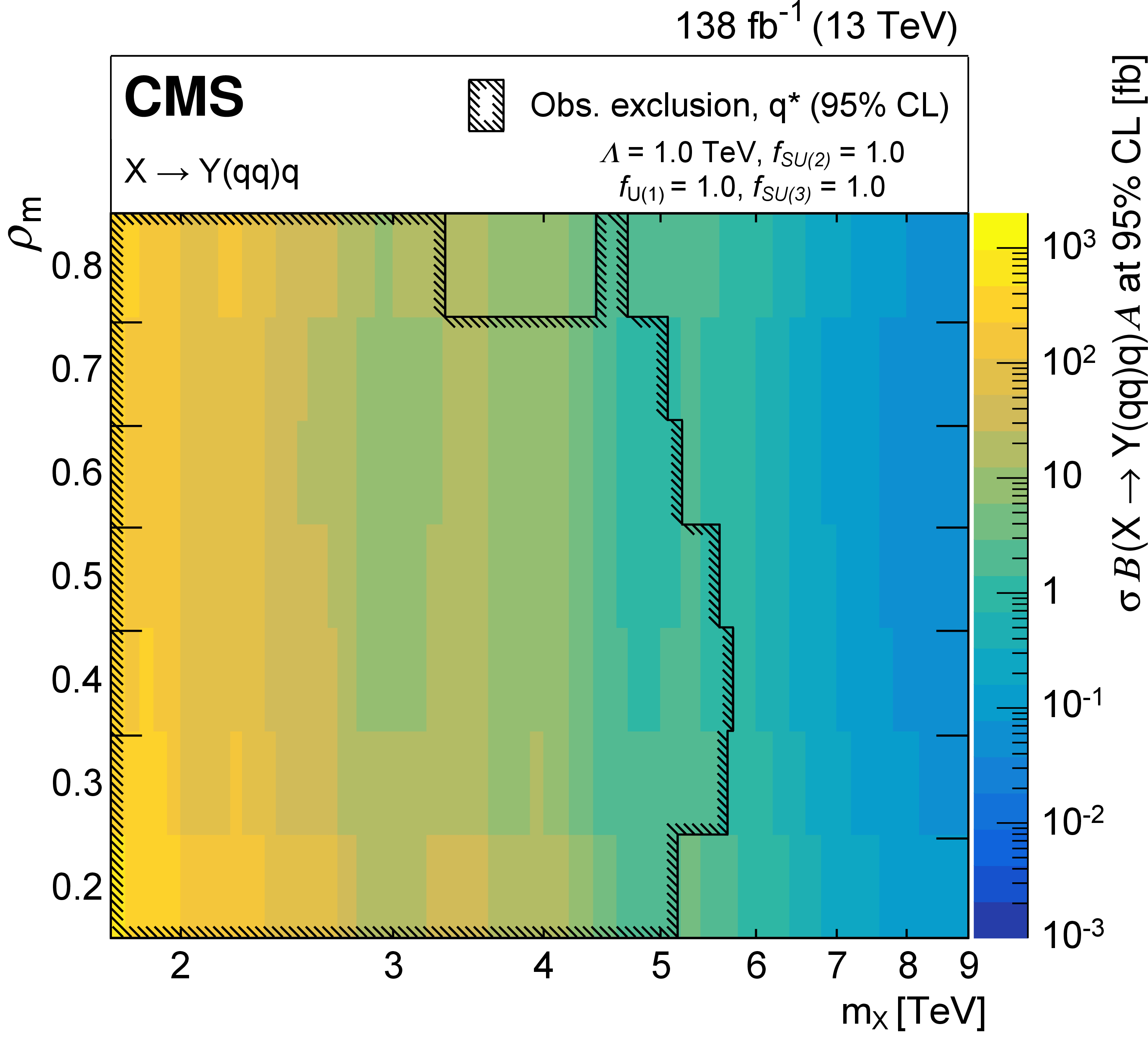
Observed limits at 95% CL as a function of $ m_{\mathrm{X}} $ and $ \rho_{\mathrm{m}} $ on $ \sigma\mathcal{B}(\mathrm{X}\to{\mathrm{Y}}(\mathrm{q}\mathrm{q})\mathrm{q})\mathcal{A} $. Only 2016 data are used to derive limits below 2.0 TeV because of the higher trigger thresholds in 2017 and 2018. The legend shows the model parameters for the chosen benchmark [24], and their corresponding mass exclusion ranges are depicted with areas inside the black hatched contours. |
| Summary |
| In summary, the first generic search for new particles decaying to three hadronic jets has been presented. The search uses proton-proton collision data at $ \sqrt{s}= $ 13 TeV recorded by the CMS experiment in 2016-2018, corresponding to an integrated luminosity of 138 fb$^{-1}$. The three-jet invariant mass spectrum is scanned for narrow peaks corresponding to new particles. No significant excesses above the standard model background expectations are observed. Limits are set on the product of the production cross section, branching fraction, and acceptance to three resolved jets. The results are interpreted in the context of a new right-handed boson $ \mathrm{Z}_{R} $ decaying to three gluons, a Kaluza-Klein gluon $\mathrm{G}_{\mathrm{KK}}$ decaying via an intermediate radion to three gluons ($ \mathrm{g}\mathrm{g}\mathrm{g} $), and an excited quark decaying via a vector boson to three quarks ($ \mathrm{q}\mathrm{q}\mathrm{q} $). This is the first search for the three-body decay of high-mass resonances ($ \mathrm{X} $) into three resolved jets at the LHC, and also the first search for $ \mathrm{X} $ that decays into three resolved jets through an intermediate resonance ($\mathrm{Y}$) with a mass ratio $ m_{{\mathrm{Y}}}/m_{\mathrm{X}} $ between 0.3-0.8 for the $ \mathrm{g}\mathrm{g}\mathrm{g} $ decay mode and 0.2-0.8 for the $ \mathrm{q}\mathrm{q}\mathrm{q} $ decay mode, significantly extending the model parameter space explored by a previous search [20]. |
| Additional Figures | |
png pdf |
Additional Figure 1:
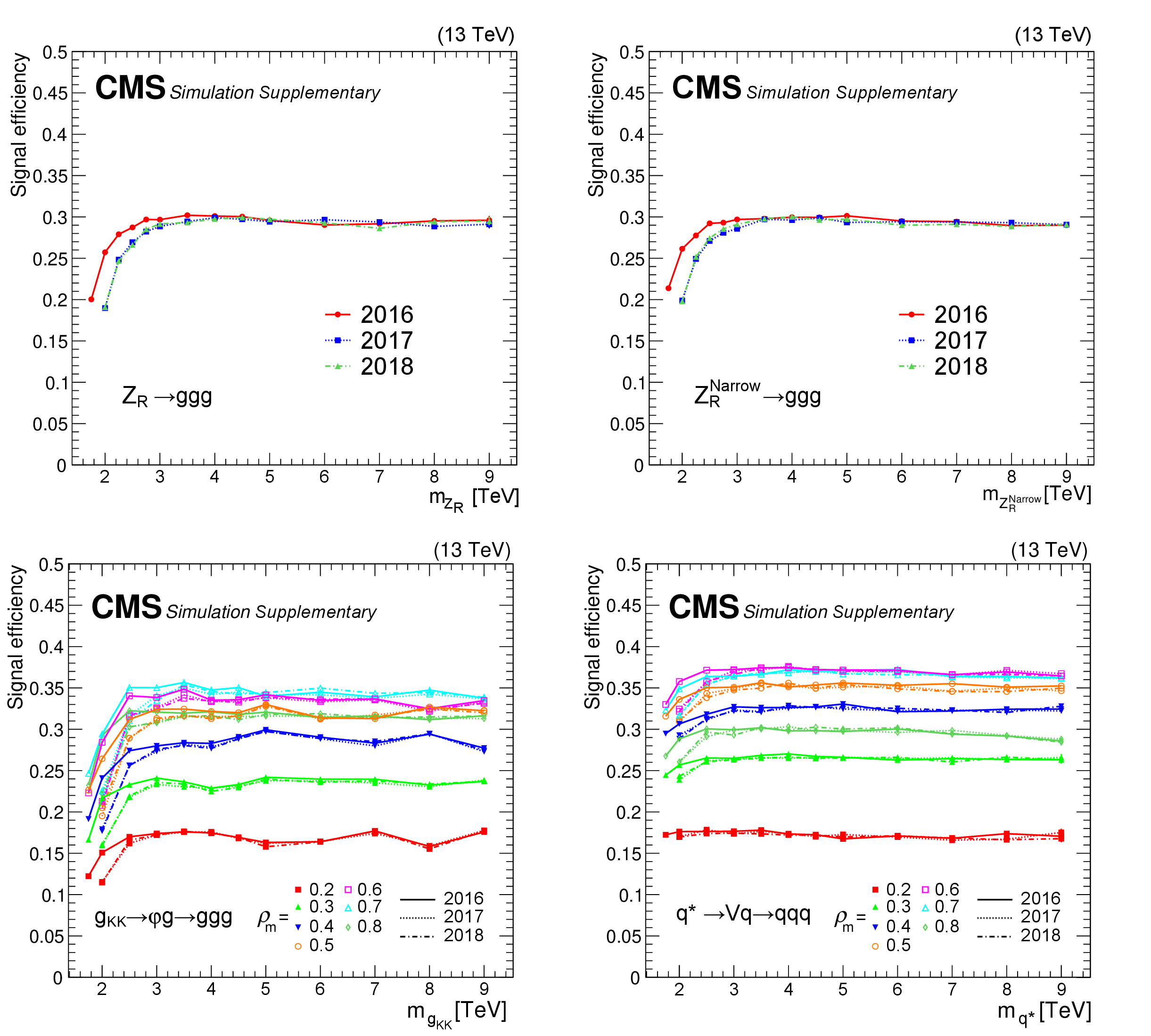
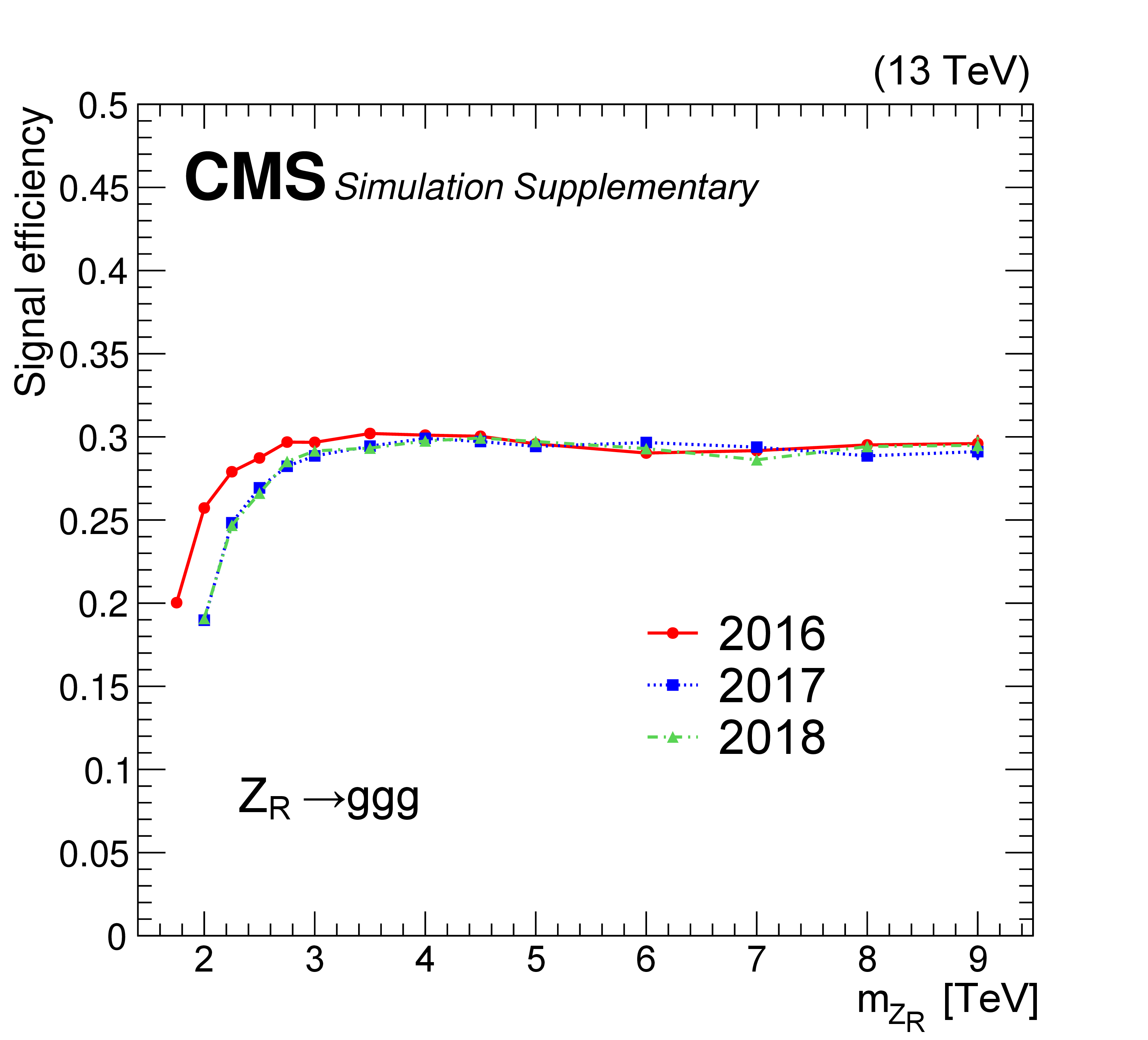
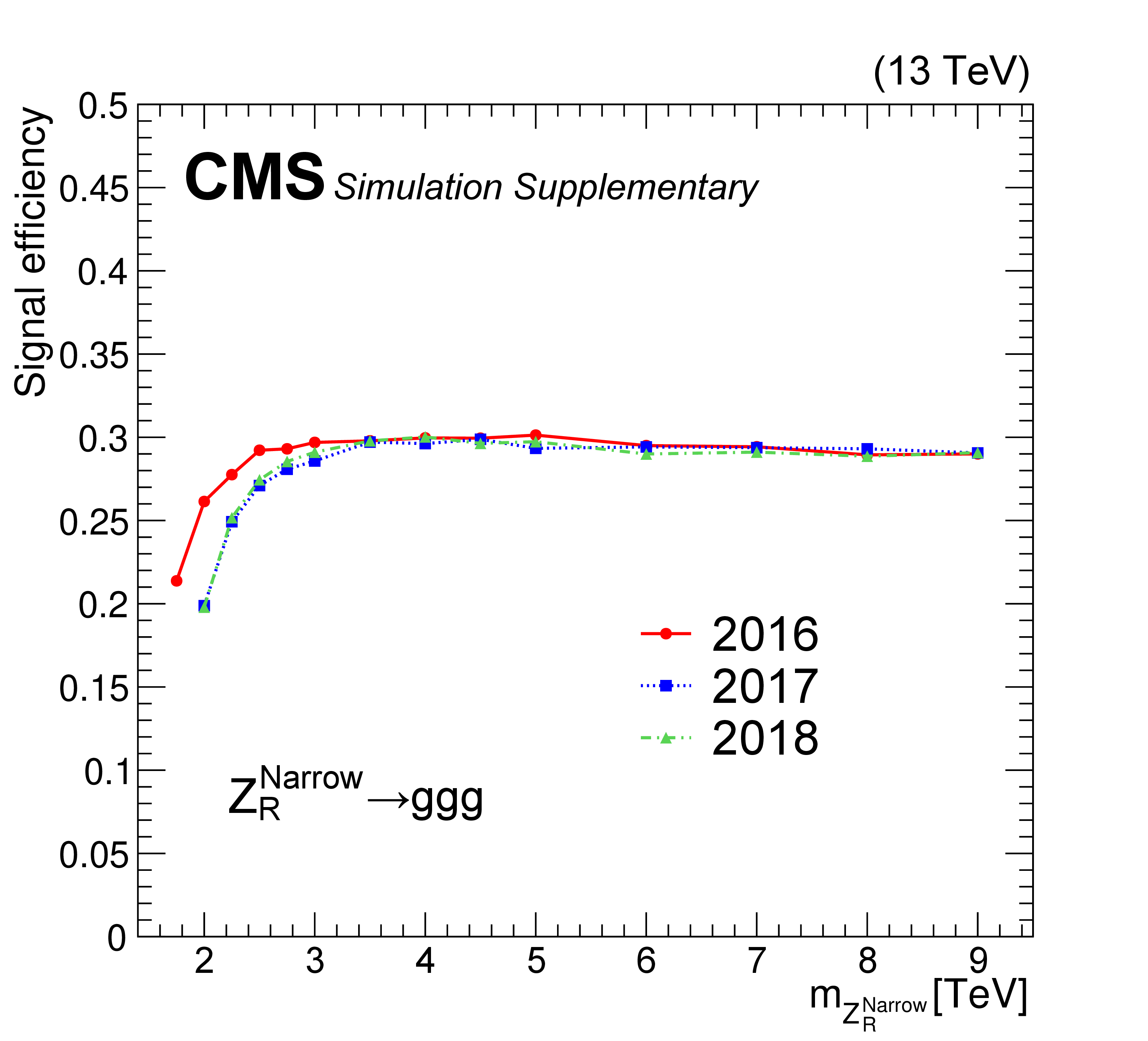
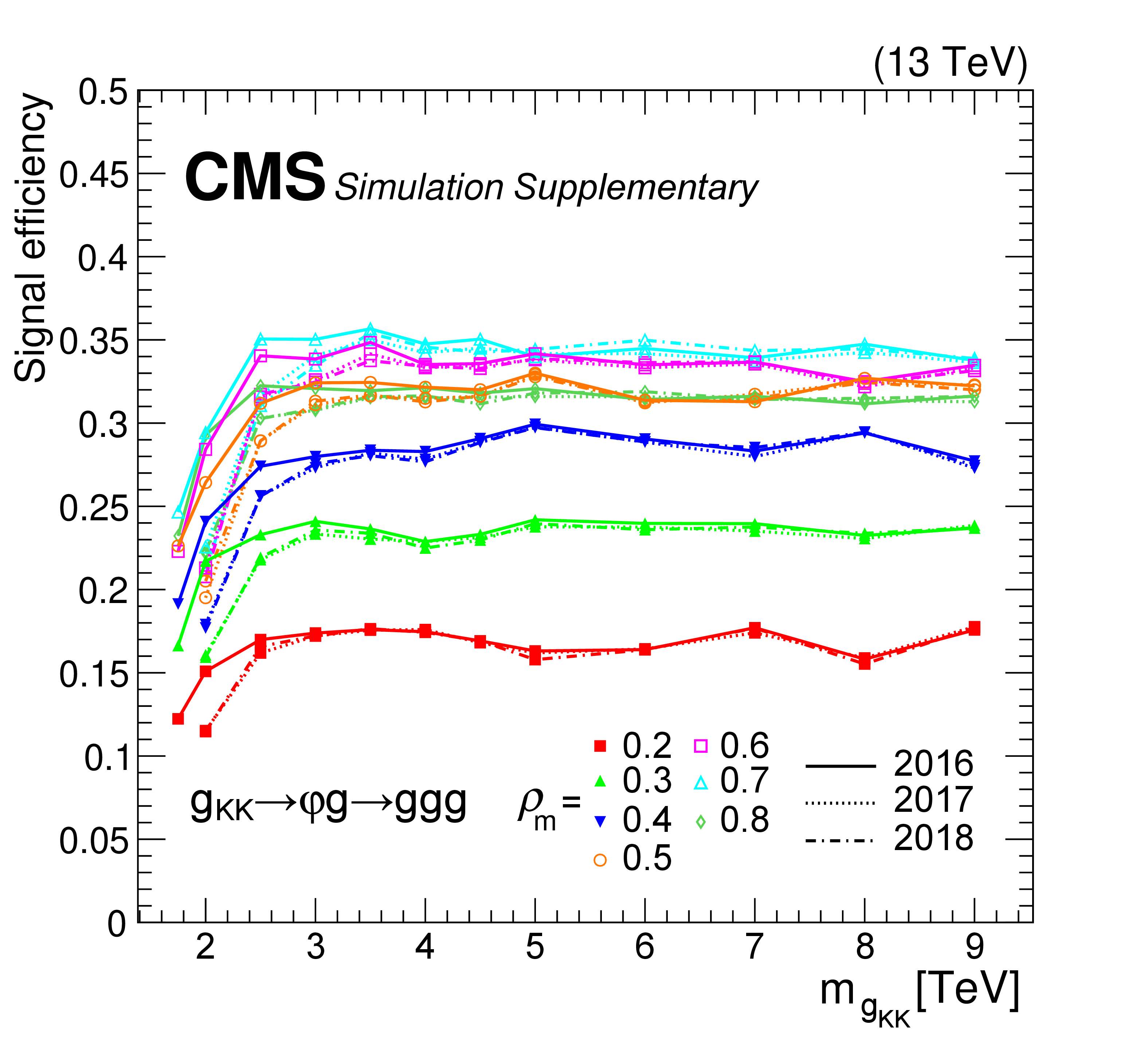
Efficiencies of the selection requirements on the benchmark signal processes: $ \mathrm{Z}_{R}\to\mathrm{g}\mathrm{g}\mathrm{g} $ with nominal width $ \Gamma_{\mathrm{Z}_{R}}/ m_{\mathrm{Z}_{R}}\sim3% $ (top left), $ \mathrm{Z}_{R}\to\mathrm{g}\mathrm{g}\mathrm{g} $ with narrow width $ \Gamma_{\mathrm{Z}_{R}}/ m_{\mathrm{Z}_{R}}\sim0.01% $ (top right), $ g_{\mathrm{KK}} \to\varphi(\mathrm{g}\mathrm{g})\mathrm{g} $ (bottom left), and $ \mathrm{q}^{*}\to \text{V}(\mathrm{q}\mathrm{q})\mathrm{q} $ (bottom right). $ \varphi $ is the radion and V is a beyond-the-SM vector boson. The efficiencies for 2016, 2017, and 2018 data-taking conditions are shown separately. The bottom two figures also show efficiencies for different $ \rho_{m} $ scenarios for cascade decays with intermediate resonances. |
png pdf |
Additional Figure 1-a:
Efficiencies of the selection requirements on the benchmark signal processes: $ \mathrm{Z}_{R}\to\mathrm{g}\mathrm{g}\mathrm{g} $ with nominal width $ \Gamma_{\mathrm{Z}_{R}}/ m_{\mathrm{Z}_{R}}\sim3% $ (top left), $ \mathrm{Z}_{R}\to\mathrm{g}\mathrm{g}\mathrm{g} $ with narrow width $ \Gamma_{\mathrm{Z}_{R}}/ m_{\mathrm{Z}_{R}}\sim0.01% $ (top right), $ g_{\mathrm{KK}} \to\varphi(\mathrm{g}\mathrm{g})\mathrm{g} $ (bottom left), and $ \mathrm{q}^{*}\to \text{V}(\mathrm{q}\mathrm{q})\mathrm{q} $ (bottom right). $ \varphi $ is the radion and V is a beyond-the-SM vector boson. The efficiencies for 2016, 2017, and 2018 data-taking conditions are shown separately. The bottom two figures also show efficiencies for different $ \rho_{m} $ scenarios for cascade decays with intermediate resonances. |
png pdf |
Additional Figure 1-b:
Efficiencies of the selection requirements on the benchmark signal processes: $ \mathrm{Z}_{R}\to\mathrm{g}\mathrm{g}\mathrm{g} $ with nominal width $ \Gamma_{\mathrm{Z}_{R}}/ m_{\mathrm{Z}_{R}}\sim3% $ (top left), $ \mathrm{Z}_{R}\to\mathrm{g}\mathrm{g}\mathrm{g} $ with narrow width $ \Gamma_{\mathrm{Z}_{R}}/ m_{\mathrm{Z}_{R}}\sim0.01% $ (top right), $ g_{\mathrm{KK}} \to\varphi(\mathrm{g}\mathrm{g})\mathrm{g} $ (bottom left), and $ \mathrm{q}^{*}\to \text{V}(\mathrm{q}\mathrm{q})\mathrm{q} $ (bottom right). $ \varphi $ is the radion and V is a beyond-the-SM vector boson. The efficiencies for 2016, 2017, and 2018 data-taking conditions are shown separately. The bottom two figures also show efficiencies for different $ \rho_{m} $ scenarios for cascade decays with intermediate resonances. |
png pdf |
Additional Figure 1-c:
Efficiencies of the selection requirements on the benchmark signal processes: $ \mathrm{Z}_{R}\to\mathrm{g}\mathrm{g}\mathrm{g} $ with nominal width $ \Gamma_{\mathrm{Z}_{R}}/ m_{\mathrm{Z}_{R}}\sim3% $ (top left), $ \mathrm{Z}_{R}\to\mathrm{g}\mathrm{g}\mathrm{g} $ with narrow width $ \Gamma_{\mathrm{Z}_{R}}/ m_{\mathrm{Z}_{R}}\sim0.01% $ (top right), $ g_{\mathrm{KK}} \to\varphi(\mathrm{g}\mathrm{g})\mathrm{g} $ (bottom left), and $ \mathrm{q}^{*}\to \text{V}(\mathrm{q}\mathrm{q})\mathrm{q} $ (bottom right). $ \varphi $ is the radion and V is a beyond-the-SM vector boson. The efficiencies for 2016, 2017, and 2018 data-taking conditions are shown separately. The bottom two figures also show efficiencies for different $ \rho_{m} $ scenarios for cascade decays with intermediate resonances. |

png pdf |
Additional Figure 1-d:
Efficiencies of the selection requirements on the benchmark signal processes: $ \mathrm{Z}_{R}\to\mathrm{g}\mathrm{g}\mathrm{g} $ with nominal width $ \Gamma_{\mathrm{Z}_{R}}/ m_{\mathrm{Z}_{R}}\sim3% $ (top left), $ \mathrm{Z}_{R}\to\mathrm{g}\mathrm{g}\mathrm{g} $ with narrow width $ \Gamma_{\mathrm{Z}_{R}}/ m_{\mathrm{Z}_{R}}\sim0.01% $ (top right), $ g_{\mathrm{KK}} \to\varphi(\mathrm{g}\mathrm{g})\mathrm{g} $ (bottom left), and $ \mathrm{q}^{*}\to \text{V}(\mathrm{q}\mathrm{q})\mathrm{q} $ (bottom right). $ \varphi $ is the radion and V is a beyond-the-SM vector boson. The efficiencies for 2016, 2017, and 2018 data-taking conditions are shown separately. The bottom two figures also show efficiencies for different $ \rho_{m} $ scenarios for cascade decays with intermediate resonances. |
png pdf |
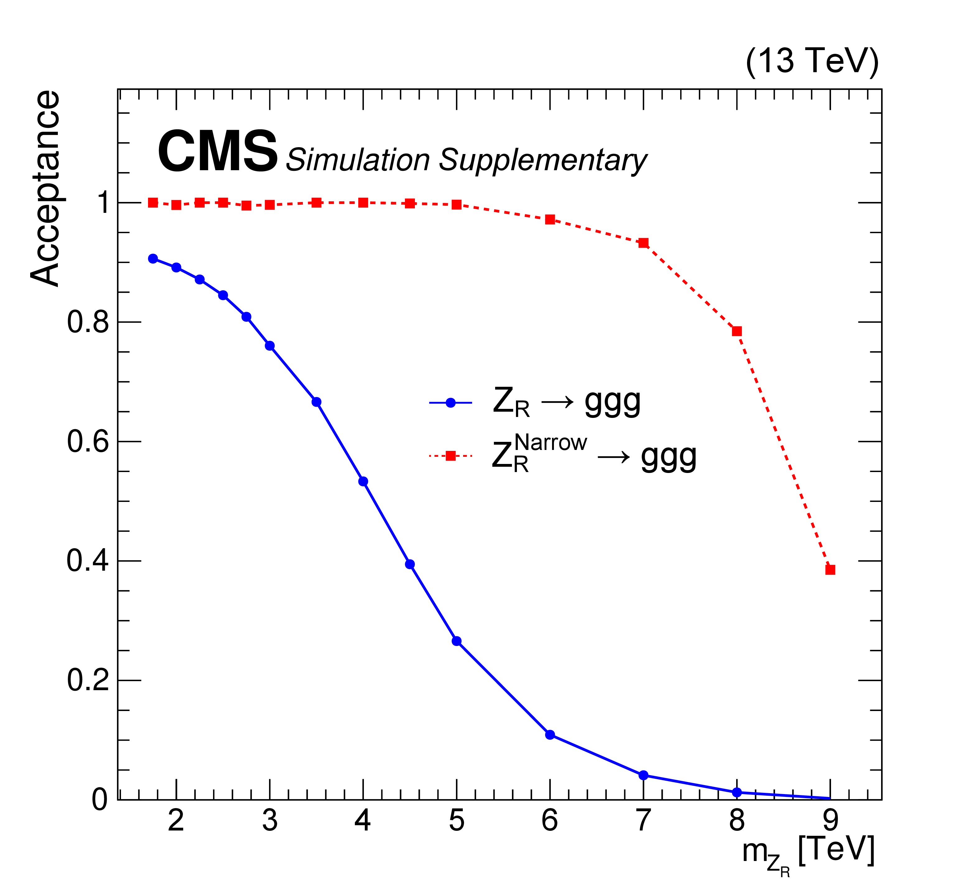
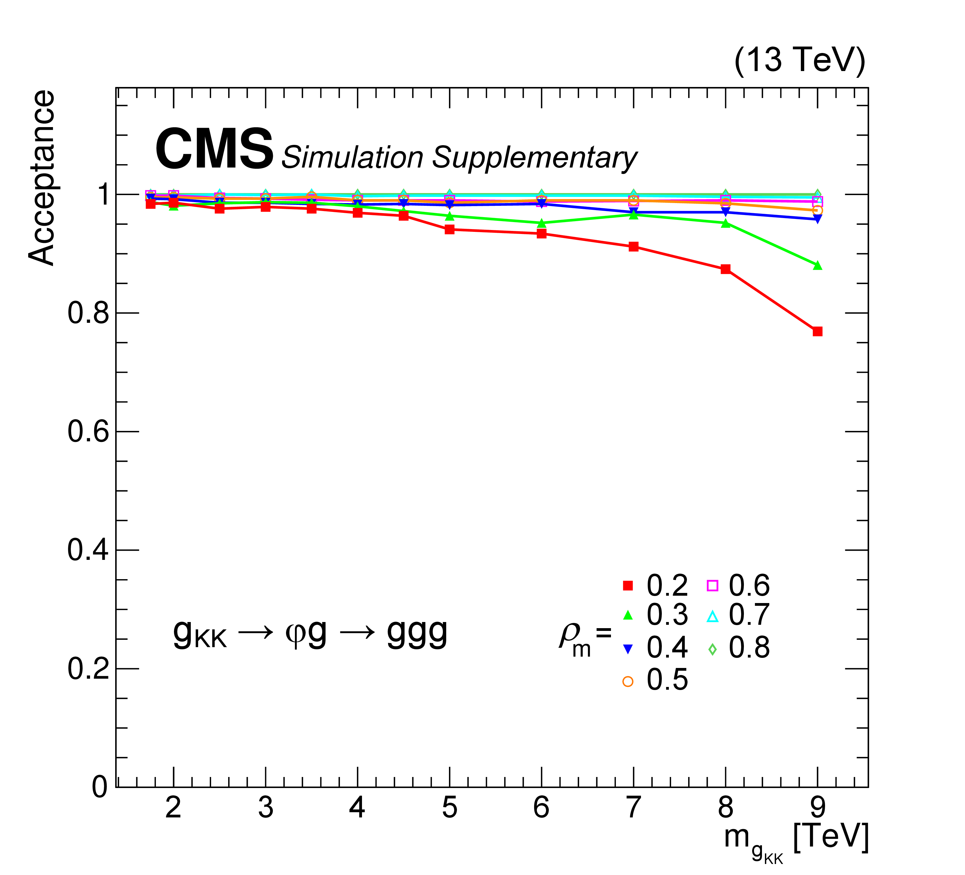
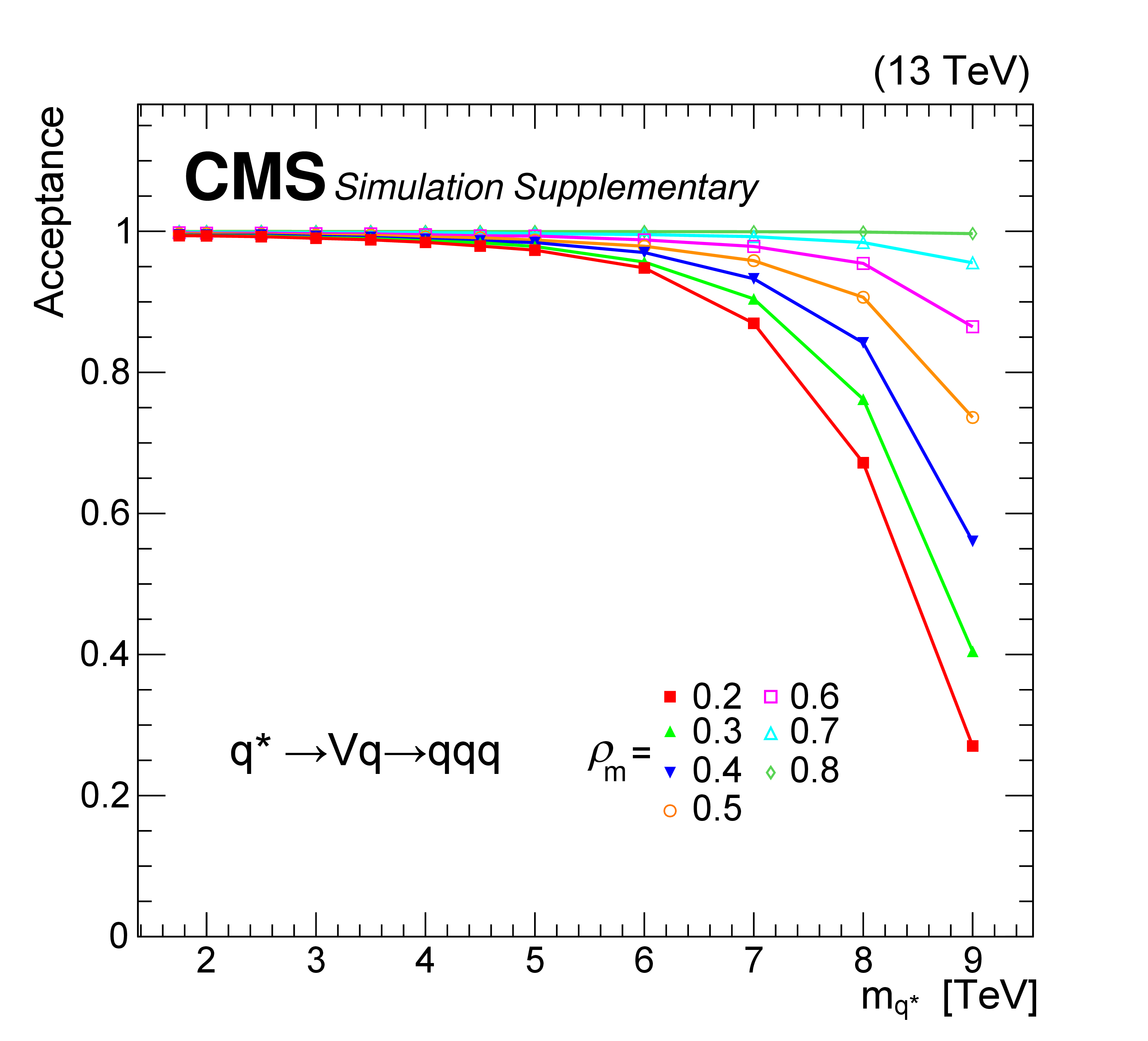
Additional Figure 2:
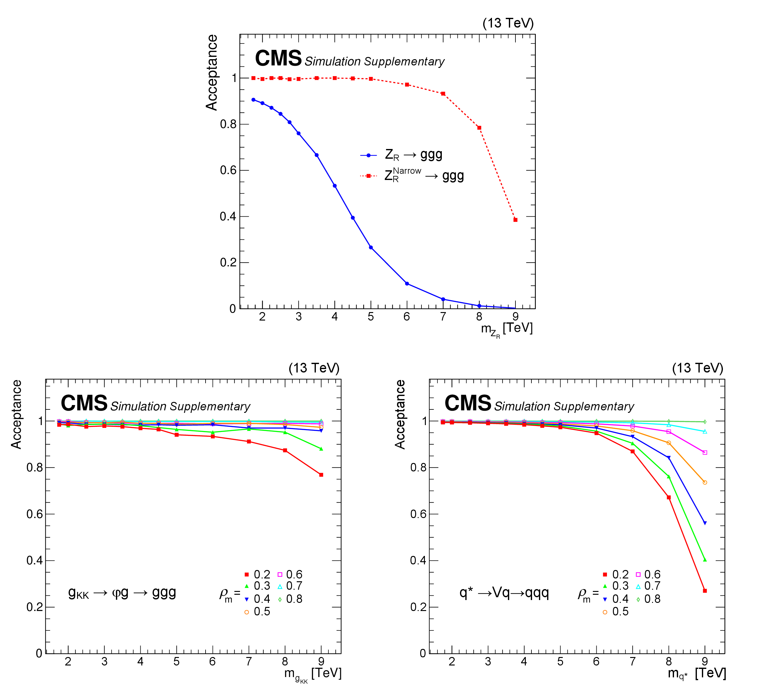
Acceptance of the signal selection requirement $ m_{\mathrm{X}}^{GEN}/m_{\mathrm{X}}^{input} > $ 85% on the benchmark signal process $ \mathrm{Z}_{R}\to\mathrm{g}\mathrm{g}\mathrm{g} $ (top), $ g_{\mathrm{KK}} \to\varphi(\mathrm{g}\mathrm{g})\mathrm{g} $ (bottom left), and $ \mathrm{q}^{*}\to \text{V}(\mathrm{q}\mathrm{q})\mathrm{q} $ (bottom right). $ m_{\mathrm{X}}^{\text{GEN}} $ is the mass of the new resonances generated by the MC simulation. $ m_{\mathrm{X}}^{\text{input}} $ is the resonance mass point under consideration. The acceptance is defined as $ \mathcal{A} = $ N (events with $ m_{\mathrm{X}}^{\text{GEN}}/m_{\mathrm{X}}^{\text{input}} > $ 85%) / $ N $(events generated in the full phase space defined by the CMS default generator settings). |
png pdf |
Additional Figure 2-a:
Acceptance of the signal selection requirement $ m_{\mathrm{X}}^{GEN}/m_{\mathrm{X}}^{input} > $ 85% on the benchmark signal process $ \mathrm{Z}_{R}\to\mathrm{g}\mathrm{g}\mathrm{g} $ (top), $ g_{\mathrm{KK}} \to\varphi(\mathrm{g}\mathrm{g})\mathrm{g} $ (bottom left), and $ \mathrm{q}^{*}\to \text{V}(\mathrm{q}\mathrm{q})\mathrm{q} $ (bottom right). $ m_{\mathrm{X}}^{\text{GEN}} $ is the mass of the new resonances generated by the MC simulation. $ m_{\mathrm{X}}^{\text{input}} $ is the resonance mass point under consideration. The acceptance is defined as $ \mathcal{A} = $ N (events with $ m_{\mathrm{X}}^{\text{GEN}}/m_{\mathrm{X}}^{\text{input}} > $ 85%) / $ N $(events generated in the full phase space defined by the CMS default generator settings). |
png pdf |
Additional Figure 2-b:
Acceptance of the signal selection requirement $ m_{\mathrm{X}}^{GEN}/m_{\mathrm{X}}^{input} > $ 85% on the benchmark signal process $ \mathrm{Z}_{R}\to\mathrm{g}\mathrm{g}\mathrm{g} $ (top), $ g_{\mathrm{KK}} \to\varphi(\mathrm{g}\mathrm{g})\mathrm{g} $ (bottom left), and $ \mathrm{q}^{*}\to \text{V}(\mathrm{q}\mathrm{q})\mathrm{q} $ (bottom right). $ m_{\mathrm{X}}^{\text{GEN}} $ is the mass of the new resonances generated by the MC simulation. $ m_{\mathrm{X}}^{\text{input}} $ is the resonance mass point under consideration. The acceptance is defined as $ \mathcal{A} = $ N (events with $ m_{\mathrm{X}}^{\text{GEN}}/m_{\mathrm{X}}^{\text{input}} > $ 85%) / $ N $(events generated in the full phase space defined by the CMS default generator settings). |
png pdf |
Additional Figure 2-c:
Acceptance of the signal selection requirement $ m_{\mathrm{X}}^{GEN}/m_{\mathrm{X}}^{input} > $ 85% on the benchmark signal process $ \mathrm{Z}_{R}\to\mathrm{g}\mathrm{g}\mathrm{g} $ (top), $ g_{\mathrm{KK}} \to\varphi(\mathrm{g}\mathrm{g})\mathrm{g} $ (bottom left), and $ \mathrm{q}^{*}\to \text{V}(\mathrm{q}\mathrm{q})\mathrm{q} $ (bottom right). $ m_{\mathrm{X}}^{\text{GEN}} $ is the mass of the new resonances generated by the MC simulation. $ m_{\mathrm{X}}^{\text{input}} $ is the resonance mass point under consideration. The acceptance is defined as $ \mathcal{A} = $ N (events with $ m_{\mathrm{X}}^{\text{GEN}}/m_{\mathrm{X}}^{\text{input}} > $ 85%) / $ N $(events generated in the full phase space defined by the CMS default generator settings). |
png pdf |
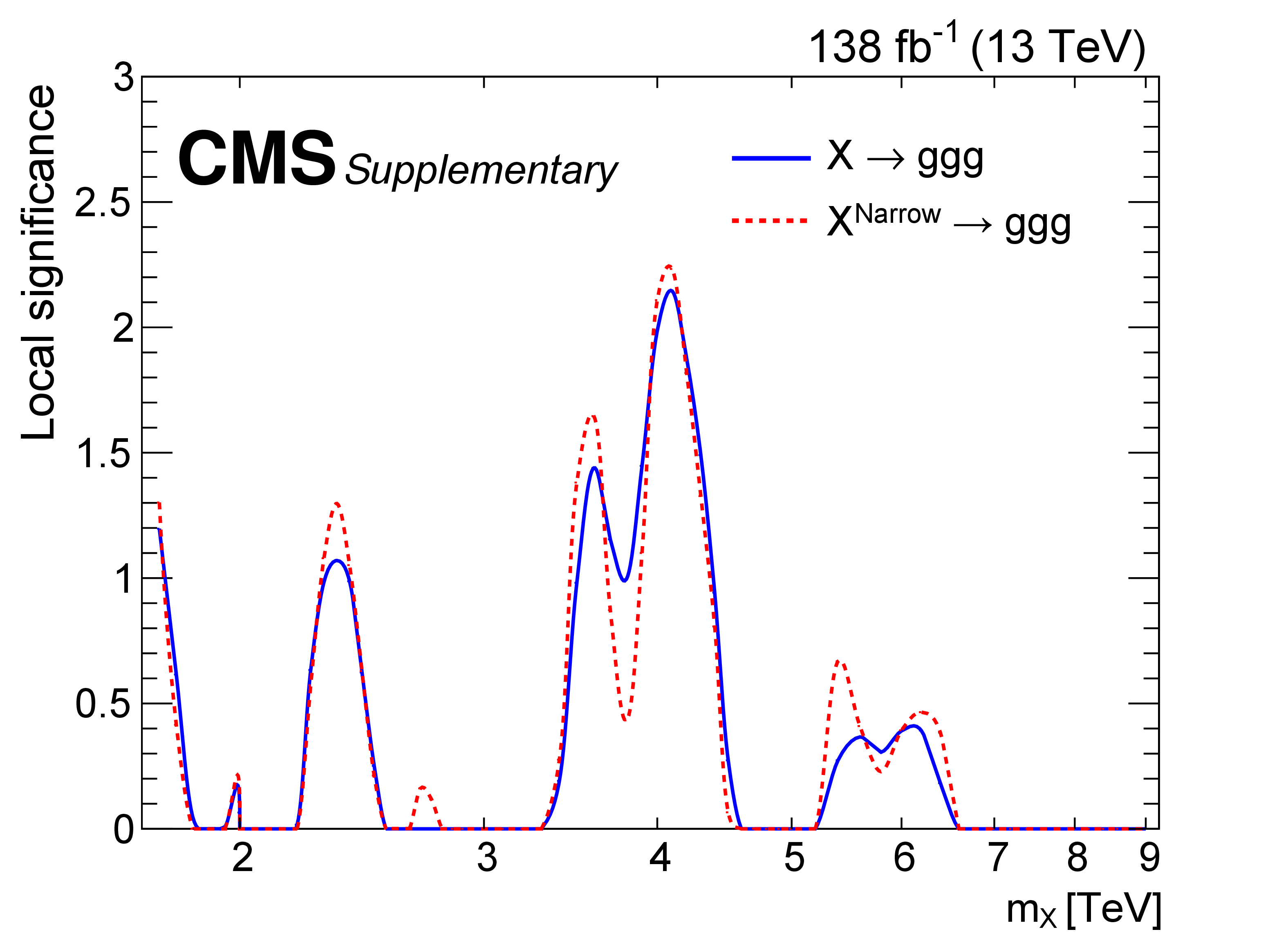
Additional Figure 3:
The observed local significance for a $ \mathrm{g}\mathrm{g}\mathrm{g} $ resonance versus X mass, shown for resonances with nominal width (blue) and narrow width (red). The most significant excesses correspond to 2.1 (2.2) standard deviations. |
png pdf |
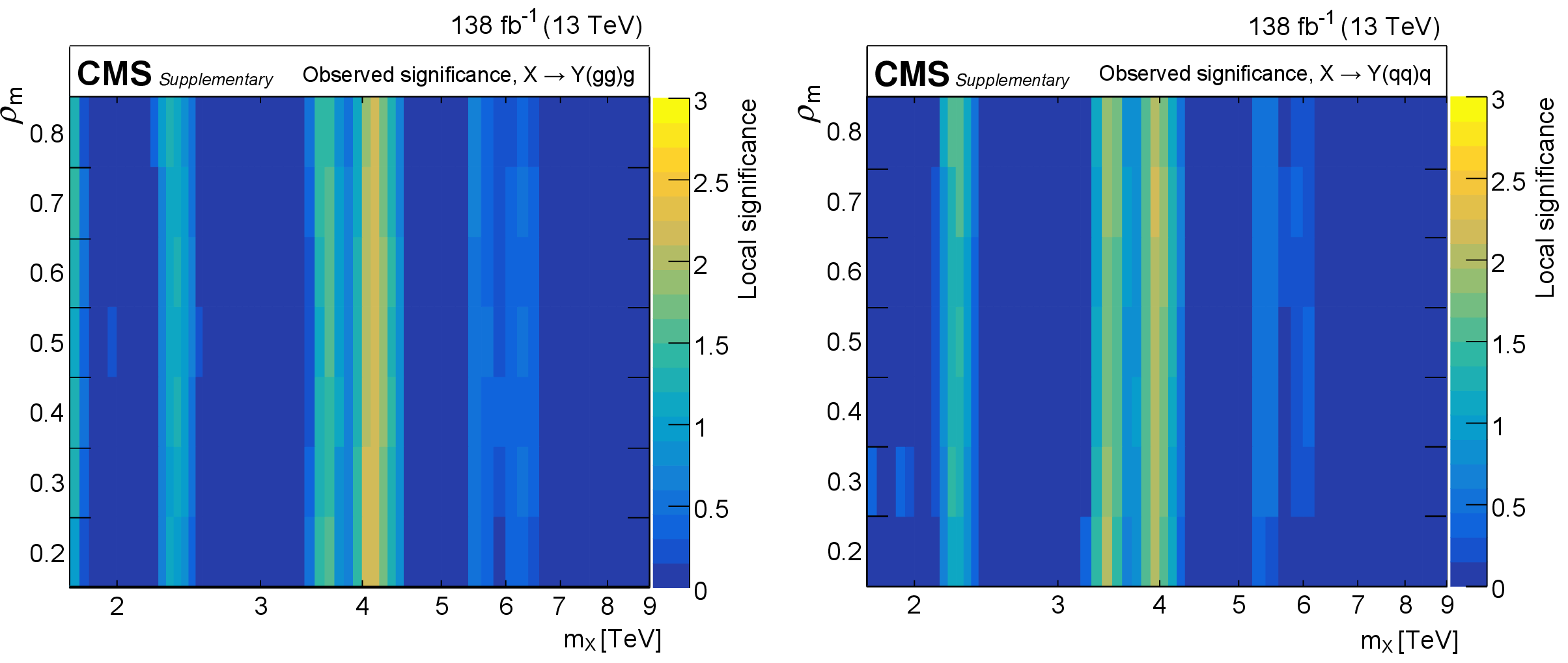
Additional Figure 4:
The observed local significance versus $ m_{\mathrm{X}} $ and $ \rho_{m} $ for resonances decaying via a cascade. The largest deviations are observed at $ \rho_{m} = 0.3, m_{\mathrm{X}} = $ 4.1 TeV for $ \mathrm{X}\to \mathrm{Y} (\mathrm{g}\mathrm{g})\mathrm{g} $ and $ \rho_{m} =$ 0.7, $ m_{\mathrm{X}} = $ 3.9 TeV for $ \mathrm{X}\to \mathrm{Y} (\mathrm{q}\mathrm{q})\mathrm{q} $. The corresponding local (global) significance values are 2.2 (0.4) and 2.1 (0.3) standard deviations, respectively. |

png pdf |
Additional Figure 4-a:
The observed local significance versus $ m_{\mathrm{X}} $ and $ \rho_{m} $ for resonances decaying via a cascade. The largest deviations are observed at $ \rho_{m} = 0.3, m_{\mathrm{X}} = $ 4.1 TeV for $ \mathrm{X}\to \mathrm{Y} (\mathrm{g}\mathrm{g})\mathrm{g} $ and $ \rho_{m} =$ 0.7, $ m_{\mathrm{X}} = $ 3.9 TeV for $ \mathrm{X}\to \mathrm{Y} (\mathrm{q}\mathrm{q})\mathrm{q} $. The corresponding local (global) significance values are 2.2 (0.4) and 2.1 (0.3) standard deviations, respectively. |

png pdf |
Additional Figure 4-b:
The observed local significance versus $ m_{\mathrm{X}} $ and $ \rho_{m} $ for resonances decaying via a cascade. The largest deviations are observed at $ \rho_{m} = 0.3, m_{\mathrm{X}} = $ 4.1 TeV for $ \mathrm{X}\to \mathrm{Y} (\mathrm{g}\mathrm{g})\mathrm{g} $ and $ \rho_{m} =$ 0.7, $ m_{\mathrm{X}} = $ 3.9 TeV for $ \mathrm{X}\to \mathrm{Y} (\mathrm{q}\mathrm{q})\mathrm{q} $. The corresponding local (global) significance values are 2.2 (0.4) and 2.1 (0.3) standard deviations, respectively. |
png pdf |
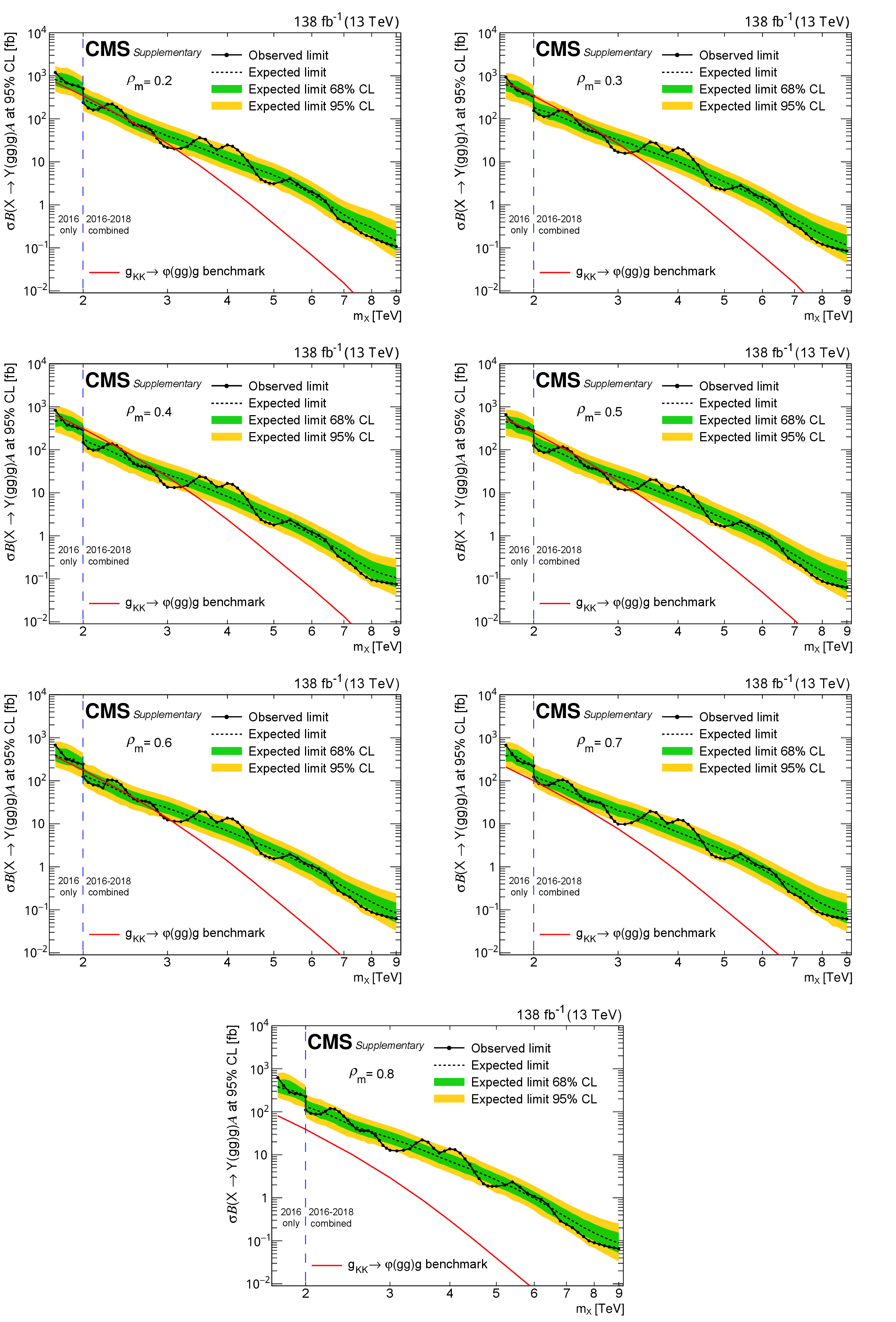
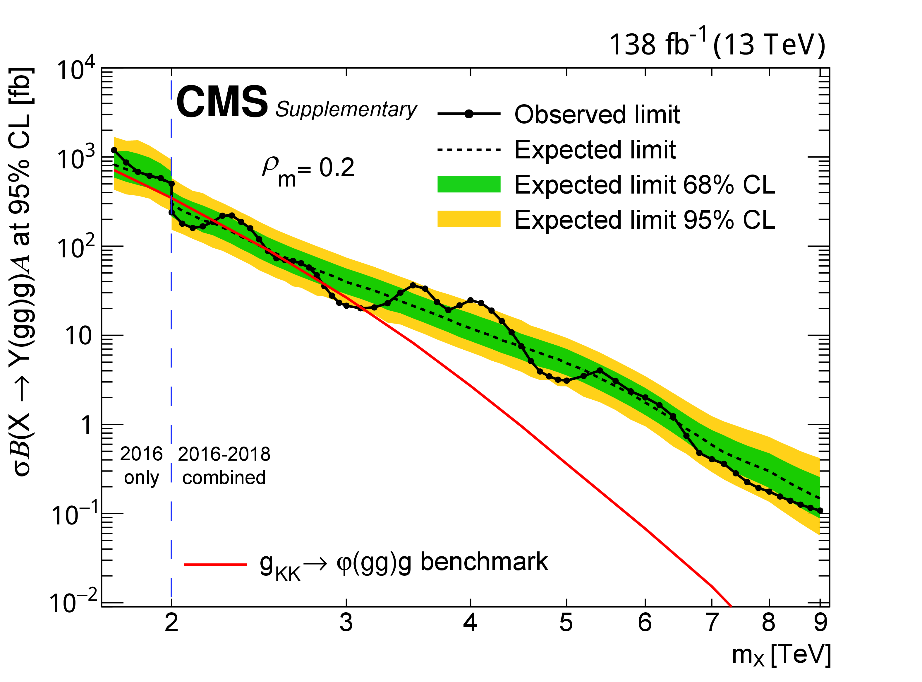
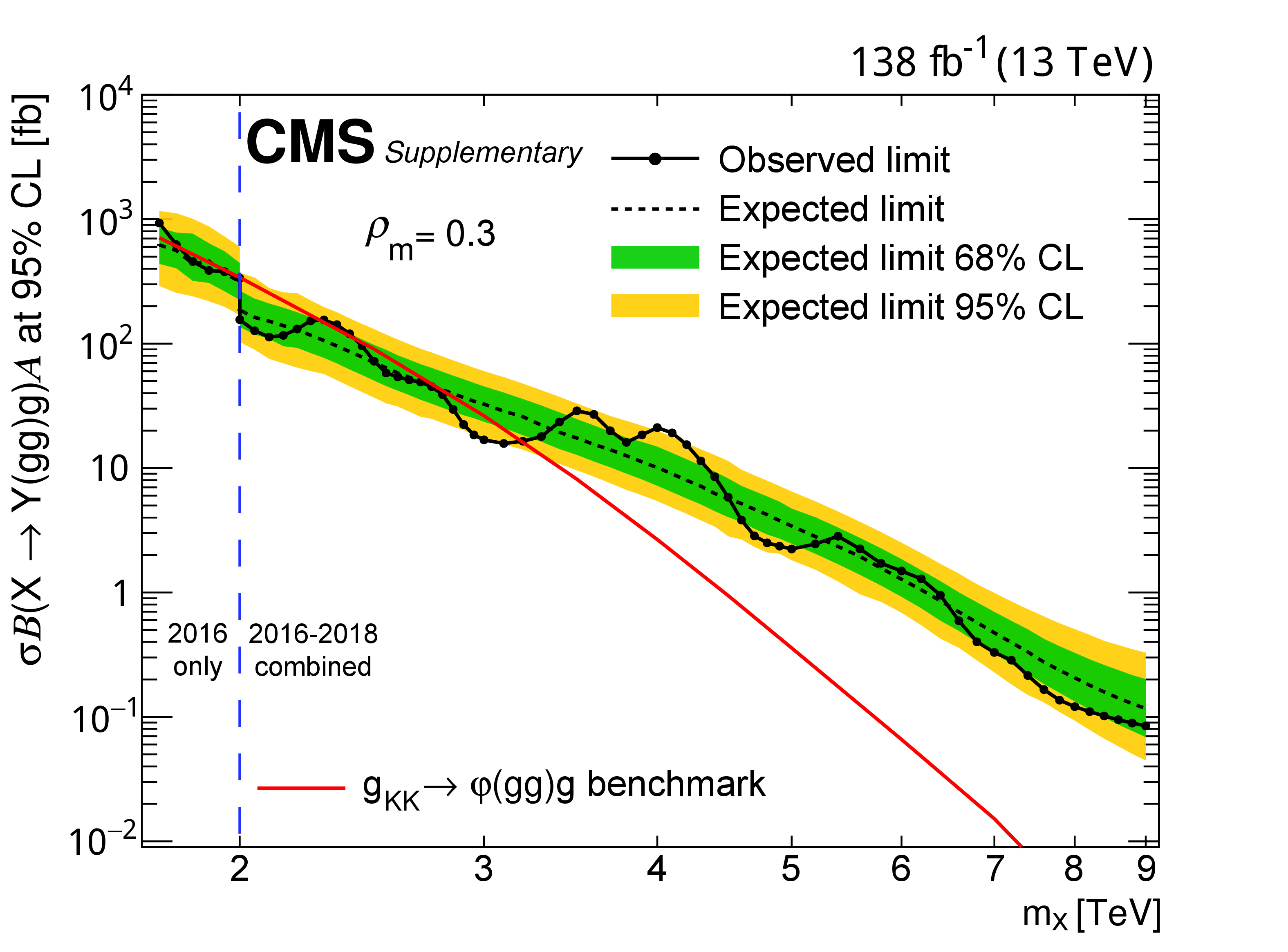
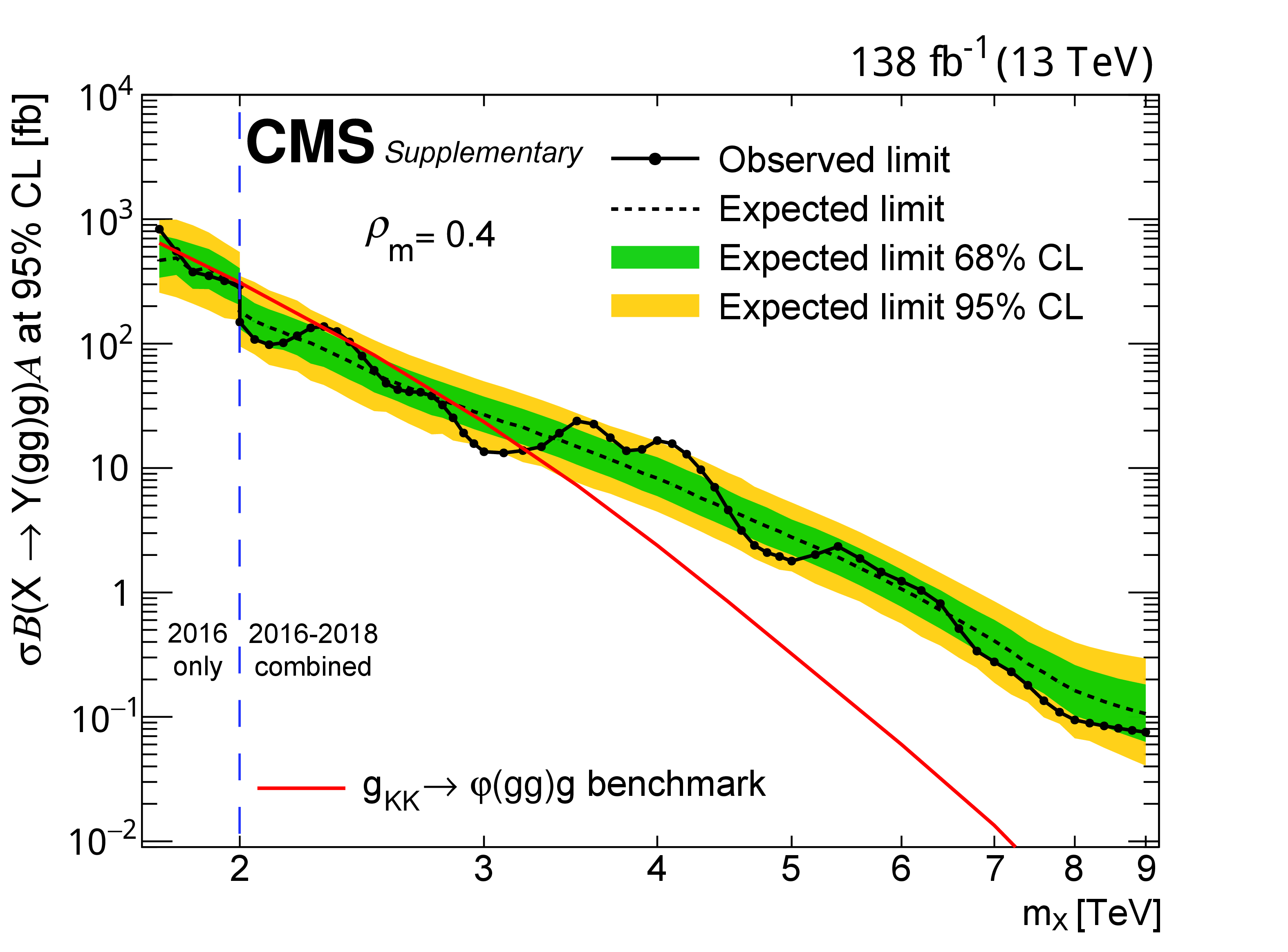
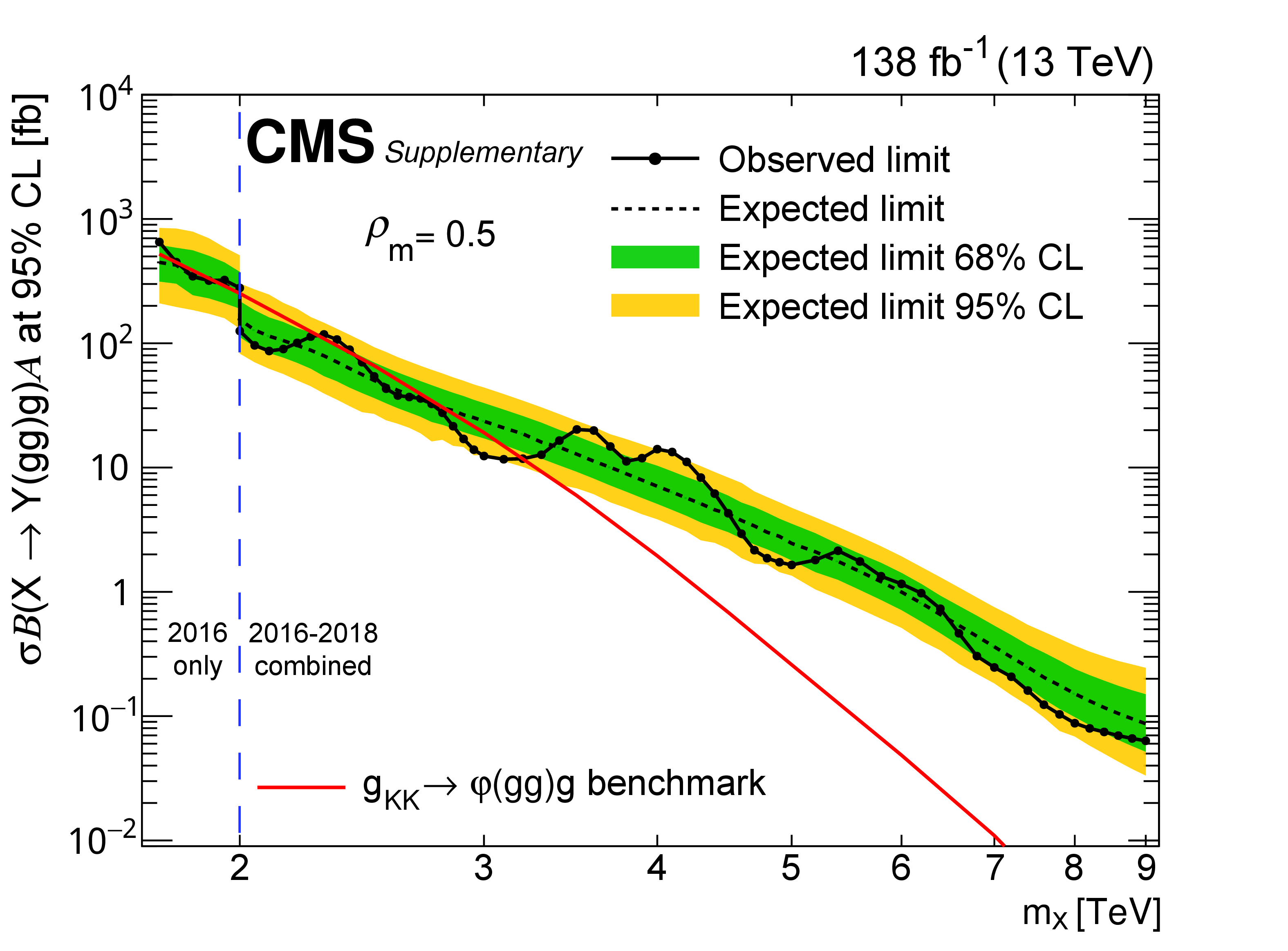
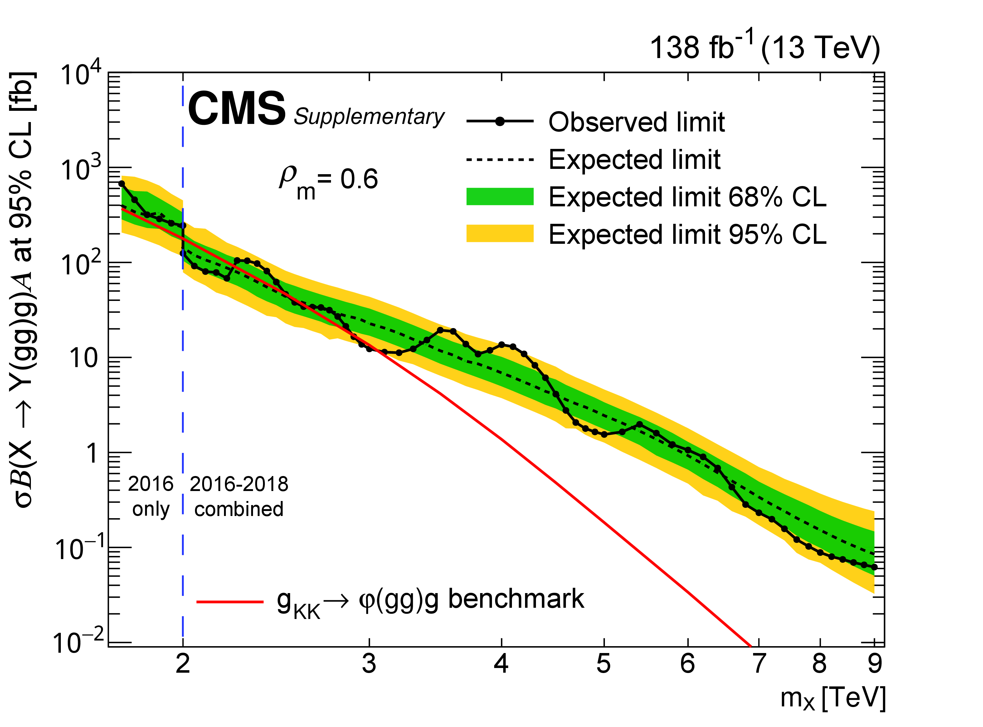
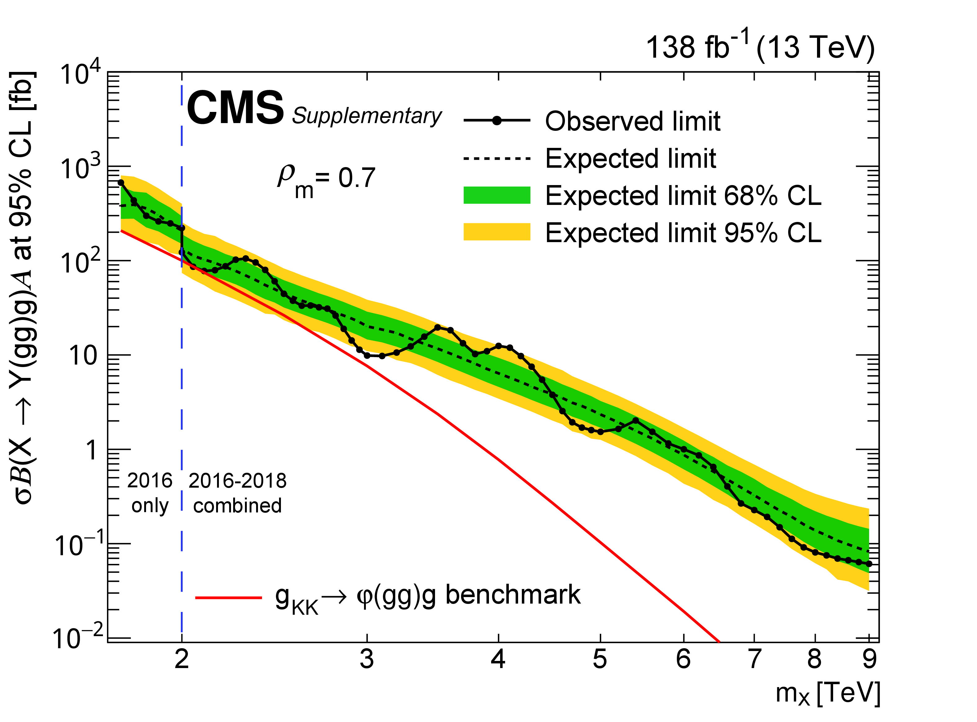
Additional Figure 5:
Limits at 95% CL on $ \sigma\mathcal{B}(\mathrm{X}\to \mathrm{Y} (\mathrm{g}\mathrm{g})\mathrm{g})\mathcal{A} $ for resonances X in different $ \rho_{m} $ scenarios. Only 2016 data is used to derive limits below 2.0 TeV because of the higher trigger thresholds in 2017 and 2018. Theoretical predictions are also shown for the benchmark $ g_{\mathrm{KK}} $ model. |
png pdf |
Additional Figure 5-a:
Limits at 95% CL on $ \sigma\mathcal{B}(\mathrm{X}\to \mathrm{Y} (\mathrm{g}\mathrm{g})\mathrm{g})\mathcal{A} $ for resonances X in different $ \rho_{m} $ scenarios. Only 2016 data is used to derive limits below 2.0 TeV because of the higher trigger thresholds in 2017 and 2018. Theoretical predictions are also shown for the benchmark $ g_{\mathrm{KK}} $ model. |
png pdf |
Additional Figure 5-b:
Limits at 95% CL on $ \sigma\mathcal{B}(\mathrm{X}\to \mathrm{Y} (\mathrm{g}\mathrm{g})\mathrm{g})\mathcal{A} $ for resonances X in different $ \rho_{m} $ scenarios. Only 2016 data is used to derive limits below 2.0 TeV because of the higher trigger thresholds in 2017 and 2018. Theoretical predictions are also shown for the benchmark $ g_{\mathrm{KK}} $ model. |
png pdf |
Additional Figure 5-c:
Limits at 95% CL on $ \sigma\mathcal{B}(\mathrm{X}\to \mathrm{Y} (\mathrm{g}\mathrm{g})\mathrm{g})\mathcal{A} $ for resonances X in different $ \rho_{m} $ scenarios. Only 2016 data is used to derive limits below 2.0 TeV because of the higher trigger thresholds in 2017 and 2018. Theoretical predictions are also shown for the benchmark $ g_{\mathrm{KK}} $ model. |
png pdf |
Additional Figure 5-d:
Limits at 95% CL on $ \sigma\mathcal{B}(\mathrm{X}\to \mathrm{Y} (\mathrm{g}\mathrm{g})\mathrm{g})\mathcal{A} $ for resonances X in different $ \rho_{m} $ scenarios. Only 2016 data is used to derive limits below 2.0 TeV because of the higher trigger thresholds in 2017 and 2018. Theoretical predictions are also shown for the benchmark $ g_{\mathrm{KK}} $ model. |
png pdf |
Additional Figure 5-e:
Limits at 95% CL on $ \sigma\mathcal{B}(\mathrm{X}\to \mathrm{Y} (\mathrm{g}\mathrm{g})\mathrm{g})\mathcal{A} $ for resonances X in different $ \rho_{m} $ scenarios. Only 2016 data is used to derive limits below 2.0 TeV because of the higher trigger thresholds in 2017 and 2018. Theoretical predictions are also shown for the benchmark $ g_{\mathrm{KK}} $ model. |
png pdf |
Additional Figure 5-f:
Limits at 95% CL on $ \sigma\mathcal{B}(\mathrm{X}\to \mathrm{Y} (\mathrm{g}\mathrm{g})\mathrm{g})\mathcal{A} $ for resonances X in different $ \rho_{m} $ scenarios. Only 2016 data is used to derive limits below 2.0 TeV because of the higher trigger thresholds in 2017 and 2018. Theoretical predictions are also shown for the benchmark $ g_{\mathrm{KK}} $ model. |

png pdf |
Additional Figure 5-g:
Limits at 95% CL on $ \sigma\mathcal{B}(\mathrm{X}\to \mathrm{Y} (\mathrm{g}\mathrm{g})\mathrm{g})\mathcal{A} $ for resonances X in different $ \rho_{m} $ scenarios. Only 2016 data is used to derive limits below 2.0 TeV because of the higher trigger thresholds in 2017 and 2018. Theoretical predictions are also shown for the benchmark $ g_{\mathrm{KK}} $ model. |
png pdf |
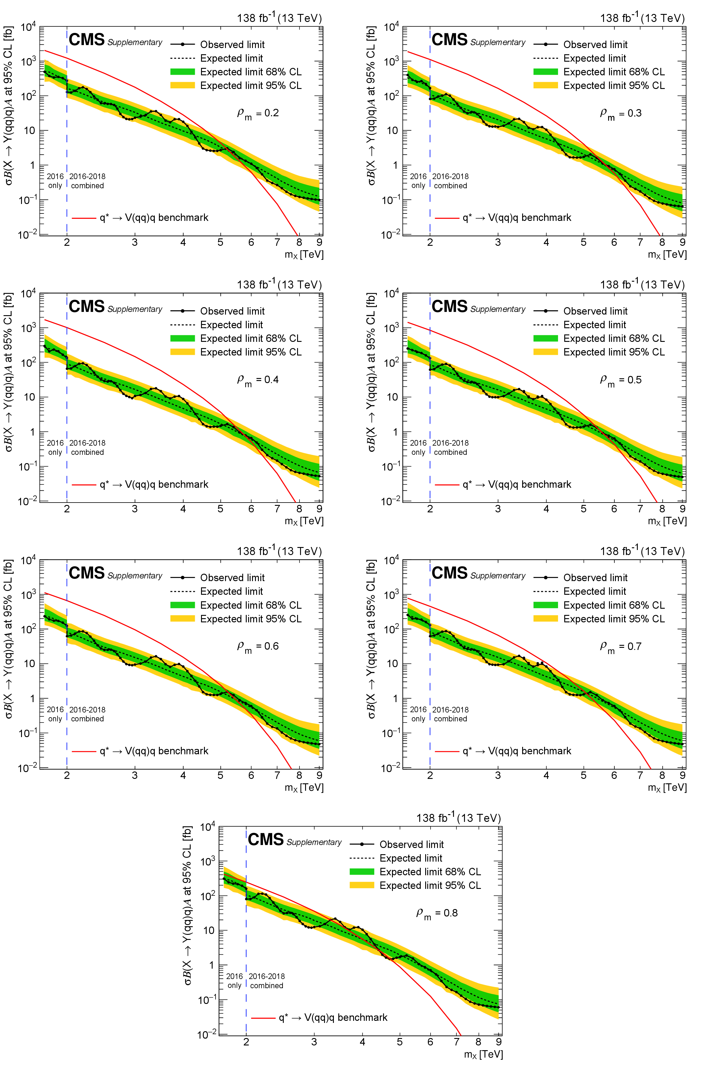
Additional Figure 6:
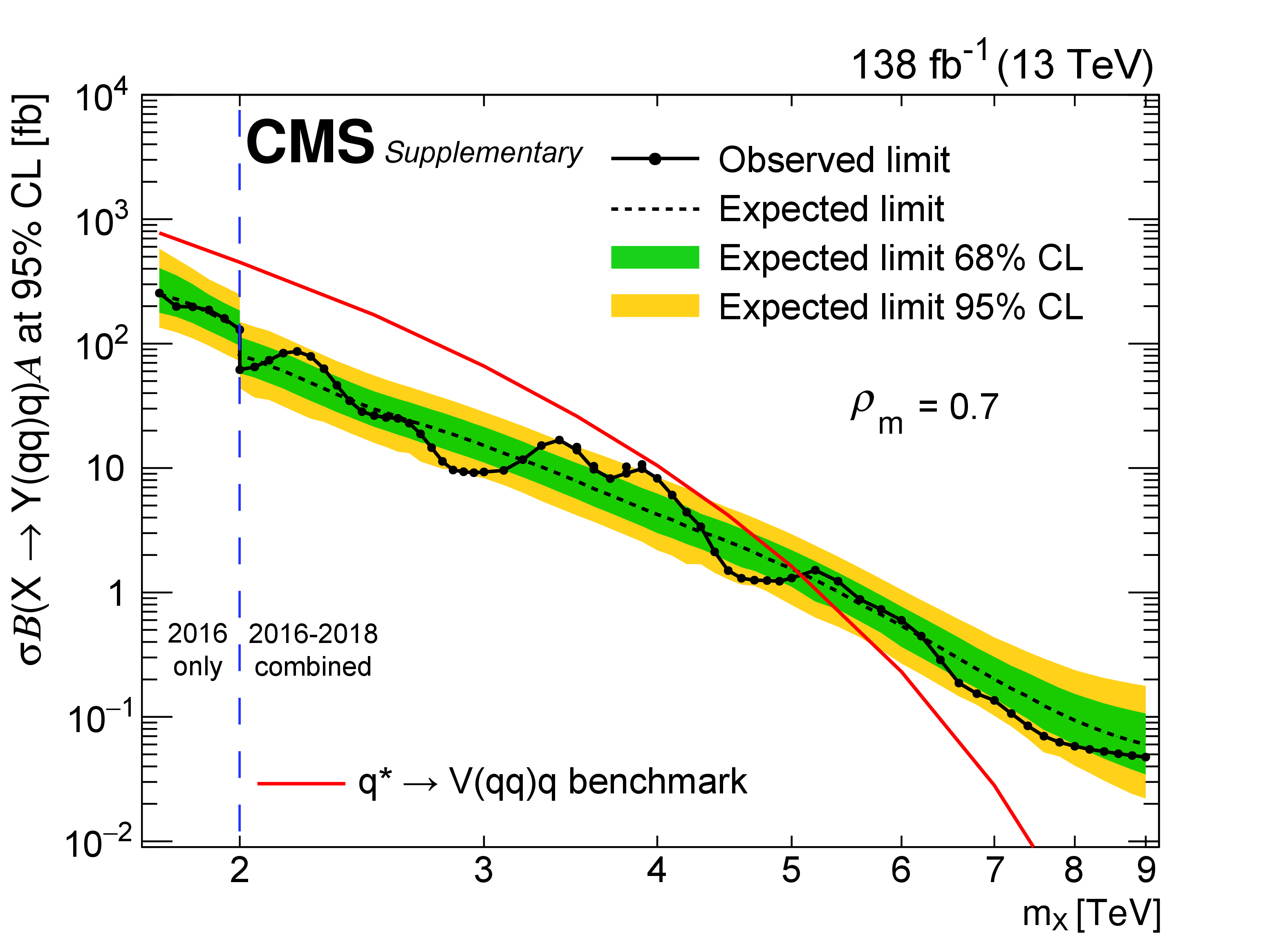
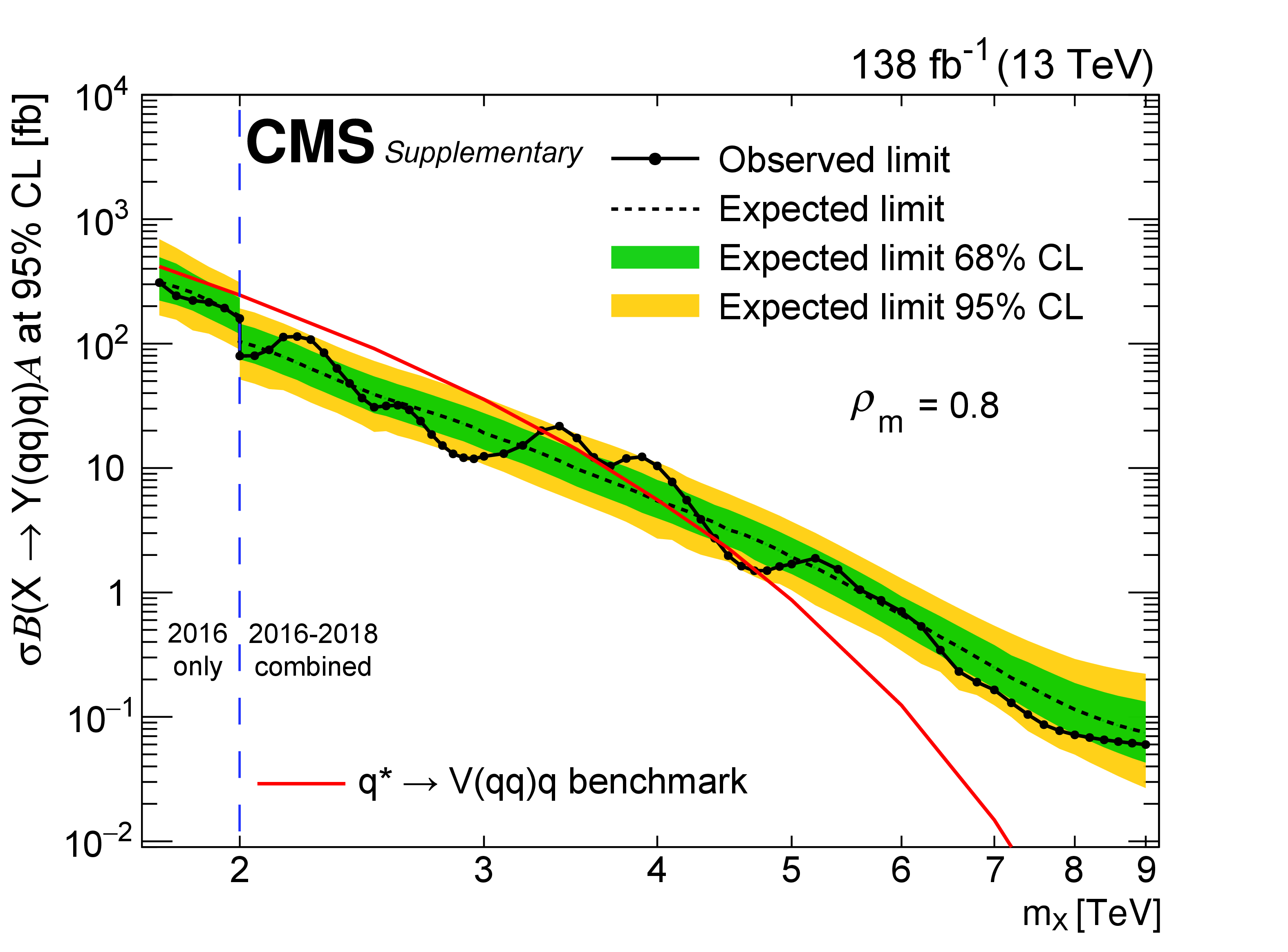
Limits at 95% CL on $ \sigma\mathcal{B}(\mathrm{X}\to \mathrm{Y} (\mathrm{q}\mathrm{q})\mathrm{q})\mathcal{A} $ for resonances X in different $ \rho_{m} $ scenarios. Only 2016 data is used to derive limits below 2.0 TeV because of the higher trigger thresholds in 2017 and 2018. Theoretical predictions are also shown for the benchmark $ \mathrm{q}^{*} $ model. |
png pdf |
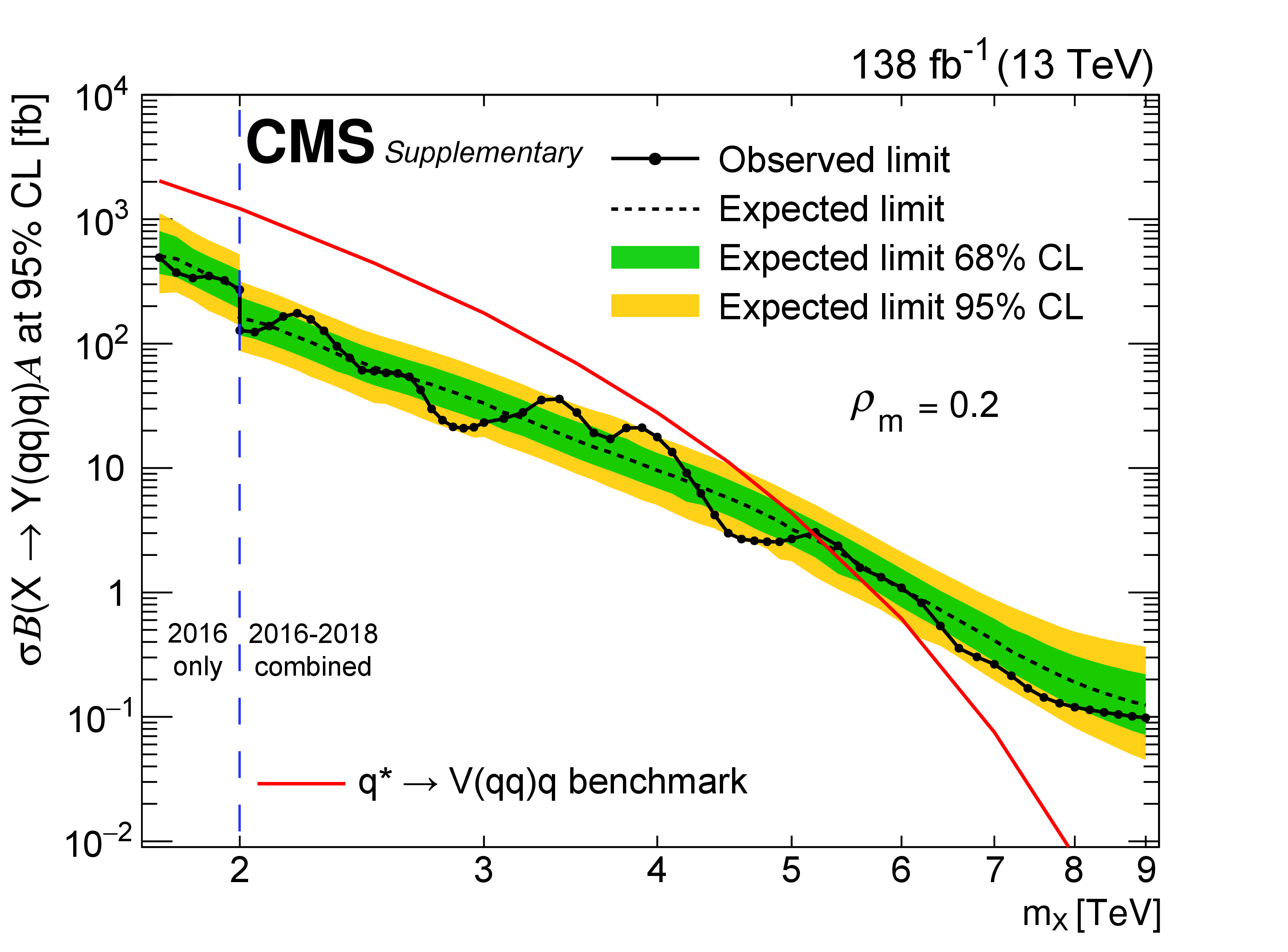
Additional Figure 6-a:
Limits at 95% CL on $ \sigma\mathcal{B}(\mathrm{X}\to \mathrm{Y} (\mathrm{q}\mathrm{q})\mathrm{q})\mathcal{A} $ for resonances X in different $ \rho_{m} $ scenarios. Only 2016 data is used to derive limits below 2.0 TeV because of the higher trigger thresholds in 2017 and 2018. Theoretical predictions are also shown for the benchmark $ \mathrm{q}^{*} $ model. |
png pdf |
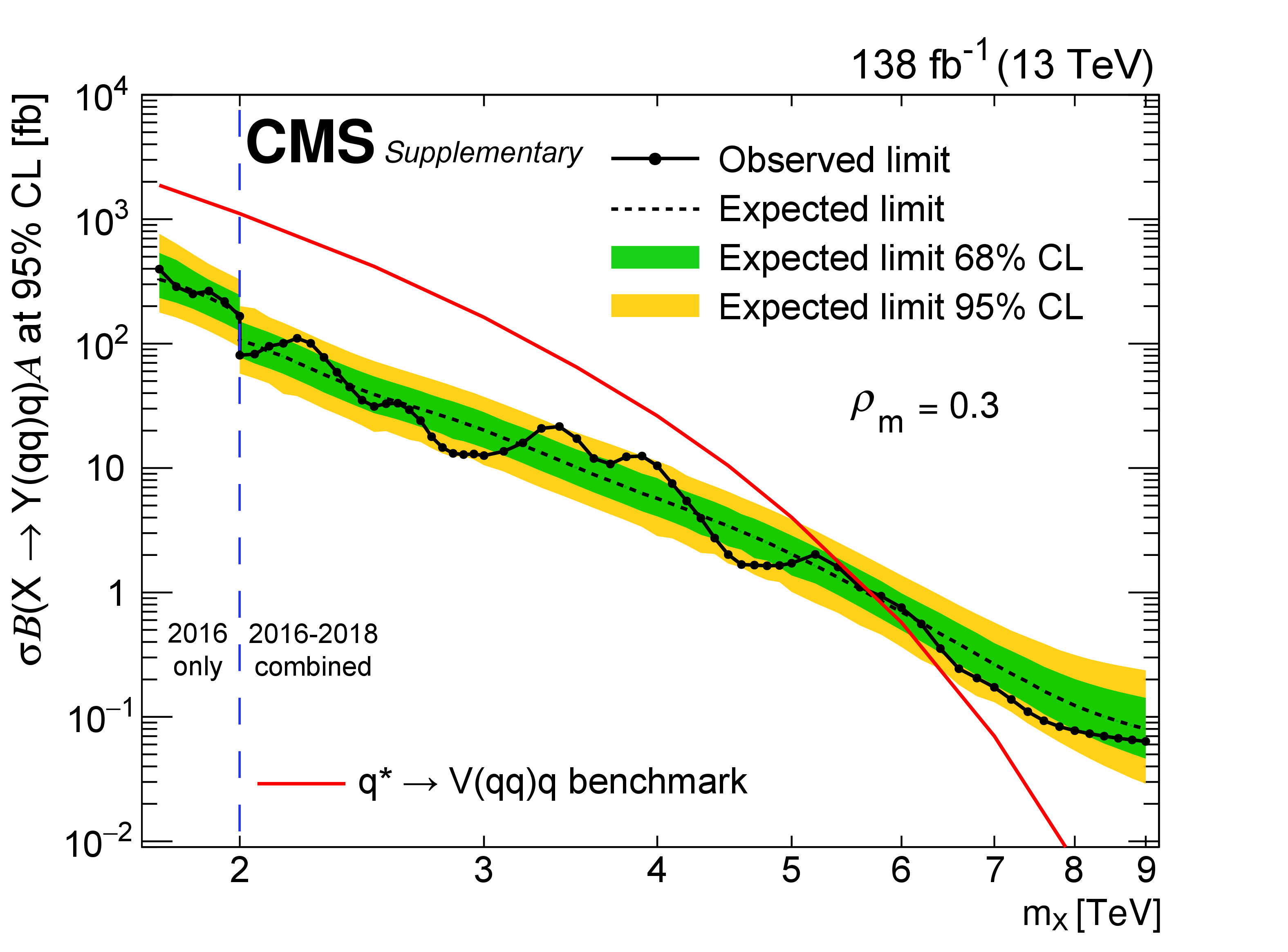
Additional Figure 6-b:
Limits at 95% CL on $ \sigma\mathcal{B}(\mathrm{X}\to \mathrm{Y} (\mathrm{q}\mathrm{q})\mathrm{q})\mathcal{A} $ for resonances X in different $ \rho_{m} $ scenarios. Only 2016 data is used to derive limits below 2.0 TeV because of the higher trigger thresholds in 2017 and 2018. Theoretical predictions are also shown for the benchmark $ \mathrm{q}^{*} $ model. |
png pdf |
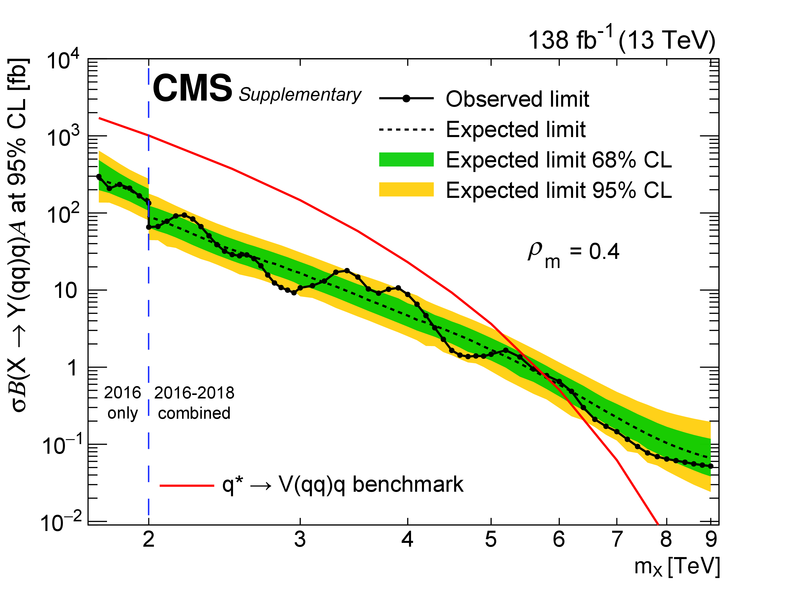
Additional Figure 6-c:
Limits at 95% CL on $ \sigma\mathcal{B}(\mathrm{X}\to \mathrm{Y} (\mathrm{q}\mathrm{q})\mathrm{q})\mathcal{A} $ for resonances X in different $ \rho_{m} $ scenarios. Only 2016 data is used to derive limits below 2.0 TeV because of the higher trigger thresholds in 2017 and 2018. Theoretical predictions are also shown for the benchmark $ \mathrm{q}^{*} $ model. |

png pdf |
Additional Figure 6-d:
Limits at 95% CL on $ \sigma\mathcal{B}(\mathrm{X}\to \mathrm{Y} (\mathrm{q}\mathrm{q})\mathrm{q})\mathcal{A} $ for resonances X in different $ \rho_{m} $ scenarios. Only 2016 data is used to derive limits below 2.0 TeV because of the higher trigger thresholds in 2017 and 2018. Theoretical predictions are also shown for the benchmark $ \mathrm{q}^{*} $ model. |
png pdf |
Additional Figure 6-e:
Limits at 95% CL on $ \sigma\mathcal{B}(\mathrm{X}\to \mathrm{Y} (\mathrm{q}\mathrm{q})\mathrm{q})\mathcal{A} $ for resonances X in different $ \rho_{m} $ scenarios. Only 2016 data is used to derive limits below 2.0 TeV because of the higher trigger thresholds in 2017 and 2018. Theoretical predictions are also shown for the benchmark $ \mathrm{q}^{*} $ model. |
png pdf |
Additional Figure 6-f:
Limits at 95% CL on $ \sigma\mathcal{B}(\mathrm{X}\to \mathrm{Y} (\mathrm{q}\mathrm{q})\mathrm{q})\mathcal{A} $ for resonances X in different $ \rho_{m} $ scenarios. Only 2016 data is used to derive limits below 2.0 TeV because of the higher trigger thresholds in 2017 and 2018. Theoretical predictions are also shown for the benchmark $ \mathrm{q}^{*} $ model. |
png pdf |
Additional Figure 6-g:
Limits at 95% CL on $ \sigma\mathcal{B}(\mathrm{X}\to \mathrm{Y} (\mathrm{q}\mathrm{q})\mathrm{q})\mathcal{A} $ for resonances X in different $ \rho_{m} $ scenarios. Only 2016 data is used to derive limits below 2.0 TeV because of the higher trigger thresholds in 2017 and 2018. Theoretical predictions are also shown for the benchmark $ \mathrm{q}^{*} $ model. |

png pdf jpg |
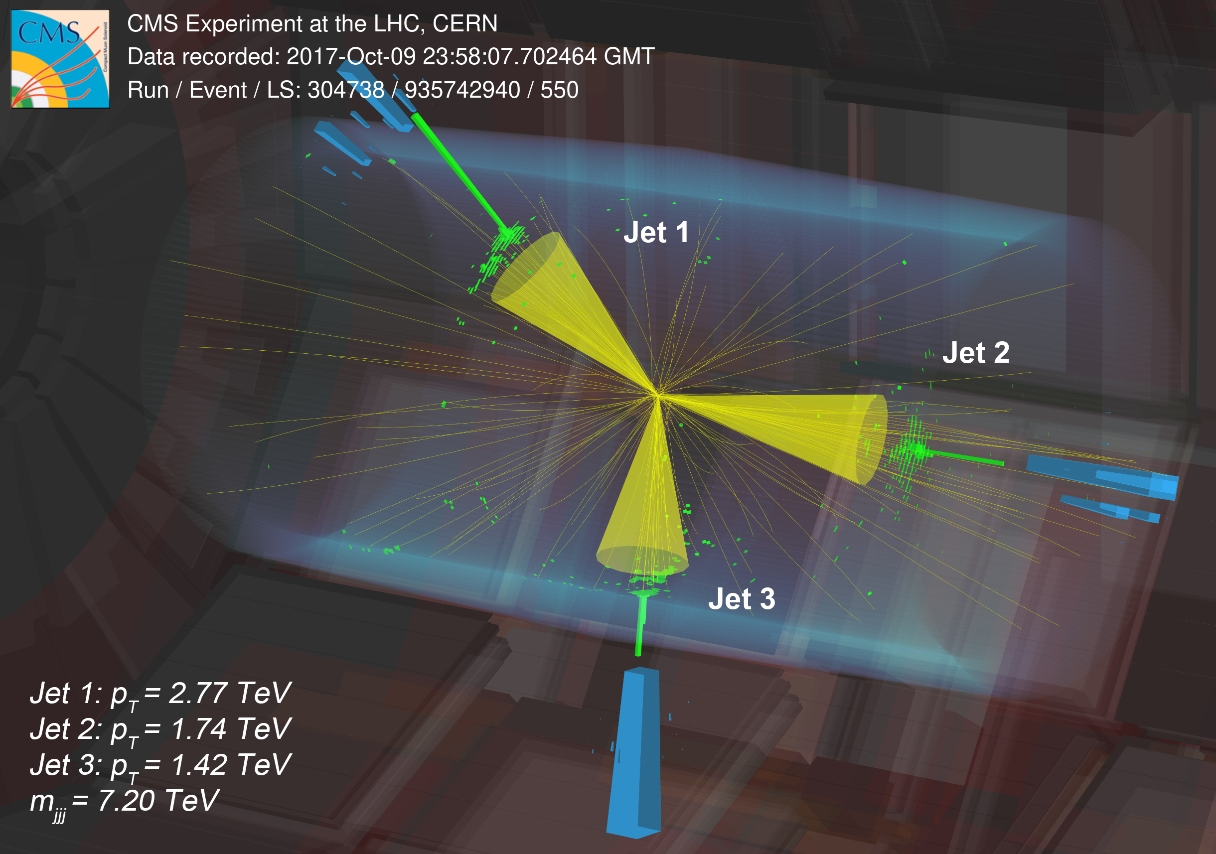
Additional Figure 7:
Three-dimensional display of the event with the highest $ m_{\mathrm{jjj}} $ of 7.20 TeV. Energy deposited in the electromagnetic (green) and hadronic (blue) calorimeters and the reconstructed tracks of charged particles (yellow) are shown. Reconstructed three most energetic jets are represented by the yellow cones. |
| References | ||||
| 1 | R. M. Harris and K. Kousouris | Searches for Dijet Resonances at Hadron Colliders | Int. J. Mod. Phys. A 26 (2011) 5005 | 1110.5302 |
| 2 | UA1 Collaboration | Two-jet mass distributions at the CERN proton-antiproton collider | PLB 209 (1988) 127 | |
| 3 | UA2 Collaboration | A search for new intermediate vector mesons and excited quarks decaying to two jets at the CERN $ \overline{\mathrm{p}}\mathrm{p} $ collider | NPB 400 (1993) 3 | |
| 4 | CDF Collaboration | Search for new particles decaying into dijets in proton-antiproton collisions at $ \sqrt{s} = $ 1.96 TeV | PRD 79 (2009) 112002 | 0812.4036 |
| 5 | D0 Collaboration | Search for new particles in the two-jet decay channel with the D0 detector | PRD 69 (2004) 111101 | hep-ex/0308033 |
| 6 | ATLAS Collaboration | Search for new resonances in mass distributions of jet pairs using 139 fb$ ^{-1} $ of $ pp $ collisions at $ \sqrt{s}= $ 13 TeV with the ATLAS detector | JHEP 03 (2020) 145 | 1910.08447 |
| 7 | ATLAS Collaboration | Search for light resonances decaying to boosted quark pairs and produced in association with a photon or a jet in proton-proton collisions at $ \sqrt{s}= $ 13 TeV with the ATLAS detector | PLB 788 (2019) 316 | 1801.08769 |
| 8 | ATLAS Collaboration | Search for resonances in the mass distribution of jet pairs with one or two jets identified as $ b $-jets in proton-proton collisions at $ \sqrt{s}= $ 13 TeV with the ATLAS detector | PRD 98 (2018) 032016 | 1805.09299 |
| 9 | CMS Collaboration | Search for high mass dijet resonances with a new background prediction method in proton-proton collisions at $ \sqrt{s} = $ 13 TeV | JHEP 05 (2020) 033 | CMS-EXO-19-012 1911.03947 |
| 10 | CMS Collaboration | Search for low mass vector resonances decaying into quark-antiquark pairs in proton-proton collisions at $ \sqrt{s}= $ 13 TeV | PRD 100 (2019) 112007 | CMS-EXO-18-012 1909.04114 |
| 11 | CMS Collaboration | Search for narrow resonances in the b-tagged dijet mass spectrum in proton-proton collisions at $ \sqrt{s}= $ 13 TeV | PRD 108 (2023) 012009 | CMS-EXO-20-008 2205.01835 |
| 12 | CDF Collaboration | First search for multijet resonances in $ \sqrt{s} = $ 1.96 TeV $ {\mathrm{p}\overline{\mathrm{p}}} $ collisions | PRL 107 (2011) 042001 | 1105.2815 |
| 13 | CDF Collaboration | Search for pair production of strongly interacting particles decaying to pairs of jets in $ {\mathrm{p}\overline{\mathrm{p}}} $ collisions at $ \sqrt{s}= $ 1.96 TeV | PRL 111 (2013) 031802 | 1303.2699 |
| 14 | ATLAS Collaboration | A search for pair-produced resonances in four-jet final states at $ \sqrt{s} = $ 13 TeV with the ATLAS detector | EPJC 78 (2018) 250 | 1710.07171 |
| 15 | CMS Collaboration | Search for pair-produced resonances decaying to quark pairs in proton-proton collisions at $ \sqrt{s}= $ 13 TeV | PRD 98 (2018) 112014 | CMS-EXO-17-021 1808.03124 |
| 16 | CMS Collaboration | Search for pair-produced resonances each decaying into at least four quarks in proton-proton collisions at $ \sqrt{s} = $ 13 TeV | PRL 121 (2018) 141802 | CMS-EXO-17-022 1806.01058 |
| 17 | ATLAS Collaboration | Search for R-parity-violating supersymmetric particles in multi-jet final states produced in $ pp $ collisions at $ \sqrt{s} = $ 13 TeV using the ATLAS detector at the LHC | PLB 785 (2018) 136 | 1804.03568 |
| 18 | CMS Collaboration | Search for pair-produced three-jet resonances in proton-proton collisions at $ \sqrt{s} = $ 13 TeV | PRD 99 (2019) 012010 | CMS-EXO-17-030 1810.10092 |
| 19 | CMS Collaboration | Search for resonant and nonresonant production of pairs of dijet resonances in proton-proton collisions at $ \sqrt{s} = $ 13 TeV | JHEP 07 (2023) 161 | CMS-EXO-21-010 2206.09997 |
| 20 | CMS Collaboration | Search for high-mass resonances decaying to a jet and a Lorentz-boosted resonance in proton-proton collisions at $ \sqrt{s}= $ 13 TeV | PLB 832 (2022) 137263 | CMS-EXO-20-007 2201.02140 |
| 21 | K. Huitu, J. Maalampi, A. Pietila, and M. Raidal | Doubly charged higgs at LHC | NPB 487 (1997) 27 | hep-ph/9606311 |
| 22 | K. S. Agashe et al. | LHC signals from cascade decays of warped vector resonances | JHEP 05 (2017) 078 | 1612.00047 |
| 23 | K. Agashe, M. Ekhterachian, D. Kim, and D. Sathyan | LHC signals for KK graviton from an extended warped extra dimension | JHEP 11 (2020) 109 | 2008.06480 |
| 24 | U. Baur, M. Spira, and P. M. Zerwas | Excited-quark and -lepton production at hadron colliders | PRD 42 (1990) 815 | |
| 25 | CMS Collaboration | HEPData record for this analysis | link | |
| 26 | CMS Collaboration | The CMS experiment at the CERN LHC | JINST 3 (2008) S08004 | |
| 27 | CMS Collaboration | Performance of the CMS Level-1 trigger in proton-proton collisions at $ \sqrt{s} = $ 13 TeV | JINST 15 (2020) P10017 | CMS-TRG-17-001 2006.10165 |
| 28 | CMS Collaboration | The CMS trigger system | JINST 12 (2017) P01020 | CMS-TRG-12-001 1609.02366 |
| 29 | CMS Collaboration | Electron and photon reconstruction and identification with the CMS experiment at the CERN LHC | JINST 16 (2021) P05014 | CMS-EGM-17-001 2012.06888 |
| 30 | CMS Collaboration | Performance of the CMS muon detector and muon reconstruction with proton-proton collisions at $ \sqrt{s}= $ 13 TeV | JINST 13 (2018) P06015 | CMS-MUO-16-001 1804.04528 |
| 31 | CMS Collaboration | Description and performance of track and primary-vertex reconstruction with the CMS tracker | JINST 9 (2014) P10009 | CMS-TRK-11-001 1405.6569 |
| 32 | CMS Collaboration | Particle-flow reconstruction and global event description with the CMS detector | JINST 12 (2017) P10003 | CMS-PRF-14-001 1706.04965 |
| 33 | CMS Collaboration | Performance of reconstruction and identification of $ \tau $ leptons decaying to hadrons and $ \nu_\tau $ in pp collisions at $ \sqrt{s}= $ 13 TeV | JINST 13 (2018) P10005 | CMS-TAU-16-003 1809.02816 |
| 34 | CMS Collaboration | Jet energy scale and resolution in the CMS experiment in pp collisions at 8 TeV | JINST 12 (2017) P02014 | CMS-JME-13-004 1607.03663 |
| 35 | CMS Collaboration | Performance of missing transverse momentum reconstruction in proton-proton collisions at $ \sqrt{s} = $ 13 TeV using the CMS detector | JINST 14 (2019) P07004 | CMS-JME-17-001 1903.06078 |
| 36 | CMS Collaboration | Technical proposal for the Phase-II upgrade of the Compact Muon Solenoid | CMS Technical Proposal CERN-LHCC-2015-010, CMS-TDR-15-02, 2015 CDS |
|
| 37 | M. Cacciari, G. P. Salam, and G. Soyez | The anti-$ k_{\mathrm{T}} $ jet clustering algorithm | JHEP 04 (2008) 063 | 0802.1189 |
| 38 | M. Cacciari, G. P. Salam, and G. Soyez | FastJet user manual | EPJC 72 (2012) 1896 | 1111.6097 |
| 39 | CMS Collaboration | Jet algorithms performance in 13 TeV data | CMS Physics Analysis Summary, 2017 CMS-PAS-JME-16-003 |
CMS-PAS-JME-16-003 |
| 40 | CMS Collaboration | Pileup mitigation at CMS in 13 TeV data | JINST 15 (2020) P09018 | CMS-JME-18-001 2003.00503 |
| 41 | CMS Collaboration | Search for resonances in the dijet mass spectrum from 7 TeV pp collisions at CMS | PLB 704 (2011) 123 | CMS-EXO-11-015 1107.4771 |
| 42 | T. Sjöstrand et al. | An introduction to PYTHIA 8.2 | Comput. Phys. Commun. 191 (2015) 159 | 1410.3012 |
| 43 | J. Alwall et al. | The automated computation of tree-level and next-to-leading order differential cross sections, and their matching to parton shower simulations | JHEP 07 (2014) 079 | 1405.0301 |
| 44 | NNPDF Collaboration | Parton distributions from high-precision collider data | EPJC 77 (2017) 663 | 1706.00428 |
| 45 | CMS Collaboration | Extraction and validation of a new set of CMS PYTHIA8 tunes from underlying-event measurements | EPJC 80 (2020) 4 | CMS-GEN-17-001 1903.12179 |
| 46 | GEANT4 Collaboration | GEANT 4---a simulation toolkit | NIM A 506 (2003) 250 | |
| 47 | R. A. Fisher | On the interpretation of $ \chi^{2} $ from contingency tables, and the calculation of P | J. R. Stat. Soc. 85 (1922) 87 | |
| 48 | ATLAS and CMS Collaborations, and LHC Higgs Combination Group | Procedure for the LHC Higgs boson search combination in Summer 2011 | Technical Report CMS-NOTE-2011-005, ATL-PHYS-PUB-2011-11, 2011 | |
| 49 | P. D. Dauncey, M. Kenzie, N. Wardle, and G. J. Davies | Handling uncertainties in background shapes: the discrete profiling method | JINST 10 (2015) P04015 | 1408.6865 |
| 50 | CMS Collaboration | Precision luminosity measurement in proton-proton collisions at $ \sqrt{s} = $ 13 TeV in 2015 and 2016 at CMS | EPJC 81 (2021) 800 | CMS-LUM-17-003 2104.01927 |
| 51 | CMS Collaboration | CMS luminosity measurement for the 2017 data-taking period at $ \sqrt{s} = $ 13 TeV | CMS Physics Analysis Summary, 2018 link |
CMS-PAS-LUM-17-004 |
| 52 | CMS Collaboration | CMS luminosity measurement for the 2018 data-taking period at $ \sqrt{s} = $ 13 TeV | CMS Physics Analysis Summary, 2019 link |
CMS-PAS-LUM-18-002 |
| 53 | E. Gross and O. Vitells | Trial factors for the look elsewhere effect in high energy physics | EPJC 70 (2010) 525 | 1005.1891 |
| 54 | A. L. Read | Presentation of search results: The CL$ _{\text{s}} $ technique | JPG 28 (2002) 2693 | |
| 55 | T. Junk | Confidence level computation for combining searches with small statistics | NIM A 434 (1999) 435 | hep-ex/9902006 |
| 56 | G. Cowan, K. Cranmer, E. Gross, and O. Vitells | Asymptotic formulae for likelihood-based tests of new physics | EPJC 71 (2011) 1554 | 1007.1727 |
|
|
Compact Muon Solenoid LHC, CERN |
|

|

|

|

|

|