

Compact Muon Solenoid
LHC, CERN
| CMS-HIG-17-033 ; CERN-EP-2019-230 | ||
| Search for a heavy Higgs boson decaying to a pair of W bosons in proton-proton collisions at $\sqrt{s} = $ 13 TeV | ||
| CMS Collaboration | ||
| 3 December 2019 | ||
| JHEP 03 (2020) 034 | ||
| Abstract: A search for a heavy Higgs boson in the mass range from 0.2 to 3.0 TeV, decaying to a pair of W bosons, is presented. The analysis is based on proton-proton collisions at $\sqrt{s} = $ 13 TeV recorded by the CMS experiment at the LHC in 2016, corresponding to an integrated luminosity of 35.9 fb$^{-1}$. The W boson pair decays are reconstructed in the ${2\ell 2\nu}$ and $ {\ell\nu 2\mathrm{q}}$ final states (with $\ell = $ e or $\mu$). Both gluon fusion and vector boson fusion production of the signal are considered. Interference effects between the signal and background are also taken into account. The observed data are consistent with the standard model (SM) expectation. Combined upper limits at 95% confidence level on the product of the cross section and branching fraction exclude a heavy Higgs boson with SM-like couplings and decays up to 1870 GeV. Exclusion limits are also set in the context of a number of two-Higgs-doublet model formulations, further reducing the allowed parameter space for SM extensions. | ||
| Links: e-print arXiv:1912.01594 [hep-ex] (PDF) ; CDS record ; inSPIRE record ; CADI line (restricted) ; | ||
| Figures | |
png pdf |
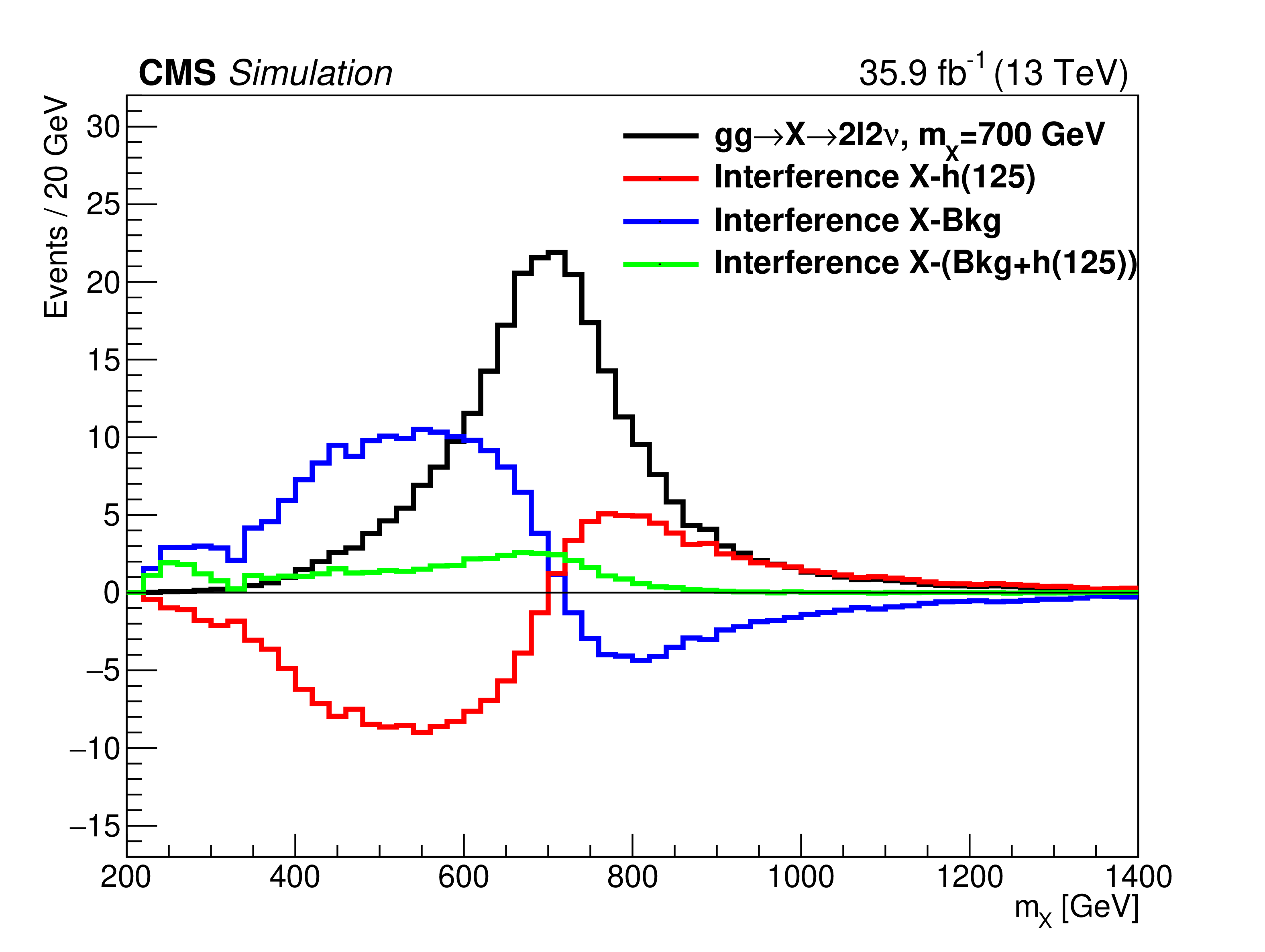
Figure 1:
Generator-level mass of a ggF-produced 700 GeV signal (black line) normalized to the SM cross section. The effects of the interference of the signal with the ${\mathrm{g} \mathrm{g} {\to} {{\mathrm{W}} {\mathrm{W}}}}$ continuum and the ${\mathrm{g} \mathrm{g} {\to} {\mathrm{h} (125)}}$ off-shell tail are shown, together with the total interference effect. |
png pdf |
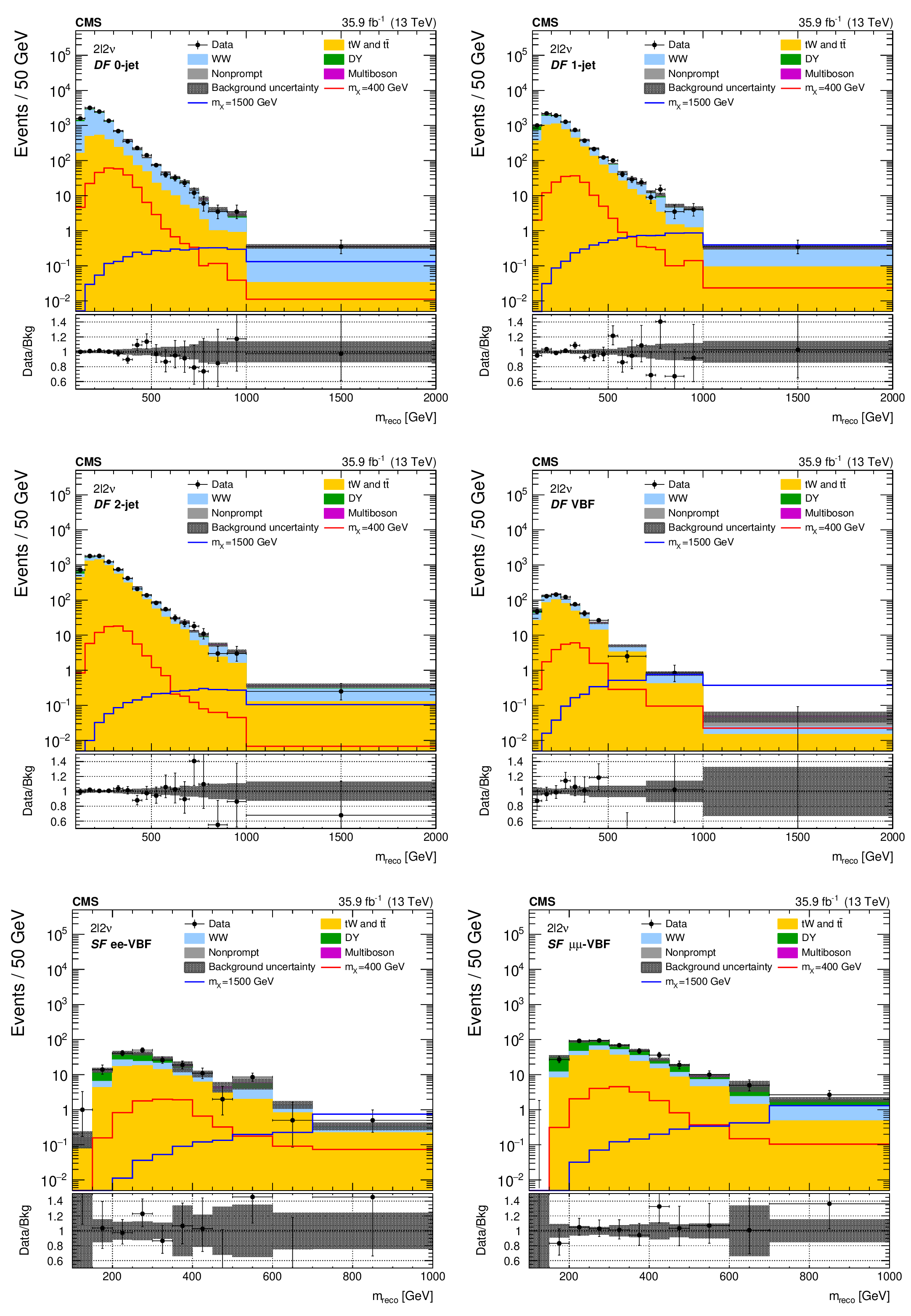
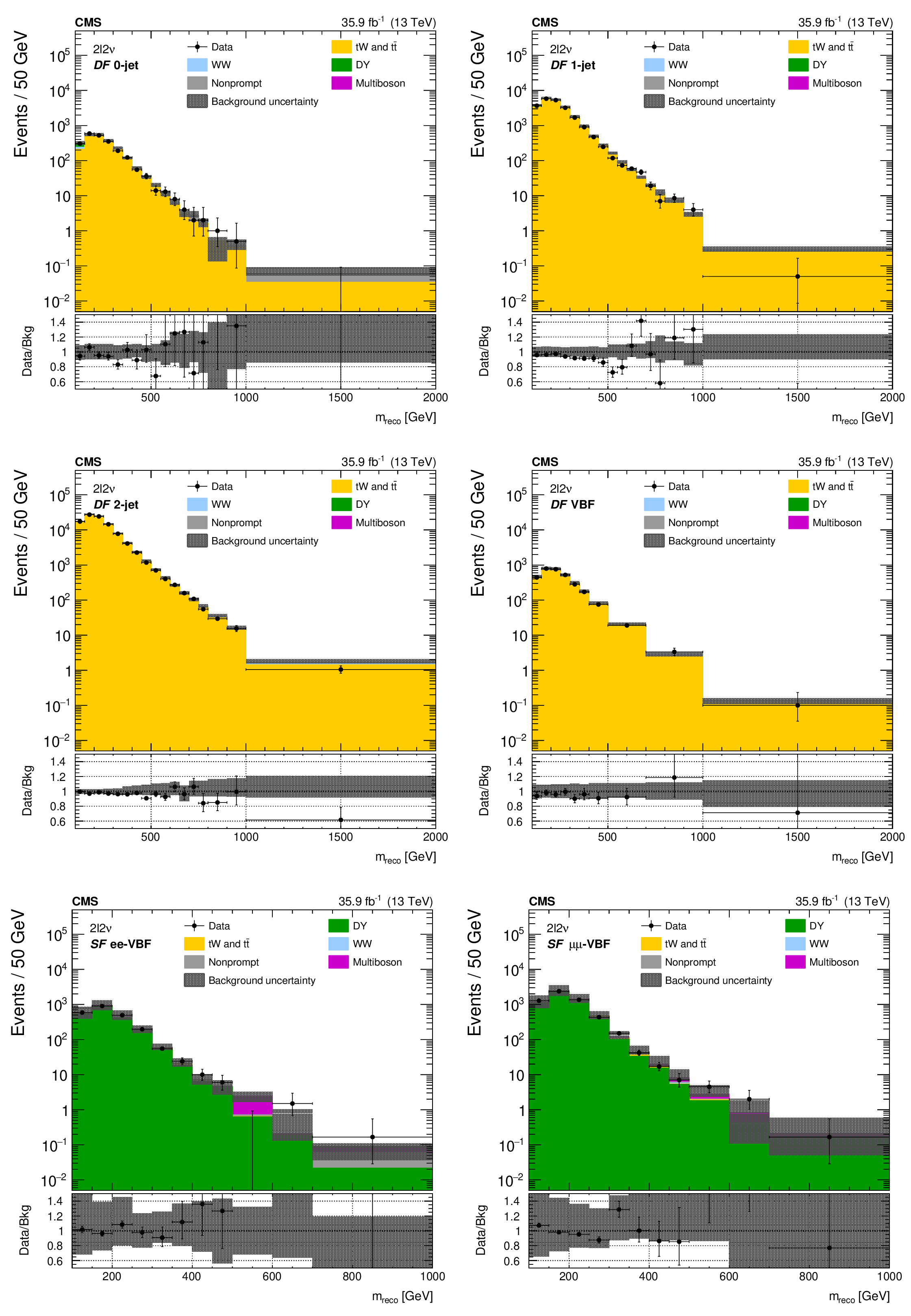
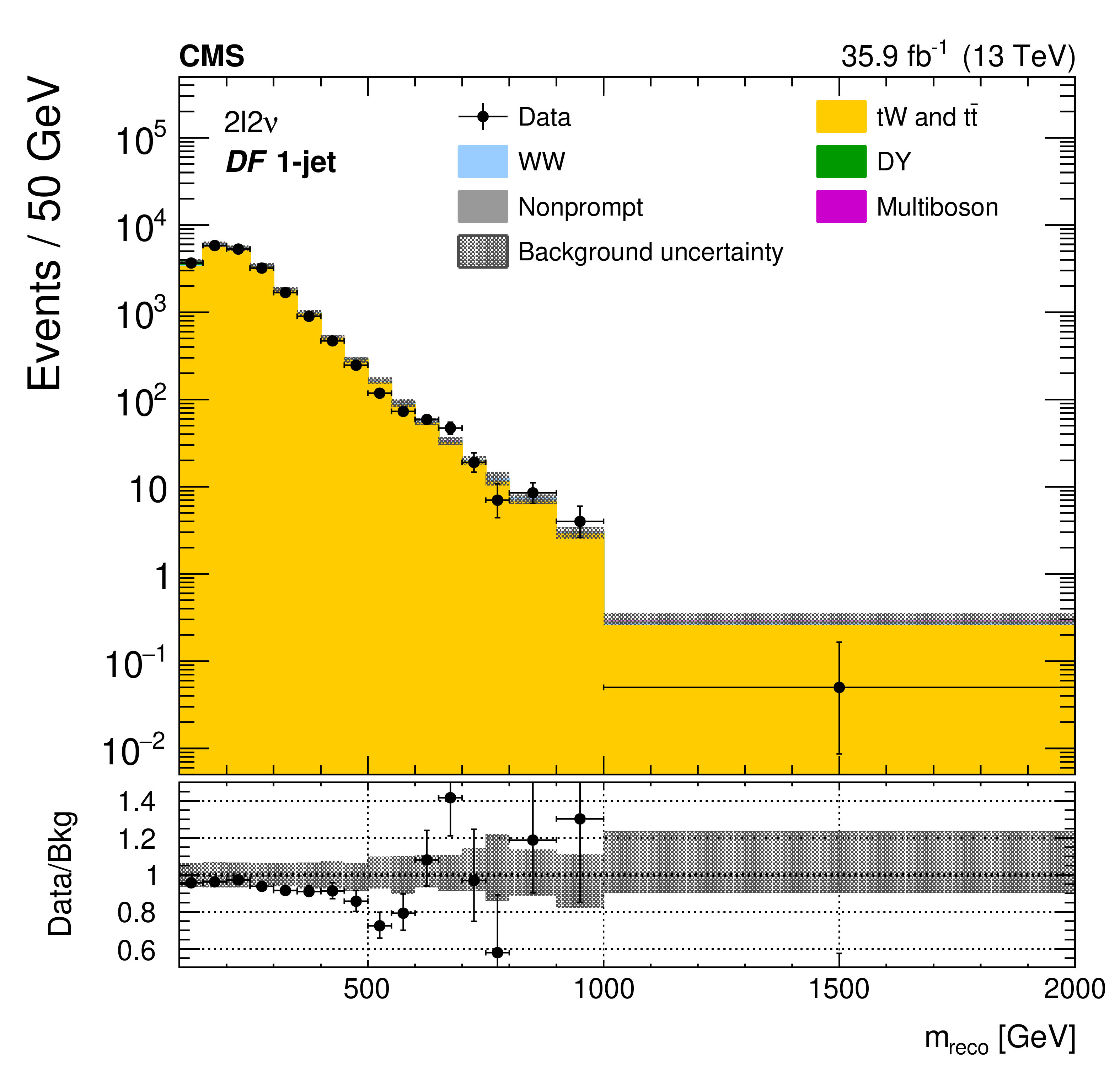
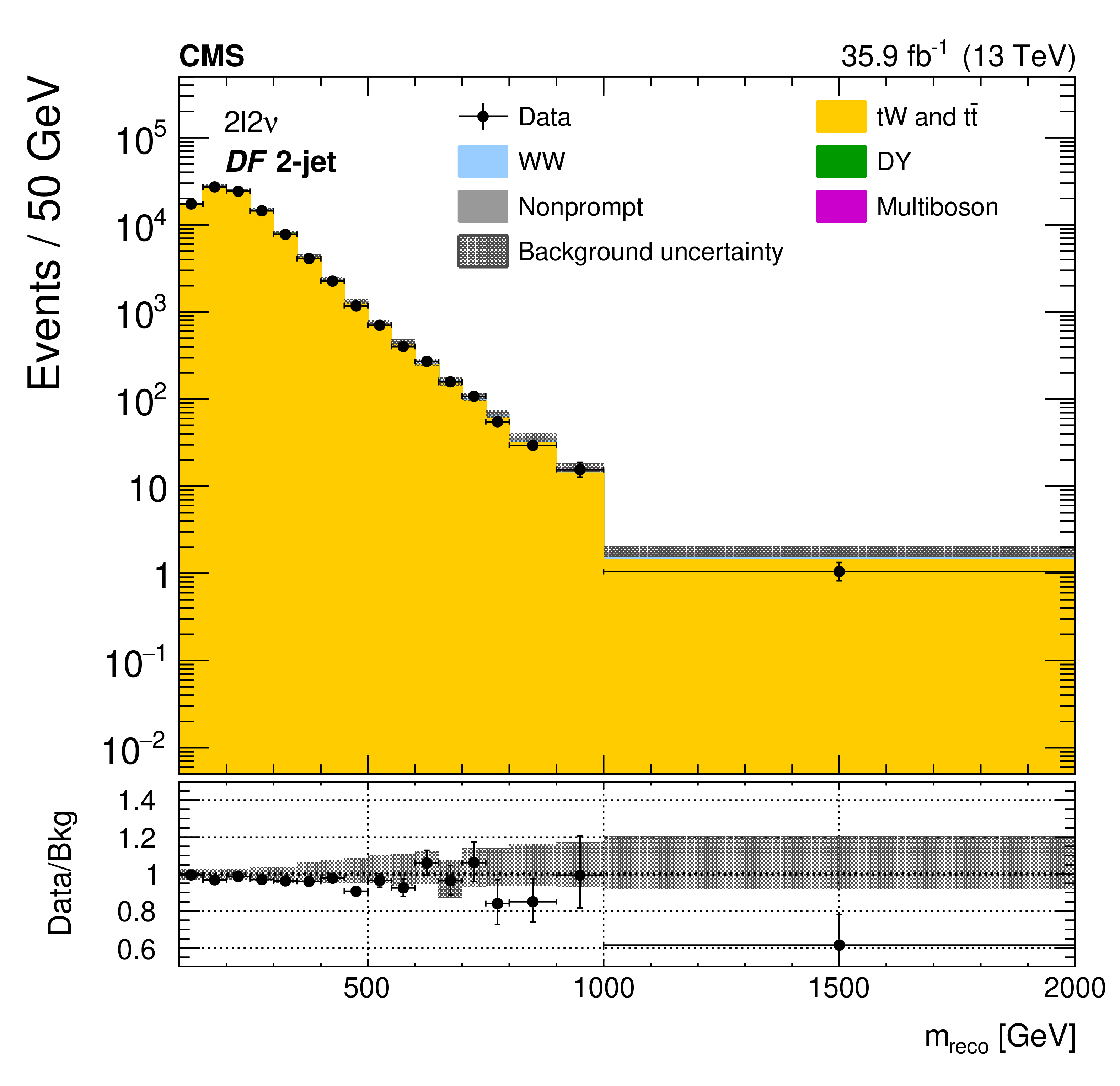
Figure 2:
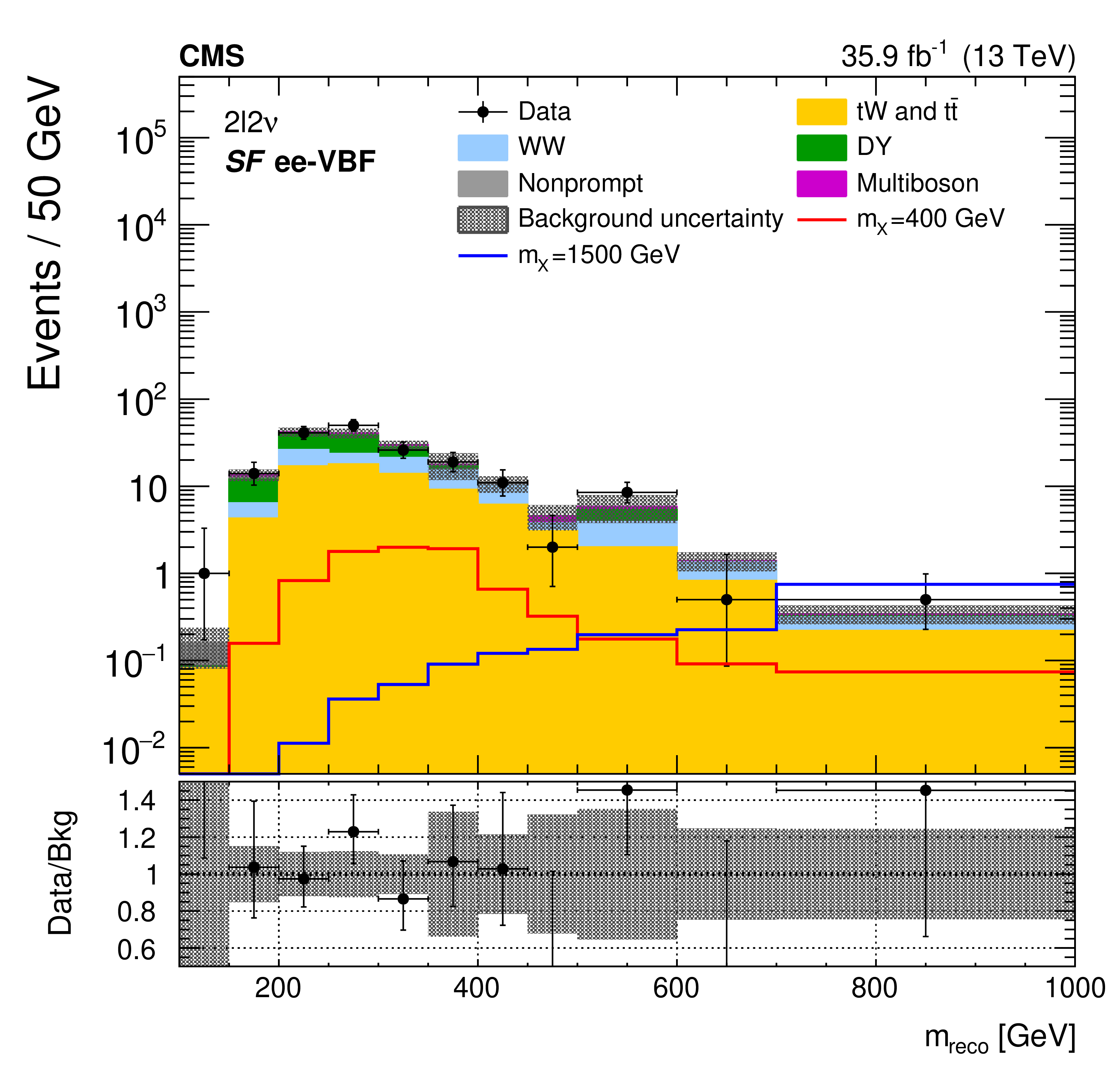
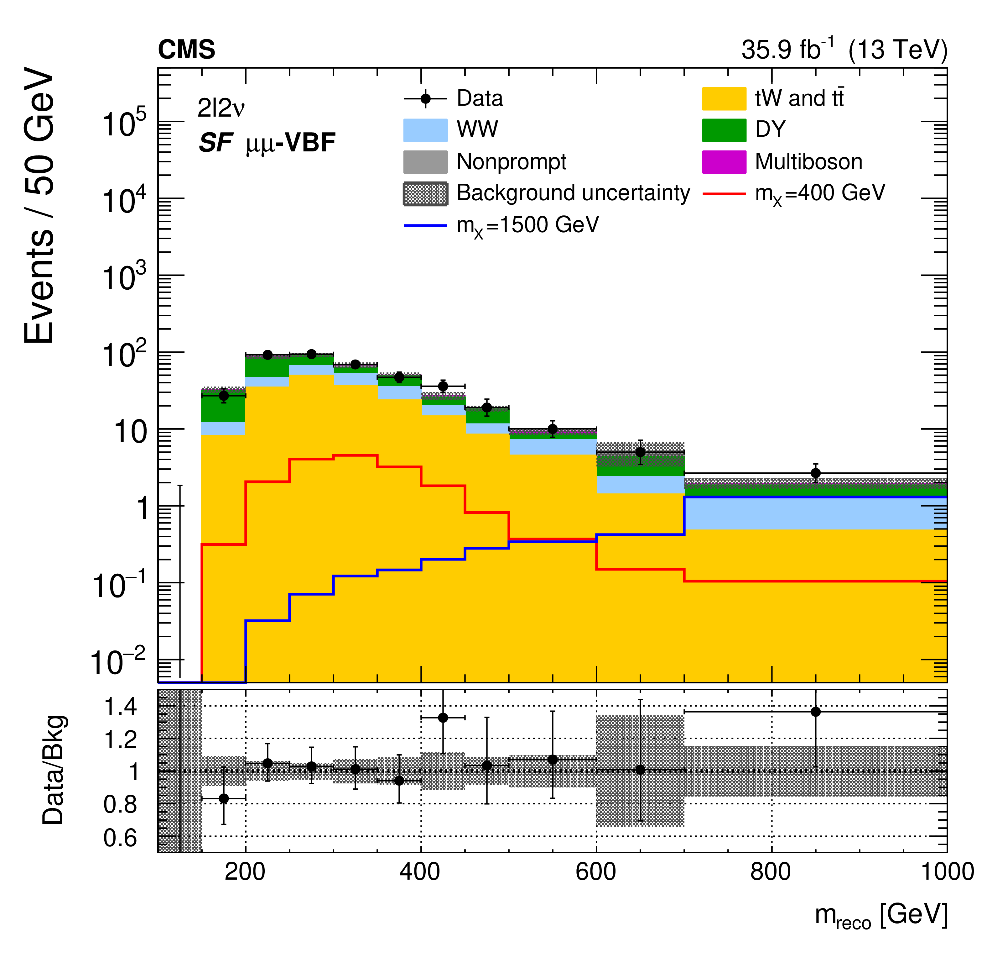
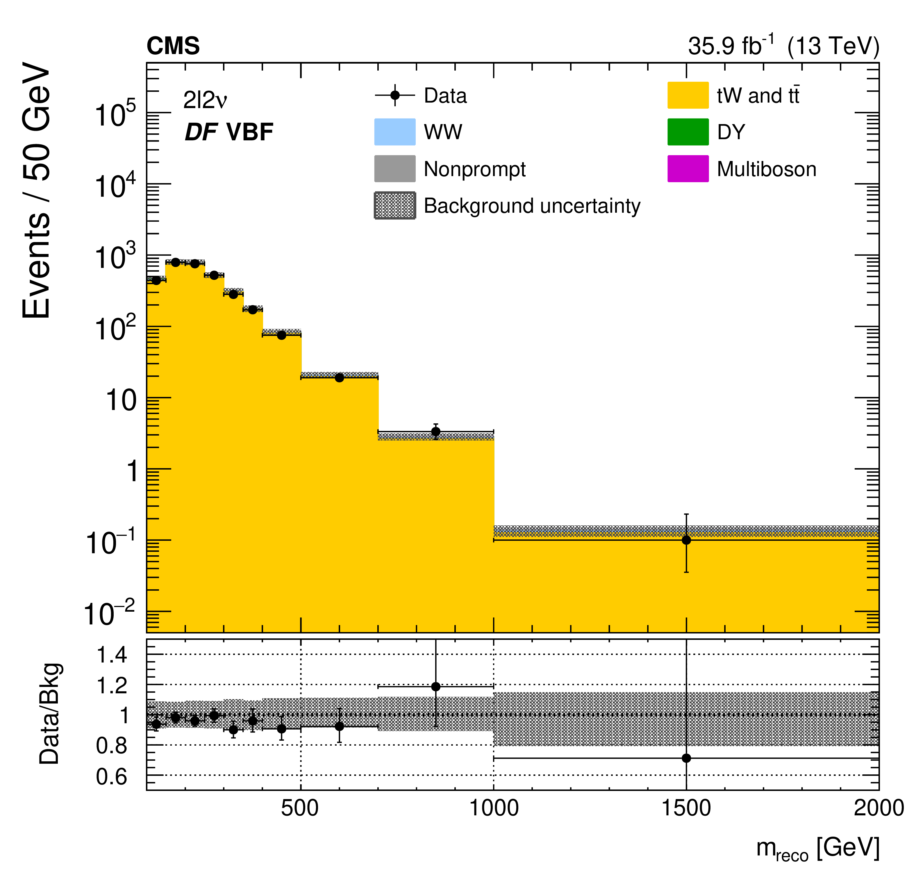
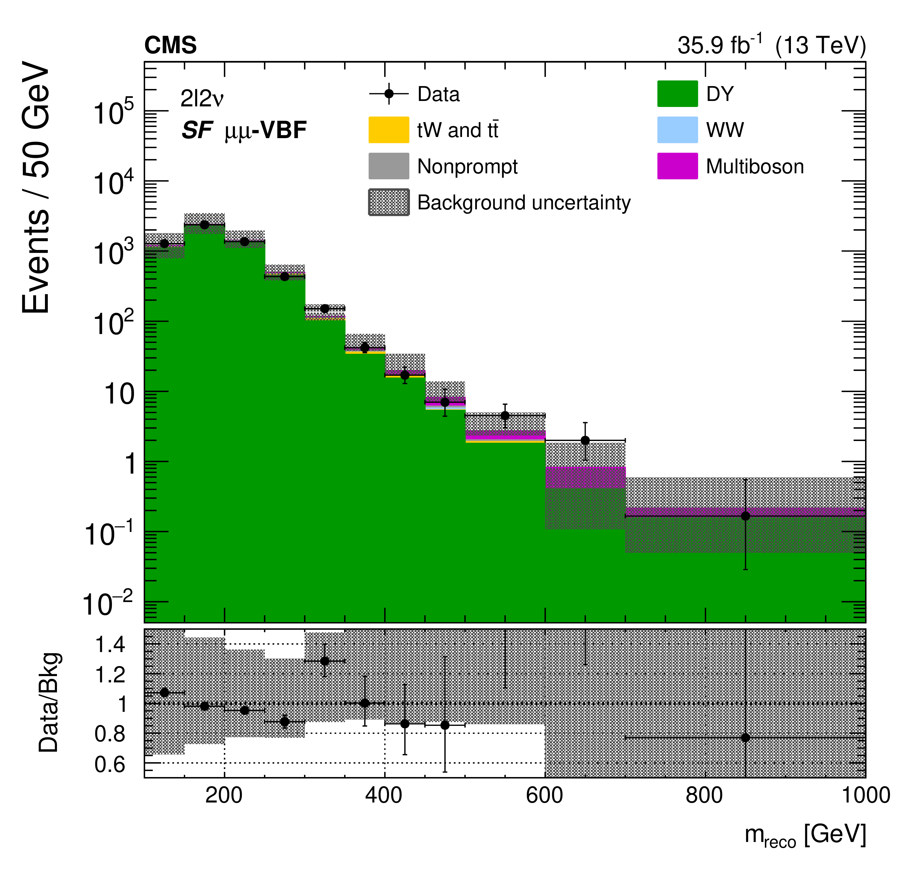
The ${m_\text {reco}}$ distributions in the ${2\ell 2\nu}$ different- (upper and middle) and same-flavour (lower) categories, after performing a background-only fit with the dominant background normalizations determined using control regions. The points represent the data and the stacked histograms the expected backgrounds. Also shown are the sum of the expected ggF- and VBF-produced signals for $ {m_{\mathrm{X}}} = $ 400 and 1500 GeV, normalized to the SM cross sections, and without considering interference effects. The hatched area shows the combined statistical and systematic uncertainties in the background estimation. Lower panels show the ratio of data to expected background. Larger bin widths are used at higher ${m_\text {reco}}$ ; the bin widths are indicated by the horizontal error bars. |

png pdf |
Figure 2-a:
The ${m_\text {reco}}$ distributions in the ${2\ell 2\nu}$ different- (upper and middle) and same-flavour (lower) categories, after performing a background-only fit with the dominant background normalizations determined using control regions. The points represent the data and the stacked histograms the expected backgrounds. Also shown are the sum of the expected ggF- and VBF-produced signals for $ {m_{\mathrm{X}}} = $ 400 and 1500 GeV, normalized to the SM cross sections, and without considering interference effects. The hatched area shows the combined statistical and systematic uncertainties in the background estimation. Lower panels show the ratio of data to expected background. Larger bin widths are used at higher ${m_\text {reco}}$ ; the bin widths are indicated by the horizontal error bars. |
png pdf |
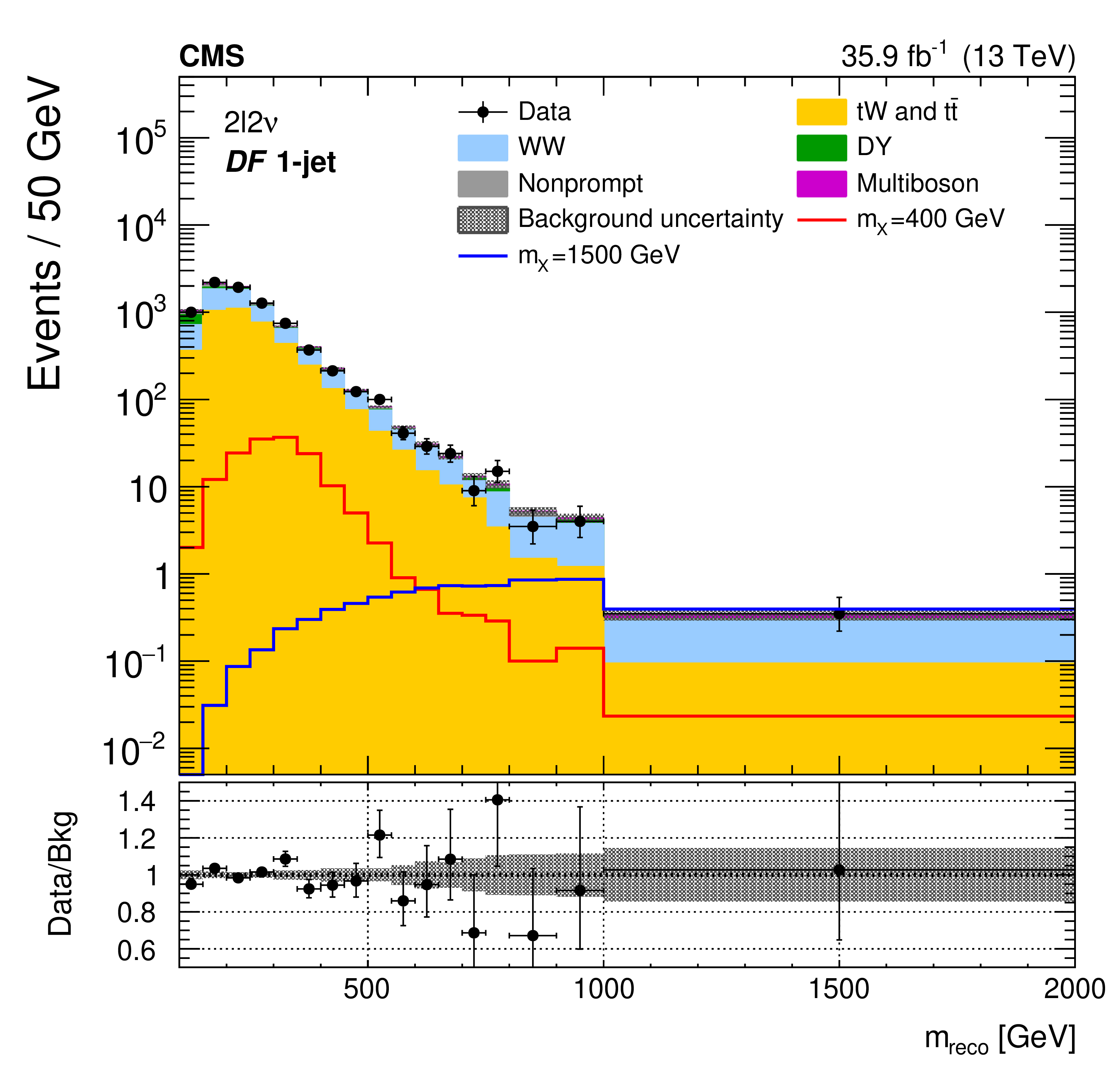
Figure 2-b:
The ${m_\text {reco}}$ distributions in the ${2\ell 2\nu}$ different- (upper and middle) and same-flavour (lower) categories, after performing a background-only fit with the dominant background normalizations determined using control regions. The points represent the data and the stacked histograms the expected backgrounds. Also shown are the sum of the expected ggF- and VBF-produced signals for $ {m_{\mathrm{X}}} = $ 400 and 1500 GeV, normalized to the SM cross sections, and without considering interference effects. The hatched area shows the combined statistical and systematic uncertainties in the background estimation. Lower panels show the ratio of data to expected background. Larger bin widths are used at higher ${m_\text {reco}}$ ; the bin widths are indicated by the horizontal error bars. |

png pdf |
Figure 2-c:
The ${m_\text {reco}}$ distributions in the ${2\ell 2\nu}$ different- (upper and middle) and same-flavour (lower) categories, after performing a background-only fit with the dominant background normalizations determined using control regions. The points represent the data and the stacked histograms the expected backgrounds. Also shown are the sum of the expected ggF- and VBF-produced signals for $ {m_{\mathrm{X}}} = $ 400 and 1500 GeV, normalized to the SM cross sections, and without considering interference effects. The hatched area shows the combined statistical and systematic uncertainties in the background estimation. Lower panels show the ratio of data to expected background. Larger bin widths are used at higher ${m_\text {reco}}$ ; the bin widths are indicated by the horizontal error bars. |
png pdf |
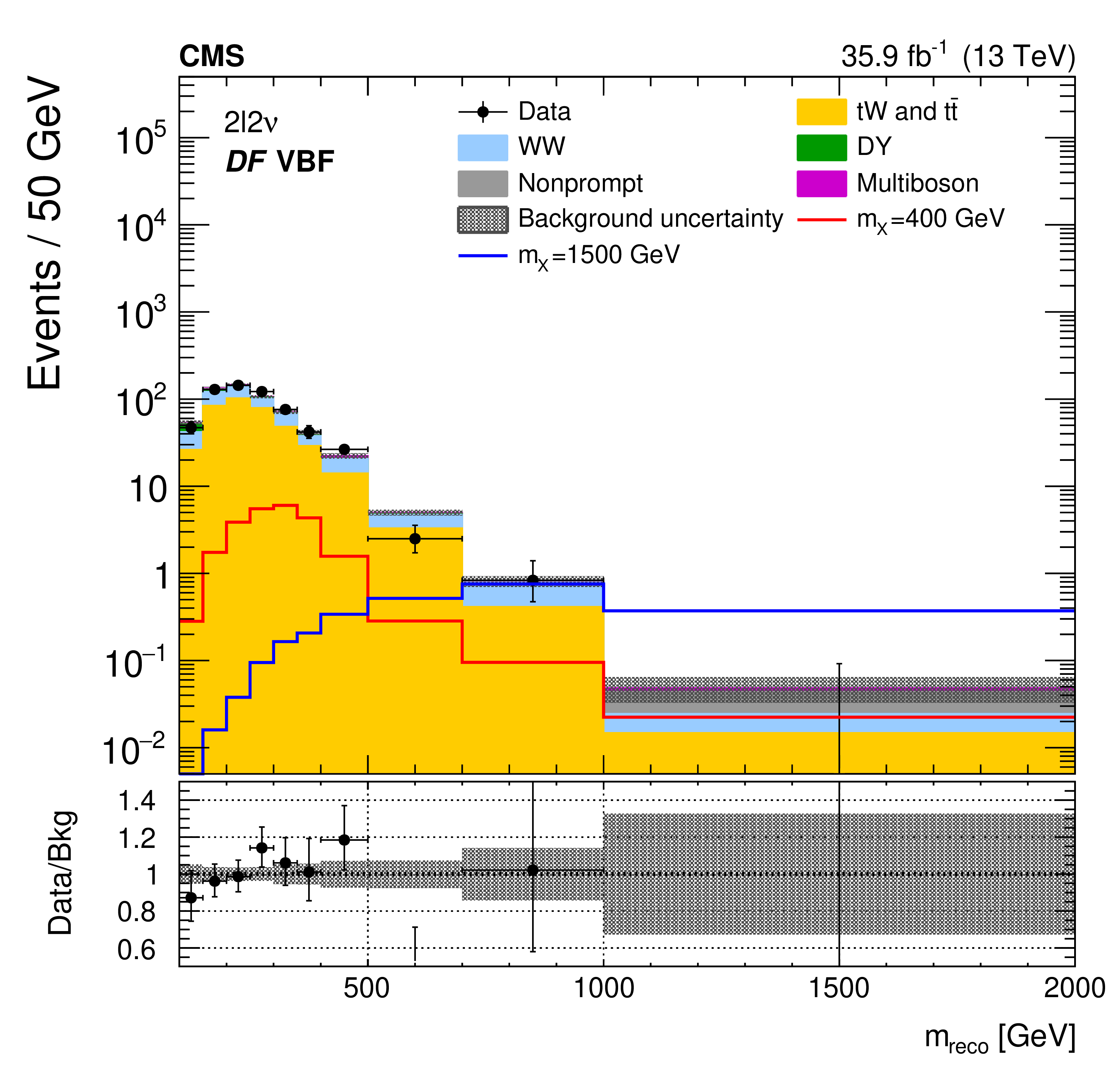
Figure 2-d:
The ${m_\text {reco}}$ distributions in the ${2\ell 2\nu}$ different- (upper and middle) and same-flavour (lower) categories, after performing a background-only fit with the dominant background normalizations determined using control regions. The points represent the data and the stacked histograms the expected backgrounds. Also shown are the sum of the expected ggF- and VBF-produced signals for $ {m_{\mathrm{X}}} = $ 400 and 1500 GeV, normalized to the SM cross sections, and without considering interference effects. The hatched area shows the combined statistical and systematic uncertainties in the background estimation. Lower panels show the ratio of data to expected background. Larger bin widths are used at higher ${m_\text {reco}}$ ; the bin widths are indicated by the horizontal error bars. |
png pdf |
Figure 2-e:
The ${m_\text {reco}}$ distributions in the ${2\ell 2\nu}$ different- (upper and middle) and same-flavour (lower) categories, after performing a background-only fit with the dominant background normalizations determined using control regions. The points represent the data and the stacked histograms the expected backgrounds. Also shown are the sum of the expected ggF- and VBF-produced signals for $ {m_{\mathrm{X}}} = $ 400 and 1500 GeV, normalized to the SM cross sections, and without considering interference effects. The hatched area shows the combined statistical and systematic uncertainties in the background estimation. Lower panels show the ratio of data to expected background. Larger bin widths are used at higher ${m_\text {reco}}$ ; the bin widths are indicated by the horizontal error bars. |
png pdf |
Figure 2-f:
The ${m_\text {reco}}$ distributions in the ${2\ell 2\nu}$ different- (upper and middle) and same-flavour (lower) categories, after performing a background-only fit with the dominant background normalizations determined using control regions. The points represent the data and the stacked histograms the expected backgrounds. Also shown are the sum of the expected ggF- and VBF-produced signals for $ {m_{\mathrm{X}}} = $ 400 and 1500 GeV, normalized to the SM cross sections, and without considering interference effects. The hatched area shows the combined statistical and systematic uncertainties in the background estimation. Lower panels show the ratio of data to expected background. Larger bin widths are used at higher ${m_\text {reco}}$ ; the bin widths are indicated by the horizontal error bars. |
png pdf |
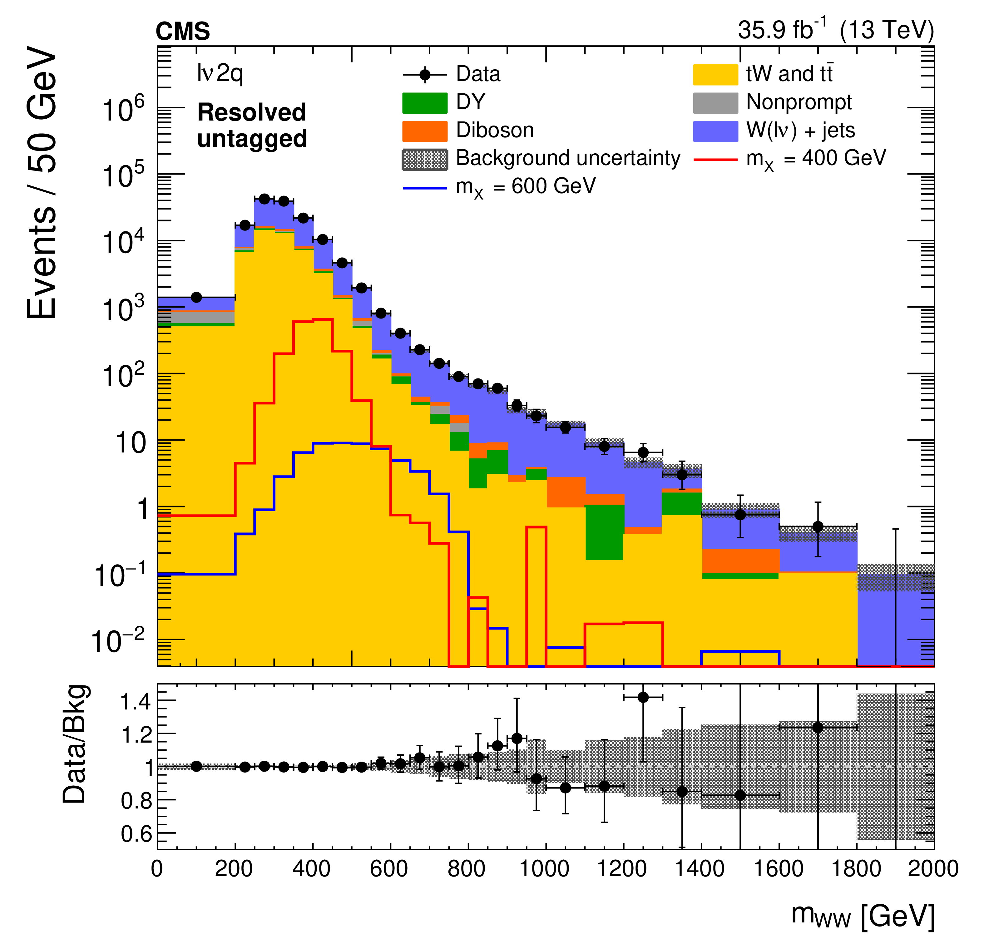
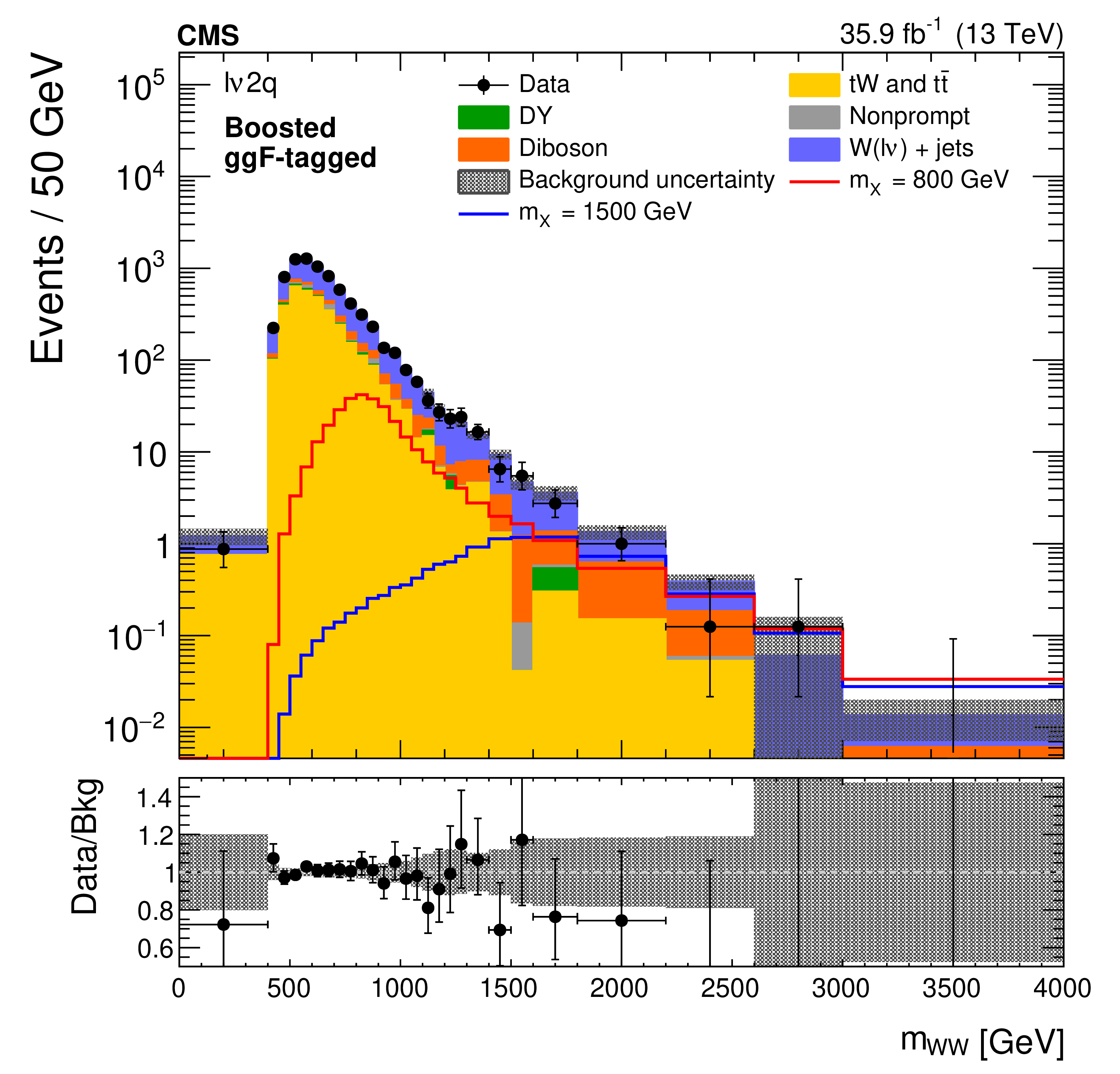
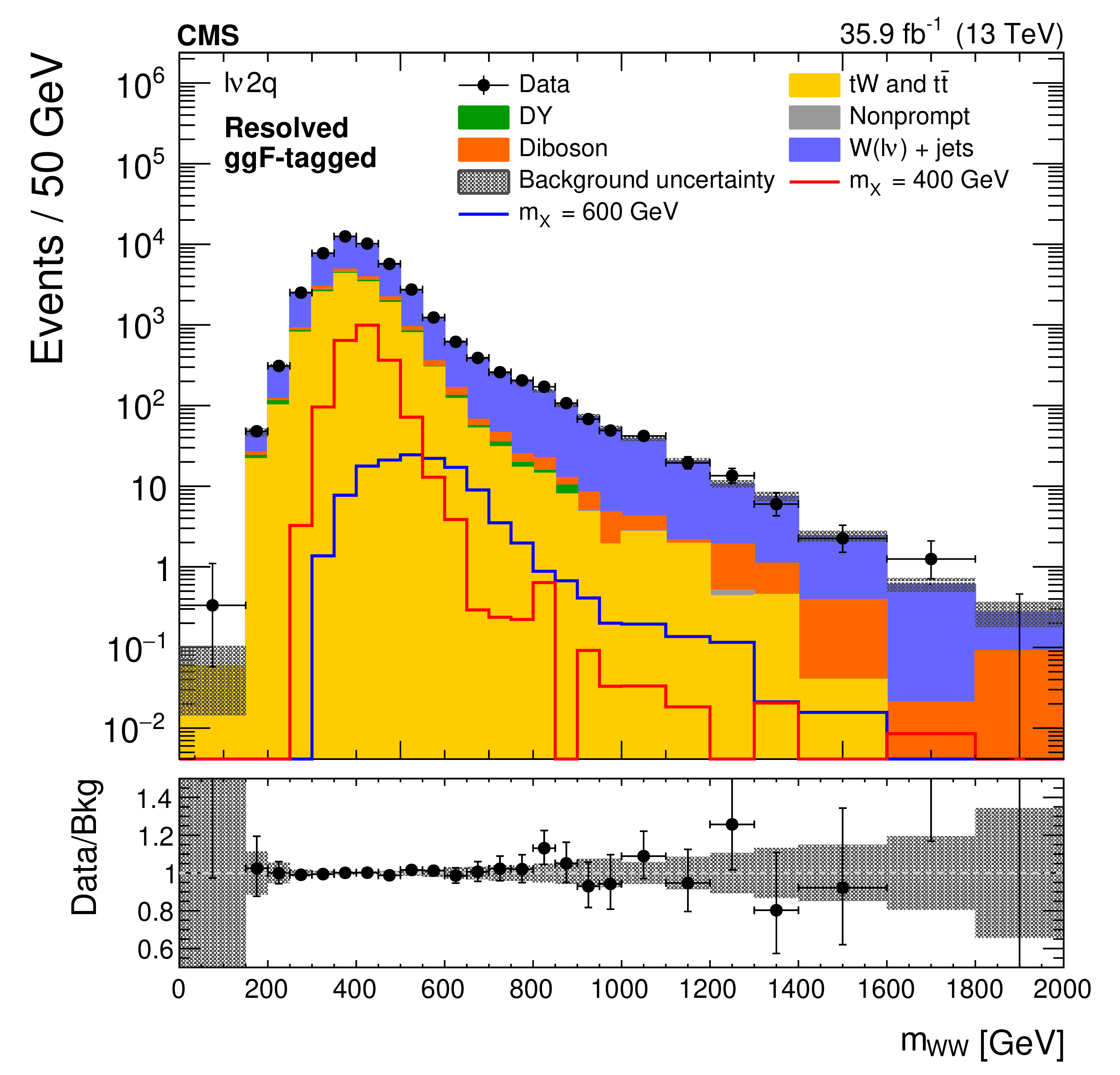
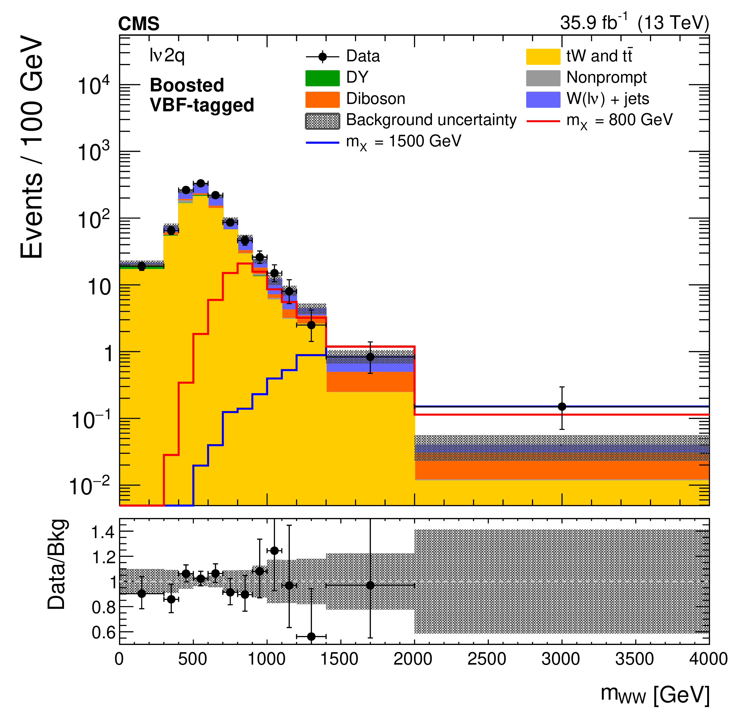
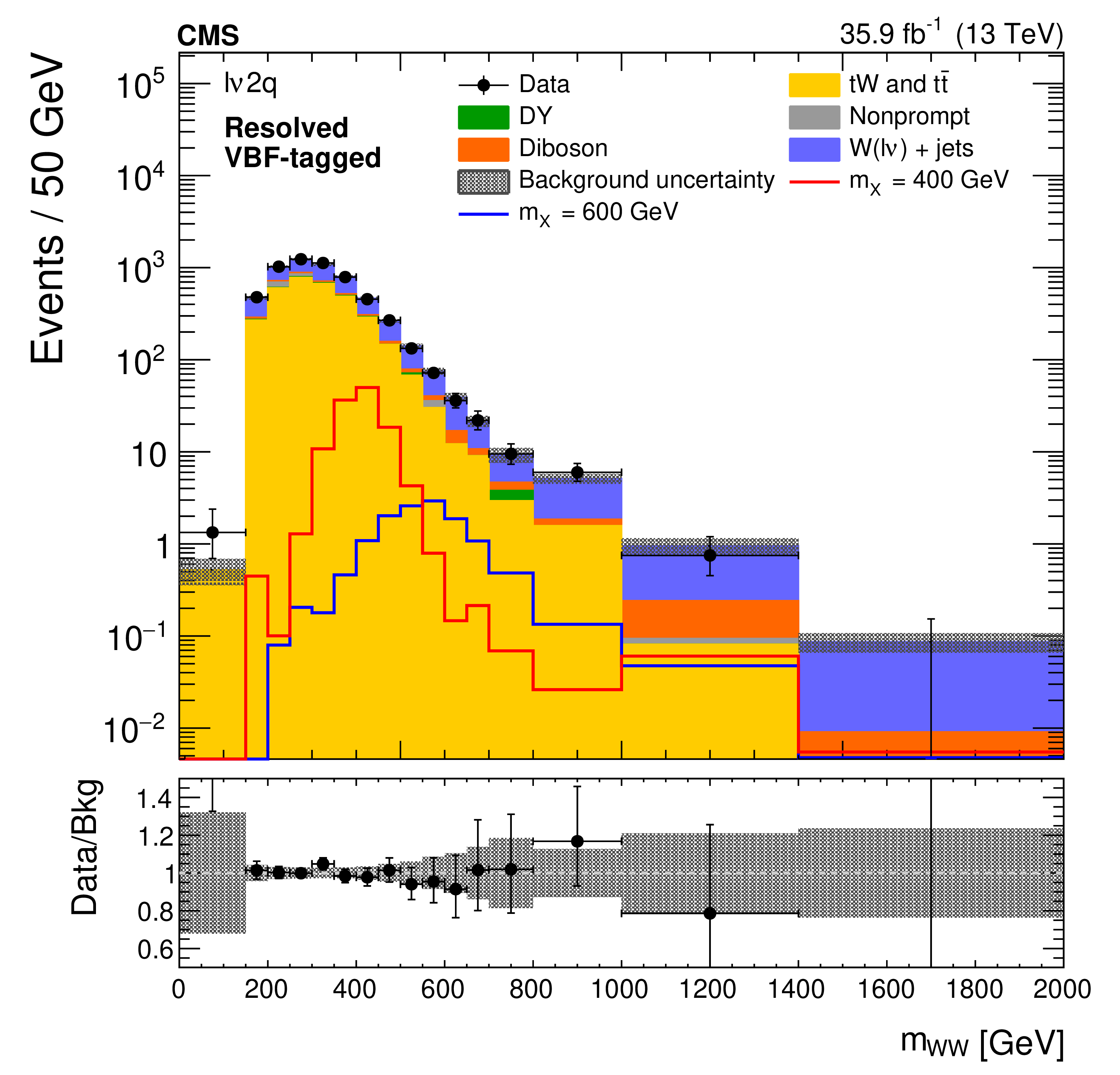
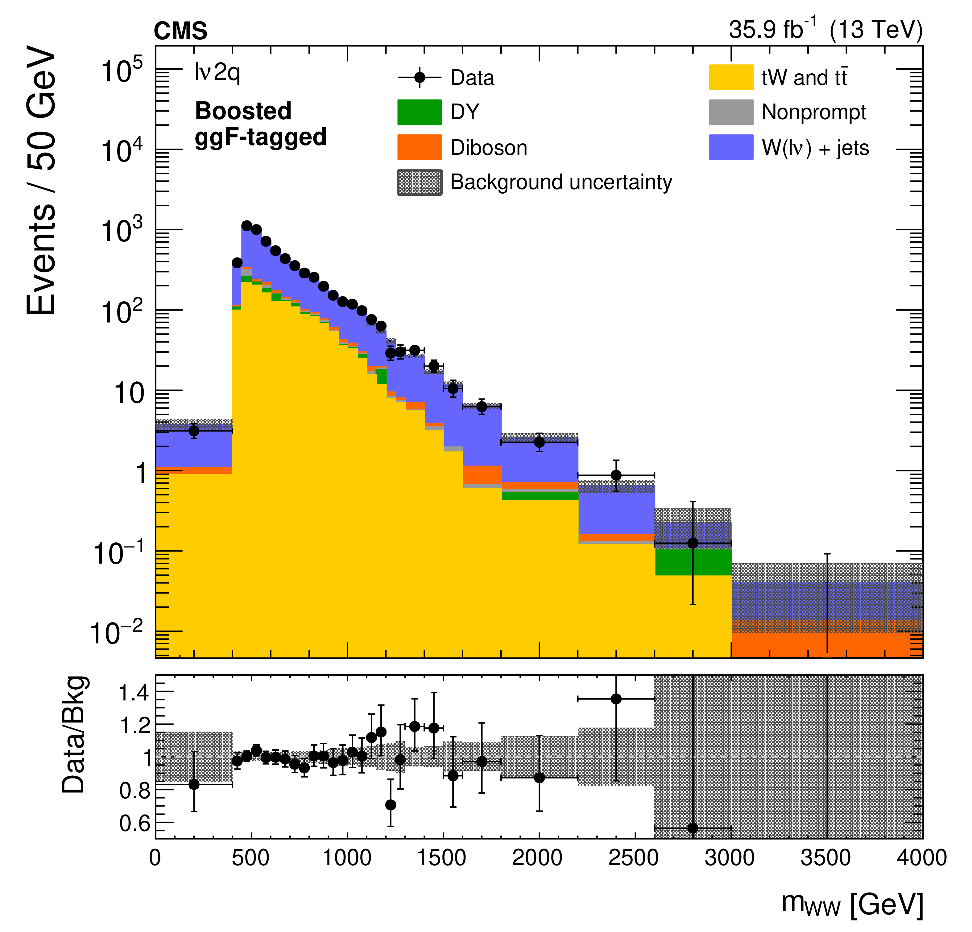
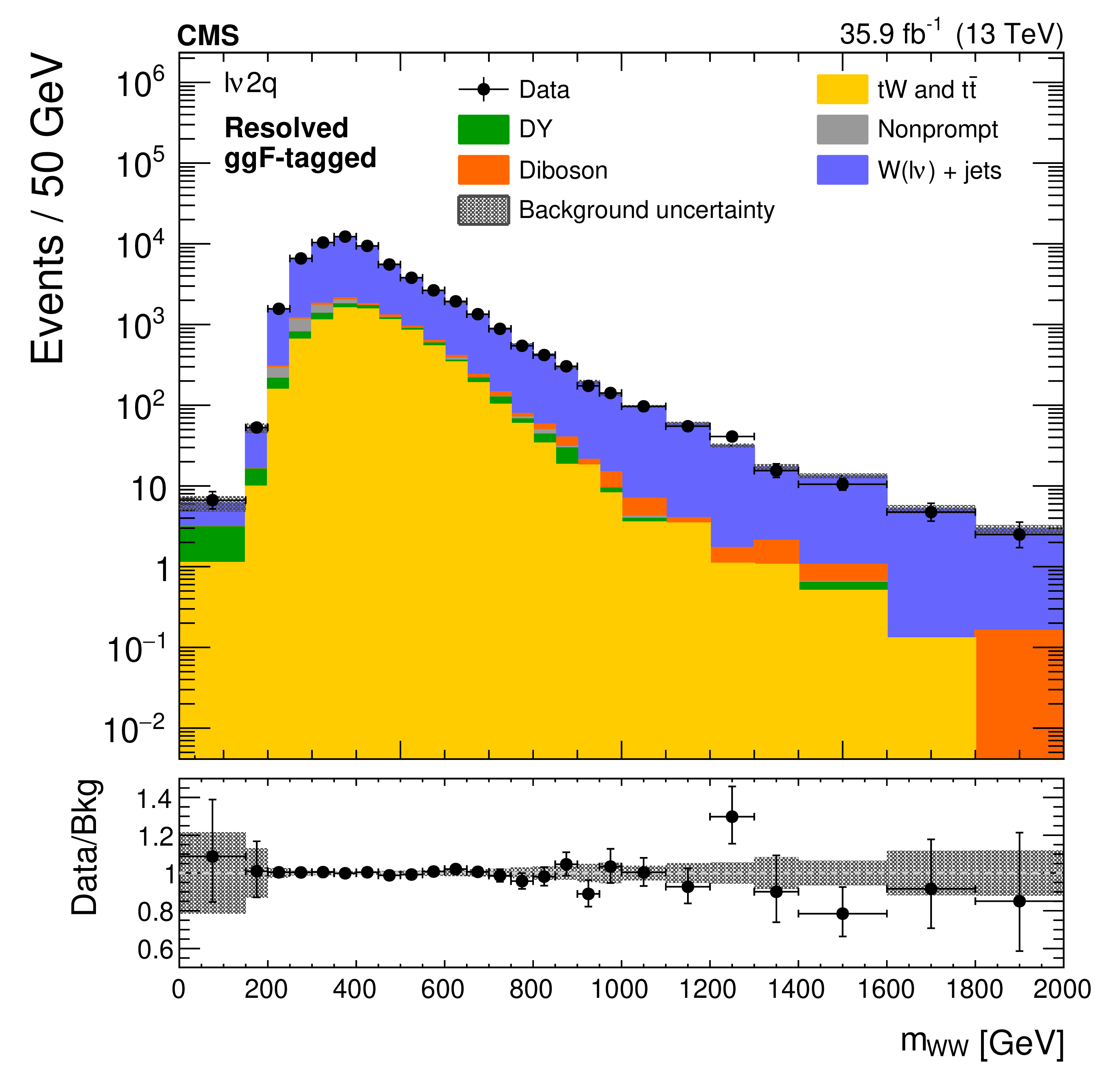
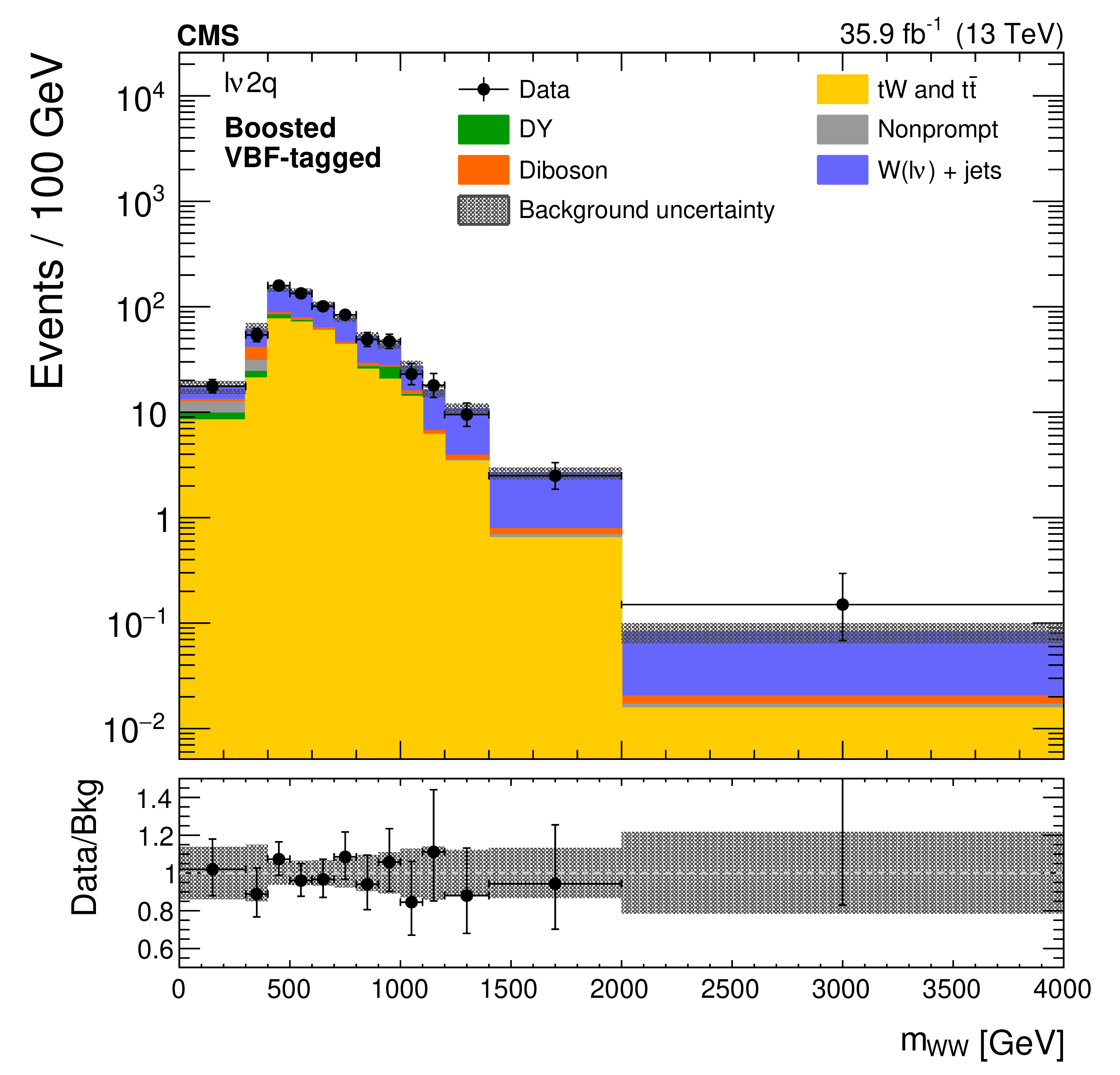
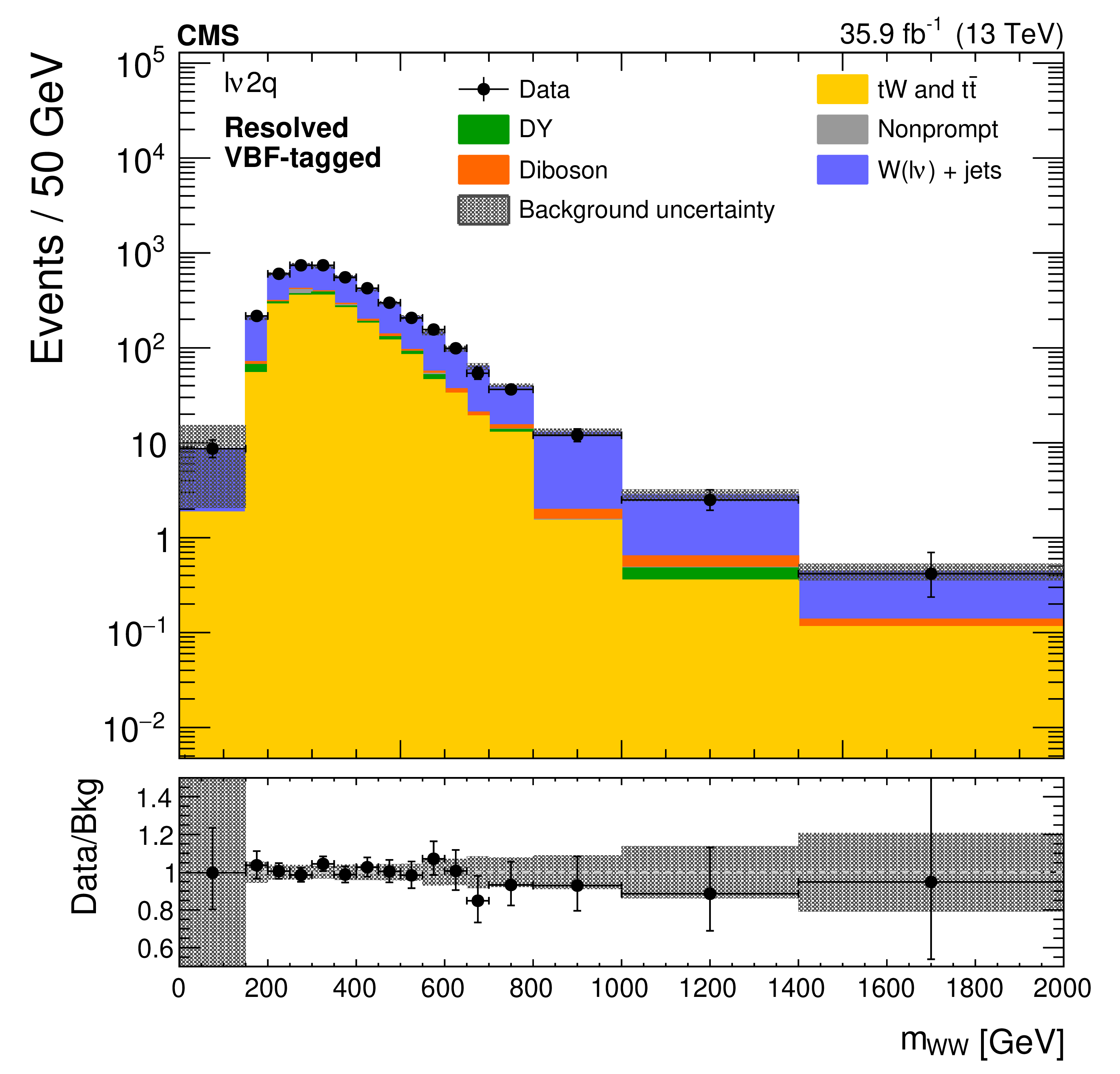
Figure 3:
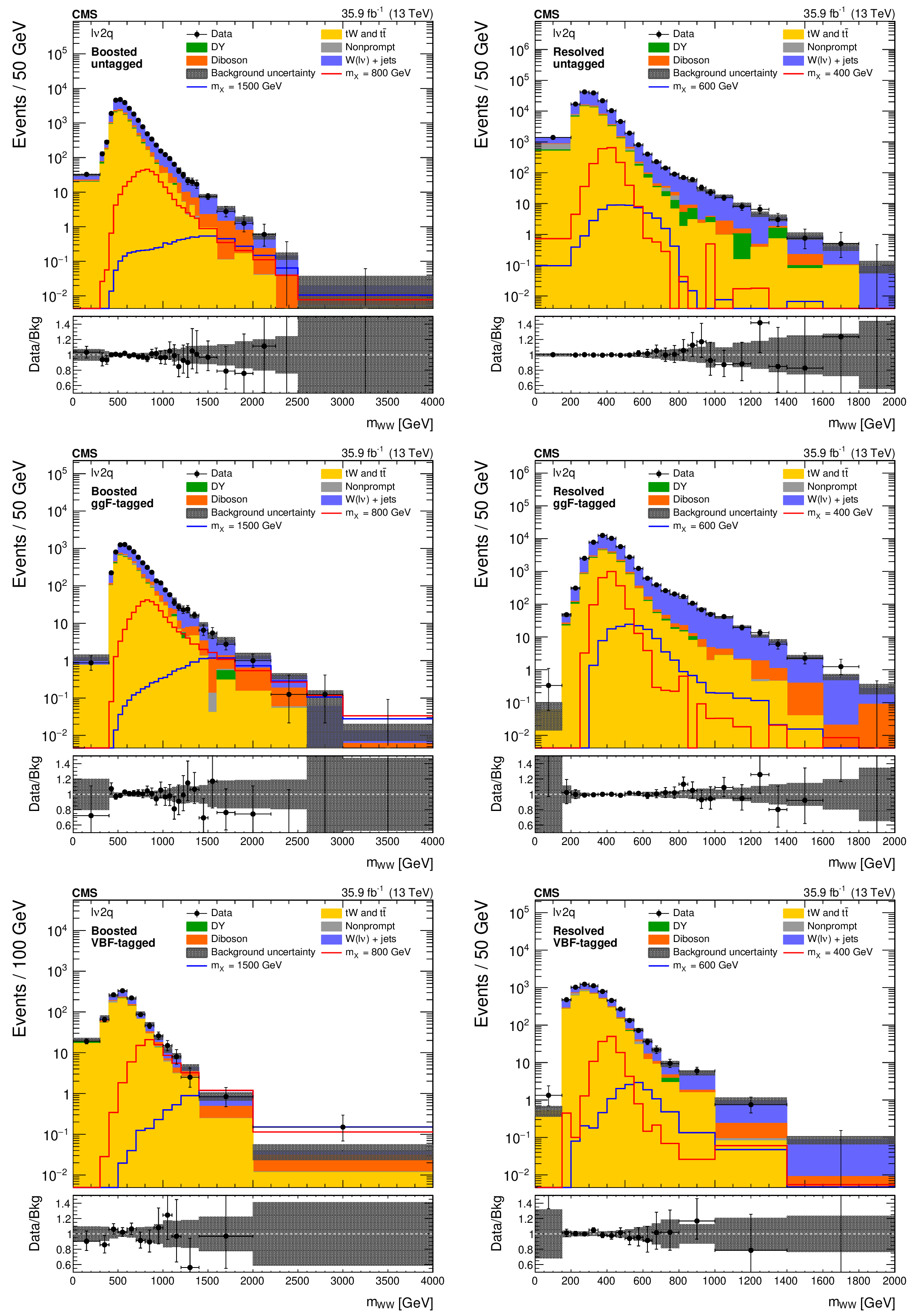
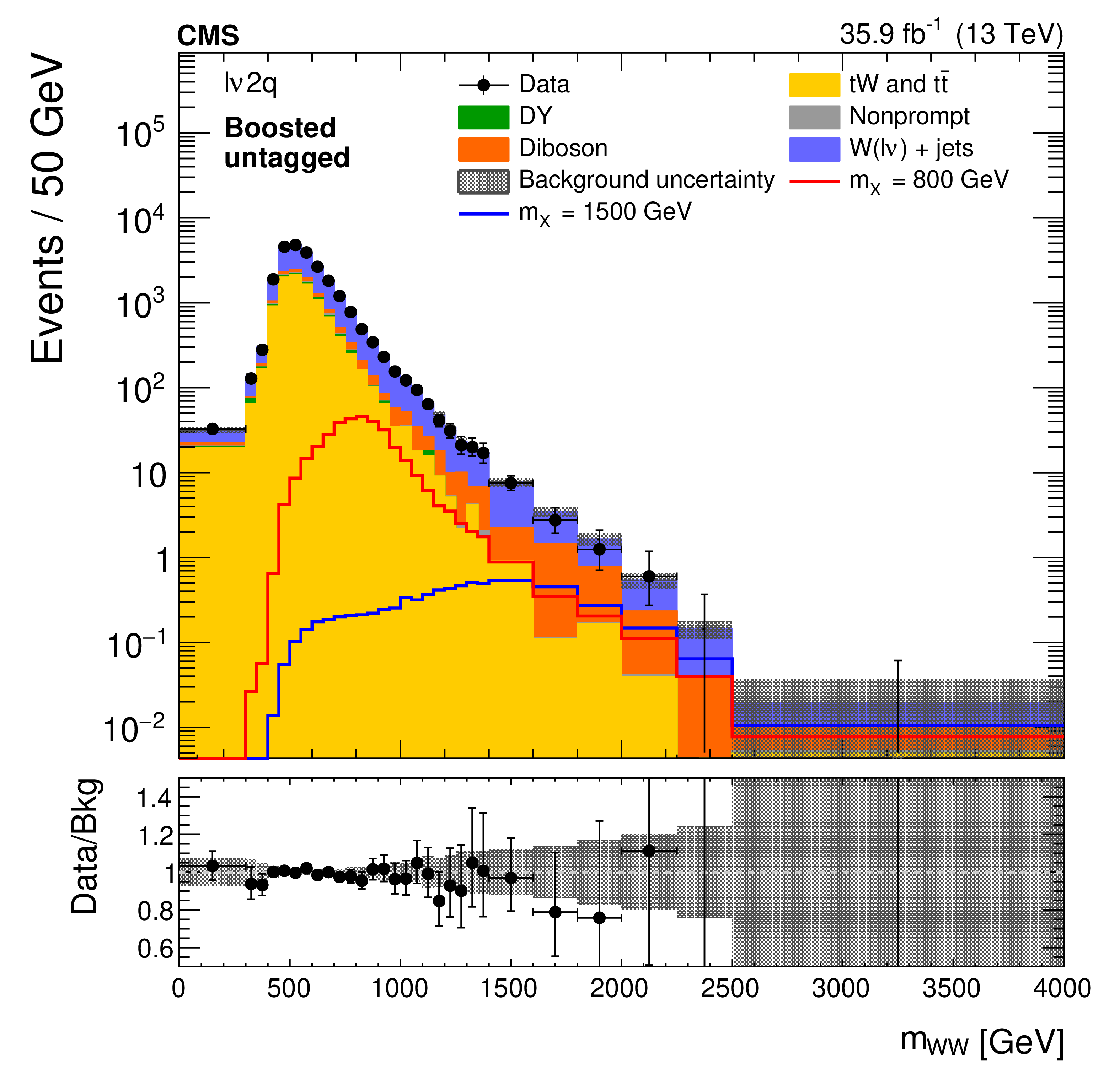
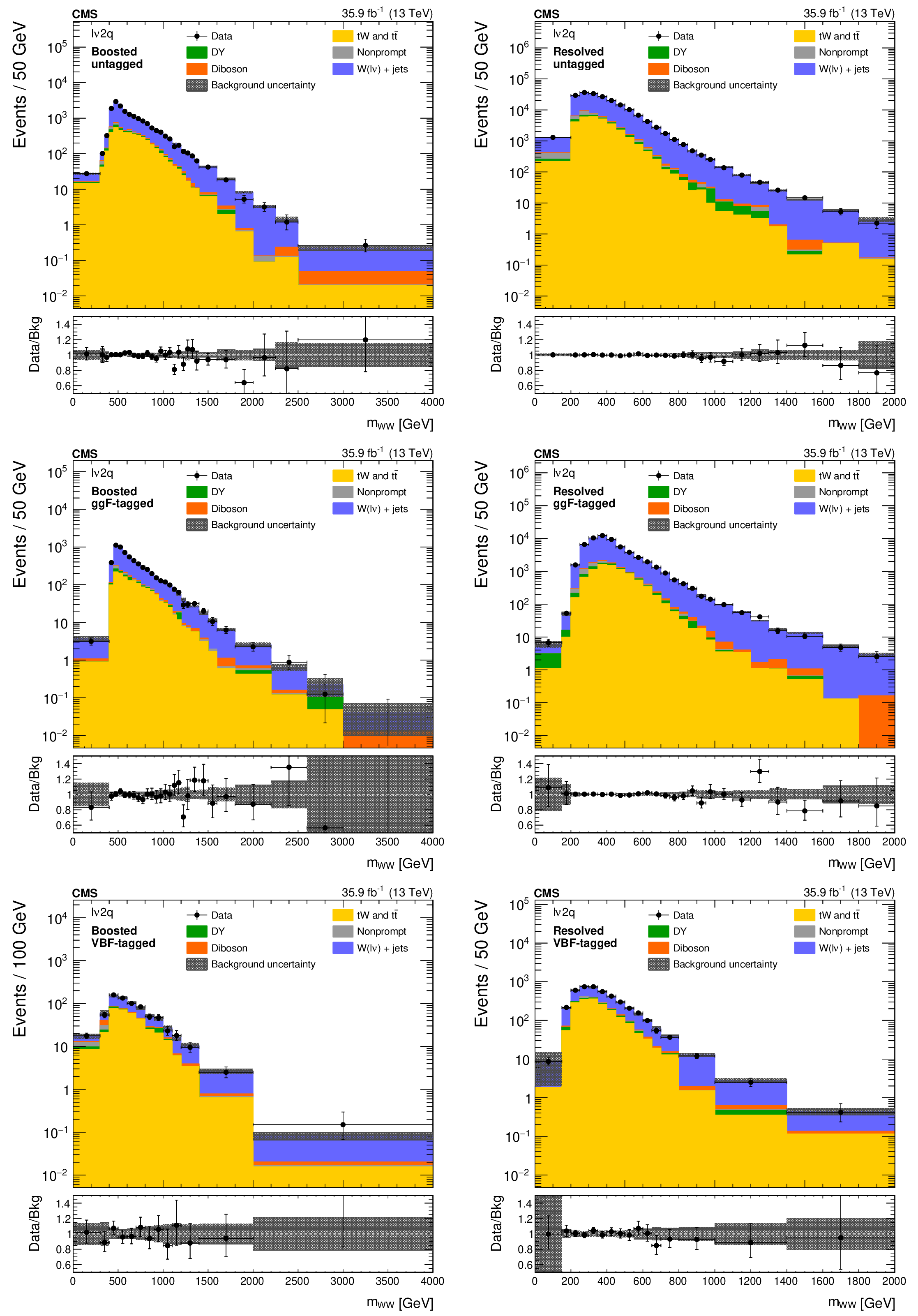
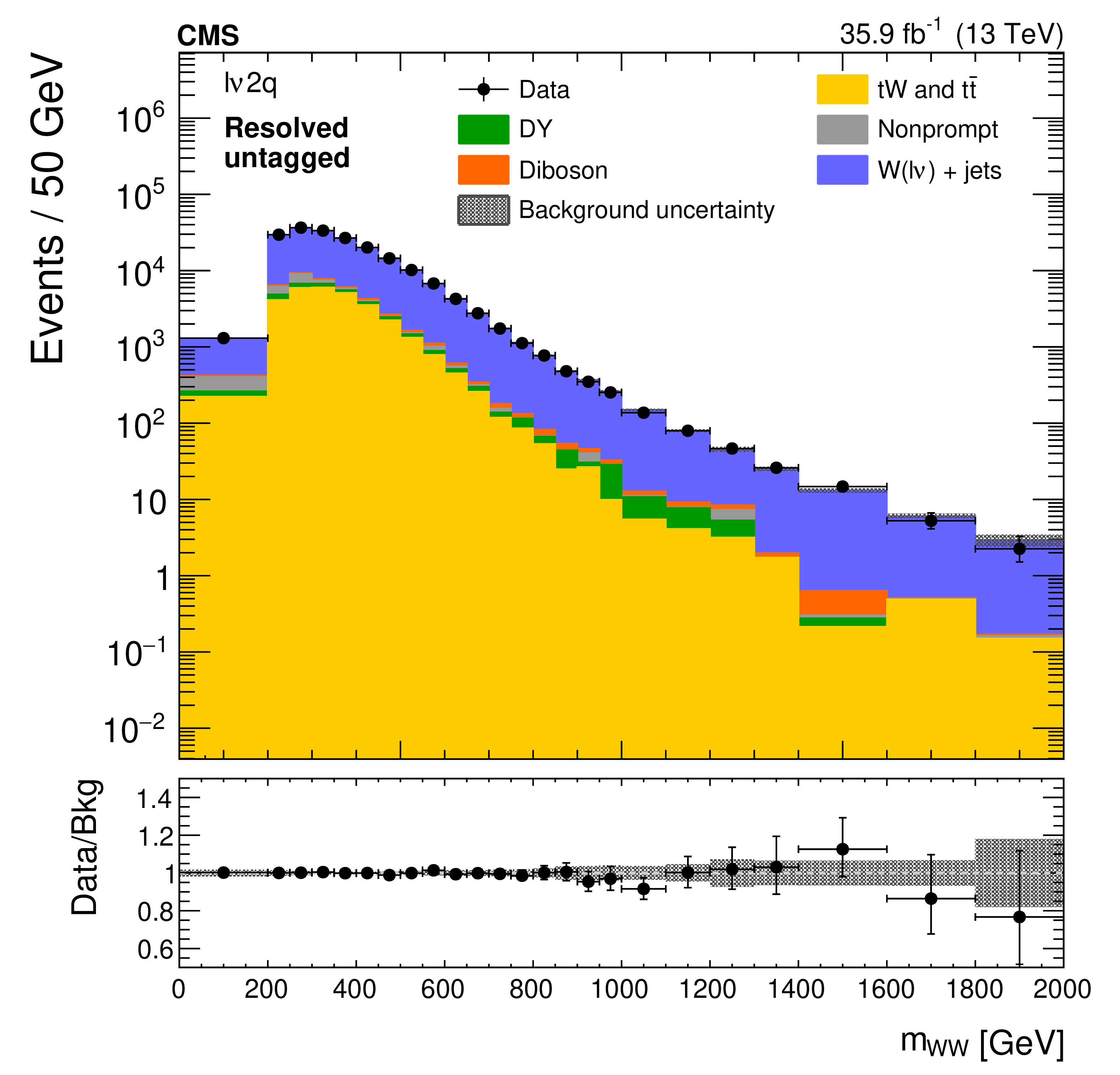
The ${m_{{{\mathrm{W}} {\mathrm{W}}}}}$ distributions in the ${\ell \nu 2\mathrm{q}}$ boosted (left) and resolved (right) categories, after performing a background-only fit with the dominant background normalizations determined using control regions. Electron and muon channels are combined. The points represent the data and the stacked histograms the expected backgrounds. Also shown are the sum of the expected ggF- and VBF-produced signals for $ {m_{\mathrm{X}}} = $ 800 and 1500 GeV (left), and $ {m_{\mathrm{X}}} = $ 400 and 600 GeV (right), normalized to the SM cross sections, and without considering interference effects. The hatched area shows the combined statistical and systematic uncertainties in the background estimation. Lower panels show the ratio of data to expected background. Larger bin widths are used at higher ${m_{{{\mathrm{W}} {\mathrm{W}}}}}$ ; the bin widths are indicated by the horizontal error bars. |
png pdf |
Figure 3-a:
The ${m_{{{\mathrm{W}} {\mathrm{W}}}}}$ distributions in the ${\ell \nu 2\mathrm{q}}$ boosted (left) and resolved (right) categories, after performing a background-only fit with the dominant background normalizations determined using control regions. Electron and muon channels are combined. The points represent the data and the stacked histograms the expected backgrounds. Also shown are the sum of the expected ggF- and VBF-produced signals for $ {m_{\mathrm{X}}} = $ 800 and 1500 GeV (left), and $ {m_{\mathrm{X}}} = $ 400 and 600 GeV (right), normalized to the SM cross sections, and without considering interference effects. The hatched area shows the combined statistical and systematic uncertainties in the background estimation. Lower panels show the ratio of data to expected background. Larger bin widths are used at higher ${m_{{{\mathrm{W}} {\mathrm{W}}}}}$ ; the bin widths are indicated by the horizontal error bars. |
png pdf |
Figure 3-b:
The ${m_{{{\mathrm{W}} {\mathrm{W}}}}}$ distributions in the ${\ell \nu 2\mathrm{q}}$ boosted (left) and resolved (right) categories, after performing a background-only fit with the dominant background normalizations determined using control regions. Electron and muon channels are combined. The points represent the data and the stacked histograms the expected backgrounds. Also shown are the sum of the expected ggF- and VBF-produced signals for $ {m_{\mathrm{X}}} = $ 800 and 1500 GeV (left), and $ {m_{\mathrm{X}}} = $ 400 and 600 GeV (right), normalized to the SM cross sections, and without considering interference effects. The hatched area shows the combined statistical and systematic uncertainties in the background estimation. Lower panels show the ratio of data to expected background. Larger bin widths are used at higher ${m_{{{\mathrm{W}} {\mathrm{W}}}}}$ ; the bin widths are indicated by the horizontal error bars. |
png pdf |
Figure 3-c:
The ${m_{{{\mathrm{W}} {\mathrm{W}}}}}$ distributions in the ${\ell \nu 2\mathrm{q}}$ boosted (left) and resolved (right) categories, after performing a background-only fit with the dominant background normalizations determined using control regions. Electron and muon channels are combined. The points represent the data and the stacked histograms the expected backgrounds. Also shown are the sum of the expected ggF- and VBF-produced signals for $ {m_{\mathrm{X}}} = $ 800 and 1500 GeV (left), and $ {m_{\mathrm{X}}} = $ 400 and 600 GeV (right), normalized to the SM cross sections, and without considering interference effects. The hatched area shows the combined statistical and systematic uncertainties in the background estimation. Lower panels show the ratio of data to expected background. Larger bin widths are used at higher ${m_{{{\mathrm{W}} {\mathrm{W}}}}}$ ; the bin widths are indicated by the horizontal error bars. |
png pdf |
Figure 3-d:
The ${m_{{{\mathrm{W}} {\mathrm{W}}}}}$ distributions in the ${\ell \nu 2\mathrm{q}}$ boosted (left) and resolved (right) categories, after performing a background-only fit with the dominant background normalizations determined using control regions. Electron and muon channels are combined. The points represent the data and the stacked histograms the expected backgrounds. Also shown are the sum of the expected ggF- and VBF-produced signals for $ {m_{\mathrm{X}}} = $ 800 and 1500 GeV (left), and $ {m_{\mathrm{X}}} = $ 400 and 600 GeV (right), normalized to the SM cross sections, and without considering interference effects. The hatched area shows the combined statistical and systematic uncertainties in the background estimation. Lower panels show the ratio of data to expected background. Larger bin widths are used at higher ${m_{{{\mathrm{W}} {\mathrm{W}}}}}$ ; the bin widths are indicated by the horizontal error bars. |
png pdf |
Figure 3-e:
The ${m_{{{\mathrm{W}} {\mathrm{W}}}}}$ distributions in the ${\ell \nu 2\mathrm{q}}$ boosted (left) and resolved (right) categories, after performing a background-only fit with the dominant background normalizations determined using control regions. Electron and muon channels are combined. The points represent the data and the stacked histograms the expected backgrounds. Also shown are the sum of the expected ggF- and VBF-produced signals for $ {m_{\mathrm{X}}} = $ 800 and 1500 GeV (left), and $ {m_{\mathrm{X}}} = $ 400 and 600 GeV (right), normalized to the SM cross sections, and without considering interference effects. The hatched area shows the combined statistical and systematic uncertainties in the background estimation. Lower panels show the ratio of data to expected background. Larger bin widths are used at higher ${m_{{{\mathrm{W}} {\mathrm{W}}}}}$ ; the bin widths are indicated by the horizontal error bars. |
png pdf |
Figure 3-f:
The ${m_{{{\mathrm{W}} {\mathrm{W}}}}}$ distributions in the ${\ell \nu 2\mathrm{q}}$ boosted (left) and resolved (right) categories, after performing a background-only fit with the dominant background normalizations determined using control regions. Electron and muon channels are combined. The points represent the data and the stacked histograms the expected backgrounds. Also shown are the sum of the expected ggF- and VBF-produced signals for $ {m_{\mathrm{X}}} = $ 800 and 1500 GeV (left), and $ {m_{\mathrm{X}}} = $ 400 and 600 GeV (right), normalized to the SM cross sections, and without considering interference effects. The hatched area shows the combined statistical and systematic uncertainties in the background estimation. Lower panels show the ratio of data to expected background. Larger bin widths are used at higher ${m_{{{\mathrm{W}} {\mathrm{W}}}}}$ ; the bin widths are indicated by the horizontal error bars. |
png pdf |
Figure 4:
The ${m_\text {reco}}$ distributions in the top quark control regions of the ${2\ell 2\nu}$ different-flavour categories (upper and middle) and the DY control regions of the ${2\ell 2\nu}$ same-flavour categories (lower). The points represent the data and the stacked histograms show the expected backgrounds. The hatched area shows the combined statistical and systematic uncertainties in the background estimation. Lower panels show the ratio of data to expected background. Larger bin widths are used at higher ${m_\text {reco}}$ ; the bin widths are indicated by the horizontal error bars. |

png pdf |
Figure 4-a:
The ${m_\text {reco}}$ distributions in the top quark control regions of the ${2\ell 2\nu}$ different-flavour categories (upper and middle) and the DY control regions of the ${2\ell 2\nu}$ same-flavour categories (lower). The points represent the data and the stacked histograms show the expected backgrounds. The hatched area shows the combined statistical and systematic uncertainties in the background estimation. Lower panels show the ratio of data to expected background. Larger bin widths are used at higher ${m_\text {reco}}$ ; the bin widths are indicated by the horizontal error bars. |
png pdf |
Figure 4-b:
The ${m_\text {reco}}$ distributions in the top quark control regions of the ${2\ell 2\nu}$ different-flavour categories (upper and middle) and the DY control regions of the ${2\ell 2\nu}$ same-flavour categories (lower). The points represent the data and the stacked histograms show the expected backgrounds. The hatched area shows the combined statistical and systematic uncertainties in the background estimation. Lower panels show the ratio of data to expected background. Larger bin widths are used at higher ${m_\text {reco}}$ ; the bin widths are indicated by the horizontal error bars. |
png pdf |
Figure 4-c:
The ${m_\text {reco}}$ distributions in the top quark control regions of the ${2\ell 2\nu}$ different-flavour categories (upper and middle) and the DY control regions of the ${2\ell 2\nu}$ same-flavour categories (lower). The points represent the data and the stacked histograms show the expected backgrounds. The hatched area shows the combined statistical and systematic uncertainties in the background estimation. Lower panels show the ratio of data to expected background. Larger bin widths are used at higher ${m_\text {reco}}$ ; the bin widths are indicated by the horizontal error bars. |
png pdf |
Figure 4-d:
The ${m_\text {reco}}$ distributions in the top quark control regions of the ${2\ell 2\nu}$ different-flavour categories (upper and middle) and the DY control regions of the ${2\ell 2\nu}$ same-flavour categories (lower). The points represent the data and the stacked histograms show the expected backgrounds. The hatched area shows the combined statistical and systematic uncertainties in the background estimation. Lower panels show the ratio of data to expected background. Larger bin widths are used at higher ${m_\text {reco}}$ ; the bin widths are indicated by the horizontal error bars. |

png pdf |
Figure 4-e:
The ${m_\text {reco}}$ distributions in the top quark control regions of the ${2\ell 2\nu}$ different-flavour categories (upper and middle) and the DY control regions of the ${2\ell 2\nu}$ same-flavour categories (lower). The points represent the data and the stacked histograms show the expected backgrounds. The hatched area shows the combined statistical and systematic uncertainties in the background estimation. Lower panels show the ratio of data to expected background. Larger bin widths are used at higher ${m_\text {reco}}$ ; the bin widths are indicated by the horizontal error bars. |
png pdf |
Figure 4-f:
The ${m_\text {reco}}$ distributions in the top quark control regions of the ${2\ell 2\nu}$ different-flavour categories (upper and middle) and the DY control regions of the ${2\ell 2\nu}$ same-flavour categories (lower). The points represent the data and the stacked histograms show the expected backgrounds. The hatched area shows the combined statistical and systematic uncertainties in the background estimation. Lower panels show the ratio of data to expected background. Larger bin widths are used at higher ${m_\text {reco}}$ ; the bin widths are indicated by the horizontal error bars. |
png pdf |
Figure 5:
The ${m_{{{\mathrm{W}} {\mathrm{W}}}}}$ distributions in the sideband control regions of the ${\ell \nu 2\mathrm{q}}$ boosted (left) and resolved (right) categories, after fitting the sideband data with the top quark background normalization determined using a control region. Electron and muon channels are combined. The points represent the data and the stacked histograms show the expected backgrounds. The hatched area shows the combined statistical and systematic uncertainties in the background estimation. Lower panels show the ratio of data to expected background. Larger bin widths are used at higher ${m_{{{\mathrm{W}} {\mathrm{W}}}}}$ ; the bin widths are indicated by the horizontal error bars. |

png pdf |
Figure 5-a:
The ${m_{{{\mathrm{W}} {\mathrm{W}}}}}$ distributions in the sideband control regions of the ${\ell \nu 2\mathrm{q}}$ boosted (left) and resolved (right) categories, after fitting the sideband data with the top quark background normalization determined using a control region. Electron and muon channels are combined. The points represent the data and the stacked histograms show the expected backgrounds. The hatched area shows the combined statistical and systematic uncertainties in the background estimation. Lower panels show the ratio of data to expected background. Larger bin widths are used at higher ${m_{{{\mathrm{W}} {\mathrm{W}}}}}$ ; the bin widths are indicated by the horizontal error bars. |
png pdf |
Figure 5-b:
The ${m_{{{\mathrm{W}} {\mathrm{W}}}}}$ distributions in the sideband control regions of the ${\ell \nu 2\mathrm{q}}$ boosted (left) and resolved (right) categories, after fitting the sideband data with the top quark background normalization determined using a control region. Electron and muon channels are combined. The points represent the data and the stacked histograms show the expected backgrounds. The hatched area shows the combined statistical and systematic uncertainties in the background estimation. Lower panels show the ratio of data to expected background. Larger bin widths are used at higher ${m_{{{\mathrm{W}} {\mathrm{W}}}}}$ ; the bin widths are indicated by the horizontal error bars. |
png pdf |
Figure 5-c:
The ${m_{{{\mathrm{W}} {\mathrm{W}}}}}$ distributions in the sideband control regions of the ${\ell \nu 2\mathrm{q}}$ boosted (left) and resolved (right) categories, after fitting the sideband data with the top quark background normalization determined using a control region. Electron and muon channels are combined. The points represent the data and the stacked histograms show the expected backgrounds. The hatched area shows the combined statistical and systematic uncertainties in the background estimation. Lower panels show the ratio of data to expected background. Larger bin widths are used at higher ${m_{{{\mathrm{W}} {\mathrm{W}}}}}$ ; the bin widths are indicated by the horizontal error bars. |
png pdf |
Figure 5-d:
The ${m_{{{\mathrm{W}} {\mathrm{W}}}}}$ distributions in the sideband control regions of the ${\ell \nu 2\mathrm{q}}$ boosted (left) and resolved (right) categories, after fitting the sideband data with the top quark background normalization determined using a control region. Electron and muon channels are combined. The points represent the data and the stacked histograms show the expected backgrounds. The hatched area shows the combined statistical and systematic uncertainties in the background estimation. Lower panels show the ratio of data to expected background. Larger bin widths are used at higher ${m_{{{\mathrm{W}} {\mathrm{W}}}}}$ ; the bin widths are indicated by the horizontal error bars. |
png pdf |
Figure 5-e:
The ${m_{{{\mathrm{W}} {\mathrm{W}}}}}$ distributions in the sideband control regions of the ${\ell \nu 2\mathrm{q}}$ boosted (left) and resolved (right) categories, after fitting the sideband data with the top quark background normalization determined using a control region. Electron and muon channels are combined. The points represent the data and the stacked histograms show the expected backgrounds. The hatched area shows the combined statistical and systematic uncertainties in the background estimation. Lower panels show the ratio of data to expected background. Larger bin widths are used at higher ${m_{{{\mathrm{W}} {\mathrm{W}}}}}$ ; the bin widths are indicated by the horizontal error bars. |
png pdf |
Figure 5-f:
The ${m_{{{\mathrm{W}} {\mathrm{W}}}}}$ distributions in the sideband control regions of the ${\ell \nu 2\mathrm{q}}$ boosted (left) and resolved (right) categories, after fitting the sideband data with the top quark background normalization determined using a control region. Electron and muon channels are combined. The points represent the data and the stacked histograms show the expected backgrounds. The hatched area shows the combined statistical and systematic uncertainties in the background estimation. Lower panels show the ratio of data to expected background. Larger bin widths are used at higher ${m_{{{\mathrm{W}} {\mathrm{W}}}}}$ ; the bin widths are indicated by the horizontal error bars. |
png pdf |
Figure 6:
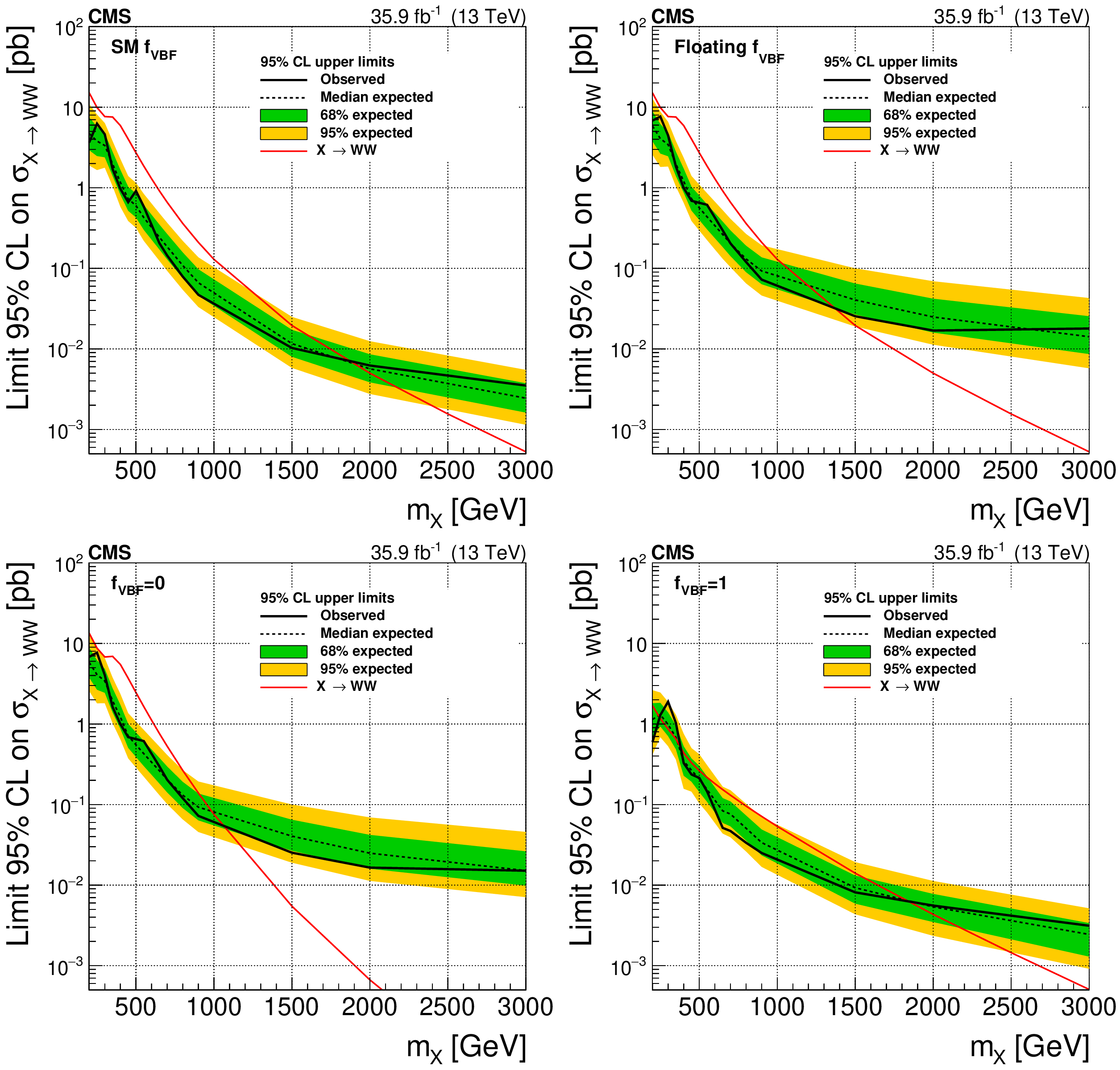
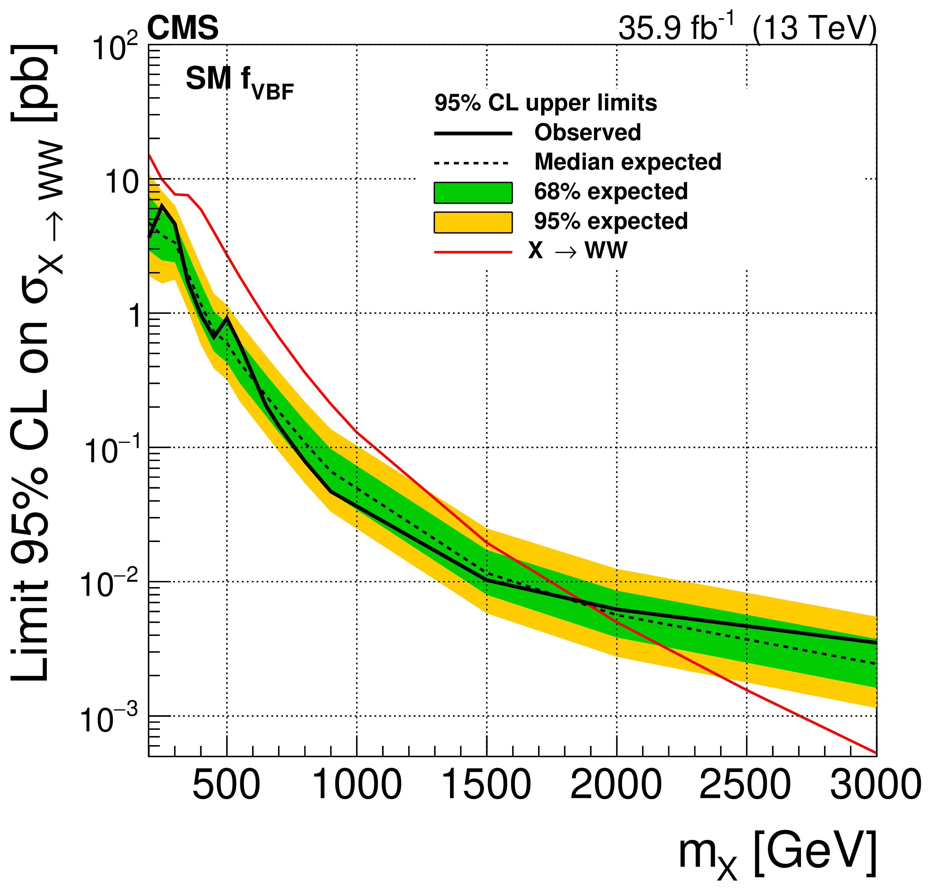
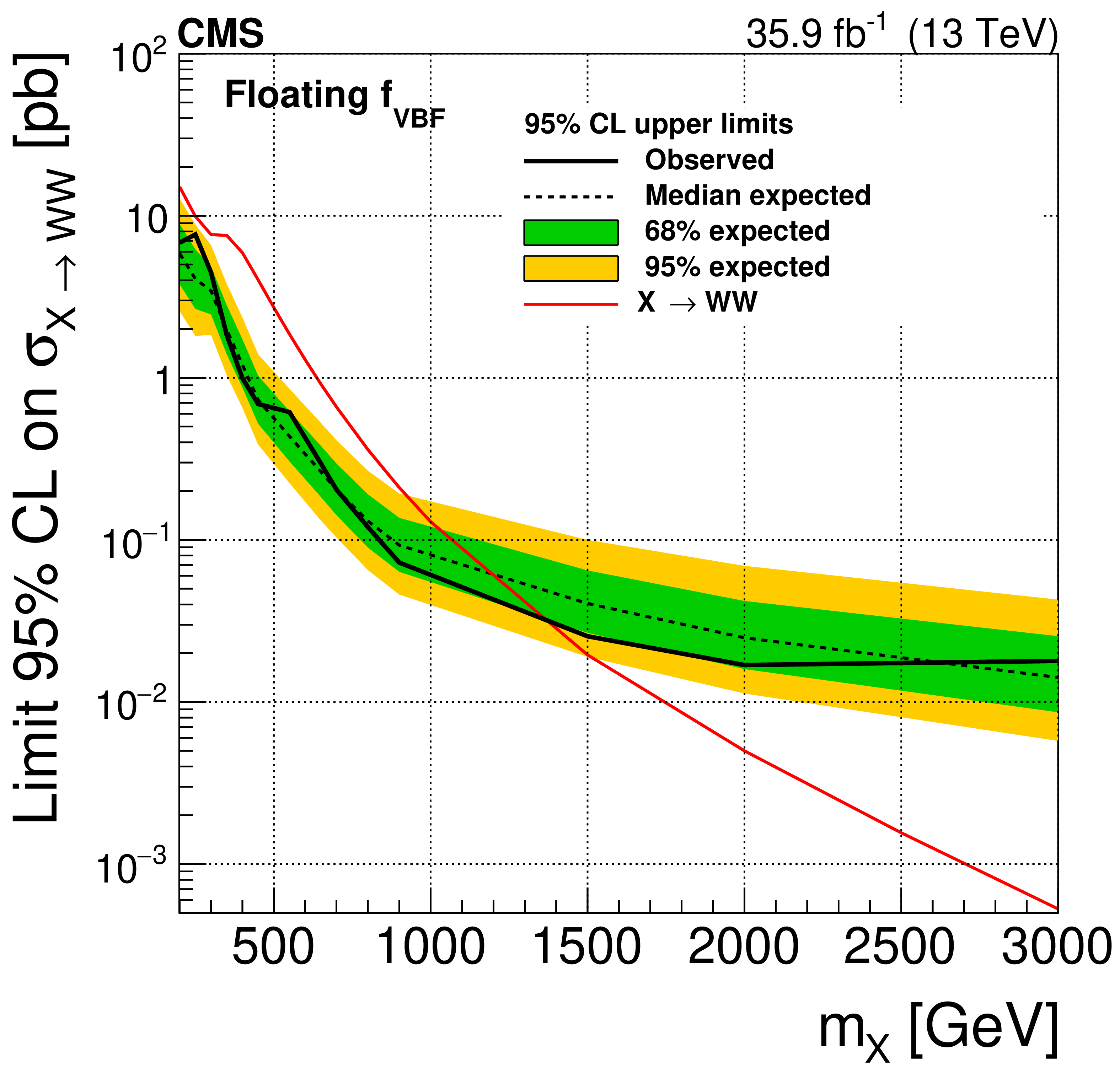
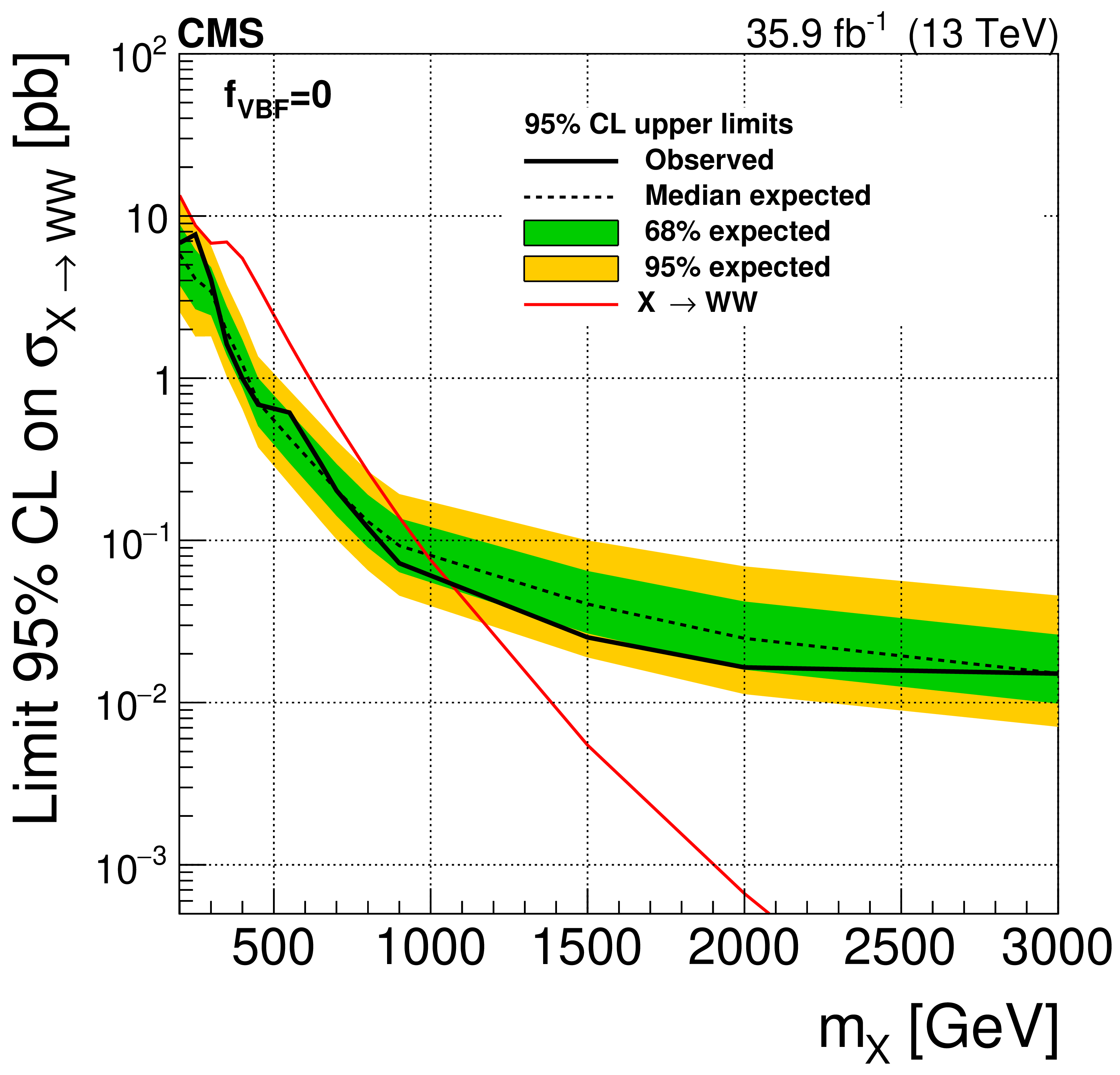
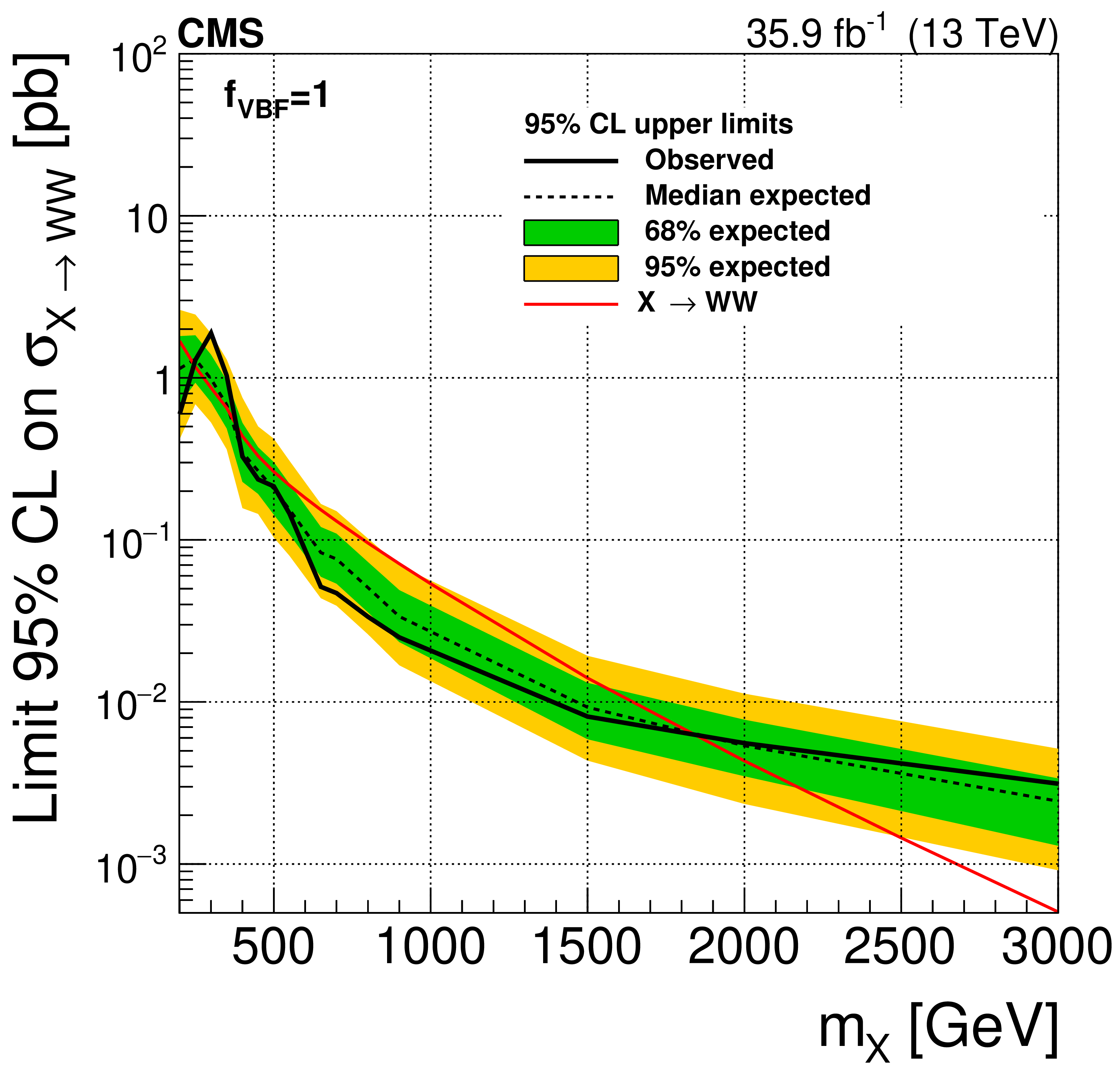
Expected and observed exclusion limits at 95% CL on the X cross section times branching fraction to WW for a number of ${f_\text {VBF}}$ hypotheses. For the SM ${f_\text {VBF}}$ (upper left) and floating ${f_\text {VBF}}$ (upper right) cases the red line represents the sum of the SM cross sections for ggF and VBF production, while for the $ {f_\text {VBF}} = $ 0 (lower left) and the $ {f_\text {VBF}} = $ 1 (lower right) cases it represents the ggF and VBF production cross sections, respectively. The black dotted line corresponds to the central expected value while the yellow and green bands represent the 68 and 95% CL uncertainties, respectively. |
png pdf |
Figure 6-a:
Expected and observed exclusion limits at 95% CL on the X cross section times branching fraction to WW for a number of ${f_\text {VBF}}$ hypotheses. For the SM ${f_\text {VBF}}$ (upper left) and floating ${f_\text {VBF}}$ (upper right) cases the red line represents the sum of the SM cross sections for ggF and VBF production, while for the $ {f_\text {VBF}} = $ 0 (lower left) and the $ {f_\text {VBF}} = $ 1 (lower right) cases it represents the ggF and VBF production cross sections, respectively. The black dotted line corresponds to the central expected value while the yellow and green bands represent the 68 and 95% CL uncertainties, respectively. |
png pdf |
Figure 6-b:
Expected and observed exclusion limits at 95% CL on the X cross section times branching fraction to WW for a number of ${f_\text {VBF}}$ hypotheses. For the SM ${f_\text {VBF}}$ (upper left) and floating ${f_\text {VBF}}$ (upper right) cases the red line represents the sum of the SM cross sections for ggF and VBF production, while for the $ {f_\text {VBF}} = $ 0 (lower left) and the $ {f_\text {VBF}} = $ 1 (lower right) cases it represents the ggF and VBF production cross sections, respectively. The black dotted line corresponds to the central expected value while the yellow and green bands represent the 68 and 95% CL uncertainties, respectively. |
png pdf |
Figure 6-c:
Expected and observed exclusion limits at 95% CL on the X cross section times branching fraction to WW for a number of ${f_\text {VBF}}$ hypotheses. For the SM ${f_\text {VBF}}$ (upper left) and floating ${f_\text {VBF}}$ (upper right) cases the red line represents the sum of the SM cross sections for ggF and VBF production, while for the $ {f_\text {VBF}} = $ 0 (lower left) and the $ {f_\text {VBF}} = $ 1 (lower right) cases it represents the ggF and VBF production cross sections, respectively. The black dotted line corresponds to the central expected value while the yellow and green bands represent the 68 and 95% CL uncertainties, respectively. |
png pdf |
Figure 6-d:
Expected and observed exclusion limits at 95% CL on the X cross section times branching fraction to WW for a number of ${f_\text {VBF}}$ hypotheses. For the SM ${f_\text {VBF}}$ (upper left) and floating ${f_\text {VBF}}$ (upper right) cases the red line represents the sum of the SM cross sections for ggF and VBF production, while for the $ {f_\text {VBF}} = $ 0 (lower left) and the $ {f_\text {VBF}} = $ 1 (lower right) cases it represents the ggF and VBF production cross sections, respectively. The black dotted line corresponds to the central expected value while the yellow and green bands represent the 68 and 95% CL uncertainties, respectively. |
png pdf |
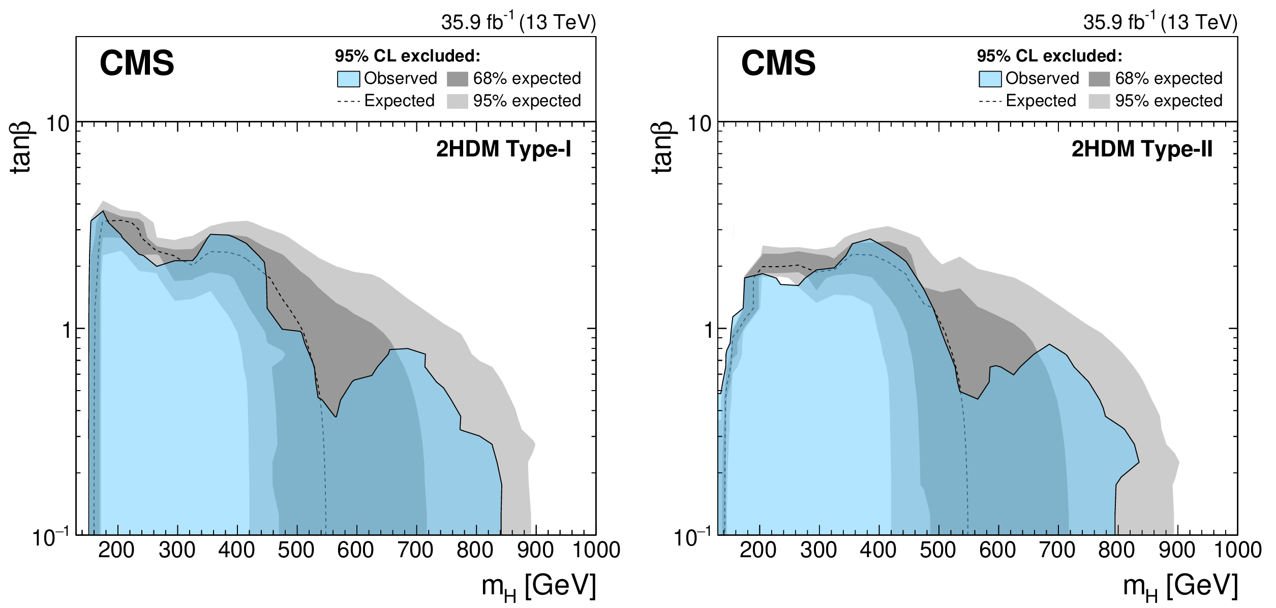
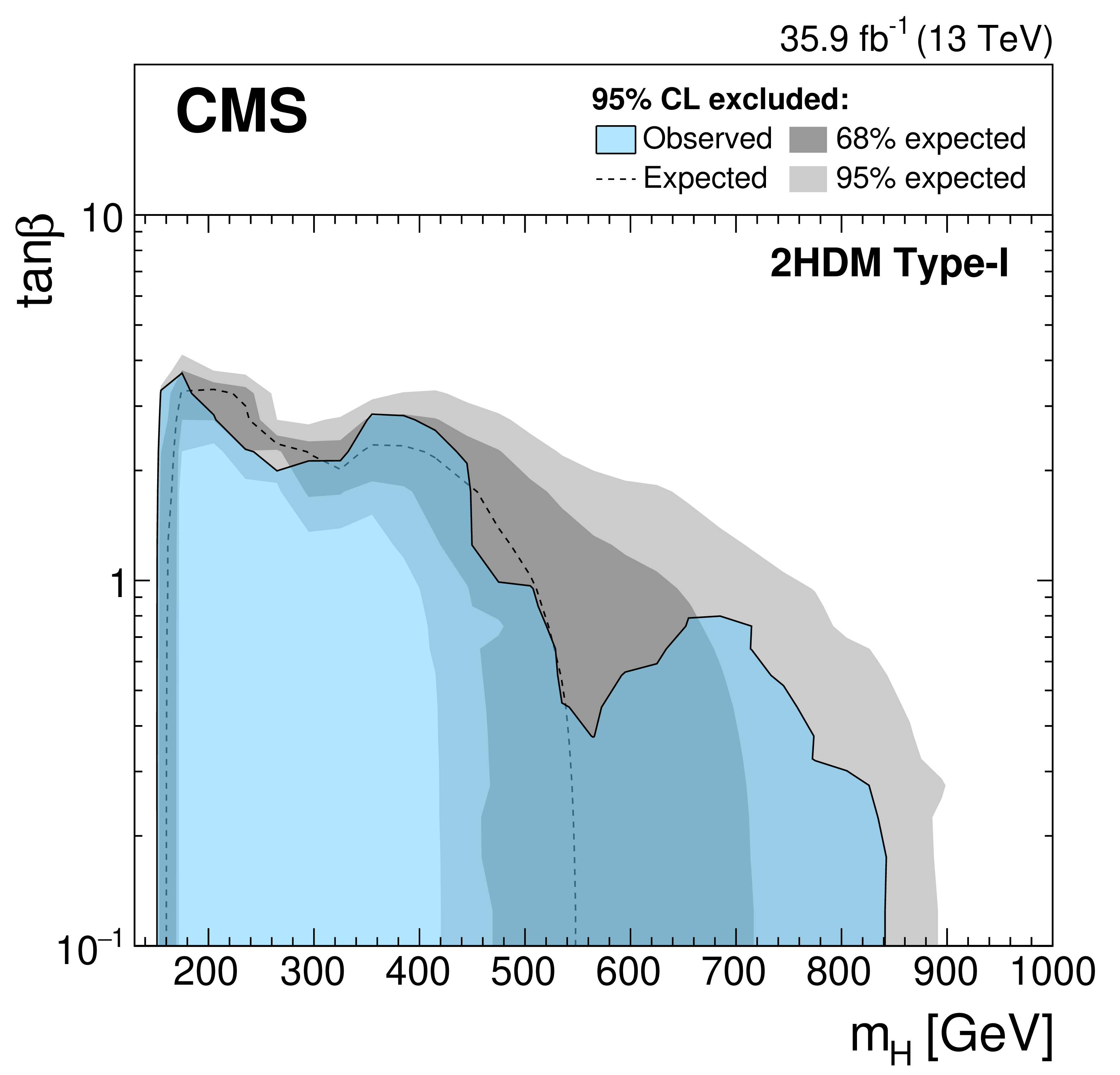
Figure 7:
Expected and observed 95% CL upper limits on ${\tan\beta}$ as a function of ${m_{\mathrm{H}}}$ for a Type-I (left) and Type-II (right) 2HDMs. It is assumed that $ {m_{\mathrm{H}}} = {m_{\mathrm{A} }} $ and $ {\cos(\beta -\alpha)} = $ 0.1. The expected limit is shown as a dashed black line while the dark and light gray bands indicate the 68 and 95% CL uncertainties, respectively. The observed exclusion contour is indicated by the blue area. |
png pdf |
Figure 7-a:
Expected and observed 95% CL upper limits on ${\tan\beta}$ as a function of ${m_{\mathrm{H}}}$ for a Type-I (left) and Type-II (right) 2HDMs. It is assumed that $ {m_{\mathrm{H}}} = {m_{\mathrm{A} }} $ and $ {\cos(\beta -\alpha)} = $ 0.1. The expected limit is shown as a dashed black line while the dark and light gray bands indicate the 68 and 95% CL uncertainties, respectively. The observed exclusion contour is indicated by the blue area. |

png pdf |
Figure 7-b:
Expected and observed 95% CL upper limits on ${\tan\beta}$ as a function of ${m_{\mathrm{H}}}$ for a Type-I (left) and Type-II (right) 2HDMs. It is assumed that $ {m_{\mathrm{H}}} = {m_{\mathrm{A} }} $ and $ {\cos(\beta -\alpha)} = $ 0.1. The expected limit is shown as a dashed black line while the dark and light gray bands indicate the 68 and 95% CL uncertainties, respectively. The observed exclusion contour is indicated by the blue area. |
png pdf |
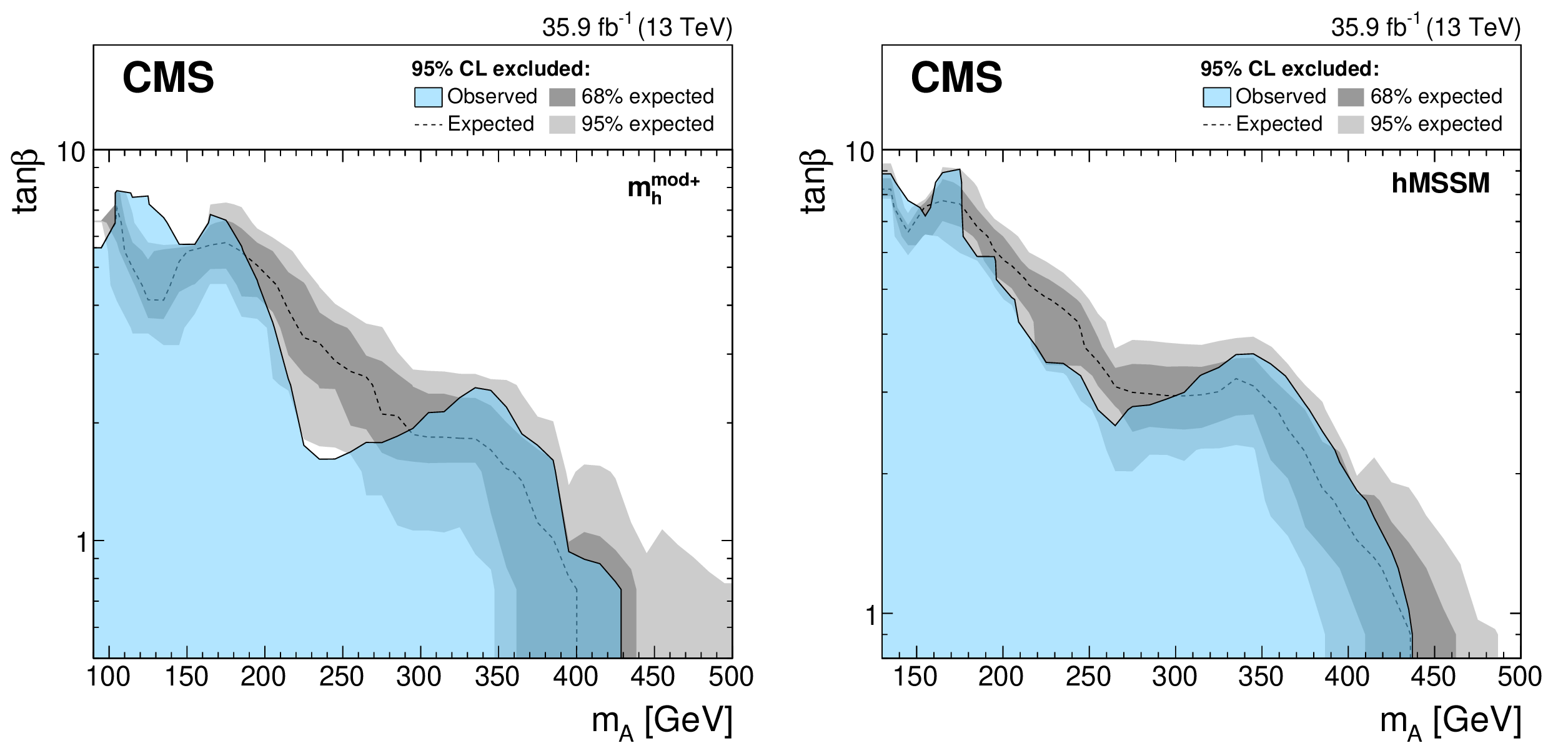
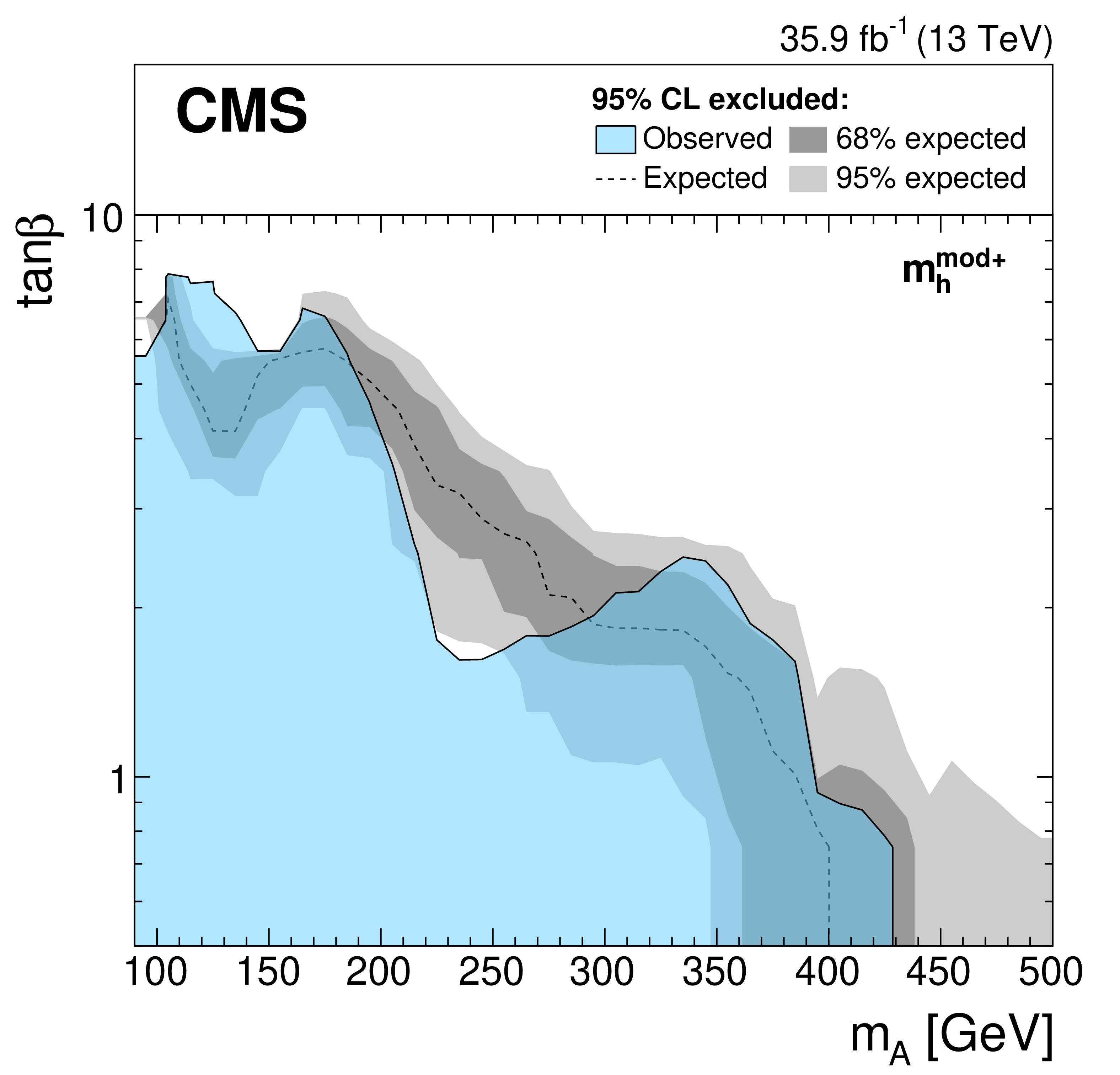
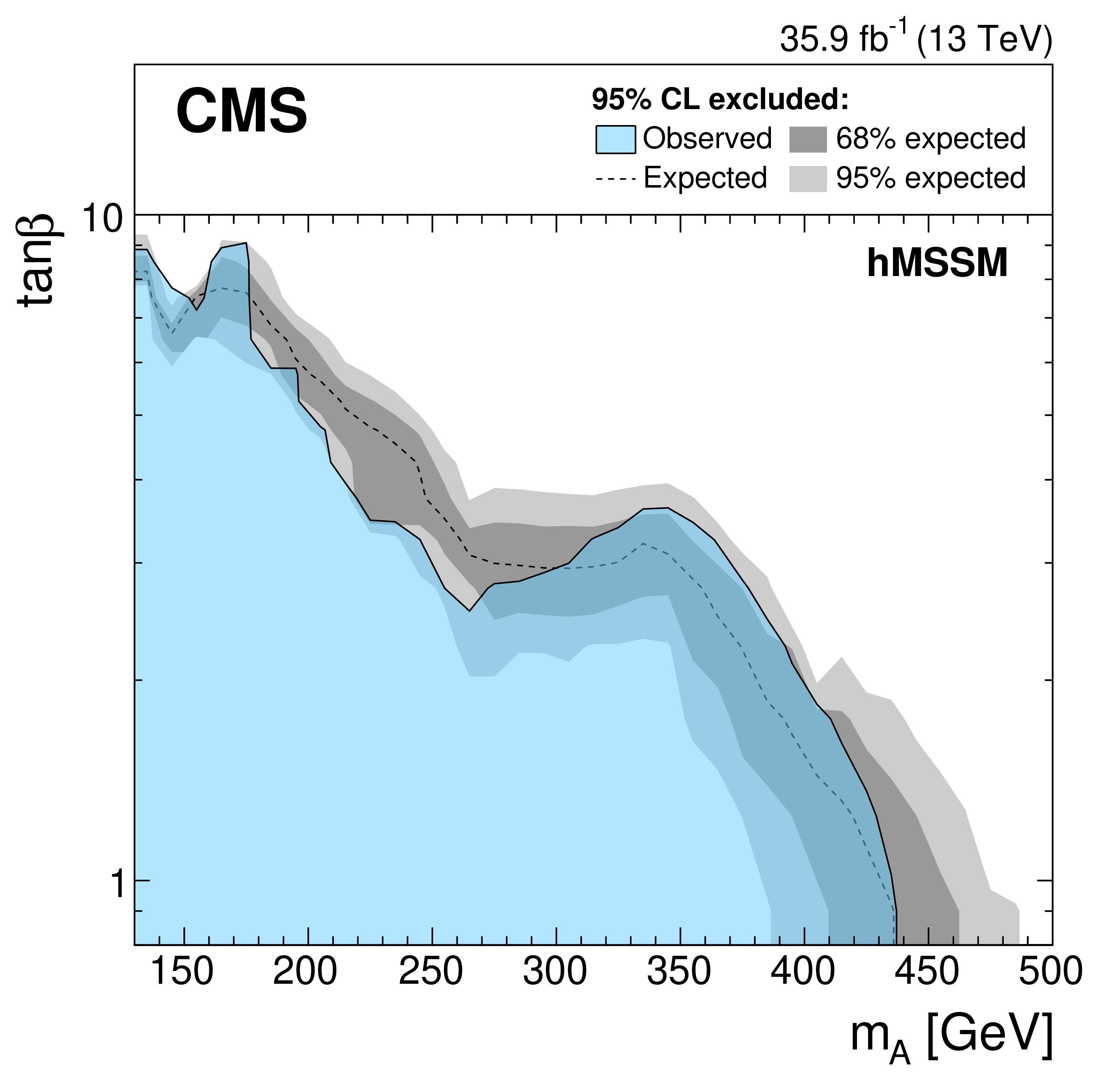
Figure 8:
Expected and observed 95% CL upper limits on ${\tan\beta}$ as a function of ${m_{\mathrm{A} }}$ for the ${m_{{\mathrm{h}}}^\text {mod+}}$ (left) and hMSSM (right) scenarios. The expected limit is shown as a dashed black line while the dark and light gray bands indicate the 68 and 95% CL uncertainties, respectively. The observed exclusion contour is indicated by the blue area. |
png pdf |
Figure 8-a:
Expected and observed 95% CL upper limits on ${\tan\beta}$ as a function of ${m_{\mathrm{A} }}$ for the ${m_{{\mathrm{h}}}^\text {mod+}}$ (left) and hMSSM (right) scenarios. The expected limit is shown as a dashed black line while the dark and light gray bands indicate the 68 and 95% CL uncertainties, respectively. The observed exclusion contour is indicated by the blue area. |
png pdf |
Figure 8-b:
Expected and observed 95% CL upper limits on ${\tan\beta}$ as a function of ${m_{\mathrm{A} }}$ for the ${m_{{\mathrm{h}}}^\text {mod+}}$ (left) and hMSSM (right) scenarios. The expected limit is shown as a dashed black line while the dark and light gray bands indicate the 68 and 95% CL uncertainties, respectively. The observed exclusion contour is indicated by the blue area. |

png pdf |
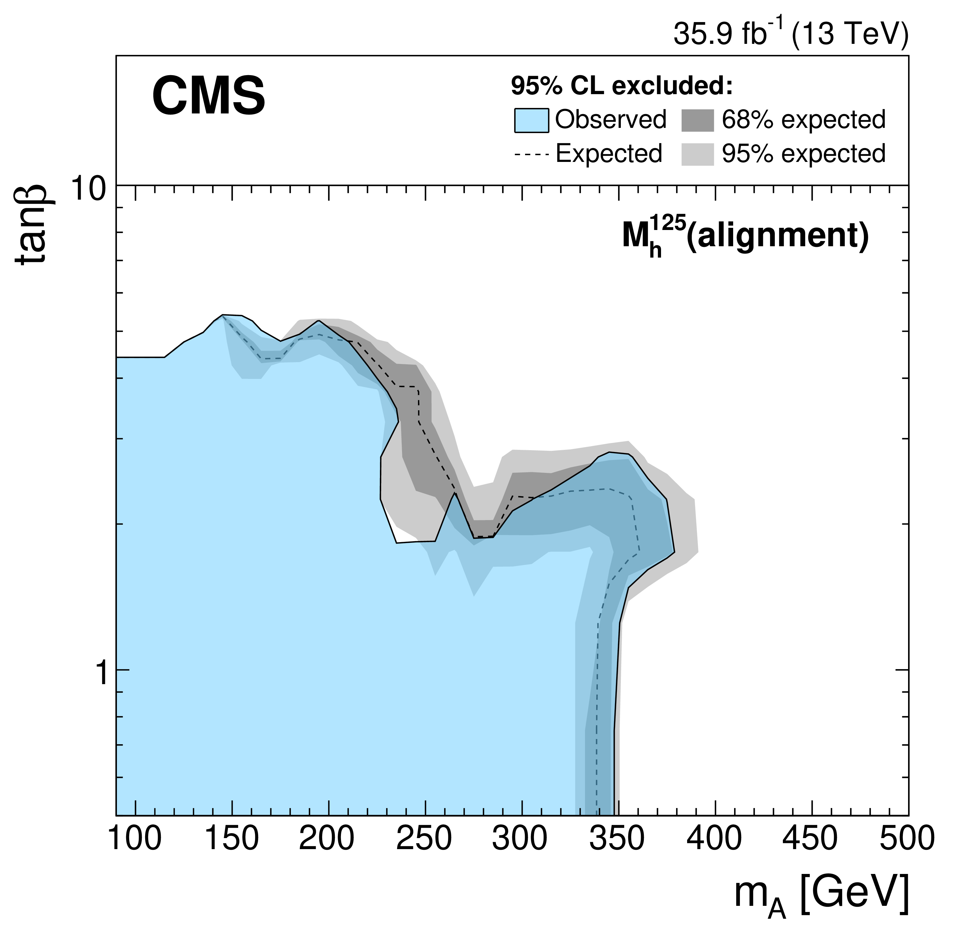
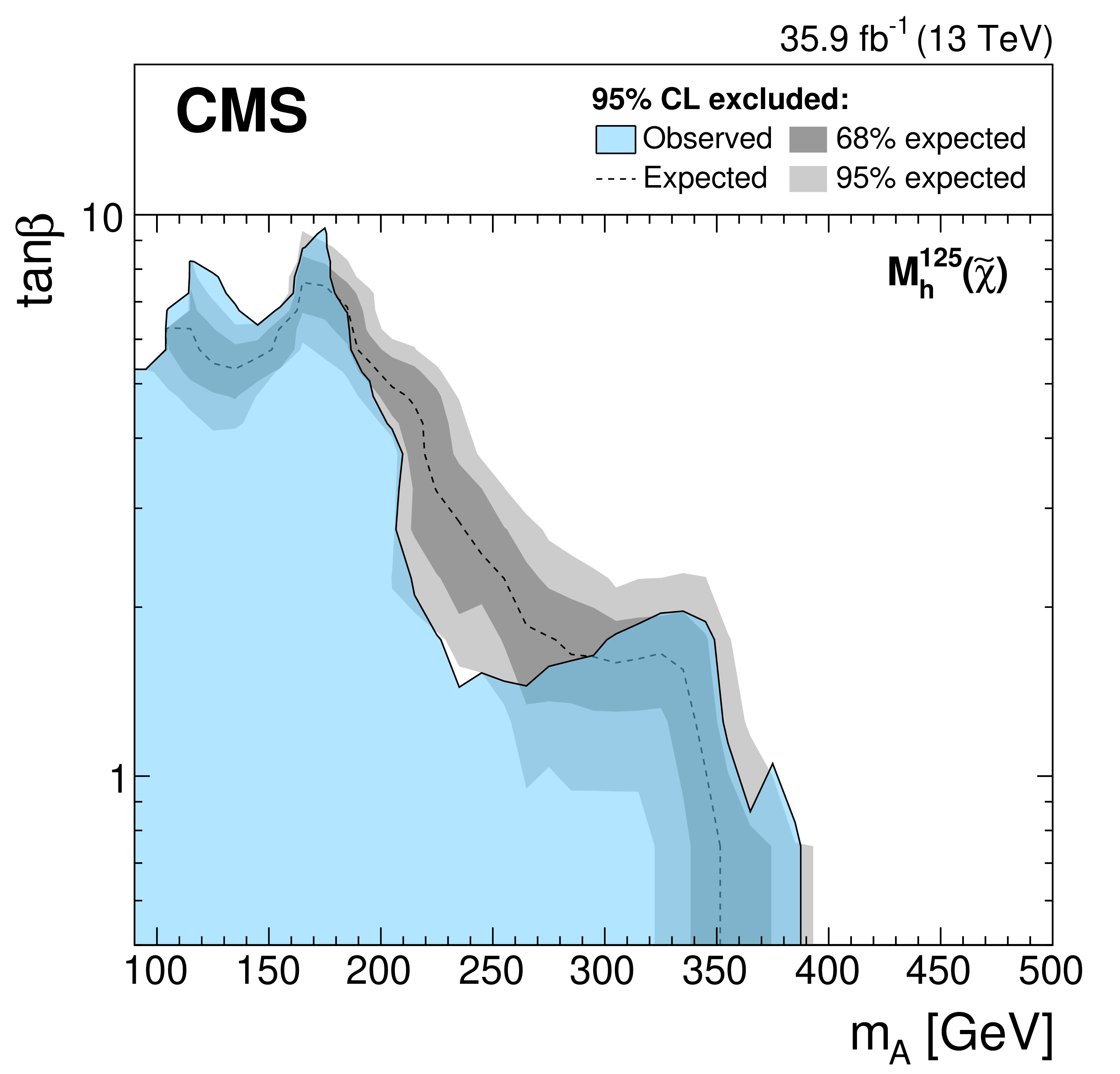
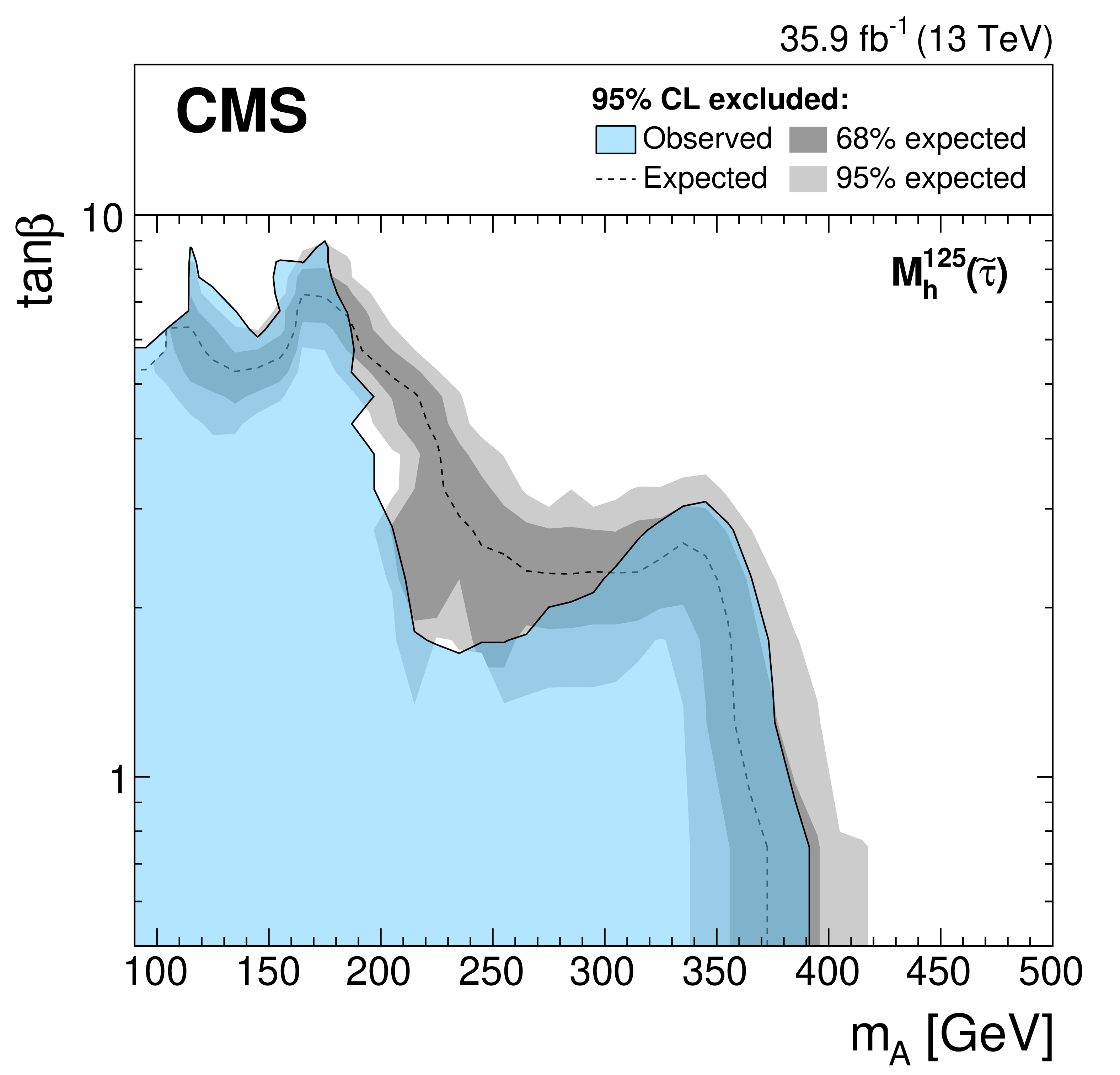
Figure 9:
Expected and observed 95% CL upper limits on ${\tan\beta}$ as a function of ${m_{\mathrm{A} }}$ for the ${M_{{\mathrm{h}}}^{125}}$ (upper left), ${M_{{\mathrm{h}}}^{125}\text {(alignment)}}$ (upper right), ${M_{{\mathrm{h}}}^{125}(\tilde{\chi})}$ (lower left), and ${M_{{\mathrm{h}}}^{125}(\tilde{\tau})}$ (lower right) scenarios. The expected limit is shown as a dashed black line while the dark and light gray bands indicate the 68 and 95% CL uncertainties, respectively. The observed exclusion contour is indicated by the blue area. |

png pdf |
Figure 9-a:
Expected and observed 95% CL upper limits on ${\tan\beta}$ as a function of ${m_{\mathrm{A} }}$ for the ${M_{{\mathrm{h}}}^{125}}$ (upper left), ${M_{{\mathrm{h}}}^{125}\text {(alignment)}}$ (upper right), ${M_{{\mathrm{h}}}^{125}(\tilde{\chi})}$ (lower left), and ${M_{{\mathrm{h}}}^{125}(\tilde{\tau})}$ (lower right) scenarios. The expected limit is shown as a dashed black line while the dark and light gray bands indicate the 68 and 95% CL uncertainties, respectively. The observed exclusion contour is indicated by the blue area. |
png pdf |
Figure 9-b:
Expected and observed 95% CL upper limits on ${\tan\beta}$ as a function of ${m_{\mathrm{A} }}$ for the ${M_{{\mathrm{h}}}^{125}}$ (upper left), ${M_{{\mathrm{h}}}^{125}\text {(alignment)}}$ (upper right), ${M_{{\mathrm{h}}}^{125}(\tilde{\chi})}$ (lower left), and ${M_{{\mathrm{h}}}^{125}(\tilde{\tau})}$ (lower right) scenarios. The expected limit is shown as a dashed black line while the dark and light gray bands indicate the 68 and 95% CL uncertainties, respectively. The observed exclusion contour is indicated by the blue area. |
png pdf |
Figure 9-c:
Expected and observed 95% CL upper limits on ${\tan\beta}$ as a function of ${m_{\mathrm{A} }}$ for the ${M_{{\mathrm{h}}}^{125}}$ (upper left), ${M_{{\mathrm{h}}}^{125}\text {(alignment)}}$ (upper right), ${M_{{\mathrm{h}}}^{125}(\tilde{\chi})}$ (lower left), and ${M_{{\mathrm{h}}}^{125}(\tilde{\tau})}$ (lower right) scenarios. The expected limit is shown as a dashed black line while the dark and light gray bands indicate the 68 and 95% CL uncertainties, respectively. The observed exclusion contour is indicated by the blue area. |
png pdf |
Figure 9-d:
Expected and observed 95% CL upper limits on ${\tan\beta}$ as a function of ${m_{\mathrm{A} }}$ for the ${M_{{\mathrm{h}}}^{125}}$ (upper left), ${M_{{\mathrm{h}}}^{125}\text {(alignment)}}$ (upper right), ${M_{{\mathrm{h}}}^{125}(\tilde{\chi})}$ (lower left), and ${M_{{\mathrm{h}}}^{125}(\tilde{\tau})}$ (lower right) scenarios. The expected limit is shown as a dashed black line while the dark and light gray bands indicate the 68 and 95% CL uncertainties, respectively. The observed exclusion contour is indicated by the blue area. |
| Tables | |
png pdf |
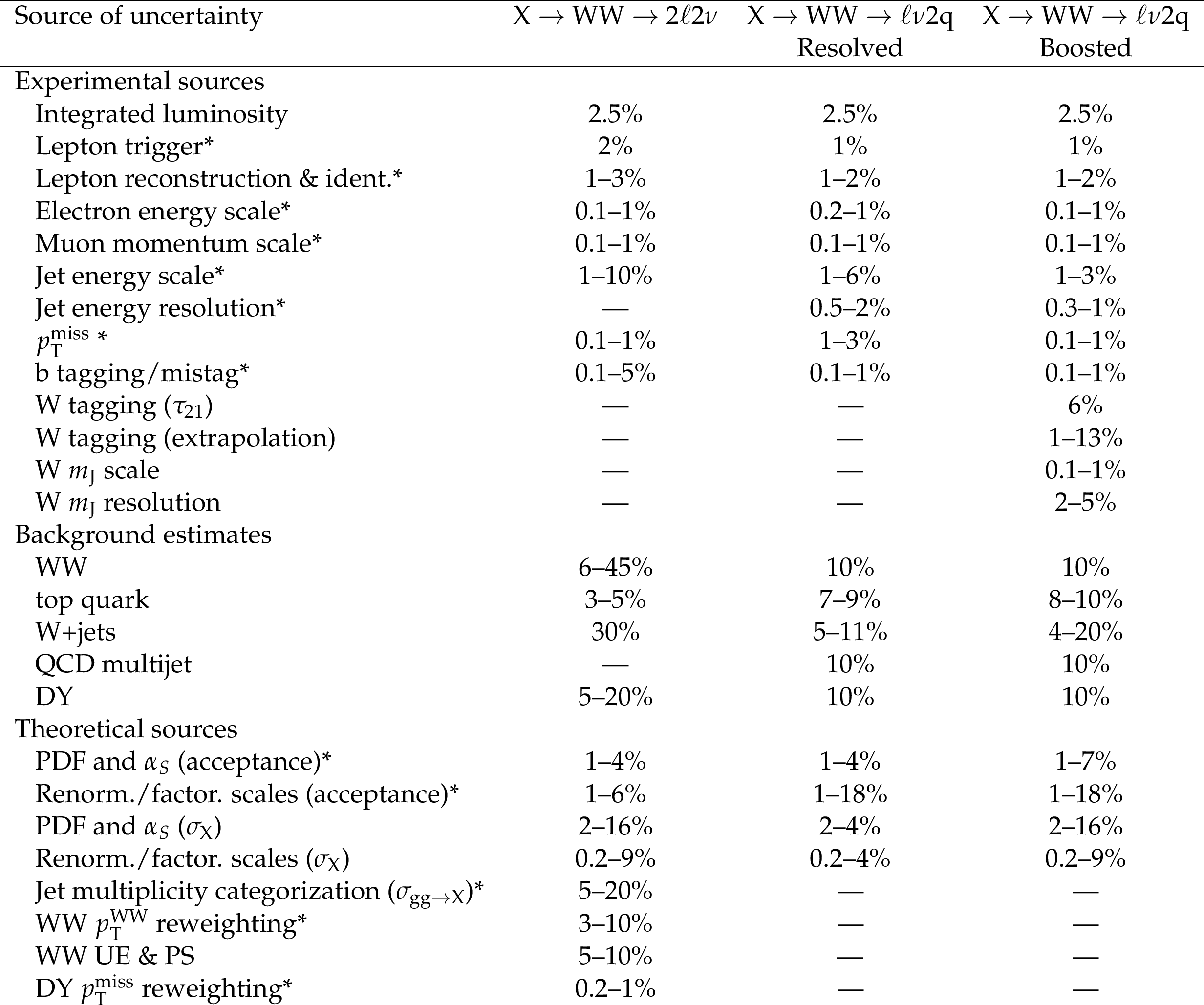
Table 1:
Summary of systematic uncertainties, quoted in percent, affecting the normalization of the background and signal samples. The uncertainties on the WW, top quark and DY (W+jets and top quark) background estimates in the ${2\ell 2\nu}$ (${\ell \nu 2\mathrm{q}}$) categories have been determined during the fit to the data. The numbers shown as ranges represent the uncertainties for different processes and categories. Missing values represent uncertainties either estimated to be negligible ($ < $0.1%), or not applicable in a specific channel. Those systematic uncertainties found to affect the shape of kinematic distributions are labeled with *. |
| Summary |
| A search for a heavy Higgs boson decaying to a pair of W bosons in the mass range from 0.2 to 3.0 TeV has been presented. The data analysed were collected by the CMS experiment at the LHC in 2016, corresponding to an integrated luminosity of 35.9 fb$^{-1}$ at $\sqrt{s} = $ 13 TeV. The W boson pair decays are reconstructed in the ${2\ell 2\nu}$ and $ {\ell\nu 2\mathrm{q}}$ final states. Both gluon fusion and vector boson fusion production of the signal are considered, with a number of hypotheses for their relative contributions investigated. Interference effects between the signal and background are also taken into account. Dedicated event categorizations based on both the kinematic properties of associated jets and matrix element techniques are employed to optimize the signal sensitivity. No evidence for an excess of events with respect to the standard model (SM) predictions is observed. Combined upper limits at 95% confidence level on the product of the cross section and branching fraction exclude a heavy Higgs boson with SM-like couplings and decays up to 1870 GeV. Exclusion limits are also set in the context of a number of two-Higgs-doublet model formulations, further reducing the allowed parameter space for extensions of the SM. |
| References | ||||
| 1 | ATLAS Collaboration | Observation of a new particle in the search for the standard model Higgs boson with the ATLAS detector at the LHC | PLB 716 (2012) 1 | 1207.7214 |
| 2 | CMS Collaboration | Observation of a new boson at a mass of 125 GeV with the CMS experiment at the LHC | PLB 716 (2012) 30 | CMS-HIG-12-028 1207.7235 |
| 3 | CMS Collaboration | Observation of a new boson with mass near 125 GeV in pp Collisions at $ \sqrt{s} = $ 7 and 8 TeV | JHEP 06 (2013) 081 | CMS-HIG-12-036 1303.4571 |
| 4 | ATLAS Collaboration | Study of the spin and parity of the Higgs boson in diboson decays with the ATLAS detector | EPJC 75 (2015) 476 | 1506.05669 |
| 5 | ATLAS Collaboration | Combined measurements of Higgs boson production and decay using up to 80 fb$ ^{-1} $ of proton-proton collision data at $ \sqrt{s}= $ 13 TeV collected with the ATLAS experiment | Accepted by PRD | 1909.02845 |
| 6 | ATLAS Collaboration | Combined measurement of differential and total cross sections in the H $ \rightarrow \gamma \gamma $ and the H $ \rightarrow $ ZZ$ ^* \rightarrow 4\ell $ decay channels at $ \sqrt{s} = $ 13 TeV with the ATLAS detector | PLB 786 (2018) 114 | 1805.10197 |
| 7 | ATLAS Collaboration | Constraints on off-shell Higgs boson production and the Higgs boson total width in ZZ$ \to4\ell $ and ZZ$ \to2\ell2\nu $ final states with the ATLAS detector | PLB 786 (2018) 223 | 1808.01191 |
| 8 | ATLAS Collaboration | Measurement of the Higgs boson coupling properties in the H$ \rightarrow $ ZZ$ ^{*} \rightarrow 4\ell $ decay channel at $ \sqrt{s} = $ 13 TeV with the ATLAS detector | JHEP 03 (2018) 095 | 1712.02304 |
| 9 | ATLAS and CMS Collaborations | Measurements of the Higgs boson production and decay rates and constraints on its couplings from a combined ATLAS and CMS analysis of the LHC pp collision data at $ \sqrt{s}= $ 7 and 8 TeV | JHEP 08 (2016) 045 | 1606.02266 |
| 10 | CMS Collaboration | Combined search for anomalous pseudoscalar HVV couplings in VH(H $ \to b \bar b $) production and H $ \to $ VV decay | PLB 759 (2016) 672 | CMS-HIG-14-035 1602.04305 |
| 11 | CMS Collaboration | Constraints on anomalous Higgs boson couplings using production and decay information in the four-lepton final state | PLB 775 (2017) 1 | CMS-HIG-17-011 1707.00541 |
| 12 | CMS Collaboration | Measurements of the Higgs boson width and anomalous HVV couplings from on-shell and off-shell production in the four-lepton final state | PRD 99 (2019) 112003 | CMS-HIG-18-002 1901.00174 |
| 13 | CMS Collaboration | Measurement and interpretation of differential cross sections for Higgs boson production at $ \sqrt{s} = $ 13 TeV | PLB 792 (2019) 369 | CMS-HIG-17-028 1812.06504 |
| 14 | CMS Collaboration | Combined measurements of Higgs boson couplings in proton-proton collisions at $ \sqrt{s} = $ 13 TeV | EPJC 79 (2019) 421 | CMS-HIG-17-031 1809.10733 |
| 15 | CMS Collaboration | Constraints on anomalous HVV couplings from the production of Higgs bosons decaying to $ \tau $ lepton pairs | Accepted by PRD | CMS-HIG-17-034 1903.06973 |
| 16 | C. Englert et al. | Precision measurements of Higgs couplings: Implications for new physics scales | JPG 41 (2014) 113001 | 1403.7191 |
| 17 | T. Plehn, D. L. Rainwater, and D. Zeppenfeld | Determining the structure of Higgs couplings at the LHC | PRL 88 (2002) 051801 | hep-ph/0105325 |
| 18 | I. Anderson et al. | Constraining anomalous HVV interactions at proton and lepton colliders | PRD 89 (2014) 035007 | 1309.4819 |
| 19 | F. Bishara, U. Haisch, P. F. Monni, and E. Re | Constraining light-quark Yukawa couplings from Higgs distributions | PRL 118 (2017) 121801 | 1606.09253 |
| 20 | M. Grazzini, A. Ilnicka, M. Spira, and M. Wiesemann | Modeling BSM effects on the Higgs transverse-momentum spectrum in an EFT approach | JHEP 03 (2017) 115 | 1612.00283 |
| 21 | V. Barger et al. | LHC phenomenology of an extended standard model with a real scalar singlet | PRD 77 (2008) 035005 | 0706.4311 |
| 22 | G. C. Branco et al. | Theory and phenomenology of two-Higgs-doublet models | PR 516 (2012) 1 | 1106.0034 |
| 23 | ATLAS Collaboration | Search for a high-mass Higgs boson decaying to a W boson pair in pp collisions at $ \sqrt{s} = $ 8 TeV with the ATLAS detector | JHEP 01 (2016) 032 | 1509.00389 |
| 24 | ATLAS Collaboration | Search for an additional, heavy Higgs boson in the H$ \rightarrow $ZZ decay channel at $ \sqrt{s} = $ 8 TeV in pp collision data with the ATLAS detector | EPJC 76 (2016) 45 | 1507.05930 |
| 25 | ATLAS Collaboration | Search for heavy resonances decaying into WW in the $ e\nu\mu\nu $ final state in pp collisions at $ \sqrt{s} = $ 13 TeV with the ATLAS detector | EPJC 78 (2018) 24 | 1710.01123 |
| 26 | CMS Collaboration | Search for a Higgs boson in the mass range from 145 to 1000 GeV decaying to a pair of W or Z bosons | JHEP 10 (2015) 144 | CMS-HIG-13-031 1504.00936 |
| 27 | CMS Collaboration | Search for a new scalar resonance decaying to a pair of Z bosons in proton-proton collisions at $ \sqrt{s} = $ 13 TeV | JHEP 06 (2018) 127 | CMS-HIG-17-012 1804.01939 |
| 28 | A. Denner et al. | Standard model Higgs boson branching ratios with uncertainties | EPJC 71 (2011) 1753 | 1107.5909 |
| 29 | N. Kauer and C. O'Brien | Heavy Higgs signal background interference in gg$ \rightarrow $VV in the standard model plus real singlet | EPJC 75 (2015) 374 | 1502.04113 |
| 30 | S. P. Martin | A supersymmetry primer | Adv. Ser. Direct. High Energy Phys. 18 (1998) 1 | hep-ph/9709356 |
| 31 | J. E. Kim | Light pseudoscalars, particle physics and cosmology | PR 150 (1987) 1 | |
| 32 | J. M. Cline, K. Kainulainen, and M. Trott | Electroweak baryogenesis in two Higgs doublet models and B meson anomalies | JHEP 11 (2011) 089 | 1107.3559 |
| 33 | CMS Collaboration | The CMS experiment at the CERN LHC | JINST 3 (2008) S08004 | CMS-00-001 |
| 34 | CMS Collaboration | The CMS trigger system | JINST 12 (2017) P01020 | CMS-TRG-12-001 1609.02366 |
| 35 | P. Nason | A new method for combining NLO QCD with shower Monte Carlo algorithms | JHEP 11 (2004) 040 | hep-ph/0409146 |
| 36 | S. Frixione, P. Nason, and C. Oleari | Matching NLO QCD computations with parton shower simulations: the $ POWHEG $ method | JHEP 11 (2007) 070 | 0709.2092 |
| 37 | S. Alioli, P. Nason, C. Oleari, and E. Re | A general framework for implementing NLO calculations in shower Monte Carlo programs: the $ POWHEG $ BOX | JHEP 06 (2010) 043 | 1002.2581 |
| 38 | E. Bagnaschi, G. Degrassi, P. Slavich, and A. Vicini | Higgs production via gluon fusion in the $ POWHEG $ approach in the SM and in the MSSM | JHEP 02 (2012) 088 | 1111.2854 |
| 39 | P. Nason and C. Oleari | NLO Higgs boson production via vector-boson fusion matched with shower in $ POWHEG $ | JHEP 02 (2010) 037 | 0911.5299 |
| 40 | Y. Gao et al. | Spin determination of single-produced resonances at hadron colliders | PRD 81 (2010) 075022 | 1001.3396 |
| 41 | S. Bolognesi et al. | On the spin and parity of a single-produced resonance at the LHC | PRD 86 (2012) 095031 | 1208.4018 |
| 42 | LHC Higgs Cross Section Working Group | Handbook of LHC Higgs cross sections: 4. deciphering the nature of the Higgs sector | CERN (2016) | 1610.07922 |
| 43 | J. Alwall et al. | The automated computation of tree-level and next-to-leading order differential cross sections, and their matching to parton shower simulations | JHEP 07 (2014) 079 | 1405.0301 |
| 44 | R. Frederix and S. Frixione | Merging meets matching in MC@NLO | JHEP 12 (2012) 061 | 1209.6215 |
| 45 | Y. Li and F. Petriello | Combining QCD and electroweak corrections to dilepton production in $ FEWZ $ | PRD 86 (2012) 094034 | 1208.5967 |
| 46 | E. Re | Single-top Wt-channel production matched with parton showers using the $ POWHEG $ method | EPJC 71 (2011) 1547 | 1009.2450 |
| 47 | S. Frixione, P. Nason, and G. Ridolfi | A positive-weight next-to-leading order Monte Carlo for heavy flavour hadroproduction | JHEP 09 (2007) 126 | 0707.3088 |
| 48 | P. Kant et al. | HATHOR for single top-quark production: Updated predictions and uncertainty estimates for single top-quark production in hadronic collisions | CPC 191 (2015) 74 | 1406.4403 |
| 49 | M. Czakon and A. Mitov | Top++: A program for the calculation of the top-pair cross-section at hadron colliders | CPC 185 (2014) 2930 | 1112.5675 |
| 50 | T. Melia, P. Nason, R. Rontsch, and G. Zanderighi | $ \mathrm{W^{+}W^{-}} $, WZ and ZZ production in the $ POWHEG $ BOX | JHEP 11 (2011) 078 | 1107.5051 |
| 51 | J. M. Campbell, R. K. Ellis, and C. Williams | Bounding the Higgs width at the LHC: Complementary results from H $ \to $ WW | PRD 89 (2014) 053011 | 1312.1628 |
| 52 | T. Gehrmann et al. | W$ ^+ $W$ ^- $ production at hadron colliders in next-to-next-to-leading order QCD | PRL 113 (2014) 212001 | 1408.5243 |
| 53 | F. Caola, K. Melnikov, R. Rontsch, and L. Tancredi | QCD corrections to W$ ^{+} $W$ ^{-} $ production through gluon fusion | PLB 754 (2016) 275 | 1511.08617 |
| 54 | P. Meade, H. Ramani, and M. Zeng | Transverse momentum resummation effects in W$ ^+ $W$ ^- $ measurements | PRD 90 (2014) 114006 | 1407.4481 |
| 55 | P. Jaiswal and T. Okui | Explanation of the WW excess at the LHC by jet-veto resummation | PRD 90 (2014) 073009 | 1407.4537 |
| 56 | T. Sjostrand et al. | An introduction to PYTHIA 8.2 | CPC 191 (2015) 159 | 1410.3012 |
| 57 | NNPDF Collaboration | Parton distributions with QED corrections | NPB 877 (2013) 290 | 1308.0598 |
| 58 | NNPDF Collaboration | Unbiased global determination of parton distributions and their uncertainties at NNLO and at LO | NPB 855 (2012) 153 | 1107.2652 |
| 59 | CMS Collaboration | Event generator tunes obtained from underlying event and multiparton scattering measurements | EPJC 76 (2016) 155 | CMS-GEN-14-001 1512.00815 |
| 60 | P. Richardson and A. Wilcock | Monte Carlo simulation of hard radiation in decays in beyond the standard model physics in Herwig++ | EPJC 74 (2014) 2713 | 1303.4563 |
| 61 | M. Bahr et al. | Herwig++ physics and manual | EPJC 58 (2008) 639 | 0803.0883 |
| 62 | GEANT4 Collaboration | GEANT4 ---a simulation toolkit | NIMA 506 (2003) 250 | |
| 63 | CMS Collaboration | Particle-flow reconstruction and global event description with the CMS detector | JINST 12 (2017) P10003 | CMS-PRF-14-001 1706.04965 |
| 64 | M. Cacciari, G. P. Salam, and G. Soyez | The anti-$ {k_{\mathrm{T}}} $ jet clustering algorithm | JHEP 04 (2008) 063 | 0802.1189 |
| 65 | M. Cacciari, G. P. Salam, and G. Soyez | $ FastJet $ user manual | EPJC 72 (2012) 1896 | 1111.6097 |
| 66 | CMS Collaboration | Performance of electron reconstruction and selection with the CMS detector in proton proton collisions at $ \sqrt{s} = $ 8 TeV | JINST 10 (2015) P06005 | CMS-EGM-13-001 1502.02701 |
| 67 | CMS Collaboration | Performance of the CMS muon detector and muon reconstruction with proton-proton collisions at $ \sqrt{s}= $ 13 TeV | JINST 13 (2018) P06015 | CMS-MUO-16-001 1804.04528 |
| 68 | M. Cacciari and G. P. Salam | Pileup subtraction using jet areas | PLB 659 (2008) 119 | 0707.1378 |
| 69 | CMS Collaboration | Determination of jet energy calibration and transverse momentum resolution in CMS | JINST 6 (2011) P11002 | CMS-JME-10-011 1107.4277 |
| 70 | D. Bertolini, P. Harris, M. Low, and N. Tran | Pileup per particle identification | JHEP 10 (2014) 059 | 1407.6013 |
| 71 | M. Dasgupta, A. Fregoso, S. Marzani, and G. P. Salam | Towards an understanding of jet substructure | JHEP 09 (2013) 029 | 1307.0007 |
| 72 | J. M. Butterworth, A. R. Davison, M. Rubin, and G. P. Salam | Jet substructure as a new Higgs search channel at the LHC | PRL 100 (2008) 242001 | 0802.2470 |
| 73 | A. J. Larkoski, S. Marzani, G. Soyez, and J. Thaler | Soft Drop | JHEP 05 (2014) 146 | 1402.2657 |
| 74 | J. Thaler and K. Van Tilburg | Identifying boosted objects with $ N $-subjettiness | JHEP 03 (2011) 015 | 1011.2268 |
| 75 | CMS Collaboration | Identification of heavy-flavour jets with the CMS detector in pp collisions at 13 TeV | JINST 13 (2018) P05011 | CMS-BTV-16-002 1712.07158 |
| 76 | P. Fayet | Supergauge invariant extension of the Higgs mechanism and a model for the electron and its neutrino | NPB 90 (1975) 104 | |
| 77 | P. Fayet | Spontaneously broken supersymmetric theories of weak, electromagnetic and strong interactions | PLB 69 (1977) 489 | |
| 78 | M. Carena et al. | MSSM Higgs boson searches at the LHC: Benchmark scenarios after the discovery of a Higgs-like particle | EPJC 73 (2013) 2552 | 1302.7033 |
| 79 | A. Djouadi et al. | The post-Higgs MSSM scenario: Habemus MSSM? | EPJC 73 (2013) 2650 | 1307.5205 |
| 80 | A. Djouadi et al. | Fully covering the MSSM Higgs sector at the LHC | JHEP 06 (2015) 168 | 1502.05653 |
| 81 | E. Bagnaschi et al. | MSSM Higgs boson searches at the LHC: Benchmark scenarios for Run 2 and beyond | EPJC 79 (2019) 617 | 1808.07542 |
| 82 | R. V. Harlander, S. Liebler, and H. Mantler | SusHi: A program for the calculation of Higgs production in gluon fusion and bottom-quark annihilation in the standard model and the MSSM | CPC 184 (2013) 1605 | 1212.3249 |
| 83 | S. Heinemeyer, W. Hollik, and G. Weiglein | FeynHiggs: A program for the calculation of the masses of the neutral CP even Higgs bosons in the MSSM | CPC 124 (2000) 76 | hep-ph/9812320 |
| 84 | S. Heinemeyer, W. Hollik, and G. Weiglein | The masses of the neutral CP-even Higgs bosons in the MSSM: Accurate analysis at the two loop level | EPJC 9 (1999) 343 | hep-ph/9812472 |
| 85 | G. Degrassi et al. | Towards high precision predictions for the MSSM Higgs sector | EPJC 28 (2003) 133 | hep-ph/0212020 |
| 86 | M. Frank et al. | The Higgs boson masses and mixings of the complex MSSM in the Feynman-diagrammatic approach | JHEP 02 (2007) 047 | hep-ph/0611326 |
| 87 | T. Hahn et al. | High-precision predictions for the light CP-even Higgs boson mass of the minimal supersymmetric standard model | PRL 112 (2014) 141801 | 1312.4937 |
| 88 | A. Djouadi, J. Kalinowski, and M. Spira | HDECAY: A program for Higgs boson decays in the standard model and its supersymmetric extension | CPC 108 (1998) 56 | hep-ph/9704448 |
| 89 | A. Djouadi, J. Kalinowski, M. Muehlleitner, and M. Spira | HDECAY: Twenty++ years after | CPC 238 (2019) 214 | 1801.09506 |
| 90 | D. Eriksson, J. Rathsman, and O. St\ral | 2HDMC: two-Higgs-doublet model calculator physics and manual | CPC 181 (2010) 189 | 0902.0851 |
| 91 | D0 Collaboration | Direct measurement of the top quark mass at D0 | PRD 58 (1998) 052001 | hep-ex/9801025 |
| 92 | CMS Collaboration | Measurement of the inclusive W and Z production cross sections in pp collisions at $ \sqrt{s} = $ 7 TeV | JHEP 10 (2011) 132 | CMS-EWK-10-005 1107.4789 |
| 93 | CMS Collaboration | Identification of b-quark jets with the CMS experiment | JINST 8 (2013) P04013 | CMS-BTV-12-001 1211.4462 |
| 94 | CMS Collaboration | Identification techniques for highly boosted W bosons that decay into hadrons | JHEP 12 (2014) 017 | CMS-JME-13-006 1410.4227 |
| 95 | T. Junk | Confidence level computation for combining searches with small statistics | NIMA 434 (1999) 435 | hep-ex/9902006 |
| 96 | A. L. Read | Presentation of search results: the CLs technique | JPG 28 (2002) 2693 | |
| 97 | G. Cowan, K. Cranmer, E. Gross, and O. Vitells | Asymptotic formulae for likelihood-based tests of new physics | EPJC 71 (2011) 1554 | 1007.1727 |
| 98 | R. J. Barlow and C. Beeston | Fitting using finite Monte Carlo samples | CPC 77 (1993) 219 | |
| 99 | J. Butterworth et al. | PDF4LHC recommendations for LHC Run II | JPG 43 (2016) 023001 | 1510.03865 |
| 100 | M. Cacciari et al. | The $ \mathrm{t\bar{t}} $ cross section at 1.8 TeV and 1.96$ TeV: $ A study of the systematics due to parton densities and scale dependence | JHEP 04 (2004) 068 | hep-ph/0303085 |
| 101 | CMS Collaboration | CMS luminosity measurements for the 2016 data taking period | ||
| 102 | R. Boughezal et al. | Combining resummed Higgs predictions across jet bins | PRD 89 (2014) 074044 | 1312.4535 |
| 103 | CMS Collaboration | Measurements of the pp $ \to $ WZ inclusive and differential production cross section and constraints on charged anomalous triple gauge couplings at $ \sqrt{s} = $ 13 TeV | JHEP 04 (2019) 122 | CMS-SMP-18-002 1901.03428 |
| 104 | CMS Collaboration | Measurement of differential cross sections for Z boson production in association with jets in proton-proton collisions at $ \sqrt{s} = $ 13 TeV | EPJC 78 (2018) 965 | CMS-SMP-16-015 1804.05252 |
| 105 | CMS Collaboration | Search for additional neutral MSSM Higgs bosons in the $ \tau\tau $ final state in proton-proton collisions at $ \sqrt{s} = $ 13 TeV | JHEP 09 (2018) 007 | CMS-HIG-17-020 1803.06553 |
|
|
Compact Muon Solenoid LHC, CERN |
|

|

|

|

|

|