

Compact Muon Solenoid
LHC, CERN
| CMS-SMP-18-002 ; CERN-EP-2018-322 | ||
| Measurements of the ${{\mathrm{p}}{\mathrm{p}}\to\mathrm{W}\mathrm{Z}}$ inclusive and differential production cross section and constraints on charged anomalous triple gauge couplings at ${\sqrt{s}} = $ 13 TeV | ||
| CMS Collaboration | ||
| 10 January 2019 | ||
| JHEP 04 (2019) 122 | ||
| Abstract: The WZ production cross section is measured in proton-proton collisions at a centre-of-mass energy ${\sqrt{s}} = $ 13 TeV using data collected with the CMS detector, corresponding to an integrated luminosity of 35.9 fb$^{-1}$. The inclusive cross section is measured to be ${\sigma_{\text{tot}}}({{\mathrm{p}}{\mathrm{p}}\to\mathrm{W}\mathrm{Z}}) = $ 48.09 $^{+1.00}_{-0.96}$ (stat) $^{+0.44}_{-0.37}$ (theo) $^{+2.39}_{-2.17}$ (syst) $\pm$ 1.39 (lumi) pb, resulting in a total uncertainty of $-2.78/+2.98$ pb. Fiducial cross section and charge asymmetry measurements are provided. Differential cross section measurements are also presented with respect to three variables: the Z boson transverse momentum ${p_{\mathrm{T}}}$, the leading jet ${p_{\mathrm{T}}}$, and the ${m({\mathrm{W}\mathrm{Z}} )}$ variable, defined as the invariant mass of the system composed of the three leptons and the missing transverse momentum. Differential measurements with respect to the W boson $ {p_{\mathrm{T}}}$, separated by charge, are also shown. Results are consistent with standard model predictions, favouring next-to-next-to-leading-order predictions over those at next-to-leading order. Constraints on anomalous triple gauge couplings are derived via a binned maximum likelihood fit to the ${m({\mathrm{W}\mathrm{Z}} )}$ variable. | ||
| Links: e-print arXiv:1901.03428 [hep-ex] (PDF) ; CDS record ; inSPIRE record ; HepData record ; CADI line (restricted) ; | ||
| Figures | |

png pdf |
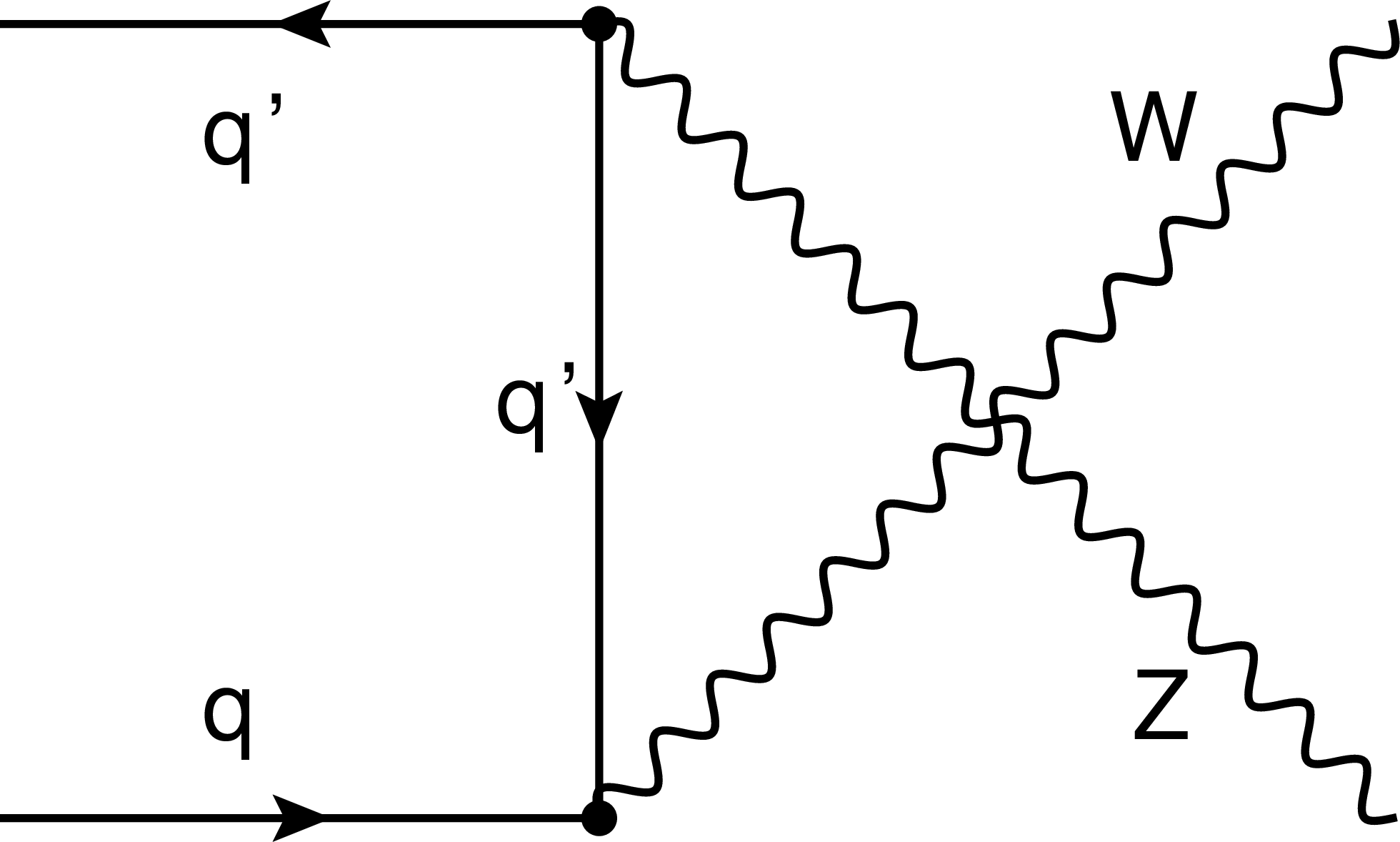
Figure 1:
Feynman diagrams for WZ production at leading order in perturbative QCD in proton-proton collisions for the $s$-channel (left), $t$-channel (middle), and $u$-channel (right). The contribution from $s$-channel proceeds through TGC. |

png pdf |
Figure 1-a:
Feynman diagram for WZ production at leading order in perturbative QCD in proton-proton collisions for the $s$-channel. The contribution from $s$-channel proceeds through TGC. |

png pdf |
Figure 1-b:
Feynman diagram for WZ production at leading order in perturbative QCD in proton-proton collisions for the $t$-channel. Figure 1-c |
png pdf |
Figure 1-c:
Feynman diagrams for WZ production at leading order in perturbative QCD in proton-proton collisions for the $s$-channel (left), $t$-channel (middle), and $u$-channel (right). The contribution from $s$-channel proceeds through TGC. |
png pdf |
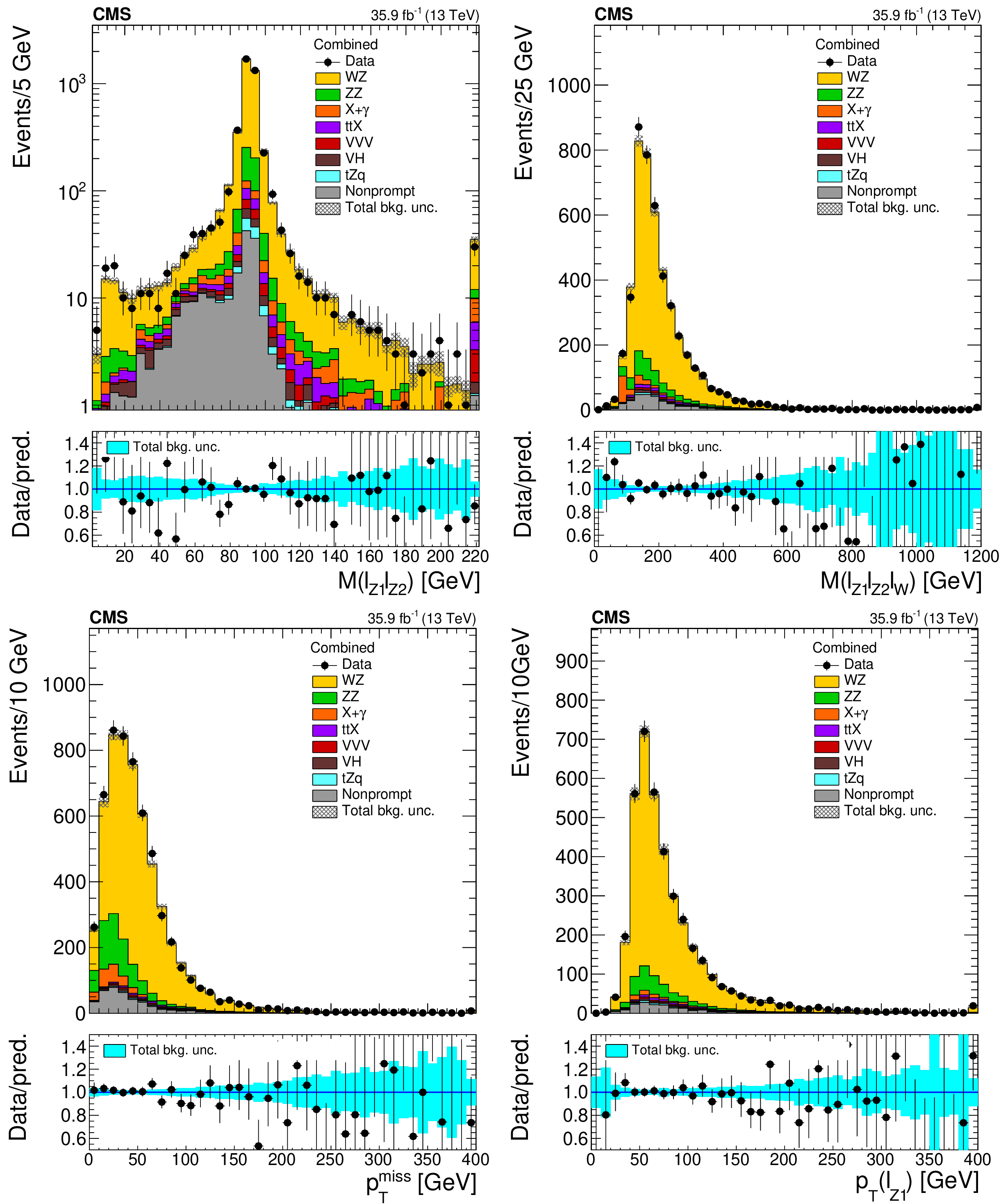
Figure 2:
Distribution of key observables in the signal region: invariant mass of the lepton pair assigned to the Z boson (top left), invariant mass of the three-lepton system (top right), missing transverse momentum (bottom left), and transverse momentum of the leading lepton assigned to the W boson. For each distribution all the signal region requirements are applied except the requirement relating to the particular observable so that the effect of the requirement on that observable can be easily seen. The last bin contains the overflow. Vertical bars on the data points include the statistical uncertainty and shaded bands over the prediction include the contributions of the different sources of uncertainty at their values after the signal extraction fit. |

png pdf |
Figure 2-a:
Distribution of the invariant mass of the lepton pair assigned to the Z boson in the signal region. The last bin contains the overflow. Vertical bars on the data points include the statistical uncertainty and shaded bands over the prediction include the contributions of the different sources of uncertainty at their values after the signal extraction fit. |

png pdf |
Figure 2-b:
Distribution of the invariant mass of the three-lepton system in the signal region. The last bin contains the overflow. Vertical bars on the data points include the statistical uncertainty and shaded bands over the prediction include the contributions of the different sources of uncertainty at their values after the signal extraction fit. |

png pdf |
Figure 2-c:
Distribution of the missing transverse momentum in the signal region. The last bin contains the overflow. Vertical bars on the data points include the statistical uncertainty and shaded bands over the prediction include the contributions of the different sources of uncertainty at their values after the signal extraction fit. |

png pdf |
Figure 2-d:
Distribution of the transverse momentum of the leading lepton assigned to the W boson in the signal region. The last bin contains the overflow. Vertical bars on the data points include the statistical uncertainty and shaded bands over the prediction include the contributions of the different sources of uncertainty at their values after the signal extraction fit. |

png pdf |
Figure 3:
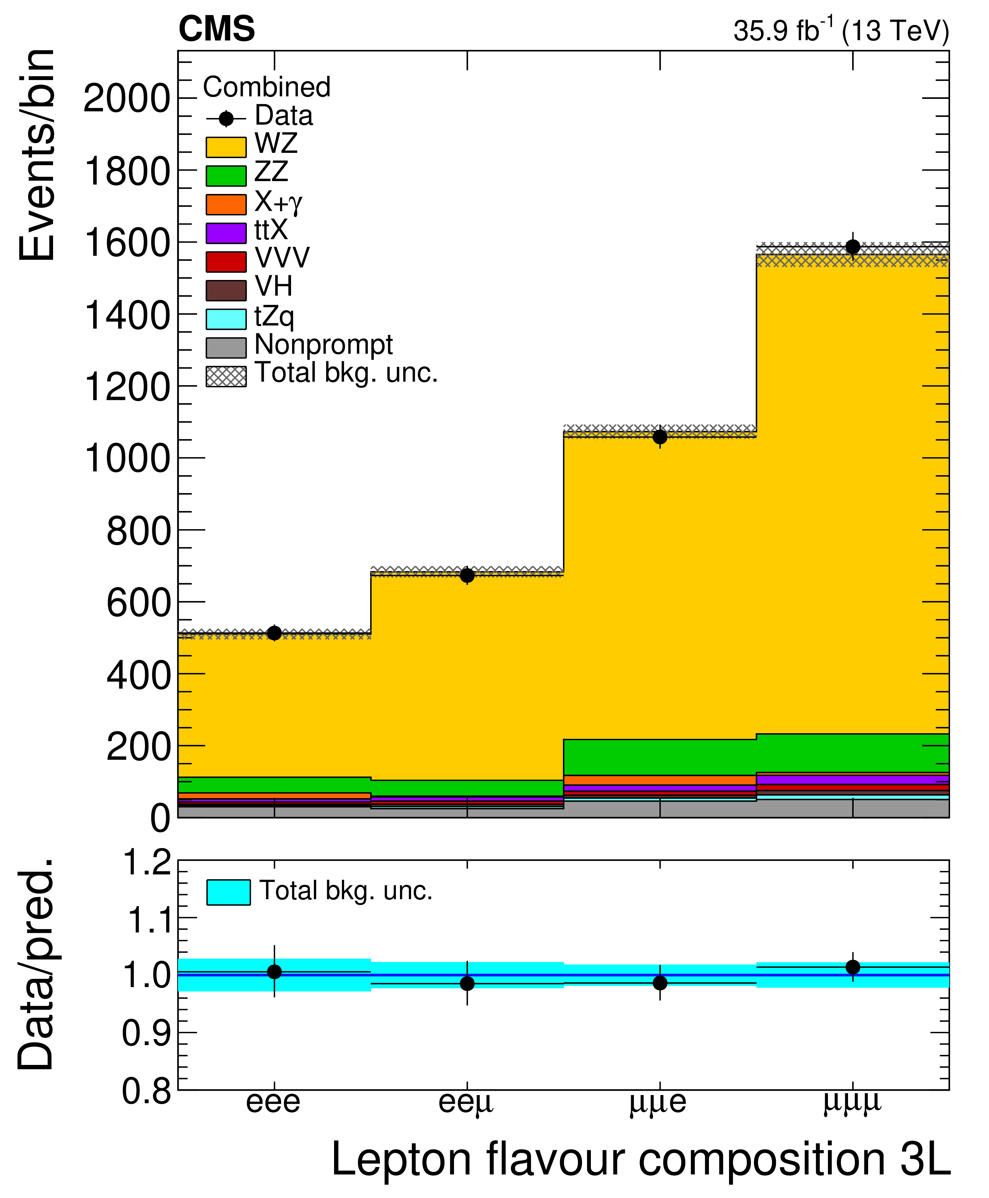
Distribution of key observables in the ZZ control region defined in Table 1: flavour composition of the three leading leptons (top left), invariant mass of the three leptons plus missing transverse momentum (top right), transverse momentum of the W boson reconstructed from the $ {p_{\mathrm {T}}} $ of the two leptons assigned to it (bottom left), and transverse momentum of the leading jet (bottom right). Vertical bars on the data points include the statistical uncertainty and shaded bands over the prediction include the contributions of the different sources of uncertainty evaluated after the signal extraction fit. |
png pdf |
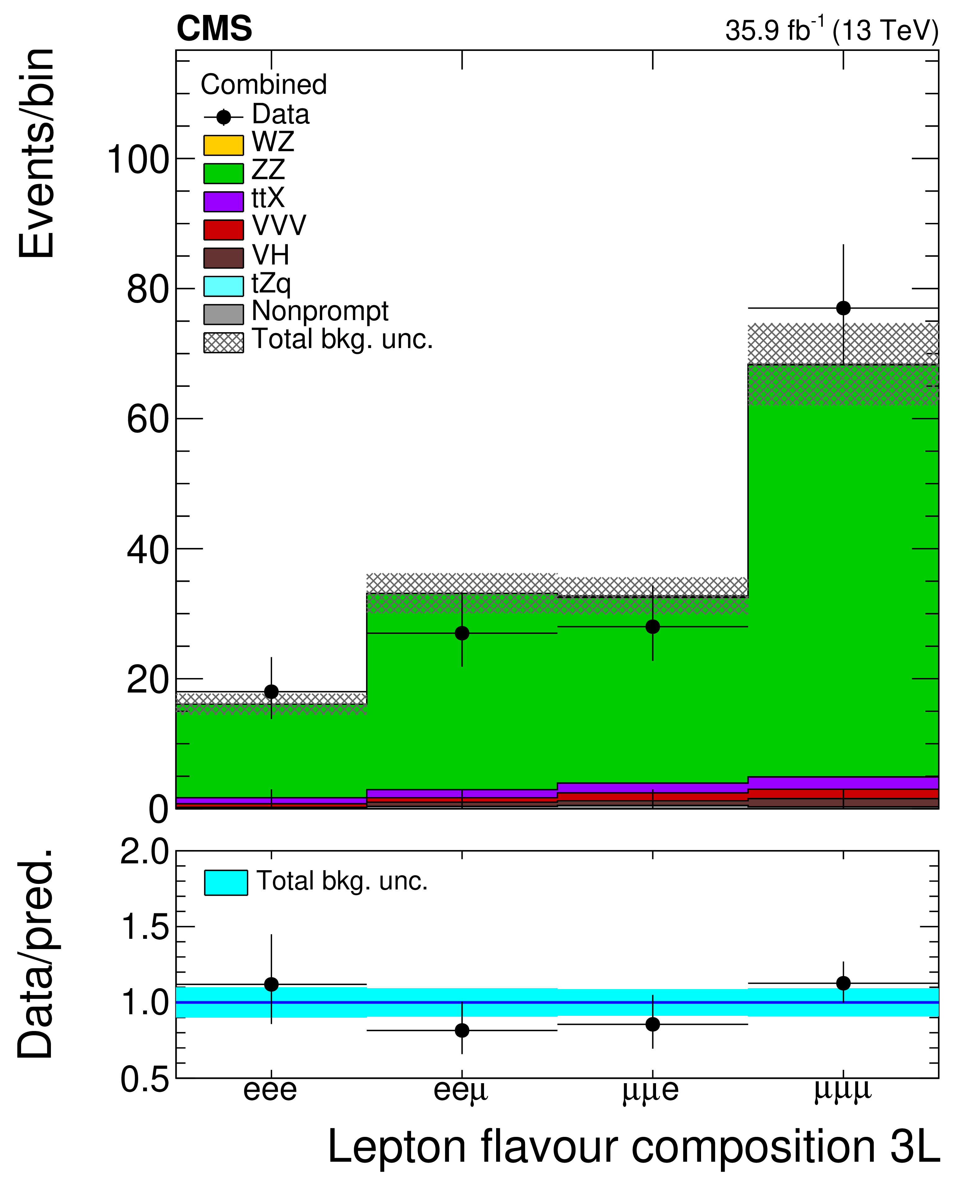
Figure 3-a:
Distribution of the flavour composition of the three leading leptons in the ZZ control region defined in Table 1. Vertical bars on the data points include the statistical uncertainty and shaded bands over the prediction include the contributions of the different sources of uncertainty evaluated after the signal extraction fit. |

png pdf |
Figure 3-b:
Distribution of the invariant mass of the three leptons plus missing transverse momentum in the ZZ control region defined in Table 1. Vertical bars on the data points include the statistical uncertainty and shaded bands over the prediction include the contributions of the different sources of uncertainty evaluated after the signal extraction fit. |

png pdf |
Figure 3-c:
Distribution of the transverse momentum of the W boson reconstructed from the $ {p_{\mathrm {T}}} $ of the two leptons assigned to it in the ZZ control region defined in Table 1. Vertical bars on the data points include the statistical uncertainty and shaded bands over the prediction include the contributions of the different sources of uncertainty evaluated after the signal extraction fit. |

png pdf |
Figure 3-d:
Distribution of the transverse momentum of the leading jet in the ZZ control region defined in Table 1. Vertical bars on the data points include the statistical uncertainty and shaded bands over the prediction include the contributions of the different sources of uncertainty evaluated after the signal extraction fit. |

png pdf |
Figure 4:
Distribution of key observables in the top enriched control region defined in Table 1: flavour composition of the three leading leptons (top left), invariant mass of the three lepton plus missing transverse momentum (top right), transverse momentum of the Z boson reconstructed from the ${p_{\mathrm {T}}}$ of the two leptons assigned to it (bottom left), and transverse momentum of the leading jet (bottom right). Vertical bars on the data points include the statistical uncertainty and shaded bands over the prediction include the contributions of the different sources of uncertainty evaluated after the signal extraction fit. |

png pdf |
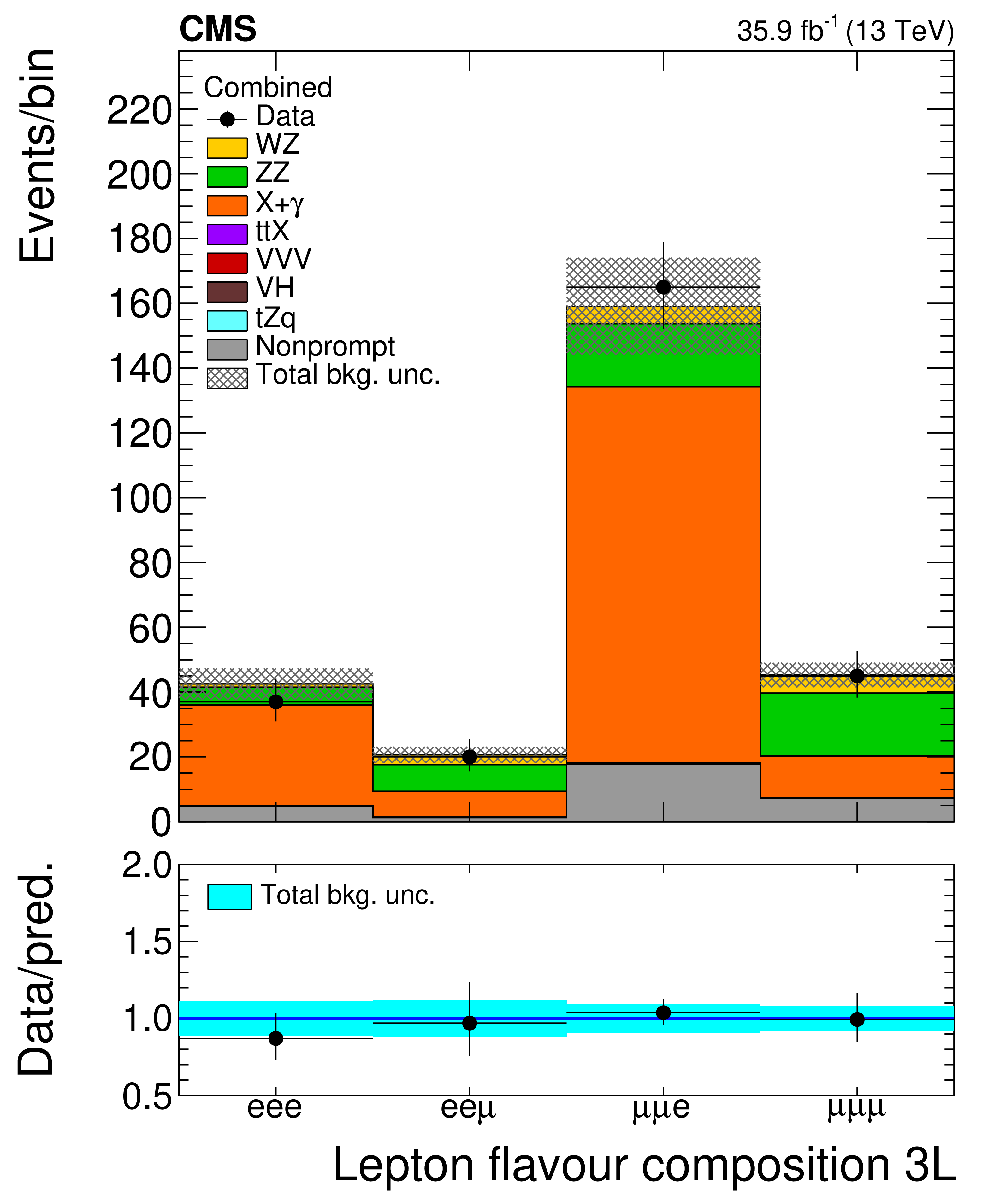
Figure 4-a:
Distribution flavour composition of the three leading leptons in the top enriched control region defined in Table 1. Vertical bars on the data points include the statistical uncertainty and shaded bands over the prediction include the contributions of the different sources of uncertainty evaluated after the signal extraction fit. |

png pdf |
Figure 4-b:
Distribution invariant mass of the three lepton plus missing transverse momentum in the top enriched control region defined in Table 1. Vertical bars on the data points include the statistical uncertainty and shaded bands over the prediction include the contributions of the different sources of uncertainty evaluated after the signal extraction fit. |

png pdf |
Figure 4-c:
Distribution transverse momentum of the Z boson reconstructed from the $ {p_{\mathrm {T}}} $ of the two leptons assigned to it in the top enriched control region defined in Table 1. Vertical bars on the data points include the statistical uncertainty and shaded bands over the prediction include the contributions of the different sources of uncertainty evaluated after the signal extraction fit. |

png pdf |
Figure 4-d:
Distribution transverse momentum of the leading jet in the top enriched control region defined in Table 1. Vertical bars on the data points include the statistical uncertainty and shaded bands over the prediction include the contributions of the different sources of uncertainty evaluated after the signal extraction fit. |

png pdf |
Figure 5:
Distribution of key observables in the conversion control region defined in Table 1: flavour composition of the three leading leptons (top left), invariant mass of the three lepton plus missing transverse momentum (top right), transverse momentum of the Z boson reconstructed from the $ {p_{\mathrm {T}}} $ of the two leptons assigned to it (bottom left), and transverse momentum of the leading jet (bottom right). Vertical bars on the data points include the statistical uncertainty and shaded bands over the prediction include the contributions of the different sources of uncertainty evaluated after the signal extraction fit. |
png pdf |
Figure 5-a:
Distribution of the flavour composition of the three leading leptons in the conversion control region defined in Table 1. Vertical bars on the data points include the statistical uncertainty and shaded bands over the prediction include the contributions of the different sources of uncertainty evaluated after the signal extraction fit. |

png pdf |
Figure 5-b:
Distribution of the invariant mass of the three lepton plus missing transverse momentum in the conversion control region defined in Table 1. Vertical bars on the data points include the statistical uncertainty and shaded bands over the prediction include the contributions of the different sources of uncertainty evaluated after the signal extraction fit. |

png pdf |
Figure 5-c:
Distribution of the transverse momentum of the Z boson reconstructed from the $ {p_{\mathrm {T}}} $ of the two leptons assigned to it in the conversion control region defined in Table 1. Vertical bars on the data points include the statistical uncertainty and shaded bands over the prediction include the contributions of the different sources of uncertainty evaluated after the signal extraction fit. |

png pdf |
Figure 5-d:
Distribution of the transverse momentum of the leading jet in the conversion control region defined in Table 1. Vertical bars on the data points include the statistical uncertainty and shaded bands over the prediction include the contributions of the different sources of uncertainty evaluated after the signal extraction fit. |
png pdf |
Figure 6:
Distribution of expected and observed event yields in the four flavour categories used for the cross section measurement. Vertical bars on the data points include the statistical uncertainty and shaded bands over the prediction include the contributions of the different sources of uncertainty evaluated after the signal extraction fit. |
png pdf |
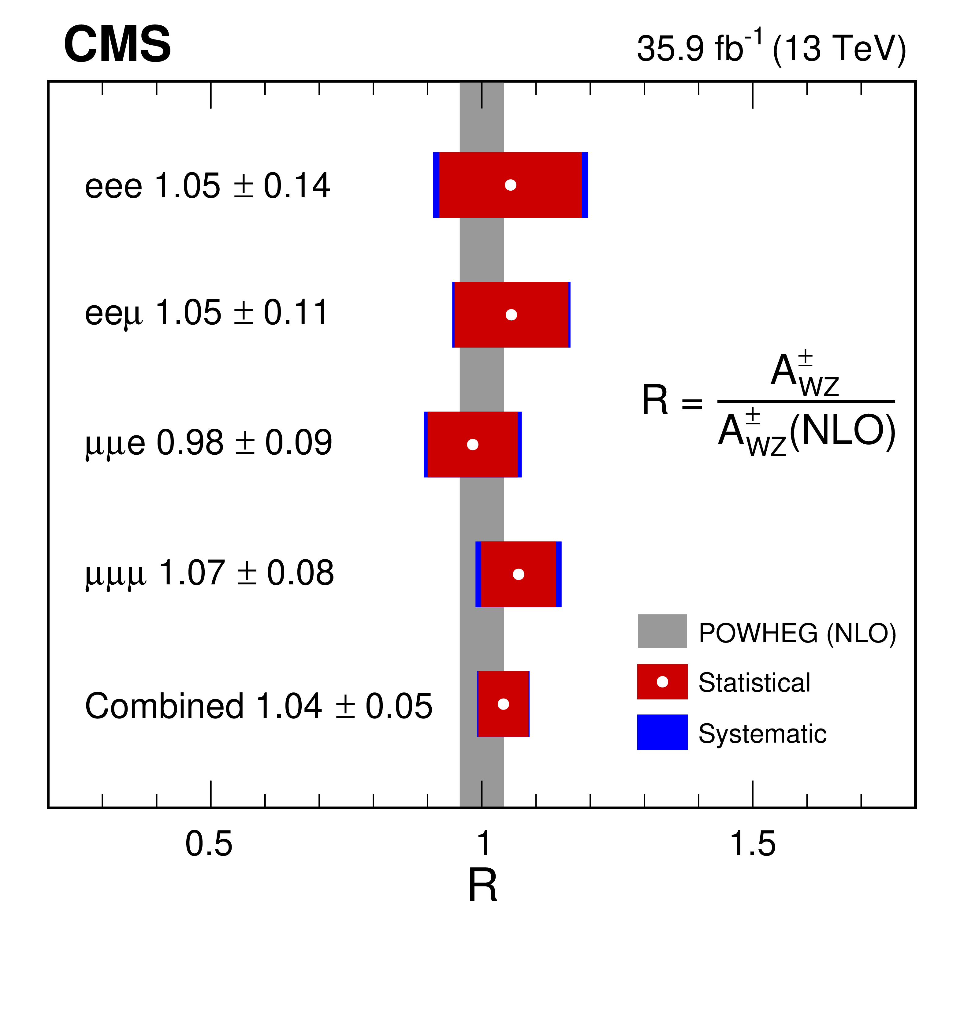
Figure 7:
Measured ratio of cross sections for the two charge channels for each of the flavour categories and their combination. Values are normalized to the NLO prediction obtained with POWHEG. Coloured bands for each of the points include both systematic and statistical uncertainties. Shaded bands correspond to the MC prediction from the nominal POWHEG sample and its associated uncertainty. |

png pdf |
Figure 8:
Prefit distributions of key observables in the signal region. The transverse momentum of the Z boson (top left), the transverse momentum of the leading jet (top right), and the mass of the WZ system (bottom). The last bin contains the overflow. Vertical bars on the data points include the statistical uncertainty and the shaded band over the MC prediction include both the statistical and the systematic uncertainties in the normalization of each of the background processes. An additional 15% uncertainty is assigned to the signal WZ process in the figures to account for the NLO/NNLO normalization differences. |

png pdf |
Figure 8-a:
Prefit distribution of the transverse momentum of the Z boson in the signal region. The last bin contains the overflow. Vertical bars on the data points include the statistical uncertainty and the shaded band over the MC prediction include both the statistical and the systematic uncertainties in the normalization of each of the background processes. An additional 15% uncertainty is assigned to the signal WZ process to account for the NLO/NNLO normalization differences. |

png pdf |
Figure 8-b:
Prefit distribution of the transverse momentum of the leading jet in the signal region. The last bin contains the overflow. Vertical bars on the data points include the statistical uncertainty and the shaded band over the MC prediction include both the statistical and the systematic uncertainties in the normalization of each of the background processes. An additional 15% uncertainty is assigned to the signal WZ process to account for the NLO/NNLO normalization differences. |

png pdf |
Figure 8-c:
Prefit distribution of the mass of the WZ system in the signal region. The last bin contains the overflow. Vertical bars on the data points include the statistical uncertainty and the shaded band over the MC prediction include both the statistical and the systematic uncertainties in the normalization of each of the background processes. An additional 15% uncertainty is assigned to the signal WZ process to account for the NLO/NNLO normalization differences. |

png pdf |
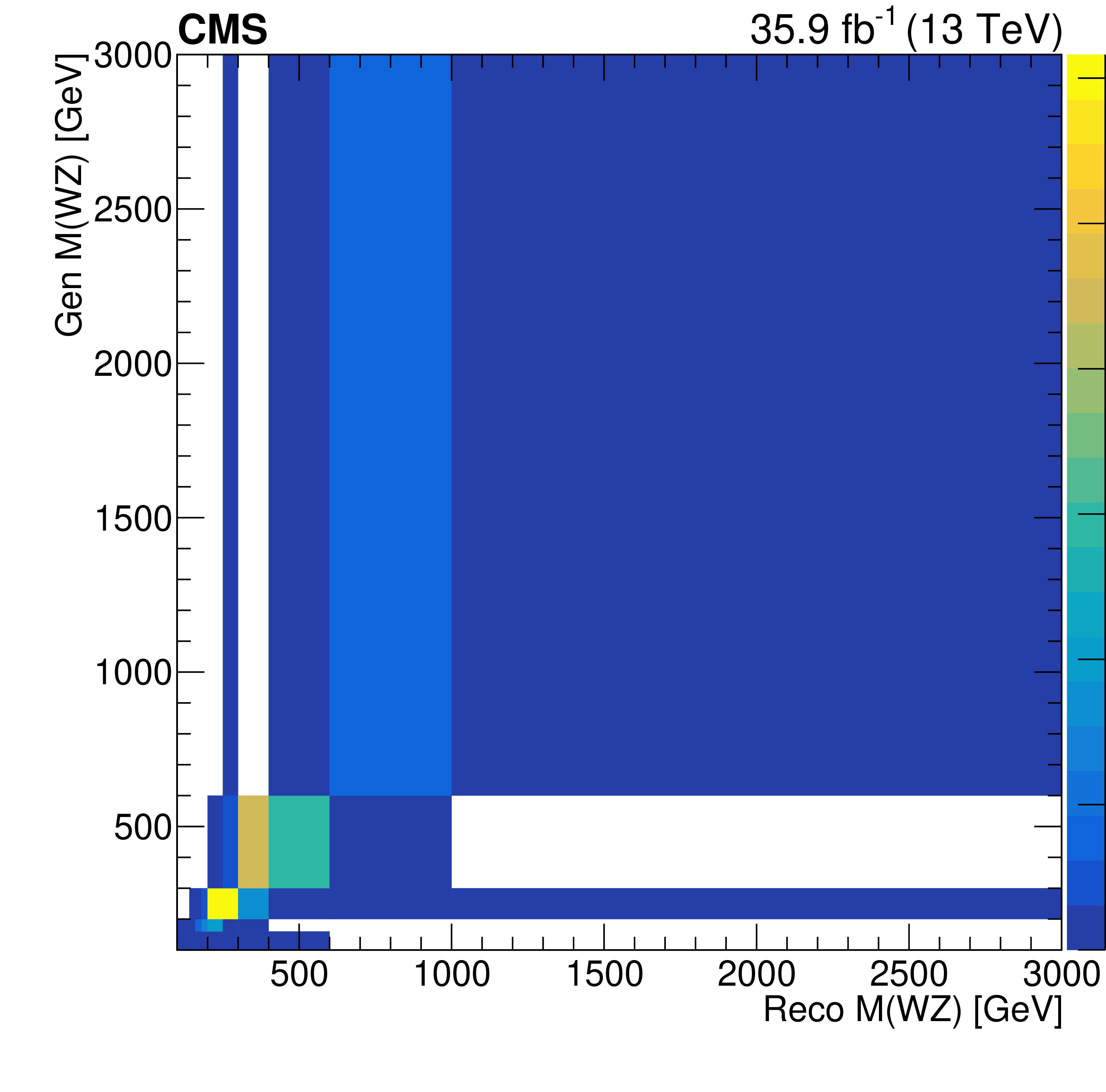
Figure 9:
Response matrices obtained using NLO samples, simulated with the POWHEG generator. The transverse momentum of the Z boson (top left), the leading jet transverse momentum (top right) and the mass of the WZ system (bottom) are shown. |

png pdf |
Figure 9-a:
Response matrice for the transverse momentum of the Z boson, obtained using NLO samples simulated with the POWHEG generator. |

png pdf |
Figure 9-b:
Response matrice for the leading jet transverse momentum (top right) and the mass of the WZ system, obtained using NLO samples simulated with the POWHEG generator. |
png pdf |
Figure 9-c:
Response matrices obtained using NLO samples, simulated with the POWHEG generator. The transverse momentum of the Z boson (top left), the leading jet transverse momentum (top right) and the mass of the WZ system (bottom) are shown. |

png pdf |
Figure 10:
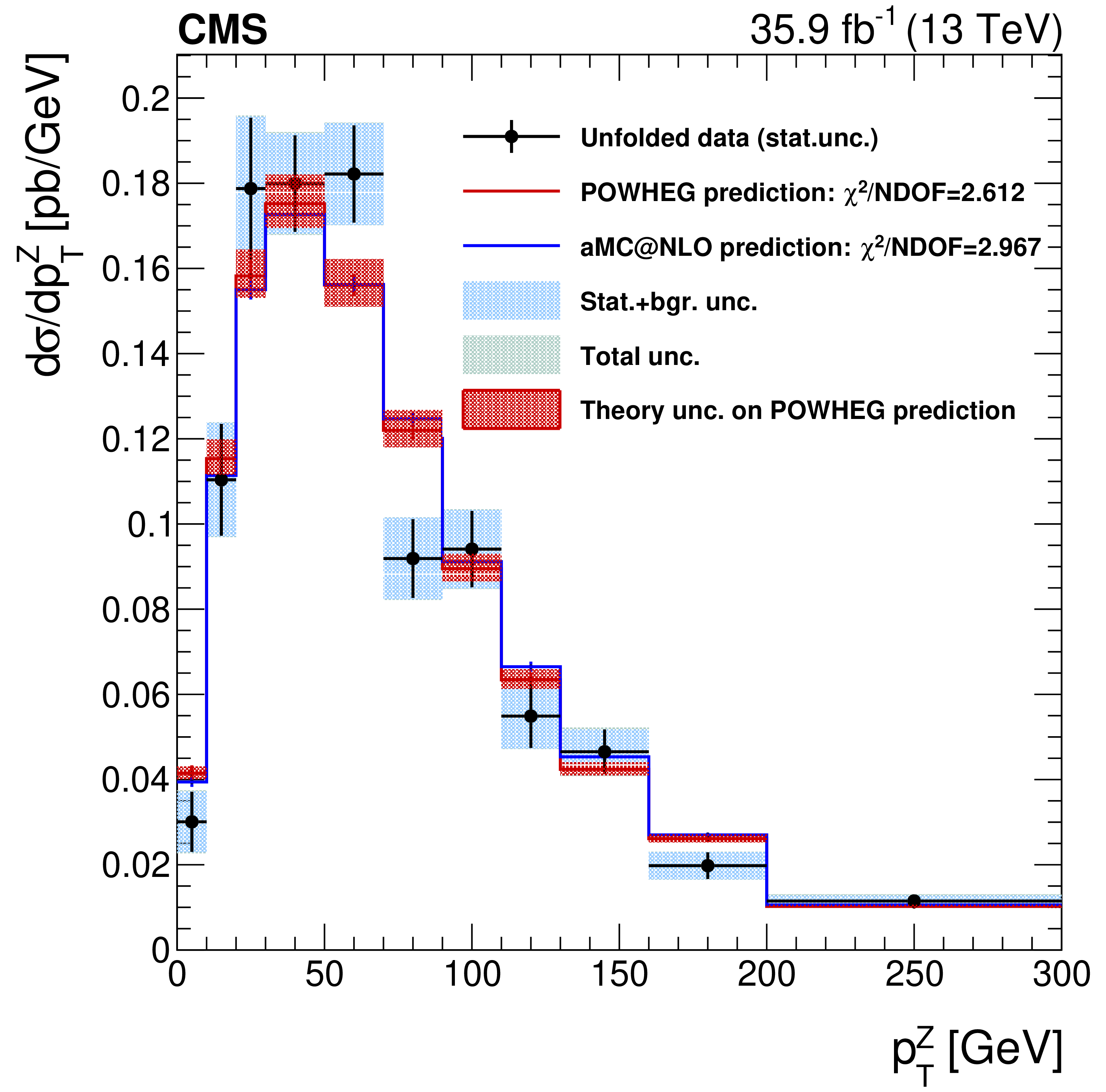
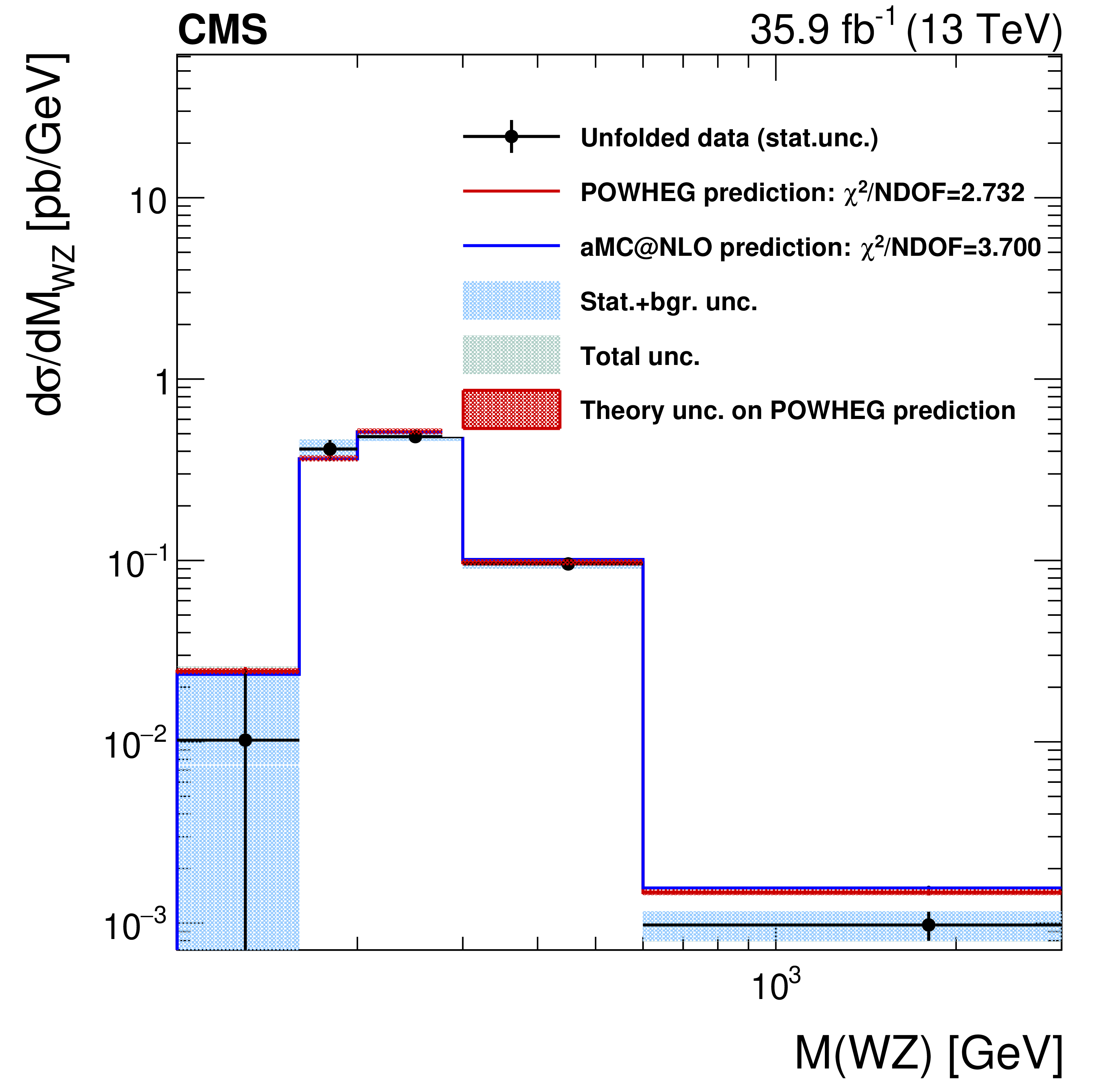
Differential distributions for the Z boson $ {p_{\mathrm {T}}} $ (top left), leading jet $ {p_{\mathrm {T}}} $ (top right), and mass of the WZ system (bottom). Data distributions are unfolded at the dressed leptons level and compared with the POWHEG, MadGraph 5_aMC@NLO NLO generators, and PYTHIA predictions, as described in the text. The red band around the POWHEG prediction represents the theory uncertainty in it; the effect on the unfolded data of this uncertainty, through the unfolding matrix, is included in the shaded bands described in the legend. |

png pdf |
Figure 10-a:
Differential distribution for the Z boson $ {p_{\mathrm {T}}} $. The data distribution is unfolded at the dressed leptons level and compared with the POWHEG, MadGraph 5_aMC@NLO NLO generators, and PYTHIA predictions, as described in the text. The red band around the POWHEG prediction represents the theory uncertainty in it; the effect on the unfolded data of this uncertainty, through the unfolding matrix, is included in the shaded bands described in the legend. |

png pdf |
Figure 10-b:
Differential distribution for the leading jet $ {p_{\mathrm {T}}} $. The data distribution is unfolded at the dressed leptons level and compared with the POWHEG, MadGraph 5_aMC@NLO NLO generators, and PYTHIA predictions, as described in the text. The red band around the POWHEG prediction represents the theory uncertainty in it; the effect on the unfolded data of this uncertainty, through the unfolding matrix, is included in the shaded bands described in the legend. |

png pdf |
Figure 10-c:
Differential distribution for the mass of the WZ system. The data distribution is unfolded at the dressed leptons level and compared with the POWHEG, MadGraph 5_aMC@NLO NLO generators, and PYTHIA predictions, as described in the text. The red band around the POWHEG prediction represents the theory uncertainty in it; the effect on the unfolded data of this uncertainty, through the unfolding matrix, is included in the shaded bands described in the legend. |

png pdf |
Figure 11:
Differential distributions for W$^{+}$ (left) and W$^{-}$ (right), in the full SR. The leading jet transverse momentum is unfolded at the dressed leptons level, as described in the text. The red band around the POWHEG prediction represents the theory uncertainty in it. The effect on the unfolded data of this uncertainty, through the unfolding matrix, is included in the shaded bands described in the legend. |

png pdf |
Figure 11-a:
Differential distribution for W$^{+}$, in the full SR. The leading jet transverse momentum is unfolded at the dressed leptons level, as described in the text. The red band around the POWHEG prediction represents the theory uncertainty in it. The effect on the unfolded data of this uncertainty, through the unfolding matrix, is included in the shaded bands described in the legend. |

png pdf |
Figure 11-b:
Differential distribution for W$^{-}$, in the full SR. The leading jet transverse momentum is unfolded at the dressed leptons level, as described in the text. The red band around the POWHEG prediction represents the theory uncertainty in it. The effect on the unfolded data of this uncertainty, through the unfolding matrix, is included in the shaded bands described in the legend. |

png pdf |
Figure 12:
Differential distributions for W$^{+}$ (left) and W$^{-}$ (right), in the full SR. The transverse momentum of the Z boson is unfolded at the dressed leptons level, as described in the text. The red band around the POWHEG prediction represents the theory uncertainty in it; the effect on the unfolded data of this uncertainty, through the unfolding matrix, is included in the shaded bands described in the legend. |
png pdf |
Figure 12-a:
Differential distribution for W$^{+}$, in the full SR. The transverse momentum of the Z boson is unfolded at the dressed leptons level, as described in the text. The red band around the POWHEG prediction represents the theory uncertainty in it; the effect on the unfolded data of this uncertainty, through the unfolding matrix, is included in the shaded bands described in the legend. |

png pdf |
Figure 12-b:
Differential distribution for W$^{-}$, in the full SR. The transverse momentum of the Z boson is unfolded at the dressed leptons level, as described in the text. The red band around the POWHEG prediction represents the theory uncertainty in it; the effect on the unfolded data of this uncertainty, through the unfolding matrix, is included in the shaded bands described in the legend. |

png pdf |
Figure 13:
Differential distributions for W$^{+}$ (left) and W$^{-}$ (right), in the full SR. The mass of the WZ system data distribution is unfolded at the dressed leptons level, as described in the text. The red band around the POWHEG prediction represents the theory uncertainty in it; the effect on the unfolded data of this uncertainty, through the unfolding matrix, is included in the shaded bands described in the legend. |
png pdf |
Figure 13-a:
Differential distribution for W$^{+}$, in the full SR. The mass of the WZ system data distribution is unfolded at the dressed leptons level, as described in the text. The red band around the POWHEG prediction represents the theory uncertainty in it; the effect on the unfolded data of this uncertainty, through the unfolding matrix, is included in the shaded bands described in the legend. |

png pdf |
Figure 13-b:
Differential distribution for W$^{-}$, in the full SR. The mass of the WZ system data distribution is unfolded at the dressed leptons level, as described in the text. The red band around the POWHEG prediction represents the theory uncertainty in it; the effect on the unfolded data of this uncertainty, through the unfolding matrix, is included in the shaded bands described in the legend. |

png pdf |
Figure 14:
Differential distributions for W$^{+}$ (left) and W$^{-}$ (right), in the full SR. The W boson transverse momentum is unfolded at the dressed leptons level, as described in the text. The red band around the POWHEG prediction represents the theory uncertainty in it; the effect on the unfolded data of this uncertainty, through the unfolding matrix, is included in the shaded bands described in the legend. |

png pdf |
Figure 14-a:
Differential distribution for W$^{+}$, in the full SR. The W boson transverse momentum is unfolded at the dressed leptons level, as described in the text. The red band around the POWHEG prediction represents the theory uncertainty in it; the effect on the unfolded data of this uncertainty, through the unfolding matrix, is included in the shaded bands described in the legend. |

png pdf |
Figure 14-b:
Differential distribution for W$^{-}$, in the full SR. The W boson transverse momentum is unfolded at the dressed leptons level, as described in the text. The red band around the POWHEG prediction represents the theory uncertainty in it; the effect on the unfolded data of this uncertainty, through the unfolding matrix, is included in the shaded bands described in the legend. |
png pdf |
Figure 15:
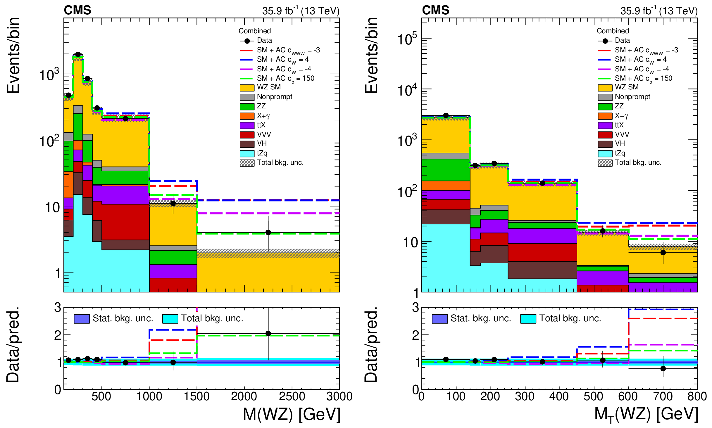
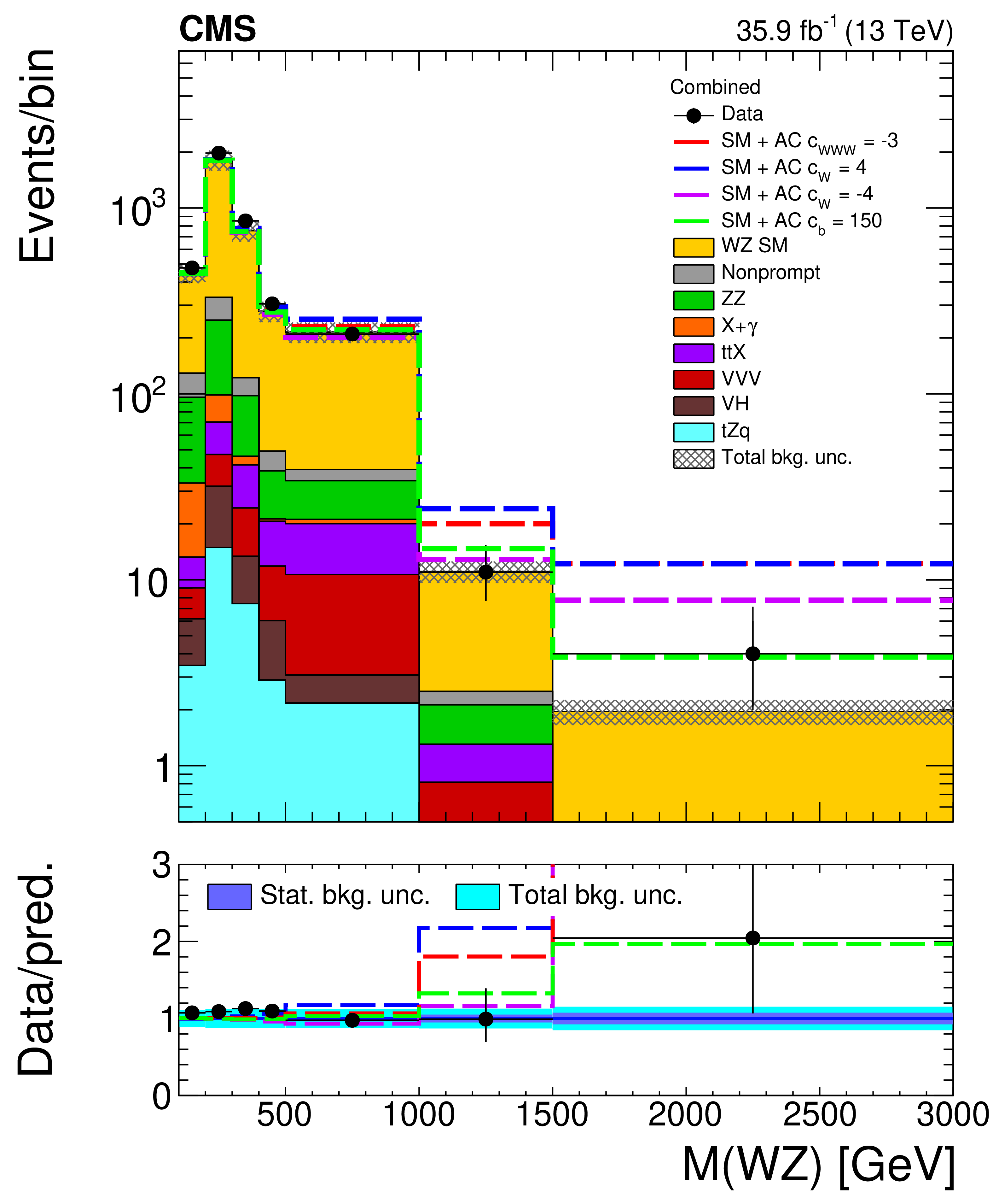
Distributions of discriminant observables in the anomalous triple gauge couplings searches. The invariant mass of the three lepton and missing transverse momentum system (left) and the transverse mass of the same configuration (right). The dashed lines represent the total yields expected from the sum of the SM processes, with the total WZ yields for different values of the associated anomalous coupling (AC) parameters. The SM prediction for the WZ process is obtained from the aTGC simulated sample with the AC parameters set to 0. |
png pdf |
Figure 15-a:
Distribution of the invariant mass of the three lepton and missing transverse momentum system in the anomalous triple gauge couplings searches. The dashed lines represent the total yields expected from the sum of the SM processes, with the total WZ yields for different values of the associated anomalous coupling (AC) parameters. The SM prediction for the WZ process is obtained from the aTGC simulated sample with the AC parameters set to 0. |

png pdf |
Figure 15-b:
Distribution of the transverse mass of the same configuration in the anomalous triple gauge couplings searches. The dashed lines represent the total yields expected from the sum of the SM processes, with the total WZ yields for different values of the associated anomalous coupling (AC) parameters. The SM prediction for the WZ process is obtained from the aTGC simulated sample with the AC parameters set to 0. |

png pdf |
Figure 16:
Two-dimensional confidence regions for each of the possible combinations of the considered aTGC parameters. The contours of the expected confidence regions for 68% and 95% confidence level are presented in each case. The parameters considered in each plot are ${c_{{\mathrm {W}}}} - {c_{{\mathrm {W}} {\mathrm {W}} {\mathrm {W}}}}$ (top), ${c_{{\mathrm {W}}}} - {c_{{\mathrm {b}}}}$ (middle) and ${c_{{\mathrm {W}} {\mathrm {W}} {\mathrm {W}}}} - {c_{{\mathrm {b}}}}$ (bottom). |

png pdf |
Figure 16-a:
Two-dimensional confidence region of the ${c_{{\mathrm {W}}}} - {c_{{\mathrm {W}} {\mathrm {W}} {\mathrm {W}}}}$ combination of the aTGC parameters. The contours of the expected confidence regions for 68% and 95% confidence level are presented in each case. |

png pdf |
Figure 16-b:
Two-dimensional confidence region of the ${c_{{\mathrm {W}}}} - {c_{{\mathrm {b}}}}$ combination of the aTGC parameters. The contours of the expected confidence regions for 68% and 95% confidence level are presented in each case. |

png pdf |
Figure 16-c:
Two-dimensional confidence region of the ${c_{{\mathrm {W}} {\mathrm {W}} {\mathrm {W}}}} - {c_{{\mathrm {b}}}}$ combination of the aTGC parameters. The contours of the expected confidence regions for 68% and 95% confidence level are presented in each case. |

png pdf |
Figure 17:
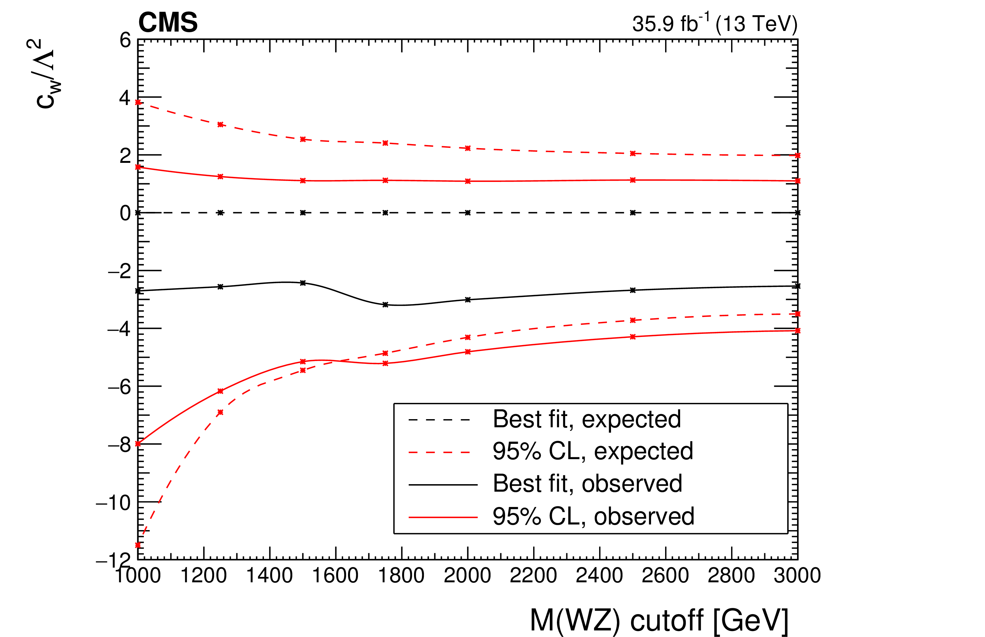
Evolution of the expected and observed confidence intervals of the EFT anomalous coupling parameters in terms of the cutoff scale given by different restrictions in the ${m({{\mathrm {W}} {\mathrm {Z}}})}$ variable. For each point and parameter, the confidence intervals are computed imposing the additional restriction of no anomalous coupling contribution over the given value of the ${m({{\mathrm {W}} {\mathrm {Z}}})}$ cutoff. The last point is equivalent to no cutoff requirement being imposed. The parameters considered are: ${c_{{\mathrm {W}}}}$ (top), ${c_{{\mathrm {W}} {\mathrm {W}} {\mathrm {W}}}}$ (middle) and ${c_{{\mathrm {b}}}}$ (bottom). |
png pdf |
Figure 17-a:
Evolution of the expected and observed confidence intervals of the ${c_{{\mathrm {W}}}}$ anomalous coupling parameter in terms of the cutoff scale given by different restrictions in the ${m({{\mathrm {W}} {\mathrm {Z}}})}$ variable. For each point and parameter, the confidence intervals are computed imposing the additional restriction of no anomalous coupling contribution over the given value of the ${m({{\mathrm {W}} {\mathrm {Z}}})}$ cutoff. The last point is equivalent to no cutoff requirement being imposed. |

png pdf |
Figure 17-b:
Evolution of the expected and observed confidence intervals of the ${c_{{\mathrm {W}} {\mathrm {W}} {\mathrm {W}}}}$ anomalous coupling parameter in terms of the cutoff scale given by different restrictions in the ${m({{\mathrm {W}} {\mathrm {Z}}})}$ variable. For each point and parameter, the confidence intervals are computed imposing the additional restriction of no anomalous coupling contribution over the given value of the ${m({{\mathrm {W}} {\mathrm {Z}}})}$ cutoff. The last point is equivalent to no cutoff requirement being imposed. |

png pdf |
Figure 17-c:
Evolution of the expected and observed confidence intervals of the ${c_{{\mathrm {b}}}}$ anomalous coupling parameter in terms of the cutoff scale given by different restrictions in the ${m({{\mathrm {W}} {\mathrm {Z}}})}$ variable. For each point and parameter, the confidence intervals are computed imposing the additional restriction of no anomalous coupling contribution over the given value of the ${m({{\mathrm {W}} {\mathrm {Z}}})}$ cutoff. The last point is equivalent to no cutoff requirement being imposed. |
| Tables | |

png pdf |
Table 1:
Requirements for the definition of the signal region of the analysis and the three different regions designed to estimate the main background sources. |

png pdf |
Table 2:
Expected and observed yields for each of the relevant processes and flavour categories. Combined statistical and systematic uncertainties are shown for each case except for the observed data yields for which only statistical uncertainties are presented. All expected yields correspond to quantities estimated after the maximum likelihood fit. Uncertainties are computed taking into account the full correlation matrix between sources of uncertainty, processes, and flavour categories. |

png pdf |
Table 3:
Summary of the total postfit impact of each uncertainty source on the uncertainty in the signal strength measurement, for the four flavour categories and their combination. Theoretical uncertainties are only included in the signal acceptance during the extrapolation to the total phase space, so they are not included in the likelihood fit. The values are percentages and correspond to half the difference between the up and down variation of each systematic uncertainty component. |
png pdf |
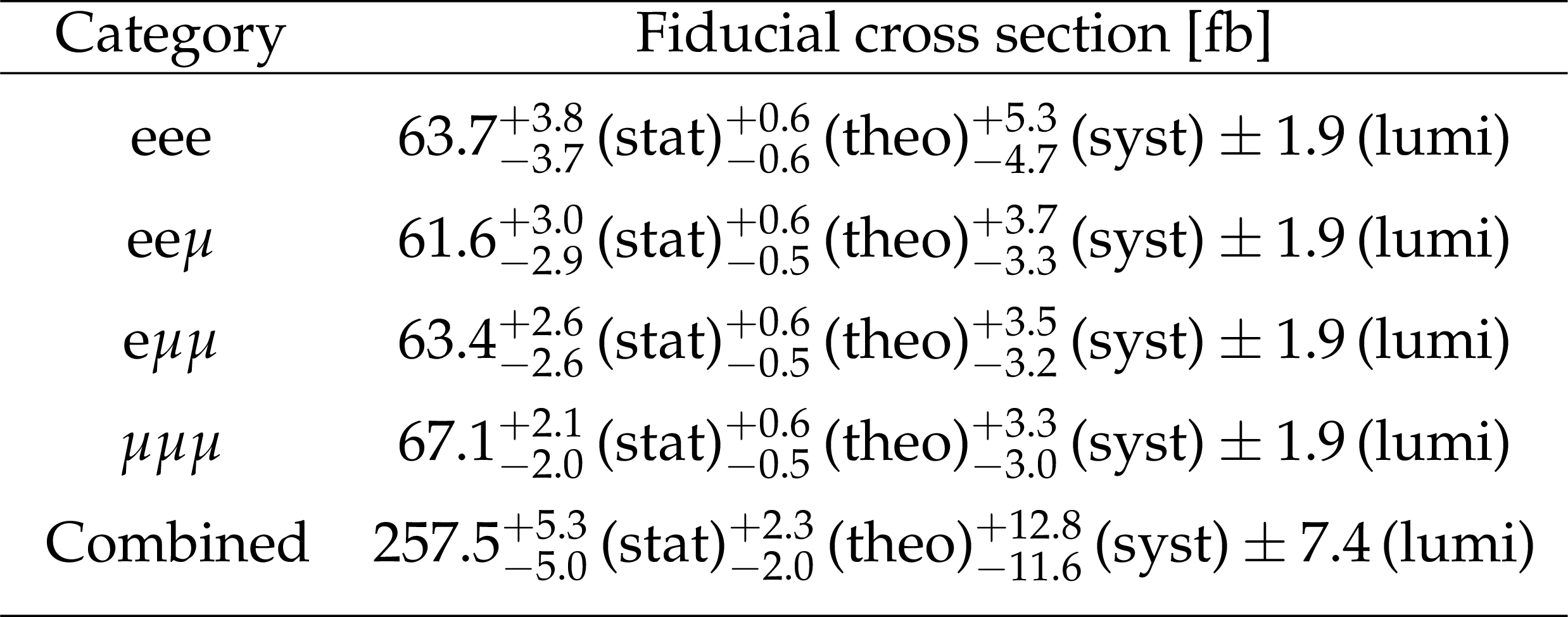
Table 4:
Measured fiducial cross sections and their corresponding uncertainties for each of the individual flavour categories, as well as for the combination of the four. |

png pdf |
Table 5:
Measured WZ production cross sections computed separately in each of the flavour categories. |
png pdf |
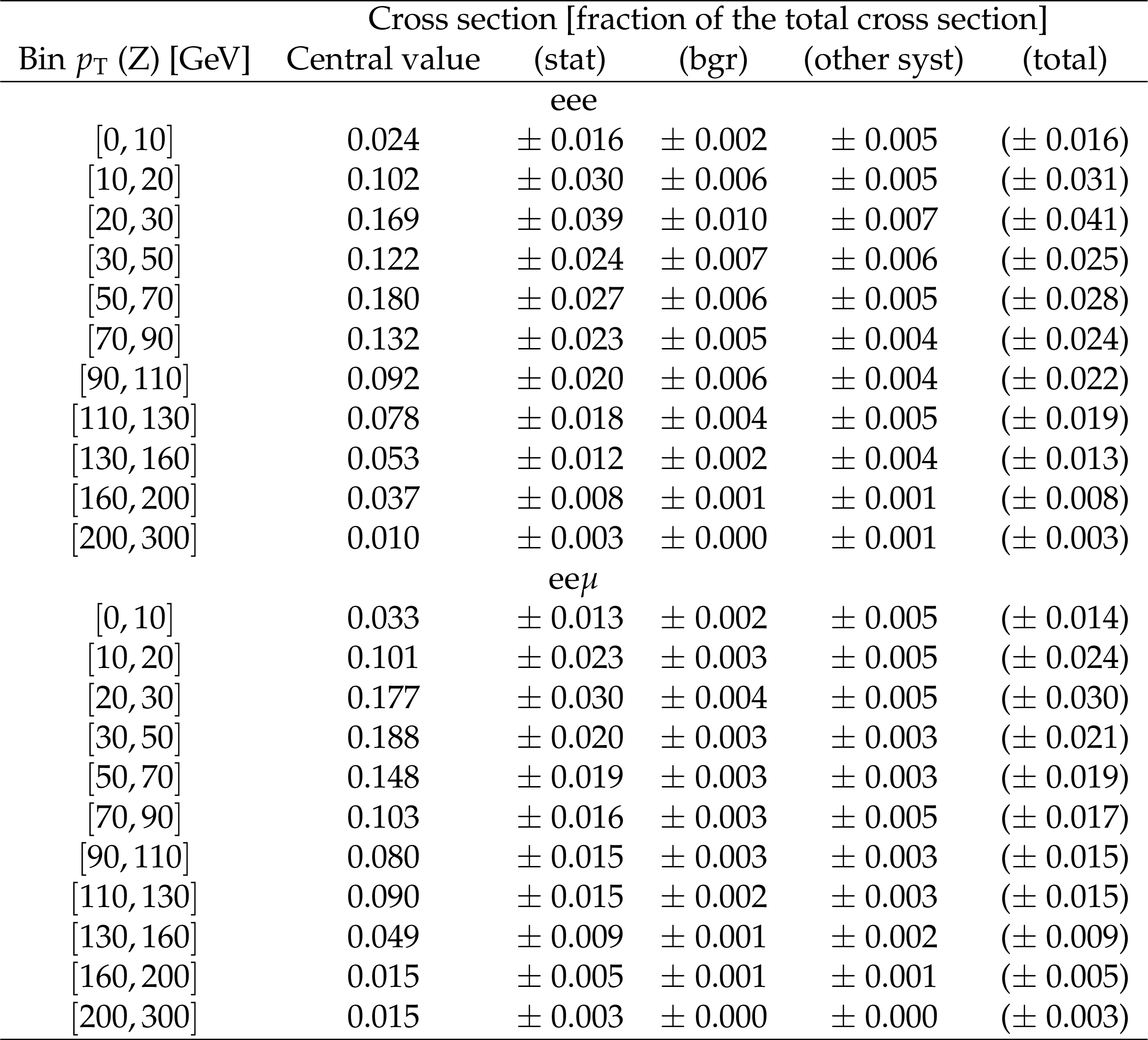
Table 6:
Differential cross section in bins of $ {p_{\mathrm {T}}} $ (Z). Values are expressed as fraction of the total cross section. The eee and ee$\mu$ final states are shown. |

png pdf |
Table 7:
Differential cross section in bins of $ {p_{\mathrm {T}}} $ (Z). Values are expressed as fraction of the total cross section. The e${{\mu}} {{\mu}}$ and $ {{\mu}} {{\mu}} {{\mu}}$ final states are shown. |

png pdf |
Table 8:
Differential cross section in bins of $ {p_{\mathrm {T}}} $ (Z). Values are expressed as fraction of the total cross section. The inclusive final state is shown |

png pdf |
Table 9:
Differential cross section in bins of $ {p_{\mathrm {T}}} $ (Leading jet). Values are expressed as fraction of the total cross section. The eee, ee${{\mu}}$, e${{\mu}} {{\mu}}$, and ${{\mu}} {{\mu}} {{\mu}}$ final states are shown. |

png pdf |
Table 10:
Differential cross section in bins of $ {p_{\mathrm {T}}} $ (Leading jet). Values are expressed as fraction of the total cross section. The inclusive final state is shown. |

png pdf |
Table 11:
Differential cross section in bins of mass of the WZ system. Values are expressed as fraction of the total cross section. |

png pdf |
Table 12:
Expected and observed one-dimensional confidence intervals (CI) at 95% confidence level for each of the considered EFT parameters. |
| Summary |
|
The production process ${{\mathrm{p}}{\mathrm{p}}\to\mathrm{W}\mathrm{Z}}$ is studied in the trilepton final state at ${\sqrt{s}} = $ 13 TeV, using the full 2016 data set with a total integrated luminosity of 35.9 fb$^{-1}$ collected with the CMS detector. Fiducial results are obtained in each of the flavour categories (eee, ee$\mu$, e$\mu\mu$, and $\mu\mu\mu$) and in the combined category, and are extrapolated to the total WZ production cross section for 60 $ < {m_{\mathrm{Z}}} ^{OSSF} < $ 120 GeV. The combined measurement yields a cross section of ${\sigma_{\text{tot}}}({\mathrm{p}}{\mathrm{p}} \to {\mathrm{W}\mathrm{Z}} ) = $ 48.09 $^{+1.00}_{-0.96}$ (stat) $^{+0.44}_{-0.37}$ (theo) $^{+2.39}_{-2.17}$ (syst) $\pm$ 1.39 (lumi) pb, for a total uncertainty of $+2.98$ and $-2.78$ pb. The result is in good agreement with the MATRIX next-to-next-to-leading-order (NNLO) prediction [56] of $\sigma_{\mathrm{NNLO}}({\mathrm{p}}{\mathrm{p}} \to {\mathrm{W}\mathrm{Z}} ) = $ 49.98 ($+$2.2%)($-$2.0%) pb. This result supersedes the result from the CMS Collaboration using data corresponding to a smaller integrated luminosity of 2.3 fb$^{-1}$ [14]. A measurement in the fiducial region yields a value of $\sigma_{\text{fid}}({\mathrm{p}}{\mathrm{p}} \to {\mathrm{W}\mathrm{Z}} ) = $ 257.5 $^{+5.3}_{-5.0}$ (stat) $^{+2.3}_{-2.0}$ (theo) $^{+12.8}_{-11.6}$ (syst) $\pm$ 7.4 (lumi) fb, pointing to an excess over the POWHEG next-to-leading-order cross section $\sigma_{\text{fid}}^{POWHEG} = $ 227.6 $^{+9.4}_{-8.0}$ fb. The cross sections are also measured independently for the two possible values of the W boson charge, yielding a ratio of ${A^{+-}_{{\mathrm{W}\mathrm{Z}} }} = {\sigma_{\text{tot}}}({\mathrm{p}}{\mathrm{p}} \to \mathrm{W}^+\mathrm{Z})/{\sigma_{\text{tot}}}({\mathrm{p}}{\mathrm{p}} \to \mathrm{W}^-\mathrm{Z}) = $ 1.48 $\pm$ 0.06, which is compatible within uncertainties with the POWHEG + PYTHIA prediction of 1.43$^{+0.06}_{-0.05}$. Similar results are obtained when splitting by flavour category. All the measurements of this paper are compatible with the SM when the appropriate order of theoretical calculations is considered. Differential cross sections are measured as a function of the transverse momentum of the Z boson, of the transverse momentum of the leading jet, and of an estimate of the mass of the WZ system; results are compared with predictions from the POWHEG and MadGraph5+MCatNLO generators. Differential cross sections as a function of the transverse momentum of the leading jet are also measured for each sign of the W boson charge. Confidence intervals for anomalous triple gauge boson couplings are extracted for each of the possible one- and two-dimensional combinations of the anomalous couplings parameters, using the ${m({\mathrm{W}\mathrm{Z}} )}$ variable in a maximum likelihood fit. The confidence intervals obtained represent the most stringent results on the anomalous $\mathrm{W{\mathrm{W}\mathrm{Z}}} $ triple gauge coupling to date. |
| References | ||||
| 1 | UA1 Collaboration | Production of $ \mathrm{W}'s $ with large transverse momentum at the CERN proton-antiproton collider | Physics Letters B 193 (1987) 389 | |
| 2 | D0 Collaboration | Measurement of the $ \mathrm{W}\mathrm{Z}\rightarrow \ell\nu\ell\ell $ cross section and limits on anomalous triple gauge couplings in $ \mathrm{t \bar{t}} $ collisions at $ \sqrt{s} = $ 1.96 TeV | PLB 695 (2011) 67 | 1006.0761 |
| 3 | CDF Collaboration | Observation of $ \mathrm{W}\mathrm{Z} $ production | PRLett 98 (2007) 161801 | hep-ex/0702027 |
| 4 | ATLAS Collaboration | Measurement of the $ \mathrm{W}^\pm \mathrm{Z} $ production cross section and limits on anomalous triple gauge couplings in proton-proton collisions at $ \sqrt{s}= $ 7 TeV with the ATLAS detector | PLB 709 (2012) 341 | 1111.5570 |
| 5 | ATLAS Collaboration | Measurement of $ \mathrm{W}\mathrm{Z} $ production in proton-proton collisions at $ \sqrt{s}= $ 7 TeV with the ATLAS detector | EPJC 72 (2012) 2173 | 1208.1390 |
| 6 | ATLAS Collaboration | Measurement of the $ \mathrm{W}\mathrm{W}+\mathrm{W}\mathrm{Z} $ cross section and limits on anomalous triple gauge couplings using final states with one lepton, missing transverse momentum, and two jets with the ATLAS detector at $ \sqrt{\rm{s}} = $ 7 TeV | JHEP 01 (2015) 049 | 1410.7238 |
| 7 | ATLAS Collaboration | Measurements of $ \mathrm{W}^\pm \mathrm{Z} $ production cross sections in pp collisions at $ \sqrt{s} = $ 8 TeV with the ATLAS detector and limits on anomalous gauge boson self-couplings | PRD 93 (2016) 092004 | 1603.02151 |
| 8 | ATLAS Collaboration | Measurement of the $ \mathrm{W}^{\pm}\mathrm{Z} $ boson pair-production cross section in pp collisions at $ \sqrt{s}= $ 13 TeV with the ATLAS Detector | PLB 762 (2016) 1 | 1606.04017 |
| 9 | ATLAS Collaboration | Search for anomalous electroweak production of $ \mathrm{W}\mathrm{W}/\mathrm{W}\mathrm{Z} $ in association with a high-mass dijet system in pp collisions at $ \sqrt{s}= $ 8 TeV with the ATLAS detector | PRD 95 (2017) 032001 | 1609.05122 |
| 10 | ATLAS Collaboration | Measurement of $ \mathrm{W}\mathrm{W}/\mathrm{W}\mathrm{Z} \rightarrow \ell \nu q q^{\prime} $ production with the hadronically decaying boson reconstructed as one or two jets in pp collisions at $ \sqrt{s}= $ 8 TeV with ATLAS, and constraints on anomalous gauge couplings | EPJC 77 (2017) 563 | 1706.01702 |
| 11 | CMS Collaboration | Study of the dijet mass spectrum in $ {\mathrm{p}}{\mathrm{p}} \rightarrow \mathrm{W} + $ jets events at $ \sqrt{s}= $ 7 TeV | PRL 109 (2012) 251801 | CMS-EWK-11-017 1208.3477 |
| 12 | CMS Collaboration | Measurement of the sum of $ \mathrm{W}\mathrm{W} $ and $ \mathrm{W}\mathrm{Z} $ production with $ \mathrm{W}+ $dijet events in pp collisions at $ \sqrt{s}= $ 7 TeV | EPJC 73 (2013) 2283 | CMS-SMP-12-015 1210.7544 |
| 13 | CMS Collaboration | Measurement of $ \mathrm{W}\mathrm{Z} $ and $ \mathrm{Z}\mathrm{Z} $ production in pp collisions at $ \sqrt{s} = $ 8 TeV in final states with b-tagged jets | EPJC 74 (2014) 2973 | CMS-SMP-13-011 1403.3047 |
| 14 | CMS Collaboration | Measurement of the $ \mathrm{W}\mathrm{Z} $ production cross section in $ {\mathrm{p}}{\mathrm{p}} $ collisions at $ \sqrt{s} = $ 13 TeV | PLB 766 (2017) 268 | CMS-SMP-16-002 1607.06943 |
| 15 | CMS Collaboration | Measurement of the $ \mathrm{W}\mathrm{Z} $ production cross section in pp collisions at $ \sqrt{s} = $ 7 and 8 TeV and search for anomalous triple gauge couplings at $ \sqrt{s} = $ 8 TeV | EPJC 77 (2017) 236 | CMS-SMP-14-014 1609.05721 |
| 16 | CMS Collaboration | Search for anomalous couplings in boosted $ \mathrm{W}\mathrm{W}/\mathrm{W}\mathrm{Z}\to\ell\nu\mathrm{q\bar{q}} $ production in proton-proton collisions at $ \sqrt{s} = $ 8 TeV | PLB 772 (2017) 21 | CMS-SMP-13-008 1703.06095 |
| 17 | CMS Collaboration | The CMS trigger system | JINST 12 (2017) P01020 | CMS-TRG-12-001 1609.02366 |
| 18 | CMS Collaboration | The CMS experiment at the CERN LHC | JINST 3 (2008) S08004 | CMS-00-001 |
| 19 | T. Melia, P. Nason, R. Rontsch, and G. Zanderighi | $ \mathrm{W}^+ \mathrm{W}^- $, $ \mathrm{W} \mathrm{Z} $ and $ \mathrm{Z} \mathrm{Z} $ production in the POWHEG BOX | JHEP 11 (2011) 078 | 1107.5051 |
| 20 | P. Nason and G. Zanderighi | $ \mathrm{W}^+ \mathrm{W}^- $, $ \mathrm{W} \mathrm{Z} $ and $ \mathrm{Z} \mathrm{Z} $ production in the POWHEG-BOX-V2 | EPJC 74 (2014) 2702 | 1311.1365 |
| 21 | J. Alwall et al. | The automated computation of tree-level and next-to-leading order differential cross sections, and their matching to parton shower simulations | JHEP 07 (2014) 079 | 1405.0301 |
| 22 | R. Frederix and S. Frixione | Merging meets matching in MC@NLO | JHEP 12 (2012) 061 | 1209.6215 |
| 23 | J. Alwall et al. | Comparative study of various algorithms for the merging of parton showers and matrix elements in hadronic collisions | EPJC 53 (2008) 473 | 0706.2569 |
| 24 | O. Mattelaer | On the maximal use of Monte Carlo samples: re-weighting events at NLO accuracy | EPJC 76 (2016) 010 | 1607.00763 |
| 25 | NNPDF Collaboration | Parton distributions for the LHC Run II | JHEP 04 (2015) 040 | 1410.8849 |
| 26 | T. Sjostrand et al. | An introduction to PYTHIA 8.2 | CPC 191 (2015) 159 | 1410.3012 |
| 27 | P. Skands, S. Carrazza, and J. Rojo | Tuning PYTHIA 8.1: the Monash 2013 tune | EPJC 74 (2014) 3024 | 1404.5630 |
| 28 | CMS Collaboration | Event generator tunes obtained from underlying event and multiparton scattering measurements | EPJC 76 (2016) 155 | CMS-GEN-14-001 1512.00815 |
| 29 | GEANT4 Collaboration | GEANT4--a simulation toolkit | NIMA 506 (2003) 250 | |
| 30 | CMS Collaboration | Particle-flow reconstruction and global event description with the CMS detector | JINST 12 (2017) P10003 | CMS-PRF-14-001 1706.04965 |
| 31 | M. Cacciari, G. P. Salam, and G. Soyez | The anti-$ {k_{\mathrm{T}}} $ jet clustering algorithm | JHEP 04 (2008) 063 | 0802.1189 |
| 32 | M. Cacciari, G. P. Salam, and G. Soyez | FastJet user manual | EPJC 72 (2012) 1896 | 1111.6097 |
| 33 | CMS Collaboration | Technical proposal for the phase-II upgrade of the compact muon solenoid | CMS-PAS-TDR-15-002 | CMS-PAS-TDR-15-002 |
| 34 | CMS Collaboration | Performance of electron reconstruction and selection with the CMS detector in proton-proton collisions at $ \sqrt{s} = $ 8 TeV | JINST 10 (2015) P06005 | CMS-EGM-13-001 1502.02701 |
| 35 | S. Weinberg | A model of leptons | PRL 19 (Nov, 1967) 1264 | |
| 36 | CMS Collaboration | Performance of the CMS muon detector and muon reconstruction with proton-proton collisions at $ \sqrt{s}= $ 13 TeV | JINST 13 (2018) P06015 | |
| 37 | CMS Collaboration | Search for electroweak production of charginos and neutralinos in multilepton final states in proton-proton collisions at $ \sqrt{s}= $ 13 TeV | JHEP 03 (2018) 166 | CMS-SUS-16-039 1709.05406 |
| 38 | CMS Collaboration | Evidence for associated production of a Higgs boson with a top quark pair in final states with electrons, muons, and hadronically decaying $ \tau $ leptons at $ \sqrt{s} = $ 13 TeV | JHEP 08 (2018) 066 | CMS-HIG-17-018 1803.05485 |
| 39 | K. Rehermann and B. Tweedie | Efficient identification of boosted semileptonic top quarks at the LHC | JHEP 03 (2011) 059 | 1007.2221 |
| 40 | CMS Collaboration | Search for new physics in same-sign dilepton events in proton-proton collisions at $ \sqrt{s} = $ 13 TeV | EPJC 76 (2016) 439 | CMS-SUS-15-008 1605.03171 |
| 41 | CMS Collaboration | Jet energy scale and resolution performances with 13~TeV data | CDS | |
| 42 | CMS Collaboration | Jet energy scale and resolution in the CMS experiment in pp collisions at 8 TeV | JINST 12 (2017) P02014 | CMS-JME-13-004 1607.03663 |
| 43 | CMS Collaboration | Jet performance in pp collisions at $ \sqrt{s} = $ 7 TeV | CMS-PAS-JME-10-003 | |
| 44 | CMS Collaboration | Determination of jet energy calibration and transverse momentum resolution in CMS | JINST 6 (2011) 11002 | CMS-JME-10-011 1107.4277 |
| 45 | CMS Collaboration | Identification of heavy-flavour jets with the CMS detector in pp collisions at 13 TeV | JINST 13 (2018) P05011 | CMS-BTV-16-002 1712.07158 |
| 46 | CMS Collaboration | Performance of the CMS missing transverse momentum reconstruction in pp data at $ \sqrt{s} = $ 8 TeV | JINST 10 (2015) P02006 | CMS-JME-13-003 1411.0511 |
| 47 | CMS Collaboration | Performance of missing energy reconstruction in 13 $ TeV {\mathrm{p}}{\mathrm{p}} $ collision data using the CMS detector | CMS-PAS-JME-16-004 | CMS-PAS-JME-16-004 |
| 48 | Particle Data Group, C. Patrignani et al. | Review of particle physics | CPC 40 (2016) 100001 | |
| 49 | CMS Collaboration | Measurements of the $ {\mathrm{p}}{\mathrm{p}}\rightarrow \mathrm{Z}\mathrm{Z} $ production cross section and the $ \mathrm{Z}\rightarrow 4\ell $ branching fraction, and constraints on anomalous triple gauge couplings at $ \sqrt{s} = $ 13 TeV | EPJC 78 (2018) 165 | CMS-SMP-16-017 1709.08601 |
| 50 | CMS Collaboration | Measurement of the associated production of a single top quark and a $ \mathrm{Z} $ boson in pp collisions at $ \sqrt{s}= $ 13 ~TeV | PLB 779 (2018) 358 | CMS-TOP-16-020 1712.02825 |
| 51 | CMS Collaboration | Measurement of the cross section for top quark pair production in association with a $ \mathrm{W} $ or $ \mathrm{Z} $ boson in proton-proton collisions at $ \sqrt{s}= $ 13 TeV | JHEP 08 (2018) 011 | CMS-TOP-17-005 1711.02547 |
| 52 | CMS Collaboration | Performance of CMS muon reconstruction in pp collision events at $ \sqrt{s} = $ 7 TeV | JINST 7 (2012) P10002 | CMS-MUO-10-004 1206.4071 |
| 53 | C. J. Clopper and E. S. Pearson | The use of confidence or fiducial limits illustrated in the case of the binomial | Biometrika 26 (1934) 404 | |
| 54 | J. Butterworth et al. | PDF4LHC recommendations for LHC Run II | JPG 43 (2016) 023001 | 1510.03865 |
| 55 | CMS Collaboration | CMS luminosity measurements for the 2016 data taking period | CMS-PAS-LUM-17-001 | CMS-PAS-LUM-17-001 |
| 56 | M. Grazzini, S. Kallweit, D. Rathlev, and M. Wiesemann | $ \mathrm{W}^{\pm}\mathrm{Z} $ production at hadron colliders in NNLO QCD | PLB 761 (2016) 179 | 1604.08576 |
| 57 | G. Cowan | Statistical data analysis | Oxford University Press, Oxford, England, 1998 ISBN 978-0198501558 | |
| 58 | S. Schmitt | Data unfolding methods in high energy physics | in Proceedings, 12th Conference on Quark Confinement and the Hadron Spectrum (Confinement XII), p. 11008 Thessaloniki, Greece, 2017 [Euro. Phys. J. Web Conf. 137, 11008] | 1611.01927 |
| 59 | A. N. Tikhonov, A. Goncharsky, V. V. Stepanov, and A. G. Yagola | Numerical methods for the solution of ill-posed problems | Springer, 1995 MAIA, volume 328. , ISBN 978-0792335832 | |
| 60 | A. E. Hoerl and R. W. Kennard | Ridge regression: Biased estimation for nonorthogonal problems | Technometrics 12 (1970) 55 | |
| 61 | S. Schmitt | TUnfold: an algorithm for correcting migration effects in high energy physics | JINST 7 (2012) T10003 | 1205.6201 |
| 62 | P. C. Hansen | The L-curve and its use in the numerical treatment of inverse problems | in Computational Inverse Problems in Electrocardiology (Advances in Computational Bioengineering), P. R. Johnston, ed., p. 119 WIT Press, Southampton, England | |
| 63 | R. D. Cousins, S. J. May, and Y. Sun | Should unfolded histograms be used to test hypotheses? | 1607.07038 | |
| 64 | ATLAS Collaboration | Measurement of total and differential $ \mathrm{W}^+\mathrm{W}^- $ production cross sections in proton-proton collisions at $ \sqrt{s}= $ 8 TeV with the ATLAS detector and limits on anomalous triple-gauge-boson couplings | JHEP 09 (2016) 029 | 1603.01702 |
|
|
Compact Muon Solenoid LHC, CERN |
|

|

|

|

|

|