CMS-EXO-21-002

CMS-EXO-21-002 ; CERN-EP-2022-008
Inclusive nonresonant multilepton probes of new phenomena at $\sqrt{s} = $ 13 TeV
CMS Collaboration
17 February 2022
Phys. Rev. D 105 (2022) 112007
Abstract: An inclusive search for nonresonant signatures of beyond the standard model (SM) phenomena in events with three or more charged leptons, including hadronically decaying $\tau$ leptons, is presented. The analysis is based on a data sample corresponding to an integrated luminosity of 138 fb$^{-1}$ of proton-proton collisions at $\sqrt{s} = $ 13 TeV, collected by the CMS experiment at the LHC in 2016-2018. Events are categorized based on the lepton and b-tagged jet multiplicities and various kinematic variables. Three scenarios of physics beyond the SM are probed, and signal-specific boosted decision trees are used for enhancing sensitivity. No significant deviations from the background expectations are observed. Lower limits are set at 95% confidence level on the mass of type-III seesaw heavy fermions in the range 845-1065 GeV for various decay branching fraction combinations to SM leptons. Doublet and singlet vector-like $\tau$ lepton extensions of the SM are excluded for masses below 1045 GeV and in the mass range 125-150 GeV, respectively. Scalar leptoquarks decaying exclusively to a top quark and a lepton are excluded below 1.12-1.42 TeV, depending on the lepton flavor. For the type-III seesaw as well as the vector-like doublet model, these constraints are the most stringent to date. For the vector-like singlet model, these are the first constraints from the LHC experiments. Detailed results are also presented to facilitate alternative theoretical interpretations.
Links: e-print arXiv:2202.08676 [hep-ex] (PDF) ; CDS record ; inSPIRE record ; HepData record ; CADI line (restricted) ;

Figures & Tables	Summary	Additional Figures	References	CMS Publications

Figures
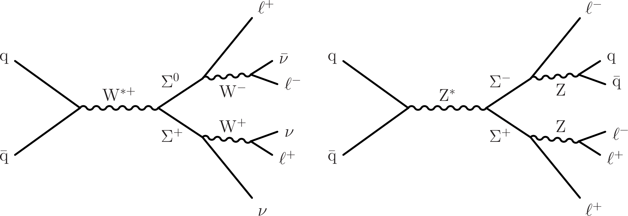
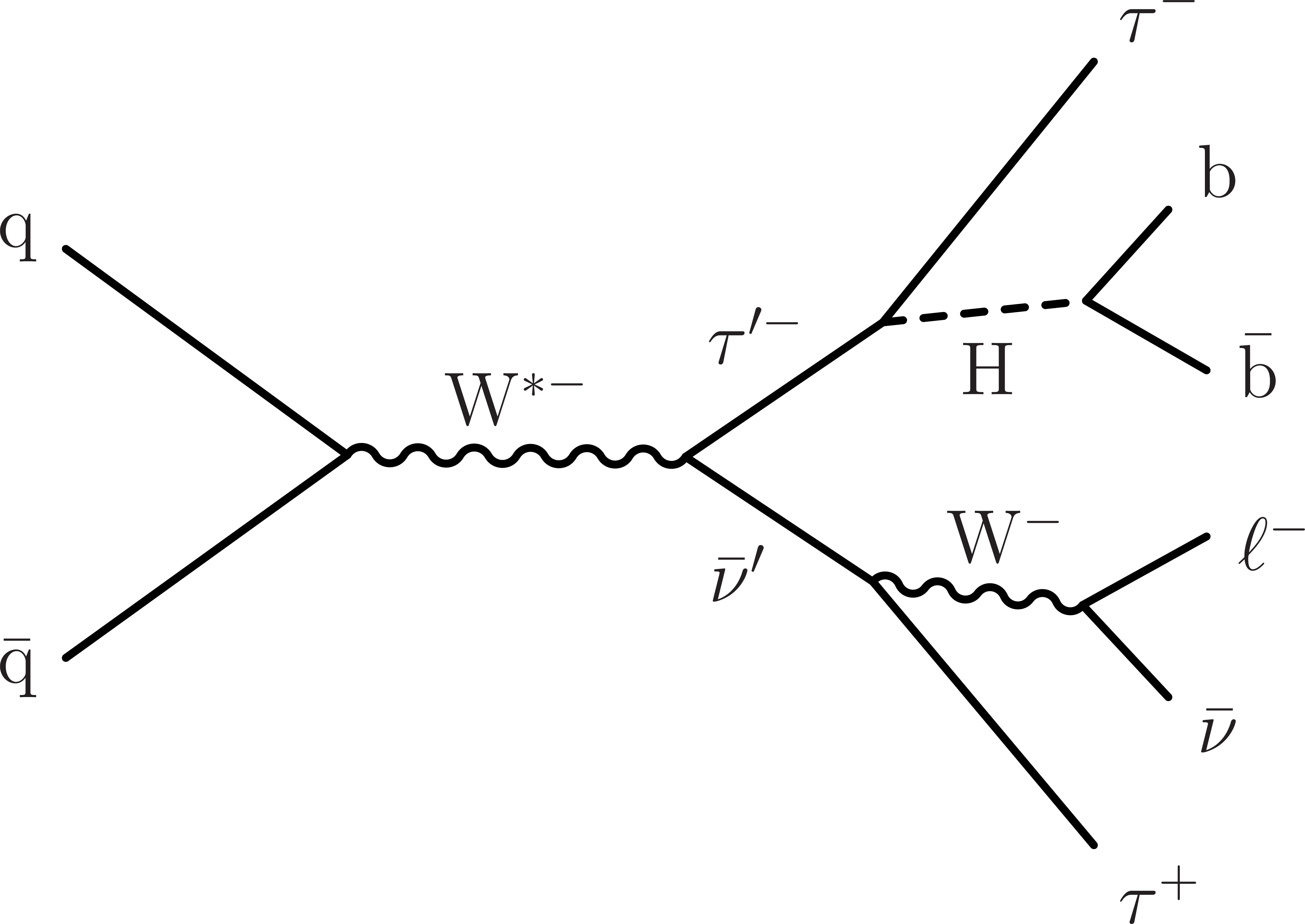
png pdf	Figure 1: Example processes illustrating production and decay of type-III seesaw heavy fermion pairs at the LHC that result in multilepton final states.
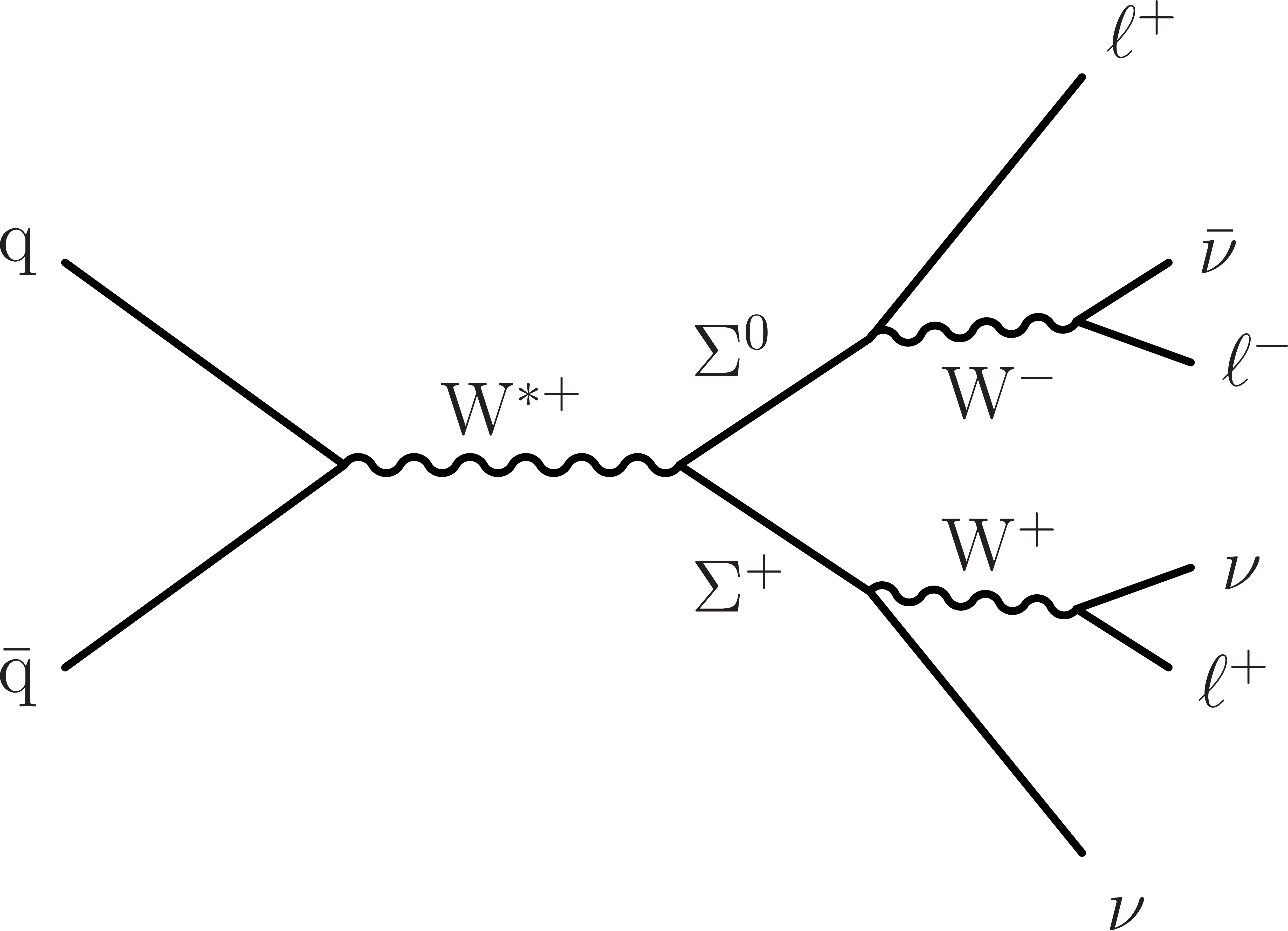
png pdf	Figure 1-a: Example processes illustrating production and decay of type-III seesaw heavy fermion pairs at the LHC that result in multilepton final states.
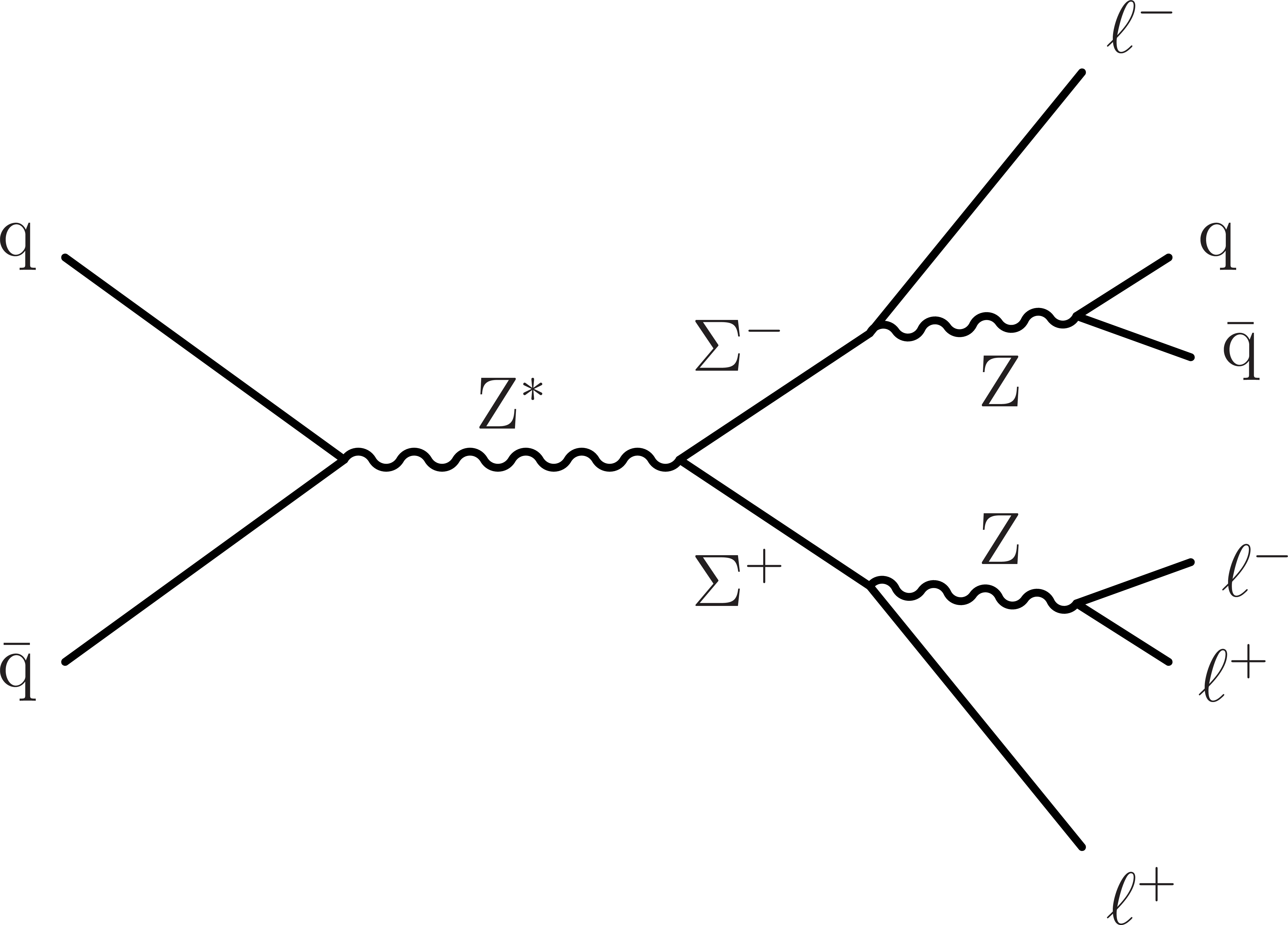
png pdf	Figure 1-b: Example processes illustrating production and decay of type-III seesaw heavy fermion pairs at the LHC that result in multilepton final states.
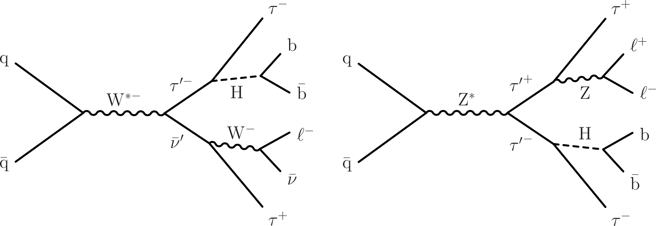
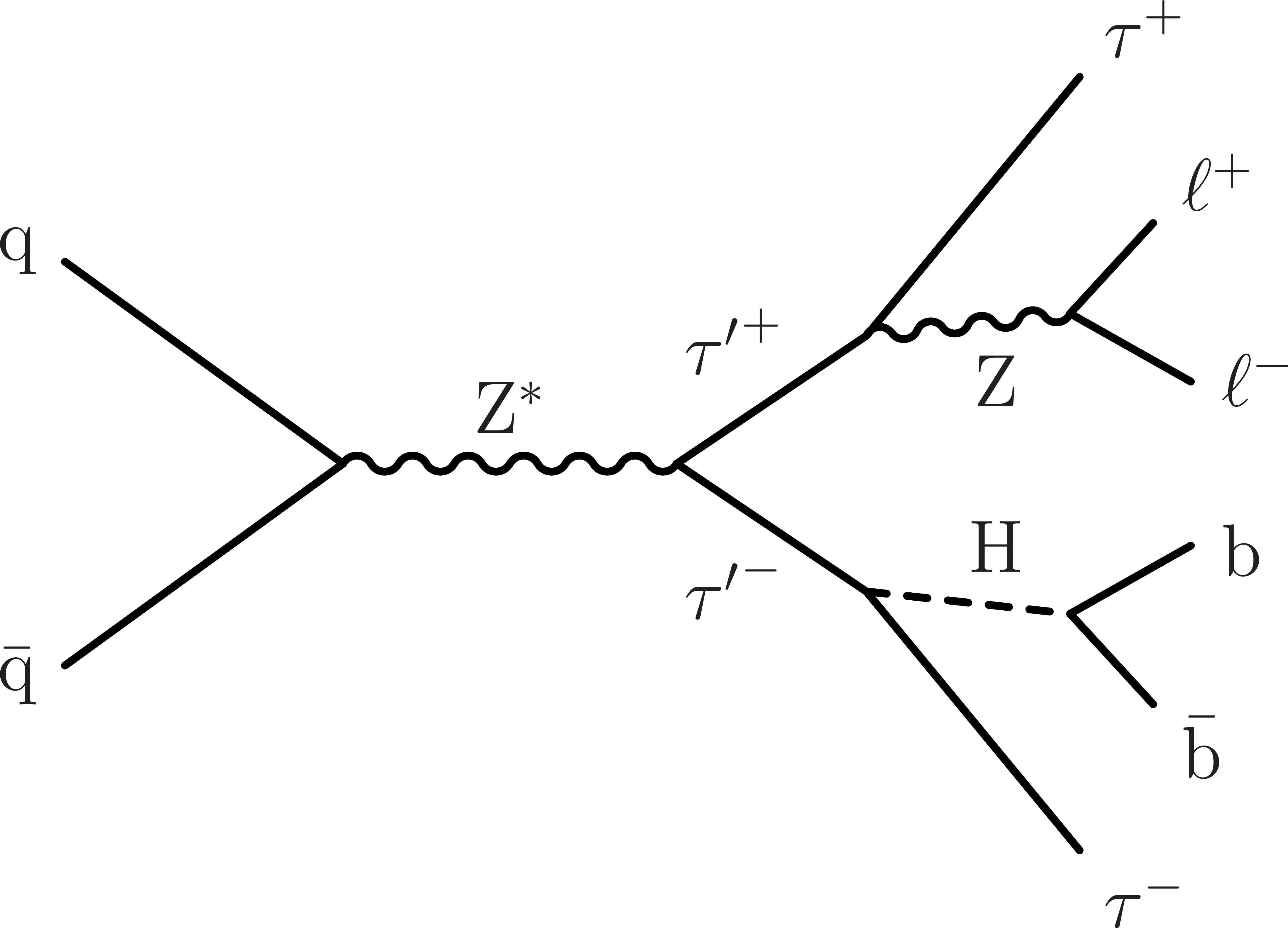
png pdf	Figure 2: Example processes illustrating production and decay of doublet vector-like $\tau$ lepton pairs at the LHC that result in multilepton final states. The right diagram also illustrates the singlet scenario.
png pdf	Figure 2-a: Example processes illustrating production and decay of doublet vector-like $\tau$ lepton pairs at the LHC that result in multilepton final states. The right diagram also illustrates the singlet scenario.
png pdf	Figure 2-b: Example processes illustrating production and decay of doublet vector-like $\tau$ lepton pairs at the LHC that result in multilepton final states. The right diagram also illustrates the singlet scenario.
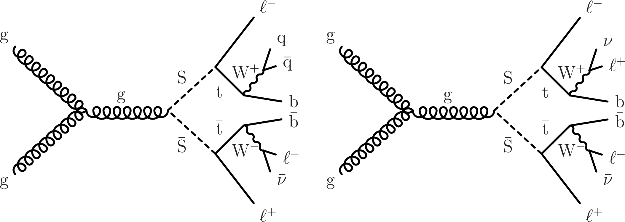
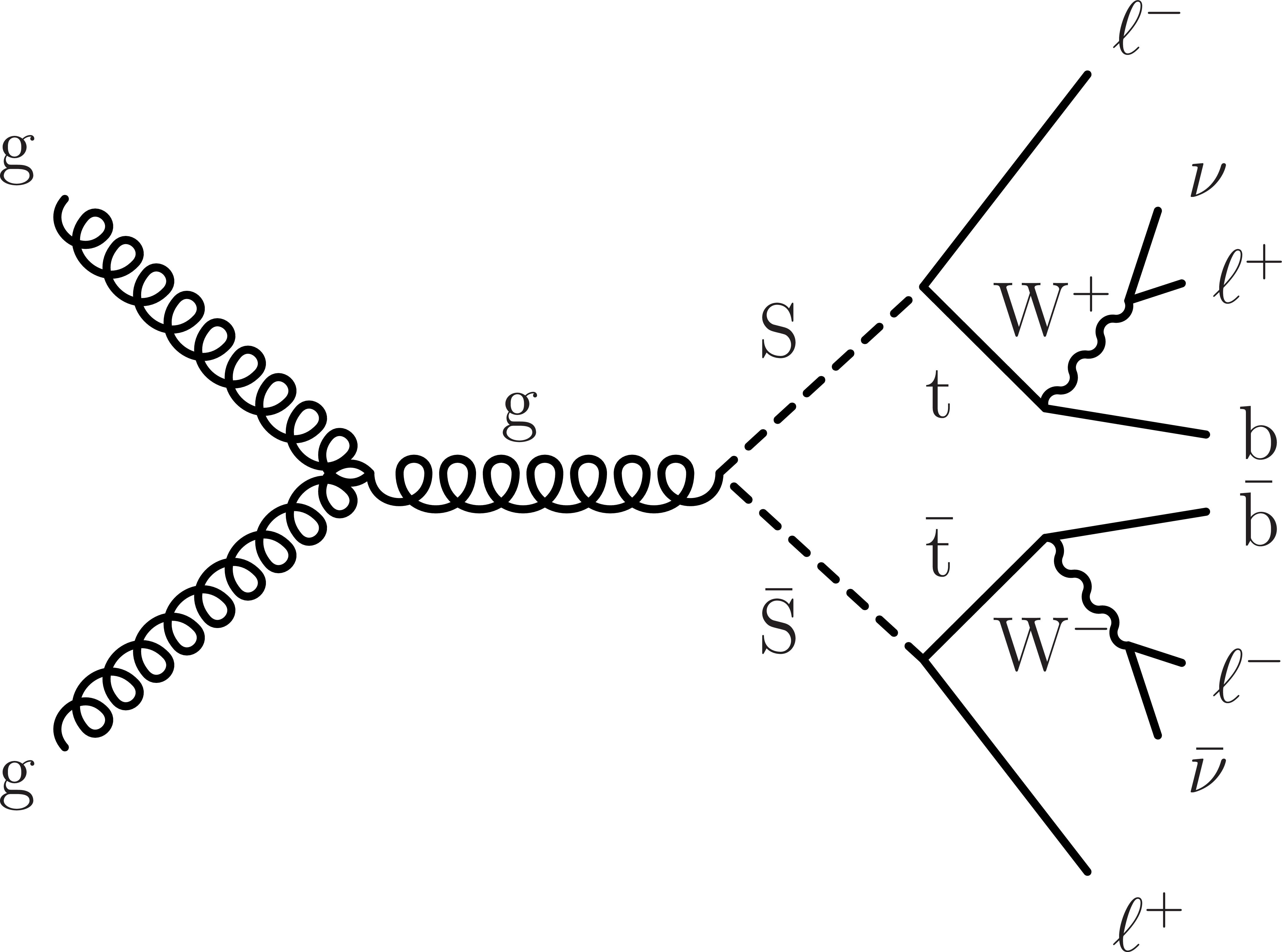
png pdf	Figure 3: Example processes illustrating the production and decay of scalar leptoquark pairs in pp collisions at the LHC that result in multilepton final states.
png pdf	Figure 3-a: Example processes illustrating the production and decay of scalar leptoquark pairs in pp collisions at the LHC that result in multilepton final states.
png pdf	Figure 3-b: Example processes illustrating the production and decay of scalar leptoquark pairs in pp collisions at the LHC that result in multilepton final states.
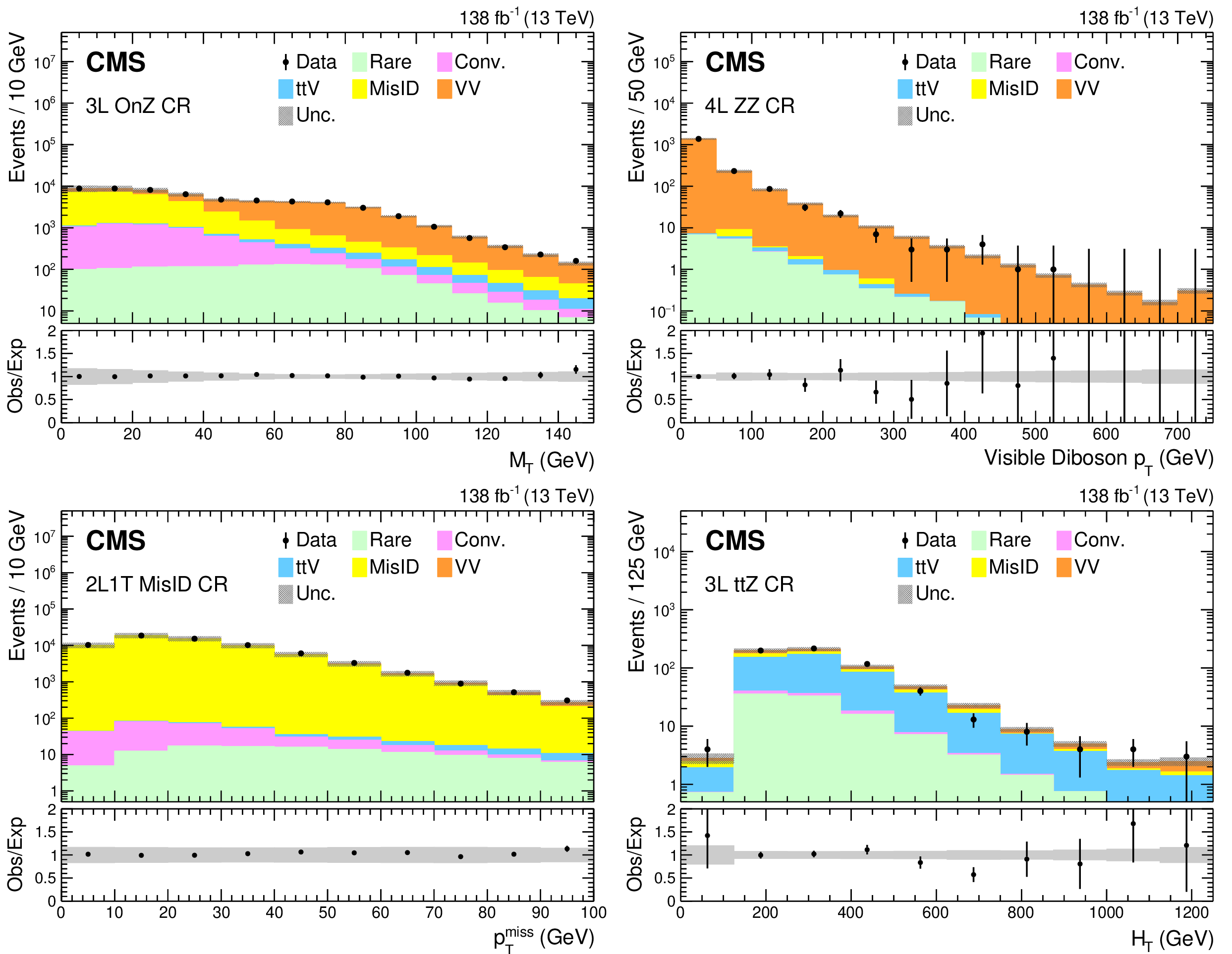
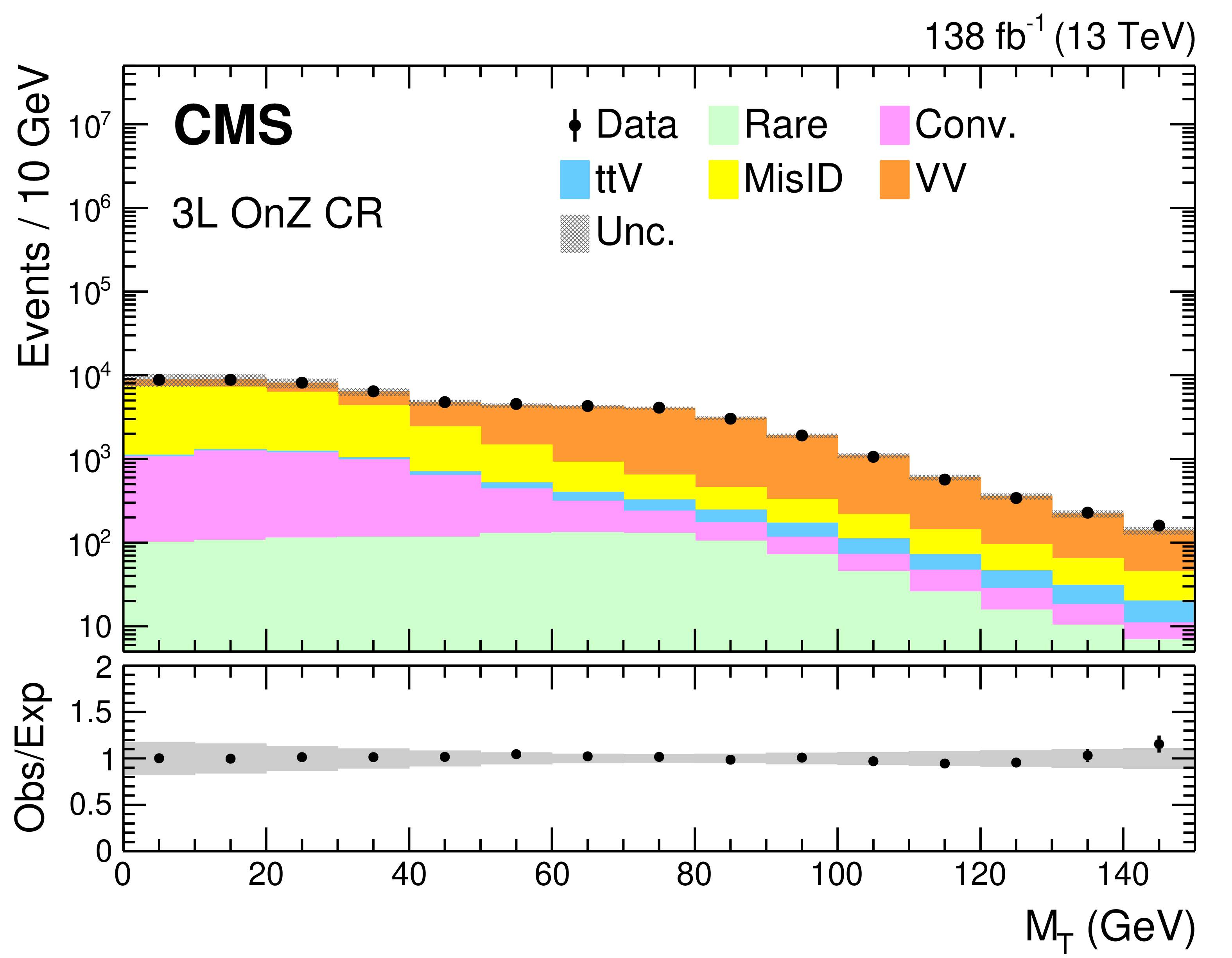
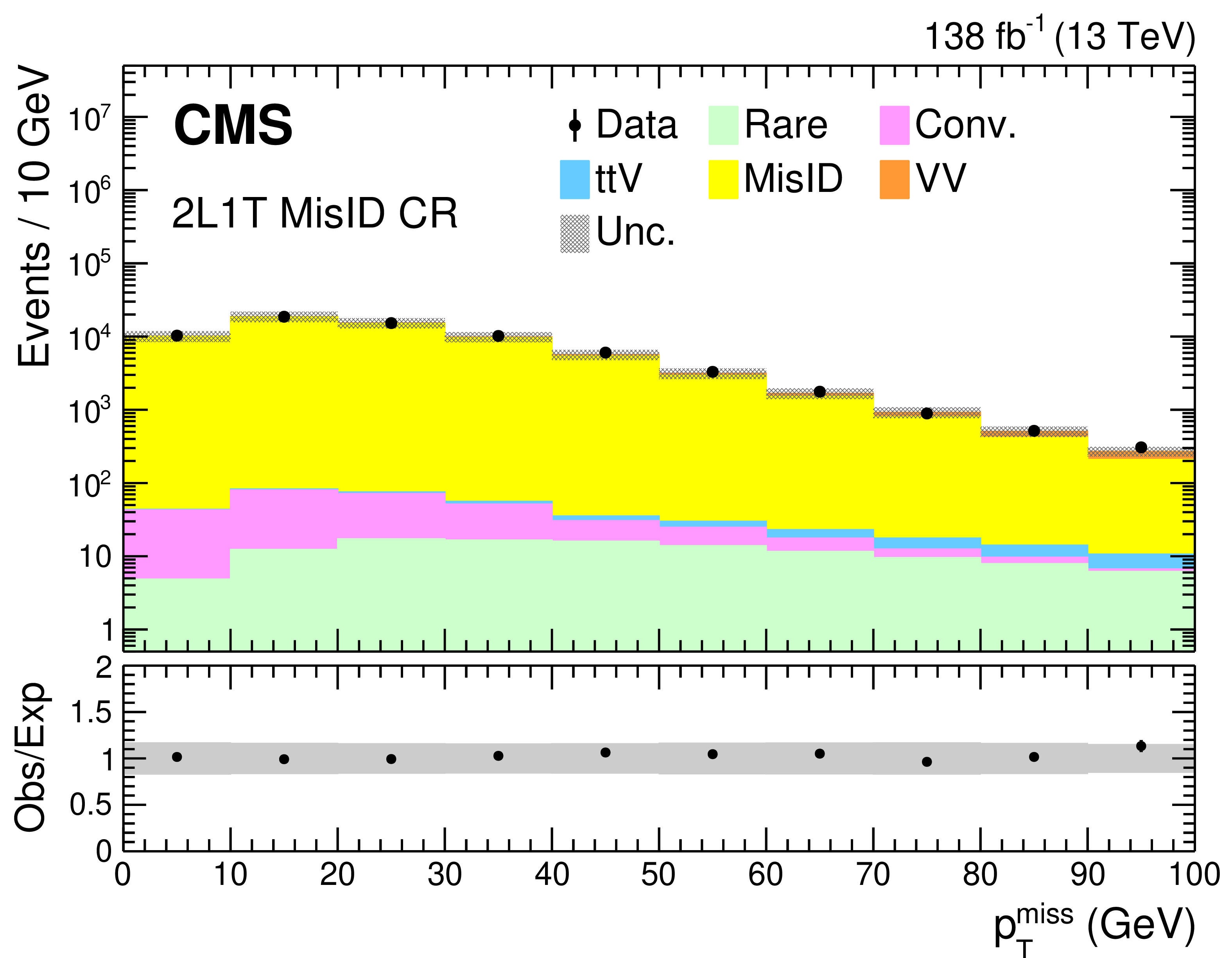
png pdf	Figure 4: The distributions of ${M_{\mathrm {T}}}$ in 3L OnZ CR (upper left), visible diboson ${p_{\mathrm {T}}}$ in 4L ZZ CR (upper right), ${{p_{\mathrm {T}}} ^\text {miss}}$ in 2L1T MisID CR (lower left), and $ {H_{\mathrm {T}}} $ in 3L $ {{\mathrm{t} {}\mathrm{\bar{t}}} }$Z CR (lower right) events. The rightmost bin contains the overflow events in each distribution. The lower panel shows the ratio of observed events to the total expected background prediction. The gray band on the ratio represents the sum of statistical and systematic uncertainties in the SM background prediction.
png pdf	Figure 4-a: The distributions of ${M_{\mathrm {T}}}$ in 3L OnZ CR (upper left), visible diboson ${p_{\mathrm {T}}}$ in 4L ZZ CR (upper right), ${{p_{\mathrm {T}}} ^\text {miss}}$ in 2L1T MisID CR (lower left), and $ {H_{\mathrm {T}}} $ in 3L $ {{\mathrm{t} {}\mathrm{\bar{t}}} }$Z CR (lower right) events. The rightmost bin contains the overflow events in each distribution. The lower panel shows the ratio of observed events to the total expected background prediction. The gray band on the ratio represents the sum of statistical and systematic uncertainties in the SM background prediction.
png pdf	Figure 4-b: The distributions of ${M_{\mathrm {T}}}$ in 3L OnZ CR (upper left), visible diboson ${p_{\mathrm {T}}}$ in 4L ZZ CR (upper right), ${{p_{\mathrm {T}}} ^\text {miss}}$ in 2L1T MisID CR (lower left), and $ {H_{\mathrm {T}}} $ in 3L $ {{\mathrm{t} {}\mathrm{\bar{t}}} }$Z CR (lower right) events. The rightmost bin contains the overflow events in each distribution. The lower panel shows the ratio of observed events to the total expected background prediction. The gray band on the ratio represents the sum of statistical and systematic uncertainties in the SM background prediction.
png pdf	Figure 4-c: The distributions of ${M_{\mathrm {T}}}$ in 3L OnZ CR (upper left), visible diboson ${p_{\mathrm {T}}}$ in 4L ZZ CR (upper right), ${{p_{\mathrm {T}}} ^\text {miss}}$ in 2L1T MisID CR (lower left), and $ {H_{\mathrm {T}}} $ in 3L $ {{\mathrm{t} {}\mathrm{\bar{t}}} }$Z CR (lower right) events. The rightmost bin contains the overflow events in each distribution. The lower panel shows the ratio of observed events to the total expected background prediction. The gray band on the ratio represents the sum of statistical and systematic uncertainties in the SM background prediction.
png pdf	Figure 4-d: The distributions of ${M_{\mathrm {T}}}$ in 3L OnZ CR (upper left), visible diboson ${p_{\mathrm {T}}}$ in 4L ZZ CR (upper right), ${{p_{\mathrm {T}}} ^\text {miss}}$ in 2L1T MisID CR (lower left), and $ {H_{\mathrm {T}}} $ in 3L $ {{\mathrm{t} {}\mathrm{\bar{t}}} }$Z CR (lower right) events. The rightmost bin contains the overflow events in each distribution. The lower panel shows the ratio of observed events to the total expected background prediction. The gray band on the ratio represents the sum of statistical and systematic uncertainties in the SM background prediction.
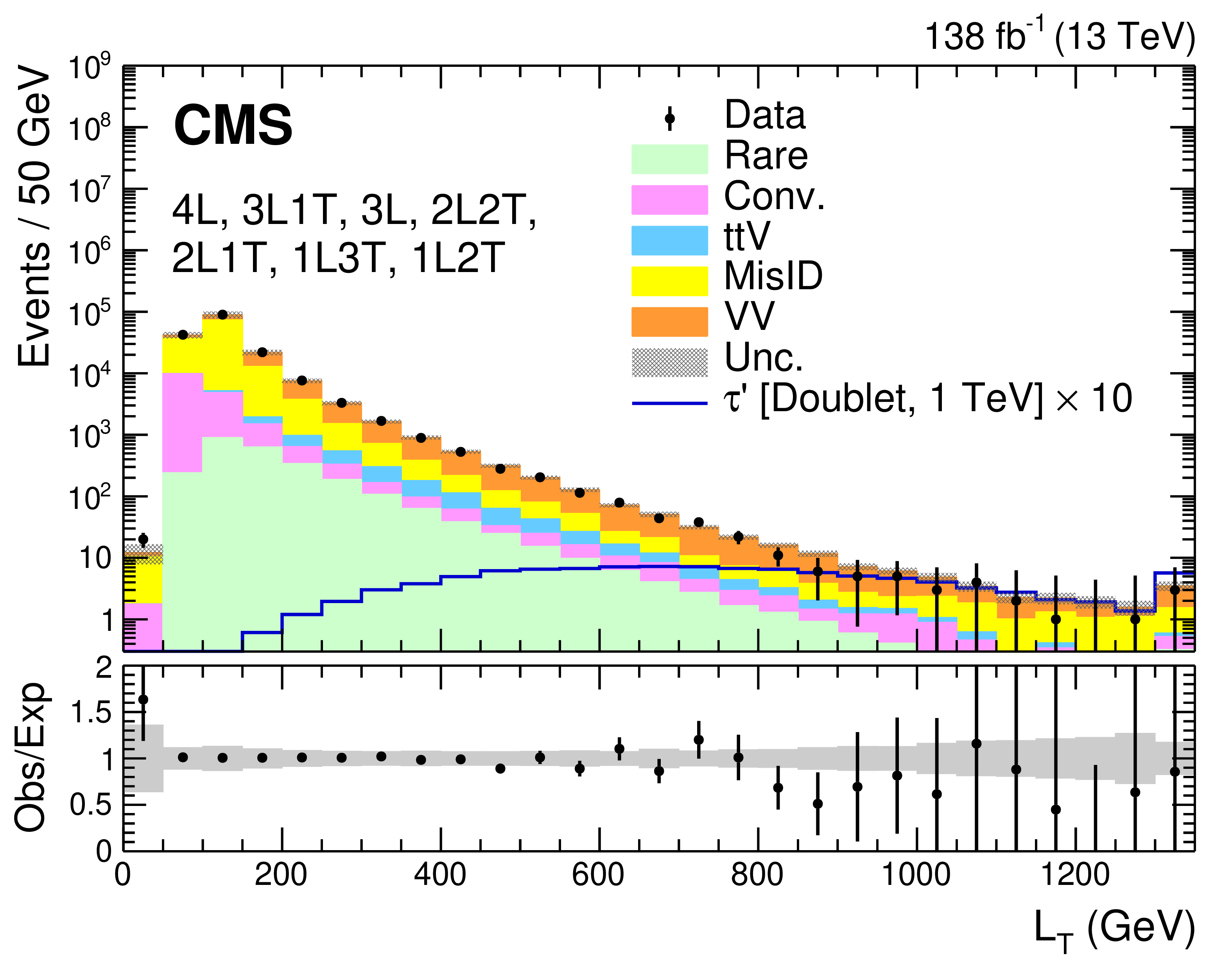
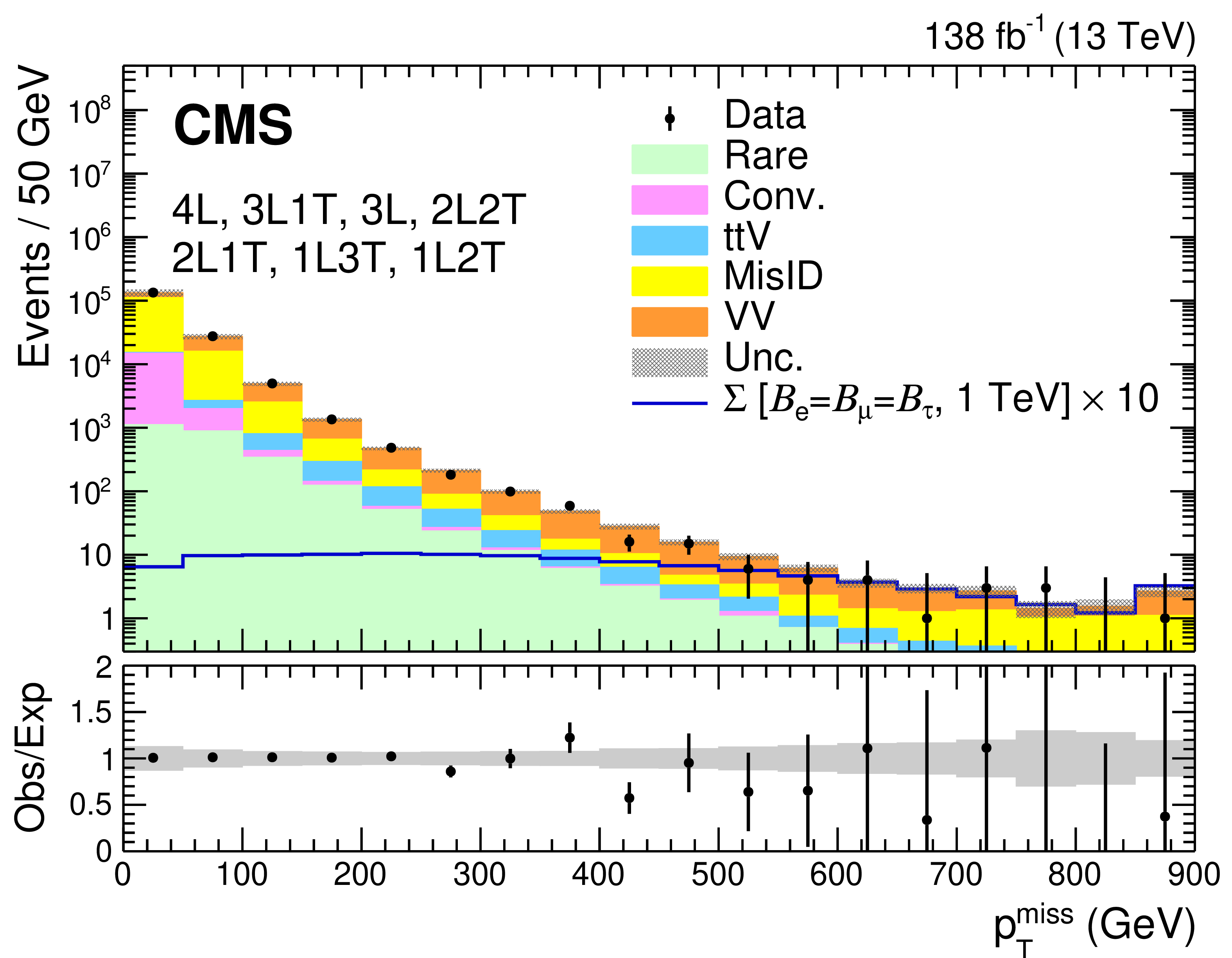
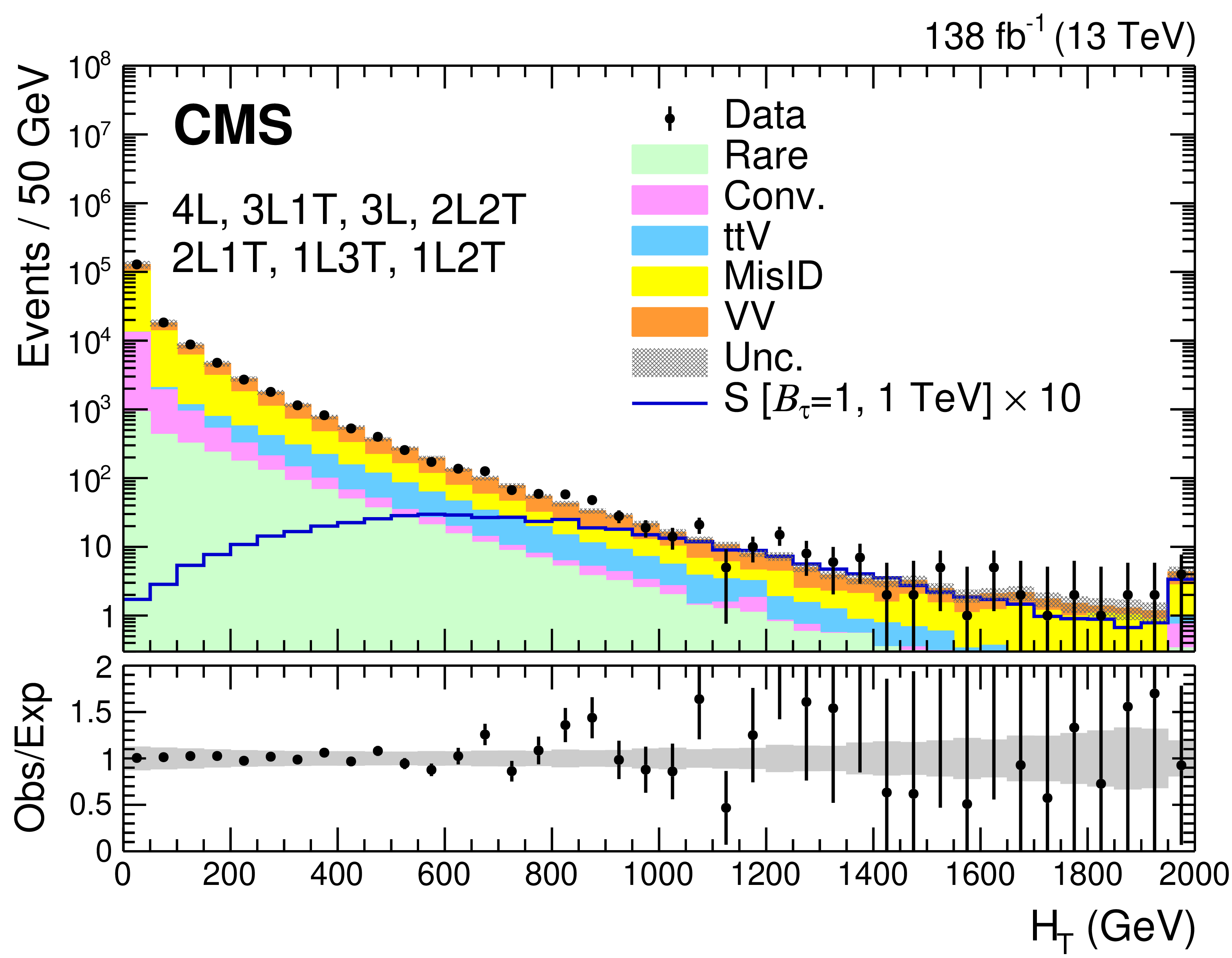
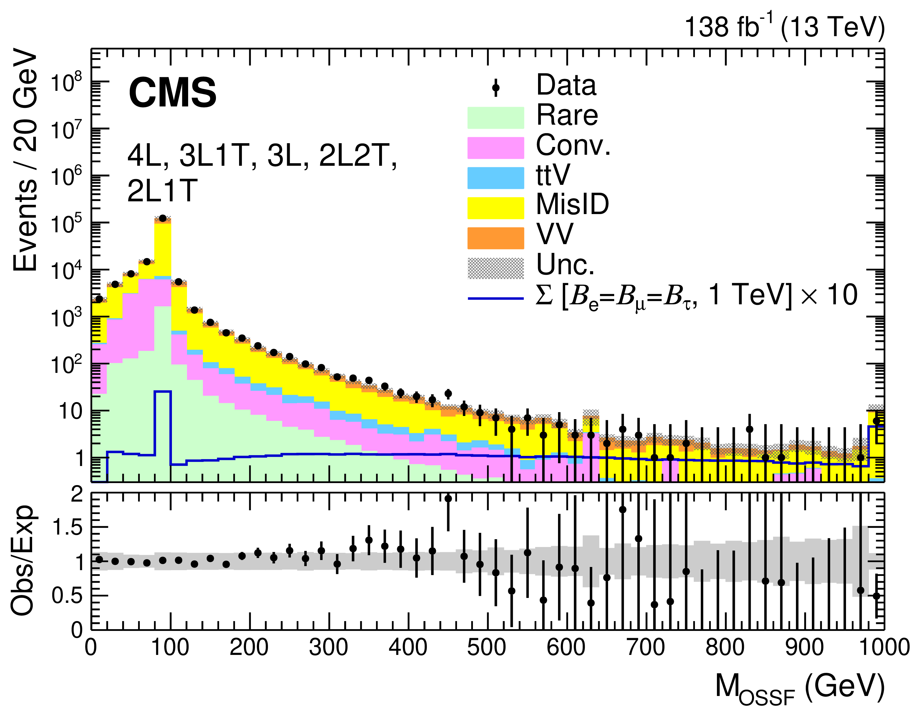
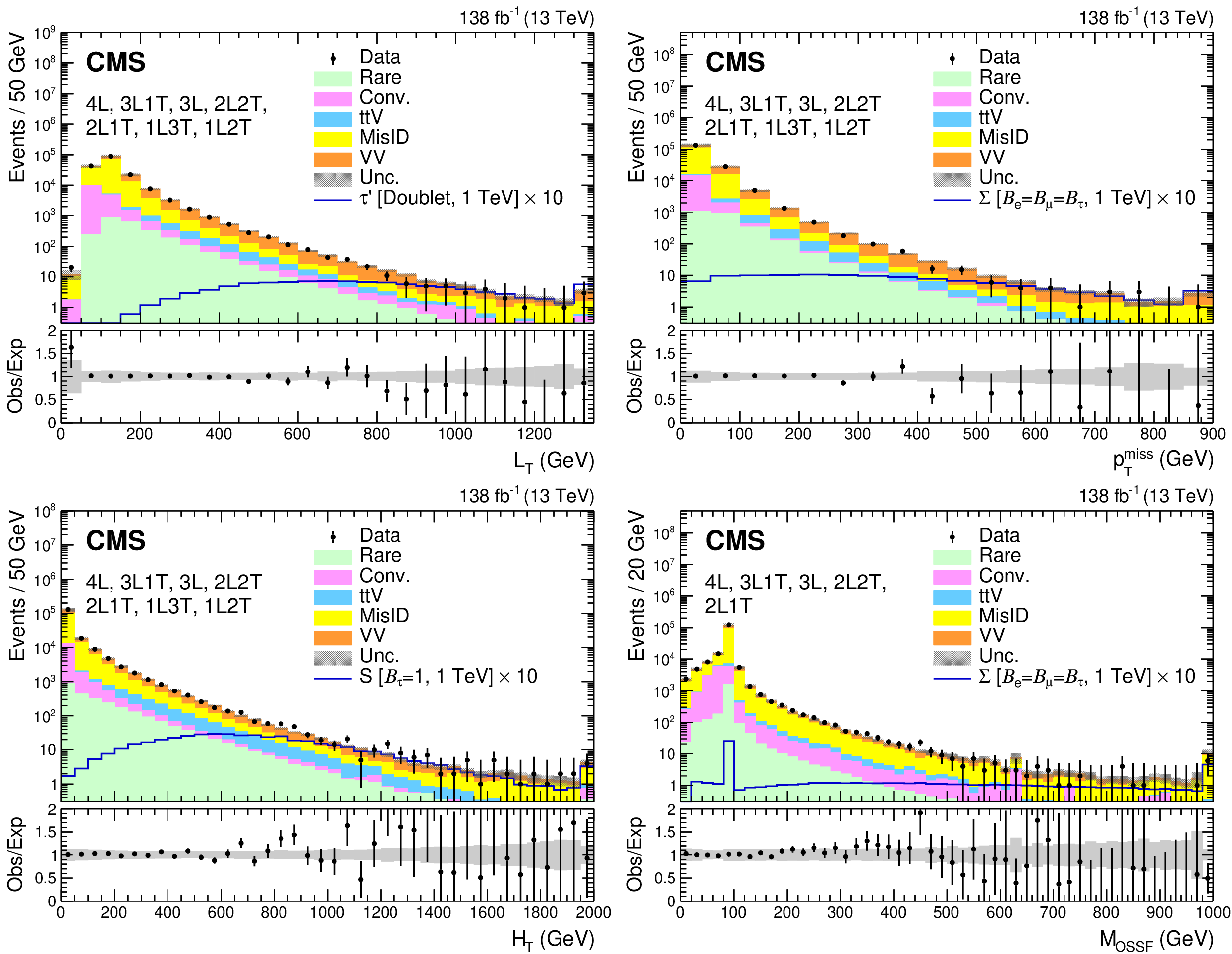
png pdf	Figure 5: The distributions of ${L_{\mathrm {T}}}$ (upper left), ${{p_{\mathrm {T}}} ^\text {miss}}$ (upper right), and $ {H_{\mathrm {T}}} $ (lower left) in all seven multilepton channels, and ${M_{\text {OSSF}}}$ (lower right) in channels with at least one light lepton pair (4L, 3L1T, 3L, 2L2T, and 2L1T). The rightmost bin contains the overflow events in each distribution. The lower panel shows the ratio of observed events to the total expected background prediction. The gray band on the ratio represents the sum of statistical and systematic uncertainties in the SM background prediction. As illustrative examples, a signal hypothesis for the production of the vector-like $\tau$ lepton in the doublet scenario of $m_{{\tau ^{\prime}}} = $ 1 TeV and a scalar leptoquark coupled to a top quark and a $\tau$ lepton of $m_{\mathrm{S}} = $ 1 TeV are overlaid in the ${L_{\mathrm {T}}}$ and $ {H_{\mathrm {T}}} $ distributions respectively. Similarly, a signal hypothesis for the production of the type-III seesaw heavy fermions in the flavor-democratic scenario of $m_{\Sigma} = $ 1 TeV is overlaid for the ${{p_{\mathrm {T}}} ^\text {miss}}$ and ${M_{\text {OSSF}}}$ distributions.
png pdf	Figure 5-a: The distributions of ${L_{\mathrm {T}}}$ (upper left), ${{p_{\mathrm {T}}} ^\text {miss}}$ (upper right), and $ {H_{\mathrm {T}}} $ (lower left) in all seven multilepton channels, and ${M_{\text {OSSF}}}$ (lower right) in channels with at least one light lepton pair (4L, 3L1T, 3L, 2L2T, and 2L1T). The rightmost bin contains the overflow events in each distribution. The lower panel shows the ratio of observed events to the total expected background prediction. The gray band on the ratio represents the sum of statistical and systematic uncertainties in the SM background prediction. As illustrative examples, a signal hypothesis for the production of the vector-like $\tau$ lepton in the doublet scenario of $m_{{\tau ^{\prime}}} = $ 1 TeV and a scalar leptoquark coupled to a top quark and a $\tau$ lepton of $m_{\mathrm{S}} = $ 1 TeV are overlaid in the ${L_{\mathrm {T}}}$ and $ {H_{\mathrm {T}}} $ distributions respectively. Similarly, a signal hypothesis for the production of the type-III seesaw heavy fermions in the flavor-democratic scenario of $m_{\Sigma} = $ 1 TeV is overlaid for the ${{p_{\mathrm {T}}} ^\text {miss}}$ and ${M_{\text {OSSF}}}$ distributions.
png pdf	Figure 5-b: The distributions of ${L_{\mathrm {T}}}$ (upper left), ${{p_{\mathrm {T}}} ^\text {miss}}$ (upper right), and $ {H_{\mathrm {T}}} $ (lower left) in all seven multilepton channels, and ${M_{\text {OSSF}}}$ (lower right) in channels with at least one light lepton pair (4L, 3L1T, 3L, 2L2T, and 2L1T). The rightmost bin contains the overflow events in each distribution. The lower panel shows the ratio of observed events to the total expected background prediction. The gray band on the ratio represents the sum of statistical and systematic uncertainties in the SM background prediction. As illustrative examples, a signal hypothesis for the production of the vector-like $\tau$ lepton in the doublet scenario of $m_{{\tau ^{\prime}}} = $ 1 TeV and a scalar leptoquark coupled to a top quark and a $\tau$ lepton of $m_{\mathrm{S}} = $ 1 TeV are overlaid in the ${L_{\mathrm {T}}}$ and $ {H_{\mathrm {T}}} $ distributions respectively. Similarly, a signal hypothesis for the production of the type-III seesaw heavy fermions in the flavor-democratic scenario of $m_{\Sigma} = $ 1 TeV is overlaid for the ${{p_{\mathrm {T}}} ^\text {miss}}$ and ${M_{\text {OSSF}}}$ distributions.
png pdf	Figure 5-c: The distributions of ${L_{\mathrm {T}}}$ (upper left), ${{p_{\mathrm {T}}} ^\text {miss}}$ (upper right), and $ {H_{\mathrm {T}}} $ (lower left) in all seven multilepton channels, and ${M_{\text {OSSF}}}$ (lower right) in channels with at least one light lepton pair (4L, 3L1T, 3L, 2L2T, and 2L1T). The rightmost bin contains the overflow events in each distribution. The lower panel shows the ratio of observed events to the total expected background prediction. The gray band on the ratio represents the sum of statistical and systematic uncertainties in the SM background prediction. As illustrative examples, a signal hypothesis for the production of the vector-like $\tau$ lepton in the doublet scenario of $m_{{\tau ^{\prime}}} = $ 1 TeV and a scalar leptoquark coupled to a top quark and a $\tau$ lepton of $m_{\mathrm{S}} = $ 1 TeV are overlaid in the ${L_{\mathrm {T}}}$ and $ {H_{\mathrm {T}}} $ distributions respectively. Similarly, a signal hypothesis for the production of the type-III seesaw heavy fermions in the flavor-democratic scenario of $m_{\Sigma} = $ 1 TeV is overlaid for the ${{p_{\mathrm {T}}} ^\text {miss}}$ and ${M_{\text {OSSF}}}$ distributions.
png pdf	Figure 5-d: The distributions of ${L_{\mathrm {T}}}$ (upper left), ${{p_{\mathrm {T}}} ^\text {miss}}$ (upper right), and $ {H_{\mathrm {T}}} $ (lower left) in all seven multilepton channels, and ${M_{\text {OSSF}}}$ (lower right) in channels with at least one light lepton pair (4L, 3L1T, 3L, 2L2T, and 2L1T). The rightmost bin contains the overflow events in each distribution. The lower panel shows the ratio of observed events to the total expected background prediction. The gray band on the ratio represents the sum of statistical and systematic uncertainties in the SM background prediction. As illustrative examples, a signal hypothesis for the production of the vector-like $\tau$ lepton in the doublet scenario of $m_{{\tau ^{\prime}}} = $ 1 TeV and a scalar leptoquark coupled to a top quark and a $\tau$ lepton of $m_{\mathrm{S}} = $ 1 TeV are overlaid in the ${L_{\mathrm {T}}}$ and $ {H_{\mathrm {T}}} $ distributions respectively. Similarly, a signal hypothesis for the production of the type-III seesaw heavy fermions in the flavor-democratic scenario of $m_{\Sigma} = $ 1 TeV is overlaid for the ${{p_{\mathrm {T}}} ^\text {miss}}$ and ${M_{\text {OSSF}}}$ distributions.
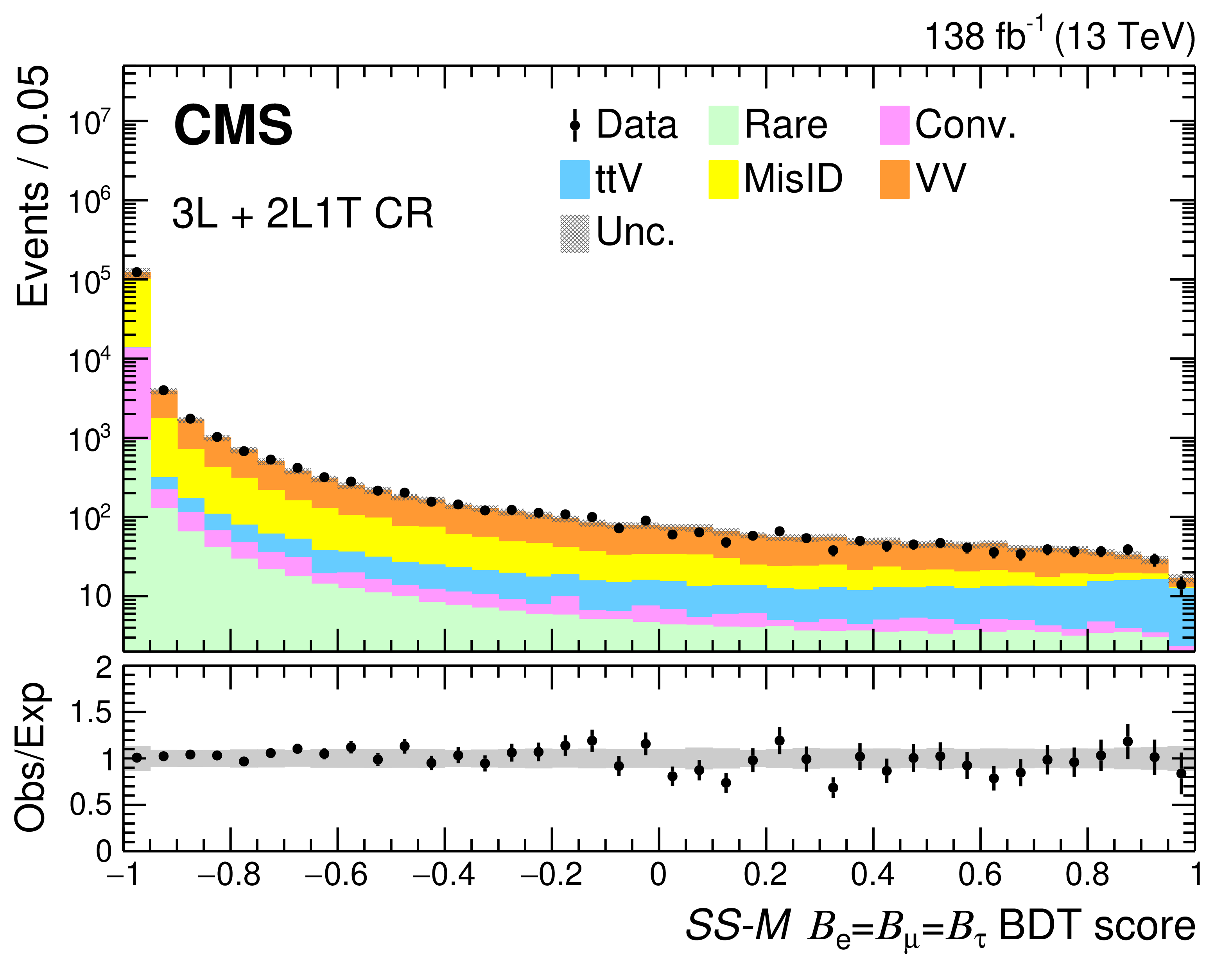
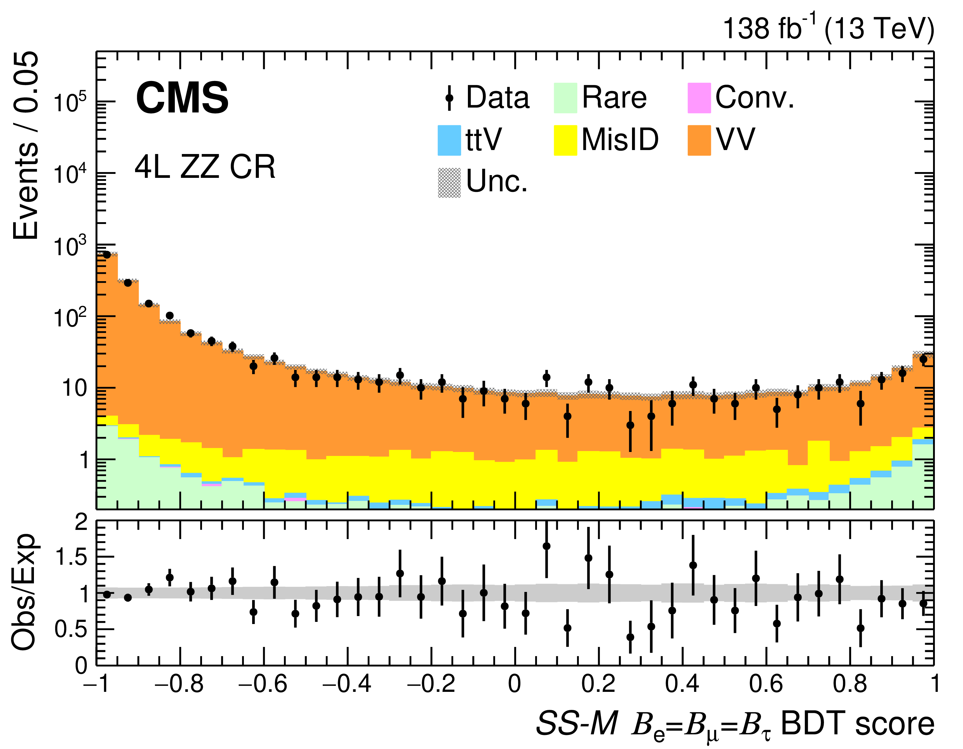
png pdf	Figure 6: Distributions of BDT score from the SS-M $\mathcal {B}_{\mathrm{e}}=\mathcal {B}_{\mu}=\mathcal {B}_{\tau}$ BDT are shown for the 3L+2L1T CR (left), and the 4L ZZ CR (right). The 3L+2L1T CR consists of the 3L OnZ, 3L Z$\gamma$, and 2L1T MisID CRs. The lower panel shows the ratio of observed events to the total expected background prediction. The gray band on the ratio represents the sum of statistical and systematic uncertainties in the SM background prediction.
png pdf	Figure 6-a: Distributions of BDT score from the SS-M $\mathcal {B}_{\mathrm{e}}=\mathcal {B}_{\mu}=\mathcal {B}_{\tau}$ BDT are shown for the 3L+2L1T CR (left), and the 4L ZZ CR (right). The 3L+2L1T CR consists of the 3L OnZ, 3L Z$\gamma$, and 2L1T MisID CRs. The lower panel shows the ratio of observed events to the total expected background prediction. The gray band on the ratio represents the sum of statistical and systematic uncertainties in the SM background prediction.
png pdf	Figure 6-b: Distributions of BDT score from the SS-M $\mathcal {B}_{\mathrm{e}}=\mathcal {B}_{\mu}=\mathcal {B}_{\tau}$ BDT are shown for the 3L+2L1T CR (left), and the 4L ZZ CR (right). The 3L+2L1T CR consists of the 3L OnZ, 3L Z$\gamma$, and 2L1T MisID CRs. The lower panel shows the ratio of observed events to the total expected background prediction. The gray band on the ratio represents the sum of statistical and systematic uncertainties in the SM background prediction.
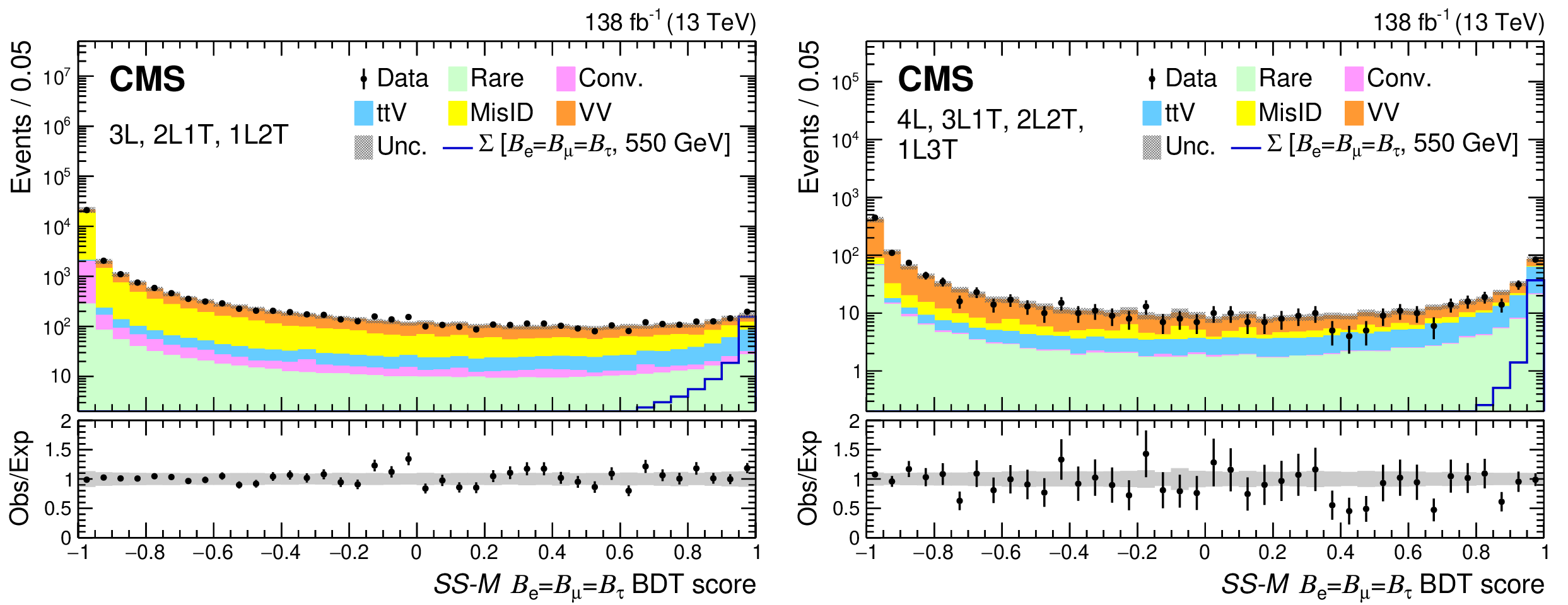
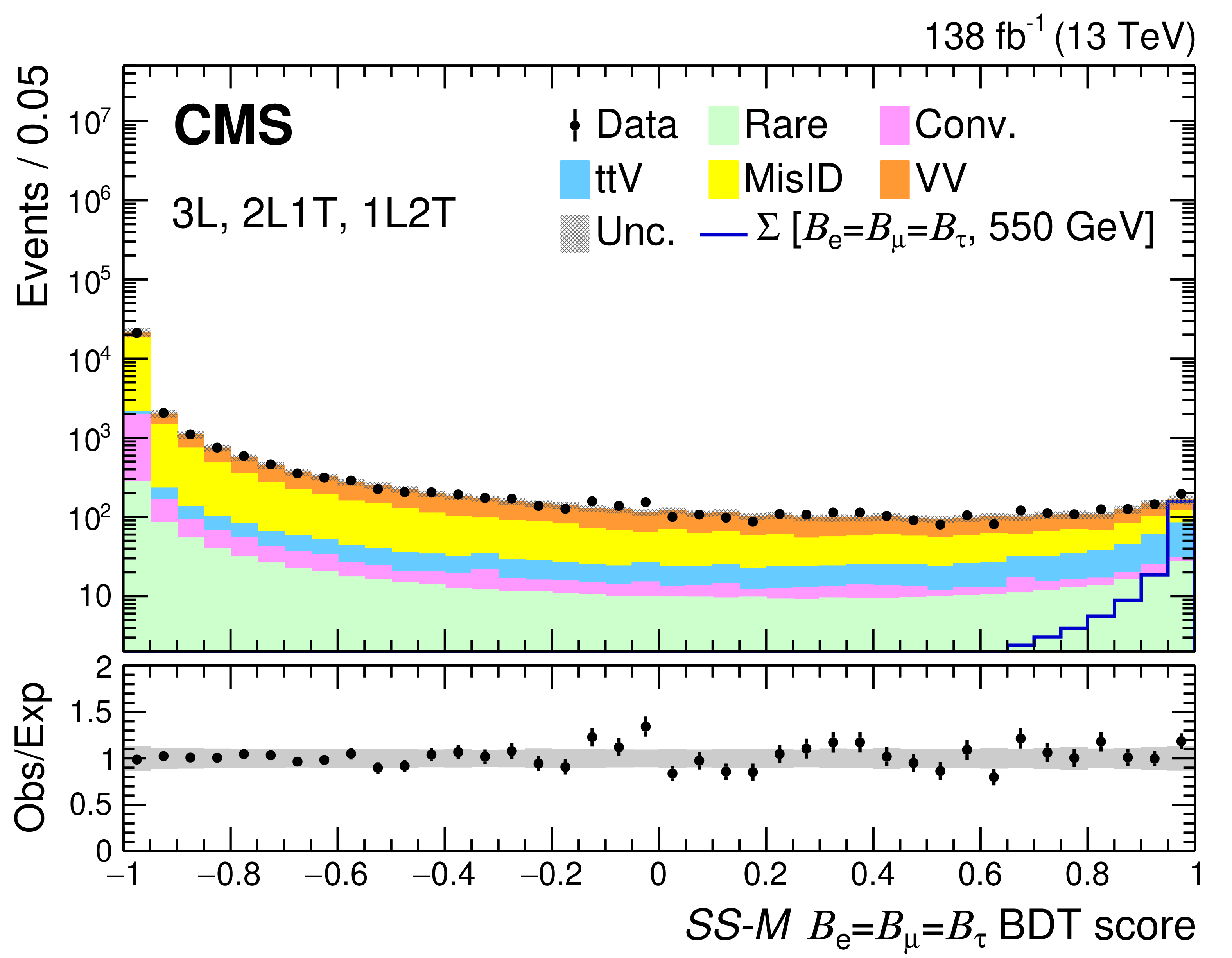
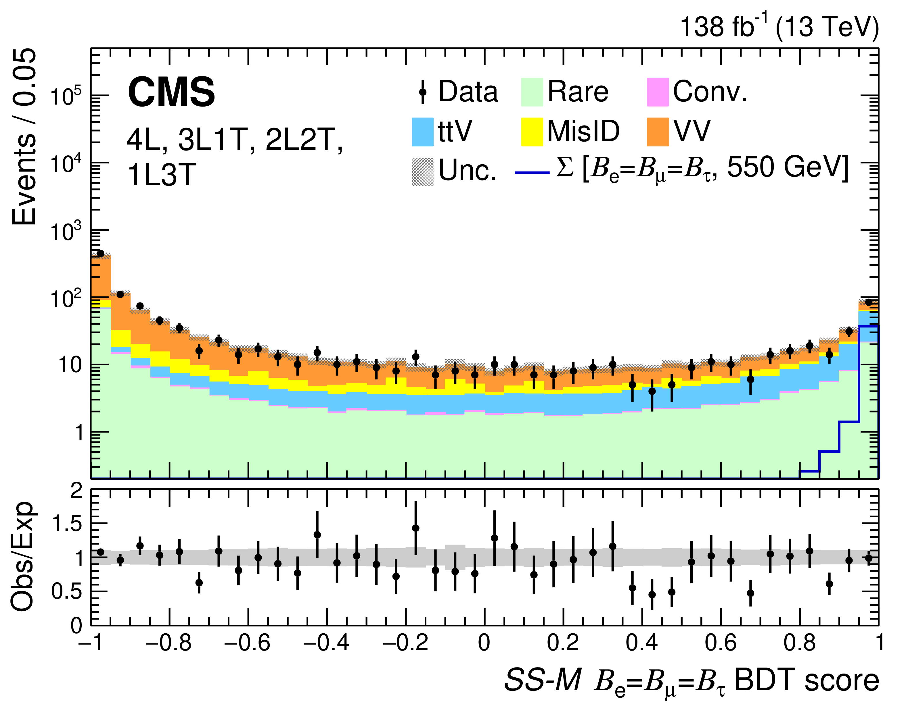
png pdf	Figure 7: Distributions of BDT score from the SS-M $\mathcal {B}_{\mathrm{e}}=\mathcal {B}_{\mu}=\mathcal {B}_{\tau}$ BDT are shown for events lying outside the control regions in the three-lepton (3L, 2L1T, 1L2T) channels (left), and the four-lepton (4L, 3L1T, 2L2T, 1L3T) channels (right). The lower panel shows the ratio of observed events to the total expected background prediction. The gray band on the ratio represents the sum of statistical and systematic uncertainties in the SM background prediction. For illustration, an example signal hypothesis for the production of the type-III seesaw heavy fermions in the flavor-democratic scenario for $m_{\Sigma} = $ 550 GeV is also overlaid.
png pdf	Figure 7-a: Distributions of BDT score from the SS-M $\mathcal {B}_{\mathrm{e}}=\mathcal {B}_{\mu}=\mathcal {B}_{\tau}$ BDT are shown for events lying outside the control regions in the three-lepton (3L, 2L1T, 1L2T) channels (left), and the four-lepton (4L, 3L1T, 2L2T, 1L3T) channels (right). The lower panel shows the ratio of observed events to the total expected background prediction. The gray band on the ratio represents the sum of statistical and systematic uncertainties in the SM background prediction. For illustration, an example signal hypothesis for the production of the type-III seesaw heavy fermions in the flavor-democratic scenario for $m_{\Sigma} = $ 550 GeV is also overlaid.
png pdf	Figure 7-b: Distributions of BDT score from the SS-M $\mathcal {B}_{\mathrm{e}}=\mathcal {B}_{\mu}=\mathcal {B}_{\tau}$ BDT are shown for events lying outside the control regions in the three-lepton (3L, 2L1T, 1L2T) channels (left), and the four-lepton (4L, 3L1T, 2L2T, 1L3T) channels (right). The lower panel shows the ratio of observed events to the total expected background prediction. The gray band on the ratio represents the sum of statistical and systematic uncertainties in the SM background prediction. For illustration, an example signal hypothesis for the production of the type-III seesaw heavy fermions in the flavor-democratic scenario for $m_{\Sigma} = $ 550 GeV is also overlaid.
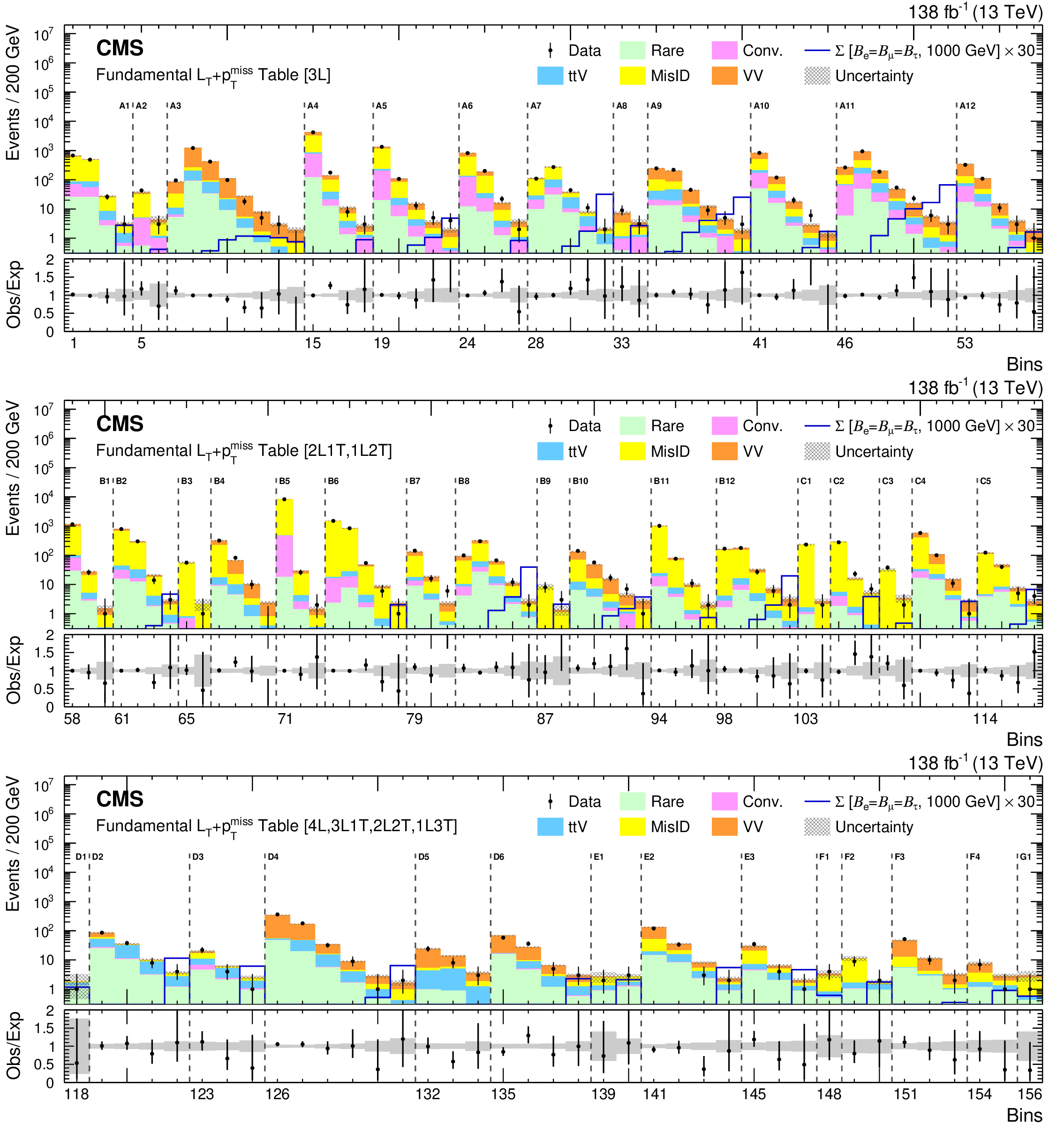
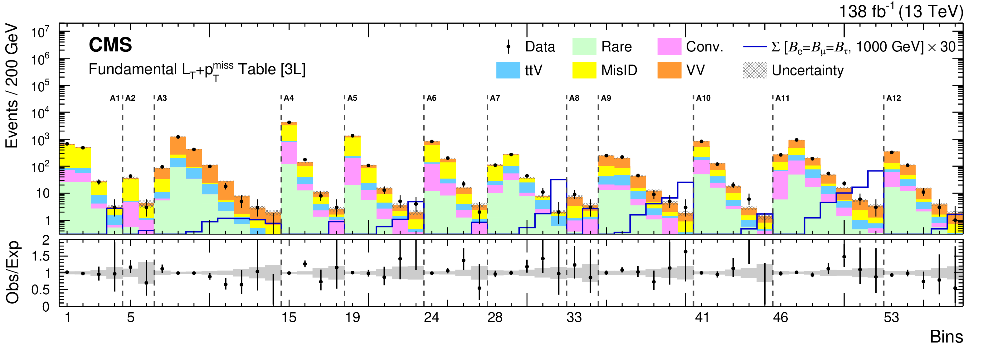
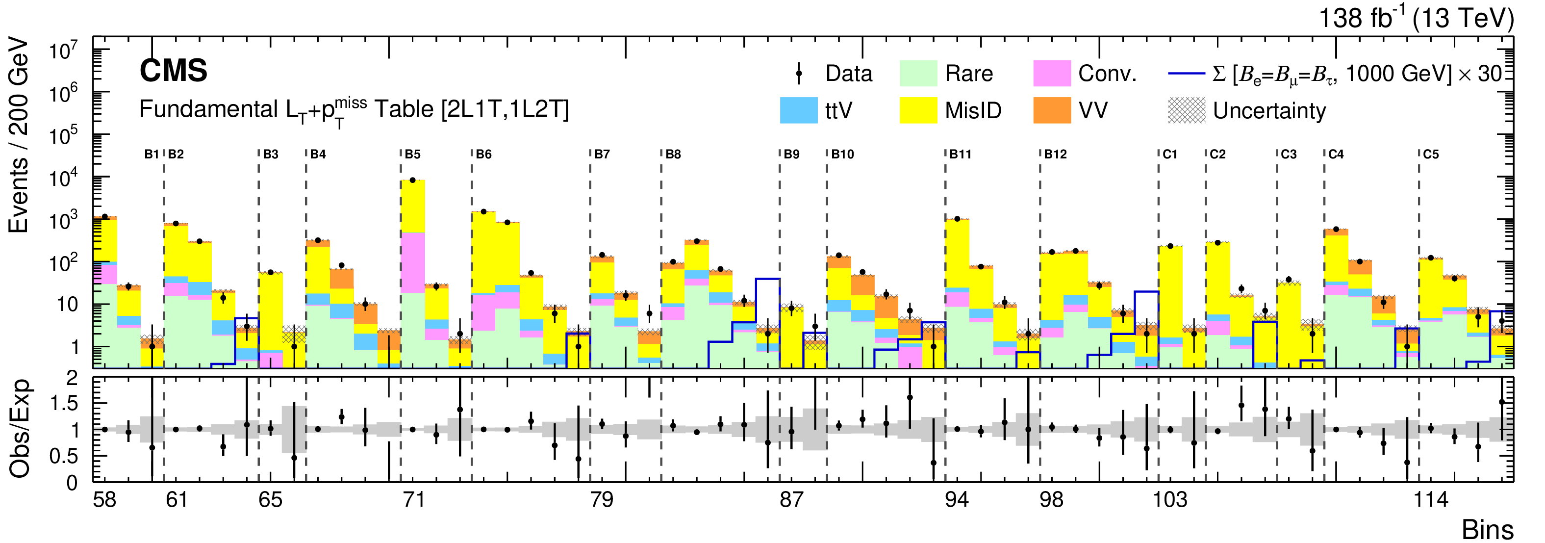
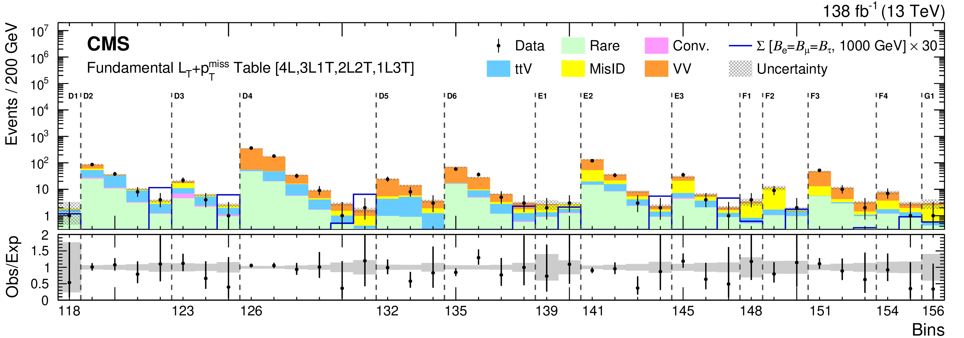
png pdf	Figure 8: The SR distributions of the fundamental $ {L_{\mathrm {T}}} $+${{p_{\mathrm {T}}} ^\text {miss}}$ table for the combined 2016-2018 data set. The detailed description of the bin numbers can be found in Tables 3-6. The lower panel shows the ratio of observed events to the total expected background prediction. The gray band on the ratio represents the sum of statistical and systematic uncertainties in the SM background prediction. The expected SM background distributions and the uncertainties are shown after fitting the data under the background-only hypothesis. For illustration, an example signal hypothesis for the production of the type-III seesaw heavy fermions in the flavor-democratic scenario for $m_{\Sigma} = $ 1 TeV, before the fit, is also overlaid.
png pdf	Figure 8-a: The SR distributions of the fundamental $ {L_{\mathrm {T}}} $+${{p_{\mathrm {T}}} ^\text {miss}}$ table for the combined 2016-2018 data set. The detailed description of the bin numbers can be found in Tables 3-6. The lower panel shows the ratio of observed events to the total expected background prediction. The gray band on the ratio represents the sum of statistical and systematic uncertainties in the SM background prediction. The expected SM background distributions and the uncertainties are shown after fitting the data under the background-only hypothesis. For illustration, an example signal hypothesis for the production of the type-III seesaw heavy fermions in the flavor-democratic scenario for $m_{\Sigma} = $ 1 TeV, before the fit, is also overlaid.
png pdf	Figure 8-b: The SR distributions of the fundamental $ {L_{\mathrm {T}}} $+${{p_{\mathrm {T}}} ^\text {miss}}$ table for the combined 2016-2018 data set. The detailed description of the bin numbers can be found in Tables 3-6. The lower panel shows the ratio of observed events to the total expected background prediction. The gray band on the ratio represents the sum of statistical and systematic uncertainties in the SM background prediction. The expected SM background distributions and the uncertainties are shown after fitting the data under the background-only hypothesis. For illustration, an example signal hypothesis for the production of the type-III seesaw heavy fermions in the flavor-democratic scenario for $m_{\Sigma} = $ 1 TeV, before the fit, is also overlaid.
png pdf	Figure 8-c: The SR distributions of the fundamental $ {L_{\mathrm {T}}} $+${{p_{\mathrm {T}}} ^\text {miss}}$ table for the combined 2016-2018 data set. The detailed description of the bin numbers can be found in Tables 3-6. The lower panel shows the ratio of observed events to the total expected background prediction. The gray band on the ratio represents the sum of statistical and systematic uncertainties in the SM background prediction. The expected SM background distributions and the uncertainties are shown after fitting the data under the background-only hypothesis. For illustration, an example signal hypothesis for the production of the type-III seesaw heavy fermions in the flavor-democratic scenario for $m_{\Sigma} = $ 1 TeV, before the fit, is also overlaid.
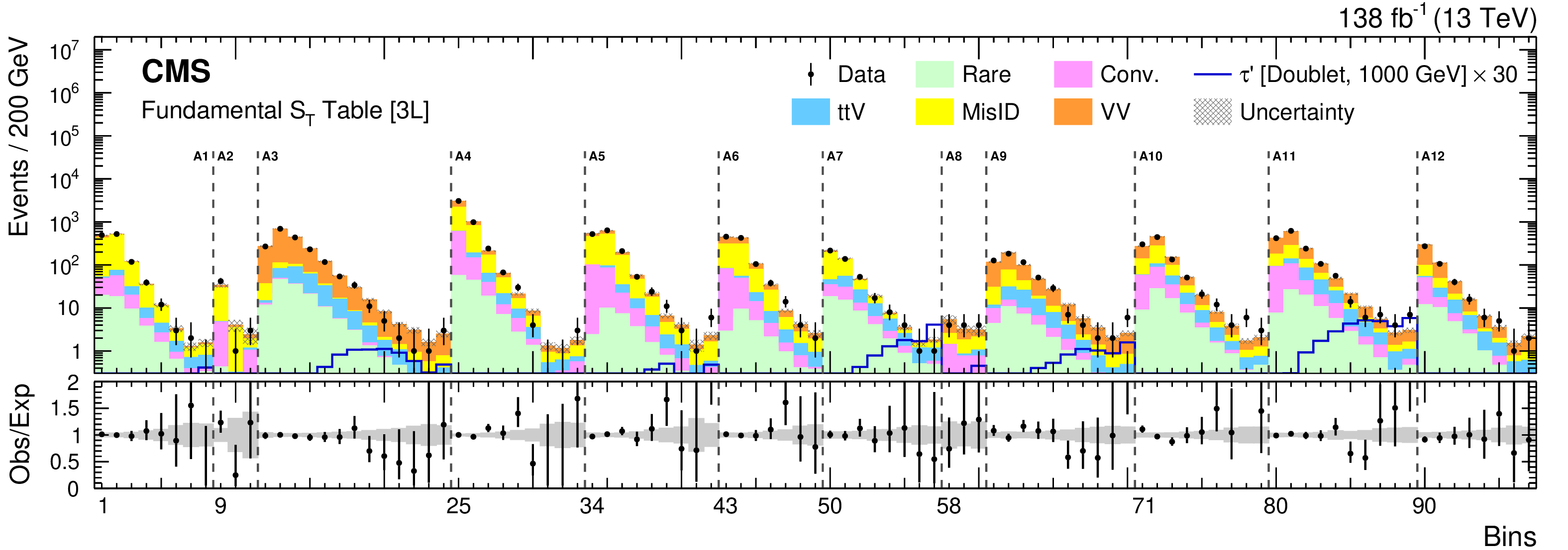
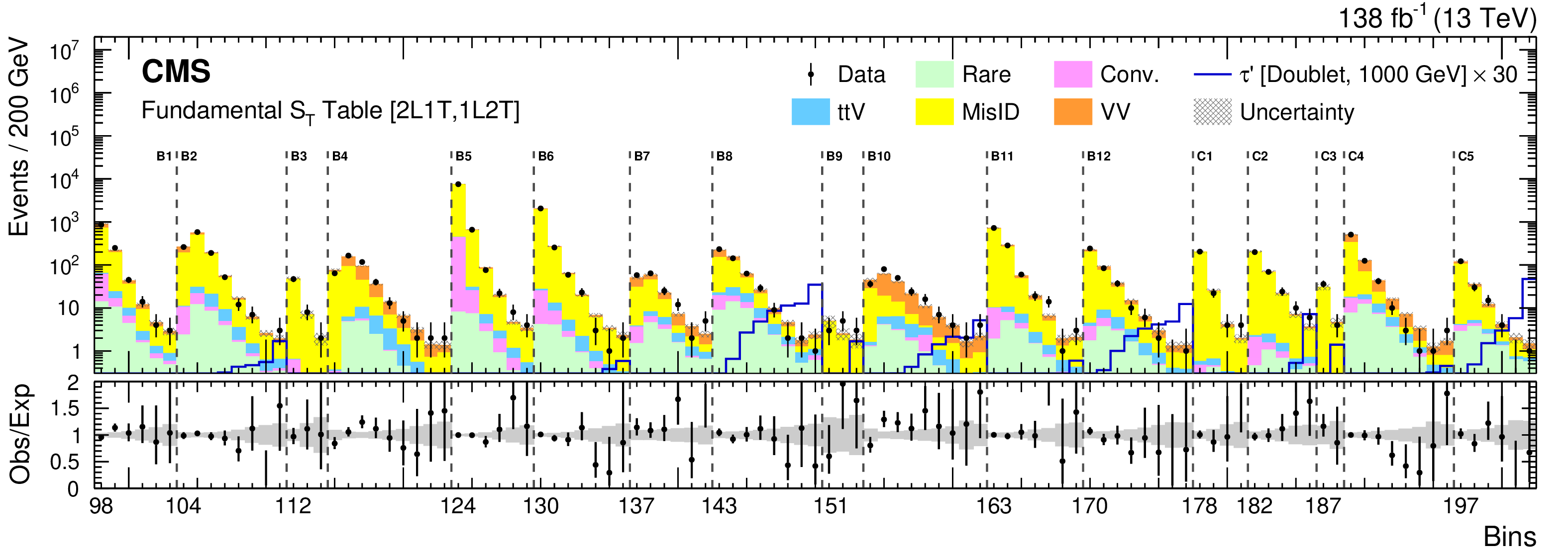
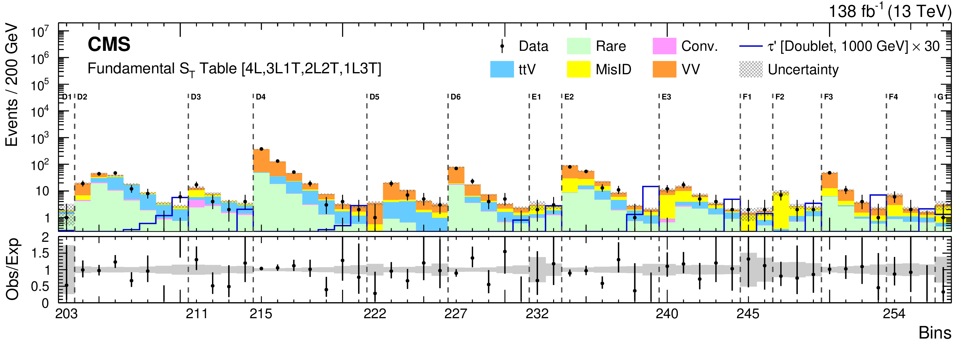
png pdf	Figure 9: The SR distributions of the fundamental ${S_{\mathrm {T}}}$ table for the combined 2016-2018 data set. The detailed description of the bin numbers can be found in Tables 3-6. The lower panel shows the ratio of observed events to the total expected background prediction. The gray band on the ratio represents the sum of statistical and systematic uncertainties in the SM background prediction. The expected SM background distributions and the uncertainties are shown after fitting the data under the background-only hypothesis. For illustration, an example signal hypothesis for the production of the vector-like $\tau$ lepton in the doublet scenario for $m_{{\tau ^{\prime}}} = $ 1 TeV, before the fit, is also overlaid.
png pdf	Figure 9-a: The SR distributions of the fundamental ${S_{\mathrm {T}}}$ table for the combined 2016-2018 data set. The detailed description of the bin numbers can be found in Tables 3-6. The lower panel shows the ratio of observed events to the total expected background prediction. The gray band on the ratio represents the sum of statistical and systematic uncertainties in the SM background prediction. The expected SM background distributions and the uncertainties are shown after fitting the data under the background-only hypothesis. For illustration, an example signal hypothesis for the production of the vector-like $\tau$ lepton in the doublet scenario for $m_{{\tau ^{\prime}}} = $ 1 TeV, before the fit, is also overlaid.
png pdf	Figure 9-b: The SR distributions of the fundamental ${S_{\mathrm {T}}}$ table for the combined 2016-2018 data set. The detailed description of the bin numbers can be found in Tables 3-6. The lower panel shows the ratio of observed events to the total expected background prediction. The gray band on the ratio represents the sum of statistical and systematic uncertainties in the SM background prediction. The expected SM background distributions and the uncertainties are shown after fitting the data under the background-only hypothesis. For illustration, an example signal hypothesis for the production of the vector-like $\tau$ lepton in the doublet scenario for $m_{{\tau ^{\prime}}} = $ 1 TeV, before the fit, is also overlaid.
png pdf	Figure 9-c: The SR distributions of the fundamental ${S_{\mathrm {T}}}$ table for the combined 2016-2018 data set. The detailed description of the bin numbers can be found in Tables 3-6. The lower panel shows the ratio of observed events to the total expected background prediction. The gray band on the ratio represents the sum of statistical and systematic uncertainties in the SM background prediction. The expected SM background distributions and the uncertainties are shown after fitting the data under the background-only hypothesis. For illustration, an example signal hypothesis for the production of the vector-like $\tau$ lepton in the doublet scenario for $m_{{\tau ^{\prime}}} = $ 1 TeV, before the fit, is also overlaid.
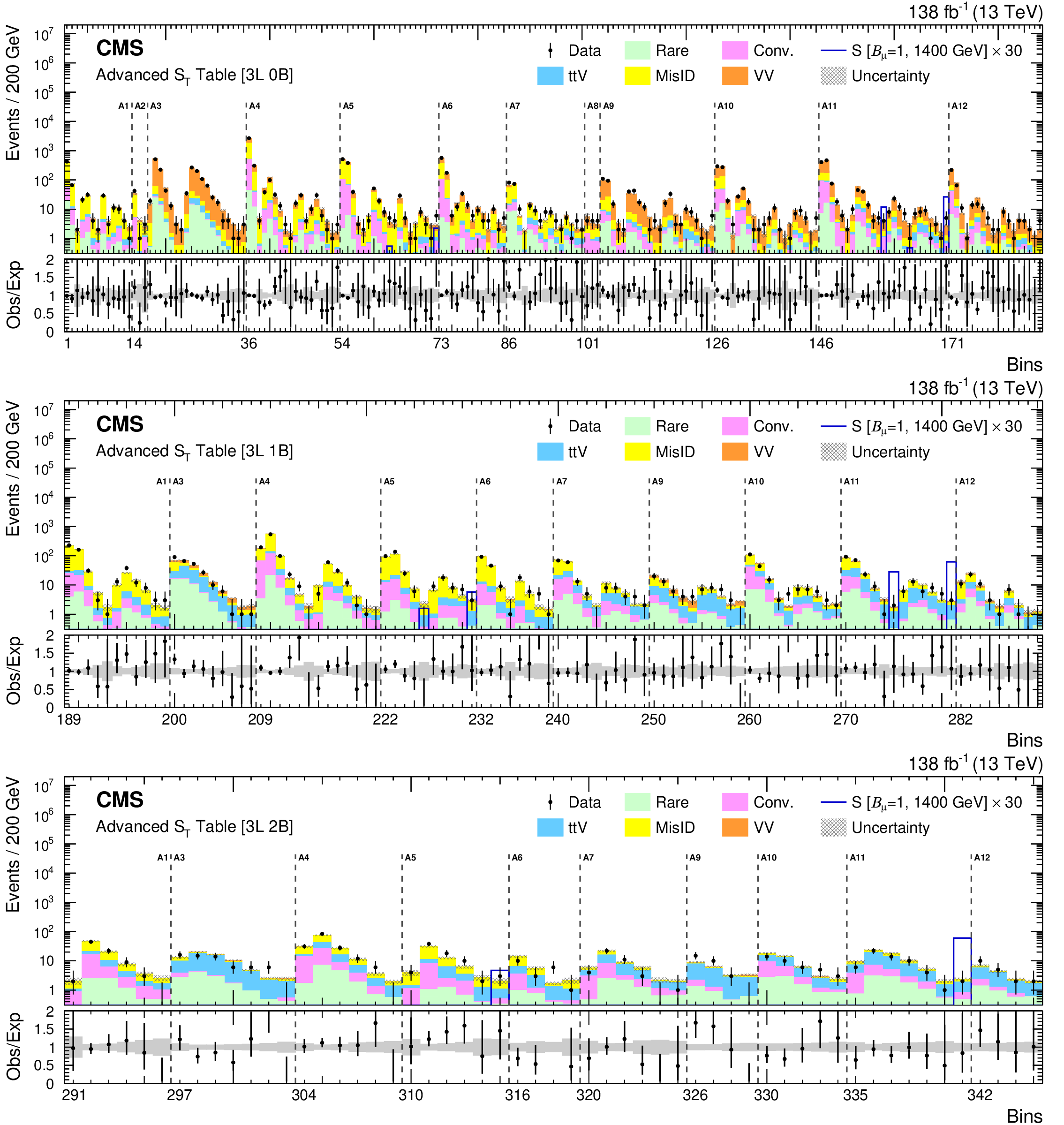
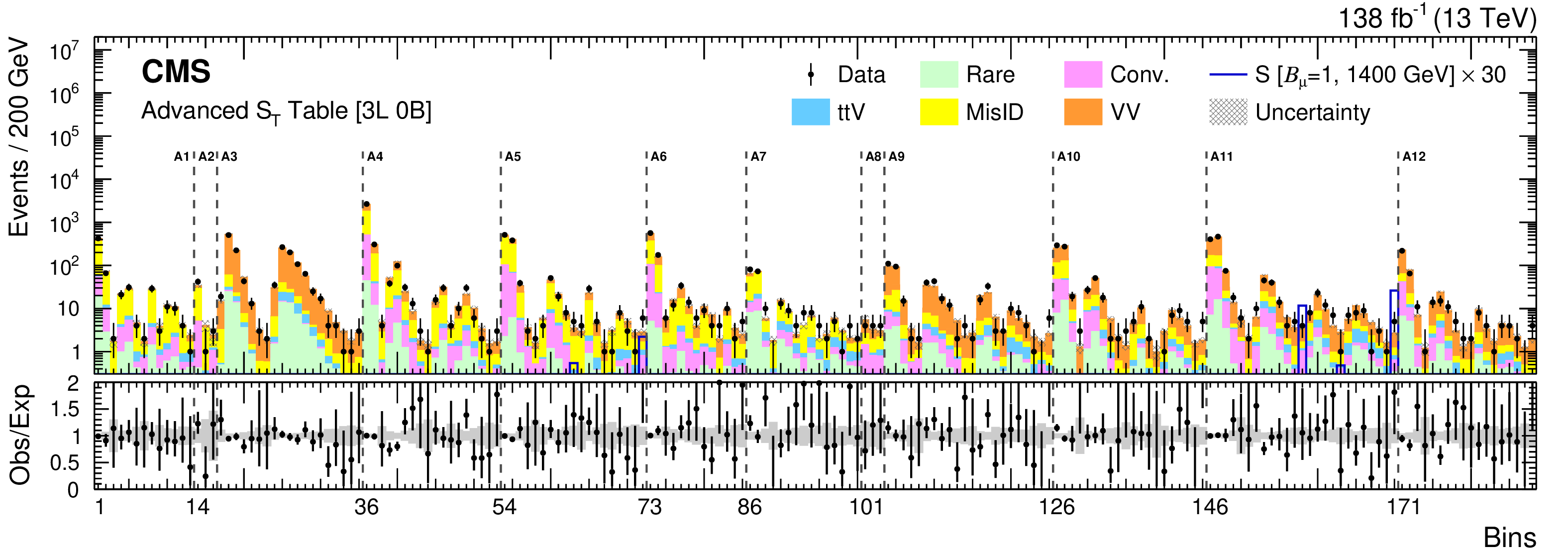
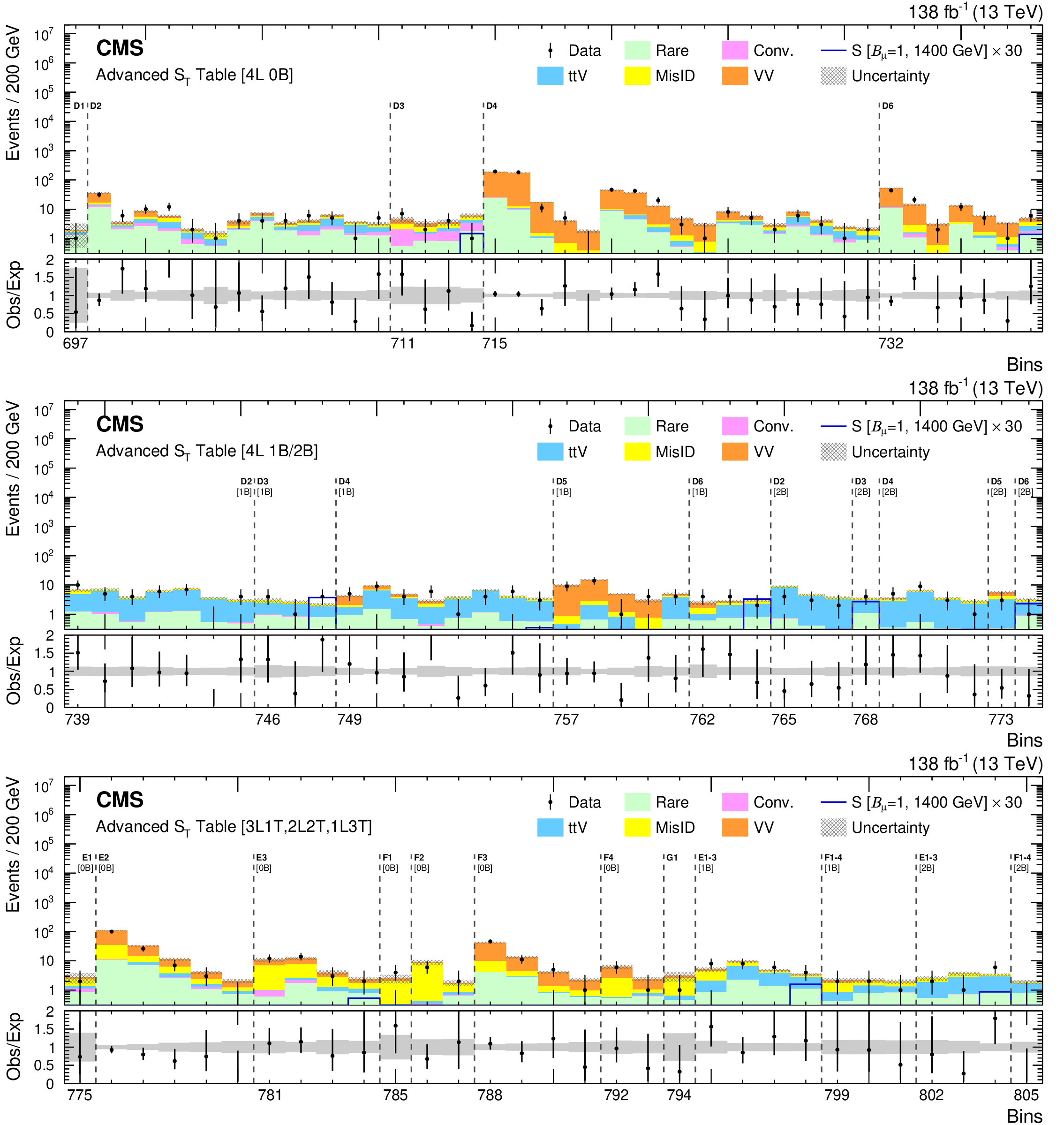
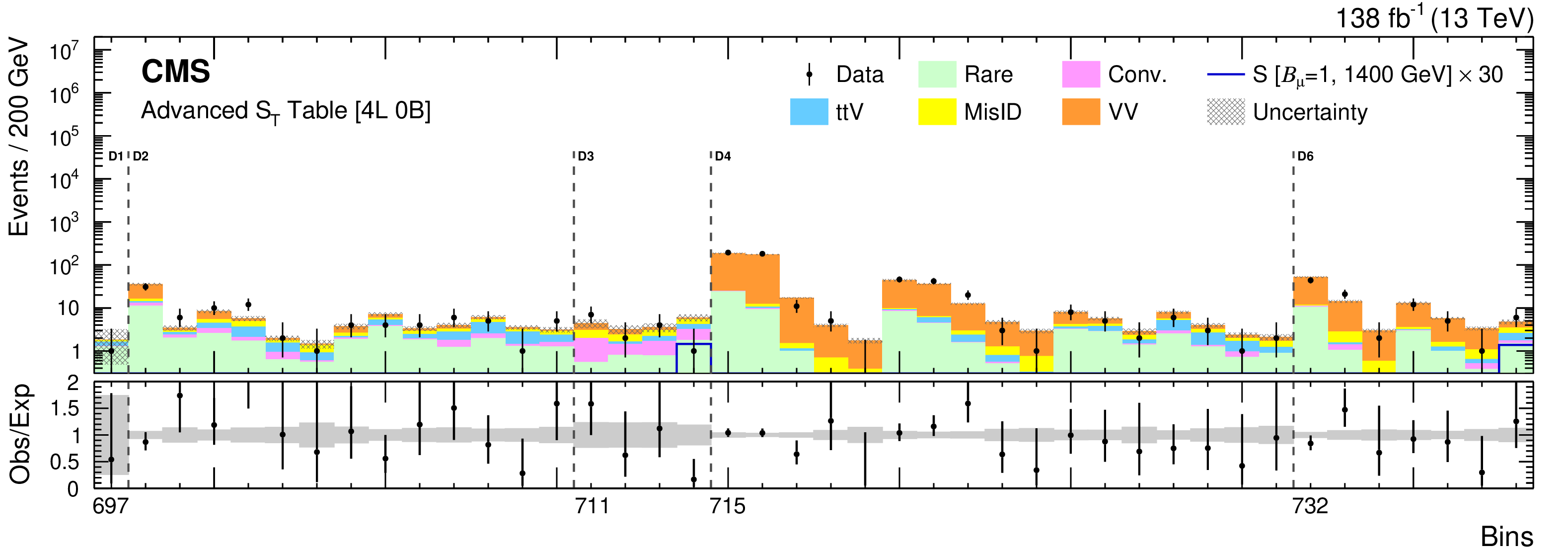
png pdf	Figure 10: The 3L SR distributions of the advanced ${S_{\mathrm {T}}}$ table for the combined 2016-2018 data set. The detailed description of the bin numbers can be found in Table 3. The lower panel shows the ratio of observed events to the total expected background prediction. The gray band on the ratio represents the sum of statistical and systematic uncertainties in the SM background prediction. The expected SM background distributions and the uncertainties are shown after fitting the data under the background-only hypothesis. For illustration, an example signal hypothesis for the production of the scalar leptoquark coupled to a top quark and a muon for $m_{\mathrm{S}} = $ 1.4 TeV, before the fit, is also overlaid.
png pdf	Figure 10-a: The 3L SR distributions of the advanced ${S_{\mathrm {T}}}$ table for the combined 2016-2018 data set. The detailed description of the bin numbers can be found in Table 3. The lower panel shows the ratio of observed events to the total expected background prediction. The gray band on the ratio represents the sum of statistical and systematic uncertainties in the SM background prediction. The expected SM background distributions and the uncertainties are shown after fitting the data under the background-only hypothesis. For illustration, an example signal hypothesis for the production of the scalar leptoquark coupled to a top quark and a muon for $m_{\mathrm{S}} = $ 1.4 TeV, before the fit, is also overlaid.
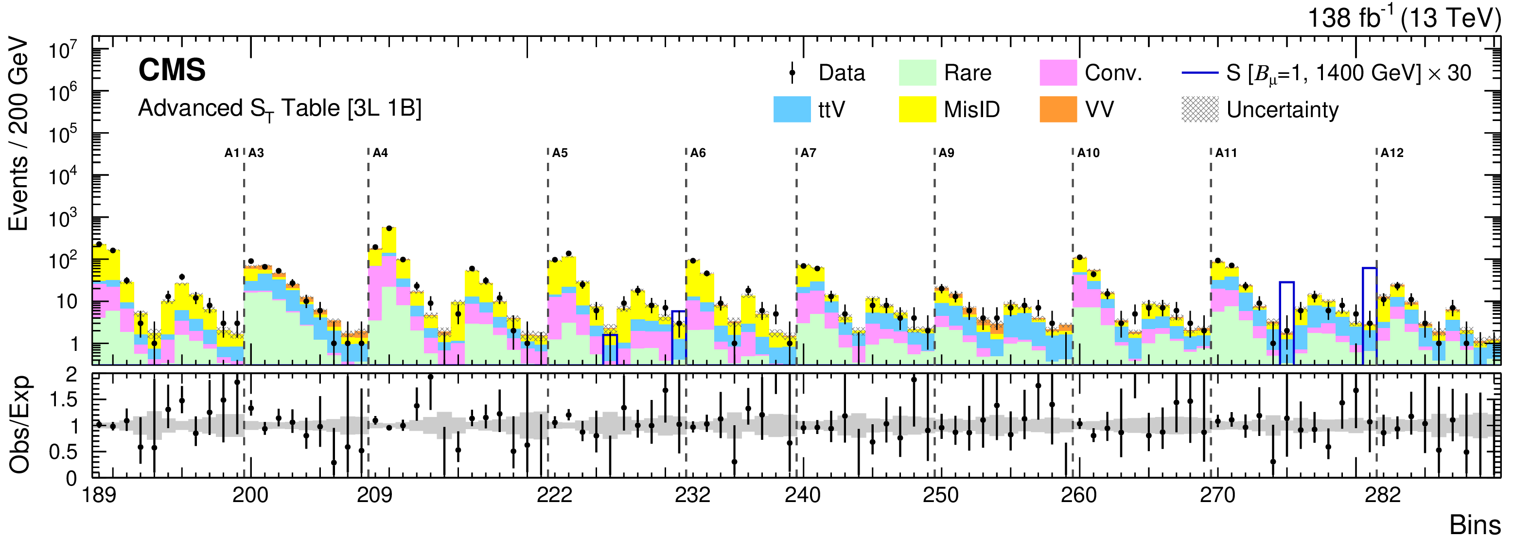
png pdf	Figure 10-b: The 3L SR distributions of the advanced ${S_{\mathrm {T}}}$ table for the combined 2016-2018 data set. The detailed description of the bin numbers can be found in Table 3. The lower panel shows the ratio of observed events to the total expected background prediction. The gray band on the ratio represents the sum of statistical and systematic uncertainties in the SM background prediction. The expected SM background distributions and the uncertainties are shown after fitting the data under the background-only hypothesis. For illustration, an example signal hypothesis for the production of the scalar leptoquark coupled to a top quark and a muon for $m_{\mathrm{S}} = $ 1.4 TeV, before the fit, is also overlaid.
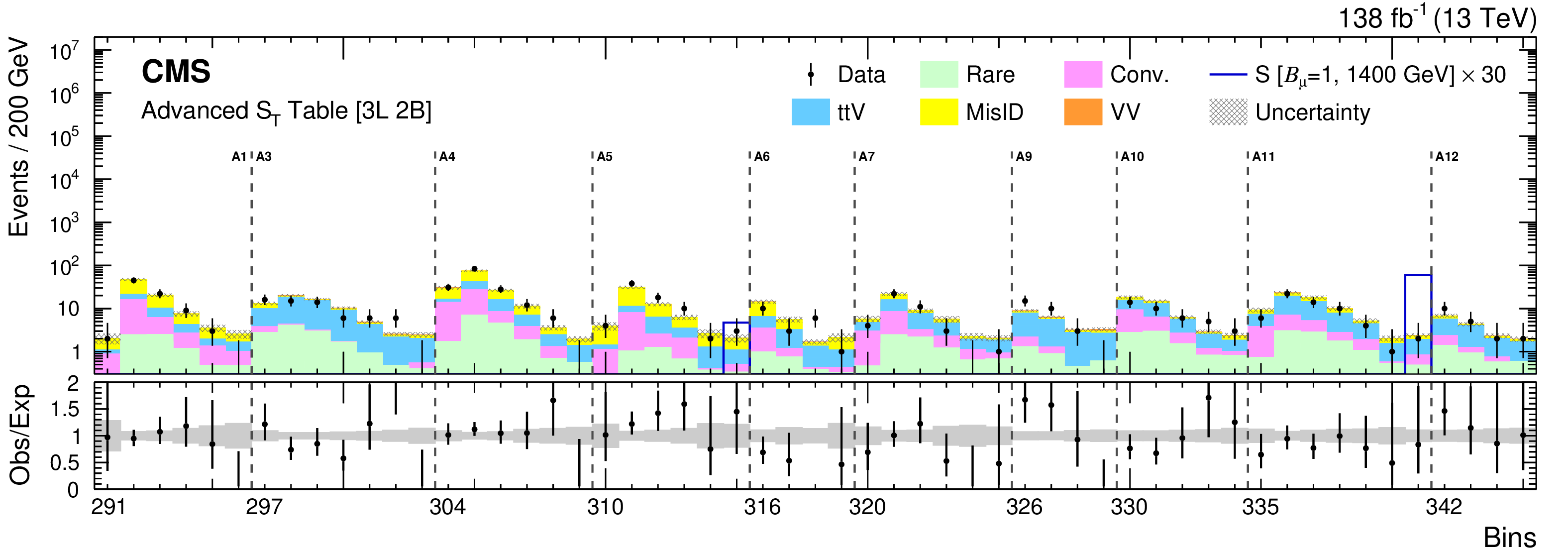
png pdf	Figure 10-c: The 3L SR distributions of the advanced ${S_{\mathrm {T}}}$ table for the combined 2016-2018 data set. The detailed description of the bin numbers can be found in Table 3. The lower panel shows the ratio of observed events to the total expected background prediction. The gray band on the ratio represents the sum of statistical and systematic uncertainties in the SM background prediction. The expected SM background distributions and the uncertainties are shown after fitting the data under the background-only hypothesis. For illustration, an example signal hypothesis for the production of the scalar leptoquark coupled to a top quark and a muon for $m_{\mathrm{S}} = $ 1.4 TeV, before the fit, is also overlaid.
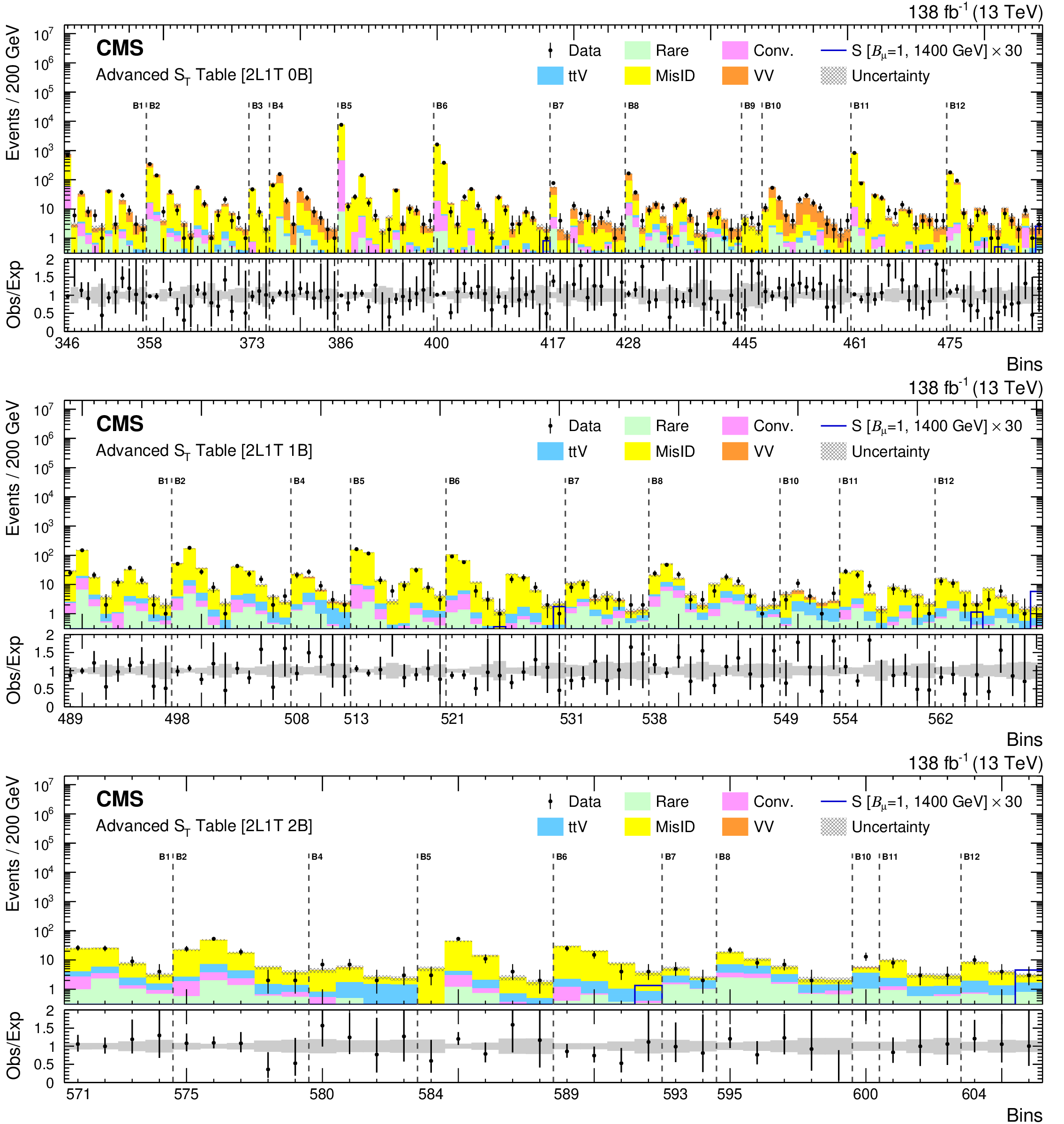
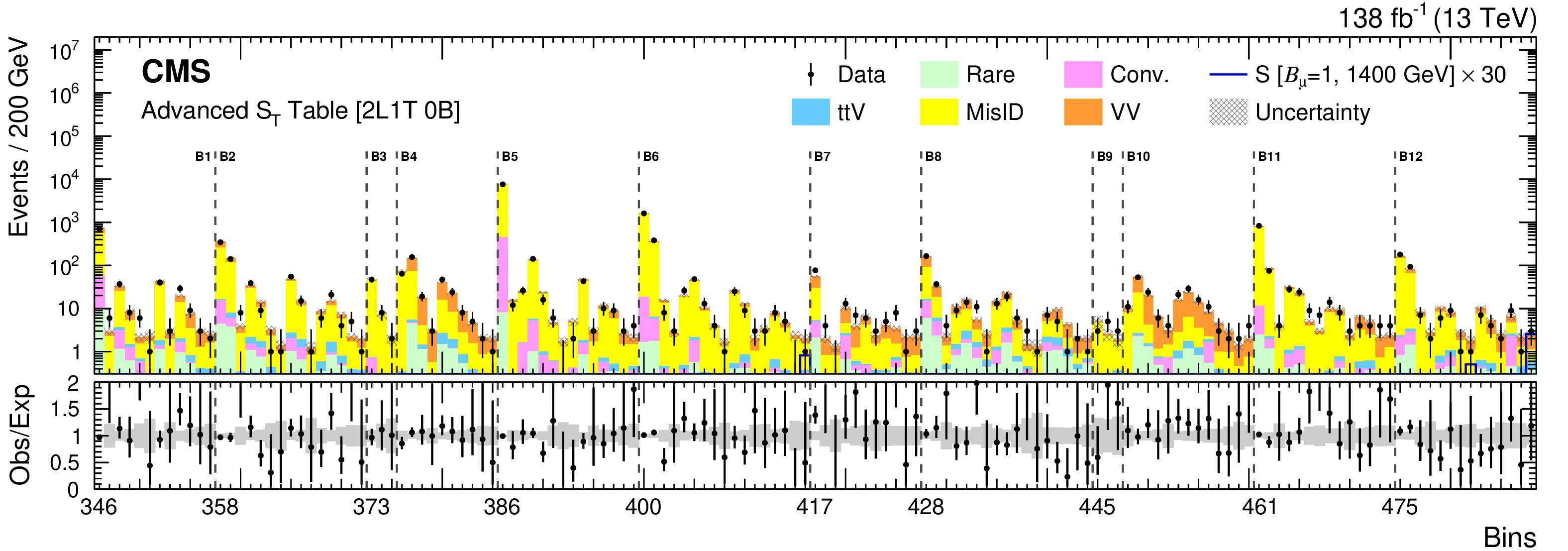
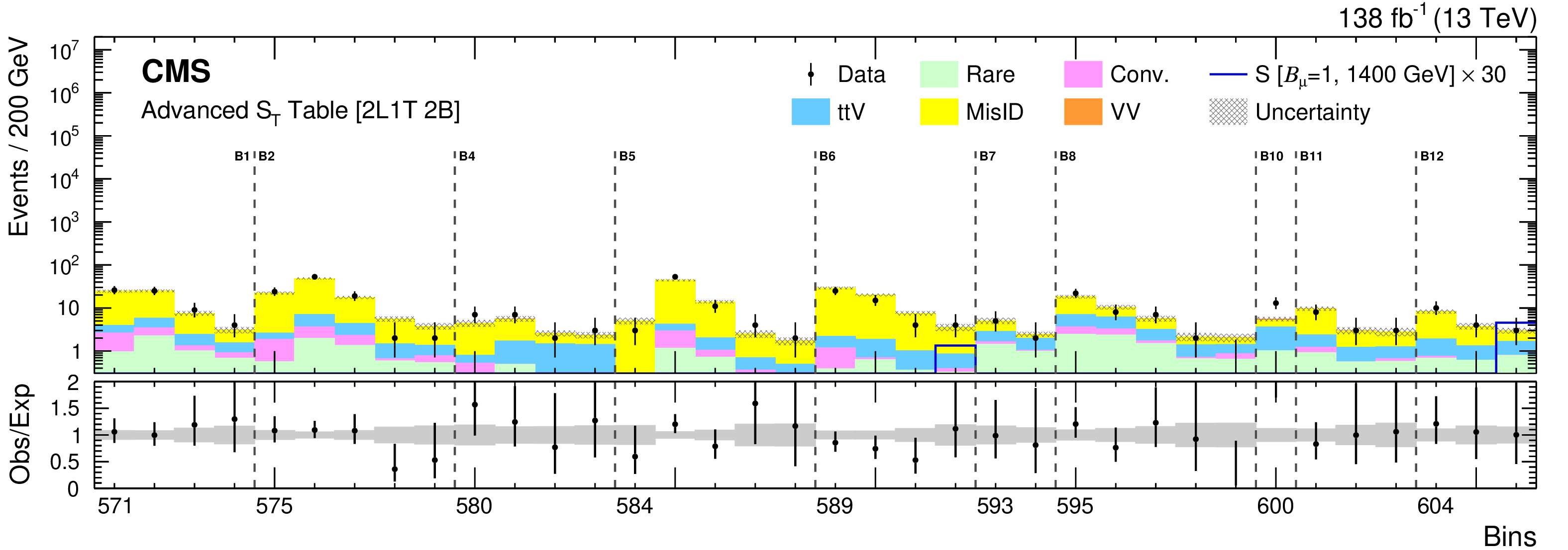
png pdf	Figure 11: The 2L1T SR distributions of the advanced ${S_{\mathrm {T}}}$ table for the combined 2016-2018 data set. The detailed description of the bin numbers can be found in Table 4. The lower panel shows the ratio of observed events to the total expected background prediction. The gray band on the ratio represents the sum of statistical and systematic uncertainties in the SM background prediction. The expected SM background distributions and the uncertainties are shown after fitting the data under the background-only hypothesis. For illustration, an example signal hypothesis for the production of the scalar leptoquark coupled to a top quark and a muon for $m_{\mathrm{S}} = $ 1.4 TeV, before the fit, is also overlaid.
png pdf	Figure 11-a: The 2L1T SR distributions of the advanced ${S_{\mathrm {T}}}$ table for the combined 2016-2018 data set. The detailed description of the bin numbers can be found in Table 4. The lower panel shows the ratio of observed events to the total expected background prediction. The gray band on the ratio represents the sum of statistical and systematic uncertainties in the SM background prediction. The expected SM background distributions and the uncertainties are shown after fitting the data under the background-only hypothesis. For illustration, an example signal hypothesis for the production of the scalar leptoquark coupled to a top quark and a muon for $m_{\mathrm{S}} = $ 1.4 TeV, before the fit, is also overlaid.
png pdf	Figure 11-b: The 2L1T SR distributions of the advanced ${S_{\mathrm {T}}}$ table for the combined 2016-2018 data set. The detailed description of the bin numbers can be found in Table 4. The lower panel shows the ratio of observed events to the total expected background prediction. The gray band on the ratio represents the sum of statistical and systematic uncertainties in the SM background prediction. The expected SM background distributions and the uncertainties are shown after fitting the data under the background-only hypothesis. For illustration, an example signal hypothesis for the production of the scalar leptoquark coupled to a top quark and a muon for $m_{\mathrm{S}} = $ 1.4 TeV, before the fit, is also overlaid.
png pdf	Figure 11-c: The 2L1T SR distributions of the advanced ${S_{\mathrm {T}}}$ table for the combined 2016-2018 data set. The detailed description of the bin numbers can be found in Table 4. The lower panel shows the ratio of observed events to the total expected background prediction. The gray band on the ratio represents the sum of statistical and systematic uncertainties in the SM background prediction. The expected SM background distributions and the uncertainties are shown after fitting the data under the background-only hypothesis. For illustration, an example signal hypothesis for the production of the scalar leptoquark coupled to a top quark and a muon for $m_{\mathrm{S}} = $ 1.4 TeV, before the fit, is also overlaid.
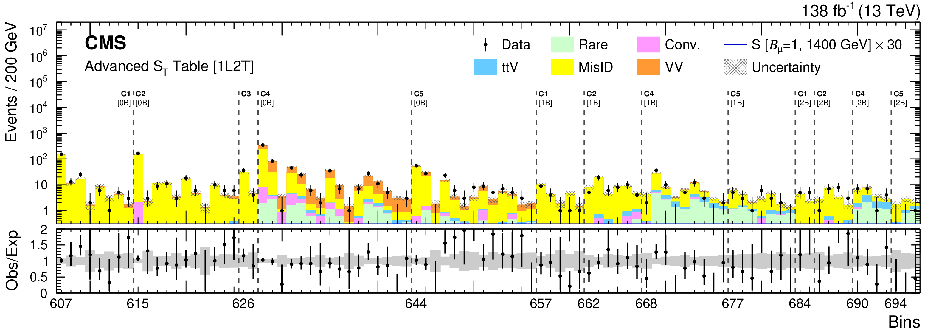
png pdf	Figure 12: The 1L2T SR distribution of the advanced ${S_{\mathrm {T}}}$ table for the combined 2016-2018 data set. The detailed description of the bin numbers can be found in Table 5. The lower panel shows the ratio of observed events to the total expected background prediction. The gray band on the ratio represents the sum of statistical and systematic uncertainties in the SM background prediction. The expected SM background distributions and the uncertainties are shown after fitting the data under the background-only hypothesis. An example signal hypothesis for the production of the scalar leptoquark coupled to a top quark and a muon for $m_{\mathrm{S}} = $ 1.4 TeV, before the fit, is also overlaid. For this category, the signal yield is negligible and is not visible in the figure.
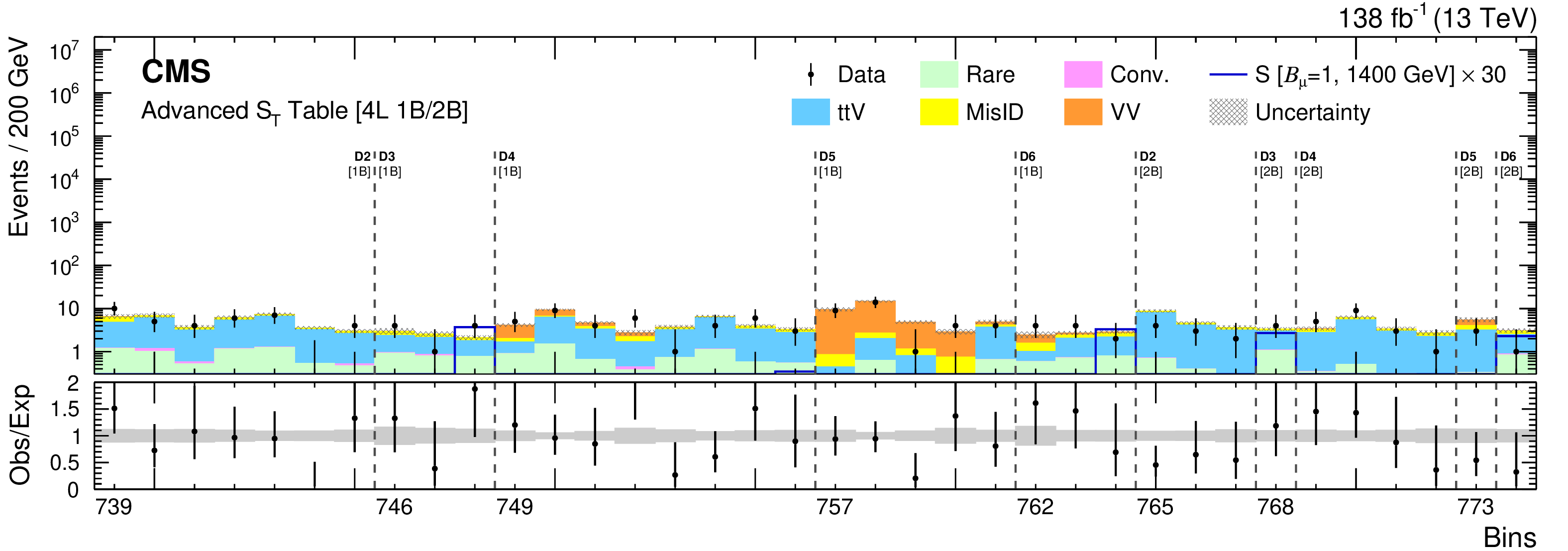
png pdf	Figure 13: The 4L, 3L1T, 2L2T and 1L3T SR distributions of the advanced ${S_{\mathrm {T}}}$ table for the combined 2016-2018 data set. The detailed description of the bin numbers can be found in Table 6. The lower panel shows the ratio of observed events to the total expected background prediction. The gray band on the ratio represents the sum of statistical and systematic uncertainties in the SM background prediction. The expected SM background distributions and the uncertainties are shown after fitting the data under the background-only hypothesis. For illustration, an example signal hypothesis for the production of the scalar leptoquark coupled to a top quark and a muon for $m_{\mathrm{S}} = $ 1.4 TeV, before the fit, is also overlaid.
png pdf	Figure 13-a: The 4L, 3L1T, 2L2T and 1L3T SR distributions of the advanced ${S_{\mathrm {T}}}$ table for the combined 2016-2018 data set. The detailed description of the bin numbers can be found in Table 6. The lower panel shows the ratio of observed events to the total expected background prediction. The gray band on the ratio represents the sum of statistical and systematic uncertainties in the SM background prediction. The expected SM background distributions and the uncertainties are shown after fitting the data under the background-only hypothesis. For illustration, an example signal hypothesis for the production of the scalar leptoquark coupled to a top quark and a muon for $m_{\mathrm{S}} = $ 1.4 TeV, before the fit, is also overlaid.
png pdf	Figure 13-b: The 4L, 3L1T, 2L2T and 1L3T SR distributions of the advanced ${S_{\mathrm {T}}}$ table for the combined 2016-2018 data set. The detailed description of the bin numbers can be found in Table 6. The lower panel shows the ratio of observed events to the total expected background prediction. The gray band on the ratio represents the sum of statistical and systematic uncertainties in the SM background prediction. The expected SM background distributions and the uncertainties are shown after fitting the data under the background-only hypothesis. For illustration, an example signal hypothesis for the production of the scalar leptoquark coupled to a top quark and a muon for $m_{\mathrm{S}} = $ 1.4 TeV, before the fit, is also overlaid.
png pdf	Figure 13-c: The 4L, 3L1T, 2L2T and 1L3T SR distributions of the advanced ${S_{\mathrm {T}}}$ table for the combined 2016-2018 data set. The detailed description of the bin numbers can be found in Table 6. The lower panel shows the ratio of observed events to the total expected background prediction. The gray band on the ratio represents the sum of statistical and systematic uncertainties in the SM background prediction. The expected SM background distributions and the uncertainties are shown after fitting the data under the background-only hypothesis. For illustration, an example signal hypothesis for the production of the scalar leptoquark coupled to a top quark and a muon for $m_{\mathrm{S}} = $ 1.4 TeV, before the fit, is also overlaid.
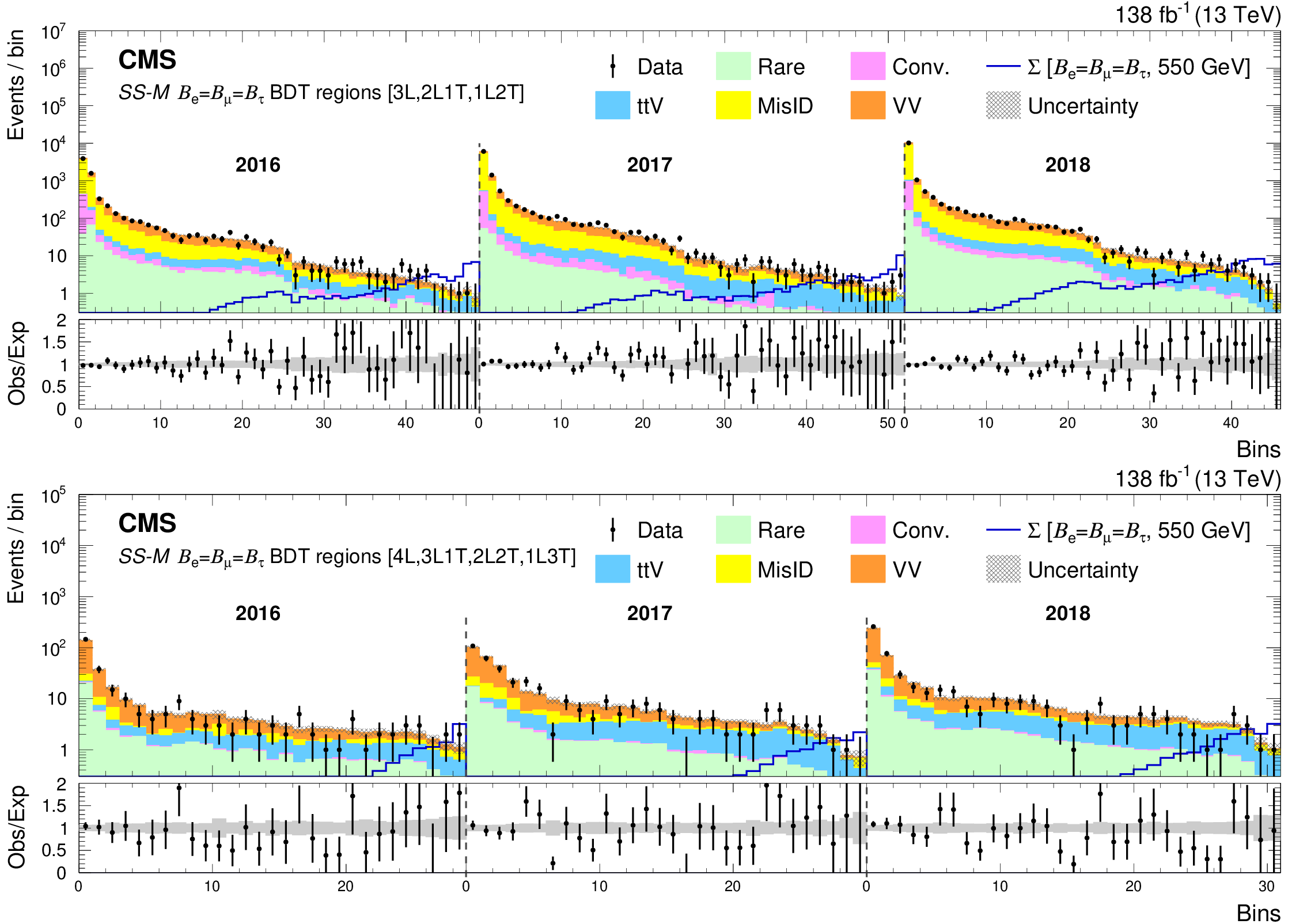
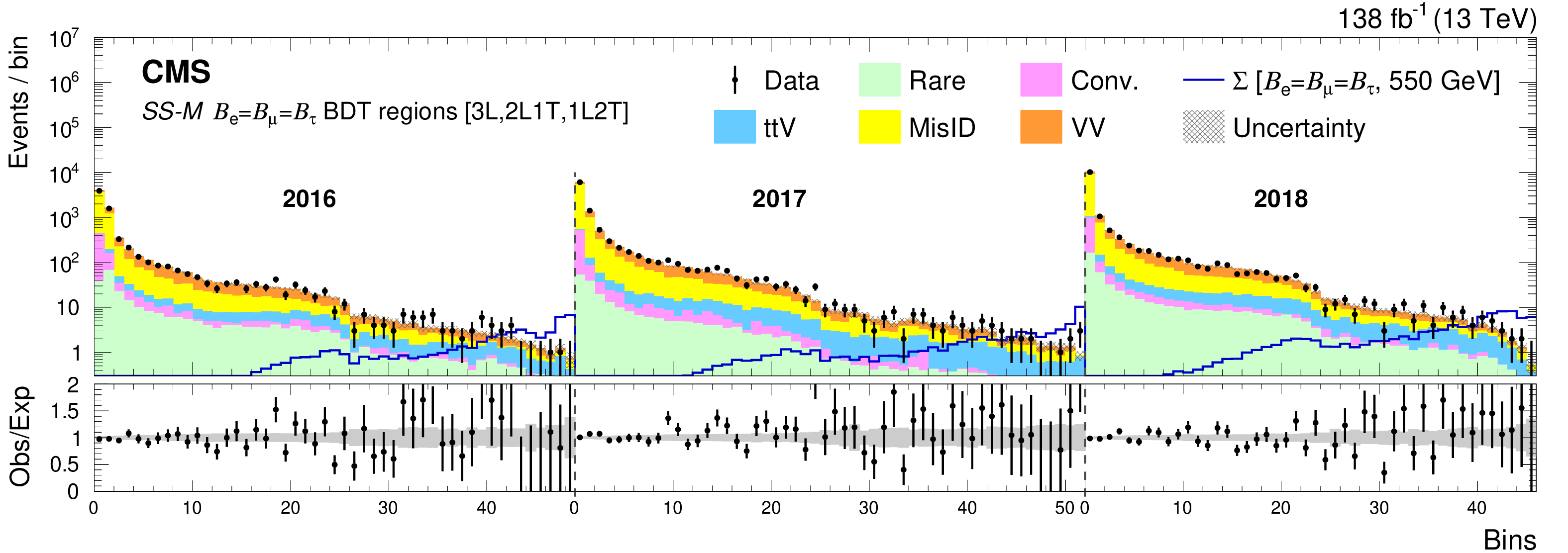
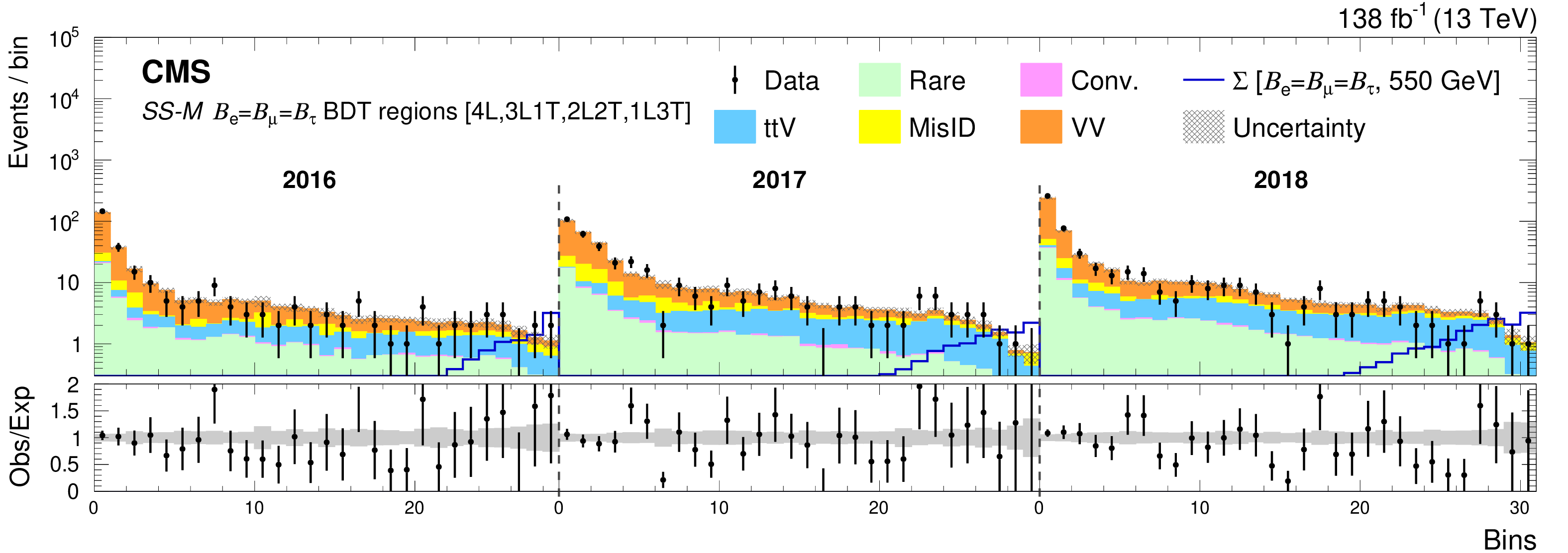
png pdf	Figure 14: The SS-M $\mathcal {B}_{\mathrm{e}}=\mathcal {B}_{\mu}=\mathcal {B}_{\tau}$ BDT regions for the 3-lepton (upper) and 4-lepton (lower) channels for the 2016-2018 data sets. The lower panel shows the ratio of observed events to the total expected background prediction. The gray band on the ratio represents the sum of statistical and systematic uncertainties in the SM background prediction. The expected SM background distributions and the uncertainties are shown after fitting the data under the background-only hypothesis. For illustration, an example signal hypothesis for the production of the type-III seesaw heavy fermions in the flavor-democratic scenario for $m_{\Sigma} = $ 550 GeV, before the fit, is also overlaid.
png pdf	Figure 14-a: The SS-M $\mathcal {B}_{\mathrm{e}}=\mathcal {B}_{\mu}=\mathcal {B}_{\tau}$ BDT regions for the 3-lepton (upper) and 4-lepton (lower) channels for the 2016-2018 data sets. The lower panel shows the ratio of observed events to the total expected background prediction. The gray band on the ratio represents the sum of statistical and systematic uncertainties in the SM background prediction. The expected SM background distributions and the uncertainties are shown after fitting the data under the background-only hypothesis. For illustration, an example signal hypothesis for the production of the type-III seesaw heavy fermions in the flavor-democratic scenario for $m_{\Sigma} = $ 550 GeV, before the fit, is also overlaid.
png pdf	Figure 14-b: The SS-M $\mathcal {B}_{\mathrm{e}}=\mathcal {B}_{\mu}=\mathcal {B}_{\tau}$ BDT regions for the 3-lepton (upper) and 4-lepton (lower) channels for the 2016-2018 data sets. The lower panel shows the ratio of observed events to the total expected background prediction. The gray band on the ratio represents the sum of statistical and systematic uncertainties in the SM background prediction. The expected SM background distributions and the uncertainties are shown after fitting the data under the background-only hypothesis. For illustration, an example signal hypothesis for the production of the type-III seesaw heavy fermions in the flavor-democratic scenario for $m_{\Sigma} = $ 550 GeV, before the fit, is also overlaid.
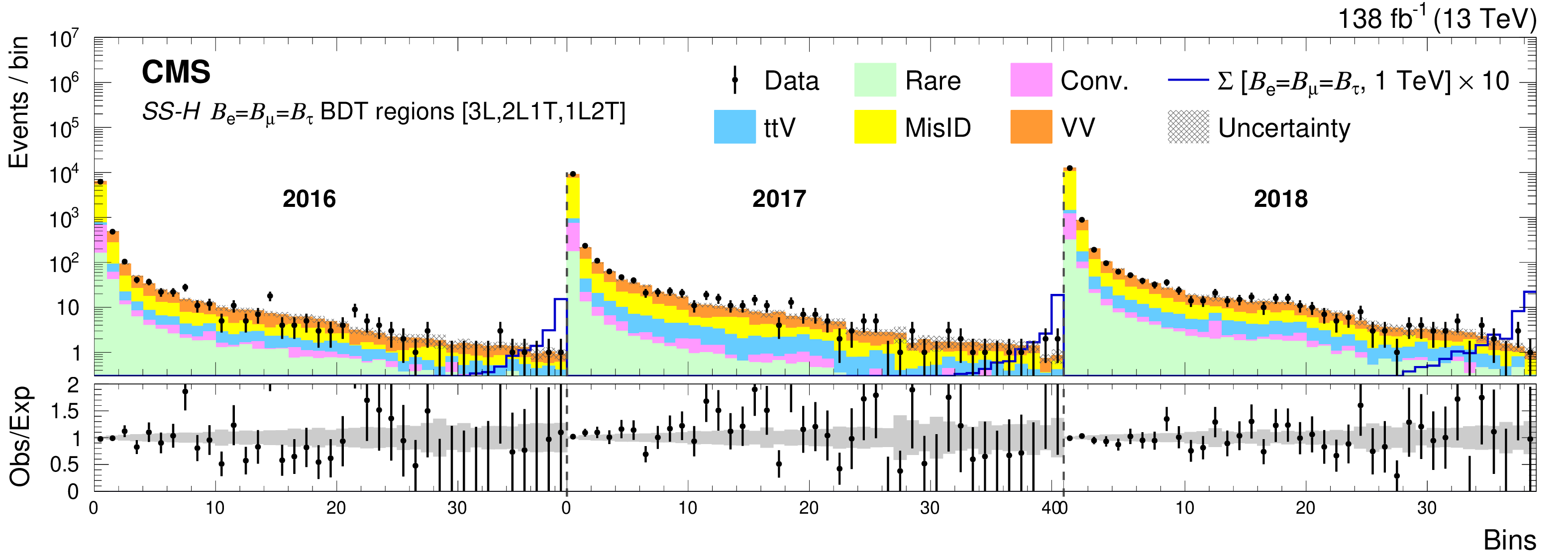
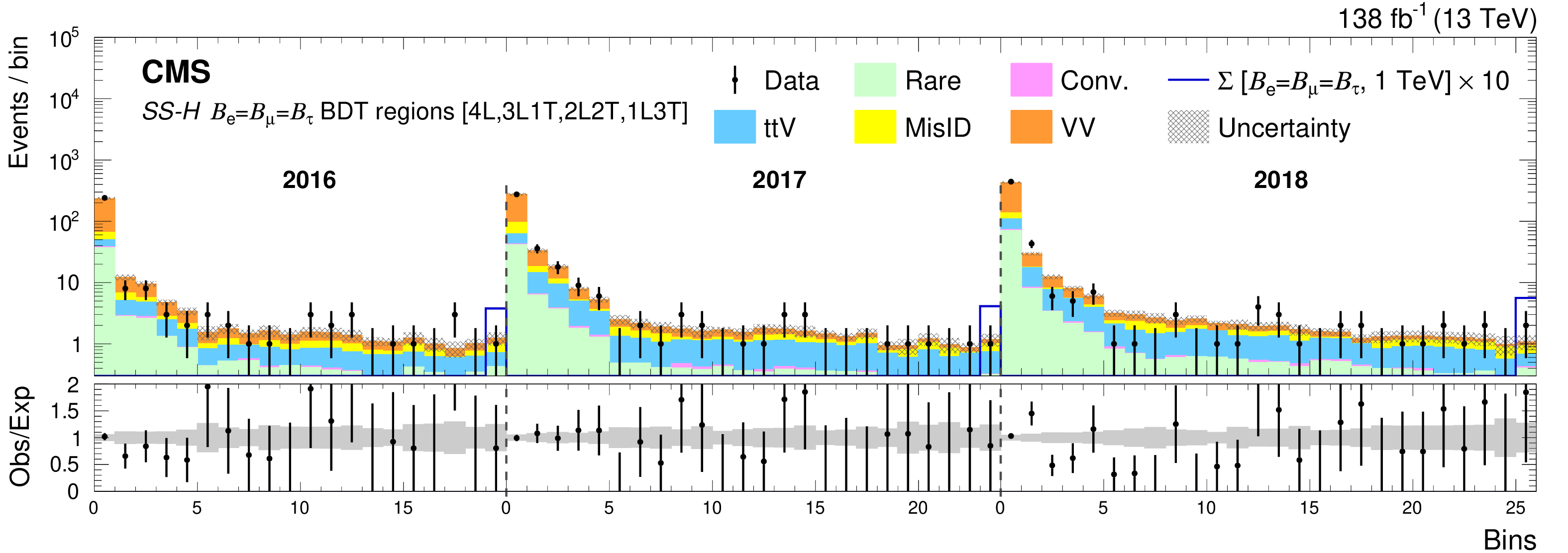
png pdf	Figure 15: The SS-H $\mathcal {B}_{\mathrm{e}}=\mathcal {B}_{\mu}=\mathcal {B}_{\tau}$ BDT regions for the 3-lepton (upper) and 4-lepton (lower) channels for the 2016-2018 data sets. The lower panel shows the ratio of observed events to the total expected background prediction. The gray band on the ratio represents the sum of statistical and systematic uncertainties in the SM background prediction. The expected SM background distributions and the uncertainties are shown after fitting the data under the background-only hypothesis. For illustration, an example signal hypothesis for the production of the type-III seesaw heavy fermions in the flavor-democratic scenario for $m_{\Sigma} = $ 1 TeV, before the fit, is also overlaid.
png pdf	Figure 15-a: The SS-H $\mathcal {B}_{\mathrm{e}}=\mathcal {B}_{\mu}=\mathcal {B}_{\tau}$ BDT regions for the 3-lepton (upper) and 4-lepton (lower) channels for the 2016-2018 data sets. The lower panel shows the ratio of observed events to the total expected background prediction. The gray band on the ratio represents the sum of statistical and systematic uncertainties in the SM background prediction. The expected SM background distributions and the uncertainties are shown after fitting the data under the background-only hypothesis. For illustration, an example signal hypothesis for the production of the type-III seesaw heavy fermions in the flavor-democratic scenario for $m_{\Sigma} = $ 1 TeV, before the fit, is also overlaid.
png pdf	Figure 15-b: The SS-H $\mathcal {B}_{\mathrm{e}}=\mathcal {B}_{\mu}=\mathcal {B}_{\tau}$ BDT regions for the 3-lepton (upper) and 4-lepton (lower) channels for the 2016-2018 data sets. The lower panel shows the ratio of observed events to the total expected background prediction. The gray band on the ratio represents the sum of statistical and systematic uncertainties in the SM background prediction. The expected SM background distributions and the uncertainties are shown after fitting the data under the background-only hypothesis. For illustration, an example signal hypothesis for the production of the type-III seesaw heavy fermions in the flavor-democratic scenario for $m_{\Sigma} = $ 1 TeV, before the fit, is also overlaid.
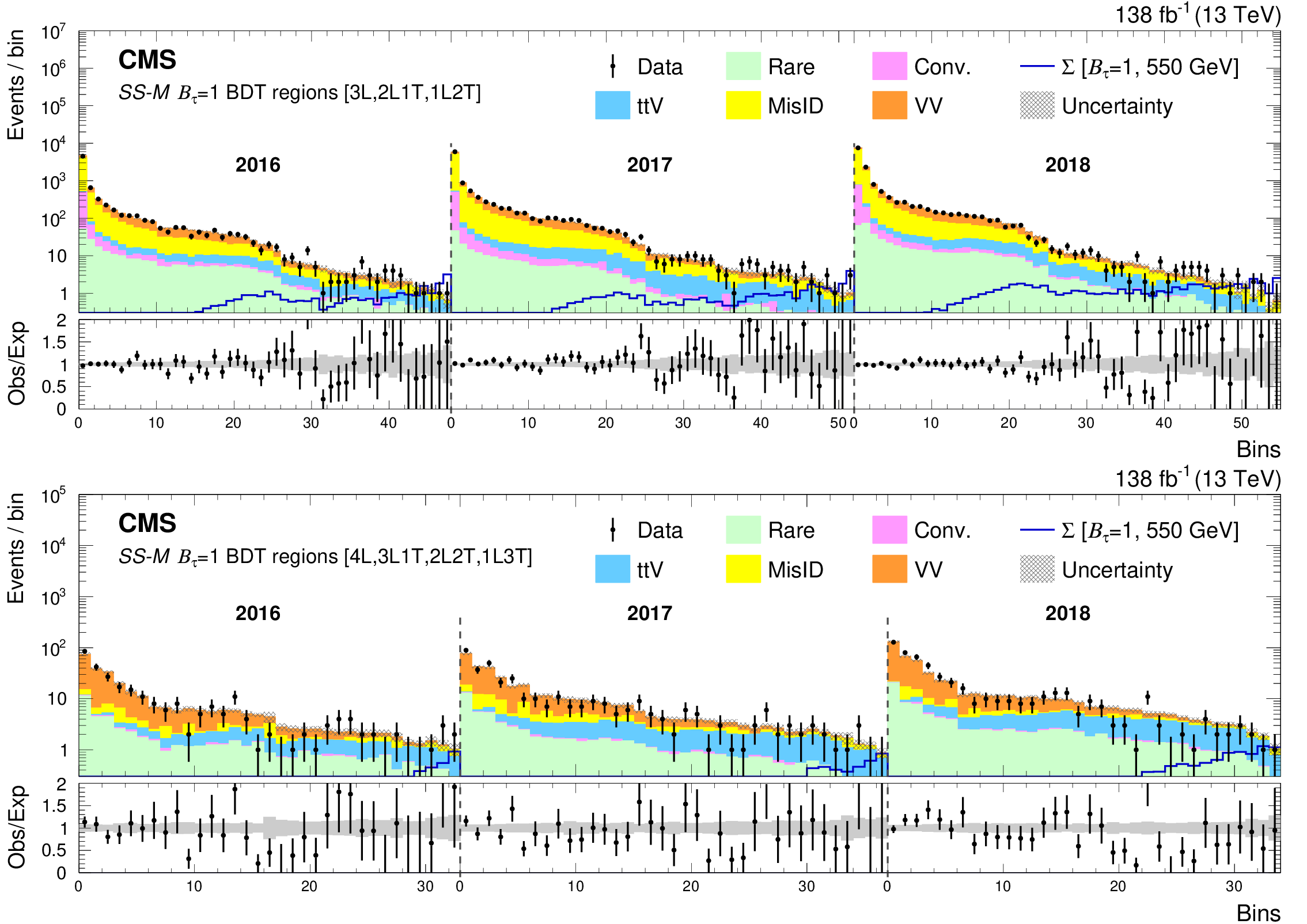
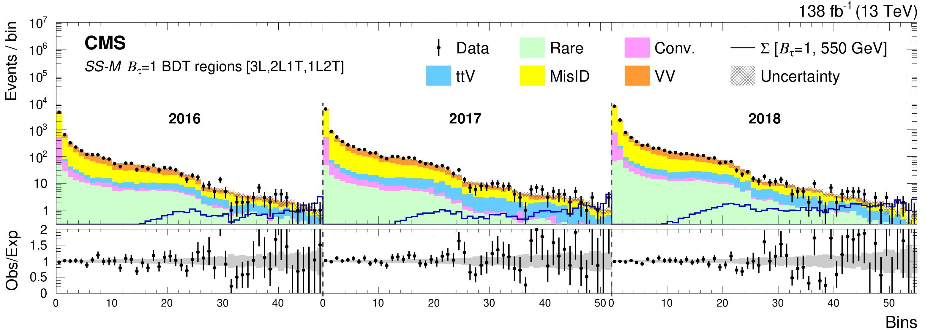
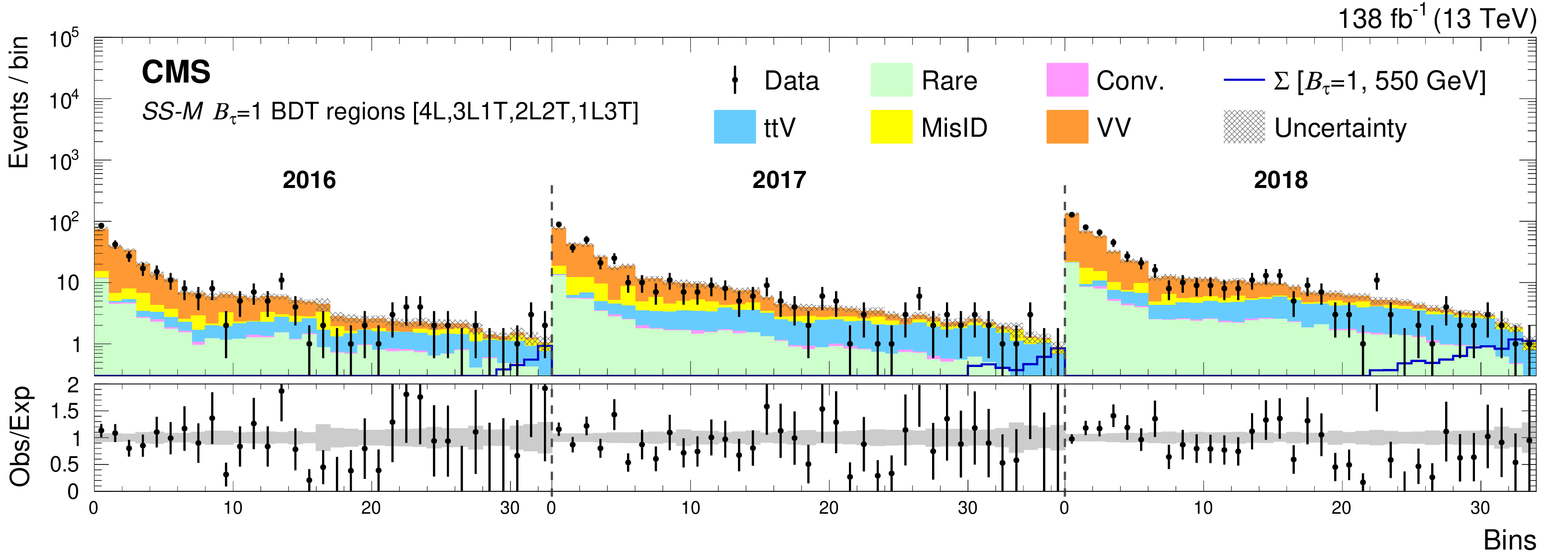
png pdf	Figure 16: The SS-M $\mathcal {B}_{\tau}=1$ BDT regions for the 3-lepton (upper) and 4-lepton (lower) channels for the 2016-2018 data sets. The lower panel shows the ratio of observed events to the total expected background prediction. The gray band on the ratio represents the sum of statistical and systematic uncertainties in the SM background prediction. The expected SM background distributions and the uncertainties are shown after fitting the data under the background-only hypothesis. For illustration, an example signal hypothesis for the production of the type-III seesaw heavy fermions in the scenario with mixing exclusively to $\tau$ lepton for $m_{\Sigma} = $ 550 GeV, before the fit, is also overlaid.
png pdf	Figure 16-a: The SS-M $\mathcal {B}_{\tau}=1$ BDT regions for the 3-lepton (upper) and 4-lepton (lower) channels for the 2016-2018 data sets. The lower panel shows the ratio of observed events to the total expected background prediction. The gray band on the ratio represents the sum of statistical and systematic uncertainties in the SM background prediction. The expected SM background distributions and the uncertainties are shown after fitting the data under the background-only hypothesis. For illustration, an example signal hypothesis for the production of the type-III seesaw heavy fermions in the scenario with mixing exclusively to $\tau$ lepton for $m_{\Sigma} = $ 550 GeV, before the fit, is also overlaid.
png pdf	Figure 16-b: The SS-M $\mathcal {B}_{\tau}=1$ BDT regions for the 3-lepton (upper) and 4-lepton (lower) channels for the 2016-2018 data sets. The lower panel shows the ratio of observed events to the total expected background prediction. The gray band on the ratio represents the sum of statistical and systematic uncertainties in the SM background prediction. The expected SM background distributions and the uncertainties are shown after fitting the data under the background-only hypothesis. For illustration, an example signal hypothesis for the production of the type-III seesaw heavy fermions in the scenario with mixing exclusively to $\tau$ lepton for $m_{\Sigma} = $ 550 GeV, before the fit, is also overlaid.
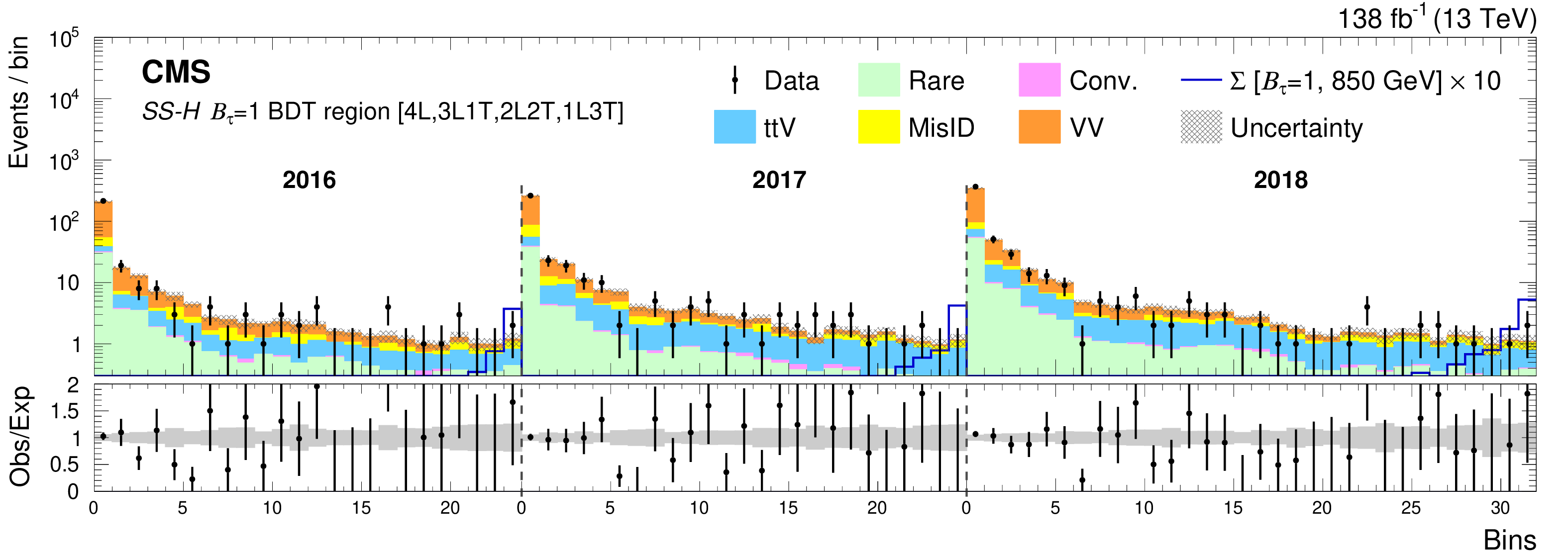
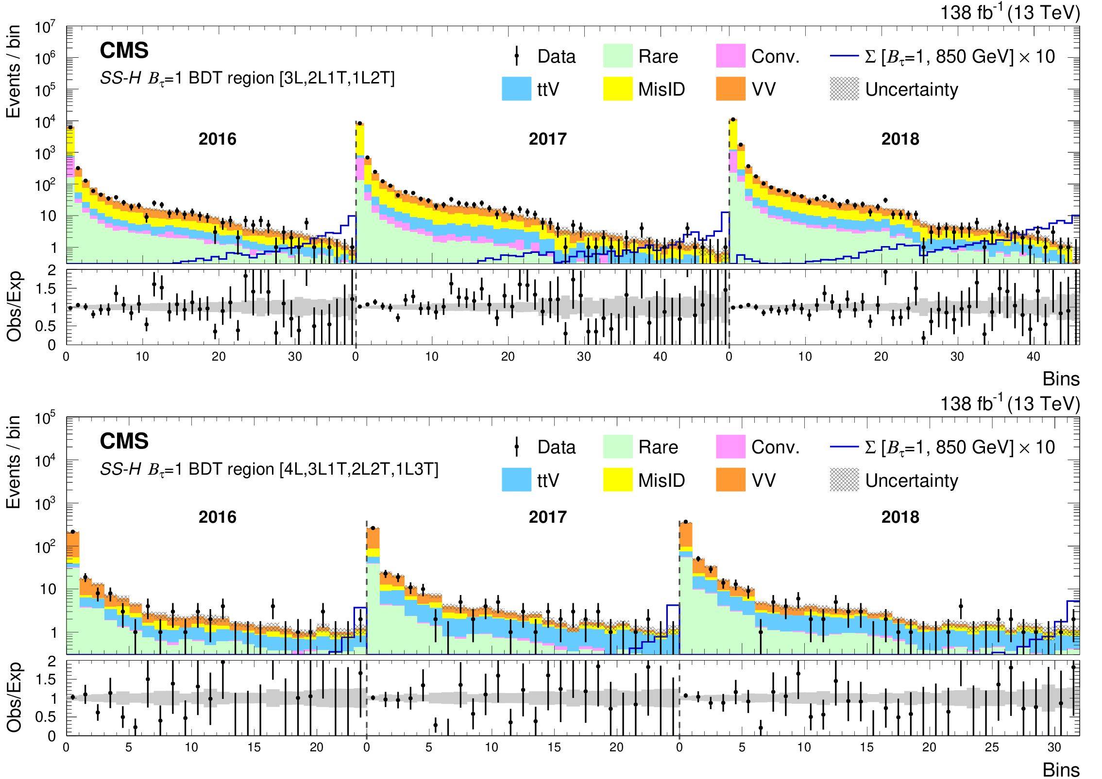
png pdf	Figure 17: The SS-H $\mathcal {B}_{\tau}=1$ BDT regions for the 3-lepton (upper) and 4-lepton (lower) channels for the 2016-2018 data sets. The lower panel shows the ratio of observed events to the total expected background prediction. The gray band on the ratio represents the sum of statistical and systematic uncertainties in the SM background prediction. The expected SM background distributions and the uncertainties are shown after fitting the data under the background-only hypothesis. For illustration, an example signal hypothesis for the production of the type-III seesaw heavy fermions in the scenario with mixing exclusively to $\tau$ lepton for $m_{\Sigma} = $ 850 GeV, before the fit, is also overlaid.
png pdf	Figure 17-a: The SS-H $\mathcal {B}_{\tau}=1$ BDT regions for the 3-lepton (upper) and 4-lepton (lower) channels for the 2016-2018 data sets. The lower panel shows the ratio of observed events to the total expected background prediction. The gray band on the ratio represents the sum of statistical and systematic uncertainties in the SM background prediction. The expected SM background distributions and the uncertainties are shown after fitting the data under the background-only hypothesis. For illustration, an example signal hypothesis for the production of the type-III seesaw heavy fermions in the scenario with mixing exclusively to $\tau$ lepton for $m_{\Sigma} = $ 850 GeV, before the fit, is also overlaid.
png pdf	Figure 17-b: The SS-H $\mathcal {B}_{\tau}=1$ BDT regions for the 3-lepton (upper) and 4-lepton (lower) channels for the 2016-2018 data sets. The lower panel shows the ratio of observed events to the total expected background prediction. The gray band on the ratio represents the sum of statistical and systematic uncertainties in the SM background prediction. The expected SM background distributions and the uncertainties are shown after fitting the data under the background-only hypothesis. For illustration, an example signal hypothesis for the production of the type-III seesaw heavy fermions in the scenario with mixing exclusively to $\tau$ lepton for $m_{\Sigma} = $ 850 GeV, before the fit, is also overlaid.
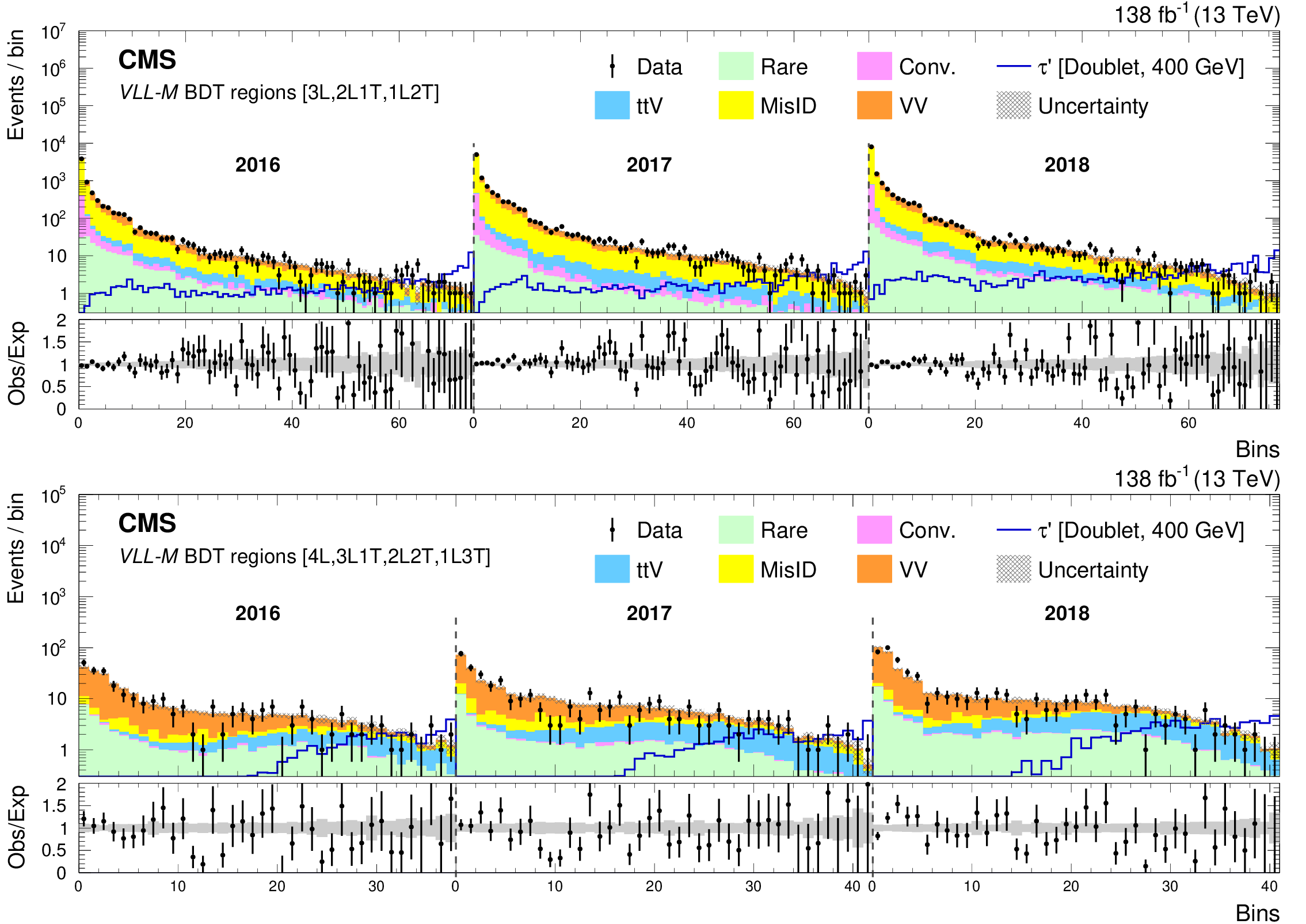
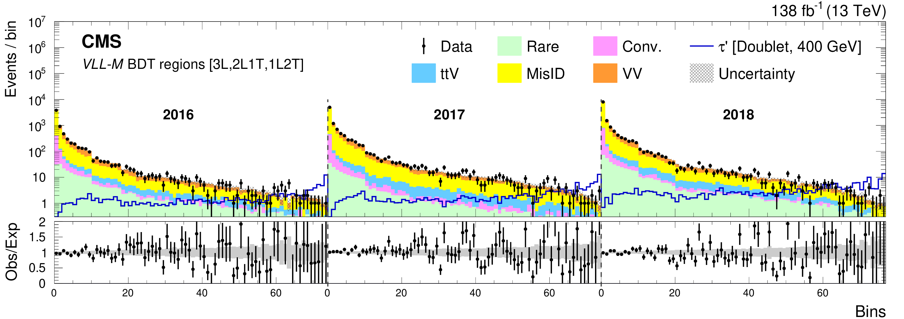
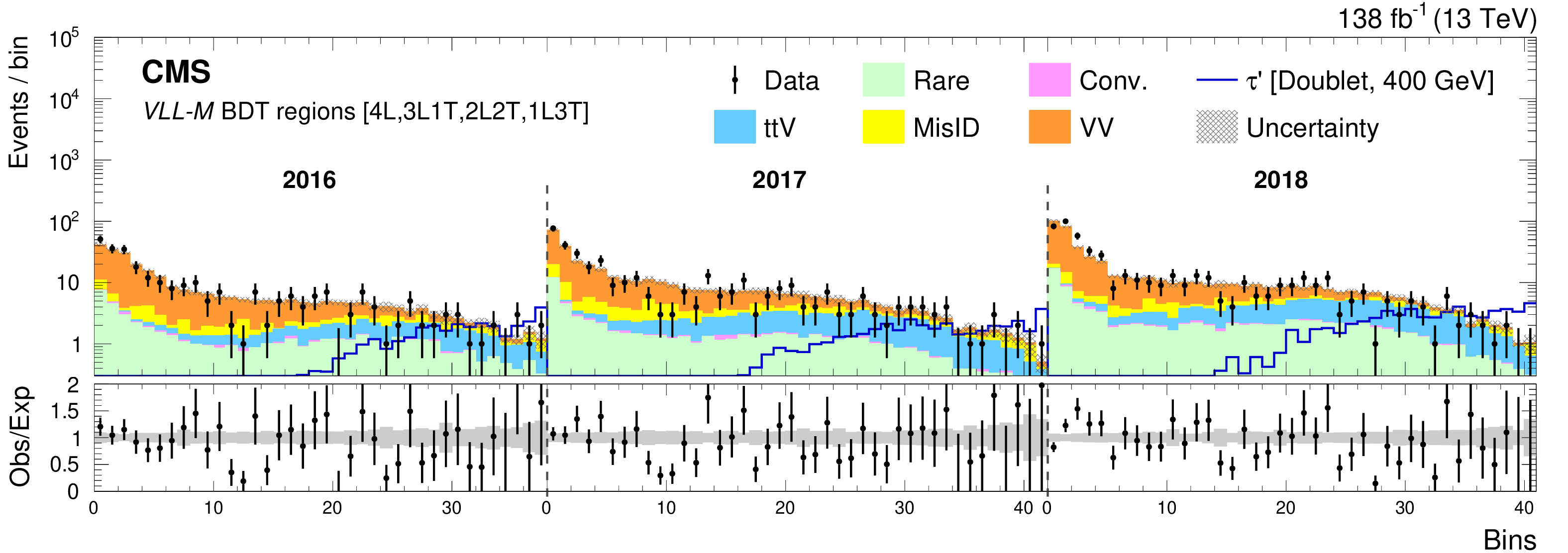
png pdf	Figure 18: The VLL-M BDT regions for the 3-lepton (upper) and 4-lepton (lower) channels for the 2016-2018 data sets. The lower panel shows the ratio of observed events to the total expected background prediction. The gray band on the ratio represents the sum of statistical and systematic uncertainties in the SM background prediction. The expected SM background distributions and the uncertainties are shown after fitting the data under the background-only hypothesis. For illustration, an example signal hypothesis for the production of the vector-like $\tau$ lepton in the doublet scenario for $m_{{\tau ^{\prime}}} = $ 400 GeV, before the fit, is also overlaid.
png pdf	Figure 18-a: The VLL-M BDT regions for the 3-lepton (upper) and 4-lepton (lower) channels for the 2016-2018 data sets. The lower panel shows the ratio of observed events to the total expected background prediction. The gray band on the ratio represents the sum of statistical and systematic uncertainties in the SM background prediction. The expected SM background distributions and the uncertainties are shown after fitting the data under the background-only hypothesis. For illustration, an example signal hypothesis for the production of the vector-like $\tau$ lepton in the doublet scenario for $m_{{\tau ^{\prime}}} = $ 400 GeV, before the fit, is also overlaid.
png pdf	Figure 18-b: The VLL-M BDT regions for the 3-lepton (upper) and 4-lepton (lower) channels for the 2016-2018 data sets. The lower panel shows the ratio of observed events to the total expected background prediction. The gray band on the ratio represents the sum of statistical and systematic uncertainties in the SM background prediction. The expected SM background distributions and the uncertainties are shown after fitting the data under the background-only hypothesis. For illustration, an example signal hypothesis for the production of the vector-like $\tau$ lepton in the doublet scenario for $m_{{\tau ^{\prime}}} = $ 400 GeV, before the fit, is also overlaid.
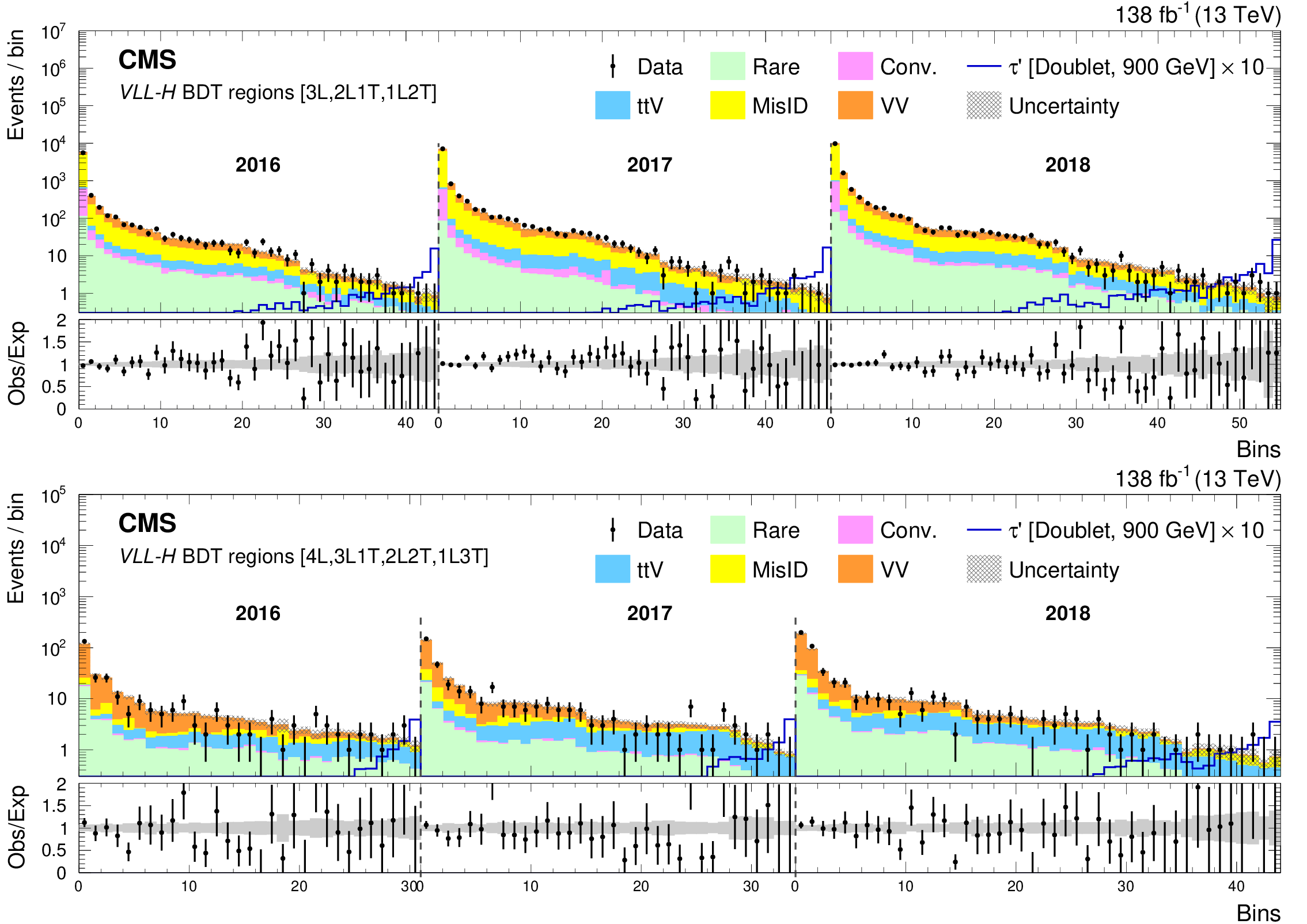
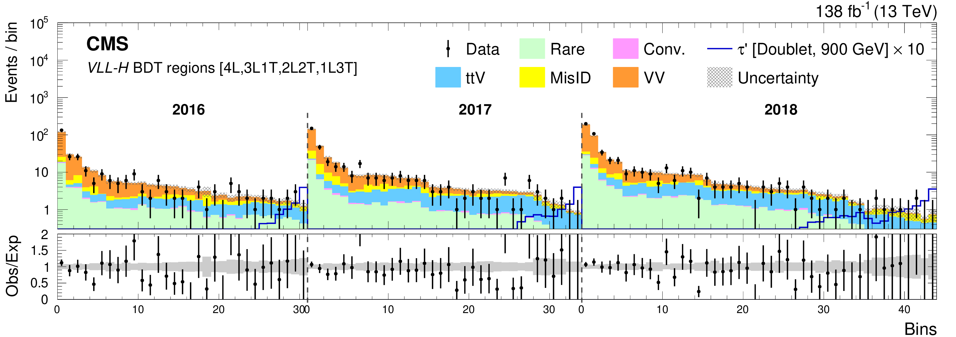
png pdf	Figure 19: The VLL-H BDT regions for the 3-lepton (upper) and 4-lepton (lower) channels for the 2016-2018 data sets. The lower panel shows the ratio of observed events to the total expected background prediction. The gray band on the ratio represents the sum of statistical and systematic uncertainties in the SM background prediction. The expected SM background distributions and the uncertainties are shown after fitting the data under the background-only hypothesis. For illustration, an example signal hypothesis for the production of the vector-like $\tau$ lepton in the doublet scenario for $m_{{\tau ^{\prime}}} = $ 900 GeV, before the fit, is also overlaid.
png pdf	Figure 19-a: The VLL-H BDT regions for the 3-lepton (upper) and 4-lepton (lower) channels for the 2016-2018 data sets. The lower panel shows the ratio of observed events to the total expected background prediction. The gray band on the ratio represents the sum of statistical and systematic uncertainties in the SM background prediction. The expected SM background distributions and the uncertainties are shown after fitting the data under the background-only hypothesis. For illustration, an example signal hypothesis for the production of the vector-like $\tau$ lepton in the doublet scenario for $m_{{\tau ^{\prime}}} = $ 900 GeV, before the fit, is also overlaid.
png pdf	Figure 19-b: The VLL-H BDT regions for the 3-lepton (upper) and 4-lepton (lower) channels for the 2016-2018 data sets. The lower panel shows the ratio of observed events to the total expected background prediction. The gray band on the ratio represents the sum of statistical and systematic uncertainties in the SM background prediction. The expected SM background distributions and the uncertainties are shown after fitting the data under the background-only hypothesis. For illustration, an example signal hypothesis for the production of the vector-like $\tau$ lepton in the doublet scenario for $m_{{\tau ^{\prime}}} = $ 900 GeV, before the fit, is also overlaid.
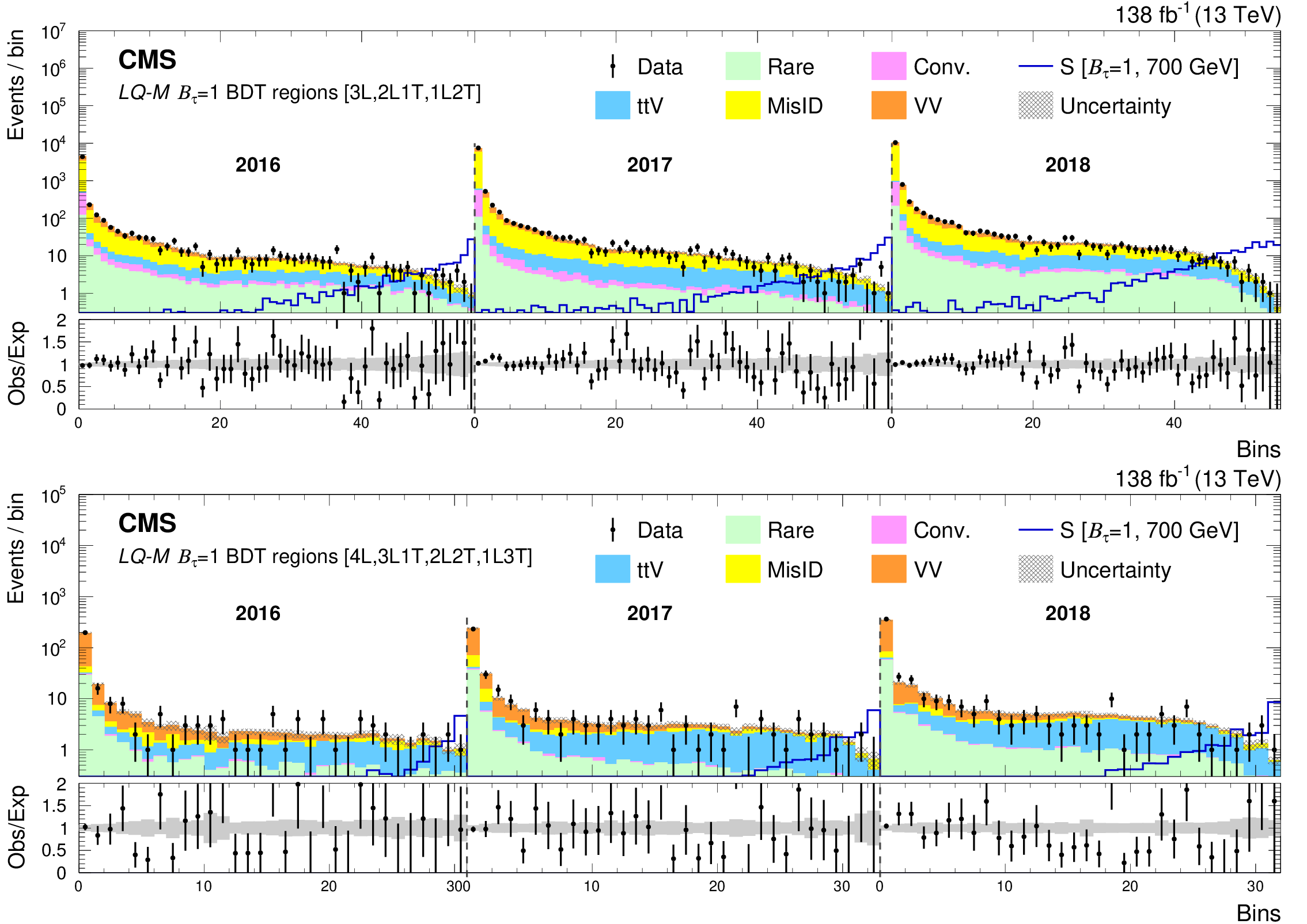
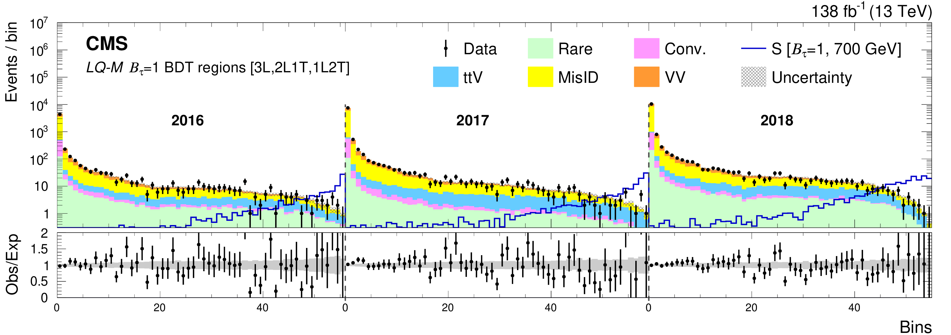
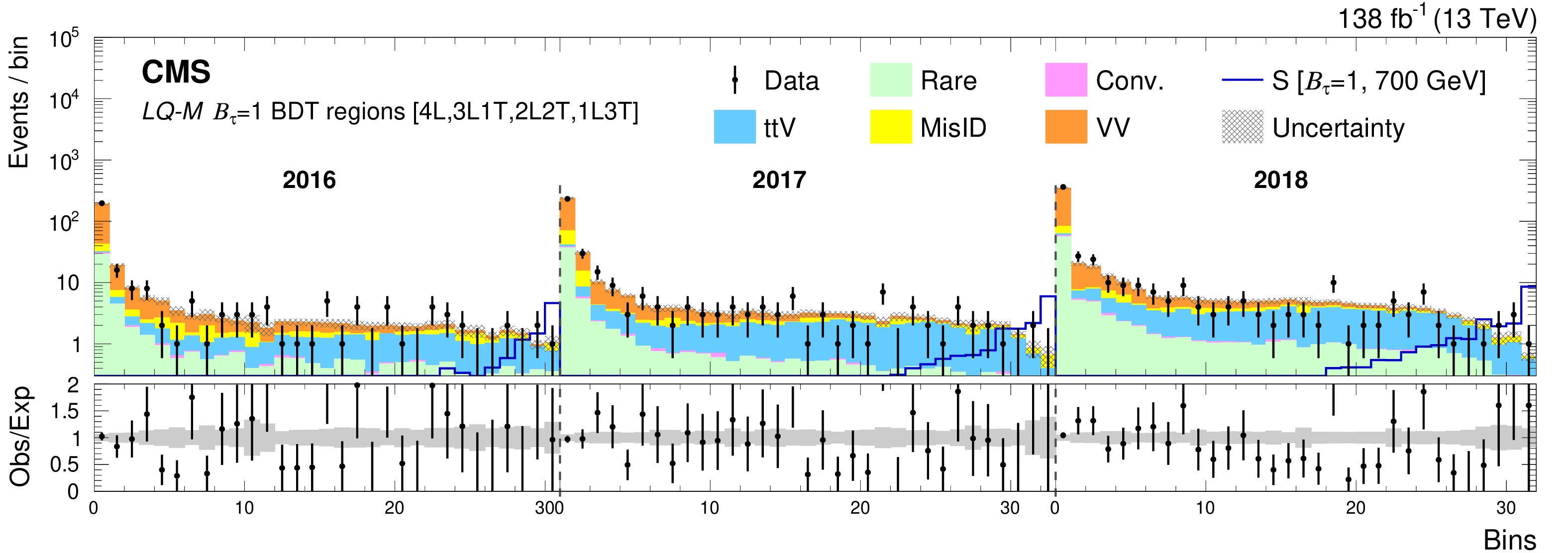
png pdf	Figure 20: The LQ-M $\mathcal {B}_{\tau}=1$ BDT regions for the 3-lepton (upper) and 4-lepton (lower) channels for the 2016-2018 data sets. The lower panel shows the ratio of observed events to the total expected background prediction. The gray band on the ratio represents the sum of statistical and systematic uncertainties in the SM background prediction. The expected SM background distributions and the uncertainties are shown after fitting the data under the background-only hypothesis. For illustration, an example signal hypothesis for the production of the scalar leptoquark coupled to a top quark and a $\tau$ lepton for $m_{\mathrm{S}} = $ 700 GeV, before the fit, is also overlaid.
png pdf	Figure 20-a: The LQ-M $\mathcal {B}_{\tau}=1$ BDT regions for the 3-lepton (upper) and 4-lepton (lower) channels for the 2016-2018 data sets. The lower panel shows the ratio of observed events to the total expected background prediction. The gray band on the ratio represents the sum of statistical and systematic uncertainties in the SM background prediction. The expected SM background distributions and the uncertainties are shown after fitting the data under the background-only hypothesis. For illustration, an example signal hypothesis for the production of the scalar leptoquark coupled to a top quark and a $\tau$ lepton for $m_{\mathrm{S}} = $ 700 GeV, before the fit, is also overlaid.
png pdf	Figure 20-b: The LQ-M $\mathcal {B}_{\tau}=1$ BDT regions for the 3-lepton (upper) and 4-lepton (lower) channels for the 2016-2018 data sets. The lower panel shows the ratio of observed events to the total expected background prediction. The gray band on the ratio represents the sum of statistical and systematic uncertainties in the SM background prediction. The expected SM background distributions and the uncertainties are shown after fitting the data under the background-only hypothesis. For illustration, an example signal hypothesis for the production of the scalar leptoquark coupled to a top quark and a $\tau$ lepton for $m_{\mathrm{S}} = $ 700 GeV, before the fit, is also overlaid.
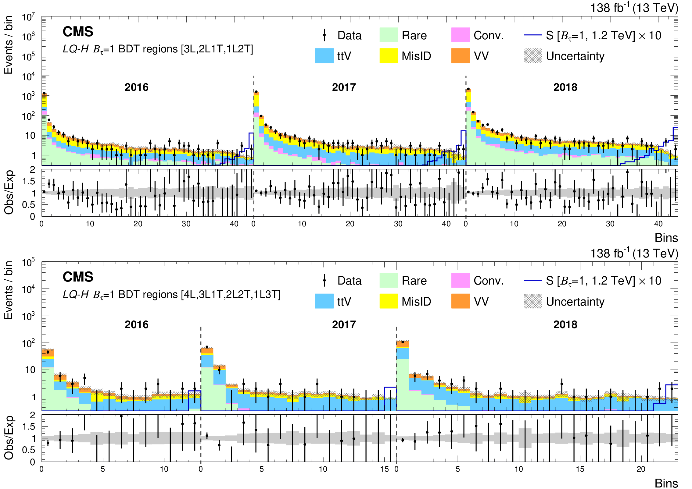
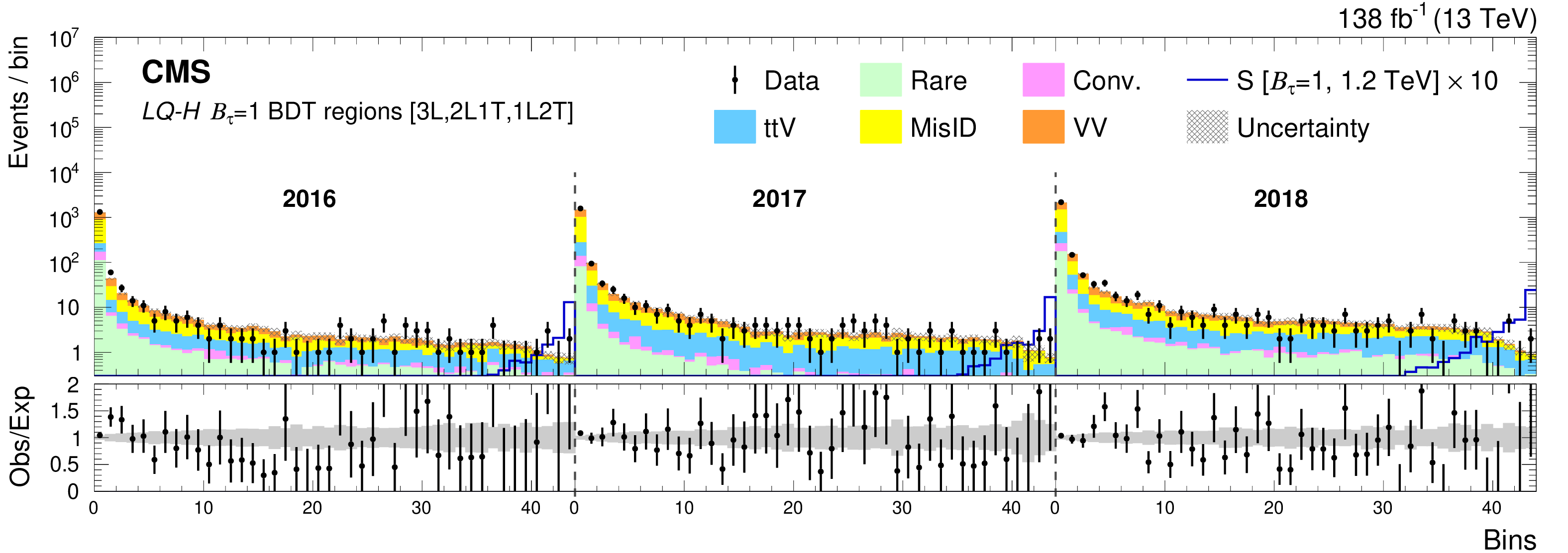
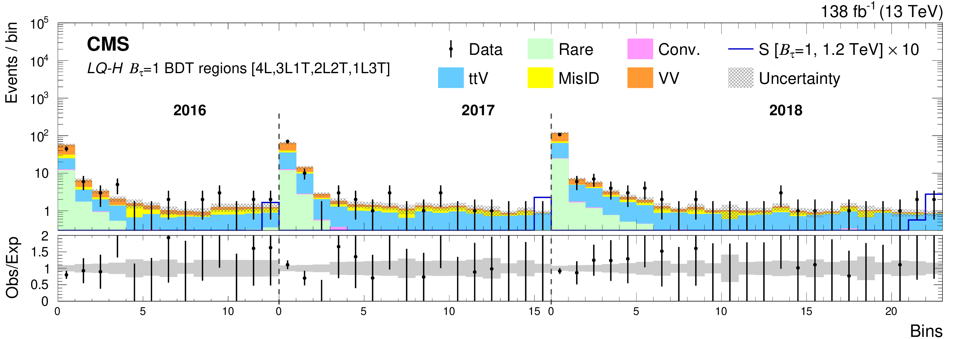
png pdf	Figure 21: The LQ-H $\mathcal {B}_{\tau}=1$ BDT regions for the 3-lepton (upper) and 4-lepton (lower) channels for the 2016-2018 data sets. The lower panel shows the ratio of observed events to the total expected background prediction. The gray band on the ratio represents the sum of statistical and systematic uncertainties in the SM background prediction. The expected SM background distributions and the uncertainties are shown after fitting the data under the background-only hypothesis. For illustration, an example signal hypothesis for the production of the scalar leptoquark coupled to a top quark and a $\tau$ lepton for $m_{\mathrm{S}} = $ 1.2 TeV, before the fit, is also overlaid.
png pdf	Figure 21-a: The LQ-H $\mathcal {B}_{\tau}=1$ BDT regions for the 3-lepton (upper) and 4-lepton (lower) channels for the 2016-2018 data sets. The lower panel shows the ratio of observed events to the total expected background prediction. The gray band on the ratio represents the sum of statistical and systematic uncertainties in the SM background prediction. The expected SM background distributions and the uncertainties are shown after fitting the data under the background-only hypothesis. For illustration, an example signal hypothesis for the production of the scalar leptoquark coupled to a top quark and a $\tau$ lepton for $m_{\mathrm{S}} = $ 1.2 TeV, before the fit, is also overlaid.
png pdf	Figure 21-b: The LQ-H $\mathcal {B}_{\tau}=1$ BDT regions for the 3-lepton (upper) and 4-lepton (lower) channels for the 2016-2018 data sets. The lower panel shows the ratio of observed events to the total expected background prediction. The gray band on the ratio represents the sum of statistical and systematic uncertainties in the SM background prediction. The expected SM background distributions and the uncertainties are shown after fitting the data under the background-only hypothesis. For illustration, an example signal hypothesis for the production of the scalar leptoquark coupled to a top quark and a $\tau$ lepton for $m_{\mathrm{S}} = $ 1.2 TeV, before the fit, is also overlaid.
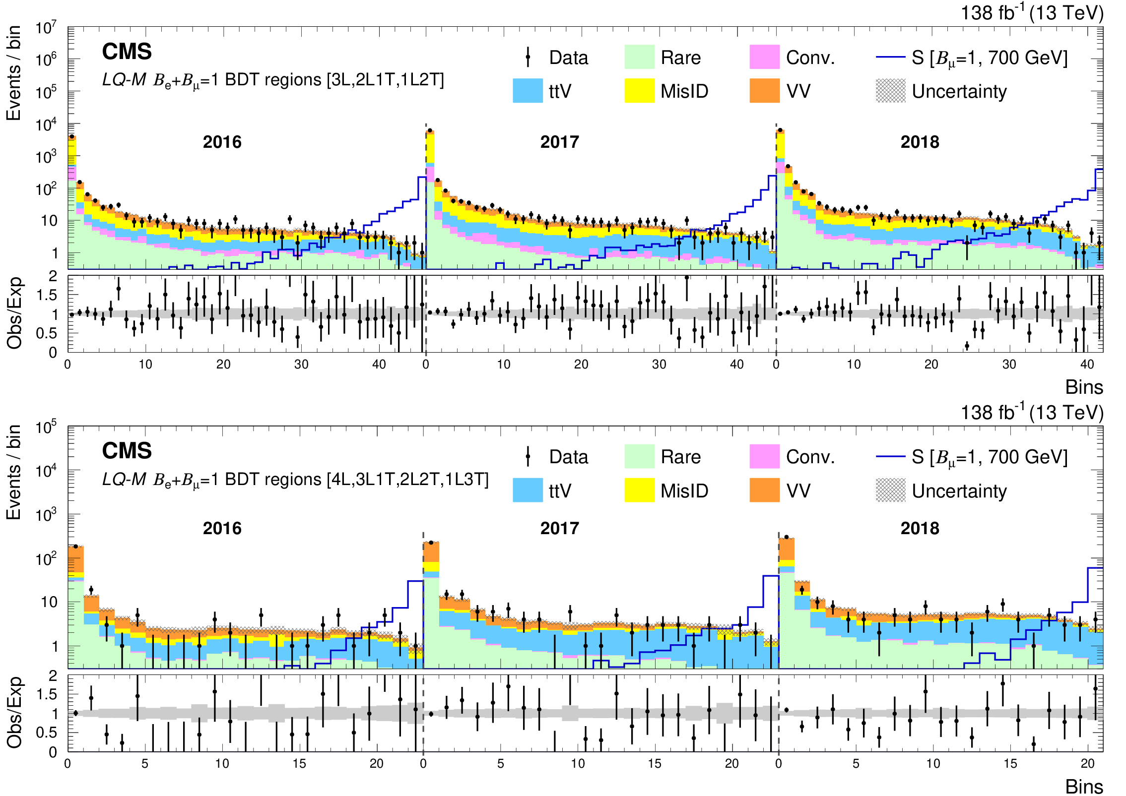
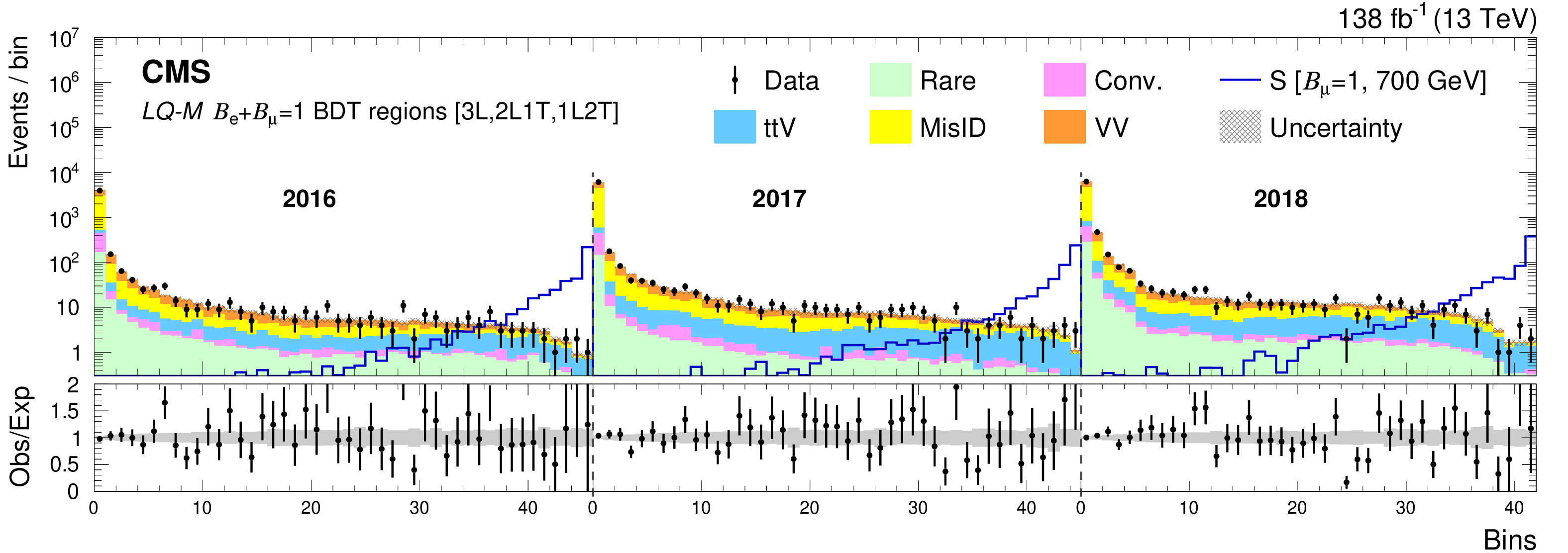
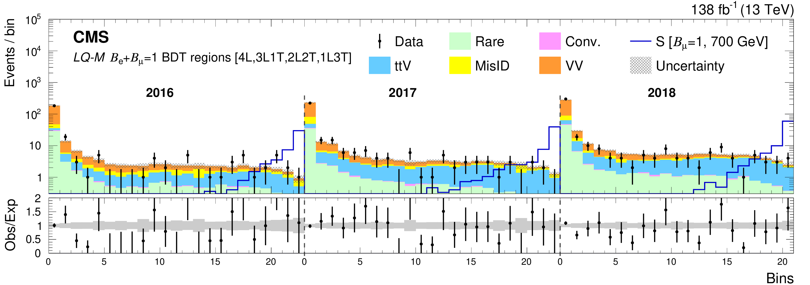
png pdf	Figure 22: The LQ-M $\mathcal {B}_{\mathrm{e}}+\mathcal {B}_{\mu}=1$ BDT regions for the 3-lepton (upper) and 4-lepton (lower) channels for the 2016-2018 data sets. The lower panel shows the ratio of observed events to the total expected background prediction. The gray band on the ratio represents the sum of statistical and systematic uncertainties in the SM background prediction. The expected SM background distributions and the uncertainties are shown after fitting the data under the background-only hypothesis. For illustration, an example signal hypothesis for the production of the scalar leptoquark coupled to a top quark and a muon for $m_{\mathrm{S}} = $ 700 GeV, before the fit, is also overlaid.
png pdf	Figure 22-a: The LQ-M $\mathcal {B}_{\mathrm{e}}+\mathcal {B}_{\mu}=1$ BDT regions for the 3-lepton (upper) and 4-lepton (lower) channels for the 2016-2018 data sets. The lower panel shows the ratio of observed events to the total expected background prediction. The gray band on the ratio represents the sum of statistical and systematic uncertainties in the SM background prediction. The expected SM background distributions and the uncertainties are shown after fitting the data under the background-only hypothesis. For illustration, an example signal hypothesis for the production of the scalar leptoquark coupled to a top quark and a muon for $m_{\mathrm{S}} = $ 700 GeV, before the fit, is also overlaid.
png pdf	Figure 22-b: The LQ-M $\mathcal {B}_{\mathrm{e}}+\mathcal {B}_{\mu}=1$ BDT regions for the 3-lepton (upper) and 4-lepton (lower) channels for the 2016-2018 data sets. The lower panel shows the ratio of observed events to the total expected background prediction. The gray band on the ratio represents the sum of statistical and systematic uncertainties in the SM background prediction. The expected SM background distributions and the uncertainties are shown after fitting the data under the background-only hypothesis. For illustration, an example signal hypothesis for the production of the scalar leptoquark coupled to a top quark and a muon for $m_{\mathrm{S}} = $ 700 GeV, before the fit, is also overlaid.
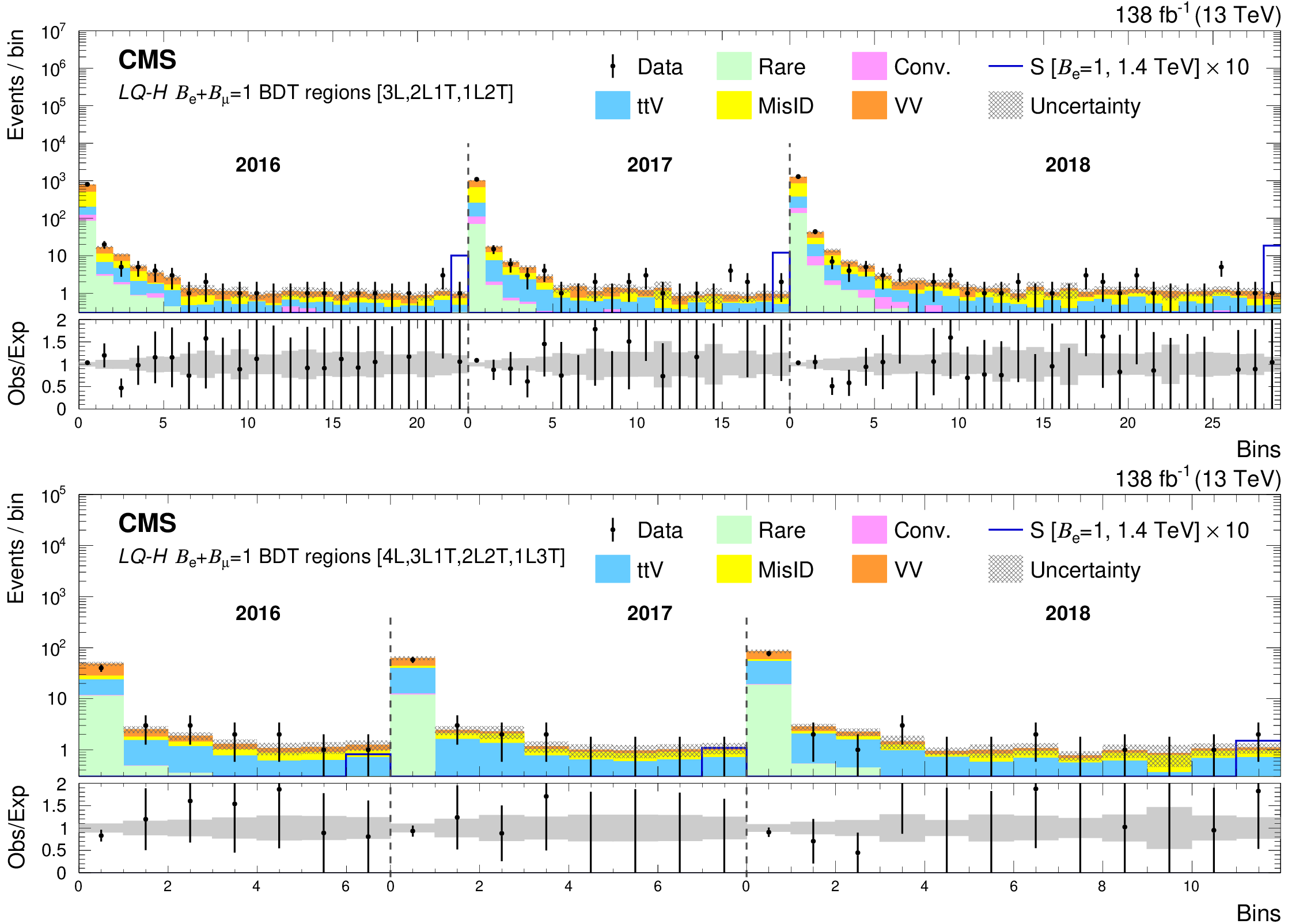
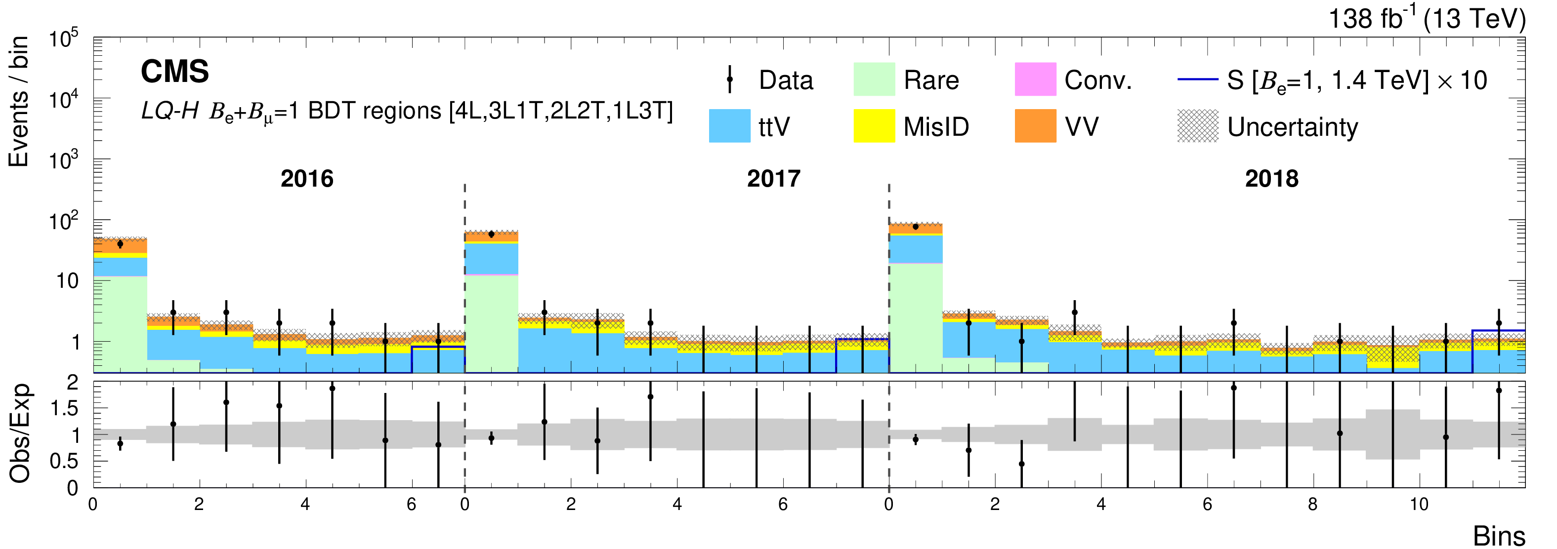
png pdf	Figure 23: The LQ-H $\mathcal {B}_{\mathrm{e}}+\mathcal {B}_{\mu}=1$ BDT regions for the 3-lepton (upper) and 4-lepton (lower) channels for the 2016-2018 data sets. The lower panel shows the ratio of observed events to the total expected background prediction. The gray band on the ratio represents the sum of statistical and systematic uncertainties in the SM background prediction. The expected SM background distributions and the uncertainties are shown after fitting the data under the background-only hypothesis. For illustration, an example signal hypothesis for the production of the scalar leptoquark coupled to a top quark and an electron for $m_{\mathrm{S}} = $ 1.4 TeV, before the fit, is also overlaid.
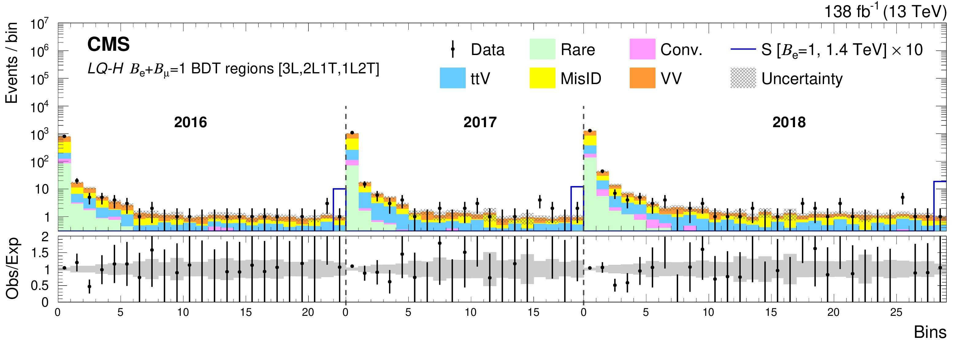
png pdf	Figure 23-a: The LQ-H $\mathcal {B}_{\mathrm{e}}+\mathcal {B}_{\mu}=1$ BDT regions for the 3-lepton (upper) and 4-lepton (lower) channels for the 2016-2018 data sets. The lower panel shows the ratio of observed events to the total expected background prediction. The gray band on the ratio represents the sum of statistical and systematic uncertainties in the SM background prediction. The expected SM background distributions and the uncertainties are shown after fitting the data under the background-only hypothesis. For illustration, an example signal hypothesis for the production of the scalar leptoquark coupled to a top quark and an electron for $m_{\mathrm{S}} = $ 1.4 TeV, before the fit, is also overlaid.
png pdf	Figure 23-b: The LQ-H $\mathcal {B}_{\mathrm{e}}+\mathcal {B}_{\mu}=1$ BDT regions for the 3-lepton (upper) and 4-lepton (lower) channels for the 2016-2018 data sets. The lower panel shows the ratio of observed events to the total expected background prediction. The gray band on the ratio represents the sum of statistical and systematic uncertainties in the SM background prediction. The expected SM background distributions and the uncertainties are shown after fitting the data under the background-only hypothesis. For illustration, an example signal hypothesis for the production of the scalar leptoquark coupled to a top quark and an electron for $m_{\mathrm{S}} = $ 1.4 TeV, before the fit, is also overlaid.
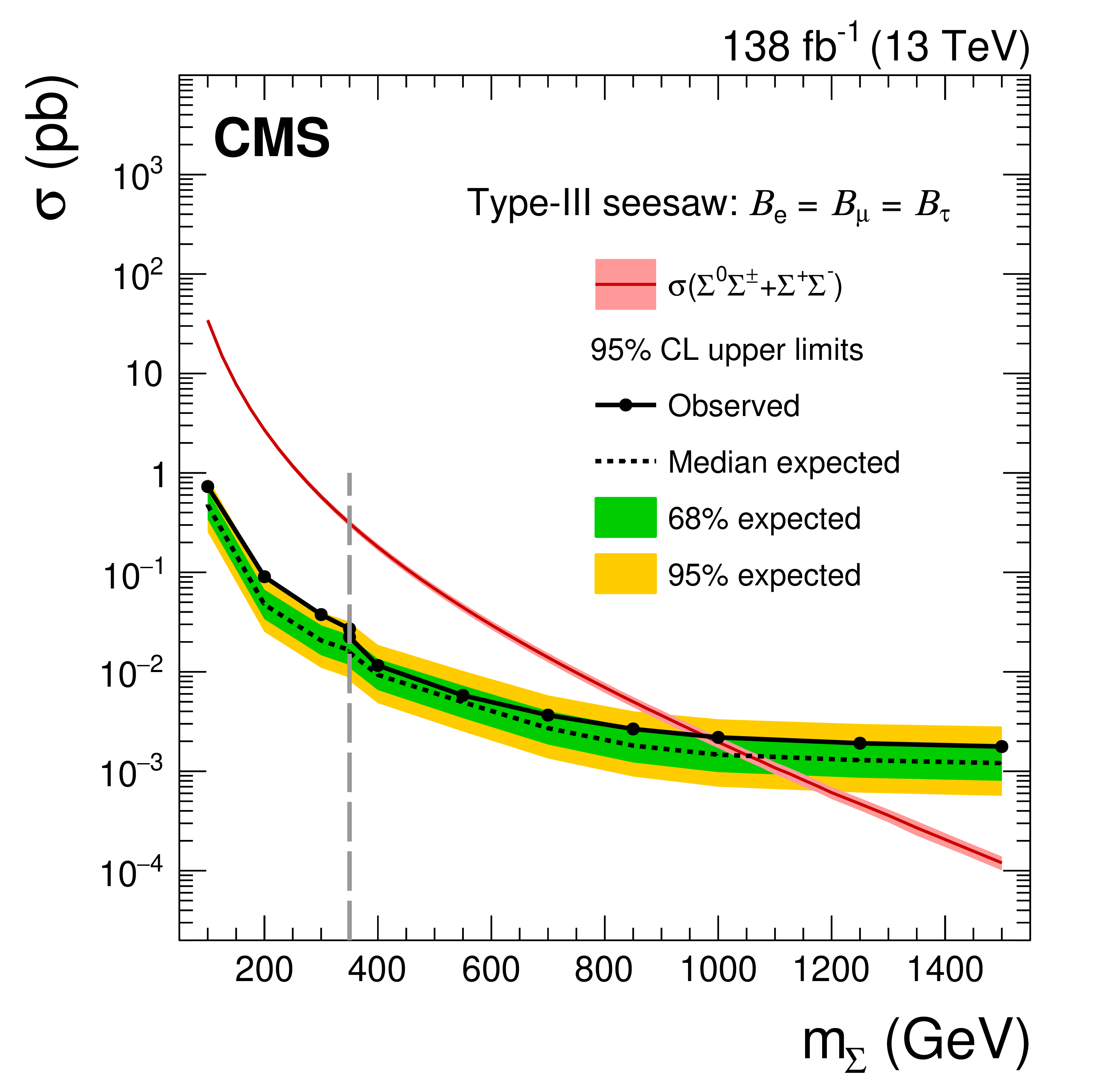
png pdf	Figure 24: Observed and expected upper limits at 95% CL on the production cross section for the type-III seesaw fermions in the flavor-democratic scenario using the table schemes and the BDT regions of the SS-M and the SS-H $\mathcal {B}_{\mathrm{e}}=\mathcal {B}_{\mu}=\mathcal {B}_{\tau}$ BDTs. To the left of the vertical dashed gray line, the limits are shown from the advanced ${S_{\mathrm {T}}}$ table, and to the right the limits are shown from the BDT regions.
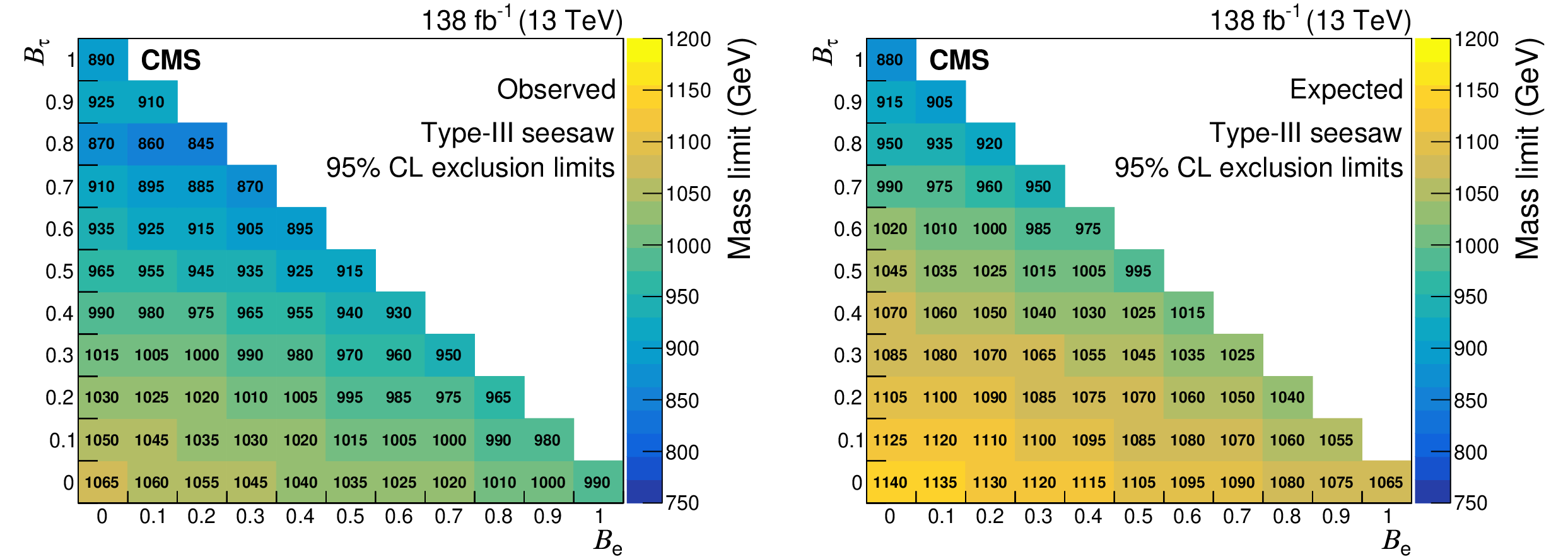
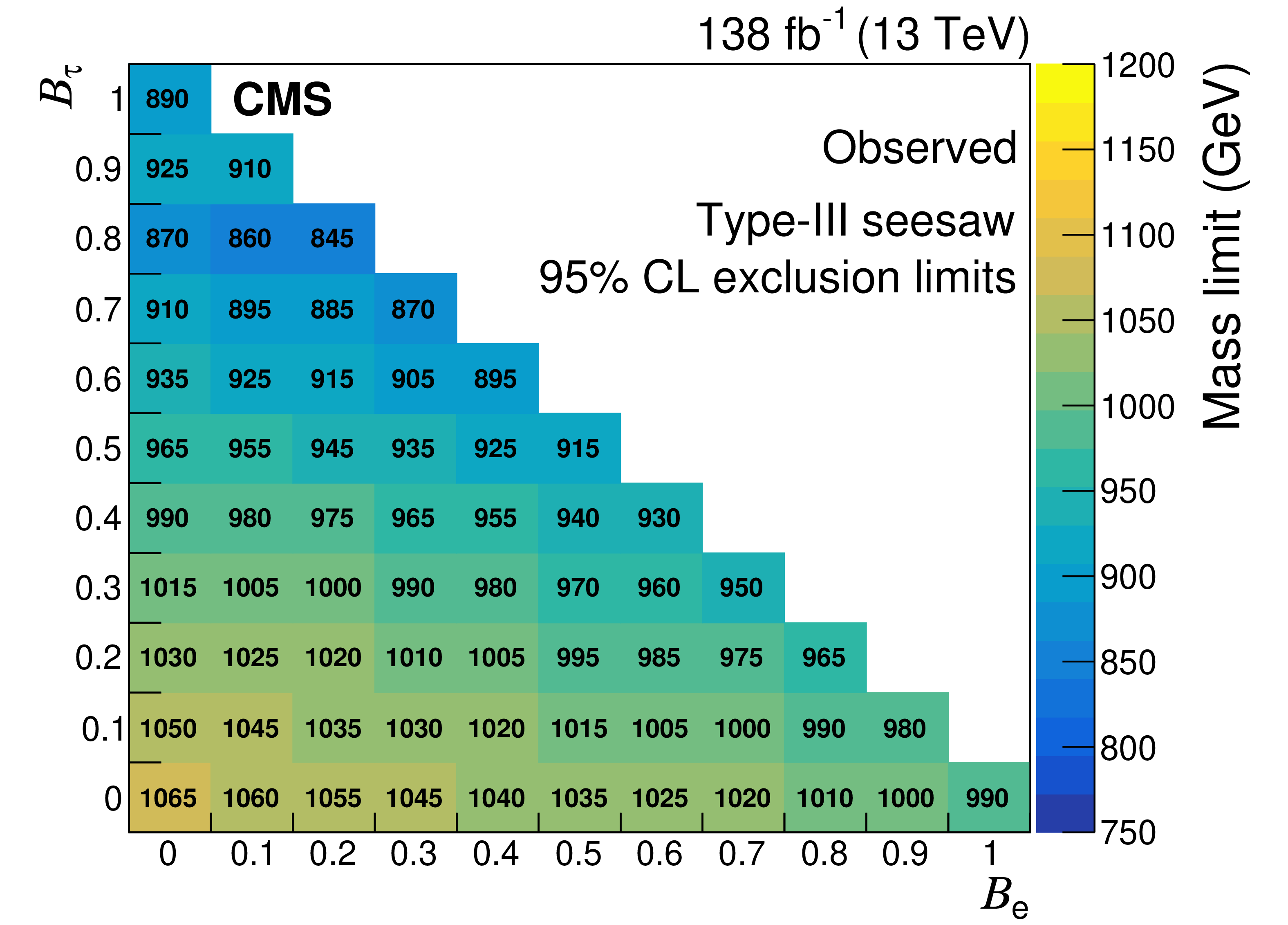
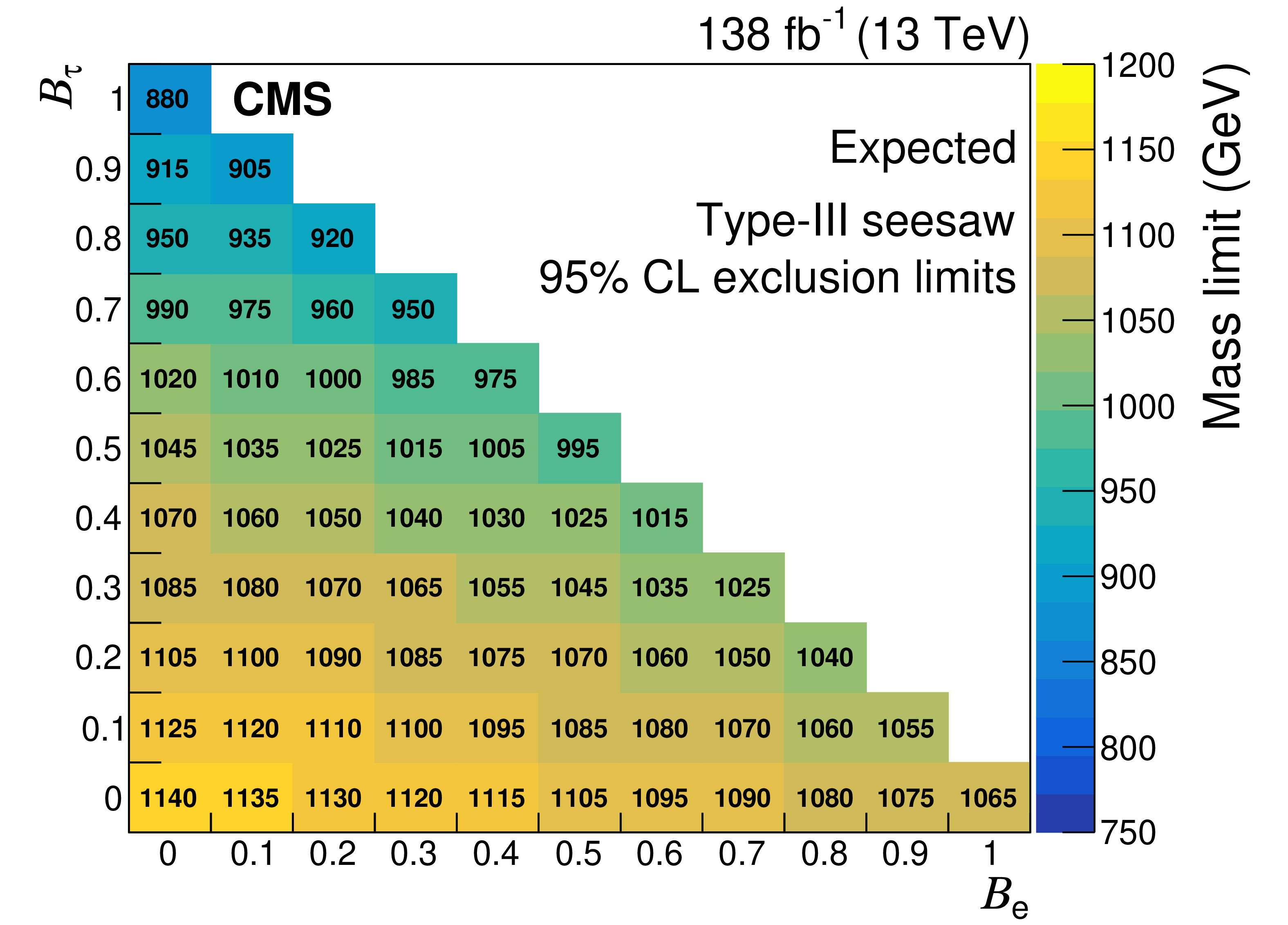
png pdf	Figure 25: Observed (left) and expected (right) lower limits at 95% CL on the mass of the type-III seesaw fermions in the plane defined by $\mathcal {B}_{\mathrm{e}}$ and $\mathcal {B}_{\tau}$, with the constraint that $\mathcal {B}_{\mathrm{e}} + \mathcal {B}_{\mu} + \mathcal {B}_{\tau}=$ 1. These limits arise from the SS-H $\mathcal {B}_{\tau}=$ 1 BDT when $\mathcal {B}_{\tau} \ge $ 0.9, and by the SS-H $\mathcal {B}_{\mathrm{e}}=\mathcal {B}_{\mu}=\mathcal {B}_{\tau}$ BDT for the other decay branching fraction combinations.
png pdf	Figure 25-a: Observed (left) and expected (right) lower limits at 95% CL on the mass of the type-III seesaw fermions in the plane defined by $\mathcal {B}_{\mathrm{e}}$ and $\mathcal {B}_{\tau}$, with the constraint that $\mathcal {B}_{\mathrm{e}} + \mathcal {B}_{\mu} + \mathcal {B}_{\tau}=$ 1. These limits arise from the SS-H $\mathcal {B}_{\tau}=$ 1 BDT when $\mathcal {B}_{\tau} \ge $ 0.9, and by the SS-H $\mathcal {B}_{\mathrm{e}}=\mathcal {B}_{\mu}=\mathcal {B}_{\tau}$ BDT for the other decay branching fraction combinations.
png pdf	Figure 25-b: Observed (left) and expected (right) lower limits at 95% CL on the mass of the type-III seesaw fermions in the plane defined by $\mathcal {B}_{\mathrm{e}}$ and $\mathcal {B}_{\tau}$, with the constraint that $\mathcal {B}_{\mathrm{e}} + \mathcal {B}_{\mu} + \mathcal {B}_{\tau}=$ 1. These limits arise from the SS-H $\mathcal {B}_{\tau}=$ 1 BDT when $\mathcal {B}_{\tau} \ge $ 0.9, and by the SS-H $\mathcal {B}_{\mathrm{e}}=\mathcal {B}_{\mu}=\mathcal {B}_{\tau}$ BDT for the other decay branching fraction combinations.
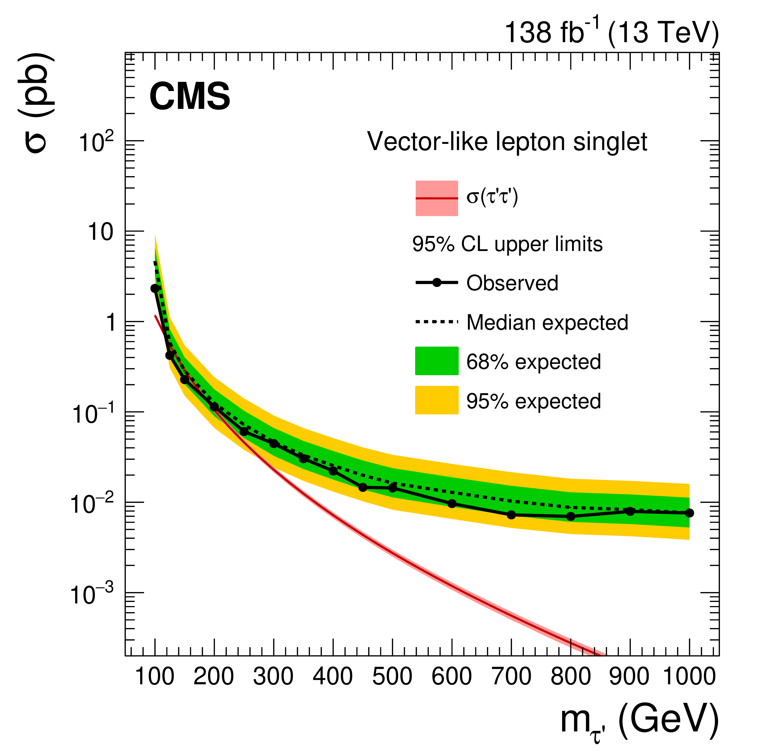
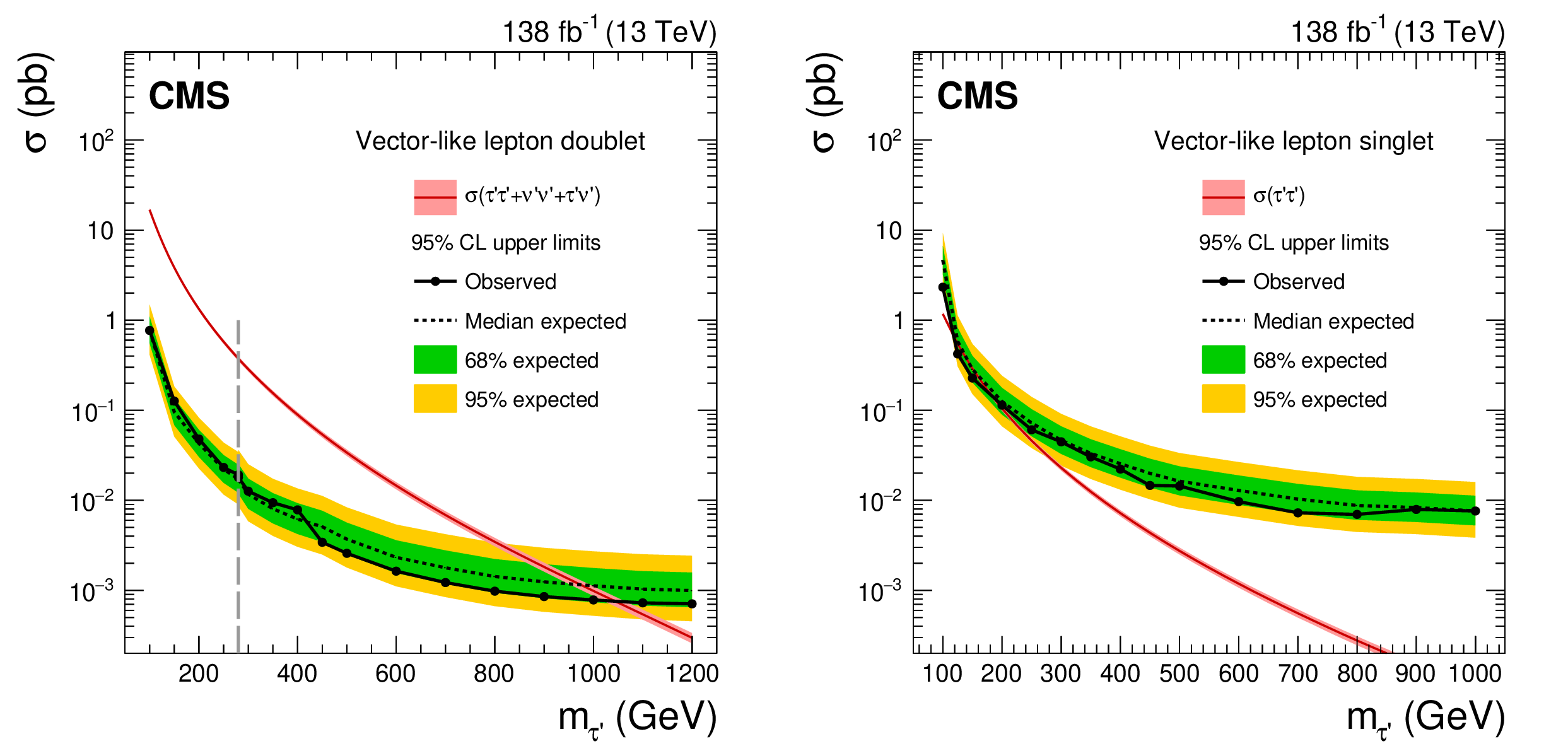
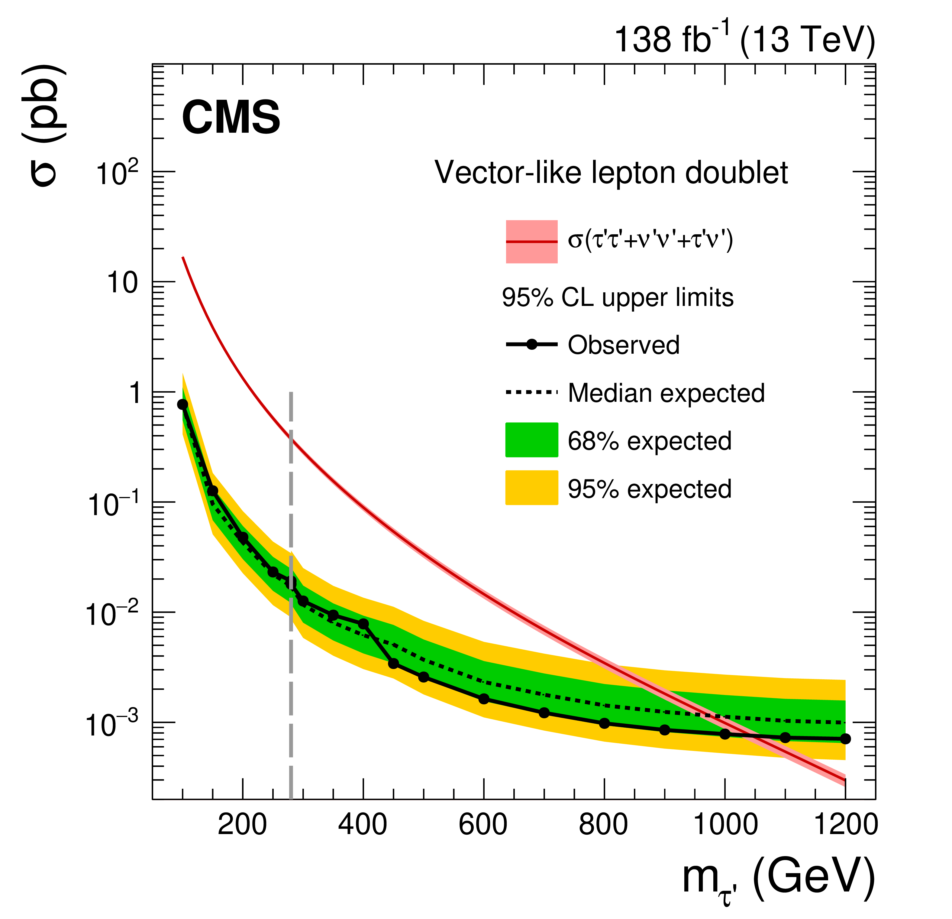
png pdf	Figure 26: Observed and expected upper limits at 95% CL on the production cross section for the vector-like $\tau$ leptons: doublet model (left), and singlet model (right). For the doublet vector-like lepton model, to the left of the vertical dashed gray line, the limits are shown from the advanced ${S_{\mathrm {T}}}$ table, while to the right the limits are shown from the BDT regions. For the singlet vector-like lepton model, the limit is shown from the advanced ${S_{\mathrm {T}}}$ table for all masses.
png pdf	Figure 26-a: Observed and expected upper limits at 95% CL on the production cross section for the vector-like $\tau$ leptons: doublet model (left), and singlet model (right). For the doublet vector-like lepton model, to the left of the vertical dashed gray line, the limits are shown from the advanced ${S_{\mathrm {T}}}$ table, while to the right the limits are shown from the BDT regions. For the singlet vector-like lepton model, the limit is shown from the advanced ${S_{\mathrm {T}}}$ table for all masses.
png pdf	Figure 26-b: Observed and expected upper limits at 95% CL on the production cross section for the vector-like $\tau$ leptons: doublet model (left), and singlet model (right). For the doublet vector-like lepton model, to the left of the vertical dashed gray line, the limits are shown from the advanced ${S_{\mathrm {T}}}$ table, while to the right the limits are shown from the BDT regions. For the singlet vector-like lepton model, the limit is shown from the advanced ${S_{\mathrm {T}}}$ table for all masses.
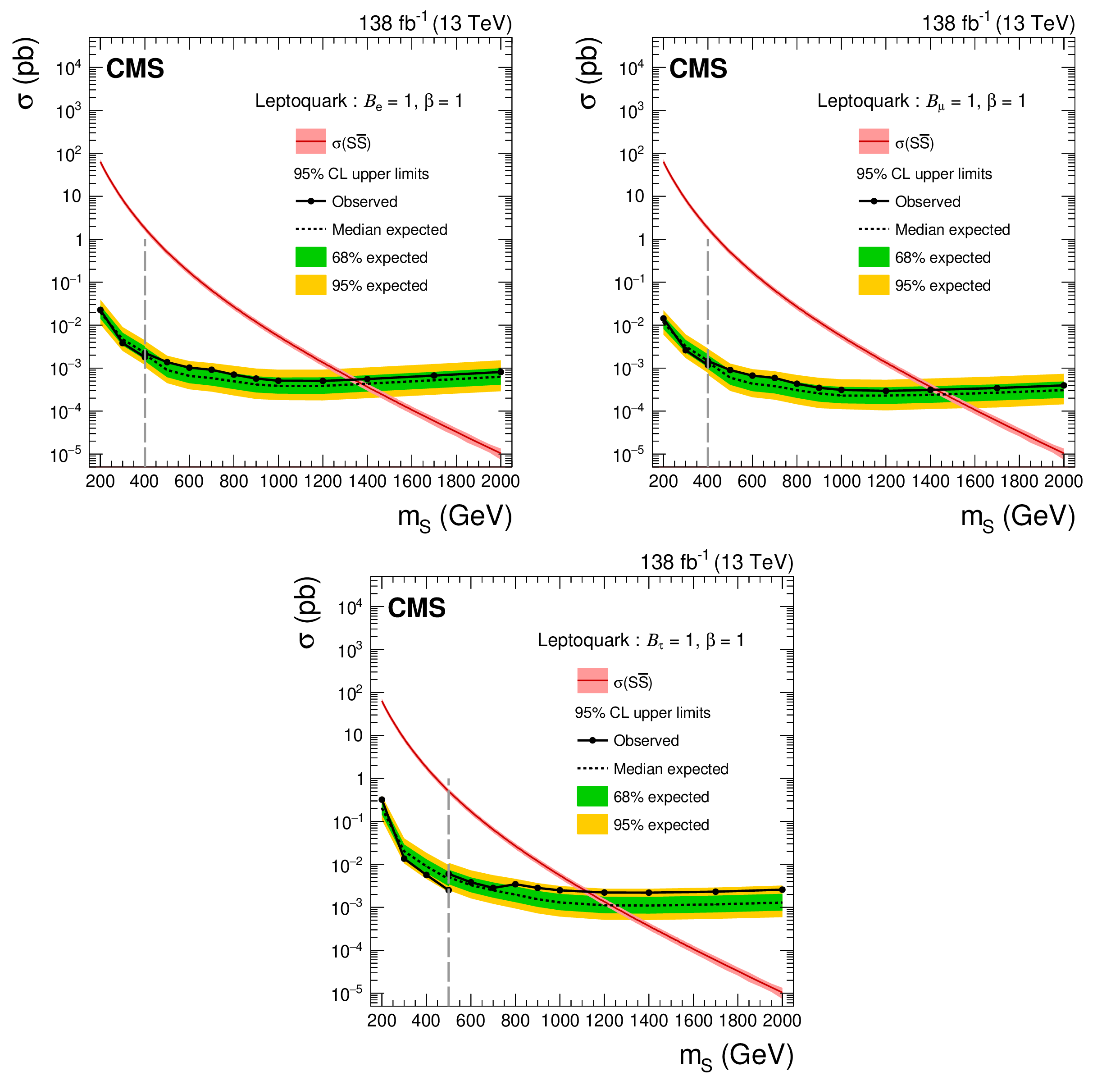
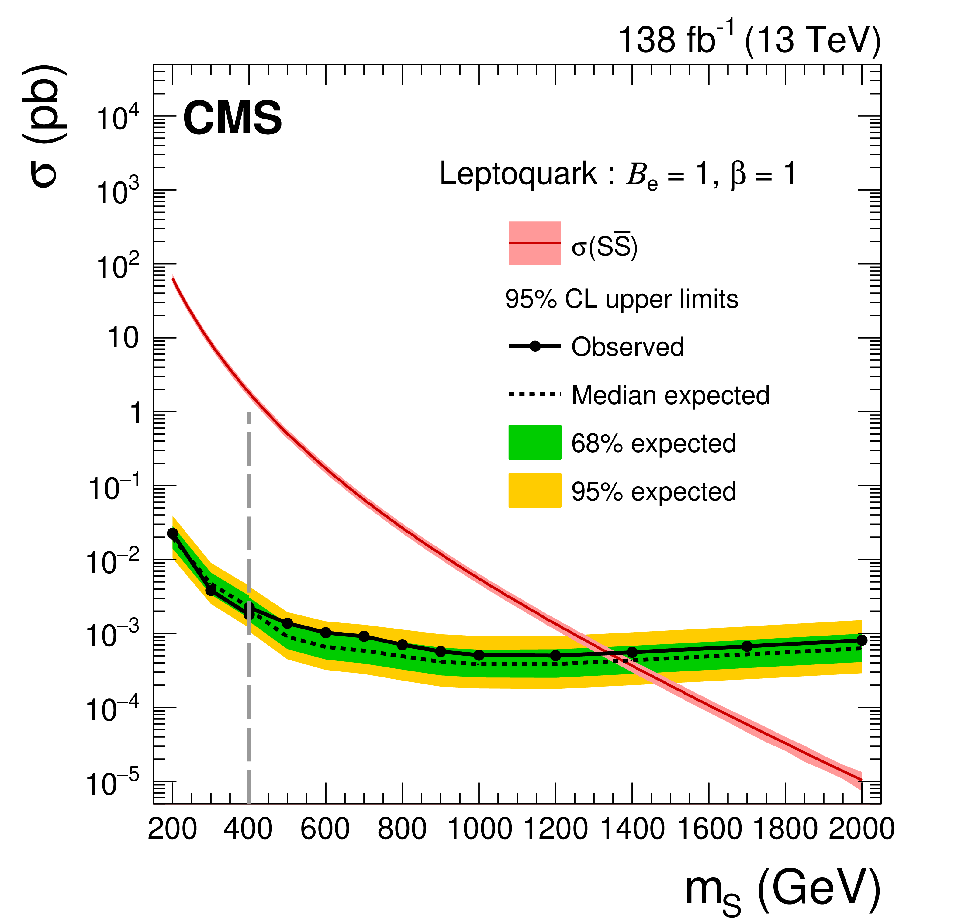
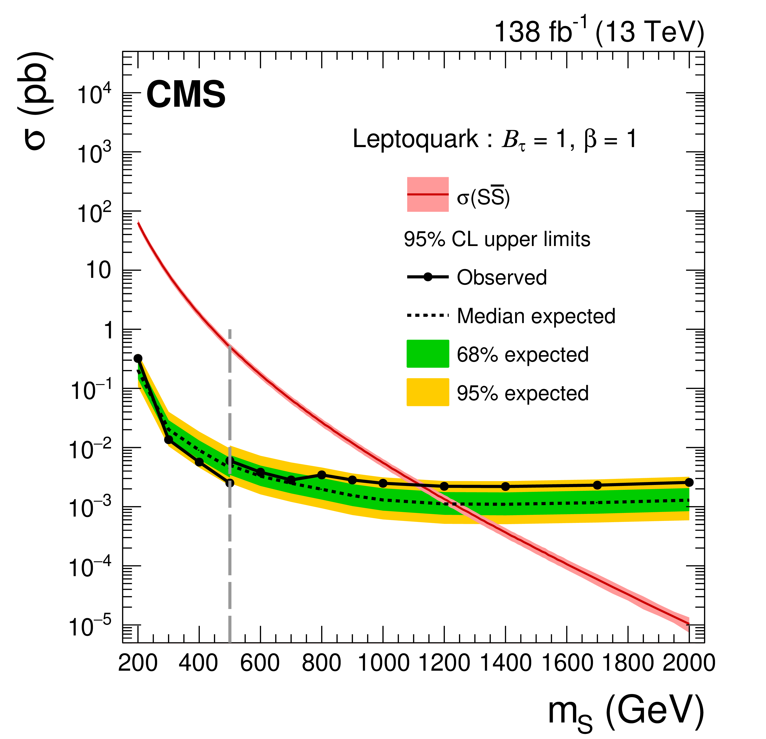
png pdf	Figure 27: Observed and expected upper limits at 95% CL on the production cross section for the scalar leptoquarks: $\mathcal {B}_{\mathrm{e}}=$ 1 (upper left), $\mathcal {B}_{\mu}=$ 1 (upper right), and $\mathcal {B}_{\tau}=$ 1 (lower). In each figure, the limits to the left of the vertical dashed gray line are shown from the advanced ${S_{\mathrm {T}}}$ table, and to the right are shown from the BDT regions.
png pdf	Figure 27-a: Observed and expected upper limits at 95% CL on the production cross section for the scalar leptoquarks: $\mathcal {B}_{\mathrm{e}}=$ 1 (upper left), $\mathcal {B}_{\mu}=$ 1 (upper right), and $\mathcal {B}_{\tau}=$ 1 (lower). In each figure, the limits to the left of the vertical dashed gray line are shown from the advanced ${S_{\mathrm {T}}}$ table, and to the right are shown from the BDT regions.
png pdf	Figure 27-b: Observed and expected upper limits at 95% CL on the production cross section for the scalar leptoquarks: $\mathcal {B}_{\mathrm{e}}=$ 1 (upper left), $\mathcal {B}_{\mu}=$ 1 (upper right), and $\mathcal {B}_{\tau}=$ 1 (lower). In each figure, the limits to the left of the vertical dashed gray line are shown from the advanced ${S_{\mathrm {T}}}$ table, and to the right are shown from the BDT regions.
png pdf	Figure 27-c: Observed and expected upper limits at 95% CL on the production cross section for the scalar leptoquarks: $\mathcal {B}_{\mathrm{e}}=$ 1 (upper left), $\mathcal {B}_{\mu}=$ 1 (upper right), and $\mathcal {B}_{\tau}=$ 1 (lower). In each figure, the limits to the left of the vertical dashed gray line are shown from the advanced ${S_{\mathrm {T}}}$ table, and to the right are shown from the BDT regions.

Tables
png pdf	Table 1: A summary of control regions for the irreducible SM processes Z$ \gamma $, WZ, $ {{\mathrm{t} {}\mathrm{\bar{t}}} }$Z, and ZZ, and for the misidentified lepton backgrounds. The ${{p_{\mathrm {T}}} ^\text {miss}}$, ${M_{\mathrm {T}}}$, the minimum 3L lepton ${p_{\mathrm {T}}}$ (${p_{\mathrm {T}}} ^{\mathrm {3}}$), and ${S_{\mathrm {T}}}$ are in units of GeV. The 3L OnZ CR is further split into 3L MisID e/$\mu $ CR, 3L WZ CR, and 3L $ {{\mathrm{t} {}\mathrm{\bar{t}}} }$Z CR.
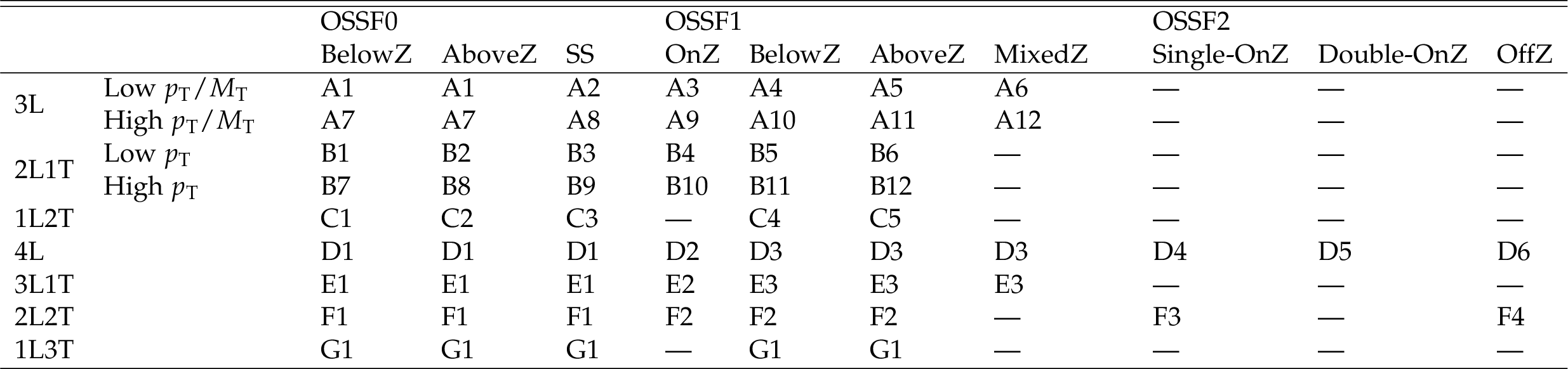
png pdf	Table 2: Fundamental scheme of event categorization, as a function of lepton charge combinations and mass variables. The mass categorizations refer to masses of OSSF pairs if present, and of OSDF pairs otherwise, as explained in the text. For categorization purposes, all possible opposite-sign dielectron and dimuon pair masses in the event are considered, whereas only the largest mass in the event is considered for all other opposite-sign pairs. Only the dielectron and dimuon pairs are considered to tag events as OnZ. The 1L3T OSSF0 and OSSF1 events are combined into a single category. Disallowed categories are marked with "--''.
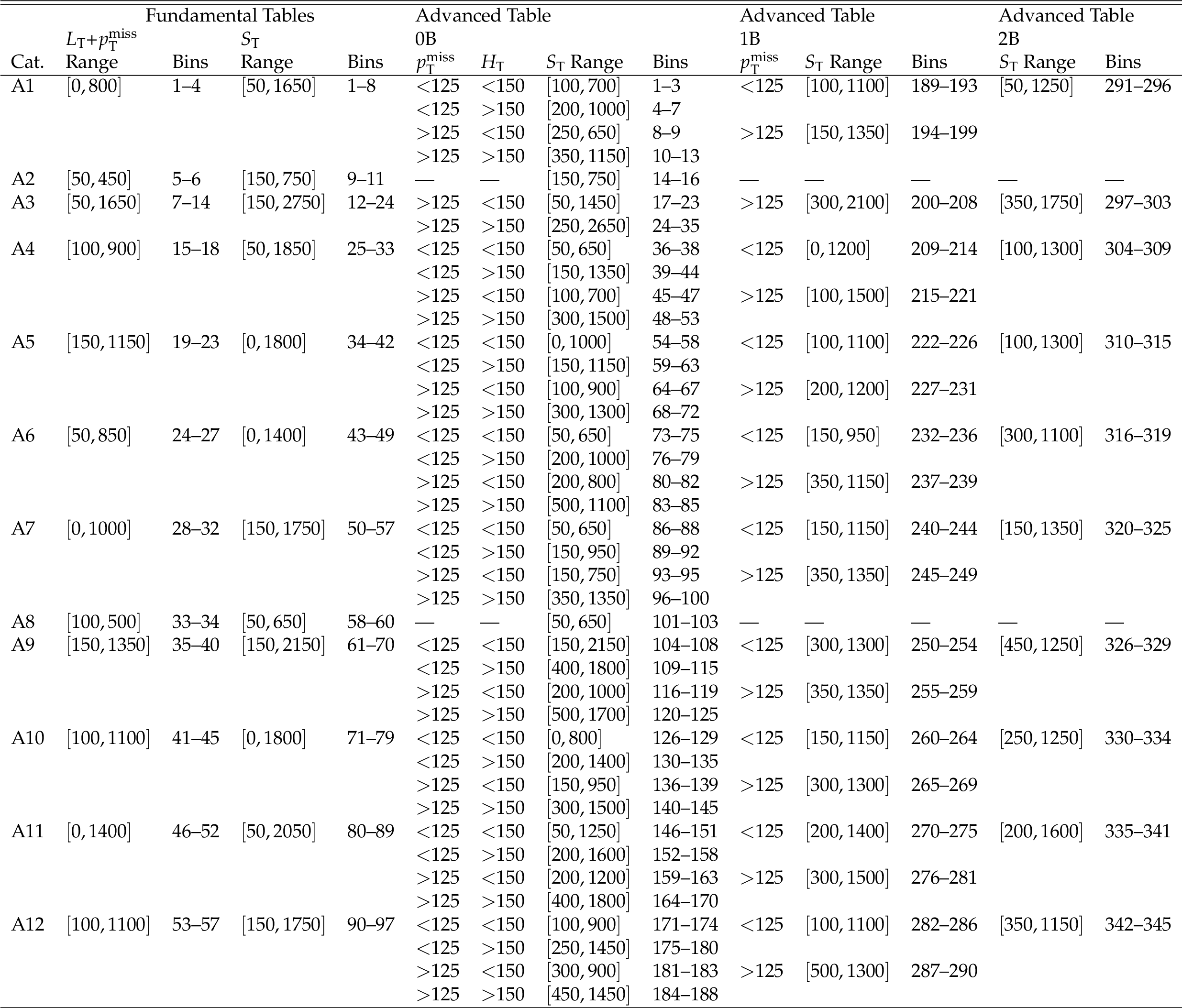
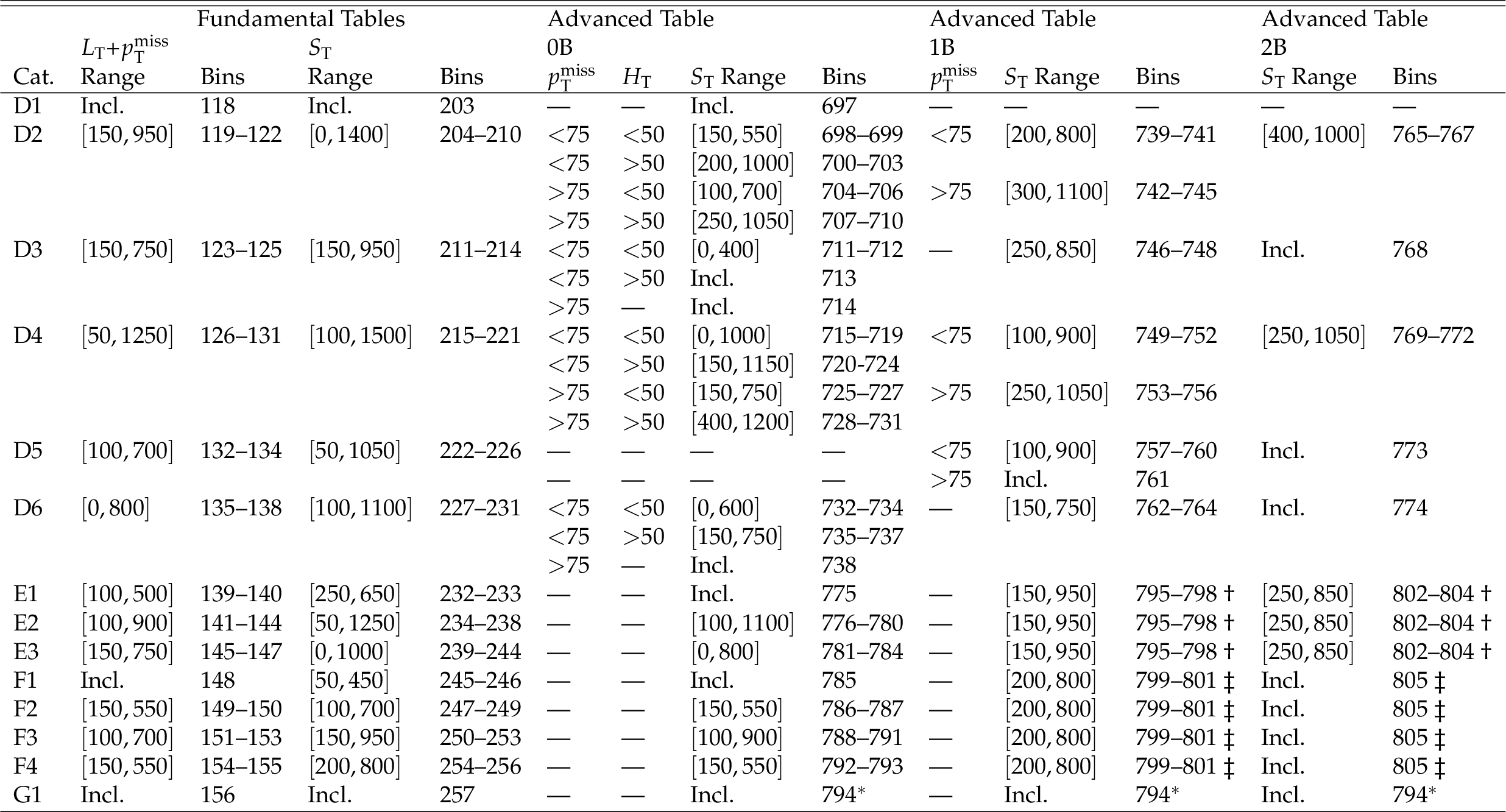
png pdf	Table 3: The binning of $ {L_{\mathrm {T}}} $+${{p_{\mathrm {T}}} ^\text {miss}}$ and ${S_{\mathrm {T}}}$ distributions for the fundamental scheme in the 3L channel, and the binning of ${S_{\mathrm {T}}}$ distribution for the advanced scheme in the 3L channel. The categorization is described in Table 2. The ranges, as well the ${{p_{\mathrm {T}}} ^\text {miss}}$ and $ {H_{\mathrm {T}}} $ requirements, are given in GeV. The first bins in the $ {L_{\mathrm {T}}} $+$ {{p_{\mathrm {T}}} ^\text {miss}}$ or ${S_{\mathrm {T}}}$ range contain the underflow, the last bins contain the overflow.
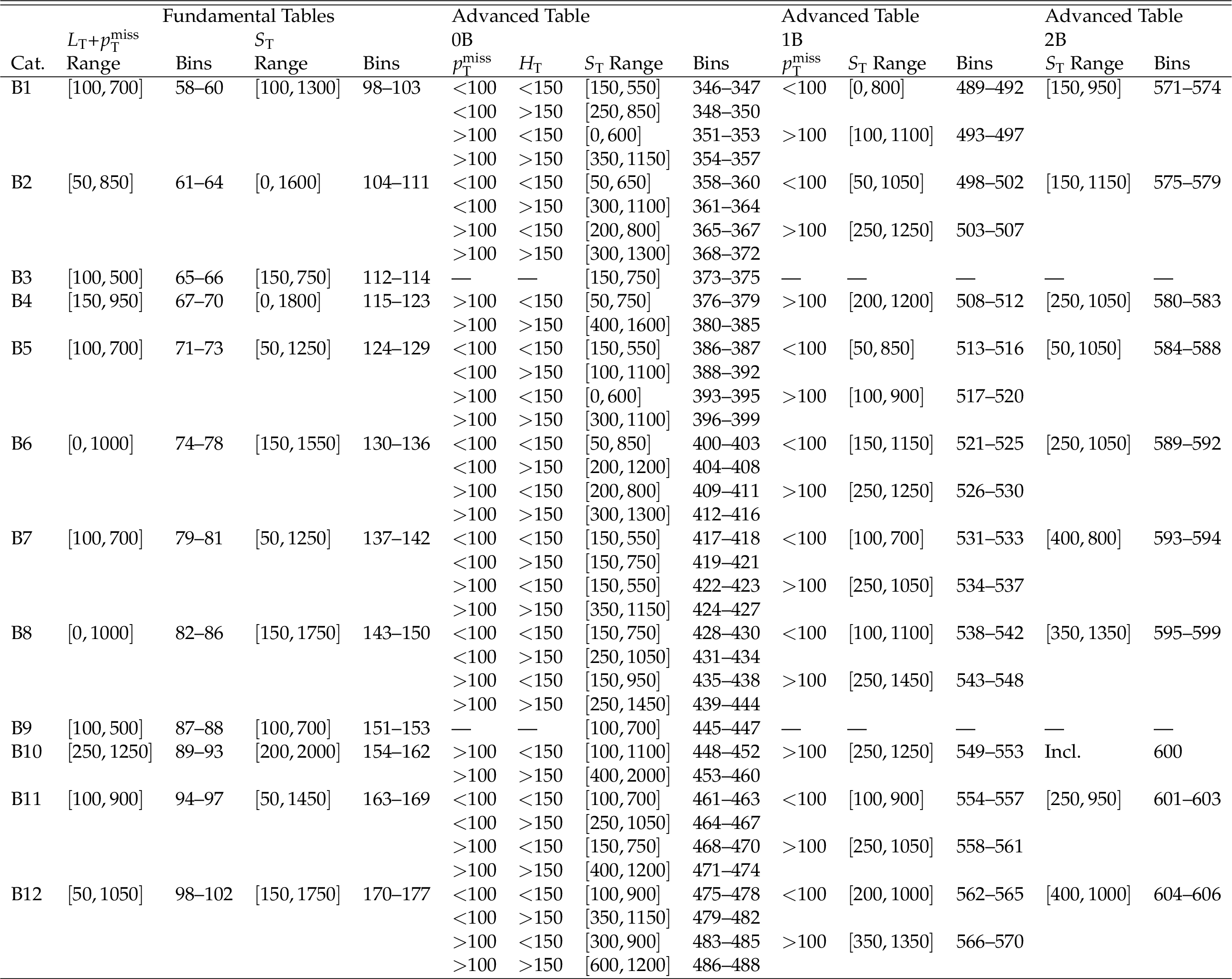
png pdf	Table 4: The binning of $ {L_{\mathrm {T}}} $+${{p_{\mathrm {T}}} ^\text {miss}}$ and ${S_{\mathrm {T}}}$ distributions for the fundamental scheme in the 2L1T channel, and the binning of ${S_{\mathrm {T}}}$ distribution for the advanced scheme in the 2L1T channel. The categorization is described in Table 2. The ranges, as well as the ${{p_{\mathrm {T}}} ^\text {miss}}$ and $ {H_{\mathrm {T}}} $ requirements, are given in GeV. The first bins in the $ {L_{\mathrm {T}}} $+${{p_{\mathrm {T}}} ^\text {miss}}$ or ${S_{\mathrm {T}}}$ range contain the underflow, and the last bins contain the overflow.
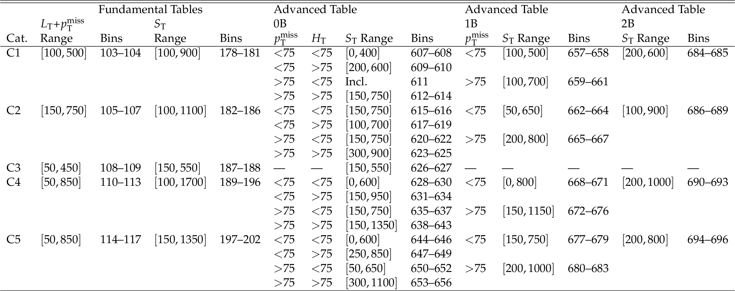
png pdf	Table 5: The binning of $ {L_{\mathrm {T}}} $+${{p_{\mathrm {T}}} ^\text {miss}}$ and ${S_{\mathrm {T}}}$ distributions for the fundamental scheme in the 1L2T channel, and the binning of ${S_{\mathrm {T}}}$ distribution for the advanced scheme in the 1L2T channel. The categorization is described in Table 2. The ranges, as well as the ${{p_{\mathrm {T}}} ^\text {miss}}$ and $ {H_{\mathrm {T}}} $ requirements, are given in GeV. The first bins in the $ {L_{\mathrm {T}}} $+${{p_{\mathrm {T}}} ^\text {miss}}$ or ${S_{\mathrm {T}}}$ range contain the underflow, and the last bins contain the overflow.
png pdf	Table 6: The binning of $ {L_{\mathrm {T}}} $+${{p_{\mathrm {T}}} ^\text {miss}}$ and ${S_{\mathrm {T}}}$ distributions for the fundamental scheme in the 4L, 3L1T, 2L2T, and 1L3T channels, and the binning of ${S_{\mathrm {T}}}$ distribution for the advanced scheme in the 4L, 3L1T, 2L2T, and 1L3T channels. The categorization is described in Table 2. The ranges, as well as the ${{p_{\mathrm {T}}} ^\text {miss}}$ and $ {H_{\mathrm {T}}} $ requirements, are given in GeV. The first bins in the $ {L_{\mathrm {T}}} $+${{p_{\mathrm {T}}} ^\text {miss}}$ or ${S_{\mathrm {T}}}$ range contain the underflow, and the last bins contain the overflow. For the 3L1T and 2L2T channels, multiple categories in the 1B or 2B selections are combined. These bins are marked with a single- or a double-dagger. For the 1L3T channel, all the b tag categories are combined and the corresponding bins are marked with an asterisk.
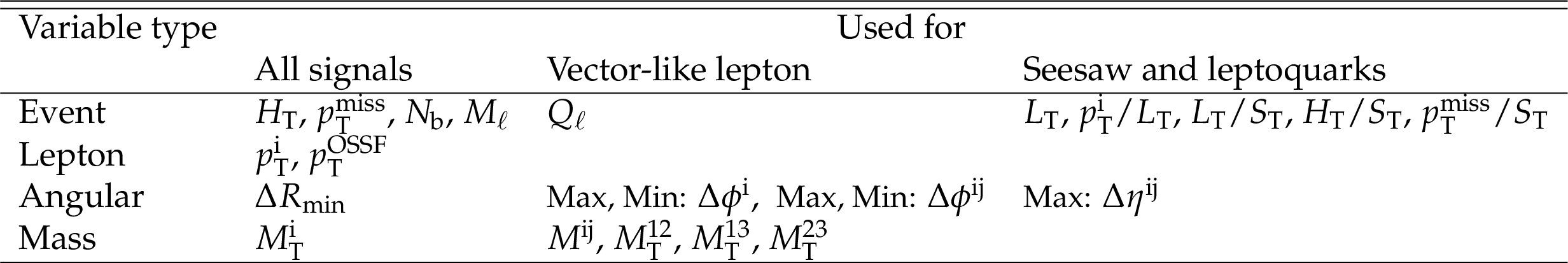
png pdf	Table 7: Input variables used for the BDTs trained for the various BSM models. Note that the indices $i,j$ run over the leptons of all flavors ($i,j=1,2,3,4$) in a given event. If a given variable is not defined in a given channel, the variable is set to a nonphysical default value for signal and background processes, and plays no role in training.
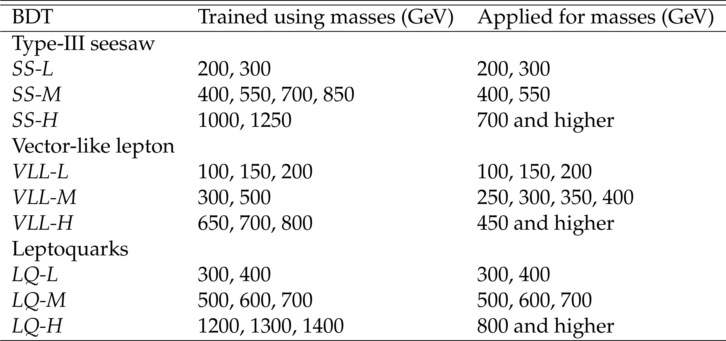
png pdf	Table 8: Signal mass points as used in the training of BDTs and the masses for which the specific trained BDT is applied in the SRs according to the best sensitivity. The labels \textit {L}, \textit {M}, and \textit {H} denote low, medium, and high mass ranges, respectively.
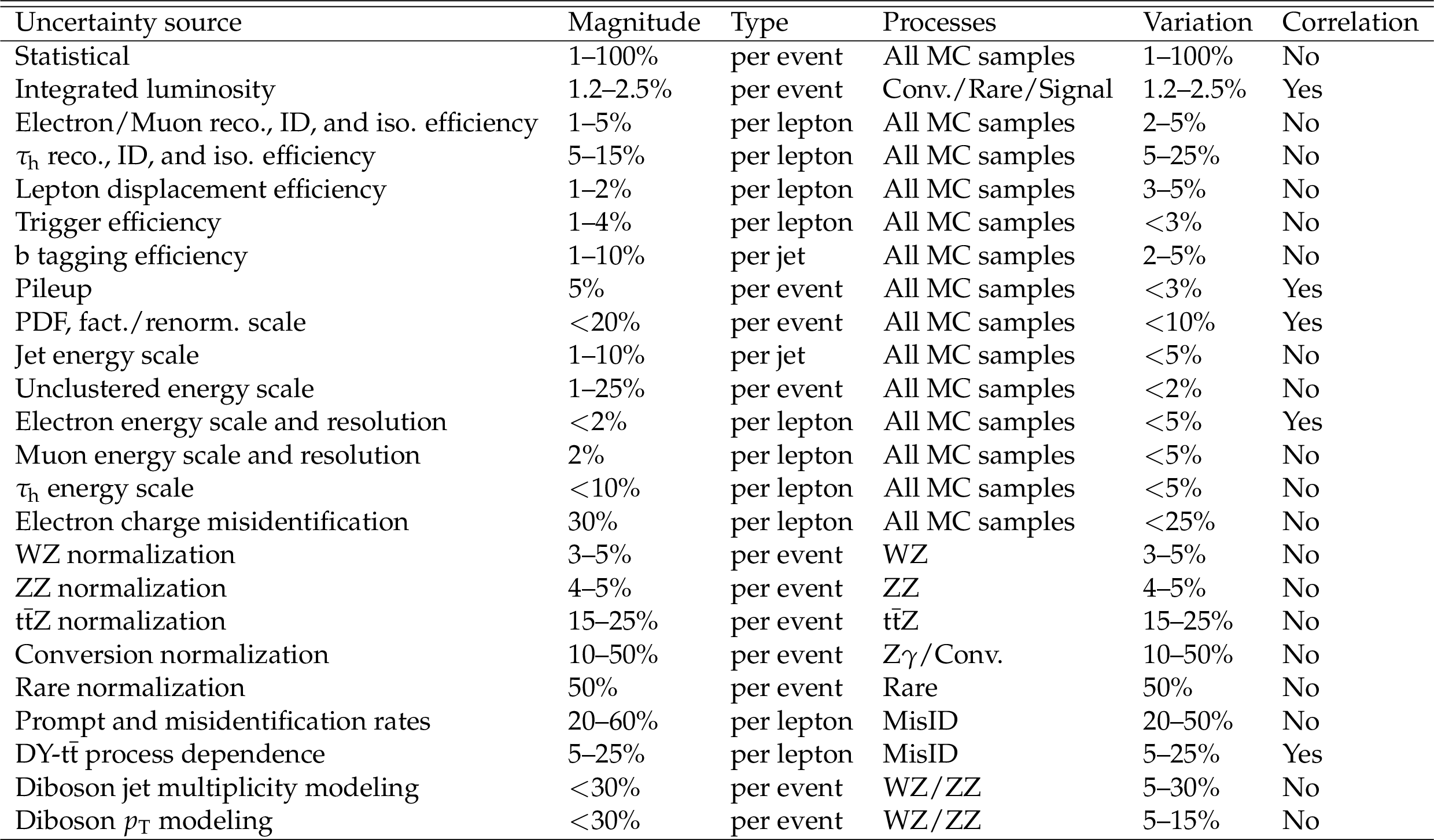
png pdf	Table 9: Sources, magnitudes, effective variations, and correlation properties of systematic uncertainties in the SRs. Uncertainty sources marked as "Yes'' in the Correlation column have their nuisance parameters correlated across the 3 years of data collection.

Summary

A search has been performed for physics beyond the standard model (SM), using multilepton events in proton-proton collision data at $\sqrt{s} = $ 13 TeV, collected in 2016-2018 by the CMS experiment at the LHC, corresponding to an integrated luminosity of 138 fb$^{-1}$. The search is carried out in seven orthogonal channels based on the number of light leptons and hadronically decaying $\tau$ leptons. Three model-independent schemes are used to define signal regions for the search. In addition, for each model scenario considered, a boosted decision tree is used to define model-specific signal regions. In all cases, the observations are found to be consistent with the expectations from the SM processes. Constraints are set on the production cross section of a number of beyond the SM signal models predicting a variety of multilepton final states.

Type-III seesaw heavy fermions are excluded at 95% confidence level (CL) with masses below 980 GeV (expected 1060 GeV), assuming flavor-democratic mixings with SM leptons, and below 990 GeV (expected 1065 GeV), 1065 GeV (expected 1140 GeV), and 890 GeV (expected 880 GeV), assuming mixings exclusively with electron, muon, and $\tau$ lepton flavors, respectively. Lower limits on the masses of the heavy fermions are also presented for various decay branching fractions of the heavy fermions to the different SM lepton flavors. These are the most stringent constraints on the type-III seesaw heavy fermions to date.

In the vector-like lepton doublet model, vector-like $\tau$ leptons are excluded at 95% CL with masses below 1045 GeV, with an expected exclusion of 975 GeV. These are the most stringent constraints on the doublet model. For the singlet model, vector-like $\tau$ leptons are excluded in the mass range from 125 to 150 GeV, while the expected exclusion range is from 125 to 170 GeV. These are the first constraints from the LHC on the singlet model.

Scalar leptoquarks coupled to top quarks and individual lepton flavors are also probed. In the scenario with the leptoquark coupling to a top quark and a $\tau$ lepton, leptoquarks with masses below 1120 GeV are excluded at 95% CL (expected 1235 GeV). For the decay to a top quark and an electron, leptoquarks are excluded with masses below 1340 GeV (expected 1370 GeV), and for the decay into a top quark and a muon, masses below 1420 GeV (expected 1460 GeV) are excluded.

Additional Figures
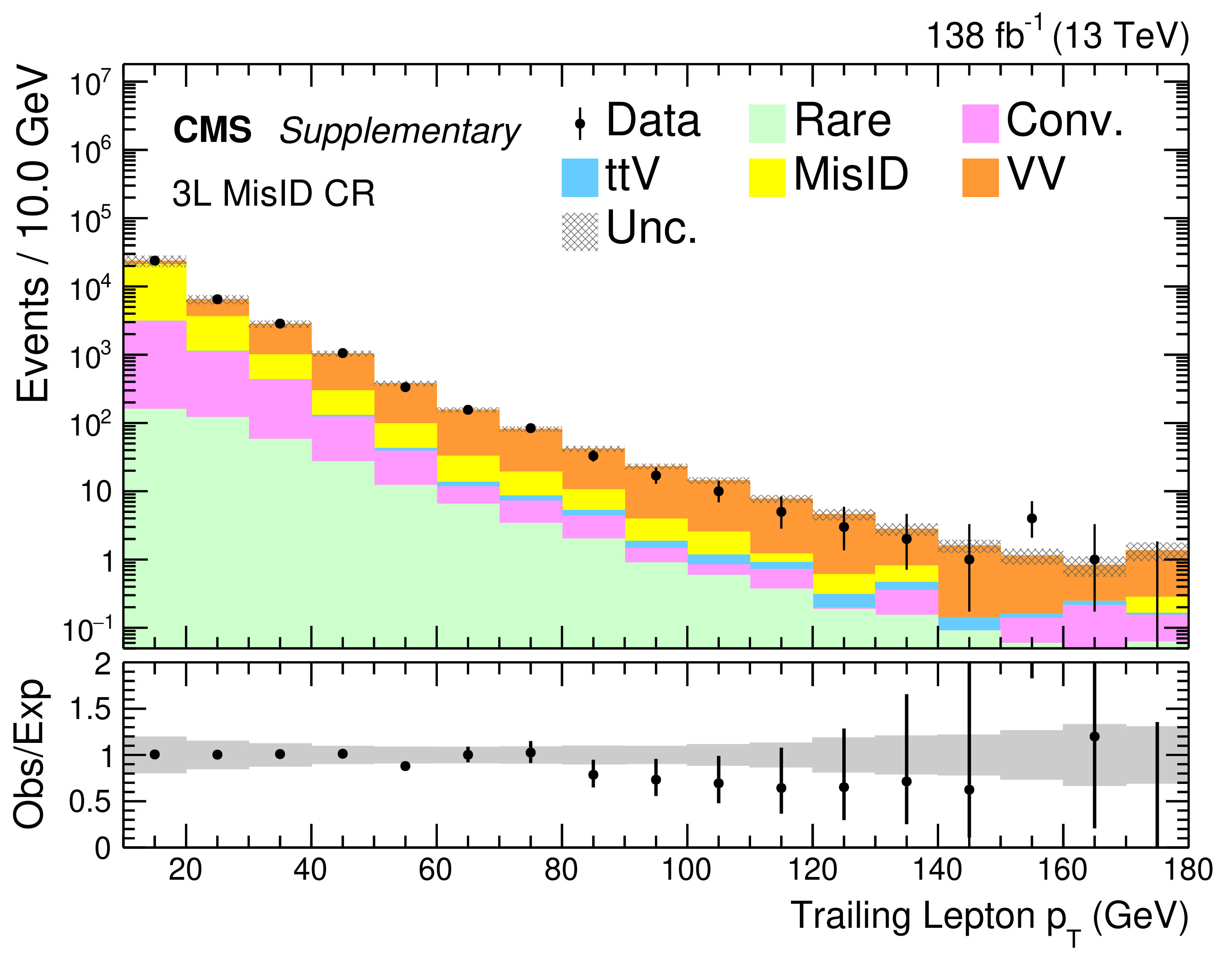
png pdf	Additional Figure 1: The $ {p_{\mathrm {T}}} $ distribution of the trailing lepton in 3L MisID CR events. The rightmost bin contains the overflow events. The lower panel shows the ratio of observed events to the total expected background prediction. The gray band on the ratio represents the sum of statistical and systematic uncertainties in the SM background prediction.
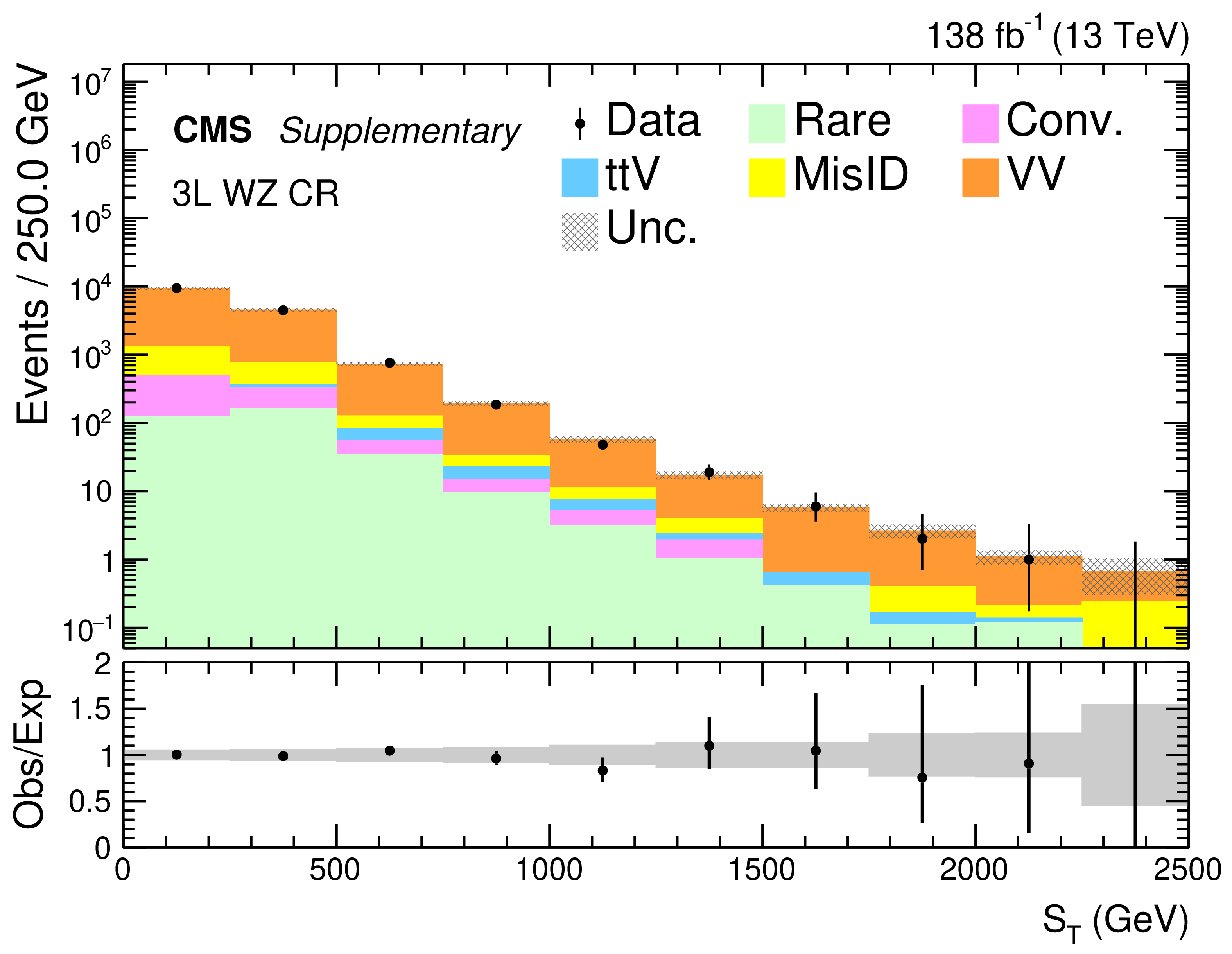
png pdf	Additional Figure 2: The $S_{\rm T}$ distribution in 3L WZ CR events. The rightmost bin contains the overflow events. The lower panel shows the ratio of observed events to the total expected background prediction. The gray band on the ratio represents the sum of statistical and systematic uncertainties in the SM background prediction.
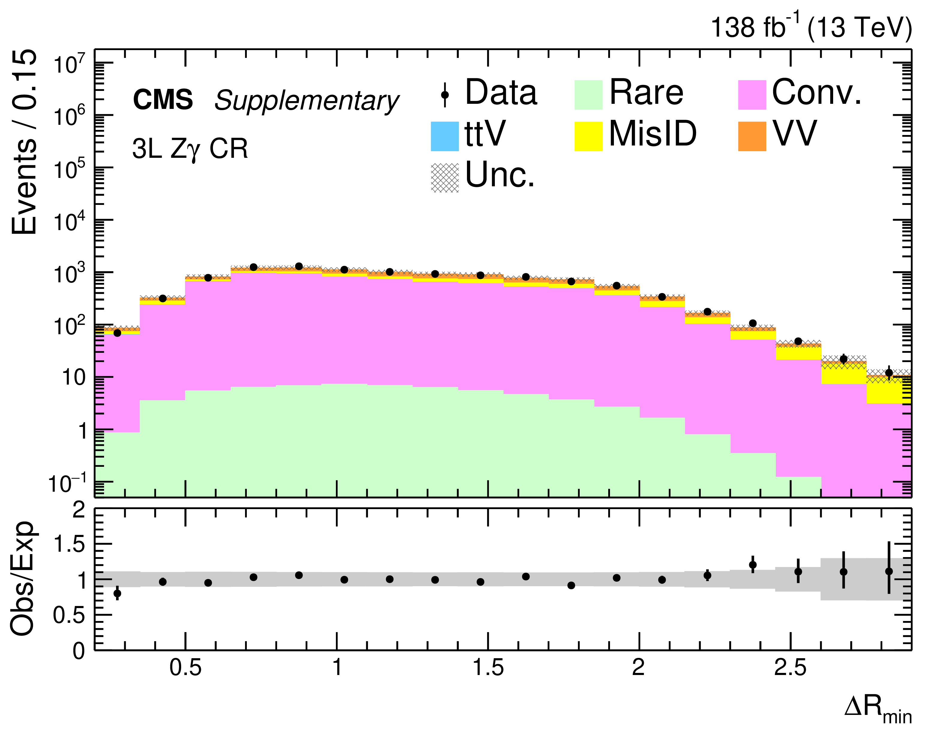
png pdf	Additional Figure 3: The $\Delta {R}_{\rm min}$ distribution in 3L Z$\gamma $ CR events. The rightmost bin contains the overflow events. The lower panel shows the ratio of observed events to the total expected background prediction. The gray band on the ratio represents the sum of statistical and systematic uncertainties in the SM background prediction.
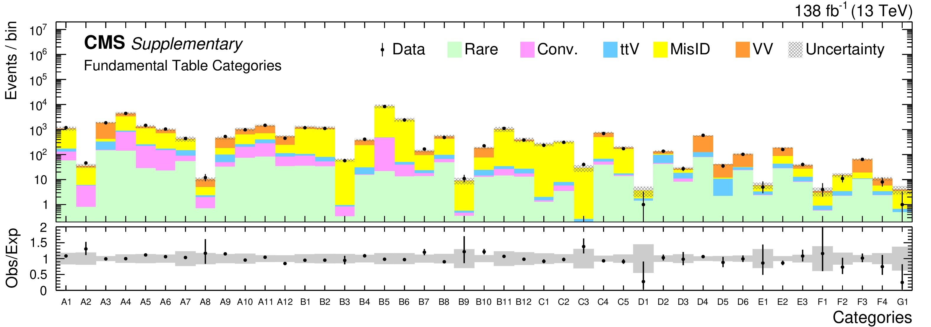
png pdf	Additional Figure 4: The model independent fundamental table categories, as defined in Table 1 in the paper. The lower panel shows the ratio of observed events to the total expected background prediction. The gray band on the ratio represents the sum of statistical and systematic uncertainties in the SM background prediction.
png pdf	Additional Figure 5: The $N_{\rm b}$ distribution in 3L, 2L1T, and 1L2T events. The rightmost bin contains the overflow events. The lower panel shows the ratio of observed events to the total expected background prediction. The gray band on the ratio represents the sum of statistical and systematic uncertainties in the SM background prediction. For illustration, an example signal hypothesis for the production of the scalar leptoquark coupled to a top quark and a $\tau$ lepton for $m_{S} = $ 1 TeV, before the fit, is also overlaid.
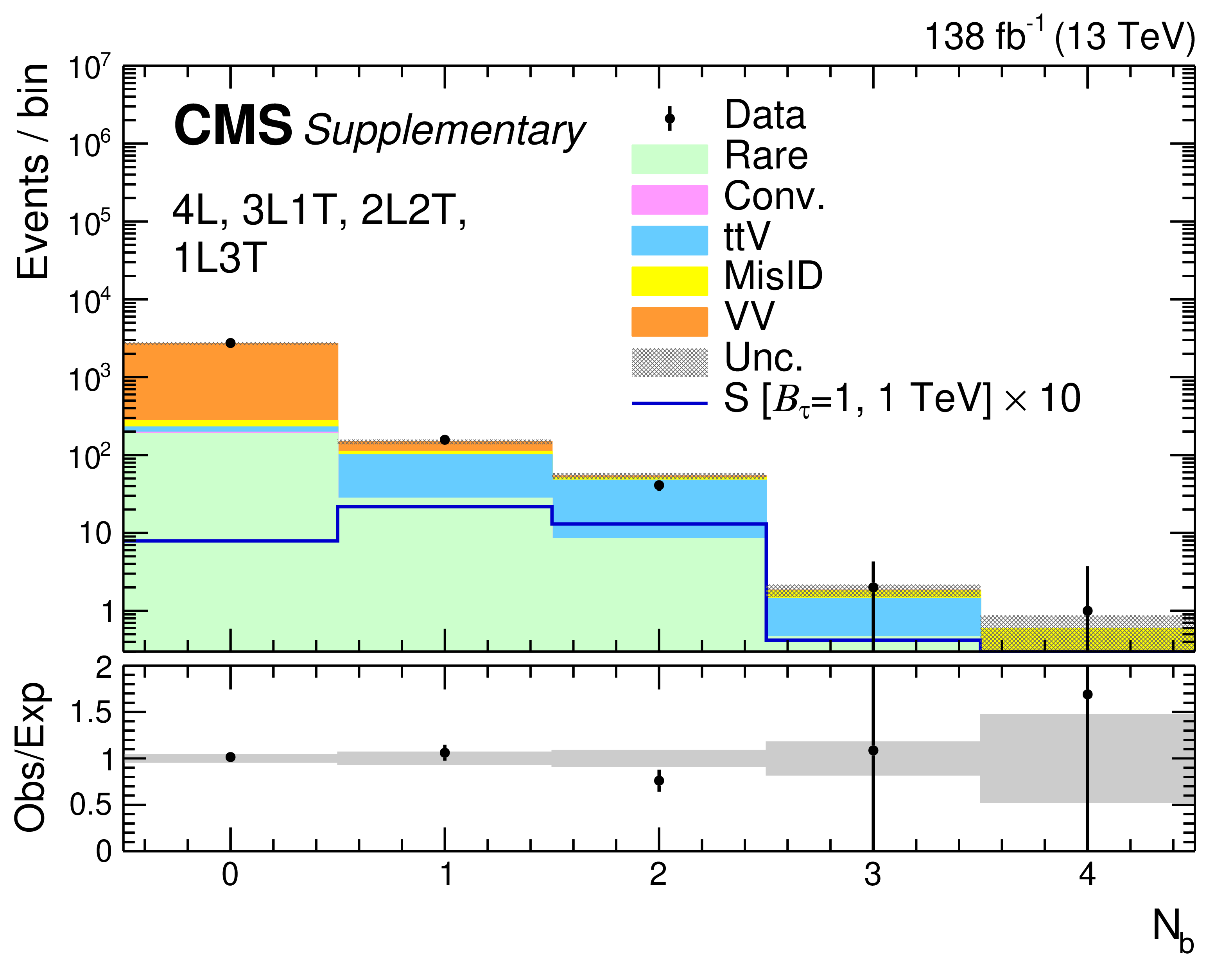
png pdf	Additional Figure 6: The $N_{\rm b}$ distribution in 4L, 3L1T, 2L2T, and 1L3T events. The rightmost bin contains the overflow events. The lower panel shows the ratio of observed events to the total expected background prediction. The gray band on the ratio represents the sum of statistical and systematic uncertainties in the SM background prediction. For illustration, an example signal hypothesis for the production of the scalar leptoquark coupled to a top quark and a $\tau$ lepton for $m_{S} = $ 1 TeV, before the fit, is also overlaid.
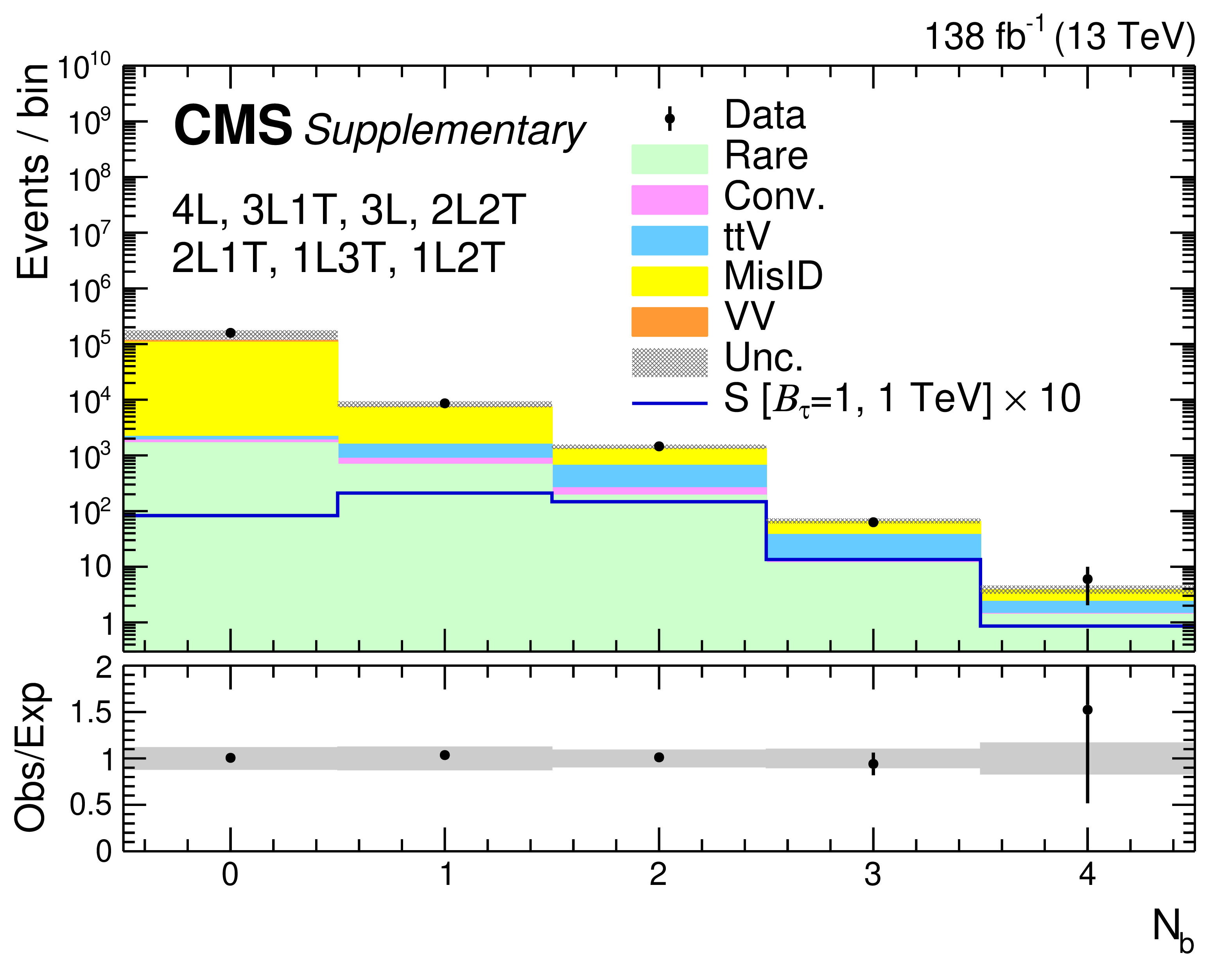
png pdf	Additional Figure 7: The $N_{\rm b}$ distribution in 4L, 3L1T, 3L, 2L2T, 2L1T, 1L3T, and 1L2T events. The rightmost bin contains the overflow events. The lower panel shows the ratio of observed events to the total expected background prediction. The gray band on the ratio represents the sum of statistical and systematic uncertainties in the SM background prediction. For illustration, an example signal hypothesis for the production of the scalar leptoquark coupled to a top quark and a $\tau$ lepton for $m_{S} = $ 1 TeV, before the fit, is also overlaid.
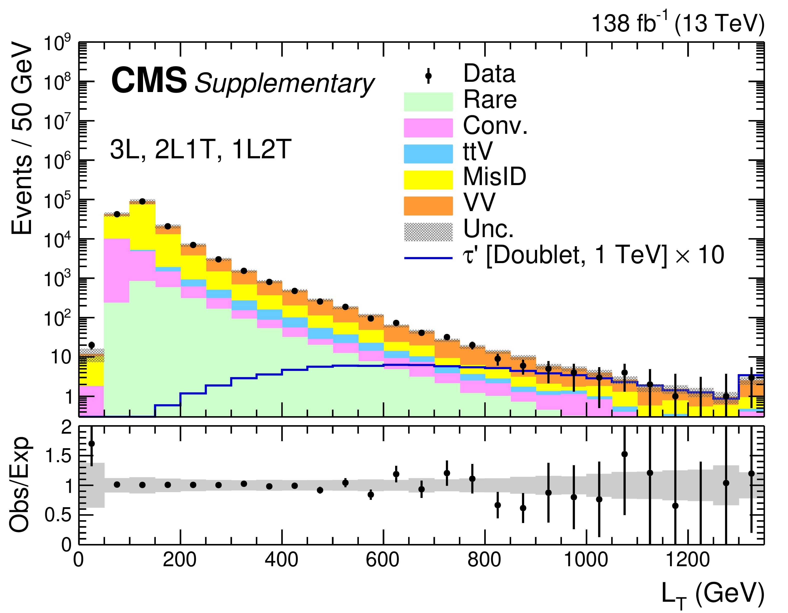
png pdf	Additional Figure 8: The $L_{\rm T}$ distribution in 3L, 2L1T, and 1L2T events. The rightmost bin contains the overflow events. The lower panel shows the ratio of observed events to the total expected background prediction. The gray band on the ratio represents the sum of statistical and systematic uncertainties in the SM background prediction. For illustration, an example signal hypothesis for the production of the vector-like $\tau$ lepton in the doublet scenario for $m_{\tau ^{\prime}} = $ 1 TeV, before the fit, is also overlaid.
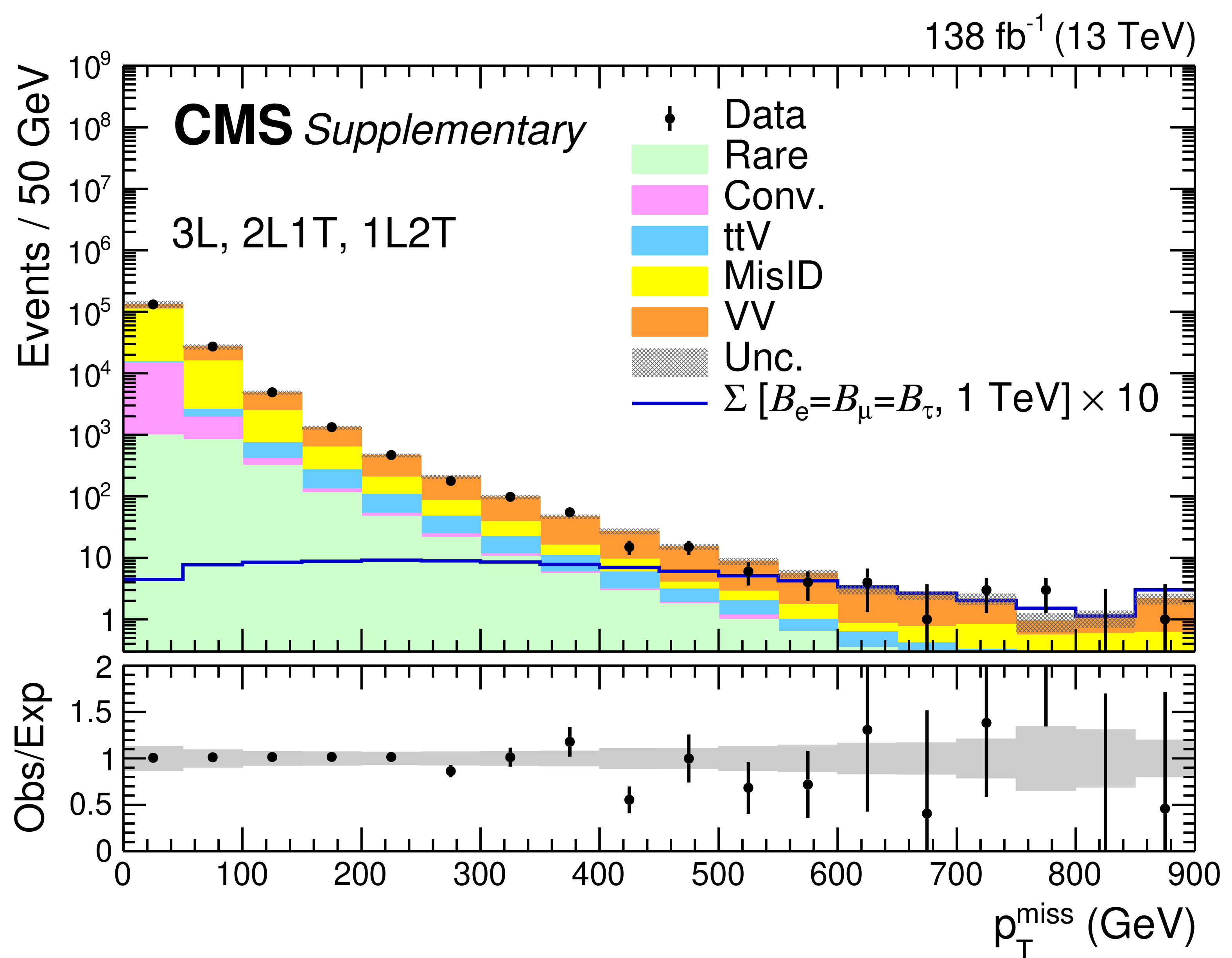
png pdf	Additional Figure 9: The $ {{p_{\mathrm {T}}} ^\text {miss}} $ distribution in 3L, 2L1T, and 1L2T events. The rightmost bin contains the overflow events. The lower panel shows the ratio of observed events to the total expected background prediction. The gray band on the ratio represents the sum of statistical and systematic uncertainties in the SM background prediction. For illustration, an example signal hypothesis for the production of the type-III seesaw heavy fermions in the flavor-democratic scenario for $m_{\Sigma} = $ 1 TeV, before the fit, is also overlaid.
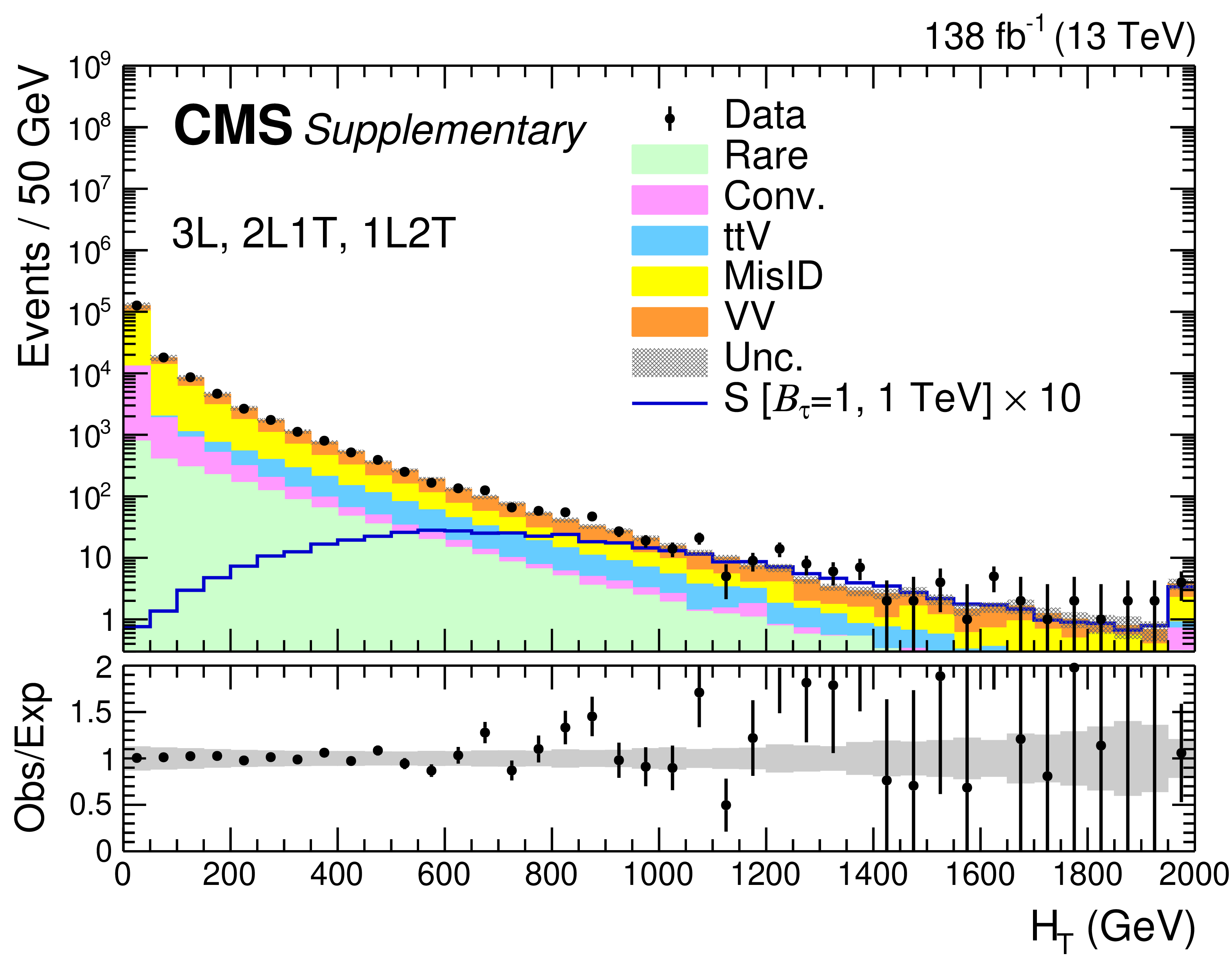
png pdf	Additional Figure 10: The $H_{\rm T}$ distribution in 3L, 2L1T, and 1L2T events. The rightmost bin contains the overflow events. The lower panel shows the ratio of observed events to the total expected background prediction. The gray band on the ratio represents the sum of statistical and systematic uncertainties in the SM background prediction. For illustration, an example signal hypothesis for the production of the scalar leptoquark coupled to a top quark and a $\tau$ lepton for $m_{S} = $ 1 TeV, before the fit, is also overlaid.
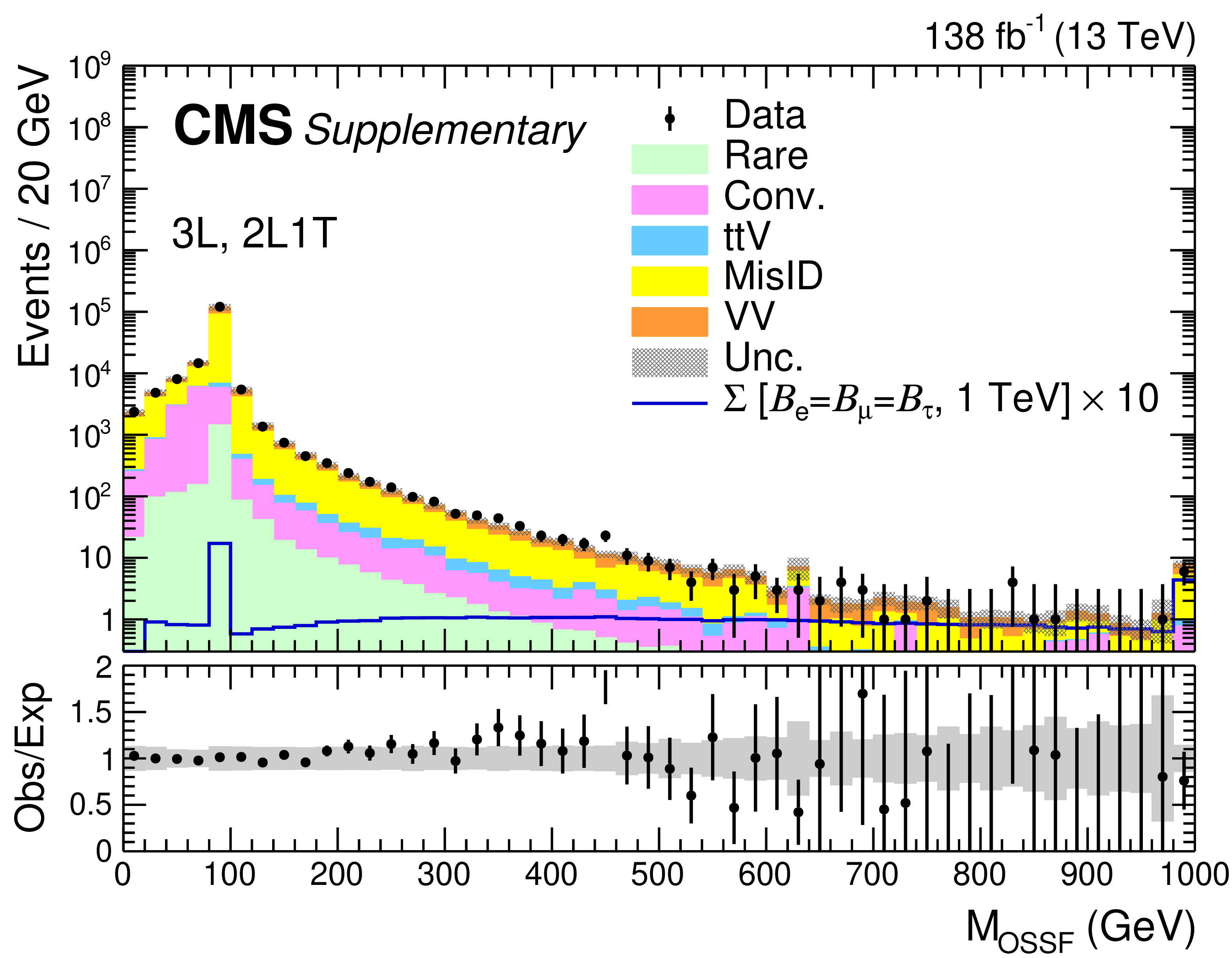
png pdf	Additional Figure 11: The $M_{\rm OSSF}$ distribution in 3L and 2L1T events. The rightmost bin contains the overflow events. The lower panel shows the ratio of observed events to the total expected background prediction. The gray band on the ratio represents the sum of statistical and systematic uncertainties in the SM background prediction. For illustration, an example signal hypothesis for the production of the type-III seesaw heavy fermions in the flavor-democratic scenario for $m_{\Sigma} = $ 1 TeV, before the fit, is also overlaid.
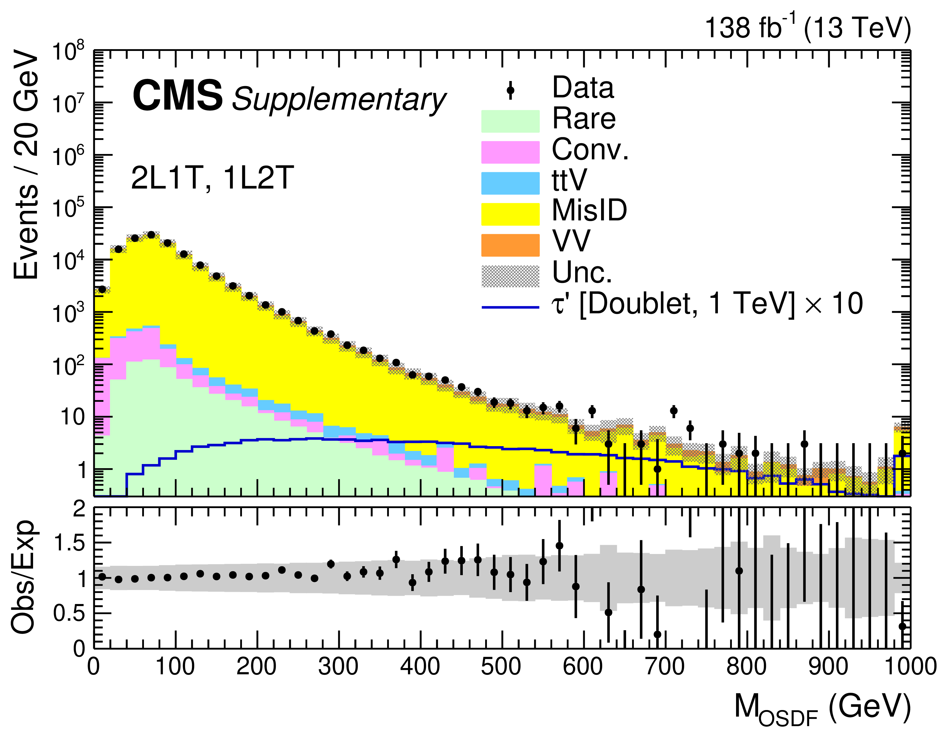
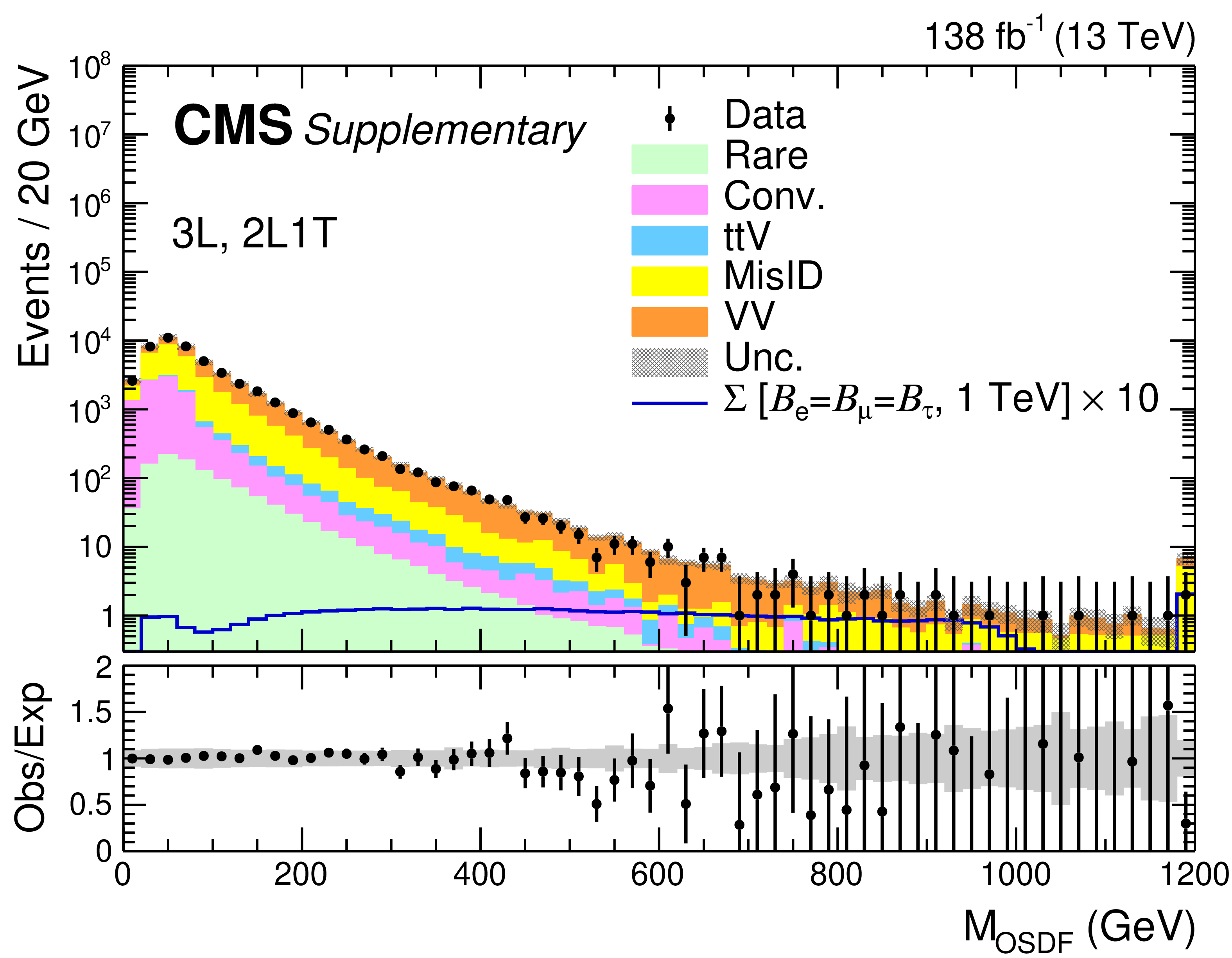
png pdf	Additional Figure 12: The invariant mass distribution of the opposite-sign different-flavor ($M_{\rm OSDF}$) light lepton pair in 3L and 2L1T events. The rightmost bin contains the overflow events. The lower panel shows the ratio of observed events to the total expected background prediction. The gray band on the ratio represents the sum of statistical and systematic uncertainties in the SM background prediction. For illustration, an example signal hypothesis for the production of the type-III seesaw heavy fermions in the flavor-democratic scenario for $m_{\Sigma} = $ 1 TeV, before the fit, is also overlaid.
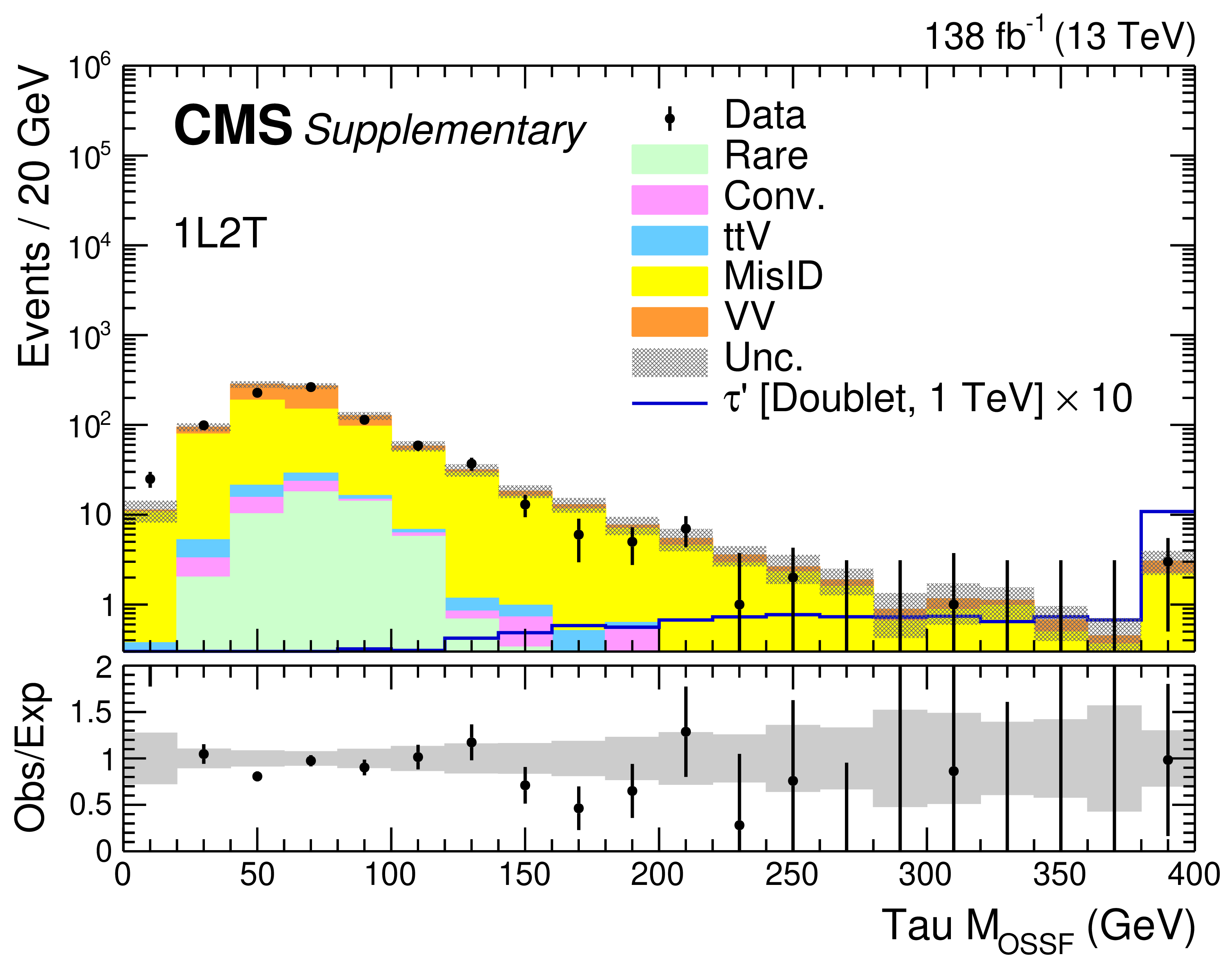
png pdf	Additional Figure 13: The invariant mass distribution of the opposite-sign same-flavor ($M_{\rm OSSF}$) tau lepton pair in 1L2T events. The rightmost bin contains the overflow events. The lower panel shows the ratio of observed events to the total expected background prediction. The gray band on the ratio represents the sum of statistical and systematic uncertainties in the SM background prediction. For illustration, an example signal hypothesis for the production of the vector-like $\tau$ lepton in the doublet scenario for $m_{\tau ^{\prime}} = $ 1 TeV, before the fit, is also overlaid.
png pdf	Additional Figure 14: The invariant mass distribution of the opposite-sign same-flavor ($M_{\rm OSSF}$) tau lepton pair in 2L2T, 1L3T, and 1L2T events. The rightmost bin contains the overflow events. The lower panel shows the ratio of observed events to the total expected background prediction. The gray band on the ratio represents the sum of statistical and systematic uncertainties in the SM background prediction. For illustration, an example signal hypothesis for the production of the vector-like $\tau$ lepton in the doublet scenario for $m_{\tau ^{\prime}} = $ 1 TeV, before the fit, is also overlaid.
png pdf	Additional Figure 15: The invariant mass distribution of the opposite-sign different-flavor ($M_{\rm OSDF}$) light lepton and tau lepton pair in 2L1T and 1L2T events. The rightmost bin contains the overflow events. The lower panel shows the ratio of observed events to the total expected background prediction. The gray band on the ratio represents the sum of statistical and systematic uncertainties in the SM background prediction. For illustration, an example signal hypothesis for the production of the vector-like $\tau$ lepton in the doublet scenario for $m_{\tau ^{\prime}} = $ 1 TeV, before the fit, is also overlaid.
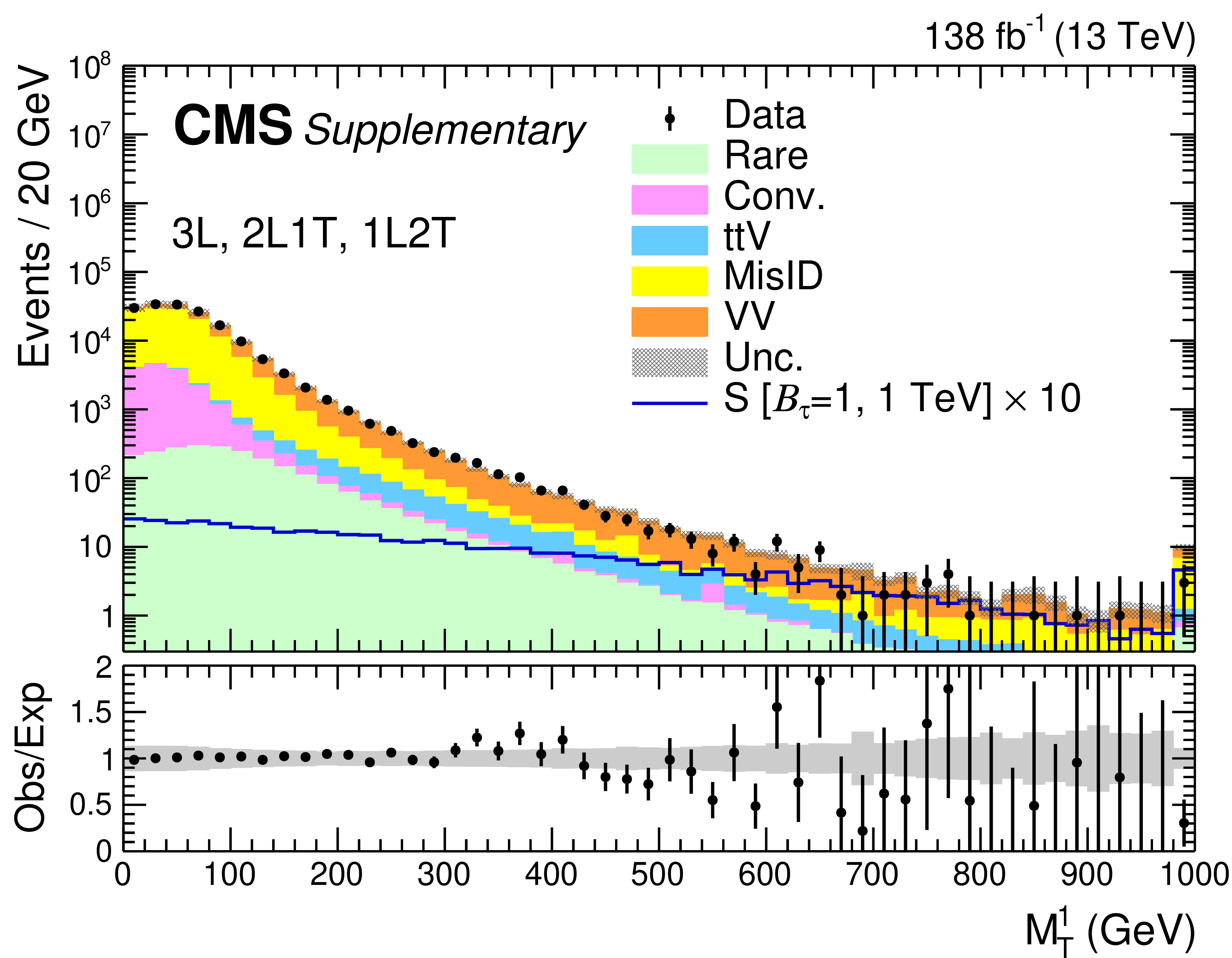
png pdf	Additional Figure 16: The $M_{\rm T}^{\textrm {1}}$ in 3L, 2L1T, and 1L2T events. The rightmost bin contains the overflow events. The lower panel shows the ratio of observed events to the total expected background prediction. The gray band on the ratio represents the sum of statistical and systematic uncertainties in the SM background prediction. For illustration, an example signal hypothesis for the production of the scalar leptoquark coupled to a top quark and a $\tau$ lepton for $m_{S} = $ 1 TeV, before the fit, is also overlaid.
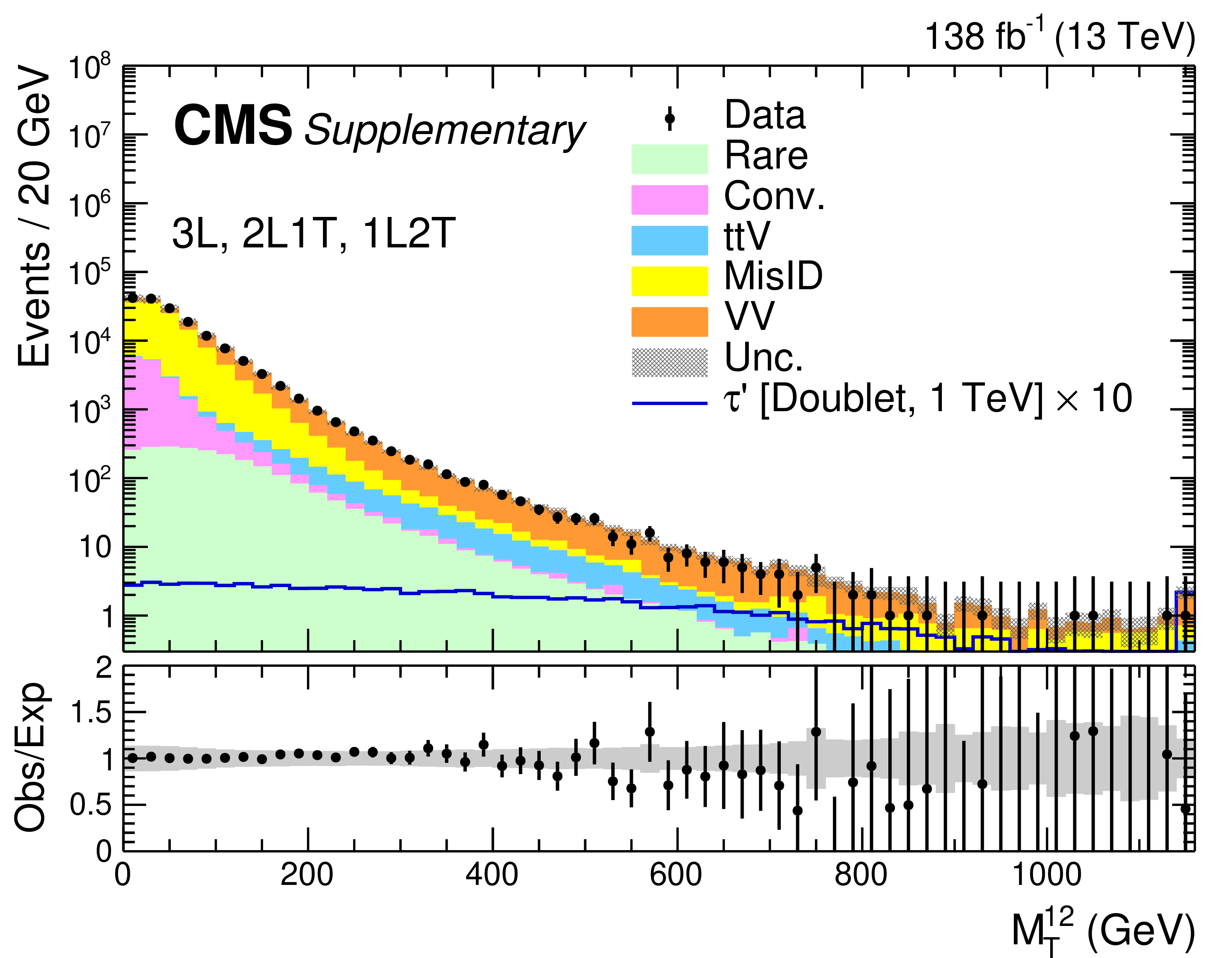
png pdf	Additional Figure 17: The $M_{\rm T}^{\textrm {12}}$ in 3L, 2L1T, and 1L2T events. The rightmost bin contains the overflow events. The lower panel shows the ratio of observed events to the total expected background prediction. The gray band on the ratio represents the sum of statistical and systematic uncertainties in the SM background prediction. For illustration, an example signal hypothesis for the production of the vector-like $\tau$ lepton in the doublet scenario for $m_{\tau ^{\prime}} = $ 1 TeV, before the fit, is also overlaid.
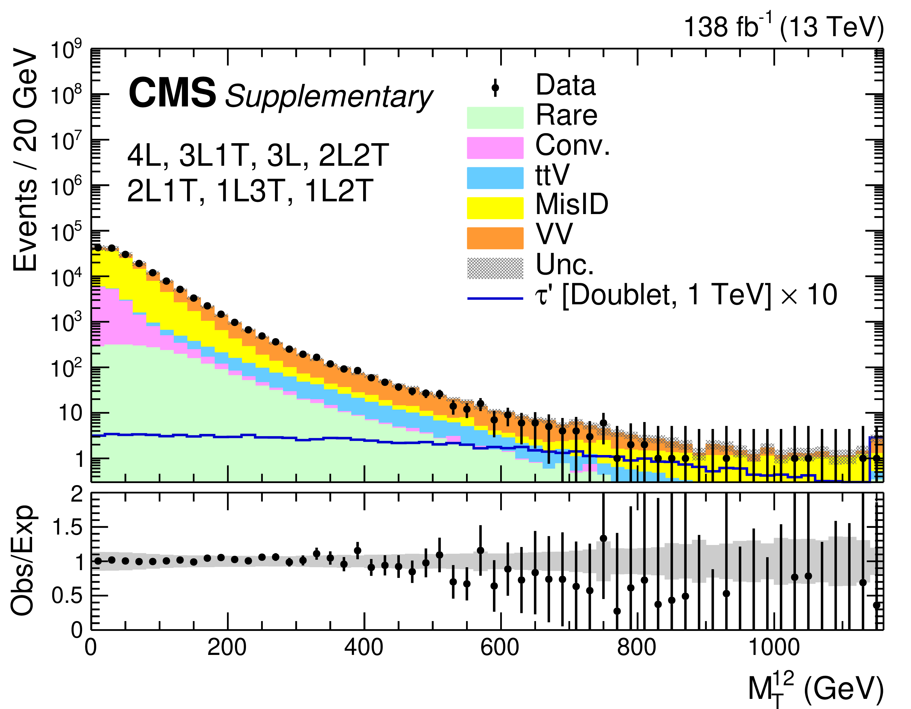
png pdf	Additional Figure 18: The $M_{\rm T}^{\textrm {12}}$ in 4L, 3L1T, 2L2T, 2L1T, 1L3T, and 1L2T events. The rightmost bin contains the overflow events. The lower panel shows the ratio of observed events to the total expected background prediction. The gray band on the ratio represents the sum of statistical and systematic uncertainties in the SM background prediction. For illustration, an example signal hypothesis for the production of the vector-like $\tau$ lepton in the doublet scenario for $m_{\tau ^{\prime}} = $ 1 TeV, before the fit, is also overlaid.
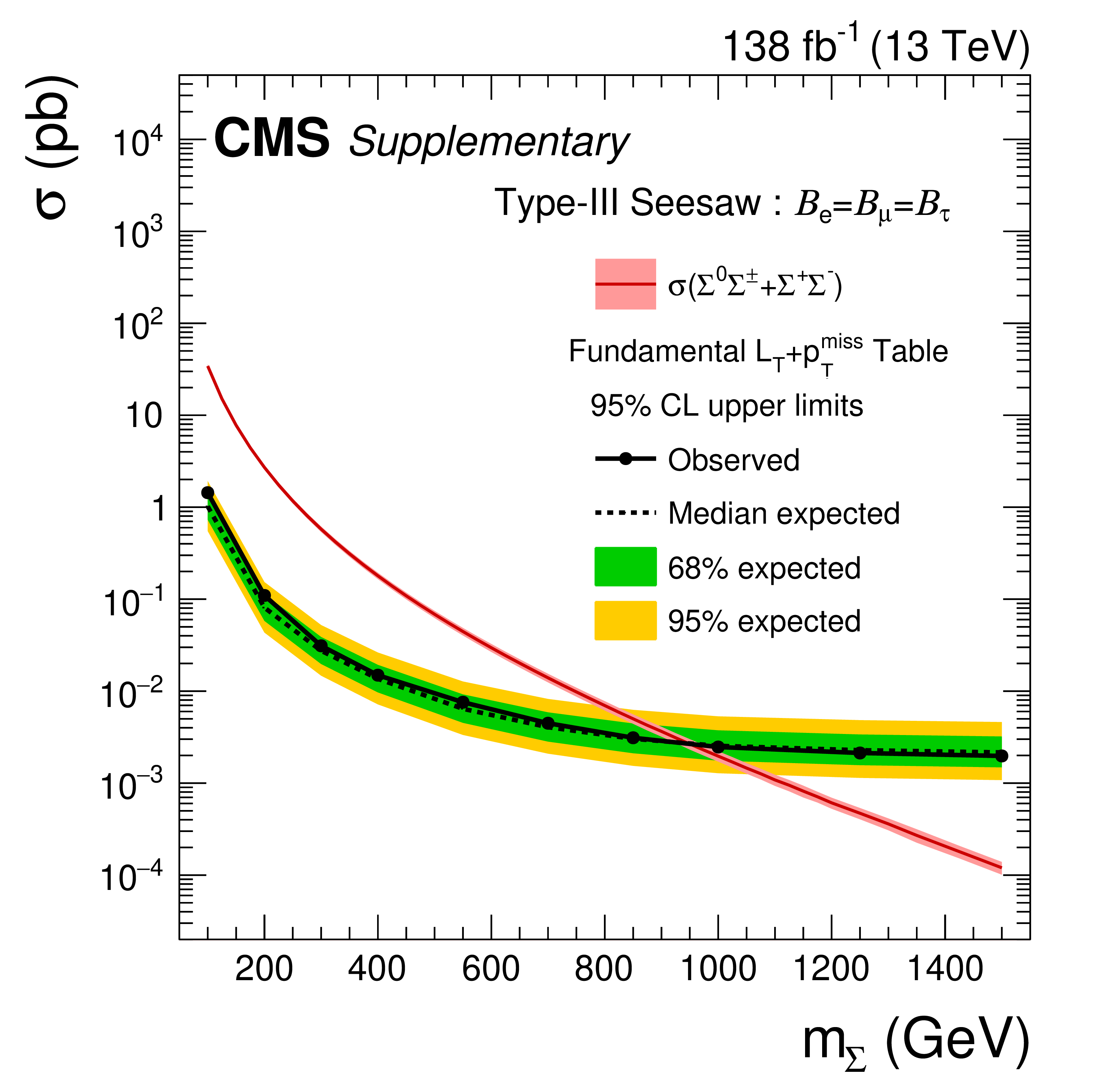
png pdf	Additional Figure 19: Observed and expected upper limits at 95% CL on the production cross section for the type-III seesaw fermions in the flavor-democratic scenario using the fundamental $L_{\rm T}+ {{p_{\mathrm {T}}} ^\text {miss}} $ table.
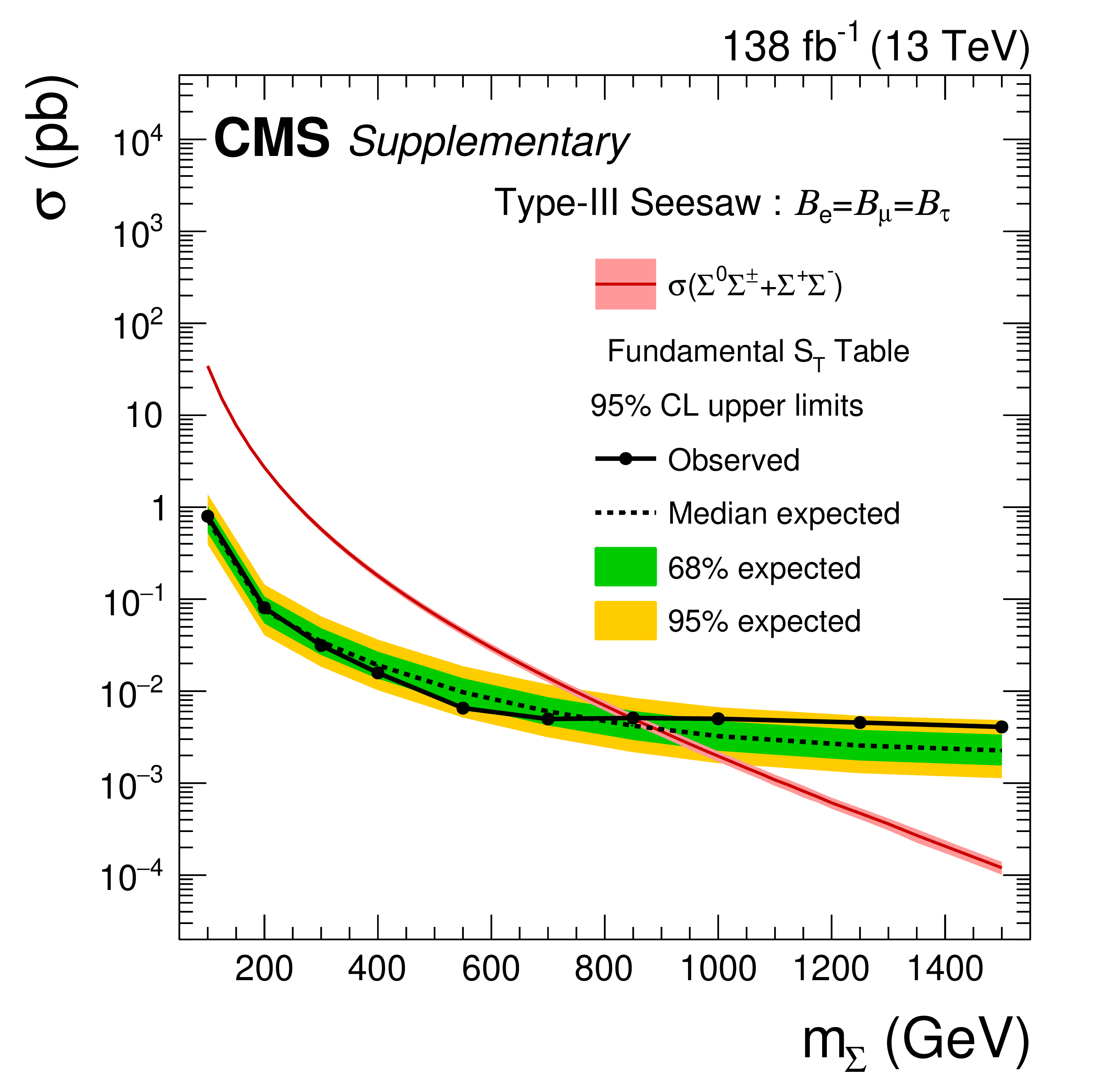
png pdf	Additional Figure 20: Observed and expected upper limits at 95% CL on the production cross section for the type-III seesaw fermions in the flavor-democratic scenario using the fundamental $S_{\rm T}$ table.
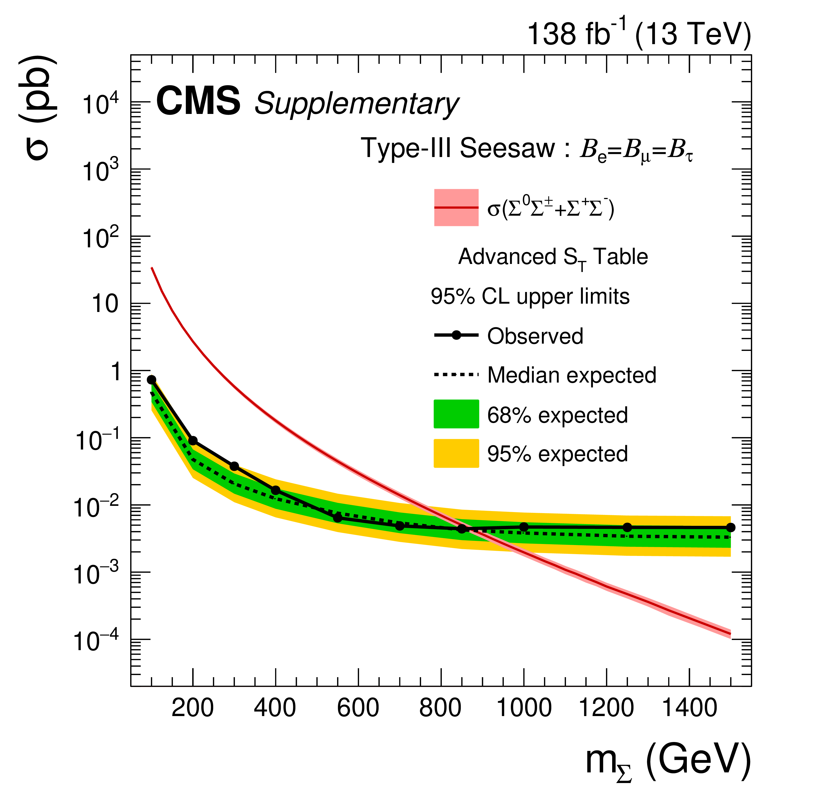
png pdf	Additional Figure 21: Observed and expected upper limits at 95% CL on the production cross section for the type-III seesaw fermions in the flavor-democratic scenario using the advanced $S_{\rm T}$ table.
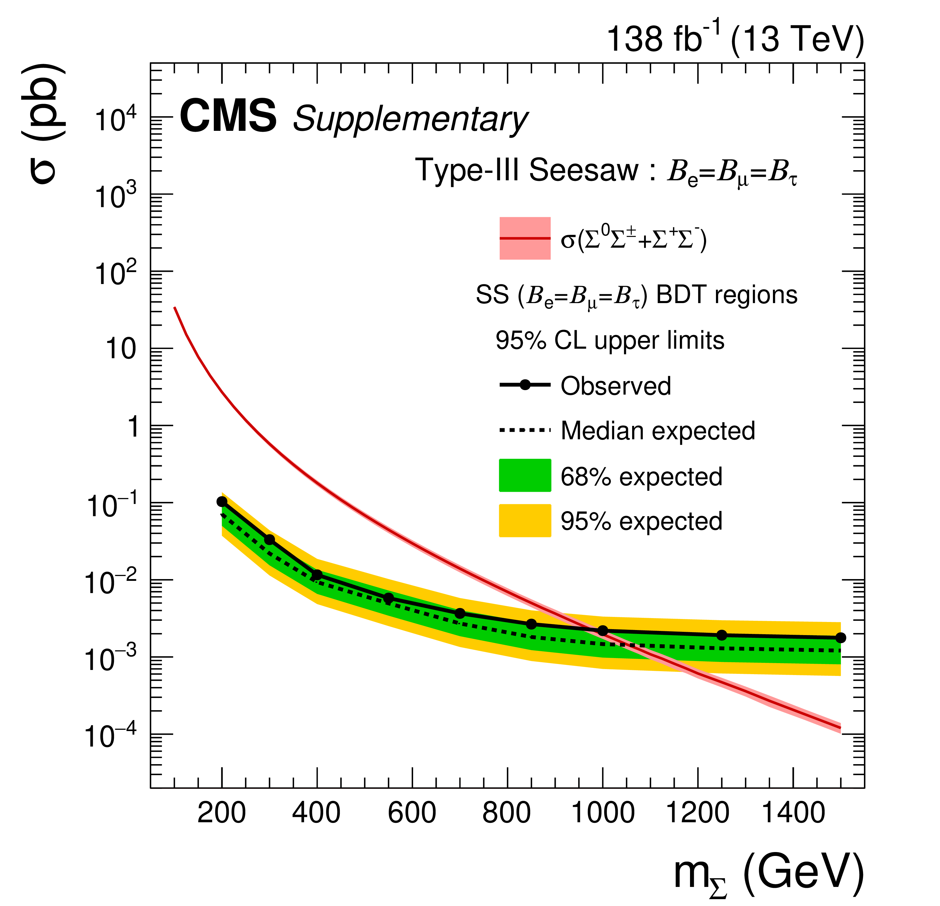
png pdf	Additional Figure 22: Observed and expected upper limits at 95% CL on the production cross section for the type-III seesaw fermions in the flavor-democratic scenario using the SS ($\mathcal {B}_{\mathrm{e}}=\mathcal {B}_{\mu}=\mathcal {B}_{\tau}$) BDT regions.
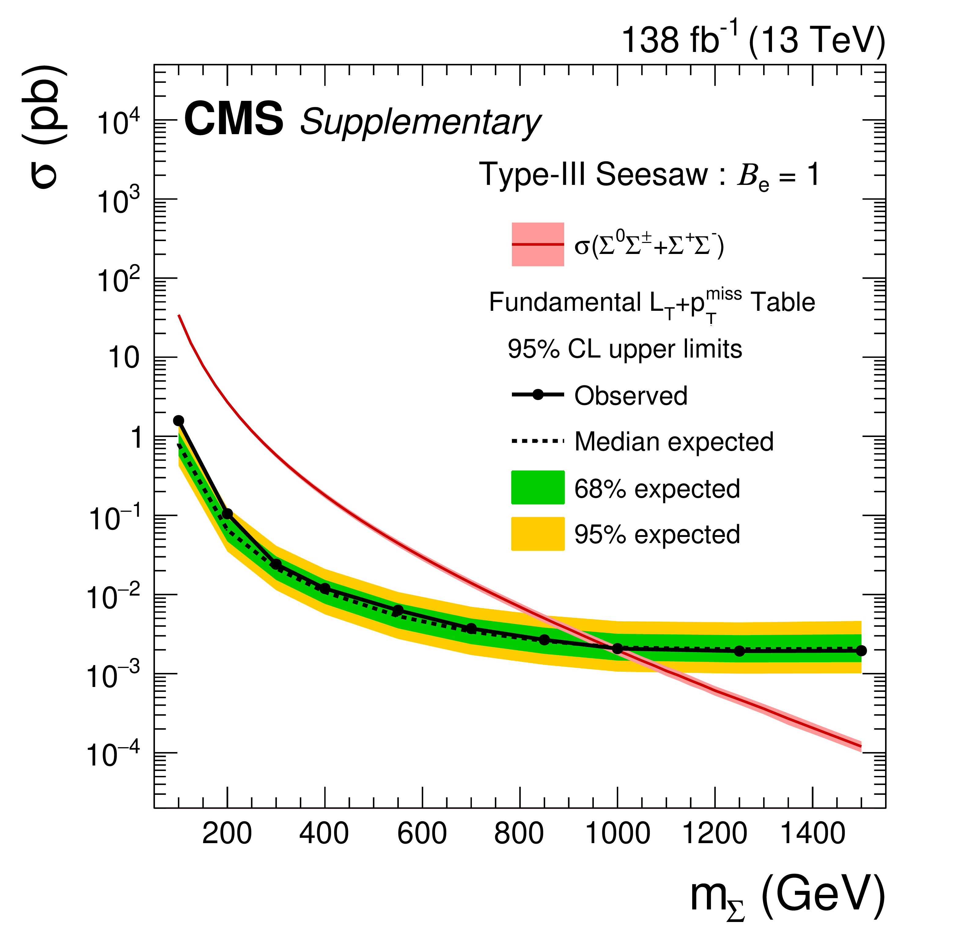
png pdf	Additional Figure 23: Observed and expected upper limits at 95% CL on the production cross section for the type-III seesaw fermions in the $\mathcal {B}_{\mathrm{e}}=$ 1 scenario using the fundamental $L_{\rm T}+ {{p_{\mathrm {T}}} ^\text {miss}} $ table.
png pdf	Additional Figure 24: Observed and expected upper limits at 95% CL on the production cross section for the type-III seesaw fermions in the $\mathcal {B}_{\mathrm{e}}=$ 1 scenario using the fundamental $S_{\rm T}$ table.
png pdf	Additional Figure 25: Observed and expected upper limits at 95% CL on the production cross section for the type-III seesaw fermions in the $\mathcal {B}_{\mathrm{e}}=$ 1 scenario using the advanced $S_{\rm T}$ table.
png pdf	Additional Figure 26: Observed and expected upper limits at 95% CL on the production cross section for the type-III seesaw fermions in the $\mathcal {B}_{\mathrm{e}}=$ 1 scenario using the SS ($\mathcal {B}_{\mathrm{e}}=\mathcal {B}_{\mu}=\mathcal {B}_{\tau}$) BDT regions.
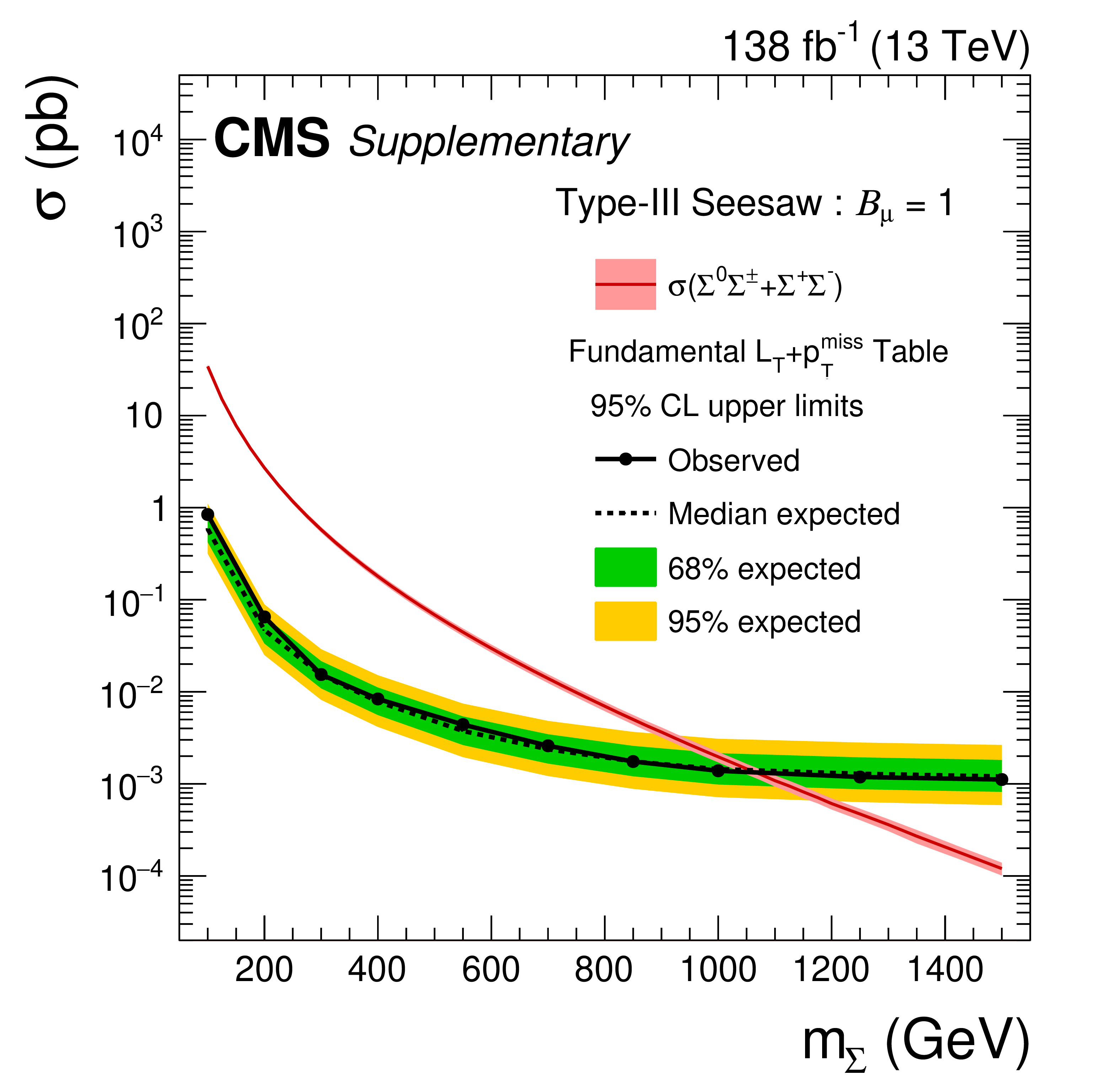
png pdf	Additional Figure 27: Observed and expected upper limits at 95% CL on the production cross section for the type-III seesaw fermions in the $\mathcal {B}_{\mu}=$ 1 scenario using the fundamental $L_{\rm T}+ {{p_{\mathrm {T}}} ^\text {miss}} $ table.
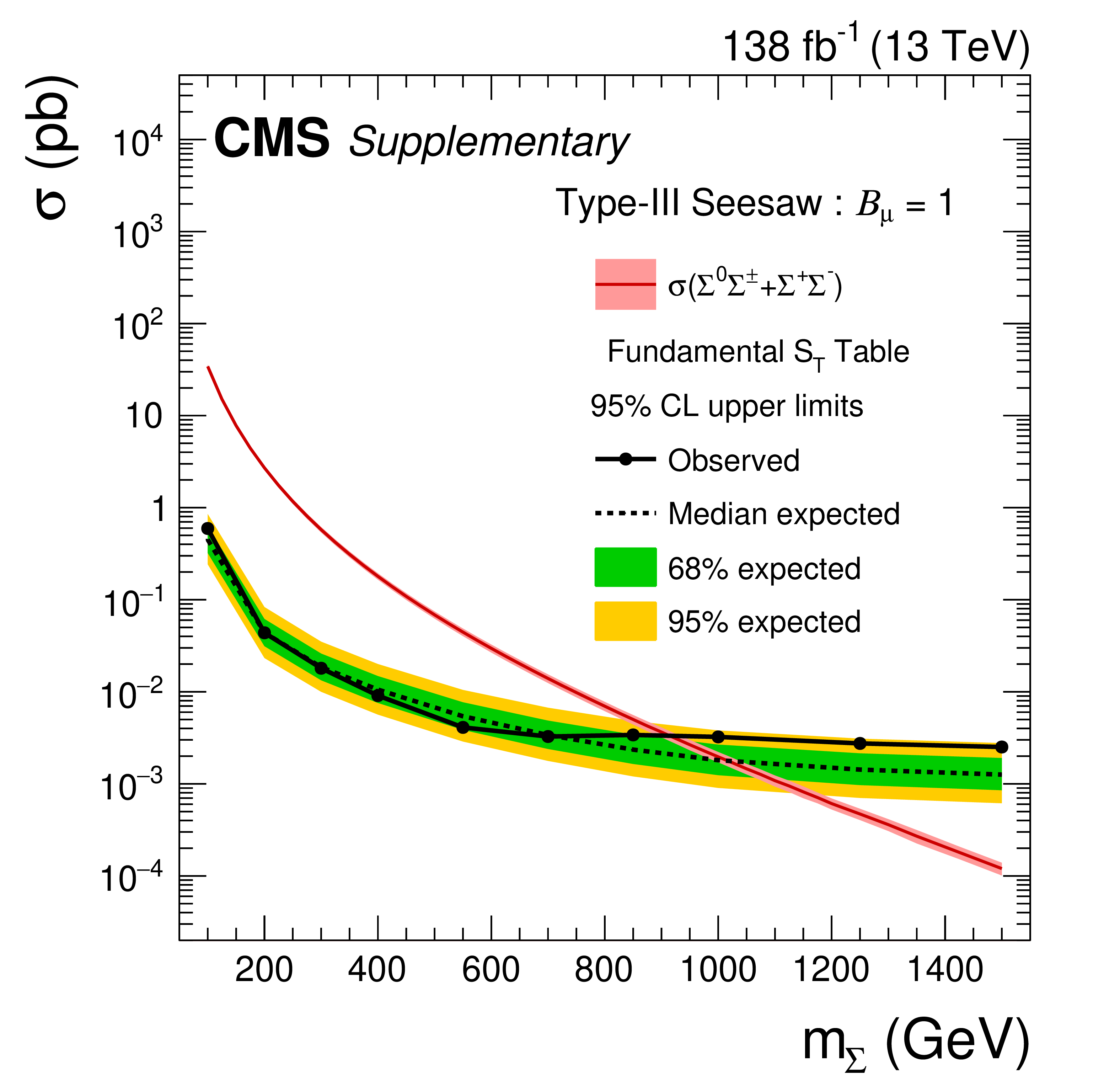
png pdf	Additional Figure 28: Observed and expected upper limits at 95% CL on the production cross section for the type-III seesaw fermions in the $\mathcal {B}_{\mu}=$ 1 scenario using the fundamental $S_{\rm T}$ table.
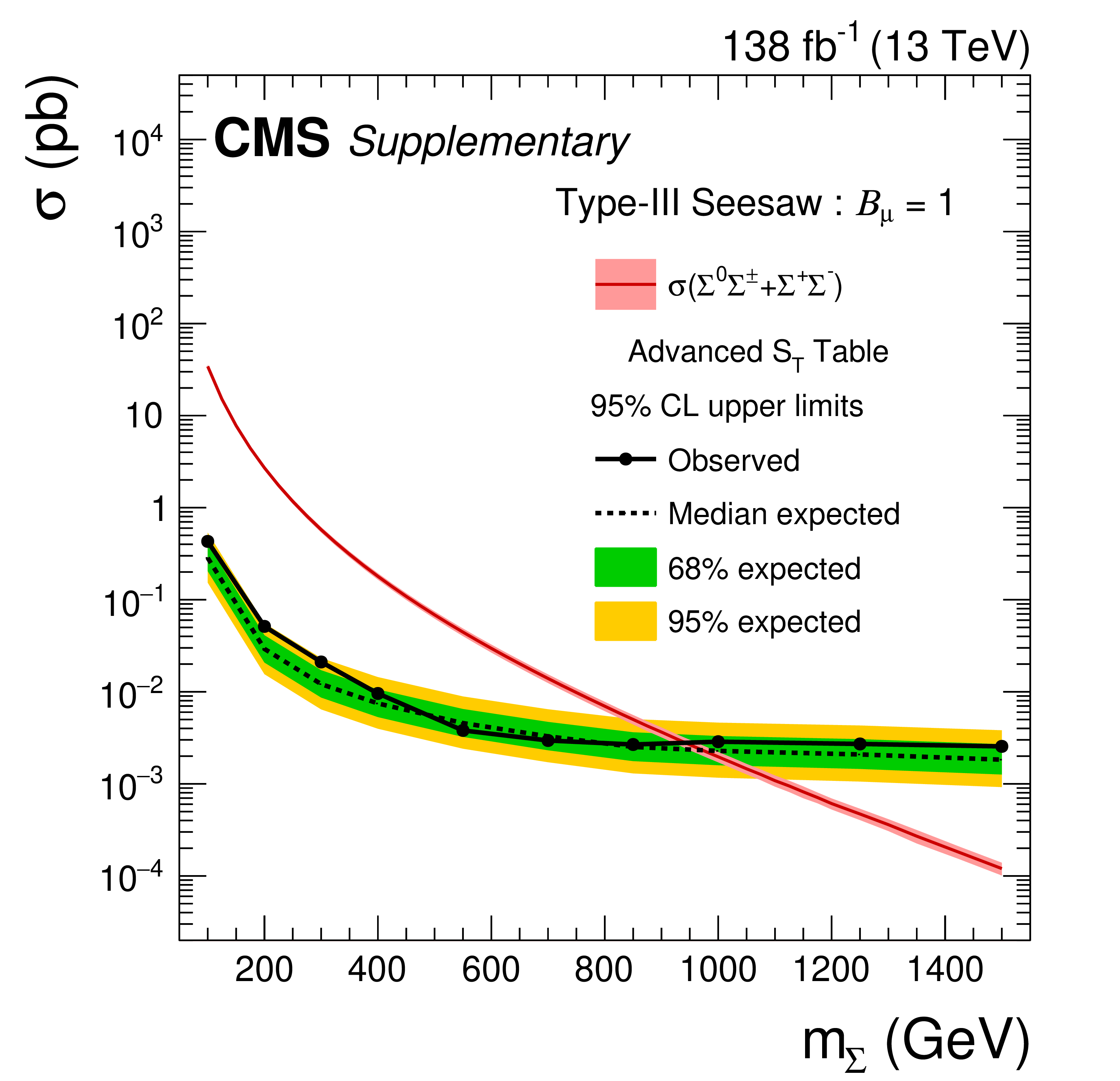
png pdf	Additional Figure 29: Observed and expected upper limits at 95% CL on the production cross section for the type-III seesaw fermions in the $\mathcal {B}_{\mu}=$ 1 scenario using the advanced $S_{\rm T}$ table.
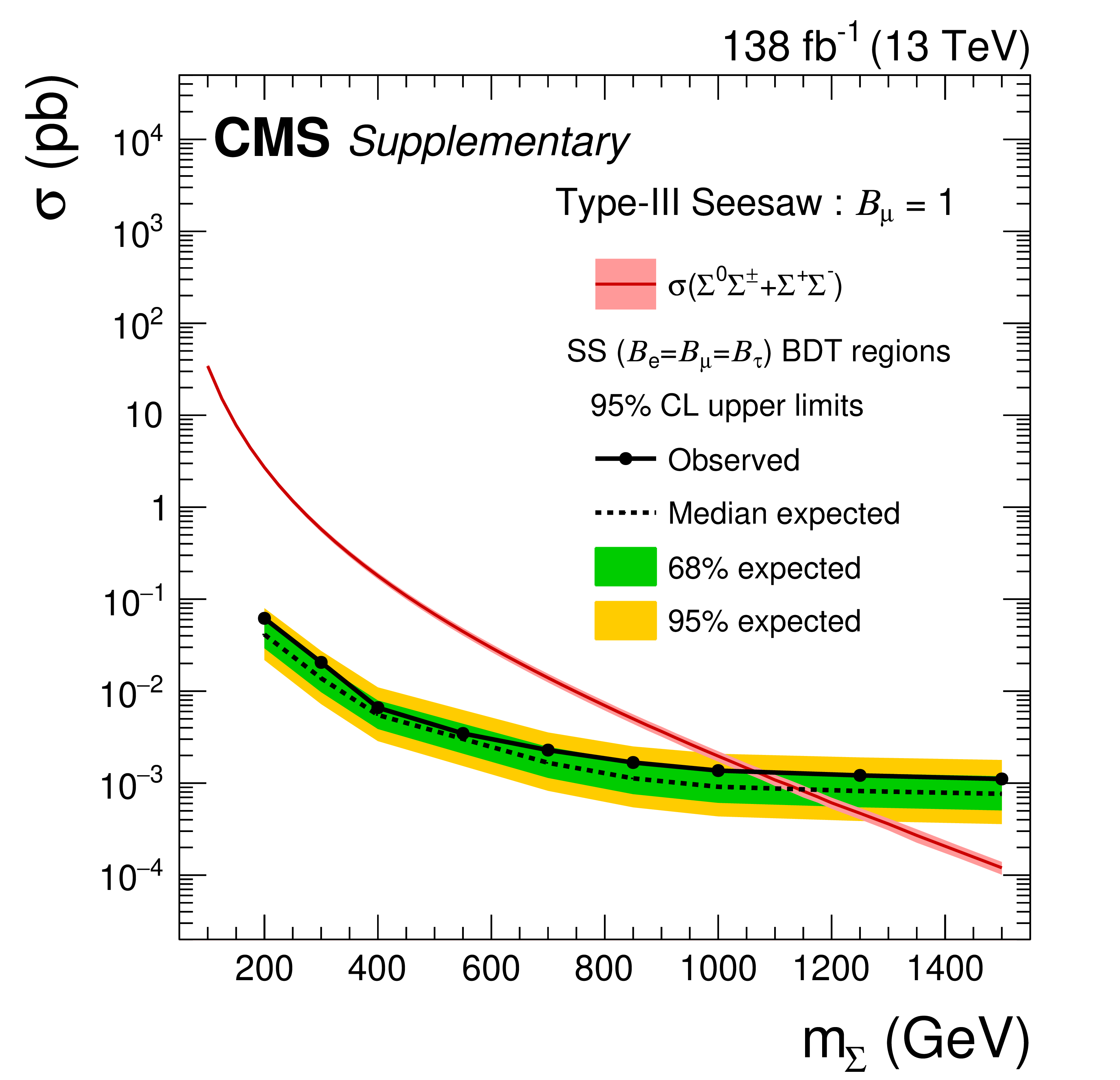
png pdf	Additional Figure 30: Observed and expected upper limits at 95% CL on the production cross section for the type-III seesaw fermions in the $\mathcal {B}_{\mu}=$ 1 scenario using the SS ($\mathcal {B}_{\mathrm{e}}=\mathcal {B}_{\mu}=\mathcal {B}_{\tau}$) BDT regions.
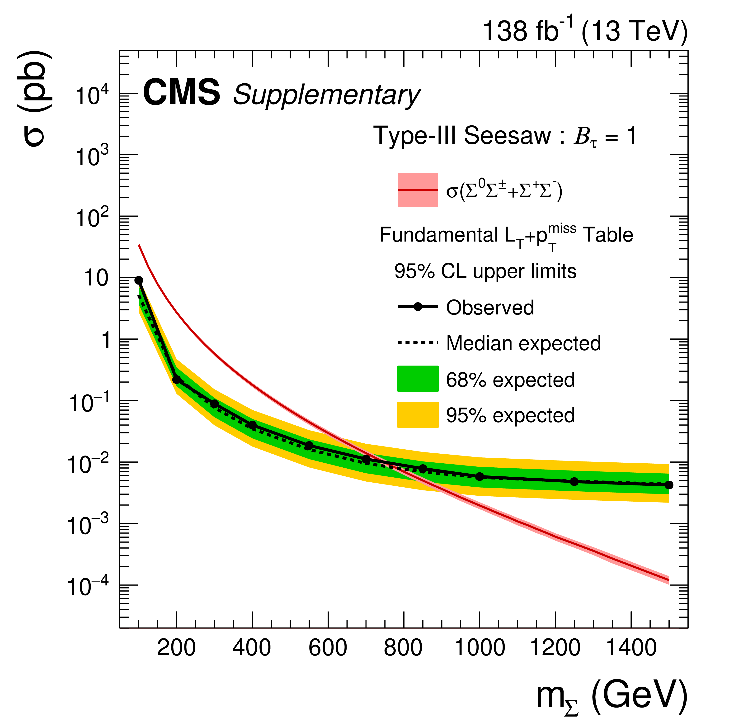
png pdf	Additional Figure 31: Observed and expected upper limits at 95% CL on the production cross section for the type-III seesaw fermions in the $\mathcal {B}_{\tau}=$ 1 scenario using the fundamental $L_{\rm T}+ {{p_{\mathrm {T}}} ^\text {miss}} $ table.
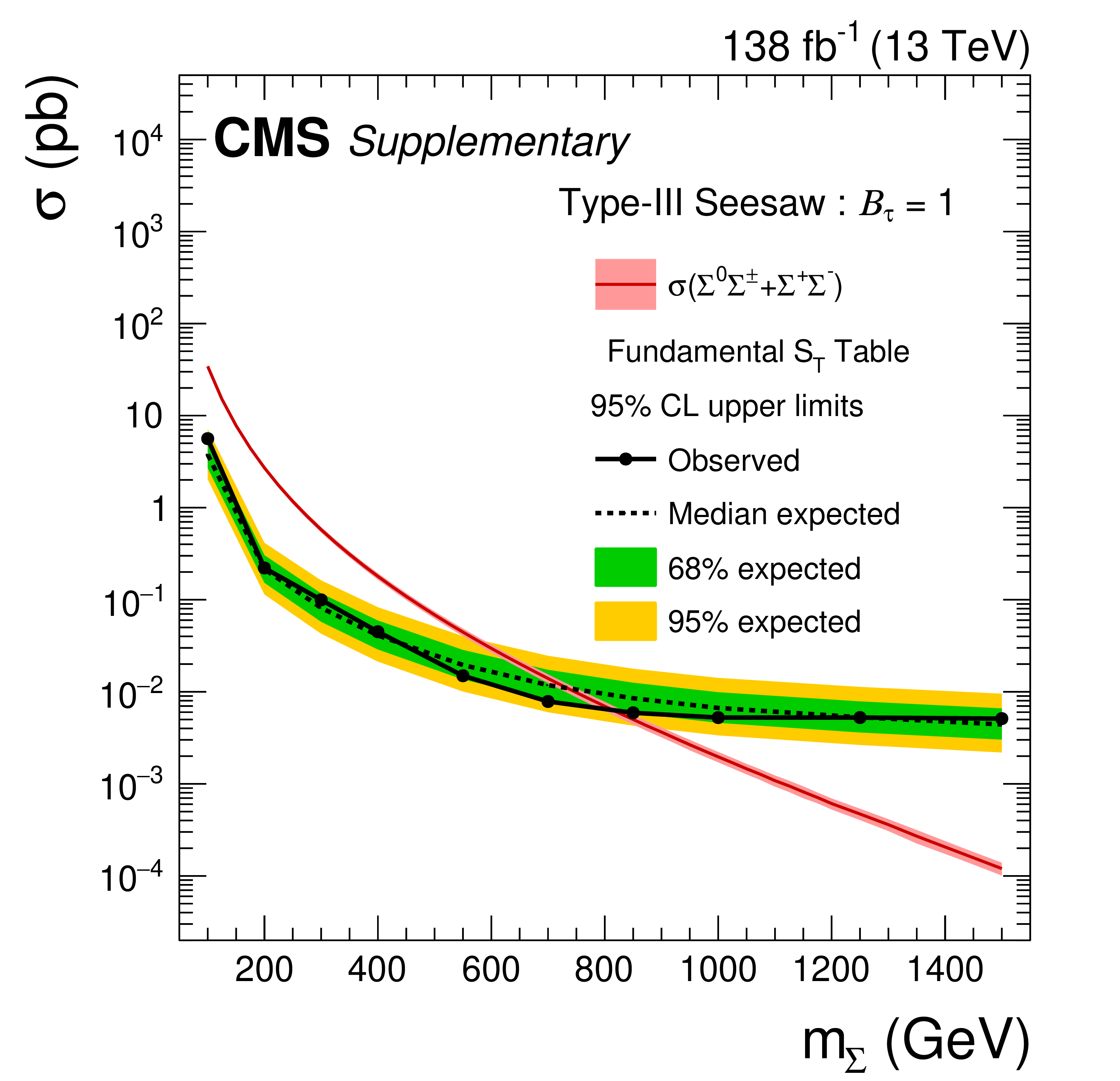
png pdf	Additional Figure 32: Observed and expected upper limits at 95% CL on the production cross section for the type-III seesaw fermions in the $\mathcal {B}_{\tau}=$ 1 scenario using the fundamental $S_{\rm T}$ table.
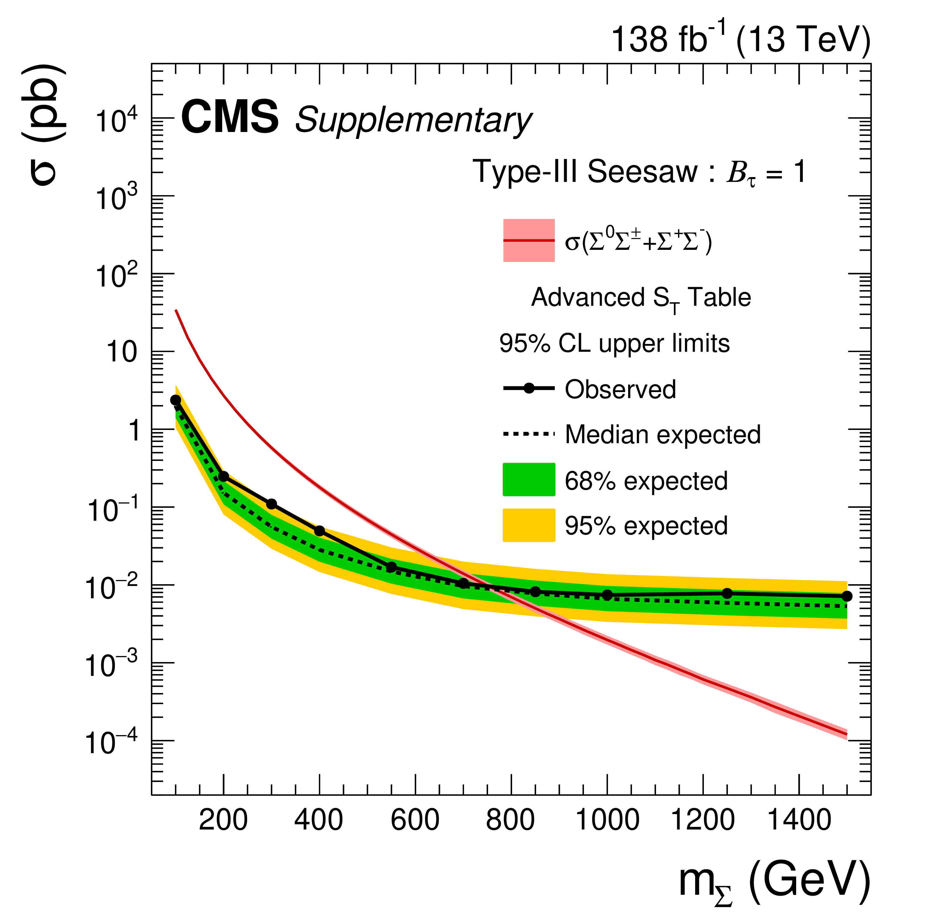
png pdf	Additional Figure 33: Observed and expected upper limits at 95% CL on the production cross section for the type-III seesaw fermions in the $\mathcal {B}_{\tau}=$ 1 scenario using the advanced $S_{\rm T}$ table.
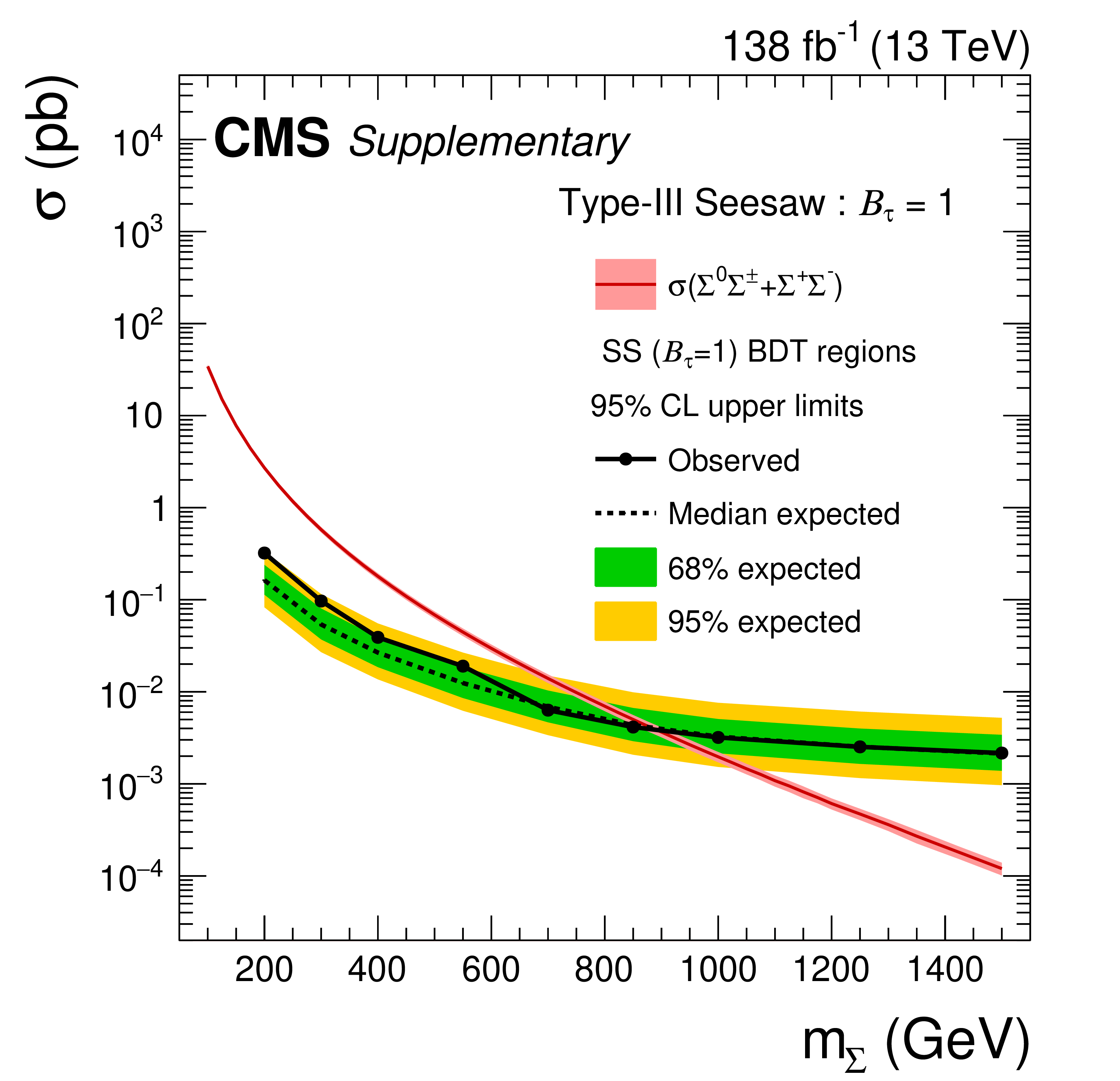
png pdf	Additional Figure 34: Observed and expected upper limits at 95% CL on the production cross section for the type-III seesaw fermions in the $\mathcal {B}_{\tau}=$ 1 scenario using the SS ($\mathcal {B}_{\tau}=$ 1) BDT regions.
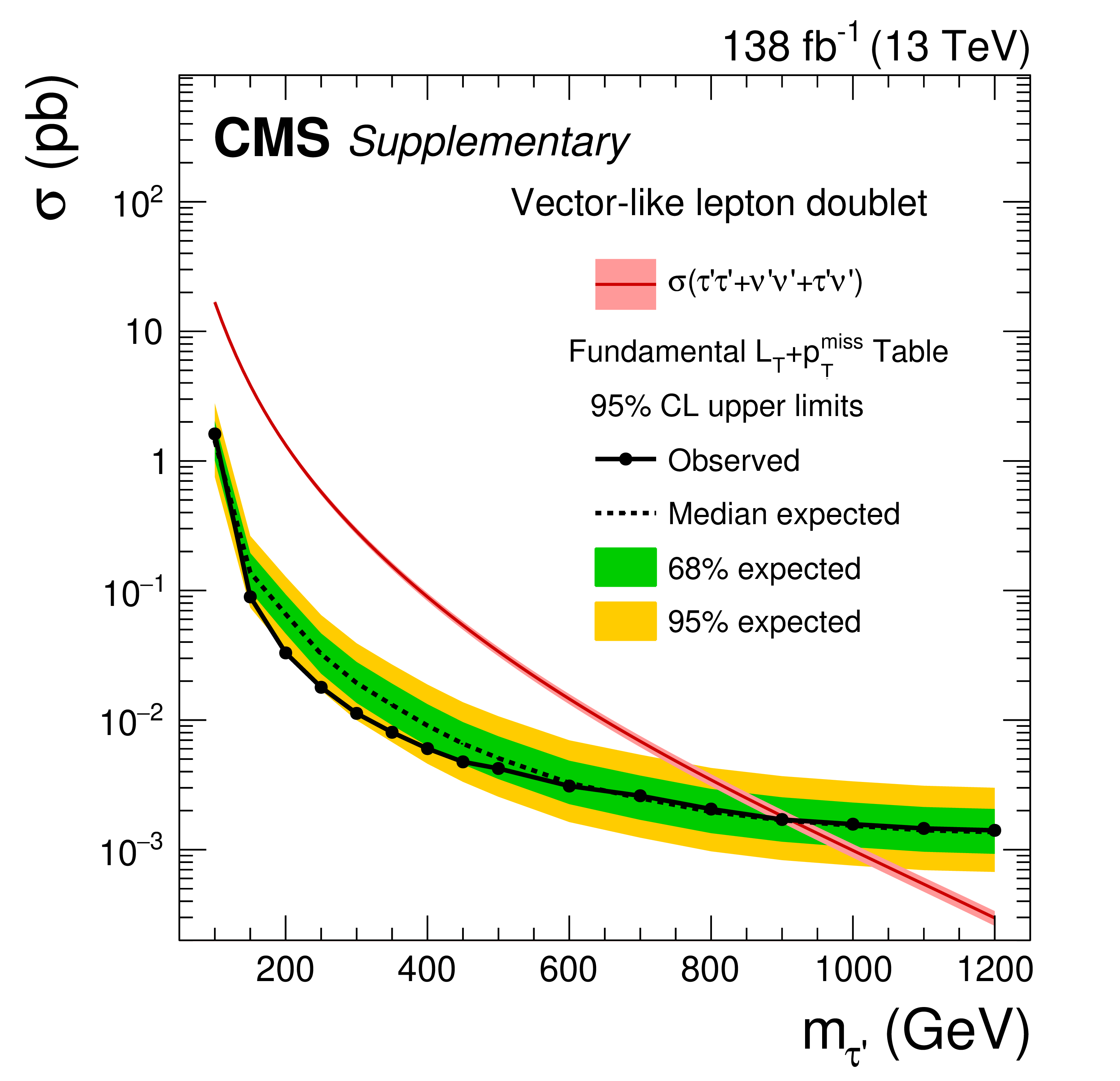
png pdf	Additional Figure 35: Observed and expected upper limits at 95% CL on the production cross section for the vector-like tau leptons in the doublet model using the fundamental $L_{\rm T}+ {{p_{\mathrm {T}}} ^\text {miss}} $ table.
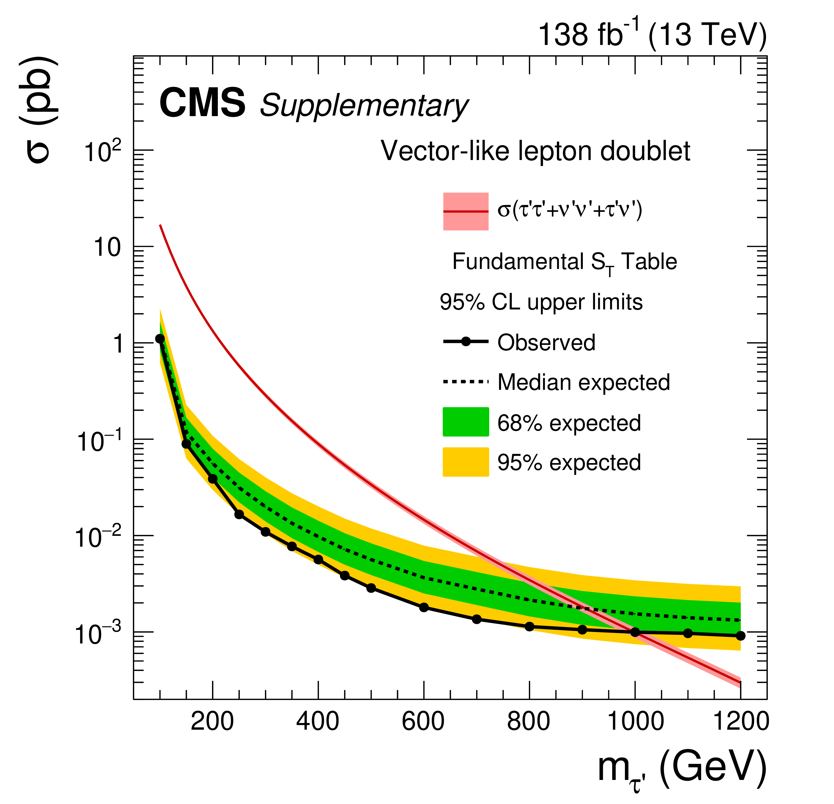
png pdf	Additional Figure 36: Observed and expected upper limits at 95% CL on the production cross section for the vector-like tau leptons in the doublet model using the fundamental $S_{\rm T}$ table.
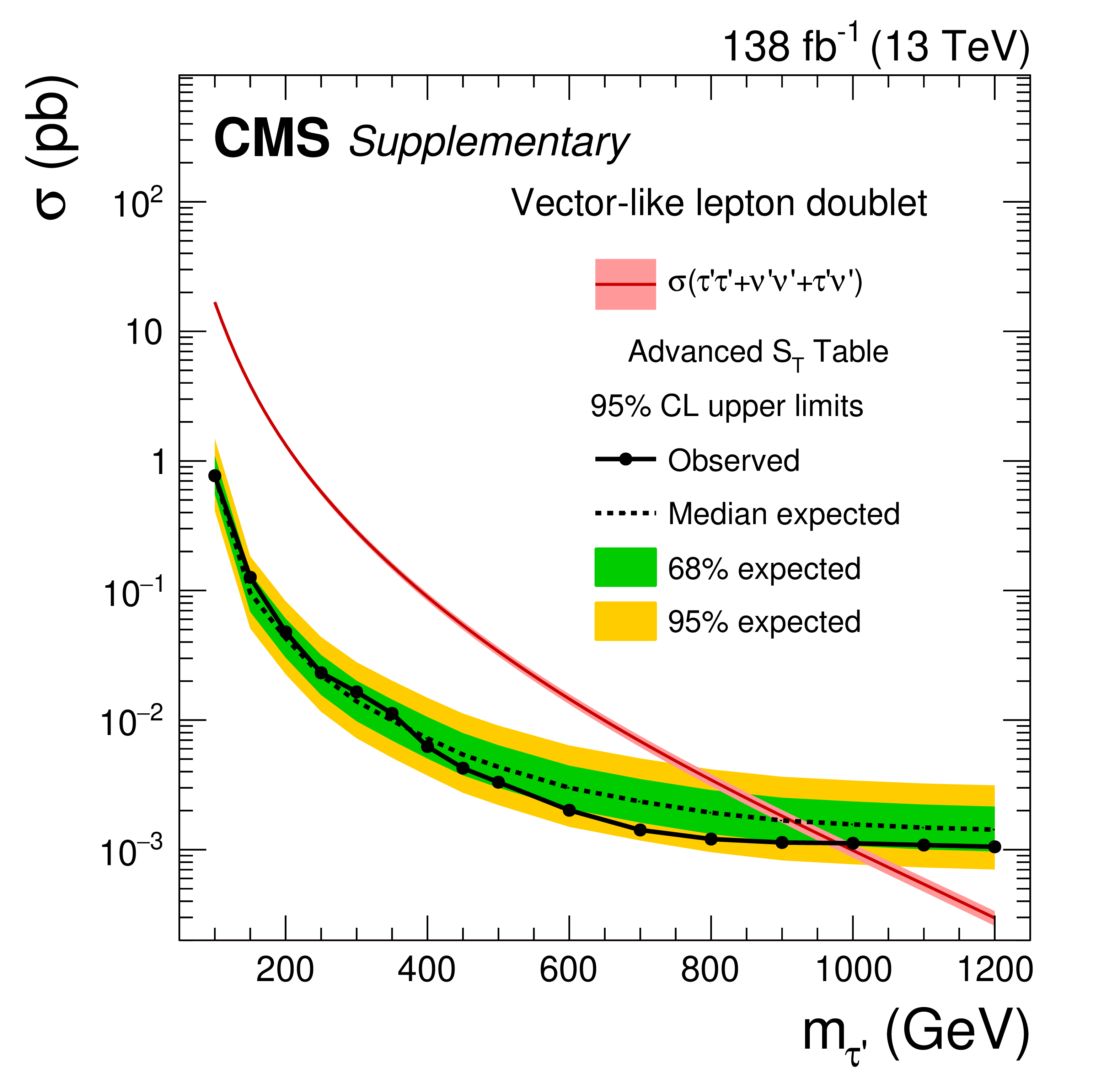
png pdf	Additional Figure 37: Observed and expected upper limits at 95% CL on the production cross section for the vector-like tau leptons in the doublet model using the advanced $S_{\rm T}$ table.
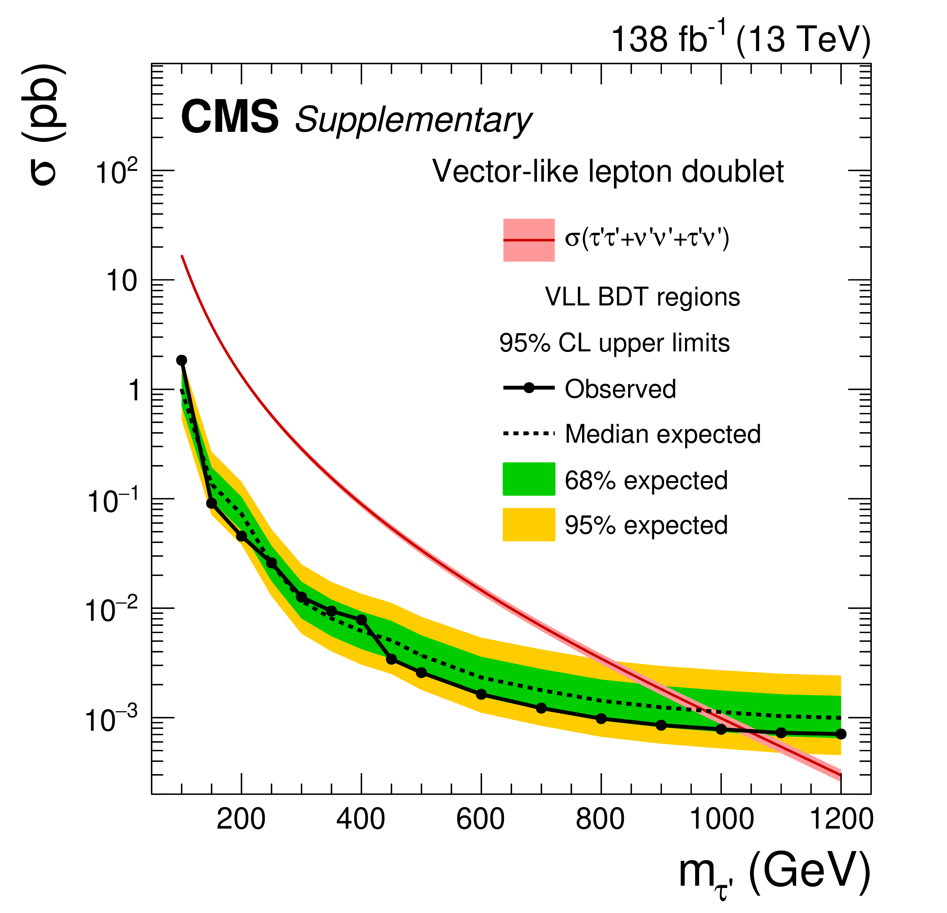
png pdf	Additional Figure 38: Observed and expected upper limits at 95% CL on the production cross section for the vector-like tau leptons in the doublet model using the VLL BDT regions.
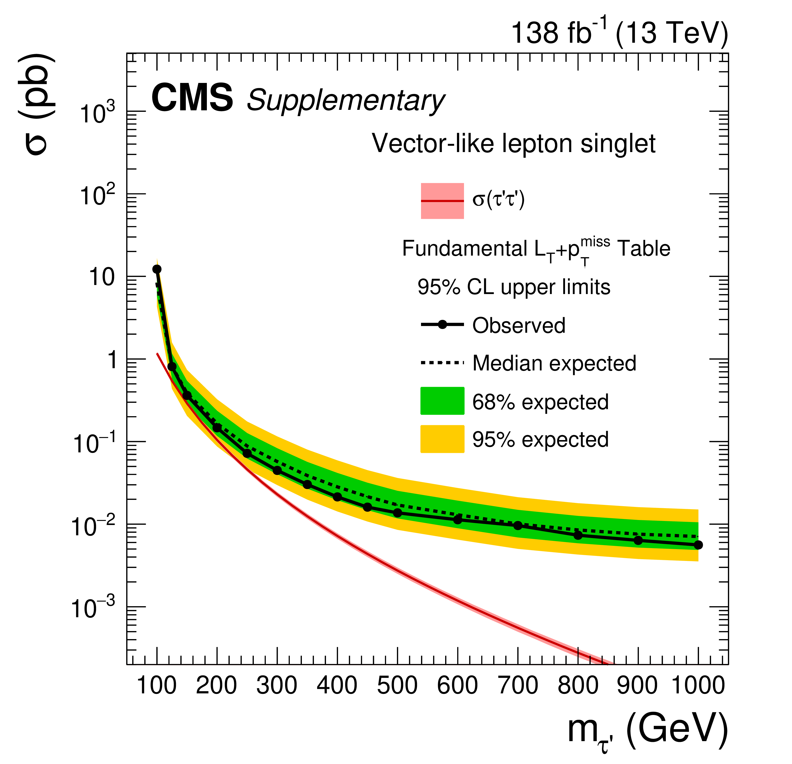
png pdf	Additional Figure 39: Observed and expected upper limits at 95% CL on the production cross section for the vector-like tau leptons in the singlet model using the fundamental $L_{\rm T}+ {{p_{\mathrm {T}}} ^\text {miss}} $ table.
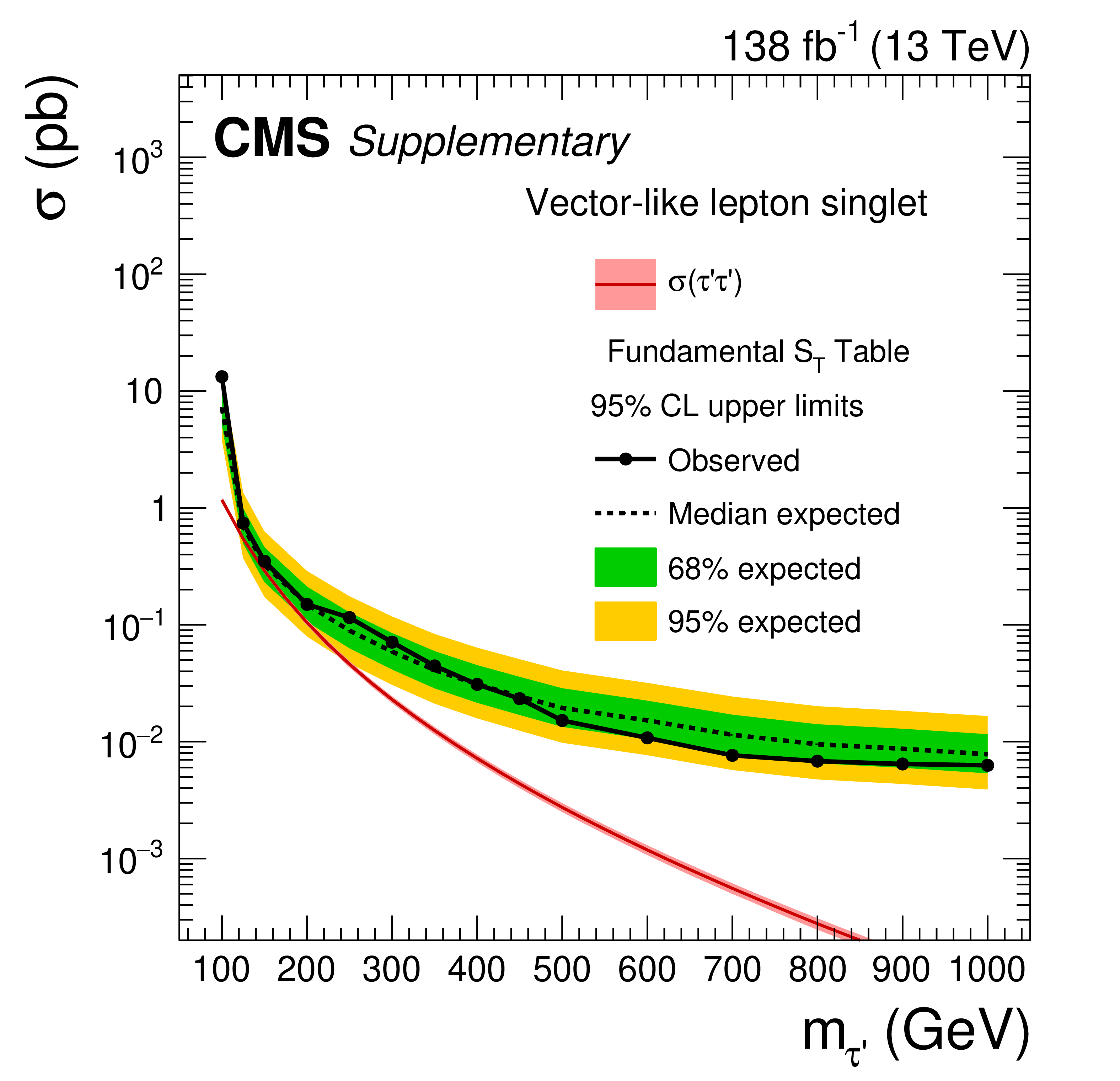
png pdf	Additional Figure 40: Observed and expected upper limits at 95% CL on the production cross section for the vector-like tau leptons in the singlet model using the fundamental $S_{\rm T}$ table.
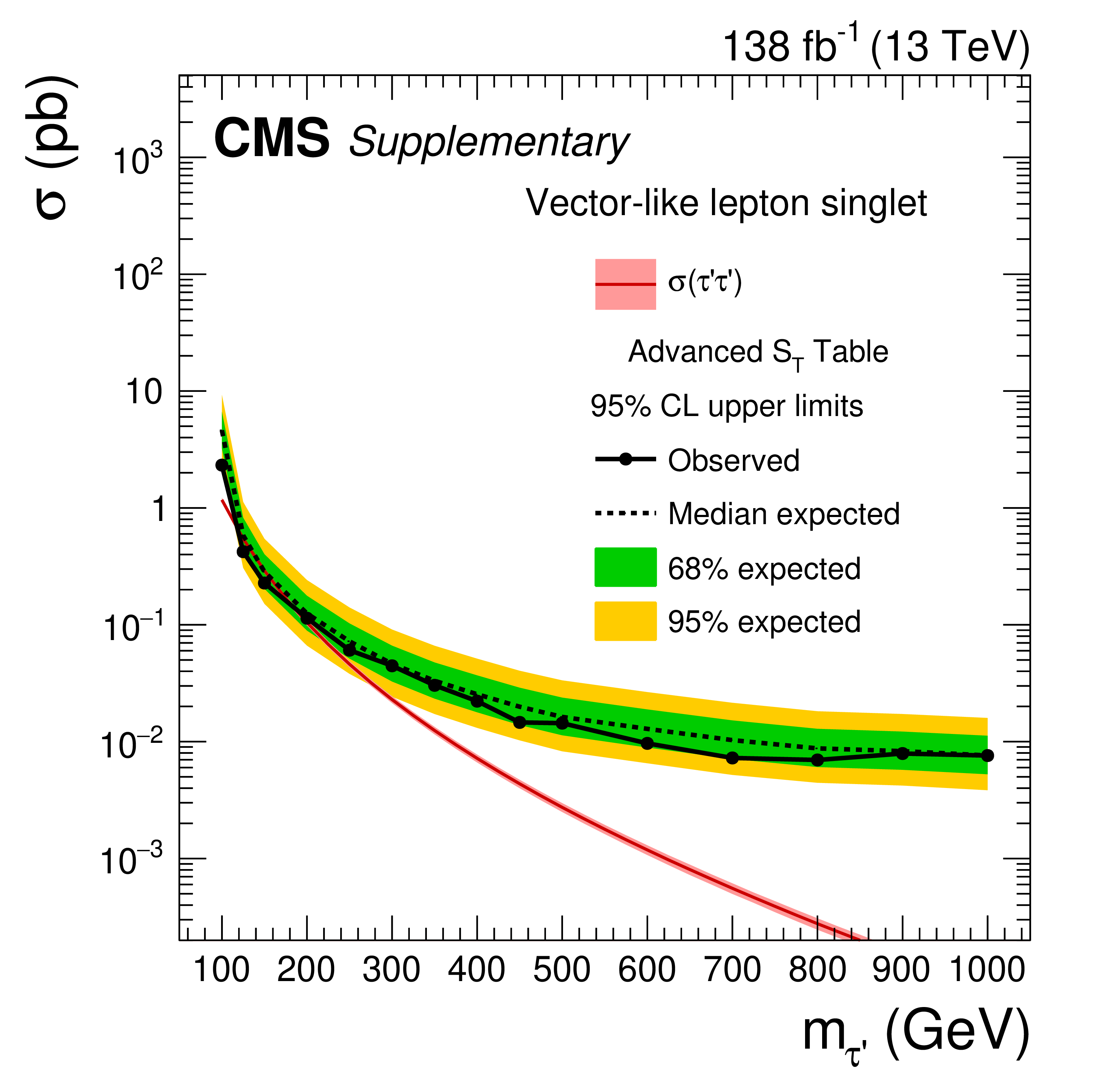
png pdf	Additional Figure 41: Observed and expected upper limits at 95% CL on the production cross section for the vector-like tau leptons in the singlet model using the advanced $S_{\rm T}$ table.
png pdf	Additional Figure 42: Observed and expected upper limits at 95% CL on the production cross section for the scalar leptoquarks with $\mathcal {B}_{\mathrm{e}}=$ 1 coupling using the fundamental $L_{\rm T}+ {{p_{\mathrm {T}}} ^\text {miss}} $ table.
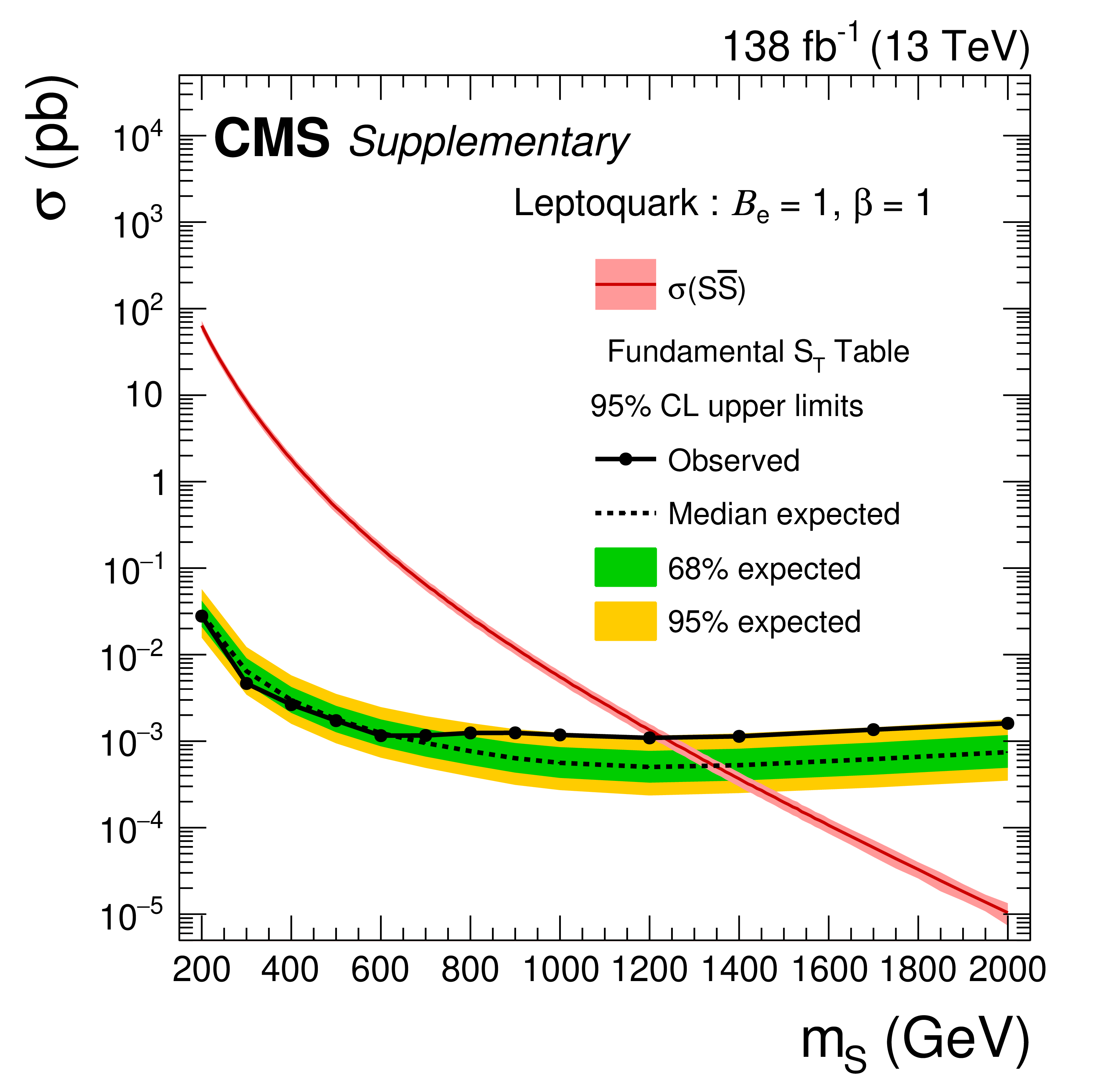
png pdf	Additional Figure 43: Observed and expected upper limits at 95% CL on the production cross section for the scalar leptoquarks with $\mathcal {B}_{\mathrm{e}}=$ 1 coupling using the fundamental $S_{\rm T}$ table.
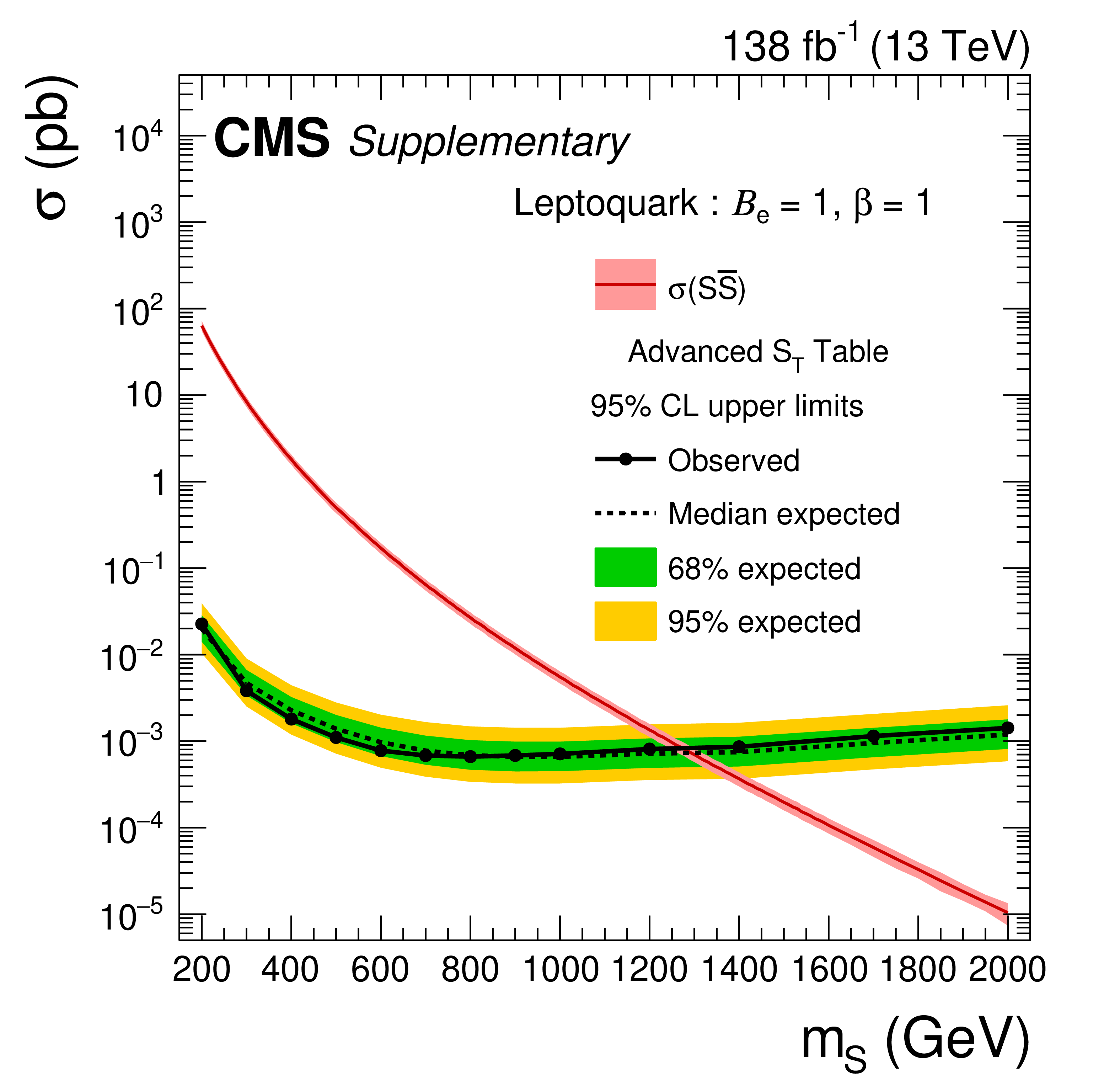
png pdf	Additional Figure 44: Observed and expected upper limits at 95% CL on the production cross section for the scalar leptoquarks with $\mathcal {B}_{\mathrm{e}}=$ 1 coupling using the advanced $S_{\rm T}$ table.
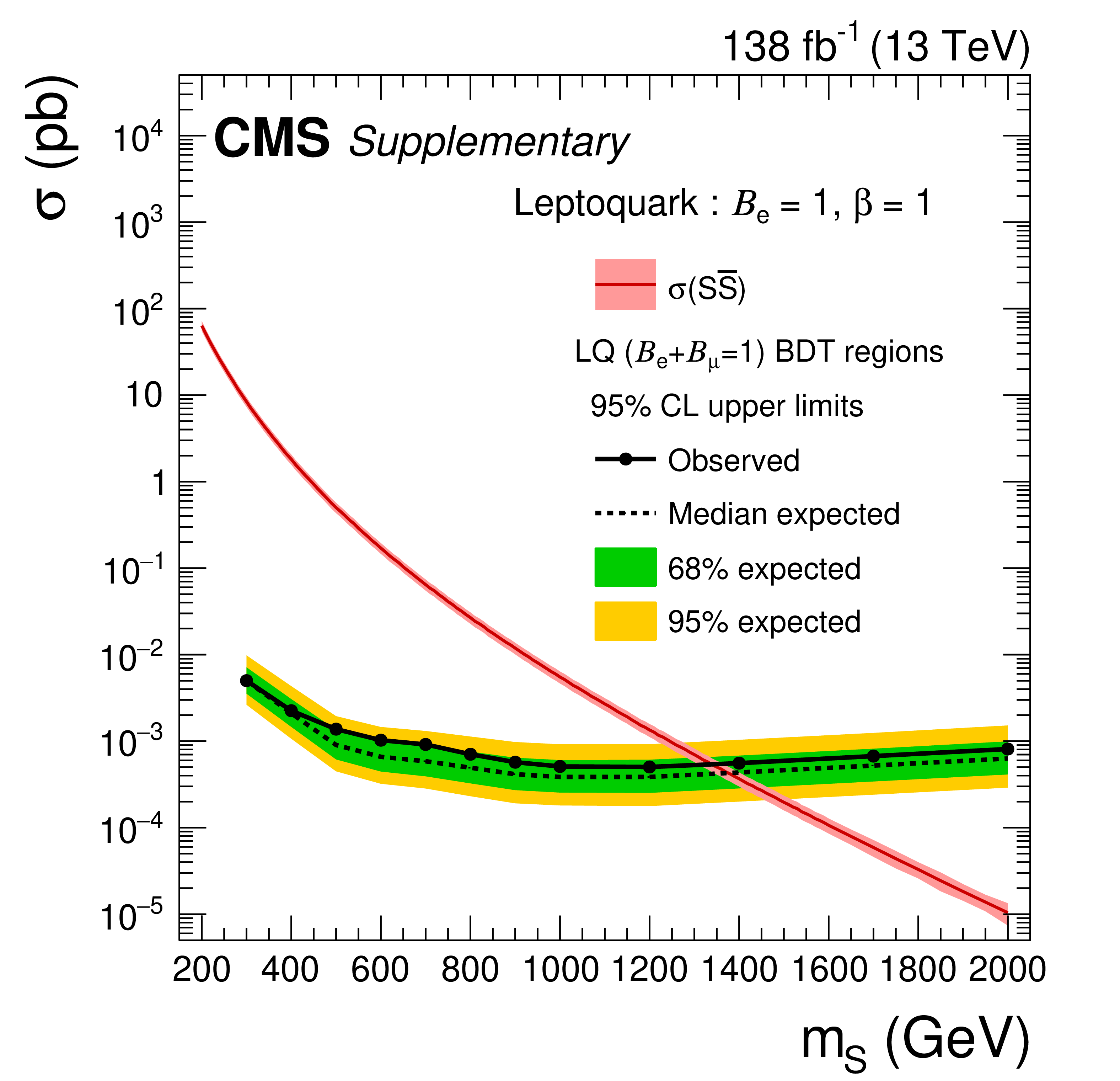
png pdf	Additional Figure 45: Observed and expected upper limits at 95% CL on the production cross section for the scalar leptoquarks with $\mathcal {B}_{\mathrm{e}}=$ 1 coupling using the LQ ($\mathcal {B}_{\mathrm{e}}+\mathcal {B}_{\mu}=$ 1) BDT regions.
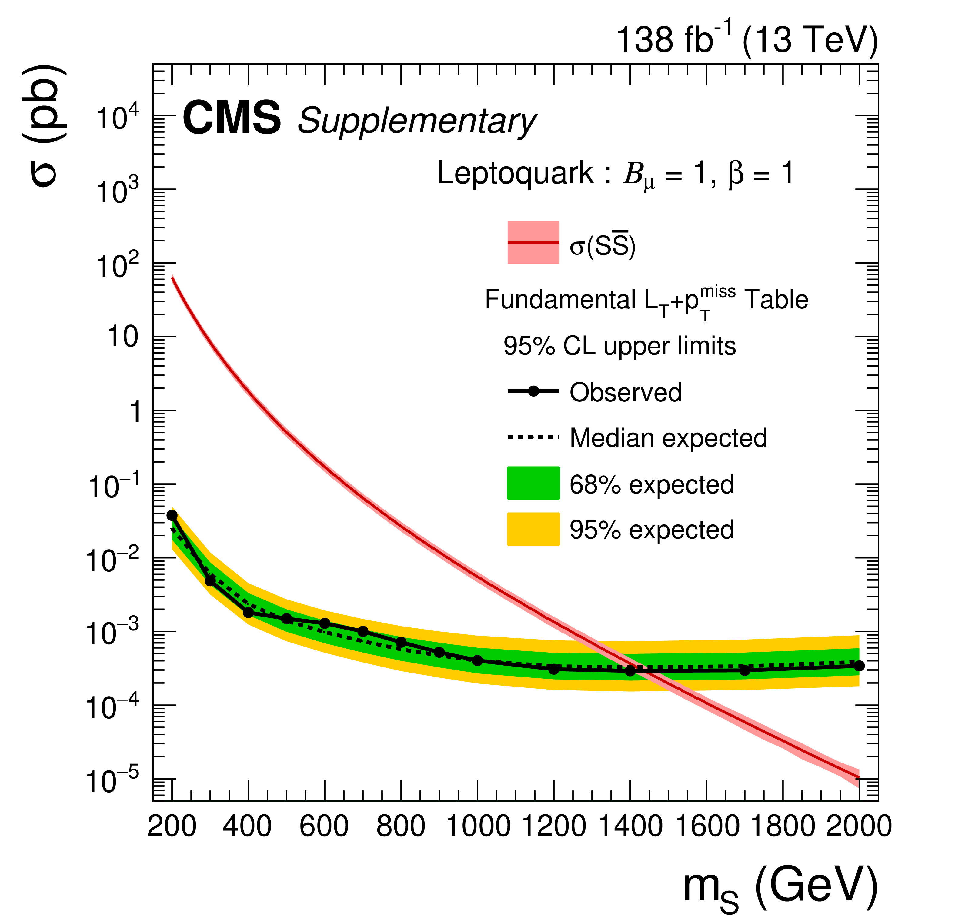
png pdf	Additional Figure 46: Observed and expected upper limits at 95% CL on the production cross section for the scalar leptoquarks with $\mathcal {B}_{\mu}=$ 1 coupling using the fundamental $L_{\rm T}+ {{p_{\mathrm {T}}} ^\text {miss}} $ table.
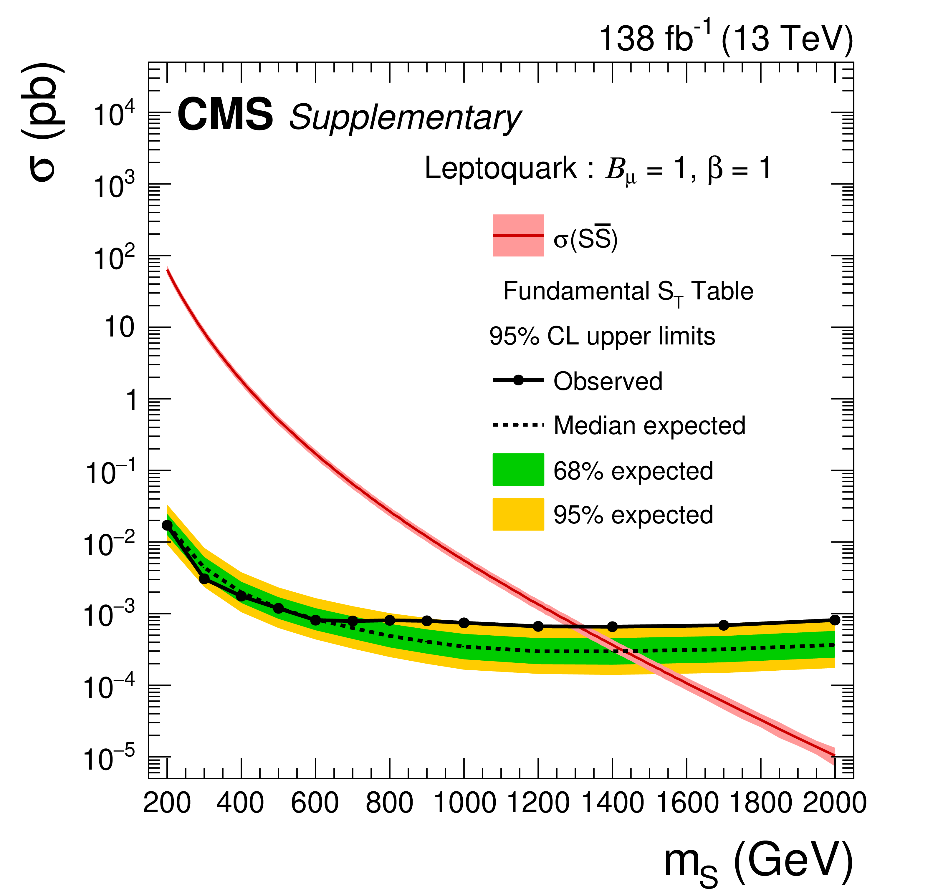
png pdf	Additional Figure 47: Observed and expected upper limits at 95% CL on the production cross section for the scalar leptoquarks with $\mathcal {B}_{\mu}=$ 1 coupling using the fundamental $S_{\rm T}$ table.
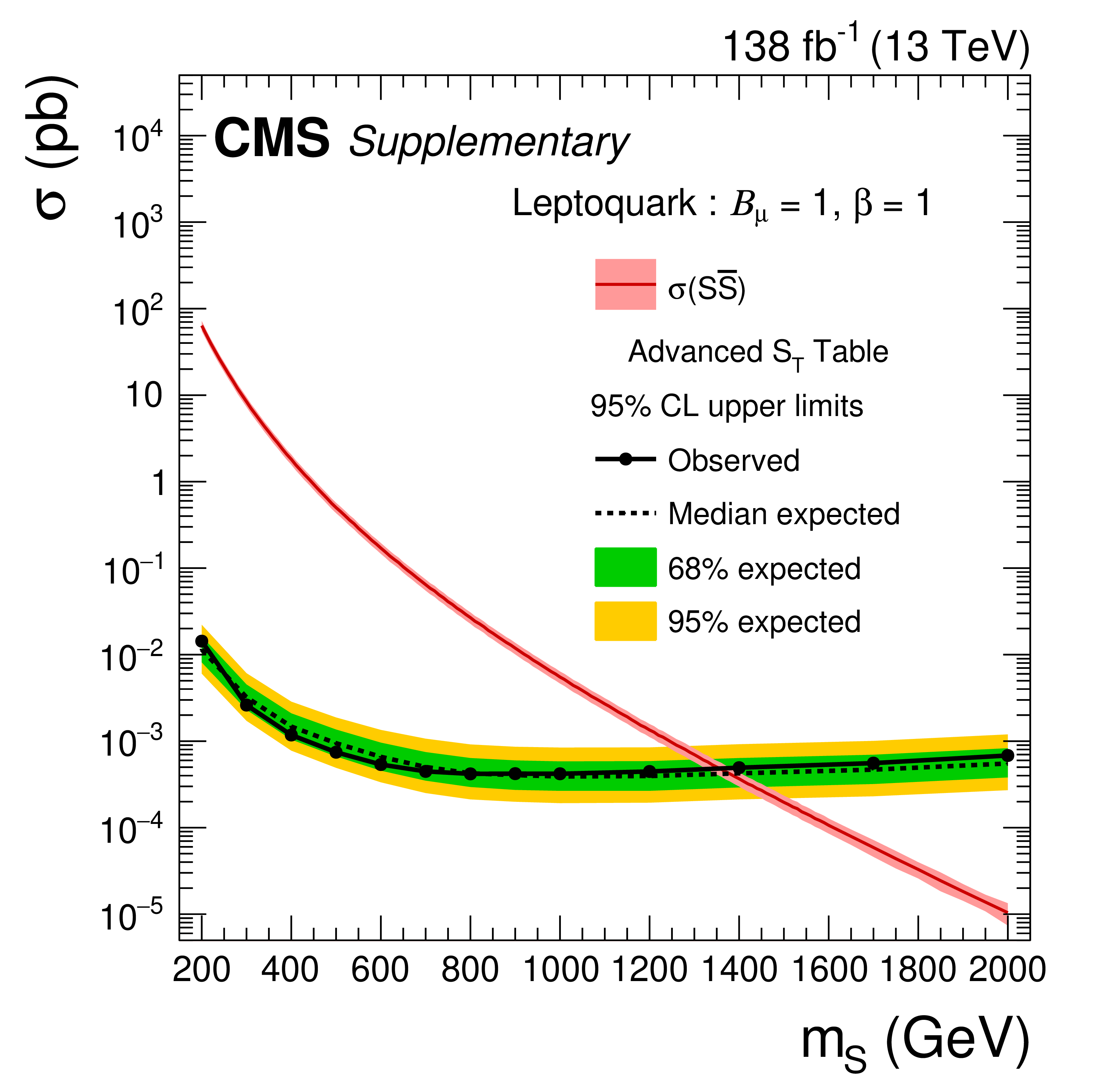
png pdf	Additional Figure 48: Observed and expected upper limits at 95% CL on the production cross section for the scalar leptoquarks with $\mathcal {B}_{\mu}=$ 1 coupling using the advanced $S_{\rm T}$ table.
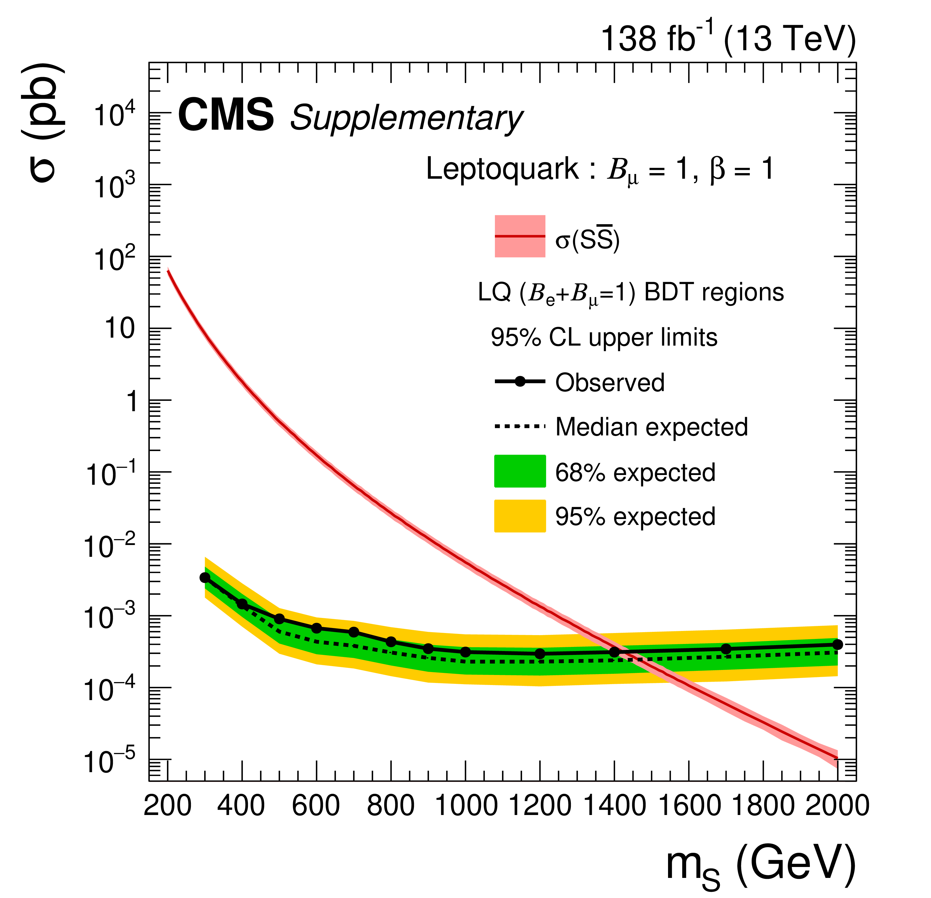
png pdf	Additional Figure 49: Observed and expected upper limits at 95% CL on the production cross section for the scalar leptoquarks with $\mathcal {B}_{\mu}=$ 1 coupling using the LQ ($\mathcal {B}_{\mathrm{e}}+\mathcal {B}_{\mu}=$ 1) regions.
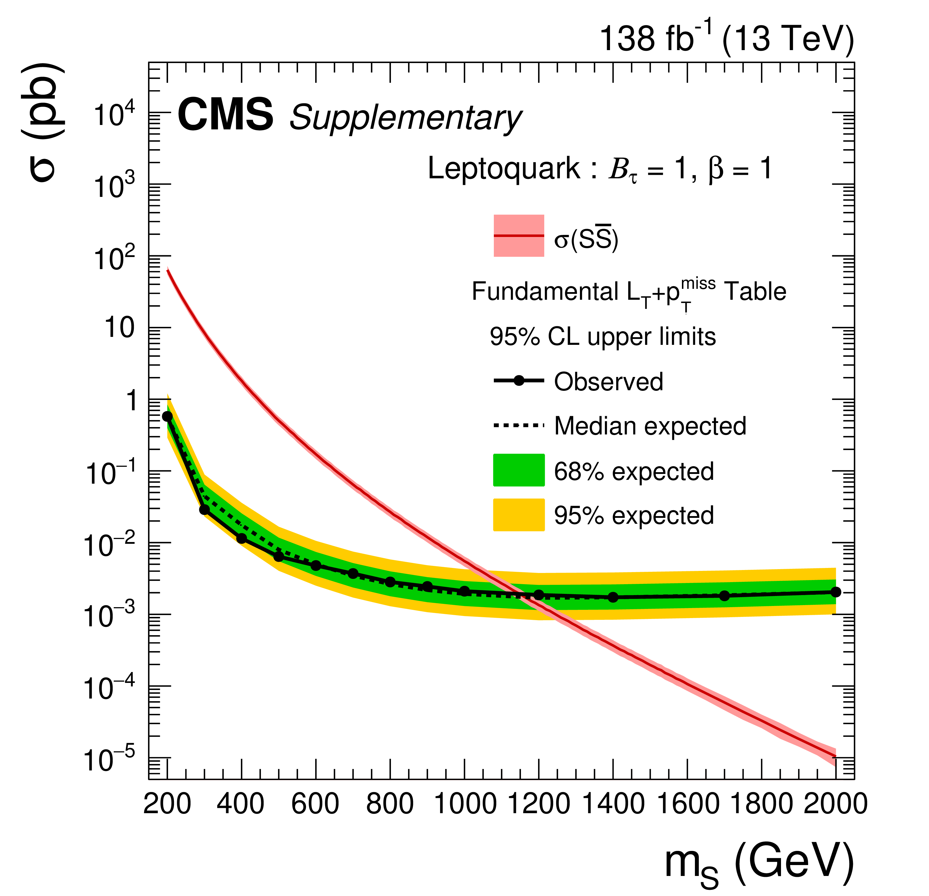
png pdf	Additional Figure 50: Observed and expected upper limits at 95% CL on the production cross section for the scalar leptoquarks with $\mathcal {B}_{\tau}=$ 1 coupling using the fundamental $L_{\rm T}+ {{p_{\mathrm {T}}} ^\text {miss}} $ table.
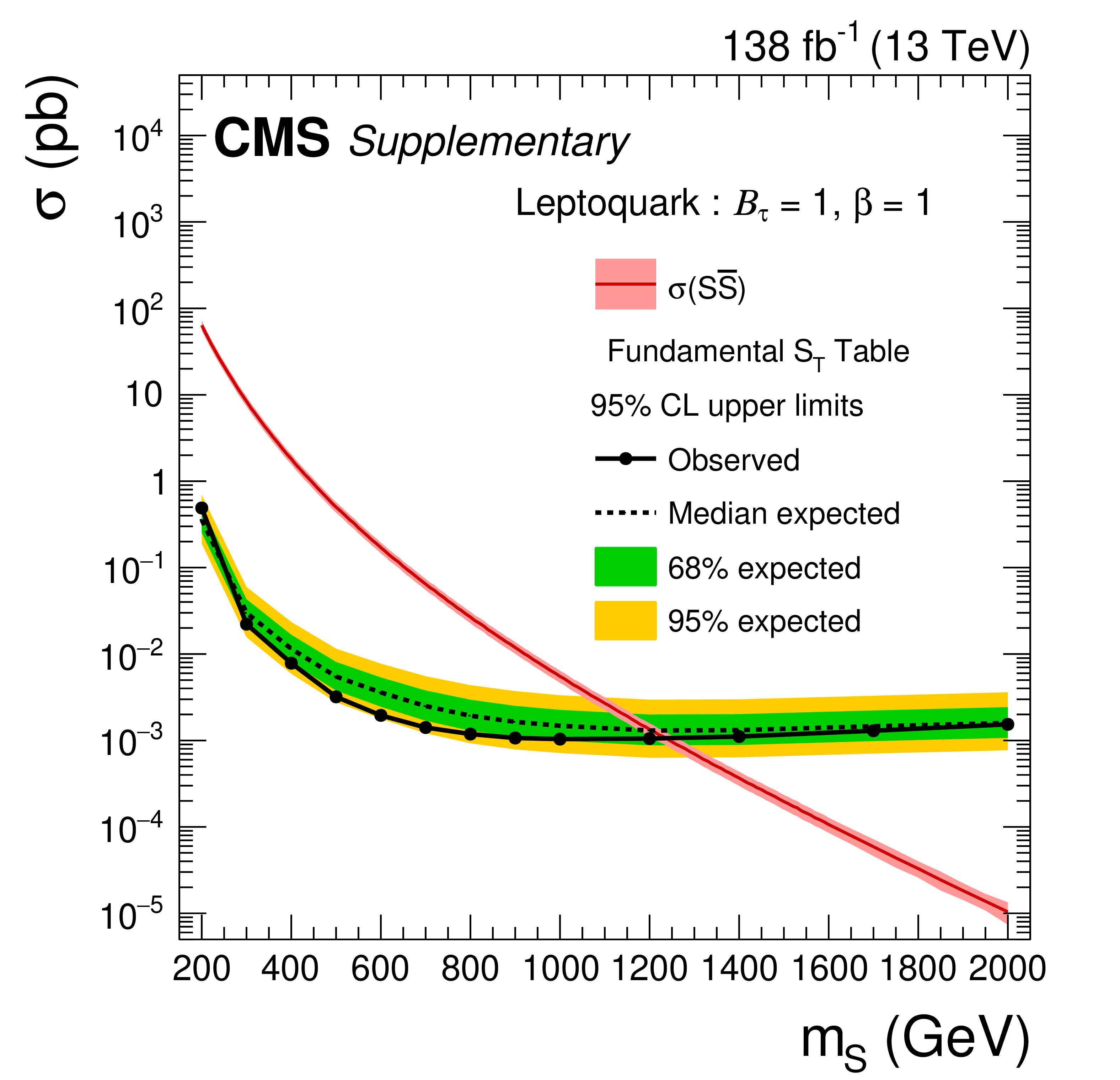
png pdf	Additional Figure 51: Observed and expected upper limits at 95% CL on the production cross section for the scalar leptoquarks with $\mathcal {B}_{\tau}=$ 1 coupling using the fundamental $S_{\rm T}$ table.
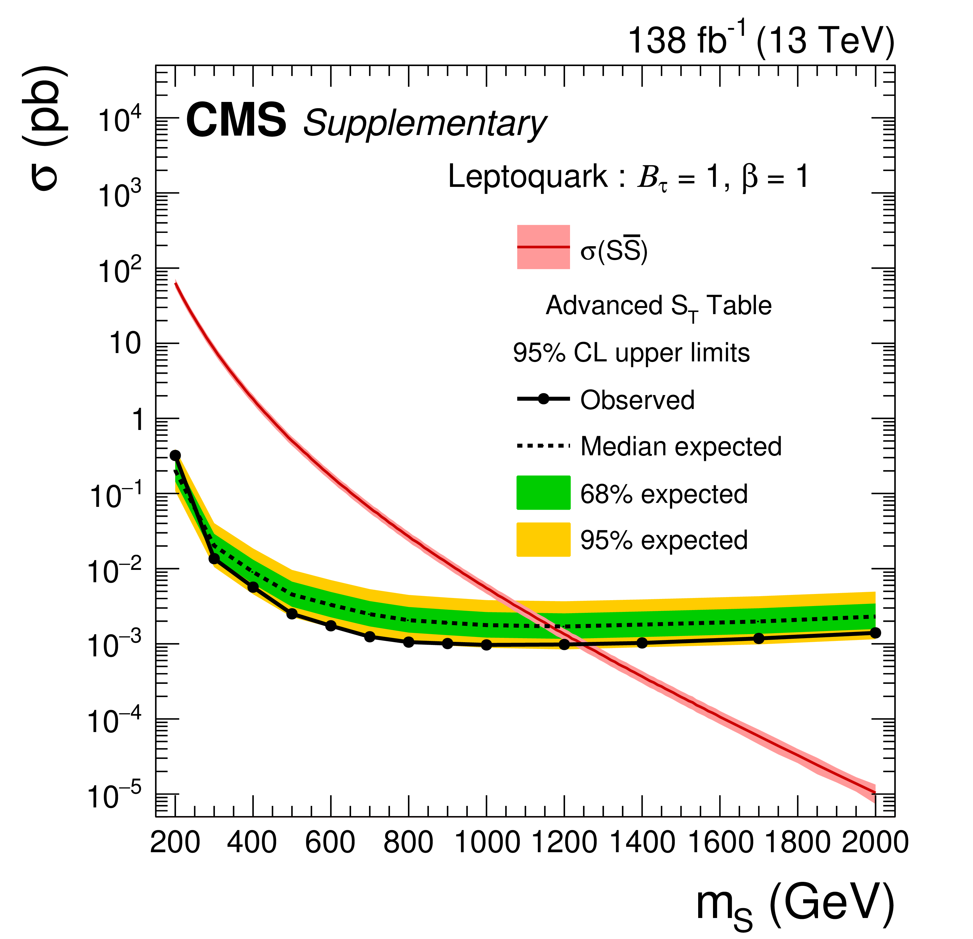
png pdf	Additional Figure 52: Observed and expected upper limits at 95% CL on the production cross section for the scalar leptoquarks with $\mathcal {B}_{\tau}=$ 1 coupling using the advanced $S_{\rm T}$ table.
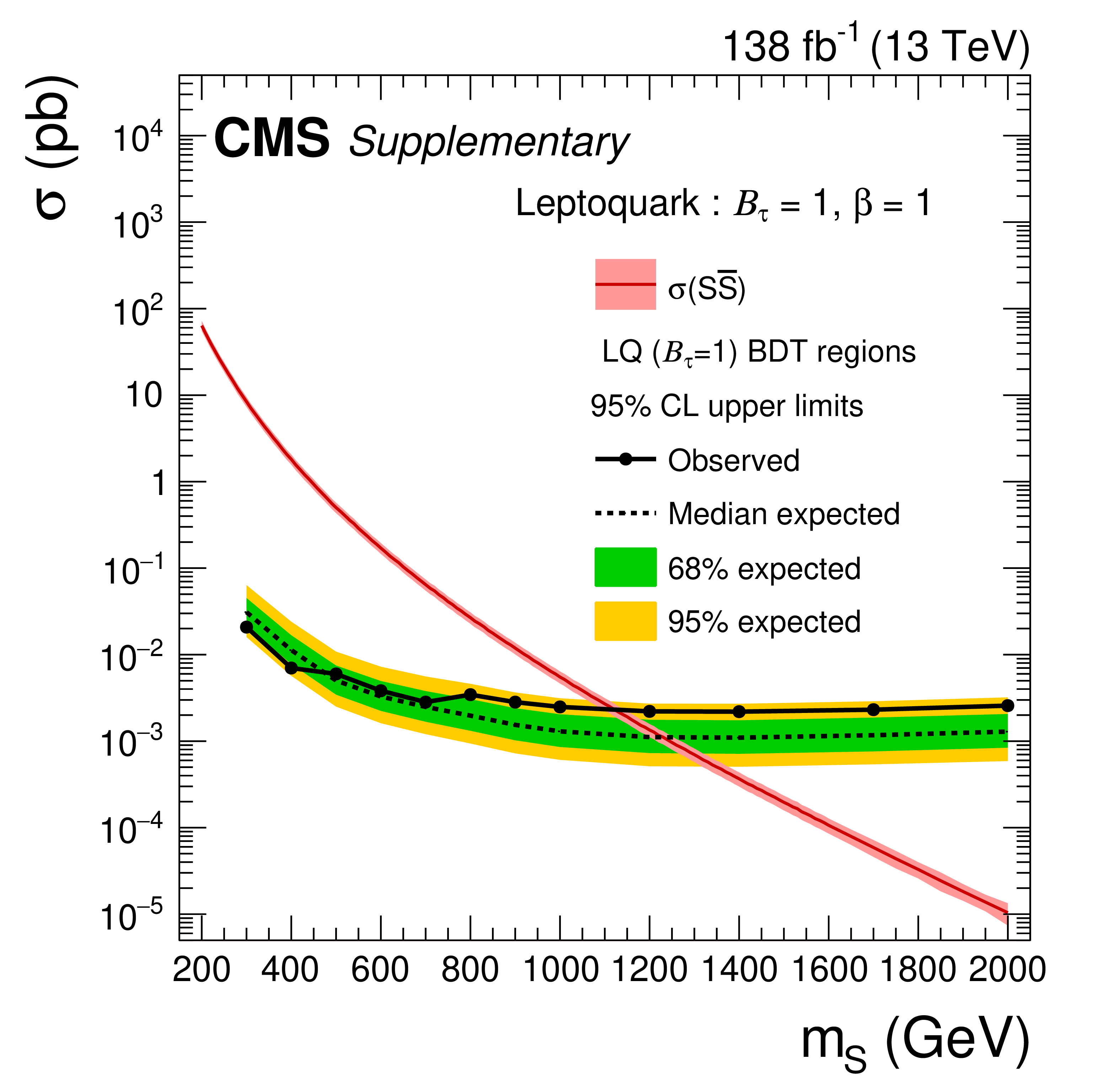
png pdf	Additional Figure 53: Observed and expected upper limits at 95% CL on the production cross section for the scalar leptoquarks with $\mathcal {B}_{\tau}=$ 1 coupling using the LQ ($\mathcal {B}_{\tau}=$ 1) regions.
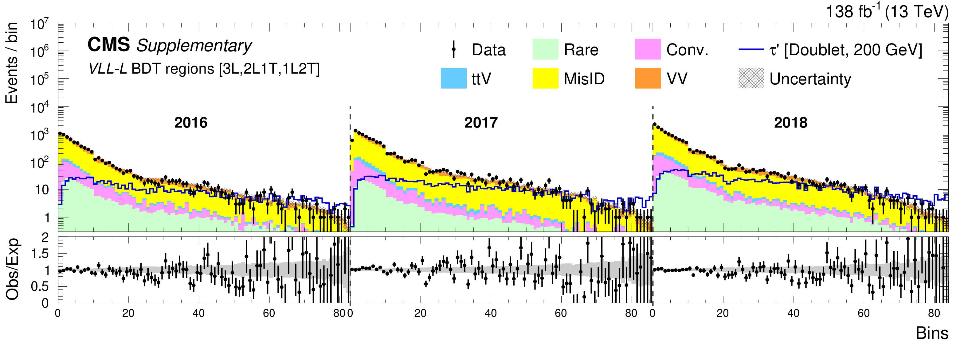
png pdf	Additional Figure 54: The VLL-L BDT regions for the 3-lepton channel for the 2016-2018 data sets. The lower panel shows the ratio of observed events to the total expected background prediction. The gray band on the ratio represents the sum of statistical and systematic uncertainties in the SM background prediction. The expected SM background distributions and the uncertainties are shown after fitting the data under the background-only hypothesis. For illustration, an example signal hypothesis for the production of the vector-like $\tau$ lepton in the doublet scenario for $m_{\tau ^{\prime}} = $ 200 GeV, before the fit, is also overlaid.
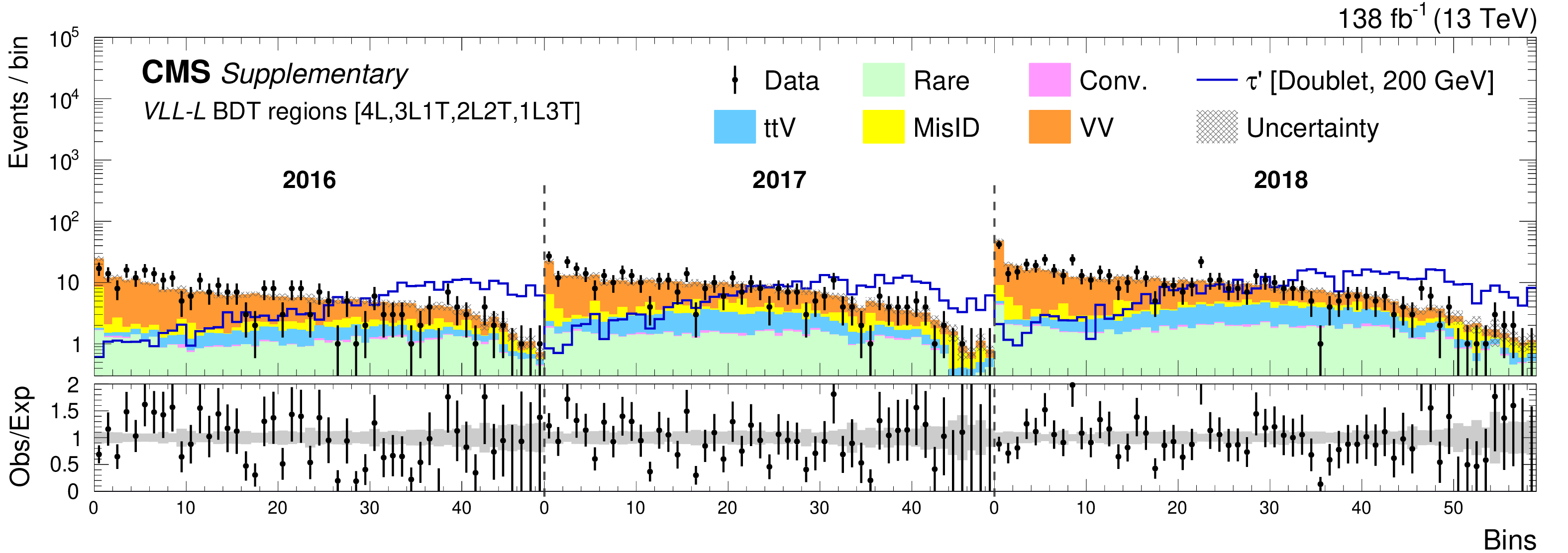
png pdf	Additional Figure 55: The VLL-L BDT regions for the 4-lepton channel for the 2016-2018 data sets. The lower panel shows the ratio of observed events to the total expected background prediction. The gray band on the ratio represents the sum of statistical and systematic uncertainties in the SM background prediction. The expected SM background distributions and the uncertainties are shown after fitting the data under the background-only hypothesis. For illustration, an example signal hypothesis for the production of the vector-like $\tau$ lepton in the doublet scenario for $m_{\tau ^{\prime}} = $ 200 GeV, before the fit, is also overlaid.
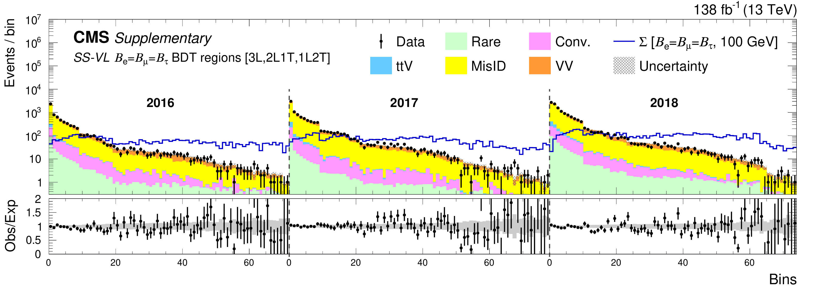
png pdf	Additional Figure 56: The SS-VL $\mathcal {B}_{\mathrm{e}}=\mathcal {B}_{\mu}=\mathcal {B}_{\tau}$ BDT regions for the 3-lepton channel for the 2016-2018 data sets. The lower panel shows the ratio of observed events to the total expected background prediction. The gray band on the ratio represents the sum of statistical and systematic uncertainties in the SM background prediction. The expected SM background distributions and the uncertainties are shown after fitting the data under the background-only hypothesis. For illustration, an example signal hypothesis for the production of the type-III seesaw heavy fermions in the flavor-democratic scenario for $m_{\Sigma} = $ 100 GeV, before the fit, is also overlaid.
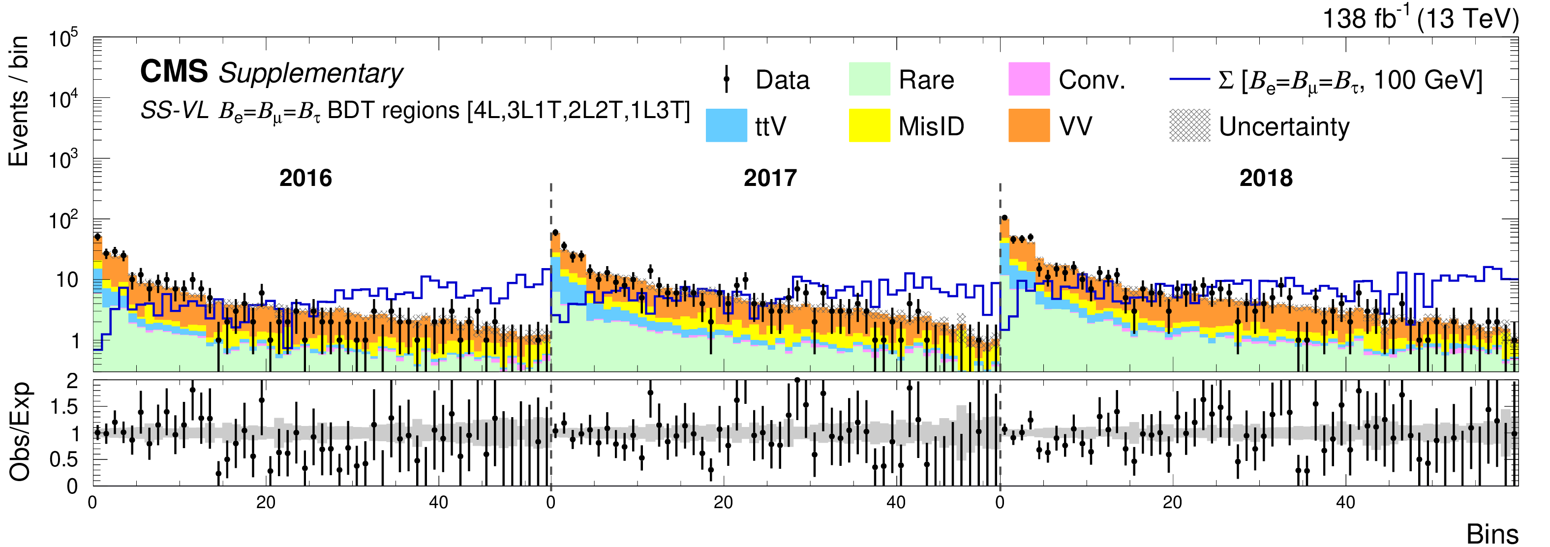
png pdf	Additional Figure 57: The SS-VL $\mathcal {B}_{\mathrm{e}}=\mathcal {B}_{\mu}=\mathcal {B}_{\tau}$ BDT regions for the 4-lepton channel for the 2016-2018 data sets. The lower panel shows the ratio of observed events to the total expected background prediction. The gray band on the ratio represents the sum of statistical and systematic uncertainties in the SM background prediction. The expected SM background distributions and the uncertainties are shown after fitting the data under the background-only hypothesis. For illustration, an example signal hypothesis for the production of the type-III seesaw heavy fermions in the flavor-democratic scenario for $m_{\Sigma} = $ 100 GeV, before the fit, is also overlaid.
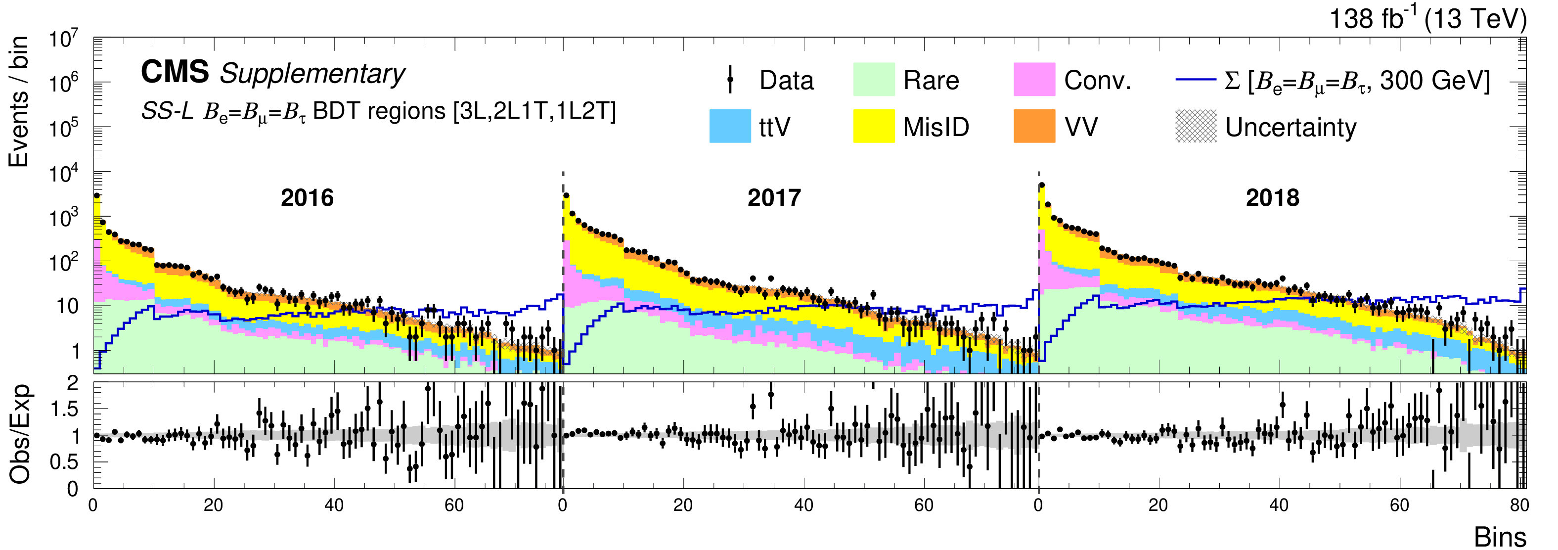
png pdf	Additional Figure 58: The SS-L $\mathcal {B}_{\mathrm{e}}=\mathcal {B}_{\mu}=\mathcal {B}_{\tau}$ BDT regions for the 3-lepton channel for the 2016-2018 data sets. The lower panel shows the ratio of observed events to the total expected background prediction. The gray band on the ratio represents the sum of statistical and systematic uncertainties in the SM background prediction. The expected SM background distributions and the uncertainties are shown after fitting the data under the background-only hypothesis. For illustration, an example signal hypothesis for the production of the type-III seesaw heavy fermions in the flavor-democratic scenario for $m_{\Sigma} = $ 300 GeV, before the fit, is also overlaid.
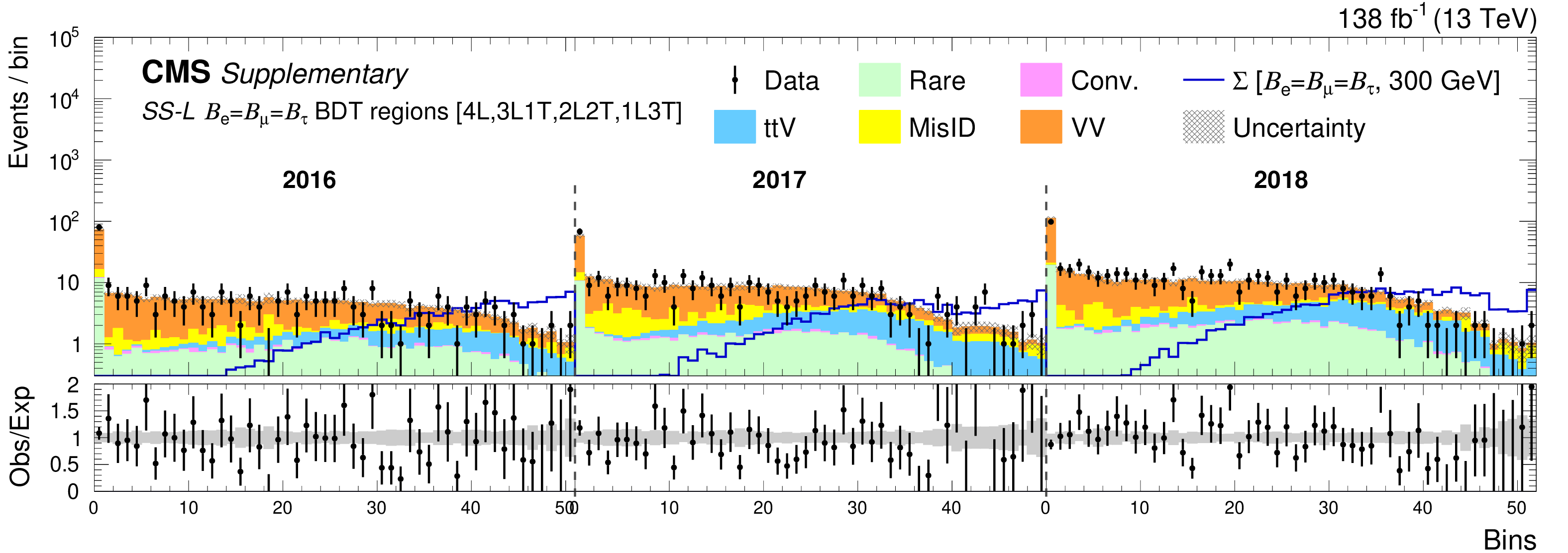
png pdf	Additional Figure 59: The SS-L $\mathcal {B}_{\mathrm{e}}=\mathcal {B}_{\mu}=\mathcal {B}_{\tau}$ BDT regions for the 4-lepton channel for the 2016-2018 data sets. The lower panel shows the ratio of observed events to the total expected background prediction. The gray band on the ratio represents the sum of statistical and systematic uncertainties in the SM background prediction. The expected SM background distributions and the uncertainties are shown after fitting the data under the background-only hypothesis. For illustration, an example signal hypothesis for the production of the type-III seesaw heavy fermions in the flavor-democratic scenario for $m_{\Sigma} = $ 300 GeV, before the fit, is also overlaid.
png pdf	Additional Figure 60: The SS-VL $\mathcal {B}_{\tau}=$ 1 BDT regions for the 3-lepton channel for the 2016-2018 data sets. The lower panel shows the ratio of observed events to the total expected background prediction. The gray band on the ratio represents the sum of statistical and systematic uncertainties in the SM background prediction. The expected SM background distributions and the uncertainties are shown after fitting the data under the background-only hypothesis. For illustration, an example signal hypothesis for the production of the type-III seesaw heavy fermions in the scenario with mixing exclusively to $\tau$ lepton for $m_{\Sigma} = $ 100 GeV, before the fit, is also overlaid.
png pdf	Additional Figure 61: The SS-VL $\mathcal {B}_{\tau}=$ 1 BDT regions for the 4-lepton channel for the 2016-2018 data sets. The lower panel shows the ratio of observed events to the total expected background prediction. The gray band on the ratio represents the sum of statistical and systematic uncertainties in the SM background prediction. The expected SM background distributions and the uncertainties are shown after fitting the data under the background-only hypothesis. For illustration, an example signal hypothesis for the production of the type-III seesaw heavy fermions in the scenario with mixing exclusively to $\tau$ lepton for $m_{\Sigma} = $ 100 GeV, before the fit, is also overlaid.
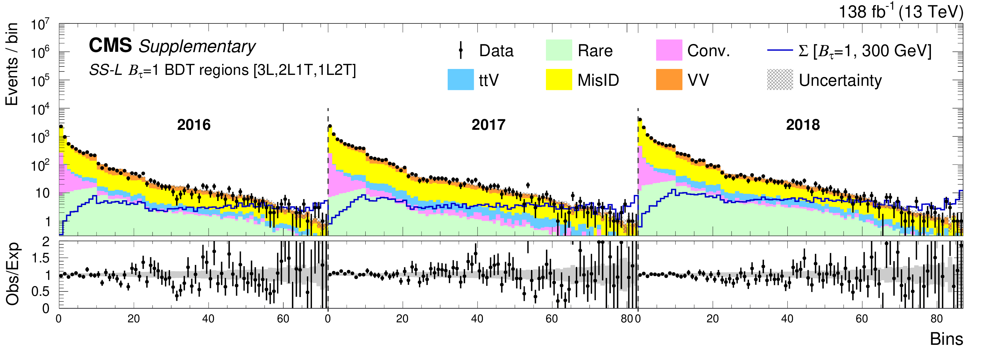
png pdf	Additional Figure 62: The SS-L $\mathcal {B}_{\tau}=$ 1 BDT regions for the 3-lepton channel for the 2016-2018 data sets. The lower panel shows the ratio of observed events to the total expected background prediction. The gray band on the ratio represents the sum of statistical and systematic uncertainties in the SM background prediction. The expected SM background distributions and the uncertainties are shown after fitting the data under the background-only hypothesis. For illustration, an example signal hypothesis for the production of the type-III seesaw heavy fermions in the scenario with mixing exclusively to $\tau$ lepton for $m_{\Sigma} = $ 300 GeV, before the fit, is also overlaid.
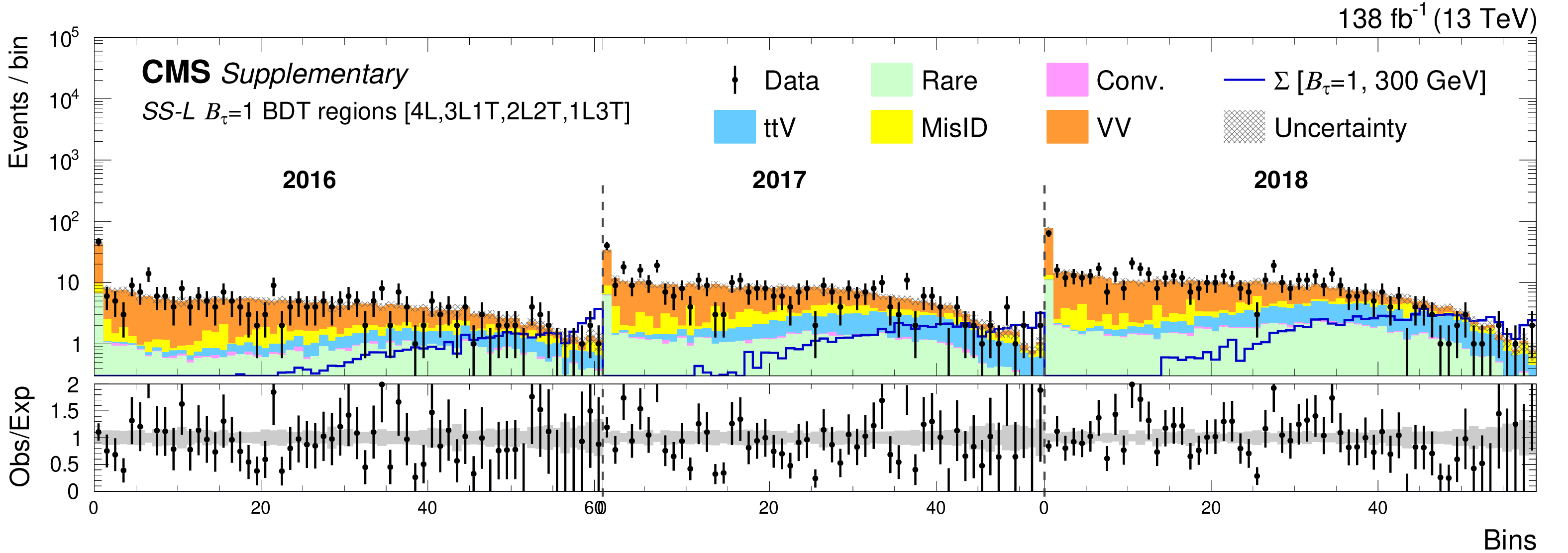
png pdf	Additional Figure 63: The SS-L $\mathcal {B}_{\tau}=$ 1 BDT regions for the 4-lepton channel for the 2016-2018 data sets. The lower panel shows the ratio of observed events to the total expected background prediction. The gray band on the ratio represents the sum of statistical and systematic uncertainties in the SM background prediction. The expected SM background distributions and the uncertainties are shown after fitting the data under the background-only hypothesis. For illustration, an example signal hypothesis for the production of the type-III seesaw heavy fermions in the scenario with mixing exclusively to $\tau$ lepton for $m_{\Sigma} = $ 300 GeV, before the fit, is also overlaid.
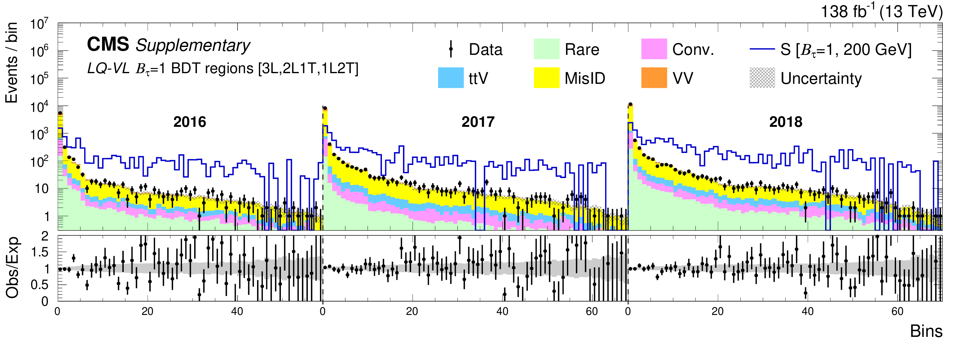
png pdf	Additional Figure 64: The LQ-VL $\mathcal {B}_{\tau}=$ 1 BDT regions for the 3-lepton channel for the 2016-2018 data sets. The lower panel shows the ratio of observed events to the total expected background prediction. The gray band on the ratio represents the sum of statistical and systematic uncertainties in the SM background prediction. The expected SM background distributions and the uncertainties are shown after fitting the data under the background-only hypothesis. For illustration, an example signal hypothesis for the production of the scalar leptoquark coupled to a top quark and a $\tau$ lepton for $m_{S} = $ 200 GeV, before the fit, is also overlaid.
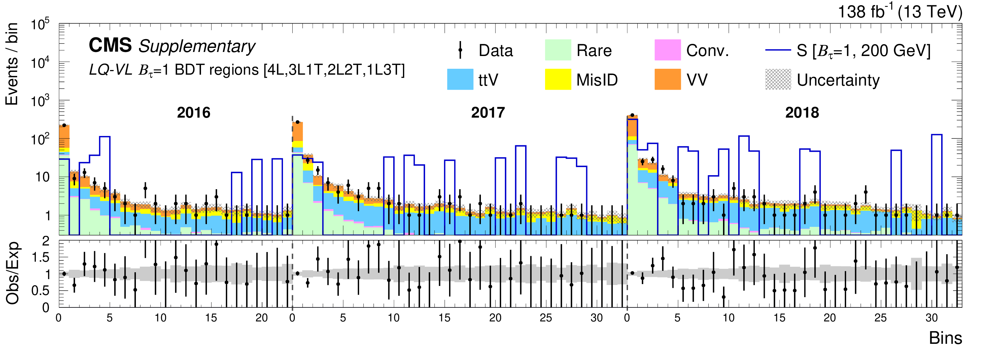
png pdf	Additional Figure 65: The LQ-VL $\mathcal {B}_{\tau}=$ 1 BDT regions for the 4-lepton channel for the 2016-2018 data sets. The lower panel shows the ratio of observed events to the total expected background prediction. The gray band on the ratio represents the sum of statistical and systematic uncertainties in the SM background prediction. The expected SM background distributions and the uncertainties are shown after fitting the data under the background-only hypothesis. For illustration, an example signal hypothesis for the production of the scalar leptoquark coupled to a top quark and a $\tau$ lepton for $m_{S} = $ 200 GeV, before the fit, is also overlaid.
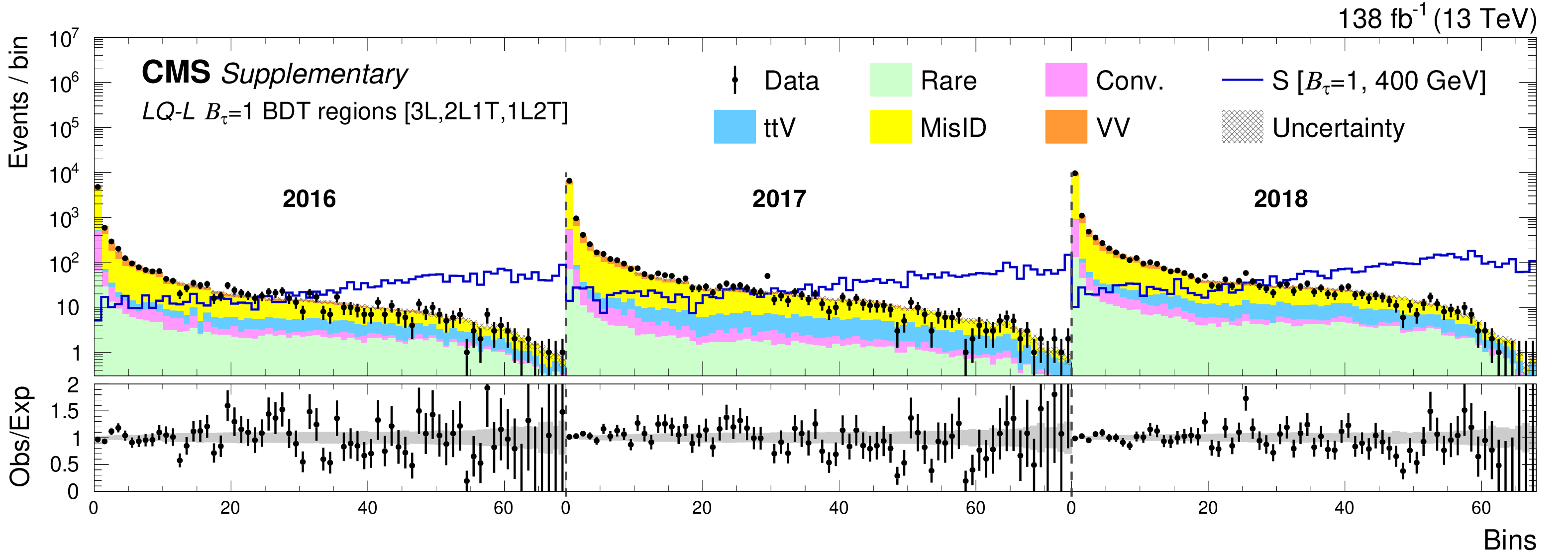
png pdf	Additional Figure 66: The LQ-L $\mathcal {B}_{\tau}=$ 1 BDT regions for the 3-lepton channel for the 2016-2018 data sets. The lower panel shows the ratio of observed events to the total expected background prediction. The gray band on the ratio represents the sum of statistical and systematic uncertainties in the SM background prediction. The expected SM background distributions and the uncertainties are shown after fitting the data under the background-only hypothesis. For illustration, an example signal hypothesis for the production of the scalar leptoquark coupled to a top quark and a $\tau$ lepton for $m_{S} = $ 400 GeV, before the fit, is also overlaid.
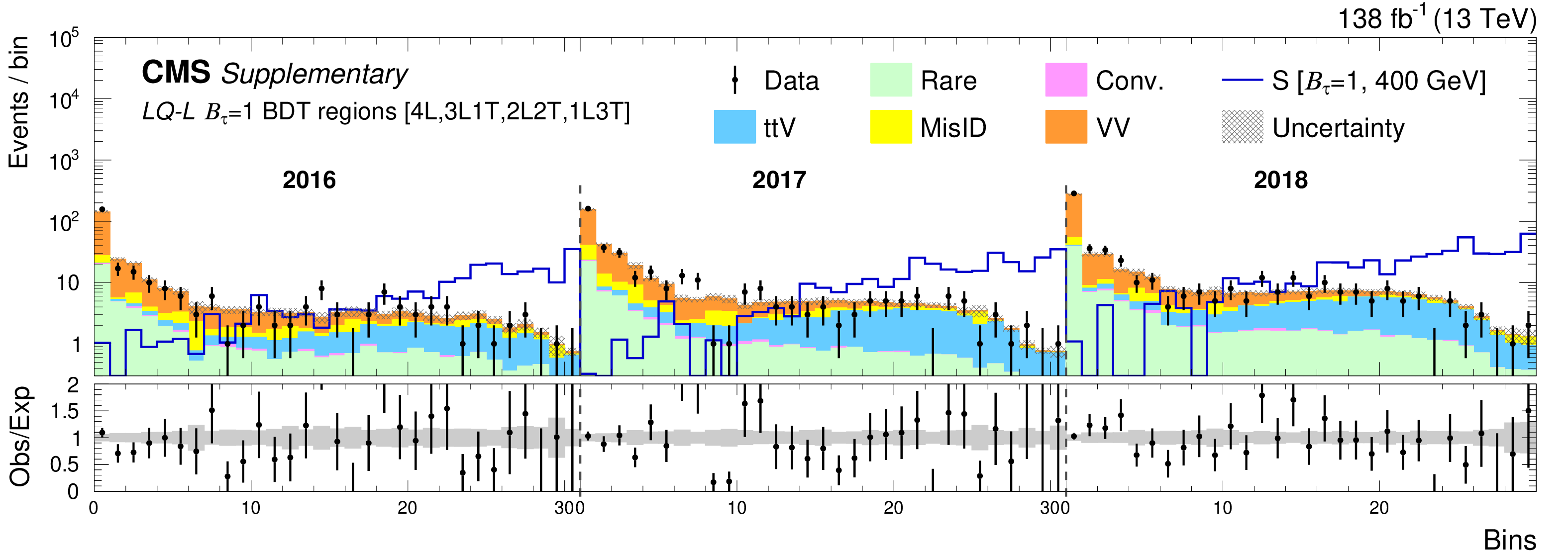
png pdf	Additional Figure 67: The LQ-L $\mathcal {B}_{\tau}=$ 1 BDT regions for the 4-lepton channel for the 2016-2018 data sets. The lower panel shows the ratio of observed events to the total expected background prediction. The gray band on the ratio represents the sum of statistical and systematic uncertainties in the SM background prediction. The expected SM background distributions and the uncertainties are shown after fitting the data under the background-only hypothesis. For illustration, an example signal hypothesis for the production of the scalar leptoquark coupled to a top quark and a $\tau$ lepton for $m_{S} = $ 400 GeV, before the fit, is also overlaid.
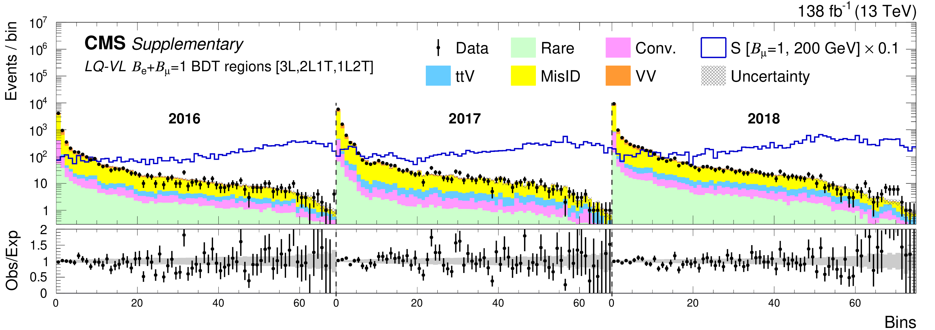
png pdf	Additional Figure 68: The LQ-VL $\mathcal {B}_{\mathrm{e}}+\mathcal {B}_{\mu}=$ 1 BDT regions for the 3-lepton channel for the 2016-2018 data sets. The lower panel shows the ratio of observed events to the total expected background prediction. The gray band on the ratio represents the sum of statistical and systematic uncertainties in the SM background prediction. The expected SM background distributions and the uncertainties are shown after fitting the data under the background-only hypothesis. For illustration, an example signal hypothesis for the production of the scalar leptoquark coupled to a top quark and a muon for $m_{S} = $ 200 GeV, before the fit, is also overlaid.
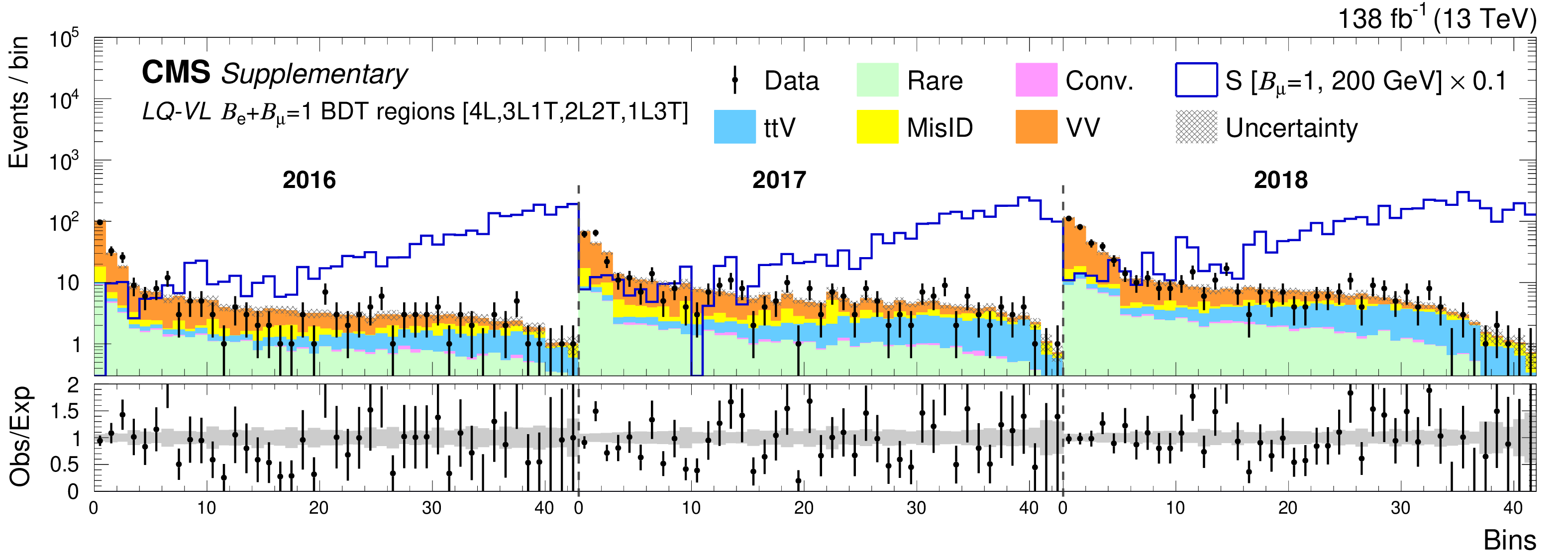
png pdf	Additional Figure 69: The LQ-VL $\mathcal {B}_{\mathrm{e}}+\mathcal {B}_{\mu}=$ 1 BDT regions for the 4-lepton channel for the 2016-2018 data sets. The lower panel shows the ratio of observed events to the total expected background prediction. The gray band on the ratio represents the sum of statistical and systematic uncertainties in the SM background prediction. The expected SM background distributions and the uncertainties are shown after fitting the data under the background-only hypothesis. For illustration, an example signal hypothesis for the production of the scalar leptoquark coupled to a top quark and a muon for $m_{S} = $ 200 GeV, before the fit, is also overlaid.
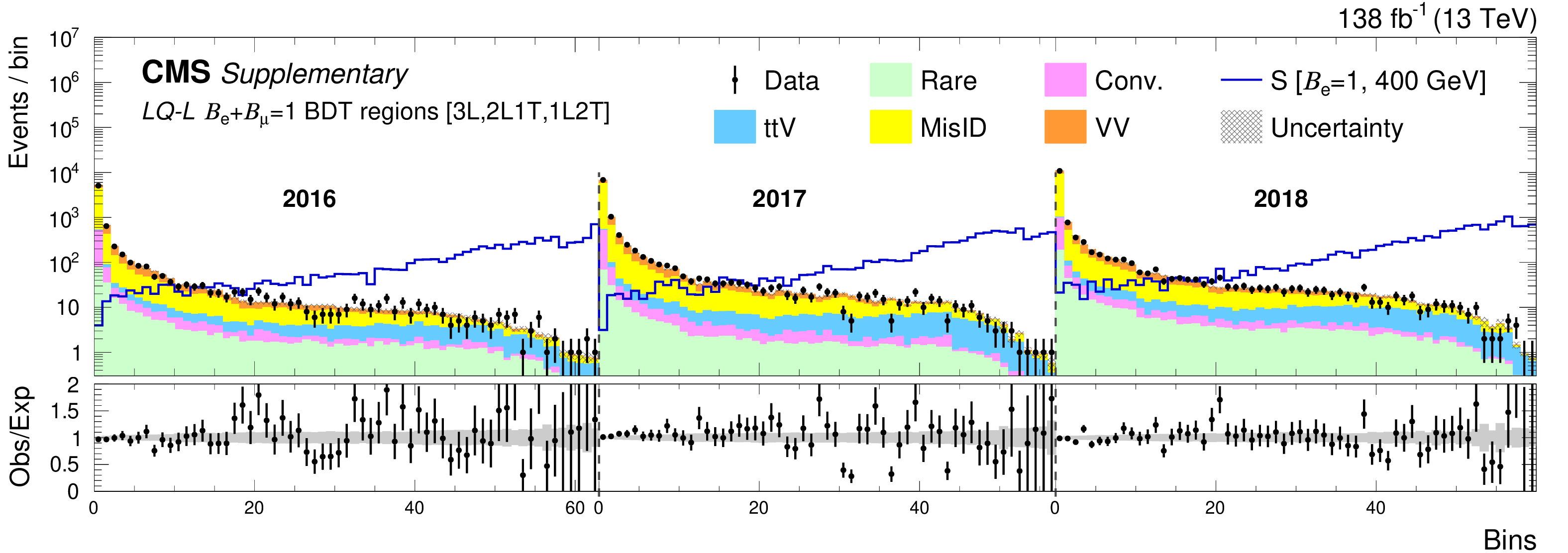
png pdf	Additional Figure 70: The LQ-L $\mathcal {B}_{\mathrm{e}}+\mathcal {B}_{\mu}=$ 1 BDT regions for the 3-lepton channel for the 2016-2018 data sets. The lower panel shows the ratio of observed events to the total expected background prediction. The gray band on the ratio represents the sum of statistical and systematic uncertainties in the SM background prediction. The expected SM background distributions and the uncertainties are shown after fitting the data under the background-only hypothesis. For illustration, an example signal hypothesis for the production of the scalar leptoquark coupled to a top quark and an electron for $m_{S} = $ 400 GeV, before the fit, is also overlaid.
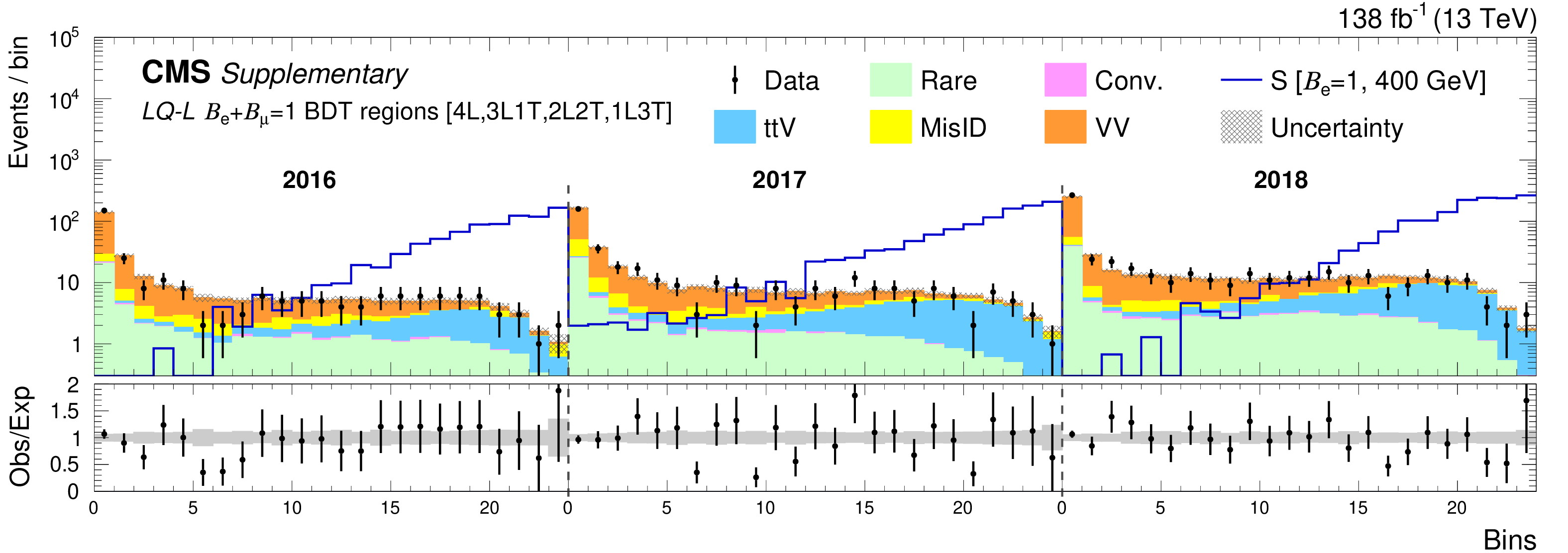
png pdf	Additional Figure 71: The LQ-L $\mathcal {B}_{\mathrm{e}}+\mathcal {B}_{\mu}=$ 1 BDT regions for the 4-lepton channel for the 2016-2018 data sets. The lower panel shows the ratio of observed events to the total expected background prediction. The gray band on the ratio represents the sum of statistical and systematic uncertainties in the SM background prediction. The expected SM background distributions and the uncertainties are shown after fitting the data under the background-only hypothesis. For illustration, an example signal hypothesis for the production of the scalar leptoquark coupled to a top quark and an electron for $m_{S} = $ 400 GeV, before the fit, is also overlaid.

References
1	P. Minkowski	$ \mu \to \mathrm{e}\gamma $ at a rate of one out of 10$^{9} $ muon decays?	PLB 67 (1977) 421
2	R. N. Mohapatra and G. Senjanović	Neutrino mass and spontaneous parity nonconservation	PRL 44 (1980) 912
3	M. Magg and C. Wetterich	Neutrino mass problem and gauge hierarchy	PLB 94 (1980) 61
4	R. N. Mohapatra and G. Senjanović	Neutrino masses and mixings in gauge models with spontaneous parity violation	PRD 23 (1981) 165
5	J. Schechter and J. W. F. Valle	Neutrino masses in SU(2) x U(1) theories	PRD 22 (1980) 2227
6	J. Schechter and J. W. F. Valle	Neutrino decay and spontaneous violation of lepton number	PRD 25 (1982) 774
7	R. N. Mohapatra	Mechanism for understanding small neutrino mass in superstring theories	PRL 56 (1986) 561
8	R. N. Mohapatra and J. W. F. Valle	Neutrino mass and baryon number nonconservation in superstring models	PRD 34 (1986) 1642
9	R. Foot, H. Lew, X. G. He, and G. C. Joshi	Seesaw neutrino masses induced by a triplet of leptons	Z. Phys. C 44 (1989) 441
10	F. del Aguila and M. J. Bowick	The possibility of new fermions with $ \delta _i$ = 0 mass	NPB 224 (1983) 107
11	P. M. Fishbane, R. E. Norton, and M. J. Rivard	Experimental implications of heavy isosinglet quarks and leptons	PRD 33 (1986) 2632
12	P. M. Fishbane and P. Q. Hung	Lepton masses in a dynamical model of family symmetry	Z. Phys. C 38 (1988) 649
13	I. Montvay	Three mirror pairs of fermion families	PLB 205 (1988) 315
14	F. del Aguila, L. Ametller, G. L. Kane, and J. Vidal	Vector-like fermion and standard Higgs production at hadron colliders	NPB 334 (1990) 1
15	K. Fujikawa	A vector-like extension of the standard model	Prog. Theor. Phys. 92 (1994) 1149	hep-ph/9411258
16	F. del Aguila, J. de Blas, and M. Peréz-Victoria	Effects of new leptons in electroweak precision data	PRD 78 (2008) 013010	0803.4008
17	J. C. Pati and A. Salam	Unified Lepton-Hadron Symmetry and a Gauge Theory of the Basic Interactions	PRD 8 (1973) 1240
18	W. Buchmuller, R. Ruckl, and D. Wyler	Leptoquarks in lepton-quark collisions	PLB 191 (1987) 442
19	S. Davidson and P. Verdier	Leptoquarks decaying to a top quark and a charged lepton at hadron colliders	PRD 83 (2011) 115016	1102.4562
20	B. Diaz, M. Schmaltz, and Y.-M. Zhong	The leptoquark hunter's guide: Pair production	JHEP 10 (2017) 097	1706.05033
21	CMS Collaboration	HEPData record for this analysis	link
22	C. Biggio and F. Bonnet	Implementation of the Type-III seesaw model in Feynrules/MadGraph and prospects for discovery with early LHC data	EPJC 72 (2012) 1899	1107.3463
23	C. Biggio et al.	Global bounds on the Type-III seesaw	JHEP 05 (2020) 022	1911.11790
24	A. Das and S. Mandal	Bounds on the triplet fermions in Type-III seesaw and implications for collider searches	NPB 966 (2021) 115374	2006.04123
25	A. Abada et al.	Low energy effects of neutrino masses	JHEP 12 (2007) 061	0707.4058
26	A. Abada et al.	$ \mu \to \mathrm{e}\gamma $ and $ \tau\to\ell\gamma $ decays in the fermion triplet seesaw model	PRD 78 (2008) 033007	0803.0481
27	R. Franceschini, T. Hambye, and A. Strumia	Type-III seesaw at LHC	PRD 78 (2008) 033002	0805.1613
28	Y. Cai, T. Han, T. Li, and R. Ruiz	Lepton number violation: Seesaw models and their collider tests	Frontiers in Physics 6 (2018) 40	1711.02180
29	S. Ashanujjaman and K. Ghosh	Type-III seesaw: Phenomenological implications of the information lost in decoupling from high-energy to low-energy	PLB 819 (2021) 136403	2102.09536
30	S. Ashanujjaman and K. Ghosh	Type-III seesaw: Search for triplet fermions in final states with multiple leptons and fat-jets at 13 TeV LHC	PLB 825 (2022) 136889	2111.07949
31	ATLAS Collaboration	Search for type-III seesaw heavy leptons in leptonic final states in pp collisions at $ \sqrt{s} = $ 13 TeV with the ATLAS detector	Submitted to EPJC	2202.02039
32	CMS Collaboration	Search for physics beyond the standard model in multilepton final states in proton-proton collisions at $ \sqrt{s} = $ 13 TeV	JHEP 03 (2020) 051	CMS-EXO-19-002 1911.04968
33	S. P. Martin	Extra vector-like matter and the lightest Higgs scalar boson mass in low-energy supersymmetry	PRD 81 (2010) 035004	0910.2732
34	P. W. Graham, A. Ismail, S. Rajendran, and P. Saraswat	A little solution to the little hierarchy problem: A vector-like generation	PRD 81 (2010) 055016	0910.3020
35	M. Endo, K. Hamaguchi, S. Iwamoto, and N. Yokozaki	Higgs mass and muon anomalous magnetic moment in supersymmetric models with vector-like matters	PRD 84 (2011) 075017	1108.3071
36	S. Zheng	Minimal vectorlike model in supersymmetric unification	EPJC 80 (2020) 273	1904.10145
37	K. Kong, S. C. Park, and T. G. Rizzo	A vector-like fourth generation with a discrete symmetry from split-ued	JHEP 07 (2010) 059	1004.4635
38	G.-Y. Huang, K. Kong, and S. C. Park	Bounds on the fermion-bulk masses in models with universal extra dimensions	JHEP 06 (2012) 099	1204.0522
39	R. Nevzorov	$ e_6 $ inspired supersymmetric models with exact custodial symmetry	PRD 87 (2013) 015029	1205.5967
40	I. Doršner, S. Fajfer, and I. Mustać	Light vector-like fermions in a minimal SU(5) setup	PRD 89 (2014) 115004	1401.6870
41	A. Joglekar and J. L. Rosner	Searching for signatures of $ e_{\rm 6} $	PRD 96 (2017) 015026	1607.06900
42	P. Schwaller, T. M. P. Tait, and R. Vega-Morales	Dark matter and vectorlike leptons from gauged lepton number	PRD 88 (2013) 035001	1305.1108
43	J. Halverson, N. Orlofsky, and A. Pierce	Vectorlike leptons as the tip of the dark matter iceberg	PRD 90 (2014) 015002	1403.1592
44	S. Bahrami et al.	Dark matter and collider studies in the left-right symmetric model with vectorlike leptons	PRD 95 (2017) 095024	1612.06334
45	S. Bhattacharya, P. Ghosh, N. Sahoo, and N. Sahu	Mini review on vector-like leptonic dark matter, neutrino mass, and collider signatures	Frontiers in Physics 7 (2019) 80	1812.06505
46	K. Agashe, T. Okui, and R. Sundrum	A common origin for neutrino anarchy and charged hierarchies	PRL 102 (2009) 101801	0810.1277
47	M. Redi	Leptons in composite MFV	JHEP 09 (2013) 060	1306.1525
48	A. Falkowski, D. M. Straub, and A. Vicente	Vector-like leptons: Higgs decays and collider phenomenology	JHEP 05 (2014) 092	1312.5329
49	R. Dermíšek and A. Raval	Explanation of the muon $g{-}2$ anomaly with vectorlike leptons and its implications for Higgs decays	PRD 88 (2013) 013017	1305.3522
50	E. Megias, M. Quiros, and L. Salas	Muon $g{-}2$ from vector-like leptons in warped space	JHEP 05 (2017) 016	1701.05072
51	J. Kawamura, S. Raby, and A. Trautner	Complete vectorlike fourth family and new U(1)' for muon anomalies	PRD 100 (2019) 055030	1906.11297
52	G. Hiller, C. Hormigos-Feliu, D. F. Litim, and T. Steudtner	Model building from asymptotic safety with Higgs and flavor portals	PRD 102 (2020) 095023	2008.08606
53	Muon $g{-}2$ Collaboration	Final report of the muon e821 anomalous magnetic moment measurement at BNL	PRD 73 (2006) 072003	hep-ex/0602035
54	Muon $g{-}2$ Collaboration	Measurement of the positive muon anomalous magnetic moment to 0.46 ppm	PRL 126 (2021) 141801	2104.03281
55	N. Kumar and S. P. Martin	Vectorlike leptons at the large hadron collider	PRD 92 (2015) 115018	1510.03456
56	P. N. Bhattiprolu and S. P. Martin	Prospects for vectorlike leptons at future proton-proton colliders	PRD 100 (2019) 015033	1905.00498
57	R. Dermíšek, A. Raval, and S. Shin	Effects of vectorlike leptons on $ h\to 4\ell $ and the connection to the muon $g{-}2$ anomaly	PRD 90 (2014) 034023	1406.7018
58	R. Dermíšek, J. P. Hall, E. Lunghi, and S. Shin	Limits on vectorlike leptons from searches for anomalous production of multi-lepton events	JHEP 12 (2014) 013	1408.3123
59	CMS Collaboration	Search for vector-like leptons in multilepton final states in proton-proton collisions at $ \sqrt{s} = $ 13 TeV	PRD 100 (2019) 052003	CMS-EXO-18-005 1905.10853
60	L3 Collaboration	Search for heavy neutral and charged leptons in e$^{+}$e$^{-}$ annihilation at lep	PLB 517 (2001) 75	hep-ex/0107015
61	J. C. Pati and A. Salam	Lepton number as the fourth color	PRD 10 (1974) 275
62	H. Georgi and S. L. Glashow	Unity of all elementary particle forces	PRL 32 (1974) 438
63	H. Fritzsch and P. Minkowski	Unified interactions of leptons and hadrons	Annals Phys. 93 (1975) 193
64	B. Gripaios, M. Nardecchia, and S. A. Renner	Composite leptoquarks and anomalies in b-meson decays	JHEP 05 (2015) 006	1412.1791
65	L. Da Rold and F. Lamagna	Composite Higgs and leptoquarks from a simple group	JHEP 03 (2019) 135	1812.08678
66	S. Weinberg	Supersymmetry at ordinary energies. Masses and conservation laws	PRD 26 (1982) 287
67	R. Barbier et al.	$ {R} $-parity violating supersymmetry	PR 420 (2005) 1	hep-ph/0406039
68	R. Mandal and A. Pich	Constraints on scalar leptoquarks from lepton and kaon physics	JHEP 12 (2019) 089	1908.11155
69	J. K. Mizukoshi, O. J. P. Éboli, and M. C. Gonzalez-Garcia	Bounds on scalar leptoquarks from Z physics	NPB 443 (1995) 20	hep-ph/9411392
70	E. Alvarez et al.	A composite PNGB leptoquark at the LHC	JHEP 12 (2018) 027	1808.02063
71	A. Angelescu, D. Bečirević, D. A. Faroughy, and O. Sumensari	Closing the window on single leptoquark solutions to the b-physics anomalies	JHEP 10 (2018) 183	1808.08179
72	A. Crivellin, D. Muller, and F. Saturnino	Flavor phenomenology of the leptoquark singlet-triplet model	JHEP 06 (2020) 020	1912.04224
73	S. Saad and A. Thapa	Common origin of neutrino masses and $ r_{D^{(\ast)}} $, $ r_{K^{(\ast)}} $ anomalies	PRD 102 (2020) 015014	2004.07880
74	U. Haisch and G. Polesello	Resonant third-generation leptoquark signatures at the large hadron collider	JHEP 05 (2021) 057	2012.11474
75	BaBar Collaboration	Measurement of an excess of $ \bar{B} \to d^{(*)}\tau^- \bar{\nu}_\tau $ decays and implications for charged Higgs bosons	PRD 88 (2013) 072012	1303.0571
76	Belle Collaboration	Measurement of $ \mathcal{R}(d) $ and $ \mathcal{R}(d^*) $ with a semileptonic tagging method	PRL 124 (2020) 161803	1910.05864
77	LHCb Collaboration	Measurement of the ratio of branching fractions $ \mathcal{B}(b_c^+ \to j/\psi\tau^+\nu_\tau) $/$ \mathcal{B}(b_c^+ \to j/\psi\mu^+\nu_\mu) $	PRL 120 (2018) 121801	1711.05623
78	LHCb Collaboration	Measurement of the ratio of the $ b^0 \to d^{-} \tau^+ \nu_{\tau} $ and $ b^0 \to d^{-} \mu^+ \nu_{\mu} $ branching fractions using three-prong $ \tau $-lepton decays	PRL 120 (2018) 171802	1708.08856
79	LHCb Collaboration	Test of lepton universality in beauty-quark decays		2103.11769
80	Belle Collaboration	Lepton-flavor-dependent angular analysis of $ B\to K^\ast \ell^+\ell^- $	PRL 118 (2017) 111801	1612.05014
81	LHCb Collaboration	Test of lepton universality with $ B^{0} \rightarrow K^{*0}\ell^{+}\ell^{-} $ decays	JHEP 08 (2017) 055	1705.05802
82	LHCb Collaboration	Search for lepton-universality violation in $ B^+\to K^+\ell^+\ell^- $ decays	PRL 122 (2019) 191801	1903.09252
83	ATLAS Collaboration	Search for pair production of scalar leptoquarks decaying into first- or second-generation leptons and top quarks in proton-proton collisions at $ \sqrt{s} = $ 13 TeV with the ATLAS detector	EPJC 81 (2021) 313	2010.02098
84	ATLAS Collaboration	Search for pair production of third-generation scalar leptoquarks decaying into a top quark and a $ \tau $-lepton in pp collisions at $ \sqrt{s}= $ 13 TeV with the ATLAS detector	JHEP 06 (2021) 179	2101.11582
85	ATLAS Collaboration	Searches for third-generation scalar leptoquarks in $ \sqrt{s} = $ 13 TeV pp collisions with the ATLAS detector	JHEP 06 (2019) 144	1902.08103
86	CMS Collaboration	Search for leptoquarks coupled to third-generation quarks in proton-proton collisions at $ \sqrt{s}= $ 13 TeV	PRL 121 (2018) 241802	CMS-B2G-16-027 1809.05558
87	CMS Collaboration	Search for third-generation scalar leptoquarks decaying to a top quark and a $ \tau $ lepton at $ \sqrt{s}= $ 13 TeV	EPJC 78 (2018) 707	CMS-B2G-16-028 1803.02864
88	CMS Collaboration	Search for singly and pair-produced leptoquarks coupling to third-generation fermions in proton-proton collisions at $ \sqrt{s} = $ 13 TeV	PLB 819 (2021) 136446	CMS-EXO-19-015 2012.04178
89	CMS Collaboration	Constraints on models of scalar and vector leptoquarks decaying to a quark and a neutrino at $ \sqrt{s}= $ 13 TeV	PRD 98 (2018) 032005	CMS-SUS-18-001 1805.10228
90	CMS Collaboration	Search for heavy neutrinos and third-generation leptoquarks in hadronic states of two $ \tau $ leptons and two jets in proton-proton collisions at $ \sqrt{s} = $ 13 TeV	JHEP 03 (2019) 170	CMS-EXO-17-016 1811.00806
91	CMS Collaboration	Search for a singly produced third-generation scalar leptoquark decaying to a $ \tau $ lepton and a bottom quark in proton-proton collisions at $ \sqrt{s} = $ 13 TeV	JHEP 07 (2018) 115	CMS-EXO-17-029 1806.03472
92	CMS Collaboration	The CMS experiment at the CERN LHC	JINST 3 (2008) S08004	CMS-00-001
93	CMS Collaboration	Performance of the CMS level-1 trigger in proton-proton collisions at $ \sqrt{s} = $ 13 TeV	JINST 15 (2020) P10017	CMS-TRG-17-001 2006.10165
94	CMS Collaboration	The CMS trigger system	JINST 12 (2017) P01020	CMS-TRG-12-001 1609.02366
95	J. Alwall et al.	The automated computation of tree-level and next-to-leading order differential cross sections, and their matching to parton shower simulations	JHEP 07 (2014) 079	1405.0301
96	P. Nason	A new method for combining NLO QCD with shower monte carlo algorithms	JHEP 11 (2004) 040	hep-ph/0409146
97	S. Frixione, P. Nason, and C. Oleari	Matching NLO QCD computations with parton shower simulations: the POWHEG method	JHEP 11 (2007) 070	0709.2092
98	S. Alioli, P. Nason, C. Oleari, and E. Re	A general framework for implementing NLO calculations in shower monte carlo programs: the POWHEG BOX	JHEP 06 (2010) 043	1002.2581
99	J. M. Campbell and R. K. Ellis	MCFM for the tevatron and the LHC	NPB Proc. Suppl. 205-206 (2010) 10	1007.3492
100	Y. Gao et al.	Spin determination of single-produced resonances at hadron colliders	PRD 81 (2010) 075022	1001.3396
101	S. Bolognesi et al.	On the spin and parity of a single-produced resonance at the LHC	PRD 86 (2012) 095031	1208.4018
102	I. Anderson et al.	Constraining anomalous HVV interactions at proton and lepton colliders	PRD 89 (2014) 035007	1309.4819
103	A. V. Gritsan, R. Rontsch, M. Schulze, and M. Xiao	Constraining anomalous Higgs boson couplings to the heavy flavor fermions using matrix element techniques	PRD 94 (2016) 055023	1606.03107
104	T. Sjostrand et al.	An introduction to PYTHIA 8.2	CPC 191 (2015) 159	1410.3012
105	B. Fuks, M. Klasen, D. R. Lamprea, and M. Rothering	Gaugino production in proton-proton collisions at a center-of-mass energy of 8 TeV	JHEP 10 (2012) 081	1207.2159
106	B. Fuks, M. Klasen, D. R. Lamprea, and M. Rothering	Precision predictions for electroweak superpartner production at hadron colliders with resummino	EPJC 73 (2013) 2480	1304.0790
107	J. Blumlein, E. Boos, and A. Kryukov	Leptoquark pair production in hadronic interactions	Z. Phys. C 76 (1997) 137	hep-ph/9610408
108	M. Kramer, T. Plehn, M. Spira, and P. M. Zerwas	Pair production of scalar leptoquarks at the CERN LHC	PRD 71 (2005) 057503	hep-ph/0411038
109	NNPDF Collaboration	Parton distributions for the LHC Run II	JHEP 04 (2015) 040	1410.8849
110	NNPDF Collaboration	Parton distributions from high-precision collider data	EPJC 77 (2017) 663	1706.00428
111	CMS Collaboration	Event generator tunes obtained from underlying event and multiparton scattering measurements	EPJC 76 (2016) 155	CMS-GEN-14-001 1512.00815
112	CMS Collaboration	Extraction and validation of a new set of CMS PYTHIA8 tunes from underlying-event measurements	EPJC 80 (2020) 4	CMS-GEN-17-001 1903.12179
113	S. Hoeche et al.	Matching parton showers and matrix elements		hep-ph/0602031
114	R. Frederix and S. Frixione	Merging meets matching in MC@NLO	JHEP 12 (2012) 061	1209.6215
115	GEANT4 Collaboration	GEANT4--a simulation toolkit	NIMA 506 (2003) 250
116	M. Cacciari, G. P. Salam, and G. Soyez	The anti-$ {k_{\mathrm{T}}} $ jet clustering algorithm	JHEP 04 (2008) 063	0802.1189
117	M. Cacciari, G. P. Salam, and G. Soyez	Fastjet user manual	EPJC 72 (2012) 1896	1111.6097
118	CMS Collaboration	Particle-flow reconstruction and global event description with the CMS detector	JINST 12 (2017) P10003	CMS-PRF-14-001 1706.04965
119	CMS Collaboration	Electron and photon reconstruction and identification with the CMS experiment at the CERN LHC	JINST 16 (2021) P05014	CMS-EGM-17-001 2012.06888
120	CMS Collaboration	Performance of the CMS muon detector and muon reconstruction with proton-proton collisions at $ \sqrt{s}= $ 13 TeV	JINST 13 (2018) P06015	CMS-MUO-16-001 1804.04528
121	CMS Collaboration	Performance of reconstruction and identification of $ \tau $ leptons decaying to hadrons and $ \nu_\tau $ in pp collisions at $ \sqrt{s}= $ 13 TeV	JINST 13 (2018) P10005	CMS-TAU-16-003 1809.02816
122	M. Cacciari, G. P. Salam, and G. Soyez	The catchment area of jets	JHEP 04 (2008) 005	0802.1188
123	M. Cacciari and G. P. Salam	Pileup subtraction using jet areas	PLB 659 (2008) 119	0707.1378
124	CMS Collaboration	Jet energy scale and resolution in the CMS experiment in pp collisions at 8 TeV	JINST 12 (2017) P02014	CMS-JME-13-004 1607.03663
125	CMS Collaboration	Jet algorithms performance in 13 TeV data	CMS-PAS-JME-16-003	CMS-PAS-JME-16-003
126	CMS Collaboration	Identification of heavy-flavour jets with the CMS detector in pp collisions at 13 TeV	JINST 13 (2018) P05011	CMS-BTV-16-002 1712.07158
127	CMS Collaboration	Performance of missing transverse momentum reconstruction in proton-proton collisions at $ \sqrt{s} = $ 13 TeV using the CMS detector	JINST 14 (2019) P07004	CMS-JME-17-001 1903.06078
128	D. Bertolini, P. Harris, M. Low, and N. Tran	Pileup per particle identification	JHEP 10 (2014) 059	1407.6013
129	CMS Collaboration	Identification of hadronic tau lepton decays using a deep neural network	Submitted to JINST	CMS-TAU-20-001 2201.08458
130	Particle Data Group Collaboration	Review of particle physics	Prog. Theor. Exp. Phys. 2020 (2020) 083C01
131	CMS Collaboration	Search for third-generation scalar leptoquarks in the t$ \tau $ channel in proton-proton collisions at $ \sqrt{s} = $ 8 TeV	JHEP 07 (2015) 042	CMS-EXO-14-008 1503.09049
132	CMS Collaboration	Measurement of the inclusive W and Z production cross sections in pp collisions at $ \sqrt{s}= $ 7 TeV	JHEP 10 (2011) 132	CMS-EWK-10-005 1107.4789
133	H. Voss, A. Hocker, J. Stelzer, and F. Tegenfeldt	TMVA, the toolkit for multivariate data analysis with ROOT	in Proceedings of XI International Workshop on Advanced Computing and Analysis Techniques in Physics Research, 2009	physics/0703039
134	M. Cacciari et al.	The $ t\bar{t} $ cross-section at 1.8 and 1.96 TeV: A study of the systematics due to parton densities and scale dependence	JHEP 04 (2004) 068	hep-ph/0303085
135	CMS Collaboration	Precision luminosity measurement in proton-proton collisions at $ \sqrt{s} = $ 13 TeV in 2015 and 2016 at CMS	EPJC 81 (2021) 800	CMS-LUM-17-003 2104.01927
136	CMS Collaboration	CMS luminosity measurement for the 2017 data-taking period at $ \sqrt{s} = $ 13 TeV	CMS-PAS-LUM-17-004	CMS-PAS-LUM-17-004
137	CMS Collaboration	CMS luminosity measurement for the 2018 data-taking period at $ \sqrt{s} = $ 13 TeV	CMS-PAS-LUM-18-002	CMS-PAS-LUM-18-002
138	S. Baker and R. D. Cousins	Clarification of the use of chi square and likelihood functions in fits to histograms	NIM221 (1984) 437
139	L. Demortier	P-values and nuisance parameters	in Statistical issues for LHC physics. Proceedings, Workshop, PHYSTAT-LHC, Geneva, Switzerland, June 27-29, 2007, p. 23 2008
140	E. Gross and O. Vitells	Trial factors for the look elsewhere effect in high energy physics	EPJC 70 (2010) 525	1005.1891
141	T. Junk	Confidence level computation for combining searches with small statistics	NIMA 434 (1999) 435	hep-ex/9902006
142	A. L. Read	Presentation of search results: The CL$ _{s} $ technique	JPG 28 (2002) 2693
143	G. Cowan, K. Cranmer, E. Gross, and O. Vitells	Asymptotic formulae for likelihood-based tests of new physics	EPJC 71 (2011) 1554	1007.1727
144	ATLAS and CMS Collaborations, and LHC Higgs Combination Group	Procedure for the LHC Higgs boson search combination in summer 2011	CMS-NOTE-2011-005
145	CMS Collaboration	Simplified likelihood for the re-interpretation of public CMS results	CDS