

Compact Muon Solenoid
LHC, CERN
| CMS-HIG-19-016 ; CERN-EP-2022-142 | ||
| Measurement of the Higgs boson inclusive and differential fiducial production cross sections in the diphoton decay channel with pp collisions at $ \sqrt{s} = $ 13 TeV | ||
| CMS Collaboration | ||
| 25 August 2022 | ||
| JHEP 07 (2023) 091 | ||
| Abstract: The measurements of the inclusive and differential fiducial cross sections of the Higgs boson decaying to a pair of photons are presented. The analysis is performed using proton-proton collisions data recorded with the CMS detector at the LHC at a centre-of-mass energy of 13 TeV and corresponding to an integrated luminosity of 137 fb$ ^{-1} $. The inclusive fiducial cross section is measured to be $ \sigma_{\text{fid}}=$ 73.4$_{-5.3}^{+5.4} $ (stat) $ _{-2.2}^{+2.4} $ (syst) fb, in agreement with the standard model expectation of 75.4 $ \pm $ 4.1 fb. The measurements are also performed in fiducial regions targeting different production modes and as function of several observables describing the diphoton system, the number of additional jets present in the event, and other kinematic observables. Two double differential measurements are performed. No significant deviations from the standard model expectations are observed. | ||
| Links: e-print arXiv:2208.12279 [hep-ex] (PDF) ; CDS record ; inSPIRE record ; HepData record ; CADI line (restricted) ; | ||
| Figures | |
png pdf |
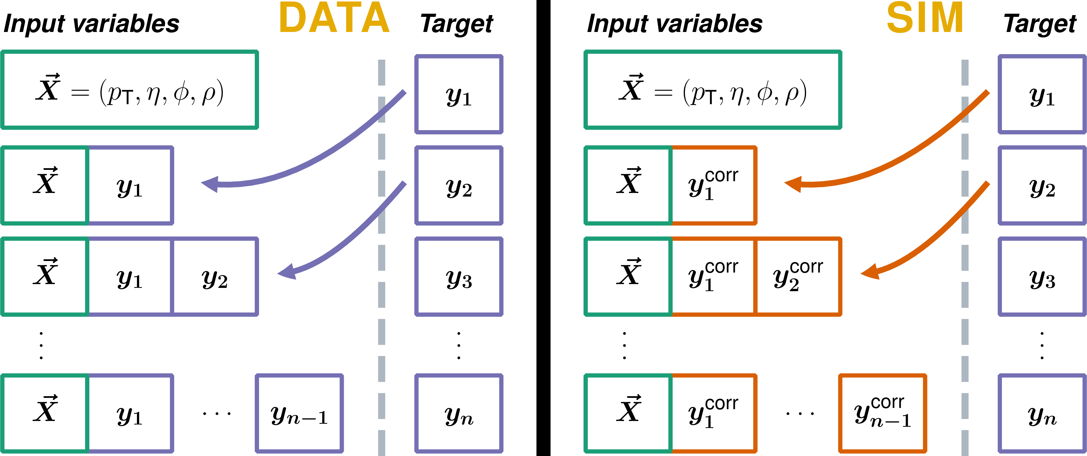
Figure 1:
The chained approach for the set of input variables for the quantile BDTs. The input variables for the BDT for each variable being corrected are given. The variables to be corrected are used as the target, and the quantile is learned through the learning objective given in Eq. (1). Within one group of variables ($ y_{1} $,..., $ y_{n} $), with nonnegligible correlations, an order is set. The quantile BDT for a given variable includes the prior set of variables, within this ordering, as additional inputs. For simulation (right), the additional input variables are corrected before using them as inputs for the quantile BDTs. |

png pdf |
Figure 2:
The upper pane shows the distribution of the photon isolation sum ($ \mathcal{I}_{\text{ph}} $) in 2018 data (black dots) and simulation (coloured histograms). The green histogram shows the uncorrected distribution, the orange one the distribution after equalizing the number of events with zero isolation in simulation with data, and the purple one the distribution after applying the equalizing step and the CQR technique to its tail part. The arrows show the two ways events can be shifted. From peak to tail (green) and from tail to peak (yellow) with their respective probabilities $ p $ (peak to tail) and $ p $ (tail to peak). The lower pane shows the ratio of the three simulation distributions to the one from data. The distributions shown in this figure are taken from a set of events distinct from the ones used for the derivation of the correction method. |
png pdf |
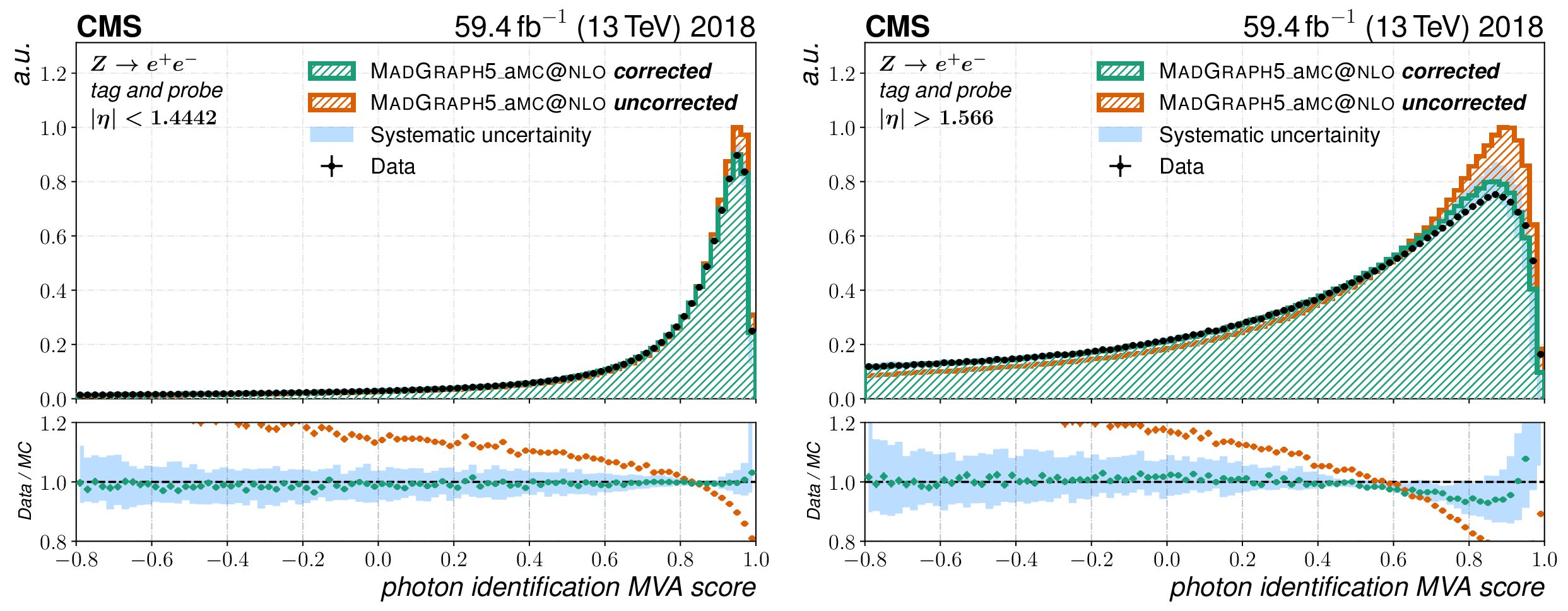
Figure 3:
Distribution of the output of the photon identification MVA for the probe candidate in a $ \mathrm{Z} \to \mathrm{e}\mathrm{e} $ tag-and-probe sample for data and the MadGraph-5_aMC@NLO simulation. The electrons have been reconstructed as photons and a selection to reduce the number of misidentified electrons in data is applied. The simulated events have been reweighted with respect to $ p_{\mathrm{T}} $, $ \eta $, $ \phi $, and $ \rho $ to match data in order to remove effects from mismodelled kinematic variables. Electrons that are detected in the barrel ($ |\eta| < $ 1.4442) or endcap ($ |\eta| > $ 1.566) part of the ECAL and the corresponding distributions are shown on the left or right, respectively. The blue band shows the systematic uncertainty assigned to the data simulation mismatch of the output of the photon identification MVA. The orange histogram and points in the upper and lower plots, respectively, show the photon identification MVA distribution and its ratio to data evaluated using the uncorrected version of its input variables in simulation. |
png pdf |
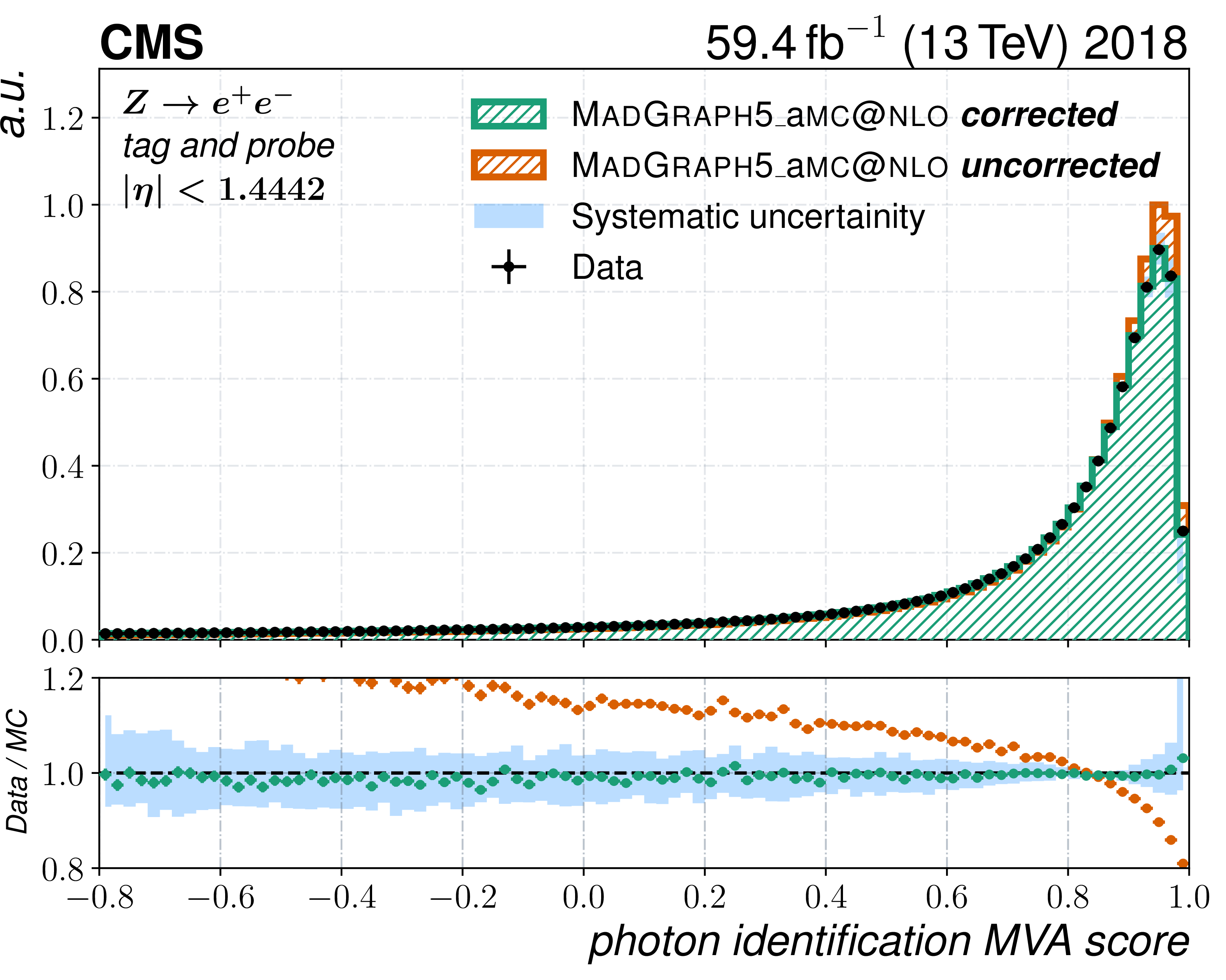
Figure 3-a:
Distribution of the output of the photon identification MVA for the probe candidate in a $ \mathrm{Z} \to \mathrm{e}\mathrm{e} $ tag-and-probe sample for data and the MadGraph-5_aMC@NLO simulation. The electrons have been reconstructed as photons and a selection to reduce the number of misidentified electrons in data is applied. The simulated events have been reweighted with respect to $ p_{\mathrm{T}} $, $ \eta $, $ \phi $, and $ \rho $ to match data in order to remove effects from mismodelled kinematic variables. Electrons that are detected in the barrel ($ |\eta| < $ 1.4442) part of the ECAL and the corresponding distribution is shown. The blue band shows the systematic uncertainty assigned to the data simulation mismatch of the output of the photon identification MVA. The orange histogram and points in the upper and lower plots, respectively, show the photon identification MVA distribution and its ratio to data evaluated using the uncorrected version of its input variables in simulation. |
png pdf |
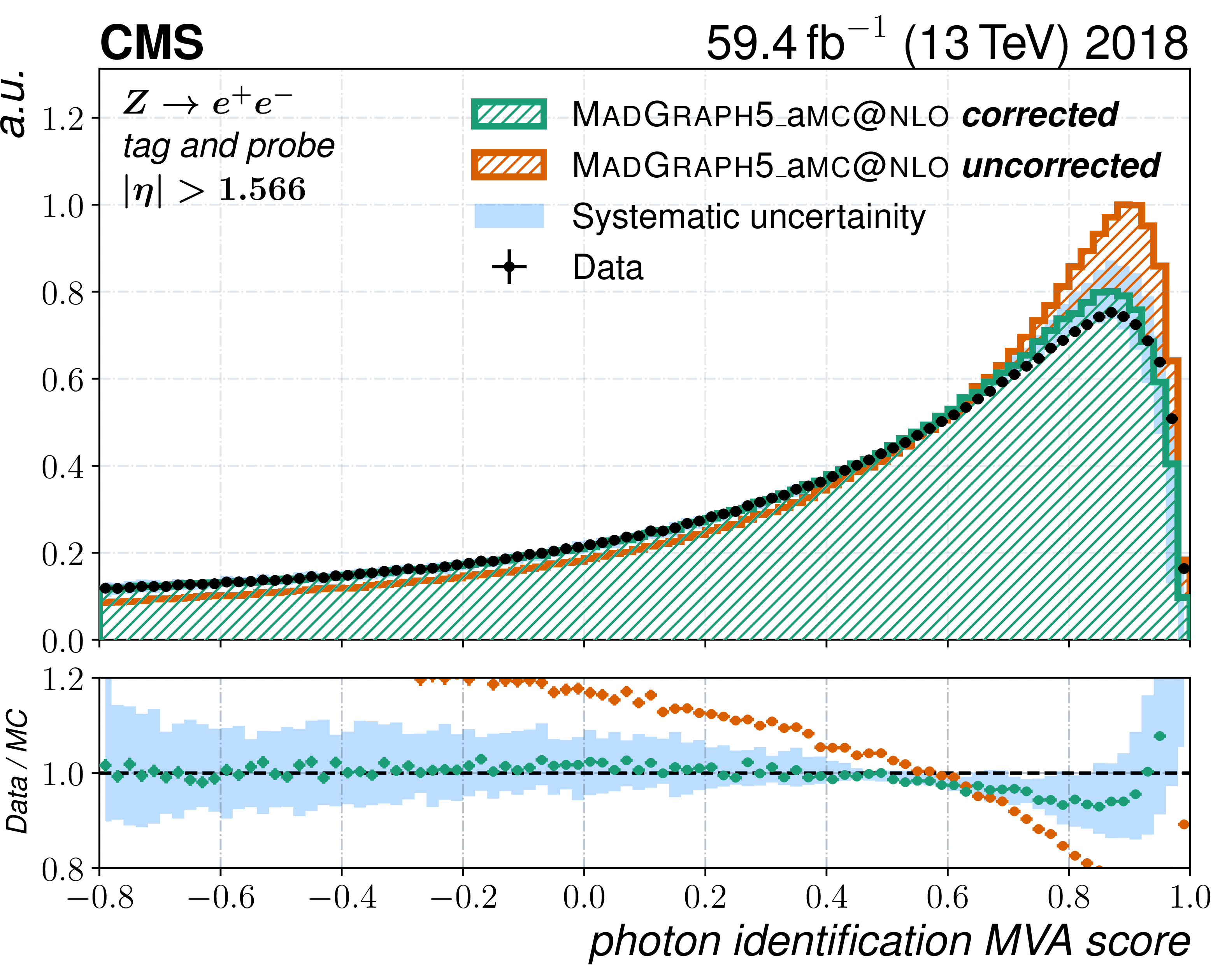
Figure 3-b:
Distribution of the output of the photon identification MVA for the probe candidate in a $ \mathrm{Z} \to \mathrm{e}\mathrm{e} $ tag-and-probe sample for data and the MadGraph-5_aMC@NLO simulation. The electrons have been reconstructed as photons and a selection to reduce the number of misidentified electrons in data is applied. The simulated events have been reweighted with respect to $ p_{\mathrm{T}} $, $ \eta $, $ \phi $, and $ \rho $ to match data in order to remove effects from mismodelled kinematic variables. Electrons that are detected in the endcap ($ |\eta| > $ 1.566) part of the ECAL and the corresponding distribution is shown. The blue band shows the systematic uncertainty assigned to the data simulation mismatch of the output of the photon identification MVA. The orange histogram and points in the upper and lower plots, respectively, show the photon identification MVA distribution and its ratio to data evaluated using the uncorrected version of its input variables in simulation. |
png pdf |
Figure 4:
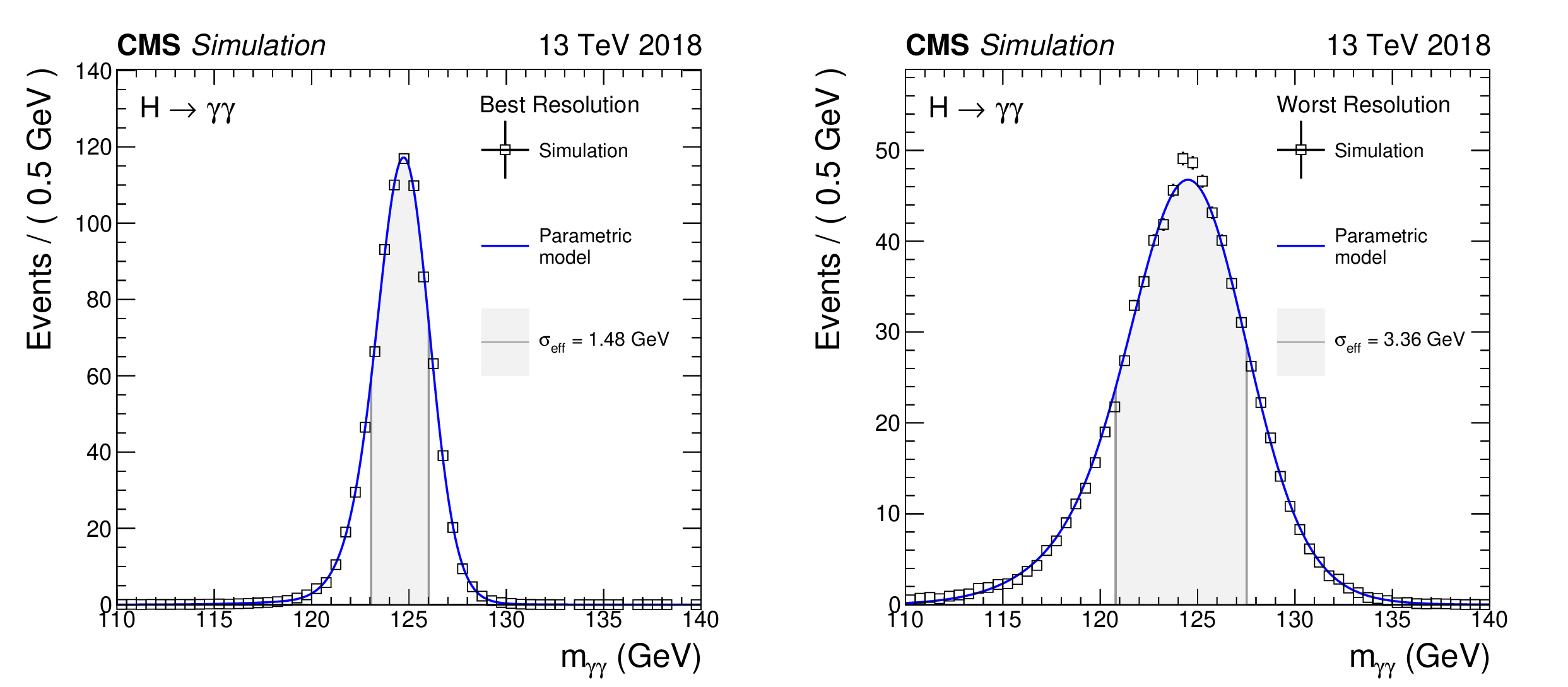
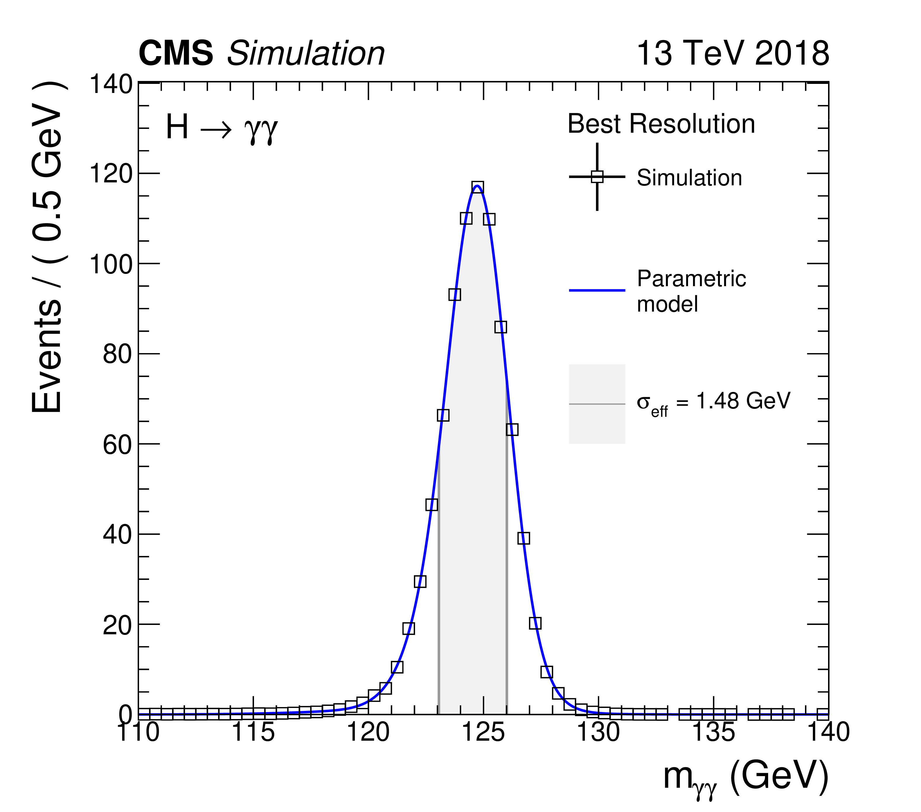
The signal model distributions used in the fiducial cross section measurement for the best and worst resolution categories in 2018. The half width of the $ m_{\gamma\gamma} $ distribution region around its peak that contains 68.3% of the total integral is denoted as $ \sigma_{\text{eff}} $. The distributions shown here are taken from the signal simulation including the four dominant Higgs boson production mechanisms with a mass hypothesis of $ m_{\mathrm{H}}= $ 125 GeV. Details of the derivation of the signal model distributions are discussed in Section 8.1. |
png pdf |
Figure 4-a:
The signal model distributions used in the fiducial cross section measurement for the best resolution category in 2018. The half width of the $ m_{\gamma\gamma} $ distribution region around its peak that contains 68.3% of the total integral is denoted as $ \sigma_{\text{eff}} $. The distributions shown here are taken from the signal simulation including the four dominant Higgs boson production mechanisms with a mass hypothesis of $ m_{\mathrm{H}}= $ 125 GeV. Details of the derivation of the signal model distributions are discussed in Section 8.1. |

png pdf |
Figure 4-b:
The signal model distributions used in the fiducial cross section measurement for the worst resolution category in 2018. The half width of the $ m_{\gamma\gamma} $ distribution region around its peak that contains 68.3% of the total integral is denoted as $ \sigma_{\text{eff}} $. The distributions shown here are taken from the signal simulation including the four dominant Higgs boson production mechanisms with a mass hypothesis of $ m_{\mathrm{H}}= $ 125 GeV. Details of the derivation of the signal model distributions are discussed in Section 8.1. |
png pdf |
Figure 5:
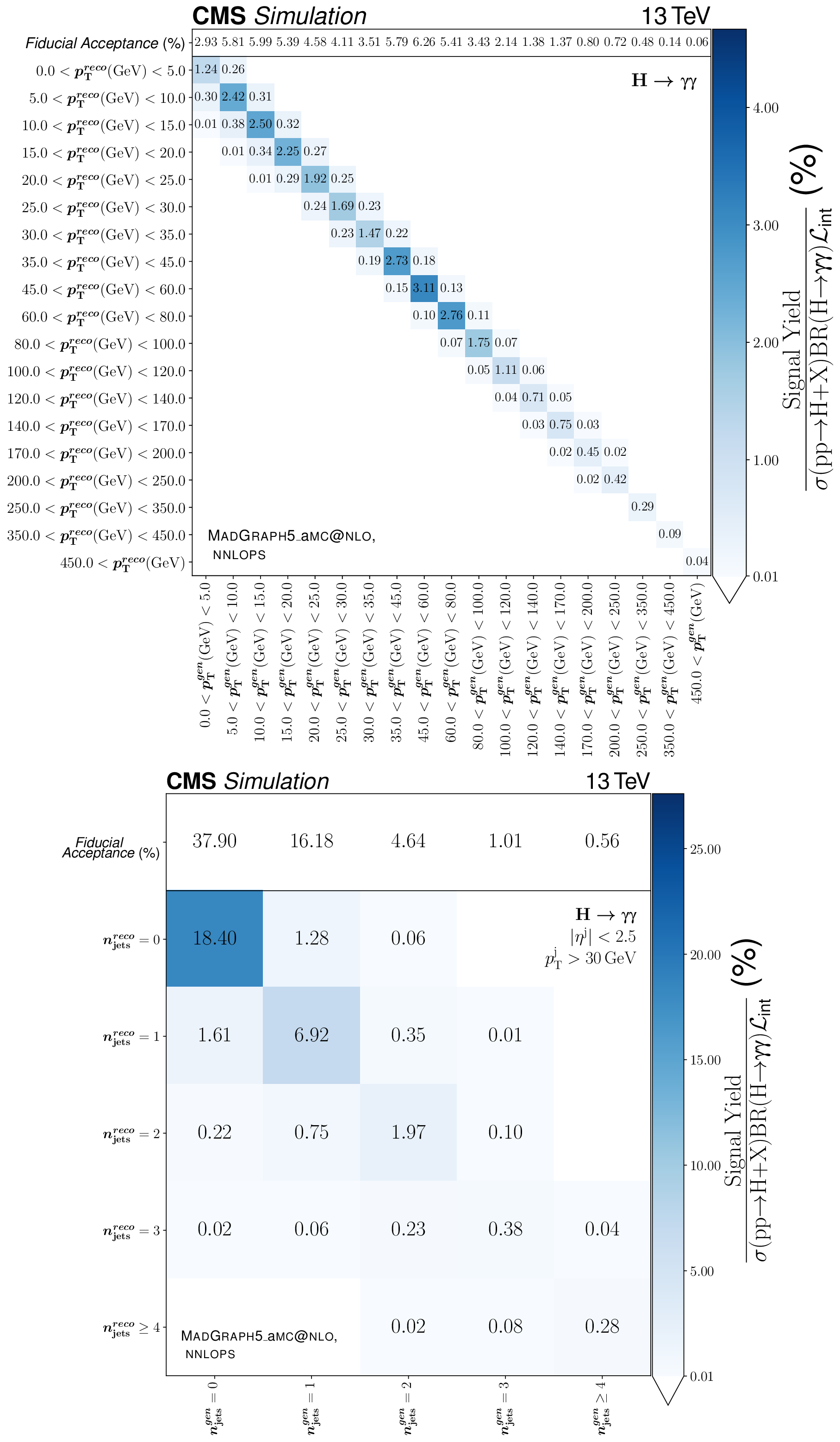
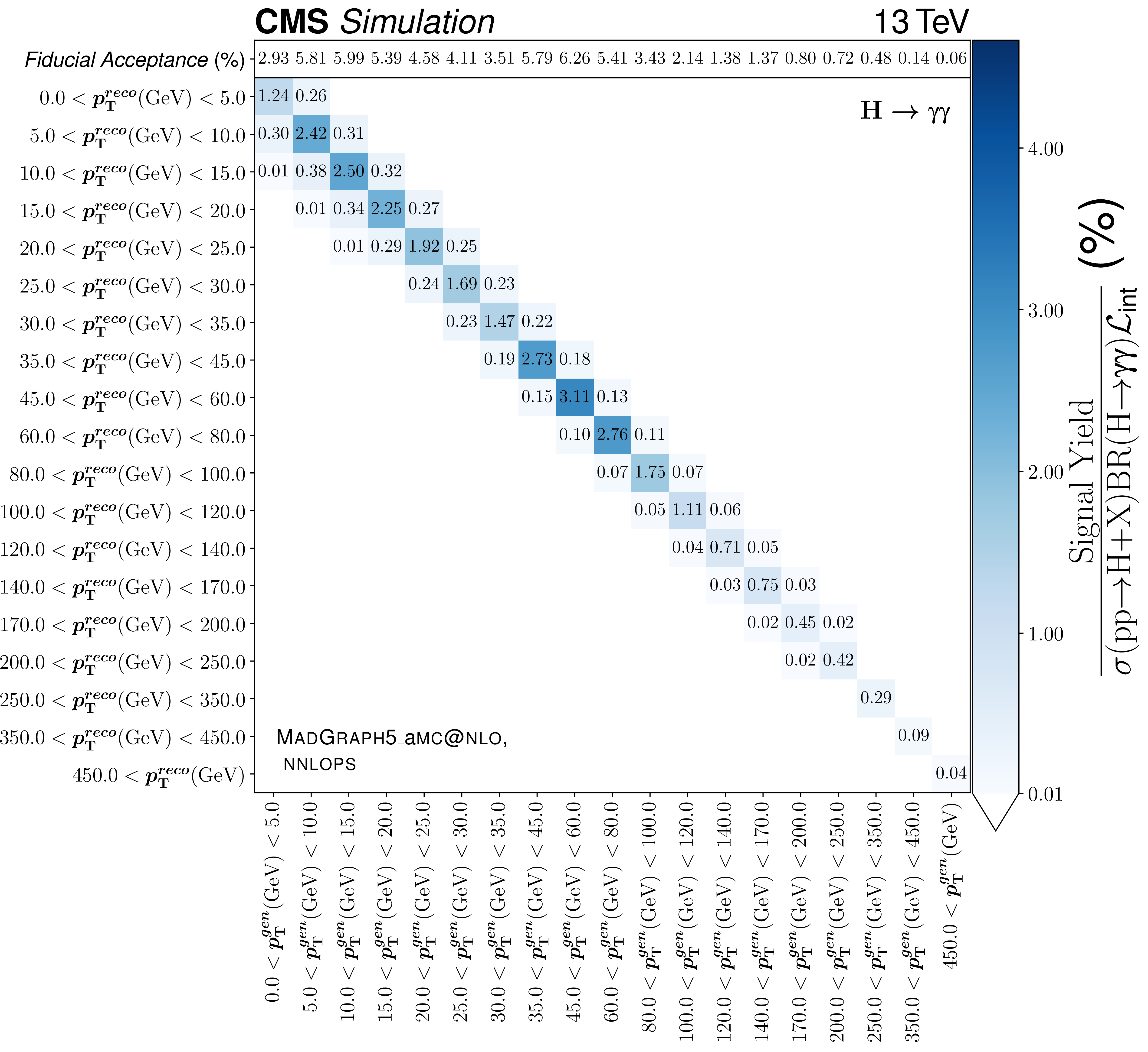
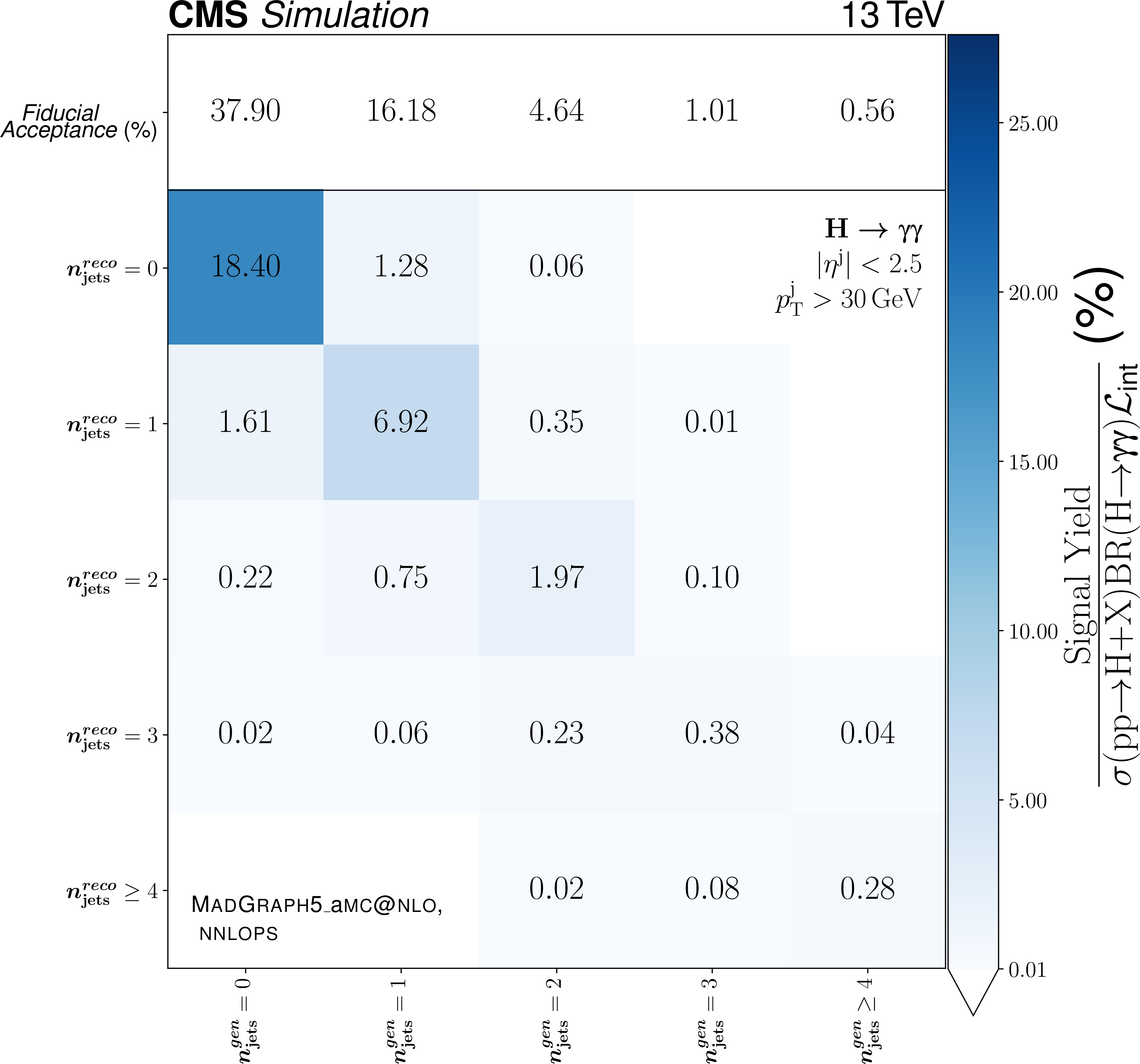
The event yields summed across all resolution categories divided by the total $ \mathrm{H}\to\gamma\gamma $ cross section [15] multiplied by the integrated luminosity for the bins in the particle-level, reconstruction-level observables for the year 2018 for the observables $ p_{\mathrm{T}} $ and $ n_{\text{jets}} $ are shown. There is one column per particle-level bin and one row per reconstruction-level bin. The top row shows the predicted fiducial acceptance, i.e., the per particle-level bin $ \mathrm{H}\to\gamma\gamma $ cross section divided by the total $ \mathrm{H}\to\gamma\gamma $ cross section. The values of the matrix $ K $ in Eq. (5) can be computed by dividing, column by column, the values in each bin by the predicted fiducial acceptance reported in the top row. The version of PYTHIA used here is 8.240 and the MadGraph-5_aMC@NLO version is 2.6.5. |
png pdf |
Figure 5-a:
The event yields summed across all resolution categories divided by the total $ \mathrm{H}\to\gamma\gamma $ cross section [15] multiplied by the integrated luminosity for the bins in the particle-level, reconstruction-level observables for the year 2018 for the $ p_{\mathrm{T}} $ observable are shown. There is one column per particle-level bin and one row per reconstruction-level bin. The top row shows the predicted fiducial acceptance, i.e., the per particle-level bin $ \mathrm{H}\to\gamma\gamma $ cross section divided by the total $ \mathrm{H}\to\gamma\gamma $ cross section. The values of the matrix $ K $ in Eq. (5) can be computed by dividing, column by column, the values in each bin by the predicted fiducial acceptance reported in the top row. The version of PYTHIA used here is 8.240 and the MadGraph-5_aMC@NLO version is 2.6.5. |
png pdf |
Figure 5-b:
The event yields summed across all resolution categories divided by the total $ \mathrm{H}\to\gamma\gamma $ cross section [15] multiplied by the integrated luminosity for the bins in the particle-level, reconstruction-level observables for the year 2018 for the $ n_{\text{jets}} $ observable are shown. There is one column per particle-level bin and one row per reconstruction-level bin. The top row shows the predicted fiducial acceptance, i.e., the per particle-level bin $ \mathrm{H}\to\gamma\gamma $ cross section divided by the total $ \mathrm{H}\to\gamma\gamma $ cross section. The values of the matrix $ K $ in Eq. (5) can be computed by dividing, column by column, the values in each bin by the predicted fiducial acceptance reported in the top row. The version of PYTHIA used here is 8.240 and the MadGraph-5_aMC@NLO version is 2.6.5. |
png pdf |
Figure 6:
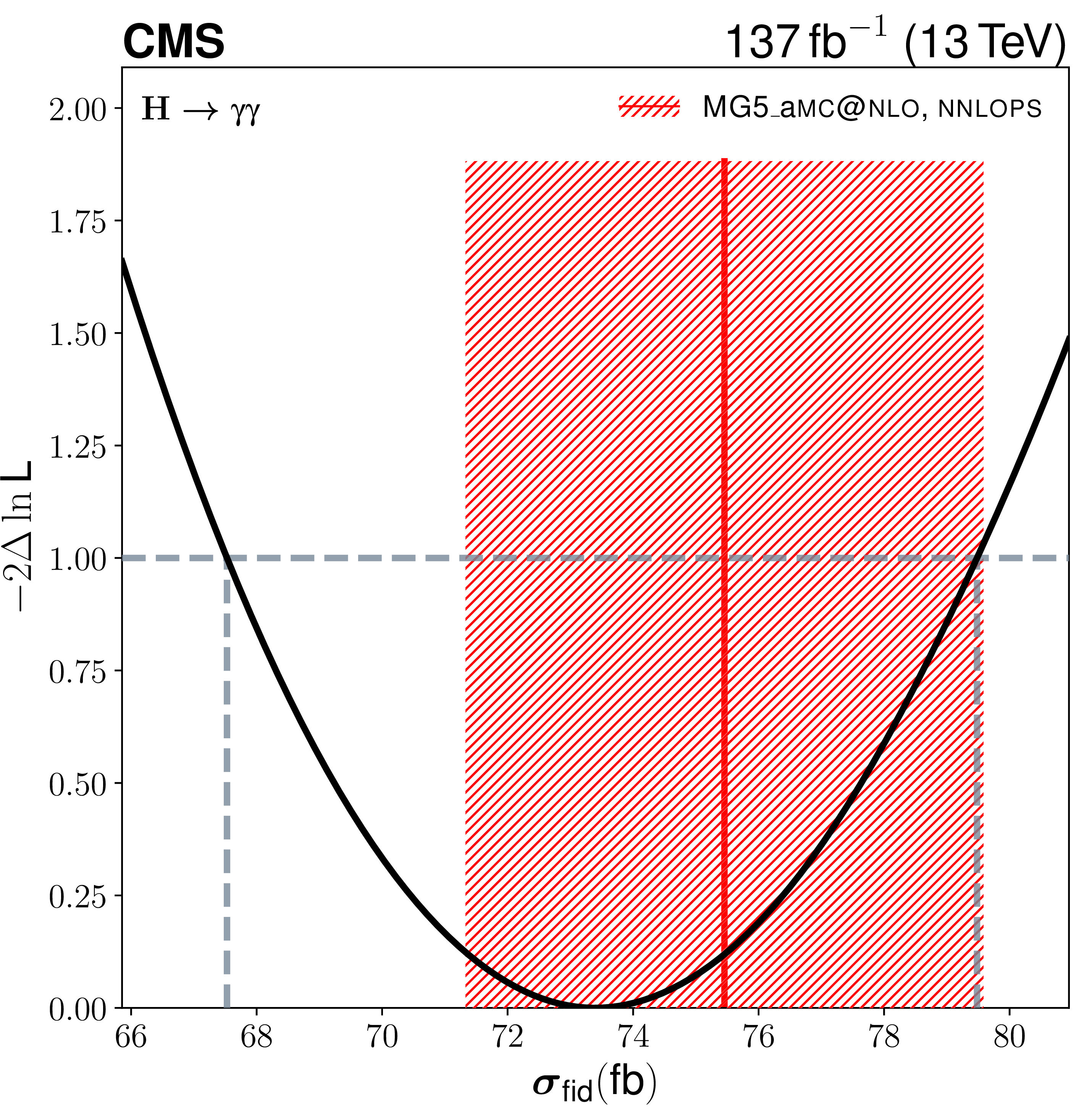
The black line shows the scan of $ q\left(\Delta\vec{\sigma}\right)=-2\Delta\ln\mathrm{L} $ for the $ \mathrm{H}\to\gamma\gamma $ cross section in the fiducial region. The red line shows the theoretical prediction for the SM, obtained with MadGraph-5_aMC@NLO. Its uncertainty is shown as the hatched area. |
png pdf |
Figure 7:
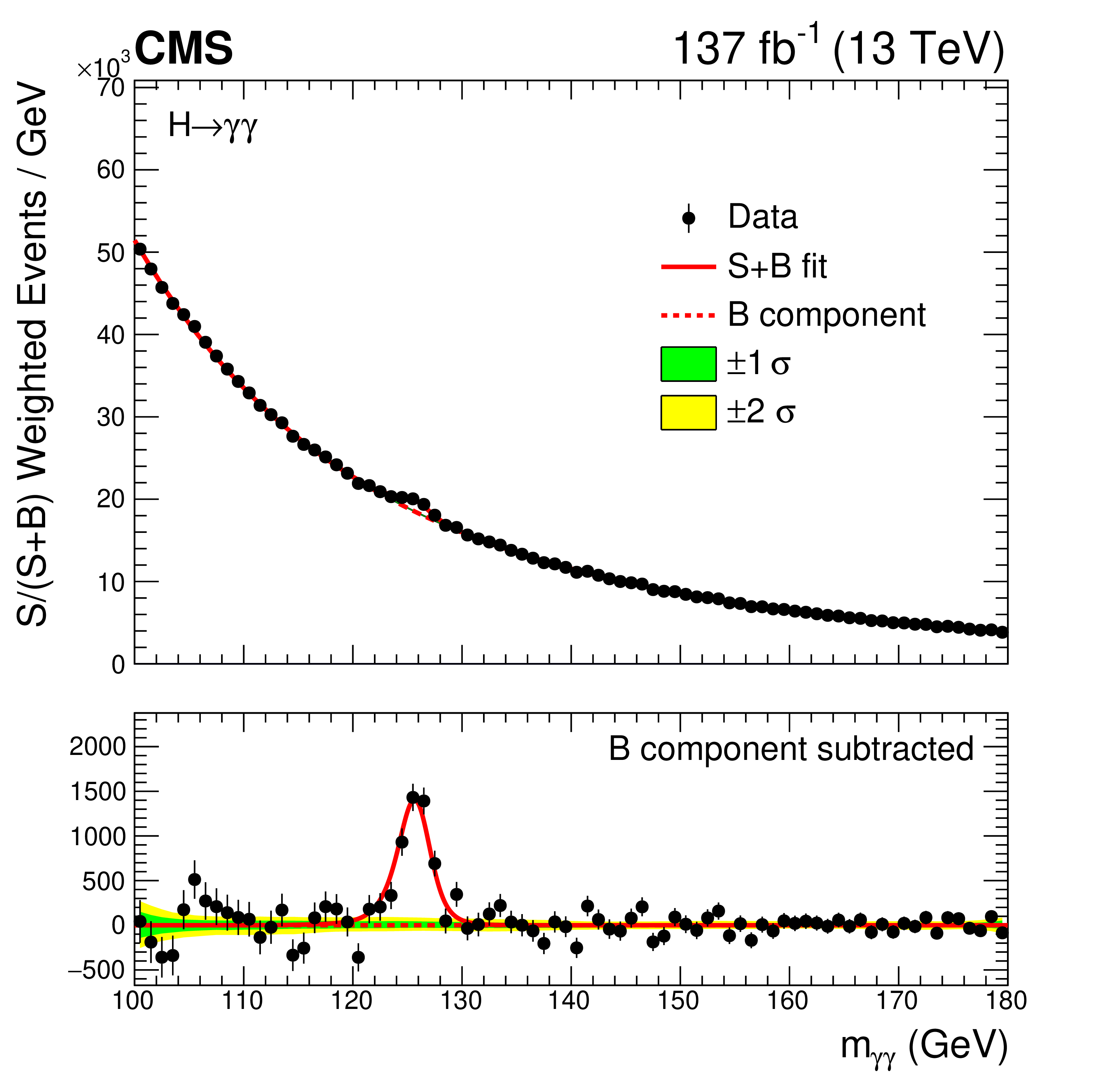
Diphoton invariant mass distribution with combining all categories used for the inclusive fiducial cross section measurement. The displayed $ m_{\gamma\gamma} $ histogram and signal+background hypothesis (red line) represent their sums across all categories weighted by their respective $ S/(S+B) $ ratio. In the lower panel, the $ m_{\gamma\gamma} $ histogram subtracting the background component, as estimated by the background pdf, is shown. |
png pdf |
Figure 8:
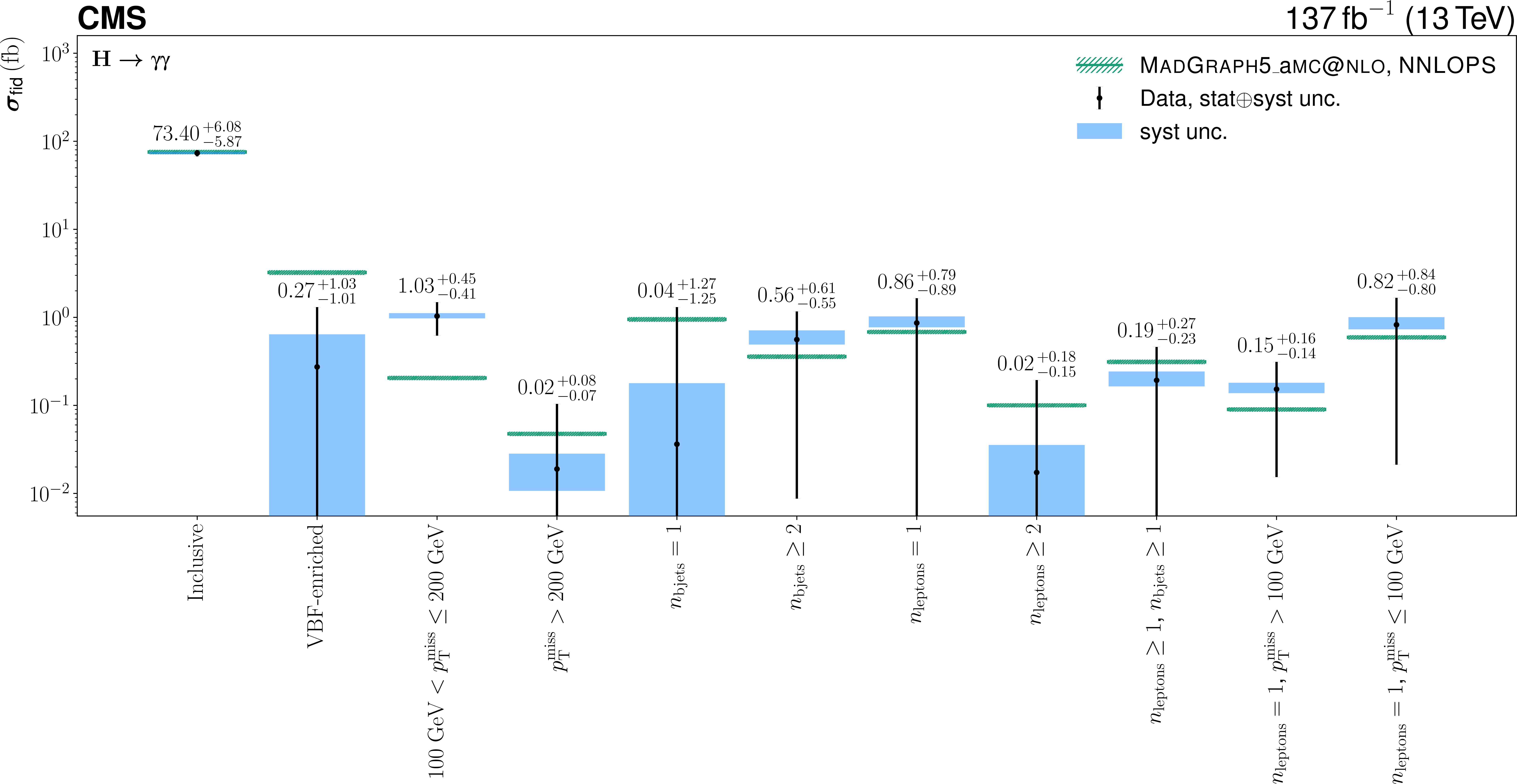
The $ \mathrm{H}\to\gamma\gamma $ cross section in dedicated regions of the fiducial phase space. Their selection criteria on top of the fiducial requirements are indicated on the plot. The prediction from MadGraph-5_aMC@NLO including the NNLOPS reweighting, with its uncertainty from acceptance variation due to PDF, $ \alpha_\mathrm{S} $, and scale uncertainties, as well as cross section and branching fraction uncertainties, is shown. The systematic uncertainty in the measured value is shown as a blue band and the full systematic$ \oplus $statistical uncertainty is shown as the error bar, where $ \oplus $ stands for the sum in quadrature. |
png pdf |
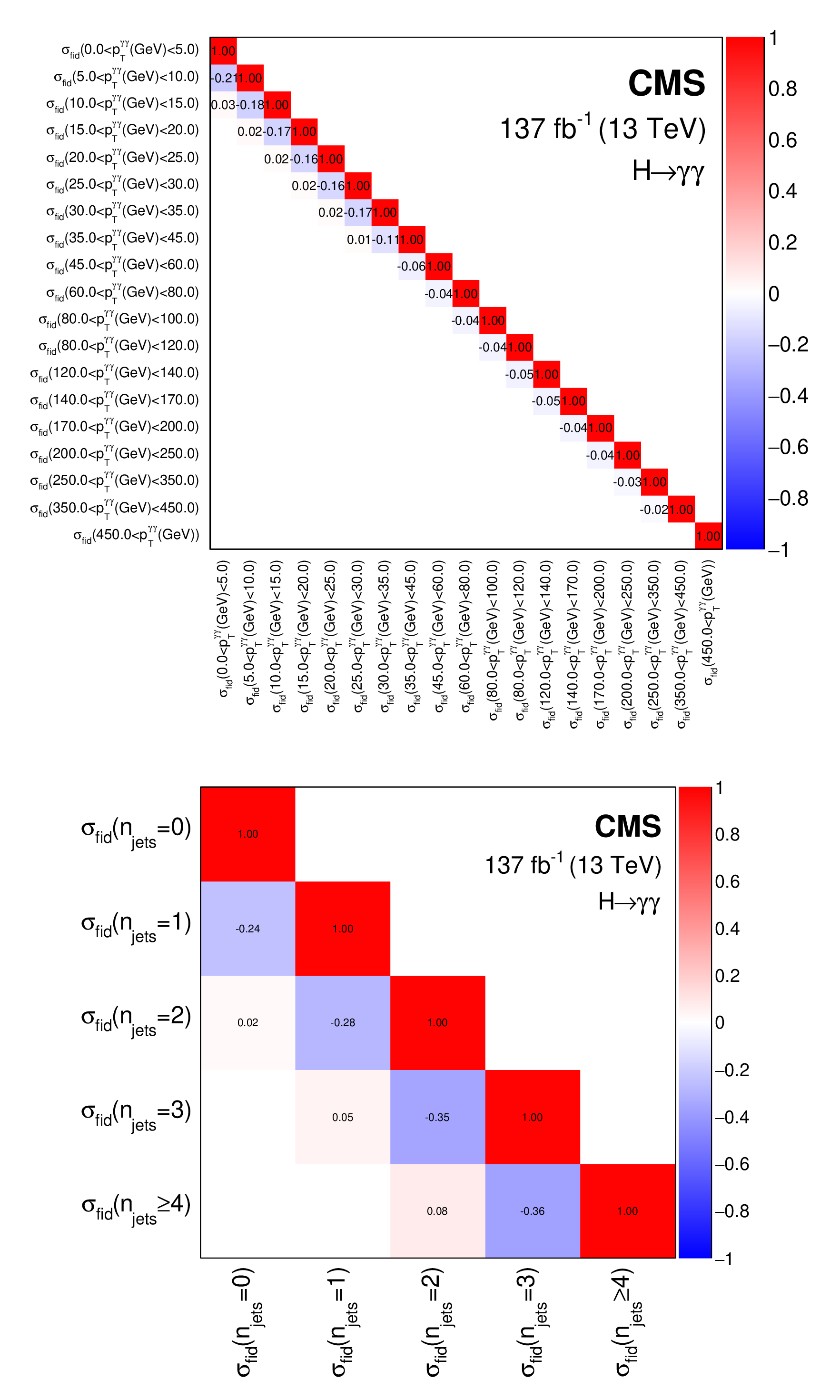
Figure 9:
The correlation matrices for the cross sections $ \sigma_{\text{fid}} $ per particle-level bin for $ p_{\mathrm{T}}^{\gamma\gamma} $ (upper), and $ n_{\text{jets}} $ (lower), as given in Table 3, extracted from the simultaneous maximum likelihood fit for the cross sections. |
png pdf |
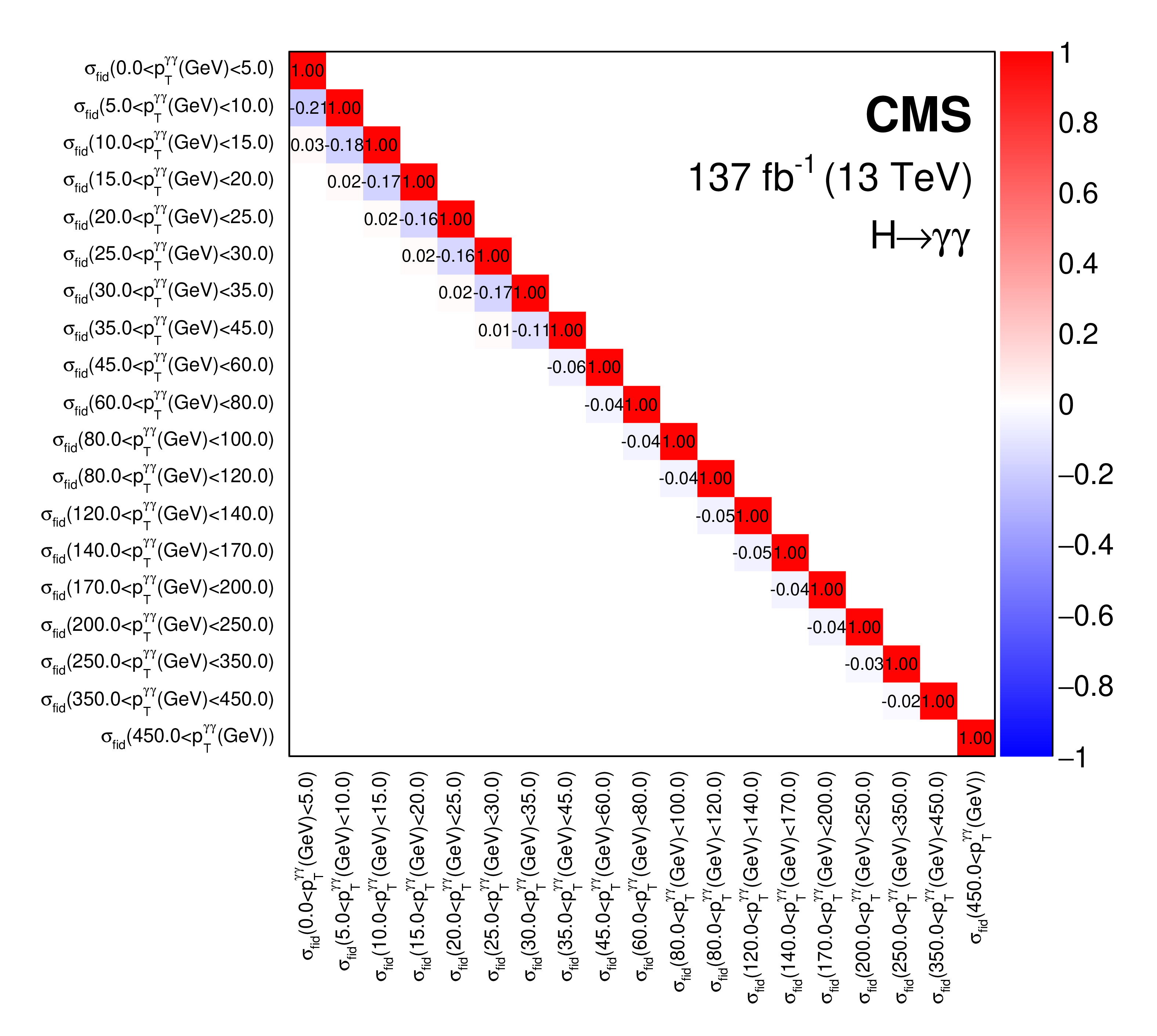
Figure 9-a:
The correlation matrix for the cross sections $ \sigma_{\text{fid}} $ per particle-level bin for $ p_{\mathrm{T}}^{\gamma\gamma} $, as given in Table 3, extracted from the simultaneous maximum likelihood fit for the cross sections. |

png pdf |
Figure 9-b:
The correlation matrix for the cross sections $ \sigma_{\text{fid}} $ per particle-level bin for $ n_{\text{jets}} $, as given in Table 3, extracted from the simultaneous maximum likelihood fit for the cross sections. |
png pdf |
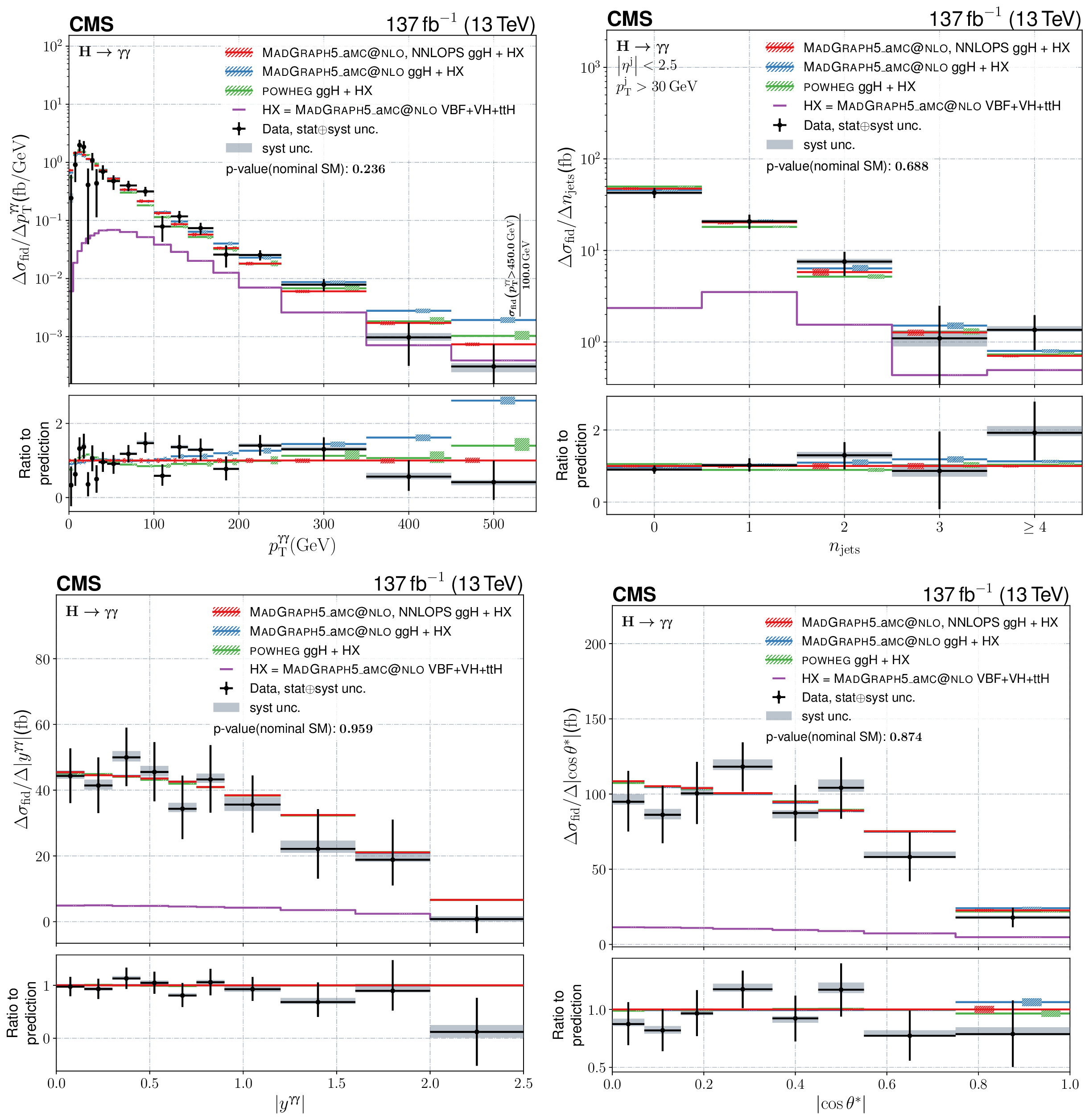
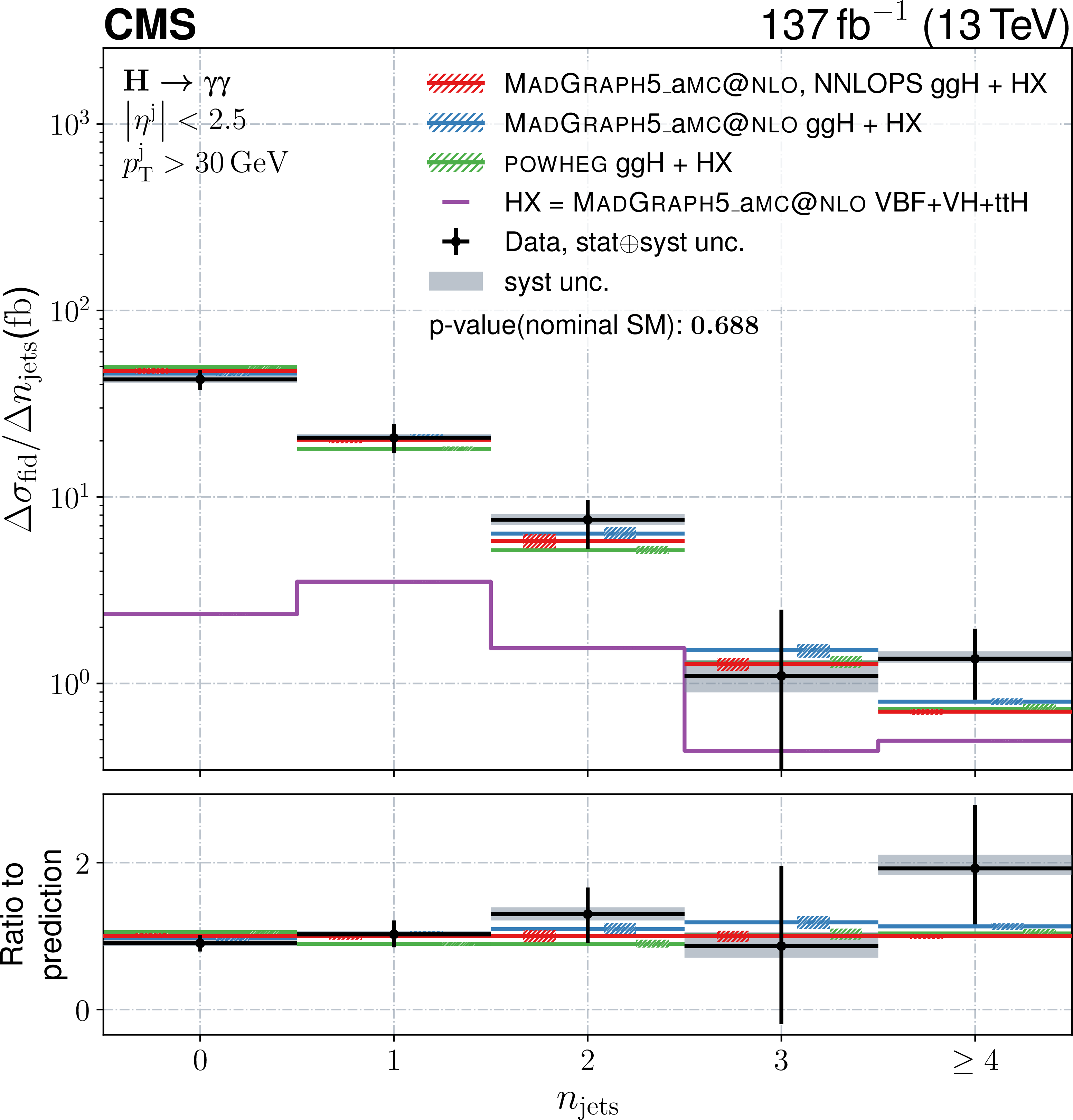
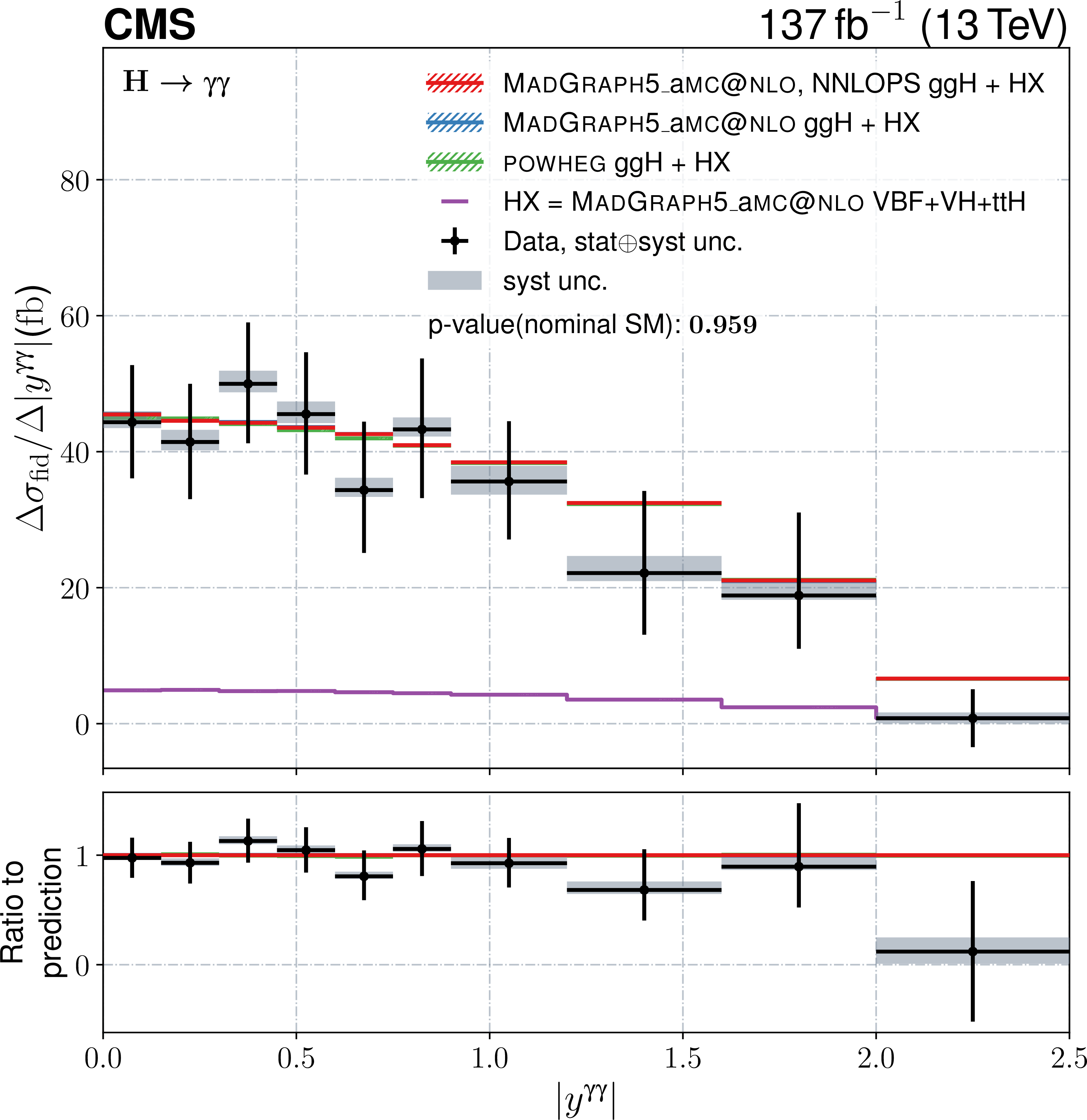
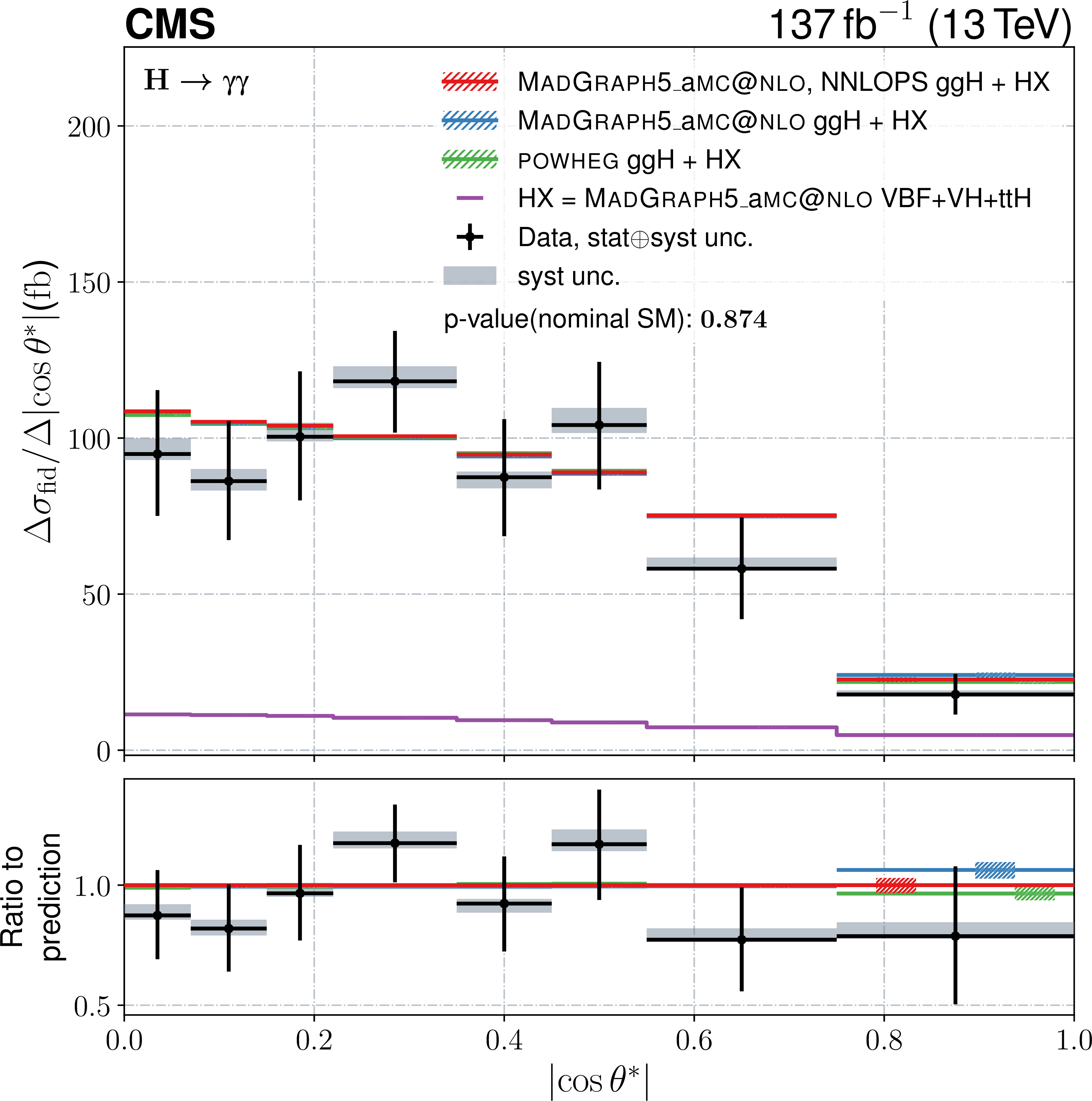
Figure 10:
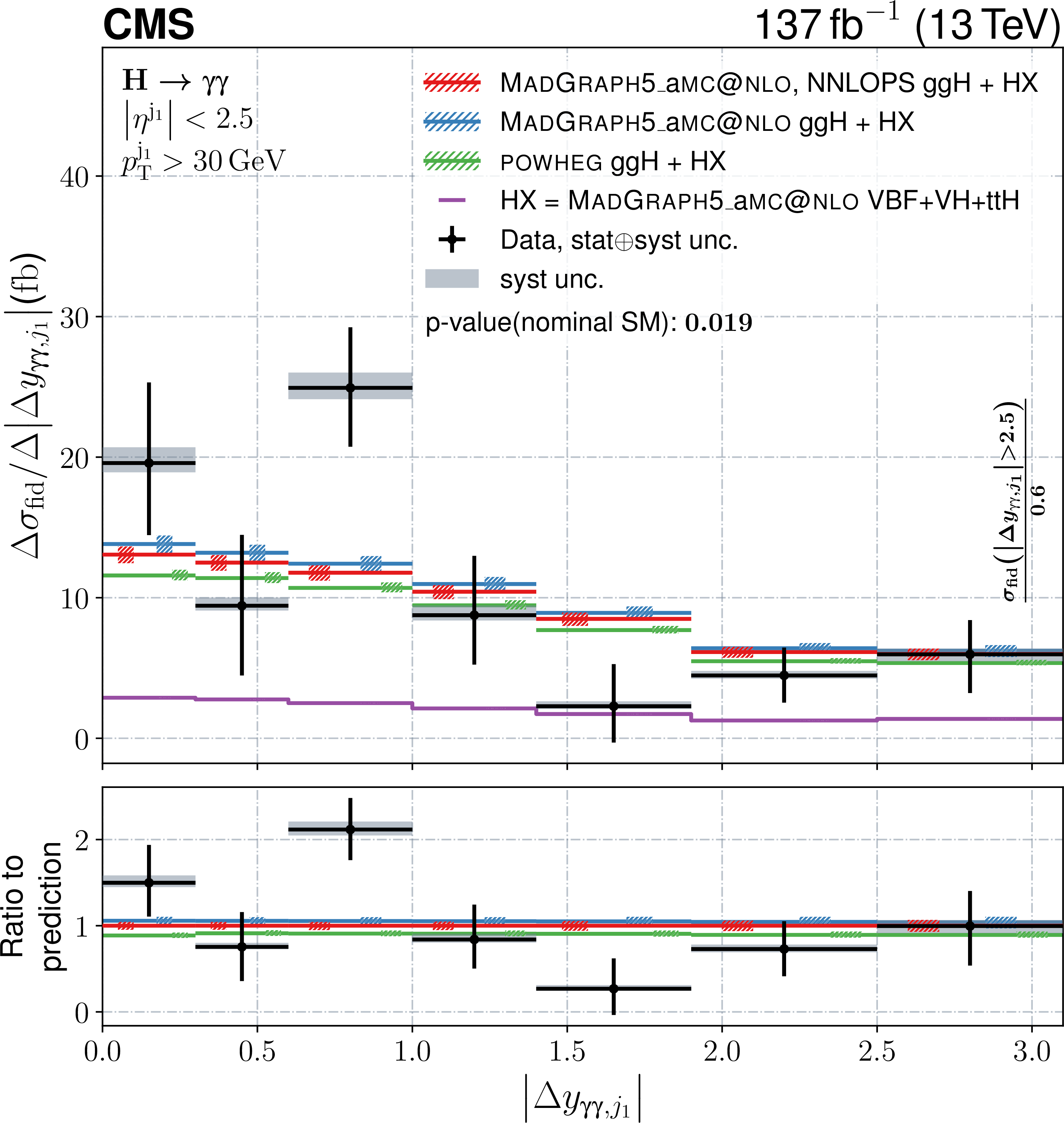
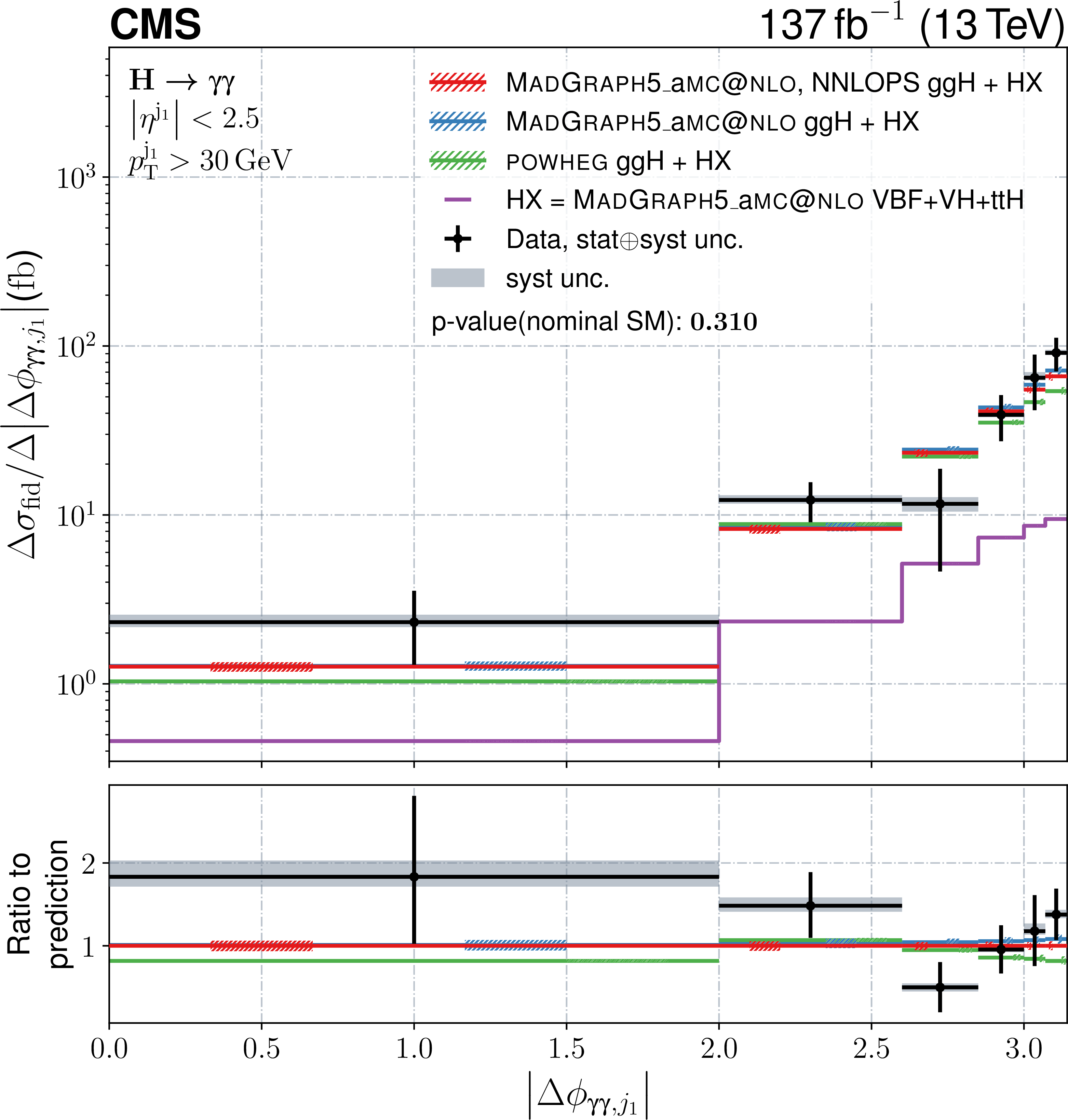
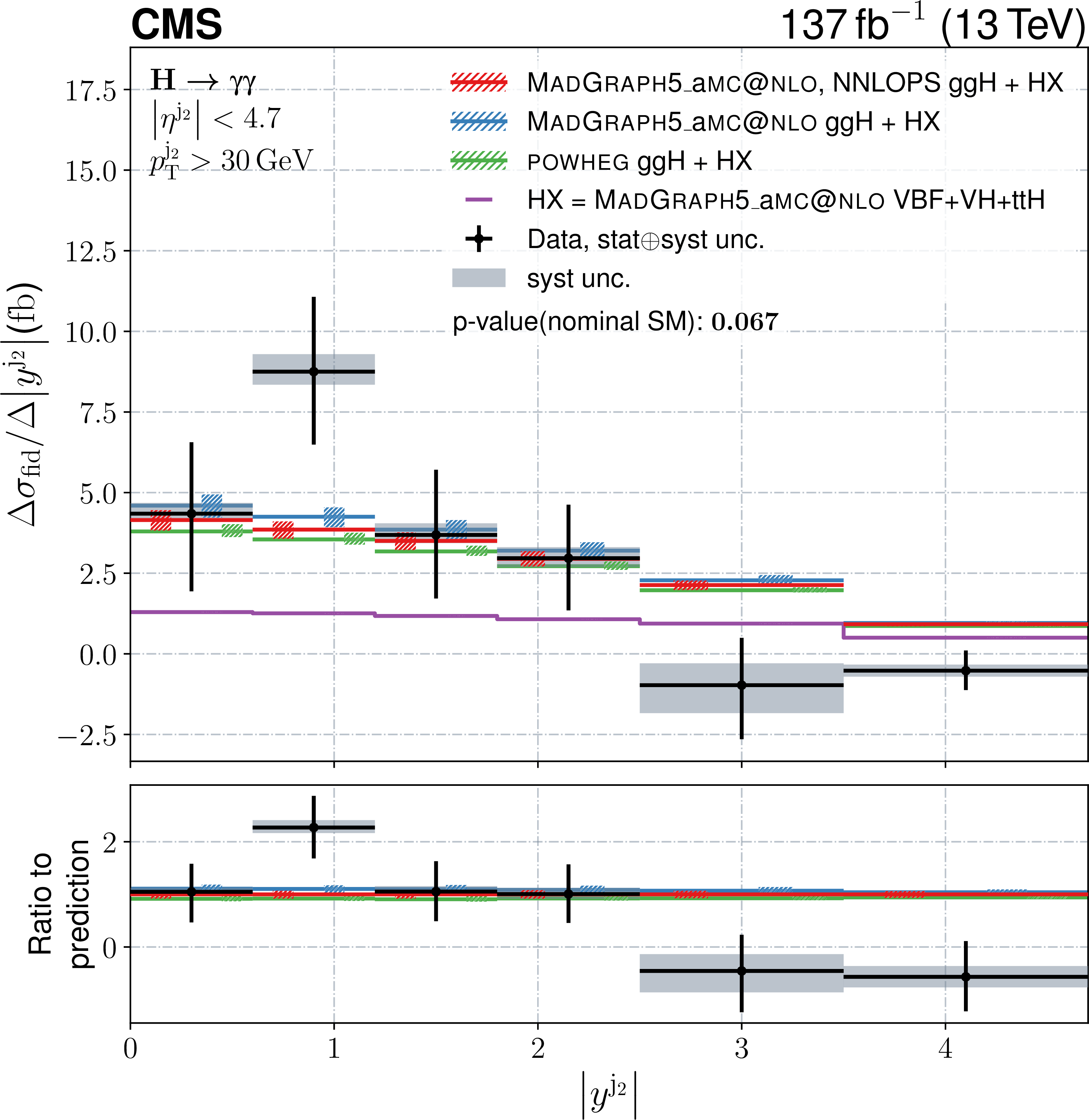
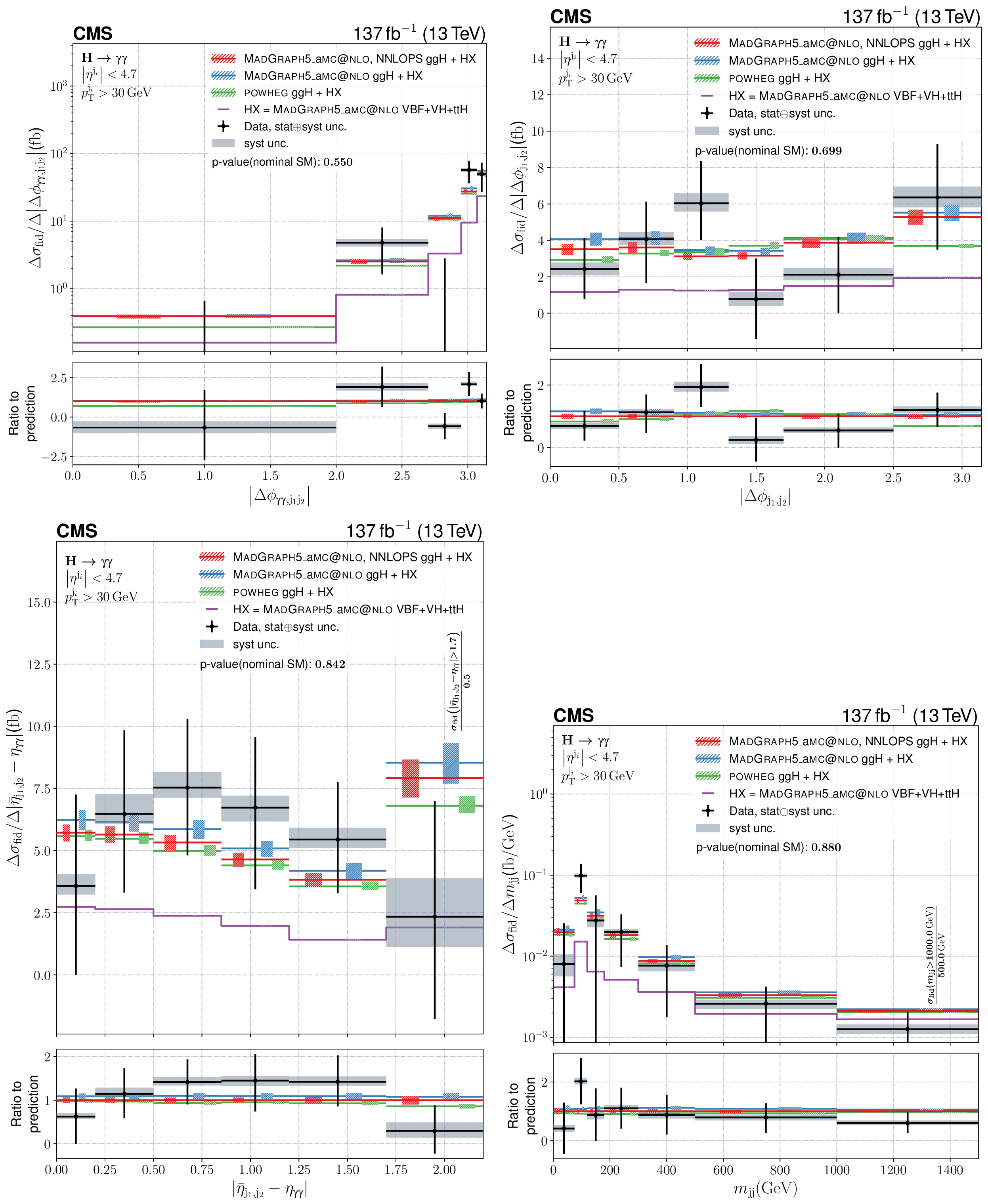
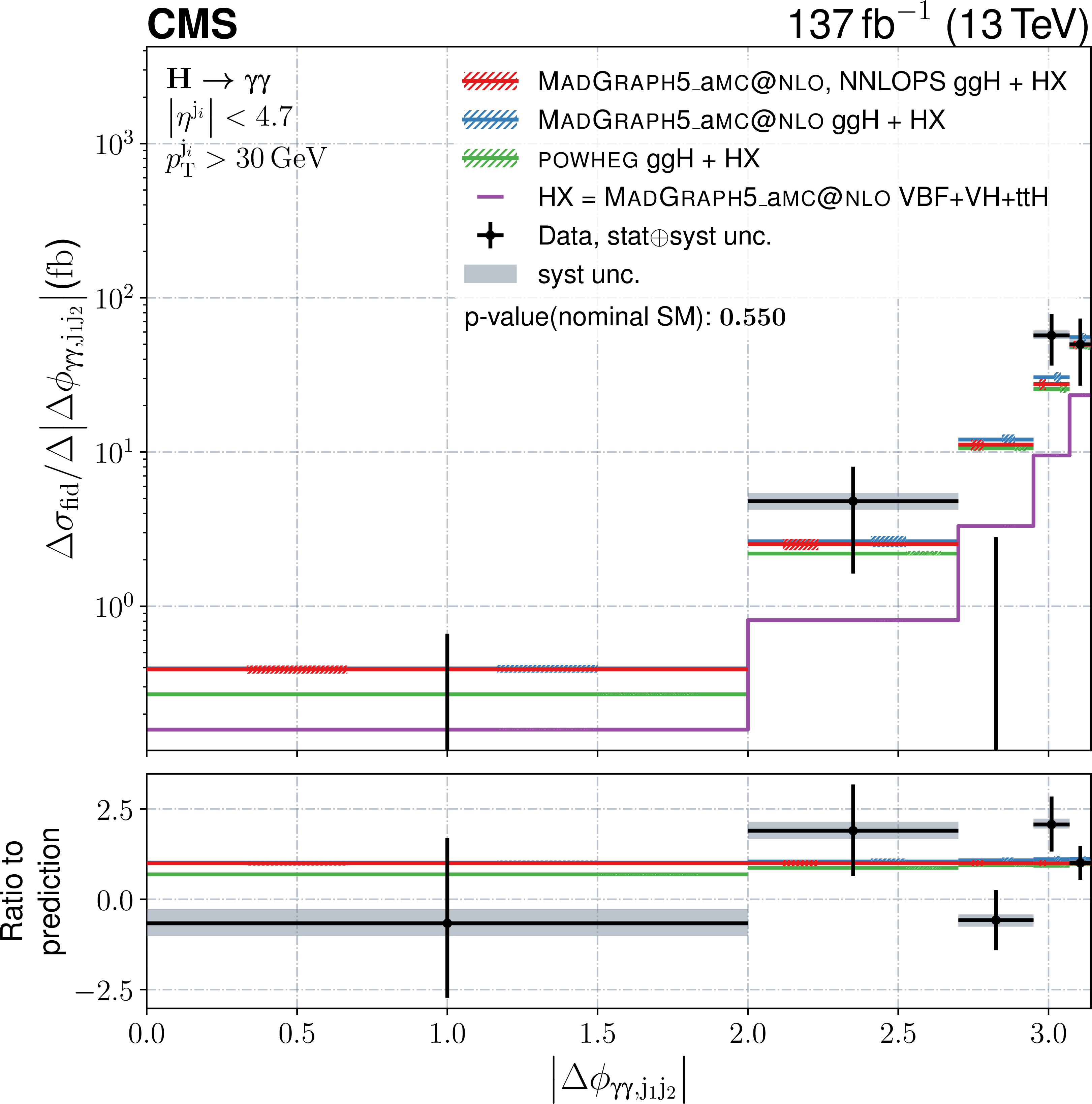
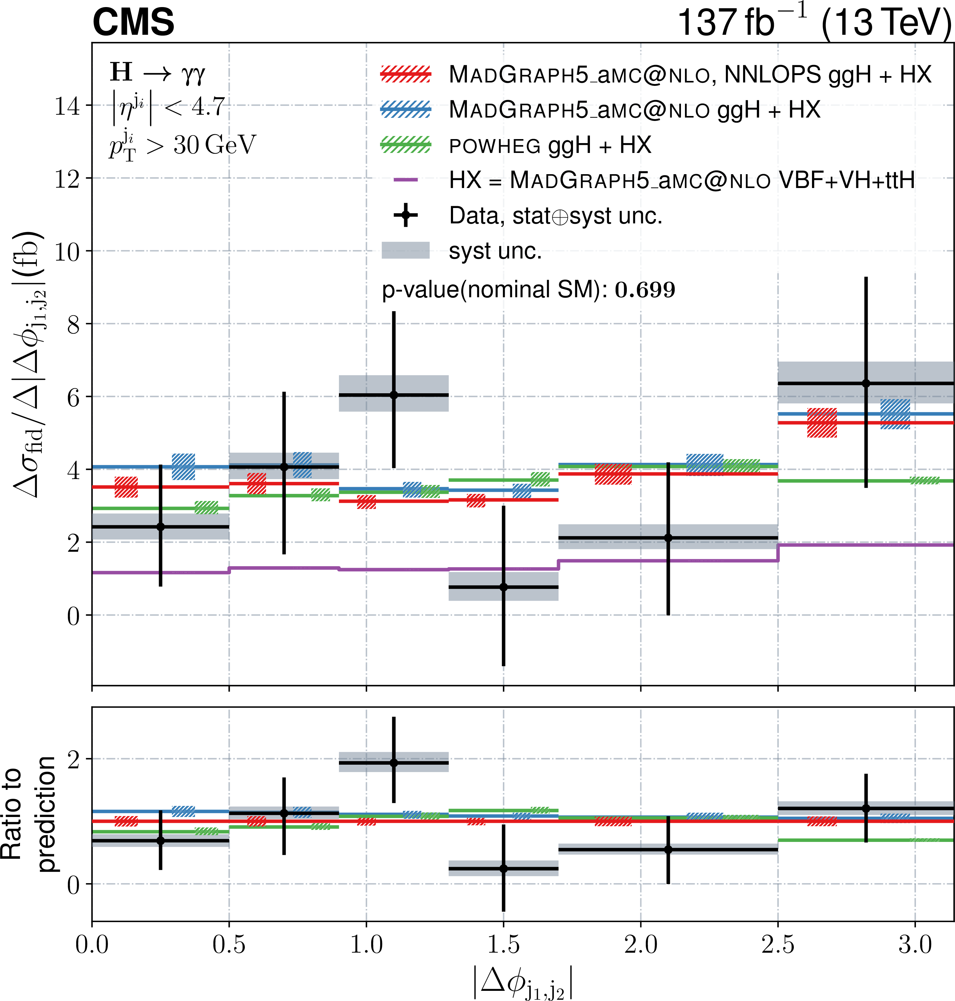
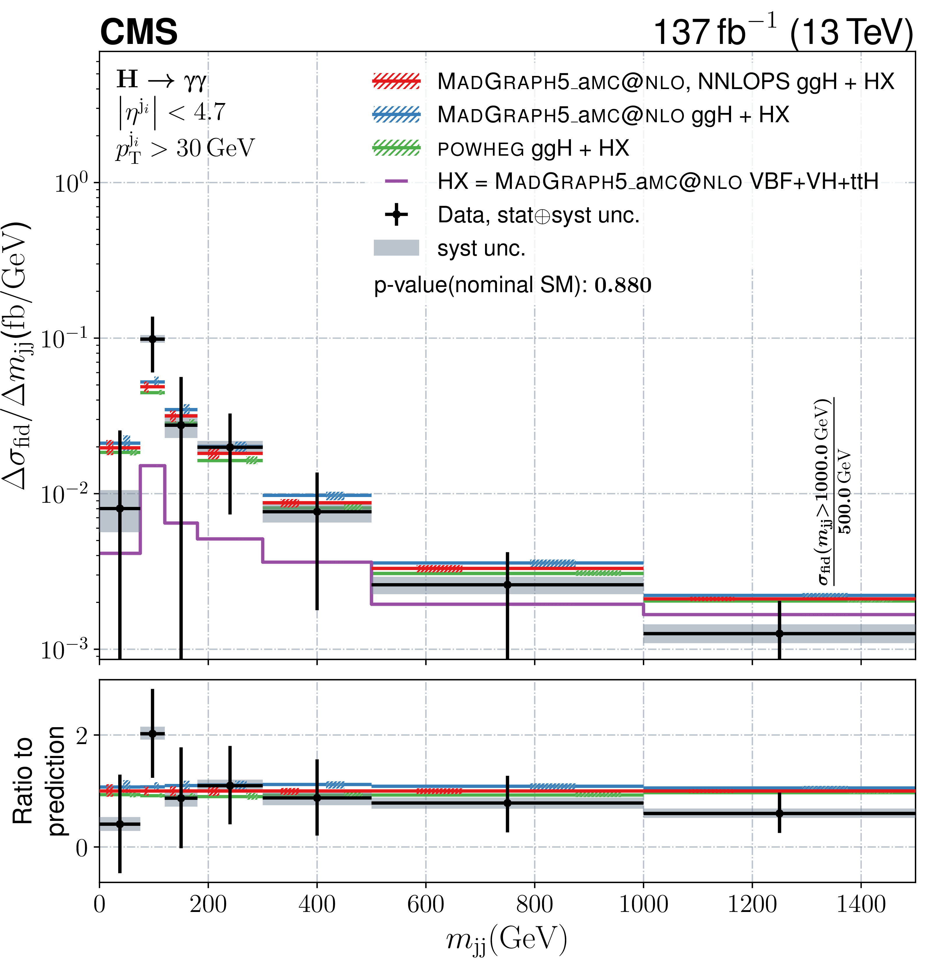
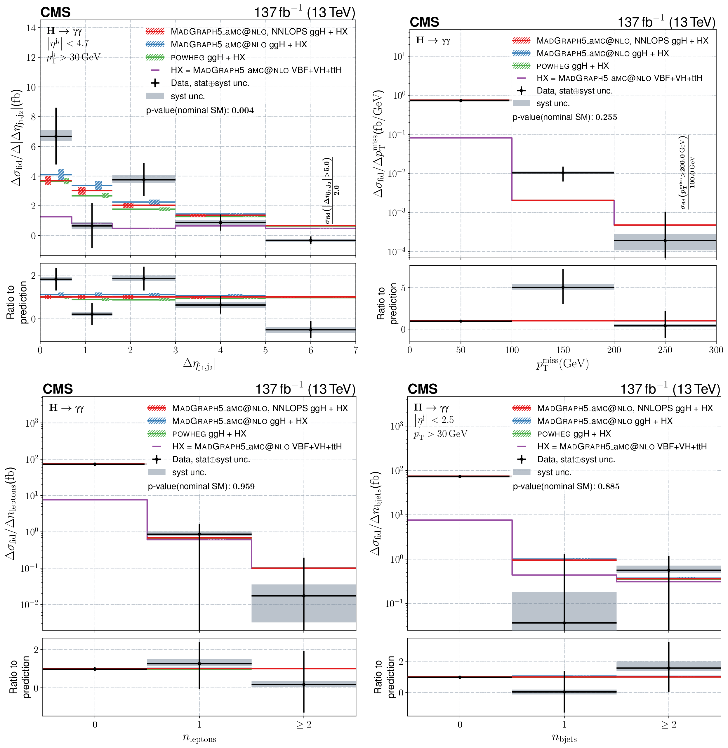
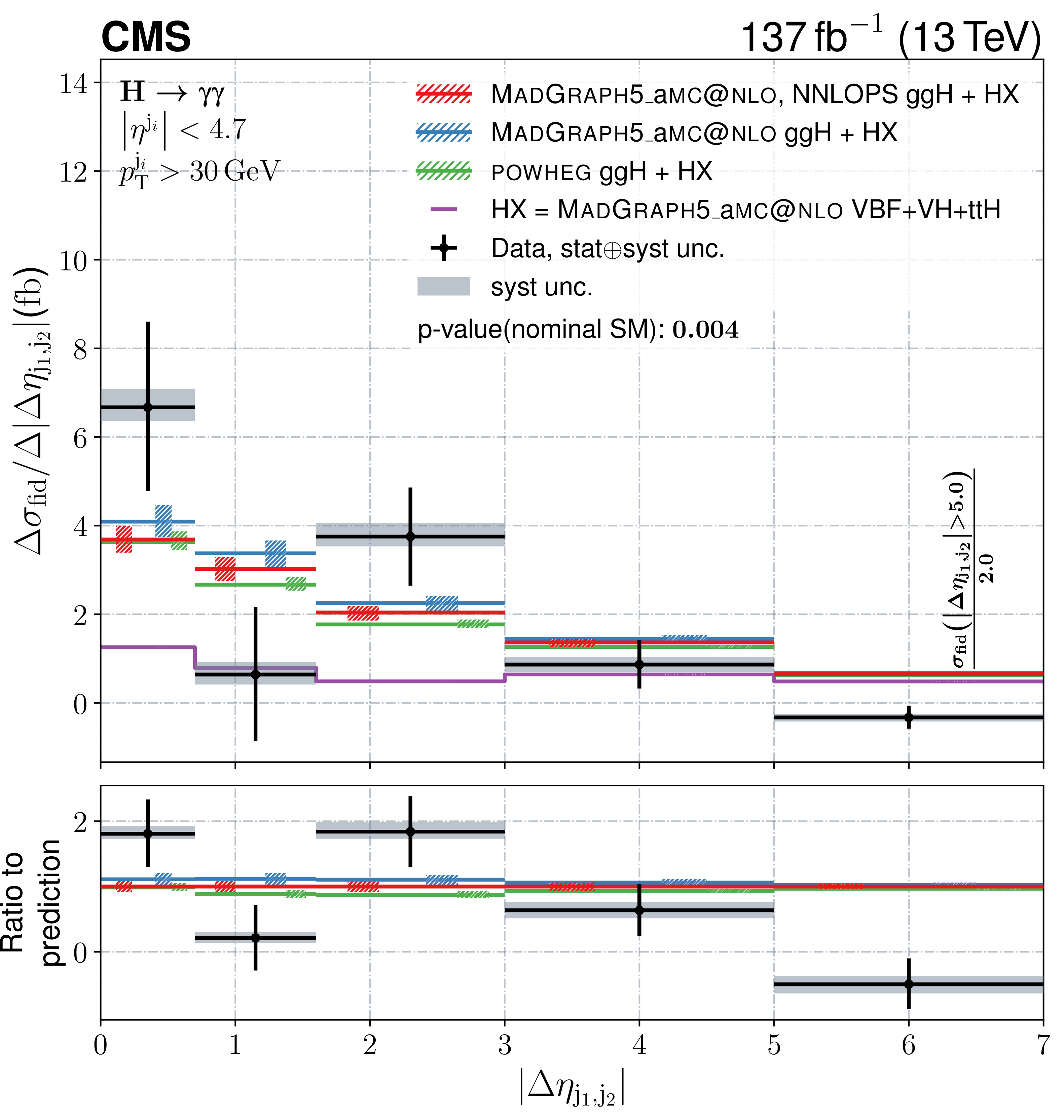
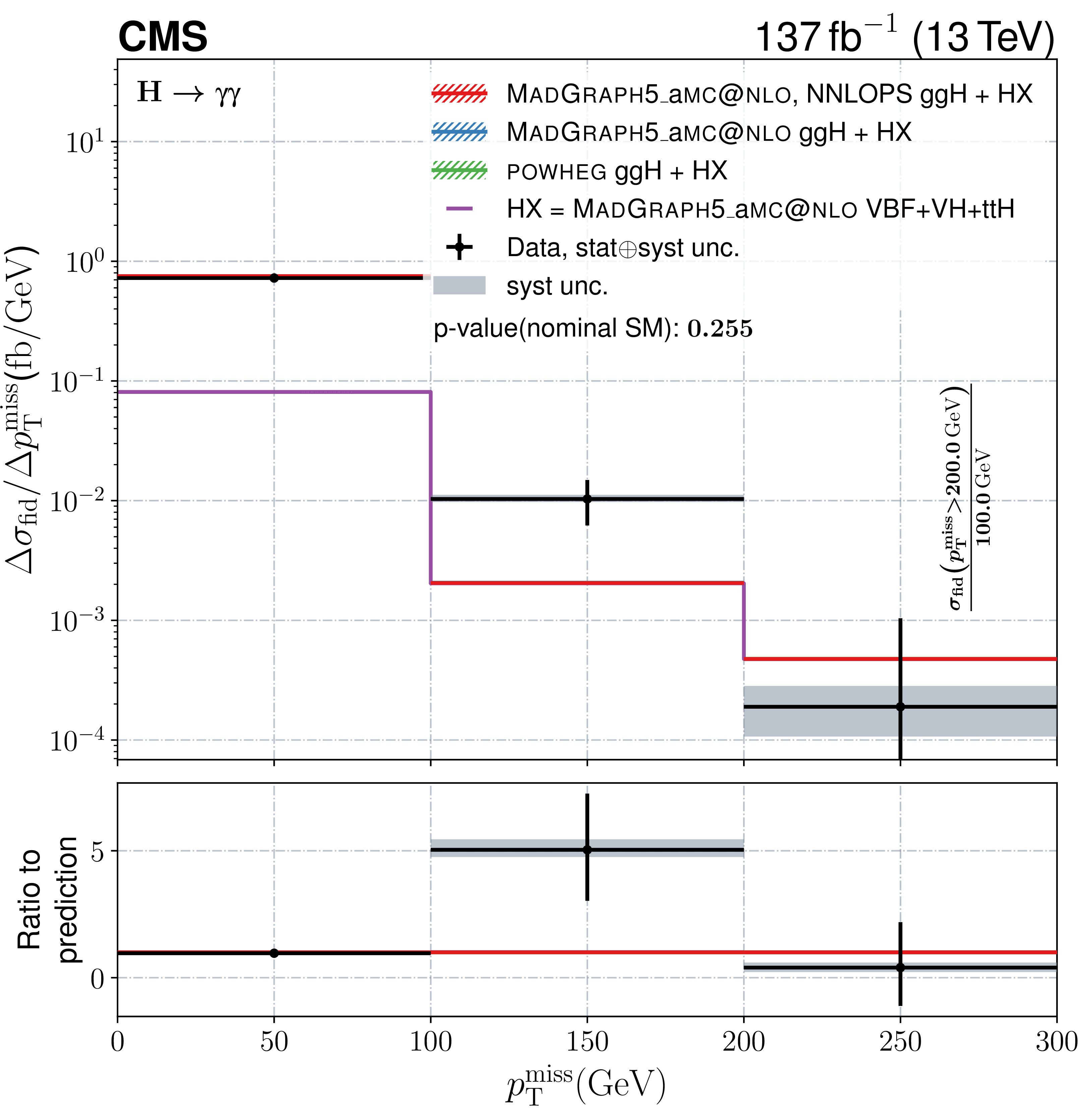
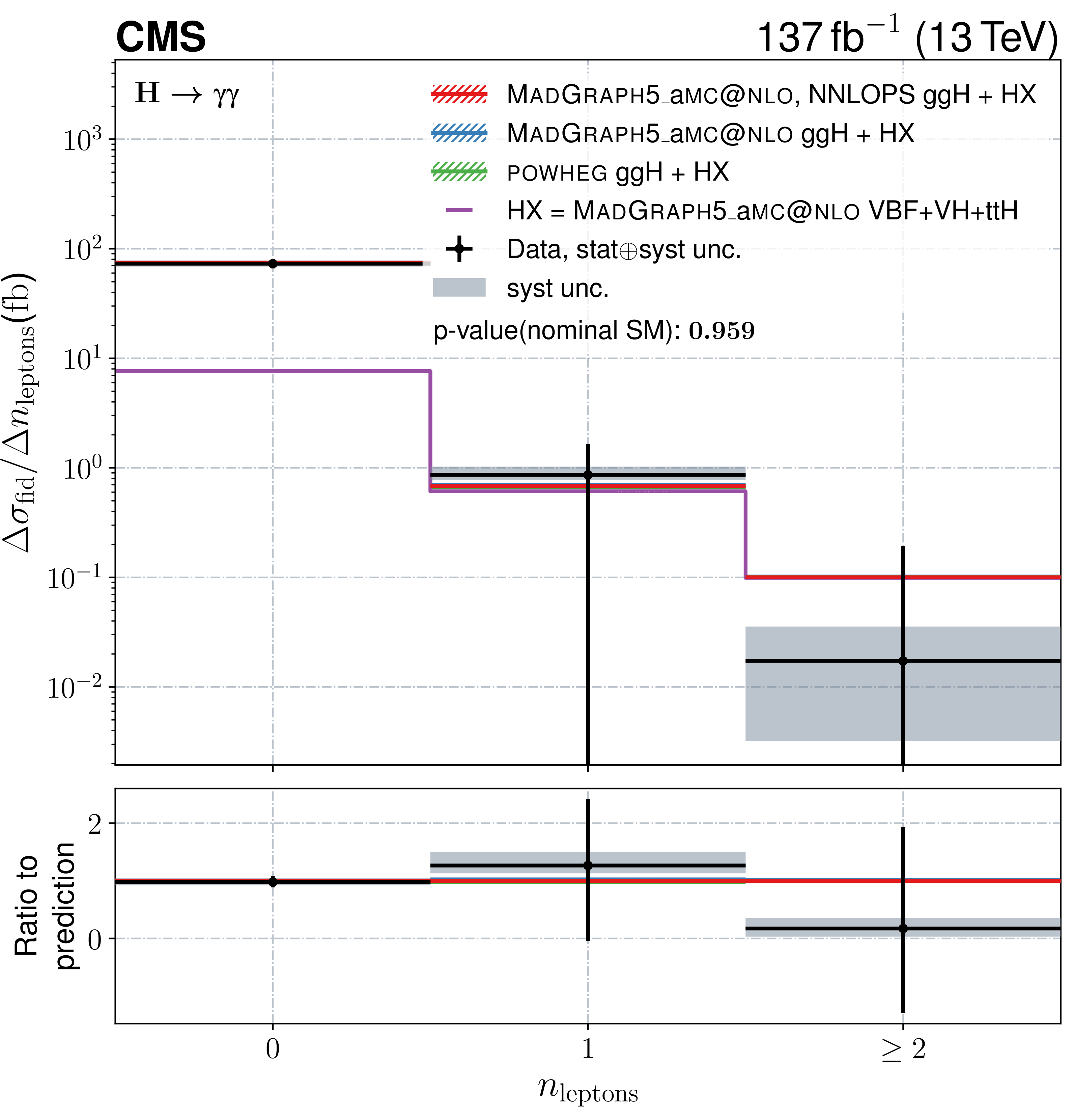
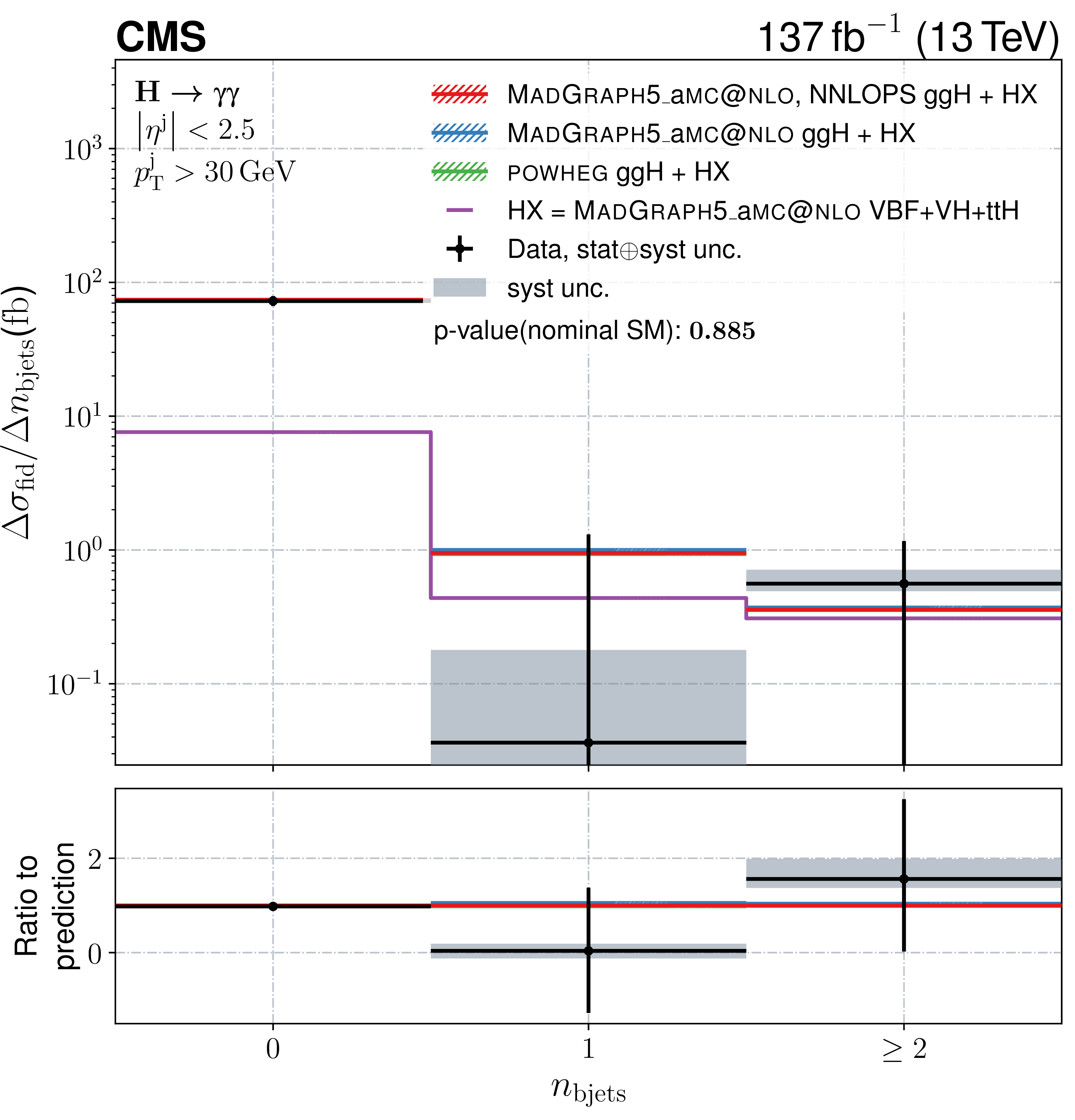
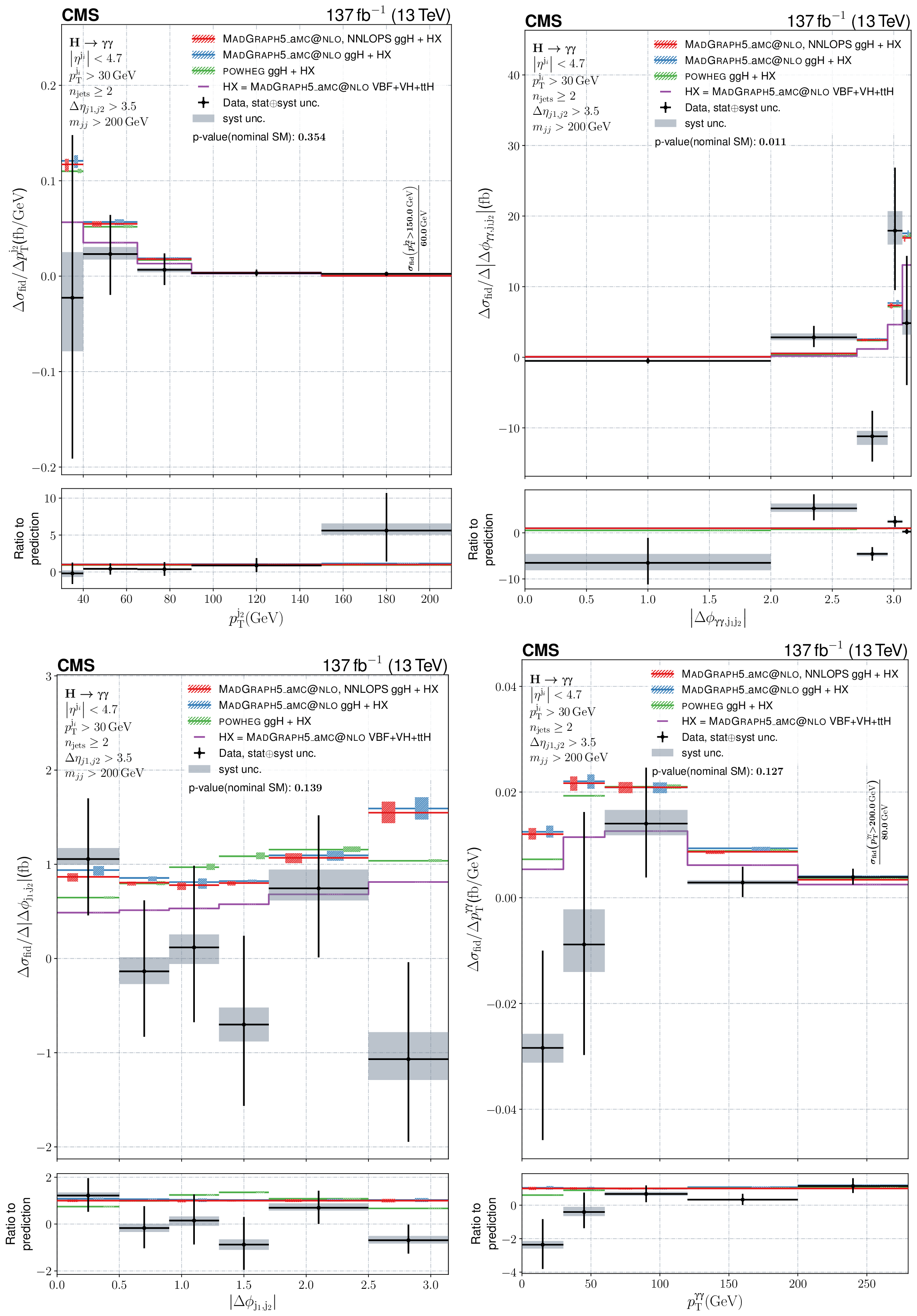
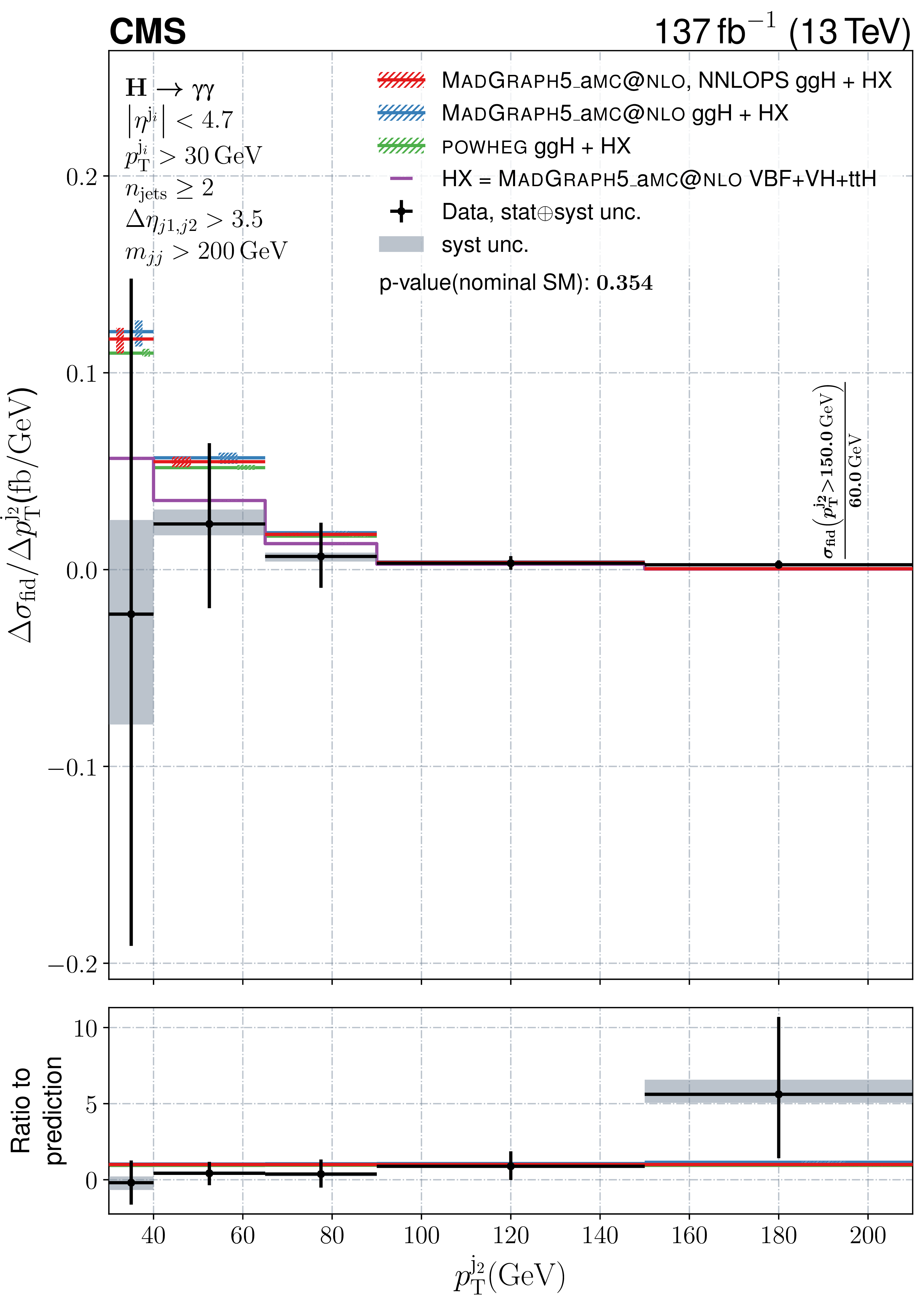
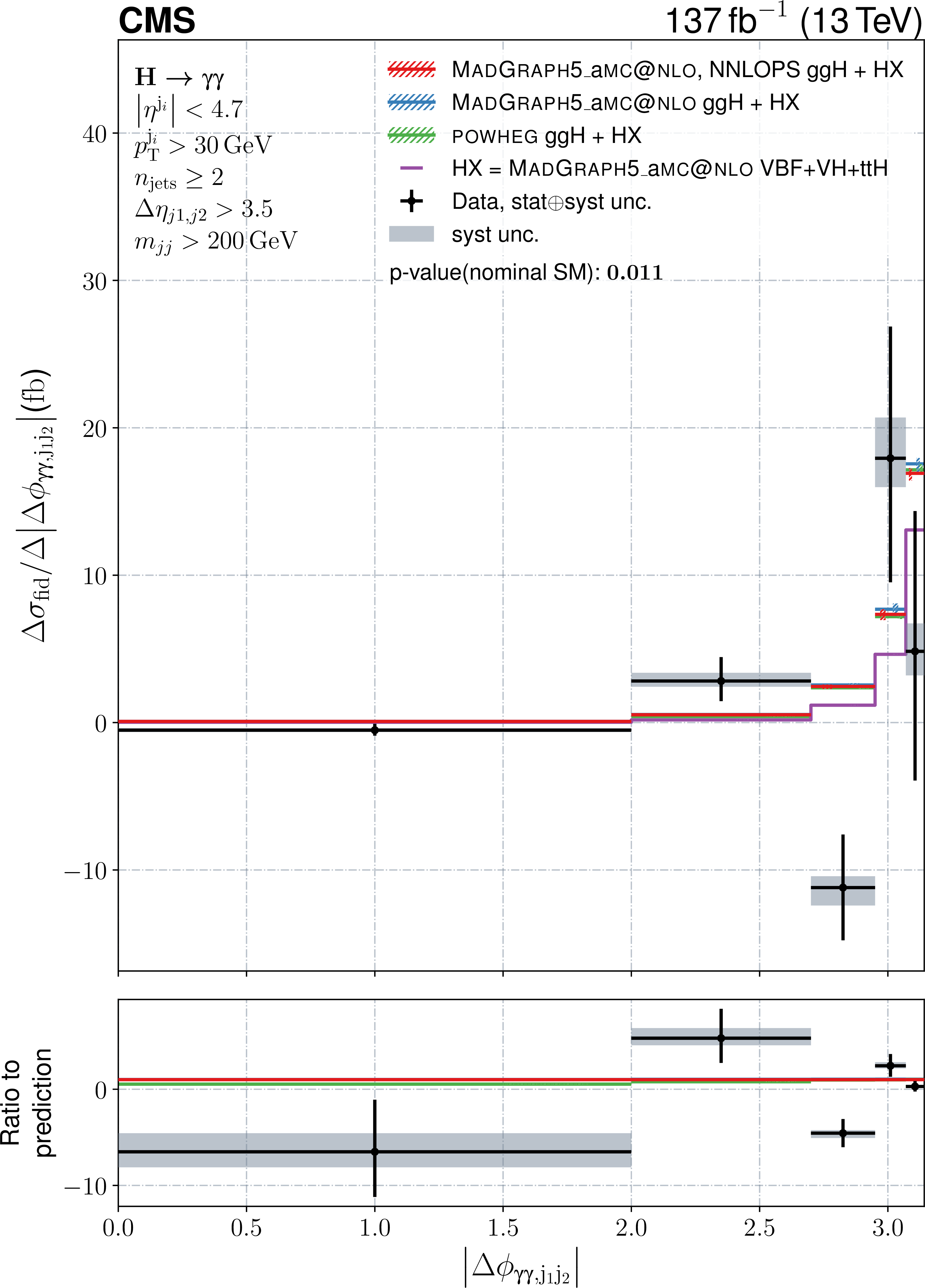
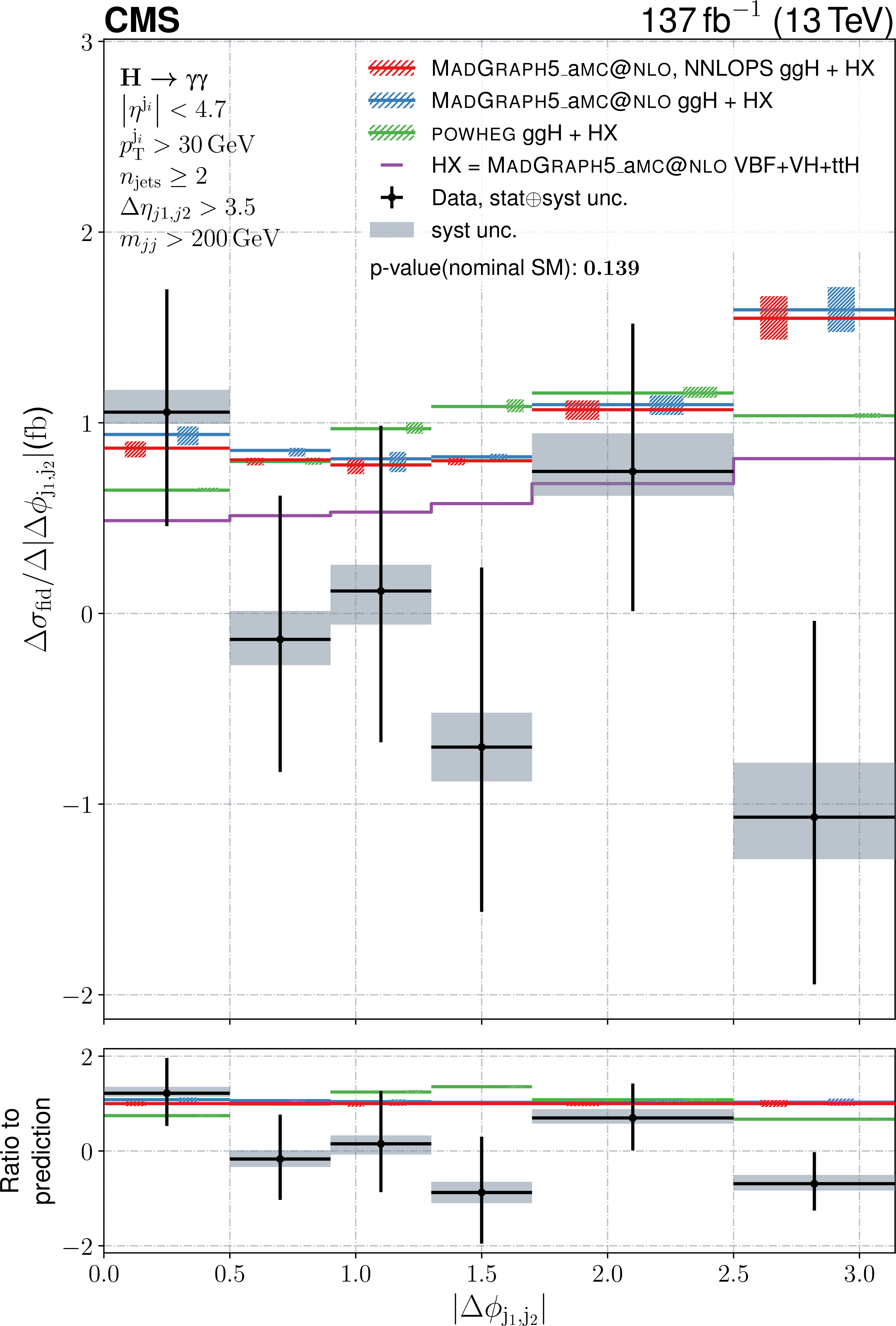
Differential fiducial cross sections for $ p_{\mathrm{T}}^{\gamma\gamma} $, $ n_{\text{jets}} $, $ |y^{\gamma\gamma}| $, and $ |\cos\theta^{\ast}| $. The observed differential fiducial cross section values are shown as black points with the vertical error bars showing the full uncertainty, the horizontal error bars show the width of the respective bin. The grey shaded areas visualize the systematic component of the uncertainty. The coloured lines denote the predictions from different setups of the event generator. All of them have the HX=VBF+VH+ttH component from MADGRAPH5_aMC@NLO in common, which is displayed in violet without uncertainties. The red lines show the sum of HX and the ggH component from MADGRAPH5_aMC@NLO reweighted to match the NNLOPS prediction. For the blue lines no NNLOPS reweighting is applied and the green lines take the prediction for the ggH production mode from POWHEG. The hatched areas show the uncertainties in theoretical predictions on both the $ \mathrm{g}\mathrm{g}\mathrm{F} $ and HX components. Only effects coming from varying the set of PDF replicas, the $ \alpha_\mathrm{S} $ value, and the renormalization and factorization scales that impact the shape are taken into account here, the total cross section is kept constant at the value from Ref. [15]. The given $ p $-values are calculated for the nominal SM prediction and the bottom panes show the ratio to the same prediction. If the last particle-level bin expands to infinity is explicitly marked on the plot together with the normalization of this bin. |
png pdf |
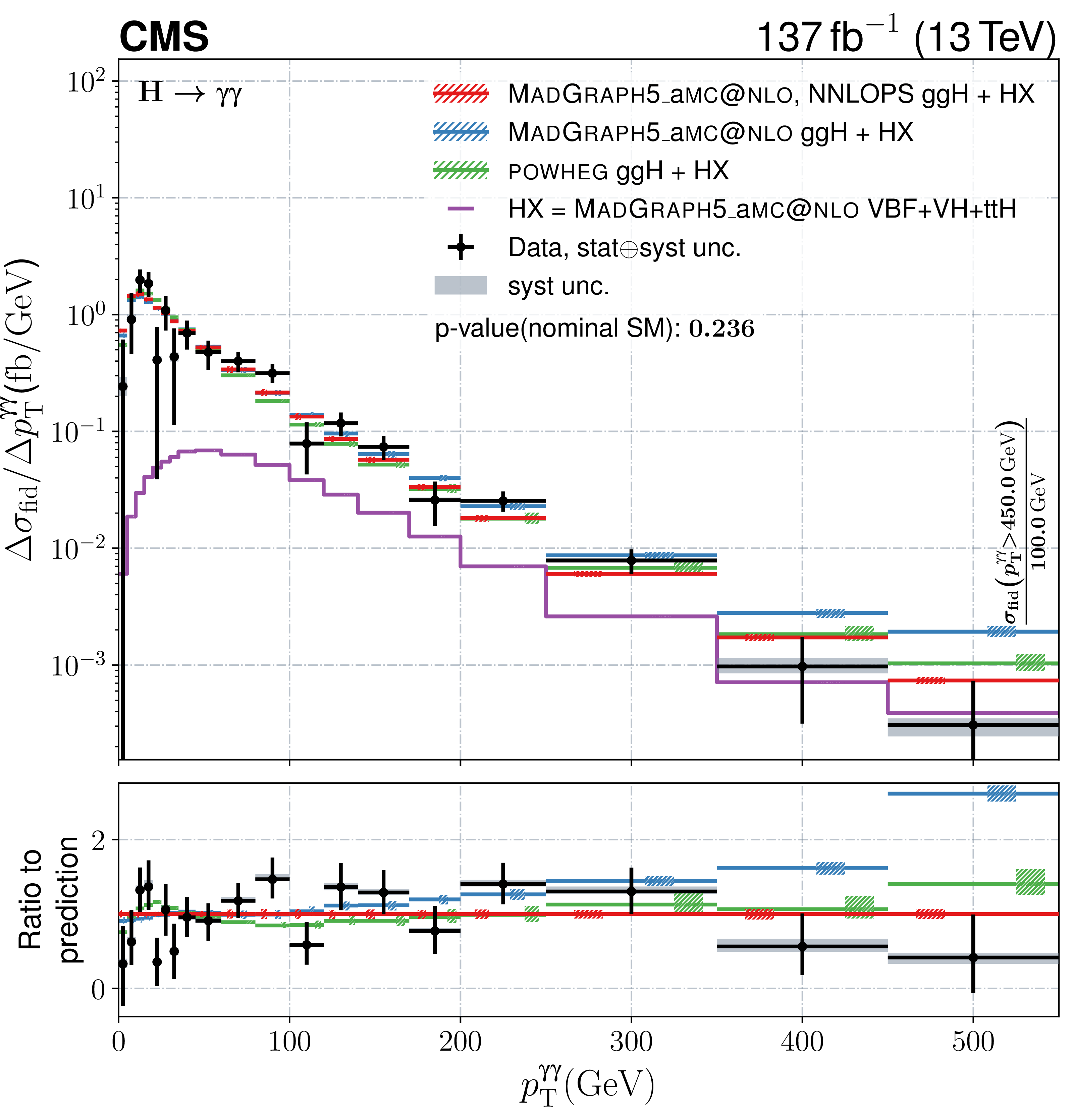
Figure 10-a:
Differential fiducial cross sections for $ p_{\mathrm{T}}^{\gamma\gamma} $. The observed differential fiducial cross section values are shown as black points with the vertical error bars showing the full uncertainty, the horizontal error bars show the width of the respective bin. The grey shaded areas visualize the systematic component of the uncertainty. The coloured lines denote the predictions from different setups of the event generator. All of them have the HX=VBF+VH+ttH component from MADGRAPH5_aMC@NLO in common, which is displayed in violet without uncertainties. The red lines show the sum of HX and the ggH component from MADGRAPH5_aMC@NLO reweighted to match the NNLOPS prediction. For the blue lines no NNLOPS reweighting is applied and the green lines take the prediction for the ggH production mode from POWHEG. The hatched areas show the uncertainties in theoretical predictions on both the $ \mathrm{g}\mathrm{g}\mathrm{F} $ and HX components. Only effects coming from varying the set of PDF replicas, the $ \alpha_\mathrm{S} $ value, and the renormalization and factorization scales that impact the shape are taken into account here, the total cross section is kept constant at the value from Ref. [15]. The given $ p $-values are calculated for the nominal SM prediction and the bottom panes show the ratio to the same prediction. If the last particle-level bin expands to infinity is explicitly marked on the plot together with the normalization of this bin. |
png pdf |
Figure 10-b:
Differential fiducial cross sections for $ n_{\text{jets}} $. The observed differential fiducial cross section values are shown as black points with the vertical error bars showing the full uncertainty, the horizontal error bars show the width of the respective bin. The grey shaded areas visualize the systematic component of the uncertainty. The coloured lines denote the predictions from different setups of the event generator. All of them have the HX=VBF+VH+ttH component from MADGRAPH5_aMC@NLO in common, which is displayed in violet without uncertainties. The red lines show the sum of HX and the ggH component from MADGRAPH5_aMC@NLO reweighted to match the NNLOPS prediction. For the blue lines no NNLOPS reweighting is applied and the green lines take the prediction for the ggH production mode from POWHEG. The hatched areas show the uncertainties in theoretical predictions on both the $ \mathrm{g}\mathrm{g}\mathrm{F} $ and HX components. Only effects coming from varying the set of PDF replicas, the $ \alpha_\mathrm{S} $ value, and the renormalization and factorization scales that impact the shape are taken into account here, the total cross section is kept constant at the value from Ref. [15]. The given $ p $-values are calculated for the nominal SM prediction and the bottom panes show the ratio to the same prediction. If the last particle-level bin expands to infinity is explicitly marked on the plot together with the normalization of this bin. |
png pdf |
Figure 10-c:
Differential fiducial cross sections for $ |y^{\gamma\gamma}| $. The observed differential fiducial cross section values are shown as black points with the vertical error bars showing the full uncertainty, the horizontal error bars show the width of the respective bin. The grey shaded areas visualize the systematic component of the uncertainty. The coloured lines denote the predictions from different setups of the event generator. All of them have the HX=VBF+VH+ttH component from MADGRAPH5_aMC@NLO in common, which is displayed in violet without uncertainties. The red lines show the sum of HX and the ggH component from MADGRAPH5_aMC@NLO reweighted to match the NNLOPS prediction. For the blue lines no NNLOPS reweighting is applied and the green lines take the prediction for the ggH production mode from POWHEG. The hatched areas show the uncertainties in theoretical predictions on both the $ \mathrm{g}\mathrm{g}\mathrm{F} $ and HX components. Only effects coming from varying the set of PDF replicas, the $ \alpha_\mathrm{S} $ value, and the renormalization and factorization scales that impact the shape are taken into account here, the total cross section is kept constant at the value from Ref. [15]. The given $ p $-values are calculated for the nominal SM prediction and the bottom panes show the ratio to the same prediction. If the last particle-level bin expands to infinity is explicitly marked on the plot together with the normalization of this bin. |
png pdf |
Figure 10-d:
Differential fiducial cross sections for $ |\cos\theta^{\ast}| $. The observed differential fiducial cross section values are shown as black points with the vertical error bars showing the full uncertainty, the horizontal error bars show the width of the respective bin. The grey shaded areas visualize the systematic component of the uncertainty. The coloured lines denote the predictions from different setups of the event generator. All of them have the HX=VBF+VH+ttH component from MADGRAPH5_aMC@NLO in common, which is displayed in violet without uncertainties. The red lines show the sum of HX and the ggH component from MADGRAPH5_aMC@NLO reweighted to match the NNLOPS prediction. For the blue lines no NNLOPS reweighting is applied and the green lines take the prediction for the ggH production mode from POWHEG. The hatched areas show the uncertainties in theoretical predictions on both the $ \mathrm{g}\mathrm{g}\mathrm{F} $ and HX components. Only effects coming from varying the set of PDF replicas, the $ \alpha_\mathrm{S} $ value, and the renormalization and factorization scales that impact the shape are taken into account here, the total cross section is kept constant at the value from Ref. [15]. The given $ p $-values are calculated for the nominal SM prediction and the bottom panes show the ratio to the same prediction. If the last particle-level bin expands to infinity is explicitly marked on the plot together with the normalization of this bin. |
png pdf |
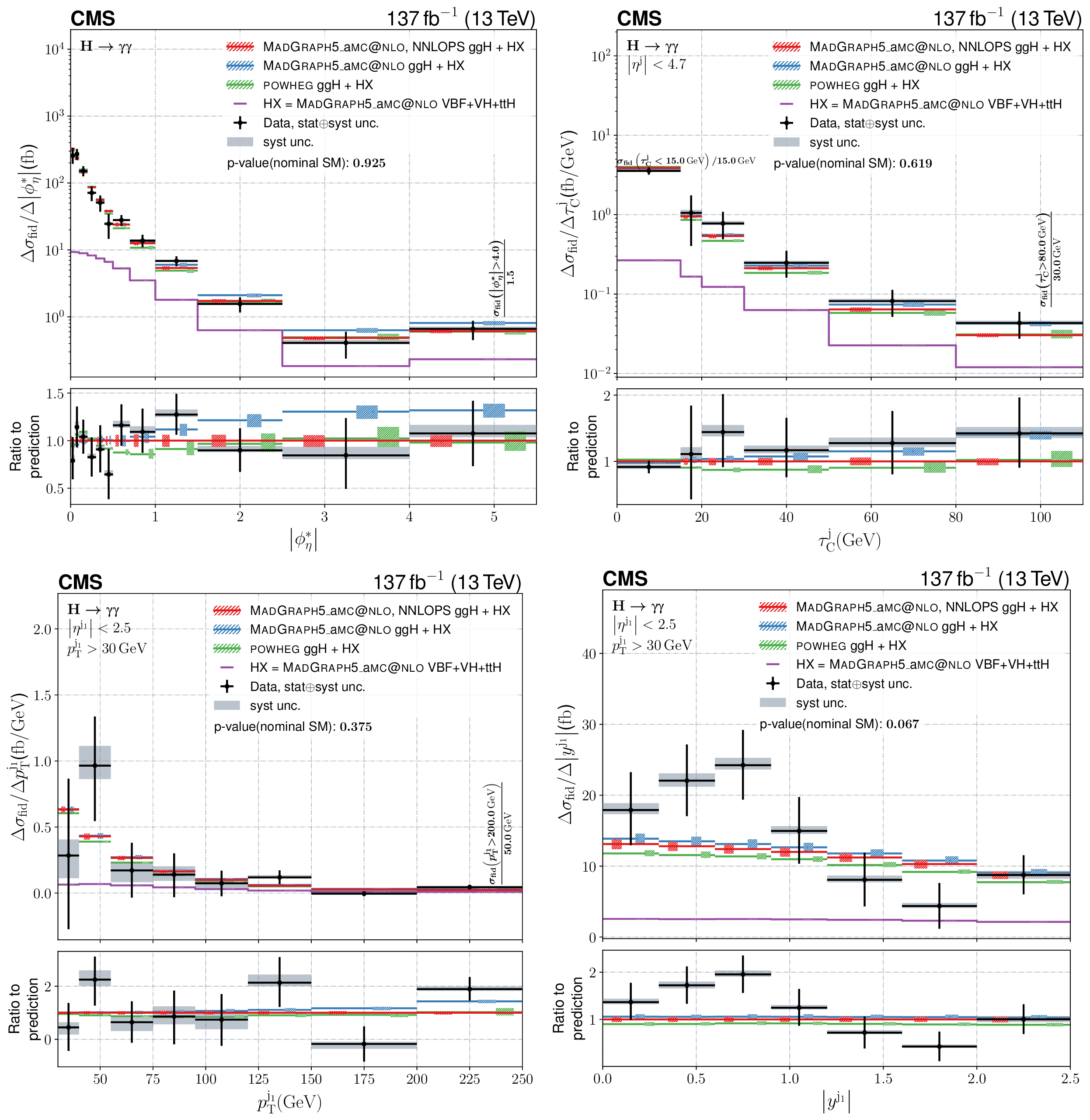
Figure 11:
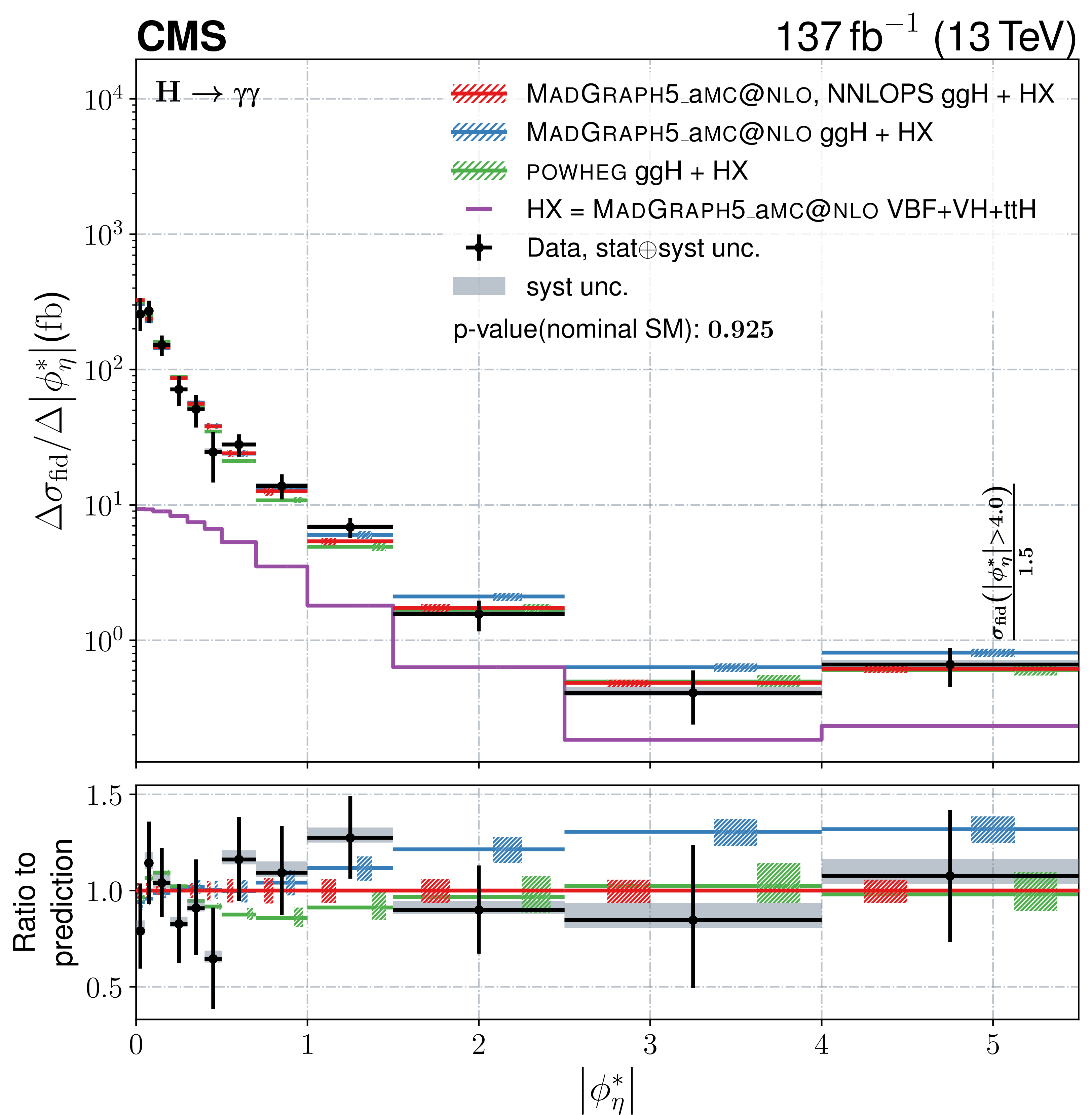
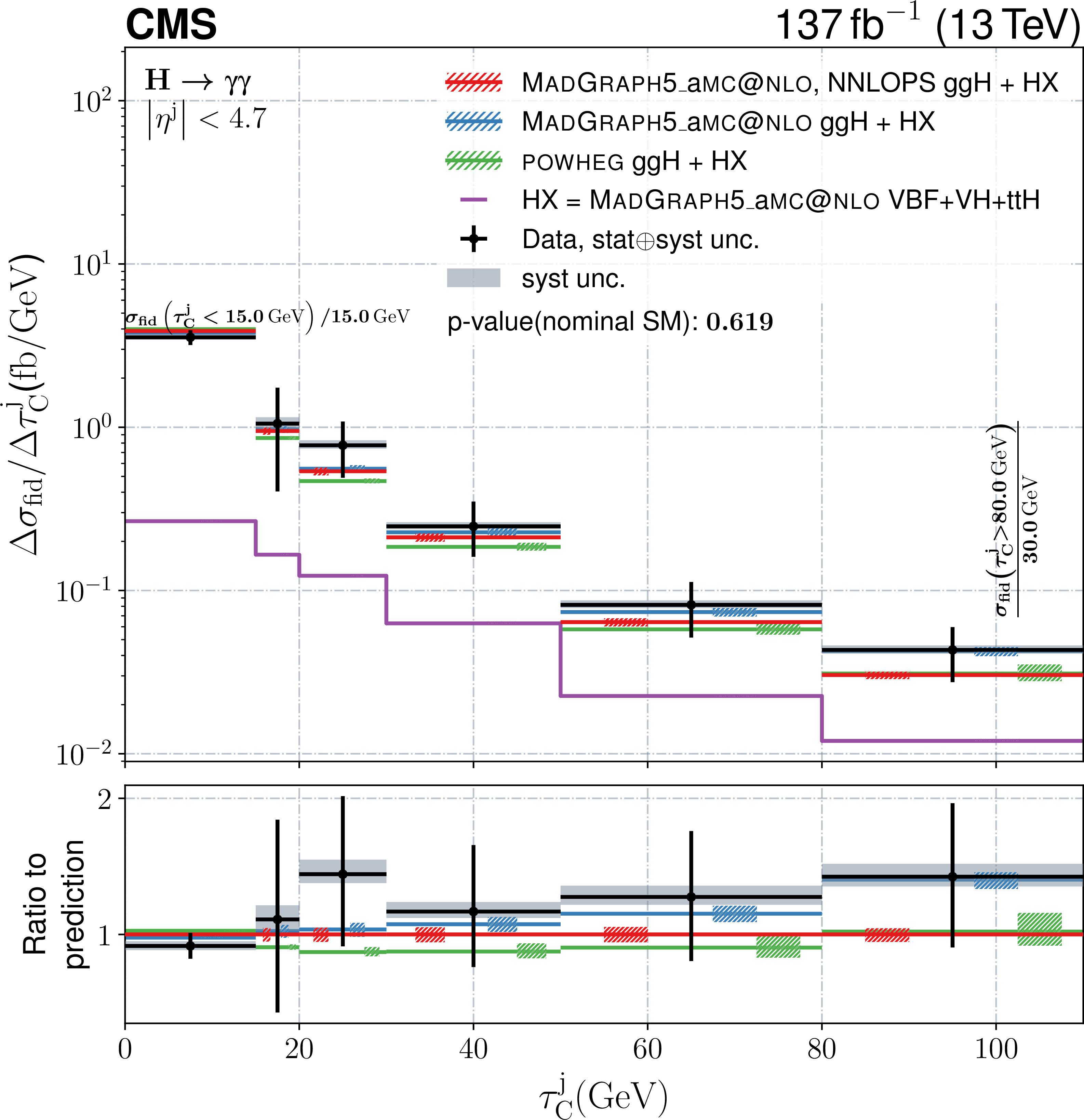
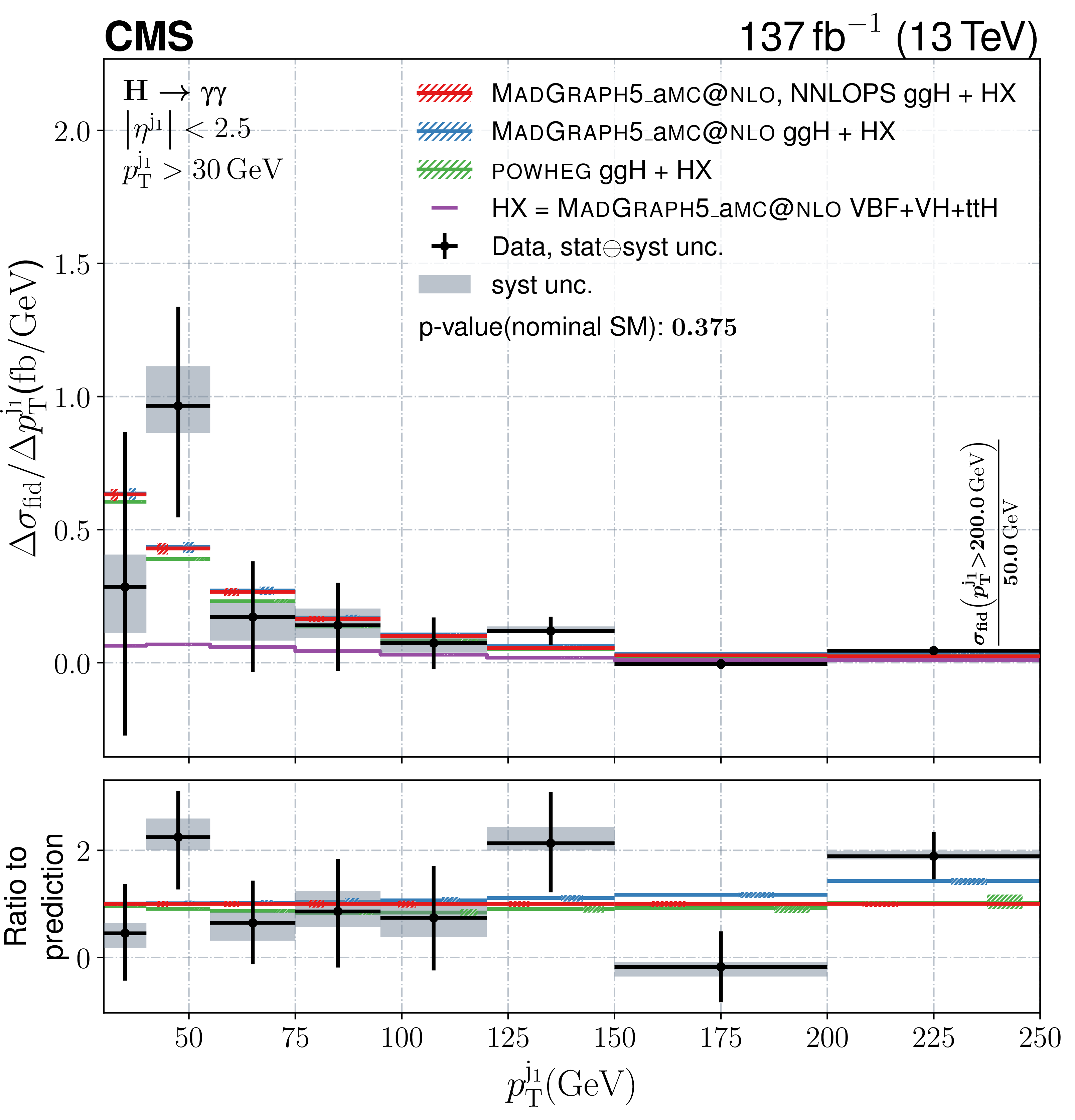
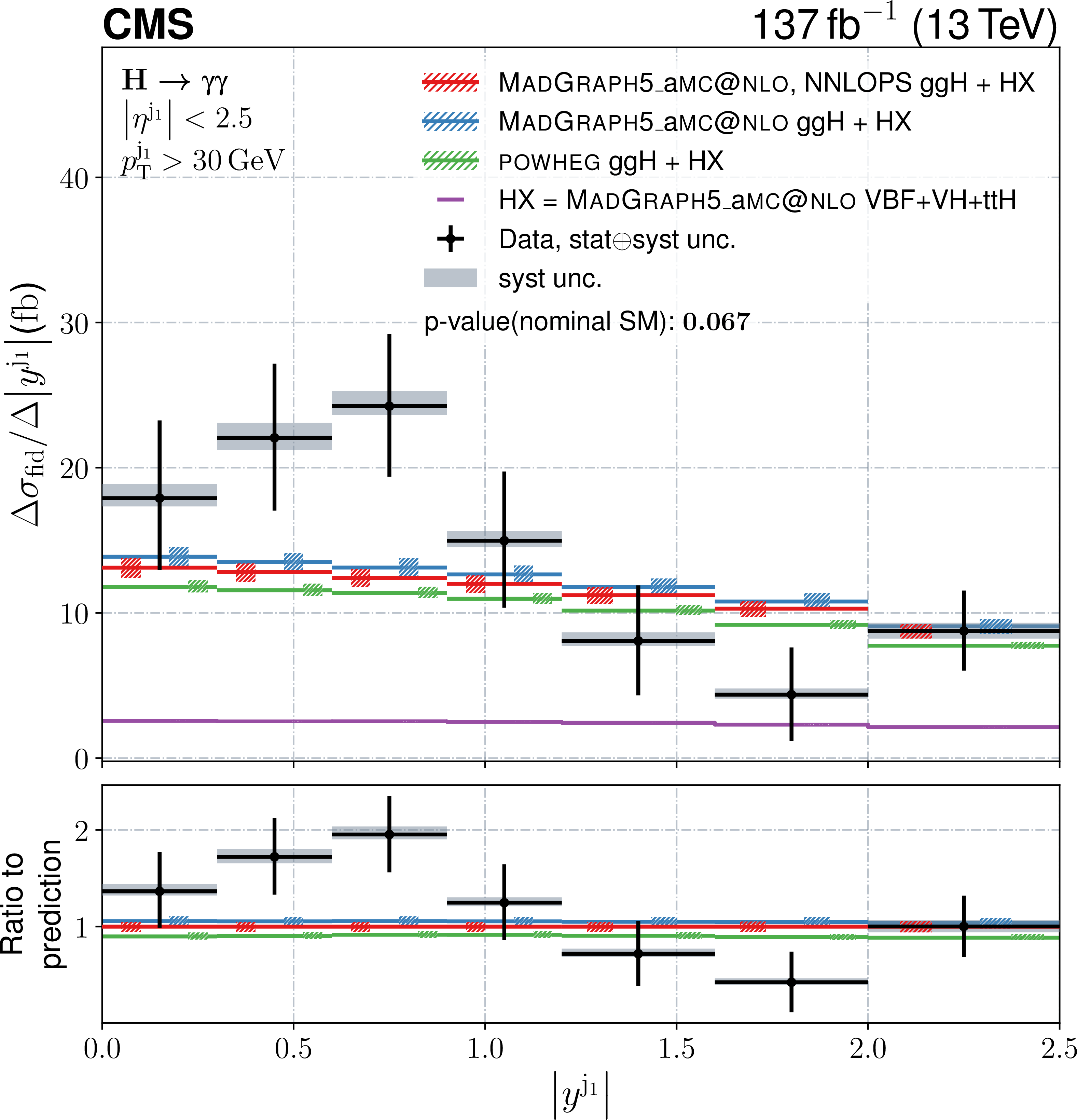
Differential fiducial cross section for $ |\phi_{\eta}^{\ast}| $, $ \tau_{\mathrm{C}}^{\mathrm{j}} $, $ p_{\mathrm{T}}^{\mathrm{j}_{1}} $, and $ |y^{\mathrm{j}_{1}}| $. The content of each plot is described in the caption of Fig. 10. The first bin in the upper right plot shows the cross section for $ \tau_{\mathrm{C}}^{\mathrm{j}} < $ 15 GeV. This is marked in the plot together with the corresponding normalization. |
png pdf |
Figure 11-a:
Differential fiducial cross section for $ |\phi_{\eta}^{\ast}| $. The content of each plot is described in the caption of Fig. 10. The first bin in the upper right plot shows the cross section for $ \tau_{\mathrm{C}}^{\mathrm{j}} < $ 15 GeV. This is marked in the plot together with the corresponding normalization. |
png pdf |
Figure 11-b:
Differential fiducial cross section for $ \tau_{\mathrm{C}}^{\mathrm{j}} $. The content of each plot is described in the caption of Fig. 10. The first bin in the upper right plot shows the cross section for $ \tau_{\mathrm{C}}^{\mathrm{j}} < $ 15 GeV. This is marked in the plot together with the corresponding normalization. |
png pdf |
Figure 11-c:
Differential fiducial cross section for $ p_{\mathrm{T}}^{\mathrm{j}_{1}} $. The content of each plot is described in the caption of Fig. 10. The first bin in the upper right plot shows the cross section for $ \tau_{\mathrm{C}}^{\mathrm{j}} < $ 15 GeV. This is marked in the plot together with the corresponding normalization. |
png pdf |
Figure 11-d:
Differential fiducial cross section for $ |y^{\mathrm{j}_{1}}| $. The content of each plot is described in the caption of Fig. 10. The first bin in the upper right plot shows the cross section for $ \tau_{\mathrm{C}}^{\mathrm{j}} < $ 15 GeV. This is marked in the plot together with the corresponding normalization. |

png pdf |
Figure 12:
Differential fiducial cross sections for $ |\Delta y_{\gamma\gamma,\mathrm{j}_{1}}| $, $ |\Delta\phi_{\gamma\gamma,\mathrm{j}_{1}}| $, $ p_{\mathrm{T}}^{\mathrm{j}_{2}} $, and $ |y^{\mathrm{j}_{2}}| $. The content of each plot is described in the caption of Fig. 10. |
png pdf |
Figure 12-a:
Differential fiducial cross sections for $ |\Delta y_{\gamma\gamma,\mathrm{j}_{1}}| $. The content of each plot is described in the caption of Fig. 10. |
png pdf |
Figure 12-b:
Differential fiducial cross sections for $ |\Delta\phi_{\gamma\gamma,\mathrm{j}_{1}}| $. The content of each plot is described in the caption of Fig. 10. |

png pdf |
Figure 12-c:
Differential fiducial cross sections for $ p_{\mathrm{T}}^{\mathrm{j}_{2}} $. The content of each plot is described in the caption of Fig. 10. |
png pdf |
Figure 12-d:
Differential fiducial cross sections for $ |y^{\mathrm{j}_{2}}| $. The content of each plot is described in the caption of Fig. 10. |
png pdf |
Figure 13:
Differential fiducial cross sections for $ |\Delta\phi_{\gamma\gamma,\mathrm{j}_{1}\mathrm{j}_{2}}| $, $ |\Delta\phi_{\mathrm{j}_{1},\mathrm{j}_{2}}| $, $ |\overline{\eta}_{\mathrm{j}_{1}\mathrm{j}_{2}}-\eta_{\gamma\gamma}| $, and $ m_{\mathrm{jj}} $. The content of each plot is described in the caption of Fig. 10. |
png pdf |
Figure 13-a:
Differential fiducial cross sections for $ |\Delta\phi_{\gamma\gamma,\mathrm{j}_{1}\mathrm{j}_{2}}| $. The content of each plot is described in the caption of Fig. 10. |
png pdf |
Figure 13-b:
Differential fiducial cross sections for $ |\Delta\phi_{\mathrm{j}_{1},\mathrm{j}_{2}}| $,. The content of each plot is described in the caption of Fig. 10. |

png pdf |
Figure 13-c:
Differential fiducial cross sections for $ |\overline{\eta}_{\mathrm{j}_{1}\mathrm{j}_{2}}-\eta_{\gamma\gamma}| $. The content of each plot is described in the caption of Fig. 10. |
png pdf |
Figure 13-d:
Differential fiducial cross sections for $ m_{\mathrm{jj}} $. The content of each plot is described in the caption of Fig. 10. |
png pdf |
Figure 14:
Differential fiducial cross sections for $ |\Delta\eta_{\mathrm{j}_{1}\mathrm{j}_{2}}| $, $ n_{\text{leptons}} $, $ n_{\mathrm{b}\text{jets}} $, and $ p_{\mathrm{T}}^\text{miss} $. The content of each plot is described in the caption of Fig. 10. |
png pdf |
Figure 14-a:
Differential fiducial cross sections for $ |\Delta\eta_{\mathrm{j}_{1}\mathrm{j}_{2}}| $. The content of each plot is described in the caption of Fig. 10. |
png pdf |
Figure 14-b:
Differential fiducial cross sections for $ n_{\text{leptons}} $. The content of each plot is described in the caption of Fig. 10. |
png pdf |
Figure 14-c:
Differential fiducial cross sections for $ n_{\mathrm{b}\text{jets}} $. The content of each plot is described in the caption of Fig. 10. |
png pdf |
Figure 14-d:
Differential fiducial cross sections for $ p_{\mathrm{T}}^\text{miss} $. The content of each plot is described in the caption of Fig. 10. |
png pdf |
Figure 15:
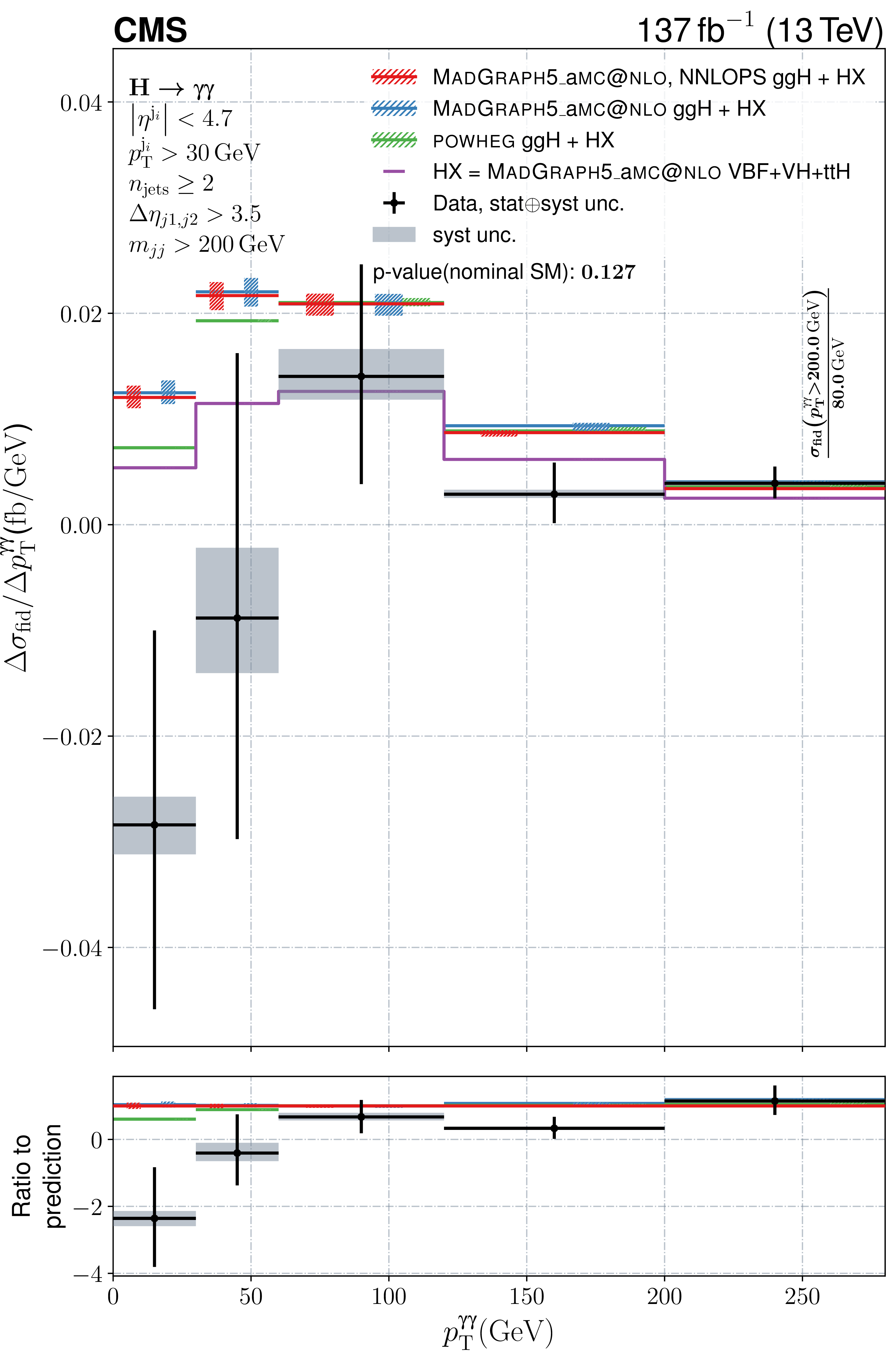
Differential fiducial cross sections for $ p_{\mathrm{T}}^{\mathrm{j}_{2}} $, $ |\Delta\phi_{\gamma\gamma,\mathrm{j}_{1}\mathrm{j}_{2}}| $, $ |\Delta\phi_{\mathrm{j}_{1},\mathrm{j}_{2}}| $, and $ p_{\mathrm{T}}^{\gamma\gamma} $ in the VBF-enriched phase space region. The content of each plot is described in the caption of Fig. 10. |
png pdf |
Figure 15-a:
Differential fiducial cross sections for $ p_{\mathrm{T}}^{\mathrm{j}_{2}} $ in the VBF-enriched phase space region. The content of each plot is described in the caption of Fig. 10. |
png pdf |
Figure 15-b:
Differential fiducial cross sections for $ |\Delta\phi_{\gamma\gamma,\mathrm{j}_{1}\mathrm{j}_{2}}| $ in the VBF-enriched phase space region. The content of each plot is described in the caption of Fig. 10. |
png pdf |
Figure 15-c:
Differential fiducial cross sections for $ |\Delta\phi_{\mathrm{j}_{1},\mathrm{j}_{2}}| $ in the VBF-enriched phase space region. The content of each plot is described in the caption of Fig. 10. |
png pdf |
Figure 15-d:
Differential fiducial cross sections for $ p_{\mathrm{T}}^{\gamma\gamma} $ in the VBF-enriched phase space region. The content of each plot is described in the caption of Fig. 10. |

png pdf |
Figure 16:
Double-differential fiducial cross section measured in bins of $ p_{\mathrm{T}}^{\gamma\gamma} $ and $ n_{\text{jets}} $. The content of this plot is described in the caption of Fig. 10. |
png pdf |
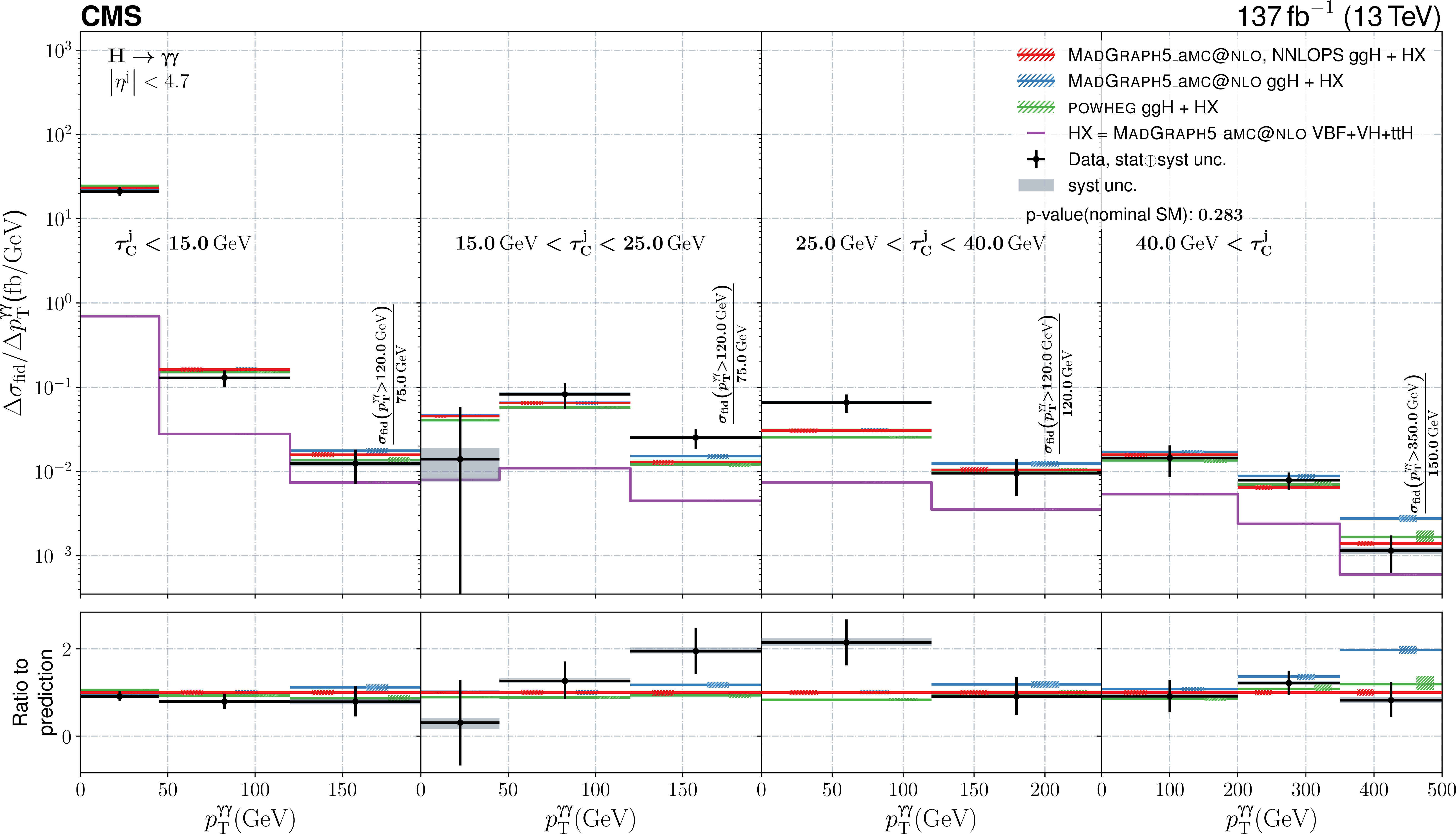
Figure 17:
Double-differential fiducial cross section measured in bins of $ p_{\mathrm{T}}^{\gamma\gamma} $ and $ \tau_{\mathrm{C}}^{\mathrm{j}} $. The content of this plot is described in the caption of Fig. 10. |
| Tables | |

png pdf |
Table 1:
Efficiencies of the photon identification MVA and $ \sigma_{m}^{\mathrm{D}} $ categories for events taken from the signal sample for all three years of data taking. The second row shows the efficiency of the photon identification MVA selection in the three $ \sigma_{m}^{\mathrm{D}} $ categories and for the full sample (Overall). The third row shows the efficiencies of the selections for the three $ \sigma_{m}^{\mathrm{D}} $ categories without the photon identification MVA selection applied. The forth row reports the effective width ($ \sigma_{\text{eff}} $) of the Higgs boson signal in each category. The four dominant Higgs boson production modes considered for this analysis are included in the sample and $ m_{\mathrm{H}}= $ 125 GeV is used. Only events satisfying the fiducial selection are included. |
png pdf |
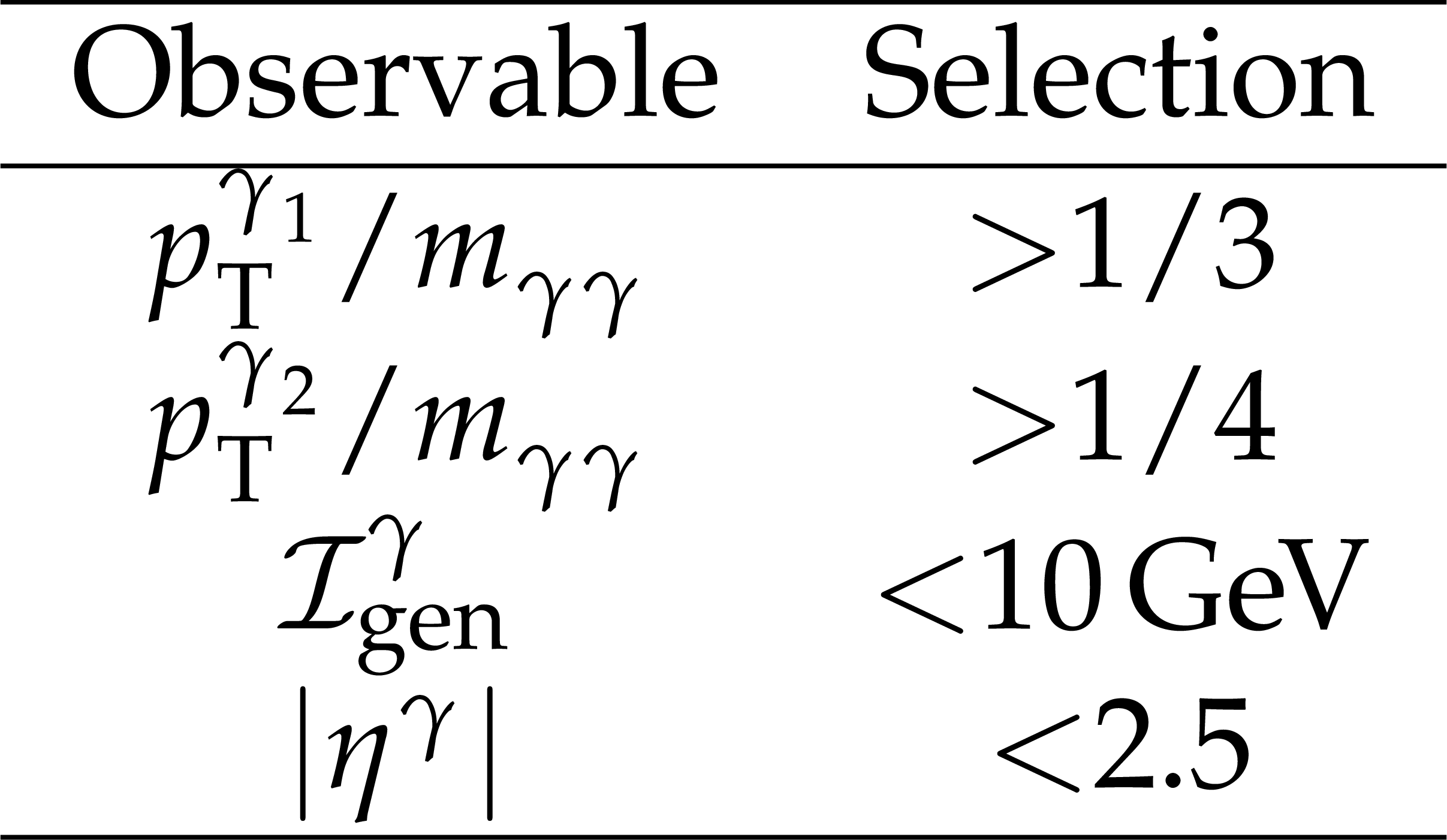
Table 2:
Definition of the fiducial phase space. The labels 1, 2 refer to the $ p_{\mathrm{T}} $-ordered leading and subleading photon in the diphoton system. The variable $ \mathcal{I}_{\text{gen}}^{\gamma} $ is defined as the sum of the energy of all stable hadrons produced in a cone of radius $ \Delta R= $ 0.3 around the photon. |
png pdf |
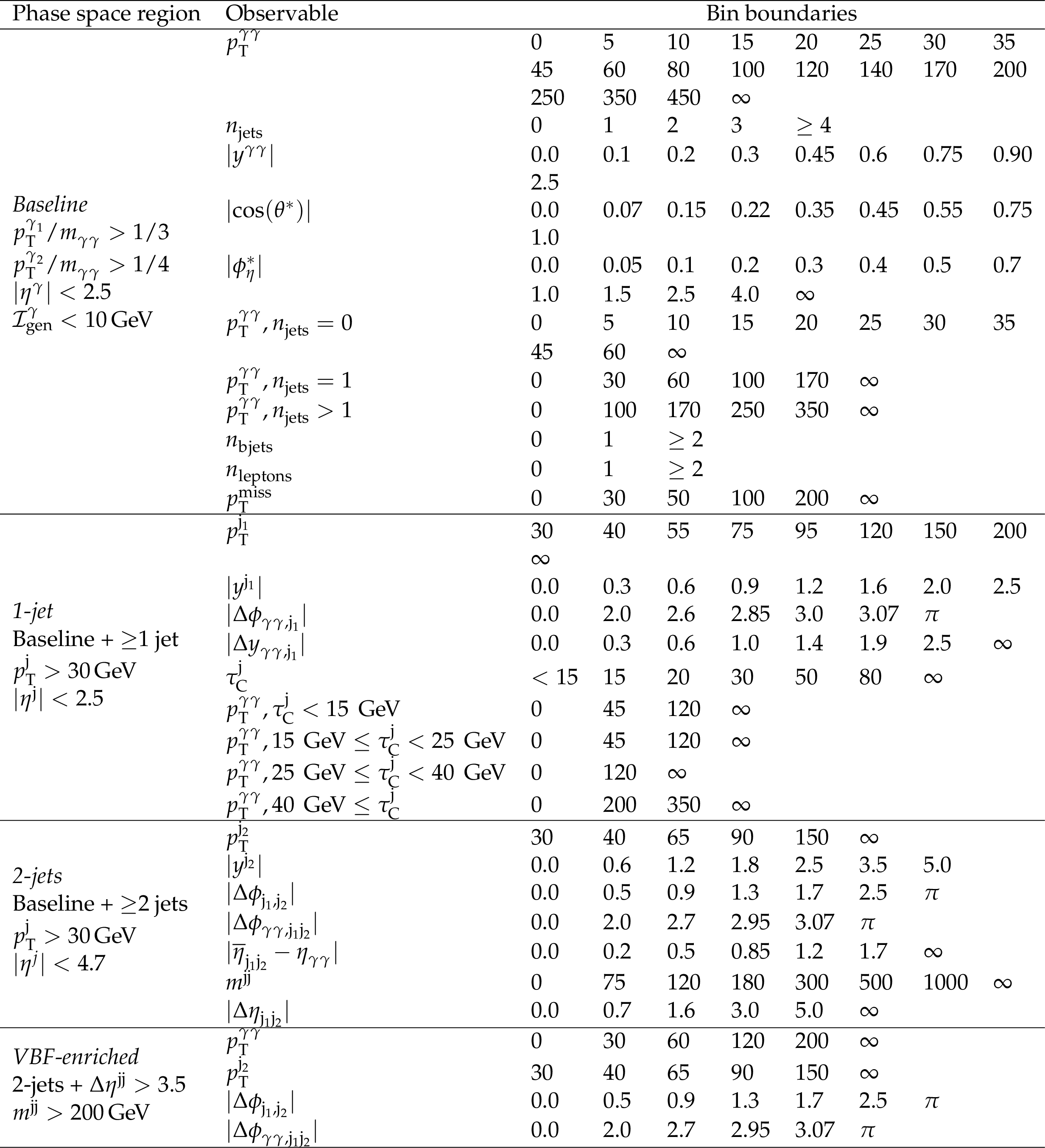
Table 3:
Binning per observable of interest. The first block of rows of the table shows the observables measured in the baseline fiducial phase space, the second one observables involving one additional jet, and the third one involving two or more additional jets. In the fourth block observables for the VBF-enriched phase space are shown. Energy, invariant mass and momentum are in GeV. |
png pdf |
Table 4:
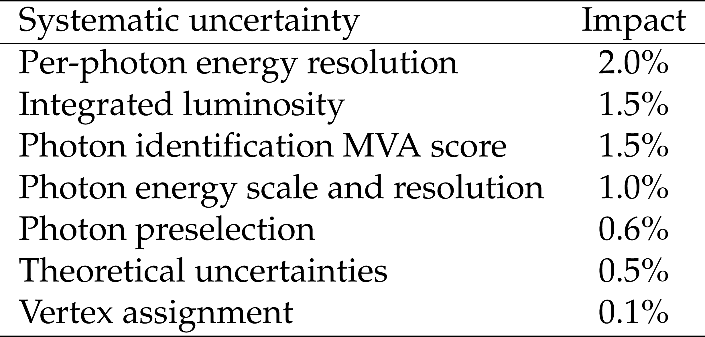
Breakdown of the systematic uncertainties in the inclusive fiducial cross-section measurament. The impacts on the measured inclusive fiducial $ \mathrm{H}\to\gamma\gamma $ cross section by varying the nuisance parameters for the dominating sources of systematic uncertainties by one standard deviation are given. The distinct contributions for systematic uncertainties that were split by category or year of data taking are added in quadrature for simplicity. Theoretical uncertainties summarizes the theoretical systematic uncertainties given above. |
| Summary |
| The measurement of the fiducial inclusive Higgs boson (H) production cross section with the $ \mathrm{H}\to\gamma\gamma $ decay mode has been presented. The fiducial phase space is defined by the ratio of the transverse momentum ($ p_{\mathrm{T}} $) of the leading (subleading) photon to diphoton invariant mass satisfying $ p_{\mathrm{T}}/m_{\gamma\gamma} > $ 1/3 (1/4), their pseudorapidity being within $ |\eta| < $ 2.5, and both photons being isolated. The production cross section for the Higgs boson decaying into two photons in the aforementioned phase space is measured to $ \sigma_{\text{fid}}=$ 73.4$_{-5.9}^{+6.1} $ fb, in agreement with the theoretical prediction from the standard model (SM) of 75.4 $ \pm $ 4.1 fb. Furthermore, the $ \mathrm{p}\mathrm{p}\to\mathrm{H}+\mathrm{X} $, $ \mathrm{H}\to\gamma\gamma $ cross section in the fiducial phase space has been measured as a function of observables of the diphoton system, as well as several others involving properties of the leading-$ p_{\mathrm{T}} $ and subleading-$ p_{\mathrm{T}} $ jets. Observables corresponding to the number of jets, leptons, and b-tagged jets are included as well. For the first time using the CMS detector, the cross section has been measured as a function of the rapidity weighted jet-$ p_{\mathrm{T}} $ ($ \tau_{\mathrm{C}}^{\mathrm{j}} $), using up to six additional jets in the event. The cross section as a function of a measure for the deviation from ``back-to-backness" $ |\phi_{\eta}^{\ast}| $ for the diphoton system has been measured for the first time using the $ \mathrm{H}\to\gamma\gamma $ channel. Two double-differential cross section measurements have been performed: one in bins of $ p_{\mathrm{T}} $ and the number of jets, the other in bins of $ p_{\mathrm{T}} $ and $ \tau_{\mathrm{C}}^{\mathrm{j}} $. A selected set of differential measurements has been performed in a dedicated phase space enriched with events compatible with vector boson fusion Higgs boson production. Finally, the production cross section has been measured in three fiducial phase spaces loosely targeting the vector boson and $ \mathrm{t} \overline{\mathrm{t}} $ associated production modes. Overall, the performed differential fiducial cross section measurements of the Higgs boson production in proton-proton collisions are found to be in agreement with the SM prediction within the uncertainties. |
| References | ||||
| 1 | ATLAS Collaboration | Observation of a new particle in the search for the standard model Higgs boson with the ATLAS detector at the LHC | PLB 716 (2012) 1 | 1207.7214 |
| 2 | CMS Collaboration | Observation of a new boson at a mass of 125 GeV with the CMS experiment at the LHC | PLB 716 (2012) 30 | CMS-HIG-12-028 1207.7235 |
| 3 | CMS Collaboration | Observation of a new boson with mass near 125 GeV in pp collisions at $ \sqrt{s} = $ 7 and 8 TeV | JHEP 06 (2013) 081 | CMS-HIG-12-036 1303.4571 |
| 4 | ATLAS and CMS Collaborations | Measurements of the Higgs boson production and decay rates and constraints on its couplings from a combined ATLAS and CMS analysis of the LHC pp collision data at $ \sqrt{s} = $ 7 and 8 TeV | JHEP 08 (2016) 045 | 1606.02266 |
| 5 | ATLAS Collaboration | Measurements of fiducial and differential cross sections for Higgs boson production in the diphoton decay channel at $ \sqrt{s}= $ 8 TeV with ATLAS | JHEP 09 (2014) 112 | 1407.4222 |
| 6 | CMS Collaboration | Measurement of differential cross sections for Higgs boson production in the diphoton decay channel in pp collisions at $ \sqrt{s}= $ 8 TeV | EPJC 76 (2016) 13 | CMS-HIG-14-016 1508.07819 |
| 7 | ATLAS Collaboration | Fiducial and differential cross sections of Higgs boson production measured in the four-lepton decay channel in pp collisions at $ \sqrt{s} = $ 8 TeV with the ATLAS detector | PLB 738 (2014) 234 | 1408.3226 |
| 8 | CMS Collaboration | Measurement of differential and integrated fiducial cross sections for Higgs boson production in the four-lepton decay channel in pp collisions at $ \sqrt{s}= $ 7 and 8 TeV | JHEP 04 (2016) 005 | CMS-HIG-14-028 1512.08377 |
| 9 | ATLAS Collaboration | Measurement of fiducial differential cross sections of gluon-fusion production of Higgs bosons decaying to $ \mathrm{W}\mathrm{W}^{\ast}\rightarrow\mathrm{e}\nu\mu\nu $ with the ATLAS detector at $ \sqrt{s}= $ 8 TeV | JHEP 08 (2016) 104 | 1604.02997 |
| 10 | CMS Collaboration | Measurement of the transverse momentum spectrum of the Higgs boson produced in pp collisions at $ \sqrt{s}= $ 8 TeV using $ \mathrm{H} \to \mathrm{W}\mathrm{W} $ decays | JHEP 03 (2017) 032 | CMS-HIG-15-010 1606.01522 |
| 11 | ATLAS Collaboration | Measurement of inclusive and differential cross sections in the $ \mathrm{H} \rightarrow \mathrm{Z}\mathrm{Z}^{\ast} \rightarrow 4\ell $ decay channel in pp collisions at $ \sqrt{s}= $ 13 TeV with the ATLAS detector | JHEP 10 (2017) 132 | 1708.02810 |
| 12 | CMS Collaboration | Measurements of properties of the Higgs boson decaying into the four-lepton final state in pp collisions at $ \sqrt{s}= $ 13 TeV | JHEP 11 (2017) 047 | CMS-HIG-16-041 1706.09936 |
| 13 | CMS Collaboration | Measurements of Higgs boson properties in the diphoton decay channel in proton-proton collisions at $ \sqrt{s} = $ 13 TeV | JHEP 11 (2018) 185 | CMS-HIG-16-040 1804.02716 |
| 14 | ATLAS Collaboration | Combined measurement of differential and total cross sections in the $ \mathrm{H} \rightarrow \gamma \gamma $ and the $ \mathrm{H} \rightarrow \mathrm{Z}\mathrm{Z}^{\ast} \rightarrow 4\ell $ decay channels at $ \sqrt{s} = $ 13 TeV with the ATLAS detector | PLB 786 (2018) 114 | 1805.10197 |
| 15 | LHC Higgs Cross Section Working Group | Handbook of LHC Higgs cross sections: 4. Deciphering the nature of the Higgs sector | CERN-2017-002-M | 1610.07922 |
| 16 | ATLAS Collaboration | Higgs boson production cross-section measurements and their EFT interpretation in the 4$ \ell $ decay channel at $ \sqrt{s}= $ 13 TeV with the ATLAS detector | EPJC 80 (2020) 957 | 2004.03447 |
| 17 | ATLAS Collaboration | Measurements of WH and ZH production in the $ \mathrm{H} \rightarrow \mathrm{b}\overline{\mathrm{b}} $ decay channel in pp collisions at 13 TeV with the ATLAS detector | EPJC 81 (2021) 178 | 2007.02873 |
| 18 | ATLAS Collaboration | Measurements of Higgs boson production cross-sections in the $ \mathrm{H}\to\tau^{+}\tau^{-} $ decay channel in pp collisions at $ \sqrt{s} = $ 13 TeV with the ATLAS detector | JHEP 08 (2022) 175 | 2201.08269 |
| 19 | ATLAS Collaboration | Measurements of Higgs boson production by gluon-gluon fusion and vector-boson fusion using $ \mathrm{H}\to \mathrm{W}\mathrm{W}^* \to \mathrm{e}\nu\mu\nu $ decays in pp collisions at $ \sqrt{s}= $ 13 TeV with the atlas detector | Submitted to PRD, 2022 | 2207.00338 |
| 20 | ATLAS Collaboration | A detailed map of Higgs boson interactions by the ATLAS experiment ten years after the discovery | Nature 607 (2022) 52 | 2207.00092 |
| 21 | ATLAS Collaboration | Measurement of the properties of Higgs boson production at $ \sqrt{s} = $ 13 TeV in the $ \mathrm{H}\to\gamma\gamma $ channel using 139 fb$^{-1}$ of pp collision data with the ATLAS experiment | Submitted to JHEP, 2022 | 2207.00348 |
| 22 | CMS Collaboration | Measurements of production cross sections of the Higgs boson in the four-lepton final state in proton-proton collisions at $ \sqrt{s} = $ 13 TeV | EPJC 81 (2021) 488 | CMS-HIG-19-001 2103.04956 |
| 23 | CMS Collaboration | Measurements of Higgs boson production cross sections and couplings in the diphoton decay channel at $ \sqrt{s} = $ 13 TeV | JHEP 07 (2021) 027 | CMS-HIG-19-015 2103.06956 |
| 24 | ATLAS Collaboration | Measurements of the Higgs boson inclusive and differential fiducial cross sections in the 4$ \ell $ decay channel at $ \sqrt{s} = $ 13 TeV | EPJC 80 (2020) 942 | 2004.03969 |
| 25 | ATLAS Collaboration | Measurements of the Higgs boson inclusive and differential fiducial cross-sections in the diphoton decay channel with pp collisions at $ \sqrt{s} = $ 13 TeV with the ATLAS detector | Submitted to JHEP, 2022 | 2202.00487 |
| 26 | CMS Collaboration | Measurement of the inclusive and differential Higgs boson production cross sections in the leptonic WW decay mode at $ \sqrt{s} = $ 13 TeV | JHEP 03 (2021) 003 | CMS-HIG-19-002 2007.01984 |
| 27 | CMS Collaboration | Measurement of the inclusive and differential Higgs boson production cross sections in the decay mode to a pair of $\tau$ leptons in pp collisions at $ \sqrt{s}= $ 13 TeV | PRL 128 (2022) 081805 | CMS-HIG-20-015 2107.11486 |
| 28 | CMS Collaboration | Measurement of inclusive and differential Higgs boson production cross sections in the diphoton decay channel in proton-proton collisions at $ \sqrt{s}= $ 13 TeV | JHEP 01 (2019) 183 | CMS-HIG-17-025 1807.03825 |
| 29 | CMS Collaboration | HEPData record for this analysis | link | |
| 30 | CMS Collaboration | The CMS trigger system | JINST 12 (2017) P01020 | CMS-TRG-12-001 1609.02366 |
| 31 | CMS Collaboration | The CMS experiment at the CERN LHC | JINST 3 (2008) S08004 | |
| 32 | CMS Collaboration | Precision luminosity measurement in proton-proton collisions at $ \sqrt{s} = $ 13 TeV in 2015 and 2016 at CMS | EPJC 81 (2021) 800 | CMS-LUM-17-003 2104.01927 |
| 33 | CMS Collaboration | CMS luminosity measurement for the 2017 data-taking period at $ \sqrt{s} = $ 13 TeV | CMS Physics Analysis Summary, 2018 CMS-PAS-LUM-17-004 |
CMS-PAS-LUM-17-004 |
| 34 | CMS Collaboration | CMS luminosity measurement for the 2018 data-taking period at $ \sqrt{s} = $ 13 TeV | CMS Physics Analysis Summary, 2019 CMS-PAS-LUM-18-002 |
CMS-PAS-LUM-18-002 |
| 35 | CMS Collaboration | Measurements of inclusive W and Z cross sections in pp collisions at $ \sqrt{s}= $ 7 TeV | JHEP 01 (2011) 080 | CMS-EWK-10-002 1012.2466 |
| 36 | CMS Collaboration | Electron and photon reconstruction and identification with the CMS experiment at the CERN LHC | JINST 16 (2021) P05014 | CMS-EGM-17-001 2012.06888 |
| 37 | J. Alwall et al. | The automated computation of tree-level and next-to-leading order differential cross sections, and their matching to parton shower simulations | JHEP 07 (2014) 079 | 1405.0301 |
| 38 | K. Hamilton, P. Nason, E. Re, and G. Zanderighi | NNLOPS simulation of Higgs boson production | JHEP 10 (2013) 222 | 1309.0017 |
| 39 | K. Hamilton, P. Nason, and G. Zanderighi | MINLO: Multi-scale improved NLO | JHEP 10 (2012) 155 | 1206.3572 |
| 40 | A. Kardos, P. Nason, and C. Oleari | Three-jet production in POWHEG | JHEP 04 (2014) 043 | 1402.4001 |
| 41 | T. Sjöstrand et al. | An introduction to PYTHIA 8.2 | Comput. Phys. Commun. 191 (2015) 159 | 1410.3012 |
| 42 | CMS Collaboration | Event generator tunes obtained from underlying event and multiparton scattering measurements | EPJC 76 (2016) 155 | CMS-GEN-14-001 1512.00815 |
| 43 | CMS Collaboration | Extraction and validation of a new set of CMS PYTHIA8 tunes from underlying-event measurements | EPJC 80 (2020) 4 | CMS-GEN-17-001 1903.12179 |
| 44 | Sherpa Collaboration | Event generation with Sherpa 2.2 | SciPost Phys. 7 (2019) 034 | 1905.09127 |
| 45 | CMS Collaboration | Particle-flow reconstruction and global event description with the CMS detector | JINST 12 (2017) P10003 | CMS-PRF-14-001 1706.04965 |
| 46 | CMS Collaboration | A measurement of the Higgs boson mass in the diphoton decay channel | PLB 805 (2020) 135425 | CMS-HIG-19-004 2002.06398 |
| 47 | CMS Collaboration | Measurements of $ \mathrm{t\bar{t}}\mathrm{H} $ production and the CP structure of the Yukawa interaction between the Higgs boson and top quark in the diphoton decay channel | PRL 125 (2020) 061801 | CMS-HIG-19-013 2003.10866 |
| 48 | CMS Collaboration | Search for nonresonant Higgs boson pair production in final states with two bottom quarks and two photons in proton-proton collisions at $ \sqrt{s} = $ 13 TeV | JHEP 03 (2021) 257 | CMS-HIG-19-018 2011.12373 |
| 49 | E. Spyromitros-Xioufis, G. Tsoumakas, W. Groves, and I. Vlahavas | Multi-target regression via input space expansion: treating targets as inputs | Mach. Learn. 104 (2016) 55 | 1211.6581 |
| 50 | R. Koenker and K. F. Hallock | Quantile regression | J. Econ. Perspect. 15 (2001) 143 | |
| 51 | F. Pedregosa et al. | Scikit-learn: Machine learning in Python | J. Mach. Learn. Res. 12 (2011) 2825 | 1201.0490 |
| 52 | T. Chen and C. Guestrin | XGBoost: A scalable tree boosting system | in 22nd ACM SIGKDD Int. Conf. Know. Discov. Data Min, 2016 Proc. 2 (2016) 785 |
|
| 53 | M. Cacciari, G. P. Salam, and G. Soyez | The anti-$ k_{\mathrm{T}} $ jet clustering algorithm | JHEP 04 (2008) 063 | 0802.1189 |
| 54 | M. Cacciari, G. P. Salam, and G. Soyez | FastJet user manual | EPJC 72 (2012) 1896 | 1111.6097 |
| 55 | E. Bols et al. | Jet flavour classification using DeepJet | JINST 15 (2020) P12012 | 2008.10519 |
| 56 | CMS Collaboration | Performance of missing transverse momentum reconstruction in proton-proton collisions at $ \sqrt{s} = $ 13 TeV using the CMS detector | JINST 14 (2019) P07004 | CMS-JME-17-001 1903.06078 |
| 57 | CMS Collaboration | Performance of the CMS muon detector and muon reconstruction with proton-proton collisions at $ \sqrt{s}= $ 13 TeV | JINST 13 (2018) P06015 | CMS-MUO-16-001 1804.04528 |
| 58 | J. C. Collins and D. E. Soper | Angular distribution of dileptons in high-energy hadron collisions | PRD 16 (1977) 2219 | |
| 59 | A. Banfi et al. | Optimisation of variables for studying dilepton transverse momentum distributions at hadron colliders | EPJC 71 (2011) 1600 | 1009.1580 |
| 60 | M. Boggia et al. | The HiggsTools handbook: a beginners guide to decoding the Higgs sector | JPG 45 (2018) 065004 | 1711.09875 |
| 61 | S. Gangal, M. Stahlhofen, and F. J. Tackmann | Rapidity-dependent jet vetoes | PRD 91 (2015) 054023 | 1412.4792 |
| 62 | D. L. Rainwater, R. Szalapski, and D. Zeppenfeld | Probing color singlet exchange in $ Z $ + two jet events at the CERN LHC | PRD 54 (1996) 6680 | hep-ph/9605444 |
| 63 | P. D. Dauncey, M. Kenzie, N. Wardle, and G. J. Davies | Handling uncertainties in background shapes: the discrete profiling method | JINST 10 (2015) P04015 | 1408.6865 |
| 64 | G. Cowan, K. Cranmer, E. Gross, and O. Vitells | Asymptotic formulae for likelihood-based tests of new physics | EPJC 71 (2011) 1554 | 1007.1727 |
| 65 | J. Butterworth et al. | PDF4LHC recommendations for LHC Run II | JPG 43 (2016) 023001 | 1510.03865 |
| 66 | NNPDF Collaboration | Parton distributions from high-precision collider data | EPJC 77 (2017) 663 | 1706.00428 |
| 67 | NNPDF Collaboration | Parton distributions for the LHC run II | JHEP 04 (2015) 040 | 1410.8849 |
| 68 | S. Carrazza et al. | An unbiased Hessian representation for Monte Carlo PDFs | EPJC 75 (2015) 369 | 1505.06736 |
| 69 | CMS Collaboration | Observation of the diphoton decay of the Higgs boson and measurement of its properties | EPJC 74 (2014) 3076 | CMS-HIG-13-001 1407.0558 |
| 70 | CMS Collaboration | Jet algorithms performance in 13 TeV data | CMS Physics Analysis Summary, 2017 CMS-PAS-JME-16-003 |
CMS-PAS-JME-16-003 |
| 71 | J. Campbell, M. Carena, R. Harnik, and Z. Liu | Interference in the $ \mathrm{g}\mathrm{g}\rightarrow \mathrm{h} \rightarrow \gamma\gamma $ on-shell rate and the Higgs boson total width | [Addendum: \DOI10.1103/PhysRevLett.119.01], 2017 PRL 119 (2017) 181801 |
1704.08259 |
| 72 | P. Nason | A new method for combining NLO QCD with shower monte carlo algorithms | JHEP 11 (2004) 040 | hep-ph/0409146 |
| 73 | S. Frixione, P. Nason, and C. Oleari | Matching NLO QCD computations with parton shower simulations: the \sc powheg method | JHEP 11 (2007) 070 | 0709.2092 |
| 74 | S. Alioli, P. Nason, C. Oleari, and E. Re | A general framework for implementing NLO calculations in shower Monte Carlo programs: the \sc powheg box | JHEP 06 (2010) 043 | 1002.2581 |
| 75 | E. Bagnaschi, G. Degrassi, P. Slavich, and A. Vicini | Higgs production via gluon fusion in the POWHEG approach in the SM and in the MSSM | JHEP 02 (2012) 088 | 1111.2854 |
|
|
Compact Muon Solenoid LHC, CERN |
|

|

|

|

|

|