

Compact Muon Solenoid
LHC, CERN
| CMS-HIG-19-018 ; CERN-EP-2020-222 | ||
| Search for nonresonant Higgs boson pair production in final states with two bottom quarks and two photons in proton-proton collisions at $\sqrt{s} = $ 13 TeV | ||
| CMS Collaboration | ||
| 24 November 2020 | ||
| JHEP 03 (2021) 257 | ||
| Abstract: A search for nonresonant production of Higgs boson pairs via gluon-gluon and vector boson fusion processes in final states with two bottom quarks and two photons is presented. The search uses data from proton-proton collisions at a center-of-mass energy of $\sqrt{s} = $ 13 TeV recorded with the CMS detector at the LHC, corresponding to an integrated luminosity of 137 fb$^{-1}$. No significant deviation from the background-only hypothesis is observed. An upper limit at 95% confidence level is set on the product of the Higgs boson pair production cross section and branching fraction into ${\mathrm{b\bar{b}}} \gamma\gamma$. The observed (expected) upper limit is determined to be 0.67 (0.45) fb, which corresponds to 7.7 (5.2) times the standard model prediction. This search has the highest sensitivity to Higgs boson pair production to date. Assuming all other Higgs boson couplings are equal to their values in the standard model, the observed coupling modifiers of the trilinear Higgs boson self-coupling ${\kappa_{\lambda}} $ and the coupling between a pair of Higgs bosons and a pair of vector bosons ${c_{2V}}$ are constrained within the ranges $-3.3 < {\kappa_{\lambda}} < 8.5$ and $-1.3 < c_{2V} < 3.5$ at 95% confidence level. Constraints on ${\kappa_{\lambda}} $ are also set by combining this analysis with a search for single Higgs bosons decaying to two photons, produced in association with top quark-antiquark pairs, and by performing a simultaneous fit of ${\kappa_{\lambda}} $ and the top quark Yukawa coupling modifier ${\kappa_{\mathrm{t}}} $. | ||
| Links: e-print arXiv:2011.12373 [hep-ex] (PDF) ; CDS record ; inSPIRE record ; CADI line (restricted) ; | ||
| Figures & Tables | Summary | Additional Figures | References | CMS Publications |
|---|
| Figures | |
png pdf |
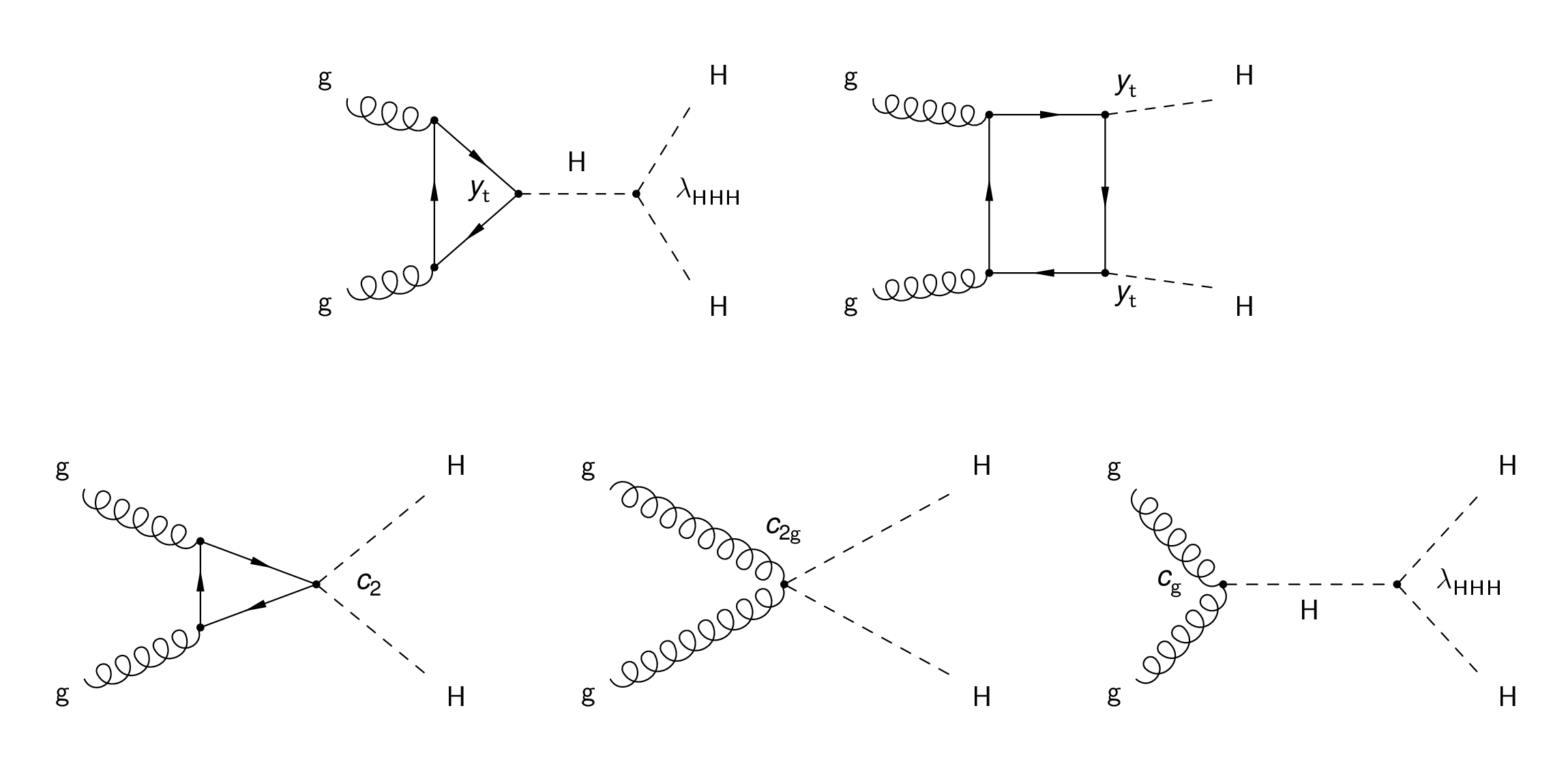
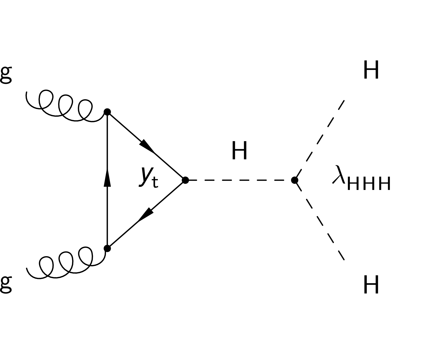
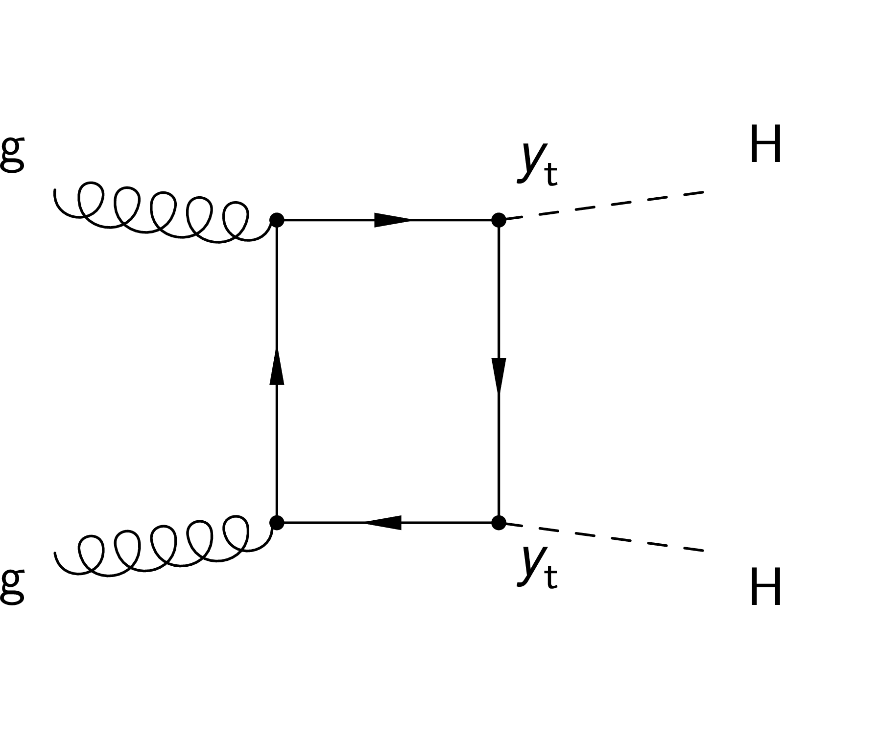
Figure 1:
Feynman diagrams of the processes contributing to the production of Higgs boson pairs via ggF at LO. The upper diagrams correspond to SM processes, involving the top Yukawa coupling ${y_{\mathrm{t}}}$ and the trilinear Higgs boson self-coupling ${\lambda _{\mathrm{H} \mathrm{H} \mathrm{H}}}$, respectively. The lower diagrams correspond to BSM processes: the diagram on the left involves the contact interaction of two Higgs bosons with two top quarks (${c_2}$), the middle diagram shows the quartic coupling between the Higgs bosons and two gluons (${c_{2\mathrm{g}}}$), and the diagram on the right describes the contact interactions between the Higgs boson and gluons (${c_{\mathrm{g}}}$). |
png pdf |
Figure 1-a:
Feynman diagram of a SM process contributing to the production of Higgs boson pairs via ggF at LO, involving the top Yukawa coupling ${y_{\mathrm{t}}}$ and the trilinear Higgs boson self-coupling ${\lambda _{\mathrm{H} \mathrm{H} \mathrm{H}}}$. |
png pdf |
Figure 1-b:
Feynman diagram of a SM process contributing to the production of Higgs boson pairs via ggF at LO, involving the top Yukawa coupling ${y_{\mathrm{t}}}$. |
png pdf |
Figure 1-c:
Feynman diagram of a BSM process contributing to the production of Higgs boson pairs via ggF at LO, involving the contact interaction of two Higgs bosons with two top quarks (${c_2}$). |
png pdf |
Figure 1-d:
Feynman diagram of a BSM process contributing to the production of Higgs boson pairs via ggF at LO, involving the quartic coupling between the Higgs boson and two gluons (${c_{2\mathrm{g}}}$). |
png pdf |
Figure 1-e:
Feynman diagram of a BSM process contributing to the production of Higgs boson pairs via ggF at LO, involving the contact interactions between the Higgs boson and gluons (${c_{\mathrm{g}}}$). |
png pdf |
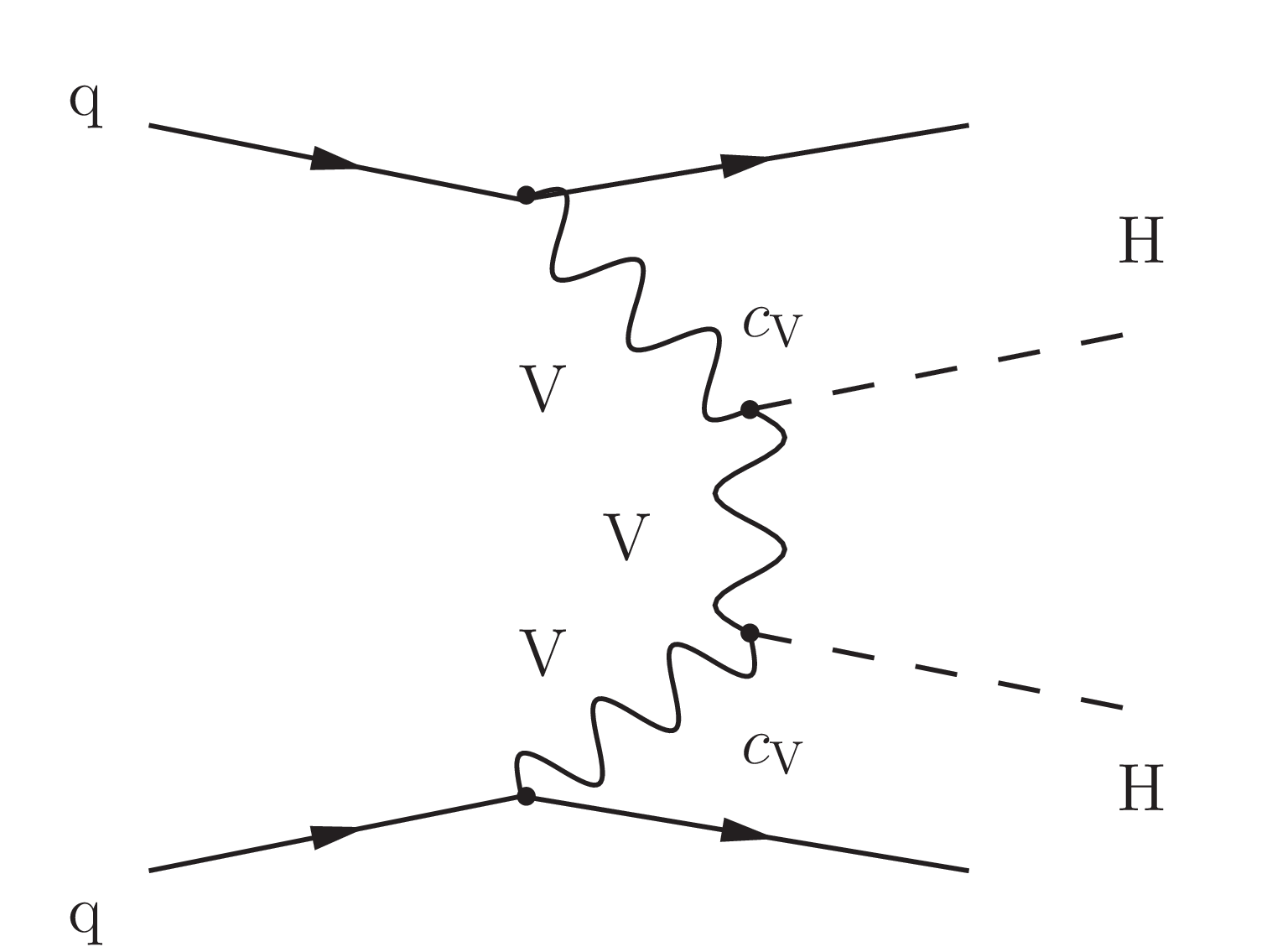
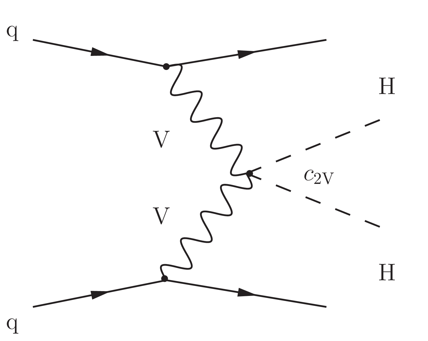
Figure 2:
Feynman diagrams that contribute to the production of Higgs boson pairs via VBF at LO. On the left the diagram involving the HHH vertex (${\lambda _{\mathrm{H} \mathrm{H} \mathrm{H}}}$), in the middle the diagram with two HVV vertices ($ {c_{\mathrm{V}}} $), and on the right the diagram with the HHVV vertex ($ {c_{2\mathrm{V}}} $). |
png pdf |
Figure 2-a:
Feynman diagram that contributes to the production of Higgs boson pairs via VBF at LO, involving the HHH vertex (${\lambda _{\mathrm{H} \mathrm{H} \mathrm{H}}}$). |
png pdf |
Figure 2-b:
Feynman diagram that contributes to the production of Higgs boson pairs via VBF at LO, involving two HVV vertices ($ {c_{\mathrm{V}}} $). |
png pdf |
Figure 2-c:
Feynman diagram that contributes to the production of Higgs boson pairs via VBF at LO, involving the HHVV vertex ($ {c_{2\mathrm{V}}} $). |

png pdf |
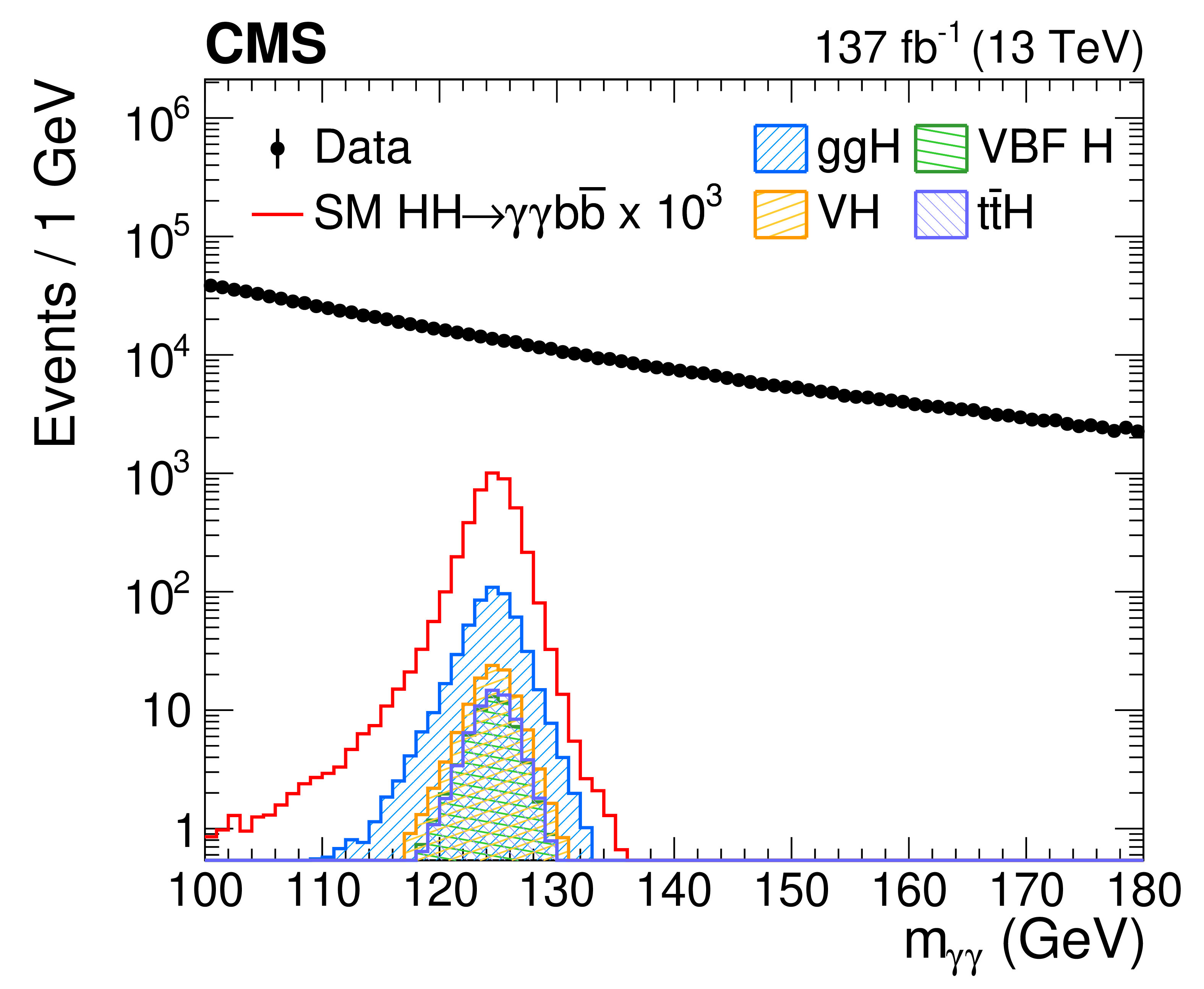
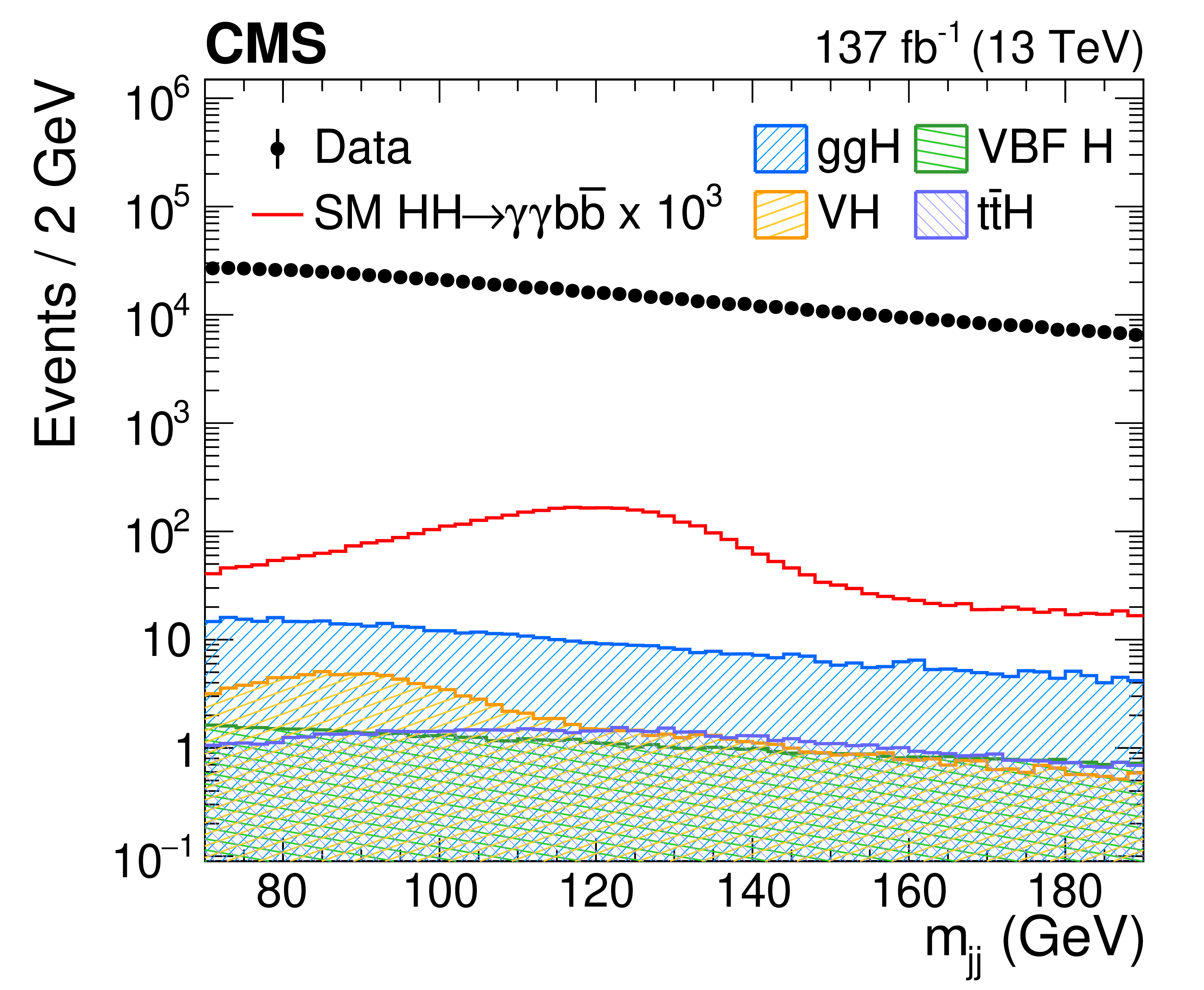
Figure 3:
The invariant mass distributions of the reconstructed Higgs boson candidates $ {m_{\gamma \gamma}} $ (left) and $ {m_\text {jj}}$ (right) in data and simulated events. Data, dominated by the $ \gamma \gamma $+jets and $ \gamma $+jets backgrounds, are compared to the SM ggF HH signal samples and single H samples (ttH, ggH, VBF H, VH) after imposing the selection criteria described in Section 5. The error bars on the data points indicate statistical uncertainties. The HH signal has been scaled by a factor of 10$^{3}$ for display purposes. |
png pdf |
Figure 3-a:
The invariant mass distribution of the reconstructed Higgs boson candidates $ {m_{\gamma \gamma}} $ in data and simulated events. Data, dominated by the $ \gamma \gamma $+jets and $ \gamma $+jets backgrounds, are compared to the SM ggF HH signal samples and single H samples (ttH, ggH, VBF H, VH) after imposing the selection criteria described in Section 5. The error bars on the data points indicate statistical uncertainties. The HH signal has been scaled by a factor of 10$^{3}$ for display purposes. |
png pdf |
Figure 3-b:
The invariant mass distribution of the reconstructed Higgs boson candidates $ {m_\text {jj}}$ in data and simulated events. Data, dominated by the $ \gamma \gamma $+jets and $ \gamma $+jets backgrounds, are compared to the SM ggF HH signal samples and single H samples (ttH, ggH, VBF H, VH) after imposing the selection criteria described in Section 5. The error bars on the data points indicate statistical uncertainties. The HH signal has been scaled by a factor of 10$^{3}$ for display purposes. |
png pdf |
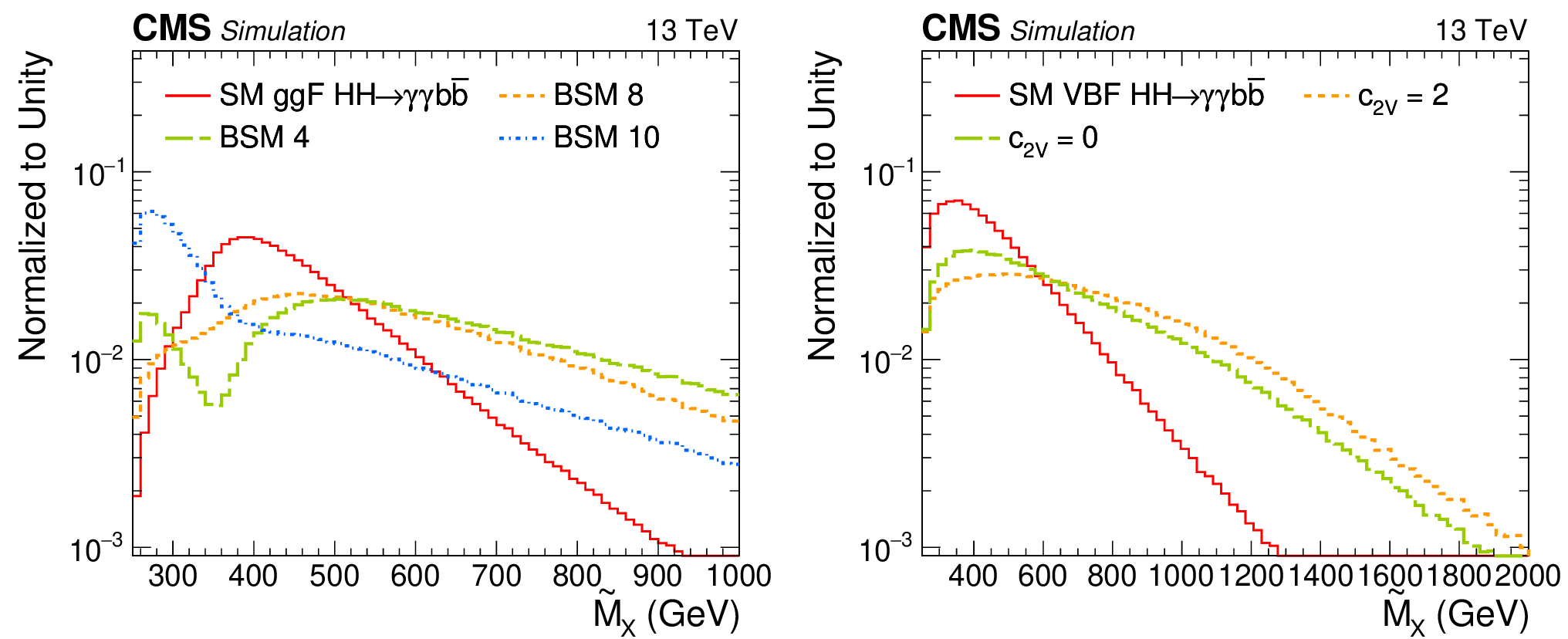
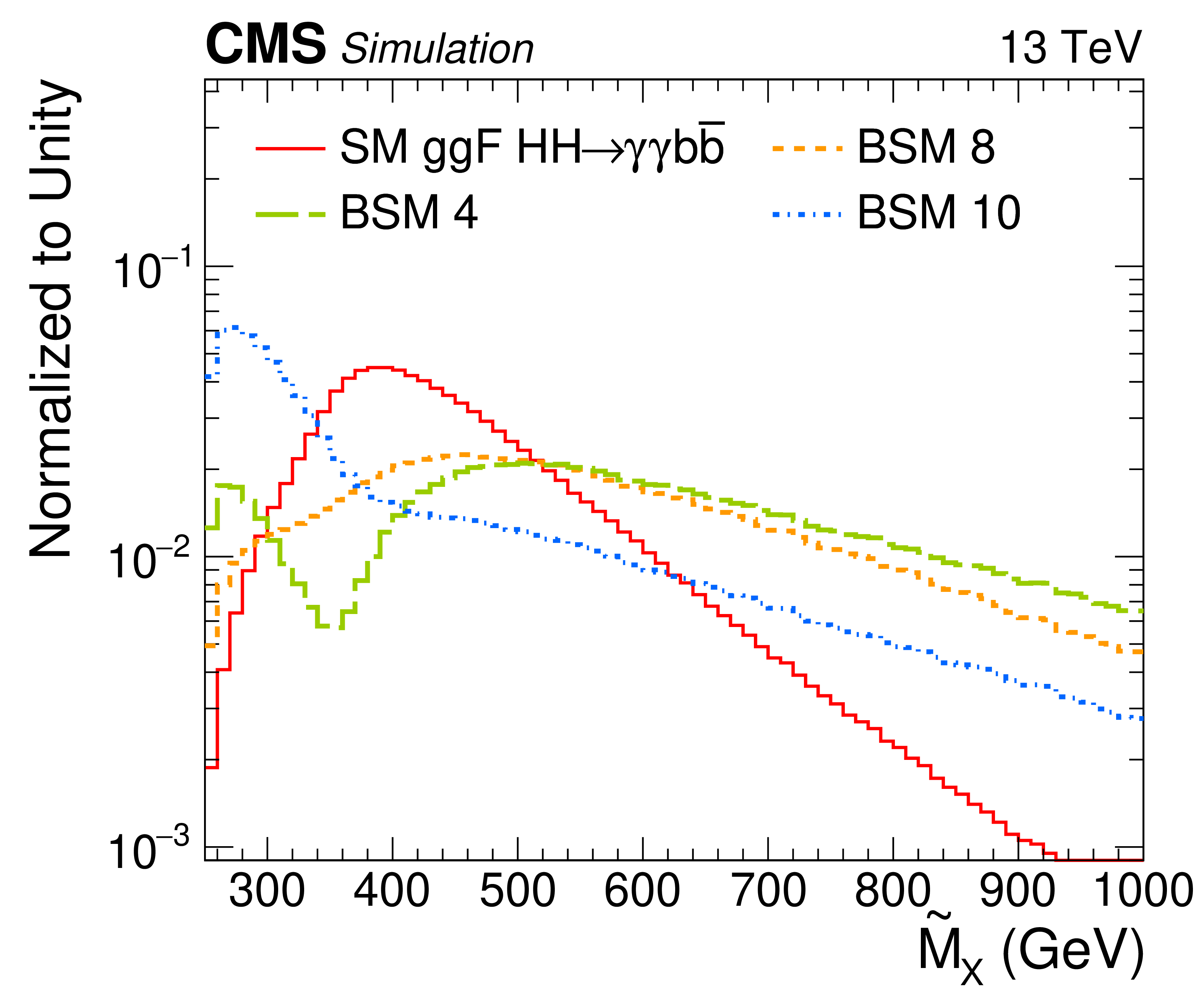
Figure 4:
Distributions of $ {\tilde{M}_{\mathrm {X}}} $. The SM ggF HH signal is compared with several BSM hypotheses listed in Table 1 (left), and the SM VBF HH signal is compared with two different anomalous values of $ {c_{2\mathrm{V}}} $ (right). All distributions are normalized to unity. |
png pdf |
Figure 4-a:
Distribution of $ {\tilde{M}_{\mathrm {X}}} $. The SM ggF HH signal is compared with several BSM hypotheses listed in Table. All distributions are normalized to unity. |

png pdf |
Figure 4-b:
Distribution of $ {\tilde{M}_{\mathrm {X}}} $. The SM VBF HH signal is compared with two different anomalous values of $ {c_{2\mathrm{V}}} $. All distributions are normalized to unity. |
png pdf |
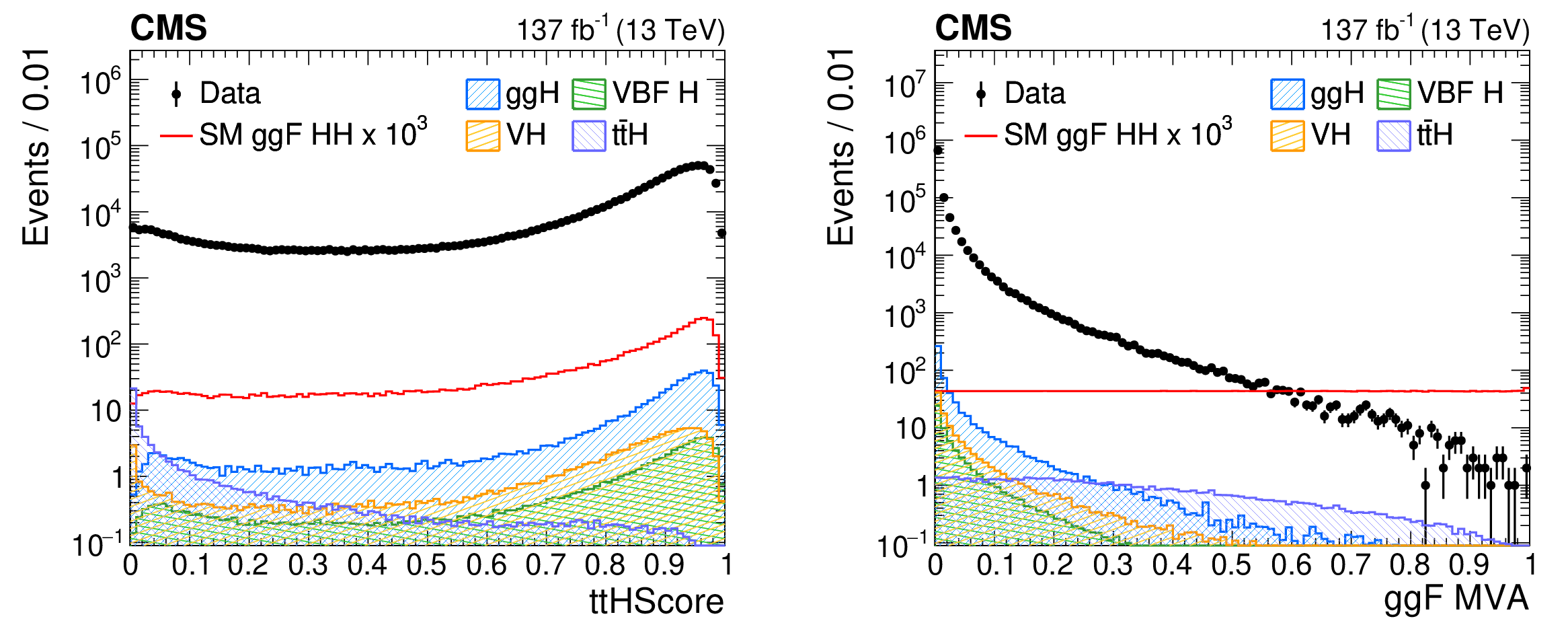
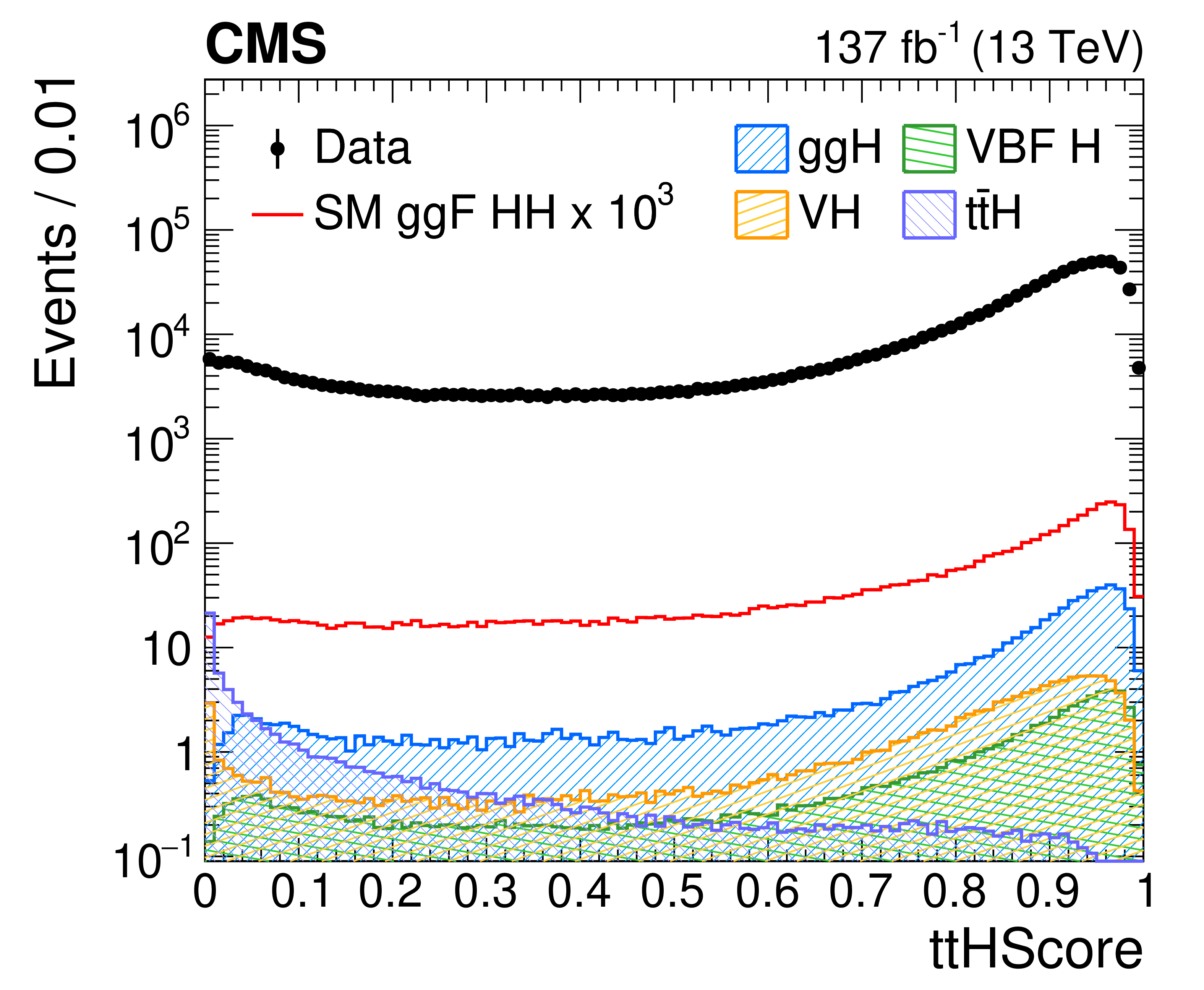
Figure 5:
The distribution of the ttHScore (left) and MVA output (right) in data and simulated events. Data, dominated by $ \gamma \gamma $+jets and $ \gamma $+jets background, are compared to the SM ggF HH signal samples and single H samples (ttH, ggH, VBF H, VH) after imposing the selection criteria described in Section 5. The error bars on the data points indicate statistical uncertainties. The HH signal has been scaled by a factor of 10$^{3}$ for display purposes. |
png pdf |
Figure 5-a:
The distribution of the ttHScore in data and simulated events. Data, dominated by $ \gamma \gamma $+jets and $ \gamma $+jets background, are compared to the SM ggF HH signal samples and single H samples (ttH, ggH, VBF H, VH) after imposing the selection criteria described in Section 5. The error bars on the data points indicate statistical uncertainties. The HH signal has been scaled by a factor of 10$^{3}$ for display purposes. |
png pdf |
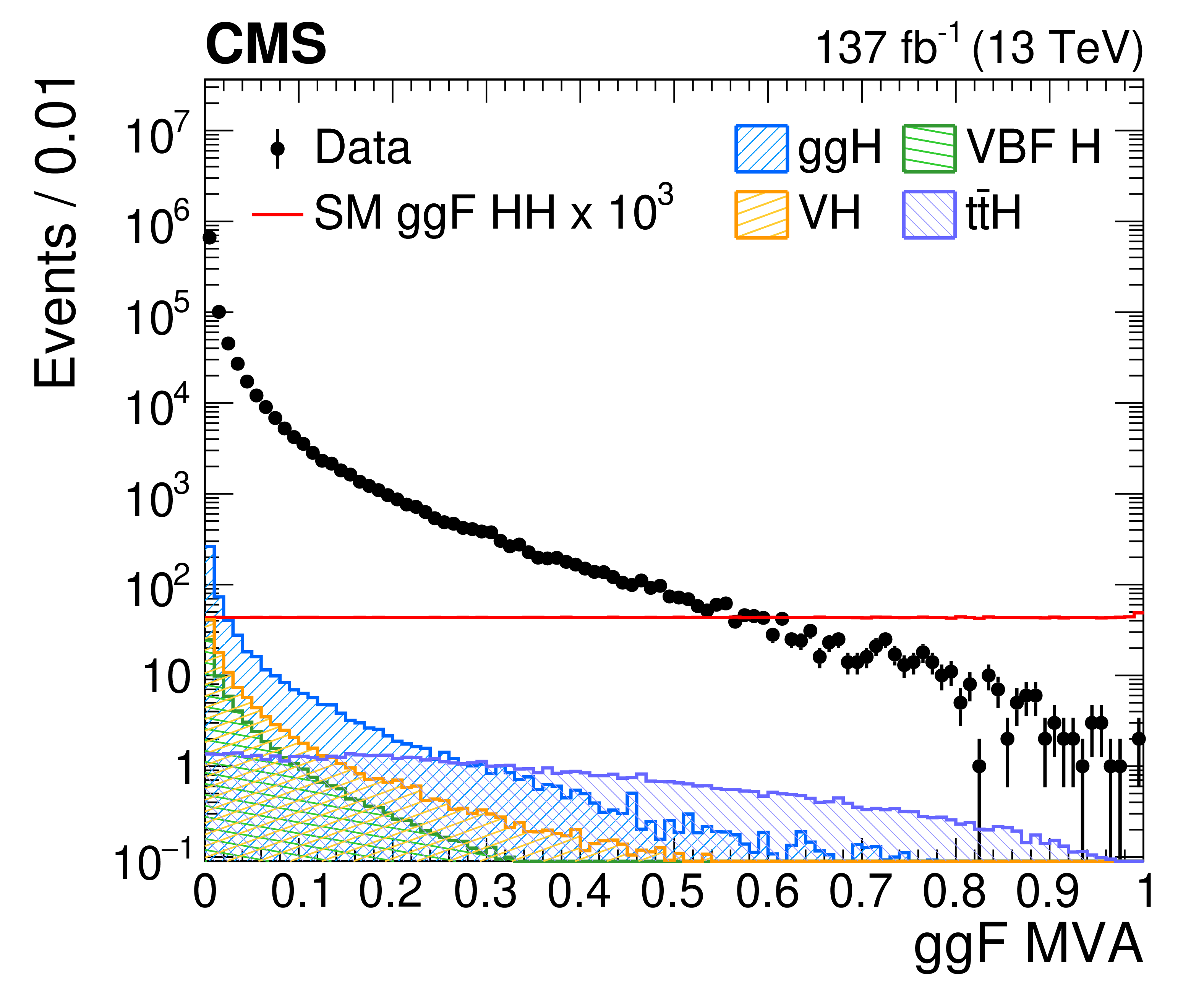
Figure 5-b:
The distribution of the MVA output in data and simulated events. Data, dominated by $ \gamma \gamma $+jets and $ \gamma $+jets background, are compared to the SM ggF HH signal samples and single H samples (ttH, ggH, VBF H, VH) after imposing the selection criteria described in Section 5. The error bars on the data points indicate statistical uncertainties. The HH signal has been scaled by a factor of 10$^{3}$ for display purposes. |
png pdf |
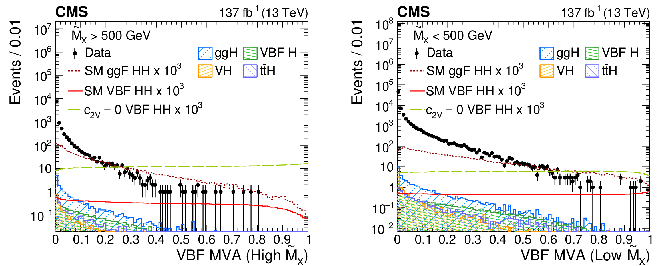
Figure 6:
The distribution of the two MVA outputs is shown in data and simulated events in the two VBF $ {\tilde{M}_{\mathrm {X}}} $ regions: $ {\tilde{M}_{\mathrm {X}}} > $ 500 GeV (left) and $ {\tilde{M}_{\mathrm {X}}} < $ 500 GeV (right). Data, dominated by the $ \gamma \gamma $+jets and $ \gamma $+jets backgrounds, are compared to the VBF HH signal samples with SM couplings and $ {c_{2\mathrm{V}}} =$ 0, SM ggF HH and single H samples (ttH, ggH, VBF H, VH) after imposing the VBF selection criteria described in Section 5. The error bars on the data points indicate statistical uncertainties. The HH signal has been scaled by a factor of 10$^{3}$ for display purposes. |
png pdf |
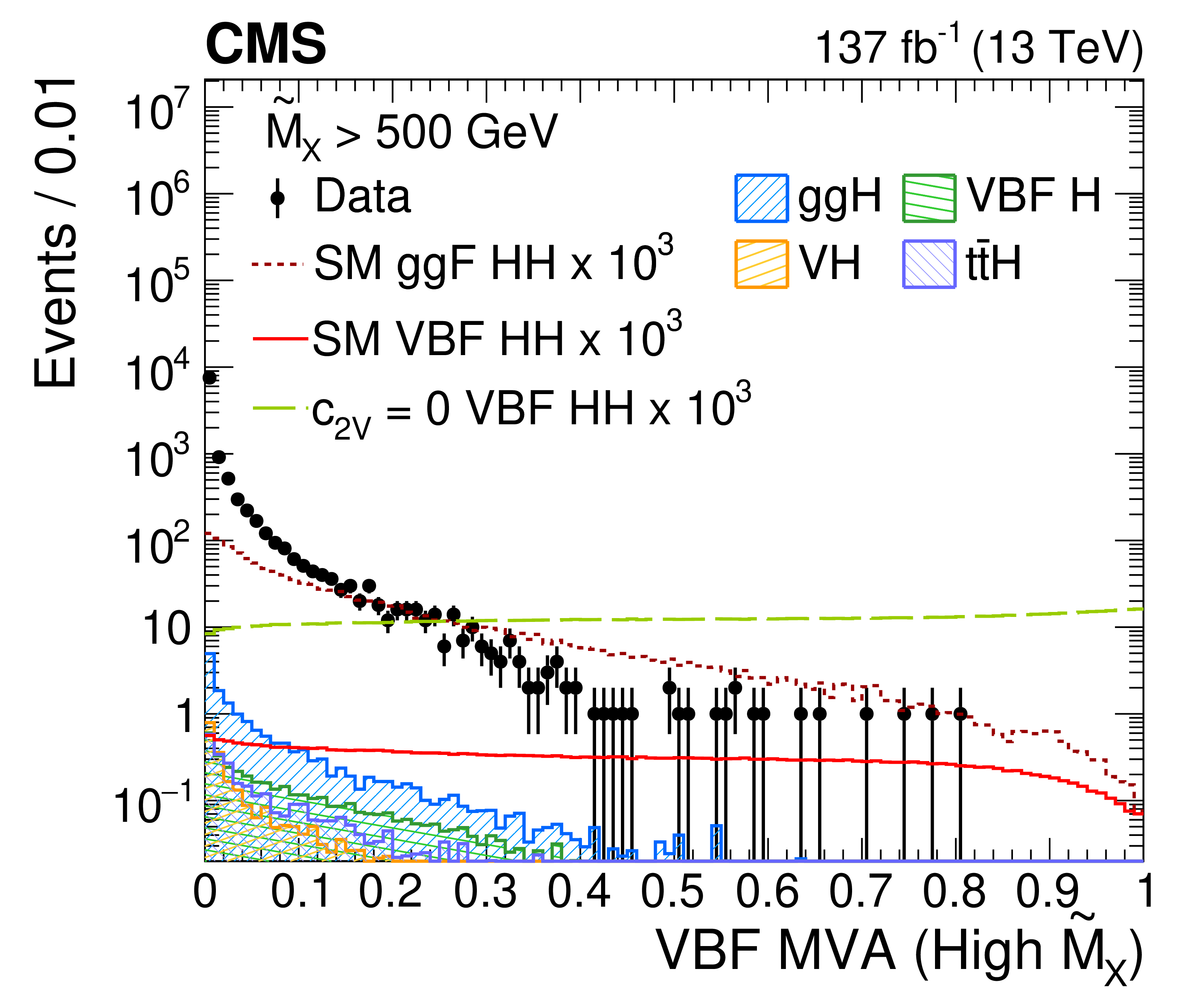
Figure 6-a:
The distribution of the MVA output is shown in data and simulated events in the VBF $ {\tilde{M}_{\mathrm {X}}} > $ 500 GeV region. Data, dominated by the $ \gamma \gamma $+jets and $ \gamma $+jets backgrounds, are compared to the VBF HH signal samples with SM couplings and $ {c_{2\mathrm{V}}} =$ 0, SM ggF HH and single H samples (ttH, ggH, VBF H, VH) after imposing the VBF selection criteria described in Section 5. The error bars on the data points indicate statistical uncertainties. The HH signal has been scaled by a factor of 10$^{3}$ for display purposes. |
png pdf |
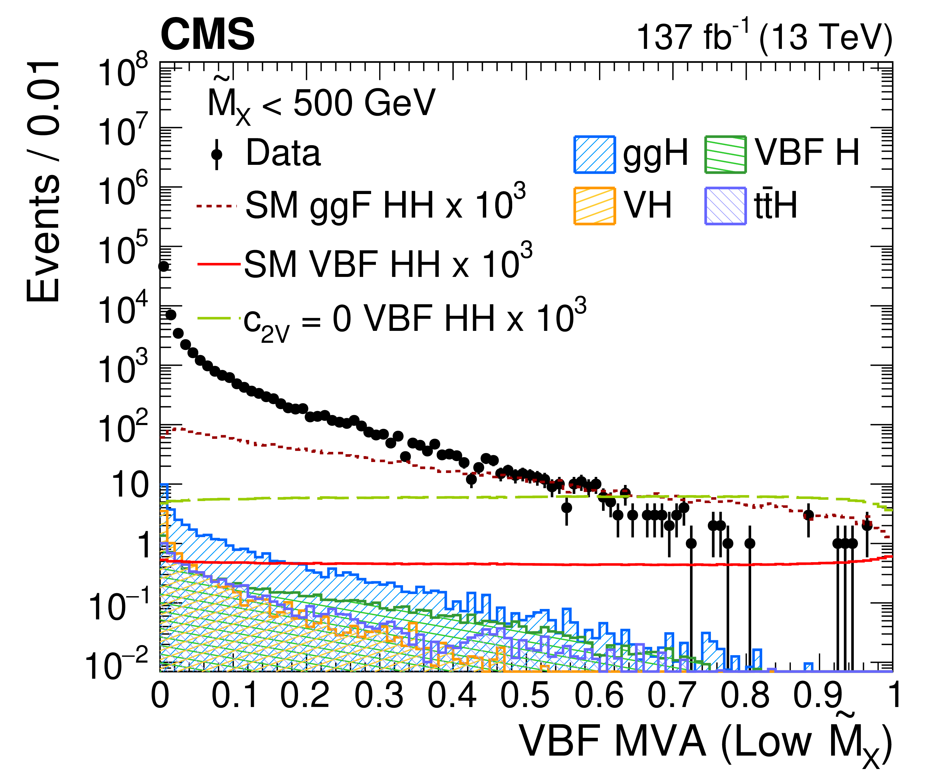
Figure 6-b:
The distribution of the MVA output is shown in data and simulated events in the VBF $ {\tilde{M}_{\mathrm {X}}} < $ 500 GeV region. Data, dominated by the $ \gamma \gamma $+jets and $ \gamma $+jets backgrounds, are compared to the VBF HH signal samples with SM couplings and $ {c_{2\mathrm{V}}} =$ 0, SM ggF HH and single H samples (ttH, ggH, VBF H, VH) after imposing the VBF selection criteria described in Section 5. The error bars on the data points indicate statistical uncertainties. The HH signal has been scaled by a factor of 10$^{3}$ for display purposes. |
png pdf |
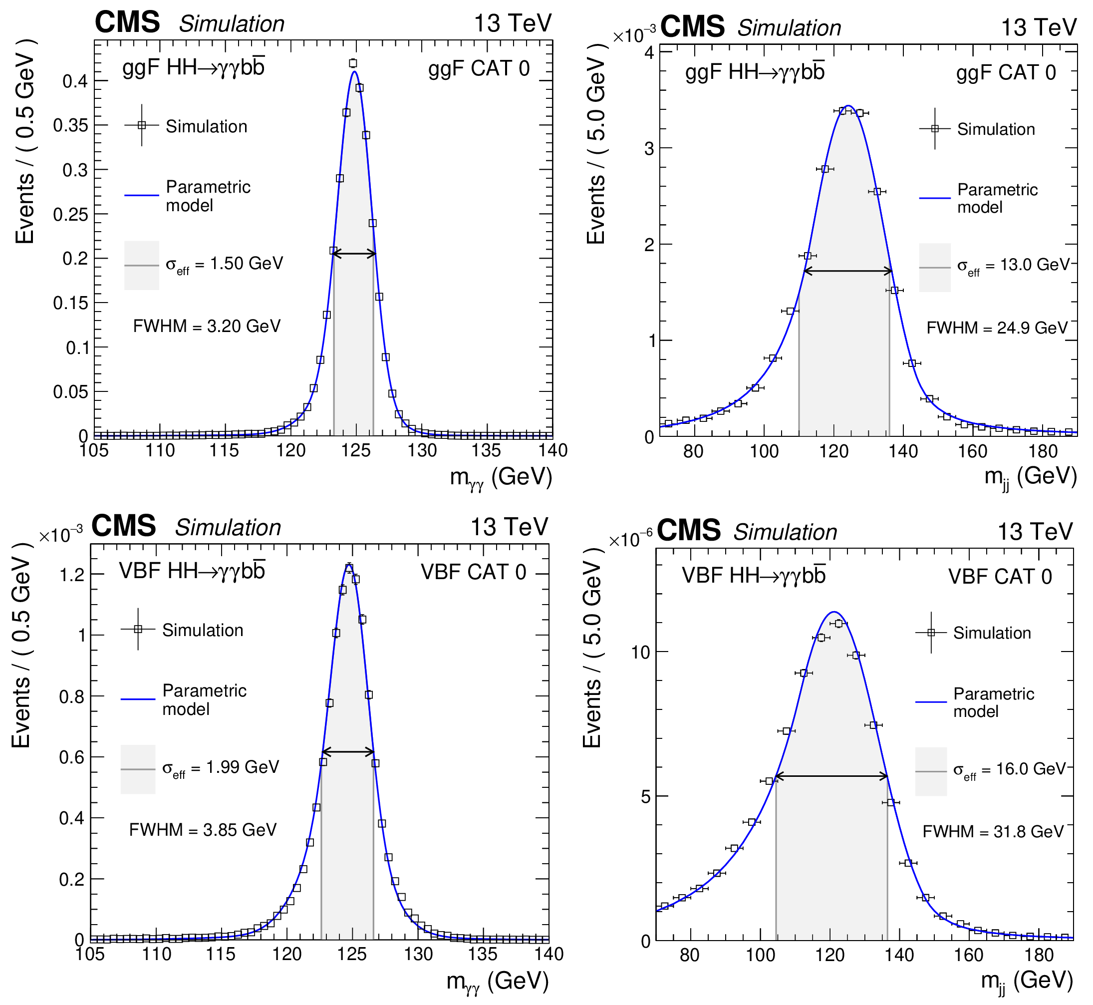
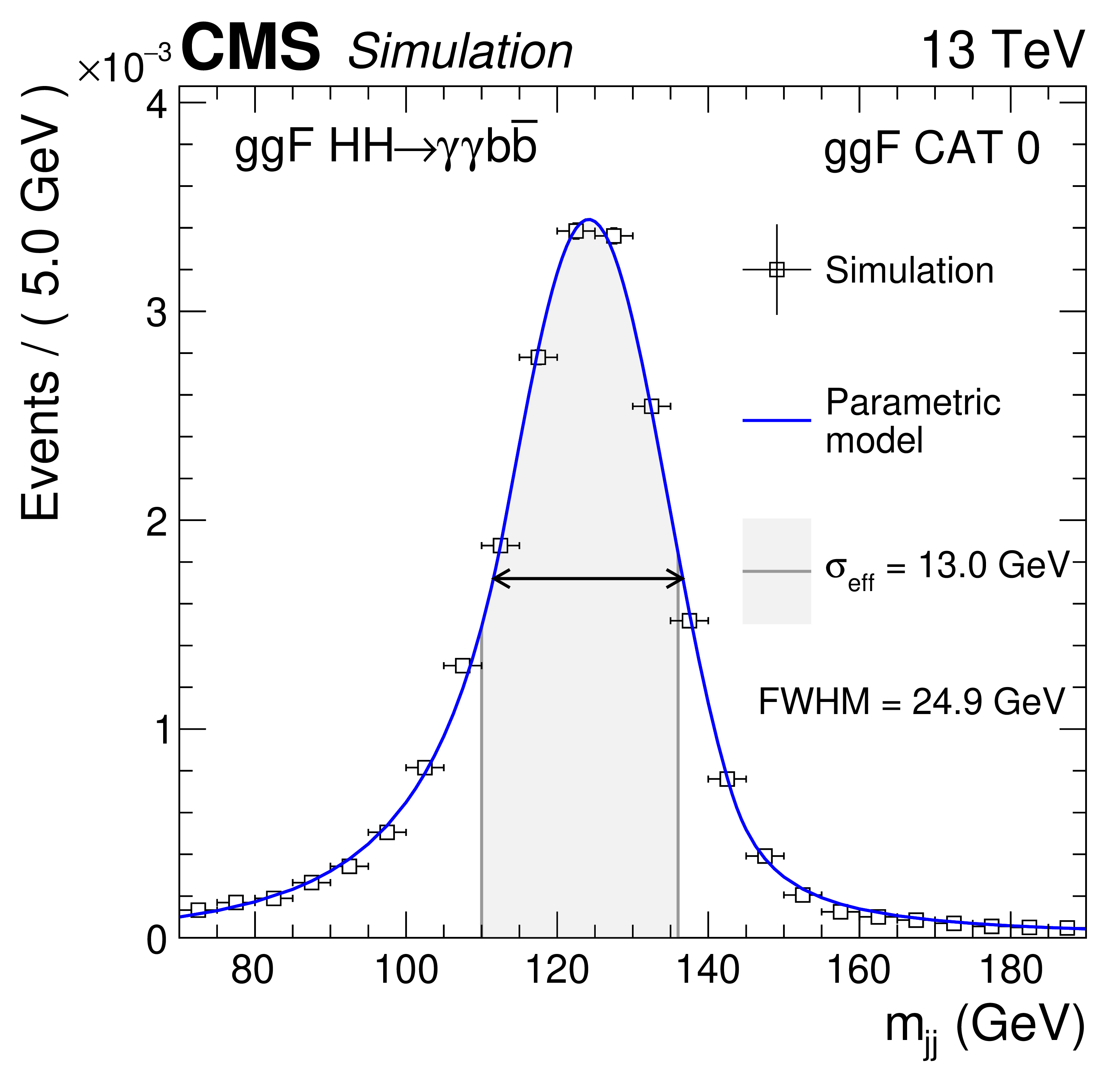
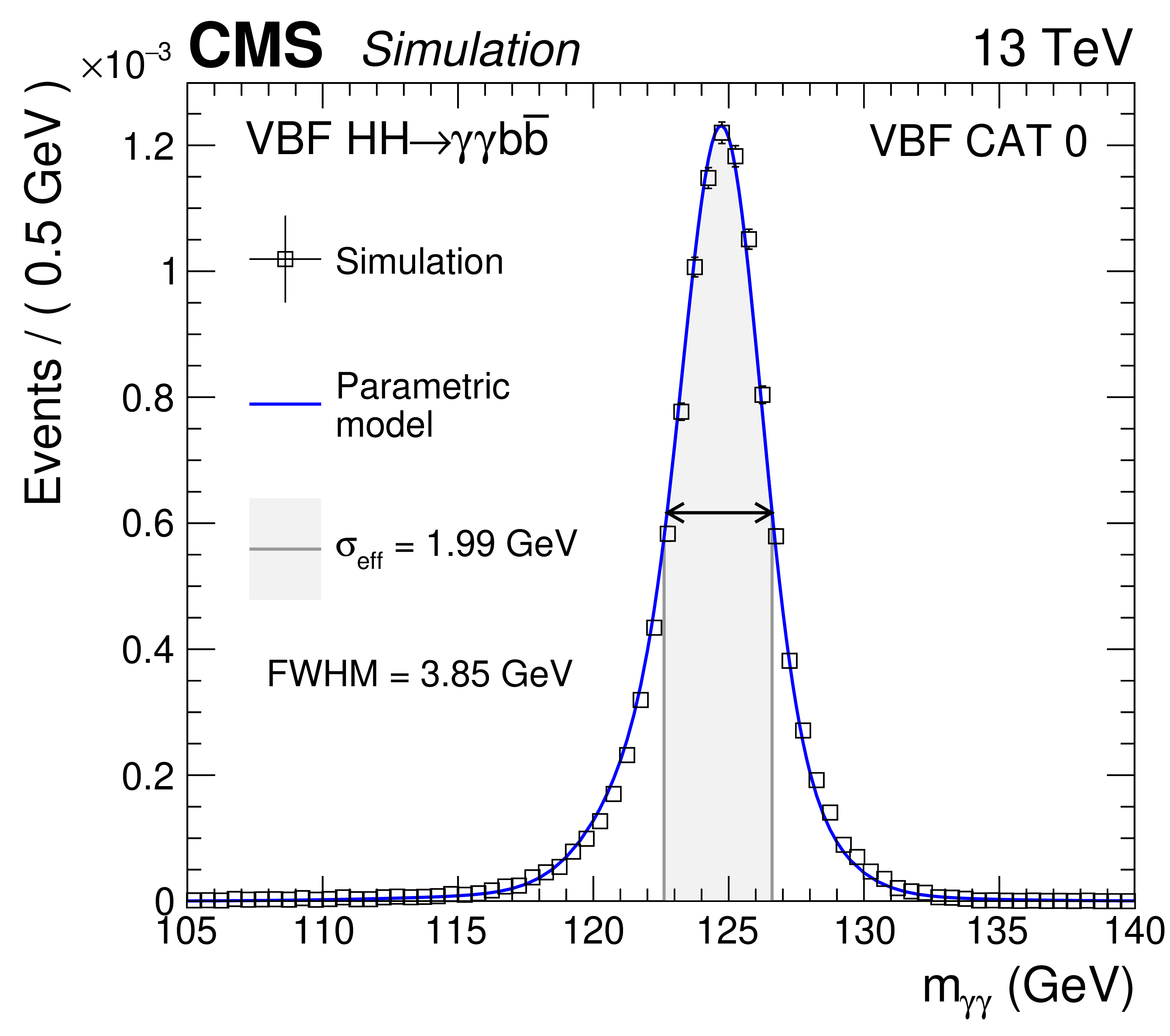
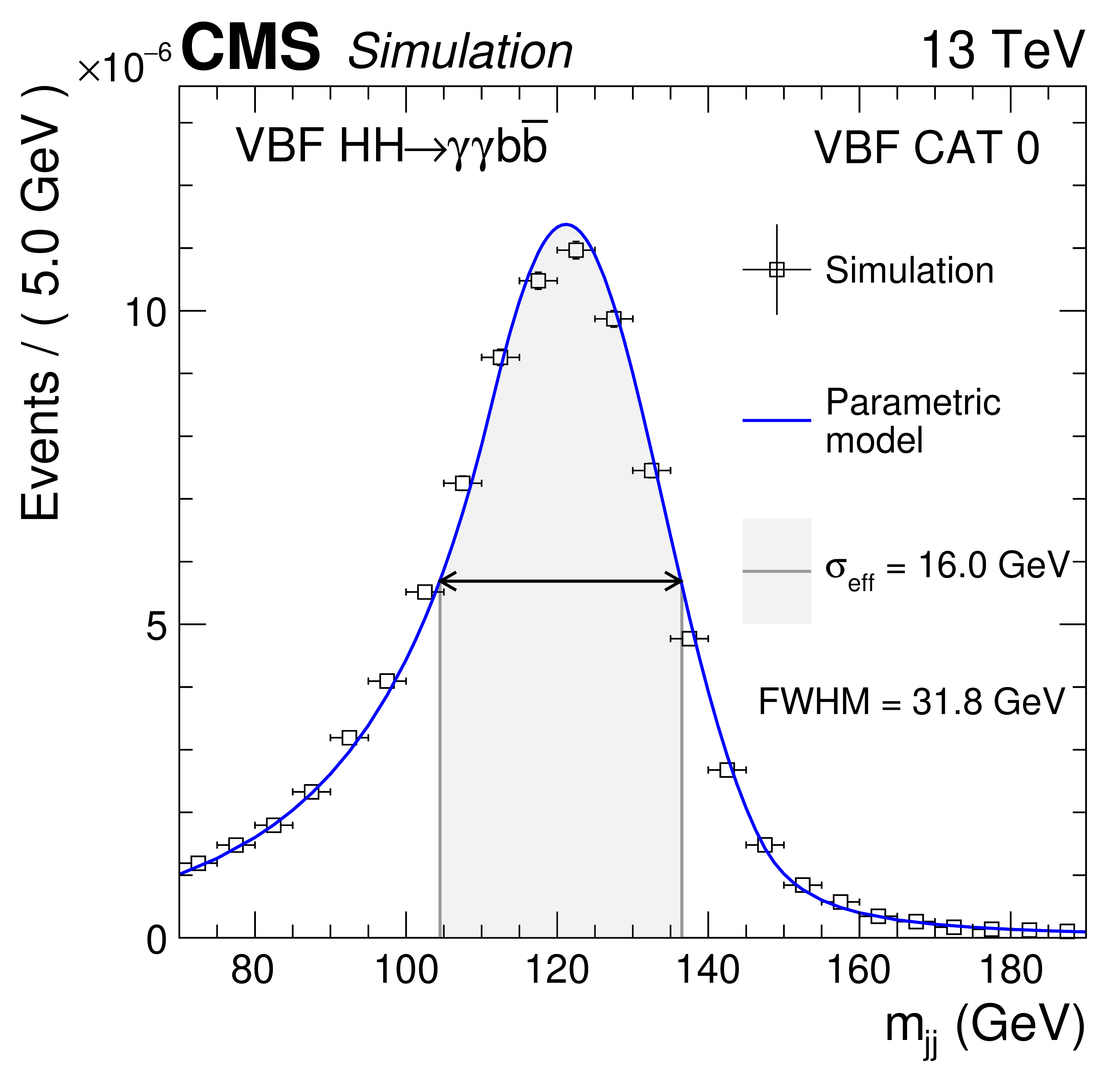
Figure 7:
Parametrized signal shape for $ {m_{\gamma \gamma}} $ (left) and ${m_\text {jj}}$ (right) in the best resolution ggF (upper) and VBF (lower) categories. The open squares represent simulated events and the blue lines are the corresponding models. Also shown are the $\sigma _{\text {eff}}$ value (half the width of the narrowest interval containing 68.3% of the invariant mass distribution) and the corresponding interval as a gray band, and the full width at half the maximum (FWHM) and the corresponding interval as a double arrow. |

png pdf |
Figure 7-a:
Parametrized signal shape for $ {m_{\gamma \gamma}} $ in the best resolution ggF category. The open squares represent simulated events and the blue lines are the corresponding models. Also shown are the $\sigma _{\text {eff}}$ value (half the width of the narrowest interval containing 68.3% of the invariant mass distribution) and the corresponding interval as a gray band, and the full width at half the maximum (FWHM) and the corresponding interval as a double arrow. |
png pdf |
Figure 7-b:
Parametrized signal shape for ${m_\text {jj}}$ in the best resolution VBF category. The open squares represent simulated events and the blue lines are the corresponding models. Also shown are the $\sigma _{\text {eff}}$ value (half the width of the narrowest interval containing 68.3% of the invariant mass distribution) and the corresponding interval as a gray band, and the full width at half the maximum (FWHM) and the corresponding interval as a double arrow. |
png pdf |
Figure 7-c:
Parametrized signal shape for $ {m_{\gamma \gamma}} $ in the best resolution ggF category. The open squares represent simulated events and the blue lines are the corresponding models. Also shown are the $\sigma _{\text {eff}}$ value (half the width of the narrowest interval containing 68.3% of the invariant mass distribution) and the corresponding interval as a gray band, and the full width at half the maximum (FWHM) and the corresponding interval as a double arrow. |
png pdf |
Figure 7-d:
Parametrized signal shape for ${m_\text {jj}}$ in the best resolution VBF category. The open squares represent simulated events and the blue lines are the corresponding models. Also shown are the $\sigma _{\text {eff}}$ value (half the width of the narrowest interval containing 68.3% of the invariant mass distribution) and the corresponding interval as a gray band, and the full width at half the maximum (FWHM) and the corresponding interval as a double arrow. |
png pdf |
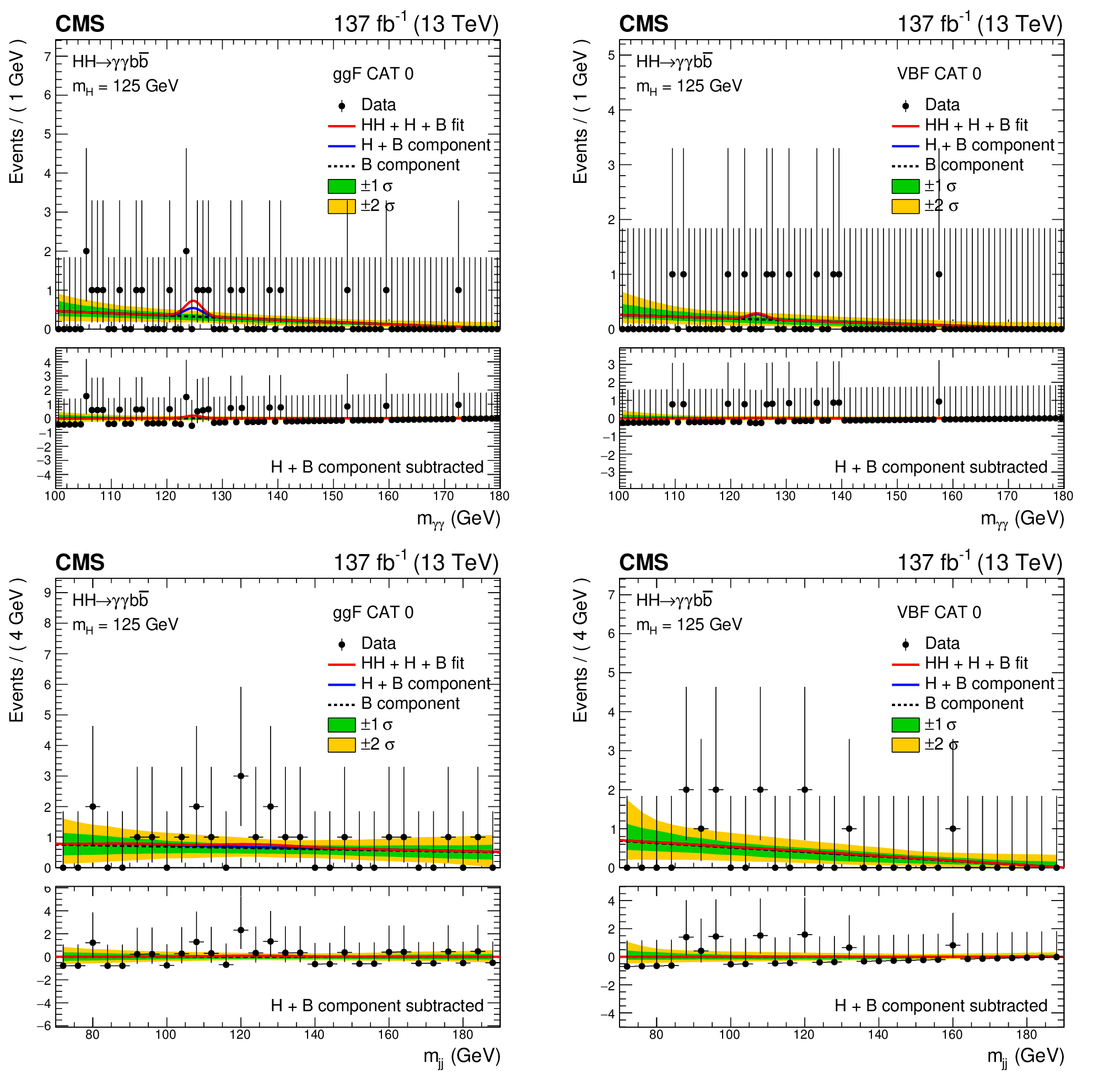
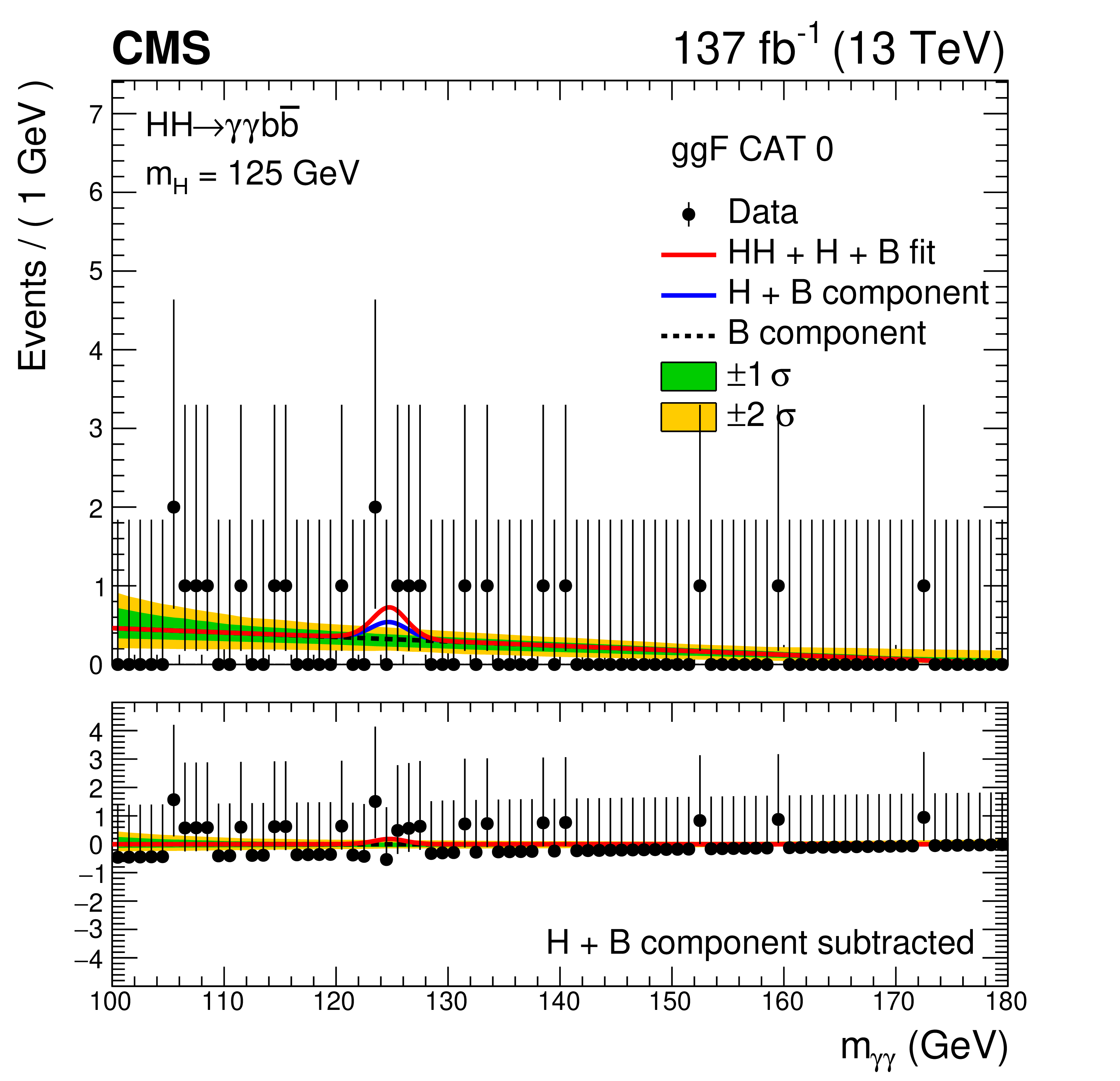
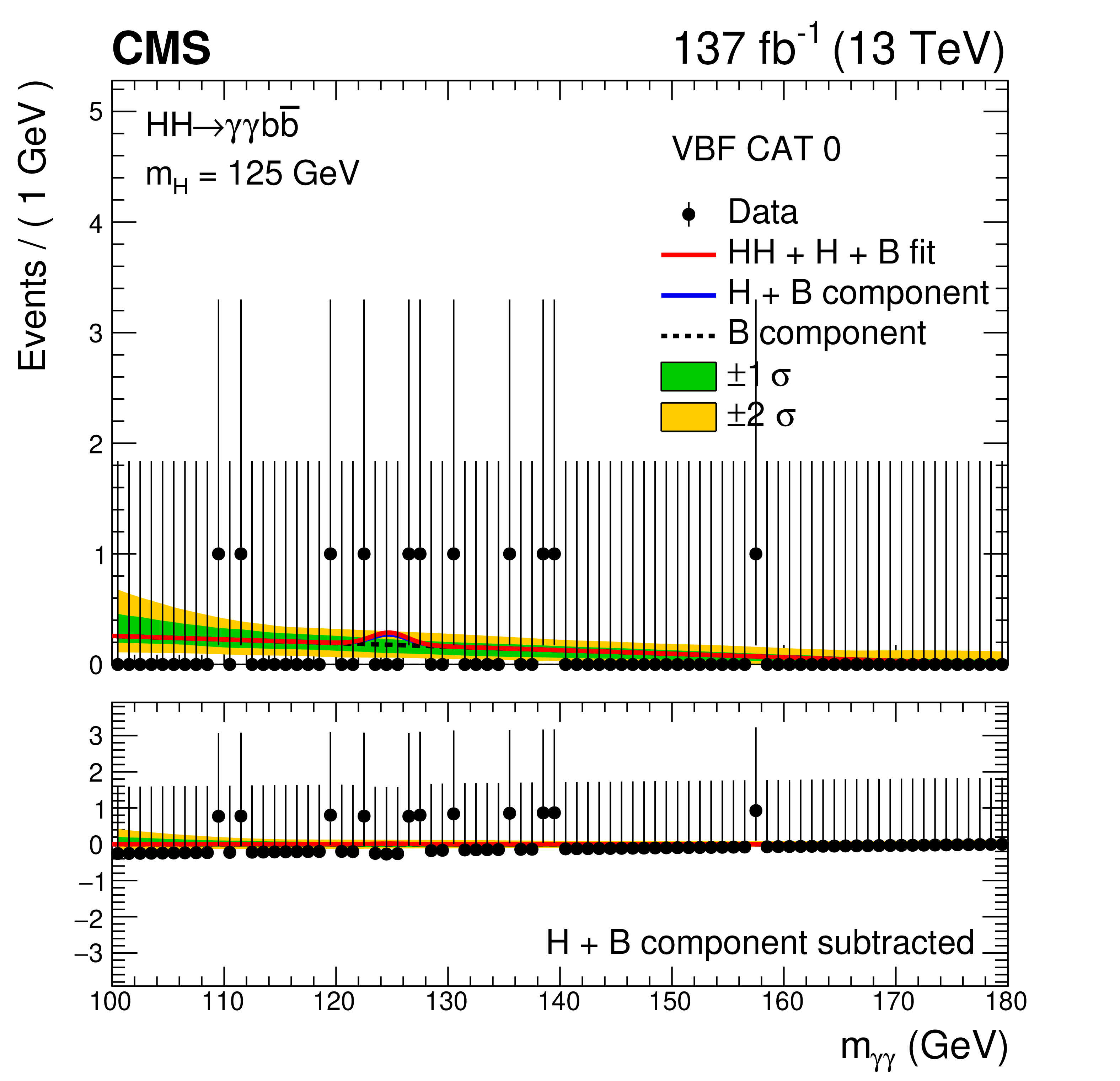
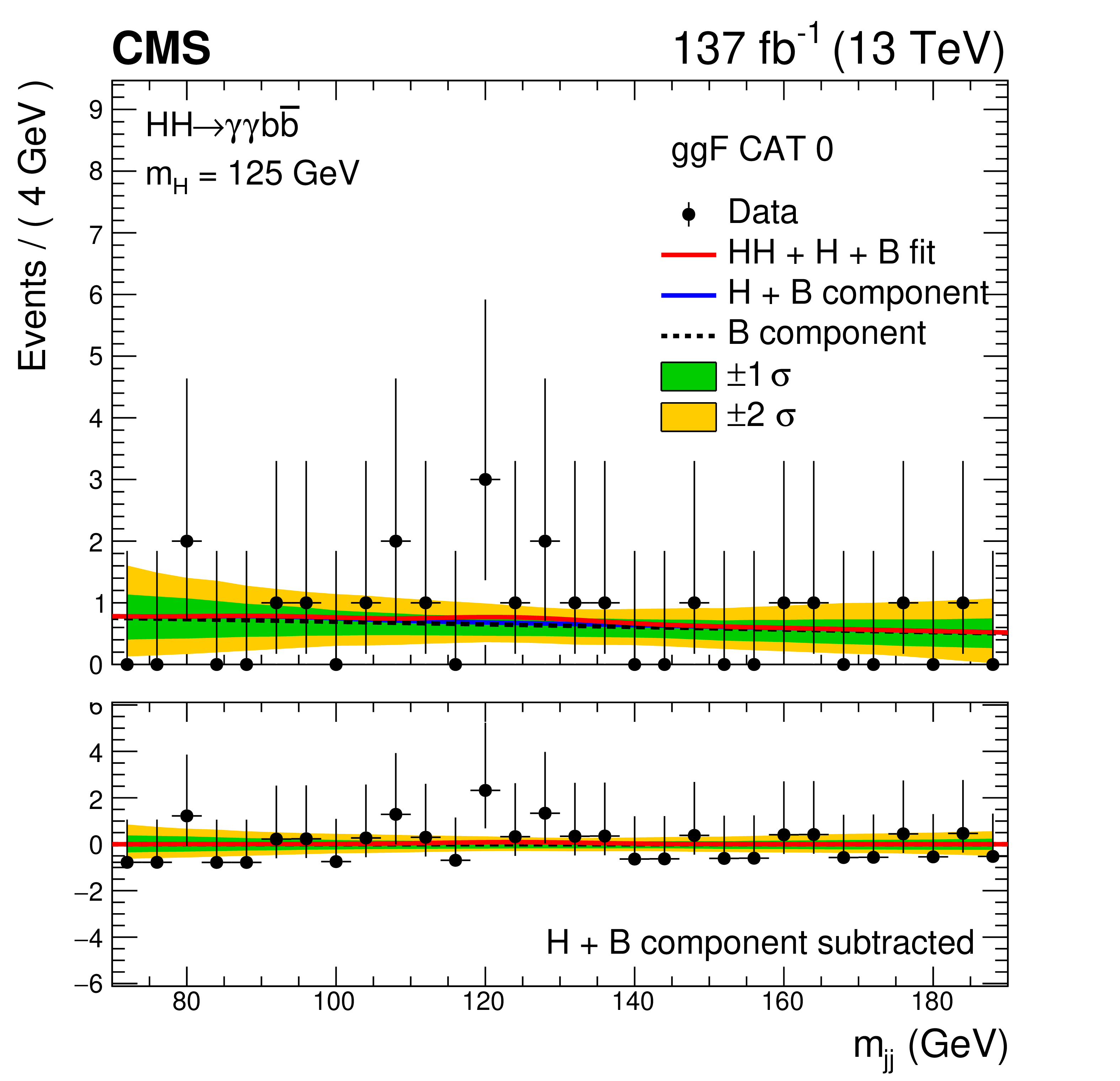
Figure 8:
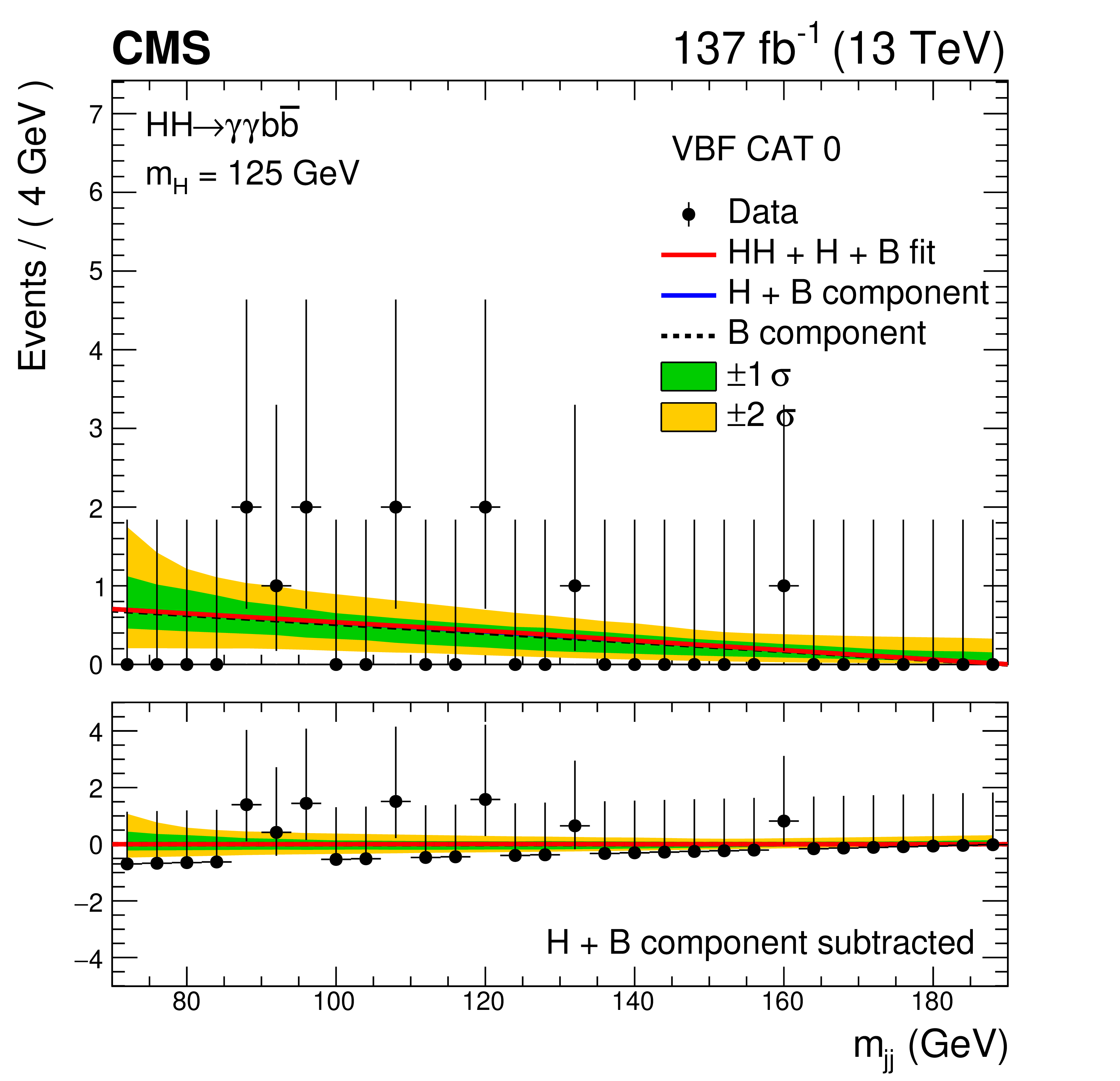
Invariant mass distributions $ {m_{\gamma \gamma}} $ (upper) and $ {m_\text {jj}}$ (lower) for the selected events in data (black points) in the best resolution ggF (CAT0) and VBF (CAT0) categories. The solid red line shows the sum of the fitted signal and background (HH+H+B), the solid blue line shows the background component from the single Higgs boson and the nonresonant processes (H+B), and the dashed black line shows the nonresonant background component (B). The normalization of each component (HH, H, B) is extracted from the combined fit to the data in all analysis categories. The one (green) and two (yellow) standard deviation bands include the uncertainties in the background component of the fit. The lower panel in each plot shows the residual signal yield after the background (H+B) subtraction. |
png pdf |
Figure 8-a:
Invariant mass distributions $ {m_{\gamma \gamma}} $ for the selected events in data (black points) in the best resolution ggF (CAT0) category. The solid red line shows the sum of the fitted signal and background (HH+H+B), the solid blue line shows the background component from the single Higgs boson and the nonresonant processes (H+B), and the dashed black line shows the nonresonant background component (B). The normalization of each component (HH, H, B) is extracted from the combined fit to the data in all analysis categories. The one (green) and two (yellow) standard deviation bands include the uncertainties in the background component of the fit. The lower panel shows the residual signal yield after the background (H+B) subtraction. |
png pdf |
Figure 8-b:
Invariant mass distributions $ {m_{\gamma \gamma}} $ for the selected events in data (black points) in the best resolution VBF (CAT0) category. The solid red line shows the sum of the fitted signal and background (HH+H+B), the solid blue line shows the background component from the single Higgs boson and the nonresonant processes (H+B), and the dashed black line shows the nonresonant background component (B). The normalization of each component (HH, H, B) is extracted from the combined fit to the data in all analysis categories. The one (green) and two (yellow) standard deviation bands include the uncertainties in the background component of the fit. The lower panel shows the residual signal yield after the background (H+B) subtraction. |
png pdf |
Figure 8-c:
Invariant mass distributions $ {m_\text {jj}}$ for the selected events in data (black points) in the best resolution ggF (CAT0) category. The solid red line shows the sum of the fitted signal and background (HH+H+B), the solid blue line shows the background component from the single Higgs boson and the nonresonant processes (H+B), and the dashed black line shows the nonresonant background component (B). The normalization of each component (HH, H, B) is extracted from the combined fit to the data in all analysis categories. The one (green) and two (yellow) standard deviation bands include the uncertainties in the background component of the fit. The lower panel shows the residual signal yield after the background (H+B) subtraction. |
png pdf |
Figure 8-d:
Invariant mass distributions $ {m_\text {jj}}$ for the selected events in data (black points) in the best resolution VBF (CAT0) category. The solid red line shows the sum of the fitted signal and background (HH+H+B), the solid blue line shows the background component from the single Higgs boson and the nonresonant processes (H+B), and the dashed black line shows the nonresonant background component (B). The normalization of each component (HH, H, B) is extracted from the combined fit to the data in all analysis categories. The one (green) and two (yellow) standard deviation bands include the uncertainties in the background component of the fit. The lower panel shows the residual signal yield after the background (H+B) subtraction. |
png pdf |
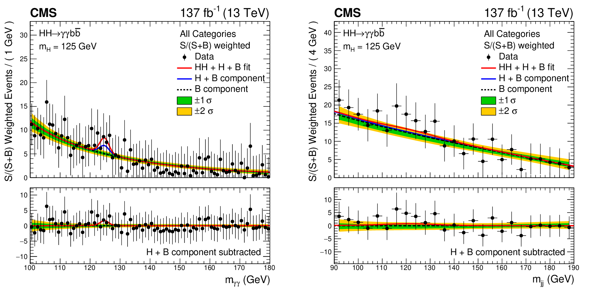
Figure 9:
Invariant mass distributions $ {m_{\gamma \gamma}} $ (left) and $ {m_\text {jj}}$ (right) for the selected events in data (black points) weighted by S/(S+B), where S (B) is the number of signal (background) events extracted from the signal-plus-background fit. The solid red line shows the sum of the fitted signal and background (HH+H+B), the solid blue line shows the background component from the single Higgs boson and the nonresonant processes (H+B), and the dashed black line shows the nonresonant background component (B). The normalization of each component (HH, H, B) is extracted from the combined fit to the data in all analysis categories. The one (green) and two (yellow) standard deviation bands include the uncertainties in the background component of the fit. The lower panel in each plot shows the residual signal yield after the background (H+B) subtraction. |

png pdf |
Figure 9-a:
Invariant mass distributions $ {m_{\gamma \gamma}} $ for the selected events in data (black points) weighted by S/(S+B), where S (B) is the number of signal (background) events extracted from the signal-plus-background fit. The solid red line shows the sum of the fitted signal and background (HH+H+B), the solid blue line shows the background component from the single Higgs boson and the nonresonant processes (H+B), and the dashed black line shows the nonresonant background component (B). The normalization of each component (HH, H, B) is extracted from the combined fit to the data in all analysis categories. The one (green) and two (yellow) standard deviation bands include the uncertainties in the background component of the fit. The lower panel shows the residual signal yield after the background (H+B) subtraction. |

png pdf |
Figure 9-b:
Invariant mass distributions $ {m_\text {jj}}$ for the selected events in data (black points) weighted by S/(S+B), where S (B) is the number of signal (background) events extracted from the signal-plus-background fit. The solid red line shows the sum of the fitted signal and background (HH+H+B), the solid blue line shows the background component from the single Higgs boson and the nonresonant processes (H+B), and the dashed black line shows the nonresonant background component (B). The normalization of each component (HH, H, B) is extracted from the combined fit to the data in all analysis categories. The one (green) and two (yellow) standard deviation bands include the uncertainties in the background component of the fit. The lower panel shows the residual signal yield after the background (H+B) subtraction. |
png pdf |
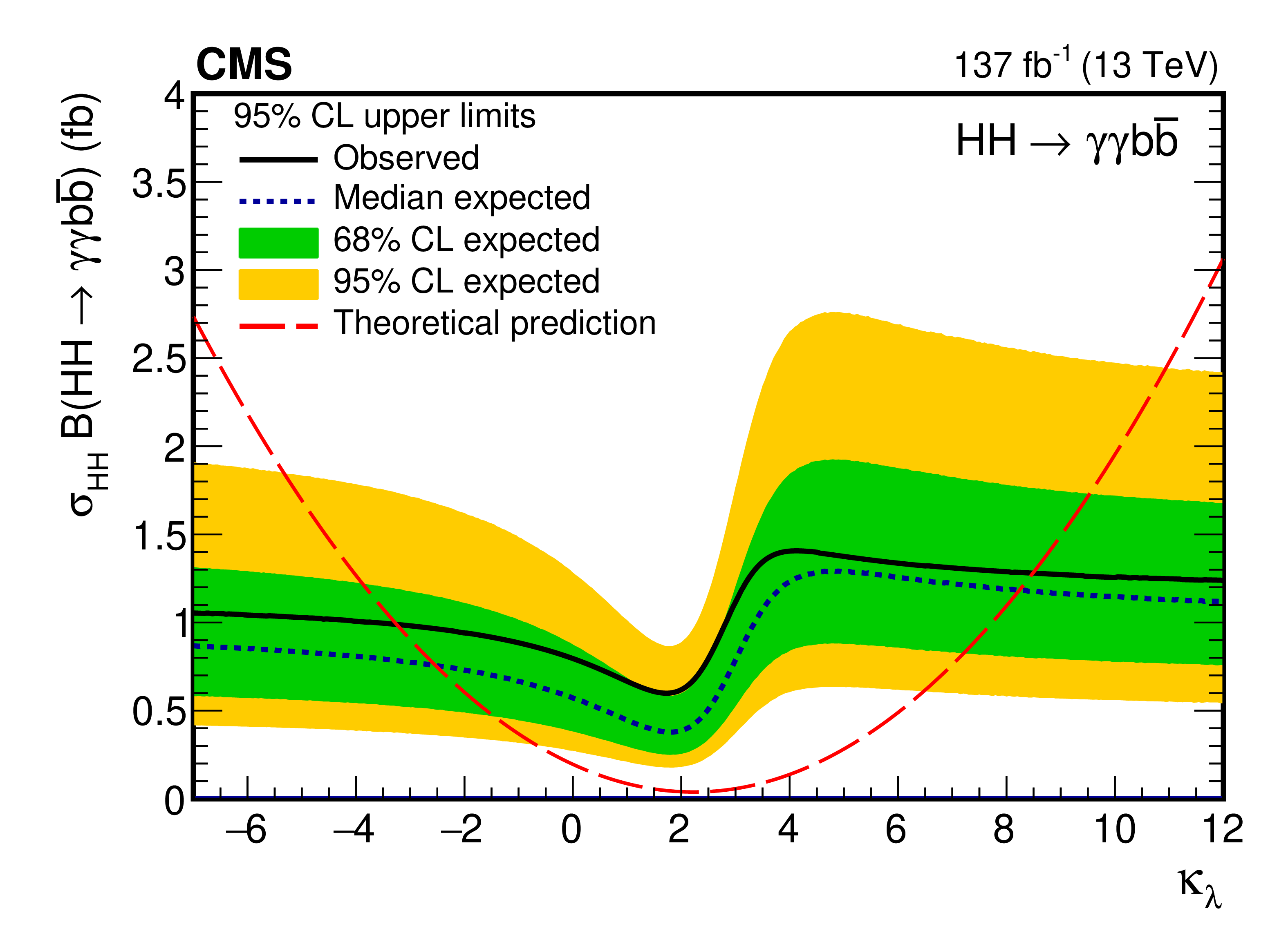
Figure 10:
Expected and observed 95% CL upper limits on the product of the HH production cross section and $\mathcal {B}({{\mathrm{H} \mathrm{H}}} \to {\gamma \gamma \mathrm{b} {}\mathrm{\bar{b}}})$ obtained for different values of $ {\kappa _{\lambda}} $ assuming $ {\kappa _{\mathrm{t}}} $ = 1. The green and yellow bands represent, respectively, the one and two standard deviation extensions beyond the expected limit. The long-dashed red line shows the theoretical prediction. |
png pdf |
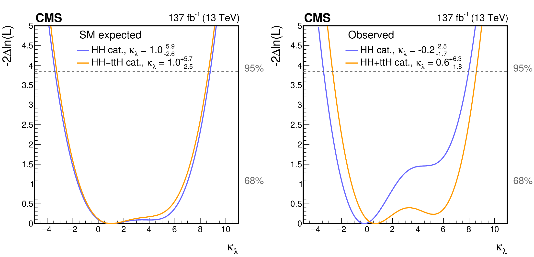
Figure 11:
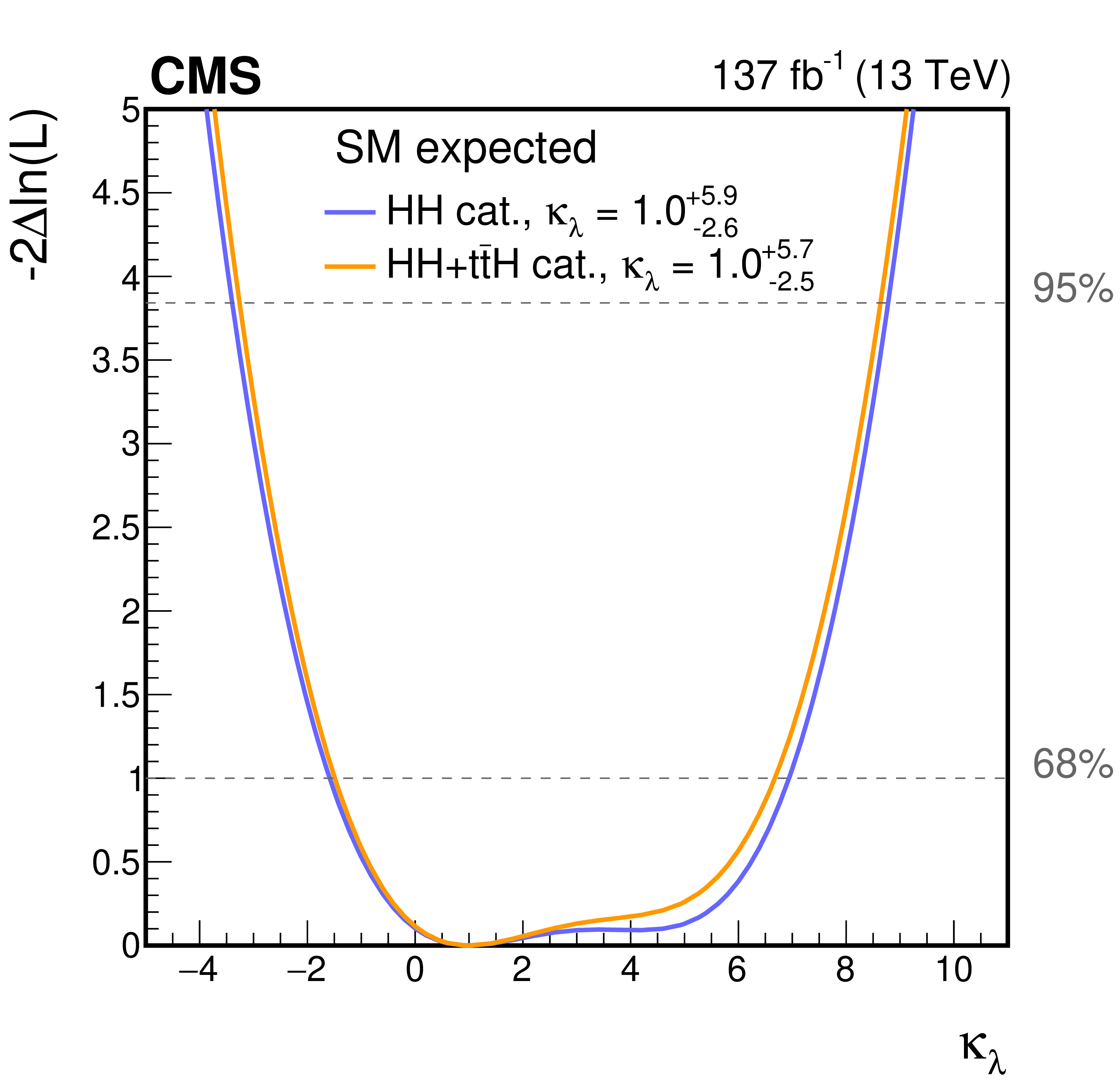
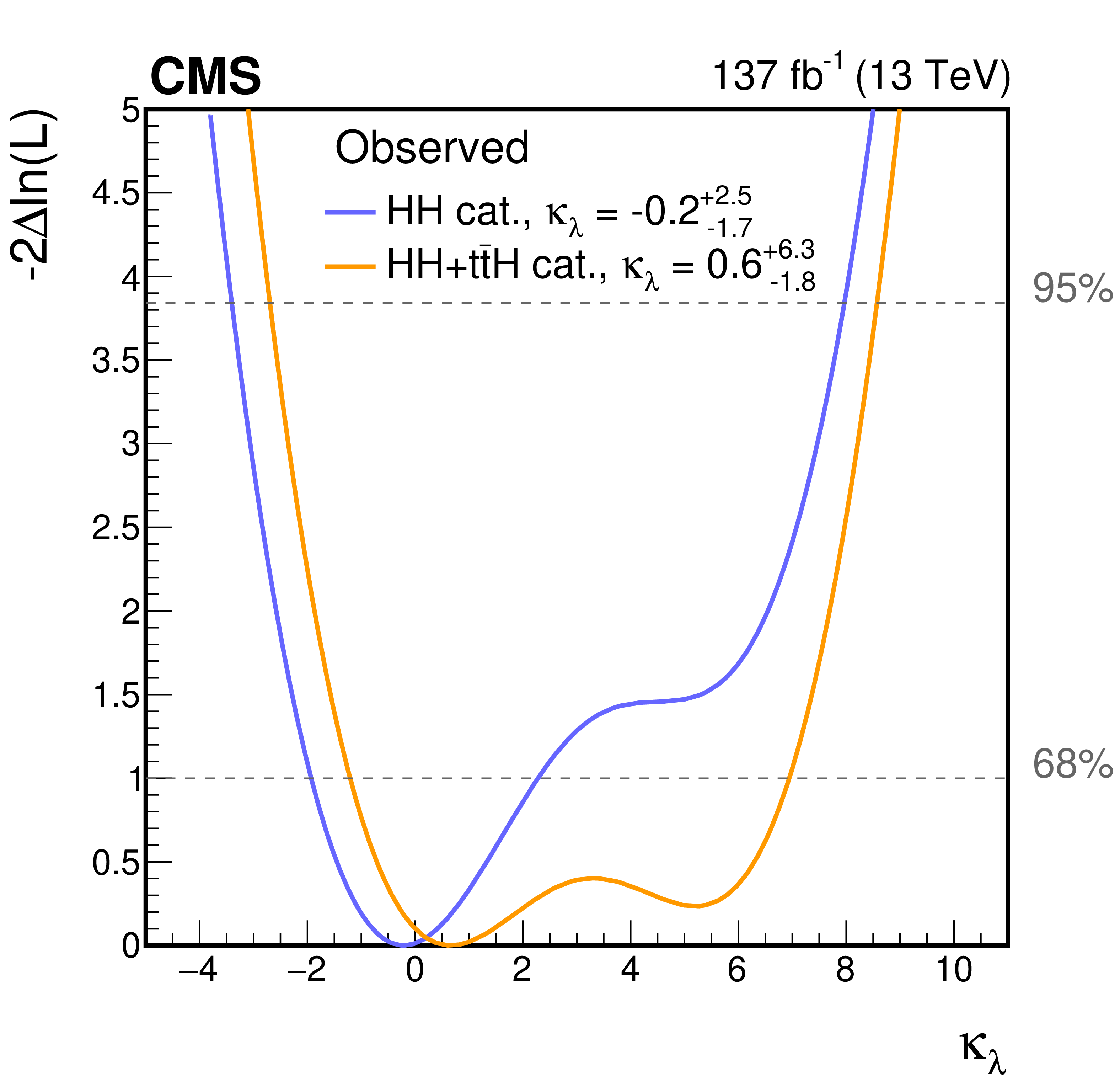
Negative log-likelihood, as a function of $ {\kappa _{\lambda}} $, evaluated with an Asimov data set assuming the SM hypothesis (left) and the observed data (right). The 68 and 95% CL intervals are shown with the dashed gray lines. The two curves are shown for the HH (blue) and HH+ttH (orange) analysis categories. All other couplings are set to their SM values. |
png pdf |
Figure 11-a:
Negative log-likelihood, as a function of $ {\kappa _{\lambda}} $, evaluated with an Asimov data set assuming the SM hypothesis. The 68 and 95% CL intervals are shown with the dashed gray lines. The two curves are shown for the HH (blue) and HH+ttH (orange) analysis categories. All other couplings are set to their SM values. |
png pdf |
Figure 11-b:
Negative log-likelihood, as a function of $ {\kappa _{\lambda}} $, evaluated with an Asimov data set assuming the observed data. The 68 and 95% CL intervals are shown with the dashed gray lines. The two curves are shown for the HH (blue) and HH+ttH (orange) analysis categories. All other couplings are set to their SM values. |
png pdf |
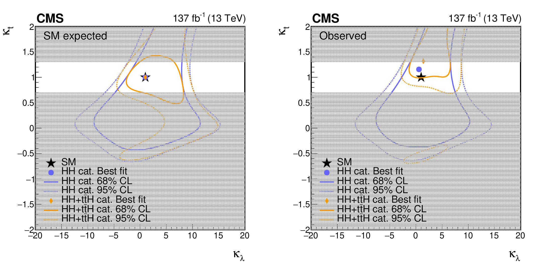
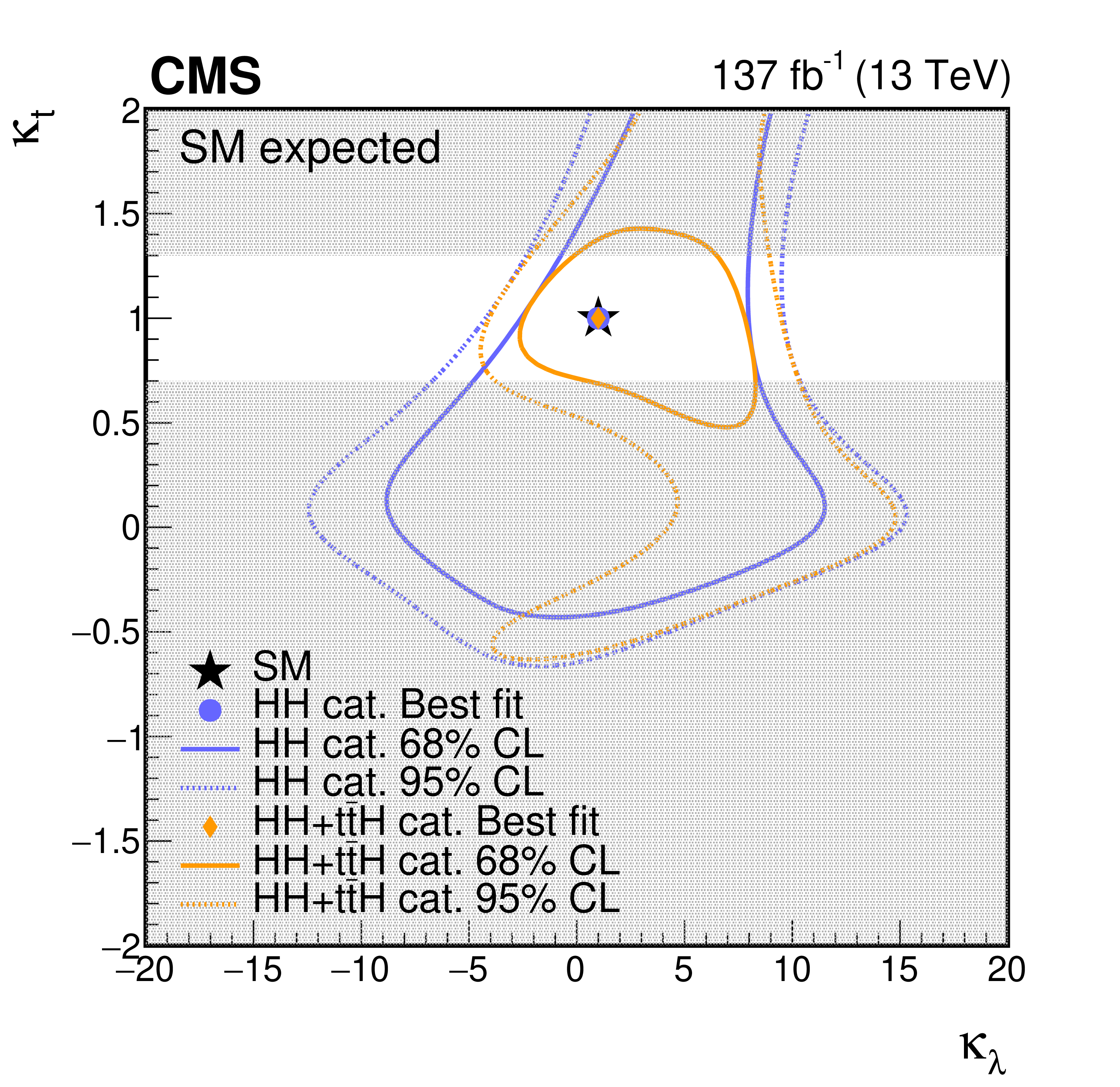
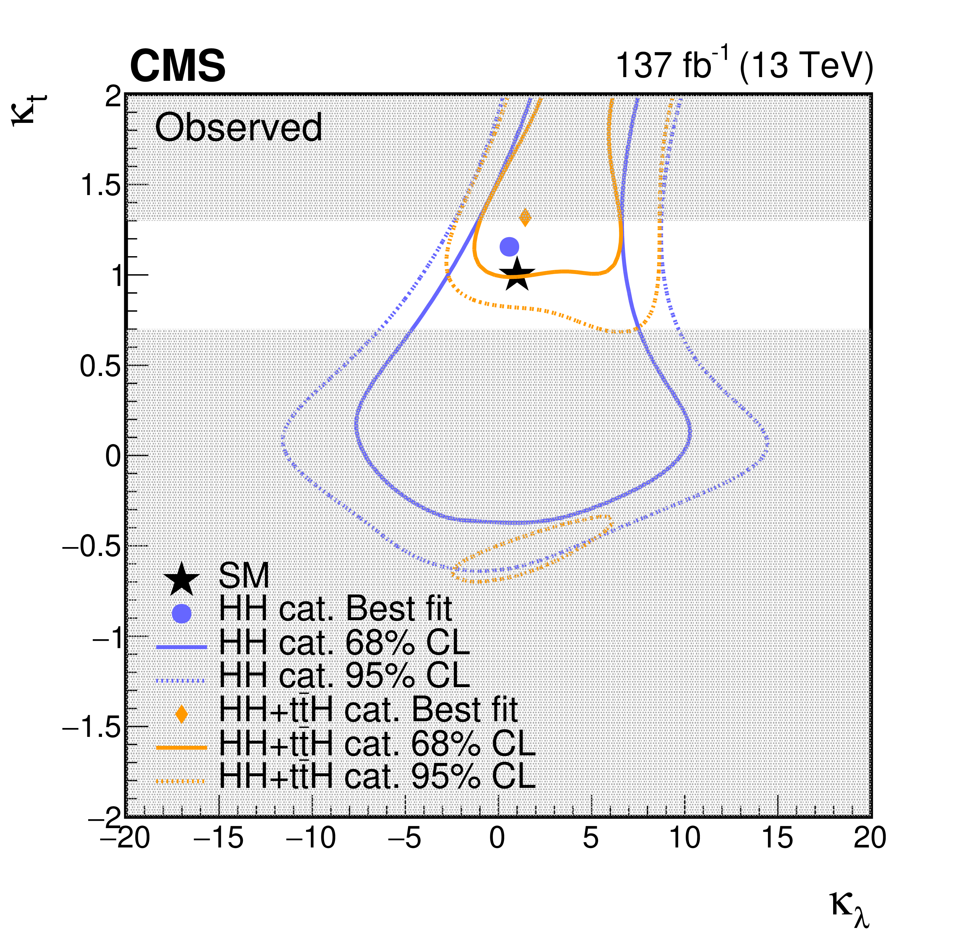
Figure 12:
Negative log-likelihood contours at 68 and 95% CL in the ($ {\kappa _{\lambda}} $, $ {\kappa _{\mathrm{t}}} $) plane evaluated with an Asimov data set assuming the SM hypothesis (left) and the observed data (right). The contours obtained using the HH analysis categories only are shown in blue, and in orange when combined with the ttH categories. The best fit value for the HH categories only ($ {\kappa _{\lambda}} $ = 0.6, $ {\kappa _{\mathrm{t}}} $ = 1.2) is indicated by a blue circle, for the HH+ttH categories ($ {\kappa _{\lambda}} $ = 1.4, $ {\kappa _{\mathrm{t}}} $ = 1.3) by an orange diamond, and the SM prediction ($ {\kappa _{\lambda}} $ = 1.0, $ {\kappa _{\mathrm{t}}} $ = 1.0) by a black star. The regions of the 2D scan where the ${\kappa _{\mathrm{t}}}$ parametrization for anomalous values of ${\kappa _{\lambda}}$ at LO is not reliable are shown with a gray band. |
png pdf |
Figure 12-a:
Negative log-likelihood contours at 68 and 95% CL in the ($ {\kappa _{\lambda}} $, $ {\kappa _{\mathrm{t}}} $) plane evaluated with an Asimov data set assuming the SM hypothesis. The contours obtained using the HH analysis categories only are shown in blue, and in orange when combined with the ttH categories. The best fit value for the HH categories only ($ {\kappa _{\lambda}} $ = 0.6, $ {\kappa _{\mathrm{t}}} $ = 1.2) is indicated by a blue circle, for the HH+ttH categories ($ {\kappa _{\lambda}} $ = 1.4, $ {\kappa _{\mathrm{t}}} $ = 1.3) by an orange diamond, and the SM prediction ($ {\kappa _{\lambda}} $ = 1.0, $ {\kappa _{\mathrm{t}}} $ = 1.0) by a black star. The regions of the 2D scan where the ${\kappa _{\mathrm{t}}}$ parametrization for anomalous values of ${\kappa _{\lambda}}$ at LO is not reliable are shown with a gray band. |
png pdf |
Figure 12-b:
Negative log-likelihood contours at 68 and 95% CL in the ($ {\kappa _{\lambda}} $, $ {\kappa _{\mathrm{t}}} $) plane evaluated with an Asimov data set assuming the observed data. The contours obtained using the HH analysis categories only are shown in blue, and in orange when combined with the ttH categories. The best fit value for the HH categories only ($ {\kappa _{\lambda}} $ = 0.6, $ {\kappa _{\mathrm{t}}} $ = 1.2) is indicated by a blue circle, for the HH+ttH categories ($ {\kappa _{\lambda}} $ = 1.4, $ {\kappa _{\mathrm{t}}} $ = 1.3) by an orange diamond, and the SM prediction ($ {\kappa _{\lambda}} $ = 1.0, $ {\kappa _{\mathrm{t}}} $ = 1.0) by a black star. The regions of the 2D scan where the ${\kappa _{\mathrm{t}}}$ parametrization for anomalous values of ${\kappa _{\lambda}}$ at LO is not reliable are shown with a gray band. |
png pdf |
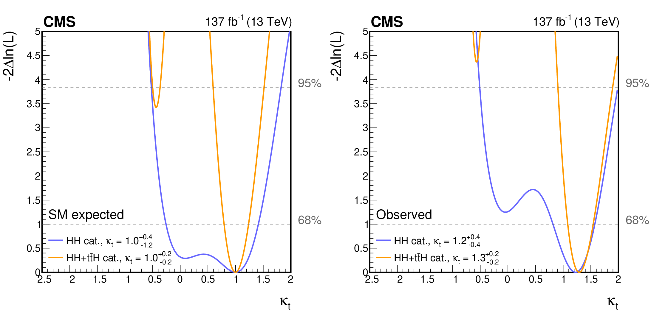
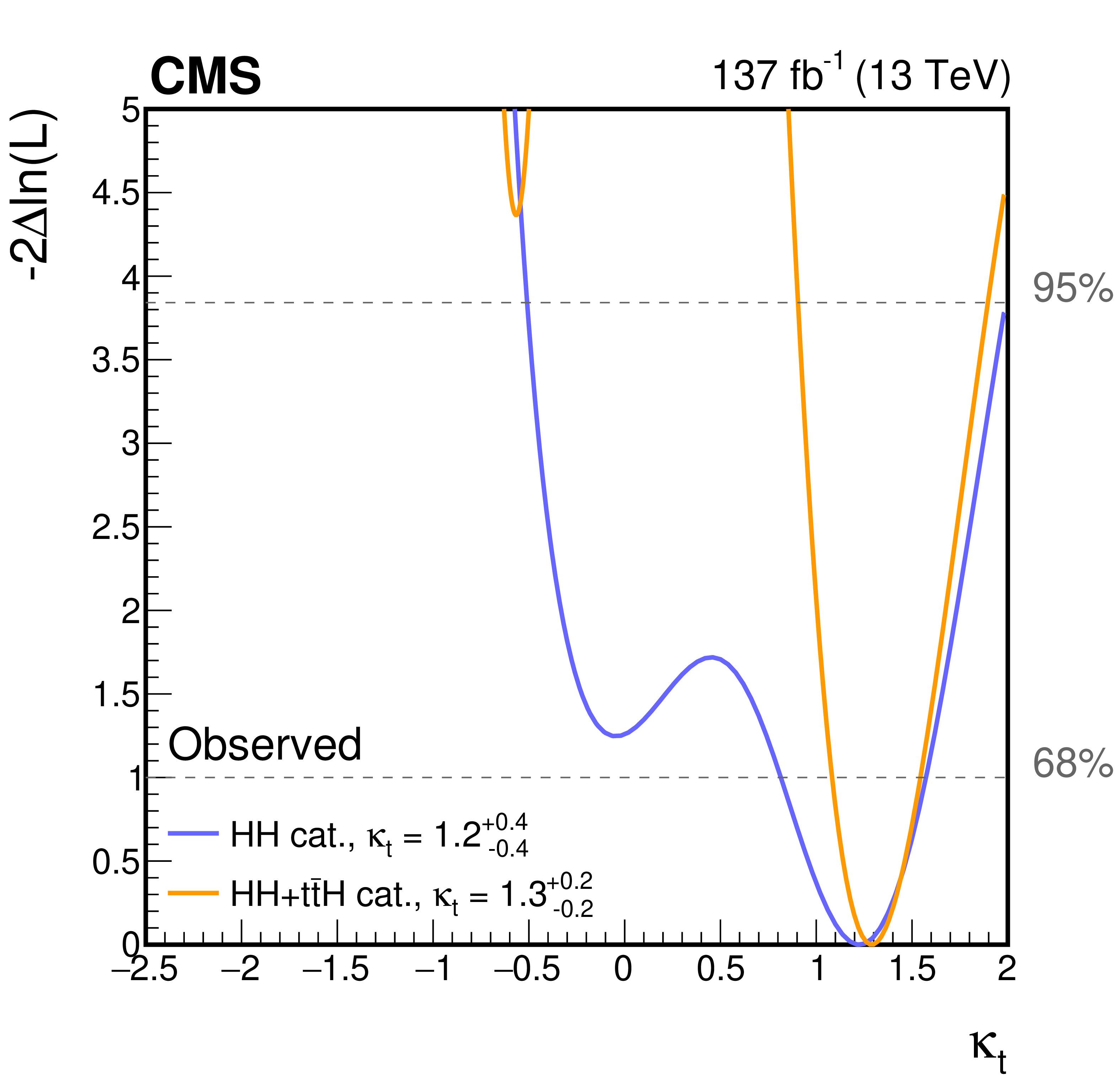
Figure 13:
Negative log-likelihood scan, as a function of $ {\kappa _{\mathrm{t}}} $, evaluated with an Asimov data set assuming the SM hypothesis (left) and the observed data (right). The 68 and 95% CL intervals are shown with the dashed gray lines. The two curves are shown for the HH (blue) and the HH+ttH (orange) analysis categories. All other couplings are fixed to their SM values. |

png pdf |
Figure 13-a:
Negative log-likelihood scan, as a function of $ {\kappa _{\mathrm{t}}} $, evaluated with an Asimov data set assuming the SM hypothesis. The 68 and 95% CL intervals are shown with the dashed gray lines. The two curves are shown for the HH (blue) and the HH+ttH (orange) analysis categories. All other couplings are fixed to their SM values. |
png pdf |
Figure 13-b:
Negative log-likelihood scan, as a function of $ {\kappa _{\mathrm{t}}} $, evaluated with an Asimov data set assuming the observed data. The 68 and 95% CL intervals are shown with the dashed gray lines. The two curves are shown for the HH (blue) and the HH+ttH (orange) analysis categories. All other couplings are fixed to their SM values. |
png pdf |
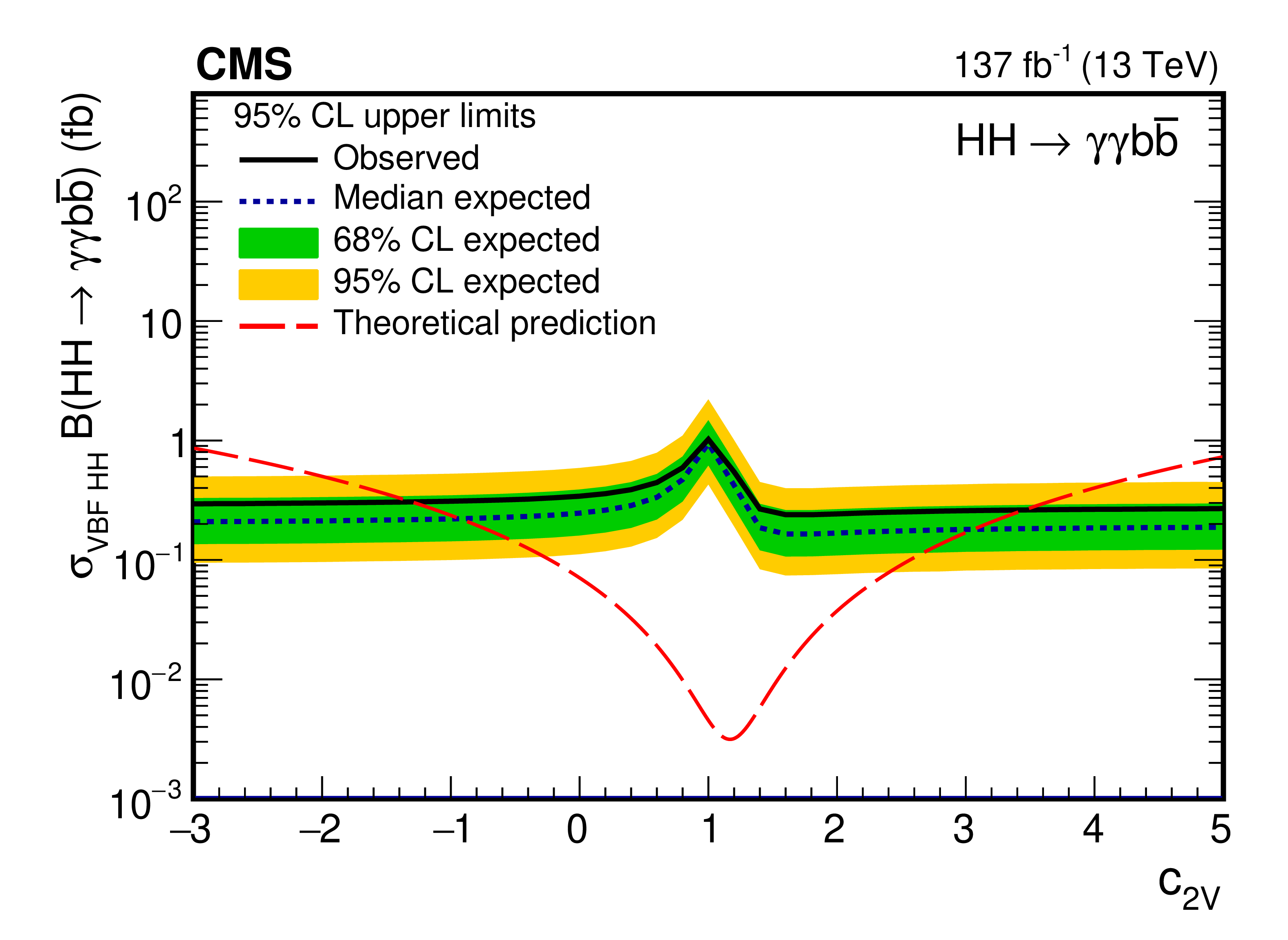
Figure 14:
Expected and observed 95% CL upper limits on the product of the VBF HH production cross section and $\mathcal {B}({{\mathrm{H} \mathrm{H}}} \to {\gamma \gamma \mathrm{b} {}\mathrm{\bar{b}}})$ obtained for different values of $ {c_{2\mathrm{V}}} $. The green and yellow bands represent, respectively, the one and two standard deviation extensions beyond the expected limit. The long-dashed red line shows the theoretical prediction. |
png pdf |
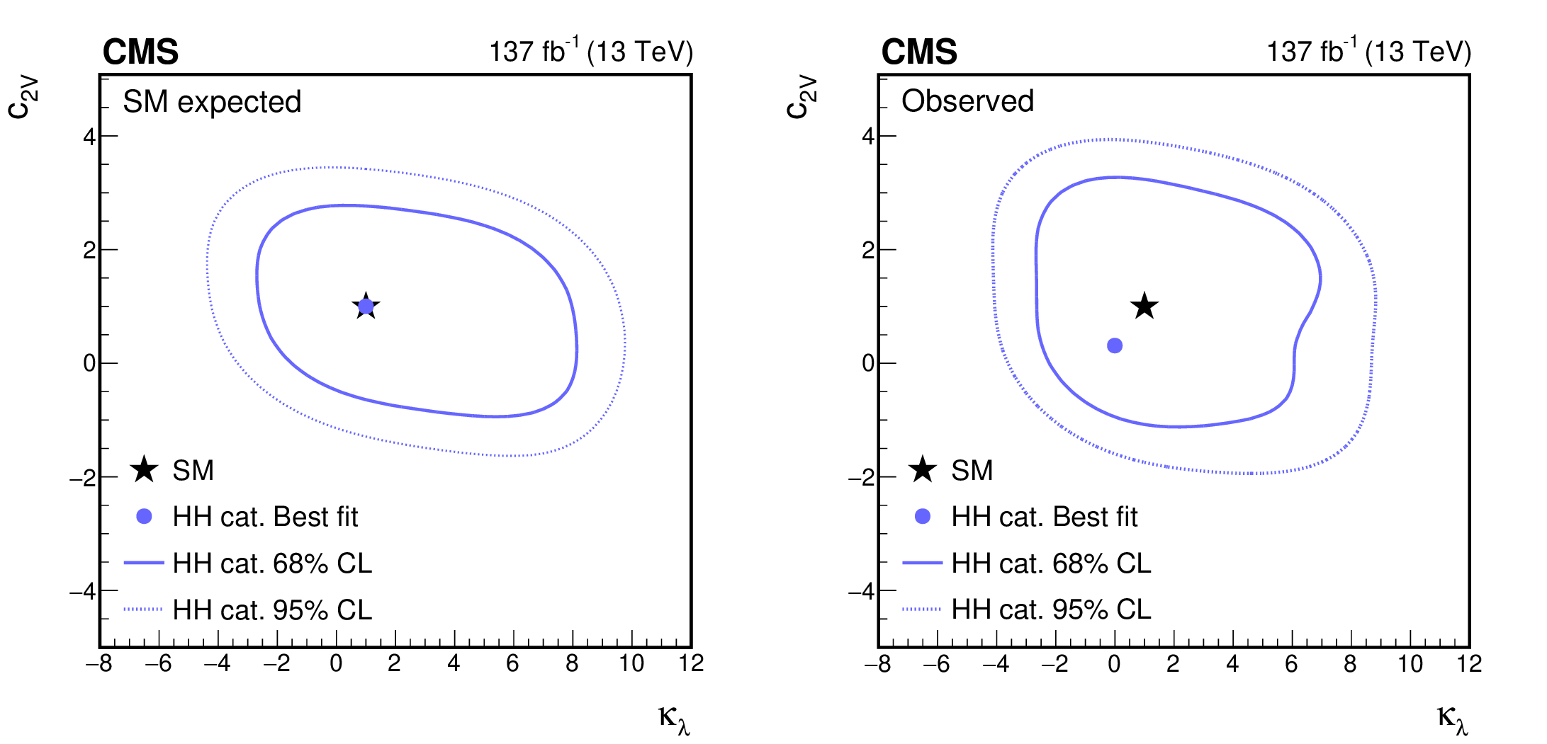
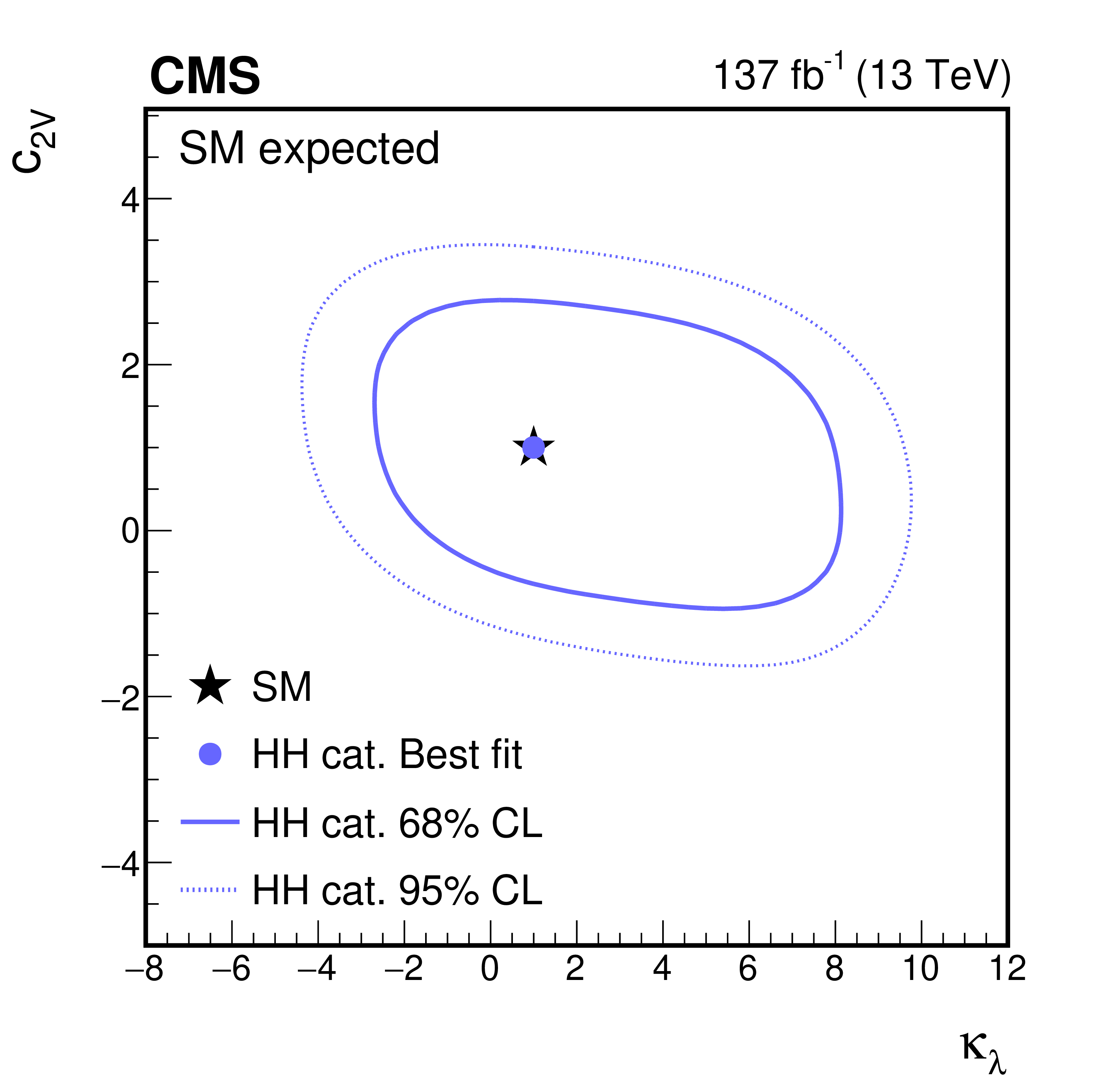
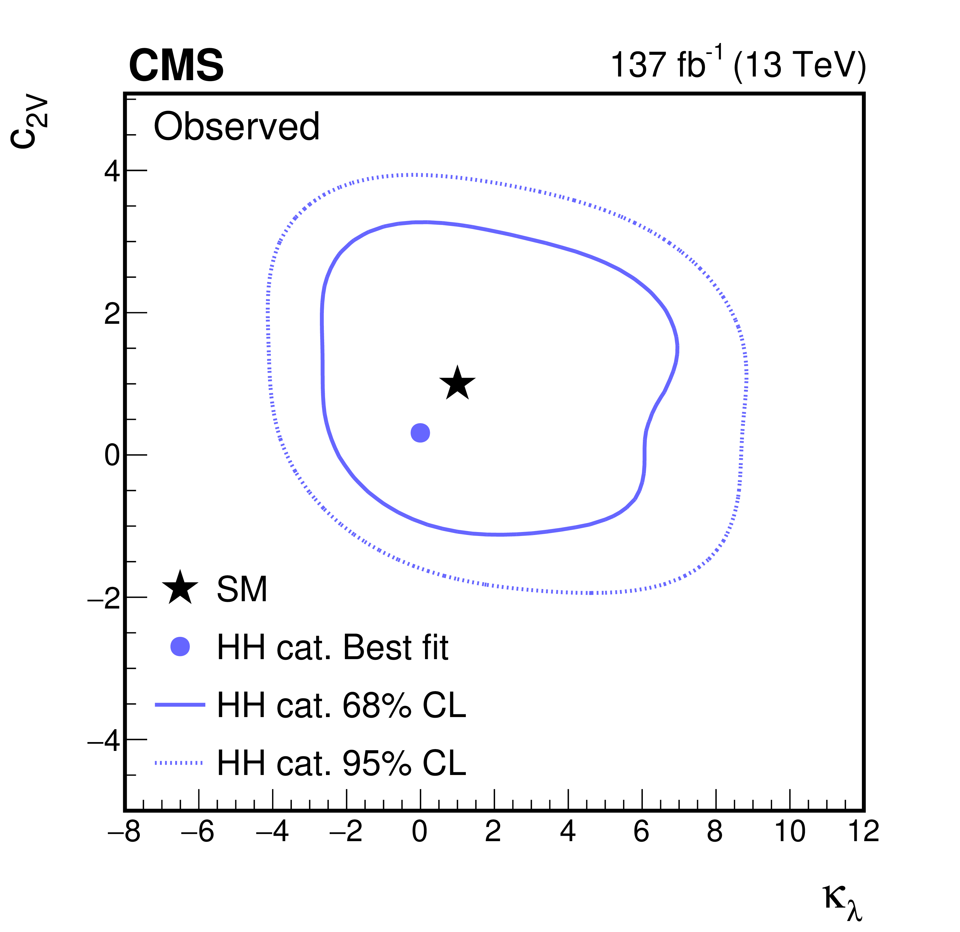
Figure 15:
Negative log-likelihood contours at 68 and 95% CL in the ($ {\kappa _{\lambda}} $, $ {c_{2\mathrm{V}}} $) plane evaluated with an Asimov data set assuming the SM hypothesis (left) and with the observed data (right). The contours are obtained using the HH analysis categories only. The best fit value ($ {\kappa _{\lambda}} $ = 0.0, $ {c_{2\mathrm{V}}} $ = 0.3) is indicated by a blue circle, and the SM prediction ($ {\kappa _{\lambda}} $ = 1.0, $ {c_{2\mathrm{V}}} $ = 1.0) by a black star. |
png pdf |
Figure 15-a:
Negative log-likelihood contours at 68 and 95% CL in the ($ {\kappa _{\lambda}} $, $ {c_{2\mathrm{V}}} $) plane evaluated with an Asimov data set assuming the SM hypothesis. The contours are obtained using the HH analysis categories only. The best fit value ($ {\kappa _{\lambda}} $ = 0.0, $ {c_{2\mathrm{V}}} $ = 0.3) is indicated by a blue circle, and the SM prediction ($ {\kappa _{\lambda}} $ = 1.0, $ {c_{2\mathrm{V}}} $ = 1.0) by a black star. |
png pdf |
Figure 15-b:
Negative log-likelihood contours at 68 and 95% CL in the ($ {\kappa _{\lambda}} $, $ {c_{2\mathrm{V}}} $) plane evaluated with an Asimov data set assuming the observed data. The contours are obtained using the HH analysis categories only. The best fit value ($ {\kappa _{\lambda}} $ = 0.0, $ {c_{2\mathrm{V}}} $ = 0.3) is indicated by a blue circle, and the SM prediction ($ {\kappa _{\lambda}} $ = 1.0, $ {c_{2\mathrm{V}}} $ = 1.0) by a black star. |
png pdf |
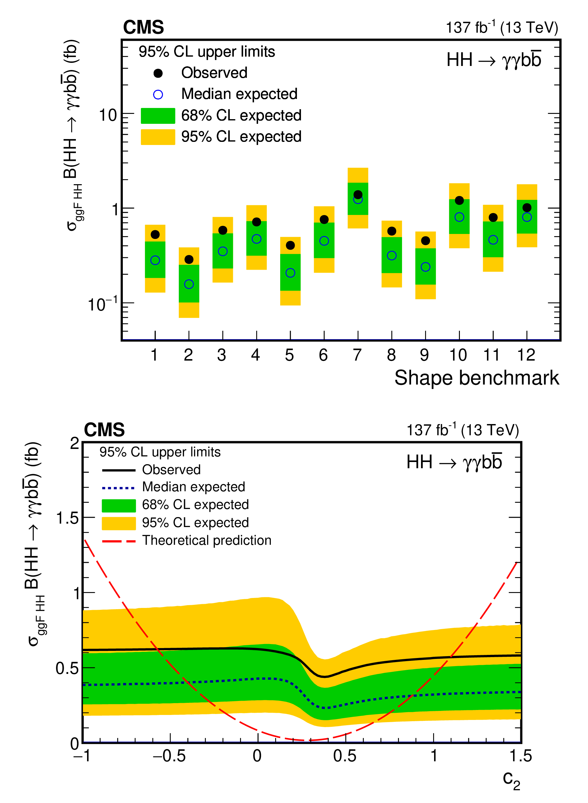
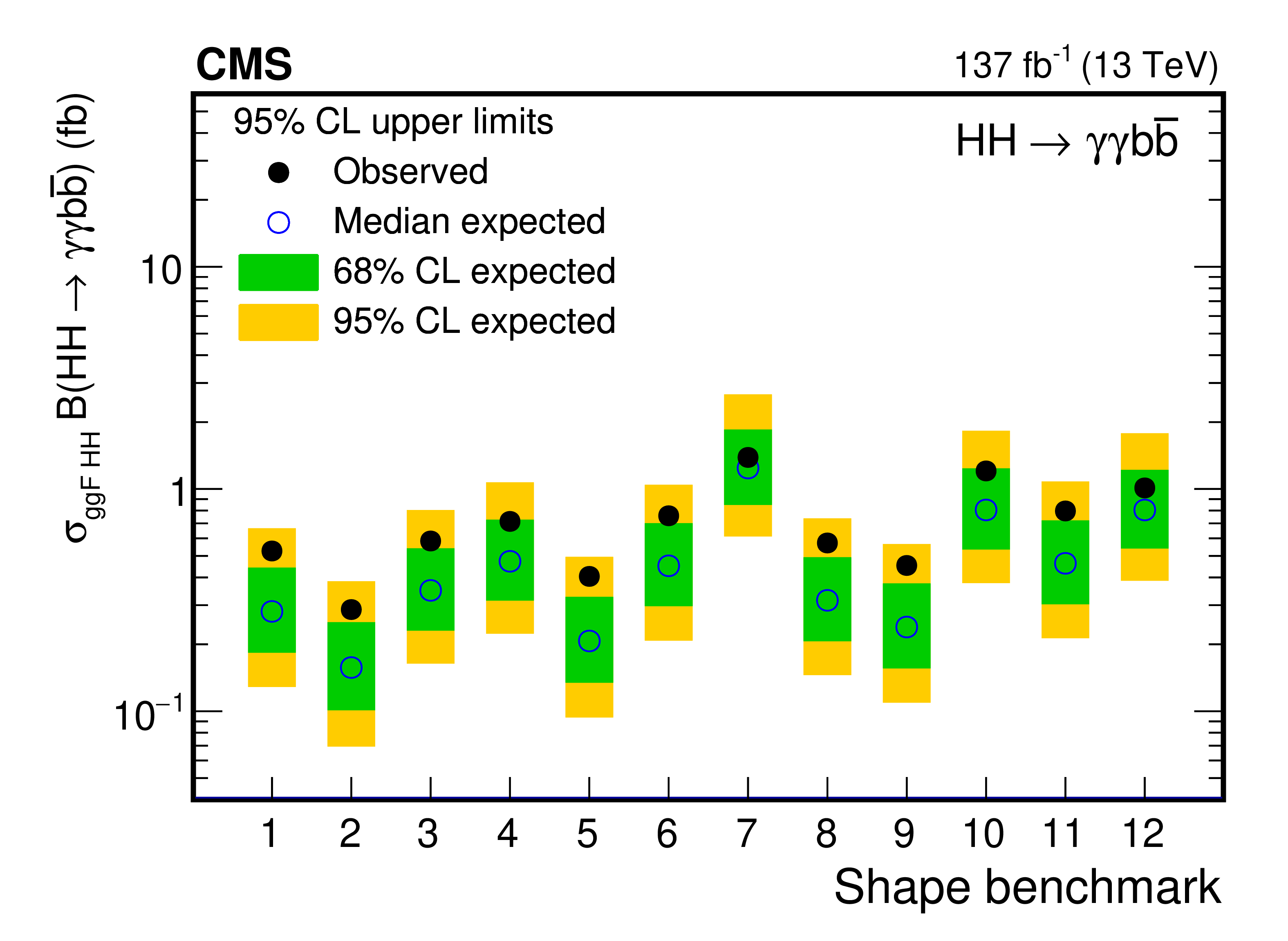
Figure 16:
Expected and observed 95% CL upper limits on the product of the ggF HH production cross section and $\mathcal {B}({{\mathrm{H} \mathrm{H}}} \to {\gamma \gamma \mathrm{b} {}\mathrm{\bar{b}}})$ obtained for different nonresonant benchmark models (defined in Table 1) (upper) and BSM coupling $ {c_2} $ (lower). In this fit, the yield of the VBF HH signal is constrained within uncertainties to the one predicted in the SM. The green and yellow bands represent, respectively, the one and two standard deviation extensions beyond the expected limit. On the lower plot the long-dashed red line shows the theoretical prediction. |
png pdf |
Figure 16-a:
Expected and observed 95% CL upper limits on the product of the ggF HH production cross section and $\mathcal {B}({{\mathrm{H} \mathrm{H}}} \to {\gamma \gamma \mathrm{b} {}\mathrm{\bar{b}}})$ obtained for different nonresonant benchmark models (defined in Table 1). In this fit, the yield of the VBF HH signal is constrained within uncertainties to the one predicted in the SM. The green and yellow bands represent, respectively, the one and two standard deviation extensions beyond the expected limit. |

png pdf |
Figure 16-b:
Expected and observed 95% CL upper limits on the product of the ggF HH production cross section and $\mathcal {B}({{\mathrm{H} \mathrm{H}}} \to {\gamma \gamma \mathrm{b} {}\mathrm{\bar{b}}})$ obtained for BSM coupling $ {c_2} $. In this fit, the yield of the VBF HH signal is constrained within uncertainties to the one predicted in the SM. The green and yellow bands represent, respectively, the one and two standard deviation extensions beyond the expected limit. The long-dashed red line shows the theoretical prediction. |
| Tables | |
png pdf |
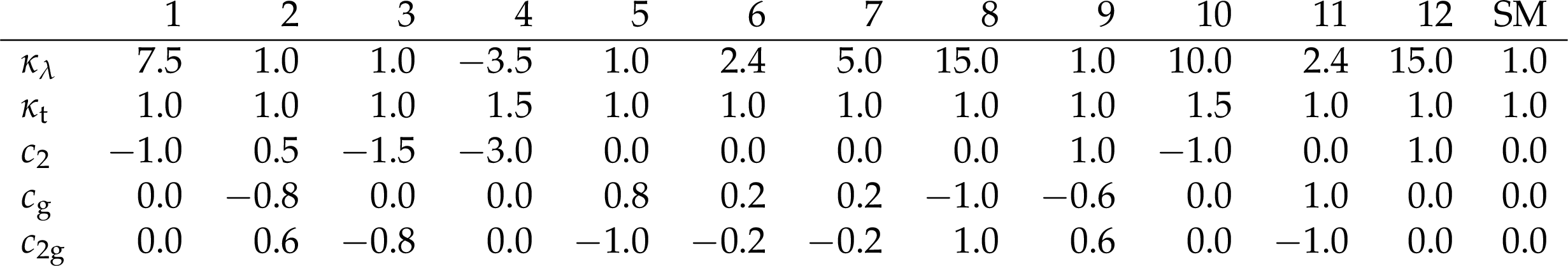
Table 1:
Coupling parameter values in the SM and in twelve BSM benchmark hypotheses identified using the method described in Ref. [43]. |

png pdf |
Table 2:
Summary of the analysis categories. Two VBF- and twelve ggF-enriched categories are defined based on the output of the MVA classifier and the mass of the Higgs boson pair system $ {\tilde{M}_{\mathrm {X}}} $. The VBF and ggF categories are mutually exclusive. |
| Summary |
|
A search for nonresonant Higgs boson pair production (HH) has been presented, where one of the Higgs bosons decays to a pair of bottom quarks and the other to a pair of photons. This search uses proton-proton collision data collected at $\sqrt{s} = $ 13 TeV by the CMS experiment at the LHC, corresponding to a total integrated luminosity of 137 fb$^{-1}$. No significant deviation from the background-only hypothesis is observed. Upper limits at 95% confidence level (CL) on the product of the HH production cross section and the branching fraction into ${\mathrm{b\bar{b}}} \gamma\gamma$ are extracted for production in the standard model (SM) and in several scenarios beyond the SM. The expected upper limit at 95% CL on ${\sigma_{\mathrm{H}\mathrm{H}}} {\mathcal{B}({{\mathrm{H}\mathrm{H}}} \to\mathrm{b\bar{b}}\gamma\gamma)}$ is 0.45 fb, corresponding to about 5.2 times the SM prediction, while the observed upper limit is 0.67 fb, corresponding to 7.7 times the expected value for the SM process. The presented search has the highest sensitivity to the SM HH production to date. Upper limits at 95% CL on the SM HH production cross section are also derived as a function of the Higgs boson self-coupling modifier ${\kappa_{\lambda}} \equiv {\lambda_{\mathrm{H}\mathrm{H}\mathrm{H}}} /{\lambda^\mathrm{SM}_{\mathrm{H}\mathrm{H}\mathrm{H}}} $ assuming that the top quark Yukawa coupling is SM-like. The coupling modifier ${\kappa_{\lambda}} $ is constrained within a range $-3.3 < \kappa_{\lambda} < 8.5$, while the expected constraint is within a range $-2.5 < \kappa_{\lambda} < 8.2$ at 95% CL. This search is combined with an analysis that targets top quark-antiquark associated production of a single Higgs boson decaying to a diphoton pair. In the scenario in which the HH signal has the properties predicted by the SM, the coupling modifier ${\kappa_{\lambda}}$ has been constrained. In addition, a simultaneous constraint on ${\kappa_{\lambda}}$ and the modifier of the coupling between the Higgs boson and the top quark ${\kappa_{\mathrm{t}}}$ is presented when both the HH and single Higgs boson processes are considered as signals. Limits are also set on the cross section of nonresonant HH production via vector boson fusion (VBF). The most stringent limit to date is set on the product of the HH VBF production cross section and the branching fraction into ${\mathrm{b\bar{b}}} \gamma\gamma$. The observed (expected) upper limit at 95% CL amounts to 1.02 (0.94) fb, corresponding to 225 (208) times the SM prediction. Limits are also set as a function of the modifier of the coupling between two vector bosons and two Higgs bosons, ${c_{2V}}$. The observed excluded region corresponds to ${c_{2V}} < -1.3$ and ${c_{2V}} > 3.5$, while the expected exclusion is ${c_{2V}} < -0.9$ and ${c_{2V}} > 3.1$. Numerous hypotheses on coupling modifiers beyond the SM have been explored, both in the context of inclusive Higgs boson pair production and for HH production via gluon-gluon fusion and VBF. The production of Higgs boson pairs was also combined with the top quark-antiquark pair associated production of a single Higgs boson. Overall, all of the results are consistent with the SM predictions. |
| Additional Figures | |
png pdf |
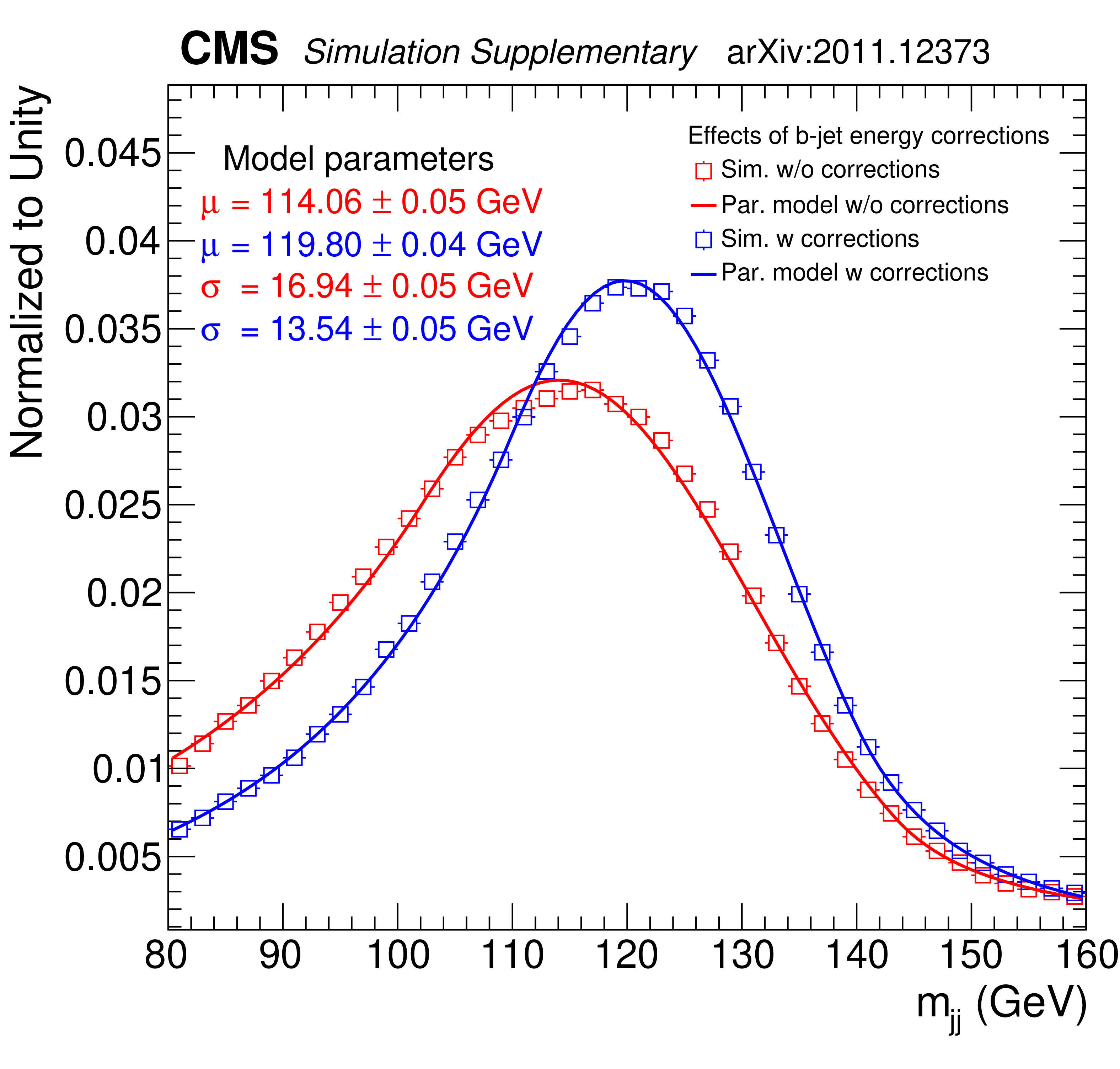
Additional Figure 1:
Impact of the b-jet energy corrections to the Higgs boson mass reconstruction obtained in the standard model process of HH production via ggF. The open squares are the distributions of the simulated di-jet invariant mass before (red) and after (blue) the application of the two-step b-jet energy regression. In both cases, the two distributions are fitted with a double sided-crystal ball parametric shape, and the average value ($\mu $) and core resolution ($\sigma $) are also shown. |
| References | ||||
| 1 | ATLAS Collaboration | Observation of a new particle in the search for the standard model Higgs boson with the ATLAS detector at the LHC | PLB 716 (2012) 1 | 1207.7214 |
| 2 | CMS Collaboration | Observation of a new boson at a mass of 125 GeV with the CMS experiment at the LHC | PLB 716 (2012) 30 | CMS-HIG-12-028 1207.7235 |
| 3 | CMS Collaboration | Observation of a new boson with mass near 125 GeV in pp collisions at $ \sqrt{s} = $ 7 and 8 TeV | JHEP 06 (2013) 081 | CMS-HIG-12-036 1303.4571 |
| 4 | F. Englert and R. Brout | Broken symmetries and the masses of gauge bosons | PRL 13 (1964) 321 | |
| 5 | P. W. Higgs | Broken symmetries and the masses of gauge bosons | PRL 13 (1964) 508 | |
| 6 | M. Grazzini et al. | Higgs boson pair production at NNLO with top quark mass effects | JHEP 05 (2018) 059 | 1803.02463 |
| 7 | S. Dawson, S. Dittmaier, and M. Spira | Neutral Higgs boson pair production at hadron colliders: QCD corrections | PRD 58 (1998) 115012 | hep-ph/9805244 |
| 8 | S. Borowka et al. | Higgs boson pair production in gluon fusion at next-to-leading order with full top-quark mass dependence | PRL 117 (2016) 012001 | 1604.06447 |
| 9 | J. Baglio et al. | Gluon fusion into Higgs pairs at NLO QCD and the top mass scheme | EPJC 79 (2019) 459 | 1811.05692 |
| 10 | D. de Florian and J. Mazzitelli | Higgs boson pair production at next-to-next-to-leading order in QCD | PRL 111 (2013) 201801 | 1309.6594 |
| 11 | D. Y. Shao, C. S. Li, H. T. Li, and J. Wang | Threshold resummation effects in Higgs boson pair production at the LHC | JHEP 07 (2013) 169 | 1301.1245 |
| 12 | D. de Florian and J. Mazzitelli | Higgs pair production at next-to-next-to-leading logarithmic accuracy at the LHC | JHEP 09 (2015) 053 | 1505.07122 |
| 13 | F. A. Dreyer and A. Karlberg | Vector-boson fusion Higgs pair production at N$ ^3 $LO | PRD 98 (2018) 114016 | 1811.07906 |
| 14 | J. Baglio et al. | The measurement of the Higgs self-coupling at the LHC: theoretical status | JHEP 04 (2013) 151 | 1212.5581 |
| 15 | L.-S. Ling et al. | NNLO QCD corrections to Higgs pair production via vector boson fusion at hadron colliders | PRD 89 (2014) 073001 | 1401.7754 |
| 16 | D. de Florian et al. | Handbook of LHC Higgs cross sections: 4. Deciphering the nature of the Higgs sector | CERN-2017-002-M | 1610.07922 |
| 17 | CMS Collaboration | Combined measurements of Higgs boson couplings in proton-proton collisions at $ \sqrt{s}=13 \text {Te}\text {V} $ | EPJC 79 (2019) 421 | CMS-HIG-17-031 1809.10733 |
| 18 | ATLAS Collaboration | Search for Higgs boson pair production in the $ \gamma\gamma b\bar{b} $ final state using pp collision data at $ \sqrt{s}= $ 8 TeV from the ATLAS detector | PRL 114 (2015) 081802 | 1406.5053 |
| 19 | ATLAS Collaboration | Search for Higgs boson pair production in the $ b\bar{b}b\bar{b} $ final state from pp collisions at $ \sqrt{s} = $ 8 TeV with the ATLAS detector | EPJC 75 (2015) 412 | 1506.00285 |
| 20 | ATLAS Collaboration | Searches for Higgs boson pair production in the $ HH\to bb\tau\tau$, $\gamma\gamma WW^*$, $\gamma\gamma $bb, bbbb channels with the ATLAS detector | PRD 92 (2015) 092004 | 1509.04670 |
| 21 | ATLAS Collaboration | Search for pair production of Higgs bosons in the $ \mathrm{b\bar{b}}\mathrm{b\bar{b}} $ final state using proton--proton collisions at $ \sqrt{s} = $ 13 TeV with the ATLAS detector | PRD 94 (2016) 052002 | 1606.04782 |
| 22 | ATLAS Collaboration | Combination of searches for Higgs boson pairs in pp collisions at $ \sqrt{s} = $ 13 TeV with the ATLAS detector | PLB 800 (2020) 135103 | 1906.02025 |
| 23 | CMS Collaboration | Search for two Higgs bosons in final states containing two photons and two bottom quarks in proton-proton collisions at 8 TeV | PRD 94 (2016) 052012 | CMS-HIG-13-032 1603.06896 |
| 24 | ATLAS Collaboration | Search for Higgs boson pair production in the $ \gamma\gamma b\bar{b} $ final state with 13 TeV pp collision data collected by the ATLAS experiment | JHEP 11 (2018) 040 | 1807.04873 |
| 25 | CMS Collaboration | Search for Higgs boson pair production in the $ \mathrm{b\bar{b}}\tau\tau $ final state in proton-proton collisions at $ \sqrt{s}= $ 8 TeV | PRD 96 (2017) 072004 | CMS-HIG-15-013 1707.00350 |
| 26 | CMS Collaboration | Search for Higgs boson pair production in events with two bottom quarks and two tau leptons in proton--proton collisions at $ \sqrt s = $ 13 TeV | PLB 778 (2018) 101 | CMS-HIG-17-002 1707.02909 |
| 27 | CMS Collaboration | Search for resonant and nonresonant Higgs boson pair production in the $ \mathrm{b\bar{b}}\ell\nu\ell\nu $ final state in proton-proton collisions at $ \sqrt{s}= $ 13 TeV | JHEP 01 (2018) 054 | CMS-HIG-17-006 1708.04188 |
| 28 | CMS Collaboration | Search for Higgs boson pair production in the $ \gamma\gamma\mathrm{b\overline{b}} $ final state in pp collisions at $ \sqrt{s}= $ 13 TeV | PLB 788 (2019) 7 | CMS-HIG-17-008 1806.00408 |
| 29 | CMS Collaboration | Combination of searches for Higgs boson pair production in proton-proton collisions at $ \sqrt{s} = $ 13 TeV | PRL 122 (2019) 121803 | CMS-HIG-17-030 1811.09689 |
| 30 | ATLAS Collaboration | Search for the $ HH \rightarrow b \bar{b} b \bar{b} $ process via vector-boson fusion production using proton-proton collisions at $ \sqrt{s} = $ 13 TeV with the ATLAS detector | JHEP 07 (2020) 108 | 2001.05178 |
| 31 | CMS Collaboration | Measurements of $ \mathrm{t\bar{t}H} $ production and the CP structure of the Yukawa interaction between the Higgs boson and top quark in the diphoton decay channel | PRL 125 (2020) 061801 | CMS-HIG-19-013 2003.10866 |
| 32 | F. Maltoni, D. Pagani, A. Shivaji, and X. Zhao | Trilinear Higgs coupling determination via single-Higgs differential measurements at the LHC | EPJC 77 (2017) 887 | 1709.08649 |
| 33 | G. Degrassi, P. P. Giardino, F. Maltoni, and D. Pagani | Probing the Higgs self coupling via single Higgs production at the LHC | JHEP 12 (2016) 080 | 1607.04251 |
| 34 | CMS Collaboration | The CMS experiment at the CERN LHC | JINST 3 (2008) S08004 | CMS-00-001 |
| 35 | CMS Collaboration | The CMS trigger system | JINST 12 (2017) P01020 | CMS-TRG-12-001 1609.02366 |
| 36 | CMS Trigger, Data Acquisition Group Collaboration | The CMS high level trigger | EPJC 46 (2006) 605 | hep-ex/0512077 |
| 37 | CMS Collaboration | Particle-flow reconstruction and global event description with the cms detector | JINST 12 (2017) P10003 | CMS-PRF-14-001 1706.04965 |
| 38 | M. Cacciari, G. P. Salam, and G. Soyez | The anti-$ {k_{\mathrm{T}}} $ jet clustering algorithm | JHEP 04 (2008) 063 | 0802.1189 |
| 39 | M. Cacciari, G. P. Salam, and G. Soyez | FastJet user manual | EPJC 72 (2012) 1896 | 1111.6097 |
| 40 | CMS Collaboration | Jet energy scale and resolution in the CMS experiment in pp collisions at 8 TeV | JINST 12 (2017) P02014 | CMS-JME-13-004 1607.03663 |
| 41 | CMS Collaboration | Performance of missing transverse momentum reconstruction in proton-proton collisions at $ \sqrt{s} = $ 13 TeV using the CMS detector | JINST 14 (2019) P07004 | CMS-JME-17-001 1903.06078 |
| 42 | G. F. Giudice, C. Grojean, A. Pomarol, and R. Rattazzi | The strongly-interacting light Higgs | JHEP 06 (2007) 045 | hep-ph/0703164 |
| 43 | A. Carvalho et al. | Higgs pair production: Choosing benchmarks with cluster analysis | JHEP 04 (2016) 126 | 1507.02245 |
| 44 | CMS Collaboration | Measurements of Higgs boson properties in the diphoton decay channel in proton-proton collisions at $ \sqrt{s} = $ 13 TeV | JHEP 11 (2018) 185 | CMS-HIG-16-040 1804.02716 |
| 45 | E. Bagnaschi, G. Degrassi, P. Slavich, and A. Vicini | Higgs production via gluon fusion in the POWHEG approach in the SM and in the MSSM | JHEP 02 (2012) 088 | 1111.2854 |
| 46 | G. Heinrich et al. | NLO predictions for Higgs boson pair production with full top quark mass dependence matched to parton showers | JHEP 08 (2017) 088 | 1703.09252 |
| 47 | G. Heinrich et al. | Probing the trilinear Higgs boson coupling in di-Higgs production at NLO QCD including parton shower effects | JHEP 06 (2019) 066 | 1903.08137 |
| 48 | S. P. Jones and S. Kuttimalai | Parton shower and NLO-matching uncertainties in Higgs boson pair production | JHEP 02 (2018) 176 | 1711.03319 |
| 49 | G. Buchalla et al. | Higgs boson pair production in non-linear Effective Field Theory with full $ m_t $-dependence at NLO QCD | JHEP 09 (2018) 057 | 1806.05162 |
| 50 | J. Alwall et al. | The automated computation of tree-level and next-to-leading order differential cross sections, and their matching to parton shower simulations | JHEP 07 (2014) 079 | 1405.0301 |
| 51 | B. Hespel, D. Lopez-Val, and E. Vryonidou | Higgs pair production via gluon fusion in the two-Higgs-doublet model | JHEP 09 (2014) 124 | 1407.0281 |
| 52 | R. Frederix et al. | Higgs pair production at the LHC with NLO and parton-shower effects | PLB 732 (2014) 142 | 1401.7340 |
| 53 | T. Gleisberg et al. | Event generation with SHERPA 1.1 | JHEP 02 (2009) 007 | 0811.4622 |
| 54 | T. Sjostrand et al. | An introduction to PYTHIA 8.2 | CPC 191 (2015) 159 | 1410.3012 |
| 55 | P. Nason | A new method for combining NLO QCD with shower Monte Carlo algorithms | JHEP 11 (2004) 040 | hep-ph/0409146 |
| 56 | S. Frixione, P. Nason, and C. Oleari | Matching NLO QCD computations with Parton Shower simulations: the POWHEG method | JHEP 11 (2007) 070 | 0709.2092 |
| 57 | S. Alioli, P. Nason, C. Oleari, and E. Re | A general framework for implementing NLO calculations in shower Monte Carlo programs: the POWHEG BOX | JHEP 06 (2010) 043 | 1002.2581 |
| 58 | CMS Collaboration | Event generator tunes obtained from underlying event and multiparton scattering measurements | EPJC 76 (2016) 155 | CMS-GEN-14-001 1512.00815 |
| 59 | CMS Collaboration | Extraction and validation of a new set of CMS PYTHIA8 tunes from underlying-event measurements | EPJC 80 (2020) 4 | CMS-GEN-17-001 1903.12179 |
| 60 | NNPDF Collaboration | Parton distributions for the LHC Run II | JHEP 04 (2015) 040 | 1410.8849 |
| 61 | NNPDF Collaboration | Parton distributions from high-precision collider data | EPJC 77 (2017) 663 | 1706.00428 |
| 62 | S. Carrazza, J. I. Latorre, J. Rojo, and G. Watt | A compression algorithm for the combination of PDF sets | EPJC 75 (2015) 474 | 1504.06469 |
| 63 | J. Butterworth et al. | PDF4LHC recommendations for LHC Run II | JPG 43 (2016) 023001 | 1510.03865 |
| 64 | S. Dulat et al. | New parton distribution functions from a global analysis of quantum chromodynamics | PRD 93 (2016) 033006 | 1506.07443 |
| 65 | L. A. Harland-Lang, A. D. Martin, P. Motylinski, and R. S. Thorne | Parton distributions in the LHC era: MMHT 2014 PDFs | EPJC 75 (2015) 204 | 1412.3989 |
| 66 | GEANT4 Collaboration | GEANT4---a simulation toolkit | NIMA 506 (2003) 250 | |
| 67 | B. Cabouat and T. Sjostrand | Some dipole shower studies | EPJC 78 (2018) 226 | 1710.00391 |
| 68 | B. Jager et al. | Parton-shower effects in Higgs production via vector-boson fusion | EPJC 80 (2020) 756 | 2003.12435 |
| 69 | E. Spyromitros-Xioufis, G. Tsoumakas, W. Groves, and I. Vlahavas | Multi-target regression via input space expansion: treating targets as inputs | Machine Learning 104 (2016) 55 | 1211.6581 |
| 70 | CMS Collaboration | Observation of the diphoton decay of the Higgs boson and measurement of its properties | EPJC 74 (2014) 3076 | CMS-HIG-13-001 1407.0558 |
| 71 | B. Vormwald | The CMS phase-1 pixel detector - experience and lessons learned from two years of operation | JINST 14 (2019) C07008 | |
| 72 | CMS Collaboration | Pileup mitigation at CMS in 13 TeV data | JINST 15 (2020) P09018 | CMS-JME-18-001 2003.00503 |
| 73 | CMS Collaboration | Performance of the DeepJet b tagging algorithm using 41.9 fb$^{-1} $ of data from proton-proton collisions at 13 TeV with Phase 1 CMS detector | CDS | |
| 74 | E. Bols et al. | Jet flavour classification using DeepJet | Submitted to JINST | 2008.10519 |
| 75 | CMS Collaboration | Determination of jet energy calibration and transverse momentum resolution in CMS | JINST 6 (2011) P11002 | CMS-JME-10-011 1107.4277 |
| 76 | CMS Collaboration | A deep neural network for simultaneous estimation of b jet energy and resolution | Comput. Softw. Big Sci. 4 (2020) 10 | CMS-HIG-18-027 1912.06046 |
| 77 | N. Kumar and S. P. Martin | LHC search for di-Higgs decays of stoponium and other scalars in events with two photons and two bottom jets | PRD 90 (2014) 055007 | 1404.0996 |
| 78 | S. Hochreiter and J. Schmidhuber | Long short-term memory | Neur. Comput. 9 (1997) 1735 | |
| 79 | T. Q. Nguyen et al. | Topology classification with deep learning to improve real-time event selection at the LHC | Comput. Softw. Big Sci. 3 (2019) 12 | 1807.00083 |
| 80 | F. Chollet et al. | Keras | link | |
| 81 | M. Abadi et al. | TensorFlow: Large-scale machine learning on heterogeneous systems | 2015 Software available from tensorflow.org. \url http://tensorflow.org/ | |
| 82 | J. C. Collins and D. E. Soper | Angular distribution of dileptons in high-energy hadron collisions | PRD 16 (Oct, 1977) 2219 | |
| 83 | T. Chen and C. Guestrin | XGBoost: A scalable tree boosting system | in Proceedings of the 22nd ACM SIGKDD International Conference on Knowledge Discovery and Data Mining, KDD, p. 785 ACM, New York, NY, USA | |
| 84 | T. Hastie, R. Tibshirani, and J. Friedman | The elements of statistical learning | Springer-Verlag New York, 2nd edition | |
| 85 | CMS Collaboration | Performance of quark/gluon discrimination in 8 TeV pp data | CMS-PAS-JME-13-002 | CMS-PAS-JME-13-002 |
| 86 | CMS Collaboration | Jet algorithms performance in 13 TeV data | CMS-PAS-JME-16-003 | CMS-PAS-JME-16-003 |
| 87 | CMS Collaboration | Search for direct production of supersymmetric partners of the top quark in the all-jets final state in proton-proton collisions at $ \sqrt{s}= $ 13 TeV | JHEP 10 (2017) 005 | CMS-SUS-16-049 1707.03316 |
| 88 | M. J. Oreglia | A study of the reactions $\psi' \to \gamma\gamma \psi$ | PhD thesis, Stanford University, 1980 SLAC Report SLAC-R-236, see A | |
| 89 | P. D. Dauncey, M. Kenzie, N. Wardle, and G. J. Davies | Handling uncertainties in background shapes: the discrete profiling method | JINST 10 (2015) P04015 | 1408.6865 |
| 90 | CMS Collaboration | Performance of photon reconstruction and identification with the CMS detector in proton-proton collisions at $ \sqrt{s} = $ 8 TeV | JINST 10 (2015) P08010 | CMS-EGM-14-001 1502.02702 |
| 91 | CMS Collaboration | Identification of heavy-flavour jets with the CMS detector in pp collisions at 13 TeV | JINST 13 (2018) P05011 | CMS-BTV-16-002 1712.07158 |
| 92 | CMS Collaboration | Measurement of the inclusive $ W $ and $ Z $ production cross sections in pp collisions at $ \sqrt{s}= $ 7 TeV | JHEP 10 (2011) 132 | CMS-EWK-10-005 1107.4789 |
| 93 | CMS Collaboration | CMS luminosity measurements for the 2016 data-taking period | CMS-PAS-LUM-17-001 | CMS-PAS-LUM-17-001 |
| 94 | CMS Collaboration | CMS luminosity measurement for the 2017 data-taking period at $ \sqrt{s} = $ 13 TeV | CMS-PAS-LUM-17-004 | CMS-PAS-LUM-17-004 |
| 95 | CMS Collaboration | CMS luminosity measurement for the 2018 data-taking period at $ \sqrt{s} = $ 13 TeV | CMS-PAS-LUM-18-002 | CMS-PAS-LUM-18-002 |
| 96 | T. Junk | Confidence level computation for combining searches with small statistics | NIMA 434 (1999) 435 | hep-ex/9902006 |
| 97 | A. L. Read | Presentation of search results: the CL$ _s $ technique | JPG 28 (2002) 2693 | |
| 98 | G. Cowan, K. Cranmer, E. Gross, and O. Vitells | Asymptotic formulae for likelihood-based tests of new physics | EPJC 71 (2011) 1554 | 1007.1727 |
| 99 | ATLAS and CMS Collaborations | Procedure for the LHC Higgs boson search combination in summer 2011 | CMS-NOTE-2011-005 | |
| 100 | CMS Collaboration | A measurement of the Higgs boson mass in the diphoton decay channel | PLB 805 (2020) 135425 | CMS-HIG-19-004 2002.06398 |
| 101 | CMS Collaboration | Measurement of the Higgs boson production rate in association with top quarks in final states with electrons, muons, and hadronically decaying tau leptons at $ \sqrt{s} = $ 13 TeV | Submitted to EPJC | CMS-HIG-19-008 2011.03652 |
|
|
Compact Muon Solenoid LHC, CERN |
|

|

|

|

|

|