

Compact Muon Solenoid
LHC, CERN
| CMS-HIG-20-001 ; CERN-EP-2023-270 | ||
| Measurement of simplified template cross sections of the Higgs boson produced in association with W or Z bosons in the H $ \to \mathrm{b}\overline{\mathrm{b}} $ decay channel in proton-proton collisions at $ \sqrt{s}= $ 13 TeV | ||
| CMS Collaboration | ||
| 10 December 2023 | ||
| Accepted for publication in Phys. Rev. D | ||
| Abstract: Differential cross sections are measured for the standard model Higgs boson produced in association with vector bosons (W, Z) and decaying to a pair of b quarks. Measurements are performed within the framework of the simplified template cross sections. The analysis relies on the leptonic decays of the W and Z bosons, resulting in final states with 0, 1, or 2 electrons or muons. The Higgs boson candidates are either reconstructed from pairs of resolved b-tagged jets, or from single large distance parameter jets containing the particles arising from two b quarks. Proton-proton collision data at $ \sqrt{s}= $ 13 TeV, collected by the CMS experiment in 2016-2018 and corresponding to a total integrated luminosity of 138 fb$ ^{-1} $, are analyzed. The inclusive signal strength, defined as the product of the observed production cross section and branching fraction relative to the standard model expectation, combining all analysis categories, is found to be $ \mu= $ 1.15 $ ^{+0.22}_{-0.20} $. This corresponds to an observed (expected) significance of 6.3 (5.6) standard deviations. | ||
| Links: e-print arXiv:2312.07562 [hep-ex] (PDF) ; CDS record ; inSPIRE record ; HepData record ; CADI line (restricted) ; | ||
| Figures & Tables | Summary | Additional Figures | References | CMS Publications |
|---|
| Figures | |

png pdf |
Figure 1:
Overview of the STXS bins for the three VH production modes [29]. The vertical axis reflects the $ p_{\mathrm{T}}(\mathrm{V}) $ bin ranges and the horizontal axis the number of additional jets. The general bin definitions are indicated by the green boxes. No distinction is made between gluon- and quark-induced production modes in the analysis. As mentioned in Section 5.1, some STXS bins are not explicitly targeted by the analysis: contributions from these bins are fixed to their SM expectations. |

png pdf |
Figure 2:
Dijet invariant mass distributions in samples of simulated (2017 simulation) signal events passing the 2-lepton channel requirements without any additional recoiling jet. Distributions are shown without the usage of the FSR recovery algorithm (purple triangles), before (red triangles) and after (blue squares) the energy corrections from the b jet regression are applied, and when a kinematic fit procedure (green circles) is used in addition to them. The fitted mean and width of the core of the distribution, obtained by fitting a Bukin function [72], are displayed in the figure. The statistical uncertainties are smaller than the marker height. |

png pdf |
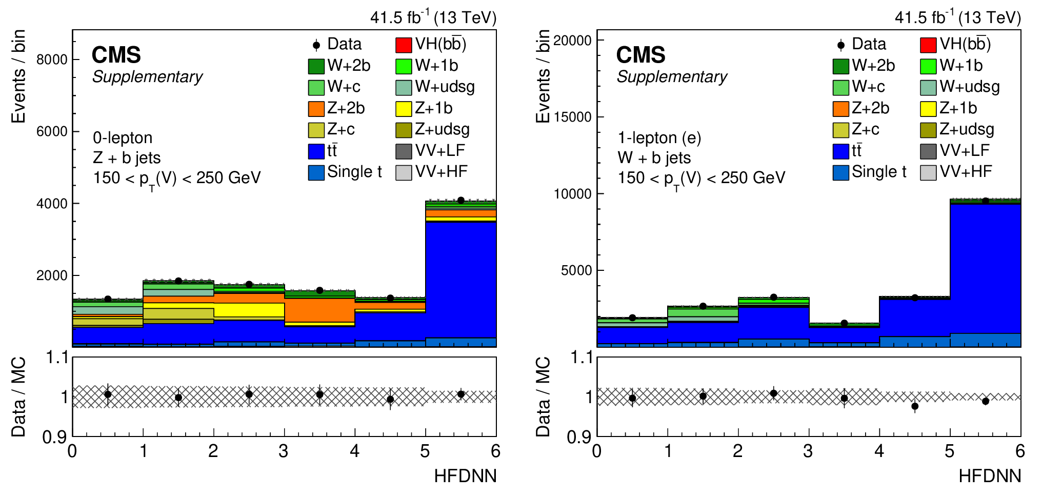
Figure 3:
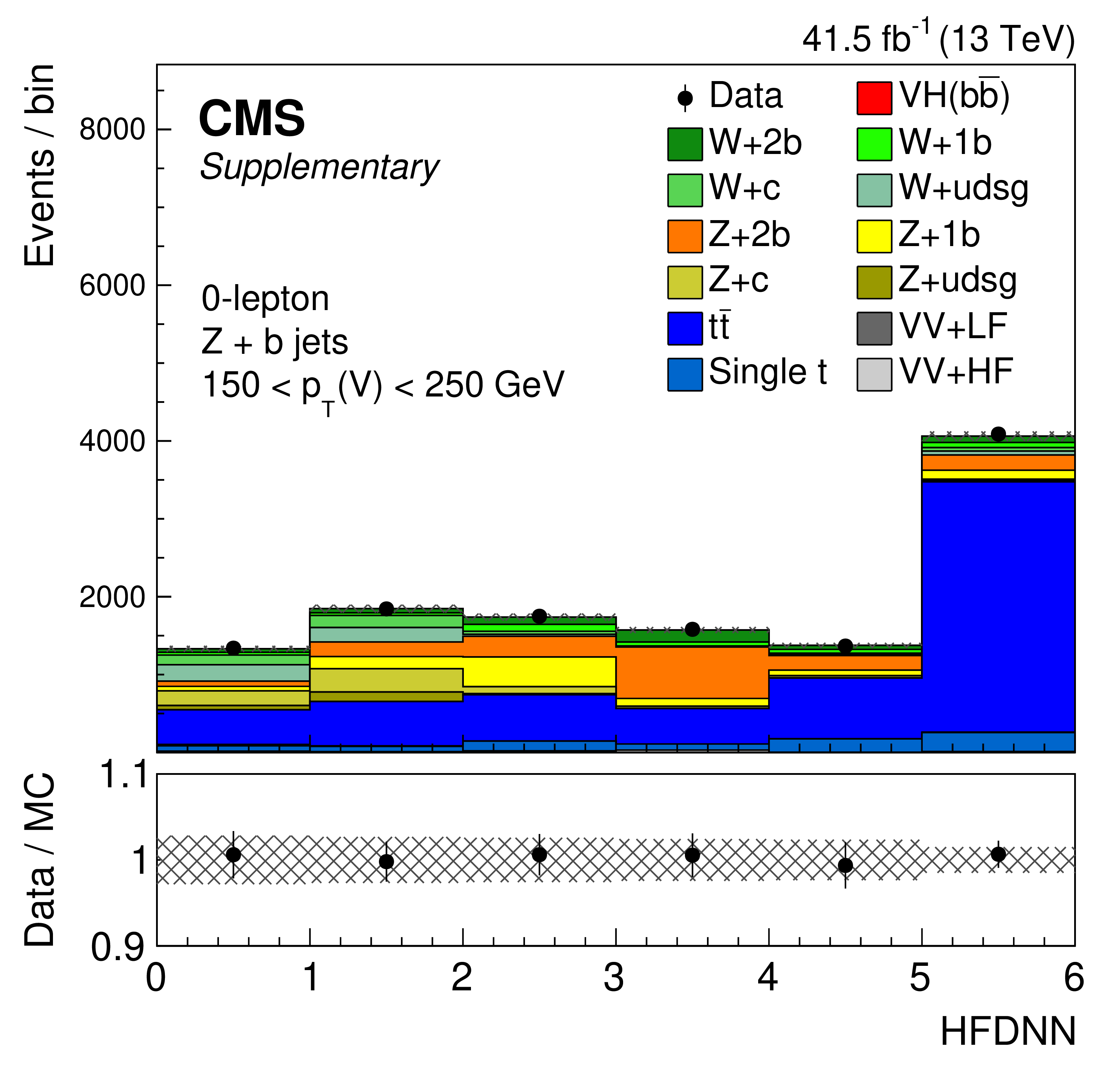
Distribution of the HFDNN scores in the 0-lepton (left) and 1-lepton (right) heavy-flavor CRs for the 2016 data set, after the fit to data. The output nodes target enrichment in the V+light-quark (first bin), V+c (second bin), V+b (third bin), V+$ \mathrm{b}\overline{\mathrm{b}} $ (fourth bin), single top quark (fifth bin), and $ {\mathrm{t}\overline{\mathrm{t}}} $ (sixth bin) backgrounds. The lower plots display the ratio of the data to the MC expectations. The vertical bars on the points represent the statistical uncertainty in the ratio, and the hatched area shows the MC uncertainty. |

png pdf |
Figure 3-a:
Distribution of the HFDNN scores in the 0-lepton (left) and 1-lepton (right) heavy-flavor CRs for the 2016 data set, after the fit to data. The output nodes target enrichment in the V+light-quark (first bin), V+c (second bin), V+b (third bin), V+$ \mathrm{b}\overline{\mathrm{b}} $ (fourth bin), single top quark (fifth bin), and $ {\mathrm{t}\overline{\mathrm{t}}} $ (sixth bin) backgrounds. The lower plots display the ratio of the data to the MC expectations. The vertical bars on the points represent the statistical uncertainty in the ratio, and the hatched area shows the MC uncertainty. |

png pdf |
Figure 3-b:
Distribution of the HFDNN scores in the 0-lepton (left) and 1-lepton (right) heavy-flavor CRs for the 2016 data set, after the fit to data. The output nodes target enrichment in the V+light-quark (first bin), V+c (second bin), V+b (third bin), V+$ \mathrm{b}\overline{\mathrm{b}} $ (fourth bin), single top quark (fifth bin), and $ {\mathrm{t}\overline{\mathrm{t}}} $ (sixth bin) backgrounds. The lower plots display the ratio of the data to the MC expectations. The vertical bars on the points represent the statistical uncertainty in the ratio, and the hatched area shows the MC uncertainty. |

png pdf |
Figure 4:
Correlation matrix of the parameters of interest in the STXS measurement. The vector boson momenta have units of GeV. |

png pdf |
Figure 5:
Contributions of the different STXS signal bins as a fraction of the total signal yield in each SR. The vector boson momenta have units of GeV. |

png pdf |
Figure 6:
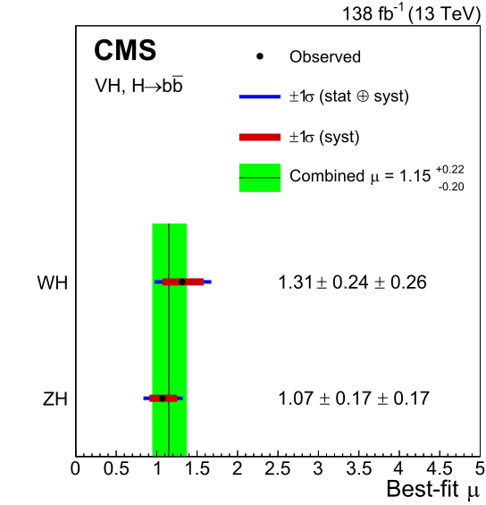
Signal strengths (points) for the 0-, 1-, and 2-lepton channels (left) and the ZH and WH production modes (right). The horizontal red and blue bars on the points represent the systematic and total uncertainties, respectively. The combined inclusive signal strength is shown by the vertical line, with the green band giving the 68% confidence interval. The results combine the 2016-2018 data-taking years. The first and the second uncertainty values correspond to the statistical and systematic uncertainties, respectively. |

png pdf |
Figure 6-a:
Signal strengths (points) for the 0-, 1-, and 2-lepton channels (left) and the ZH and WH production modes (right). The horizontal red and blue bars on the points represent the systematic and total uncertainties, respectively. The combined inclusive signal strength is shown by the vertical line, with the green band giving the 68% confidence interval. The results combine the 2016-2018 data-taking years. The first and the second uncertainty values correspond to the statistical and systematic uncertainties, respectively. |
png pdf |
Figure 6-b:
Signal strengths (points) for the 0-, 1-, and 2-lepton channels (left) and the ZH and WH production modes (right). The horizontal red and blue bars on the points represent the systematic and total uncertainties, respectively. The combined inclusive signal strength is shown by the vertical line, with the green band giving the 68% confidence interval. The results combine the 2016-2018 data-taking years. The first and the second uncertainty values correspond to the statistical and systematic uncertainties, respectively. |

png pdf |
Figure 7:
STXS signal strengths from the analysis of the 2016-2018 data. The vertical dashed line corresponds to the SM value of the signal strength. The first and the second uncertainty values correspond to the statistical and systematic uncertainties, respectively. |

png pdf |
Figure 8:
Measured values of $ \sigma\mathcal{B} $, defined as the product of the VH production cross sections multiplied by the branching fractions of $ \mathrm{V} \to $ leptons and $ \mathrm{H}\to\mathrm{b}\overline{\mathrm{b}} $, evaluated in the same STXS bins as for the signal strengths, combining all years. In the lower panel, the ratio of the observed results, with associated uncertainties, to the SM expectations is shown. If the observed signal strength for a given STXS bin is negative, no value is plotted for $ \sigma\mathcal{B} $ in the upper panel. |

png pdf |
Figure 9:
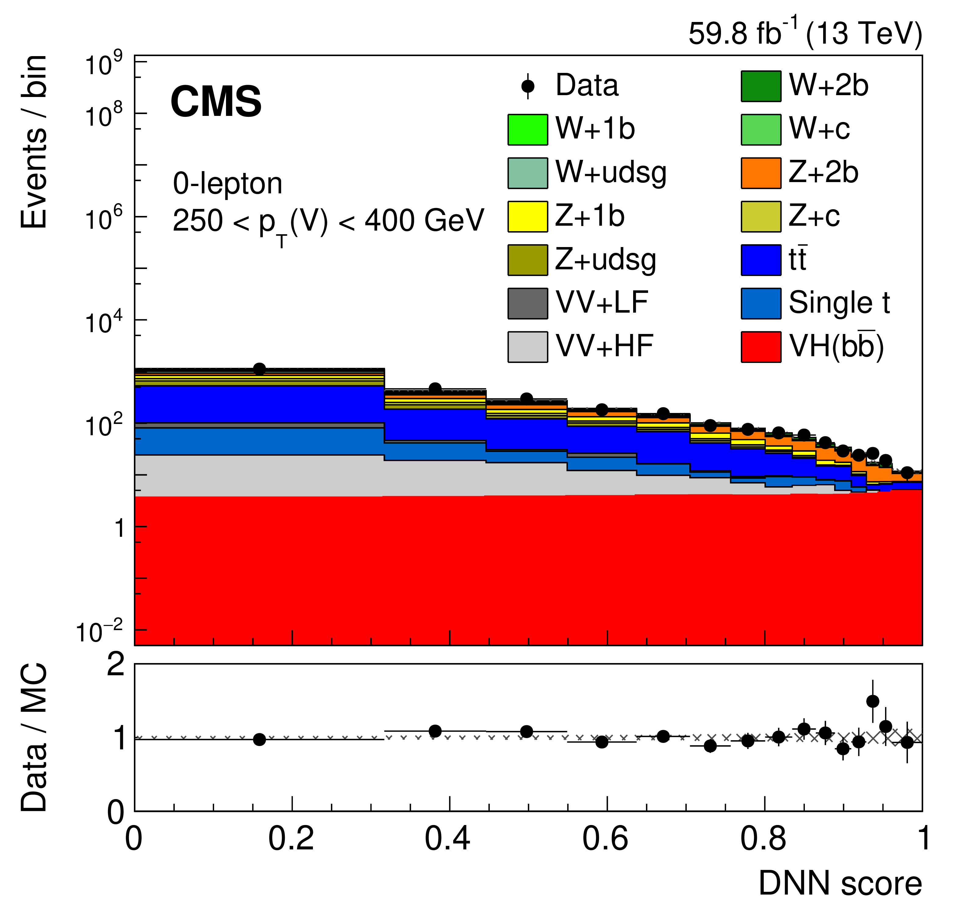
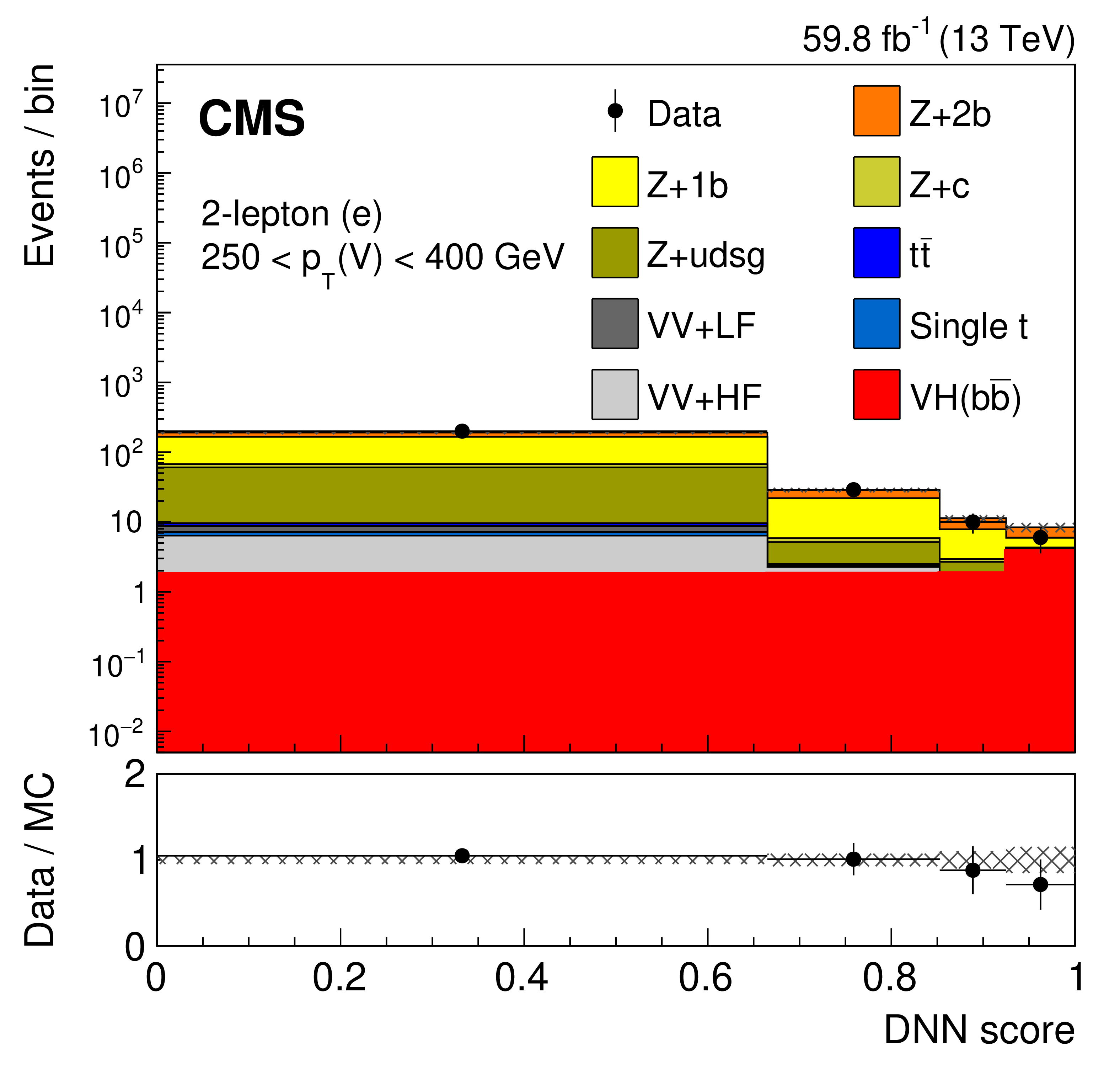
Post-fit distributions of the DNN discriminant in the 250 $ < p_{\mathrm{T}}(\mathrm{V}) < $ 400 GeV category of the 0-lepton (top left), 1-lepton (top right) and 2-lepton (bottom) channels for the electron final state using the 2018 data set. The background contributions after the maximum likelihood fit are shown as filled histograms. The Higgs boson signal is also shown as a filled histogram, and is normalized to the signal strength shown in Fig. 7. The hatched band indicates the combined statistical and systematic uncertainty in the sum of the signal and background templates. The ratio of the data to the sum of the fitted signal and background is shown in the lower panel. The distributions that enter the maximum likelihood fit use the same binning as shown here. |
png pdf |
Figure 9-a:
Post-fit distributions of the DNN discriminant in the 250 $ < p_{\mathrm{T}}(\mathrm{V}) < $ 400 GeV category of the 0-lepton (top left), 1-lepton (top right) and 2-lepton (bottom) channels for the electron final state using the 2018 data set. The background contributions after the maximum likelihood fit are shown as filled histograms. The Higgs boson signal is also shown as a filled histogram, and is normalized to the signal strength shown in Fig. 7. The hatched band indicates the combined statistical and systematic uncertainty in the sum of the signal and background templates. The ratio of the data to the sum of the fitted signal and background is shown in the lower panel. The distributions that enter the maximum likelihood fit use the same binning as shown here. |

png pdf |
Figure 9-b:
Post-fit distributions of the DNN discriminant in the 250 $ < p_{\mathrm{T}}(\mathrm{V}) < $ 400 GeV category of the 0-lepton (top left), 1-lepton (top right) and 2-lepton (bottom) channels for the electron final state using the 2018 data set. The background contributions after the maximum likelihood fit are shown as filled histograms. The Higgs boson signal is also shown as a filled histogram, and is normalized to the signal strength shown in Fig. 7. The hatched band indicates the combined statistical and systematic uncertainty in the sum of the signal and background templates. The ratio of the data to the sum of the fitted signal and background is shown in the lower panel. The distributions that enter the maximum likelihood fit use the same binning as shown here. |
png pdf |
Figure 9-c:
Post-fit distributions of the DNN discriminant in the 250 $ < p_{\mathrm{T}}(\mathrm{V}) < $ 400 GeV category of the 0-lepton (top left), 1-lepton (top right) and 2-lepton (bottom) channels for the electron final state using the 2018 data set. The background contributions after the maximum likelihood fit are shown as filled histograms. The Higgs boson signal is also shown as a filled histogram, and is normalized to the signal strength shown in Fig. 7. The hatched band indicates the combined statistical and systematic uncertainty in the sum of the signal and background templates. The ratio of the data to the sum of the fitted signal and background is shown in the lower panel. The distributions that enter the maximum likelihood fit use the same binning as shown here. |

png pdf |
Figure 10:
Distributions of signal, background, and observed data event yields sorted into bins of similar signal-to-background ratio, as given by the result of the fit to the multivariate discriminants in the resolved and boosted categories. All events in the signal regions of the 2016-2018 data set are included. The red histogram indicates the Higgs boson signal assuming SM yields ($ \mu= $ 1) and the sum of all backgrounds is given by the gray histogram. The lower panel shows the ratio of the observed data to the background expectation, with the total uncertainty in the background prediction indicated by the gray hatching. The red line indicates the sum of signal assuming the SM prediction plus background contribution, divided by the background. |
| Tables | |

png pdf |
Table 1:
Definition of the SR and CRs for the resolved selection in the 0-lepton channel. If the same selection is applied in all SRs and CRs, this is indicated by the $ \div $ symbol in the latter. The $ M $ (jj) and momenta variables have units of GeV. |

png pdf |
Table 2:
Definition of the SR and CRs for the resolved selection of the 1-lepton channel. If the same selection is applied in all SRs and CRs, this is indicated by the $ \div $ symbol in the latter. The $ M $ (jj) and momenta variables have units of GeV. |
png pdf |
Table 3:
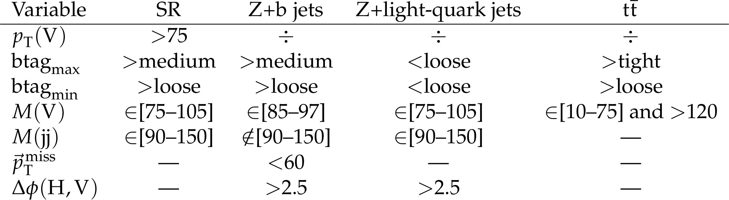
Definition of the SR and CRs for the resolved selection in the 2-lepton channel. If the same selection is applied in all SRs and CRs, this is indicated by the $ \div $ symbol in the latter. The $ M $ (jj), $ M(\mathrm{V}) $, and momenta variables have units of GeV. |

png pdf |
Table 4:
Input variables used for the DNN training in the resolved SR of the 0-, 1-, and 2-lepton channels. Reconstructed jets are classified as leading and subleading based on their b tag score. |
png pdf |
Table 5:
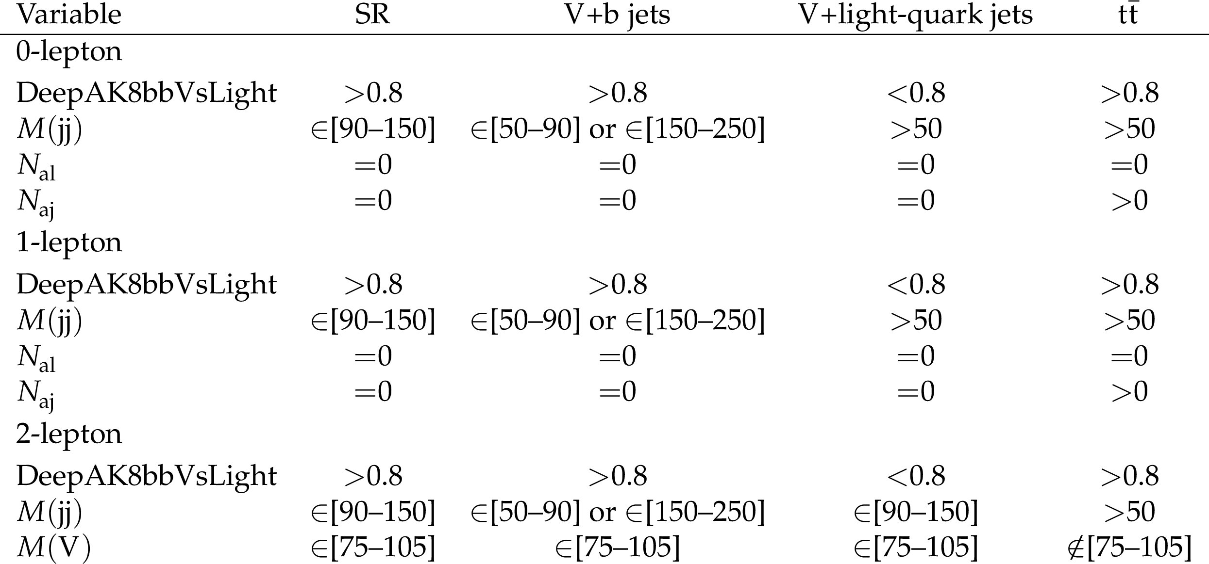
Selection criteria for the SR and CRs in the boosted topology for 0-, 1-, and 2-lepton channels. The DeepAK8bbVsLight designation represents the DEEPAK8 discriminant for the light-quark flavor discrimination node. The $ M $ (jj) and $ M(\mathrm{V}) $ variables have units of GeV. |

png pdf |
Table 6:
Discriminating variables fitted in each SR and CR. The DeepAK8bbVsLight designation represents the DEEPAK8 discriminant for the light-quark flavor discrimination node. |
png pdf |
Table 7:
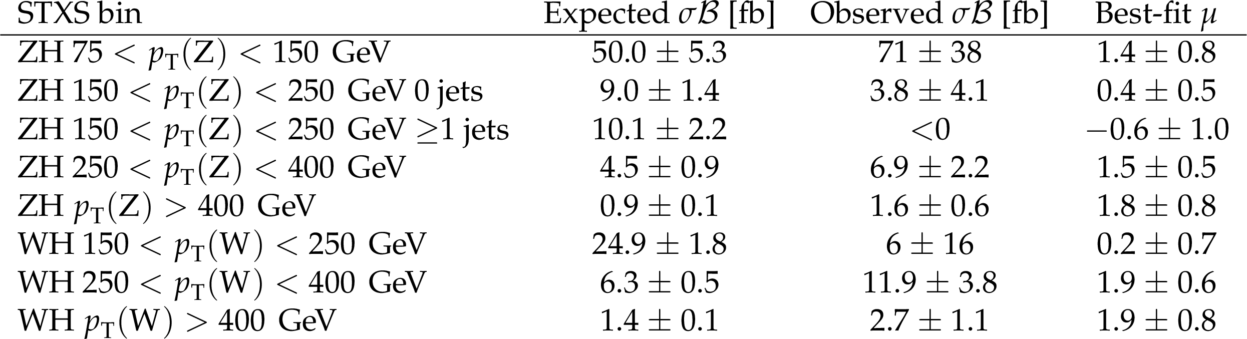
Predicted and measured values of the product of the cross section and branching fractions in the V(leptonic)H STXS process scheme. The SM predictions for each bin are calculated using the inclusive values reported in Ref. [28]. The uncertainties shown are the combined statistical and systematic components. |

png pdf |
Table 8:
The sources of systematic uncertainty in the inclusive signal strength measurement and their positive and negative values. |
| Summary |
| Measurements are presented of the cross section for the associated production of the 125 GeV Higgs boson and a W or Z boson, where the Higgs boson decays to $ \mathrm{b} \overline{\mathrm{b}} $ and the vector bosons decay to leptons. Proton-proton collision data collected by the CMS experiment during 2016-2018 at $ \sqrt{s}= $ 13 TeV are used, corresponding to an integrated luminosity of 138 fb$ ^{-1} $. Five decay channels are analyzed, and both resolved as well as merged-jet topology are employed in each vector boson decay mode. An additional subcategorization in the transverse momentum of the vector boson and the number of additional jets in the event is applied to maximize the sensitivity of different simplified template cross section bins. The overall signal strength, combining all analysis categories, is found to be $ \mu= $ 1.15 $ ^{+0.22}_{-0.20} $. The production of the Higgs boson in association with a vector boson and decays to bottom quark pairs is established with an observed (expected) significance of 6.3 (5.6) standard deviations. |
| Additional Figures | |

png pdf |
Additional Figure 1:
Dijet invariant mass distribution combining all channels, both for the VH, $ \mathrm{H}\to\mathrm{b}\overline{\mathrm{b}} $ and for the VZ, $ \mathrm{Z}\to\mathrm{b}\overline{\mathrm{b}} $ processes without (left) and with (right) all other background processes subtracted. This distribution is obtained using dedicated DNNs in the resolved SRs. These DNNs do not use the dijet mass as an input feature to avoid biasing the background shape. All the events are weighted according to S/(S+B) to emphasize the signal contribution in the distribution. Here, S and B are the number of signal and background events after the fit to data. The fit result is consistent with the signal excess at $ m_{\mathrm{H}}= $ 125 GeV of the nominal analysis. As expected, the signal strength uncertainty of this cross-check analysis is significantly, about 50%, larger than the nominal VH, $ \mathrm{H}\to\mathrm{b}\overline{\mathrm{b}} $ measurement, as the DNN discriminant employed to separate the VH signal from the sum of all backgrounds does not take into account the dijet mass in the input features of the network. Different channels require different thresholds on the low dijet invariant mass, producing the visible steps in the distributions of the backgrounds in the left plot. |

png pdf |
Additional Figure 1-a:
Dijet invariant mass distribution combining all channels, both for the VH, $ \mathrm{H}\to\mathrm{b}\overline{\mathrm{b}} $ and for the VZ, $ \mathrm{Z}\to\mathrm{b}\overline{\mathrm{b}} $ processes with all other background processes subtracted. This distribution is obtained using dedicated DNNs in the resolved SRs. These DNNs do not use the dijet mass as an input feature to avoid biasing the background shape. All the events are weighted according to S/(S+B) to emphasize the signal contribution in the distribution. Here, S and B are the number of signal and background events after the fit to data. The fit result is consistent with the signal excess at $ m_{\mathrm{H}}= $ 125 GeV of the nominal analysis. As expected, the signal strength uncertainty of this cross-check analysis is significantly, about 50%, larger than the nominal VH, $ \mathrm{H}\to\mathrm{b}\overline{\mathrm{b}} $ measurement, as the DNN discriminant employed to separate the VH signal from the sum of all backgrounds does not take into account the dijet mass in the input features of the network. Different channels require different thresholds on the low dijet invariant mass, producing the visible steps in the distributions of the backgrounds in the left plot. |

png pdf |
Additional Figure 1-b:
Dijet invariant mass distribution combining all channels, both for the VH, $ \mathrm{H}\to\mathrm{b}\overline{\mathrm{b}} $ and for the VZ, $ \mathrm{Z}\to\mathrm{b}\overline{\mathrm{b}} $ processes without all other background processes subtracted. This distribution is obtained using dedicated DNNs in the resolved SRs. These DNNs do not use the dijet mass as an input feature to avoid biasing the background shape. All the events are weighted according to S/(S+B) to emphasize the signal contribution in the distribution. Here, S and B are the number of signal and background events after the fit to data. The fit result is consistent with the signal excess at $ m_{\mathrm{H}}= $ 125 GeV of the nominal analysis. As expected, the signal strength uncertainty of this cross-check analysis is significantly, about 50%, larger than the nominal VH, $ \mathrm{H}\to\mathrm{b}\overline{\mathrm{b}} $ measurement, as the DNN discriminant employed to separate the VH signal from the sum of all backgrounds does not take into account the dijet mass in the input features of the network. Different channels require different thresholds on the low dijet invariant mass, producing the visible steps in the distributions of the backgrounds in the left plot. |

png pdf |
Additional Figure 2:
Post-fit distributions of multivariate discriminants (DNNs for resolved regions and BDTs for boosted regions) in all signal regions for the 0-lepton channel with 2016 data. |

png pdf |
Additional Figure 3:
Post-fit distributions of multivariate discriminants (DNNs for resolved regions and BDTs for boosted regions) in all signal regions for the 0-lepton channel with 2017 data. |

png pdf |
Additional Figure 4:
Post-fit distributions of multivariate discriminants (DNNs for resolved regions and BDTs for boosted regions) in all signal regions for the 0-lepton channel with 2018 data. |

png pdf |
Additional Figure 5:
Post-fit distributions of multivariate discriminants (DNNs for resolved regions and BDTs for boosted regions) in all signal regions for the 1-lepton channel with 2016 data. |
png pdf |
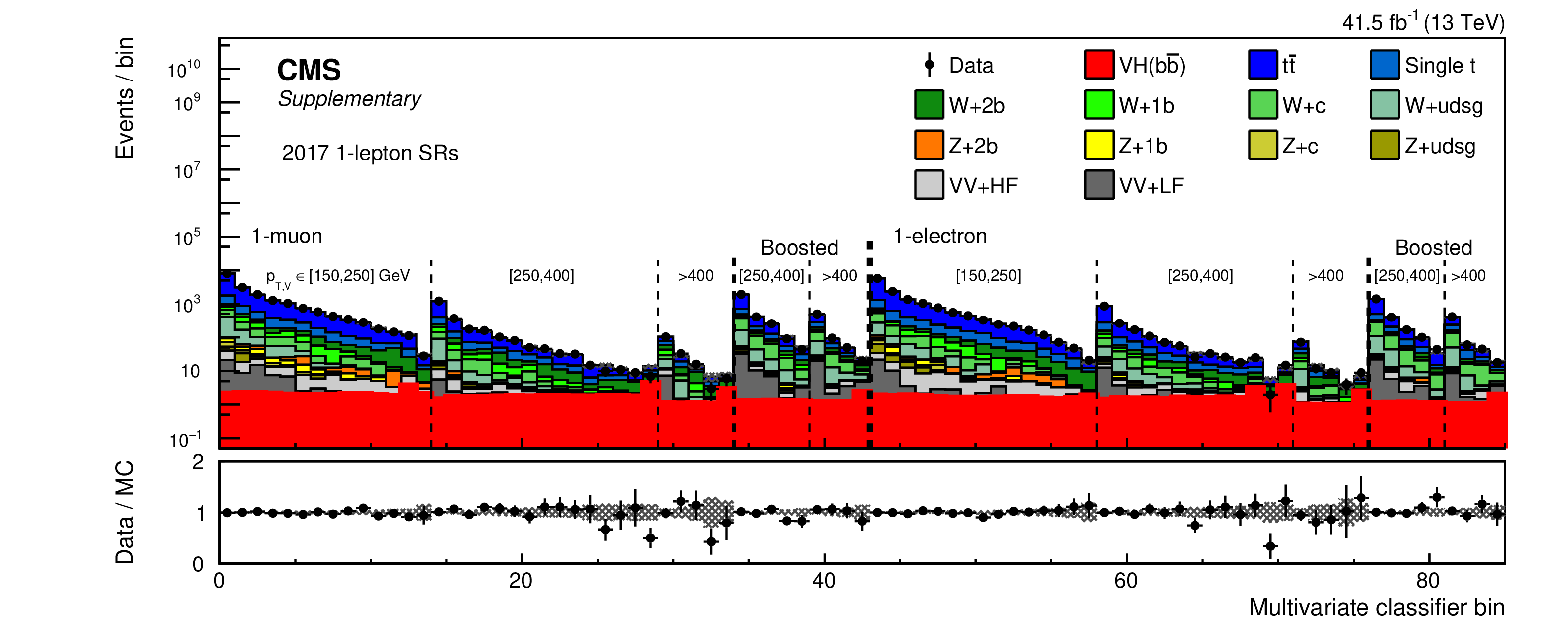
Additional Figure 6:
Post-fit distributions of multivariate discriminants (DNNs for resolved regions and BDTs for boosted regions) in all signal regions for the 1-lepton channel with 2017 data. |

png pdf |
Additional Figure 7:
Post-fit distributions of multivariate discriminants (DNNs for resolved regions and BDTs for boosted regions) in all signal regions for the 1-lepton channel with 2018 data. |

png pdf |
Additional Figure 8:
Post-fit distributions of multivariate discriminants (DNNs for resolved regions and BDTs for boosted regions) in all signal regions for the 2-lepton channel with 2016 data. |

png pdf |
Additional Figure 9:
Post-fit distributions of multivariate discriminants (DNNs for resolved regions and BDTs for boosted regions) in all signal regions for the 2-lepton channel with 2017 data. |

png pdf |
Additional Figure 10:
Post-fit distributions of multivariate discriminants (DNNs for resolved regions and BDTs for boosted regions) in all signal regions for the 2-lepton channel with 2018 data. |

png pdf |
Additional Figure 11:
Post-fit distribution of $ p_{\mathrm{T}}(\mathrm{V}) $ in the light-quark flavor control region of the 0-lepton channel for 2018 data. |
png pdf |
Additional Figure 12:
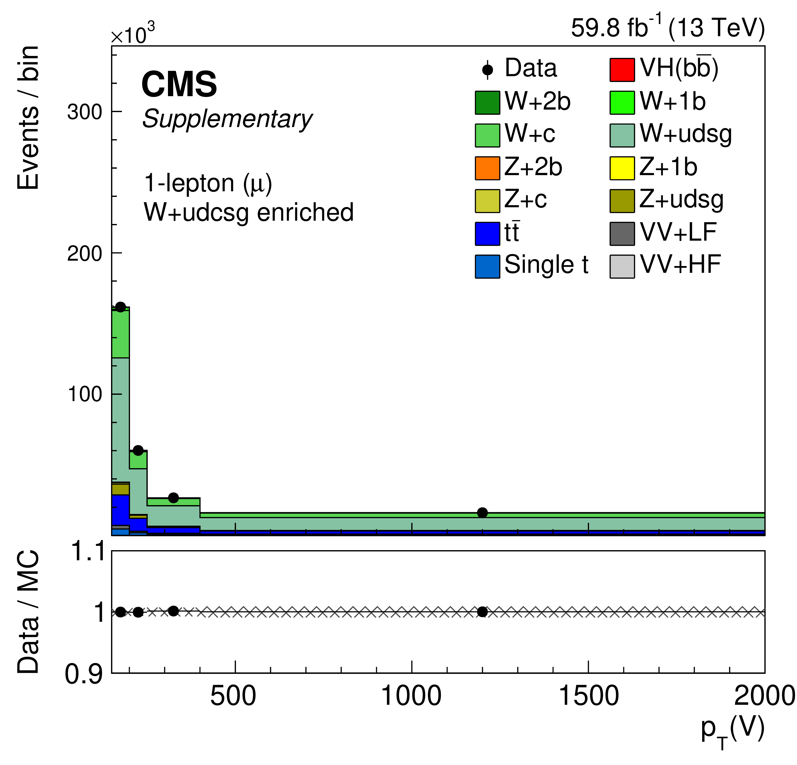
Post-fit distribution of $ p_{\mathrm{T}}(\mathrm{V}) $ in the light-quark flavor control region of the 1-muon channel for 2018 data. |

png pdf |
Additional Figure 13:
Post-fit distribution of $ p_{\mathrm{T}}(\mathrm{V}) $ in the light-quark flavor control region of the 2-electron channel for 2018 data. |

png pdf |
Additional Figure 14:
Post-fit distribution of $ p_{\mathrm{T}}(\mathrm{V}) $ in the $ \mathrm{t} \overline{\mathrm{t}} $ control region of the 0-lepton channel for 2018 data. |

png pdf |
Additional Figure 15:
Post-fit distribution of $ p_{\mathrm{T}}(\mathrm{V}) $ in the $ \mathrm{t} \overline{\mathrm{t}} $ control region of the 1-electron channel for 2018 data. |
png pdf |
Additional Figure 16:
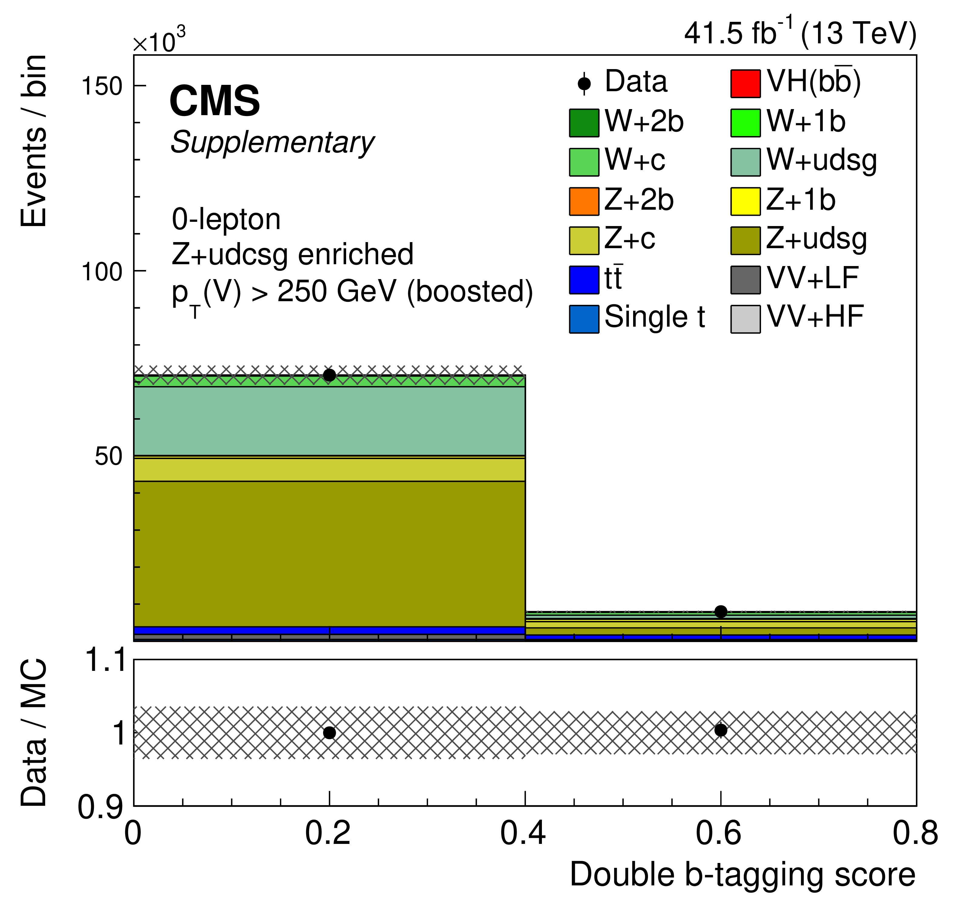
Post-fit distribution of the double b-tagger discriminant in the light-quark flavor boosted control region 0-lepton 2017 channel. |

png pdf |
Additional Figure 17:
Post-fit distribution of the double b-tagger discriminant in the heavy flavor boosted control region 0-lepton 2017 channel. |

png pdf |
Additional Figure 18:
Post-fit distribution of the double b-tagger discriminant in the $ \mathrm{t} \overline{\mathrm{t}} $ boosted control region 0-lepton 2017 channel. |

png pdf |
Additional Figure 19:
Two views of an event display of a $ \mathrm{H}\rightarrow\mathrm{b}\mathrm{b} $ candidate produced in association with a muon-anti-muon pair, in $ pp $ collisions at $ \sqrt{s}= $ 13 TeV recorded by CMS in 2018 with a very high DNN score. The charged-particle tracks, reconstructed in the inner tracker, are shown in yellow; muons are represented by red tracks. The energy deposited by electrons in the ECAL is displayed as green towers, proportional to the deposited energy. Blue towers indicate energy deposits in the HCAL, and yellow cones represent reconstructed jets. |
png |
Additional Figure 19-a:
View of an event display of a $ \mathrm{H}\rightarrow\mathrm{b}\mathrm{b} $ candidate produced in association with a muon-anti-muon pair, in $ pp $ collisions at $ \sqrt{s}= $ 13 TeV recorded by CMS in 2018 with a very high DNN score. The charged-particle tracks, reconstructed in the inner tracker, are shown in yellow; muons are represented by red tracks. The energy deposited by electrons in the ECAL is displayed as green towers, proportional to the deposited energy. Blue towers indicate energy deposits in the HCAL, and yellow cones represent reconstructed jets. |

png |
Additional Figure 19-b:
View of an event display of a $ \mathrm{H}\rightarrow\mathrm{b}\mathrm{b} $ candidate produced in association with a muon-anti-muon pair, in $ pp $ collisions at $ \sqrt{s}= $ 13 TeV recorded by CMS in 2018 with a very high DNN score. The charged-particle tracks, reconstructed in the inner tracker, are shown in yellow; muons are represented by red tracks. The energy deposited by electrons in the ECAL is displayed as green towers, proportional to the deposited energy. Blue towers indicate energy deposits in the HCAL, and yellow cones represent reconstructed jets. |

png pdf |
Additional Figure 20:
Two views of an event display of a $ \mathrm{H}\rightarrow\mathrm{b}\mathrm{b} $ candidate produced in association with an electron-positron pair, in $ pp $ collisions at $ \sqrt{s}= $ 13 TeV recorded by CMS in 2018 with a very high DNN score. The charged-particle tracks are in yellow, electrons are represented by green tracks, and energy deposited in the ECAL is displayed as green towers. Blue towers indicate HCAL energy deposits, and yellow cones represent reconstructed jets. |

png |
Additional Figure 20-a:
View of an event display of a $ \mathrm{H}\rightarrow\mathrm{b}\mathrm{b} $ candidate produced in association with an electron-positron pair, in $ pp $ collisions at $ \sqrt{s}= $ 13 TeV recorded by CMS in 2018 with a very high DNN score. The charged-particle tracks are in yellow, electrons are represented by green tracks, and energy deposited in the ECAL is displayed as green towers. Blue towers indicate HCAL energy deposits, and yellow cones represent reconstructed jets. |
png |
Additional Figure 20-b:
View of an event display of a $ \mathrm{H}\rightarrow\mathrm{b}\mathrm{b} $ candidate produced in association with an electron-positron pair, in $ pp $ collisions at $ \sqrt{s}= $ 13 TeV recorded by CMS in 2018 with a very high DNN score. The charged-particle tracks are in yellow, electrons are represented by green tracks, and energy deposited in the ECAL is displayed as green towers. Blue towers indicate HCAL energy deposits, and yellow cones represent reconstructed jets. |

png pdf |
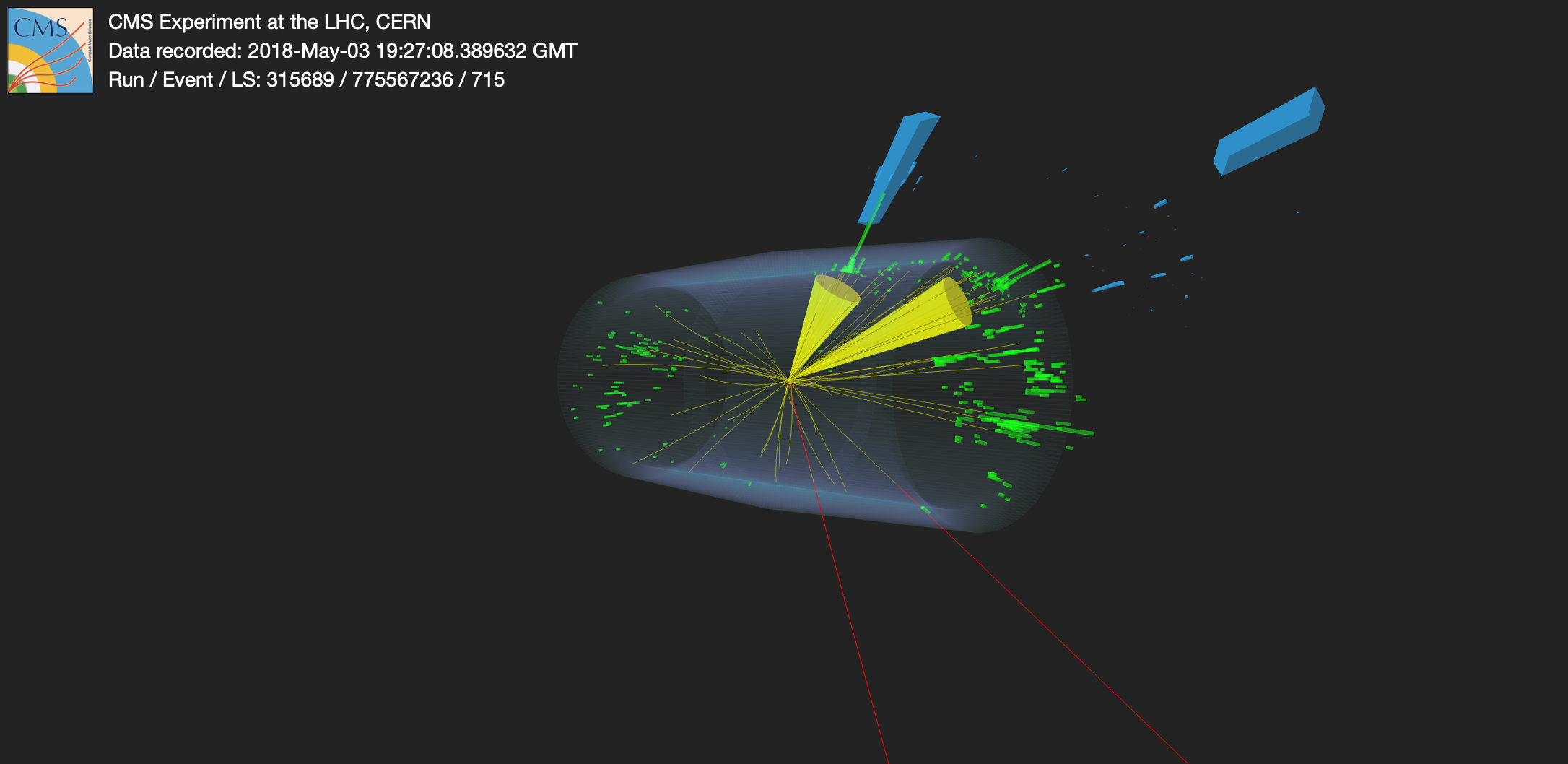
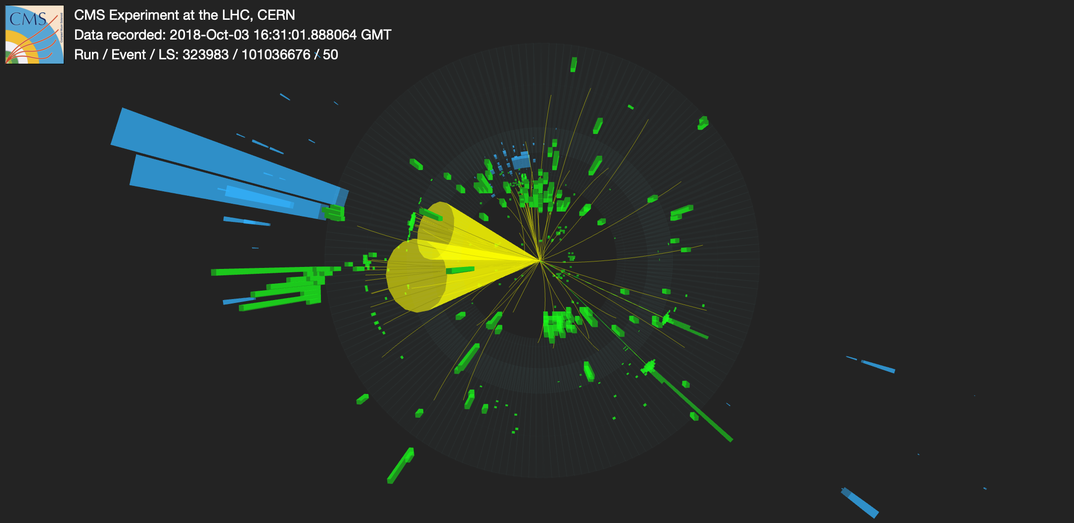
Additional Figure 21:
Two views of an event display of a $ \mathrm{H}\rightarrow\mathrm{b}\mathrm{b} $ candidate produced in association with large $ p_{\mathrm{T}}^\text{miss} $ stemming from the presence of a neutrino pair, produced by the Z boson decay, escaping the detector undetected. Charged-particle tracks in the inner tracker are shown in yellow. The energy deposited in the ECAL is displayed as green towers. Blue towers represent HCAL energy deposits, and yellow cones indicate reconstructed jets. The large missing energy created by the neutrino pair is shown as a violet arrow opposite to the yellow cones. |

png |
Additional Figure 21-a:
View of an event display of a $ \mathrm{H}\rightarrow\mathrm{b}\mathrm{b} $ candidate produced in association with large $ p_{\mathrm{T}}^\text{miss} $ stemming from the presence of a neutrino pair, produced by the Z boson decay, escaping the detector undetected. Charged-particle tracks in the inner tracker are shown in yellow. The energy deposited in the ECAL is displayed as green towers. Blue towers represent HCAL energy deposits, and yellow cones indicate reconstructed jets. The large missing energy created by the neutrino pair is shown as a violet arrow opposite to the yellow cones. |

png |
Additional Figure 21-b:
View of an event display of a $ \mathrm{H}\rightarrow\mathrm{b}\mathrm{b} $ candidate produced in association with large $ p_{\mathrm{T}}^\text{miss} $ stemming from the presence of a neutrino pair, produced by the Z boson decay, escaping the detector undetected. Charged-particle tracks in the inner tracker are shown in yellow. The energy deposited in the ECAL is displayed as green towers. Blue towers represent HCAL energy deposits, and yellow cones indicate reconstructed jets. The large missing energy created by the neutrino pair is shown as a violet arrow opposite to the yellow cones. |
png pdf |
Additional Figure 22:
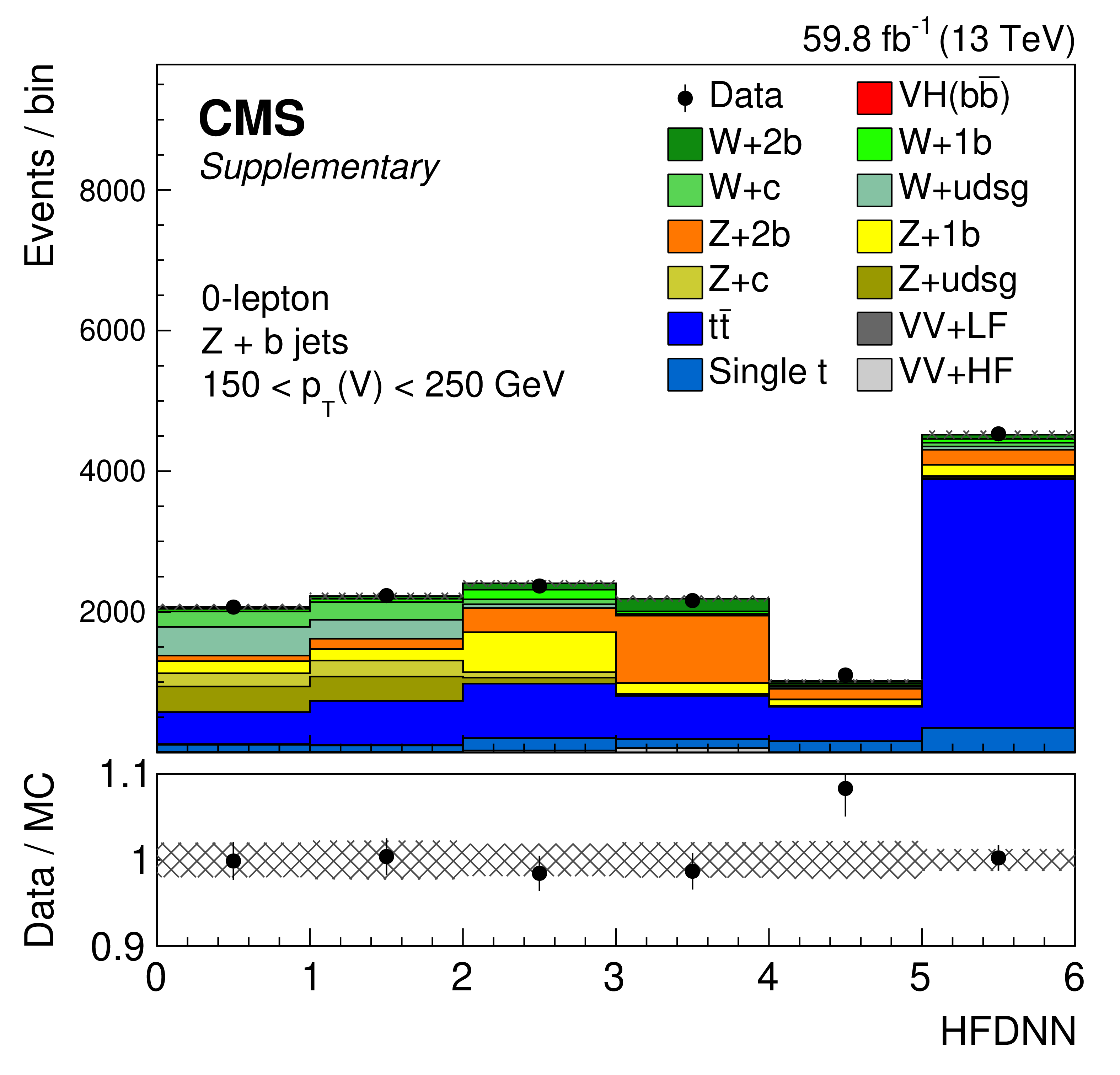
Distribution of the HFDNN scores in the 0-lepton (left) and 1-lepton (right) heavy-flavor CRs for the 2017 data set, after the fit to data. The output nodes target enrichment in the V+light-quark (first bin), V+c (second bin), V+b (third bin), V+$ \mathrm{b}\overline{\mathrm{b}} $ (fourth bin), single top quark (fifth bin), and $ {\mathrm{t}\overline{\mathrm{t}}} $ (sixth bin) backgrounds. The lower plots display the ratio of the data to the MC expectations. The vertical bars on the points represent the statistical uncertainty in the ratio, and the hatched area shows the MC uncertainty. |
png pdf |
Additional Figure 22-a:
Distribution of the HFDNN scores in the 0-lepton heavy-flavor CRs for the 2017 data set, after the fit to data. The output nodes target enrichment in the V+light-quark (first bin), V+c (second bin), V+b (third bin), V+$ \mathrm{b}\overline{\mathrm{b}} $ (fourth bin), single top quark (fifth bin), and $ {\mathrm{t}\overline{\mathrm{t}}} $ (sixth bin) backgrounds. The lower plot displays the ratio of the data to the MC expectations. The vertical bars on the points represent the statistical uncertainty in the ratio, and the hatched area shows the MC uncertainty. |

png pdf |
Additional Figure 22-b:
Distribution of the HFDNN scores in the 1-lepton heavy-flavor CRs for the 2017 data set, after the fit to data. The output nodes target enrichment in the V+light-quark (first bin), V+c (second bin), V+b (third bin), V+$ \mathrm{b}\overline{\mathrm{b}} $ (fourth bin), single top quark (fifth bin), and $ {\mathrm{t}\overline{\mathrm{t}}} $ (sixth bin) backgrounds. The lower plot displays the ratio of the data to the MC expectations. The vertical bars on the points represent the statistical uncertainty in the ratio, and the hatched area shows the MC uncertainty. |

png pdf |
Additional Figure 23:
Distribution of the HFDNN scores in the 0-lepton (left) and 1-lepton (right) heavy-flavor CRs for the 2018 data set, after the fit to data. The output nodes target enrichment in the V+light-quark (first bin), V+c (second bin), V+b (third bin), V+$ \mathrm{b}\overline{\mathrm{b}} $ (fourth bin), single top quark (fifth bin), and $ {\mathrm{t}\overline{\mathrm{t}}} $ (sixth bin) backgrounds. The lower plots display the ratio of the data to the MC expectations. The vertical bars on the points represent the statistical uncertainty in the ratio, and the hatched area shows the MC uncertainty. |
png pdf |
Additional Figure 23-a:
Distribution of the HFDNN scores in the 0-lepton heavy-flavor CRs for the 2018 data set, after the fit to data. The output nodes target enrichment in the V+light-quark (first bin), V+c (second bin), V+b (third bin), V+$ \mathrm{b}\overline{\mathrm{b}} $ (fourth bin), single top quark (fifth bin), and $ {\mathrm{t}\overline{\mathrm{t}}} $ (sixth bin) backgrounds. The lower plot displays the ratio of the data to the MC expectations. The vertical bars on the points represent the statistical uncertainty in the ratio, and the hatched area shows the MC uncertainty. |

png pdf |
Additional Figure 23-b:
Distribution of the HFDNN scores in the 1-lepton heavy-flavor CRs for the 2018 data set, after the fit to data. The output nodes target enrichment in the V+light-quark (first bin), V+c (second bin), V+b (third bin), V+$ \mathrm{b}\overline{\mathrm{b}} $ (fourth bin), single top quark (fifth bin), and $ {\mathrm{t}\overline{\mathrm{t}}} $ (sixth bin) backgrounds. The lower plot displays the ratio of the data to the MC expectations. The vertical bars on the points represent the statistical uncertainty in the ratio, and the hatched area shows the MC uncertainty. |
| References | ||||
| 1 | ATLAS Collaboration | Observation of a new particle in the search for the Standard Model Higgs boson with the ATLAS detector at the LHC | PLB 716 (2012) 1 | 1207.7214 |
| 2 | CMS Collaboration | Observation of a new boson at a mass of 125 GeV with the CMS experiment at the LHC | PLB 716 (2012) 30 | CMS-HIG-12-028 1207.7235 |
| 3 | CMS Collaboration | Observation of a new boson with mass near 125 GeV in pp collisions at $ \sqrt{s} = $ 7 and 8 TeV | JHEP 06 (2013) 081 | CMS-HIG-12-036 1303.4571 |
| 4 | F. Englert and R. Brout | Broken symmetry and the mass of gauge vector mesons | PRL 13 (1964) 321 | |
| 5 | P. W. Higgs | Broken symmetries, massless particles and gauge fields | PL 12 (1964) 132 | |
| 6 | P. W. Higgs | Broken symmetries and the masses of gauge bosons | PRL 13 (1964) 508 | |
| 7 | G. S. Guralnik, C. R. Hagen, and T. W. B. Kibble | Global conservation laws and massless particles | PRL 13 (1964) 585 | |
| 8 | P. W. Higgs | Spontaneous symmetry breakdown without massless bosons | PR 145 (1966) 1156 | |
| 9 | T. W. B. Kibble | Symmetry breaking in non-Abelian gauge theories | PR 155 (1967) 1554 | |
| 10 | ATLAS Collaboration | Measurement of Higgs boson production in the diphoton decay channel in pp collisions at center-of-mass energies of 7 and 8 TeV with the ATLAS detector | PRD 90 (2014) 112015 | 1408.7084 |
| 11 | CMS Collaboration | Observation of the diphoton decay of the Higgs boson and measurement of its properties | EPJC 74 (2014) 3076 | CMS-HIG-13-001 1407.0558 |
| 12 | ATLAS Collaboration | Measurements of Higgs boson production and couplings in the four-lepton channel in pp collisions at center-of-mass energies of 7 and 8 TeV with the ATLAS detector | PRD 91 (2015) 012006 | 1408.5191 |
| 13 | CMS Collaboration | Measurement of the properties of a Higgs boson in the four-lepton final state | PRD 89 (2014) 092007 | CMS-HIG-13-002 1312.5353 |
| 14 | ATLAS Collaboration | Observation and measurement of Higgs boson decays to WW$ ^* $ with the ATLAS detector | PRD 92 (2015) 012006 | 1412.2641 |
| 15 | ATLAS Collaboration | Study of (W/Z)H production and Higgs boson couplings using H $ \rightarrow $ WW$ ^{\ast} $ decays with the ATLAS detector | JHEP 08 (2015) 137 | 1506.06641 |
| 16 | CMS Collaboration | Measurement of Higgs boson production and properties in the WW decay channel with leptonic final states | JHEP 01 (2014) 096 | CMS-HIG-13-023 1312.1129 |
| 17 | ATLAS Collaboration | Evidence for the Higgs boson Yukawa coupling to tau leptons with the ATLAS detector | JHEP 04 (2015) 117 | 1501.04943 |
| 18 | CMS Collaboration | Evidence for the 125 GeV Higgs boson decaying to a pair of $ \tau $ leptons | JHEP 05 (2014) 104 | CMS-HIG-13-004 1401.5041 |
| 19 | CMS Collaboration | Observation of Higgs boson decays to a pair of tau leptons | PLB 779 (2017) 283 | CMS-HIG-16-043 1708.00373 |
| 20 | CMS Collaboration | Measurements of properties of the Higgs boson decaying to a W boson pair in pp collisions at $ \sqrt{s}= $ 13 TeV | PLB 791 (2019) | CMS-HIG-16-042 1806.05246 |
| 21 | ATLAS Collaboration | Observation of $ H \rightarrow b\bar{b} $ decays and $ VH $ production with the ATLAS detector | PLB 786 (2018) 59 | 1808.08238 |
| 22 | CMS Collaboration | Observation of $ \mathrm{t\overline{t}} $H production | PRL 120 (2018) 231801 | CMS-HIG-17-035 1804.02610 |
| 23 | ATLAS Collaboration | Observation of Higgs boson production in association with a top quark pair at the LHC with the ATLAS detector | PLB 784 (2018) 173 | 1806.00425 |
| 24 | ATLAS Collaboration | A detailed map of Higgs boson interactions by the ATLAS experiment ten years after the discovery | Nature 607 (2022) 52 | 2207.00092 |
| 25 | CMS Collaboration | A portrait of the Higgs boson by the CMS experiment ten years after the discovery | Nature 607 (2022) 60 | CMS-HIG-22-001 2207.00043 |
| 26 | CMS Collaboration | Evidence for Higgs boson decay to a pair of muons | JHEP 01 (2021) 148 | CMS-HIG-19-006 2009.04363 |
| 27 | CMS Collaboration | Observation of Higgs boson decay to bottom quarks | PRL 121 (2018) 121801 | CMS-HIG-18-016 1808.08242 |
| 28 | LHC Higgs Cross Section Working Group | Handbook of LHC Higgs Cross Sections: 4. Deciphering the Nature of the Higgs sector | 1610.07922 | |
| 29 | J. R. Andersen et al. | Les Houches 2015: Physics at TeV Colliders Standard Model working group report | in 9th Les Houches Workshop on Physics at TeV Colliders, Les Houches, France, 2015 PhysTeV 201 (2015) 5 |
1605.04692 |
| 30 | ATLAS Collaboration | Measurements of $ WH $ and $ ZH $ production in the $ H \rightarrow b\bar{b} $ decay channel in $ pp $ collisions at 13 TeV with the ATLAS detector | EPJC 81 (2021) 178 | 2007.02873 |
| 31 | CMS Collaboration | Precision luminosity measurement in proton-proton collisions at $ \sqrt{s} = $ 13 TeV in 2015 and 2016 at CMS | EPJC 81 (2021) 800 | CMS-LUM-17-003 2104.01927 |
| 32 | CMS Collaboration | CMS luminosity measurement for the 2017 data-taking period at $ \sqrt{s} = $ 13 TeV | CMS Physics Analysis Summary, 2018 CMS-PAS-LUM-17-004 |
CMS-PAS-LUM-17-004 |
| 33 | CMS Collaboration | CMS luminosity measurement for the 2018 data-taking period at $ \sqrt{s} = $ 13 TeV | CMS Physics Analysis Summary, 2019 CMS-PAS-LUM-18-002 |
CMS-PAS-LUM-18-002 |
| 34 | CMS Collaboration | Search for the standard model Higgs boson produced in association with a W or a Z boson and decaying to bottom quarks | PRD 89 (2014) 012003 | CMS-HIG-13-012 1310.3687 |
| 35 | CMS Collaboration | Evidence for the Higgs boson decay to a bottom quark-antiquark pair | PLB 780 (2018) 501 | CMS-HIG-16-044 1709.07497 |
| 36 | ATLAS Collaboration | Measurement of the associated production of a Higgs boson decaying into $ b $-quarks with a vector boson at high transverse momentum in $ pp $ collisions at $ \sqrt{s} = $ 13 TeV with the ATLAS detector | PLB 816 (2021) 136204 | 2008.02508 |
| 37 | CMS Collaboration | HEPData record for this analysis | link | |
| 38 | CMS Collaboration | The CMS trigger system | JINST 12 (2017) P01020 | CMS-TRG-12-001 1609.02366 |
| 39 | CMS Collaboration | The CMS experiment at the CERN LHC | JINST 3 (2008) S08004 | |
| 40 | P. Nason | A new method for combining NLO QCD with shower Monte Carlo algorithms | JHEP 11 (2004) 040 | hep-ph/0409146 |
| 41 | S. Frixione, P. Nason, and C. Oleari | Matching NLO QCD computations with parton shower simulations: the POWHEG method | JHEP 11 (2007) 070 | 0709.2092 |
| 42 | S. Alioli, P. Nason, C. Oleari, and E. Re | A general framework for implementing NLO calculations in shower Monte Carlo programs: the POWHEG BOX | JHEP 06 (2010) 043 | 1002.2581 |
| 43 | K. Hamilton, P. Nason, and G. Zanderighi | MINLO: Multi-scale improved NLO | JHEP 10 (2012) 155 | 1206.3572 |
| 44 | G. Luisoni, P. Nason, C. Oleari, and F. Tramontano | HW/HZ + 0 and 1 jet at NLO with the POWHEG BOX interfaced to GoSam and their merging within MiNLO | JHEP 10 (2013) 083 | 1306.2542 |
| 45 | J. Alwall et al. | The automated computation of tree-level and next-to-leading order differential cross sections, and their matching to parton shower simulations | JHEP 07 (2014) 079 | 1405.0301 |
| 46 | R. Frederix and S. Frixione | Merging meets matching in MC@NLO | JHEP 12 (2012) 061 | 1209.6215 |
| 47 | J. Alwall et al. | Comparative study of various algorithms for the merging of parton showers and matrix elements in hadronic collisions | EPJC 53 (2008) 473 | 0706.2569 |
| 48 | S. Kallweit et al. | NLO QCD+EW predictions for V+jets including off-shell vector-boson decays and multijet merging | JHEP 04 (2016) 021 | 1511.08692 |
| 49 | G. Ferrera, M. Grazzini, and F. Tramontano | Higher-order QCD effects for associated WH production and decay at the LHC | JHEP 04 (2014) 039 | 1312.1669 |
| 50 | G. Ferrera, M. Grazzini, and F. Tramontano | Associated ZH production at hadron colliders: the fully differential NNLO QCD calculation | PLB 740 (2015) 51 | 1407.4747 |
| 51 | O. Brein, R. V. Harlander, and T. J. E. Zirke | VH@NNLO --- Higgs Strahlung at hadron colliders | Comput. Phys. Commun. 184 (2013) 998 | 1210.5347 |
| 52 | R. V. Harlander, S. Liebler, and T. Zirke | Higgs Strahlung at the Large Hadron Collider in the 2-Higgs-Doublet Model | JHEP 02 (2014) 023 | 1307.8122 |
| 53 | A. Denner, S. Dittmaier, S. Kallweit, and A. Mück | HAWK 2.0: A Monte Carlo program for Higgs production in vector-boson fusion and Higgs Strahlung at hadron colliders | Comput. Phys. Commun. 195 (2015) 161 | 1412.5390 |
| 54 | M. Czakon and A. Mitov | Top++: A program for the calculation of the top-pair cross-section at hadron colliders | Comput. Phys. Commun. 185 (2014) 2930 | 1112.5675 |
| 55 | NNPDF Collaboration | Parton distributions for the LHC Run II | JHEP 04 (2015) 040 | 1410.8849 |
| 56 | T. Sjöstrand, S. Mrenna, and P. Z. Skands | An introduction to PYTHIA 8.2 | Comput. Phys. Commun. 191 (2015) 159 | 1410.3012 |
| 57 | CMS Collaboration | Event generator tunes obtained from underlying event and multiparton scattering measurements | EPJC 76 (2016) 155 | CMS-GEN-14-001 1512.00815 |
| 58 | P. Skands, S. Carrazza, and J. Rojo | Tuning PYTHIA 8.1: the Monash 2013 tune | EPJC 74 (2014) 3024 | 1404.5630 |
| 59 | GEANT4 Collaboration | GEANT4 --- a simulation toolkit | NIM A 506 (2003) 250 | |
| 60 | CMS Collaboration | Particle-flow reconstruction and global event description with the CMS detector | JINST 12 (2017) P10003 | CMS-PRF-14-001 1706.04965 |
| 61 | CMS Collaboration | Technical proposal for the Phase-II upgrade of the Compact Muon Solenoid | CMS Technical Proposal CERN-LHCC-2015-010, CMS-TDR-15-02, 2015 CDS |
|
| 62 | W. Waltenberger, R. Frühwirth, and P. Vanlaer | Adaptive vertex fitting | JPG 34 (2007) 343 | |
| 63 | CMS Collaboration | Electron and photon reconstruction and identification with the CMS experiment at the CERN LHC | JINST 16 (2021) P05014 | CMS-EGM-17-001 2012.06888 |
| 64 | CMS Collaboration | Performance of the CMS muon detector and muon reconstruction with proton-proton collisions at $ \sqrt{s} = $ 13 TeV | JINST 13 (2018) P06015 | CMS-MUO-16-001 1804.04528 |
| 65 | CMS Collaboration | Jet energy scale and resolution in the CMS experiment in pp collisions at 8 TeV | JINST 12 (2017) P02014 | CMS-JME-13-004 1607.03663 |
| 66 | CMS Collaboration | Identification of heavy-flavour jets with the CMS detector in pp collisions at 13 TeV | JINST 13 (2018) P05011 | CMS-BTV-16-002 1712.07158 |
| 67 | CMS Collaboration | A deep neural network for simultaneous estimation of b-jet energy and resolution | Comput. Softw. Big Sci. 4 (2020) 10 | CMS-HIG-18-027 1912.06046 |
| 68 | M. Cacciari, G. P. Salam, and G. Soyez | The anti-$ k_{\mathrm{T}} $ jet clustering algorithm | JHEP 04 (2008) 063 | 0802.1189 |
| 69 | A. Larkoski, S. Marzani, G. Soyez, and J. Thaler | Soft drop | JHEP 05 (2014) 146 | 1402.2657 |
| 70 | CMS Collaboration | W and top tagging scale factors for Run 2 data | CMS Detector Performance Note CMS-DP-2020-025, 2020 CDS |
|
| 71 | CMS Collaboration | Performance of missing transverse momentum reconstruction in proton-proton collisions at $ \sqrt{s} = $ 13 TeV using the CMS detector | JINST 14 (2019) P07004 | CMS-JME-17-001 1903.06078 |
| 72 | A. D. Bukin | Fitting function for asymmetric peaks | 0711.4449 | |
| 73 | I. J. Goodfellow, Y. Bengio, and A. Courville | Deep Learning | MIT Press, Cambridge, MA, USA, 2016 link |
|
| 74 | P. K. Diederik and B. Jimmy | Adam: A method for stochastic optimisation | 1412.6980 | |
| 75 | J. Butterworth et al. | PDF4LHC recommendations for LHC run II | JPG 43 (2016) 040 | 1510.03865 |
| 76 | CMS Collaboration | Measurement of the inclusive and differential WZ production cross sections, polarization angles, and triple gauge couplings in pp collisions at $ \sqrt{s} = $ 13 TeV | JHEP 07 (2022) 032 | CMS-SMP-20-014 2110.11231 |
| 77 | CMS Collaboration | Measurements of pp $ \rightarrow $ ZZ production cross sections and constraints on anomalous triple gauge couplings at $ \sqrt{s} = $ 13 TeV | EPJC 81 (2021) 200 | CMS-SMP-19-001 2009.01186 |
| 78 | CMS Collaboration | Measurement of the inelastic proton-proton cross section at $ \sqrt{s} = $ 13 TeV | JHEP 07 (2018) 161 | CMS-FSQ-15-005 1802.02613 |
| 79 | R. Barlow and C. Beeston | Fitting using finite Monte Carlo samples | Comput. Phys. Commun. 77 (1993) 219 | |
|
|
Compact Muon Solenoid LHC, CERN |
|

|

|

|

|

|