

Compact Muon Solenoid
LHC, CERN
| CMS-HIG-21-013 ; CERN-EP-2021-272 | ||
| Measurement of the Higgs boson width and evidence of its off-shell contributions to ZZ production | ||
| CMS Collaboration | ||
| 14 February 2022 | ||
| Nat. Phys. 18 (2022) 1329 | ||
| Abstract: Since the discovery of the Higgs boson in 2012, detailed studies of its properties have been ongoing. Besides its mass, its width --- related to its lifetime --- is an important parameter. One way to determine this quantity is by measuring its off-shell production, where the Higgs boson mass is far away from its nominal value, and relating it to its on-shell production, where the mass is close to the nominal value. Here, we report evidence for such off-shell contributions to the production cross section of two Z bosons with data from the CMS experiment at the CERN Large Hadron Collider. We constrain the total rate of the off-shell Higgs boson contribution beyond the Z boson pair production threshold, relative to its standard model expectation, to the interval [0.0061, 2.0] at 95% confidence level. The scenario with no off-shell contribution is excluded at a $ p $-value of 0.0003 (3.6 standard deviations). We measure the width of the Higgs boson as $ \Gamma_{\mathrm{H}} = $ 3.2$_{-1.7}^{+2.4}$ MeV, in agreement with the standard model expectation of 4.1 MeV. In addition, we set constraints on anomalous Higgs boson couplings to W and Z boson pairs. | ||
| Links: e-print arXiv:2202.06923 [hep-ex] (PDF) ; CDS record ; inSPIRE record ; HepData record ; Physics Briefing ; CADI line (restricted) ; | ||
| Figures | |
png pdf |
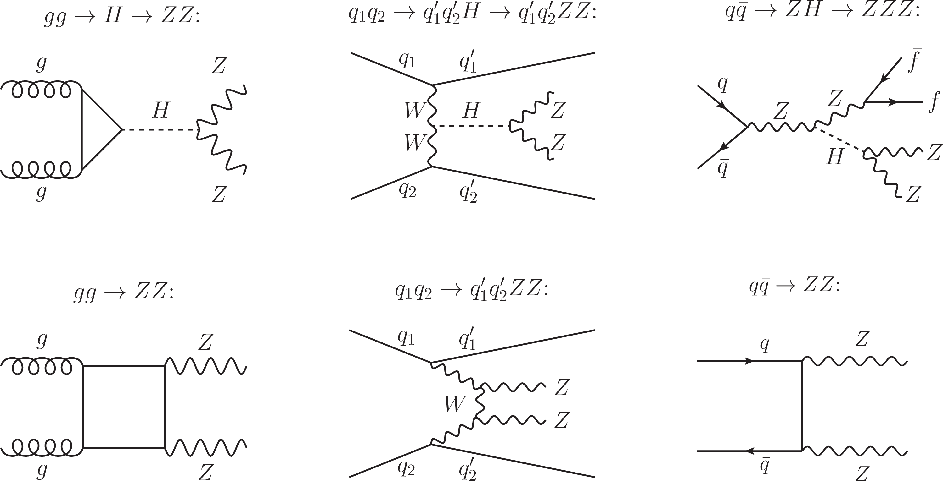
Figure 1:
Feynman diagrams for important contributions to ZZ production. Diagrams can be distinguished as those involving the H boson (top), and those that give rise to continuum ZZ production (bottom). The interaction displayed at tree level in each diagram is meant to progress from left to right. Each straight, curvy, or curly line refers to the different set of particles denoted. Straight, solid lines with no arrows indicate the line could refer to either a particle or an antiparticle, whereas those with forward (backward) arrows refer to a particle (an antiparticle). |

png pdf |
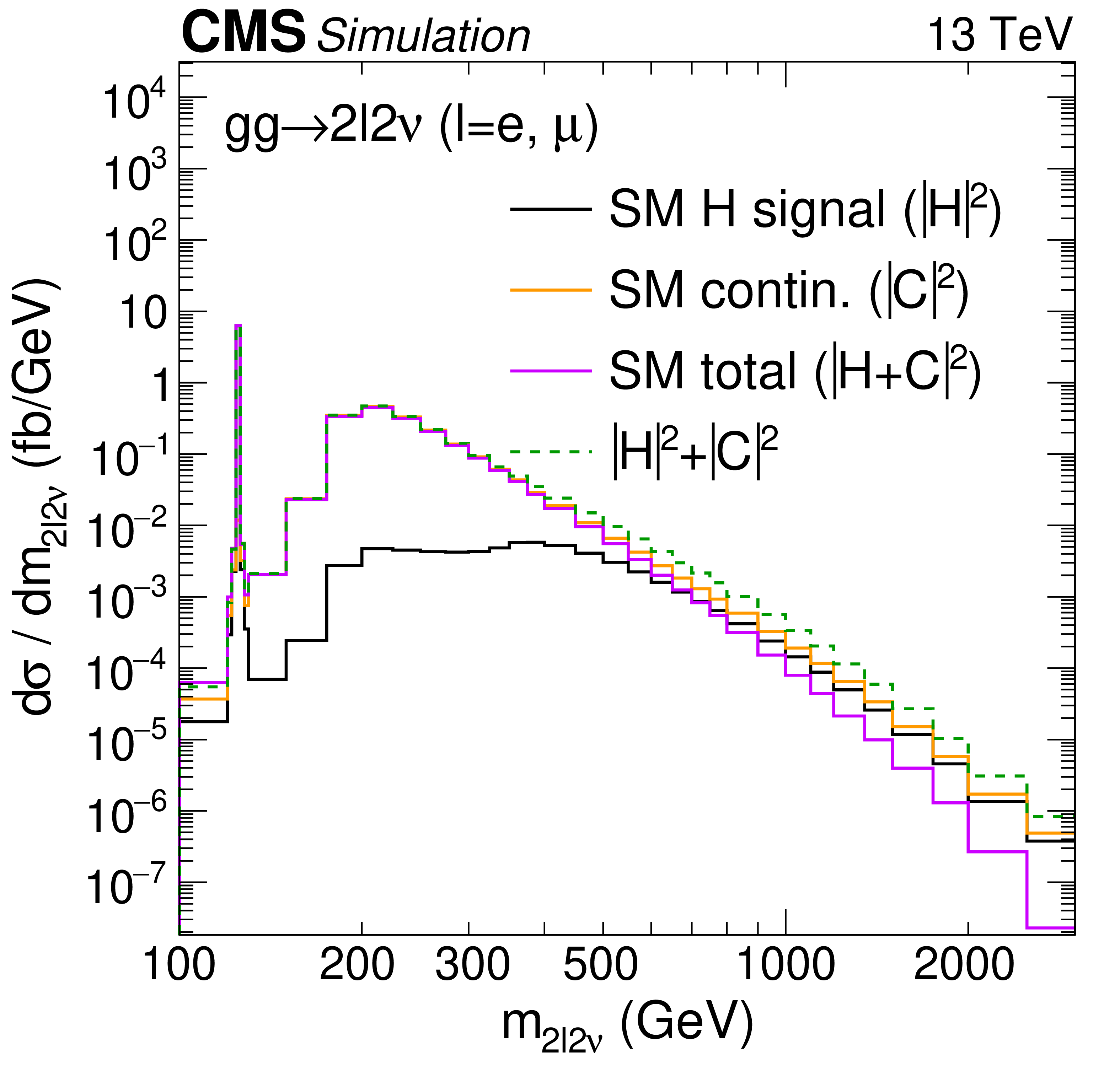
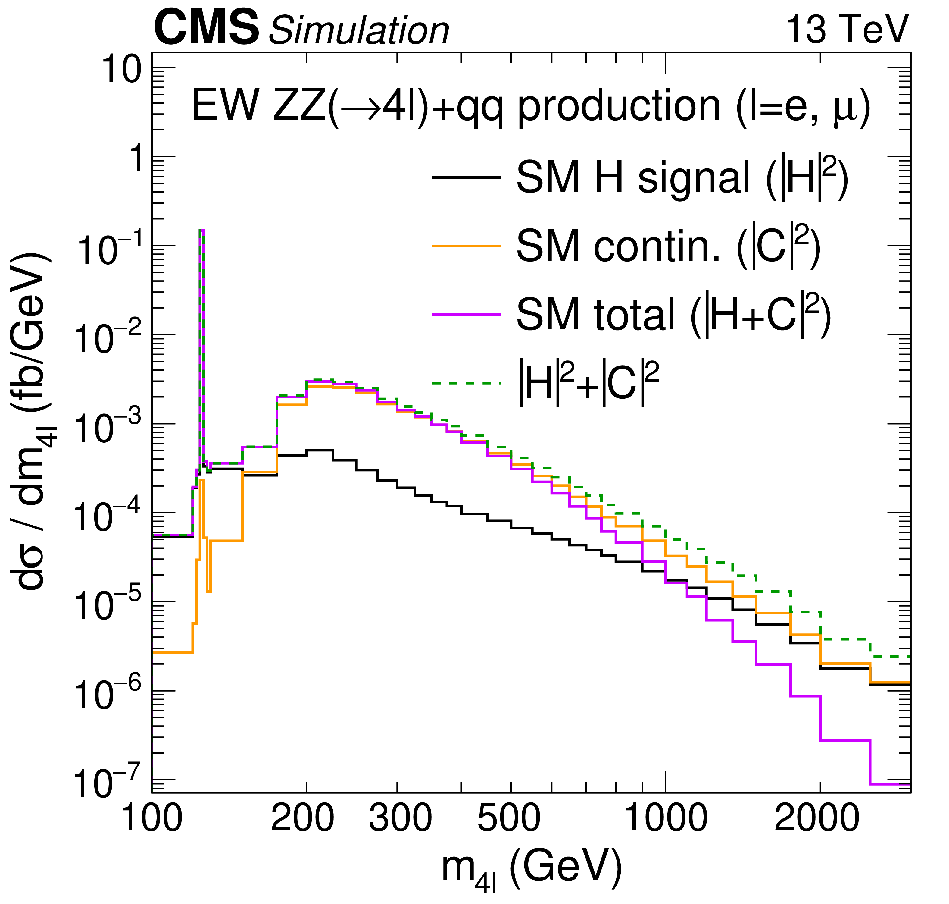
Figure 2:
Standard model calculations of ZZ invariant mass in the gg and EW processes. Shown are the distributions for the 2$ \ell$2$\nu $ invariant mass, $ m_{2\ell2\nu} $, from the $ \mathrm{g}\mathrm{g} \to 2\ell2\nu $ process on the left panel, and the 4$ \ell $ invariant mass, $ m_{4\ell} $, from the EW $ \mathrm{Z}\mathrm{Z} (\to 4\ell)+\mathrm{q}\mathrm{q} $ processes on the right. These processes involve the H boson ($ |\mathrm{H}|^2 $) and interfering continuum ($ |\mathrm{C}|^2 $) contributions to the scattering amplitude, shown in black and gold, respectively. The dashed green curve represents their direct sum without the interference ($ |\mathrm{H}|^2+|\mathrm{C}|^2 $), and the solid magenta curve represents the sum with interference included ($ |\mathrm{H}+\mathrm{C}|^2 $). Note that the interference is destructive, and its importance grows as the mass increases. The integrated luminosity is taken to be 1 fb$^{-1}$, so these distributions are equivalent to the differential cross section spectra $ d\sigma/dm_{2\ell2\nu} $ (left) and $ d\sigma/dm_{4\ell} $ (right). The distributions are shown after requiring that all charged leptons satisfy $ p_{\mathrm{T}} > $ 7 GeV and $ |\eta| < $ 2.4, and that the invariant mass of any charged lepton pair with same flavor and opposite charge is greater than 4 GeV. Here, $ p_{\mathrm{T}} $ denotes the magnitude of the momentum of these leptons transverse to the $ \mathrm{p}\mathrm{p} $ collision axis, and $ \eta $ denotes their pseudorapidity, defined as $ -\ln\left[\tan\left(\theta/2\right)\right] $ using the angle $ \theta $ between their momentum vector and the collision axis. Calculations for the $ \mathrm{g}\mathrm{g} \to 4\ell $ and EW $ \mathrm{Z}\mathrm{Z} (\to 2\ell2\nu)+\mathrm{q}\mathrm{q} $ processes exhibit similar qualitative properties. The details of the Monte Carlo programs used for these calculations are given in the Methods section. |
png pdf |
Figure 2-a:
Shown is the distribution for the 2$ \ell$2$\nu $ invariant mass, $ m_{2\ell2\nu} $, from the $ \mathrm{g}\mathrm{g} \to 2\ell2\nu $ process. This process involves the H boson ($ |\mathrm{H}|^2 $) and interfering continuum ($ |\mathrm{C}|^2 $) contributions to the scattering amplitude, shown in black and gold, respectively. The dashed green curve represents their direct sum without the interference ($ |\mathrm{H}|^2+|\mathrm{C}|^2 $), and the solid magenta curve represents the sum with interference included ($ |\mathrm{H}+\mathrm{C}|^2 $). Note that the interference is destructive, and its importance grows as the mass increases. The integrated luminosity is taken to be 1 fb$^{-1}$, so these distributions are equivalent to the differential cross section spectrum $ d\sigma/dm_{2\ell2\nu} $. The distributions are shown after requiring that all charged leptons satisfy $ p_{\mathrm{T}} > $ 7 GeV and $ |\eta| < $ 2.4, and that the invariant mass of any charged lepton pair with same flavor and opposite charge is greater than 4 GeV. Here, $ p_{\mathrm{T}} $ denotes the magnitude of the momentum of these leptons transverse to the $ \mathrm{p}\mathrm{p} $ collision axis, and $ \eta $ denotes their pseudorapidity, defined as $ -\ln\left[\tan\left(\theta/2\right)\right] $ using the angle $ \theta $ between their momentum vector and the collision axis. The details of the Monte Carlo programs used for these calculations are given in the Methods section. |
png pdf |
Figure 2-b:
Shown is the distribution for the 4$ \ell $ invariant mass, $ m_{4\ell} $, from the EW $ \mathrm{Z}\mathrm{Z} (\to 4\ell)+\mathrm{q}\mathrm{q} $ processes.These processes involve the H boson ($ |\mathrm{H}|^2 $) and interfering continuum ($ |\mathrm{C}|^2 $) contributions to the scattering amplitude, shown in black and gold, respectively. The dashed green curve represents their direct sum without the interference ($ |\mathrm{H}|^2+|\mathrm{C}|^2 $), and the solid magenta curve represents the sum with interference included ($ |\mathrm{H}+\mathrm{C}|^2 $). Note that the interference is destructive, and its importance grows as the mass increases. The integrated luminosity is taken to be 1 fb$^{-1}$, so these distributions are equivalent to the differential cross section spectrum $ d\sigma/dm_{4\ell} $. The distributions are shown after requiring that all charged leptons satisfy $ p_{\mathrm{T}} > $ 7 GeV and $ |\eta| < $ 2.4, and that the invariant mass of any charged lepton pair with same flavor and opposite charge is greater than 4 GeV. Here, $ p_{\mathrm{T}} $ denotes the magnitude of the momentum of these leptons transverse to the $ \mathrm{p}\mathrm{p} $ collision axis, and $ \eta $ denotes their pseudorapidity, defined as $ -\ln\left[\tan\left(\theta/2\right)\right] $ using the angle $ \theta $ between their momentum vector and the collision axis. The details of the Monte Carlo programs used for these calculations are given in the Methods section. |
png pdf |
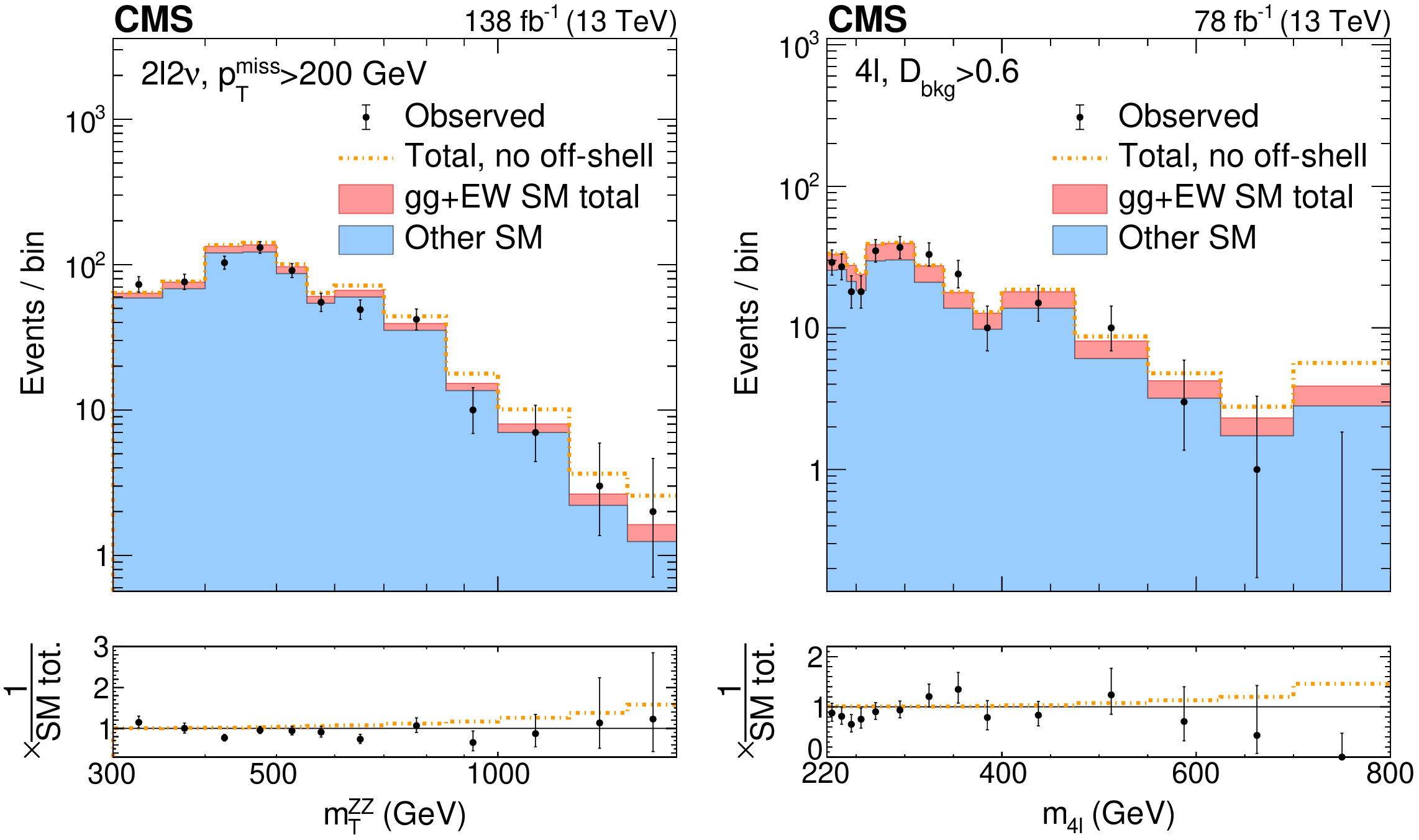
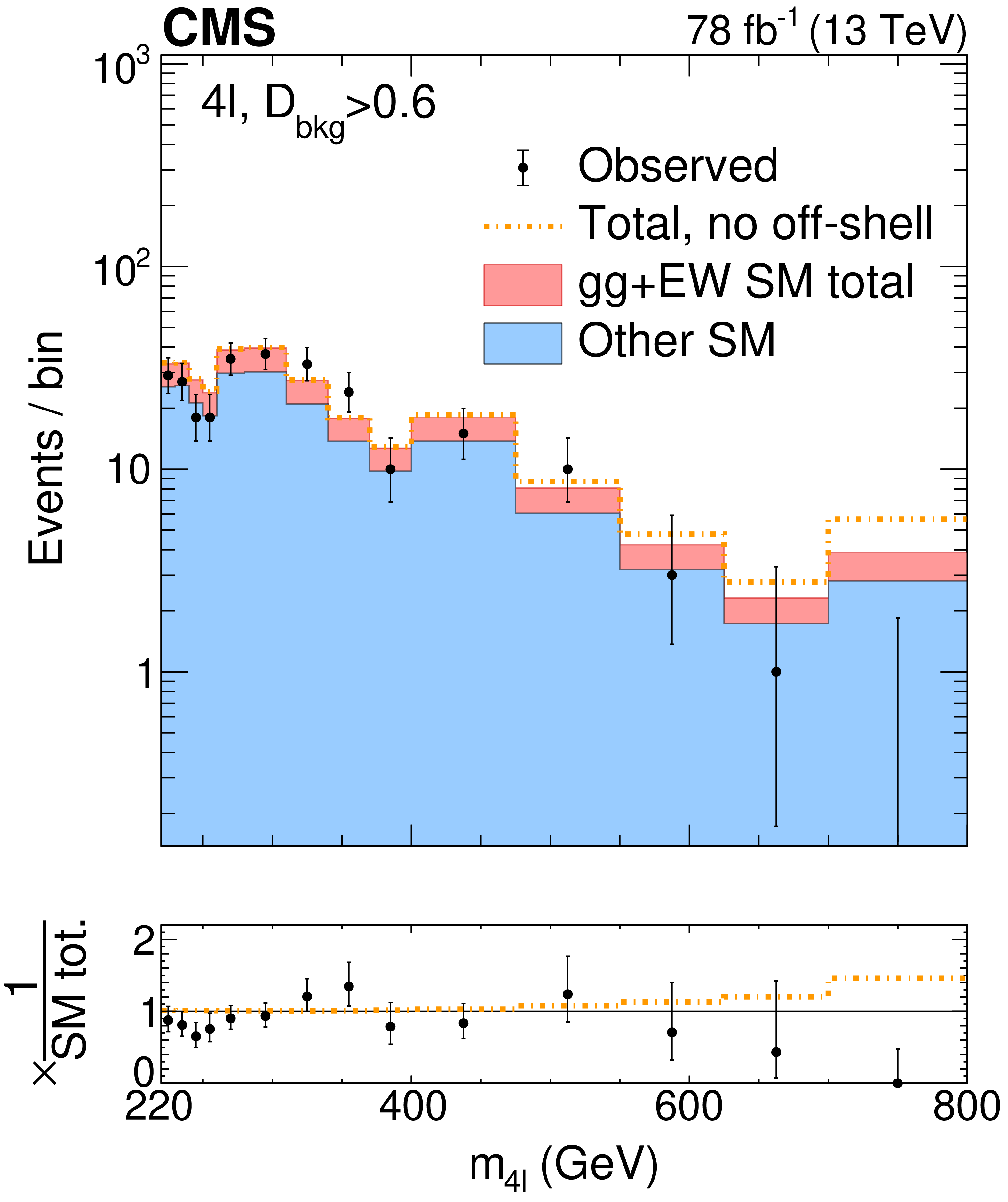
Figure 3:
Distributions of ZZ invariant mass observables in the off-shell signal regions. The distributions of transverse ZZ invariant mass, $ m_\mathrm{T}^{\mathrm{Z}\mathrm{Z}} $ from the 2$ \ell$2$\nu $ off-shell signal region are displayed on the left panel, and those of the 4$ \ell $ invariant mass, $ m_{4\ell} $, from the 4$ \ell $ off-shell signal region are displayed on the right. The stacked histogram displays the distribution after a fit to the data with SM couplings, with the blue filled area corresponding to the SM processes that do not include H boson interactions, and the pink filled area adding processes that include H boson and interference contributions. The gold dot-dashed line shows the fit to the no off-shell hypothesis. The black points with error bars as uncertainties at 68% CL show the observed data, which is consistent with the prediction with SM couplings within one standard deviation. The last bins contain the overflow. The requirements on the missing transverse momentum $ p_{\mathrm{T}}^\text{miss} $ in 2$ \ell$2$\nu $ events, and the $ {\mathcal{D}}_{\text{bkg}} $-type kinematic background discriminants (see Table II of Ref. [15]) in 4$ \ell $ events are applied in order to enhance the H boson signal contribution. The values of integrated luminosity displayed correspond to those included in the off-shell analyses of each final state. The bottom panels show the ratio of the data or dashed histograms to the SM prediction (stacked histogram). The black horizontal line in these panels marks unit ratio. |

png pdf |
Figure 3-a:
The distributions of transverse ZZ invariant mass, $ m_\mathrm{T}^{\mathrm{Z}\mathrm{Z}} $ from the 2$ \ell$2$\nu $ off-shell signal region are displayed. The stacked histogram displays the distribution after a fit to the data with SM couplings, with the blue filled area corresponding to the SM processes that do not include H boson interactions, and the pink filled area adding processes that include H boson and interference contributions. The gold dot-dashed line shows the fit to the no off-shell hypothesis. The black points with error bars as uncertainties at 68% CL show the observed data, which is consistent with the prediction with SM couplings within one standard deviation. The last bins contain the overflow. The requirements on the missing transverse momentum $ p_{\mathrm{T}}^\text{miss} $ in 2$ \ell$2$\nu $ events, and the $ {\mathcal{D}}_{\text{bkg}} $-type kinematic background discriminants (see Table II of Ref. [15]) in 4$ \ell $ events are applied in order to enhance the H boson signal contribution. The values of integrated luminosity displayed correspond to those included in the off-shell analyses of each final state. The bottom panel shows the ratio of the data or dashed histograms to the SM prediction (stacked histogram). The black horizontal line in these panels marks unit ratio. |
png pdf |
Figure 3-b:
The distributions of the 4$ \ell $ invariant mass, $ m_{4\ell} $, from the 4$ \ell $ off-shell signal region are displayed. The stacked histogram displays the distribution after a fit to the data with SM couplings, with the blue filled area corresponding to the SM processes that do not include H boson interactions, and the pink filled area adding processes that include H boson and interference contributions. The gold dot-dashed line shows the fit to the no off-shell hypothesis. The black points with error bars as uncertainties at 68% CL show the observed data, which is consistent with the prediction with SM couplings within one standard deviation. The last bins contain the overflow. The requirements on the missing transverse momentum $ p_{\mathrm{T}}^\text{miss} $ in 2$ \ell$2$\nu $ events, and the $ {\mathcal{D}}_{\text{bkg}} $-type kinematic background discriminants (see Table II of Ref. [15]) in 4$ \ell $ events are applied in order to enhance the H boson signal contribution. The values of integrated luminosity displayed correspond to those included in the off-shell analyses of each final state. The bottom panel shows the ratio of the data or dashed histograms to the SM prediction (stacked histogram). The black horizontal line in these panels marks unit ratio. |
png pdf |
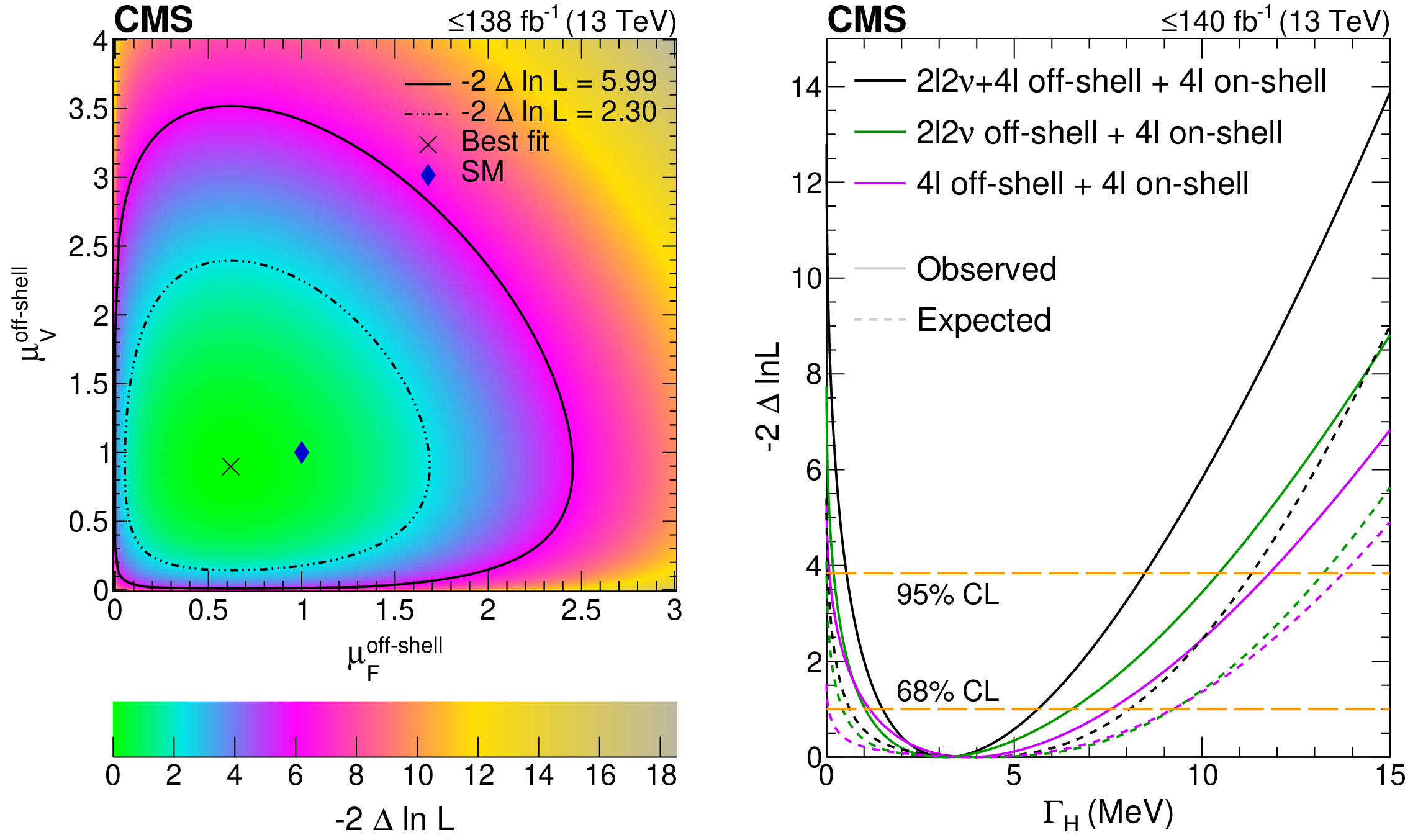
Figure 4:
Log-likelihood scans of $ \mu^{\text{off-shell}}_{\mathrm{F}} $ and $ \mu^{\text{off-shell}}_{{\mathrm{V}}} $, and $ \Gamma_{\mathrm{H}} $. Left panel: Two-parameter likelihood scan of the off-shell gg and EW production signal strength parameters, $ \mu^{\text{off-shell}}_{\mathrm{F}} $ and $ \mu^{\text{off-shell}}_{{\mathrm{V}}} $, respectively. The dot-dashed and dashed contours enclose the 68% ($ -$2$\Delta\ln\mathcal{L}= $ 2.30) and 95% ($ -$2$\Delta\ln\mathcal{L}= $ 5.99) CL regions. The cross marks the minimum, and the blue diamond marks the SM expectation. The integrated luminosity reaches only up to 138 fb$^{-1}$ as on-shell 4$ \ell $ events are not included in performing this scan. Right panel: The observed (solid) and expected (dashed) one-parameter likelihood scans over $ \Gamma_{\mathrm{H}} $. Scans are shown for the combination of 4$ \ell $ on-shell data with 4$ \ell $ off-shell (magenta) or 2$ \ell$2$\nu $ off-shell data (green) alone, or with both data sets (black). The horizontal lines indicate the 68% ($ -$2$\Delta\ln\mathcal{L}= $ 1.0) and 95% ($ -$2$\Delta\ln\mathcal{L}= $ 3.84) CL regions. The integrated luminosity reaches up to 140 fb$^{-1}$ as on-shell 4$ \ell $ events are included in performing these scans. The exclusion of the no off-shell hypothesis is consistent with 3.6 standard deviations on both panels. |
png pdf |
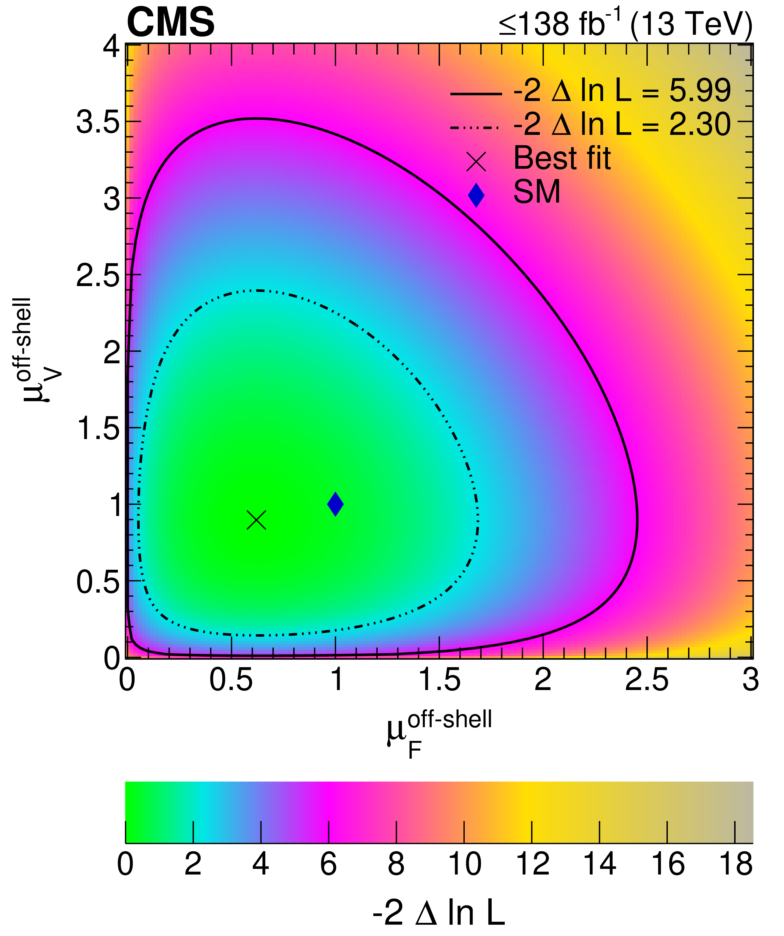
Figure 4-a:
Two-parameter likelihood scan of the off-shell gg and EW production signal strength parameters, $ \mu^{\text{off-shell}}_{\mathrm{F}} $ and $ \mu^{\text{off-shell}}_{{\mathrm{V}}} $, respectively. The dot-dashed and dashed contours enclose the 68% ($ -$2$\Delta\ln\mathcal{L}= $ 2.30) and 95% ($ -$2$\Delta\ln\mathcal{L}= $ 5.99) CL regions. The cross marks the minimum, and the blue diamond marks the SM expectation. The integrated luminosity reaches only up to 138 fb$^{-1}$ as on-shell 4$ \ell $ events are not included in performing this scan. |
png pdf |
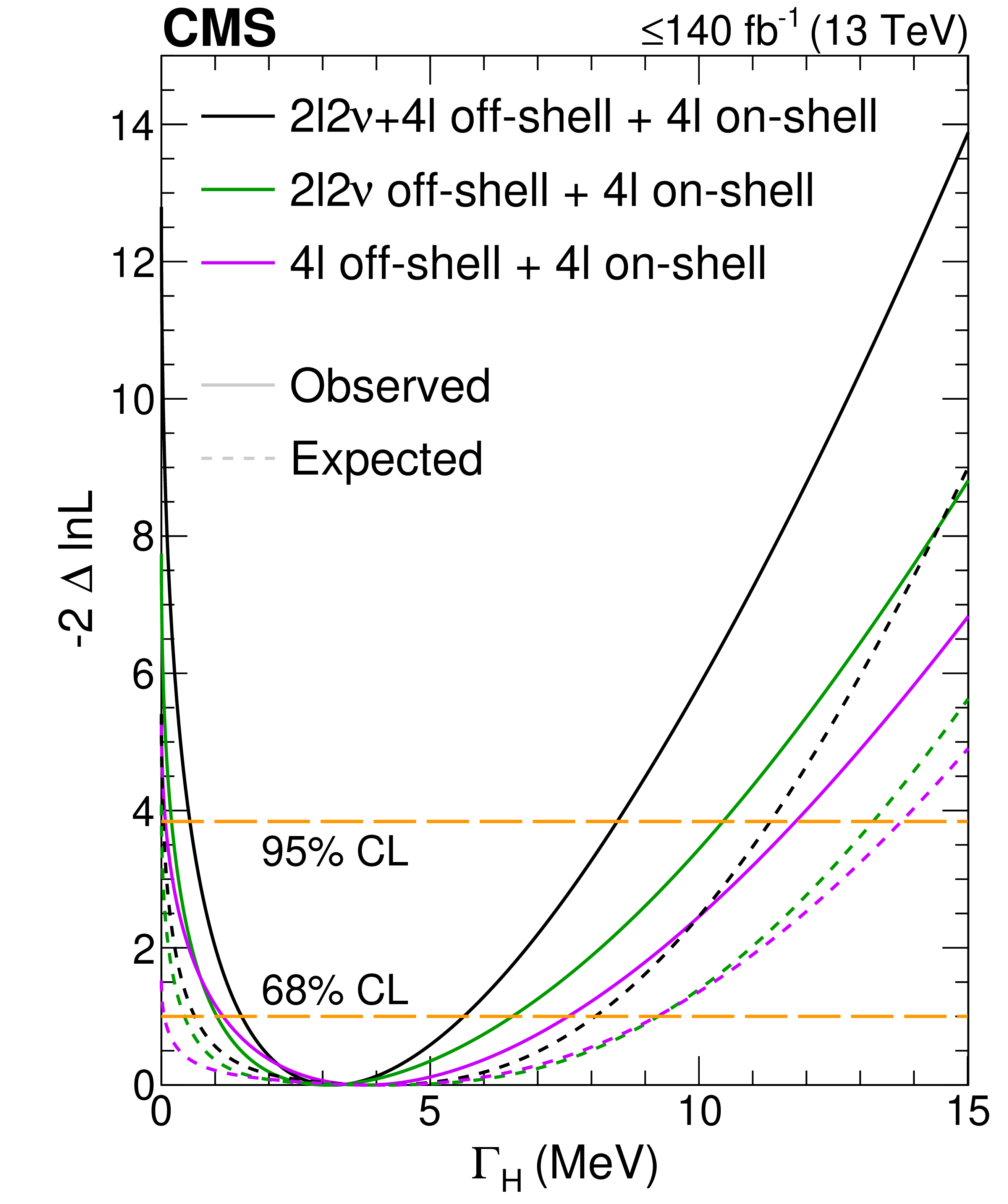
Figure 4-b:
The observed (solid) and expected (dashed) one-parameter likelihood scans over $ \Gamma_{\mathrm{H}} $. Scans are shown for the combination of 4$ \ell $ on-shell data with 4$ \ell $ off-shell (magenta) or 2$ \ell$2$\nu $ off-shell data (green) alone, or with both data sets (black). The horizontal lines indicate the 68% ($ -$2$\Delta\ln\mathcal{L}= $ 1.0) and 95% ($ -$2$\Delta\ln\mathcal{L}= $ 3.84) CL regions. The integrated luminosity reaches up to 140 fb$^{-1}$ as on-shell 4$ \ell $ events are included in performing these scans. The exclusion of the no off-shell hypothesis is consistent with 3.6 standard deviations on both panels. |
png pdf |
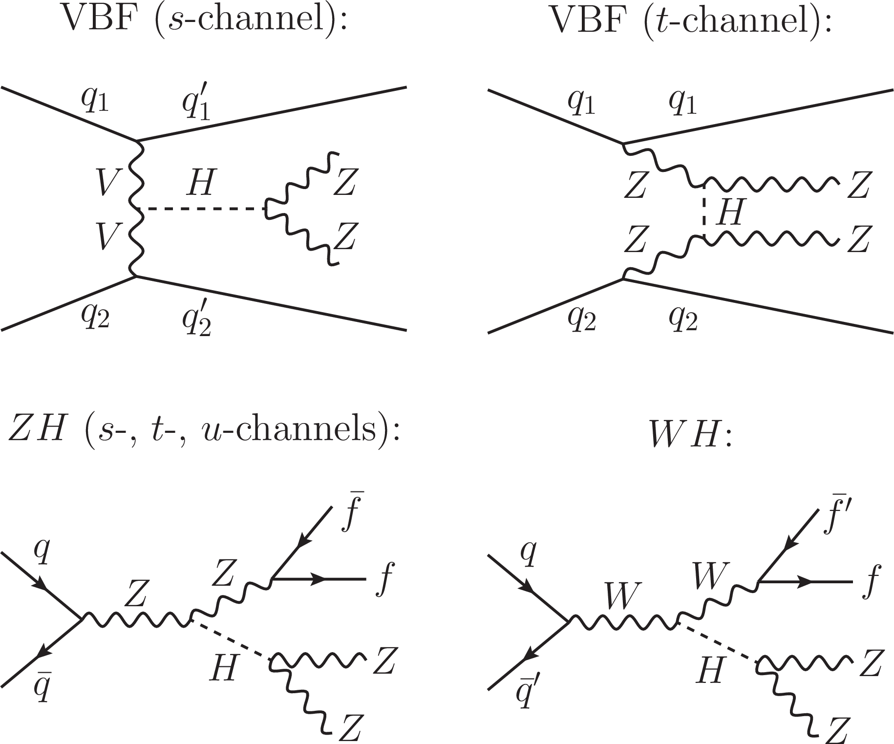
Figure S1:
Feynman diagrams for the H boson -mediated EW ZZ production contributions. Here, $ f $ refers to any $ \ell $, $ \nu $, or $ q $. The tree-level diagrams featuring VBF production are grouped together in the upper row, and those featuring VH production are grouped in the lower row. The interaction displayed in each diagram is meant to progress from left to right. Each straight, curvy, or curly line refers to the different set of particles denoted. Straight, solid lines with no arrows indicate the line could refer to either a particle or an antiparticle, whereas those with forward (backward) arrows refer to a particle (an antiparticle). |
png pdf |
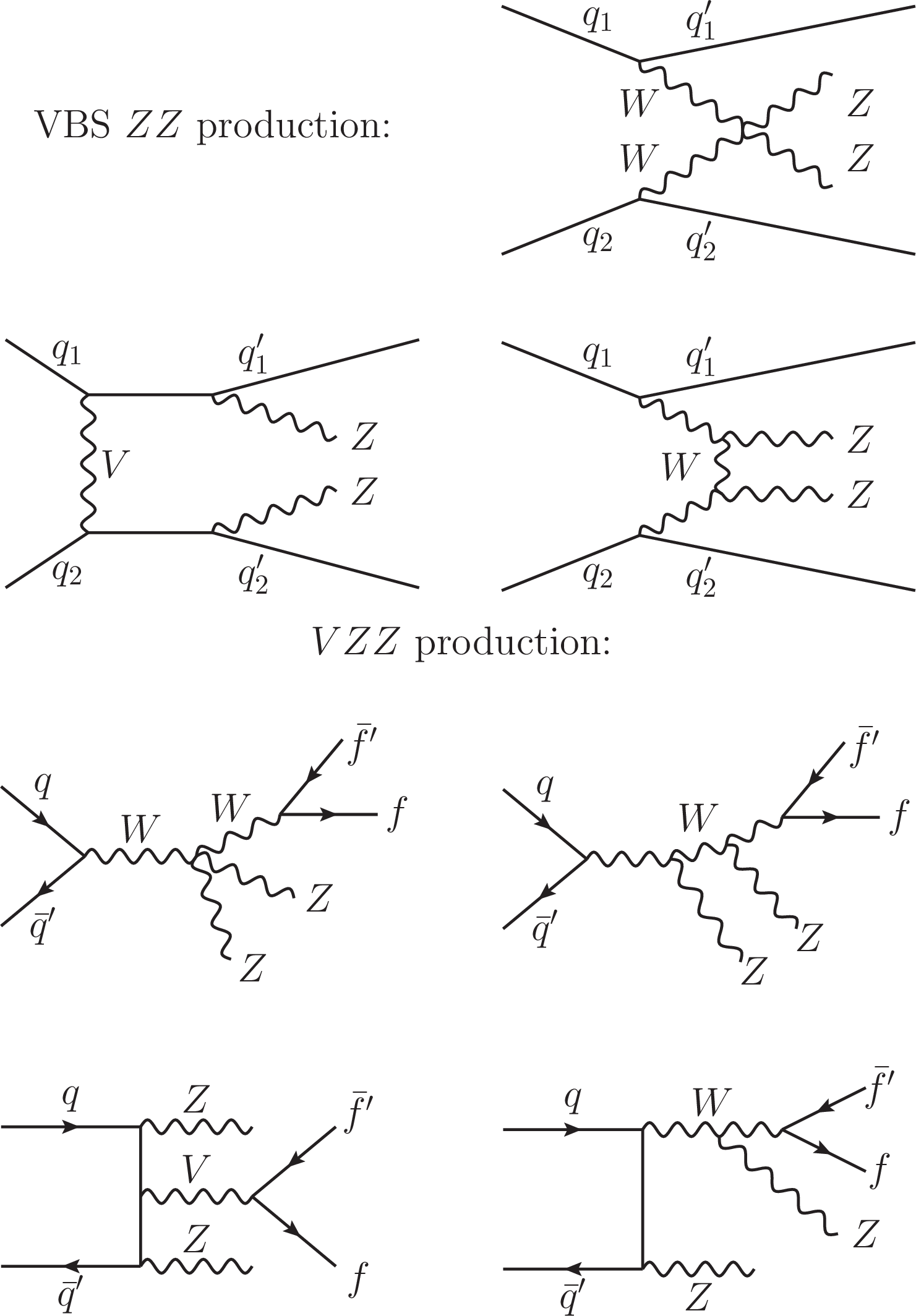
Figure S2:
Feynman diagrams for the EW continuum ZZ production contributions. Here, $ f $ refers to any $ \ell $, $ \nu $, or $ q $. The tree-level diagrams featuring vector boson scattering (VBS) production are grouped together in the upper half, and those featuring VZZ production are grouped in the lower half. The interaction displayed in each diagram is meant to progress from left to right. Each straight, curvy, or curly line refers to the different set of particles denoted. Straight, solid lines with no arrows indicate the line could refer to either a particle or an antiparticle, whereas those with forward (backward) arrows refer to a particle (an antiparticle). |
png pdf |
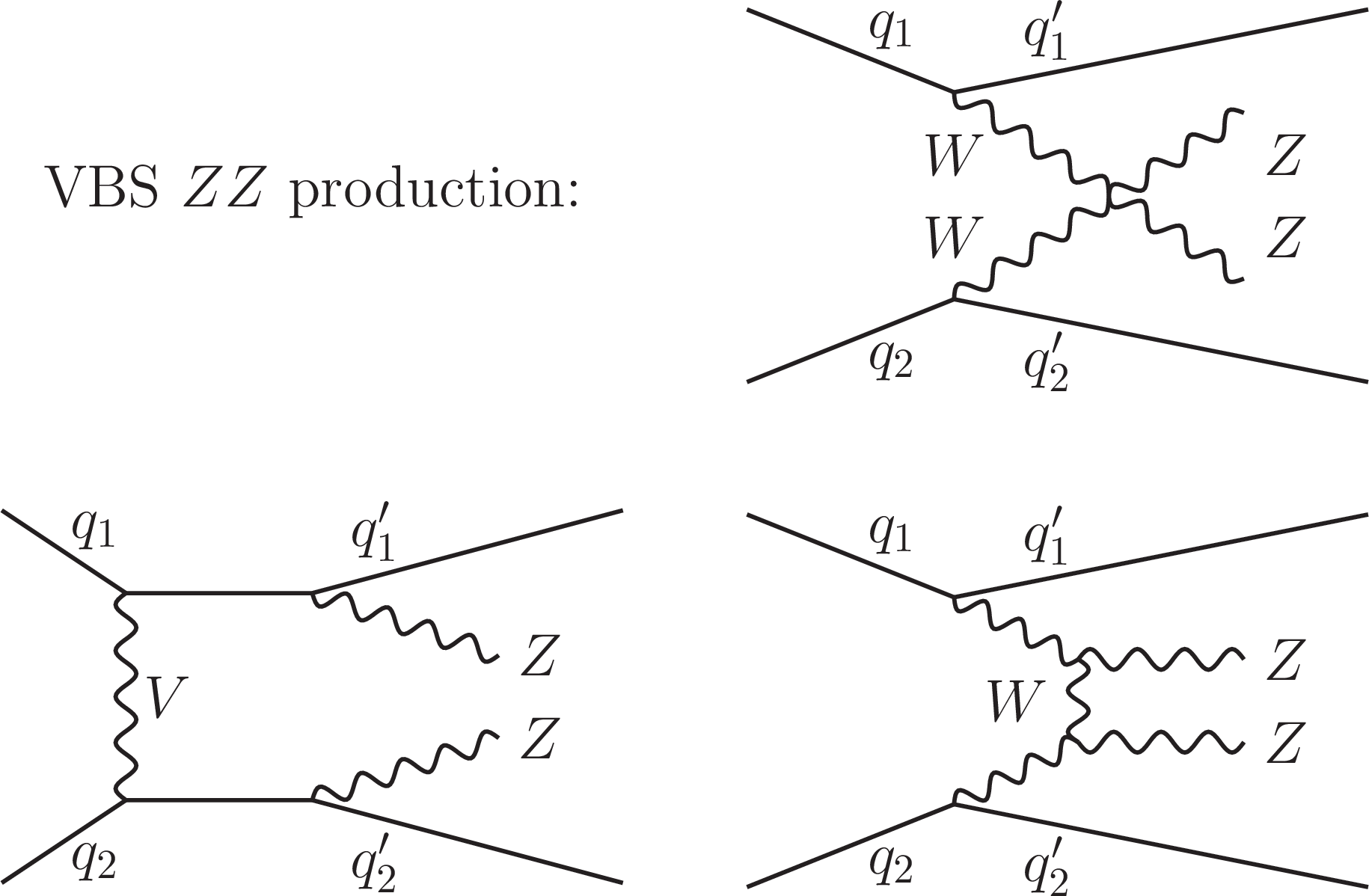
Figure S2-a:
The tree-level diagrams featuring vector boson scattering (VBS) production are grouped together. The interaction displayed in each diagram is meant to progress from left to right. Each straight, curvy, or curly line refers to the different set of particles denoted. Straight, solid lines with no arrows indicate the line could refer to either a particle or an antiparticle, whereas those with forward (backward) arrows refer to a particle (an antiparticle). |
png pdf |
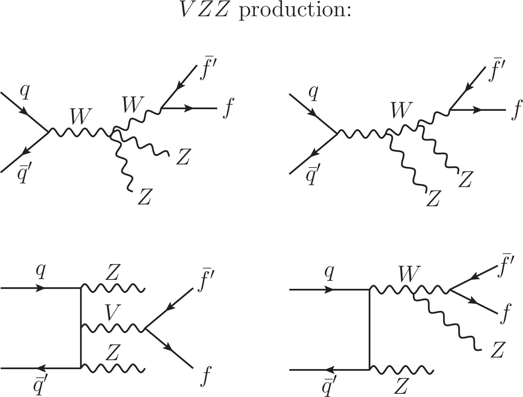
Figure S2-b:
The tree-level diagrams featuring VZZ production are grouped together. The interaction displayed in each diagram is meant to progress from left to right. Each straight, curvy, or curly line refers to the different set of particles denoted. Straight, solid lines with no arrows indicate the line could refer to either a particle or an antiparticle, whereas those with forward (backward) arrows refer to a particle (an antiparticle). |
png pdf |
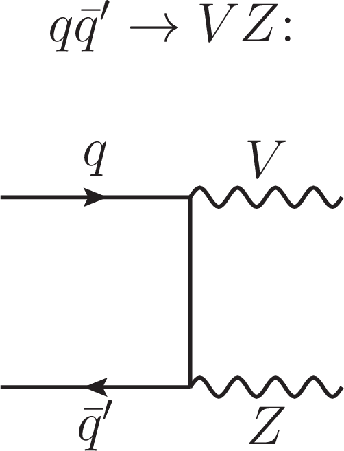
Figure S3:
Feynman diagram for the $ \mathrm{q}\overline{\mathrm{q}} \to \mathrm{Z}\mathrm{Z} $ and $ \mathrm{q}{\mathrm{\bar{q}}'} \to {\mathrm{W}}\mathrm{Z} $ processes. Both processes are represented at tree level with a single diagram. These two processes constitute the major irreducible, noninterfering background contributions in the off-shell region. The interaction displayed in each diagram is meant to progress from left to right. Each straight, curvy, or curly line refers to the different set of particles denoted. Straight, solid lines with no arrows indicate the line could refer to either a particle or an antiparticle, whereas those with forward (backward) arrows refer to a particle (an antiparticle). |

png pdf |
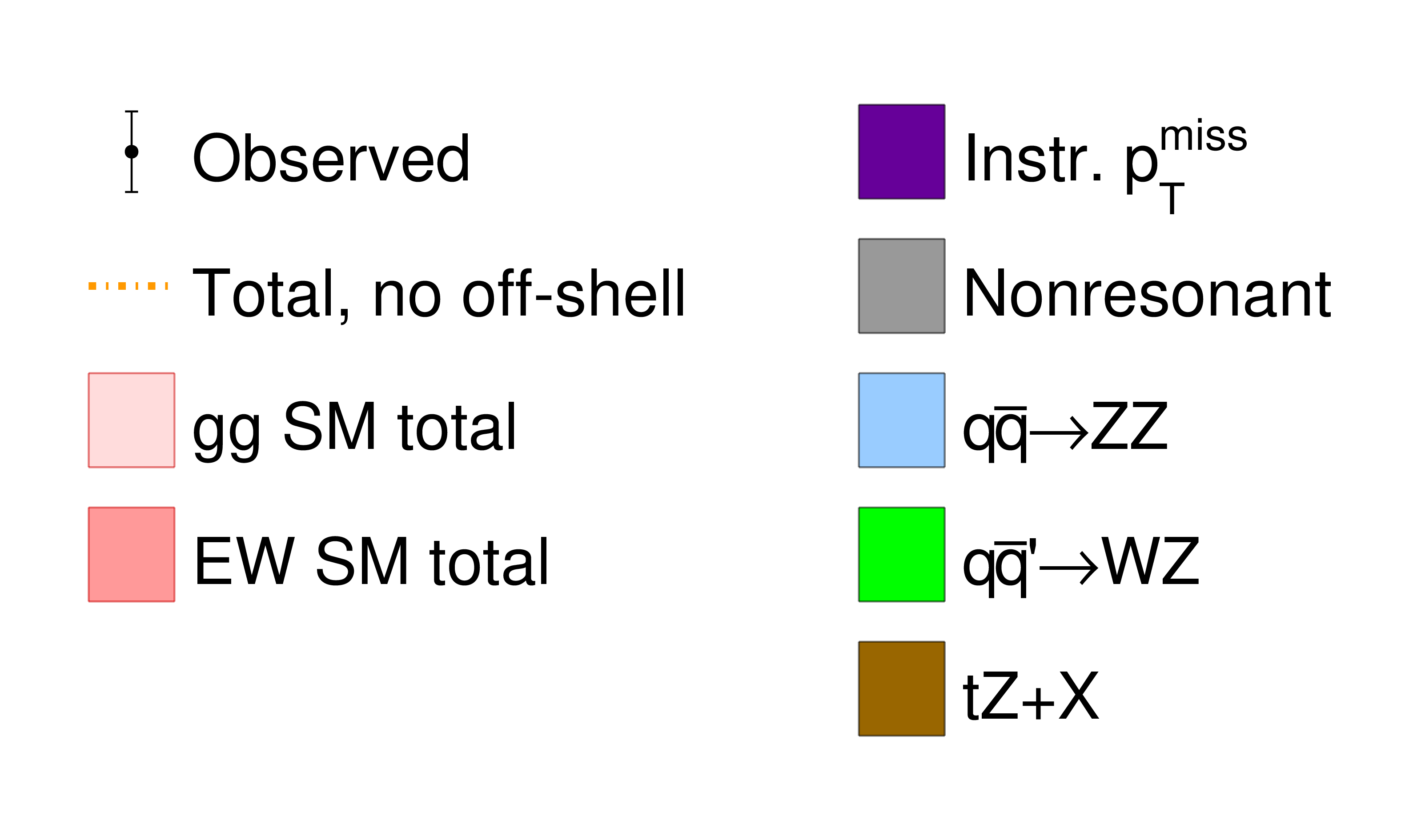
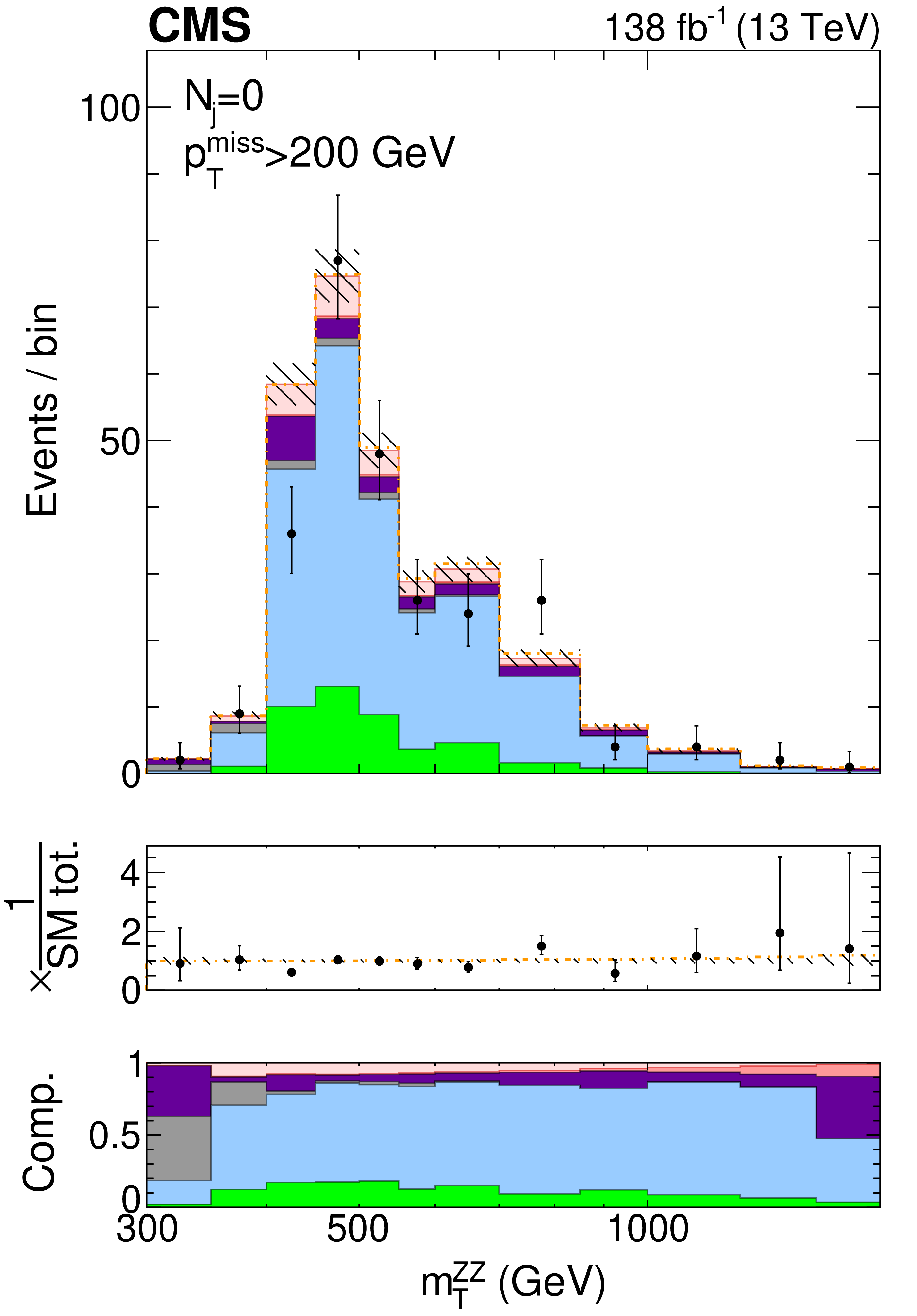
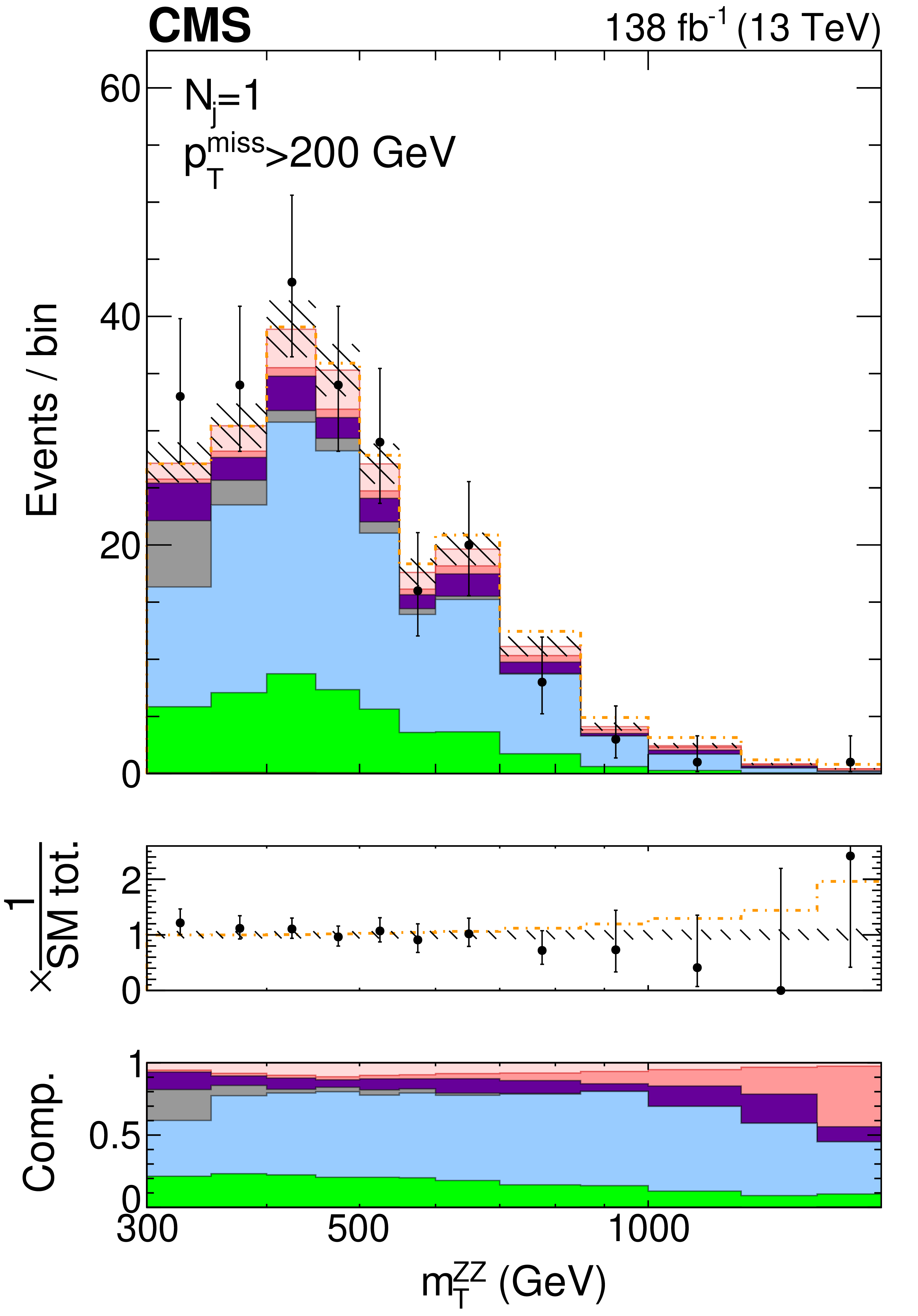
Figure S4:
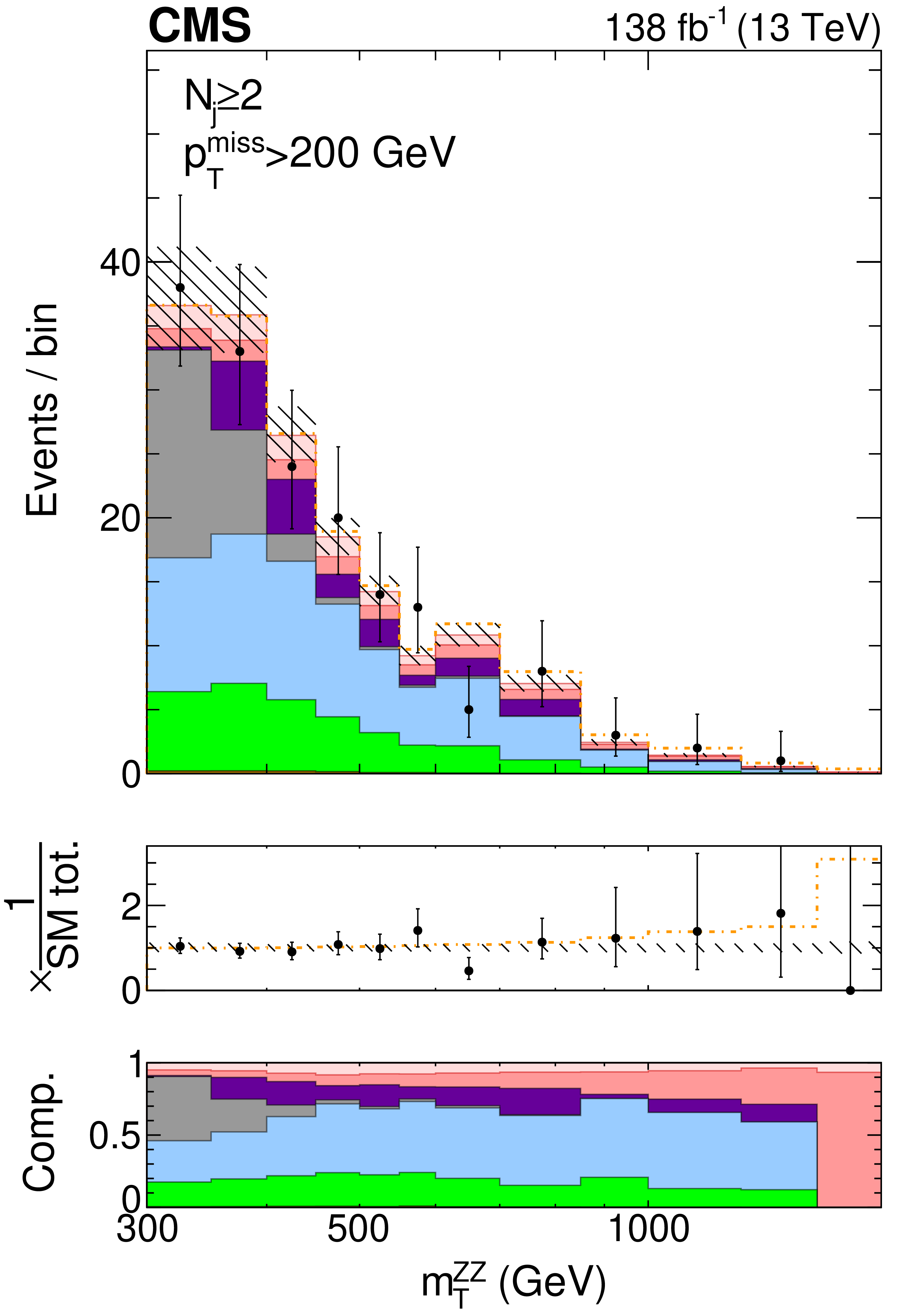
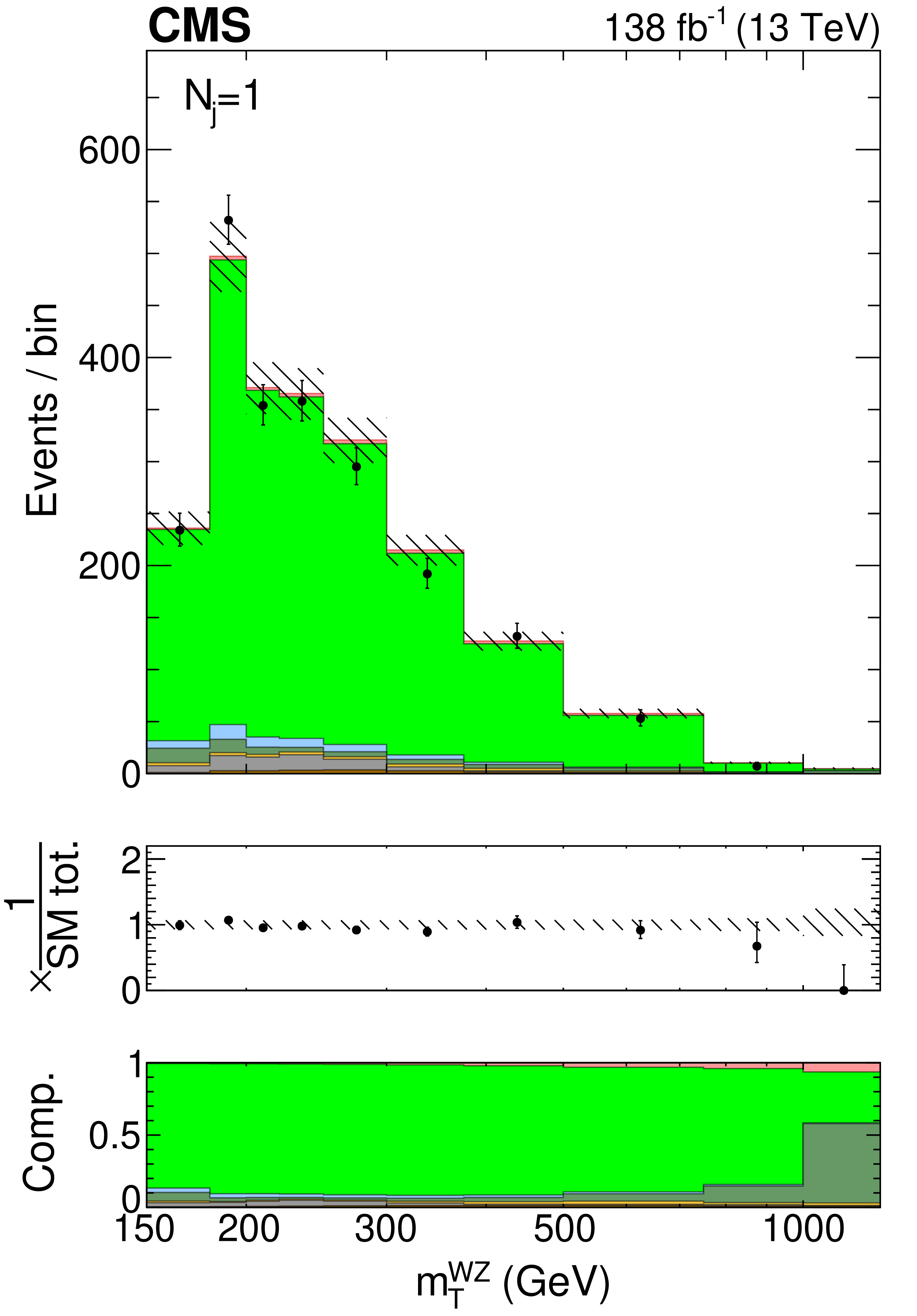
Distributions of $ m_\mathrm{T}^{\mathrm{Z}\mathrm{Z}} $ in the different $ N_{\mathrm{j}} $ categories of the 2$ \ell$2$\nu $ signal region. The postfit distributions of the transverse ZZ invariant mass are displayed in the jet multiplicity categories of $ N_{\mathrm{j}}= $ 0 (left), $ = $ 1 (middle), and $ \geq $ 2 (right) with a missing transverse momentum requirement of $ p_{\mathrm{T}}^\text{miss} > $ 200 GeV to enrich H boson contributions. The color legend for the stacked or dot-dashed histograms is given above the plots. The stacked histogram is split into the following components: gg (light pink) and EW (dark pink) ZZ production, instrumental $ p_{\mathrm{T}}^\text{miss} $ background (purple), nonresonant proceses (gray), the $ \mathrm{q}\overline{\mathrm{q}} \to \mathrm{Z}\mathrm{Z} $ (blue) and $ \mathrm{q}{\mathrm{\bar{q}}'} \to {\mathrm{W}}\mathrm{Z} $ (green) processes, and tZ+X production, where X refers to any other particle. Postfit refers to individual fits of the data (shown as black points with error bars as uncertainties at 68% CL) to the combined 2$ \ell$2$\nu$+4$\ell $ sample, including the WZ control region, and assuming either SM H boson parameters (stacked histogram with the hashed band as the total postfit uncertainty at 68% CL) or no off-shell H boson production (dot-dashed gold line). The middle panels along the vertical show the ratio of the data or dashed histograms to the stacked histogram, and the lower panels show the predicted relative contributions of each process. The rightmost bins contain the overflow. |
png pdf |
Figure S4-a:
The color legend for the stacked or dot-dashed histograms for the following plots. |
png pdf |
Figure S4-b:
The postfit distributions of the transverse ZZ invariant mass are displayed in the jet multiplicity category of $ N_{\mathrm{j}}= $ 0 with a missing transverse momentum requirement of $ p_{\mathrm{T}}^\text{miss} > $ 200 GeV to enrich H boson contributions. The stacked histogram is split into the following components: gg (light pink) and EW (dark pink) ZZ production, instrumental $ p_{\mathrm{T}}^\text{miss} $ background (purple), nonresonant proceses (gray), the $ \mathrm{q}\overline{\mathrm{q}} \to \mathrm{Z}\mathrm{Z} $ (blue) and $ \mathrm{q}{\mathrm{\bar{q}}'} \to {\mathrm{W}}\mathrm{Z} $ (green) processes, and tZ+X production, where X refers to any other particle. Postfit refers to individual fits of the data (shown as black points with error bars as uncertainties at 68% CL) to the combined 2$ \ell$2$\nu$+4$\ell $ sample, including the WZ control region, and assuming either SM H boson parameters (stacked histogram with the hashed band as the total postfit uncertainty at 68% CL) or no off-shell H boson production (dot-dashed gold line). The middle panel shows the ratio of the data or dashed histograms to the stacked histogram, and the lower panel shows the predicted relative contributions. The rightmost bins contain the overflow. |
png pdf |
Figure S4-c:
The postfit distributions of the transverse ZZ invariant mass are displayed in the jet multiplicity category of $ N_{\mathrm{j}}= $ 1 with a missing transverse momentum requirement of $ p_{\mathrm{T}}^\text{miss} > $ 200 GeV to enrich H boson contributions. The stacked histogram is split into the following components: gg (light pink) and EW (dark pink) ZZ production, instrumental $ p_{\mathrm{T}}^\text{miss} $ background (purple), nonresonant proceses (gray), the $ \mathrm{q}\overline{\mathrm{q}} \to \mathrm{Z}\mathrm{Z} $ (blue) and $ \mathrm{q}{\mathrm{\bar{q}}'} \to {\mathrm{W}}\mathrm{Z} $ (green) processes, and tZ+X production, where X refers to any other particle. Postfit refers to individual fits of the data (shown as black points with error bars as uncertainties at 68% CL) to the combined 2$ \ell$2$\nu$+4$\ell $ sample, including the WZ control region, and assuming either SM H boson parameters (stacked histogram with the hashed band as the total postfit uncertainty at 68% CL) or no off-shell H boson production (dot-dashed gold line). The middle panel shows the ratio of the data or dashed histograms to the stacked histogram, and the lower panel shows the predicted relative contributions. The rightmost bins contain the overflow. |
png pdf |
Figure S4-d:
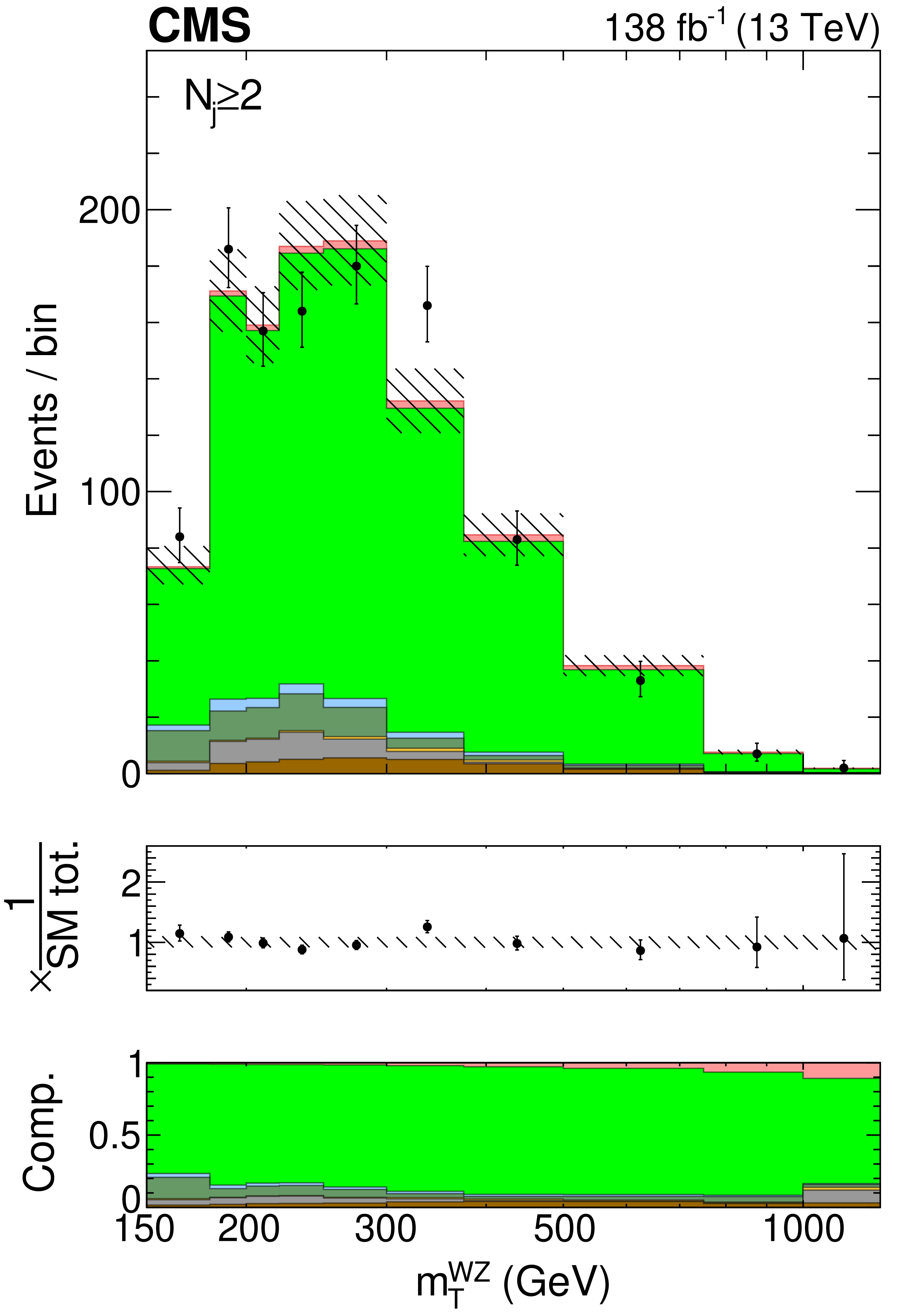
The postfit distributions of the transverse ZZ invariant mass are displayed in the jet multiplicity category of $ N_{\mathrm{j}} \geq $ 2 with a missing transverse momentum requirement of $ p_{\mathrm{T}}^\text{miss} > $ 200 GeV to enrich H boson contributions. The stacked histogram is split into the following components: gg (light pink) and EW (dark pink) ZZ production, instrumental $ p_{\mathrm{T}}^\text{miss} $ background (purple), nonresonant proceses (gray), the $ \mathrm{q}\overline{\mathrm{q}} \to \mathrm{Z}\mathrm{Z} $ (blue) and $ \mathrm{q}{\mathrm{\bar{q}}'} \to {\mathrm{W}}\mathrm{Z} $ (green) processes, and tZ+X production, where X refers to any other particle. Postfit refers to individual fits of the data (shown as black points with error bars as uncertainties at 68% CL) to the combined 2$ \ell$2$\nu$+4$\ell $ sample, including the WZ control region, and assuming either SM H boson parameters (stacked histogram with the hashed band as the total postfit uncertainty at 68% CL) or no off-shell H boson production (dot-dashed gold line). The middle panel shows the ratio of the data or dashed histograms to the stacked histogram, and the lower panel shows the predicted relative contributions. The rightmost bins contain the overflow. |
png pdf |
Figure S5:
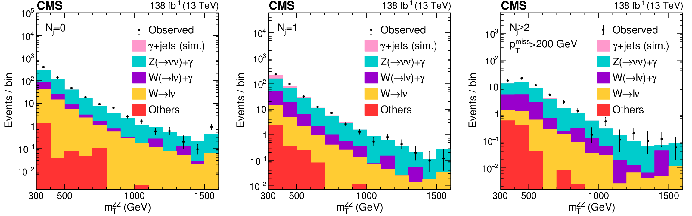
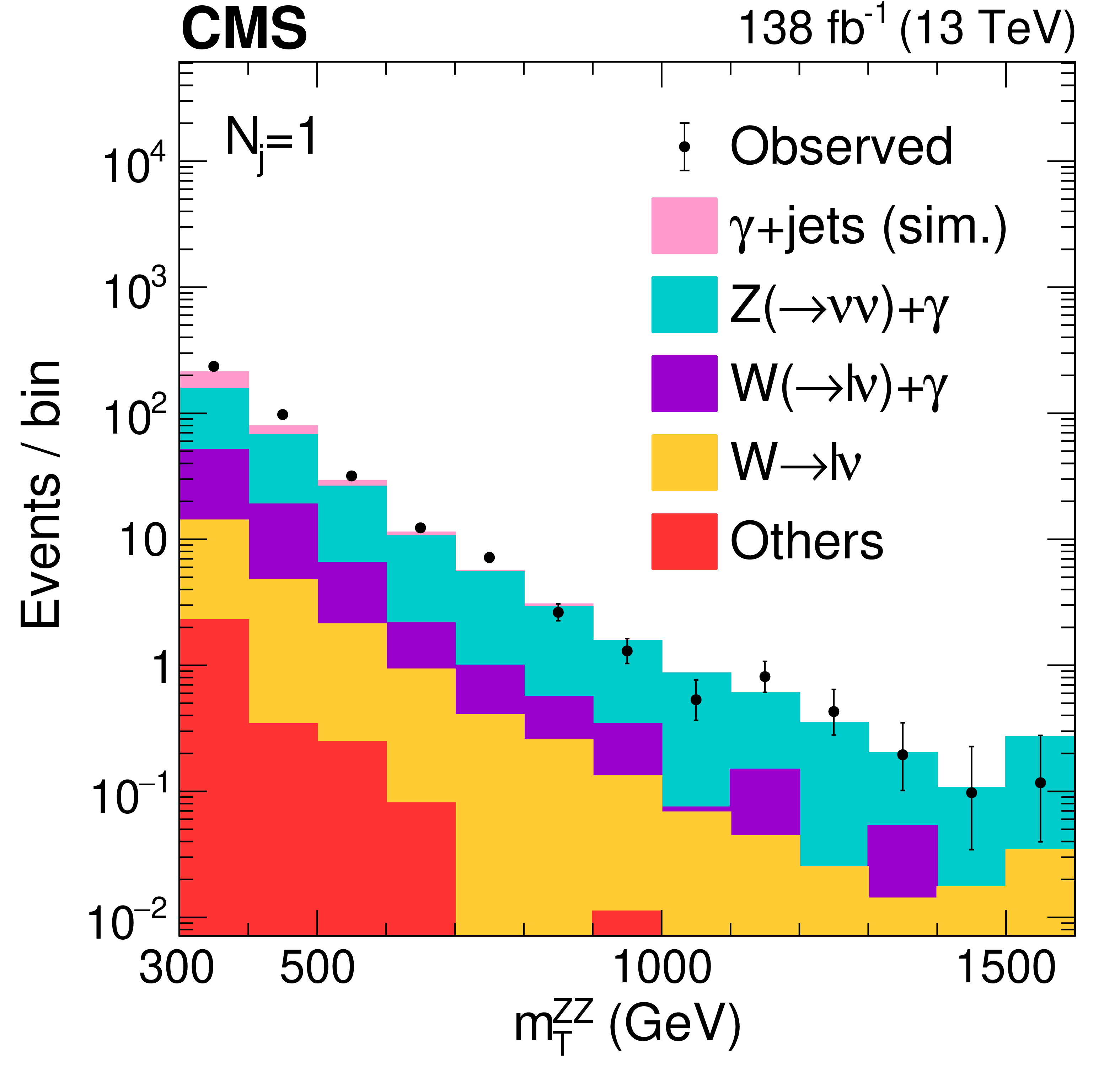
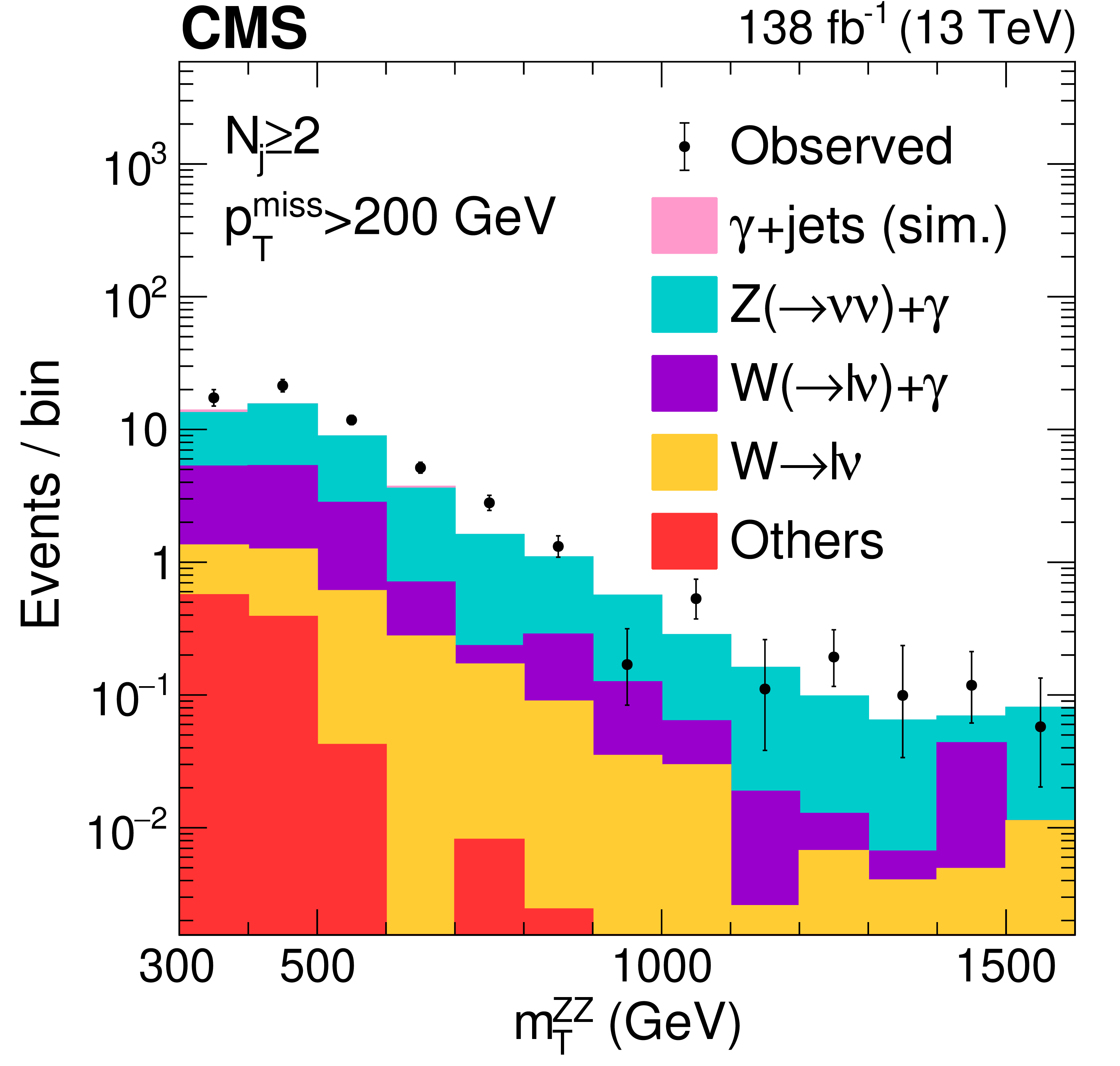
Distributions of $ m_\mathrm{T}^{\mathrm{Z}\mathrm{Z}} $ in the different $ N_{\mathrm{j}} $ categories of the $ {\gamma} $+jets CR. The distributions of the transverse ZZ invariant mass are displayed for the $ N_{\mathrm{j}}= $ 0, $ N_{\mathrm{j}}= $ 1, and $ N_{\mathrm{j}}\geq $ 2 jet multiplicity categories from left to right. The missing transverse momentum requirement $ p_{\mathrm{T}}^\text{miss} > $ 200 GeV is applied in the $ N_{\mathrm{j}}\geq $ 2 category to focus on the region more sensitive to off-shell H boson production. The stacked histogram shows the predictions for contributions with genuine, large $ p_{\mathrm{T}}^\text{miss} $, or the instrumental $ p_{\mathrm{T}}^\text{miss} $ background from the $ {\gamma} $+jets simulation. Contributions with genuine, large $ p_{\mathrm{T}}^\text{miss} $ are split as those coming from the more dominant $ \mathrm{Z}(\to\nu\nu){\gamma} $ (teal), $ \mathrm{W}(\to\ell\nu){\gamma} $ (purple), and $ \mathrm{W}(\to\ell\nu) $+jets (yellow) processes, and other small components (red). The prediction for instrumental $ p_{\mathrm{T}}^\text{miss} $ background from simulation is shown in light pink. The black points with error bars as uncertainties at 68% CL show the observed CR data. The distributions are reweighted with the $ \gamma \to \ell\ell $ transfer factors extracted from the $ p_{\mathrm{T}}^\text{miss} < $ 125 GeV sidebands. The rightmost bins include the overflow. In these distributions, we find a discrepancy between the observed data and the predicted distributions because the reweighted $ {\gamma} $+jets samples have inaccurate $ p_{\mathrm{T}}^\text{miss} $ response and the simulation is at LO in QCD. Therefore, we use the difference between the observed data and the genuine-$ p_{\mathrm{T}}^\text{miss} $ contributions to model the instrumental $ p_{\mathrm{T}}^\text{miss} $ background instead of using simulation for this estimate. |

png pdf |
Figure S5-a:
The distributions of the transverse ZZ invariant mass are displayed for the $ N_{\mathrm{j}}= $ 0 jet multiplicity category. The stacked histogram shows the predictions for contributions with genuine, large $ p_{\mathrm{T}}^\text{miss} $, or the instrumental $ p_{\mathrm{T}}^\text{miss} $ background from the $ {\gamma} $+jets simulation. Contributions with genuine, large $ p_{\mathrm{T}}^\text{miss} $ are split as those coming from the more dominant $ \mathrm{Z}(\to\nu\nu){\gamma} $ (teal), $ \mathrm{W}(\to\ell\nu){\gamma} $ (purple), and $ \mathrm{W}(\to\ell\nu) $+jets (yellow) processes, and other small components (red). The prediction for instrumental $ p_{\mathrm{T}}^\text{miss} $ background from simulation is shown in light pink. The black points with error bars as uncertainties at 68% CL show the observed CR data. The distributions are reweighted with the $ \gamma \to \ell\ell $ transfer factors extracted from the $ p_{\mathrm{T}}^\text{miss} < $ 125 GeV sidebands. The rightmost bins include the overflow. In these distributions, we find a discrepancy between the observed data and the predicted distributions because the reweighted $ {\gamma} $+jets samples have inaccurate $ p_{\mathrm{T}}^\text{miss} $ response and the simulation is at LO in QCD. Therefore, we use the difference between the observed data and the genuine-$ p_{\mathrm{T}}^\text{miss} $ contributions to model the instrumental $ p_{\mathrm{T}}^\text{miss} $ background instead of using simulation for this estimate. |
png pdf |
Figure S5-b:
The distributions of the transverse ZZ invariant mass are displayed for the $ N_{\mathrm{j}}= $ 1 jet multiplicity category. The stacked histogram shows the predictions for contributions with genuine, large $ p_{\mathrm{T}}^\text{miss} $, or the instrumental $ p_{\mathrm{T}}^\text{miss} $ background from the $ {\gamma} $+jets simulation. Contributions with genuine, large $ p_{\mathrm{T}}^\text{miss} $ are split as those coming from the more dominant $ \mathrm{Z}(\to\nu\nu){\gamma} $ (teal), $ \mathrm{W}(\to\ell\nu){\gamma} $ (purple), and $ \mathrm{W}(\to\ell\nu) $+jets (yellow) processes, and other small components (red). The prediction for instrumental $ p_{\mathrm{T}}^\text{miss} $ background from simulation is shown in light pink. The black points with error bars as uncertainties at 68% CL show the observed CR data. The distributions are reweighted with the $ \gamma \to \ell\ell $ transfer factors extracted from the $ p_{\mathrm{T}}^\text{miss} < $ 125 GeV sidebands. The rightmost bins include the overflow. In these distributions, we find a discrepancy between the observed data and the predicted distributions because the reweighted $ {\gamma} $+jets samples have inaccurate $ p_{\mathrm{T}}^\text{miss} $ response and the simulation is at LO in QCD. Therefore, we use the difference between the observed data and the genuine-$ p_{\mathrm{T}}^\text{miss} $ contributions to model the instrumental $ p_{\mathrm{T}}^\text{miss} $ background instead of using simulation for this estimate. |
png pdf |
Figure S5-c:
The distributions of the transverse ZZ invariant mass are displayed for the $ N_{\mathrm{j}}\geq $ 2 jet multiplicity category. The missing transverse momentum requirement $ p_{\mathrm{T}}^\text{miss} > $ 200 GeV is applied to focus on the region more sensitive to off-shell H boson production. The stacked histogram shows the predictions for contributions with genuine, large $ p_{\mathrm{T}}^\text{miss} $, or the instrumental $ p_{\mathrm{T}}^\text{miss} $ background from the $ {\gamma} $+jets simulation. Contributions with genuine, large $ p_{\mathrm{T}}^\text{miss} $ are split as those coming from the more dominant $ \mathrm{Z}(\to\nu\nu){\gamma} $ (teal), $ \mathrm{W}(\to\ell\nu){\gamma} $ (purple), and $ \mathrm{W}(\to\ell\nu) $+jets (yellow) processes, and other small components (red). The prediction for instrumental $ p_{\mathrm{T}}^\text{miss} $ background from simulation is shown in light pink. The black points with error bars as uncertainties at 68% CL show the observed CR data. The distributions are reweighted with the $ \gamma \to \ell\ell $ transfer factors extracted from the $ p_{\mathrm{T}}^\text{miss} < $ 125 GeV sidebands. The rightmost bins include the overflow. In these distributions, we find a discrepancy between the observed data and the predicted distributions because the reweighted $ {\gamma} $+jets samples have inaccurate $ p_{\mathrm{T}}^\text{miss} $ response and the simulation is at LO in QCD. Therefore, we use the difference between the observed data and the genuine-$ p_{\mathrm{T}}^\text{miss} $ contributions to model the instrumental $ p_{\mathrm{T}}^\text{miss} $ background instead of using simulation for this estimate. |
png pdf |
Figure S6:
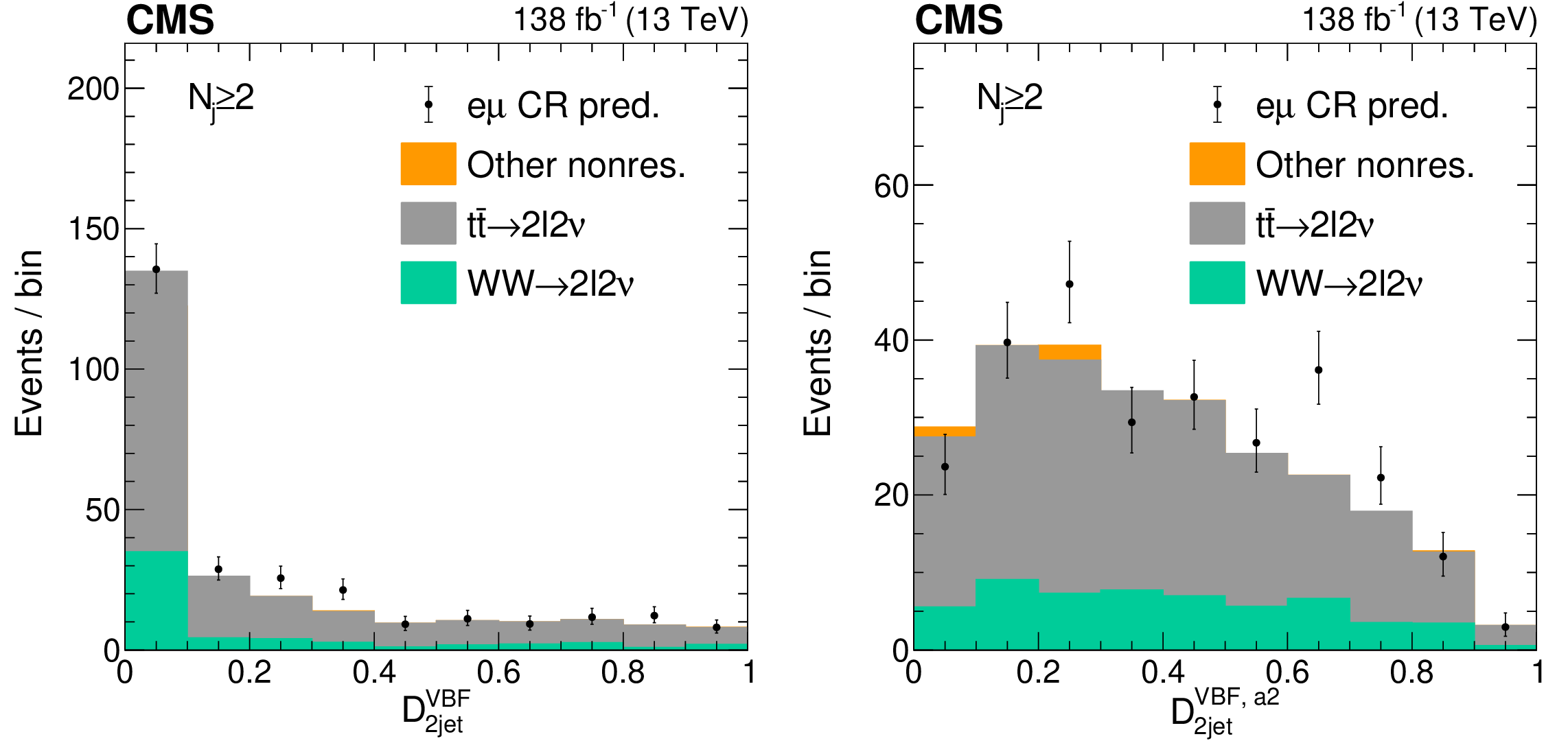
Distributions of the VBF discriminants for nonresonant background. The distributions of the SM $ {\mathcal{D}}^{{\text{VBF}}}_{\text{2jet}} $ (left) and $ {\mathcal{D}}^{{\text{VBF}}, a2}_{\text{2jet}} $ (right) kinematic VBF discriminants are shown in the 2$ \ell$2$\nu $ signal region, $ N_{\mathrm{j}}\geq $ 2 category. The stacked histogram shows the predictions from simulation, which consists of nonresonant contributions from $ {\mathrm{W}}{\mathrm{W}} $ (green) and $ {\mathrm{t}\overline{\mathrm{t}}} $ (gray) production, or other small components (orange). The black points with error bars as uncertainties at 68% CL show the prediction from the e$\mu$ CR data. While only the data is used in the final estimate of the nonresonant background, we note that predictions from simulation already agree well with the data estimate. |

png pdf |
Figure S6-a:
Distributions of the VBF discriminants for nonresonant background. The distributions of the SM $ {\mathcal{D}}^{{\text{VBF}}}_{\text{2jet}} $ (left) and $ {\mathcal{D}}^{{\text{VBF}}, a2}_{\text{2jet}} $ (right) kinematic VBF discriminants are shown in the 2$ \ell$2$\nu $ signal region, $ N_{\mathrm{j}}\geq $ 2 category. The stacked histogram shows the predictions from simulation, which consists of nonresonant contributions from $ {\mathrm{W}}{\mathrm{W}} $ (green) and $ {\mathrm{t}\overline{\mathrm{t}}} $ (gray) production, or other small components (orange). The black points with error bars as uncertainties at 68% CL show the prediction from the e$\mu$ CR data. While only the data is used in the final estimate of the nonresonant background, we note that predictions from simulation already agree well with the data estimate. |
png pdf |
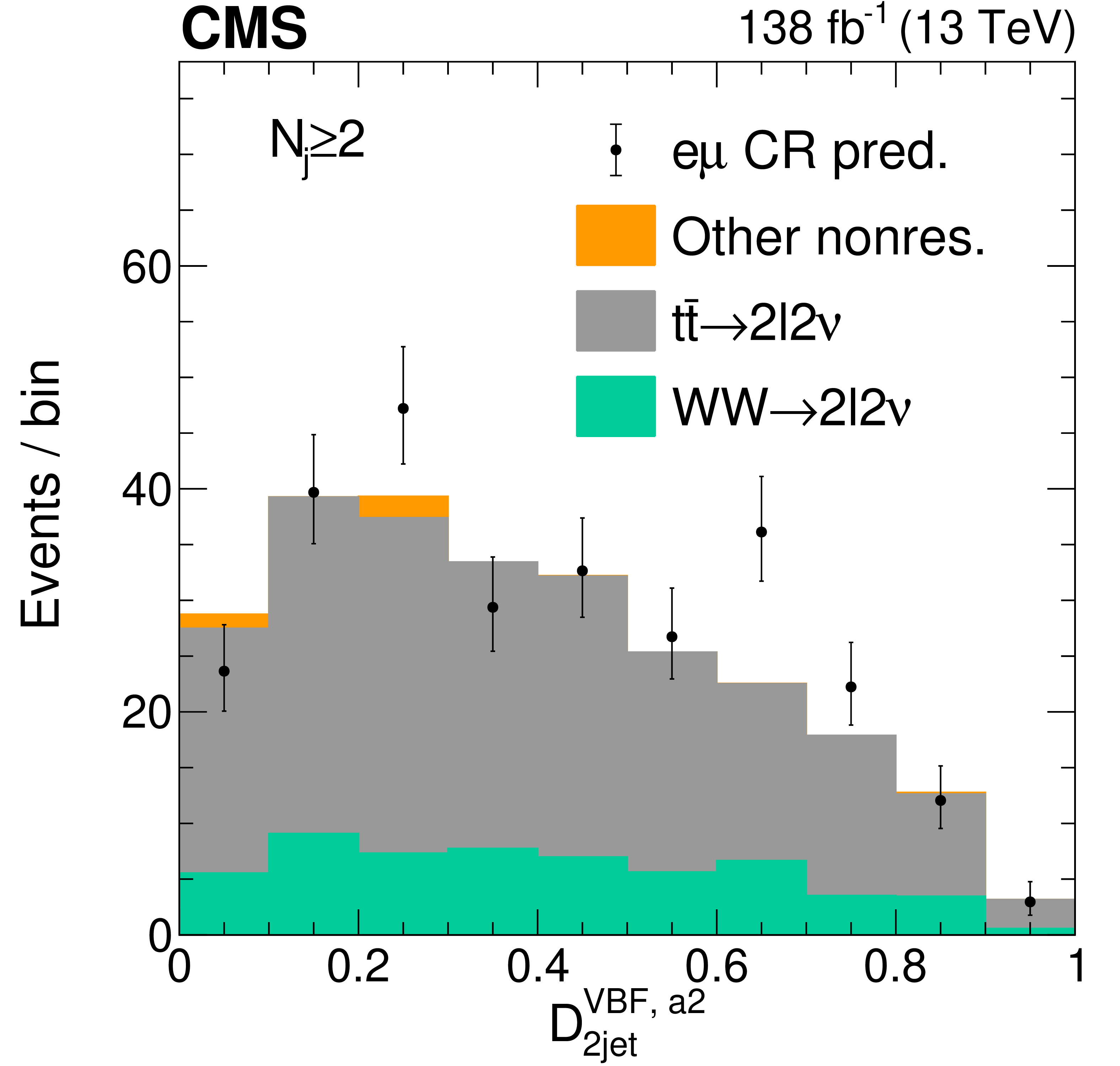
Figure S6-b:
Distributions of the VBF discriminants for nonresonant background. The distributions of the SM $ {\mathcal{D}}^{{\text{VBF}}}_{\text{2jet}} $ (left) and $ {\mathcal{D}}^{{\text{VBF}}, a2}_{\text{2jet}} $ (right) kinematic VBF discriminants are shown in the 2$ \ell$2$\nu $ signal region, $ N_{\mathrm{j}}\geq $ 2 category. The stacked histogram shows the predictions from simulation, which consists of nonresonant contributions from $ {\mathrm{W}}{\mathrm{W}} $ (green) and $ {\mathrm{t}\overline{\mathrm{t}}} $ (gray) production, or other small components (orange). The black points with error bars as uncertainties at 68% CL show the prediction from the e$\mu$ CR data. While only the data is used in the final estimate of the nonresonant background, we note that predictions from simulation already agree well with the data estimate. |
png pdf |
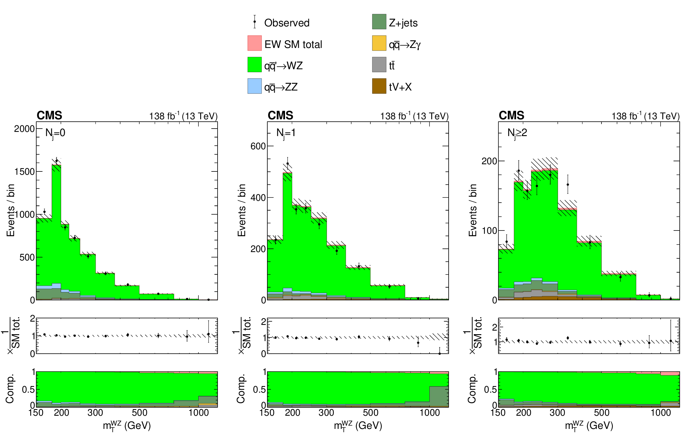
Figure S7:
Distributions of $ m_\mathrm{T}^{{\mathrm{W}}\mathrm{Z}} $ in different $ N_{\mathrm{j}} $ categories of the WZ control region. The postfit distributions of the transverse WZ invariant mass are displayed for the $ N_{\mathrm{j}}= $ 0, $ N_{\mathrm{j}}= $ 1, and $ N_{\mathrm{j}}\geq $ 2 jet multiplicity categories of the $ {\mathrm{W}}\mathrm{Z} \to 3\ell1\nu $ control region from left to right. Postfit refers to a combined 2$ \ell$2$\nu$+4$\ell $ fit, together with this control region, assuming SM H boson parameters. The stacked histogram is shown with the hashed band as the total postfit uncertainty at 68% CL. The color legend is given above the plots, with the different contributions referring to the WZ (light green), ZZ (blue), Z+jets (dark green), $ \mathrm{Z}{\gamma} $ (yellow), $ {\mathrm{t}\overline{\mathrm{t}}} $ (gray), and $ \mathrm{t}{\mathrm{V}} $+X (brown, with X being any other particle) production processes, as well as the small EW ZZ production component (dark pink). The black points with error bars as uncertainties at 68% CL show the observed data. The middle panels along the vertical show the ratio of the data to the total prediction, and the lower panels show the predicted relative contributions of each process. The rightmost bins contain the overflow. |
png pdf |
Figure S7-a:
Distributions of $ m_\mathrm{T}^{{\mathrm{W}}\mathrm{Z}} $ in different $ N_{\mathrm{j}} $ categories of the WZ control region. The postfit distributions of the transverse WZ invariant mass are displayed for the $ N_{\mathrm{j}}= $ 0, $ N_{\mathrm{j}}= $ 1, and $ N_{\mathrm{j}}\geq $ 2 jet multiplicity categories of the $ {\mathrm{W}}\mathrm{Z} \to 3\ell1\nu $ control region from left to right. Postfit refers to a combined 2$ \ell$2$\nu$+4$\ell $ fit, together with this control region, assuming SM H boson parameters. The stacked histogram is shown with the hashed band as the total postfit uncertainty at 68% CL. The color legend is given above the plots, with the different contributions referring to the WZ (light green), ZZ (blue), Z+jets (dark green), $ \mathrm{Z}{\gamma} $ (yellow), $ {\mathrm{t}\overline{\mathrm{t}}} $ (gray), and $ \mathrm{t}{\mathrm{V}} $+X (brown, with X being any other particle) production processes, as well as the small EW ZZ production component (dark pink). The black points with error bars as uncertainties at 68% CL show the observed data. The middle panels along the vertical show the ratio of the data to the total prediction, and the lower panels show the predicted relative contributions of each process. The rightmost bins contain the overflow. |

png pdf |
Figure S7-b:
Distributions of $ m_\mathrm{T}^{{\mathrm{W}}\mathrm{Z}} $ in different $ N_{\mathrm{j}} $ categories of the WZ control region. The postfit distributions of the transverse WZ invariant mass are displayed for the $ N_{\mathrm{j}}= $ 0, $ N_{\mathrm{j}}= $ 1, and $ N_{\mathrm{j}}\geq $ 2 jet multiplicity categories of the $ {\mathrm{W}}\mathrm{Z} \to 3\ell1\nu $ control region from left to right. Postfit refers to a combined 2$ \ell$2$\nu$+4$\ell $ fit, together with this control region, assuming SM H boson parameters. The stacked histogram is shown with the hashed band as the total postfit uncertainty at 68% CL. The color legend is given above the plots, with the different contributions referring to the WZ (light green), ZZ (blue), Z+jets (dark green), $ \mathrm{Z}{\gamma} $ (yellow), $ {\mathrm{t}\overline{\mathrm{t}}} $ (gray), and $ \mathrm{t}{\mathrm{V}} $+X (brown, with X being any other particle) production processes, as well as the small EW ZZ production component (dark pink). The black points with error bars as uncertainties at 68% CL show the observed data. The middle panels along the vertical show the ratio of the data to the total prediction, and the lower panels show the predicted relative contributions of each process. The rightmost bins contain the overflow. |
png pdf |
Figure S7-c:
Distributions of $ m_\mathrm{T}^{{\mathrm{W}}\mathrm{Z}} $ in different $ N_{\mathrm{j}} $ categories of the WZ control region. The postfit distributions of the transverse WZ invariant mass are displayed for the $ N_{\mathrm{j}}= $ 0, $ N_{\mathrm{j}}= $ 1, and $ N_{\mathrm{j}}\geq $ 2 jet multiplicity categories of the $ {\mathrm{W}}\mathrm{Z} \to 3\ell1\nu $ control region from left to right. Postfit refers to a combined 2$ \ell$2$\nu$+4$\ell $ fit, together with this control region, assuming SM H boson parameters. The stacked histogram is shown with the hashed band as the total postfit uncertainty at 68% CL. The color legend is given above the plots, with the different contributions referring to the WZ (light green), ZZ (blue), Z+jets (dark green), $ \mathrm{Z}{\gamma} $ (yellow), $ {\mathrm{t}\overline{\mathrm{t}}} $ (gray), and $ \mathrm{t}{\mathrm{V}} $+X (brown, with X being any other particle) production processes, as well as the small EW ZZ production component (dark pink). The black points with error bars as uncertainties at 68% CL show the observed data. The middle panels along the vertical show the ratio of the data to the total prediction, and the lower panels show the predicted relative contributions of each process. The rightmost bins contain the overflow. |
png pdf |
Figure S7-d:
Distributions of $ m_\mathrm{T}^{{\mathrm{W}}\mathrm{Z}} $ in different $ N_{\mathrm{j}} $ categories of the WZ control region. The postfit distributions of the transverse WZ invariant mass are displayed for the $ N_{\mathrm{j}}= $ 0, $ N_{\mathrm{j}}= $ 1, and $ N_{\mathrm{j}}\geq $ 2 jet multiplicity categories of the $ {\mathrm{W}}\mathrm{Z} \to 3\ell1\nu $ control region from left to right. Postfit refers to a combined 2$ \ell$2$\nu$+4$\ell $ fit, together with this control region, assuming SM H boson parameters. The stacked histogram is shown with the hashed band as the total postfit uncertainty at 68% CL. The color legend is given above the plots, with the different contributions referring to the WZ (light green), ZZ (blue), Z+jets (dark green), $ \mathrm{Z}{\gamma} $ (yellow), $ {\mathrm{t}\overline{\mathrm{t}}} $ (gray), and $ \mathrm{t}{\mathrm{V}} $+X (brown, with X being any other particle) production processes, as well as the small EW ZZ production component (dark pink). The black points with error bars as uncertainties at 68% CL show the observed data. The middle panels along the vertical show the ratio of the data to the total prediction, and the lower panels show the predicted relative contributions of each process. The rightmost bins contain the overflow. |
png pdf |
Figure S8:
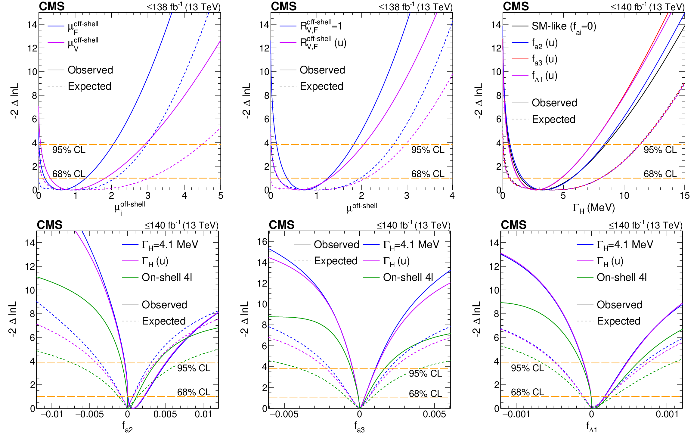
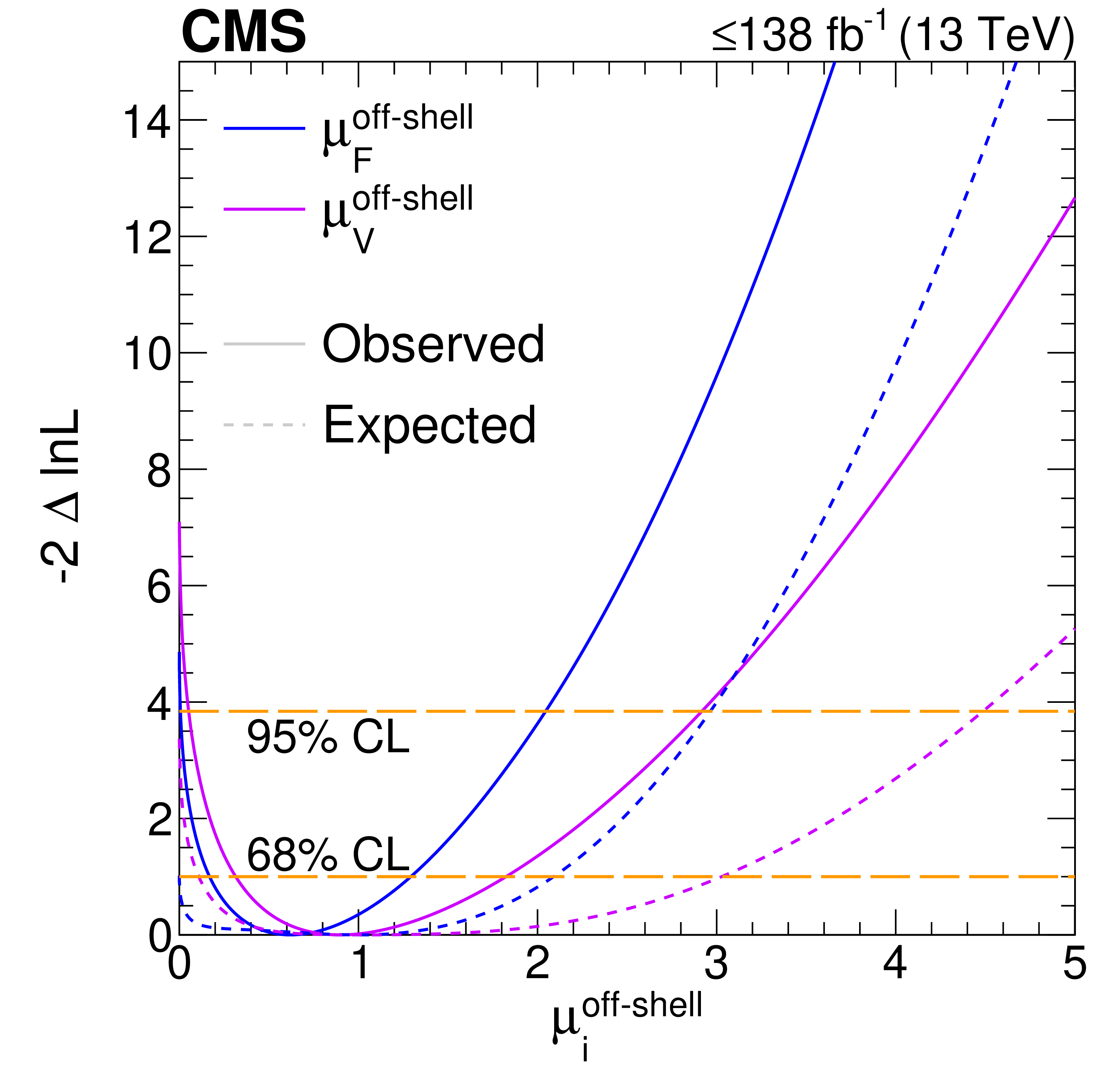
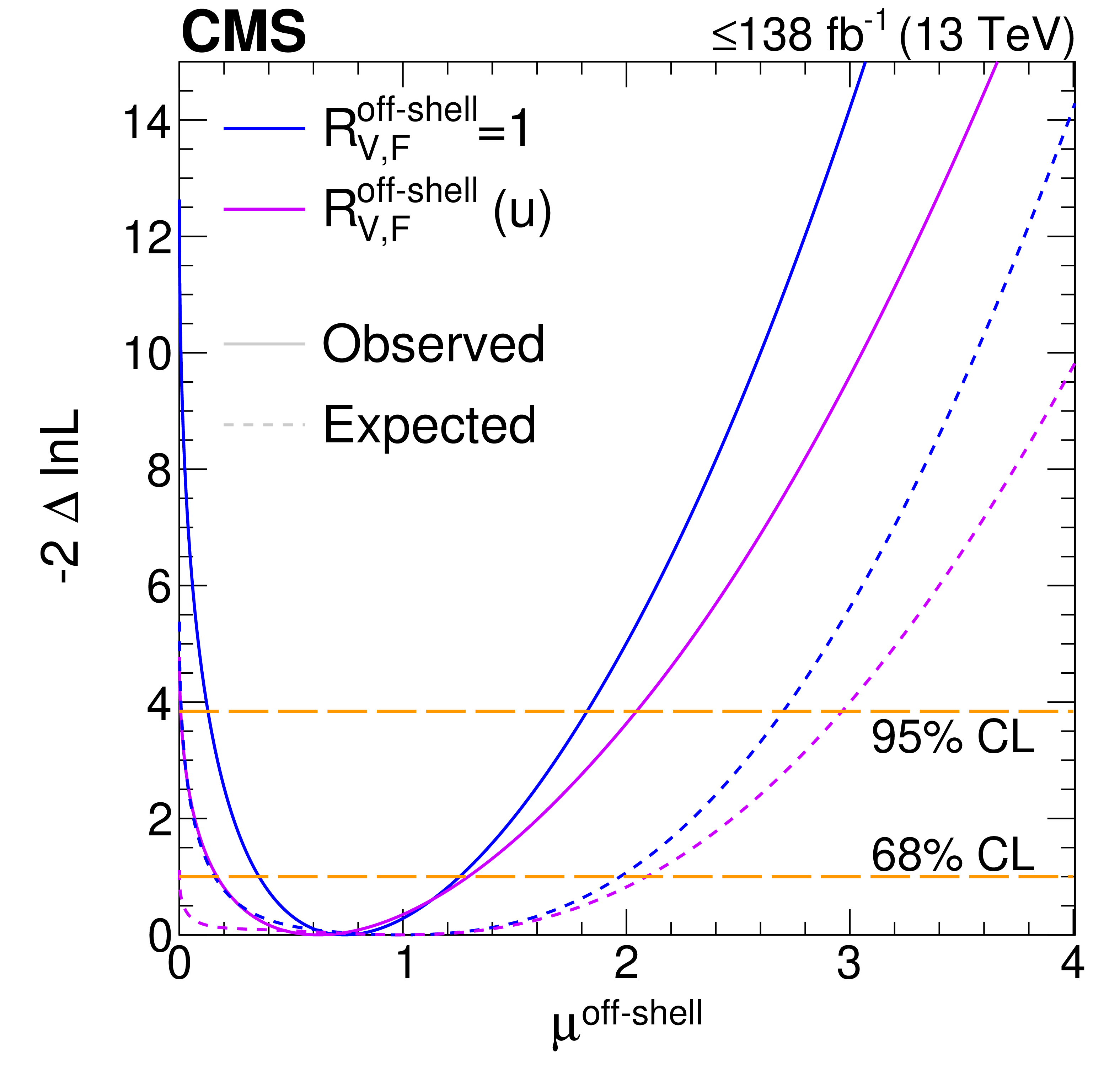
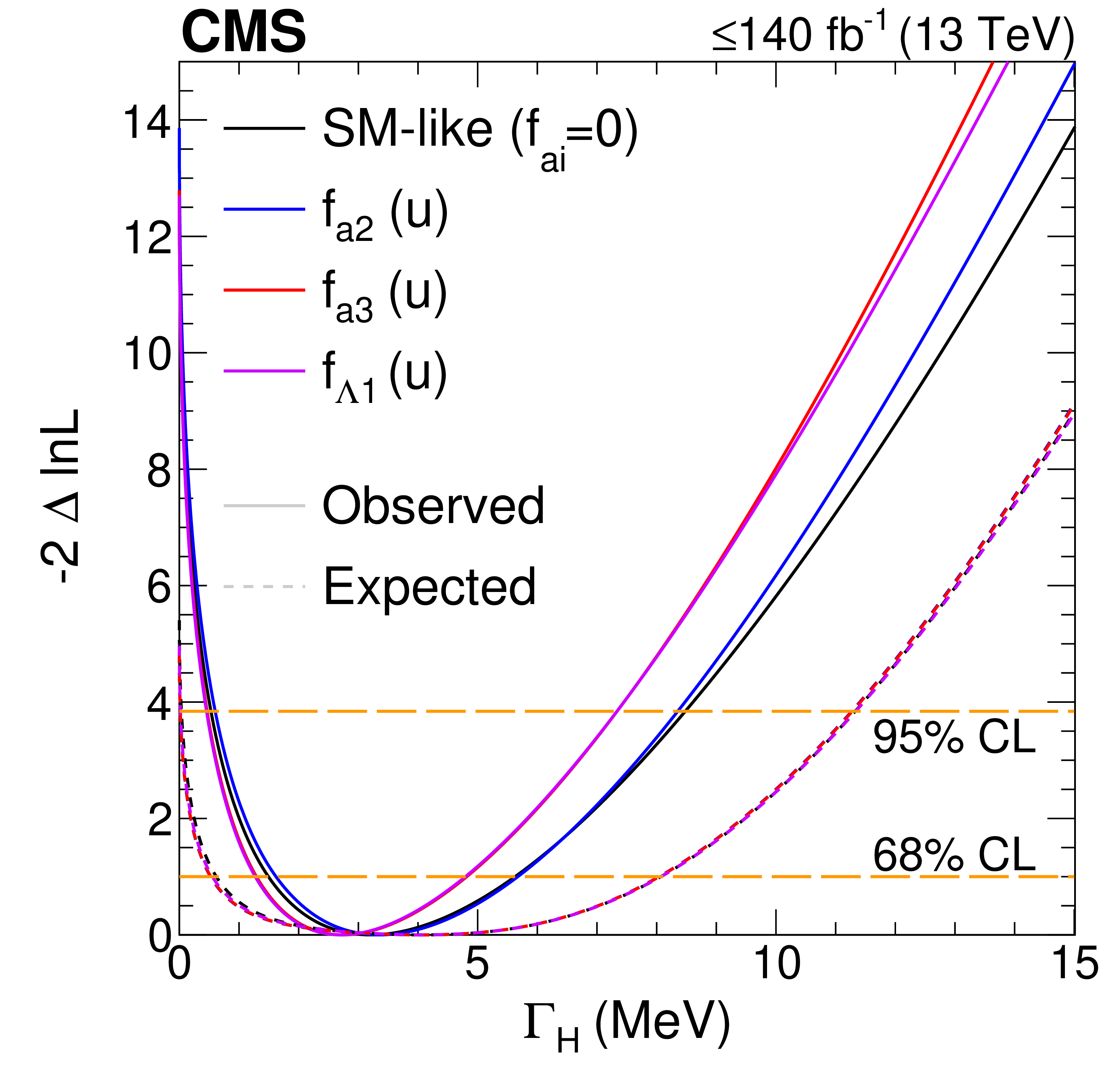
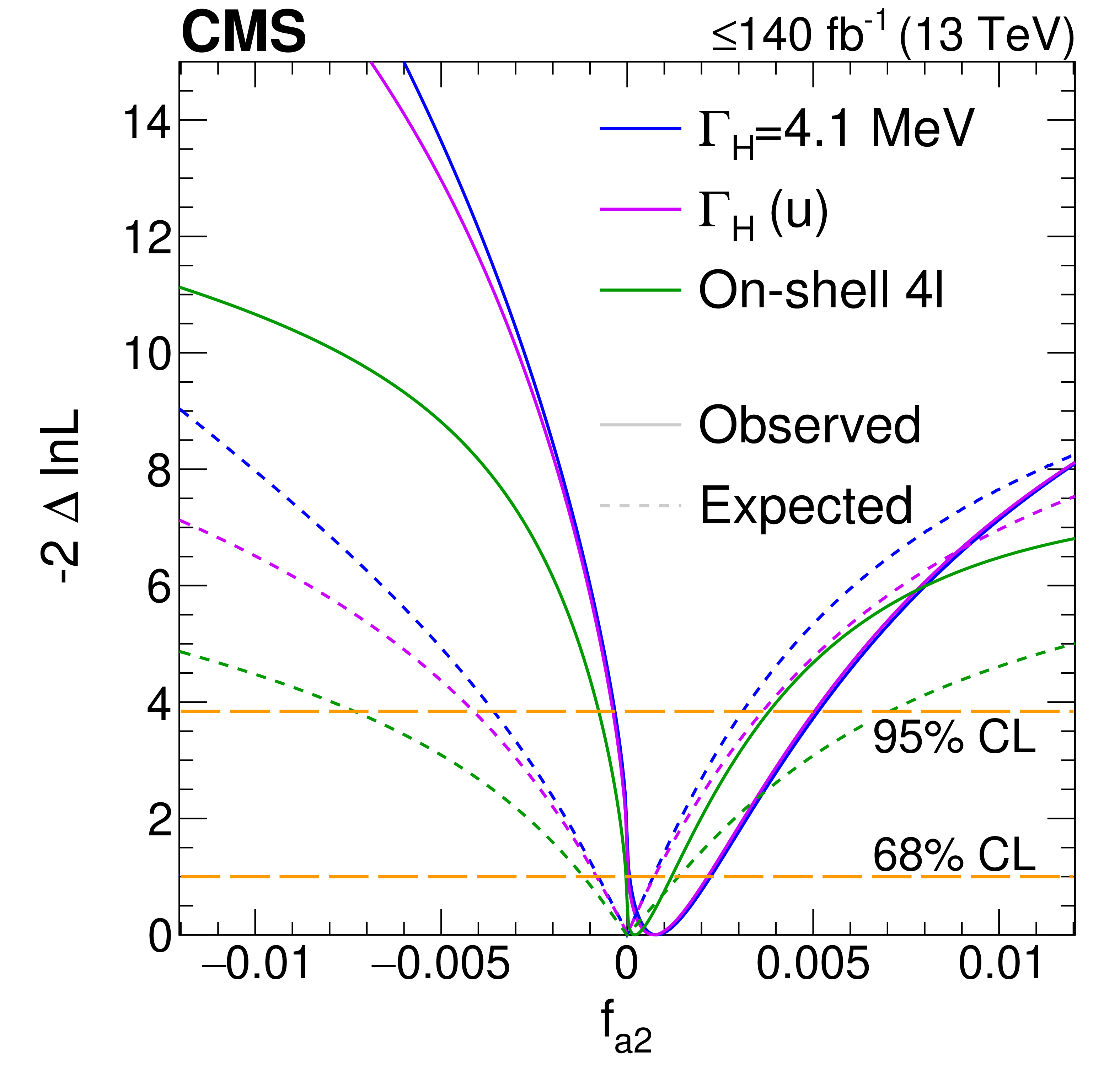
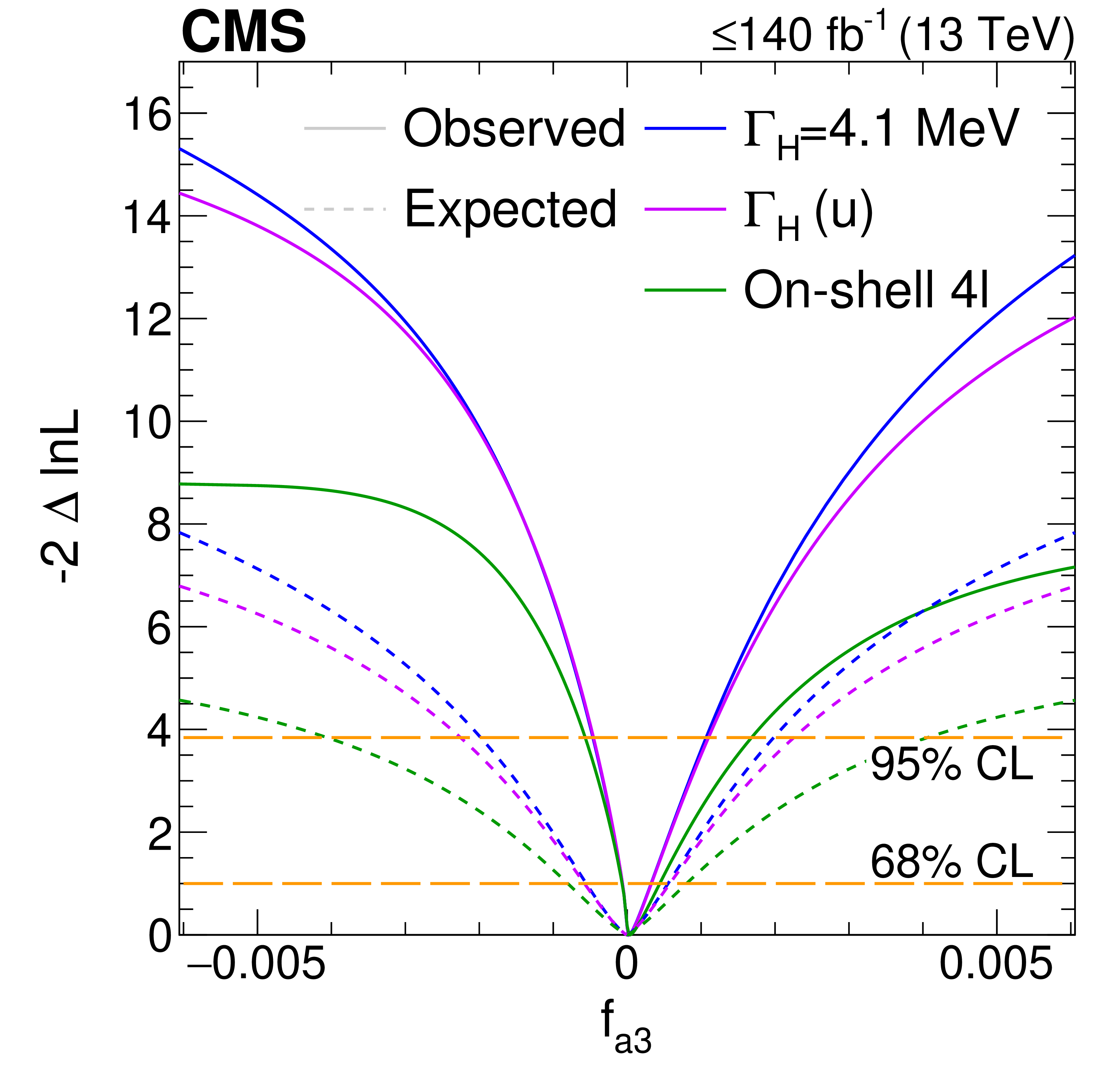
Log-likelihood scans of the off-shell signal strengths, $ \Gamma_{\mathrm{H}} $, and $ f_{ai} $.Top panels: The likelihood scans are shown for $ \mu^{\text{off-shell}}_{\mathrm{F}} $ or $ \mu^{\text{off-shell}}_{{\mathrm{V}}} $ (left), $ \mu^{\text{off-shell}} $ (middle), and $ \Gamma_{\mathrm{H}} $ (right). Scans for $ \mu^{\text{off-shell}}_{\mathrm{F}} $ (blue) and $ \mu^{\text{off-shell}}_{{\mathrm{V}}} $ (magenta) are obtained with the other parameter unconstrained. Those for $ \mu^{\text{off-shell}} $ are shown with (blue) and without (magenta) the constraint $ R^{\text{off-shell}}_{{\mathrm{V}},\mathrm{F}} (=\mu^{\text{off-shell}}_{{\mathrm{V}}}/\mu^{\text{off-shell}}_{\mathrm{F}}) = $ 1. Constraints on $ \Gamma_{\mathrm{H}} $ are shown with and without anomalous HVV couplings. Bottom panels: The likelihood scans of the anomalous HVV coupling parameters $f_{a2}$ (left), $f_{a3}$ (middle), and $f_{\Lambda 1}$ (right) are shown with the constraint $ \Gamma_{\mathrm{H}}=\Gamma_{\mathrm{H}}^{\text{SM}}= $ 4.1 MeV (blue), $ \Gamma_{\mathrm{H}} $ unconstrained (magenta), or based on on-shell 4$ \ell $ data only (green). Observed (expected) scans are shown with solid (dashed) curves. The horizontal lines indicate the 68% ($ -$2$\Delta\ln\mathcal{L}= $ 1.0) and 95% ($ -$2$\Delta\ln\mathcal{L}= $ 3.84) CL regions. The integrated luminosity reaches up to 138 fb$^{-1}$ when only off-shell information is used, and up to 140 fb$^{-1}$ when on-shell 4$ \ell $ events are included. |
png pdf |
Figure S8-a:
Log-likelihood scans of the off-shell signal strengths, $ \Gamma_{\mathrm{H}} $, and $ f_{ai} $.Top panels: The likelihood scans are shown for $ \mu^{\text{off-shell}}_{\mathrm{F}} $ or $ \mu^{\text{off-shell}}_{{\mathrm{V}}} $ (left), $ \mu^{\text{off-shell}} $ (middle), and $ \Gamma_{\mathrm{H}} $ (right). Scans for $ \mu^{\text{off-shell}}_{\mathrm{F}} $ (blue) and $ \mu^{\text{off-shell}}_{{\mathrm{V}}} $ (magenta) are obtained with the other parameter unconstrained. Those for $ \mu^{\text{off-shell}} $ are shown with (blue) and without (magenta) the constraint $ R^{\text{off-shell}}_{{\mathrm{V}},\mathrm{F}} (=\mu^{\text{off-shell}}_{{\mathrm{V}}}/\mu^{\text{off-shell}}_{\mathrm{F}}) = $ 1. Constraints on $ \Gamma_{\mathrm{H}} $ are shown with and without anomalous HVV couplings. Bottom panels: The likelihood scans of the anomalous HVV coupling parameters $f_{a2}$ (left), $f_{a3}$ (middle), and $f_{\Lambda 1}$ (right) are shown with the constraint $ \Gamma_{\mathrm{H}}=\Gamma_{\mathrm{H}}^{\text{SM}}= $ 4.1 MeV (blue), $ \Gamma_{\mathrm{H}} $ unconstrained (magenta), or based on on-shell 4$ \ell $ data only (green). Observed (expected) scans are shown with solid (dashed) curves. The horizontal lines indicate the 68% ($ -$2$\Delta\ln\mathcal{L}= $ 1.0) and 95% ($ -$2$\Delta\ln\mathcal{L}= $ 3.84) CL regions. The integrated luminosity reaches up to 138 fb$^{-1}$ when only off-shell information is used, and up to 140 fb$^{-1}$ when on-shell 4$ \ell $ events are included. |
png pdf |
Figure S8-b:
Log-likelihood scans of the off-shell signal strengths, $ \Gamma_{\mathrm{H}} $, and $ f_{ai} $.Top panels: The likelihood scans are shown for $ \mu^{\text{off-shell}}_{\mathrm{F}} $ or $ \mu^{\text{off-shell}}_{{\mathrm{V}}} $ (left), $ \mu^{\text{off-shell}} $ (middle), and $ \Gamma_{\mathrm{H}} $ (right). Scans for $ \mu^{\text{off-shell}}_{\mathrm{F}} $ (blue) and $ \mu^{\text{off-shell}}_{{\mathrm{V}}} $ (magenta) are obtained with the other parameter unconstrained. Those for $ \mu^{\text{off-shell}} $ are shown with (blue) and without (magenta) the constraint $ R^{\text{off-shell}}_{{\mathrm{V}},\mathrm{F}} (=\mu^{\text{off-shell}}_{{\mathrm{V}}}/\mu^{\text{off-shell}}_{\mathrm{F}}) = $ 1. Constraints on $ \Gamma_{\mathrm{H}} $ are shown with and without anomalous HVV couplings. Bottom panels: The likelihood scans of the anomalous HVV coupling parameters $f_{a2}$ (left), $f_{a3}$ (middle), and $f_{\Lambda 1}$ (right) are shown with the constraint $ \Gamma_{\mathrm{H}}=\Gamma_{\mathrm{H}}^{\text{SM}}= $ 4.1 MeV (blue), $ \Gamma_{\mathrm{H}} $ unconstrained (magenta), or based on on-shell 4$ \ell $ data only (green). Observed (expected) scans are shown with solid (dashed) curves. The horizontal lines indicate the 68% ($ -$2$\Delta\ln\mathcal{L}= $ 1.0) and 95% ($ -$2$\Delta\ln\mathcal{L}= $ 3.84) CL regions. The integrated luminosity reaches up to 138 fb$^{-1}$ when only off-shell information is used, and up to 140 fb$^{-1}$ when on-shell 4$ \ell $ events are included. |
png pdf |
Figure S8-c:
Log-likelihood scans of the off-shell signal strengths, $ \Gamma_{\mathrm{H}} $, and $ f_{ai} $.Top panels: The likelihood scans are shown for $ \mu^{\text{off-shell}}_{\mathrm{F}} $ or $ \mu^{\text{off-shell}}_{{\mathrm{V}}} $ (left), $ \mu^{\text{off-shell}} $ (middle), and $ \Gamma_{\mathrm{H}} $ (right). Scans for $ \mu^{\text{off-shell}}_{\mathrm{F}} $ (blue) and $ \mu^{\text{off-shell}}_{{\mathrm{V}}} $ (magenta) are obtained with the other parameter unconstrained. Those for $ \mu^{\text{off-shell}} $ are shown with (blue) and without (magenta) the constraint $ R^{\text{off-shell}}_{{\mathrm{V}},\mathrm{F}} (=\mu^{\text{off-shell}}_{{\mathrm{V}}}/\mu^{\text{off-shell}}_{\mathrm{F}}) = $ 1. Constraints on $ \Gamma_{\mathrm{H}} $ are shown with and without anomalous HVV couplings. Bottom panels: The likelihood scans of the anomalous HVV coupling parameters $f_{a2}$ (left), $f_{a3}$ (middle), and $f_{\Lambda 1}$ (right) are shown with the constraint $ \Gamma_{\mathrm{H}}=\Gamma_{\mathrm{H}}^{\text{SM}}= $ 4.1 MeV (blue), $ \Gamma_{\mathrm{H}} $ unconstrained (magenta), or based on on-shell 4$ \ell $ data only (green). Observed (expected) scans are shown with solid (dashed) curves. The horizontal lines indicate the 68% ($ -$2$\Delta\ln\mathcal{L}= $ 1.0) and 95% ($ -$2$\Delta\ln\mathcal{L}= $ 3.84) CL regions. The integrated luminosity reaches up to 138 fb$^{-1}$ when only off-shell information is used, and up to 140 fb$^{-1}$ when on-shell 4$ \ell $ events are included. |
png pdf |
Figure S8-d:
Log-likelihood scans of the off-shell signal strengths, $ \Gamma_{\mathrm{H}} $, and $ f_{ai} $.Top panels: The likelihood scans are shown for $ \mu^{\text{off-shell}}_{\mathrm{F}} $ or $ \mu^{\text{off-shell}}_{{\mathrm{V}}} $ (left), $ \mu^{\text{off-shell}} $ (middle), and $ \Gamma_{\mathrm{H}} $ (right). Scans for $ \mu^{\text{off-shell}}_{\mathrm{F}} $ (blue) and $ \mu^{\text{off-shell}}_{{\mathrm{V}}} $ (magenta) are obtained with the other parameter unconstrained. Those for $ \mu^{\text{off-shell}} $ are shown with (blue) and without (magenta) the constraint $ R^{\text{off-shell}}_{{\mathrm{V}},\mathrm{F}} (=\mu^{\text{off-shell}}_{{\mathrm{V}}}/\mu^{\text{off-shell}}_{\mathrm{F}}) = $ 1. Constraints on $ \Gamma_{\mathrm{H}} $ are shown with and without anomalous HVV couplings. Bottom panels: The likelihood scans of the anomalous HVV coupling parameters $f_{a2}$ (left), $f_{a3}$ (middle), and $f_{\Lambda 1}$ (right) are shown with the constraint $ \Gamma_{\mathrm{H}}=\Gamma_{\mathrm{H}}^{\text{SM}}= $ 4.1 MeV (blue), $ \Gamma_{\mathrm{H}} $ unconstrained (magenta), or based on on-shell 4$ \ell $ data only (green). Observed (expected) scans are shown with solid (dashed) curves. The horizontal lines indicate the 68% ($ -$2$\Delta\ln\mathcal{L}= $ 1.0) and 95% ($ -$2$\Delta\ln\mathcal{L}= $ 3.84) CL regions. The integrated luminosity reaches up to 138 fb$^{-1}$ when only off-shell information is used, and up to 140 fb$^{-1}$ when on-shell 4$ \ell $ events are included. |
png pdf |
Figure S8-e:
Log-likelihood scans of the off-shell signal strengths, $ \Gamma_{\mathrm{H}} $, and $ f_{ai} $.Top panels: The likelihood scans are shown for $ \mu^{\text{off-shell}}_{\mathrm{F}} $ or $ \mu^{\text{off-shell}}_{{\mathrm{V}}} $ (left), $ \mu^{\text{off-shell}} $ (middle), and $ \Gamma_{\mathrm{H}} $ (right). Scans for $ \mu^{\text{off-shell}}_{\mathrm{F}} $ (blue) and $ \mu^{\text{off-shell}}_{{\mathrm{V}}} $ (magenta) are obtained with the other parameter unconstrained. Those for $ \mu^{\text{off-shell}} $ are shown with (blue) and without (magenta) the constraint $ R^{\text{off-shell}}_{{\mathrm{V}},\mathrm{F}} (=\mu^{\text{off-shell}}_{{\mathrm{V}}}/\mu^{\text{off-shell}}_{\mathrm{F}}) = $ 1. Constraints on $ \Gamma_{\mathrm{H}} $ are shown with and without anomalous HVV couplings. Bottom panels: The likelihood scans of the anomalous HVV coupling parameters $f_{a2}$ (left), $f_{a3}$ (middle), and $f_{\Lambda 1}$ (right) are shown with the constraint $ \Gamma_{\mathrm{H}}=\Gamma_{\mathrm{H}}^{\text{SM}}= $ 4.1 MeV (blue), $ \Gamma_{\mathrm{H}} $ unconstrained (magenta), or based on on-shell 4$ \ell $ data only (green). Observed (expected) scans are shown with solid (dashed) curves. The horizontal lines indicate the 68% ($ -$2$\Delta\ln\mathcal{L}= $ 1.0) and 95% ($ -$2$\Delta\ln\mathcal{L}= $ 3.84) CL regions. The integrated luminosity reaches up to 138 fb$^{-1}$ when only off-shell information is used, and up to 140 fb$^{-1}$ when on-shell 4$ \ell $ events are included. |

png pdf |
Figure S8-f:
Log-likelihood scans of the off-shell signal strengths, $ \Gamma_{\mathrm{H}} $, and $ f_{ai} $.Top panels: The likelihood scans are shown for $ \mu^{\text{off-shell}}_{\mathrm{F}} $ or $ \mu^{\text{off-shell}}_{{\mathrm{V}}} $ (left), $ \mu^{\text{off-shell}} $ (middle), and $ \Gamma_{\mathrm{H}} $ (right). Scans for $ \mu^{\text{off-shell}}_{\mathrm{F}} $ (blue) and $ \mu^{\text{off-shell}}_{{\mathrm{V}}} $ (magenta) are obtained with the other parameter unconstrained. Those for $ \mu^{\text{off-shell}} $ are shown with (blue) and without (magenta) the constraint $ R^{\text{off-shell}}_{{\mathrm{V}},\mathrm{F}} (=\mu^{\text{off-shell}}_{{\mathrm{V}}}/\mu^{\text{off-shell}}_{\mathrm{F}}) = $ 1. Constraints on $ \Gamma_{\mathrm{H}} $ are shown with and without anomalous HVV couplings. Bottom panels: The likelihood scans of the anomalous HVV coupling parameters $f_{a2}$ (left), $f_{a3}$ (middle), and $f_{\Lambda 1}$ (right) are shown with the constraint $ \Gamma_{\mathrm{H}}=\Gamma_{\mathrm{H}}^{\text{SM}}= $ 4.1 MeV (blue), $ \Gamma_{\mathrm{H}} $ unconstrained (magenta), or based on on-shell 4$ \ell $ data only (green). Observed (expected) scans are shown with solid (dashed) curves. The horizontal lines indicate the 68% ($ -$2$\Delta\ln\mathcal{L}= $ 1.0) and 95% ($ -$2$\Delta\ln\mathcal{L}= $ 3.84) CL regions. The integrated luminosity reaches up to 138 fb$^{-1}$ when only off-shell information is used, and up to 140 fb$^{-1}$ when on-shell 4$ \ell $ events are included. |
png pdf |
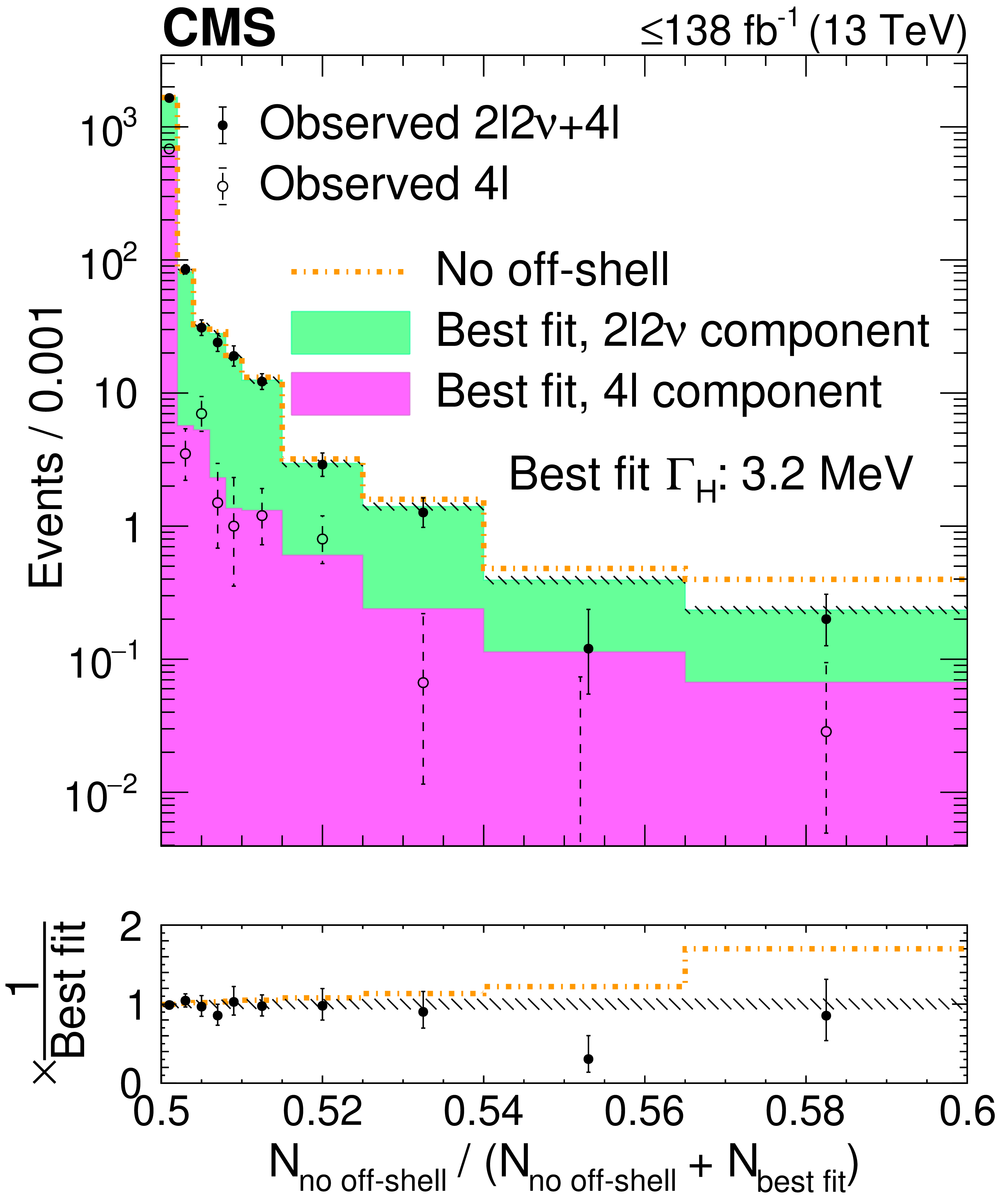
Figure S9:
Distributions of ratios of the numbers of events in each off-shell signal region bin. The ratios are taken after separate fits to the no off-shell hypothesis ($ N_{\text{no off-shell }} $) and the best overall fit ($ N_{\text{best fit}} $) with the observed $ \Gamma_{\mathrm{H}} $ value of 3.2 MeV in the SM-like HVV couplings scenario. The stacked histogram displays the predicted contributions (pink from the 4$ \ell $ off-shell and green from the 2$ \ell$2$\nu $ off-shell signal regions) after the best fit, with the hashed band representing the total postfit uncertainty at 68% CL, and the gold dot-dashed line shows the predicted distribution of these ratios for a fit to the no off-shell hypothesis. The black solid (hollow) points, with error bars as uncertainties at 68% CL, represent the observed 2$ \ell$2$\nu $ and 4$ \ell $ (4$ \ell $-only) data. The first and last bins contain the underflow and the overflow, respectively. The bottom panel displays the ratio of the various displayed hypotheses or observed data to the prediction from the best fit. The integrated luminosity reaches only up to 138 fb$^{-1}$ since on-shell 4$ \ell $ events are not displayed. |
| Tables | |
png pdf |
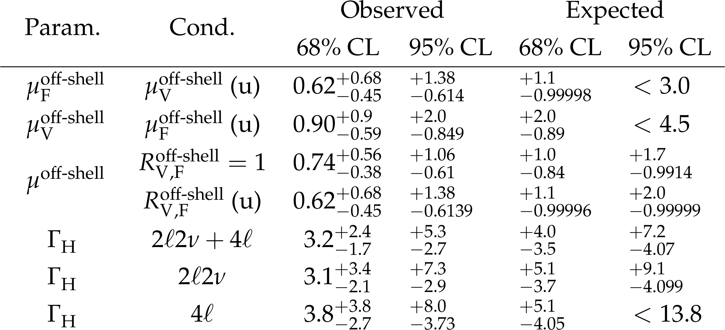
Table 1:
Results on the off-shell signal strengths and $ \Gamma_{\mathrm{H}} $. The various fit conditions are indicated in the column labeled ``Cond.'': Results on $ \mu^{\text{off-shell}} $ are presented with $ R^{\text{off-shell}}_{{\mathrm{V}},\mathrm{F}}=\mu^{\text{off-shell}}_{{\mathrm{V}}} / \mu^{\text{off-shell}}_{\mathrm{F}} $ either unconstrained (u) or $ = $ 1, and constraints on $ \mu^{\text{off-shell}}_{\mathrm{F}} $ and $ \mu^{\text{off-shell}}_{{\mathrm{V}}} $ are shown with the other signal strength unconstrained. Results on $ \Gamma_{\mathrm{H}} $ (in units of MeV) are obtained with the on-shell signal strengths unconstrained, and the different conditions listed for this quantity reflect which off-shell final states are combined with on-shell 4$ \ell $ data. The expected central values, not quoted explicitly in this table, are either unity for $ \mu^{\text{off-shell}} $, $ \mu^{\text{off-shell}}_{\mathrm{F}} $, and $ \mu^{\text{off-shell}}_{{\mathrm{V}}} $, or $ \Gamma_{\mathrm{H}}= $ 4.1 MeV. |
png pdf |
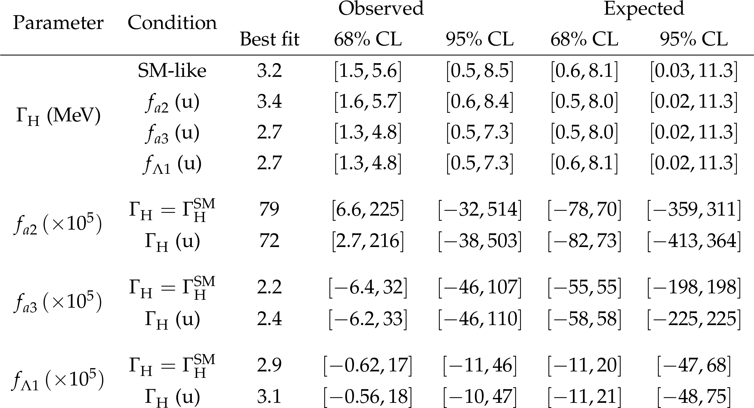
Table S1:
Results on $ \Gamma_{\mathrm{H}} $ and the different anomalous HVV couplings. The results on $ \Gamma_{\mathrm{H}} $ are displayed in units of MeV, and those on the anomalous HVV couplings are summarized in terms of the corresponding on-shell cross section fractions $ f_{a2} $, $ f_{a3} $, and $ f_{\Lambda 1} $ ($ f_{ai} $ in short, and scaled by 10$^5 $). For the results on $ \Gamma_{\mathrm{H}} $, the tests with the anomalous HVV couplings are distinguished by the denoted $ f_{ai} $, and the expected best-fit values, not quoted explicitly in the table, are always $ \Gamma_{\mathrm{H}}= $ 4.1 MeV. The SM-like result is the same as that from the combination of all 4$ \ell $ and 2$ \ell$2$\nu $ data sets in Table \reftable:interp. For the results on $ f_{ai} $, the constraints are shown with either $ \Gamma_{\mathrm{H}}=\Gamma_{\mathrm{H}}^{\text{SM}}= $ 4.1 MeV required, or $ \Gamma_{\mathrm{H}} $ left unconstrained, and the expected best-fit values, also not quoted explicitly, are always null. The various fit conditions are indicated in the column labeled ``Condition'', where the abbreviation ``(u)'' indicates which parameter is unconstrained. |
| Summary |
| We report evidence for off-shell contributions to the production cross section of two Z bosons with data from the CMS experiment at the CERN Large Hadron Collider. The scenario with no off-shell contribution is excluded at 3.6 standard deviations. We measure the width of the Higgs boson as $ \Gamma_{\mathrm{H}} = $ 3.2$_{-1.7}^{+2.4}$ MeV. In addition, we set constraints on anomalous Higgs boson couplings to W and Z boson pairs. |
| References | ||||
| 1 | F. Englert and R. Brout | Broken symmetry and the mass of gauge vector mesons | PRL 13 (1964) 321 | |
| 2 | P. W. Higgs | Broken symmetries and the masses of gauge bosons | PRL 13 (1964) 508 | |
| 3 | G. S. Guralnik, C. R. Hagen, and T. W. B. Kibble | Global conservation laws and massless particles | PRL 13 (1964) 585 | |
| 4 | ATLAS Collaboration | Observation of a new particle in the search for the Standard Model Higgs boson with the ATLAS detector at the LHC | PLB 716 (2012) 1 | 1207.7214 |
| 5 | CMS Collaboration | Observation of a new boson at a mass of 125 GeV with the CMS experiment at the LHC | PLB 716 (2012) 30 | CMS-HIG-12-028 1207.7235 |
| 6 | CMS Collaboration | Observation of a new boson with mass near 125 GeV in pp collisions at $ \sqrt{s}= $ 7 and 8 TeV | JHEP 06 (2013) 081 | CMS-HIG-12-036 1303.4571 |
| 7 | W. Heisenberg | Über den anschaulichen inhalt der quantentheoretischen kinematik und mechanik | Z. Phys. 43 (1927) 172 | |
| 8 | G. Breit and E. Wigner | Capture of slow neutrons | PR 49 (1936) 519 | |
| 9 | ALEPH, DELPHI, L3, OPAL, SLD, LEP Electroweak Working Group, SLD Electroweak Group, SLD Heavy Flavour Group Collaboration | Precision electroweak measurements on the Z resonance | Phys. Rept. 427 (2006) 257 | hep-ex/0509008 |
| 10 | LHC Higgs Cross Section Working Group | Handbook of LHC Higgs cross sections: 4. Deciphering the nature of the Higgs sector | CERN Report CERN-2017-002-M, 2016 link |
1610.07922 |
| 11 | CMS Collaboration | Limits on the Higgs boson lifetime and width from its decay to four charged leptons | PRD 92 (2015) 072010 | CMS-HIG-14-036 1507.06656 |
| 12 | F. Caola and K. Melnikov | Constraining the Higgs boson width with ZZ production at the LHC | PRD 88 (2013) 054024 | 1307.4935 |
| 13 | J. M. Campbell, R. K. Ellis, and C. Williams | Bounding the Higgs width at the LHC using full analytic results for $ \mathrm{g}\mathrm{g}\to \mathrm{e}^{-}\mathrm{e}^{+} \mu^{-} \mu^{+} $ | JHEP 04 (2014) 060 | 1311.3589 |
| 14 | ATLAS Collaboration | Constraints on off-shell Higgs boson production and the Higgs boson total width in $ \mathrm{Z}\mathrm{Z}\to4\ell $ and $ \mathrm{Z}\mathrm{Z}\to2\ell2\nu $ final states with the ATLAS detector | PLB 786 (2018) 223 | 1808.01191 |
| 15 | CMS Collaboration | Measurements of the Higgs boson width and anomalous HVV couplings from on-shell and off-shell production in the four-lepton final state | PRD 99 (2019) 112003 | CMS-HIG-18-002 1901.00174 |
| 16 | C. H. Llewellyn Smith | High-energy behavior and gauge symmetry | PLB 46 (1973) 233 | |
| 17 | J. M. Cornwall, D. N. Levin, and G. Tiktopoulos | Derivation of gauge invariance from high-energy unitarity bounds on the $ S $-matrix | PRD 10 (1974) 1145 | |
| 18 | B. W. Lee, C. Quigg, and H. B. Thacker | Weak interactions at very high-energies: the role of the Higgs boson mass | PRD 16 (1977) 1519 | |
| 19 | E. W. N. Glover and J. J. van der Bij | Z boson pair production via gluon fusion | NPB 321 (1989) 561 | |
| 20 | F. Campanario, Q. Li, M. Rauch, and M. Spira | ZZ+jet production via gluon fusion at the LHC | JHEP 06 (2013) 069 | 1211.5429 |
| 21 | N. Kauer and G. Passarino | Inadequacy of zero-width approximation for a light Higgs boson signal | JHEP 08 (2012) 116 | 1206.4803 |
| 22 | CMS Collaboration | Constraints on anomalous Higgs boson couplings using production and decay information in the four-lepton final state | PLB 775 (2017) 1 | CMS-HIG-17-011 1707.00541 |
| 23 | CMS Collaboration | Constraints on anomalous Higgs boson couplings to vector bosons and fermions in its production and decay using the four-lepton final state | PRD 104 (2021) 052004 | CMS-HIG-19-009 2104.12152 |
| 24 | J. S. Gainer et al. | Beyond geolocating: Constraining higher dimensional operators in $ \mathrm{H} \to 4\ell $ with off-shell production and more | PRD 91 (2015) 035011 | 1403.4951 |
| 25 | C. Englert and M. Spannowsky | Limitations and opportunities of off-shell coupling measurements | PRD 90 (2014) 053003 | 1405.0285 |
| 26 | A. V. Gritsan et al. | New features in the JHU generator framework: constraining Higgs boson properties from on-shell and off-shell production | PRD 102 (2020) 056022 | 2002.09888 |
| 27 | U. Sarica | Measurements of Higgs boson properties in proton-proton collisions at $ \sqrt{s} = $ 7, 8 and 13 TeV at the CERN Large Hadron Collider | PhD thesis, Johns Hopkins U, 2019 link |
|
| 28 | CMS Collaboration | Measurements of $ {\mathrm{t}\overline{\mathrm{t}}} \mathrm{H} $ production and the CP structure of the Yukawa interaction between the Higgs boson and top quark in the diphoton decay channel | PRL 125 (2020) 061801 | CMS-HIG-19-013 2003.10866 |
| 29 | ATLAS Collaboration | CP properties of Higgs boson interactions with top quarks in the $ {\mathrm{t}\overline{\mathrm{t}}} \mathrm{H} $ and $ \mathrm{t}\mathrm{H} $ processes using $ \mathrm{H} \to \gamma\gamma $ with the ATLAS detector | PRL 125 (2020) 061802 | 2004.04545 |
| 30 | SMEFiT Collaboration | Combined SMEFT interpretation of Higgs, diboson, and top quark data from the LHC | JHEP 11 (2021) 089 | 2105.00006 |
| 31 | A. Bierweiler, T. Kasprzik, and J. H. Kühn | Vector-boson pair production at the LHC to $ \mathcal{O}(\alpha^3) $ accuracy | JHEP 12 (2013) 071 | 1305.5402 |
| 32 | A. Manohar, P. Nason, G. P. Salam, and G. Zanderighi | How bright is the proton? A precise determination of the photon parton distribution function | PRL 117 (2016) 242002 | 1607.04266 |
| 33 | CMS Collaboration | Precision luminosity measurement in proton-proton collisions at $ \sqrt{s} = $ 13 TeV in 2015 and 2016 at CMS | EPJC 81 (2021) 800 | CMS-LUM-17-003 2104.01927 |
| 34 | CMS Collaboration | CMS luminosity measurement for the 2017 data-taking period at $ \sqrt{s} = $ 13 TeV | CMS Physics Analysis Summary, 2018 CMS-PAS-LUM-17-004 |
CMS-PAS-LUM-17-004 |
| 35 | CMS Collaboration | CMS luminosity measurement for the 2018 data-taking period at $ \sqrt{s} = $ 13 TeV | CMS Physics Analysis Summary, 2019 CMS-PAS-LUM-18-002 |
CMS-PAS-LUM-18-002 |
| 36 | CMS Collaboration | Jet energy scale and resolution in the CMS experiment in $ \mathrm{p}\mathrm{p} $ collisions at 8 TeV | JINST 12 (2017) P02014 | CMS-JME-13-004 1607.03663 |
| 37 | G. J. Feldman and R. D. Cousins | A unified approach to the classical statistical analysis of small signals | PRD 57 (1998) 3873 | physics/9711021 |
| 38 | CMS Collaboration | HEPData record for this analysis | link | |
| 39 | CMS Collaboration | The CMS experiment at the CERN LHC | JINST 3 (2008) S08004 | |
| 40 | CMS Collaboration | The CMS trigger system | JINST 12 (2017) P01020 | CMS-TRG-12-001 1609.02366 |
| 41 | CMS Collaboration | Performance of the CMS muon detector and muon reconstruction with proton-proton collisions at $ \sqrt{s}= $ 13 TeV | JINST 13 (2018) P06015 | CMS-MUO-16-001 1804.04528 |
| 42 | CMS Collaboration | Electron and photon reconstruction and identification with the CMS experiment at the CERN LHC | JINST 16 (2021) P05014 | CMS-EGM-17-001 2012.06888 |
| 43 | CMS Collaboration | Description and performance of track and primary-vertex reconstruction with the CMS tracker | JINST 9 (2014) P10009 | CMS-TRK-11-001 1405.6569 |
| 44 | CMS Collaboration | Particle-flow reconstruction and global event description with the CMS detector | JINST 12 (2017) P10003 | CMS-PRF-14-001 1706.04965 |
| 45 | CMS Collaboration | Performance of missing transverse momentum reconstruction in proton-proton collisions at $ \sqrt{s} = $ 13 TeV using the CMS detector | JINST 14 (2019) P07004 | CMS-JME-17-001 1903.06078 |
| 46 | CMS Collaboration | Performance of reconstruction and identification of $ \tau $ leptons decaying to hadrons and $ \nu_\tau $ in $ \mathrm{p}\mathrm{p} $ collisions at $ \sqrt{s}= $ 13 TeV | JINST 13 (2018) P10005 | CMS-TAU-16-003 1809.02816 |
| 47 | CMS Collaboration | Measurements of inclusive W and Z cross sections in $ \mathrm{p}\mathrm{p} $ collisions at $ \sqrt{s}= $ 7 TeV | JHEP 01 (2011) 080 | CMS-EWK-10-002 1012.2466 |
| 48 | M. Cacciari, G. P. Salam, and G. Soyez | FastJet user manual | EPJC 72 (2012) 1896 | 1111.6097 |
| 49 | CMS Collaboration | Pileup mitigation at CMS in 13 TeV data | JINST 15 (2020) P09018 | CMS-JME-18-001 2003.00503 |
| 50 | E. Bols et al. | Jet flavour classification using DeepJet | JINST 15 (2020) 12012 | 2008.10519 |
| 51 | CMS Collaboration | Missing transverse energy performance of the CMS detector | JINST 6 (2011) P09001 | CMS-JME-10-009 1106.5048 |
| 52 | S. Frixione, P. Nason, and C. Oleari | Matching NLO QCD computations with parton shower simulations: the POWHEG method | JHEP 11 (2007) 070 | 0709.2092 |
| 53 | P. Nason and C. Oleari | NLO Higgs boson production via vector-boson fusion matched with shower in POWHEG | JHEP 02 (2010) 037 | 0911.5299 |
| 54 | E. Bagnaschi, G. Degrassi, P. Slavich, and A. Vicini | Higgs production via gluon fusion in the POWHEG approach in the SM and in the MSSM | JHEP 02 (2012) 088 | 1111.2854 |
| 55 | G. Luisoni, P. Nason, C. Oleari, and F. Tramontano | $ \mathrm{H}\mathrm{W}^{\pm} $/HZ + 0 and 1 jet at NLO with the POWHEG BOX interfaced to GoSam and their merging within MiNLO | JHEP 10 (2013) 083 | 1306.2542 |
| 56 | J. M. Campbell and R. K. Ellis | MCFM for the Tevatron and the LHC | Nucl. Phys. Proc. Suppl. 205-206 (2010) 10-15 link |
1007.3492 |
| 57 | J. M. Campbell, R. K. Ellis, and C. Williams | Vector boson pair production at the LHC | JHEP 07 (2011) 018 | 1105.0020 |
| 58 | J. M. Campbell and R. K. Ellis | Higgs constraints from vector boson fusion and scattering | JHEP 04 (2015) 030 | 1502.02990 |
| 59 | Particle Data Group , P. A. Zyla et al. | Review of Particle Physics | PTEP 2020 (2020) 083C01 | |
| 60 | M. Grazzini, S. Kallweit, and M. Wiesemann | Fully differential NNLO computations with MATRIX | EPJC 78 (2018) 537 | 1711.06631 |
| 61 | R. Frederix and S. Frixione | Merging meets matching in MC@NLO | JHEP 12 (2012) 061 | 1209.6215 |
| 62 | J. Alwall et al. | Comparative study of various algorithms for the merging of parton showers and matrix elements in hadronic collisions | EPJC 53 (2008) 473 | 0706.2569 |
| 63 | T. Sjöstrand et al. | An introduction to PYTHIA 8.2 | Comput. Phys. Commun. 191 (2015) 159 | 1410.3012 |
| 64 | CMS Collaboration | Event generator tunes obtained from underlying event and multiparton scattering measurements | EPJC 76 (2016) 155 | CMS-GEN-14-001 1512.00815 |
| 65 | CMS Collaboration | Extraction and validation of a new set of CMS PYTHIA8 tunes from underlying-event measurements | EPJC 80 (2020) 4 | CMS-GEN-17-001 1903.12179 |
| 66 | NNPDF Collaboration | Parton distributions for the LHC Run II | JHEP 04 (2015) 040 | 1410.8849 |
| 67 | GEANT4 Collaboration | GEANT 4---a simulation toolkit | NIM A 506 (2003) 250 | |
| 68 | CMS Collaboration | Search for physics beyond the standard model in events with a Z boson, jets, and missing transverse energy in $ \mathrm{p}\mathrm{p} $ collisions at $ \sqrt{s}= $ 7 TeV | PLB 716 (2012) 260 | CMS-SUS-11-021 1204.3774 |
|
|
Compact Muon Solenoid LHC, CERN |
|

|

|

|

|

|