

Compact Muon Solenoid
LHC, CERN
| CMS-HIG-22-006 ; CERN-EP-2024-064 | ||
| Search for Higgs boson pair production with one associated vector boson in proton-proton collisions at $ \sqrt{s}= $ 13 TeV | ||
| CMS Collaboration | ||
| 12 April 2024 | ||
| Submitted to JHEP | ||
| Abstract: A search for Higgs boson pair (HH) production in association with a vector boson V (W or Z boson) is presented. The search is based on proton-proton collision data at a center-of-mass energy of 13 TeV, collected with the CMS detector at the LHC, corresponding to an integrated luminosity of 138 fb$ ^{-1} $. All hadronic and leptonic decays of V bosons are used. The leptons considered are electrons, muons, and neutrinos. The HH production is searched for in the $ \mathrm{b}\overline{\mathrm{b}}\mathrm{b}\overline{\mathrm{b}} $ decay channel. An observed (expected) upper limit at 95% confidence level of VHH production cross section is set at 294 (124) times the standard model prediction. Constraints are also set on the modifiers of the Higgs boson trilinear self-coupling, $ \kappa_{\lambda} $, assuming $ \kappa_{2\mathrm{V}} = $ 1 and vice versa on the coupling of two Higgs bosons with two vector bosons, $ \kappa_{2\mathrm{V}} $. The observed (expected) 95% confidence intervals of these coupling modifiers are $ -$37.7 $ < \kappa_{\lambda} < $ 37.2 ($ -$30.1 $ < \kappa_{\lambda} < $ 28.9) and $ -$12.2 $ < \kappa_{2\mathrm{V}} < $ 13.5 ($ -$7.2 $ < \kappa_{2\mathrm{V}} < $ 8.9), respectively. | ||
| Links: e-print arXiv:2404.08462 [hep-ex] (PDF) ; CDS record ; inSPIRE record ; CADI line (restricted) ; | ||
| Figures | |

png pdf |
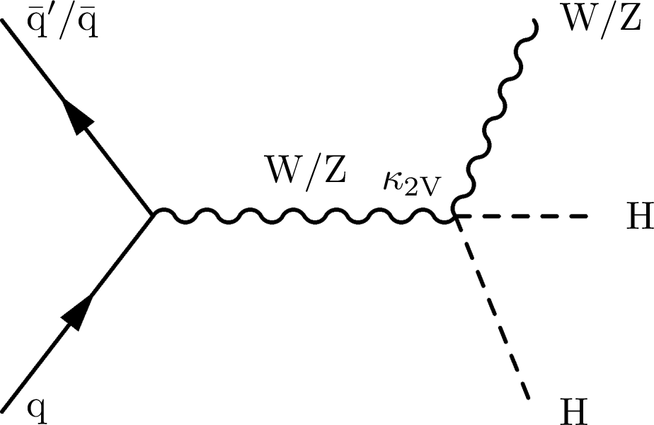
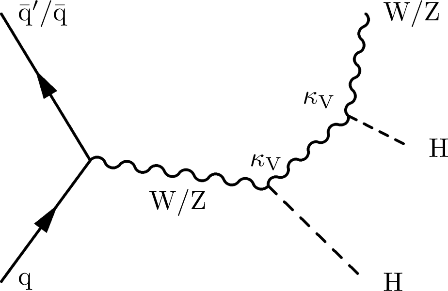
Figure 1:
The three leading-order quark-initiated Feynman diagrams above result in a final state with two Higgs bosons and a W or Z boson. The left diagram requires one $ \kappa_{\mathrm{V}} $ coupling vertex and one $ \kappa_{\lambda} $ coupling vertex. The middle diagram requires only one $ \kappa_{2\mathrm{V}} $ coupling vertex, and the right diagram requires two $ \kappa_{\mathrm{V}} $ coupling vertices. |

png pdf |
Figure 1-a:
The three leading-order quark-initiated Feynman diagrams above result in a final state with two Higgs bosons and a W or Z boson. The left diagram requires one $ \kappa_{\mathrm{V}} $ coupling vertex and one $ \kappa_{\lambda} $ coupling vertex. The middle diagram requires only one $ \kappa_{2\mathrm{V}} $ coupling vertex, and the right diagram requires two $ \kappa_{\mathrm{V}} $ coupling vertices. |
png pdf |
Figure 1-b:
The three leading-order quark-initiated Feynman diagrams above result in a final state with two Higgs bosons and a W or Z boson. The left diagram requires one $ \kappa_{\mathrm{V}} $ coupling vertex and one $ \kappa_{\lambda} $ coupling vertex. The middle diagram requires only one $ \kappa_{2\mathrm{V}} $ coupling vertex, and the right diagram requires two $ \kappa_{\mathrm{V}} $ coupling vertices. |
png pdf |
Figure 1-c:
The three leading-order quark-initiated Feynman diagrams above result in a final state with two Higgs bosons and a W or Z boson. The left diagram requires one $ \kappa_{\mathrm{V}} $ coupling vertex and one $ \kappa_{\lambda} $ coupling vertex. The middle diagram requires only one $ \kappa_{2\mathrm{V}} $ coupling vertex, and the right diagram requires two $ \kappa_{\mathrm{V}} $ coupling vertices. |
png pdf |
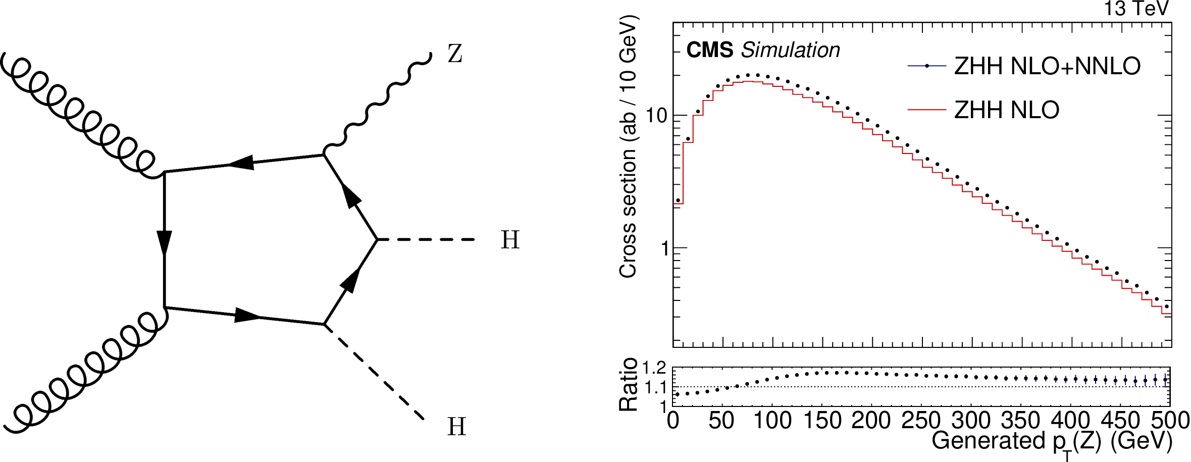
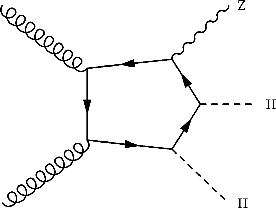
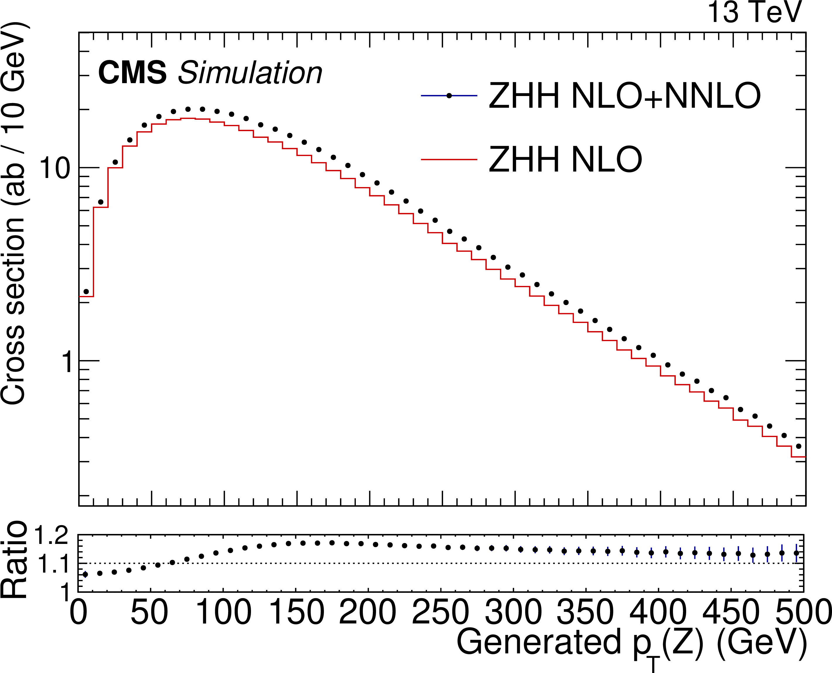
Figure 2:
Left: representative Feynman diagram for ggF ZHH production, which represents approximately 14% of the total cross section for ZHH production. Right: distribution of $ p_{\mathrm{T}}(\mathrm{Z}) $ with and without ggZHH process. The ratio is applied to NLO to incorporate the ggZHH cross section enhancement. |
png pdf |
Figure 2-a:
Left: representative Feynman diagram for ggF ZHH production, which represents approximately 14% of the total cross section for ZHH production. Right: distribution of $ p_{\mathrm{T}}(\mathrm{Z}) $ with and without ggZHH process. The ratio is applied to NLO to incorporate the ggZHH cross section enhancement. |
png pdf |
Figure 2-b:
Left: representative Feynman diagram for ggF ZHH production, which represents approximately 14% of the total cross section for ZHH production. Right: distribution of $ p_{\mathrm{T}}(\mathrm{Z}) $ with and without ggZHH process. The ratio is applied to NLO to incorporate the ggZHH cross section enhancement. |
png pdf |
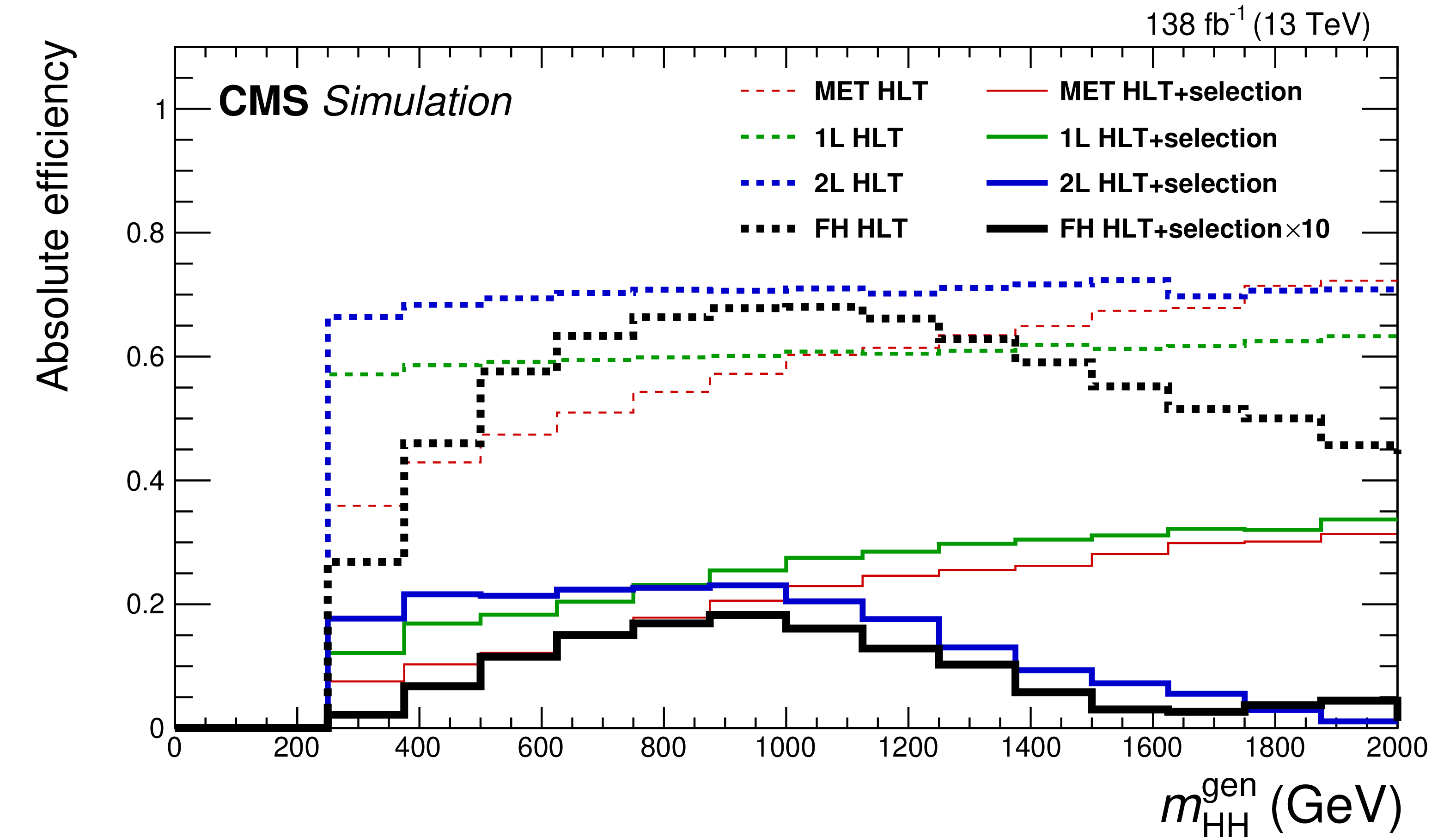
Figure 3:
The SM VHH efficiencies of trigger selections (dashed lines) and full selections (solid lines) are shown for all four analysis channels. The full selection efficiency in the FH channel is scaled up by 10 for visibility. Both sets of efficiencies are absolute efficiencies (acceptance times selections efficiencies). |
png pdf |
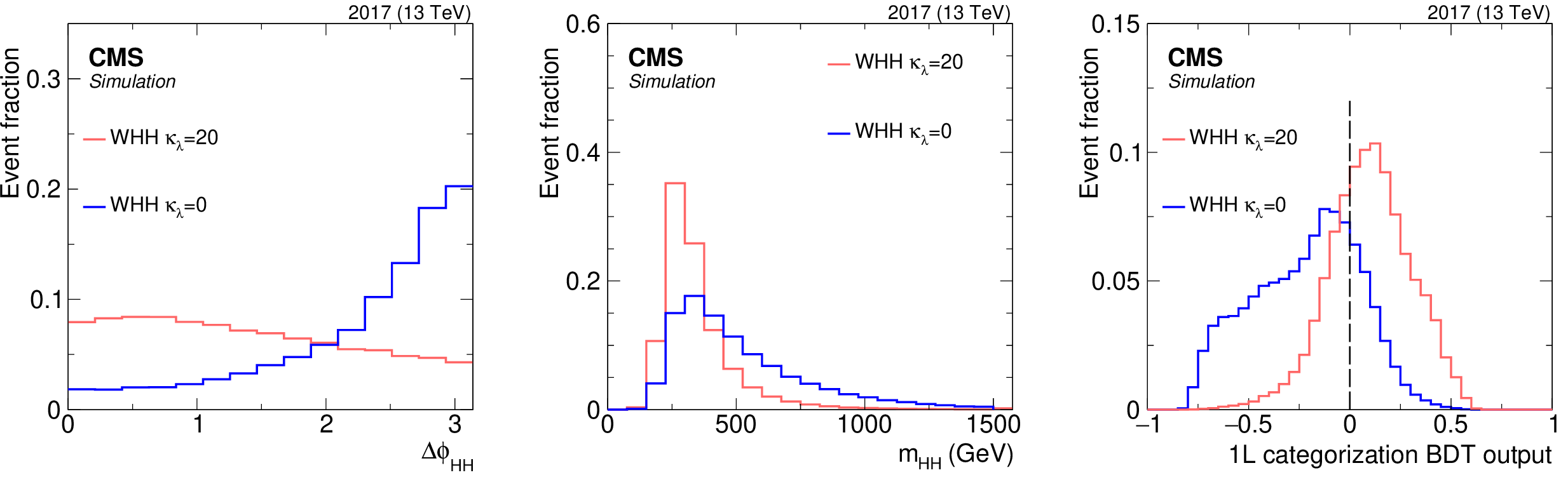
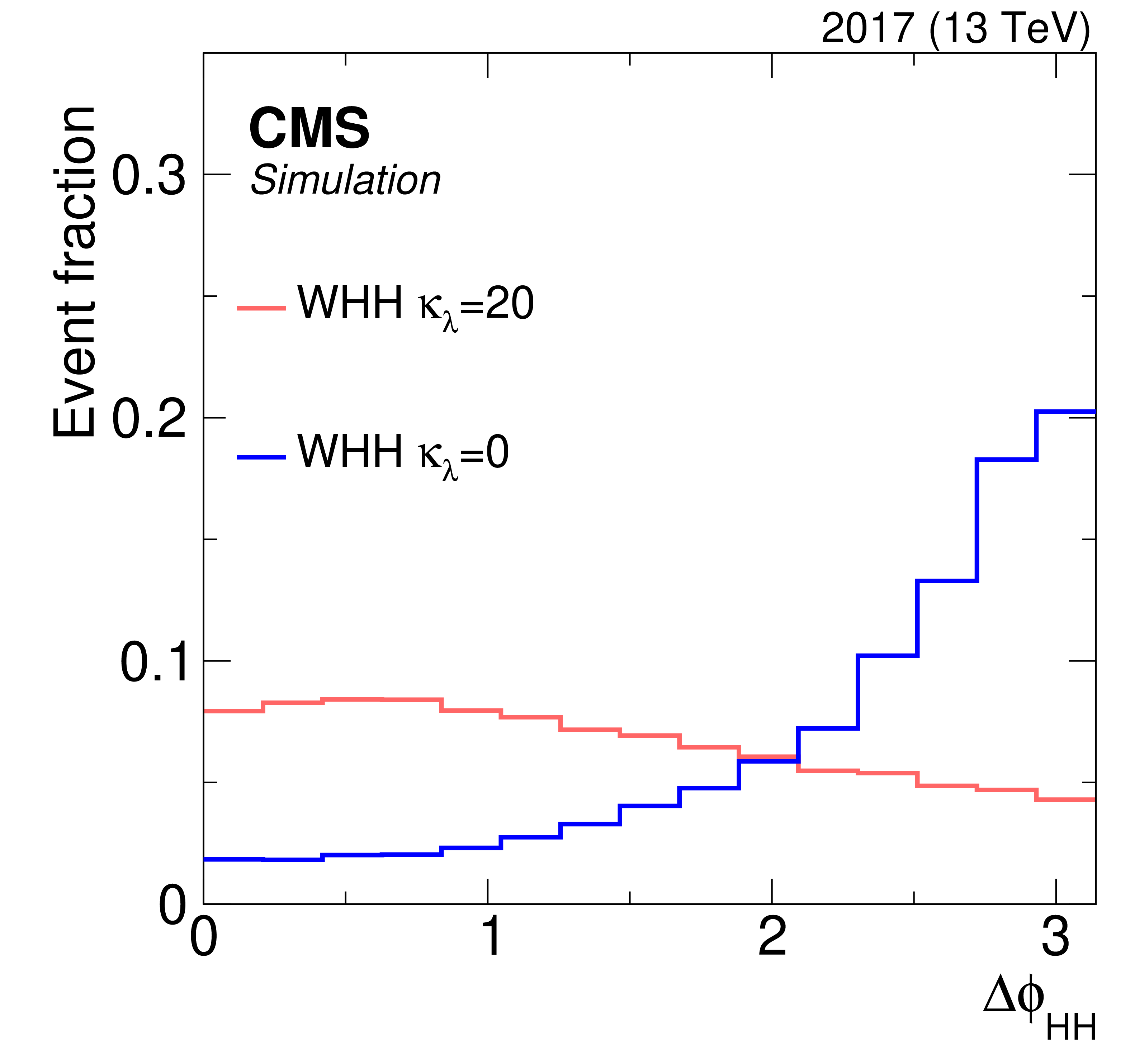
Figure 4:
Kinematic distributions vary for different coupling strengths. Left and middle: azimuthal angle between the two reconstructed Higgs boson candidates, $ \Delta\phi_{\mathrm{H}\mathrm{H}} $, and the reconstructed HH mass, $ m_{\mathrm{H}\mathrm{H}} $, in the 1L SR for two different coupling models, $ \kappa_{\lambda}= $ 20 and 0. Right: the categorization BDT output for the same two models. The dashed vertical line shows where the categorization boundary is set. |
png pdf |
Figure 4-a:
Kinematic distributions vary for different coupling strengths. Left and middle: azimuthal angle between the two reconstructed Higgs boson candidates, $ \Delta\phi_{\mathrm{H}\mathrm{H}} $, and the reconstructed HH mass, $ m_{\mathrm{H}\mathrm{H}} $, in the 1L SR for two different coupling models, $ \kappa_{\lambda}= $ 20 and 0. Right: the categorization BDT output for the same two models. The dashed vertical line shows where the categorization boundary is set. |

png pdf |
Figure 4-b:
Kinematic distributions vary for different coupling strengths. Left and middle: azimuthal angle between the two reconstructed Higgs boson candidates, $ \Delta\phi_{\mathrm{H}\mathrm{H}} $, and the reconstructed HH mass, $ m_{\mathrm{H}\mathrm{H}} $, in the 1L SR for two different coupling models, $ \kappa_{\lambda}= $ 20 and 0. Right: the categorization BDT output for the same two models. The dashed vertical line shows where the categorization boundary is set. |

png pdf |
Figure 4-c:
Kinematic distributions vary for different coupling strengths. Left and middle: azimuthal angle between the two reconstructed Higgs boson candidates, $ \Delta\phi_{\mathrm{H}\mathrm{H}} $, and the reconstructed HH mass, $ m_{\mathrm{H}\mathrm{H}} $, in the 1L SR for two different coupling models, $ \kappa_{\lambda}= $ 20 and 0. Right: the categorization BDT output for the same two models. The dashed vertical line shows where the categorization boundary is set. |
png pdf |
Figure 5:
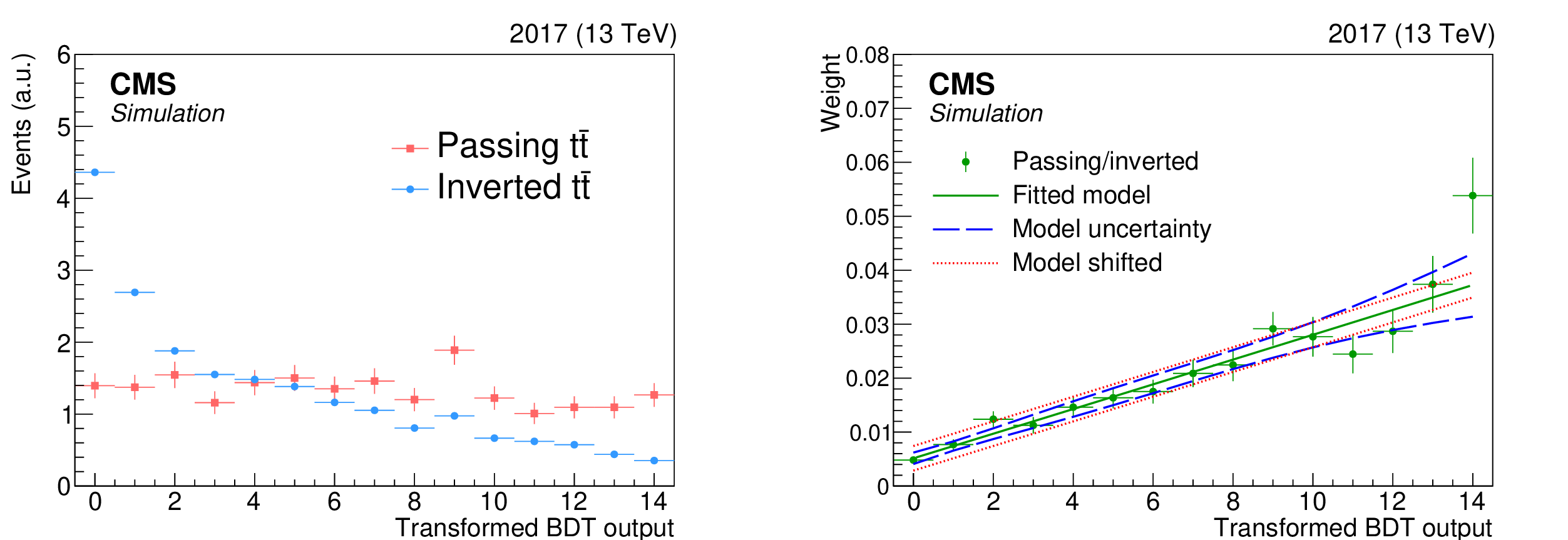
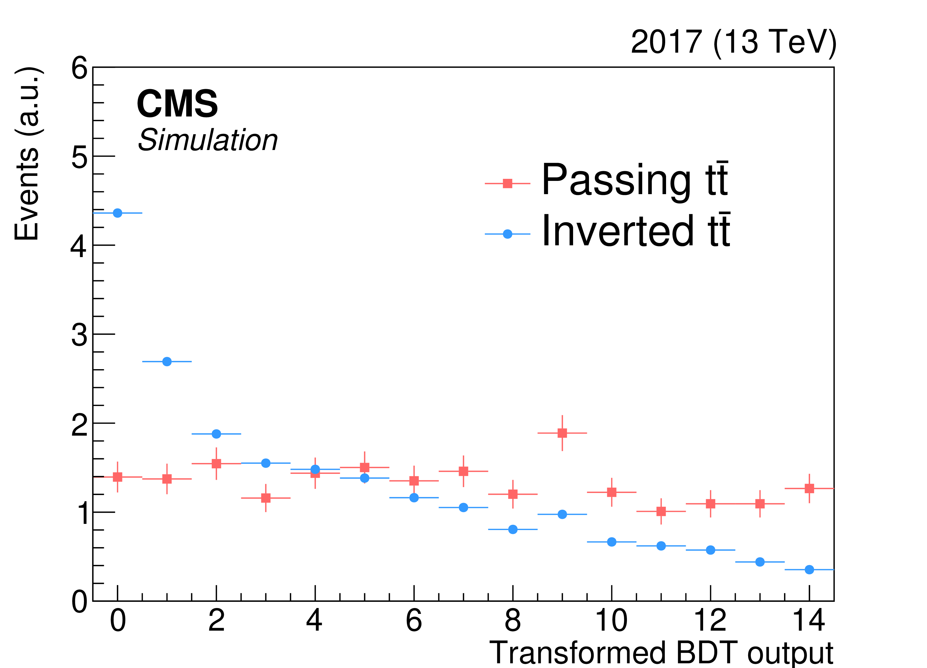
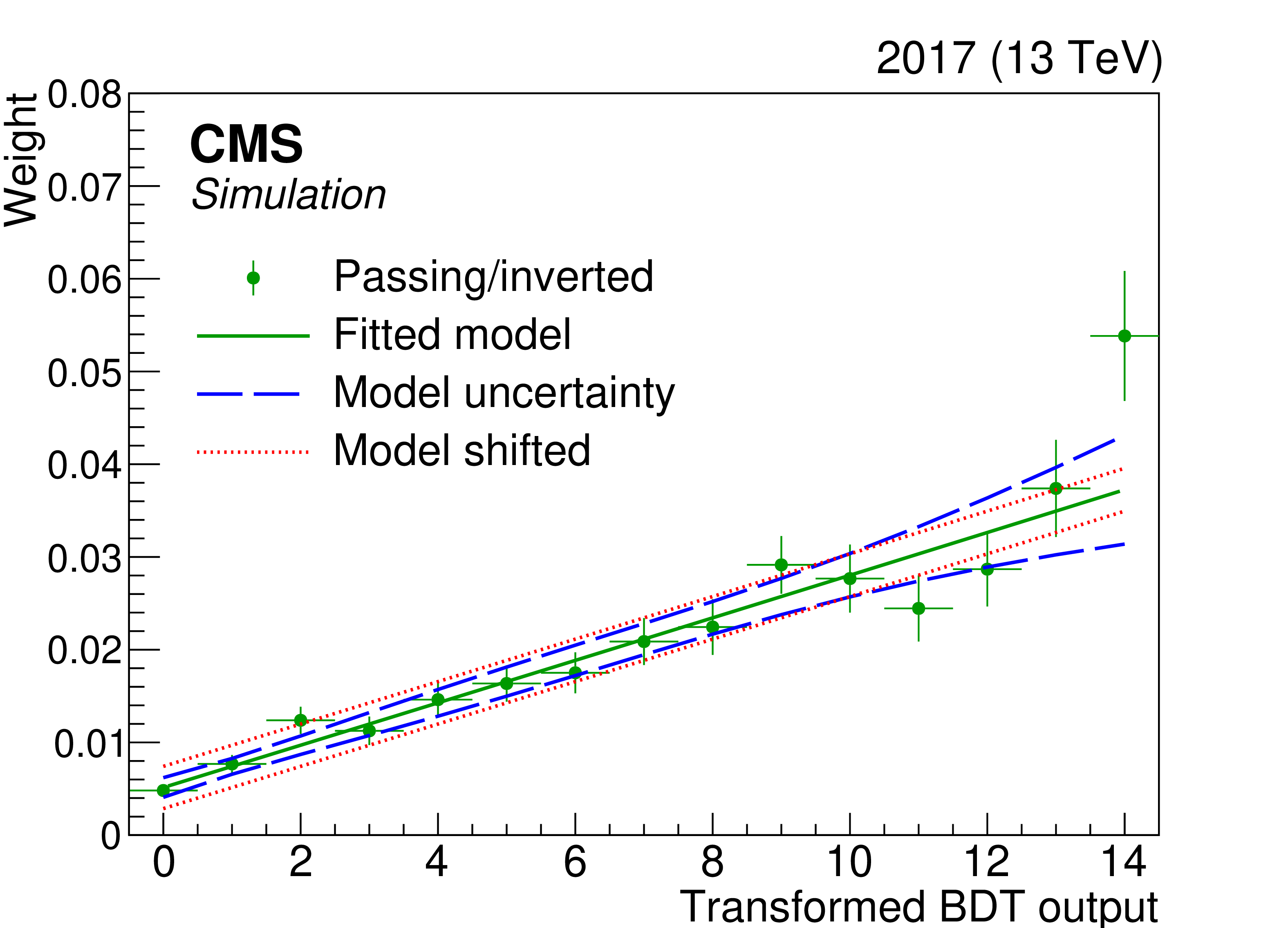
Left: a reweighting BDT in the 1L LP region for the $ \mathrm{t} \overline{\mathrm{t}} $ process that is transformed such that the limited-precision passing $ \mathrm{t} \overline{\mathrm{t}} $ sample, shown as red squares, is evenly distributed across all bins. In blue circles is the same process where the b tagging selections are inverted. Right: the ratio is shown of passing $ \mathrm{t} \overline{\mathrm{t}} $ to inverted $ \mathrm{t} \overline{\mathrm{t}} $ (green points) as a function of the transformed reweighting BDT score. The solid line is the second-order polynomial fit of the green points, which is used for the reweighting. In dotted red and dashed blue are the associated systematic uncertainties, which are obtained from shifting the BDT score bin in evaluation of the model and the evaluation of the fit uncertainties on the weight, respectively. These systematic variations account for finite binning and limited statistical precision of the passing events, and they enhance the flexibility of the model. |
png pdf |
Figure 5-a:
Left: a reweighting BDT in the 1L LP region for the $ \mathrm{t} \overline{\mathrm{t}} $ process that is transformed such that the limited-precision passing $ \mathrm{t} \overline{\mathrm{t}} $ sample, shown as red squares, is evenly distributed across all bins. In blue circles is the same process where the b tagging selections are inverted. Right: the ratio is shown of passing $ \mathrm{t} \overline{\mathrm{t}} $ to inverted $ \mathrm{t} \overline{\mathrm{t}} $ (green points) as a function of the transformed reweighting BDT score. The solid line is the second-order polynomial fit of the green points, which is used for the reweighting. In dotted red and dashed blue are the associated systematic uncertainties, which are obtained from shifting the BDT score bin in evaluation of the model and the evaluation of the fit uncertainties on the weight, respectively. These systematic variations account for finite binning and limited statistical precision of the passing events, and they enhance the flexibility of the model. |
png pdf |
Figure 5-b:
Left: a reweighting BDT in the 1L LP region for the $ \mathrm{t} \overline{\mathrm{t}} $ process that is transformed such that the limited-precision passing $ \mathrm{t} \overline{\mathrm{t}} $ sample, shown as red squares, is evenly distributed across all bins. In blue circles is the same process where the b tagging selections are inverted. Right: the ratio is shown of passing $ \mathrm{t} \overline{\mathrm{t}} $ to inverted $ \mathrm{t} \overline{\mathrm{t}} $ (green points) as a function of the transformed reweighting BDT score. The solid line is the second-order polynomial fit of the green points, which is used for the reweighting. In dotted red and dashed blue are the associated systematic uncertainties, which are obtained from shifting the BDT score bin in evaluation of the model and the evaluation of the fit uncertainties on the weight, respectively. These systematic variations account for finite binning and limited statistical precision of the passing events, and they enhance the flexibility of the model. |

png pdf |
Figure 6:
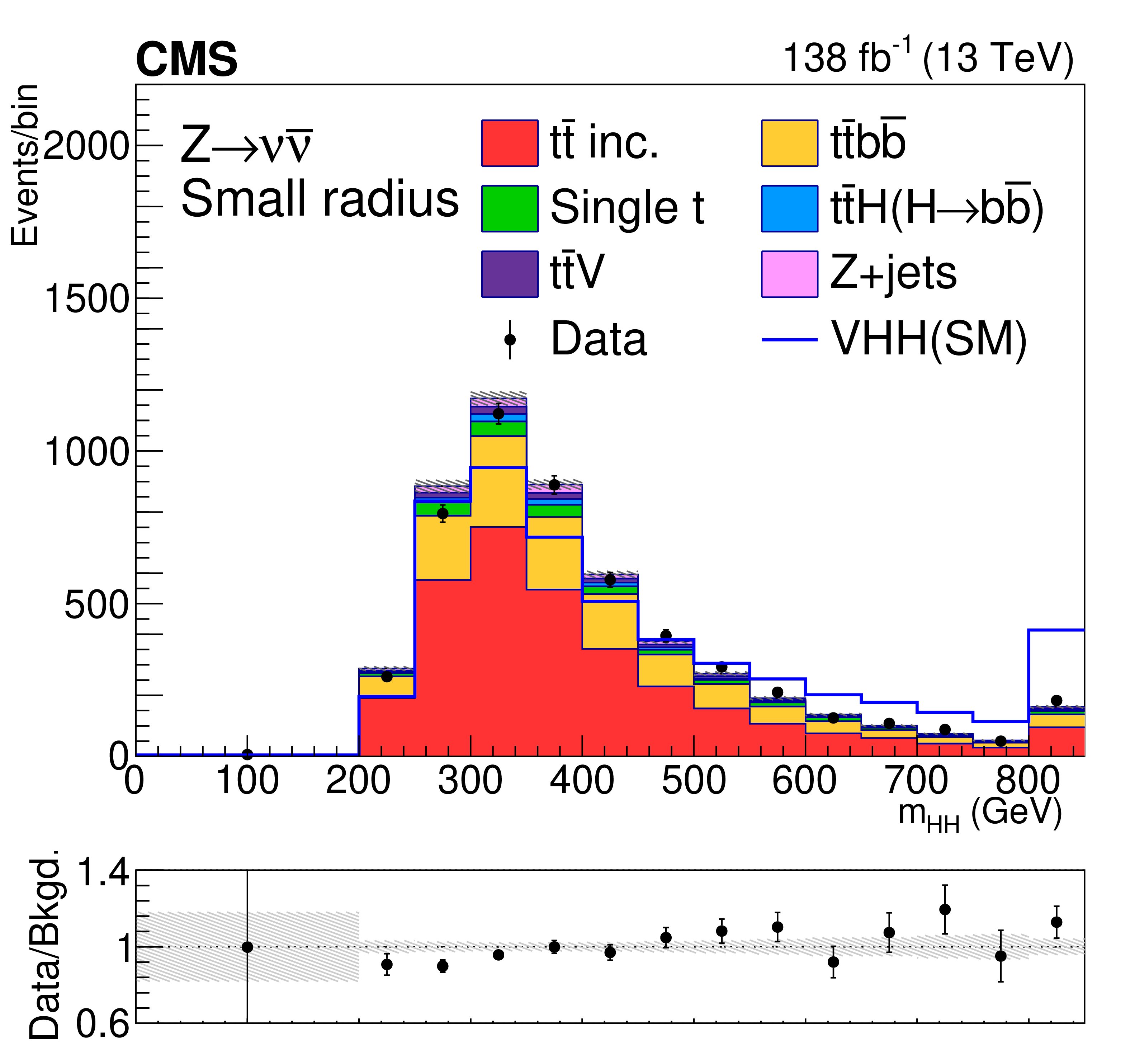
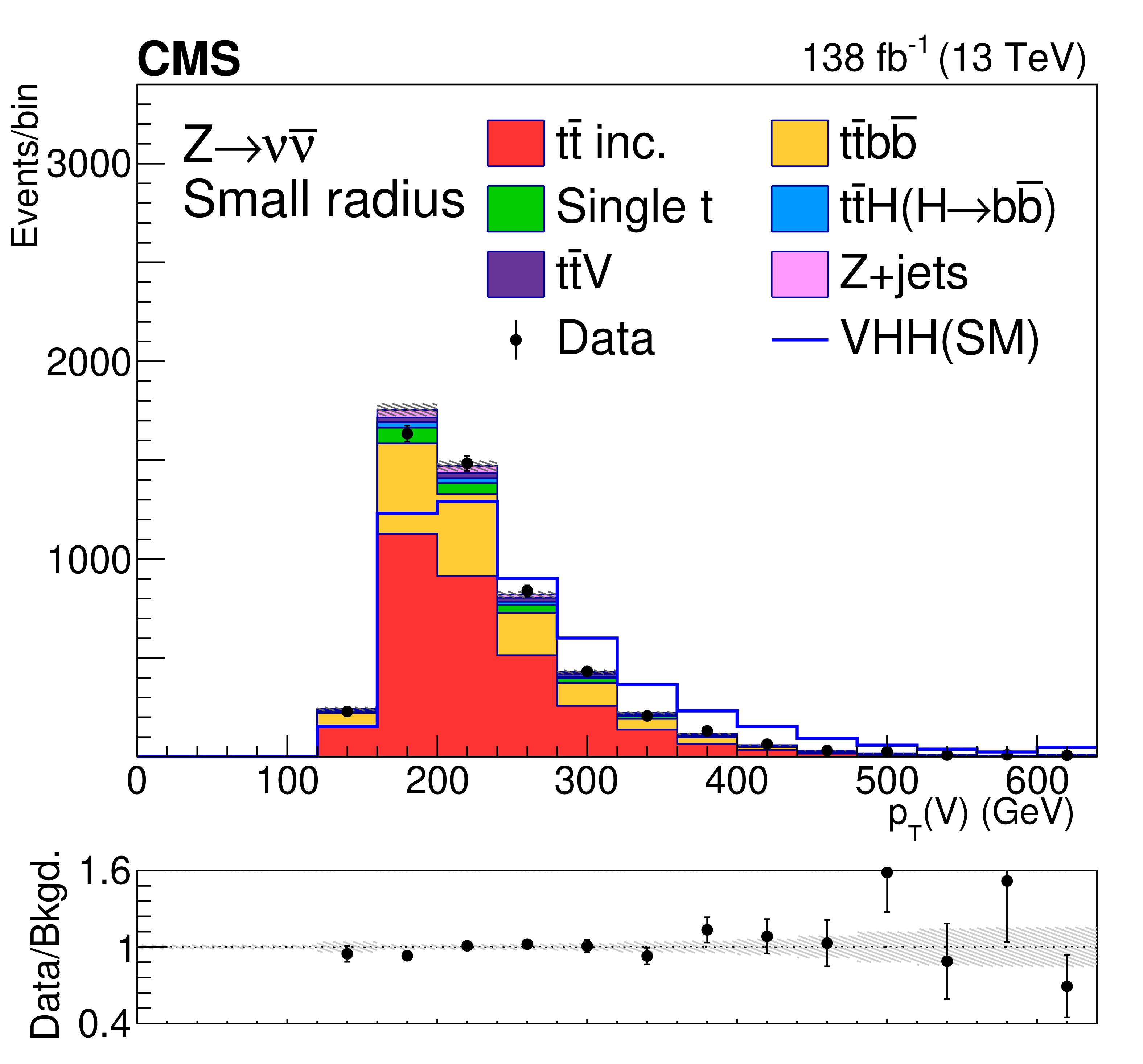
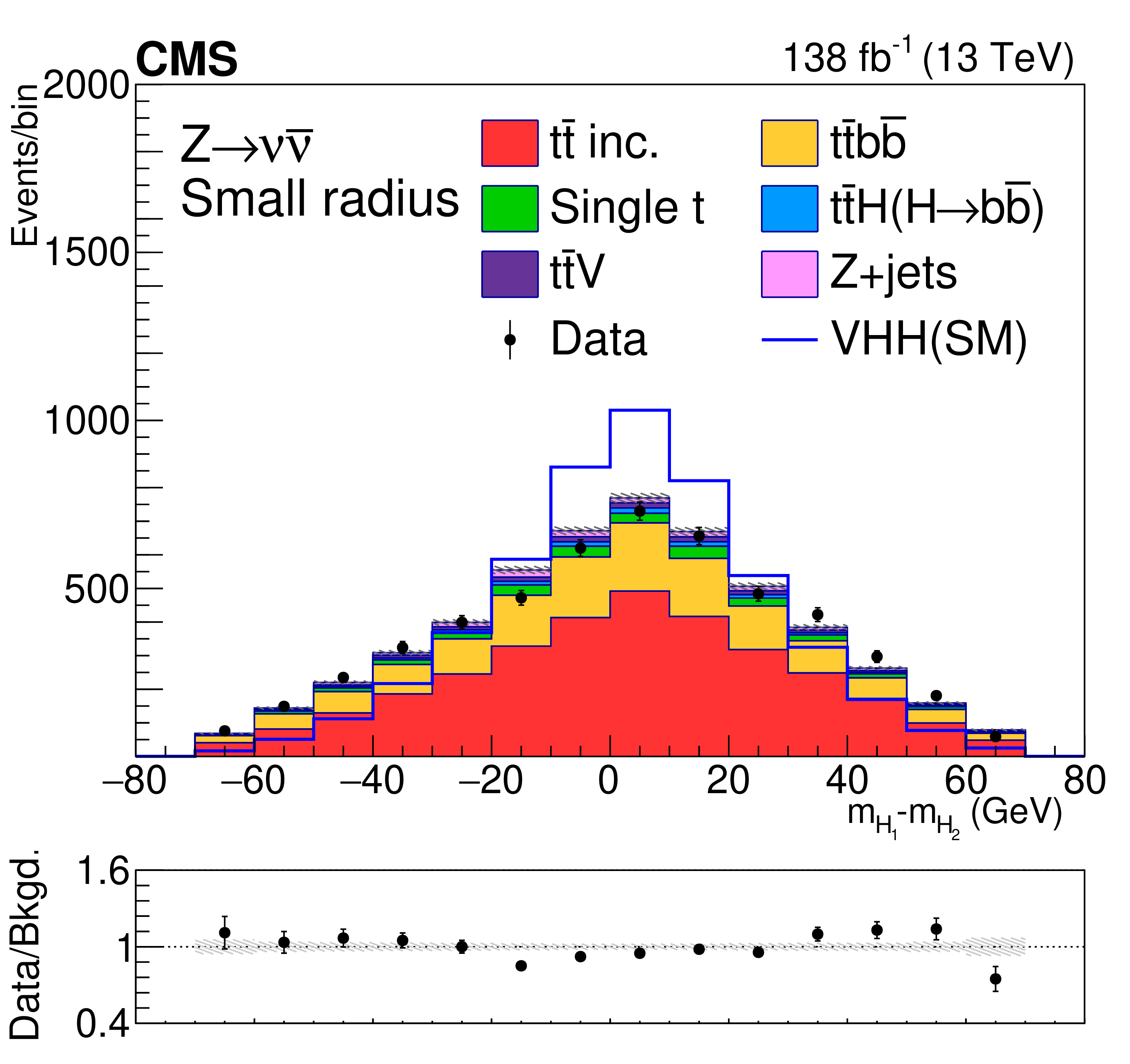
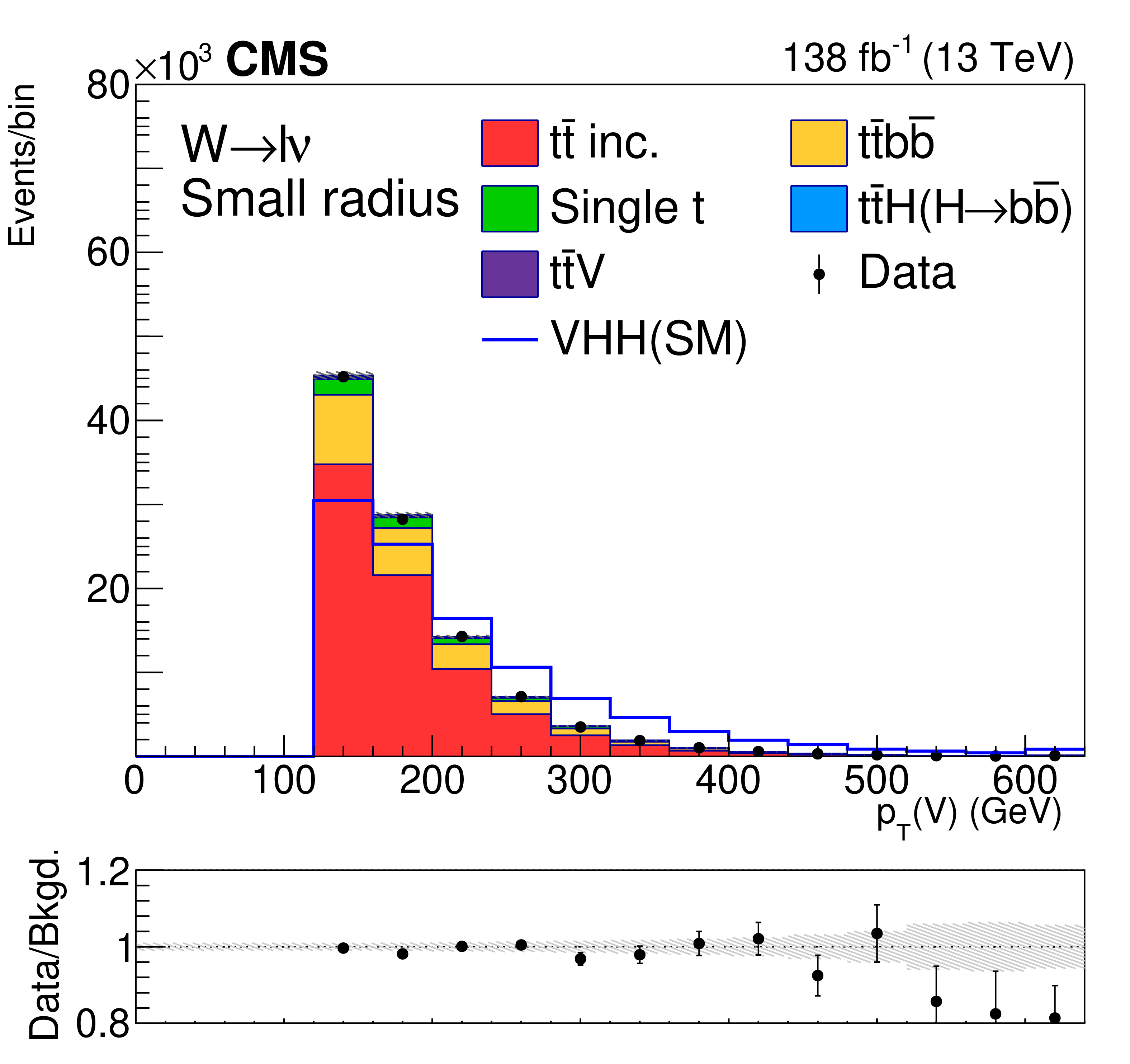
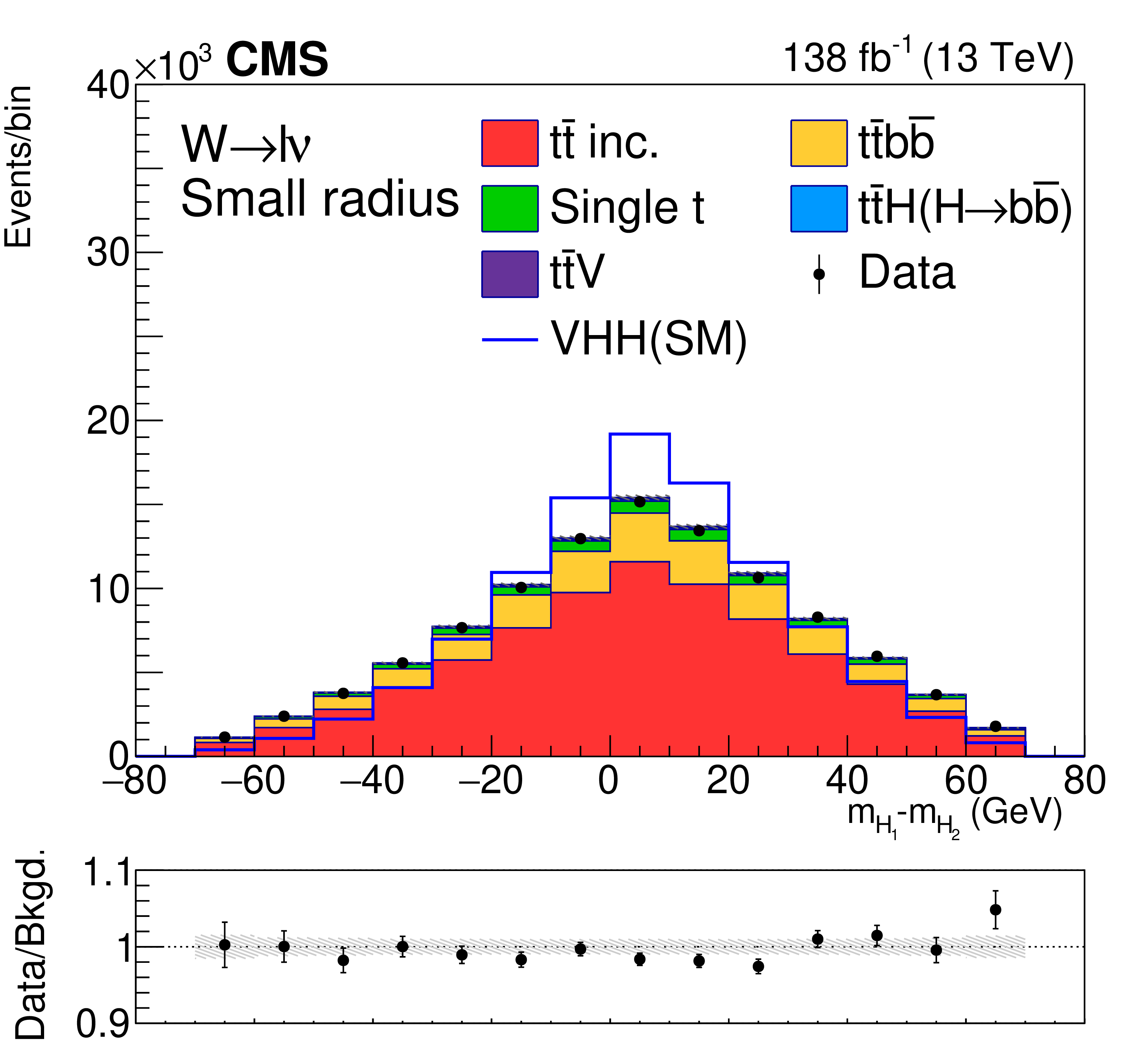
Postfit distributions of kinematic variables in the small-radius jet regions. From upper to lower, the rows show the MET and 1L channels. The variables in each channel are $ m_{\mathrm{H}\mathrm{H}} $, $ p_{\mathrm{T}}(\mathrm{V}) $, and $ m_{ {\mathrm{H}_{1}} }{-}m_{ {\mathrm{H}_{2}} } $. The fit is done with the background-only hypotheses and the final bin in each plot includes overflows. The ratios of data to the total expected background are shown in the lower panel of each plot and the hatched bands are the combined statistical and systematic uncertainties of total background. The blue lines are SM signal distributions, which are scaled to have the same number of events as the background. |
png pdf |
Figure 6-a:
Postfit distributions of kinematic variables in the small-radius jet regions. From upper to lower, the rows show the MET and 1L channels. The variables in each channel are $ m_{\mathrm{H}\mathrm{H}} $, $ p_{\mathrm{T}}(\mathrm{V}) $, and $ m_{ {\mathrm{H}_{1}} }{-}m_{ {\mathrm{H}_{2}} } $. The fit is done with the background-only hypotheses and the final bin in each plot includes overflows. The ratios of data to the total expected background are shown in the lower panel of each plot and the hatched bands are the combined statistical and systematic uncertainties of total background. The blue lines are SM signal distributions, which are scaled to have the same number of events as the background. |
png pdf |
Figure 6-b:
Postfit distributions of kinematic variables in the small-radius jet regions. From upper to lower, the rows show the MET and 1L channels. The variables in each channel are $ m_{\mathrm{H}\mathrm{H}} $, $ p_{\mathrm{T}}(\mathrm{V}) $, and $ m_{ {\mathrm{H}_{1}} }{-}m_{ {\mathrm{H}_{2}} } $. The fit is done with the background-only hypotheses and the final bin in each plot includes overflows. The ratios of data to the total expected background are shown in the lower panel of each plot and the hatched bands are the combined statistical and systematic uncertainties of total background. The blue lines are SM signal distributions, which are scaled to have the same number of events as the background. |
png pdf |
Figure 6-c:
Postfit distributions of kinematic variables in the small-radius jet regions. From upper to lower, the rows show the MET and 1L channels. The variables in each channel are $ m_{\mathrm{H}\mathrm{H}} $, $ p_{\mathrm{T}}(\mathrm{V}) $, and $ m_{ {\mathrm{H}_{1}} }{-}m_{ {\mathrm{H}_{2}} } $. The fit is done with the background-only hypotheses and the final bin in each plot includes overflows. The ratios of data to the total expected background are shown in the lower panel of each plot and the hatched bands are the combined statistical and systematic uncertainties of total background. The blue lines are SM signal distributions, which are scaled to have the same number of events as the background. |

png pdf |
Figure 6-d:
Postfit distributions of kinematic variables in the small-radius jet regions. From upper to lower, the rows show the MET and 1L channels. The variables in each channel are $ m_{\mathrm{H}\mathrm{H}} $, $ p_{\mathrm{T}}(\mathrm{V}) $, and $ m_{ {\mathrm{H}_{1}} }{-}m_{ {\mathrm{H}_{2}} } $. The fit is done with the background-only hypotheses and the final bin in each plot includes overflows. The ratios of data to the total expected background are shown in the lower panel of each plot and the hatched bands are the combined statistical and systematic uncertainties of total background. The blue lines are SM signal distributions, which are scaled to have the same number of events as the background. |
png pdf |
Figure 6-e:
Postfit distributions of kinematic variables in the small-radius jet regions. From upper to lower, the rows show the MET and 1L channels. The variables in each channel are $ m_{\mathrm{H}\mathrm{H}} $, $ p_{\mathrm{T}}(\mathrm{V}) $, and $ m_{ {\mathrm{H}_{1}} }{-}m_{ {\mathrm{H}_{2}} } $. The fit is done with the background-only hypotheses and the final bin in each plot includes overflows. The ratios of data to the total expected background are shown in the lower panel of each plot and the hatched bands are the combined statistical and systematic uncertainties of total background. The blue lines are SM signal distributions, which are scaled to have the same number of events as the background. |
png pdf |
Figure 6-f:
Postfit distributions of kinematic variables in the small-radius jet regions. From upper to lower, the rows show the MET and 1L channels. The variables in each channel are $ m_{\mathrm{H}\mathrm{H}} $, $ p_{\mathrm{T}}(\mathrm{V}) $, and $ m_{ {\mathrm{H}_{1}} }{-}m_{ {\mathrm{H}_{2}} } $. The fit is done with the background-only hypotheses and the final bin in each plot includes overflows. The ratios of data to the total expected background are shown in the lower panel of each plot and the hatched bands are the combined statistical and systematic uncertainties of total background. The blue lines are SM signal distributions, which are scaled to have the same number of events as the background. |

png pdf |
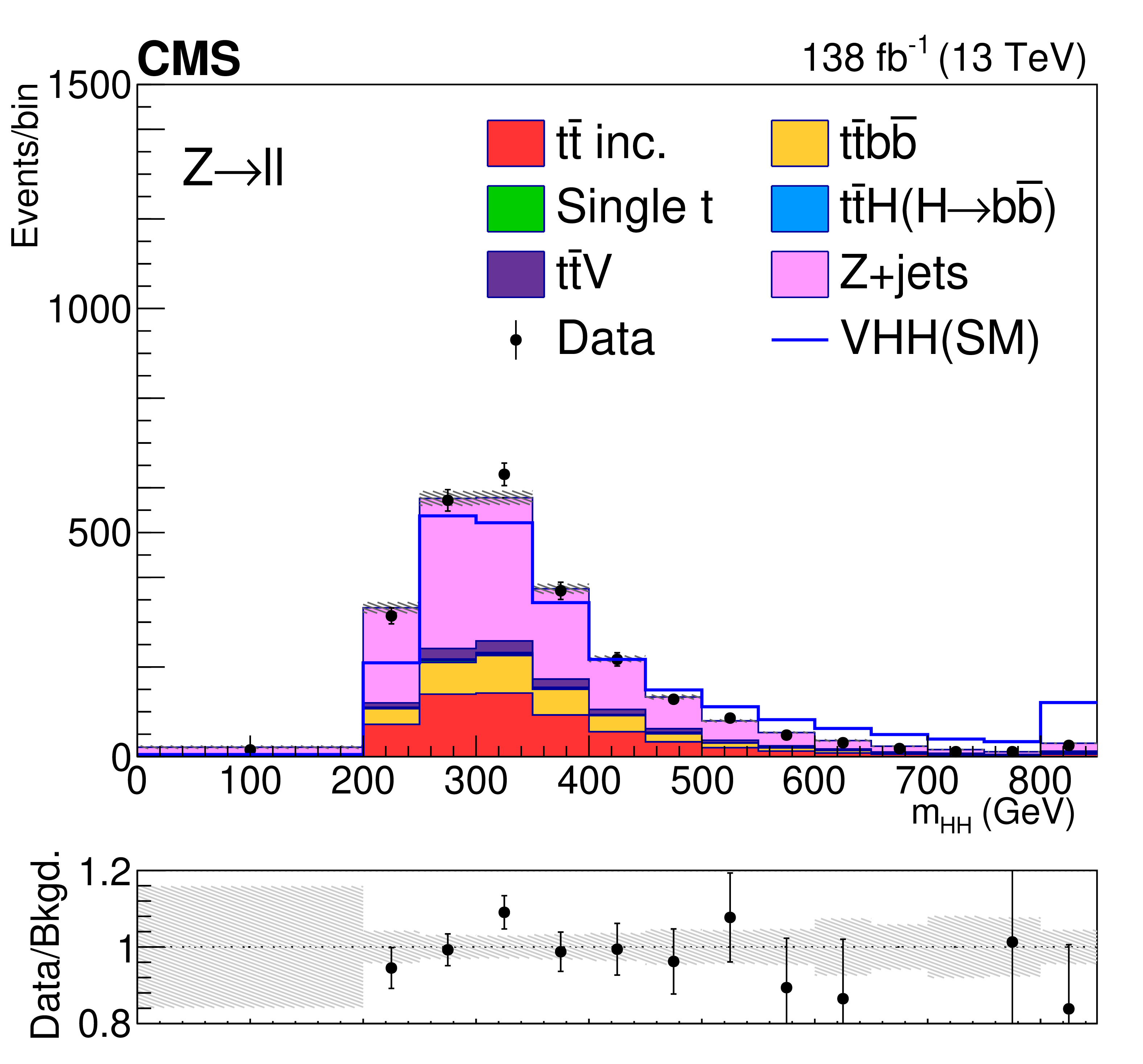
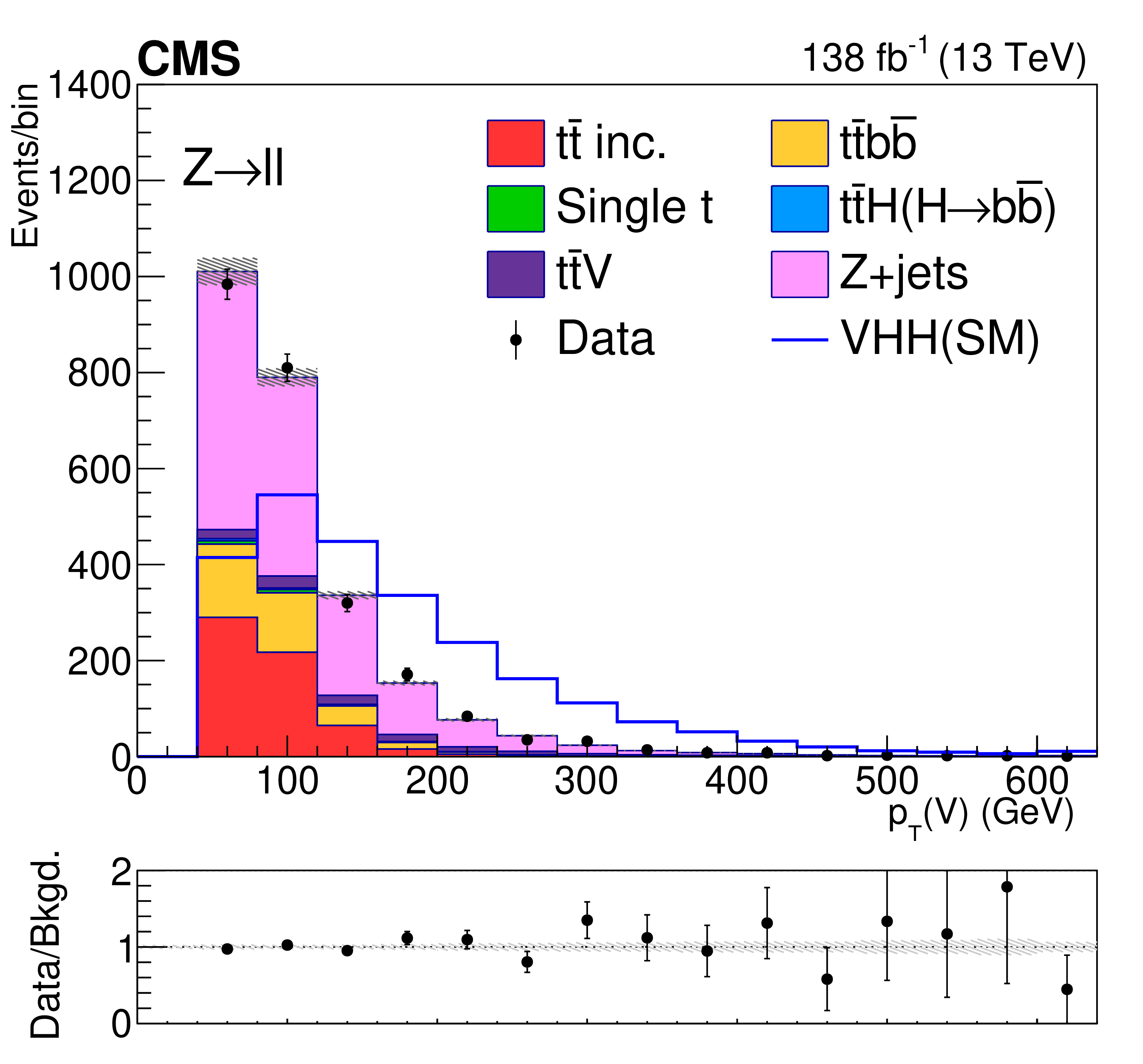
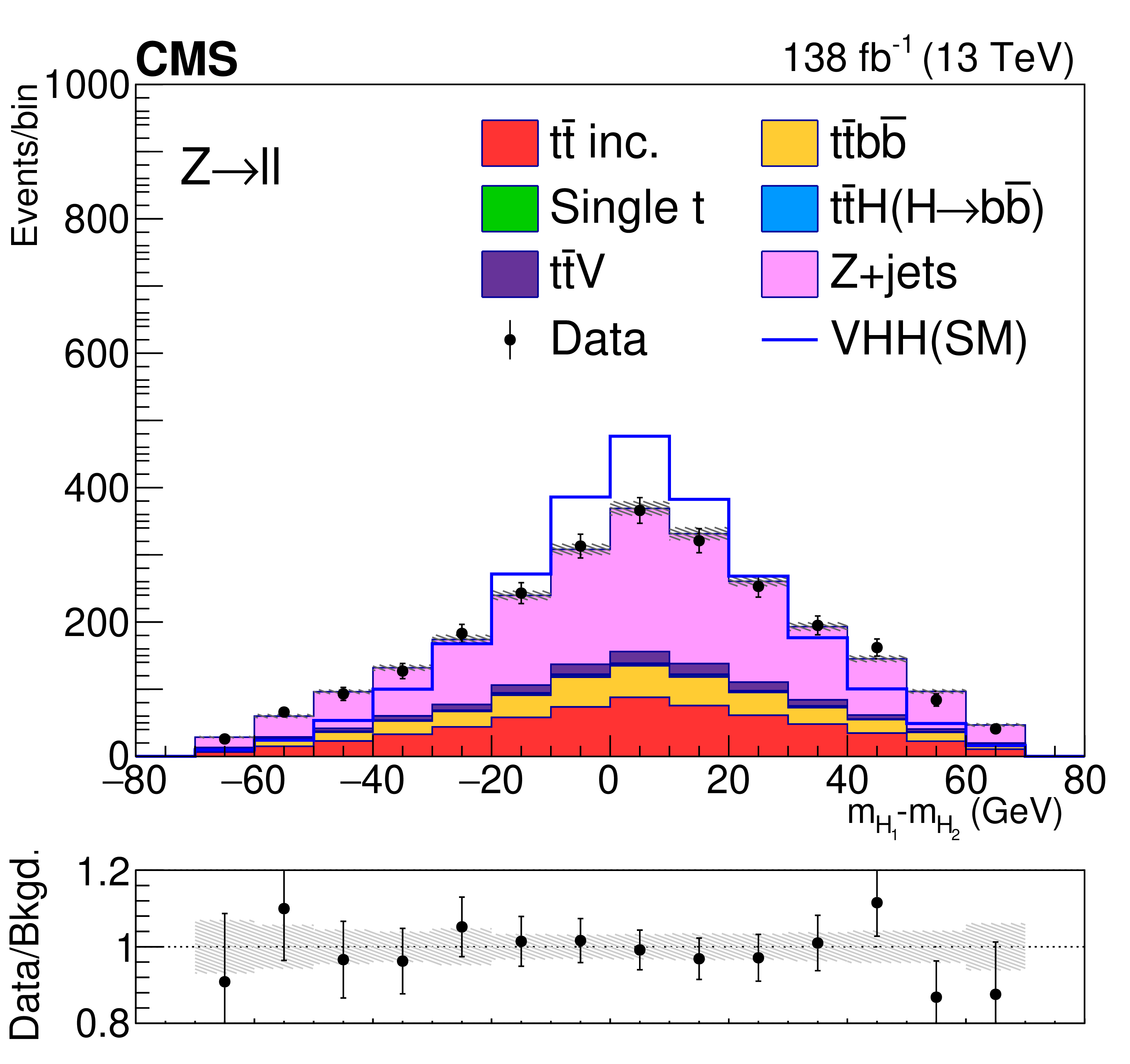
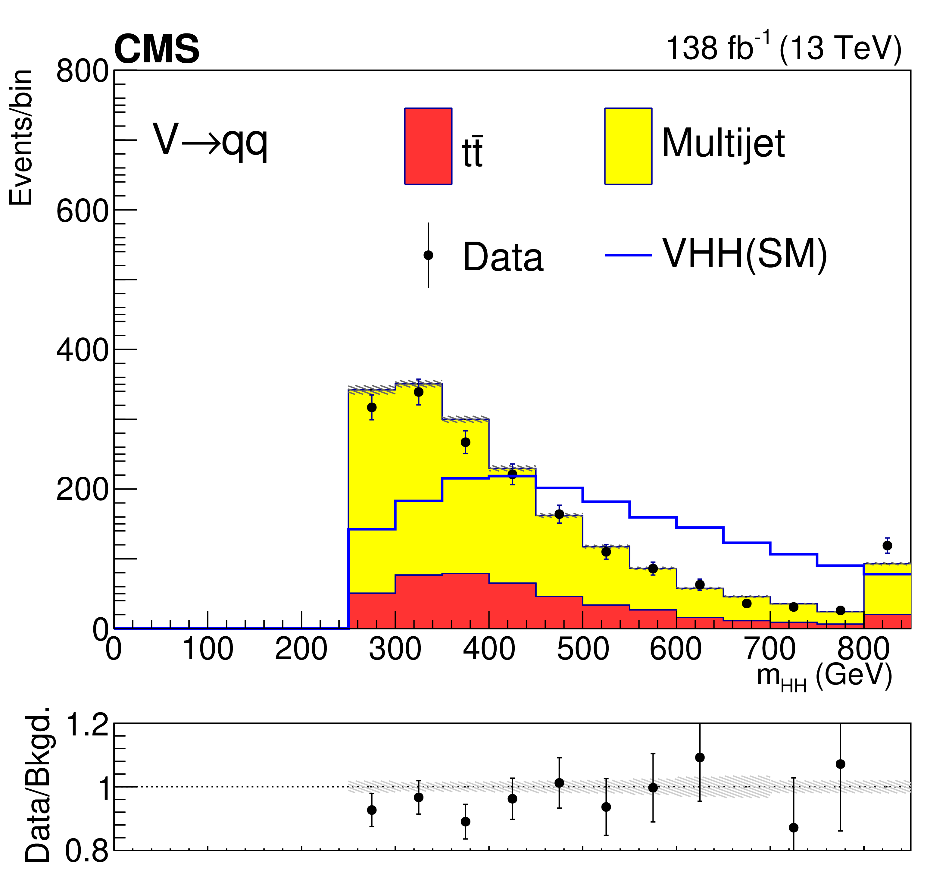
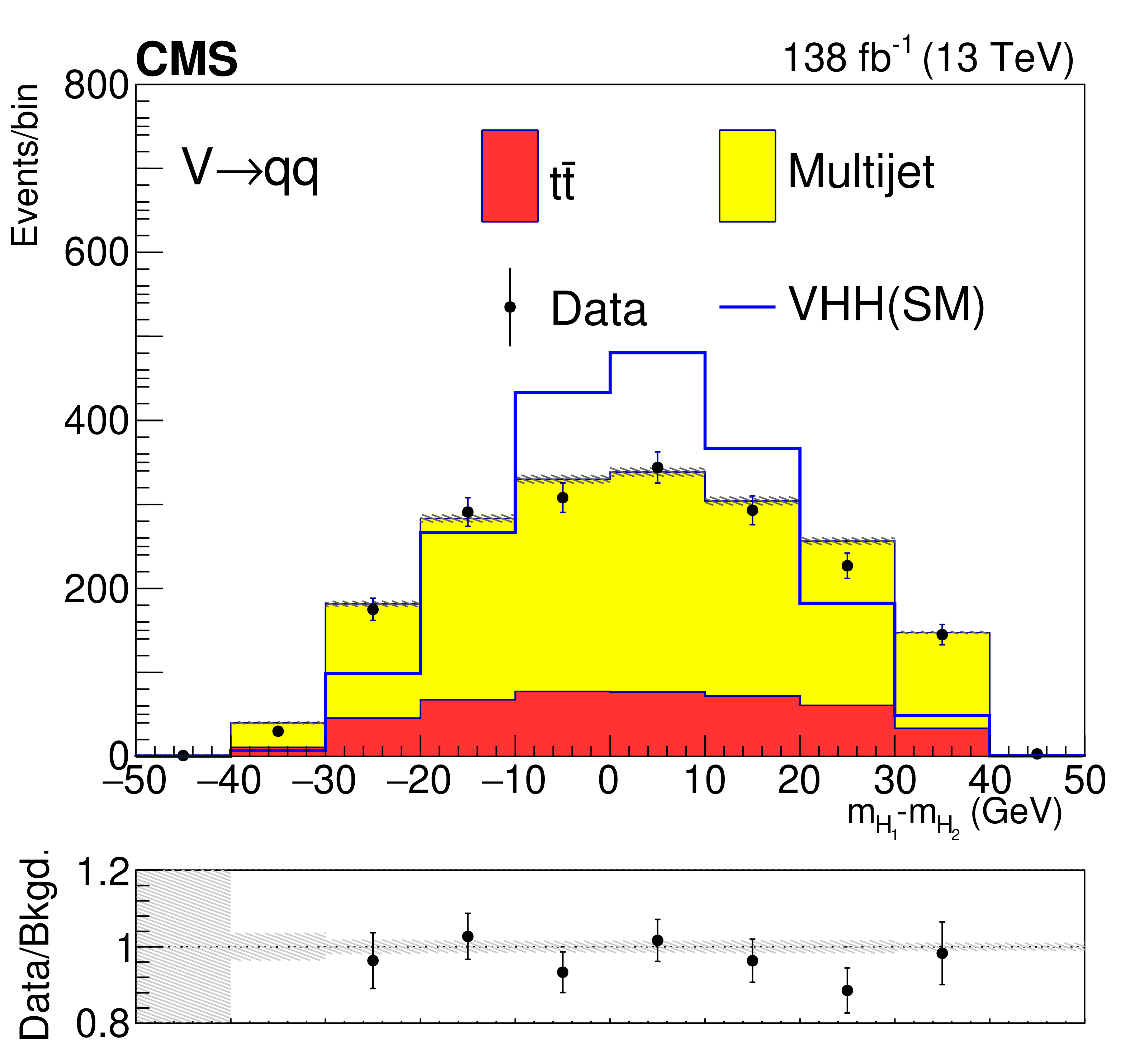
Figure 7:
Postfit distributions of kinematic variables in the small-radius jet regions. From upper to lower, the rows show the 2L and FH channels. The variables in each channel are $ m_{\mathrm{H}\mathrm{H}} $, $ p_{\mathrm{T}}(\mathrm{V}) $, and $ m_{ {\mathrm{H}_{1}} }{-}m_{ {\mathrm{H}_{2}} } $. The fit is done with the background-only hypotheses and the final bin in each plot includes overflows. The ratios of data to the total expected background are shown in the lower panel of each plot and the hatched bands are the combined statistical and systematic uncertainties of total background. The blue lines are SM signal distributions, which are scaled to have the same number of events as the background. |
png pdf |
Figure 7-a:
Postfit distributions of kinematic variables in the small-radius jet regions. From upper to lower, the rows show the 2L and FH channels. The variables in each channel are $ m_{\mathrm{H}\mathrm{H}} $, $ p_{\mathrm{T}}(\mathrm{V}) $, and $ m_{ {\mathrm{H}_{1}} }{-}m_{ {\mathrm{H}_{2}} } $. The fit is done with the background-only hypotheses and the final bin in each plot includes overflows. The ratios of data to the total expected background are shown in the lower panel of each plot and the hatched bands are the combined statistical and systematic uncertainties of total background. The blue lines are SM signal distributions, which are scaled to have the same number of events as the background. |
png pdf |
Figure 7-b:
Postfit distributions of kinematic variables in the small-radius jet regions. From upper to lower, the rows show the 2L and FH channels. The variables in each channel are $ m_{\mathrm{H}\mathrm{H}} $, $ p_{\mathrm{T}}(\mathrm{V}) $, and $ m_{ {\mathrm{H}_{1}} }{-}m_{ {\mathrm{H}_{2}} } $. The fit is done with the background-only hypotheses and the final bin in each plot includes overflows. The ratios of data to the total expected background are shown in the lower panel of each plot and the hatched bands are the combined statistical and systematic uncertainties of total background. The blue lines are SM signal distributions, which are scaled to have the same number of events as the background. |
png pdf |
Figure 7-c:
Postfit distributions of kinematic variables in the small-radius jet regions. From upper to lower, the rows show the 2L and FH channels. The variables in each channel are $ m_{\mathrm{H}\mathrm{H}} $, $ p_{\mathrm{T}}(\mathrm{V}) $, and $ m_{ {\mathrm{H}_{1}} }{-}m_{ {\mathrm{H}_{2}} } $. The fit is done with the background-only hypotheses and the final bin in each plot includes overflows. The ratios of data to the total expected background are shown in the lower panel of each plot and the hatched bands are the combined statistical and systematic uncertainties of total background. The blue lines are SM signal distributions, which are scaled to have the same number of events as the background. |
png pdf |
Figure 7-d:
Postfit distributions of kinematic variables in the small-radius jet regions. From upper to lower, the rows show the 2L and FH channels. The variables in each channel are $ m_{\mathrm{H}\mathrm{H}} $, $ p_{\mathrm{T}}(\mathrm{V}) $, and $ m_{ {\mathrm{H}_{1}} }{-}m_{ {\mathrm{H}_{2}} } $. The fit is done with the background-only hypotheses and the final bin in each plot includes overflows. The ratios of data to the total expected background are shown in the lower panel of each plot and the hatched bands are the combined statistical and systematic uncertainties of total background. The blue lines are SM signal distributions, which are scaled to have the same number of events as the background. |

png pdf |
Figure 7-e:
Postfit distributions of kinematic variables in the small-radius jet regions. From upper to lower, the rows show the 2L and FH channels. The variables in each channel are $ m_{\mathrm{H}\mathrm{H}} $, $ p_{\mathrm{T}}(\mathrm{V}) $, and $ m_{ {\mathrm{H}_{1}} }{-}m_{ {\mathrm{H}_{2}} } $. The fit is done with the background-only hypotheses and the final bin in each plot includes overflows. The ratios of data to the total expected background are shown in the lower panel of each plot and the hatched bands are the combined statistical and systematic uncertainties of total background. The blue lines are SM signal distributions, which are scaled to have the same number of events as the background. |
png pdf |
Figure 7-f:
Postfit distributions of kinematic variables in the small-radius jet regions. From upper to lower, the rows show the 2L and FH channels. The variables in each channel are $ m_{\mathrm{H}\mathrm{H}} $, $ p_{\mathrm{T}}(\mathrm{V}) $, and $ m_{ {\mathrm{H}_{1}} }{-}m_{ {\mathrm{H}_{2}} } $. The fit is done with the background-only hypotheses and the final bin in each plot includes overflows. The ratios of data to the total expected background are shown in the lower panel of each plot and the hatched bands are the combined statistical and systematic uncertainties of total background. The blue lines are SM signal distributions, which are scaled to have the same number of events as the background. |
png pdf |
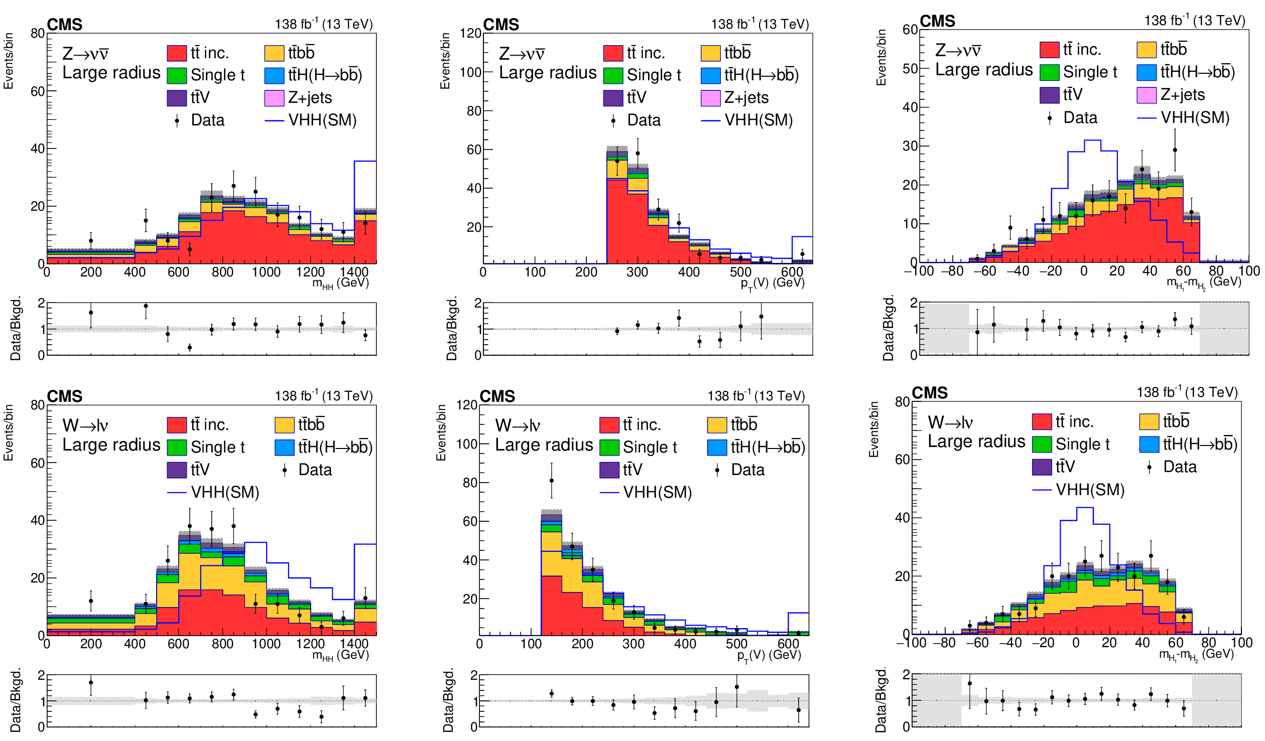
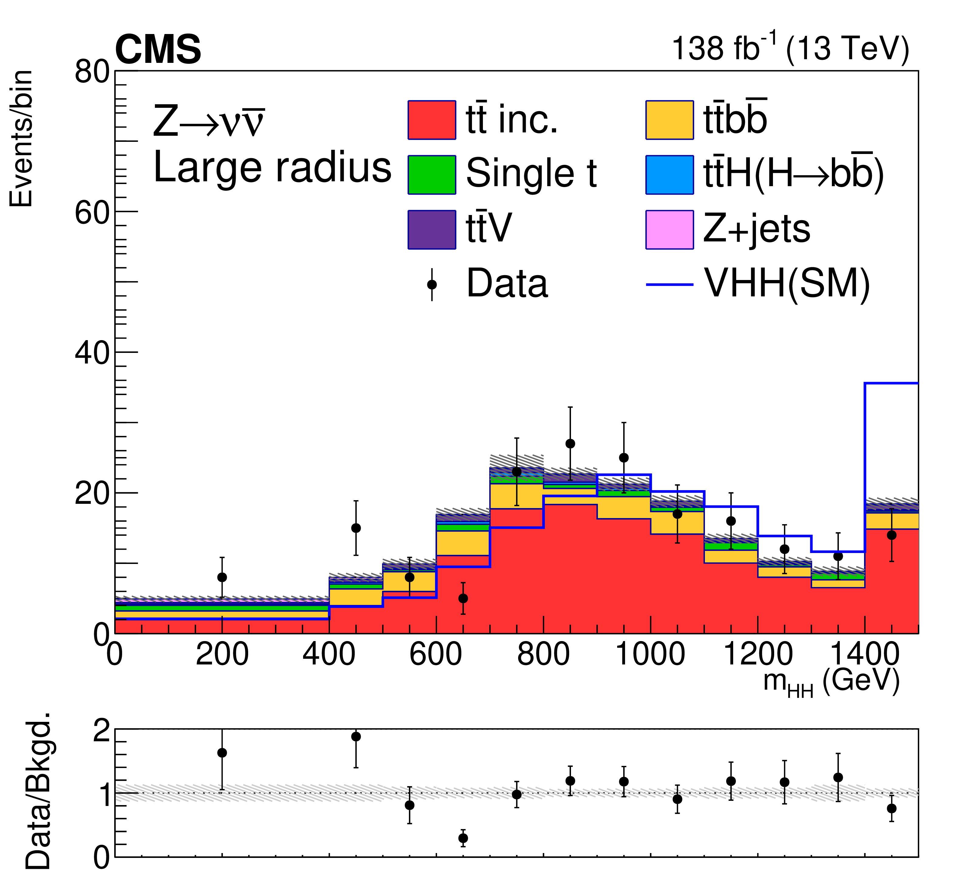
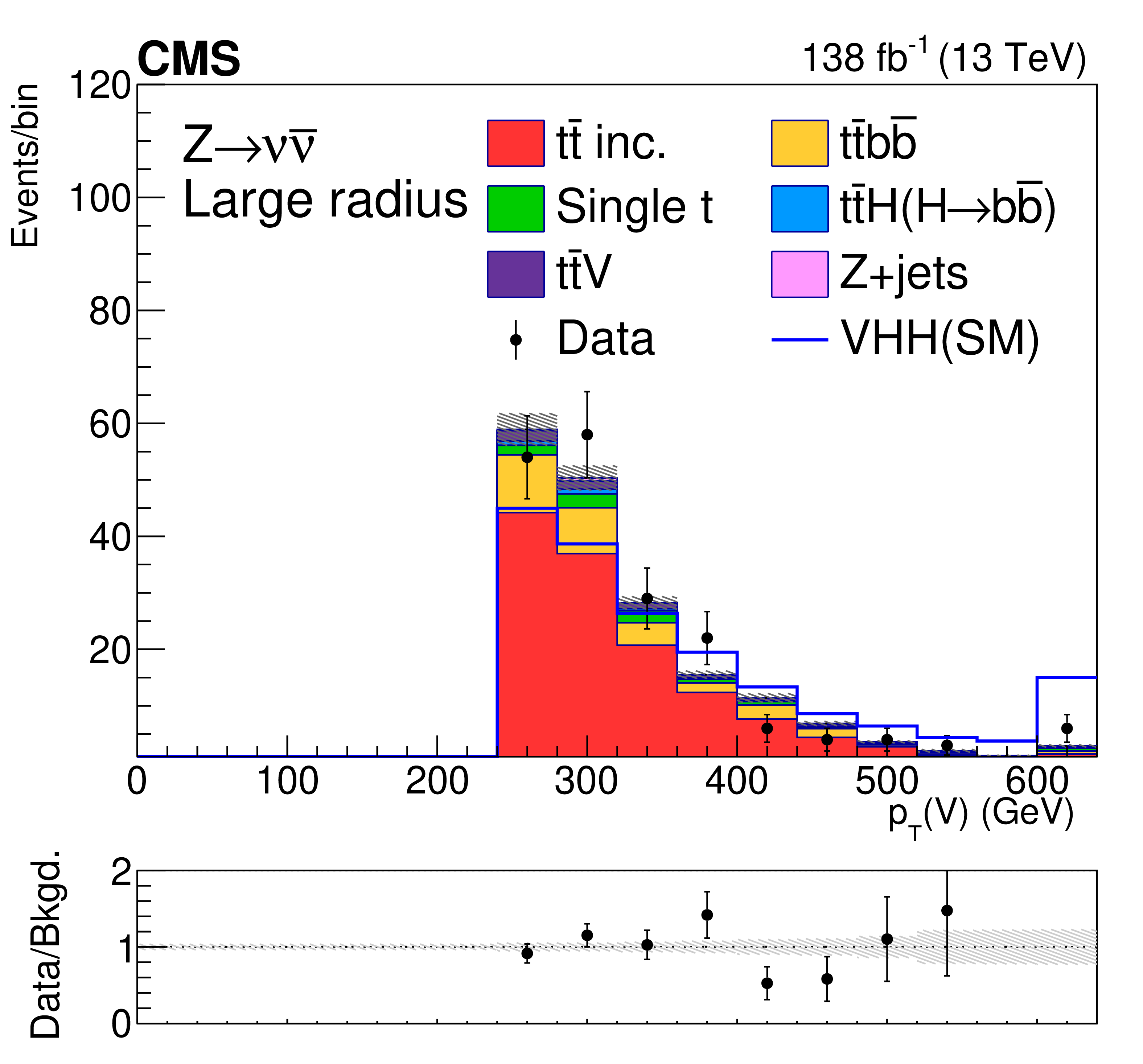
Figure 8:
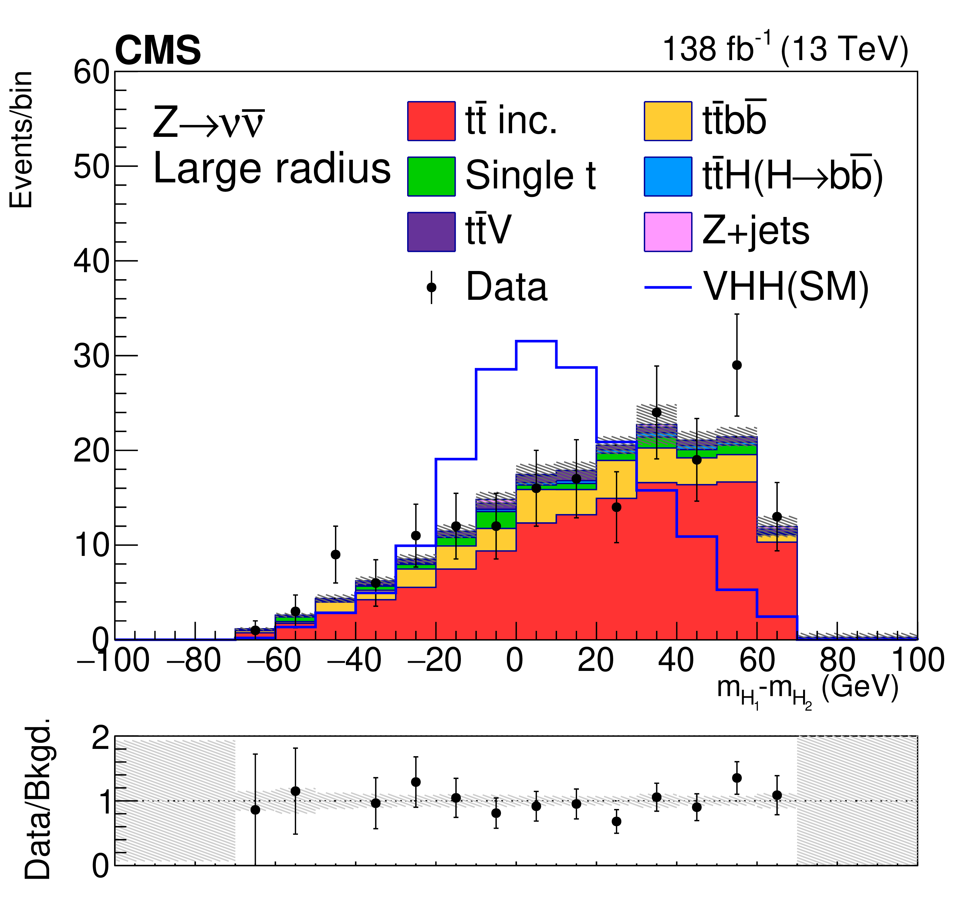
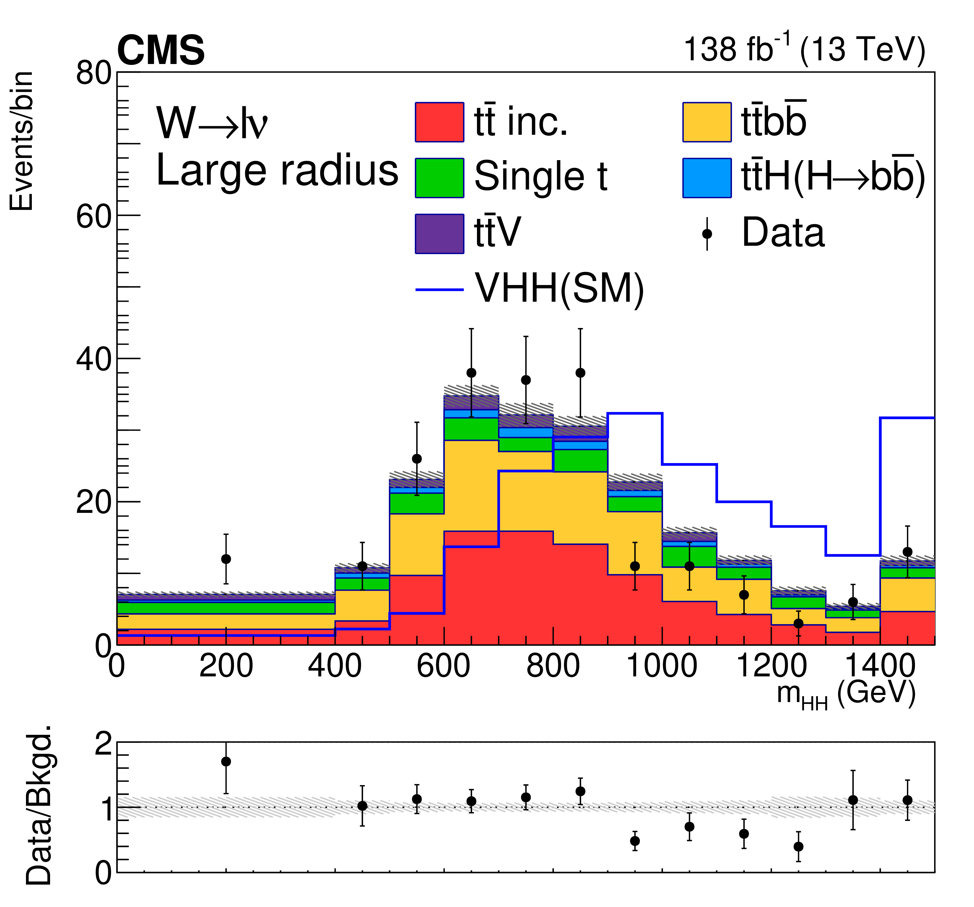
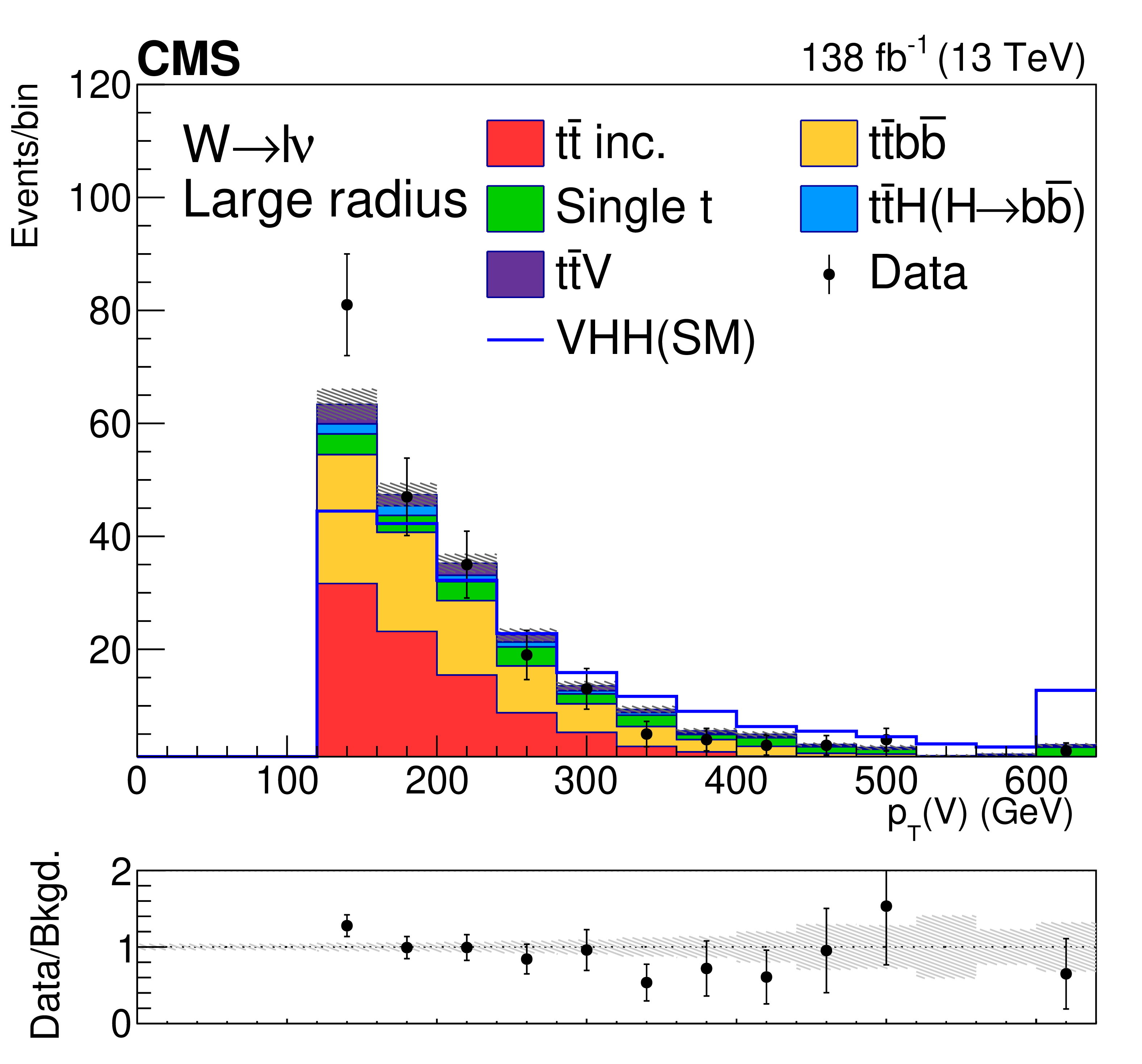
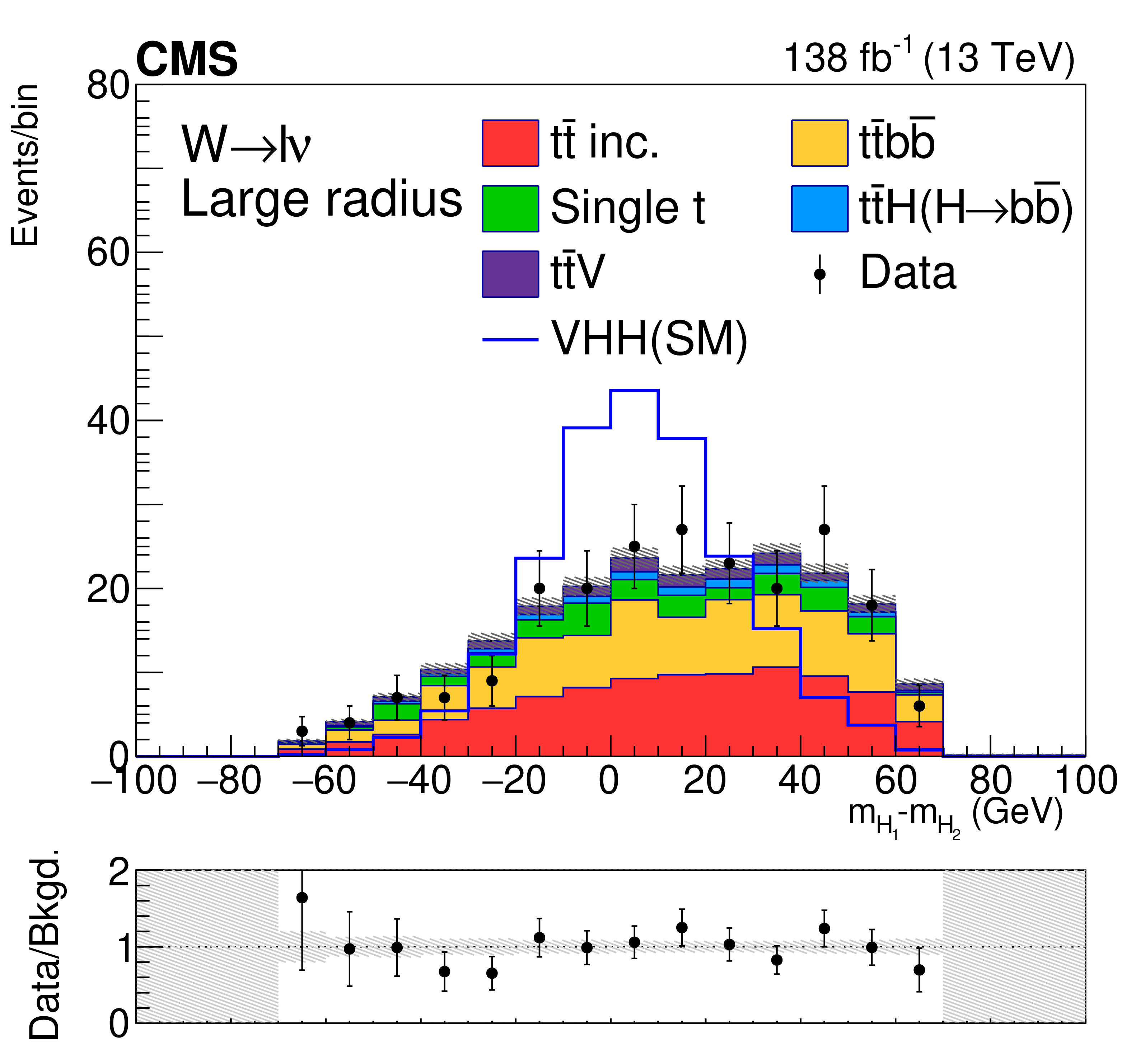
Postfit distributions of kinematic variables in the large-radius jet regions. From upper to lower, the rows show the MET and 1L channels. The variables in each channel are $ m_{\mathrm{H}\mathrm{H}} $, $ p_{\mathrm{T}}(\mathrm{V}) $, and $ m_{ {\mathrm{H}_{1}} }{-}m_{ {\mathrm{H}_{2}} } $. The fit is done with the background-only hypotheses and the final bin in each plot includes overflows. The ratios of data to the total expected background are shown in the lower panel of each plot and the hatched bands are the combined statistical and systematic uncertainties of total background. The blue lines are SM signal distributions, which are scaled to have the same number of events as the background. |
png pdf |
Figure 8-a:
Postfit distributions of kinematic variables in the large-radius jet regions. From upper to lower, the rows show the MET and 1L channels. The variables in each channel are $ m_{\mathrm{H}\mathrm{H}} $, $ p_{\mathrm{T}}(\mathrm{V}) $, and $ m_{ {\mathrm{H}_{1}} }{-}m_{ {\mathrm{H}_{2}} } $. The fit is done with the background-only hypotheses and the final bin in each plot includes overflows. The ratios of data to the total expected background are shown in the lower panel of each plot and the hatched bands are the combined statistical and systematic uncertainties of total background. The blue lines are SM signal distributions, which are scaled to have the same number of events as the background. |
png pdf |
Figure 8-b:
Postfit distributions of kinematic variables in the large-radius jet regions. From upper to lower, the rows show the MET and 1L channels. The variables in each channel are $ m_{\mathrm{H}\mathrm{H}} $, $ p_{\mathrm{T}}(\mathrm{V}) $, and $ m_{ {\mathrm{H}_{1}} }{-}m_{ {\mathrm{H}_{2}} } $. The fit is done with the background-only hypotheses and the final bin in each plot includes overflows. The ratios of data to the total expected background are shown in the lower panel of each plot and the hatched bands are the combined statistical and systematic uncertainties of total background. The blue lines are SM signal distributions, which are scaled to have the same number of events as the background. |
png pdf |
Figure 8-c:
Postfit distributions of kinematic variables in the large-radius jet regions. From upper to lower, the rows show the MET and 1L channels. The variables in each channel are $ m_{\mathrm{H}\mathrm{H}} $, $ p_{\mathrm{T}}(\mathrm{V}) $, and $ m_{ {\mathrm{H}_{1}} }{-}m_{ {\mathrm{H}_{2}} } $. The fit is done with the background-only hypotheses and the final bin in each plot includes overflows. The ratios of data to the total expected background are shown in the lower panel of each plot and the hatched bands are the combined statistical and systematic uncertainties of total background. The blue lines are SM signal distributions, which are scaled to have the same number of events as the background. |
png pdf |
Figure 8-d:
Postfit distributions of kinematic variables in the large-radius jet regions. From upper to lower, the rows show the MET and 1L channels. The variables in each channel are $ m_{\mathrm{H}\mathrm{H}} $, $ p_{\mathrm{T}}(\mathrm{V}) $, and $ m_{ {\mathrm{H}_{1}} }{-}m_{ {\mathrm{H}_{2}} } $. The fit is done with the background-only hypotheses and the final bin in each plot includes overflows. The ratios of data to the total expected background are shown in the lower panel of each plot and the hatched bands are the combined statistical and systematic uncertainties of total background. The blue lines are SM signal distributions, which are scaled to have the same number of events as the background. |
png pdf |
Figure 8-e:
Postfit distributions of kinematic variables in the large-radius jet regions. From upper to lower, the rows show the MET and 1L channels. The variables in each channel are $ m_{\mathrm{H}\mathrm{H}} $, $ p_{\mathrm{T}}(\mathrm{V}) $, and $ m_{ {\mathrm{H}_{1}} }{-}m_{ {\mathrm{H}_{2}} } $. The fit is done with the background-only hypotheses and the final bin in each plot includes overflows. The ratios of data to the total expected background are shown in the lower panel of each plot and the hatched bands are the combined statistical and systematic uncertainties of total background. The blue lines are SM signal distributions, which are scaled to have the same number of events as the background. |
png pdf |
Figure 8-f:
Postfit distributions of kinematic variables in the large-radius jet regions. From upper to lower, the rows show the MET and 1L channels. The variables in each channel are $ m_{\mathrm{H}\mathrm{H}} $, $ p_{\mathrm{T}}(\mathrm{V}) $, and $ m_{ {\mathrm{H}_{1}} }{-}m_{ {\mathrm{H}_{2}} } $. The fit is done with the background-only hypotheses and the final bin in each plot includes overflows. The ratios of data to the total expected background are shown in the lower panel of each plot and the hatched bands are the combined statistical and systematic uncertainties of total background. The blue lines are SM signal distributions, which are scaled to have the same number of events as the background. |
png pdf |
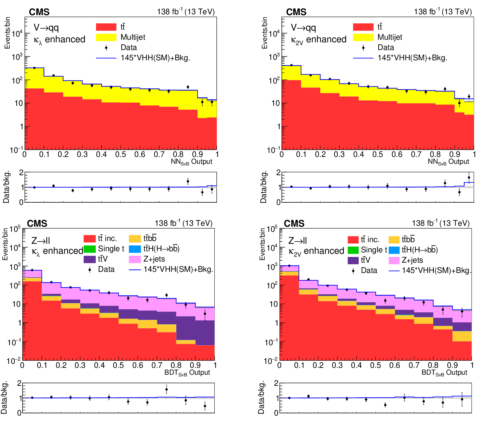
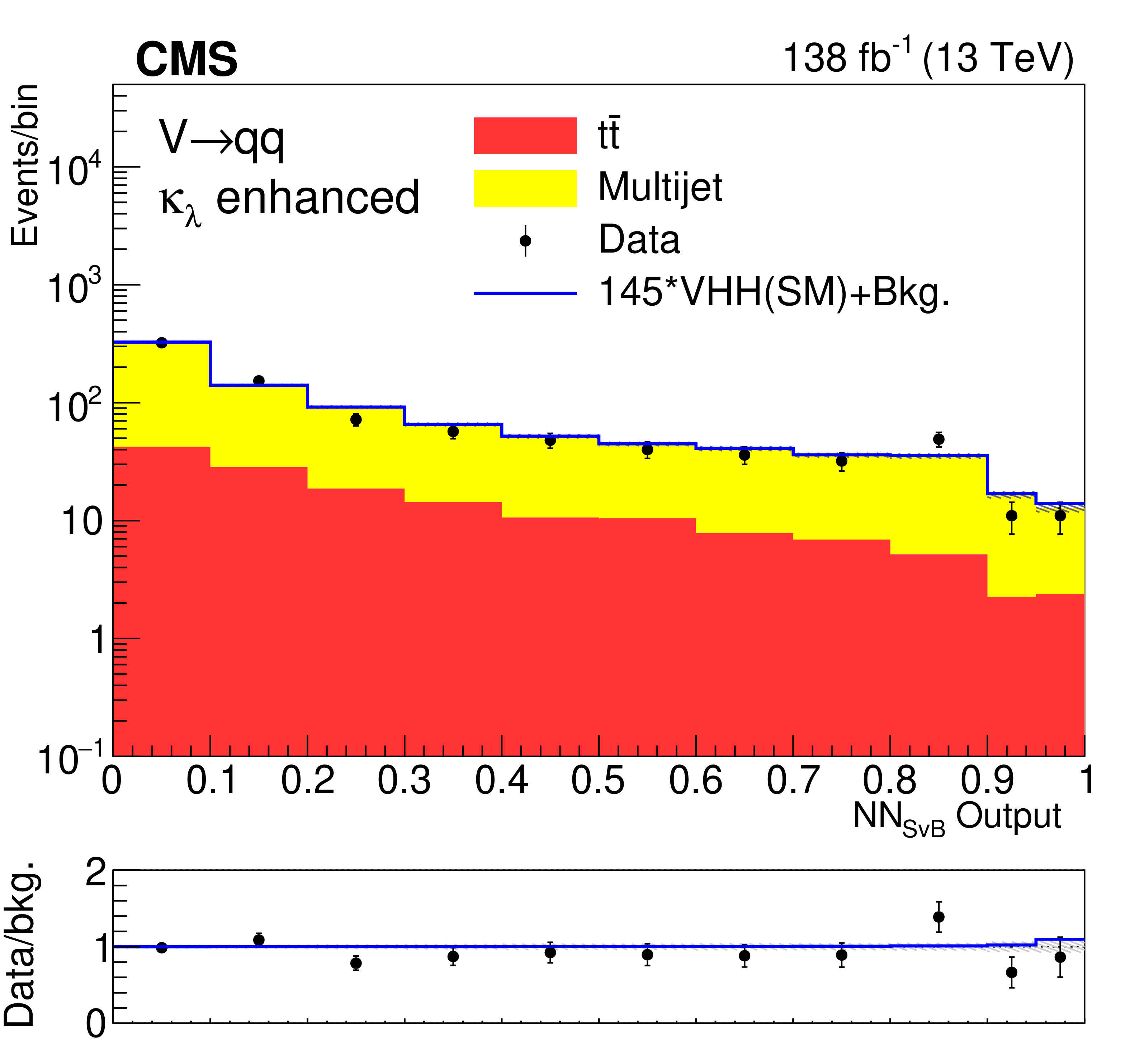
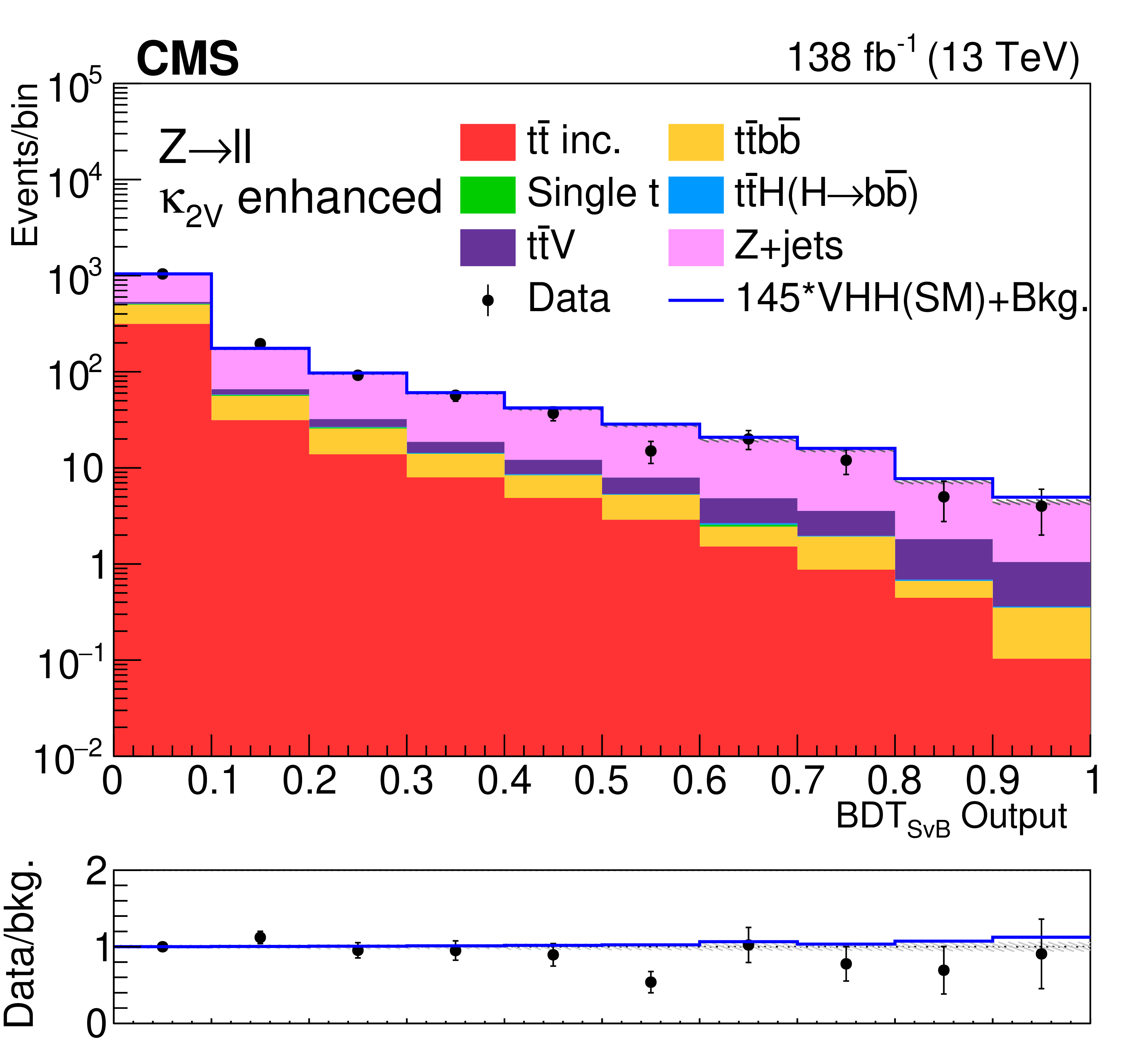
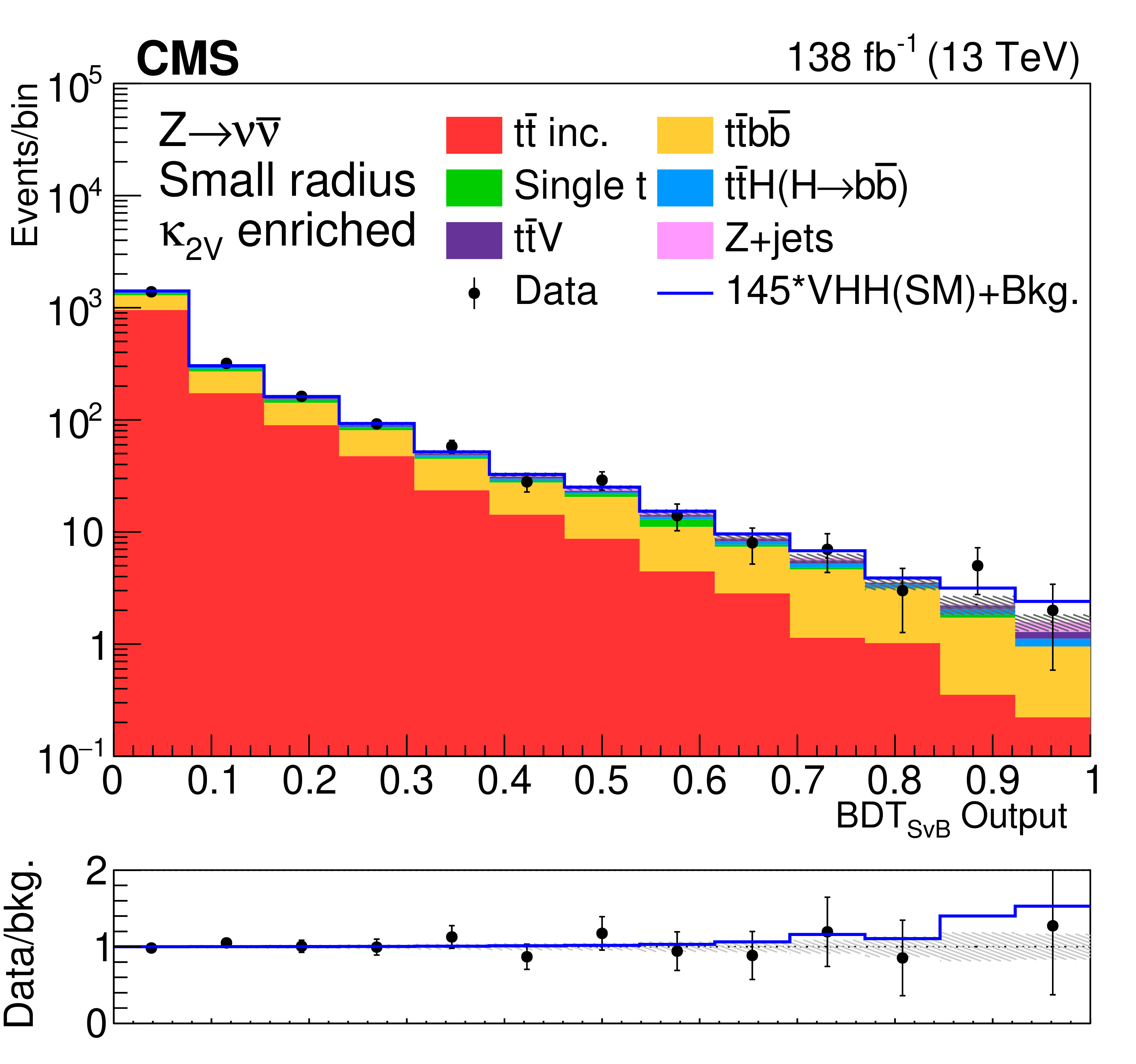
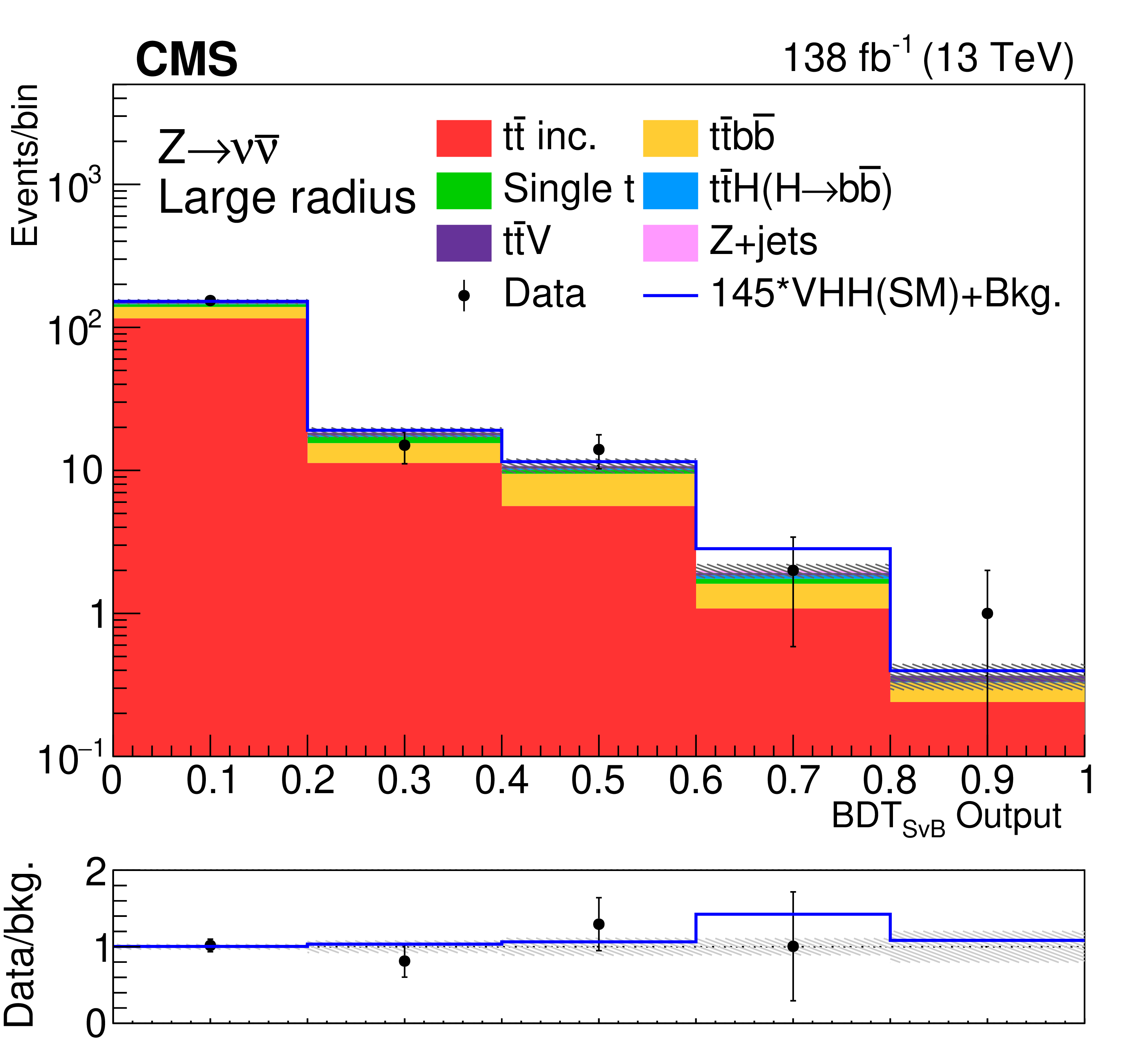
Figure 9:
Postfit BDT distributions with the signal-plus-background hypotheses of the FH and 2L channels. |
png pdf |
Figure 9-a:
Postfit BDT distributions with the signal-plus-background hypotheses of the FH and 2L channels. |

png pdf |
Figure 9-b:
Postfit BDT distributions with the signal-plus-background hypotheses of the FH and 2L channels. |

png pdf |
Figure 9-c:
Postfit BDT distributions with the signal-plus-background hypotheses of the FH and 2L channels. |
png pdf |
Figure 9-d:
Postfit BDT distributions with the signal-plus-background hypotheses of the FH and 2L channels. |
png pdf |
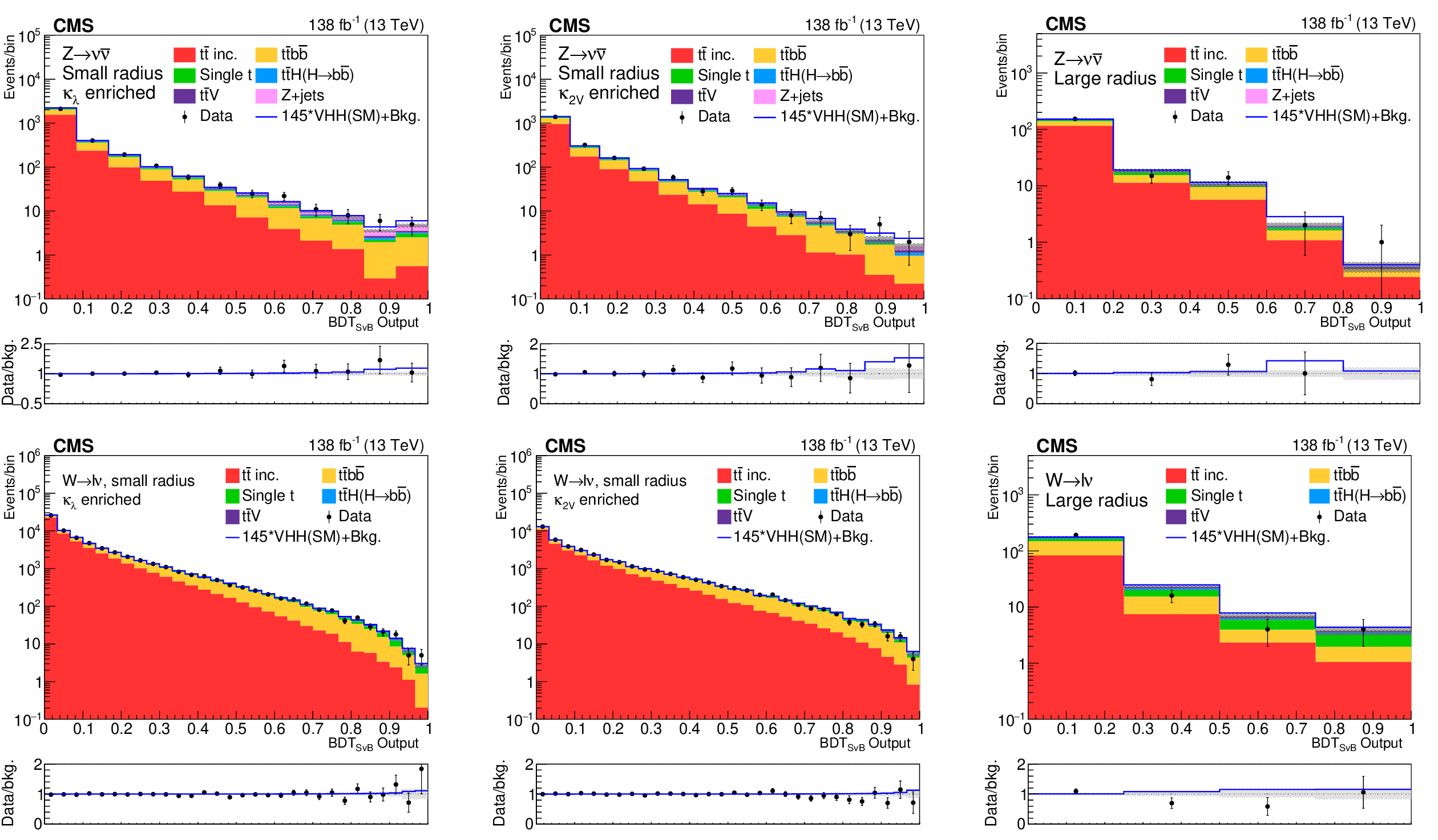
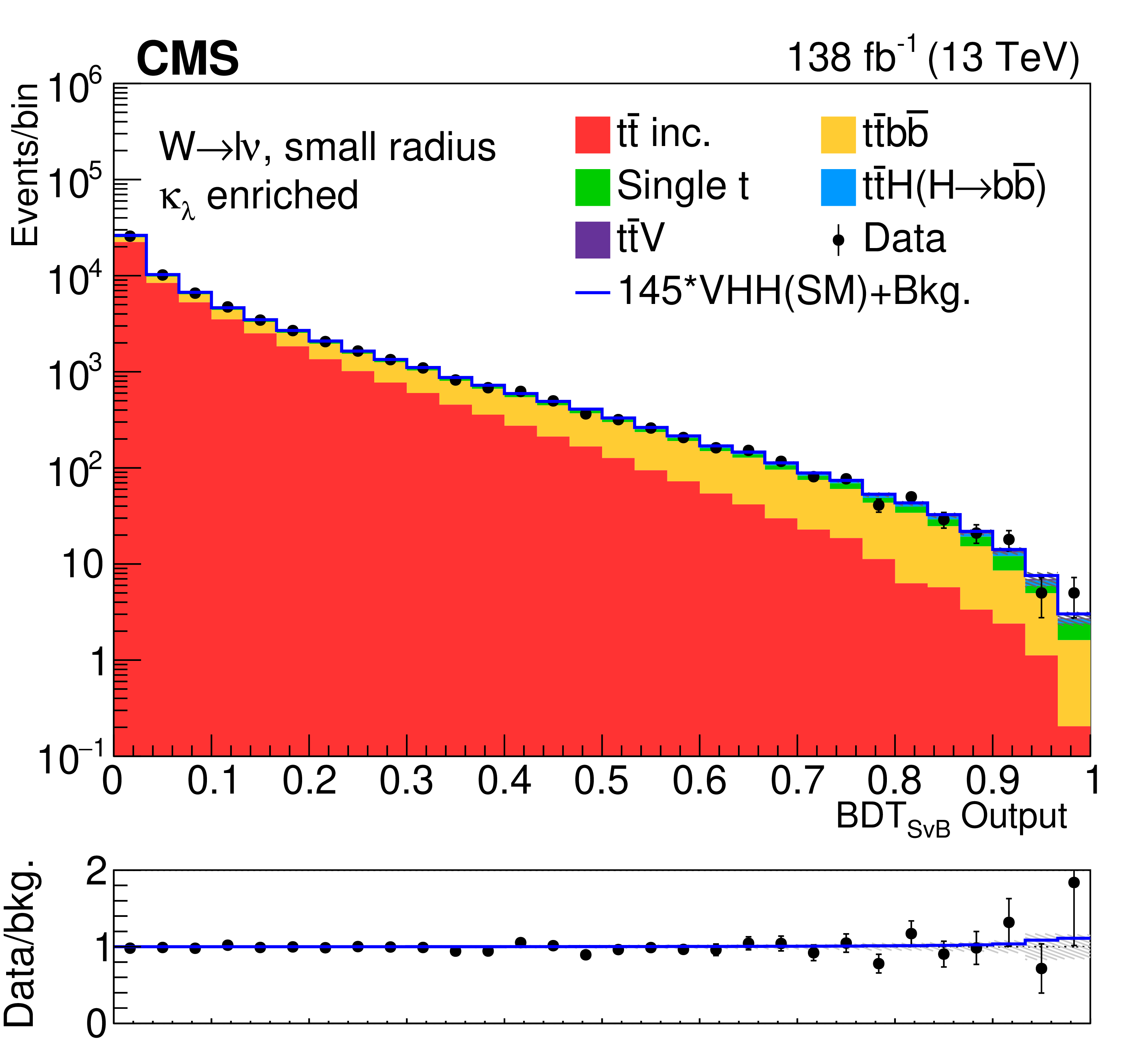
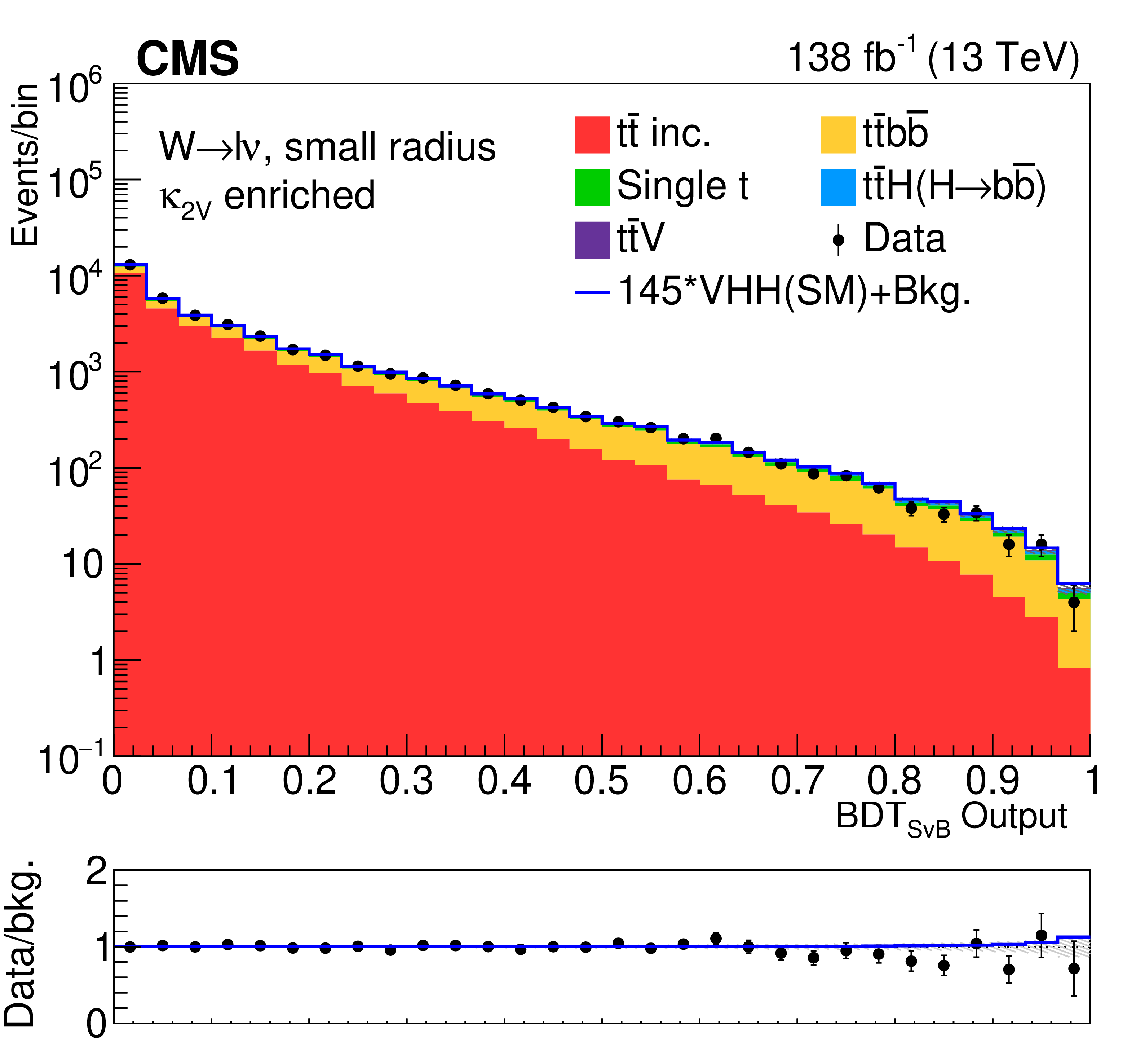
Figure 10:
Postfit BDT distributions with the signal-plus-background hypotheses of the MET and 1L channels. |

png pdf |
Figure 10-a:
Postfit BDT distributions with the signal-plus-background hypotheses of the MET and 1L channels. |
png pdf |
Figure 10-b:
Postfit BDT distributions with the signal-plus-background hypotheses of the MET and 1L channels. |
png pdf |
Figure 10-c:
Postfit BDT distributions with the signal-plus-background hypotheses of the MET and 1L channels. |
png pdf |
Figure 10-d:
Postfit BDT distributions with the signal-plus-background hypotheses of the MET and 1L channels. |
png pdf |
Figure 10-e:
Postfit BDT distributions with the signal-plus-background hypotheses of the MET and 1L channels. |

png pdf |
Figure 10-f:
Postfit BDT distributions with the signal-plus-background hypotheses of the MET and 1L channels. |
png pdf |
Figure 11:
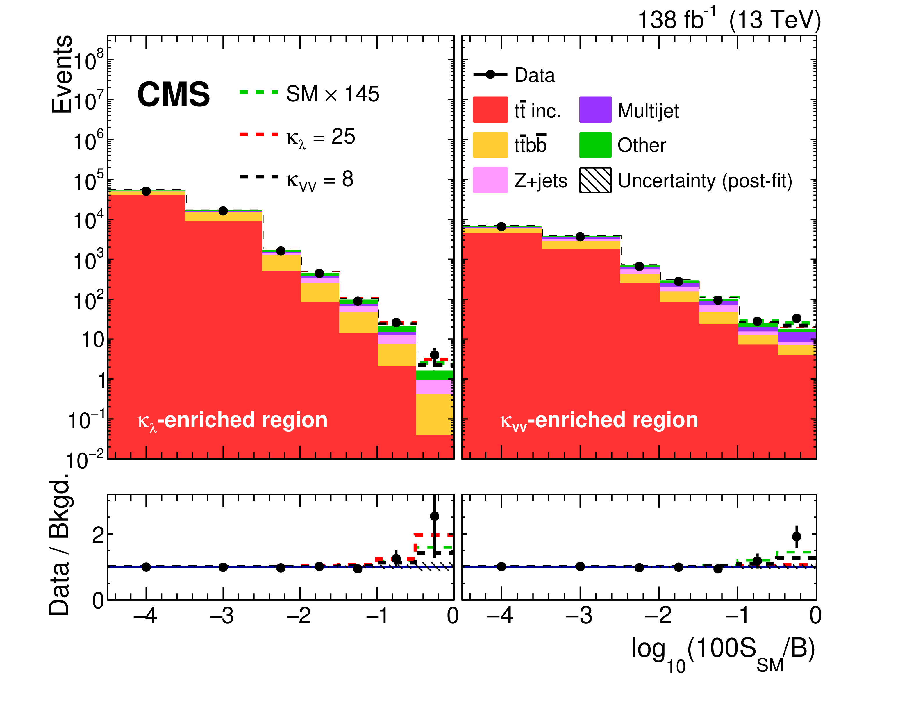
Machine learning output distributions are transformed to $ \log_{10}\left(100(\mathrm{S}_{\mathrm{SM}}/\mathrm{B})\right) $ and summed for $ \kappa_{\lambda} $- and $ \kappa_{2\mathrm{V}} $-enriched SR samples separately. The filled histograms represent the postfit simulation. The total postfit uncertainty is represented by the hatched band. The SM contribution and two signal models near expected exclusion at the 95% CL are shown with the dashed lines. |
png pdf |
Figure 12:
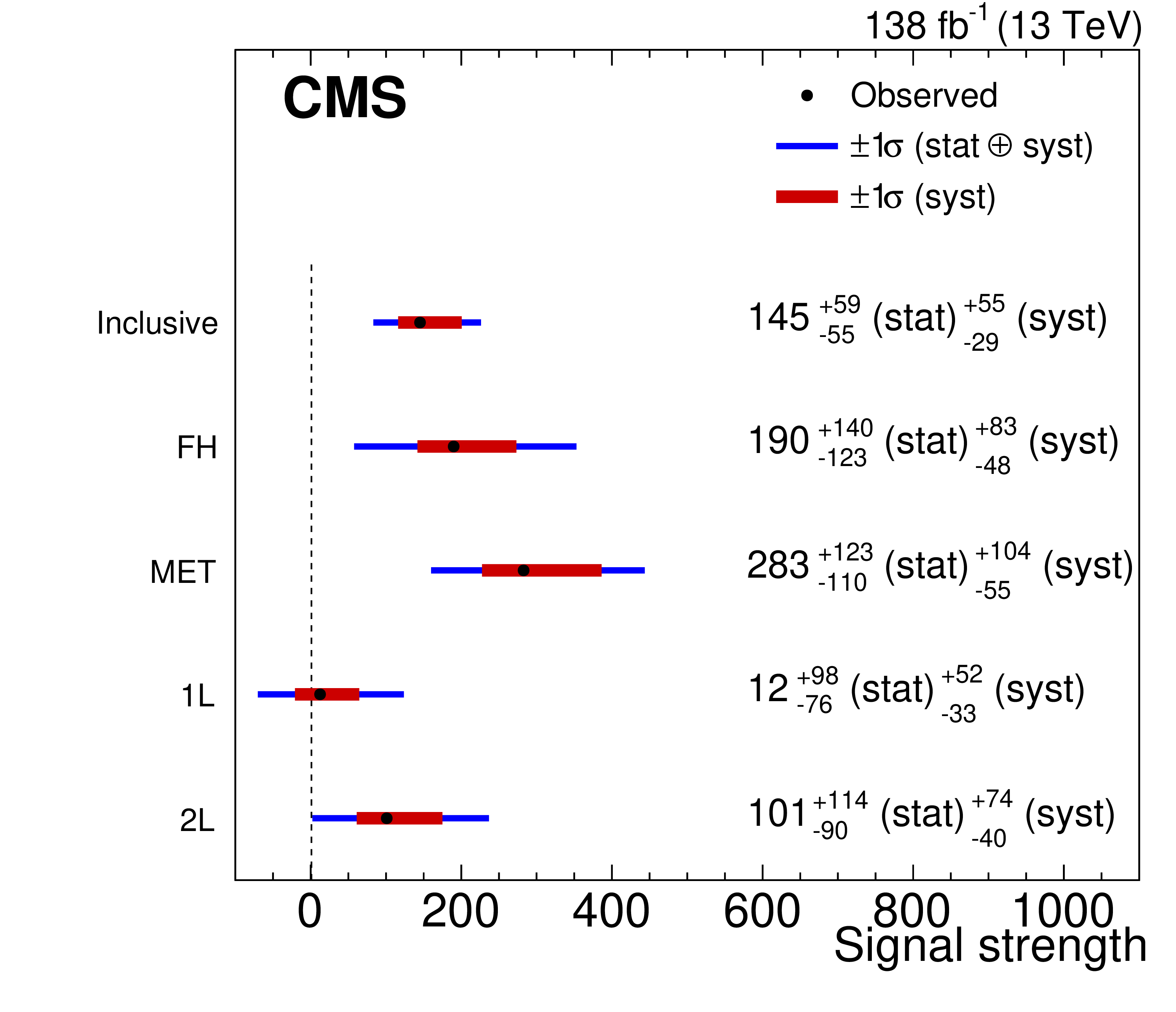
Results of two maximum likelihood fits. The top entry, labeled ``Inclusive'', is the result of a single signal strength fit of all channels. The other four entries are from a fit of the same regions but with independent signal strengths in each channel. The thinner blue bands are one standard deviation from the full likelihood scan in that parameter, while the thicker red bands are one standard deviation bands of the systematic uncertainties only. |

png pdf |
Figure 13:
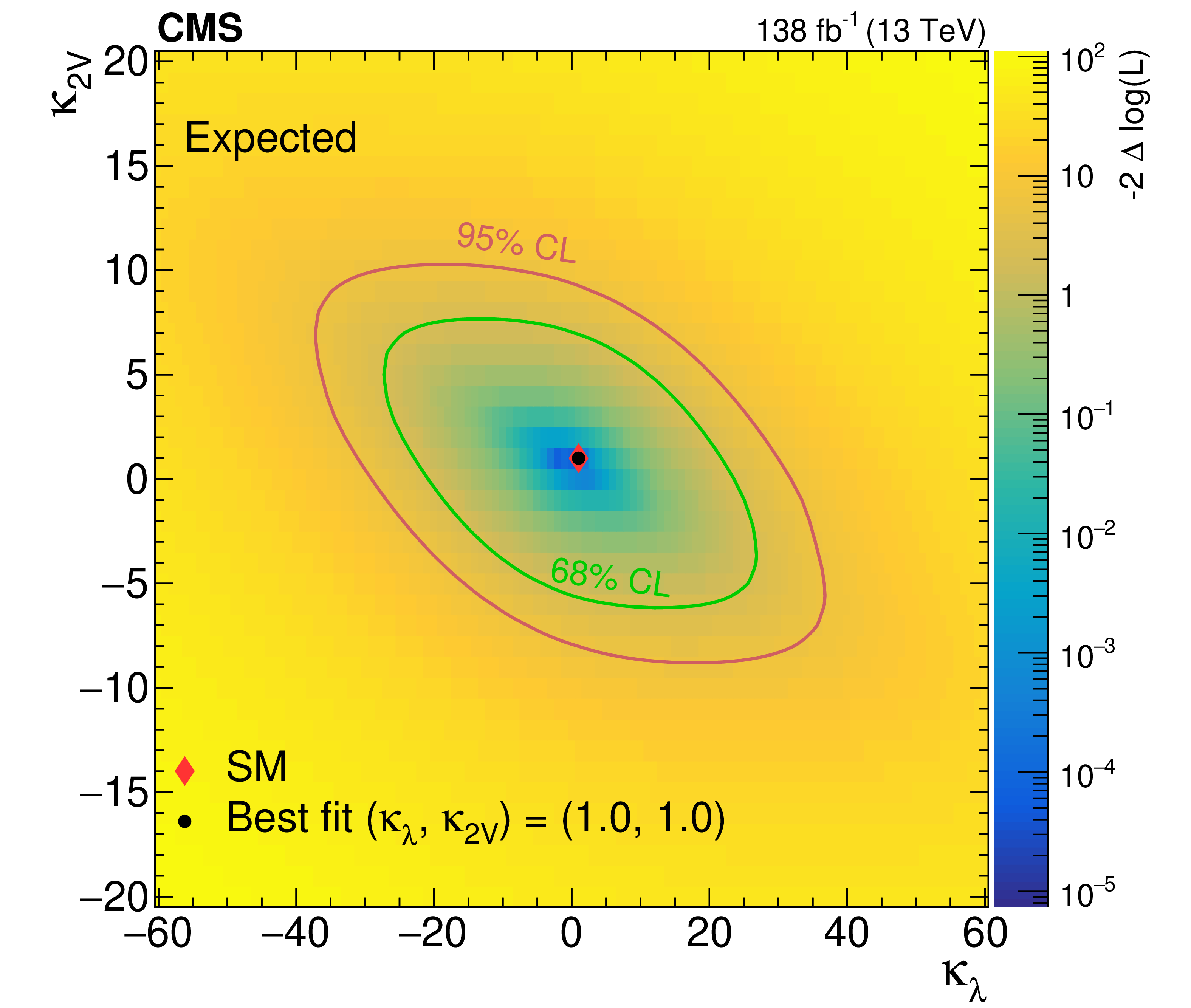
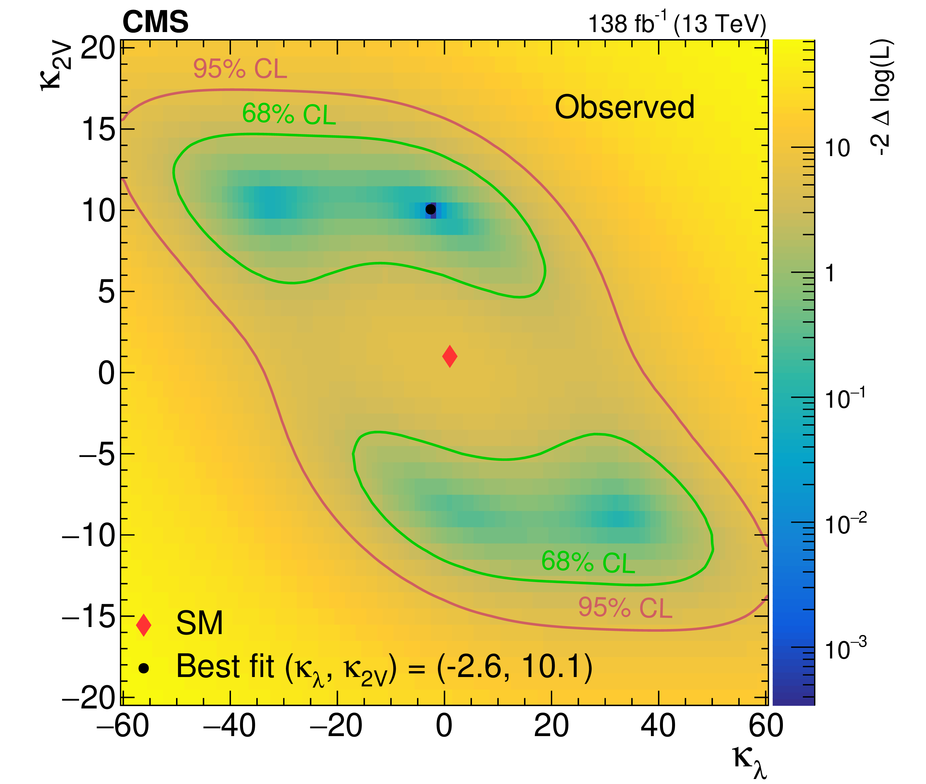
Expected (left) and observed (right) likelihood scans in $ \kappa_{\lambda} $ versus $ \kappa_{2\mathrm{V}} $ are shown, with other couplings fixed to the SM predicted strength. The excess is most prominent in the $ \kappa_{2\mathrm{V}} $-enriched region, and so the most likely point of the scan at $ \kappa_{2\mathrm{V}}= $ 10.1 and $ \kappa_{\lambda}=- $ 2.6 is pulled from the SM mostly in the $ \kappa_{2\mathrm{V}} $ dimension. |
png pdf |
Figure 13-a:
Expected (left) and observed (right) likelihood scans in $ \kappa_{\lambda} $ versus $ \kappa_{2\mathrm{V}} $ are shown, with other couplings fixed to the SM predicted strength. The excess is most prominent in the $ \kappa_{2\mathrm{V}} $-enriched region, and so the most likely point of the scan at $ \kappa_{2\mathrm{V}}= $ 10.1 and $ \kappa_{\lambda}=- $ 2.6 is pulled from the SM mostly in the $ \kappa_{2\mathrm{V}} $ dimension. |
png pdf |
Figure 13-b:
Expected (left) and observed (right) likelihood scans in $ \kappa_{\lambda} $ versus $ \kappa_{2\mathrm{V}} $ are shown, with other couplings fixed to the SM predicted strength. The excess is most prominent in the $ \kappa_{2\mathrm{V}} $-enriched region, and so the most likely point of the scan at $ \kappa_{2\mathrm{V}}= $ 10.1 and $ \kappa_{\lambda}=- $ 2.6 is pulled from the SM mostly in the $ \kappa_{2\mathrm{V}} $ dimension. |
png pdf |
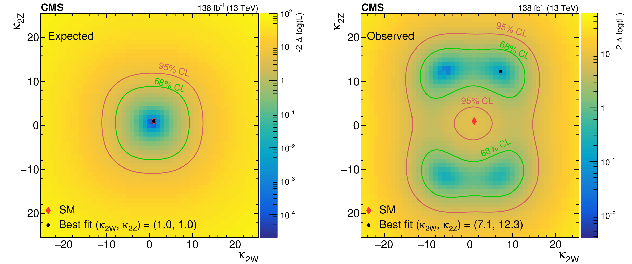
Figure 14:
Expected (left) and observed (right) likelihood scans of $ \kappa_{2\mathrm{W}} $ versus $ \kappa_{2\mathrm{Z}} $ are shown, with other couplings fixed to the SM predicted strength. The excess is most prominent in the MET channel, and so the most likely point of the scan at $ \kappa_{2\mathrm{W}}= $ 7.1 and $ \kappa_{2\mathrm{Z}}= $ 12.3 is pulled from the SM mostly in the $ \kappa_{2\mathrm{Z}} $ dimension, to which the signal in the MET channel is solely sensitive. |

png pdf |
Figure 14-a:
Expected (left) and observed (right) likelihood scans of $ \kappa_{2\mathrm{W}} $ versus $ \kappa_{2\mathrm{Z}} $ are shown, with other couplings fixed to the SM predicted strength. The excess is most prominent in the MET channel, and so the most likely point of the scan at $ \kappa_{2\mathrm{W}}= $ 7.1 and $ \kappa_{2\mathrm{Z}}= $ 12.3 is pulled from the SM mostly in the $ \kappa_{2\mathrm{Z}} $ dimension, to which the signal in the MET channel is solely sensitive. |
png pdf |
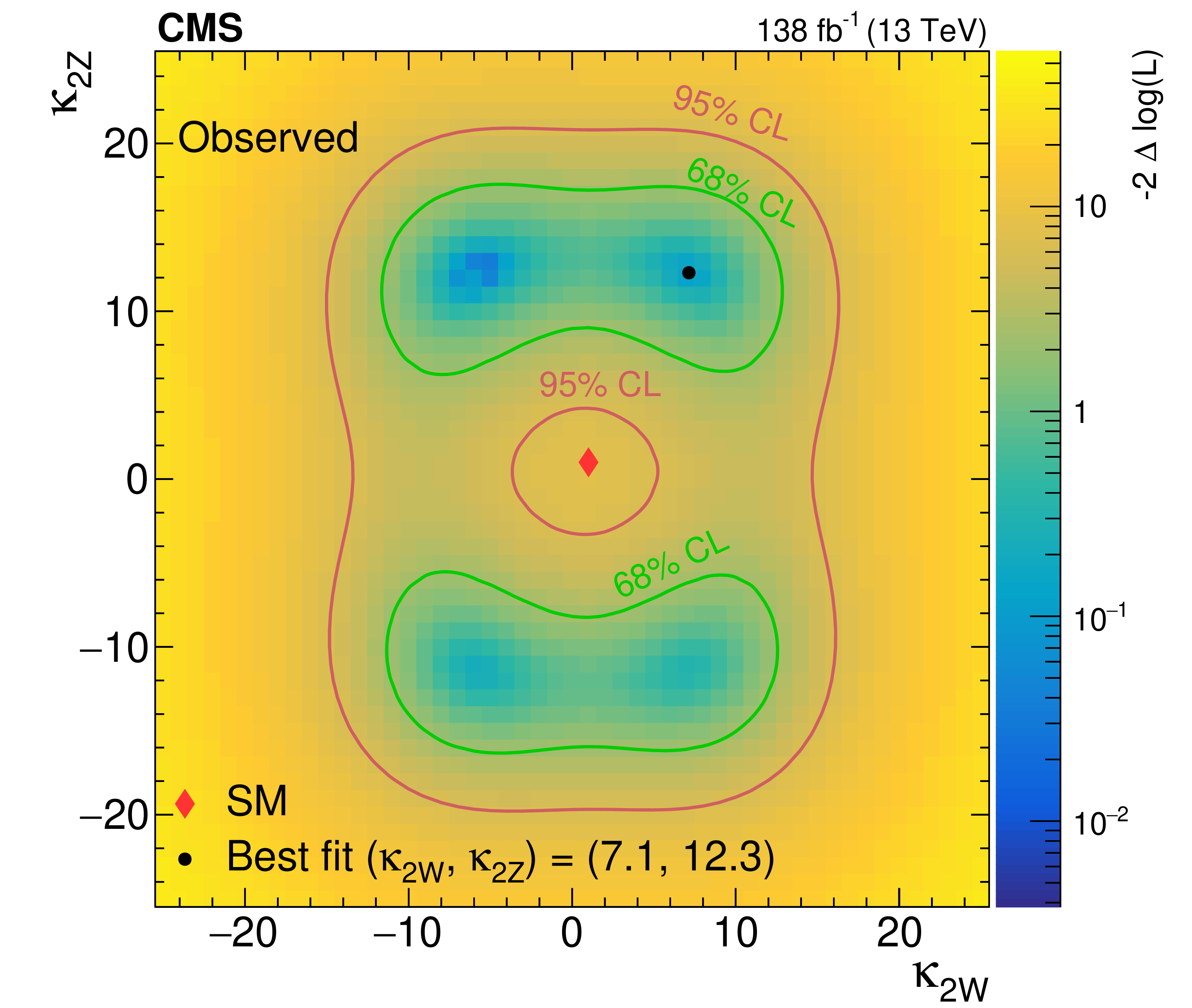
Figure 14-b:
Expected (left) and observed (right) likelihood scans of $ \kappa_{2\mathrm{W}} $ versus $ \kappa_{2\mathrm{Z}} $ are shown, with other couplings fixed to the SM predicted strength. The excess is most prominent in the MET channel, and so the most likely point of the scan at $ \kappa_{2\mathrm{W}}= $ 7.1 and $ \kappa_{2\mathrm{Z}}= $ 12.3 is pulled from the SM mostly in the $ \kappa_{2\mathrm{Z}} $ dimension, to which the signal in the MET channel is solely sensitive. |
png pdf |
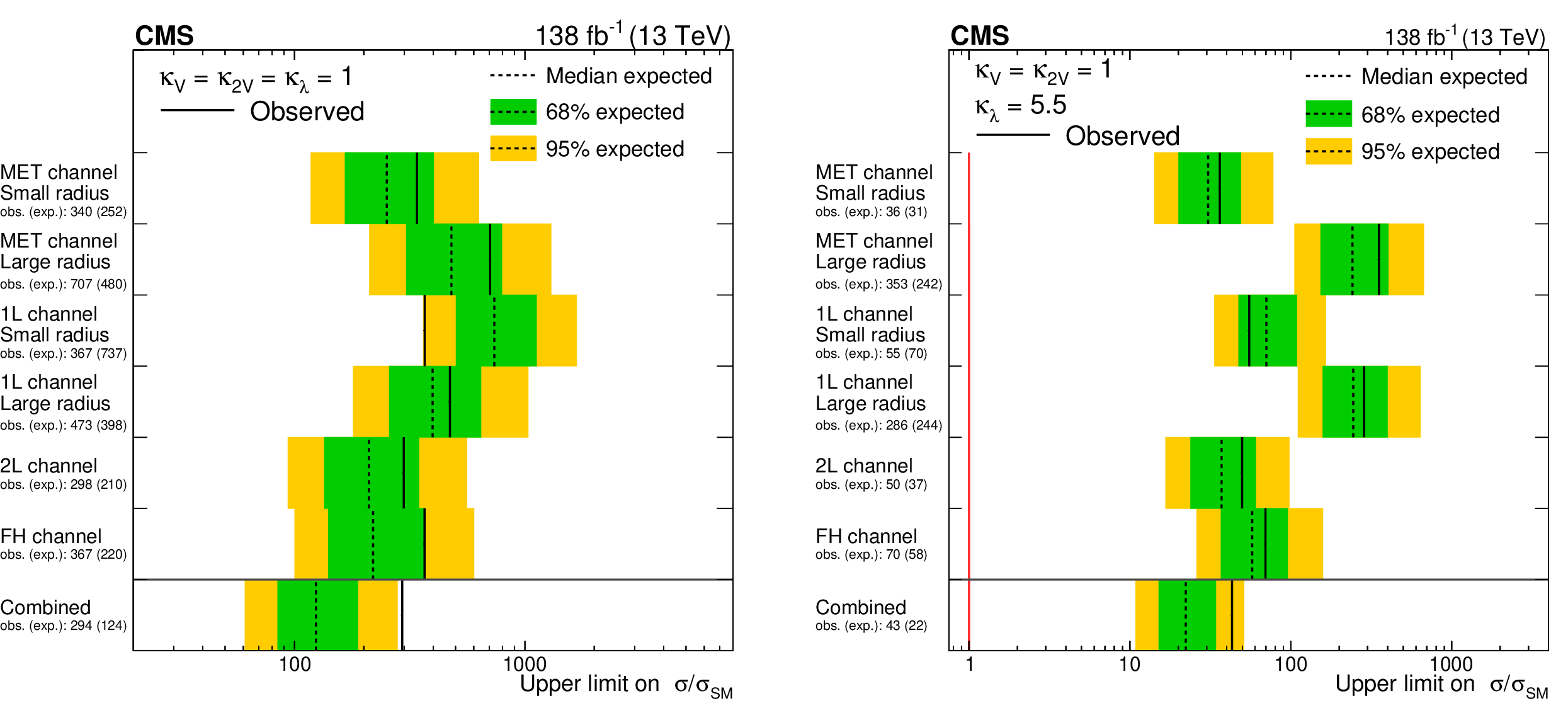
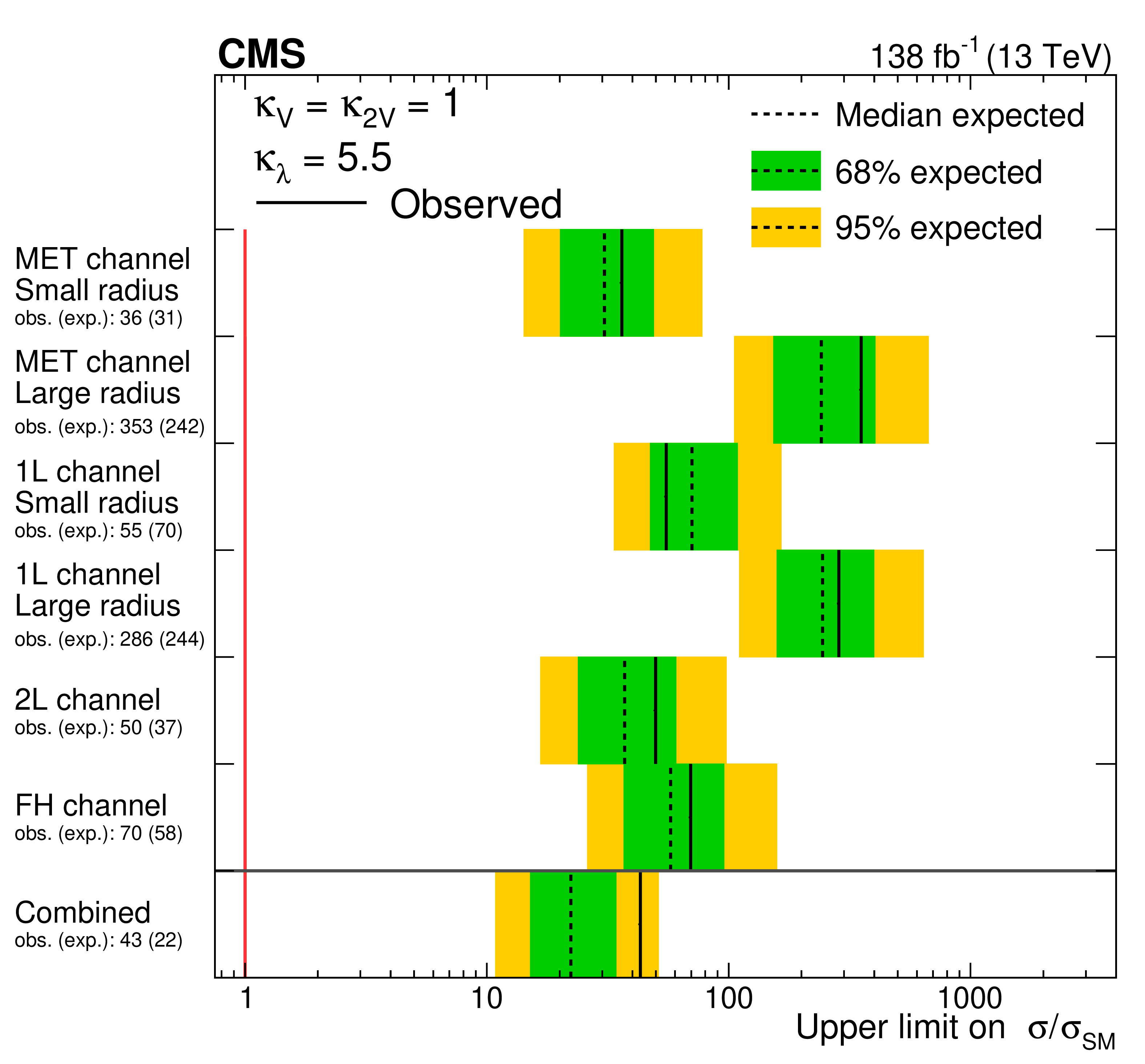
Figure 15:
The left plot shows the VHH cross section limits per channel and combined for SM value couplings, while results with $ \kappa_{\lambda}= $ 5.5 and $ \kappa_{2\mathrm{V}}=\kappa_{\mathrm{V}}= $ 1.0 are shown on the right. |
png pdf |
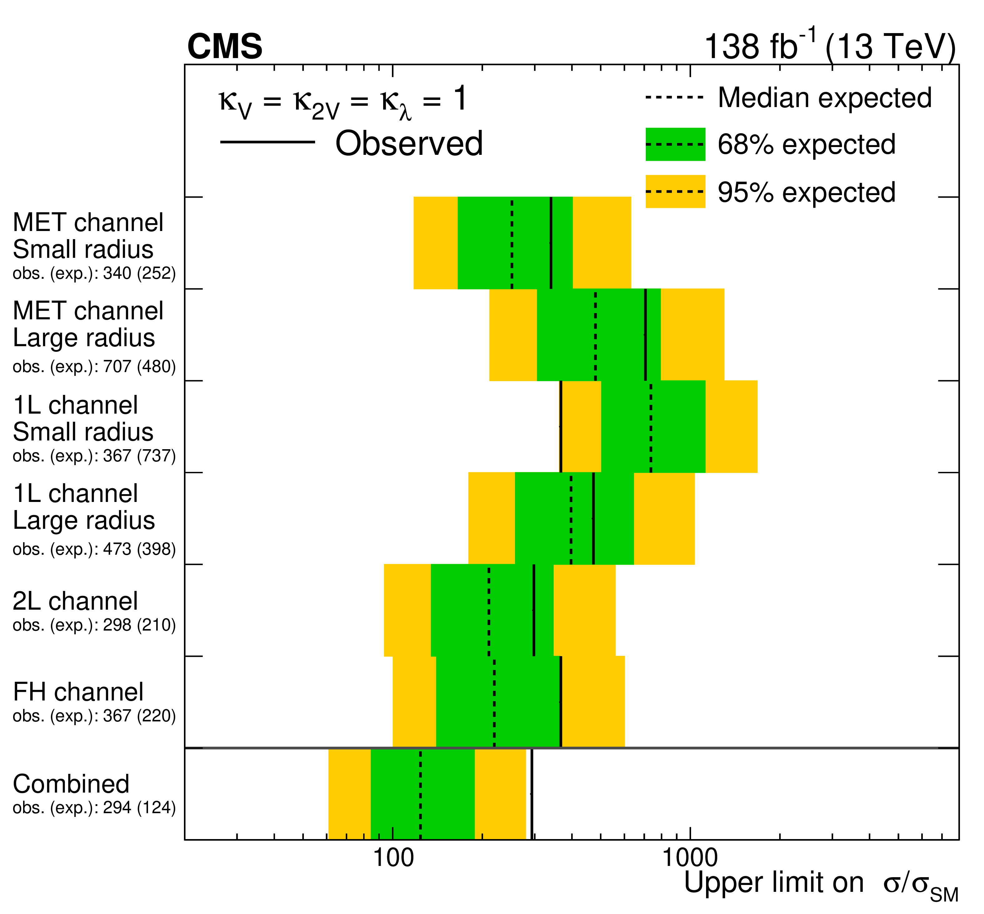
Figure 15-a:
The left plot shows the VHH cross section limits per channel and combined for SM value couplings, while results with $ \kappa_{\lambda}= $ 5.5 and $ \kappa_{2\mathrm{V}}=\kappa_{\mathrm{V}}= $ 1.0 are shown on the right. |
png pdf |
Figure 15-b:
The left plot shows the VHH cross section limits per channel and combined for SM value couplings, while results with $ \kappa_{\lambda}= $ 5.5 and $ \kappa_{2\mathrm{V}}=\kappa_{\mathrm{V}}= $ 1.0 are shown on the right. |
png pdf |
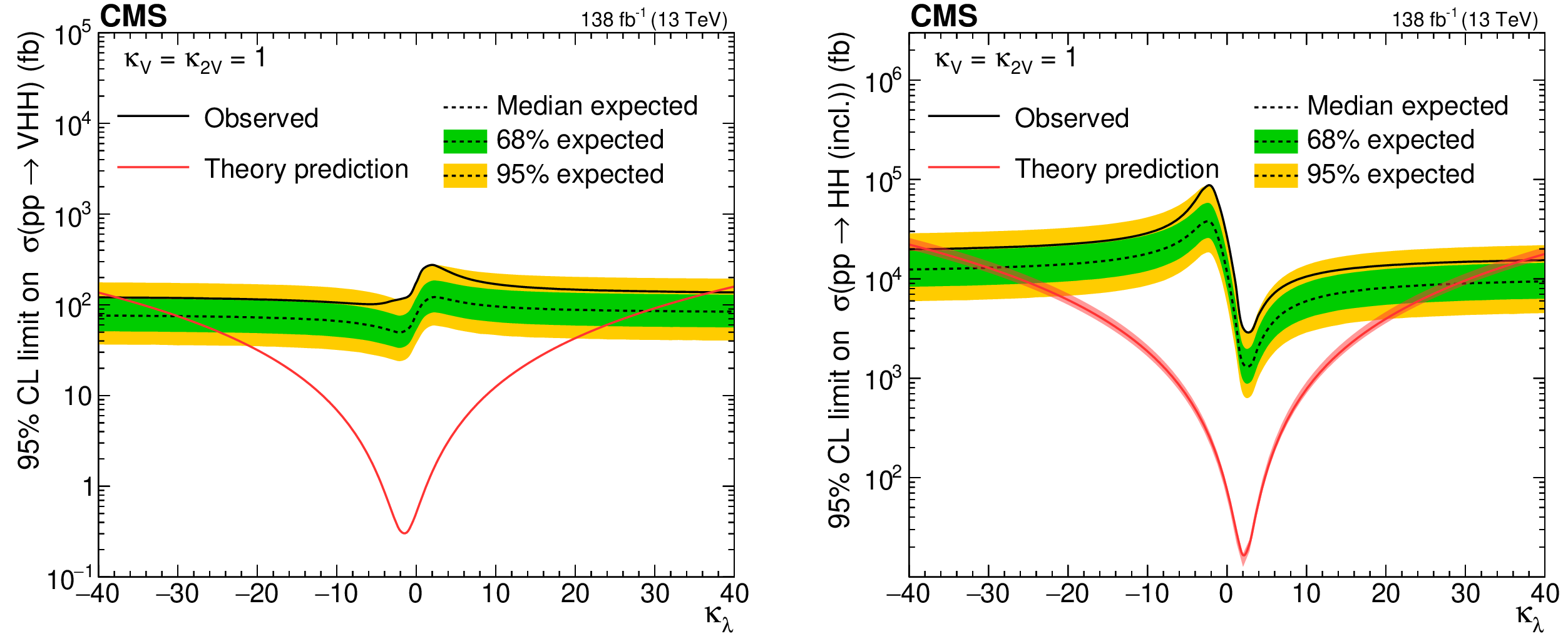
Figure 16:
Upper 95% CL limits on VHH (left) and HH (right) signal cross section scanned over the $ \kappa_{\lambda} $ parameter while fixing the $ \kappa_{2\mathrm{V}} $ and $ \kappa_{\mathrm{V}} $ to their SM-predicted values. The independent axis is the scanned $ \kappa_{\lambda} $ parameter, and the dependent axis is the 95% CL upper limit on signal cross section. The theoretic prediction of VHH (left) and HH (right) production cross sections are shown with the red lines. |
png pdf |
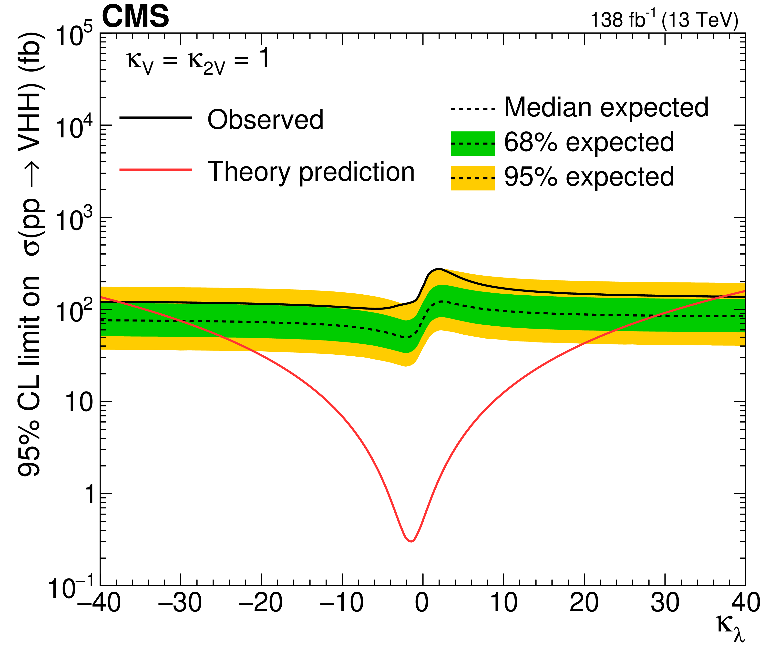
Figure 16-a:
Upper 95% CL limits on VHH (left) and HH (right) signal cross section scanned over the $ \kappa_{\lambda} $ parameter while fixing the $ \kappa_{2\mathrm{V}} $ and $ \kappa_{\mathrm{V}} $ to their SM-predicted values. The independent axis is the scanned $ \kappa_{\lambda} $ parameter, and the dependent axis is the 95% CL upper limit on signal cross section. The theoretic prediction of VHH (left) and HH (right) production cross sections are shown with the red lines. |

png pdf |
Figure 16-b:
Upper 95% CL limits on VHH (left) and HH (right) signal cross section scanned over the $ \kappa_{\lambda} $ parameter while fixing the $ \kappa_{2\mathrm{V}} $ and $ \kappa_{\mathrm{V}} $ to their SM-predicted values. The independent axis is the scanned $ \kappa_{\lambda} $ parameter, and the dependent axis is the 95% CL upper limit on signal cross section. The theoretic prediction of VHH (left) and HH (right) production cross sections are shown with the red lines. |
png pdf |
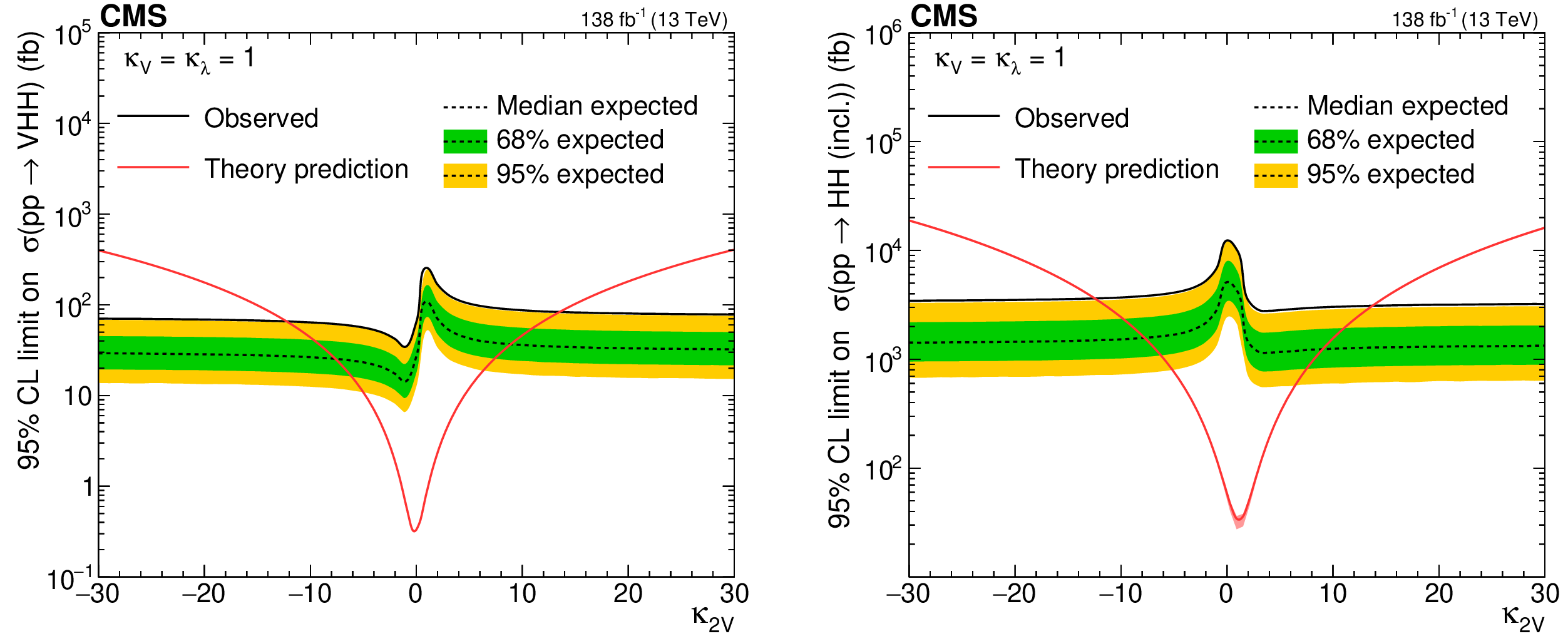
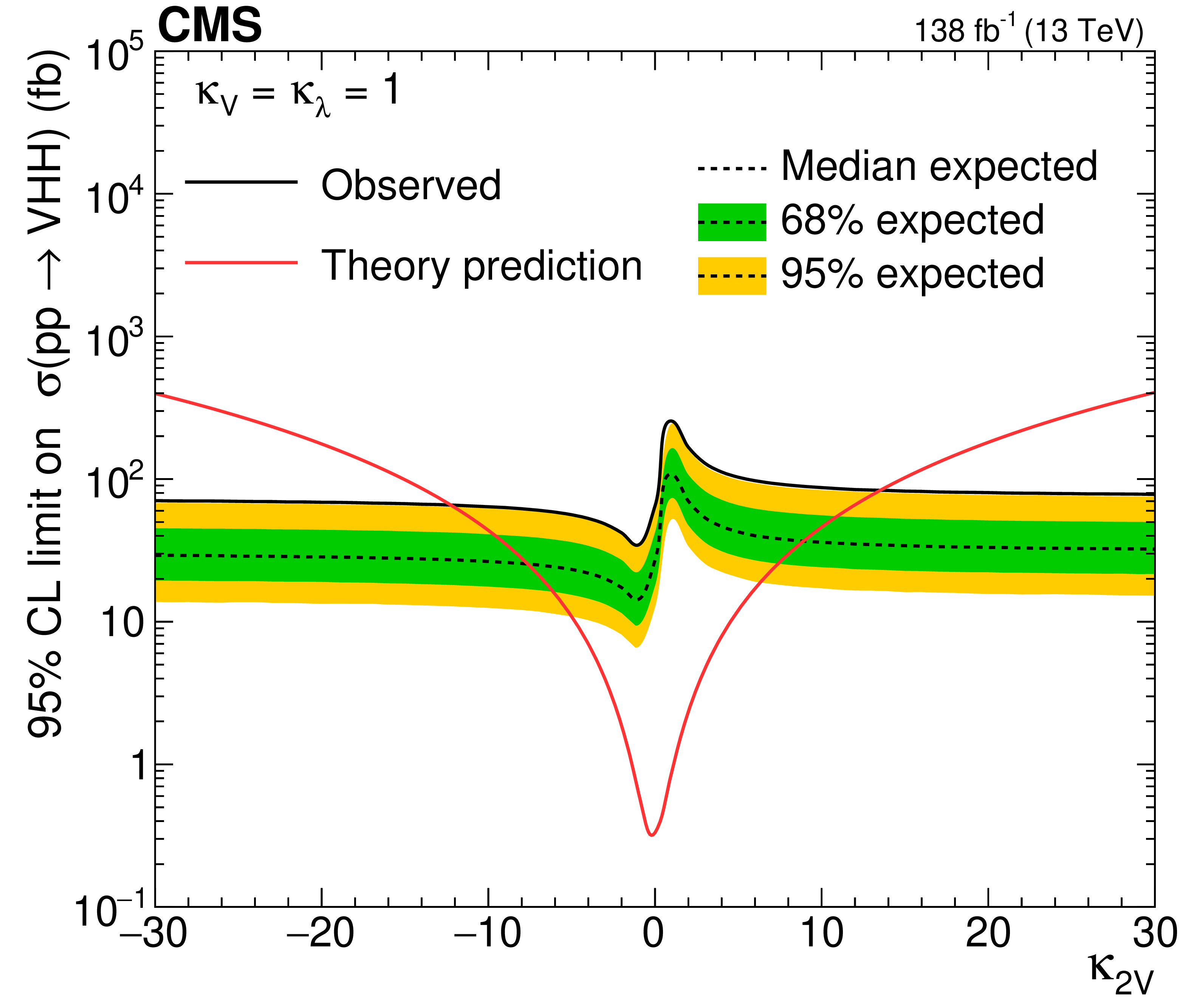
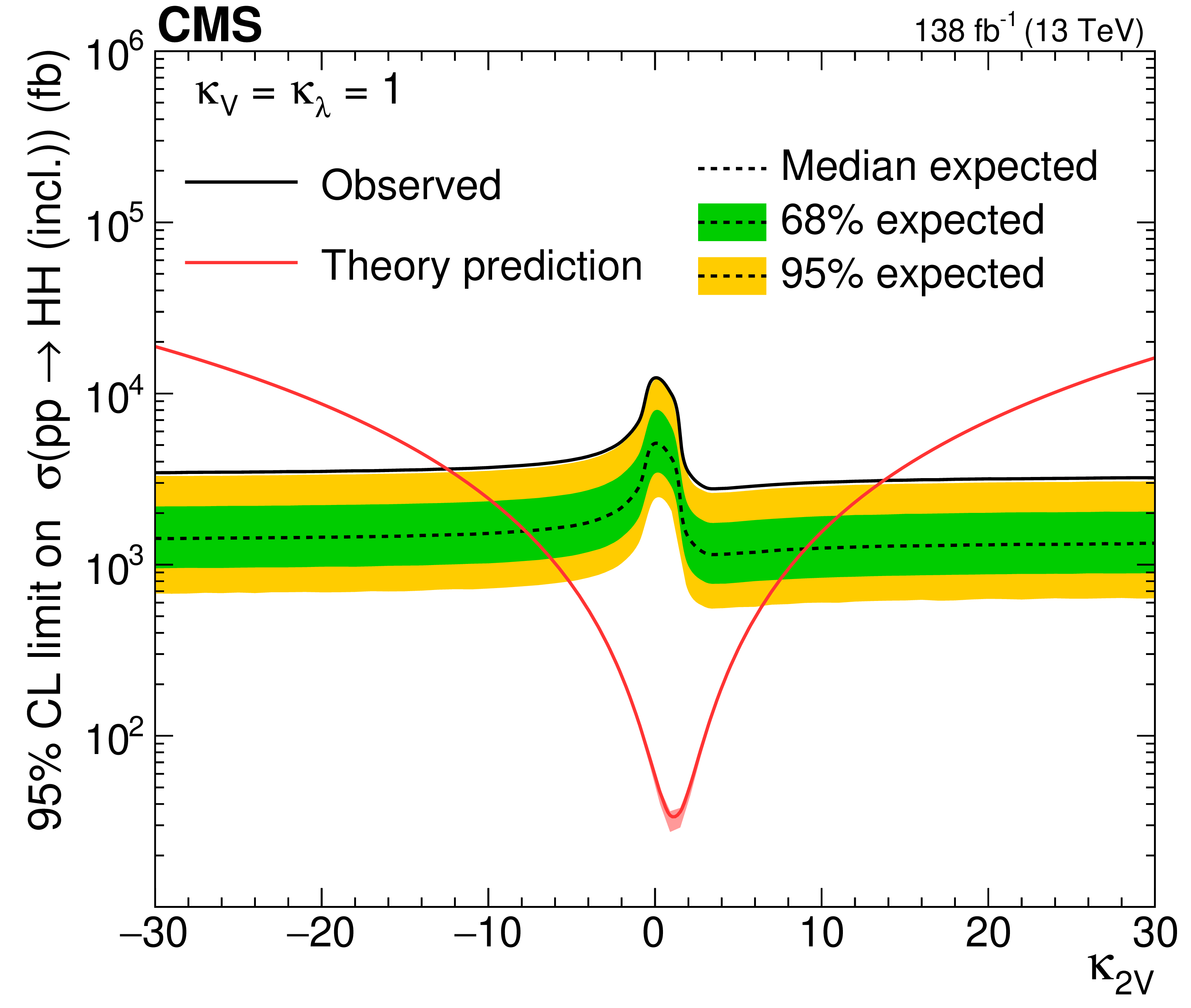
Figure 17:
Upper 95% CL limits on VHH (left) and HH (right) signal cross section scanned over the $ \kappa_{2\mathrm{V}} $ parameter while fixing the $ \kappa_{\lambda} $ and $ \kappa_{\mathrm{V}} $ to their SM-predicted values. The independent axis is the scanned $ \kappa_{2\mathrm{V}} $ parameter, and the dependent axis is the 95% CL upper limit on signal cross section. The theoretic prediction of VHH (left) and HH (right) production cross sections are shown with the red lines. |
png pdf |
Figure 17-a:
Upper 95% CL limits on VHH (left) and HH (right) signal cross section scanned over the $ \kappa_{2\mathrm{V}} $ parameter while fixing the $ \kappa_{\lambda} $ and $ \kappa_{\mathrm{V}} $ to their SM-predicted values. The independent axis is the scanned $ \kappa_{2\mathrm{V}} $ parameter, and the dependent axis is the 95% CL upper limit on signal cross section. The theoretic prediction of VHH (left) and HH (right) production cross sections are shown with the red lines. |
png pdf |
Figure 17-b:
Upper 95% CL limits on VHH (left) and HH (right) signal cross section scanned over the $ \kappa_{2\mathrm{V}} $ parameter while fixing the $ \kappa_{\lambda} $ and $ \kappa_{\mathrm{V}} $ to their SM-predicted values. The independent axis is the scanned $ \kappa_{2\mathrm{V}} $ parameter, and the dependent axis is the 95% CL upper limit on signal cross section. The theoretic prediction of VHH (left) and HH (right) production cross sections are shown with the red lines. |
png pdf |
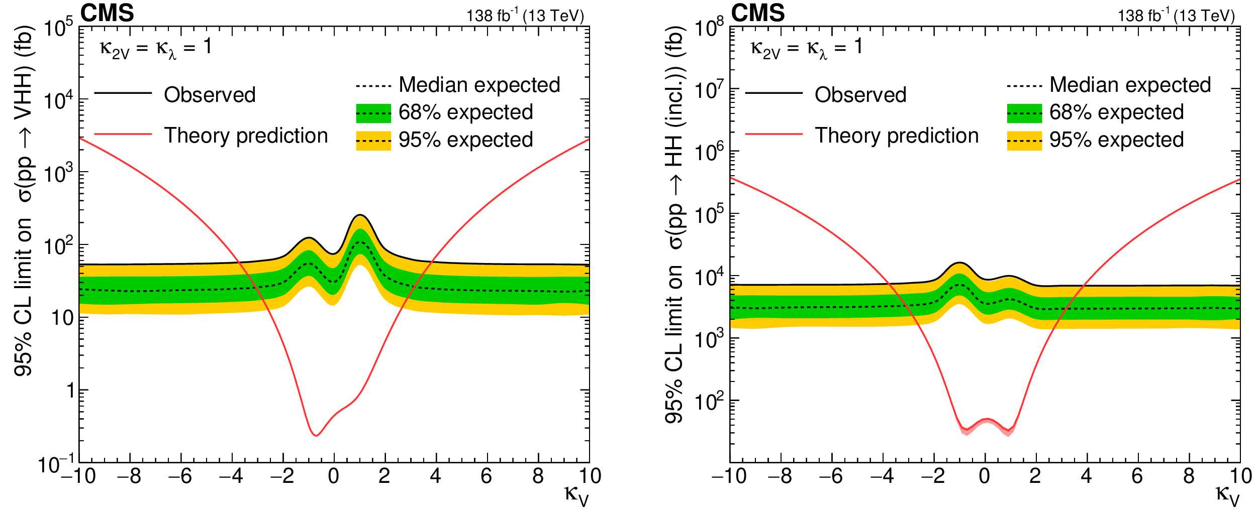
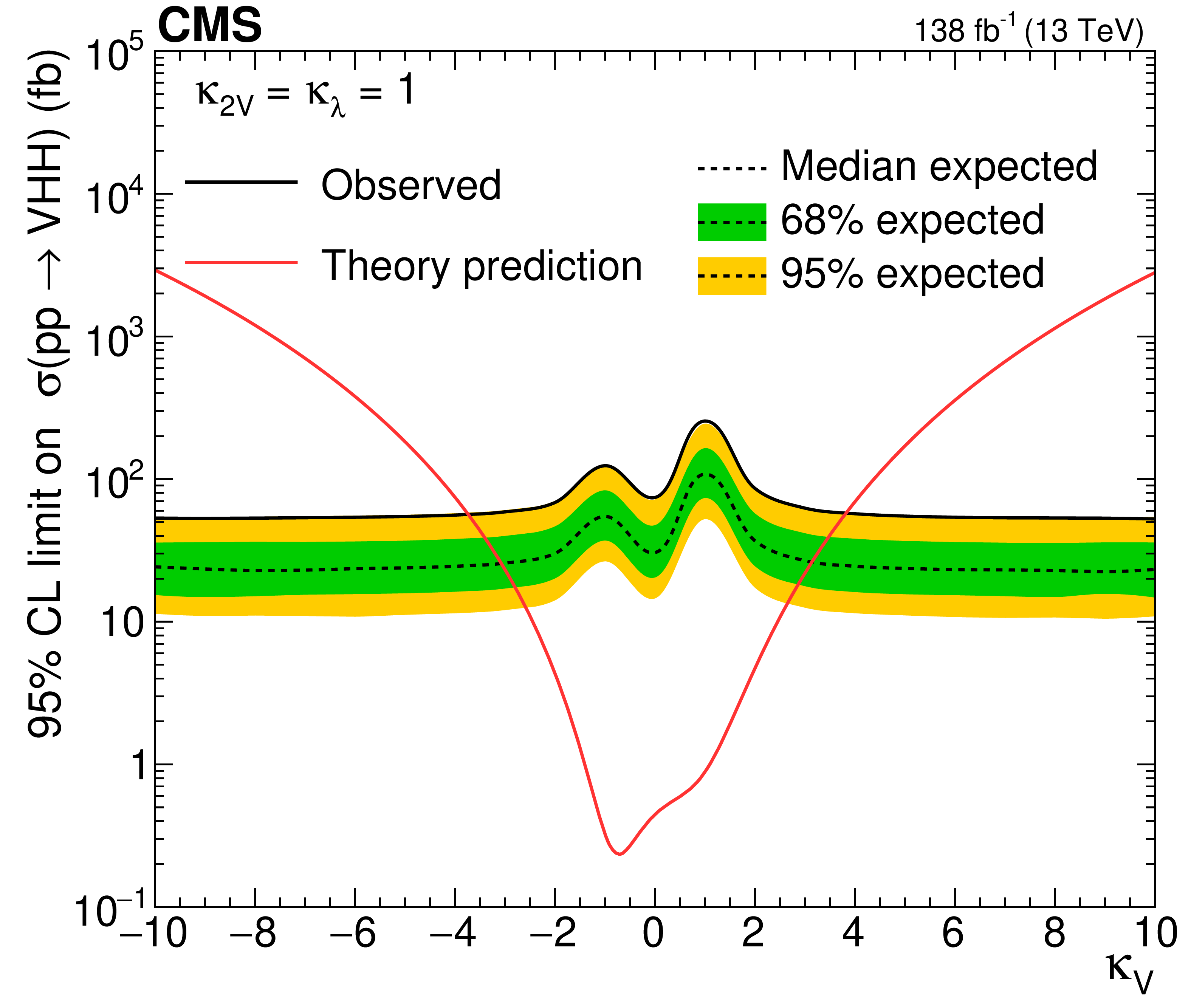
Figure 18:
Upper 95% CL limits on VHH (left) and HH (right) signal cross section scanned over the $ \kappa_{\mathrm{V}} $ parameter while fixing the $ \kappa_{2\mathrm{V}} $ and $ \kappa_{\lambda} $ to their SM-predicted values. The independent axis is the scanned $ \kappa_{\mathrm{V}} $ parameter, and the dependent axis is the 95% CL upper limit on signal cross section. The theoretic prediction of VHH (left) and HH (right) production cross sections are shown with the red lines. |
png pdf |
Figure 18-a:
Upper 95% CL limits on VHH (left) and HH (right) signal cross section scanned over the $ \kappa_{\mathrm{V}} $ parameter while fixing the $ \kappa_{2\mathrm{V}} $ and $ \kappa_{\lambda} $ to their SM-predicted values. The independent axis is the scanned $ \kappa_{\mathrm{V}} $ parameter, and the dependent axis is the 95% CL upper limit on signal cross section. The theoretic prediction of VHH (left) and HH (right) production cross sections are shown with the red lines. |

png pdf |
Figure 18-b:
Upper 95% CL limits on VHH (left) and HH (right) signal cross section scanned over the $ \kappa_{\mathrm{V}} $ parameter while fixing the $ \kappa_{2\mathrm{V}} $ and $ \kappa_{\lambda} $ to their SM-predicted values. The independent axis is the scanned $ \kappa_{\mathrm{V}} $ parameter, and the dependent axis is the 95% CL upper limit on signal cross section. The theoretic prediction of VHH (left) and HH (right) production cross sections are shown with the red lines. |
| Tables | |
png pdf |
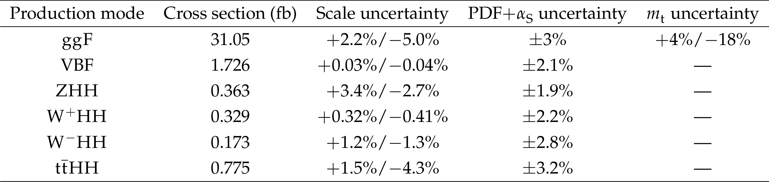
Table 1:
The cross sections and uncertainties of different HH production modes [11-14], where PDF is the parton distribution function, $ \alpha_\mathrm{S} $ is the strong coupling constant, and $ m_{\mathrm{t}} $ is the top quark mass. |

png pdf |
Table 2:
Kinematic thresholds at L1 triggers and the HLT are listed below for each analysis channel with variations per year as needed. HLT reconstruction is very similar to that for the offline reconstruction. The L1 reconstruction does not include any information from tracking. Transverse energy from ECAL plus HCAL systems is referred to as $ E_{\mathrm{T},\text{L1}} $. The scalar sum of $ E_{\mathrm{T},\text{L1}} $ from all energy deposits over a threshold of 30 GeV is denoted by $ H_{\mathrm{T}} $. |
png pdf |
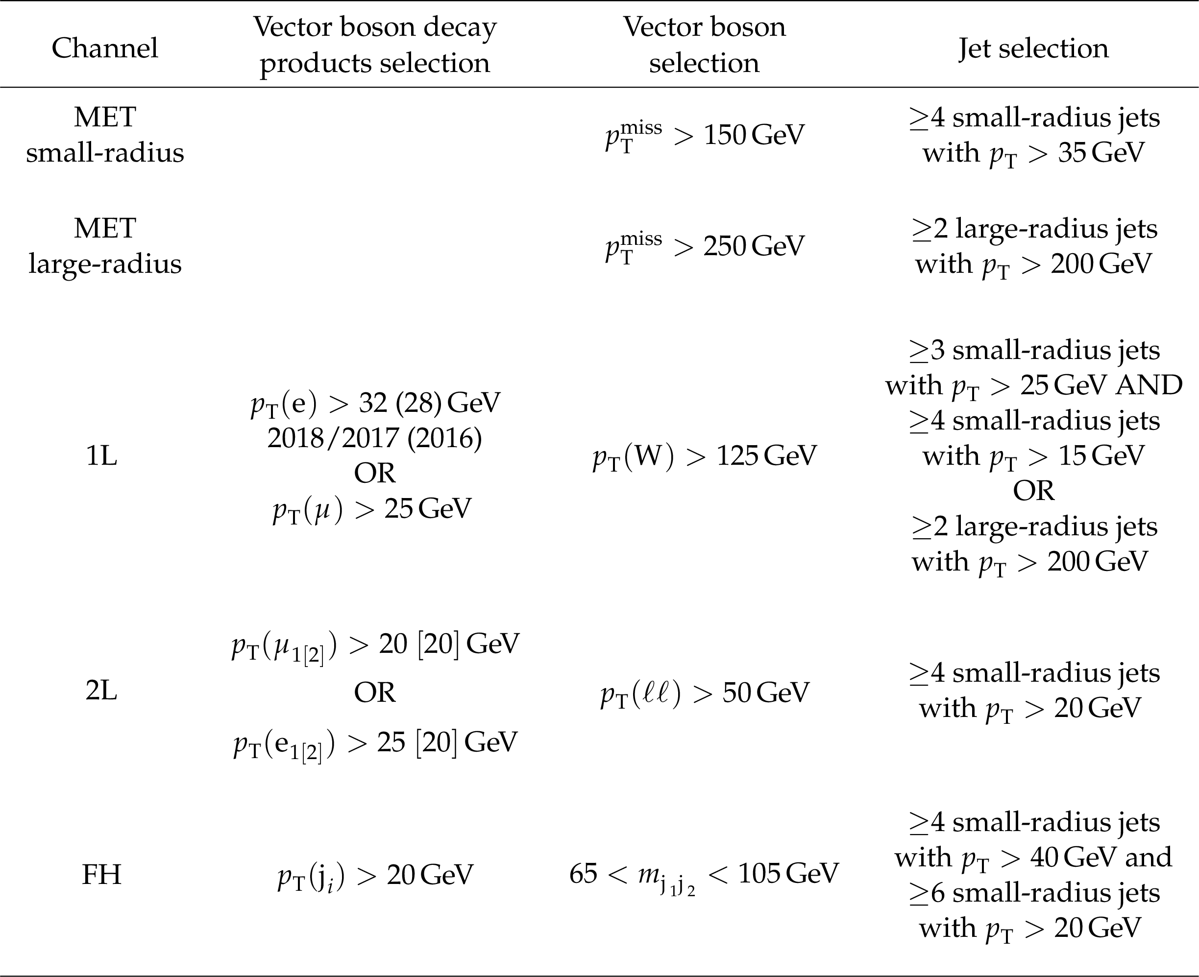
Table 3:
Thresholds on kinematic variables for all selected objects are listed for each channel. Objects are always required to be within the acceptance of the CMS subdetectors, which is $ |\eta| < $ 2.5 for electrons and 2.4 for all other objects, as well as outside of barrel-endcap transition regions near $ |\eta|\sim $ 1.5. The dijet mass of the two jets with the lowest b tagging scores in the FH channel is denoted $ m_{\mathrm{j}_{1}\mathrm{j}_{2}} $. |
png pdf |
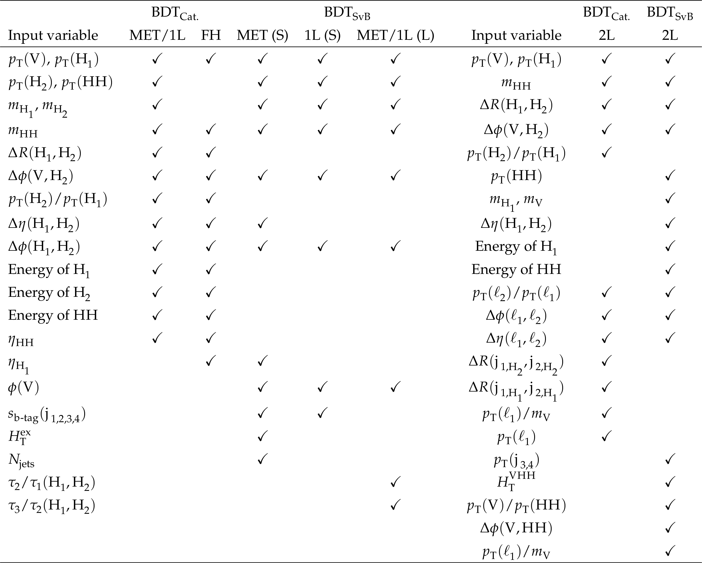
Table 4:
Variables used in the $ p_{\mathrm{T}}(\mathrm{Z}) $ categorization BDTs for the separation of the $ \kappa_{\lambda} $- and $ \kappa_{2\mathrm{V}} $-enriched regions and in $ \text{BDT}_{\text{SvB}} $ for extracting signal-like events. The $ \checkmark $ symbol indicates that the BDTs include the variable. These variables include the reconstructed Higgs boson with higher transverse momentum ($ \mathrm{H}_{1} $) and the lower one ($ \mathrm{H}_{2} $), the Higgs boson candidate jets ordered by the DEEPJET b tagging score ($ \mathrm{j}_{1,2,3,4} $), the scalar sum of the transverse energy of all the jets excluding $ \mathrm{j}_{1,2,3,4} $ ($ H_{\mathrm{T}}^{\text{ex}} $), the number of jets ($ N_{\text{jets}} $), the selected leptons in the 2L channel ($ \ell_{1} $, $ \ell_{2} $), the $ N $-subjettiness [73] ratio $ \tau_2/\tau_1 $ and $ \tau_3/\tau_2 $. The small-radius (large-radius) regions are designated with an ``S'' (``L'') in parentheses. |
png pdf |
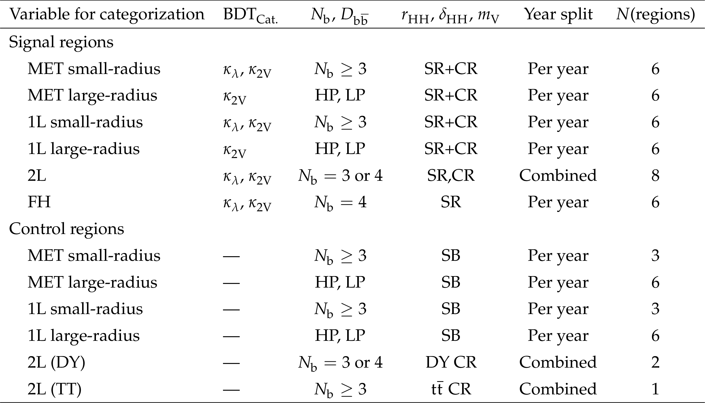
Table 5:
A summary of categorization in all channels, where DY is Drell--Yan. The first row outlines the variables used for the categorization. HP and LP are regions defined based on $ D_{\mathrm{b}\overline{\mathrm{b}}} $ cuts: $\mathrm{min}(D_{\mathrm{b}\overline{\mathrm{b}},1},D_{\mathrm{b}\overline{\mathrm{b}},2}) > $ 0.94 (HP), and $\mathrm{min}(D_{\mathrm{b}\overline{\mathrm{b}},1},D_{\mathrm{b}\overline{\mathrm{b}},2}) < $ 0.90 (LP). $ N_{\mathrm{b}} $ is the number of jets that pass DEEPJET b tagging score medium working point. |
png pdf |
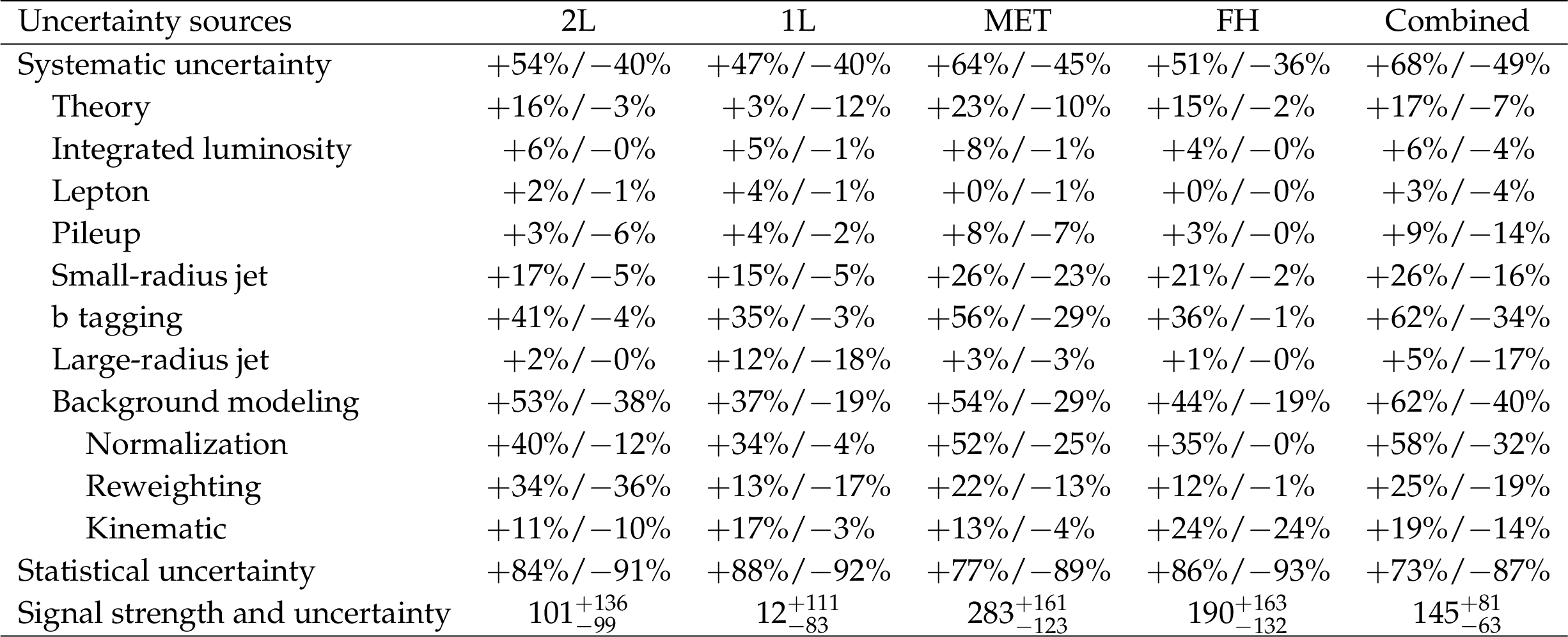
Table 6:
The contribution of each group of uncertainties is quantified relative to the total uncertainty in the signal strength, which is listed in the final line. To compute the relative contributions, the group of nuisance parameters is fixed to the best fit value while the likelihood is scanned again profiling all other nuisance parameters. The reductions in the upper and lower variations are shown in each line. The likelihood shape is asymmetric, and so the upper and lower variations are quantified separately. |
png pdf |
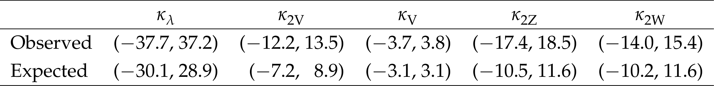
Table 7:
Observed and expected 95% CL upper limits on the coupling modifiers. |
| Summary |
| A search for Higgs boson pair production in association with a vector boson (VHH) using a data set of proton-proton collisions at $ \sqrt{s}= $ 13 TeV, corresponding to an integrated luminosity of 138 fb$ ^{-1} $, is presented. Final states including Higgs boson decay to bottom quarks are analyzed in events where the W or Z boson decay to electrons, muons, neutrinos, and hadrons. An observed (expected) upper limit at 95% confidence level of VHH production cross section is set at 294 (124) times the standard model prediction. Coupling modifiers, defined relative to the standard model coupling strengths, are scanned and constrained for the Higgs boson trilinear coupling ($ \kappa_{\lambda} $) and the coupling between two V bosons with two Higgs bosons ($ \kappa_{2\mathrm{V}} $). The observed (expected) 95% confidence level limits constrain $ \kappa_{\lambda} $ and $ \kappa_{2\mathrm{V}} $ to be $ -$37.7 $ < \kappa_{\lambda} < $ 37.2 ($ -$30.1 $ < \kappa_{\lambda} < $ 28.9) and $ -$12.2 $ < \kappa_{2\mathrm{V}} < $ 13.5 ($ -$7.2 $ < \kappa_{2\mathrm{V}} < $ 8.9), respectively. |
| References | ||||
| 1 | ATLAS Collaboration | Observation of a new particle in the search for the standard model Higgs boson with the ATLAS detector at the LHC | PLB 716 (2012) 1 | 1207.7214 |
| 2 | CMS Collaboration | Observation of a new boson at a mass of 125 GeV with the CMS experiment at the LHC | PLB 716 (2012) 30 | CMS-HIG-12-028 1207.7235 |
| 3 | CMS Collaboration | Observation of a new boson with mass near 125 GeV in $ {\mathrm{p}\mathrm{p}} $ collisions at $ \sqrt{s}= $ 7 and 8 TeV | JHEP 06 (2013) 081 | CMS-HIG-12-036 1303.4571 |
| 4 | CMS Collaboration | A portrait of the Higgs boson by the CMS experiment ten years after the discovery | Nature 607 (2022) 60 | CMS-HIG-22-001 2207.00043 |
| 5 | ATLAS Collaboration | A detailed map of Higgs boson interactions by the ATLAS experiment ten years after the discovery | Nature 607 (2022) 52 | 2207.00092 |
| 6 | A. G. Cohen, D. B. Kaplan, and A. E. Nelson | Baryogenesis at the weak phase transition | NPB 349 (1991) 727 | |
| 7 | D. E. Morrissey and M. J. Ramsey-Musolf | Electroweak baryogenesis | New J. Phys. 14 (2012) 125003 | 1206.2942 |
| 8 | A. Noble and M. Perelstein | Higgs self-coupling as a probe of electroweak phase transition | PRD 78 (2008) 063518 | 0711.3018 |
| 9 | Q.-H. Cao, Y. Liu, and B. Yan | Measuring trilinear Higgs coupling in $ {\mathrm{W}\mathrm{H}\mathrm{H}} $ and $ {\mathrm{Z}\mathrm{H}\mathrm{H}} $ productions at the high-luminosity LHC | PRD 95 (2017) 073006 | 1511.03311 |
| 10 | K. Nordström and A. Papaefstathiou | $ {\mathrm{V}\mathrm{H}\mathrm{H}} $ production at the high-luminosity LHC | Eur. Phys. J. Plus 134 (2019) 288 | 1807.01571 |
| 11 | LHC Higgs Cross Section Working Group , D. de Florian et al. | Handbook of LHC Higgs cross sections: 4. Deciphering the nature of the Higgs sector | CERN Report CERN-2017-002-M, 2016 link |
1610.07922 |
| 12 | J. Baglio et al. | The measurement of the Higgs self-coupling at the LHC: theoretical status | JHEP 04 (2013) 151 | 1212.5581 |
| 13 | J. Baglio et al. | $ {\mathrm{g}\mathrm{g}\to\mathrm{H}\mathrm{H}} $: Combined uncertainties | PRD 103 (2021) 056002 | 2008.11626 |
| 14 | F. A. Dreyer and A. Karlberg | Vector-boson fusion Higgs pair production at N\textsuperscript3LO | PRD 98 (2018) 114016 | 1811.07906 |
| 15 | CMS Collaboration | Search for nonresonant Higgs boson pair production in final states with two bottom quarks and two photons in proton-proton collisions at $ \sqrt{s}= $ 13 TeV | JHEP 03 (2021) 257 | CMS-HIG-19-018 2011.12373 |
| 16 | CMS Collaboration | Search for Higgs boson pair production in the four b quark final state in proton-proton collisions at $ \sqrt{s}= $ 13 TeV | PRL 129 (2022) 081802 | CMS-HIG-20-005 2202.09617 |
| 17 | CMS Collaboration | Search for nonresonant pair production of highly energetic Higgs bosons decaying to bottom quarks | PRL 131 (2023) 041803 | 2205.06667 |
| 18 | CMS Collaboration | Search for nonresonant Higgs boson pair production in final state with two bottom quarks and two tau leptons in proton-proton collisions at $ \sqrt{s}= $ 13 TeV | PLB 842 (2023) 137531 | CMS-HIG-20-010 2206.09401 |
| 19 | CMS Collaboration | Search for nonresonant Higgs boson pair production in the four leptons plus two b jets final state in proton-proton collisions at $ \sqrt{s}= $ 13 TeV | JHEP 06 (2023) 130 | CMS-HIG-20-004 2206.10657 |
| 20 | CMS Collaboration | Search for Higgs boson pairs decaying to $ {\mathrm{W}\mathrm{W}\mathrm{W}\mathrm{W}} $, $ {\mathrm{W}\mathrm{W}\tau\tau} $, and $ {\tau\tau\tau\tau} $ in proton-proton collisions at $ \sqrt{s}= $ 13 TeV | JHEP 07 (2023) 095 | CMS-HIG-21-002 2206.10268 |
| 21 | ATLAS Collaboration | Search for Higgs boson pair production in the two bottom quarks plus two photons final state in $ {\mathrm{p}\mathrm{p}} $ collisions at $ \sqrt{s}= $ 13 TeV with the ATLAS detector | PRD 106 (2022) 052001 | 2112.11876 |
| 22 | ATLAS Collaboration | Search for resonant and non-resonant Higgs boson pair production in the $ \mathrm{b}\overline{\mathrm{b}}{\tau^{+}\tau^{-}} $ decay channel using 13 TeV $ {\mathrm{p}\mathrm{p}} $ collision data from the ATLAS detector | JHEP 07 (2023) 040 | 2209.10910 |
| 23 | ATLAS Collaboration | Search for nonresonant pair production of Higgs bosons in the $ \mathrm{b}\overline{\mathrm{b}}\mathrm{b}\overline{\mathrm{b}} $ final state in $ {\mathrm{p}\mathrm{p}} $ collisions at $ \sqrt{s}= $ 13 TeV with the ATLAS detector | PRD 108 (2023) 052003 | 2301.03212 |
| 24 | ATLAS Collaboration | Search for non-resonant Higgs boson pair production in the $ {\mathrm{b}\mathrm{b}\ell\nu\ell\nu} $ final state with the ATLAS detector in $ {\mathrm{p}\mathrm{p}} $ collisions at $ \sqrt{s}= $ 13 TeV | PLB 801 (2020) 135145 | 1908.06765 |
| 25 | ATLAS Collaboration | Constraints on the Higgs boson self-coupling from single- and double-Higgs production with the ATLAS detector using $ {\mathrm{p}\mathrm{p}} $ collisions at $ \sqrt{s}= $ 13 TeV | PLB 843 (2023) 137745 | 2211.01216 |
| 26 | ATLAS Collaboration | Search for Higgs boson pair production in association with a vector boson in $ {\mathrm{p}\mathrm{p}} $ collisions at $ \sqrt{s}= $ 13 TeV with the ATLAS detector | EPJC 83 (2023) 519 | 2210.05415 |
| 27 | CMS Collaboration | HEPData record for this analysis | link | |
| 28 | CMS Collaboration | The CMS experiment at the CERN LHC | JINST 3 (2008) S08004 | |
| 29 | CMS Collaboration | Development of the CMS detector for the CERN LHC Run 3 | Accepted by JINST, 2023 | CMS-PRF-21-001 2309.05466 |
| 30 | CMS Collaboration | Performance of the CMS Level-1 trigger in proton-proton collisions at $ \sqrt{s}= $ 13 TeV | JINST 15 (2020) P10017 | CMS-TRG-17-001 2006.10165 |
| 31 | CMS Collaboration | The CMS trigger system | JINST 12 (2017) P01020 | CMS-TRG-12-001 1609.02366 |
| 32 | CMS Collaboration | Precision luminosity measurement in proton-proton collisions at $ \sqrt{s}= $ 13 TeV in 2015 and 2016 at CMS | EPJC 81 (2021) 800 | CMS-LUM-17-003 2104.01927 |
| 33 | CMS Collaboration | CMS luminosity measurement for the 2017 data-taking period at $ \sqrt{s}= $ 13 TeV | CMS Physics Analysis Summary, 2018 CMS-PAS-LUM-17-004 |
CMS-PAS-LUM-17-004 |
| 34 | CMS Collaboration | CMS luminosity measurement for the 2018 data-taking period at $ \sqrt{s}= $ 13 TeV | CMS Physics Analysis Summary, 2019 CMS-PAS-LUM-18-002 |
CMS-PAS-LUM-18-002 |
| 35 | CMS Collaboration | Performance of missing transverse momentum reconstruction in proton-proton collisions at $ \sqrt{s}= $ 13 TeV using the CMS detector | JINST 14 (2019) P07004 | CMS-JME-17-001 1903.06078 |
| 36 | J. Alwall et al. | The automated computation of tree-level and next-to-leading order differential cross sections, and their matching to parton shower simulations | JHEP 07 (2014) 079 | 1405.0301 |
| 37 | T. Sjöstrand et al. | An introduction to PYTHIA8.2 | Comput. Phys. Commun. 191 (2015) 159 | 1410.3012 |
| 38 | NNPDF Collaboration | Parton distributions from high-precision collider data | EPJC 77 (2017) 663 | 1706.00428 |
| 39 | CMS Collaboration | Extraction and validation of a new set of CMS PYTHIA8 tunes from underlying-event measurements | EPJC 80 (2020) 4 | CMS-GEN-17-001 1903.12179 |
| 40 | E. H. Moore | On the reciprocal of the general algebraic matrix | in Proc. 14th Western Meeting of the American Mathematical Society, Chicago, 1920 Bull. Amer. Math. Soc. 26 (1920) 385 |
|
| 41 | R. Penrose | A generalized inverse for matrices | Proc. Cambridge Phil. Soc. 51 (1955) 406 | |
| 42 | P. Nason | A new method for combining NLO QCD with shower Monte Carlo algorithms | JHEP 11 (2004) 040 | hep-ph/0409146 |
| 43 | S. Frixione, P. Nason, and C. Oleari | Matching NLO QCD computations with parton shower simulations: the POWHEG method | JHEP 11 (2007) 070 | 0709.2092 |
| 44 | S. Alioli, P. Nason, C. Oleari, and E. Re | A general framework for implementing NLO calculations in shower Monte Carlo programs: the POWHEG box | JHEP 06 (2010) 043 | 1002.2581 |
| 45 | T. Je \v z o and P. Nason | On the treatment of resonances in next-to-leading order calculations matched to a parton shower | JHEP 12 (2015) 065 | 1509.09071 |
| 46 | F. Buccioni et al. | OpenLoops 2 | EPJC 79 (2019) 866 | 1907.13071 |
| 47 | T. Je \v z o, J. M. Lindert, N. Moretti, and S. Pozzorini | New NLOPS predictions for $ \mathrm{t} \overline{\mathrm{t}} $ +b-jet production at the LHC | EPJC 78 (2018) 502 | 1802.00426 |
| 48 | J. Alwall et al. | MadGraph 5: going beyond | JHEP 06 (2011) 128 | 1106.0522 |
| 49 | J. Alwall et al. | Comparative study of various algorithms for the merging of parton showers and matrix elements in hadronic collisions | EPJC 53 (2008) 473 | 0706.2569 |
| 50 | S. Kallweit et al. | NLO QCD+EW predictions for V+jets including off-shell vector-boson decays and multijet merging | JHEP 04 (2016) 021 | 1511.08692 |
| 51 | G. Ferrera, M. Grazzini, and F. Tramontano | Higher-order QCD effects for associated $ {\mathrm{W}\mathrm{H}} $ production and decay at the LHC | JHEP 04 (2014) 039 | 1312.1669 |
| 52 | O. Brein, R. V. Harlander, and T. J. E. Zirke | VH@NNLO---Higgs strahlung at hadron colliders | Comput. Phys. Commun. 184 (2013) 998 | 1210.5347 |
| 53 | G. Ferrera, M. Grazzini, and F. Tramontano | Associated $ {\mathrm{Z}\mathrm{H}} $ production at hadron colliders: The fully differential NNLO QCD calculation | PLB 740 (2015) 51 | 1407.4747 |
| 54 | R. Frederix and S. Frixione | Merging meets matching in MC@NLO | JHEP 12 (2012) 061 | 1209.6215 |
| 55 | CompHEP Collaboration | COMPHEP 4.4---automatic computations from Lagrangians to events | NIM A 534 (2004) 250 | hep-ph/0403113 |
| 56 | GEANT4 Collaboration | GEANT 4---a simulation toolkit | NIM A 506 (2003) 250 | |
| 57 | CMS Collaboration | Particle-flow reconstruction and global event description with the CMS detector | JINST 12 (2017) P10003 | CMS-PRF-14-001 1706.04965 |
| 58 | CMS Collaboration | Technical proposal for the Phase-II upgrade of the Compact Muon Solenoid | CMS Technical Proposal CERN-LHCC-2015-010, CMS-TDR-15-02, 2015 CDS |
|
| 59 | M. Cacciari, G. P. Salam, and G. Soyez | The anti-$ k_{\mathrm{T}} $ jet clustering algorithm | JHEP 04 (2008) 063 | 0802.1189 |
| 60 | M. Cacciari, G. P. Salam, and G. Soyez | FASTJET user manual | EPJC 72 (2012) 1896 | 1111.6097 |
| 61 | CMS Collaboration | Jet energy scale and resolution in the CMS experiment in $ {\mathrm{p}\mathrm{p}} $ collisions at 8 TeV | JINST 12 (2017) P02014 | CMS-JME-13-004 1607.03663 |
| 62 | CMS Collaboration | A deep neural network for simultaneous estimation of b jet energy and resolution | Comput. Softw. Big Sci. 4 (2020) 10 | CMS-HIG-18-027 1912.06046 |
| 63 | CMS Collaboration | Pileup mitigation at CMS in 13 TeV data | JINST 15 (2020) P09018 | CMS-JME-18-001 2003.00503 |
| 64 | D. Bertolini, P. Harris, M. Low, and N. Tran | Pileup per particle identification | JHEP 10 (2014) 059 | 1407.6013 |
| 65 | E. Bols et al. | Jet flavour classification using DeepJet | JINST 15 (2020) P12012 | 2008.10519 |
| 66 | CMS Collaboration | Performance of the DeepJet b tagging algorithm using 41.9 fb$ ^{-1} $ of data from proton-proton collisions at 13 TeV with Phase 1 CMS detector | CMS Detector Performance Note CMS-DP-2018-058, 2018 CDS |
|
| 67 | CMS Collaboration | Identification of heavy-flavour jets with the CMS detector in $ {\mathrm{p}\mathrm{p}} $ collisions at 13 TeV | JINST 13 (2018) P05011 | CMS-BTV-16-002 1712.07158 |
| 68 | H. Qu and L. Gouskos | Jet tagging via particle clouds | PRD 101 (2020) 056019 | 1902.08570 |
| 69 | CMS Collaboration | Electron and photon reconstruction and identification with the CMS experiment at the CERN LHC | JINST 16 (2021) P05014 | CMS-EGM-17-001 2012.06888 |
| 70 | CMS Collaboration | ECAL 2016 refined calibration and Run2 summary plots | CMS Detector Performance Note CMS-DP-2020-021, 2020 CDS |
|
| 71 | CMS Collaboration | Performance of the CMS muon detector and muon reconstruction with proton-proton collisions at $ \sqrt{s}= $ 13 TeV | JINST 13 (2018) P06015 | CMS-MUO-16-001 1804.04528 |
| 72 | F. Pedregosa et al. | Scikit-learn: Machine learning in Python | J. Mach. Learn. Res. 12 (2011) 2825 | |
| 73 | J. Thaler and K. Van Tilburg | Identifying boosted objects with $ {N} $-subjettiness | JHEP 03 (2011) 015 | 1011.2268 |
| 74 | K. He, X. Zhang, R. Ren, and J. Sun | Deep residual learning for image recognition | in Proc. 2016 IEEE Conference on Computer Vision and Pattern Recognition (CVPR): Las Vegas, 2016 link |
1512.03385 |
| 75 | A. Vaswani et al. | Attention is all you need | in Proc. 31st Conference on Neural Information Processing Systems (NIPS ): Long Beach CA, USA, December 04--09,, 2017 link |
1706.03762 |
| 76 | A. Rogozhnikov | Reweighting with boosted decision trees | in Proc. 17th International Workshop on Advanced Computing and Analysis Techniques in Physics Research (ACAT ): Valparaiso, Chile, 2016 J. Phys. Conf. Ser. 762 (2016) 012036 |
1608.05806 |
| 77 | ATLAS and CMS Collaborations, and LHC Higgs Combination Group | Procedure for the LHC Higgs boson search combination in Summer 2011 | Technical Report CMS-NOTE-2011-005, ATL-PHYS-PUB-2011-11, 2011 | |
| 78 | NNPDF Collaboration | Parton distributions for the LHC run II | JHEP 04 (2015) 040 | 1410.8849 |
| 79 | R. Barlow and C. Beeston | Fitting using finite Monte Carlo samples | Comput. Phys. Commun. 77 (1993) 219 | |
| 80 | CMS Collaboration | Mass regression of highly-boosted jets using graph neural networks | CMS Detector Performance Note CMS-DP-2021-017, 2021 CDS |
|
| 81 | R. A. Fisher | On the interpretation of $ \chi^2 $ from contingency tables, and the calculation of $ {P} $ | J. R. Stat. Soc 85 (1922) 87 | |
| 82 | T. Junk | Confidence level computation for combining searches with small statistics | NIM A 434 (1999) 435 | hep-ex/9902006 |
| 83 | A. L. Read | Presentation of search results: The $ \text{CL}_\text{s} $ technique | JPG 28 (2002) 2693 | |
| 84 | G. Cowan, K. Cranmer, E. Gross, and O. Vitells | Asymptotic formulae for likelihood-based tests of new physics | EPJC 71 (2011) 1554 | 1007.1727 |
|
|
Compact Muon Solenoid LHC, CERN |
|

|

|

|

|

|