

Compact Muon Solenoid
LHC, CERN
| CMS-SMP-18-004 ; CERN-EP-2020-144 | ||
| $\mathrm{W^{+}W^{-}}$ boson pair production in proton-proton collisions at $\sqrt{s} = $ 13 TeV | ||
| CMS Collaboration | ||
| 1 September 2020 | ||
| Phys. Rev. D 102 (2020) 092001 | ||
| Abstract: A measurement of the $\mathrm{W^{+}W^{-}}$ boson pair production cross section in proton-proton collisions at $\sqrt{s} = $ 13 TeV is presented. The data used in this study are collected with the CMS detector at the CERN LHC and correspond to an integrated luminosity of 35.9 fb$^{-1}$. The $\mathrm{W^{+}W^{-}}$ candidate events are selected by requiring two oppositely charged leptons (electrons or muons). Two methods for reducing background contributions are employed. In the first one, a sequence of requirements on kinematic quantities is applied allowing a measurement of the total production cross section: 117.6 $\pm$ 6.8 pb, which agrees well with the theoretical prediction. Fiducial cross sections are also reported for events with zero or one jet, and the change in the zero-jet fiducial cross section with the jet transverse momentum threshold is measured. Normalized differential cross sections are reported within the fiducial region. A second method for suppressing background contributions employs two random forest classifiers. The analysis based on this method includes a measurement of the total production cross section and also a measurement of the normalized jet multiplicity distribution in $\mathrm{W^{+}W^{-}}$ events. Finally, a dilepton invariant mass distribution is used to probe for physics beyond the standard model in the context of an effective field theory, and constraints on the presence of dimension-6 operators are derived. | ||
| Links: e-print arXiv:2009.00119 [hep-ex] (PDF) ; CDS record ; inSPIRE record ; HepData record ; CADI line (restricted) ; | ||
| Figures & Tables | Summary | Additional Figures | References | CMS Publications |
|---|
| Figures | |
png pdf |
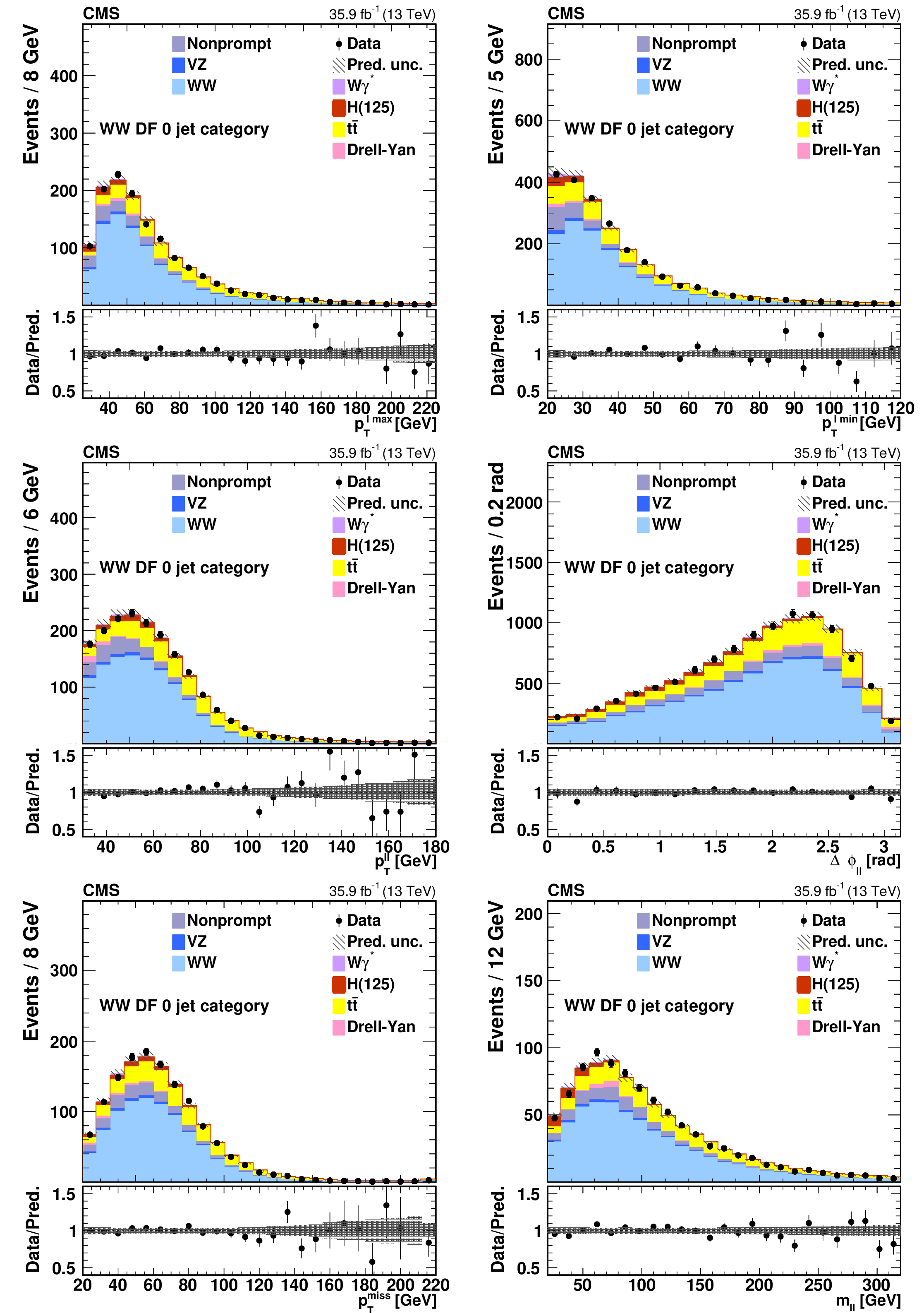
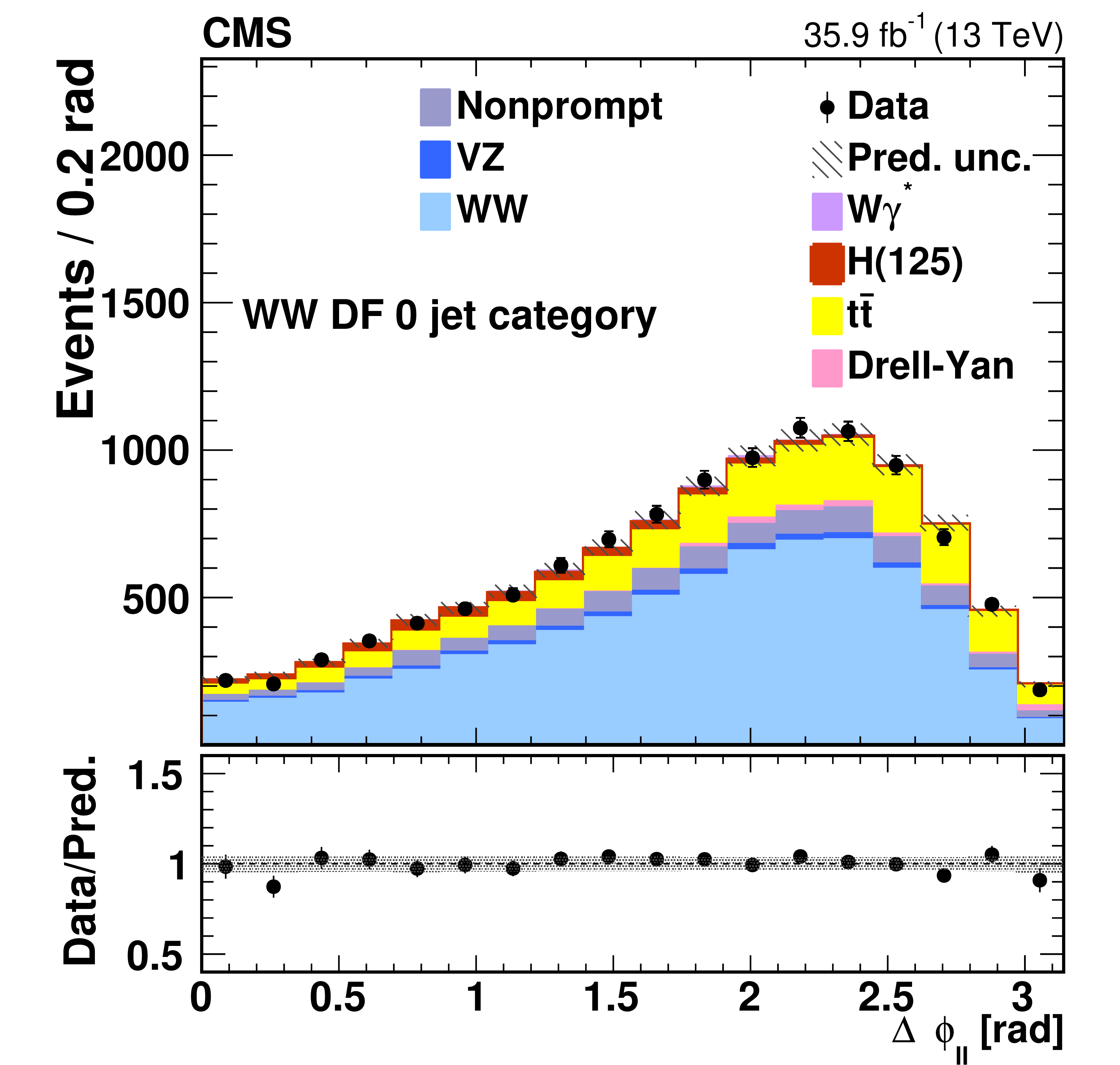
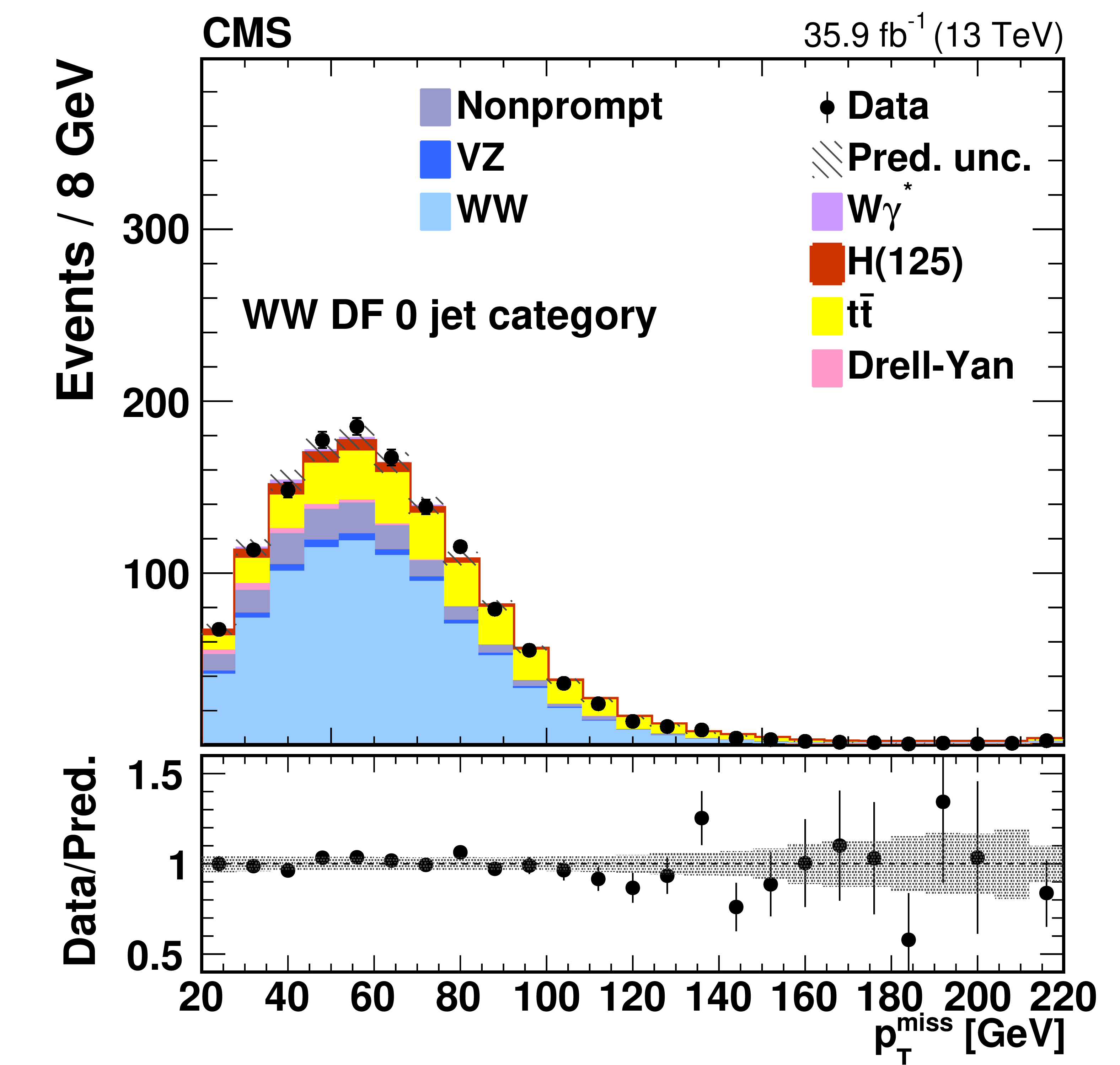
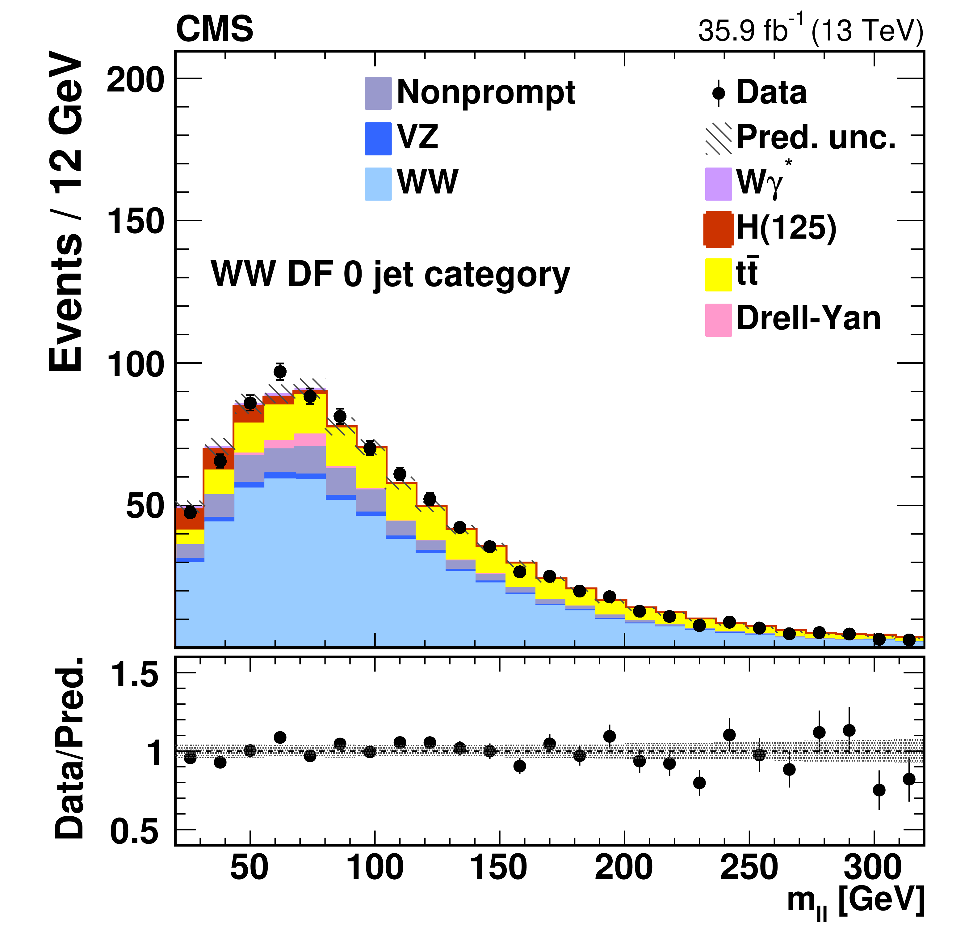
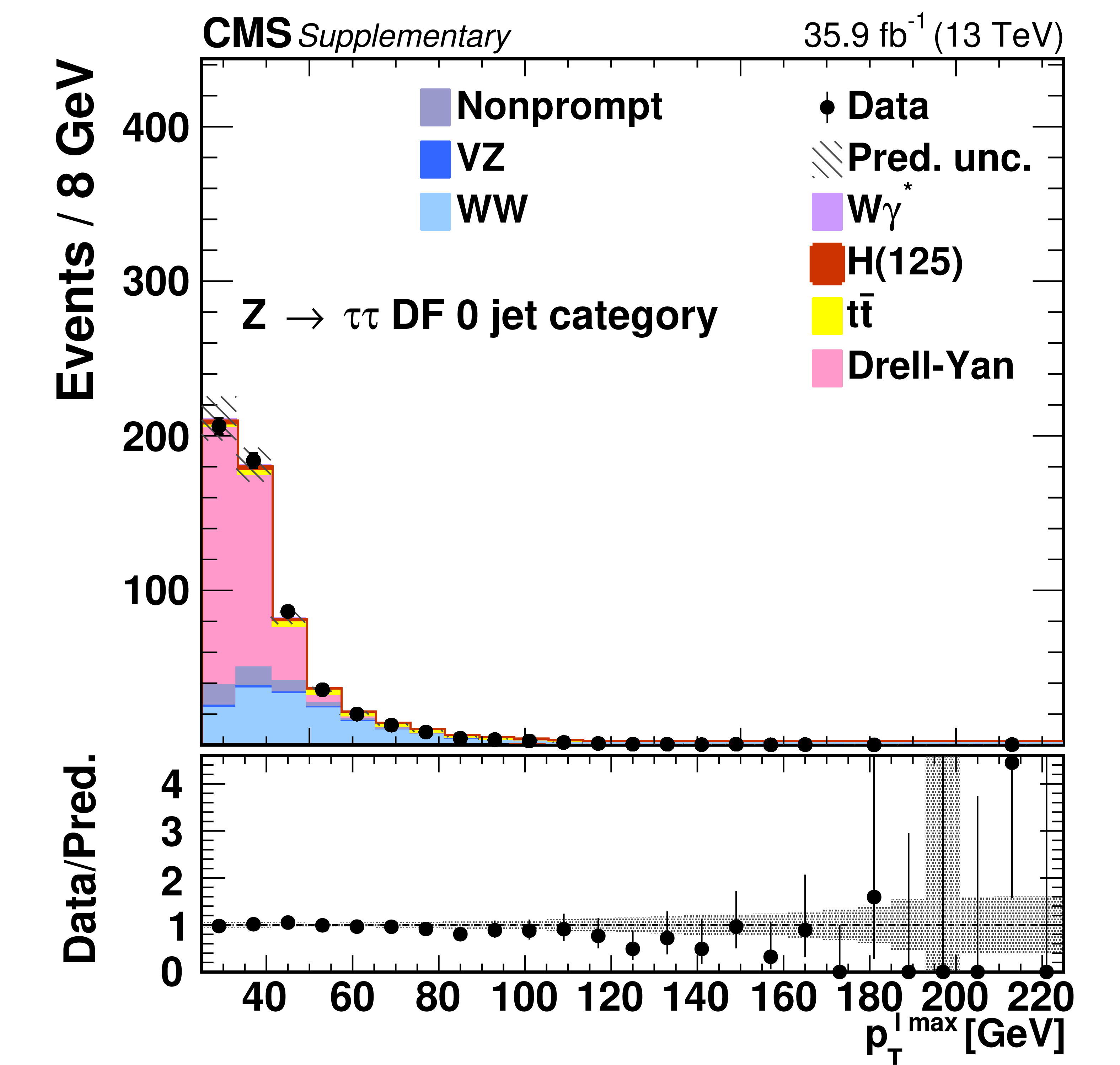
Figure 1:
Kinematic distributions for events with zero jets and DF leptons in the sequential cut analysis. The distributions show the leading and trailing lepton ${p_{\mathrm {T}}}$ ($ {{p_{\mathrm {T}}} ^{\ell \, \text {max}}} $ and $ {{p_{\mathrm {T}}} ^{\ell \, \text {min}}} $), the dilepton transverse momentum $ {p_{\mathrm {T}}} ^{\ell \ell}$, the azimuthal angle between the two leptons $ {\Delta \phi _{\ell \ell}} $, the missing transverse momentum ${{p_{\mathrm {T}}} ^\text {miss}}$, and the dilepton invariant mass $ {m_{\ell \ell}} $. The error bars on the data points represent the statistical uncertainty of the data, and the hatched areas represent the combined systematic and statistical uncertainty of the predicted yield in each bin. The last bin includes the overflow. |
png pdf |
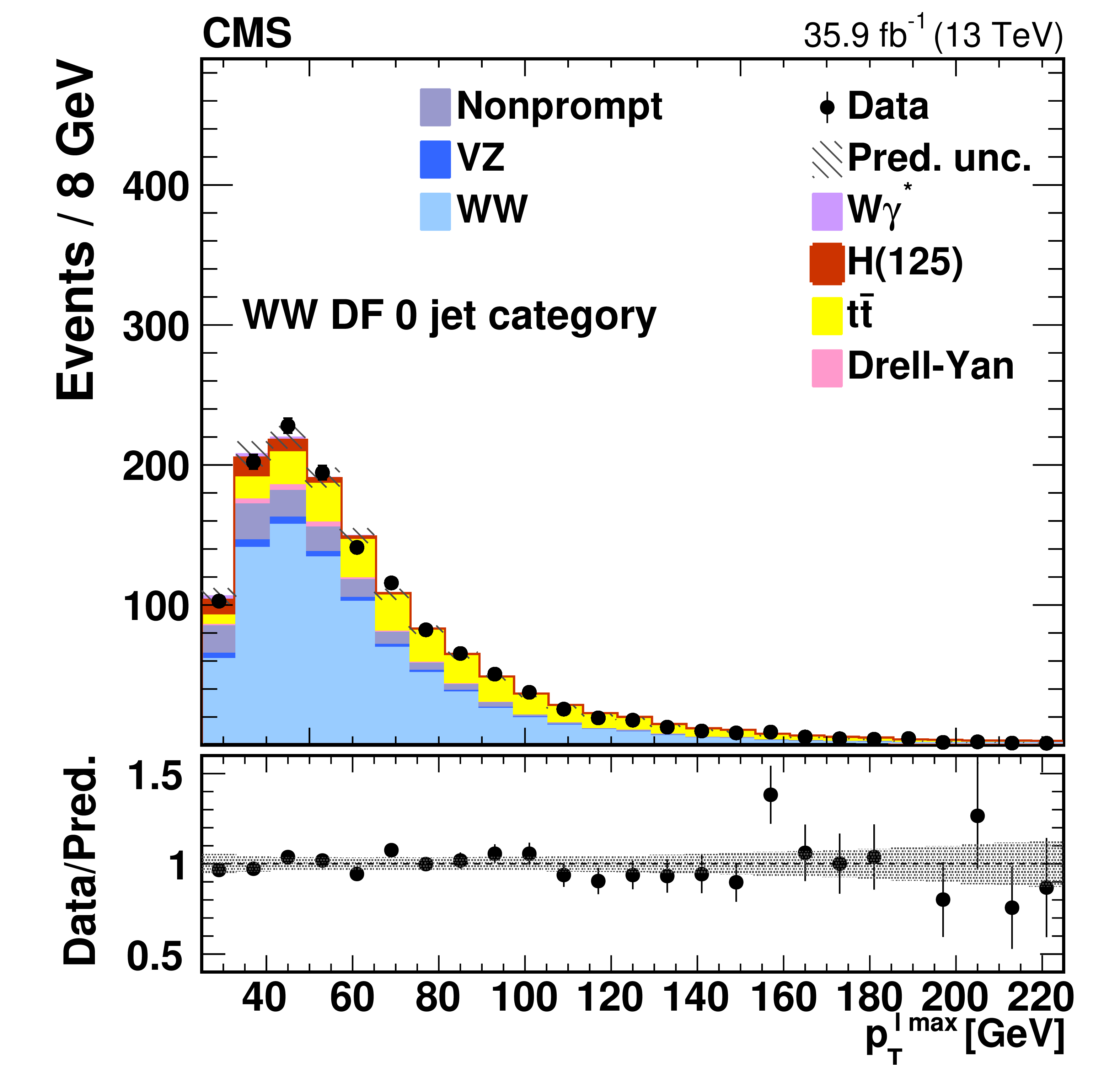
Figure 1-a:
Kinematic distributions for events with zero jets and DF leptons in the sequential cut analysis. The distributions show the leading and trailing lepton ${p_{\mathrm {T}}}$ ($ {{p_{\mathrm {T}}} ^{\ell \, \text {max}}} $ and $ {{p_{\mathrm {T}}} ^{\ell \, \text {min}}} $), the dilepton transverse momentum $ {p_{\mathrm {T}}} ^{\ell \ell}$, the azimuthal angle between the two leptons $ {\Delta \phi _{\ell \ell}} $, the missing transverse momentum ${{p_{\mathrm {T}}} ^\text {miss}}$, and the dilepton invariant mass $ {m_{\ell \ell}} $. The error bars on the data points represent the statistical uncertainty of the data, and the hatched areas represent the combined systematic and statistical uncertainty of the predicted yield in each bin. The last bin includes the overflow. |
png pdf |
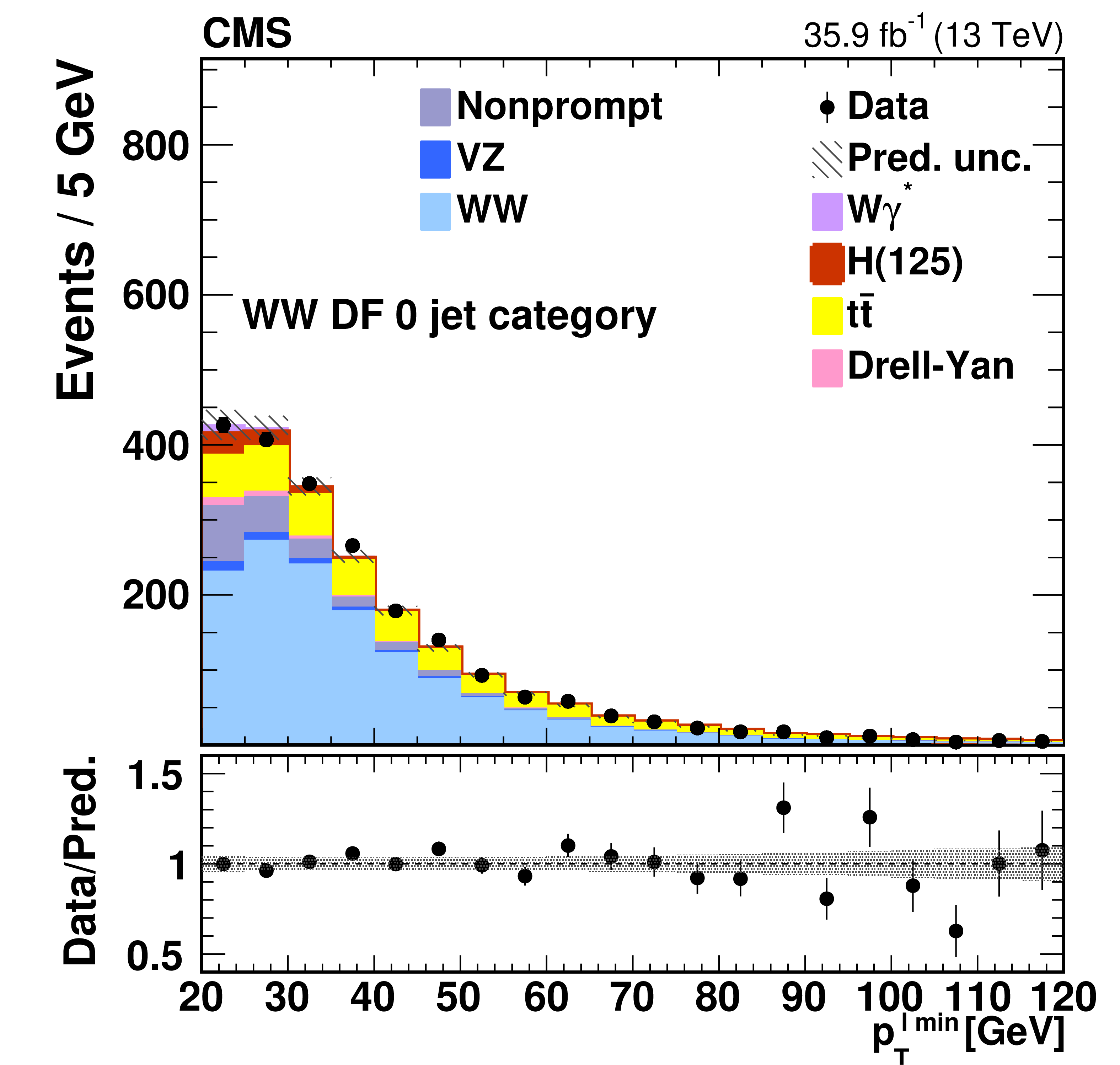
Figure 1-b:
Kinematic distributions for events with zero jets and DF leptons in the sequential cut analysis. The distributions show the leading and trailing lepton ${p_{\mathrm {T}}}$ ($ {{p_{\mathrm {T}}} ^{\ell \, \text {max}}} $ and $ {{p_{\mathrm {T}}} ^{\ell \, \text {min}}} $), the dilepton transverse momentum $ {p_{\mathrm {T}}} ^{\ell \ell}$, the azimuthal angle between the two leptons $ {\Delta \phi _{\ell \ell}} $, the missing transverse momentum ${{p_{\mathrm {T}}} ^\text {miss}}$, and the dilepton invariant mass $ {m_{\ell \ell}} $. The error bars on the data points represent the statistical uncertainty of the data, and the hatched areas represent the combined systematic and statistical uncertainty of the predicted yield in each bin. The last bin includes the overflow. |
png pdf |
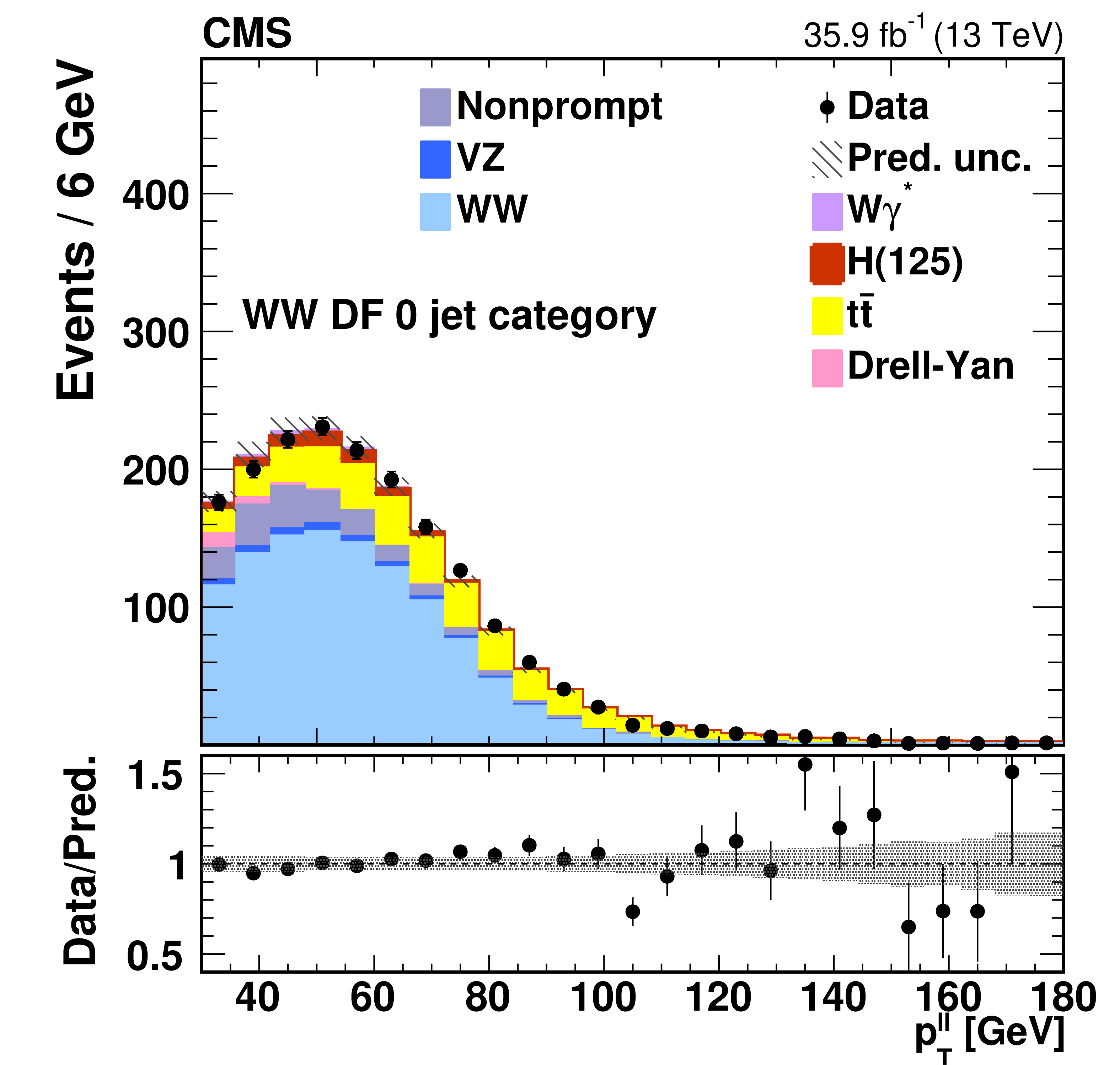
Figure 1-c:
Kinematic distributions for events with zero jets and DF leptons in the sequential cut analysis. The distributions show the leading and trailing lepton ${p_{\mathrm {T}}}$ ($ {{p_{\mathrm {T}}} ^{\ell \, \text {max}}} $ and $ {{p_{\mathrm {T}}} ^{\ell \, \text {min}}} $), the dilepton transverse momentum $ {p_{\mathrm {T}}} ^{\ell \ell}$, the azimuthal angle between the two leptons $ {\Delta \phi _{\ell \ell}} $, the missing transverse momentum ${{p_{\mathrm {T}}} ^\text {miss}}$, and the dilepton invariant mass $ {m_{\ell \ell}} $. The error bars on the data points represent the statistical uncertainty of the data, and the hatched areas represent the combined systematic and statistical uncertainty of the predicted yield in each bin. The last bin includes the overflow. |
png pdf |
Figure 1-d:
Kinematic distributions for events with zero jets and DF leptons in the sequential cut analysis. The distributions show the leading and trailing lepton ${p_{\mathrm {T}}}$ ($ {{p_{\mathrm {T}}} ^{\ell \, \text {max}}} $ and $ {{p_{\mathrm {T}}} ^{\ell \, \text {min}}} $), the dilepton transverse momentum $ {p_{\mathrm {T}}} ^{\ell \ell}$, the azimuthal angle between the two leptons $ {\Delta \phi _{\ell \ell}} $, the missing transverse momentum ${{p_{\mathrm {T}}} ^\text {miss}}$, and the dilepton invariant mass $ {m_{\ell \ell}} $. The error bars on the data points represent the statistical uncertainty of the data, and the hatched areas represent the combined systematic and statistical uncertainty of the predicted yield in each bin. The last bin includes the overflow. |
png pdf |
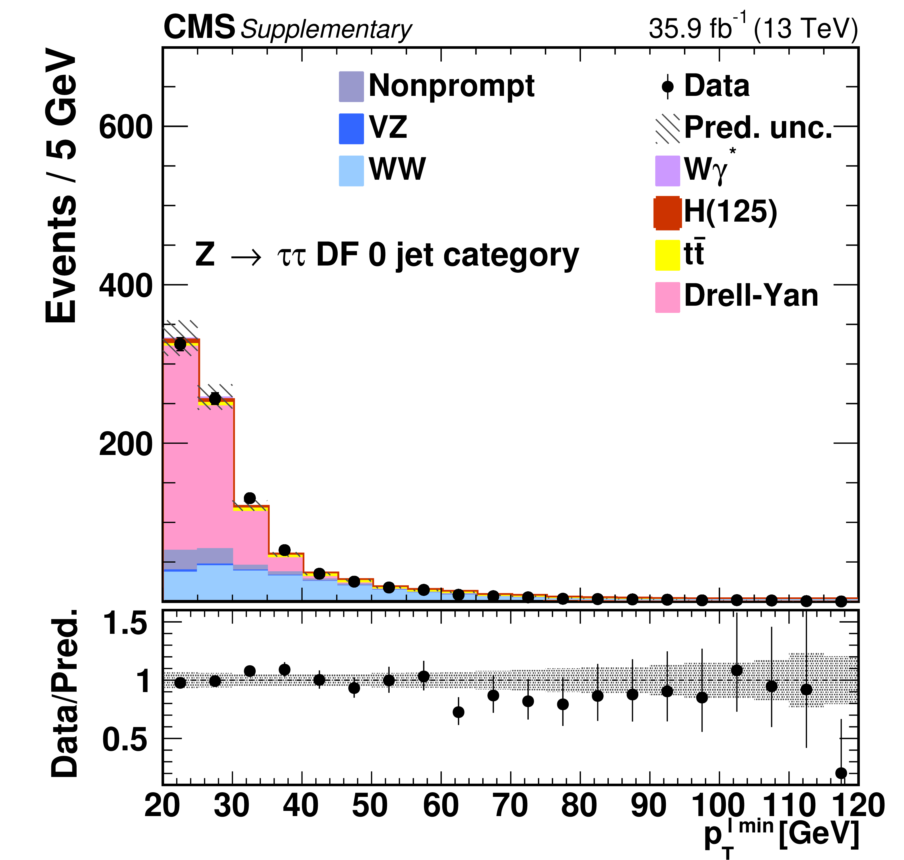
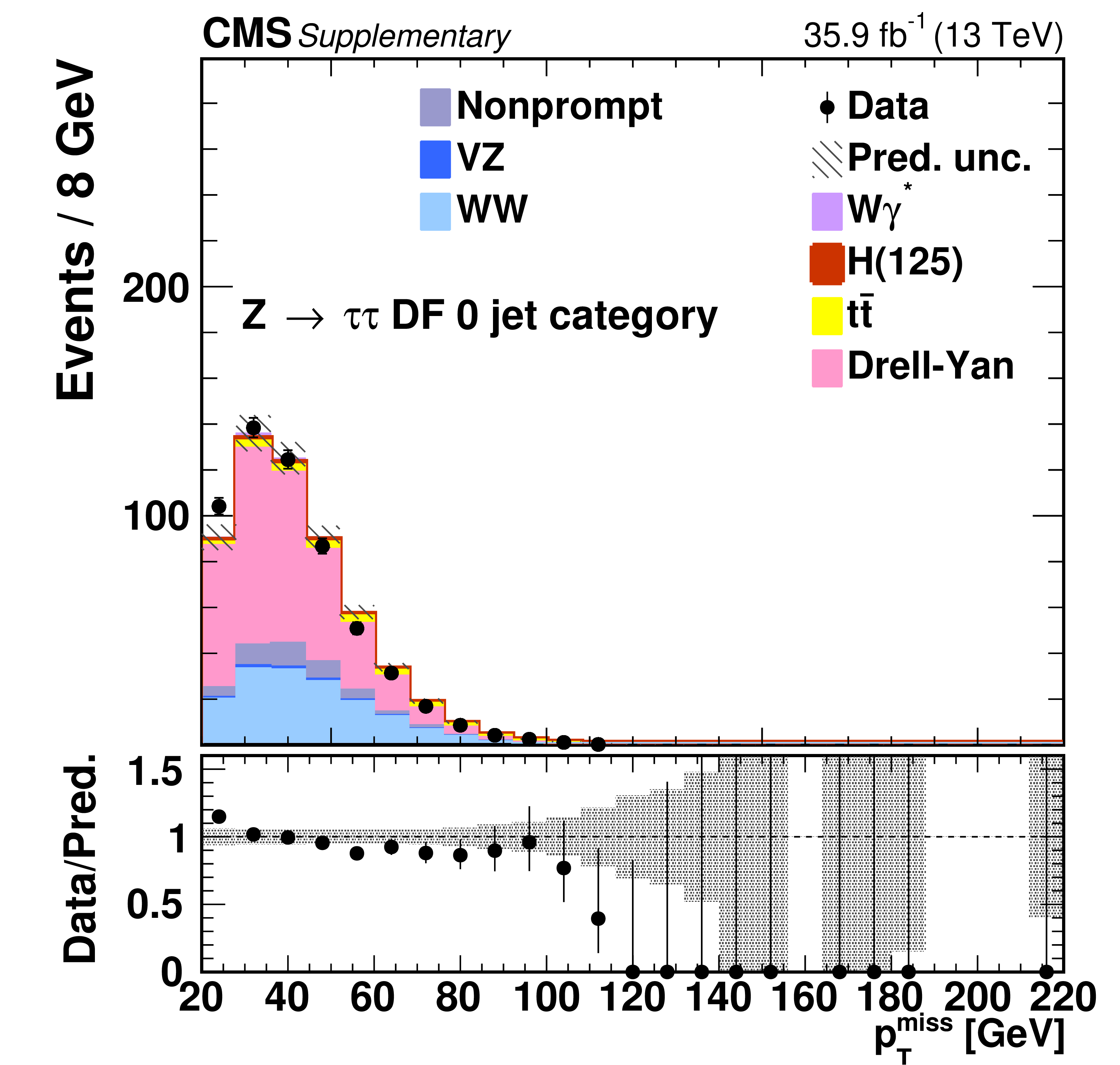
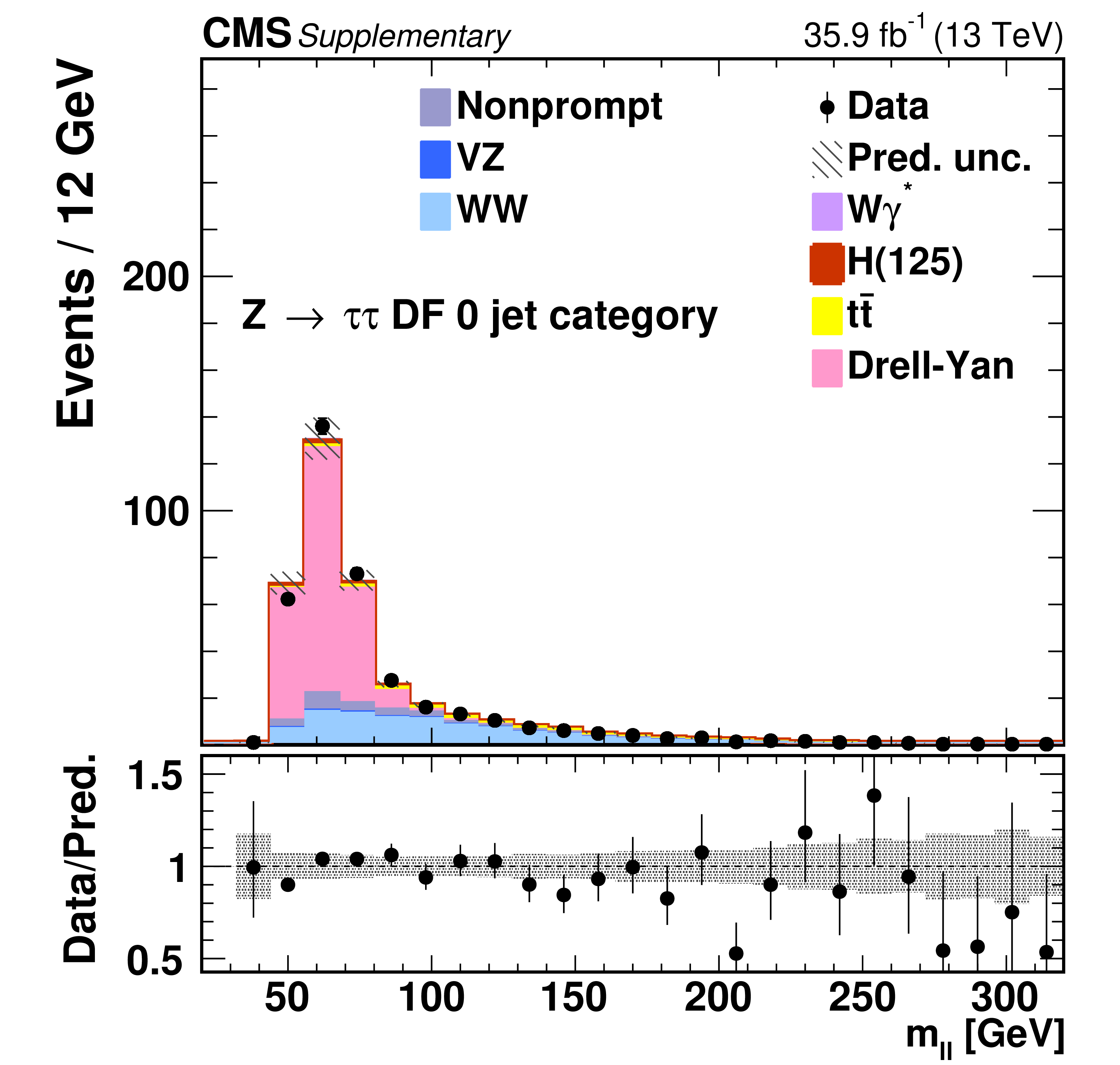
Figure 1-e:
Kinematic distributions for events with zero jets and DF leptons in the sequential cut analysis. The distributions show the leading and trailing lepton ${p_{\mathrm {T}}}$ ($ {{p_{\mathrm {T}}} ^{\ell \, \text {max}}} $ and $ {{p_{\mathrm {T}}} ^{\ell \, \text {min}}} $), the dilepton transverse momentum $ {p_{\mathrm {T}}} ^{\ell \ell}$, the azimuthal angle between the two leptons $ {\Delta \phi _{\ell \ell}} $, the missing transverse momentum ${{p_{\mathrm {T}}} ^\text {miss}}$, and the dilepton invariant mass $ {m_{\ell \ell}} $. The error bars on the data points represent the statistical uncertainty of the data, and the hatched areas represent the combined systematic and statistical uncertainty of the predicted yield in each bin. The last bin includes the overflow. |
png pdf |
Figure 1-f:
Kinematic distributions for events with zero jets and DF leptons in the sequential cut analysis. The distributions show the leading and trailing lepton ${p_{\mathrm {T}}}$ ($ {{p_{\mathrm {T}}} ^{\ell \, \text {max}}} $ and $ {{p_{\mathrm {T}}} ^{\ell \, \text {min}}} $), the dilepton transverse momentum $ {p_{\mathrm {T}}} ^{\ell \ell}$, the azimuthal angle between the two leptons $ {\Delta \phi _{\ell \ell}} $, the missing transverse momentum ${{p_{\mathrm {T}}} ^\text {miss}}$, and the dilepton invariant mass $ {m_{\ell \ell}} $. The error bars on the data points represent the statistical uncertainty of the data, and the hatched areas represent the combined systematic and statistical uncertainty of the predicted yield in each bin. The last bin includes the overflow. |
png pdf |
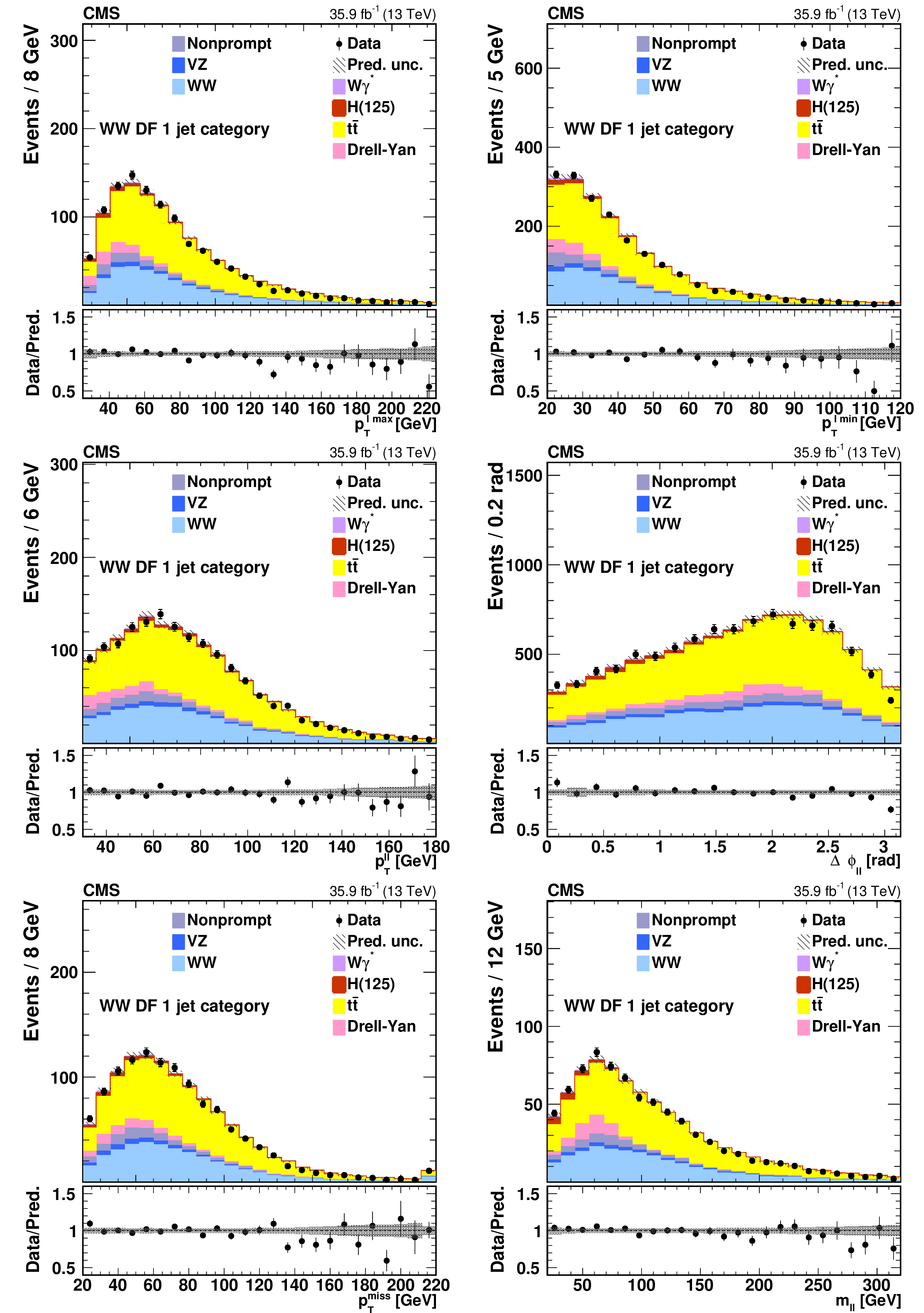
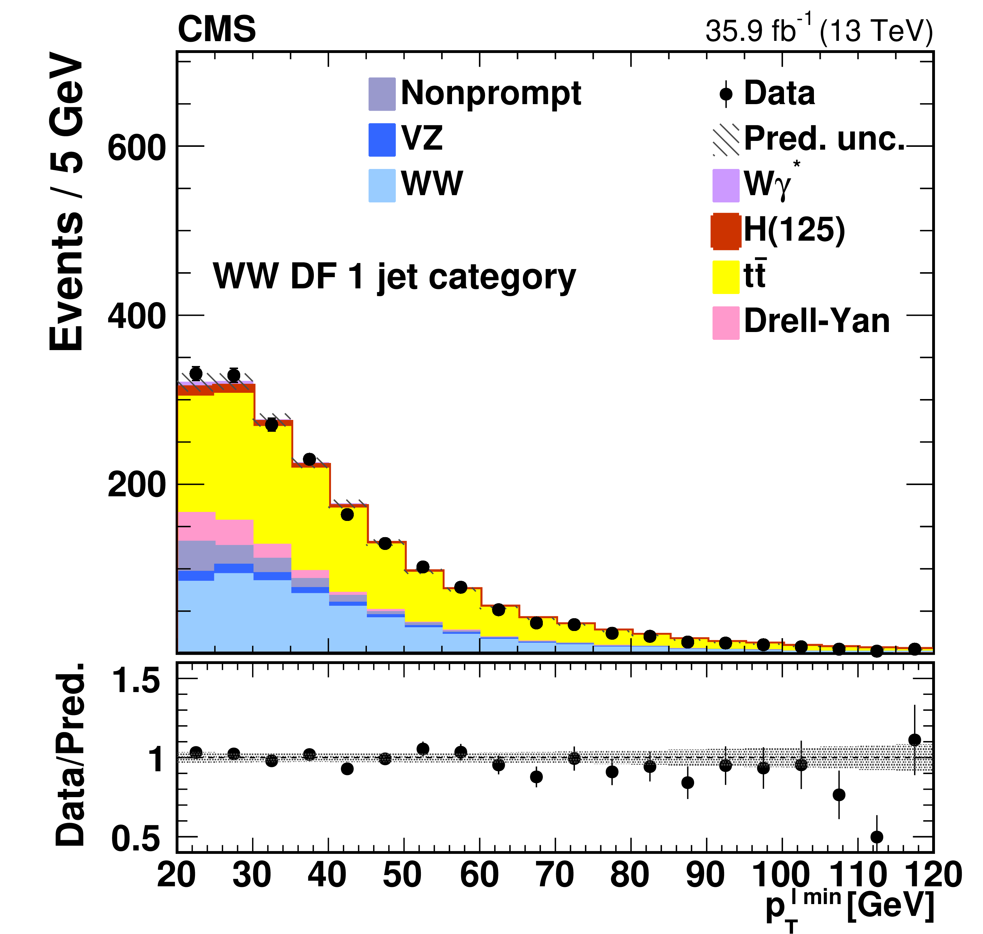
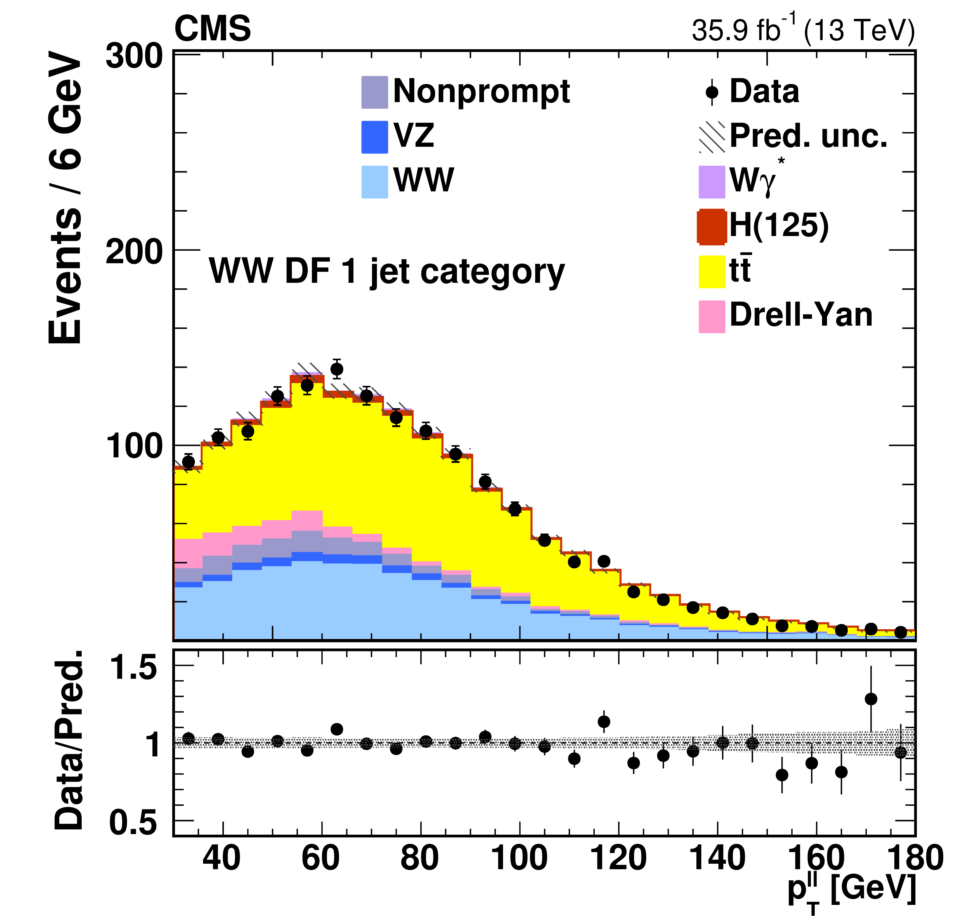
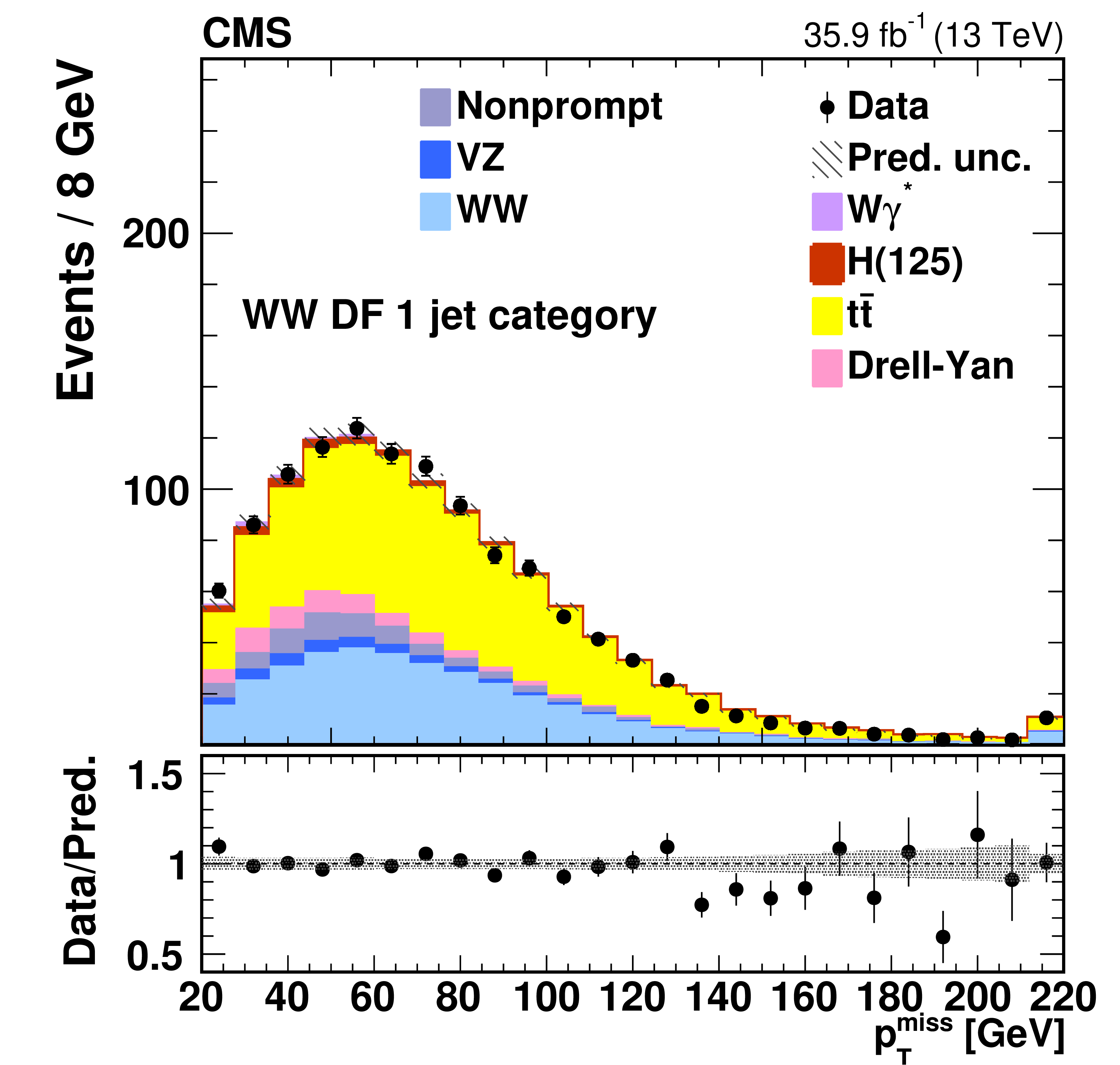
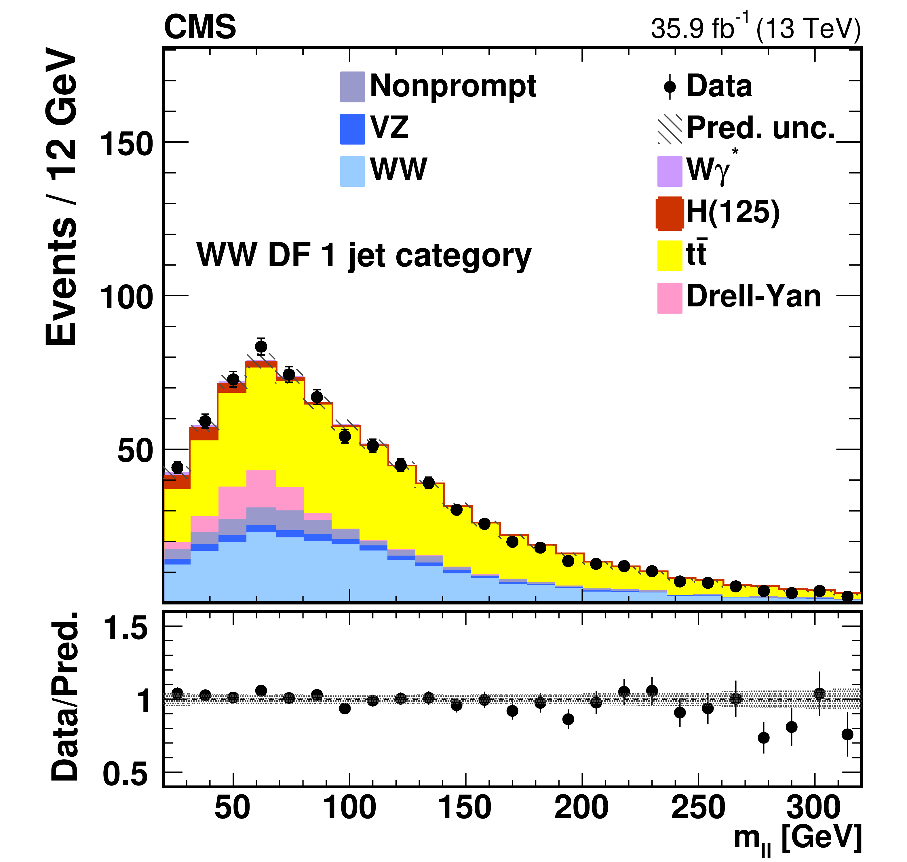
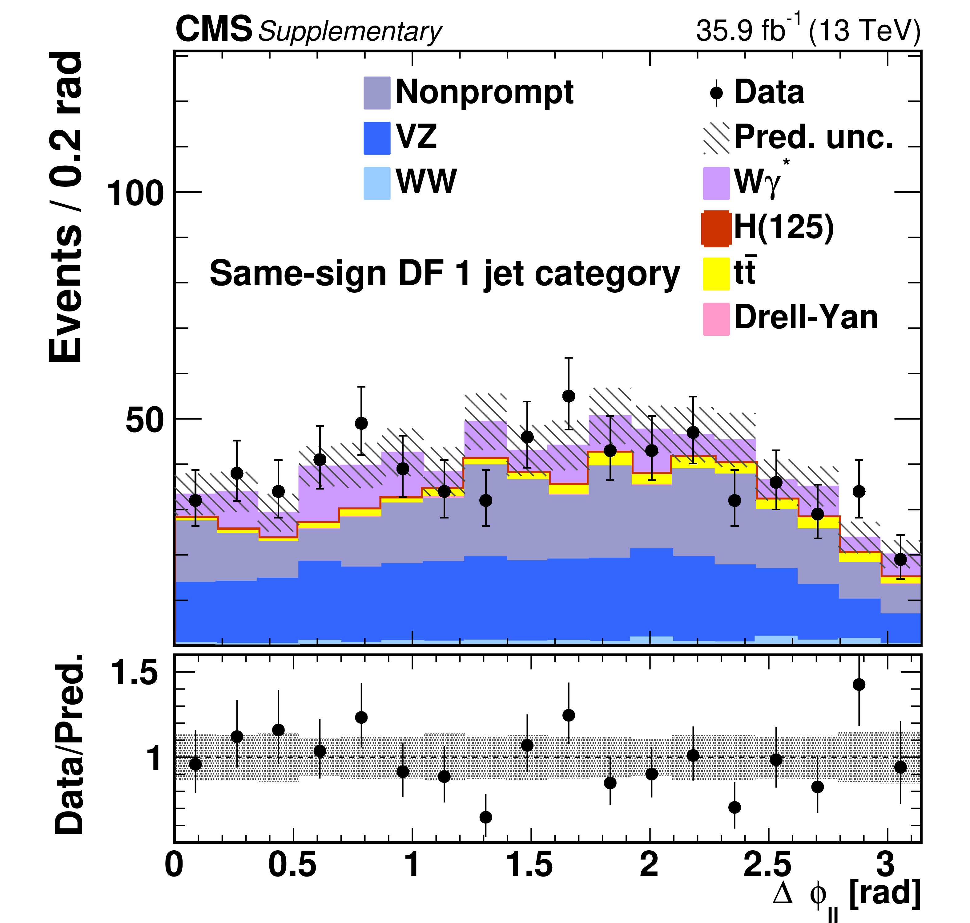
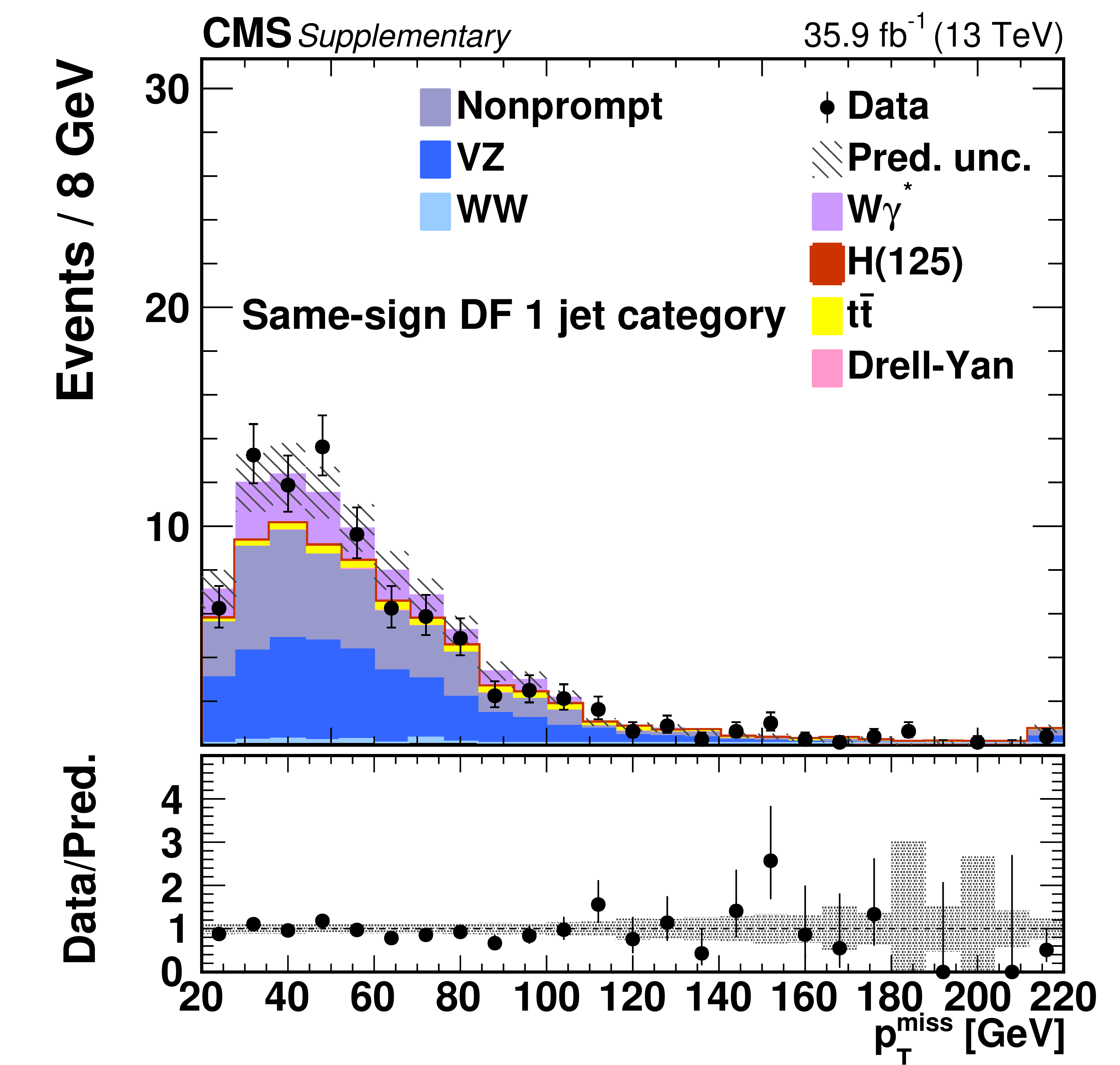
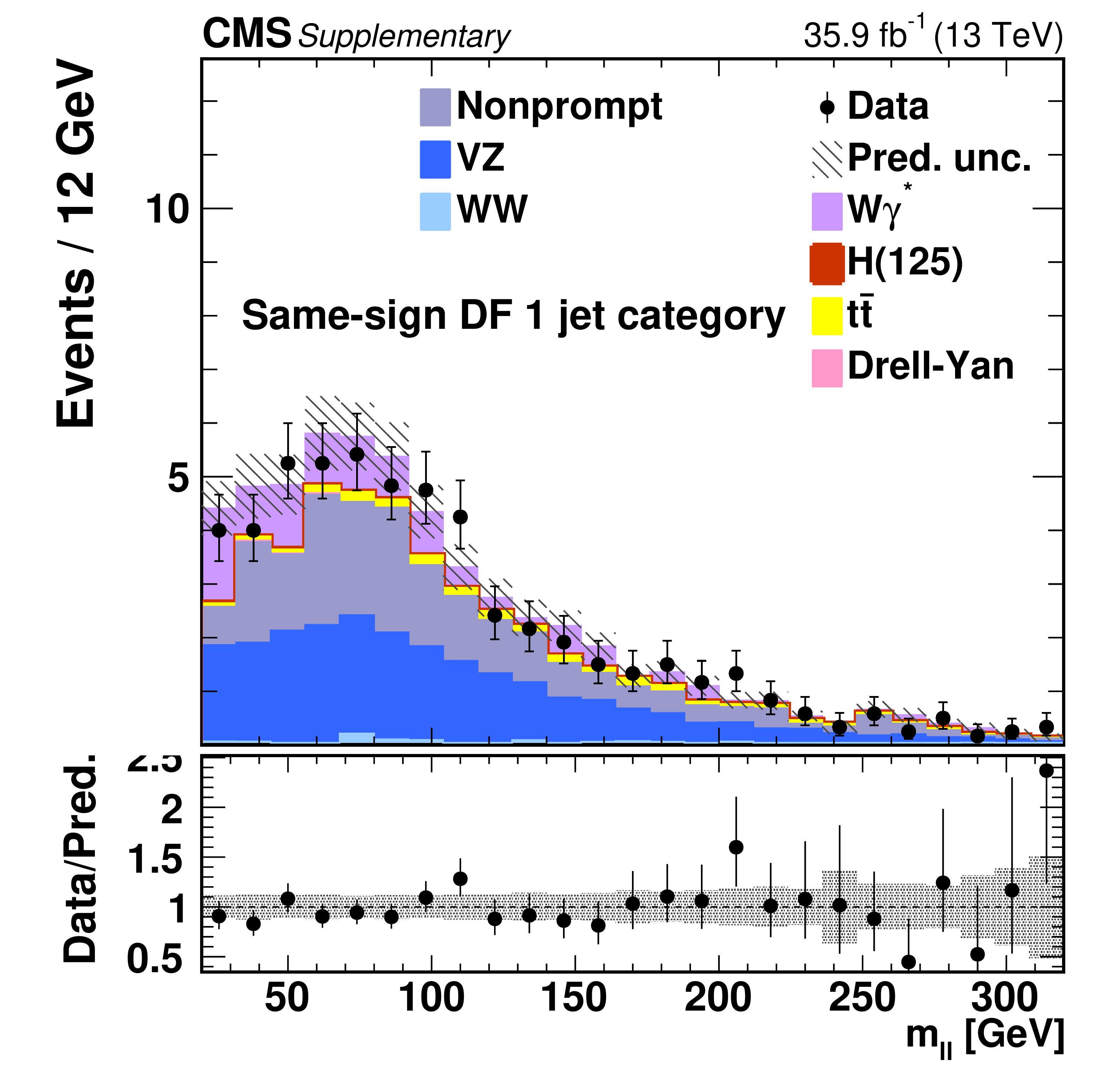
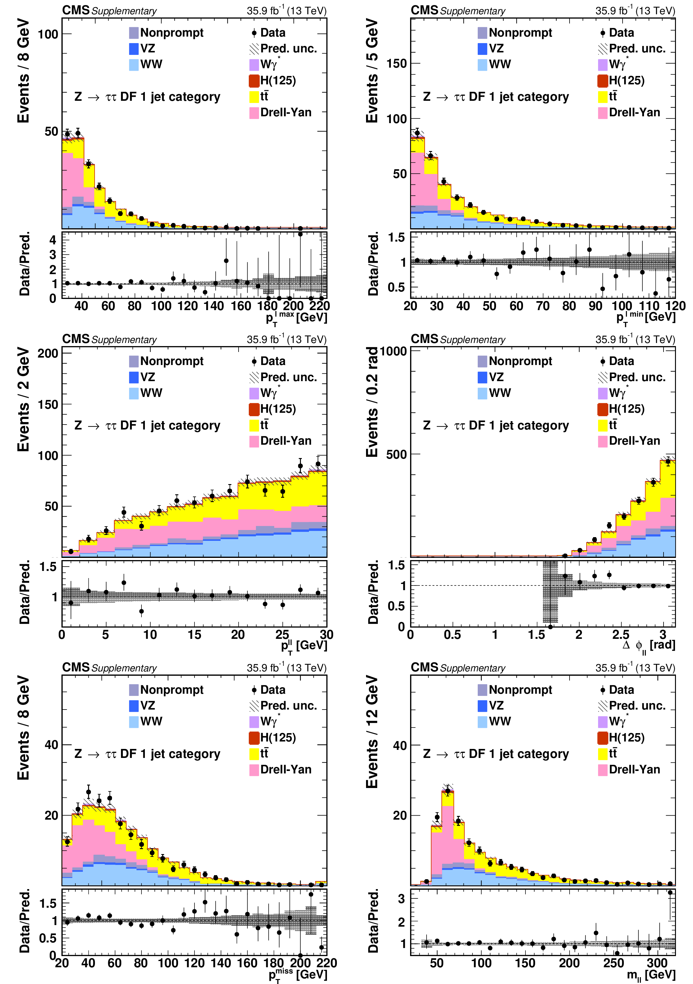
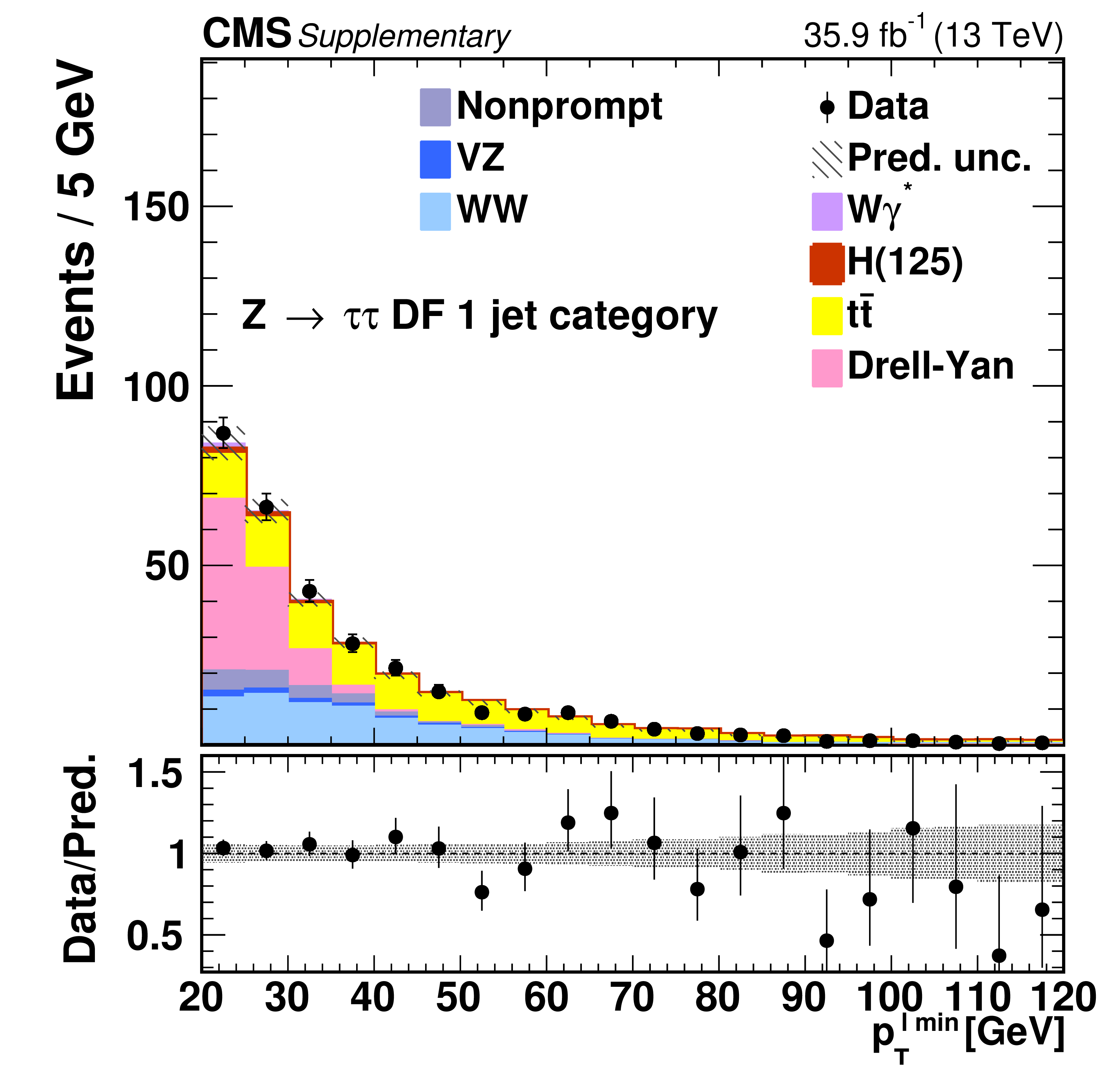
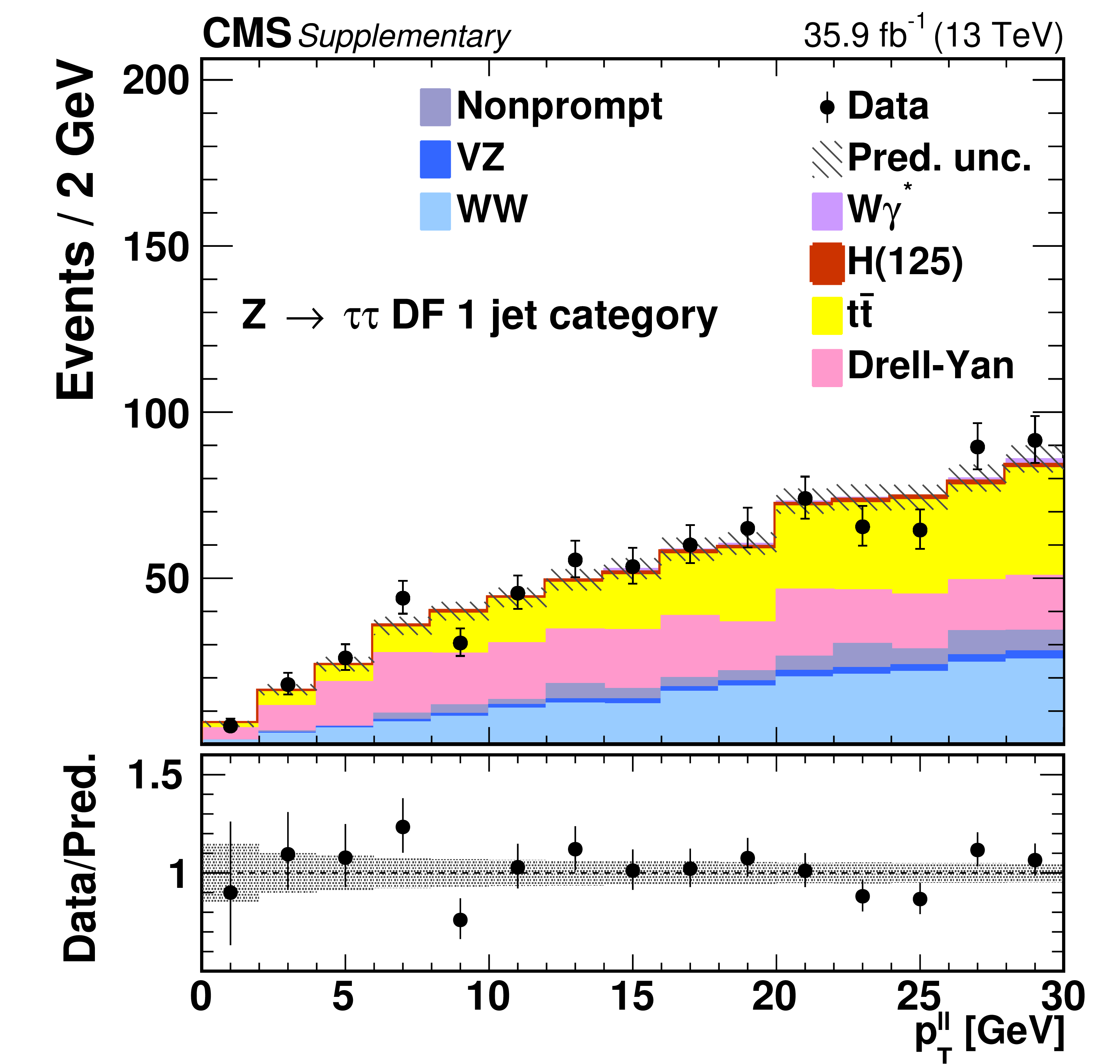
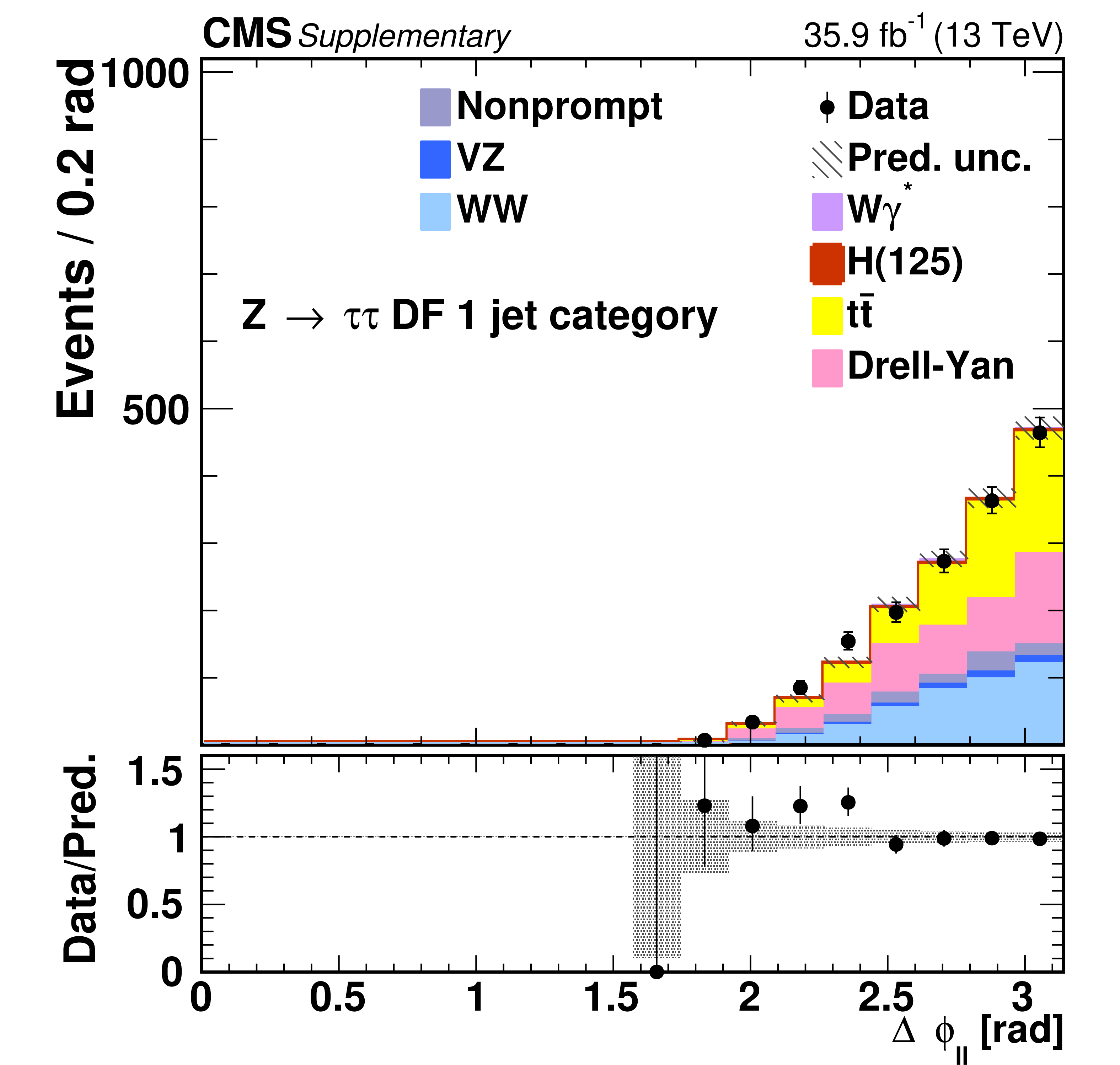
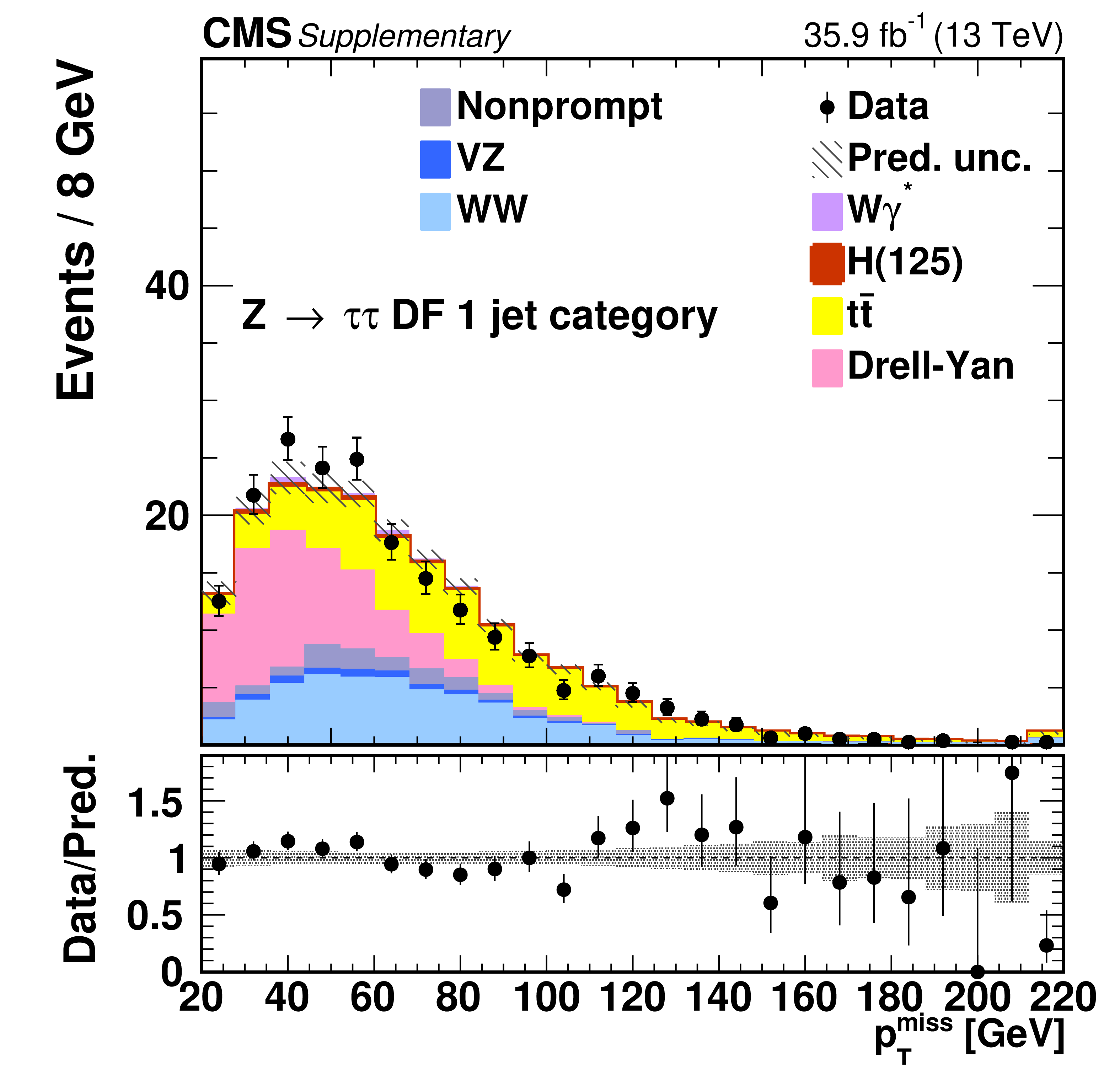
Figure 2:
Kinematic distributions for events with exactly one jet and DF leptons in the sequential cut analysis. The quantities, error bars, and hatched areas are the same as in Fig. 1. |

png pdf |
Figure 2-a:
Kinematic distributions for events with exactly one jet and DF leptons in the sequential cut analysis. The quantities, error bars, and hatched areas are the same as in Fig. 1. |
png pdf |
Figure 2-b:
Kinematic distributions for events with exactly one jet and DF leptons in the sequential cut analysis. The quantities, error bars, and hatched areas are the same as in Fig. 1. |
png pdf |
Figure 2-c:
Kinematic distributions for events with exactly one jet and DF leptons in the sequential cut analysis. The quantities, error bars, and hatched areas are the same as in Fig. 1. |

png pdf |
Figure 2-d:
Kinematic distributions for events with exactly one jet and DF leptons in the sequential cut analysis. The quantities, error bars, and hatched areas are the same as in Fig. 1. |
png pdf |
Figure 2-e:
Kinematic distributions for events with exactly one jet and DF leptons in the sequential cut analysis. The quantities, error bars, and hatched areas are the same as in Fig. 1. |
png pdf |
Figure 2-f:
Kinematic distributions for events with exactly one jet and DF leptons in the sequential cut analysis. The quantities, error bars, and hatched areas are the same as in Fig. 1. |
png pdf |
Figure 3:
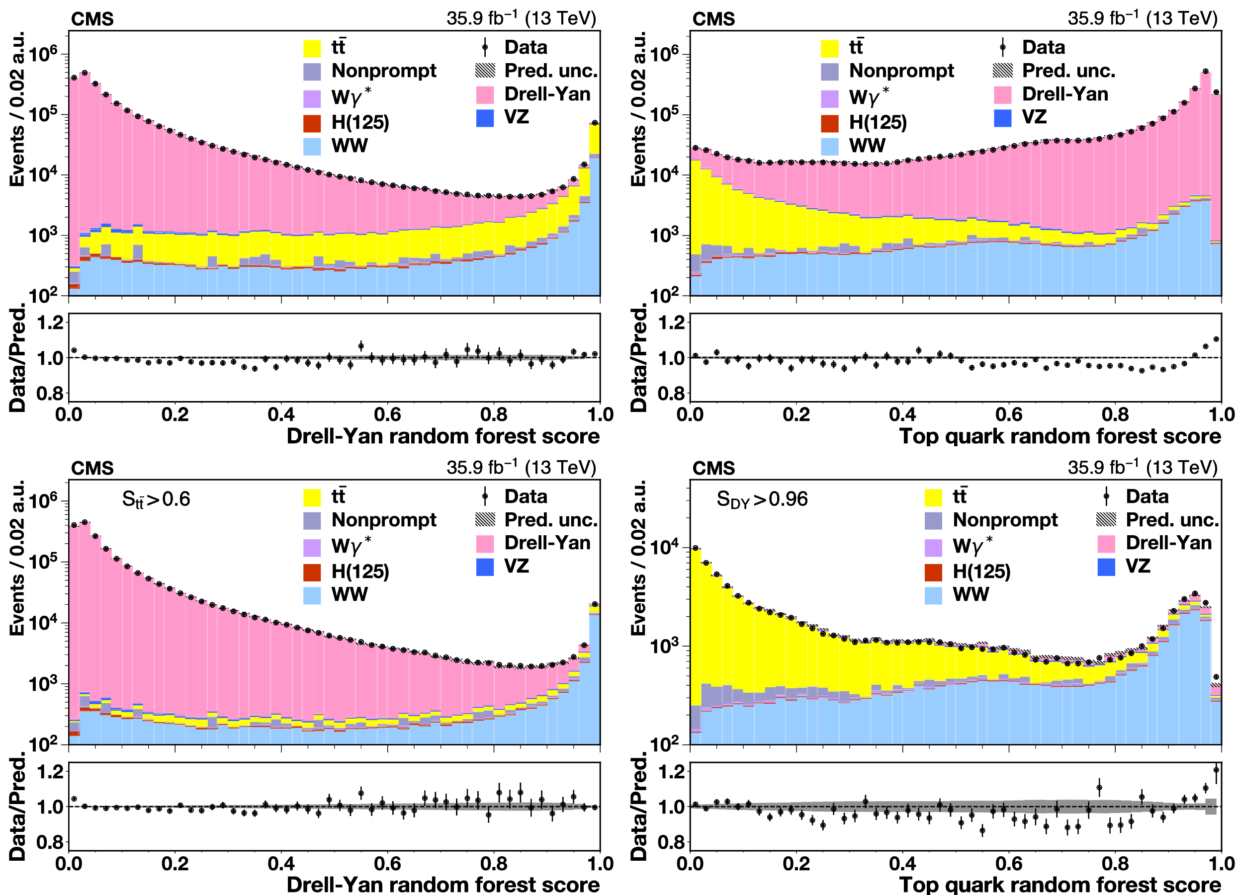
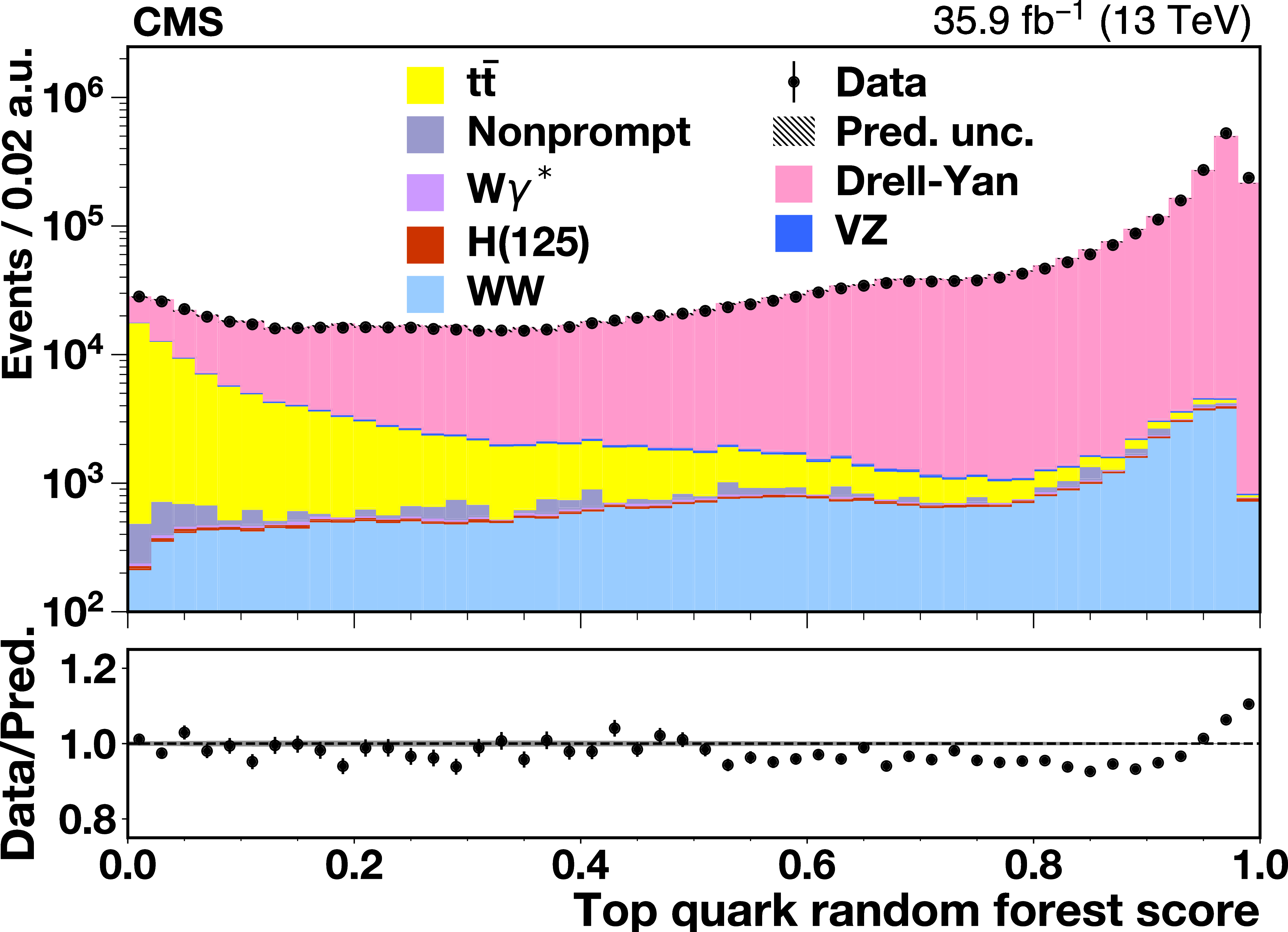
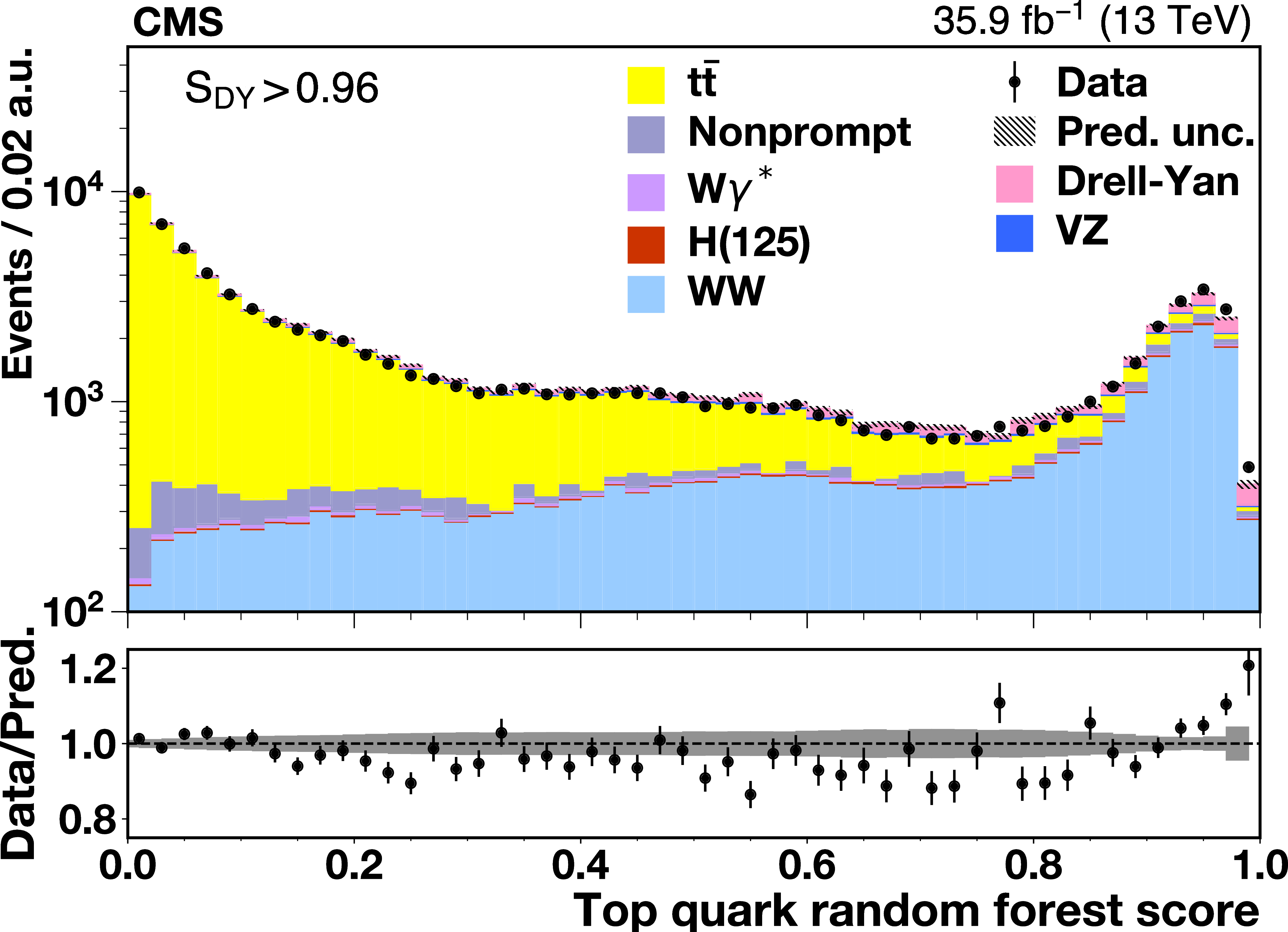
Top left: score $S_{\text {DY}}$ distribution for the Drell-Yan discriminating random forest discriminant. The Drell-Yan distribution peaks toward zero and the ${\mathrm{W^{+}}W^{-}}$ distribution peaks toward one. Top right: score $S_{{\mathrm{t} {}\mathrm{\bar{t}}}}$ distribution for the top quark random forest discriminant. The ${\mathrm{t} {}\mathrm{\bar{t}}}$ distribution peaks toward zero and the ${\mathrm{W^{+}}W^{-}}$ peaks toward one. Bottom left: the $S_{\text {DY}}$ distribution after suppressing top quark events with $S_{{\mathrm{t} {}\mathrm{\bar{t}}}} > S_{{\mathrm{t} {}\mathrm{\bar{t}}}}^{\text {min}}=$ 0.6. Bottom right: the $S_{{\mathrm{t} {}\mathrm{\bar{t}}}}$ distribution after suppressing Drell-Yan events with $S_{\text {DY}} > S_{\text {DY}}^{\text {min}}=$ 0.96. The error bars on the points represent the statistical uncertainties for the data, and the hatched areas represent the combined systematic and statistical uncertainties of the predicted yield in each bin. |

png pdf |
Figure 3-a:
Top left: score $S_{\text {DY}}$ distribution for the Drell-Yan discriminating random forest discriminant. The Drell-Yan distribution peaks toward zero and the ${\mathrm{W^{+}}W^{-}}$ distribution peaks toward one. Top right: score $S_{{\mathrm{t} {}\mathrm{\bar{t}}}}$ distribution for the top quark random forest discriminant. The ${\mathrm{t} {}\mathrm{\bar{t}}}$ distribution peaks toward zero and the ${\mathrm{W^{+}}W^{-}}$ peaks toward one. Bottom left: the $S_{\text {DY}}$ distribution after suppressing top quark events with $S_{{\mathrm{t} {}\mathrm{\bar{t}}}} > S_{{\mathrm{t} {}\mathrm{\bar{t}}}}^{\text {min}}=$ 0.6. Bottom right: the $S_{{\mathrm{t} {}\mathrm{\bar{t}}}}$ distribution after suppressing Drell-Yan events with $S_{\text {DY}} > S_{\text {DY}}^{\text {min}}=$ 0.96. The error bars on the points represent the statistical uncertainties for the data, and the hatched areas represent the combined systematic and statistical uncertainties of the predicted yield in each bin. |
png pdf |
Figure 3-b:
Top left: score $S_{\text {DY}}$ distribution for the Drell-Yan discriminating random forest discriminant. The Drell-Yan distribution peaks toward zero and the ${\mathrm{W^{+}}W^{-}}$ distribution peaks toward one. Top right: score $S_{{\mathrm{t} {}\mathrm{\bar{t}}}}$ distribution for the top quark random forest discriminant. The ${\mathrm{t} {}\mathrm{\bar{t}}}$ distribution peaks toward zero and the ${\mathrm{W^{+}}W^{-}}$ peaks toward one. Bottom left: the $S_{\text {DY}}$ distribution after suppressing top quark events with $S_{{\mathrm{t} {}\mathrm{\bar{t}}}} > S_{{\mathrm{t} {}\mathrm{\bar{t}}}}^{\text {min}}=$ 0.6. Bottom right: the $S_{{\mathrm{t} {}\mathrm{\bar{t}}}}$ distribution after suppressing Drell-Yan events with $S_{\text {DY}} > S_{\text {DY}}^{\text {min}}=$ 0.96. The error bars on the points represent the statistical uncertainties for the data, and the hatched areas represent the combined systematic and statistical uncertainties of the predicted yield in each bin. |

png pdf |
Figure 3-c:
Top left: score $S_{\text {DY}}$ distribution for the Drell-Yan discriminating random forest discriminant. The Drell-Yan distribution peaks toward zero and the ${\mathrm{W^{+}}W^{-}}$ distribution peaks toward one. Top right: score $S_{{\mathrm{t} {}\mathrm{\bar{t}}}}$ distribution for the top quark random forest discriminant. The ${\mathrm{t} {}\mathrm{\bar{t}}}$ distribution peaks toward zero and the ${\mathrm{W^{+}}W^{-}}$ peaks toward one. Bottom left: the $S_{\text {DY}}$ distribution after suppressing top quark events with $S_{{\mathrm{t} {}\mathrm{\bar{t}}}} > S_{{\mathrm{t} {}\mathrm{\bar{t}}}}^{\text {min}}=$ 0.6. Bottom right: the $S_{{\mathrm{t} {}\mathrm{\bar{t}}}}$ distribution after suppressing Drell-Yan events with $S_{\text {DY}} > S_{\text {DY}}^{\text {min}}=$ 0.96. The error bars on the points represent the statistical uncertainties for the data, and the hatched areas represent the combined systematic and statistical uncertainties of the predicted yield in each bin. |
png pdf |
Figure 3-d:
Top left: score $S_{\text {DY}}$ distribution for the Drell-Yan discriminating random forest discriminant. The Drell-Yan distribution peaks toward zero and the ${\mathrm{W^{+}}W^{-}}$ distribution peaks toward one. Top right: score $S_{{\mathrm{t} {}\mathrm{\bar{t}}}}$ distribution for the top quark random forest discriminant. The ${\mathrm{t} {}\mathrm{\bar{t}}}$ distribution peaks toward zero and the ${\mathrm{W^{+}}W^{-}}$ peaks toward one. Bottom left: the $S_{\text {DY}}$ distribution after suppressing top quark events with $S_{{\mathrm{t} {}\mathrm{\bar{t}}}} > S_{{\mathrm{t} {}\mathrm{\bar{t}}}}^{\text {min}}=$ 0.6. Bottom right: the $S_{{\mathrm{t} {}\mathrm{\bar{t}}}}$ distribution after suppressing Drell-Yan events with $S_{\text {DY}} > S_{\text {DY}}^{\text {min}}=$ 0.96. The error bars on the points represent the statistical uncertainties for the data, and the hatched areas represent the combined systematic and statistical uncertainties of the predicted yield in each bin. |

png pdf |
Figure 4:
Comparison of efficiencies for the sequential cut and random forest analyses as a function of ${{p_{\mathrm {T}}} ^{\mathrm{W} \mathrm{W}}}$. The sequential cut analysis includes 0- and 1-jet events from both DF and SF lepton combinations, for which the contributions from 0- and 1-jet are shown separately. The efficiency curve for $S_{{\mathrm{t} {}\mathrm{\bar{t}}}}^{\text {min}}= $ 0.2 is also shown; this value is used in measuring the jet multiplicity distribution. |
png pdf |
Figure 5:
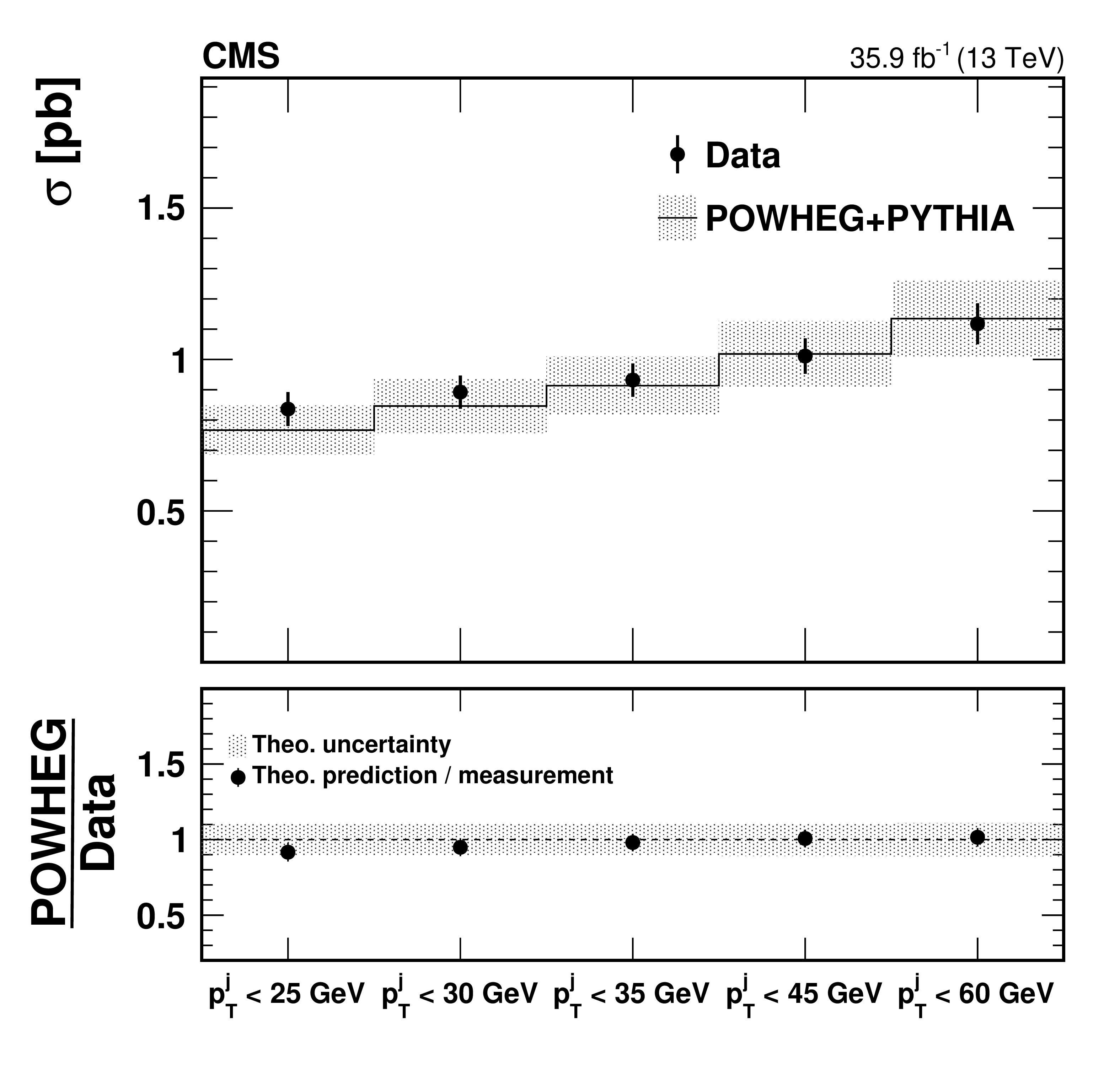
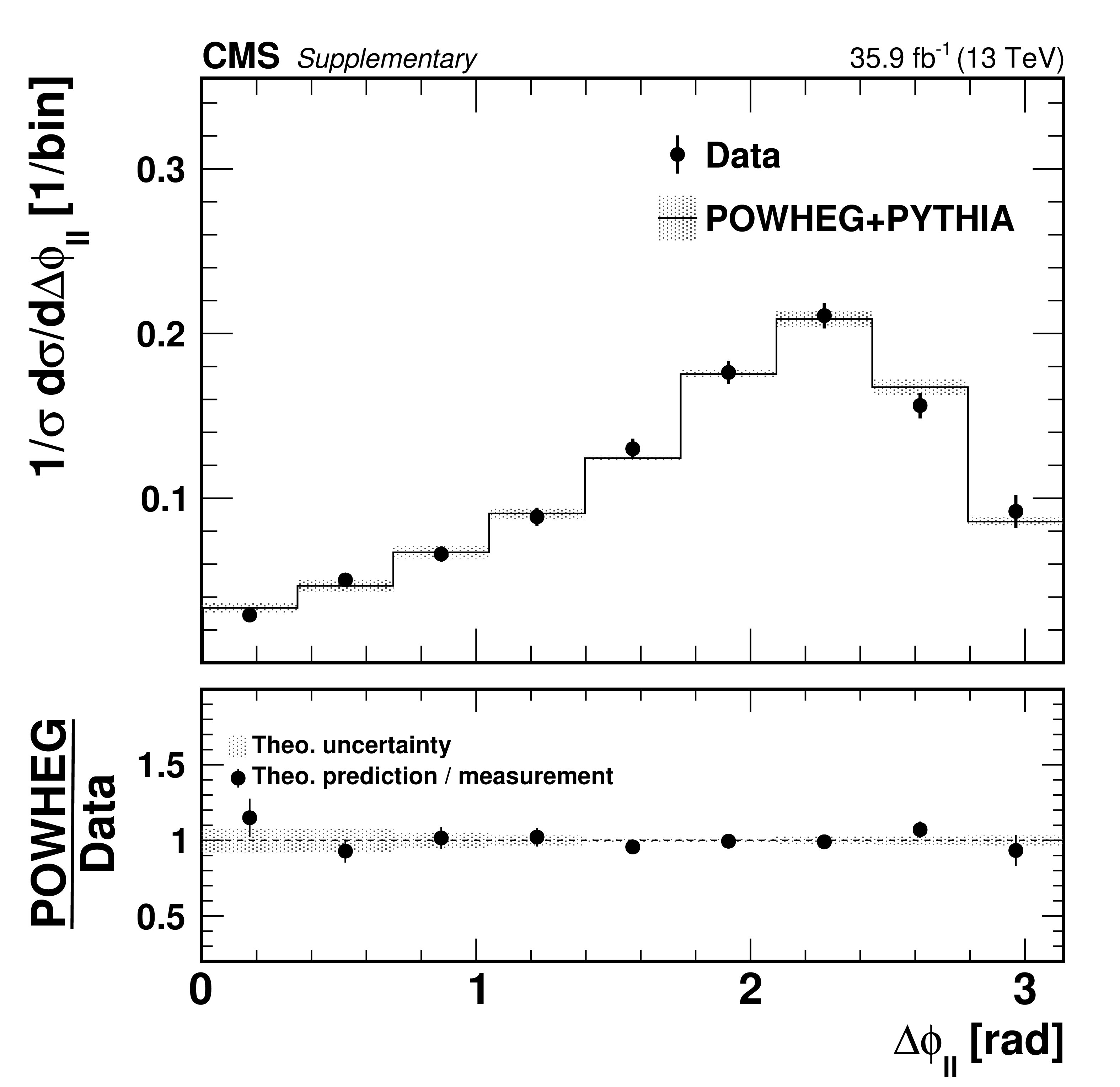
The upper panel shows the fiducial cross sections for the production of $ {\mathrm{W^{+}} \mathrm{W^{-}}} $+0-jets as the ${p_{\mathrm {T}}}$ threshold for jets is varied. The fiducial region is defined by two opposite-sign leptons with $ {p_{\mathrm {T}}} > $ 20 GeV and $ {| \eta |} < $ 2.5 excluding the products of $\tau $ lepton decay, and $ {m_{\ell \ell}} > $ 20 GeV, $ {p_{\mathrm {T}}} ^{\ell \ell} > $ 30 GeV, and $ {{p_{\mathrm {T}}} ^\text {miss}} > $ 30 GeV. Jets must have $ {p_{\mathrm {T}}} $ above the stated threshold, $ {| \eta |} < $ 4.5, and be separated from each of the two leptons by $\Delta R > $ 0.4. The lower panel shows the ratio of the theoretical prediction to the measurement. In both the upper and lower panels, the error bars on the data points represent the total uncertainty of the measurement, and the shaded band depicts the uncertainty of the MC prediction. |

png pdf |
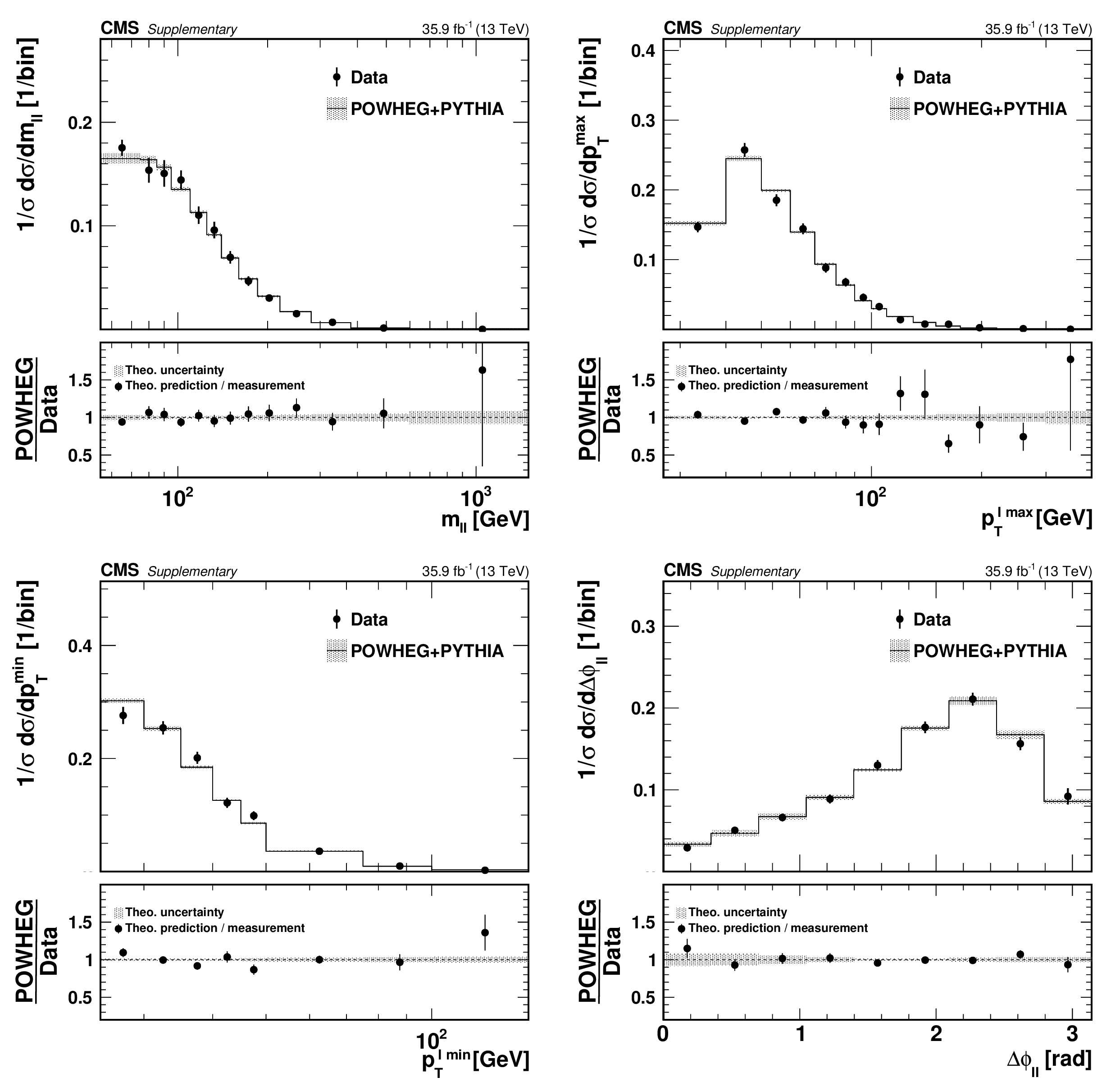
Figure 6:
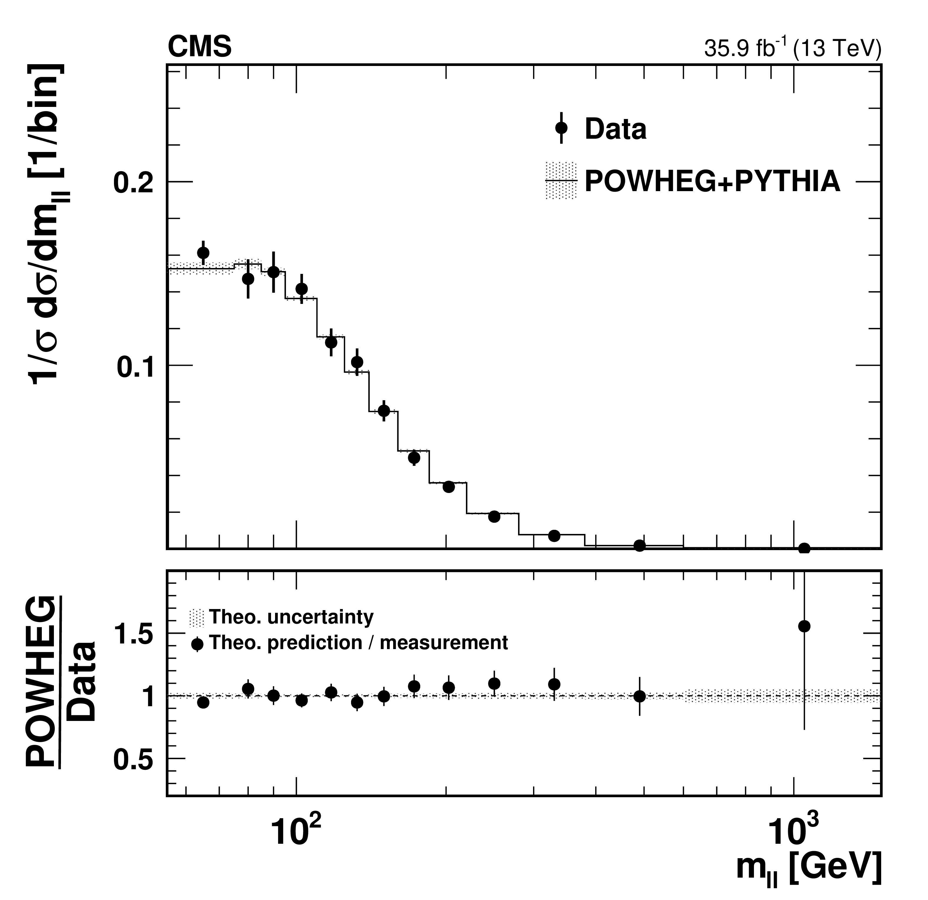
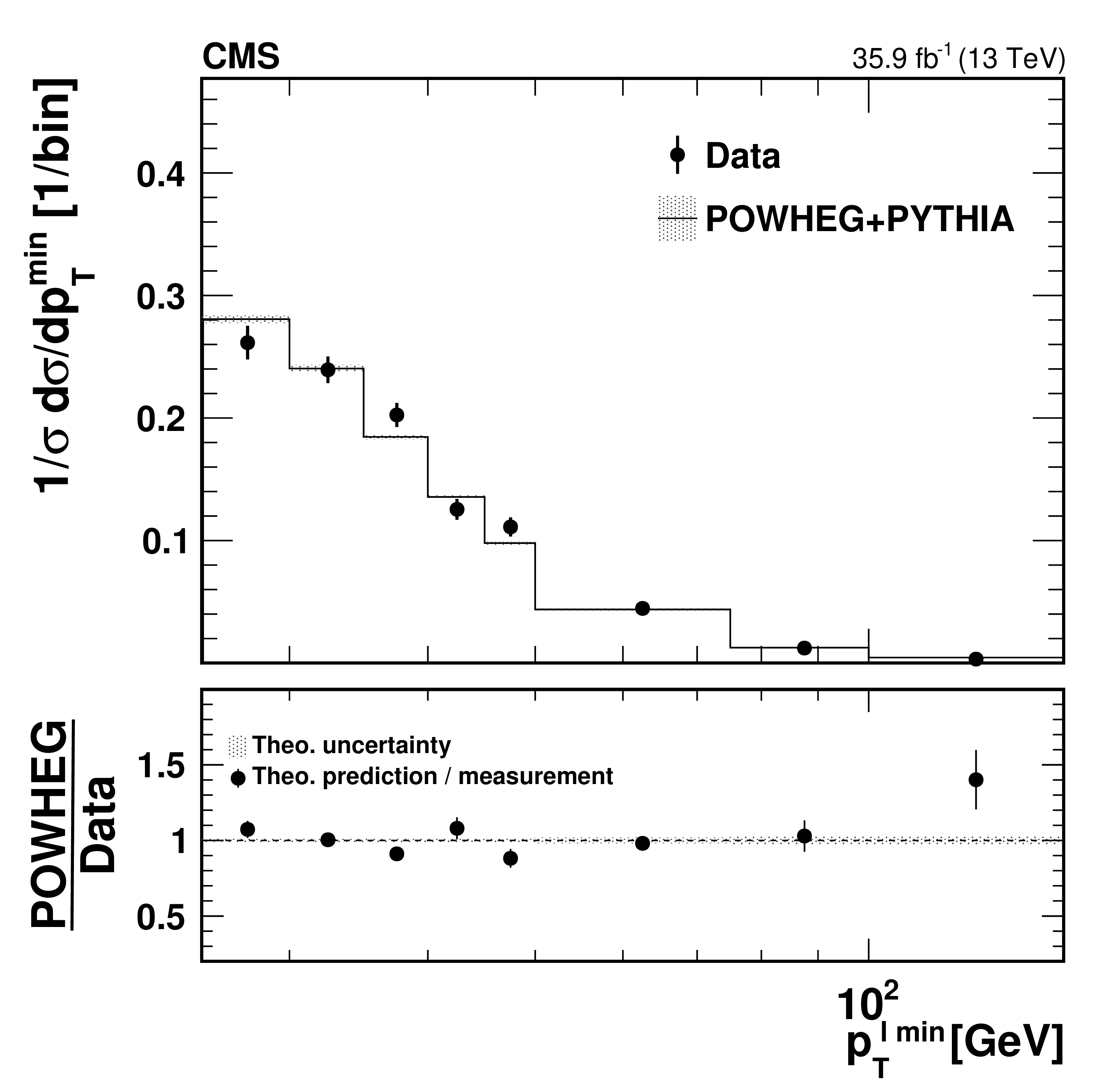
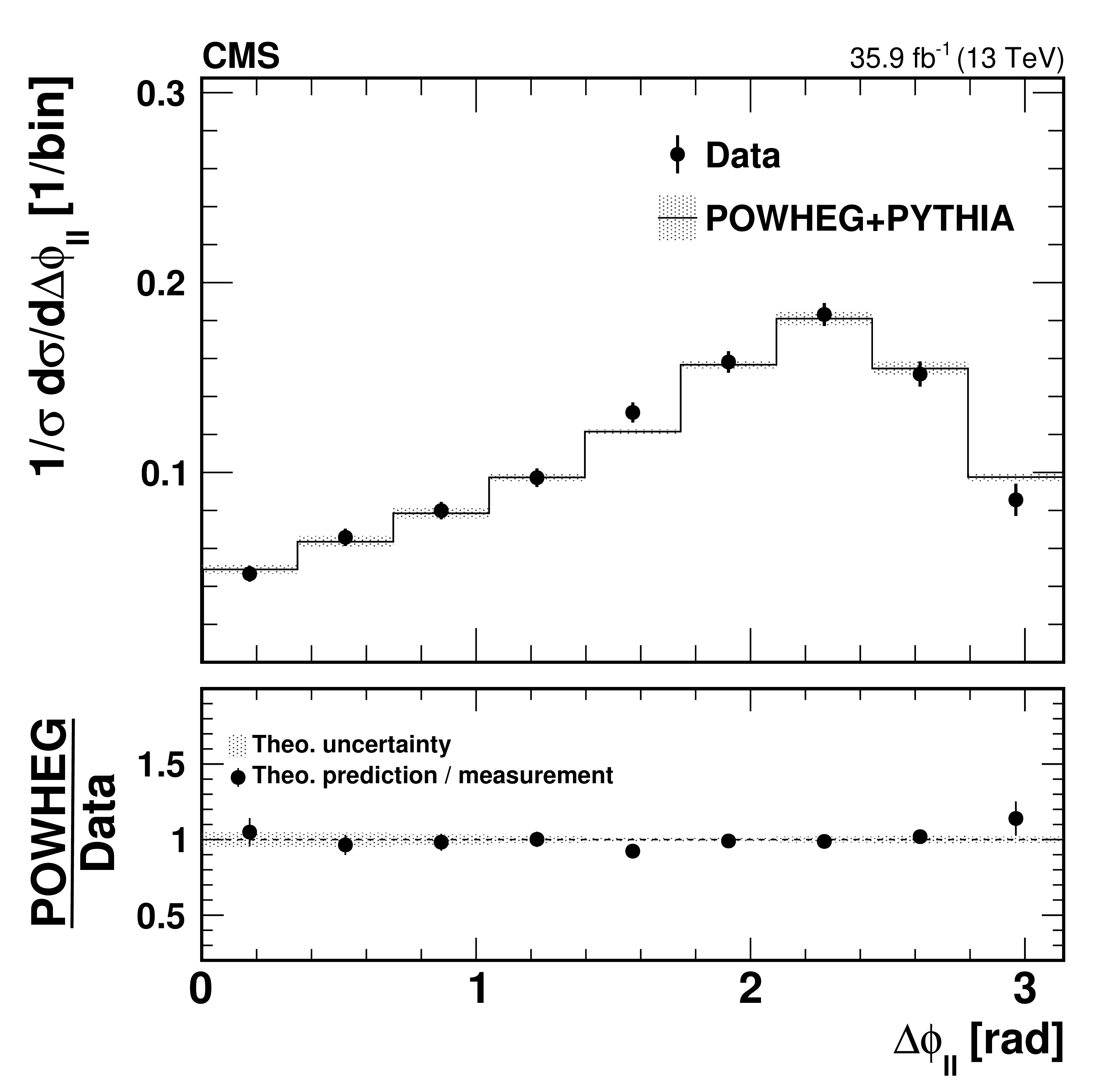
The upper panels show the normalized differential cross sections with respect to the dilepton mass ${m_{\ell \ell}}$, leading lepton ${{p_{\mathrm {T}}} ^{\ell \, \text {max}}}$, trailing lepton ${{p_{\mathrm {T}}} ^{\ell \, \text {min}}}$, and dilepton azimuthal angular separation $ {\Delta \phi _{\ell \ell}} $, compared to {powheg} predictions. The lower panels show the ratio of the theoretical predictions to the measured values. The meaning of the error bars and the shaded bands is the same as in Fig. 5. |
png pdf |
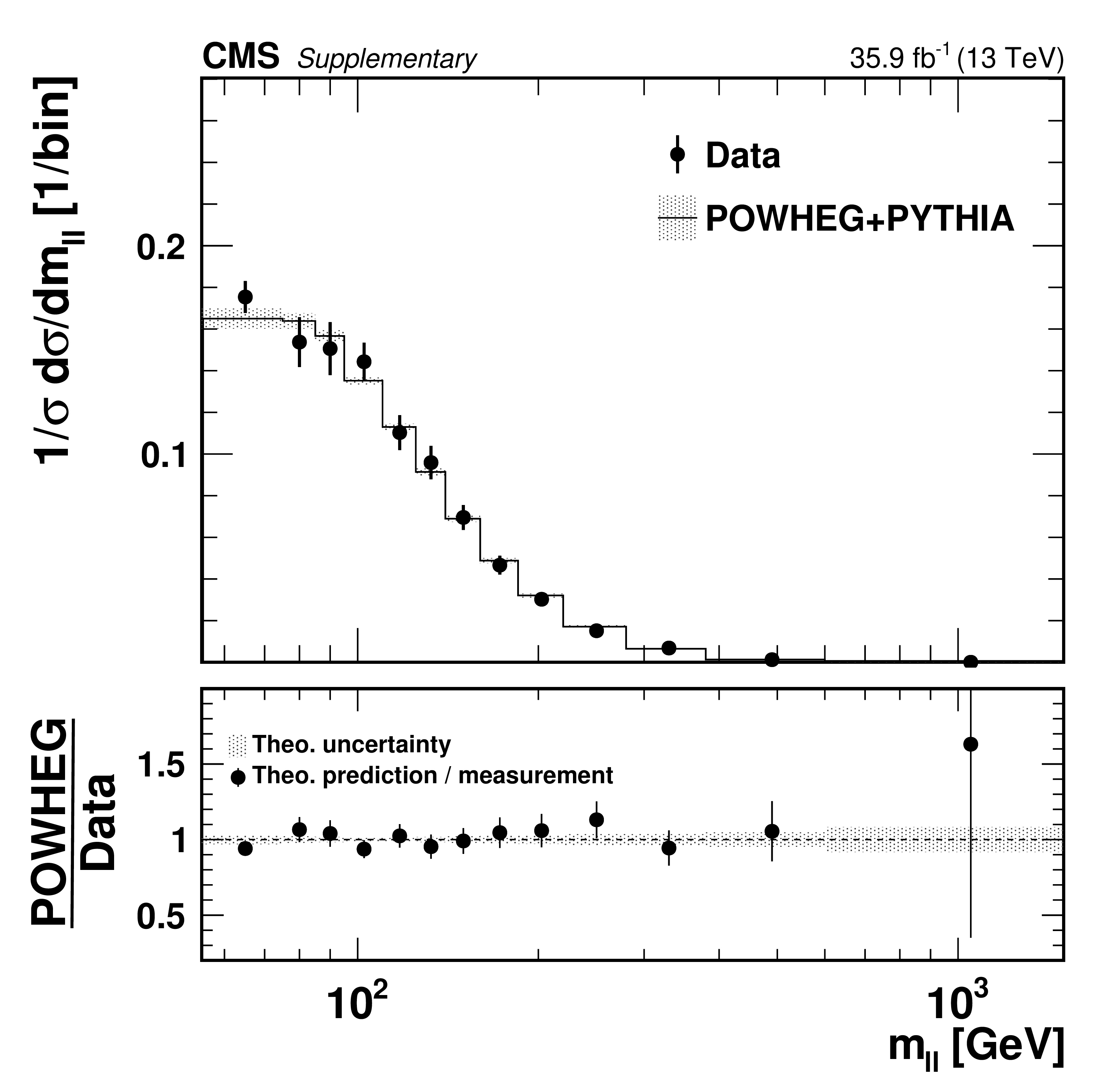
Figure 6-a:
The upper panels show the normalized differential cross sections with respect to the dilepton mass ${m_{\ell \ell}}$, leading lepton ${{p_{\mathrm {T}}} ^{\ell \, \text {max}}}$, trailing lepton ${{p_{\mathrm {T}}} ^{\ell \, \text {min}}}$, and dilepton azimuthal angular separation $ {\Delta \phi _{\ell \ell}} $, compared to {powheg} predictions. The lower panels show the ratio of the theoretical predictions to the measured values. The meaning of the error bars and the shaded bands is the same as in Fig. 5. |
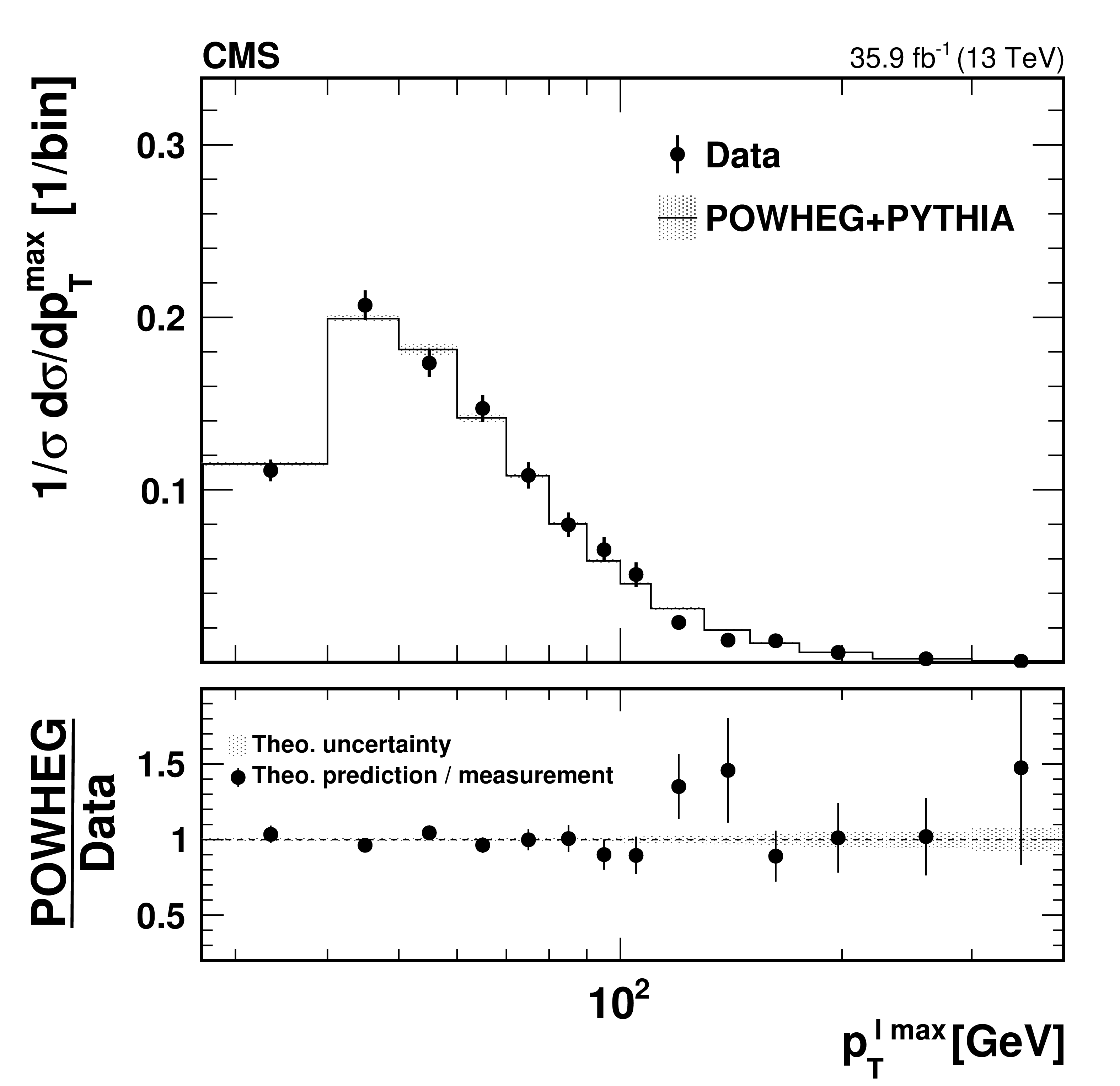
png pdf |
Figure 6-b:
The upper panels show the normalized differential cross sections with respect to the dilepton mass ${m_{\ell \ell}}$, leading lepton ${{p_{\mathrm {T}}} ^{\ell \, \text {max}}}$, trailing lepton ${{p_{\mathrm {T}}} ^{\ell \, \text {min}}}$, and dilepton azimuthal angular separation $ {\Delta \phi _{\ell \ell}} $, compared to {powheg} predictions. The lower panels show the ratio of the theoretical predictions to the measured values. The meaning of the error bars and the shaded bands is the same as in Fig. 5. |
png pdf |
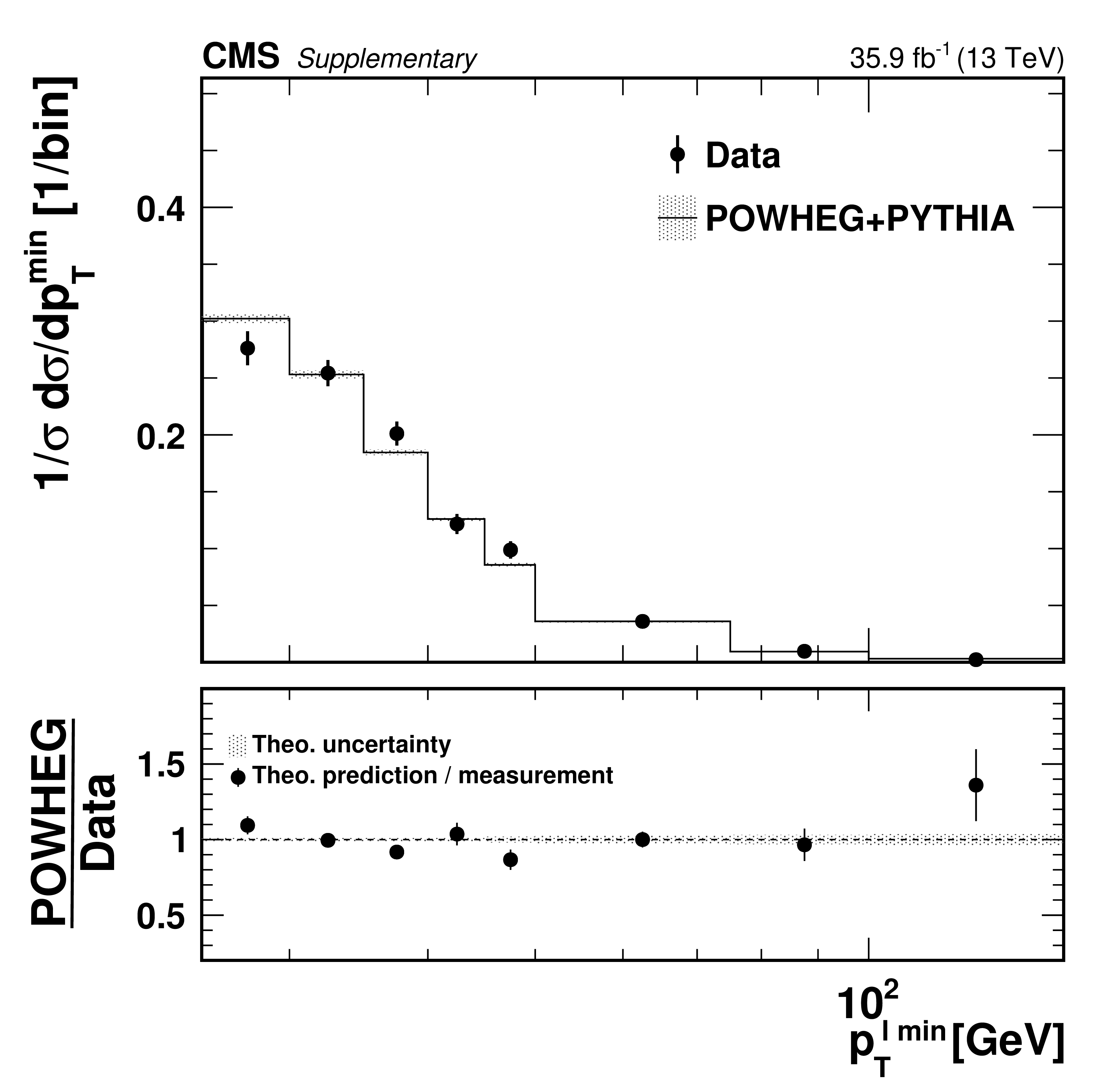
Figure 6-c:
The upper panels show the normalized differential cross sections with respect to the dilepton mass ${m_{\ell \ell}}$, leading lepton ${{p_{\mathrm {T}}} ^{\ell \, \text {max}}}$, trailing lepton ${{p_{\mathrm {T}}} ^{\ell \, \text {min}}}$, and dilepton azimuthal angular separation $ {\Delta \phi _{\ell \ell}} $, compared to {powheg} predictions. The lower panels show the ratio of the theoretical predictions to the measured values. The meaning of the error bars and the shaded bands is the same as in Fig. 5. |
png pdf |
Figure 6-d:
The upper panels show the normalized differential cross sections with respect to the dilepton mass ${m_{\ell \ell}}$, leading lepton ${{p_{\mathrm {T}}} ^{\ell \, \text {max}}}$, trailing lepton ${{p_{\mathrm {T}}} ^{\ell \, \text {min}}}$, and dilepton azimuthal angular separation $ {\Delta \phi _{\ell \ell}} $, compared to {powheg} predictions. The lower panels show the ratio of the theoretical predictions to the measured values. The meaning of the error bars and the shaded bands is the same as in Fig. 5. |
png pdf |
Figure 7:
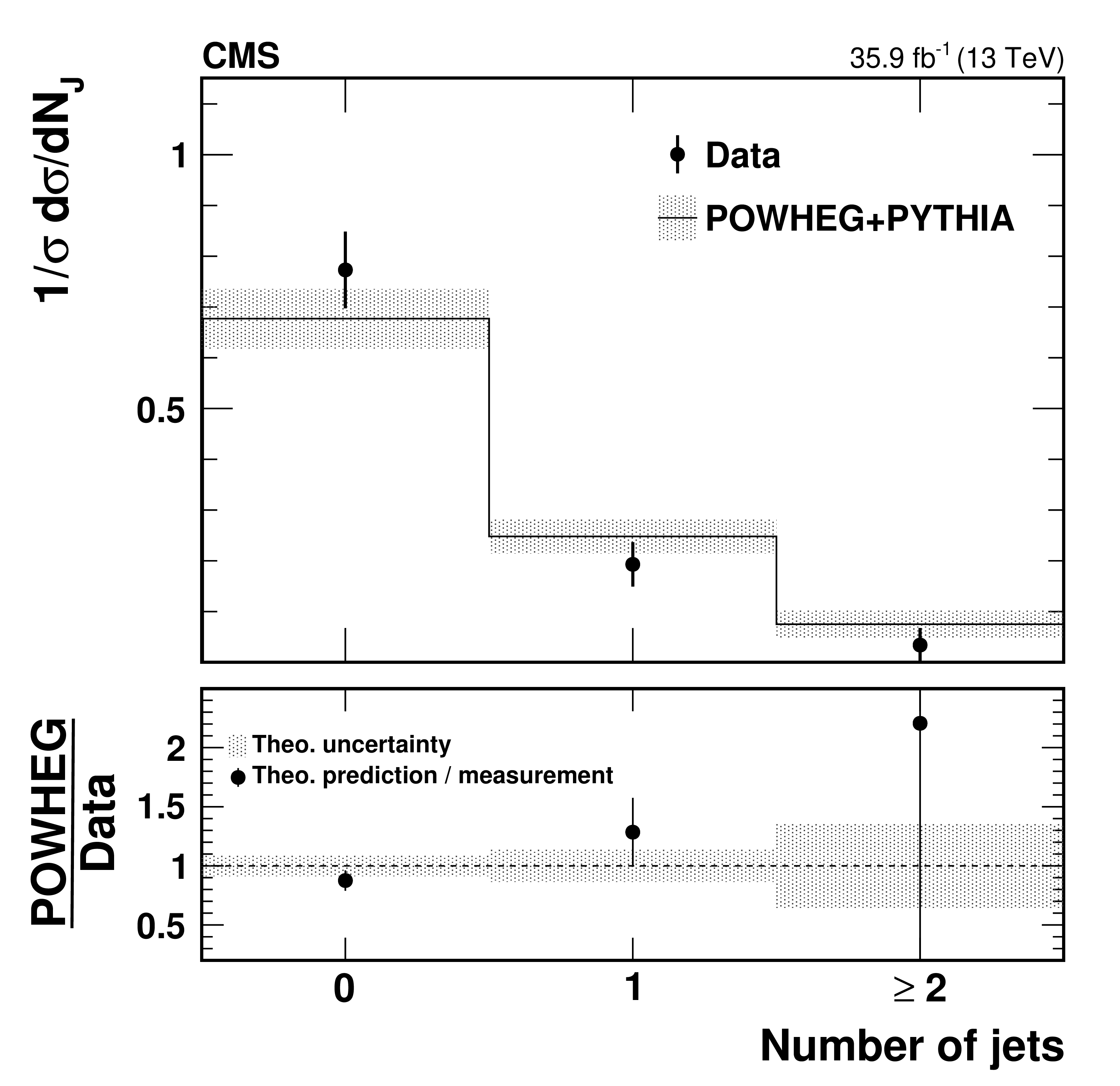
The upper panel shows the fractions of events with $ {N_{\mathrm {J}}} =$ 0, 1, $\ge $2 jets. The filled circles represent the data after backgrounds are subtracted and pileup and energy resolution are taken into account. The solid lines represent the {{powheg}}+{pythia} prediction. The lower panel shows the ratio of the theoretical prediction to the measurement. The meaning of the error bars and the shaded bands is the same as in Fig. 5. |
png pdf |
Figure 8:
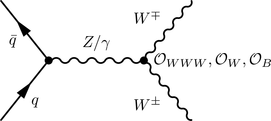
One of the Feynman diagrams through which dimension-6 operators modify the ${\mathrm{p}} {\mathrm{p}} \to {\mathrm{W^{+}} \mathrm{W^{-}}} $ cross section. |

png pdf |
Figure 9:
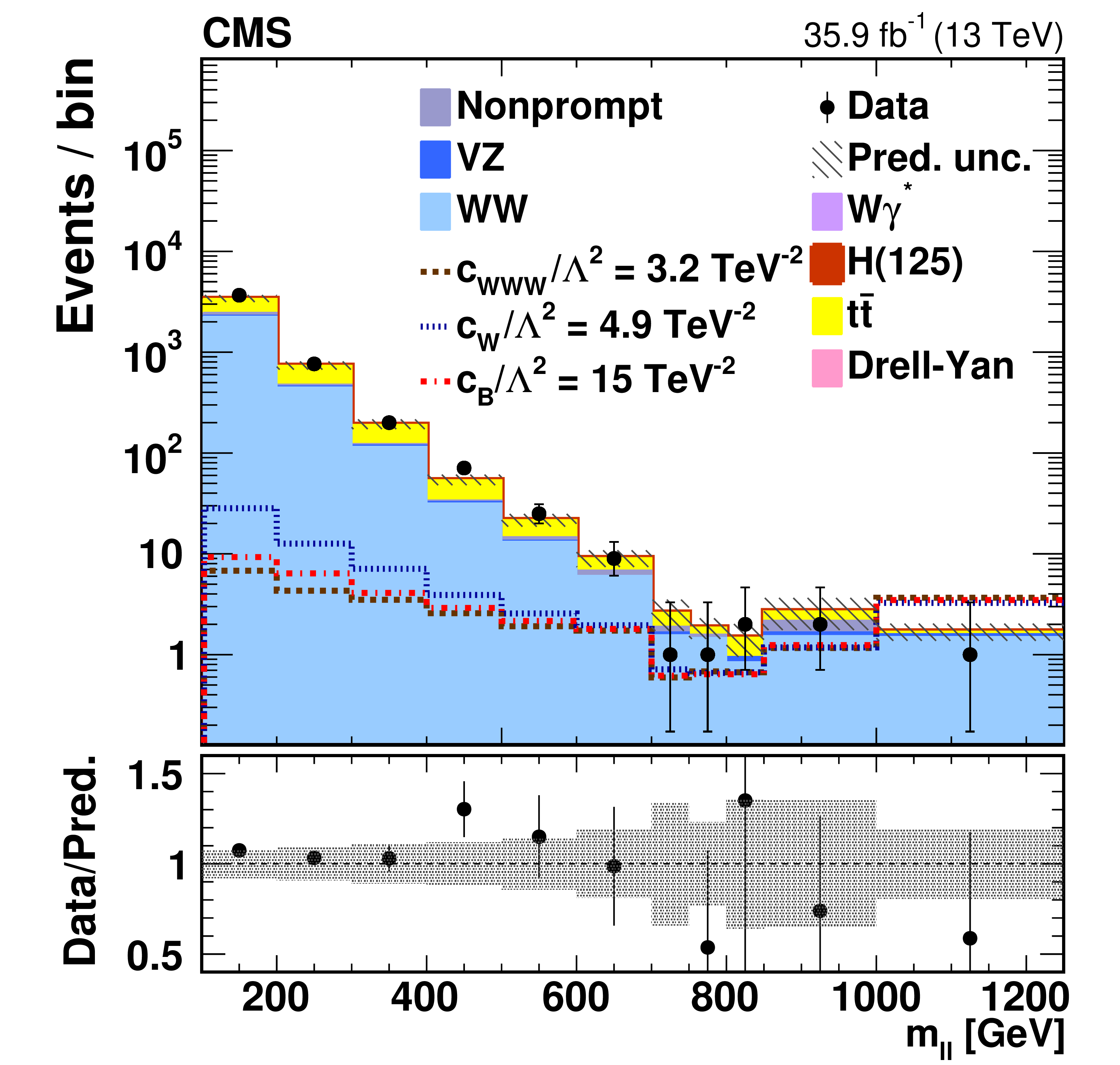
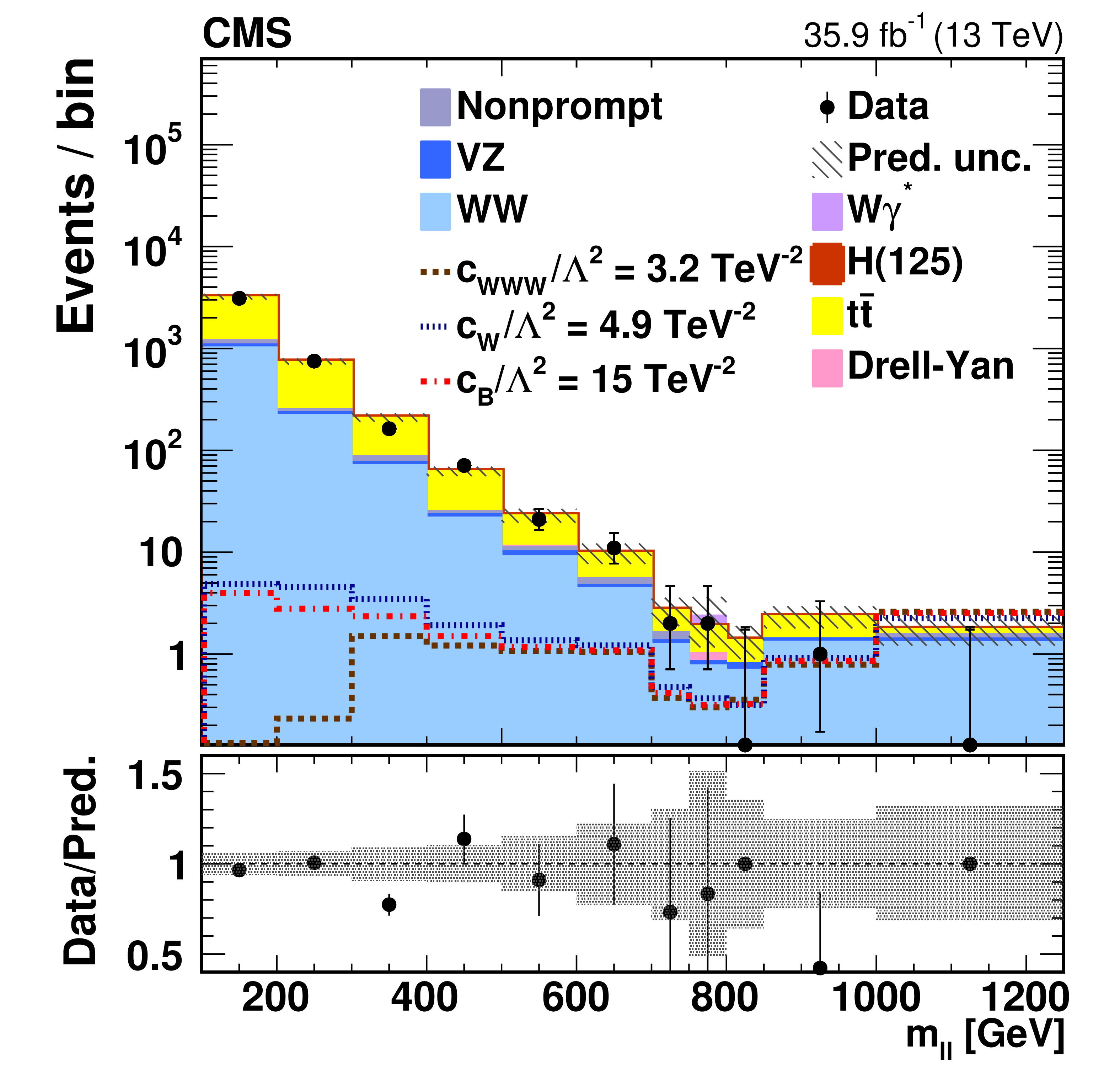
Comparison of the template fits to the observed ${m_{\mathrm{e} \mu}}$ distributions in the 0-jet (left) and 1-jet (right) categories. The non-SM contributions for $c_{\mathrm{W} \mathrm{W} \mathrm{W}}/\Lambda ^2=3.2 TeV ^{-2}$, $c_{\mathrm{W}}/\Lambda ^2=$ 4.9 TeV$ ^{-2}$, and $c_{B}/\Lambda ^2=$ 15.0 TeV$ ^{-2}$ are shown, not stacked on top of the other contributions. In the plot on the right, the decrease in the non-SM contribution at low ${m_{\mathrm{e} \mu}}$ is not statistically significant and results from limited precision in the subtraction of two large yields (SM and SM+non-SM). The last bin contains all events with reconstructed $ {m_{\mathrm{e} \mu}} > $ 1 TeV. The error bars on the data points represent the statistical uncertainties for the data, and the hatched areas represent the total uncertainty for the predicted yield in each bin. |
png pdf |
Figure 9-a:
Comparison of the template fits to the observed ${m_{\mathrm{e} \mu}}$ distributions in the 0-jet (left) and 1-jet (right) categories. The non-SM contributions for $c_{\mathrm{W} \mathrm{W} \mathrm{W}}/\Lambda ^2=3.2 TeV ^{-2}$, $c_{\mathrm{W}}/\Lambda ^2=$ 4.9 TeV$ ^{-2}$, and $c_{B}/\Lambda ^2=$ 15.0 TeV$ ^{-2}$ are shown, not stacked on top of the other contributions. In the plot on the right, the decrease in the non-SM contribution at low ${m_{\mathrm{e} \mu}}$ is not statistically significant and results from limited precision in the subtraction of two large yields (SM and SM+non-SM). The last bin contains all events with reconstructed $ {m_{\mathrm{e} \mu}} > $ 1 TeV. The error bars on the data points represent the statistical uncertainties for the data, and the hatched areas represent the total uncertainty for the predicted yield in each bin. |
png pdf |
Figure 9-b:
Comparison of the template fits to the observed ${m_{\mathrm{e} \mu}}$ distributions in the 0-jet (left) and 1-jet (right) categories. The non-SM contributions for $c_{\mathrm{W} \mathrm{W} \mathrm{W}}/\Lambda ^2=3.2 TeV ^{-2}$, $c_{\mathrm{W}}/\Lambda ^2=$ 4.9 TeV$ ^{-2}$, and $c_{B}/\Lambda ^2=$ 15.0 TeV$ ^{-2}$ are shown, not stacked on top of the other contributions. In the plot on the right, the decrease in the non-SM contribution at low ${m_{\mathrm{e} \mu}}$ is not statistically significant and results from limited precision in the subtraction of two large yields (SM and SM+non-SM). The last bin contains all events with reconstructed $ {m_{\mathrm{e} \mu}} > $ 1 TeV. The error bars on the data points represent the statistical uncertainties for the data, and the hatched areas represent the total uncertainty for the predicted yield in each bin. |
png pdf |
Figure 10:
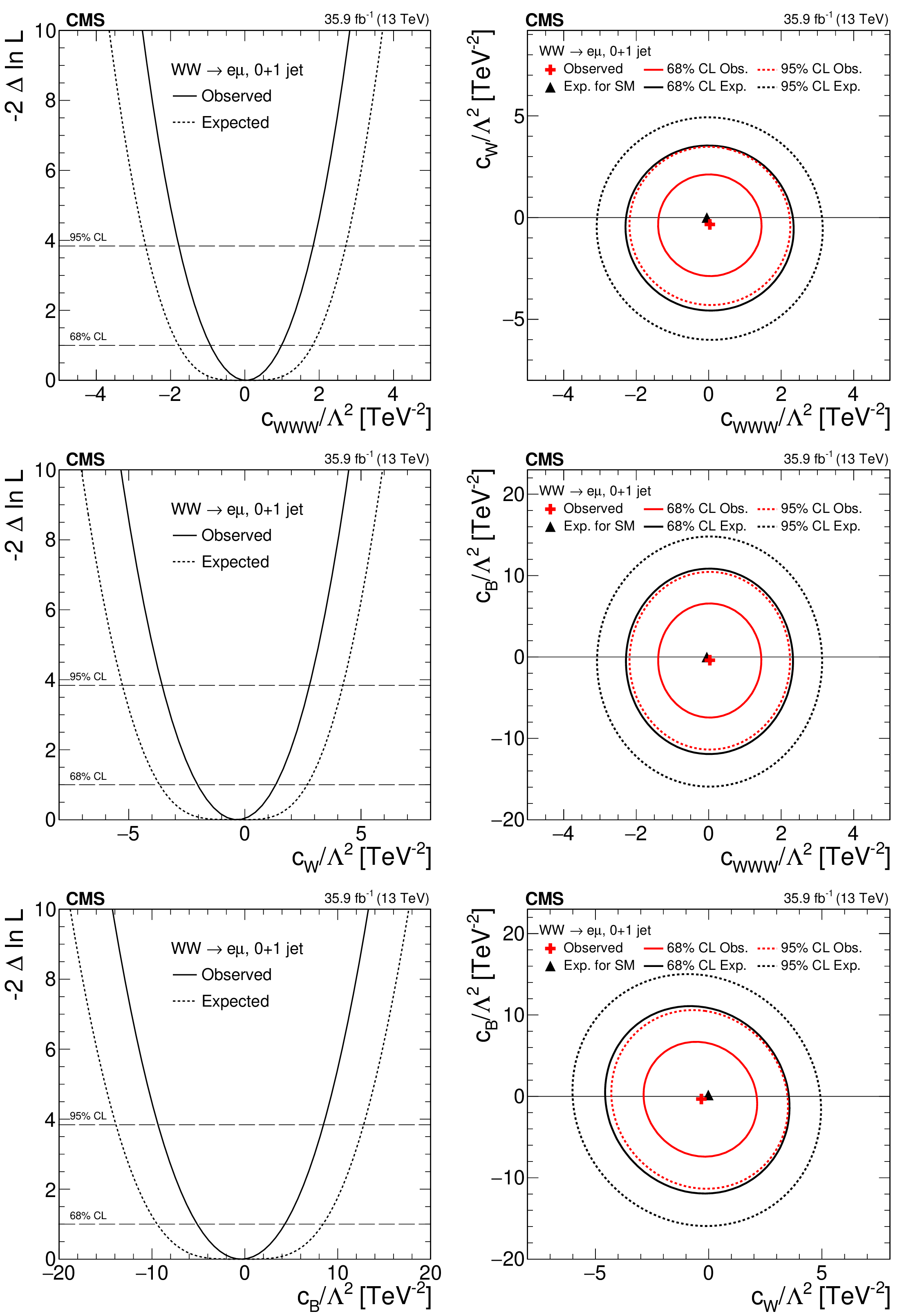
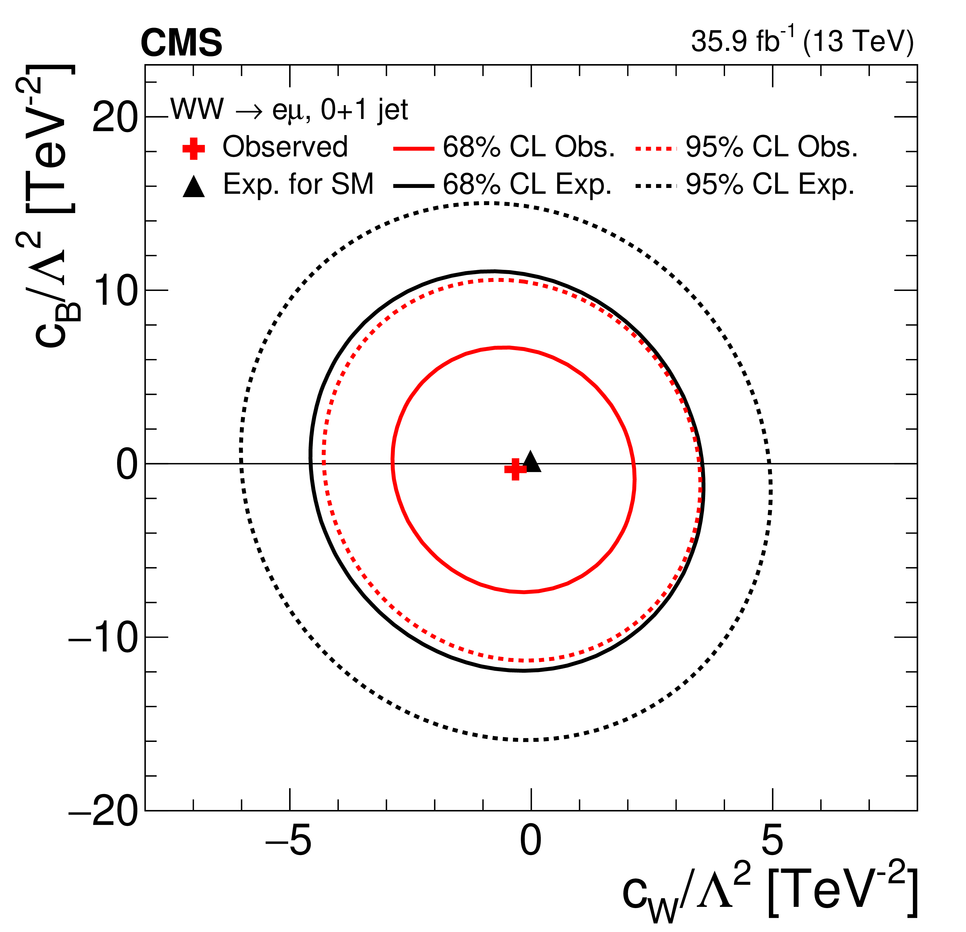
On the left, the expected and observed $-2\Delta \ln L$ curves for the $c_{\mathrm{W} \mathrm{W} \mathrm{W}}/\Lambda ^2$, $ c_{\mathrm{W}}/\Lambda ^2$, and $c_{B}/\Lambda ^2$ combining the 0- and 1-jet categories. On the right, the expected and observed 68 and 95% confidence level contours in the $(c_{\mathrm{W} \mathrm{W} \mathrm{W}}/\Lambda ^2, c_{\mathrm{W}}/\Lambda ^2)$, $(c_{\mathrm{W} \mathrm{W} \mathrm{W}}/\Lambda ^2, c_{B}/\Lambda ^2)$, and $(c_{\mathrm{W}}/\Lambda ^2, c_{B}/\Lambda ^2)$ planes combining the 0- and 1-jet categories. |
png pdf |
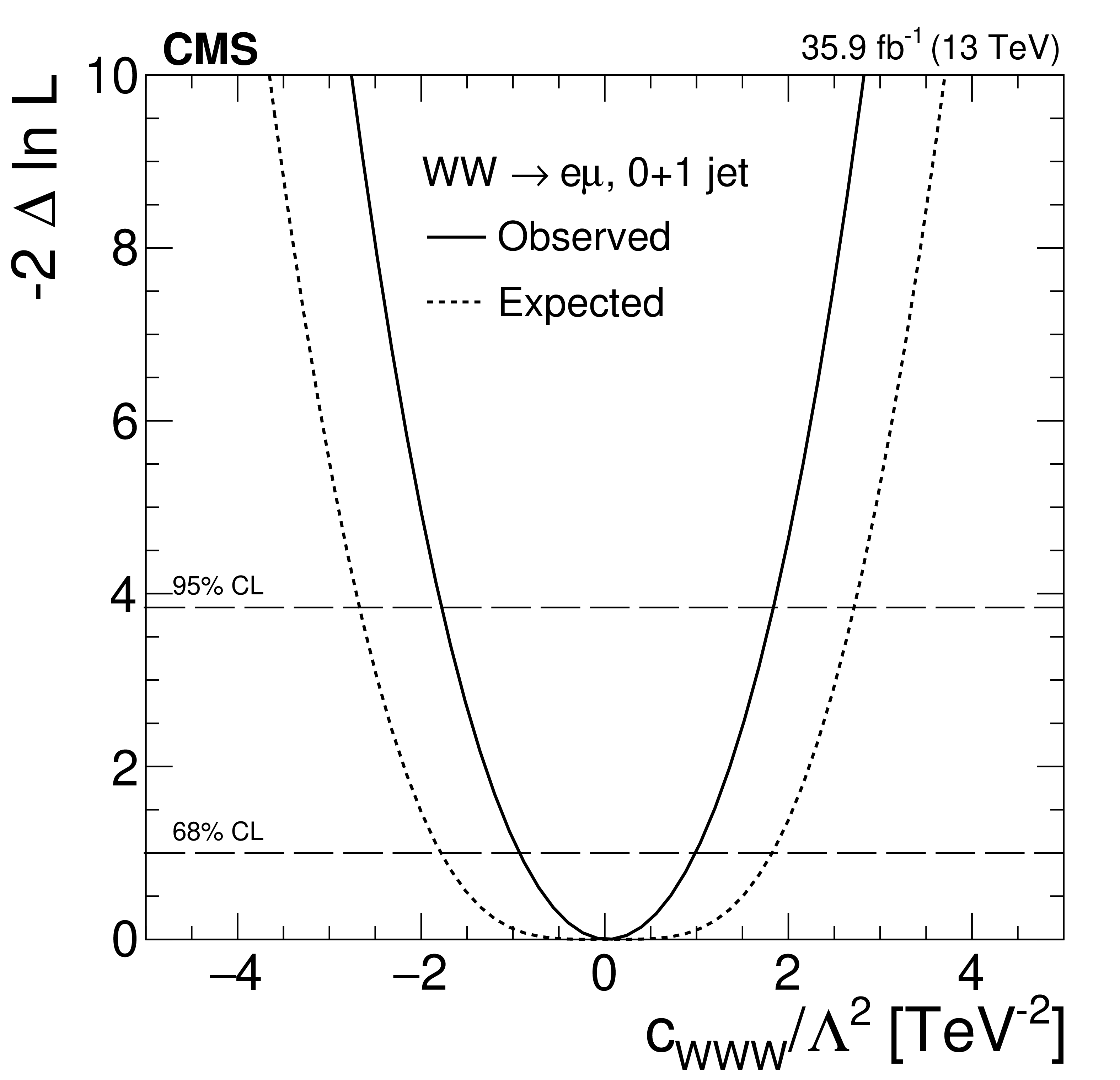
Figure 10-a:
On the left, the expected and observed $-2\Delta \ln L$ curves for the $c_{\mathrm{W} \mathrm{W} \mathrm{W}}/\Lambda ^2$, $ c_{\mathrm{W}}/\Lambda ^2$, and $c_{B}/\Lambda ^2$ combining the 0- and 1-jet categories. On the right, the expected and observed 68 and 95% confidence level contours in the $(c_{\mathrm{W} \mathrm{W} \mathrm{W}}/\Lambda ^2, c_{\mathrm{W}}/\Lambda ^2)$, $(c_{\mathrm{W} \mathrm{W} \mathrm{W}}/\Lambda ^2, c_{B}/\Lambda ^2)$, and $(c_{\mathrm{W}}/\Lambda ^2, c_{B}/\Lambda ^2)$ planes combining the 0- and 1-jet categories. |
png pdf |
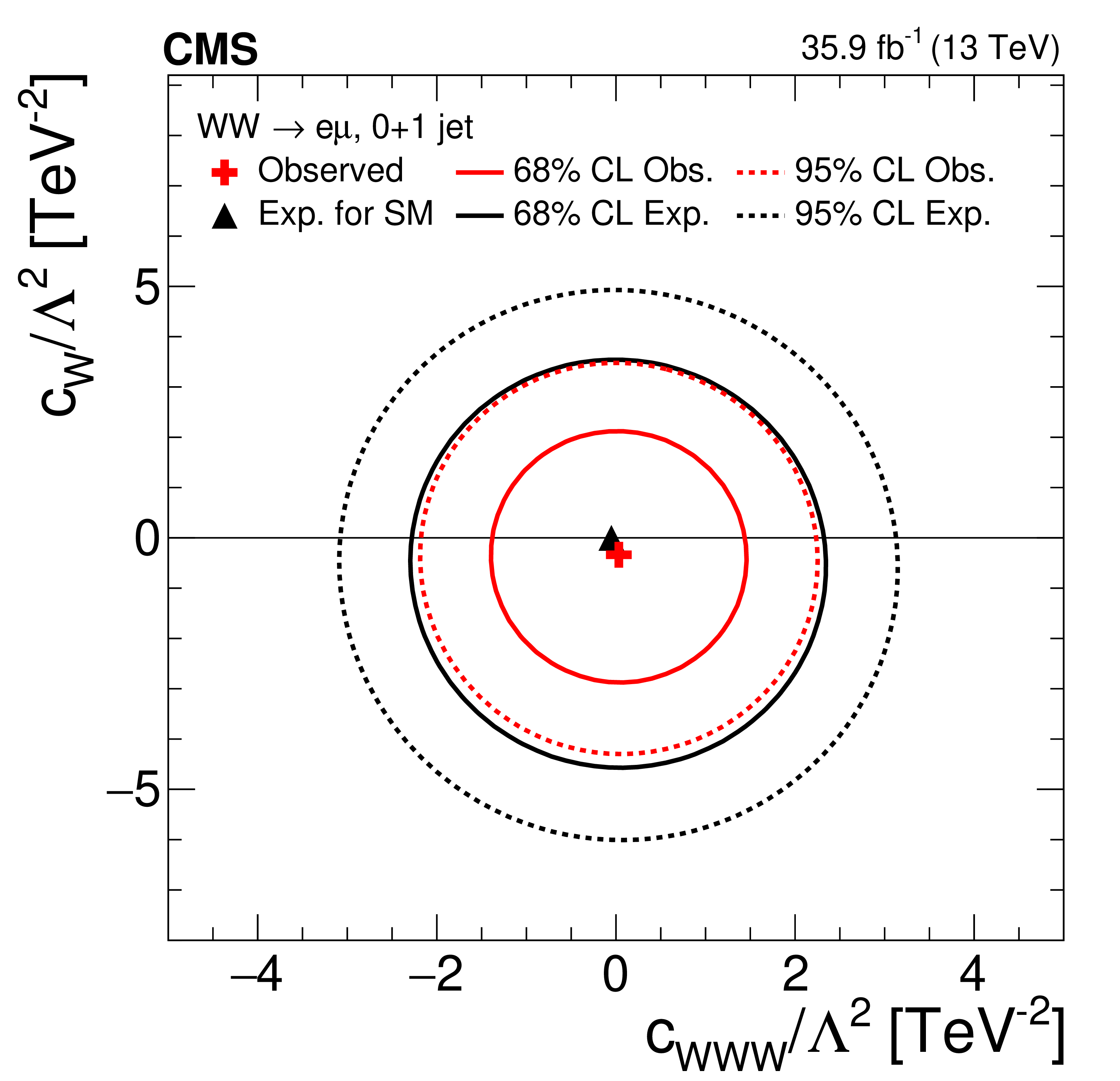
Figure 10-b:
On the left, the expected and observed $-2\Delta \ln L$ curves for the $c_{\mathrm{W} \mathrm{W} \mathrm{W}}/\Lambda ^2$, $ c_{\mathrm{W}}/\Lambda ^2$, and $c_{B}/\Lambda ^2$ combining the 0- and 1-jet categories. On the right, the expected and observed 68 and 95% confidence level contours in the $(c_{\mathrm{W} \mathrm{W} \mathrm{W}}/\Lambda ^2, c_{\mathrm{W}}/\Lambda ^2)$, $(c_{\mathrm{W} \mathrm{W} \mathrm{W}}/\Lambda ^2, c_{B}/\Lambda ^2)$, and $(c_{\mathrm{W}}/\Lambda ^2, c_{B}/\Lambda ^2)$ planes combining the 0- and 1-jet categories. |

png pdf |
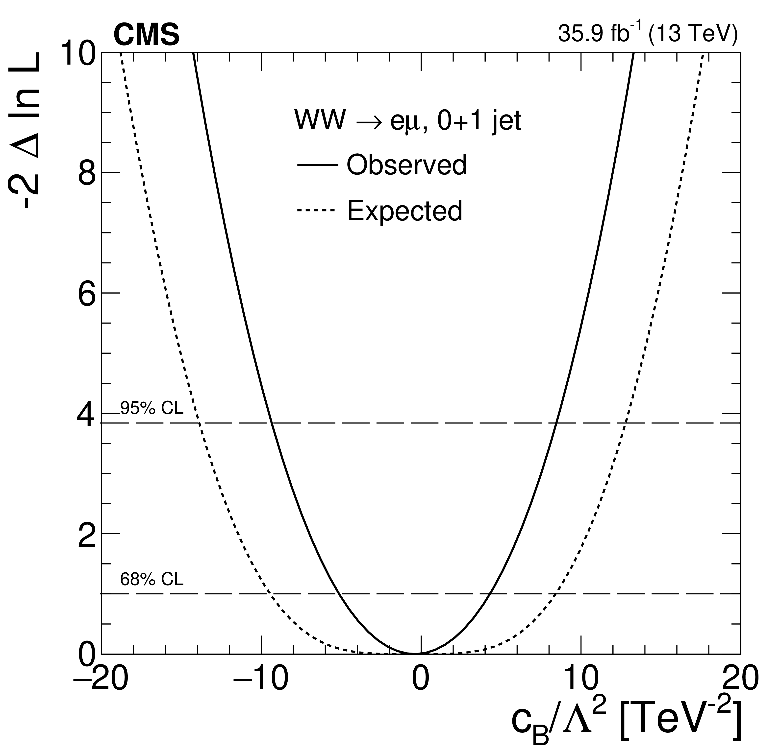
Figure 10-c:
On the left, the expected and observed $-2\Delta \ln L$ curves for the $c_{\mathrm{W} \mathrm{W} \mathrm{W}}/\Lambda ^2$, $ c_{\mathrm{W}}/\Lambda ^2$, and $c_{B}/\Lambda ^2$ combining the 0- and 1-jet categories. On the right, the expected and observed 68 and 95% confidence level contours in the $(c_{\mathrm{W} \mathrm{W} \mathrm{W}}/\Lambda ^2, c_{\mathrm{W}}/\Lambda ^2)$, $(c_{\mathrm{W} \mathrm{W} \mathrm{W}}/\Lambda ^2, c_{B}/\Lambda ^2)$, and $(c_{\mathrm{W}}/\Lambda ^2, c_{B}/\Lambda ^2)$ planes combining the 0- and 1-jet categories. |

png pdf |
Figure 10-d:
On the left, the expected and observed $-2\Delta \ln L$ curves for the $c_{\mathrm{W} \mathrm{W} \mathrm{W}}/\Lambda ^2$, $ c_{\mathrm{W}}/\Lambda ^2$, and $c_{B}/\Lambda ^2$ combining the 0- and 1-jet categories. On the right, the expected and observed 68 and 95% confidence level contours in the $(c_{\mathrm{W} \mathrm{W} \mathrm{W}}/\Lambda ^2, c_{\mathrm{W}}/\Lambda ^2)$, $(c_{\mathrm{W} \mathrm{W} \mathrm{W}}/\Lambda ^2, c_{B}/\Lambda ^2)$, and $(c_{\mathrm{W}}/\Lambda ^2, c_{B}/\Lambda ^2)$ planes combining the 0- and 1-jet categories. |
png pdf |
Figure 10-e:
On the left, the expected and observed $-2\Delta \ln L$ curves for the $c_{\mathrm{W} \mathrm{W} \mathrm{W}}/\Lambda ^2$, $ c_{\mathrm{W}}/\Lambda ^2$, and $c_{B}/\Lambda ^2$ combining the 0- and 1-jet categories. On the right, the expected and observed 68 and 95% confidence level contours in the $(c_{\mathrm{W} \mathrm{W} \mathrm{W}}/\Lambda ^2, c_{\mathrm{W}}/\Lambda ^2)$, $(c_{\mathrm{W} \mathrm{W} \mathrm{W}}/\Lambda ^2, c_{B}/\Lambda ^2)$, and $(c_{\mathrm{W}}/\Lambda ^2, c_{B}/\Lambda ^2)$ planes combining the 0- and 1-jet categories. |
png pdf |
Figure 10-f:
On the left, the expected and observed $-2\Delta \ln L$ curves for the $c_{\mathrm{W} \mathrm{W} \mathrm{W}}/\Lambda ^2$, $ c_{\mathrm{W}}/\Lambda ^2$, and $c_{B}/\Lambda ^2$ combining the 0- and 1-jet categories. On the right, the expected and observed 68 and 95% confidence level contours in the $(c_{\mathrm{W} \mathrm{W} \mathrm{W}}/\Lambda ^2, c_{\mathrm{W}}/\Lambda ^2)$, $(c_{\mathrm{W} \mathrm{W} \mathrm{W}}/\Lambda ^2, c_{B}/\Lambda ^2)$, and $(c_{\mathrm{W}}/\Lambda ^2, c_{B}/\Lambda ^2)$ planes combining the 0- and 1-jet categories. |
| Tables | |
png pdf |
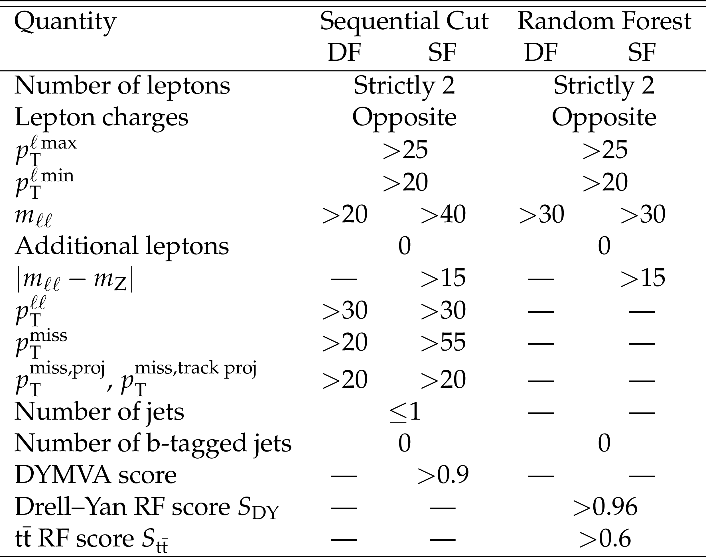
Table 1:
Summary of the event selection criteria for the sequential cut and the random forest analyses. DYMVA refers to an event classifier used in the sequential cut analysis to suppress Drell-Yan background events. RF refers to random forest classifiers. Kinematic quantities are measured in GeV. The symbol (--) means no requirement applied. |
png pdf |
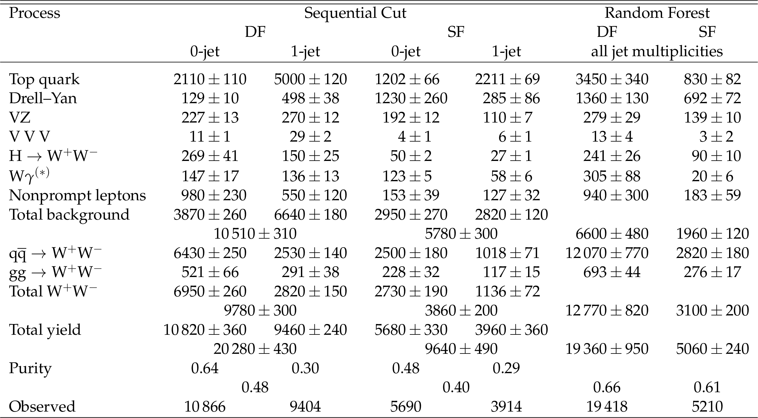
Table 2:
Sample composition for the sequential cut and random forest selections after the fits described in Section 7 have been executed; the uncertainties shown are based on the total uncertainty obtained from the fit. The purity is the fraction of selected events that are ${\mathrm{W^{+}}W^{-}}$ signal events. "Observed'' refers to the number of events observed in the data. |
png pdf |
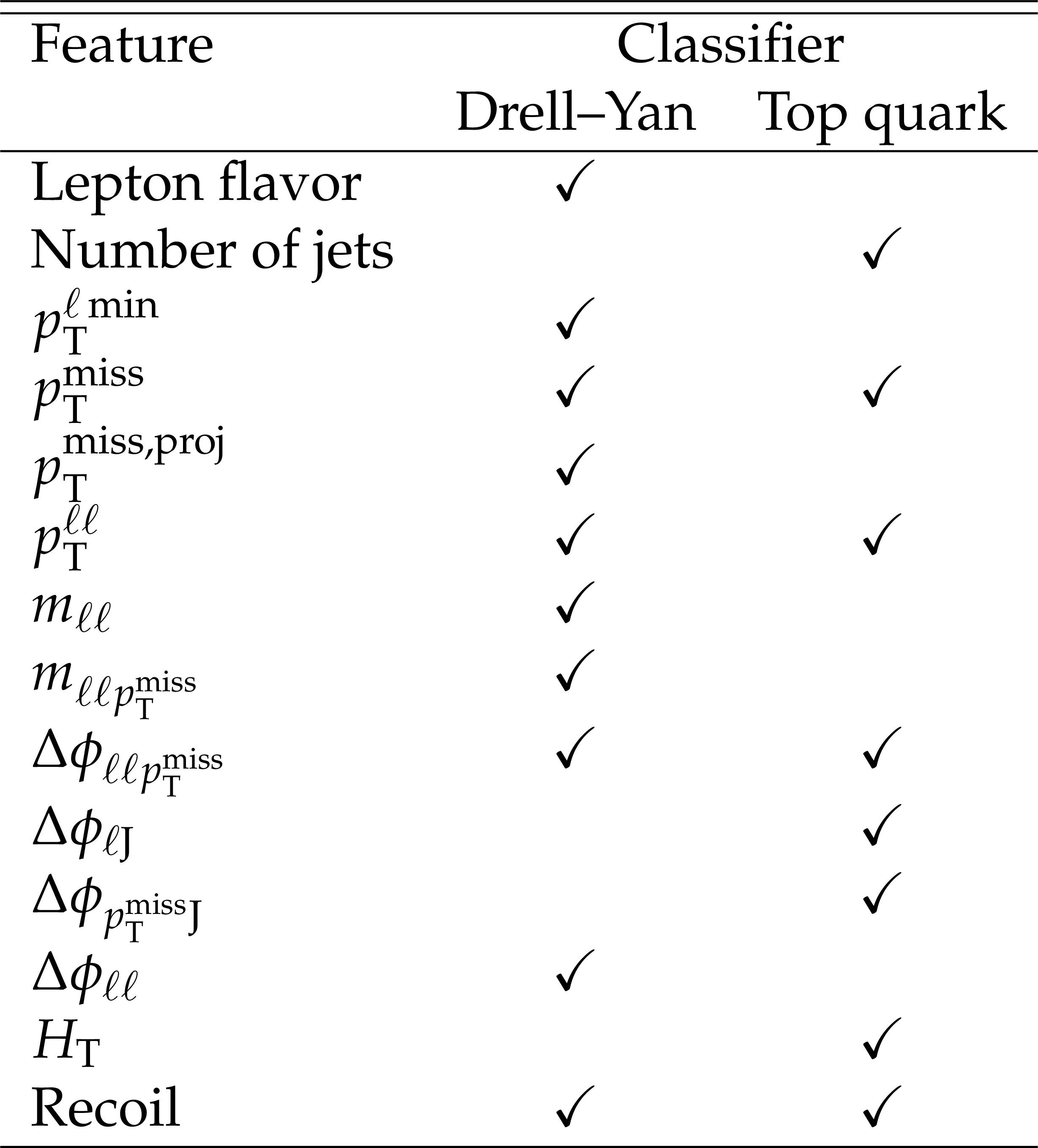
Table 3:
Features used for the random forest classifiers. The first classifier distinguishes Drell-Yan and ${\mathrm{W^{+}}W^{-}}$ signal events, and the second one distinguishes top quark events and signal events. |
png pdf |
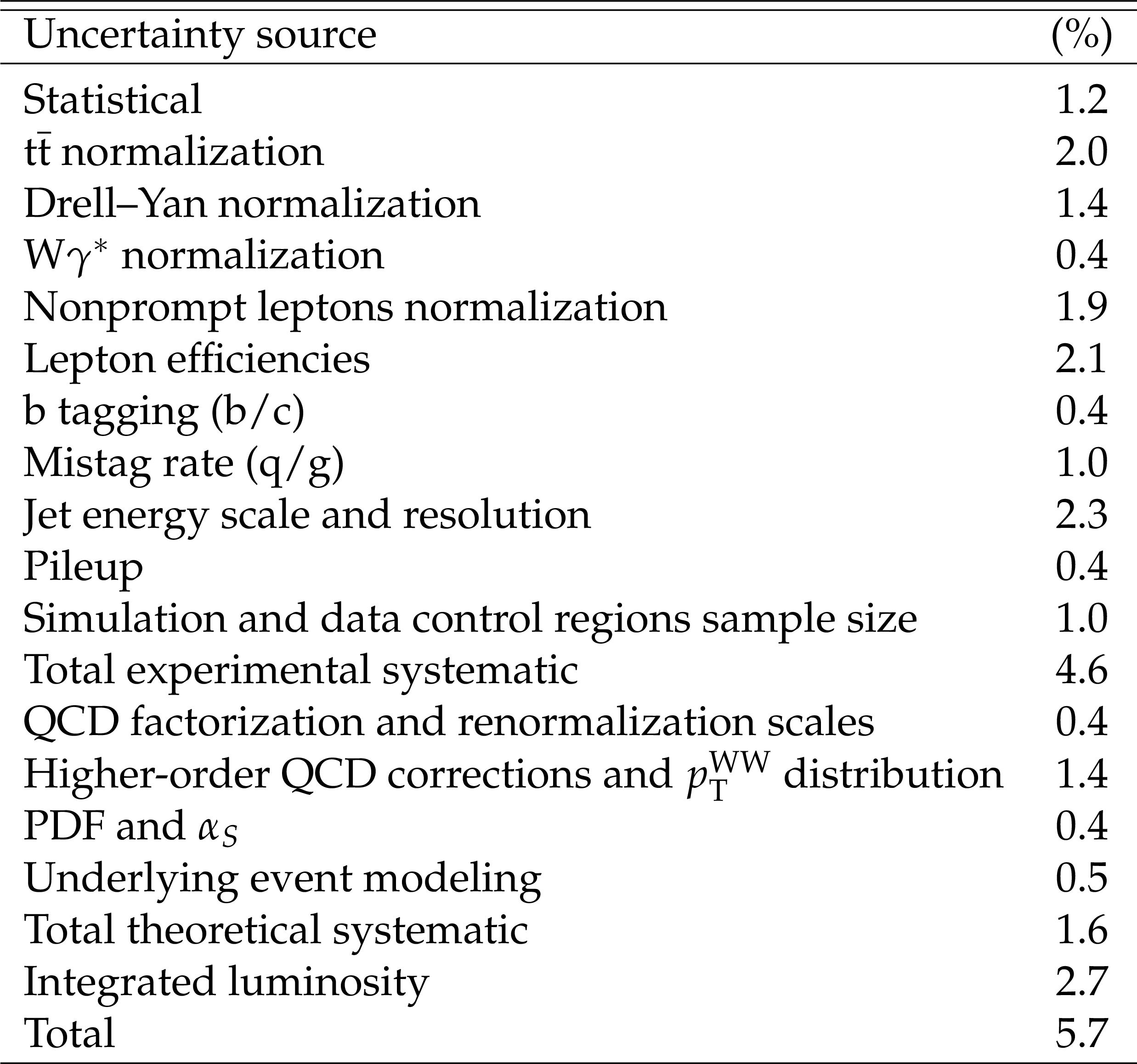
Table 4:
Relative systematic uncertainties in the total cross section measurement (0- and 1-jet, DF and SF) based on the sequential cut analysis. |
png pdf |
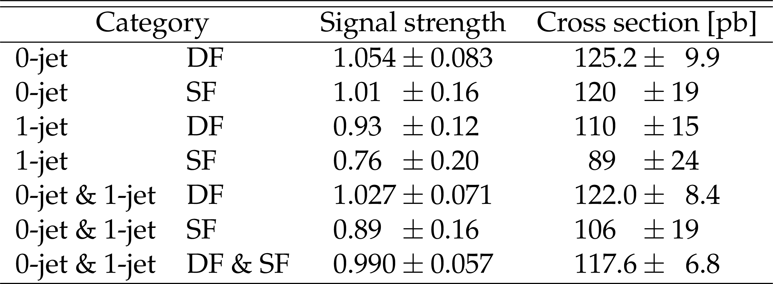
Table 5:
Summary of the signal strength and total production cross section obtained in the sequential cut analysis. The uncertainty listed is the total uncertainty obtained from the fit to the yields. |
png pdf |
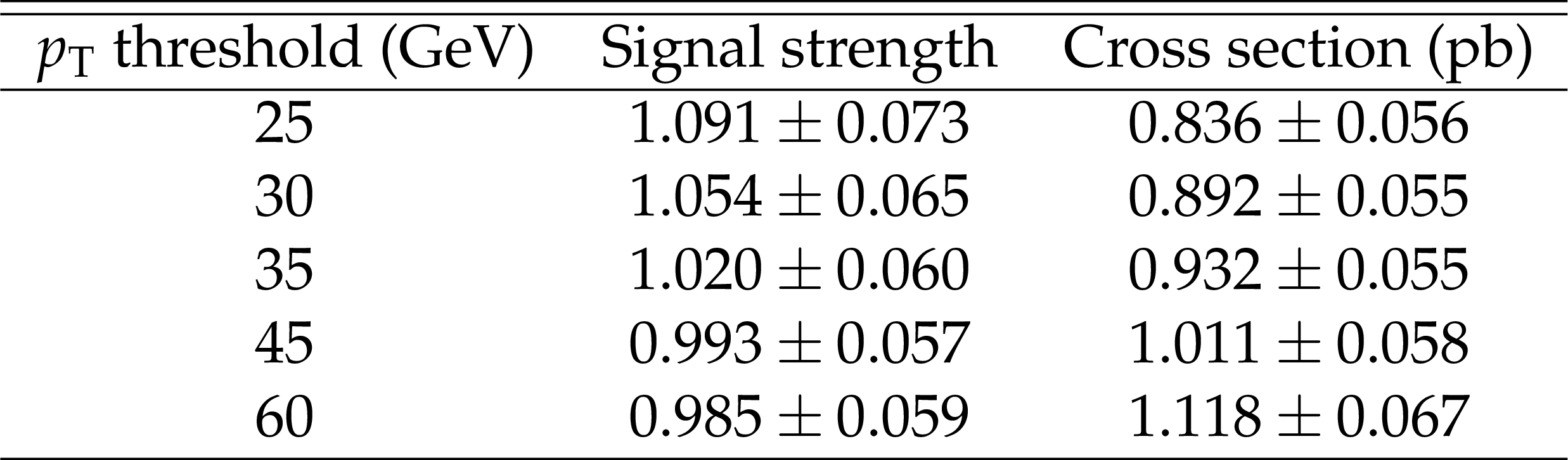
Table 6:
Fiducial cross section for the production of $ {\mathrm{W^{+}} \mathrm{W^{-}}} $+0-jets as the ${p_{\mathrm {T}}}$ threshold for jets is varied. The fiducial region is defined by two opposite-sign leptons with $ {p_{\mathrm {T}}} > $ 20 GeV and $ {| \eta |} < $ 2.5 excluding the products of $\tau $ lepton decay, and $ {m_{\ell \ell}} > $ 20 GeV, $ {p_{\mathrm {T}}} ^{\ell \ell} > $ 30 GeV, and $ {{p_{\mathrm {T}}} ^\text {miss}} > $ 30 GeV. Jets must have $ {p_{\mathrm {T}}} $ above the stated threshold, $ {| \eta |} < $ 4.5, and be separated from each of the two leptons by $\Delta R > $ 0.4. The total uncertainty is reported. |

png pdf |
Table 7:
Efficiency for the random forest selection with respect to preselected events as a function of jet multiplicity. The stated uncertainties are statistical only. |
png pdf |
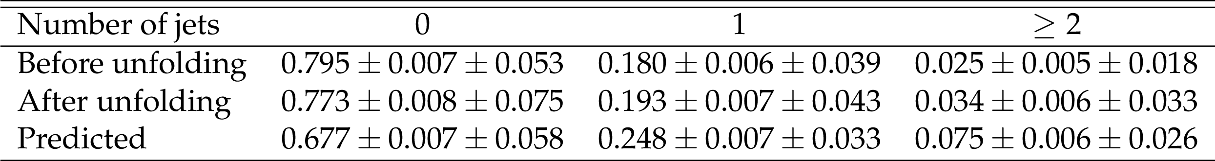
Table 8:
Fractions of events with $ {N_{\mathrm {J}}} =$ 0, 1, $\ge $2 jets. The first uncertainty is statistical and the second combines systematic uncertainties from the response matrix and from the background subtraction. |
png pdf |
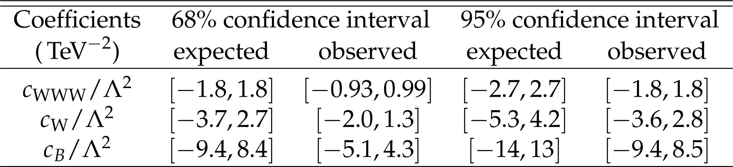
Table 9:
Expected and observed 68 and 95% confidence intervals on the measurement of the Wilson coefficients associated with the three CP-conserving, dimension-6 operators. |
| Summary |
| Measurements of $\mathrm{W^{+}W^{-}}$ boson pair production in proton-proton collisions at $\sqrt{s} = $ 13 TeV was performed. The analysis is based on data collected with the CMS detector at the LHC corresponding to an integrated luminosity of 35.9 fb$^{-1}$. Candidate events were selected that have two leptons (electrons or muons) with opposite charges. Two analysis methods were described. The first method imposes a sequence of requirements on kinematic quantities to suppress backgrounds, while the second uses a pair of random forest classifiers. The total production cross section is $\sigma_{\text{SC}}^{\text{tot}} = $ 117.6 $\pm$ 1.4 (stat) $\pm$ 5.5 (syst) $\pm$ 1.9 (theo) $\pm$ 3.2 (lumi) pb = 117.6 $\pm$ 6.8 pb, where the individual uncertainties are statistical, experimental systematic, theoretical, and of integrated luminosity; this measured value is consistent with the next-to-next-to-leading-order theoretical prediction 118.8 $\pm$ 3.6 pb. Fiducial cross sections are also measured including the change in the 0-jet fiducial cross section with jet transverse momentum threshold. Normalized differential cross sections are measured and compared with next-to-leading-order Monte Carlo simulations. Good agreement is observed. The normalized jet multiplicity distribution in $\mathrm{W^{+}W^{-}}$ events is measured. Finally, bounds on coefficients of dimension-6 operators in the context of an effective field theory are set using electron-muon invariant mass distributions. |
| Additional Figures | |
png pdf |
Additional Figure 1:
The upper panels show the normalized differential cross sections in the 0-jet category with respect to the dilepton mass ${m_{\ell\ell}}$, leading lepton ${p_{\mathrm{T}}^{\,\text {max}}}$, trailing lepton ${p_{\mathrm{T}}^{\,\text {min}}}$, and dilepton azimuthal angular separation $ {\Delta \phi _{\ell\ell}} $, compared to POWHEG predictions. The lower panels show the ratio of the theoretical predictions to the measured values. In both the upper and lower panels, the error bars on the data points represent the total uncertainty of the measurement, and the shaded band depicts the uncertainty of the MC prediction. |
png pdf |
Additional Figure 1-a:
The upper panel shows the normalized differential cross section in the 0-jet category with respect to the dilepton mass ${m_{\ell\ell}}$, compared to POWHEG predictions. The lower panel shows the ratio of the theoretical predictions to the measured values. In both the upper and lower panels, the error bars on the data points represent the total uncertainty of the measurement, and the shaded band depicts the uncertainty of the MC prediction. |

png pdf |
Additional Figure 1-b:
The upper panel shows the normalized differential cross section in the 0-jet category with respect to the leading lepton ${p_{\mathrm{T}}^{\,\text {max}}}$, compared to POWHEG predictions. The lower panel shows the ratio of the theoretical predictions to the measured values. In both the upper and lower panels, the error bars on the data points represent the total uncertainty of the measurement, and the shaded band depicts the uncertainty of the MC prediction. |
png pdf |
Additional Figure 1-c:
The upper panel shows the normalized differential cross section in the 0-jet category with respect to the trailing lepton ${p_{\mathrm{T}}^{\,\text {min}}}$, compared to POWHEG predictions. The lower panel shows the ratio of the theoretical predictions to the measured values. In both the upper and lower panels, the error bars on the data points represent the total uncertainty of the measurement, and the shaded band depicts the uncertainty of the MC prediction. |
png pdf |
Additional Figure 1-d:
The upper panel shows the normalized differential cross section in the 0-jet category with respect to the dilepton azimuthal angular separation $ {\Delta \phi _{\ell\ell}} $, compared to POWHEG predictions. The lower panel shows the ratio of the theoretical predictions to the measured values. In both the upper and lower panels, the error bars on the data points represent the total uncertainty of the measurement, and the shaded band depicts the uncertainty of the MC prediction. |
png pdf |
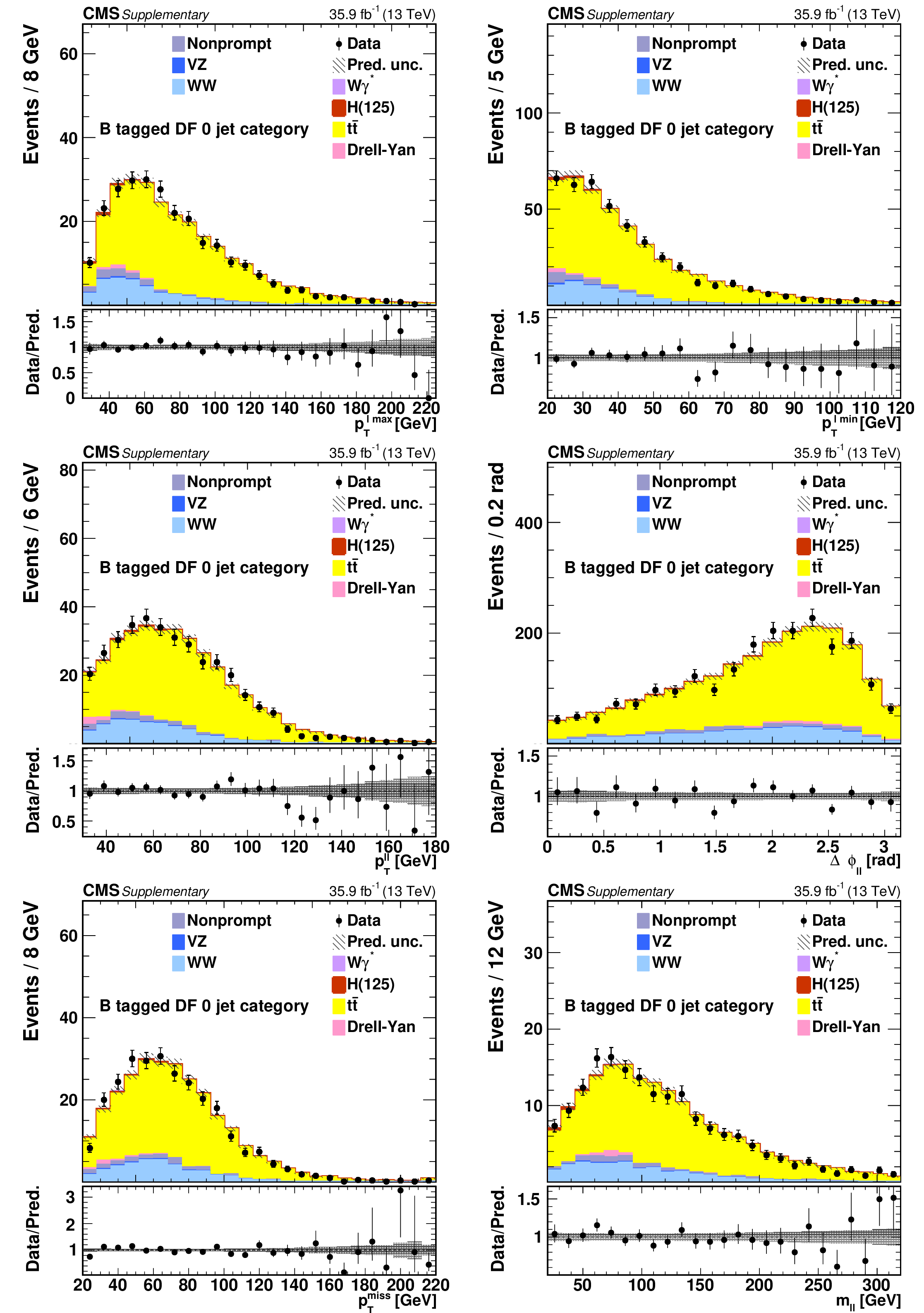
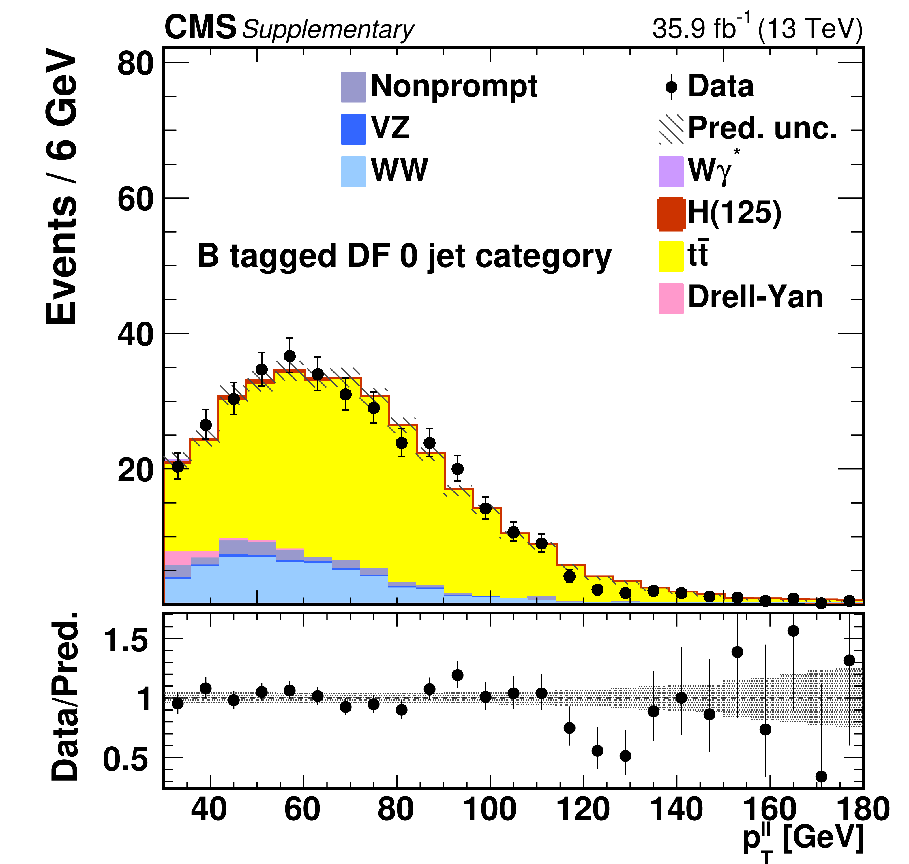
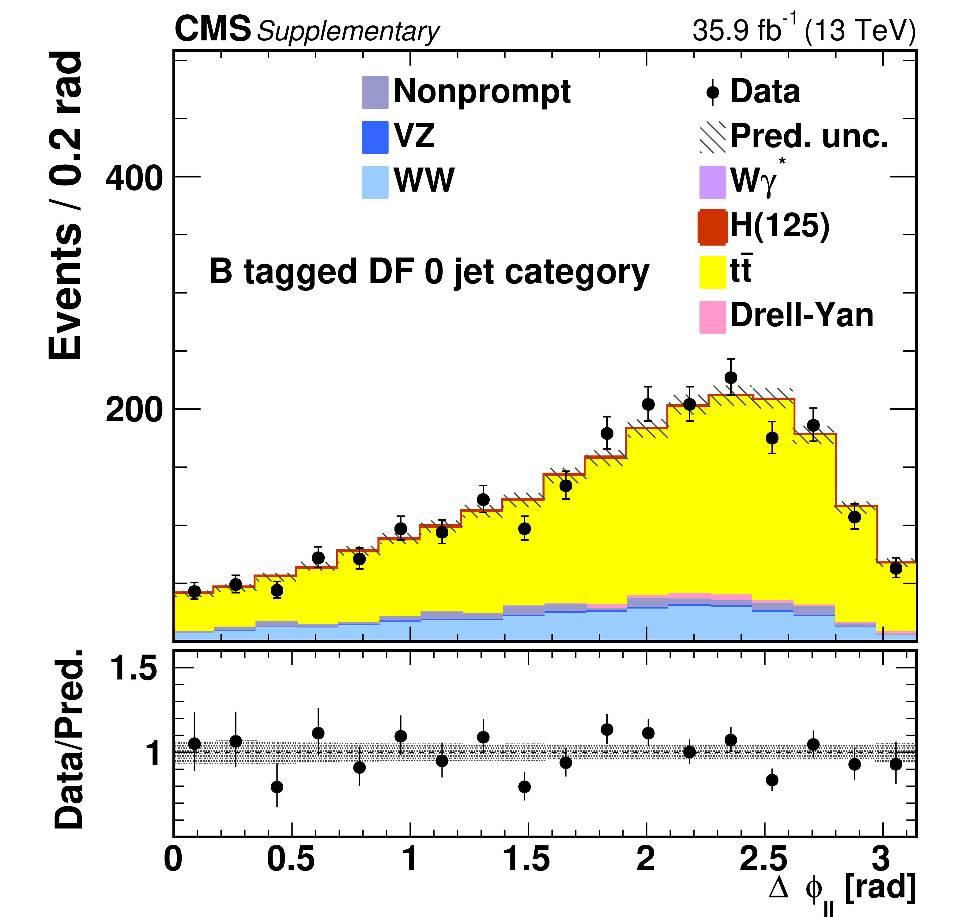
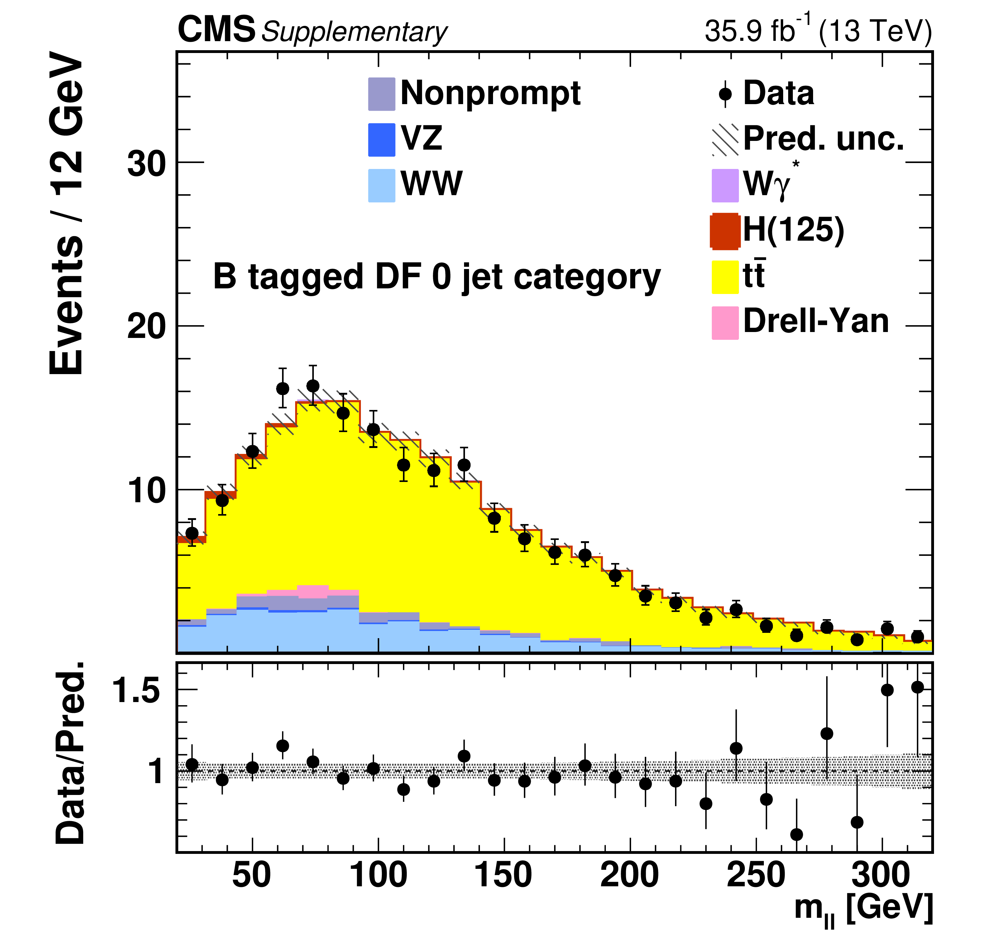
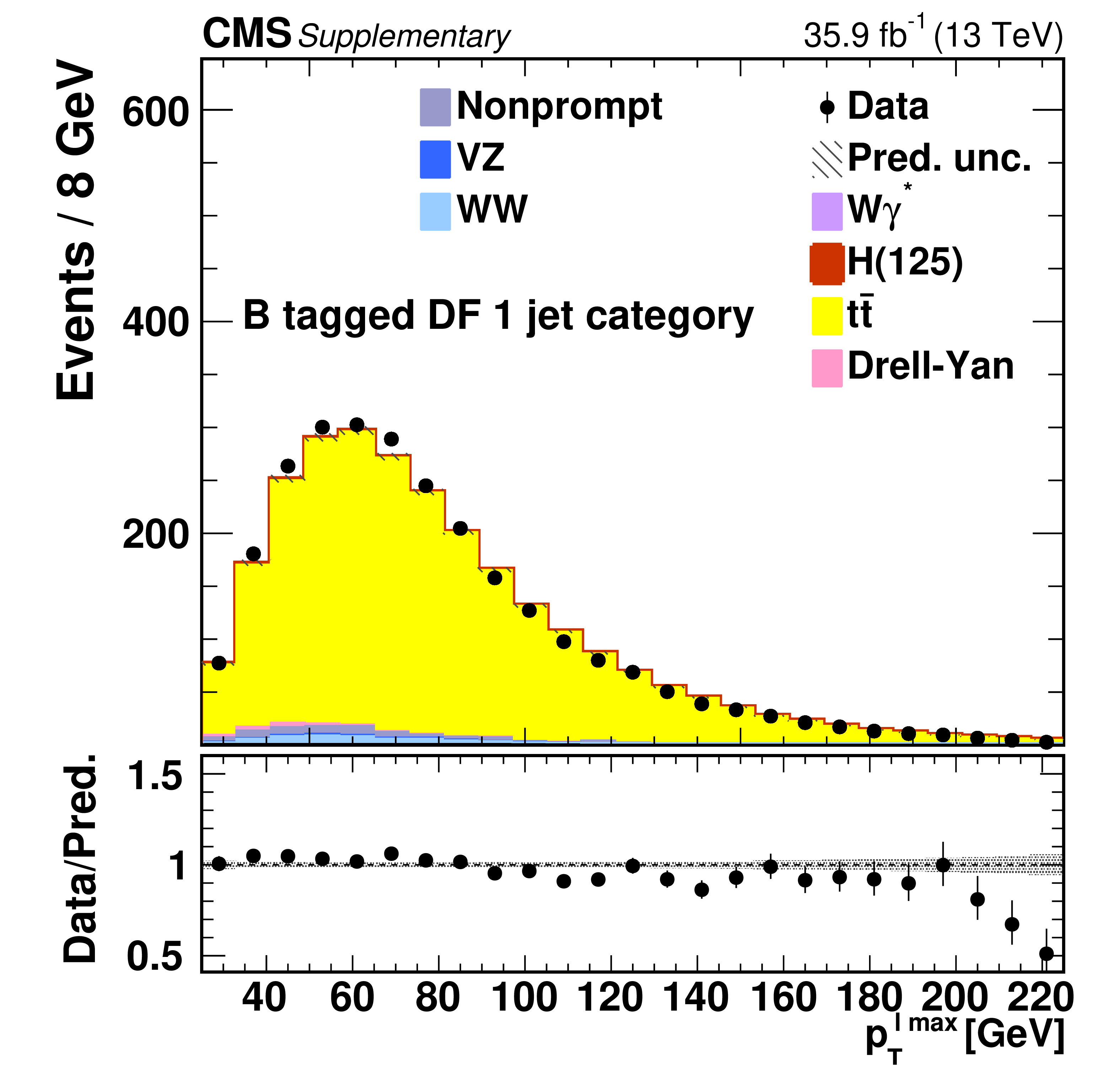
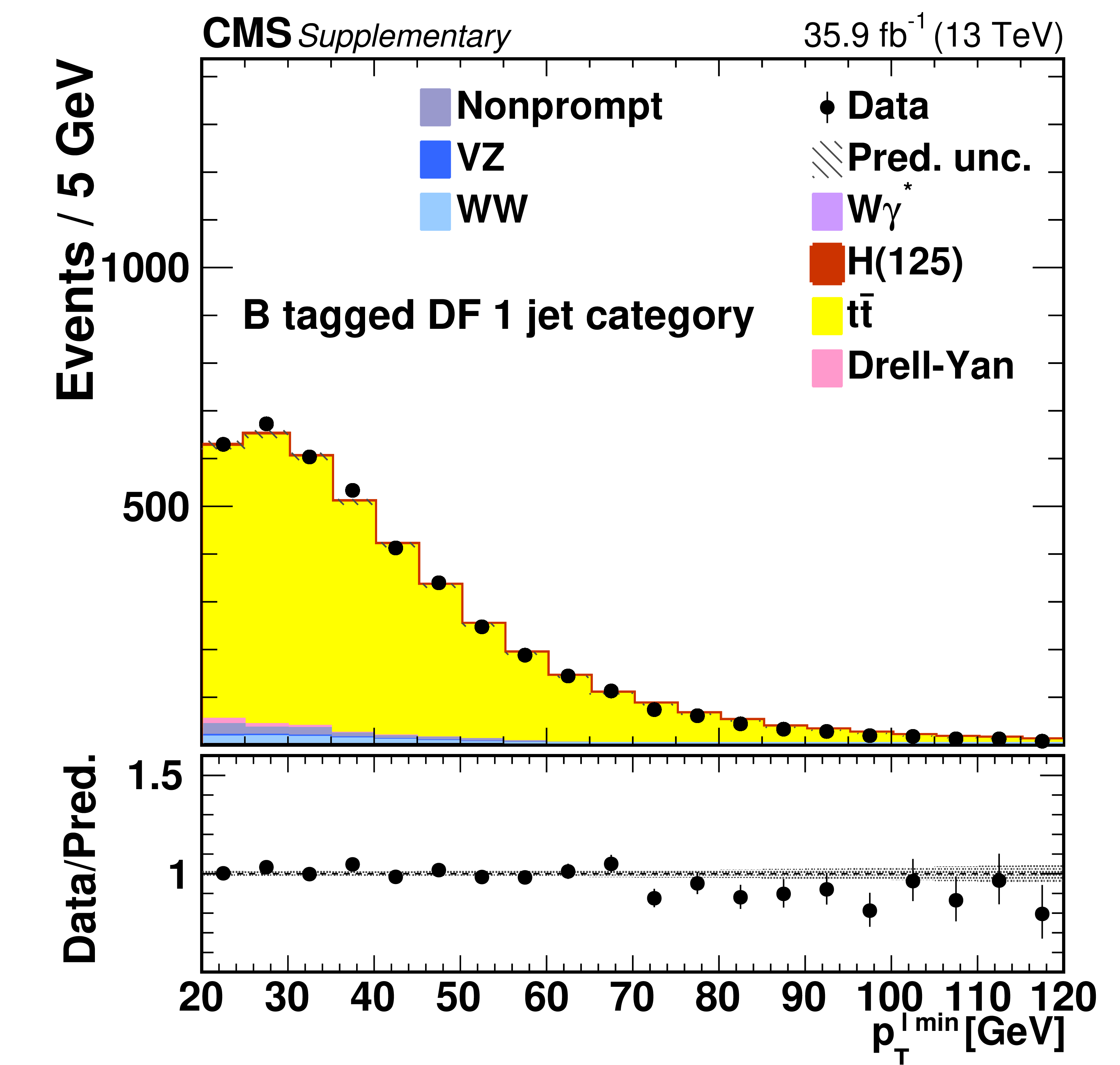
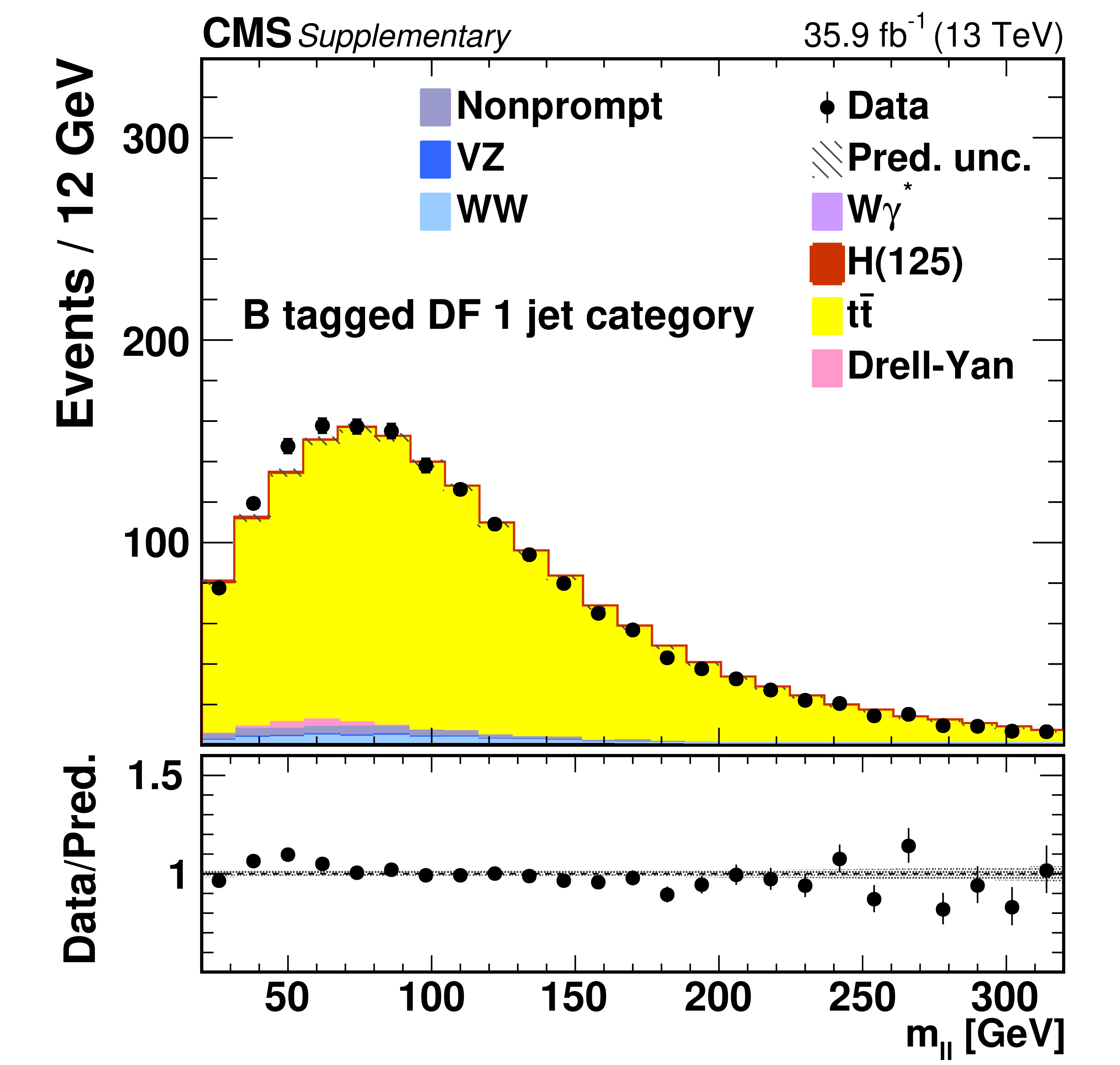
Additional Figure 2:
Kinematic distributions for events with zero jets and DF leptons in the b-tagged control region in the sequential cut analysis. The distributions show the leading and trailing lepton ${p_{\mathrm {T}}}$ ($ {p_{\mathrm{T}}^{\,\text {max}}} $ and $ {p_{\mathrm{T}}^{\,\text {min}}} $), the dilepton transverse momentum $ {p_{\mathrm {T}}} ^{\ell\ell}$, the azimuthal angle between the two leptons $ {\Delta \phi _{\ell\ell}} $, the missing transverse momentum ${{p_{\mathrm {T}}} ^\text {miss}}$, and the dilepton invariant mass $ {m_{\ell\ell}}$. The predicted yields are shown with their best fit normalizations from the simultaneous fit. The error bars on the data points represent the statistical uncertainty of the data, and the hatched areas represent the combined systematic and statistical uncertainty of the predicted yield in each bin. The last bin includes the overflow. |
png pdf |
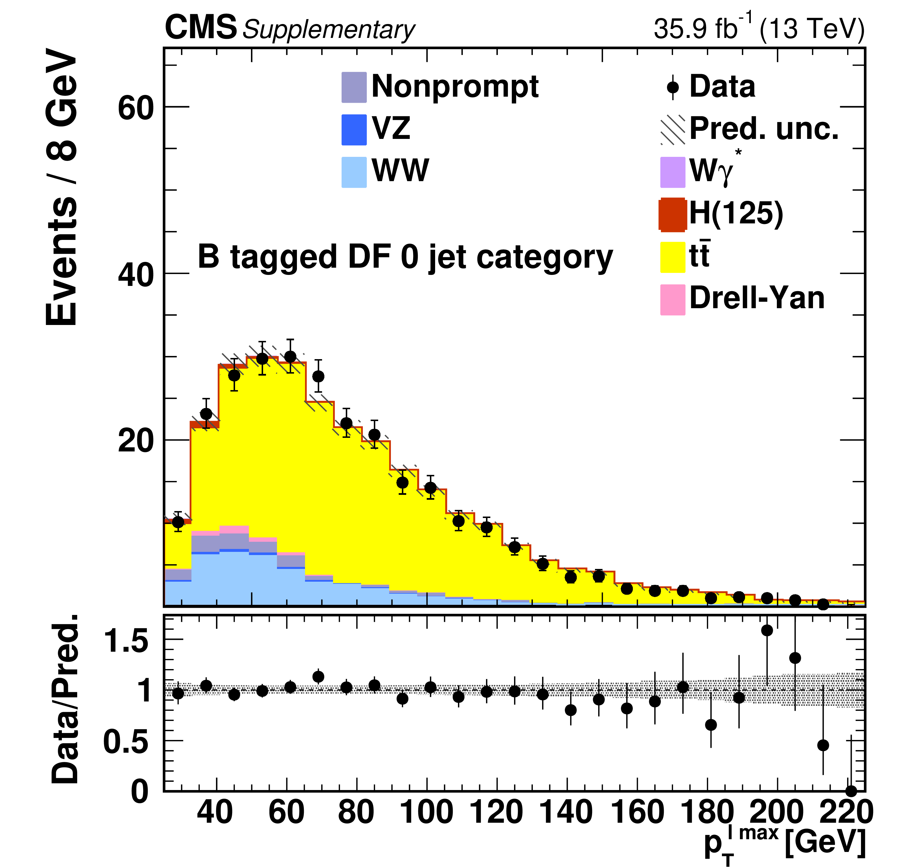
Additional Figure 2-a:
Kinematic distributions for events with zero jets and DF leptons in the b-tagged control region in the sequential cut analysis. The distribution shows the leading lepton ${p_{\mathrm {T}}}$ ($ {p_{\mathrm{T}}^{\,\text {max}}} $). The predicted yields are shown with their best fit normalizations from the simultaneous fit. The error bars on the data points represent the statistical uncertainty of the data, and the hatched areas represent the combined systematic and statistical uncertainty of the predicted yield in each bin. The last bin includes the overflow. |
png pdf |
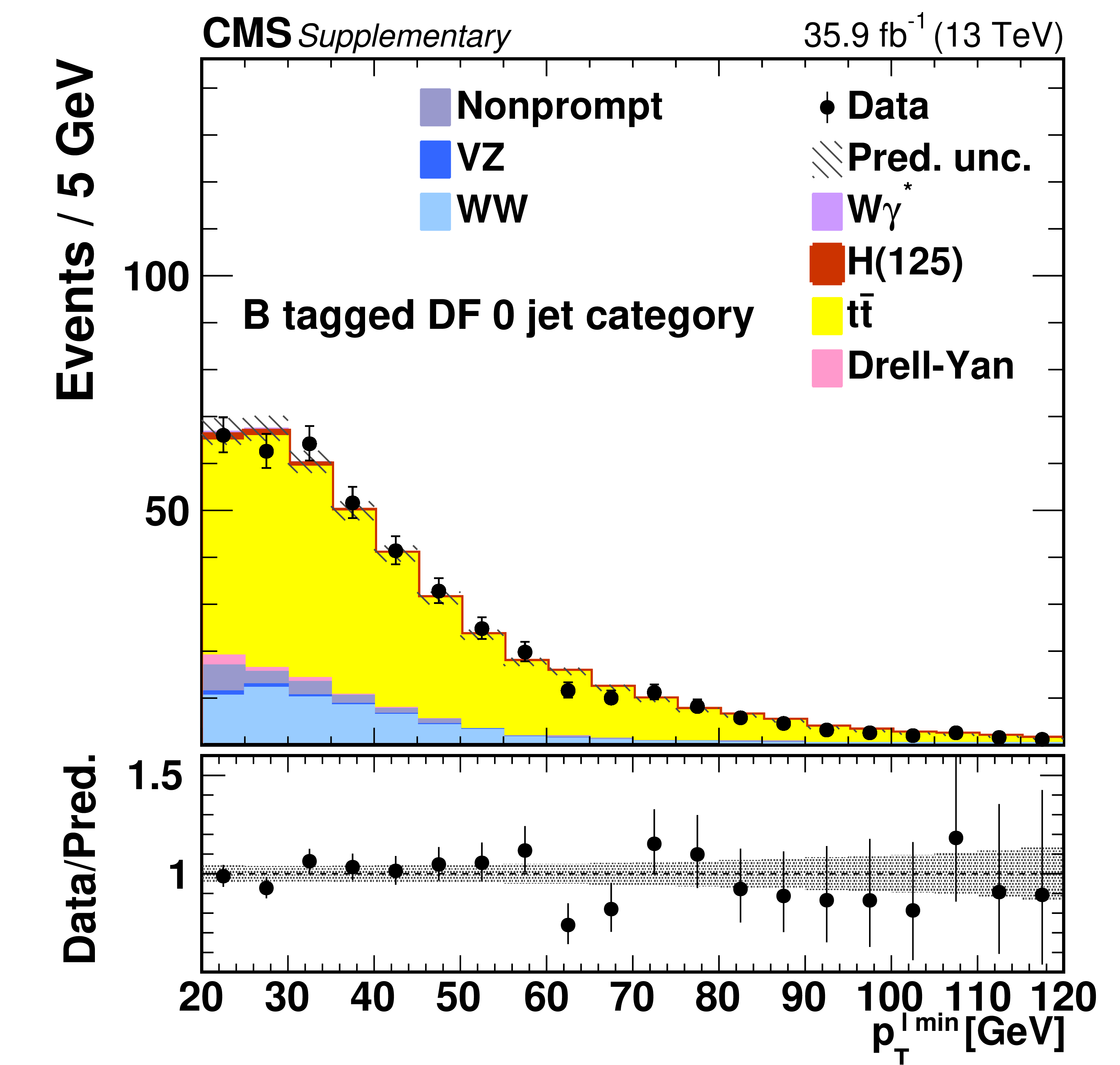
Additional Figure 2-b:
Kinematic distributions for events with zero jets and DF leptons in the b-tagged control region in the sequential cut analysis. The distribution shows the trailing lepton ${p_{\mathrm {T}}}$ ($ {p_{\mathrm{T}}^{\,\text {min}}} $). The predicted yields are shown with their best fit normalizations from the simultaneous fit. The error bars on the data points represent the statistical uncertainty of the data, and the hatched areas represent the combined systematic and statistical uncertainty of the predicted yield in each bin. The last bin includes the overflow. |
png pdf |
Additional Figure 2-c:
Kinematic distributions for events with zero jets and DF leptons in the b-tagged control region in the sequential cut analysis. The distribution shows the dilepton transverse momentum $ {p_{\mathrm {T}}} ^{\ell\ell}$. The predicted yields are shown with their best fit normalizations from the simultaneous fit. The error bars on the data points represent the statistical uncertainty of the data, and the hatched areas represent the combined systematic and statistical uncertainty of the predicted yield in each bin. The last bin includes the overflow. |
png pdf |
Additional Figure 2-d:
Kinematic distributions for events with zero jets and DF leptons in the b-tagged control region in the sequential cut analysis. The distribution shows the azimuthal angle between the two leptons $ {\Delta \phi _{\ell\ell}} $. The predicted yields are shown with their best fit normalizations from the simultaneous fit. The error bars on the data points represent the statistical uncertainty of the data, and the hatched areas represent the combined systematic and statistical uncertainty of the predicted yield in each bin. The last bin includes the overflow. |

png pdf |
Additional Figure 2-e:
Kinematic distributions for events with zero jets and DF leptons in the b-tagged control region in the sequential cut analysis. The distribution shows the missing transverse momentum ${{p_{\mathrm {T}}} ^\text {miss}}$. The predicted yields are shown with their best fit normalizations from the simultaneous fit. The error bars on the data points represent the statistical uncertainty of the data, and the hatched areas represent the combined systematic and statistical uncertainty of the predicted yield in each bin. The last bin includes the overflow. |
png pdf |
Additional Figure 2-f:
Kinematic distributions for events with zero jets and DF leptons in the b-tagged control region in the sequential cut analysis. The distribution shows the dilepton invariant mass $ {m_{\ell\ell}}$. The predicted yields are shown with their best fit normalizations from the simultaneous fit. The error bars on the data points represent the statistical uncertainty of the data, and the hatched areas represent the combined systematic and statistical uncertainty of the predicted yield in each bin. The last bin includes the overflow. |
png pdf |
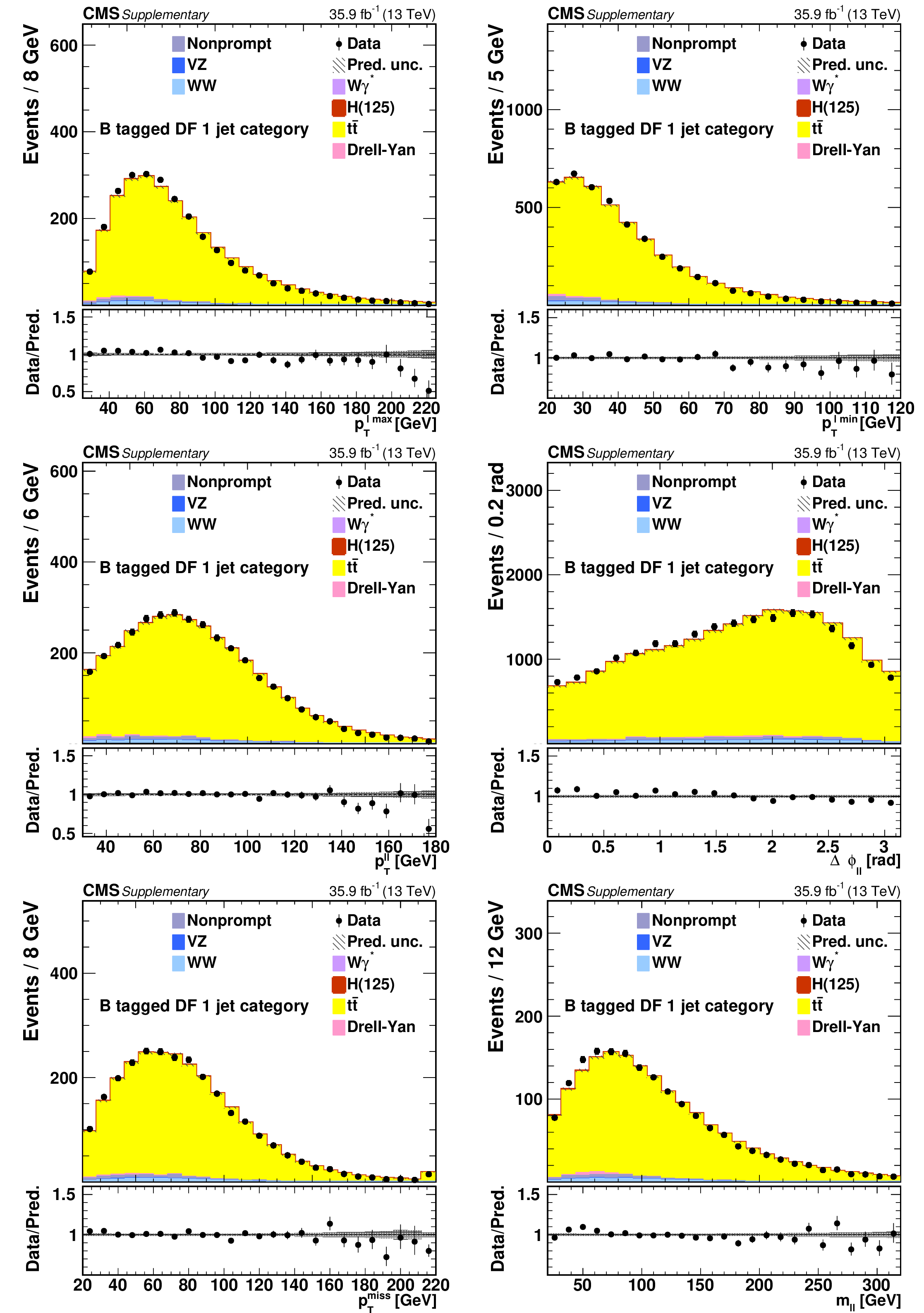
Additional Figure 3:
Kinematic distributions for events with one jet and DF leptons in the b-tagged control region in the sequential cut analysis. The distributions show the leading and trailing lepton ${p_{\mathrm {T}}}$ ($ {p_{\mathrm{T}}^{\,\text {max}}} $ and $ {p_{\mathrm{T}}^{\,\text {min}}} $), the dilepton transverse momentum $ {p_{\mathrm {T}}} ^{\ell\ell}$, the azimuthal angle between the two leptons $ {\Delta \phi _{\ell\ell}} $, the missing transverse momentum ${{p_{\mathrm {T}}} ^\text {miss}}$, and the dilepton invariant mass $ {m_{\ell\ell}}$. The predicted yields are shown with their best fit normalizations from the simultaneous fit. The error bars on the data points represent the statistical uncertainty of the data, and the hatched areas represent the combined systematic and statistical uncertainty of the predicted yield in each bin. The last bin includes the overflow. |
png pdf |
Additional Figure 3-a:
Kinematic distributions for events with one jet and DF leptons in the b-tagged control region in the sequential cut analysis. The distribution shows the leading lepton ${p_{\mathrm {T}}}$ ($ {p_{\mathrm{T}}^{\,\text {max}}} $). The predicted yields are shown with their best fit normalizations from the simultaneous fit. The error bars on the data points represent the statistical uncertainty of the data, and the hatched areas represent the combined systematic and statistical uncertainty of the predicted yield in each bin. The last bin includes the overflow. |
png pdf |
Additional Figure 3-b:
Kinematic distributions for events with one jet and DF leptons in the b-tagged control region in the sequential cut analysis. The distribution shows the trailing lepton ${p_{\mathrm {T}}}$ ($ {p_{\mathrm{T}}^{\,\text {min}}} $). The predicted yields are shown with their best fit normalizations from the simultaneous fit. The error bars on the data points represent the statistical uncertainty of the data, and the hatched areas represent the combined systematic and statistical uncertainty of the predicted yield in each bin. The last bin includes the overflow. |

png pdf |
Additional Figure 3-c:
Kinematic distributions for events with one jet and DF leptons in the b-tagged control region in the sequential cut analysis. The distribution shows the dilepton transverse momentum $ {p_{\mathrm {T}}} ^{\ell\ell}$. The predicted yields are shown with their best fit normalizations from the simultaneous fit. The error bars on the data points represent the statistical uncertainty of the data, and the hatched areas represent the combined systematic and statistical uncertainty of the predicted yield in each bin. The last bin includes the overflow. |

png pdf |
Additional Figure 3-d:
Kinematic distributions for events with one jet and DF leptons in the b-tagged control region in the sequential cut analysis. The distribution shows the azimuthal angle between the two leptons $ {\Delta \phi _{\ell\ell}} $. The predicted yields are shown with their best fit normalizations from the simultaneous fit. The error bars on the data points represent the statistical uncertainty of the data, and the hatched areas represent the combined systematic and statistical uncertainty of the predicted yield in each bin. The last bin includes the overflow. |

png pdf |
Additional Figure 3-e:
Kinematic distributions for events with one jet and DF leptons in the b-tagged control region in the sequential cut analysis. The distribution shows the missing transverse momentum ${{p_{\mathrm {T}}} ^\text {miss}}$. The predicted yields are shown with their best fit normalizations from the simultaneous fit. The error bars on the data points represent the statistical uncertainty of the data, and the hatched areas represent the combined systematic and statistical uncertainty of the predicted yield in each bin. The last bin includes the overflow. |
png pdf |
Additional Figure 3-f:
Kinematic distributions for events with one jet and DF leptons in the b-tagged control region in the sequential cut analysis. The distribution shows the dilepton invariant mass $ {m_{\ell\ell}}$. The predicted yields are shown with their best fit normalizations from the simultaneous fit. The error bars on the data points represent the statistical uncertainty of the data, and the hatched areas represent the combined systematic and statistical uncertainty of the predicted yield in each bin. The last bin includes the overflow. |
png pdf |
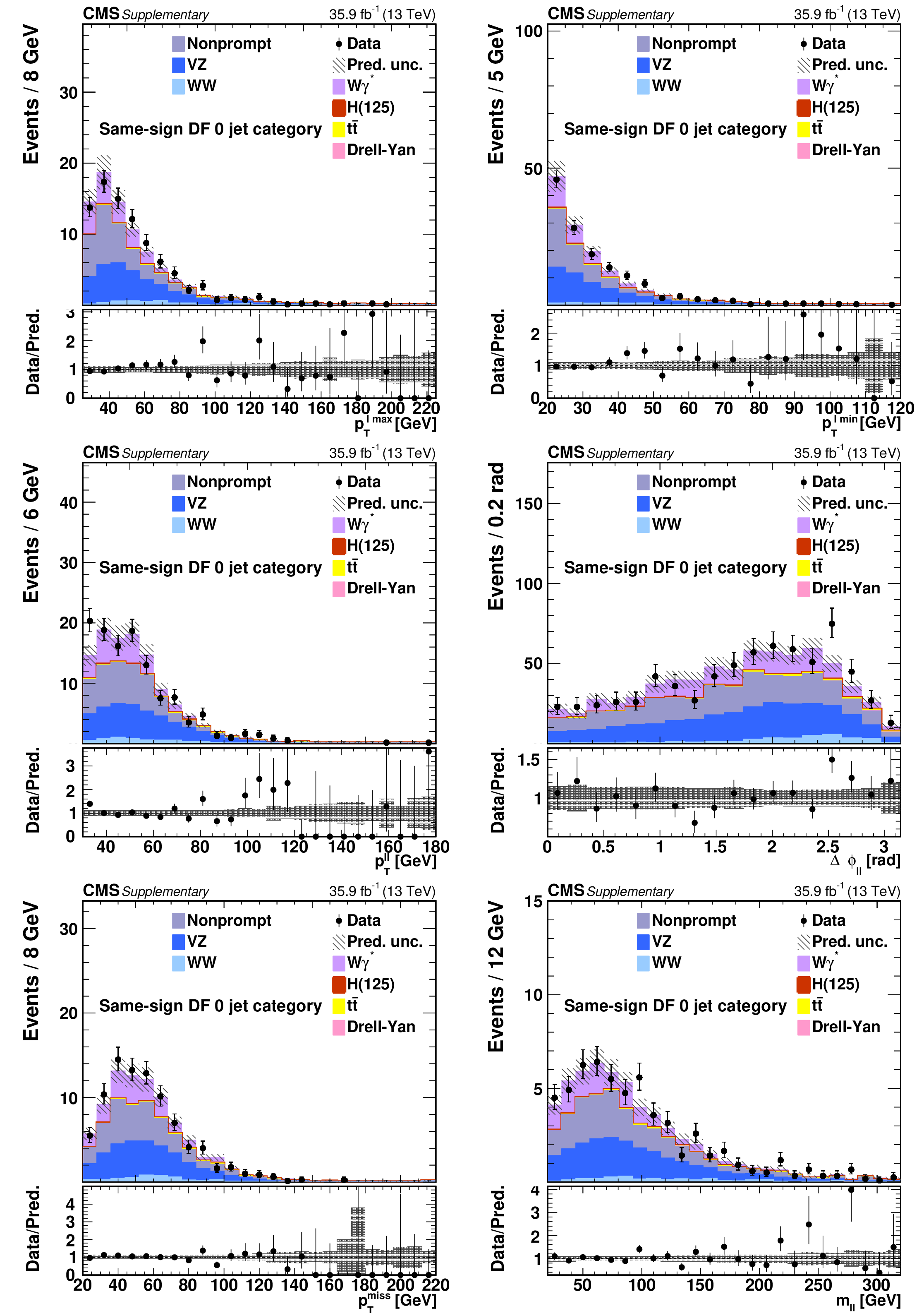
Additional Figure 4:
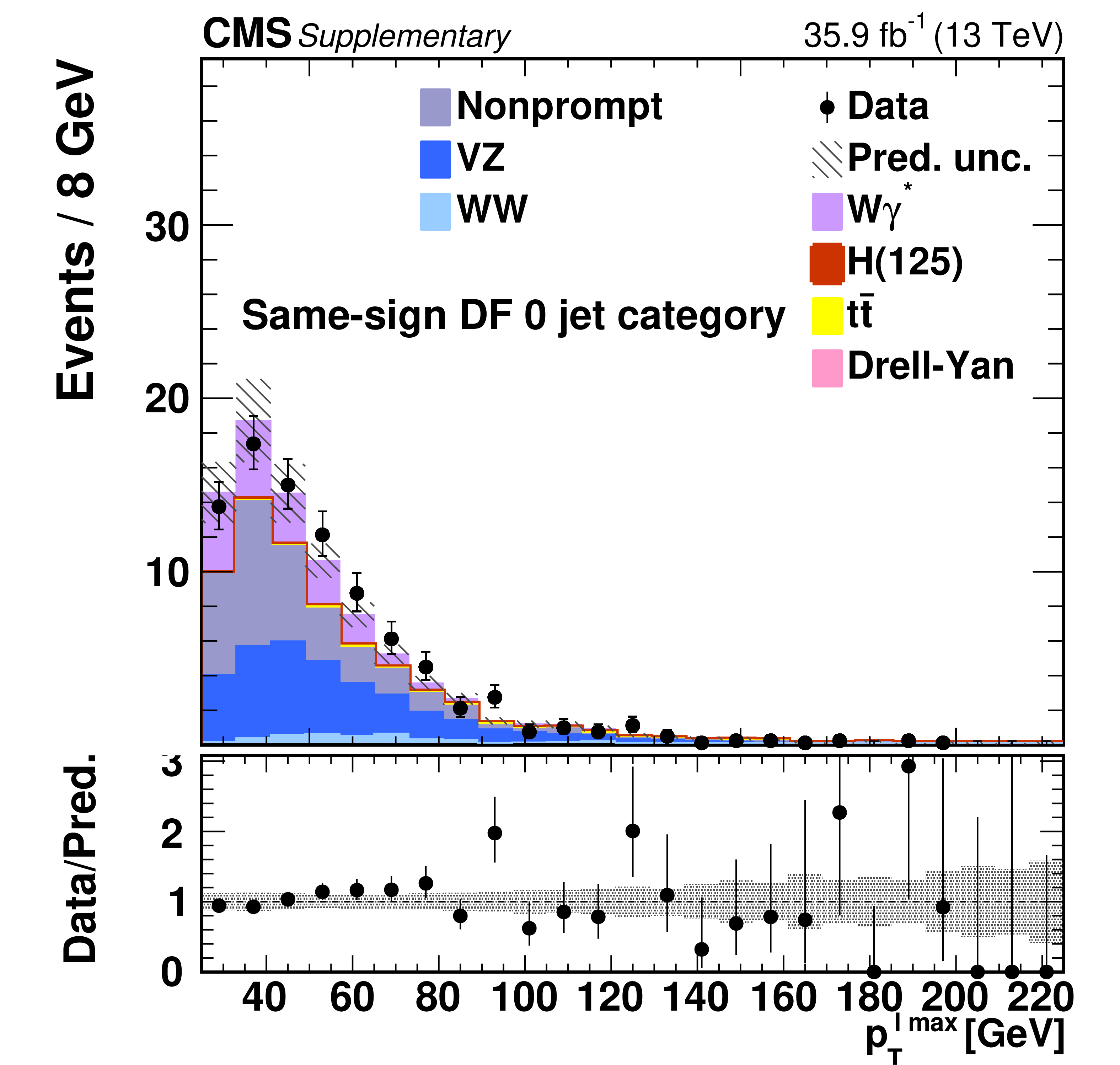
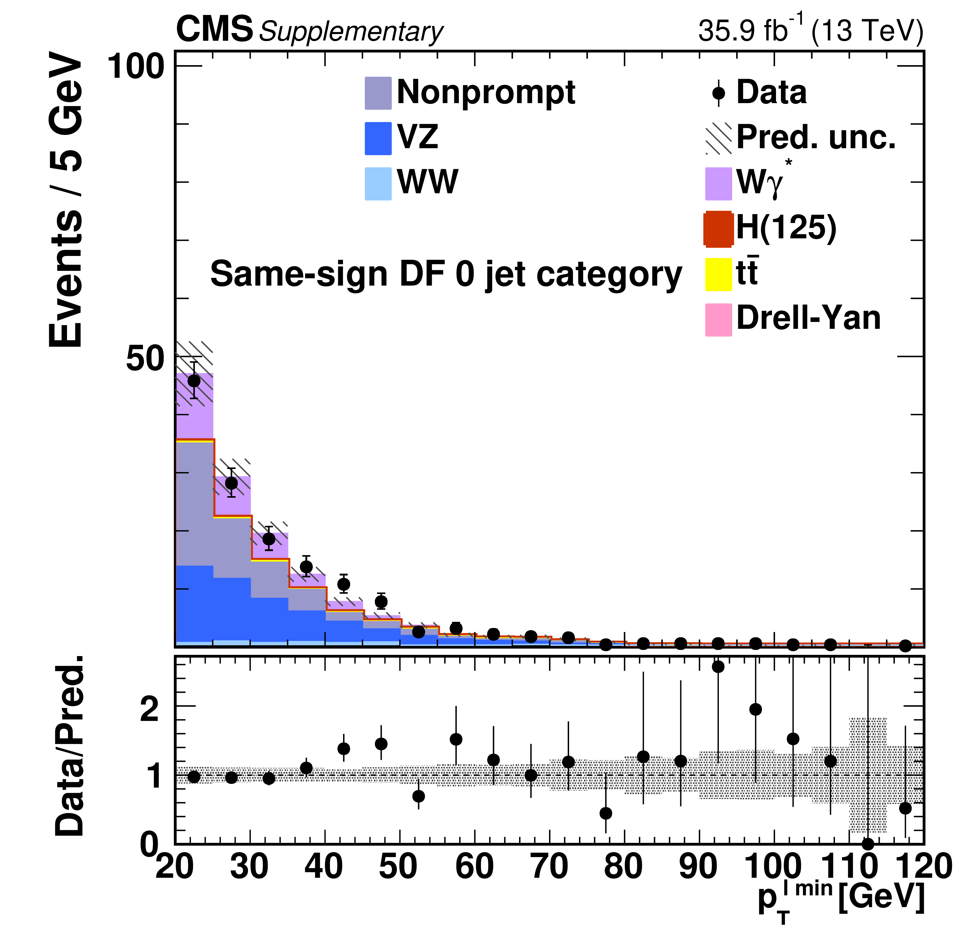
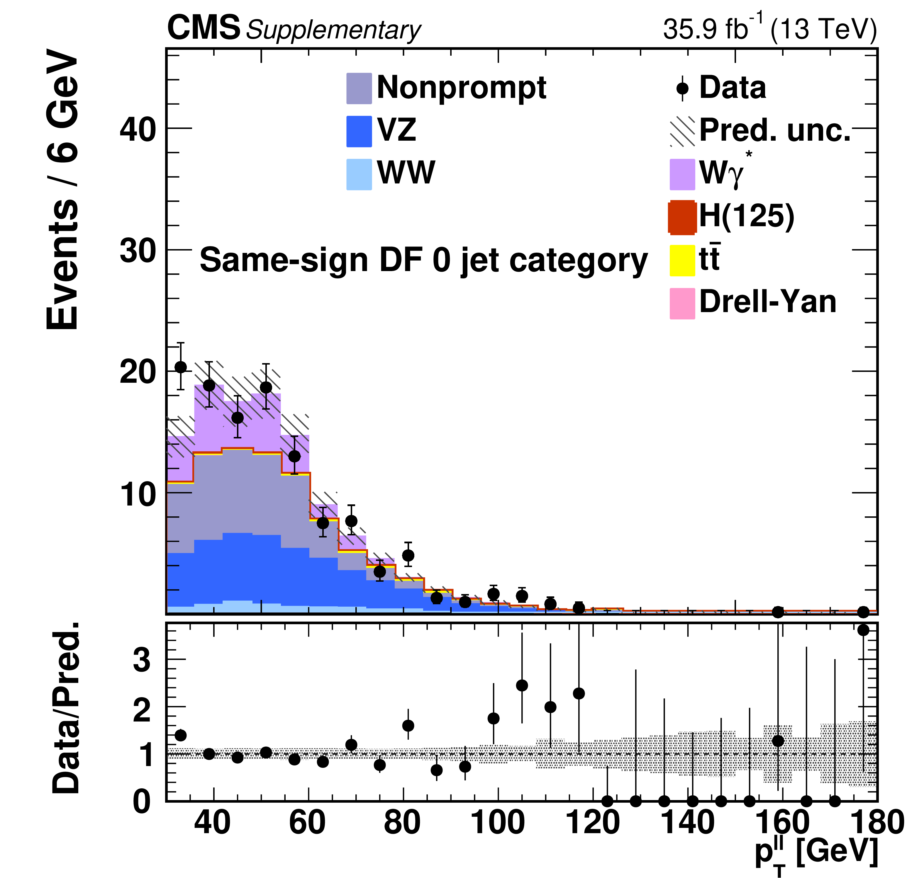
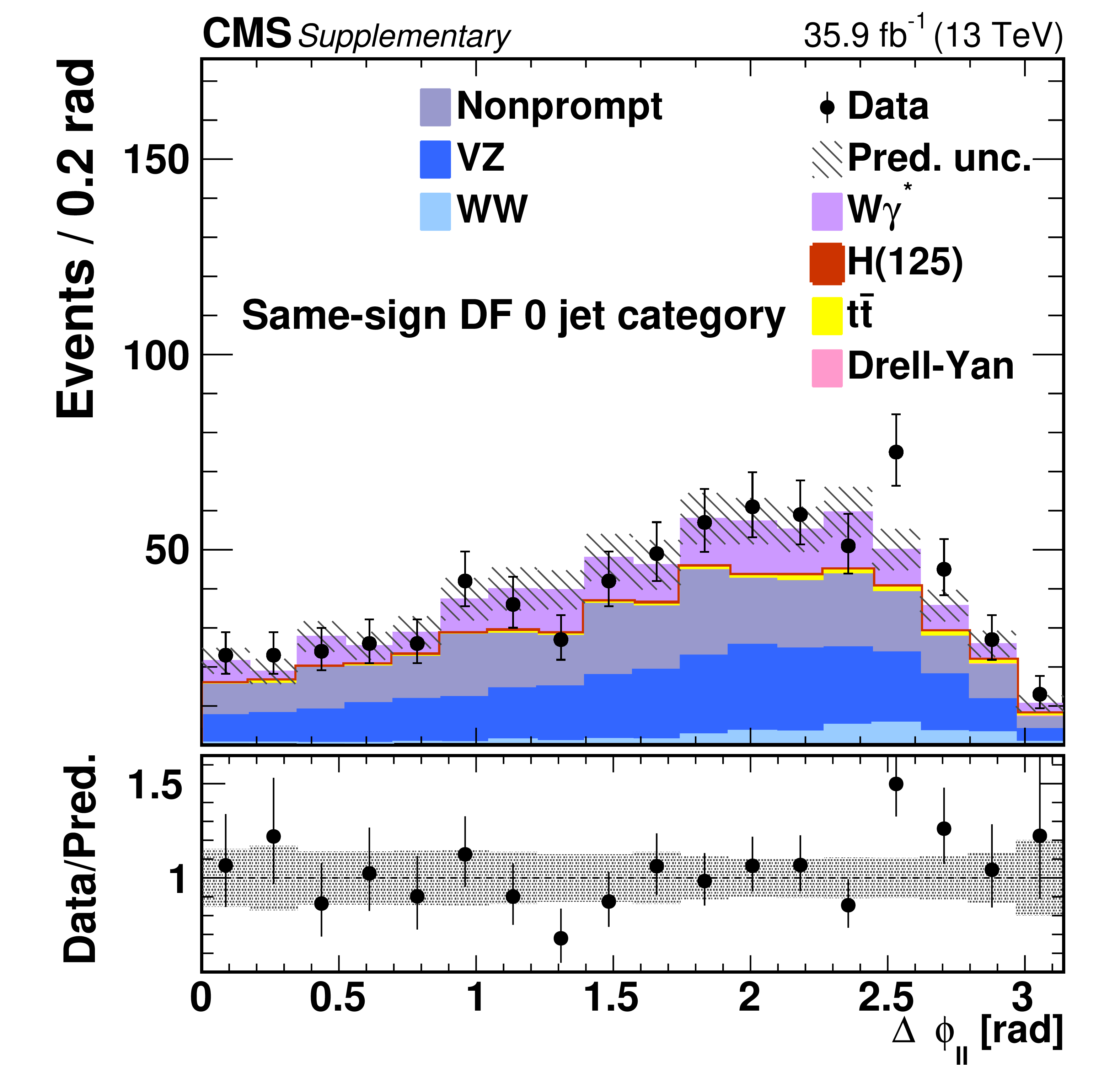
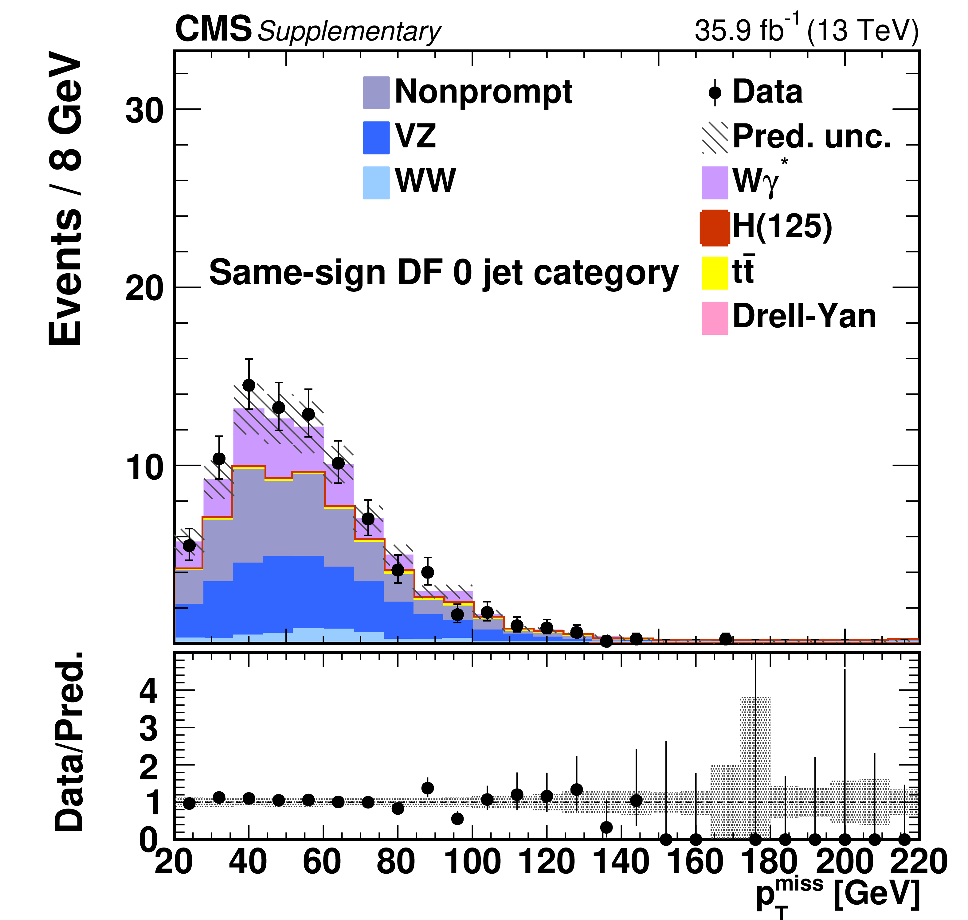
Kinematic distributions for events with zero jets and DF leptons in the same-sign control region in the sequential cut analysis. The distributions show the leading and trailing lepton ${p_{\mathrm {T}}}$ ($ {p_{\mathrm{T}}^{\,\text {max}}} $ and $ {p_{\mathrm{T}}^{\,\text {min}}} $), the dilepton transverse momentum $ {p_{\mathrm {T}}} ^{\ell\ell}$, the azimuthal angle between the two leptons $ {\Delta \phi _{\ell\ell}} $, the missing transverse momentum ${{p_{\mathrm {T}}} ^\text {miss}}$, and the dilepton invariant mass $ {m_{\ell\ell}}$. The predicted yields are shown with their best fit normalizations from the simultaneous fit. The error bars on the data points represent the statistical uncertainty of the data, and the hatched areas represent the combined systematic and statistical uncertainty of the predicted yield in each bin. The last bin includes the overflow. |
png pdf |
Additional Figure 4-a:
Kinematic distributions for events with zero jets and DF leptons in the same-sign control region in the sequential cut analysis. The distribution shows the leading lepton ${p_{\mathrm {T}}}$ ($ {p_{\mathrm{T}}^{\,\text {max}}} $). The predicted yields are shown with their best fit normalizations from the simultaneous fit. The error bars on the data points represent the statistical uncertainty of the data, and the hatched areas represent the combined systematic and statistical uncertainty of the predicted yield in each bin. The last bin includes the overflow. |
png pdf |
Additional Figure 4-b:
Kinematic distributions for events with zero jets and DF leptons in the same-sign control region in the sequential cut analysis. The distribution shows the trailing lepton ${p_{\mathrm {T}}}$ ($ {p_{\mathrm{T}}^{\,\text {min}}} $). The predicted yields are shown with their best fit normalizations from the simultaneous fit. The error bars on the data points represent the statistical uncertainty of the data, and the hatched areas represent the combined systematic and statistical uncertainty of the predicted yield in each bin. The last bin includes the overflow. |
png pdf |
Additional Figure 4-c:
Kinematic distributions for events with zero jets and DF leptons in the same-sign control region in the sequential cut analysis. The distribution shows the dilepton transverse momentum $ {p_{\mathrm {T}}} ^{\ell\ell}$. The predicted yields are shown with their best fit normalizations from the simultaneous fit. The error bars on the data points represent the statistical uncertainty of the data, and the hatched areas represent the combined systematic and statistical uncertainty of the predicted yield in each bin. The last bin includes the overflow. |
png pdf |
Additional Figure 4-d:
Kinematic distributions for events with zero jets and DF leptons in the same-sign control region in the sequential cut analysis. The distribution shows the azimuthal angle between the two leptons $ {\Delta \phi _{\ell\ell}} $. The predicted yields are shown with their best fit normalizations from the simultaneous fit. The error bars on the data points represent the statistical uncertainty of the data, and the hatched areas represent the combined systematic and statistical uncertainty of the predicted yield in each bin. The last bin includes the overflow. |
png pdf |
Additional Figure 4-e:
Kinematic distributions for events with zero jets and DF leptons in the same-sign control region in the sequential cut analysis. The distribution shows the missing transverse momentum ${{p_{\mathrm {T}}} ^\text {miss}}$. The predicted yields are shown with their best fit normalizations from the simultaneous fit. The error bars on the data points represent the statistical uncertainty of the data, and the hatched areas represent the combined systematic and statistical uncertainty of the predicted yield in each bin. The last bin includes the overflow. |

png pdf |
Additional Figure 4-f:
Kinematic distributions for events with zero jets and DF leptons in the same-sign control region in the sequential cut analysis. The distribution shows the dilepton invariant mass $ {m_{\ell\ell}}$. The predicted yields are shown with their best fit normalizations from the simultaneous fit. The error bars on the data points represent the statistical uncertainty of the data, and the hatched areas represent the combined systematic and statistical uncertainty of the predicted yield in each bin. The last bin includes the overflow. |

png pdf |
Additional Figure 5:
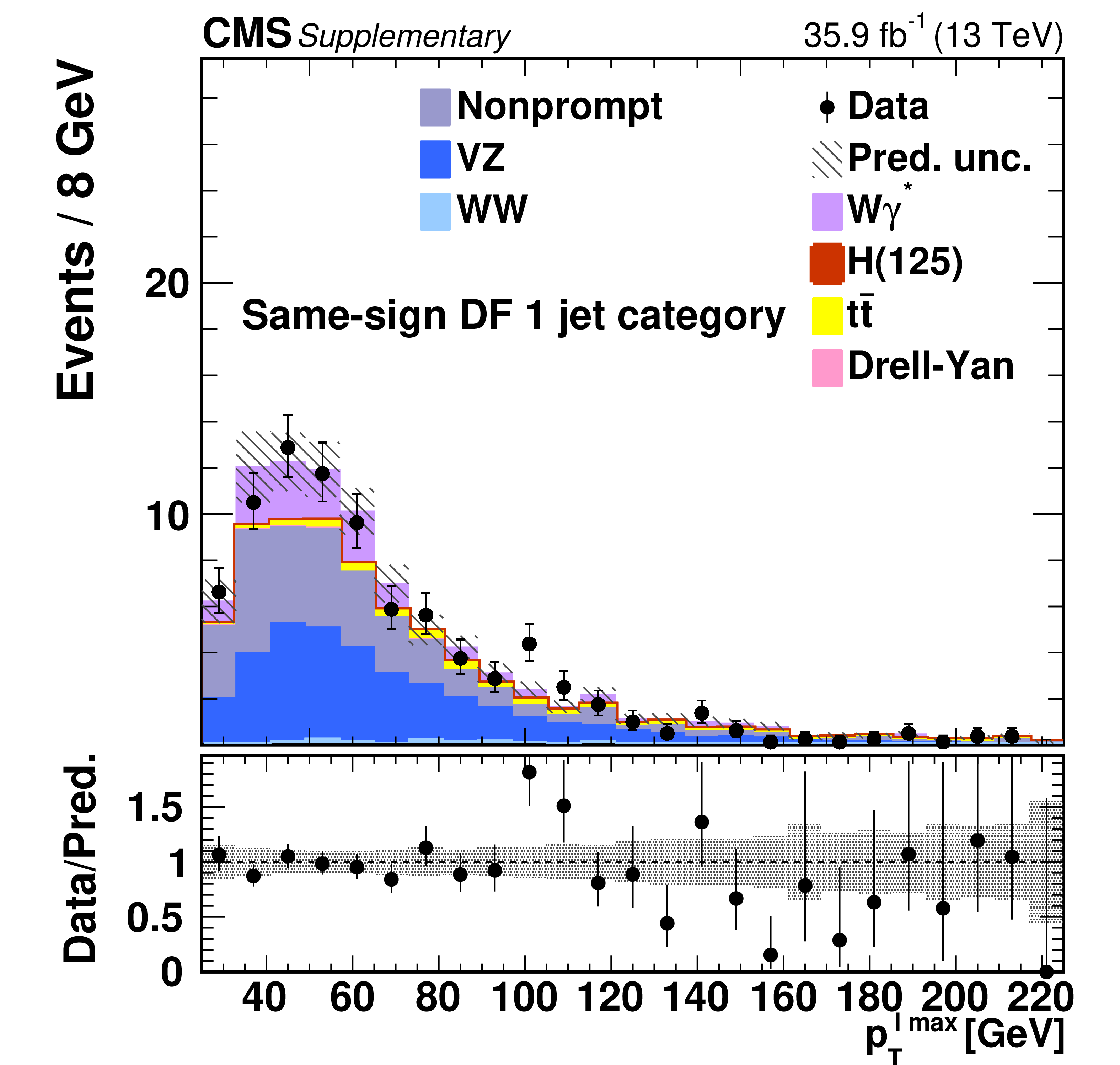
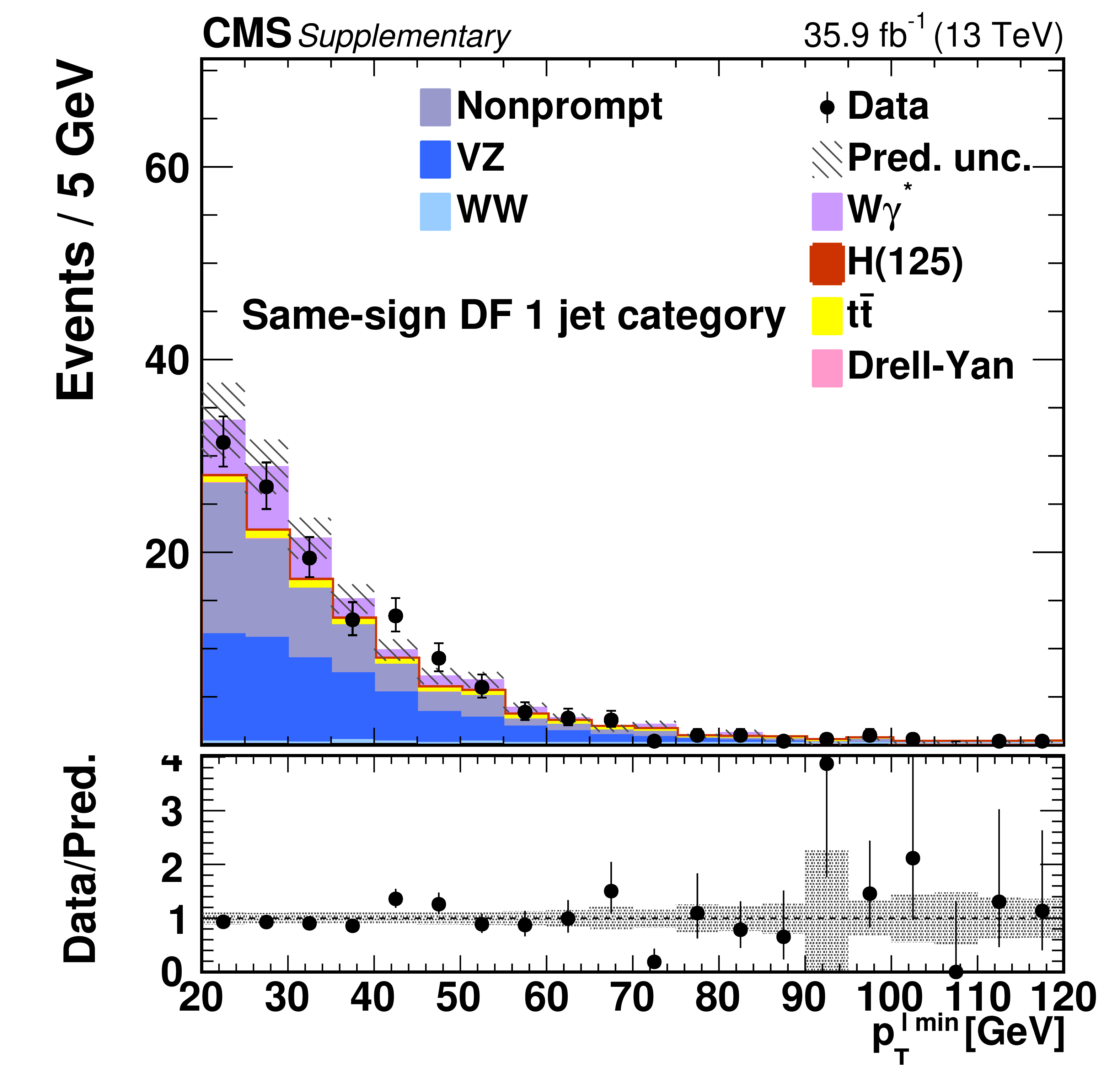
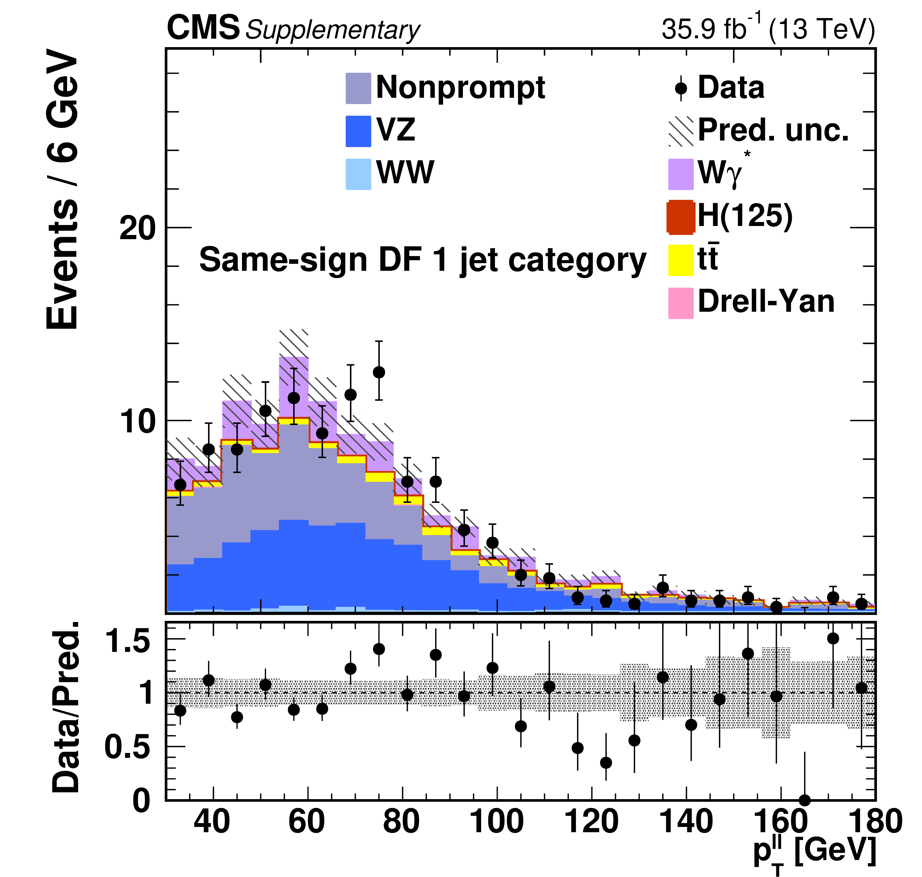
Kinematic distributions for events with one jet and DF leptons in the same-sign control region in the sequential cut analysis. The distributions show the leading and trailing lepton ${p_{\mathrm {T}}}$ ($ {p_{\mathrm{T}}^{\,\text {max}}} $ and $ {p_{\mathrm{T}}^{\,\text {min}}} $), the dilepton transverse momentum $ {p_{\mathrm {T}}} ^{\ell\ell}$, the azimuthal angle between the two leptons $ {\Delta \phi _{\ell\ell}} $, the missing transverse momentum ${{p_{\mathrm {T}}} ^\text {miss}}$, and the dilepton invariant mass $ {m_{\ell\ell}}$. The predicted yields are shown with their best fit normalizations from the simultaneous fit. The error bars on the data points represent the statistical uncertainty of the data, and the hatched areas represent the combined systematic and statistical uncertainty of the predicted yield in each bin. The last bin includes the overflow. |
png pdf |
Additional Figure 5-a:
Kinematic distributions for events with one jet and DF leptons in the same-sign control region in the sequential cut analysis. The distribution shows the leading lepton ${p_{\mathrm {T}}}$ ($ {p_{\mathrm{T}}^{\,\text {max}}} $). The predicted yields are shown with their best fit normalizations from the simultaneous fit. The error bars on the data points represent the statistical uncertainty of the data, and the hatched areas represent the combined systematic and statistical uncertainty of the predicted yield in each bin. The last bin includes the overflow. |
png pdf |
Additional Figure 5-b:
Kinematic distributions for events with one jet and DF leptons in the same-sign control region in the sequential cut analysis. The distribution shows the trailing lepton ${p_{\mathrm {T}}}$ ($ {p_{\mathrm{T}}^{\,\text {min}}} $). The predicted yields are shown with their best fit normalizations from the simultaneous fit. The error bars on the data points represent the statistical uncertainty of the data, and the hatched areas represent the combined systematic and statistical uncertainty of the predicted yield in each bin. The last bin includes the overflow. |
png pdf |
Additional Figure 5-c:
Kinematic distributions for events with one jet and DF leptons in the same-sign control region in the sequential cut analysis. The distribution shows the dilepton transverse momentum $ {p_{\mathrm {T}}} ^{\ell\ell}$. The predicted yields are shown with their best fit normalizations from the simultaneous fit. The error bars on the data points represent the statistical uncertainty of the data, and the hatched areas represent the combined systematic and statistical uncertainty of the predicted yield in each bin. The last bin includes the overflow. |
png pdf |
Additional Figure 5-d:
Kinematic distributions for events with one jet and DF leptons in the same-sign control region in the sequential cut analysis. The distribution shows the azimuthal angle between the two leptons $ {\Delta \phi _{\ell\ell}} $. The predicted yields are shown with their best fit normalizations from the simultaneous fit. The error bars on the data points represent the statistical uncertainty of the data, and the hatched areas represent the combined systematic and statistical uncertainty of the predicted yield in each bin. The last bin includes the overflow. |
png pdf |
Additional Figure 5-e:
Kinematic distributions for events with one jet and DF leptons in the same-sign control region in the sequential cut analysis. The distribution shows the missing transverse momentum ${{p_{\mathrm {T}}} ^\text {miss}}$. The predicted yields are shown with their best fit normalizations from the simultaneous fit. The error bars on the data points represent the statistical uncertainty of the data, and the hatched areas represent the combined systematic and statistical uncertainty of the predicted yield in each bin. The last bin includes the overflow. |
png pdf |
Additional Figure 5-f:
Kinematic distributions for events with one jet and DF leptons in the same-sign control region in the sequential cut analysis. The distribution shows the dilepton invariant mass $ {m_{\ell\ell}}$. The predicted yields are shown with their best fit normalizations from the simultaneous fit. The error bars on the data points represent the statistical uncertainty of the data, and the hatched areas represent the combined systematic and statistical uncertainty of the predicted yield in each bin. The last bin includes the overflow. |

png pdf |
Additional Figure 6:
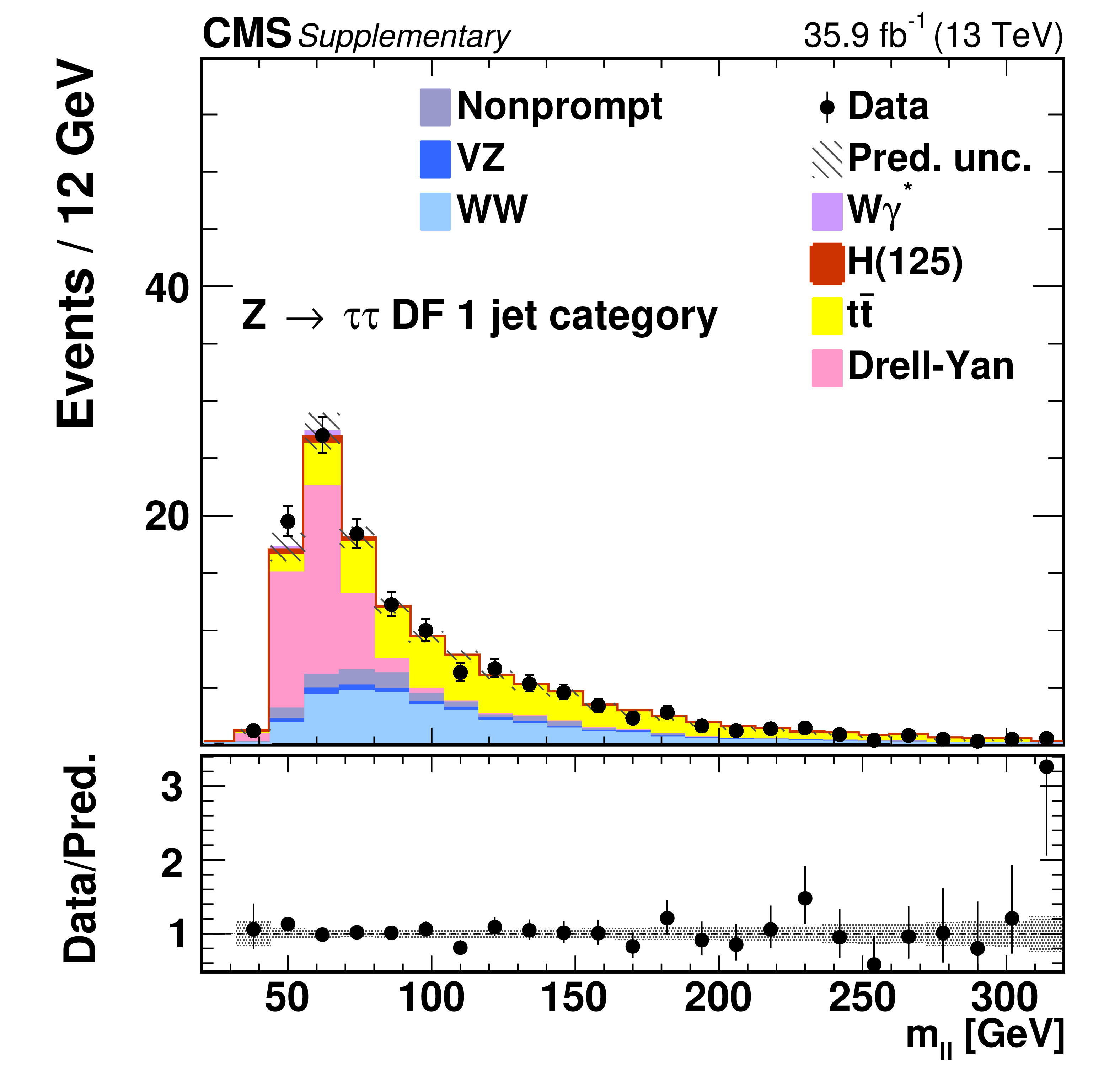
Kinematic distributions for events with zero jets and DF leptons in the $ {\mathrm {Z}} \to \tau ^+\tau ^-$ control region in the sequential cut analysis. The distributions show the leading and trailing lepton ${p_{\mathrm {T}}}$ ($ {p_{\mathrm{T}}^{\,\text {max}}} $ and $ {p_{\mathrm{T}}^{\,\text {min}}} $), the dilepton transverse momentum $ {p_{\mathrm {T}}} ^{\ell\ell}$, the azimuthal angle between the two leptons $ {\Delta \phi _{\ell\ell}} $, the missing transverse momentum ${{p_{\mathrm {T}}} ^\text {miss}}$, and the dilepton invariant mass $ {m_{\ell\ell}}$. The predicted yields are shown with their best fit normalizations from the simultaneous fit. The error bars on the data points represent the statistical uncertainty of the data, and the hatched areas represent the combined systematic and statistical uncertainty of the predicted yield in each bin. The last bin includes the overflow. |
png pdf |
Additional Figure 6-a:
Kinematic distributions for events with zero jets and DF leptons in the $ {\mathrm {Z}} \to \tau ^+\tau ^-$ control region in the sequential cut analysis. The distribution shows the leading lepton ${p_{\mathrm {T}}}$ ($ {p_{\mathrm{T}}^{\,\text {max}}} $). The predicted yields are shown with their best fit normalizations from the simultaneous fit. The error bars on the data points represent the statistical uncertainty of the data, and the hatched areas represent the combined systematic and statistical uncertainty of the predicted yield in each bin. The last bin includes the overflow. |
png pdf |
Additional Figure 6-b:
Kinematic distributions for events with zero jets and DF leptons in the $ {\mathrm {Z}} \to \tau ^+\tau ^-$ control region in the sequential cut analysis. The distribution shows the trailing lepton ${p_{\mathrm {T}}}$ ($ {p_{\mathrm{T}}^{\,\text {min}}} $). The predicted yields are shown with their best fit normalizations from the simultaneous fit. The error bars on the data points represent the statistical uncertainty of the data, and the hatched areas represent the combined systematic and statistical uncertainty of the predicted yield in each bin. The last bin includes the overflow. |

png pdf |
Additional Figure 6-c:
Kinematic distributions for events with zero jets and DF leptons in the $ {\mathrm {Z}} \to \tau ^+\tau ^-$ control region in the sequential cut analysis. The distribution shows the dilepton transverse momentum $ {p_{\mathrm {T}}} ^{\ell\ell}$. The predicted yields are shown with their best fit normalizations from the simultaneous fit. The error bars on the data points represent the statistical uncertainty of the data, and the hatched areas represent the combined systematic and statistical uncertainty of the predicted yield in each bin. The last bin includes the overflow. |

png pdf |
Additional Figure 6-d:
Kinematic distributions for events with zero jets and DF leptons in the $ {\mathrm {Z}} \to \tau ^+\tau ^-$ control region in the sequential cut analysis. The distribution shows the azimuthal angle between the two leptons $ {\Delta \phi _{\ell\ell}} $. The predicted yields are shown with their best fit normalizations from the simultaneous fit. The error bars on the data points represent the statistical uncertainty of the data, and the hatched areas represent the combined systematic and statistical uncertainty of the predicted yield in each bin. The last bin includes the overflow. |
png pdf |
Additional Figure 6-e:
Kinematic distributions for events with zero jets and DF leptons in the $ {\mathrm {Z}} \to \tau ^+\tau ^-$ control region in the sequential cut analysis. The distribution shows the missing transverse momentum ${{p_{\mathrm {T}}} ^\text {miss}}$. The predicted yields are shown with their best fit normalizations from the simultaneous fit. The error bars on the data points represent the statistical uncertainty of the data, and the hatched areas represent the combined systematic and statistical uncertainty of the predicted yield in each bin. The last bin includes the overflow. |
png pdf |
Additional Figure 6-f:
Kinematic distributions for events with zero jets and DF leptons in the $ {\mathrm {Z}} \to \tau ^+\tau ^-$ control region in the sequential cut analysis. The distribution shows the dilepton invariant mass $ {m_{\ell\ell}}$. The predicted yields are shown with their best fit normalizations from the simultaneous fit. The error bars on the data points represent the statistical uncertainty of the data, and the hatched areas represent the combined systematic and statistical uncertainty of the predicted yield in each bin. The last bin includes the overflow. |
png pdf |
Additional Figure 7:
Kinematic distributions for events with one jet and DF leptons in the $ {\mathrm {Z}} \to \tau ^+\tau ^-$ control region in the sequential cut analysis. The distributions show the leading and trailing lepton ${p_{\mathrm {T}}}$ ($ {p_{\mathrm{T}}^{\,\text {max}}} $ and $ {p_{\mathrm{T}}^{\,\text {min}}} $), the dilepton transverse momentum $ {p_{\mathrm {T}}} ^{\ell\ell}$, the azimuthal angle between the two leptons $ {\Delta \phi _{\ell\ell}} $, the missing transverse momentum ${{p_{\mathrm {T}}} ^\text {miss}}$, and the dilepton invariant mass $ {m_{\ell\ell}}$. The predicted yields are shown with their best fit normalizations from the simultaneous fit. The error bars on the data points represent the statistical uncertainty of the data, and the hatched areas represent the combined systematic and statistical uncertainty of the predicted yield in each bin. The last bin includes the overflow. |

png pdf |
Additional Figure 7-a:
Kinematic distributions for events with one jet and DF leptons in the $ {\mathrm {Z}} \to \tau ^+\tau ^-$ control region in the sequential cut analysis. The distribution shows the leading lepton ${p_{\mathrm {T}}}$ ($ {p_{\mathrm{T}}^{\,\text {max}}} $). The predicted yields are shown with their best fit normalizations from the simultaneous fit. The error bars on the data points represent the statistical uncertainty of the data, and the hatched areas represent the combined systematic and statistical uncertainty of the predicted yield in each bin. The last bin includes the overflow. |
png pdf |
Additional Figure 7-b:
Kinematic distributions for events with one jet and DF leptons in the $ {\mathrm {Z}} \to \tau ^+\tau ^-$ control region in the sequential cut analysis. The distribution shows the trailing lepton ${p_{\mathrm {T}}}$ ($ {p_{\mathrm{T}}^{\,\text {min}}} $). The predicted yields are shown with their best fit normalizations from the simultaneous fit. The error bars on the data points represent the statistical uncertainty of the data, and the hatched areas represent the combined systematic and statistical uncertainty of the predicted yield in each bin. The last bin includes the overflow. |
png pdf |
Additional Figure 7-c:
Kinematic distributions for events with one jet and DF leptons in the $ {\mathrm {Z}} \to \tau ^+\tau ^-$ control region in the sequential cut analysis. The distribution shows the dilepton transverse momentum $ {p_{\mathrm {T}}} ^{\ell\ell}$. The predicted yields are shown with their best fit normalizations from the simultaneous fit. The error bars on the data points represent the statistical uncertainty of the data, and the hatched areas represent the combined systematic and statistical uncertainty of the predicted yield in each bin. The last bin includes the overflow. |
png pdf |
Additional Figure 7-d:
Kinematic distributions for events with one jet and DF leptons in the $ {\mathrm {Z}} \to \tau ^+\tau ^-$ control region in the sequential cut analysis. The distribution shows the azimuthal angle between the two leptons $ {\Delta \phi _{\ell\ell}} $. The predicted yields are shown with their best fit normalizations from the simultaneous fit. The error bars on the data points represent the statistical uncertainty of the data, and the hatched areas represent the combined systematic and statistical uncertainty of the predicted yield in each bin. The last bin includes the overflow. |
png pdf |
Additional Figure 7-e:
Kinematic distributions for events with one jet and DF leptons in the $ {\mathrm {Z}} \to \tau ^+\tau ^-$ control region in the sequential cut analysis. The distribution shows the missing transverse momentum ${{p_{\mathrm {T}}} ^\text {miss}}$. The predicted yields are shown with their best fit normalizations from the simultaneous fit. The error bars on the data points represent the statistical uncertainty of the data, and the hatched areas represent the combined systematic and statistical uncertainty of the predicted yield in each bin. The last bin includes the overflow. |
png pdf |
Additional Figure 7-f:
Kinematic distributions for events with one jet and DF leptons in the $ {\mathrm {Z}} \to \tau ^+\tau ^-$ control region in the sequential cut analysis. The distribution shows the dilepton invariant mass $ {m_{\ell\ell}}$. The predicted yields are shown with their best fit normalizations from the simultaneous fit. The error bars on the data points represent the statistical uncertainty of the data, and the hatched areas represent the combined systematic and statistical uncertainty of the predicted yield in each bin. The last bin includes the overflow. |
| References | ||||
| 1 | D0 Collaboration | Measurement of the WW production cross section with dilepton final states in $ \mathrm{p\bar{p}} $ collisions at $ \sqrt{s} = $ 1.96 TeV and limits on anomalous trilinear gauge couplings | PRL 103 (2009) 191801 | 0904.0673 |
| 2 | CDF Collaboration | Measurement of the $ \mathrm{W^{+}W^{-}} $ production cross section and search for anomalous $ \mathrm{WW}\gamma $ and $ \mathrm{WWZ} $ couplings in $ \mathrm{p\bar{p}} $ collisions at $ \sqrt{s} = $ 1.96 TeV | PRL 104 (2010) 201801 | 0912.4500 |
| 3 | ATLAS Collaboration | Measurement of $ \mathrm{W^{+}}\mathrm{W^{-}} $ production in $ {\mathrm{p}}{\mathrm{p}} $ collisions at $ \sqrt{s} = $ 7 TeV with the ATLAS detector and limits on anomalous WWZ and WW$ \gamma $ couplings | PRD 87 (2013) 112001 | 1210.2979 |
| 4 | CMS Collaboration | Measurement of the $ \mathrm{W^{+}W^{-}} $ cross section in $ {\mathrm{p}}{\mathrm{p}} $ collisions at $ \sqrt{s} = $ 7 TeV and limits on anomalous $ \mathrm{W}\mathrm{W}\gamma $ and $ \mathrm{W}\mathrm{W}\mathrm{Z} $ couplings | EPJC 73 (2013) 2610 | CMS-SMP-12-005 1306.1126 |
| 5 | CMS Collaboration | Measurement of the $ \mathrm{W^{+}W^{-}} $ cross section in $ {\mathrm{p}}{\mathrm{p}} $ collisions at $ \sqrt{s} = $ 8 TeV and limits on anomalous gauge couplings | EPJC 76 (2016) 401 | CMS-SMP-14-016 1507.03268 |
| 6 | ATLAS Collaboration | Measurement of total and differential $ \mathrm{W^{+}}\mathrm{W^{-}} $ production cross sections in proton-proton collisions at $ \sqrt{s} = $ 8 TeV with the ATLAS detector and limits on anomalous triple-gauge-boson couplings | JHEP 09 (2016) 029 | 1603.01702 |
| 7 | ATLAS Collaboration | Measurement of fiducial and differential $ \mathrm{W^{+}}\mathrm{W^{-}} $ production cross sections at $ \sqrt{s}= $ 13 TeV with the ATLAS detector | EPJC 79 (2019) 884 | 1905.04242 |
| 8 | T. Gehrmann et al. | $ \mathrm{W^{+}W^{-}} $ production at hadron colliders in next-to-next-to-leading-order QCD | PRL 113 (2014) 212001 | 1408.5243 |
| 9 | F. Caola, K. Melnikov, R. Rontsch, and L. Tancredi | QCD corrections to $ \mathrm{W^{+}}\mathrm{W^{-}} $ production through gluon fusion | PLB 754 (2016) 275 | 1511.08617 |
| 10 | S. Gieseke, T. Kasprzik, and J. H. Kuhn | Vector-boson pair production and electroweak corrections in HERWIG++ | EPJC 74 (2014) 2988 | 1401.3964 |
| 11 | L. Breiman | Random Forests | Mach. Learn. 45 (2001) 5 | |
| 12 | T. K. Ho | The random subspace method for constructing decision forests | IEEE Trans. Pattern Anal. Mach. Intell. 20 (1998) 832 | |
| 13 | R. Caruana and A. Niculescu-Mizil | An empirical comparison of supervised learning algorithms using different performance metrics | in In Proc. 23rd Intl. Conf. Machine Learning (ICML'06), p. 161 2005 | |
| 14 | S. Weinberg | Phenomenological Lagrangians | Physica A 96 (1979) 327 | |
| 15 | C. Degrande et al. | Effective field theory: A modern approach to anomalous couplings | Annals Phys. 335 (2013) 21 | 1205.4231 |
| 16 | CMS Collaboration | The CMS trigger system | JINST 12 (2017) P01020 | CMS-TRG-12-001 1609.02366 |
| 17 | CMS Collaboration | The CMS Experiment at the CERN LHC | JINST 3 (2008) S08004 | CMS-00-001 |
| 18 | P. Nason | A new method for combining NLO QCD with shower Monte Carlo algorithms | JHEP 11 (2004) 040 | hep-ph/0409146 |
| 19 | S. Frixione, P. Nason, and C. Oleari | Matching NLO QCD computations with parton shower simulations: the POWHEG method | JHEP 11 (2007) 070 | 0709.2092 |
| 20 | S. Alioli, P. Nason, C. Oleari, and E. Re | A general framework for implementing NLO calculations in shower Monte Carlo programs: the POWHEG BOX | JHEP 06 (2010) 043 | 1002.2581 |
| 21 | P. Nason and G. Zanderighi | $ \mathrm{W^{+}W^{-}} $ , $ \mathrm{W}\mathrm{Z} $ and $ \mathrm{Z}\mathrm{Z} $ production in the POWHEG-BOX-V2 | EPJC 74 (2014) 2702 | 1311.1365 |
| 22 | S. Alioli, P. Nason, C. Oleari, and E. Re | NLO vector-boson production matched with shower in POWHEG | JHEP 07 (2008) 060 | 0805.4802 |
| 23 | S. Alioli, P. Nason, C. Oleari, and E. Re | NLO Higgs boson production via gluon fusion matched with shower in POWHEG | JHEP 04 (2009) 002 | 0812.0578 |
| 24 | J. M. Campbell and R. K. Ellis | MCFM for the Tevatron and the LHC | NPPS 205-206 (2010) 10 | 1007.3492 |
| 25 | Y. Gao et al. | Spin determination of single-produced resonances at hadron colliders | PRD 81 (2010) 075022 | 1001.3396 |
| 26 | J. Alwall et al. | The automated computation of tree-level and next-to-leading order differential cross sections, and their matching to parton shower simulations | JHEP 07 (2014) 079 | 1405.0301 |
| 27 | J. M. Campbell, R. K. Ellis, P. Nason, and E. Re | Top-pair production and decay at NLO matched with parton showers | JHEP 04 (2015) 114 | 1412.1828 |
| 28 | E. Re | Single-top Wqt-channel production matched with parton showers using the POWHEG method | EPJC 71 (2011) 1547 | 1009.2450 |
| 29 | T. Sjostrand, S. Mrenna, and P. Z. Skands | An introduction to PYTHIA 8.2 | CPC 191 (2015) 159 | hep-ph/1410.3012 |
| 30 | CMS Collaboration | Event generator tunes obtained from underlying event and multiparton scattering measurements | EPJC 76 (2016) 155 | CMS-GEN-14-001 1512.00815 |
| 31 | NNPDF Collaboration | Parton distributions with LHC data | NPB 867 (2013) 244 | 1207.1303 |
| 32 | NNPDF Collaboration | Parton distributions for the LHC Run II | JHEP 04 (2015) 040 | 1410.8849 |
| 33 | CMS Collaboration | Investigations of the impact of the parton shower tuning in $ PYTHIA8 $ in the modelling of $ \mathrm{t\bar{t}} $ at $ \sqrt{s} = $ 8 and 13 TeV | CMS-PAS-TOP-16-021 | CMS-PAS-TOP-16-021 |
| 34 | GEANT4 Collaboration | GEANT4--a simulation toolkit | NIMA 506 (2003) 250 | |
| 35 | CMS Collaboration | Particle-flow reconstruction and global event description with the CMS detector | JINST 12 (2017) P10003 | CMS-PRF-14-001 1706.04965 |
| 36 | M. Cacciari, G. P. Salam, and G. Soyez | The anti-$ {k_{\mathrm{T}}} $ jet clustering algorithm | JHEP 04 (2008) 063 | 0802.1189 |
| 37 | M. Cacciari, G. P. Salam, and G. Soyez | FastJet user manual | EPJC 72 (2012) 1896 | 1111.6097 |
| 38 | CMS Collaboration | Jet performance in $ {\mathrm{p}}{\mathrm{p}} $ collisions at 7 TeV | CMS-PAS-JME-10-003 | |
| 39 | CMS Collaboration | Pileup mitigation at CMS in 13 TeV data | (submitted to JINST) | CMS-JME-18-001 2003.00503 |
| 40 | CMS Collaboration | Identification of b-quark jets with the CMS experiment | JINST 8 (2013) P04013 | CMS-BTV-12-001 1211.4462 |
| 41 | CMS Collaboration | Identification of heavy-flavour jets with the CMS detector in $ {\mathrm{p}}{\mathrm{p}} $ collisions at 13 TeV | JINST 13 (2018) P05011 | CMS-BTV-16-002 1712.07158 |
| 42 | CMS Collaboration | Performance of electron reconstruction and selection with the CMS detector in proton-proton collisions at $ \sqrt{s} = $ 8 TeV | JINST 10 (2015) P06005 | CMS-EGM-13-001 1502.02701 |
| 43 | CMS Collaboration | The performance of the CMS muon detector in proton-proton collisions at $ \sqrt{s} = $ 7 TeV at the LHC | JINST 8 (2013) P11002 | CMS-MUO-11-001 1306.6905 |
| 44 | CMS Collaboration | Performance of the CMS muon detector and muon reconstruction with proton-proton collisions at $ \sqrt{s} = $ 13 TeV | JINST 13 (2018) P06015 | CMS-MUO-16-001 1804.04528 |
| 45 | H. Voss, A. Hocker, J. Stelzer, and F. Tegenfeldt | TMVA, the toolkit for multivariate data analysis with ROOT | in XIth International Workshop on Advanced Computing and Analysis Techniques in Physics Research (ACAT), p. 40 2007 [PoS(ACAT)040] | physics/0703039 |
| 46 | CMS Collaboration | Measurement of Higgs boson production and properties in the $ \mathrm{W}\mathrm{W} $ decay channel with leptonic final states | JHEP 01 (2014) 096 | CMS-HIG-13-023 1312.1129 |
| 47 | CMS Collaboration | Measurements of properties of the Higgs boson decaying to a $ \mathrm{W} $ boson pair in $ {\mathrm{p}}{\mathrm{p}} $ collisions at $ \sqrt{s} = $ 13 TeV | PLB 791 (2019) 96 | CMS-HIG-16-042 1806.05246 |
| 48 | CMS Collaboration | Jet energy scale and resolution in the CMS experiment in $ {\mathrm{p}}{\mathrm{p}} $ collisions at 8 TeV | JINST 12 (2017) P02014 | CMS-JME-13-004 1607.03663 |
| 49 | CMS Collaboration | Measurement of the inelastic proton-proton cross section at $ \sqrt{s} = $ 13 TeV | JHEP 07 (2018) 161 | CMS-FSQ-15-005 1802.02613 |
| 50 | CMS Collaboration | CMS luminosity measurements for the 2016 data taking period | CMS-PAS-LUM-17-001 | CMS-PAS-LUM-17-001 |
| 51 | M. Grazzini, S. Kallweit, D. Rathlev, and M. Wiesemann | Transverse-momentum resummation for vector-boson pair production at NNLL+NNLO | JHEP 08 (2015) 154 | 1507.02565 |
| 52 | P. Meade, H. Ramani, and M. Zeng | Transverse momentum resummation effects in $ \mathrm{W^{+}W^{-}} $ measurements | PRD 90 (2014) 114006 | 1407.4481 |
| 53 | P. Jaiswal and T. Okui | Explanation of the $ \mathrm{W}\mathrm{W} $ excess at the LHC by jet-veto resummation | PRD 90 (2014) 073009 | 1407.4537 |
| 54 | P. Jaiswal, P. Meade, and H. Ramani | Precision diboson measurements and the interplay of $ p_{\mathrm{T}} $ and jet-veto resummations | PRD 93 (2016) 093007 | 1509.07118 |
| 55 | J. Butterworth et al. | PDF4LHC recommendations for LHC Run II | JPG 43 (2016) 023001 | 1510.03865 |
| 56 | Particle Data Group, M. Tanabashi et al. | Review of particle physics | PRD 98 (2018) 030001 | |
| 57 | W. Buchmuller and D. Wyler | Effective Lagrangian analysis of new interactions and flavor conservation | NPB 268 (1986) 621 | |
| 58 | B. Grzadkowski, M. Iskrzyński, M. Misiak, and J. Rosiek | Dimension-six terms in the standard model Lagrangian | JHEP 10 (2010) 085 | 1008.4884 |
| 59 | CMS Collaboration | Measurements of the $ {\mathrm{p}}{\mathrm{p}}\to\mathrm{W}\mathrm{Z} $ inclusive and differential production cross section and constraints on charged anomalous triple gauge couplings at $ \sqrt{s}= $ 13 TeV | JHEP 04 (2019) 122 | CMS-SMP-18-002 1901.03428 |
| 60 | CMS Collaboration | Search for anomalous triple gauge couplings in $ \mathrm{W}\mathrm{W} $ and $ \mathrm{W}\mathrm{Z} $ production in lepton+jet events in proton-proton collisions at $ \sqrt{s}= $ 13 TeV | JHEP 12 (2019) 062 | CMS-SMP-18-008 1907.08354 |
|
|
Compact Muon Solenoid LHC, CERN |
|

|

|

|

|

|