

Compact Muon Solenoid
LHC, CERN
| CMS-SUS-19-009 ; CERN-EP-2019-233 | ||
| Search for direct top squark pair production in events with one lepton, jets, and missing transverse momentum at 13 TeV with the CMS experiment | ||
| CMS Collaboration | ||
| 18 December 2019 | ||
| JHEP 05 (2020) 032 | ||
| Abstract: A search for direct top squark pair production is presented. The search is based on proton-proton collision data at a center-of-mass energy of 13 TeV recorded by the CMS experiment at the LHC during 2016, 2017, and 2018, corresponding to an integrated luminosity of 137 fb$^{-1}$. The search is carried out using events with a single isolated electron or muon, multiple jets, and large transverse momentum imbalance. The observed data are consistent with the expectations from standard model processes. Exclusions are set in the context of simplified top squark pair production models. Depending on the model, exclusion limits at 95% confidence level for top squark masses up to 1.2 TeV are set for a massless lightest supersymmetric particle, assumed to be the neutralino. For models with top squark masses of 1 TeV, neutralino masses up to 600 GeV are excluded. | ||
| Links: e-print arXiv:1912.08887 [hep-ex] (PDF) ; CDS record ; inSPIRE record ; CADI line (restricted) ; | ||
| Figures & Tables | Summary | Additional Figures & Tables | References | CMS Publications |
|---|
| Figures | |
png pdf |
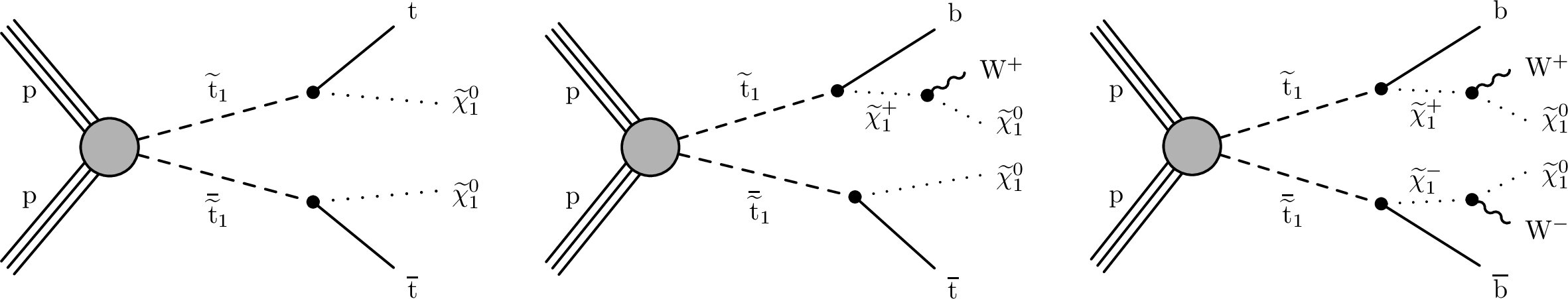
Figure 1:
Diagrams for top squark pair production, with each $\tilde{\mathrm{t}}$ decaying either to $\mathrm{t} \tilde{\chi}^0_1 $ or to $\mathrm{b} \tilde{\chi}^{\pm}_1 $. For the latter decay, the $\tilde{\chi}^{\pm}_1$ decays further into a W boson and a $\tilde{\chi}^0_1$. |
png pdf |
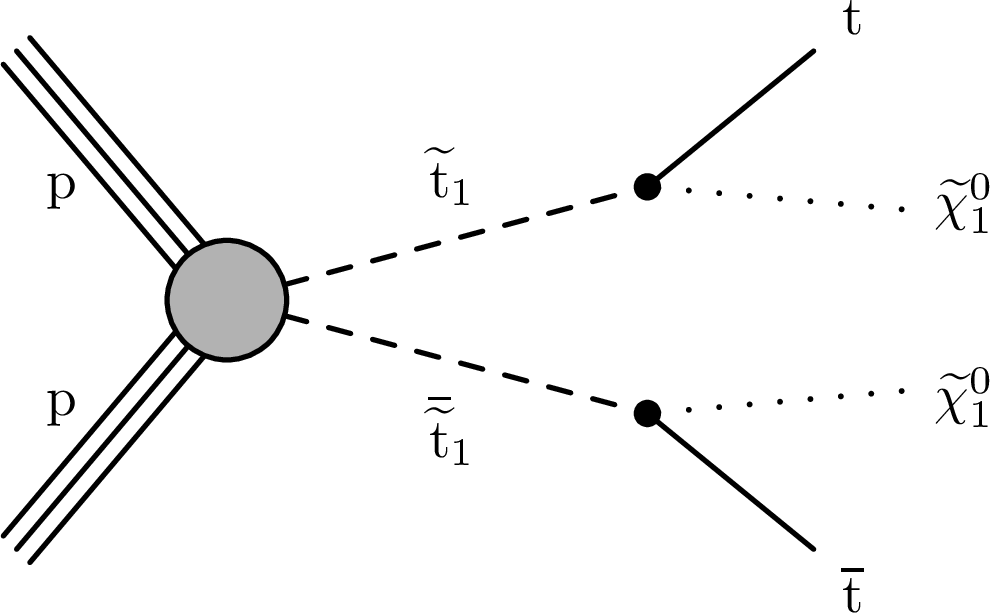
Figure 1-a:
Diagram for top squark pair production, with both $\tilde{\mathrm{t}}$ decaying to $\mathrm{t} \tilde{\chi}^0_1 $. |

png pdf |
Figure 1-b:
Diagram for top squark pair production, with each $\tilde{\mathrm{t}}$ decaying either to $\mathrm{t} \tilde{\chi}^0_1 $ or to $\mathrm{b} \tilde{\chi}^{\pm}_1 $. For the latter decay, the $\tilde{\chi}^{\pm}_1$ decays further into a W boson and a $\tilde{\chi}^0_1$. |
png pdf |
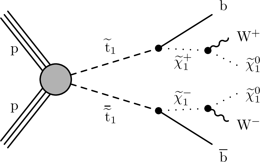
Figure 1-c:
Diagram for top squark pair production, with both $\tilde{\mathrm{t}}$ decaying to $\mathrm{b} \tilde{\chi}^{\pm}_1 $. The $\tilde{\chi}^{\pm}_1$ decays further into a W boson and a $\tilde{\chi}^0_1$. |
png pdf |
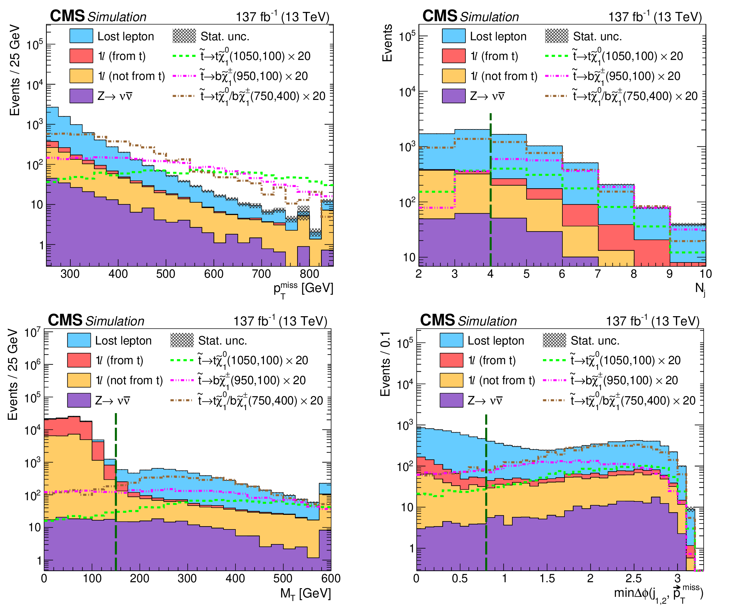
Figure 2:
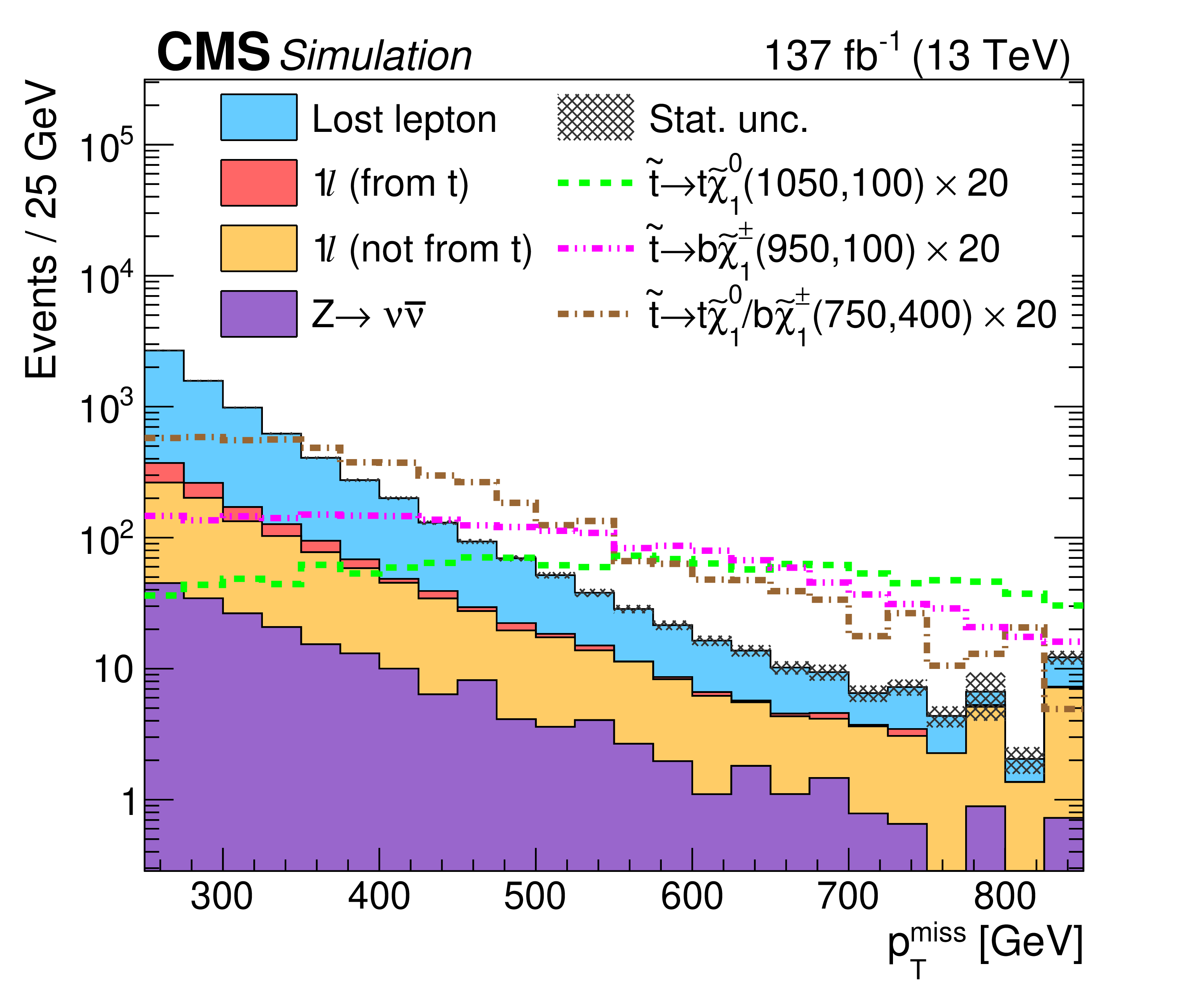
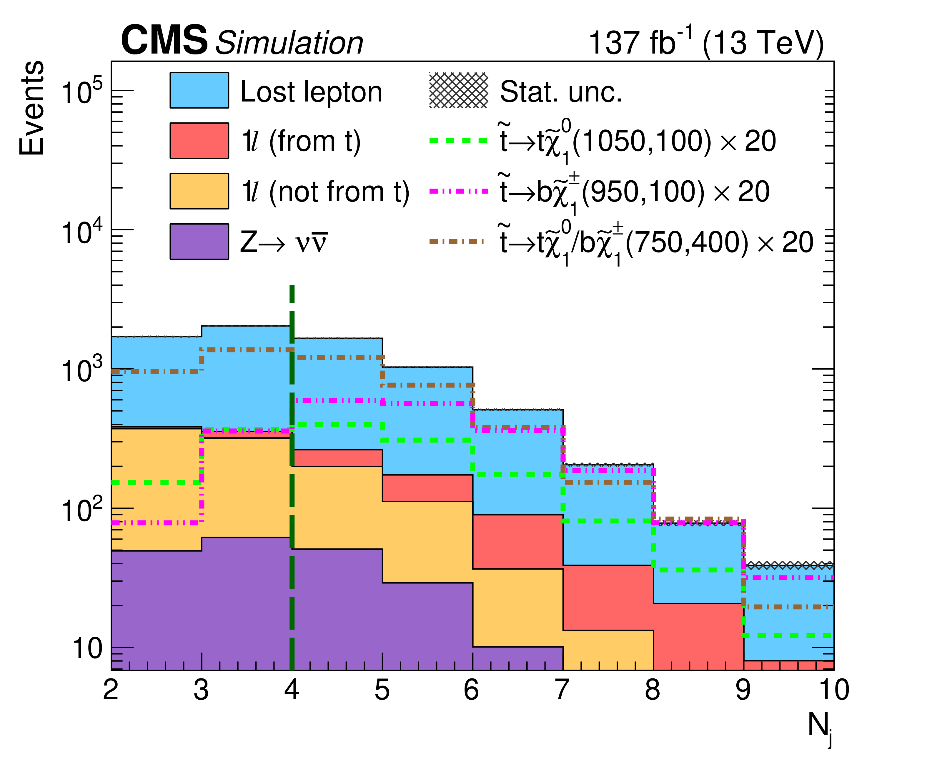
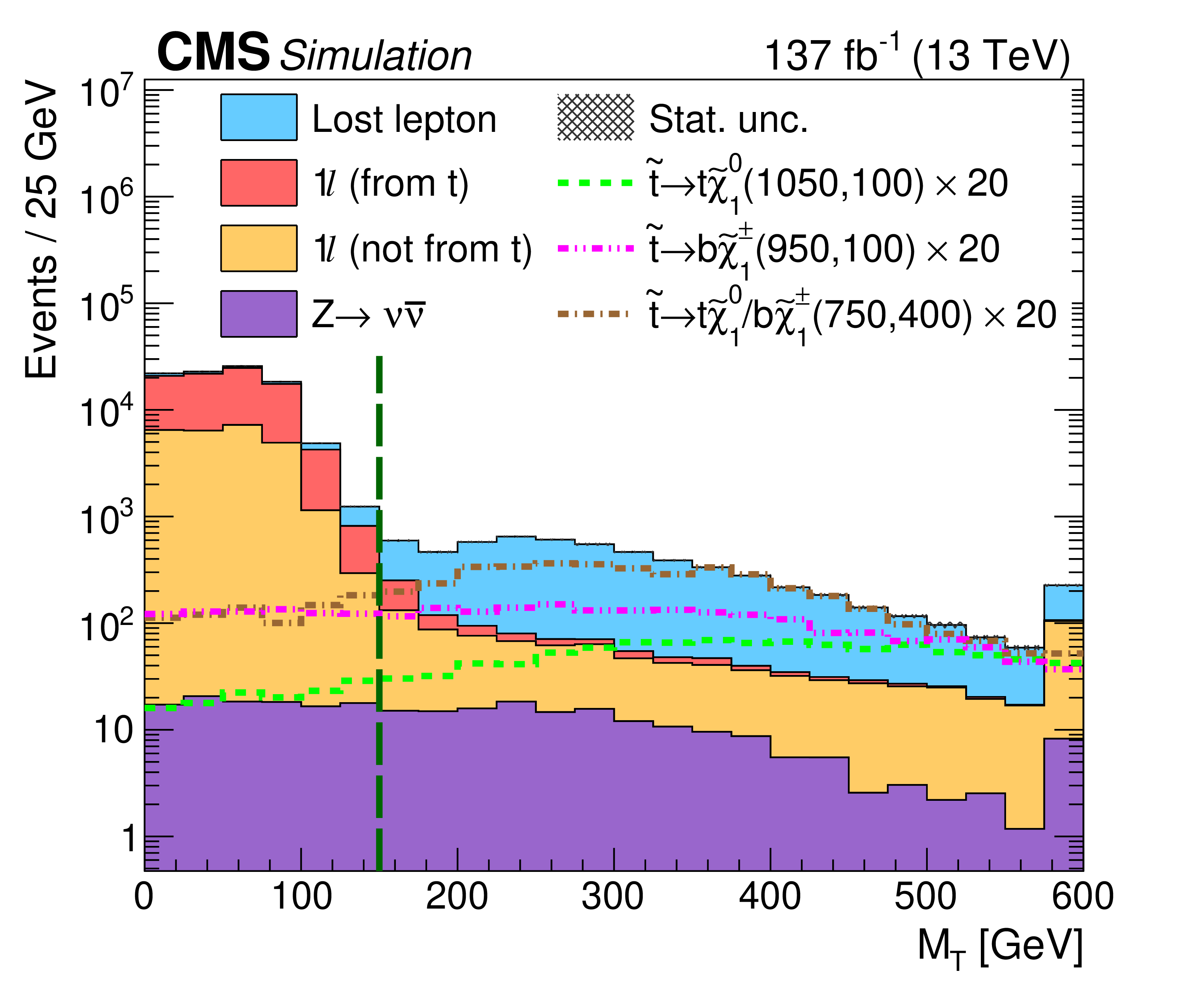
The distributions of ${{p_{\mathrm {T}}} ^\text {miss}}$ (upper left) and ${N_{\mathrm {j}}}$ (upper right) are shown after applying the preselection requirements of Table 1, including the requirement on the variable shown, and the distributions of ${M_{\mathrm {T}}}$ (lower left) and ${\min{\Delta \phi (j_{1,2}, {\vec{p}_{\mathrm {T}}^{\text {miss}}})}}$ (lower right) are shown after applying the preselection requirements, excluding the requirement on the variable shown with the green, dashed vertical line marking the location of the requirement. The stacked histograms for the SM background contributions (categorized as described in Section 5) are from the simulation to illustrate the discriminating power of these variables. The gray hashed region indicates the statistical uncertainty of the simulated samples. The last bin in each distribution includes the overflow events. The expectations for three signal hypotheses are overlaid, and the corresponding numbers in parentheses in the legends refer to the masses of the top squark and neutralino, respectively. For models with ${\mathrm{b}}\tilde{\chi}^{\pm}_1 $ decays, the mass of the chargino is chosen to be $(m_{\tilde{\mathrm{t}}} + m_{\tilde{\chi}^0_1})/2$. |
png pdf |
Figure 2-a:
The distribution of ${{p_{\mathrm {T}}} ^\text {miss}}$ is shown after applying the preselection requirements of Table 1, including the requirement on the variable shown. The stacked histograms for the SM background contributions (categorized as described in Section 5) are from the simulation to illustrate the discriminating power of the variable. The gray hashed region indicates the statistical uncertainty of the simulated samples. The last bin in each distribution includes the overflow events. The expectations for three signal hypotheses are overlaid, and the corresponding numbers in parentheses in the legends refer to the masses of the top squark and neutralino, respectively. For models with ${\mathrm{b}}\tilde{\chi}^{\pm}_1 $ decays, the mass of the chargino is chosen to be $(m_{\tilde{\mathrm{t}}} + m_{\tilde{\chi}^0_1})/2$. |
png pdf |
Figure 2-b:
The distribution of ${N_{\mathrm {j}}}$ is shown after applying the preselection requirements of Table 1, including the requirement on the variable shown. The stacked histograms for the SM background contributions (categorized as described in Section 5) are from the simulation to illustrate the discriminating power of the variable. The gray hashed region indicates the statistical uncertainty of the simulated samples. The last bin in each distribution includes the overflow events. The expectations for three signal hypotheses are overlaid, and the corresponding numbers in parentheses in the legends refer to the masses of the top squark and neutralino, respectively. For models with ${\mathrm{b}}\tilde{\chi}^{\pm}_1 $ decays, the mass of the chargino is chosen to be $(m_{\tilde{\mathrm{t}}} + m_{\tilde{\chi}^0_1})/2$. |
png pdf |
Figure 2-c:
The distribution of ${M_{\mathrm {T}}}$ is shown after applying the preselection requirements, excluding the requirement on the variable shown with the green, dashed vertical line marking the location of the requirement. The stacked histograms for the SM background contributions (categorized as described in Section 5) are from the simulation to illustrate the discriminating power of the variable. The gray hashed region indicates the statistical uncertainty of the simulated samples. The last bin in each distribution includes the overflow events. The expectations for three signal hypotheses are overlaid, and the corresponding numbers in parentheses in the legends refer to the masses of the top squark and neutralino, respectively. For models with ${\mathrm{b}}\tilde{\chi}^{\pm}_1 $ decays, the mass of the chargino is chosen to be $(m_{\tilde{\mathrm{t}}} + m_{\tilde{\chi}^0_1})/2$. |

png pdf |
Figure 2-d:
The distribution of ${\min{\Delta \phi (j_{1,2}, {\vec{p}_{\mathrm {T}}^{\text {miss}}})}}$ is shown after applying the preselection requirements, excluding the requirement on the variable shown with the green, dashed vertical line marking the location of the requirement. The stacked histograms for the SM background contributions (categorized as described in Section 5) are from the simulation to illustrate the discriminating power of the variable. The gray hashed region indicates the statistical uncertainty of the simulated samples. The last bin in each distribution includes the overflow events. The expectations for three signal hypotheses are overlaid, and the corresponding numbers in parentheses in the legends refer to the masses of the top squark and neutralino, respectively. For models with ${\mathrm{b}}\tilde{\chi}^{\pm}_1 $ decays, the mass of the chargino is chosen to be $(m_{\tilde{\mathrm{t}}} + m_{\tilde{\chi}^0_1})/2$. |
png pdf |
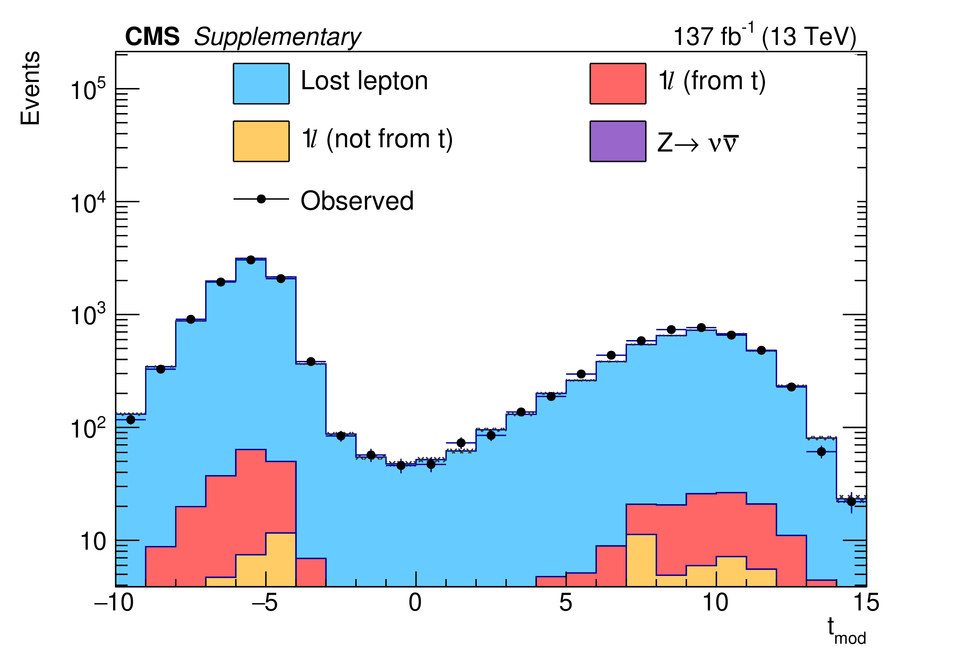
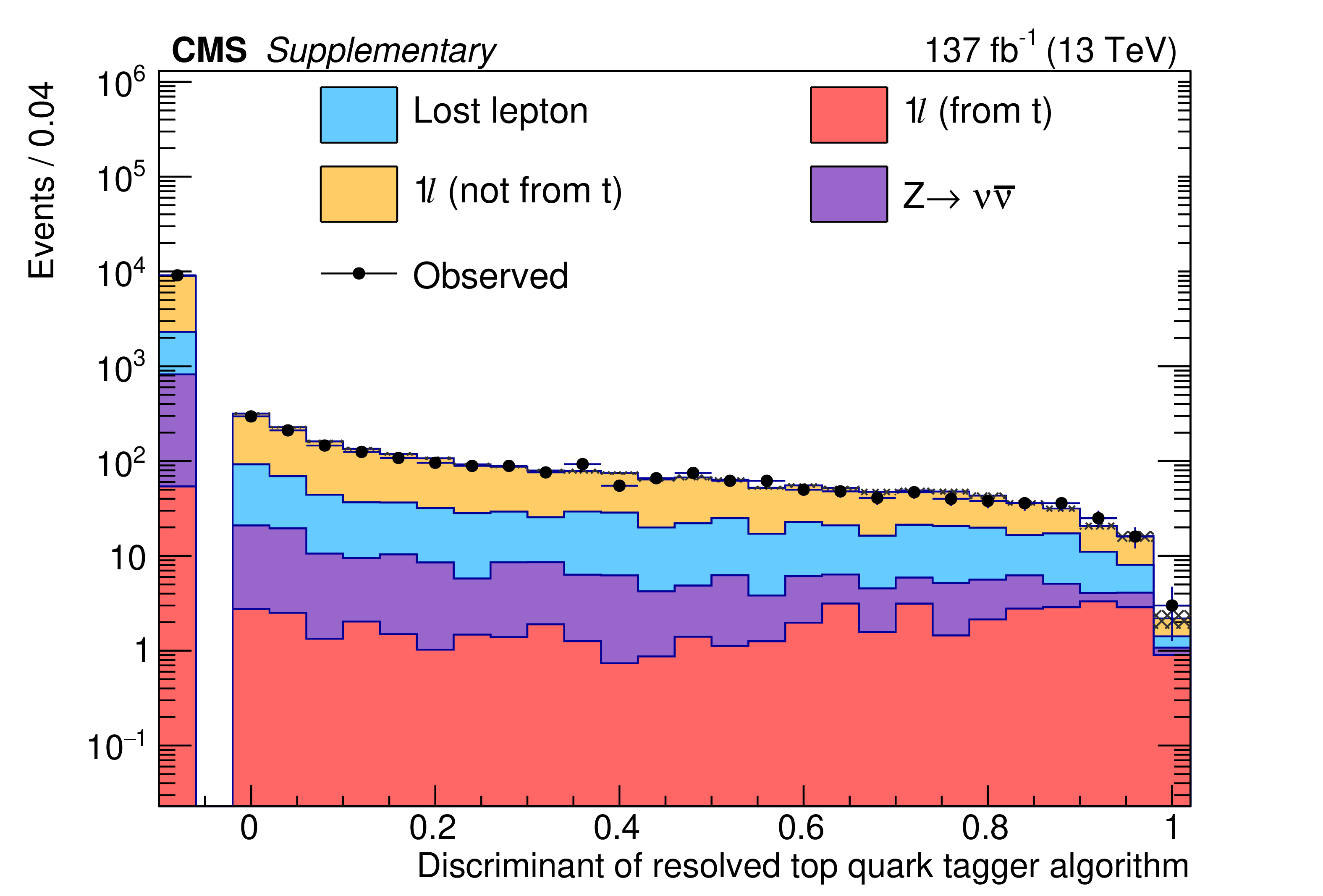
Figure 3:
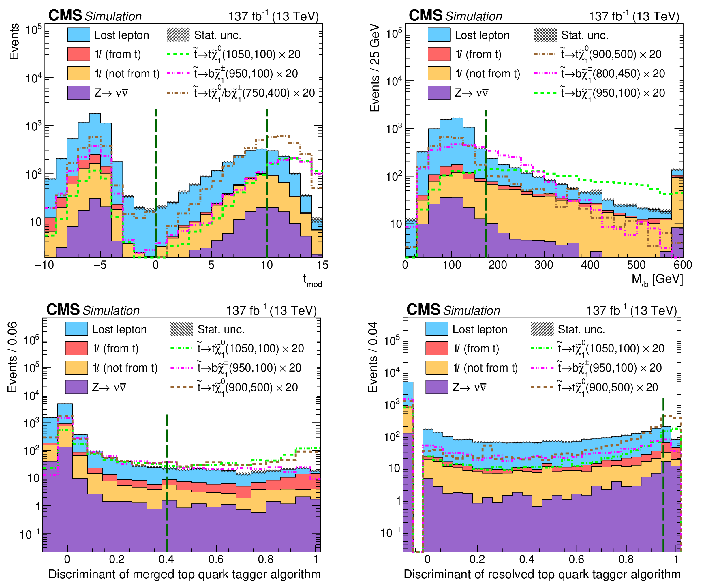
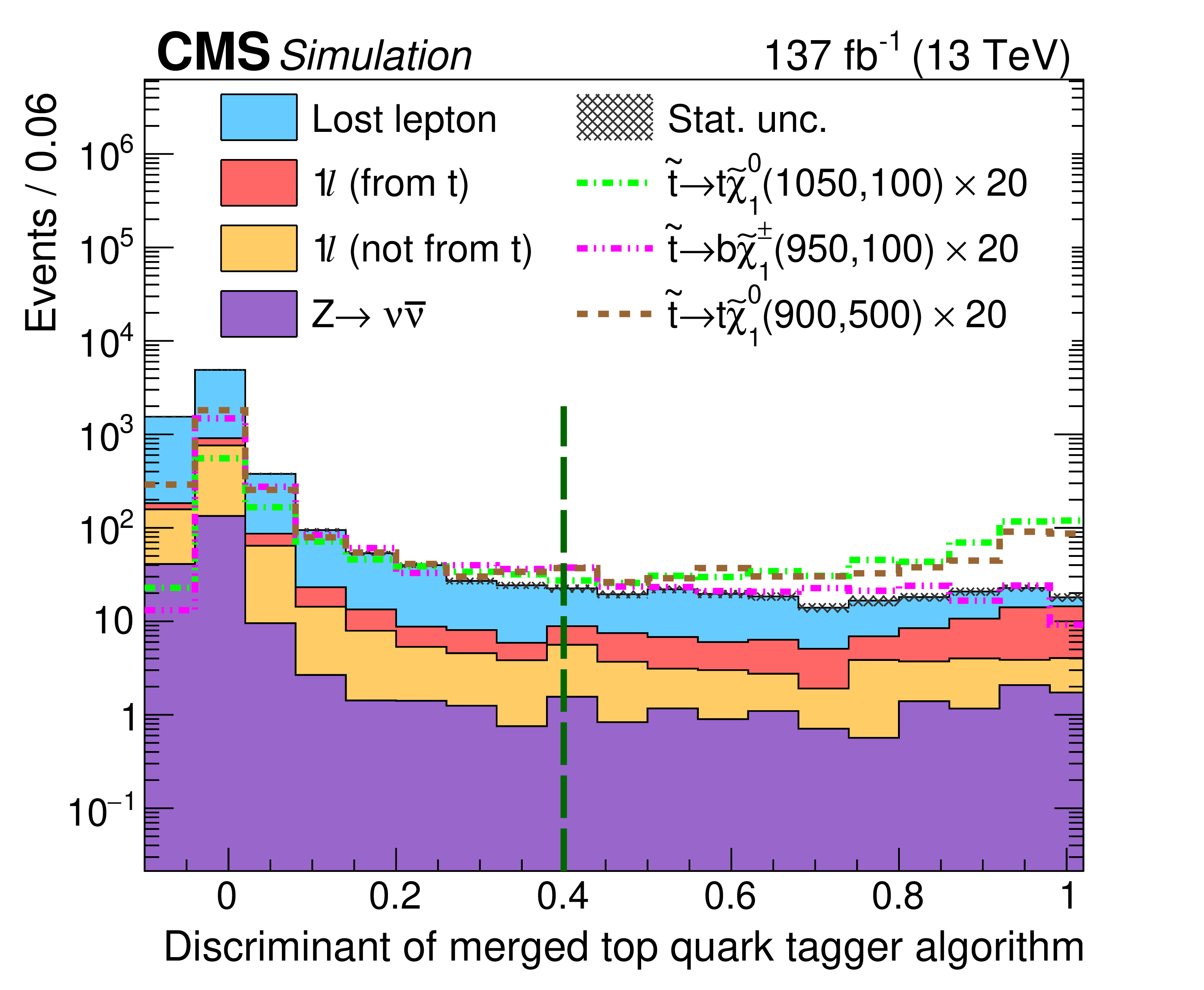
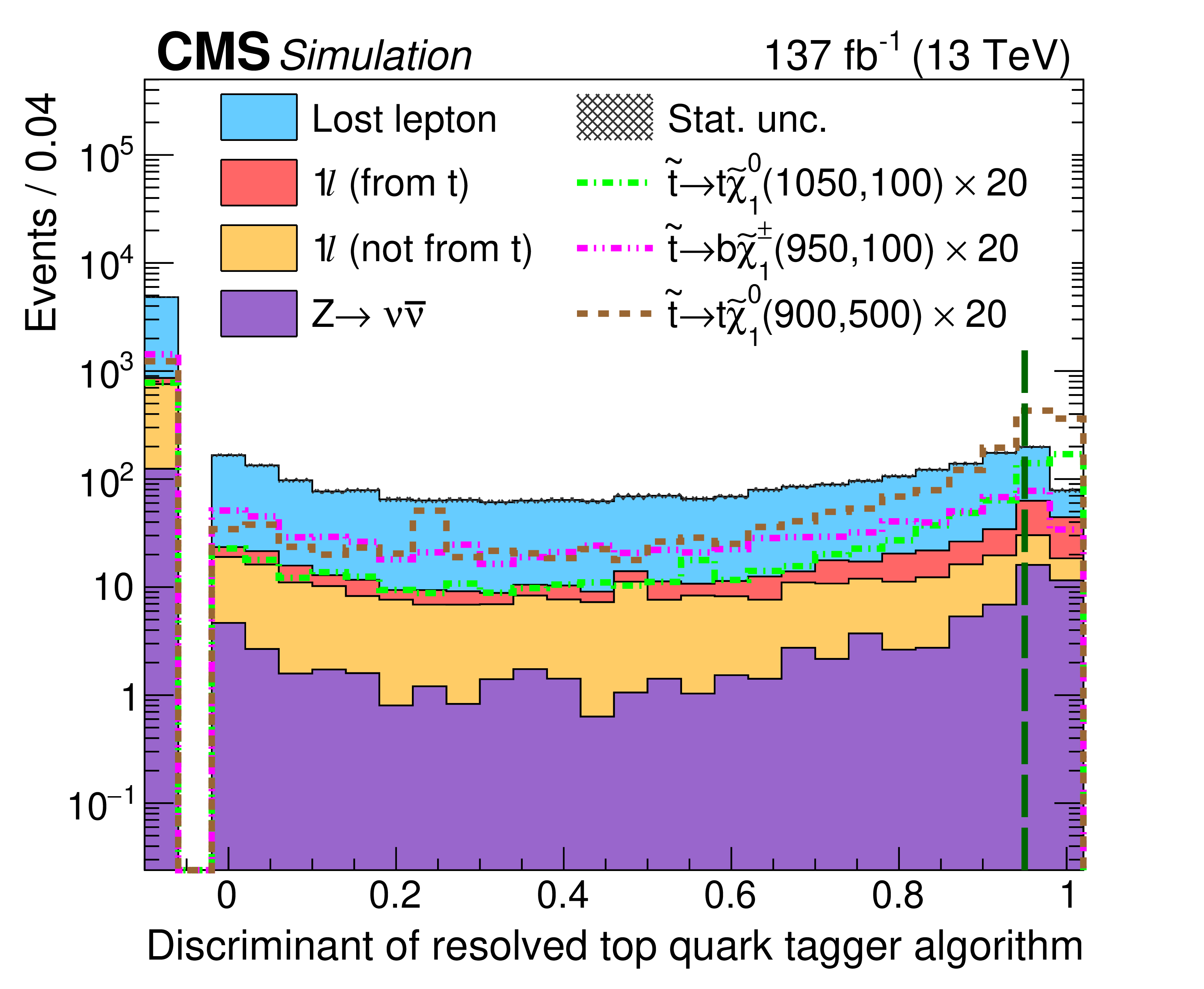
The distribution of ${t_{\text {mod}}}$ (upper left), ${M_{\ell {\mathrm{b}}}}$ (upper right), the merged top quark tagging discriminant (lower left), and the resolved top quark tagging discriminant (lower right) are shown after the preselection requirements. The green, dashed vertical lines mark the locations of the binning or tagging requirements. The stacked histograms showing the SM background contributions (categorized as described in Section 5) are from the simulation to illustrate the discriminating power of these variables. The gray hashed region indicates the statistical uncertainty of the simulated samples. Events outside the range of the distributions shown are included in the first or last bins. The expectations for three signal hypotheses are overlaid, and the corresponding numbers in parentheses in the legends refer to the masses of the top squark and neutralino, respectively. For models with ${\mathrm{b}}\tilde{\chi}^{\pm}_1 $ decays, the mass of the chargino is chosen to be $(m_{\tilde{\mathrm{t}}} + m_{\tilde{\chi}^0_1})/2$. |

png pdf |
Figure 3-a:
The distribution of ${t_{\text {mod}}}$ is shown after the preselection requirements. The green, dashed vertical lines mark the locations of the binning or tagging requirements. The stacked histograms showing the SM background contributions (categorized as described in Section 5) are from the simulation to illustrate the discriminating power of these variables. The gray hashed region indicates the statistical uncertainty of the simulated samples. Events outside the range of the distributions shown are included in the first or last bins. The expectations for three signal hypotheses are overlaid, and the corresponding numbers in parentheses in the legends refer to the masses of the top squark and neutralino, respectively. For models with ${\mathrm{b}}\tilde{\chi}^{\pm}_1 $ decays, the mass of the chargino is chosen to be $(m_{\tilde{\mathrm{t}}} + m_{\tilde{\chi}^0_1})/2$. |

png pdf |
Figure 3-b:
The distribution of ${M_{\ell {\mathrm{b}}}}$ is shown after the preselection requirements. The green, dashed vertical lines mark the locations of the binning or tagging requirements. The stacked histograms showing the SM background contributions (categorized as described in Section 5) are from the simulation to illustrate the discriminating power of these variables. The gray hashed region indicates the statistical uncertainty of the simulated samples. Events outside the range of the distributions shown are included in the first or last bins. The expectations for three signal hypotheses are overlaid, and the corresponding numbers in parentheses in the legends refer to the masses of the top squark and neutralino, respectively. For models with ${\mathrm{b}}\tilde{\chi}^{\pm}_1 $ decays, the mass of the chargino is chosen to be $(m_{\tilde{\mathrm{t}}} + m_{\tilde{\chi}^0_1})/2$. |
png pdf |
Figure 3-c:
The distribution of the merged top quark tagging discriminant is shown after the preselection requirements. The green, dashed vertical lines mark the locations of the binning or tagging requirements. The stacked histograms showing the SM background contributions (categorized as described in Section 5) are from the simulation to illustrate the discriminating power of these variables. The gray hashed region indicates the statistical uncertainty of the simulated samples. Events outside the range of the distributions shown are included in the first or last bins. The expectations for three signal hypotheses are overlaid, and the corresponding numbers in parentheses in the legends refer to the masses of the top squark and neutralino, respectively. For models with ${\mathrm{b}}\tilde{\chi}^{\pm}_1 $ decays, the mass of the chargino is chosen to be $(m_{\tilde{\mathrm{t}}} + m_{\tilde{\chi}^0_1})/2$. |
png pdf |
Figure 3-d:
The distribution of the resolved top quark tagging discriminant is shown after the preselection requirements. The green, dashed vertical lines mark the locations of the binning or tagging requirements. The stacked histograms showing the SM background contributions (categorized as described in Section 5) are from the simulation to illustrate the discriminating power of these variables. The gray hashed region indicates the statistical uncertainty of the simulated samples. Events outside the range of the distributions shown are included in the first or last bins. The expectations for three signal hypotheses are overlaid, and the corresponding numbers in parentheses in the legends refer to the masses of the top squark and neutralino, respectively. For models with ${\mathrm{b}}\tilde{\chi}^{\pm}_1 $ decays, the mass of the chargino is chosen to be $(m_{\tilde{\mathrm{t}}} + m_{\tilde{\chi}^0_1})/2$. |
png pdf |
Figure 4:
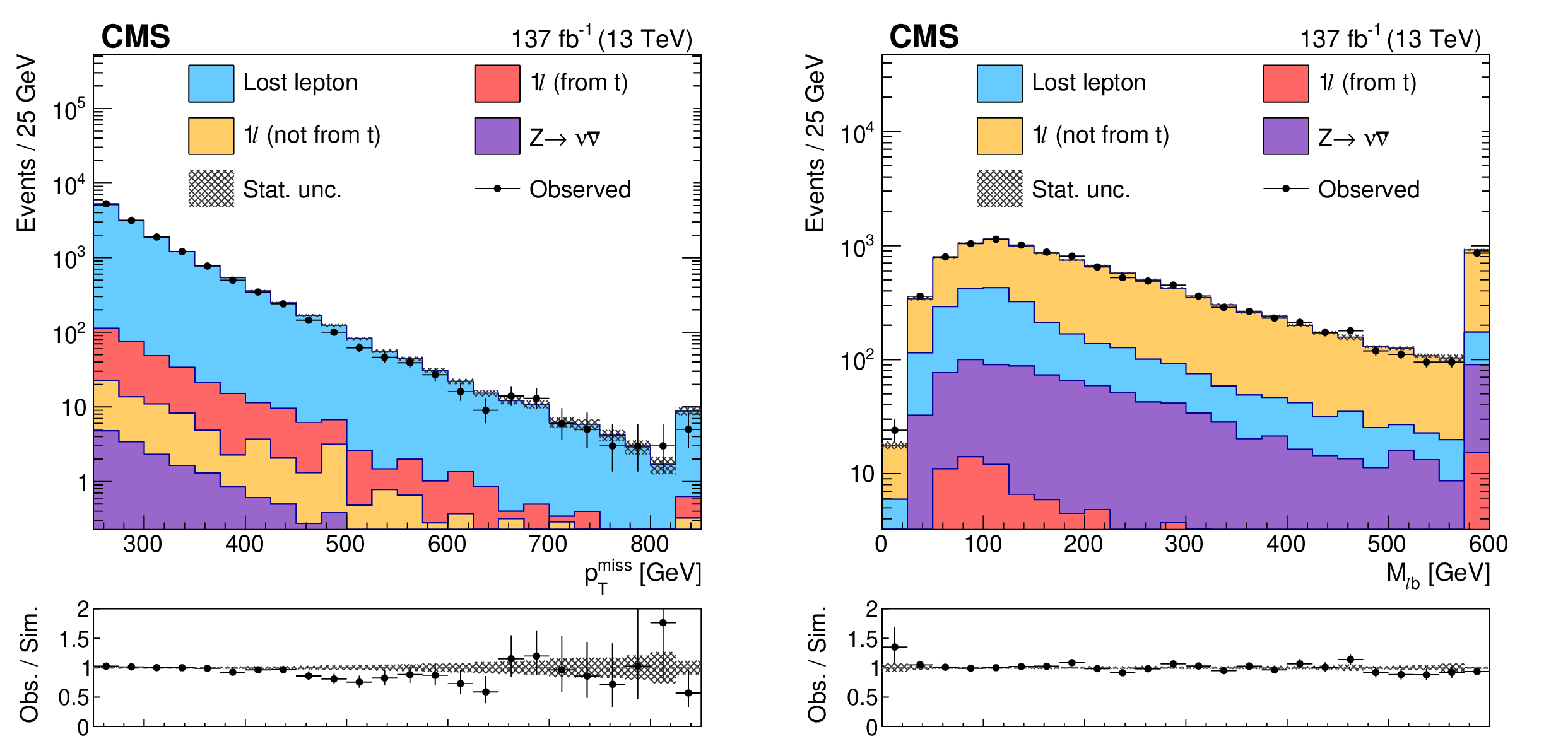
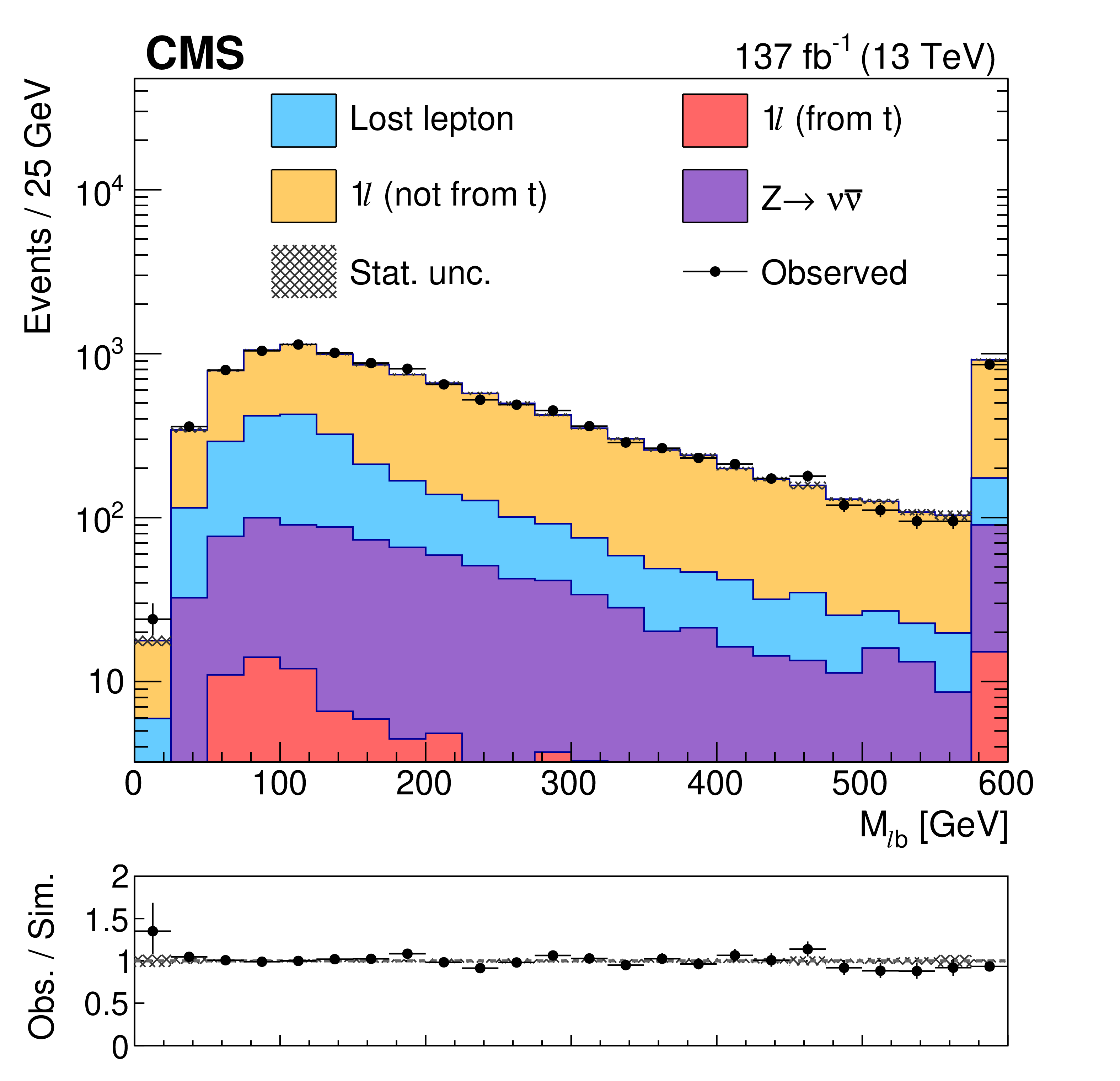
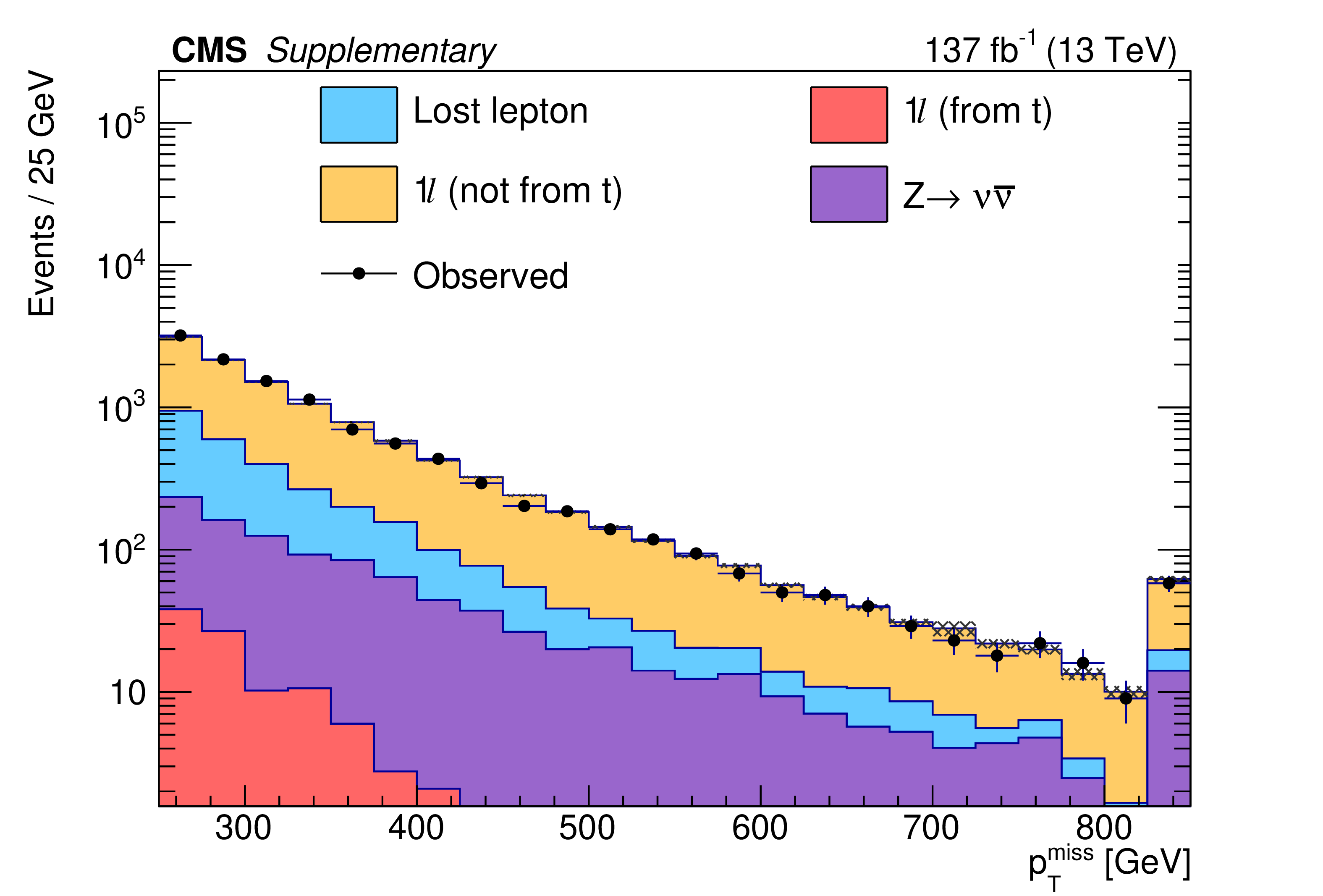
Distributions of kinematic variables in the inclusive control samples used for the background estimation. The gray hashed region indicates the statistical uncertainty of the simulated samples. The distributions for data are shown as points with error bars corresponding to the statistical uncertainty. The stacked histograms show the expected SM background contributions from simulation, normalized to the number of events observed in data. The last bin in each distribution also includes the overflow. Left: Distribution of ${{p_{\mathrm {T}}} ^\text {miss}}$ in the dilepton control sample. Right: Distribution of ${M_{\ell {\mathrm{b}}}}$ in the 0b control sample. |

png pdf |
Figure 4-a:
Distribution ${{p_{\mathrm {T}}} ^\text {miss}}$ in the dilepton control sample. The gray hashed region indicates the statistical uncertainty of the simulated samples. The distributions for data are shown as points with error bars corresponding to the statistical uncertainty. The stacked histograms show the expected SM background contributions from simulation, normalized to the number of events observed in data. The last bin in the distribution also includes the overflow. |
png pdf |
Figure 4-b:
Distribution of ${M_{\ell {\mathrm{b}}}}$ in the 0b control sample. The gray hashed region indicates the statistical uncertainty of the simulated samples. The distributions for data are shown as points with error bars corresponding to the statistical uncertainty. The stacked histograms show the expected SM background contributions from simulation, normalized to the number of events observed in data. The last bin in each distribution also includes the overflow. |
png pdf |
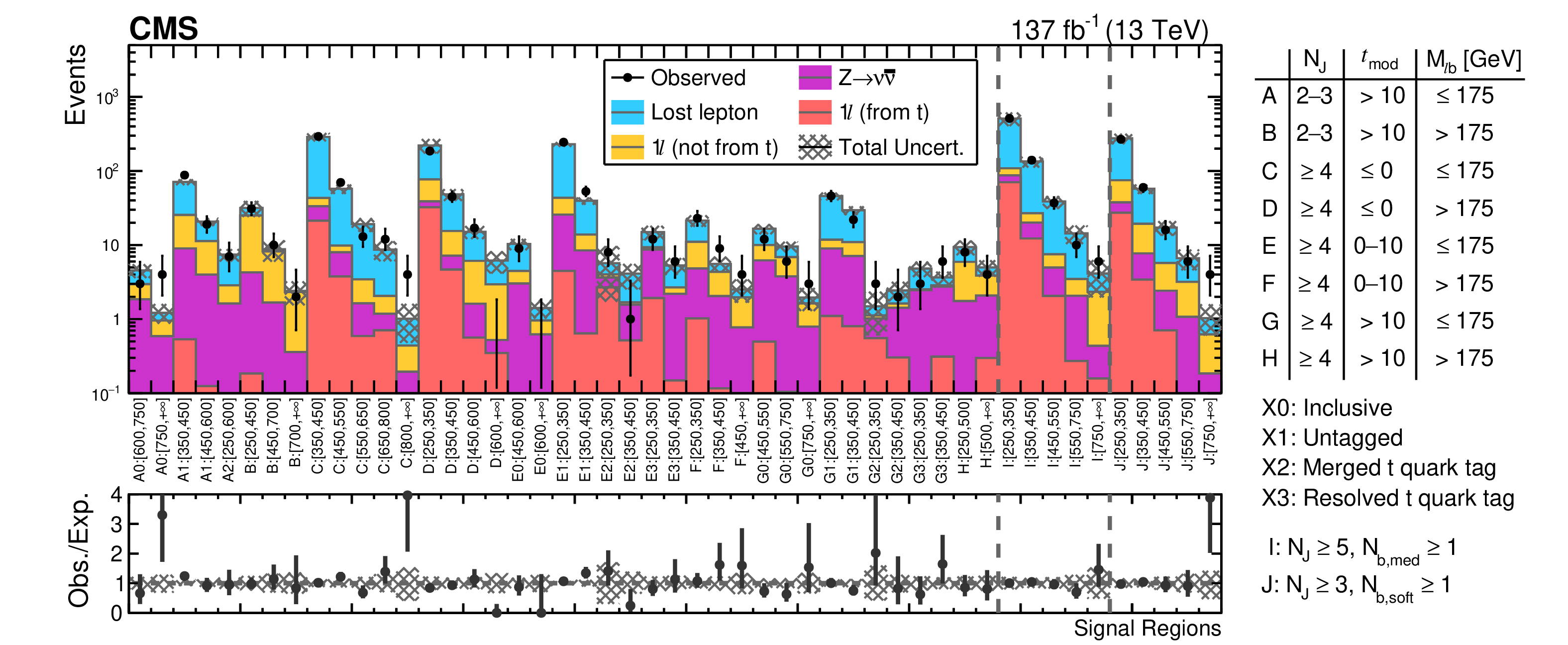
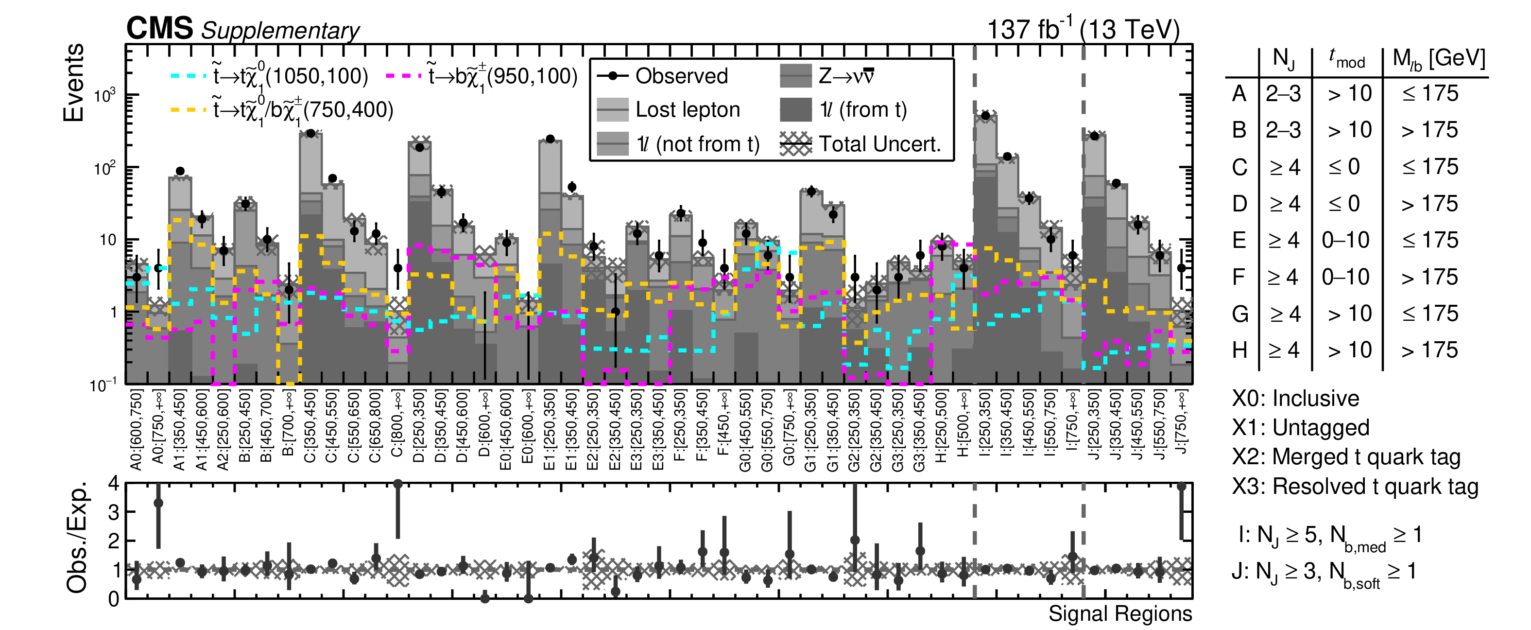
Figure 5:
The observed and expected yields in Tables 7 and 8 and their ratios are shown as stacked histograms. The lost lepton and 1$\ell $ (not from t) are estimated from data-driven methods, while 1$\ell $ (from t) and $\mathrm{Z}\to\nu\bar{\nu}$ backgrounds are taken from simulation. The uncertainties consist of statistical and systematic components summed in quadrature and are shown as shaded bands. |
png pdf root |
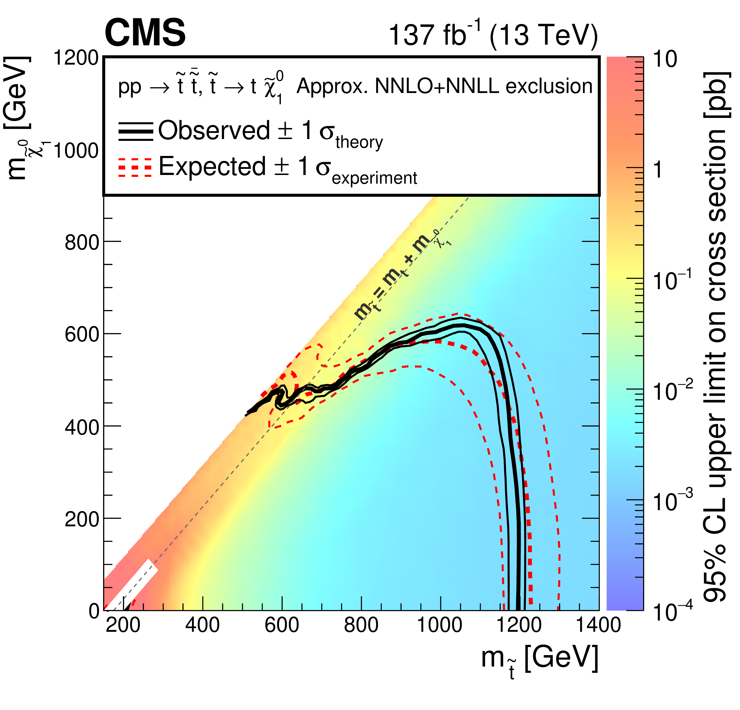
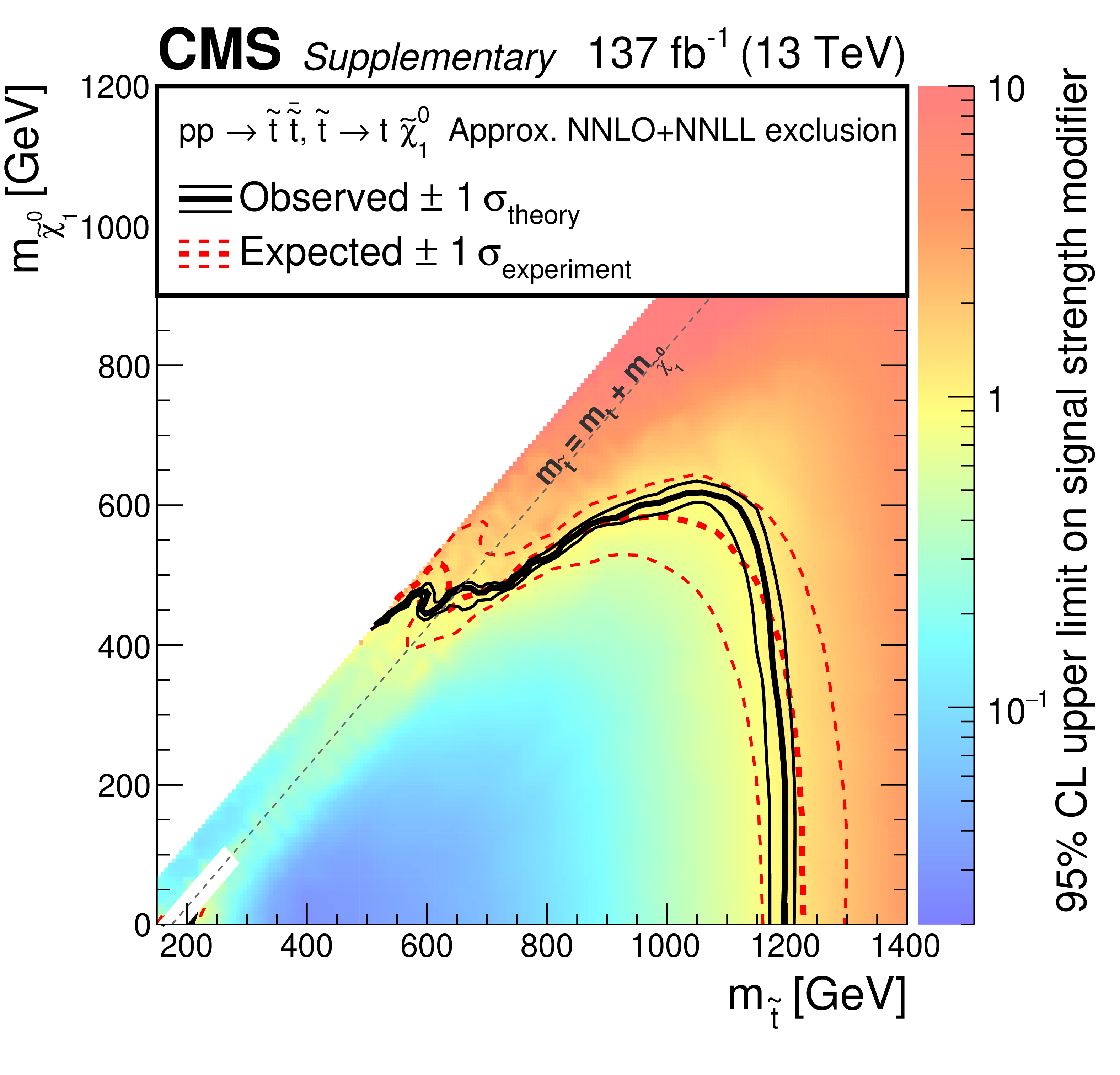
Figure 6:
Exclusion limits at 95% CL for the ${\mathrm{p}} {\mathrm{p}} \to \tilde{\mathrm{t}} \bar{\tilde{\mathrm{t}}} \to \mathrm{t} \mathrm{\bar{t}} \tilde{\chi}^0_1 \tilde{\chi}^0_1 $ scenario. The colored map illustrates the 95% CL upper limits on the product of the production cross section and branching fraction. The area enclosed by the thick black curve represents the observed exclusion region, and that enclosed by the thick, dashed red curve represents the expected exclusion. The thin dotted (red) curves indicate the region containing 68% of the distribution of limits expected under the background-only hypothesis. The thin solid (black) curves show the change in the observed limit by varying the signal cross sections within their theoretical uncertainties. The white band excluded from the limits corresponds to the region $ {| m_{\tilde{\mathrm{t}}}-m_{\mathrm {t}}-m_{\tilde{\chi}^0_1} |} < $ 25 GeV, $ m_{\tilde{\mathrm{t}}} < $ 275 GeV, where the selection acceptance for top squark pair production changes rapidly and is therefore very sensitive to the details of the simulation. |
png pdf root |
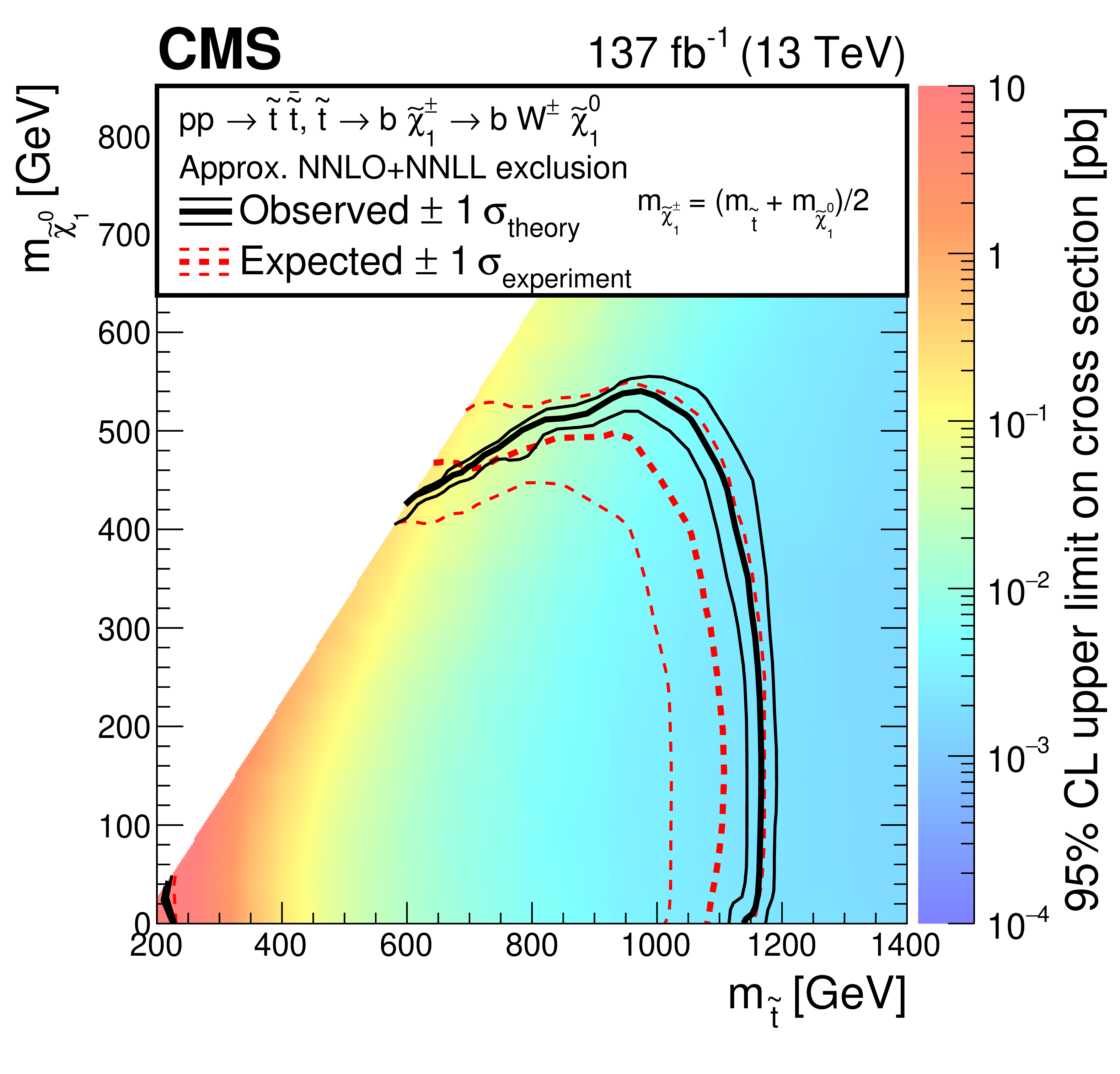
Figure 7:
Exclusion limits at 95% CL for the ${\mathrm{p}} {\mathrm{p}} \to \tilde{\mathrm{t}} \bar{\tilde{\mathrm{t}}} \to \mathrm{b} \mathrm{\bar{b}} \tilde{\chi}^{\pm}_1 \tilde{\chi}^{\pm}_1 \left (\tilde{\chi}^{\pm}_1 \to \mathrm{W} \tilde{\chi}^0_1 \right)$ scenario. The mass of $\tilde{\chi}^{\pm}_1$ is chosen to be $(m_{\tilde{\mathrm{t}}} + m_{\tilde{\chi}^0_1})/2$. The colored map illustrates the 95% CL upper limits on the product of the production cross section and branching fraction. The area enclosed by the thick black curve represents the observed exclusion region, and that enclosed by the thick, dashed red curve represents the expected exclusion. The thin dotted (red) curves indicate the region containing 68% of the distribution of limits expected under the background-only hypothesis. The thin solid (black) curves show the change in the observed limit by varying the signal cross sections within their theoretical uncertainties. |
png pdf root |
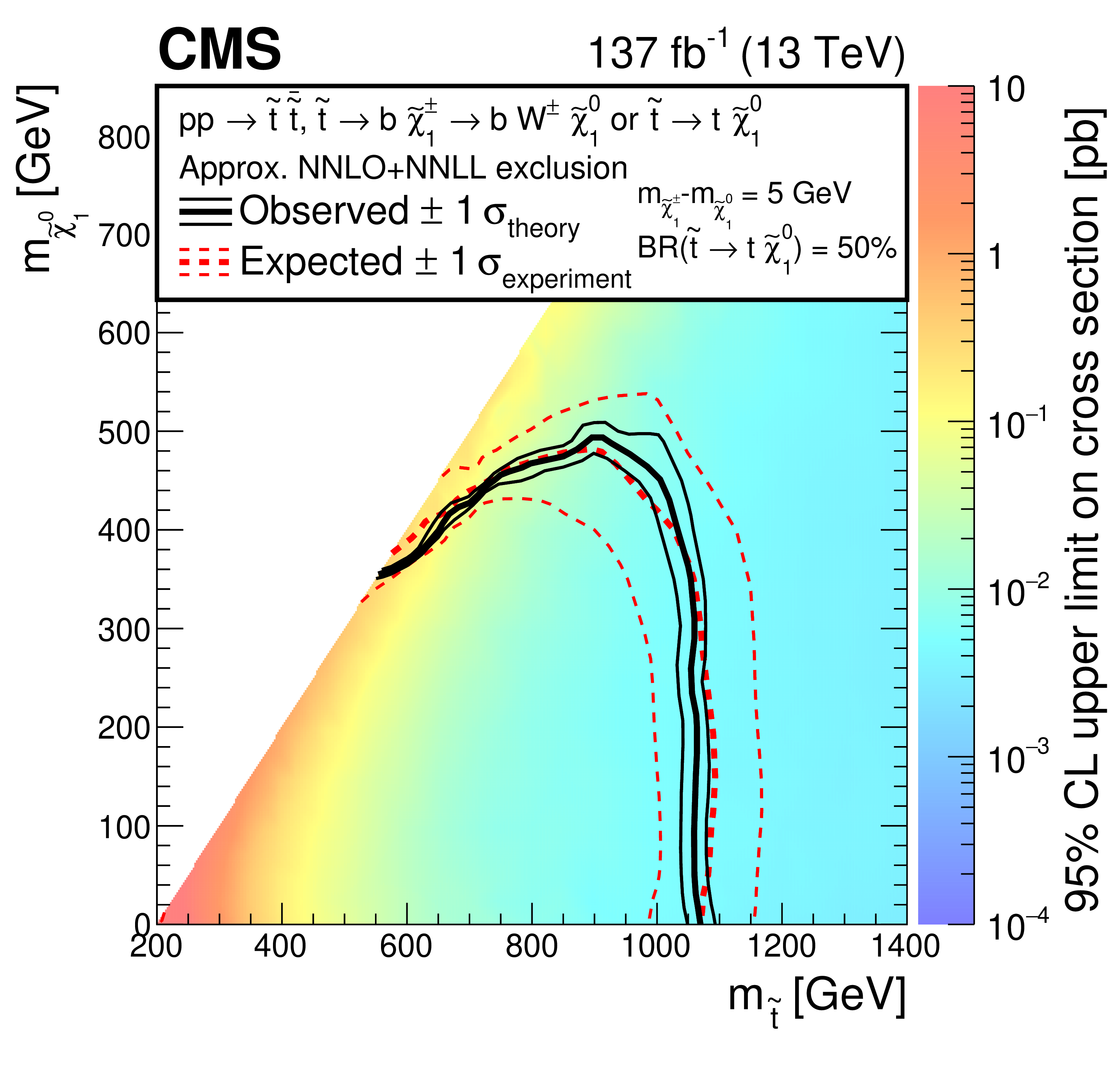
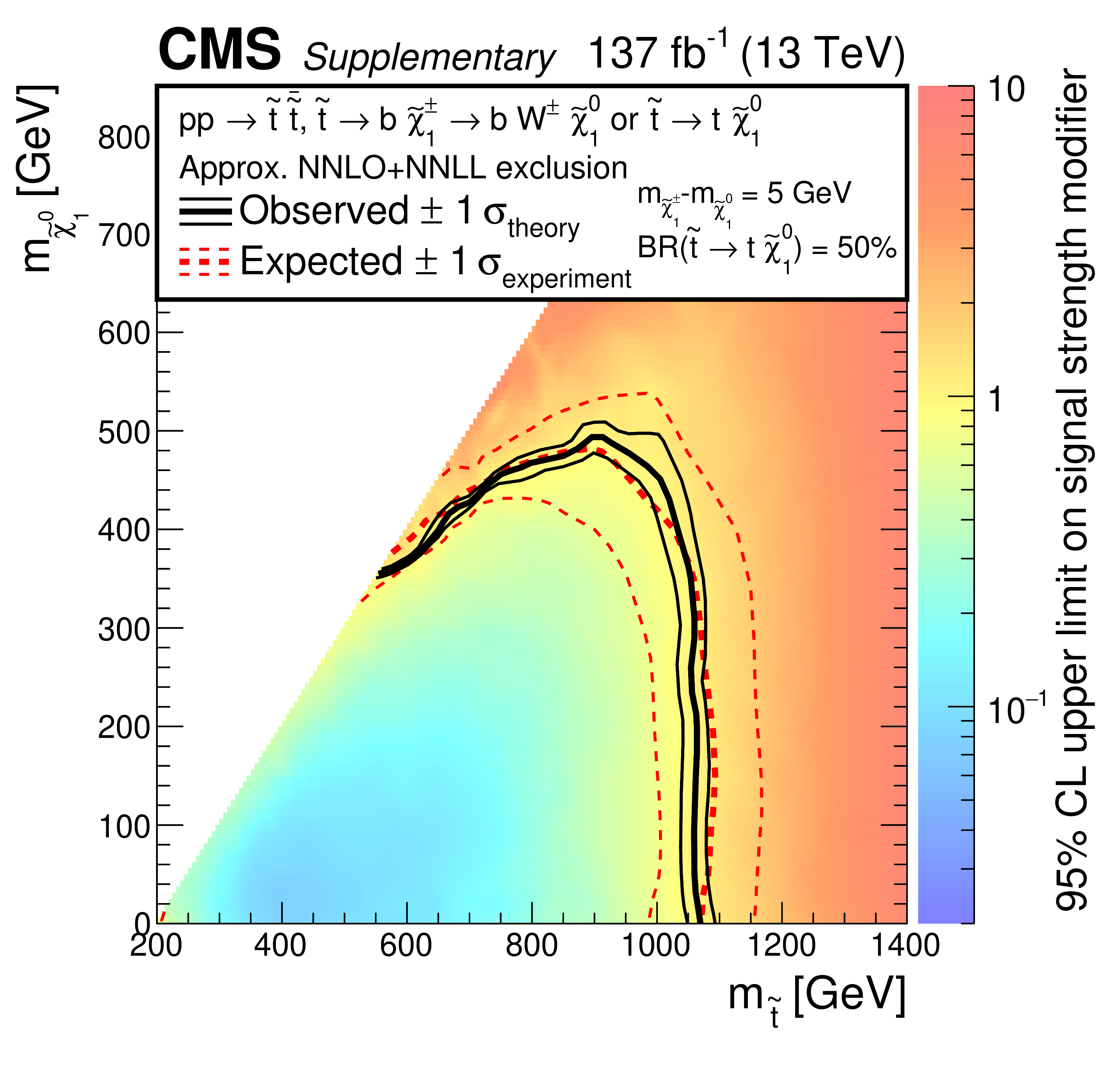
Figure 8:
Exclusion limits at 95% CL for the ${\mathrm{p}} {\mathrm{p}} \to \tilde{\mathrm{t}} \bar{\tilde{\mathrm{t}}} \to \mathrm{t} {\mathrm{b}}\tilde{\chi}^{\pm}_1 \tilde{\chi}^0_1 \left (\tilde{\chi}^{\pm}_1 \to \mathrm{W} ^{*}\tilde{\chi}^0_1 \right)$ scenario. The mass difference between the $\tilde{\chi}^{\pm}_1$ and the $\tilde{\chi}^0_1$ is taken to be 5 GeV. The colored map illustrates the 95% CL upper limits on the product of the production cross section and branching fraction. The area enclosed by the thick black curve represents the observed exclusion region, and that enclosed by the thick, dashed red curve represents the expected exclusion. The thin dotted (red) curves indicate the region containing 68% of the distribution of limits expected under the background-only hypothesis. The thin solid (black) curves show the change in the observed limit by varying the signal cross sections within their theoretical uncertainties. |
| Tables | |
png pdf |
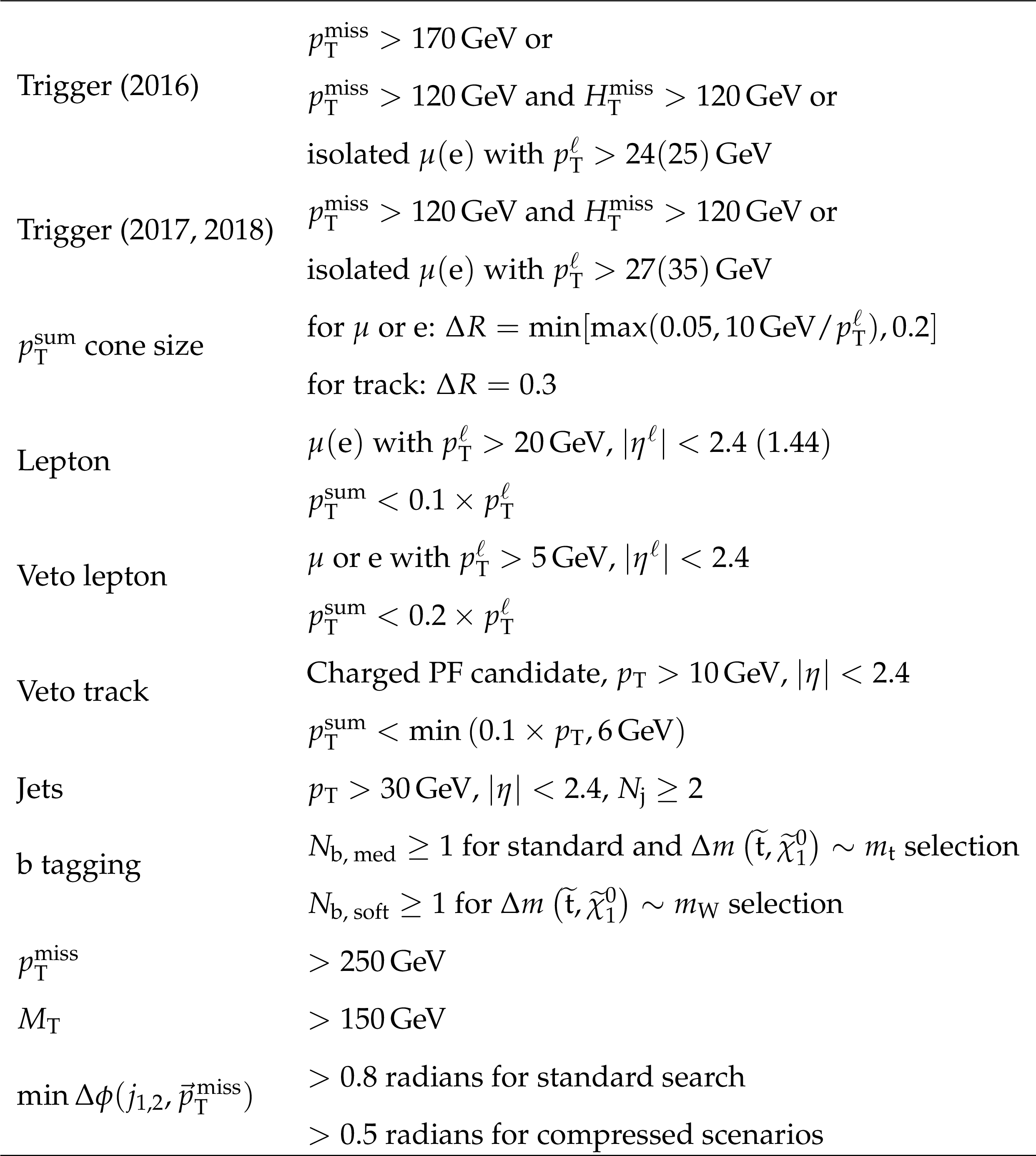
Table 1:
Summary of the event preselection requirements. The magnitude of the vector sum of the ${p_{\mathrm {T}}}$ of all jets and leptons in the event is denoted by ${H_{\mathrm {T}}^{\text {miss}}}$. The symbols $ {p_{\mathrm {T}}} ^{\ell}$ and $\eta ^{\ell}$ correspond to the transverse momentum and pseudorapidity of the lepton. The symbol $ {{p_{\mathrm {T}}} ^{\text {sum}}} $ is the scalar sum of the ${p_{\mathrm {T}}}$ of all (charged) PF candidates in a cone around the lepton (track), excluding the lepton (track) itself. Finally, $ {N_{\mathrm{b},\text {med}}} $ and $ {N_{\mathrm{b},\text {soft}}} $ are the multiplicity of b-tagged jets (medium working point) and soft b objects, respectively. |
png pdf |
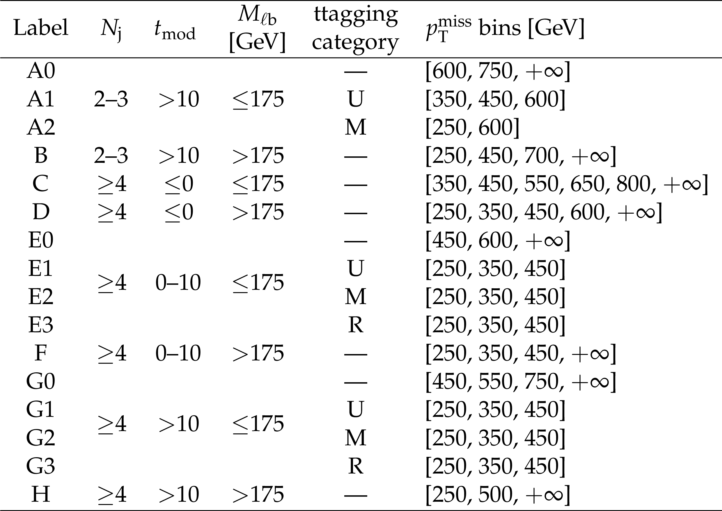
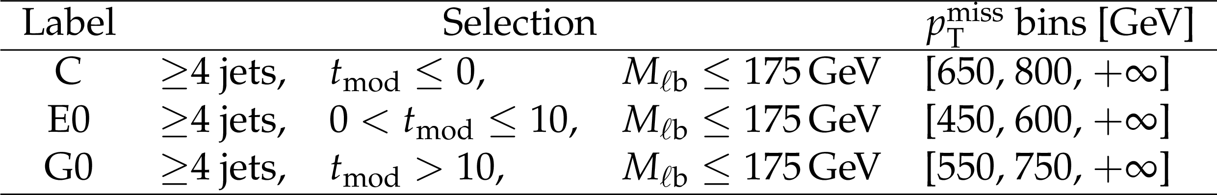
Table 2:
The 39 signal regions of the standard selection, with each neighboring pair of values in the ${{p_{\mathrm {T}}} ^\text {miss}}$ bins column defines a single signal region. At least one b-tagged jet selected using the medium (tight) working point is required for search regions with $ {M_{\ell {\mathrm{b}}}} $ lower (higher) than 175 GeV. For the top quark tagging categories, we use the abbreviations U for untagged, M for merged, and R for resolved. |
png pdf |
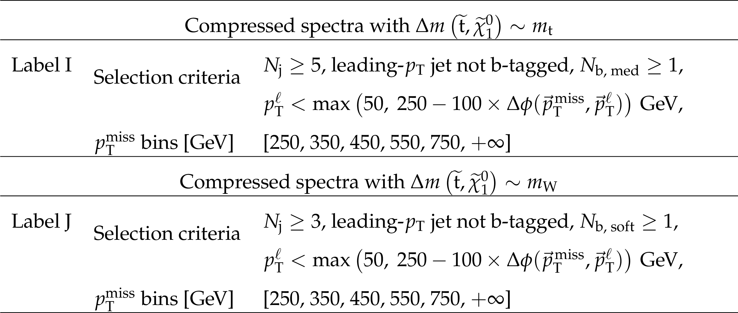
Table 3:
Definitions of the total 10 search regions targeting signal scenarios with a compressed mass spectrum. Search regions for $\Delta m\left (\tilde{\mathrm{t}},\tilde{\chi}^0_1 \right)\sim m_{\mathrm{t}}$ and $\sim m_{\mathrm{W}}$ scenarios are labeled with the letter I and J, respectively. The symbol $ {p_{\mathrm {T}}} ^{\ell}$ denotes the transverse momentum of the lepton. Each neighboring pair of values in the ${{p_{\mathrm {T}}} ^\text {miss}}$ bins column defines a single signal region. |
png pdf |
Table 4:
Dilepton control samples that are combined when estimating the lost-lepton background. |
png pdf |
Table 5:
Search regions where the corresponding 0b control samples are combined when estimating the W+jets background. |
png pdf |
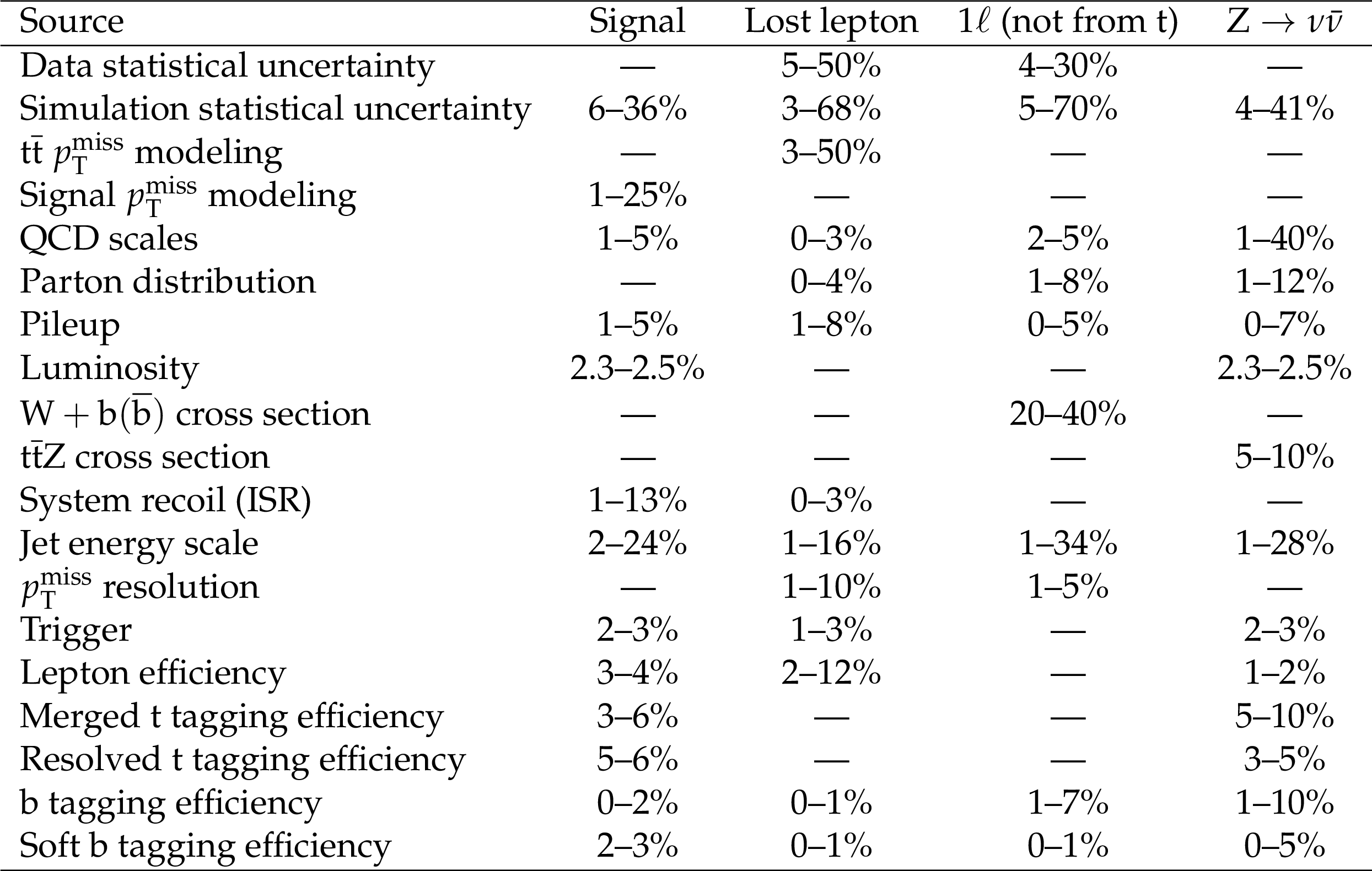
Table 6:
Summary of major systematic uncertainties. The range of values reflect their impact on the estimated backgrounds and signal yields in different signal regions. A 100% uncertainty is assigned to the 1$\ell $ (from t) background estimated from simulation. |
png pdf |
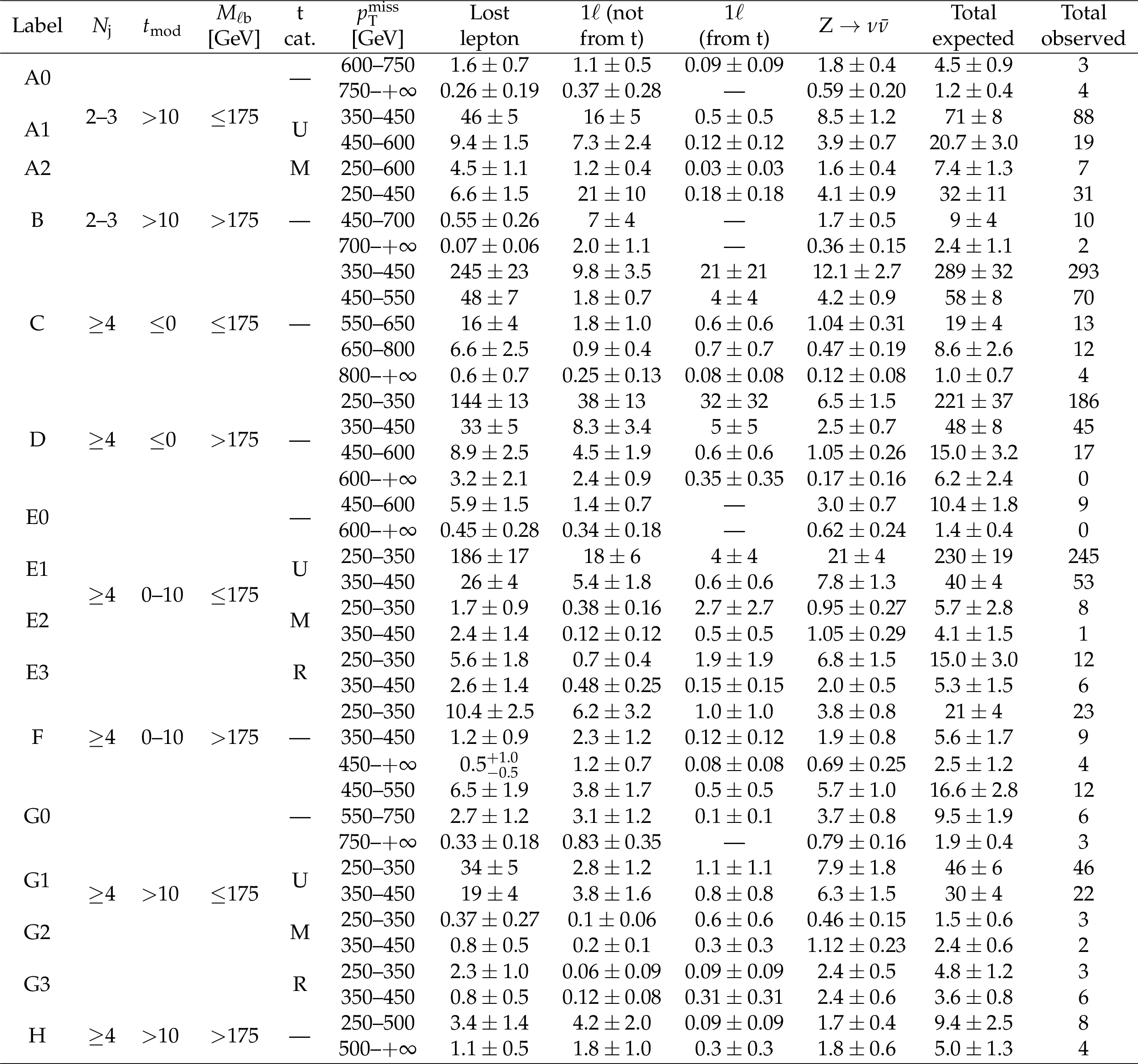
Table 7:
The observed and expected yields in the standard search regions. For the top quark tagging categories, we use the abbreviations U for untagged, M for merged, and R for resolved. |
png pdf |
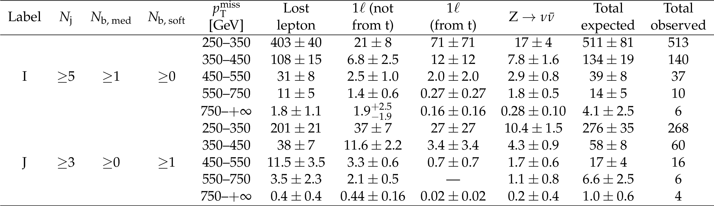
Table 8:
The observed and expected yields for signal regions targeting scenarios of top squark production with a compressed mass spectrum. |
| Summary |
| A search for direct top squark pair production is performed using events with one lepton, jets, and significant missing transverse momentum. The search is based on proton-proton collision data at a center-of-mass energy of 13 TeV recorded by the CMS experiment at the LHC during 2016-2018 and corresponding to an integrated luminosity of 137 fb$^{-1}$. The leading backgrounds in this analysis, mainly dileptonic $\mathrm{t\bar{t}}$ decays, where one of the leptons is not reconstructed or identified, and W+jets production are estimated from data control regions. The semileptonic $\mathrm{t\bar{t}}$ and $\mathrm{Z}\to\nu\bar{\nu}$ backgrounds are taken from simulation. No significant deviations from the standard model expectations are observed. Limits on pair-produced top squarks are established in the context of supersymmetry models conserving $R$-parity. Exclusion limits at 95% CL for top squark masses up to 1.2 TeV are set for a massless neutralino. For models with a top squark mass of 1 TeV, neutralino masses up to 600 GeV are excluded. |
| Additional Figures | |
png pdf |
Additional Figure 1:
The distributions of $t_{\mathrm {mod}}$ in the standard search dilepton control sample are shown for the different background components from simulation, which are stacked on top of each other, and the observation. The ${\vec{p}}_{\mathrm {T}}$ vector of the additional lepton in these events is added to the ${\vec{p}}_{\mathrm {T}}^{\,\text {miss}}$ vector during the computation of this variable. The simulation is used only in the extraction of transfer factors, so the total prediction from the simulation is normalized to the observed total yield. The last bin in each distribution also includes the overflow events. |

png pdf |
Additional Figure 2:
The distributions of the merged ${{\mathrm {t}}}$ tagging discriminant in the standard search dilepton control sample are shown for the different background components from simulation, which are stacked on top of each other, and the observation. The simulation is used only in the extraction of transfer factors, so the total prediction from the simulation is normalized to the observed total yield. |
png pdf |
Additional Figure 3:
The distributions of ${{p_{\mathrm {T}}} ^\text {miss}}$ in the standard search control sample with no b-tagged jets are shown for the different background components from simulation, which are stacked on top of each other, and the observation. The simulation is used only in the extraction of transfer factors, so the total prediction from the simulation is normalized to the observed total yield. The last bin in each distribution also includes the overflow events. |
png pdf |
Additional Figure 4:
The distributions of the resolved ${{\mathrm {t}}}$ tagging discriminant in the standard search control sample with no b-tagged jets are shown for the different background components from simulation, which are stacked on top of each other, and the observation. The simulation is used only in the extraction of transfer factors, so the total prediction from the simulation is normalized to the observed total yield. |
png pdf |
Additional Figure 5:
The observed and expected yields for SM background in the signal regions and their ratios are shown as stacked histograms, colors in grayscale. The uncertainties consist of statistical and systematic components summed in quadrature and are shown as shaded bands. Expected yields for some selected signal points are shown overlaid with the stacked histograms. |
png pdf |
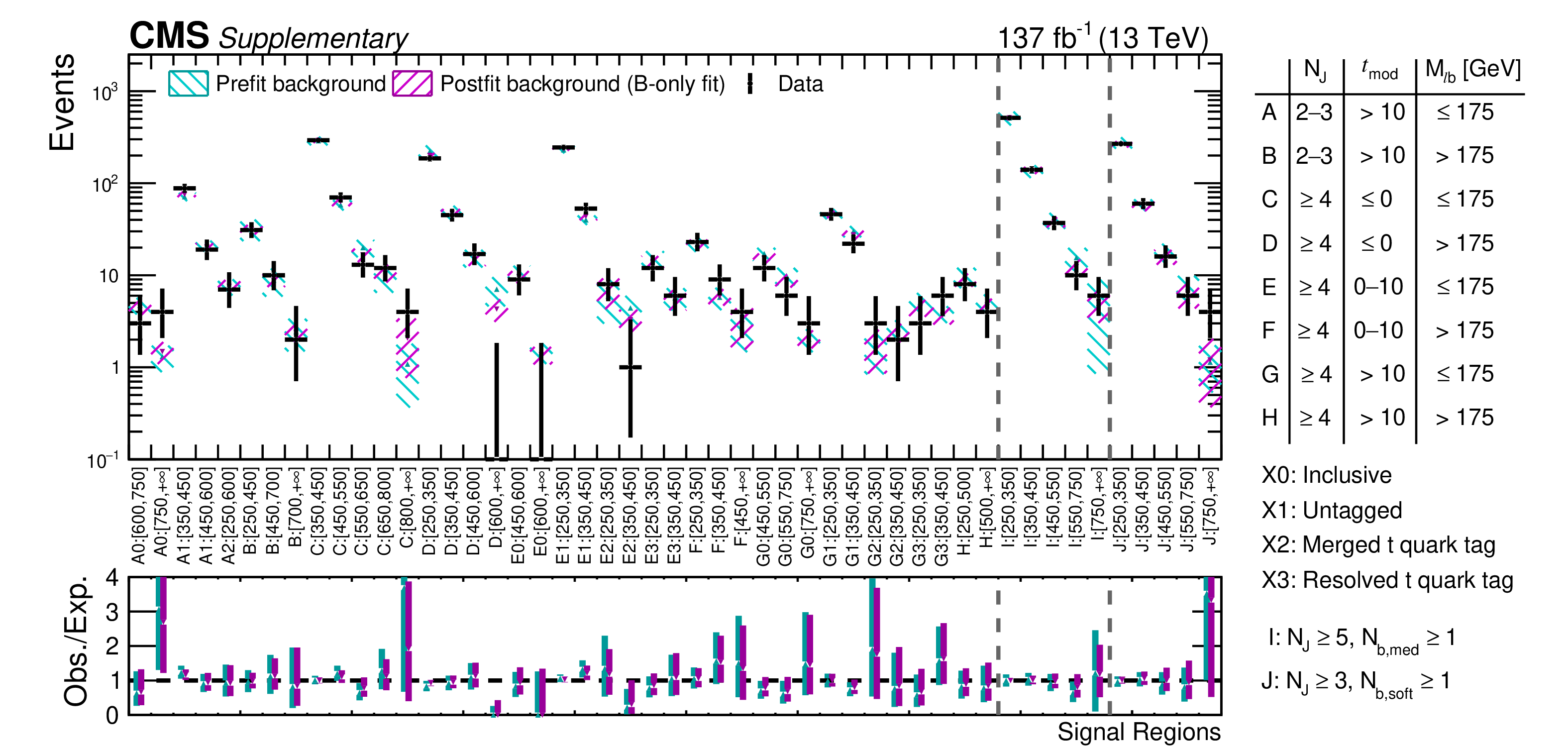
Additional Figure 6:
Comparison between postfit and prefit background predictions and data for 137 fb$^{-1}$ collected during 2016, 2017 and 2018 pp collisions. |
png pdf |
Additional Figure 7:
Exclusion limits as presented in the paper, with the color map showing the 95% CL on the signal strength modifier for direct $ {\tilde{\mathrm {t}}} $ production with the $ {\mathrm {p}} {\mathrm {p}}\to {\tilde{\mathrm {t}}} {\overline {\tilde{\mathrm {t}}}} \to {\mathrm {t}} {\overline {\mathrm {t}}} {\tilde{\chi}^{0}_{1}} {\tilde{\chi}^{0}_{1}} $ decay scenario. |

png pdf |
Additional Figure 8:
Exclusion limits as presented in the paper, with the color map showing the 95% CL on the signal strength modifier for direct $ {\tilde{\mathrm {t}}} $ production with the $ {\mathrm {p}} {\mathrm {p}}\to {\tilde{\mathrm {t}}} {\overline {\tilde{\mathrm {t}}}} \to {\mathrm {b}} {\overline {\mathrm {b}}} {\tilde{\chi}^\pm _{1}} {\tilde{\chi}^\pm _{1}} \left ({\tilde{\chi}^\pm _{1}} \to {\mathrm {W}} {\tilde{\chi}^{0}_{1}} \right)$ decay scenario.. The mass of ${\tilde{\chi}^\pm _{1}}$ is chosen to be $(m_{{\tilde{\mathrm {t}}}} + m_{{\tilde{\chi}^{0}_{1}}})/2$. |
png pdf |
Additional Figure 9:
Exclusion limits as presented in the paper, with the color map showing the 95% CL on the signal strength modifier for direct $ {\tilde{\mathrm {t}}} $ production with $ {\mathrm {p}} {\mathrm {p}}\to {\tilde{\mathrm {t}}} {\overline {\tilde{\mathrm {t}}}} \to {\mathrm {t}} {{\mathrm {b}}} {\tilde{\chi}^\pm _{1}} {\tilde{\chi}^{0}_{1}} \left ({\tilde{\chi}^\pm _{1}} \to {\mathrm {W}}^{*} {\tilde{\chi}^{0}_{1}} \right)$ decay scenario. The mass difference between the ${\tilde{\chi}^\pm _{1}}$ and the ${\tilde{\chi}^{0}_{1}}$ is taken to be 5 GeV. |
png pdf |
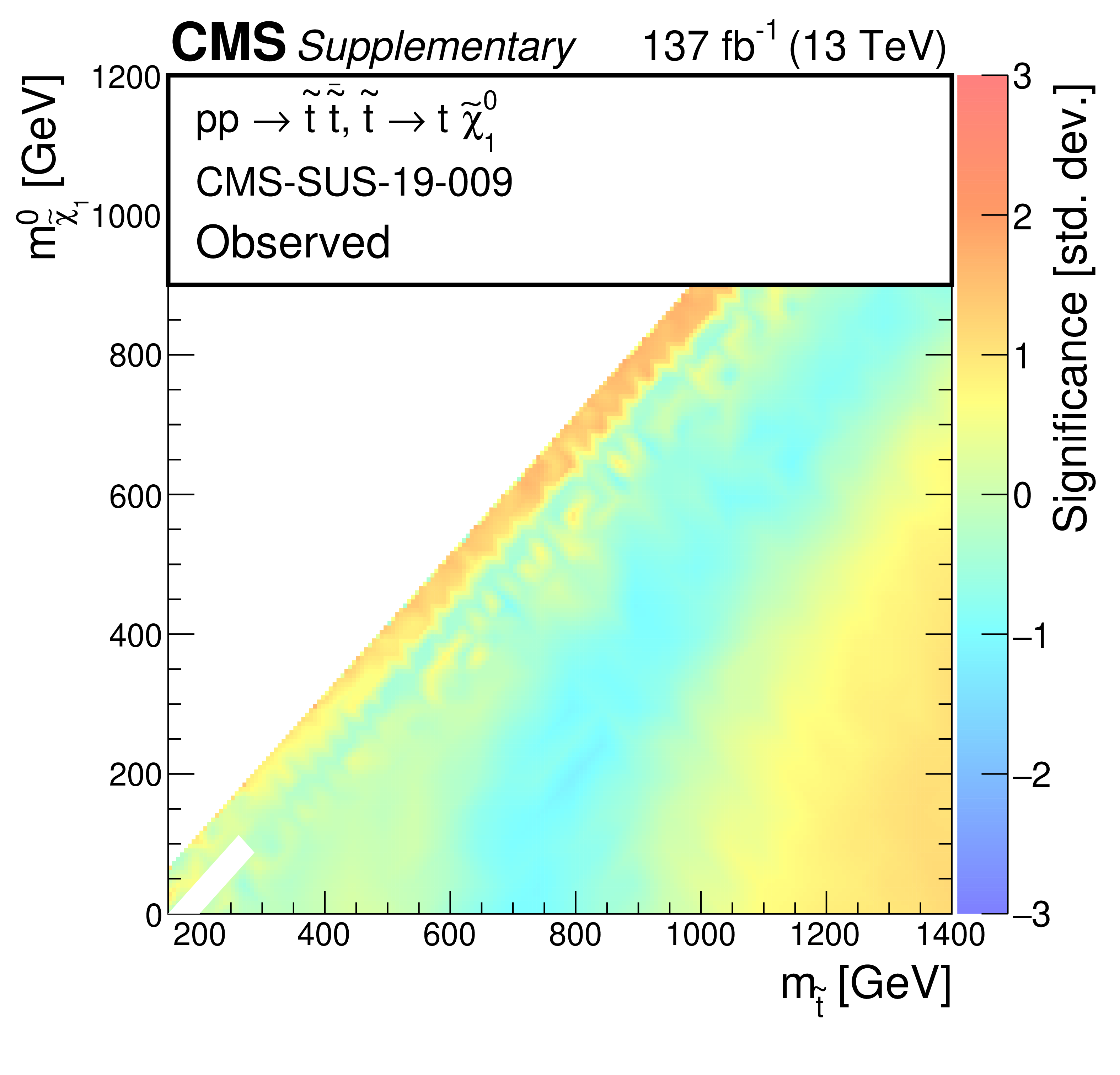
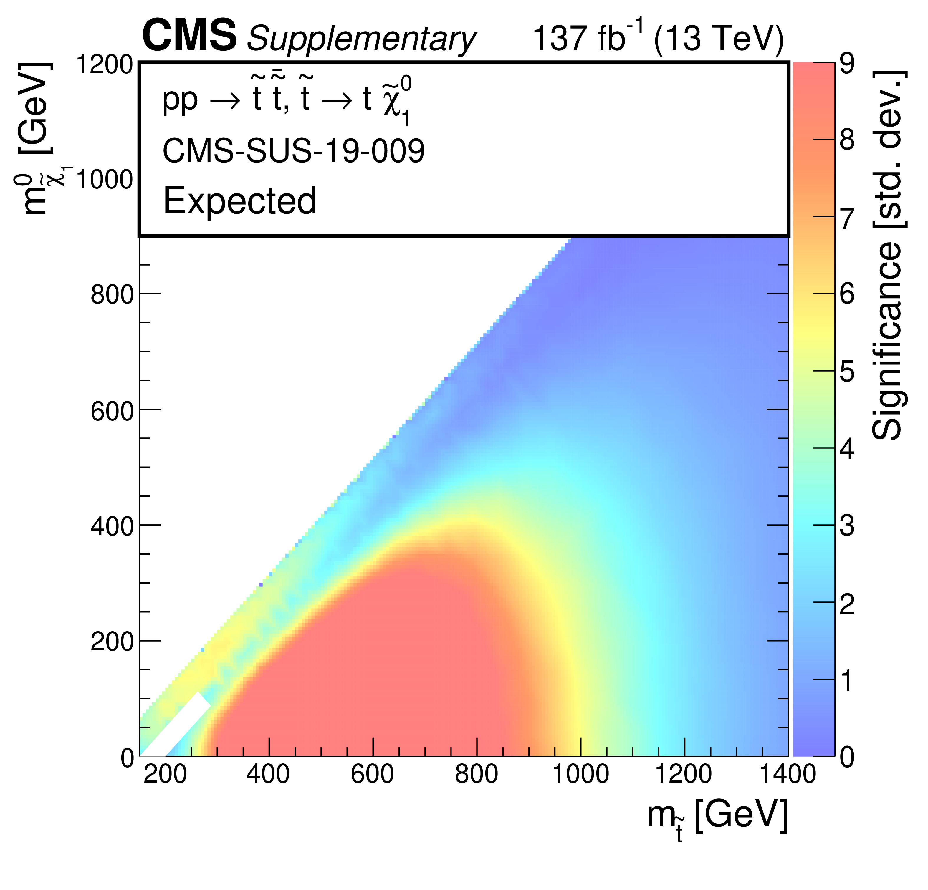
Additional Figure 10:
The observed significances for the exclusion limits at 95% CL for direct $ {\tilde{\mathrm {t}}} $ production with the $ {\mathrm {p}} {\mathrm {p}}\to {\tilde{\mathrm {t}}} {\overline {\tilde{\mathrm {t}}}} \to {\mathrm {t}} {\overline {\mathrm {t}}} {\tilde{\chi}^{0}_{1}} {\tilde{\chi}^{0}_{1}} $ decay scenario. |
png pdf |
Additional Figure 11:
The expected significances for the exclusion limits at 95% CL for direct $ {\tilde{\mathrm {t}}} $ production with the $ {\mathrm {p}} {\mathrm {p}}\to {\tilde{\mathrm {t}}} {\overline {\tilde{\mathrm {t}}}} \to {\mathrm {t}} {\overline {\mathrm {t}}} {\tilde{\chi}^{0}_{1}} {\tilde{\chi}^{0}_{1}} $ decay scenario. |

png pdf |
Additional Figure 12:
The observed significances for the exclusion limits at 95% CL for direct $ {\tilde{\mathrm {t}}} $ production with the $ {\mathrm {p}} {\mathrm {p}}\to {\tilde{\mathrm {t}}} {\overline {\tilde{\mathrm {t}}}} \to {\mathrm {b}} {\overline {\mathrm {b}}} {\tilde{\chi}^\pm _{1}} {\tilde{\chi}^\pm _{1}} \left ({\tilde{\chi}^\pm _{1}} \to {\mathrm {W}} {\tilde{\chi}^{0}_{1}} \right)$ decay scenario.. The mass of ${\tilde{\chi}^\pm _{1}}$ is chosen to be $(m_{{\tilde{\mathrm {t}}}} + m_{{\tilde{\chi}^{0}_{1}}})/2$. |
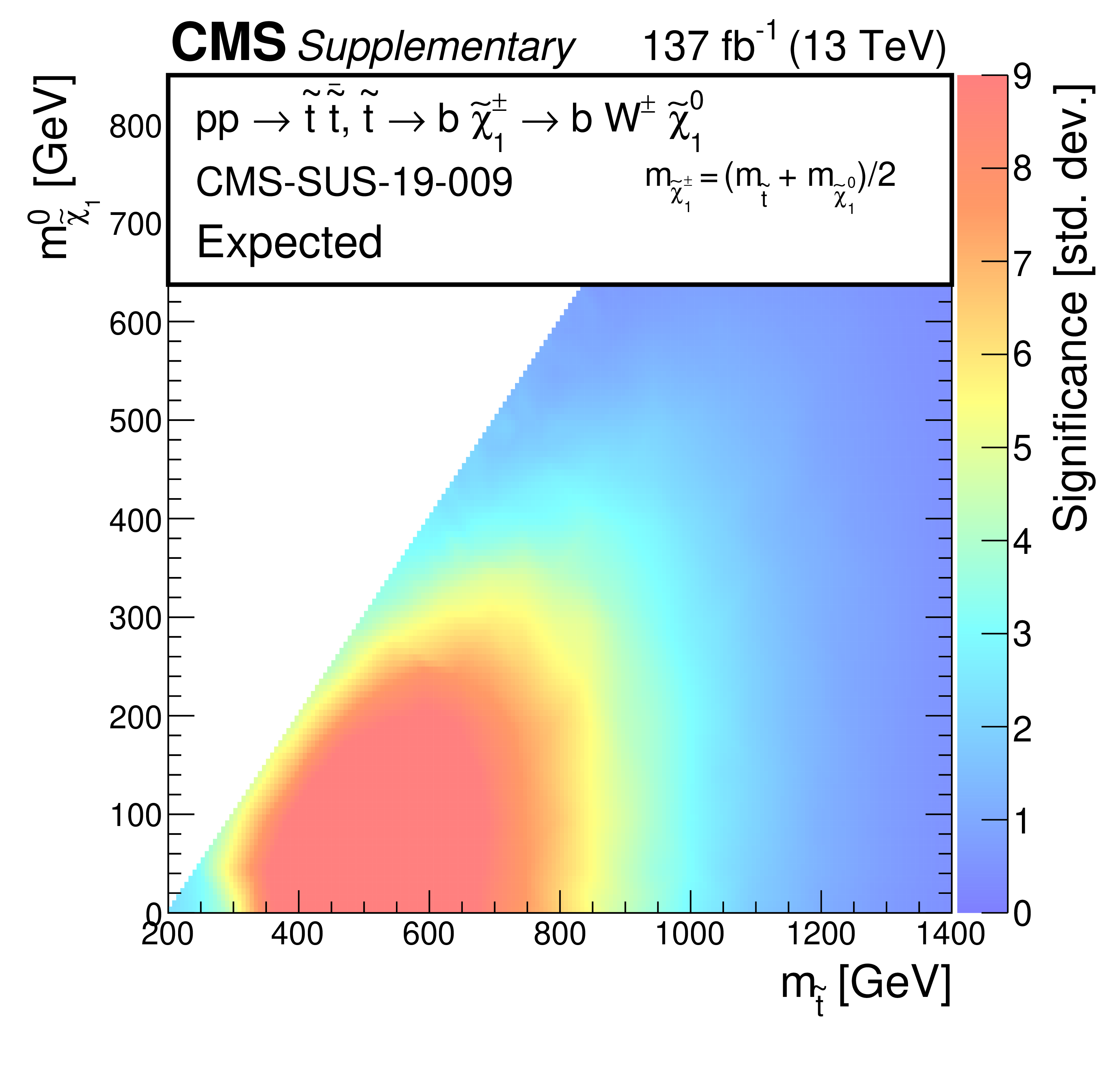
png pdf |
Additional Figure 13:
The expected significances for the exclusion limits at 95% CL for direct $ {\tilde{\mathrm {t}}} $ production with the $ {\mathrm {p}} {\mathrm {p}}\to {\tilde{\mathrm {t}}} {\overline {\tilde{\mathrm {t}}}} \to {\mathrm {b}} {\overline {\mathrm {b}}} {\tilde{\chi}^\pm _{1}} {\tilde{\chi}^\pm _{1}} \left ({\tilde{\chi}^\pm _{1}} \to {\mathrm {W}} {\tilde{\chi}^{0}_{1}} \right)$ decay scenario.. The mass of ${\tilde{\chi}^\pm _{1}}$ is chosen to be $(m_{{\tilde{\mathrm {t}}}} + m_{{\tilde{\chi}^{0}_{1}}})/2$. |
png pdf |
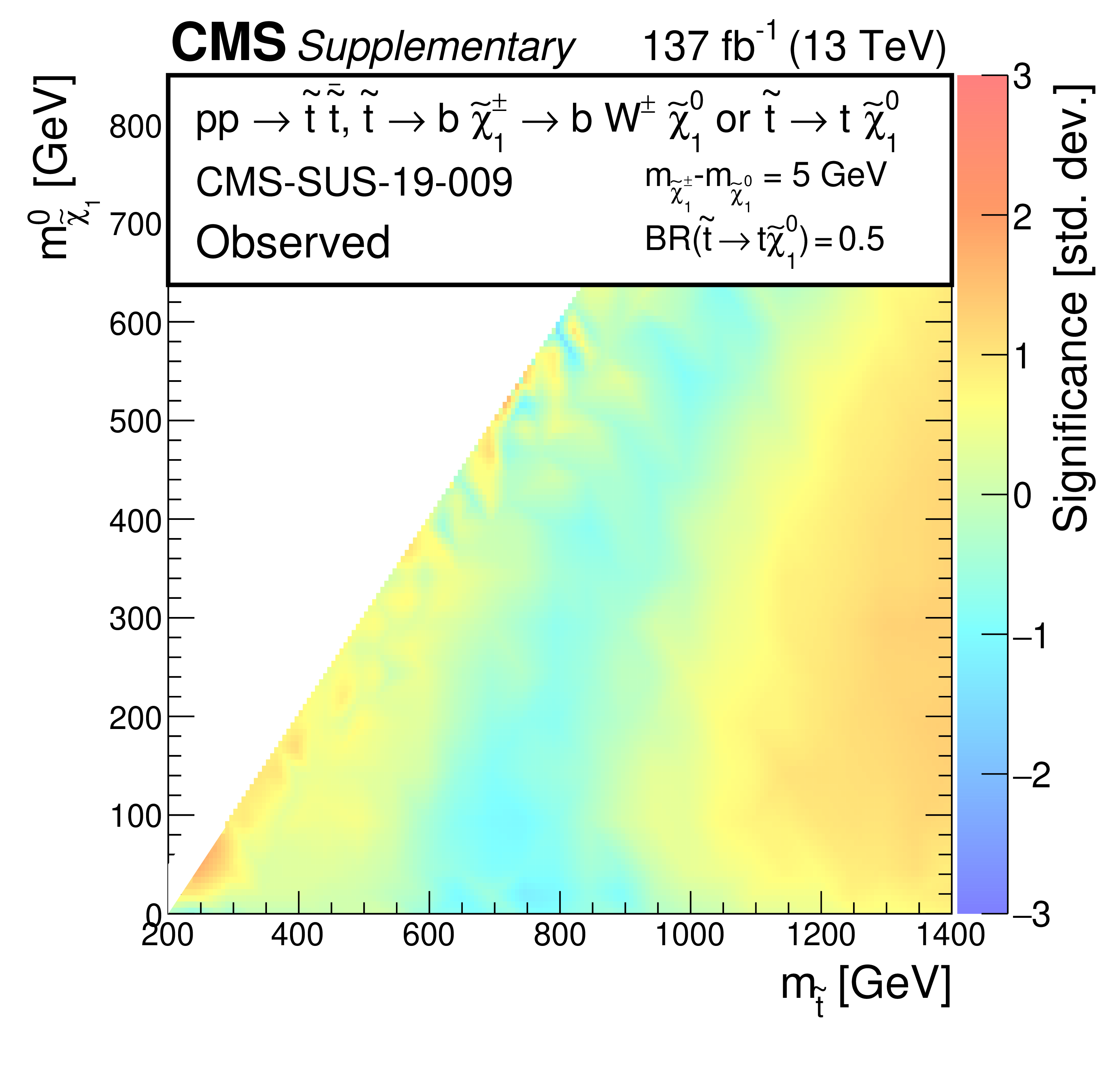
Additional Figure 14:
The observed significances for the exclusion limits at 95% CL for direct $ {\tilde{\mathrm {t}}} $ production with $ {\mathrm {p}} {\mathrm {p}}\to {\tilde{\mathrm {t}}} {\overline {\tilde{\mathrm {t}}}} \to {\mathrm {t}} {{\mathrm {b}}} {\tilde{\chi}^\pm _{1}} {\tilde{\chi}^{0}_{1}} \left ({\tilde{\chi}^\pm _{1}} \to {\mathrm {W}}^{*} {\tilde{\chi}^{0}_{1}} \right)$ decay scenario. The mass difference between the ${\tilde{\chi}^\pm _{1}}$ and the ${\tilde{\chi}^{0}_{1}}$ is taken to be 5 GeV. |

png pdf |
Additional Figure 15:
The expected significances for the exclusion limits at 95% CL for direct $ {\tilde{\mathrm {t}}} $ production with $ {\mathrm {p}} {\mathrm {p}}\to {\tilde{\mathrm {t}}} {\overline {\tilde{\mathrm {t}}}} \to {\mathrm {t}} {{\mathrm {b}}} {\tilde{\chi}^\pm _{1}} {\tilde{\chi}^{0}_{1}} \left ({\tilde{\chi}^\pm _{1}} \to {\mathrm {W}}^{*} {\tilde{\chi}^{0}_{1}} \right)$ decay scenario. The mass difference between the ${\tilde{\chi}^\pm _{1}}$ and the ${\tilde{\chi}^{0}_{1}}$ is taken to be 5 GeV. |
png pdf |
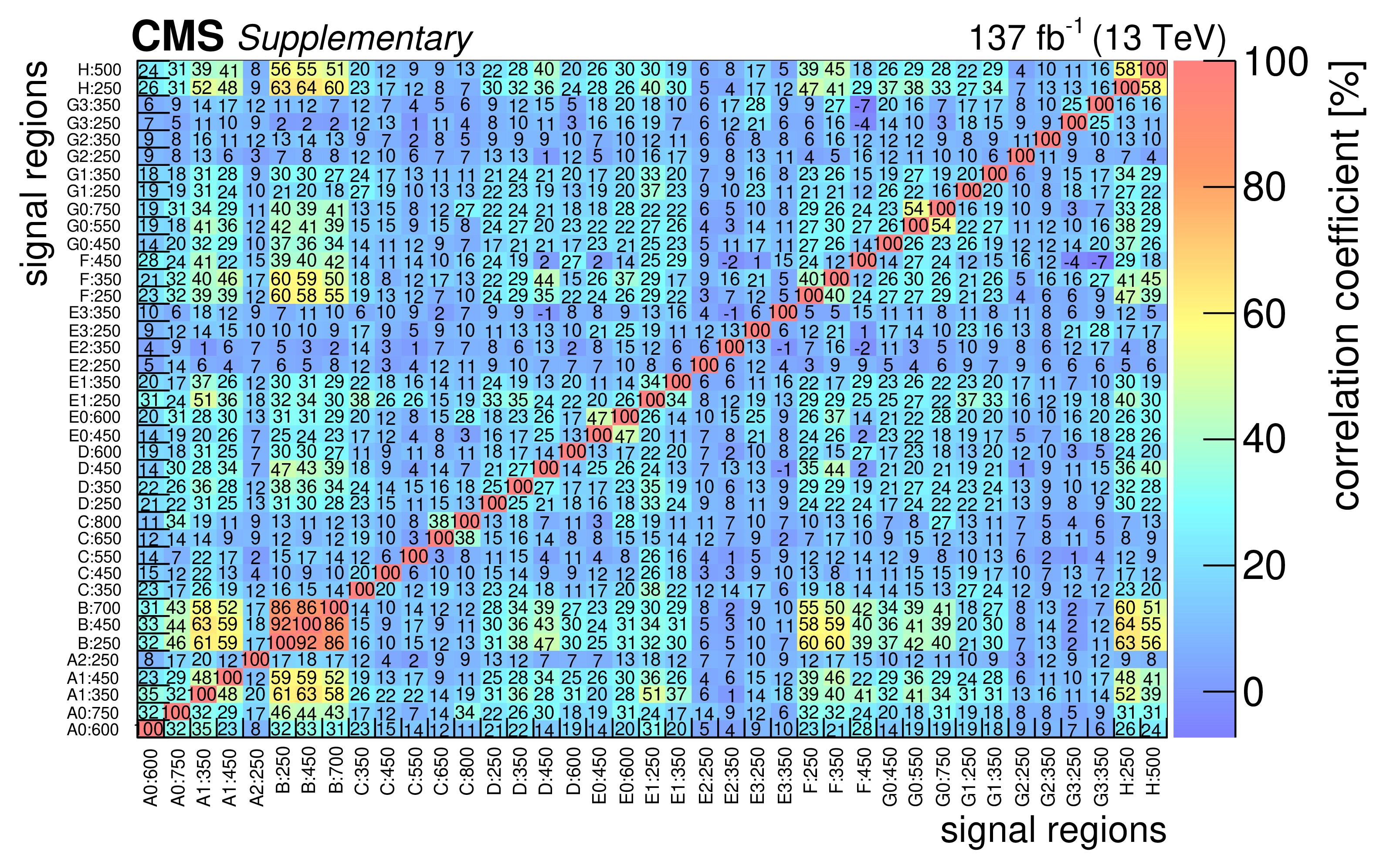
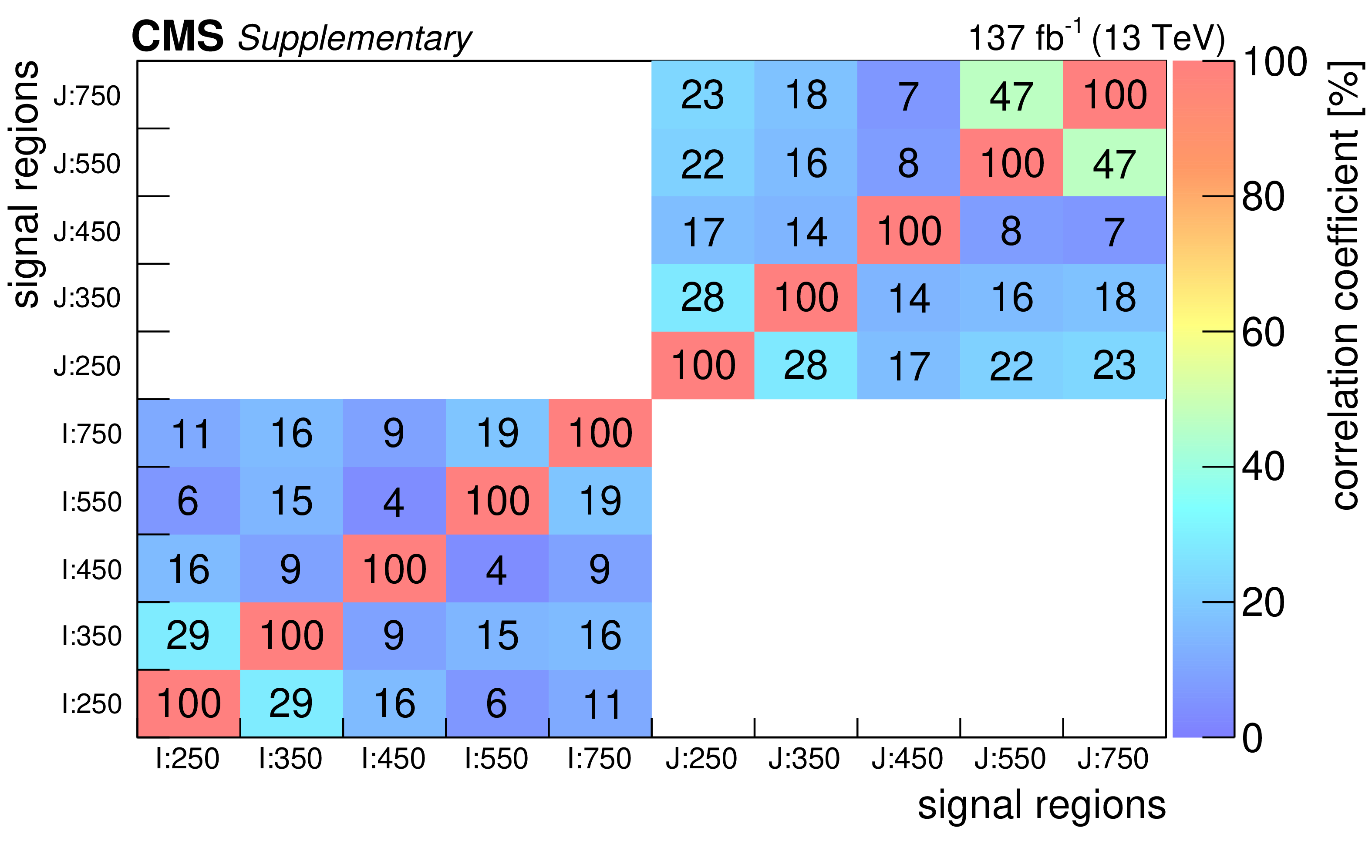
Additional Figure 16:
Correlation matrix for the background predictions for the signal regions for the standard selection (in percent). The labeling of the regions follows the convention of Fig. 5 in the paper. |
png pdf |
Additional Figure 17:
Covariance matrices for the background predictions for the signal regions for the dedicated selection for low $\Delta (m_{{\tilde{\mathrm {t}}}}, m_{{\tilde{\chi}^{0}_{1}}})$ for $ {\mathrm {p}} {\mathrm {p}}\to {\tilde{\mathrm {t}}} {\overline {\tilde{\mathrm {t}}}} \to {\mathrm {t}} {\overline {\mathrm {t}}} {\tilde{\chi}^{0}_{1}} {\tilde{\chi}^{0}_{1}} $ signals (in percent). The labeling of the regions follows the convention of Fig. 5 in the paper. |

png pdf |
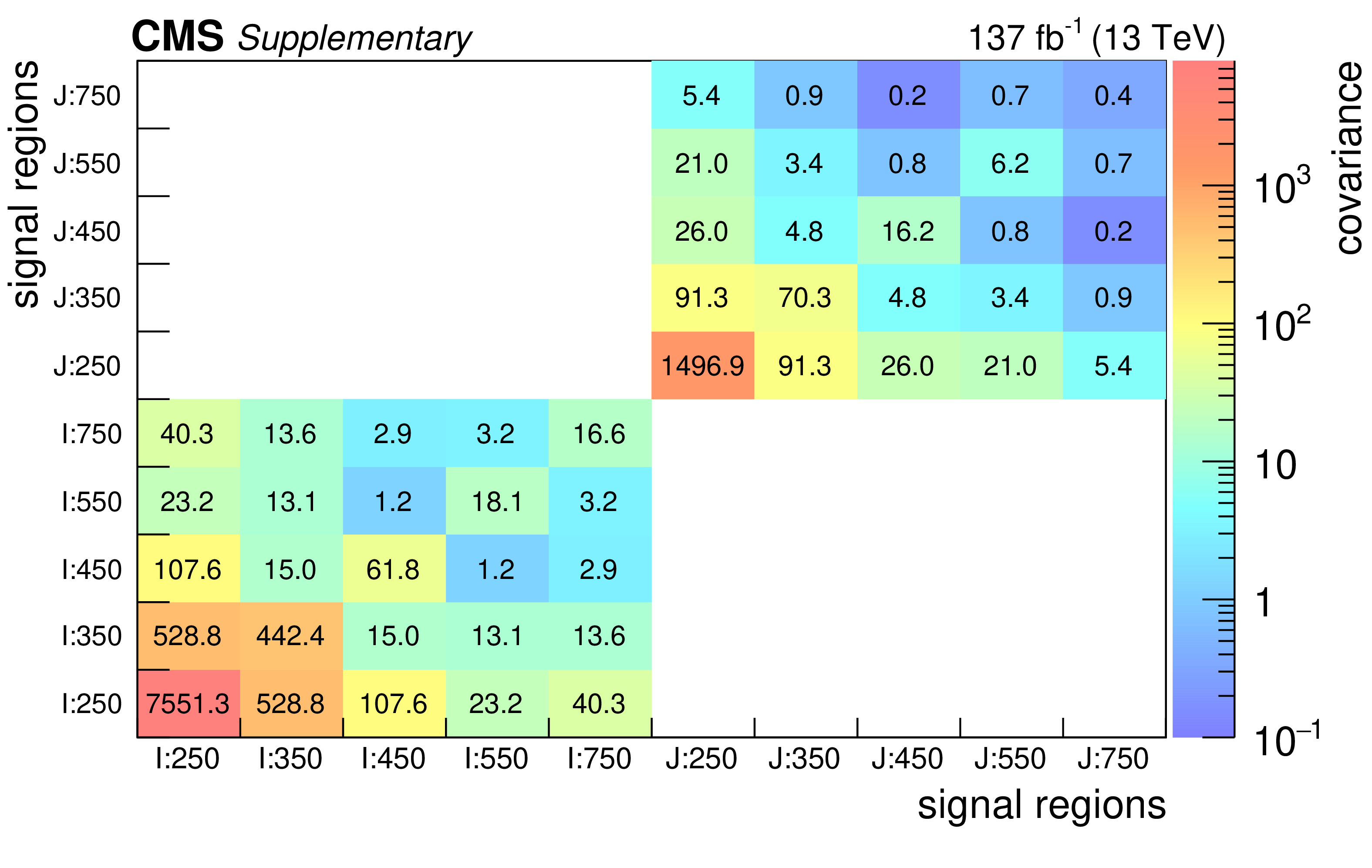
Additional Figure 18:
Covariance matrix for the background predictions for the signal regions for the standard selection. The labeling of the regions follows the convention of Fig. 5 in the paper. |
png pdf |
Additional Figure 19:
Covariance matrices for the background predictions for the signal regions for the dedicated selection for low $\Delta (m_{{\tilde{\mathrm {t}}}}, m_{{\tilde{\chi}^{0}_{1}}})$ for $ {\mathrm {p}} {\mathrm {p}}\to {\tilde{\mathrm {t}}} {\overline {\tilde{\mathrm {t}}}} \to {\mathrm {t}} {\overline {\mathrm {t}}} {\tilde{\chi}^{0}_{1}} {\tilde{\chi}^{0}_{1}} $ signals. The labeling of the regions follows the convention of Fig. 5 in the paper. |
| Additional Tables | |
png pdf |
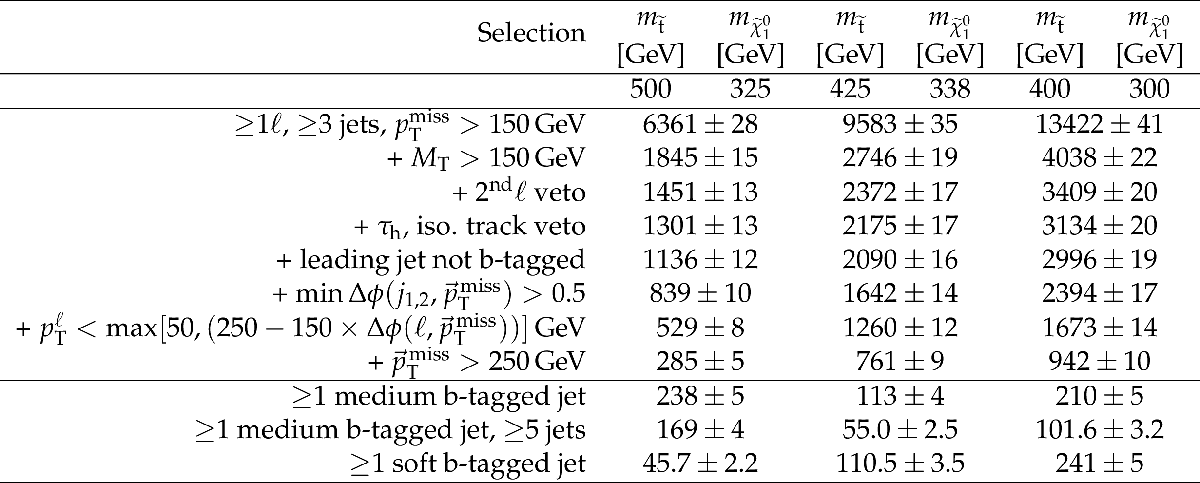
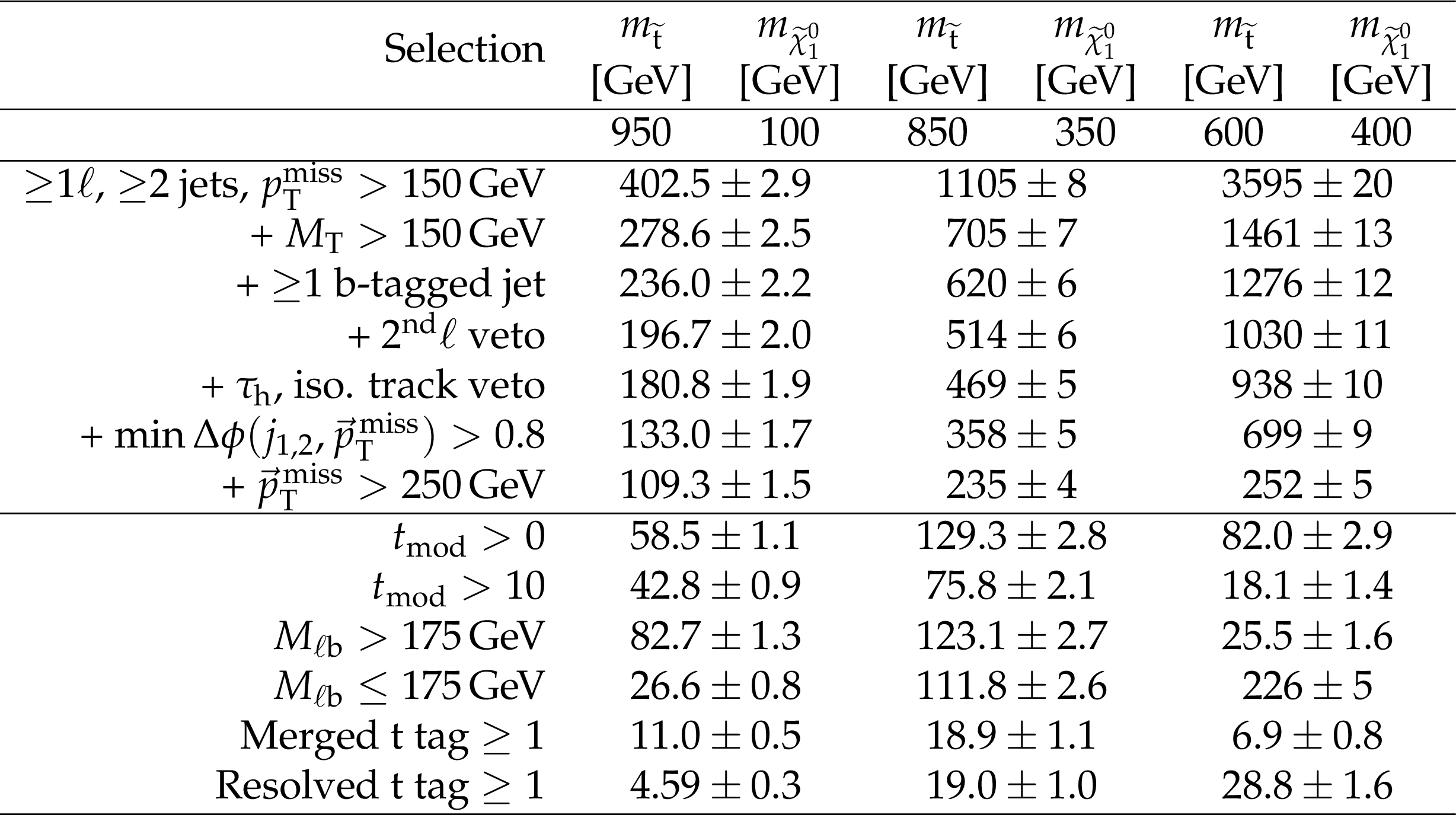
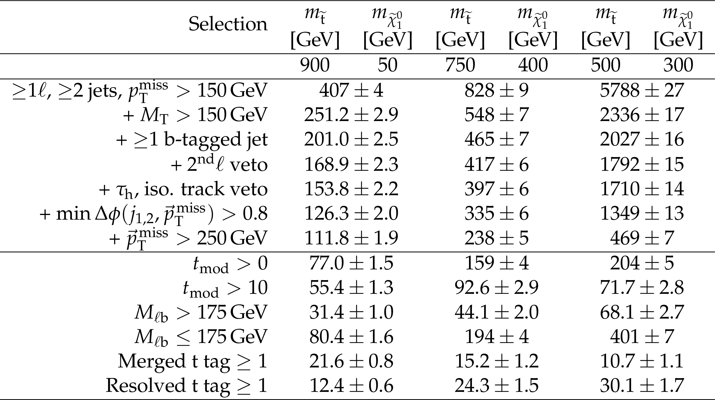
Additional Table 1:
Cutflow using the standard selection for $ {\mathrm {p}} {\mathrm {p}}\to {\tilde{\mathrm {t}}} {\overline {\tilde{\mathrm {t}}}} \to {\mathrm {t}} {\overline {\mathrm {t}}} {\tilde{\chi}^{0}_{1}} {\tilde{\chi}^{0}_{1}} $ signals for an integrated luminosity of 137 fb$^{-1}$. The uncertainties are purely statistical. No correction for signal contamination in data control regions are applied. |
png pdf |
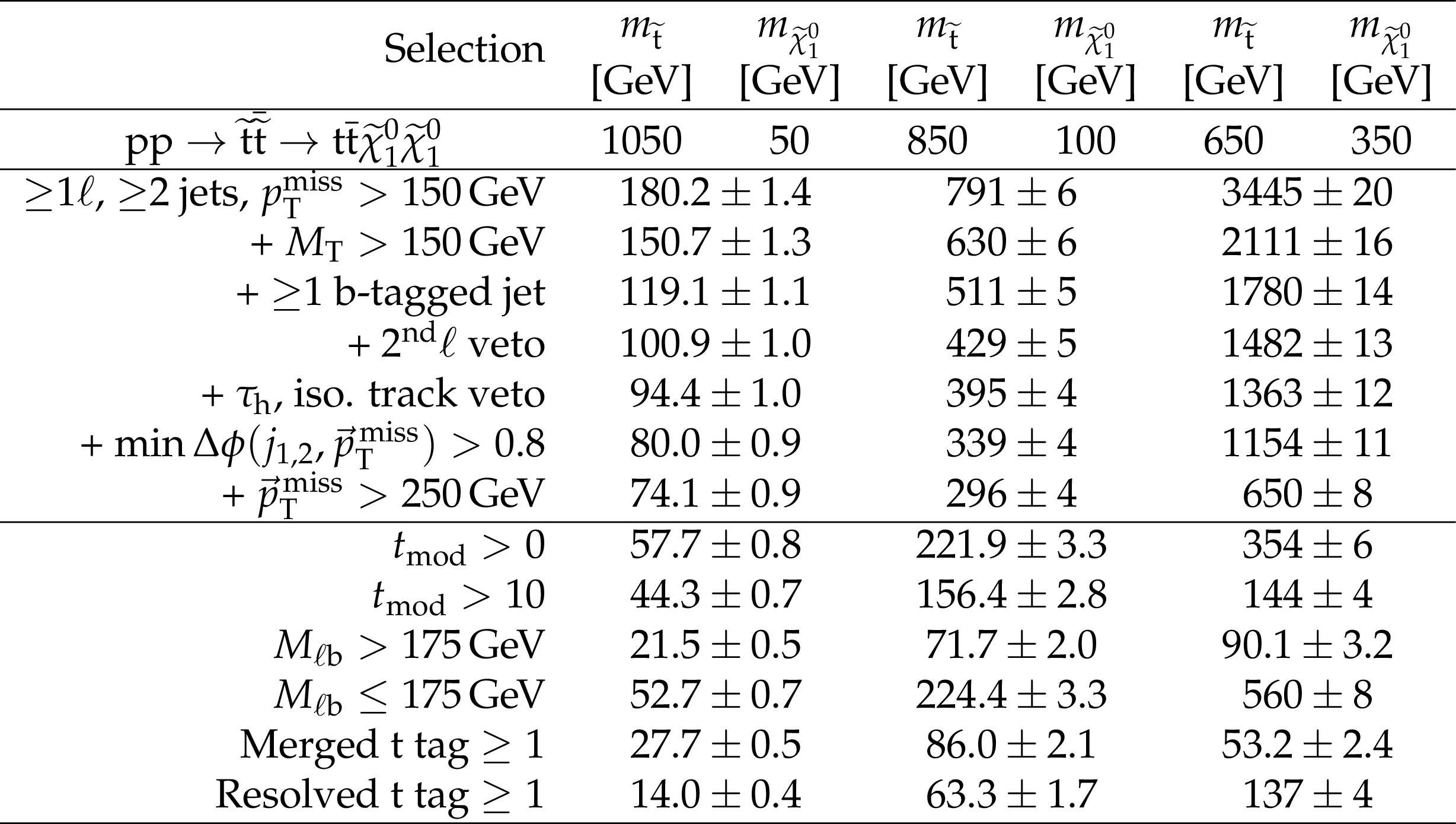
Additional Table 2:
Cutflow using the dedicated selection for low $\Delta (m_{{\tilde{\mathrm {t}}}}, m_{{\tilde{\chi}^{0}_{1}}})$ for $ {\mathrm {p}} {\mathrm {p}}\to {\tilde{\mathrm {t}}} {\overline {\tilde{\mathrm {t}}}} \to {\mathrm {t}} {\overline {\mathrm {t}}} {\tilde{\chi}^{0}_{1}} {\tilde{\chi}^{0}_{1}} $ signals for an integrated luminosity of 137 fb$^{-1}$. The uncertainties are purely statistical. No correction for signal contamination in data control regions are applied. |
png pdf |
Additional Table 3:
Cutflow for $ {\mathrm {p}} {\mathrm {p}}\to {\tilde{\mathrm {t}}} {\overline {\tilde{\mathrm {t}}}} \to {\mathrm {b}} {\overline {\mathrm {b}}} {\tilde{\chi}^\pm _{1}} {\tilde{\chi}^\pm _{1}} \left ({\tilde{\chi}^\pm _{1}} \to {\mathrm {W}} {\tilde{\chi}^{0}_{1}} \right)$ signals for an integrated luminosity of 137 fb$^{-1}$. The uncertainties are purely statistical. No correction for signal contamination in data control regions are applied. |
png pdf |
Additional Table 4:
Cutflow for $ {\mathrm {p}} {\mathrm {p}}\to {\tilde{\mathrm {t}}} {\overline {\tilde{\mathrm {t}}}} \to {\mathrm {t}} {{\mathrm {b}}} {\tilde{\chi}^\pm _{1}} {\tilde{\chi}^{0}_{1}} \left ({\tilde{\chi}^\pm _{1}} \to {\mathrm {W}}^{*} {\tilde{\chi}^{0}_{1}} \right)$ signals for an integrated luminosity of 137 fb$^{-1}$. The uncertainties are purely statistical. No correction for signal contamination in data control regions are applied. |
png pdf |
Additional Table 5:
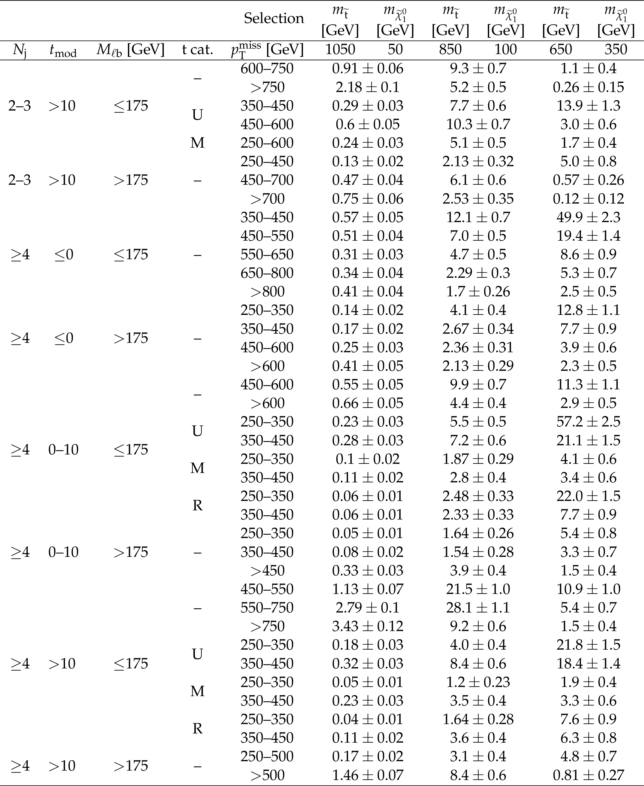
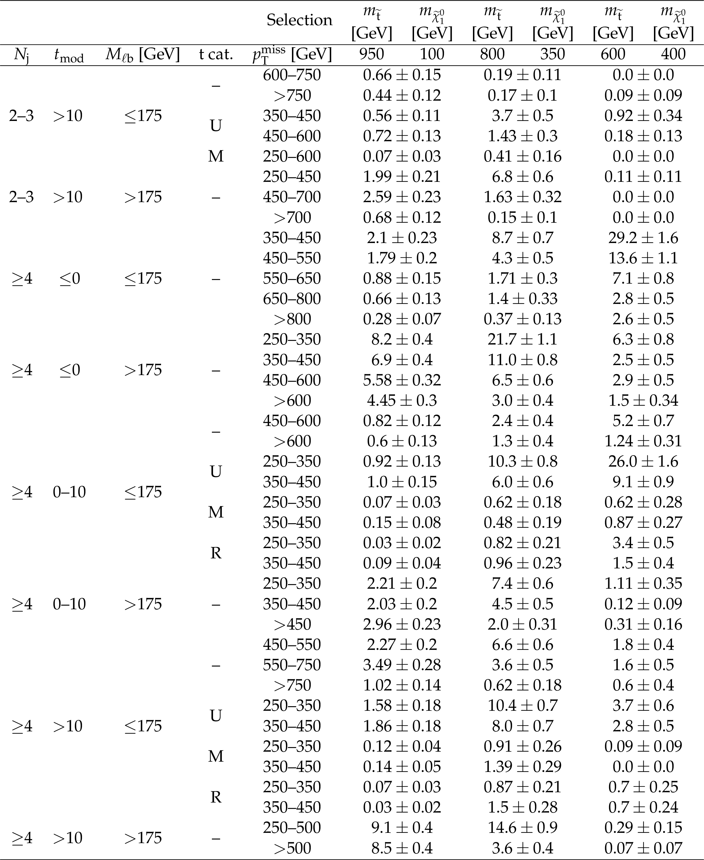
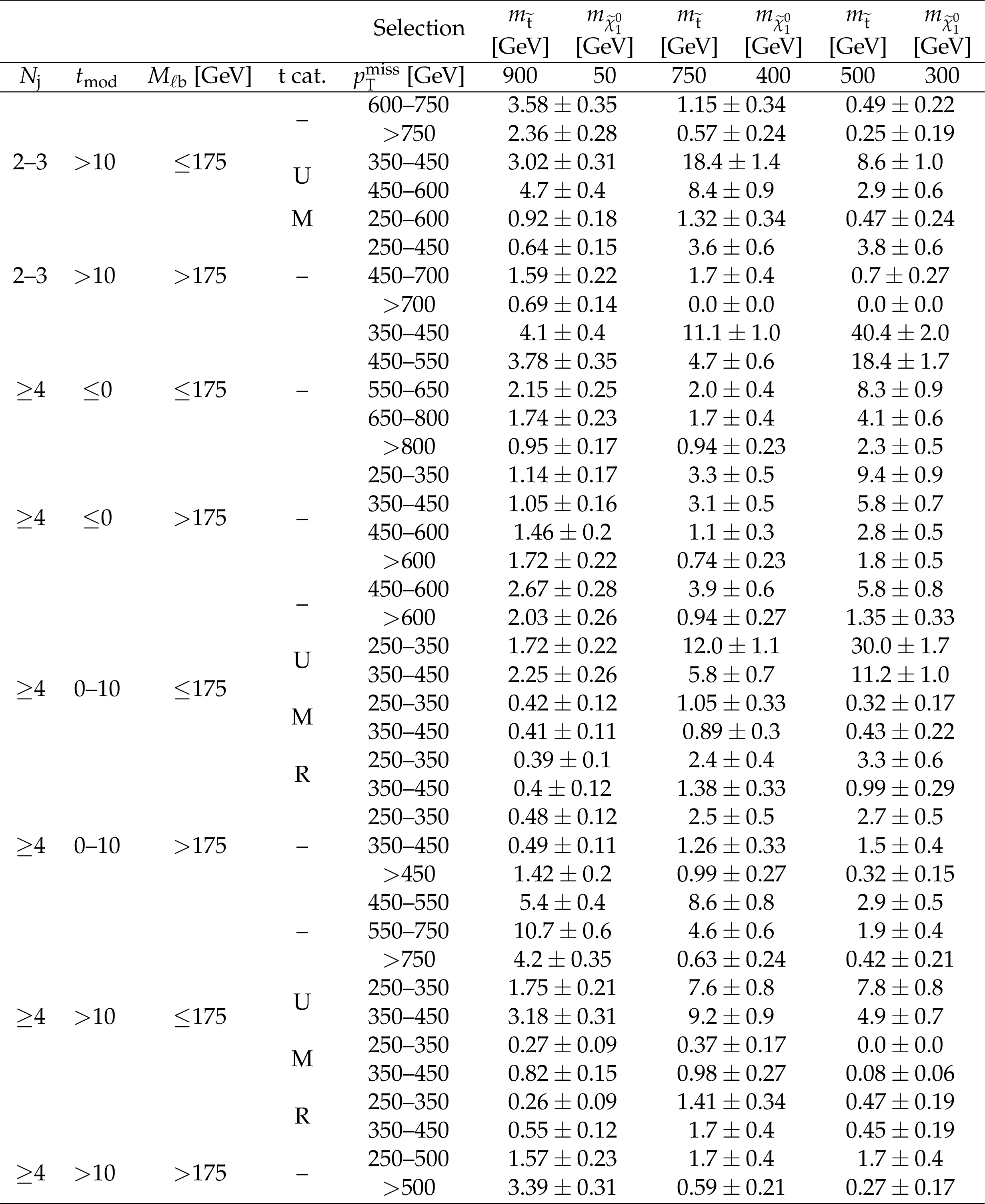
Yields for $ {\mathrm {p}} {\mathrm {p}}\to {\tilde{\mathrm {t}}} {\overline {\tilde{\mathrm {t}}}} \to {\mathrm {t}} {\overline {\mathrm {t}}} {\tilde{\chi}^{0}_{1}} {\tilde{\chi}^{0}_{1}} $ signals for an integrated luminosity of 137 fb$^{-1}$. The uncertainties are purely statistical. No correction for signal contamination in data control regions are applied. |
png pdf |
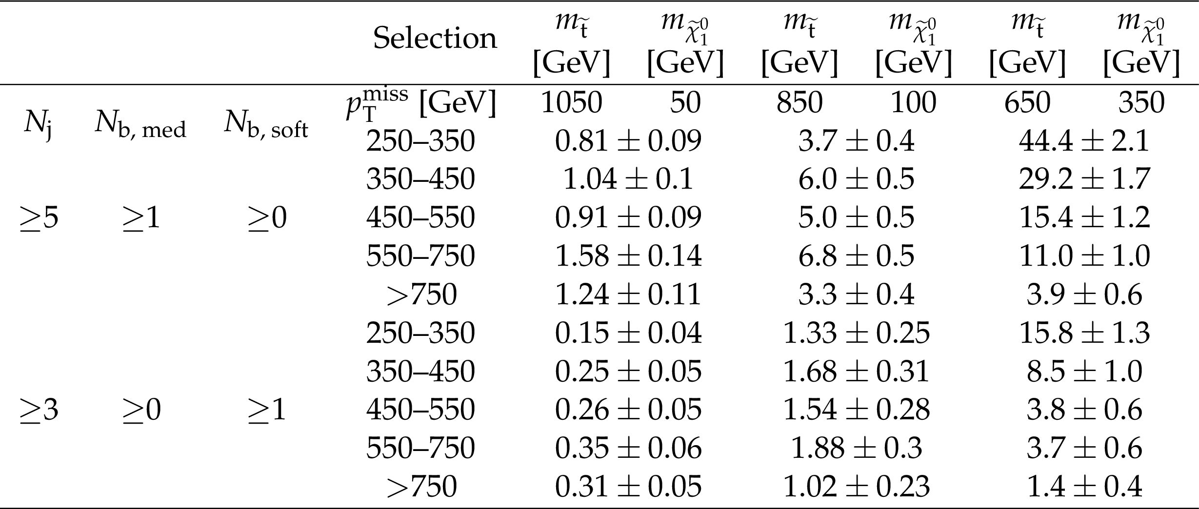
Additional Table 6:
Yields for $ {\mathrm {p}} {\mathrm {p}}\to {\tilde{\mathrm {t}}} {\overline {\tilde{\mathrm {t}}}} \to {\mathrm {t}} {\overline {\mathrm {t}}} {\tilde{\chi}^{0}_{1}} {\tilde{\chi}^{0}_{1}} $ signals under the dedicated compressed mass spectrum selection for an integrated luminosity of 137 fb$^{-1}$. The uncertainties are purely statistical. No correction for signal contamination in data control regions are applied. |
png pdf |
Additional Table 7:
Yields for $ {\mathrm {p}} {\mathrm {p}}\to {\tilde{\mathrm {t}}} {\overline {\tilde{\mathrm {t}}}} \to {\mathrm {b}} {\overline {\mathrm {b}}} {\tilde{\chi}^\pm _{1}} {\tilde{\chi}^\pm _{1}} \left ({\tilde{\chi}^\pm _{1}} \to {\mathrm {W}} {\tilde{\chi}^{0}_{1}} \right)$ signals for an integrated luminosity of 137 fb$^{-1}$. The uncertainties are purely statistical. No correction for signal contamination in data control regions are applied. |
png pdf |
Additional Table 8:
Yields for $ {\mathrm {p}} {\mathrm {p}}\to {\tilde{\mathrm {t}}} {\overline {\tilde{\mathrm {t}}}} \to {\mathrm {t}} {{\mathrm {b}}} {\tilde{\chi}^\pm _{1}} {\tilde{\chi}^{0}_{1}} \left ({\tilde{\chi}^\pm _{1}} \to {\mathrm {W}}^{*} {\tilde{\chi}^{0}_{1}} \right)$ signals for an integrated luminosity of 137 fb$^{-1}$. The uncertainties are purely statistical. No correction for signal contamination in data control regions are applied. |
| References | ||||
| 1 | P. Ramond | Dual theory for free fermions | PRD 3 (1971) 2415 | |
| 2 | Y. A. Gol'fand and E. P. Likhtman | Extension of the algebra of Poincare group generators and violation of P invariance | JEPTL 13 (1971) 323.[Pisma Zh. Eksp. Teor. Fiz. 13 (1971) 452] | |
| 3 | A. Neveu and J. H. Schwarz | Factorizable dual model of pions | NPB 31 (1971) 86 | |
| 4 | D. V. Volkov and V. P. Akulov | Possible universal neutrino interaction | JEPTL 16 (1972) 438.[Pisma Zh. Eksp. Teor. Fiz. 16 (1972) 621] | |
| 5 | J. Wess and B. Zumino | A Lagrangian model invariant under supergauge transformations | PLB 49 (1974) 52 | |
| 6 | J. Wess and B. Zumino | Supergauge transformations in four-dimensions | NPB 70 (1974) 39 | |
| 7 | P. Fayet | Supergauge invariant extension of the Higgs mechanism and a model for the electron and its neutrino | NPB 90 (1975) 104 | |
| 8 | H. P. Nilles | Supersymmetry, supergravity and particle physics | PR 110 (1984) 1 | |
| 9 | G. R. Farrar and P. Fayet | Phenomenology of the production, decay, and detection of new hadronic states associated with supersymmetry | PLB 76 (1978) 575 | |
| 10 | G. Jungman, M. Kamionkowski, and K. Griest | Supersymmetric dark matter | PR 267 (1996) 195 | hep-ph/9506380 |
| 11 | G. 't Hooft | Naturalness, chiral symmetry, and spontaneous chiral symmetry breaking | NATO Sci. Ser. B 59 (1980) 135 | |
| 12 | M. Dine, W. Fischler, and M. Srednicki | Supersymmetric technicolor | NPB 189 (1981) 575 | |
| 13 | S. Dimopoulos and S. Raby | Supercolor | NPB 192 (1981) 353 | |
| 14 | S. Dimopoulos and H. Georgi | Softly broken supersymmetry and SU(5) | NPB 193 (1981) 150 | |
| 15 | R. K. Kaul and P. Majumdar | Cancellation of quadratically divergent mass corrections in globally supersymmetric spontaneously broken gauge theories | NPB 199 (1982) 36 | |
| 16 | ATLAS Collaboration | Search for top squarks in final states with one isolated lepton, jets, and missing transverse momentum in $ \sqrt{s} = $ 13 TeV pp collisions with the ATLAS detector | PRD 94 (2016) 052009 | 1606.03903 |
| 17 | ATLAS Collaboration | Search for heavy long-lived charged R-hadrons with the ATLAS detector in 3.2 fb$^{-1}$ of proton--proton collision data at $ \sqrt{s} = $ 13 TeV | PLB 760 (2016) 647 | 1606.05129 |
| 18 | ATLAS Collaboration | Search for direct top squark pair production in events with a Higgs or $ \mathrm{Z} $ boson, and missing transverse momentum in $ \sqrt{s} = $ 13 TeV pp collisions with the ATLAS detector | JHEP 08 (2017) 006 | 1706.03986 |
| 19 | ATLAS Collaboration | Search for direct top squark pair production in final states with two leptons in $ \sqrt{s} = $ 13 TeV pp collisions with the ATLAS detector | EPJC 77 (2017) 898 | 1708.03247 |
| 20 | ATLAS Collaboration | Search for a scalar partner of the top quark in the jets plus missing transverse momentum final state at $ \sqrt{s} = $ 13 TeV with the ATLAS detector | JHEP 12 (2017) 085 | 1709.04183 |
| 21 | ATLAS Collaboration | Search for $ B-L $ R-parity-violating top squarks in $ \sqrt{s} = $ 13 TeV pp collisions with the ATLAS experiment | PRD 97 (2018) 032003 | 1710.05544 |
| 22 | ATLAS Collaboration | A search for pair-produced resonances in four-jet final states at $ \sqrt{s} = $ 13 TeV with the ATLAS detector | EPJC 78 (2018) 250 | 1710.07171 |
| 23 | ATLAS Collaboration | Search for top-squark pair production in final states with one lepton, jets, and missing transverse momentum using 36 fb$^{-1}$ of $ \sqrt{s} = $ 13 TeV pp collision data with the ATLAS detector | JHEP 06 (2018) 108 | 1711.11520 |
| 24 | ATLAS Collaboration | Search for top squarks decaying to tau sleptons in pp collisions at $ \sqrt{s} = $ 13 TeV with the ATLAS detector | PRD 98 (2018) 032008 | 1803.10178 |
| 25 | ATLAS Collaboration | Search for supersymmetry in final states with charm jets and missing transverse momentum in 13 TeV pp collisions with the ATLAS detector | JHEP 09 (2018) 050 | 1805.01649 |
| 26 | CMS Collaboration | Search for top squark pair production in compressed-mass-spectrum scenarios in proton-proton collisions at $ \sqrt{s} = $ 8 TeV using the $ \alpha_{\mathrm{T}} $ variable | PLB 767 (2017) 403 | CMS-SUS-14-006 1605.08993 |
| 27 | CMS Collaboration | Searches for pair production of third-generation squarks in $ \sqrt{s} = $ 13 TeV pp collisions | EPJC 77 (2017) 327 | CMS-SUS-16-008 1612.03877 |
| 28 | CMS Collaboration | Search for supersymmetry in the all-hadronic final state using top quark tagging in pp collisions at $ \sqrt{s} = $ 13 TeV | PRD 96 (2017) 012004 | CMS-SUS-16-009 1701.01954 |
| 29 | CMS Collaboration | Search for top squark pair production in pp collisions at $ \sqrt{s} = $ 13 TeV using single lepton events | JHEP 10 (2017) 019 | CMS-SUS-16-051 1706.04402 |
| 30 | CMS Collaboration | Search for direct production of supersymmetric partners of the top quark in the all-jets final state in proton-proton collisions at $ \sqrt{s} = $ 13 TeV | JHEP 10 (2017) 005 | CMS-SUS-16-049 1707.03316 |
| 31 | CMS Collaboration | Search for the pair production of third-generation squarks with two-body decays to a bottom or charm quark and a neutralino in proton-proton collisions at $ \sqrt{s} = $ 13 TeV | PLB 778 (2018) 263 | CMS-SUS-16-032 1707.07274 |
| 32 | CMS Collaboration | Search for supersymmetry in proton-proton collisions at 13 TeV using identified top quarks | PRD 97 (2018) 012007 | CMS-SUS-16-050 1710.11188 |
| 33 | CMS Collaboration | Search for top squarks and dark matter particles in opposite-charge dilepton final states at $ \sqrt{s} = $ 13 TeV | PRD 97 (2018) 032009 | CMS-SUS-17-001 1711.00752 |
| 34 | CMS Collaboration | Search for new physics in events with two soft oppositely charged leptons and missing transverse momentum in proton-proton collisions at $ \sqrt{s} = $ 13 TeV | PLB 782 (2018) 440 | CMS-SUS-16-048 1801.01846 |
| 35 | CMS Collaboration | Search for top squarks decaying via four-body or chargino-mediated modes in single-lepton final states in proton-proton collisions at $ \sqrt{s} = $ 13 TeV | JHEP 09 (2018) 065 | CMS-SUS-17-005 1805.05784 |
| 36 | CMS Collaboration | Search for pair-produced resonances decaying to quark pairs in proton-proton collisions at $ \sqrt{s} = $ 13 TeV | PRD 98 (2018) 112014 | CMS-EXO-17-021 1808.03124 |
| 37 | CMS Collaboration | Inclusive search for supersymmetry in pp collisions at $ \sqrt{s} = $ 13 TeV using razor variables and boosted object identification in zero and one lepton final states | JHEP 03 (2019) 031 | CMS-SUS-16-017 1812.06302 |
| 38 | CMS Collaboration | Search for the pair production of light top squarks in the $ \mathrm{e^{\pm}}\mu^{\mp} $ final state in proton-proton collisions at $ \sqrt{s} = $ 13 TeV | JHEP 03 (2019) 101 | CMS-SUS-18-003 1901.01288 |
| 39 | CMS Collaboration | The CMS experiment at the CERN LHC | JINST 3 (2008) S08004 | CMS-00-001 |
| 40 | CMS Collaboration | The CMS trigger system | JINST 12 (2017) P01020 | CMS-TRG-12-001 1609.02366 |
| 41 | CMS Collaboration | CMS technical design report for the pixel detector upgrade | CERN-LHCC-2012-016, CMS-TDR-011 | |
| 42 | J. Alwall et al. | The automated computation of tree-level and next-to-leading order differential cross sections, and their matching to parton shower simulations | JHEP 07 (2014) 079 | 1405.0301 |
| 43 | P. Nason | A new method for combining NLO QCD with shower Monte Carlo algorithms | JHEP 11 (2004) 040 | hep-ph/0409146 |
| 44 | S. Frixione, P. Nason, and C. Oleari | Matching NLO QCD computations with parton shower simulations: the $ POWHEG $ method | JHEP 11 (2007) 070 | 0709.2092 |
| 45 | S. Alioli, P. Nason, C. Oleari, and E. Re | A general framework for implementing NLO calculations in shower Monte Carlo programs: the $ POWHEG $ BOX | JHEP 06 (2010) 043 | 1002.2581 |
| 46 | E. Re | Single-top $ \mathrm{W}\mathrm{t} $-channel production matched with parton showers using the POWHEG method | EPJC 71 (2011) 1547 | 1009.2450 |
| 47 | NNPDF Collaboration | Unbiased global determination of parton distributions and their uncertainties at NNLO and at LO | NPB 855 (2012) 153 | 1107.2652 |
| 48 | NNPDF Collaboration | Parton distributions for the LHC Run II | JHEP 04 (2015) 040 | 1410.8849 |
| 49 | NNPDF Collaboration | Parton distributions from high-precision collider data | EPJC 77 (2017) 663 | 1706.00428 |
| 50 | T. Sjostrand et al. | An introduction to PYTHIA 8.2 | CPC 191 (2015) 159 | 1410.3012 |
| 51 | J. Alwall et al. | Comparative study of various algorithms for the merging of parton showers and matrix elements in hadronic collisions | EPJC 53 (2008) 473 | 0706.2569 |
| 52 | R. Frederix and S. Frixione | Merging meets matching in MC@NLO | JHEP 12 (2012) 061 | 1209.6215 |
| 53 | CMS Collaboration | Event generator tunes obtained from underlying event and multiparton scattering measurements | EPJC 76 (2016) 155 | CMS-GEN-14-001 1512.00815 |
| 54 | CMS Collaboration | Extraction and validation of a new set of CMS PYTHIA8 tunes from underlying-event measurements | Submitted to EPJC | CMS-GEN-17-001 1903.12179 |
| 55 | \GEANTfour Collaboration | $ GEANT4 -- a $ simulation toolkit | NIMA 506 (2003) 250 | |
| 56 | S. Abdullin et al. | The fast simulation of the CMS detector at LHC | J. Phys. Conf. Ser. 331 (2011) 032049 | |
| 57 | A. Giammanco | The Fast Simulation of the CMS Experiment | J. Phys. Conf. Ser. 513 (2014) 022012 | |
| 58 | Y. Li and F. Petriello | Combining QCD and electroweak corrections to dilepton production in FEWZ | PRD 86 (2012) 094034 | 1208.5967 |
| 59 | M. Aliev et al. | HATHOR: HAdronic Top and Heavy quarks crOss section calculatoR | CPC 182 (2011) 1034 | 1007.1327 |
| 60 | P. Kant et al. | HatHor for single top-quark production: Updated predictions and uncertainty estimates for single top-quark production in hadronic collisions | CPC 191 (2015) 74 | 1406.4403 |
| 61 | M. Beneke, P. Falgari, S. Klein, and C. Schwinn | Hadronic top-quark pair production with NNLL threshold resummation | NPB 855 (2012) 695 | 1109.1536 |
| 62 | M. Cacciari et al. | Top-pair production at hadron colliders with next-to-next-to-leading logarithmic soft-gluon resummation | PLB 710 (2012) 612 | 1111.5869 |
| 63 | M. Czakon and A. Mitov | Top++: A Program for the Calculation of the Top-Pair Cross-Section at Hadron Colliders | CPC 185 (2014) 2930 | 1112.5675 |
| 64 | P. Barnreuther, M. Czakon, and A. Mitov | Percent level precision physics at the tevatron: First genuine NNLO QCD corrections to $ q \bar{q} \to t \bar{t} + X $ | PRL 109 (2012) 132001 | 1204.5201 |
| 65 | M. Czakon and A. Mitov | NNLO corrections to top-pair production at hadron colliders: the all-fermionic scattering channels | JHEP 12 (2012) 054 | 1207.0236 |
| 66 | M. Czakon and A. Mitov | NNLO corrections to top pair production at hadron colliders: the quark-gluon reaction | JHEP 01 (2013) 080 | 1210.6832 |
| 67 | M. Czakon, P. Fiedler, and A. Mitov | Total top-quark pair-production cross section at hadron colliders through $ O({\alpha_S}^4) $ | PRL 110 (2013) 252004 | 1303.6254 |
| 68 | W. Beenakker, R. Hopker, M. Spira, and P. M. Zerwas | Squark and gluino production at hadron colliders | NPB 492 (1997) 51 | hep-ph/9610490 |
| 69 | A. Kulesza and L. Motyka | Threshold resummation for squark-antisquark and gluino-pair production at the LHC | PRL 102 (2009) 111802 | 0807.2405 |
| 70 | A. Kulesza and L. Motyka | Soft gluon resummation for the production of gluino-gluino and squark-antisquark pairs at the LHC | PRD 80 (2009) 095004 | 0905.4749 |
| 71 | W. Beenakker et al. | Soft-gluon resummation for squark and gluino hadroproduction | JHEP 12 (2009) 041 | 0909.4418 |
| 72 | W. Beenakker et al. | Squark and Gluino Hadroproduction | Int. J. Mod. Phys. A 26 (2011) 2637 | 1105.1110 |
| 73 | C. Borschensky et al. | Squark and gluino production cross sections in $ pp $ collisions at $ \sqrt{s} = $ 13, 14, 33 and 100 TeV | EPJC 74 (2014) 3174 | 1407.5066 |
| 74 | W. Beenakker et al. | NNLL-fast: predictions for coloured supersymmetric particle production at the LHC with threshold and Coulomb resummation | JHEP 12 (2016) 133 | 1607.07741 |
| 75 | CMS Collaboration | Particle-flow reconstruction and global event description with the CMS detector | JINST 12 (2017) P10003 | CMS-PRF-14-001 1706.04965 |
| 76 | M. Cacciari and G. P. Salam | Dispelling the $ N^{3} $ myth for the $ {k_{\mathrm{T}}} $ jet-finder | PLB 641 (2006) 57 | hep-ph/0512210 |
| 77 | M. Cacciari, G. P. Salam, and G. Soyez | The anti-$ {k_{\mathrm{T}}} $ jet clustering algorithm | JHEP 04 (2008) 063 | 0802.1189 |
| 78 | M. Cacciari, G. P. Salam, and G. Soyez | FastJet user manual | EPJC 72 (2012) 1896 | 1111.6097 |
| 79 | CMS Collaboration | Missing transverse energy performance of the CMS detector | JINST 6 (2011) P09001 | CMS-JME-10-009 1106.5048 |
| 80 | CMS Collaboration | Performance of electron reconstruction and selection with the CMS detector in proton-proton collisions at $ \sqrt{s} = $ 8 TeV | JINST 10 (2015) P06005 | CMS-EGM-13-001 1502.02701 |
| 81 | CMS Collaboration | Performance of the CMS muon detector and muon reconstruction with proton-proton collisions at $ \sqrt{s} = $ 13 TeV | JINST 13 (2018) P06015 | CMS-MUO-16-001 1804.04528 |
| 82 | M. Cacciari and G. P. Salam | Pileup subtraction using jet areas | PLB 659 (2008) 119 | 0707.1378 |
| 83 | CMS Collaboration | Jet algorithms performance in 13 TeV data | CMS-PAS-JME-16-003 | CMS-PAS-JME-16-003 |
| 84 | CMS Collaboration | Jet energy scale and resolution in the CMS experiment in pp collisions at 8 TeV | JINST 12 (2017) P02014 | CMS-JME-13-004 1607.03663 |
| 85 | CMS Collaboration | Jet energy scale and resolution performance with 13 TeV data collected by CMS in 2016 | CDS | |
| 86 | CMS Collaboration | Identification of heavy-flavour jets with the CMS detector in pp collisions at 13 TeV | JINST 13 (2018) P05011 | CMS-BTV-16-002 1712.07158 |
| 87 | CMS Collaboration | Measurement of $ B\bar{B} $ Angular Correlations based on Secondary Vertex Reconstruction at $ \sqrt{s}= $ 7 TeV | JHEP 03 (2011) 136 | CMS-BPH-10-010 1102.3194 |
| 88 | Y. Ganin and V. Lempitsky | Unsupervised domain adaptation by backpropagation | 2014 | |
| 89 | CMS Collaboration | Machine learning-based identification of highly Lorentz-boosted hadronically decaying particles at the CMS experiment | CMS-PAS-JME-18-002 | CMS-PAS-JME-18-002 |
| 90 | M. L. Graesser and J. Shelton | Hunting mixed top squark decays | PRL 111 (2013) 121802 | 1212.4495 |
| 91 | CMS Collaboration | Measurement of the cross section for top quark pair production in association with a $ \mathrm{W} $ or $ \mathrm{Z} $ boson in proton-proton collisions at $ \sqrt{s} = $ 13 TeV | JHEP 08 (2018) 011 | CMS-TOP-17-005 1711.02547 |
| 92 | S. Catani, D. de Florian, M. Grazzini, and P. Nason | Soft-gluon resummation for Higgs boson production at hadron colliders | JHEP 07 (2003) 028 | hep-ph/0306211 |
| 93 | M. Cacciari et al. | The $ \mathrm{t\bar{t}} $ cross-section at $ 1.8 $ TeV and $ 1.96 $ TeV: a study of the systematics due to parton densities and scale dependence | JHEP 04 (2004) 068 | hep-ph/0303085 |
| 94 | J. Butterworth et al. | PDF4LHC recommendations for LHC Run II | JPG 43 (2016) 023001 | 1510.03865 |
| 95 | T. Junk | Confidence level computation for combining searches with small statistics | NIMA 434 (1999) 435 | hep-ex/9902006 |
| 96 | A. L. Read | Presentation of search results: the $ CL_{S} $ technique | JPG 28 (2002) 2693 | |
| 97 | G. Cowan, K. Cranmer, E. Gross, and O. Vitells | Asymptotic formulae for likelihood-based tests of new physics | EPJC 71 (2011) 1554 | 1007.1727 |
| 98 | ATLAS and CMS Collaborations, and the LHC Higgs Combination Group | Procedure for the LHC Higgs boson search combination in summer 2011 | CMS-NOTE-2011-005 | |
|
|
Compact Muon Solenoid LHC, CERN |
|

|

|

|

|

|