

Compact Muon Solenoid
LHC, CERN
| CMS-SUS-16-017 ; CERN-EP-2018-307 | ||
| Inclusive search for supersymmetry in pp collisions at $\sqrt{s} = $ 13 TeV using razor variables and boosted object identification in zero and one lepton final states | ||
| CMS Collaboration | ||
| 15 December 2018 | ||
| JHEP 03 (2019) 031 | ||
| Abstract: An inclusive search for supersymmetry (SUSY) using the razor variables is performed using a data sample of proton-proton collisions corresponding to an integrated luminosity of 35.9 fb$^{-1}$ , collected with the CMS experiment in 2016 at a center-of-mass energy of $\sqrt{s} = $ 13 TeV. The search looks for an excess of events with large transverse energy, large jet multiplicity, and large missing transverse momentum. The razor kinematic variables are sensitive to large mass differences between the parent particle and the invisible particles of a decay chain and help to identify the presence of SUSY particles. The search covers final states with zero or one charged lepton and features event categories divided according to the presence of a high transverse momentum hadronically decaying W boson or top quark, the number of jets, the number of b-tagged jets, and the values of the razor kinematic variables, in order to separate signal from background for a broad range of SUSY signatures. The addition of the Lorentz-boosted W boson and top quark categories within the analysis further increases the sensitivity of the search, particularly to signal models with large mass splitting between the produced gluino or squark and the lightest SUSY particle. The analysis is interpreted using simplified models of R-parity conserving SUSY, focusing on gluino pair production and top squark pair production. Limits on the gluino mass extend to 2.0 TeV, while limits on top squark mass reach 1.14 TeV. | ||
| Links: e-print arXiv:1812.06302 [hep-ex] (PDF) ; CDS record ; inSPIRE record ; CADI line (restricted) ; | ||
| Figures | |

png pdf |
Figure 1:
Diagrams for the simplified models considered in this analysis: (left) pair-produced gluinos, each decaying to two top quarks and the LSP, denoted T1tttt; (middle) pair-produced gluinos, each decaying to a top quark and a low mass top squark that subsequently decays to a charm quark and the LSP, denoted T5ttcc; (right) pair-produced top squarks, each decaying to a top quark and the LSP, denoted T2tt. In the diagrams, the gluino is denoted by $ {\mathrm {\tilde{g}}} $, the top squark is denoted by $ {\tilde{\mathrm {t}}} $, and the lightest neutralino is denoted by $ {\tilde{\chi}^{0}_{1}} $ and is the LSP. |

png pdf |
Figure 1-a:
Example diagram for the T1tttt simplified model: pair-produced gluinos, each decaying to two top quarks and the LSP, denoted T1tttt. The gluino is denoted by $ {\mathrm {\tilde{g}}} $ and the lightest neutralino is denoted by $ {\tilde{\chi}^{0}_{1}} $ and is the LSP. |

png pdf |
Figure 1-b:
Example diagram for the T5ttcc simplified model: pair-produced gluinos, each decaying to a top quark and a low mass top squark that subsequently decays to a charm quark and the LSP, denoted T5ttcc. The gluino is denoted by $ {\mathrm {\tilde{g}}} $, the top squark is denoted by $ {\tilde{\mathrm {t}}} $, and the lightest neutralino is denoted by $ {\tilde{\chi}^{0}_{1}} $ and is the LSP. |

png pdf |
Figure 1-c:
Example diagram for the T2tt simplified model: pair-produced top squarks, each decaying to a top quark and the LSP, denoted T2tt. The top squark is denoted by $ {\tilde{\mathrm {t}}} $ and the lightest neutralino is denoted by $ {\tilde{\chi}^{0}_{1}} $ and is the LSP. |

png pdf |
Figure 2:
The $ {M_\mathrm {R}} $ distribution in the $ {{\mathrm {t}\overline {\mathrm {t}}}} $ dilepton CR (upper row) and of $ {p_{\mathrm {T}}} $ for leptons passing the veto criteria (lower row) are displayed in the 2-3 (left) and 4-6 (right) jet categories along with the corresponding MC predictions. The corrections derived from the $ {{\mathrm {t}\overline {\mathrm {t}}}} $ and W+jets CR have been applied. The ratio of data to the MC prediction is shown on the bottom panel, with the statistical uncertainty expressed through the data point error bars and the systematic uncertainty in the background prediction represented by the shaded region. |

png pdf |
Figure 2-a:
The $ {M_\mathrm {R}} $ distribution in the $ {{\mathrm {t}\overline {\mathrm {t}}}} $ dilepton CR in the 2-3 jet category, along with the corresponding MC predictions. The corrections derived from the $ {{\mathrm {t}\overline {\mathrm {t}}}} $ and W+jets CR have been applied. The ratio of data to the MC prediction is shown on the bottom panel, with the statistical uncertainty expressed through the data point error bars and the systematic uncertainty in the background prediction represented by the shaded region. |
png pdf |
Figure 2-b:
The $ {M_\mathrm {R}} $ distribution in the $ {{\mathrm {t}\overline {\mathrm {t}}}} $ dilepton CR in the 4-6 jet category, along with the corresponding MC predictions. The corrections derived from the $ {{\mathrm {t}\overline {\mathrm {t}}}} $ and W+jets CR have been applied. The ratio of data to the MC prediction is shown on the bottom panel, with the statistical uncertainty expressed through the data point error bars and the systematic uncertainty in the background prediction represented by the shaded region. |

png pdf |
Figure 2-c:
The $ {p_{\mathrm {T}}} $ distribution for leptons passing the veto criteria in the 2-3 jet category, along with the corresponding MC predictions. The corrections derived from the $ {{\mathrm {t}\overline {\mathrm {t}}}} $ and W+jets CR have been applied. The ratio of data to the MC prediction is shown on the bottom panel, with the statistical uncertainty expressed through the data point error bars and the systematic uncertainty in the background prediction represented by the shaded region. |

png pdf |
Figure 2-d:
The $ {p_{\mathrm {T}}} $ distribution for leptons passing the veto criteria in the 4-6 jet category, along with the corresponding MC predictions. The corrections derived from the $ {{\mathrm {t}\overline {\mathrm {t}}}} $ and W+jets CR have been applied. The ratio of data to the MC prediction is shown on the bottom panel, with the statistical uncertainty expressed through the data point error bars and the systematic uncertainty in the background prediction represented by the shaded region. |

png pdf |
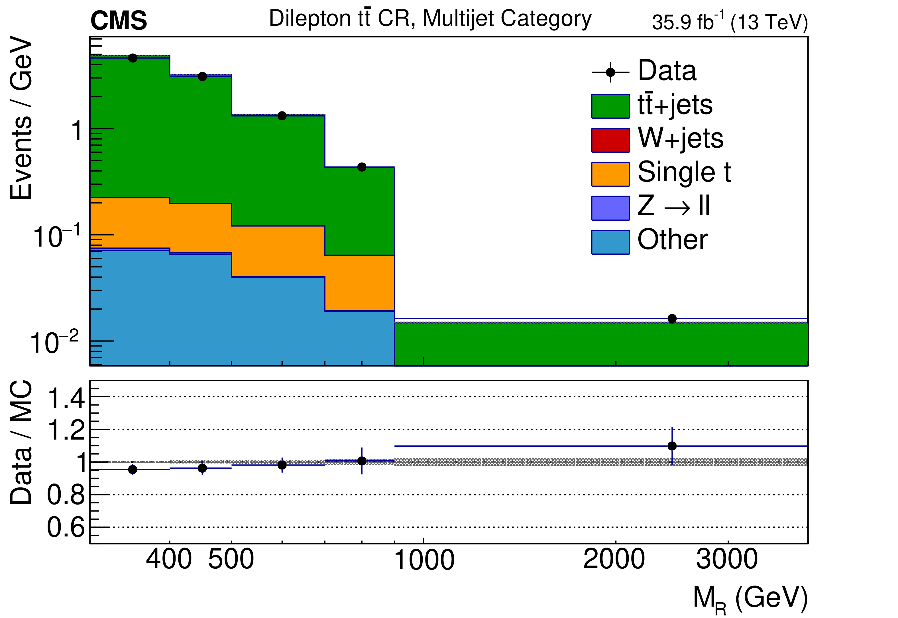
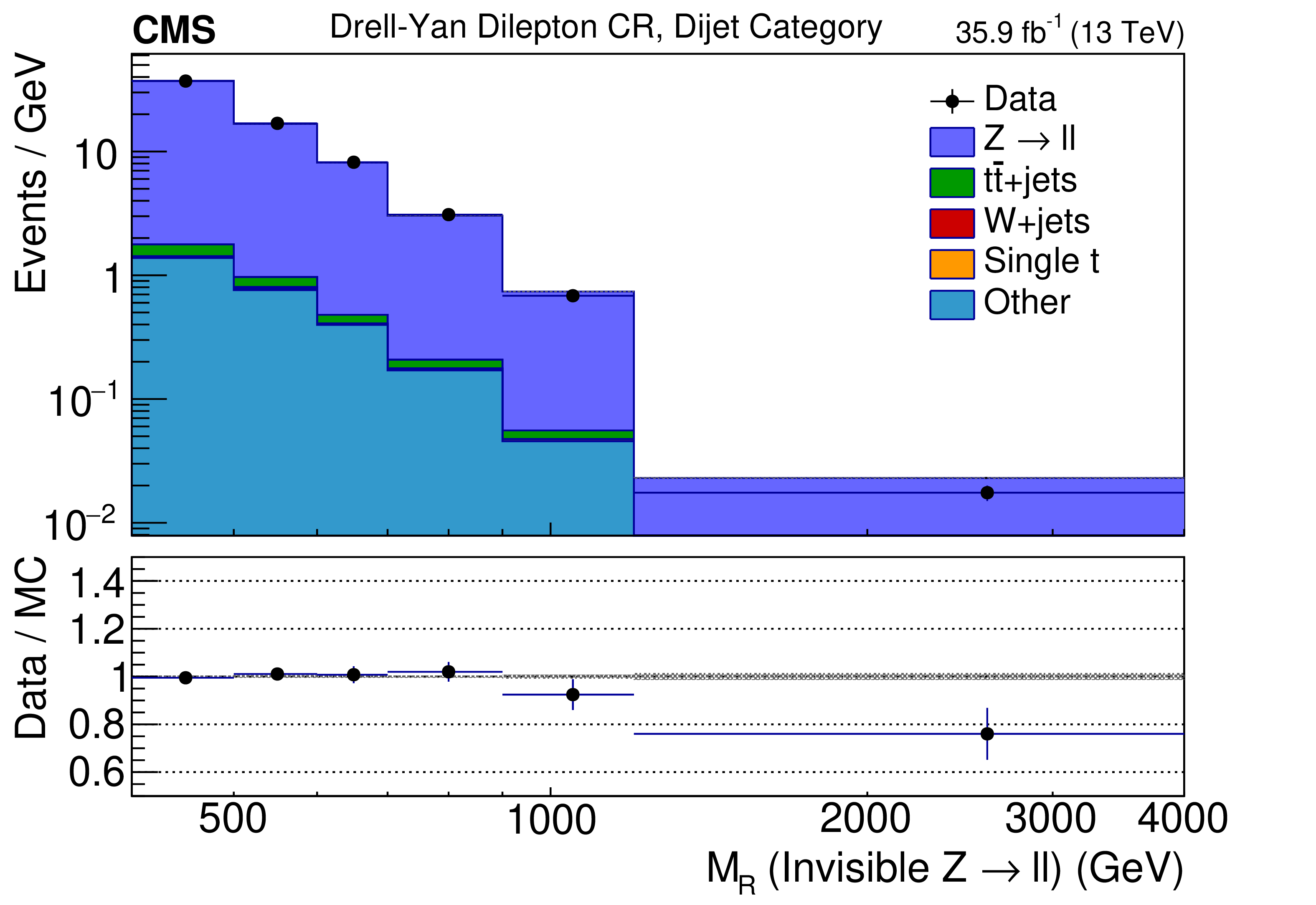
Figure 3:
The $ {M_\mathrm {R}} $ distribution in the $ {\mathrm {Z}}\to \ell \ell $+jets CR is displayed in the 2-3 (left) and 4-6 (right) jet categories along with the corresponding MC predictions. The corrections derived from the $ {\gamma}$+jets CR, as well as the overall normalization correction, have been applied in this figure. |
png pdf |
Figure 3-a:
The $ {M_\mathrm {R}} $ distribution in the $ {\mathrm {Z}}\to \ell \ell $+jets CR is displayed in the 2-3 jet category along with the corresponding MC predictions. The corrections derived from the $ {\gamma}$+jets CR, as well as the overall normalization correction, have been applied in this figure. |

png pdf |
Figure 3-b:
The $ {M_\mathrm {R}} $ distribution in the $ {\mathrm {Z}}\to \ell \ell $+jets CR is displayed in the 4-6 jet category along with the corresponding MC predictions. The corrections derived from the $ {\gamma}$+jets CR, as well as the overall normalization correction, have been applied in this figure. |

png pdf |
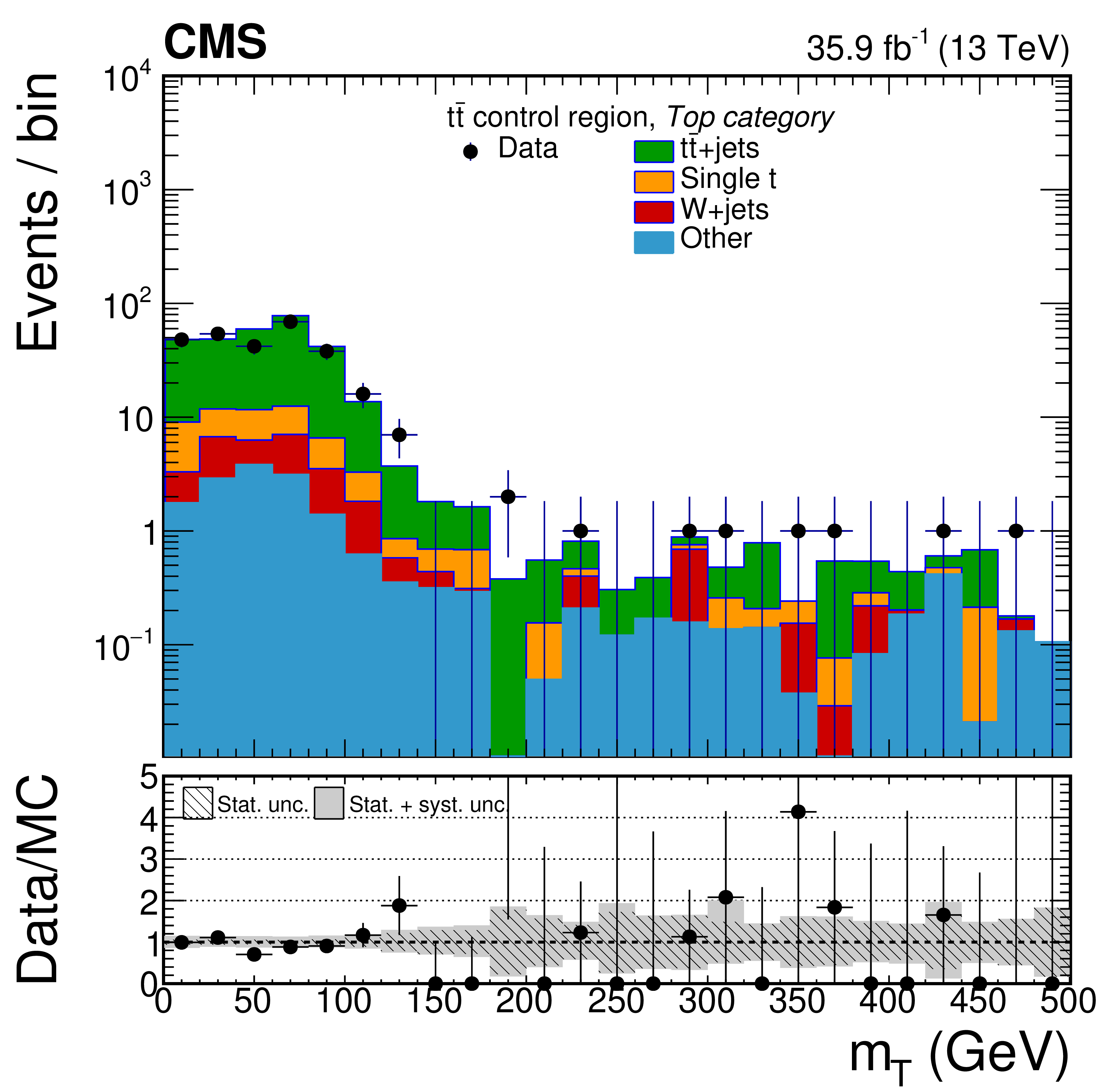
Figure 4:
The distribution of b-tagged jet multiplicity before applying the b tagging selection requirement in the $ {{\mathrm {t}\overline {\mathrm {t}}}} $ CR of the boosted W 6 jet category (left), and the distribution in $ {m_{\mathrm {T}}} $ before applying the $ {m_{\mathrm {T}}} $ selection requirement in the $ {{\mathrm {t}\overline {\mathrm {t}}}} $ CR of the boosted top category (right) are shown. The ratio of data over MC prediction is shown in the lower panels, where the gray band is the total uncertainty and the dashed band is the statistical uncertainty in the MC prediction. |

png pdf |
Figure 4-a:
The distribution of b-tagged jet multiplicity before applying the b tagging selection requirement in the $ {{\mathrm {t}\overline {\mathrm {t}}}} $ CR of the boosted W 6 jet category. The ratio of data over MC prediction is shown in the lower panels, where the gray band is the total uncertainty and the dashed band is the statistical uncertainty in the MC prediction. |
png pdf |
Figure 4-b:
The distribution in $ {m_{\mathrm {T}}} $ before applying the $ {m_{\mathrm {T}}} $ selection requirement in the $ {{\mathrm {t}\overline {\mathrm {t}}}} $ CR of the boosted top category. The ratio of data over MC prediction is shown in the lower panels, where the gray band is the total uncertainty and the dashed band is the statistical uncertainty in the MC prediction. |

png pdf |
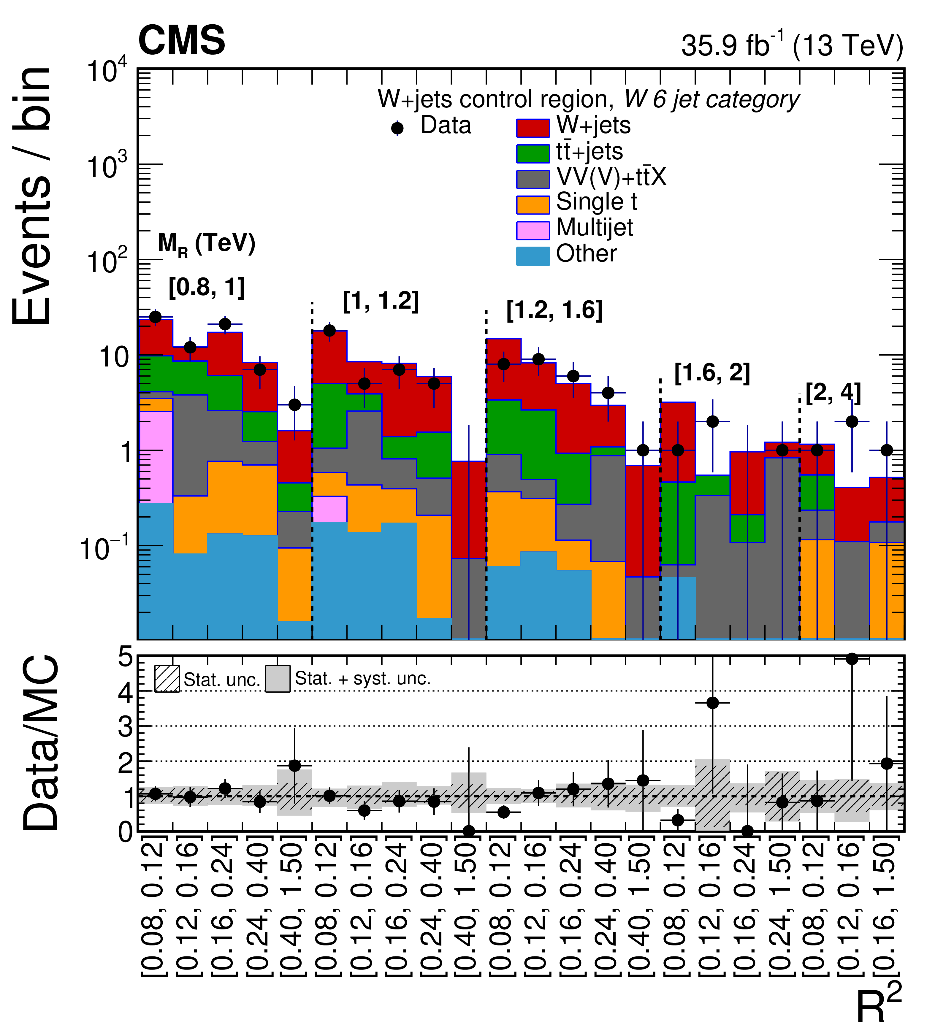
Figure 5:
$ {M_\mathrm {R}} $-$ {\mathrm {R}^2} $ distributions in the W+jets CRs of the boosted W 4-5 jet (upper left) and boosted W 6 jet (upper right) categories, and the $ {{\mathrm {t}\overline {\mathrm {t}}}} $ CR (lower) of the boosted top category. The ratio of data over MC prediction is shown in the lower panels, where the gray band is the total uncertainty and the dashed band is the statistical uncertainty in the MC prediction. |

png pdf |
Figure 5-a:
$ {M_\mathrm {R}} $-$ {\mathrm {R}^2} $ distribution in the boosted W 4-5 jet CR category. The ratio of data over MC prediction is shown in the lower panel, where the gray band is the total uncertainty and the dashed band is the statistical uncertainty in the MC prediction. |
png pdf |
Figure 5-b:
$ {M_\mathrm {R}} $-$ {\mathrm {R}^2} $ distribution in the boosted W 6 jet CR category. The ratio of data over MC prediction is shown in the lower panel, where the gray band is the total uncertainty and the dashed band is the statistical uncertainty in the MC prediction. |

png pdf |
Figure 5-c:
$ {M_\mathrm {R}} $-$ {\mathrm {R}^2} $ distribution in the $ {{\mathrm {t}\overline {\mathrm {t}}}} $ CR of the boosted top category. The ratio of data over MC prediction is shown in the lower panel, where the gray band is the total uncertainty and the dashed band is the statistical uncertainty in the MC prediction. |

png pdf |
Figure 6:
$ {M_\mathrm {R}} $-$ {\mathrm {R}^2} $ distributions for the $ {\gamma}$+jets CR of the boosted W 4-5 jet (left) and boosted top (right) category. The ratio of data over MC prediction is shown in the lower panel, where the gray band is the total uncertainty and the dashed band is the statistical uncertainty in the MC prediction. |

png pdf |
Figure 6-a:
$ {M_\mathrm {R}} $-$ {\mathrm {R}^2} $ distributions for the $ {\gamma}$+jets CR of the boosted W 4-5 jet category. The ratio of data over MC prediction is shown in the lower panel, where the gray band is the total uncertainty and the dashed band is the statistical uncertainty in the MC prediction. |

png pdf |
Figure 6-b:
$ {M_\mathrm {R}} $-$ {\mathrm {R}^2} $ distributions for the $ {\gamma}$+jets CR of the boosted top category. The ratio of data over MC prediction is shown in the lower panel, where the gray band is the total uncertainty and the dashed band is the statistical uncertainty in the MC prediction. |

png pdf |
Figure 7:
Comparison of the estimate of the $\mathrm{Z}(\to \nu \nu)$+jets background contribution in the SR extrapolated from the $ {\gamma}$+jets CR with the estimate extrapolated from the $\mathrm{W}(\to \ell \nu)$+jets CR for the boosted W 4-5 jet (upper left), boosted W 6 jet (upper right) and boosted top (lower) categories in bins of $ {M_\mathrm {R}} $ and $ {\mathrm {R}^2} $. The prediction from the uncorrected MC simulation is also shown. The black labels indicate the range in $ {M_\mathrm {R}} $ that each set of bins correspond to. |

png pdf |
Figure 7-a:
Comparison of the estimate of the $\mathrm{Z}(\to \nu \nu)$+jets background contribution in the SR extrapolated from the $ {\gamma}$+jets CR with the estimate extrapolated from the $\mathrm{W}(\to \ell \nu)$+jets CR for the boosted W 4-5 jet category in bins of $ {M_\mathrm {R}} $ and $ {\mathrm {R}^2} $. The prediction from the uncorrected MC simulation is also shown. The black labels indicate the range in $ {M_\mathrm {R}} $ that each set of bins correspond to. |

png pdf |
Figure 7-b:
Comparison of the estimate of the $\mathrm{Z}(\to \nu \nu)$+jets background contribution in the SR extrapolated from the $ {\gamma}$+jets CR with the estimate extrapolated from the $\mathrm{W}(\to \ell \nu)$+jets CR for the boosted W 6 jet category in bins of $ {M_\mathrm {R}} $ and $ {\mathrm {R}^2} $. The prediction from the uncorrected MC simulation is also shown. The black labels indicate the range in $ {M_\mathrm {R}} $ that each set of bins correspond to. |

png pdf |
Figure 7-c:
Comparison of the estimate of the $\mathrm{Z}(\to \nu \nu)$+jets background contribution in the SR extrapolated from the $ {\gamma}$+jets CR with the estimate extrapolated from the $\mathrm{W}(\to \ell \nu)$+jets CR for the boosted top category in bins of $ {M_\mathrm {R}} $ and $ {\mathrm {R}^2} $. The prediction from the uncorrected MC simulation is also shown. The black labels indicate the range in $ {M_\mathrm {R}} $ that each set of bins correspond to. |
png pdf |
Figure 8:
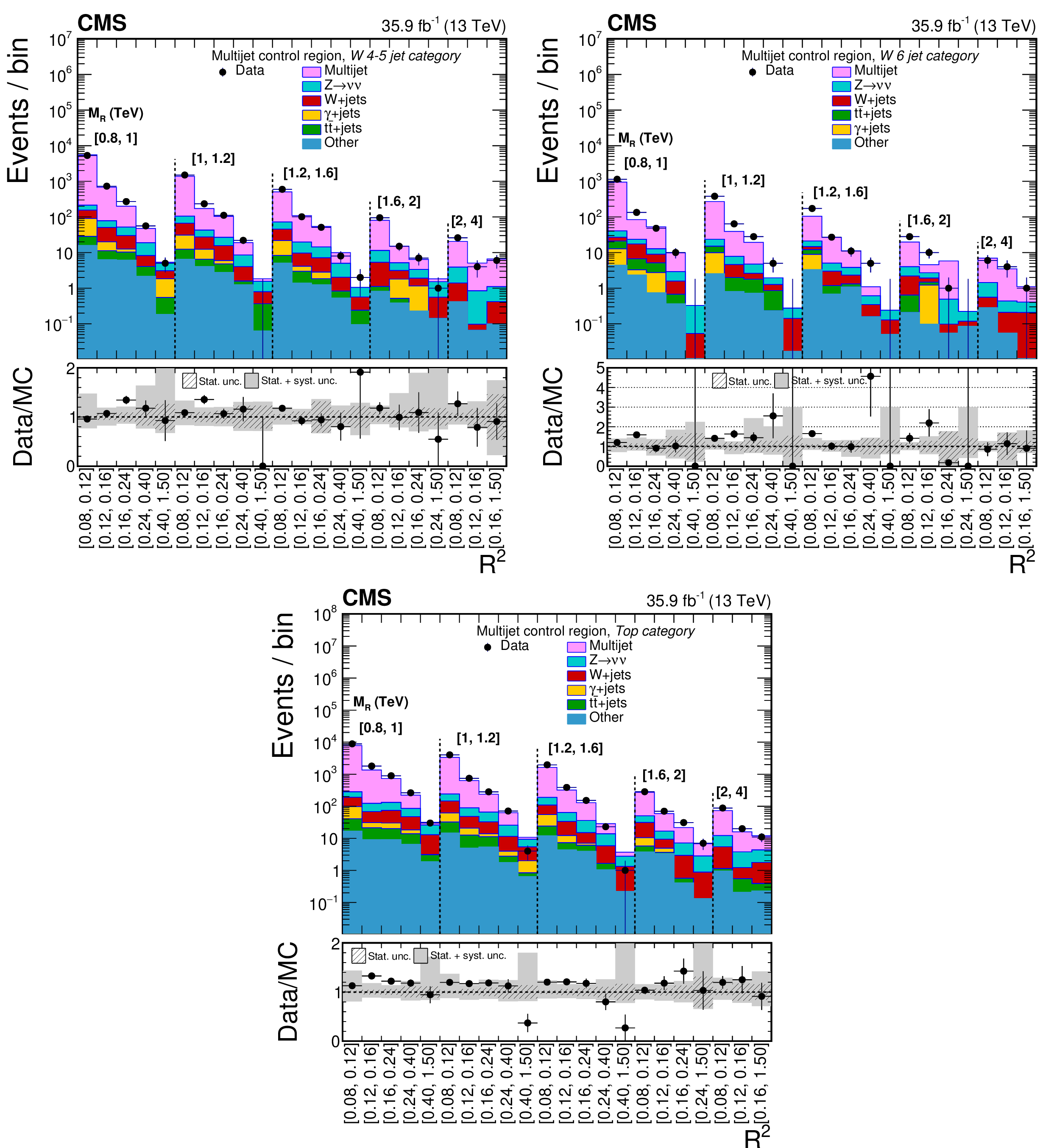
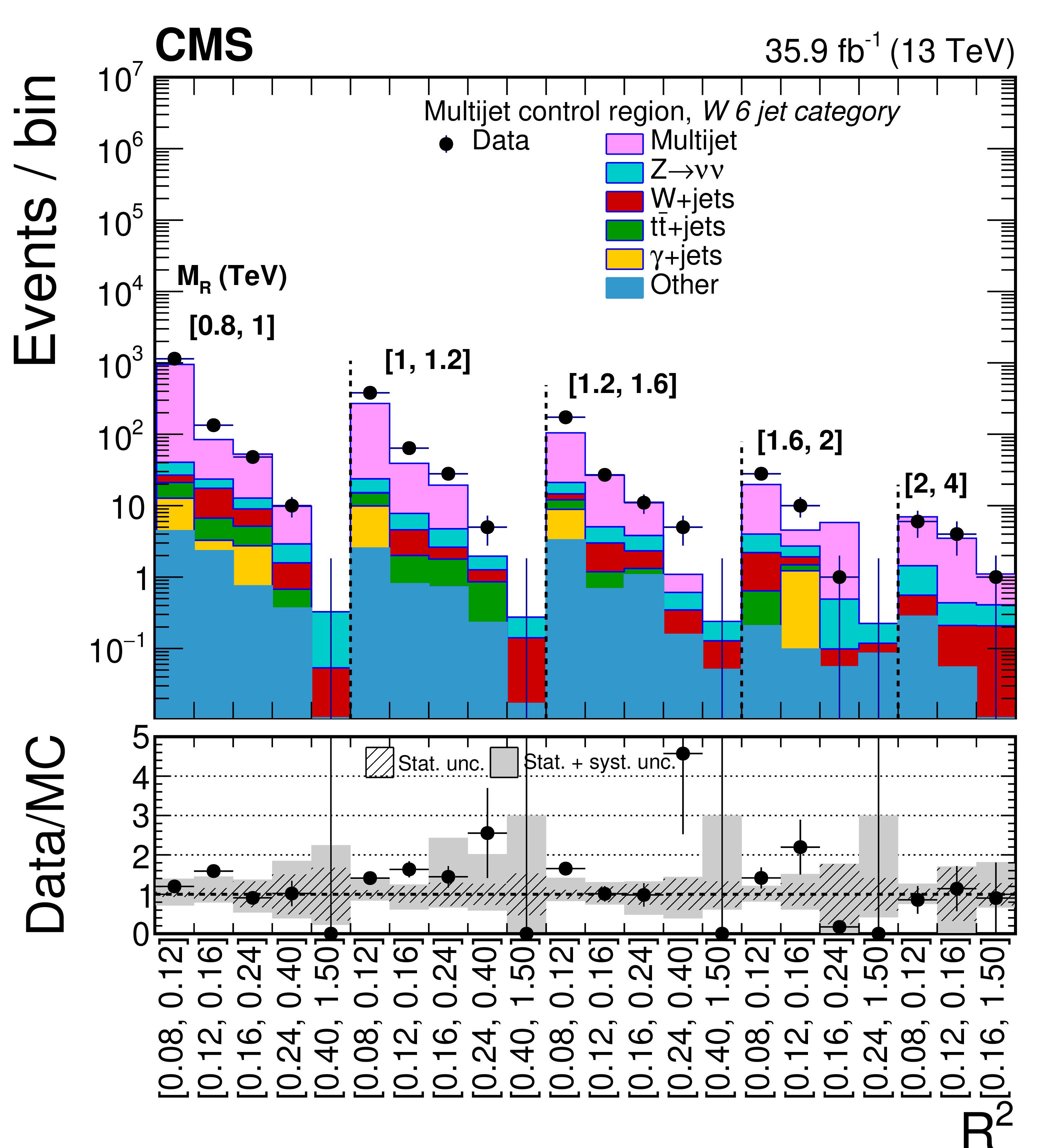
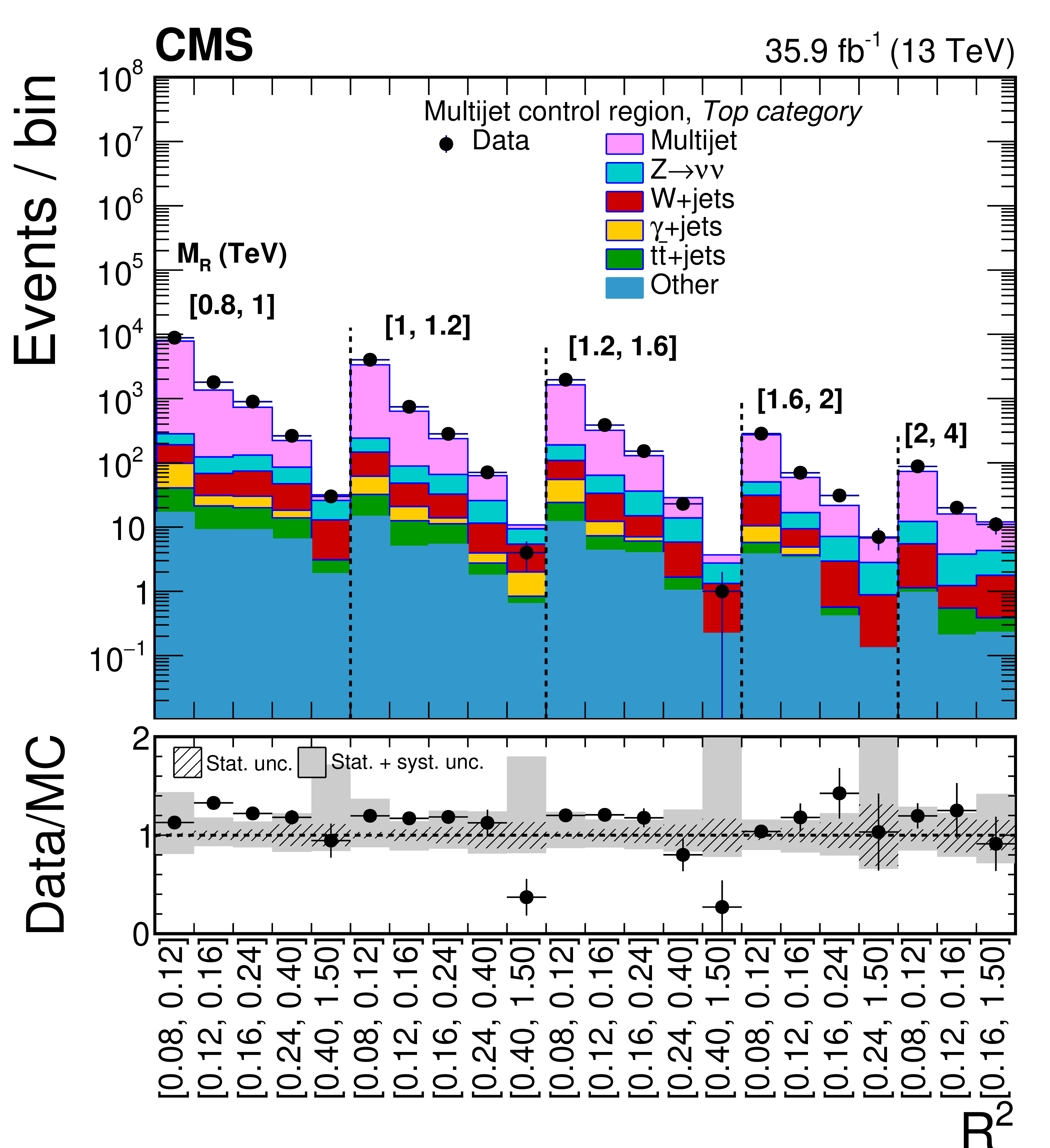
The $ {M_\mathrm {R}} $-$ {\mathrm {R}^2} $ distributions in the QCD multijet CRs of the boosted W 4-5 jet (upper left), boosted W 6 jet (upper right), and boosted top (lower) categories. The ratios of data over MC prediction is shown in the lower panels, where the gray band is the total uncertainty and the dashed band is the statistical uncertainty in the MC prediction. |

png pdf |
Figure 8-a:
The $ {M_\mathrm {R}} $-$ {\mathrm {R}^2} $ distributions in the QCD multijet CRs of the boosted W 4-5 jet category. The ratios of data over MC prediction is shown in the lower panel, where the gray band is the total uncertainty and the dashed band is the statistical uncertainty in the MC prediction. |
png pdf |
Figure 8-b:
The $ {M_\mathrm {R}} $-$ {\mathrm {R}^2} $ distributions in the QCD multijet CRs of the boosted W 6 jet category. The ratios of data over MC prediction is shown in the lower panel, where the gray band is the total uncertainty and the dashed band is the statistical uncertainty in the MC prediction. |
png pdf |
Figure 8-c:
The $ {M_\mathrm {R}} $-$ {\mathrm {R}^2} $ distributions in the QCD multijet CRs of the boosted top category. The ratios of data over MC prediction is shown in the lower panel, where the gray band is the total uncertainty and the dashed band is the statistical uncertainty in the MC prediction. |

png pdf |
Figure 9:
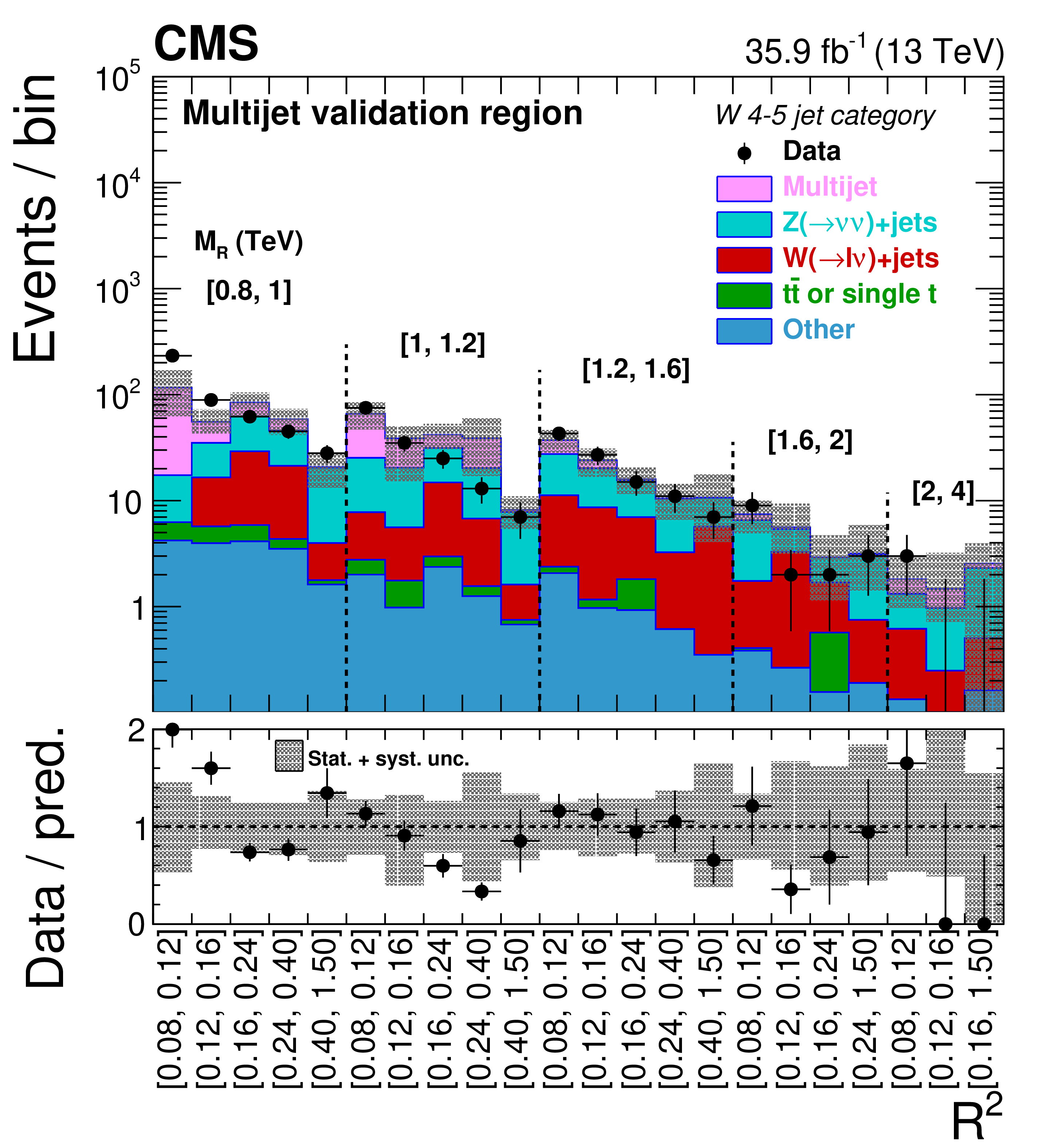
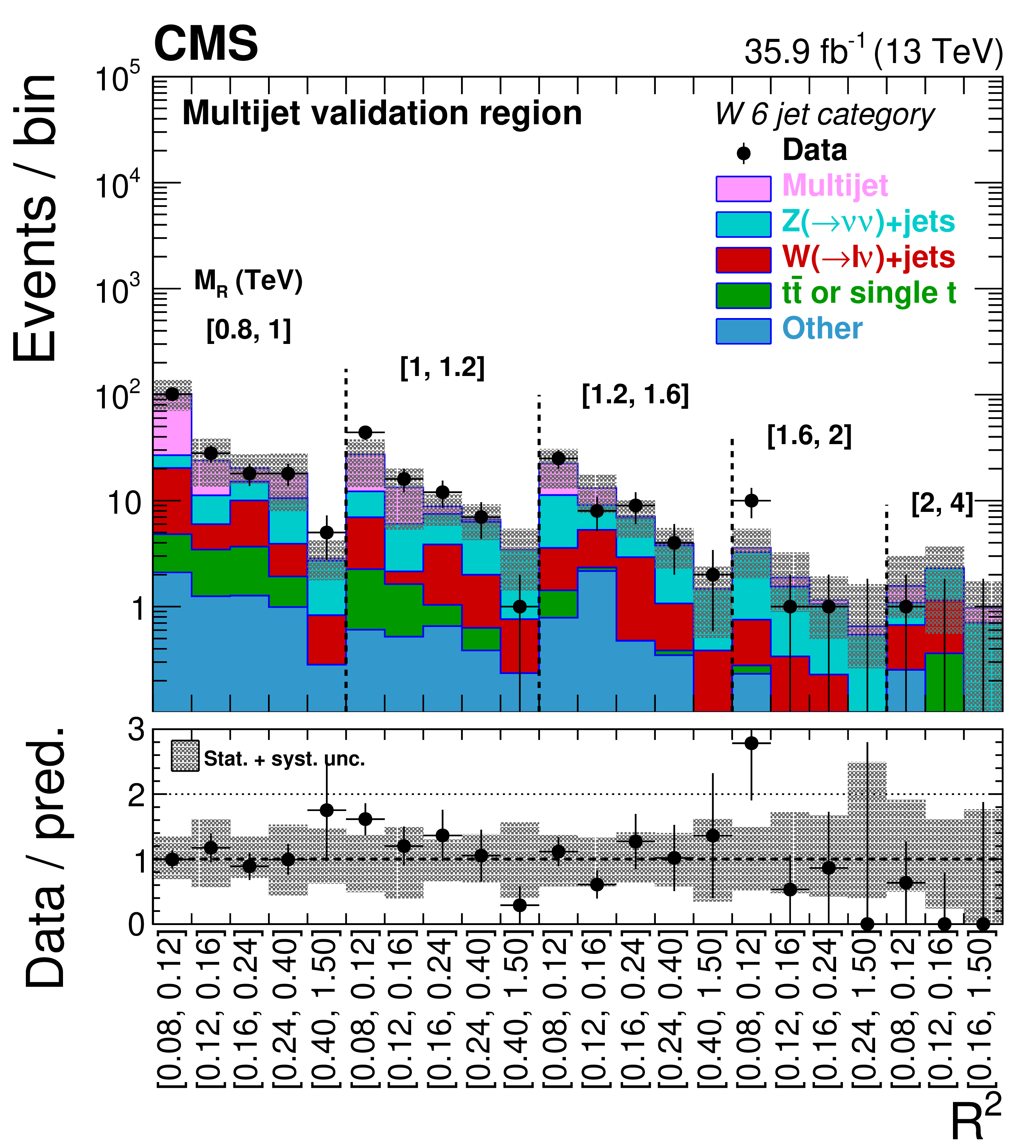
Comparisons between data and the predicted background for the inverted $ {\Delta \phi _\mathrm {R}} $ validation region for the boosted W 4-5 jet (upper left), boosted W 6 jet (upper right), and boosted top (lower) categories. |

png pdf |
Figure 9-a:
Comparisons between data and the predicted background for the inverted $ {\Delta \phi _\mathrm {R}} $ validation region for the boosted W 4-5 jet category. |

png pdf |
Figure 9-b:
Comparisons between data and the predicted background for the inverted $ {\Delta \phi _\mathrm {R}} $ validation region for the boosted W 6 jet category. |

png pdf |
Figure 9-c:
Comparisons between data and the predicted background for the inverted $ {\Delta \phi _\mathrm {R}} $ validation region for the boosted top category. |

png pdf |
Figure 10:
Comparisons between data and the predicted background for the validation region with antitagged W boson or top quark candidates for the boosted W 4-5 jet (upper left), boosted W 6 jet (upper right), and boosted top (lower) categories. |
png pdf |
Figure 10-a:
Comparisons between data and the predicted background for the validation region with antitagged W boson or top quark candidates for the boosted W 4-5 jet category. |
png pdf |
Figure 10-b:
Comparisons between data and the predicted background for the validation region with antitagged W boson or top quark candidates for the boosted W 6 jet category. |

png pdf |
Figure 10-c:
Comparisons between data and the predicted background for the validation region with antitagged W boson or top quark candidates for the boosted top category. |

png pdf |
Figure 11:
The $ {M_\mathrm {R}} $-$ {\mathrm {R}^2} $ distribution observed in data is shown along with the background prediction obtained for the Lepton Multijet event category in the 0 b tag (upper) and 1 b tag (lower) bins. The two-dimensional $ {M_\mathrm {R}} $-$ {\mathrm {R}^2} $ distribution is shown in a one-dimensional representation, with each $ {M_\mathrm {R}} $ bin denoted by the dashed lines and labeled above, and each $ {\mathrm {R}^2} $ bin labeled below. The background labeled as "Other'' includes single top quark production, diboson production, associated production of a top quark pair and a W or Z boson, and triboson production. The ratio of data to the background prediction is shown on the bottom panel, with the statistical uncertainty expressed through the data point error bars and the systematic uncertainty in the background prediction represented by the shaded region. Signal benchmarks shown are T5ttcc with $m_{{\mathrm {\tilde{g}}}} = $ 1.4 TeV, $m_{{\tilde{\mathrm {t}}}} = $ 320 GeV and $m_{{\tilde{\chi}^{0}_{1}}} = $ 300 GeV; T1tttt with $m_{{\mathrm {\tilde{g}}}} = $ 1.4 TeV and $m_{{\tilde{\chi}^{0}_{1}}} = $ 300 GeV; and T2tt with $m_{{\tilde{\mathrm {t}}}} = $ 850 GeV and $m_{{\tilde{\chi}^{0}_{1}}} = $ 100 GeV. The diagrams corresponding to these signal models are shown in Fig. 1. |

png pdf |
Figure 11-a:
The $ {M_\mathrm {R}} $-$ {\mathrm {R}^2} $ distribution observed in data is shown along with the background prediction obtained for the Lepton Multijet event category in the 0 b tag bin. The two-dimensional $ {M_\mathrm {R}} $-$ {\mathrm {R}^2} $ distribution is shown in a one-dimensional representation, with each $ {M_\mathrm {R}} $ bin denoted by the dashed lines and labeled above, and each $ {\mathrm {R}^2} $ bin labeled below. The background labeled as "Other'' includes single top quark production, diboson production, associated production of a top quark pair and a W or Z boson, and triboson production. The ratio of data to the background prediction is shown on the bottom panel, with the statistical uncertainty expressed through the data point error bars and the systematic uncertainty in the background prediction represented by the shaded region. Signal benchmarks shown are T5ttcc with $m_{{\mathrm {\tilde{g}}}} = $ 1.4 TeV, $m_{{\tilde{\mathrm {t}}}} = $ 320 GeV and $m_{{\tilde{\chi}^{0}_{1}}} = $ 300 GeV; T1tttt with $m_{{\mathrm {\tilde{g}}}} = $ 1.4 TeV and $m_{{\tilde{\chi}^{0}_{1}}} = $ 300 GeV; and T2tt with $m_{{\tilde{\mathrm {t}}}} = $ 850 GeV and $m_{{\tilde{\chi}^{0}_{1}}} = $ 100 GeV. The diagrams corresponding to these signal models are shown in Fig. 1. |

png pdf |
Figure 11-b:
The $ {M_\mathrm {R}} $-$ {\mathrm {R}^2} $ distribution observed in data is shown along with the background prediction obtained for the Lepton Multijet event category in the 1 b tag bin. The two-dimensional $ {M_\mathrm {R}} $-$ {\mathrm {R}^2} $ distribution is shown in a one-dimensional representation, with each $ {M_\mathrm {R}} $ bin denoted by the dashed lines and labeled above, and each $ {\mathrm {R}^2} $ bin labeled below. The background labeled as "Other'' includes single top quark production, diboson production, associated production of a top quark pair and a W or Z boson, and triboson production. The ratio of data to the background prediction is shown on the bottom panel, with the statistical uncertainty expressed through the data point error bars and the systematic uncertainty in the background prediction represented by the shaded region. Signal benchmarks shown are T5ttcc with $m_{{\mathrm {\tilde{g}}}} = $ 1.4 TeV, $m_{{\tilde{\mathrm {t}}}} = $ 320 GeV and $m_{{\tilde{\chi}^{0}_{1}}} = $ 300 GeV; T1tttt with $m_{{\mathrm {\tilde{g}}}} = $ 1.4 TeV and $m_{{\tilde{\chi}^{0}_{1}}} = $ 300 GeV; and T2tt with $m_{{\tilde{\mathrm {t}}}} = $ 850 GeV and $m_{{\tilde{\chi}^{0}_{1}}} = $ 100 GeV. The diagrams corresponding to these signal models are shown in Fig. 1. |

png pdf |
Figure 12:
The $ {M_\mathrm {R}} $-$ {\mathrm {R}^2} $ distribution observed in data is shown along with the background prediction obtained for the Lepton Multijet event category in the 2 b tag (upper) and 3 or more b tag (lower) bins. Further details of the plots are explained in the caption of Fig. 11. |

png pdf |
Figure 12-a:
The $ {M_\mathrm {R}} $-$ {\mathrm {R}^2} $ distribution observed in data is shown along with the background prediction obtained for the Lepton Multijet event category in the 2 b tag bin. Further details of the plot are explained in the caption of Fig. 11. |

png pdf |
Figure 12-b:
The $ {M_\mathrm {R}} $-$ {\mathrm {R}^2} $ distribution observed in data is shown along with the background prediction obtained for the Lepton Multijet event category in the 3 or more b tag bin. Further details of the plot are explained in the caption of Fig. 11. |

png pdf |
Figure 13:
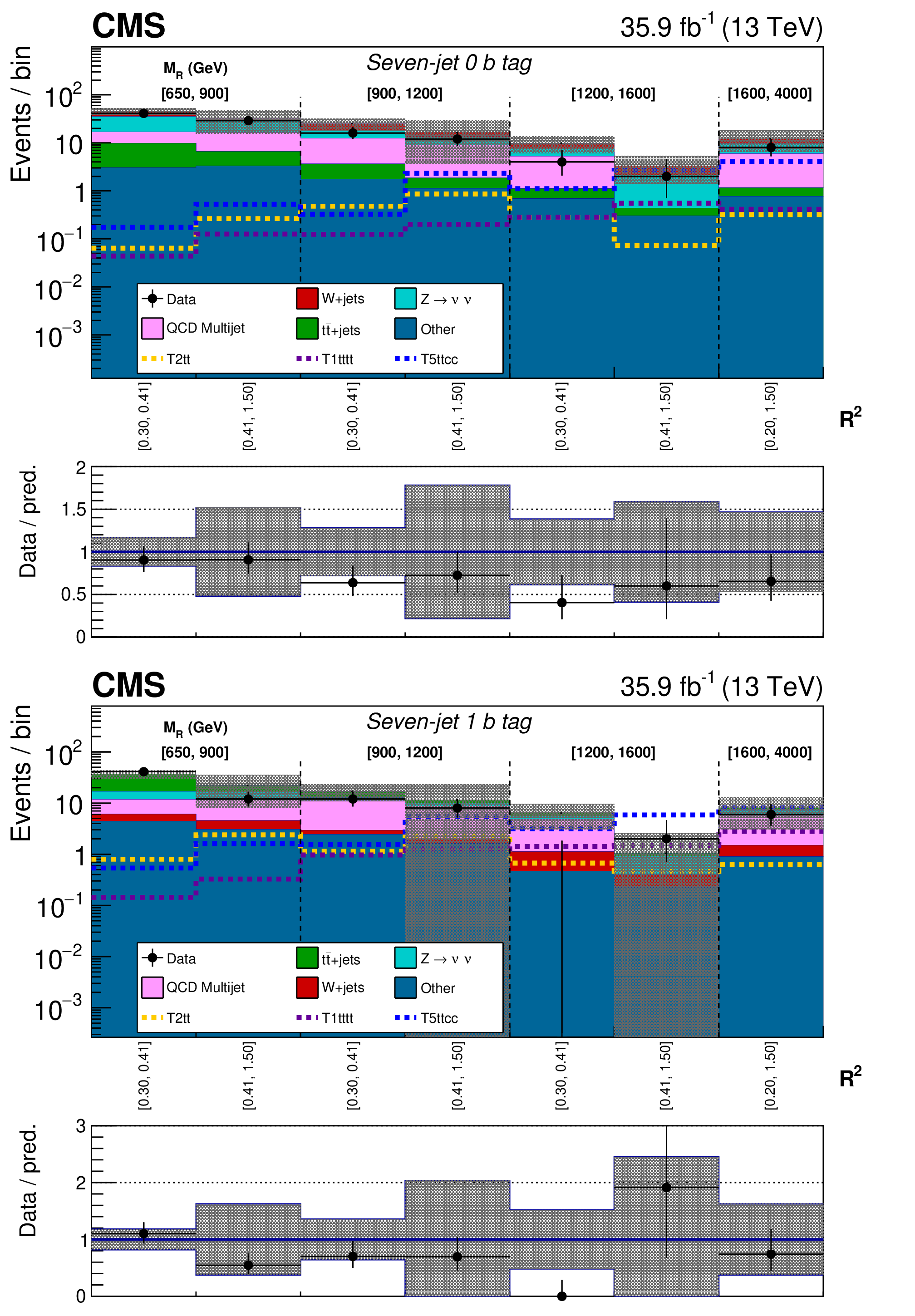
The $ {M_\mathrm {R}} $-$ {\mathrm {R}^2} $ distribution observed in data is shown along with the background prediction obtained for the Lepton Seven-jet event category in the 0 b tag (upper) and 1 b tag (lower) bins. Further details of the plots are explained in the caption of Fig. 11. |

png pdf |
Figure 13-a:
The $ {M_\mathrm {R}} $-$ {\mathrm {R}^2} $ distribution observed in data is shown along with the background prediction obtained for the Lepton Seven-jet event category in the 0 b tag bin. Further details of the plot are explained in the caption of Fig. 11. |

png pdf |
Figure 13-b:
The $ {M_\mathrm {R}} $-$ {\mathrm {R}^2} $ distribution observed in data is shown along with the background prediction obtained for the Lepton Seven-jet event category in the 1 b tag bin. Further details of the plot are explained in the caption of Fig. 11. |

png pdf |
Figure 14:
The $ {M_\mathrm {R}} $-$ {\mathrm {R}^2} $ distribution observed in data is shown along with the background prediction obtained for the Lepton Seven-jet event category in the 2 b tag (upper) and 3 or more b tag (lower) bins. Further details of the plots are explained in the caption of Fig. 11. |

png pdf |
Figure 14-a:
The $ {M_\mathrm {R}} $-$ {\mathrm {R}^2} $ distribution observed in data is shown along with the background prediction obtained for the Lepton Seven-jet event category in the 2 b tag bin. Further details of the plot are explained in the caption of Fig. 11. |

png pdf |
Figure 14-b:
The $ {M_\mathrm {R}} $-$ {\mathrm {R}^2} $ distribution observed in data is shown along with the background prediction obtained for the Lepton Seven-jet event category in the 3 or more b tag bin. Further details of the plot are explained in the caption of Fig. 11. |

png pdf |
Figure 15:
The $ {M_\mathrm {R}} $-$ {\mathrm {R}^2} $ distribution observed in data is shown along with the background prediction obtained for the boosted W 4-5 jet (upper left), boosted W 6 jet (upper right), and Top (lower) categories. Further details of the plots are explained in the caption of Fig. 11. |

png pdf |
Figure 15-a:
The $ {M_\mathrm {R}} $-$ {\mathrm {R}^2} $ distribution observed in data is shown along with the background prediction obtained for the boosted W 4-5 jet category. Further details of the plot are explained in the caption of Fig. 11. |

png pdf |
Figure 15-b:
The $ {M_\mathrm {R}} $-$ {\mathrm {R}^2} $ distribution observed in data is shown along with the background prediction obtained for the boosted W 6 jet category. Further details of the plot are explained in the caption of Fig. 11. |

png pdf |
Figure 15-c:
The $ {M_\mathrm {R}} $-$ {\mathrm {R}^2} $ distribution observed in data is shown along with the background prediction obtained for the boosted Top category. Further details of the plot are explained in the caption of Fig. 11. |

png pdf |
Figure 16:
The $ {M_\mathrm {R}} $-$ {\mathrm {R}^2} $ distribution observed in data is shown along with the background prediction obtained for the Dijet event category in the 0 b tag (upper) and 1 b tag (lower) bins. Further details of the plots are explained in the caption of Fig. 11. |

png pdf |
Figure 16-a:
The $ {M_\mathrm {R}} $-$ {\mathrm {R}^2} $ distribution observed in data is shown along with the background prediction obtained for the Dijet event category in the 0 b tag bin. Further details of the plot are explained in the caption of Fig. 11. |

png pdf |
Figure 16-b:
The $ {M_\mathrm {R}} $-$ {\mathrm {R}^2} $ distribution observed in data is shown along with the background prediction obtained for the Dijet event category in the 1 b tag bin. Further details of the plot are explained in the caption of Fig. 11. |

png pdf |
Figure 17:
The $ {M_\mathrm {R}} $-$ {\mathrm {R}^2} $ distribution observed in data is shown along with the background prediction obtained for the Dijet event category in the 2 or more b tag bin. Further details of the plots are explained in the caption of Fig. 11. |

png pdf |
Figure 18:
The $ {M_\mathrm {R}} $-$ {\mathrm {R}^2} $ distribution observed in data is shown along with the background prediction obtained for the Multijet event category in the 0 b tag (upper) and 1 b tag (lower) bins. Further details of the plots are explained in the caption of Fig. 11. |

png pdf |
Figure 18-a:
The $ {M_\mathrm {R}} $-$ {\mathrm {R}^2} $ distribution observed in data is shown along with the background prediction obtained for the Multijet event category in the 0 b tag bin. Further details of the plot are explained in the caption of Fig. 11. |

png pdf |
Figure 18-b:
The $ {M_\mathrm {R}} $-$ {\mathrm {R}^2} $ distribution observed in data is shown along with the background prediction obtained for the Multijet event category in the 1 b tag bin. Further details of the plot are explained in the caption of Fig. 11. |

png pdf |
Figure 19:
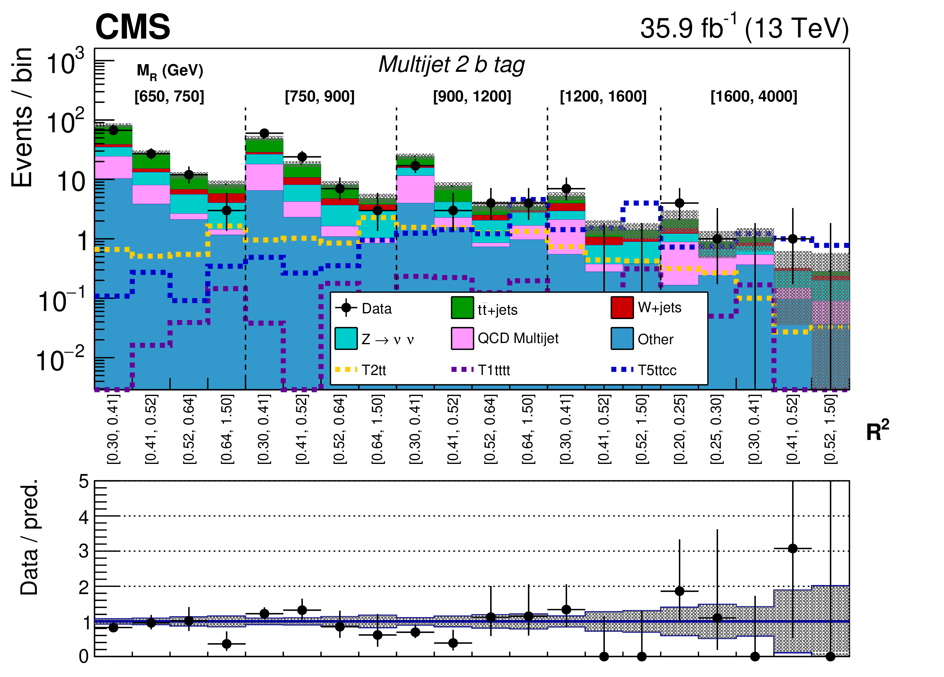
The $ {M_\mathrm {R}} $-$ {\mathrm {R}^2} $ distribution observed in data is shown along with the background prediction obtained for the Multijet event category in the 2 b tag (upper) and 3 or more b tag (lower) bins. Further details of the plots are explained in the caption of Fig. 11. |
png pdf |
Figure 19-a:
The $ {M_\mathrm {R}} $-$ {\mathrm {R}^2} $ distribution observed in data is shown along with the background prediction obtained for the Multijet event category in the 2 b tag bin. Further details of the plot are explained in the caption of Fig. 11. |

png pdf |
Figure 19-b:
The $ {M_\mathrm {R}} $-$ {\mathrm {R}^2} $ distribution observed in data is shown along with the background prediction obtained for the Multijet event category in the 3 or more b tag bin. Further details of the plot are explained in the caption of Fig. 11. |
png pdf |
Figure 20:
The $ {M_\mathrm {R}} $-$ {\mathrm {R}^2} $ distribution observed in data is shown along with the background prediction obtained for the Seven-jet event category in the 0 b tag (upper) and 1 b tag (lower) bins. Further details of the plots are explained in the caption of Fig. 11. |

png pdf |
Figure 20-a:
The $ {M_\mathrm {R}} $-$ {\mathrm {R}^2} $ distribution observed in data is shown along with the background prediction obtained for the Seven-jet event category in the 0 b tag bin. Further details of the plot are explained in the caption of Fig. 11. |

png pdf |
Figure 20-b:
The $ {M_\mathrm {R}} $-$ {\mathrm {R}^2} $ distribution observed in data is shown along with the background prediction obtained for the Seven-jet event category in the 1 b tag bin. Further details of the plot are explained in the caption of Fig. 11. |

png pdf |
Figure 21:
The $ {M_\mathrm {R}} $-$ {\mathrm {R}^2} $ distribution observed in data is shown along with the background prediction obtained for the Seven-jet event category in the 2 b tag (upper) and 3 or more b tag (lower) bins. Further details of the plots are explained in the caption of Fig. 11. |

png pdf |
Figure 21-a:
The $ {M_\mathrm {R}} $-$ {\mathrm {R}^2} $ distribution observed in data is shown along with the background prediction obtained for the Seven-jet event category in the 2 b tag bin. Further details of the plot are explained in the caption of Fig. 11. |

png pdf |
Figure 21-b:
The $ {M_\mathrm {R}} $-$ {\mathrm {R}^2} $ distribution observed in data is shown along with the background prediction obtained for the Seven-jet event category in the 3 or more b tag bin. Further details of the plot are explained in the caption of Fig. 11. |

png pdf |
Figure 22:
Expected and observed 95% CL limits on the production cross section for pair-produced gluinos each decaying to the LSP and top quarks. The blue dashed contour represents the expected 95% CL upper limit using data in the nonboosted categories only. |

png pdf |
Figure 23:
Expected and observed 95% CL limits on the production cross section for pair-produced gluinos each decaying to a top quark and a low mass top squark that subsequently decays to a charm quark and the LSP. The mass splitting ($m_{{\tilde{\mathrm {t}}}}-m_{{\tilde{\chi}^{0}} _1}$) is fixed to be $20 GeV $. The blue dashed contour represents the expected 95% CL upper limit using data in the nonboosted categories only. |

png pdf |
Figure 24:
Expected and observed 95% CL limits on the production cross section for pair-produced squarks each decaying to a top quark and the LSP. The blue dashed contour represents the expected 95% CL upper limit using data in the nonboosted categories only. The white diagonal band corresponds to the region $ {{^\circ}limiter 69640972 m_{{\tilde{\mathrm {t}}}}-m_{{\mathrm {t}}}-m_{{\tilde{\chi}^{0}} _1} {^\circ}limiter 86418188} < $ 25 GeV, where the mass difference between the $ {\tilde{\mathrm {t}}} $ and the $ {\tilde{\chi}^{0}} _1$ is very close to the top quark mass. In this region the signal acceptance depends strongly on the $ {\tilde{\chi}^{0}} _1$ mass and is therefore difficult to model. |
| Tables | |

png pdf |
Table 1:
Summary of the search categories, their charged lepton and jet count requirements, and the b tag bins that define the subcategories. Events passing the "Lepton veto'' requirement must have no electron or muon passing the veto selection, and no $ {{\tau} _\mathrm {h}} $ candidate. |

png pdf |
Table 2:
The baseline requirements on the razor variables $ {M_\mathrm {R}} $ and $ {\mathrm {R}^2} $, additional requirements on $ {m_{\mathrm {T}}} $ and $ {\Delta \phi _\mathrm {R}} $, and the trigger requirements are shown for each event category. |

png pdf |
Table 3:
Summary of the main instrumental and theoretical systematic uncertainties. |

png pdf |
Table 4:
Summary of systematic uncertainties from the background estimation methodology expressed as relative or fractional uncertainties. |
| Summary |
|
We have presented an inclusive search for supersymmetry (SUSY) in events with no more than one lepton, a large multiplicity of energetic jets, and evidence of invisible particles using the razor kinematic variables. To enhance sensitivity to a broad range of signal models, the events are categorized according to the number of leptons, the presence of jets consistent with hadronically decaying W bosons or top quarks, and the number of jets and b-tagged jets. The analysis uses $\sqrt{s} = $ 13 TeV proton-proton collision data collected by the CMS experiment in 2016 and corresponding to an integrated luminosity of 35.9 fb$^{-1}$ . Standard model backgrounds were estimated using control regions in data and Monte Carlo simulation yields in signal and control regions. Background estimation procedures were verified using validation regions with kinematics resembling that of the signal regions and closure tests. Data are observed to be consistent with the standard model expectation. The results were interpreted in the context of simplified models of pair-produced gluinos and direct top squark pair production. Limits on the gluino mass extend to 2.0 TeV, while limits on top squark masses reach 1.14 TeV. The combination of a large variety of final states enables this analysis to improve the sensitivity in various signal scenarios. The analysis extended the exclusion limit of the gluino mass from the CMS experiment by ${\approx}$100 GeV in decays to a low-mass top squark and a top quark, and the exclusion limit of the top squark mass by ${\approx}$20 GeV in direct top squark pair production. |
| References | ||||
| 1 | C. Rogan | Kinematical variables towards new dynamics at the LHC | 1006.2727 | |
| 2 | CMS Collaboration | Inclusive search for supersymmetry using razor variables in pp collisions at $ \sqrt s= $ 13 TeV | PRD 95 (2017) 012003 | CMS-SUS-15-004 1609.07658 |
| 3 | CMS Collaboration | Search for supersymmetry in pp collisions at $ \sqrt{s} = $ 8 TeV in final states with boosted W bosons and b jets using razor variables | PRD 93 (2016) 092009 | CMS-SUS-14-007 1602.02917 |
| 4 | J. Wess and B. Zumino | Supergauge transformations in four dimensions | NPB 70 (1974) 39 | |
| 5 | Y. A. Gol'fand and E. P. Likhtman | Extension of the algebra of Poincar$ \'e $ group generators and violation of P invariance | JEPTL 13 (1971) 323 | |
| 6 | D. V. Volkov and V. P. Akulov | Possible universal neutrino interaction | JEPTL 16 (1972) 438 | |
| 7 | A. H. Chamseddine, R. L. Arnowitt, and P. Nath | Locally supersymmetric grand unification | PRL 49 (1982) 970 | |
| 8 | G. L. Kane, C. F. Kolda, L. Roszkowski, and J. D. Wells | Study of constrained minimal supersymmetry | PRD 49 (1994) 6173 | hep-ph/9312272 |
| 9 | P. Fayet | Supergauge invariant extension of the Higgs mechanism and a model for the electron and its neutrino | NPB 90 (1975) 104 | |
| 10 | R. Barbieri, S. Ferrara, and C. A. Savoy | Gauge models with spontaneously broken local supersymmetry | PLB 119 (1982) 343 | |
| 11 | L. J. Hall, J. D. Lykken, and S. Weinberg | Supergravity as the messenger of supersymmetry breaking | PRD 27 (1983) 2359 | |
| 12 | P. Ramond | Dual theory for free fermions | PRD 3 (1971) 2415 | |
| 13 | E. Witten | Dynamical breaking of supersymmetry | NPB 188 (1981) 513 | |
| 14 | S. Dimopoulos and H. Georgi | Softly broken supersymmetry and SU(5) | NPB 193 (1981) 150 | |
| 15 | M. Dine, W. Fischler, and M. Srednicki | Supersymmetric technicolor | NPB 189 (1981) 575 | |
| 16 | S. Dimopoulos and S. Raby | Supercolor | NPB 192 (1981) 353 | |
| 17 | N. Sakai | Naturalness in supersymmetric GUTs | Z. Phys. C 11 (1981) 153 | |
| 18 | R. K. Kaul and P. Majumdar | Cancellation of quadratically divergent mass corrections in globally supersymmetric spontaneously broken gauge theories | NPB 199 (1982) 36 | |
| 19 | S. Dimopoulos, S. Raby, and F. Wilczek | Supersymmetry and the scale of unification | PRD 24 (1981) 1681 | |
| 20 | W. J. Marciano and G. Senjanovic | Predictions of supersymmetric grand unified theories | PRD 25 (1982) 3092 | |
| 21 | M. B. Einhorn and D. R. T. Jones | The weak mixing angle and unification mass in supersymmetric SU(5) | NPB 196 (1982) 475 | |
| 22 | L. E. Ibanez and G. G. Ross | Low-energy predictions in supersymmetric grand unified theories | PLB 105 (1981) 439 | |
| 23 | U. Amaldi, W. de Boer, and H. Furstenau | Comparison of grand unified theories with electroweak and strong coupling constants measured at LEP | PLB 260 (1991) 447 | |
| 24 | P. Langacker and N. Polonsky | The strong coupling, unification, and recent data | PRD 52 (1995) 3081 | hep-ph/9503214 |
| 25 | J. R. Ellis et al. | Supersymmetric relics from the Big Bang | NPB 238 (1984) 453 | |
| 26 | G. Jungman, M. Kamionkowski, and K. Griest | Supersymmetric dark matter | PR 267 (1996) 195 | hep-ph/9506380 |
| 27 | G. R. Farrar and P. Fayet | Phenomenology of the production, decay, and detection of new hadronic states associated with supersymmetry | PLB 76 (1978) 575 | |
| 28 | CMS Collaboration | Search for natural and split supersymmetry in proton-proton collisions at $ \sqrt{s}= $ 13 TeV in final states with jets and missing transverse momentum | JHEP 05 (2018) 025 | CMS-SUS-16-038 1802.02110 |
| 29 | CMS Collaboration | Search for top squark pair production in pp collisions at $ \sqrt{s}= $ 13 TeV using single lepton events | JHEP 10 (2017) 019 | CMS-SUS-16-051 1706.04402 |
| 30 | CMS Collaboration | Search for new phenomena with the $ M_{\mathrm {T2}} $ variable in the all-hadronic final state produced in proton-proton collisions at $ \sqrt{s} = $ 13 TeV | EPJC 77 (2017) 710 | CMS-SUS-16-036 1705.04650 |
| 31 | CMS Collaboration | Search for supersymmetry in pp collisions at $ \sqrt{s}= $ 13 TeV in the single-lepton final state using the sum of masses of large-radius jets | PRL 119 (2017) 151802 | CMS-SUS-16-037 1705.04673 |
| 32 | CMS Collaboration | Search for supersymmetry in multijet events with missing transverse momentum in proton-proton collisions at 13 TeV | PRD 96 (2017) 032003 | CMS-SUS-16-033 1704.07781 |
| 33 | CMS Collaboration | Search for physics beyond the standard model in events with two leptons of same sign, missing transverse momentum, and jets in proton-proton collisions at $ \sqrt{s} = $ 13 TeV | EPJC 77 (2017) 578 | CMS-SUS-16-035 1704.07323 |
| 34 | CMS Collaboration | Search for supersymmetry in the all-hadronic final state using top quark tagging in pp collisions at $ \sqrt{s} = $ 13 TeV | PRD 96 (2017) 012004 | CMS-SUS-16-009 1701.01954 |
| 35 | CMS Collaboration | Search for supersymmetry in proton-proton collisions at 13 TeV using identified top quarks | PRD 97 (2018) 012007 | CMS-SUS-16-050 1710.11188 |
| 36 | CMS Collaboration | Searches for pair production of third-generation squarks in $ \sqrt{s}= $ 13 TeV pp collisions | EPJC 77 (2017) 327 | CMS-SUS-16-008 1612.03877 |
| 37 | ATLAS Collaboration | Search for a scalar partner of the top quark in the jets plus missing transverse momentum final state at $ \sqrt{s}= $ 13 TeV with the ATLAS detector | JHEP 12 (2017) 085 | 1709.04183 |
| 38 | ATLAS Collaboration | Search for supersymmetry in events with $ b $-tagged jets and missing transverse momentum in $ pp $ collisions at $ \sqrt{s}= $ 13 TeV with the ATLAS detector | JHEP 11 (2017) 195 | 1708.09266 |
| 39 | ATLAS Collaboration | Search for squarks and gluinos in events with an isolated lepton, jets, and missing transverse momentum at $ \sqrt{s}= $ 13 TeV with the ATLAS detector | PRD 96 (2017) 112010 | 1708.08232 |
| 40 | ATLAS Collaboration | Search for direct top squark pair production in final states with two leptons in $ \sqrt{s} = 13 TeV pp $ collisions with the ATLAS detector | EPJC 77 (2017) 898 | 1708.03247 |
| 41 | ATLAS Collaboration | Search for new phenomena with large jet multiplicities and missing transverse momentum using large-radius jets and flavour-tagging at ATLAS in 13 $ TeV pp $ collisions | JHEP 12 (2017) 034 | 1708.02794 |
| 42 | ATLAS Collaboration | Search for supersymmetry in final states with two same-sign or three leptons and jets using 36 fb$ ^{-1} $ of $ \sqrt{s}=13 TeV pp $ collision data with the ATLAS detector | JHEP 09 (2017) 084 | 1706.03731 |
| 43 | ATLAS Collaboration | Search for new phenomena in a lepton plus high jet multiplicity final state with the ATLAS experiment using $ \sqrt{s}= $ 13 TeV proton-proton collision data | JHEP 09 (2017) 088 | 1704.08493 |
| 44 | N. Arkani-Hamed et al. | MARMOSET: The path from LHC data to the new standard model via on-shell effective theories | hep-ph/0703088 | |
| 45 | J. Alwall, P. C. Schuster, and N. Toro | Simplified models for a first characterization of new physics at the LHC | PRD 79 (2009) 075020 | 0810.3921 |
| 46 | J. Alwall, M.-P. Le, M. Lisanti, and J. G. Wacker | Model-independent jets plus missing energy searches | PRD 79 (2009) 015005 | 0809.3264 |
| 47 | D. Alves et al. | Simplified models for LHC new physics searches | JPG 39 (2012) 105005 | 1105.2838 |
| 48 | CMS Collaboration | The CMS experiment at the CERN LHC | JINST 3 (2008) S08004 | CMS-00-001 |
| 49 | CMS Collaboration | Particle-flow reconstruction and global event description with the CMS detector | JINST 12 (2017) P10003 | CMS-PRF-14-001 1706.04965 |
| 50 | M. Cacciari, G. P. Salam, and G. Soyez | The anti-$ {k_{\mathrm{T}}} $ jet clustering algorithm | JHEP 04 (2008) 063 | 0802.1189 |
| 51 | M. Cacciari, G. P. Salam, and G. Soyez | FastJet user manual | EPJC 72 (2012) 1896 | 1111.6097 |
| 52 | CMS Collaboration | Jet energy scale and resolution in the CMS experiment in pp collisions at 8 TeV | JINST 12 (2017) P02014 | CMS-JME-13-004 1607.03663 |
| 53 | CMS Collaboration | Jet algorithms performance in 13 TeV data | CMS-PAS-JME-16-003 | CMS-PAS-JME-16-003 |
| 54 | CMS Collaboration | Identification of heavy-flavour jets with the CMS detector in pp collisions at 13 TeV | JINST 13 (2018) P05011 | CMS-BTV-16-002 1712.07158 |
| 55 | J. Thaler and K. Van Tilburg | Identifying boosted objects with $ N $-subjettiness | JHEP 03 (2011) 015 | 1011.2268 |
| 56 | A. J. Larkoski, S. Marzani, G. Soyez, and J. Thaler | Soft Drop | JHEP 05 (2014) 146 | 1402.2657 |
| 57 | CMS Collaboration | Missing transverse energy performance of the CMS detector | JINST 6 (2011) P09001 | CMS-JME-10-009 1106.5048 |
| 58 | CMS Collaboration | Performance of the CMS missing transverse momentum reconstruction in pp data at $ \sqrt{s} = $ 8 TeV | JINST 10 (2015) P02006 | CMS-JME-13-003 1411.0511 |
| 59 | CMS Collaboration | Performance of missing transverse momentum in pp collisions at $ \sqrt{s}= $ 13 TeV using the CMS detector | CMS-PAS-JME-17-001 | CMS-PAS-JME-17-001 |
| 60 | CMS Collaboration | Performance of electron reconstruction and selection with the CMS detector in proton-proton collisions at 8 TeV | JINST 10 (2015) P06005 | CMS-EGM-13-001 1502.02701 |
| 61 | CMS Collaboration | Performance of the CMS muon detector and muon reconstruction with proton-proton collisions at $ \sqrt{s}= $ 13 TeV | JINST 13 (2018) P06015 | CMS-MUO-16-001 1804.04528 |
| 62 | CMS Collaboration | Reconstruction and identification of $ \tau $ lepton decays to hadrons and $ \nu_{\tau} $ at CMS | JINST 11 (2016) P01019 | CMS-TAU-14-001 1510.07488 |
| 63 | CMS Collaboration | Performance of photon reconstruction and identification with the CMS detector in proton-proton collisions at $ \sqrt{s} = $ 8 TeV | JINST 10 (2015) P08010 | CMS-EGM-14-001 1502.02702 |
| 64 | J. Alwall et al. | MadGraph5: going beyond | JHEP 06 (2011) 128 | 1106.0522 |
| 65 | J. Alwall et al. | The automated computation of tree-level and next-to-leading order differential cross sections, and their matching to parton shower simulations | JHEP 07 (2014) 079 | 1405.0301 |
| 66 | T. Sjostrand et al. | An Introduction to PYTHIA 8.2 | CPC 191 (2015) 159 | 1410.3012 |
| 67 | S. Hoeche et al. | Matching parton showers and matrix elements | in HERA and the LHC: A Workshop on the implications of HERA for LHC physics: Proceedings Part A, p. 288 2005 | hep-ph/0602031 |
| 68 | J. Alwall et al. | Comparative study of various algorithms for the merging of parton showers and matrix elements in hadronic collisions | EPJC 53 (2008) 473 | 0706.2569 |
| 69 | CMS Collaboration | Event generator tunes obtained from underlying event and multiparton scattering measurements | EPJC 76 (2016) 155 | CMS-GEN-14-001 1512.00815 |
| 70 | S. Frixione, P. Nason, and G. Ridolfi | A positive-weight next-to-leading-order Monte Carlo for heavy flavour hadroproduction | JHEP 09 (2007) 126 | 0707.3088 |
| 71 | S. Alioli, P. Nason, C. Oleari, and E. Re | NLO single-top production matched with shower in POWHEG: $ s $- and $ t $-channel contributions | JHEP 09 (2009) 111 | 0907.4076 |
| 72 | E. Re | Single-top Wt-channel production matched with parton showers using the POWHEG method | EPJC 71 (2011) 1547 | 1009.2450 |
| 73 | NNPDF Collaboration | Parton distributions for the LHC Run II | JHEP 04 (2015) 040 | 1410.8849 |
| 74 | S. Agostinelli et al. | Geant4 --- a simulation toolkit | NIMA 506 (2003) 250 | |
| 75 | CMS Collaboration | The fast simulation of the CMS detector at LHC | J. Phys.: Conf. Ser. 331 (2011) 032049 | |
| 76 | W. Beenakker, R. Hopker, M. Spira, and P. M. Zerwas | Squark and gluino production at hadron colliders | NPB 492 (1997) 51 | hep-ph/9610490 |
| 77 | A. Kulesza and L. Motyka | Threshold resummation for squark-antisquark and gluino-pair production at the LHC | PRL 102 (2009) 111802 | 0807.2405 |
| 78 | A. Kulesza and L. Motyka | Soft gluon resummation for the production of gluino-gluino and squark-antisquark pairs at the LHC | PRD 80 (2009) 095004 | 0905.4749 |
| 79 | W. Beenakker et al. | Soft-gluon resummation for squark and gluino hadroproduction | JHEP 12 (2009) 041 | 0909.4418 |
| 80 | W. Beenakker et al. | Squark and gluino hadroproduction | Int. J. Mod. Phys. A 26 (2011) 2637 | 1105.1110 |
| 81 | C. Borschensky et al. | Squark and gluino production cross sections in pp collisions at $ \sqrt{s}= $ 13, 14, 33 and 100 TeV | EPJC 74 (2014) 3174 | 1407.5066 |
| 82 | CMS Collaboration | Inclusive search for squarks and gluinos in pp collisions at $ \sqrt{s} = $ 7 TeV | PRD 85 (2012) 012004 | CMS-SUS-10-009 1107.1279 |
| 83 | CMS Collaboration | Comparison of the Z/$ \gamma^{\ast} $+jets to $ \gamma $+jets cross sections in pp collisions at $ \sqrt{s}= $ 8 TeV | JHEP 10 (2015) 128 | CMS-SMP-14-005 1505.06520 |
| 84 | S. D. Ellis, R. Kleiss, and W. J. Stirling | W's, Z's and jets | PLB 154 (1985) 435 | |
| 85 | F. A. Berends et al. | Multijet production in $ \mathrm{W} $, $ \mathrm{Z} $ events at $ p \bar{p} $ Colliders | PLB 224 (1989) 237 | |
| 86 | CMS Collaboration | CMS luminosity measurements for the 2016 data taking period | CMS-PAS-LUM-17-001 | CMS-PAS-LUM-17-001 |
| 87 | A. L. Read | Presentation of search results: The CL$ _{\text{s}} $ technique | JPG 28 (2002) 2693 | |
| 88 | T. Junk | Confidence level computation for combining searches with small statistics | NIMA 434 (1999) 435 | hep-ex/9902006 |
| 89 | The ATLAS Collaboration, The CMS Collaboration, The LHC Higgs Combination Group | Procedure for the LHC Higgs boson search combination in Summer 2011 | CMS-NOTE-2011-005 | |
|
|
Compact Muon Solenoid LHC, CERN |
|

|

|

|

|

|