

Compact Muon Solenoid
LHC, CERN
| CMS-B2G-18-002 ; CERN-EP-2019-107 | ||
| A multi-dimensional search for new heavy resonances decaying to boosted WW, WZ, or ZZ boson pairs in the dijet final state at 13 TeV | ||
| CMS Collaboration | ||
| 14 June 2019 | ||
| Eur. Phys. J. C 80 (2020) 237 | ||
| Abstract: A search in an all-jet final state for new massive resonances decaying to WW, WZ, or ZZ boson pairs using a novel analysis method is presented. The analysis is performed on data corresponding to an integrated luminosity of 77.3 fb$^{-1}$ recorded with the CMS experiment at the LHC at a centre-of-mass energy of 13 TeV. The search is focussed on potential resonances with masses above 1.2 TeV, where the decay products of each W or Z boson are expected to be collimated into a single, large-radius jet. The signal is extracted using a three-dimensional maximum likelihood fit of the two jet masses and the dijet invariant mass, yielding an improvement in sensitivity of up to 30% relative to previous search methods. No excess is observed above the estimated standard model background. In a heavy vector triplet model, spin-1 Z' and W' resonances with masses below 3.5 and 3.8 TeV, respectively, are excluded at 95% confidence level. In a narrow-width bulk graviton model, upper limits on cross sections are set between 27 and 0.2 fb for resonance masses between 1.2 and 5.2 TeV, respectively. The limits presented in this paper are the best to date in the dijet final state. | ||
| Links: e-print arXiv:1906.05977 [hep-ex] (PDF) ; CDS record ; inSPIRE record ; CADI line (restricted) ; | ||
| Figures | |

png pdf |
Figure 1:
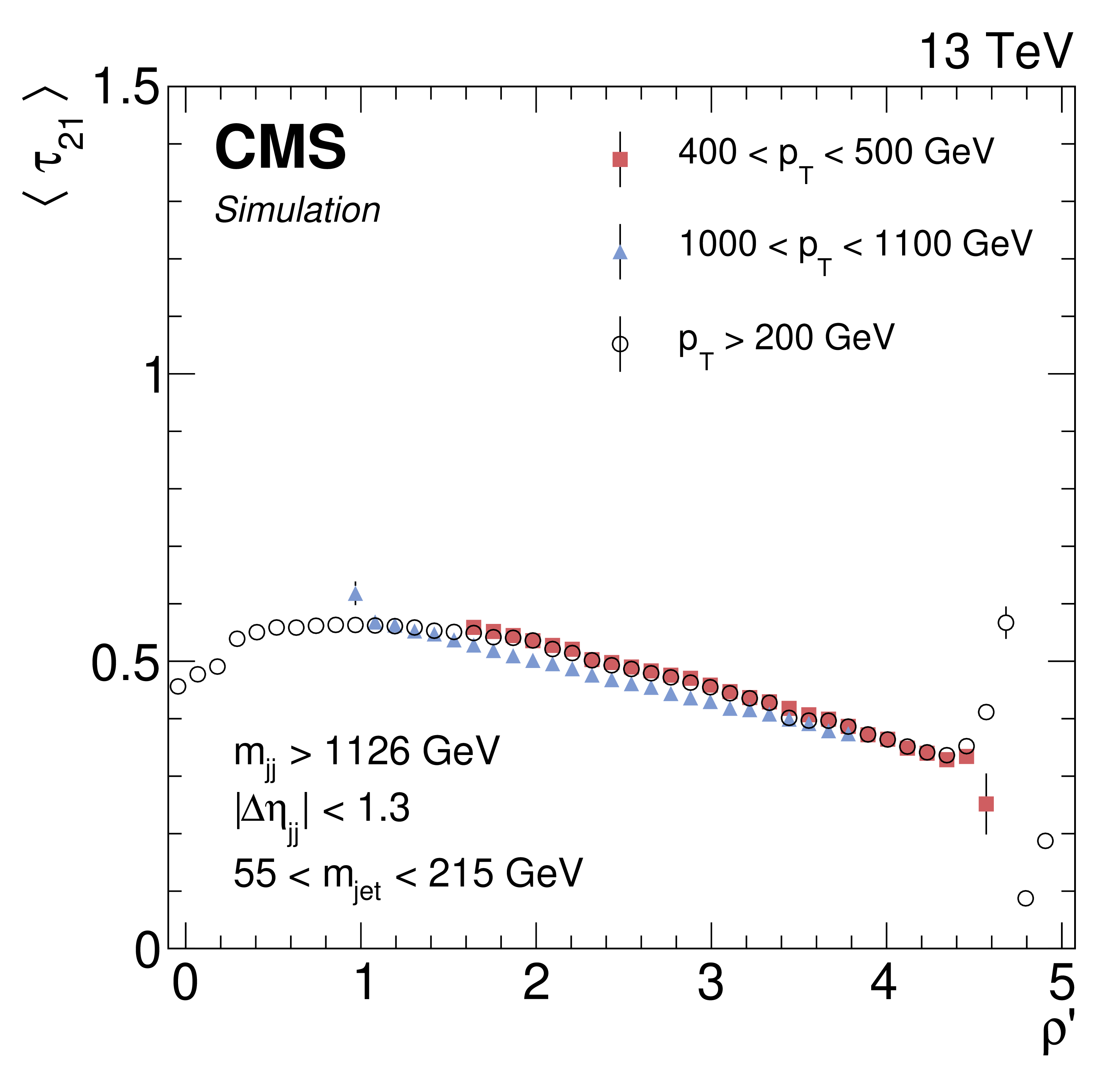
The ${\tau _{21}}$ (left) and ${\tau _{21}^\text {DDT}}$ (right) profile dependencies on $\rho '=\ln({m_\mathrm {jet}} ^2/({p_{\mathrm {T}}} \mu))$ examined in QCD multijet events. A fit to the linear part of the spectrum for $ {p_{\mathrm {T}}} > $ 200 GeV yields the slope $M=-0.080$, which is used to define the mass- and ${p_{\mathrm {T}}} $-decorrelated variable $ {\tau _{21}^\text {DDT}} = {\tau _{21}} -M\rho '$. |
png pdf |
Figure 1-a:
The ${\tau _{21}}$ profile dependency on $\rho '=\ln({m_\mathrm {jet}} ^2/({p_{\mathrm {T}}} \mu))$ examined in QCD multijet events. A fit to the linear part of the spectrum for $ {p_{\mathrm {T}}} > $ 200 GeV yields the slope $M=-0.080$, which is used to define the mass- and ${p_{\mathrm {T}}} $-decorrelated variable $ {\tau _{21}^\text {DDT}} = {\tau _{21}} -M\rho '$. |

png pdf |
Figure 1-b:
The ${\tau _{21}^\text {DDT}}$ profile dependency on $\rho '=\ln({m_\mathrm {jet}} ^2/({p_{\mathrm {T}}} \mu))$ examined in QCD multijet events. A fit to the linear part of the spectrum for $ {p_{\mathrm {T}}} > $ 200 GeV yields the slope $M=-0.080$, which is used to define the mass- and ${p_{\mathrm {T}}} $-decorrelated variable $ {\tau _{21}^\text {DDT}} = {\tau _{21}} -M\rho '$. |

png pdf |
Figure 2:
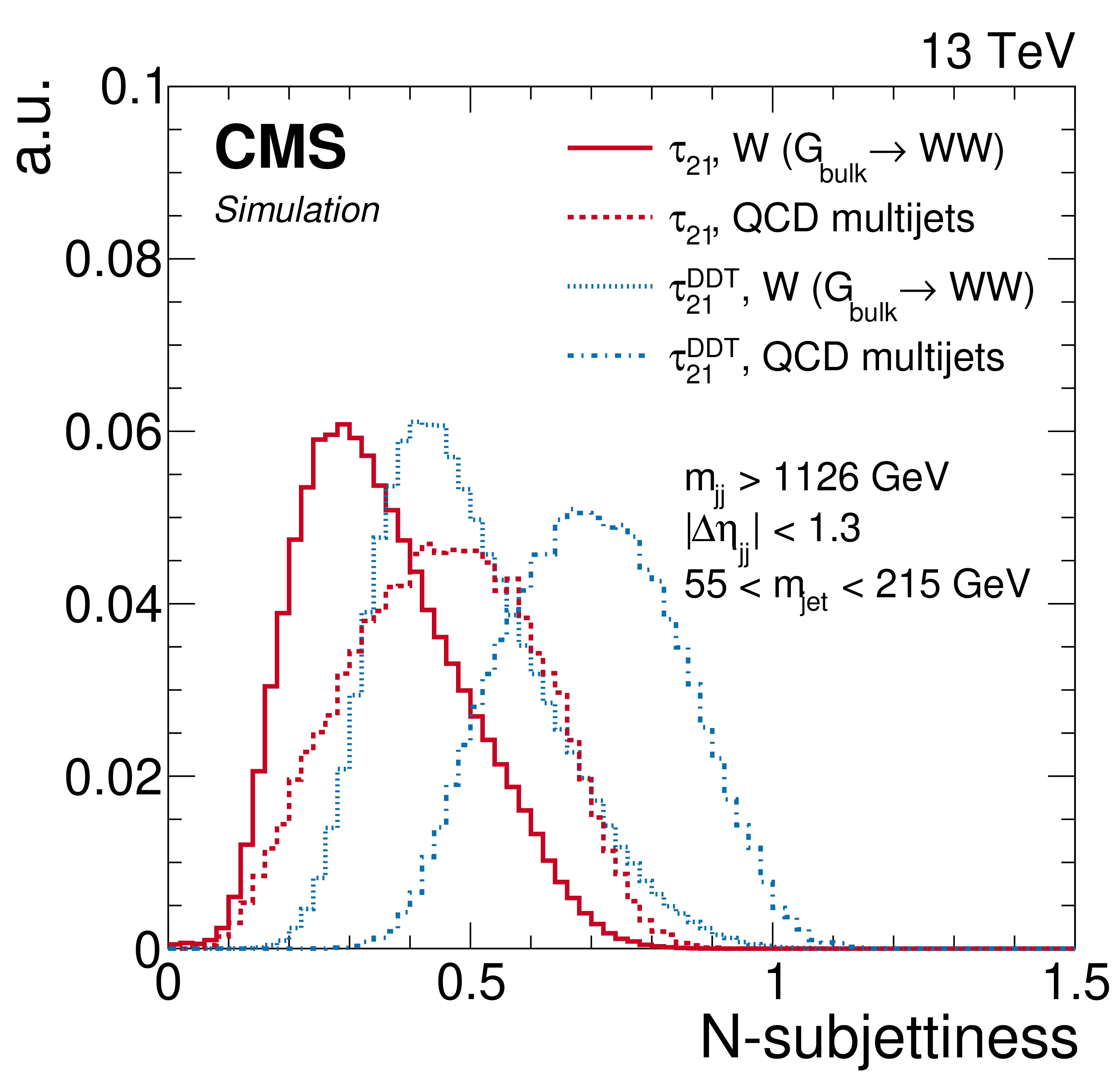
Performance of the $N$-subjettiness discriminants (${\tau _{21}}$ and ${\tau _{21}^\text {DDT}}$) in the background-signal efficiency plane (left). Distribution of ${\tau _{21}}$ and ${\tau _{21}^\text {DDT}}$ for W -jets and quark/gluon jets from QCD multijet events (right). The analysis selections applied to derive these distributions are specified in the figures. For this analysis the working point (WP) of ${\tau _{21}^\text {DDT}} {\leq}0.43$ is chosen. |

png pdf |
Figure 2-a:
Performance of the $N$-subjettiness discriminants (${\tau _{21}}$ and ${\tau _{21}^\text {DDT}}$) in the background-signal efficiency plane. The analysis selections applied to derive this distribution are specified in the figures. For this analysis the working point (WP) of ${\tau _{21}^\text {DDT}} {\leq}0.43$ is chosen. |
png pdf |
Figure 2-b:
Distribution of ${\tau _{21}}$ and ${\tau _{21}^\text {DDT}}$ for W -jets and quark/gluon jets from QCD multijet events. The analysis selections applied to derive this distribution are specified in the figures. For this analysis the working point (WP) of ${\tau _{21}^\text {DDT}} {\leq}0.43$ is chosen. |

png pdf |
Figure 3:
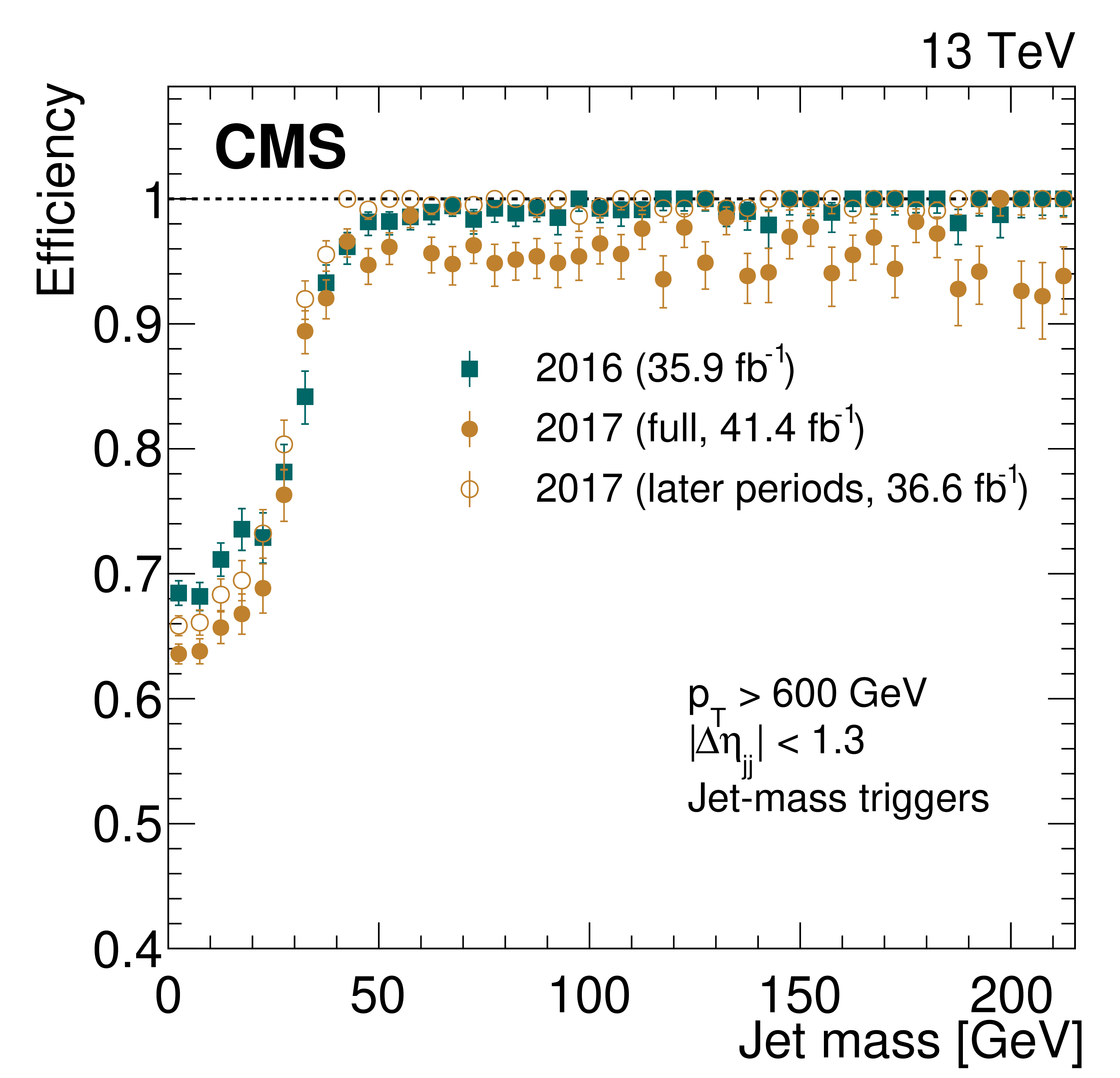
The trigger efficiency as a function of the dijet invariant mass for a combination of all triggers used in this analysis (left) and as a function of the jet mass for triggers requiring an online trimmed mass of at least 30 GeV (right). The solid yellow circles correspond to the trigger efficiencies for the full 2017 data set and do not reach 100% efficiency because the jet mass based triggers were unavailable for a period at the beginning of data taking (corresponding to 4.8 fb$^{-1}$). The open yellow circles are the corresponding efficiencies excluding this period. The uncertainties shown are statistical only. |

png pdf |
Figure 3-a:
The trigger efficiency as a function of the jet mass for triggers requiring an online trimmed mass of at least 30 GeV. The solid yellow circles correspond to the trigger efficiencies for the full 2017 data set and do not reach 100% efficiency because the jet mass based triggers were unavailable for a period at the beginning of data taking (corresponding to 4.8 fb$^{-1}$). The open yellow circles are the corresponding efficiencies excluding this period. The uncertainties shown are statistical only. |
png pdf |
Figure 3-b:
The trigger efficiency as a function of the jet mass for triggers requiring an online trimmed mass of at least 30 GeV. The solid yellow circles correspond to the trigger efficiencies for the full 2017 data set and do not reach 100% efficiency because the jet mass based triggers were unavailable for a period at the beginning of data taking (corresponding to 4.8 fb$^{-1}$). The open yellow circles are the corresponding efficiencies excluding this period. The uncertainties shown are statistical only. |

png pdf |
Figure 4:
Jet mass (upper left) and ${\tau _{21}^\text {DDT}}$ (upper right) distributions for selected jets (one random jet per event), and dijet invariant mass distribution (lower), for events with a jet mass between 55 and 215 GeV. For the QCD multijet simulation, several alternative predictions are shown, scaled to the data minus the other background processes, which are scaled to their SM expectation as described in the text. The different signal distributions are scaled to be visible. No selection on ${\tau _{21}^\text {DDT}}$ is applied. The ratio plots show the fraction of data over QCD multijet simulation for PYTHIA 8 (black markers), HERWIG++ (dotted line), and MadGraph+PYTHIA 8 (dashed line). |

png pdf |
Figure 4-a:
Jet mass distribution for selected jets (one random jet per event), for events with a jet mass between 55 and 215 GeV. For the QCD multijet simulation, several alternative predictions are shown, scaled to the data minus the other background processes, which are scaled to their SM expectation as described in the text. The different signal distributions are scaled to be visible. No selection on ${\tau _{21}^\text {DDT}}$ is applied. The ratio plot shows the fraction of data over QCD multijet simulation for PYTHIA 8 (black markers), HERWIG++ (dotted line), and MadGraph+PYTHIA 8 (dashed line). |

png pdf |
Figure 4-b:
${\tau _{21}^\text {DDT}}$ distribution for selected jets (one random jet per event), for events with a jet mass between 55 and 215 GeV. For the QCD multijet simulation, several alternative predictions are shown, scaled to the data minus the other background processes, which are scaled to their SM expectation as described in the text. The different signal distributions are scaled to be visible. No selection on ${\tau _{21}^\text {DDT}}$ is applied. The ratio plot shows the fraction of data over QCD multijet simulation for PYTHIA 8 (black markers), HERWIG++ (dotted line), and MadGraph+PYTHIA 8 (dashed line). |

png pdf |
Figure 4-c:
Dijet invariant mass distribution, for events with a jet mass between 55 and 215 GeV. For the QCD multijet simulation, several alternative predictions are shown, scaled to the data minus the other background processes, which are scaled to their SM expectation as described in the text. The different signal distributions are scaled to be visible. No selection on ${\tau _{21}^\text {DDT}}$ is applied. The ratio plot shows the fraction of data over QCD multijet simulation for PYTHIA 8 (black markers), HERWIG++ (dotted line), and MadGraph+PYTHIA 8 (dashed line). |
png pdf |
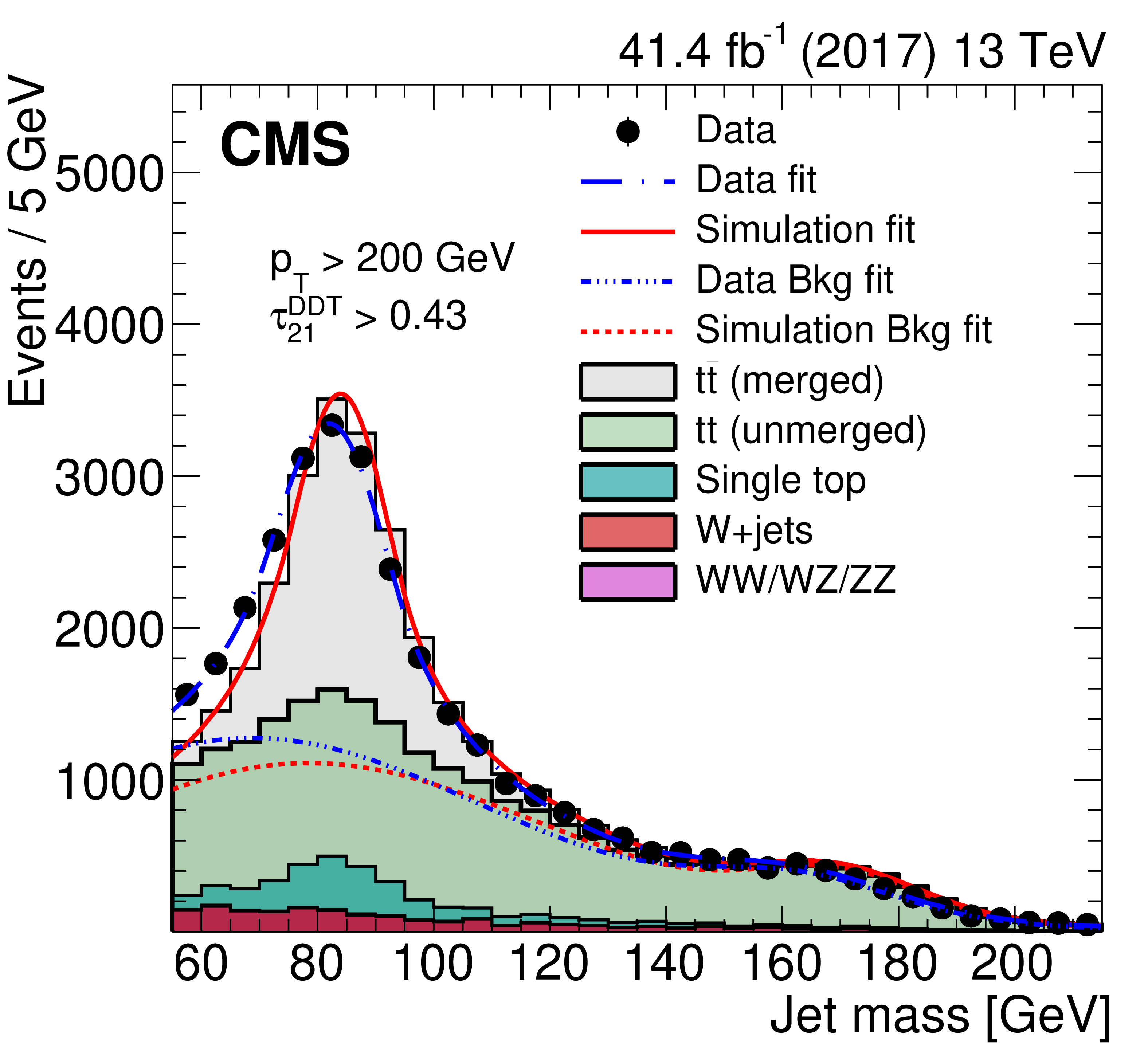
Figure 5:
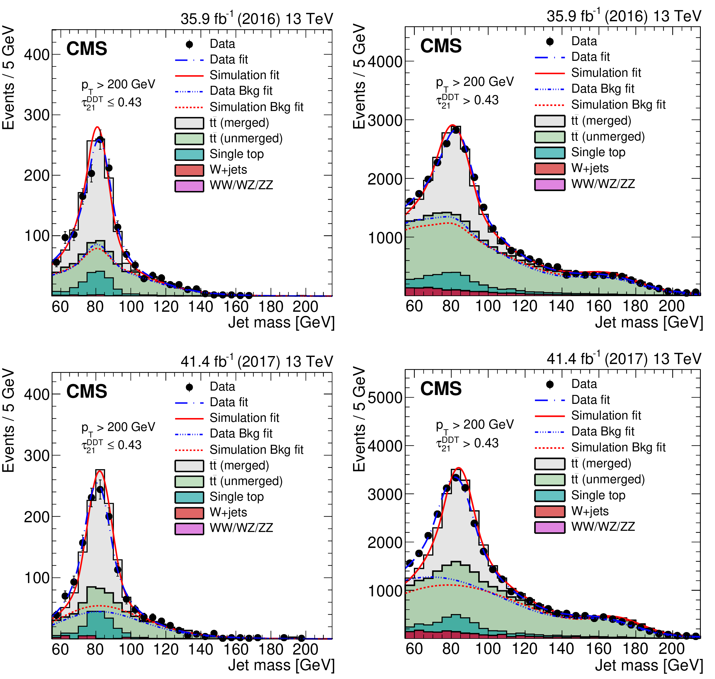
The jet mass distribution for events that pass (left) and fail (right) the $ {\tau _{21}^\text {DDT}} \leq 0.43$ selection in the ${\mathrm{t} {}\mathrm{\bar{t}}}$ control sample. The results of the fits to data and to simulation are shown by the dash-dotted blue and solid red lines, respectively. The background components of the fits are shown as dashed and dash-dotted lines. The fit to 2016 data is shown in the upper panels and the fit to 2017 data in the lower panels. |

png pdf |
Figure 5-a:
The jet mass distribution for events that pass the $ {\tau _{21}^\text {DDT}} \leq 0.43$ selection in the ${\mathrm{t} {}\mathrm{\bar{t}}}$ control sample. The results of the fits to data and to simulation are shown by the dash-dotted blue and solid red lines, respectively. The background components of the fits are shown as dashed and dash-dotted lines. The fit to 2016 data is shown. |

png pdf |
Figure 5-b:
The jet mass distribution for events that fail the $ {\tau _{21}^\text {DDT}} \leq 0.43$ selection in the ${\mathrm{t} {}\mathrm{\bar{t}}}$ control sample. The results of the fits to data and to simulation are shown by the dash-dotted blue and solid red lines, respectively. The background components of the fits are shown as dashed and dash-dotted lines. The fit to 2016 data is shown. |

png pdf |
Figure 5-c:
The jet mass distribution for events that pass the $ {\tau _{21}^\text {DDT}} \leq 0.43$ selection in the ${\mathrm{t} {}\mathrm{\bar{t}}}$ control sample. The results of the fits to data and to simulation are shown by the dash-dotted blue and solid red lines, respectively. The background components of the fits are shown as dashed and dash-dotted lines. The fit to 2017 data is shown. |
png pdf |
Figure 5-d:
The jet mass distribution for events that fail the $ {\tau _{21}^\text {DDT}} \leq 0.43$ selection in the ${\mathrm{t} {}\mathrm{\bar{t}}}$ control sample. The results of the fits to data and to simulation are shown by the dash-dotted blue and solid red lines, respectively. The background components of the fits are shown as dashed and dash-dotted lines. The fit to 2017 data is shown. |

png pdf |
Figure 6:
Total signal efficiency as a function of ${m_\mathrm {X}}$ after all selections are applied, for signal models with a Z' decaying to WW, $ {\mathrm{G} _{\text {bulk}}} $ decaying to WW, W' decaying to WZ, and $ {\mathrm{G} _{\text {bulk}}} $ decaying to ZZ. The denominator is the number of generated events. The solid and dashed lines show the signal efficiencies for the HPHP and HPLP categories, respectively. The decrease in efficiency between 5.0 and 5.5 TeV is due to the requirement $ {m_\mathrm {jj}} < $ 5500 GeV. |

png pdf |
Figure 7:
The final ${m_\mathrm {jj}}$ (left) and ${m_\text {jet1}}$ (right) signal shapes extracted from the parameterization of the dCB function. The same ${m_\mathrm {jj}}$ shapes are used for both purity categories. The jet mass distributions are shown for a range of resonance masses between 1.2 and 5.2 TeV for one of the two jets in the events in the HPHP category. Because the jets are labelled randomly, the jet mass distributions for the second jet are essentially the same as the one shown. The distributions for a $ {\mathrm{G} _{\text {bulk}}} $ decaying to WW have the same shapes as those for the Z' signal and are therefore not visible. |

png pdf |
Figure 7-a:
The final ${m_\mathrm {jj}}$ signal shapes extracted from the parameterization of the dCB function. The same ${m_\mathrm {jj}}$ shapes are used for both purity categories. |

png pdf |
Figure 7-b:
The final ${m_\text {jet1}}$ signal shapes extracted from the parameterization of the dCB function. The jet mass distributions are shown for a range of resonance masses between 1.2 and 5.2 TeV for one of the two jets in the events in the HPHP category. Because the jets are labelled randomly, the jet mass distributions for the second jet are essentially the same as the one shown. The distributions for a $ {\mathrm{G} _{\text {bulk}}} $ decaying to WW have the same shapes as those for the Z' signal and are therefore not visible. |

png pdf |
Figure 8:
The mass scale (left) and resolution (right) of the jet as a function of ${m_\mathrm {X}}$, obtained from the mean and width of the dCB function used to fit the jet mass spectrum. The HPHP (solid lines) and HPLP (dotted lines) categories are shown for different signal models. The distributions are only shown for one of the two jets in the event, since the distributions for the second jet are essentially the same. |

png pdf |
Figure 8-a:
The mass scale of the jet as a function of ${m_\mathrm {X}}$, obtained from the mean and width of the dCB function used to fit the jet mass spectrum. The HPHP (solid lines) and HPLP (dotted lines) categories are shown for different signal models. The distributions are only shown for one of the two jets in the event, since the distributions for the second jet are essentially the same. |

png pdf |
Figure 8-b:
The mass resolution of the jet as a function of ${m_\mathrm {X}}$, obtained from the mean and width of the dCB function used to fit the jet mass spectrum. The HPHP (solid lines) and HPLP (dotted lines) categories are shown for different signal models. The distributions are only shown for one of the two jets in the event, since the distributions for the second jet are essentially the same. |

png pdf |
Figure 9:
Nominal QCD multijet simulation using PYTHIA 8 (data points) and three-dimensional pdfs derived using a forward-folding kernel approach (black solid line), shown together with the five alternate shapes that are added to the multi-dimensional fit as shape nuisance parameters. The shapes for the high-purity (left) and low-purity (right) categories obtained with the 2017 simulation are shown for the projection on ${m_\text {jet1}}$ (upper) and ${m_\mathrm {jj}}$ (lower). The projection on ${m_\text {jet2}}$ is omitted since it is equivalent to the ${m_\text {jet1}}$ projection except for statistical fluctuations. The distributions for 2016 simulations are similar. |

png pdf |
Figure 9-a:
Nominal QCD multijet simulation using PYTHIA 8 (data points) and three-dimensional pdfs derived using a forward-folding kernel approach (black solid line), shown together with the five alternate shapes that are added to the multi-dimensional fit as shape nuisance parameters. The shapes for the high-purity category obtained with the 2017 simulation are shown for the projection on ${m_\text {jet1}}$. The projection on ${m_\text {jet2}}$ is omitted since it is equivalent to the ${m_\text {jet1}}$ projection except for statistical fluctuations. |

png pdf |
Figure 9-b:
Nominal QCD multijet simulation using PYTHIA 8 (data points) and three-dimensional pdfs derived using a forward-folding kernel approach (black solid line), shown together with the five alternate shapes that are added to the multi-dimensional fit as shape nuisance parameters. The shapes for the low-purity category obtained with the 2017 simulation are shown for the projection on ${m_\text {jet1}}$. The projection on ${m_\text {jet2}}$ is omitted since it is equivalent to the ${m_\text {jet1}}$ projection except for statistical fluctuations. |

png pdf |
Figure 9-c:
Nominal QCD multijet simulation using PYTHIA 8 (data points) and three-dimensional pdfs derived using a forward-folding kernel approach (black solid line), shown together with the five alternate shapes that are added to the multi-dimensional fit as shape nuisance parameters. The shapes for the high-purity category obtained with the 2017 simulation are shown for the projection on ${m_\mathrm {jj}}$. |

png pdf |
Figure 9-d:
Nominal QCD multijet simulation using PYTHIA 8 (data points) and three-dimensional pdfs derived using a forward-folding kernel approach (black solid line), shown together with the five alternate shapes that are added to the multi-dimensional fit as shape nuisance parameters. The shapes for the low-purity category obtained with the 2017 simulation are shown for the projection on ${m_\mathrm {jj}}$. |

png pdf |
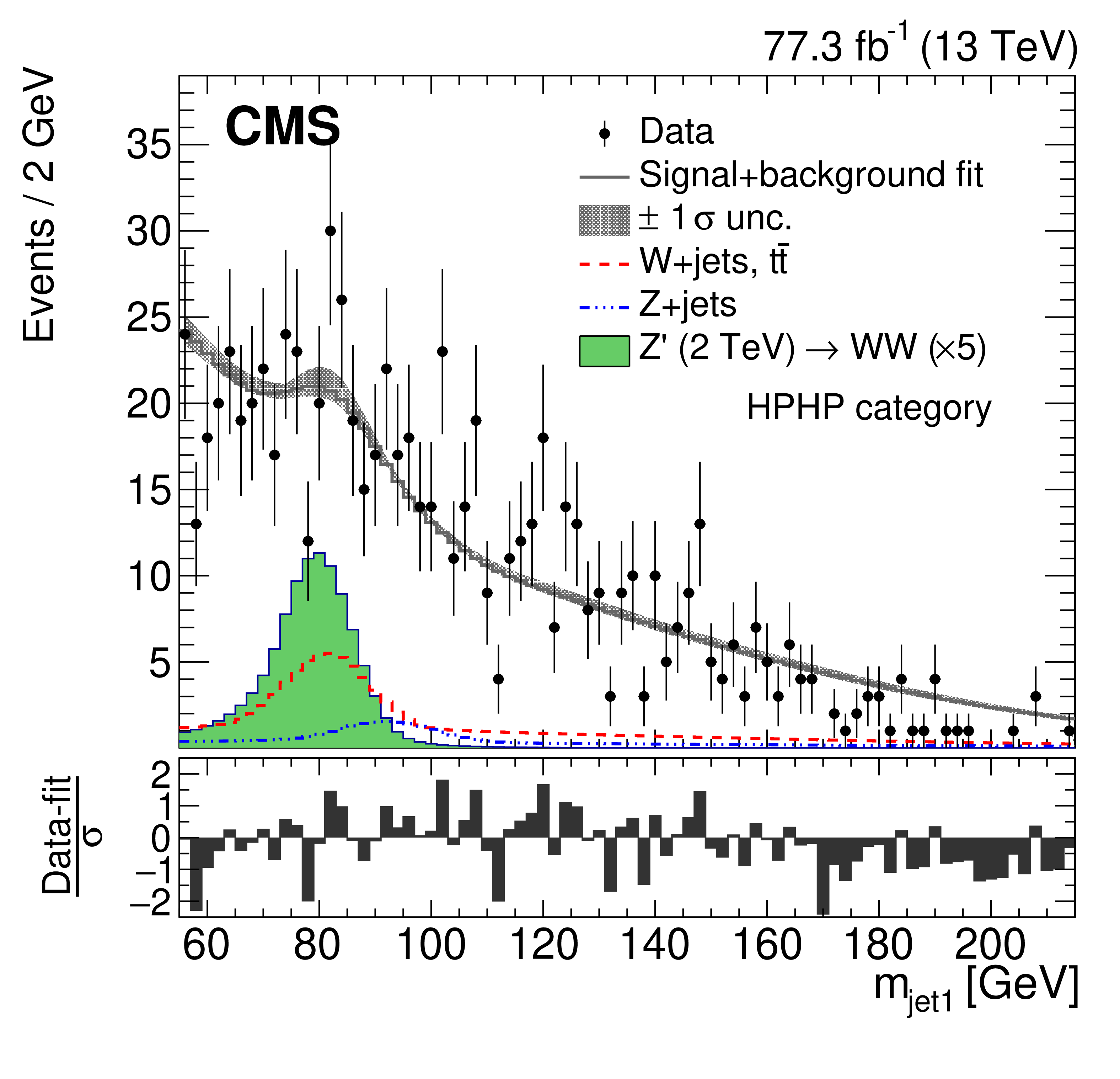
Figure 10:
For the HPHP category: comparison between the fitted result and the data distributions of ${m_\text {jet1}}$ (upper left), ${m_\text {jet2}}$ (upper right), and ${m_\mathrm {jj}}$ (lower). The background shape uncertainty is shown as a gray shaded band, and the statistical uncertainties of the data are shown as vertical bars. An example of a signal distribution is overlaid, where the number of expected events is scaled by a factor of 5. Shown below each mass plot is the corresponding pull distribution (Data-fit)/$\sigma $, where $\sigma =\sqrt {\sigma _\mathrm {data}^2-\sigma _\mathrm {fit}^2}$ for each bin to ensure a Gaussian pull-distribution, as defined in Ref. [83]. |
png pdf |
Figure 10-a:
For the HPHP category: comparison between the fitted result and the data distributions of ${m_\text {jet1}}$. The background shape uncertainty is shown as a gray shaded band, and the statistical uncertainties of the data are shown as vertical bars. An example of a signal distribution is overlaid, where the number of expected events is scaled by a factor of 5. Shown below the mass plot is the corresponding pull distribution (Data-fit)/$\sigma $, where $\sigma =\sqrt {\sigma _\mathrm {data}^2-\sigma _\mathrm {fit}^2}$ for each bin to ensure a Gaussian pull-distribution, as defined in Ref. [83]. |

png pdf |
Figure 10-b:
For the HPHP category: comparison between the fitted result and the data distributions of ${m_\text {jet2}}$. The background shape uncertainty is shown as a gray shaded band, and the statistical uncertainties of the data are shown as vertical bars. An example of a signal distribution is overlaid, where the number of expected events is scaled by a factor of 5. Shown below the mass plot is the corresponding pull distribution (Data-fit)/$\sigma $, where $\sigma =\sqrt {\sigma _\mathrm {data}^2-\sigma _\mathrm {fit}^2}$ for each bin to ensure a Gaussian pull-distribution, as defined in Ref. [83]. |

png pdf |
Figure 10-c:
For the HPHP category: comparison between the fitted result and the data distributions of ${m_\mathrm {jj}}$. The background shape uncertainty is shown as a gray shaded band, and the statistical uncertainties of the data are shown as vertical bars. An example of a signal distribution is overlaid, where the number of expected events is scaled by a factor of 5. Shown below the mass plot is the corresponding pull distribution (Data-fit)/$\sigma $, where $\sigma =\sqrt {\sigma _\mathrm {data}^2-\sigma _\mathrm {fit}^2}$ for each bin to ensure a Gaussian pull-distribution, as defined in Ref. [83]. |
png pdf |
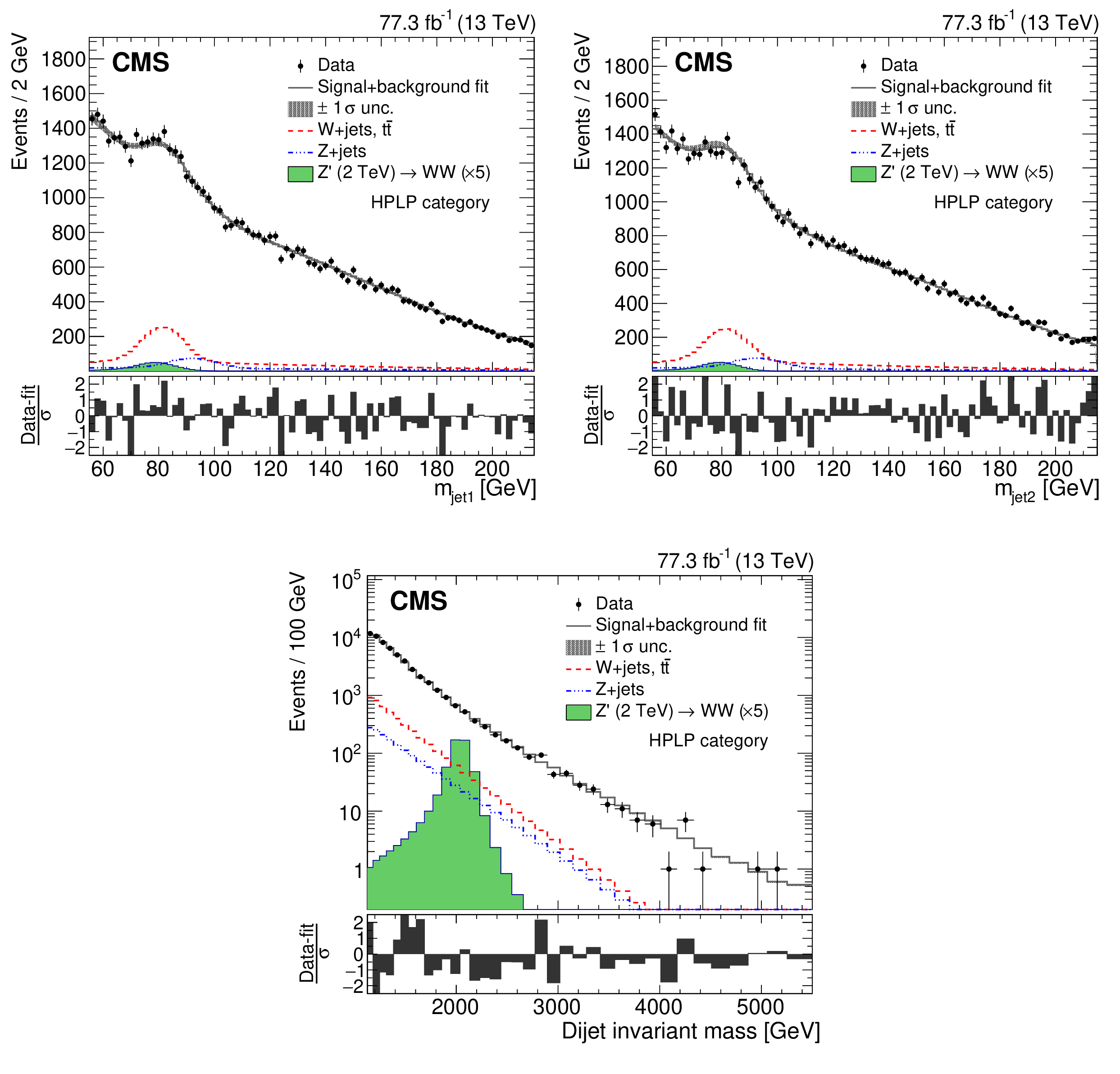
Figure 11:
For the HPLP category: comparison between the fitted result and the data distributions of ${m_\text {jet1}}$ (upper left), ${m_\text {jet2}}$ (upper right), and ${m_\mathrm {jj}}$ (lower). The background shape uncertainty is shown as a gray shaded band, and the statistical uncertainties of the data are shown as vertical bars. An example of a signal distribution is overlaid, where the number of expected events is scaled by a factor of 5. Shown below each mass plot is the corresponding pull distribution (Data-fit)/$\sigma $, where $\sigma =\sqrt {\sigma _\mathrm {data}^2-\sigma _\mathrm {fit}^2}$ for each bin to ensure a Gaussian pull-distribution, as defined in Ref. [83]. |

png pdf |
Figure 11-a:
For the HPLP category: comparison between the fitted result and the data distributions of ${m_\text {jet1}}$. The background shape uncertainty is shown as a gray shaded band, and the statistical uncertainties of the data are shown as vertical bars. An example of a signal distribution is overlaid, where the number of expected events is scaled by a factor of 5. Shown below the mass plot is the corresponding pull distribution (Data-fit)/$\sigma $, where $\sigma =\sqrt {\sigma _\mathrm {data}^2-\sigma _\mathrm {fit}^2}$ for each bin to ensure a Gaussian pull-distribution, as defined in Ref. [83]. |

png pdf |
Figure 11-b:
For the HPLP category: comparison between the fitted result and the data distributions of ${m_\text {jet2}}$. The background shape uncertainty is shown as a gray shaded band, and the statistical uncertainties of the data are shown as vertical bars. An example of a signal distribution is overlaid, where the number of expected events is scaled by a factor of 5. Shown below the mass plot is the corresponding pull distribution (Data-fit)/$\sigma $, where $\sigma =\sqrt {\sigma _\mathrm {data}^2-\sigma _\mathrm {fit}^2}$ for each bin to ensure a Gaussian pull-distribution, as defined in Ref. [83]. |

png pdf |
Figure 11-c:
For the HPLP category: comparison between the fitted result and the data distributions of ${m_\mathrm {jj}}$. The background shape uncertainty is shown as a gray shaded band, and the statistical uncertainties of the data are shown as vertical bars. An example of a signal distribution is overlaid, where the number of expected events is scaled by a factor of 5. Shown below the mass plot is the corresponding pull distribution (Data-fit)/$\sigma $, where $\sigma =\sqrt {\sigma _\mathrm {data}^2-\sigma _\mathrm {fit}^2}$ for each bin to ensure a Gaussian pull-distribution, as defined in Ref. [83]. |

png pdf |
Figure 12:
Observed and expected 95% CL upper limits on the product of the production cross section ($\sigma $) and the branching fraction, obtained after combining categories of all purities with 77.3 fb$^{-1}$ of 13 TeV data, for $ {\mathrm{G} _{\text {bulk}}} \to \mathrm{W} \mathrm{W} $ (upper left), $ {\mathrm{G} _{\text {bulk}}} \to \mathrm{Z} \mathrm{Z} $ (upper right), $\mathrm{W'} \to \mathrm{W} \mathrm{Z} $ (lower left), and $\mathrm{Z'} \to \mathrm{W} \mathrm{W} $ (lower right) signals. For each signal scenario the theoretical prediction (red line) and its uncertainty associated with the choice of PDF set (red hashed band) is shown. The theory cross sections (red line) are calculated at LO in QCD [34,6]. |

png pdf |
Figure 12-a:
Observed and expected 95% CL upper limits on the product of the production cross section ($\sigma $) and the branching fraction, obtained after combining categories of all purities with 77.3 fb$^{-1}$ of 13 TeV data, for the$ {\mathrm{G} _{\text {bulk}}} \to \mathrm{W} \mathrm{W} $ signal. The theoretical prediction (red line) and its uncertainty associated with the choice of PDF set (red hashed band) is shown. The theory cross section (red line) is calculated at LO in QCD [34,6]. |

png pdf |
Figure 12-b:
Observed and expected 95% CL upper limits on the product of the production cross section ($\sigma $) and the branching fraction, obtained after combining categories of all purities with 77.3 fb$^{-1}$ of 13 TeV data, for the $ {\mathrm{G} _{\text {bulk}}} \to \mathrm{Z} \mathrm{Z} $ signal. The theoretical prediction (red line) and its uncertainty associated with the choice of PDF set (red hashed band) is shown. The theory cross section (red line) is calculated at LO in QCD [34,6]. |

png pdf |
Figure 12-c:
Observed and expected 95% CL upper limits on the product of the production cross section ($\sigma $) and the branching fraction, obtained after combining categories of all purities with 77.3 fb$^{-1}$ of 13 TeV data, for the $\mathrm{W'} \to \mathrm{W} \mathrm{Z} $ signal. The theoretical prediction (red line) and its uncertainty associated with the choice of PDF set (red hashed band) is shown. The theory cross section (red line) is calculated at LO in QCD [34,6]. |

png pdf |
Figure 12-d:
Observed and expected 95% CL upper limits on the product of the production cross section ($\sigma $) and the branching fraction, obtained after combining categories of all purities with 77.3 fb$^{-1}$ of 13 TeV data, for the $\mathrm{Z'} \to \mathrm{W} \mathrm{W} $ signal. The theoretical prediction (red line) and its uncertainty associated with the choice of PDF set (red hashed band) is shown. The theory cross section (red line) is calculated at LO in QCD [34,6]. |

png pdf |
Figure 13:
Expected 95% CL upper limits on the product of the production cross section ($\sigma $) and the branching fraction for a $ {\mathrm{G} _{\text {bulk}}} \to \mathrm{W} \mathrm{W} $ signal using 35.9 fb$^{-1}$ of data collected in 2016 obtained using the multi-dimensional fit method presented here (red solid line), compared to the result obtained with previous methods (black dash-dotted line) [29]. The final limit obtained when combining data collected in 2016 and 2017 is also shown (blue dashed line). |
| Tables | |

png pdf |
Table 1:
The W jet mass peak position (m) and resolution ($\sigma $), and the W-tagging efficiencies, as extracted from top quark enriched data and from simulation, together with the corresponding data-to-simulation scale factors. The uncertainties in the scale factors include systematic uncertainties estimated as described in Ref. [62]. |

png pdf |
Table 2:
Summary of the systematic uncertainties and the quantities they affect. Numbers in parentheses correspond to uncertainties for the 2016 analysis if these differ from those for 2017. Dashes indicate shape variations that cannot be described by a single parameter, and are discussed in the text. |

png pdf |
Table 3:
Observed yield and background yields extracted from the multi-dimensional fit together with post-fit uncertainties, in the two purity categories. |
| Summary |
| A search is presented for resonances with masses above 1.2 TeV that decay to WW, ZZ, or WZ boson pairs. Each of the two bosons decays into one large-radius jet, yielding dijet final states. The search is conducted using a novel approach based on a three-dimensional maximum likelihood fit in the dijet invariant mass as well as the two jet masses, thus taking advantage of the fact that the expected signal is resonant in all three mass dimensions. This method yields an improvement in sensitivity of up to 30% relative to previous search methods. The new method places additional constraints on systematic uncertainties affecting the signal by measuring the standard model background from W or Z production with associated jets. Decays of W and Z bosons are identified using jet substructure observables that reduce the background from quantum chromodynamics multijet production. No evidence is found for a signal, and upper limits on the resonance production cross section are set as a function of the resonance mass. The limits presented in this paper are the best to date in the dijet final state, and have a similar sensitivity as the combination of different VV, VH, and HH decay channels using the 2016 data set. The results are interpreted within bulk graviton models, and as limits on the production of the W' and Z' bosons within the heavy vector triplet framework. For the heavy vector triplet model B, we exclude at 95% confidence level W' and Z' spin-1 resonances with masses below 3.8 and 3.5 TeV, respectively. In the narrow-width bulk graviton model, upper limits on the production cross sections for ${\mathrm{G}_{\text{bulk}}} \to\mathrm{WW} (\mathrm{ZZ})$ are set in the range of 20 (27) fb to 0.2 fb for resonance masses between 1.2 and 5.2 TeV. |
| References | ||||
| 1 | L. Randall and R. Sundrum | A large mass hierarchy from a small extra dimension | PRL 83 (1999) 3370 | hep-ph/9905221 |
| 2 | L. Randall and R. Sundrum | An alternative to compactification | PRL 83 (1999) 4690 | hep-th/9906064 |
| 3 | K. Agashe, H. Davoudiasl, G. Perez, and A. Soni | Warped gravitons at the LHC and beyond | PRD 76 (2007) 036006 | hep-ph/0701186 |
| 4 | A. L. Fitzpatrick, J. Kaplan, L. Randall, and L.-T. Wang | Searching for the Kaluza--Klein graviton in bulk RS models | JHEP 09 (2007) 013 | hep-ph/0701150 |
| 5 | O. Antipin, D. Atwood, and A. Soni | Search for RS gravitons via $ \mathrm{W}_\mathrm{L}\mathrm{W}_\mathrm{L} $ decays | PLB 666 (2008) 155 | 0711.3175 |
| 6 | D. Pappadopulo, A. Thamm, R. Torre, and A. Wulzer | Heavy vector triplets: Bridging theory and data | JHEP 09 (2014) 060 | 1402.4431 |
| 7 | CMS Collaboration | Search for massive resonances in dijet systems containing jets tagged as W or Z boson decays in pp collisions at $ \sqrt{s} = $ 8 TeV | JHEP 08 (2014) 173 | CMS-EXO-12-024 1405.1994 |
| 8 | CMS Collaboration | Search for massive resonances decaying into pairs of boosted bosons in semi-leptonic final states at $ \sqrt{s}= $ 8 TeV | JHEP 08 (2014) 174 | CMS-EXO-13-009 1405.3447 |
| 9 | CMS Collaboration | Search for new resonances decaying via WZ to leptons in proton-proton collisions at $ \sqrt{s} = $ 8 TeV | PLB 740 (2015) 83 | CMS-EXO-12-025 1407.3476 |
| 10 | CMS Collaboration | Search for massive resonances decaying into WW, WZ or ZZ bosons in proton-proton collisions at $ \sqrt{s} = $ 13 TeV | JHEP 03 (2017) 162 | CMS-B2G-16-004 1612.09159 |
| 11 | CMS Collaboration | Search for a heavy resonance decaying to a pair of vector bosons in the lepton plus merged jet final state at $ \sqrt{s}= $ 13 TeV | JHEP 05 (2018) 088 | CMS-B2G-16-029 1802.09407 |
| 12 | CMS Collaboration | Search for narrow high-mass resonances in proton-proton collisions at $ \sqrt{s} = $ 8 TeV decaying to a Z and a Higgs boson | PLB 748 (2015) 255 | CMS-EXO-13-007 1502.04994 |
| 13 | CMS Collaboration | Search for heavy resonances that decay into a vector boson and a Higgs boson in hadronic final states at $ \sqrt{s} = $ 13 TeV | EPJC 77 (2017) 636 | CMS-B2G-17-002 1707.01303 |
| 14 | CMS Collaboration | Search for heavy resonances decaying into a vector boson and a Higgs boson in final states with charged leptons, neutrinos, and b quarks | PLB 768 (2017) 137 | CMS-B2G-16-003 1610.08066 |
| 15 | CMS Collaboration | Search for a massive resonance decaying into a Higgs boson and a W or Z boson in hadronic final states in proton-proton collisions at $ \sqrt{s} = $ 8 TeV | JHEP 02 (2016) 145 | CMS-EXO-14-009 1506.01443 |
| 16 | CMS Collaboration | Search for massive WH resonances decaying into the $ \ell \nu \mathrm{b} \overline{\mathrm{b}} $ final state at $ \sqrt{s} = $ 8 TeV | EPJC 76 (2016) 237 | CMS-EXO-14-010 1601.06431 |
| 17 | CMS Collaboration | Search for heavy resonances decaying to two Higgs bosons in final states containing four b quarks | EPJC 76 (2016) 371 | CMS-EXO-12-053 1602.08762 |
| 18 | ATLAS Collaboration | Search for WZ resonances in the fully leptonic channel using pp collisions at $ \sqrt{s} = $ 8 TeV collisions with the ATLAS detector | PLB 737 (2014) 223 | 1406.4456 |
| 19 | ATLAS Collaboration | Search for resonant diboson production in the $ \mathrm{\ell\ell q\bar{q}} $ final state in pp collisions at $ \sqrt{s} = $ 8 TeV with the ATLAS detector | EPJC 75 (2015) 69 | 1409.6190 |
| 20 | ATLAS Collaboration | Search for production of WW/WZ resonances decaying to a lepton, neutrino and jets in pp collisions at $ \sqrt{s}= $ 8 TeV with the ATLAS detector | EPJC 75 (2015) 209 | 1503.04677 |
| 21 | ATLAS Collaboration | Search for high-mass diboson resonances with boson-tagged jets in proton-proton collisions at $ \sqrt{s} = $ 8 TeV with the ATLAS detector | JHEP 12 (2015) 055 | 1506.00962 |
| 22 | ATLAS Collaboration | Search for heavy resonances decaying to a W or Z boson and a Higgs boson in the $ \mathrm{q\bar{q}^{(\prime)}b\bar{b}} $ final state in pp collisions at $ \sqrt{s}= $ 13 TeV with the ATLAS detector | PLB 774 (2017) 494 | 1707.06958 |
| 23 | ATLAS Collaboration | Search for diboson resonances with boson-tagged jets in pp collisions at $ \sqrt{s}= $ 13 TeV with the ATLAS detector | PLB 777 (2018) 91 | 1708.04445 |
| 24 | ATLAS Collaboration | Search for a new resonance decaying to a W or Z boson and a Higgs boson in the $ \ell \ell / \ell \nu / \nu \nu + \mathrm{b \bar{b}} $ final states with the ATLAS detector | EPJC 75 (2015) 263 | 1503.08089 |
| 25 | ATLAS Collaboration | Searches for heavy diboson resonances in pp collisions at $ \sqrt{s} = $ 13 TeV with the ATLAS detector | JHEP 09 (2016) 173 | 1606.04833 |
| 26 | ATLAS Collaboration | Search for new resonances decaying to a W or Z boson and a Higgs boson in the $ \ell^+ \ell^- \mathrm{b\bar b} $, $ \ell \nu \mathrm{b\bar b} $, and $ \nu\bar{\nu} \mathrm{b\bar b} $ channels with pp collisions at $ \sqrt{s}= $ 13 TeV with the ATLAS detector | PLB 765 (2017) 32 | 1607.05621 |
| 27 | CMS Collaboration | Combination of CMS searches for heavy resonances decaying to pairs of bosons or leptons | CMS-B2G-18-006 1906.00057 |
|
| 28 | ATLAS Collaboration | Combination of searches for heavy resonances decaying into bosonic and leptonic final states using 36 fb$ ^{-1} $ of proton-proton collision data at $ \sqrt{s} = $ 13 TeV with the ATLAS detector | PRD (2018) 052008 | 1808.02380 |
| 29 | CMS Collaboration | Search for massive resonances decaying into WW, WZ, ZZ, qW, and qZ with dijet final states at $ \sqrt{s}= $ 13 TeV | PRD 97 (2018) 072006 | CMS-B2G-17-001 1708.05379 |
| 30 | CMS Collaboration | The CMS experiment at the CERN LHC | JINST 3 (2008) S08004 | CMS-00-001 |
| 31 | CMS Collaboration | The CMS trigger system | JINST 12 (2017) P01020 | CMS-TRG-12-001 1609.02366 |
| 32 | C. Grojean, E. Salvioni, and R. Torre | A weakly constrained W' at the early LHC | JHEP 07 (2011) 002 | 1103.2761 |
| 33 | E. Salvioni, G. Villadoro, and F. Zwirner | Minimal Z' models: present bounds and early LHC reach | JHEP 11 (2009) 068 | 0909.1320 |
| 34 | A. Oliveira | Gravity particles from warped extra dimensions, predictions for LHC | 1404.0102 | |
| 35 | B. Bellazzini, C. Cs\'aki, and J. Serra | Composite Higgses | EPJC 74 (2014) 2766 | 1401.2457 |
| 36 | R. Contino, D. Marzocca, D. Pappadopulo, and R. Rattazzi | On the effect of resonances in composite Higgs phenomenology | JHEP 10 (2011) 081 | 1109.1570 |
| 37 | D. Marzocca, M. Serone, and J. Shu | General composite Higgs models | JHEP 08 (2012) 013 | 1205.0770 |
| 38 | D. Greco and D. Liu | Hunting composite vector resonances at the LHC: naturalness facing data | JHEP 12 (2014) 126 | 1410.2883 |
| 39 | K. Lane and L. Pritchett | The light composite Higgs boson in strong extended technicolor | JHEP 06 (2017) 140 | 1604.07085 |
| 40 | M. Schmaltz and D. Tucker-Smith | Little Higgs review | Ann. Rev. Nucl. Part. Sci. 55 (2005) 229 | hep-ph/0502182 |
| 41 | N. Arkani-Hamed, A. G. Cohen, E. Katz, and A. E. Nelson | The littlest Higgs | JHEP 07 (2002) 034 | hep-ph/0206021 |
| 42 | J. Alwall et al. | The automated computation of tree-level and next-to-leading order differential cross sections, and their matching to parton shower simulations | JHEP 07 (2014) 079 | 1405.0301 |
| 43 | T. Sjostrand et al. | An introduction to PYTHIA 8.2 | CPC 191 (2015) 159 | 1410.3012 |
| 44 | NNPDF Collaboration | Parton distributions for the LHC Run II | JHEP 04 (2015) 040 | 1410.8849 |
| 45 | CMS Collaboration | Event generator tunes obtained from underlying event and multiparton scattering measurements | EPJC 76 (2016) 155 | CMS-GEN-14-001 1512.00815 |
| 46 | CMS Collaboration | Extraction and validation of a new set of CMS PYTHIA8 tunes from underlying-event measurements | Submitted to EPJC | CMS-GEN-17-001 1903.12179 |
| 47 | J. Alwall et al. | Comparative study of various algorithms for the merging of parton showers and matrix elements in hadronic collisions | EPJC 53 (2008) 473 | 0706.2569 |
| 48 | S. Alioli et al. | Jet pair production in POWHEG | JHEP 04 (2011) 081 | 1012.3380 |
| 49 | P. Nason | A new method for combining NLO QCD with shower Monte Carlo algorithms | JHEP 11 (2004) 040 | hep-ph/0409146 |
| 50 | S. Frixione, P. Nason, and C. Oleari | Matching NLO QCD computations with parton shower simulations: the POWHEG method | JHEP 11 (2007) 070 | 0709.2092 |
| 51 | S. Alioli, P. Nason, C. Oleari, and E. Re | A general framework for implementing NLO calculations in shower Monte Carlo programs: the POWHEG BOX | JHEP 06 (2010) 043 | 1002.2581 |
| 52 | M. Bahr et al. | Herwig++ physics and manual | EPJC 58 (2008) 639 | 0803.0883 |
| 53 | S. Alioli, S.-O. Moch, and P. Uwer | Hadronic top-quark pair-production with one jet and parton showering | JHEP 01 (2012) 137 | 1110.5251 |
| 54 | S. Kallweit et al. | NLO electroweak automation and precise predictions for W+multijet production at the LHC | JHEP 04 (2015) 012 | 1412.5157 |
| 55 | S. Kallweit et al. | NLO QCD+EW predictions for V+jets including off-shell vector-boson decays and multijet merging | JHEP 04 (2016) 021 | 1511.08692 |
| 56 | NNPDF Collaboration | Parton distributions from high-precision collider data | EPJC 77 (2017) 663 | 1706.00428 |
| 57 | GEANT4 Collaboration | GEANT4 -- a simulation toolkit | NIMA 506 (2003) 250 | |
| 58 | CMS Collaboration | Particle-flow reconstruction and global event description with the CMS detector | JINST 12 (2017) P10003 | CMS-PRF-14-001 1706.04965 |
| 59 | M. Cacciari, G. P. Salam, and G. Soyez | The anti-$ {k_{\mathrm{T}}} $ jet clustering algorithm | JHEP 04 (2008) 063 | 0802.1189 |
| 60 | M. Cacciari, G. P. Salam, and G. Soyez | FastJet user manual | EPJC 72 (2012) 1896 | 1111.6097 |
| 61 | D. Bertolini, P. Harris, M. Low, and N. Tran | Pileup per particle identification | JHEP 10 (2014) 59 | 1407.6013 |
| 62 | CMS Collaboration | Jet algorithms performance in 13 TeV data | CMS-PAS-JME-16-003 | CMS-PAS-JME-16-003 |
| 63 | CMS Collaboration | Jet energy scale and resolution in the CMS experiment in $ {\mathrm{p}}{\mathrm{p}} $ collisions at 8 TeV | JINST 12 (2017) P02014 | CMS-JME-13-004 1607.03663 |
| 64 | M. Cacciari, G. P. Salam, and G. Soyez | The catchment area of jets | JHEP 04 (2008) 005 | 0802.1188 |
| 65 | M. Dasgupta, A. Fregoso, S. Marzani, and G. P. Salam | Towards an understanding of jet substructure | JHEP 09 (2013) 029 | 1307.0007 |
| 66 | J. M. Butterworth, A. R. Davison, M. Rubin, and G. P. Salam | Jet substructure as a new Higgs search channel at the LHC | PRL 100 (2008) 242001 | 0802.2470 |
| 67 | A. J. Larkoski, S. Marzani, G. Soyez, and J. Thaler | Soft drop | JHEP 05 (2014) 146 | 1402.2657 |
| 68 | J. Thaler and K. Van Tilburg | Maximizing boosted top identification by minimizing $ N $-subjettiness | JHEP 02 (2012) 093 | 1108.2701 |
| 69 | Y. L. Dokshitzer, G. D. Leder, S. Moretti, and B. R. Webber | Better jet clustering algorithms | JHEP 08 (1997) 001 | hep-ph/9707323 |
| 70 | M. Wobisch and T. Wengler | Hadronization corrections to jet cross-sections in deep inelastic scattering | in Monte Carlo generators for HERA physics 1998 | hep-ph/9907280 |
| 71 | D. Krohn, J. Thaler, and L.-T. Wang | Jet trimming | JHEP 02 (2010) 084 | 0912.1342 |
| 72 | S. Catani, \relax Yu. L. Dokshitzer, M. H. Seymour, and B. R. Webber | Longitudinally invariant $ {k_{\mathrm{T}}} $ clustering algorithms for hadron hadron collisions | NPB 406 (1993) 187 | |
| 73 | J. Dolen et al. | Thinking outside the ROCs: Designing decorrelated taggers (DDT) for jet substructure | JHEP 05 (2016) 156 | 1603.00027 |
| 74 | CMS Collaboration | Description and performance of track and primary-vertex reconstruction with the CMS tracker | JINST 9 (2014) P10009 | CMS-TRK-11-001 1405.6569 |
| 75 | CMS Collaboration | Performance of the CMS muon detector and muon reconstruction with proton-proton collisions at $ \sqrt{s}= $ 13 TeV | JINST 13 (2018) P06015 | CMS-MUO-16-001 1804.04528 |
| 76 | CMS Collaboration | Performance of electron reconstruction and selection with the CMS detector in proton-proton collisions at $ \sqrt{s} = 8{TeV} $ | JINST 10 (2015) P06005 | CMS-EGM-13-001 1502.02701 |
| 77 | CMS Collaboration | Measurement of differential cross sections for top quark pair production using the lepton+jets final state in proton-proton collisions at 13 TeV | PRD 95 (2017) 092001 | CMS-TOP-16-008 1610.04191 |
| 78 | M. J. Oreglia | A study of the reactions $\psi' \to \gamma\gamma \psi$ | PhD thesis, Stanford University, 1980 SLAC Report SLAC-R-236, see A | |
| 79 | K. S. Cranmer | Kernel estimation in high-energy physics | CPC 136 (2001) 198 | hep-ex/0011057 |
| 80 | A. L. Read | Presentation of search results: the $ \rm CL_s $ technique | JPG 28 (2002) 2693 | |
| 81 | T. Junk | Confidence level computation for combining searches with small statistics | NIMA 434 (1999) 435 | hep-ex/9902006 |
| 82 | G. Cowan, K. Cranmer, E. Gross, and O. Vitells | Asymptotic formulae for likelihood-based tests of new physics | EPJC 71 (2011) 1554 | 1007.1727 |
| 83 | L. Demortier and L. Lyons | Everything you always wanted to know about pulls | CDF/ANAL/PUBLIC/5776, CDF | |
|
|
Compact Muon Solenoid LHC, CERN |
|

|

|

|

|

|