

Compact Muon Solenoid
LHC, CERN
| CMS-SMP-21-002 ; CERN-EP-2022-013 | ||
| Measurement of the Drell-Yan forward-backward asymmetry at high dilepton masses in proton-proton collisions at $\sqrt{s} = $ 13 TeV | ||
| CMS Collaboration | ||
| 24 February 2022 | ||
| JHEP 08 (2022) 063 | ||
| Abstract: A measurement of the forward-backward asymmetry of pairs of oppositely charged leptons (dimuons and dielectrons) produced by the Drell-Yan process in proton-proton collisions is presented. The data sample corresponds to an integrated luminosity of 138 fb$^{-1}$ collected with the CMS detector at the LHC at a center-of-mass energy of 13 TeV. The asymmetry is measured as a function of lepton pair mass for masses larger than 170 GeV and compared with standard model predictions. An inclusive measurement across both channels and the full mass range yields an asymmetry of 0.599 $\pm$ 0.005 (stat) $\pm$ 0.007 (syst). As a test of lepton flavor universality, the difference between the dimuon and dielectron asymmetries is measured as well. No statistically significant deviations from standard model predictions are observed. The measurements are used to set limits on the presence of additional gauge bosons. For a Z' in the sequential standard model, a lower mass limit of 4.4 TeV is set at 95% confidence level. | ||
| Links: e-print arXiv:2202.12327 [hep-ex] (PDF) ; CDS record ; inSPIRE record ; HepData record ; CADI line (restricted) ; | ||
| Figures | |
png pdf |
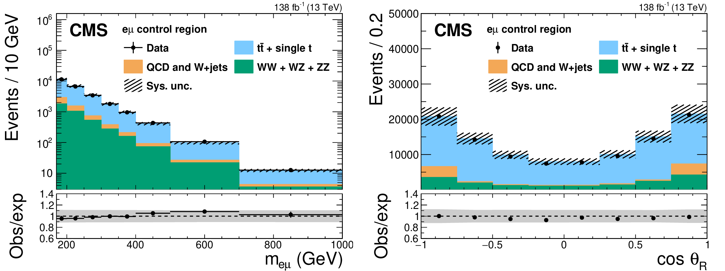
Figure 1:
The invariant mass distribution (left) and ${\cos\theta _\mathrm {R}}$ distribution (right) of e$\mu$ events observed in CMS data (black dots with statistical uncertainties) and expected backgrounds (stacked histograms). The hatched bands show the systematic uncertainty in the expected yield. The sources of this uncertainty are discussed in Section 8. The lower panels show the ratio of the data to the expectations. The gray bands represent the total uncertainty in the predicted yields. |
png pdf |
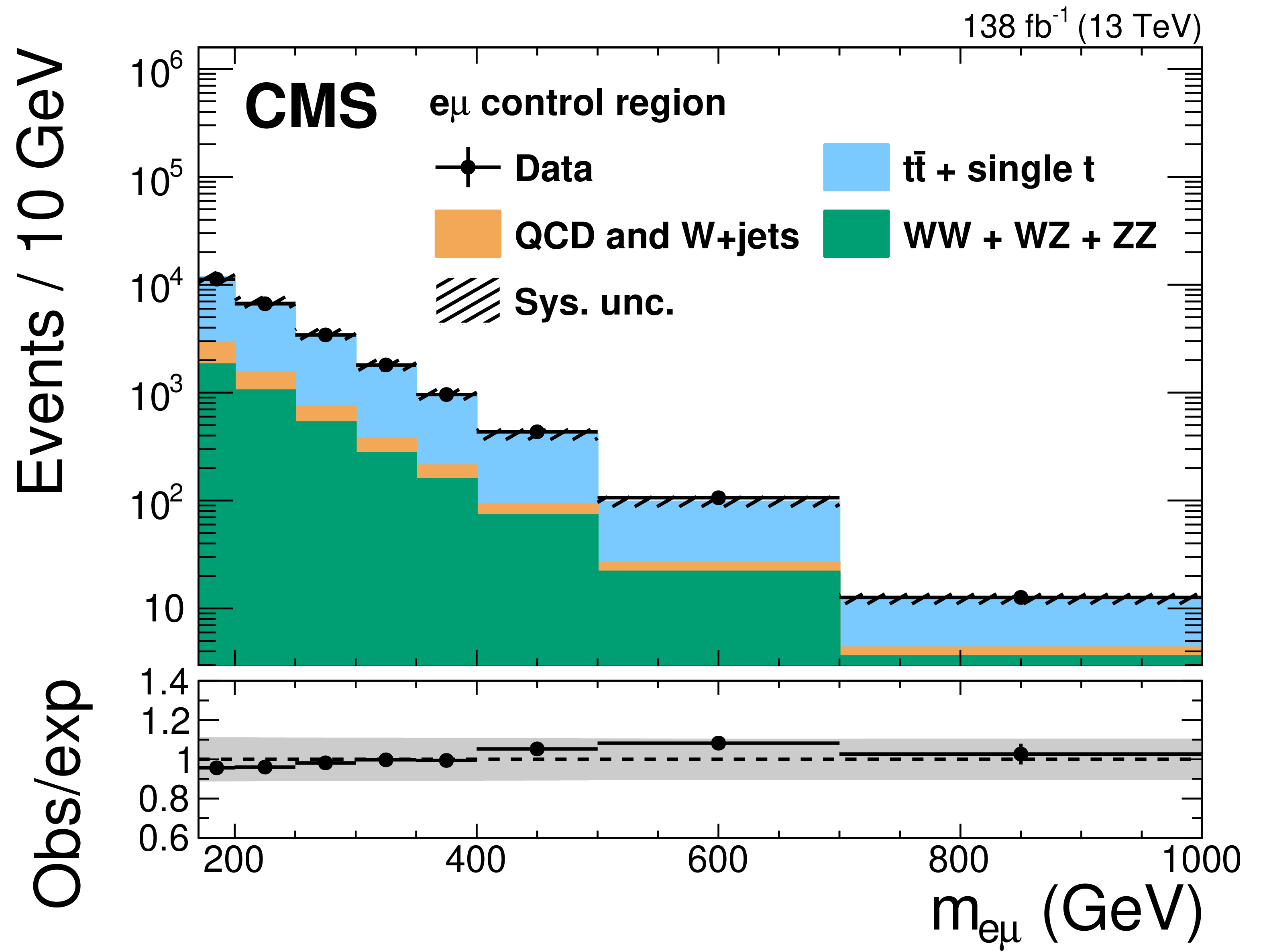
Figure 1-a:
The invariant mass distribution of e$\mu$ events observed in CMS data (black dots with statistical uncertainties) and expected backgrounds (stacked histograms). The hatched bands show the systematic uncertainty in the expected yield. The sources of this uncertainty are discussed in Section 8. The lower panel shows the ratio of the data to the expectations. The gray bands represent the total uncertainty in the predicted yields. |

png pdf |
Figure 1-b:
The ${\cos\theta _\mathrm {R}}$ distribution of e$\mu$ events observed in CMS data (black dots with statistical uncertainties) and expected backgrounds (stacked histograms). The hatched bands show the systematic uncertainty in the expected yield. The sources of this uncertainty are discussed in Section 8. The lower panel shows the ratio of the data to the expectations. The gray bands represent the total uncertainty in the predicted yields. |
png pdf |
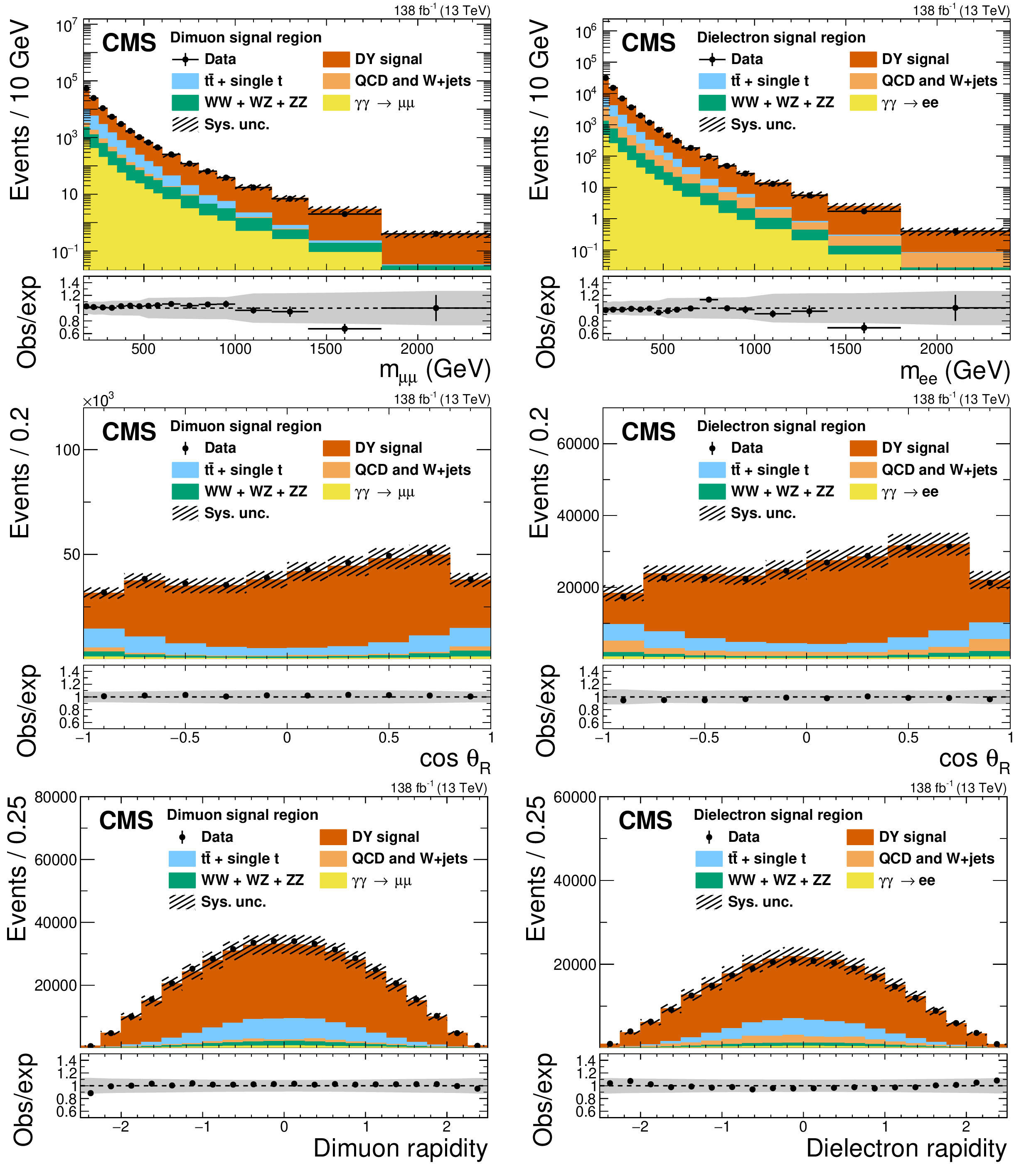
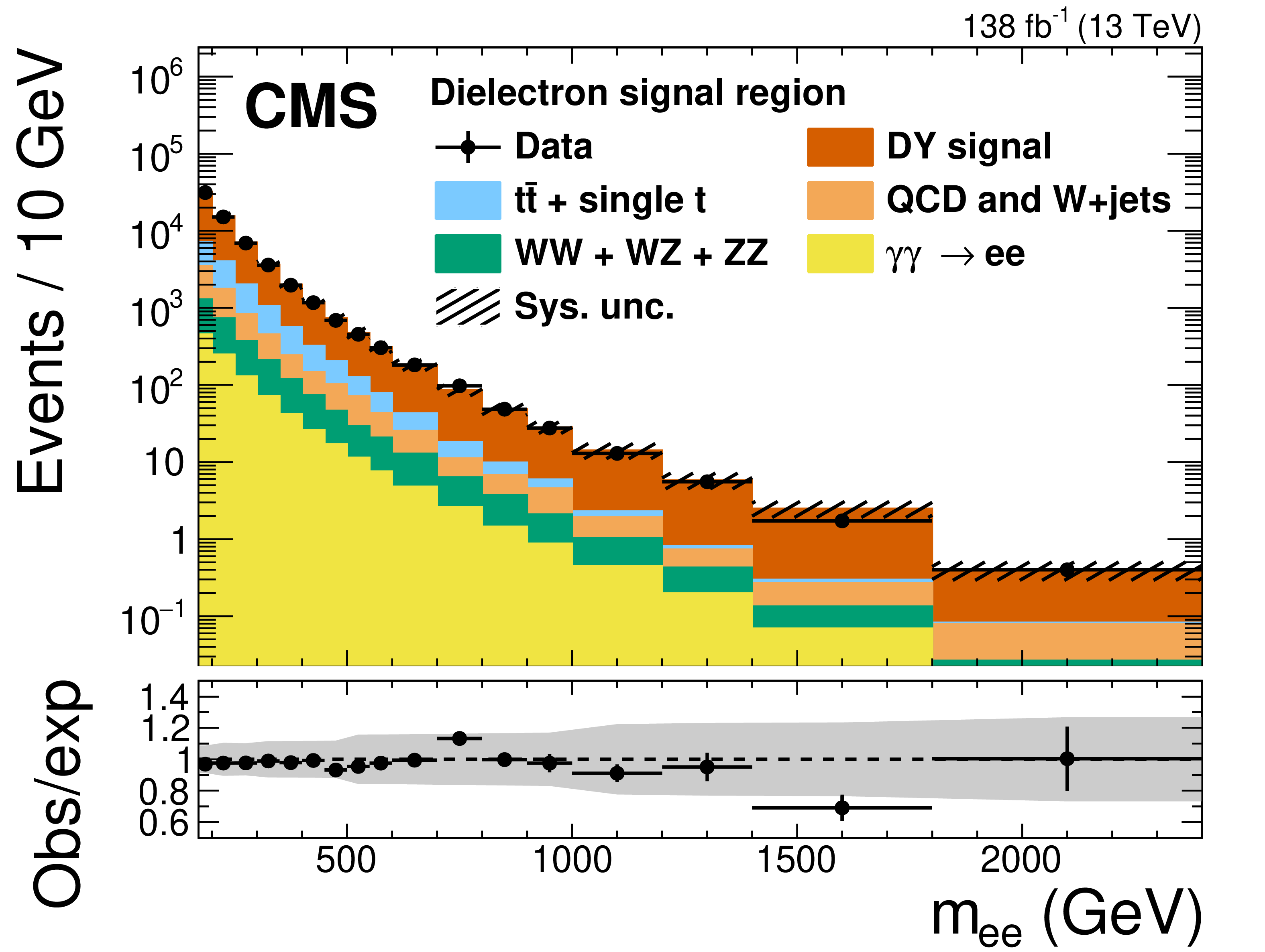
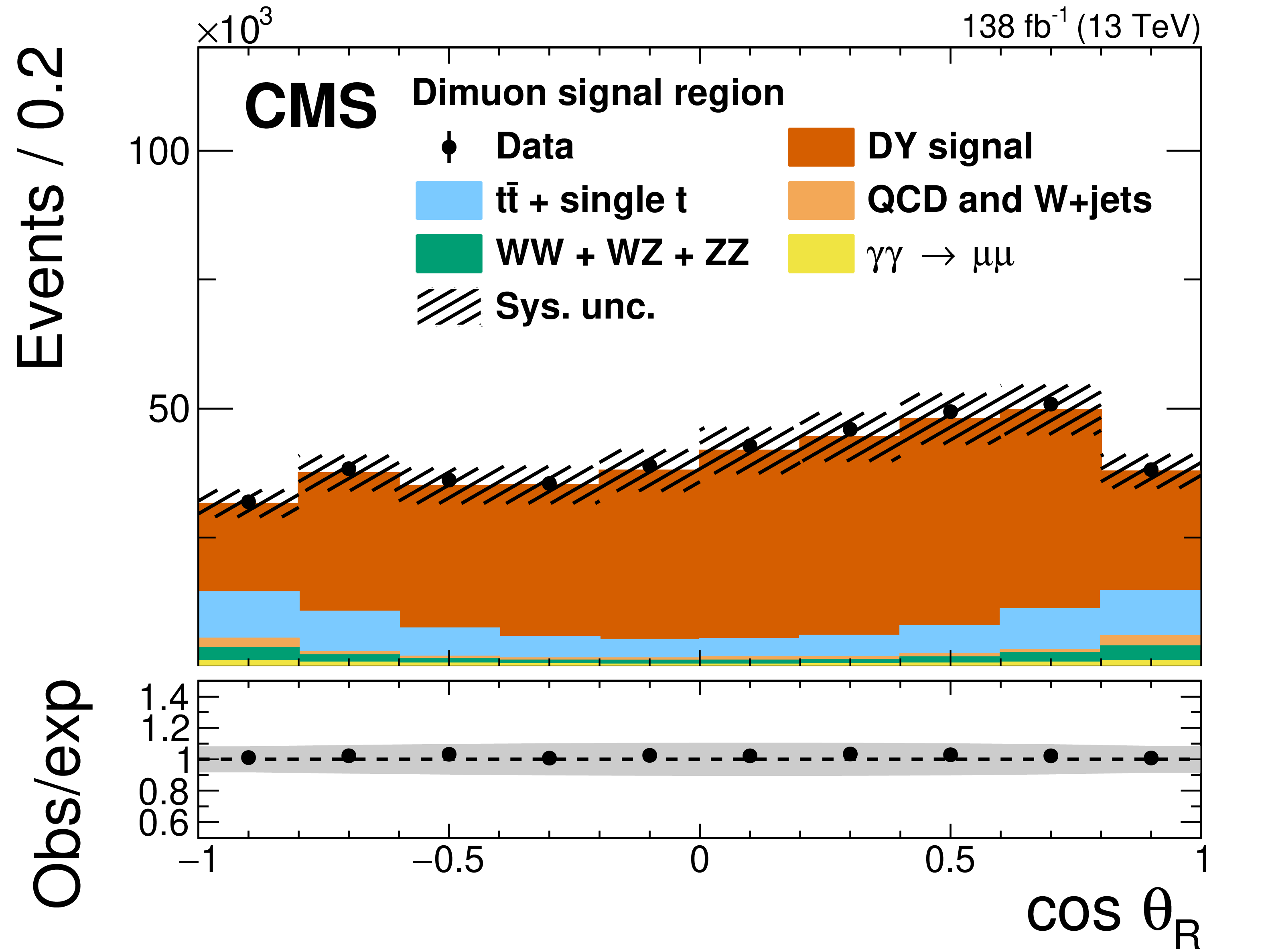
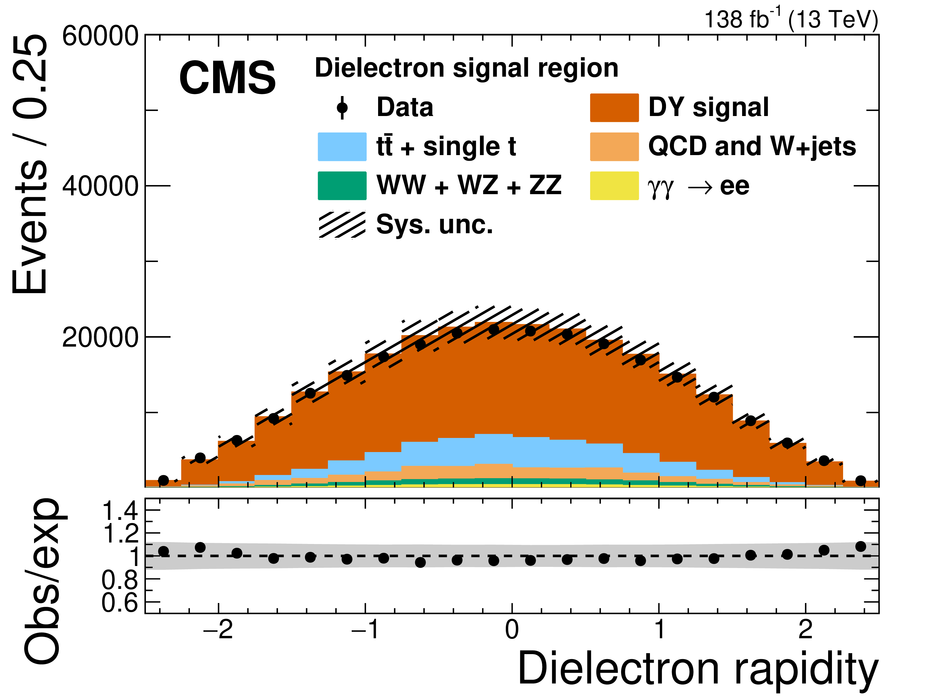
Figure 2:
A comparison of CMS data and expected signal and background distributions in dilepton invariant mass (upper row), ${\cos\theta _\mathrm {R}}$ (middle row) and dilepton rapidity (lower row). The left plot shows the $ {{\mu}} {{\mu}}$ channel and the right plot the ee channel. The black points with error bars represent the data and their statistical uncertainties, whereas the combined signal and background expectation is shown as stacked histograms. The hatched band shows the systematic uncertainty in the expected signal and background yield. The sources of this uncertainty are discussed in Section 8. The lower panels show the ratio of the data to the expectation. The gray bands represents the total uncertainty in the predicted yield. |
png pdf |
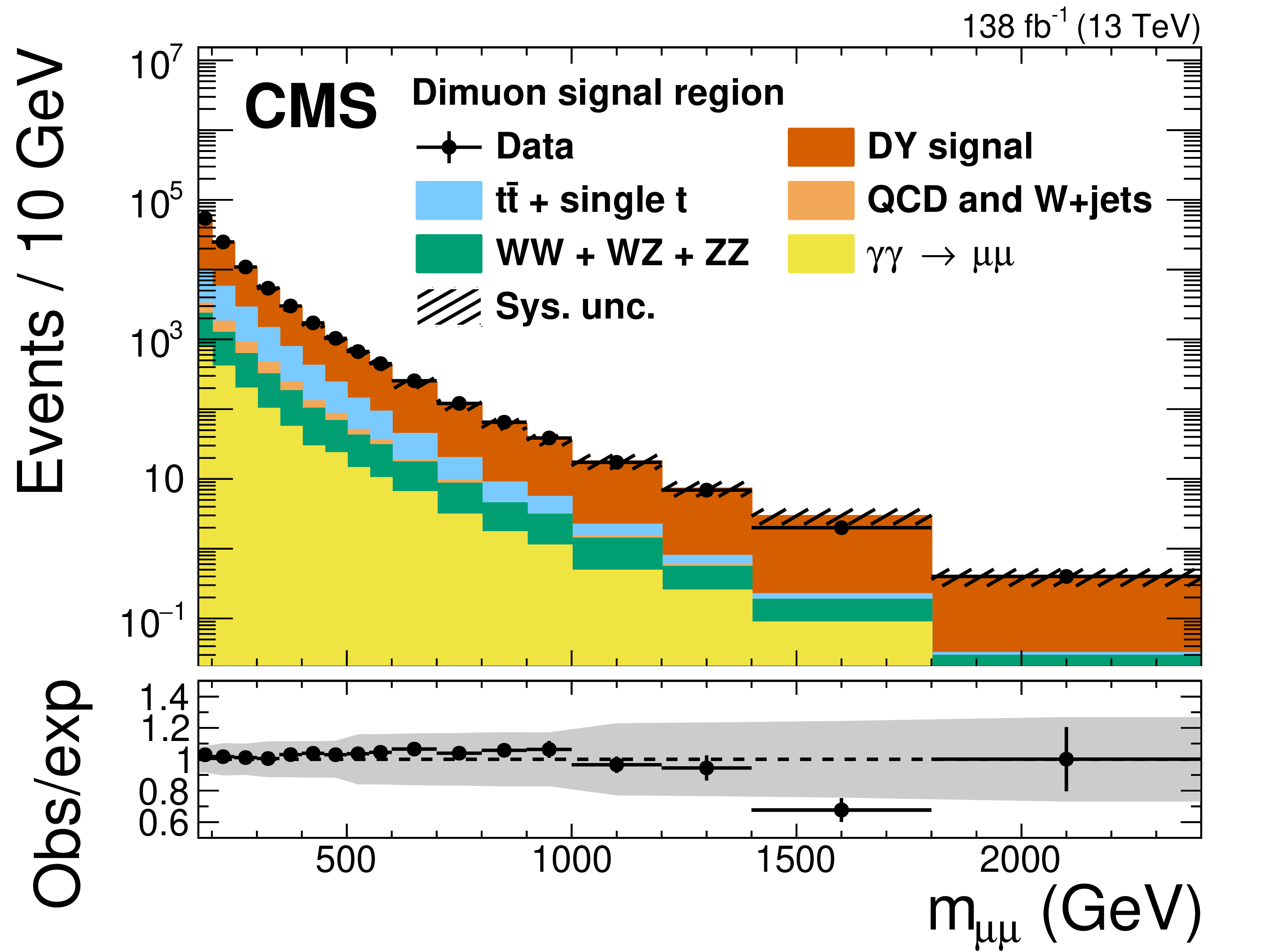
Figure 2-a:
A comparison of CMS data and expected signal and background dilepton invariant mass distributions. The plot shows the $ {{\mu}} {{\mu}}$ channel. The black points with error bars represent the data and their statistical uncertainties, whereas the combined signal and background expectation is shown as stacked histograms. The hatched band shows the systematic uncertainty in the expected signal and background yield. The sources of this uncertainty are discussed in Section 8. The lower panel shows the ratio of the data to the expectation. The gray bands represents the total uncertainty in the predicted yield. |
png pdf |
Figure 2-b:
A comparison of CMS data and expected signal and background ${\cos\theta _\mathrm {R}}$ dilepton rapidity distributions. The plot shows the ee channel. The black points with error bars represent the data and their statistical uncertainties, whereas the combined signal and background expectation is shown as stacked histograms. The hatched band shows the systematic uncertainty in the expected signal and background yield. The sources of this uncertainty are discussed in Section 8. The lower panel shows the ratio of the data to the expectation. The gray bands represents the total uncertainty in the predicted yield. |
png pdf |
Figure 2-c:
A comparison of CMS data and expected signal and background ${\cos\theta _\mathrm {R}}$ distributions. The plot shows the $ {{\mu}} {{\mu}}$ channel. The black points with error bars represent the data and their statistical uncertainties, whereas the combined signal and background expectation is shown as stacked histograms. The hatched band shows the systematic uncertainty in the expected signal and background yield. The sources of this uncertainty are discussed in Section 8. The lower panel shows the ratio of the data to the expectation. The gray bands represents the total uncertainty in the predicted yield. |

png pdf |
Figure 2-d:
A comparison of CMS data and expected signal and background ${\cos\theta _\mathrm {R}}$ distributions. The plot shows the ee channel. The black points with error bars represent the data and their statistical uncertainties, whereas the combined signal and background expectation is shown as stacked histograms. The hatched band shows the systematic uncertainty in the expected signal and background yield. The sources of this uncertainty are discussed in Section 8. The lower panel shows the ratio of the data to the expectation. The gray bands represents the total uncertainty in the predicted yield. |

png pdf |
Figure 2-e:
A comparison of CMS data and expected signal and background dilepton rapidity distributions. The plot shows the $ {{\mu}} {{\mu}}$ channel. The black points with error bars represent the data and their statistical uncertainties, whereas the combined signal and background expectation is shown as stacked histograms. The hatched band shows the systematic uncertainty in the expected signal and background yield. The sources of this uncertainty are discussed in Section 8. The lower panel shows the ratio of the data to the expectation. The gray bands represents the total uncertainty in the predicted yield. |
png pdf |
Figure 2-f:
A comparison of CMS data and expected signal and background dilepton rapidity distributions. The plot shows the ee channel. The black points with error bars represent the data and their statistical uncertainties, whereas the combined signal and background expectation is shown as stacked histograms. The hatched band shows the systematic uncertainty in the expected signal and background yield. The sources of this uncertainty are discussed in Section 8. The lower panel shows the ratio of the data to the expectation. The gray bands represents the total uncertainty in the predicted yield. |
png pdf |
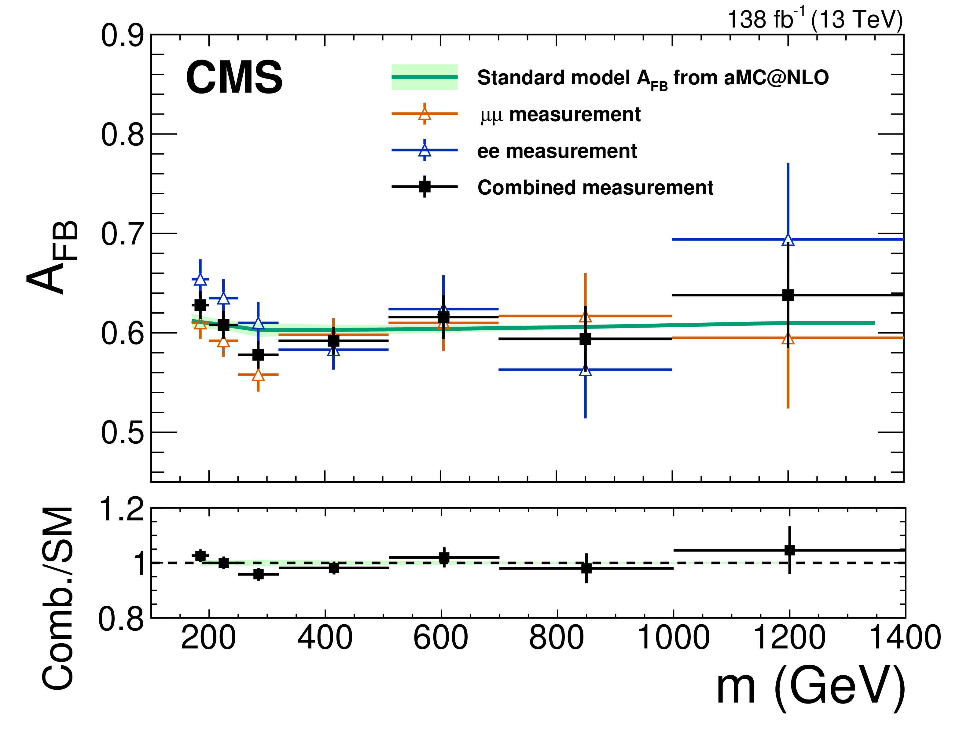
Figure 3:
Measurement of the DY forward-backward asymmetry as a function the dilepton mass compared with the MC predictions. The green line is the predicted value for ${A_\text {FB}}$ from the aMC@NLO simulation and the shaded green region its uncertainty. The blue, red, and black points and error bars represent the dimuon, dielectron, and combined measurements, respectively. Error bars on the measurements include both statistical and systematic components. The bottom panel shows the ratio between the combined measurement and the aMC@NLO prediction. In the bottom panel, the vertical error bars represent the uncertainty in the combined measurement and the shaded green band the uncertainty in the aMC@NLO prediction. |
png pdf |
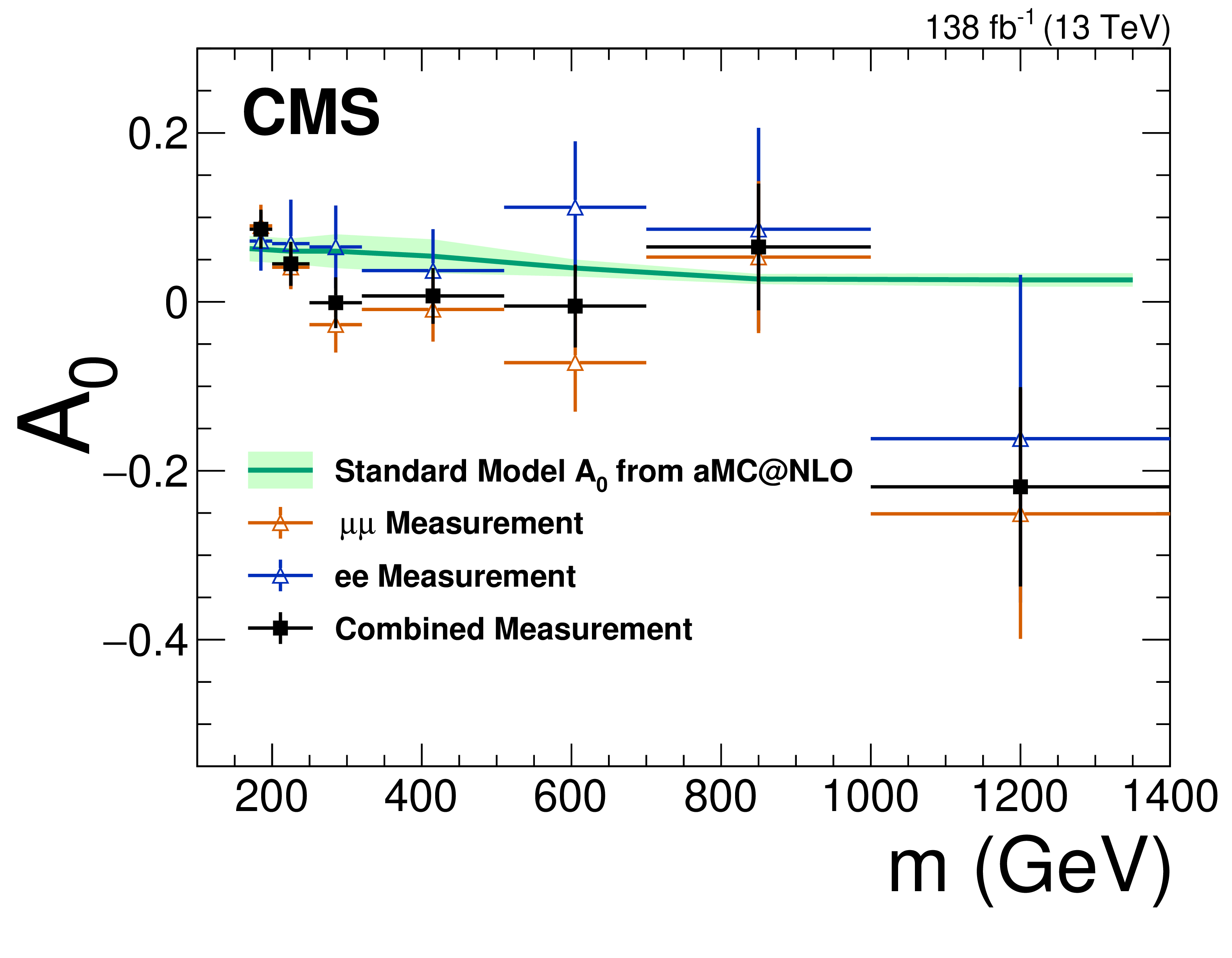
Figure 4:
Measurement of the DY forward-backward asymmetry as a function the dilepton mass compared with the MC predictions. The green line is the predicted value for ${A_\text {FB}}$ from the aMC@NLO simulation and the shaded green region its uncertainty. The blue, red, and black points and error bars represent the dimuon, dielectron, and combined measurements, respectively. Error bars on the measurements include both statistical and systematic components. |
png pdf |
Figure 5:
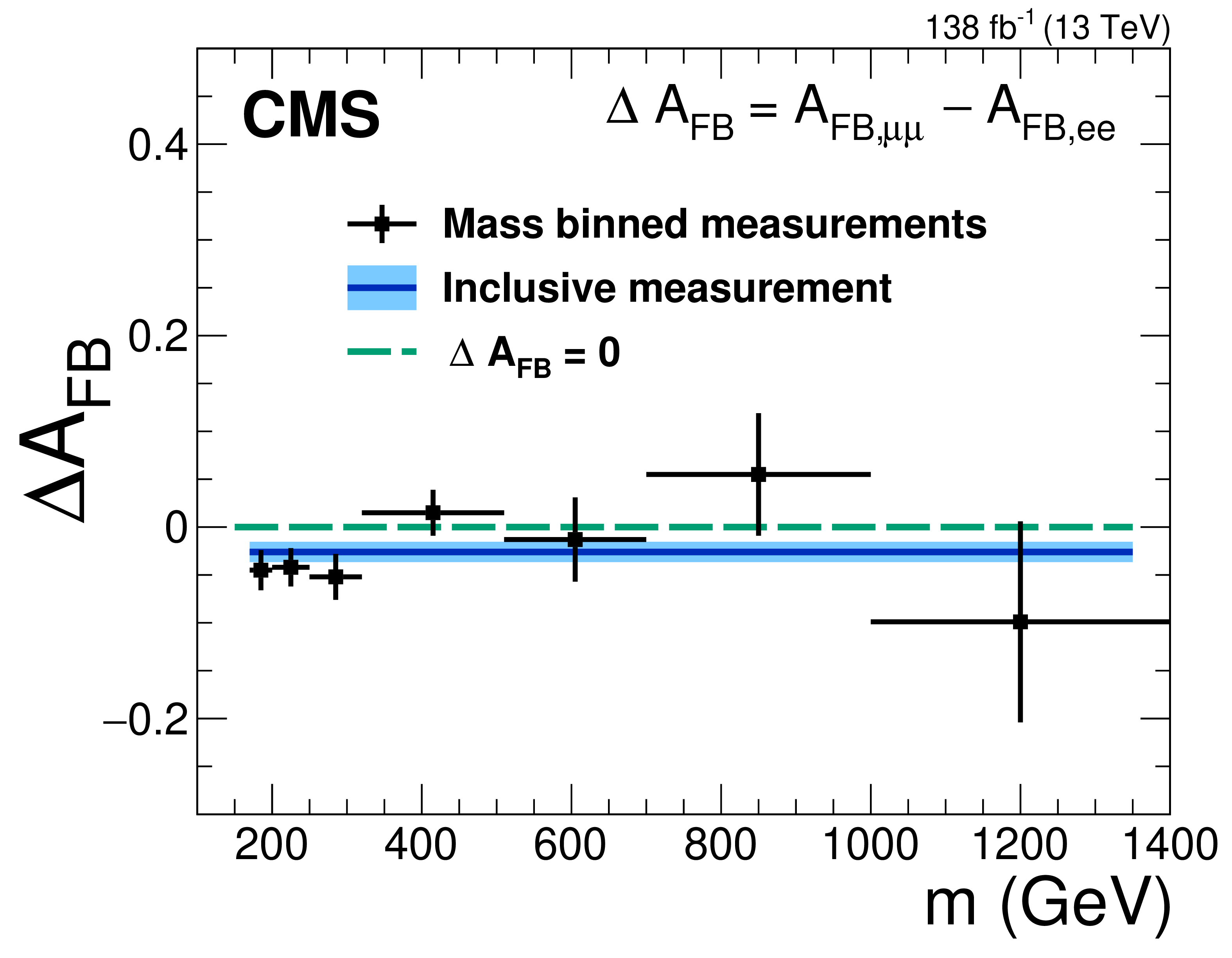
Measurement of the difference in forward-backward asymmetry between the dimuon and dielectron channels. The green line is drawn at zero, the predicted value for $\Delta {A_\text {FB}} $ assuming lepton flavor universality. The black points and error bars represent the measurements of $\Delta {A_\text {FB}} $ in different mass bins. The blue line and shaded light blue region represent the inclusive measurement of $\Delta {A_\text {FB}} $ and corresponding uncertainty. The error bars on the measurements and the shaded region include both statistical and systematic components. |
png pdf |
Figure 6:
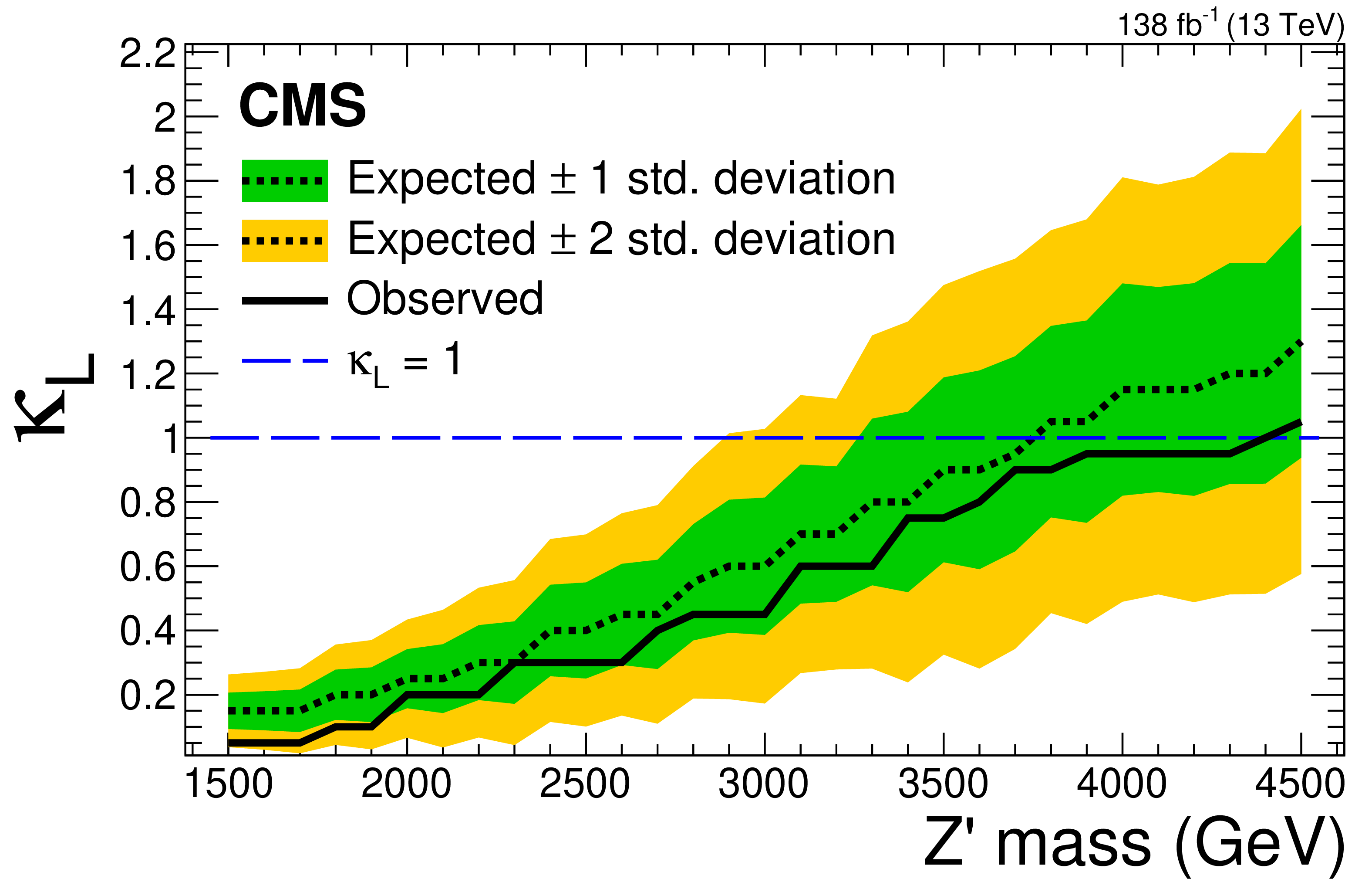
Exclusion limits at 95% CL on the coupling parameter $\kappa _\mathrm {L}$ for a Z' in the sequential standard model as a function of the Z' mass. The expected (observed) limit is shown by the dashed (solid) line. The inner and outer shaded areas around the expected limits show the 68% (green) and 95% (yellow) CL intervals, respectively. The dashed blue line shows $\kappa _{L} = $ 1 which corresponds to a Z' with exactly the same couplings as the SM Z boson. |

png pdf |
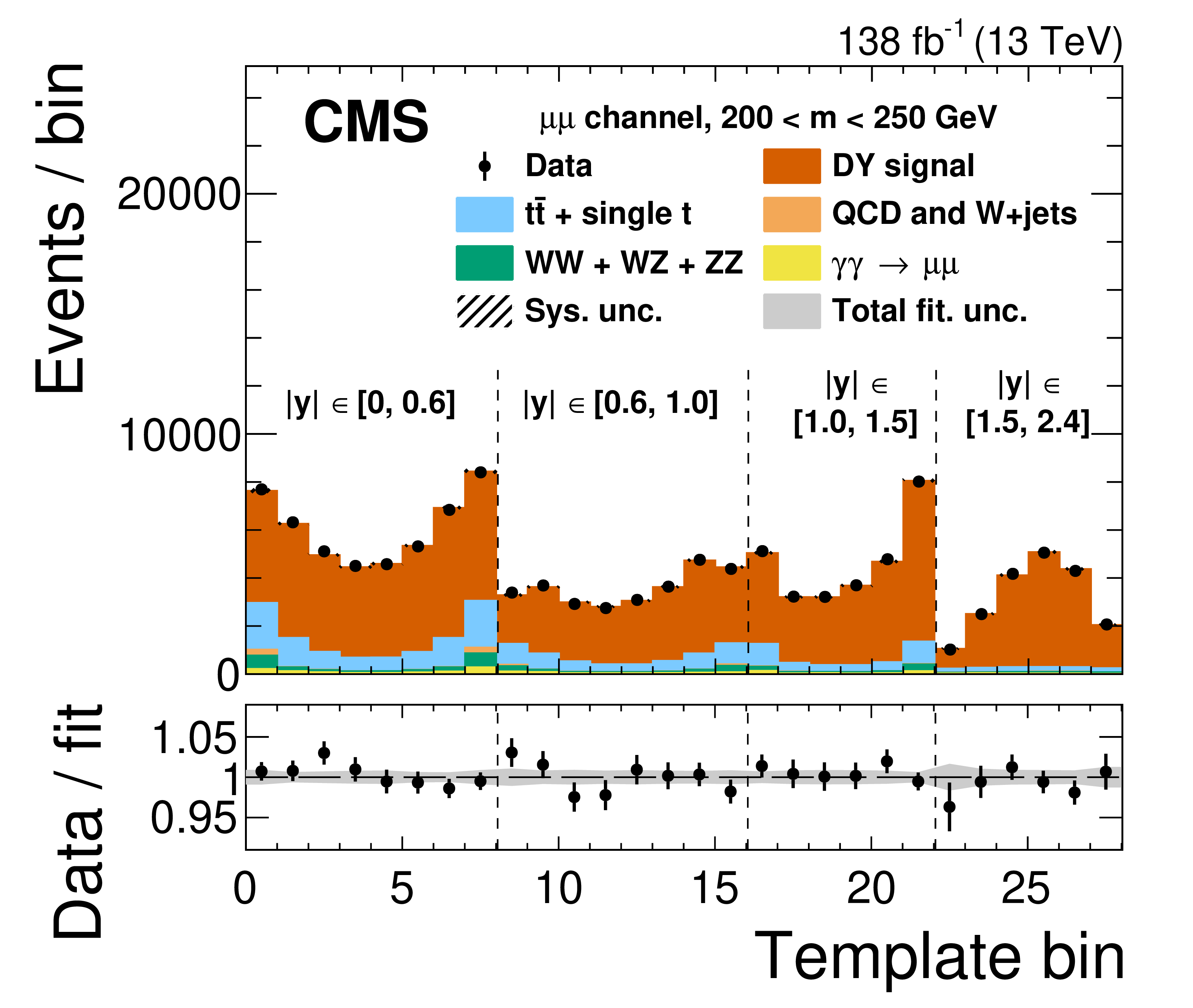
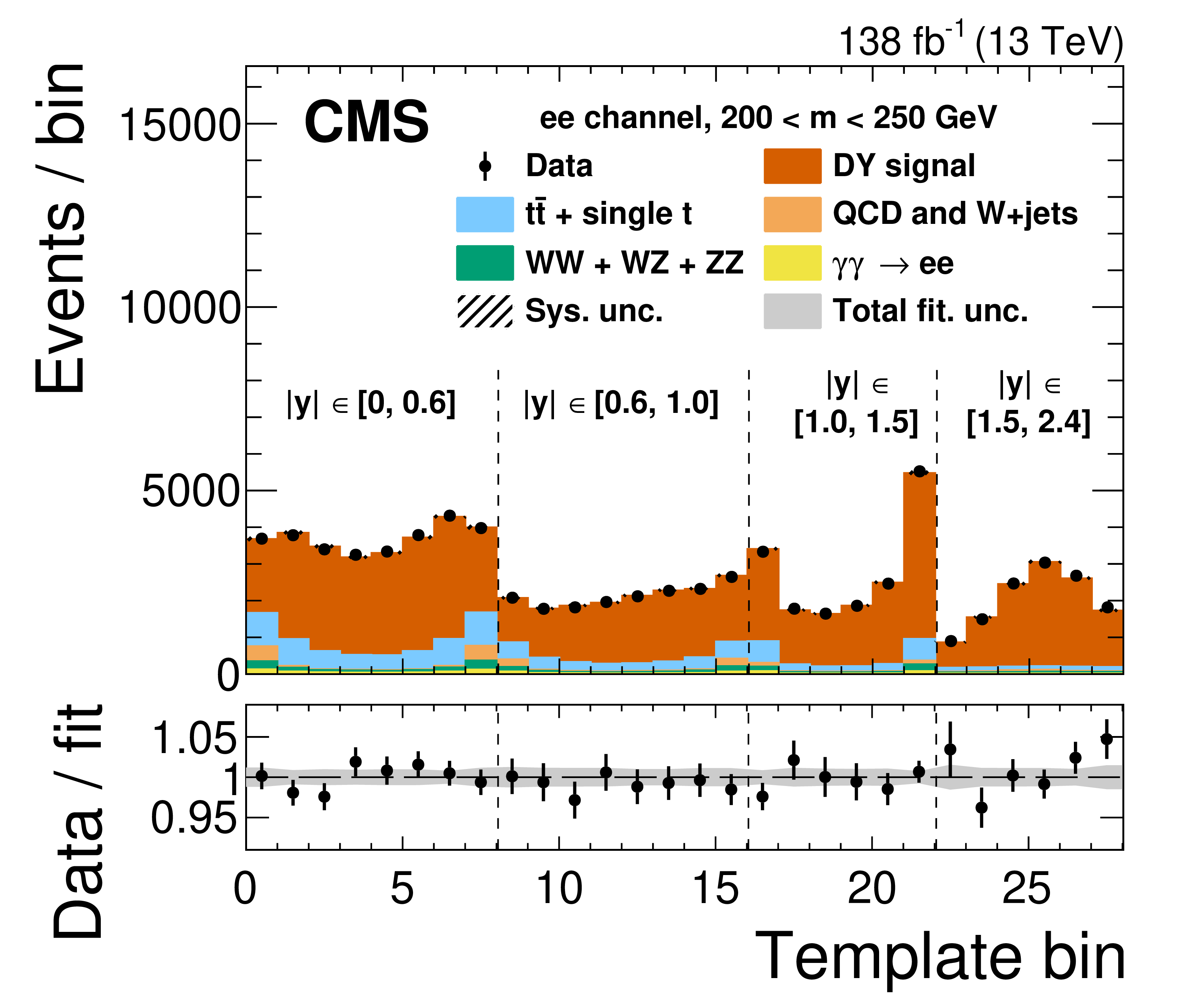
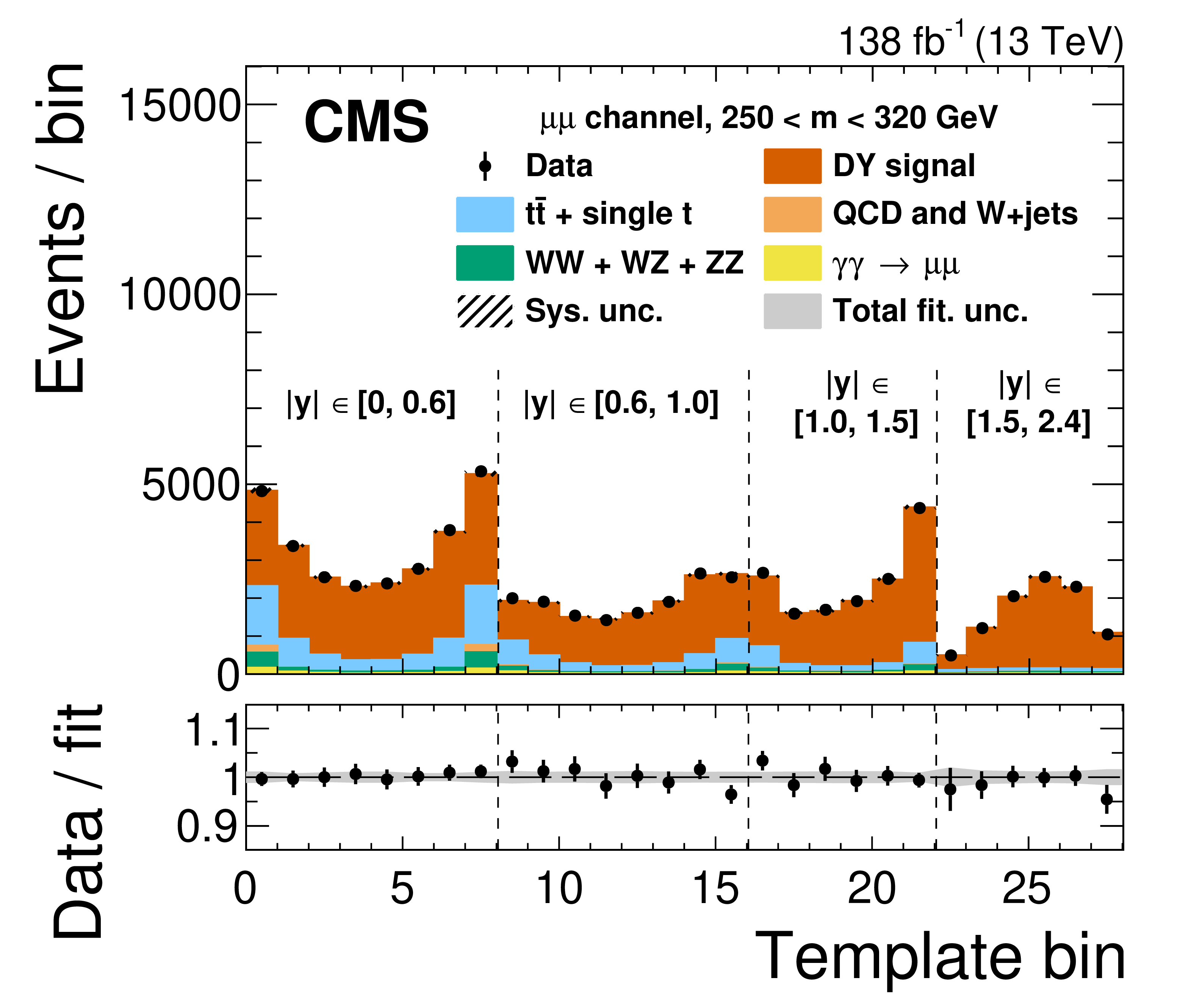
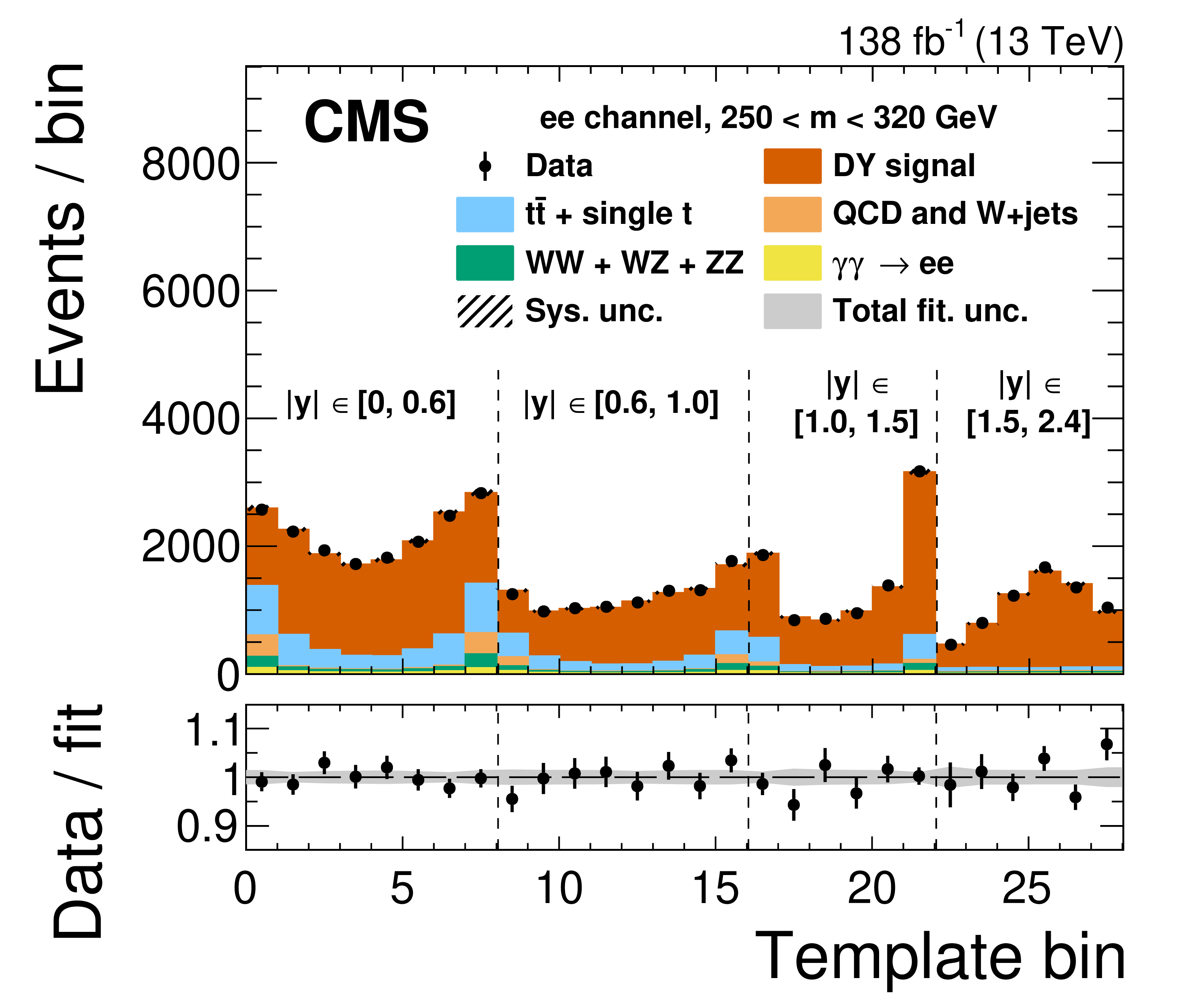
Figure 7:
The postfit distributions in the 170-200, 200-250 and 250-320 GeV mass bins are shown in upper, middle and lower rows, respectively. The left column is the $ {{\mu}} {{\mu}}$ channel, and the right column the ee channel. The contribution of the $ {\tau} {\tau} $ background is not visible on the scale of these plots and has been omitted. The 2D templates follow the ${\cos\theta _\mathrm {R}}$ and $ {| y |}$ binning defined in Section 7 but are presented here in one dimension, with the the dotted lines indicating the different $ {| y |}$ bins. The black points and error bars represent the data and their statistical uncertainties. The bottom panel in each figure shows the ratio between the number of events observed in data and the best fit value. The gray shaded region in the bottom panel shows the total uncertainty in the best fit result. |

png pdf |
Figure 7-a:
The postfit distributions in the 170-200 GeV mass bin, in the $ {{\mu}} {{\mu}}$ channel. The contribution of the $ {\tau} {\tau} $ background is not visible on the scale of these plots and has been omitted. The 2D templates follow the ${\cos\theta _\mathrm {R}}$ and $ {| y |}$ binning defined in Section 7 but are presented here in one dimension, with the the dotted lines indicating the different $ {| y |}$ bins. The black points and error bars represent the data and their statistical uncertainties. The bottom panel shows the ratio between the number of events observed in data and the best fit value. The gray shaded region in the bottom panel shows the total uncertainty in the best fit result. |
png pdf |
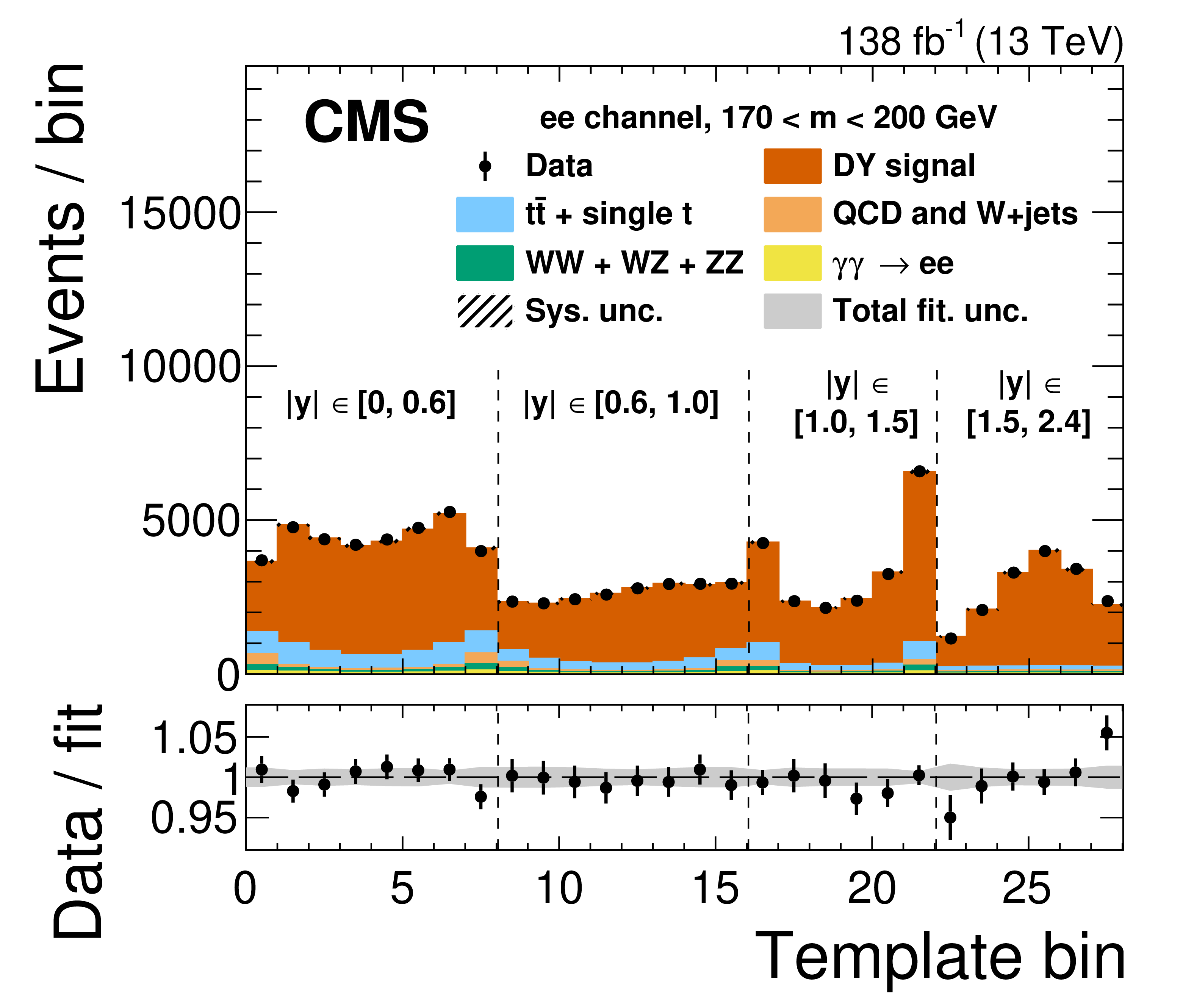
Figure 7-b:
The postfit distributions in the 170-200 GeV mass bin, in the ee channel. The contribution of the $ {\tau} {\tau} $ background is not visible on the scale of these plots and has been omitted. The 2D templates follow the ${\cos\theta _\mathrm {R}}$ and $ {| y |}$ binning defined in Section 7 but are presented here in one dimension, with the the dotted lines indicating the different $ {| y |}$ bins. The black points and error bars represent the data and their statistical uncertainties. The bottom panel shows the ratio between the number of events observed in data and the best fit value. The gray shaded region in the bottom panel shows the total uncertainty in the best fit result. |
png pdf |
Figure 7-c:
The postfit distributions in the 200-250 GeV mass bin, in the $ {{\mu}} {{\mu}}$ channel. The contribution of the $ {\tau} {\tau} $ background is not visible on the scale of these plots and has been omitted. The 2D templates follow the ${\cos\theta _\mathrm {R}}$ and $ {| y |}$ binning defined in Section 7 but are presented here in one dimension, with the the dotted lines indicating the different $ {| y |}$ bins. The black points and error bars represent the data and their statistical uncertainties. The bottom panel shows the ratio between the number of events observed in data and the best fit value. The gray shaded region in the bottom panel shows the total uncertainty in the best fit result. |
png pdf |
Figure 7-d:
The postfit distributions in the 200-250 GeV mass bin, in the ee channel. The contribution of the $ {\tau} {\tau} $ background is not visible on the scale of these plots and has been omitted. The 2D templates follow the ${\cos\theta _\mathrm {R}}$ and $ {| y |}$ binning defined in Section 7 but are presented here in one dimension, with the the dotted lines indicating the different $ {| y |}$ bins. The black points and error bars represent the data and their statistical uncertainties. The bottom panel shows the ratio between the number of events observed in data and the best fit value. The gray shaded region in the bottom panel shows the total uncertainty in the best fit result. |
png pdf |
Figure 7-e:
The postfit distributions in the 250-320 GeV mass bin, in the $ {{\mu}} {{\mu}}$ channel. The contribution of the $ {\tau} {\tau} $ background is not visible on the scale of these plots and has been omitted. The 2D templates follow the ${\cos\theta _\mathrm {R}}$ and $ {| y |}$ binning defined in Section 7 but are presented here in one dimension, with the the dotted lines indicating the different $ {| y |}$ bins. The black points and error bars represent the data and their statistical uncertainties. The bottom panel shows the ratio between the number of events observed in data and the best fit value. The gray shaded region in the bottom panel shows the total uncertainty in the best fit result. |
png pdf |
Figure 7-f:
The postfit distributions in the 250-320 GeV mass bin, in the ee channel. The contribution of the $ {\tau} {\tau} $ background is not visible on the scale of these plots and has been omitted. The 2D templates follow the ${\cos\theta _\mathrm {R}}$ and $ {| y |}$ binning defined in Section 7 but are presented here in one dimension, with the the dotted lines indicating the different $ {| y |}$ bins. The black points and error bars represent the data and their statistical uncertainties. The bottom panel shows the ratio between the number of events observed in data and the best fit value. The gray shaded region in the bottom panel shows the total uncertainty in the best fit result. |
png pdf |
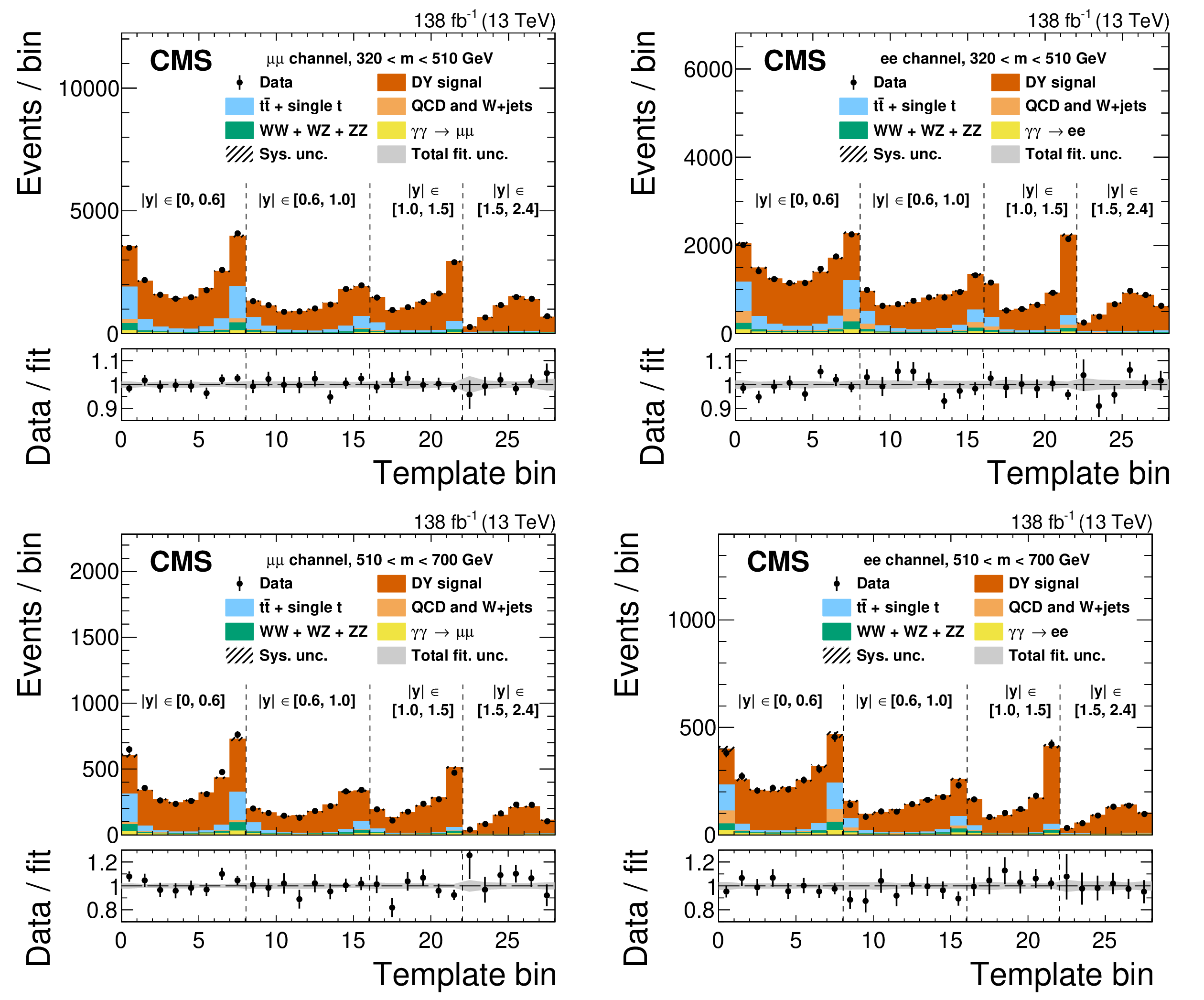
Figure 8:
The postfit distributions in the 320-510 and 510-700 GeV mass bins are shown in the upper and lower rows, respectively. The left column is the $ {{\mu}} {{\mu}}$ channel, and the right column the ee channel. The contribution of the $ {\tau} {\tau} $ background is not visible on the scale of these plots and has been omitted. The 2D templates follow the ${\cos\theta _\mathrm {R}}$ and $ {| y |}$ binning defined in Section 7 but are presented here in one dimension, with the the dotted lines indicating the different $ {| y |}$ bins. The black points and error bars represent the data and their statistical uncertainties. The bottom panel in each figure shows the ratio between the number of events observed in data and the best fit value. The gray shaded region in the bottom panel shows the total uncertainty in the best fit result. |

png pdf |
Figure 8-a:
The postfit distributions in the 320-510 GeV mass bin, in the $ {{\mu}} {{\mu}}$ channel. The contribution of the $ {\tau} {\tau} $ background is not visible on the scale of these plots and has been omitted. The 2D templates follow the ${\cos\theta _\mathrm {R}}$ and $ {| y |}$ binning defined in Section 7 but are presented here in one dimension, with the the dotted lines indicating the different $ {| y |}$ bins. The black points and error bars represent the data and their statistical uncertainties. The bottom panel shows the ratio between the number of events observed in data and the best fit value. The gray shaded region in the bottom panel shows the total uncertainty in the best fit result. |
png pdf |
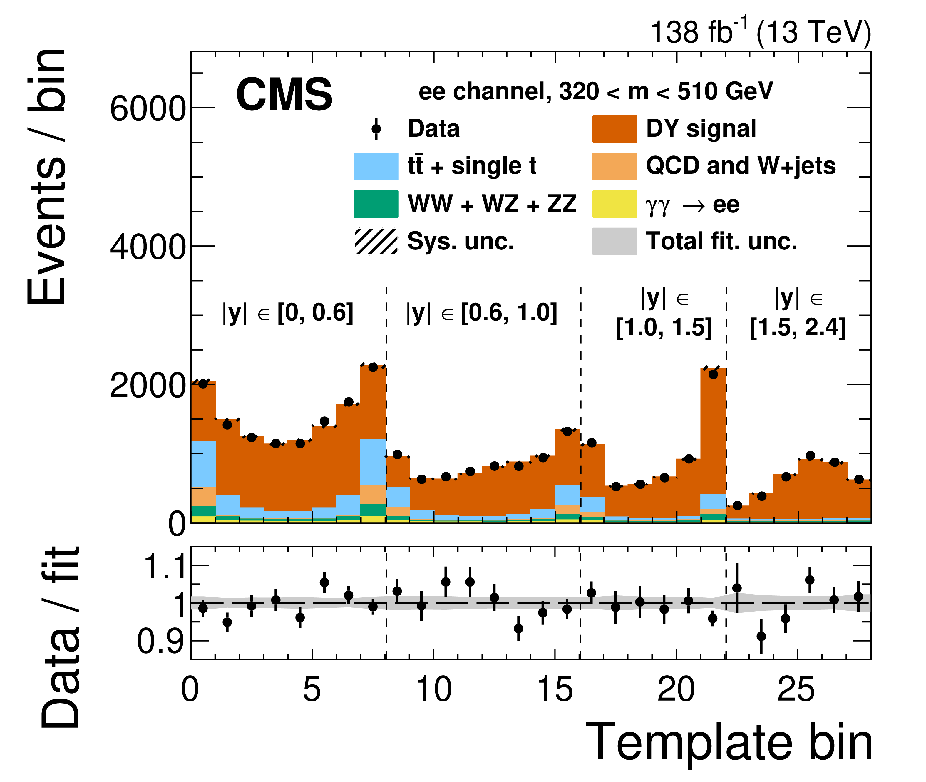
Figure 8-b:
The postfit distributions in the 320-510 GeV mass bin, in the ee channel. The contribution of the $ {\tau} {\tau} $ background is not visible on the scale of these plots and has been omitted. The 2D templates follow the ${\cos\theta _\mathrm {R}}$ and $ {| y |}$ binning defined in Section 7 but are presented here in one dimension, with the the dotted lines indicating the different $ {| y |}$ bins. The black points and error bars represent the data and their statistical uncertainties. The bottom panel shows the ratio between the number of events observed in data and the best fit value. The gray shaded region in the bottom panel shows the total uncertainty in the best fit result. |
png pdf |
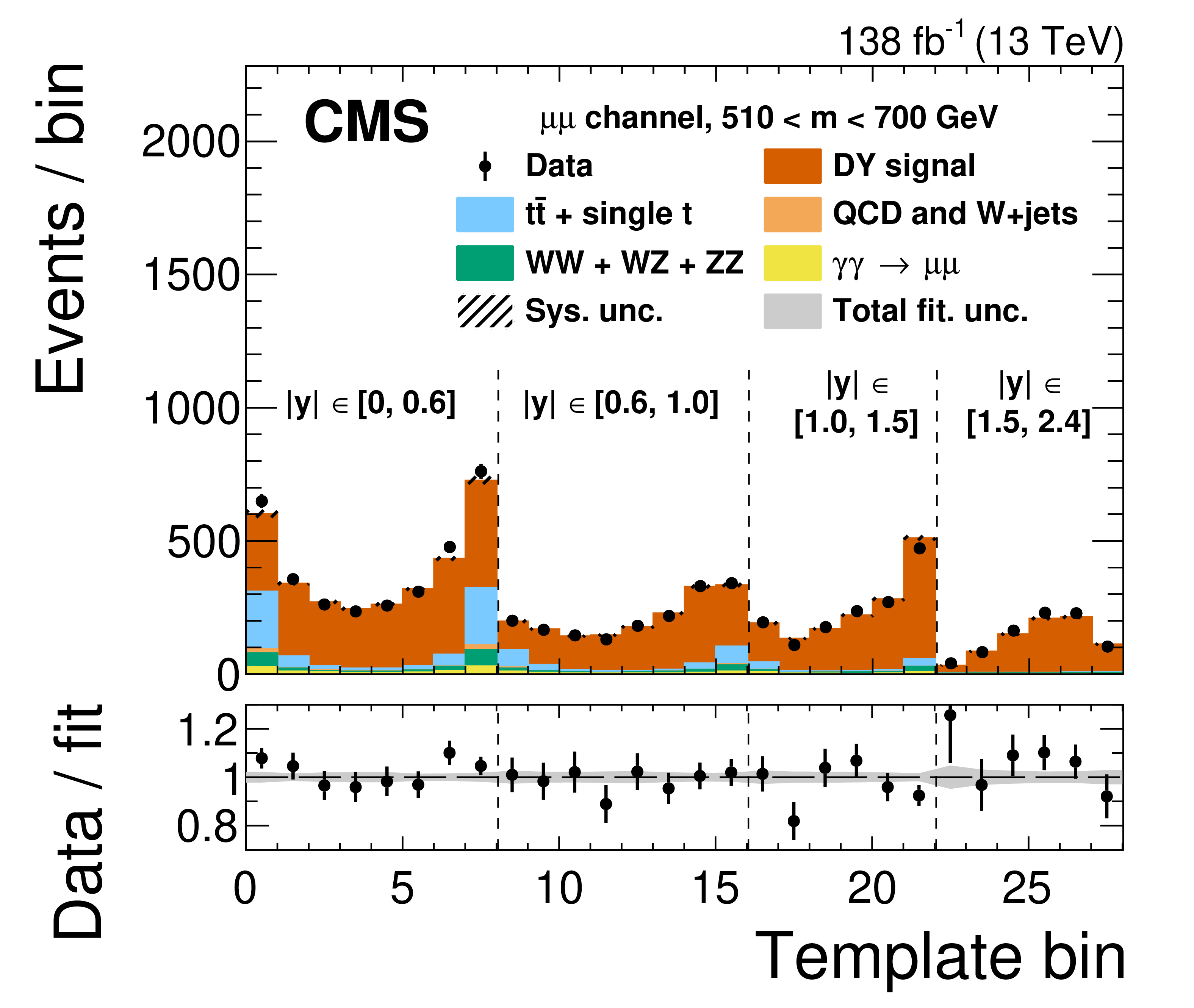
Figure 8-c:
The postfit distributions in the 510-700 GeV mass bin, in the $ {{\mu}} {{\mu}}$ channel. The contribution of the $ {\tau} {\tau} $ background is not visible on the scale of these plots and has been omitted. The 2D templates follow the ${\cos\theta _\mathrm {R}}$ and $ {| y |}$ binning defined in Section 7 but are presented here in one dimension, with the the dotted lines indicating the different $ {| y |}$ bins. The black points and error bars represent the data and their statistical uncertainties. The bottom panel shows the ratio between the number of events observed in data and the best fit value. The gray shaded region in the bottom panel shows the total uncertainty in the best fit result. |
png pdf |
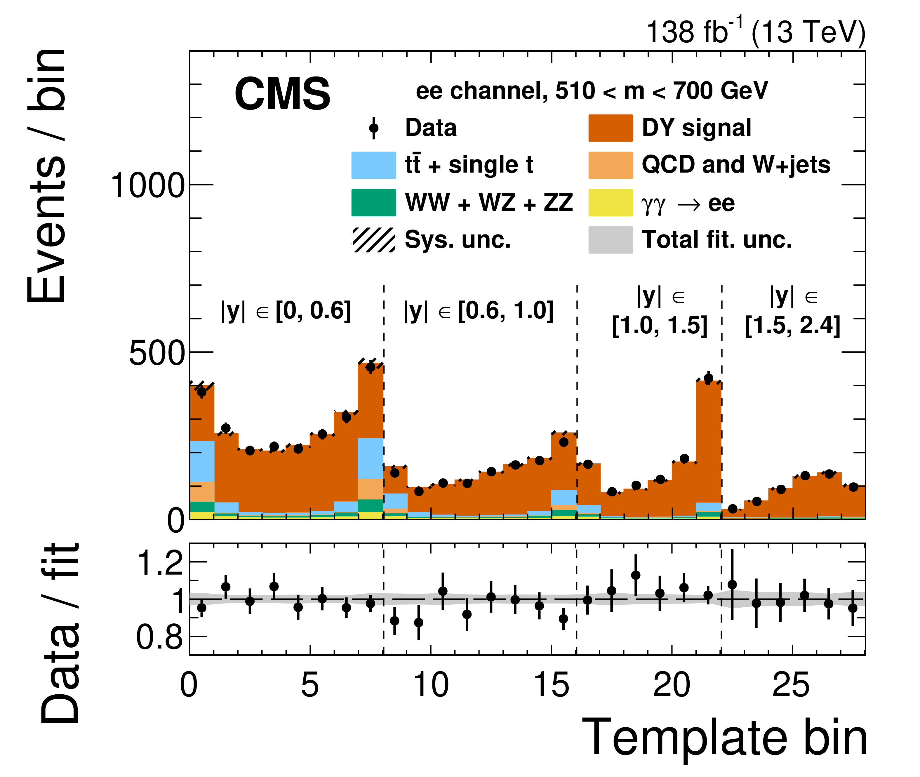
Figure 8-d:
The postfit distributions in the 510-700 GeV mass bin, in the ee channel. The contribution of the $ {\tau} {\tau} $ background is not visible on the scale of these plots and has been omitted. The 2D templates follow the ${\cos\theta _\mathrm {R}}$ and $ {| y |}$ binning defined in Section 7 but are presented here in one dimension, with the the dotted lines indicating the different $ {| y |}$ bins. The black points and error bars represent the data and their statistical uncertainties. The bottom panel shows the ratio between the number of events observed in data and the best fit value. The gray shaded region in the bottom panel shows the total uncertainty in the best fit result. |
png pdf |
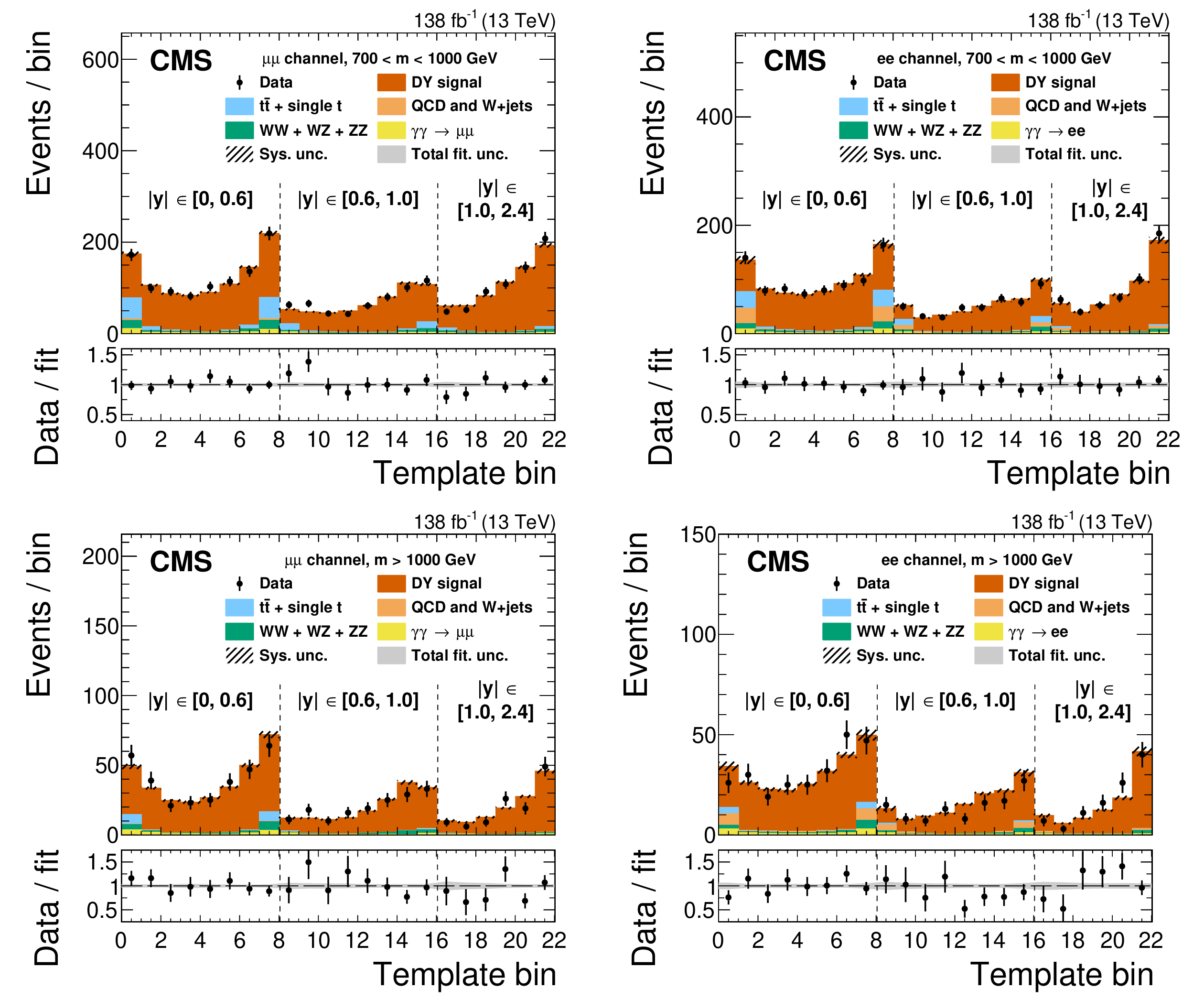
Figure 9:
The postfit distributions in the 700-1000 and $ > $1000 GeV mass bins are shown in the upper and lower rows, respectively. The left plot is the $ {{\mu}} {{\mu}}$ channel, and the right plot the ee channel. The contribution of the $ {\tau} {\tau} $ background is not visible on the scale of these plots and has been omitted. The 2D templates follow the ${\cos\theta _\mathrm {R}}$ and $ {| y |}$ binning defined in Section 7 but are presented here in one dimension, with the the dotted lines indicating the different $ {| y |}$ bins. The black points and error bars represent the data and their statistical uncertainties. The bottom panel in each figure shows the ratio between the number of events observed in data and the best fit value. The gray shaded region in the bottom panel shows the total uncertainty in the best fit result. |
png pdf |
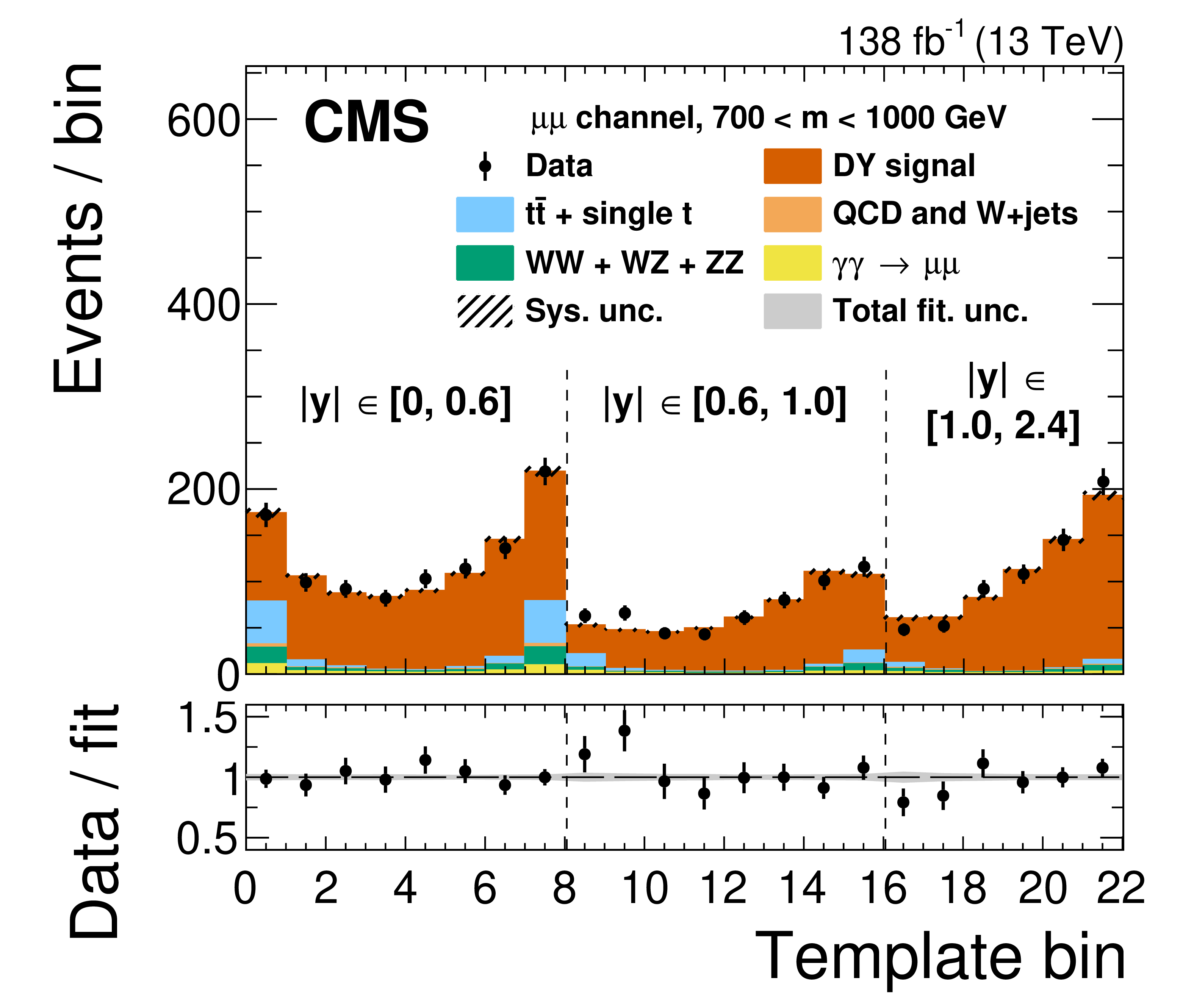
Figure 9-a:
The postfit distributions in the 700-1000 GeV mass bin, in the $ {{\mu}} {{\mu}}$ channel. The contribution of the $ {\tau} {\tau} $ background is not visible on the scale of these plots and has been omitted. The 2D templates follow the ${\cos\theta _\mathrm {R}}$ and $ {| y |}$ binning defined in Section 7 but are presented here in one dimension, with the the dotted lines indicating the different $ {| y |}$ bins. The black points and error bars represent the data and their statistical uncertainties. The bottom panel shows the ratio between the number of events observed in data and the best fit value. The gray shaded region in the bottom panel shows the total uncertainty in the best fit result. |
png pdf |
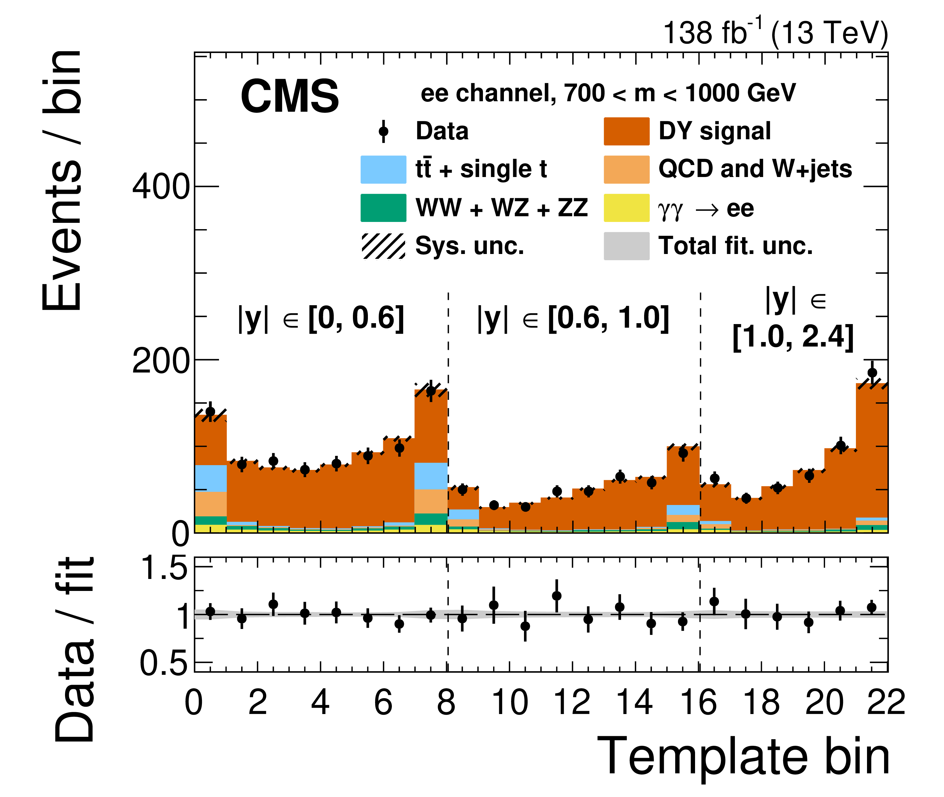
Figure 9-b:
The postfit distributions in the 700-1000 GeV mass bin, in the ee channel. The contribution of the $ {\tau} {\tau} $ background is not visible on the scale of these plots and has been omitted. The 2D templates follow the ${\cos\theta _\mathrm {R}}$ and $ {| y |}$ binning defined in Section 7 but are presented here in one dimension, with the the dotted lines indicating the different $ {| y |}$ bins. The black points and error bars represent the data and their statistical uncertainties. The bottom panel shows the ratio between the number of events observed in data and the best fit value. The gray shaded region in the bottom panel shows the total uncertainty in the best fit result. |

png pdf |
Figure 9-c:
The postfit distributions in the $ > $1000 GeV mass bin, in the $ {{\mu}} {{\mu}}$ channel. The contribution of the $ {\tau} {\tau} $ background is not visible on the scale of these plots and has been omitted. The 2D templates follow the ${\cos\theta _\mathrm {R}}$ and $ {| y |}$ binning defined in Section 7 but are presented here in one dimension, with the the dotted lines indicating the different $ {| y |}$ bins. The black points and error bars represent the data and their statistical uncertainties. The bottom panel shows the ratio between the number of events observed in data and the best fit value. The gray shaded region in the bottom panel shows the total uncertainty in the best fit result. |
png pdf |
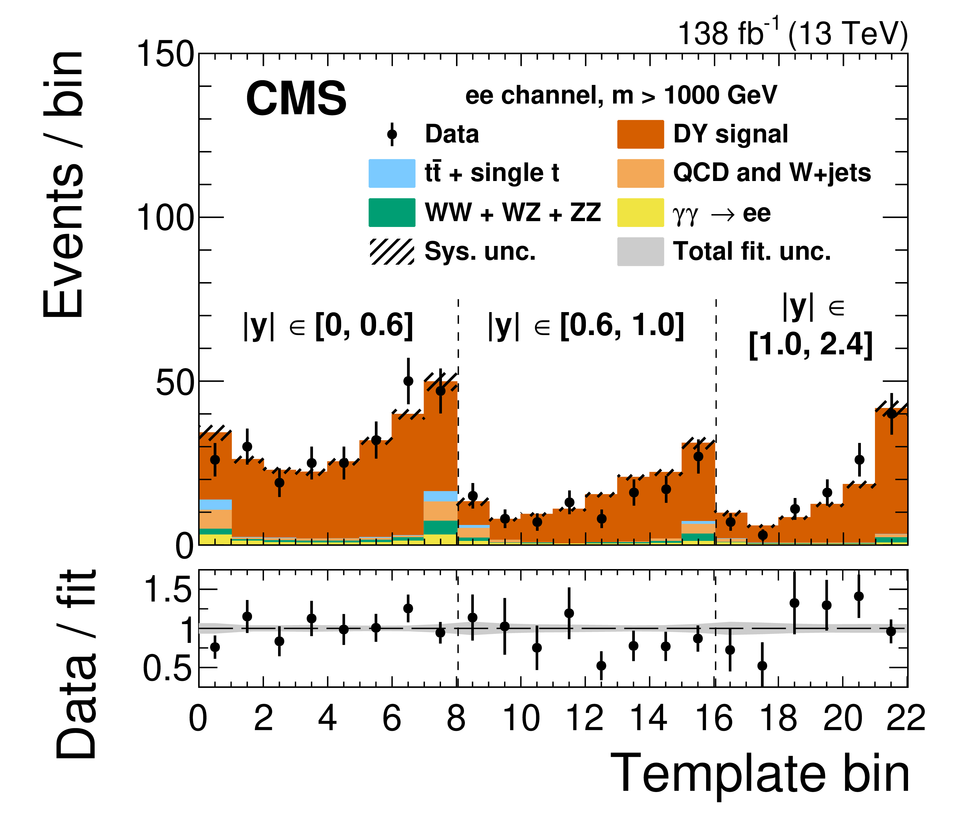
Figure 9-d:
The postfit distributions in the $ > $1000 GeV mass bin, in the ee channel. The contribution of the $ {\tau} {\tau} $ background is not visible on the scale of these plots and has been omitted. The 2D templates follow the ${\cos\theta _\mathrm {R}}$ and $ {| y |}$ binning defined in Section 7 but are presented here in one dimension, with the the dotted lines indicating the different $ {| y |}$ bins. The black points and error bars represent the data and their statistical uncertainties. The bottom panel shows the ratio between the number of events observed in data and the best fit value. The gray shaded region in the bottom panel shows the total uncertainty in the best fit result. |
| Tables | |
png pdf |
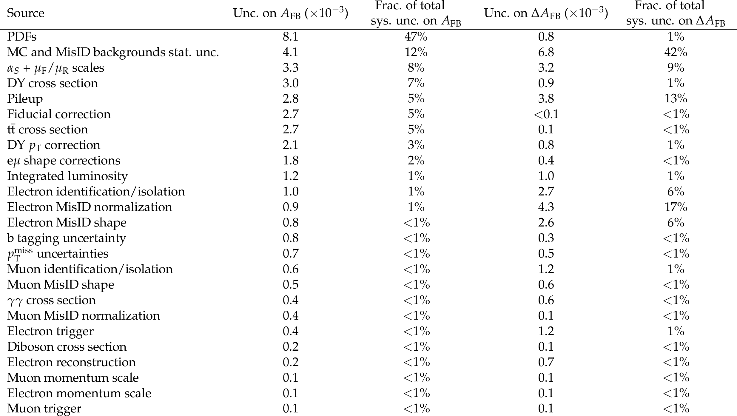
Table 1:
A comparison of the magnitude of the different sources of systematic uncertainty for the measurement of ${A_\text {FB}}$ when combining the muon and electron channels and for the measurement of $\Delta {A_\text {FB}} $. Results for the 170-200 GeV mass bin are shown because that is the mass bin in which the systematic uncertainty has the largest contribution to the total uncertainty; the results for other mass bins are similar. Results are also reported as a fraction of the overall systematic uncertainty for the measurement of ${A_\text {FB}}$ and $\Delta {A_\text {FB}} $. Sources are listed in order of the size of their contribution to the uncertainty in ${A_\text {FB}}$. |
png pdf |
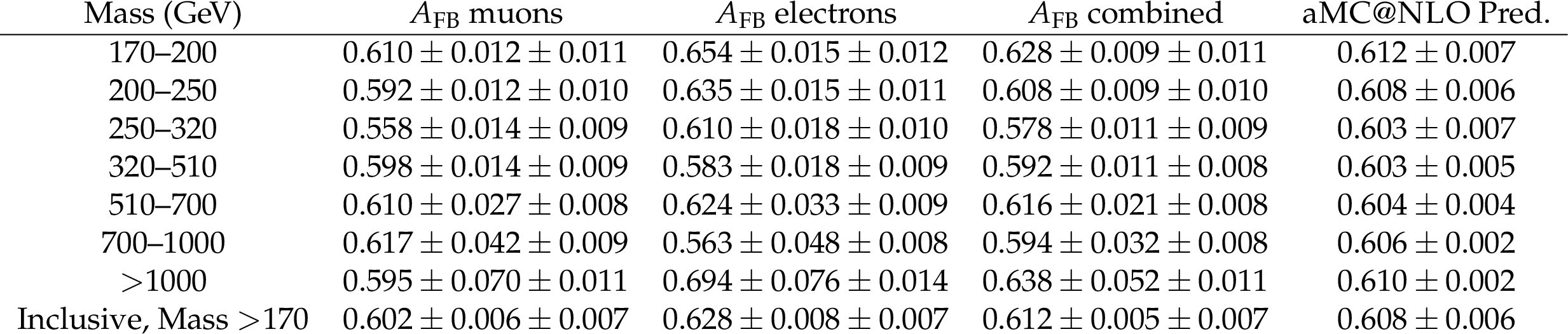
Table 2:
Results for the measurement of ${A_\text {FB}}$ from the maximum likelihood fit to data in different dilepton mass bins in the different channels as well as an inclusive measurement across all mass bins. The first and second uncertainties listed with each measurement are statistical and systematic, respectively. |
png pdf |
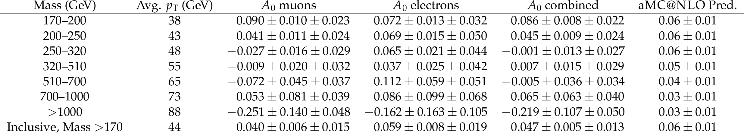
Table 3:
Results for the measurement of ${A_{0}}$ from the maximum likelihood fit to data in different dilepton mass bins in the different channels as well as an inclusive measurement across all mass bins. The first and second uncertainties listed with each measurement are statistical and systematic, respectively. To help in the interpretation of these results, we also list the average dilepton $ {p_{\mathrm {T}}} $ of the data events in each mass bin. |
png pdf |
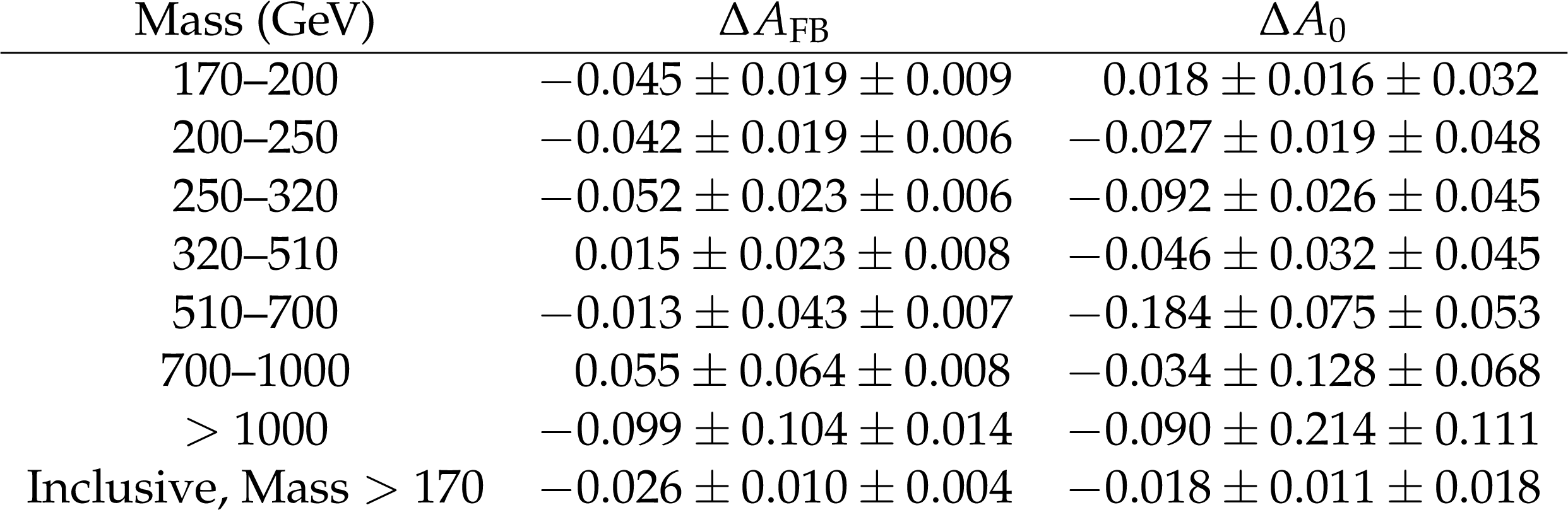
Table 4:
Results for the measurement of $\Delta {A_\text {FB}} $ and $\Delta {A_{0}} $ between the muon and electron channels from the maximum likelihood fit to data in different dilepton mass bins as well as an inclusive measurement across all mass bins. The first and second uncertainties listed with each measurement are statistical and systematic, respectively. |

png pdf |
Table 5:
The fraction of photon-induced background as compared with the total amount of DY signal plus photon-induced events ($N_{{\gamma} {\gamma}}/(N_{{\gamma} {\gamma}} + N_\mathrm {DY})$) in different dilepton mass bins. These numbers are averaged across the different years and channels. |
| Summary |
| The CMS detector at the LHC has been used to measure the Drell-Yan forward-backward asymmetry (${A_\text{FB}}$) and the angular coefficient $A_{0}$ as functions of dilepton mass for muon and electron pairs with invariant mass above 170 GeV. The measurement is performed using proton-proton collision data collected in 2016-2018 at $\sqrt{s} = $ 13 TeV with an integrated luminosity of 138 fb$^{-1}$ using a template fitting approach. The combined dimuon and dielectron ${A_\text{FB}}$ measurements show good agreement with the standard model predictions across the full mass range. An inclusive measurement across the full mass range yields an ${A_\text{FB}}$ of 0.599 $\pm$ 0.005 (stat) $\pm$ 0.007 (syst) and an $A_{0}$ of 0.047 $\pm$ 0.005 (stat) $\pm$ 0.013 (syst). As a test of lepton flavor universality, the difference between the dimuon and dielectron ${A_\text{FB}}\mathrm{s}$ is measured and found to agree with zero to within 2.4 standard deviations. Using the combined ${A_\text{FB}}$ measurements, limits are set on the existence of additional gauge bosons. For a Z' boson in the canonical sequential standard model, masses of $m_{\mathrm{Z'}} < $ 4.4 TeV are excluded at 95% confidence level. |
| References | ||||
| 1 | D. London and J. Rosner | Extra gauge bosons in E$ _6 $ | PRD 34 (1986) 1530 | |
| 2 | J. Rosner | Off-peak lepton asymmetries from new Z's | PRD 35 (1987) 2244 | |
| 3 | J. Rosner | Forward-backward asymmetries in hadronically produced lepton pairs | PRD 54 (1996) 1078 | hep-ph/9512299 |
| 4 | A. Bodek and U. Baur | Implications of a 300-500 GeV/$ c^2$ Z' boson on $ p\bar{p} $ collider data at $ \sqrt{s}= $ 1.8 TeV | EPJC 21 (2001) 607 | hep-ph/0102160 |
| 5 | T. G. Rizzo | Z' Phenomenology and the LHC | in Theoretical Advanced Study Institute in Elementary Particle Physics: Exploring New Frontiers Using Colliders and Neutrinos 10 | hep-ph/0610104 |
| 6 | E. Accomando et al. | Forward-backward asymmetry as a discovery tool for Z' bosons at the LHC | JHEP 01 (2016) 127 | 1503.02672 |
| 7 | E. Accomando et al. | Production of Z'-boson resonances with large width at the LHC | PLB 803 (2020) 135293 | 1910.13759 |
| 8 | E. Eichten, K. D. Lane, and M. E. Peskin | New tests for quark and lepton substructure | PRL 50 (1983) 811 | |
| 9 | J. L. Hewett | Indirect collider signals for extra dimensions | PRL 82 (1999) 4765 | hep-ph/9811356 |
| 10 | C. Gross, O. Lebedev, and J. M. No | Drell-Yan constraints on new electroweak states: LHC as a pp $ \to \ell^+ \ell^- $ precision machine | MPLA 32 (2017) 1750094 | 1602.03877 |
| 11 | R. M. Capdevilla, A. Delgado, A. Martin, and N. Raj | Characterizing dark matter at the LHC in Drell-Yan events | PRD 97 (2018) 035016 | 1709.00439 |
| 12 | N. Raj | Anticipating nonresonant new physics in dilepton angular spectra at the LHC | PRD 95 (2017) 015011 | 1610.03795 |
| 13 | LHCb Collaboration | Test of lepton universality with $ B^{0} \rightarrow K^{*0}\ell^{+}\ell^{-} $ decays | JHEP 08 (2017) 055 | 1705.05802 |
| 14 | LHCb Collaboration | Search for lepton-universality violation in $ B^+\to K^+\ell^+\ell^- $ decays | PRL 122 (2019) 191801 | 1903.09252 |
| 15 | LHCb Collaboration | Test of lepton universality in beauty-quark decays | 2103.11769 | |
| 16 | B. C. Allanach | $ \mathrm{ U(1)_{B_3-L_2} }$ explanation of the neutral current B-anomalies | EPJC 81 (2021) 56 | 2009.02197 |
| 17 | D. Bečirević, N. Košnik, O. Sumensari, and R. Zukanovich Funchal | Palatable leptoquark scenarios for lepton flavor violation in exclusive $ b\to s\ell_1\ell_2 $ modes | JHEP 11 (2016) 035 | 1608.07583 |
| 18 | A. Greljo and D. Marzocca | High-$ p_{\mathrm{T}} $ dilepton tails and flavor physics | EPJC 77 (2017) 548 | 1704.09015 |
| 19 | E. Mirkes | Angular decay distribution of leptons from W bosons at NLO in hadronic collisions | NPB 387 (1992) 3 | |
| 20 | E. Mirkes and J. Ohnemus | Angular distributions of Drell-Yan lepton pairs at the Tevatron: Order $ \alpha-s^{2} $ corrections and Monte Carlo studies | PRD 51 (1995) 4891 | hep-ph/9412289 |
| 21 | ATLAS Collaboration | Search for high-mass dilepton resonances using 139 fb$ ^{-1} $ of pp collision data collected at $ \sqrt{s}= $ 13 TeV with the ATLAS detector | PLB 796 (2019) 68 | 1903.06248 |
| 22 | CMS Collaboration | Search for resonant and nonresonant new phenomena in high-mass dilepton final states at $ \sqrt{s} = $ 13 TeV | JHEP 07 (2021) 208 | CMS-EXO-19-019 2103.02708 |
| 23 | J. Collins and D. Soper | Angular distribution of dileptons in high-energy hadron collisions | PRD 16 (1977) 2219 | |
| 24 | CMS Collaboration | Forward-backward asymmetry of Drell-Yan lepton pairs in pp collisions at $ \sqrt{s} = $ 7 TeV | PLB 718 (2013) 752 | |
| 25 | CMS Collaboration | Forward-backward asymmetry of Drell-Yan lepton pairs in pp collisions at $ \sqrt{s} = $ 8 TeV | EPJC 76 (2016) 325 | |
| 26 | ATLAS Collaboration | Measurement of the forward-backward asymmetry of electron and muon pair-production in pp collisions at $ \sqrt{s} = $ 7 TeV with the ATLAS detector | JHEP 09 (2015) 049 | 1503.03709 |
| 27 | CMS Collaboration | Measurement of the weak mixing angle using the forward-backward asymmetry of Drell-Yan events in pp collisions at 8 TeV | EPJC 78 (2018) 701 | CMS-SMP-16-007 1806.00863 |
| 28 | A. Bodek | A simple event weighting technique for optimizing the measurement of the forward-backward asymmetry of Drell-Yan dilepton pairs at hadron colliders | EPJC 67 (2010) 321 | 0911.2850 |
| 29 | CMS Collaboration | The CMS experiment at the CERN LHC | JINST 3 (2008) S08004 | CMS-00-001 |
| 30 | CMS Collaboration | Performance of the CMS Level-1 trigger in proton-proton collisions at $ \sqrt{s} = $ 13 TeV | JINST 15 (2020) P10017 | CMS-TRG-17-001 2006.10165 |
| 31 | CMS Collaboration | The CMS trigger system | JINST 12 (2017) P01020 | CMS-TRG-12-001 1609.02366 |
| 32 | CMS Collaboration | Particle-flow reconstruction and global event description with the CMS detector | JINST 12 (2017) P10003 | CMS-PRF-14-001 1706.04965 |
| 33 | M. Cacciari, G. P. Salam, and G. Soyez | The anti-$ {k_{\mathrm{T}}} $ jet clustering algorithm | JHEP 04 (2008) 063 | 0802.1189 |
| 34 | M. Cacciari, G. P. Salam, and G. Soyez | FastJet user manual | EPJC 72 (2012) 1896 | 1111.6097 |
| 35 | CMS Collaboration | Performance of the CMS muon detector and muon reconstruction with proton-proton collisions at $ \sqrt{s} = $ 13 TeV | JINST 13 (2018) P06015 | CMS-MUO-16-001 1804.04528 |
| 36 | CMS Collaboration | Electron and photon reconstruction and identification with the CMS experiment at the CERN LHC | JINST 16 (2021) P05014 | CMS-EGM-17-001 2012.06888 |
| 37 | CMS Collaboration | Pileup mitigation at CMS in 13 TeV data | JINST 15 (2020) P09018 | CMS-JME-18-001 2003.00503 |
| 38 | CMS Collaboration | Jet energy scale and resolution in the CMS experiment in pp collisions at 8 TeV | JINST 12 (2017) P02014 | CMS-JME-13-004 1607.03663 |
| 39 | CMS Collaboration | Performance of missing transverse momentum reconstruction in proton-proton collisions at $ \sqrt{s} = $ 13 TeV using the CMS detector | JINST 14 (2019) P07004 | CMS-JME-17-001 1903.06078 |
| 40 | CMS Collaboration | Precision luminosity measurement in proton-proton collisions at $ \sqrt{s} = $ 13 TeV in 2015 and 2016 at CMS | EPJC 81 (2021) 800 | CMS-LUM-17-003 2104.01927 |
| 41 | CMS Collaboration | CMS luminosity measurement for the 2017 data-taking period at $ \sqrt{s} = $ 13 TeV | CMS-PAS-LUM-17-004 | CMS-PAS-LUM-17-004 |
| 42 | CMS Collaboration | CMS luminosity measurement for the 2018 data-taking period at $ \sqrt{s} = $ 13 TeV | CMS-PAS-LUM-18-002 | CMS-PAS-LUM-18-002 |
| 43 | J. Alwall et al. | The automated computation of tree-level and next-to-leading order differential cross sections, and their matching to parton shower simulations | JHEP 07 (2014) 079 | 1405.0301 |
| 44 | R. Frederix and S. Frixione | Merging meets matching in MC@NLO | JHEP 12 (2012) 061 | 1209.6215 |
| 45 | T. Sjostrand et al. | An introduction to PYTHIA 8.2 | CPC 191 (2015) 159 | 1410.3012 |
| 46 | CMS Collaboration | Event generator tunes obtained from underlying event and multiparton scattering measurements | EPJC 76 (2016) 155 | CMS-GEN-14-001 1512.00815 |
| 47 | CMS Collaboration | Extraction and validation of a new set of CMS PYTHIA8 tunes from underlying-event measurements | EPJC 80 (2020) 4 | CMS-GEN-17-001 1903.12179 |
| 48 | R. D. Ball et al. | A first unbiased global NLO determination of parton distributions and their uncertainties | NPB 838 (2010) 136 | 1002.4407 |
| 49 | NNPDF Collaboration | Parton distributions for the LHC Run II | JHEP 04 (2015) 040 | 1410.8849 |
| 50 | P. Nason | A new method for combining NLO QCD with shower Monte Carlo algorithms | JHEP 11 (2004) 040 | hep-ph/0409146 |
| 51 | S. Frixione, P. Nason, and C. Oleari | Matching NLO QCD computations with parton shower simulations: the POWHEG method | JHEP 11 (2007) 070 | 0709.2092 |
| 52 | S. Alioli, P. Nason, C. Oleari, and E. Re | A general framework for implementing NLO calculations in shower Monte Carlo programs: the POWHEG BOX | JHEP 06 (2010) 043 | 1002.2581 |
| 53 | S. Frixione, P. Nason, and G. Ridolfi | A positive-weight next-to-leading-order Monte Carlo for heavy flavour hadroproduction | JHEP 09 (2007) 126 | 0707.3088 |
| 54 | CMS Collaboration | Investigations of the impact of the parton shower tuning in Pythia 8 in the modelling of $ \mathrm{t\overline{t}} $ at $ \sqrt{s}= $ 8 and 13 TeV | CMS-PAS-TOP-16-021 | CMS-PAS-TOP-16-021 |
| 55 | L. Forthomme | CepGen -- A generic central exclusive processes event generator for hadron-hadron collisions | CPC 271 (2022) 108225 | 1808.06059 |
| 56 | J. A. M. Vermaseren | Two photon processes at very high-energies | NPB 229 (1983) 347 | |
| 57 | S. Baranov, O. Duenger, H. Shooshtari, and J. Vermaseren | LPAIR: A generator for lepton pair production | in Workshop on Physics at HERA, p. 1478 1991 | |
| 58 | T. Sjostrand, S. Mrenna, and P. Z. Skands | PYTHIA 6.4 physics and manual | JHEP 05 (2006) 026 | hep-ph/0603175 |
| 59 | A. Suri and D. R. Yennie | The space-time phenomenology of photon absorbtion and inelastic electron scattering | Annals Phys. 72 (1972) 243 | |
| 60 | J. M. Campbell, R. K. Ellis, and W. T. Giele | A multi-threaded version of MCFM | EPJC 75 (2015) 246 | 1503.06182 |
| 61 | T. Gehrmann et al. | W$^+$W$^- $ production at hadron colliders in next to next to leading order QCD | PRL 113 (2014) 212001 | 1408.5243 |
| 62 | M. Czakon and A. Mitov | Top++: A program for the calculation of the top-pair cross-section at hadron colliders | CPC 185 (2014) 2930 | 1112.5675 |
| 63 | GEANT4 Collaboration | GEANT4---a simulation toolkit | NIMA 506 (2003) 250 | |
| 64 | CMS Collaboration | Performance of the reconstruction and identification of high-momentum muons in proton-proton collisions at $ \sqrt{s} = $ 13 TeV | JINST 15 (2020) P02027 | CMS-MUO-17-001 1912.03516 |
| 65 | CMS Collaboration | Identification of heavy-flavour jets with the CMS detector in pp collisions at 13 TeV | JINST 13 (2018) P05011 | CMS-BTV-16-002 1712.07158 |
| 66 | CMS Collaboration | Measurement of the differential Drell-Yan cross section in proton-proton collisions at $ \sqrt{s} = $ 13 TeV | JHEP 12 (2019) 059 | CMS-SMP-17-001 1812.10529 |
| 67 | CMS Collaboration | Search for physics beyond the standard model in dilepton mass spectra in proton-proton collisions at $ \sqrt{s}= $ 8 TeV | JHEP 04 (2015) 025 | CMS-EXO-12-061 1412.6302 |
| 68 | Particle Data Group, P. A. Zyla et al. | Review of particle physics | Prog. Theor. Exp. Phys. 2020 (2020) 083C01 | |
| 69 | CMS Collaboration | Measurement of the top quark forward-backward production asymmetry and the anomalous chromoelectric and chromomagnetic moments in pp collisions at $ \sqrt{s} = $ 13 TeV | JHEP 06 (2020) 146 | CMS-TOP-15-018 1912.09540 |
| 70 | S. Carrazza et al. | An unbiased Hessian representation for Monte Carlo PDFs | EPJC 75 (2015) 369 | 1505.06736 |
| 71 | A. Bodek et al. | Extracting muon momentum scale corrections for hadron collider experiments | EPJC 72 (2012) 2194 | 1208.3710 |
| 72 | R. Gavin, Y. Li, F. Petriello, and S. Quackenbush | FEWZ 2.0: A code for hadronic Z production at next-to-next-to-leading order | CPC 182 (2011) 2388 | 1011.3540 |
| 73 | F. Cascioli et al. | ZZ production at hadron colliders in NNLO QCD | PLB 735 (2014) 311 | 1405.2219 |
| 74 | J. M. Campbell, R. K. Ellis, and C. Williams | Vector boson pair production at the LHC | JHEP 07 (2011) 018 | 1105.0020 |
| 75 | A. Manohar, P. Nason, G. P. Salam, and G. Zanderighi | How bright is the proton? A precise determination of the photon parton distribution function | PRL 117 (2016) 242002 | 1607.04266 |
| 76 | A. V. Manohar, P. Nason, G. P. Salam, and G. Zanderighi | The photon content of the proton | JHEP 12 (2017) 046 | 1708.01256 |
| 77 | J. S. Conway | Incorporating nuisance parameters in likelihoods for multisource spectra | in Proceedings, PHYSTAT 2011 Workshop on Statistical Issues Related to Discovery Claims in Search Experiments and Unfolding, CERN 2011 | 1103.0354 |
| 78 | J. Butterworth et al. | PDF4LHC recommendations for LHC Run II | JPG 43 (2016) 023001 | 1510.03865 |
| 79 | ATLAS Collaboration | Measurement of the transverse momentum distribution of Drell-Yan lepton pairs in proton-proton collisions at $ \sqrt{s}= $ 13 TeV with the ATLAS detector | EPJC 80 (2020) 616 | 1912.02844 |
| 80 | CMS Collaboration | Measurements of differential Z boson production cross sections in proton-proton collisions at $ \sqrt{s} = $ 13 TeV | JHEP 12 (2019) 061 | CMS-SMP-17-010 1909.04133 |
| 81 | CMS Collaboration | Measurement of the inelastic proton-proton cross section at $ \sqrt{s}= $ 13 TeV | JHEP 07 (2018) 161 | CMS-FSQ-15-005 1802.02613 |
| 82 | CMS Collaboration | Precise determination of the mass of the Higgs boson and tests of compatibility of its couplings with the standard model predictions using proton collisions at 7 and 8 TeV | EPJC 75 (2015) 212 | CMS-HIG-14-009 1412.8662 |
| 83 | G. Altarelli, B. Mele, and M. Ruiz-Altaba | Searching for new heavy vector bosons in $\mathrm{p \bar{p}} $ colliders | Z. Phys. C 45 (1989) 109 | |
| 84 | B. Fuks and R. Ruiz | A comprehensive framework for studying W' and Z' bosons at hadron colliders with automated jet veto resummation | JHEP 05 (2017) 032 | 1701.05263 |
| 85 | X. Cid Vidal et al. | Report from working group 3: Beyond the standard model physics at the HL-LHC and HE-LHC | CERN-LPCC-2018-05 | 1812.07831 |
| 86 | I. Zurbano Fernandez et al. | High-Luminosity Large Hadron Collider (HL-LHC): technical design report | CERN-2020-010, 12 | |
| 87 | CMS Collaboration | HEPData record for this analysis | link | |
|
|
Compact Muon Solenoid LHC, CERN |
|

|

|

|

|

|