

Compact Muon Solenoid
LHC, CERN
| CMS-SUS-18-004 ; CERN-EP-2021-168 | ||
| Search for supersymmetry in final states with two or three soft leptons and missing transverse momentum in proton-proton collisions at $\sqrt{s} = $ 13 TeV | ||
| CMS Collaboration | ||
| 11 November 2021 | ||
| JHEP 04 (2022) 091 | ||
| Abstract: A search for supersymmetry in events with two or three low-momentum leptons and missing transverse momentum is performed. The search uses proton-proton collisions at $\sqrt{s} = $ 13 TeV collected in the three-year period 2016-2018 by the CMS experiment at the LHC and corresponding to an integrated luminosity of up to 137 fb$^{-1}$. The data are found to be in agreement with expectations from standard model processes. The results are interpreted in terms of electroweakino and top squark pair production with a small mass difference between the produced supersymmetric particles and the lightest neutralino. For the electroweakino interpretation, two simplified models are used, a wino-bino model and a higgsino model. Exclusion limits at 95% confidence level are set on $\tilde{\chi}^{0}_{2}\,/\,\tilde{\chi}^{\pm}_1$ masses up to 275 GeV for a mass difference of 10 GeV in the wino-bino case, and up to 205(150) GeV for a mass difference of 7.5 (3) GeV in the higgsino case. The results for the higgsino are further interpreted using a phenomenological minimal supersymmetric standard model, excluding the higgsino mass parameter $\mu$ up to 180 GeV with the bino mass parameter $M_1$ at 800 GeV. In the top squark interpretation, exclusion limits are set at top squark masses up to 540 GeV for four-body top squark decays and up to 480 GeV for chargino-mediated decays with a mass difference of 30 GeV. | ||
| Links: e-print arXiv:2111.06296 [hep-ex] (PDF) ; CDS record ; inSPIRE record ; HepData record ; CADI line (restricted) ; | ||
| Cutflows and cut efficiencies for the analysis signal regions for a few benchmark signal mass points, and covariances matrices are available here. |
| Figures | |

png pdf |
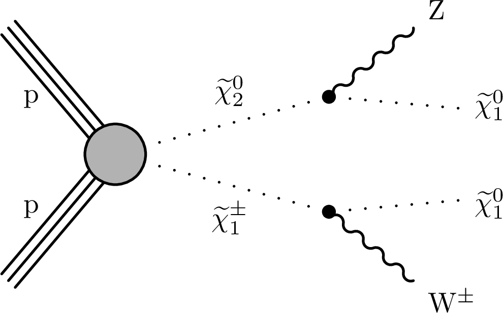
Figure 1:
Production and decay of electroweakinos in the TChiWZ model (upper left), in the higgsino simplified model (upper left and right), in the T2bff$\tilde{\chi}^0_1$ model (lower left) and in the T2bW model (lower right). |
png pdf |
Figure 1-a:
Production and decay of electroweakinos in the TChiWZ model and higgsino simplified model. |
png pdf |
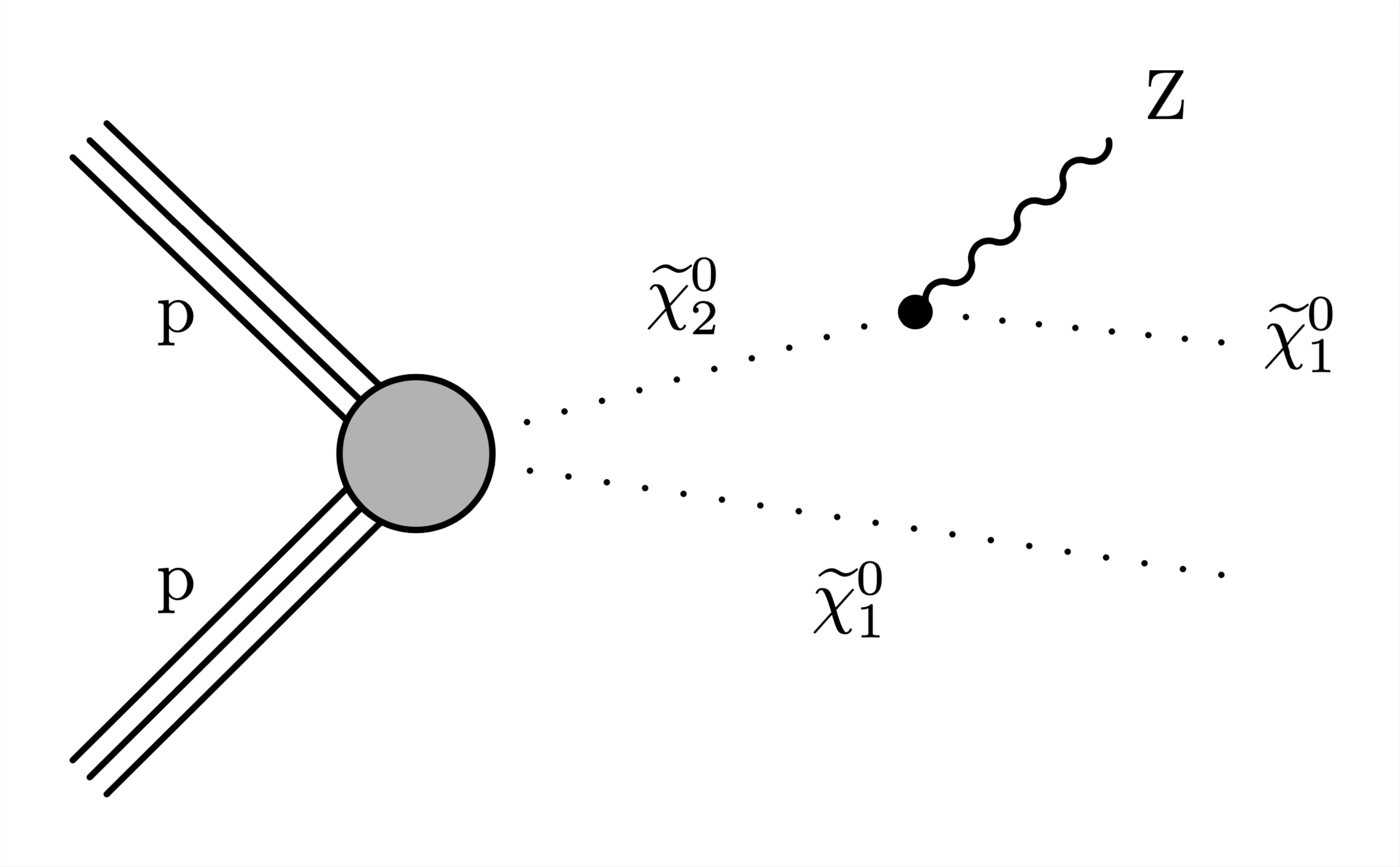
Figure 1-b:
Production and decay of electroweakinos in the higgsino simplified model. |
png pdf |
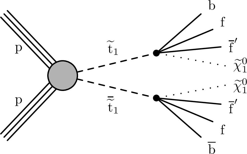
Figure 1-c:
Production and decay of electroweakinos in the T2bff$\tilde{\chi}^0_1$ model. |
png pdf |
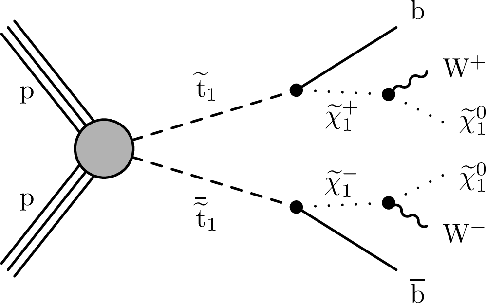
Figure 1-d:
Production and decay of electroweakinos in the T2bW model. |
png pdf |
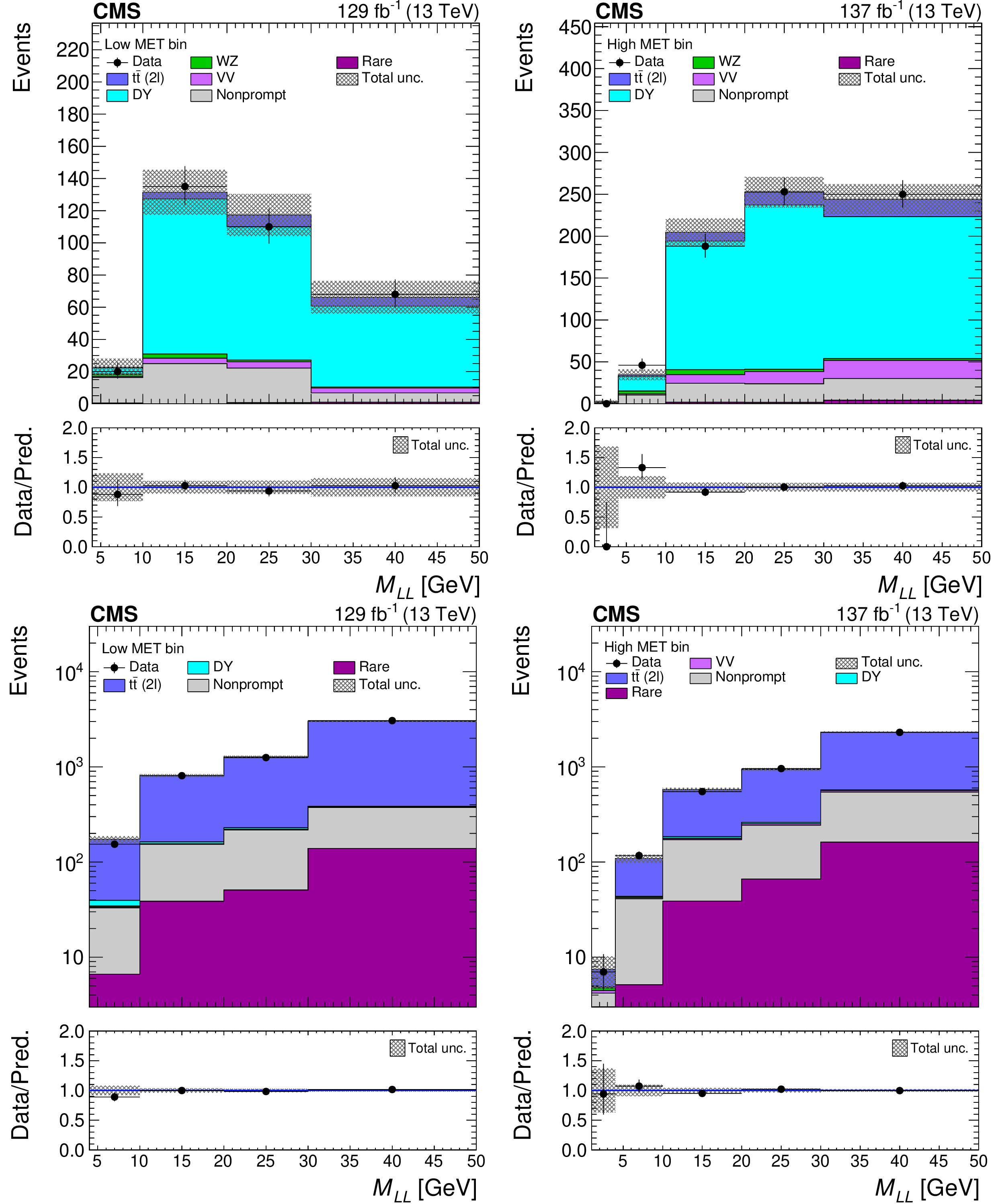
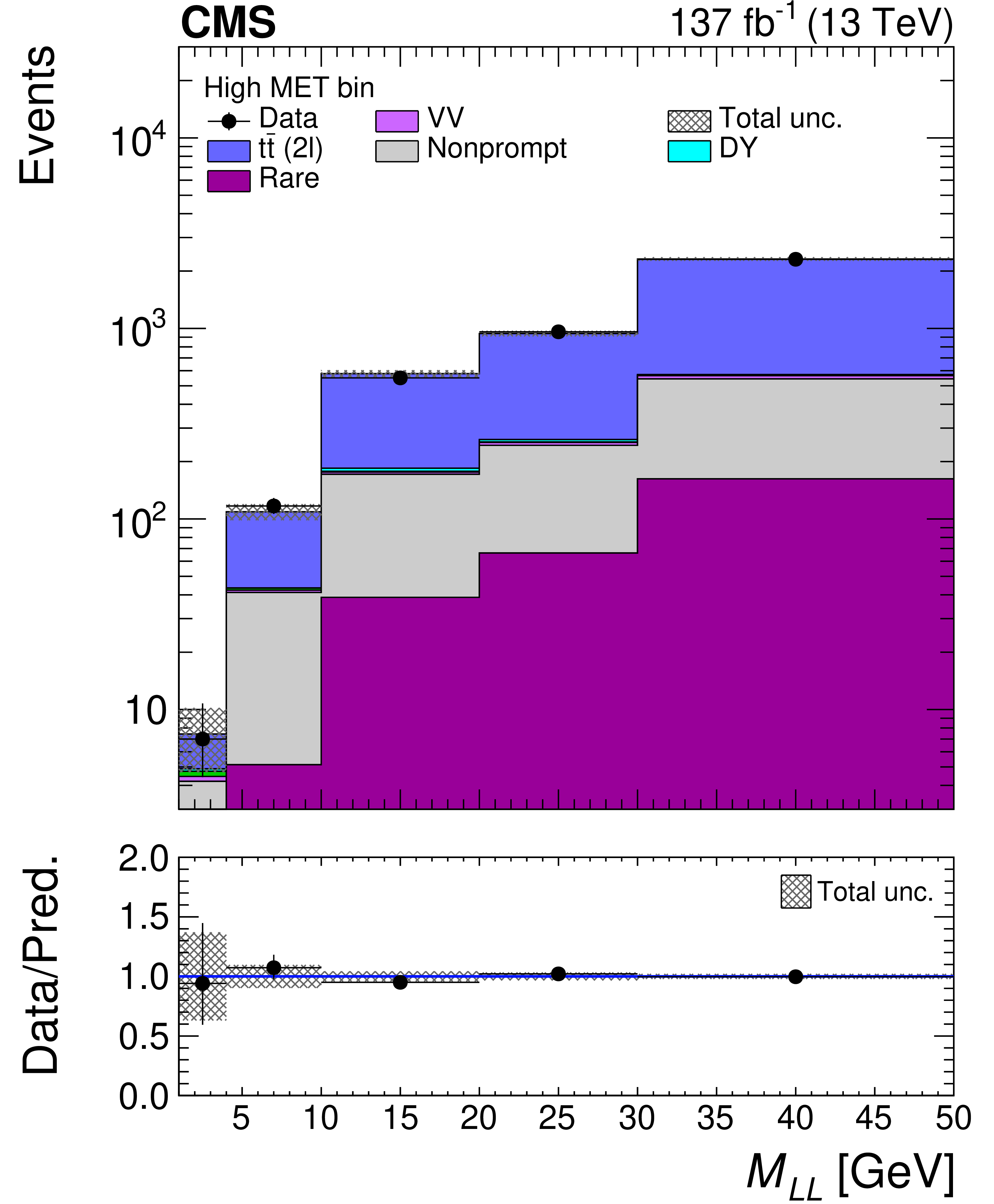
Figure 2:
The post-fit distribution of the ${M(\ell \ell)}$ variable is shown for the low- (left) and high- (right) MET bins for the DY (upper) and ${\mathrm{t} {}\mathrm{\bar{t}}}$ (lower) CRs. Uncertainties include both the statistical and systematic components. |
png pdf |
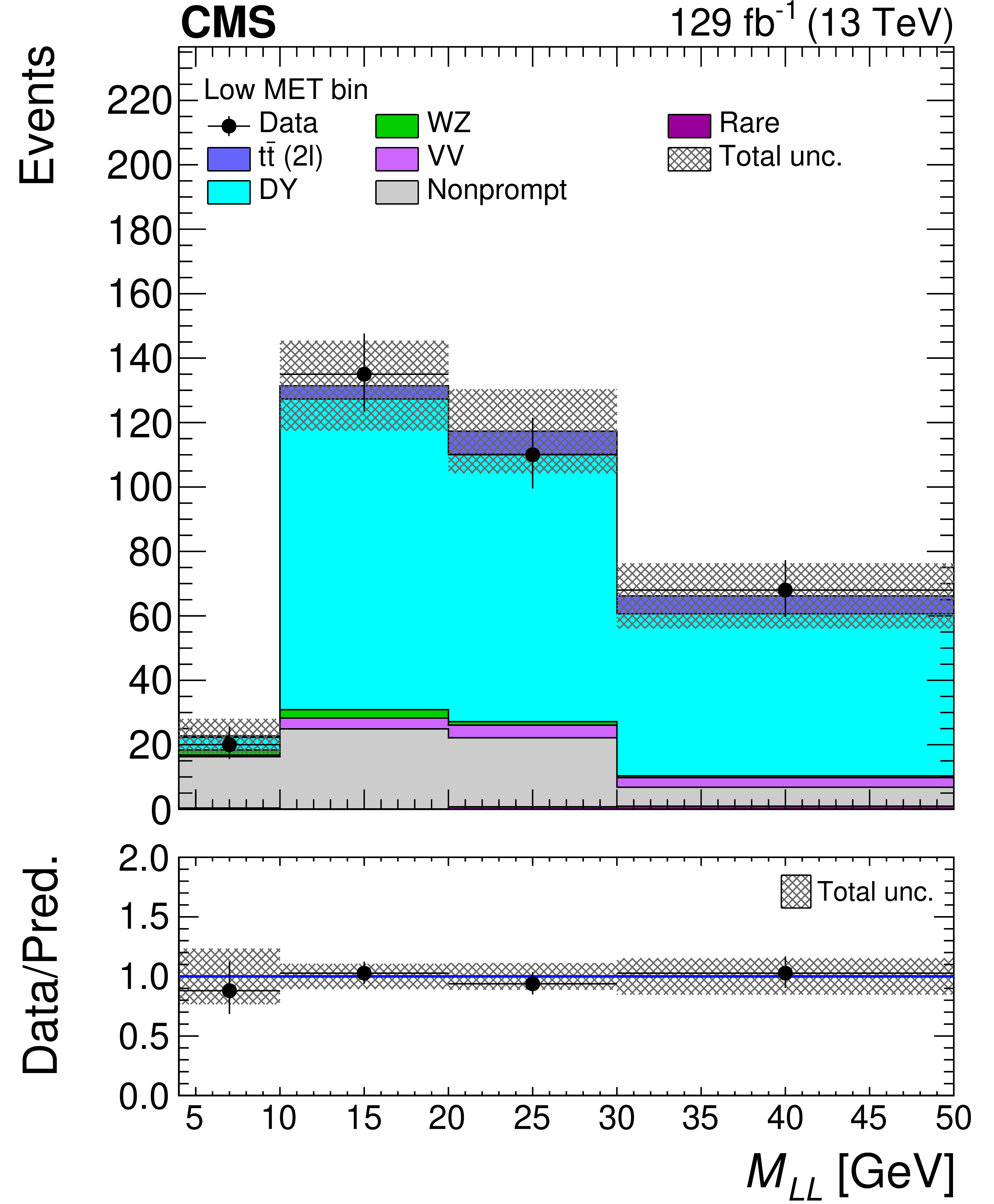
Figure 2-a:
The post-fit distribution of the ${M(\ell \ell)}$ variable is shown for the low- (left) and high- (right) MET bins for the DY (upper) and ${\mathrm{t} {}\mathrm{\bar{t}}}$ (lower) CRs. Uncertainties include both the statistical and systematic components. |
png pdf |
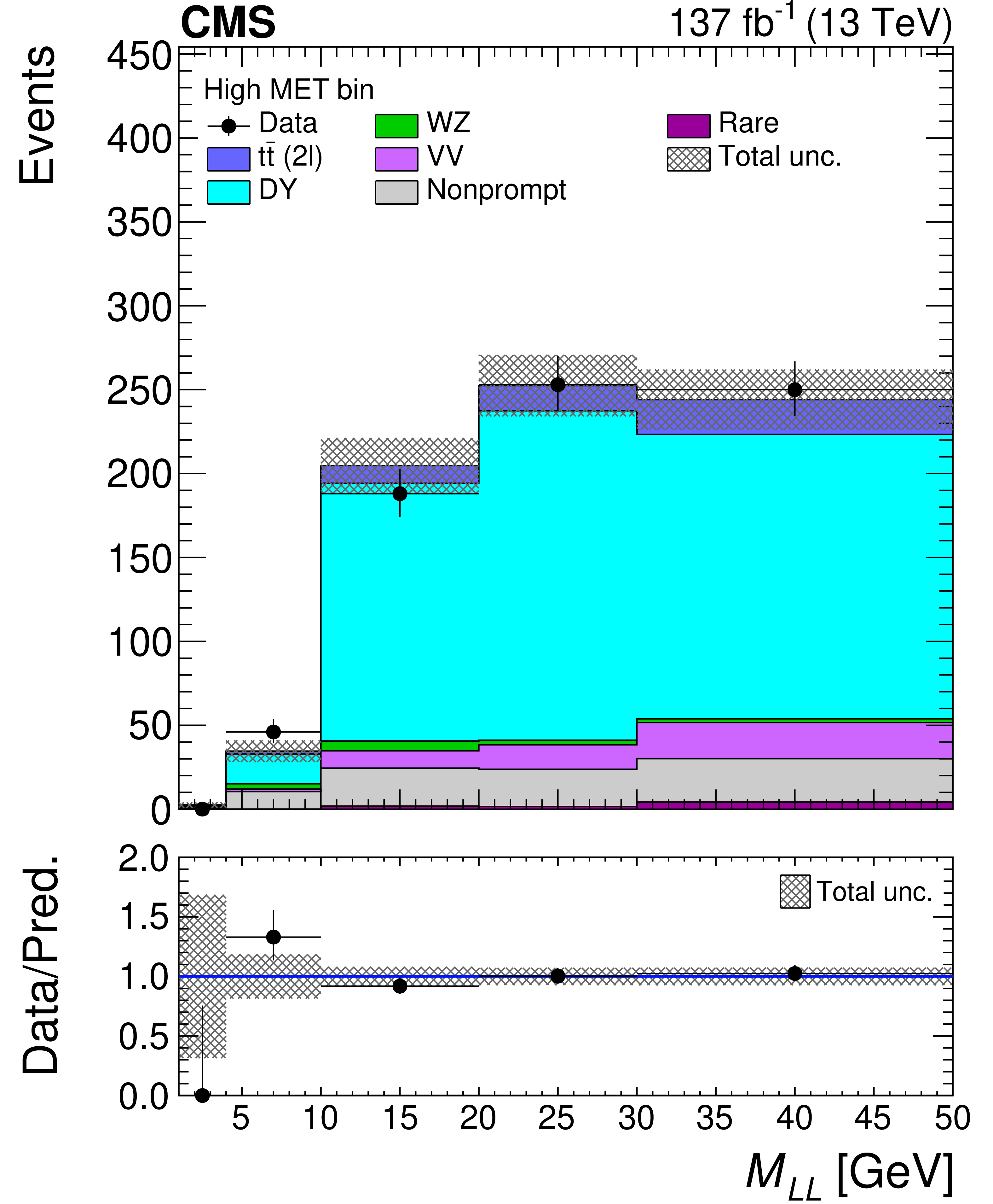
Figure 2-b:
The post-fit distribution of the ${M(\ell \ell)}$ variable is shown for the low- (left) and high- (right) MET bins for the DY (upper) and ${\mathrm{t} {}\mathrm{\bar{t}}}$ (lower) CRs. Uncertainties include both the statistical and systematic components. |
png pdf |
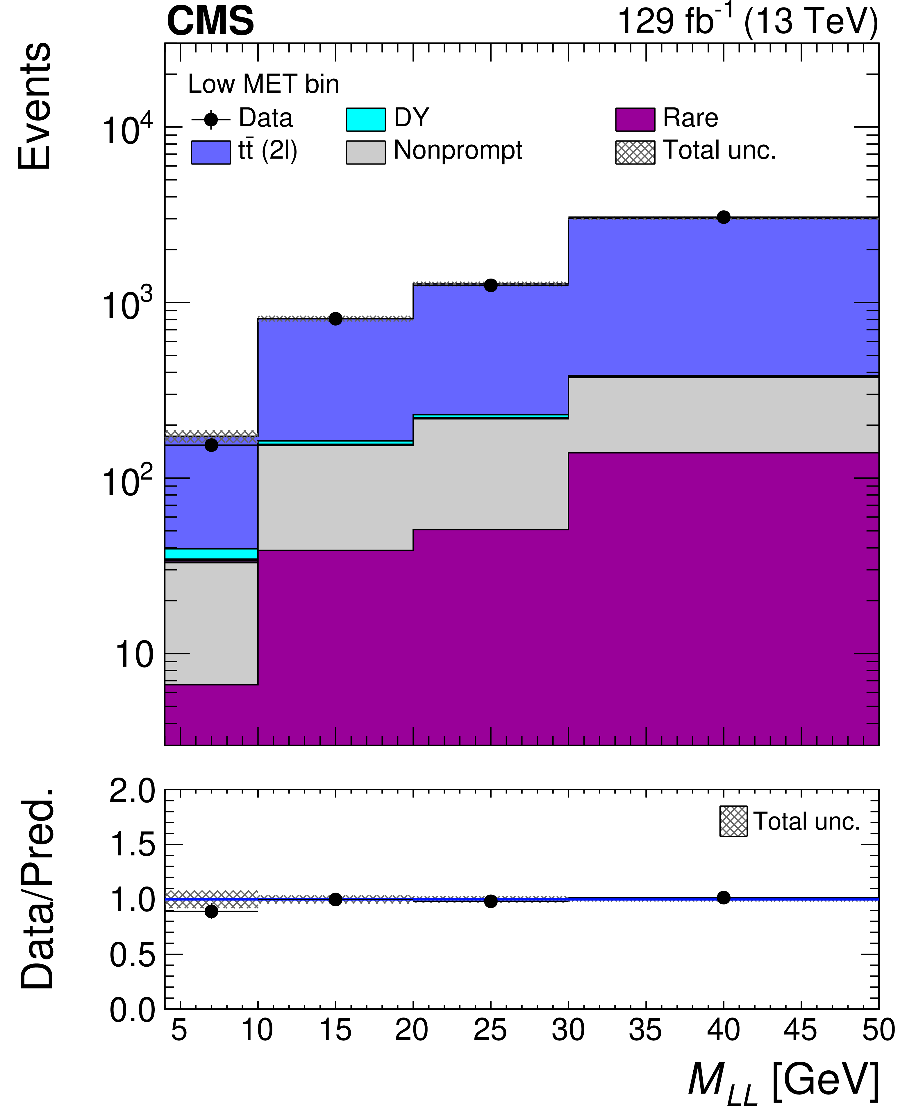
Figure 2-c:
The post-fit distribution of the ${M(\ell \ell)}$ variable is shown for the low- (left) and high- (right) MET bins for the DY (upper) and ${\mathrm{t} {}\mathrm{\bar{t}}}$ (lower) CRs. Uncertainties include both the statistical and systematic components. |
png pdf |
Figure 2-d:
The post-fit distribution of the ${M(\ell \ell)}$ variable is shown for the low- (left) and high- (right) MET bins for the DY (upper) and ${\mathrm{t} {}\mathrm{\bar{t}}}$ (lower) CRs. Uncertainties include both the statistical and systematic components. |

png pdf |
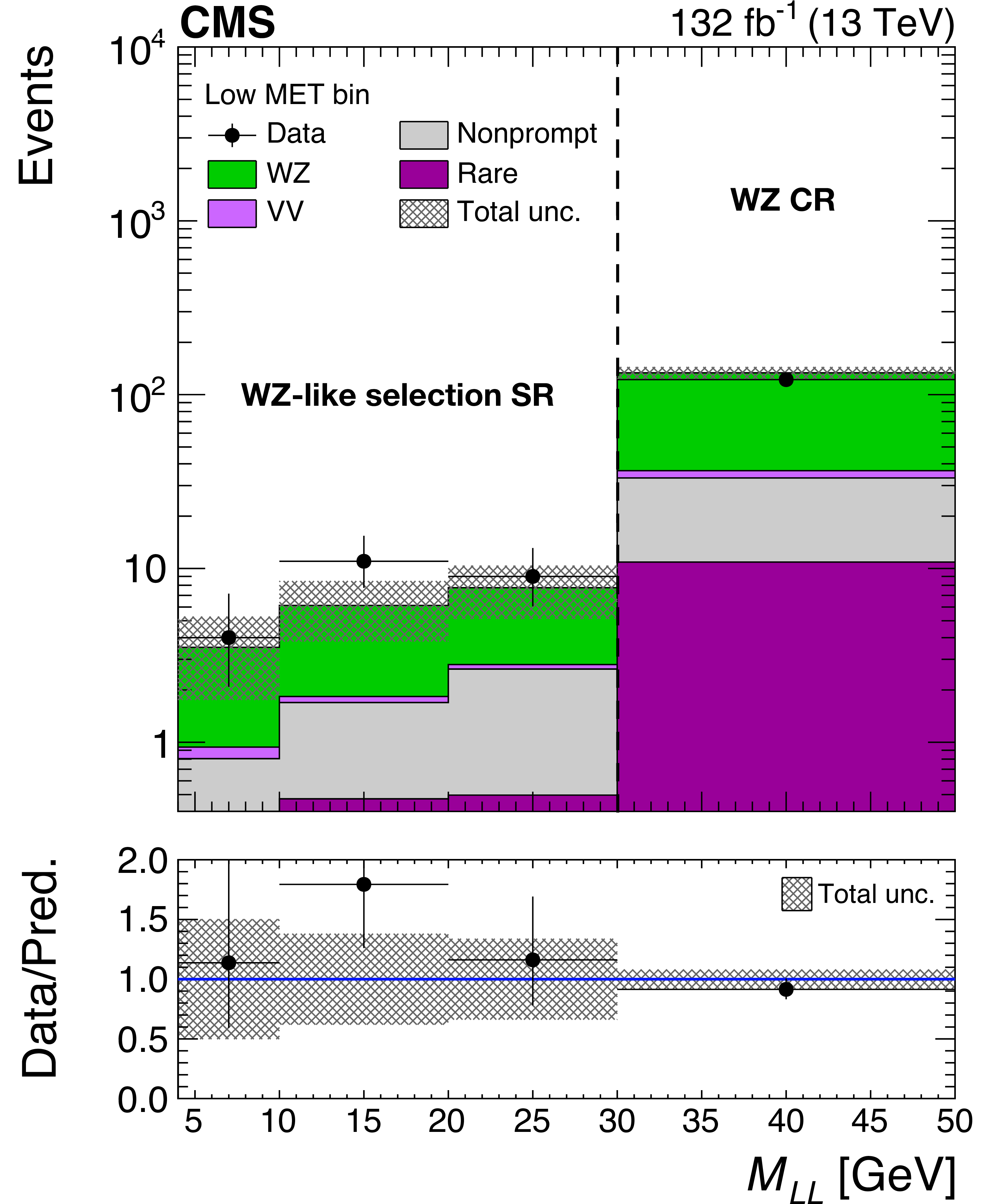
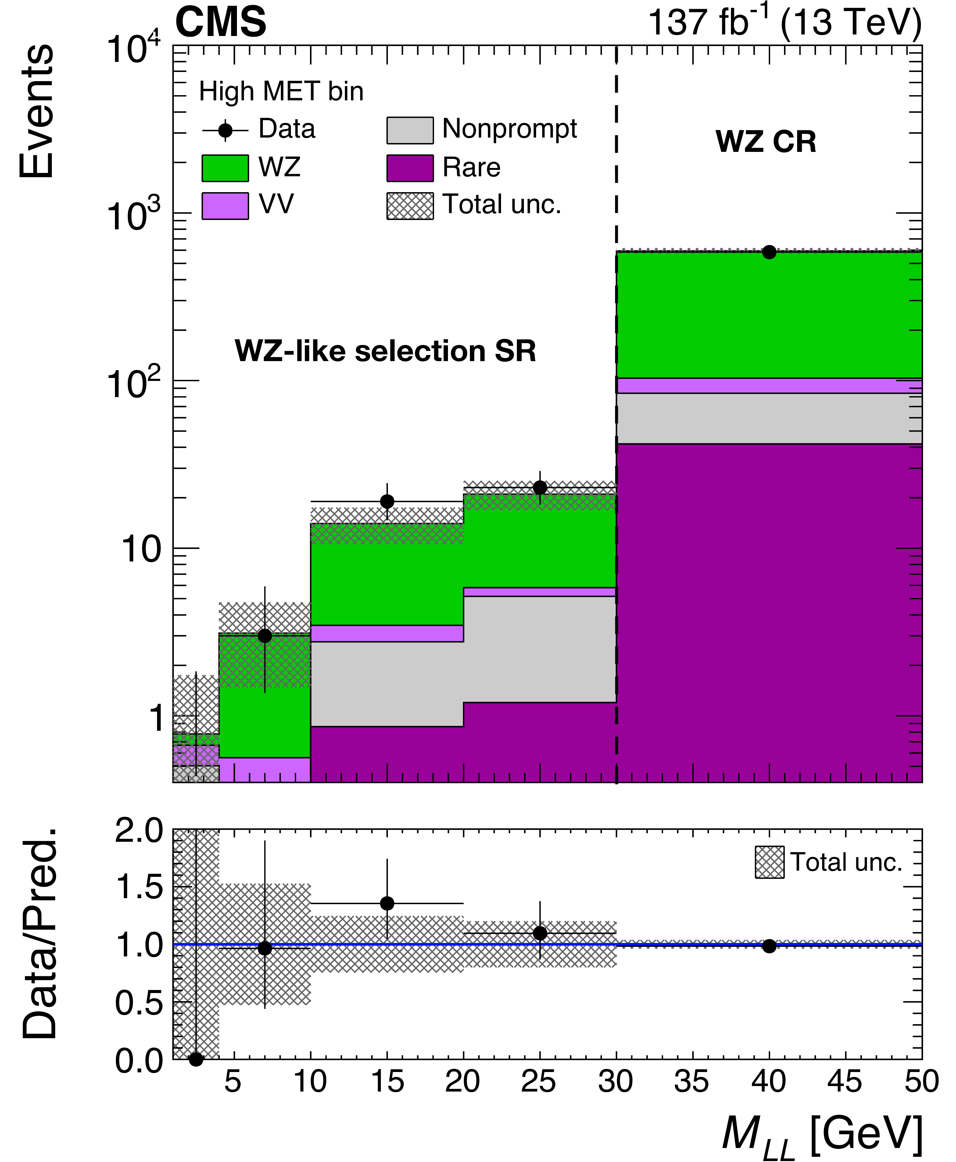
Figure 3:
The post-fit distribution of the ${M(\ell \ell)}$ variable is shown for the low- (left) and high- (right) MET bins for the WZ-enriched region. Uncertainties include both the statistical and systematic components. |
png pdf |
Figure 3-a:
The post-fit distribution of the ${M(\ell \ell)}$ variable is shown for the low- (left) and high- (right) MET bins for the WZ-enriched region. Uncertainties include both the statistical and systematic components. |
png pdf |
Figure 3-b:
The post-fit distribution of the ${M(\ell \ell)}$ variable is shown for the low- (left) and high- (right) MET bins for the WZ-enriched region. Uncertainties include both the statistical and systematic components. |
png pdf |
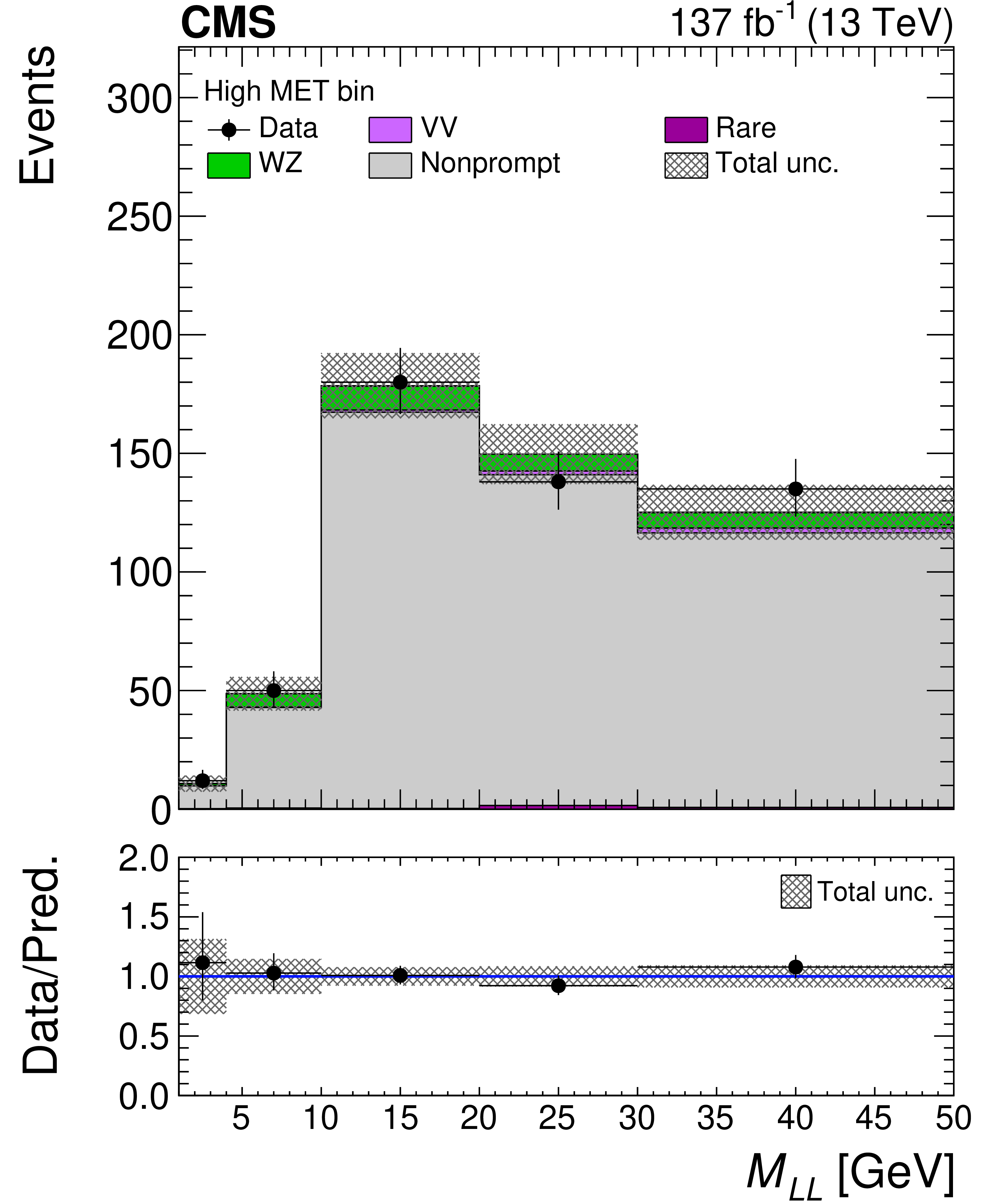
Figure 4:
The post-fit distribution of the ${M(\ell \ell)}$ variable is shown for the high-MET bin for the SS CR. Uncertainties include both the statistical and systematic components. |
png pdf |
Figure 5:
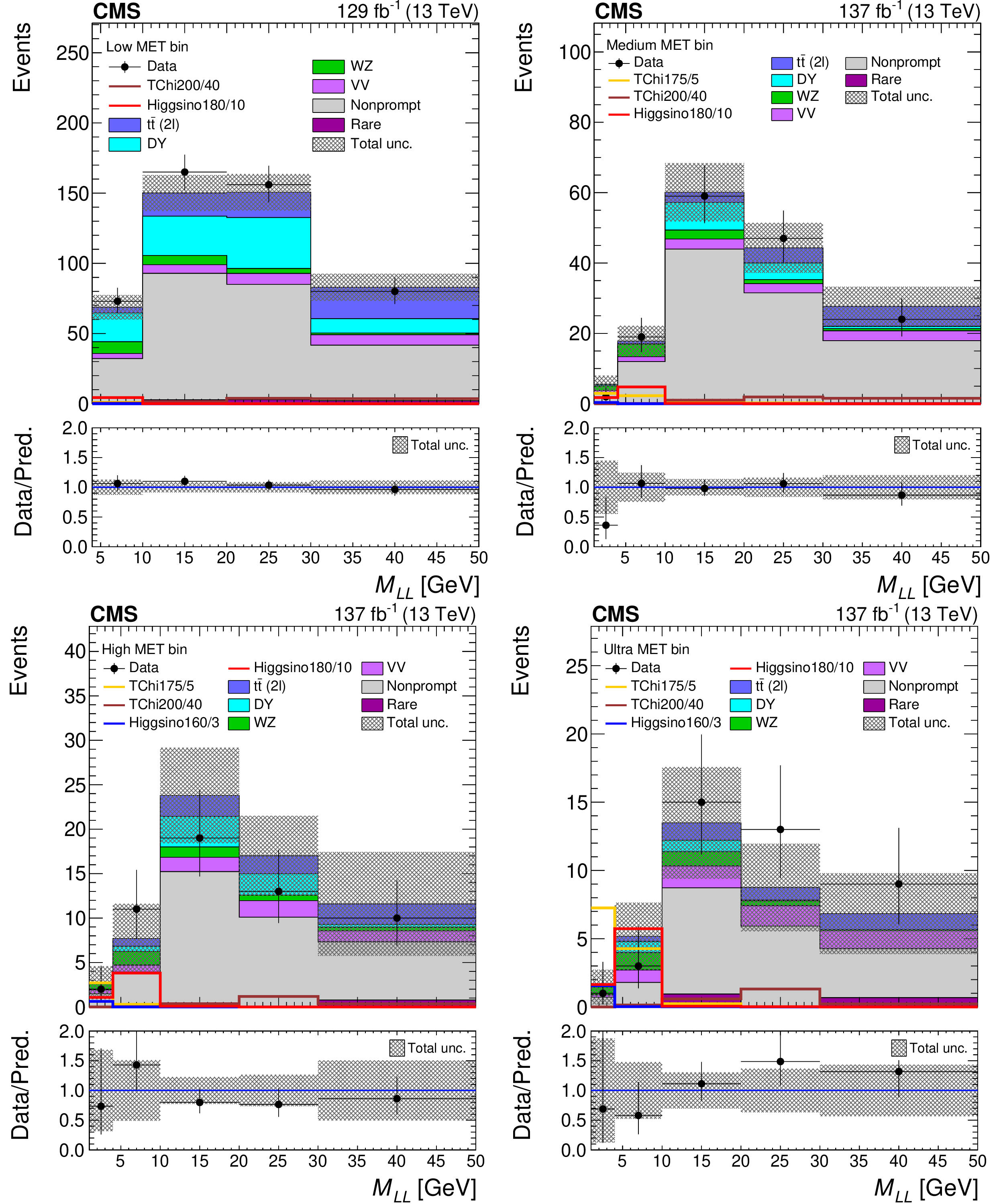
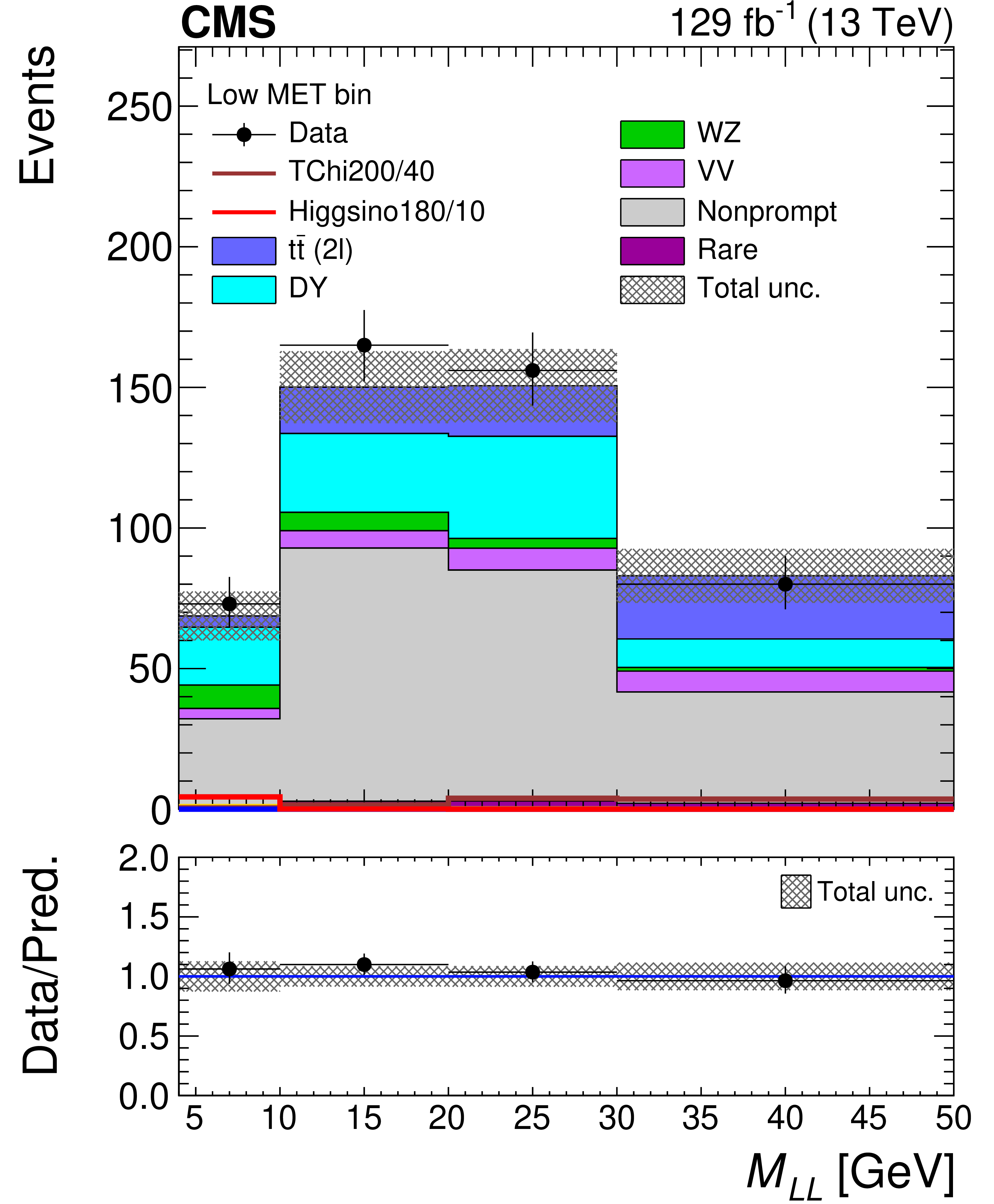
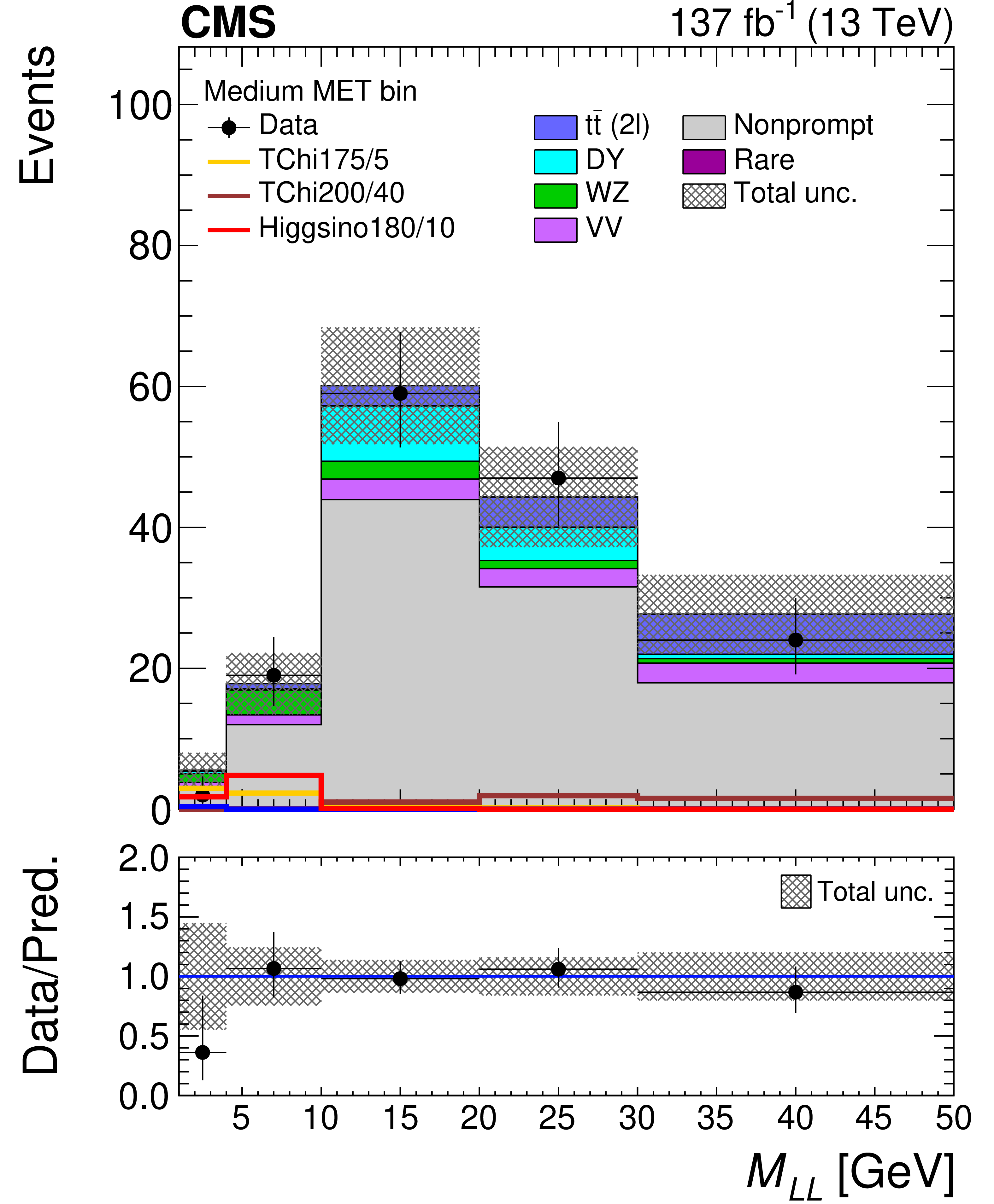
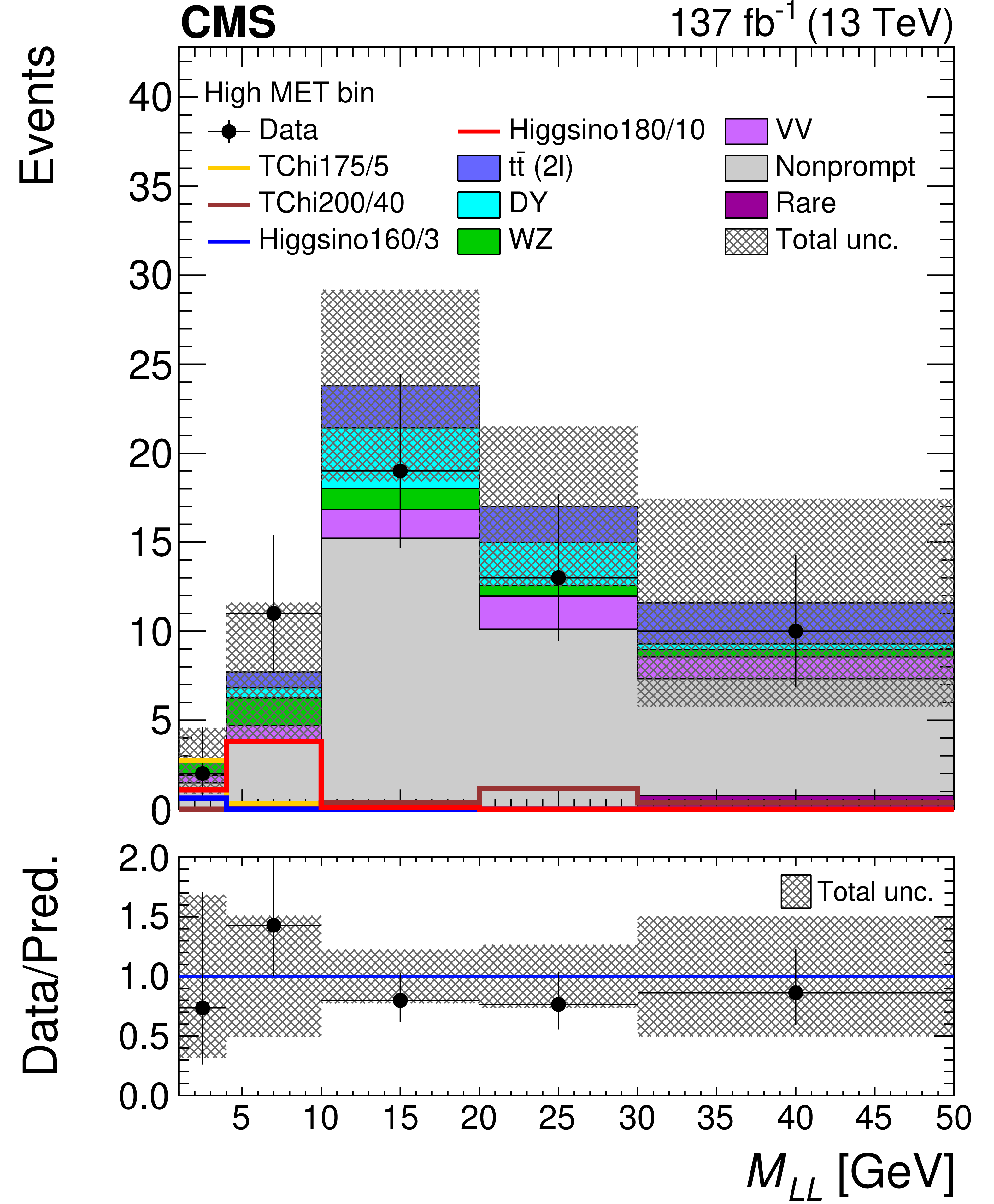
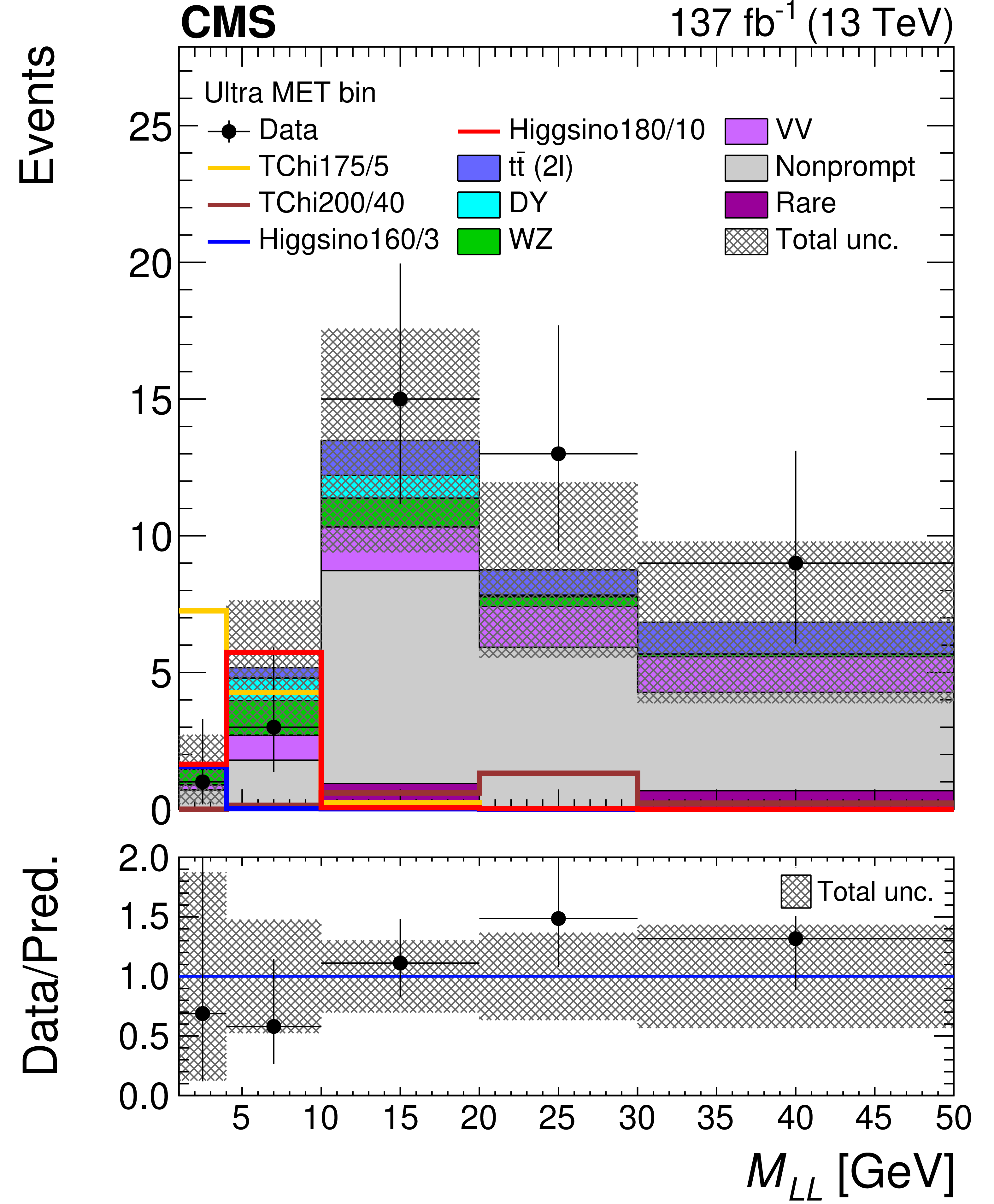
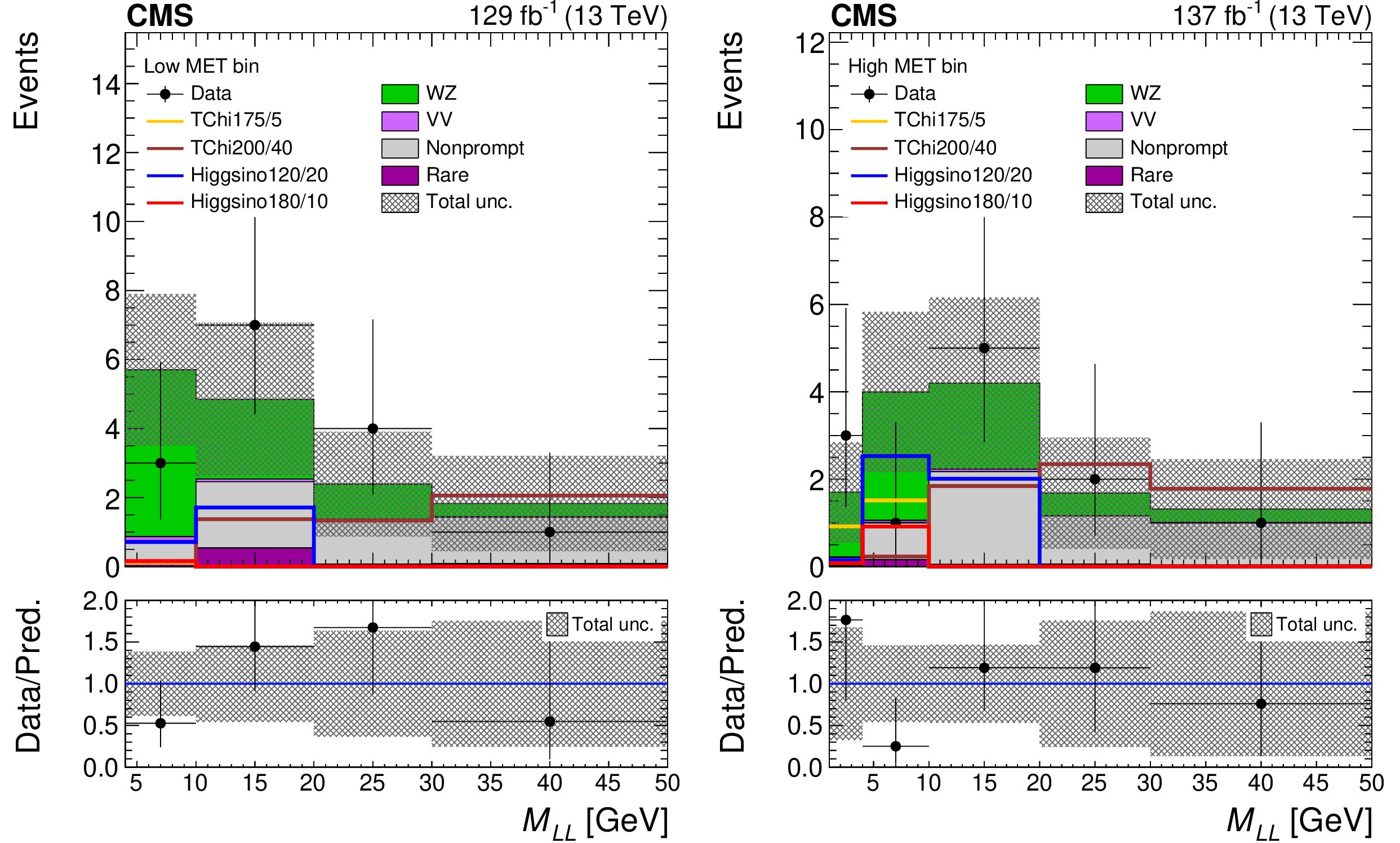
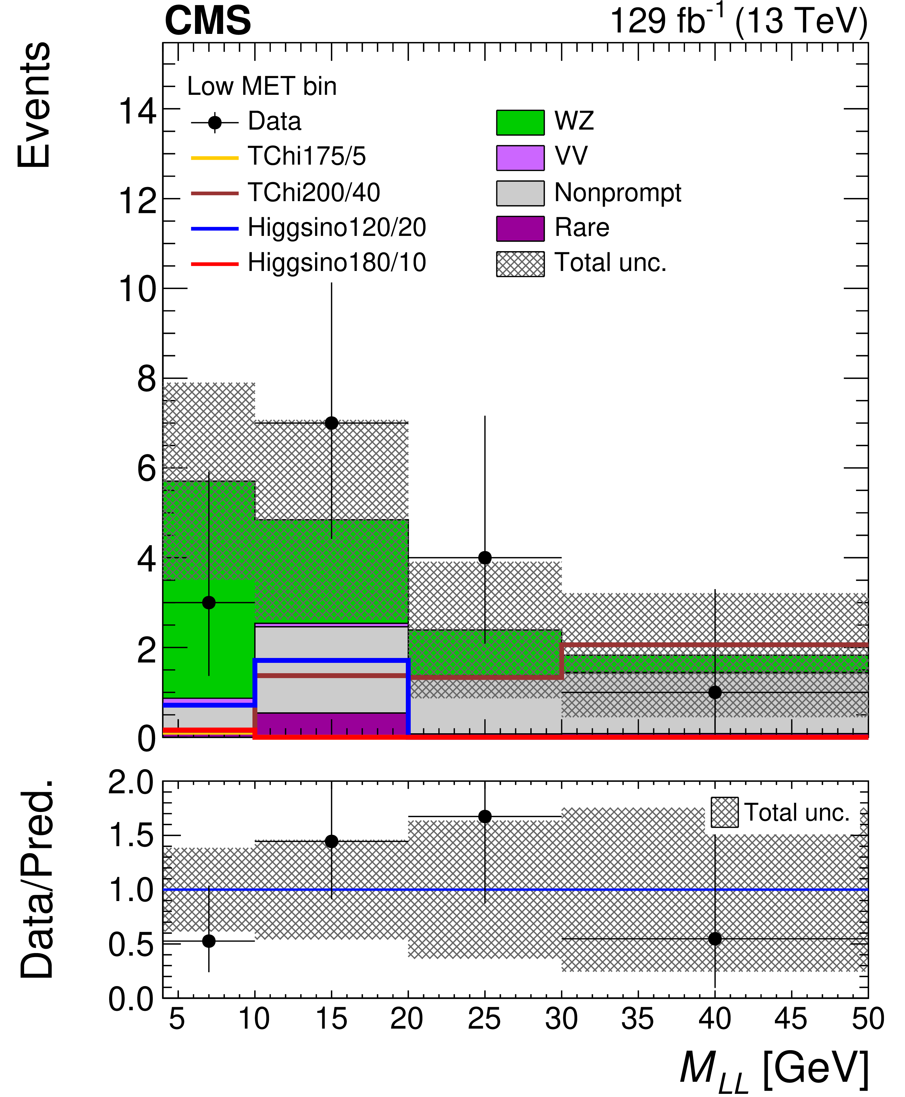
The 2$\ell $-Ewk SR: the post-fit distribution of the ${M(\ell \ell)}$ variable is shown for the low- (upper left), medium- (upper right), high- (lower left) and ultra- (lower right) MET bins. Uncertainties include both the statistical and systematic components. The signal distributions overlaid on the plot are from the TChiWZ and the simplified higgsino models in the scenario where the product of $ {\tilde{m}_{\tilde{\chi}^0_1}} {\tilde{m}_{\tilde{\chi}^{0}_{2}}} $ eigenvalues is positive and negative, respectively. The numbers after the model name in the legend indicate the mass of the NLSP and the mass splitting between the NLSP and LSP, in GeV. |
png pdf |
Figure 5-a:
The 2$\ell $-Ewk SR: the post-fit distribution of the ${M(\ell \ell)}$ variable is shown for the low- (upper left), medium- (upper right), high- (lower left) and ultra- (lower right) MET bins. Uncertainties include both the statistical and systematic components. The signal distributions overlaid on the plot are from the TChiWZ and the simplified higgsino models in the scenario where the product of $ {\tilde{m}_{\tilde{\chi}^0_1}} {\tilde{m}_{\tilde{\chi}^{0}_{2}}} $ eigenvalues is positive and negative, respectively. The numbers after the model name in the legend indicate the mass of the NLSP and the mass splitting between the NLSP and LSP, in GeV. |
png pdf |
Figure 5-b:
The 2$\ell $-Ewk SR: the post-fit distribution of the ${M(\ell \ell)}$ variable is shown for the low- (upper left), medium- (upper right), high- (lower left) and ultra- (lower right) MET bins. Uncertainties include both the statistical and systematic components. The signal distributions overlaid on the plot are from the TChiWZ and the simplified higgsino models in the scenario where the product of $ {\tilde{m}_{\tilde{\chi}^0_1}} {\tilde{m}_{\tilde{\chi}^{0}_{2}}} $ eigenvalues is positive and negative, respectively. The numbers after the model name in the legend indicate the mass of the NLSP and the mass splitting between the NLSP and LSP, in GeV. |
png pdf |
Figure 5-c:
The 2$\ell $-Ewk SR: the post-fit distribution of the ${M(\ell \ell)}$ variable is shown for the low- (upper left), medium- (upper right), high- (lower left) and ultra- (lower right) MET bins. Uncertainties include both the statistical and systematic components. The signal distributions overlaid on the plot are from the TChiWZ and the simplified higgsino models in the scenario where the product of $ {\tilde{m}_{\tilde{\chi}^0_1}} {\tilde{m}_{\tilde{\chi}^{0}_{2}}} $ eigenvalues is positive and negative, respectively. The numbers after the model name in the legend indicate the mass of the NLSP and the mass splitting between the NLSP and LSP, in GeV. |
png pdf |
Figure 5-d:
The 2$\ell $-Ewk SR: the post-fit distribution of the ${M(\ell \ell)}$ variable is shown for the low- (upper left), medium- (upper right), high- (lower left) and ultra- (lower right) MET bins. Uncertainties include both the statistical and systematic components. The signal distributions overlaid on the plot are from the TChiWZ and the simplified higgsino models in the scenario where the product of $ {\tilde{m}_{\tilde{\chi}^0_1}} {\tilde{m}_{\tilde{\chi}^{0}_{2}}} $ eigenvalues is positive and negative, respectively. The numbers after the model name in the legend indicate the mass of the NLSP and the mass splitting between the NLSP and LSP, in GeV. |
png pdf |
Figure 6:
The 3$\ell $-Ewk search regions: the post-fit distribution of the ${M^{\text {min}}_{\text {SFOS}}(\ell \ell)}$ variable is shown for the low- (left) and high- (right) MET bins. Uncertainties include both the statistical and systematic components. The signal distributions overlaid on the plot are from the TChiWZ and the simplified higgsino models in the scenario where the product of $ {\tilde{m}_{\tilde{\chi}^0_1}} {\tilde{m}_{\tilde{\chi}^{0}_{2}}} $ eigenvalues is positive and negative, respectively. The numbers after the model name in the legend indicate the mass of the NLSP and the mass splitting between the NLSP and LSP, in GeV. |
png pdf |
Figure 6-a:
The 3$\ell $-Ewk search regions: the post-fit distribution of the ${M^{\text {min}}_{\text {SFOS}}(\ell \ell)}$ variable is shown for the low- (left) and high- (right) MET bins. Uncertainties include both the statistical and systematic components. The signal distributions overlaid on the plot are from the TChiWZ and the simplified higgsino models in the scenario where the product of $ {\tilde{m}_{\tilde{\chi}^0_1}} {\tilde{m}_{\tilde{\chi}^{0}_{2}}} $ eigenvalues is positive and negative, respectively. The numbers after the model name in the legend indicate the mass of the NLSP and the mass splitting between the NLSP and LSP, in GeV. |

png pdf |
Figure 6-b:
The 3$\ell $-Ewk search regions: the post-fit distribution of the ${M^{\text {min}}_{\text {SFOS}}(\ell \ell)}$ variable is shown for the low- (left) and high- (right) MET bins. Uncertainties include both the statistical and systematic components. The signal distributions overlaid on the plot are from the TChiWZ and the simplified higgsino models in the scenario where the product of $ {\tilde{m}_{\tilde{\chi}^0_1}} {\tilde{m}_{\tilde{\chi}^{0}_{2}}} $ eigenvalues is positive and negative, respectively. The numbers after the model name in the legend indicate the mass of the NLSP and the mass splitting between the NLSP and LSP, in GeV. |

png pdf |
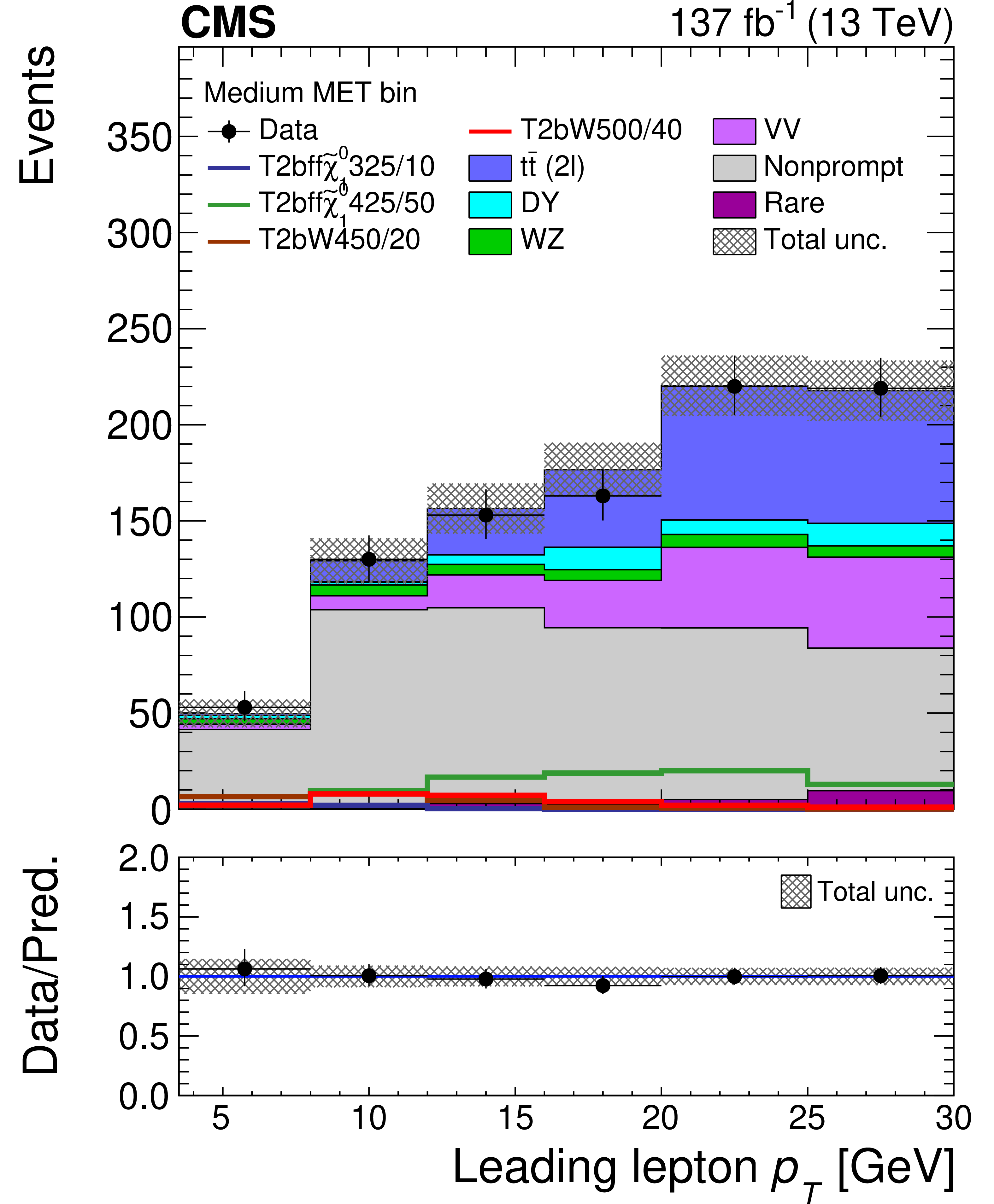
Figure 7:
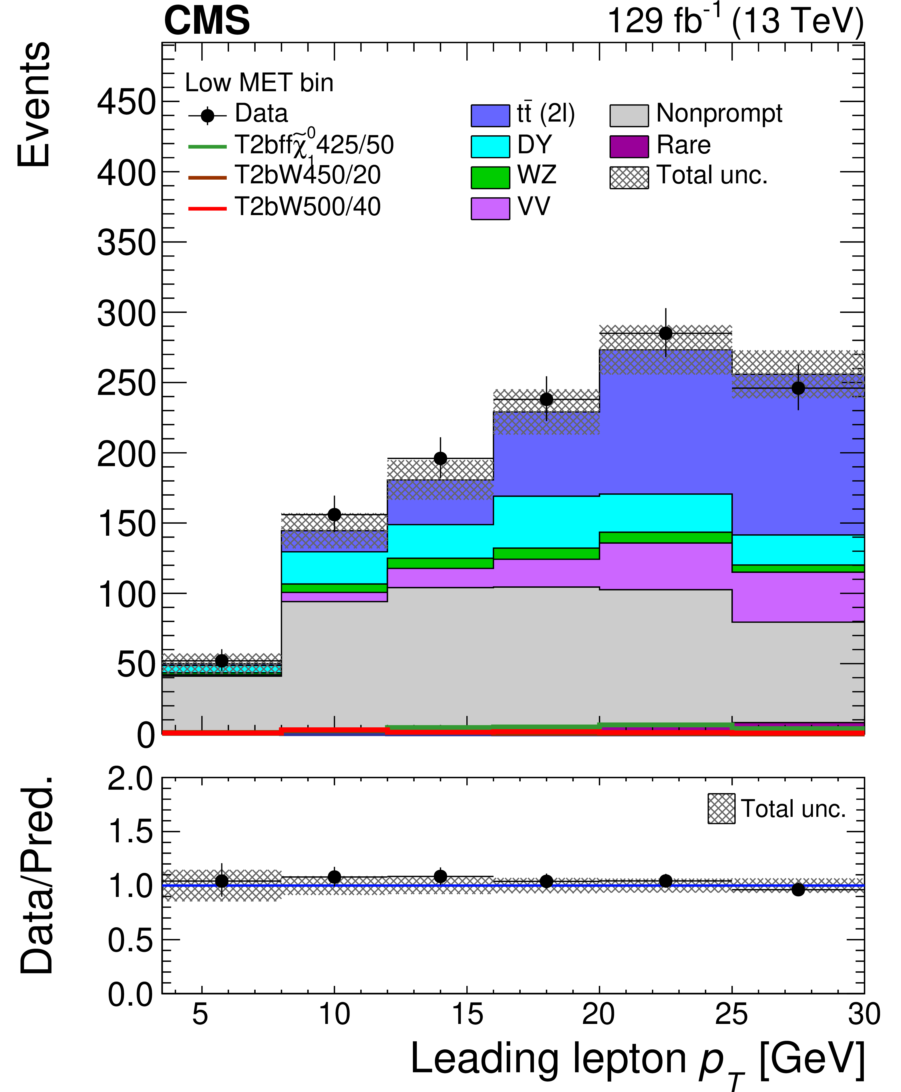
The 2$\ell $-Stop SR: the post-fit distribution of the leading lepton ${p_{\mathrm {T}}}$ variable is shown for the low- (upper left), medium- (upper right), high- (lower left) and ultra- (lower right) MET bins. Uncertainties include both the statistical and systematic components. The signal distributions overlaid on the plot are from the T2bff$\tilde{\chi}^0_1$ and the T2bW models. The numbers after the model name in the legend indicate the mass of the top squark and the mass splitting between the top squark and LSP, in GeV. |
png pdf |
Figure 7-a:
The 2$\ell $-Stop SR: the post-fit distribution of the leading lepton ${p_{\mathrm {T}}}$ variable is shown for the low- (upper left), medium- (upper right), high- (lower left) and ultra- (lower right) MET bins. Uncertainties include both the statistical and systematic components. The signal distributions overlaid on the plot are from the T2bff$\tilde{\chi}^0_1$ and the T2bW models. The numbers after the model name in the legend indicate the mass of the top squark and the mass splitting between the top squark and LSP, in GeV. |
png pdf |
Figure 7-b:
The 2$\ell $-Stop SR: the post-fit distribution of the leading lepton ${p_{\mathrm {T}}}$ variable is shown for the low- (upper left), medium- (upper right), high- (lower left) and ultra- (lower right) MET bins. Uncertainties include both the statistical and systematic components. The signal distributions overlaid on the plot are from the T2bff$\tilde{\chi}^0_1$ and the T2bW models. The numbers after the model name in the legend indicate the mass of the top squark and the mass splitting between the top squark and LSP, in GeV. |
png pdf |
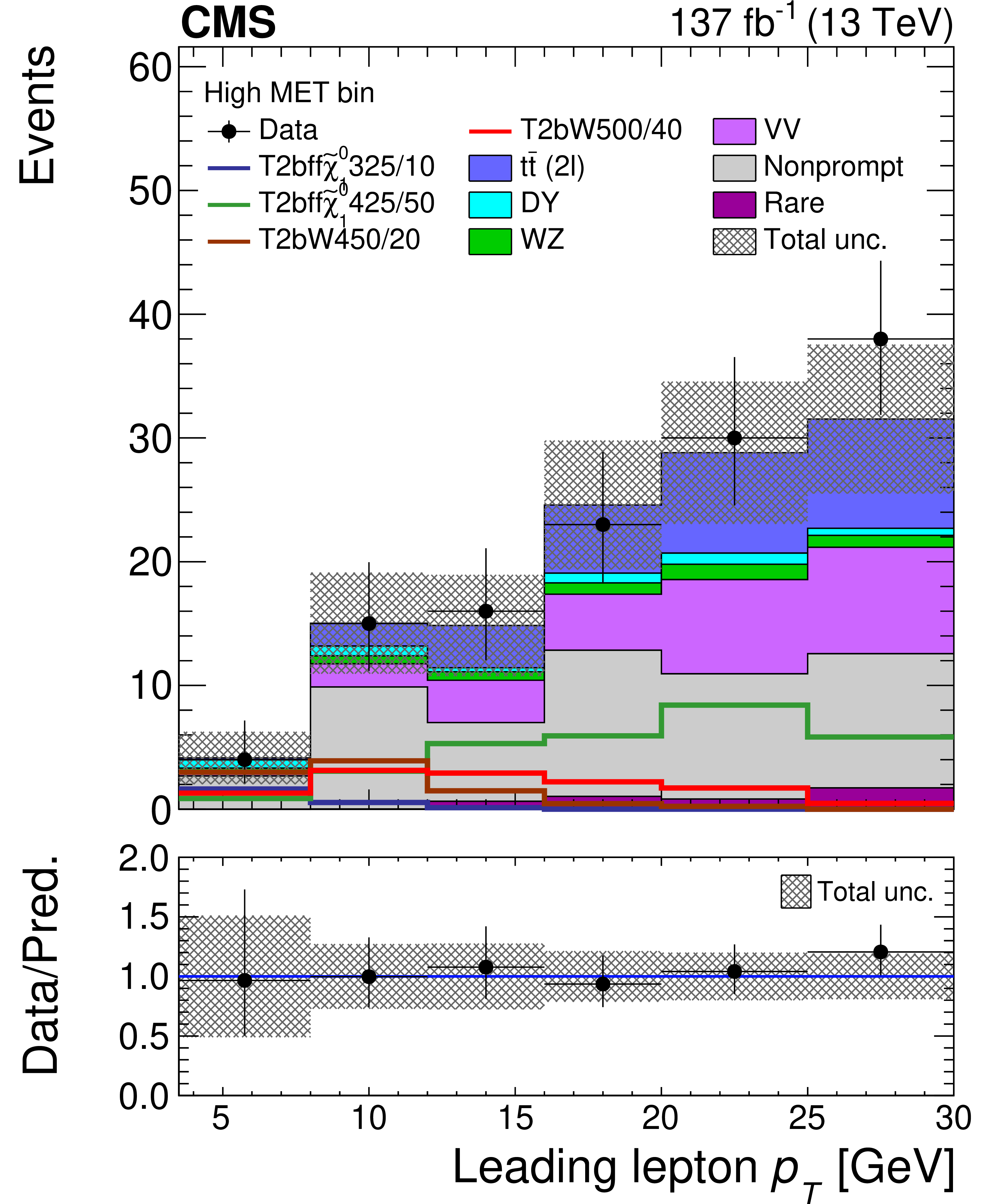
Figure 7-c:
The 2$\ell $-Stop SR: the post-fit distribution of the leading lepton ${p_{\mathrm {T}}}$ variable is shown for the low- (upper left), medium- (upper right), high- (lower left) and ultra- (lower right) MET bins. Uncertainties include both the statistical and systematic components. The signal distributions overlaid on the plot are from the T2bff$\tilde{\chi}^0_1$ and the T2bW models. The numbers after the model name in the legend indicate the mass of the top squark and the mass splitting between the top squark and LSP, in GeV. |
png pdf |
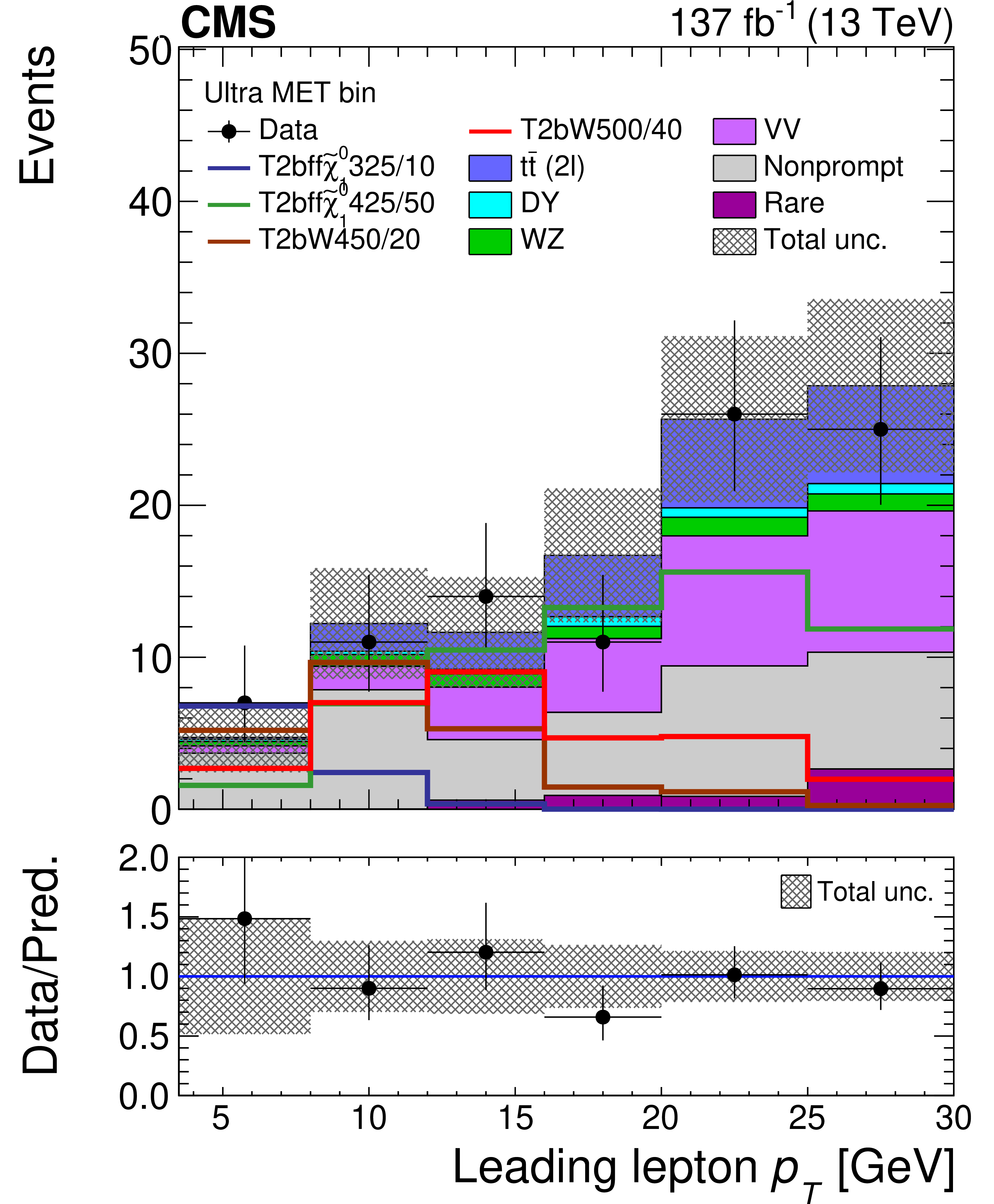
Figure 7-d:
The 2$\ell $-Stop SR: the post-fit distribution of the leading lepton ${p_{\mathrm {T}}}$ variable is shown for the low- (upper left), medium- (upper right), high- (lower left) and ultra- (lower right) MET bins. Uncertainties include both the statistical and systematic components. The signal distributions overlaid on the plot are from the T2bff$\tilde{\chi}^0_1$ and the T2bW models. The numbers after the model name in the legend indicate the mass of the top squark and the mass splitting between the top squark and LSP, in GeV. |
png pdf |
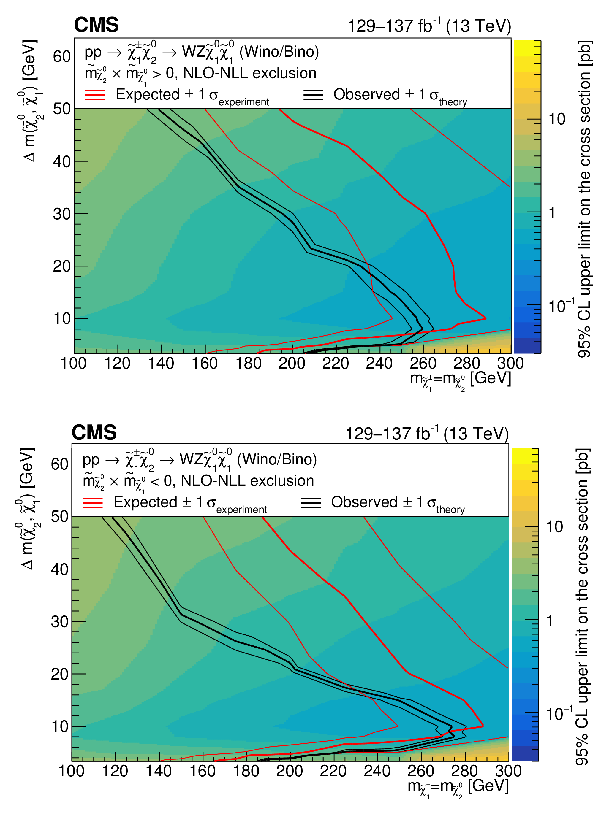
Figure 8:
The observed 95% CL exclusion contours (black curves) assuming the NLO+NLL cross sections, with the variations (thin lines) corresponding to the uncertainty in the cross section for the TChiWZ model. The red curves present the 95% CL expected limits with the band (thin lines) covering 68% of the limits in the absence of signal. Results are reported for the $ {\tilde{m}_{\tilde{\chi}^{0}_{2}}} {\tilde{m}_{\tilde{\chi}^0_1}} > 0(< 0)$ ${M(\ell \ell)}$ spectrum reweighting scenario in the upper (lower) plot. The range of luminosities of the analysis regions included in the fit is indicated on the plot. |

png pdf |
Figure 8-a:
The observed 95% CL exclusion contours (black curves) assuming the NLO+NLL cross sections, with the variations (thin lines) corresponding to the uncertainty in the cross section for the TChiWZ model. The red curves present the 95% CL expected limits with the band (thin lines) covering 68% of the limits in the absence of signal. Results are reported for the $ {\tilde{m}_{\tilde{\chi}^{0}_{2}}} {\tilde{m}_{\tilde{\chi}^0_1}} > 0(< 0)$ ${M(\ell \ell)}$ spectrum reweighting scenario in the upper (lower) plot. The range of luminosities of the analysis regions included in the fit is indicated on the plot. |

png pdf |
Figure 8-b:
The observed 95% CL exclusion contours (black curves) assuming the NLO+NLL cross sections, with the variations (thin lines) corresponding to the uncertainty in the cross section for the TChiWZ model. The red curves present the 95% CL expected limits with the band (thin lines) covering 68% of the limits in the absence of signal. Results are reported for the $ {\tilde{m}_{\tilde{\chi}^{0}_{2}}} {\tilde{m}_{\tilde{\chi}^0_1}} > 0(< 0)$ ${M(\ell \ell)}$ spectrum reweighting scenario in the upper (lower) plot. The range of luminosities of the analysis regions included in the fit is indicated on the plot. |
png pdf |
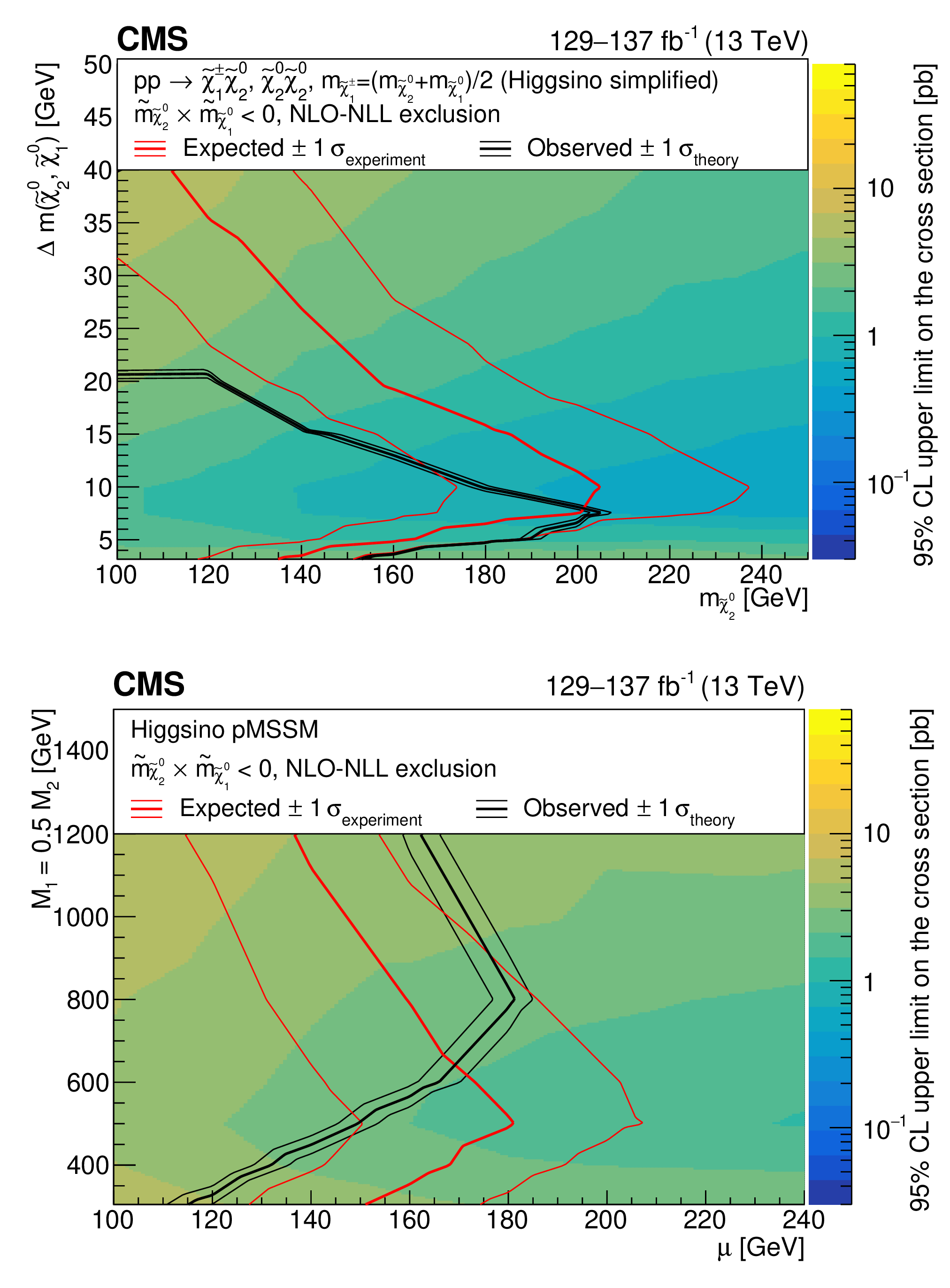
Figure 9:
The observed 95% CL exclusion contours (black curves) assuming the NLO+NLL cross sections, with the variations (thin lines) corresponding to the uncertainty in the cross section for the simplified (upper) and the pMSSM (lower) higgsino models. The simplified model includes both neutralino pair and neutralino-chargino production modes, while the pMSSM one includes all possible production modes. The red curves present the 95% CL expected limits with the band (thin lines) covering 68% of the limits in the absence of signal. The results are reported for the $ {\tilde{m}_{\tilde{\chi}^{0}_{2}}} {\tilde{m}_{\tilde{\chi}^0_1}} < $ 0 ${M(\ell \ell)}$ spectrum reweighting scenario. The range of luminosities of the analysis regions included in the fit is indicated on the plot. |
png pdf |
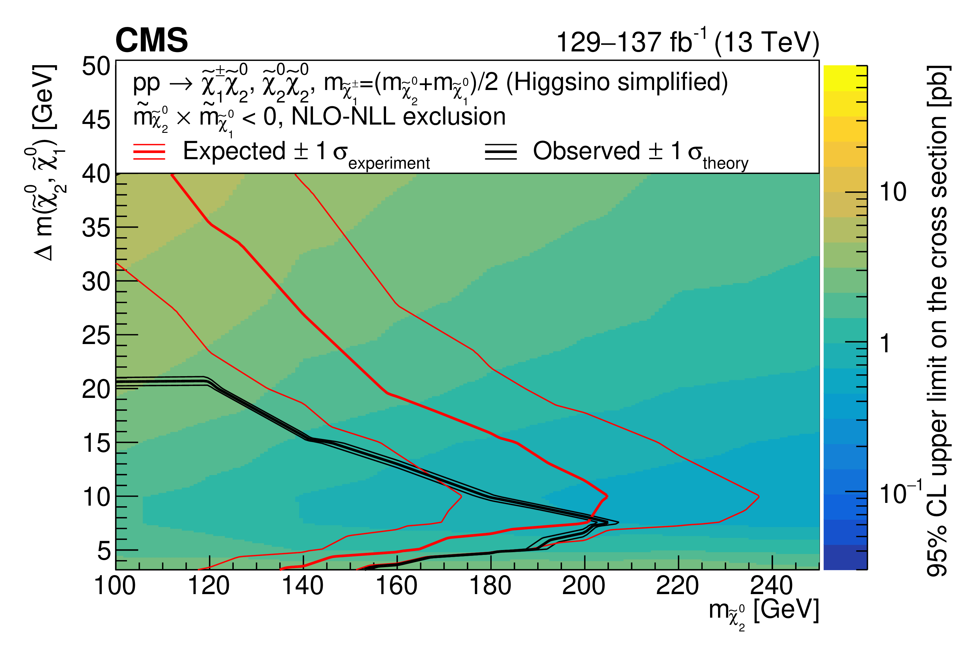
Figure 9-a:
The observed 95% CL exclusion contours (black curves) assuming the NLO+NLL cross sections, with the variations (thin lines) corresponding to the uncertainty in the cross section for the simplified (upper) and the pMSSM (lower) higgsino models. The simplified model includes both neutralino pair and neutralino-chargino production modes, while the pMSSM one includes all possible production modes. The red curves present the 95% CL expected limits with the band (thin lines) covering 68% of the limits in the absence of signal. The results are reported for the $ {\tilde{m}_{\tilde{\chi}^{0}_{2}}} {\tilde{m}_{\tilde{\chi}^0_1}} < $ 0 ${M(\ell \ell)}$ spectrum reweighting scenario. The range of luminosities of the analysis regions included in the fit is indicated on the plot. |
png pdf |
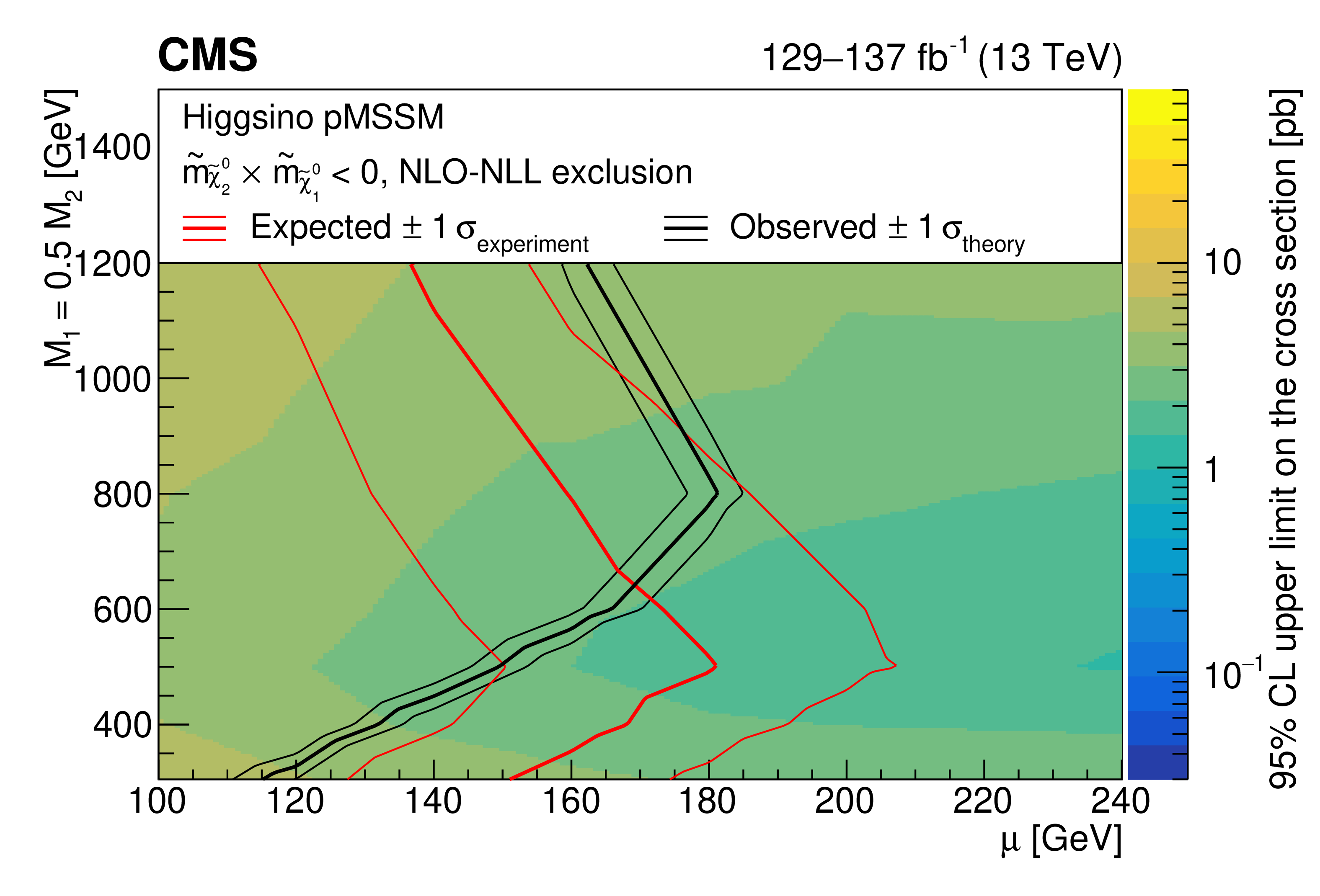
Figure 9-b:
The observed 95% CL exclusion contours (black curves) assuming the NLO+NLL cross sections, with the variations (thin lines) corresponding to the uncertainty in the cross section for the simplified (upper) and the pMSSM (lower) higgsino models. The simplified model includes both neutralino pair and neutralino-chargino production modes, while the pMSSM one includes all possible production modes. The red curves present the 95% CL expected limits with the band (thin lines) covering 68% of the limits in the absence of signal. The results are reported for the $ {\tilde{m}_{\tilde{\chi}^{0}_{2}}} {\tilde{m}_{\tilde{\chi}^0_1}} < $ 0 ${M(\ell \ell)}$ spectrum reweighting scenario. The range of luminosities of the analysis regions included in the fit is indicated on the plot. |
png pdf |
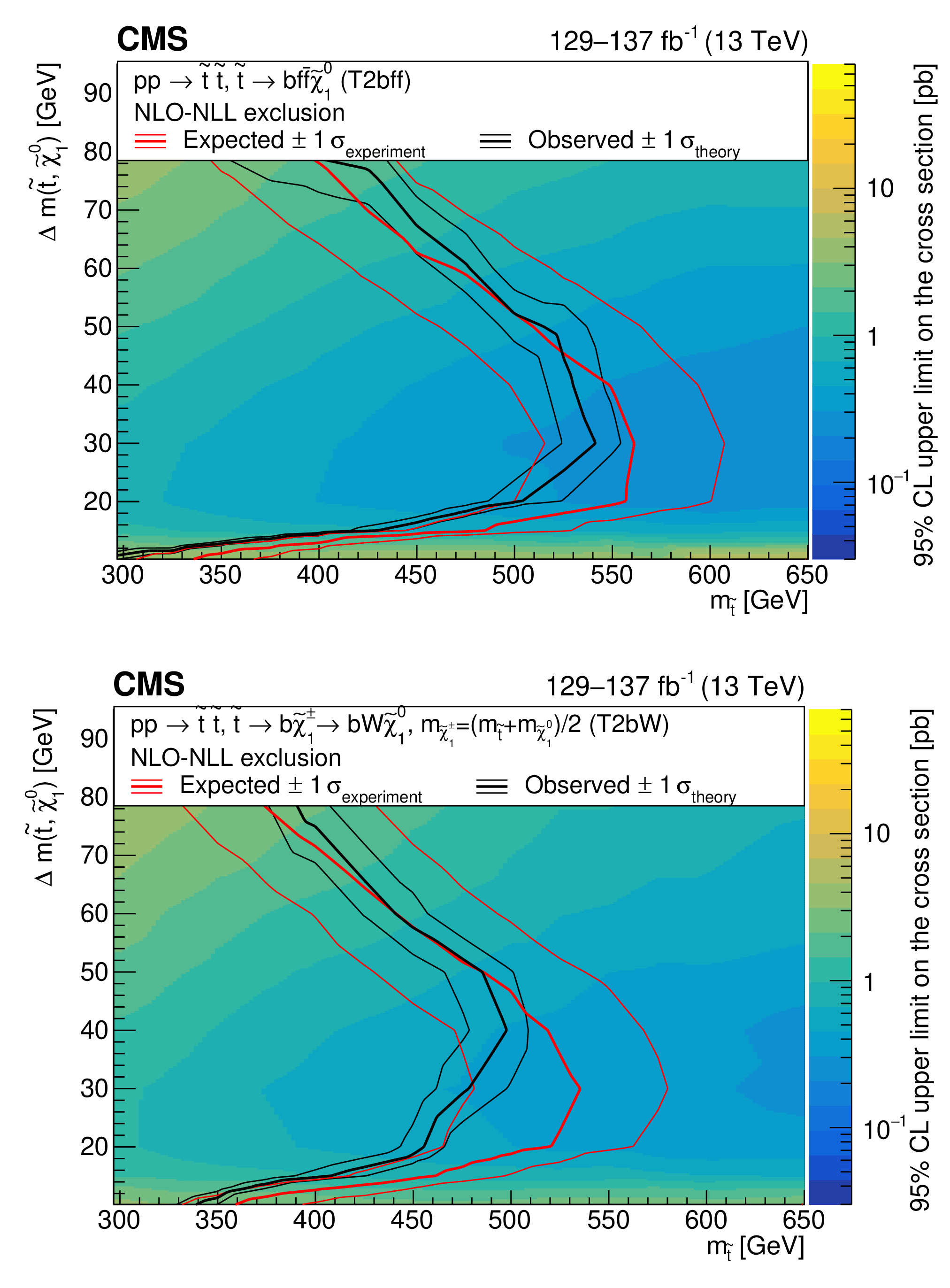
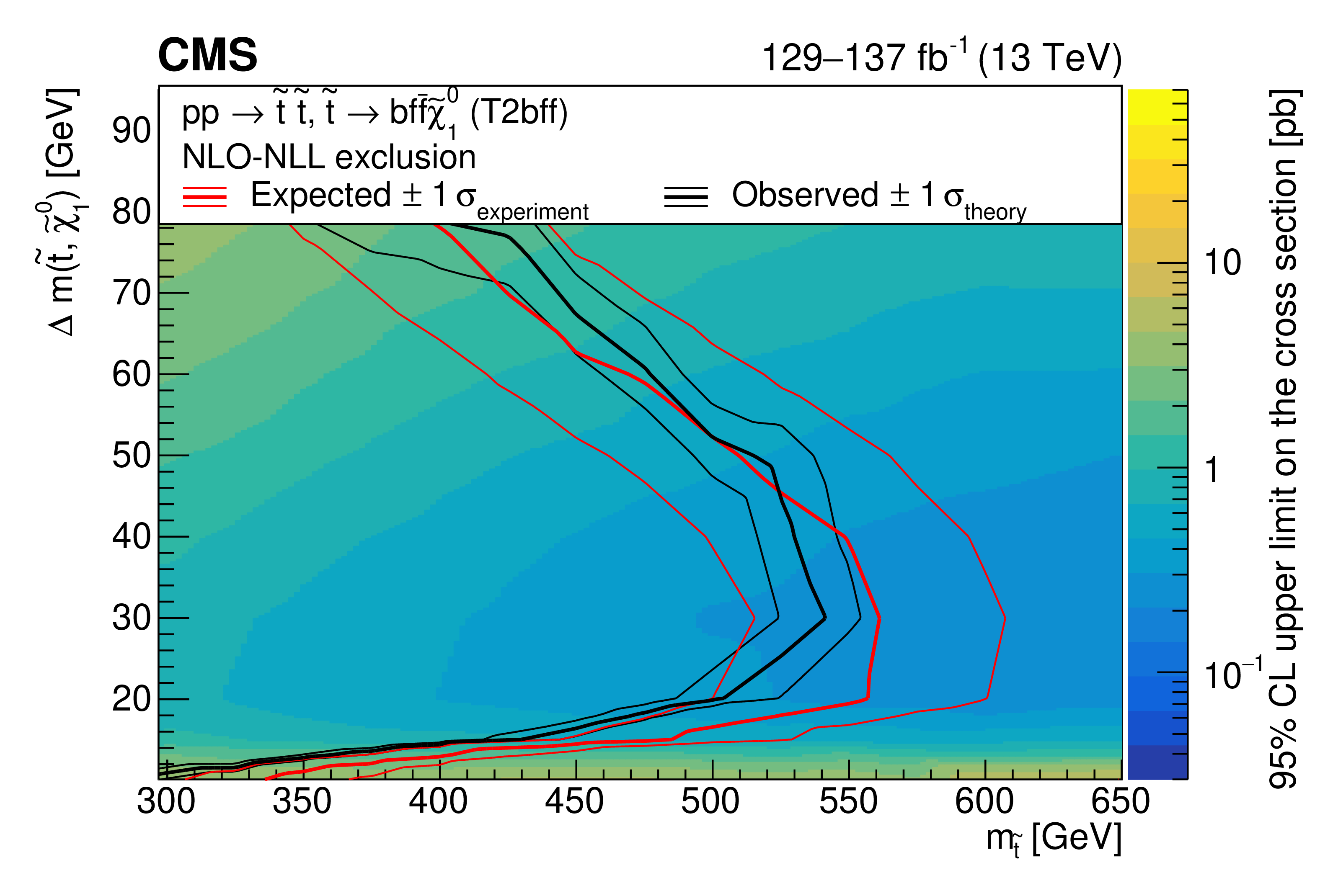
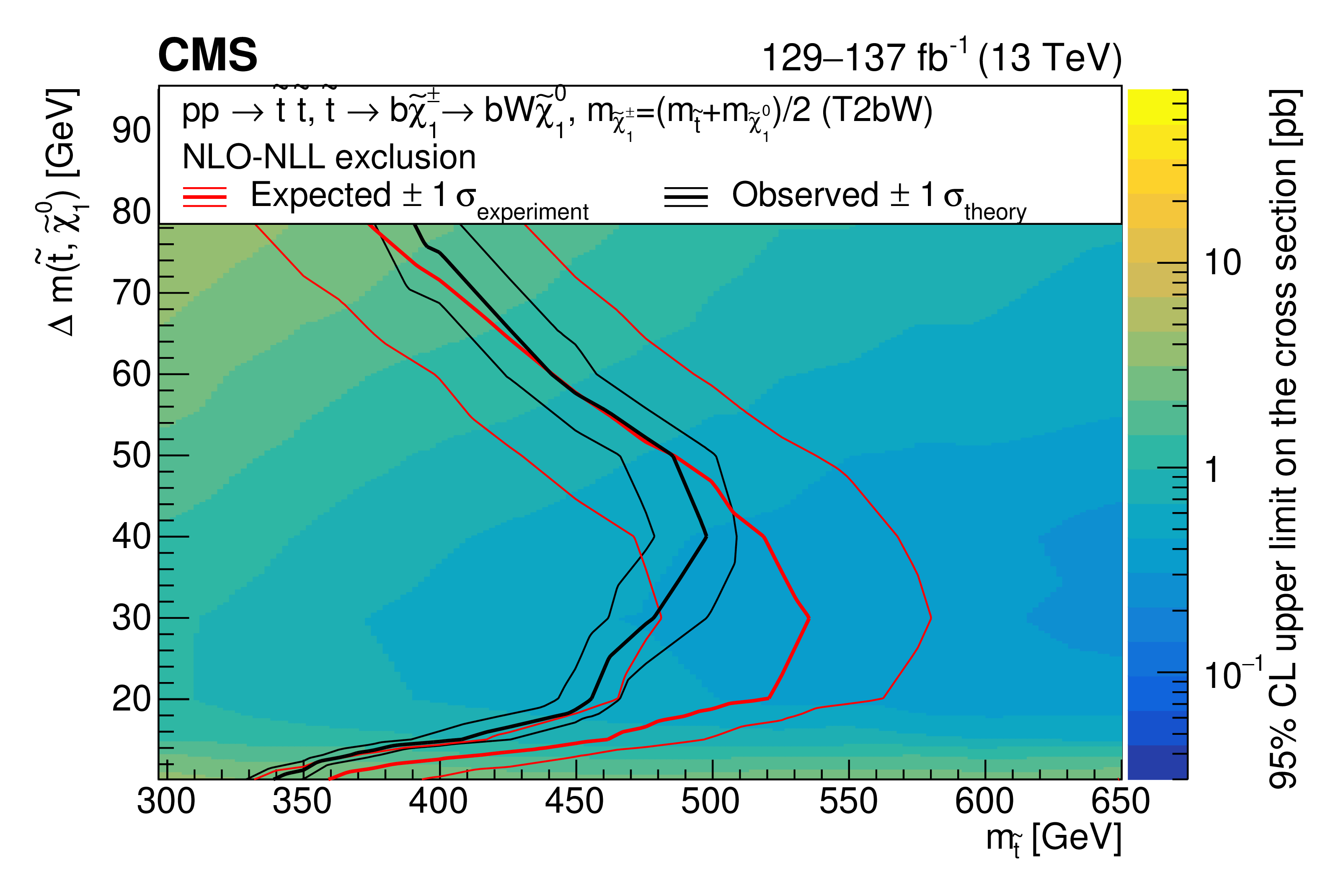
Figure 10:
The observed 95% CL exclusion contours (black curves) assuming the NLO+NLL cross sections, with the variations (thin lines) corresponding to the uncertainty in the cross section for the T2bff$\tilde{\chi}^0_1$ (upper) and T2bW (lower) simplified models. The red curves present the 95% CL expected limits with the band (thin lines) covering 68% of the limits in the absence of signal. The range of luminosities of the analysis regions included in the fit is indicated on the plot. |
png pdf |
Figure 10-a:
The observed 95% CL exclusion contours (black curves) assuming the NLO+NLL cross sections, with the variations (thin lines) corresponding to the uncertainty in the cross section for the T2bff$\tilde{\chi}^0_1$ (upper) and T2bW (lower) simplified models. The red curves present the 95% CL expected limits with the band (thin lines) covering 68% of the limits in the absence of signal. The range of luminosities of the analysis regions included in the fit is indicated on the plot. |
png pdf |
Figure 10-b:
The observed 95% CL exclusion contours (black curves) assuming the NLO+NLL cross sections, with the variations (thin lines) corresponding to the uncertainty in the cross section for the T2bff$\tilde{\chi}^0_1$ (upper) and T2bW (lower) simplified models. The red curves present the 95% CL expected limits with the band (thin lines) covering 68% of the limits in the absence of signal. The range of luminosities of the analysis regions included in the fit is indicated on the plot. |
| Tables | |
png pdf |
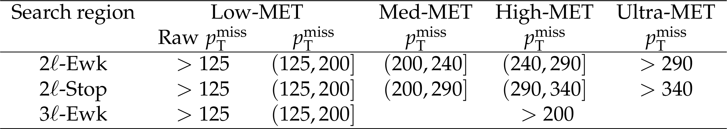
Table 1:
Definition of the MET bins of the SRs. The boundaries of raw ${{p_{\mathrm {T}}} ^\text {miss}}$ and ${{p_{\mathrm {T}}} ^\text {miss}}$ (in GeV) of every bin are described. |
png pdf |
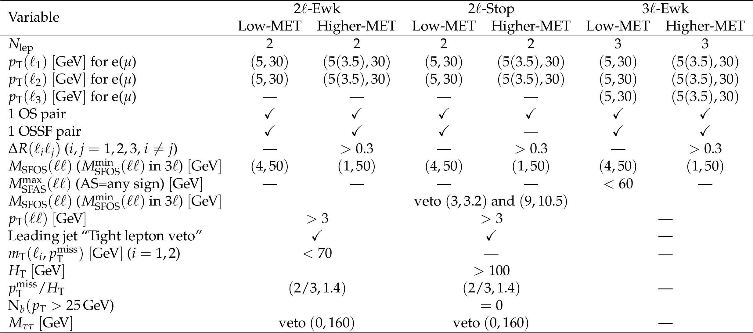
Table 2:
List of all criteria that events must satisfy to be selected in one of the SRs. The label "Low-MET" refers to the low-MET bin of the analysis, while the label "Higher-MET" refers collectively to the Med-, High- and Ultra-MET bins of the analysis. |
png pdf |
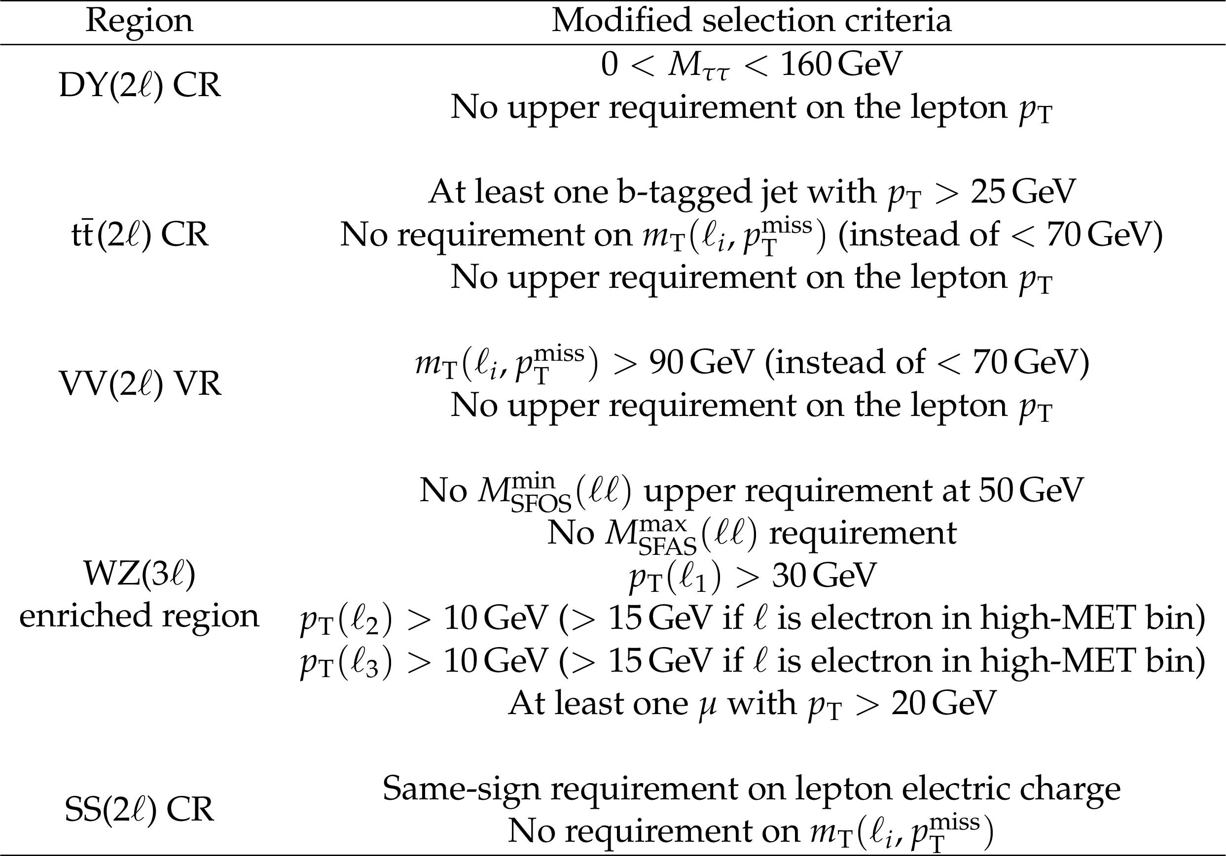
Table 3:
Summary of changes in the selection criteria with respect to the SR for all the background control and validation regions. |
png pdf |
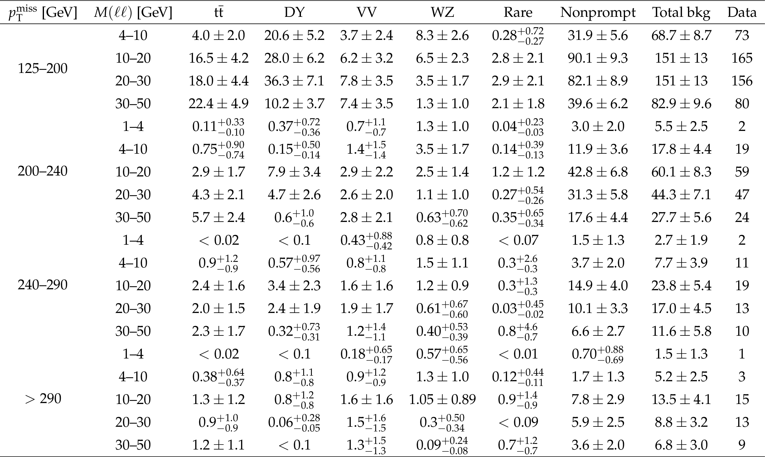
Table 4:
Observed and predicted yields as extracted from the maximum likelihood fit, in the 2$\ell $-Ewk SRs. Uncertainties include both the statistical and systematic components. |
png pdf |
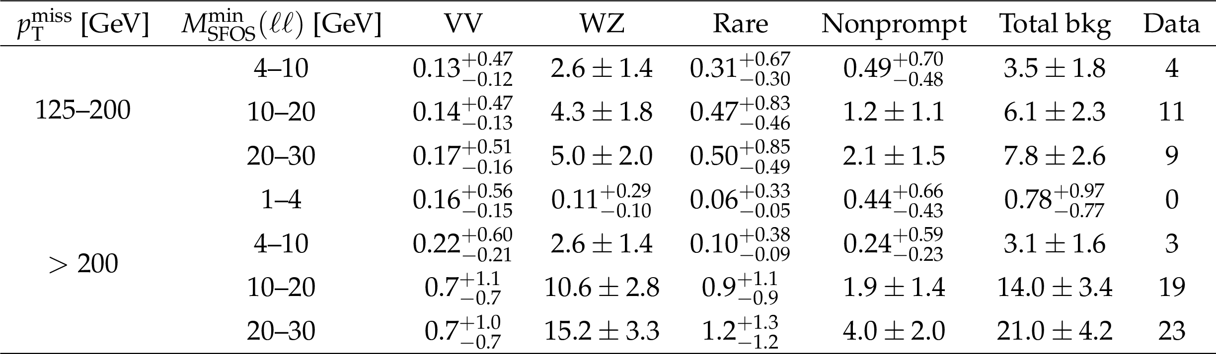
Table 5:
Observed and predicted yields as extracted from the maximum likelihood fit, in the 3$\ell $-Ewk SRs. Uncertainties include both the statistical and systematic components. |
png pdf |
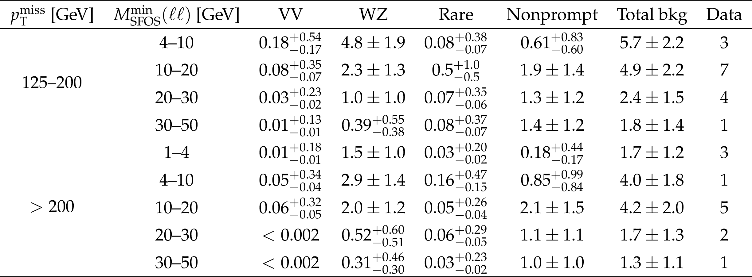
Table 6:
Observed and predicted yields as extracted from the maximum likelihood fit, in the WZ-like selection SRs. Uncertainties include both the statistical and systematic components. |

png pdf |
Table 7:
Observed and predicted yields as extracted from the maximum likelihood fit, in the 2$\ell $-Stop SRs. Uncertainties include both the statistical and systematic components. |
| Summary |
|
A search for new physics is performed using events with two or three soft leptons and missing transverse momentum. These signatures are motivated by models predicting a weakly interacting massive particle that originates from the decay of another new particle with nearly degenerate mass. The results are based on data collected by the CMS experiment at the LHC during 2016-2018, corresponding to an integrated luminosity of up to 137 fb$^{-1}$. The observed event yields are in agreement with the standard model expectations. The results are interpreted in the framework of supersymmetric (SUSY) simplified models targeting electroweakino mass-degenerate spectra and top squark-lightest neutralino ($\tilde{\mathrm{t}}$-$\tilde{\chi}^0_1$) mass-degenerate benchmark models. An interpretation of the analysis is performed also in the phenomenological minimal SUSY standard model (pMSSM) framework. In particular, the simplified wino-bino model in which the next-to-lightest neutralino and the lightest chargino are produced and decay according to $\tilde{\chi}^{0}_{2}\tilde{\chi}^{\pm}_1\to\mathrm{Z}^{*}\mathrm{W}^{*}\tilde{\chi}^0_1\tilde{\chi}^0_1$ are explored for mass differences ($\Delta m$) between $\tilde{\chi}^{0}_{2}$ and $\tilde{\chi}^0_1$ of less than 50 GeV, assuming wino production cross sections. At 95% confidence level, wino-like $\tilde{\chi}^{\pm}_1$/$\tilde{\chi}^{0}_{2}$ masses are excluded up to 275 GeV for $\Delta m$ of 10 GeV relative to the lightest neutralino. The higgsino simplified model is of particular interest; mass-degenerate electroweakinos are expected in natural SUSY, which predicts light higgsinos. In this model, excluded masses reach up to 205 GeV for $\Delta m$ of 7.5 GeV and 150 GeV for a highly compressed scenario with $\Delta m$ of 3 GeV. In the pMSSM higgsino model, the limits are presented in the plane of the higgsino-bino mass parameters $\mu$-$M_1$; the higgsino mass parameter $\mu$ is excluded up to 170 GeV, when the bino mass parameter $M_1$ is 600 GeV. For larger values of $M_1$, the mass splitting $\Delta m (\tilde{\chi}^{0}_{2}, \tilde{\chi}^0_1)$ becomes smaller; for $M_1 = $ 800 GeV, $\mu$ is excluded up to 180 GeV. Finally, two $\tilde{\mathrm{t}}$-$\tilde{\chi}^0_1$ mass-degenerate benchmark models are considered. Top squarks with masses below 540 (480) GeV are excluded for the four-body (chargino-mediated) top squark decay model, with a ($\tilde{\mathrm{t}}$-$\tilde{\chi}^0_1$) mass splitting at 30 GeV. |
| References | ||||
| 1 | J. Wess and B. Zumino | Supergauge transformations in four dimensions | NPB 70 (1974) 39 | |
| 2 | H. P. Nilles | Supersymmetry, supergravity and particle physics | PR 110 (1984) 1 | |
| 3 | H. E. Haber and G. L. Kane | The search for supersymmetry: Probing physics beyond the standard model | PR 117 (1985) 75 | |
| 4 | R. Barbieri, S. Ferrara, and C. A. Savoy | Gauge models with spontaneously broken local supersymmetry | PLB 119 (1982) 343 | |
| 5 | S. Dawson, E. Eichten, and C. Quigg | Search for supersymmetric particles in hadron-hadron collisions | PRD 31 (1985) 1581 | |
| 6 | R. Barbieri and G. Giudice | Upper bounds on supersymmetric particle masses | NPB 306 (1988) 63 | |
| 7 | E. Witten | Dynamical breaking of supersymmetry | NPB 188 (1981) 513 | |
| 8 | S. Dimopoulos and H. Georgi | Softly broken supersymmetry and SU(5) | NPB 193 (1981) 150 | |
| 9 | G. R. Farrar and P. Fayet | Phenomenology of the production, decay, and detection of new hadronic states associated with supersymmetry | PLB 76 (1978) 575 | |
| 10 | Particle Data Group, P. A. Zyla et al. | Review of particle physics | Prog. Theor. Exp. Phys. 2020 (2020) 083C01 | |
| 11 | B. de Carlos and J. Casas | One-loop analysis of the electroweak breaking in supersymmetric models and the fine-tuning problem | PLB 309 (1993) 320 | hep-ph/9303291 |
| 12 | M. Dine, W. Fischler, and M. Srednicki | Supersymmetric technicolor | NPB 189 (1981) 575 | |
| 13 | S. Dimopoulos and S. Raby | Supercolor | NPB 192 (1981) 353 | |
| 14 | N. Sakai | Naturalness in supersymmetric GUTS | Z. Phys. C 11 (1981) 153 | |
| 15 | R. K. Kaul and P. Majumdar | Cancellation of quadratically divergent mass corrections in globally supersymmetric spontaneously broken gauge theories | NPB 199 (1982) 36 | |
| 16 | K. Griest and D. Seckel | Three exceptions in the calculation of relic abundances | PRD 43 (1991) 3191 | |
| 17 | J. Edsjo and P. Gondolo | Neutralino relic density including coannihilations | PRD 56 (1997) 1879 | hep-ph/9704361 |
| 18 | H. Baer, V. Barger, and P. Huang | Hidden SUSY at the LHC: the light higgsino-world scenario and the role of a lepton collider | JHEP 11 (2011) 031 | 1107.5581 |
| 19 | H. Baer, A. Mustafayev, and X. Tata | Monojet plus soft dilepton signal from light higgsino pair production at LHC14 | PRD 90 (2014) 115007 | 1409.7058 |
| 20 | C. Han et al. | Probing light higgsinos in natural SUSY from monojet signals at the LHC | JHEP 02 (2014) 049 | 1310.4274 |
| 21 | Z. Han, G. D. Kribs, A. Martin, and A. Menon | Hunting quasidegenerate higgsinos | PRD 89 (2014) 075007 | 1401.1235 |
| 22 | MSSM Working Group | The minimal supersymmetric standard model: Group summary report | 1998 | hep-ph/9901246 |
| 23 | C. Bal\'azs, M. Carena, and C. E. M. Wagner | Dark matter, light stops and electroweak baryogenesis | PRD 70 (2004) 015007 | hep-ph/0403224 |
| 24 | CMS Collaboration | Search for supersymmetry in events with soft leptons, low jet multiplicity, and missing transverse energy in proton-proton collisions at $ \sqrt{s} = $ 8 TeV | PLB 759 (2016) 9 | CMS-SUS-14-021 1512.08002 |
| 25 | CMS Collaboration | Search for new physics in events with two soft oppositely charged leptons and missing transverse momentum in proton-proton collisions at $ \sqrt{s} = $ 13 TeV | PLB 782 (2018) 440 | CMS-SUS-16-048 1801.01846 |
| 26 | ATLAS Collaboration | Search for electroweak production of supersymmetric states in scenarios with compressed mass spectra at $ \sqrt{s} = $ 13 TeV with the ATLAS detector | PRD 97 (2018) 052010 | 1712.08119 |
| 27 | ATLAS Collaboration | Searches for electroweak production of supersymmetric particles with compressed mass spectra in $ \sqrt{s} = $ 13 TeV pp collisions with the ATLAS detector | PRD 101 (2020) 052005 | 1911.12606 |
| 28 | ATLAS Collaboration | Search for chargino-neutralino pair production in final states with three leptons and missing transverse momentum in $ \sqrt{s} = $ 13 TeV pp collisions with the ATLAS detector | 2021. Submitted to EPJC | {2106.01676} |
| 29 | CMS Collaboration | HEPData record for this analysis | link | |
| 30 | CMS Collaboration | Performance of the CMS level-1 trigger in proton-proton collisions at $ \sqrt{s} = $ 13 TeV | JINST 15 (2020) P10017 | CMS-TRG-17-001 2006.10165 |
| 31 | CMS Collaboration | The CMS trigger system | JINST 12 (2017) P01020 | CMS-TRG-12-001 1609.02366 |
| 32 | CMS Collaboration | The CMS experiment at the CERN LHC | JINST 3 (2008) P08004 | CMS-00-001 |
| 33 | J. Alwall et al. | The automated computation of tree-level and next-to-leading order differential cross sections, and their matching to parton shower simulations | JHEP 07 (2014) 079 | 1405.0301 |
| 34 | R. Frederix and S. Frixione | Merging meets matching in MC@NLO | JHEP 12 (2012) 061 | 1209.6215 |
| 35 | J. Alwall et al. | Comparative study of various algorithms for the merging of parton showers and matrix elements in hadronic collisions | EPJC 53 (2008) 473 | 0706.2569 |
| 36 | P. Nason | A new method for combining NLO QCD with shower Monte Carlo algorithms | JHEP 11 (2004) 040 | hep-ph/0409146 |
| 37 | S. Frixione, P. Nason, and C. Oleari | Matching NLO QCD computations with parton shower simulations: the POWHEG method | JHEP 11 (2007) 070 | 0709.2092 |
| 38 | S. Alioli, P. Nason, C. Oleari, and E. Re | A general framework for implementing NLO calculations in shower Monte Carlo programs: the POWHEG BOX | JHEP 06 (2010) 043 | 1002.2581 |
| 39 | T. Melia, P. Nason, R. Rontsch, and G. Zanderighi | $ \mathrm{W}^+\mathrm{W}^- $, $ \mathrm{W}\mathrm{Z} $ and $ \mathrm{Z}\mathrm{Z} $ production in the POWHEG BOX | JHEP 11 (2011) 078 | 1107.5051 |
| 40 | P. Nason and G. Zanderighi | $ \mathrm{W^{+}}\mathrm{W^{-}} $, $ \mathrm{W}\mathrm{Z} $ and $ \mathrm{Z}\mathrm{Z} $ production in the POWHEG-BOX-V2 | EPJC 74 (2014) 2702 | 1311.1365 |
| 41 | E. Re | Single-top Wt-channel production matched with parton showers using the POWHEG method | EPJC 71 (2011) 1547 | 1009.2450 |
| 42 | NNPDF Collaboration | Parton distributions for the LHC Run II | JHEP 04 (2015) 040 | 1410.8849 |
| 43 | NNPDF Collaboration | Parton distributions from high-precision collider data | EPJC 77 (2017) 663 | |
| 44 | T. Sjostrand et al. | An introduction to PYTHIA 8.2 | CPC 191 (2015) 159 | 1410.3012 |
| 45 | P. Skands, S. Carrazza, and J. Rojo | Tuning PYTHIA 8.1: the Monash 2013 tune | EPJC 74 (2014) 3024 | 1404.5630 |
| 46 | CMS Collaboration | Event generator tunes obtained from underlying event and multiparton scattering measurements | EPJC 76 (2016) 155 | CMS-GEN-14-001 1512.00815 |
| 47 | CMS Collaboration | Extraction and validation of a new set of CMS PYTHIA8 tunes from underlying-event measurements | EPJC 80 (2020) 7499 | CMS-GEN-17-001 1903.12179 |
| 48 | GEANT4 Collaboration | GEANT4--a simulation toolkit | NIMA 506 (2003) 250 | |
| 49 | J. Alwall, P. Schuster, and N. Toro | Simplified models for a first characterization of new physics at the LHC | PRD 79 (2009) 075020 | 0810.3921 |
| 50 | D. Alves et al. | Simplified models for LHC new physics searches | JPG 39 (2012) 105005 | 1105.2838 |
| 51 | CMS Collaboration | Interpretation of searches for supersymmetry with simplified models | PRD 88 (2013) 052017 | CMS-SUS-11-016 1301.2175 |
| 52 | W. Beenakker et al. | Production of charginos, neutralinos, and sleptons at hadron colliders | PRL 83 (1999) 3780 | hep-ph/9906298 |
| 53 | B. Fuks, M. Klasen, D. R. Lamprea, and M. Rothering | Gaugino production in proton-proton collisions at a center-of-mass energy of 8 TeV | JHEP 10 (2012) 081 | 1207.2159 |
| 54 | B. Fuks, M. Klasen, D. R. Lamprea, and M. Rothering | Precision predictions for electroweak superpartner production at hadron colliders with resummino $ | EPJC 73 (2013) 2480 | 1304.0790 |
| 55 | W. Beenakker, R. Hopker, and M. Spira | PROSPINO: A program for the production of supersymmetric particles in next-to-leading order QCD | hep-ph/9611232 | |
| 56 | A. Djouadi, J.-L. Kneur, and G. Moultaka | SuSpect: A Fortran code for the supersymmetric and higgs particle spectrum in the MSSM | CPC 176 (2007) 426 | hep-ph/0211331 |
| 57 | M. Muhlleitner, A. Djouadi, and Y. Mambrini | SDECAY: A Fortran code for the decays of the supersymmetric particles in the MSSM | CPC 168 (2005) 46 | hep-ph/0311167 |
| 58 | A. Djouadi, J. Kalinowski, and M. Spira | HDECAY: A program for Higgs boson decays in the standard model and its supersymmetric extension | CPC 108 (1998) 56 | hep-ph/9704448 |
| 59 | M. M. Muhlleitner, A. Djouadi, and M. Spira | Decays of supersymmetric particles: The program SUSY-HIT | in Physics at LHC. Proc. 3rd Conf., Acta Phys. Polon. B 38 (2007) 635 | hep-ph/0609292 |
| 60 | P. Z. Skands et al. | SUSY Les Houches accord: Interfacing SUSY spectrum calculators, decay packages, and event generators | JHEP 07 (2004) 036 | hep-ph/0311123 |
| 61 | U. De Sanctis, T. Lari, S. Montesano, and C. Troncon | Perspectives for the detection and measurement of supersymmetry in the focus point region of mSUGRA models with the ATLAS detector at LHC | EPJC 52 (2007) 743 | 0704.2515 |
| 62 | R. Grober, M. M. Muhlleitner, E. Popenda, and A. Wlotzka | Light stop decays: Implications for LHC searches | EPJC 75 (2015) 420 | 1408.4662 |
| 63 | CMS Collaboration | The fast simulation of the CMS detector at LHC | J. Phys. Conf. Ser. 331 (2011) 032049 | |
| 64 | A. Giammanco | The fast simulation of the CMS experiment | J. Phys. Conf. Ser. 513 (2014) 022012 | |
| 65 | CMS Collaboration | Identification of heavy-flavour jets with the CMS detector in pp collisions at 13 TeV | JINST 13 (2018) P5011 | CMS-BTV-16-002 1712.07158 |
| 66 | E. Chabanat and N. Estre | Deterministic annealing for vertex finding at CMS | in Proceedings of Computing in High Energy Physics and Nuclear Physics 2004 | |
| 67 | M. Cacciari, G. P. Salam, and G. Soyez | The anti-$ {k_{\mathrm{T}}} $ jet clustering algorithm | JHEP 04 (2008) 063 | 0802.1189 |
| 68 | M. Cacciari, G. P. Salam, and G. Soyez | FastJet user manual | EPJC 72 (2012) 1896 | 1111.6097 |
| 69 | CMS Collaboration | Pileup mitigation at CMS in 13 TeV data | JINST 15 (2020) P09018 | CMS-JME-18-001 2003.00503 |
| 70 | M. Cacciari and G. P. Salam | Pileup subtraction using jet areas | PLB 659 (2008) 119 | 0707.1378 |
| 71 | CMS Collaboration | Particle-flow reconstruction and global event description with the CMS detector | JINST 12 (2017) P10003 | CMS-PRF-14-001 1706.04965 |
| 72 | CMS Collaboration | Performance of electron reconstruction and selection with the CMS detector in proton-proton collisions at $ \sqrt{s} = $ 8 TeV | JINST 10 (2015) P06005 | CMS-EGM-13-001 1502.02701 |
| 73 | CMS Collaboration | Performance of the CMS muon detector and muon reconstruction with proton-proton collisions at $ \sqrt{s} = $ 13 TeV | JINST 13 (2018) P06015 | CMS-MUO-16-001 1804.04528 |
| 74 | CMS Collaboration | Description and performance of track and primary-vertex reconstruction with the CMS tracker | JINST 9 (2014) P10009 | CMS-TRK-11-001 1405.6569 |
| 75 | CMS Collaboration | Determination of jet energy calibration and transverse momentum resolution in CMS | JINST 6 (2011) P11002 | CMS-JME-10-011 1107.4277 |
| 76 | CMS Collaboration | Jet energy scale and resolution in the CMS experiment in pp collisions at 8 TeV | JINST 12 (2017) P02014 | CMS-JME-13-004 1607.03663 |
| 77 | CMS Collaboration | Performance of missing transverse momentum reconstruction in proton-proton collisions at $ \sqrt{s} = $ 13 TeV using the CMS detector | JINST 14 (2019) P07004 | CMS-JME-17-001 1903.06078 |
| 78 | CMS Collaboration | Jet algorithms performance in 13 TeV data | CMS-PAS-JME-16-003 | CMS-PAS-JME-16-003 |
| 79 | A. Elagin, P. Murat, A. Pranko, and A. Safonov | A new mass reconstruction technique for resonances decaying to $ \tau\tau $ | NIMA 654 (2011) 481 | 1012.4686 |
| 80 | CMS Collaboration | Search for new phenomena with multiple charged leptons in proton-proton collisions at $ \sqrt{s} = $ 13 TeV | EPJC 77 (2017) 635 | CMS-SUS-16-003 1701.06940 |
| 81 | CMS Collaboration | Measurement of the inelastic proton-proton cross section at $ \sqrt{s} = $ 13 TeV | JHEP 07 (2018) | CMS-FSQ-15-005 1802.02613 |
| 82 | CMS Collaboration | CMS luminosity measurements for the 2016 data taking period | CMS-PAS-LUM-17-001 | CMS-PAS-LUM-17-001 |
| 83 | CMS Collaboration | CMS luminosity measurement for the 2017 data-taking period at $ \sqrt{s} = $ 13 TeV | CMS-PAS-LUM-17-004 | CMS-PAS-LUM-17-004 |
| 84 | CMS Collaboration | CMS luminosity measurement for the 2018 data-taking period at $ \sqrt{s} = $ 13 TeV | CMS-PAS-LUM-18-002 | CMS-PAS-LUM-18-002 |
| 85 | T. Junk | Confidence level computation for combining searches with small statistics | NIMA 434 (1999) 435 | hep-ex/9902006 |
| 86 | A. L. Read | Presentation of search results: the CL$_{\text{s}} $ technique | JPG 28 (2002) 2693 | |
| 87 | G. Cowan, K. Cranmer, E. Gross, and O. Vitells | Asymptotic formulae for likelihood-based tests of new physics | EPJC 71 (2011) 1554 | 1007.1727 |
| 88 | ATLAS and CMS Collaborations, LHC Higgs Combination Group | Procedure for the LHC Higgs boson search combination in summer 2011 | ATL-PHYS-PUB/2011-11, CMS NOTE 2011/005 | |
|
|
Compact Muon Solenoid LHC, CERN |
|

|

|

|

|

|