

Compact Muon Solenoid
LHC, CERN
| CMS-SUS-19-012 ; CERN-EP-2021-097 | ||
| Search for electroweak production of charginos and neutralinos in proton-proton collisions at $\sqrt{s} = $ 13 TeV | ||
| CMS Collaboration | ||
| 27 June 2021 | ||
| JHEP 04 (2022) 147 | ||
| Abstract: A direct search for electroweak production of charginos and neutralinos is presented. Events with three or four leptons, with up to two hadronically decaying $\tau$ leptons, or two same-sign light leptons are analyzed. The data sample consists of 137 fb$^{-1}$ of proton-proton collisions with a center of mass energy of 13 TeV, recorded with the CMS detector at the LHC. The results are interpreted in terms of several simplified models. These represent a broad range of production and decay scenarios for charginos and neutralinos. A parametric neural network is used to target several of the models with large backgrounds. In addition, results using orthogonal search regions are provided for all the models, simplifying alternative theoretical interpretations of the results. Depending on the model hypotheses, charginos and neutralinos with masses up to values between 300 and 1450 GeV are excluded at 95% confidence level. | ||
| Links: e-print arXiv:2106.14246 [hep-ex] (PDF) ; CDS record ; inSPIRE record ; CADI line (restricted) ; | ||
| We dedicate this paper to the memory of our friend and colleague Luc Pape whose seminal contributions to the CMS experiment and to searches for new physics, including supersymmetry, made this work possible. |
| Figures | |
png pdf |
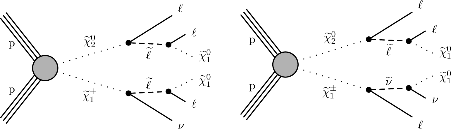
Figure 1:
Production of ${\tilde{\chi}^{\pm}_1 \tilde{\chi}^{0}_{2}}$ with subsequent decays via sleptons (left) and a slepton and a sneutrino (right). |
png pdf |
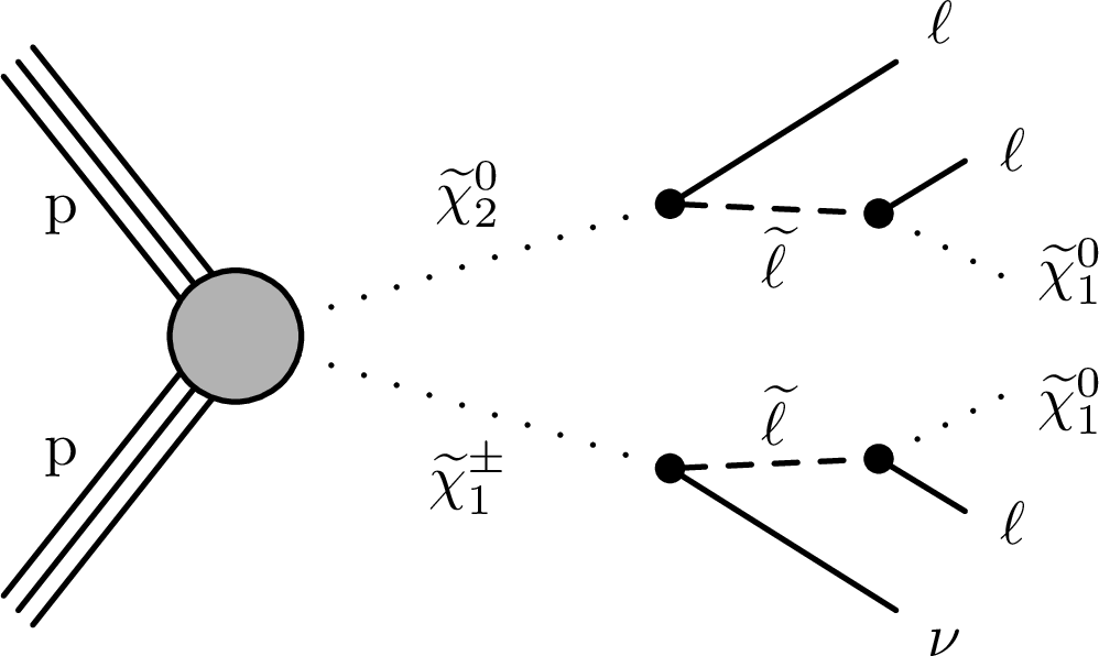
Figure 1-a:
Production of ${\tilde{\chi}^{\pm}_1 \tilde{\chi}^{0}_{2}}$ with subsequent decays via sleptons. |
png pdf |
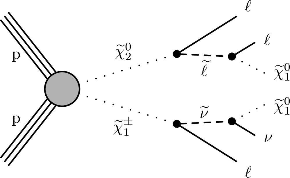
Figure 1-b:
Production of ${\tilde{\chi}^{\pm}_1 \tilde{\chi}^{0}_{2}}$ with subsequent decays via a slepton and a sneutrino. |
png pdf |
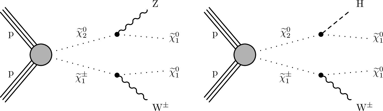
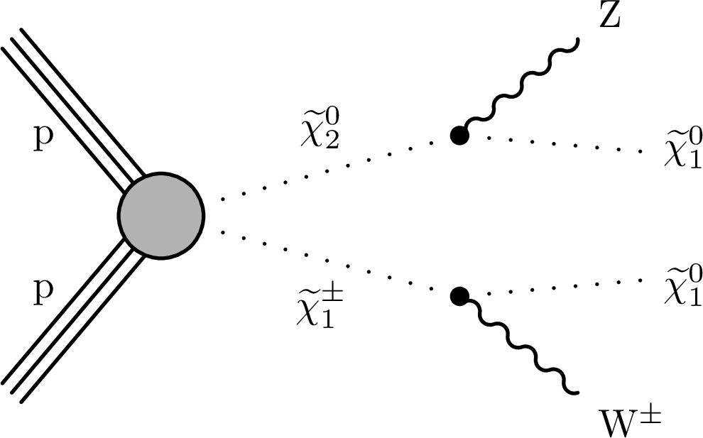
Figure 2:
Production of ${\tilde{\chi}^{\pm}_1 \tilde{\chi}^{0}_{2}}$ with subsequent decay of $\tilde{\chi}^{\pm}_1$ via a W boson and $\tilde{\chi}^{0}_{2}$ via a Z boson (left) or H boson (right). |
png pdf |
Figure 2-a:
Production of ${\tilde{\chi}^{\pm}_1 \tilde{\chi}^{0}_{2}}$ with subsequent decay of $\tilde{\chi}^{\pm}_1$ via a W boson and $\tilde{\chi}^{0}_{2}$ via a Z boson. |

png pdf |
Figure 2-b:
Production of ${\tilde{\chi}^{\pm}_1 \tilde{\chi}^{0}_{2}}$ with subsequent decay of $\tilde{\chi}^{\pm}_1$ via a W boson and $\tilde{\chi}^{0}_{2}$ via a H boson. |
png pdf |
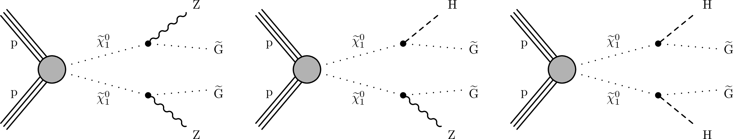
Figure 3:
Effective $\tilde{\chi}^0_1$ pair production with decays mediated by Z or H bosons. |
png pdf |
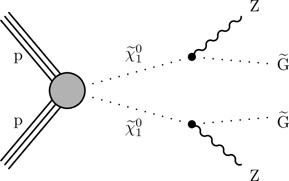
Figure 3-a:
Effective $\tilde{\chi}^0_1$ pair production with decays mediated by Z bosons. |

png pdf |
Figure 3-b:
Effective $\tilde{\chi}^0_1$ pair production with decays mediated by Z and H bosons. |
png pdf |
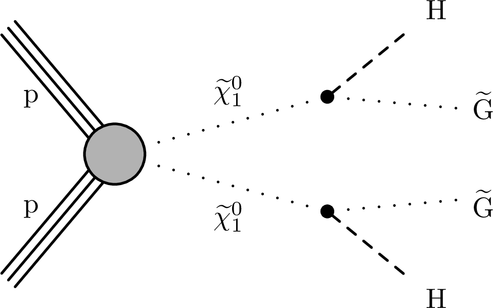
Figure 3-c:
Effective $\tilde{\chi}^0_1$ pair production with decays mediated by H bosons. |

png pdf |
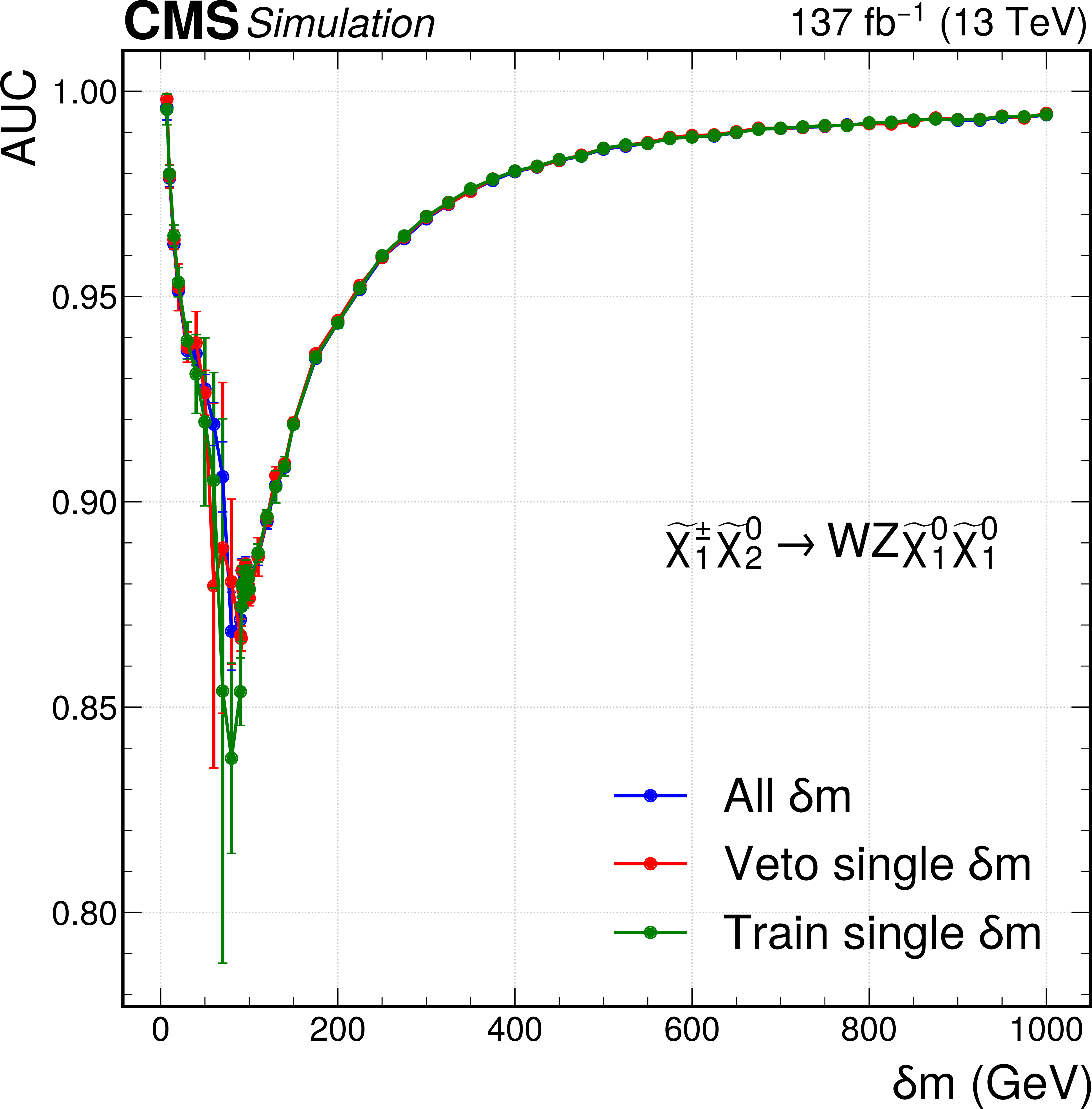
Figure 4:
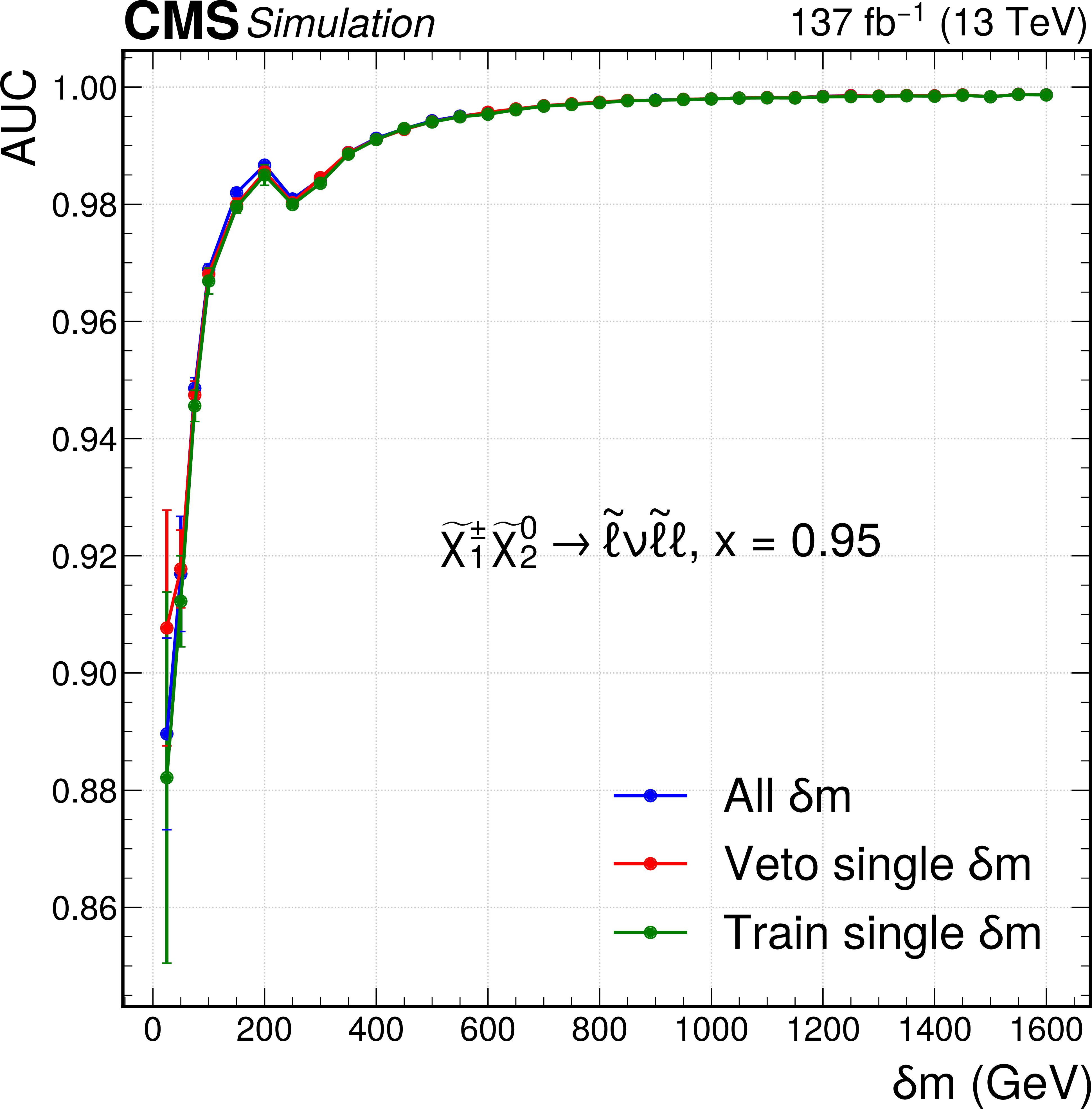
The AUC performance of the parametric neural networks for discriminating the signal from the total background predicted in simulation, as a function of $\delta m$ for the trainings targeting different signal models. The top row corresponds to the neutral network targeting signals with WZ-mediated decays with different mass ranges to show all points. The bottom row corresponds to the models with slepton-mediated decays at $x=$ 0.05 (left), $x=$ 0.5 (middle) and $x=$ 0.95 (right). Neural network models shown in blue are trained using all available $\delta m$ points, those in red are trained with all available points except the point for which the performance is shown. The models in green are not parametric and only trained to find a signal at the point where the performance is indicated. Each neural network is retrained ten times, and the mean performances are shown, with error bars indicating the standard deviation computed from ten performance values. This means that each red and green point correspond to ten neural network trainings. The entire blue curve in each figure also corresponds to ten trainings. |
png pdf |
Figure 4-a:
The AUC performance of the parametric neural networks for discriminating the signal from the total background predicted in simulation, as a function of $\delta m$ for the trainings targeting different signal models. The plot corresponds to the neutral network targeting signals with WZ-mediated decays. Neural network models shown in blue are trained using all available $\delta m$ points, those in red are trained with all available points except the point for which the performance is shown. The models in green are not parametric and only trained to find a signal at the point where the performance is indicated. Each neural network is retrained ten times, and the mean performances are shown, with error bars indicating the standard deviation computed from ten performance values. This means that each red and green point correspond to ten neural network trainings. The entire blue curve in each figure also corresponds to ten trainings. |
png pdf |
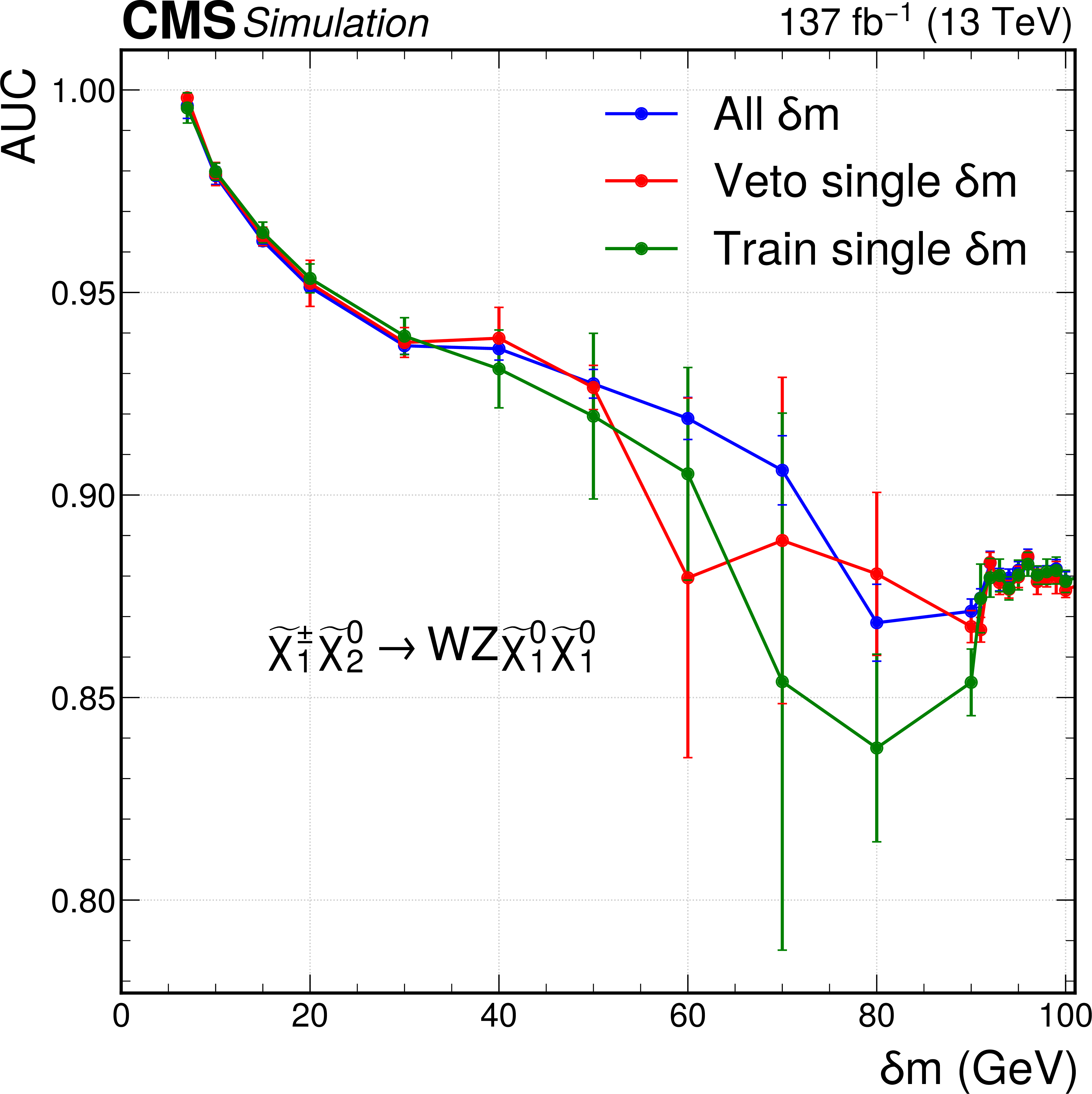
Figure 4-b:
The AUC performance of the parametric neural networks for discriminating the signal from the total background predicted in simulation, as a function of $\delta m$ for the trainings targeting different signal models. The plot corresponds to the neutral network targeting signals with WZ-mediated decays. Neural network models shown in blue are trained using all available $\delta m$ points, those in red are trained with all available points except the point for which the performance is shown. The models in green are not parametric and only trained to find a signal at the point where the performance is indicated. Each neural network is retrained ten times, and the mean performances are shown, with error bars indicating the standard deviation computed from ten performance values. This means that each red and green point correspond to ten neural network trainings. The entire blue curve in each figure also corresponds to ten trainings. |
png pdf |
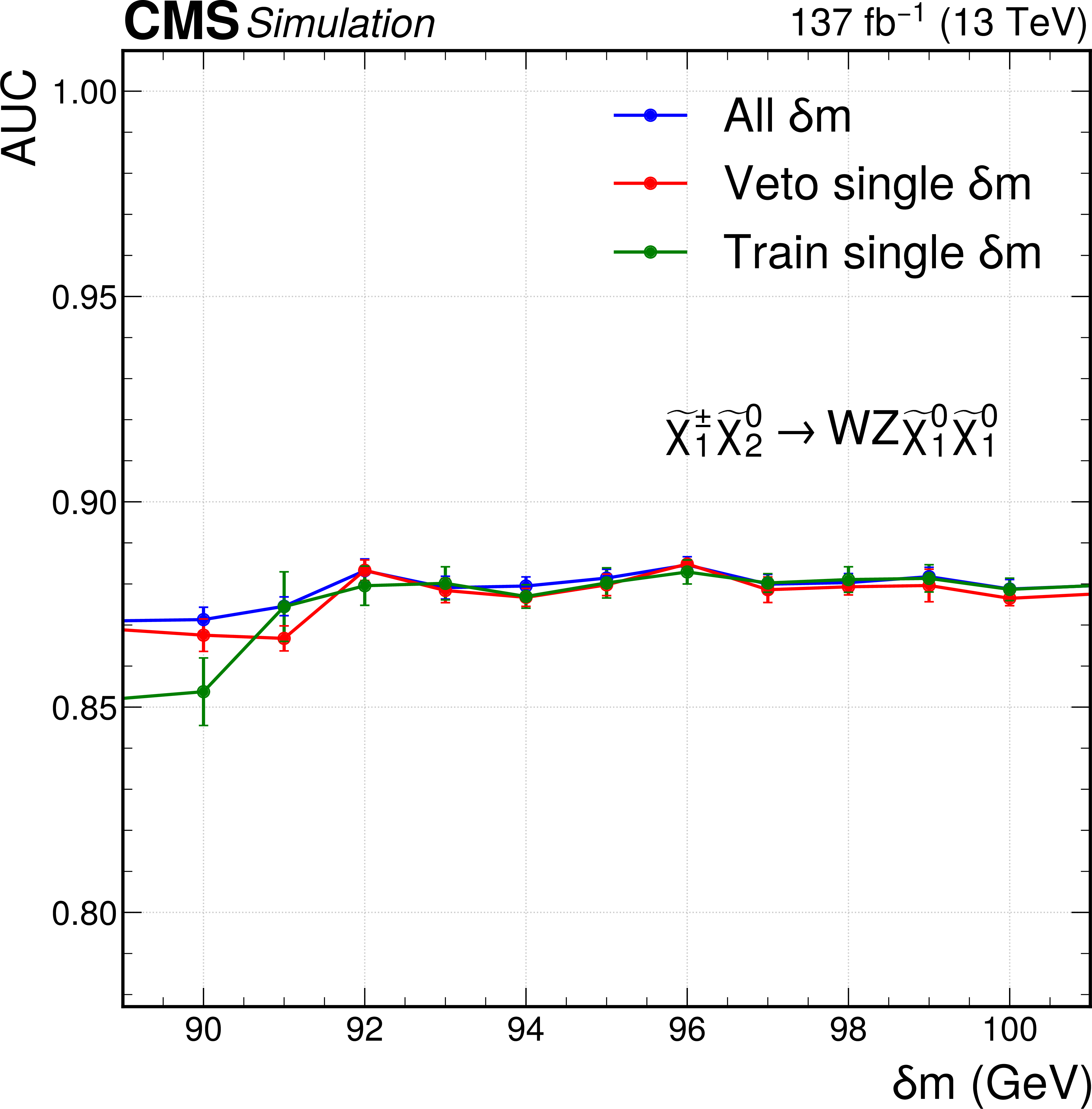
Figure 4-c:
The AUC performance of the parametric neural networks for discriminating the signal from the total background predicted in simulation, as a function of $\delta m$ for the trainings targeting different signal models. |
png pdf |
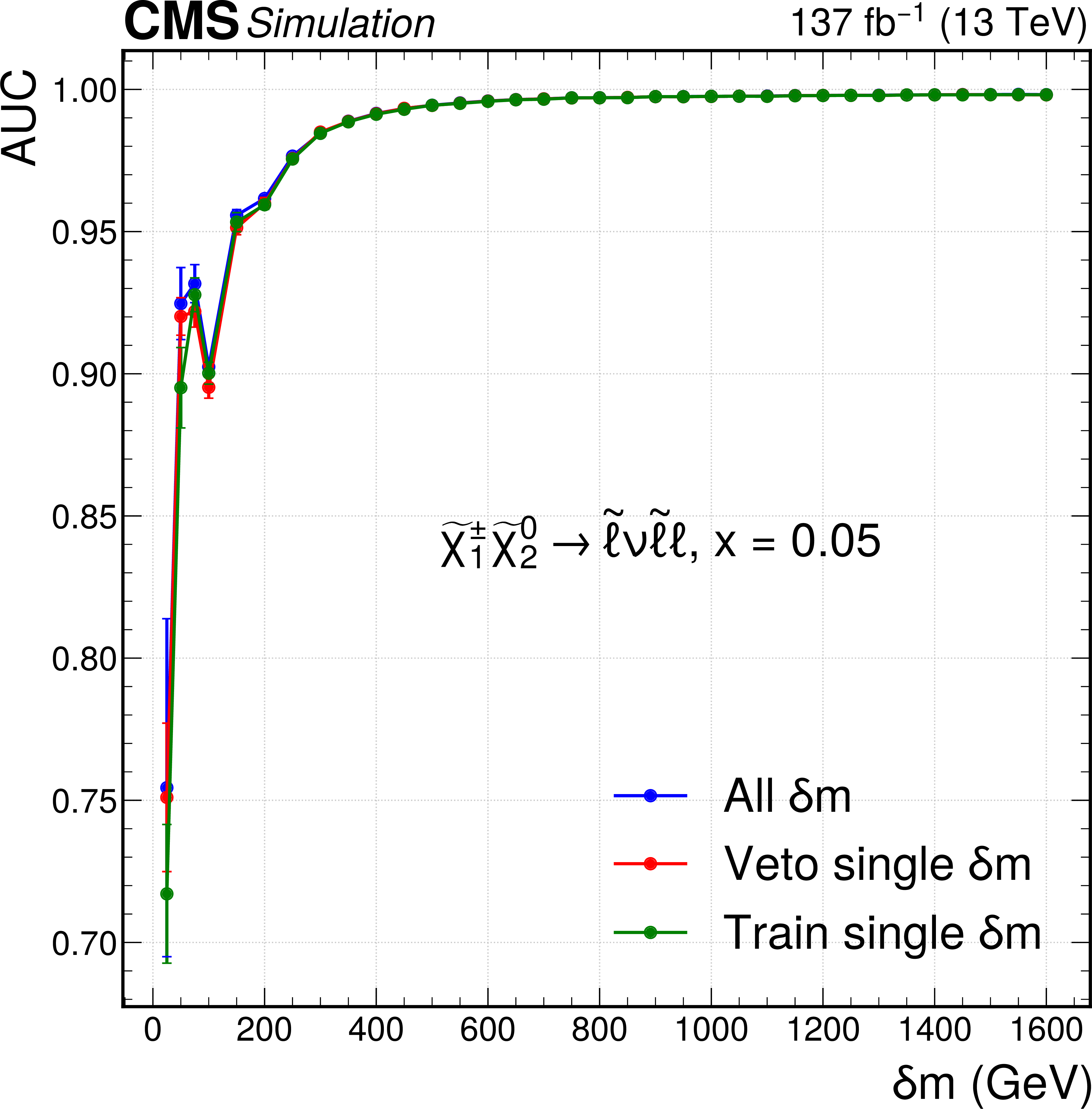
Figure 4-d:
The AUC performance of the parametric neural networks for discriminating the signal from the total background predicted in simulation, as a function of $\delta m$ for the trainings targeting different signal models. The plot corresponds to the model with slepton-mediated decays at $x=$ 0.05. Neural network models shown in blue are trained using all available $\delta m$ points, those in red are trained with all available points except the point for which the performance is shown. The models in green are not parametric and only trained to find a signal at the point where the performance is indicated. Each neural network is retrained ten times, and the mean performances are shown, with error bars indicating the standard deviation computed from ten performance values. This means that each red and green point correspond to ten neural network trainings. The entire blue curve in each figure also corresponds to ten trainings. |

png pdf |
Figure 4-e:
The AUC performance of the parametric neural networks for discriminating the signal from the total background predicted in simulation, as a function of $\delta m$ for the trainings targeting different signal models. The plot corresponds to the model with slepton-mediated decays at $x=$ 0.5. Neural network models shown in blue are trained using all available $\delta m$ points, those in red are trained with all available points except the point for which the performance is shown. The models in green are not parametric and only trained to find a signal at the point where the performance is indicated. Each neural network is retrained ten times, and the mean performances are shown, with error bars indicating the standard deviation computed from ten performance values. This means that each red and green point correspond to ten neural network trainings. The entire blue curve in each figure also corresponds to ten trainings. |
png pdf |
Figure 4-f:
The AUC performance of the parametric neural networks for discriminating the signal from the total background predicted in simulation, as a function of $\delta m$ for the trainings targeting different signal models. The plot corresponds to the model with slepton-mediated decays at $x=$ 0.95. Neural network models shown in blue are trained using all available $\delta m$ points, those in red are trained with all available points except the point for which the performance is shown. The models in green are not parametric and only trained to find a signal at the point where the performance is indicated. Each neural network is retrained ten times, and the mean performances are shown, with error bars indicating the standard deviation computed from ten performance values. This means that each red and green point correspond to ten neural network trainings. The entire blue curve in each figure also corresponds to ten trainings. |
png pdf |
Figure 5:
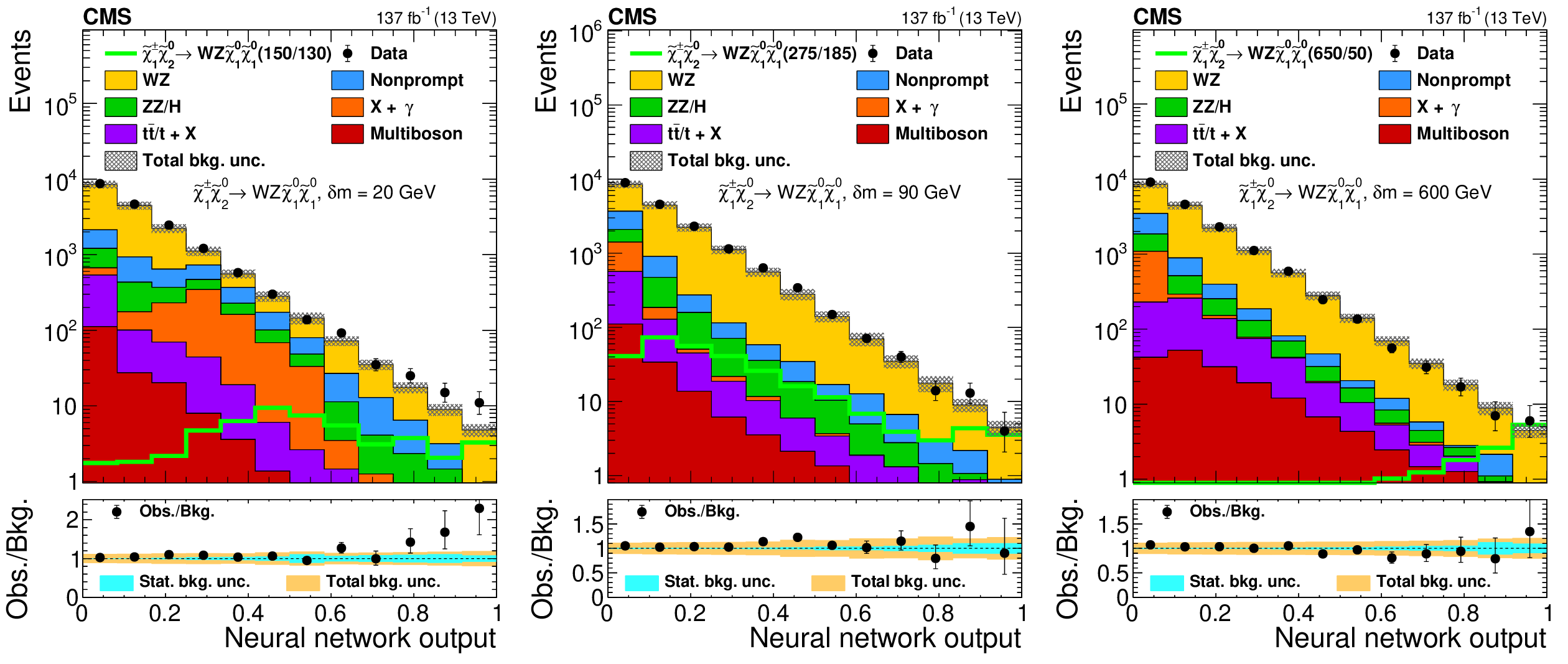
Observed and expected yields as functions of the output of the neural network used to search for ${\tilde{\chi}^{\pm}_1 \tilde{\chi}^{0}_{2}}$ production with WZ-mediated decays, evaluated at $ {\delta m} = $ 20 GeV (left), 90 GeV (center), and 600 GeV (right). The legends specify the masses of $\tilde{\chi}^{0}_{2}$ and $\tilde{\chi}^0_1$ for the shown signal distributions as ($m_{\tilde{\chi}^{0}_{2}}$/$m_{\tilde{\chi}^0_1}$). The top panels show only the total uncertainty in the background prediction, while the lower panels show the total and statistical uncertainties separately. The following abbreviations are used in the legends of this and the following figures: "bkg.'' stands for background, "unc.'' for uncertainty and "obs.'' for observed. |

png pdf |
Figure 5-a:
Observed and expected yields as functions of the output of the neural network used to search for ${\tilde{\chi}^{\pm}_1 \tilde{\chi}^{0}_{2}}$ production with WZ-mediated decays, evaluated at $ {\delta m} = $ 20 GeV. The legends specify the masses of $\tilde{\chi}^{0}_{2}$ and $\tilde{\chi}^0_1$ for the shown signal distributions as ($m_{\tilde{\chi}^{0}_{2}}$/$m_{\tilde{\chi}^0_1}$). The top panels show only the total uncertainty in the background prediction, while the lower panels show the total and statistical uncertainties separately. The following abbreviations are used in the legends of this and the following figures: "bkg.'' stands for background, "unc.'' for uncertainty and "obs.'' for observed. |
png pdf |
Figure 5-b:
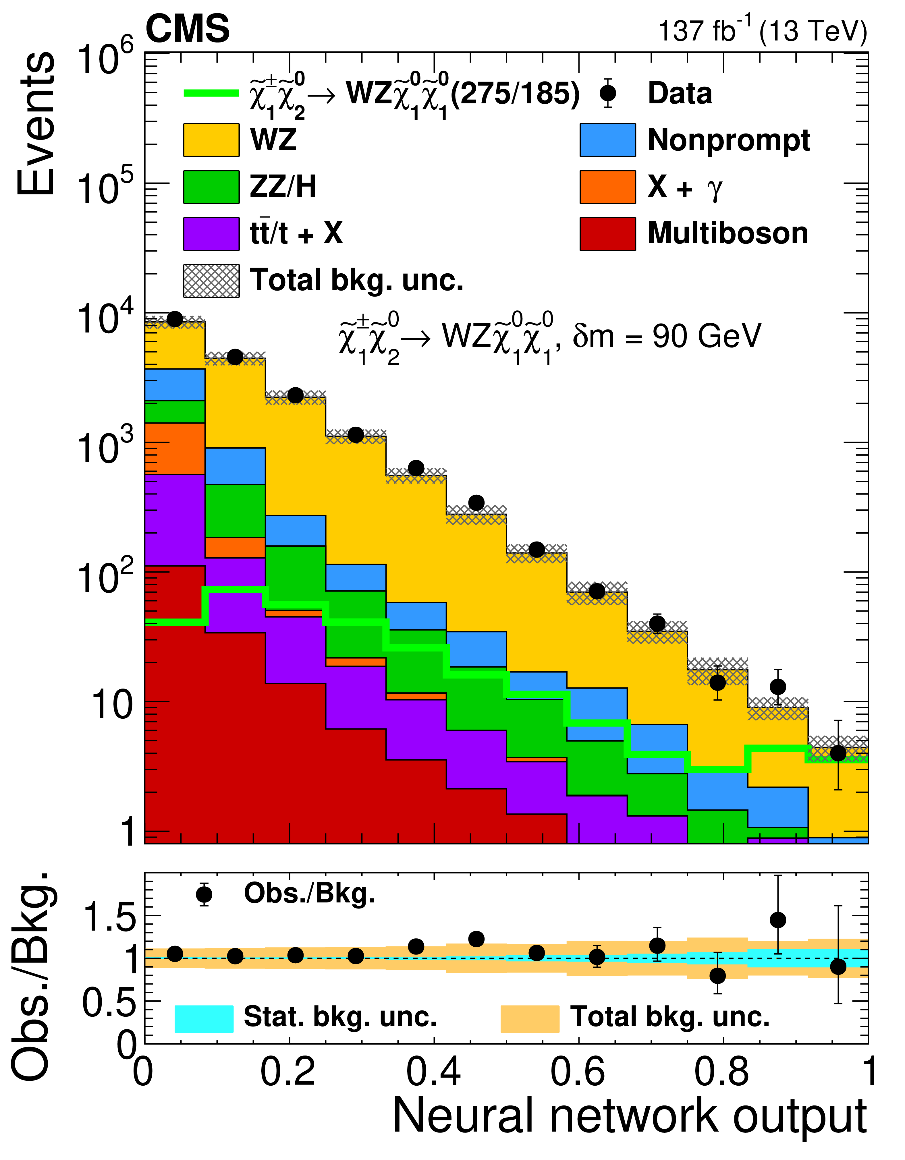
Observed and expected yields as functions of the output of the neural network used to search for ${\tilde{\chi}^{\pm}_1 \tilde{\chi}^{0}_{2}}$ production with WZ-mediated decays, evaluated at $ {\delta m} = $ 90 GeV. The legends specify the masses of $\tilde{\chi}^{0}_{2}$ and $\tilde{\chi}^0_1$ for the shown signal distributions as ($m_{\tilde{\chi}^{0}_{2}}$/$m_{\tilde{\chi}^0_1}$). The top panels show only the total uncertainty in the background prediction, while the lower panels show the total and statistical uncertainties separately. The following abbreviations are used in the legends of this and the following figures: "bkg.'' stands for background, "unc.'' for uncertainty and "obs.'' for observed. |
png pdf |
Figure 5-c:
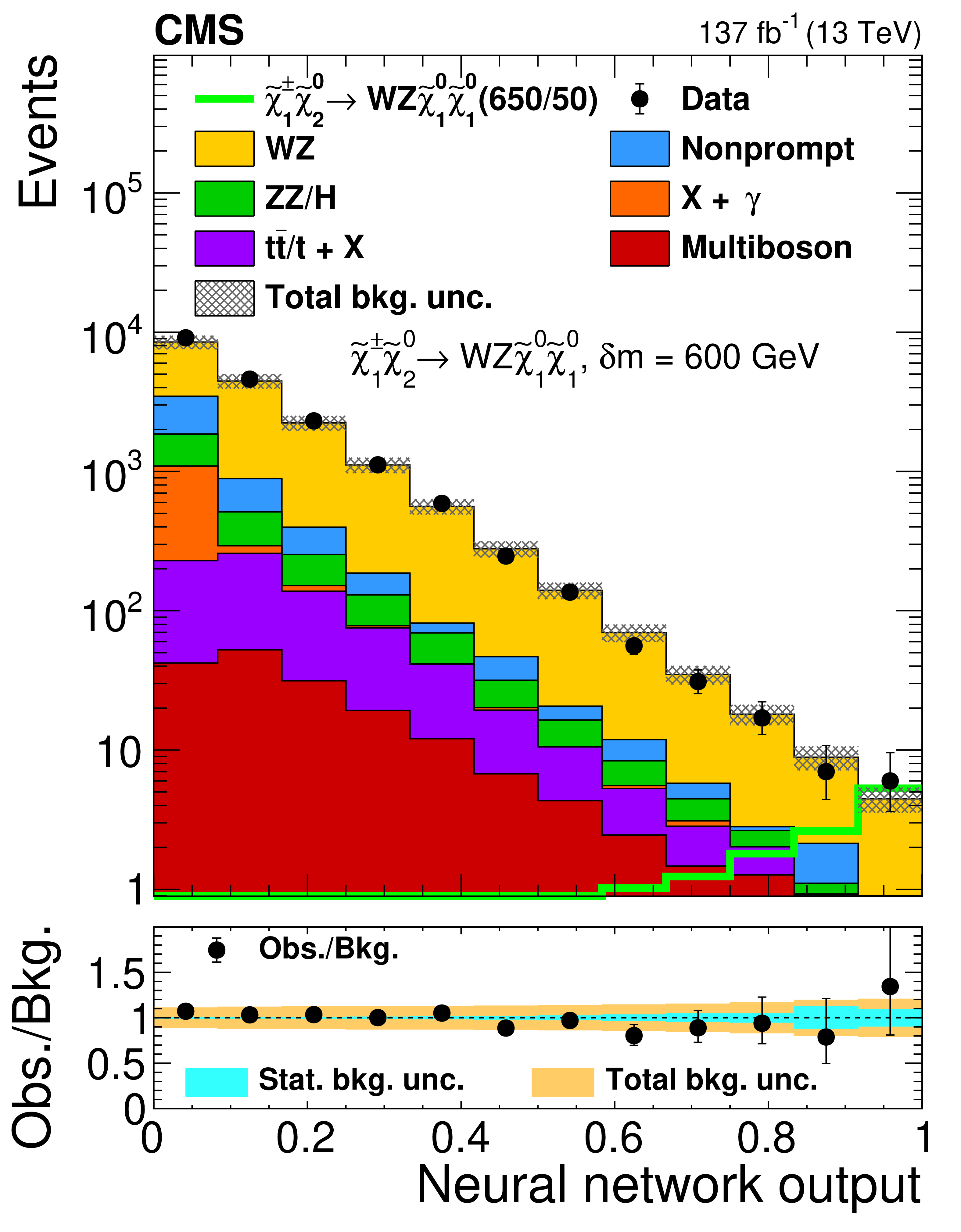
Observed and expected yields as functions of the output of the neural network used to search for ${\tilde{\chi}^{\pm}_1 \tilde{\chi}^{0}_{2}}$ production with WZ-mediated decays, evaluated at $ {\delta m} = $ 600 GeV. The legends specify the masses of $\tilde{\chi}^{0}_{2}$ and $\tilde{\chi}^0_1$ for the shown signal distributions as ($m_{\tilde{\chi}^{0}_{2}}$/$m_{\tilde{\chi}^0_1}$). The top panels show only the total uncertainty in the background prediction, while the lower panels show the total and statistical uncertainties separately. The following abbreviations are used in the legends of this and the following figures: "bkg.'' stands for background, "unc.'' for uncertainty and "obs.'' for observed. |
png pdf |
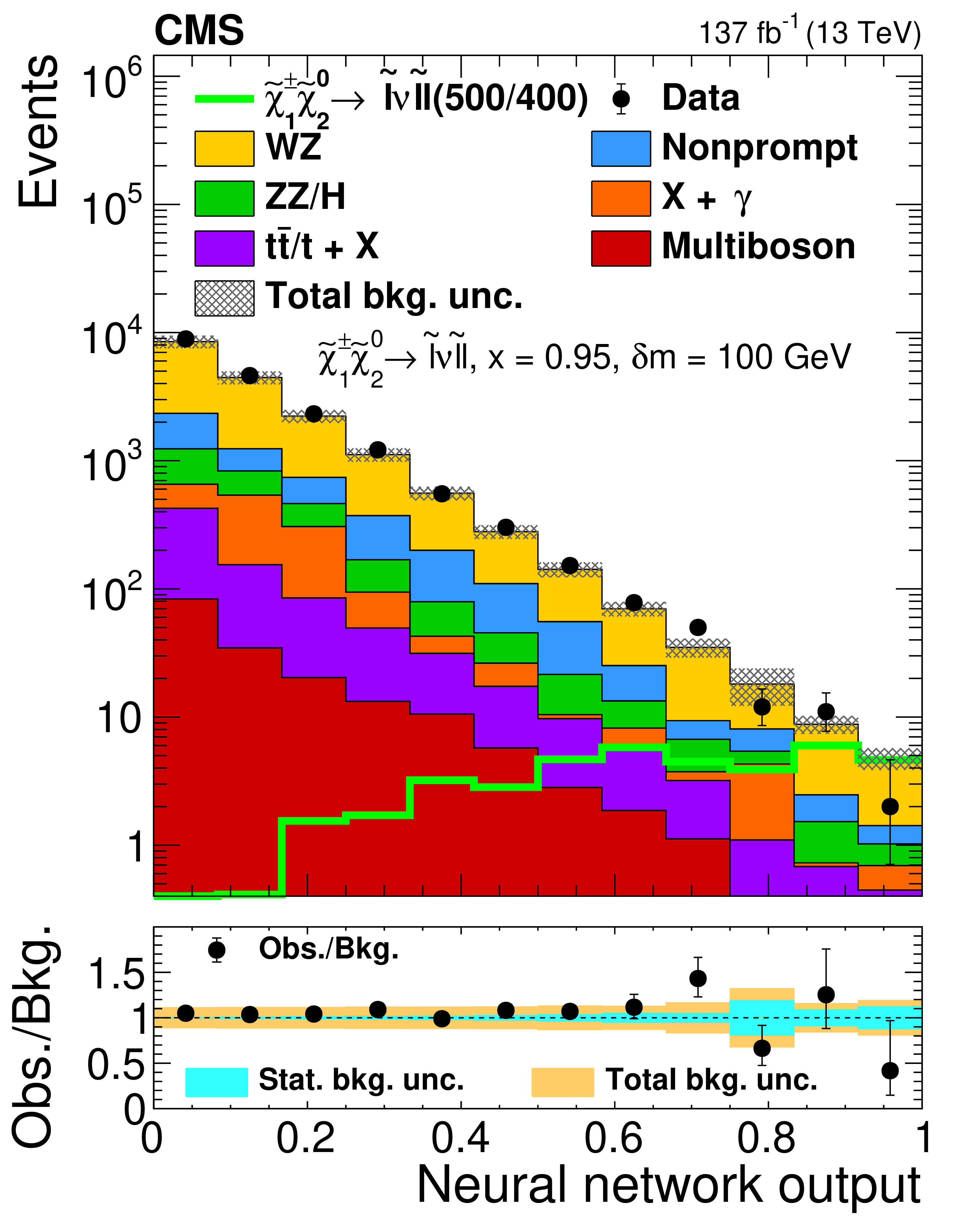
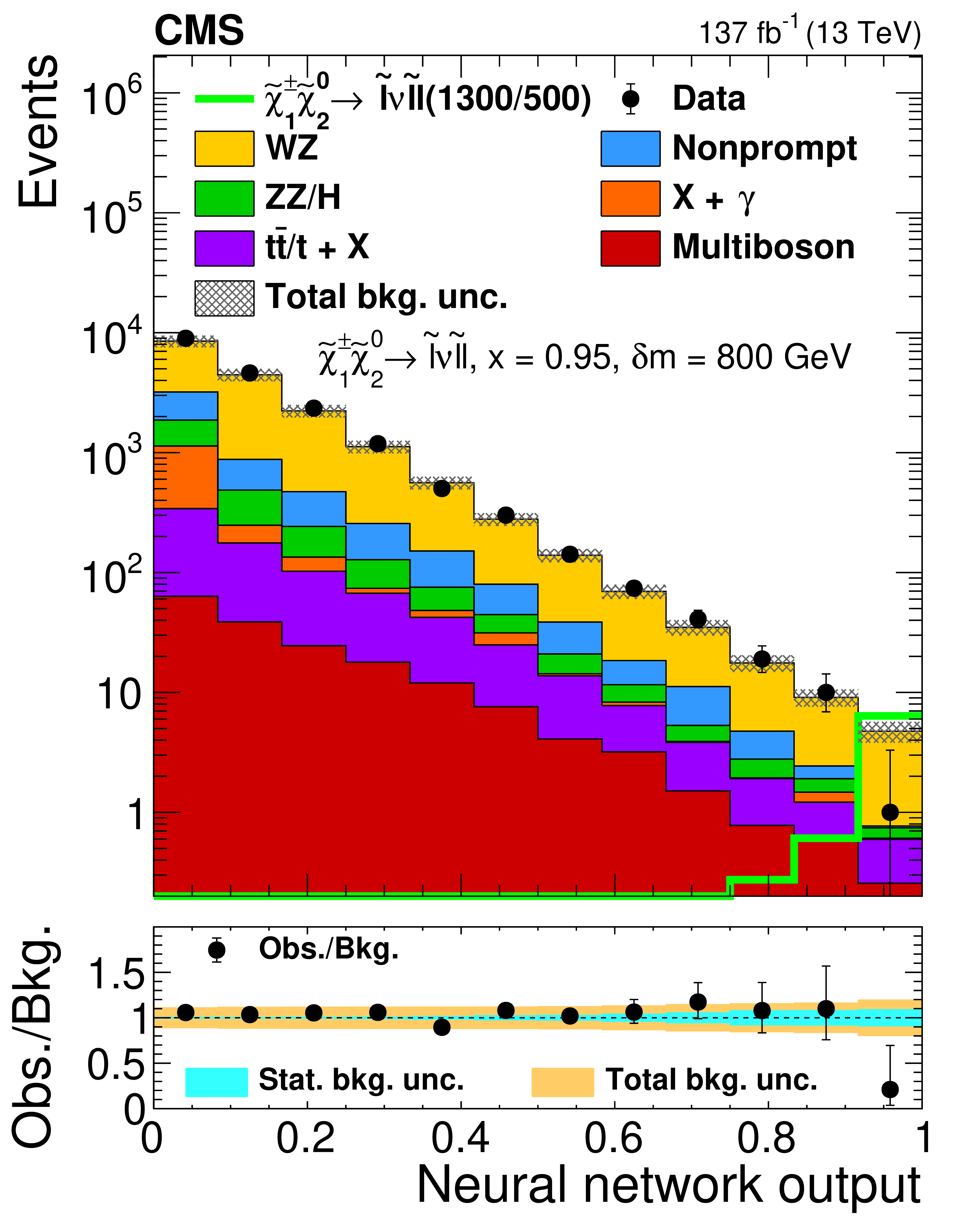
Figure 6:
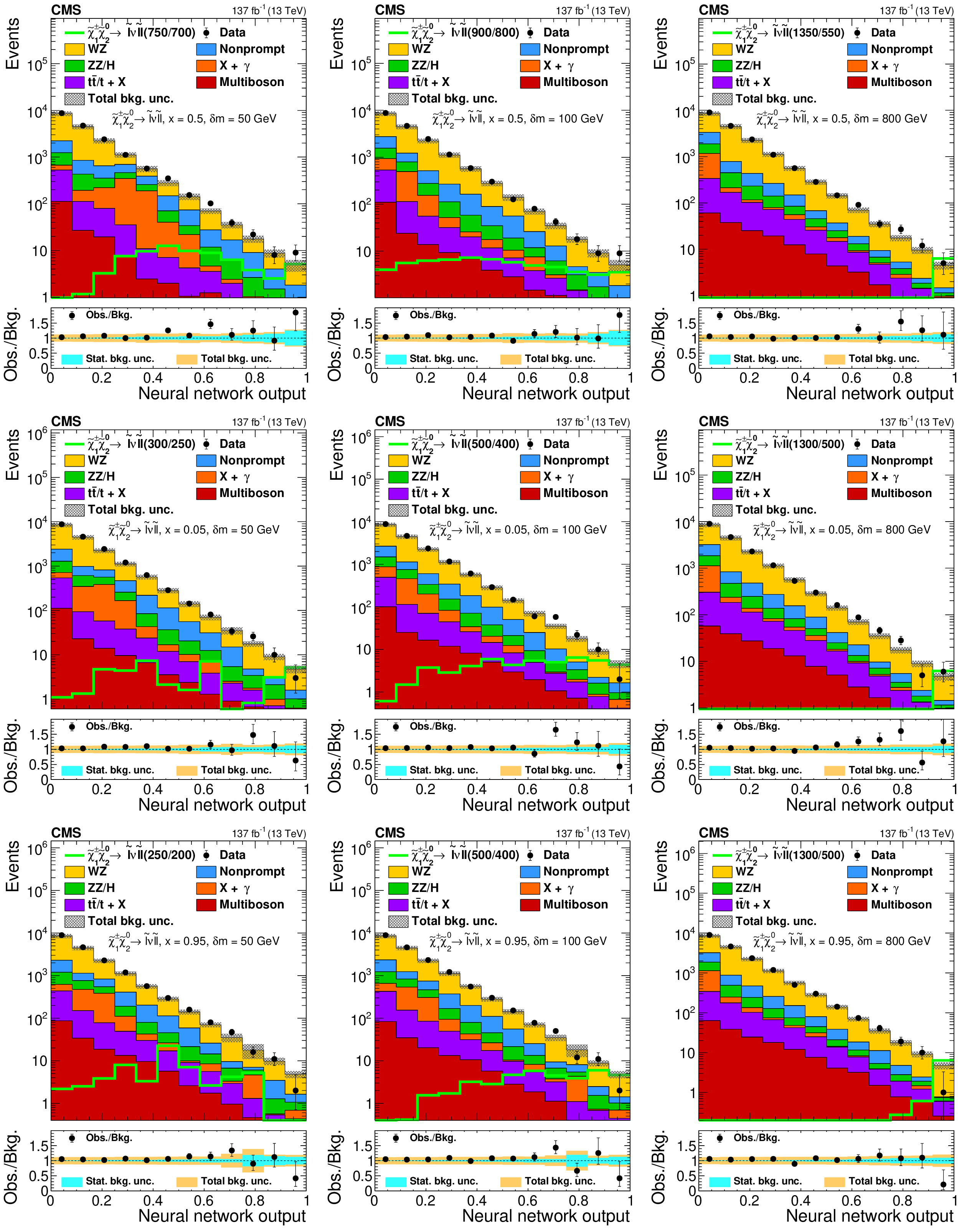
Observed and expected yields as functions of the output of the neural network used to search for ${\tilde{\chi}^{\pm}_1 \tilde{\chi}^{0}_{2}}$ production with slepton-mediated decays at $x = $ 0.5 (upper), 0.05 (middle), and 0.95 (lower), evaluated at $ {\delta m} = $ 50 GeV (left), 100 GeV (center), and 800 GeV (right). The legends specify the masses of $\tilde{\chi}^{0}_{2}$ and $\tilde{\chi}^0_1$ for the shown signal distributions as ($m_{\tilde{\chi}^{0}_{2}}$/$m_{\tilde{\chi}^0_1}$). |

png pdf |
Figure 6-a:
Observed and expected yields as functions of the output of the neural network used to search for ${\tilde{\chi}^{\pm}_1 \tilde{\chi}^{0}_{2}}$ production with slepton-mediated decays at $x = $ 0.5, evaluated at $ {\delta m} = $ 50 GeV. The legends specify the masses of $\tilde{\chi}^{0}_{2}$ and $\tilde{\chi}^0_1$ for the shown signal distributions as ($m_{\tilde{\chi}^{0}_{2}}$/$m_{\tilde{\chi}^0_1}$). |

png pdf |
Figure 6-b:
Observed and expected yields as functions of the output of the neural network used to search for ${\tilde{\chi}^{\pm}_1 \tilde{\chi}^{0}_{2}}$ production with slepton-mediated decays at $x = $ 0.5, evaluated at $ {\delta m} = $ 100 GeV. The legends specify the masses of $\tilde{\chi}^{0}_{2}$ and $\tilde{\chi}^0_1$ for the shown signal distributions as ($m_{\tilde{\chi}^{0}_{2}}$/$m_{\tilde{\chi}^0_1}$). |
png pdf |
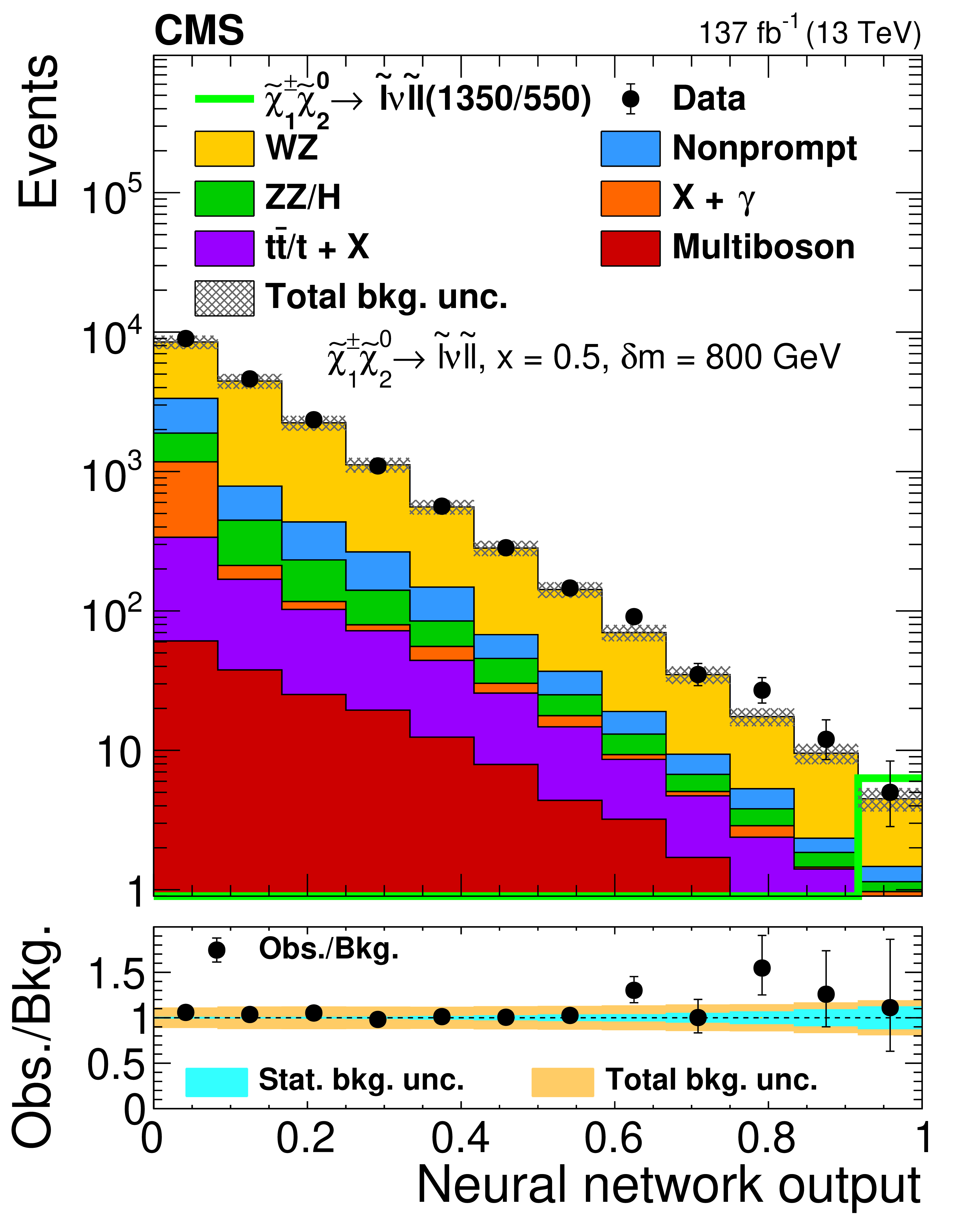
Figure 6-c:
Observed and expected yields as functions of the output of the neural network used to search for ${\tilde{\chi}^{\pm}_1 \tilde{\chi}^{0}_{2}}$ production with slepton-mediated decays at $x = $ 0.5, evaluated at $ {\delta m} = $ 800 GeV. The legends specify the masses of $\tilde{\chi}^{0}_{2}$ and $\tilde{\chi}^0_1$ for the shown signal distributions as ($m_{\tilde{\chi}^{0}_{2}}$/$m_{\tilde{\chi}^0_1}$). |

png pdf |
Figure 6-d:
Observed and expected yields as functions of the output of the neural network used to search for ${\tilde{\chi}^{\pm}_1 \tilde{\chi}^{0}_{2}}$ production with slepton-mediated decays at $x = $ 0.05, evaluated at $ {\delta m} = $ 50 GeV. The legends specify the masses of $\tilde{\chi}^{0}_{2}$ and $\tilde{\chi}^0_1$ for the shown signal distributions as ($m_{\tilde{\chi}^{0}_{2}}$/$m_{\tilde{\chi}^0_1}$). |
png pdf |
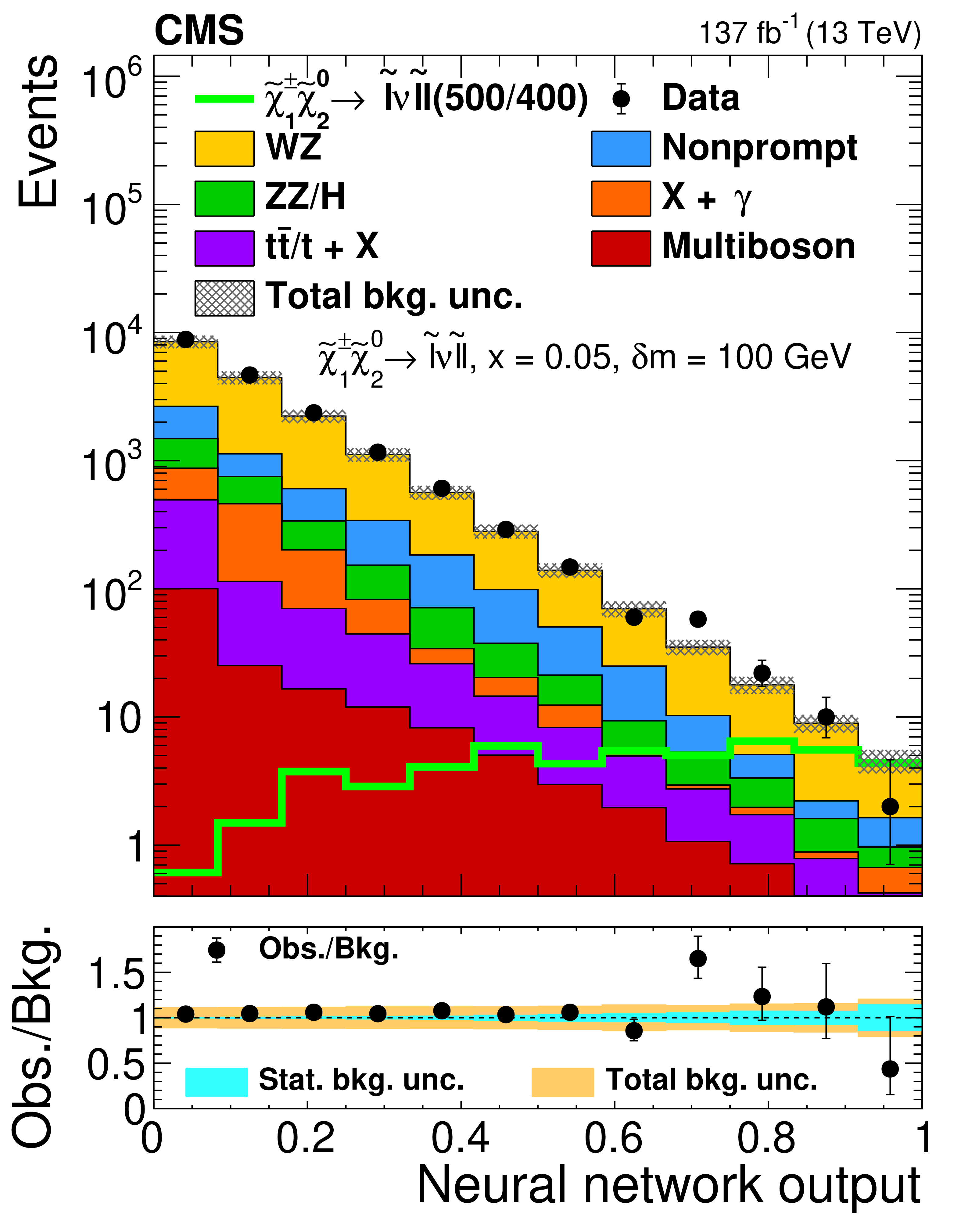
Figure 6-e:
Observed and expected yields as functions of the output of the neural network used to search for ${\tilde{\chi}^{\pm}_1 \tilde{\chi}^{0}_{2}}$ production with slepton-mediated decays at $x = $ 0.05, evaluated at $ {\delta m} = $ 100 GeV. The legends specify the masses of $\tilde{\chi}^{0}_{2}$ and $\tilde{\chi}^0_1$ for the shown signal distributions as ($m_{\tilde{\chi}^{0}_{2}}$/$m_{\tilde{\chi}^0_1}$). |
png pdf |
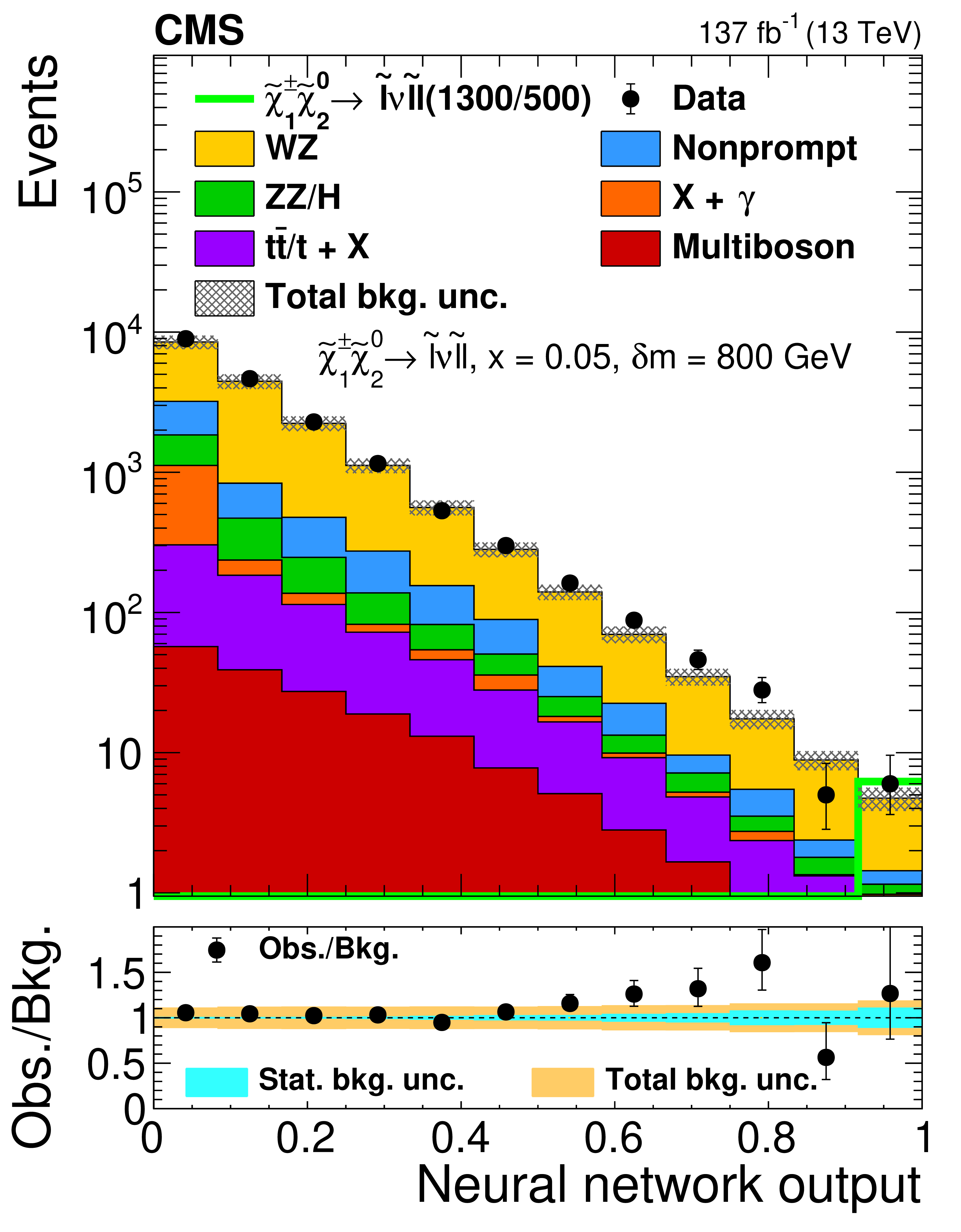
Figure 6-f:
Observed and expected yields as functions of the output of the neural network used to search for ${\tilde{\chi}^{\pm}_1 \tilde{\chi}^{0}_{2}}$ production with slepton-mediated decays at $x = $ 0.05, evaluated at $ {\delta m} = $ 800 GeV. The legends specify the masses of $\tilde{\chi}^{0}_{2}$ and $\tilde{\chi}^0_1$ for the shown signal distributions as ($m_{\tilde{\chi}^{0}_{2}}$/$m_{\tilde{\chi}^0_1}$). |

png pdf |
Figure 6-g:
Observed and expected yields as functions of the output of the neural network used to search for ${\tilde{\chi}^{\pm}_1 \tilde{\chi}^{0}_{2}}$ production with slepton-mediated decays at $x = $ 0.95, evaluated at $ {\delta m} = $ 50 GeV. The legends specify the masses of $\tilde{\chi}^{0}_{2}$ and $\tilde{\chi}^0_1$ for the shown signal distributions as ($m_{\tilde{\chi}^{0}_{2}}$/$m_{\tilde{\chi}^0_1}$). |
png pdf |
Figure 6-h:
Observed and expected yields as functions of the output of the neural network used to search for ${\tilde{\chi}^{\pm}_1 \tilde{\chi}^{0}_{2}}$ production with slepton-mediated decays at $x = $ 0.95, evaluated at $ {\delta m} = $ 100 GeV. The legends specify the masses of $\tilde{\chi}^{0}_{2}$ and $\tilde{\chi}^0_1$ for the shown signal distributions as ($m_{\tilde{\chi}^{0}_{2}}$/$m_{\tilde{\chi}^0_1}$). |
png pdf |
Figure 6-i:
Observed and expected yields as functions of the output of the neural network used to search for ${\tilde{\chi}^{\pm}_1 \tilde{\chi}^{0}_{2}}$ production with slepton-mediated decays at $x = $ 0.95, evaluated at $ {\delta m} = $ 800 GeV. The legends specify the masses of $\tilde{\chi}^{0}_{2}$ and $\tilde{\chi}^0_1$ for the shown signal distributions as ($m_{\tilde{\chi}^{0}_{2}}$/$m_{\tilde{\chi}^0_1}$). |
png pdf |
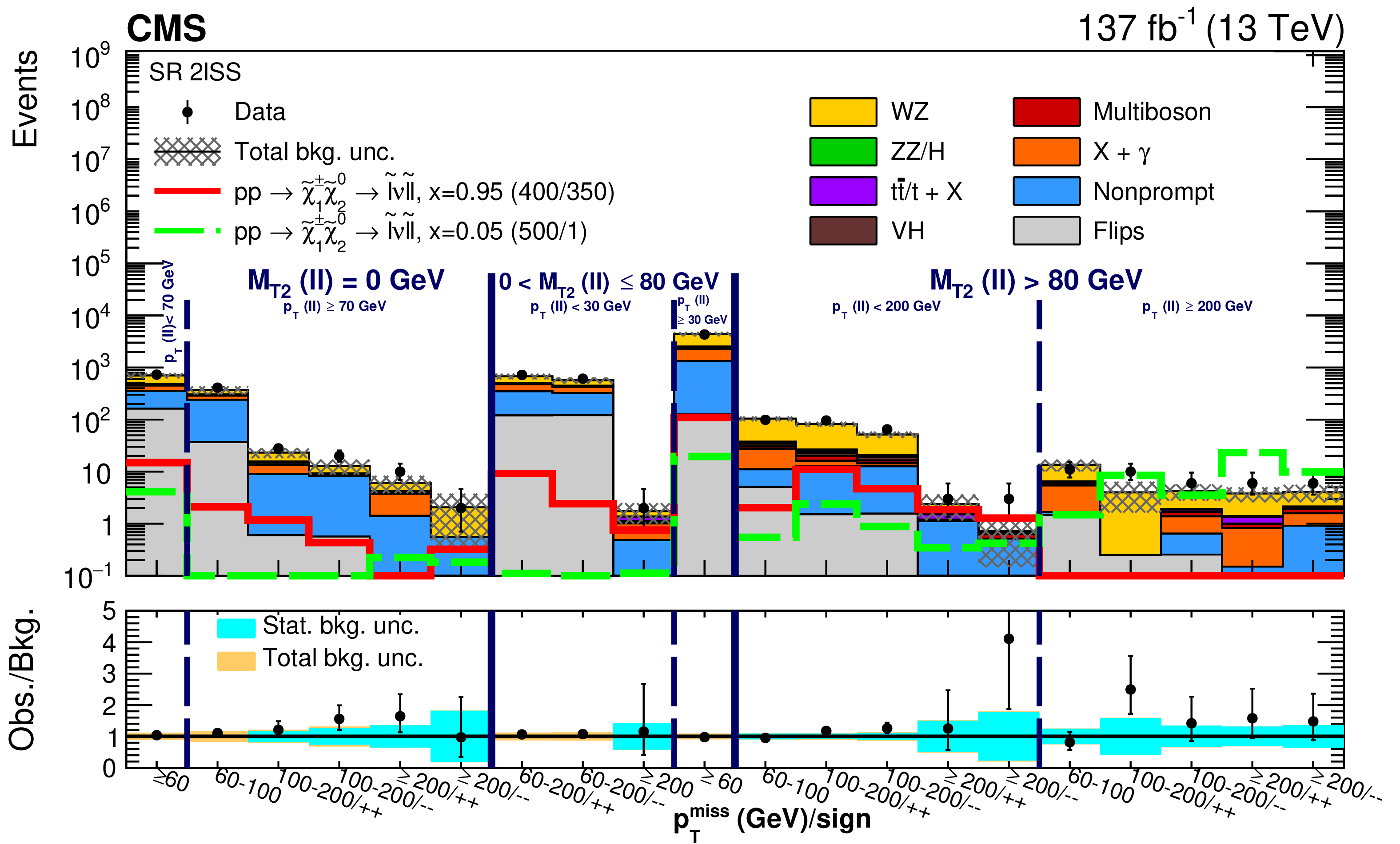
Figure 7:
Observed and expected yields across the search regions in events with two same-sign light leptons (2$\ell $SS). Several signal models are shown superimposed. They correspond to ${\tilde{\chi}^{\pm}_1 \tilde{\chi}^{0}_{2}}$ production with slepton-mediated decays in the flavor-democratic hypothesis for a compressed $ {\delta m} = $ 50 GeV (red line) and uncompressed $ {\delta m} = $ 500 GeV (green dashed line) scenario. The legends specify the masses of $\tilde{\chi}^{0}_{2}$ and $\tilde{\chi}^0_1$ for the shown signal distributions as ($m_{\tilde{\chi}^{0}_{2}}$/$m_{\tilde{\chi}^0_1}$). |
png pdf |
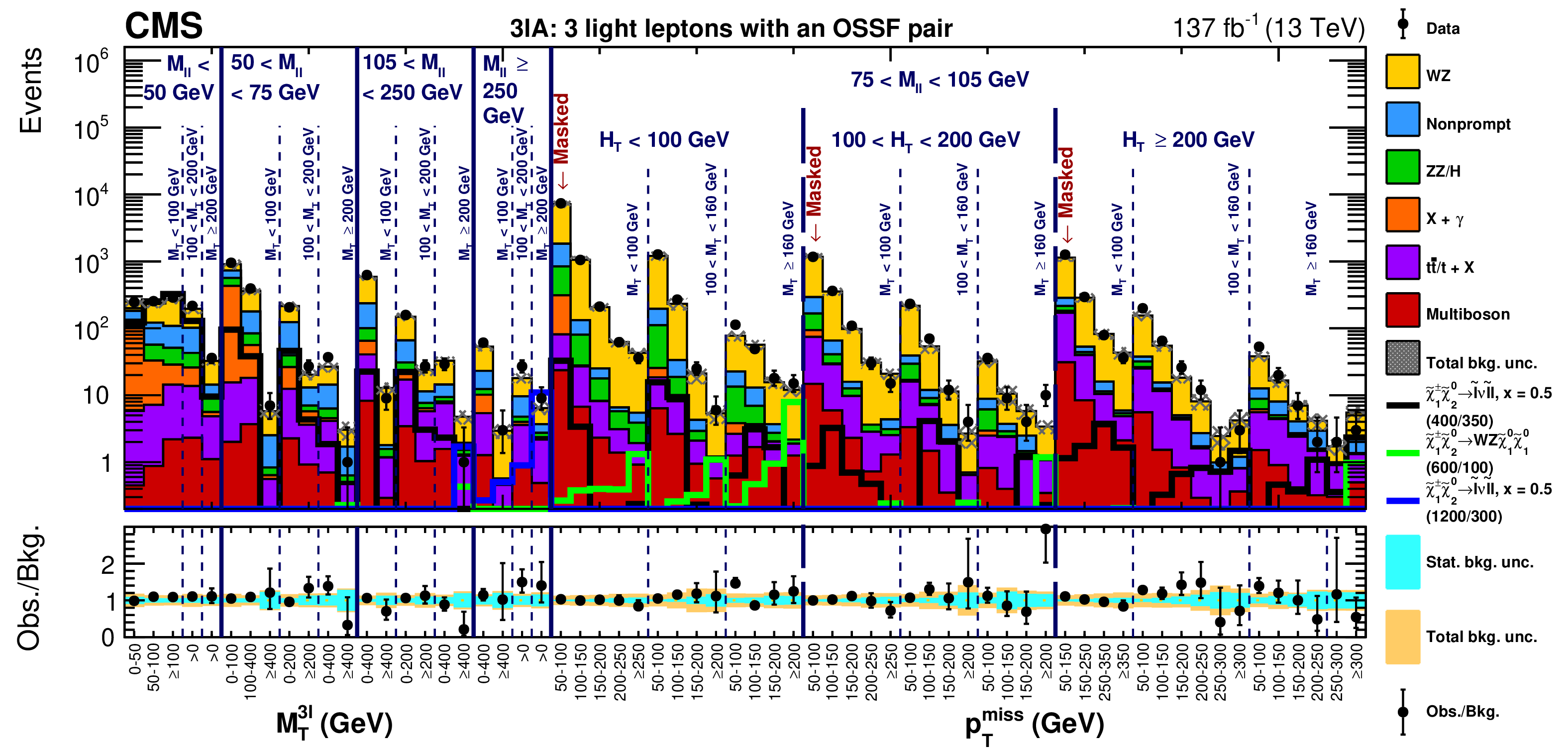
Figure 8:
Observed and expected yields across the search regions in events with three light leptons, at least two of which form an OSSF pair (3$\ell $A). Several signal models are shown superimposed. They correspond to ${\tilde{\chi}^{\pm}_1 \tilde{\chi}^{0}_{2}}$ production with slepton-mediated decays in the flavor-democratic hypothesis for a compressed $ {\delta m} = $ 50 GeV (black line) and uncompressed $ {\delta m} = $ 900 GeV (blue line) scenario, and for WZ-mediated decays in an uncompressed $ {\delta m} = $ 500 GeV scenario (green line). Bins labeled as "Masked'' are not considered in the interpretation of the results because of overlap with the WZ control region. The legends specify the masses of $\tilde{\chi}^{0}_{2}$ and $\tilde{\chi}^0_1$ for the shown signal distributions as ($m_{\tilde{\chi}^{0}_{2}}$/$m_{\tilde{\chi}^0_1}$). |

png pdf |
Figure 9:
Observed and expected yields across the search regions in events with three light leptons, none of which form an OSSF pair (3$\ell $B). Several signal models are shown superimposed. They correspond to ${\tilde{\chi}^{\pm}_1 \tilde{\chi}^{0}_{2}}$ production with WH-mediated decays for scenarios corresponding to a H boson like mass splitting $ {\delta m} = $ 125 GeV (black line) and a slightly less compressed $ {\delta m} = $ 150 GeV (green dashed line) scenario. The legends specify the masses of $\tilde{\chi}^{0}_{2}$ and $\tilde{\chi}^0_1$ for the shown signal distributions as ($m_{\tilde{\chi}^{0}_{2}}$/$m_{\tilde{\chi}^0_1}$). |
png pdf |
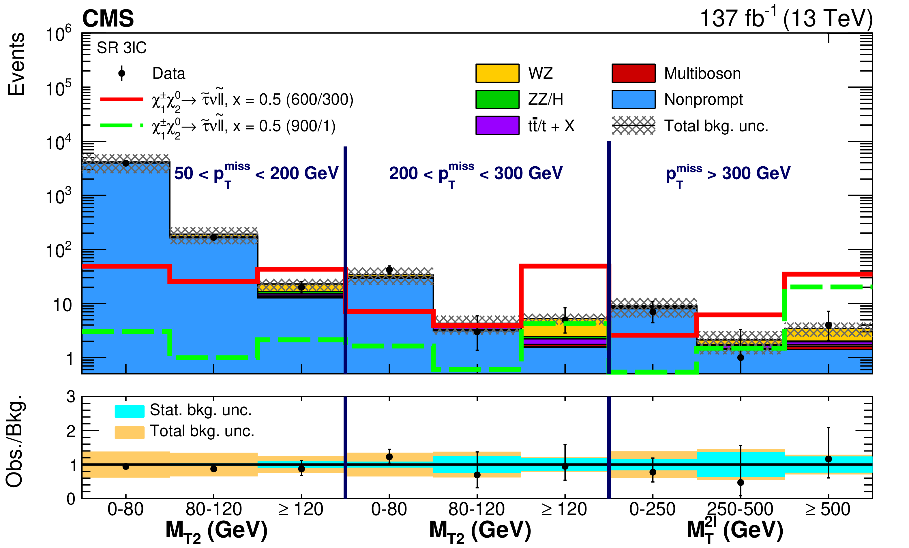
Figure 10:
Observed and expected yields across the search regions in events with a $\mu^{+} \mu^{-} $ or $\mathrm{e^{+}} \mathrm{e^{-}} $ pair and an additional ${\tau _\mathrm {h}}$ candidate (3$\ell $C). Several signal models are shown superimposed. They correspond to ${\tilde{\chi}^{\pm}_1 \tilde{\chi}^{0}_{2}}$ production with slepton-mediated decays in the $\tau $ lepton enriched hypothesis for a compressed $ {\delta m} = $ 300 GeV (red line) and uncompressed $ {\delta m} = $ 900 GeV (green dashed line) scenario. The legends specify the masses of $\tilde{\chi}^{0}_{2}$ and $\tilde{\chi}^0_1$ for the shown signal distributions as ($m_{\tilde{\chi}^{0}_{2}}$/$m_{\tilde{\chi}^0_1}$). |
png pdf |
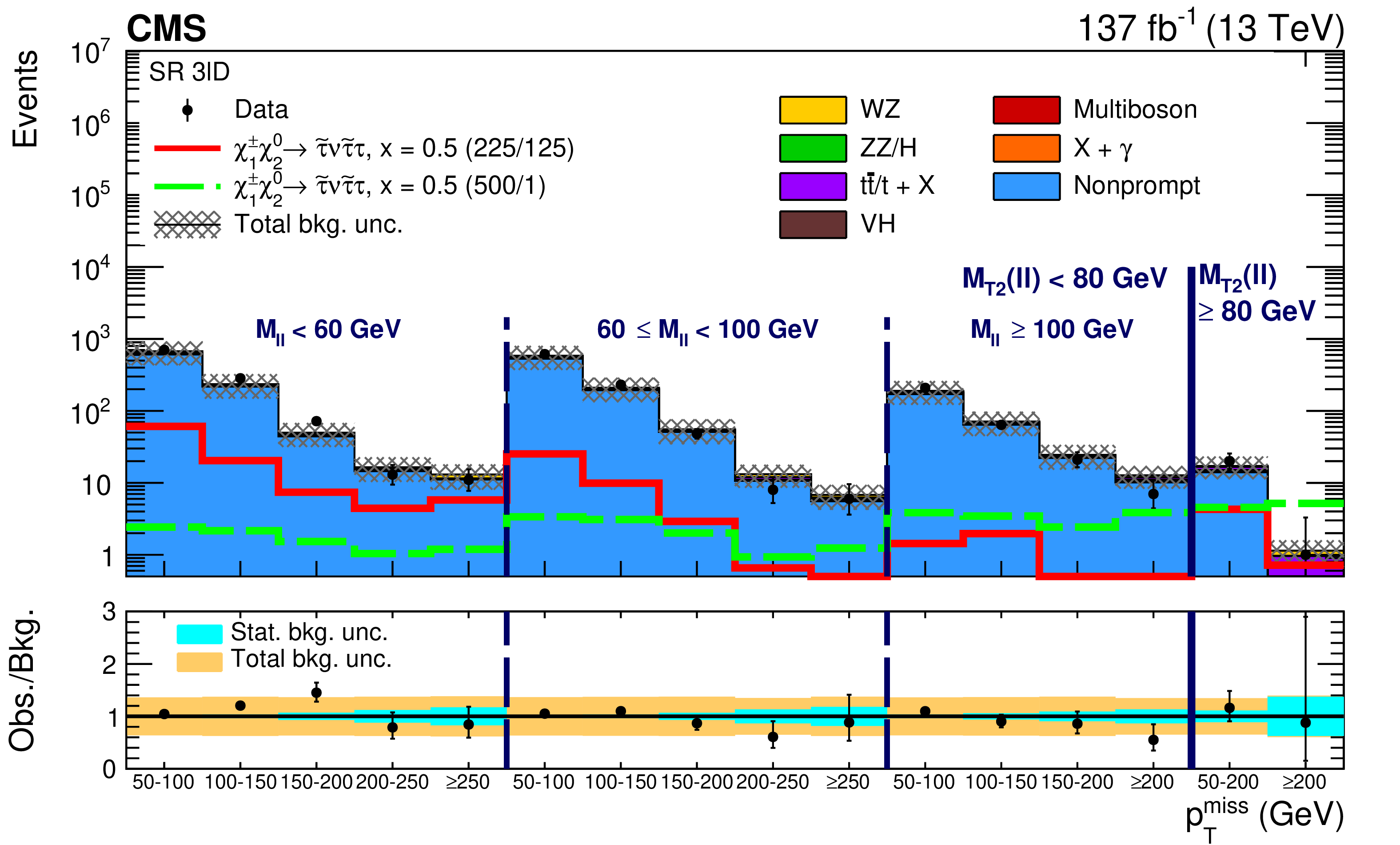
Figure 11:
Observed and expected yields across the search regions in events with an e$^{\pm}\mu ^{\mp}$ pair and a ${\tau _\mathrm {h}}$ candidate (3$\ell $D). Several signal models are shown superimposed. They correspond to ${\tilde{\chi}^{\pm}_1 \tilde{\chi}^{0}_{2}}$ production with slepton-mediated decays in the $\tau $ lepton dominated hypothesis for a compressed $ {\delta m} = $ 100 GeV (red line) and uncompressed $ {\delta m} = $ 500 GeV (green dashed line) scenario. The legends specify the masses of $\tilde{\chi}^{0}_{2}$ and $\tilde{\chi}^0_1$ for the shown signal distributions as ($m_{\tilde{\chi}^{0}_{2}}$/$m_{\tilde{\chi}^0_1}$). |
png pdf |
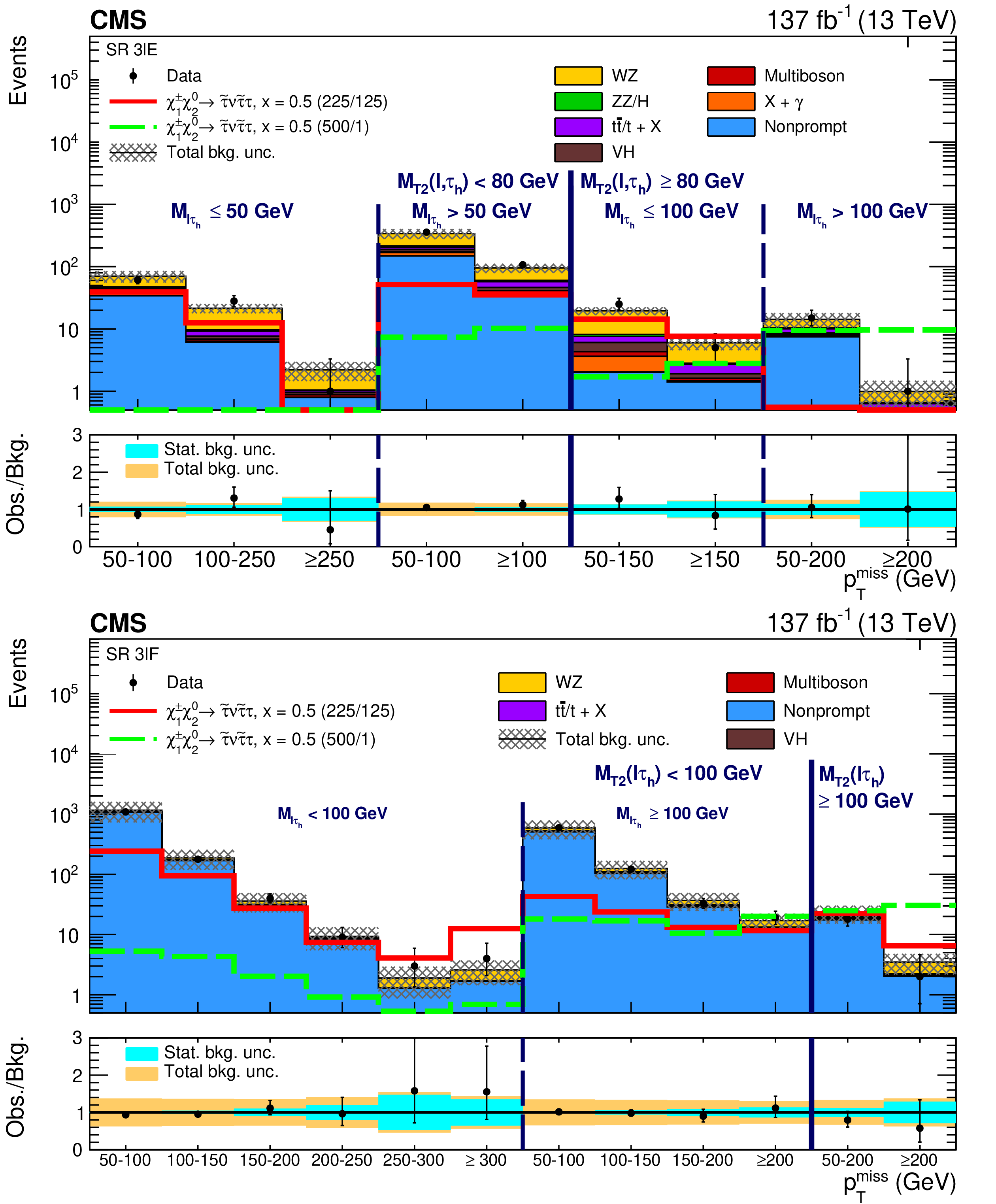
Figure 12:
Observed and expected yields across the search regions in events (upper plot) with a same-sign light lepton pair and a ${\tau _\mathrm {h}}$ candidate (3$\ell $E), and (lower plot) with two ${\tau _\mathrm {h}}$ candidates and one light lepton (3$\ell $F). Several signal models are shown superimposed. They correspond to ${\tilde{\chi}^{\pm}_1 \tilde{\chi}^{0}_{2}}$ production with slepton-mediated decays in the $\tau $ lepton dominated hypothesis for a compressed $ {\delta m} = $ 100 GeV (red line) and uncompressed $ {\delta m} = $ 500 GeV (green dashed line) scenario. The legends specify the masses of $\tilde{\chi}^{0}_{2}$ and $\tilde{\chi}^0_1$ for the shown signal distributions as ($m_{\tilde{\chi}^{0}_{2}}$/$m_{\tilde{\chi}^0_1}$). |
png pdf |
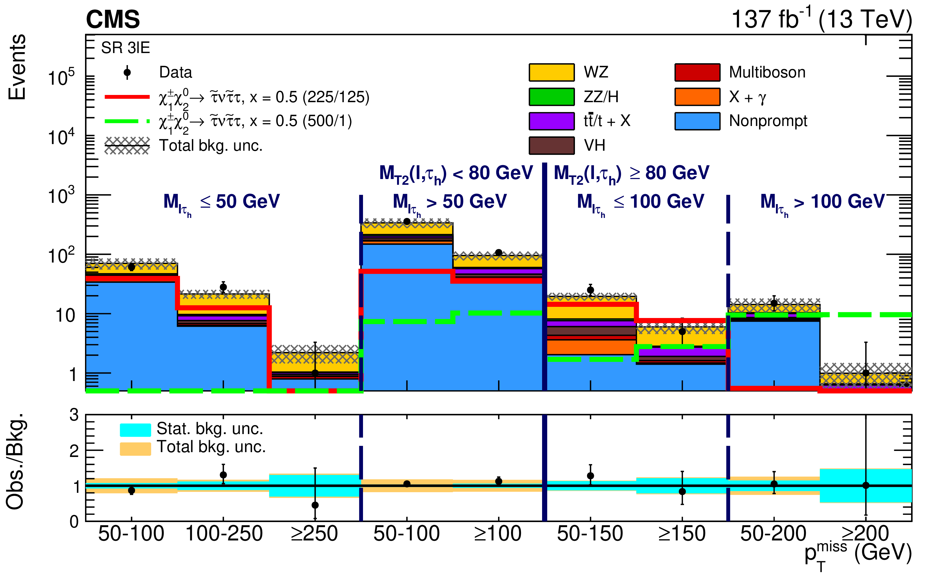
Figure 12-a:
Observed and expected yields across the search regions in events with a same-sign light lepton pair and a ${\tau _\mathrm {h}}$ candidate (3$\ell $E). Several signal models are shown superimposed. They correspond to ${\tilde{\chi}^{\pm}_1 \tilde{\chi}^{0}_{2}}$ production with slepton-mediated decays in the $\tau $ lepton dominated hypothesis for a compressed $ {\delta m} = $ 100 GeV (red line) and uncompressed $ {\delta m} = $ 500 GeV (green dashed line) scenario. The legends specify the masses of $\tilde{\chi}^{0}_{2}$ and $\tilde{\chi}^0_1$ for the shown signal distributions as ($m_{\tilde{\chi}^{0}_{2}}$/$m_{\tilde{\chi}^0_1}$). |
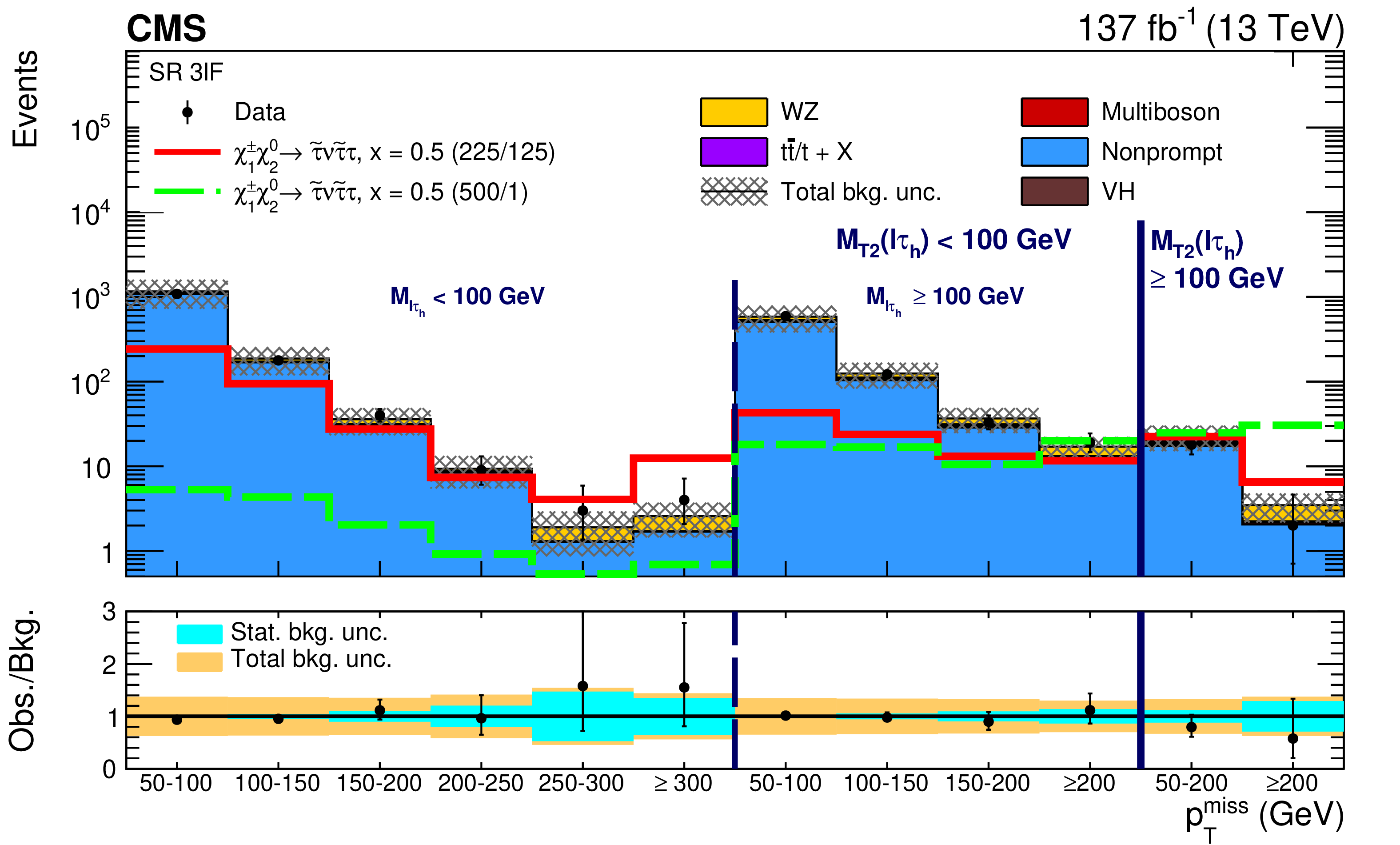
png pdf |
Figure 12-b:
Observed and expected yields across the search regions in events with two ${\tau _\mathrm {h}}$ candidates and one light lepton (3$\ell $F). Several signal models are shown superimposed. They correspond to ${\tilde{\chi}^{\pm}_1 \tilde{\chi}^{0}_{2}}$ production with slepton-mediated decays in the $\tau $ lepton dominated hypothesis for a compressed $ {\delta m} = $ 100 GeV (red line) and uncompressed $ {\delta m} = $ 500 GeV (green dashed line) scenario. The legends specify the masses of $\tilde{\chi}^{0}_{2}$ and $\tilde{\chi}^0_1$ for the shown signal distributions as ($m_{\tilde{\chi}^{0}_{2}}$/$m_{\tilde{\chi}^0_1}$). |
png pdf |
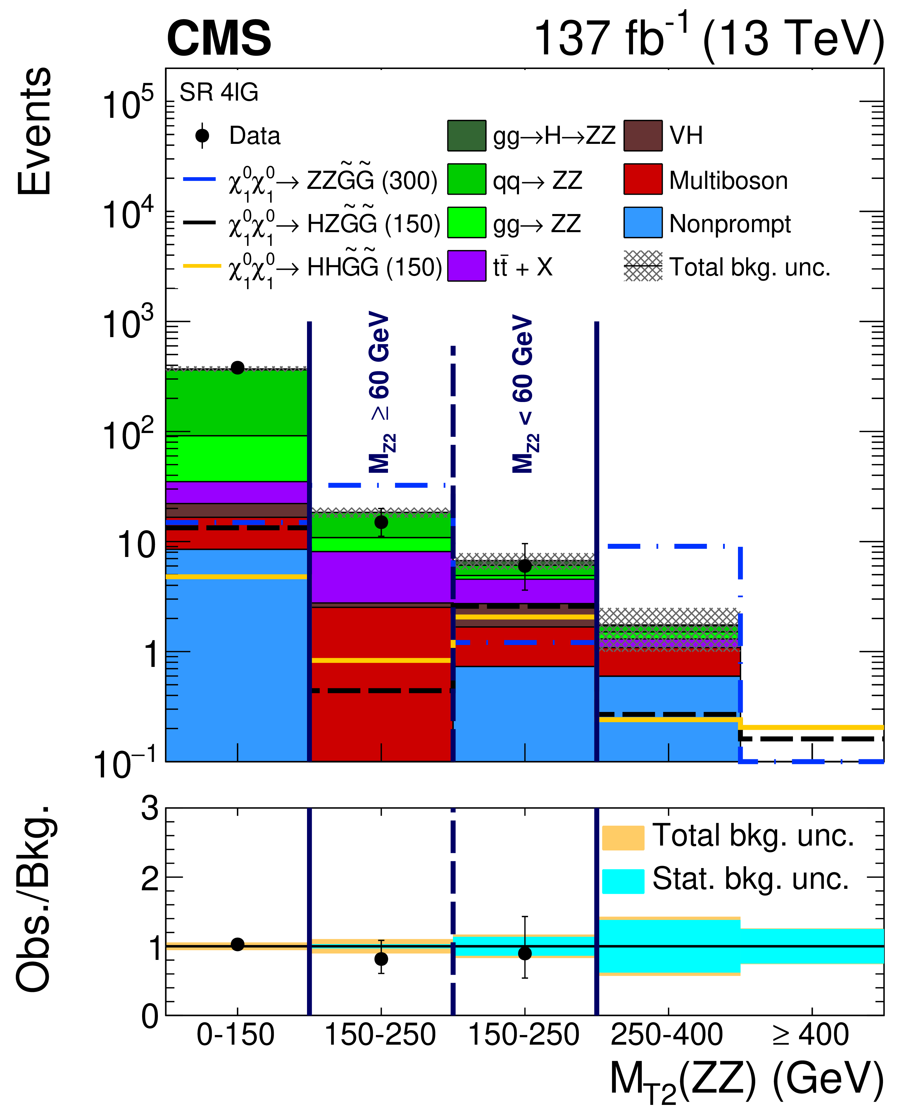
Figure 13:
Observed and expected yields across the search regions in events with four light leptons, including 2 separate OSSF pairs (4$\ell $G). Several signal models are shown superimposed. They correspond to Higgsino pair production with decays to ZZ (blue dotted line, Higgsino mass of 300 GeV), HZ (black dashed line, Higgsino mass of 150 GeV), and HH (dark yellow line, Higgsino mass of 150 GeV). |
png pdf |
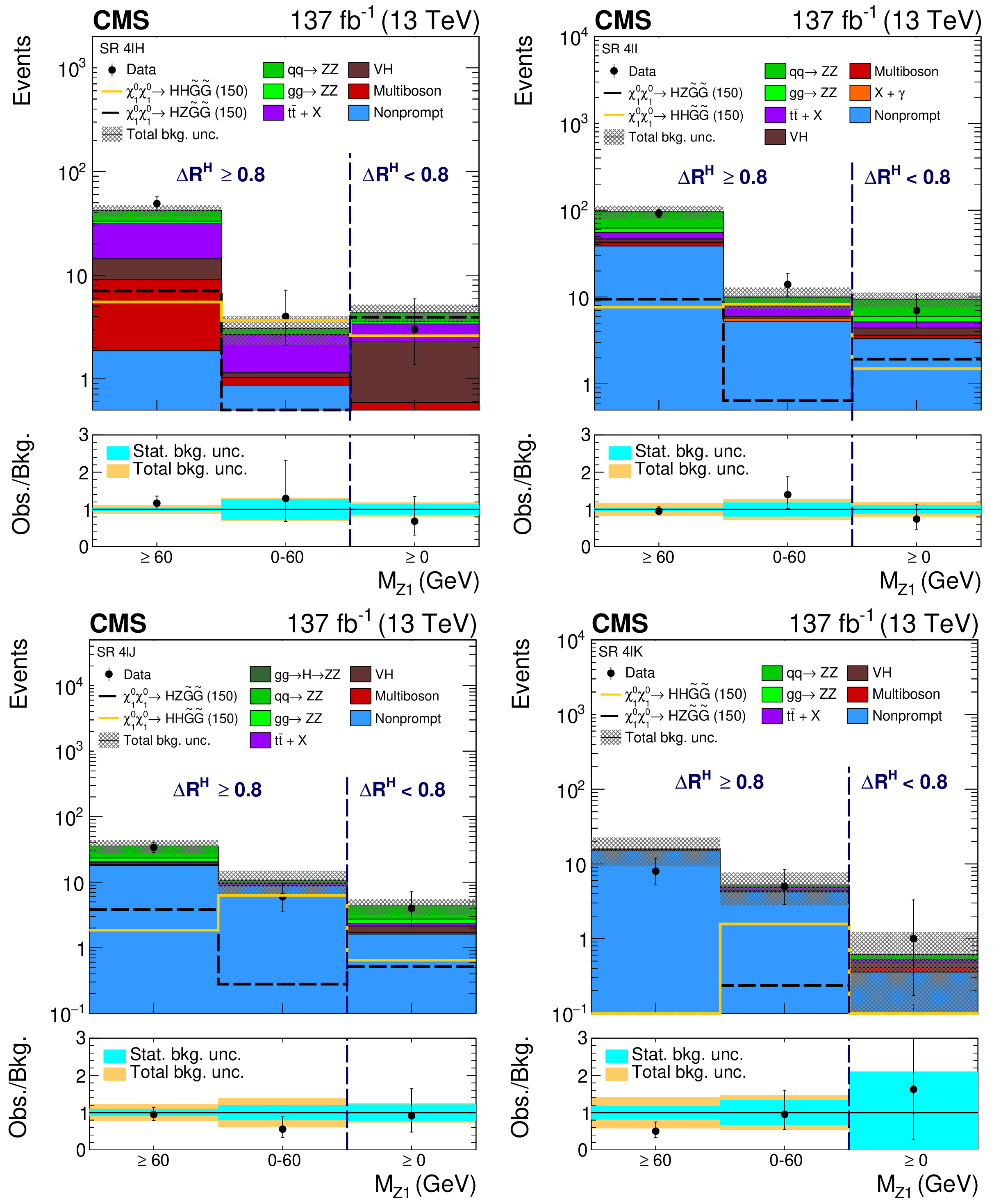
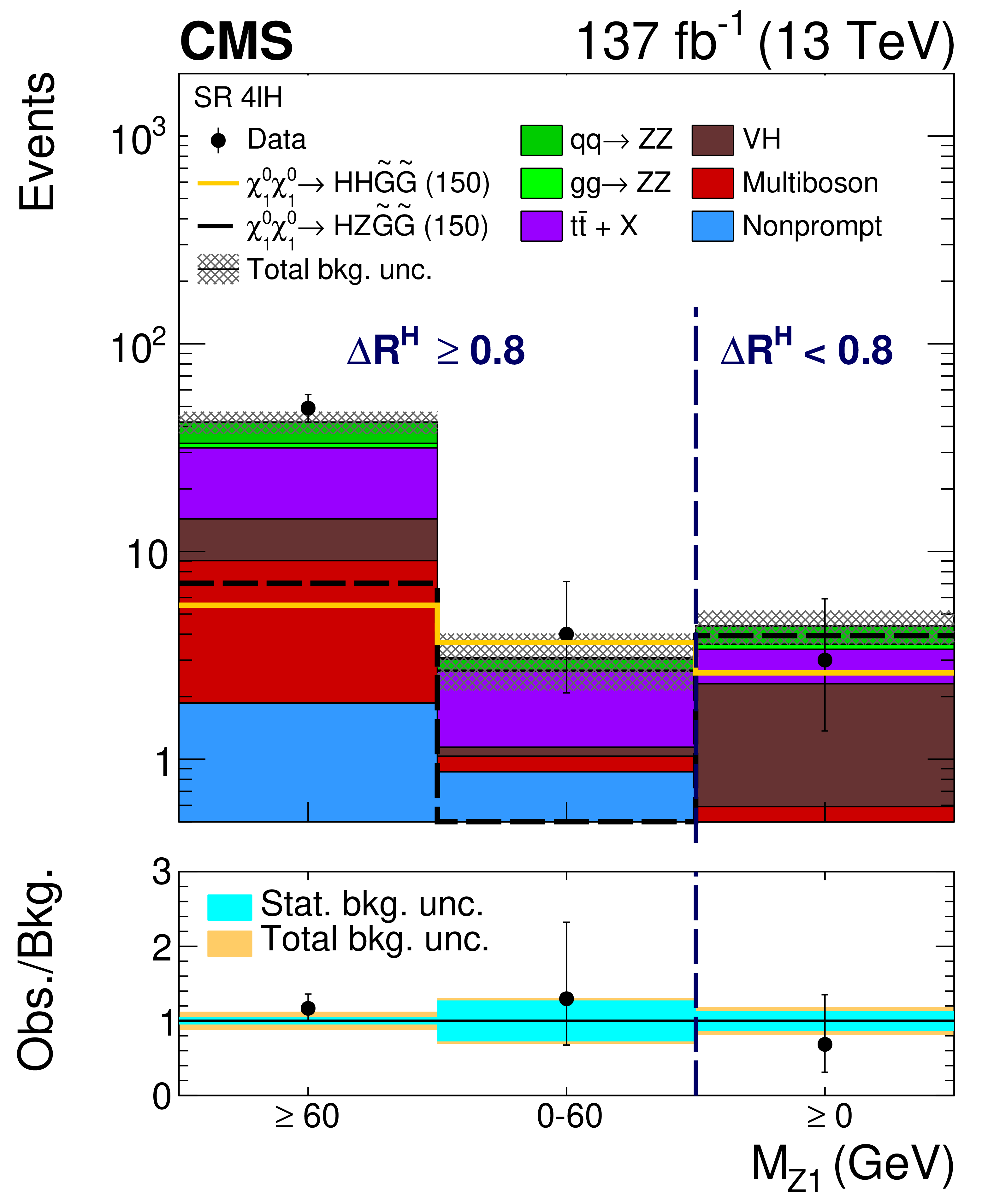
Figure 14:
Observed and expected yields across the search regions in events with four light leptons not forming two OSSF pairs (4$\ell $H, upper left), events with three light leptons and a ${\tau _\mathrm {h}}$ candidate (4$\ell $I, upper right), forming two OSSF pairs (4$\ell $J, lower left), and forming one or less OSSF pairs (4$\ell $K, lower right). Several signal models are shown superimposed. They correspond to Higgsino pair production with decays to HZ (dashed black line, Higgsino mass of 150 GeV), and HH (dark yellow line, Higgsino mass of 150 GeV). |
png pdf |
Figure 14-a:
Observed and expected yields across the search regions in events with four light leptons not forming two OSSF pairs (4$\ell $H). Several signal models are shown superimposed. They correspond to Higgsino pair production with decays to HZ (dashed black line, Higgsino mass of 150 GeV), and HH (dark yellow line, Higgsino mass of 150 GeV). |
png pdf |
Figure 14-b:
Observed and expected yields across the search regions in events with three light leptons and a ${\tau _\mathrm {h}}$ candidate (4$\ell $I). Several signal models are shown superimposed. They correspond to Higgsino pair production with decays to HZ (dashed black line, Higgsino mass of 150 GeV), and HH (dark yellow line, Higgsino mass of 150 GeV). |

png pdf |
Figure 14-c:
Observed and expected yields across the search regions in events with three light leptons forming two OSSF pairs (4$\ell $J). Several signal models are shown superimposed. They correspond to Higgsino pair production with decays to HZ (dashed black line, Higgsino mass of 150 GeV), and HH (dark yellow line, Higgsino mass of 150 GeV). |
png pdf |
Figure 14-d:
Observed and expected yields across the search regions in events with three light leptons forming one or less OSSF pairs (4$\ell $K). Several signal models are shown superimposed. They correspond to Higgsino pair production with decays to HZ (dashed black line, Higgsino mass of 150 GeV), and HH (dark yellow line, Higgsino mass of 150 GeV). |

png pdf |
Figure 15:
Expected test statistic distribution for a background-only fit compared to the observed test statistic value, drawn as black dots, for the search regions in each event category (upper plot) and the neural network targeting WZ-mediated superpartner decays for each $\delta m$ evaluation (lower plot). The gray shaded area represents the (symmetrized) probability density of the expected test statistic distribution, with 68 and 95% expected ranges respectively drawn in green and orange. |
png pdf |
Figure 15-a:
Expected test statistic distribution for a background-only fit compared to the observed test statistic value, drawn as black dots, for the search regions in each event category. The gray shaded area represents the (symmetrized) probability density of the expected test statistic distribution, with 68 and 95% expected ranges respectively drawn in green and orange. |
png pdf |
Figure 15-b:
Expected test statistic distribution for the neural network targeting WZ-mediated superpartner decays for each $\delta m$ evaluation. The gray shaded area represents the (symmetrized) probability density of the expected test statistic distribution, with 68 and 95% expected ranges respectively drawn in green and orange. |
png pdf |
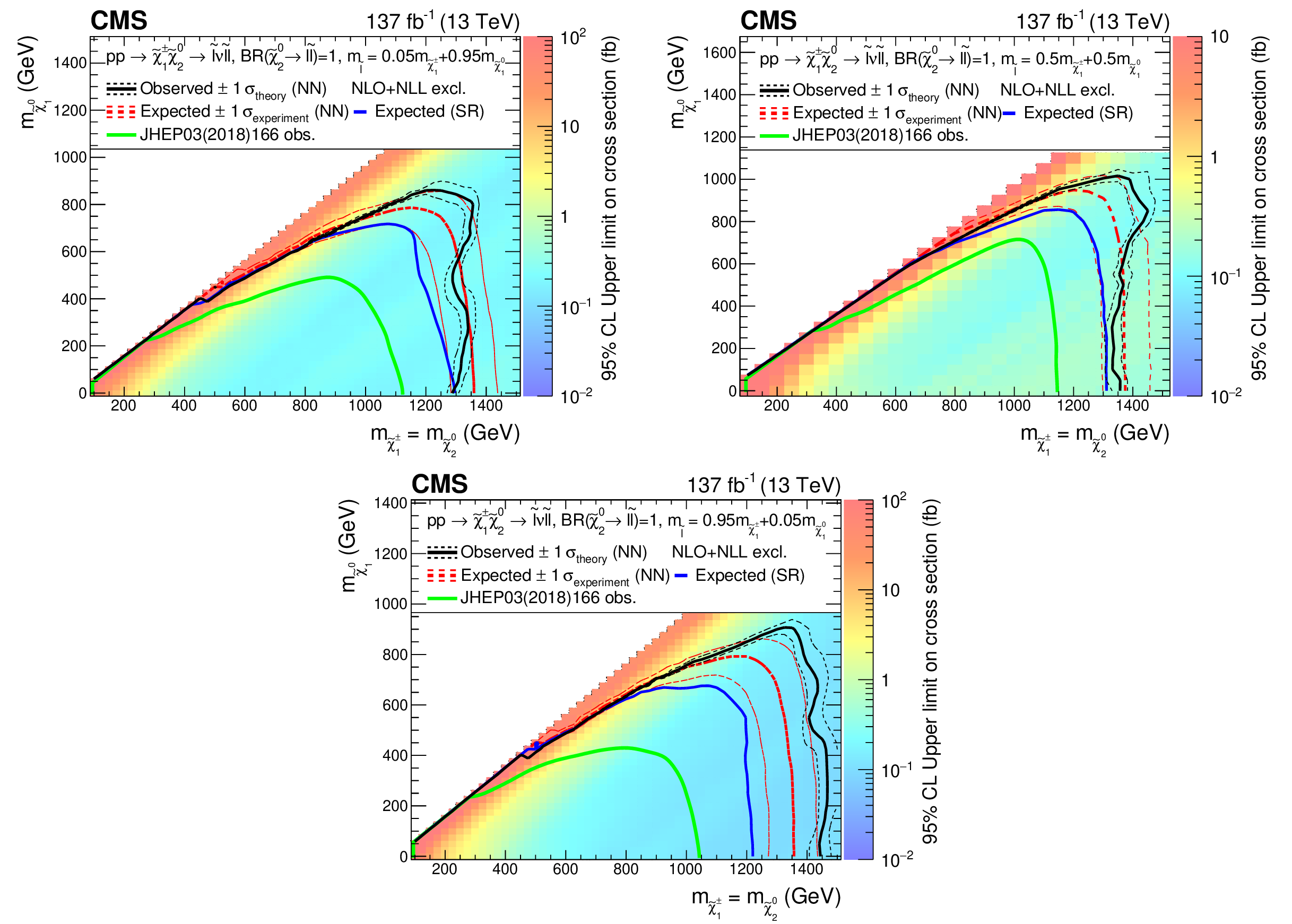
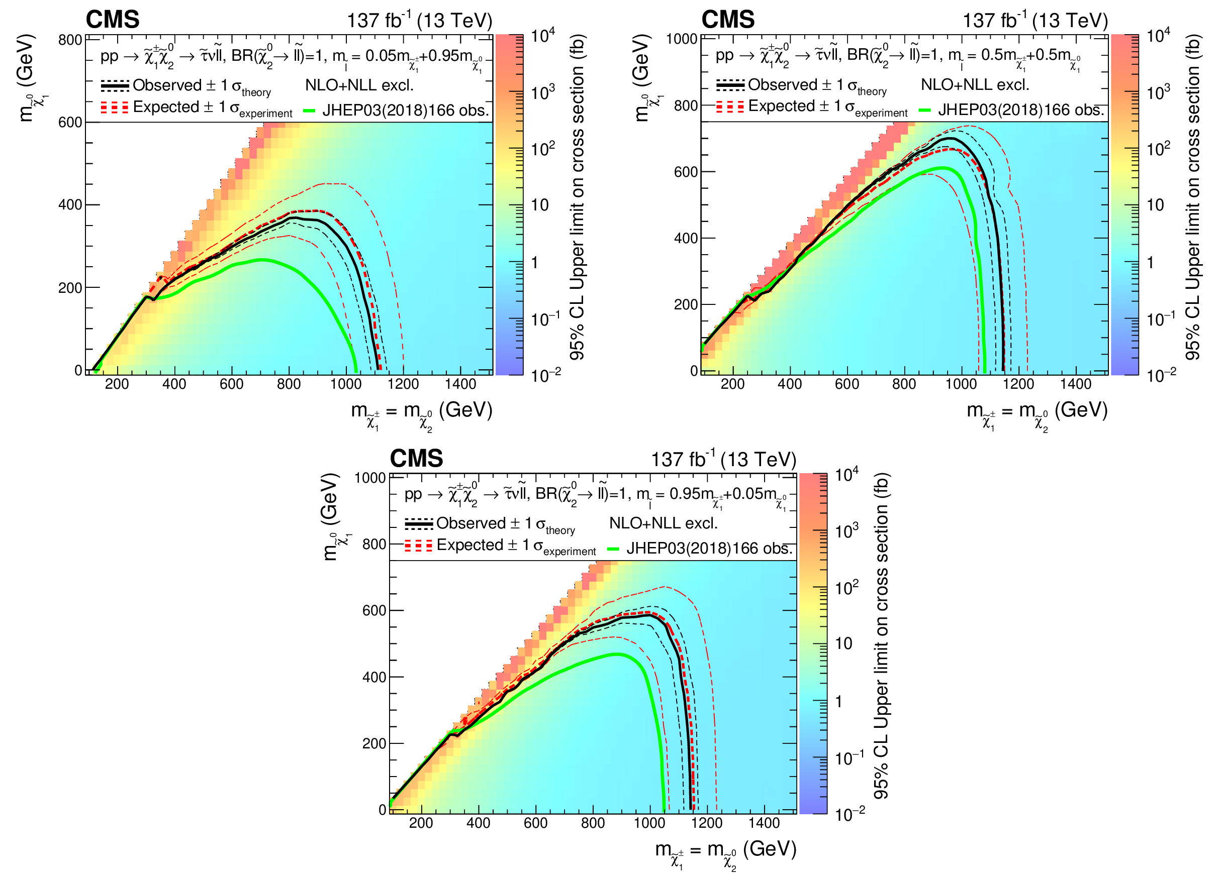
Figure 16:
Interpretation of the results for ${\tilde{\chi}^{\pm}_1 \tilde{\chi}^{0}_{2}}$ production with flavor-democratic slepton-mediated decays, and the parameter governing the mass splittings being $x=$ 0.05 (upper left), $x=$ 0.5 (upper right) and $x=$ 0.95 (lower). The shading in the $m_{\tilde{\chi}^0_1}$ versus $m_{\tilde{\chi}^{0}_{2}}$ plane indicates the 95% CL upper limit on the ${\tilde{\chi}^{\pm}_1 \tilde{\chi}^{0}_{2}}$ production cross sections. The contours delineate the mass regions excluded at 95% CL when assuming cross section computed at NLO plus NLL. All masses below the contours are excluded. The observed, observed $ \pm $1$ \sigma _{\text {theory}}$ ($\pm $1 standard deviation of the theoretical cross sections), median expected, and expected $ \pm $1$ \sigma _{\text {experiment}}$ bounds obtained with the neural network strategy are shown in black and red. The median expected bound obtained with the search region strategy is shown in blue. The observed limits obtained in the CMS analysis using 2016 data [20] are shown in green. |
png pdf |
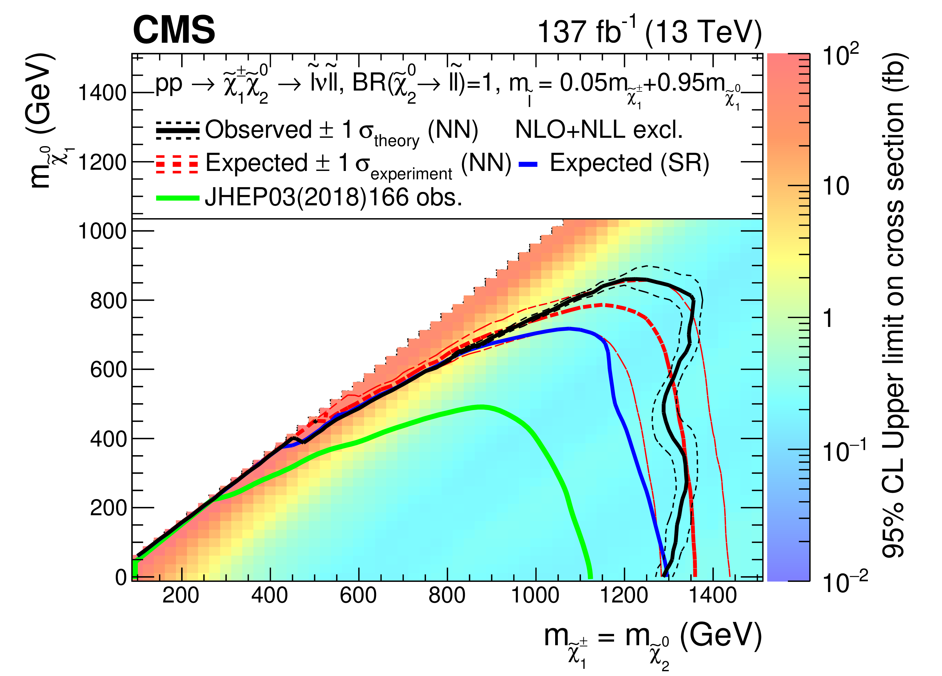
Figure 16-a:
Interpretation of the results for ${\tilde{\chi}^{\pm}_1 \tilde{\chi}^{0}_{2}}$ production with flavor-democratic slepton-mediated decays, and the parameter governing the mass splitting being $x=$ 0.05. The shading in the $m_{\tilde{\chi}^0_1}$ versus $m_{\tilde{\chi}^{0}_{2}}$ plane indicates the 95% CL upper limit on the ${\tilde{\chi}^{\pm}_1 \tilde{\chi}^{0}_{2}}$ production cross sections. The contours delineate the mass regions excluded at 95% CL when assuming cross section computed at NLO plus NLL. All masses below the contours are excluded. The observed, observed $ \pm $1$ \sigma _{\text {theory}}$ ($\pm $1 standard deviation of the theoretical cross sections), median expected, and expected $ \pm $1$ \sigma _{\text {experiment}}$ bounds obtained with the neural network strategy are shown in black and red. The median expected bound obtained with the search region strategy is shown in blue. The observed limits obtained in the CMS analysis using 2016 data [20] are shown in green. |
png pdf |
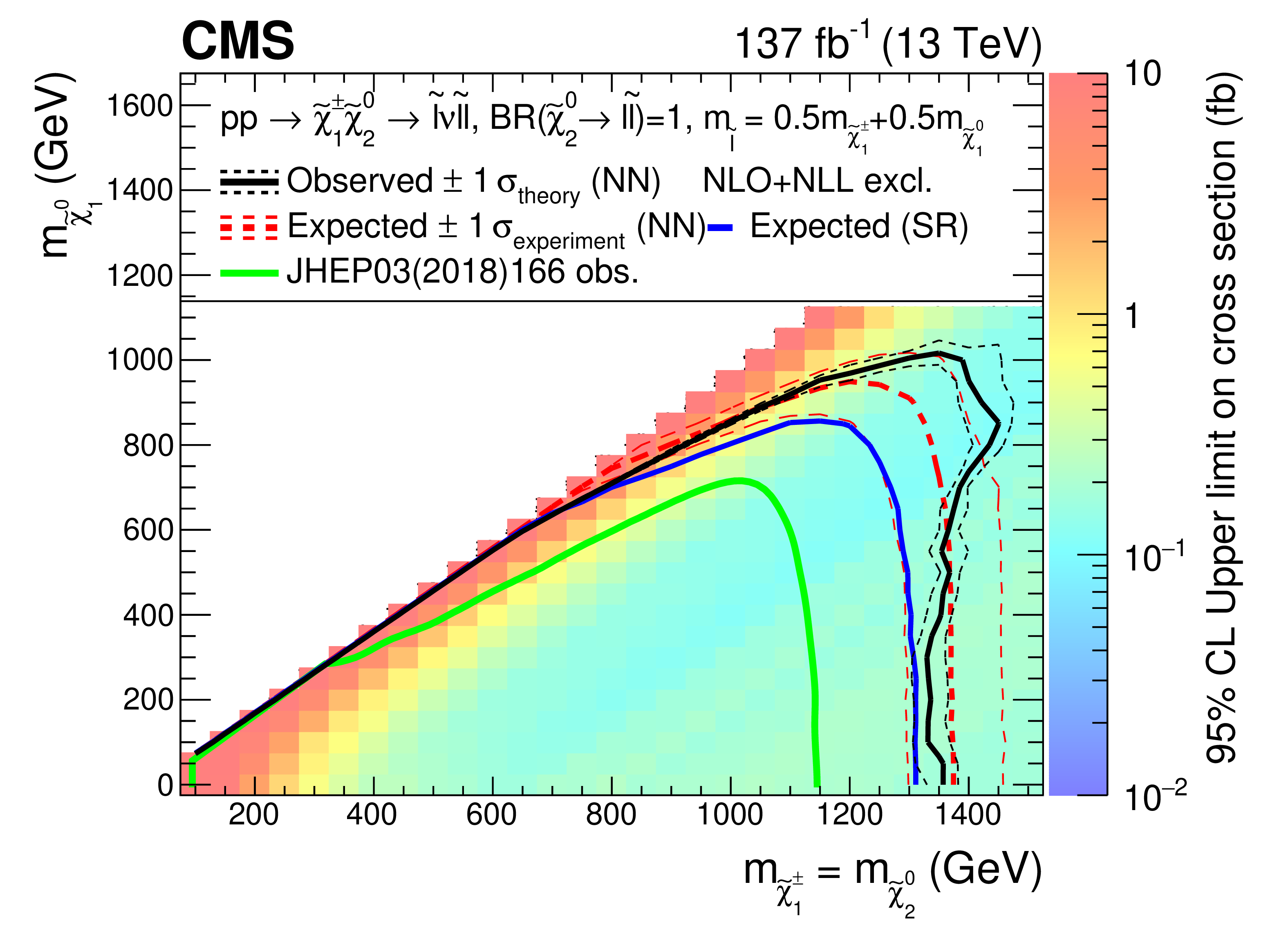
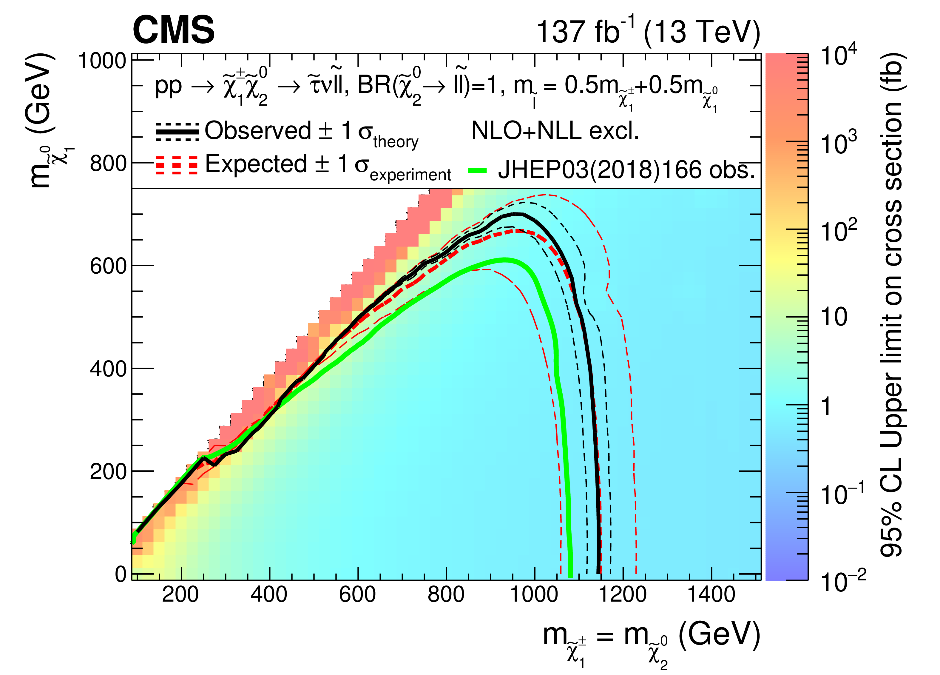
Figure 16-b:
Interpretation of the results for ${\tilde{\chi}^{\pm}_1 \tilde{\chi}^{0}_{2}}$ production with flavor-democratic slepton-mediated decays, and the parameter governing the mass splitting being $x=$ 0.5. The shading in the $m_{\tilde{\chi}^0_1}$ versus $m_{\tilde{\chi}^{0}_{2}}$ plane indicates the 95% CL upper limit on the ${\tilde{\chi}^{\pm}_1 \tilde{\chi}^{0}_{2}}$ production cross sections. The contours delineate the mass regions excluded at 95% CL when assuming cross section computed at NLO plus NLL. All masses below the contours are excluded. The observed, observed $ \pm $1$ \sigma _{\text {theory}}$ ($\pm $1 standard deviation of the theoretical cross sections), median expected, and expected $ \pm $1$ \sigma _{\text {experiment}}$ bounds obtained with the neural network strategy are shown in black and red. The median expected bound obtained with the search region strategy is shown in blue. The observed limits obtained in the CMS analysis using 2016 data [20] are shown in green. |
png pdf |
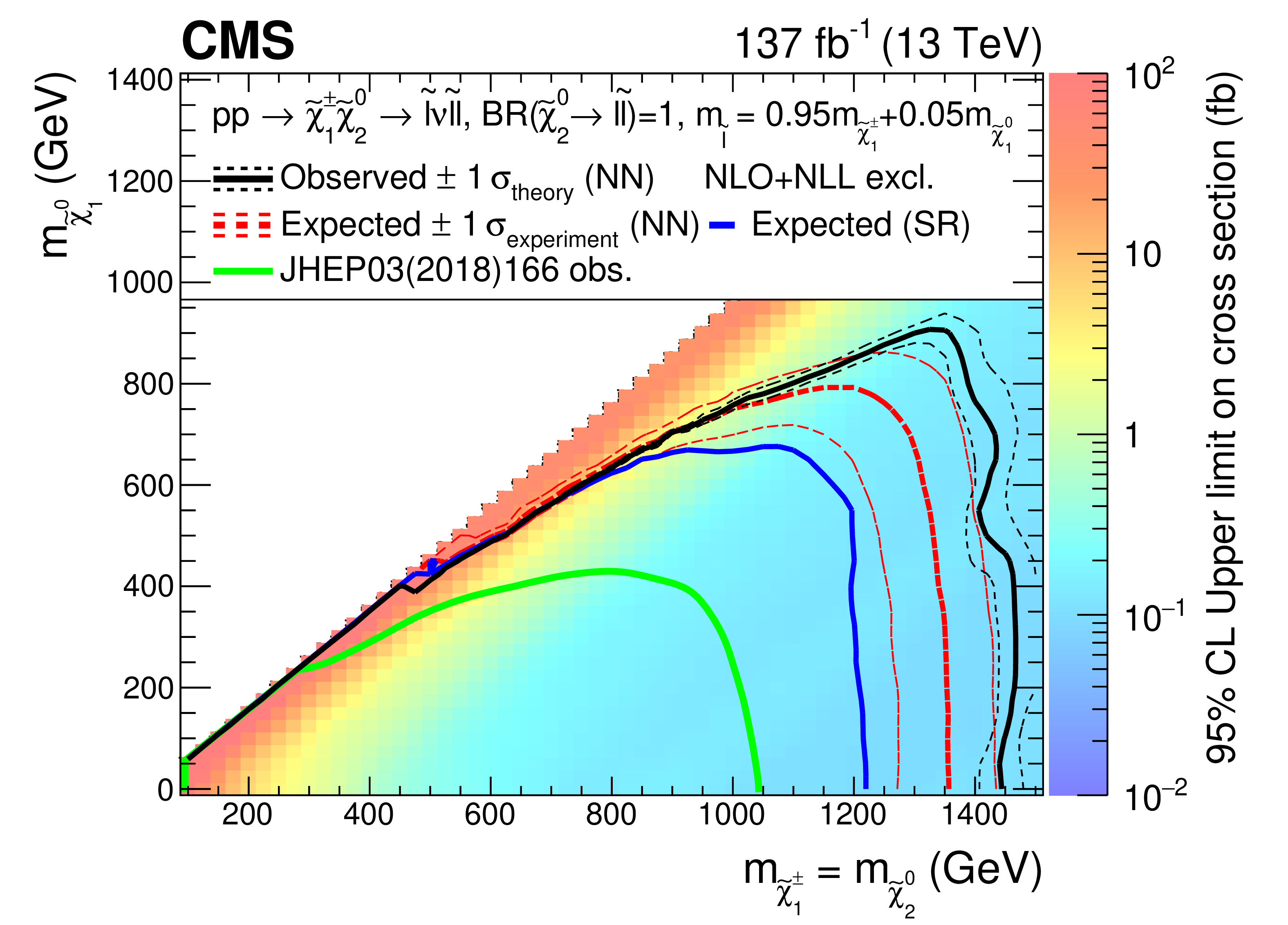
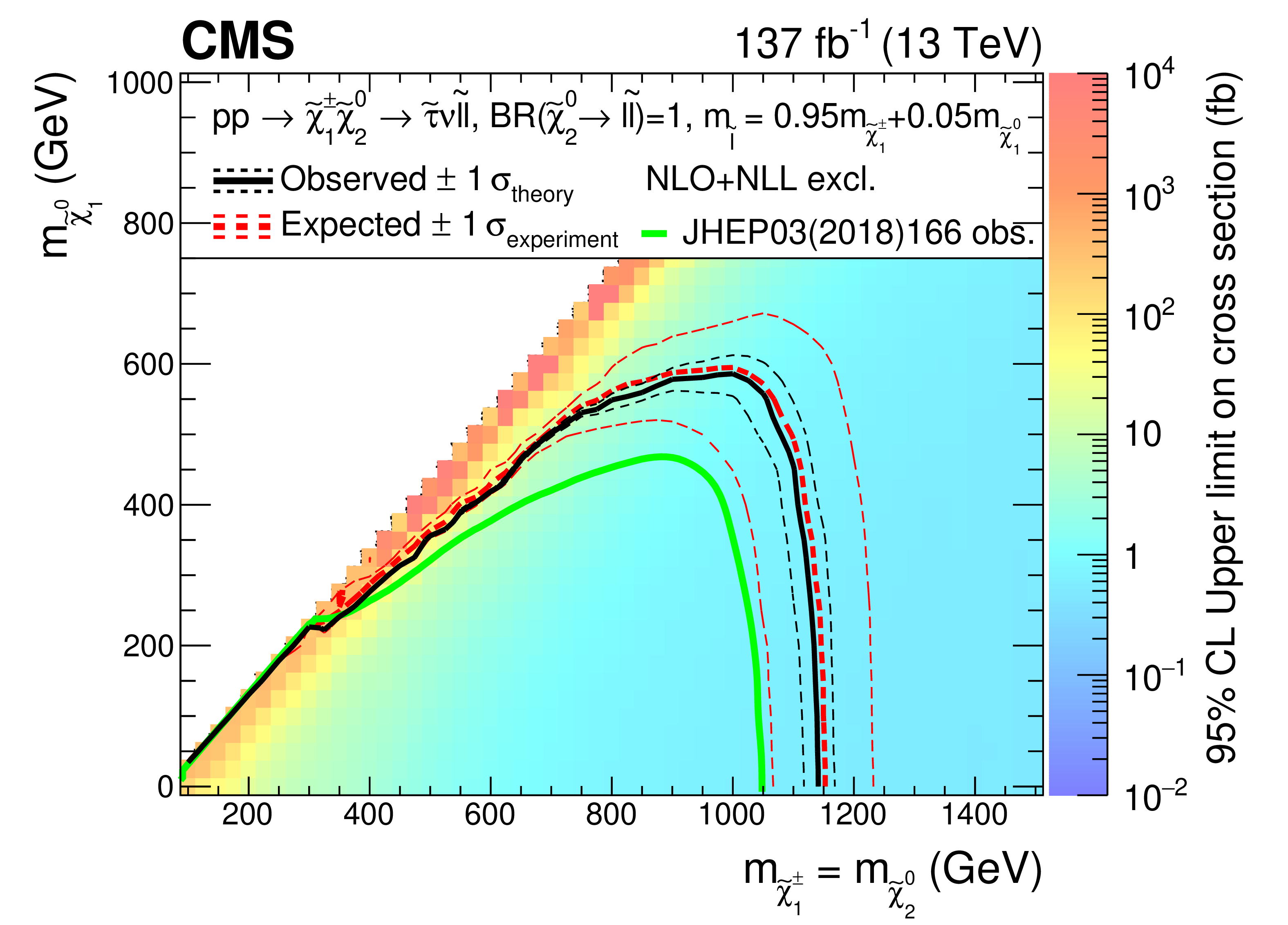
Figure 16-c:
Interpretation of the results for ${\tilde{\chi}^{\pm}_1 \tilde{\chi}^{0}_{2}}$ production with flavor-democratic slepton-mediated decays, and the parameter governing the mass splitting being $x=$ 0.95. The shading in the $m_{\tilde{\chi}^0_1}$ versus $m_{\tilde{\chi}^{0}_{2}}$ plane indicates the 95% CL upper limit on the ${\tilde{\chi}^{\pm}_1 \tilde{\chi}^{0}_{2}}$ production cross sections. The contours delineate the mass regions excluded at 95% CL when assuming cross section computed at NLO plus NLL. All masses below the contours are excluded. The observed, observed $ \pm $1$ \sigma _{\text {theory}}$ ($\pm $1 standard deviation of the theoretical cross sections), median expected, and expected $ \pm $1$ \sigma _{\text {experiment}}$ bounds obtained with the neural network strategy are shown in black and red. The median expected bound obtained with the search region strategy is shown in blue. The observed limits obtained in the CMS analysis using 2016 data [20] are shown in green. |
png pdf |
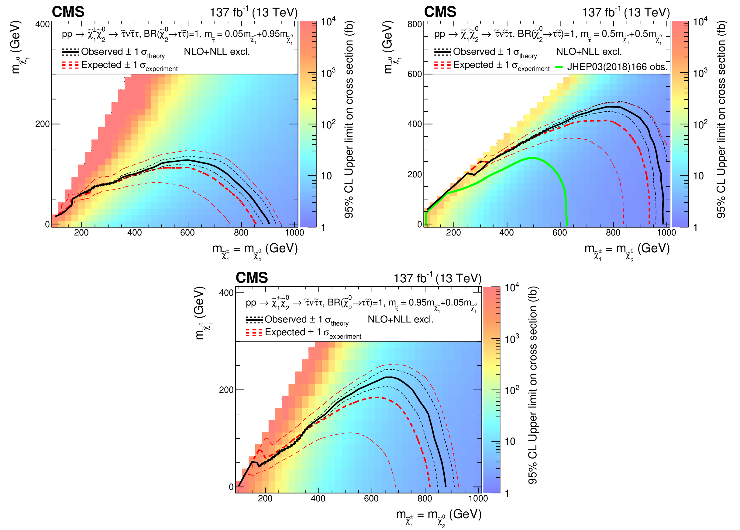
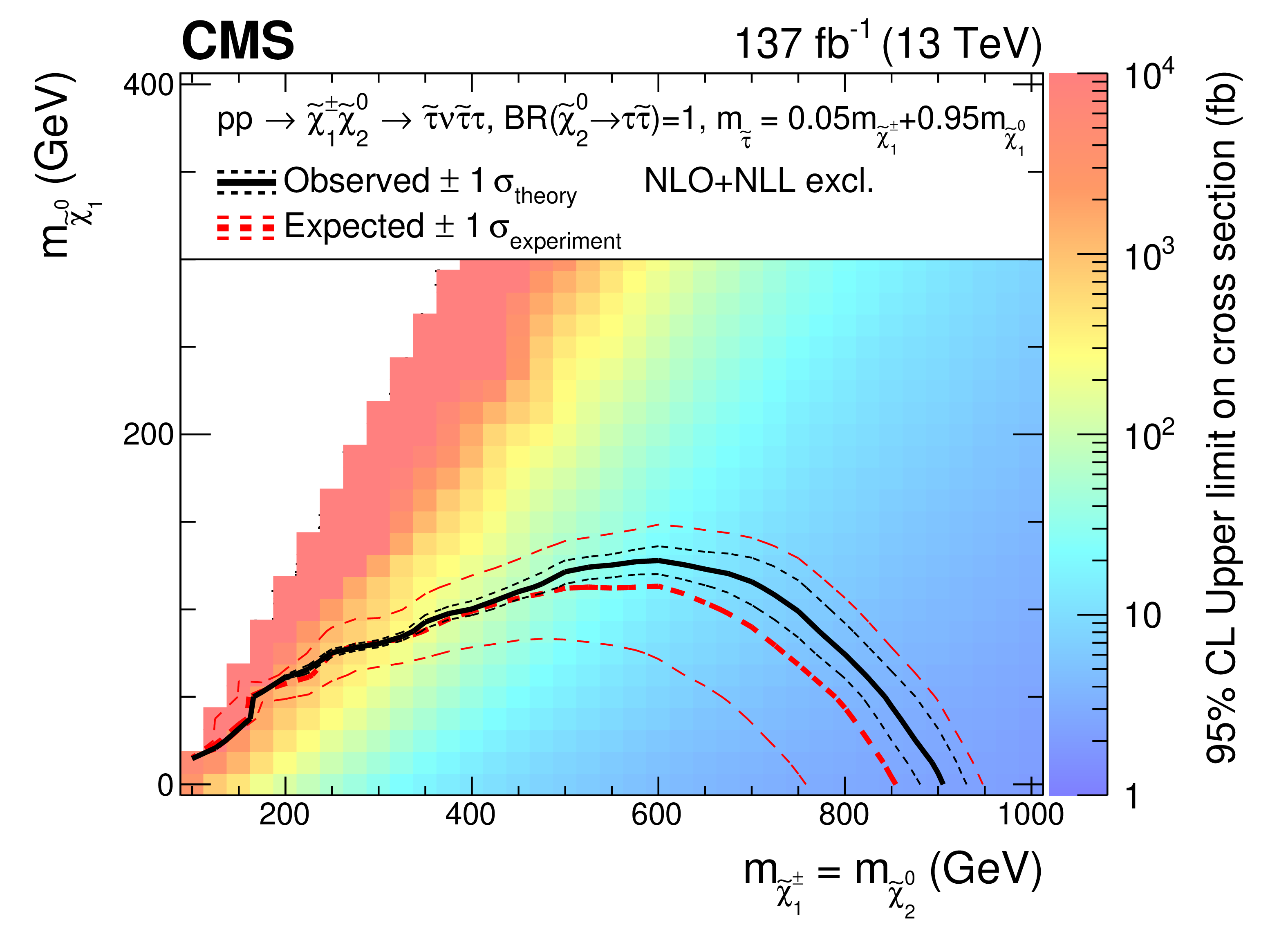
Figure 17:
Interpretation of the results for ${\tilde{\chi}^{\pm}_1 \tilde{\chi}^{0}_{2}}$ production with $\tau $-enriched slepton-mediated decays, and the parameter governing the mass splittings being $x=$ 0.05 (upper left), $x=$ 0.5 (upper right) and $x=$ 0.95 (lower). The shading in the $m_{\tilde{\chi}^0_1}$ versus $m_{\tilde{\chi}^{0}_{2}}$ plane indicates the 95% CL upper limits on the ${\tilde{\chi}^{\pm}_1 \tilde{\chi}^{0}_{2}}$ production cross sections. The contours delineate the mass regions excluded at 95% CL when assuming cross sections computed at NLO plus NLL. The observed, observed $ \pm $1$ \sigma _{\text {theory}}$ ($\pm $1 standard deviation of the theoretical cross sections), median expected, and expected $ \pm $1$ \sigma _{\text {experiment}}$ bounds are shown in black and red. The observed limits obtained in the CMS analysis using 2016 data [20] are shown in green. |

png pdf |
Figure 17-a:
Interpretation of the results for ${\tilde{\chi}^{\pm}_1 \tilde{\chi}^{0}_{2}}$ production with $\tau $-enriched slepton-mediated decays, and the parameter governing the mass splittings being $x=$ 0.05. The shading in the $m_{\tilde{\chi}^0_1}$ versus $m_{\tilde{\chi}^{0}_{2}}$ plane indicates the 95% CL upper limits on the ${\tilde{\chi}^{\pm}_1 \tilde{\chi}^{0}_{2}}$ production cross sections. The contours delineate the mass regions excluded at 95% CL when assuming cross sections computed at NLO plus NLL. The observed, observed $ \pm $1$ \sigma _{\text {theory}}$ ($\pm $1 standard deviation of the theoretical cross sections), median expected, and expected $ \pm $1$ \sigma _{\text {experiment}}$ bounds are shown in black and red. The observed limits obtained in the CMS analysis using 2016 data [20] are shown in green. |
png pdf |
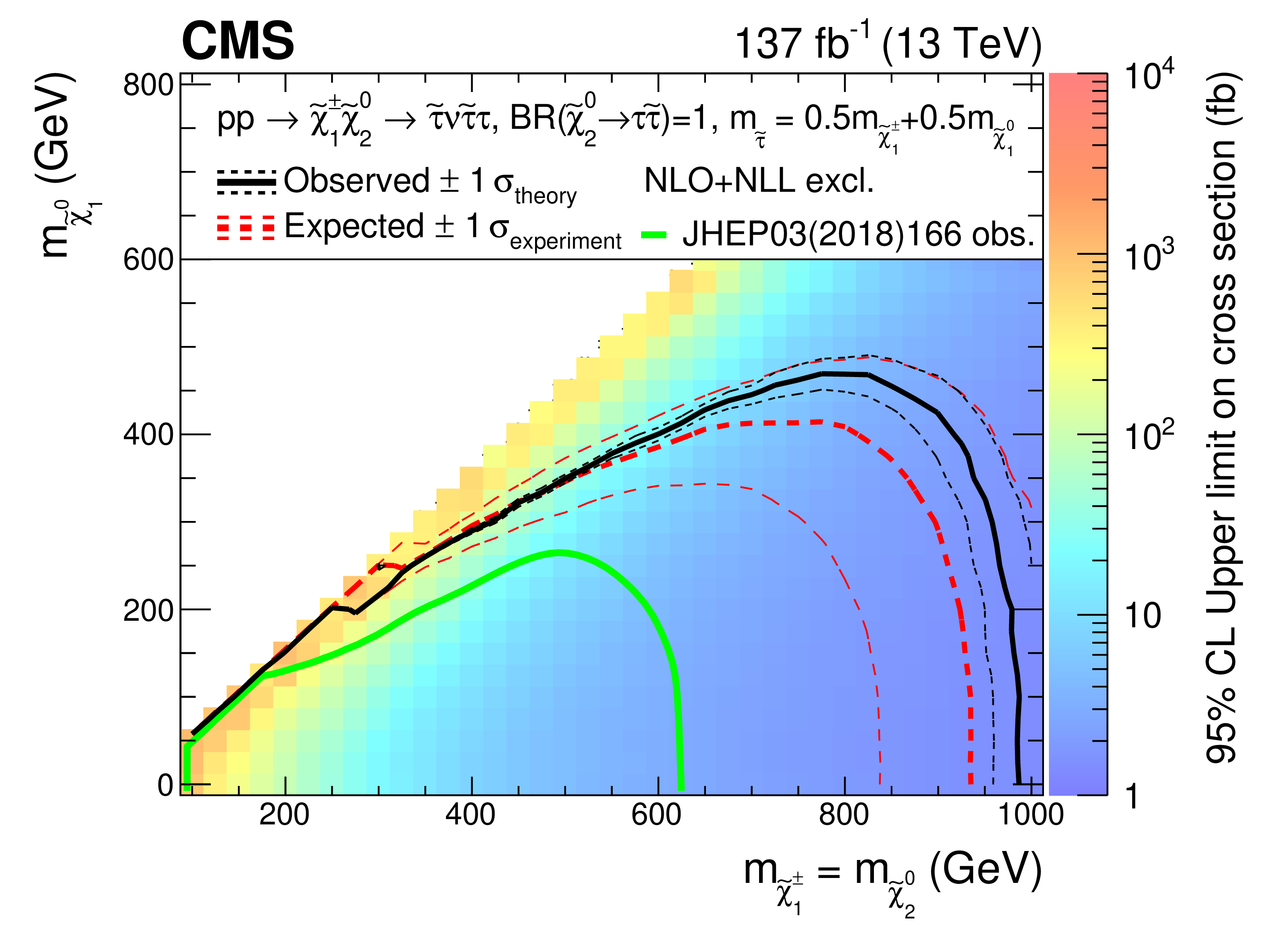
Figure 17-b:
Interpretation of the results for ${\tilde{\chi}^{\pm}_1 \tilde{\chi}^{0}_{2}}$ production with $\tau $-enriched slepton-mediated decays, and the parameter governing the mass splittings being $x=$ 0.5. The shading in the $m_{\tilde{\chi}^0_1}$ versus $m_{\tilde{\chi}^{0}_{2}}$ plane indicates the 95% CL upper limits on the ${\tilde{\chi}^{\pm}_1 \tilde{\chi}^{0}_{2}}$ production cross sections. The contours delineate the mass regions excluded at 95% CL when assuming cross sections computed at NLO plus NLL. The observed, observed $ \pm $1$ \sigma _{\text {theory}}$ ($\pm $1 standard deviation of the theoretical cross sections), median expected, and expected $ \pm $1$ \sigma _{\text {experiment}}$ bounds are shown in black and red. The observed limits obtained in the CMS analysis using 2016 data [20] are shown in green. |
png pdf |
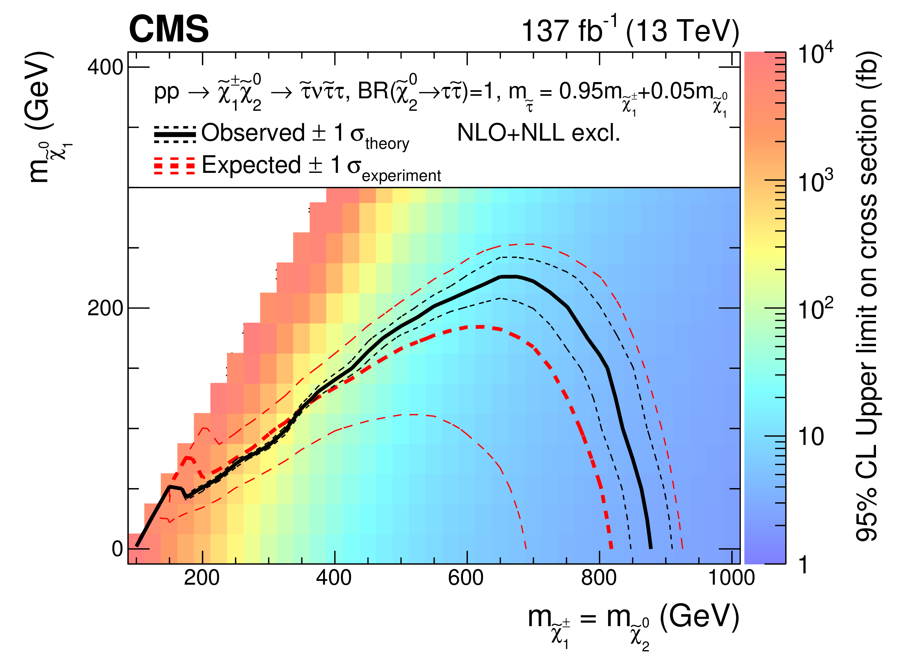
Figure 17-c:
Interpretation of the results for ${\tilde{\chi}^{\pm}_1 \tilde{\chi}^{0}_{2}}$ production with $\tau $-enriched slepton-mediated decays, and the parameter governing the mass splittings being $x=$ 0.95. The shading in the $m_{\tilde{\chi}^0_1}$ versus $m_{\tilde{\chi}^{0}_{2}}$ plane indicates the 95% CL upper limits on the ${\tilde{\chi}^{\pm}_1 \tilde{\chi}^{0}_{2}}$ production cross sections. The contours delineate the mass regions excluded at 95% CL when assuming cross sections computed at NLO plus NLL. The observed, observed $ \pm $1$ \sigma _{\text {theory}}$ ($\pm $1 standard deviation of the theoretical cross sections), median expected, and expected $ \pm $1$ \sigma _{\text {experiment}}$ bounds are shown in black and red. The observed limits obtained in the CMS analysis using 2016 data [20] are shown in green. |
png pdf |
Figure 18:
Interpretation of the results for ${\tilde{\chi}^{\pm}_1 \tilde{\chi}^{0}_{2}}$ production with $\tau $-dominated slepton-mediated decays, and the parameter governing the mass splittings being $x=$ 0.05 (upper left), $x=$ 0.5 (upper right) and $x=$ 0.95 (lower). The shading in the $m_{\tilde{\chi}^0_1}$ versus $m_{\tilde{\chi}^{0}_{2}}$ plane indicates the 95% CL upper limits on the ${\tilde{\chi}^{\pm}_1 \tilde{\chi}^{0}_{2}}$ production cross sections. The contours delineate the mass regions excluded at 95% CL when assuming cross sections computed at NLO plus NLL. The observed, observed $ \pm $1$ \sigma _{\text {theory}}$ ($\pm $1 standard deviation of the theoretical cross sections), median expected, and expected $ \pm $1$ \sigma _{\text {experiment}}$ bounds are shown in black and red. The median expected bound obtained with the search region strategy is shown in blue. The observed limits obtained in the CMS analysis using 2016 data [20] are shown in green, which only included interpretations in the $x=$ 0.5 case. |
png pdf |
Figure 18-a:
Interpretation of the results for ${\tilde{\chi}^{\pm}_1 \tilde{\chi}^{0}_{2}}$ production with $\tau $-dominated slepton-mediated decays, and the parameter governing the mass splittings being $x=$ 0.05. The shading in the $m_{\tilde{\chi}^0_1}$ versus $m_{\tilde{\chi}^{0}_{2}}$ plane indicates the 95% CL upper limits on the ${\tilde{\chi}^{\pm}_1 \tilde{\chi}^{0}_{2}}$ production cross sections. The contours delineate the mass regions excluded at 95% CL when assuming cross sections computed at NLO plus NLL. The observed, observed $ \pm $1$ \sigma _{\text {theory}}$ ($\pm $1 standard deviation of the theoretical cross sections), median expected, and expected $ \pm $1$ \sigma _{\text {experiment}}$ bounds are shown in black and red. The median expected bound obtained with the search region strategy is shown in blue. |
png pdf |
Figure 18-b:
Interpretation of the results for ${\tilde{\chi}^{\pm}_1 \tilde{\chi}^{0}_{2}}$ production with $\tau $-dominated slepton-mediated decays, and the parameter governing the mass splittings being $x=$ 0.5. The shading in the $m_{\tilde{\chi}^0_1}$ versus $m_{\tilde{\chi}^{0}_{2}}$ plane indicates the 95% CL upper limits on the ${\tilde{\chi}^{\pm}_1 \tilde{\chi}^{0}_{2}}$ production cross sections. The contours delineate the mass regions excluded at 95% CL when assuming cross sections computed at NLO plus NLL. The observed, observed $ \pm $1$ \sigma _{\text {theory}}$ ($\pm $1 standard deviation of the theoretical cross sections), median expected, and expected $ \pm $1$ \sigma _{\text {experiment}}$ bounds are shown in black and red. The median expected bound obtained with the search region strategy is shown in blue. The observed limits obtained in the CMS analysis using 2016 data [20] are shown in green. |
png pdf |
Figure 18-c:
Interpretation of the results for ${\tilde{\chi}^{\pm}_1 \tilde{\chi}^{0}_{2}}$ production with $\tau $-dominated slepton-mediated decays, and the parameter governing the mass splittings being $x=$ 0.95. The shading in the $m_{\tilde{\chi}^0_1}$ versus $m_{\tilde{\chi}^{0}_{2}}$ plane indicates the 95% CL upper limits on the ${\tilde{\chi}^{\pm}_1 \tilde{\chi}^{0}_{2}}$ production cross sections. The contours delineate the mass regions excluded at 95% CL when assuming cross sections computed at NLO plus NLL. The observed, observed $ \pm $1$ \sigma _{\text {theory}}$ ($\pm $1 standard deviation of the theoretical cross sections), median expected, and expected $ \pm $1$ \sigma _{\text {experiment}}$ bounds are shown in black and red. The median expected bound obtained with the search region strategy is shown in blue. |
png pdf |
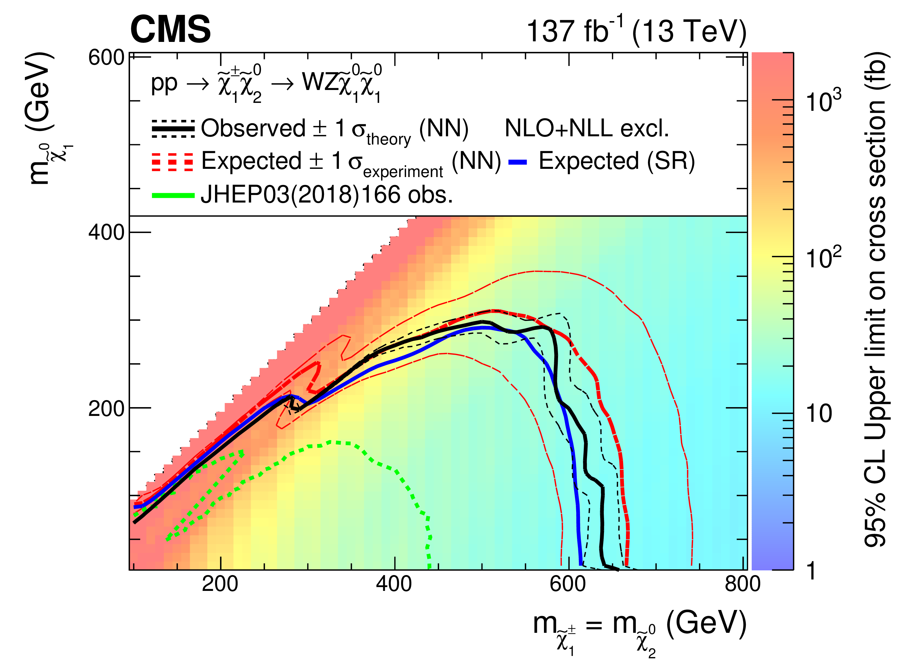
Figure 19:
Interpretation of the results for ${\tilde{\chi}^{\pm}_1 \tilde{\chi}^{0}_{2}}$ production with WZ-mediated decays. The shading in the $m_{\tilde{\chi}^0_1}$ versus $m_{\tilde{\chi}^{0}_{2}}$ plane indicates the 95% CL upper limits on the ${\tilde{\chi}^{\pm}_1 \tilde{\chi}^{0}_{2}}$ production cross sections. The contours delineate the mass regions excluded at 95% CL when assuming cross sections computed at NLO plus NLL. The observed, observed $ \pm $1$ \sigma _{\text {theory}}$ ($\pm $1 standard deviation of the theoretical cross sections), median expected, and expected $ \pm $1$ \sigma _{\text {experiment}}$ bounds obtained with the neural network strategy are shown in black and red. The median expected bound obtained with the search region strategy is shown in blue. The observed limits obtained in the CMS analysis using 2016 data [20] are shown in green. |
png pdf |
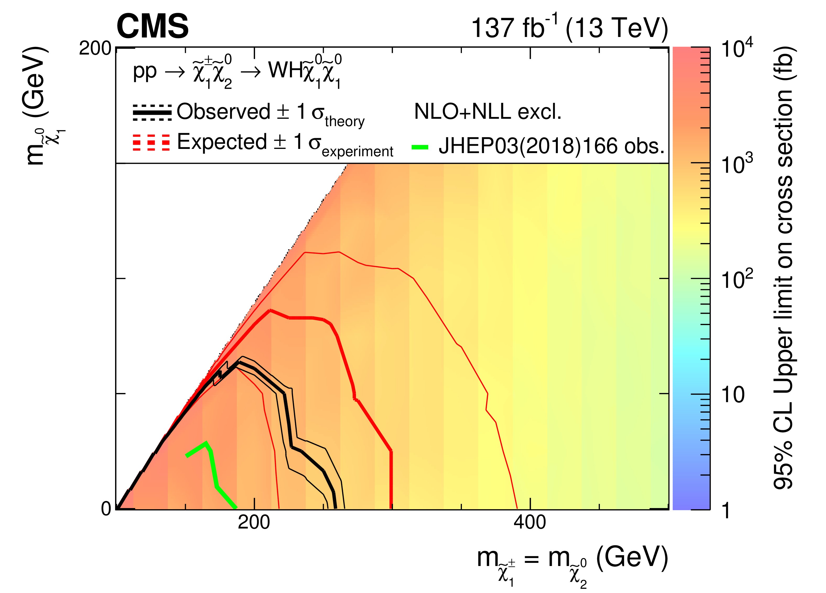
Figure 20:
Interpretation of the results for ${\tilde{\chi}^{\pm}_1 \tilde{\chi}^{0}_{2}}$ production with WH-mediated decays. The shading in the $m_{\tilde{\chi}^0_1}$ versus $m_{\tilde{\chi}^{0}_{2}}$ plane indicates the 95% CL upper limits on the ${\tilde{\chi}^{\pm}_1 \tilde{\chi}^{0}_{2}}$ production cross sections. The contours delineate the mass regions excluded at 95% CL when assuming cross sections computed at NLO plus NLL. The observed, observed $ \pm $1$ \sigma _{\text {theory}}$ ($\pm $1 standard deviation of the theoretical cross sections), median expected, and expected $ \pm $1$ \sigma _{\text {experiment}}$ bounds are shown in black and red. The observed limits obtained in the CMS analysis using 2016 data [20] are shown in green. |
png pdf |
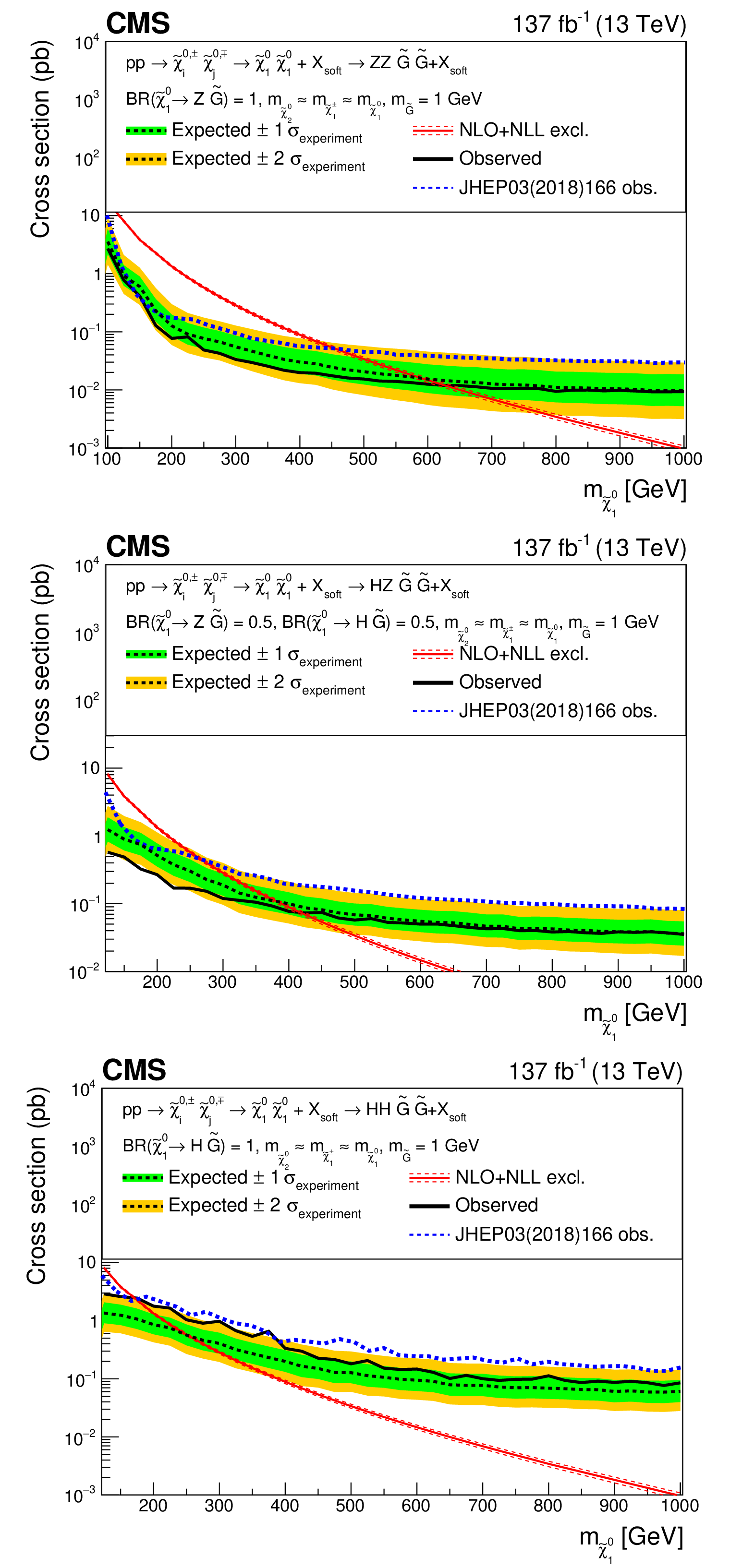
Figure 21:
Interpretation of the results for effective $\tilde{\chi}^0_1$ pair production, with ZZ-mediated decays (upper), HZ-mediated decays (middle), and HH-mediated decays (lower). The median expected upper limits (black line) are shown along with the $ \pm $1$ \sigma $ (0.16 and 0.84 quantiles, green) and $ \pm $2$ \sigma $ (0.05 and 0.95 quantiles, yellow) bands. The predicted production cross sections computed at NLO plus NLL are shown in red and the observed exclusion limits obtained in the CMS analysis using 2016 data [20] are shown in blue. |
png pdf |
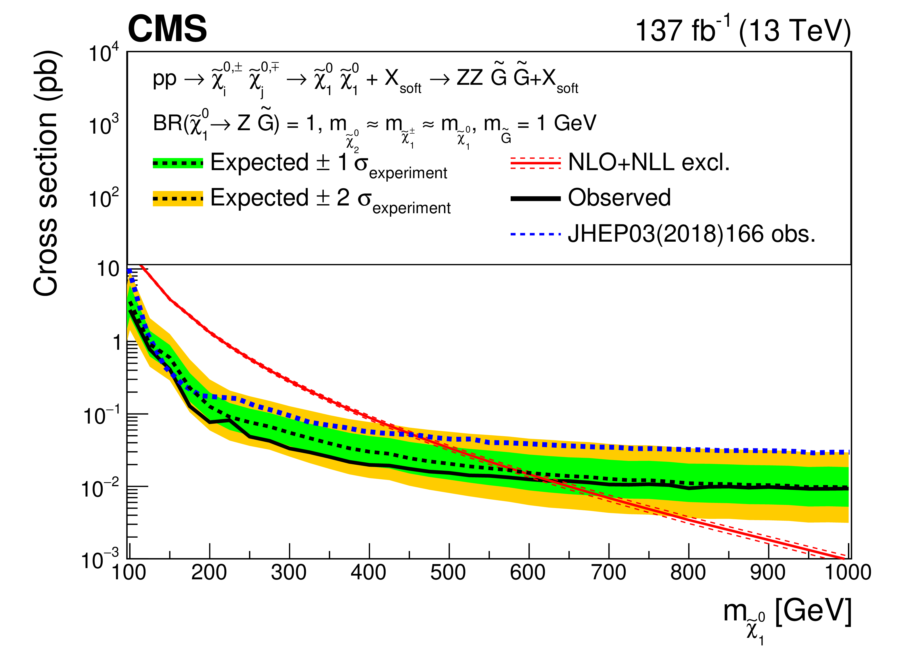
Figure 21-a:
Interpretation of the results for effective $\tilde{\chi}^0_1$ pair production, with ZZ-mediated decays. The median expected upper limits (black line) are shown along with the $ \pm $1$ \sigma $ (0.16 and 0.84 quantiles, green) and $ \pm $2$ \sigma $ (0.05 and 0.95 quantiles, yellow) bands. The predicted production cross sections computed at NLO plus NLL are shown in red and the observed exclusion limits obtained in the CMS analysis using 2016 data [20] are shown in blue. |
png pdf |
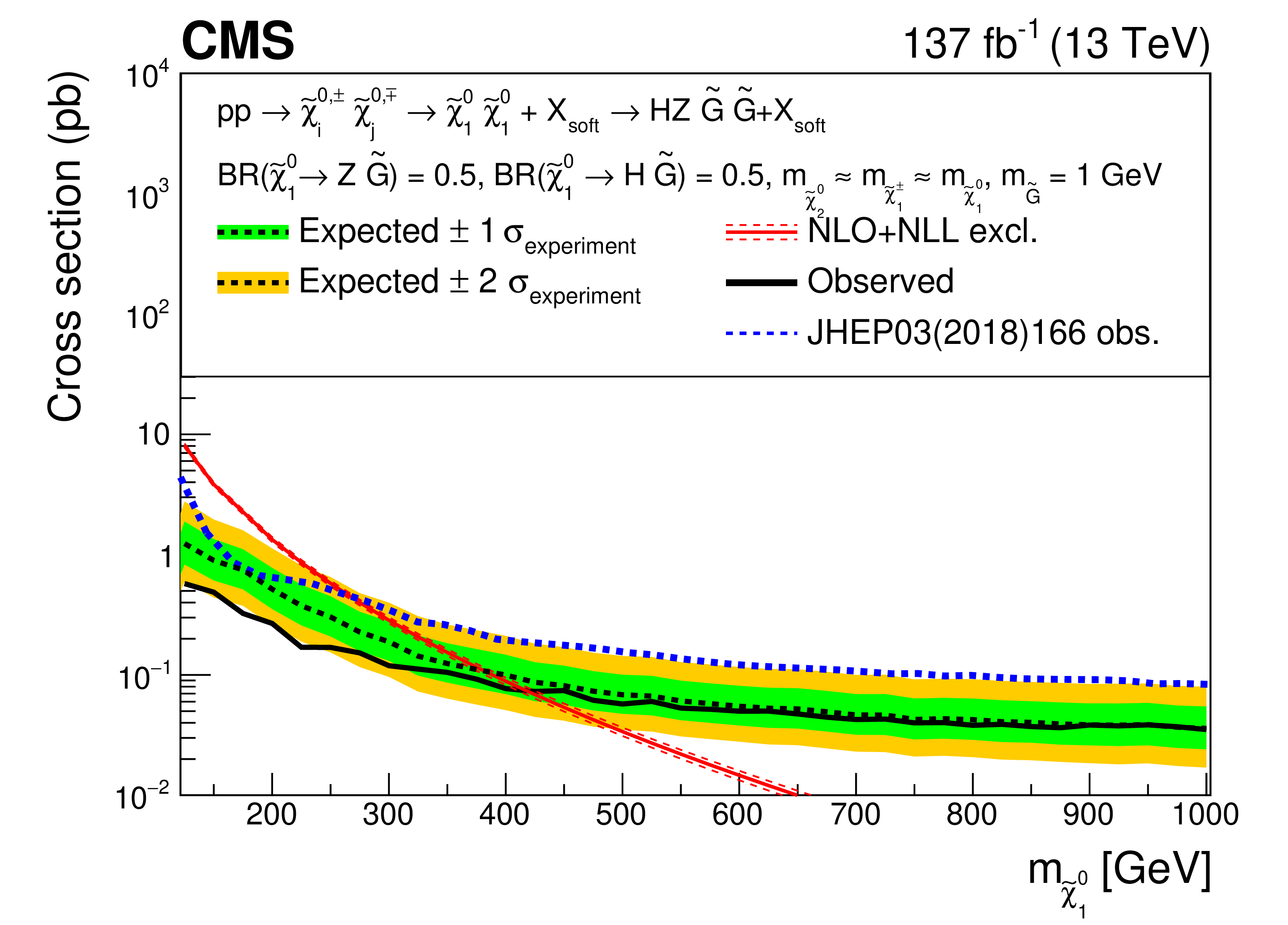
Figure 21-b:
Interpretation of the results for effective $\tilde{\chi}^0_1$ pair production, with HZ-mediated decays. The median expected upper limits (black line) are shown along with the $ \pm $1$ \sigma $ (0.16 and 0.84 quantiles, green) and $ \pm $2$ \sigma $ (0.05 and 0.95 quantiles, yellow) bands. The predicted production cross sections computed at NLO plus NLL are shown in red and the observed exclusion limits obtained in the CMS analysis using 2016 data [20] are shown in blue. |
png pdf |
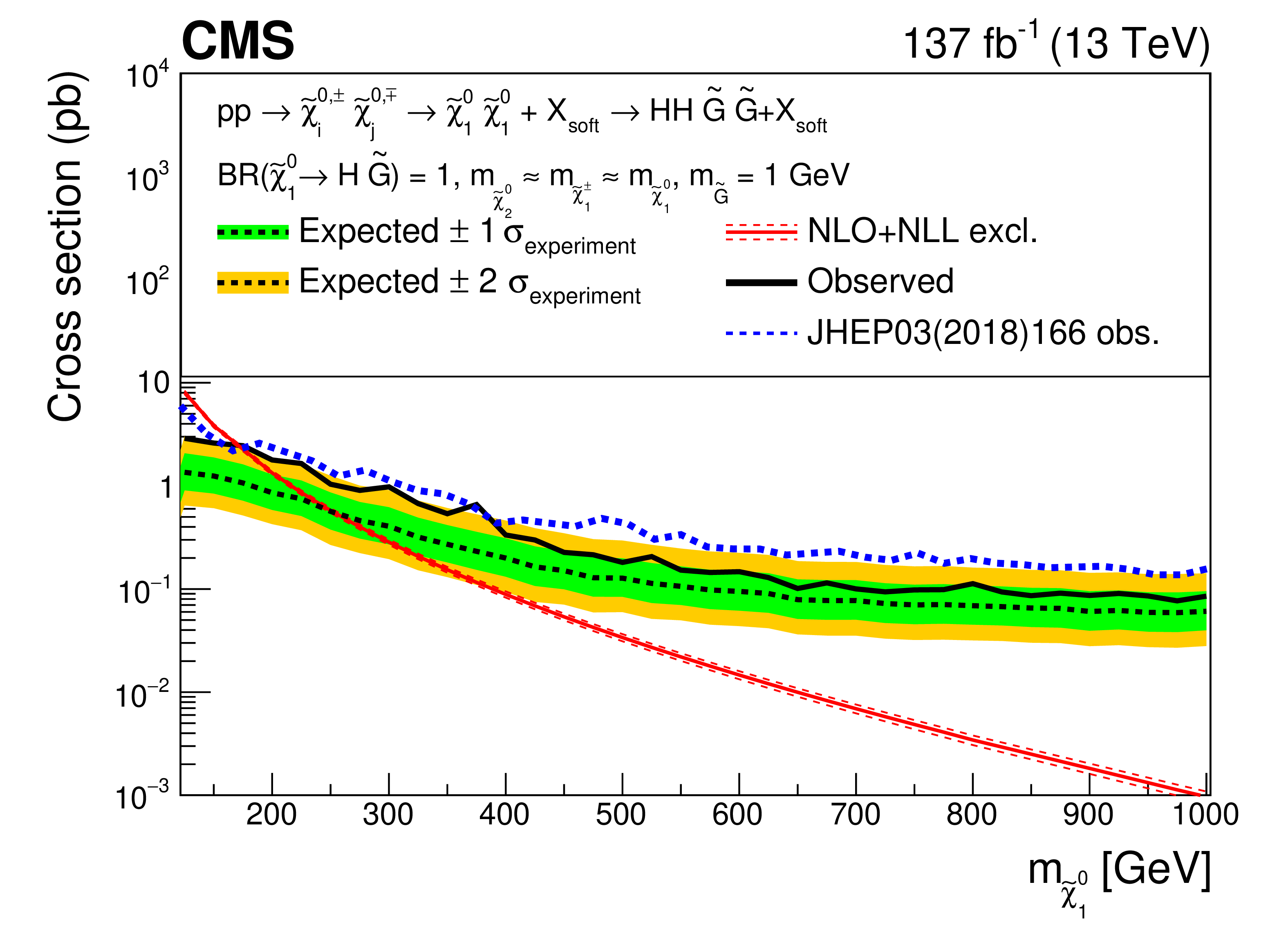
Figure 21-c:
Interpretation of the results for effective $\tilde{\chi}^0_1$ pair production, with HH-mediated decays. The median expected upper limits (black line) are shown along with the $ \pm $1$ \sigma $ (0.16 and 0.84 quantiles, green) and $ \pm $2$ \sigma $ (0.05 and 0.95 quantiles, yellow) bands. The predicted production cross sections computed at NLO plus NLL are shown in red and the observed exclusion limits obtained in the CMS analysis using 2016 data [20] are shown in blue. |
| Tables | |
png pdf |
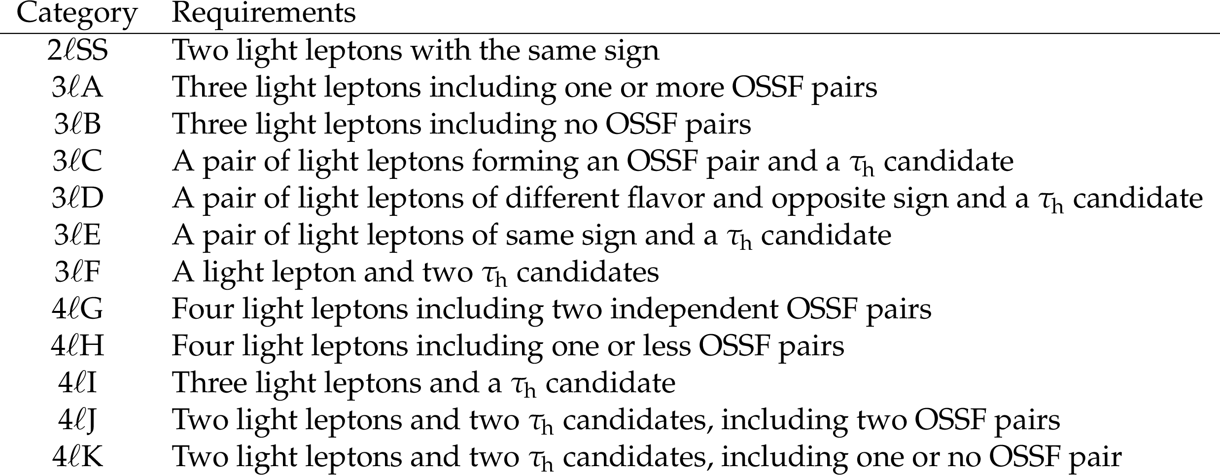
Table 1:
Brief description of the categories used to classify events in the search. |
png pdf |
Table 2:
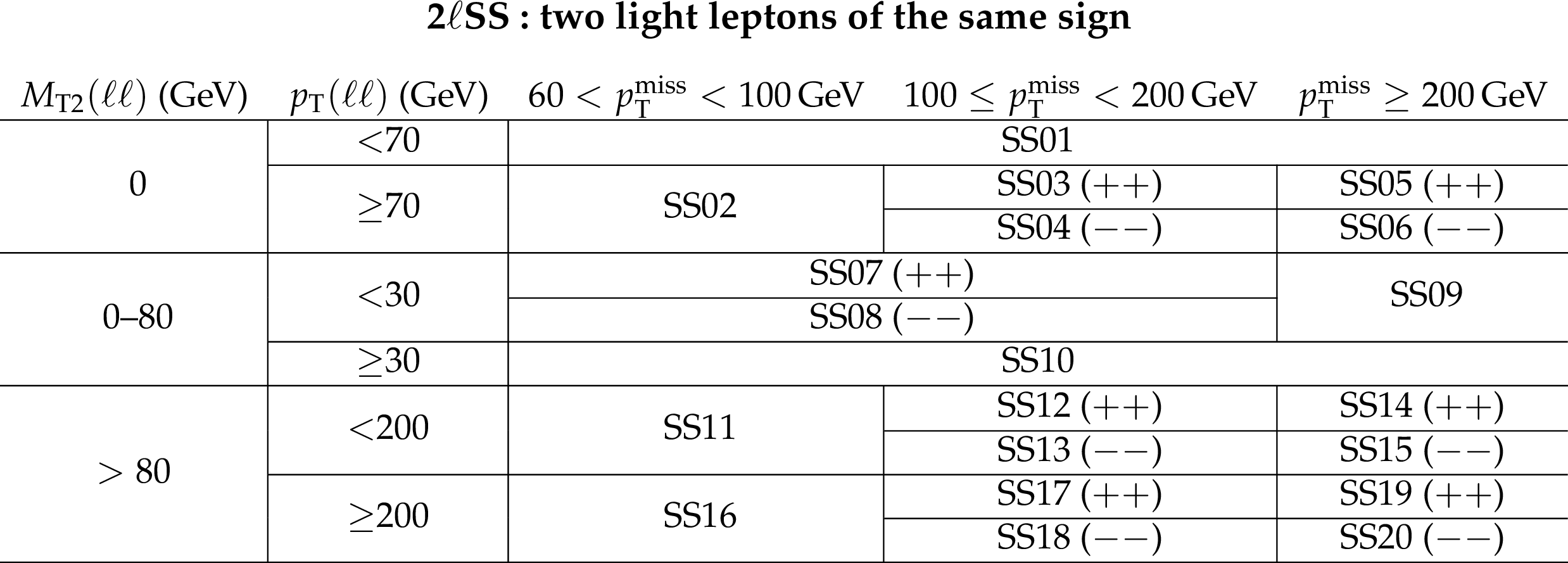
Definition of the search regions used for events with two same-sign light leptons (SSXX). The symbols ($++$) and ($-$) represent requirements on the sign of the leptons. The first ${{M_{\text {T2}}} (\ell \ell)}$ bin contains only events where ${{M_{\text {T2}}} (\ell \ell)}$ is exactly 0 [68], whereas the second bin contains events where ${{M_{\text {T2}}} (\ell \ell)}$ is larger than 0 and less than or equal to 80 GeV. The last ${{M_{\text {T2}}} (\ell \ell)}$ bin contains events where ${{M_{\text {T2}}} (\ell \ell)}$ exceeds 80 GeV. |
png pdf |
Table 3:
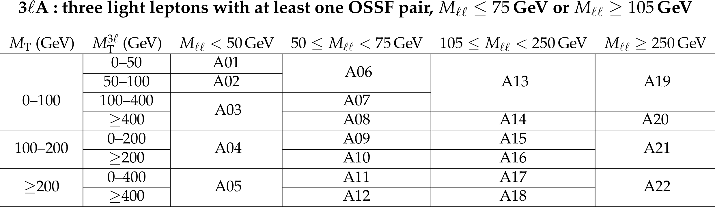
Definition of the search regions used for events with three light leptons, at least two of which form an OSSF pair, excluding those with 75 $ < {M_{\ell \ell}} < $ 105 GeV (AXX). |
png pdf |
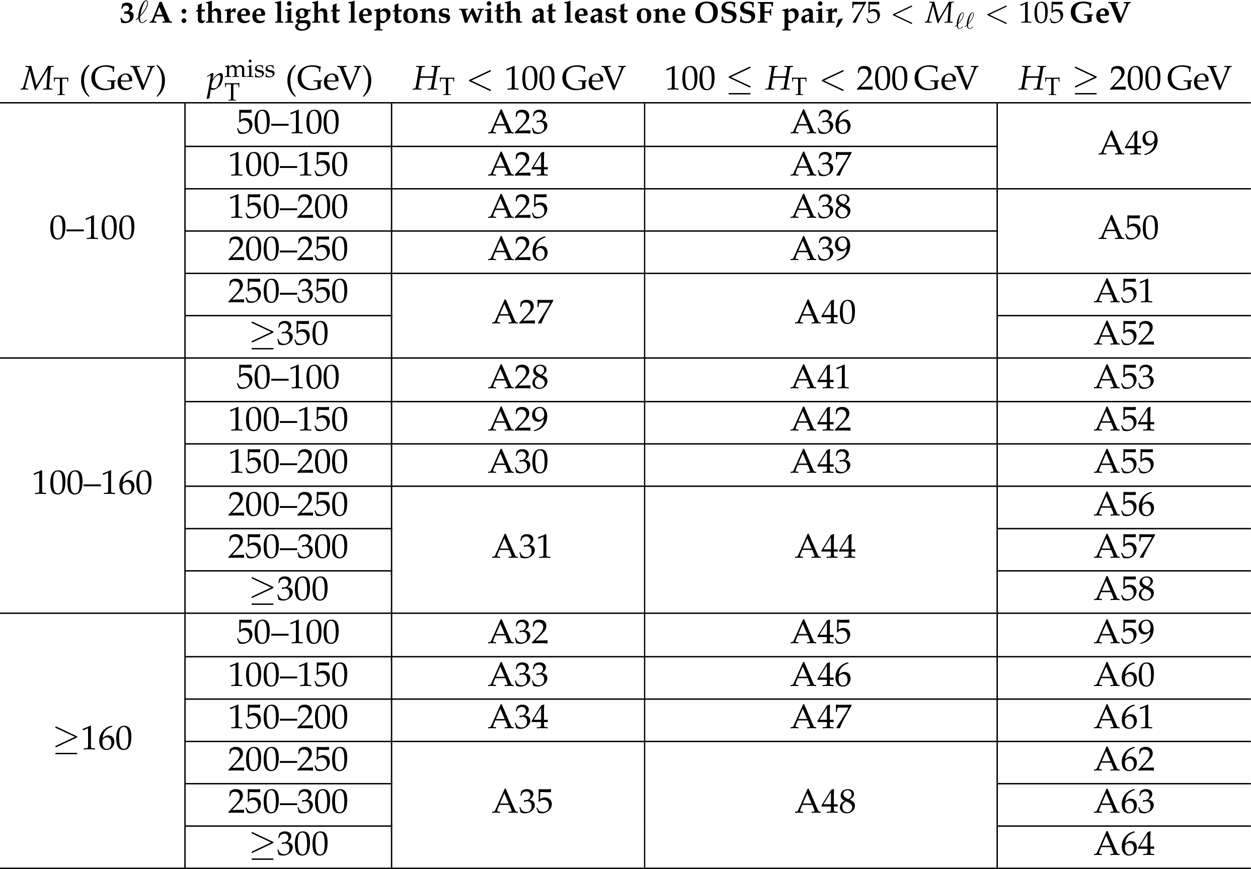
Table 4:
Definition of the search regions used for events with three light leptons, at least two of which form an OSSF pair, and which satisfy 75 $ < {M_{\ell \ell}} < $ 105 GeV (AXX). |

png pdf |
Table 5:
Definition of the search regions used for events with three light leptons, none of which form an OSSF pair (BXX). |
png pdf |
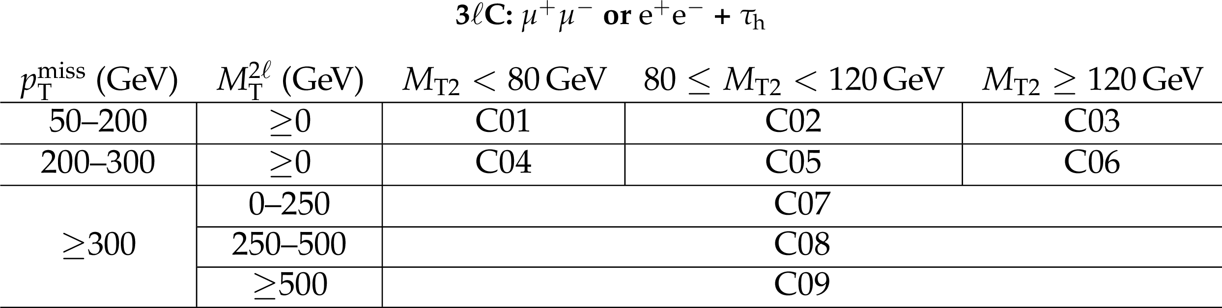
Table 6:
Definition of the search regions for events with a $\mu^{+} \mu^{-} $ or $\mathrm{e^{+}} \mathrm{e^{-}} $ pair and an additional ${\tau _\mathrm {h}}$ candidate (CXX). |
png pdf |
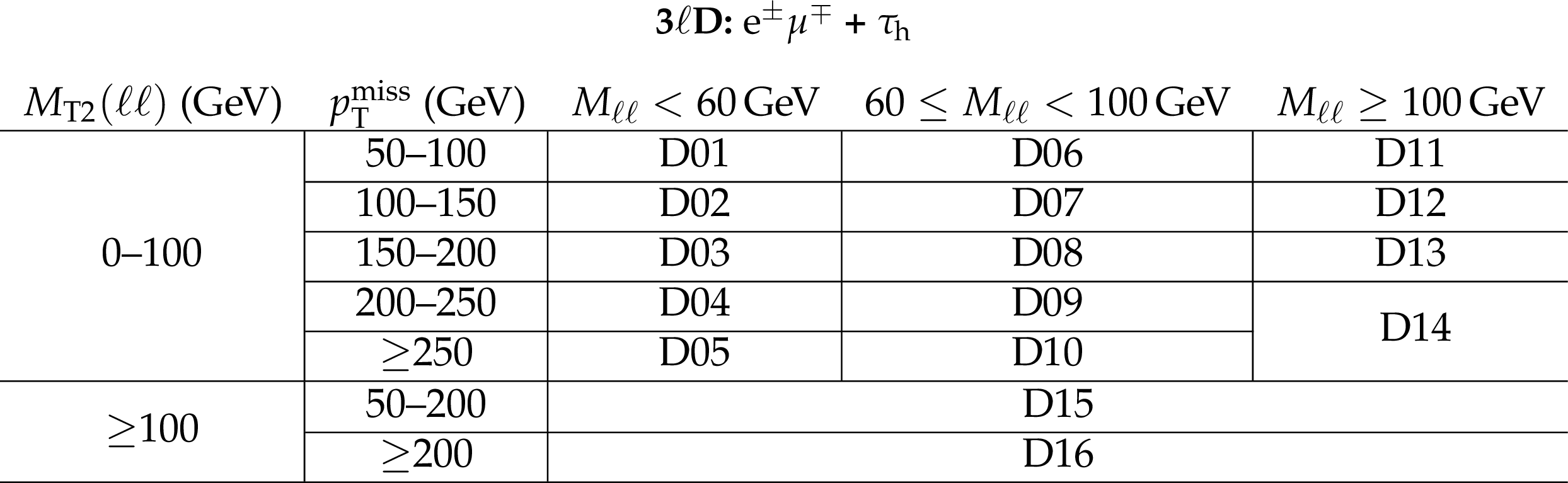
Table 7:
Definition of the search regions for events with a e$^{\pm}\mu ^{\mp}$ pair and a ${\tau _\mathrm {h}}$ candidate (DXX). |

png pdf |
Table 8:
Definition of the search regions for events with a pair of light leptons of the same sign and a ${\tau _\mathrm {h}}$ candidate (EXX). |

png pdf |
Table 9:
Definition of the search regions for events with 2 ${\tau _\mathrm {h}}$ candidates and one light lepton (FXX). |
png pdf |
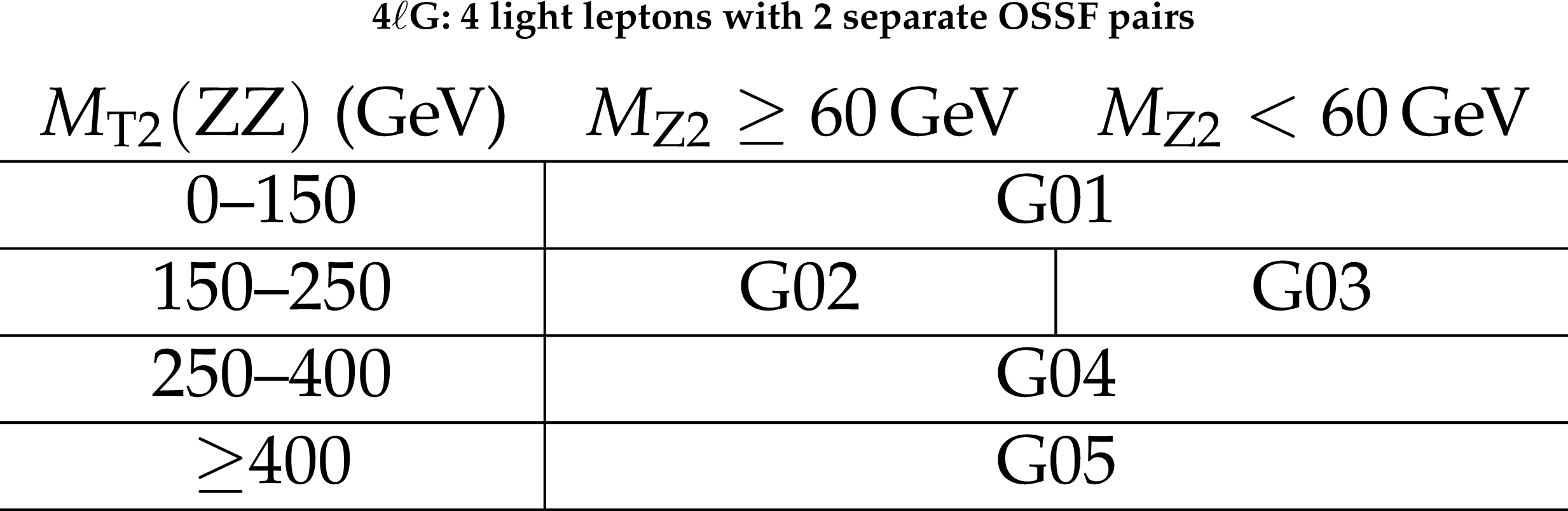
Table 10:
Definition of the search regions for events with 4 light leptons, including 2 separate OSSF pairs (GXX). |

png pdf |
Table 11:
Definition of the search regions for events with 4 leptons with one or more ${\tau _\mathrm {h}}$, or without two light-lepton OSSF pairs (XYY). |

png pdf |
Table 12:
Systematic uncertainty sources affecting the analysis, with their typical size across signal regions, and the treatment of the correlations across data-taking years. Uncertainties in the jet energy corrections and b tagging efficiencies are considered separately for signal events which use CMS fast simulation, as explained in Section {5, and for the other simulated processes. Both the overall integrated luminosity and all normalization uncertainties have effects on the predicted yields of the corresponding processes that are of the same size across all signal regions. Their quoted typical size corresponds to the size of such variations. All other uncertainties can have different effects on the predicted yields for each process and signal region. Their typical uncertainty corresponds to the range of sizes that such effects take across the analysis search regions. |
png pdf |
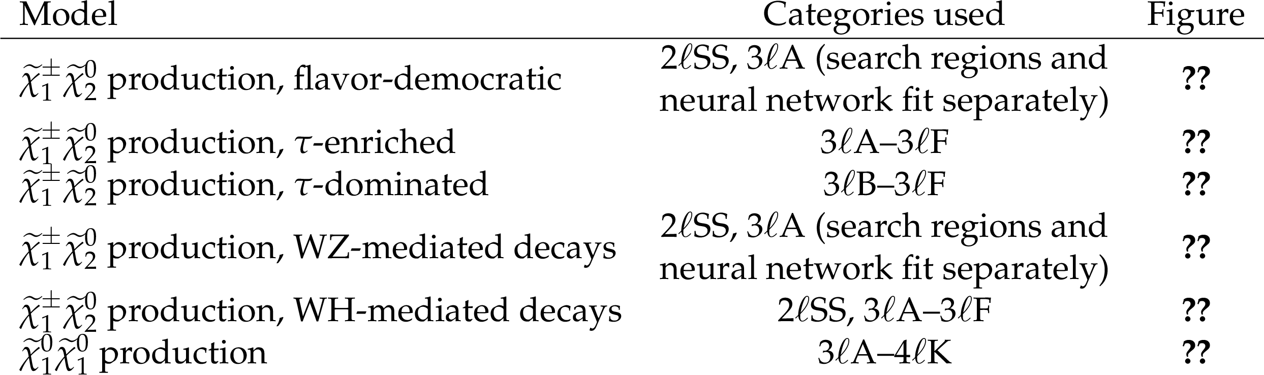
Table 13:
Summary of the event categories used for the interpretation of the results in terms of different models, and references to the associated figure summarizing the expected and observed 95% CL upper limits. |
| Summary |
|
A search for new physics in events with two leptons of the same sign, or with three or more leptons with up to two hadronically decaying $\tau$ leptons, is presented. A data set of proton-proton collisions with $\sqrt{s} = $ 13 TeV collected with the CMS detector at the LHC, corresponding to an integrated luminosity of 137 fb$^{-1}$, is analyzed. Events are categorized according to the number of leptons, their signs, and flavors. Events in each category are further binned using a plethora of kinematic quantities to maximize the sensitivity of the search to an extensive set of hypotheses of supersymmetric particle production via the electroweak interaction. In events with three light leptons, of which two have opposite sign and same flavor, parametric neural networks are used to significantly enhance the sensitivity of the search to several signal hypotheses. No significant deviation from the standard model expectation is observed in any of the event categories. The results are interpreted in terms of a number of simplified models of superpartner production. Models of chargino-neutralino pair production with the neutralino forming the lightest supersymmetric particle (LSP), as well as models of effective neutralino pair production with a nearly massless gravitino as the LSP are considered. The signal topologies depend on the masses of the leptonic superpartners and the mixing of the gauge eigenstates. If left-handed sleptons lighter than the chargino existed, the chargino-neutralino pair might undergo slepton-mediated decays resulting in final states with three leptons. The results of the analysis lead to a lower limit in the chargino mass up to 1450 GeV when using a parametric neural network. Searches in events with three light leptons including an opposite-sign, same-flavor pair provide sensitivity to these models. Events with two same-sign leptons further enhance the sensitivity in experimentally challenging scenarios with small mass differences between the chargino and the LSP. If sleptons were right-handed, the chargino, or both the chargino and the neutralino, might decay almost exclusively to $\tau$ leptons. In the former scenario, a chargino mass up to 1150 GeV is excluded, while a mass up to 970 GeV is excluded in the latter. If sleptons were sufficiently heavy, charginos and neutralinos would undergo direct decay to the LSP via the emission of W, Z, or Higgs bosons. For decays of the chargino-neutralino pair via a W and a Z boson, values of the chargino mass up to 650 GeV are excluded through the use of a parametric neural network. In case of a neutralino decay via the emission of a Higgs boson, charginos with a mass below 300 GeV are excluded for nearly massless LSPs. In models of effective neutralino production we assume the neutralinos decay to almost massless gravitino LSPs via Z and Higgs bosons. This leads to excluded values of the neutralino mass up to 600 GeV. The obtained results currently provide the most stringent limits for chargino-neutralino production with mass splittings close to the Z boson mass, nearly closing the gap in the exclusion plane found in this region of the parameter space. The exclusions obtained for the slepton-mediated decays are as well the most stringent results currently for all the considered branching fraction hypotheses. In the case of the flavor-democratic decay scenario, the obtained exclusion limits of up to 1450 GeV are the overall highest exclusion values obtained for the production of electroweak superpartners. |
| References | ||||
| 1 | P. Ramond | Dual theory for free fermions | PRD 3 (1971) 2415 | |
| 2 | J. Wess and B. Zumino | A Lagrangian model invariant under supergauge transformations | PLB 49 (1974) 52 | |
| 3 | J. Wess and B. Zumino | Supergauge transformations in four dimensions | NPB 70 (1974) 39 | |
| 4 | P. Fayet | Supergauge invariant extension of the Higgs mechanism and a model for the electron and its neutrino | NPB 90 (1975) 104 | |
| 5 | H. P. Nilles | Supersymmetry, supergravity and particle physics | Phys. Rep. 110 (1984) 1 | |
| 6 | S. P. Martin | A supersymmetry primer | volume 21, p. 1 2010 | hep-ph/9709356 |
| 7 | CMS Collaboration | Search for supersymmetry in proton-proton collisions at 13 TeV in final states with jets and missing transverse momentum | JHEP 10 (2019) 244 | CMS-SUS-19-006 1908.04722 |
| 8 | CMS Collaboration | Searches for physics beyond the standard model with the $ M_\mathrm{T2} $ variable in hadronic final states with and without disappearing tracks in proton-proton collisions at $ \sqrt{s}= $ 13 TeV | EPJC 80 (2020) 3 | CMS-SUS-19-005 1909.03460 |
| 9 | CMS Collaboration | Search for supersymmetry in pp collisions at $ \sqrt{s}= $ 13 TeV with 137 fb$ ^{-1} $ in final states with a single lepton using the sum of masses of large-radius jets | PRD 101 (2020) 052010 | CMS-SUS-19-007 1911.07558 |
| 10 | CMS Collaboration | Search for physics beyond the standard model in events with jets and two same-sign or at least three charged leptons in proton-proton collisions at $ \sqrt{s}= $ 13 TeV | EPJC 80 (2020) 752 | CMS-SUS-19-008 2001.10086 |
| 11 | CMS Collaboration | Search for direct top squark pair production in events with one lepton, jets, and missing transverse momentum at 13 TeV with the CMS experiment | JHEP 05 (2020) 032 | CMS-SUS-19-009 1912.08887 |
| 12 | ATLAS Collaboration | Search for top squarks in events with a Higgs or Z boson using 139 fb$ ^{-1} $ of pp collision data at $ \sqrt{s}= $ 13 TeV with the ATLAS detector | EPJC 80 (2020) 1080 | 2006.05880 |
| 13 | ATLAS Collaboration | Search for a scalar partner of the top quark in the all-hadronic $ t{\bar{t}} $ plus missing transverse momentum final state at $ \sqrt{s}= $ 13 TeV with the ATLAS detector | EPJC 80 (2020) 737 | 2004.14060 |
| 14 | ATLAS Collaboration | Search for long-lived, massive particles in events with a displaced vertex and a muon with large impact parameter in pp collisions at $ \sqrt{s} = $ 13 TeV with the ATLAS detector | PRD 102 (2020) 032006 | 2003.11956 |
| 15 | ATLAS Collaboration | Search for squarks and gluinos in final states with same-sign leptons and jets using 139 fb$ ^{-1} $ of data collected with the ATLAS detector | JHEP 06 (2020) 046 | 1909.08457 |
| 16 | ATLAS Collaboration | Search for bottom-squark pair production with the ATLAS detector in final states containing Higgs bosons, $ b $-jets and missing transverse momentum | JHEP 12 (2019) 060 | 1908.03122 |
| 17 | ATLAS Collaboration | Search for chargino-neutralino production with mass splittings near the electroweak scale in three-lepton final states in $ \sqrt {s} =$ 13 TeV pp collisions with the ATLAS detector | PRD 101 (2020) 072001 | 1912.08479 |
| 18 | ATLAS Collaboration | Search for electroweak production of supersymmetric particles in final states with two or three leptons at $ \sqrt{s}= $ 13 TeV with the ATLAS detector | EPJC 78 (2018) 995 | 1803.02762 |
| 19 | ATLAS Collaboration | Search for supersymmetry in events with four or more leptons in $ \sqrt{s}=$ 13 TeV pp collisions with ATLAS | PRD 98 (2018) 032009 | 1804.03602 |
| 20 | CMS Collaboration | Search for electroweak production of charginos and neutralinos in multilepton final states in proton-proton collisions at $ \sqrt{s}= $ 13 TeV | JHEP 03 (2018) 166 | CMS-SUS-16-039 1709.05406 |
| 21 | CMS Collaboration | Combined search for electroweak production of charginos and neutralinos in proton-proton collisions at $ \sqrt{s} = $ 13 TeV | JHEP 03 (2018) 160 | CMS-SUS-17-004 1801.03957 |
| 22 | P. Baldi et al. | Parameterized neural networks for high-energy physics | EPJC 76 (2016) 235 | 1601.07913 |
| 23 | CMS Collaboration | The CMS experiment at the CERN LHC | JINST 3 (2008) S08004 | CMS-00-001 |
| 24 | CMS Collaboration | The CMS trigger system | JINST 12 (2017) P01020 | CMS-TRG-12-001 1609.02366 |
| 25 | LHC New Physics Working Group Collaboration | Simplified models for LHC new physics searches | JPG 39 (2012) 105005 | 1105.2838 |
| 26 | CMS Collaboration | Interpretation of searches for supersymmetry with simplified models | PRD 88 (2013) 052017 | CMS-SUS-11-016 1301.2175 |
| 27 | LHC Higgs Cross Section Working Group | Handbook of LHC Higgs cross sections: 4. deciphering the nature of the Higgs sector | CERN (2016) | 1610.07922 |
| 28 | K. T. Matchev and S. D. Thomas | Higgs and Z boson signatures of supersymmetry | PRD 62 (2000) 077702 | hep-ph/9908482 |
| 29 | J. T. Ruderman and D. Shih | General neutralino NLSPs at the early LHC | JHEP 08 (2012) 159 | 1103.6083 |
| 30 | P. Meade, M. Reece, and D. Shih | Prompt decays of general neutralino NLSPs at the Tevatron | JHEP 05 (2010) 105 | 0911.4130 |
| 31 | W. Beenakker et al. | The production of charginos/neutralinos and sleptons at hadron colliders | PRL 83 (1999) 3780 | hep-ph/9906298 |
| 32 | B. Fuks, M. Klasen, D. R. Lamprea, and M. Rothering | Gaugino production in proton-proton collisions at a center-of-mass energy of 8 TeV | JHEP 10 (2012) 081 | 1207.2159 |
| 33 | B. Fuks, M. Klasen, D. R. Lamprea, and M. Rothering | Precision predictions for electroweak superpartner production at hadron colliders with Resummino | EPJC 73 (2013) 2480 | 1304.0790 |
| 34 | CMS Collaboration | Particle-flow reconstruction and global event description with the CMS detector | JINST 12 (2017) P10003 | CMS-PRF-14-001 1706.04965 |
| 35 | M. Cacciari, G. P. Salam, and G. Soyez | The anti-$ {k_{\mathrm{T}}} $ jet clustering algorithm | JHEP 04 (2008) 063 | 0802.1189 |
| 36 | M. Cacciari and G. P. Salam | Dispelling the $ N^{3} $ myth for the $ k_t $ jet-finder | PLB 641 (2006) 57 | hep-ph/0512210 |
| 37 | M. Cacciari, G. P. Salam, and G. Soyez | FastJet user manual | EPJC 72 (2012) 1896 | 1111.6097 |
| 38 | CMS Collaboration | Jet performance in pp collisions at $ \sqrt{s} = $ 7 TeV | CMS-PAS-JME-10-003 | |
| 39 | CMS Collaboration | Determination of jet energy calibration and transverse momentum resolution in CMS | JINST 6 (2011) P11002 | CMS-JME-10-011 1107.4277 |
| 40 | CMS Collaboration | Jet energy scale and resolution in the CMS experiment in pp collisions at 8 TeV | JINST 12 (2017) P02014 | CMS-JME-13-004 1607.03663 |
| 41 | CMS Collaboration | Performance of electron reconstruction and selection with the CMS detector in proton-proton collisions at $ \sqrt{s} = $ 8 TeV | JINST 10 (2015) P06005 | CMS-EGM-13-001 1502.02701 |
| 42 | CMS Collaboration | Performance of the CMS muon detector and muon reconstruction with proton-proton collisions at $ \sqrt{s}= $ 13 TeV | JINST 13 (2018) P06015 | CMS-MUO-16-001 1804.04528 |
| 43 | CMS Collaboration | Search for new physics in same-sign dilepton events in proton--proton collisions at $ \sqrt{s} = $ 13 TeV | EPJC 76 (2016) 439 | CMS-SUS-15-008 1605.03171 |
| 44 | CMS Collaboration | Evidence for associated production of a Higgs boson with a top quark pair in final states with electrons, muons, and hadronically decaying $ \tau $ leptons at $ \sqrt{s} = $ 13 TeV | JHEP 08 (2018) 066 | CMS-HIG-17-018 1803.05485 |
| 45 | CMS Collaboration | Observation of single top quark production in association with a Z boson in proton-proton collisions at $ \sqrt{s} = $ 13 TeV | PRL 122 (2019) 132003 | CMS-TOP-18-008 1812.05900 |
| 46 | CMS Collaboration | Performance of b tagging algorithms in proton-proton collisions at 13 TeV with Phase--1 CMS detector | CDS | |
| 47 | CMS Collaboration | Performance of reconstruction and identification of $ \tau $ leptons decaying to hadrons and $ \nu_\tau $ in pp collisions at $ \sqrt{s}= $ 13 TeV | JINST 13 (2018) P10005 | CMS-TAU-16-003 1809.02816 |
| 48 | CMS Collaboration | Identification of heavy-flavour jets with the CMS detector in pp collisions at 13 TeV | JINST 13 (2018) P05011 | CMS-BTV-16-002 1712.07158 |
| 49 | S. Frixione and B. R. Webber | Matching NLO QCD computations and parton shower simulations | JHEP 06 (2002) 029 | hep-ph/0204244 |
| 50 | J. Alwall et al. | The automated computation of tree-level and next-to-leading order differential cross sections, and their matching to parton shower simulations | JHEP 07 (2014) 079 | 1405.0301 |
| 51 | P. Nason | A new method for combining NLO QCD with shower Monte Carlo algorithms | JHEP 11 (2004) 040 | hep-ph/0409146 |
| 52 | S. Frixione, P. Nason, and C. Oleari | Matching NLO QCD computations with parton shower simulations: the POWHEG method | JHEP 11 (2007) 070 | 0709.2092 |
| 53 | T. Melia, P. Nason, R. Rontsch, and G. Zanderighi | W$^{+}$W$^{-}$, WZ and ZZ production in the POWHEG BOX | JHEP 11 (2011) 078 | 1107.5051 |
| 54 | P. Nason and G. Zanderighi | W$^{+}$W$^{-}$, WZ and ZZ production in the POWHEG-BOX-V2 | EPJC 74 (2014) 2702 | 1311.1365 |
| 55 | J. M. Campbell and R. K. Ellis | MCFM for the Tevatron and the LHC | NPB Proc. Suppl. 10 (2010) 205 | 1007.3492 |
| 56 | NNPDF Collaboration | Parton distributions for the LHC Run II | JHEP 04 (2015) 040 | 1410.8849 |
| 57 | NNPDF Collaboration | Parton distributions from high-precision collider data | EPJC 77 (2017) 663 | 1706.00428 |
| 58 | T. Sjostrand et al. | An Introduction to PYTHIA 8.2 | CPC 191 (2015) 159 | 1410.3012 |
| 59 | P. Skands, S. Carrazza, and J. Rojo | Tuning PYTHIA 8.1: the Monash 2013 Tune | EPJC 74 (2014) 3024 | 1404.5630 |
| 60 | CMS Collaboration | Event generator tunes obtained from underlying event and multiparton scattering measurements | EPJC 76 (2016) 155 | CMS-GEN-14-001 1512.00815 |
| 61 | CMS Collaboration | Extraction and validation of a new set of CMS PYTHIA8 tunes from underlying-event measurements | EPJC 80 (2020) 4 | CMS-GEN-17-001 1903.12179 |
| 62 | R. Frederix and S. Frixione | Merging meets matching in MC@NLO | JHEP 12 (2012) 061 | 1209.6215 |
| 63 | J. Alwall et al. | Comparative study of various algorithms for the merging of parton showers and matrix elements in hadronic collisions | EPJC 53 (2008) 473 | 0706.2569 |
| 64 | B. Fuks, M. Klasen, D. R. Lamprea, and M. Rothering | Revisiting slepton pair production at the Large Hadron Collider | JHEP 01 (2014) 168 | 1310.2621 |
| 65 | GEANT4 Collaboration | GEANT4---a simulation toolkit | NIMA 506 (2003) 250 | |
| 66 | CMS Collaboration | The fast simulation of the CMS detector at LHC | J. Phys. Conf. Ser. 331 (2011) 032049 | |
| 67 | C. G. Lester and D. J. Summers | Measuring masses of semiinvisibly decaying particles pair produced at hadron colliders | PLB 463 (1999) 99 | hep-ph/9906349 |
| 68 | C. G. Lester | The stransverse mass, MT2, in special cases | JHEP 05 (2011) 076 | 1103.5682 |
| 69 | M. Abadi et al. | TensorFlow: Large-scale machine learning on heterogeneous systems | Software available from | 1603.04467 |
| 70 | F. Chollet et al. | Keras | 2015 Software available from | |
| 71 | D. P. Kingma and J. Ba | Adam: A method for stochastic optimization | 2014 | |
| 72 | Y. Nesterov | A method for unconstrained convex minimization problem with the rate of convergence O(1/$k^2$) | Soviet Math. Dokl. 269 (1983) 543 | |
| 73 | S. Ioffe and C. Szegedy | Batch normalization: Accelerating deep network training by reducing internal covariate shift | 1502.03167 | |
| 74 | N. Srivastava et al. | Dropout: A simple way to prevent neural networks from overfitting | JMLR 15 (2014) 1929 | |
| 75 | CMS Collaboration | Measurement of the inelastic proton-proton cross section at $ \sqrt{s}= $ 13 TeV | JHEP 07 (2018) 161 | CMS-FSQ-15-005 1802.02613 |
| 76 | CMS Collaboration | CMS luminosity measurement for the 2017 data-taking period at 13 TeV | CMS-PAS-LUM-17-004 | CMS-PAS-LUM-17-004 |
| 77 | CMS Collaboration | CMS luminosity measurements for the 2016 data-taking period | CMS-PAS-LUM-17-001 | CMS-PAS-LUM-17-001 |
| 78 | CMS Collaboration | CMS luminosity measurement for the 2018 data-taking period at $ \sqrt{s} = $ 13 TeV | CMS-PAS-LUM-18-002 | CMS-PAS-LUM-18-002 |
| 79 | CMS Collaboration | Search for top-squark pair production in the single-lepton final state in pp collisions at $ \sqrt{s} = $ 8 TeV | EPJC 73 (2013) 2677 | CMS-SUS-13-011 1308.1586 |
| 80 | R. D. Cousins | Generalization of chisquare goodness-of-fit test for binned data using saturated models, with application to histograms | link | |
| 81 | T. Junk | Confidence level computation for combining searches with small statistics | NIMA 434 (1999) 435 | hep-ex/9902006 |
| 82 | A. L. Read | Presentation of search results: the CL$ _s $ technique | JPG 28 (2002) 2693 | |
| 83 | G. Cowan, K. Cranmer, E. Gross, and O. Vitells | Asymptotic formulae for likelihood-based tests of new physics | EPJC 71 (2011) 1554 | 1007.1727 |
| 84 | ATLAS and CMS Collaborations, and the LHC Higgs Combination Group | Procedure for the LHC Higgs boson search combination in Summer 2011 | CMS-NOTE-2011-005 | |
| 85 | J. S. Conway | Incorporating nuisance parameters in likelihoods for multisource spectra | in Proceedings, workshop on statistical issues related to discovery claims in search experiments and unfolding (PHYSTAT 2011), p. 115 2011 | 1103.0354 |
| 86 | R. J. Barlow and C. Beeston | Fitting using finite Monte Carlo samples | CPC 77 (1993) 219 | |
|
|
Compact Muon Solenoid LHC, CERN |
|

|

|

|

|

|