

Compact Muon Solenoid
LHC, CERN
| CMS-SUS-19-005 ; CERN-EP-2019-180 | ||
| Searches for physics beyond the standard model with the ${M_{\mathrm{T2}}}$ variable in hadronic final states with and without disappearing tracks in proton-proton collisions at $\sqrt{s} = $ 13 TeV | ||
| CMS Collaboration | ||
| 8 September 2019 | ||
| Eur. Phys. J. C 80 (2020) 3 | ||
| Abstract: Two related searches for phenomena beyond the standard model (BSM) are performed using events with hadronic jets and significant transverse momentum imbalance. The results are based on a sample of proton-proton collisions at a center-of-mass energy of 13 TeV, collected by the CMS experiment at the LHC in 2016-2018 and corresponding to an integrated luminosity of 137 fb$^{-1}$. The first search is inclusive, based on signal regions defined by the hadronic energy in the event, the jet multiplicity, the number of jets identified as originating from bottom quarks, and the value of the kinematic variable ${M_{\mathrm{T2}}}$ for events with at least two jets. For events with exactly one jet, the transverse momentum of the jet is used instead. The second search looks in addition for disappearing tracks produced by BSM long-lived charged particles that decay within the volume of the tracking detector. No excess event yield is observed above the predicted standard model background. This is used to constrain a range of BSM models that predict the following: the pair production of gluinos and squarks in the context of supersymmetry models conserving $R$-parity, with or without intermediate long-lived charginos produced in the decay chain; the resonant production of a colored scalar state decaying to a massive Dirac fermion and a quark; or the pair production of scalar and vector leptoquarks each decaying to a neutrino and a top, bottom, or light-flavor quark. In most of the cases, the results obtained are the most stringent constraints to date. | ||
| Links: e-print arXiv:1909.03460 [hep-ex] (PDF) ; CDS record ; inSPIRE record ; HepData record ; CADI line (restricted) ; | ||
| Figures | |

png pdf |
Figure 1:
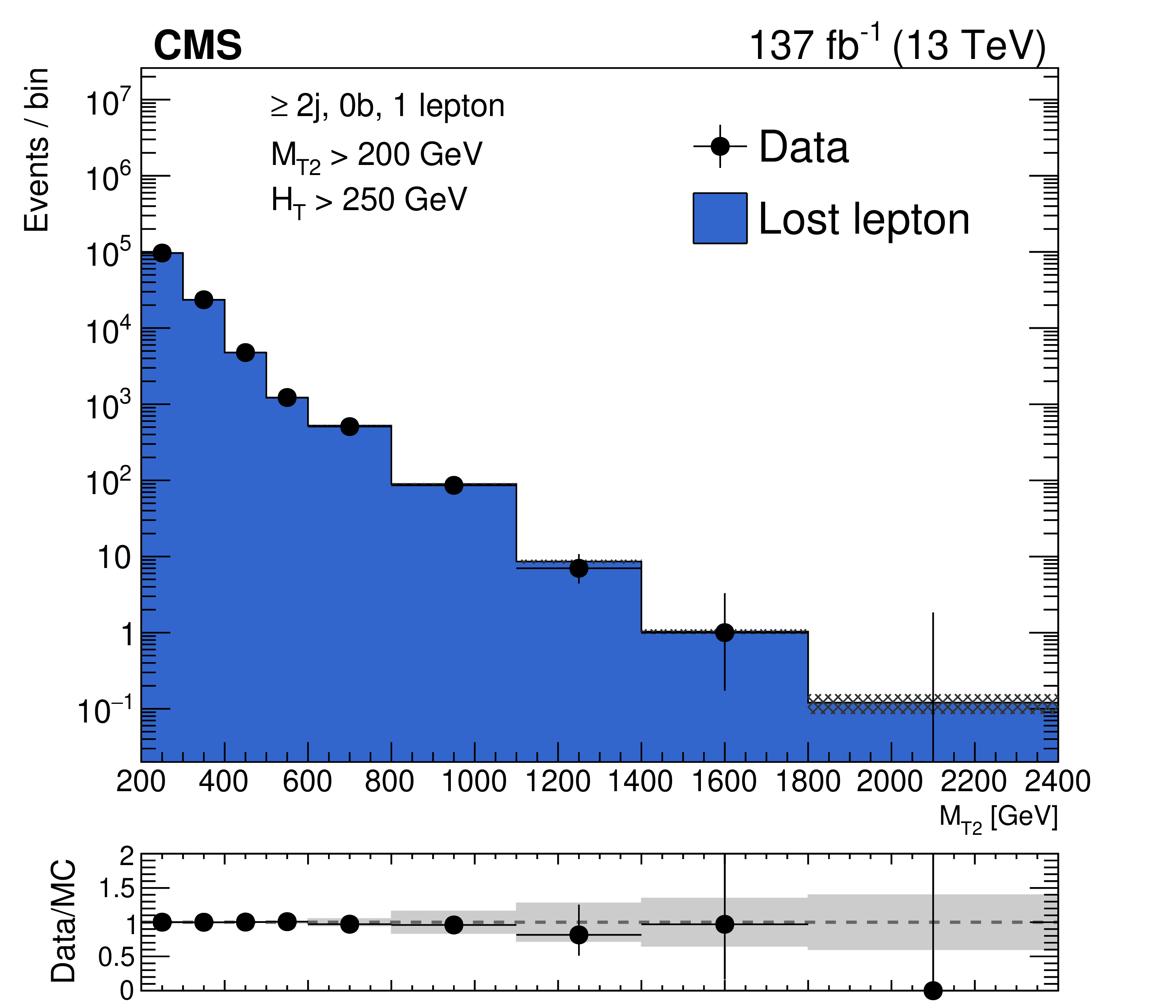
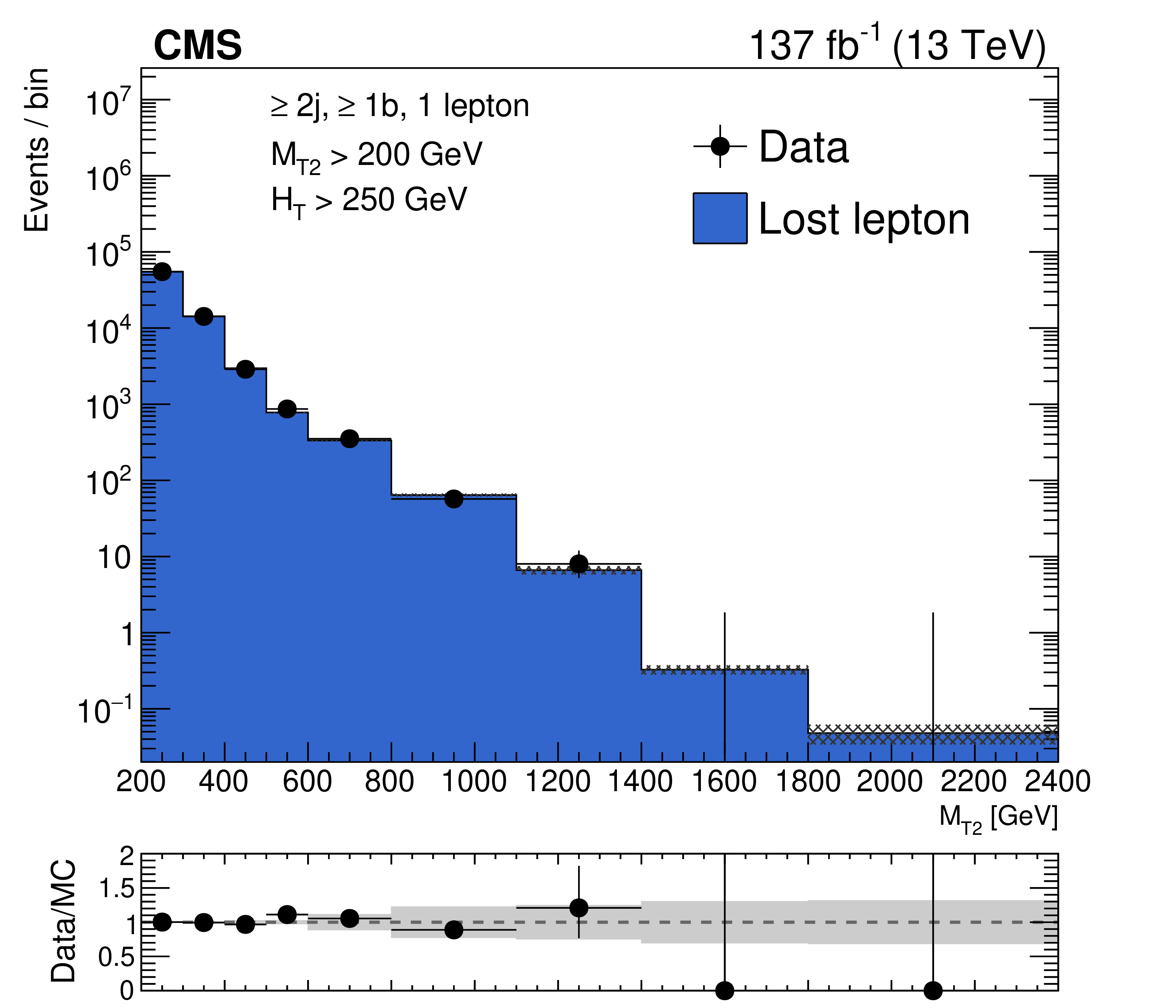
Distributions of the ${M_{\mathrm {T2}}}$ variable in data and simulation for the single-lepton control region, after normalizing the simulation to data in bins of ${H_{\mathrm {T}}}$, ${N_{\mathrm {j}}}$, and ${N_{\mathrm{b}}}$, for events with no b-tagged jets (left), and events with at least one b-tagged jet (right). The hatched bands on the top panels show the MC statistical uncertainty, while the solid gray bands in the ratio plots show the systematic uncertainty in the ${M_{\mathrm {T2}}}$ shape. The bins have different widths, denoted by the horizontal bars. |
png pdf |
Figure 1-a:
Distribution of the ${M_{\mathrm {T2}}}$ variable in data and simulation for the single-lepton control region, after normalizing the simulation to data in bins of ${H_{\mathrm {T}}}$, ${N_{\mathrm {j}}}$, and ${N_{\mathrm{b}}}$, for events with no b-tagged jets. The hatched bands on the top panel shows the MC statistical uncertainty, while the solid gray bands in the ratio plot shows the systematic uncertainty in the ${M_{\mathrm {T2}}}$ shape. The bins have different widths, denoted by the horizontal bars. |
png pdf |
Figure 1-b:
Distribution of the ${M_{\mathrm {T2}}}$ variable in data and simulation for the single-lepton control region, after normalizing the simulation to data in bins of ${H_{\mathrm {T}}}$, ${N_{\mathrm {j}}}$, and ${N_{\mathrm{b}}}$, for events with at least one b-tagged jet. The hatched bands on the top panel shows the MC statistical uncertainty, while the solid gray bands in the ratio plot shows the systematic uncertainty in the ${M_{\mathrm {T2}}}$ shape. The bins have different widths, denoted by the horizontal bars. |
png pdf |
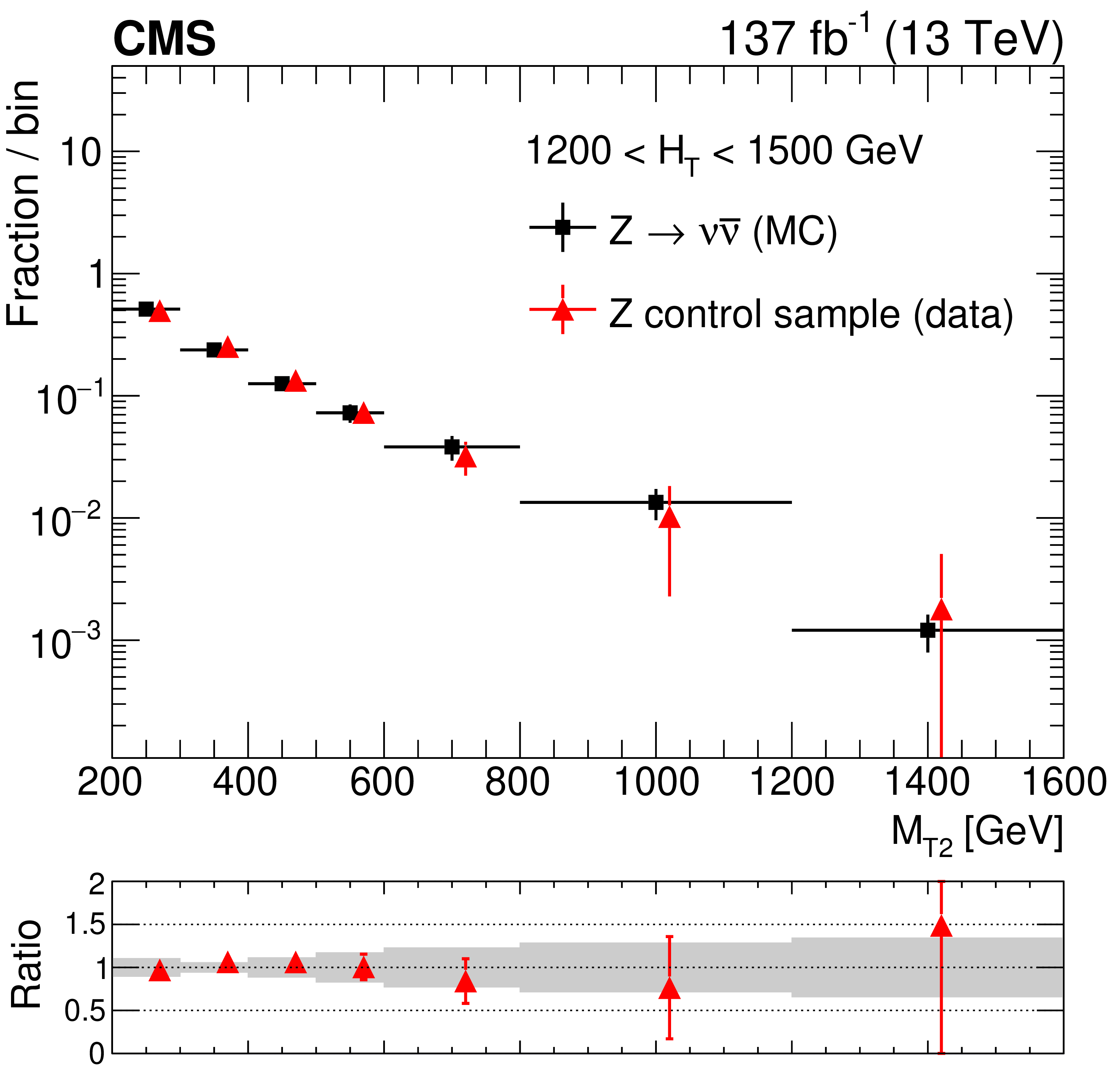
Figure 2:
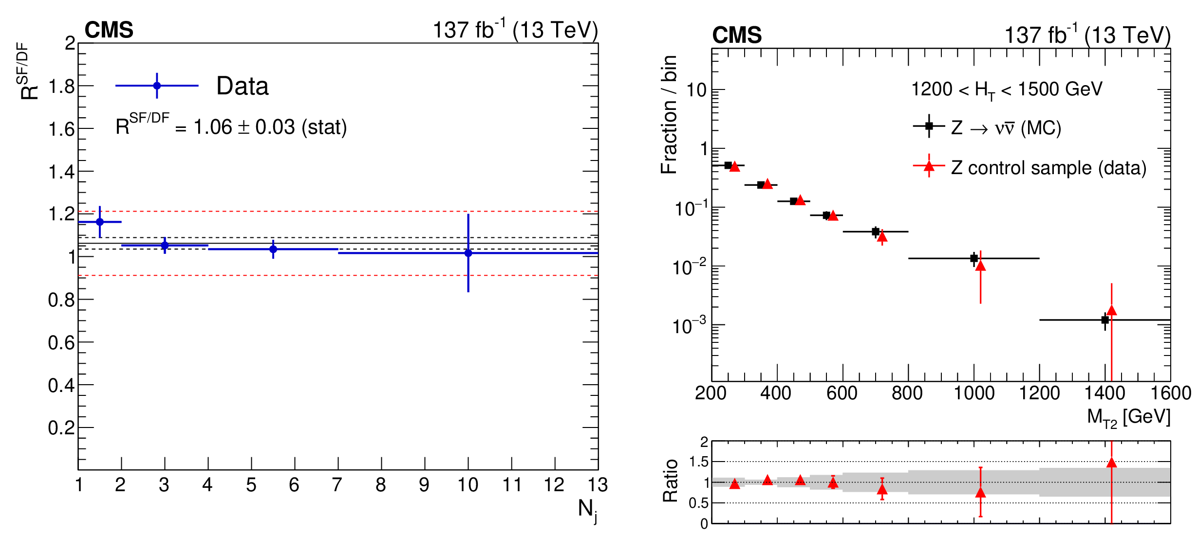
(Left) Ratio $R^{\mathrm {SF}/\mathrm {DF}}$ in data as a function of ${N_{\mathrm {j}}}$. The solid black line enclosed by the red dashed lines corresponds to a value of 1.06 $\pm$ 0.15 that is observed to be stable with respect to event kinematic variables, while the two dashed black lines denote the statistical uncertainty in the $R^{\mathrm {SF}/\mathrm {DF}}$ value. (Right) The shape of the ${M_{\mathrm {T2}}}$ distribution in $\mathrm{Z} \to \nu \bar{\nu} $ simulation compared to the one obtained from the $\mathrm{Z} \to \ell ^{+}\ell ^{-}$ data control sample, in a region with 1200 $ < {H_{\mathrm {T}}} < $ 1500 GeV and $ {N_{\mathrm {j}}} \geq $ 2, inclusive in ${N_{\mathrm{b}}}$. The solid gray band on the ratio plot shows the systematic uncertainty in the ${M_{\mathrm {T2}}}$ shape. The bins have different widths, denoted by the horizontal bars. |
png pdf |
Figure 2-a:
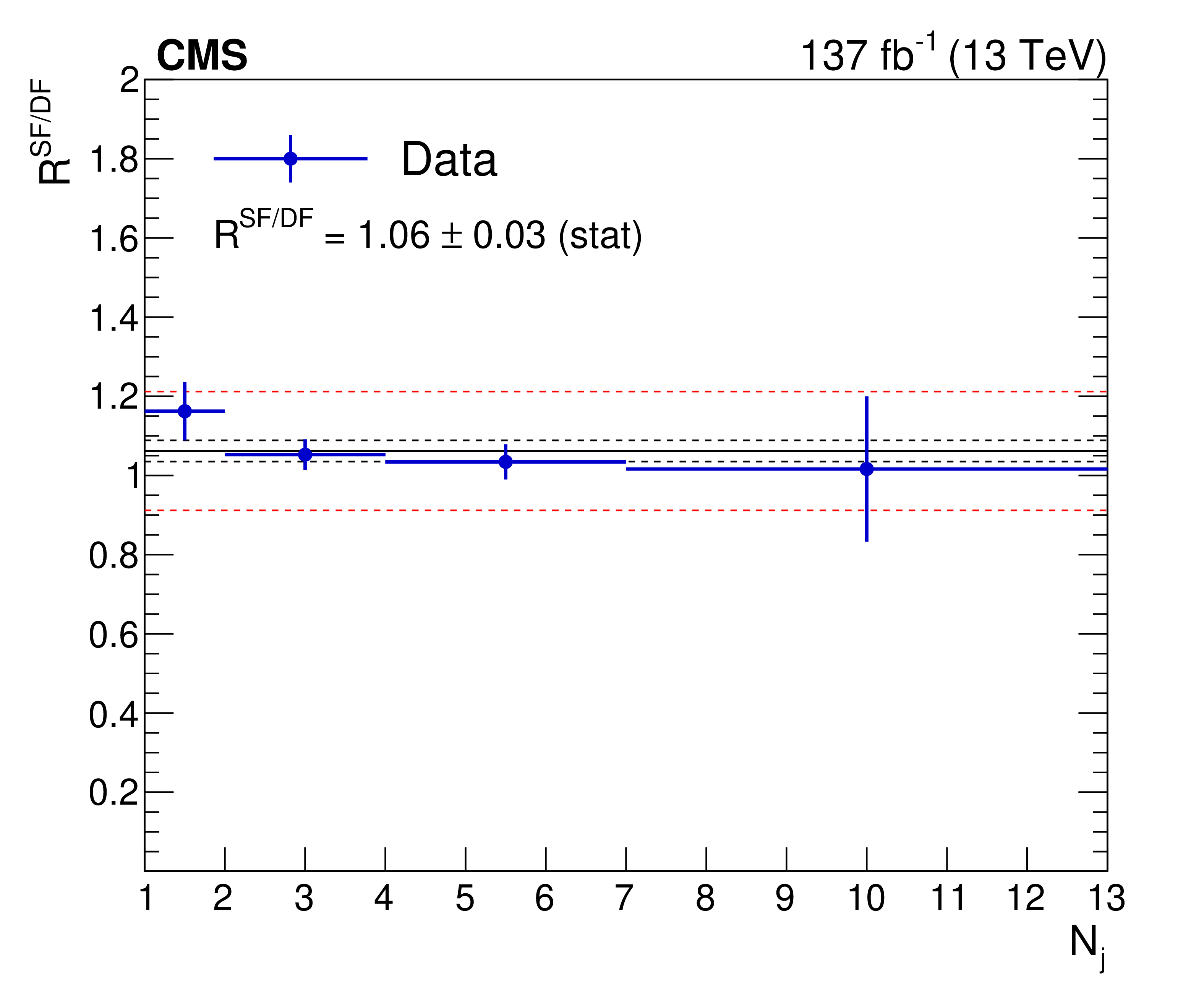
Ratio $R^{\mathrm {SF}/\mathrm {DF}}$ in data as a function of ${N_{\mathrm {j}}}$. The solid black line enclosed by the red dashed lines corresponds to a value of 1.06 $\pm$ 0.15 that is observed to be stable with respect to event kinematic variables, while the two dashed black lines denote the statistical uncertainty in the $R^{\mathrm {SF}/\mathrm {DF}}$ value. |
png pdf |
Figure 2-b:
The shape of the ${M_{\mathrm {T2}}}$ distribution in $\mathrm{Z} \to \nu \bar{\nu} $ simulation compared to the one obtained from the $\mathrm{Z} \to \ell ^{+}\ell ^{-}$ data control sample, in a region with 1200 $ < {H_{\mathrm {T}}} < $ 1500 GeV and $ {N_{\mathrm {j}}} \geq $ 2, inclusive in ${N_{\mathrm{b}}}$. The solid gray band on the ratio plot shows the systematic uncertainty in the ${M_{\mathrm {T2}}}$ shape. The bins have different widths, denoted by the horizontal bars. |
png pdf |
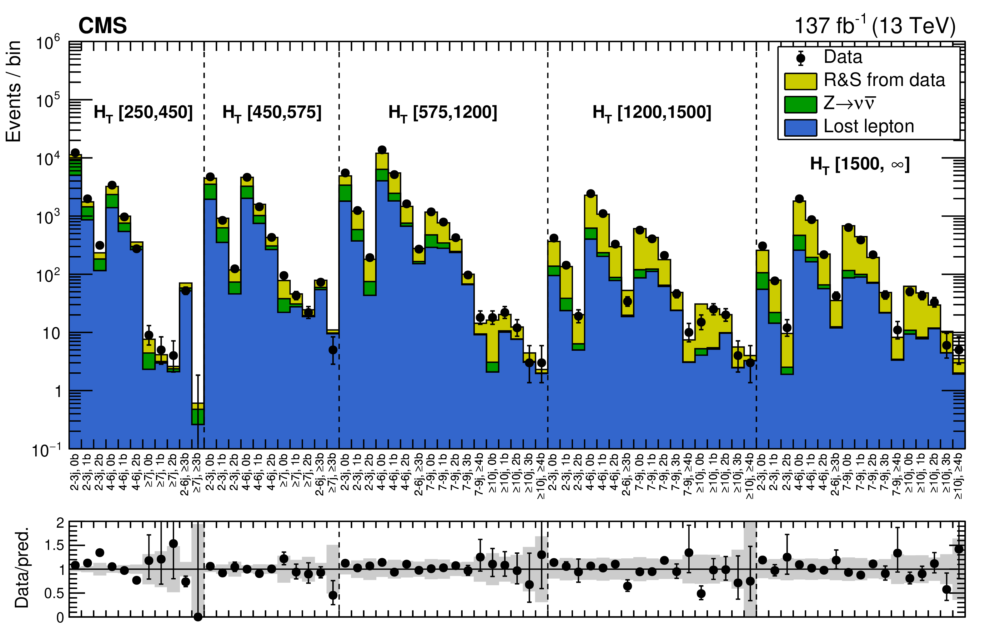
Figure 3:
Validation of the R&S multijet background prediction in control regions in data selected with $ {\Delta \phi _{\text {min}}} < $ 0.3. Electroweak backgrounds (LL and $\mathrm{Z} \to \nu \bar{\nu} $) are estimated from data. In regions where the amount of data is insufficient to estimate the electroweak backgrounds, the corresponding yields are taken directly from simulation. The bins on the horizontal axis correspond to the (${H_{\mathrm {T}}}$, ${N_{\mathrm {j}}}$, ${N_{\mathrm{b}}}$) topological regions. The gray band on the ratio plot represents the total uncertainty in the prediction. |
png pdf |
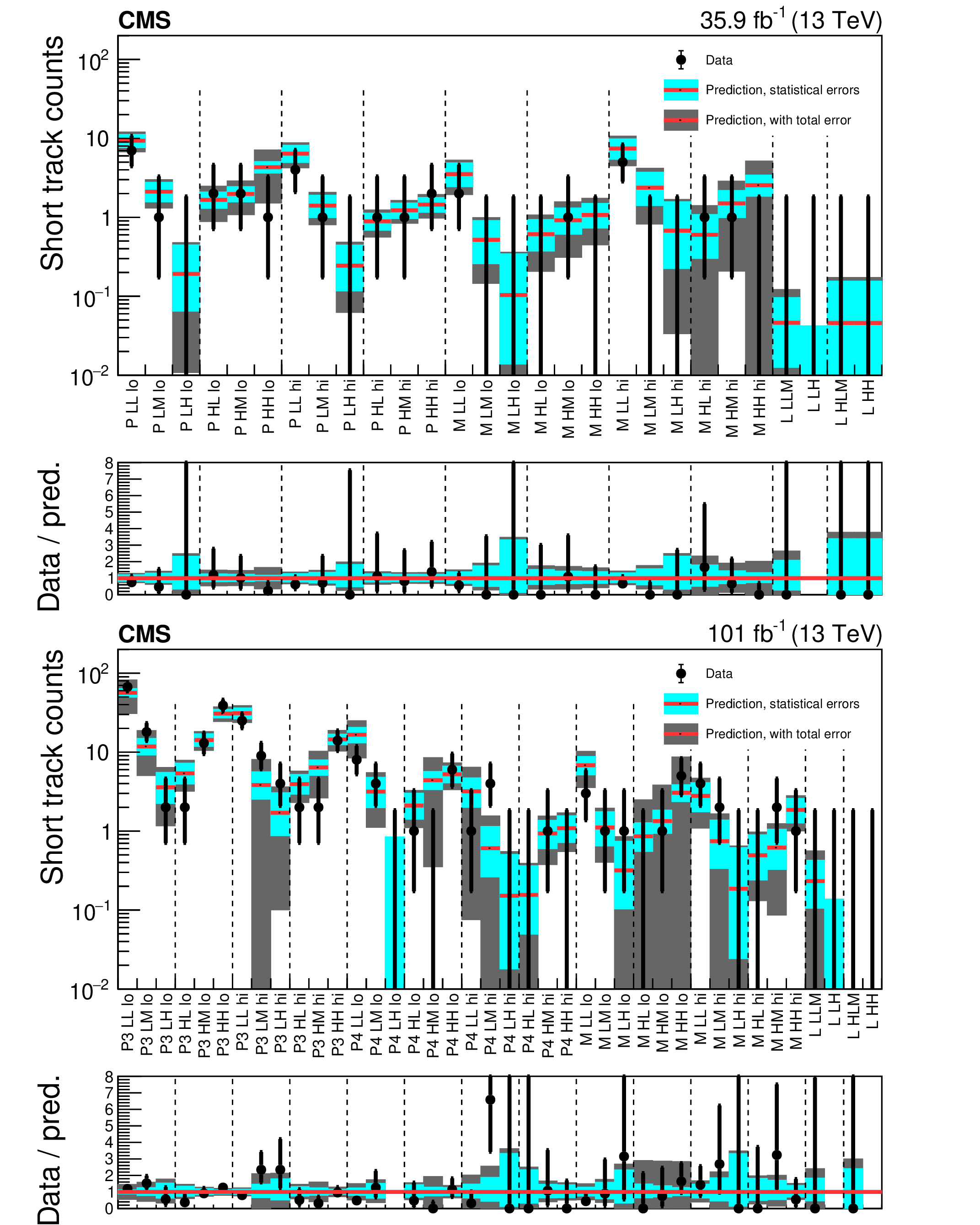
Figure 4:
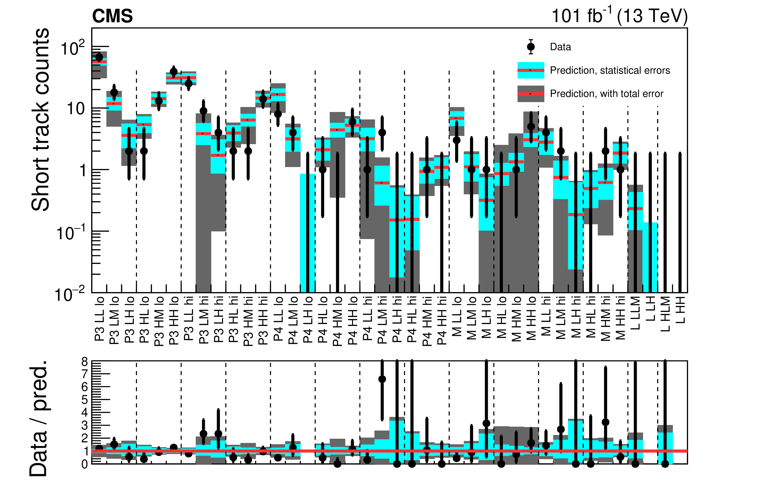
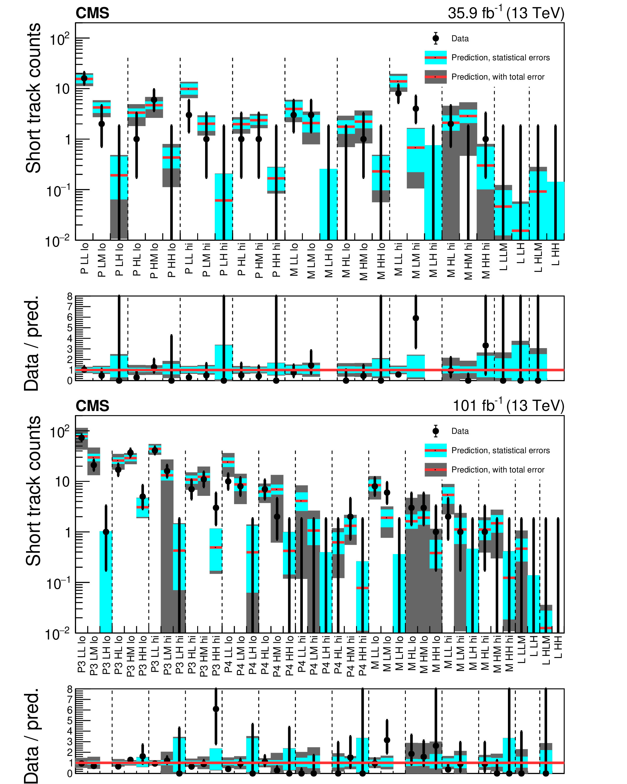
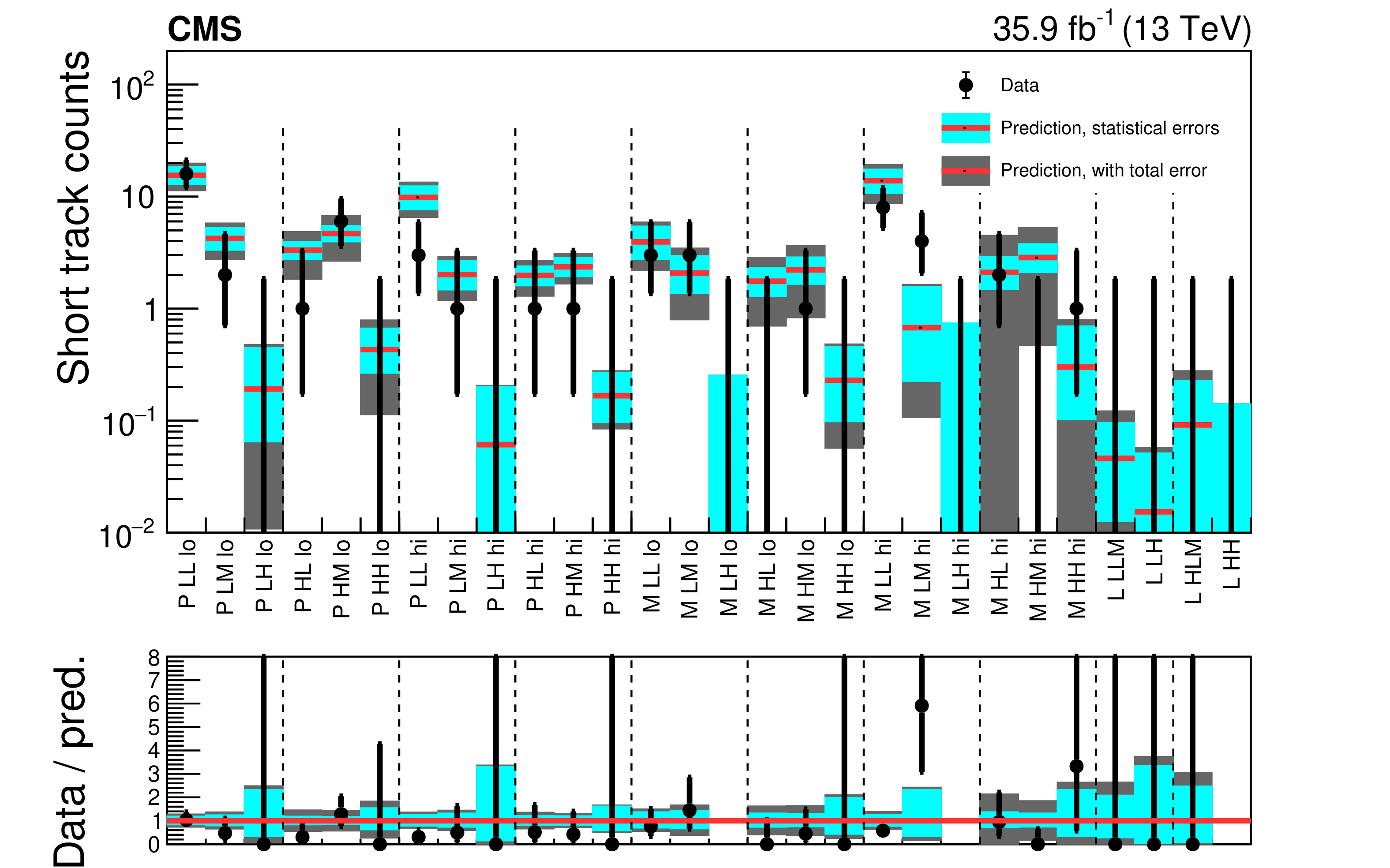
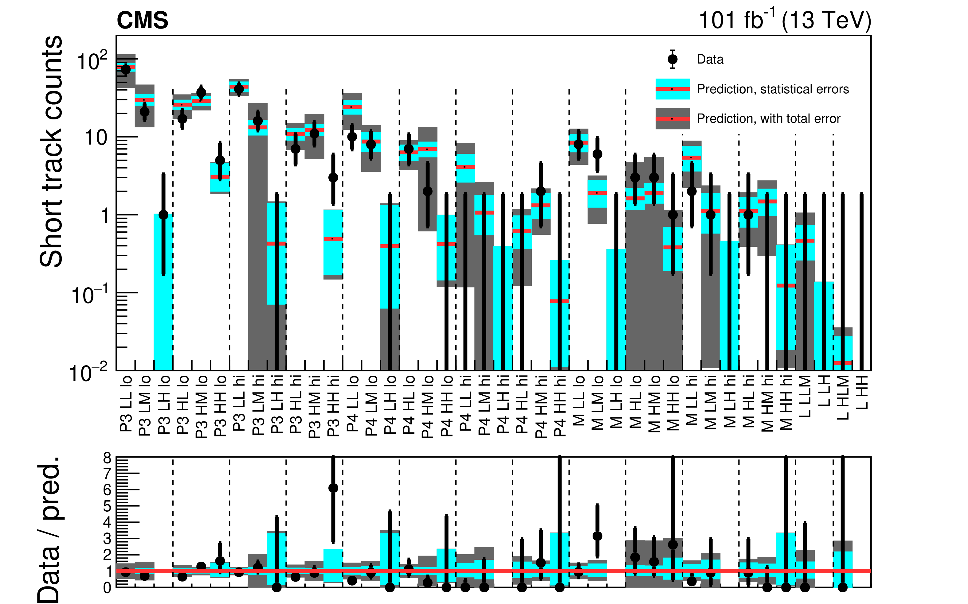
Validation of the background prediction method in (upper) 2016 and (lower) 2017-2018 data with 100 $ < {M_{\mathrm {T2}}} < $ 200 GeV, for the disappearing tracks search. The red histograms represent the predicted backgrounds, while the black markers are the observed data counts. The cyan bands represent the statistical uncertainty in the prediction. The gray bands represent the total uncertainty in the prediction. The labels on the $x$ axes are explained in Tables 24-25 of Appendix B2. Regions whose predictions use the same measurement of ${f_{\text {short}}}$ are grouped by the vertical dashed lines. Bins with no entry in the ratio have zero predicted background. |
png pdf |
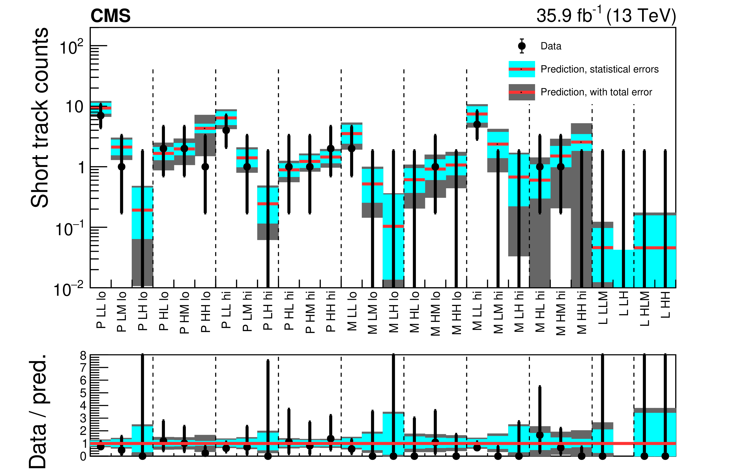
Figure 4-a:
Validation of the background prediction method in 2016 data with 100 $ < {M_{\mathrm {T2}}} < $ 200 GeV, for the disappearing tracks search. The red histograms represent the predicted backgrounds, while the black markers are the observed data counts. The cyan bands represent the statistical uncertainty in the prediction. The gray bands represent the total uncertainty in the prediction. The labels on the $x$ axes are explained in Tables 24-25 of Appendix B2. Regions whose predictions use the same measurement of ${f_{\text {short}}}$ are grouped by the vertical dashed lines. Bins with no entry in the ratio have zero predicted background. |
png pdf |
Figure 4-b:
Validation of the background prediction method in 2017-2018 data with 100 $ < {M_{\mathrm {T2}}} < $ 200 GeV, for the disappearing tracks search. The red histograms represent the predicted backgrounds, while the black markers are the observed data counts. The cyan bands represent the statistical uncertainty in the prediction. The gray bands represent the total uncertainty in the prediction. The labels on the $x$ axes are explained in Tables 24-25 of Appendix B2. Regions whose predictions use the same measurement of ${f_{\text {short}}}$ are grouped by the vertical dashed lines. Bins with no entry in the ratio have zero predicted background. |
png pdf |
Figure 5:
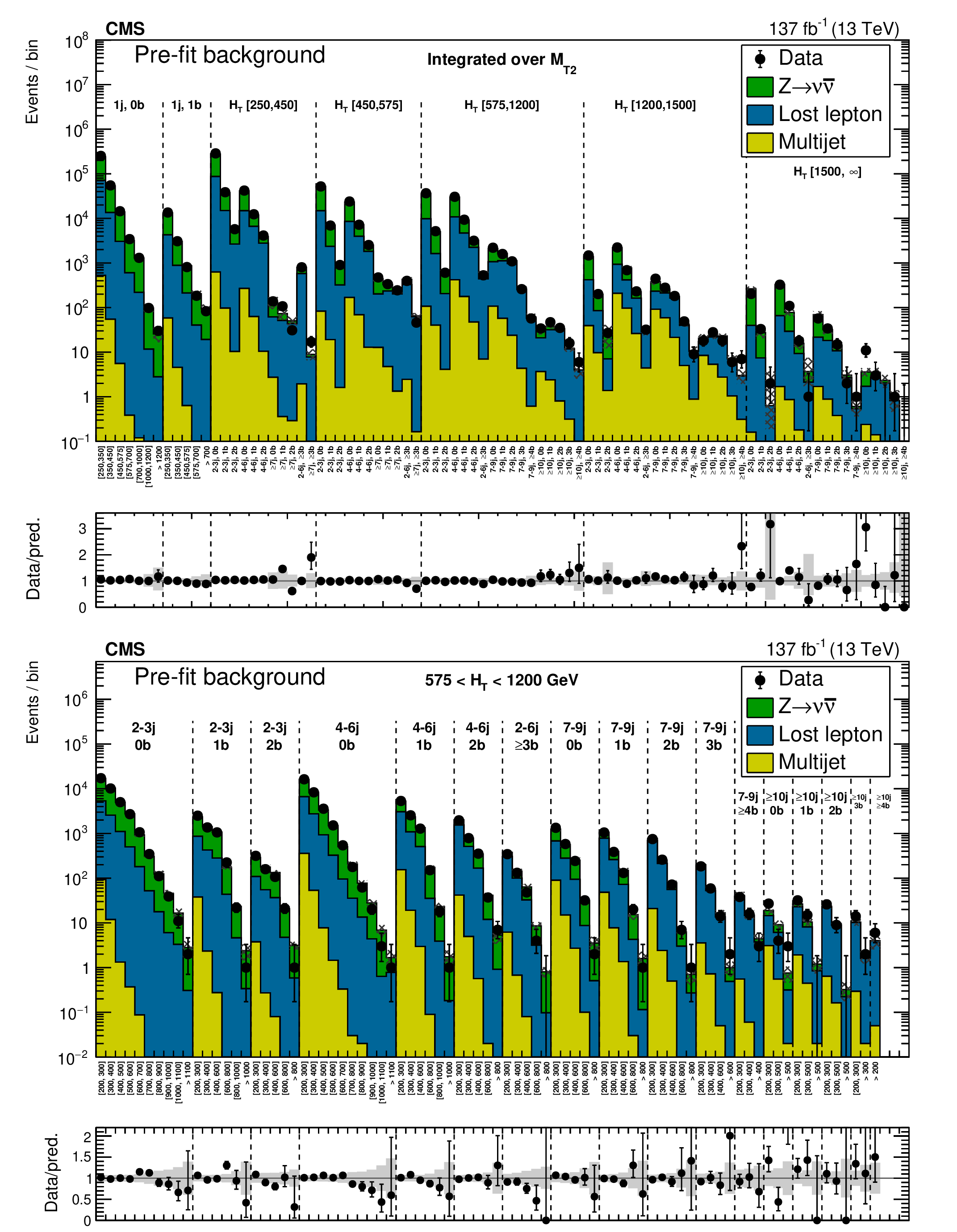
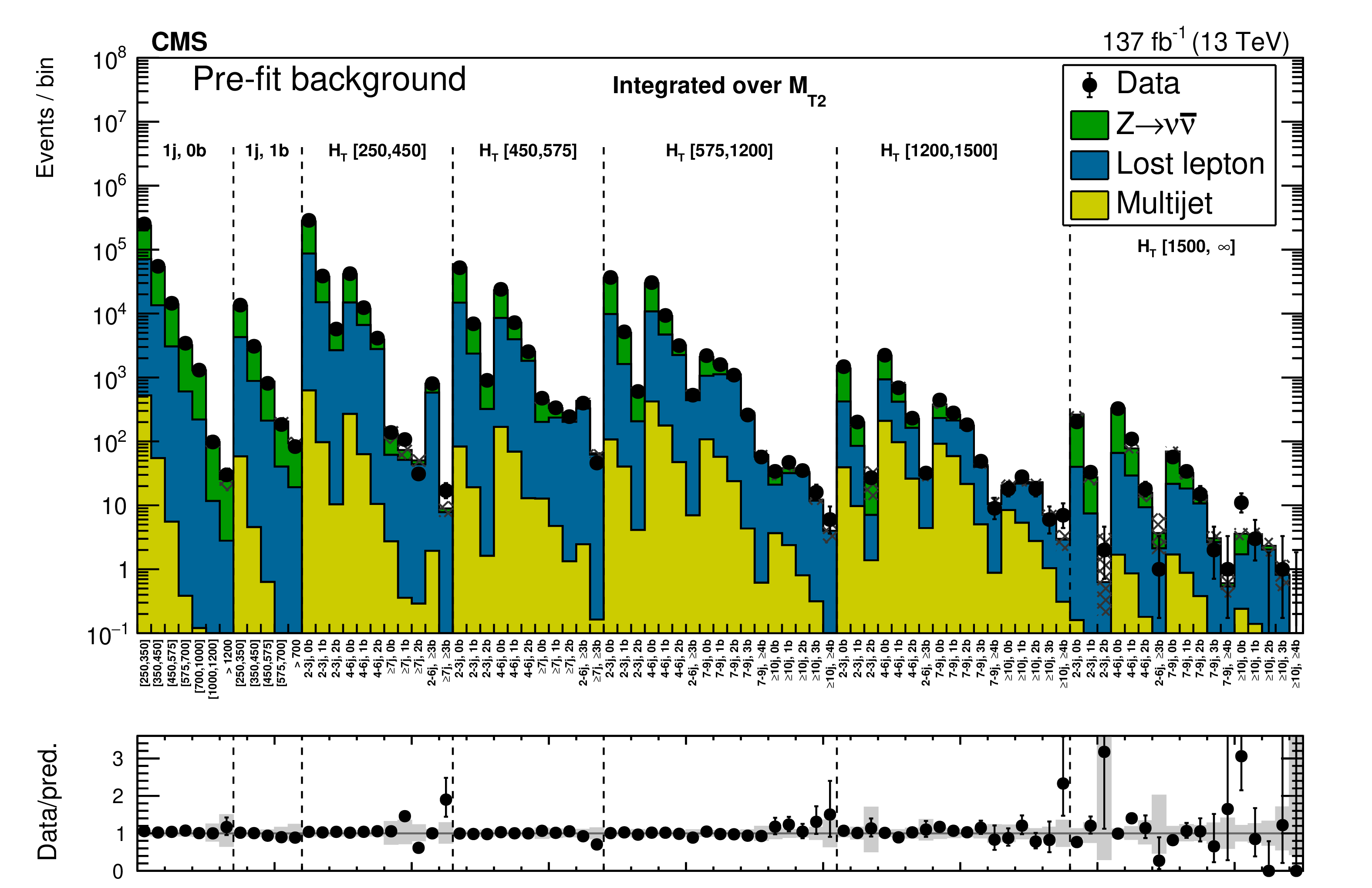
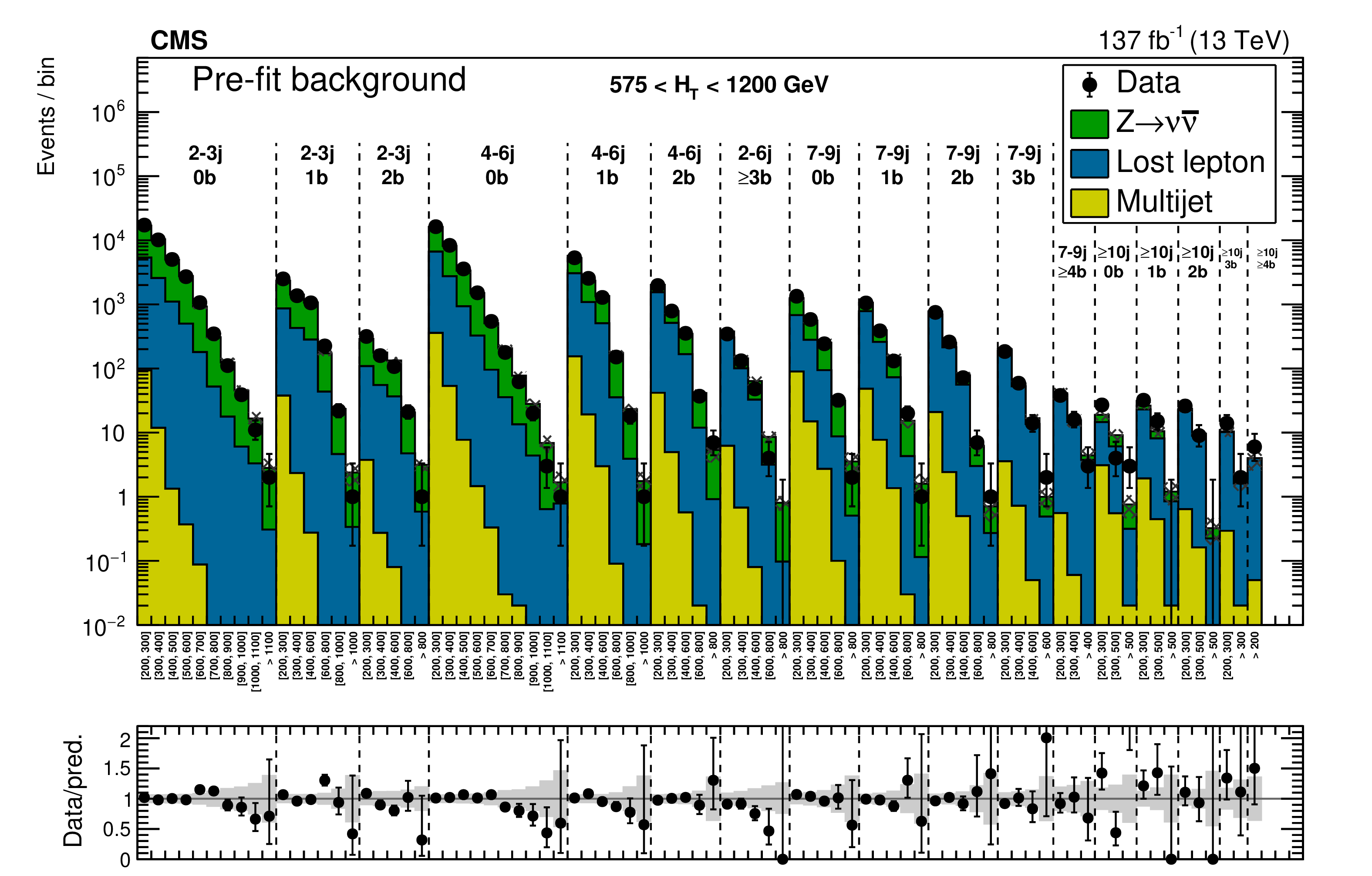
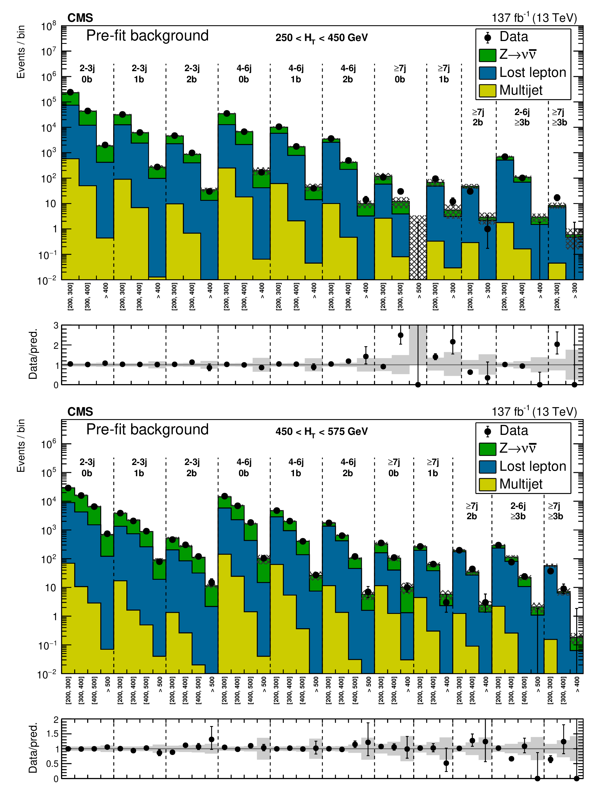
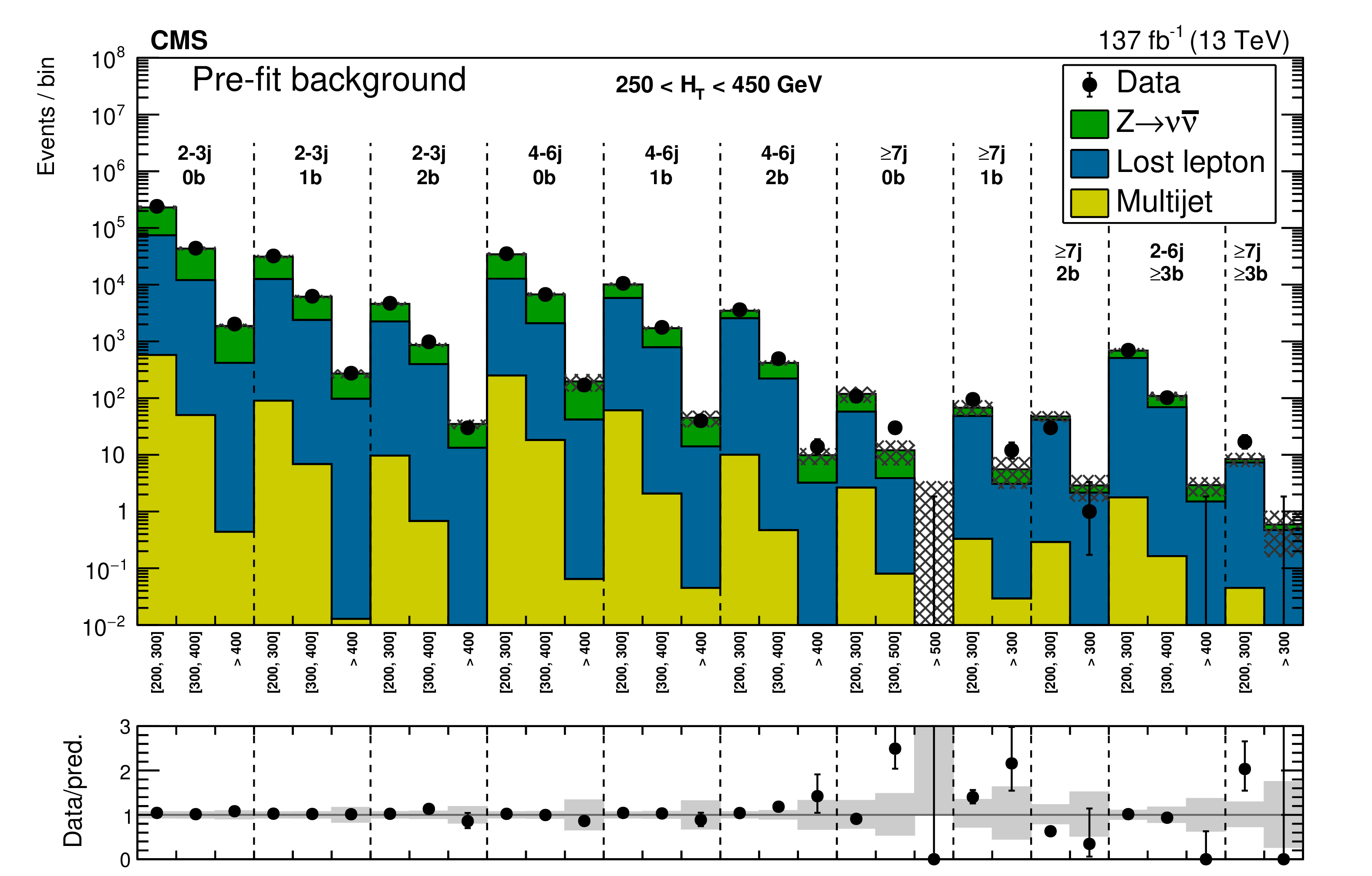
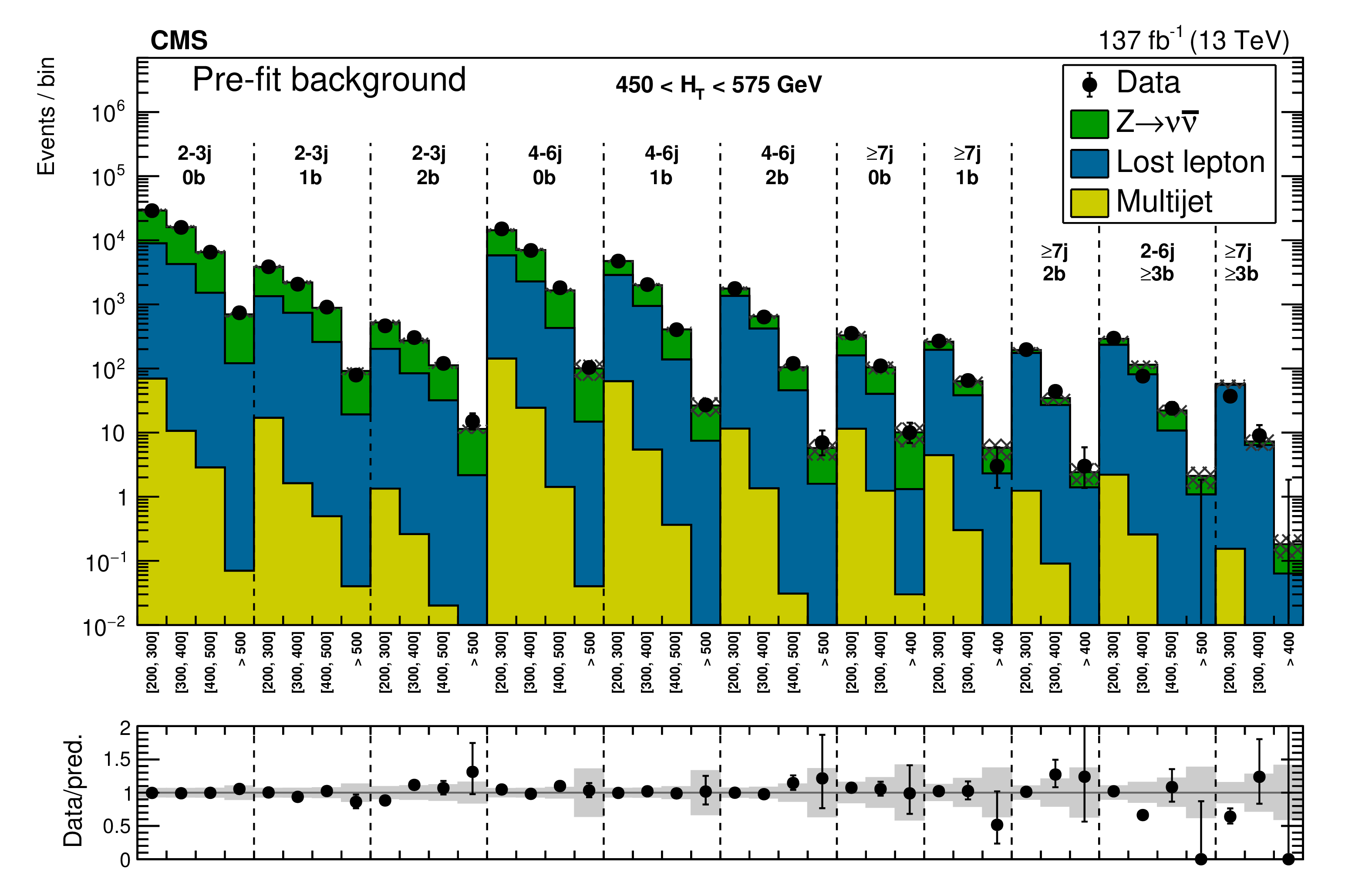
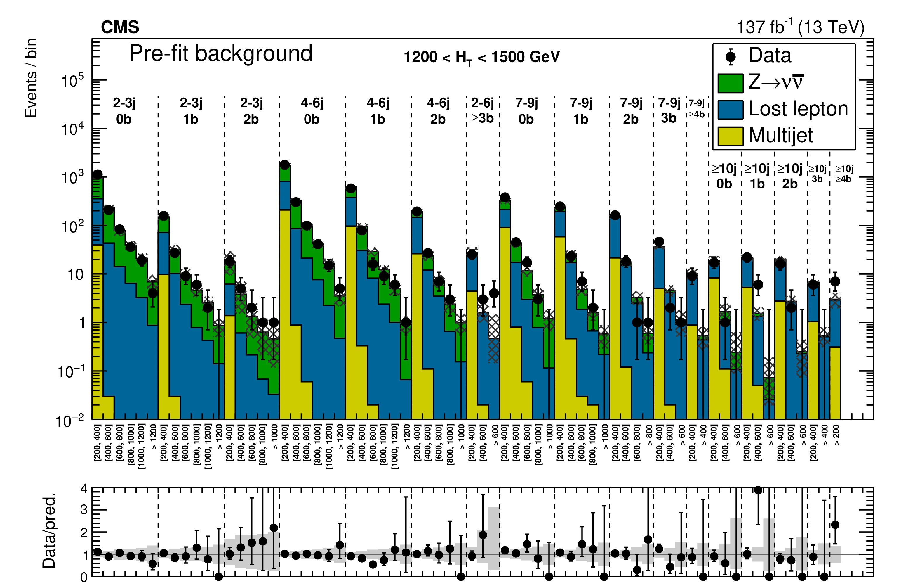
(Upper) Comparison of the estimated (pre-fit) background and observed data events in each topological region. The hatched bands represent the full uncertainty in the background estimate. The monojet regions ($ {N_{\mathrm {j}}} = $ 1) are identified by the labels "1j, 0b'' and "1j, 1b'', and are binned in jet ${p_{\mathrm {T}}}$. The multijet regions are shown for each ${H_{\mathrm {T}}}$ region separately, and are labeled accordingly. The notations j, b are short for ${N_{\mathrm {j}}}$, ${N_{\mathrm{b}}}$. (Lower) Same for individual ${M_{\mathrm {T2}}}$ search bins in the medium-${H_{\mathrm {T}}}$ region. On the $x$ axis, the ${M_{\mathrm {T2}}}$ binning is shown in units of GeV. |
png pdf |
Figure 5-a:
Comparison of the estimated (pre-fit) background and observed data events in each topological region. The hatched bands represent the full uncertainty in the background estimate. The monojet regions ($ {N_{\mathrm {j}}} = $ 1) are identified by the labels "1j, 0b'' and "1j, 1b'', and are binned in jet ${p_{\mathrm {T}}}$. The multijet regions are shown for each ${H_{\mathrm {T}}}$ region separately, and are labeled accordingly. The notations j, b are short for ${N_{\mathrm {j}}}$, ${N_{\mathrm{b}}}$. |
png pdf |
Figure 5-b:
Same for individual ${M_{\mathrm {T2}}}$ search bins in the medium-${H_{\mathrm {T}}}$ region. On the $x$ axis, the ${M_{\mathrm {T2}}}$ binning is shown in units of GeV. |
png pdf |
Figure 6:
Comparison of the estimated (pre-fit) background and observed data events in (upper) each of the 2016 search regions, and in (lower) each of the 2017-2018 search regions, in the search for disappearing tracks. The red histogram represents the predicted background, while the black markers are the observed data counts. The cyan band represents the statistical uncertainty in the prediction. The gray band represents the total uncertainty. The labels on the $x$ axes are explained in Tables 24-25 of Appendix B2. Regions whose predictions use the same measurement of ${f_{\text {short}}}$ are grouped by the vertical dashed lines. Bins with no entry in the ratio have zero pre-fit predicted background. |
png pdf |
Figure 6-a:
Comparison of the estimated (pre-fit) background and observed data events in each of the 2016 search regions, in the search for disappearing tracks. The red histogram represents the predicted background, while the black markers are the observed data counts. The cyan band represents the statistical uncertainty in the prediction. The gray band represents the total uncertainty. The labels on the $x$ axes are explained in Tables 24-25 of Appendix B2. Regions whose predictions use the same measurement of ${f_{\text {short}}}$ are grouped by the vertical dashed lines. Bins with no entry in the ratio have zero pre-fit predicted background. |
png pdf |
Figure 6-b:
Comparison of the estimated (pre-fit) background and observed data events in each of the 2017-2018 search regions, in the search for disappearing tracks. The red histogram represents the predicted background, while the black markers are the observed data counts. The cyan band represents the statistical uncertainty in the prediction. The gray band represents the total uncertainty. The labels on the $x$ axes are explained in Tables 24-25 of Appendix B2. Regions whose predictions use the same measurement of ${f_{\text {short}}}$ are grouped by the vertical dashed lines. Bins with no entry in the ratio have zero pre-fit predicted background. |
png pdf |
Figure 7:
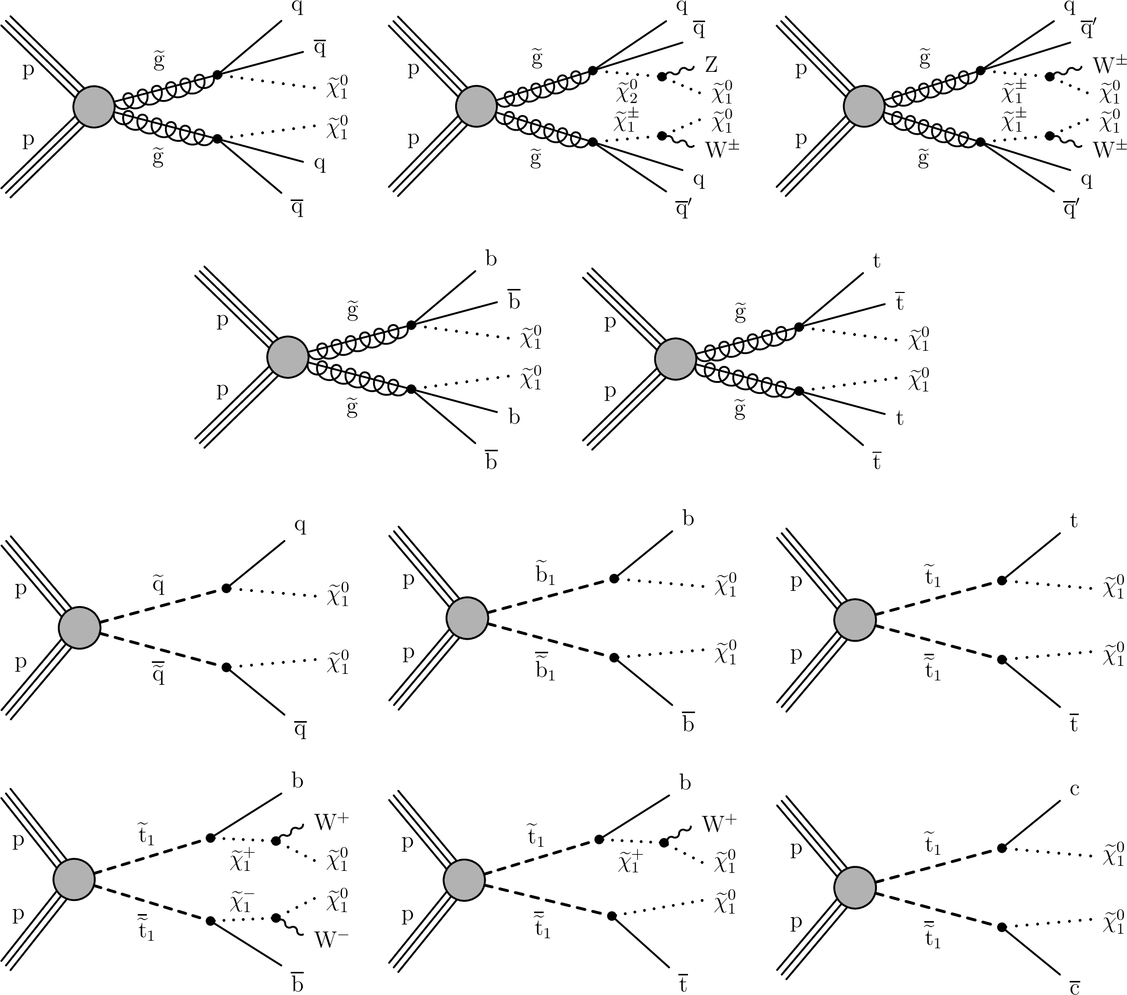
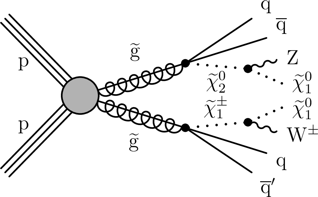
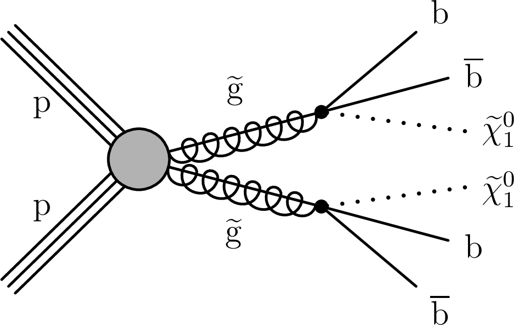
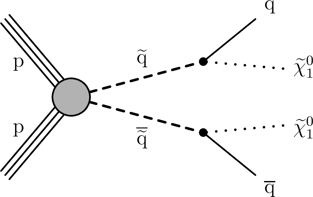
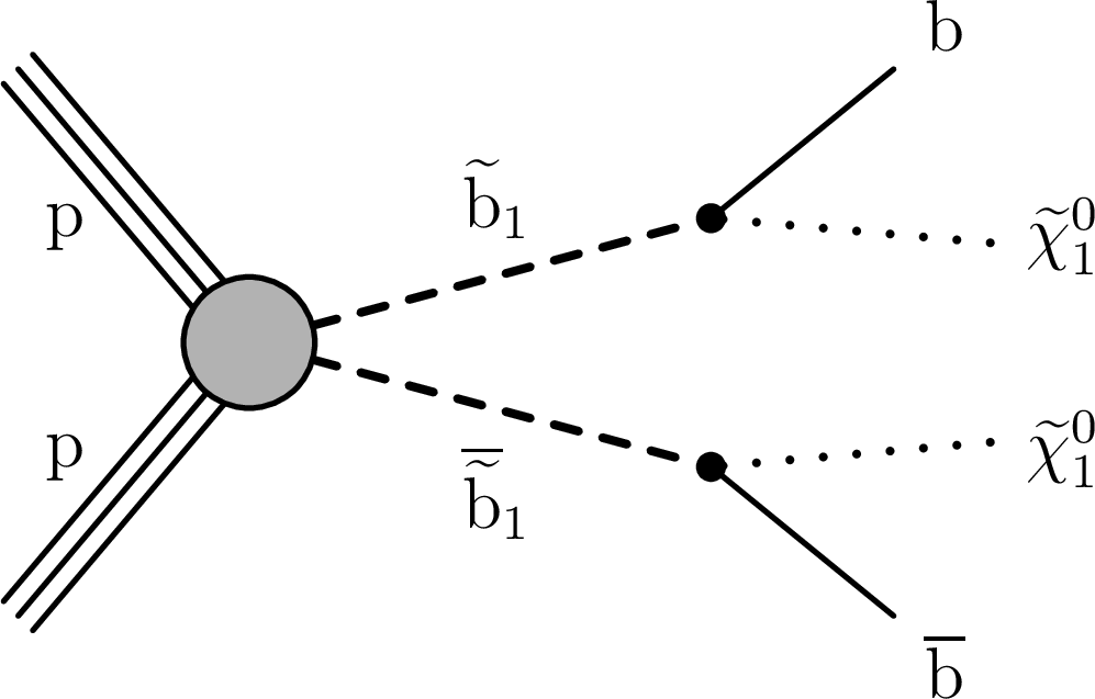
(Upper) Diagrams for three scenarios of direct gluino pair production where each gluino undergoes a three-body decay to light-flavor (u, d, s, c) quarks, with different decay modes. For mixed-decay scenarios, we assume equal branching fraction for each decay mode. (Upper middle) Diagrams for the direct gluino pair production where gluinos decay to bottom and top quarks. (Lower middle) Diagrams for the direct pair production of light-flavor, bottom, and top squark pairs. (Lower) Diagrams for three alternate scenarios of direct top squark pair production with different decay modes. For mixed-decay scenarios, we assume equal branching fraction for each decay mode. |

png pdf |
Figure 7-a:
Diagram for one of the scenarios of direct gluino pair production. |
png pdf |
Figure 7-b:
Diagram for one of the scenarios of direct gluino pair production. We assume equal branching fraction for each decay mode. |

png pdf |
Figure 7-c:
Diagram for one of the scenarios of direct gluino pair production. |
png pdf |
Figure 7-d:
Diagram for the direct gluino pair production where gluinos decay to bottom quarks. |

png pdf |
Figure 7-e:
Diagrams for the direct gluino pair production where gluinos decay to top quarks. |
png pdf |
Figure 7-f:
Diagram for the direct pair production of light-flavor squark pairs. |
png pdf |
Figure 7-g:
Diagram for the direct pair production of bottom squark pairs. |
png pdf |
Figure 7-h:
Diagram for the direct pair production of top squark pairs. |
png pdf |
Figure 7-i:
Diagram for an alternate scenario of direct top squark pair production. |
png pdf |
Figure 7-j:
Diagram for an alternate scenario of direct top squark pair production. We assume equal branching fraction for each decay mode. |

png pdf |
Figure 7-k:
Diagram for an alternate scenario of direct top squark pair production. |

png pdf |
Figure 8:
Diagram for the mono-$\phi $ model, where a colored scalar $\phi $ is resonantly produced, and it decays to an invisible massive Dirac fermion $\psi $ and an SM quark. |
png pdf |
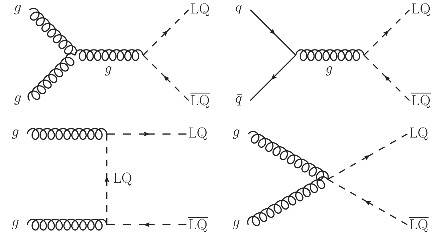
Figure 9:
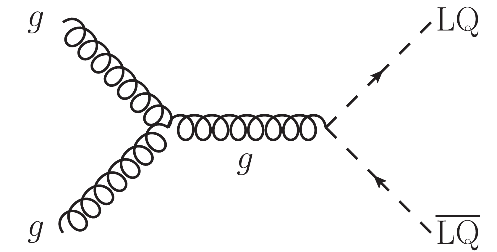
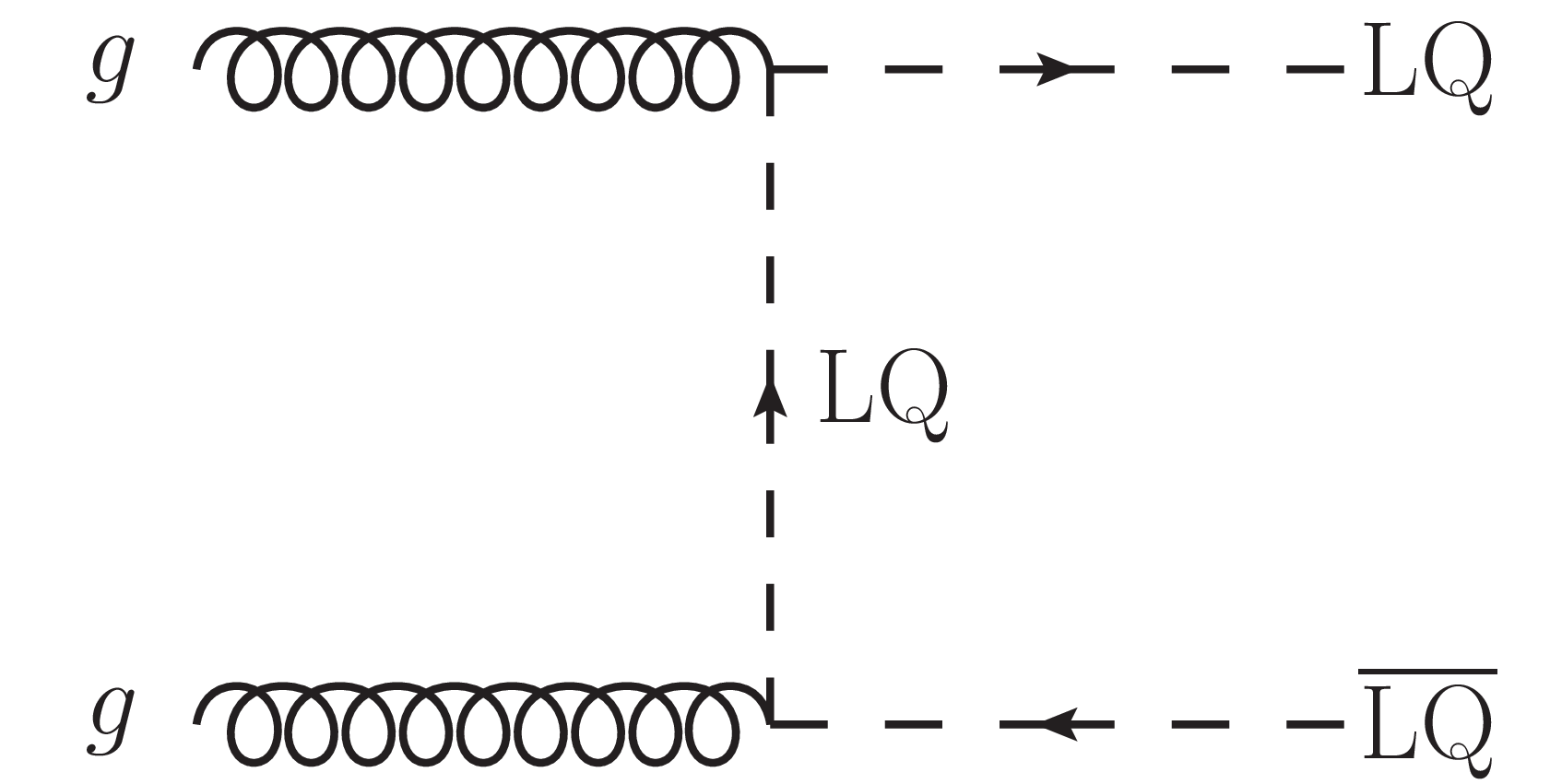
Diagrams for LQ pair production. |
png pdf |
Figure 9-a:
Diagram for LQ pair production. |
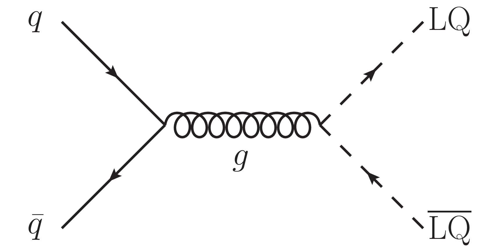
png pdf |
Figure 9-b:
Diagram for LQ pair production. |
png pdf |
Figure 9-c:
Diagram for LQ pair production. |

png pdf |
Figure 9-d:
Diagram for LQ pair production. |
png pdf |
Figure 10:
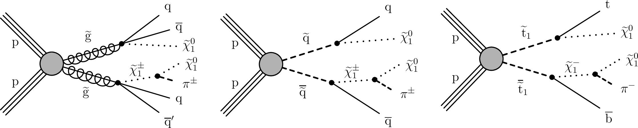
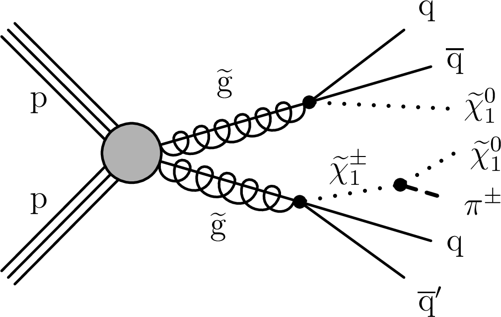
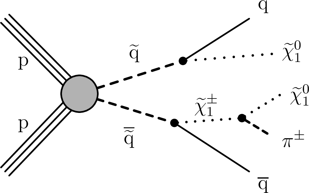
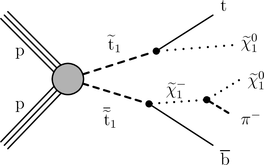
Diagrams for direct (left) gluino, (middle) light-flavor (u, d, s, c) squark, and (right) top squark pair production, where the directly produced gluinos and squarks can decay via a long-lived $\tilde{\chi}^{\pm}_1$. For gluinos, we assume a 1/3 decay branching fraction to each $\tilde{\chi}^0_1$, $\tilde{\chi}^{+}_1$, and $\tilde{\chi}^{-}_1$, and each gluino decays to light-flavor quarks. For squarks, we assume a 1/2 branching fraction for decays to $\tilde{\chi}^0_1$ and to the $\tilde{\chi}^{\pm}_1$ allowed by charge conservation. The mass of the $\tilde{\chi}^{\pm}_1$ is larger than the mass of the $\tilde{\chi}^0_1$ by hundreds of MeV. The $\tilde{\chi}^{\pm}_1$ decays to a $\tilde{\chi}^0_1$ via a pion, which is too soft to be detected. |
png pdf |
Figure 10-a:
Diagram for direct gluino pair production, where the directly produced gluinos decay via a long-lived $\tilde{\chi}^{\pm}_1$. We assume a 1/3 decay branching fraction to each $\tilde{\chi}^0_1$, $\tilde{\chi}^{+}_1$, and $\tilde{\chi}^{-}_1$, and each gluino decays to light-flavor quarks. The mass of the $\tilde{\chi}^{\pm}_1$ is larger than the mass of the $\tilde{\chi}^0_1$ by hundreds of MeV. The $\tilde{\chi}^{\pm}_1$ decays to a $\tilde{\chi}^0_1$ via a pion, which is too soft to be detected. |
png pdf |
Figure 10-b:
Diagram for direct light-flavor (u, d, s, c) squark pair production, where the directly produced squarks can decay via a long-lived $\tilde{\chi}^{\pm}_1$. We assume a 1/2 branching fraction for decays to $\tilde{\chi}^0_1$ and to the $\tilde{\chi}^{\pm}_1$ allowed by charge conservation. The mass of the $\tilde{\chi}^{\pm}_1$ is larger than the mass of the $\tilde{\chi}^0_1$ by hundreds of MeV. The $\tilde{\chi}^{\pm}_1$ decays to a $\tilde{\chi}^0_1$ via a pion, which is too soft to be detected. |
png pdf |
Figure 10-c:
Diagrams for direct top squark pair production, where the directly produced squarks can decay via a long-lived $\tilde{\chi}^{\pm}_1$. We assume a 1/2 branching fraction for decays to $\tilde{\chi}^0_1$ and to the $\tilde{\chi}^{\pm}_1$ allowed by charge conservation. The mass of the $\tilde{\chi}^{\pm}_1$ is larger than the mass of the $\tilde{\chi}^0_1$ by hundreds of MeV. The $\tilde{\chi}^{\pm}_1$ decays to a $\tilde{\chi}^0_1$ via a pion, which is too soft to be detected. |
png pdf |
Figure 11:
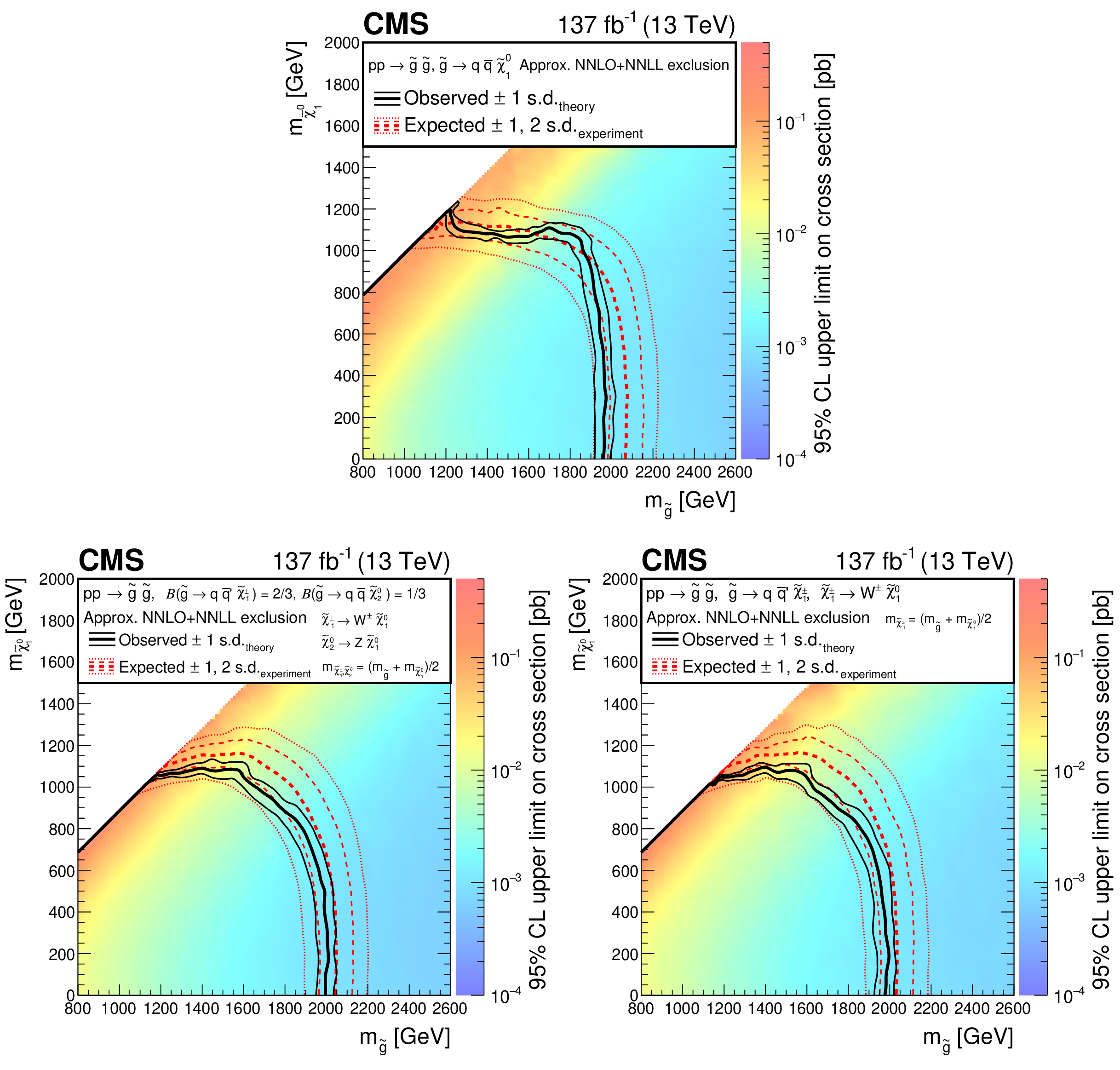
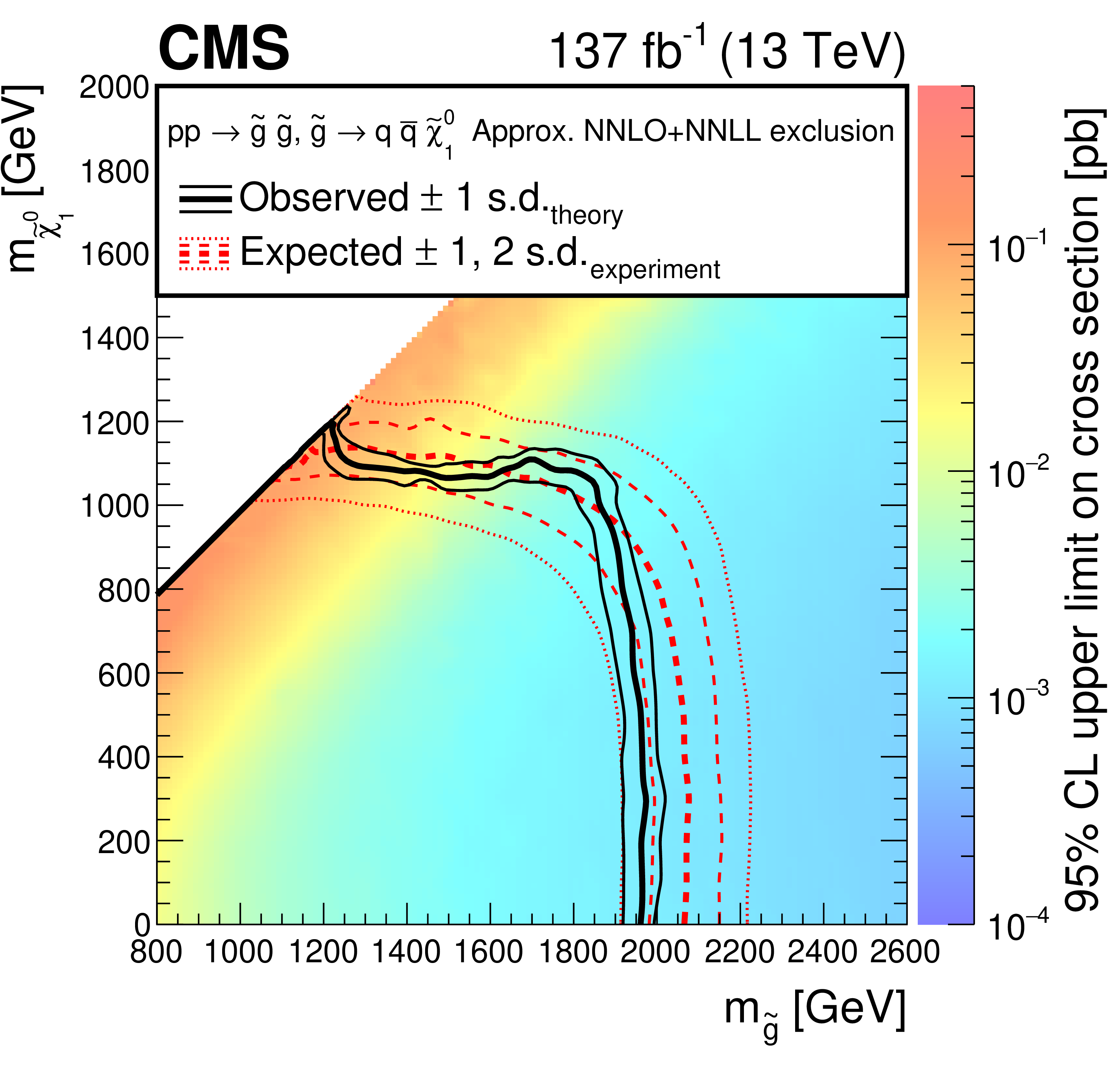
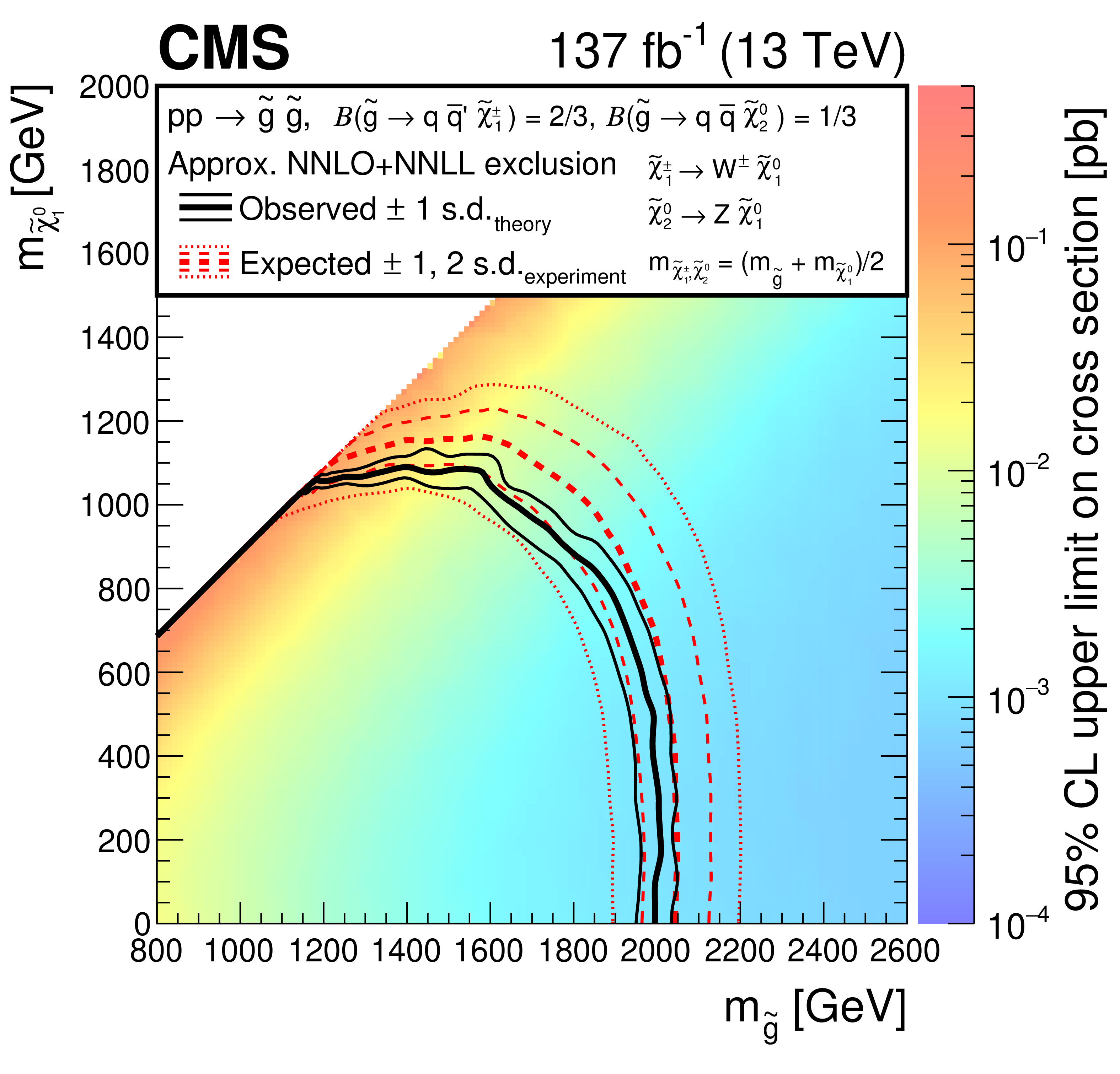
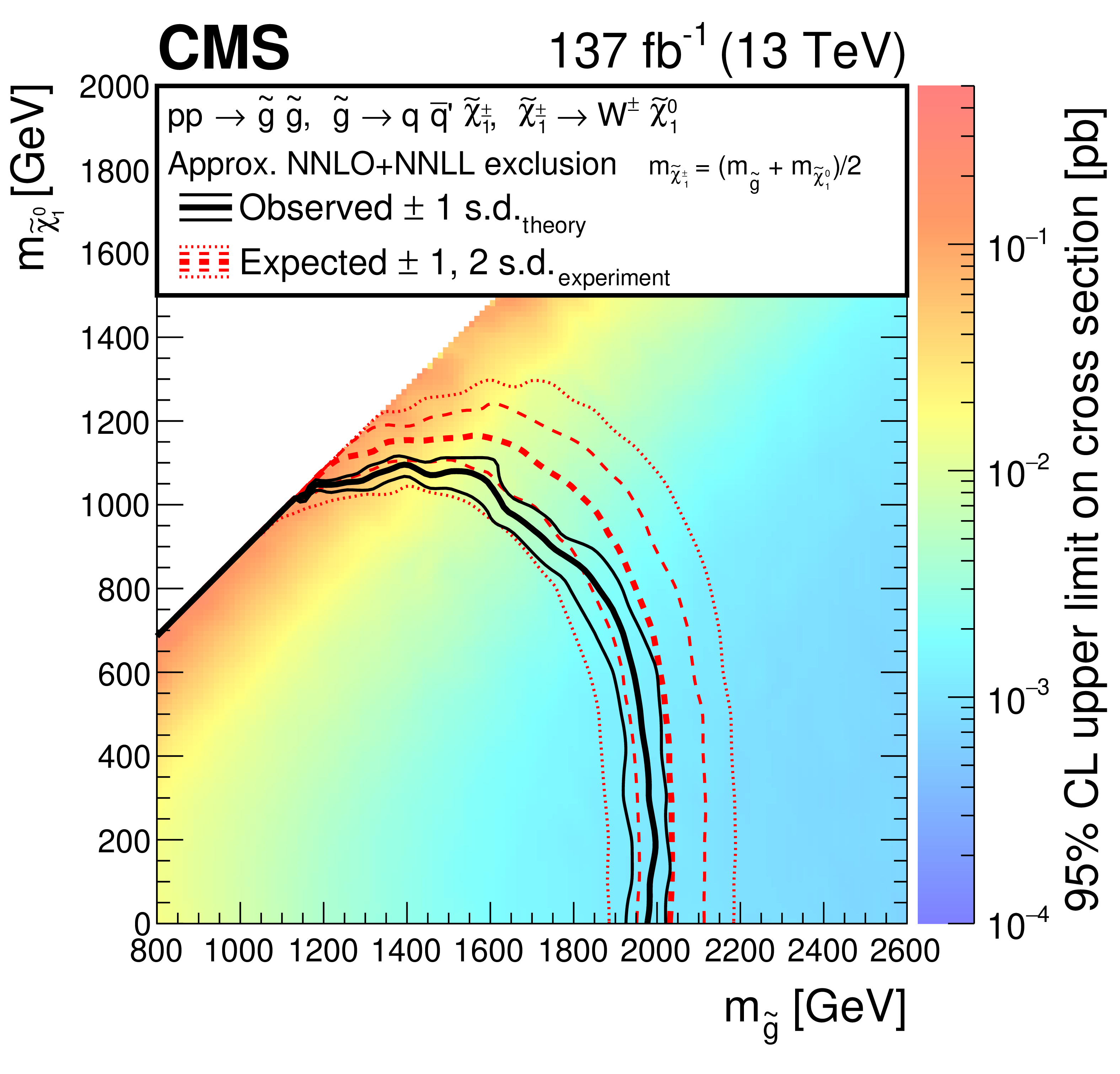
Exclusion limits at 95% CL for direct gluino pair production, where (upper) ${\mathrm{\tilde{g}}} \to {\mathrm{q} \mathrm{\bar{q}}} \tilde{\chi}^0_1 $, (lower left) ${\mathrm{\tilde{g}}} \to {\mathrm{q} \mathrm{\bar{q}}} \tilde{\chi}^{0}_{2} $ and $\tilde{\chi}^{0}_{2} \to \mathrm{Z} \tilde{\chi}^0_1 $, or ${\mathrm{\tilde{g}}} \to {{\mathrm{q} \mathrm{\bar{q}}} '} \tilde{\chi}^{\pm}_1 $ and $\tilde{\chi}^{\pm}_1 \to \mathrm{W^{\pm}} \tilde{\chi}^0_1 $, and (lower right) ${\mathrm{\tilde{g}}} \to {{\mathrm{q} \mathrm{\bar{q}}} '} \tilde{\chi}^{\pm}_1 $ and $\tilde{\chi}^{\pm}_1 \to \mathrm{W^{\pm}} \tilde{\chi}^0_1 $ (with $\mathrm{q} =$ u, d, s, or c). For the scenarios where the gluinos decay via an intermediate $\tilde{\chi}^{0}_{2}$ or $\tilde{\chi}^{\pm}_1$, $\tilde{\chi}^{0}_{2}$ and $\tilde{\chi}^{\pm}_1$ are assumed to be mass-degenerate, with $m_{\tilde{\chi}^{\pm}_1, \tilde{\chi}^{0}_{2}}=0.5(m_{{\mathrm{\tilde{g}}}}+m_{\tilde{\chi}^0_1})$. The area enclosed by the thick black curve represents the observed exclusion region, while the dashed red lines indicate the expected limits and their $\pm $1 and $\pm $2 standard deviation (s.d.) ranges. The thin black lines show the effect of the theoretical uncertainties in the signal cross section. Signal cross sections are calculated at approximately NNLO+NNLL order in ${\alpha _S}$ [136,137,138,139,140,141], assuming 1/3 branching fraction ($\mathcal {B}$) for each decay mode in the mixed-decay scenarios, or unity branching fraction for the indicated decay. |
png pdf root |
Figure 11-a:
Exclusion limits at 95% CL for direct gluino pair production, where ${\mathrm{\tilde{g}}} \to {\mathrm{q} \mathrm{\bar{q}}} \tilde{\chi}^0_1 $. The area enclosed by the thick black curve represents the observed exclusion region, while the dashed red lines indicate the expected limits and their $\pm $1 and $\pm $2 standard deviation (s.d.) ranges. The thin black lines show the effect of the theoretical uncertainties in the signal cross section. Signal cross sections are calculated at approximately NNLO+NNLL order in ${\alpha _S}$ [136,137,138,139,140,141], assuming 1/3 branching fraction ($\mathcal {B}$) for each decay mode in the mixed-decay scenarios, or unity branching fraction for the indicated decay. |
png pdf root |
Figure 11-b:
Exclusion limits at 95% CL for direct gluino pair production, where ${\mathrm{\tilde{g}}} \to {\mathrm{q} \mathrm{\bar{q}}} \tilde{\chi}^{0}_{2} $ and $\tilde{\chi}^{0}_{2} \to \mathrm{Z} \tilde{\chi}^0_1 $, or ${\mathrm{\tilde{g}}} \to {{\mathrm{q} \mathrm{\bar{q}}} '} \tilde{\chi}^{\pm}_1 $ and $\tilde{\chi}^{\pm}_1 \to \mathrm{W^{\pm}} \tilde{\chi}^0_1 $. For the scenarios where the gluinos decay via an intermediate $\tilde{\chi}^{0}_{2}$ or $\tilde{\chi}^{\pm}_1$, $\tilde{\chi}^{0}_{2}$ and $\tilde{\chi}^{\pm}_1$ are assumed to be mass-degenerate, with $m_{\tilde{\chi}^{\pm}_1, \tilde{\chi}^{0}_{2}}=0.5(m_{{\mathrm{\tilde{g}}}}+m_{\tilde{\chi}^0_1})$. The area enclosed by the thick black curve represents the observed exclusion region, while the dashed red lines indicate the expected limits and their $\pm $1 and $\pm $2 standard deviation (s.d.) ranges. The thin black lines show the effect of the theoretical uncertainties in the signal cross section. Signal cross sections are calculated at approximately NNLO+NNLL order in ${\alpha _S}$ [136,137,138,139,140,141], assuming 1/3 branching fraction ($\mathcal {B}$) for each decay mode in the mixed-decay scenarios, or unity branching fraction for the indicated decay. |
png pdf root |
Figure 11-c:
Exclusion limits at 95% CL for direct gluino pair production, where ${\mathrm{\tilde{g}}} \to {{\mathrm{q} \mathrm{\bar{q}}} '} \tilde{\chi}^{\pm}_1 $ and $\tilde{\chi}^{\pm}_1 \to \mathrm{W^{\pm}} \tilde{\chi}^0_1 $ (with $\mathrm{q} =$ u, d, s, or c). For the scenarios where the gluinos decay via an intermediate $\tilde{\chi}^{0}_{2}$ or $\tilde{\chi}^{\pm}_1$, $\tilde{\chi}^{0}_{2}$ and $\tilde{\chi}^{\pm}_1$ are assumed to be mass-degenerate, with $m_{\tilde{\chi}^{\pm}_1, \tilde{\chi}^{0}_{2}}=0.5(m_{{\mathrm{\tilde{g}}}}+m_{\tilde{\chi}^0_1})$. The area enclosed by the thick black curve represents the observed exclusion region, while the dashed red lines indicate the expected limits and their $\pm $1 and $\pm $2 standard deviation (s.d.) ranges. The thin black lines show the effect of the theoretical uncertainties in the signal cross section. Signal cross sections are calculated at approximately NNLO+NNLL order in ${\alpha _S}$ [136,137,138,139,140,141], assuming 1/3 branching fraction ($\mathcal {B}$) for each decay mode in the mixed-decay scenarios, or unity branching fraction for the indicated decay. |
png pdf |
Figure 12:
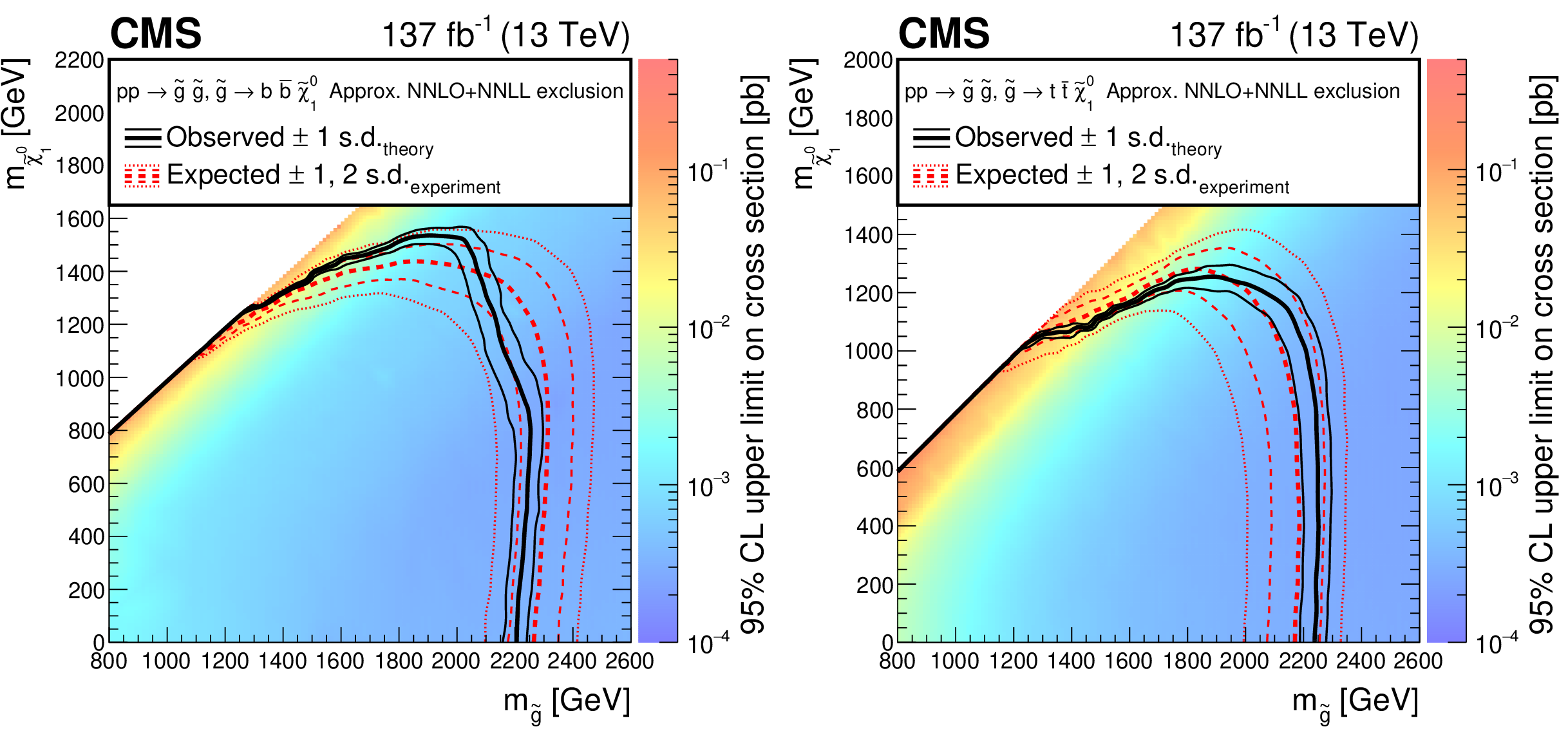
Exclusion limits at 95% CL for direct gluino pair production where the gluinos decay to (left) bottom quarks and (right) top quarks. The area enclosed by the thick black curve represents the observed exclusion region, while the dashed red lines indicate the expected limits and their $\pm $1 and $\pm $2 standard deviation (s.d.) ranges. The thin black lines show the effect of the theoretical uncertainties in the signal cross section. Signal cross sections are calculated at approximately NNLO+NNLL order in ${\alpha _S}$ [136,137,138,139,140,141], assuming unity branching fraction for the indicated decay. |

png pdf root |
Figure 12-a:
Exclusion limits at 95% CL for direct gluino pair production where the gluinos decay to bottom quarks. The area enclosed by the thick black curve represents the observed exclusion region, while the dashed red lines indicate the expected limits and their $\pm $1 and $\pm $2 standard deviation (s.d.) ranges. The thin black lines show the effect of the theoretical uncertainties in the signal cross section. Signal cross sections are calculated at approximately NNLO+NNLL order in ${\alpha _S}$ [136,137,138,139,140,141], assuming unity branching fraction for the indicated decay. |
png pdf root |
Figure 12-b:
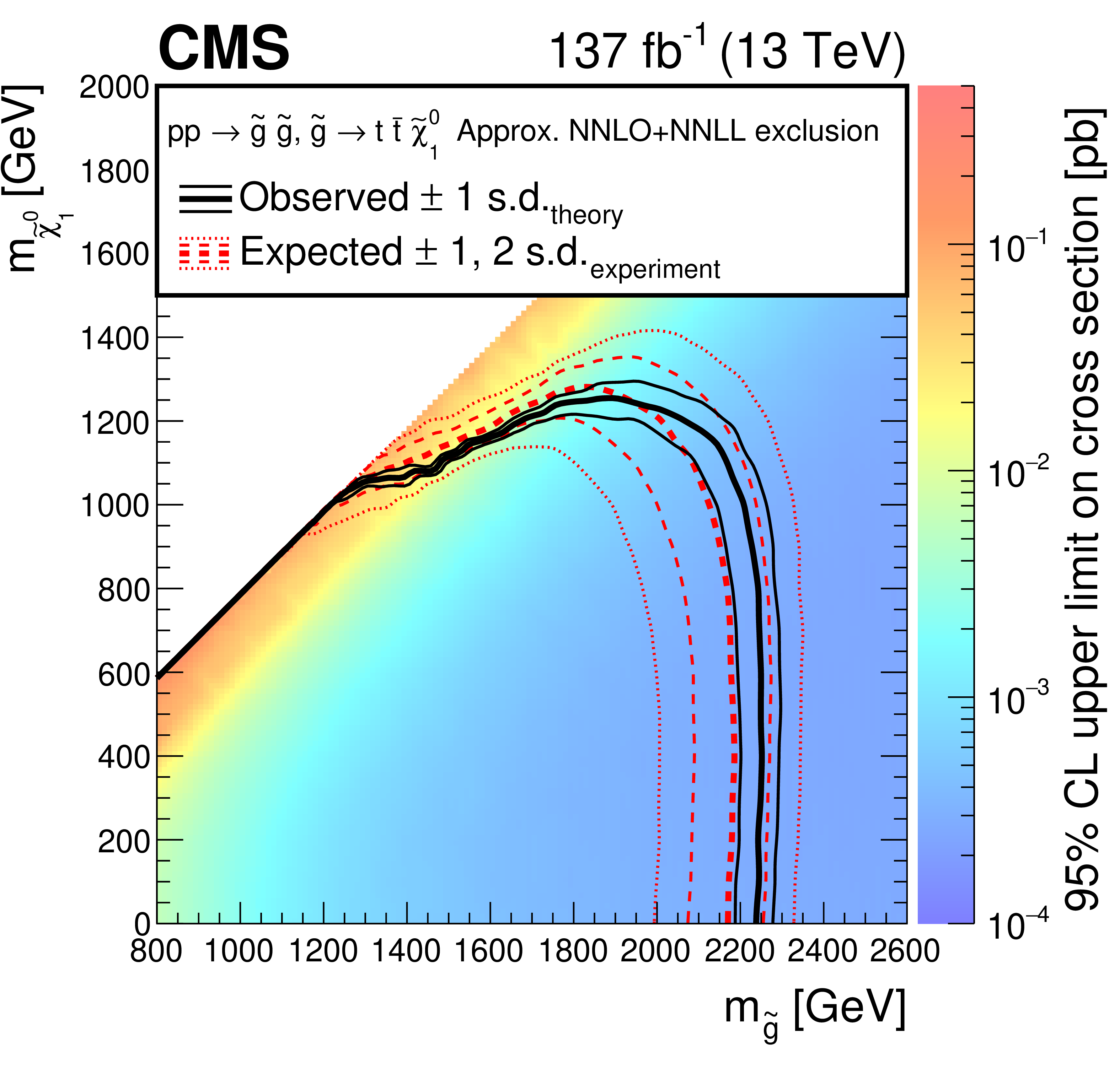
Exclusion limits at 95% CL for direct gluino pair production where the gluinos decay to top quarks. The area enclosed by the thick black curve represents the observed exclusion region, while the dashed red lines indicate the expected limits and their $\pm $1 and $\pm $2 standard deviation (s.d.) ranges. The thin black lines show the effect of the theoretical uncertainties in the signal cross section. Signal cross sections are calculated at approximately NNLO+NNLL order in ${\alpha _S}$ [136,137,138,139,140,141], assuming unity branching fraction for the indicated decay. |
png pdf |
Figure 13:
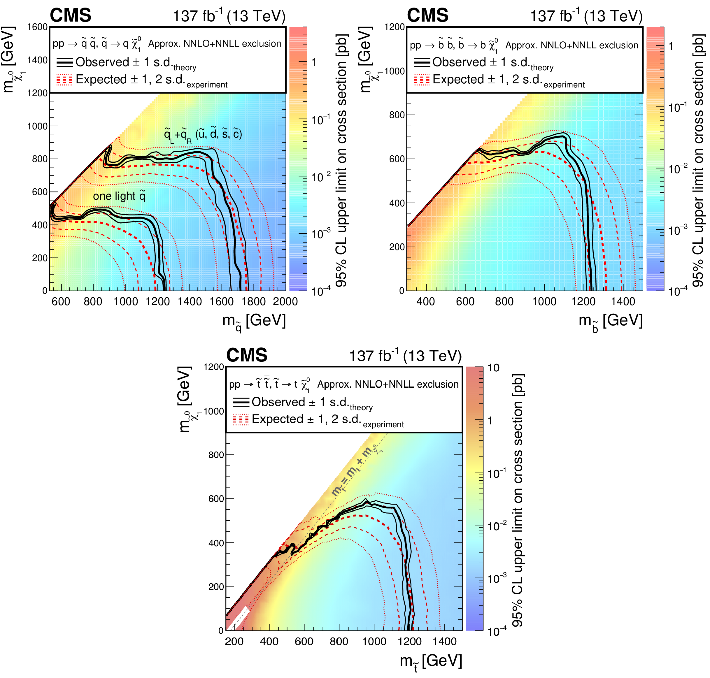
Exclusion limit at 95% CL for (upper left) light-flavor squark pair production, (upper right) bottom squark pair production, and (lower) top squark pair production. The area enclosed by the thick black curve represents the observed exclusion region, while the dashed red lines indicate the expected limits and their $\pm $1 and $\pm $2 standard deviation (s.d.) ranges. The thin black lines show the effect of the theoretical uncertainties in the signal cross section. The white diagonal band in the top squark pair production exclusion limit corresponds to the region $ {| m_{\tilde{\mathrm{t}}}-m_{\mathrm{t}}-m_{\tilde{\chi}^0_1} |} < $ 25 GeV and small $m_{\tilde{\chi}^0_1}$. Here the efficiency of the selection is a strong function of $m_{\tilde{\mathrm{t}}}-m_{\tilde{\chi}^0_1}$, and as a result the precise determination of the cross section upper limit is uncertain because of the finite granularity of the available MC samples in this region of the ($m_{\tilde{\mathrm{t}}}, m_{\tilde{\chi}^0_1}$) plane. In the same exclusion limit, the dashed black diagonal line corresponds to $m_{\tilde{\mathrm{t}}}=m_{\mathrm{t}}+m_{\tilde{\chi}^0_1}$. Signal cross sections are calculated at approximately NNLO+NNLL order in ${\alpha _S}$ [136,137,138,139,140,141], assuming unity branching fraction for the indicated decay. |
png pdf root |
Figure 13-a:
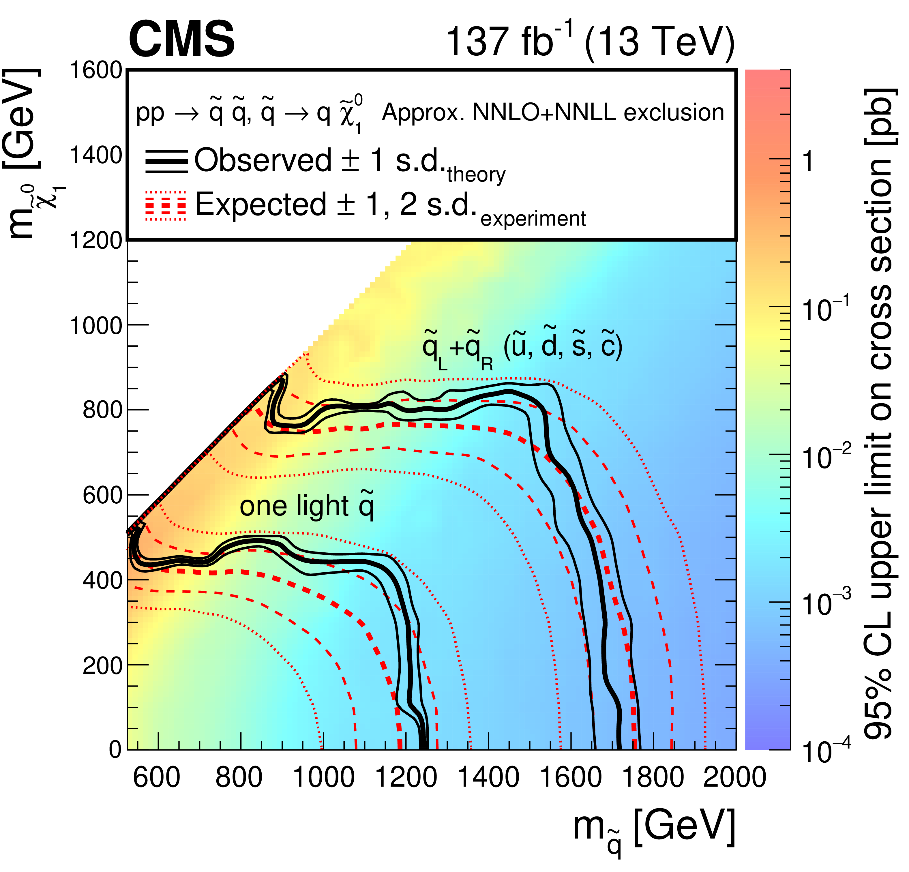
Exclusion limit at 95% CL for light-flavor squark pair production. The area enclosed by the thick black curve represents the observed exclusion region, while the dashed red lines indicate the expected limits and their $\pm $1 and $\pm $2 standard deviation (s.d.) ranges. The thin black lines show the effect of the theoretical uncertainties in the signal cross section. Signal cross sections are calculated at approximately NNLO+NNLL order in ${\alpha _S}$ [136,137,138,139,140,141], assuming unity branching fraction for the indicated decay. |
png pdf root |
Figure 13-b:
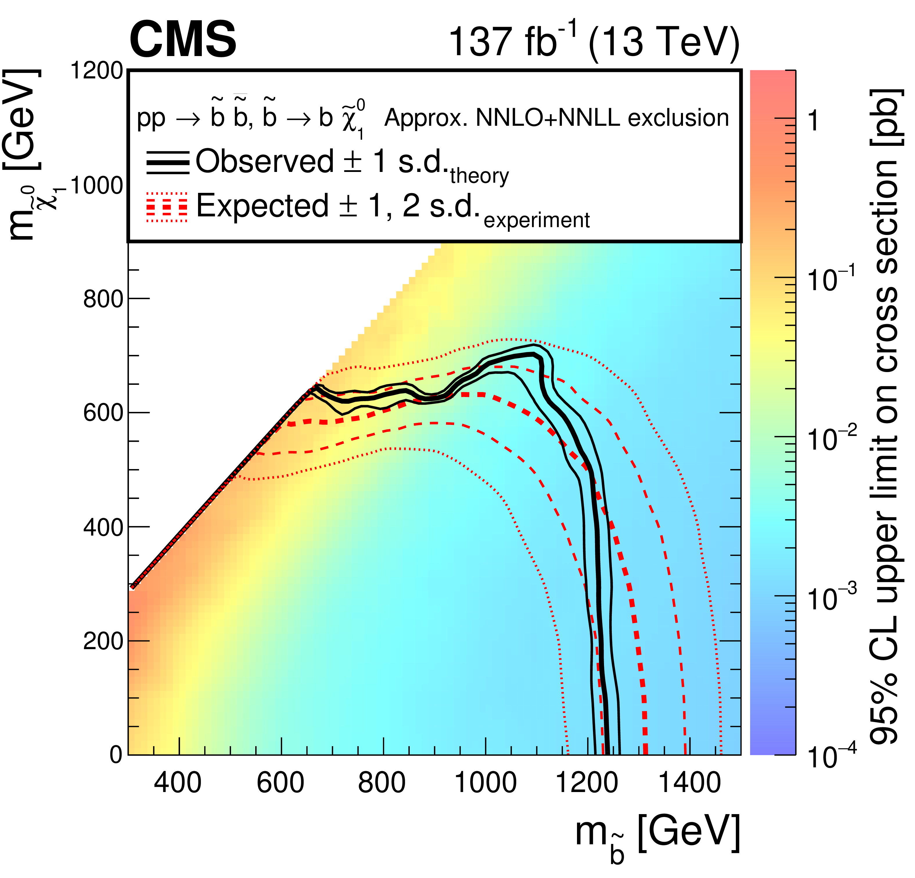
Exclusion limit at 95% CL for bottom squark pair production. The area enclosed by the thick black curve represents the observed exclusion region, while the dashed red lines indicate the expected limits and their $\pm $1 and $\pm $2 standard deviation (s.d.) ranges. The thin black lines show the effect of the theoretical uncertainties in the signal cross section. Signal cross sections are calculated at approximately NNLO+NNLL order in ${\alpha _S}$ [136,137,138,139,140,141], assuming unity branching fraction for the indicated decay. |
png root |
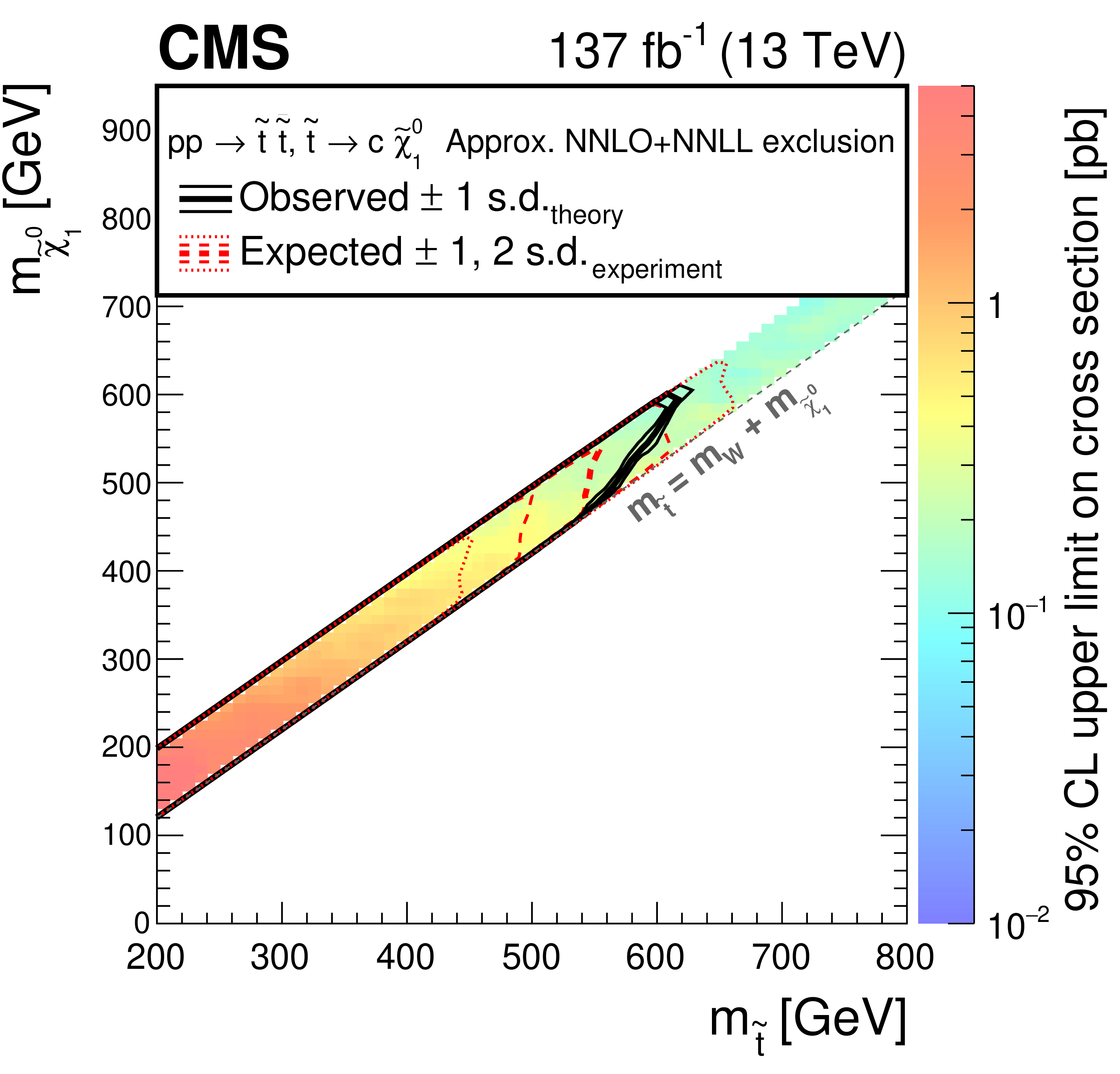
Figure 13-c:
Exclusion limit at 95% CL for top squark pair production. The area enclosed by the thick black curve represents the observed exclusion region, while the dashed red lines indicate the expected limits and their $\pm $1 and $\pm $2 standard deviation (s.d.) ranges. The thin black lines show the effect of the theoretical uncertainties in the signal cross section. The white diagonal band in the top squark pair production exclusion limit corresponds to the region $ {| m_{\tilde{\mathrm{t}}}-m_{\mathrm{t}}-m_{\tilde{\chi}^0_1} |} < $ 25 GeV and small $m_{\tilde{\chi}^0_1}$. Here the efficiency of the selection is a strong function of $m_{\tilde{\mathrm{t}}}-m_{\tilde{\chi}^0_1}$, and as a result the precise determination of the cross section upper limit is uncertain because of the finite granularity of the available MC samples in this region of the ($m_{\tilde{\mathrm{t}}}, m_{\tilde{\chi}^0_1}$) plane. In the same exclusion limit, the dashed black diagonal line corresponds to $m_{\tilde{\mathrm{t}}}=m_{\mathrm{t}}+m_{\tilde{\chi}^0_1}$. Signal cross sections are calculated at approximately NNLO+NNLL order in ${\alpha _S}$ [136,137,138,139,140,141], assuming unity branching fraction for the indicated decay. |
png pdf |
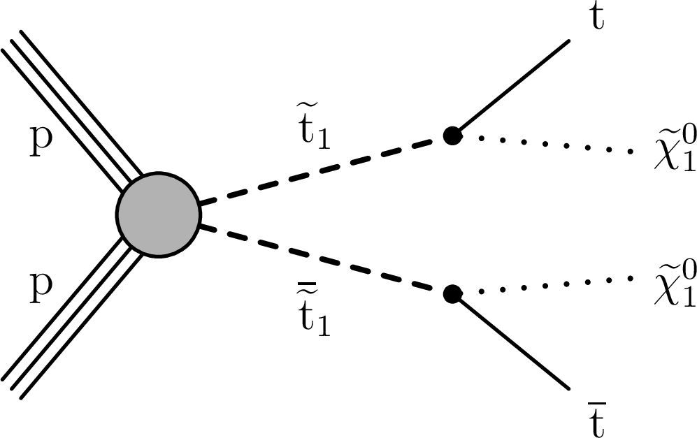
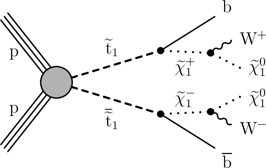
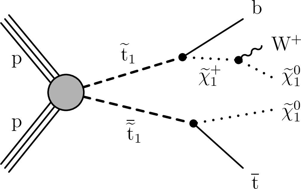
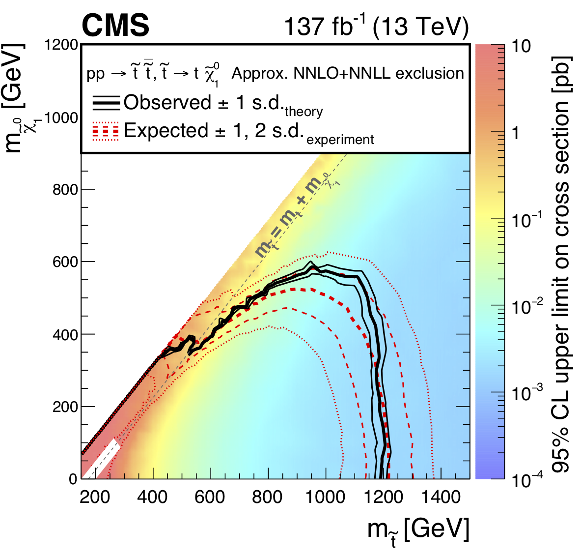
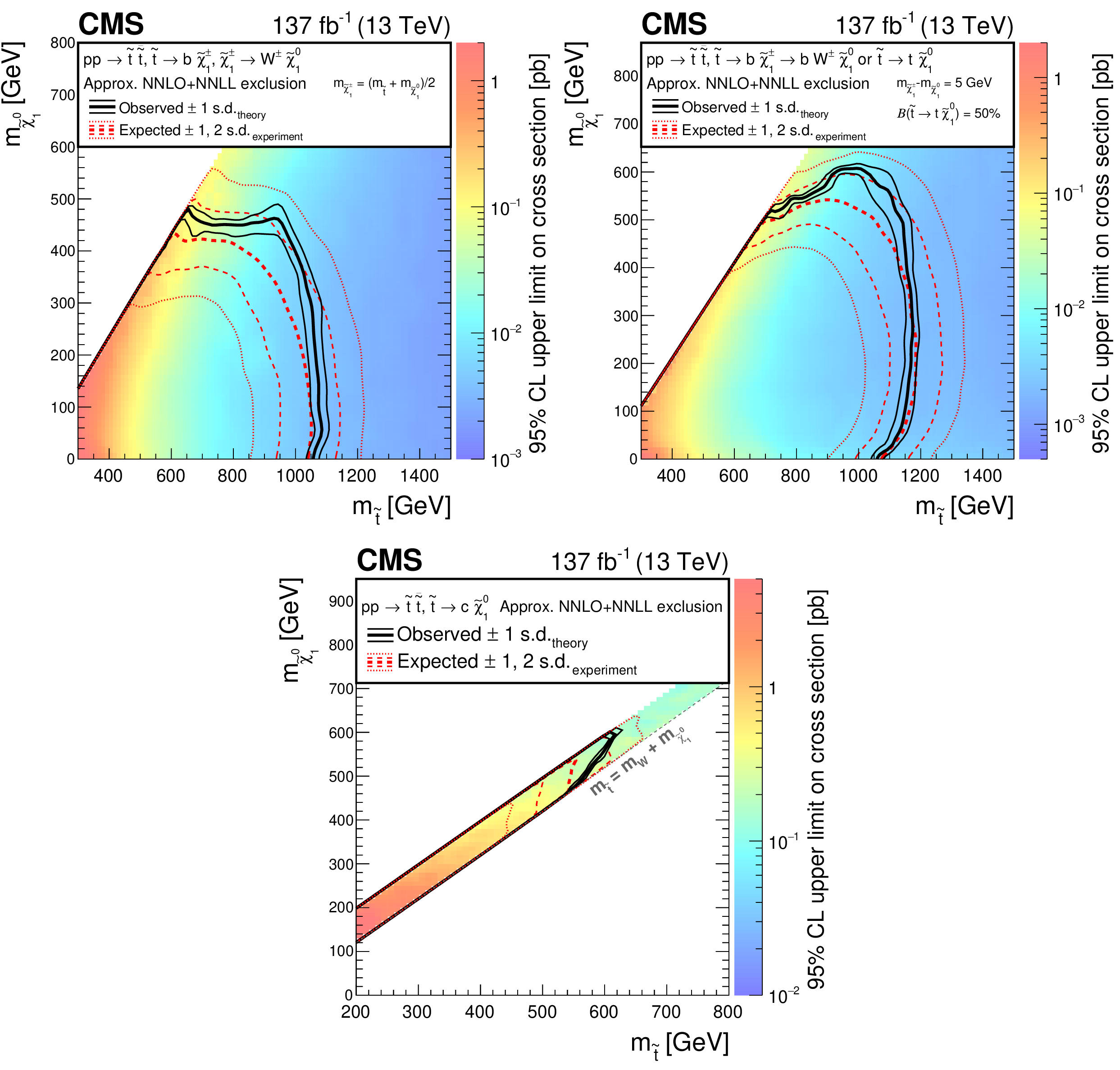
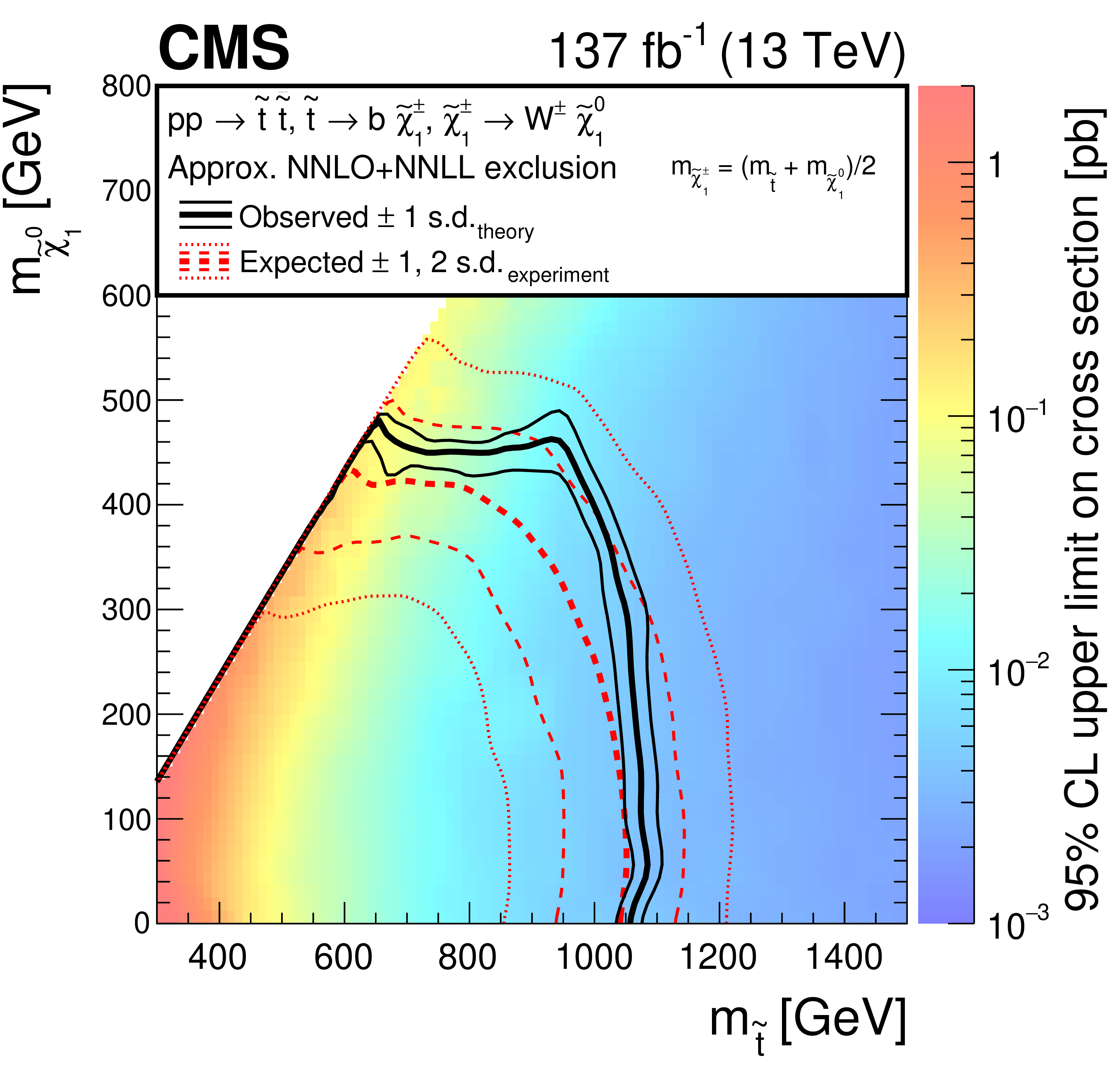
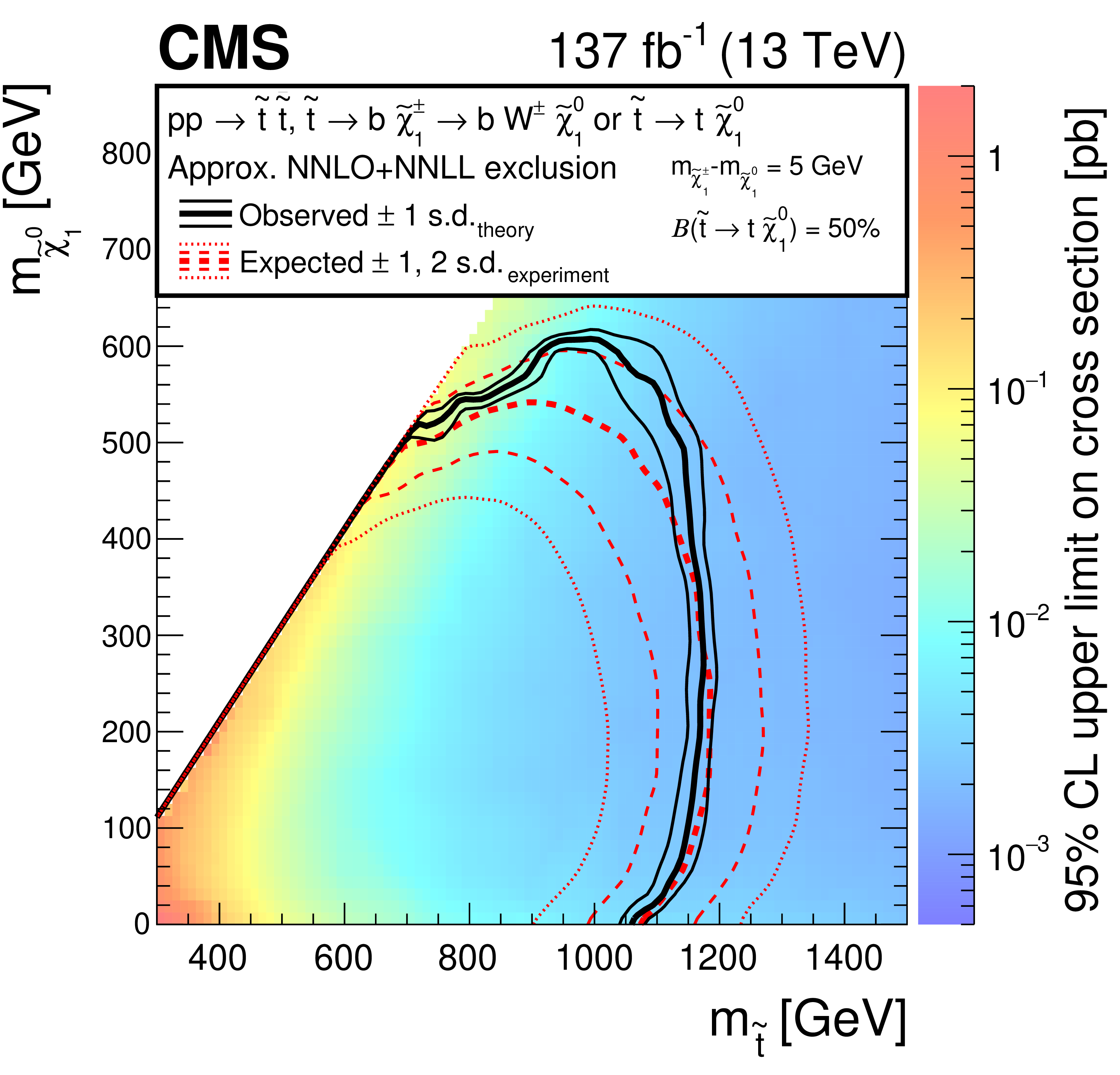
Figure 14:
Exclusion limit at 95% CL for top squark pair production for different decay modes of the top squark. (Upper left) For the scenario where ${\mathrm{p}} {\mathrm{p}} \to \tilde{\mathrm{t}} \bar{\tilde{\mathrm{t}}} \to \mathrm{b} \mathrm{\bar{b}} \tilde{\chi}^{\pm}_1 \tilde{\chi}^{\mp}_1 $, $\tilde{\chi}^{\pm}_1 \to \mathrm{W} ^{\pm} \tilde{\chi}^0_1 $, the mass of the chargino is chosen to be half way in between the masses of the top squark and the neutralino. (Upper right) A mixed-decay scenario, ${\mathrm{p}} {\mathrm{p}} \to \tilde{\mathrm{t}} \bar{\tilde{\mathrm{t}}} $ with equal branching fractions for the top squark decays $\tilde{\mathrm{t}} \to \mathrm{t} \tilde{\chi}^0_1 $ and $\tilde{\mathrm{t}} \to \mathrm{b} \tilde{\chi}^{+}_1 $, $ \tilde{\chi}^{+}_1 \to \mathrm{W} ^{*+}\tilde{\chi}^0_1 $, is also considered, with the chargino mass chosen such that $\Delta m\left (\tilde{\chi}^{\pm}_1,\tilde{\chi}^0_1 \right) = $ 5 GeV. (Lower) Finally, we also consider a compressed spectrum scenario where ${\mathrm{p}} {\mathrm{p}} \to \tilde{\mathrm{t}} \bar{\tilde{\mathrm{t}}} \to \mathrm{c} \mathrm{\bar{c}} \tilde{\chi}^0_1 \tilde{\chi}^0_1 $. In this scenario, mass ranges are considered where the $\tilde{\mathrm{t}} \to \mathrm{c} \tilde{\chi}^0_1 $ branching fraction can be significant. The area enclosed by the thick black curve represents the observed exclusion region, while the dashed red lines indicate the expected limits and their $\pm $1 and $\pm $2 standard deviation (s.d.) ranges. The thin black lines show the effect of the theoretical uncertainties in the signal cross section. Signal cross sections are calculated at approximately NNLO+NNLL order in ${\alpha _S}$ [136,137,138,139,140,141], assuming 50% branching fraction ($\mathcal {B}$) for each decay mode in the mixed-decay scenarios, or unity branching fraction for the indicated decay. |
png pdf root |
Figure 14-a:
Exclusion limit at 95% CL for top squark pair production for different decay modes of the top squark. (Upper left) For the scenario where ${\mathrm{p}} {\mathrm{p}} \to \tilde{\mathrm{t}} \bar{\tilde{\mathrm{t}}} \to \mathrm{b} \mathrm{\bar{b}} \tilde{\chi}^{\pm}_1 \tilde{\chi}^{\mp}_1 $, $\tilde{\chi}^{\pm}_1 \to \mathrm{W} ^{\pm} \tilde{\chi}^0_1 $, the mass of the chargino is chosen to be half way in between the masses of the top squark and the neutralino. (Upper right) A mixed-decay scenario, ${\mathrm{p}} {\mathrm{p}} \to \tilde{\mathrm{t}} \bar{\tilde{\mathrm{t}}} $ with equal branching fractions for the top squark decays $\tilde{\mathrm{t}} \to \mathrm{t} \tilde{\chi}^0_1 $ and $\tilde{\mathrm{t}} \to \mathrm{b} \tilde{\chi}^{+}_1 $, $ \tilde{\chi}^{+}_1 \to \mathrm{W} ^{*+}\tilde{\chi}^0_1 $, is also considered, with the chargino mass chosen such that $\Delta m\left (\tilde{\chi}^{\pm}_1,\tilde{\chi}^0_1 \right) = $ 5 GeV. (Lower) Finally, we also consider a compressed spectrum scenario where ${\mathrm{p}} {\mathrm{p}} \to \tilde{\mathrm{t}} \bar{\tilde{\mathrm{t}}} \to \mathrm{c} \mathrm{\bar{c}} \tilde{\chi}^0_1 \tilde{\chi}^0_1 $. In this scenario, mass ranges are considered where the $\tilde{\mathrm{t}} \to \mathrm{c} \tilde{\chi}^0_1 $ branching fraction can be significant. The area enclosed by the thick black curve represents the observed exclusion region, while the dashed red lines indicate the expected limits and their $\pm $1 and $\pm $2 standard deviation (s.d.) ranges. The thin black lines show the effect of the theoretical uncertainties in the signal cross section. Signal cross sections are calculated at approximately NNLO+NNLL order in ${\alpha _S}$ [136,137,138,139,140,141], assuming 50% branching fraction ($\mathcal {B}$) for each decay mode in the mixed-decay scenarios, or unity branching fraction for the indicated decay. |
png pdf root |
Figure 14-b:
Exclusion limit at 95% CL for top squark pair production for different decay modes of the top squark. (Upper left) For the scenario where ${\mathrm{p}} {\mathrm{p}} \to \tilde{\mathrm{t}} \bar{\tilde{\mathrm{t}}} \to \mathrm{b} \mathrm{\bar{b}} \tilde{\chi}^{\pm}_1 \tilde{\chi}^{\mp}_1 $, $\tilde{\chi}^{\pm}_1 \to \mathrm{W} ^{\pm} \tilde{\chi}^0_1 $, the mass of the chargino is chosen to be half way in between the masses of the top squark and the neutralino. (Upper right) A mixed-decay scenario, ${\mathrm{p}} {\mathrm{p}} \to \tilde{\mathrm{t}} \bar{\tilde{\mathrm{t}}} $ with equal branching fractions for the top squark decays $\tilde{\mathrm{t}} \to \mathrm{t} \tilde{\chi}^0_1 $ and $\tilde{\mathrm{t}} \to \mathrm{b} \tilde{\chi}^{+}_1 $, $ \tilde{\chi}^{+}_1 \to \mathrm{W} ^{*+}\tilde{\chi}^0_1 $, is also considered, with the chargino mass chosen such that $\Delta m\left (\tilde{\chi}^{\pm}_1,\tilde{\chi}^0_1 \right) = $ 5 GeV. (Lower) Finally, we also consider a compressed spectrum scenario where ${\mathrm{p}} {\mathrm{p}} \to \tilde{\mathrm{t}} \bar{\tilde{\mathrm{t}}} \to \mathrm{c} \mathrm{\bar{c}} \tilde{\chi}^0_1 \tilde{\chi}^0_1 $. In this scenario, mass ranges are considered where the $\tilde{\mathrm{t}} \to \mathrm{c} \tilde{\chi}^0_1 $ branching fraction can be significant. The area enclosed by the thick black curve represents the observed exclusion region, while the dashed red lines indicate the expected limits and their $\pm $1 and $\pm $2 standard deviation (s.d.) ranges. The thin black lines show the effect of the theoretical uncertainties in the signal cross section. Signal cross sections are calculated at approximately NNLO+NNLL order in ${\alpha _S}$ [136,137,138,139,140,141], assuming 50% branching fraction ($\mathcal {B}$) for each decay mode in the mixed-decay scenarios, or unity branching fraction for the indicated decay. |
png pdf root |
Figure 14-c:
Exclusion limit at 95% CL for top squark pair production for different decay modes of the top squark. (Upper left) For the scenario where ${\mathrm{p}} {\mathrm{p}} \to \tilde{\mathrm{t}} \bar{\tilde{\mathrm{t}}} \to \mathrm{b} \mathrm{\bar{b}} \tilde{\chi}^{\pm}_1 \tilde{\chi}^{\mp}_1 $, $\tilde{\chi}^{\pm}_1 \to \mathrm{W} ^{\pm} \tilde{\chi}^0_1 $, the mass of the chargino is chosen to be half way in between the masses of the top squark and the neutralino. (Upper right) A mixed-decay scenario, ${\mathrm{p}} {\mathrm{p}} \to \tilde{\mathrm{t}} \bar{\tilde{\mathrm{t}}} $ with equal branching fractions for the top squark decays $\tilde{\mathrm{t}} \to \mathrm{t} \tilde{\chi}^0_1 $ and $\tilde{\mathrm{t}} \to \mathrm{b} \tilde{\chi}^{+}_1 $, $ \tilde{\chi}^{+}_1 \to \mathrm{W} ^{*+}\tilde{\chi}^0_1 $, is also considered, with the chargino mass chosen such that $\Delta m\left (\tilde{\chi}^{\pm}_1,\tilde{\chi}^0_1 \right) = $ 5 GeV. (Lower) Finally, we also consider a compressed spectrum scenario where ${\mathrm{p}} {\mathrm{p}} \to \tilde{\mathrm{t}} \bar{\tilde{\mathrm{t}}} \to \mathrm{c} \mathrm{\bar{c}} \tilde{\chi}^0_1 \tilde{\chi}^0_1 $. In this scenario, mass ranges are considered where the $\tilde{\mathrm{t}} \to \mathrm{c} \tilde{\chi}^0_1 $ branching fraction can be significant. The area enclosed by the thick black curve represents the observed exclusion region, while the dashed red lines indicate the expected limits and their $\pm $1 and $\pm $2 standard deviation (s.d.) ranges. The thin black lines show the effect of the theoretical uncertainties in the signal cross section. Signal cross sections are calculated at approximately NNLO+NNLL order in ${\alpha _S}$ [136,137,138,139,140,141], assuming 50% branching fraction ($\mathcal {B}$) for each decay mode in the mixed-decay scenarios, or unity branching fraction for the indicated decay. |

png pdf root |
Figure 15:
Exclusion limit at 95% CL for the mono-$\phi $ model. We consider the mass range where such a model could be interesting based on a reinterpretation of previous analyses [35,36]. The area enclosed by the thick black curve represents the observed exclusion region, while the dashed red lines indicate the expected limits and their $\pm $1 and $\pm $2 standard deviation (s.d.) ranges. The thin black lines show the effect of the theoretical uncertainties in the signal cross section. The blue star at $\left (m_{\phi}, m_{\psi}\right)=$ (1250, 900) GeV indicates the best fit mass point reported in Refs. [35,36]. Signal cross sections are calculated at LO order in ${\alpha _S}$. |
png pdf |
Figure 16:
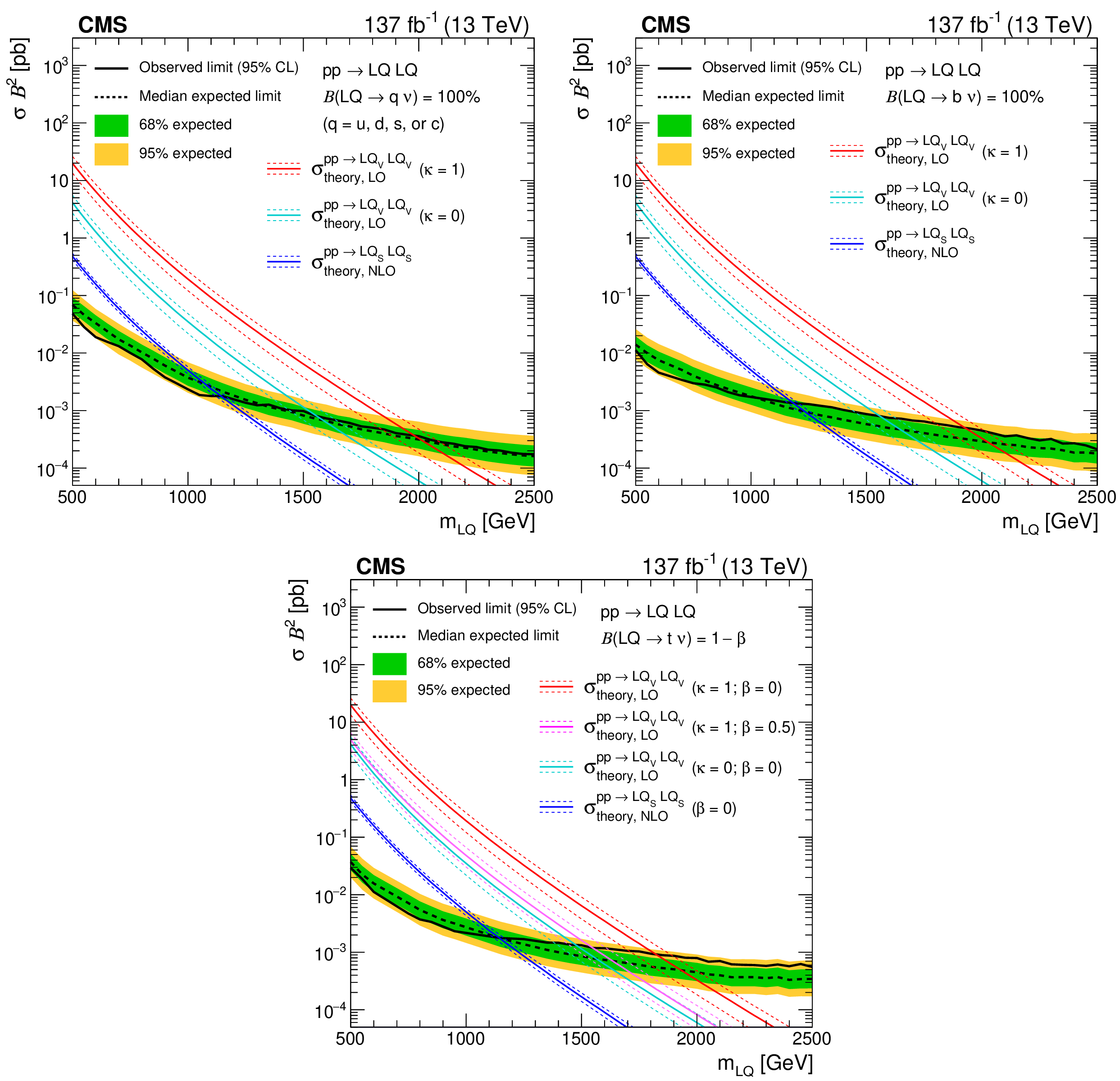
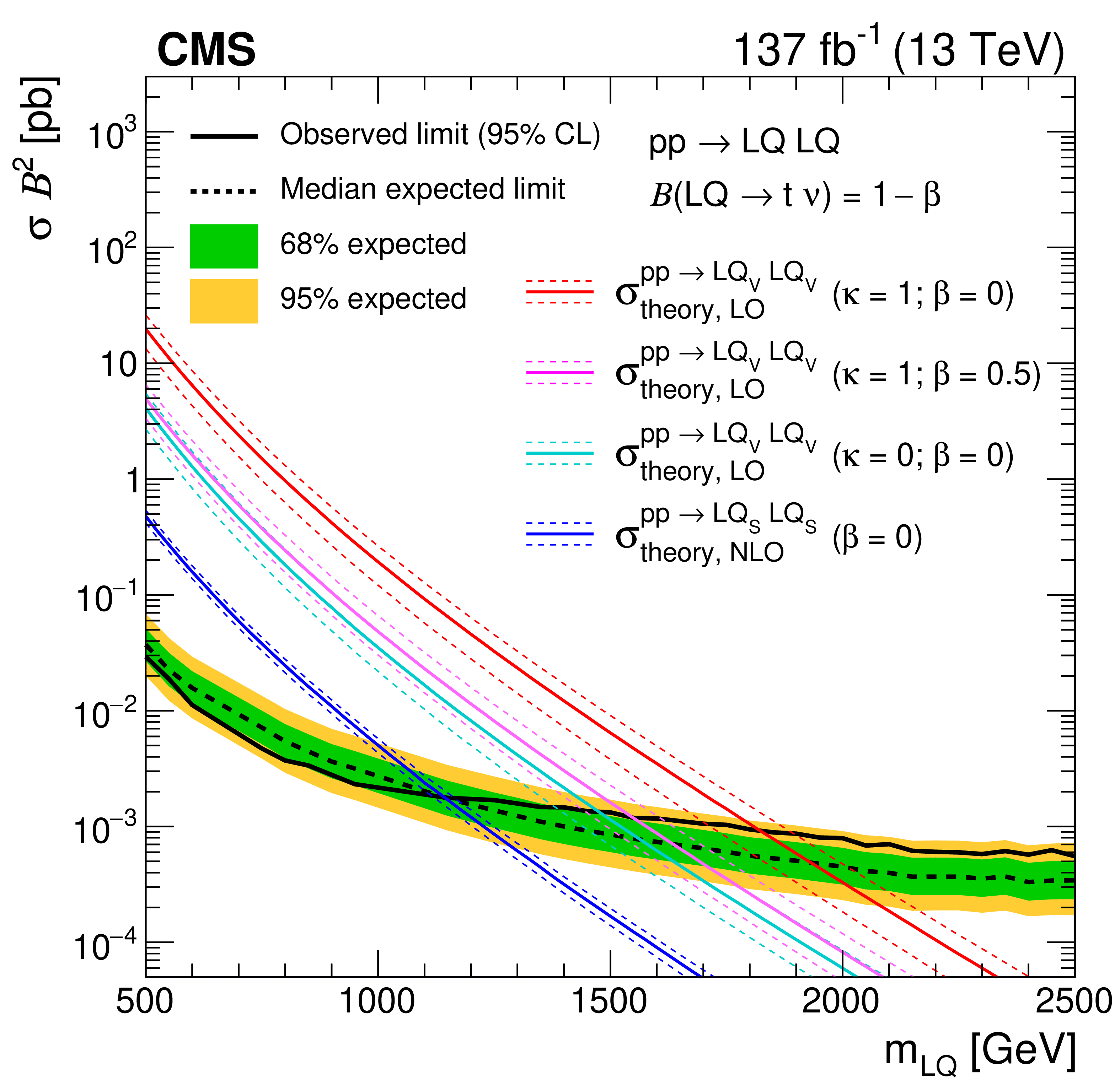
The 95% CL upper limits on the production cross sections as a function of LQ mass for LQ pair production decaying with 100% branching fraction ($\mathcal {B}$) to a neutrino and (upper left) a light quark (one of u, d, s, or c), (upper right) a bottom quark, or (lower) a top quark. The solid (dashed) black line represents the observed (median expected) exclusion. The inner green (outer yellow) band indicates the region containing 68 (95)% of the distribution of limits expected under the background-only hypothesis. The dark blue lines show the theoretical cross section for ${\mathrm {LQ}_{\mathrm {S}}}$ pair production with its uncertainty. The red (light blue) lines show the same for ${\mathrm {LQ}_{\mathrm {V}}} $ pair production assuming $\kappa = $ 1 (0). (Lower) Also shown in magenta is the product of the theoretical cross section and the square of the branching fraction ($\sigma \mathcal {B}^{2}$), for vector LQ pair production assuming $\kappa = $ 1 and a 50% branching fraction to $\mathrm{t} \nu_{\tau} $, with the remaining 50% to $\mathrm{b} \tau $. Signal cross sections are calculated at NLO (LO) in ${\alpha _S}$ for scalar (vector) LQ pair production. |
png pdf root |
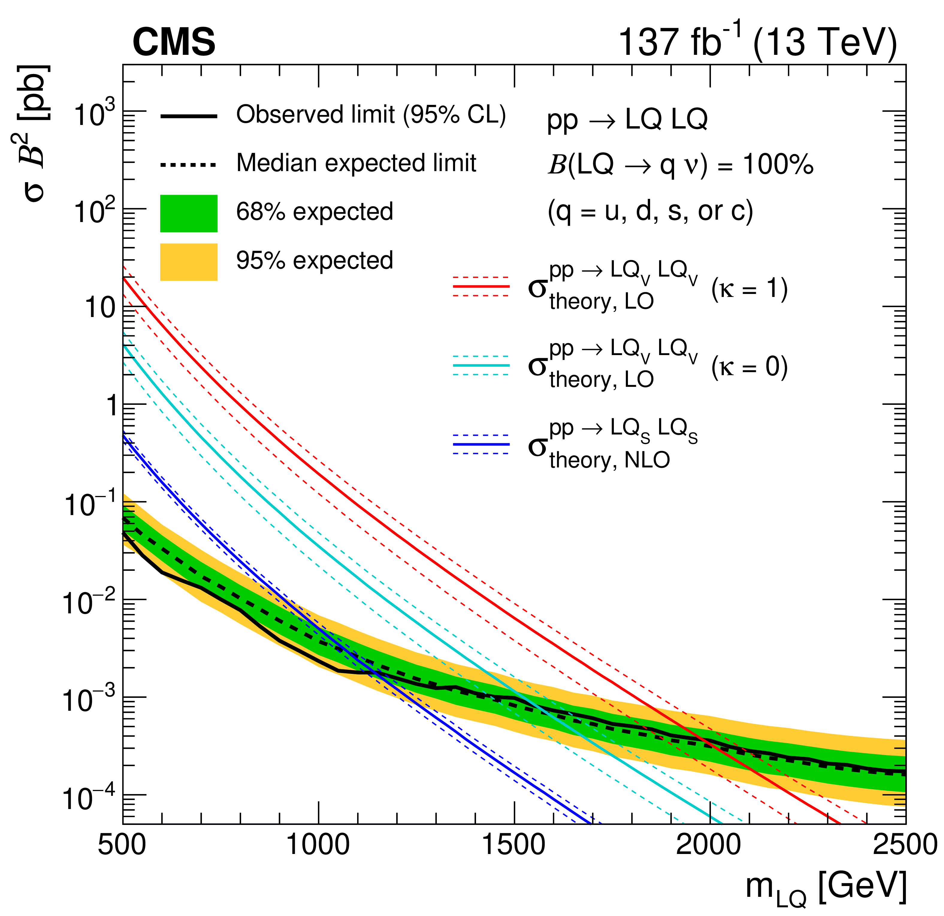
Figure 16-a:
The 95% CL upper limits on the production cross sections as a function of LQ mass for LQ pair production decaying with 100% branching fraction ($\mathcal {B}$) to a neutrino and (upper left) a light quark (one of u, d, s, or c), (upper right) a bottom quark, or (lower) a top quark. The solid (dashed) black line represents the observed (median expected) exclusion. The inner green (outer yellow) band indicates the region containing 68 (95)% of the distribution of limits expected under the background-only hypothesis. The dark blue lines show the theoretical cross section for ${\mathrm {LQ}_{\mathrm {S}}}$ pair production with its uncertainty. The red (light blue) lines show the same for ${\mathrm {LQ}_{\mathrm {V}}} $ pair production assuming $\kappa = $ 1 (0). (Lower) Also shown in magenta is the product of the theoretical cross section and the square of the branching fraction ($\sigma \mathcal {B}^{2}$), for vector LQ pair production assuming $\kappa = $ 1 and a 50% branching fraction to $\mathrm{t} \nu_{\tau} $, with the remaining 50% to $\mathrm{b} \tau $. Signal cross sections are calculated at NLO (LO) in ${\alpha _S}$ for scalar (vector) LQ pair production. |
png pdf root |
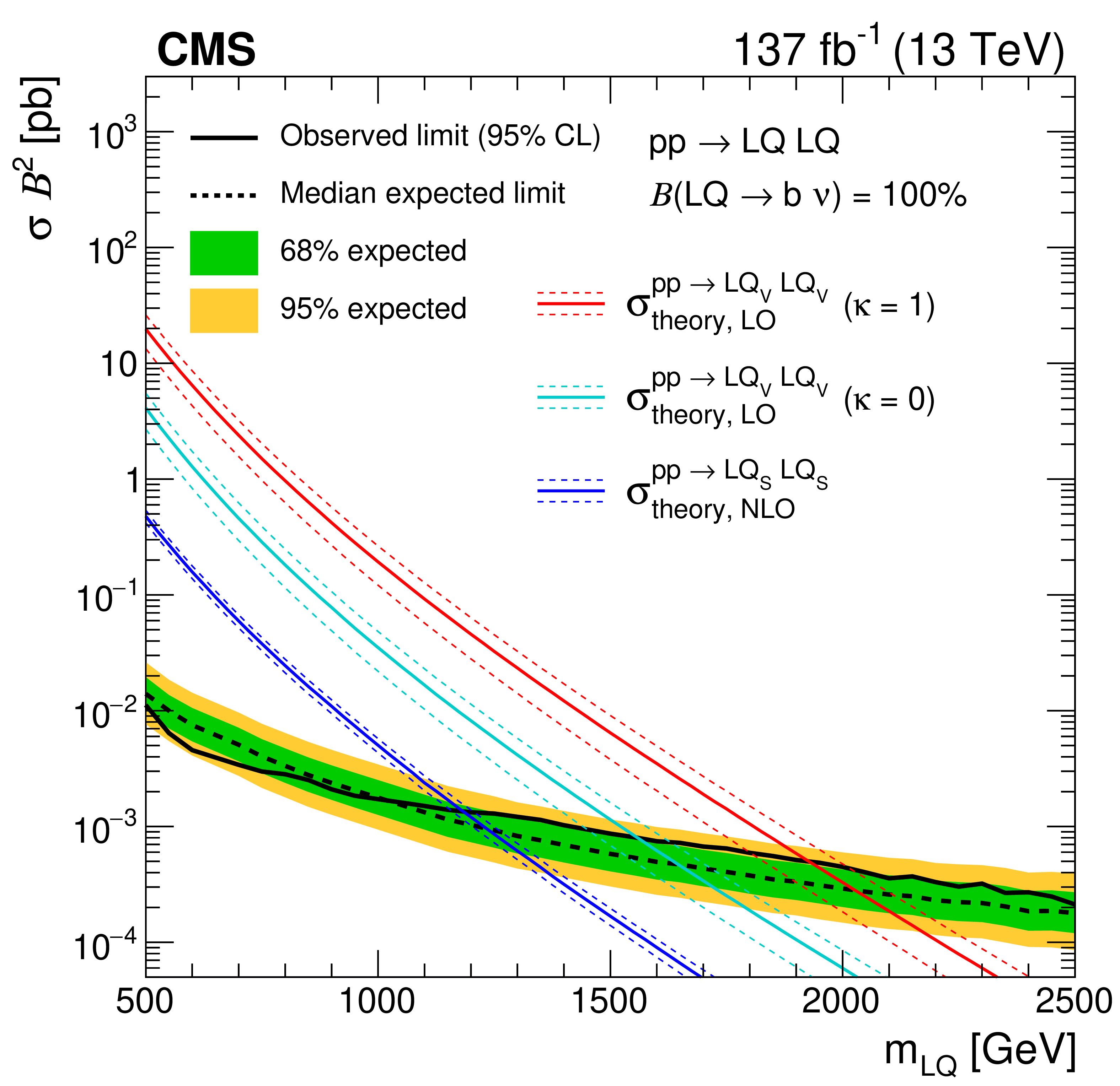
Figure 16-b:
The 95% CL upper limits on the production cross sections as a function of LQ mass for LQ pair production decaying with 100% branching fraction ($\mathcal {B}$) to a neutrino and (upper left) a light quark (one of u, d, s, or c), (upper right) a bottom quark, or (lower) a top quark. The solid (dashed) black line represents the observed (median expected) exclusion. The inner green (outer yellow) band indicates the region containing 68 (95)% of the distribution of limits expected under the background-only hypothesis. The dark blue lines show the theoretical cross section for ${\mathrm {LQ}_{\mathrm {S}}}$ pair production with its uncertainty. The red (light blue) lines show the same for ${\mathrm {LQ}_{\mathrm {V}}} $ pair production assuming $\kappa = $ 1 (0). (Lower) Also shown in magenta is the product of the theoretical cross section and the square of the branching fraction ($\sigma \mathcal {B}^{2}$), for vector LQ pair production assuming $\kappa = $ 1 and a 50% branching fraction to $\mathrm{t} \nu_{\tau} $, with the remaining 50% to $\mathrm{b} \tau $. Signal cross sections are calculated at NLO (LO) in ${\alpha _S}$ for scalar (vector) LQ pair production. |
png pdf root |
Figure 16-c:
The 95% CL upper limits on the production cross sections as a function of LQ mass for LQ pair production decaying with 100% branching fraction ($\mathcal {B}$) to a neutrino and (upper left) a light quark (one of u, d, s, or c), (upper right) a bottom quark, or (lower) a top quark. The solid (dashed) black line represents the observed (median expected) exclusion. The inner green (outer yellow) band indicates the region containing 68 (95)% of the distribution of limits expected under the background-only hypothesis. The dark blue lines show the theoretical cross section for ${\mathrm {LQ}_{\mathrm {S}}}$ pair production with its uncertainty. The red (light blue) lines show the same for ${\mathrm {LQ}_{\mathrm {V}}} $ pair production assuming $\kappa = $ 1 (0). (Lower) Also shown in magenta is the product of the theoretical cross section and the square of the branching fraction ($\sigma \mathcal {B}^{2}$), for vector LQ pair production assuming $\kappa = $ 1 and a 50% branching fraction to $\mathrm{t} \nu_{\tau} $, with the remaining 50% to $\mathrm{b} \tau $. Signal cross sections are calculated at NLO (LO) in ${\alpha _S}$ for scalar (vector) LQ pair production. |
png pdf |
Figure 17:
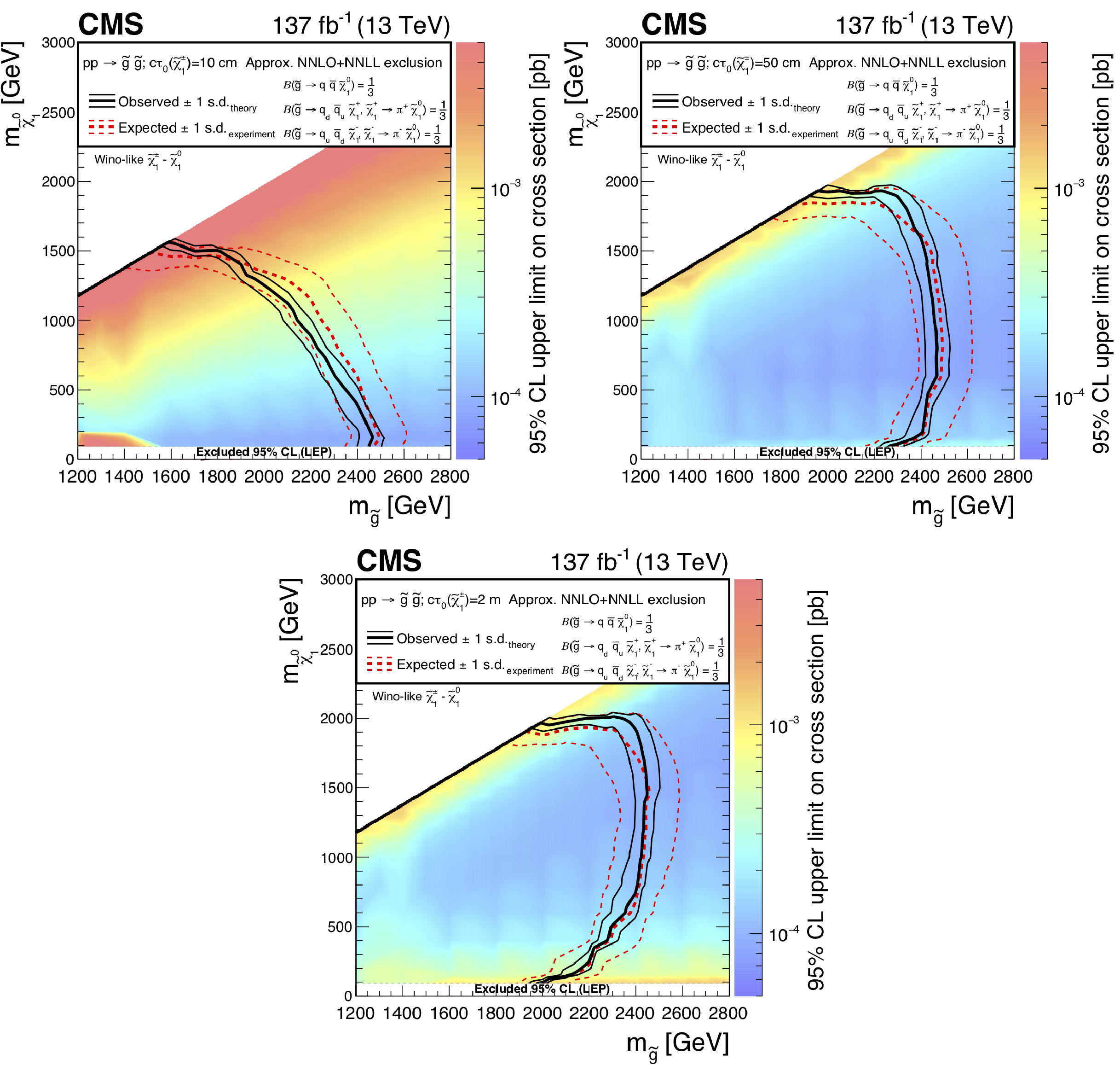
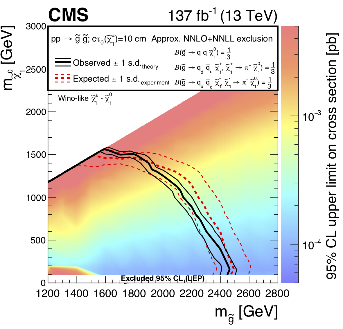
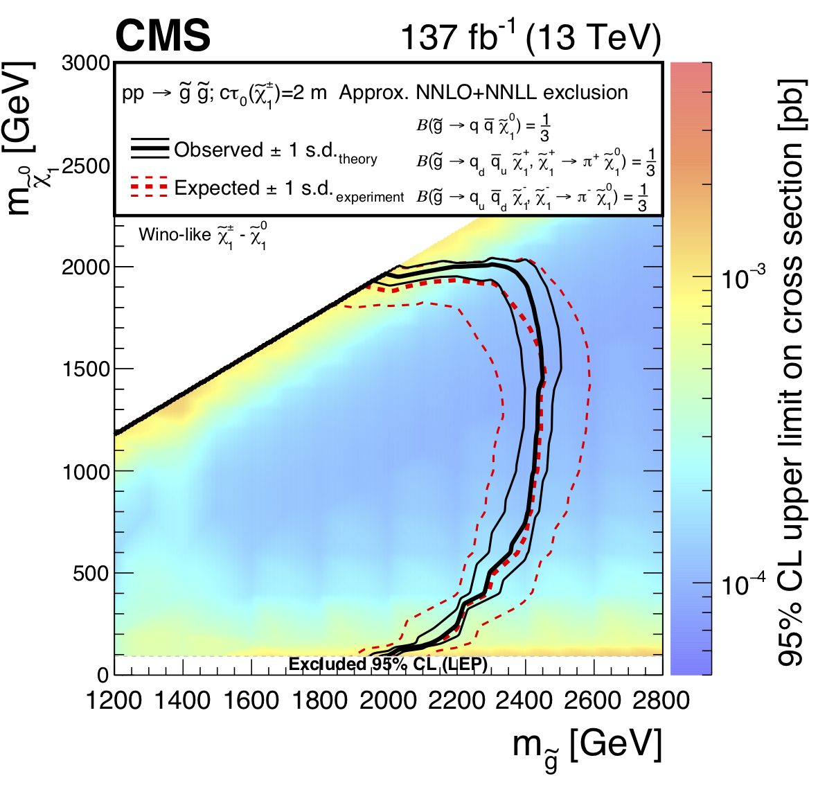
Exclusion limits at 95% CL for direct gluino pair production where the gluinos decay to light-flavor (u, d, s, c) quarks, with $c\tau _{0}(\tilde{\chi}^{\pm}_1) =$ (upper left) 10 cm, (upper right) 50 cm, and (lower) 200 cm. The area enclosed by the thick black curve represents the observed exclusion region, while the dashed red lines indicate the expected limits and their $\pm $1 standard deviation (s.d.) ranges. The thin black lines show the effect of the theoretical uncertainties in the signal cross section. The white band for masses of the $\tilde{\chi}^0_1$ below 91.9 GeV represents the region of the mass plane excluded at the CERN LEP [145]. Signal cross sections are calculated at approximately NNLO+NNLL order in ${\alpha _S}$ [136,137,138,139,140,141], assuming decay branching fractions ($\mathcal {B}$) as indicated in the figure. |
png root |
Figure 17-a:
Exclusion limits at 95% CL for direct gluino pair production where the gluinos decay to light-flavor (u, d, s, c) quarks, with $c\tau _{0}(\tilde{\chi}^{\pm}_1) =$ (upper left) 10 cm, (upper right) 50 cm, and (lower) 200 cm. The area enclosed by the thick black curve represents the observed exclusion region, while the dashed red lines indicate the expected limits and their $\pm $1 standard deviation (s.d.) ranges. The thin black lines show the effect of the theoretical uncertainties in the signal cross section. The white band for masses of the $\tilde{\chi}^0_1$ below 91.9 GeV represents the region of the mass plane excluded at the CERN LEP [145]. Signal cross sections are calculated at approximately NNLO+NNLL order in ${\alpha _S}$ [136,137,138,139,140,141], assuming decay branching fractions ($\mathcal {B}$) as indicated in the figure. |
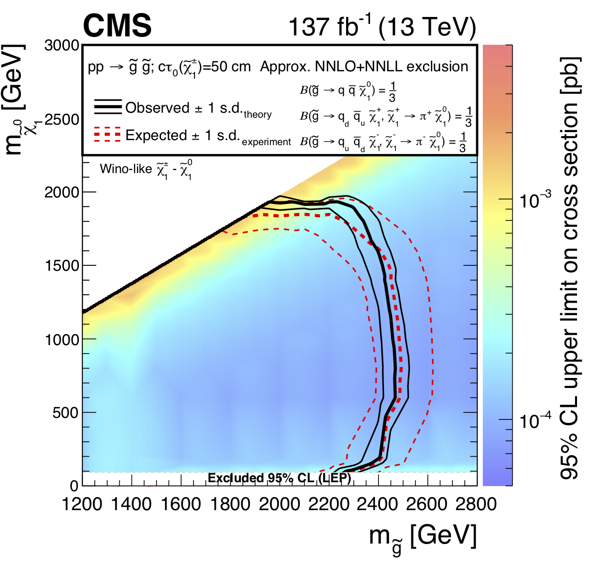
png root |
Figure 17-b:
Exclusion limits at 95% CL for direct gluino pair production where the gluinos decay to light-flavor (u, d, s, c) quarks, with $c\tau _{0}(\tilde{\chi}^{\pm}_1) =$ (upper left) 10 cm, (upper right) 50 cm, and (lower) 200 cm. The area enclosed by the thick black curve represents the observed exclusion region, while the dashed red lines indicate the expected limits and their $\pm $1 standard deviation (s.d.) ranges. The thin black lines show the effect of the theoretical uncertainties in the signal cross section. The white band for masses of the $\tilde{\chi}^0_1$ below 91.9 GeV represents the region of the mass plane excluded at the CERN LEP [145]. Signal cross sections are calculated at approximately NNLO+NNLL order in ${\alpha _S}$ [136,137,138,139,140,141], assuming decay branching fractions ($\mathcal {B}$) as indicated in the figure. |
png root |
Figure 17-c:
Exclusion limits at 95% CL for direct gluino pair production where the gluinos decay to light-flavor (u, d, s, c) quarks, with $c\tau _{0}(\tilde{\chi}^{\pm}_1) =$ (upper left) 10 cm, (upper right) 50 cm, and (lower) 200 cm. The area enclosed by the thick black curve represents the observed exclusion region, while the dashed red lines indicate the expected limits and their $\pm $1 standard deviation (s.d.) ranges. The thin black lines show the effect of the theoretical uncertainties in the signal cross section. The white band for masses of the $\tilde{\chi}^0_1$ below 91.9 GeV represents the region of the mass plane excluded at the CERN LEP [145]. Signal cross sections are calculated at approximately NNLO+NNLL order in ${\alpha _S}$ [136,137,138,139,140,141], assuming decay branching fractions ($\mathcal {B}$) as indicated in the figure. |

png pdf |
Figure 18:
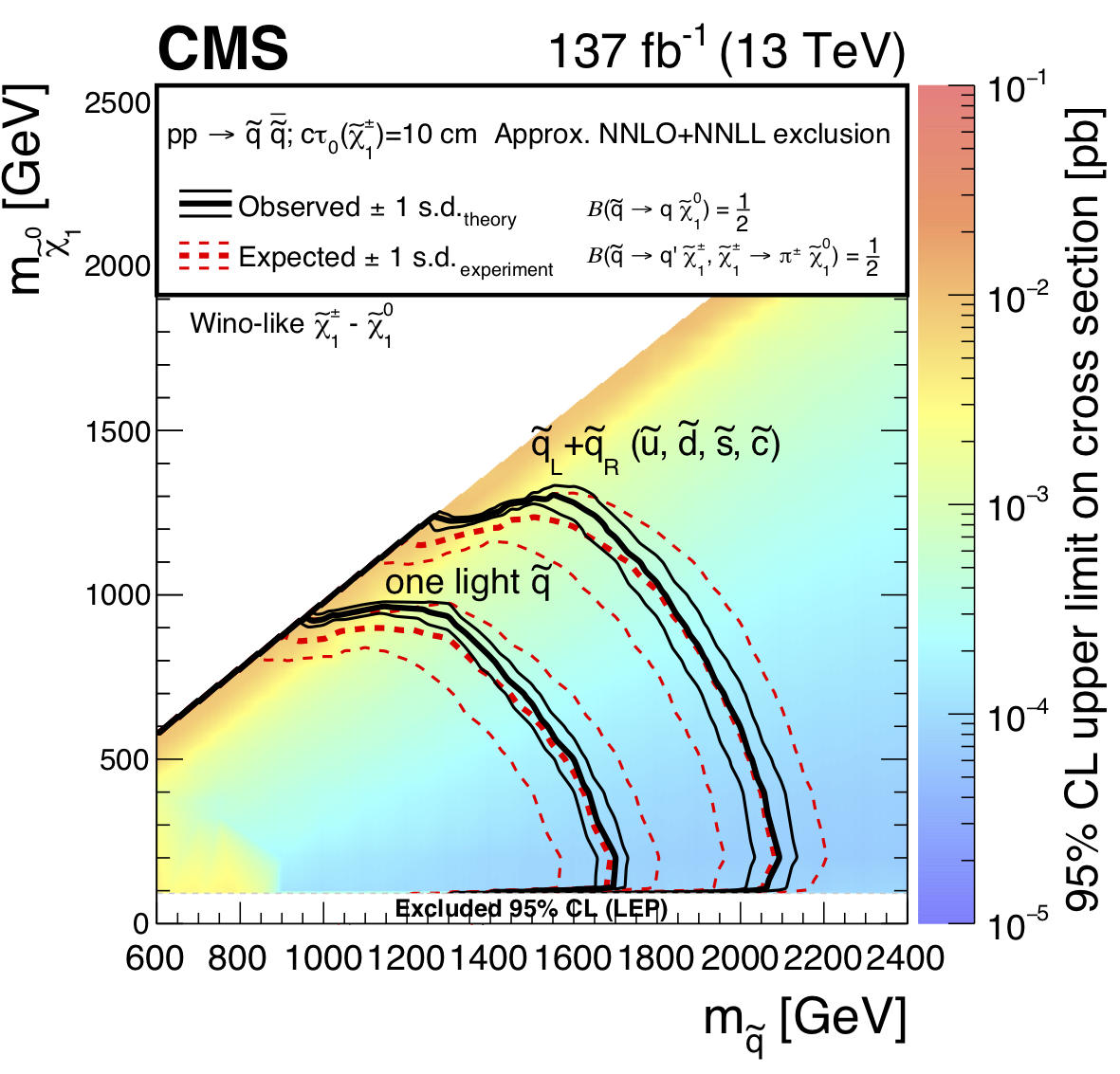
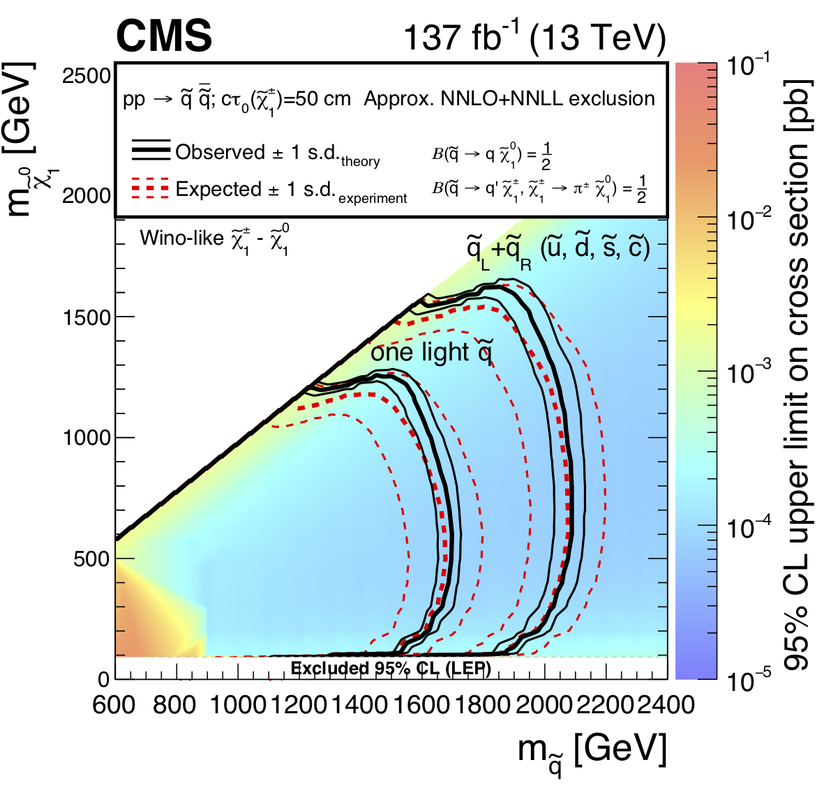
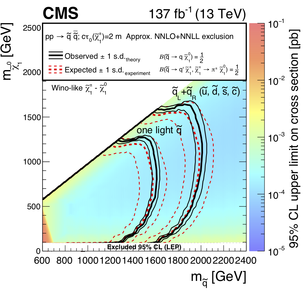
Exclusion limits at 95% CL for light squark pair production with $c\tau _{0}(\tilde{\chi}^{\pm}_1) =$ (upper left) 10 cm, (upper right) 50 cm, and (lower) 200 cm. The area enclosed by the thick black curve represents the observed exclusion region, while the dashed red lines indicate the expected limits and their $\pm $1 standard deviation (s.d.) ranges. The thin black lines show the effect of the theoretical uncertainties in the signal cross section. The white band for masses of the $\tilde{\chi}^0_1$ below 91.9 GeV represents the region of the mass plane excluded at the CERN LEP [145]. Signal cross sections are calculated at approximately NNLO+NNLL order in ${\alpha _S}$ [136,137,138,139,140,141], assuming decay branching fractions ($\mathcal {B}$) as indicated in the figure. |
png root |
Figure 18-a:
Exclusion limits at 95% CL for light squark pair production with $c\tau _{0}(\tilde{\chi}^{\pm}_1) =$ (upper left) 10 cm, (upper right) 50 cm, and (lower) 200 cm. The area enclosed by the thick black curve represents the observed exclusion region, while the dashed red lines indicate the expected limits and their $\pm $1 standard deviation (s.d.) ranges. The thin black lines show the effect of the theoretical uncertainties in the signal cross section. The white band for masses of the $\tilde{\chi}^0_1$ below 91.9 GeV represents the region of the mass plane excluded at the CERN LEP [145]. Signal cross sections are calculated at approximately NNLO+NNLL order in ${\alpha _S}$ [136,137,138,139,140,141], assuming decay branching fractions ($\mathcal {B}$) as indicated in the figure. |
png root |
Figure 18-b:
Exclusion limits at 95% CL for light squark pair production with $c\tau _{0}(\tilde{\chi}^{\pm}_1) =$ (upper left) 10 cm, (upper right) 50 cm, and (lower) 200 cm. The area enclosed by the thick black curve represents the observed exclusion region, while the dashed red lines indicate the expected limits and their $\pm $1 standard deviation (s.d.) ranges. The thin black lines show the effect of the theoretical uncertainties in the signal cross section. The white band for masses of the $\tilde{\chi}^0_1$ below 91.9 GeV represents the region of the mass plane excluded at the CERN LEP [145]. Signal cross sections are calculated at approximately NNLO+NNLL order in ${\alpha _S}$ [136,137,138,139,140,141], assuming decay branching fractions ($\mathcal {B}$) as indicated in the figure. |
png root |
Figure 18-c:
Exclusion limits at 95% CL for light squark pair production with $c\tau _{0}(\tilde{\chi}^{\pm}_1) =$ (upper left) 10 cm, (upper right) 50 cm, and (lower) 200 cm. The area enclosed by the thick black curve represents the observed exclusion region, while the dashed red lines indicate the expected limits and their $\pm $1 standard deviation (s.d.) ranges. The thin black lines show the effect of the theoretical uncertainties in the signal cross section. The white band for masses of the $\tilde{\chi}^0_1$ below 91.9 GeV represents the region of the mass plane excluded at the CERN LEP [145]. Signal cross sections are calculated at approximately NNLO+NNLL order in ${\alpha _S}$ [136,137,138,139,140,141], assuming decay branching fractions ($\mathcal {B}$) as indicated in the figure. |
png pdf |
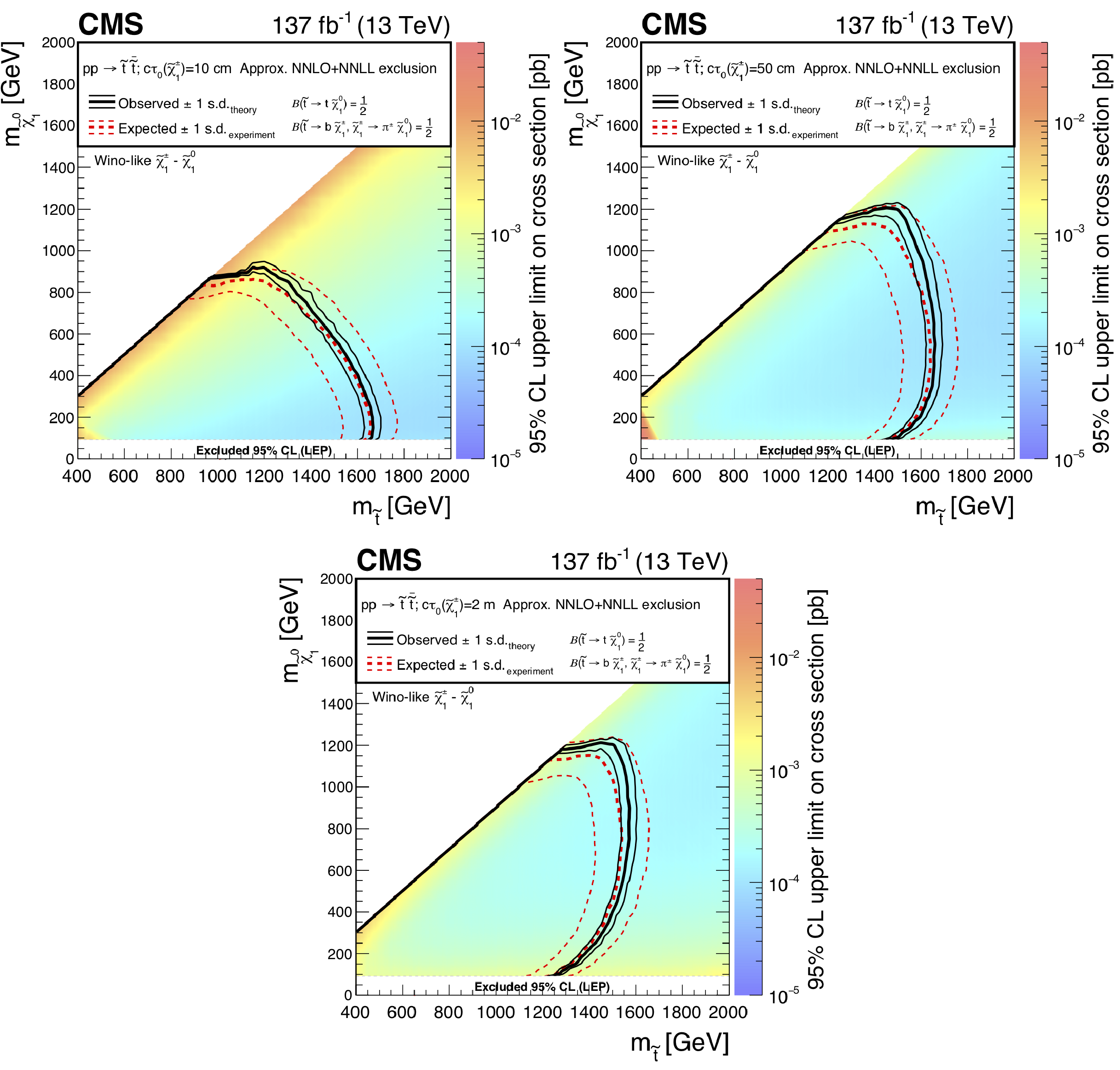
Figure 19:
Exclusion limits at 95% CL for top squark pair production with $c\tau _{0}(\tilde{\chi}^{\pm}_1) =$ (upper left) 10 cm, (upper right) 50 cm, and (lower) 200 cm. The area enclosed by the thick black curve represents the observed exclusion region, while the dashed red lines indicate the expected limits and their $\pm $1 standard deviation (s.d.) ranges. The thin black lines show the effect of the theoretical uncertainties in the signal cross section. The white band for masses of the $\tilde{\chi}^0_1$ below 91.9 GeV represents the region of the mass plane excluded at the CERN LEP [145]. Signal cross sections are calculated at approximately NNLO+NNLL order in ${\alpha _S}$ [136,137,138,139,140,141], assuming decay branching fractions ($\mathcal {B}$) as indicated in the figure. |
png root |
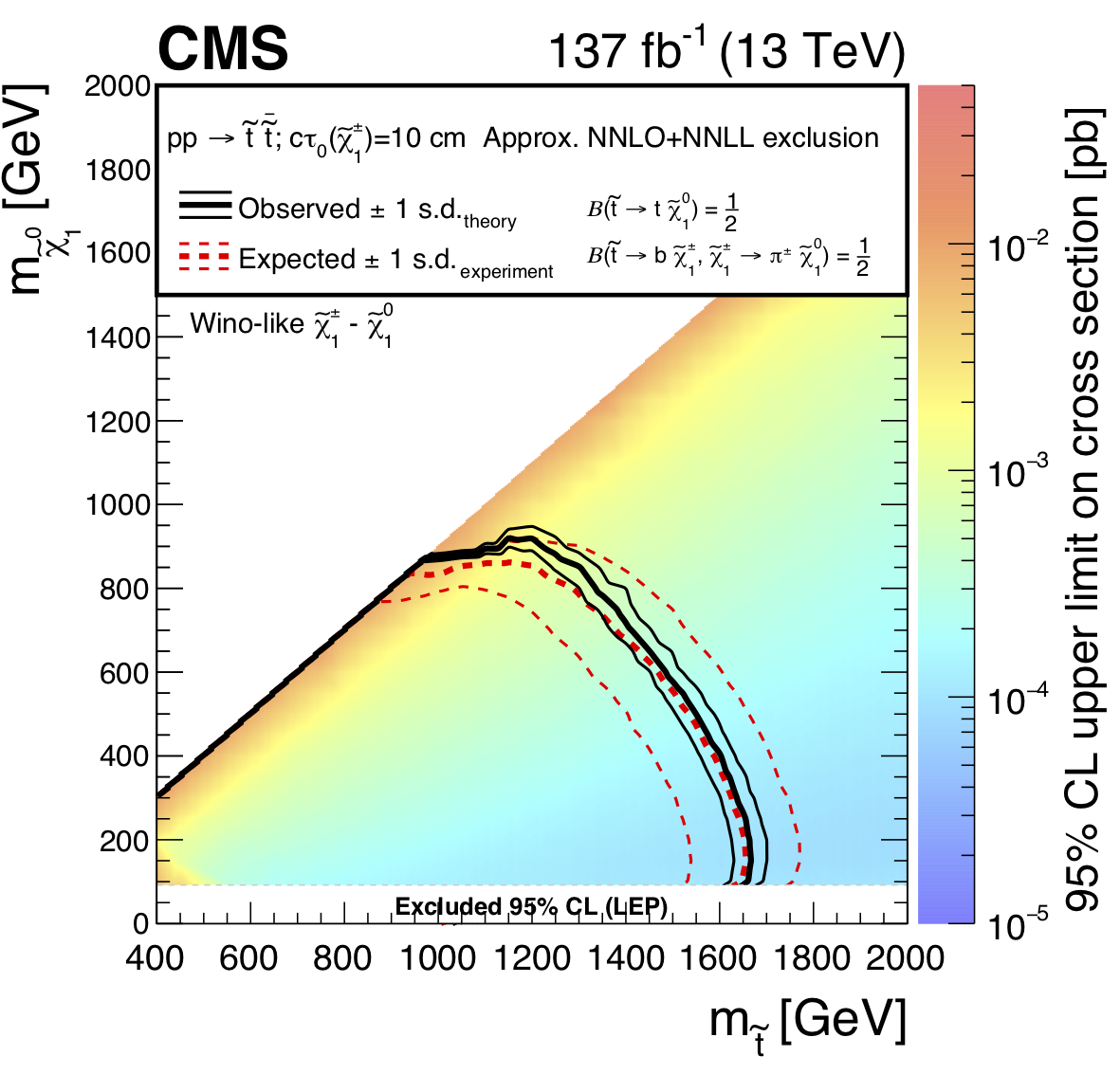
Figure 19-a:
Exclusion limits at 95% CL for top squark pair production with $c\tau _{0}(\tilde{\chi}^{\pm}_1) =$ (upper left) 10 cm, (upper right) 50 cm, and (lower) 200 cm. The area enclosed by the thick black curve represents the observed exclusion region, while the dashed red lines indicate the expected limits and their $\pm $1 standard deviation (s.d.) ranges. The thin black lines show the effect of the theoretical uncertainties in the signal cross section. The white band for masses of the $\tilde{\chi}^0_1$ below 91.9 GeV represents the region of the mass plane excluded at the CERN LEP [145]. Signal cross sections are calculated at approximately NNLO+NNLL order in ${\alpha _S}$ [136,137,138,139,140,141], assuming decay branching fractions ($\mathcal {B}$) as indicated in the figure. |
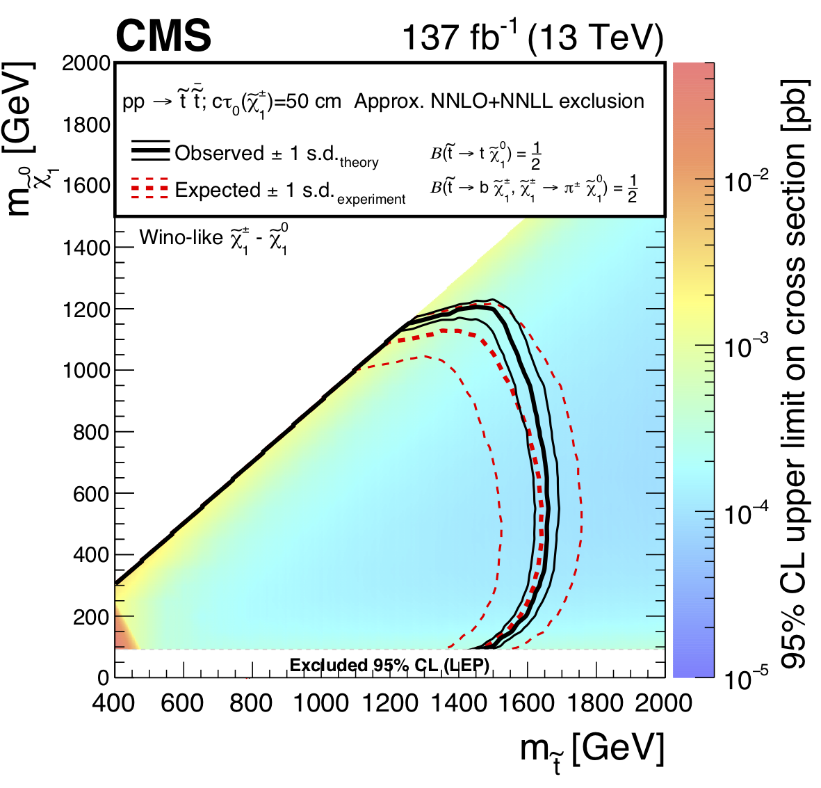
png root |
Figure 19-b:
Exclusion limits at 95% CL for top squark pair production with $c\tau _{0}(\tilde{\chi}^{\pm}_1) =$ (upper left) 10 cm, (upper right) 50 cm, and (lower) 200 cm. The area enclosed by the thick black curve represents the observed exclusion region, while the dashed red lines indicate the expected limits and their $\pm $1 standard deviation (s.d.) ranges. The thin black lines show the effect of the theoretical uncertainties in the signal cross section. The white band for masses of the $\tilde{\chi}^0_1$ below 91.9 GeV represents the region of the mass plane excluded at the CERN LEP [145]. Signal cross sections are calculated at approximately NNLO+NNLL order in ${\alpha _S}$ [136,137,138,139,140,141], assuming decay branching fractions ($\mathcal {B}$) as indicated in the figure. |
png root |
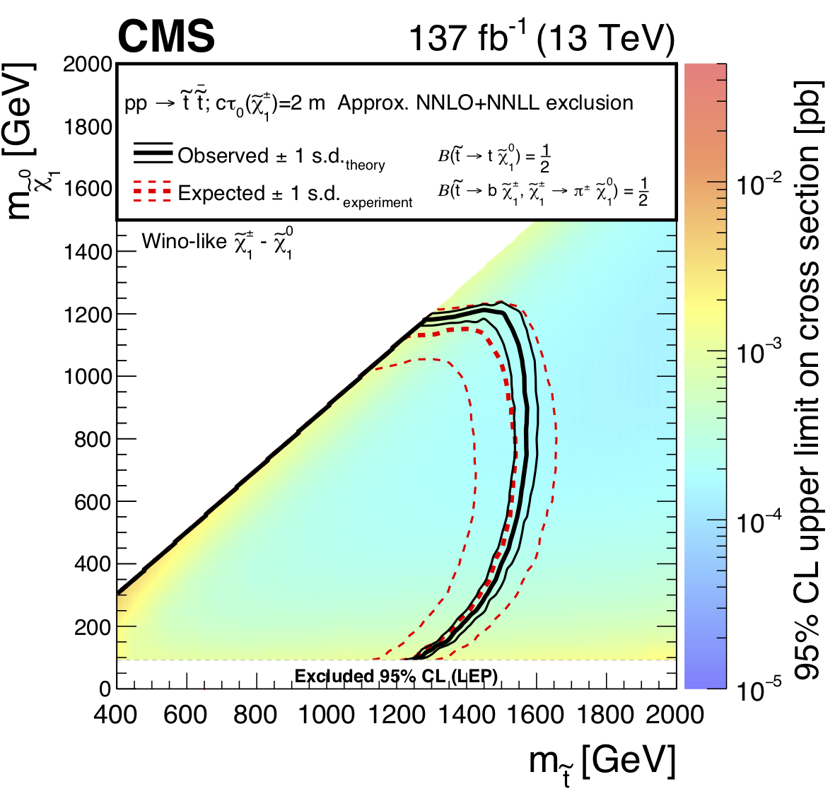
Figure 19-c:
Exclusion limits at 95% CL for top squark pair production with $c\tau _{0}(\tilde{\chi}^{\pm}_1) =$ (upper left) 10 cm, (upper right) 50 cm, and (lower) 200 cm. The area enclosed by the thick black curve represents the observed exclusion region, while the dashed red lines indicate the expected limits and their $\pm $1 standard deviation (s.d.) ranges. The thin black lines show the effect of the theoretical uncertainties in the signal cross section. The white band for masses of the $\tilde{\chi}^0_1$ below 91.9 GeV represents the region of the mass plane excluded at the CERN LEP [145]. Signal cross sections are calculated at approximately NNLO+NNLL order in ${\alpha _S}$ [136,137,138,139,140,141], assuming decay branching fractions ($\mathcal {B}$) as indicated in the figure. |
png pdf |
Figure 20:
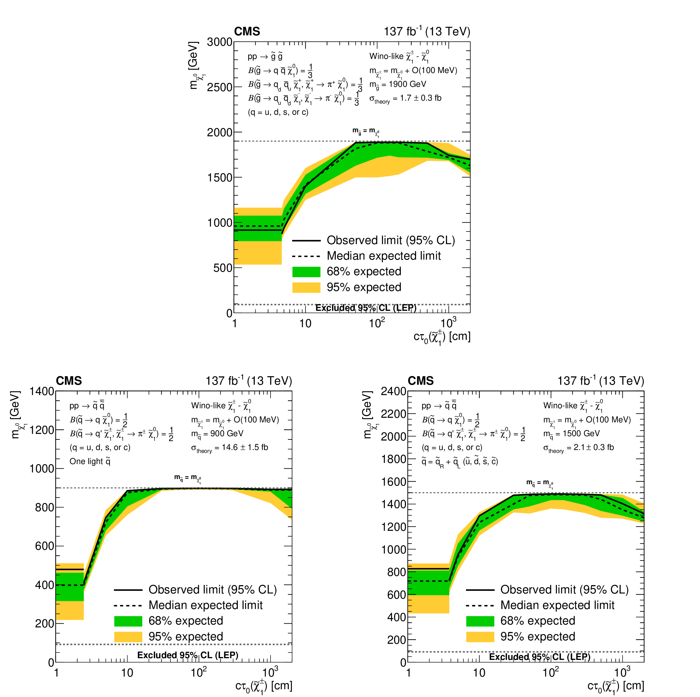
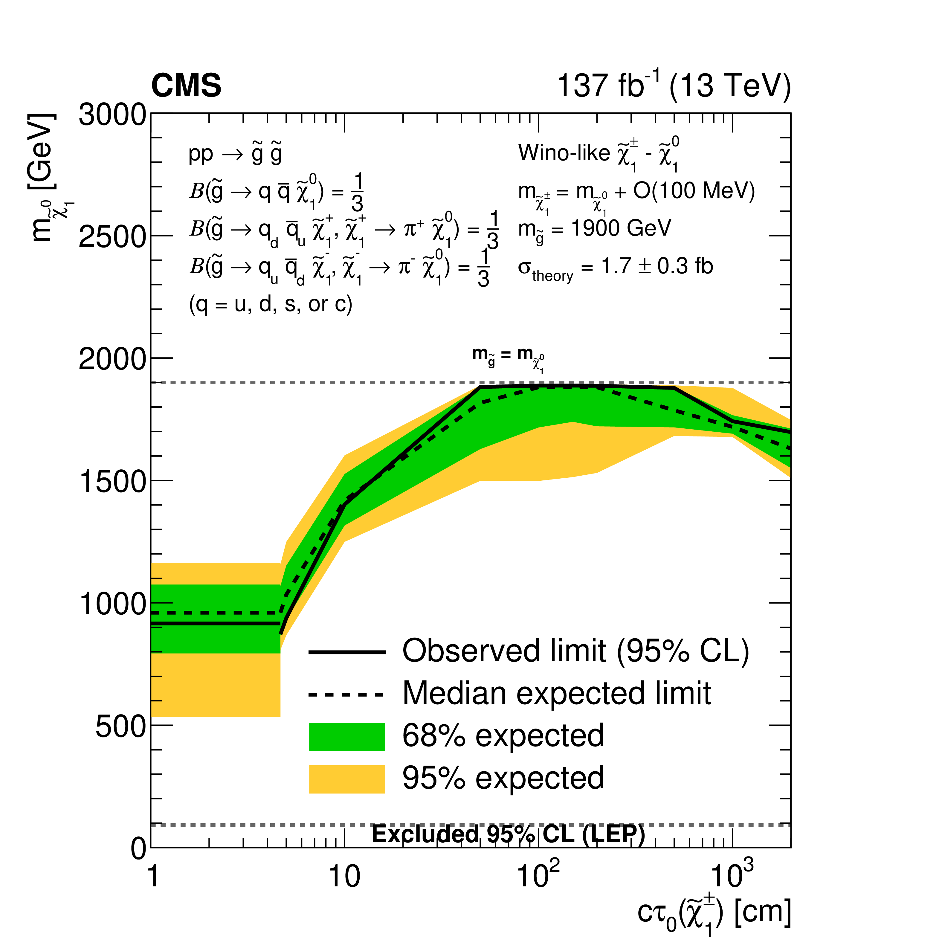
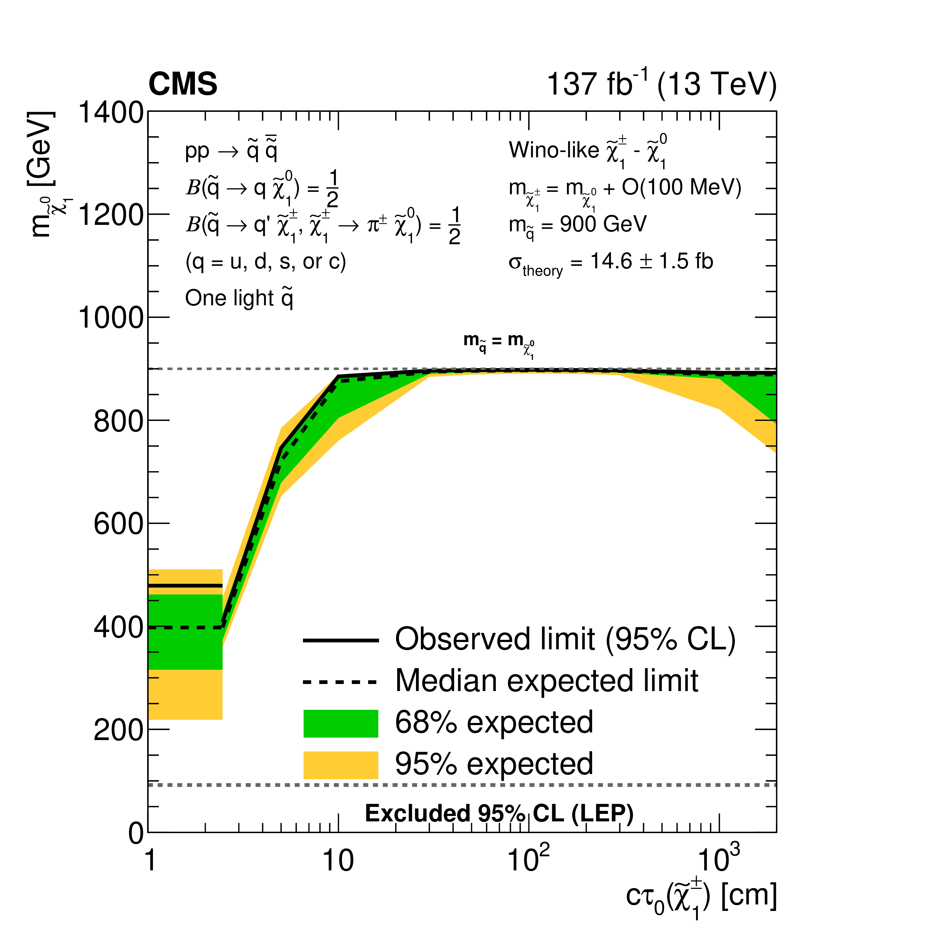
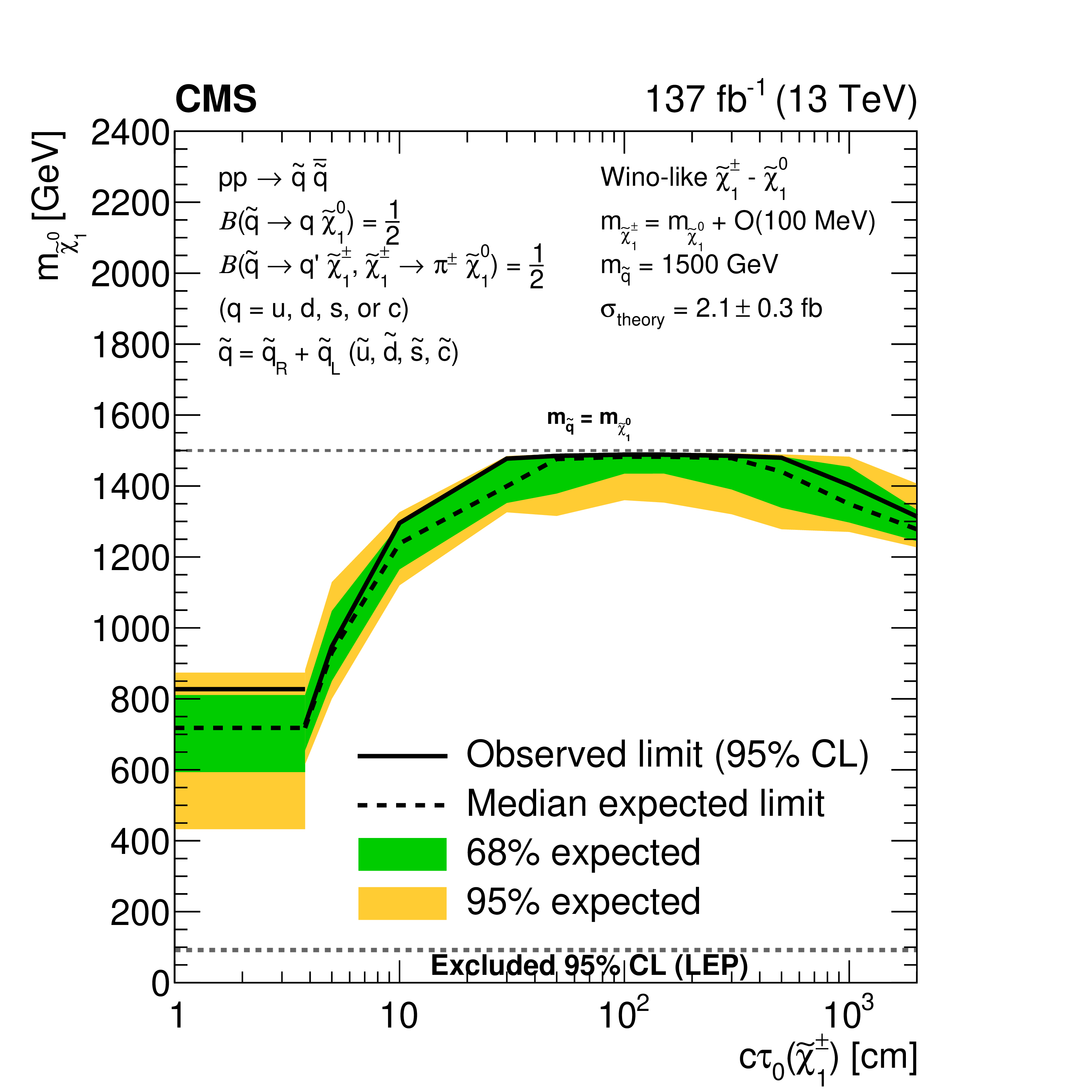
Exclusion limits at 95% CL on the $\tilde{\chi}^0_1$ mass, with $m_{\tilde{\chi}^{\pm}_1}=m_{\tilde{\chi}^0_1}+\mathcal {O}$(100 MeV), as a function of the $\tilde{\chi}^{\pm}_1$ proper decay length, for (upper) direct gluino and (lower) direct light-flavor (u, d, s, c) squark pair production, as obtained for representative gluino and squark masses. The gluinos decay to light-flavor quarks. For direct squark pair production, we assume either (lower left) one-fold or (lower right) eight-fold squark degeneracy. The area enclosed by the solid (dashed) black curve represents the observed (median expected) exclusion region, while the inner green (outer yellow) band indicates the region containing 68 (95)% of the distribution of limits expected under the background-only hypothesis. At short decay lengths, horizontal exclusion lines are obtained from the inclusive ${M_{\mathrm {T2}}}$ search, as this is not affected by track reconstruction inefficiencies, which may arise when the $\tilde{\chi}^{\pm}_1$ decays before the CMS tracker, and therefore shows better sensitivity to scenarios with very small $c\tau _{0}(\tilde{\chi}^{\pm}_1)$ compared to the disappearing track search, based on median expected limits. The horizontal dashed lines at (upper) $m_{{\mathrm{\tilde{g}}}}=m_{\tilde{\chi}^0_1}$ and (lower) $m_{\tilde{\mathrm{q}}}=m_{\tilde{\chi}^0_1}$ bound the mass range in which the decays are kinematically allowed. If all kinematically allowed $\tilde{\chi}^0_1$ masses ($m_{\tilde{\chi}^0_1} \leq m_{{\mathrm{\tilde{g}}}}$, or $m_{\tilde{\chi}^0_1} \leq m_{\tilde{\mathrm{q}}}$) are excluded, the curves, including 68 and 95% expected, tend to overlap. The band at masses of the $\tilde{\chi}^0_1$ below 91.9 GeV represents the region of the mass plane excluded at the CERN LEP [145]. Signal cross sections are calculated at approximately NNLO+NNLL order in ${\alpha _S}$ [136,137,138,139,140,141], assuming decay branching fractions ($\mathcal {B}$) as indicated in the figure. |
png pdf root |
Figure 20-a:
Exclusion limits at 95% CL on the $\tilde{\chi}^0_1$ mass, with $m_{\tilde{\chi}^{\pm}_1}=m_{\tilde{\chi}^0_1}+\mathcal {O}$(100 MeV), as a function of the $\tilde{\chi}^{\pm}_1$ proper decay length, for (upper) direct gluino and (lower) direct light-flavor (u, d, s, c) squark pair production, as obtained for representative gluino and squark masses. The gluinos decay to light-flavor quarks. For direct squark pair production, we assume either (lower left) one-fold or (lower right) eight-fold squark degeneracy. The area enclosed by the solid (dashed) black curve represents the observed (median expected) exclusion region, while the inner green (outer yellow) band indicates the region containing 68 (95)% of the distribution of limits expected under the background-only hypothesis. At short decay lengths, horizontal exclusion lines are obtained from the inclusive ${M_{\mathrm {T2}}}$ search, as this is not affected by track reconstruction inefficiencies, which may arise when the $\tilde{\chi}^{\pm}_1$ decays before the CMS tracker, and therefore shows better sensitivity to scenarios with very small $c\tau _{0}(\tilde{\chi}^{\pm}_1)$ compared to the disappearing track search, based on median expected limits. The horizontal dashed lines at (upper) $m_{{\mathrm{\tilde{g}}}}=m_{\tilde{\chi}^0_1}$ and (lower) $m_{\tilde{\mathrm{q}}}=m_{\tilde{\chi}^0_1}$ bound the mass range in which the decays are kinematically allowed. If all kinematically allowed $\tilde{\chi}^0_1$ masses ($m_{\tilde{\chi}^0_1} \leq m_{{\mathrm{\tilde{g}}}}$, or $m_{\tilde{\chi}^0_1} \leq m_{\tilde{\mathrm{q}}}$) are excluded, the curves, including 68 and 95% expected, tend to overlap. The band at masses of the $\tilde{\chi}^0_1$ below 91.9 GeV represents the region of the mass plane excluded at the CERN LEP [145]. Signal cross sections are calculated at approximately NNLO+NNLL order in ${\alpha _S}$ [136,137,138,139,140,141], assuming decay branching fractions ($\mathcal {B}$) as indicated in the figure. |
png pdf root |
Figure 20-b:
Exclusion limits at 95% CL on the $\tilde{\chi}^0_1$ mass, with $m_{\tilde{\chi}^{\pm}_1}=m_{\tilde{\chi}^0_1}+\mathcal {O}$(100 MeV), as a function of the $\tilde{\chi}^{\pm}_1$ proper decay length, for (upper) direct gluino and (lower) direct light-flavor (u, d, s, c) squark pair production, as obtained for representative gluino and squark masses. The gluinos decay to light-flavor quarks. For direct squark pair production, we assume either (lower left) one-fold or (lower right) eight-fold squark degeneracy. The area enclosed by the solid (dashed) black curve represents the observed (median expected) exclusion region, while the inner green (outer yellow) band indicates the region containing 68 (95)% of the distribution of limits expected under the background-only hypothesis. At short decay lengths, horizontal exclusion lines are obtained from the inclusive ${M_{\mathrm {T2}}}$ search, as this is not affected by track reconstruction inefficiencies, which may arise when the $\tilde{\chi}^{\pm}_1$ decays before the CMS tracker, and therefore shows better sensitivity to scenarios with very small $c\tau _{0}(\tilde{\chi}^{\pm}_1)$ compared to the disappearing track search, based on median expected limits. The horizontal dashed lines at (upper) $m_{{\mathrm{\tilde{g}}}}=m_{\tilde{\chi}^0_1}$ and (lower) $m_{\tilde{\mathrm{q}}}=m_{\tilde{\chi}^0_1}$ bound the mass range in which the decays are kinematically allowed. If all kinematically allowed $\tilde{\chi}^0_1$ masses ($m_{\tilde{\chi}^0_1} \leq m_{{\mathrm{\tilde{g}}}}$, or $m_{\tilde{\chi}^0_1} \leq m_{\tilde{\mathrm{q}}}$) are excluded, the curves, including 68 and 95% expected, tend to overlap. The band at masses of the $\tilde{\chi}^0_1$ below 91.9 GeV represents the region of the mass plane excluded at the CERN LEP [145]. Signal cross sections are calculated at approximately NNLO+NNLL order in ${\alpha _S}$ [136,137,138,139,140,141], assuming decay branching fractions ($\mathcal {B}$) as indicated in the figure. |
png pdf root |
Figure 20-c:
Exclusion limits at 95% CL on the $\tilde{\chi}^0_1$ mass, with $m_{\tilde{\chi}^{\pm}_1}=m_{\tilde{\chi}^0_1}+\mathcal {O}$(100 MeV), as a function of the $\tilde{\chi}^{\pm}_1$ proper decay length, for (upper) direct gluino and (lower) direct light-flavor (u, d, s, c) squark pair production, as obtained for representative gluino and squark masses. The gluinos decay to light-flavor quarks. For direct squark pair production, we assume either (lower left) one-fold or (lower right) eight-fold squark degeneracy. The area enclosed by the solid (dashed) black curve represents the observed (median expected) exclusion region, while the inner green (outer yellow) band indicates the region containing 68 (95)% of the distribution of limits expected under the background-only hypothesis. At short decay lengths, horizontal exclusion lines are obtained from the inclusive ${M_{\mathrm {T2}}}$ search, as this is not affected by track reconstruction inefficiencies, which may arise when the $\tilde{\chi}^{\pm}_1$ decays before the CMS tracker, and therefore shows better sensitivity to scenarios with very small $c\tau _{0}(\tilde{\chi}^{\pm}_1)$ compared to the disappearing track search, based on median expected limits. The horizontal dashed lines at (upper) $m_{{\mathrm{\tilde{g}}}}=m_{\tilde{\chi}^0_1}$ and (lower) $m_{\tilde{\mathrm{q}}}=m_{\tilde{\chi}^0_1}$ bound the mass range in which the decays are kinematically allowed. If all kinematically allowed $\tilde{\chi}^0_1$ masses ($m_{\tilde{\chi}^0_1} \leq m_{{\mathrm{\tilde{g}}}}$, or $m_{\tilde{\chi}^0_1} \leq m_{\tilde{\mathrm{q}}}$) are excluded, the curves, including 68 and 95% expected, tend to overlap. The band at masses of the $\tilde{\chi}^0_1$ below 91.9 GeV represents the region of the mass plane excluded at the CERN LEP [145]. Signal cross sections are calculated at approximately NNLO+NNLL order in ${\alpha _S}$ [136,137,138,139,140,141], assuming decay branching fractions ($\mathcal {B}$) as indicated in the figure. |
png pdf root |
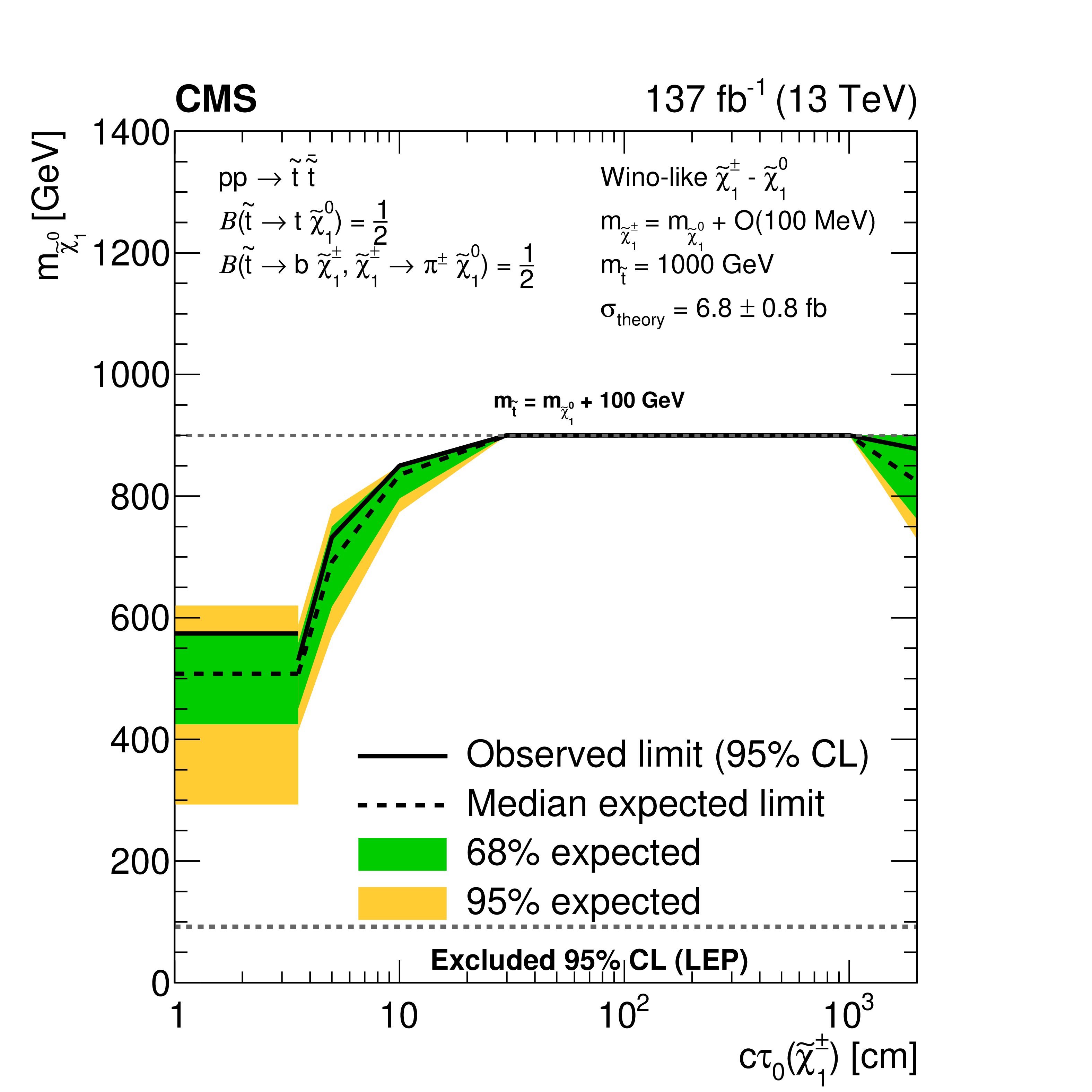
Figure 21:
Exclusion limits at 95% CL on the $\tilde{\chi}^0_1$ mass, with $m_{\tilde{\chi}^{\pm}_1}=m_{\tilde{\chi}^0_1}+\mathcal {O}$(100 MeV), as a function of the $\tilde{\chi}^{\pm}_1$ proper decay length, for direct top squark pair production, as obtained for a representative top squark mass. The area enclosed by the solid (dashed) black curve represents the observed (median expected) exclusion region, while the inner green (outer yellow) band indicates the region containing 68 (95)% of the distribution of limits expected under the background-only hypothesis. At short decay lengths, horizontal exclusion lines are obtained from the inclusive ${M_{\mathrm {T2}}}$ search, as this is not affected by track reconstruction inefficiencies, which may arise when the $\tilde{\chi}^{\pm}_1$ decays before the CMS tracker, and therefore shows better sensitivity to scenarios with very small $c\tau _{0}(\tilde{\chi}^{\pm}_1)$ compared to the disappearing track search, based on median expected limits. The horizontal dashed line at $m_{\tilde{\mathrm{t}}}=m_{\tilde{\chi}^0_1}+$ 100 GeV indicates the minimum simulated mass difference between top squark and $\tilde{\chi}^0_1$, chosen such that the decay of top quarks to on-shell $\mathrm{W} $ bosons is allowed. If all kinematically allowed $\tilde{\chi}^0_1$ masses ($m_{\tilde{\chi}^0_1} \leq m_{\tilde{\mathrm{t}}}-100 GeV $) are excluded, the curves, including 68 and 95% expected, tend to overlap. The band at masses of the $\tilde{\chi}^0_1$ below 91.9 GeV represents the region of the mass plane excluded at the CERN LEP [145]. Signal cross sections are calculated at approximately NNLO+NNLL order in ${\alpha _S}$ [136,137,138,139,140,141], assuming decay branching fractions ($\mathcal {B}$) as indicated in the figure. |
png pdf |
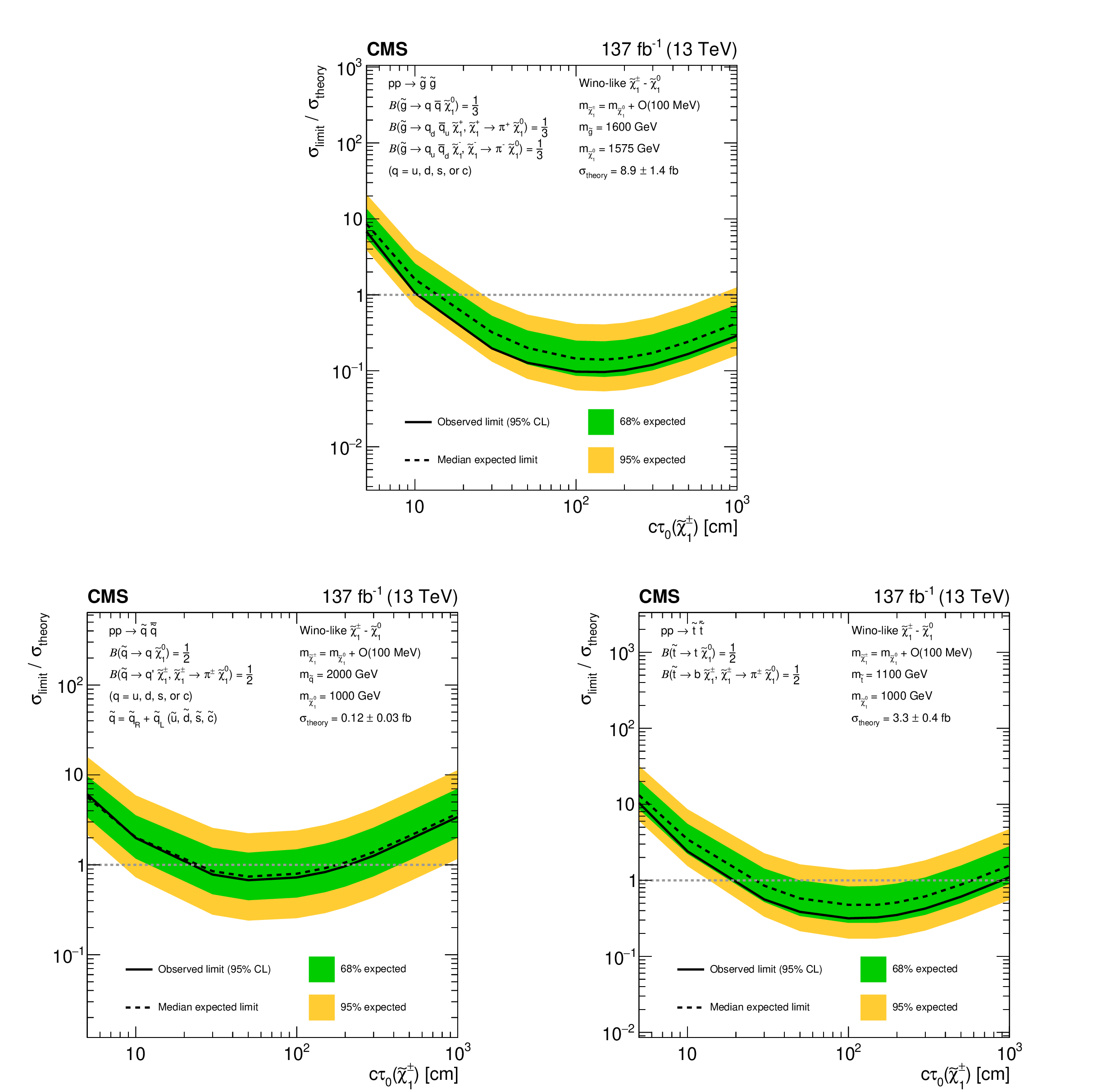
Figure 22:
Exclusion limits at 95% CL on $\sigma /\sigma _{\mathrm {theory}}$ as a function of the $\tilde{\chi}^{\pm}_1$ decay length, for a choice of signal models of (upper) direct gluino pair production where the gluinos decay to light-flavor (u, d, s, c) quarks, (lower left) direct light-flavor squark pair production, and (lower right) direct top squark pair production, as obtained from the search for disappearing tracks. The area enclosed by the solid (dashed) black curve below the horizontal dashed line at $\sigma /\sigma _{\mathrm {theory}}=$ 1 represents the observed (median expected) exclusion region, while the inner green (outer yellow) band indicates the region containing 68 (95)% of the distribution of limits expected under the background-only hypothesis. Signal cross sections are calculated at approximately NNLO+NNLL order in ${\alpha _S}$ [136,137,138,139,140,141], assuming decay branching fractions ($\mathcal {B}$) as indicated in the figure. |
png pdf root |
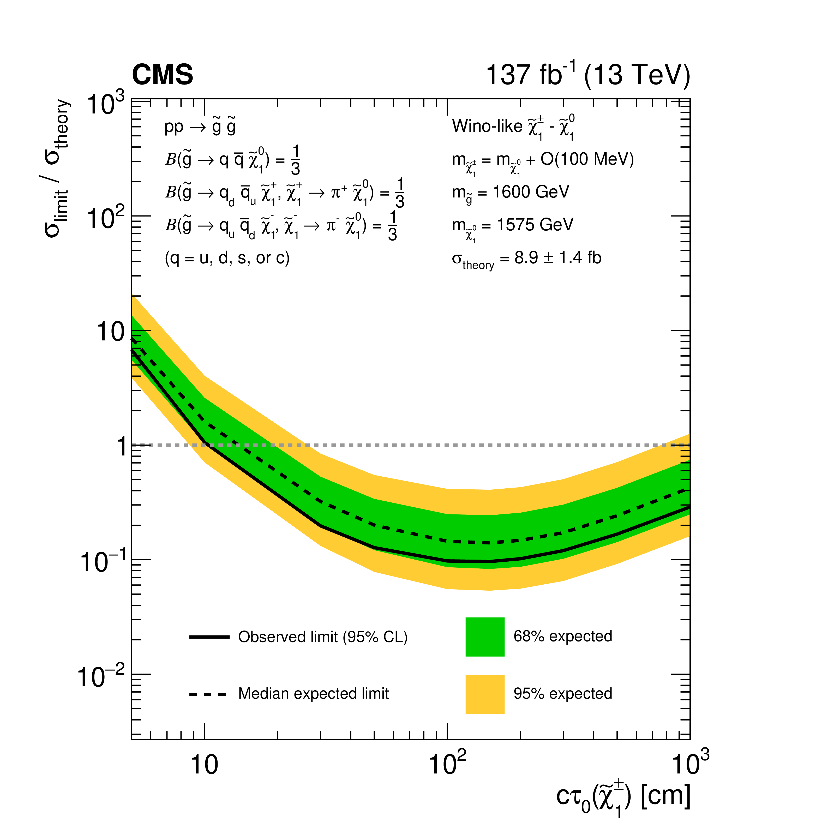
Figure 22-a:
Exclusion limits at 95% CL on $\sigma /\sigma _{\mathrm {theory}}$ as a function of the $\tilde{\chi}^{\pm}_1$ decay length, for a choice of signal models of (upper) direct gluino pair production where the gluinos decay to light-flavor (u, d, s, c) quarks, (lower left) direct light-flavor squark pair production, and (lower right) direct top squark pair production, as obtained from the search for disappearing tracks. The area enclosed by the solid (dashed) black curve below the horizontal dashed line at $\sigma /\sigma _{\mathrm {theory}}=$ 1 represents the observed (median expected) exclusion region, while the inner green (outer yellow) band indicates the region containing 68 (95)% of the distribution of limits expected under the background-only hypothesis. Signal cross sections are calculated at approximately NNLO+NNLL order in ${\alpha _S}$ [136,137,138,139,140,141], assuming decay branching fractions ($\mathcal {B}$) as indicated in the figure. |
png pdf root |
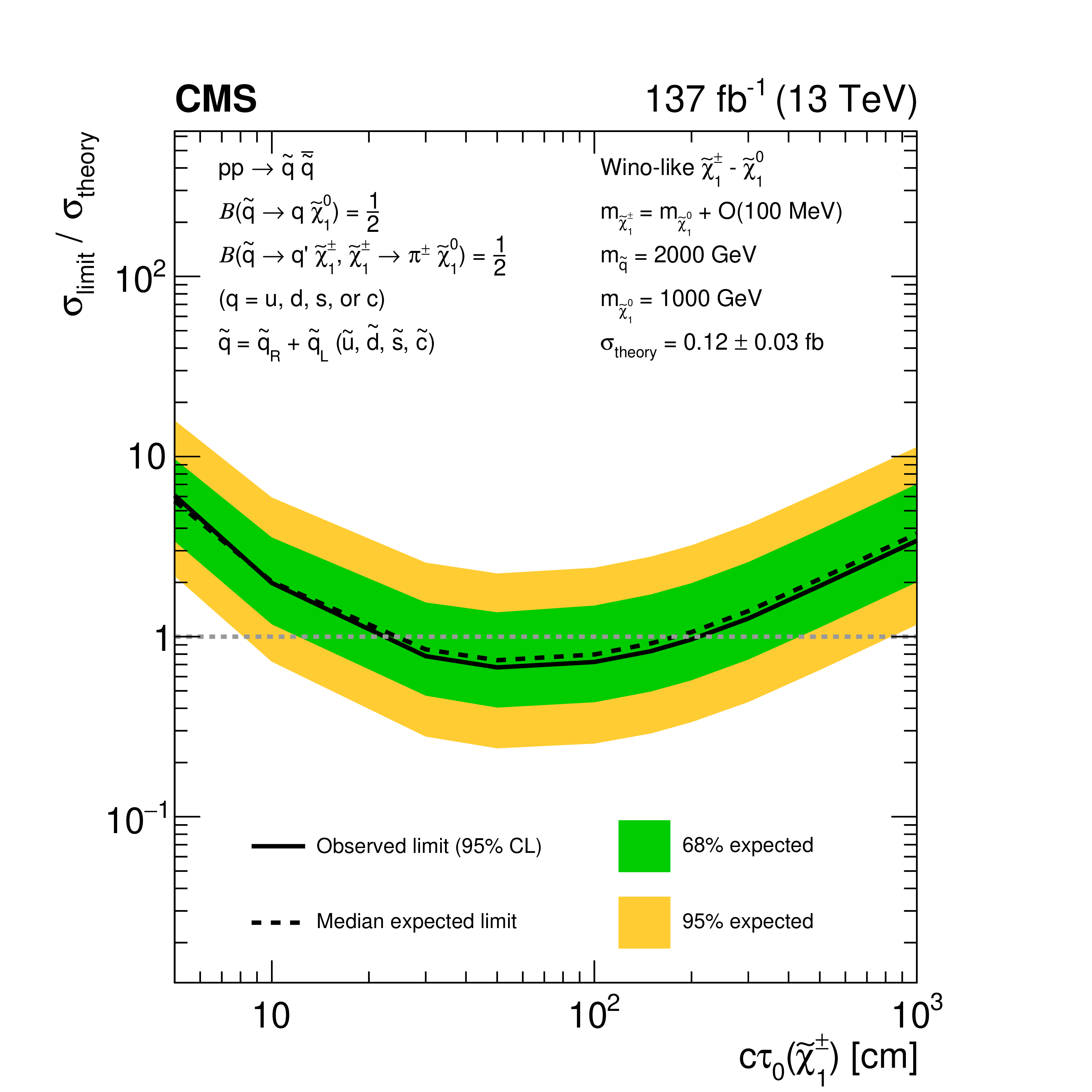
Figure 22-b:
Exclusion limits at 95% CL on $\sigma /\sigma _{\mathrm {theory}}$ as a function of the $\tilde{\chi}^{\pm}_1$ decay length, for a choice of signal models of (upper) direct gluino pair production where the gluinos decay to light-flavor (u, d, s, c) quarks, (lower left) direct light-flavor squark pair production, and (lower right) direct top squark pair production, as obtained from the search for disappearing tracks. The area enclosed by the solid (dashed) black curve below the horizontal dashed line at $\sigma /\sigma _{\mathrm {theory}}=$ 1 represents the observed (median expected) exclusion region, while the inner green (outer yellow) band indicates the region containing 68 (95)% of the distribution of limits expected under the background-only hypothesis. Signal cross sections are calculated at approximately NNLO+NNLL order in ${\alpha _S}$ [136,137,138,139,140,141], assuming decay branching fractions ($\mathcal {B}$) as indicated in the figure. |

png pdf root |
Figure 22-c:
Exclusion limits at 95% CL on $\sigma /\sigma _{\mathrm {theory}}$ as a function of the $\tilde{\chi}^{\pm}_1$ decay length, for a choice of signal models of (upper) direct gluino pair production where the gluinos decay to light-flavor (u, d, s, c) quarks, (lower left) direct light-flavor squark pair production, and (lower right) direct top squark pair production, as obtained from the search for disappearing tracks. The area enclosed by the solid (dashed) black curve below the horizontal dashed line at $\sigma /\sigma _{\mathrm {theory}}=$ 1 represents the observed (median expected) exclusion region, while the inner green (outer yellow) band indicates the region containing 68 (95)% of the distribution of limits expected under the background-only hypothesis. Signal cross sections are calculated at approximately NNLO+NNLL order in ${\alpha _S}$ [136,137,138,139,140,141], assuming decay branching fractions ($\mathcal {B}$) as indicated in the figure. |
png pdf |
Figure 23:
(Upper) Comparison of the estimated background and observed data events in each signal bin in the very-low-${H_{\mathrm {T}}}$ region. The hatched bands represent the full uncertainty in the background estimate. The notations j, b indicate ${N_{\mathrm {j}}}, {N_{\mathrm{b}}}$ labeling. (Lower) Same for the low-${H_{\mathrm {T}}}$ region. On the $x$ axis, the ${M_{\mathrm {T2}}}$ binning is shown in units of GeV. |
png pdf |
Figure 23-a:
(Upper) Comparison of the estimated background and observed data events in each signal bin in the very-low-${H_{\mathrm {T}}}$ region. The hatched bands represent the full uncertainty in the background estimate. The notations j, b indicate ${N_{\mathrm {j}}}, {N_{\mathrm{b}}}$ labeling. (Lower) Same for the low-${H_{\mathrm {T}}}$ region. On the $x$ axis, the ${M_{\mathrm {T2}}}$ binning is shown in units of GeV. |
png pdf |
Figure 23-b:
(Upper) Comparison of the estimated background and observed data events in each signal bin in the very-low-${H_{\mathrm {T}}}$ region. The hatched bands represent the full uncertainty in the background estimate. The notations j, b indicate ${N_{\mathrm {j}}}, {N_{\mathrm{b}}}$ labeling. (Lower) Same for the low-${H_{\mathrm {T}}}$ region. On the $x$ axis, the ${M_{\mathrm {T2}}}$ binning is shown in units of GeV. |
png pdf |
Figure 24:
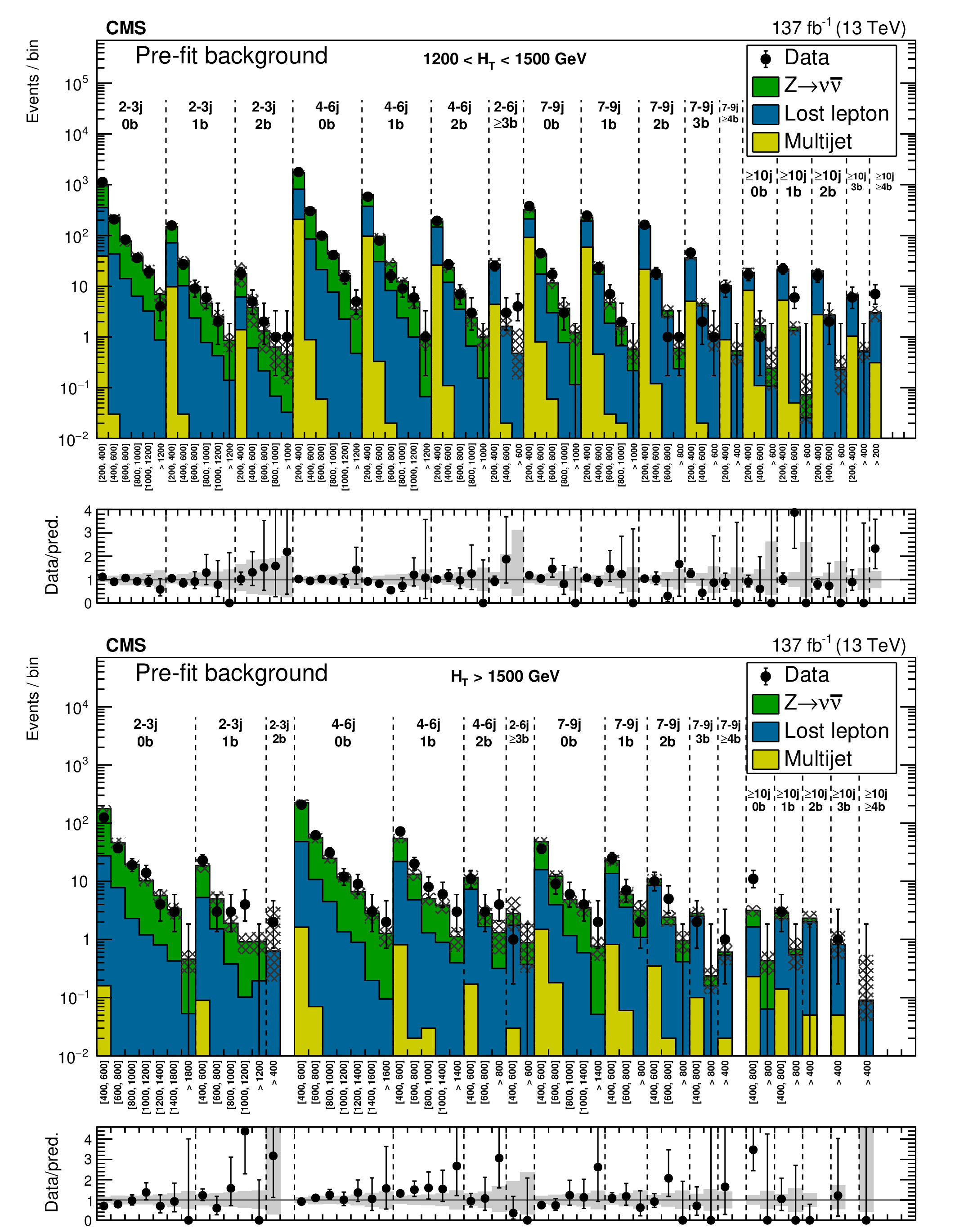
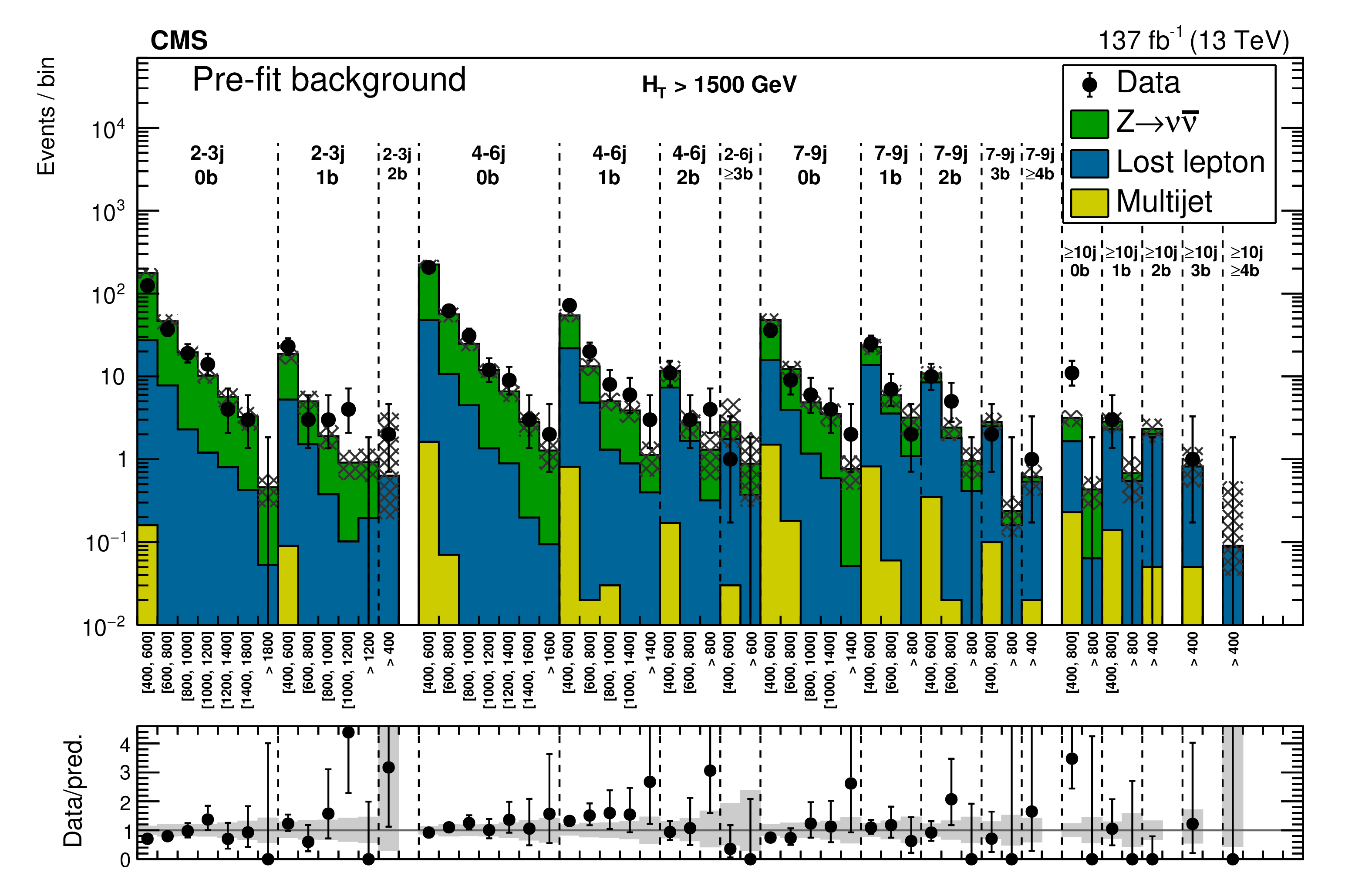
(Upper) Comparison of the estimated background and observed data events in each signal bin in the high-${H_{\mathrm {T}}}$ region. The hatched bands represent the full uncertainty in the background estimate. The notations j, b indicate ${N_{\mathrm {j}}}$, $ {N_{\mathrm{b}}}$ labeling. (Lower) Same for the extreme-${H_{\mathrm {T}}}$ region. On the $x$ axis, the ${M_{\mathrm {T2}}}$ binning is shown in units of GeV. |
png pdf |
Figure 24-a:
(Upper) Comparison of the estimated background and observed data events in each signal bin in the high-${H_{\mathrm {T}}}$ region. The hatched bands represent the full uncertainty in the background estimate. The notations j, b indicate ${N_{\mathrm {j}}}$, $ {N_{\mathrm{b}}}$ labeling. (Lower) Same for the extreme-${H_{\mathrm {T}}}$ region. On the $x$ axis, the ${M_{\mathrm {T2}}}$ binning is shown in units of GeV. |
png pdf |
Figure 24-b:
(Upper) Comparison of the estimated background and observed data events in each signal bin in the high-${H_{\mathrm {T}}}$ region. The hatched bands represent the full uncertainty in the background estimate. The notations j, b indicate ${N_{\mathrm {j}}}$, $ {N_{\mathrm{b}}}$ labeling. (Lower) Same for the extreme-${H_{\mathrm {T}}}$ region. On the $x$ axis, the ${M_{\mathrm {T2}}}$ binning is shown in units of GeV. |
| Tables | |
png pdf |
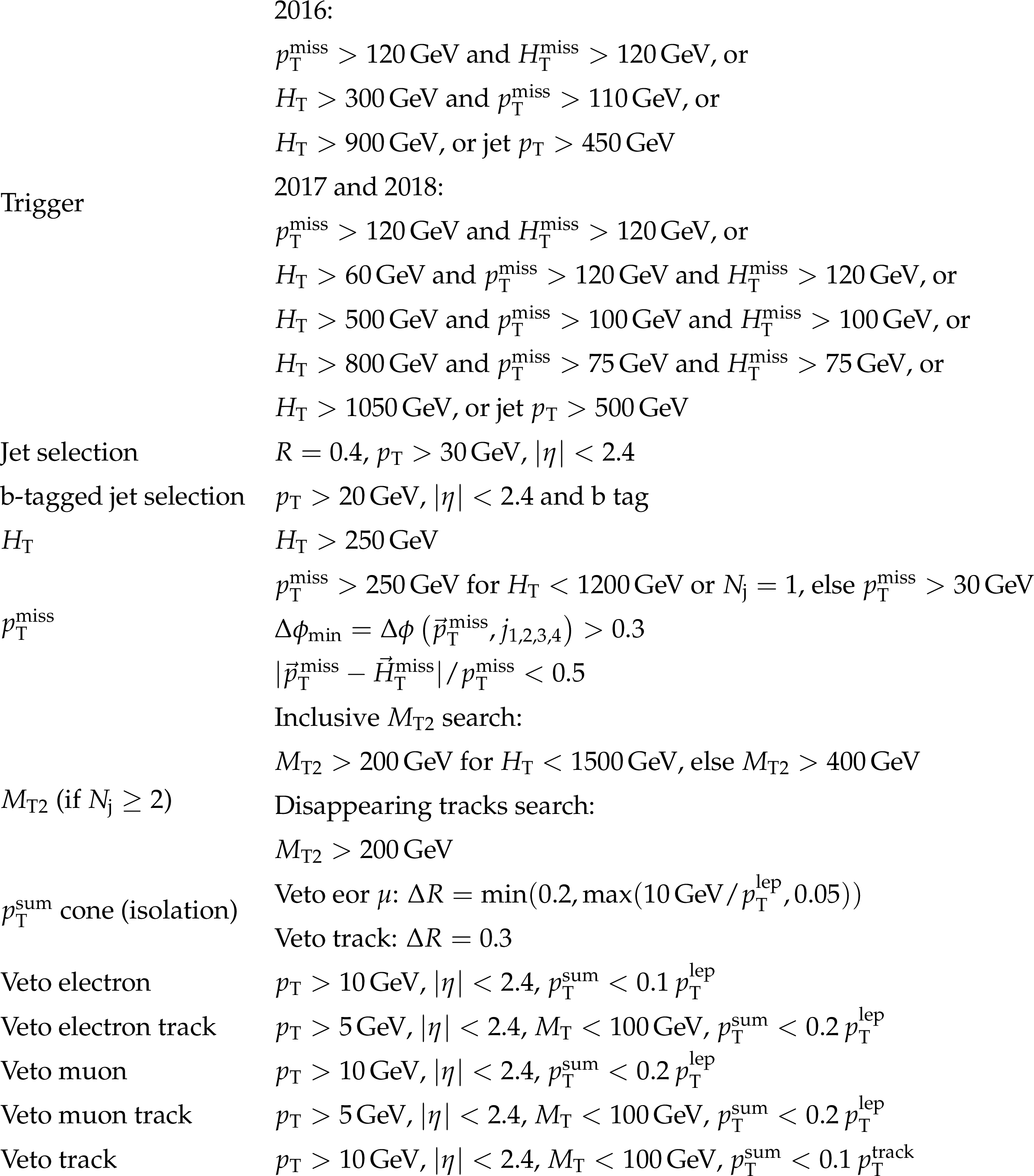
Table 1:
Summary of the trigger requirements and the kinematic offline event preselection requirements on the reconstructed physics objects, for both the inclusive ${M_{\mathrm {T2}}}$ search and the search for disappearing tracks. Here $R$ is the distance parameter of the anti-$ {k_{\mathrm {T}}}$ algorithm. To veto leptons and tracks, the transverse mass ${M_{\mathrm {T}}}$ is determined using the veto object and the ${\vec{p}_{\mathrm {T}}^{\,\text {miss}}}$. The variable $ {p_{\mathrm {T}}} ^{\text {sum}}$ is a measure of object isolation and it denotes the ${p_{\mathrm {T}}}$ sum of all additional PF candidates in a cone around the lepton or the track. The size of the cone is listed in the table in units of $\Delta R \equiv \sqrt {\smash [b]{(\Delta \phi)^2 + (\Delta \eta)^2}}$. The lepton (track) ${p_{\mathrm {T}}}$ is denoted as $ {p_{\mathrm {T}}} ^{\text {lep}}$ ($ {p_{\mathrm {T}}} ^{\text {track}}$). Further details of the lepton selection are given in Refs. [9,96]. The $i$th-highest ${p_{\mathrm {T}}}$ jet is denoted as $j_\mathrm {i}$. |
png pdf |
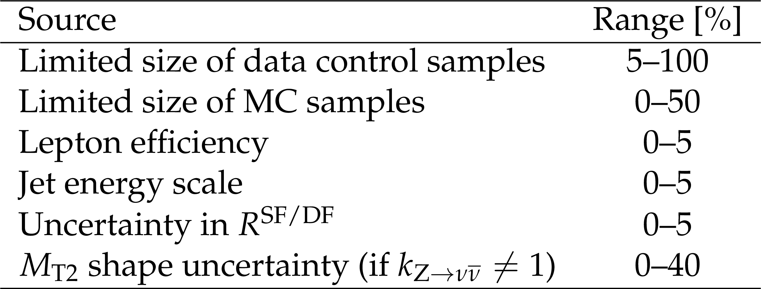
Table 2:
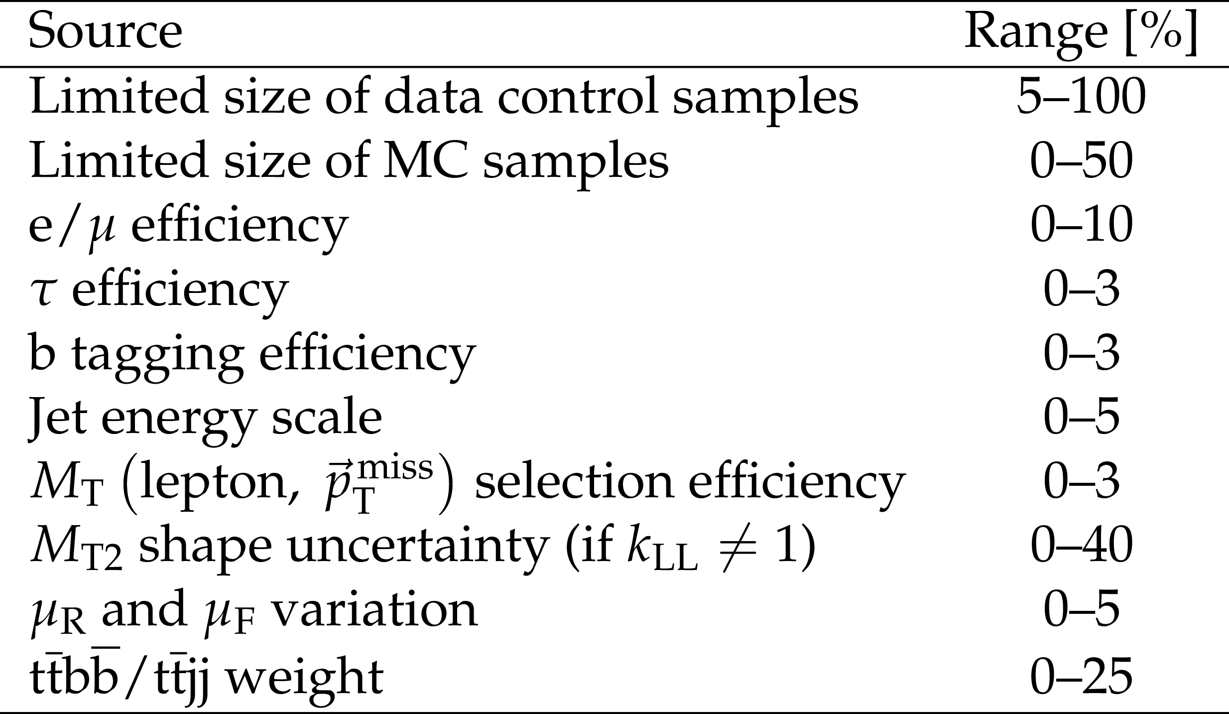
Summary of systematic uncertainties in the lost-lepton background prediction, together with their typical size ranges across the search bins. |
png pdf |
Table 3:
Summary of systematic uncertainties in the $\mathrm{Z} \to \nu \bar{\nu} $ background prediction, together with their typical size ranges across the search bins. |
png pdf |
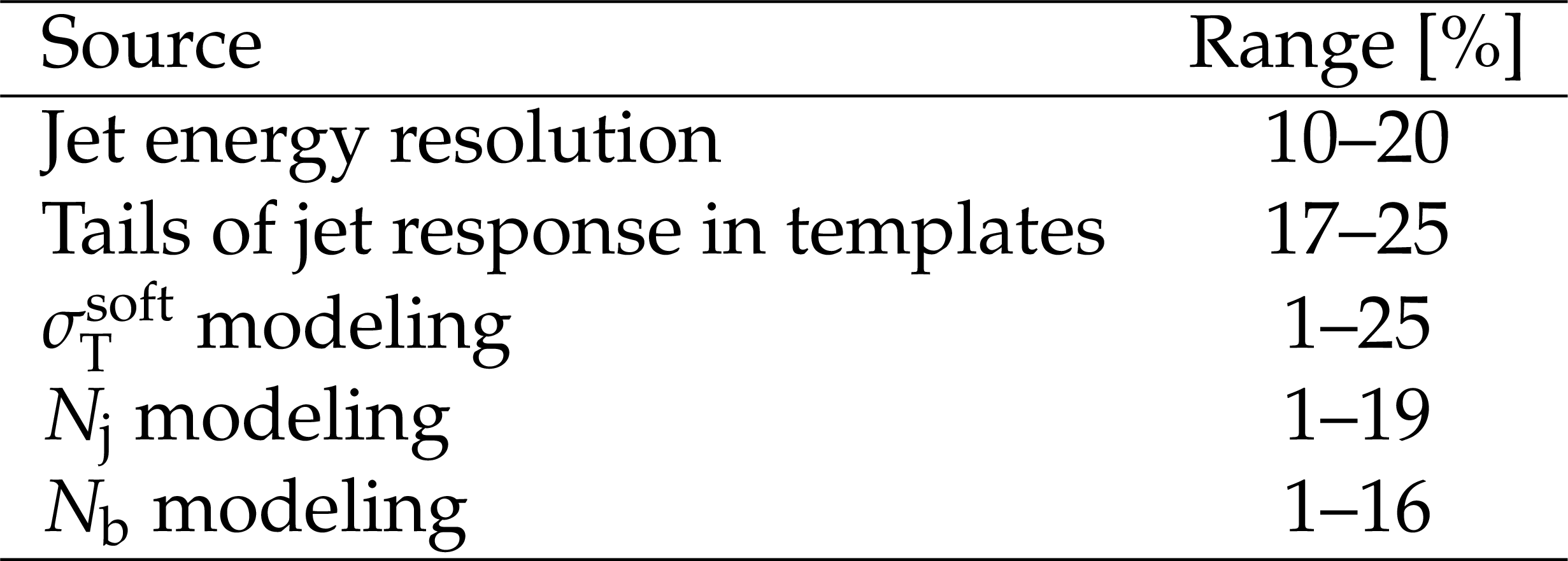
Table 4:
Summary of systematic uncertainties in the multijet background prediction, together with their typical size ranges across the search bins. |
png pdf |
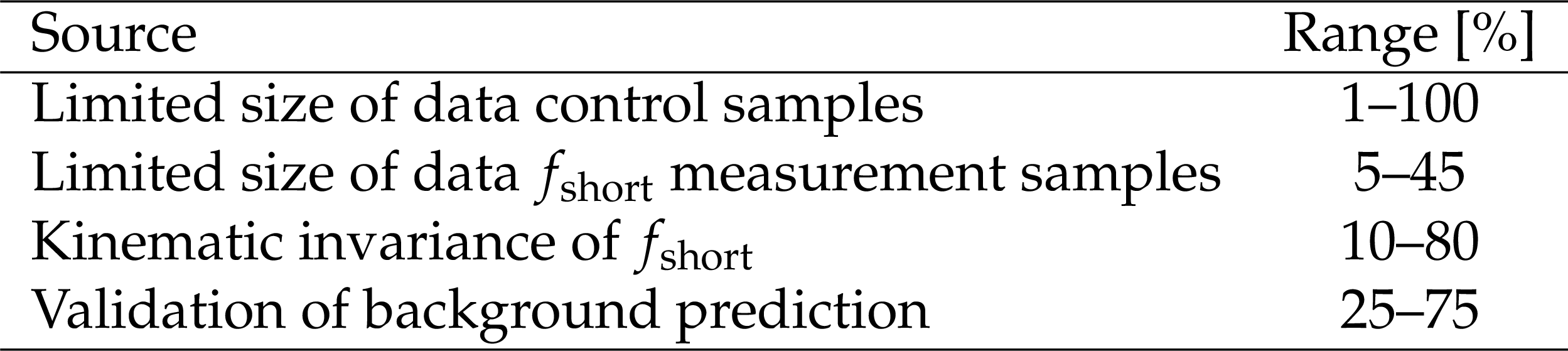
Table 5:
Summary of systematic uncertainties in the disappearing track background prediction, together with their typical size ranges across the search bins. The systematic uncertainties arising from the assumption of kinematic invariance of ${f_{\text {short}}}$ and from the validation of the background prediction are always taken to be at least as large as the statistical uncertainties on the measured values of ${f_{\text {short}}}$ and on the background prediction in the validation region, respectively. |
png pdf |
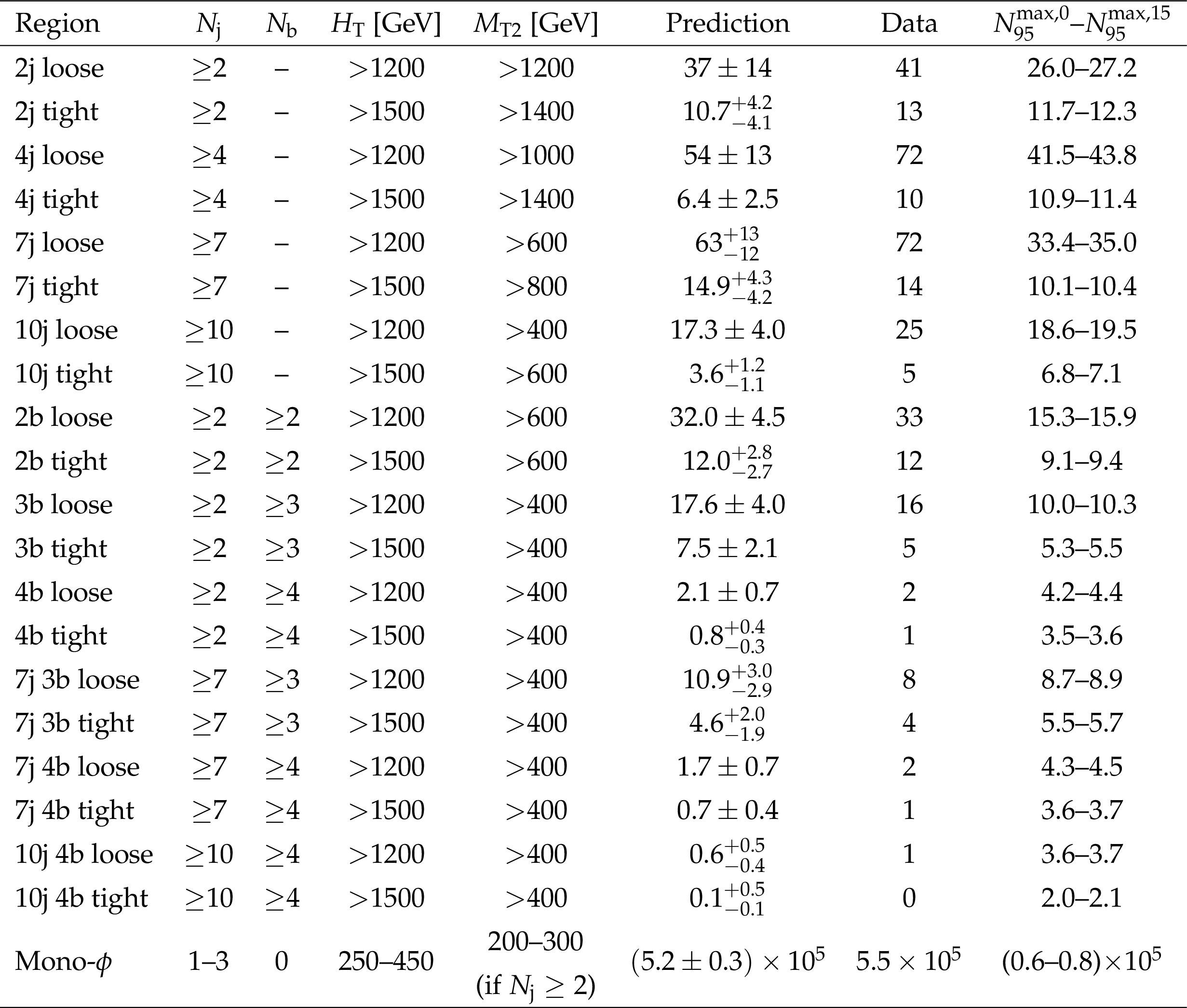
Table 6:
Definitions of super signal regions, along with predictions, observed data, and the observed 95% CL upper limits on the number of signal events contributing to each region ($N_{95}^{\mathrm {max}}$). The limits are shown as a range corresponding to an assumed uncertainty in the signal acceptance of 0 or 15% ($N_{95}^{\mathrm {max},0}$-$N_{95}^{\mathrm {max},15}$). A dash in the selection criteria means that no requirement is applied. All selection criteria as in the full analysis are applied. For regions with $ {N_{\mathrm {j}}} =$ 1, $ {H_{\mathrm {T}}} \equiv {{p_{\mathrm {T}}} ^{\text {jet}}} $. The mono-$\phi $ super signal region corresponds to the subset of analysis bins identified in Refs. [35,36] as showing a significant excess in data based on the results of Ref. [9]. |
png pdf |
Table 7:
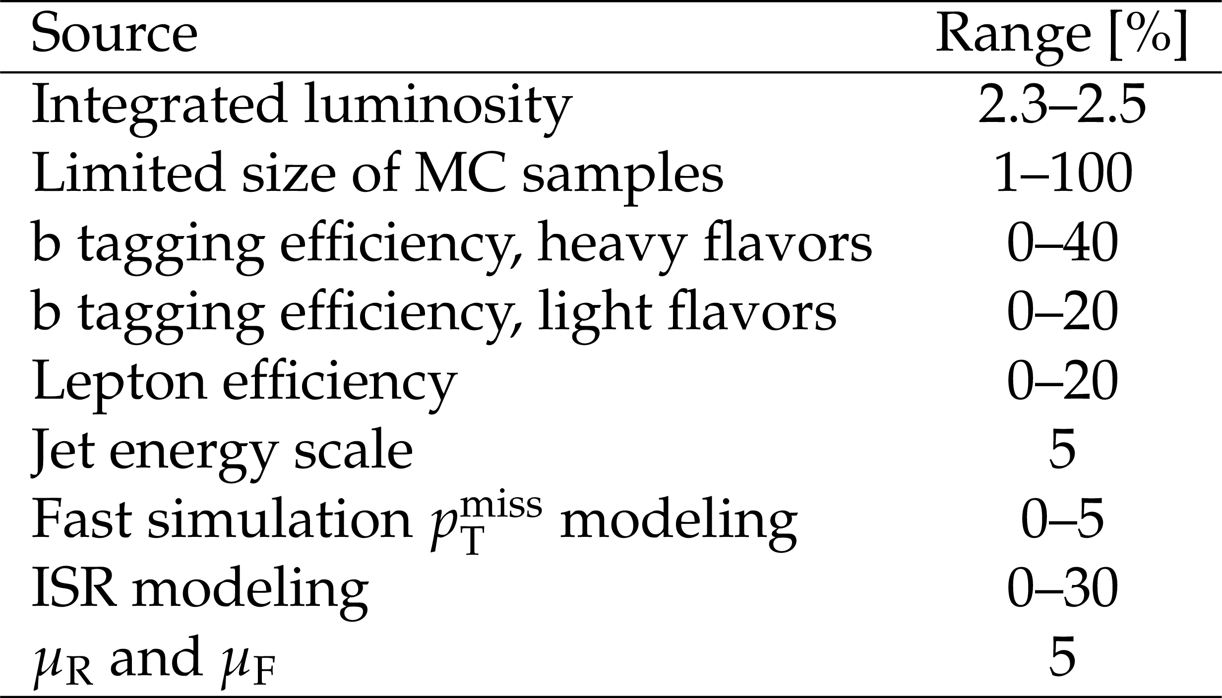
Systematic uncertainties in the signal yields for the simplified models of BSM physics. The large statistical uncertainties in the simulated signal sample come from a small number of bins with low acceptance, which are typically not among the most sensitive bins contributing to a given model benchmark point. |
png pdf |
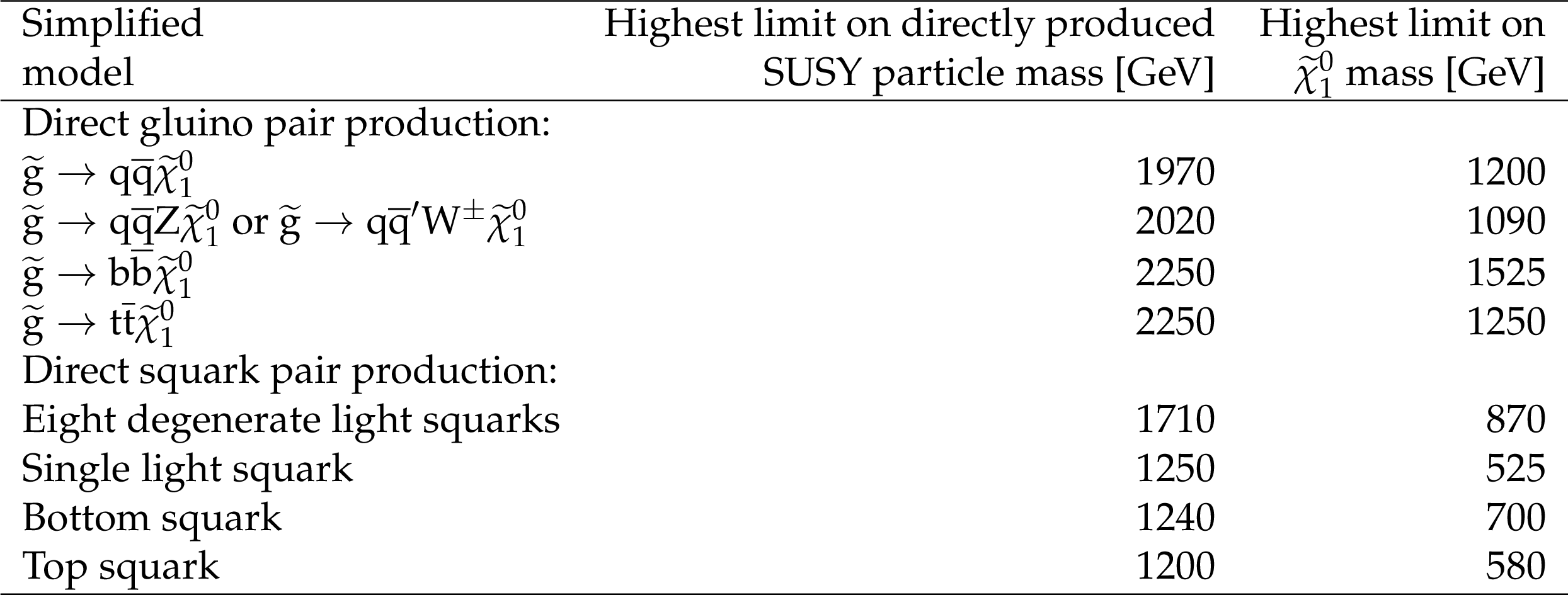
Table 8:
Summary of the observed 95% CL exclusion limits on the masses of SUSY particles for different simplified model scenarios. The highest limits on the mass of the directly produced particles and on the mass of the $\tilde{\chi}^0_1$ are quoted. |

png pdf |
Table 9:
Summary of the observed 95% CL exclusion limits on the masses of LQs for the considered scenarios. The columns show scalar or vector LQ with the choice of $\kappa $, while the rows show the LQ decay channel. For mixed-decay scenarios, the assumed branching fractions ($\mathcal {B}$) are indicated. |

png pdf |
Table 10:
Summary of the observed 95% CL exclusion limits on the masses of SUSY particles for different simplified model scenarios, where the produced particles decay with equal probability to $\tilde{\chi}^{+}_1$, $\tilde{\chi}^{-}_1$, and $\tilde{\chi}^0_1$, and the $\tilde{\chi}^{\pm}_1$ are long lived. The highest limits on the mass of the directly produced particles and on the mass of the $\tilde{\chi}^0_1$ are quoted. |
png pdf |
Table 11:
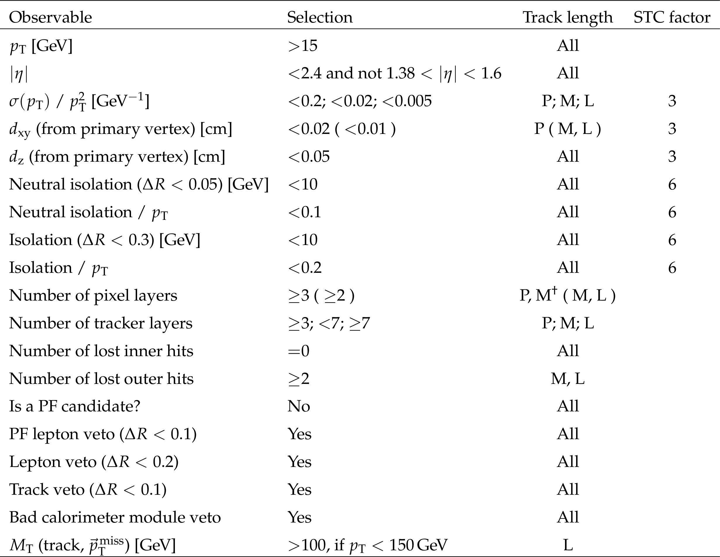
Selection requirements for STs and STCs. For the subset of medium (M) length tracks that have just four tracking layers with a measurement, the minimum required number of layers of the pixel tracking detector with a measurement is three ($\dagger $). The selected tracks are required to not overlap with identified leptons. For this selection, all electrons and muons are considered, either identified as PF candidates or not. The selected tracks are as well required to not be identified as PF candidates, and to not overlap with other tracks with $ {p_{\mathrm {T}}} > $ 15 GeV, even if those tracks are not associated with PF candidates. The factor by which the selection requirement is relaxed in order to select short track candidates is also reported. If no factor is reported, the requirement is not relaxed for the selection of short track candidates. |
png pdf |
Table 12:
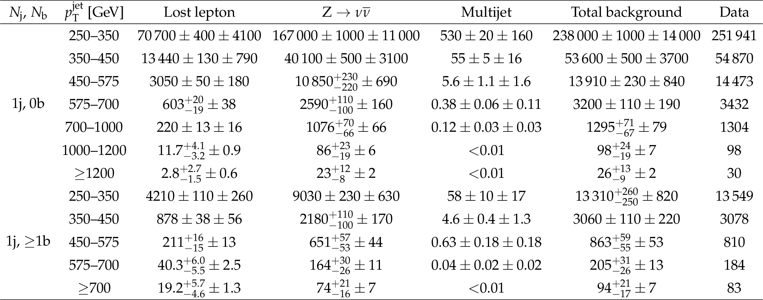
Predictions and observations for the 12 search regions with $ {N_{\mathrm {j}}} = $ 1. For each of the background predictions, the first uncertainty listed is statistical (from the limited size of data control samples and Monte Carlo samples), and the second is systematic. |
png pdf |
Table 13:
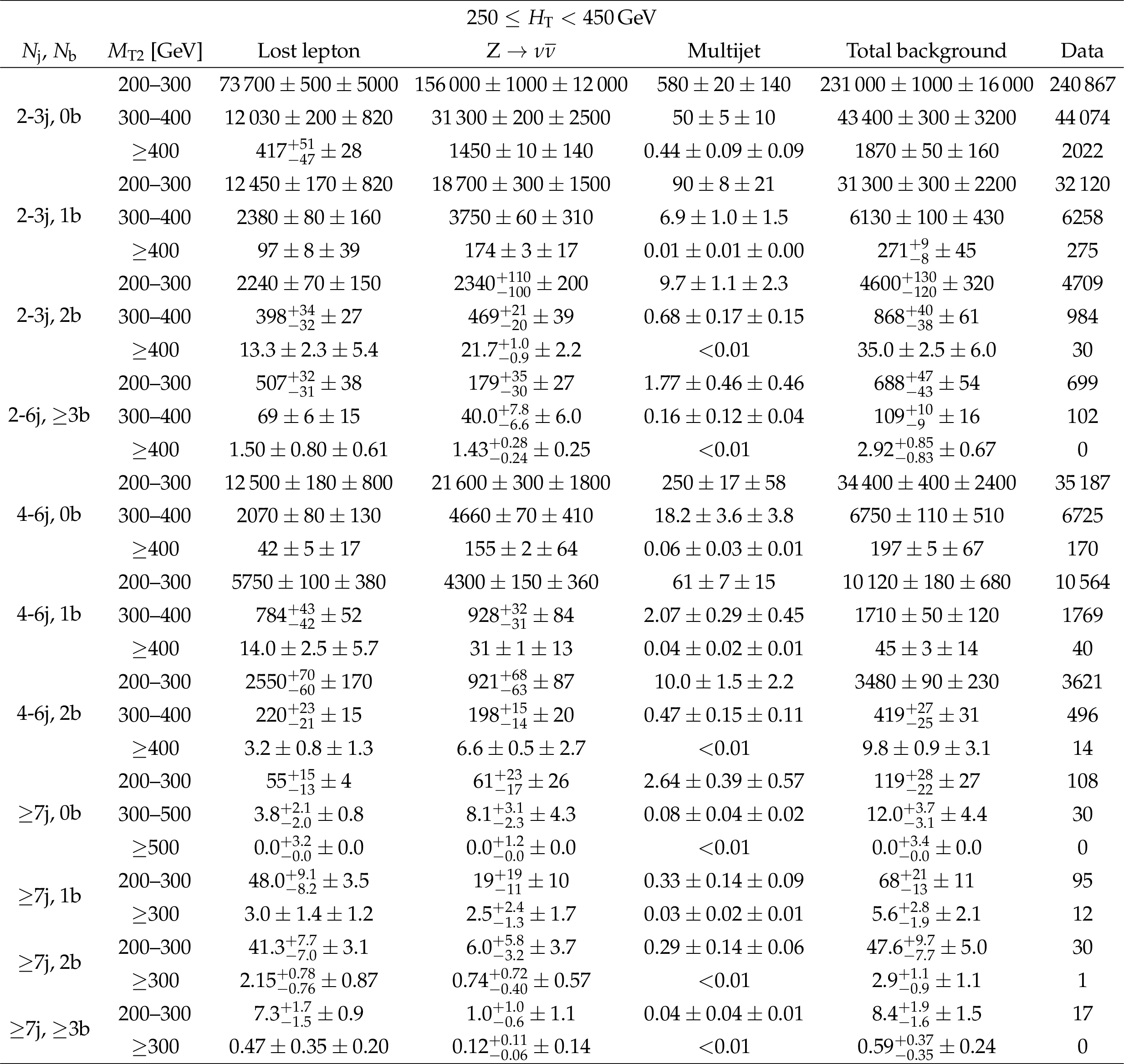
Predictions and observations for the 30 search regions with 250 $ \leq {H_{\mathrm {T}}} < $ 450 GeV. For each of the background predictions, the first uncertainty listed is statistical (from the limited size of data control samples and Monte Carlo samples), and the second is systematic. |
png pdf |
Table 14:
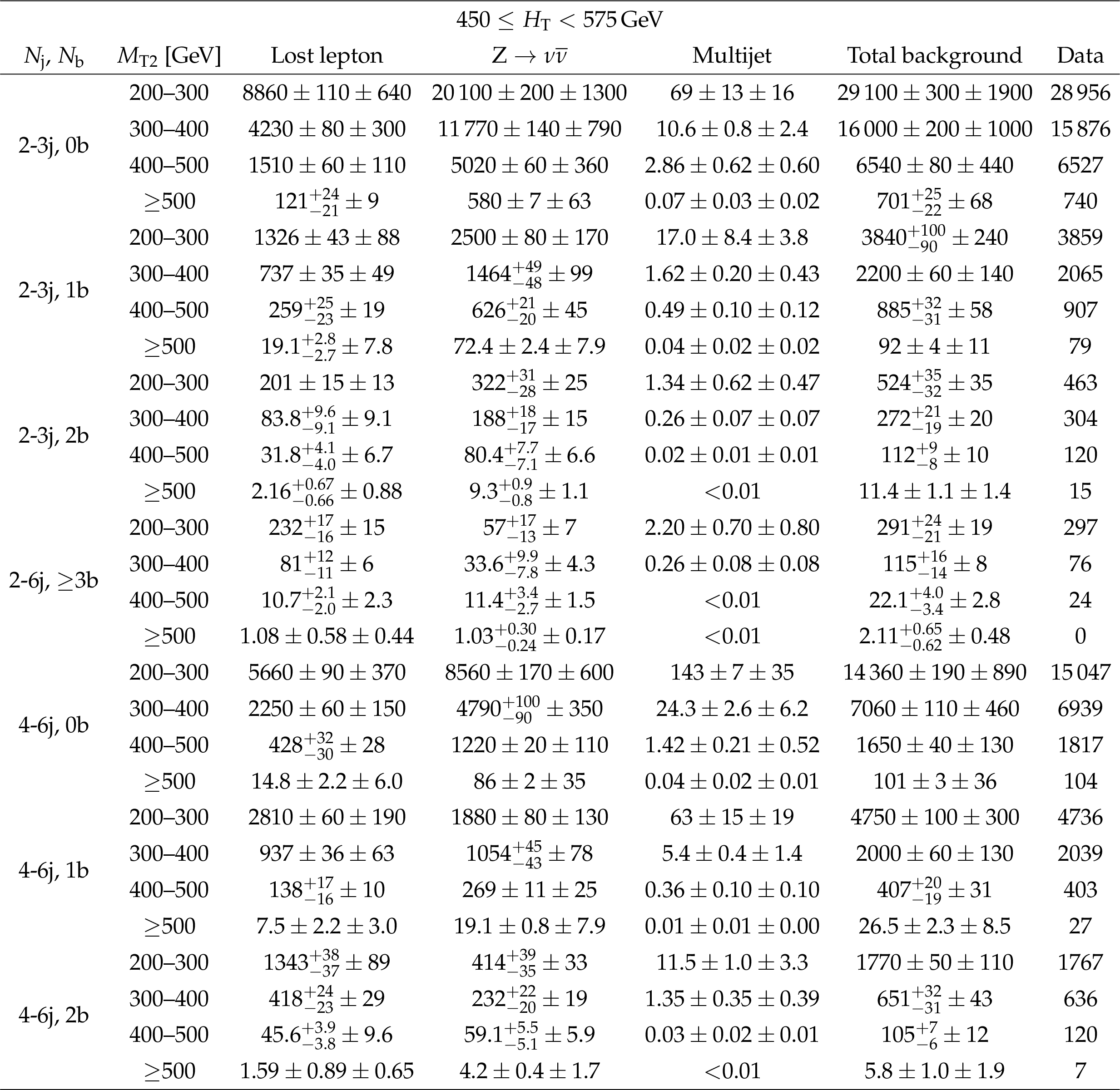
Predictions and observations for the 28 search regions with 450 $ \leq {H_{\mathrm {T}}} < $ 575 GeV, and 2 $\leq {N_{\mathrm {j}}} \leq $ 3, 2 $\leq {N_{\mathrm {j}}} \leq $ 6 and $ {N_{\mathrm{b}}} \geq $ 3, or 4 $ \leq {N_{\mathrm {j}}} \leq $ 6. For each of the background predictions, the first uncertainty listed is statistical (from the limited size of data control samples and Monte Carlo samples), and the second is systematic. |
png pdf |
Table 15:
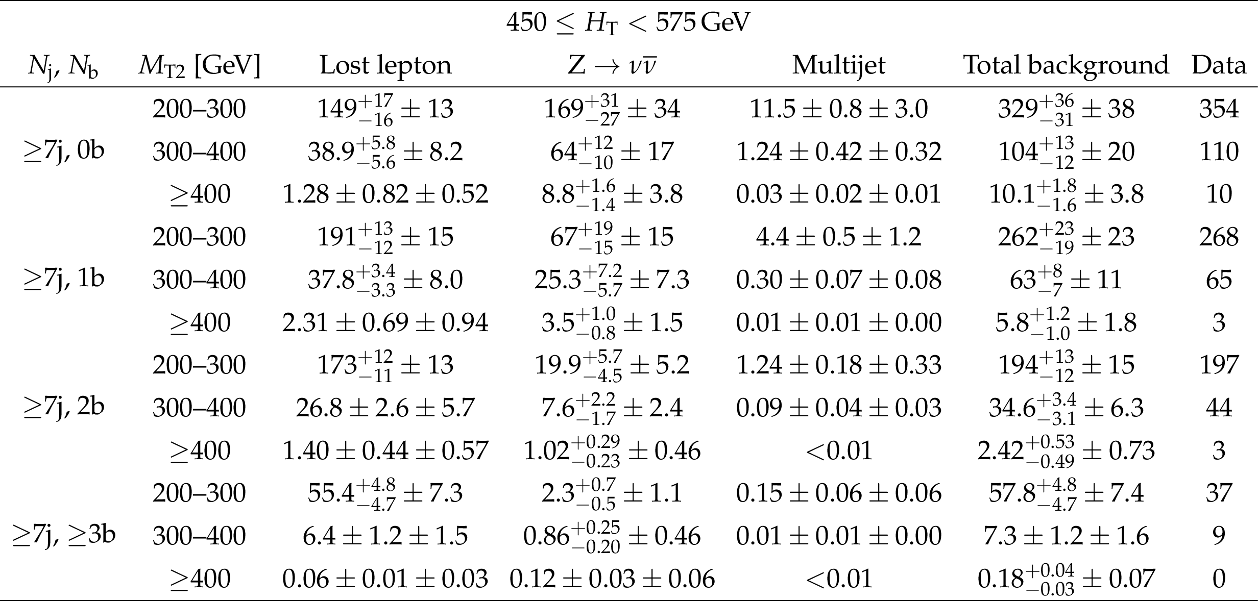
Predictions and observations for the 12 search regions with 450 $ \leq {H_{\mathrm {T}}} < $ 575 GeV and $ {N_{\mathrm {j}}} \geq $ 7. For each of the background predictions, the first uncertainty listed is statistical (from the limited size of data control samples and Monte Carlo samples), and the second is systematic. |
png pdf |
Table 16:
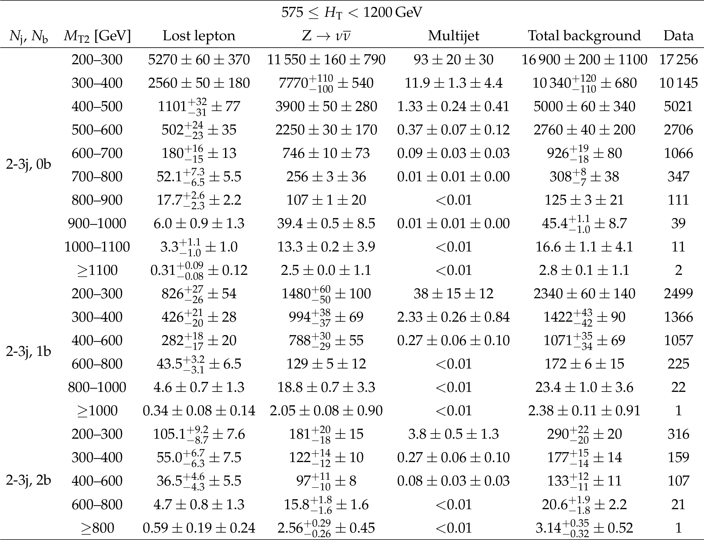
Predictions and observations for the 21 search regions with 575 $\leq {H_{\mathrm {T}}} < $ 1200 GeV and 2 $\leq {N_{\mathrm {j}}} \leq $ 3. For each of the background predictions, the first uncertainty listed is statistical (from the limited size of data control samples and Monte Carlo samples), and the second is systematic. |
png pdf |
Table 17:
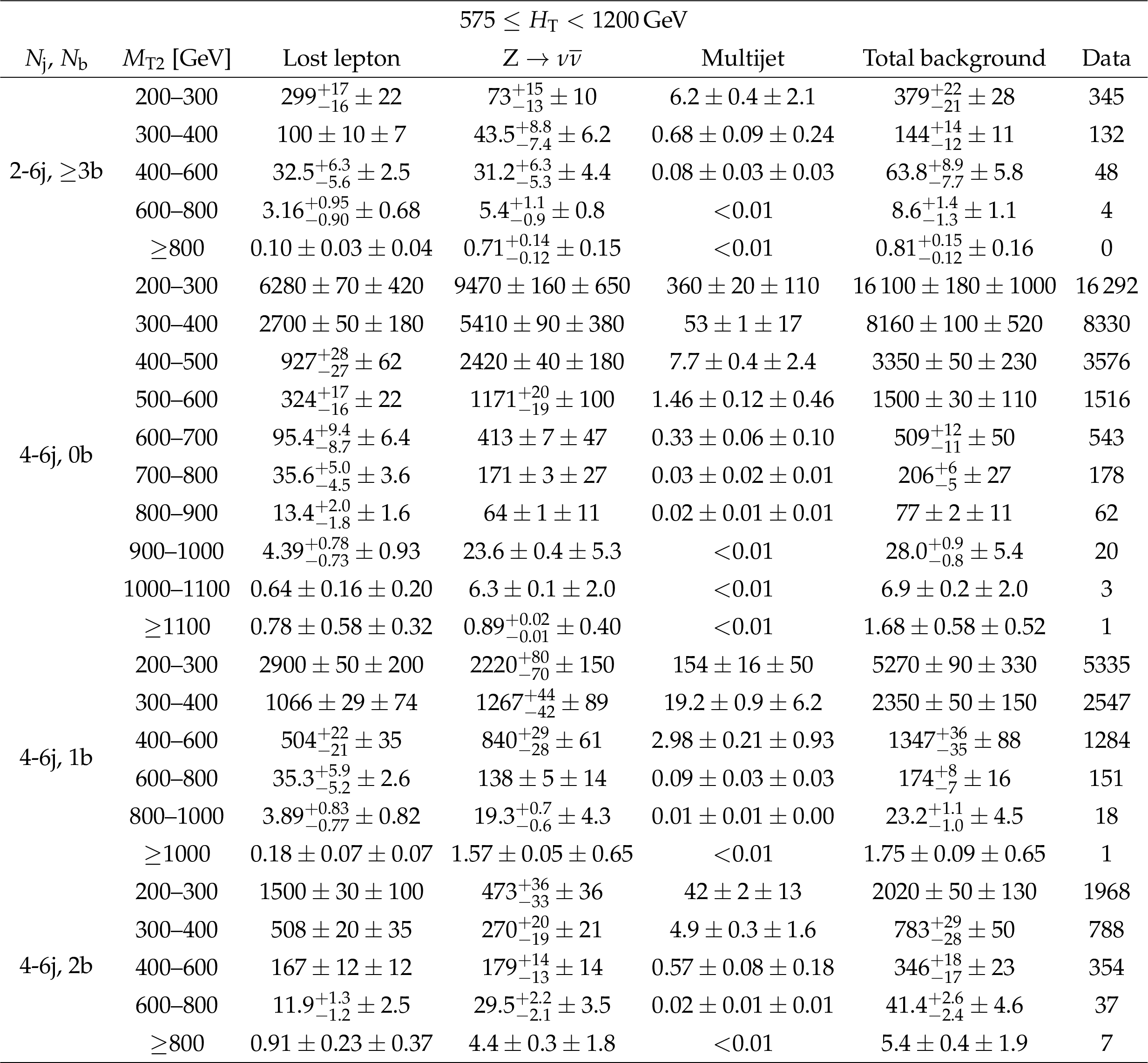
Predictions and observations for the 26 search regions with 575 $\leq {H_{\mathrm {T}}} < $ 1200 GeV, and 2 $\leq {N_{\mathrm {j}}} \leq $ 6 and $ {N_{\mathrm{b}}} \geq $ 3, or 4 $ \leq {N_{\mathrm {j}}} \leq $ 6. For each of the background predictions, the first uncertainty listed is statistical (from the limited size of data control samples and Monte Carlo samples), and the second is systematic. |
png pdf |
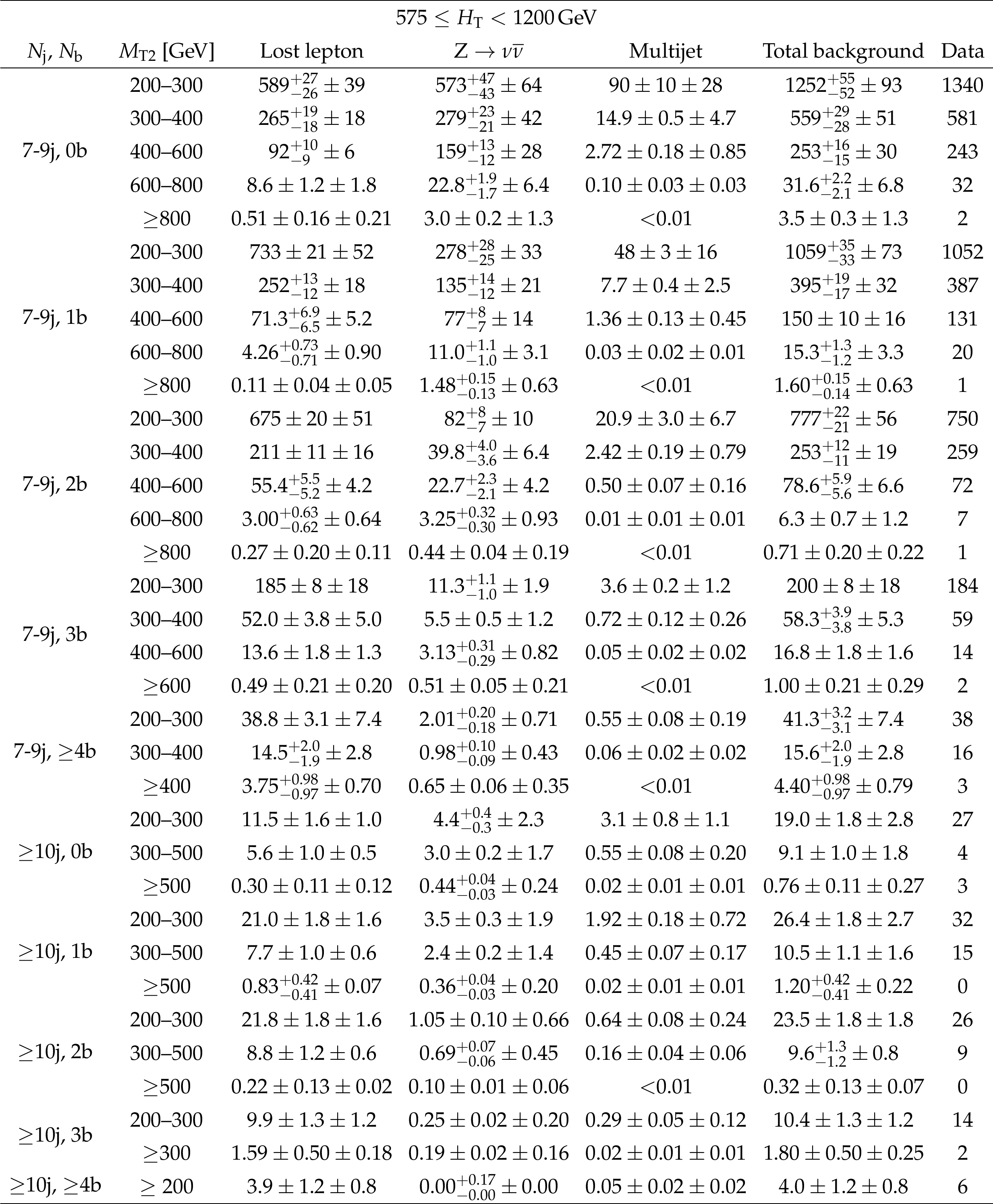
Table 18:
Predictions and observations for the 34 search regions with 575 $\leq {H_{\mathrm {T}}} < $ 1200 GeV, and 7 $\leq {N_{\mathrm {j}}} \leq $ 9, or $ {N_{\mathrm {j}}} \geq $ 10. For each of the background predictions, the first uncertainty listed is statistical (from the limited size of data control samples and Monte Carlo samples), and the second is systematic. |
png pdf |
Table 19:
Predictions and observations for the 17 search regions with 1200 $\leq {H_{\mathrm {T}}} < $ 1500 GeV and 2 $\leq {N_{\mathrm {j}}} \leq $ 3. For each of the background predictions, the first uncertainty listed is statistical (from the limited size of data control samples and Monte Carlo samples), and the second is systematic. |

png pdf |
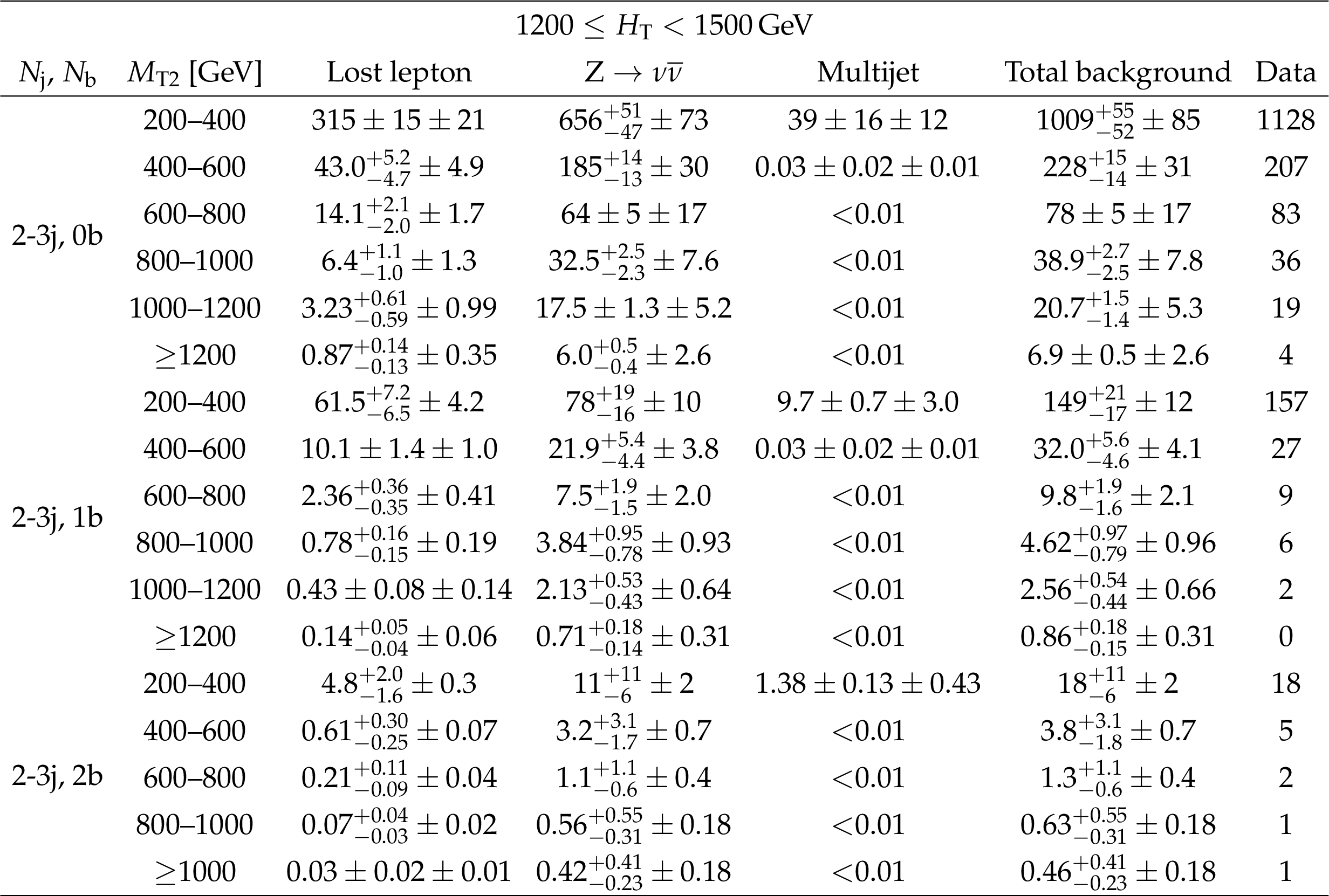
Table 20:
Predictions and observations for the 20 search regions with 1200 $\leq {H_{\mathrm {T}}} < $ 1500 GeV, and 2 $\leq {N_{\mathrm {j}}} \leq $ 6 and $ {N_{\mathrm{b}}} \geq $ 3, or 4 $ \leq {N_{\mathrm {j}}} \leq $ 6. For each of the background predictions, the first uncertainty listed is statistical (from the limited size of data control samples and Monte Carlo samples), and the second is systematic. |

png pdf |
Table 21:
Predictions and observations for the 31 search regions with 1200 $\leq {H_{\mathrm {T}}} < $ 1500 GeV, and 7 $\leq {N_{\mathrm {j}}} \leq $ 9, or $ {N_{\mathrm {j}}} \geq $ 10. For each of the background predictions, the first uncertainty listed is statistical (from the limited size of data control samples and Monte Carlo samples), and the second is systematic. |
png pdf |
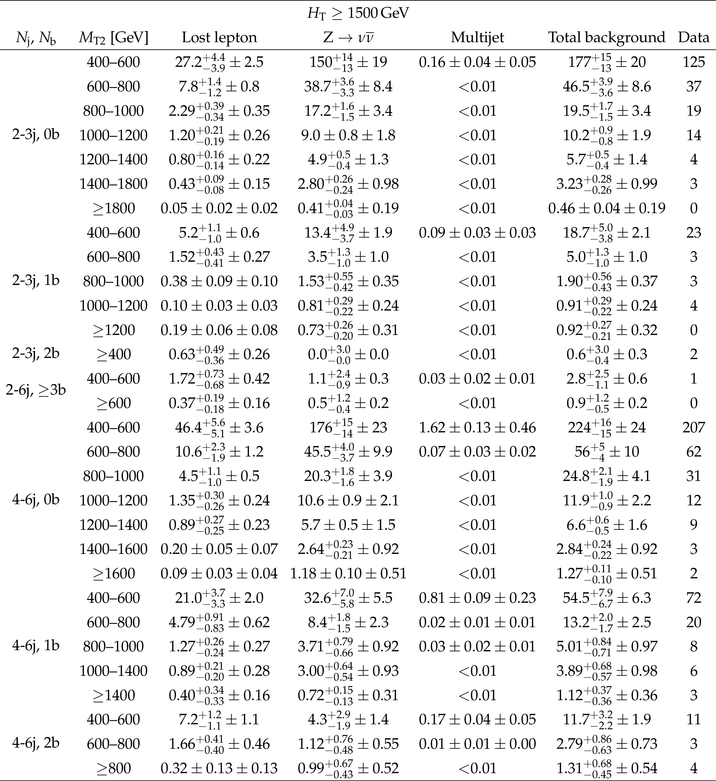
Table 22:
Predictions and observations for the 30 search regions with $ {H_{\mathrm {T}}} \geq $ 1500 GeV , and 2 $\leq {N_{\mathrm {j}}} \leq $ 3, 2 $\leq {N_{\mathrm {j}}} \leq $ 6 and $ {N_{\mathrm{b}}} \geq $ 3, or 4 $ \leq {N_{\mathrm {j}}} \leq $ 6. For each of the background predictions, the first uncertainty listed is statistical (from the limited size of data control samples and Monte Carlo samples), and the second is systematic. |
png pdf |
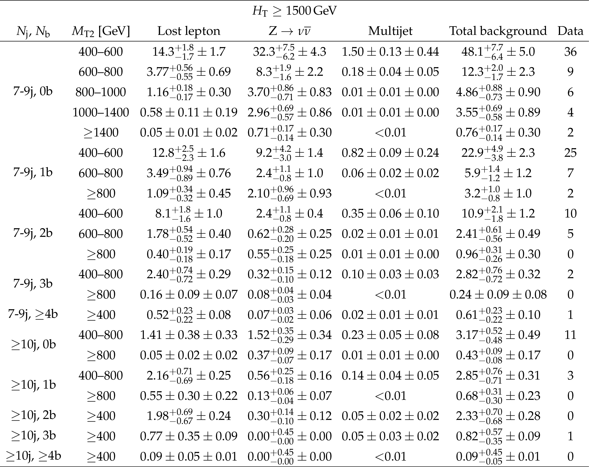
Table 23:
Predictions and observations for the 21 search regions with $ {H_{\mathrm {T}}} \geq $ 1500 GeV , and 7 $\leq {N_{\mathrm {j}}} \leq $ 9, or $ {N_{\mathrm {j}}} \geq $ 10. For each of the background predictions, the first uncertainty listed is statistical (from the limited size of data control samples and Monte Carlo samples), and the second is systematic. |
png pdf |
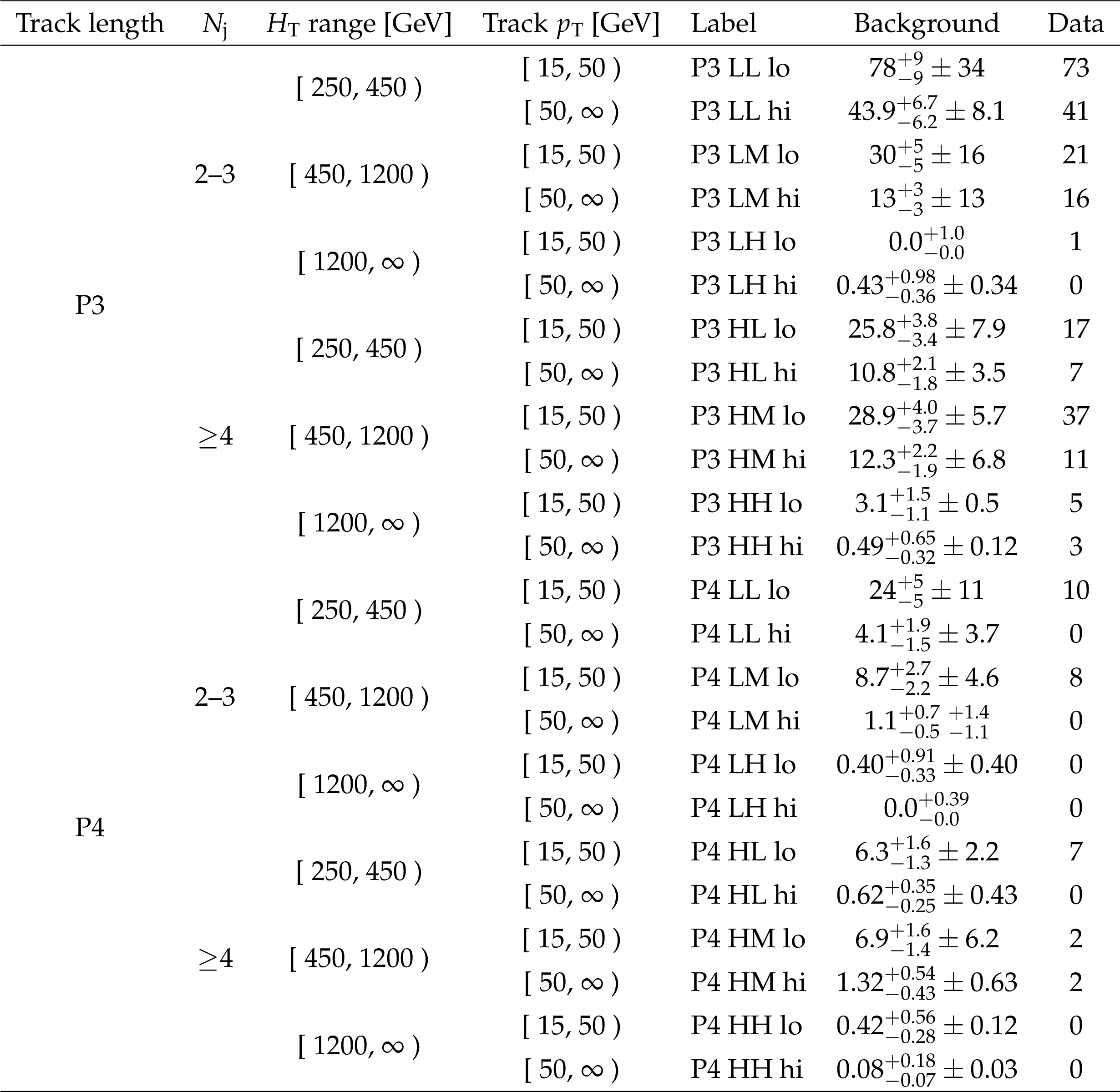
Table 24:
Summary of the 28 signal regions of the search for disappearing tracks, for the 2016 data set, together with the corresponding background predictions and observations. For the background predictions, the first uncertainty listed is statistical (from the limited size of control samples), and the second is systematic. The systematic uncertainty is not shown when it is negligible. |
png pdf |
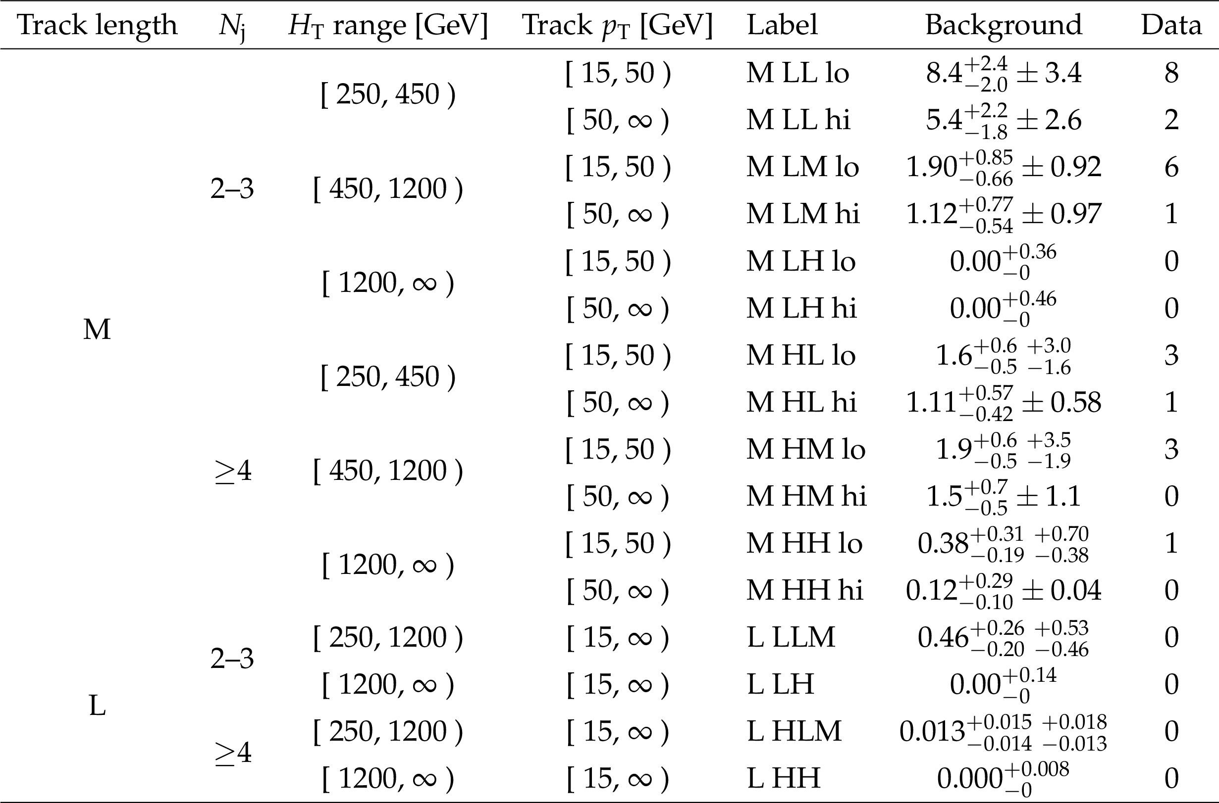
Table 25:
Summary of the 24 signal regions of the search for disappearing tracks for pixel tracks, for the 2017-2018 data set, together with the corresponding background predictions and observations. For the background predictions, the first uncertainty listed is statistical (from the limited size of control samples), and the second is systematic. The systematic uncertainty is not shown when it is negligible. |
png pdf |
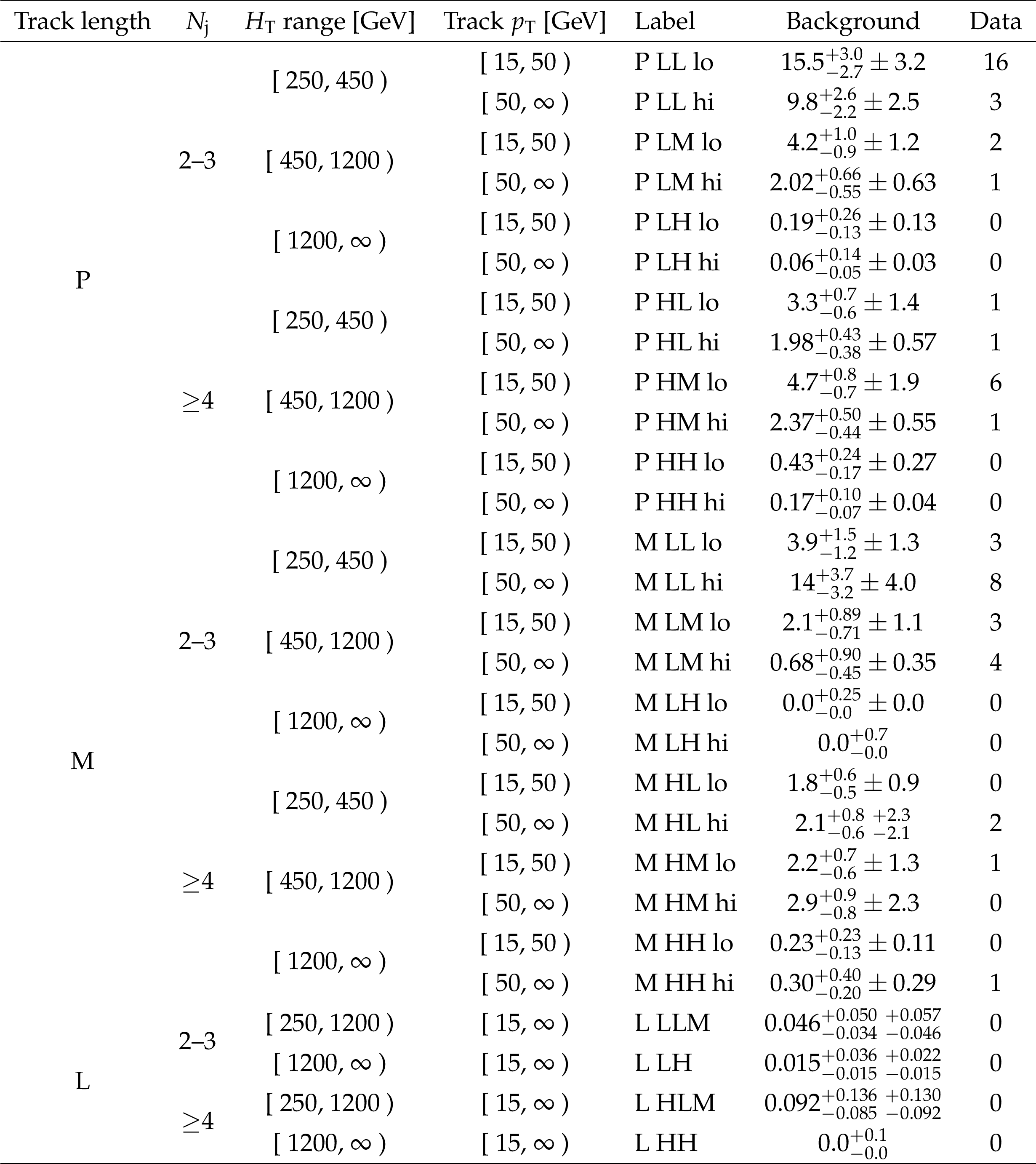
Table 26:
Summary of the 16 signal regions of the search for disappearing tracks for medium (M) length and long (L) tracks, for the 2017-2018 data set, together with the corresponding background predictions and observations. For the background predictions, the first uncertainty listed is statistical (from the limited size of control samples), and the second is systematic. The systematic uncertainty is not shown when it is negligible. |
| Summary |
| This paper presents the results of two related searches for phenomena beyond the standard model using events with jets and large values of the kinematic variable ${M_{\mathrm{T2}}}$. The first is an inclusive search, while the second requires in addition disappearing tracks. The measurements are based on a data sample of proton-proton collisions at $\sqrt{s} = $ 13 TeV collected in 2016-2018 with the CMS detector, and corresponding to an integrated luminosity of 137 fb$^{-1}$. No significant deviations from the standard model expectations are observed. Limits on pair-produced gluinos and squarks are established in the context of supersymmetry models conserving $R$-parity. The inclusive ${M_{\mathrm{T2}}}$ search probes gluino masses up to 2250 GeV and the lightest neutralino $\tilde{\chi}^0_1$ masses up to 1525 GeV, as well as light-flavor, bottom, and top squark masses up to 1710, 1240, and 1200 GeV, respectively, and $\tilde{\chi}^0_1$ masses up to 870, 700, and 580 GeV in each respective scenario. In models with a long-lived chargino $\tilde{\chi}^{\pm}_1$, where the gluinos and squarks decay with equal probability to $\tilde{\chi}^0_1$, $\tilde{\chi}^{+}_1$, and $\tilde{\chi}^{-}_1$, the search looking in addition for disappearing tracks probes gluino masses up to 2460 GeV and $\tilde{\chi}^0_1$ masses up to 2000 GeV, as well as light-flavor (top) squark masses up to 2090 (1660) GeV and $\tilde{\chi}^0_1$ masses up to 1650 (1210) GeV. A resonantly produced colored scalar state $\phi$ decaying to a massive Dirac fermion $\psi$ and a quark has recently been proposed as an explanation of an excess in data identified in regions with low jet multiplicities, based on previous results by the ATLAS and CMS Collaborations. From the inclusive ${M_{\mathrm{T2}}}$ search, mass limits as high as 1660 and 925 GeV are obtained for $\phi$ and $\psi$, respectively, and an upper limit on the product of the cross section and branching fraction of about 0.6 pb with a local significance of 1.1 standard deviations is observed for the previously reported best fit point $\left(m_{\phi},m_{\psi}\right)=\left(1250,900\right) $ GeV. The inclusive ${M_{\mathrm{T2}}}$ search is also used to constrain models of scalar and vector leptoquark (LQ) pair production with the LQ decaying to a neutrino and a top, bottom, or light-flavor quark. A vector LQ decaying with equal branching fraction to $\mathrm{t}\nu$ and $\mathrm{b}\tau$ has been proposed as part of an explanation of recent flavor anomalies. In such a model, LQ masses below 1550 GeV are excluded assuming the Yang-Mills case with coupling $\kappa=$ 1, or 1225 GeV in the minimal coupling case $\kappa=$ 0. The results presented in this paper extend the mass limits of the previous version of the CMS inclusive ${M_{\mathrm{T2}}}$ search, using a subset of the present data, by hundreds of GeV. In most of the cases, the results obtained are the most stringent constraints to date. |
| References | ||||
| 1 | C. G. Lester and D. J. Summers | Measuring masses of semiinvisibly decaying particles pair produced at hadron colliders | PLB 463 (1999) 99 | hep-ph/9906349 |
| 2 | ATLAS Collaboration | Search for new phenomena with large jet multiplicities and missing transverse momentum using large-radius jets and flavour-tagging at ATLAS in 13 $ TeV {\mathrm{p}}{\mathrm{p}} $ collisions | JHEP 12 (2017) 034 | 1708.02794 |
| 3 | ATLAS Collaboration | Search for supersymmetry in events with $ b $-tagged jets and missing transverse momentum in $ {\mathrm{p}}{\mathrm{p}} $ collisions at $ \sqrt{s} = $ 13 TeV with the ATLAS detector | JHEP 11 (2017) 195 | 1708.09266 |
| 4 | ATLAS Collaboration | Search for a scalar partner of the top quark in the jets plus missing transverse momentum final state at $ \sqrt{s} = $ 13 TeV with the ATLAS detector | JHEP 12 (2017) 085 | 1709.04183 |
| 5 | ATLAS Collaboration | Search for supersymmetry in final states with missing transverse momentum and multiple $ b $-jets in proton-proton collisions at $ \sqrt{s} = $ 13 TeV with the ATLAS detector | JHEP 06 (2018) 107 | 1711.01901 |
| 6 | ATLAS Collaboration | Search for dark matter and other new phenomena in events with an energetic jet and large missing transverse momentum using the ATLAS detector | JHEP 01 (2018) 126 | 1711.03301 |
| 7 | ATLAS Collaboration | Search for squarks and gluinos in final states with jets and missing transverse momentum using 36 fb$ ^{-1} $ of $ \sqrt{s} = 13 TeV {\mathrm{p}}{\mathrm{p}} $ collision data with the ATLAS detector | PRD 97 (2018) 112001 | 1712.02332 |
| 8 | CMS Collaboration | Search for supersymmetry in multijet events with missing transverse momentum in proton-proton collisions at 13 TeV | PRD 96 (2017) 032003 | CMS-SUS-16-033 1704.07781 |
| 9 | CMS Collaboration | Search for new phenomena with the $ M_{\mathrm {T2}} $ variable in the all-hadronic final state produced in proton-proton collisions at $ \sqrt{s} = $ 13 TeV | EPJC 77 (2017) 710 | CMS-SUS-16-036 1705.04650 |
| 10 | CMS Collaboration | Search for natural and split supersymmetry in proton-proton collisions at $ \sqrt{s} = $ 13 TeV in final states with jets and missing transverse momentum | JHEP 05 (2018) 025 | CMS-SUS-16-038 1802.02110 |
| 11 | CMS Collaboration | Constraints on models of scalar and vector leptoquarks decaying to a quark and a neutrino at $ \sqrt{s} = $ 13 TeV | PRD 98 (2018) 032005 | CMS-SUS-18-001 1805.10228 |
| 12 | CMS Collaboration | Inclusive search for supersymmetry in $ {\mathrm{p}}{\mathrm{p}} $ collisions at $ \sqrt{s} = $ 13 TeV using razor variables and boosted object identification in zero and one lepton final states | JHEP 03 (2019) 031 | CMS-SUS-16-017 1812.06302 |
| 13 | G. F. Giudice, M. A. Luty, H. Murayama, and R. Rattazzi | Gaugino mass without singlets | JHEP 12 (1998) 027 | hep-ph/9810442 |
| 14 | L. Randall and R. Sundrum | Out of this world supersymmetry breaking | NPB 557 (1999) 79 | hep-th/9810155 |
| 15 | ATLAS Collaboration | Search for charginos nearly mass degenerate with the lightest neutralino based on a disappearing-track signature in $ {\mathrm{p}}{\mathrm{p}} $ collisions at $ \sqrt{s} = $ 8 TeV with the ATLAS detector | PRD 88 (2013) 112006 | 1310.3675 |
| 16 | ATLAS Collaboration | Search for long-lived charginos based on a disappearing-track signature in $ {\mathrm{p}}{\mathrm{p}} $ collisions at $ \sqrt{s} = $ 13 TeV with the ATLAS detector | JHEP 06 (2018) 022 | 1712.02118 |
| 17 | CMS Collaboration | Search for disappearing tracks in proton-proton collisions at $ \sqrt{s} = $ 8 TeV | JHEP 01 (2015) 096 | CMS-EXO-12-034 1411.6006 |
| 18 | CMS Collaboration | Constraints on the pMSSM, AMSB model and on other models from the search for long-lived charged particles in proton-proton collisions at $ \sqrt{s} = $ 8 TeV | EPJC 75 (2015) 325 | CMS-EXO-13-006 1502.02522 |
| 19 | CMS Collaboration | Search for disappearing tracks as a signature of new long-lived particles in proton-proton collisions at $ \sqrt{s} = $ 13 TeV | JHEP 08 (2018) 016 | CMS-EXO-16-044 1804.07321 |
| 20 | CMS Collaboration | Search for long-lived charged particles in proton-proton collisions at $ \sqrt{s} = $ 13 TeV | PRD 94 (2016) 112004 | CMS-EXO-15-010 1609.08382 |
| 21 | N. Arkani-Hamed et al. | MARMOSET: The path from LHC data to the new standard model via on-shell effective theories | hep-ph/0703088 | |
| 22 | J. Alwall, P. Schuster, and N. Toro | Simplified models for a first characterization of new physics at the LHC | PRD 79 (2009) 075020 | 0810.3921 |
| 23 | J. Alwall, M.-P. Le, M. Lisanti, and J. G. Wacker | Model-independent jets plus missing energy searches | PRD 79 (2009) 015005 | 0809.3264 |
| 24 | LHC New Physics Working Group Collaboration | Simplified models for LHC new physics searches | JPG 39 (2012) 105005 | 1105.2838 |
| 25 | CMS Collaboration | Interpretation of searches for supersymmetry with simplified models | PRD 88 (2013) 052017 | CMS-SUS-11-016 1301.2175 |
| 26 | G. R. Farrar and P. Fayet | Phenomenology of the production, decay, and detection of new hadronic states associated with supersymmetry | PLB 76 (1978) 575 | |
| 27 | P. Ramond | Dual theory for free fermions | PRD 3 (1971) 2415 | |
| 28 | Y. A. Golfand and E. P. Likhtman | Extension of the algebra of Poincaré group generators and violation of P invariance | JEPTL 13 (1971)323 | |
| 29 | A. Neveu and J. H. Schwarz | Factorizable dual model of pions | NPB 31 (1971) 86 | |
| 30 | D. V. Volkov and V. P. Akulov | Possible universal neutrino interaction | JEPTL 16 (1972)438 | |
| 31 | J. Wess and B. Zumino | A Lagrangian model invariant under supergauge transformations | PLB 49 (1974) 52 | |
| 32 | J. Wess and B. Zumino | Supergauge transformations in four dimensions | NPB 70 (1974) 39 | |
| 33 | P. Fayet | Supergauge invariant extension of the Higgs mechanism and a model for the electron and its neutrino | NPB 90 (1975) 104 | |
| 34 | H. P. Nilles | Supersymmetry, supergravity and particle physics | Phys. Rep. 110 (1984) 1 | |
| 35 | P. Asadi et al. | Digging deeper for new physics in the LHC data | JHEP 11 (2017) 194 | 1707.05783 |
| 36 | P. Asadi et al. | An update on the LHC monojet excess | JHEP 03 (2018) 130 | 1712.04939 |
| 37 | CMS Collaboration | Search for new physics in final states with an energetic jet or a hadronically decaying $ W $ or $ Z $ boson and transverse momentum imbalance at $ \sqrt{s} = $ 13 TeV | PRD 97 (2018) 092005 | CMS-EXO-16-048 1712.02345 |
| 38 | J. C. Pati and A. Salam | Unified lepton-hadron symmetry and a gauge theory of the basic interactions | PRD 8 (1973) 1240 | |
| 39 | J. C. Pati and A. Salam | Lepton number as the fourth color | PRD 10 (1974) 275, .[Erratum: \DOI10.1103/PhysRevD.11.703.2] | |
| 40 | H. Georgi and S. L. Glashow | Unity of all elementary particle forces | PRL 32 (1974) 438 | |
| 41 | H. Fritzsch and P. Minkowski | Unified interactions of leptons and hadrons | Annals Phys. 93 (1975) 193 | |
| 42 | S. Dimopoulos and L. Susskind | Mass without scalars | NPB 155 (1979) 237, .[2,930(1979)] | |
| 43 | S. Dimopoulos | Technicolored signatures | NPB 168 (1980) 69 | |
| 44 | E. Farhi and L. Susskind | Technicolor | PR 74 (1981) 277 | |
| 45 | K. D. Lane and M. V. Ramana | Walking technicolor signatures at hadron colliders | PRD 44 (1991) 2678 | |
| 46 | B. Schrempp and F. Schrempp | Light leptoquarks | PLB 153 (1985) 101 | |
| 47 | B. Gripaios | Composite leptoquarks at the LHC | JHEP 02 (2010) 045 | 0910.1789 |
| 48 | R. Barbier et al. | R-parity violating supersymmetry | PR 420 (2005) 1 | hep-ph/0406039 |
| 49 | M. Tanaka and R. Watanabe | New physics in the weak interaction of $ \bar B\to D^{(*)}\tau\bar\nu $ | PRD 87 (2013) 034028 | 1212.1878 |
| 50 | Y. Sakaki, M. Tanaka, A. Tayduganov, and R. Watanabe | Testing leptoquark models in $ \bar B \to D^{(*)} \tau \bar\nu $ | PRD 88 (2013) 094012 | 1309.0301 |
| 51 | I. Dor\vsner, S. Fajfer, N. Ko\vsnik, and I. Ni\vsand\vzi\'c | Minimally flavored colored scalar in $ \bar B \to D^{(*)} \tau \bar \nu $ and the mass matrices constraints | JHEP 11 (2013) 084 | 1306.6493 |
| 52 | B. Gripaios, M. Nardecchia, and S. A. Renner | Composite leptoquarks and anomalies in $ B $-meson decays | JHEP 05 (2015) 006 | 1412.1791 |
| 53 | M. Bauer and M. Neubert | Minimal leptoquark explanation for the R$ _{D^{(*)}} $, R$ _K $, and $ (g-2)_g $ anomalies | PRL 116 (2016) 141802 | 1511.01900 |
| 54 | D. Buttazzo, A. Greljo, G. Isidori, and D. Marzocca | B-physics anomalies: a guide to combined explanations | JHEP 11 (2017) 044 | 1706.07808 |
| 55 | I. Dor\vsner and A. Greljo | Leptoquark toolbox for precision collider studies | JHEP 05 (2018) 126 | 1801.07641 |
| 56 | BaBar Collaboration | Evidence for an excess of $ \bar{B} \to D^{(*)} \tau^-\bar{\nu}_\tau $ decays | PRL 109 (2012) 101802 | 1205.5442 |
| 57 | BaBar Collaboration | Measurement of an excess of $ \bar{B} \to D^{(*)}\tau^- \bar{\nu}_\tau $ decays and implications for charged Higgs bosons | PRD 88 (2013) 072012 | 1303.0571 |
| 58 | Belle Collaboration | Observation of $ B^0 \to D^{*-}\tau^{+}\nu_{\tau} $ decay at Belle | PRL 99 (2007) 191807 | 0706.4429 |
| 59 | Belle Collaboration | Observation of $ B^+ \to \bar{D}^{*0}\tau^{+}\nu_{\tau} $ and evidence for $ B^+ \to \bar{D}^{0}\tau^{+}\nu_{\tau} $ at Belle | PRD 82 (2010) 072005 | 1005.2302 |
| 60 | Belle Collaboration | Measurement of the branching ratio of $ \bar{B} \to D^{(\ast)} \tau^- \bar{\nu}_\tau $ relative to $ \bar{B} \to D^{(\ast)} \ell^- \bar{\nu}_\ell $ decays with hadronic tagging at Belle | PRD 92 (2015) 072014 | 1507.03233 |
| 61 | Belle Collaboration | Measurement of the $ \tau $ lepton polarization and $ R(D^*) $ in the decay $ \bar{B} \to D^* \tau^- \bar{\nu}_\tau $ | PRL 118 (2017) 211801 | 1612.00529 |
| 62 | Belle Collaboration | Test of lepton flavor universality in $ {B\to K^\ast\ell^+\ell^-} $ decays at Belle | 1904.02440 | |
| 63 | LHCb Collaboration | Measurement of form-factor-independent observables in the decay $ B^{0} \to K^{*0} \mu^+ \mu^- $ | PRL 111 (2013) 191801 | 1308.1707 |
| 64 | LHCb Collaboration | Test of lepton universality using $ B^{+}\rightarrow K^{+}\ell^{+}\ell^{-} $ decays | PRL 113 (2014) 151601 | 1406.6482 |
| 65 | LHCb Collaboration | Measurement of the ratio of branching fractions $ \mathcal{B}(\bar{B}^0 \to D^{*+}\tau^{-}\bar{\nu}_{\tau})/\mathcal{B}(\bar{B}^0 \to D^{*+}\mu^{-}\bar{\nu}_{\mu}) $ | PRL 115 (2015) 111803 | 1506.08614 |
| 66 | LHCb Collaboration | Angular analysis of the $ B^{0} \to K^{*0} \mu^{+} \mu^{-} $ decay using 3 fb$ ^{-1} $ of integrated luminosity | JHEP 02 (2016) 104 | 1512.04442 |
| 67 | LHCb Collaboration | Test of lepton universality with $ B^{0} \rightarrow K^{*0}\ell^{+}\ell^{-} $ decays | JHEP 08 (2017) 055 | 1705.05802 |
| 68 | LHCb Collaboration | Search for lepton-universality violation in $ B^+\to K^+\ell^+\ell^- $ decays | PRL 122 (2019) 191801 | 1903.09252 |
| 69 | B. Diaz, M. Schmaltz, and Y.-M. Zhong | The leptoquark hunter's guide: Pair production | JHEP 10 (2017) 097 | 1706.05033 |
| 70 | ATLAS Collaboration | Searches for scalar leptoquarks in $ {\mathrm{p}}{\mathrm{p}} $ collisions at $ \sqrt{s} = $ 8 TeV with the ATLAS detector | EPJC 76 (2016) 5 | 1508.04735 |
| 71 | ATLAS Collaboration | Searches for scalar leptoquarks and differential cross-section measurements in dilepton-dijet events in proton-proton collisions at a centre-of-mass energy of $ \sqrt{s} = $ 13 TeV with the ATLAS experiment | Submitted to: EPJC | 1902.00377 |
| 72 | ATLAS Collaboration | Searches for third-generation scalar leptoquarks in $ \sqrt{s} = $ 13 TeV pp collisions with the ATLAS detector | JHEP 06 (2019) 144 | 1902.08103 |
| 73 | CMS Collaboration | Search for third-generation scalar leptoquarks decaying to a top quark and a $ \tau $ lepton at $ \sqrt{s} = $ 13 TeV | EPJC 78 (2018) 707 | CMS-B2G-16-028 1803.02864 |
| 74 | CMS Collaboration | Search for pair production of first and second generation leptoquarks in proton-proton collisions at $ \sqrt{s} = $ 8 TeV | PRD 93 (2016) 032004 | CMS-EXO-12-041 1509.03744 |
| 75 | CMS Collaboration | Search for pair production of third-generation scalar leptoquarks and top squarks in proton-proton collisions at $ \sqrt{s} = $ 8 TeV | PLB 739 (2014) 229 | CMS-EXO-12-032 1408.0806 |
| 76 | CMS Collaboration | Search for pair production of second-generation leptoquarks at $ \sqrt{s} = $ 13 TeV | PRD 99 (2019) 032014 | CMS-EXO-17-003 1808.05082 |
| 77 | CMS Collaboration | Search for pair production of first-generation scalar leptoquarks at $ \sqrt{s} = $ 13 TeV | PRD 99 (2019) 052002 | CMS-EXO-17-009 1811.01197 |
| 78 | CDF Collaboration | Search for first-generation scalar leptoquarks in $ {\mathrm{p}}\bar{{\mathrm{p}}} $ collisions at $ \sqrt{s} = $ 1.96 TeV | PRD 72 (2005) 051107 | hep-ex/0506074 |
| 79 | CDF Collaboration | Search for second-generation scalar leptoquarks in $ {\mathrm{p}}\bar{{\mathrm{p}}} $ collisions at $ \sqrt{s} = $ 1.96 TeV. | PRD 73 (2006) 051102 | hep-ex/0512055 |
| 80 | CDF Collaboration | Search for new physics with a dijet plus missing transverse energy signature in $ {\mathrm{p}}\bar{{\mathrm{p}}} $ collisions at $ \sqrt{s} = $ 1.96 TeV | PRL 105 (2010) 131801 | 0912.4691 |
| 81 | D0 Collaboration | Search for scalar leptoquarks and $ T $-odd quarks in the acoplanar jet topology using 2.5 fb$^{-1} $ of $ {\mathrm{p}} \bar{{\mathrm{p}}} $ collision data at $ \sqrt{s} = $ 1.96 TeV | PLB 668 (2008) 357 | 0808.0446 |
| 82 | D0 Collaboration | Search for pair production of second generation scalar leptoquarks | PLB 671 (2009) 224 | 0808.4023 |
| 83 | D0 Collaboration | Search for first generation leptoquark pair production in the electron + missing energy + jets final state | PRD 84 (2011) 071104 | 1107.1849 |
| 84 | H1 Collaboration | Search for first generation leptoquarks in $ ep $ collisions at HERA | PLB 704 (2011) 388 | 1107.3716 |
| 85 | ZEUS Collaboration | Search for first-generation leptoquarks at HERA | PRD 86 (2012) 012005 | 1205.5179 |
| 86 | ATLAS Collaboration | Search for third generation scalar leptoquarks in pp collisions at $ \sqrt{s} = $ 7 TeV with the ATLAS detector | JHEP 06 (2013) 033 | 1303.0526 |
| 87 | CMS Collaboration | Search for third-generation scalar leptoquarks and heavy right-handed neutrinos in final states with two tau leptons and two jets in proton-proton collisions at $ \sqrt{s} = $ 13 TeV | JHEP 07 (2017) 121 | CMS-EXO-16-023 1703.03995 |
| 88 | CMS Collaboration | Search for heavy neutrinos and third-generation leptoquarks in hadronic states of two $ \tau $ leptons and two jets in proton-proton collisions at $ \sqrt{s} = $ 13 TeV | JHEP 03 (2019) 170 | CMS-EXO-17-016 1811.00806 |
| 89 | CDF Collaboration | Search for third generation vector leptoquarks in $ {\mathrm{p}} \bar{{\mathrm{p}}} $ collisions at $ \sqrt{s} = $ 1.96 TeV | PRD 77 (2008) 091105 | 0706.2832 |
| 90 | CDF Collaboration | Search for pair production of scalar top quarks decaying to a $ \tau $ lepton and a $ b $ quark in $ {\mathrm{p}}\bar{{\mathrm{p}}} $ collisions at $ \sqrt{s} = $ 1.96 TeV | PRL 101 (2008) 071802 | 0802.3887 |
| 91 | D0 Collaboration | Search for third generation scalar leptoquarks decaying into $ \tau b $ | PRL 101 (2008) 241802 | 0806.3527 |
| 92 | CMS Collaboration | The CMS experiment at the CERN LHC | JINST 3 (2008) S08004 | CMS-00-001 |
| 93 | CMS Collaboration | The CMS trigger system | JINST 12 (2017) P01020 | CMS-TRG-12-001 1609.02366 |
| 94 | CMS Collaboration | CMS technical design report for the pixel detector upgrade | CERN-LHCC-2012-016, CMS-TDR-011 | |
| 95 | CMS Collaboration | Particle-flow reconstruction and global event description with the CMS detector | JINST 12 (2017) P10003 | CMS-PRF-14-001 1706.04965 |
| 96 | CMS Collaboration | Search for new physics with the M$ _{\mathrm{T2}} $ variable in all-jets final states produced in $ {\mathrm{p}}{\mathrm{p}} $ collisions at $ \sqrt{s} = $ 13 TeV | JHEP 10 (2016) 006 | CMS-SUS-15-003 1603.04053 |
| 97 | M. Cacciari, G. P. Salam, and G. Soyez | The anti-$ {k_{\mathrm{T}}} $ jet clustering algorithm | JHEP 04 (2008) 063 | 0802.1189 |
| 98 | M. Cacciari, G. P. Salam, and G. Soyez | FastJet user manual | EPJC 72 (2012) 1896 | 1111.6097 |
| 99 | M. Cacciari and G. P. Salam | Pileup subtraction using jet areas | PLB 659 (2008) 119 | 0707.1378 |
| 100 | CMS Collaboration | Jet energy scale and resolution in the CMS experiment in $ {\mathrm{p}}{\mathrm{p}} $ collisions at 8 TeV | JINST 12 (2017) P02014 | CMS-JME-13-004 1607.03663 |
| 101 | CMS Collaboration | Jet energy scale and resolution performance with 13 TeV data collected by CMS in 2016 | CDS | |
| 102 | CMS Collaboration | Identification of heavy-flavour jets with the CMS detector in $ {\mathrm{p}}{\mathrm{p}} $ collisions at 13 TeV | JINST 13 (2018) P05011 | CMS-BTV-16-002 1712.07158 |
| 103 | CMS Collaboration | Missing transverse energy performance of the CMS detector | JINST 6 (2011) P09001 | CMS-JME-10-009 1106.5048 |
| 104 | CMS Collaboration | Performance of missing transverse momentum reconstruction in proton-proton collisions at $ \sqrt{s} = $ 13 TeV using the CMS detector | JINST 14 (2019) P07004 | CMS-JME-17-001 1903.06078 |
| 105 | T. Sjostrand | The Lund Monte Carlo for e$ ^{+} $e$ ^{-} $ jet physics | CPC 28 (1983) 229 | |
| 106 | T. Sjostrand, S. Mrenna, and P. Skands | PYTHIA 6.4 physics and manual | JHEP 05 (2006) 026 | hep-ph/0603175 |
| 107 | UA1 Collaboration | Experimental observation of isolated large transverse energy electrons with associated missing energy at $ \sqrt{s} = $ 540 GeV | PLB 122 (1983) 103 | |
| 108 | CMS Collaboration | Searches for supersymmetry using the $ M_{\mathrm{T2}} $ variable in hadronic events produced in $ {\mathrm{p}}{\mathrm{p}} $ collisions at 8 TeV | JHEP 05 (2015) 078 | CMS-SUS-13-019 1502.04358 |
| 109 | CMS Collaboration | Search for supersymmetry in hadronic final states using $ M_\mathrm{T2} $ in $ {\mathrm{p}}{\mathrm{p}} $ collisions at $ \sqrt{s} = $ 7 TeV | JHEP 10 (2012) 018 | CMS-SUS-12-002 1207.1798 |
| 110 | J. Alwall et al. | The automated computation of tree-level and next-to-leading order differential cross sections, and their matching to parton shower simulations | JHEP 07 (2014) 079 | 1405.0301 |
| 111 | P. Nason | A new method for combining NLO QCD with shower Monte Carlo algorithms | JHEP 11 (2004) 040 | hep-ph/0409146 |
| 112 | S. Frixione, P. Nason, and C. Oleari | Matching NLO QCD computations with parton shower simulations: the POWHEG method | JHEP 11 (2007) 070 | 0709.2092 |
| 113 | S. Alioli, P. Nason, C. Oleari, and E. Re | NLO single-top production matched with shower in POWHEG: $ s $- and $ t $-channel contributions | JHEP 09 (2009) 111 | 0907.4076 |
| 114 | S. Alioli, P. Nason, C. Oleari, and E. Re | A general framework for implementing NLO calculations in shower Monte Carlo programs: the POWHEG BOX | JHEP 06 (2010) 043 | 1002.2581 |
| 115 | E. Re | Single-top $ Wt $-channel production matched with parton showers using the POWHEG method | EPJC 71 (2011) 1547 | 1009.2450 |
| 116 | R. Gavin, Y. Li, F. Petriello, and S. Quackenbush | FEWZ 2.0: A code for hadronic Z production at next-to-next-to-leading order | CPC 182 (2011) 2388 | 1011.3540 |
| 117 | R. Gavin, Y. Li, F. Petriello, and S. Quackenbush | W physics at the LHC with FEWZ 2.1 | CPC 184 (2013) 208 | 1201.5896 |
| 118 | M. Czakon and A. Mitov | Top++: A program for the calculation of the top-pair cross-section at hadron colliders | CPC 185 (2014) 2930 | 1112.5675 |
| 119 | C. Borschensky et al. | Squark and gluino production cross sections in pp collisions at $ \sqrt{s} = $ 13 , 14, 33 and 100 TeV | EPJC 74 (2014) 3174 | 1407.5066 |
| 120 | \GEANTfour Collaboration | GEANT4--a simulation toolkit | NIMA 506 (2003) 250 | |
| 121 | S. Abdullin et al. | The fast simulation of the CMS detector at LHC | J. Phys. Conf. Ser. 331 (2011) 032049 | |
| 122 | A. Giammanco | The fast simulation of the CMS experiment | J. Phys. Conf. Ser. 513 (2014) 022012 | |
| 123 | T. Sjostrand et al. | An Introduction to PYTHIA 8.2 | CPC 191 (2015) 159 | 1410.3012 |
| 124 | J. Alwall et al. | Comparative study of various algorithms for the merging of parton showers and matrix elements in hadronic collisions | EPJC 53 (2008) 473 | 0706.2569 |
| 125 | R. Frederix and S. Frixione | Merging meets matching in MC@NLO | JHEP 12 (2012) 061 | 1209.6215 |
| 126 | CMS Collaboration | Event generator tunes obtained from underlying event and multiparton scattering measurements | EPJC 76 (2016) 155 | CMS-GEN-14-001 1512.00815 |
| 127 | CMS Collaboration | Extraction and validation of a new set of CMS PYTHIA8 tunes from underlying-event measurements | Submitted to: EPJC | CMS-GEN-17-001 1903.12179 |
| 128 | NNPDF Collaboration | Parton distributions with QED corrections | NPB 877 (2013) 290 | 1308.0598 |
| 129 | NNPDF Collaboration | Parton distributions from high-precision collider data | EPJC 77 (2017) 663 | 1706.00428 |
| 130 | CMS Collaboration | Measurements of $ \mathrm{t}\bar{\mathrm{t}} $ cross sections in association with b jets and inclusive jets and their ratio using dilepton final states in $ {\mathrm{p}}{\mathrm{p}} $ collisions at $ \sqrt{s} = $ 13 TeV | PLB 776 (2018) 355 | CMS-TOP-16-010 1705.10141 |
| 131 | CMS Collaboration | Jet algorithms performance in 13 TeV data | CMS-PAS-JME-16-003 | CMS-PAS-JME-16-003 |
| 132 | T. Junk | Confidence level computation for combining searches with small statistics | NIMA 434 (1999) 435 | hep-ex/9902006 |
| 133 | A. L. Read | Presentation of search results: The $ CL_{\mathrm{s}} $ technique | JPG 28 (2002) 2693 | |
| 134 | G. Cowan, K. Cranmer, E. Gross, and O. Vitells | Asymptotic formulae for likelihood-based tests of new physics | EPJC 71 (2011) 1554 | 1007.1727 |
| 135 | ATLAS and CMS Collaborations | Procedure for the LHC Higgs boson search combination in summer 2011 | CMS-NOTE-2011-005 | |
| 136 | W. Beenakker et al. | NNLL-fast: predictions for coloured supersymmetric particle production at the LHC with threshold and Coulomb resummation | JHEP 12 (2016) 133 | 1607.07741 |
| 137 | W. Beenakker, R. Hopker, M. Spira, and P. M. Zerwas | Squark and gluino production at hadron colliders | NPB 492 (1997) 51 | hep-ph/9610490 |
| 138 | A. Kulesza and L. Motyka | Threshold resummation for squark-antisquark and gluino-pair production at the LHC | PRL 102 (2009) 111802 | 0807.2405 |
| 139 | A. Kulesza and L. Motyka | Soft gluon resummation for the production of gluino-gluino and squark-antisquark pairs at the LHC | PRD 80 (2009) 095004 | 0905.4749 |
| 140 | W. Beenakker et al. | Soft-gluon resummation for squark and gluino hadroproduction | JHEP 12 (2009) 041 | 0909.4418 |
| 141 | W. Beenakker et al. | Squark and gluino hadroproduction | Int. J. Mod. Phys. A 26 (2011) 2637 | 1105.1110 |
| 142 | CMS Collaboration | CMS luminosity measurements for the 2016 data-taking period | CMS-PAS-LUM-17-001 | CMS-PAS-LUM-17-001 |
| 143 | CMS Collaboration | CMS luminosity measurement for the 2017 data-taking period at $ \sqrt{s} = $ 13 TeV | CMS-PAS-LUM-17-004 | CMS-PAS-LUM-17-004 |
| 144 | CMS Collaboration | CMS luminosity measurement for the 2018 data-taking period at $ \sqrt{s} = $ 13 TeV | CMS-PAS-LUM-18-002 | CMS-PAS-LUM-18-002 |
| 145 | LEP2 SUSY Working Group, ALEPH, DELPHI, L3 and OPAL experiments | Combined LEP chargino results, up to 208 GeV for low $ \Delta m $ | link | |
|
|
Compact Muon Solenoid LHC, CERN |
|

|

|

|

|

|